rianne hupse- localisation techniques to improve bci
TRANSCRIPT
8/3/2019 Rianne Hupse- Localisation Techniques to improve BCI
http://slidepdf.com/reader/full/rianne-hupse-localisation-techniques-to-improve-bci 1/56
Localisation Techniques to improve BCI
Thesis submitted to obtain the degree of
Master of Science
in Cognitive Neuroscience
Rianne HupseSupervisors: Dr. ir. P. Desain and Prof. dr. C. Gielen
Music, Mind and Machine group, NICI, Radboud University Nijmegen
10th September 2006

8/3/2019 Rianne Hupse- Localisation Techniques to improve BCI
http://slidepdf.com/reader/full/rianne-hupse-localisation-techniques-to-improve-bci 2/56
Abstract
The aim of this study is to develop a new type of brain computer interface (bci)
system: a system in which selective attention to rhythmic tactile stimuli is used
to control an external device. It is known that temporal rhythmic tactile stimuliinduce a steady-state somatosensory evoked potential oscillating at the same
temporal frequency as the driving stimulus. The amplitude of this oscillation
increases when the subject is attending to the stimulus. This attention induced
power gain can be detected in the eeg and might be translated into commands
for a computer or other device. Because eeg data has a small signal to noise
ratio, it is investigated if a beamformer spatial filter improves the classification
success rates. To be sure that the beamformer filter allocates activity to the
correct anatomical locations, a new method is proposed to construct realistic
head models. During the experiment, tactile stimuli with diff erent temporal
frequencies are presented to the left and right index finger of a subject. The
subject is instructed to attend to one finger and to ignore the sensations of the
other finger. Perception conditions, in which only one finger was stimulated,
were included as a baseline. Single trial eeg and voxel data was used in a
classification algorithm to detect which finger was attended. Classification rates
are relatively high (± 90%) for perception conditions, while selective attention
conditions give succes rates at chance level. An explanation for this can be
that the attention induced power gain is too small to be detected in single
trials. Results show that beamforming allocates the frequencies presented to
left and right index finger to separate areas of the brain. This is in contrast to
electrode data, in which the two frequencies reach electrodes at both sides of the
scalp. Therefore, by using the beamformer filter the power of a single stimulus
is focused to a single area which will increase the signal to noise ratio. However,
classification success rates show no improvements when the beamformer filter isused. A suggestion for further research is to include a discrimination task in the
experiment which might increase the attention level of the subject and therefore
the attention induced power gain. The amount of trials can be increased that
is used as a training set in the cross validation procedure of the classification
algorithm. Further, the amount of trials used for estimating the covariance
between the sensors, which is necessary for building the beamformer filter, might
improve the results.

8/3/2019 Rianne Hupse- Localisation Techniques to improve BCI
http://slidepdf.com/reader/full/rianne-hupse-localisation-techniques-to-improve-bci 3/56
Contents
1 Introduction 4
1.1 Brain Computer Interfaces . . . . . . . . . . . . . . . . . . . . . . 4
1.2 History of Brain Computer Interfaces . . . . . . . . . . . . . . . . 5
1.3 The challenge of improving the signal to noise ratio . . . . . . . . 7
1.4 Beamforming . . . . . . . . . . . . . . . . . . . . . . . . . . . . . 7
1.5 Our approach . . . . . . . . . . . . . . . . . . . . . . . . . . . . . 9
1.6 Overview thesis . . . . . . . . . . . . . . . . . . . . . . . . . . . . 9
2 Materials and methods 11
2.1 Construction of realistic head models . . . . . . . . . . . . . . . . 11
2.2 Stimuli and experimental design . . . . . . . . . . . . . . . . . . 13
2.3 Data acquisition . . . . . . . . . . . . . . . . . . . . . . . . . . . 15
2.4 Data analysis . . . . . . . . . . . . . . . . . . . . . . . . . . . . . 16
2.4.1 Alignment of electrode positions to mri . . . . . . . . . . 162.4.2 Construction of the forward models . . . . . . . . . . . . 16
2.4.3 Analysis of eeg data . . . . . . . . . . . . . . . . . . . . . 18
3 Results 22
3.1 Beamformer activity images . . . . . . . . . . . . . . . . . . . . . 22
3.2 Power diff erences between contralateral and ipsilateral channels . 25
3.3 Attention induced power change . . . . . . . . . . . . . . . . . . 28
3.4 Classification success rates . . . . . . . . . . . . . . . . . . . . . . 30
4 Discussion 31
A Construction of a realistic head model 34A.1 Introduction . . . . . . . . . . . . . . . . . . . . . . . . . . . . . . 34
A.2 Segmentation and triangulation of the brain . . . . . . . . . . . . 35
A.2.1 Segmentation . . . . . . . . . . . . . . . . . . . . . . . . . 35
A.2.2 Triangulation . . . . . . . . . . . . . . . . . . . . . . . . . 36
A.3 Segmentation and triangulation of the scalp . . . . . . . . . . . . 37
A.3.1 Segmentation . . . . . . . . . . . . . . . . . . . . . . . . . 37
A.3.2 Triangulation . . . . . . . . . . . . . . . . . . . . . . . . . 37
A.4 Skull surface: direct triangulation algorithm . . . . . . . . . . . . 38
A.4.1 Preprocessing of the anatomical mri . . . . . . . . . . . . 38
2

8/3/2019 Rianne Hupse- Localisation Techniques to improve BCI
http://slidepdf.com/reader/full/rianne-hupse-localisation-techniques-to-improve-bci 4/56
A.4.2 Triangulation process . . . . . . . . . . . . . . . . . . . . 40
A.4.3 Detection of the boundary between skull and scalp . . . . 40
B Beamforming 47
B.1 Introduction . . . . . . . . . . . . . . . . . . . . . . . . . . . . . . 47
B.2 Construction of the filter . . . . . . . . . . . . . . . . . . . . . . . 47
B.2.1 The forward model . . . . . . . . . . . . . . . . . . . . . . 47
B.2.2 Filter design . . . . . . . . . . . . . . . . . . . . . . . . . 48
B.2.3 Linearly Constrained Minimum Variance . . . . . . . . . 49
B.3 The Neural Activity Index and noise . . . . . . . . . . . . . . . . 50
B.4 Correlated sources . . . . . . . . . . . . . . . . . . . . . . . . . . 51
3

8/3/2019 Rianne Hupse- Localisation Techniques to improve BCI
http://slidepdf.com/reader/full/rianne-hupse-localisation-techniques-to-improve-bci 5/56
Chapter 1
Introduction
1.1 Brain Computer Interfaces
Patients suff ering from motor diseases can have difficulties performing even the
simplest actions. One example is amyotrophic lateral sclerosis (als), a disease
in which a progressive degeneration of motor neurons leads to an inability of
the brain to control movements. In the later stage of this disease patients
may become totally paralyzed. Other examples of motor diseases are brainstem
stroke, brain or spinal cord injury and multiple sclerosis. In most cases only
motor functions are aff ected; patients do not experience impaired intellectual
reasoning, vision or hearing.
A system in which an external device like a speech synthesizer, a computer
or a wheelchair can be controlled without the usage of muscles would greatly
improve the quality of life of these patients. For this reason brain computer in-
terfaces (bci) are being developed. Using these interfaces a patient will be able
to control a device using his/her brain only, for example by directing his/her
attention to one of multiple stimuli present. While controlling the device, the
patient is wearing an electrode cap for measuring the electrocortical encephalo-
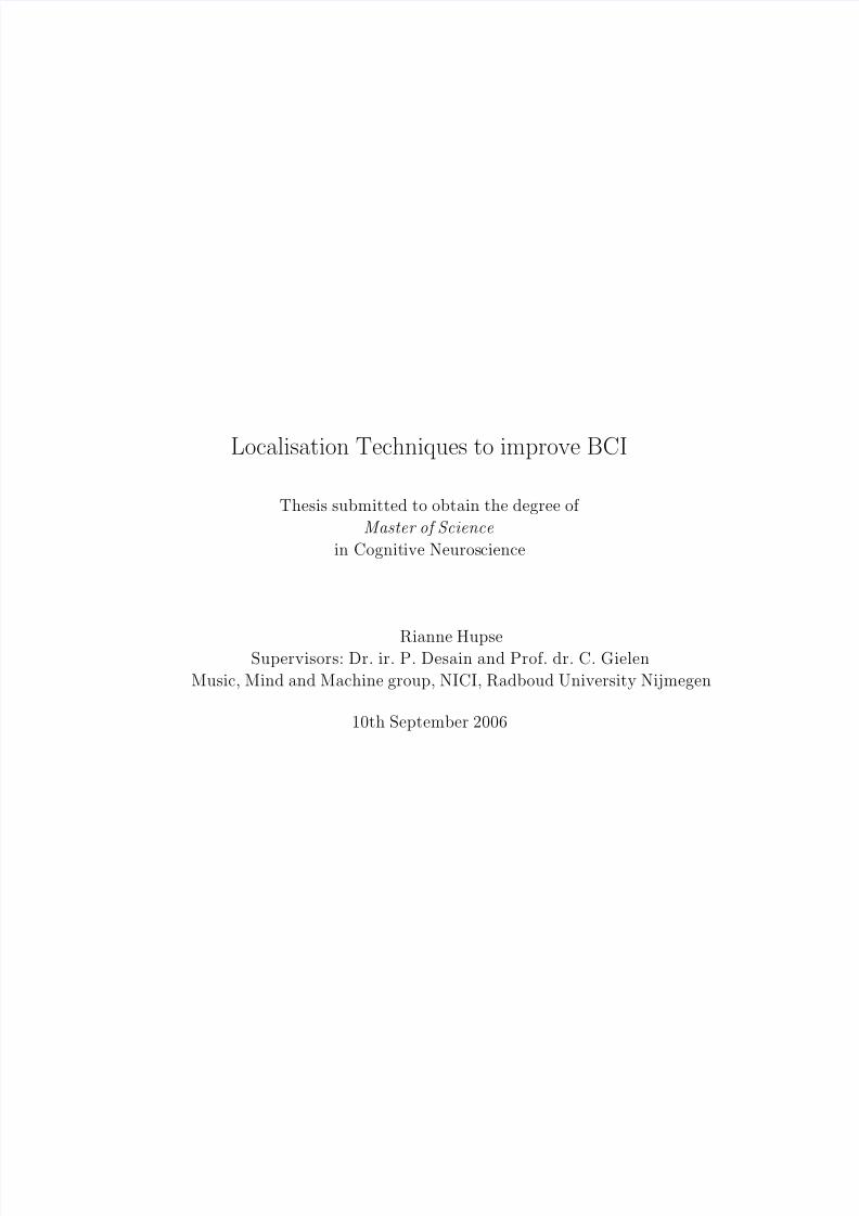
gram (eeg) signals. A basic design for a bci system is shown in figure 1.1.
Signals are measured by electrodes at the scalp or at the surface of the brain.
Specific features are extracted from the digitized signal. A translation algo-
rithm makes a decision based on these features. This decision is executed by
sending commands to an external device like a typing device, a wheelchair orhand prothesis. The loop is closed by the subject who is observing the device.
In this way the subject can learn to adapt to the system.
Besides eeg, there are multiple other techniques available to measure activ-
ity from the brain such as magnetoencephalography (meg), positron emission
tomography (pet), functional magnetic resonance imaging (f mri), and optical
imaging. However, these techniques require expensive equipment that cannot
be used in every environment. Further, f mri and optical imaging have a poor
time resolution and are therefore not suitable for a device that has to measure
rapidly changing patterns of mental activity. Because eeg measurement has
4
8/3/2019 Rianne Hupse- Localisation Techniques to improve BCI
http://slidepdf.com/reader/full/rianne-hupse-localisation-techniques-to-improve-bci 6/56
Figure 1.1: Basic design of a bci system, adopted from [25].
a high time resolution and requires simple and inexpensive equipment, it is at
present the most suitable technique to be used in bci systems.
1.2 History of Brain Computer Interfaces
The first bci studies started with research in monkeys. Electrodes were im-
planted in the brain of a monkey and firing patterns were measured of indi-
vidual and groups of neurons. In 1973 the group of Fetz found that macaque
monkeys were able to selectively adjust the firing rate of individual cortical neu-
rons to attain a particular level of cell activity. This was done by the use of a
conditioning paradigm and providing sensory feedback that signaled the level
of neuronal firing [7]. Based on these findings, Schmidt proposed in 1980 that
activity measured in cortical motor centers might be used to activate externaldevices [20].
In 2000 the group of Nicolelis developed a bci system that recorded brain
activity from implanted electrodes in monkeys. This activity was used to control
a robot arm [4] [24]. In this system, several motor parameters such as velocity,
gripping force and hand position were extracted from the neural firing patterns
of diff erent motor areas. The robot arm was invisible to the monkeys, and
feedback of the movements was provided by a visual display. During training,
the performance of the monkeys improved. Control of the robot arm was even
possible when the arms of the monkeys did not move, presumably when the
5

8/3/2019 Rianne Hupse- Localisation Techniques to improve BCI
http://slidepdf.com/reader/full/rianne-hupse-localisation-techniques-to-improve-bci 7/56
monkey made the movement in his imagination.
Another group that measured neural activity in monkeys is the group of Andersen. Activity was measured while the monkey was preparing to reach to
a stimulus that was shown before. Using activity patterns collected in these
training trials, it was possible to predict the reach direction of the monkey in
other trials [16].
The use of implanted electrodes provides a way to obtain signals from the
brain with a high signal to noise ratio. However, this invasive technique is not
well suited for use in human bci systems. Therefore techniques were developed
to control a device using the signals measured from the scalp: eeg signals.
Because of a lower signal to noise ratio and the fact that an eeg electrode
measures signals coming from a huge amount of neurons together, other features
in the signal are extracted than in the case of implanted electrodes. Systems
that use eeg signals can be divided into three groups: systems using mu and
beta rhythms, systems using slow cortical potentials and systems using P300
evoked potentials.
One of the groups that uses mu and beta rhythms for bci is the group of
Pfurtscheller. Knowledge about beta and gamma synchronization in the human
brain during the imagination of simple motor tasks was used to control several
devices like a virtual keyboard device and an orthotic device that opens and
closes a paralyzed hand [18] [19].
A group that uses slow cortical potentials, is the group of Birbaumer. Slow
cortical potentials (scps) are slow voltage changes generated in the cortex that
occur over a time period of 0.5 to 10 seconds. Negative scps are associated with
functions involving cortical activation, while positive scps are associated withreduced cortical activation [2]. It has been shown that subjects can control these
potentials and thereby control a cursor on a computer screen [3]. However, the
training period lasts for several months and is very demanding for the patient.
Besides mu and gamma rhythms and slow cortical potentials, P300 evoked
potentials can be used for bci. A P300 evoked potential is the positive peak in
the eeg that is measured over parietal cortex about 300 ms after an auditory,
visual or somatosensory stimulus is presented to a subject [6]. The group of
Donchin uses this P300 response in a paradigm in which a 6 by 6 matrix of
letters is presented to a subject, which has to select a letter. Every 125 ms, a
row or a column of this matrix flashes. After a set of trials the average P300
amplitude is calculated to the flashing of every row and column. Based on theseP300 amplitudes the system chooses a letter. The advantage of using the P300
amplitude is that it requires no initial user training. However, the P300 response
is likely to change over time and over long time periods P300 might habituate.
6
8/3/2019 Rianne Hupse- Localisation Techniques to improve BCI
http://slidepdf.com/reader/full/rianne-hupse-localisation-techniques-to-improve-bci 8/56
1.3 The challenge of improving the signal to noise
ratio
The biggest challenge of developing brain computer interfaces lies in the fact
that the signal to noise ratio of eeg signals is low, which makes recognition of
diff erent activity patterns hard. This low signal to noise ratio is due to mea-
surement noise, ongoing brain processes that do not correlate with the relevant
mental activity and ‘smearing’ out of signals by diff erent tissues in the head. In
brain research usually the averaging over multiple trials is used to reduce these
noise eff ects. However, in bci this will lead to a considerable increase in classifi-
cation time because the system has to wait for multiple trials before being able
to select an response. When developing a faster interface in which single trials
are used, filtering of the signals to obtain a higher signal to noise ratio becomesimportant. Several temporal filters like bandpass filters and notch filters are
used to decrease the noise level in single trial eeg data. Also spatial filters like
independent component analysis (ica) and principal component analysis (pca)
are used to combine the data measured by the diff erent channels in a linear way
into signals representing a few ‘virtual’ channels measuring the independent or
principal sources that are active. In this way relevant information is extracted
from the data that can be used for classification algorithms. However, these
methods do not use any information about the known location and behaviour
of active sources in the brain. By including this information in a spatial filter
the potentials stemming from certain brain areas can be optimally extracted
while potentials from other areas are suppressed. The use of this kind of spatial
filters will result in signals that can achieve a neuro-physiological interpretation
and might give better results in classification algorithms.
1.4 Beamforming
A localisation technique often used in brain research is called ‘beamforming’. In
this approach we calculate the activity present in volume units in the brain called
voxels (volume pixels) from the signals measured by the electrodes. These sig-
nals can be interpreted as stemming from virtual electrodes measuring directly
in the brain itself. Therefore there is no ’smearing out’ of potentials due to
diff erent conductivities of the diff erent tissue layers in between the brain and
the electrodes; every virtual electrode measures activity coming from one single
voxel. From the set of voxels a subset can be chosen from which the activity
patterns over time are used in the classification algorithm. By doing this, we
concentrate only on the part of signal that is expected to originate from one or
multiple brain areas that are relevant for the processing of the stimuli.
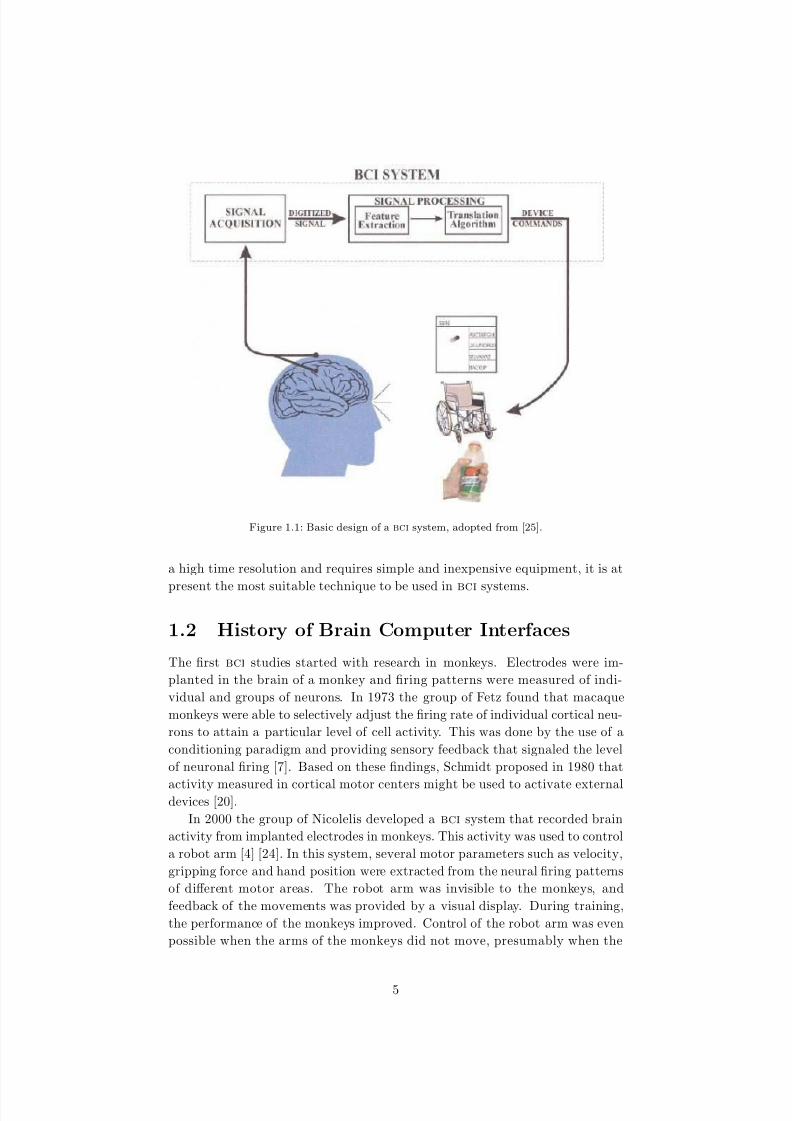
Beamforming roughly consists of constructing a forward model which pre-
dicts the potential distribution at the scalp due to activity in a certain voxel.
This model is inverted to estimate the activity in this voxel that is related to
the measured potential distribution (figure 1.2 adopted from [26]). An example
7
8/3/2019 Rianne Hupse- Localisation Techniques to improve BCI
http://slidepdf.com/reader/full/rianne-hupse-localisation-techniques-to-improve-bci 9/56
Figure 1.2: The basic principle of beamforming is to construct a forward model H that pre-
dicts the measured potentials at the scalp due to a single dipole in the brain. Using this
forward model and the covariance between the sensor measurements, a filter is constructed.
By multiplying the potentials measured at every sensor by the filter weights and summing
the results, the activity at the location of the dipole is calculated. (Figure adopted from theneuroimaging II course of the FC Donders Centre.)
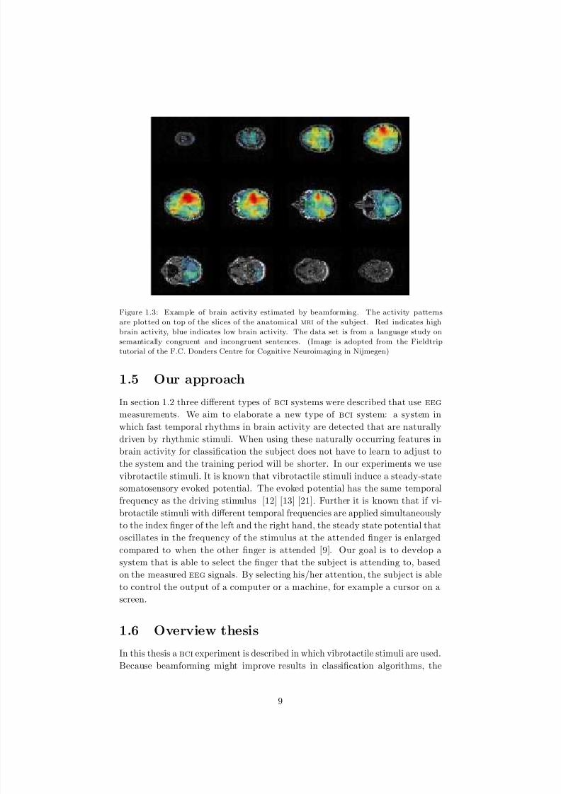
of a resulting activity pattern can be seen in figure 1.3. Beamforming is often
used in meg (magnetoencephalography) research in which the magnetic fields
close to the scalp are measured. Because magnetic fields are not aff ected by
the diff erent tissue properties, the forward model only depends on the shape
of the head of the subject. However, for eeg research the construction of the
forward model is more complicated. A model of the shape and conductivity of
all diff erent tissues in the head is necessary to be able to calculate the poten-
tials measured at the scalp due to activation of a certain brain area. Because
it is hard to construct a realistic head model containing the precise shapes andconductivity values of every tissue type, often a simplified model is used. This
simplified model usually consists of three compartments for the brain (including
cerebral spinal fluid, csf), skull and scalp. In this model the brain compart-
ment is a sphere and the skull and scalp compartments are two spherical shells
around the brain compartment. In order to obtain a more precise locatisation
of brain activity we developed head models containing more realistic shapes for
the three compartments using mri (magnetic resonance imaging) scans of the
subjects.
8
8/3/2019 Rianne Hupse- Localisation Techniques to improve BCI
http://slidepdf.com/reader/full/rianne-hupse-localisation-techniques-to-improve-bci 10/56
Figure 1.3: Example of brain activity estimated by beamforming. The activity patterns
are plotted on top of the slices of the anatomical mri of the subject. Red indicates high
brain activity, blue indicates low brain activity. The data set is from a language study on
semantically congruent and incongruent sentences. (Image is adopted from the Fieldtrip
tutorial of the F.C. Donders Centre for Cognitive Neuroimaging in Nijmegen)
1.5 Our approach
In section 1.2 three diff erent types of bci systems were described that use eeg
measurements. We aim to elaborate a new type of bci system: a system inwhich fast temporal rhythms in brain activity are detected that are naturally
driven by rhythmic stimuli. When using these naturally occurring features in
brain activity for classification the subject does not have to learn to adjust to
the system and the training period will be shorter. In our experiments we use
vibrotactile stimuli. It is known that vibrotactile stimuli induce a steady-state
somatosensory evoked potential. The evoked potential has the same temporal
frequency as the driving stimulus [12] [13] [21]. Further it is known that if vi-
brotactile stimuli with diff erent temporal frequencies are applied simultaneously
to the index finger of the left and the right hand, the steady state potential that
oscillates in the frequency of the stimulus at the attended finger is enlarged
compared to when the other finger is attended [9]. Our goal is to develop a
system that is able to select the finger that the subject is attending to, based
on the measured eeg signals. By selecting his/her attention, the subject is able
to control the output of a computer or a machine, for example a cursor on a
screen.
1.6 Overview thesis
In this thesis a bci experiment is described in which vibrotactile stimuli are used.
Because beamforming might improve results in classification algorithms, the
9

8/3/2019 Rianne Hupse- Localisation Techniques to improve BCI
http://slidepdf.com/reader/full/rianne-hupse-localisation-techniques-to-improve-bci 11/56
measured eeg data is filtered using a beamformer filter. An important aspect
of building the beamformer filter is the construction of a model of the diff erenttissues in the head. The methods we used for the construction of a realistic head
model are described in section 2.1 and more extended in appendix A. The stimuli
we used in the experiment are described in section 2.2. Section 2.3 describes
the eeg data acquisition. The analysis section 2.4 consists of the alignment
of electrode positions to the anatomical mri, the construction of the forward
model and the analysis of the eeg data including beamforming. The theory of
beamforming is described more extended in appendix B. Results are shown in
section 3. Section 3.1 shows beamformer activity images for both perception
and selective attention conditions. In section 3.2 power diff erences between
contralateral and ipsilateral channels are shown, and in section 3.3 the attention
induced power change. Section 3.4 describes the classification success rates for
both electrode (not beamformer filtered) and voxel (beamformer filtered) data.
Discussion points are given in section 4.
10

8/3/2019 Rianne Hupse- Localisation Techniques to improve BCI
http://slidepdf.com/reader/full/rianne-hupse-localisation-techniques-to-improve-bci 12/56
Chapter 2
Materials and methods
2.1 Construction of realistic head models
To obtain accurate forward models to construct the beamformer filters, we cre-
ated realistic head models for subjects that participated in the experiments.
The head models consist of three triangulated surfaces representing the out-
side of the brain, the skull and the scalp compartment. The methods we used
for obtaining these surfaces are described in appendix A. A summary of the
construction is given in this section.
First, for every subject a T1-weighed (anatomical) mri was made in a 1.5T
SIEMENS Sonata scanner. During scanning, subjects wore ear plugs in which
vitamin E gel capsules were placed. Vitamin E appears bright on mri scans and
can be used as a marker in the alignment of measured sensor coordinates to the
mri.
From the mr scan, the white matter, gray matter and cerebral spinal fluid
(csf) compartment were extracted using the segmentation tool from the Sta-
tistical Parameter Mapping software package (spm) which is a method by Ash-
burner and Friston [1]. These compartments form together the brain volume.
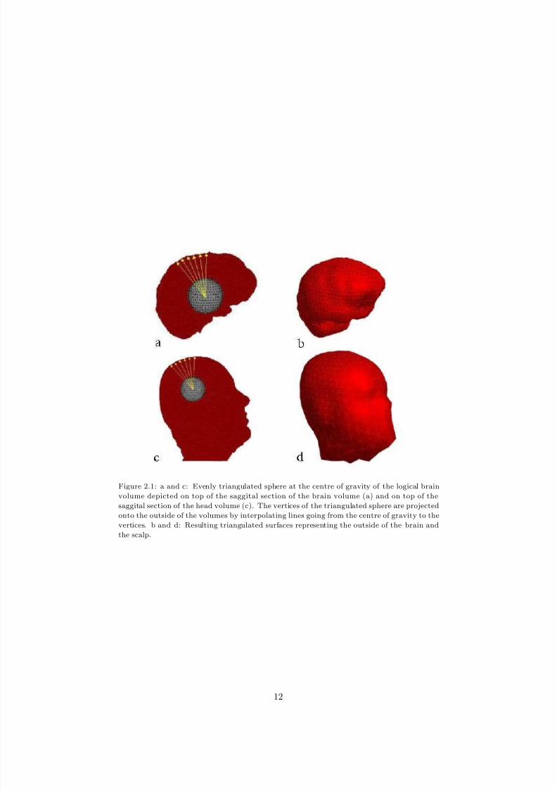
A triangulated surface of this volume is obtained by projecting the vertices of
an evenly triangulated sphere onto the outside of the volume (figure 2.1a and
b).
The original mri was thresholded to obtain a volume representing the whole
head of the subject. Vertices of an evenly triangulated sphere were projectedonto the outside of this volume to obtain the triangulated surface modeling the
outside of the scalp (figure 2.1c and d).
The construction of the surface surrounding the scalp was more difficult than
that of the brain and scalp because there was no available method to extract
the skull volume from an mri. However, the method we used to create the
forward models does not need the information which voxels are part of the skull
volume and which are not, but only a triangulated surface around the skull
volume. Therefore we combined the segmentation and triangulation into one
single process. This means we searched for the boundary between skull and
11
8/3/2019 Rianne Hupse- Localisation Techniques to improve BCI
http://slidepdf.com/reader/full/rianne-hupse-localisation-techniques-to-improve-bci 13/56
Figure 2.1: a and c: Evenly triangulated sphere at the centre of gravity of the logical brain
volume depicted on top of the saggital section of the brain volume (a) and on top of the
saggital section of the head volume (c). The vertices of the triangulated sphere are projected
onto the outside of the volumes by interpolating lines going from the centre of gravity to the
vertices. b and d: Resulting triangulated surfaces representing the outside of the brain and
the scalp.
12
8/3/2019 Rianne Hupse- Localisation Techniques to improve BCI
http://slidepdf.com/reader/full/rianne-hupse-localisation-techniques-to-improve-bci 14/56
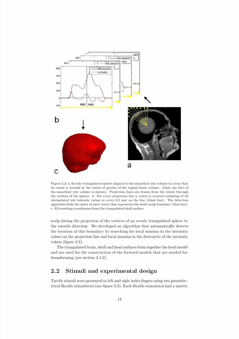
Figure 2.2: a: Evenly triangulated sphere aligned to the smoothed mri volume in a way that
its centre is located at the centre of gravity of the logical brain volume. (Only one slice of
the smoothed mri volume is shown). Projection lines are drawn from the centre through
the vertices of the sphere. b: For every projection line a vector is created consisting of all
interpolated mri intensity values at every 0.5 mm on the line (black line). The detection
algorithm finds the index of each vector that represents the skull-scalp boundary (blue line).
c: All resulting coordinates form the triangulated skull surface.
scalp during the projection of the vertices of an evenly triangulated sphere to
the outside direction. We developed an algorithm that automatically detects
the location of this boundary by searching for local minima in the intensity
values on the projection line and local maxima in the derivative of the intensityvalues (figure 2.2).
The triangulated brain, skull and head surfaces form together the head model
and are used for the construction of the forward models that are needed for
beamforming (see section 2.4.2).
2.2 Stimuli and experimental design
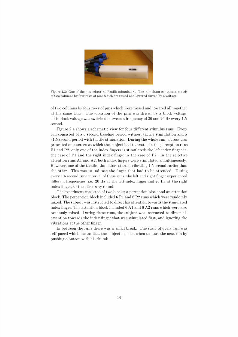
Tactile stimuli were presented to left and right index fingers using two piezoelec-
trical Braille stimulators (see figure 2.3). Each Braille stimulator had a matrix
13
8/3/2019 Rianne Hupse- Localisation Techniques to improve BCI
http://slidepdf.com/reader/full/rianne-hupse-localisation-techniques-to-improve-bci 15/56
Figure 2.3: One of the piezoelectrical Braille stimulators. The stimulator contains a matrix
of two columns by four rows of pins which are raised and lowered driven by a voltage.
of two columns by four rows of pins which were raised and lowered all together
at the same time. The vibration of the pins was driven by a block voltage.
This block voltage was switched between a frequency of 20 and 26 Hz every 1.5second.
Figure 2.4 shows a schematic view for four diff erent stimulus runs. Every
run consisted of a 6 second baseline period without tactile stimulation and a
31.5 second period with tactile stimulation. During the whole run, a cross was
presented on a screen at which the subject had to fixate. In the perception runs
P1 and P2, only one of the index fingers is stimulated; the left index finger in
the case of P1 and the right index finger in the case of P2. In the selective
attention runs A1 and A2, both index fingers were stimulated simultaneously.
However, one of the tactile stimulators started vibrating 1.5 second earlier than
the other. This was to indicate the finger that had to be attended. During
every 1.5 second time interval of these runs, the left and right finger experienceddiff erent frequencies; i.e. 20 Hz at the left index finger and 26 Hz at the right
index finger, or the other way round.
The experiment consisted of two blocks; a perception block and an attention
block. The perception block included 6 P1 and 6 P2 runs which were randomly
mixed. The subject was instructed to direct his attention towards the stimulated
index finger. The attention block included 6 A1 and 6 A2 runs which were also
randomly mixed. During these runs, the subject was instructed to direct his
attention towards the index finger that was stimulated first, and ignoring the
vibrations at the other finger.
In between the runs there was a small break. The start of every run was
self-paced which means that the subject decided when to start the next run by
pushing a button with his thumb.
14

8/3/2019 Rianne Hupse- Localisation Techniques to improve BCI
http://slidepdf.com/reader/full/rianne-hupse-localisation-techniques-to-improve-bci 16/56
Figure 2.4: Schematic view for four diff erent stimulus runs. P1 and P2 are perception runs
in which only one index finger is stimulated by alternating 20 and 26 Hz. A1 and A2 are
selective attention runs in which both index fingers are stimulated simultaneously.
2.3 Data acquisition
One of the subjects (right-handed) for which a forward model was constructedserved as a volunteer in the experiment. During the experiment, the subject was
sitting comfortably in a shielded room with his/her arms resting on cushions and
the tips of the index fingers placed on the stimulators. To avoid any influence
of the sound produced by the stimulators, pink noise (noise with a frequency
spectrum such that the power spectral density is proportional to the reciprocal
of the frequency) was presented to the subject through headphones.
Before the experiment, the exact positions of all electrodes and of three
reference points were measured using a magnetic tracker (MiniBIRD, Ascension
Technology Corporation, Burlington). The reference points were the nasion
point and the locations of the vitamin capsules in the ear plugs that the subjects
wore during the making of the mri scan.Electrophysiological data was recorded from 256 active electrodes mounted
in an elastic headcap (BIOSEMI, Amsterdam). Active electrodes and their
leads are less sensitive for noise pickup than passive electrodes because the first
amplifier stage is integrated in the electrodes. Eye movements and blinks were
monitored by electrodes above, below, and at the sides of the eyes.
The signals were recorded with an anti-aliasing sync filter, digitized at 256 Hz
and stored on a disk for offline analysis.
15

8/3/2019 Rianne Hupse- Localisation Techniques to improve BCI
http://slidepdf.com/reader/full/rianne-hupse-localisation-techniques-to-improve-bci 17/56
2.4 Data analysis
2.4.1 Alignment of electrode positions to mri
To obtain a forward model that predicts the potentials measured by the elec-
trodes due to sources in the brain, the positions of electrodes have to be ex-
pressed in the same coordinate system as the head model. Therefore we per-
formed a rigid body rotation and translation on the electrode positions mea-
sured in the magnetic tracker coordinate system (cMT,i) to obtain the electrode
positions in the mri coordinate system (cMR,i):
cMR,i = RcMT,i + d. (2.1)
In this equation cMR,i and cMT,i are matrices of size 3 by 1 containing the x-
y- and z- coordinates of electrode i, R is a 3 by 3 rotation matrix and d is
a 3 by 1 translation matrix. The rotation matrix R and translation matrix d
are calculated by a least-squares fit of rigid body rotation and translation [5].
This least-squares fit was performed on the rotation and translation of the three
reference coordinates from the magnetic tracker coordinates system to the mri
coordinate system. The exact coordinates of the reference points in the mri
coordinate system were determined by examining the mri scans in a medical
image viewer (MRIcro).
2.4.2 Construction of the forward models
Construction of the forward model was done by applying the boundary elementmethod (bem) [8]. This is a numerical computational method for solving par-
tial diff erential equations which is frequently used to solve field problems. The
method assumes that the electrical conductivity of the head is piecewise homo-
geneous and requires the surfaces of all diff erent tissue layers to be expressed
as a mesh, for example as a finite number of small triangles. These meshed
surfaces, the conductivity values, voxel grid and electrodes locations are then
used to calculate the forward model.
Section 2.1 and appendix A describe how we constructed the meshed surfaces
modeling the outside of the brain, skull and scalp. The relative conductivity
values were chosen according to Oostendorp [17] and are 15:1:15, for respectively
the brain, skull and scalp tissue. A three dimensional grid was constructed
defining the centre coordinates of the voxels. Grid points lying outside the
brain volume were removed from the grid.
The forward model was normalized in a way that the sum of potentials at
all electrodes due to activity in a single voxel was zero. This was done after
removing some electrodes from the model that measured too much noise during
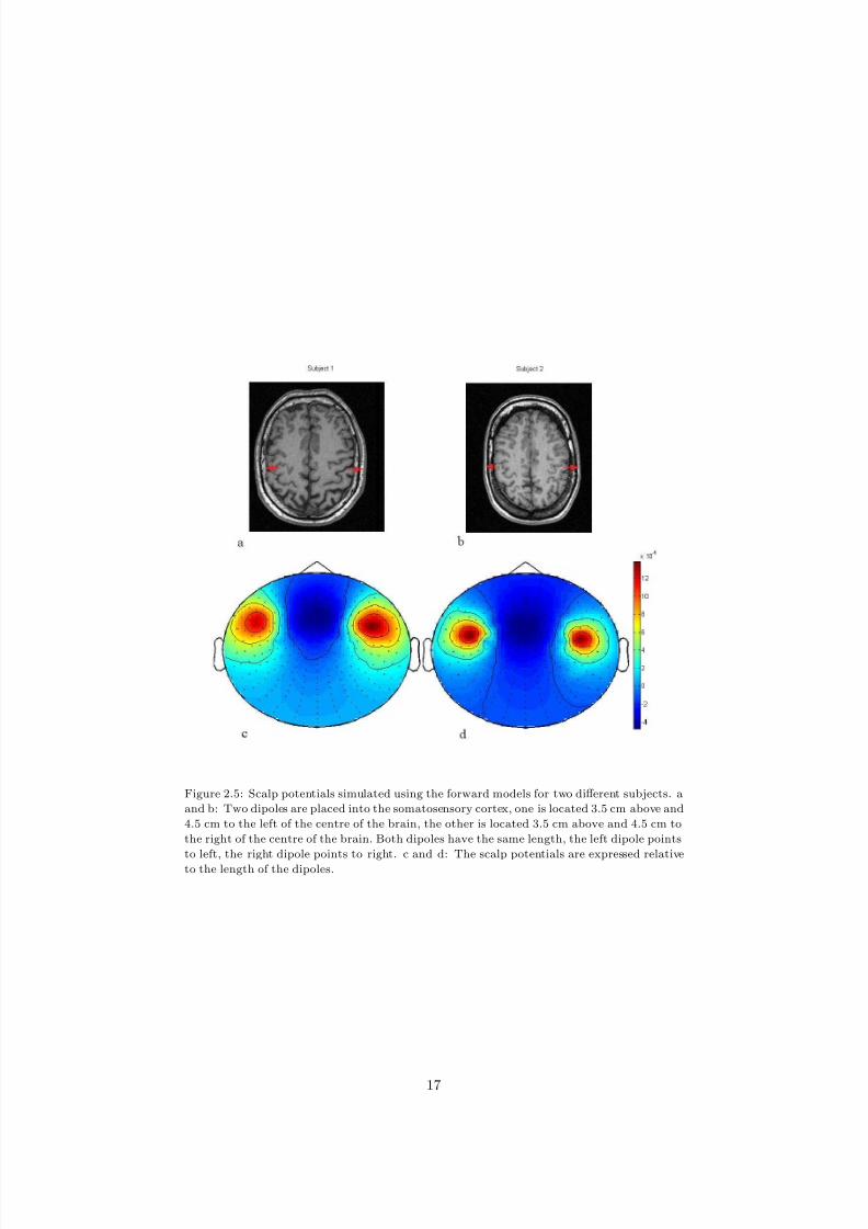
the experiment. To illustrate the diff erences between forward models made for
diff erent subjects, in figure 2.5 the scalp potentials are simulated when two
dipoles are placed into corresponding positions in diff erent head models. The
diff erences in surface potentials are caused by diff erences in the shape of brain,
skull and scalp volumes between the subjects.
16
8/3/2019 Rianne Hupse- Localisation Techniques to improve BCI
http://slidepdf.com/reader/full/rianne-hupse-localisation-techniques-to-improve-bci 18/56
Figure 2.5: Scalp potentials simulated using the forward models for two diff erent subjects. a
and b: Two dipoles are placed into the somatosensory cortex, one is located 3.5 cm above and
4.5 cm to the left of the centre of the brain, the other is located 3.5 cm above and 4.5 cm to
the right of the centre of the brain. Both dipoles have the same length, the left dipole points
to left, the right dipole points to right. c and d: The scalp potentials are expressed relative
to the length of the dipoles.
17
8/3/2019 Rianne Hupse- Localisation Techniques to improve BCI
http://slidepdf.com/reader/full/rianne-hupse-localisation-techniques-to-improve-bci 19/56
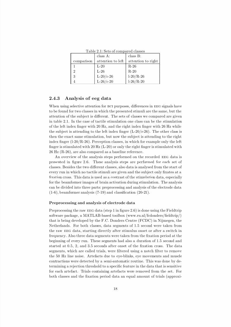
Table 2.1: Sets of compared classes
class A: class B:comparison attention to left attention to right
1 L-20 R-26
2 L-26 R-20
3 L-20/r-26 l-20/R-26
4 L-26/r-20 l-26/R-20
2.4.3 Analysis of eeg data
When using selective attention for bci purposes, diff erences in eeg signals have
to be found for two classes in which the presented stimuli are the same, but the
attention of the subject is diff erent. The sets of classes we compared are given
in table 2.1. In the case of tactile stimulation one class can be the stimulation
of the left index finger with 20 Hz, and the right index finger with 26 Hz while
the subject is attending to the left index finger (L-20/r-26). The other class is
then the exact same stimulation, but now the subject is attending to the right
index finger (l-20/R-26). Perception classes, in which for example only the left
finger is stimulated with 20 Hz (L-20) or only the right finger is stimulated with
26 Hz (R-26), are also compared as a baseline reference.
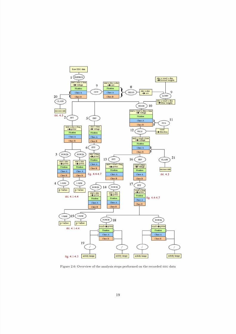
An overview of the analysis steps performed on the recorded eeg data is
presented in figure 2.6. These analysis steps are performed for each set of
classes. Besides the two diff erent classes, also data is analysed from the start of
every run in which no tactile stimuli are given and the subject only fixates at afixation cross. This data is used as a contrast of the stimulation data, especially
for the beamformer images of brain activation during stimulation. The analysis
can be divided into three parts: preprocessing and analysis of the electrode data
(1-6), beamformer analysis (7-19) and classification (20-21).
Preprocessing and analysis of electrode data
Preprocessing the raw eeg data (step 1 in figure 2.6) is done using the Fieldtrip
software package, a MATLAB-based toolbox (www.ru.nl/fcdonders/fieldtrip/)
that is being developed by the F.C. Donders Centre (FCDC) in Nijmegen, the
Netherlands. For both classes, data segments of 1.5 second were taken from
the raw eeg data, starting directly after stimulus onset or after a switch in
frequency. Also three data segments were taken from the fixation period at the
beginning of every run. These segments had also a duration of 1.5 second and
started at 0.5, 2, and 3.5 seconds after onset of the fixation cross. The data
segments, which are called trials, were filtered using a notch filter to remove
the 50 Hz line noise. Artefacts due to eye-blinks, eye movements and muscle
contractions were detected by a semi-automatic routine. This was done by de-
termining a rejection threshold to a specific feature in the data that is sensitive
for each artefact. Trials containing artefacts were removed from the set. For
both classes and the fixation period data an equal amount of trials (approxi-
18
8/3/2019 Rianne Hupse- Localisation Techniques to improve BCI
http://slidepdf.com/reader/full/rianne-hupse-localisation-techniques-to-improve-bci 20/56
Figure 2.6: Overview of the analysis steps performed on the recorded eeg data
19

8/3/2019 Rianne Hupse- Localisation Techniques to improve BCI
http://slidepdf.com/reader/full/rianne-hupse-localisation-techniques-to-improve-bci 21/56
mately 50) was used for further analysis. All trials were baseline corrected by
subtracting for every electrode the average potential over the whole duration of the trial. All data was averaged referenced by subtracting at every moment in
time the average potential of all electrodes.
Spectral analysis of the preprocessed electrode data was done in two ways.
The first way was to perform a Fast Fourier Transform trial by trial (step 2
in figure 2.6), the second way was to perform a Fast Fourier Transform on the
event related potential that was obtained after averaging the data over trials
(step 5 and 6 in figure 2.6). In both cases, the spectrum was calculated only
from the timewindow starting 0.5 second after trial onset till the end of the
trial. After calculating the direct trial by trial spectra, the power at the stimuli
frequencies 20 and 26 Hz of all trials was used in testing for diff erences between
classes and diff erences between electrodes (step 3 and 4 in figure 2.6).
Beamformer analysis
The Linearly Constrained Minimum Variance (lcmv) method [23] was used to
construct the beamformer filter. This method uses the forward model and the
covariance in time between the sensor data to calculate filter weights for every
voxel. This is done by minimizing the total amount of signal that can pass the
filter, while ensuring that the signal expected to come from the voxel of interest
is able to pass (see appendix B).
A common covariance matrix was calculated by averaging the covariance
matrices for every trial of the two classes and fixation data (step 7 and 8 in
figure 2.6). The filter was obtained by applying equation B.13 on the covariancematrix and the forward model (step 9 in figure 2.6). For every trial, the electrode
data was filtered using this filter (step 10 in figure 2.6). The resulting activity is
expressed in an estimated x-, y-, and z-component of the dipole vector modeling
the activity in the voxel. To combine these components into one single parameter
for every voxel varying over time, we estimated the general direction of the dipole
in every voxel and projected the x-, y- and z-components at every moment in
time onto this direction vector. The estimation of the general direction of a voxel
was done using Principle Component Analysis (step 11 in figure 2.6). Data from
all trials of class A and class B was used to estimated the direction in which the
dipole has the largest variance. The data of the classes and the fixation period
was then projected in this direction to obtain a measure of the length of the
dipole over time (step 12 in figure 2.6).
Spectral analysis of the voxel data was done in the same way as was done
for the electrode data. A Fast Fourier Transform was performed for every trial
separately (step 13 in figure 2.6) and for the event related potential (step 16 and
17 in figure 2.6). The power at the stimuli frequencies in the single trials was
used in testing for diff erences between classes and diff erences between electrodes
(step 14 and 15 in figure 2.6). The power at the stimuli frequencies in the event
related potential was used to obtain activity images of the brain (step 18 in
figure 2.6). In order to correct for the beamformer spatial bias as explained in
section B.3, the power for every voxel was divided by the power calculated for
20

8/3/2019 Rianne Hupse- Localisation Techniques to improve BCI
http://slidepdf.com/reader/full/rianne-hupse-localisation-techniques-to-improve-bci 22/56
the fixation period (step 19 in figure 2.6).
Classification
Both preprocessed electrode data and voxel data are used for classification (step
20 and 21 in figure 2.6). The classification scheme first combines measurements
from significant channels to a limited number of features, and classifies with
these features [14]. The class that gives rise to the highest posterior probability
is assigned to the features, i. e. a Bayesian classifier. A multivariate normal
distribution is fitted to the features per class, based on data in a training set,
to calculate the posterior probability. Significant channels are extracted from
the data with a cluster randomization method [15].
A cross-validation scheme was used to calculate the classification rate, be-
cause of the limited amount of data. A cross-validation scheme repeatedly di-vides the data into a training set and an evaluation set. The training set is used
to calculate the settings of the classifier, in this case the data is used to fit the
normal distribution, and the evaluation set is used to estimate the classification
rate. The final classification rate is the averaged value over all the individual
classification rates [10].
21

8/3/2019 Rianne Hupse- Localisation Techniques to improve BCI
http://slidepdf.com/reader/full/rianne-hupse-localisation-techniques-to-improve-bci 23/56
Chapter 3
Results
3.1 Beamformer activity images
Beamformer activity images are depicted in figures 3.1-3.3. These images are
constructed by calculating for every voxel the increase in power at 20 Hz or
26 Hz in the stimulus erp relative to the power of the same frequency in the
fixation erp. The resulting values are presented as colors on a log (dB) scale in
a smoothed mri overlay.
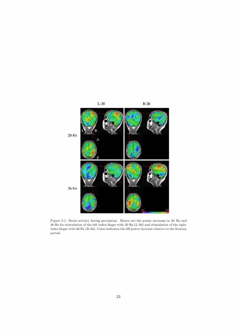
Figure 3.1 shows the activity for the two perception classes of comparison 1:
stimulation of the left index finger with 20 Hz (L-20, left column) and stimula-
tion of the right index finger with 26 Hz (R-26, right column). For both classes,
a large increase in power for the stimulus frequency is found at the contralateral
primary somatosensory cortex.
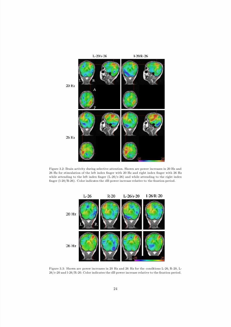
Figure 3.2 shows the activity for the two selective attention classes of com-
parison 3: stimulation of the left index finger with 20 Hz and the right index
finger with 26 Hz while attending to the left finger (L-20/r-26, left column) and
while attending to the right finger (l-20/R-26, right column). For both classes,
a large increase in power is found at the contralateral primary somatosensory
cortex for both stimulus frequencies. In the case of 26 Hz, this increase is visible
over a large area, including parts of the temporal lobe.
Figure 3.3 shows the activity for the two perception classes of comparison 2:
stimulation of the left index finger with 26 Hz (L-26) and stimulation of the right
index finger with 20 Hz (R-20). Also the activity is shown for the two selectiveattention classes of comparison 4: stimulation of the left index finger with 26 Hz
and the right index finger with 20 Hz while attending to the left finger (L-26/r-
20) and while attending to the right finger (l-26/R-20). Also for these classes,
a large increase in power is visible in the contralateral somatosensory cortex.
All figures show brain areas with small decreases in 20 and 26 Hz power.
The locations of these areas change per stimulus class, and might be due to
measurement noise in combination with the relatively small number of trials.
22
8/3/2019 Rianne Hupse- Localisation Techniques to improve BCI
http://slidepdf.com/reader/full/rianne-hupse-localisation-techniques-to-improve-bci 24/56
Figure 3.1: Brain activity during perception. Shown are the p ower increases in 20 Hz and
26 Hz for stimulation of the left index finger with 20 Hz (L-20) and stimulation of the right
index finger with 26 Hz (R-26). Color indicates the dB power increase relative to the fixation
period.
23
8/3/2019 Rianne Hupse- Localisation Techniques to improve BCI
http://slidepdf.com/reader/full/rianne-hupse-localisation-techniques-to-improve-bci 25/56
Figure 3.2: Brain activity during selective attention. Shown are power increases in 20 Hz and
26 Hz for stimulation of the left index finger with 20 Hz and right index finger with 26 Hzwhile attending to the left index finger (L-20/r-26) and while attending to the right index
finger (l-20/R-26). Color indicates the dB power increase relative to the fixation period.
Figure 3.3: Shown are power increases in 20 Hz and 26 Hz for the conditions L-26, R-20, L-
26/r-20 and l-26/R-20. Color indicates the dB power increase relative to the fixation period.
24
8/3/2019 Rianne Hupse- Localisation Techniques to improve BCI
http://slidepdf.com/reader/full/rianne-hupse-localisation-techniques-to-improve-bci 26/56
3.2 Power diff erences between contralateral and
ipsilateral channels
For both left and right hemisphere a voxel in somatosensory cortex was chosen
that showed a large increase in stimulus frequency compared to the fixation
period. The spectra of the erp (step 16 and 17 in figure 2.6) for these voxels are
shown in the first rows of figures 3.4-3.7. The second rows in these figures show
the spectra of the erp for two electrodes above the left and right hemisphere
that are expected to measure the largest potential diff erences when left or right
somatosensory cortex is active. These electrodes were chosen by simulating the
scalp potentials when a dipole was placed at the location of the chosen voxels
pointing into the direction of the activity (calculated in step 11 of figure 2.6).
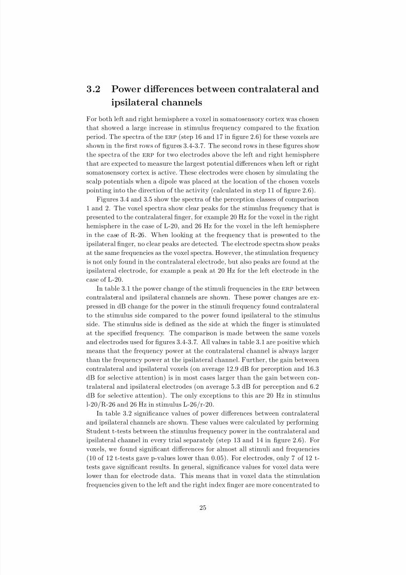
Figures 3.4 and 3.5 show the spectra of the perception classes of comparison1 and 2. The voxel spectra show clear peaks for the stimulus frequency that is
presented to the contralateral finger, for example 20 Hz for the voxel in the right
hemisphere in the case of L-20, and 26 Hz for the voxel in the left hemisphere
in the case of R-26. When looking at the frequency that is presented to the
ipsilateral finger, no clear peaks are detected. The electrode spectra show peaks
at the same frequencies as the voxel spectra. However, the stimulation frequency
is not only found in the contralateral electrode, but also peaks are found at the
ipsilateral electrode, for example a peak at 20 Hz for the left electrode in the
case of L-20.
In table 3.1 the power change of the stimuli frequencies in the erp between
contralateral and ipsilateral channels are shown. These power changes are ex-
pressed in dB change for the power in the stimuli frequency found contralateral
to the stimulus side compared to the power found ipsilateral to the stimulus
side. The stimulus side is defined as the side at which the finger is stimulated
at the specified frequency. The comparison is made between the same voxels
and electrodes used for figures 3.4-3.7. All values in table 3.1 are positive which
means that the frequency power at the contralateral channel is always larger
than the frequency power at the ipsilateral channel. Further, the gain between
contralateral and ipsilateral voxels (on average 12.9 dB for perception and 16.3
dB for selective attention) is in most cases larger than the gain between con-
tralateral and ipsilateral electrodes (on average 5.3 dB for perception and 6.2
dB for selective attention). The only exceptions to this are 20 Hz in stimulus
l-20/R-26 and 26 Hz in stimulus L-26/r-20.In table 3.2 significance values of power diff erences between contralateral
and ipsilateral channels are shown. These values were calculated by performing
Student t-tests between the stimulus frequency power in the contralateral and
ipsilateral channel in every trial separately (step 13 and 14 in figure 2.6). For
voxels, we found significant diff erences for almost all stimuli and frequencies
(10 of 12 t-tests gave p-values lower than 0.05). For electrodes, only 7 of 12 t-
tests gave significant results. In general, significance values for voxel data were
lower than for electrode data. This means that in voxel data the stimulation
frequencies given to the left and the right index finger are more concentrated to
25
8/3/2019 Rianne Hupse- Localisation Techniques to improve BCI
http://slidepdf.com/reader/full/rianne-hupse-localisation-techniques-to-improve-bci 27/56
Figure 3.4: Spectra of the erp measured by two voxels and two electrodes in the case of
stimulation of the left finger with 20 Hz (blue), stimulation of the right finger with 26 Hz
(red) or when there is no stimulation (green). Electrodes and voxels were located in and
above somatosensory cortex in left and right hemisphere.
Figure 3.5: Spectra of the erp measured by two voxels and two electrodes in the case of
stimulation of the left finger with 26 Hz (blue), stimulation of the right finger with 20 Hz
(red) or when there is no stimulation (green).
26
8/3/2019 Rianne Hupse- Localisation Techniques to improve BCI
http://slidepdf.com/reader/full/rianne-hupse-localisation-techniques-to-improve-bci 28/56
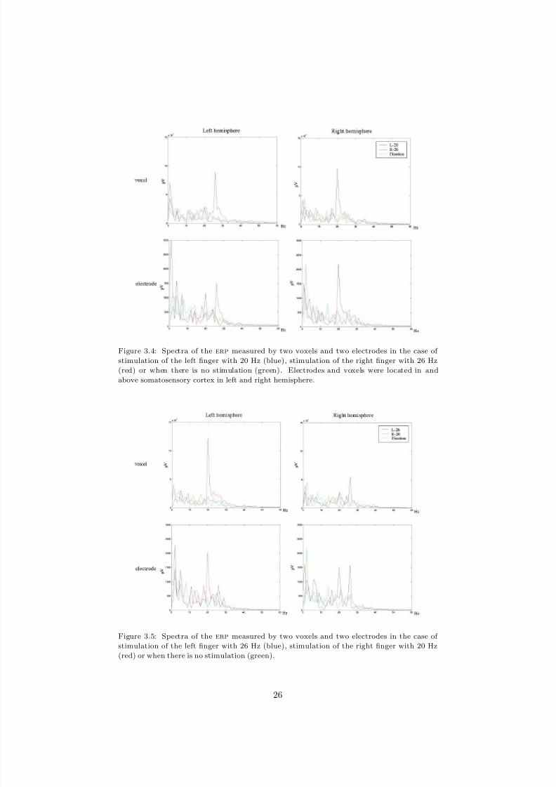
Figure 3.6: Spectra of the erp measured by two voxels and two electrodes in the case of
stimulation of the left finger with 20 Hz and the right finger with 26 Hz while attention was
to the left finger (blue), and while attention was to the right finger (red). The spectrum is
also shown for the the case when there is no stimulation (green).
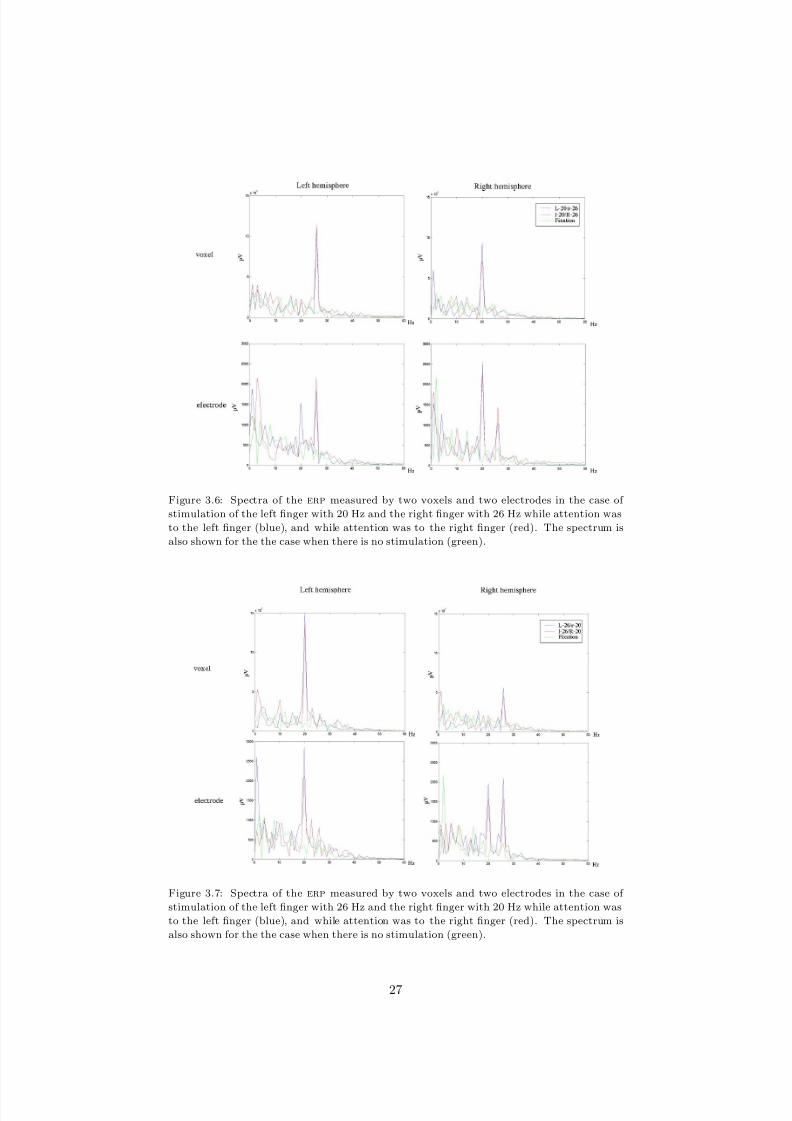
Figure 3.7: Spectra of the erp measured by two voxels and two electrodes in the case of
stimulation of the left finger with 26 Hz and the right finger with 20 Hz while attention was
to the left finger (blue), and while attention was to the right finger (red). The spectrum is
also shown for the the case when there is no stimulation (green).
27

8/3/2019 Rianne Hupse- Localisation Techniques to improve BCI
http://slidepdf.com/reader/full/rianne-hupse-localisation-techniques-to-improve-bci 29/56
Table 3.1: Power change in erp between contralateral and ipsilateral channels
(dB)voxel electrode
Stimulus 20 Hz 26 Hz 20 Hz 26 Hz
L-20 10.7 5.6
R-20 13.7 2.5
L-26 12.9 4.9
R-26 14.1 8.1
L-20/r-26 14.2 23.6 4.5 4.9
l-20/R-26 10.1 29.8 12.2 3.5
L-26/r-20 20.4 9.7 3.2 12.5
l-26/R-20 16.3 6.1 2.5 5.9
Table 3.2: Significance of diff erences between contralateral and ipsilateral chan-
nelsvoxel electrode
Stimulus 20 Hz 26 Hz 20 Hz 26 Hz
L-20 <0.0001* 0.06
R-20 <0.0001* 0.0006*
L-26 0.01* 0.04*
R-26 <0.0001* 0.01*
L-20/r-26 0.03* <0.0001* 0.5 0.0002*
l-20/R-26 0.01* <0.0001* 0.4 0.004*
L-26/r-20 <0.0001* 0.1 0.0002* 0.2l-26/R-20 <0.0001* 0.2 <0.0001* 0.4
separate areas of the brain than in electrode data.
3.3 Attention induced power change
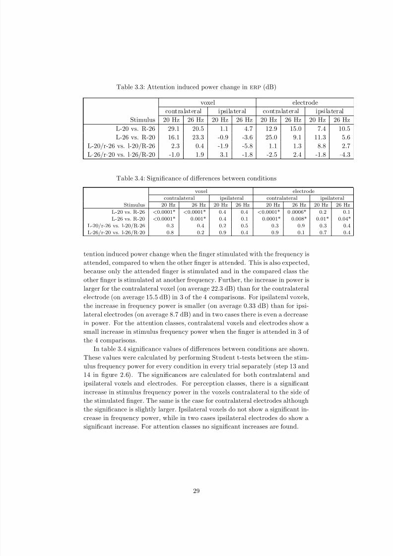
In table 3.3 the attention induced power change in the erp is shown when
comparing the power for the stimulus frequency between attention to the left
index finger and attention to the right index finger. These power changes are
expressed in dB change for the case the finger experiencing the specified fre-quency is attended compared to the case that the finger is not attended. For
example, in the cases when the left finger is stimulated with 20 Hz and the right
finger with 26 Hz (L-20/r-26 and l-20/R-26) the voxel contralateral to the 20 Hz
stimulation (the voxel in the right hemisphere) shows a 2.3 dB power increase
when the left finger is attended (L-20/r-26) compared to when the right finger
is attended (l-20/R-26). The voxel contralateral to the 26 Hz stimulation (the
voxel in the left hemisphere) shows a 0.4 power increase when the right finger is
attended (l-20/R-26) compared to when the left finger is attended (L-20/r-26).
For the perception classes, contralateral voxels and electrodes show a large at-
28
8/3/2019 Rianne Hupse- Localisation Techniques to improve BCI
http://slidepdf.com/reader/full/rianne-hupse-localisation-techniques-to-improve-bci 30/56
Table 3.3: Attention induced power change in erp (dB)
voxel electrode
contralateral ipsilateral contralateral ipsilateral
Stimulus 20 Hz 26 Hz 20 Hz 26 Hz 20 Hz 26 Hz 20 Hz 26 Hz
L-20 vs. R-26 29.1 20.5 1.1 4.7 12.9 15.0 7.4 10.5
L-26 vs. R-20 16.1 23.3 -0.9 -3.6 25.0 9.1 11.3 5.6
L-20/r-26 vs. l-20/R-26 2.3 0.4 -1.9 -5.8 1.1 1.3 8.8 2.7
L-26/r-20 vs. l-26/R-20 -1.0 1.9 3.1 -1.8 -2.5 2.4 -1.8 -4.3
Table 3.4: Significance of diff erences between conditions
voxel electrode
contralateral ipsilateral contralateral ipsilateral
Stimulus 20 Hz 26 Hz 20 Hz 26 Hz 20 Hz 26 Hz 20 Hz 26 Hz
L-20 vs. R-26 <0.0001* <0.0001* 0.4 0.4 <0.0001* 0 .0006* 0.2 0.1
L-26 vs. R-20 <0.0001* 0.001* 0.4 0.1 0.0001* 0.008* 0.01* 0.04*
L-20/r-26 vs. l-20/R-26 0.3 0.4 0.2 0.5 0.3 0.9 0.3 0.4
L-26/r-20 vs. l-26/R-20 0.8 0.2 0.9 0.4 0.9 0.1 0.7 0.4
tention induced power change when the finger stimulated with the frequency is
attended, compared to when the other finger is attended. This is also expected,
because only the attended finger is stimulated and in the compared class the
other finger is stimulated at another frequency. Further, the increase in power is
larger for the contralateral voxel (on average 22.3 dB) than for the contralateral
electrode (on average 15.5 dB) in 3 of the 4 comparisons. For ipsilateral voxels,
the increase in frequency power is smaller (on average 0.33 dB) than for ipsi-
lateral electrodes (on average 8.7 dB) and in two cases there is even a decrease
in power. For the attention classes, contralateral voxels and electrodes show a
small increase in stimulus frequency power when the finger is attended in 3 of
the 4 comparisons.
In table 3.4 significance values of diff erences between conditions are shown.
These values were calculated by performing Student t-tests between the stim-
ulus frequency power for every condition in every trial separately (step 13 and
14 in figure 2.6). The significances are calculated for both contralateral and
ipsilateral voxels and electrodes. For perception classes, there is a significant
increase in stimulus frequency power in the voxels contralateral to the side of the stimulated finger. The same is the case for contralateral electrodes although
the significance is slightly larger. Ipsilateral voxels do not show a significant in-
crease in frequency power, while in two cases ipsilateral electrodes do show a
significant increase. For attention classes no significant increases are found.
29

8/3/2019 Rianne Hupse- Localisation Techniques to improve BCI
http://slidepdf.com/reader/full/rianne-hupse-localisation-techniques-to-improve-bci 31/56
3.4 Classification success rates
In table 3.5 the success rates are given for classification. For the perception
classes both voxel and electrode data give very large success rates. For these
classes, the success rates of the electrode data are slightly larger than that of
the voxel data. Selective attention classes give for both voxel and electrode data
very small success rates, even below change level.
Table 3.5: Classification success ratesStimulus voxel data electrode data
L-20 vs. R-26 0.88 0.90
L-26 vs. R-20 0.87 0.91
L-20/r-26 vs. l-20/R-26 0.42 0.41
L-26/r-20 vs. l-26/R-20 0.49 0.39
30

8/3/2019 Rianne Hupse- Localisation Techniques to improve BCI
http://slidepdf.com/reader/full/rianne-hupse-localisation-techniques-to-improve-bci 32/56
Chapter 4
Discussion
The aim of the experiment described in this thesis was to explore the possibility
to elaborate a new type of bci system: a system in which selective attention to
temporal rhythmic stimuli is used to control an external device. Simultaneously,
beamformer techniques were used to see if the success rates of the classification
procedure would improve. To be sure that the beamformer filter allocates activ-
ity to the correct anatomical locations, a new method was proposed to construct
realistic head models.
When looking at the power of the stimulus frequencies in the erp, a clear
increase was found in the somatosensory cortex contralateral to the stimulus
side compared to the fixation period. This corresponds to the steady-state
somatosensory evoked potentials found in [12] [13] [21]. This finding meansthat the beamformer filter based on the realistic head model is able to allocate
the measured eeg activity to brain areas in an accurate way.
For both voxel and electrode channels the power in the contralateral channel
is larger than the power in the ipsilateral channel, but the gain in power is
larger for voxel data than for electrode data. Further, the significance values for
diff erences between these channels in single trials are also smaller for voxel data.
These findings indicate that beamforming allocates the diff erent stimulation
frequencies to separate areas of the brain, while the frequencies found in the
original electrode data reach both sides of the scalp. By this spatial separation
of frequencies the power of a single stimulus is focused to a single area which will
increase the signal to noise ratio. Therefore, signals allocated to voxels in theseareas might give a more accurate estimation of the power of the steady-state
somatosensory evoked potential than electrode signals.
For both contralateral voxel and electrode channels an increase in power is
found between the compared perception classes. This increase is larger for voxel
channels, which confirms the idea that voxel data has a larger signal to noise
ratio. The attention induced power gain calculated from the data measured in
the selective attention conditions is small and not significant present in single
trials.
Perception success rates are relatively high when voxel or electrode data is
31
8/3/2019 Rianne Hupse- Localisation Techniques to improve BCI
http://slidepdf.com/reader/full/rianne-hupse-localisation-techniques-to-improve-bci 33/56
used in the classification algorithm. Success rates for electrode data are slightly
larger than for voxel data. An explanation can be that cross talk between someelectrodes and the stimulator leads results in a large power for the stimula-
tion frequency in some electrode signals. If this happens at isolated electrodes,
beamforming will ignore the signals because they are not correlated with the
signals from neighbouring electrodes. Classification success rates for selective
attention classes are very low and even below chance level. Probably the signal
to noise level of the attention induced power gain is too small to be measured in
single trials and averaging over a few trials is necessary. Recently, a new classi-
fication algorithm is developed that uses the features of two successive trials for
classification. This algorithm gives higher classification success rates (± 60%).
Probably influences in frequency power due to other ongoing brain processes are
reduced by using also the power during the second trial in which the frequencies
are switched.
An important suggestion for improving the experiment is to include a period
in each run in which the stimulators are active, but the fingers of the subject
are not attached. The vibrating of the stimulators should be the same as the
experiment, and the subject should be fixating to a fixation cross during the
stimulation. The data recorded during this time period can then be used as
a baseline instead of the fixation baseline. In this way the probability that
diff erences between stimulation and baseline are the result of crosstalk is re-
duced. This baseline data can also be used in the classification algorithm to
see if the success rates are (partially) due to crosstalk. Next, a discrimination
task can be added to the experiment, for example the task to detect a small
interruption in time of the stimulus at the attended side while ignoring the in-terruptions at the not attended side. This might increase the attention level of
the subject and therefore the attention induced power gain. Further, it might
be worthwhile to examine if other tactile stimuli, for example stimuli without
alternating frequencies, give better results.
A suggestion for improving the analysis of the experimental data is to in-
crease the number of trials that is used as a training set in the cross validation
procedure. This can be done by combining the data from multiple experiment
sessions. The beamformer filter could be improved by using more trials in es-
timating the covariance matrix. If the data analysis can be performed online,
i.e. during the experiment, direct feedback about the chosen class can be given
to the subject. This might encourage the subject to concentrate and might in-crease the attention induced power gain. Further it might be necessary to use
the average signal over a small amount (2-3) of trials to increase the signal to
noise ratio. However, this will increase the time needed for every decision and
therefore slows down the system.
Further research will show if the results described in this thesis are represen-
tative to the results of experiments with other subjects. More analysis should
be done to investigate if beamforming gives better results than other spatial
filters like independent component analysis (ica). Further, a comparison can
be made between the beamformer results obtained when the forward model is
32

8/3/2019 Rianne Hupse- Localisation Techniques to improve BCI
http://slidepdf.com/reader/full/rianne-hupse-localisation-techniques-to-improve-bci 34/56
based on a simple sphere model to the results obtained when it is based on the
realistic head models we constructed.
33

8/3/2019 Rianne Hupse- Localisation Techniques to improve BCI
http://slidepdf.com/reader/full/rianne-hupse-localisation-techniques-to-improve-bci 35/56
Appendix A
Construction of a realistic
head model
A.1 Introduction
When applying beamformer techniques, a forward model has to be estimated
that predicts the potential distribution measured at the scalp when parts of the
brain are active. This forward model consists of coefficients for every combina-
tion of volume unit in the brain and electrode. Every coefficient defines how
much of the activity present in the selected volume unit is transmitted though
the diff erent tissues in the head to the selected electrode (see appendix B).The construction of a forward model involves the making of a head model
in which the shapes of the diff erent tissue volumes in the head are defined.
Every tissue layer is given a conductivity value. The forward model can then
be calculated using the boundary element method. In the case of using the
boundary element method, the shapes of the tissue layers have to be defined by
triangulated surfaces that represent the boundaries between these layers.
The accuracy of the forward model depends heavily on assumptions made
about the shape of the tissue layers in the head: the headmodel. The forward
model used in eeg experiments is often based on a spherical head model. This
model consists of multiple shells representing the brain, skull and scalp tissue
layers (figure A.1a). It has been shown that realistic head models (figure A.1b)
can obtain a more accurate source localisation, especially when signal to noise
ratio is low [22]. Although the construction is more complicated we decided
to use a realistic head model instead of a spherical head model. By using
more physiological information in the forward model the resulting estimated
activity patterns will deviate less from the real activity patterns in the brain and
therefore are expected to contain more information to be useful in classification
algorithms.
To obtain a realistic model of the head geometry, we used T1-weighed mri
(magnetic resonance imaging) scans of our 6 subjects. Using these scans, we
34

8/3/2019 Rianne Hupse- Localisation Techniques to improve BCI
http://slidepdf.com/reader/full/rianne-hupse-localisation-techniques-to-improve-bci 36/56
Figure A.1: a: The spherical head model consists of spherical shells representing diff erent
tissue layers. b: The realistic head model consists of multiple layers based on the realisticshapes of the diff erent tissues that are extracted from an anatomical mri.
created a model consisting of three triangulated surfaces representing the out-
side of the brain (including cerebral spinal fluid), skull and scalp. These surfaces
are used in the boundary element method to calculate the forward model. The
construction of the brain and scalp surfaces is done in two steps: extracting the
desired compartment from the mri and projecting the vertices of a triangulated
sphere onto this compartment. To obtain the triangulated surface representing
the outside of the skull we created a new method which combines the segmen-
tation and triangulation steps into one process that automatically searches for
the boundary between skull and scalp in the mri during the projection.
A.2 Segmentation and triangulation of the brain
A.2.1 Segmentation
To create a volume modeling the brain we first extracted the white matter, gray
matter and csf compartments from the mri using the SPM segmentation tool
which is a method by Ashburner and Friston [1]. This method aligns the mri
volume to a template and performs cluster analysis with a modified mixture
model and a-priori information about the likelihoods of each voxel being part
of the three diff
erent tissue types. The output of this tool are three volumescontaining probability values representing the likeliness for a certain voxel to be
part of one the three compartments (figure A.2b, c and d). The three volumes
were merged into one single brain volume by taking for every voxel the maximum
value of the three segments at that location (figure A.2e).
To reduce noise while preserving the surface of the segment we filtered this
volume using a 3d median filter. This is done by moving a 3d kernel with a size
of 5 mm3 over the mri volume and taking as a new value for the voxel in the
centre the median of the values of all 125 voxels in the kernel. The results is
shown in figure A.2f. Next, we rounded all values towards the nearest integer
35

8/3/2019 Rianne Hupse- Localisation Techniques to improve BCI
http://slidepdf.com/reader/full/rianne-hupse-localisation-techniques-to-improve-bci 37/56
Figure A.2: a: One slice of the mri scan made in a 1.5 T scanner, every pixel corresponds to a voxel (volume pixel)
of 1 mm3. The colored volumes depicted in b-h are laid over this original volume. b-d: Output of segmentation
tool consisting of probability values for voxels being part of respectively white matter, gray matter and cerebral
spinal fluid. e: Probability values for voxels being part of the brain segment (for every voxel the maximum value
of figure b-d is taken). f: A median filter is applied to smooth the volume while preserving edges. g: A logical
volume is obtained by applying a threshold. h: The final brain segment after smoothing the logical volume.
(0 or 1) to obtain a logical volume (figure A.2g). To smooth the surface of the
volume we eroded the volume and dilated it again by 3 mm. The result is shown
in figure A.2h.
A.2.2 Triangulation
To create a triangulated surface that surrounds the brain volume we projected
the vertices of an evenly triangulated sphere with its origin located at the centre
of gravity of the logical brain volume onto the outer surface of the volume (figure
A.3).
36
8/3/2019 Rianne Hupse- Localisation Techniques to improve BCI
http://slidepdf.com/reader/full/rianne-hupse-localisation-techniques-to-improve-bci 38/56
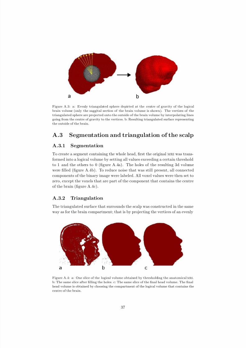
Figure A.3: a: Evenly triangulated sphere depicted at the centre of gravity of the logical
brain volume (only the saggital section of the brain volume is shown). The vertices of the
triangulated sphere are projected onto the outside of the brain volume by interpolating lines
going from the centre of gravity to the vertices. b: Resulting triangulated surface representing
the outside of the brain.
A.3 Segmentation and triangulation of the scalp
A.3.1 Segmentation
To create a segment containing the whole head, first the original mri was trans-
formed into a logical volume by setting all values exceeding a certain threshold
to 1 and the others to 0 (figure A.4a). The holes of the resulting 3d volume
were filled (figure A.4b). To reduce noise that was still present, all connected
components of the binary image were labeled. All voxel values were then set to
zero, except the voxels that are part of the component that contains the centreof the brain (figure A.4c).
A.3.2 Triangulation
The triangulated surface that surrounds the scalp was constructed in the same
way as for the brain compartment; that is by projecting the vertices of an evenly
Figure A.4: a: One slice of the logical volume obtained by thresholding the anatomical mri.
b: The same slice after filling the holes. c: The same slice of the final head volume. The final
head volume is obtained by choosing the compartment of the logical volume that contains the
centre of the brain.
37
8/3/2019 Rianne Hupse- Localisation Techniques to improve BCI
http://slidepdf.com/reader/full/rianne-hupse-localisation-techniques-to-improve-bci 39/56
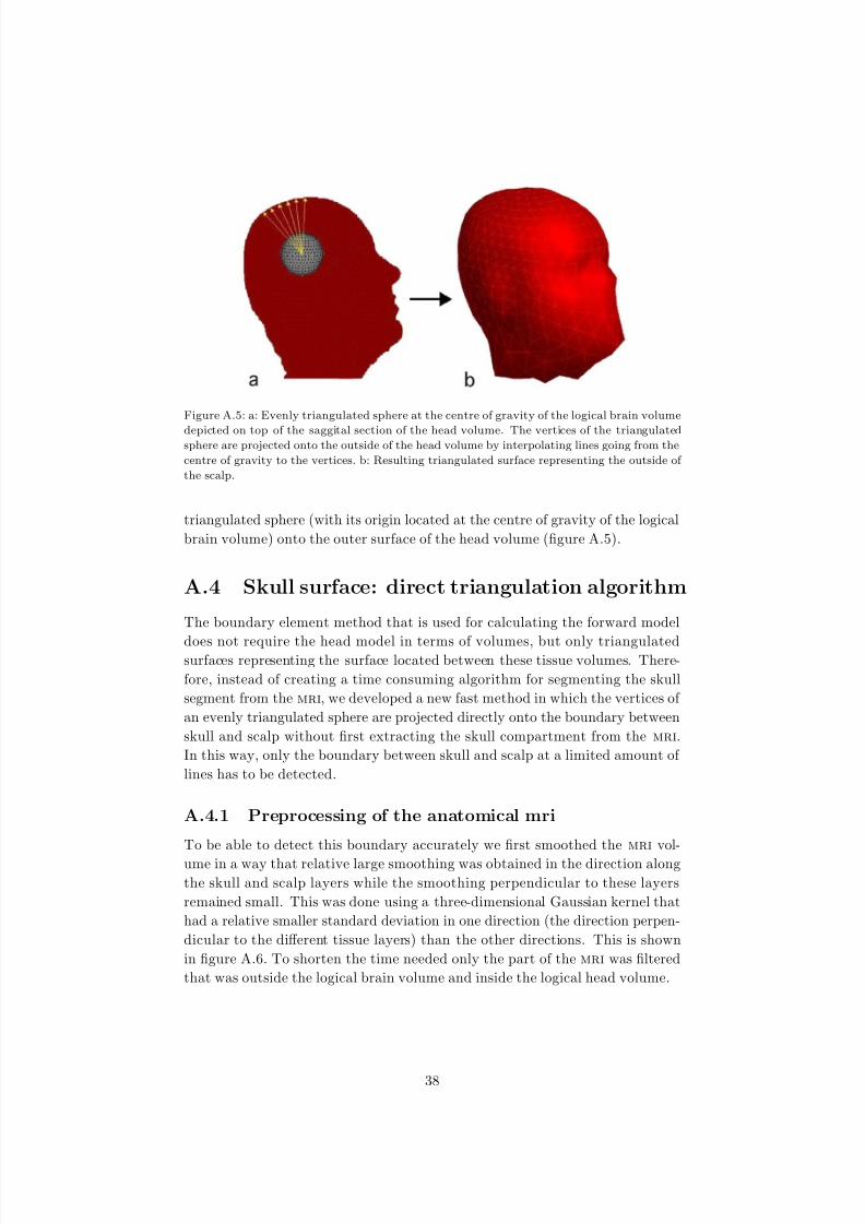
Figure A.5: a: Evenly triangulated sphere at the centre of gravity of the logical brain volume
depicted on top of the saggital section of the head volume. The vertices of the triangulatedsphere are projected onto the outside of the head volume by interpolating lines going from the
centre of gravity to the vertices. b: Resulting triangulated surface representing the outside of
the scalp.
triangulated sphere (with its origin located at the centre of gravity of the logical
brain volume) onto the outer surface of the head volume (figure A.5).
A.4 Skull surface: direct triangulation algorithm
The boundary element method that is used for calculating the forward model
does not require the head model in terms of volumes, but only triangulatedsurfaces representing the surface located between these tissue volumes. There-
fore, instead of creating a time consuming algorithm for segmenting the skull
segment from the mri, we developed a new fast method in which the vertices of
an evenly triangulated sphere are projected directly onto the boundary between
skull and scalp without first extracting the skull compartment from the mri.
In this way, only the boundary between skull and scalp at a limited amount of
lines has to be detected.
A.4.1 Preprocessing of the anatomical mri
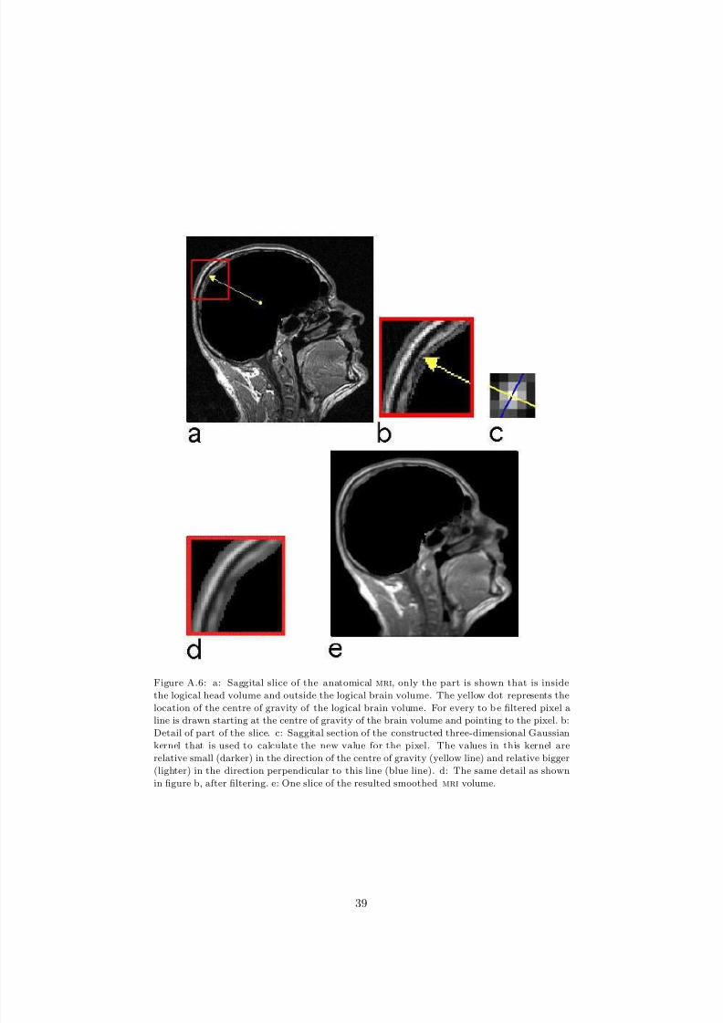
To be able to detect this boundary accurately we first smoothed the mri vol-
ume in a way that relative large smoothing was obtained in the direction along
the skull and scalp layers while the smoothing perpendicular to these layers
remained small. This was done using a three-dimensional Gaussian kernel that
had a relative smaller standard deviation in one direction (the direction perpen-
dicular to the diff erent tissue layers) than the other directions. This is shown
in figure A.6. To shorten the time needed only the part of the mri was filtered
that was outside the logical brain volume and inside the logical head volume.
38
8/3/2019 Rianne Hupse- Localisation Techniques to improve BCI
http://slidepdf.com/reader/full/rianne-hupse-localisation-techniques-to-improve-bci 40/56
Figure A.6: a: Saggital slice of the anatomical mri, only the part is shown that is inside
the logical head volume and outside the logical brain volume. The yellow dot represents the
location of the centre of gravity of the logical brain volume. For every to b e filtered pixel a
line is drawn starting at the centre of gravity of the brain volume and pointing to the pixel. b:Detail of part of the slice. c: Saggital section of the constructed three-dimensional Gaussian
kernel that is used to calculate the new value for the pixel. The values in this kernel are
relative small (darker) in the direction of the centre of gravity (yellow line) and relative bigger
(lighter) in the direction perpendicular to this line (blue line). d: The same detail as shown
in figure b, after filtering. e: One slice of the resulted smoothed mri volume.
39

8/3/2019 Rianne Hupse- Localisation Techniques to improve BCI
http://slidepdf.com/reader/full/rianne-hupse-localisation-techniques-to-improve-bci 41/56
A.4.2 Triangulation process
To construct the triangulated skull surface we again started with an evenly
triangulated sphere with its origin located at the centre of gravity of the logical
brain volume. For every vertex of this sphere we constructed a vector containing
all intensities of the smoothed mri volume that were crossed when projecting
the vertex on the outside of the mri volume. Examples of these projection lines
are shown in figure A.7a. Because these lines do not cross the voxels exactly
through their centre we interpolated the intensity values of all neighbouring
voxels according to the place where the line crosses. We did this for locations
at every 0.5 mm of the line. Examples of the interpolated mri values at these
lines are shown in figures A.7b and A.8. We constructed an algorithm that
automatically detects the position in every intensity vector that represents the
boundary between skull and scalp. This position is then easily transformed intothe corresponding mri coordinates to obtain the projection of the vertex onto
the outside of the skull. All projected vertices form together the triangulated
skull surface (figure A.7c).
A.4.3 Detection of the boundary between skull and scalp
Because T1 magnetic resonance imaging measures hydrogen density which is
not (much) present in bone tissue, the skull produces low intensity values on
mri. On the other hand, scalp tissue contains much hydrogen and appears
bright on mri. Therefore we expect when going from the outside of the brain
through the skull and the scalp to find first low intensity values representing
the skull and later high intensity values representing the scalp. In figure A.8
the values of a representative intensity vector are plotted (black line). The local
minimum in this figure represents the bone tissue. Connected to the bone there
is a layer of arachnoid and dura mater which give higher intensity values than
the bone itself. This results in an small peak at the left of the local minimum.
The scalp tissue starts with a layer of subcutaneous fat. Fat contains much
hydrogen and therefore there is a big peak in the intensity values at the right of
the local minimum representing the skull. The plateau at the most right part
of the figure represents the other layers (dermis and epidermis) of the scalp.
Automatic detection of the position representing the boundary between skull
and scalp was done by first creating a second vector containing the diff erences
between neighbouring intensity values (red line in figure A.8). For every vertexboth the mri intensity vector and the derivative vector were used in the detection
algorithm (algorithm 1). The basic idea behind this algorithm was that we
expected the intensity to go from low to high values at the boundary between
skull and scalp, and therefore to be located at a local maximum (higher than
a constant threshold, green line in A.8) in the derivative vector. Further we
expected the position of this local maximum to be located at the right side of a
local minimum in the intensity vector representing the center of the skull. This
local minimum must be somewhere in the middle in between the end of the
brain and the end of the scalp.
40
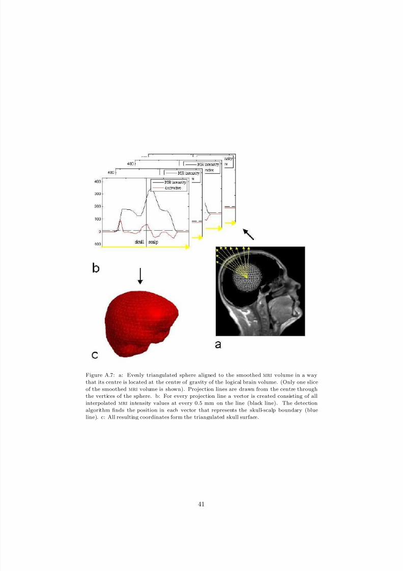
8/3/2019 Rianne Hupse- Localisation Techniques to improve BCI
http://slidepdf.com/reader/full/rianne-hupse-localisation-techniques-to-improve-bci 42/56
Figure A.7: a: Evenly triangulated sphere aligned to the smoothed mri volume in a way
that its centre is located at the centre of gravity of the logical brain volume. (Only one slice
of the smoothed mri volume is shown). Projection lines are drawn from the centre through
the vertices of the sphere. b: For every projection line a vector is created consisting of all
interpolated mri intensity values at every 0.5 mm on the line (black line). The detection
algorithm finds the position in each vector that represents the skull-scalp boundary (blue
line). c: All resulting coordinates form the triangulated skull surface.
41

8/3/2019 Rianne Hupse- Localisation Techniques to improve BCI
http://slidepdf.com/reader/full/rianne-hupse-localisation-techniques-to-improve-bci 43/56
Figure A.8: Black line: Interpolated mri intensity values at every 0.5 mm of one representative
projection line. Because mri measures hydrogen density bone tissue gives low intensity values,while fat tissue gives high values. Arachnoid, dura and (epi)dermis give moderate values. Red
line: derivative of intensity values. Green line: threshold used in detection algorithm. Blue
line: Boundary between skull and scalp chosen by the detection algorithm.
If there was no local minimum at all in the intensity vector, or there was no
local maximum at the right site of the chosen local minimum, we decided to use
the position of the second (from the start) local maximum in the derivative vec-
tor as the point representing the boundary between skull and scalp. Examples
are shown in figure A.9a and d. We chose the second local maximum because
all intensity values inside the brain volume were set to zero during filtering and
therefore the first local maximum only represents the starting of the part of the
mri that is outside the brain. If there was also no second local maximum present
in the derivative vector, we calculated the boundary point using the thickness
of the skull under the neighbouring vertex that was projected previously (figure
A.9b and c).
The automatic procedure was applied only at the lines that crossed the upper
half of the brain surface because at the lower half of the head, the skull is not
directly covered by the scalp. The upper half was defined by the plane through
three points of the triangulated brain surface that were chosen in advance. For
the lower half the boundary between skull and scalp tissue was assumed to be
at a standard distance away from the brain segment, namely the mean of the
skull thickness of the upper half.
The detection algorithm was applied for each of the 6 subjects. In tableA.1 the average number of vertices is specified for which the basic algorithm
was used and for which one of the alternative methods was used: a) the second
maximum because there was no maximum in the derivative vector at the right
of the intensity minimum chosen to be the centre of the skull, b) the skull
thickness of the neighbouring vertex because there was no maximum in the
derivative vector at the right of the minimum and also no second maximum in
the derivative vector from the start, c) the skull thickness of the neighbouring
vertex because there was no minimum at all and also no second maximum in
the derivative vector from the start, d) the second maximum because there was
42
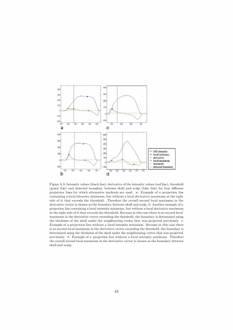
8/3/2019 Rianne Hupse- Localisation Techniques to improve BCI
http://slidepdf.com/reader/full/rianne-hupse-localisation-techniques-to-improve-bci 44/56
Figure A.9: Intensity values (black line), derivative of the intensity values (red line), threshold
(green line) and detected boundary between skull and scalp (blue line) for four diff erent
projection lines for which alternative methods are used. a: Example of a projection line
containing a local intensity minimum, but without a local derivative maximum at the right
side of it that exceeds the threshold. Therefore the overall second local maximum in the
derivative vector is chosen as the boundary between skull and scalp. b: Another example of a
projection line containing a local intensity minimum, but without a local derivative maximum
at the right side of it that exceeds the threshold. Because in this case there is no second local
maximum in the derivative vector exceeding the threshold, the boundary is determined using
the thickness of the skull under the neighbouring vertex that was projected previously. c:
Example of a projection line without a local intensity minimum. Because in this case there
is no second local maximum in the derivative vector exceeding the threshold, the boundary is
determined using the thickness of the skull under the neighbouring vertex that was projected
previously. d: Example of a projection line without a local intensity minimum. Therefore
the overall second local maximum in the derivative vector is chosen as the boundary between
skull and scalp.
43

8/3/2019 Rianne Hupse- Localisation Techniques to improve BCI
http://slidepdf.com/reader/full/rianne-hupse-localisation-techniques-to-improve-bci 45/56
Table A.1: Number of vertices for which the basic algorithm and alternative
methods are used average number of vertices percentage corrected
basic algorithm 576 2.7
method a 17 1.0
method b 1 40.0
method c 1 0.0
method d 28 0.6
Figure A.10: Detail of a saggital slice of the smoothed mri. Red dots depict the projected
vertices.
no local intensity minimum at all.
For most of the vertices this procedure gave an accurate estimate of the
location where the skull ends and the scalp starts (A.10). However, some vertices
had to be corrected manually (A.11) using a interface in which the vector values
are shown and the position of the boundary between skull and scalp can be typed
in. The percentage of vertices that had to be corrected manually are given in
table A.1.
44
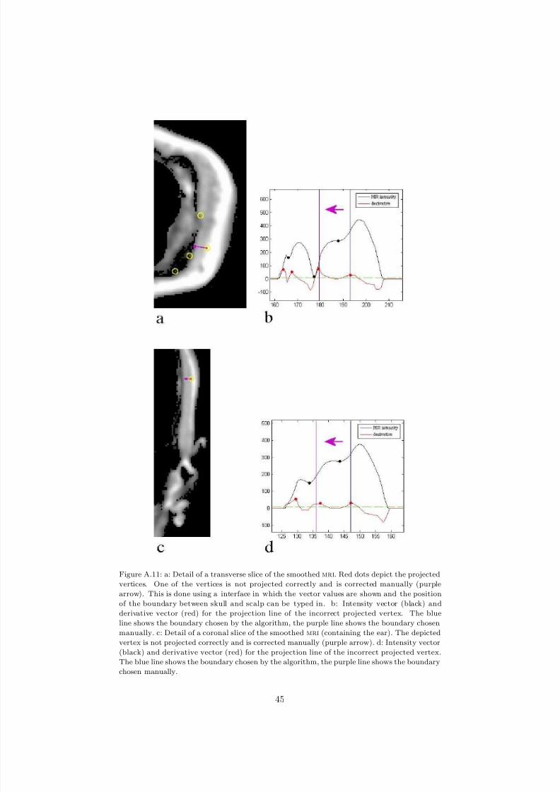
8/3/2019 Rianne Hupse- Localisation Techniques to improve BCI
http://slidepdf.com/reader/full/rianne-hupse-localisation-techniques-to-improve-bci 46/56
Figure A.11: a: Detail of a transverse slice of the smoothed mri. Red dots depict the projected
vertices. One of the vertices is not projected correctly and is corrected manually (purple
arrow). This is done using a interface in which the vector values are shown and the position
of the boundary between skull and scalp can be typed in. b: Intensity vector (black) and
derivative vector (red) for the projection line of the incorrect projected vertex. The blue
line shows the boundary chosen by the algorithm, the purple line shows the boundary chosen
manually. c: Detail of a coronal slice of the smoothed mri (containing the ear). The depicted
vertex is not projected correctly and is corrected manually (purple arrow). d: Intensity vector
(black) and derivative vector (red) for the projection line of the incorrect projected vertex.
The blue line shows the boundary chosen by the algorithm, the purple line shows the boundary
chosen manually.
45
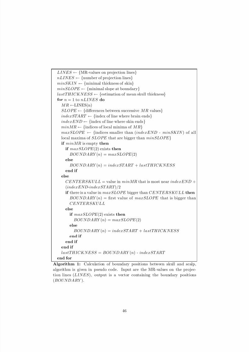
8/3/2019 Rianne Hupse- Localisation Techniques to improve BCI
http://slidepdf.com/reader/full/rianne-hupse-localisation-techniques-to-improve-bci 47/56
LINES ← {MR-values on projection lines}
nLINES ← {number of projection lines}
minSKIN ← {minimal thickness of skin}
minSLOPE ← {minimal slope at boundary}
lastTHICKNESS ← {estimation of mean skull thickness}
for n = 1 to nLINES do
MR←LINES(n)
SLOPE ← {diff erences between successive MR values}
indexSTART ← {index of line where brain ends}
indexEND← {index of line where skin ends}minMR← {indices of local minima of MR}
maxSLOPE ← {indices smaller than (indexEND - minSKIN ) of all
local maxima of SLOPE that are bigger than minSLOPE }
if minMR is empty then
if maxSLOPE (2) exists then
BOUNDARY (n) = maxSLOPE (2)
else
BOUNDARY (n) = indexSTART + lastTHICKNESS
end if
else
CENTERSKULL = value in minMR that is most near indexEND +
(indexEND-indexSTART )/2
if there is a value in maxSLOPE bigger than CENTERSKULL then
BOUNDARY (n) = first value of maxSLOPE that is bigger than
CENTERSKULL
else
if maxSLOPE (2) exists then
BOUNDARY (n) = maxSLOPE (2)
else
BOUNDARY (n) = indexSTART + lastTHICKNESS
end if
end if
end if lastTHICKNESS = BOUNDARY (n) - indexSTART
end for
Algorithm 1: Calculation of boundary positions between skull and scalp,
algorithm is given in pseudo code. Input are the MR-values on the projec-
tion lines (LINES ), output is a vector containing the boundary positions
(BOUNDARY ).
46

8/3/2019 Rianne Hupse- Localisation Techniques to improve BCI
http://slidepdf.com/reader/full/rianne-hupse-localisation-techniques-to-improve-bci 48/56
Appendix B
Beamforming
B.1 Introduction
Beamforming is a spatial filtering method to estimate the activity at every
predefined voxel (volume pixel) in the brain using potentials or magnetic fields
recorded at the surface of the head. The beamformer filter consists of weights
that have to be assigned to every sensor that is used. The estimated voxel
activity is then the weighed sum of all measurements (see equation B.3). For
every voxel of interest, the filter is calculated in a way that activity from the
specific voxel passes the filter while activity from other voxels is suppressed. In
the beamformer model all activity in a voxel is modeled as a single dipole at
the centre of the voxel.
B.2 Construction of the filter
B.2.1 The forward model
The first step in building a beamformer filter is the construction of a forward
model. A forward model describes how the brain activity is transmitted from the
voxels of interest to the sensors at the surface of the head. This forward model is
needed because its inverse describes how brain activity can be calculated from
sensor measurements, which is the purpose of beamforming. If there are N
sensors and M voxels of interest, M forward models H m of size N by 3 haveto be constructed. The three columns in the forward model H m contain the
activity that will be measured at the sensors due to a dipole source located in
the centre of the voxel of interest that has an unity moment in respectively the
x- y- and z direction and zero moment in the other directions. If the forward
model is known, the activity at the sensors for a given point in time can be
calculated by multiplying the forward model by a vector containing the dipole
moment present in the voxel at that point in time. This vector is called ym(t)
and has a size of 3 by 1. The three subsequent rows in this vector contain
respectively the length of the x-, y- and z component of the dipole representing
47

8/3/2019 Rianne Hupse- Localisation Techniques to improve BCI
http://slidepdf.com/reader/full/rianne-hupse-localisation-techniques-to-improve-bci 49/56
the activity in the voxel. The resulting vector xm of size N by 1 contains the
activity at the sensors due to the dipole in voxel m:
xm(t) = H mym(t) (B.1)
If there is activity in multiple voxels at the same moment in time, the measured
activity at the sensors is the sum of all vectors
x(t) =
M
m=1
xm(t) =
M
m=1
H mym(t). (B.2)
B.2.2 Filter design
As already mentioned in paragraph B.1, the beamformer filter consists of weights
that have to be assigned to every sensor to obtain the estimated voxel activity
by calculating the weighed sum of the electrode measurements. The activity in
a voxel is modeled by a dipole in the centre of the voxel that has a component
in the x-, y- and z direction. The beamformer filter wm contains weights for
calculating each of these components and therefore it is a matrix of size N by
3. The estimated dipole is a vector sm(t) of size 3 by 1 and can be obtained
by multiplying the transposed filter by the vector x(t) containing the measured
activity at the sensors:
sm(t) = wT mx(t). (B.3)
The ideal filter wm is constructed in a way that it gives unit response for the
activity in voxel m, this means that the estimated voxel activity is equal to theactual voxel activity.
sm(t) = wT mx(t) = ym(t). (B.4)
Substituting equation B.1 for x(t) gives:
wT mH mym(t) = ym(t). (B.5)
Therefore the ideal filter satisfies the linear response constraint:
wT mH m = I. (B.6)
Further the ideal filter let not pass any activity coming from other voxels (stop-
band attenuation): wT mH py p(t) = 0 ( p =m). (B.7)
Therefore the second constraint for the ideal filter is:
wT mH p = 0 ( p =m). (B.8)
If the columns of all forward models H are linearly independent, it is possible
to find a filter wm that satisfies equation B.6 and B.8. However, as mentioned
in paragraph B.2.1, the forward model is not based on the exact anatomy of
the human head; it is an approximation in which the head is assumed to consist
of a limited number of tissue types with their own (estimated) conductivity
48

8/3/2019 Rianne Hupse- Localisation Techniques to improve BCI
http://slidepdf.com/reader/full/rianne-hupse-localisation-techniques-to-improve-bci 50/56
properties. This means that the columns of forward models that belong to
voxels located near each other can be nearly linear dependent. This means thatwm will have a large norm and noise in the measured signal x(t) will have large
impact on the estimated brain activity sm(t). Often the signal to noise ration
in eeg measurements is very low, and therefore a filter constructed in this way
will lead to unreliable estimated brain activity. Another problem is that there
are N weights in every column of wm and therefore N degrees of freedom. This
means that the total amount of filter columns 3M can not be larger than N and
the number of voxels M for which the activity is estimated can not be larger
than N/3. Even when for example 256 sensors are used, the activity for only 85
voxels can be estimated which means that the volume of every voxel is about
15 cm3 which is much too large.
B.2.3 Linearly Constrained Minimum Variance
Because of the big limitations of using the stopband constraint as described in
paragraph B.2.2, a method is developed by Van Veen et al. [23] which is called
the linearly constrained minimum variance (lcmv) method. In this method the
filter is constructed in a way that it minimizes the total variance of the filter
output. In this way signals coming from other voxels than the voxel of interest
are attenuated while at the same time the linear response constraint is satisfied.
Therefore the filter is found by solving:
min(V ar{sm}) (B.9)
subject to:
wT mH m = I. (B.10)
Here sm is a matrix in which the rows represent the three dimensions of the
estimated dipole and the columns represent the time points at which the activity
is estimated. The variance of the filter output is given by
V ar{sm} = tr{Cov[sm]}
= tr{smsT m}. (B.11)
Substituting equation B.3 in equation B.11 gives
V ar{sm} = tr{[wT mx][wT mx]T }
= tr{wT mxxT wm}
= tr{wT mCov [x]wm}. (B.12)
Here x is a matrix of measurement values in which the rows represent the
sensors and the columns represent the time points. The solution of minimizing
the result of equation B.12 while satisfying the linear response constraint is
described in [23]. This results in the beamformer filter equation:
wT m = {H T mCov−1[x]H m}
−1H T mCov−1[x]. (B.13)
49

8/3/2019 Rianne Hupse- Localisation Techniques to improve BCI
http://slidepdf.com/reader/full/rianne-hupse-localisation-techniques-to-improve-bci 51/56
By substituting this equation into equation B.12, we obtain the estimated vari-
ance for the dipole in every voxel:
V ar{sm} = tr{wT mCov[x]wm}
= tr{{H T mCov−1[x]H m}
−1H T mCov−1[x]Cov [x]
Cov−T [x]H m{H T mCov
−1[x]H m}−T }
= tr{{H T mCov−1[x]H m}
−1
{H T mCov−T [x]H m}{H
T mCov
−T [x]H m}−1}
= tr{{H T mCov−1[x]H m}
−1}. (B.14)
Active neural populations will lead to a large variance in the dipole moment
modeling the activity in a voxel and therefore equation B.14 can be used to
estimate the activity for every voxel for the time interval in which the data ismeasured. The dipole moment at a certain time point can be calculated by
substituting equation B.13 into equation B.3.
B.3 The Neural Activity Index and noise
Often the signal to noise ratio is very low in eeg measurements. Therefore,
part of the data in xm(t) is not activity coming from neural sources. When
calculating the activity for a voxel, part of the result of equation B.14 will be
due to noise. If for example xm(t) is equal for all electrodes and totally due to
uncorrelated noise, then Cov[xm(t)] = I and equation B.14 becomes
V ar{sm} = tr{{H T mH m}−1}. (B.15)
This means that the estimated activity in a voxel only depends on the forward
model. If the voxel is located at the outside of the brain, the forward model
will contain relatively large elements because the activity in the voxel generates
relative large measurements at the sensor. Large elements in H m give small
elements in {H T mH m}−1 and therefore the estimated activity will be small. In
case of a voxel located deeper in the brain, elements in H m will be relative
small resulting in large elements in {H T mH m}−1. Therefore the estimated voxel
activity will be relative large. [23]
In general, if the measured noise has a covariance matrix Q then the esti-
mated activity due to this noise will be:
tr{{H T mQ−1H m}
−1}. (B.16)
In eeg measurements part of the measured potentials in xm(t) is due to brain
activity and part is due to noise. The part that is due to noise depends on the
location of the voxel. This can lead to unreliable activity estimations showing
large activity in the centre of the brain. Therefore a normalized estimate of the
voxel activity can be obtained by dividing equation B.14 by equation B.16:
V arN {sm} =tr{{H T mCov
−1(x)H m}−1}
tr{{H T mQ−1H m}−1}
. (B.17)
50

8/3/2019 Rianne Hupse- Localisation Techniques to improve BCI
http://slidepdf.com/reader/full/rianne-hupse-localisation-techniques-to-improve-bci 52/56
The covariance matrix Q can be estimated by measuring a period in which there
is no stimulus given to the subject. Another method is to use the covariancematrix of the measurements during the presentation of another stimulus. In
this way a contrast is calculated between activity induced by the two stimuli.
B.4 Correlated sources
The main assumption in beamformer analysis is that the activity of any neural
source is not linearly correlated to the activity of any other neural source. This
is due to the way the filter is constructed, namely by minimizing the variance of
the filter output while satisfying the unity passband constraint. If for example
activity at two locations is fully correlated in time, the forward models H i
and H j corresponding to these two locations will add as vectors:
yj = byi
xi = H iyi
xj = H jyj
= bH jyi
xt = H iyi + bH jyi
= (H i + bH j)yi, (B.18)
in which xt is the measurement due to the combined sources. The beamformer
that estimates the activity at voxel location i, allows sources with a forward
model H i to pass unattenuated, and minimizes all other components. However,due to the correlated sources, the measurement xt now seems to stem from
one source, with forward model H i + bH j . As this is not equal to H i, the
beamformer minimizes this contribution therewith underestimating the source
strength of voxel i. A similar reasoning holds for the other voxel.
Van Veen et al [23] examined the eff ect of correlated source activity by sim-
ulating two sources located in a three-shell sphere. In figure B.1 the neural
activity index at a cross section of the sphere is depicted in the case of uncor-
related, partially correlated and fully correlated sources.
51
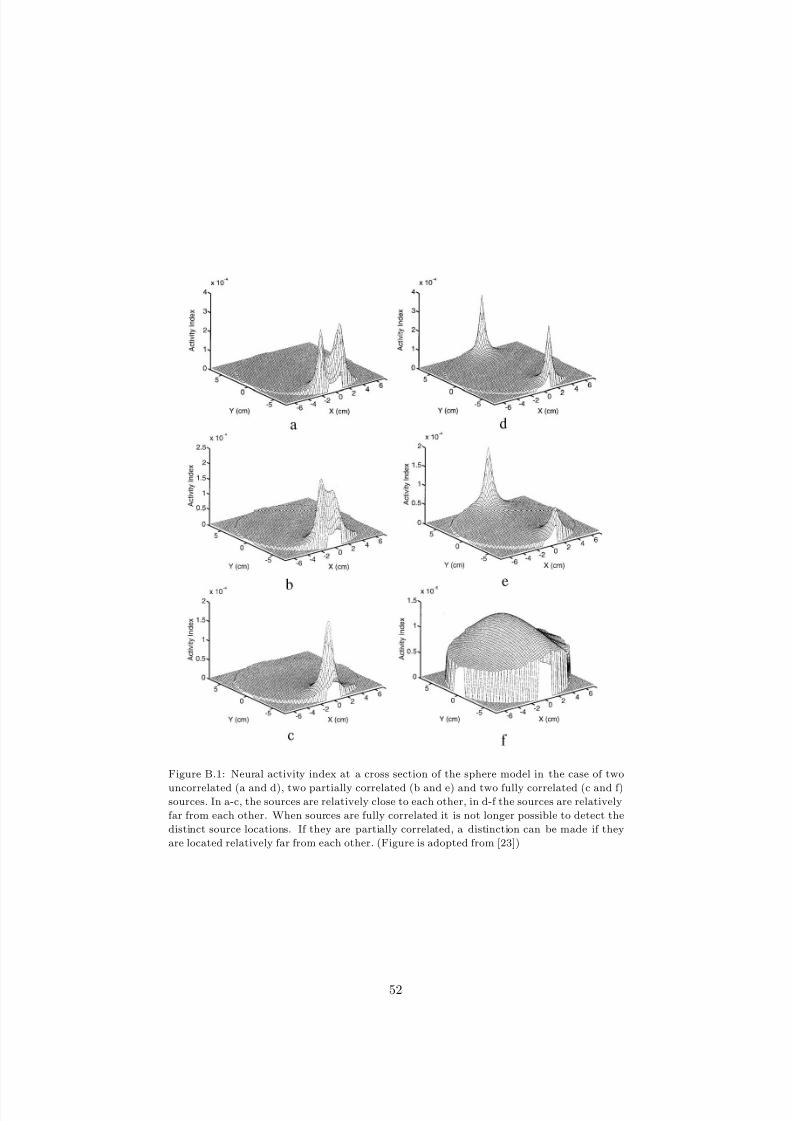
8/3/2019 Rianne Hupse- Localisation Techniques to improve BCI
http://slidepdf.com/reader/full/rianne-hupse-localisation-techniques-to-improve-bci 53/56
Figure B.1: Neural activity index at a cross section of the sphere model in the case of two
uncorrelated (a and d), two partially correlated (b and e) and two fully correlated (c and f)sources. In a-c, the sources are relatively close to each other, in d-f the sources are relatively
far from each other. When sources are fully correlated it is not longer possible to detect the
distinct source locations. If they are partially correlated, a distinction can be made if they
are located relatively far from each other. (Figure is adopted from [23])
52
8/3/2019 Rianne Hupse- Localisation Techniques to improve BCI
http://slidepdf.com/reader/full/rianne-hupse-localisation-techniques-to-improve-bci 54/56
References
[1] J. Ashburner and K.J. Friston, “Multimodal Image Coregistration and Par-
titioning - a Unified Framework,” NeuroImage., vol. 6(3), pp. 209-217, 1997.
[2] N. Birbaumer, T. Elbert, A.G.M. Canavan, and B. Roch,“Slow potentials
of the cerebral cortex and behavior,” Physiological Reviews., vol. 70, pp.1-
41, 1990.
[3] N. Birbaumer, A. Kubler, N. Ghanayim, T. Hinterberger, J. Perelmouter, J.
Kaiser, I. Iversen, B. Kotchoubey, N. Neumann, and H. Flor,“The thought
translation device (TTD) for completely paralyzed patients.” IEEE Trans-
actions on Rehabilitation Engineering ., vol. 8, pp. 190-192, 2000.
[4] J.M. Carmena, M.A. Lebedev, R.E. Crist, J.E. O’Doherty, D.M. Santucci,
D.F. Dimitrov, P.G. Patil, C.S. Henriquez, and M.A. Nicolelis,“Learning to
control a brain-machine interface for reaching and grasping by primates,”
PLoS Biol ., vol. 1(2): e2, 2003.
[5] J.H. Challis,“A prodecure for determining rigid body transformation pa-
rameters,” Journal of Biomechanics., vol. 28, pp. 733-737,1995.
[6] L.A. Farwell, and E. Donchin, “Talking off the top of your head: to-
ward a mental prothesis utilizing event-related brain potentials,” Electroen-
cephalography and Clinical Neurophysiology ., vol. 70, pp. 510-523, 1988.
[7] E.E. Fetz, and M.A. Baker, “Operantly conditioned patterns on precentral
unit activity and correlated responses in adjacent cells and contralateral
muscles,” Journal of Neurophysiology ., vol. 36(2), pp. 179-204, 1973.
[8] M. Fuchs, J. Kastner, M. Wagner, S. Hawes, and J.S. Ebersole, “A stan-
dardized boundary element method volume conductor model,” Clinical
Neuropfysiology ., vol. 113(5), pp. 702-712, 2002.
[9] C.M. Giabbiconi, C. Dancer, R. Zoph, T. Gruber, and M.M. Muller, “Se-
lective spatial attention to left or right hand flutter sensation modulates the
steady-state somatosensory evoked potential,” Cognitive Brain Research .,
vol. 20, pp. 58-66, 2004.
[10] S. Haykin, “Neural Networks, a comprehensive foundation,” Upper Saddle
River, New Jersey: Prentice Hall, 1999.
53

8/3/2019 Rianne Hupse- Localisation Techniques to improve BCI
http://slidepdf.com/reader/full/rianne-hupse-localisation-techniques-to-improve-bci 55/56
[11] A. Hillebrand, K.D. Singh, I.E. Holliday, P.L. Furlong, and G.R. Barnes, “A
New Approach to Neuroimaging With Magnetoencephalography,” Human Brain Mapping ., vol. 25, pp. 199-211, 2005.
[12] E.F. Kelly, and S.E. Folger,“EEG evidence of stimulus-directed response
dynamics in human somatosensory coretex,” Brain Research ., vol. 815, pp.
326-336, 1999.
[13] E.F. Kelly, M. Trulsson, and S.E. Folger,“Periodic microstimulation of sin-
gle mechanoreceptive aff erents produces frequency-following responses in
human EEG,” Journal of Neurophysiology ., vol. 77, pp. 137-144, 1997.
[14] B.J. de Kruif, P. Desain, and C.C.A.M. Gielen, “Combining multiple sen-
sors and measurements to improve frequency tagged BCI,” to be submitted
[15] E. Maris, “Randomization tests for erp topographies and whole spatiotem-
poral data matrices,” Psychophysiology ., vol. 41, pp. 142-151, 2004.
[16] S. Musallam, B.D. Corneil, B. Greger, H. Scherberger, and R.A. Ander-
sen,“Cognitive control signals for neural prosthetics,” Science., vol. 305,
pp. 258-262, 2004.
[17] T.F. Oostendorp, J. Delbeke and D.F. Stegeman, “The Conductivity of the
Human Skull; Results of In Vivo and In Vitro Measurements,” IEEE Trans-
actions on Biomedical Engineering ., vol. BME-47, pp. 1487-1492, 2000.
[18] G. Pfurtscheller, B. Graimann, J.E. Huggins, S.P. Levine, and L.A.
Schuh,“Spatiotemporal patterns of beta desynchronization and gamma syn-
chronization in corticographic data during self-paced movement,” Clinical
Neuropfysiology ., vol. 114(7), pp. 1226-1236, 2003.
[19] G. Pfurtscheller, C. Neuper, G.R. Muller, B. Obermaier, G. Krausz, A.
Schlogl, R. Scherer, B. Graimann, C. Keinrath, D. Skliris, M. Wortz, G.
Supp, and C. Schrank,“Graz-BCI: state of the art and clinical applications,”
IEEE Transactions on Neural Systems and Rehabilitation Engineering ., vol.
11(2), pp. 177-180, 2003.
[20] E.M. Schmidt, “Single neuron recording from motor cortex as a possible
source of signals for control of external devices,” Annals of Biomedical
Engineering ., vol. 8, pp. 339-349, 1980.
[21] S. Tobimatsu, Y.M. Zhang, and M. Kato, “Steady-state vibration so-
matosensory evoked potentials: physiological characteristics and tuning
function,” Clinical Neuropfysiology ., vol. 110, pp. 1953-1958, 1999.
[22] B. Vanrumste, G. Van Hoey, R. Van de Walle, M.R. D’Have, I.A. Lemahieu,
and P.A.. Boon, “Comparison of performance of spherical and realistic head
models in dipole localization from noisy EEG,” Med Eng & Phys., vol. 24,
pp. 403-418, 2002.
54

8/3/2019 Rianne Hupse- Localisation Techniques to improve BCI
http://slidepdf.com/reader/full/rianne-hupse-localisation-techniques-to-improve-bci 56/56
[23] B.D. Van Veen, W. van Drongelen, M. Yuchtman, and A. Suzuki, “Lo-
calization of Brain Electrical Activity via Linearly Constrained MinimumVariance Spatial Filtering,” IEEE Transactions on Biomedical Engineer-
ing ., vol. 44(9), pp. 867-880, 1997.
[24] J. Wessberg, C.R. Stambaugh, J.D. Kralik, P.D. Beck, M. Laubach, J.K.
Chapin, J. Kim, S.J. Biggs, M.A. Srinivasan, and M.A. Nicolelis, “Real-
time prediction of hand trajectory by ensembles of cortical neurons in pri-
mates,” Nature., vol. 408, pp. 361-365, 2000.
[25] J.R. Wolpaw, N. Birbaumer, D.J. McFarlanda, G. Pfurtschellere, and T.M.
Vaughana, “Brain computer interfaces for communication and control,”
Clinical Neuropfysiology ., vol. 113, pp. 767-791, 2002.
[26] Neuroimaging II course at the F.C. Donders Centre for Cognitive Neu-
roimaging, Nijmegen, The Netherlands