numerical analysis of an evolutionary variational

Available online at www.sciencedirect.com

ScienceDirect

Comput. Methods Appl. Mech. Engrg. 318 (2017) 882–897www.elsevier.com/locate/cma

Numerical analysis of an evolutionary variational–hemivariationalinequality with application in contact mechanics

Mikaël Barboteua, Krzysztof Bartoszb, Weimin Han c,∗

a LAboratoire de Mathématiques et PhySique (LAMPS), Université de Perpignan, 52 Avenue Paul Alduy, 66860 Perpignan, Franceb Faculty of Mathematics and Computer Science, Institute of Computer Science, Jagiellonian University, ul. Łojasiewicza 6, 30348 Krakow,

Polandc Department of Mathematics, University of Iowa, Iowa City, IA 52242, USA

Received 6 December 2016; accepted 1 February 2017Available online 16 February 2017

Highlights

• First paper on numerical analysis of evolutionary variational–hemivariational inequality problems.• A Céa type inequality for fully discrete numerical solutions.• An optimal order error estimate for linear element solutions.• Numerical evidence on the theoretically predicted optimal order error estimate.

Abstract

Variational–hemivariational inequalities are useful in applications in science and engineering. This paper is devoted to numericalanalysis for an evolutionary variational–hemivariational inequality. We introduce a fully discrete scheme for the inequality, usinga finite element approach for the spatial approximation and a backward finite difference to approximate the time derivative. Wepresent a Céa type inequality which is the starting point for error estimation. Then we apply the results in the numerical solutionof a problem arising in contact mechanics, and derive an optimal order error estimate when the linear elements are used. Finally,we report numerical simulation results on solving a model contact problem, and provide numerical evidence on the theoreticallypredicted optimal order error estimate.c⃝ 2017 Elsevier B.V. All rights reserved.

Keywords: Evolutionary variational–hemivariational inequality; Finite element method; Error estimation; Contact mechanics

The work of K.B. and W.H. were supported in part by the National Science Center of Poland under the Maestro 3 Project No. DEC-2012/06/A/ST1/00262. The work of W.H. was also supported by NSF under grant DMS-1521684.

∗ Corresponding author.E-mail addresses: [email protected] (M. Barboteu), [email protected] (K. Bartosz), [email protected] (W. Han).

http://dx.doi.org/10.1016/j.cma.2017.02.0030045-7825/ c⃝ 2017 Elsevier B.V. All rights reserved.

http://crossmark.crossref.org/dialog/?doi=10.1016/j.cma.2017.02.003&domain=pdf

http://www.elsevier.com/locate/cma

http://dx.doi.org/10.1016/j.cma.2017.02.003

http://www.elsevier.com/locate/cma

mailto:[email protected]



http://dx.doi.org/10.1016/j.cma.2017.02.003

M. Barboteu et al. / Comput. Methods Appl. Mech. Engrg. 318 (2017) 882–897 883

1. Introduction

Variational and hemivariational inequalities are mathematical models arising naturally in both qualitative studiesand numerical analysis of various complicated and challenging problems in sciences and engineering. Variationalinequalities are inequality problems with convex structure [1,2], whereas hemivariational inequalities are inequalityproblems involving non-convex terms [3–7].

The numerical analysis of variational inequalities is a well developed area, as illustrated in [8–10] and the referencestherein. In contrast, there are still relatively few publications devoted to numerical methods for hemivariationalinequalities and, in particular, to evolutionary hemivariational inequalities. The basic reference in the area isthe book [11]. However, while this book covers convergence of numerical methods for solving hemivariationalinequalities, it does not provide error estimates for the numerical solutions. Recently a number of papers have beenpublished on error estimation for numerical methods for hemivariational inequalities. In particular, in [12], an optimalorder error estimate is derived for the linear element solution of a static variational–hemivariational inequality; thevariational–hemivariational inequality reduces to a static hemivariational inequality in a special case. In [13], anoptimal order error estimate with respect to both the spatial mesh-size and the temporal step-size is derived forthe linear finite element solution of a hyperbolic hemivariational inequality. In [14], for a general family of elliptichemivariational inequalities with or without convex constraints, the Galerkin method is shown to converge, and forvarious elliptic hemivariational inequalities arising in contact mechanics, optimal order error estimates are proved forthe linear finite element solutions.

Variational–hemivariational inequalities involve both convex and nonconvex functions. Interest in their studyis motivated by problems in mechanics [5]. Recent results in their study have been obtained in [12,15,16]. Theinequalities studied in [12] are elliptic, whereas those in [15] are history-dependent ones. Numerical approximations ofhistory-dependent variational–hemivariational inequalities are considered in [16]. First order evolutionary variational–hemivariational inequalities are studied in [17], and the purpose of this paper is to provide numerical analysis of suchvariational–hemivariational inequalities.

We will need the notion of the subdifferential in the sense of Clarke. All spaces used in this paper are real. For anormed space X , we denote its norm by ∥ · ∥X , its topological dual by X∗, and the duality pairing of X and X∗ by⟨·, ·⟩X∗×X . For a locally Lipschitz function ϕ : X → R, its Clarke generalized directional derivative at a point x ∈ Xin a direction v ∈ X is defined by

ϕ0(x; v) = lim supy→x,λ↓0

ϕ(y + λv) − ϕ(y)λ

.

The Clarke subdifferential of ϕ at x is a subset of X∗ given by

∂Clϕ(x) =ζ ∈ X∗

: ϕ0(x; v) ≥ ⟨ζ, v⟩X∗×X ∀ v ∈ X.

Discussions of the subdifferential in the sense of Clarke can be found in the books [4,5,18,19].The rest of the paper is organized as follows. In Section 2 we introduce the class of evolutionary variational–

hemivariational inequalities studied in [17] and comment on the solution existence and uniqueness. In Section 3,we introduce and analyse a fully discrete scheme for the inequalities, and present a Cea type inequality for errorestimation. Then in Section 4, we apply the results of Section 3 to derive an error estimate for the evolutionaryvariational–hemivariational inequality that describes a frictionless contact problem with a Kelvin–Voigt viscoelasticmaterial where the contact conditions are with normal compliance and unilateral constraints. The error estimate is ofoptimal order with respect to both time step-size and space mesh-size when linear finite elements are used in spacediscretization. In Section 5, we report computer simulation results that provide numerical evidence of the predictedoptimal convergence order for numerical solutions of a model contact problem.

2. The evolutionary variational–hemivariational inequality

In this section, we introduce the evolutionary variational–hemivariational inequality studied in [17]. For thispurpose, we need some function spaces.

Let V be a strictly convex, reflexive separable Banach space. We denote by V ∗ the dual of V , and by ⟨·, ·⟩ theduality pairing between V ∗ and V . Let U be a reflexive Banach space with the dual U ∗, and denote by ⟨·, ·⟩U∗×U theduality pairing between U ∗ and U . Let ι : V → U be a linear operator and ι∗ : U ∗

→ V ∗ be its adjoint operator.

884 M. Barboteu et al. / Comput. Methods Appl. Mech. Engrg. 318 (2017) 882–897

For a positive number T , we introduce several function spaces defined on the interval [0, T ] with values in a Banachspace: V = L2(0, T ; V ), V∗

= L2(0, T ; V ∗), U = L2(0, T ; U ), U∗= L2(0, T ; U ∗), and W = v ∈ V | v ∈ V∗.

Note that hereafter the dot above the name of a function represents its time derivative. We then define a spaceM2,2(0, T ; V, V ∗). Let π be a finite partition of the interval (0, T ) by a family of disjoint subintervals σi = (ai , bi )such that [0, T ] = ∪

ni=1σi . Let F denote the family of all such partitions. Then, we define the seminorm of a function

v : [0, T ] → V by

∥v∥2BV 2(0,T ;V ) = sup

π∈F

∑σi ∈π

∥v(bi ) − v(ai )∥2V

and the space

BV 2(0, T ; V ) =v : [0, T ] → V : ∥v∥BV 2(0;T ;V ) < ∞

.

We further define

M2,2(0, T ; V, V ∗) = L2(0, T ; V ) ∩ BV 2(0, T ; V ∗).

It is well-known that M2,2(0, T ; V, V ∗) is a Banach space with the norm ∥ · ∥L2(0,T ;V ) + ∥ · ∥BV 2(0,T ;V ∗).Let there be given operators A, B : V → V ∗, functionals J : U → R and Φ : V → R ∪ +∞, and a function

f : [0, T ] → V ∗. The pointwise formulation of the problem is the following.PROBLEM (P). Find u ∈ W such that u(0) = u0 and for a.e. t ∈ (0, T ),

⟨Au(t) + Bu(t) + ι∗ξ (t), v − u(t)⟩ + Φ(v) − Φ(u(t)) ≥ ⟨ f (t), v − u(t)⟩ ∀ v ∈ V, (2.1)ξ (t) ∈ ∂Cl J (ιu(t)). (2.2)

The corresponding integral form of the problem is studied in [17].PROBLEM (P′). Find u ∈ W such that u(0) = u0,∫ T

0

[⟨Au(t) + Bu(t) + ι∗ξ (t) − f (t), v(t) − u(t)⟩ + Φ(v(t)) − Φ(u(t))

]dt ≥ 0 ∀ v ∈ V,

and for a.e. t ∈ (0, T ),

ξ (t) ∈ ∂Cl J (ιu(t)).

As in [17], we make the following assumptions on the data.H (A). The operator A : V → V ∗ is linear, bounded, coercive and symmetric, i.e.

(i) A ∈ L(V, V ∗).(ii) ⟨Av, v⟩ ≥ α∥v∥

2V ∀ v ∈ V with α > 0.

(iii) ⟨Av, w⟩ = ⟨Aw, v⟩ ∀ v, w ∈ V .

H (B). The operator B : V → V ∗ is linear, bounded and coercive, i.e.

(i) B ∈ L(V, V ∗).(ii) ⟨Bv, v⟩ ≥ β∥v∥

2V ∀ v ∈ V with β > 0.

H (J ). The functional J : U → R is such that

(i) J is locally Lipschitz.(ii) There exists cJ > 0 such that ∥ξ∥U∗ ≤ cJ (1 + ∥u∥U ) ∀ u ∈ U , ξ ∈ ∂Cl J (u).

(iii) There exists m > 0, such that

⟨ξ − η, u − v⟩U∗×U ≥ −m∥u − v∥2U ∀ u, v ∈ U, ξ ∈ ∂Cl J (u), η ∈ ∂Cl J (v).

H (Φ). The functional Φ : V → R ∪ +∞ is convex, proper and lower semicontinuous.H (ι). The operator ι : V → U is linear, continuous and compact. Moreover, the associated Nemytskii operator

ι : M2,2(0, T ; V, V ∗) → U defined by (ιv)(t) = ι(v(t)) for all t ∈ [0, T ] is also compact.H (0). f ∈ H 1(0, T ; V ∗), u0 ∈ dom(Φ) and the following compatibility condition holds: there exist ξ0 ∈ ∂Cl J (ιu0)

and η0 ∈ ∂ConvΦ(u0) such that

Bu0 + ι∗ξ0 + η0 − f (0) ∈ V .

H (s). Inequality β > m ∥ι∥2 holds.


Remark 2.1. In order to guarantee the compactness of the Nemytskii operator ι, that is required in the assumptionH (ι), it is enough to provide the following condition.

H1(ι). There exists a space Z and a linear operator π : Z → U such that V ⊂ Z compactly and ι = π i , wherei : V → Z denotes the (compact) identity mapping.

This argumentation was justified and used in [17] to show the validity of the assumption H (ι) in particular problemsof contact mechanics. In Section 4 we use the same idea, namely, we ensure that condition H1(ι) is met in our case.

We note that the symbols dom(Φ) and ∂ConvΦ in H (0) denote the effective domain of Φ and its subdifferential inthe sense of convex analysis, respectively.

It is proved in [17] that under the assumptions H (A), H (B), H (J ), H (Φ), H (ι), H (0) and H (s), Problem (P′) hasa unique solution u ∈ H 1(0, T ; V ). Under the same assumptions, it is straightforward to show a solution of Problem(P) is unique. Throughout the paper, we keep the assumptions H (A), H (B), H (J ), H (Φ), H (ι), H (0) and H (s), andassume that Problem (P), like Problem (P′), has a unique solution u ∈ H 1(0, T ; V ).

3. A fully discrete approximation

We introduce and analyse a fully discrete numerical method to solve Problem (P).

3.1. The scheme

Let V h be a finite dimensional subspace of V and uh0 ∈ V h be an approximation of u0. Let N be a positive integer,

and denote by k = T/N the time stepsize. We use notation tn = kn, n = 0, . . . , N . For any continuous function gdefined on the interval [0, T ] we denote gn = g(tn), n = 0, . . . , N . For any sequence zn

Nn=0 we introduce the notation

δzn =1k

(zn − zn−1), n = 1, . . . , N .

Then a fully discrete approximation method for Problem (P) is the following.PROBLEM (Phk). Find uhk

= uhkn

Nn=0 ⊂ V h such that uhk

0 = uh0 and for n = 1, 2, . . . , N ,⟨

Aδuhkn + Buhk

n + ι∗ξ hkn , vh

− uhkn

⟩+ Φ(vh) − Φ(uhk

n ) ≥ ⟨ fn, vh− uhk

n ⟩ ∀ vh∈ V h, (3.1)

ξ hkn ∈ ∂Cl J (ιuhk

n ). (3.2)

In the well-posedness study of Problem (Phk), we rewrite (3.1) as⟨Auhk

n + k Buhkn + k ι∗ξ hk

n , vh− uhk

n

⟩+ k Φ(vh) − k Φ(uhk

n )

≥ ⟨Auhkn−1 + k fn, v

h− uhk

n ⟩ ∀ vh∈ V h . (3.3)

This is a static variational–hemivariational inequality and we can apply the existence and uniqueness result of [20] tosee that the problem has a unique solution uhk

n ∈ V h .Next, we prove a boundedness property for the numerical solution, which will be useful in error analysis. We will

need the identity

⟨A(u − v), u⟩ =12

⟨Au, u⟩ −12

⟨Av, v⟩ +12

⟨A(u − v), u − v⟩. (3.4)

Also, it will be convenient to introduce the ∥ · ∥A norm through

∥v∥2A = ⟨Av, v⟩.

Note that under the assumption H (A), the norms ∥ · ∥A and ∥ · ∥V are equivalent.For simplicity, assume u0 ∈ V h ; this is the case, e.g., if u0 = 0. Then by letting

uhk−1 := u0 + k A−1 (

Bu0 + ι∗ξ0 + η0 − f (0)),

the inequality (3.1) holds also for n = 0. Recall that ξ0 and η0 denote the elements introduced in the assumption H (0).

Proposition 3.1. Under the stated assumptions, there is a constant c > 0 such that

max1≤n≤N

δuhkn

2V + k

N∑n=1

δuhkn

2V ≤ c. (3.5)


Proof. We take vh= uhk

n−1 in (3.1) to get⟨Aδuhk

n + Buhkn + ι∗ξ hk

n , −k δuhkn

⟩+ Φ(uhk

n−1) − Φ(uhkn ) ≥ −k ⟨ fn, δuhk

n ⟩.

Then, we write (3.1) with index n − 1 instead of n, and take vh= uhk

n to get⟨Aδuhk

n−1 + Buhkn−1 + ι∗ξ hk

n−1, k δuhkn

⟩+ Φ(uhk

n ) − Φ(uhkn−1) ≥ k ⟨ fn−1, δuhk

n ⟩.

Add the two inequalities,⟨A

(δuhk

n − δuhkn−1

)+ k Bδuhk

n + k ι∗δξ hkn , δuhk

n

⟩≤ k ⟨δ fn, δuhk

n ⟩.

Applying the identity (3.4) and using the assumptions H (B) and H (J ), we derive from the above inequality that

12

δuhkn

2A −

12

δuhkn−1

2A + k

(β − m ∥ι∥2) δuhk

n

2A ≤ k ⟨δ fn, δuhk

n ⟩.

For any ε > 0,

⟨δ fn, δuhkn ⟩ ≤ ε

δuhkn

2V +

14 ε

∥δ fn∥2V ∗ .

Thus,12

δuhkn

2A −

12

δuhkn−1

2A + k

(β − m ∥ι∥2

− ε) δuhk

n

2A ≤

k4 ε

∥δ fn∥2V ∗ .

Replacing n by j in the above inequality and making a summation from j = 1 to n, we obtain

12

δuhkn

2A + k

(β − m ∥ι∥2

− ε) n∑

j=1

δuhkj

2

A≤

12

δuhk0

2A +

k4 ε

n∑j=1

δ f j2

V ∗ . (3.6)

Now,

δ f j =1k

(f j − f j−1

)=

1k

∫ t j

t j−1

f (s) ds.

Hence,

kn∑

j=1

δ f j2

V ∗ ≤

n∑j=1

∫ t j

t j−1

∥ f (s)∥2V ∗ds ≤ ∥ f ∥

2V∗ .

When f j is defined as the average

f j :=1k

∫ t j

t j−1

f (s) ds,

we also have the above bound. Note thatδuhk0

2A =

1k2

u0 − uhk−1

2A =

Bu0 + ι∗ξ0 + η0 − f (0)2

V ∗ .

Therefore, from (3.6), we conclude the boundedness (3.5).

For n = 1, 2, . . . , N , we can write

uhkn = u0 + k

n∑j=1

δuhkj .

Then we have the following corollary from Proposition 3.1.

Corollary 3.2. Under the stated assumptions, there is a constant c > 0 such that

max1≤n≤N

uhkn

V ≤ c. (3.7)


3.2. Error analysis

We perform an error analysis of the fully discrete numerical method. Throughout this subsection we denote by c apositive constant that may differ from line to line. To simplify the notation, define

δn := δun − un.

From (2.1)–(2.2), we have, for n = 1, 2, . . . , N ,

⟨Aun + Bun + ι∗ξn, v − un⟩ + Φ(v) − Φ(un) ≥ ⟨ fn, v − un⟩ ∀ v ∈ V, (3.8)ξn ∈ ∂Cl J (ιun). (3.9)

From (3.8), we have⟨Aδun + Bun + ι∗ξn, v − un

⟩+ Φ(v) − Φ(un) ≥ ⟨ fn, v − un⟩V ∗×V + ⟨Aδn, v − un⟩ ∀ v ∈ V .

Then, ⟨Aδun + Bun + ι∗ξn, uhk

n − un⟩+ Φ(uhk

n ) − Φ(un) ≥ ⟨ fn, uhkn − un⟩ +

⟨Aδn, uhk

n − un⟩. (3.10)

Add (3.10) and (3.1),⟨Aδun + Bun + ι∗ξn, uhk

n − un⟩+

⟨Aδuhk


n , vh− uhk

n

⟩+ Φ(vh) − Φ(un)

≥ ⟨ fn, vh− un⟩ +

⟨Aδn, uhk

n − un⟩,

which is rewritten as⟨Aδ(un − uhk

n ) + B(un − uhkn ) + ι∗(ξn − ξ hk

n ), uhkn − un

⟩+

⟨Aδuhk


n , vh− un

⟩+ Φ(vh) − Φ(un)

≥ ⟨ fn, vh− un⟩ +

⟨Aδn, uhk

n − un⟩.

Introduce the notation

en := un − uhkn .

Then,1

2 k

(∥en∥

2A − ∥en−1∥

2A

)+ β ∥en∥

2V − m ∥ιen∥

2U

≤⟨Aδuhk


n − fn, vh− un

⟩+ Φ(vh) − Φ(un) −

⟨Aδn, uhk

n − un⟩.

Define a residual type quantity

Rn(v) := ⟨Aun + Bun + ι∗ξn − fn, v − un⟩ + Φ(v) − Φ(un). (3.11)

Then we have1

2 k

(∥en∥

2A − ∥en−1∥

2A

)+ β ∥en∥

2V − m ∥ιen∥

2U

≤1k

⟨Aen, un − vh

n

⟩−

1k

⟨Aen−1, un − vh

n

⟩+ ⟨Ben, un − vh

n ⟩ + ⟨ξn − ξ hkn , ι(un − vh

n )⟩

+ Rn(vhn ) + ⟨Aδn, v

hn − un⟩ + ⟨Aδn, en⟩. (3.12)

Recall the assumption H (J )(ii). Corresponding to the solution u ∈ H 1(0, T ; V ), ∥ξn∥U∗n is uniformly bounded.By Corollary 3.2, ∥ξ hk

n ∥U∗ is also uniformly bounded. Then,

∥en∥2A − ∥en−1∥

2A + 2βk ∥en∥

2V − 2mk ∥ιen∥

2U

≤ 2⟨Aen, un − vh

n

⟩− 2


n

⟩+ ε k ∥en∥

2V + ck ∥un − vh

n ∥2V

+ ck ∥ι(un − vhn )∥U + 2k |Rn(vh

n )| + ck ∥Aδn∥2V ∗ .

Choose ε > 0 sufficiently small and denote

c0 := 2(β − m ∥ι∥2)

− ε > 0.


Then,

∥en∥2A − ∥en−1∥

2A + c0k ∥en∥

2V ≤ 2

⟨Aen, un − vh

n

⟩− 2


n

⟩+ ck ∥un − vh

n ∥2V

+ ck ∥ι(un − vhn )∥U + 2k |Rn(vh

n )| + ck ∥Aδn∥2V ∗ . (3.13)

Replace n by j in (3.13) and make a summation over j = 1, 2, . . . , n:

∥en∥2A + c0k

n∑j=1

∥e j∥2V

≤ ∥e0∥2A + 2

⟨Aen, un − vh

n

⟩− 2

⟨Ae0, u1 − vh

1

⟩+ 2

n−1∑j=1

⟨Ae j , (u j − vhj ) − (u j+1 − vh

j+1)⟩

+ ckn∑

j=1

(∥u j − vh

j ∥2

V+ ∥ι(u j − vh

j )∥U + |R j (vhj )| + ∥Aδ j∥

2V ∗

). (3.14)

We now bound the terms on the right side of (3.14) involving the errors e j , 0 ≤ j ≤ n. We have

2⟨Aen, un − vh

n

⟩≤

12

∥en∥2A + c ∥un − vh

n ∥2V ,

−2⟨Ae0, u1 − vh

1

⟩≤ ∥e0∥

2A + c ∥u1 − vh

1 ∥2V ,

and

2n−1∑j=1

⟨Ae j , (u j − vhj ) − (u j+1 − vh

j+1)⟩ ≤ 2k ∥A∥

n−1∑j=1

∥e j∥V ∥δ(u j+1 − vhj+1)∥V

≤12

c0kn−1∑j=1

∥e j∥2V + c k

n∑j=2

∥δ(u j − vhj )∥

2

V.

Using these inequalities in (3.14), we have

∥en∥2A + k

n∑j=1

∥e j∥2V

≤ c[∥e0∥

2V + ∥un − vh

n ∥2V + ∥u1 − vh

1 ∥2V

+ kn∑

j=1

(∥δ(u j − vh

j )∥2

V+ ∥u j − vh

j ∥2

V+ ∥ι(u j − vh

j )∥U + |R j (vhj )| + ∥Aδ j∥

2V ∗

)].

Therefore, we have the following Cea type inequality:

max0≤n≤N

∥en∥2V + k

N∑n=1

∥en∥2V ≤ c

[∥e0∥

2V + max

0≤n≤N∥un − vh

n ∥2V

+ kN∑

n=1

(∥δ(un − vh

n )∥2V + ∥ι(un − vh

n )∥U + |Rn(vhn )| + ∥δn∥

2V

)], (3.15)

for any vhn ∈ V h , 0 ≤ n ≤ N . This inequality is the starting point in deriving error estimates, as is shown in the next

section.

4. Numerical analysis of a frictionless contact problem

In this section, we apply the result from the previous section to derive an optimal order error estimate for the fullydiscrete solution of a frictionless contact problem using linear finite elements. Modelling, analysis, and numericalmethods for contact problems are topics of numerous publications, and some comprehensive references are [4,21–24].


We now introduce the contact problem for a viscoelastic body. Let Ω be a Lipschitz domain in Rd (d = 2 or 3)occupied by the body. Its boundary ∂Ω consists of three disjoint measurable parts Γ1, Γ2 and Γ3, such that the measuresof Γ1 and Γ3 are positive, and Γ2 is allowed to be empty. The body is clamped on Γ1, is subjected to the action of avolume force of density f0 in Ω and the action of a surface traction of density f2 on Γ2. The functions f0 and f2 areallowed to be time-dependent. The body is in frictionless contact on Γ3 with an obstacle, the so-called foundation.The foundation is made of a perfectly rigid material, covered by layer of deformable material of thickness g > 0.Therefore, the contact is modelled with a normal compliance unilateral condition. The process is quasistatic and thetime interval of interest is [0, T ] for some constant T > 0.

Let Sd denote the space of second order symmetric tensors on Rd . The canonical inner products and thecorresponding norms on Rd and Sd are given by

u · v = uivi , ∥v∥Rd = (v · v)1/2∀ u = (ui ), v = (vi ) ∈ Rd ,

σ · τ = σi jτi j , ∥τ∥Sd = (τ · τ )1/2∀ σ = (σi j ), τ = (τi j ) ∈ Sd ,

respectively. Here, the indices i and j run between 1 and d and the summation convention over repeated indices isused. We use the notation u = (ui ) ∈ Rd , σ = (σi j ) ∈ Sd and ε(u) = (εi j (u)) ∈ Sd for the displacement vector, thestress tensor, and the linearized strain tensor, respectively. Note that εi j (u) =

12 (ui, j + u j,i ) where an index following

a comma indicates a partial derivative with respect to the corresponding component of the spatial variable x = (xi ).The unit outward normal vector exists a.e. on ∂Ω and is denoted by ν = (νi ) ∈ Rd . For a vector field v on ∂Ω , thenormal and tangential components of v are vν = v · ν and vτ = v − vνν. Similarly, for a stress field σ , the normal andtangential components are σν = (σν) · ν and σ τ = σν − σνν. We denote by 0 the zero element of Rd .

Then the classical formulation of the contact problem is the following.PROBLEM (PM). Find a displacement field u : Ω × [0, T ] → Rd and a stress field σ : Ω × [0, T ] → Sd such

that

σ = Cε(u) + Gε(u) in Ω × (0, T ), (4.1)Div σ + f0 = 0 in Ω × (0, T ), (4.2)u = 0 on Γ1 × (0, T ), (4.3)σν = f2 on Γ2 × (0, T ), (4.4)

σν = σ 1ν + σ 2

ν ,

−σ 1ν ∈ ∂Cl j(uν),

uν ≤ g, σ 2ν ≤ 0, σ 2

ν (uν − g) = 0

⎫⎬⎭ on Γ3 × (0, T ) (4.5)

σ τ = 0 on Γ3 × (0, T ), (4.6)u(0) = 0 in Ω . (4.7)

We comment that Eq. (4.1) is known as the Kelvin–Voigt viscoelastic constitutive law, commonly used to modelthe deformation behaviour of certain metals, rubbers and polymers. Eq. (4.2) is the equilibrium equation for thequasistatic process. Conditions (4.3) and (4.4) are the ordinary displacement and traction boundary condition. Thecontact is frictionless and it is represented by (4.6). The initial condition is (4.7). In the contact condition (4.5), thenormal stress σν on the contact surface is split into two parts, σ 1

ν and σ 2ν . The first part σ 1

ν describes the deformabilityof the obstacle with a normal compliance condition, governed by the subdifferential of a nonconvex potential j . Thesecond part σ 2

ν describes the rigidity of the obstacle with the Signorini unilateral contact condition. The condition (4.5)is used to model the contact of the body with a foundation made of a rigid body covered by a layer of elastic material.Note that penetration is allowed but is restricted by the relation uν ≤ g, where g represents the thickness of theelastic layer. When there is penetration, as long as the normal displacement does not reach the bound g, the contactis described with a nonmonotone normal compliance condition −σν ∈ ∂Cl j(uν). Due to the nonmonotonicity of ∂Cl j ,the condition can be used to describe the hardening or the softening phenomena of the foundation. Examples andmechanical interpretation associated with the nonmonotone normal compliance condition can be found in [4].

In the study of Problem (PM), we need some standard Lebesgue and Sobolev spaces. For v ∈ H 1(Ω;Rd ), wedenote by γ v its trace of v on ∂Ω . We introduce spaces

V = v = (vi ) ∈ H 1(Ω;Rd ) | γ v = 0 a.e. on Γ1,

H = τ = (τi j ) ∈ L2(Ω;Rd×d ) | τi j = τ j i , 1 ≤ i, j ≤ d.


The space H is a real Hilbert space with the canonical inner product given by

(σ , τ )H =

∫Ω

σi j (x) τi j (x) dx ∀ σ , τ ∈ H

and the associated norm ∥ · ∥H. Since Γ1 has a positive measure, it is known that V is a real Hilbert space with theinner product

(u, v)V = (ε(u), ε(v))H ∀ u, v ∈ V (4.8)

and the associated norm ∥ · ∥V . The duality pairing between V and V ∗ is denoted by ⟨·, ·⟩. Let Z = H 1−ε(Ω;Rd ) forsome ε ∈ (0, 1

2 ). Define the embedding i1 : V → Z , the trace operator γ1 : Z → H12 −ε(Γ3;Rd ), and the embedding

i2 : H12 −ε(Γ3;Rd ) → L2(Γ3;Rd ). Consider the trace operator γ = i2 γ1 i1 : V → L2(Γ3;Rd ). By the Sobolev

trace theorem,

∥γ v∥L2(Γ3;Rd ) ≤ c0∥v∥V ∀ v ∈ V (4.9)

for a constant c0 depending only on the domain Ω , Γ1 and Γ3. Let U = L2(Γ3) and define operators ν : L2(Γ3;Rd ) →

U , νv = vν for v ∈ L2(Γ3;Rd ), and ι = ν γ : V → U . The spaces V , U and W are as defined at the beginning ofSection 2, with the spaces V and U introduced here.

On the data of Problem PM, we assume the following.H (C). For the viscosity tensor C = (Ci jkl) : Ω × Sd

→ Sd ,

Ci jkl ∈ L∞(Ω ), 1 ≤ i, j, k, l ≤ d;

Cσ · τ = σ · Cτ ∀ σ , τ ∈ Sd , a.e. in Ω;

Cτ · τ ≥ α∥τ∥2Sd ∀ τ ∈ Sd , a.e. in Ω , with α > 0.

H (G). For the elasticity tensor G = (Gi jkl) : Ω × Sd→ Sd ,

Gi jkl ∈ L∞(Ω ), 1 ≤ i, j, k, l ≤ d;

Gσ · τ = σ · Gτ ∀ σ , τ ∈ Sd , a.e. in Ω;

Gτ · τ ≥ β∥τ∥2Sd ∀ τ ∈ Sd , a.e. in Ω , with β > 0.

H ( j). For the normal compliance function j : R → R,

j is locally Lipschitz;|η| ≤ c1(1 + |s|) ∀ η ∈ ∂Cl j(s), s ∈ R with d > 0;

(η1 − η2)(s1 − s2) ≥ −c2|s1 − s2|2∀ ηi ∈ ∂Cl j(si ), si ∈ R, i = 1, 2, with c2 > 0.

H ( f ). For the densities of forces and traction,

f0 ∈ H 1(0, T ; L2(Ω;Rd )), f2 ∈ H 1(0, T ; L2(Γ2;Rd ));f0(0) ∈ V, f2(0) = 0.

We define operators A, B : V → V ∗ by

⟨Au, v⟩ = (Cε(u), ε(v))H, ⟨Bu, v⟩ = (Gε(u), ε(v))H ∀ u, v ∈ V,

and functions J : L2(Γ3) → R and f : (0, T ) → V ∗ by

J (w) =

∫Γ3

j(w) dΓ , ∀ w ∈ L2(Γ3),

⟨f (t), v⟩ =

∫Ω

f0(t) · v dx +

∫Γ2

f2(t) · v dΓ ∀ v ∈ V, t ∈ [0, T ].

Let Φ : V → R ∪ +∞ be the indicator function of the set

K = v ∈ V | vν ≤ g a.e. on Γ3.

Then the weak formulation of Problem PM in terms of the displacement is the following.


PROBLEM (PMV ). Find a displacement field u ∈ W such that u(0) = 0 and for a.e. t ∈ (0, T ),

⟨Au(t) + Bu(t) + ι∗ξ (t) − f (t), v − u(t)⟩ + Φ(v) − Φ(u(t)) ≥ 0 ∀ v ∈ V,

ξ (t) ∈ ∂Cl J (ιu(t)).

It follows from the definition of function Φ that Problem PMV reduces to the following.

PROBLEM (PMV,∗). Find a displacement field u ∈ W such that u(0) = 0 and for a.e. t ∈ (0, T ), u(t) ∈ K and

⟨Au(t) + Bu(t) + ι∗ξ (t) − f (t), v − u(t)⟩ ≥ 0 ∀ v ∈ K ,

ξ (t) ∈ ∂Cl J (ιu(t)).

Problem (PMV ) is in the form of Problem (P) discussed in Section 2. It can be verified without difficulty that under

the assumptions H (C), H (G), H ( j), H ( f ), and β > c2∥ι∥2, the conditions H (A), H (B), H (J ), H (Φ), H (ι), and H (s)

of Section 2 are valid (see also Remark 2.1). Therefore, results on Problem (P) and its integral form can be applied.Thus, we assume Problem (PM

V ) admits a unique solution u ∈ H 1(0, T ; V ) and focus on numerical analysis of thecontact problem in this section.

As in Section 3, for a positive integer N , let k = N/T be the time stepsize. For simplicity, we assume Ω is apolygonal/polyhedral domain. Then

Γ j = ∪i ji=1Γ j,i , 1 ≤ j ≤ 3

where Γ j,i , 1 ≤ i ≤ i j , 1 ≤ j ≤ 3, are closed flat components of the boundary and have pairwise disjoint interiors.Consider a regular family of meshes T h

that partition Ω into triangles/tetrahedrons, compatible with the splitting ofthe boundary ∂Ω into Γ j,i , 1 ≤ i ≤ i j , 1 ≤ j ≤ 3, in the sense that if the intersection of one side/face of an elementwith one set Γ j,i has a positive measure with respect to Γ j,i , then the side/face lies entirely in Γ j,i . Corresponding toT h , we define the linear element space

V h=

vh

∈ C(Ω )d|vh

|T ∈ P1(T )d , T ∈ T h, vh= 0 onΓ1

.

Then a fully discrete approximation method for Problem PMV is the following.

PROBLEM (PMV,hk). Find uhk

= uhkn

Nn=0 ⊂ V h such that uhk

0 = 0 and for n = 1, 2, . . . , N ,⟨Aδuhk


n , vh− uhk

n

⟩+ Φ(vh) − Φ(uhk

n ) ≥ ⟨ fn, vh− uhk

n ⟩ ∀ vh∈ V h, (4.10)


n ). (4.11)

In the following, we assume g is concave. We can eliminate the explicit appearance of the function Φ in theformulation by introducing the finite element set

U h=

vh

∈ V h| vh

ν ≤ g at the nodes onΓ3.

Since g is a concave function, we have the inclusion

U h⊂ K .

Thus, an equivalent form of Problem PMV,hk is:

PROBLEM (PMV,hk,∗). Find uhk

= uhkn

Nn=0 ⊂ U h such that uhk

0 = uh0 and for n = 1, 2, . . . , N ,⟨

Aδuhkn + Buhk

n + ι∗ξ hkn , vh

− uhkn

⟩≥ ⟨ fn, vh

− uhkn ⟩ ∀ vh

∈ U h, (4.12)


n ). (4.13)

For an error analysis, assume the solution regularity

u ∈ H 1(0, T ; H 2(Ω )), u ∈ L2(0, T ; V ), (4.14)

uν |Γ3,i ∈ C(0, T ; H 2(Γ3,i )), σν |Γ3,i ∈ C(0, T ; L2(Γ3,i )), 1 ≤ i ≤ i3. (4.15)

We will apply standard finite element interpolation error estimates (cf. [25–27]).


The regularity (4.14) implies that u(t, x) is a continuous function of t and x. Thus, the pointwise values of u arewell defined. Choose vh

n = Π hun ∈ V h to be the finite element interpolant of un(x) := u(tn, x). We apply (3.15) and

max0≤n≤N

∥un − uhkn ∥

2V + k

N∑n=1

∥un − uhkn ∥

2V

≤ c[

max0≤n≤N

∥un − Π hun∥2V

+ kN∑

n=1

(∥δ(un − Π hun)∥

2V + ∥un,ν − Π hun,ν∥L2(Γ3) + |Rn(Π hun)| + ∥δn∥

2V

)], (4.16)

where

δn := δun − un, (4.17)

Rn(v) := ⟨Aun + Bun + ι∗ξn − fn, v − un⟩ + Φ(v) − Φ(un), (4.18)

ξn ∈ ∂Cl J (ιun). (4.19)

From [28, Lemma 11.5], we have

∥δn∥V ≤ ∥u∥L1(tn−1,tn ;V ).

Thus,

∥δn∥2V ≤ k ∥u∥

2L2(tn−1,tn ;V )

and

kN∑

n=1

∥δn∥2V ≤ k2

∥u∥2L2(0,T ;V ). (4.20)

Write

δ(un − Π hun) =1k

∫ tn

tn−1

(u(t) − Π h u(t)

)dt.

Then

∥δ(un − Π hun)∥2V ≤

1k

∫ tn

tn−1

u(t) − Π h u(t)2

dt,

and

kN∑

n=1

∥δ(un − Π hun)∥2V ≤

∫ T

0

u(t) − Π h u(t)2

dt.

Therefore,

kN∑

n=1

∥δ(un − Π hun)∥2V ≤ c h2

∥u∥2L2(0,T ;H2(Ω)). (4.21)

Note that on each component Γ3,i , Π hun,ν is the finite element interpolant of un,ν . By the last part of the regularityassumption (4.14), we have

kN∑

n=1

∥un,ν − Π hun,ν∥L2(Γ3) ≤ c h2i3∑

i=1

∥uν∥L∞(0,T ;H2(Γ3,i )). (4.22)

We now bound |Rn(Π hun)|. Using the relation

⟨Au(t) + Bu(t) − f (t), v⟩ =

∫Γ3

σν(t)vν dΓ ∀ v ∈ V,


we have

Rn(Π hun) =

∫Γ3

(σn,ν + ξn

) (Π hun,ν − un,ν

)dΓ ,

where σn,ν := σν(tn). Then,

|Rn(Π hun)| ≤ c ∥Π hun,ν − un,ν∥L2(Γ3),

and

kN∑

n=1

|Rn(Π hun)| ≤ c h2i3∑

i=1

∥uν∥L∞(0,T ;H2(Γ3,i )). (4.23)

Using (4.20)–(4.23) in (4.16), we obtain the following result concerning optimal error estimate for the fully discretescheme.

Corollary 4.1. Let u and uhk be solutions of Problem (PMV ) and Problem (PM

V,hk) respectively. Assume the solutionregularity (4.14)– (4.15). Then

max0≤n≤N

∥un − uhkn ∥

2V + k

N∑n=1

∥un − uhkn ∥

2V ≤ c

(k2

+ h2) , (4.24)

with a positive constant c independent of k and h.

5. Numerical simulations

This section provides computer simulation results on the contact Problem (PMV,hk,∗), including numerical

evidence of the theoretical error estimates obtained in Section 4 for the fully discrete approximation.The solution of Problem (PM

V,hk,∗) is based on numerical methods described in [29,30]. Note that hemivariationalinequalities arising in contact mechanics are related to the solution of non-convex problems. A numerical techniqueto solve this kind of problems is to use a “convexification” iterative procedure which leads to a sequence of convexprogramming problems. Then, the resulting nonsmooth convex iterative problems are solved by classical numericalmethods that can be found for instance in [23,24].

Numerical example. The physical setting used for Problem (PMV,hk,∗) is depicted in Fig. 1. The deformable body

is a rectangle, Ω = (0, 2) × (0, 1) ⊂ R2, and its boundary Γ is split as follows:

Γ1 = (0 × [0.5, 1]) ∪ (2 × [0.5, 1]),

Γ2 = ((0, 2) × 1) ∪ (0 × (0, 0.5)) ∪ (2 × (0, 0.5)),

Γ3 = [0, 2] × 0.

The domain Ω represents the cross section of a three-dimensional linearly viscoelastic body subjected to the action oftractions in such a way that a plane stress hypothesis is assumed. On the part Γ1 the body is clamped and, therefore,the displacement field vanishes there. Vertical compressions act on the part (0, 2)×1 of the boundary Γ2 and the part(0 × (0, 0.5)) ∪ (2 × (0, 0.5)) is traction free. Constant vertical body forces are assumed to act on the viscoelasticbody. The body is in frictionless contact with an obstacle on the part Γ3 of the boundary.

The compressible material’s behaviour of the domain Ω is governed by a Kelvin–Voigt viscoelastic linearconstitutive law of the form (4.1). In addition, we assume that the material is homogeneous and isotropic; then,the elasticity tensor G and the viscosity tensor C have the following forms

(Gτ )i j =Eκ

(1 + κ)(1 − 2κ)(τi i )δi j +

E1 + κ

τi j , 1 ≤ i, j ≤ 2, ∀ τ ∈ S2,

(Cτ )i j = α(τi i )δi j + βτi j , 1 ≤ i, j ≤ 2, ∀ τ ∈ S2,

where the coefficients E and κ are the Young’s modulus and the Poisson’s ratio of the material, respectively, and α

and β are the viscosity parameters. δi j denotes the Kronecker symbol.


Fig. 1. Reference configuration of the two-dimensional example.

For the numerical simulation of Problem (PMV,hk,∗), the following data are used:

E = 1000 N/m2, κ = 0.4, α = 100 N/m2, β = 50 N/m2,

f0 = (0, −0.1 × 10−3) N/m2,

f2 = (−1.5 × 10−3, 0) N/m on (0, 2) × 1,

T = 1 s, h = 1/128, k = T/N with N = 128.

The numerical results are presented in Figs. 2–5 and are described in what follows.Numerical solution of Problem (PM

V,hk,∗). In Figs. 3–4, the deformed configurations as well as the interfaceforces on Γ3 are plotted. In this case, the contact boundary conditions on Γ3 are characterized by a frictionlessmultivalued normal compliance contact in which the response follows a nonmonotone law with respect to the normaldisplacement uν and for which the maximal penetration is restricted by a unilateral constraint as follows:

− σ 1ν =

⎧⎪⎪⎪⎨⎪⎪⎪⎩0 if uν ≤ 0,

c1νuν if uν ∈ (0, u1

ν],

c1νu1

ν + c2ν(uν − u1

ν) if uν ∈ (u1ν, u2

ν),

c1νu1

ν + c2ν(u2

ν − u1ν) + c3

ν(uν − u2ν) if uν ≥ u2

ν,

(5.1)

uν ≤ g, σ 2ν ≤ 0, (uν − g)σ 2

ν = 0, (5.2)σ τ = 0 (5.3)

with c1ν = 200 N/m2, c2

ν = −100 N/m2, c3ν = 300 N/m2, u1

ν = 0.05 m and u2ν = 0.075 m and g = −0.1 m. Note that

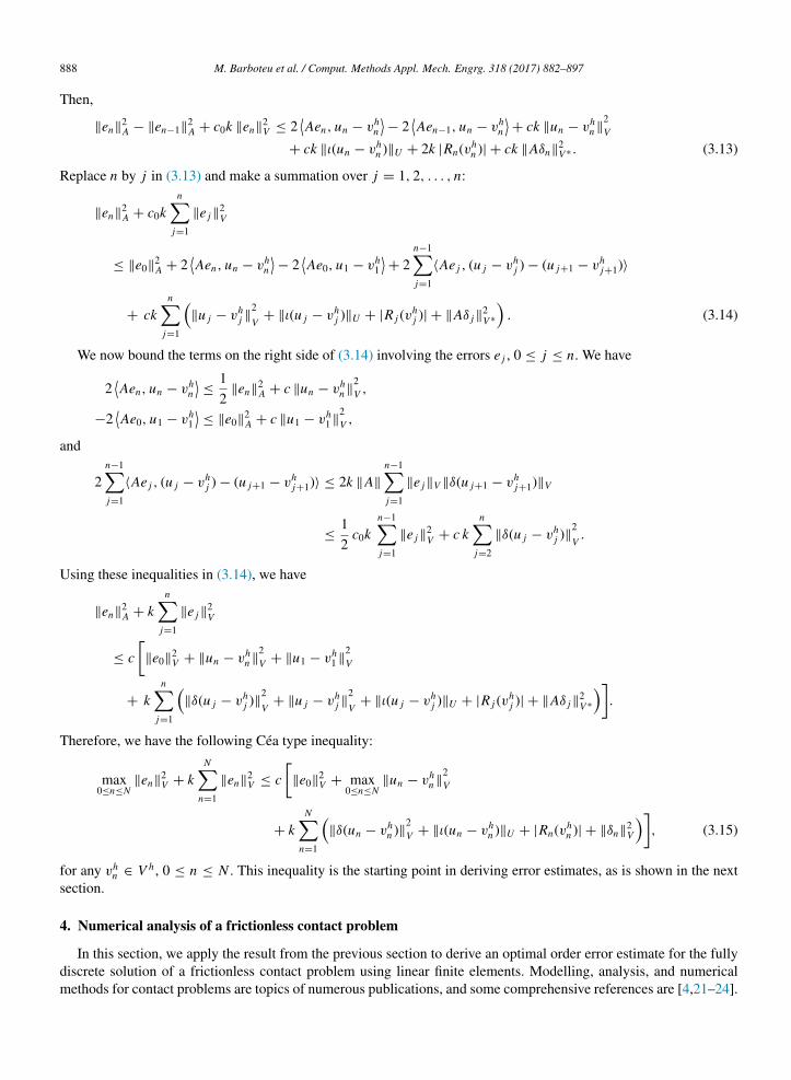
in the conditions (5.2), g represents the maximum value of the allowed penetration. When this value of penetrationis reached, the contact follows a unilateral condition without any additional penetration. For the conditions (5.1),we use a multivalued normal compliance response in which the non-monotonic behaviour of −σ 1

ν is characterized,respectively, by an increasing, a decreasing and again an increasing with respect to the normal displacement uν . Inorder to better appreciate the non-monotonic character of the normal response, we show in Fig. 2 the dependence of−σν as a function of the normal displacement uν related to the relations (5.1) and (5.2).

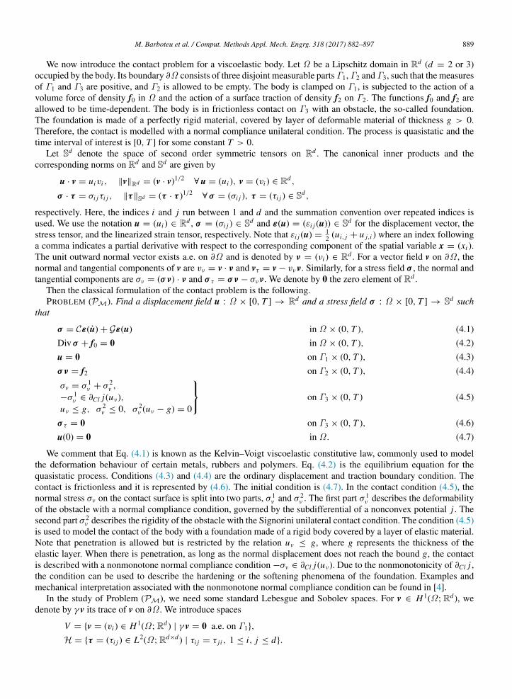
In Fig. 3, we plotted the deformed mesh as well as the interface forces on Γ3. On the extremities of the boundaryΓ3, we can see the non-monotonic behaviour of the normal compliance response −σν with respect to the penetration.On the centre of Γ3, the nodes are in unilateral contact status since the penetration reached the maximum value g.

In Fig. 4, the deformed mesh as well as the interface forces on Γ3 is plotted for various values of the maximalpenetration g. It is obvious to observe that the number of nodes in unilateral contact status increases with the reductionof the thickness of deformable layer of value g.


Fig. 2. Dependence of −σν on uν .

Fig. 3. Deformed mesh and interface force on Γ3.

The details concerning the computation for the numerical simulation related to the solution of Problem (PMV,hk,∗)

with g = −0.1 m are the following. For instance, in Fig. 3, the problem was discretized in 16 513 finite elementswith 128 contact elements (h = 1/128) and 128 time steps (k = 1/128); the total number of degrees of freedom wasequal to 17 028. For information, the average iterations number of the “convexification” procedure for the solutionof Problem (PM

V,hk,∗) was equal to 4 and the simulation runs in 665 (expressed in seconds) CPU time on a IBMcomputer equipped with Intel Dual core processors (Model 5148, 2.33 GHz).

Errors and numerical convergence orders. The aim of this part is to illustrate the convergence of the discretescheme and to provide numerical evidence of the optimal error estimate obtained in Section 4. To this end, wecomputed a sequence of numerical solutions by using uniform discretization of Problem (PM

V,hk,∗) according tothe spatial discretization parameter h and the time step k, respectively. For instance, for h = 1/128 and k = 1/128,we obtained the deformed configuration and the interface forces plotted in Fig. 3.

The numerical estimations of ∥u − uhk∥V are computed by using the energy norm ∥ · ∥E for several discretization

parameters of h and k. The energy norm is defined by the formula

∥vhk∥E :=

1√

2(G(ε(vhk)), ε(vhk))1/2

H .

Since it is not possible to calculate the exact solution u analytically, we consider a “reference” solution urefcorresponding to a fine approximation of Problem (PM

V,hk,∗). For this procedure, the boundary Γ of Ω is divided into


Fig. 4. Deformed meshes and interface forces on Γ3 for various values of g.

Fig. 5. Numerical errors.

1/h equal parts and the time interval [0, T ] is divided into 1/k time steps. We start with h = 1/4 and k = 1/4 whichare successively halved. The numerical solution ure f corresponding to h = 1/512 and k = 1/512 was taken as the“reference” solution. This fine discretization corresponds to a problem with 264 508 degrees of freedom and 262 657finite elements; the simulation runs in 93 878 (expressed in seconds) CPU time. The numerical results are presentedin Fig. 5 and in Table 1 where the dependence of the relative error estimates ∥uref − uh

∥E/∥uref∥E with respect to h


Table 1Relative errors in energy norm.

h + k 1/2 1/4 1/8 1/16 1/32 1/64

Error 24.099% 12.835% 6.407% 3.153% 1.540% 0.741%

and k are plotted. Note that these results provide a good numerical evidence of the theoretically predicted first orderconvergence of the numerical solution measured in the energy norm.

References[1] G. Duvaut, J.-L. Lions, Inequalities in Mechanics and Physics, Springer-Verlag, Berlin, 1976.[2] J.-L. Lions, G. Stampacchia, Variational inequalities, Commun. Pure Appl. Anal. 20 (1967) 493–519.[3] W. Han, S. Migorski, M. Sofonea (Eds.), Advances in Variational and Hemivariational Inequalities. Theory, Numerical Analysis and

Applications, in: Advances in Mechanics and Mathematics, vol. 33, Springer, New York, 2015.[4] S. Migorski, A. Ochal, M. Sofonea, Nonlinear Inclusions and Hemivariational Inequalities. Models and Analysis of Contact Problems,

in: Advances in Mechanics and Mathematics, vol. 26, Springer, New York, 2013.[5] Z. Naniewicz, P.D. Panagiotopoulos, Mathematical Theory of Hemivariational Inequalities and Applications, Dekker, New York, 1995.[6] P.D. Panagiotopoulos, Nonconvex energy functions, hemivariational inequalities and substationary principles, Acta Mech. 42 (1983) 160–183.[7] P.D. Panagiotopoulos, Hemivariational Inequalities, Applications in Mechanics and Engineering, SpringerVerlag, Berlin, 1993.[8] R. Glowinski, Numerical Methods for Nonlinear Variational Problems, Springer-Verlag, New York, 1984.[9] R. Glowinski, J.-L. Lions, R. Tremolieres, Numerical Analysis of Variational Inequalities, North-Holland, Amsterdam, 1981.

[10] I. Hlavacek, J. Haslinger, J. Necas, J. Lovısek, Solution of Variational Inequalities in Mechanics, Springer-Verlag, New York, 1988.[11] J. Haslinger, M. Miettinen, P.D. Panagiotopoulos, Finite Element Method for Hemivariational Inequalities: Theory, Methods and Applications,

Kluwer Academic Publishers, Dordrecht, Boston, London, 1999.[12] W. Han, S. Migorski, M. Sofonea, A class of variational-hemivariational inequalities with applications to frictional contact problems, SIAM

J. Math. Anal. 46 (2014) 3891–3912.[13] M. Barboteu, K. Bartosz, W. Han, T. Janiczko, Numerical analysis of a hyperbolic hemivariational inequality arising in dynamic contact,

SIAM J. Numer. Anal. 53 (2015) 527–550.[14] W. Han, M. Sofonea, M. Barboteu, Numerical analysis of elliptic hemivariational inequalities, SIAM J. Numer. Anal. (2017) in press.[15] S. Migorski, A. Ochal, M. Sofonea, History-dependent variational-hemivariational inequalities in contact mechanics, Nonlinear Anal. RWA

22 (2015) 604–618.[16] M. Sofonea, W. Han, S. Migorski, Numerical analysis of history-dependent variational-hemivariational inequalities with applications to

contact problems, European J. Appl. Math. 26 (2015) 427–452.[17] K. Bartosz, M. Sofonea, The Rothe method for variational-hemivariational inequalities with applications to contact mechanics, SIAM J. Math.

Anal. 48 (2016) 861–883.[18] F.H. Clarke, Optimization and Nonsmooth Analysis, Wiley, Interscience, New York, 1983.[19] Z. Denkowski, S. Migorski, N.S. Papageorgiou, An Introduction to Nonlinear Analysis: Theory, Kluwer Academic, Plenum Publishers,

Boston, Dordrecht, London, New York, 2003.[20] S. Migorski, A. Ochal, M. Sofonea, A class of variational-hemivariational inequalities in reflexive Banach spaces, J. Elasticity (2017).

http://dx.doi.org/10.1007/s10659-016-9600-7. in press.[21] W. Han, M. Sofonea, Quasistatic Contact Problems in Viscoelasticity and Viscoplasticity, American Mathematical Society, Providence, 2002

RI—Intl. Press, Sommerville, MA.[22] N. Kikuchi, J.T. Oden, Contact Problems in Elasticity: A Study of Variational Inequalities Finite Element Methods, SIAM, Philadelphia,

1988.[23] T. Laursen, Computational Contact and Impact Mechanics, Springer, 2002.[24] P. Wriggers, Computational Contact Mechanics, second ed., Springer, Berlin, 2006.[25] K. Atkinson, W. Han, Theoretical Numerical Analysis: A Functional Analysis Framework, third ed., Springer, New York, 2009.[26] S.C. Brenner, L.R. Scott, The Mathematical Theory of Finite Element Methods, third ed., Springer-Verlag, New York, 2008.[27] P.G. Ciarlet, The Finite Element Method for Elliptic Problems, North-Holland, Amsterdam, 1978.[28] W. Han, B.D. Reddy, Plasticity: Mathematical Theory Numerical Analysis, second ed., Springer-Verlag, 2013.[29] M. Barboteu, K. Bartosz, P. Kalita, An analytical and numerical approach to a bilateral contact problem with nonmonotone friction, Int. J.

Appl. Math. Comput. Sci. 23 (2013) 263–276.[30] M. Barboteu, K. Bartosz, P. Kalita, A. Ramadan, Analysis of a contact problem with normal compliance, finite penetration and nonmonotone

slip dependent friction, Commun. Contemp. Math. 15 (2013). http://dx.doi.org/10.1142/S0219199713500168.

http://refhub.elsevier.com/S0045-7825(16)31753-4/sb1





































http://dx.doi.org/10.1007/s10659-016-9600-7
















http://dx.doi.org/10.1142/S0219199713500168

numerical analysis of an evolutionary variational

Documents