nouveaux schémas de convection pour les écoulements à surface
TRANSCRIPT
École Doctorale SIELaboratoire d’Hydraulique Saint-Venant
ThèsePrésentée pour l’obtention du grade de DOCTEUR
DE L’UNIVERSITE PARIS-EST
par
Sara Pavan
Nouveaux schémas de convection pourles écoulements à surface libre
Spécialité : Mécanique des Wuides
Soutenue le 15 Février 2016 devant un jury composé de :
Rapporteur Prof. Boniface Nkonga (Université de Nice Sophia-Antipolis)Rapporteur Prof. Elena Vázquez-Cendón (Universidade de Santiago De Compostela)Examinateur Dr. Mario Ricchiuto (INRIA)Examinateur Prof. Eleuterio F. Toro (Università di Trento)Directeur de thèse Dr. Jean-Michel Hervouet (EDF R&D & Université Paris-Est)Co-encadrant de thèse Dr. Riadh Ata (EDF R&D & Université Paris-Est)
Thèse eUectuée au sein du Laboratoire d’Hydraulique Saint-Venant
de l’Université Paris-Est
6, quai Watier
BP 49
78401 Chatou cedex
France
Financements: ANR (bourse CIFRE # 2012-1654) et EDF R&D
RÉSUMÉ iii
RésuméCette thèse a pour objectif la construction de schémas d’ordre élevé et peu diUusifs pour le trans-
port d’un traceur dans les écoulements à surface libre, en deux ou trois dimensions.
On souhaite en particulier obtenir des schémas robustes, qui gardent au niveau discret les propriétés
mathématiques de l’équation de transport avec une faible diUusion numérique, et les utiliser sur
des cas industriels.
Dans ce travail deux méthodes numériques sont envisagées : une méthodes aux volumes Vnis (VF)
et une méthode aux résidus distribués (RD). Dans les deux cas, l’équation de transport est résolue
avec une approche découplée, qui est la solution la plus avantageuse en termes de précision et de
coûts de calcul. Pour ce qui concerne la méthode aux volumes Vnis, les équations de Saint-Venant
couplées à l’équation du transport sont d’abord résolues avec un schéma dit vertex-centred où le
Wux numérique est approximé avec un solveur de Riemann appelé Harten-Lax-Van Leer-Contact
[142]. A partir de cette approche, une formulation découplée est proposée. Cette dernière permet
de résoudre l’équation du transport avec un pas de temps plus grand que celui de la formulation
couplée. Cette idée a été d’abord proposée pour d’autres schémas dans [13]. Pour augmenter
l’ordre de précision en espace, la technique MUSCL [93] est utilisée avec l’approche découplée.
Finalement, la problématique des zones sèches est abordée. Dans le cas de la méthode aux résidus
distribués, les équations de Saint-Venant sont résolues avec une méthode éléments Vnis, et on fait
appel aux résidus distribués seulement pour discrétiser l’équation du transport, en se focalisant sur
les problèmes non stationnaires. L’équation de continuité du Wuide discrétisée est employée pour
garantir la conservation de la masse et le principe du maximum. Pour obtenir des schémas d’ordre
deux dans les problèmes non stationnaires, un schéma prédicteur-correcteur [117] est utilisé, en
l’adaptant au cas de concentration moyennée sur la verticale. Une version d’ordre 1 mais peu dif-
fusive, est aussi présentée dans ce travail. De plus, un schéma localement implicite, complètement
nouveau, est aussi formulé pour pouvoir traiter le problème des bancs découvrants.
Les deux techniques sont validées d’abord sur des cas simples, pour évaluer l’ordre de précision
des schémas et ensuite sur des cas plus complexes pour vériVer les autres propriétés numériques.
Les résultats montrent que les nouveaux schémas sont à la fois précis et conservatifs, tout en gar-
dant la monotonie comme le prévoient les démonstrations. Un cas d’application industriel est aussi
présenté en conclusion.
De plus, le schéma prédicteur-correcteur RD est adapté au cas 3D. Ceci ne présente aucun problème
théorique nouveau par rapport au cas 2D. Les propriétés de base des schémas sont validées sur des
cas test préliminaires.
Mots-clés:
schéma de convection - transport scalaire - ordre élevé - résidus distribués - prédicteur correcteur -
volumes Vnis-bancs découvrants

New advection schemes for free surface
Wows

ABSTRACT v
Abstract
The purpose of this thesis is to build higher order and less diUusive schemes for pollutant trans-
port in free surface Wows. We aim at schemes which are robust, with low numerical diUusion and
which respect the main mathematical properties of the advection equation. The goal is industrial
environmental applications.
Two techniques are tested in this work: a classical Vnite volume (FV) method and a residual dis-
tribution (RD) technique combined with a Vnite element method. For both methods we propose
a decoupled approach since it is the most advantageous in terms of accuracy and computational
time.
Concerning the Vrst technique, a vertex-centred Vnite volume method is used to solve the aug-
mented shallow water system where the numerical Wux is computed through an Harten-Lax-Van
Leer-Contact Riemann solver [142]. Starting from this solution, a decoupled approach is formu-
lated and is preferred since it allows the use of a larger time step for the advection of a tracer. The
idea was inspired by Audusse and Bristeau [13]. The MUSCL [93] technique is used for the second
order extension in space. The wetting and drying problem is also analysed and a possible solution
is presented.
In the second case, the shallow water system is entirely solved using the Vnite element technique
and the residual distribution method is applied to the solution of the tracer equation, focusing on
the case of time-dependent problems. However, for compatibility reasons the resolution of the
continuity equation must be considered in the numerical discretization of the tracer. In order to
get second order schemes for unsteady cases a predictor-corrector scheme [117] is used. A Vrst
order but less diUusive version of the predictor-corrector scheme is also introduced. Moreover, we
present a new locally semi-implicit version of the residual distribution method which, in addition
to good properties in terms of accuracy and stability, has the advantage to cope with dry zones.
The two methods are Vrst validated on academic test cases with analytic solutions in order to as-
sess the order of the schemes. Then more complex cases are addressed to test the robustness of the
schemes and their performance under diUerent Wow conditions. Finally a real industrial test case
for which real data are available is carried out.
An extension of the predictor-corrector residual distribution schemes to the 3D case is presented
as a Vnal contribution. Even in this case the RD technique is completely compatible with the Vnite
element framework used for the Navier-Stokes equations, thus its extension to the 3D case does
not present any extra theoretical problem. The method is tested on preliminary cases.
Keywords:
advection schemes - pollutant transport - high order - residual distribution - predictor corrector
scheme - Vnite volumes - wetting and drying phenomena

vi ABSTRACT
REMERCIEMENTS vii
Remerciements
Je remercie tout d’abord mon directeur de thèse, Jean-Michel Hervouet, et mon encadrant de thèse,
Riadh Ata, qui ont suivi avec passion et constance mon travail pendant ces trois ans.
Jean-Michel était toujours présent et il a su m’orienter dans les moments les plus sombres avec un
enthousiasme époustouWant. Grande ressource pour tout ce qui concerne les éléments Vnis et le
code Telemac, il m’a appris plein de choses grâce aussi à son approche physique et intuitive aux
problèmes scientiVques. J’exprime toute ma reconnaissance à Riadh qui m’a d’abord accueilli en
stage et après proposé cette thèse. Il m’a introduite au monde des volumes Vnis, je le remercie pour
cela et aussi pour son encadrement de manière plus générale.
Je voudrais remercier ensuite Mario Ricchiuto. Dès la première fois que je l’ai contacté il a été tout
de suite disponible pour répondre à mes questions sur les schémas distributifs. Plein de discussions
fructueuses se sont ensuite succédées.
Je tiens également à remercier les membres du jury qui ont accepté de participer à ma soutenance
et particulièrement les rapporteurs, Boniface Nkonga et Elena Vázquez-Cendón, pour le temps con-
sacré à la lecture de mon manuscript ainsi que pour leur remarques. Je remercie Eleuterio F. Toro
d’avoir présidé mon jury de thèse et aussi pour les deux semaines de cours sur les volumes Vnis qui
ont été très formatrices en début de thèse.
Je remercie EDF R&D et l’ANR qui ont Vnancé ce projet, réalisé au sein du Laboratoire d’Hydraulique
Saint-Venant. Je tiens à remercier en général toutes les personnes du labo et du LNHE qui m’ont
donné des coups de main et qui ont fait une pause de plus quand je n’avais besoin. En particulier,
je remercie Agnès pour les bons moments passés ensemble au bureau (et à Fontainebleau) et Vito,
avec qui j’ai partagé beaucoup des courses et des discussions sur l’île des impressionistes. Merci
aussi à Pablo, Cédric, Marissa pour la relecture attentive des certains chapitres de ma thèse. Merci
à Yoann pour toutes les aides en informatique qui m’ont fait gagner du temps précieux.
InVne ringrazio Andrea e la mia famiglia, veri supporti immancabili e insostituibili in questi anni di
tesi. Ringrazio Andrea che ha creduto in me sin dall’inizio e che ha avuto la pazienza di ascoltarmi e
di motivarmi quando ce n’era bisogno. Grazie alla mia famiglia per avermi insegnato l’importanza
del “conoscere, sapere, fare” e per avermi sempre incoraggiato nelle scelte più importanti. Grazie
poi a tutti gli altri amici, vicini e lontani, la cui lista sarebbe troppo lunga!

viii REMERCIEMENTS
Contents
1 Introduction 1
1.1 Context and motivations . . . . . . . . . . . . . . . . . . . . . . . . . . . . . . . . 2
1.2 Objectives of the thesis . . . . . . . . . . . . . . . . . . . . . . . . . . . . . . . . 2
1.3 Contents of the thesis . . . . . . . . . . . . . . . . . . . . . . . . . . . . . . . . . 3
1.4 Structure of the thesis . . . . . . . . . . . . . . . . . . . . . . . . . . . . . . . . . 5
2 Governing equations and main properties 7
2.1 Augmented two dimensional shallow water equations . . . . . . . . . . . . . . . 8
2.1.1 Shallow water system . . . . . . . . . . . . . . . . . . . . . . . . . . . . . 8
2.1.2 Pollutant transport equation . . . . . . . . . . . . . . . . . . . . . . . . . 14
2.2 Mathematical and numerical properties . . . . . . . . . . . . . . . . . . . . . . . 16
2.2.1 Hyperbolicity and stability . . . . . . . . . . . . . . . . . . . . . . . . . . 17
2.2.2 Solutions . . . . . . . . . . . . . . . . . . . . . . . . . . . . . . . . . . . . 19
2.2.3 Maximum principle . . . . . . . . . . . . . . . . . . . . . . . . . . . . . . 20
2.2.4 Classes of exact solutions . . . . . . . . . . . . . . . . . . . . . . . . . . . 20
2.3 Summary . . . . . . . . . . . . . . . . . . . . . . . . . . . . . . . . . . . . . . . . 24
3 State of the art 25
3.1 Coupled and decoupled discretization . . . . . . . . . . . . . . . . . . . . . . . . 26
3.2 First order schemes with low numerical diUusion . . . . . . . . . . . . . . . . . . 29
3.2.1 Method of characteristics . . . . . . . . . . . . . . . . . . . . . . . . . . . 29
3.2.2 Eulerian-Lagrangian localized adjoint method . . . . . . . . . . . . . . . 30
3.2.3 Anti-dissipative transport schemes . . . . . . . . . . . . . . . . . . . . . . 30
3.3 Conservative high order schemes . . . . . . . . . . . . . . . . . . . . . . . . . . . 32
3.3.1 Finite volumes schemes . . . . . . . . . . . . . . . . . . . . . . . . . . . . 32
x CONTENTS
3.3.2 Residual distribution schemes . . . . . . . . . . . . . . . . . . . . . . . . 41
3.4 Coping with dry zones . . . . . . . . . . . . . . . . . . . . . . . . . . . . . . . . . 47
3.5 Summary . . . . . . . . . . . . . . . . . . . . . . . . . . . . . . . . . . . . . . . . 48
4 A second order Vnite volume scheme with larger time step 51
4.1 First order scheme . . . . . . . . . . . . . . . . . . . . . . . . . . . . . . . . . . . 52
4.1.1 Unsteady tracer advection benchmark . . . . . . . . . . . . . . . . . . . . 58
4.1.2 Positivity of the scheme . . . . . . . . . . . . . . . . . . . . . . . . . . . . 58
4.1.3 Decoupling the tracer equation . . . . . . . . . . . . . . . . . . . . . . . . 61
4.1.4 Monotonicity analysis . . . . . . . . . . . . . . . . . . . . . . . . . . . . . 65
4.1.5 Boundaries and sources . . . . . . . . . . . . . . . . . . . . . . . . . . . . 65
4.2 Second order scheme . . . . . . . . . . . . . . . . . . . . . . . . . . . . . . . . . . 66
4.3 General resolution algorithm . . . . . . . . . . . . . . . . . . . . . . . . . . . . . 69
4.4 Coping with dry zones . . . . . . . . . . . . . . . . . . . . . . . . . . . . . . . . . 71
4.5 Summary . . . . . . . . . . . . . . . . . . . . . . . . . . . . . . . . . . . . . . . . 75
5 New residual distribution predictor-corrector schemes for time dependent problems 77
5.1 Preliminaries . . . . . . . . . . . . . . . . . . . . . . . . . . . . . . . . . . . . . . 78
5.1.1 Continuity equation . . . . . . . . . . . . . . . . . . . . . . . . . . . . . . 79
5.1.2 Explicit schemes for steady problems . . . . . . . . . . . . . . . . . . . . 83
5.2 Distribution schemes for time dependent problems . . . . . . . . . . . . . . . . . 88
5.2.1 Semi-implicit formulation . . . . . . . . . . . . . . . . . . . . . . . . . . 88
5.2.2 First order predictor-corrector formulation . . . . . . . . . . . . . . . . . 92
5.2.3 Second order predictor-corrector scheme . . . . . . . . . . . . . . . . . . 95
5.3 Monotonicity . . . . . . . . . . . . . . . . . . . . . . . . . . . . . . . . . . . . . . 97
5.3.1 Semi-implicit formulation . . . . . . . . . . . . . . . . . . . . . . . . . . 97
5.3.2 First order predictor-corrector scheme . . . . . . . . . . . . . . . . . . . . 99
5.3.3 Second order predictor-corrector scheme . . . . . . . . . . . . . . . . . . 102
5.4 Iterative predictor-corrector schemes . . . . . . . . . . . . . . . . . . . . . . . . . 105
5.5 Coping with dry zones . . . . . . . . . . . . . . . . . . . . . . . . . . . . . . . . . 107
5.5.1 Local semi-implicit N scheme . . . . . . . . . . . . . . . . . . . . . . . . 108
5.5.2 Local semi-implicit predictor-corrector scheme . . . . . . . . . . . . . . . 111
5.6 Summary . . . . . . . . . . . . . . . . . . . . . . . . . . . . . . . . . . . . . . . . 116
CONTENTS xi
6 VeriVcation and validation of the numerical schemes 119
6.1 VeriVcation . . . . . . . . . . . . . . . . . . . . . . . . . . . . . . . . . . . . . . . 121
6.1.1 Lake at rest with constant solute . . . . . . . . . . . . . . . . . . . . . . . 121
6.1.2 Steady tracer advection . . . . . . . . . . . . . . . . . . . . . . . . . . . . 122
6.1.3 Unsteady tracer advection benchmark . . . . . . . . . . . . . . . . . . . . 126
6.1.4 Rotating cone . . . . . . . . . . . . . . . . . . . . . . . . . . . . . . . . . 130
6.1.5 Wet dam break with pollutant . . . . . . . . . . . . . . . . . . . . . . . . 132
6.1.6 Dry dam break with pollutant . . . . . . . . . . . . . . . . . . . . . . . . 135
6.1.7 Thacker test case with tracer . . . . . . . . . . . . . . . . . . . . . . . . . 138
6.2 Validation . . . . . . . . . . . . . . . . . . . . . . . . . . . . . . . . . . . . . . . . 140
6.2.1 Open channel Wow between bridge piers with pollutant . . . . . . . . . . 140
6.2.2 Real river with tracer injection . . . . . . . . . . . . . . . . . . . . . . . . 143
6.3 Summary . . . . . . . . . . . . . . . . . . . . . . . . . . . . . . . . . . . . . . . . 149
7 Residual distribution schemes in three dimensions and validation 151
7.1 Three dimensional formulation . . . . . . . . . . . . . . . . . . . . . . . . . . . . 152
7.1.1 Preliminaries . . . . . . . . . . . . . . . . . . . . . . . . . . . . . . . . . 152
7.1.2 Explicit schemes for steady problems . . . . . . . . . . . . . . . . . . . . 155
7.1.3 Predictor-corrector schemes . . . . . . . . . . . . . . . . . . . . . . . . . 158
7.2 VeriVcation and validation of the 3D RD schemes . . . . . . . . . . . . . . . . . . 161
7.2.1 Rotating cone . . . . . . . . . . . . . . . . . . . . . . . . . . . . . . . . . 161
7.2.2 Open channel Wow between bridge piers with pollutant . . . . . . . . . . 161
7.3 Summary . . . . . . . . . . . . . . . . . . . . . . . . . . . . . . . . . . . . . . . . 163
8 Conclusions and future work 165
8.1 Concluding remarks . . . . . . . . . . . . . . . . . . . . . . . . . . . . . . . . . . 166
8.2 Perspectives . . . . . . . . . . . . . . . . . . . . . . . . . . . . . . . . . . . . . . 167
A Monotonicity of the semi implicit predictor-corrector scheme 169
Bibliography 189

xii CONTENTS
List of Figures
1 Introduction 1
2 Governing equations and main properties 7
2.1 Sketch of depth-averaged quantities in shallow water Wows. . . . . . . . . . . . . 16
3 State of the art 25
3.1 Numerical diUusion produced by an upwind scheme. u = (1, 0) aligned with the
mesh: longitudinal diUusion (on the left). u = (1, 1) not aligned with the mesh:
longitudinal and transverse diUusion (on the right). . . . . . . . . . . . . . . . . . 31
3.2 Illustration of a Vnite volume method for a 2D unstructured domain. . . . . . . . 33
4 A second order Vnite volume scheme with larger time step 51
4.1 Vertex-centered approach. . . . . . . . . . . . . . . . . . . . . . . . . . . . . . . . 53
4.2 Vertex-centred control volume for a boundary cell. . . . . . . . . . . . . . . . . . 53
4.3 HLLC approximate Riemann solver and solutions in the 4 regions: left, left star,
right star, right (on the left); approximate HLLC Wux (on the right). . . . . . . . . 55
4.4 Unsteady tracer advection benchmark: initial proVle and exact solution at y = 0.5m. 59
4.5 Unsteady tracer advection benchmark: results for the HLLC scheme at section
y = 0.5 m. . . . . . . . . . . . . . . . . . . . . . . . . . . . . . . . . . . . . . . . 59
4.6 Riemann problems at the interfaces xi+1/2 and xi−1/2 of a cell. . . . . . . . . . . 60
4.7 Unsteady tracer advection benchmark: results for the coupled and the decoupled
HLLC scheme at section y = 0.5 m. . . . . . . . . . . . . . . . . . . . . . . . . . 64
4.8 Control volumes and subtriangles for reconstruction. . . . . . . . . . . . . . . . . 67

xiv LIST OF FIGURES
4.9 Unsteady tracer advection benchmark: results at section y = 0.5m for the coupled
version of the Vrst order HLLC, the decoupled version of the Vrst order HLLC, the
decoupled version of the second order HLLC. . . . . . . . . . . . . . . . . . . . . 69
4.10 Drying of a wet cell. . . . . . . . . . . . . . . . . . . . . . . . . . . . . . . . . . . 72
4.11 Wetting of a dry cell. . . . . . . . . . . . . . . . . . . . . . . . . . . . . . . . . . . 73
5 New residual distribution predictor-corrector schemes for time dependent problems 77
5.1 Integral of basis functions for the point i. . . . . . . . . . . . . . . . . . . . . . . . 81
5.2 Unsteady tracer advection benchmark: results at section y = 0.5 m for the N and
PSI scheme. . . . . . . . . . . . . . . . . . . . . . . . . . . . . . . . . . . . . . . . 87
5.3 Unsteady tracer advection benchmark: results at section y = 0.5 m for the N, the
PSI and the Predictor-Corrector Vrst order scheme. . . . . . . . . . . . . . . . . . 94
5.4 Unsteady tracer advection benchmark: results at section y = 0.5 m for the N, the
PSI, the Predictor-Corrector Vrst order scheme (PC1) and the Predictor-Corrector
second order scheme (PC2). . . . . . . . . . . . . . . . . . . . . . . . . . . . . . . 97
5.5 Unsteady tracer advection benchmark: results at section y = 0.5 m for the N,
the PSI, the Predictor-Corrector Vrst order scheme (PC1), the Predictor-Corrector
second order scheme (PC2) and the Predictor-Corrector Vrst order scheme using 5
iterations (PC1-5it). . . . . . . . . . . . . . . . . . . . . . . . . . . . . . . . . . . 106
5.6 Unsteady tracer advection benchmark: results at section y = 0.5 m for the N,
the PSI, the Predictor-Corrector Vrst order scheme (PC1), the Predictor-Corrector
second order scheme (PC2), the Predictor-Corrector Vrst order scheme using 5 iter-
ations (PC1-5it) and the Predictor-Corrector second order scheme using 5 iterations
(PC2-5it). . . . . . . . . . . . . . . . . . . . . . . . . . . . . . . . . . . . . . . . . 107
5.7 Unsteady tracer advection benchmark: results at section y = 0.5 m for the N,
the PSI, the Predictor-Corrector Vrst order scheme (PC1), the Predictor-Corrector
second order scheme (PC2), the Predictor-Corrector Vrst order scheme using 5 iter-
ations (PC1-5it), the Predictor-Corrector second order scheme using 5 iterations
(PC2-5it) and the Locally Implicit Predictor corrector Scheme with 5 iterations
(LIPS-5it). . . . . . . . . . . . . . . . . . . . . . . . . . . . . . . . . . . . . . . . . 116
6 VeriVcation and validation of the numerical schemes 119
6.1 Lake at rest with constant solute: bathymetry. . . . . . . . . . . . . . . . . . . . . 121
6.2 Steady tracer advection: unstructured grid used for the convergence study. Ω = [2 m× 1 m]
and ∆x = 1/10 m . . . . . . . . . . . . . . . . . . . . . . . . . . . . . . . . . . . 122
LIST OF FIGURES xv
6.3 Steady tracer advection: convergence-rate (top) and tracer proVles at section x =
2 m for the case ∆x = 1/40 (bottom). . . . . . . . . . . . . . . . . . . . . . . . . 124
6.4 Steady tracer advection: regular mesh. Ω = [2 m× 1 m] and ∆x = 1/40 m . . . 126
6.5 Steady tracer advection: results at section x = 2 m for the advection of a discon-
tinuous function (top) and a continuous function (bottom) over a regular grid. . . 127
6.6 Unsteady tracer advection benchmark: convergence-rates. . . . . . . . . . . . . . 128
6.7 Unsteady tracer advection benchmark: tracer proVles at tf = 1 s and for y = 0.5 m. 129
6.8 Unsteady tracer advection benchmark: convergence for the PC2 scheme. . . . . . 130
6.9 Unsteady tracer advection benchmark: tracer proVles for the coupled and the de-
coupled HLLC scheme at section y = 0.5 m. . . . . . . . . . . . . . . . . . . . . . 131
6.10 Rotating cone: isolines for the tracer proVles (∆ = 0.05). From top left to right
bottom: exact solution, HLLC 1, N, PSI, HLLC 2, PC2, PC1, PC2-5it, PC1-5it, LIPS. 133
6.11 Wet dam break: solutions for the contact discontinuity computed with the numer-
ical schemes at time 240 s at the channel axis. . . . . . . . . . . . . . . . . . . . . 134
6.12 Wet dam break: solutions solution at the channel axis at time 240 s for the contact
discontinuity computed with the HLLC schemes (left) and the RD schemes (right). 134
6.13 Dry dam break: numerical and exact solutions at the channel axis at t = 1.5 s.
Solutions are computed with FE and FV schemes. From top to bottom: water
depth, velocity, concentration. . . . . . . . . . . . . . . . . . . . . . . . . . . . . . 137
6.14 Thacker test case: evolution of the maximum water depth in the centre of the domain. 139
6.15 Thacker test case: tracer and water depth proVles at the central axis of the domain
for the HLLC 1 (top left), HLLC 2 (top right), LIP n = 1 (bottom left), LIP n = 2
(bottom right). . . . . . . . . . . . . . . . . . . . . . . . . . . . . . . . . . . . . . 140
6.16 Thacker test case: numerical and exact solutions for the tracer proVle after 4 periods
at the central axis. . . . . . . . . . . . . . . . . . . . . . . . . . . . . . . . . . . . 141
6.17 Open channel Wow between bridge piers with pollutant: topography of the channel
with the cylindrical piers sketch. . . . . . . . . . . . . . . . . . . . . . . . . . . . 141
6.18 Open channel Wow between bridge piers with pollutant: unstructured mesh. Ω =
[28.5 m× 20 m] and ∆x = 0.5 m . . . . . . . . . . . . . . . . . . . . . . . . . . 142
6.19 Open channel Wow between bridge piers with pollutant: isolines for the tracer
(∆ = 0.05). From top to bottom: HLLC2, PC2, PC2-5it. . . . . . . . . . . . . . . . 143
6.20 Open channel Wow between bridge piers with pollutant: isolines (∆ = 0.05) for
the PSI scheme (left) and the PC2-5it scheme (right). . . . . . . . . . . . . . . . . 143
6.21 Real river with tracer injection: bathymetry of the river. . . . . . . . . . . . . . . 145
xvi LIST OF FIGURES
6.22 Real river with tracer injection: sketch of the inlet part of the river with seven
tracer source points. . . . . . . . . . . . . . . . . . . . . . . . . . . . . . . . . . . 146
6.23 Real river with tracer injection: comparison between the results obtained with the
NERD scheme (left) and the new LIP scheme (right) near the source. . . . . . . . . 147
6.24 Real river with tracer injection: comparison between the results obtained with the
NERD scheme (left) and the new LIP scheme (right) in the upstream part of the river. 148
6.25 Real river with tracer injection: comparison between the results obtained with the
NERD scheme (left) and the new LIP scheme (right) in the downstream part of the
river. . . . . . . . . . . . . . . . . . . . . . . . . . . . . . . . . . . . . . . . . . . 148
6.26 Real river with tracer injection: comparison between numerical results and data in
7 diUerent sections. . . . . . . . . . . . . . . . . . . . . . . . . . . . . . . . . . . . 150
7 Residual distribution schemes in three dimensions and validation 151
7.1 Open channel Wow between bridge piers with pollutant: 3D mesh. . . . . . . . . . 162
7.2 Open channel Wow between bridge piers with pollutant: location of the slices. . . 162
7.3 Open channel Wow between bridge piers with pollutant: results obtained with the
numerical schemes for the slice at x = −1 m. . . . . . . . . . . . . . . . . . . . . 163
7.4 Open channel Wow between bridge piers with pollutant: results obtained with the
numerical schemes for the slice at x = 13.075 m. . . . . . . . . . . . . . . . . . . 163
8 Conclusions and future work 165
A Monotonicity of the semi implicit predictor-corrector scheme 169
List of Tables
1 Introduction 1
2 Governing equations and main properties 7
3 State of the art 25
4 A second order Vnite volume scheme with larger time step 51
5 New residual distribution predictor-corrector schemes for time dependent problems 77
6 VeriVcation and validation of the numerical schemes 119
6.1 Relative mass error for the lake at rest with constant solute. . . . . . . . . . . . . 122
6.2 Steady tracer advection: order of accuracy. . . . . . . . . . . . . . . . . . . . . . . 123
6.3 Steady tracer advection: number of time-steps for the advection schemes. . . . . . 125
6.4 Unsteady tracer advection benchmark: order of accuracy. . . . . . . . . . . . . . . 128
6.5 Unsteady tracer advection benchmark: number of time-steps for the FV schemes. . 130
6.6 Unsteady tracer advection benchmark: hydrodynamic and transport iterations for
diUerent Froude numbers, for the HLLC 1. . . . . . . . . . . . . . . . . . . . . . . 130
6.7 Unsteady case: number of time-steps for the advection schemes. . . . . . . . . . . 131
6.8 Rotating cone test: minimum and maximum values of concentration. . . . . . . . 132
6.9 Wet dam break: number of hydrodynamics time steps and transport time step for
the HLLC schemes. . . . . . . . . . . . . . . . . . . . . . . . . . . . . . . . . . . . 135
6.10 Wet dam break: number transport time step for the RD schemes. . . . . . . . . . . 135
xviii LIST OF TABLES
6.11 Dry dam break: number of hydrodynamics time steps and transport time step for
the HLLC schemes. . . . . . . . . . . . . . . . . . . . . . . . . . . . . . . . . . . . 138
6.12 Thacker test case: number of iterations for the advection schemes. . . . . . . . . . 138
6.13 Thacker test case with tracer: maximum values of concentrations at after 4 periods. 140
6.14 Thacker test case with tracer: maximum and minimum values of concentration
according to diUerent εtr after 1 period. . . . . . . . . . . . . . . . . . . . . . . . 141
6.15 Open channel Wow between bridge piers with pollutant: mass balance for the dif-
ferent schemes. . . . . . . . . . . . . . . . . . . . . . . . . . . . . . . . . . . . . . 142
6.16 Real river with tracer injection: distance from the sources points. . . . . . . . . . 146
6.17 Real river with tracer injection: computational time for 43 h 40m of physical time
on 8 CPU. . . . . . . . . . . . . . . . . . . . . . . . . . . . . . . . . . . . . . . . . 149
7 Residual distribution schemes in three dimensions and validation 151
7.1 Rotating cone test: minimum and maximum values of concentration. . . . . . . . 161
7.2 Open channel Wow between bridge piers with pollutant: mass balance for the dif-
ferent schemes. . . . . . . . . . . . . . . . . . . . . . . . . . . . . . . . . . . . . . 164
8 Conclusions and future work 165
A Monotonicity of the semi implicit predictor-corrector scheme 169

Nomenclature
Abbreviations
CFL Courant Friedrichs Lewy
CPU Central Processing Unit
DG Discontinuous Galerkin
ENO Essentially non-oscillatory
FE Finite Element
FV Finite Volume
HLLC Harten-Lax-van Leer Contact
LHS Left-hand side
RD Residual Distribution
RHS Right-hand side
RS Riemann Solver
SW Shallow Water
TVD Total Variation Diminishing
WENO weighted essentially non-oscillatory
Roman symbols
∆t discrete time step . . . . . . . . . . . . . . . . . . . . . . . . . . . . . . . . . . . . . . . . . . . . . . . . . . . . . . . . . . . . . . [s]
∆x average element size . . . . . . . . . . . . . . . . . . . . . . . . . . . . . . . . . . . . . . . . . . . . . . . . . . . . . . . . . . [m]
Th triangulation of domain
n unit normal vector
xx NOMENCLATURE
U velocity vector . . . . . . . . . . . . . . . . . . . . . . . . . . . . . . . . . . . . . . . . . . . . . . . . . . . . . . . . . . . . . . (m/s)
u depth-averaged velocity vector . . . . . . . . . . . . . . . . . . . . . . . . . . . . . . . . . . . . . . . . . . . . . . . (m/s)
b bottom . . . . . . . . . . . . . . . . . . . . . . . . . . . . . . . . . . . . . . . . . . . . . . . . . . . . . . . . . . . . . . . . . . . . . . . (m)
C concentration . . . . . . . . . . . . . . . . . . . . . . . . . . . . . . . . . . . . . . . . . . . . . . . . . . . . . . . . . . . . . (g/m3)
c depth-averaged concentration . . . . . . . . . . . . . . . . . . . . . . . . . . . . . . . . . . . . . . . . . . . . . . . (g/m3)
g acceleration of gravity . . . . . . . . . . . . . . . . . . . . . . . . . . . . . . . . . . . . . . . . . . . . . . . . . . . . . . (m/s2)
h water depth . . . . . . . . . . . . . . . . . . . . . . . . . . . . . . . . . . . . . . . . . . . . . . . . . . . . . . . . . . . . . . . . . . (m)
p pressure . . . . . . . . . . . . . . . . . . . . . . . . . . . . . . . . . . . . . . . . . . . . . . . . . . . . . . . . . . . . . . . . . . . . . (Pa)
s free surface . . . . . . . . . . . . . . . . . . . . . . . . . . . . . . . . . . . . . . . . . . . . . . . . . . . . . . . . . . . . . . . . . . . (m)
t time . . . . . . . . . . . . . . . . . . . . . . . . . . . . . . . . . . . . . . . . . . . . . . . . . . . . . . . . . . . . . . . . . . . . . . . . . . (s)
u x-component of the depth-averaged velocity . . . . . . . . . . . . . . . . . . . . . . . . . . . . . . . . . . . (m/s)
v y-component of the depth-averaged velocity . . . . . . . . . . . . . . . . . . . . . . . . . . . . . . . . . . . (m/s)
Greek symbols
ρ Density . . . . . . . . . . . . . . . . . . . . . . . . . . . . . . . . . . . . . . . . . . . . . . . . . . . . . . . . . . . . . . . . . . (kg/m3)
Γ boundary of the computational domain
Ω computational domain
Mathematical Symbols
∇· Divergence operator
∇ Gradient operator
4 Laplacian operator
Chapter 1
Introduction
Les équations de transport régissent un grand nombre de phénomènes physiques. En
hydraulique, la propagation des polluants ou d’autres traceurs peut être un example
de phénomène caractérisé par la convection. Des actions pour réduire ou maîtriser les
risques liés à la pollution sont de plus en plus demandées par la loi et les entreprises
doivent répondre à ces déVs. Pour ce faire, des outils numériques robustes et à la pointe
de l’état de l’art sont nécessaires pour garantir la Vabilité des études.
Dans ce cadre, l’objectif de la thèse est d’améliorer les schémas numériques pour la
convection des traceurs dans les écoulements à surface libre. L’équation de transport
est très connue et étudiée depuis longtemps, mais sa discrétisation comporte toujours
des déVs numériques intéressants. En particulier, des études plus approfondies sont à
mener sur le problème de la précision et de la monotonie du schéma. Dans cette thèse,
deux méthodes numériques sont explorées pour modéliser le transport d’un scalaire
passif dans un Wuide : une méthode aux volumes Vnis et une méthode aux résidus
distribués. Pour chaque approche, les stratégies adoptées pour diminuer la diUusion
numérique ou pour augmenter l’ordre de précision du schéma sont détaillées. Les
conditions de monotonie de chaque schéma sont établies en suivant des méthodes clas-
siques ou alternatives. Finalement, le problème des bancs découvrants est aussi abordé
aVn de pouvoir résoudre des cas réels.
La thèse s’articule en huit chapitres. Le Chapitre 2 présente les équations à résoudre et
leurs propriétés mathématiques. Dans le Chapitre 3 un état de l’art sur les méthodes
pour les problèmes de transport est oUert au lecteur, en regard des choix numériques
qui ont marqué ce travail. Le Chapitre 4 est dédié à la description du modèle VF tandis
que le Chapitre 5 s’occupe du modèle RD. Dans les deux cas, les diUérences avec les
schémas existants sont soulignées. L’analyse des résultats numériques obtenus avec les
deux techniques fait l’objet du Chapitre 6. Le Chapitre 7 montre l’extension du schéma
RD au cas 3D avec des résultats préliminaires. Les conclusions et les perspectives de
travail sont présentées dans le Chapitre 8.
2 CHAPTER 1: INTRODUCTION
1.1 Context and motivations
The transport equation arises in a wide range of natural phenomena. Pollution propagation studies
as well as water quality studies for ecological modelling are typical applications where the convec-
tion plays an important role.
These studies are asked for more and more, due to the increasing attention on environmental prob-
lems. The legislation is more demanding so that industries and engineering departments have to
be able to handle these issues. Forecast of pollutant plumes, monitoring of biological transform
process in water and remediation projects of polluted waters are part of possible legislative re-
quirements for environmental protection.
In these cases, in situ data collection and numerical simulations are fundamental tools to study
these problems. It is even more important to have a reliable numerical tool when some data are
not available or when several scenarios have to be produced.
The shallow water equations, or the Navier-Stokes equations, augmented by one (or more) scalar
conservation equation(s) for the transport of a passive tracer(s) are used to model these phenomena.
The conservative scalar transport equation, combined with the continuity equation of the shallow
water system, makes up the non conservative equation. This partial diUerential equation is well
known and has been widely studied. However, there are still some challenging diXculties in its
discretization. These diXculties are intrinsically related to the applications considered. For exam-
ple, it is important to have high order methods or methods with low numerical diUusion when the
goal is to predict pollutant values on long distances. At the same time, when only advection is
involved, it is important that the concentration values obtained are strictly bounded and that the
mass of solute is perfectly conserved. Finally, in real river or coastal applications, the method used
must be able to handle wetting and drying processes.
1.2 Objectives of the thesis
This thesis aims at improving the convection schemes for scalar transport in free surface Wows.
The modelling eUorts focus on the increase of the order of accuracy of the schemes and on alter-
native strategies to decrease the numerical diUusion. In literature, plenty of works can be found
on second order accurate schemes and in this thesis two existing techniques are considered and
tailored to our speciVc problem. Moreover, the focus is also kept on the conservation of the mass
and on the monotonicity which are the other essential numerical requirements analysed in this
work. The wetting and drying problem with respect to the tracer variable is not often addressed in
the literature. This problem is studied here with larger attention and some possible solutions are
then described.
The schemes presented in this thesis are implemented in the Telemac system1, which is an open
source software for free surface Wows [1]. The software was initially developed at EDF R&D and
1only some of them are currently available in the oXcial version of the code
1.3 CONTENTS OF THE THESIS 3
now is managed by an international consortium of users and developers. The hydrodynamic equa-
tions are mainly solved by a Vnite element method. The latter, as well as other numerical strategies
used in the Telemac system are described in [82]. However, a Vnite volume kernel was also intro-
duced for the solution of the shallow water equations. The advection schemes already existing in
the software will be used in some test cases for comparison purpose. Telemac-2D is the name used
for the part of the code solving the shallow water equations, while Telemac-3D refers to the code
solving the Navier-Stokes equations.
1.3 Contents of the thesis
The Vrst numerical method used in the present work is a Vnite volume (FV) method. This family
of schemes is known to be conservative and thus the mass conservation issue does not deserve
too much attention in this case, as the conservation is intrinsically satisVed. In order to correctly
model the scalar transport, the Harten-Lax-Van Leer-Contact [142] Riemann solver has been im-
plemented. The structure of the solution obtained with this solver, allows to decouple the tracer
equation from the Wuid equations. Thus the tracer equation and the Wuid equations are not solved
at the same time. This solution is also adopted in [13] for another kind of solver. Decoupling the
pollutant equation allows on one hand to diminish the numerical diUusion of the scheme and on
the other hand to reduce the computational costs. The decoupled algorithm is based on a mono-
tonicity criteria and under particular Wow conditions the decoupled solution can fall back to the
coupled solution in order to fulVll the monotonicity.
To increase the spatial accuracy the Monotonic Upstream Scheme for Conservation Laws (MUSCL)
[93] has been used. This technique is very popular among FV schemes. However in case of 2D un-
structured mesh, there is no unique and right way to apply this method but rather an hodgepodge
of possibilities. For this reason a deeper review on this technique has been done in the state of the
art chapter. The main problem is that the theorems available for the 1D case have not been gener-
alized yet to the 2D. Thus the monotonicity in this case is not strictly guaranteed and this is still
an open issue, even if it does not arise in our numerical experiments. Even though, the decoupled
algorithm is used also for the second order case, yielding interesting results.
Finally, the dry bed problem for tracer is analysed with respect to the choice of a cut-oU parameter,
necessary to compute the concentration variable. A minimum requirement is identiVed to avoid
the violation of the maximum principle in regions with very small water depths.
Major eUorts are made in the development of the other numerical method, a residual distribu-
tion (RD) scheme. Unlike the FV method, the RD method is only used for the conservative scalar
transport equation, while the Wuid equations are solved by a Vnite element technique. The exist-
ing residual distribution method used for the scalar advection equation is tailored to the depth-
averaged tracer equation. It is worth noticing that the RD schemes have been already adapted to
scalar conservation laws [5, 48, 118] yet here another method is derived in order to be compatible
with the continuity equation, discretized with a FE technique.
4 CHAPTER 1: INTRODUCTION
The eUort made to adapt the scheme to the depth-averaged context has a deeper motivation: ap-
plying the same formulation to the 3D. Indeed, as we will see, for the Navier-Stokes equations a
sigma transformation is used to handle the free surface evolution and the Vnite element method
to discretize the Wuid equations. Thanks to these two features, a straightforward relation can be
established between the 2D and the 3D continuity equations. This holds true also for the tracer
equations. We just limit ourselves to say that the 2D water depth h which appears in the tracer
equation can be directly replaced by the variable 3D ∆z which represents the height of a layer of
elements.
The already existing N [125] and PSI [136] schemes are reformulated in order to be compatible with
the discretized Wuid continuity equation. These two schemes were already implemented in the code
Telemac-2D, however their theoretical formulation is recalled to stress the concept of monotonicity
and mass conservation, useful also for the next steps.
Then, the focus is kept on the second order schemes for time dependent problems. In particular, the
predictor-corrector scheme [117] is adapted to the depth-averaged equation. A Vrst order version
of the predictor-corrector scheme is also considered since characterized by low numerical diUusion,
even if only Vrst order accurate. For both the Vrst and the second order schemes, an enhanced new
version is presented. The latter is based on the possibility to iterate the corrector step increasing the
accuracy of the results, without spoiling neither mass conservation nor monotonicity. The strategy
adopted to preserve the maximum principle is diUerent from the one used by classical RD schemes
and leads to a new monotonicity condition.
In order to cope with wetting and drying problems, a new locally implicit RD scheme is presented.
The main novelty of this scheme is that for every point of the domain a local implicit coeXcient is
used to solve the tracer equation. This approach allows to have an implicit scheme characterized
by unconditional stability at the wet/dry front. In addition, no division by water depths needs to
be performed to obtain the concentration. This feature makes the scheme very robust. However,
its drawback is represented by the need to solve a linear system, which is expensive in terms of
computational time. Even in this case, the accuracy problem is addressed with particular attention.
All the schemes presented are tested and compared on several cases. First, the accuracy is computed
on simple tests with analytical solution: the steady advection and the unsteady advection. Then,
the schemes are compared on more complex cases, where the advection Veld is variable in space
and in time. The rotating cone, where a tracer represented by a gaussian function is transported
under a rotational velocity Veld, is a typical test case for convection schemes. The dam break over
wet bed and an open channel Wow between bridge piers are also useful to check the mass conser-
vation as well as the monotonicity of the solution. The results show that the strategies adopted to
improve the precision of the schemes are eXcient and that the mass is always perfectly conserved,
as well as the maximum principle is preserved. The comparison of the schemes is completed by
data on the computational times and the number of iterations is detailed for every scheme. To test
the ability to deal with wetting and drying phenomena, we consider the dam break over dry bed
and the Thacker test case. Results show that the schemes are eUectively appropriate to these prob-
1.4 STRUCTURE OF THE THESIS 5
lems. Finally, a real test case with wetting and drying is presented to validate the locally implicit
scheme on industrial applications. The numerical results are compared to real data.
The last part of this thesis is dedicated to the applications of the 2D predictor-corrector schemes
to the 3D case. As already said in the introduction, a series of discrete relations between the 2D
continuity equation and the 3D continuity equation make the schemes perfectly compatible to the
3D case without any additional theoretical problem. The validation is done on few preliminary
case studies.
1.4 Structure of the thesis
The structure of the thesis has been designed to methodically present the problems tackled in this
work.
In Chapter 2 the continuous equations and their corresponding mathematical properties are intro-
duced. The aim is to establish the foundations of the numerical model and to introduce a part of
the notations.
Chapter 3 presents the state of the art on the numerical models for transport problems. The liter-
ature review gradually introduces the numerical choices done in this work, showing the already
existing techniques in the literature.
In Chapter 4 the vertex-centred FV scheme is presented, stressing the diUerences between a classi-
cal coupled scheme and the decoupled version proposed in this work. The second order extension
and the wet/dry treatment is also detailed.
The Chapter 5 shows how the RD schemes have been tailored to the depth-averaged transport
equation. In particular, the new predictor-corrector schemes are described and the corresponding
monotonicity conditions are derived.
The Chapter 6 gathers the tests necessary to validate the numerical schemes. Every test checks a
particular property of the scheme and a global comparison of the various schemes is oUered to the
reader.
Chapter 7 shows the extension of the predictor-corrector scheme to the 3D case. Two numerical
tests are given as preliminary validation of the scheme.
In Chapter 8 conclusions and perspectives of this thesis are presented.

6 CHAPTER 1: INTRODUCTION
Chapter 2
Governing equations and main
properties
L’objectif de ce chapitre est d’introduire les équations qu’on souhaite résoudre et leurs
propriétés mathématiques.
Le système de Saint-Venant couplé avec une loi de conservation scalaire est établi suiv-
ant une méthode classique à partir des équations de Navier-Stokes. Les hypothèses de
base et le domaine de validité des équations sont rappelés aVn de bien identiVer le type
de phénomènes qu’on cherche à modéliser.
De la même manière on introduit synthétiquement certains aspects mathématiques
qui sont nécessaires dans la suite aVn de guider la construction du modèle numérique.
En particulier, on parle d’hyperbolicité, de stabilité et de principe du maximum. L’étude
de l’hyperbolicité permet aussi de bien déVnir les conditions aux limites aVn d’avoir
un problème bien posé.
Le chapitre se termine par une série de solutions exactes qui sont ensuite utilisées dans
la validation numérique des schémas.
8 CHAPTER 2: GOVERNING EQUATIONS AND MAIN PROPERTIES
This chapter presents the main characteristics of the equations solved in this work with the methods
presented in the next chapters. The assumptions, as well as the limitations and the mathematical
properties of the equations are fundamental in the construction of the numerical model. Indeed,
the numerical modelling choices will also be deVned according to these properties, in order to seek
the correct physical solutions of the equations. A part of the notations used in this work is also
introduced in this chapter.
2.1 Augmented two dimensional shallow water equations
We call the augmented 2D shallow water (SW) equations, the system formed by the classical shal-
low water equations for the Wuid augmented by one (or more) scalar conservation equations for
the transport of a passive tracer(s), which is (are) dissolved or contained in the Wuid. The concept
of passive tracers includes various substances that will be detailed later in the text. However, in
this work we often speak about pollutant since pollution phenomena and water quality problems
are among the most common industrial applications for which these equations are studied.
We Vrst present the Wuid equations and then the tracer equations.
2.1.1 Shallow water system
A large class of natural phenomena can be described by the 2D shallow water system: the Wood
wave in rivers, the dam break waves, the river and the stream Wows. However, the assumptions
made to obtain the equations have to be considered in the numerical modelling of these phenomena.
The SW system is also called Saint-Venant system, since Jean-Claude Barré de Saint-Venant is the
name of the French engineer who published the equations for the Vrst time in 1871 in the “Comptes
rendus des séances de l’Académie des sciences” [17]. The equations are the result of the integral
over the vertical direction of the Navier-Stokes equations. This involves a series of new “depth-
averaged” quantities, like velocities and concentrations (if any). The derivation of the equations
is done under several assumptions, which limit the kind of phenomena that can be tackled. These
assumptions establish a range of validity of the equations. The main assumptions are [49]:
• a thin layer of Wuid is considered: the horizontal length scale is much grater than the vertical
length scale. This implies also that the depth of the Wuid (h) is small compared to the wave
length (L) or the free surface curvature, so h << L. This explains why we can also speak
about long waves;
• the Wuid is incompressible : ρ = const, where ρ is the Wuid density;
• the eUects of boundary friction and turbulence can be accounted for through resistance laws
analogous to those used for steady state Wow;
• the average channel bed slope is much less than unity, like the slope of the Wuid surface;
• the vertical component of acceleration of the water particles has a negligible eUect on the
pressure;
2.1 AUGMENTED TWO DIMENSIONAL SHALLOWWATER EQUATIONS 9
• the pressure distribution is hydrostatic, so water depth and pressure are directly correlated.
This assumption is a result of the previous one, indeed vertical accelerations must be negli-
gible to have an hydrostatic pressure distribution;
• the impermeability condition is applied on the bottom and on the free surface. This implies
that there is no transfer of water mass through these boundaries. The Wuid particles on these
boundaries will always remain part of them.
This assumptions make the equations suitable to describe rivers and estuaries, coastal regions and
even oceans. In particular they are useful for hydraulic studies on rivers where the spatial and
the time scales can be very large (hundreds of kilometers for the space and several days for the
time) and thus the depth-averaged quantities are appropriate variables. The numerical methods
developed in this work focus on these kinds of industrial applications, but they can also be extended
to the three-dimensional cases and so to the Navier-Stokes equations, as we will see in Chapter (7).
The formulation of the SW equations starts from the Navier-Stokes equations, which are made up
by:
• the incompressible continuity equation which represents the mass conservation:
∂U
∂x+∂V
∂y+∂W
∂z= 0 (2.1)
where U = (U, V,W ) is the velocity vector with the relative x, y, z components.
• the momentum equations, which express the conservation of momentum along the x, y, z
directions:
∂U
∂t+ U
∂U
∂x+ V
∂U
∂y+W
∂U
∂z= −1
ρ
∂p
∂x+ ν4U + Fx
∂V
∂t+ U
∂V
∂x+ V
∂V
∂y+W
∂V
∂z= −1
ρ
∂p
∂y+ ν4V + Fy
∂W
∂t+ U
∂W
∂x+ V
∂W
∂y+W
∂W
∂z= −1
ρ
∂p
∂z− g + ν4W + Fz
(2.2)
where t is the time, p is the pressure, ν is the coeXcient of kinematic viscosity, g is the
acceleration of gravity, F = (Fx, Fy, Fz) are the external forces and 4 is the laplacian
operator, 4 = ∂2
∂x2+ ∂2
∂y2+ ∂2
∂z2. Note that we consider Wuids with constant coeXcient of
dynamic viscosity, hence we have the simpliVed term ν4U. The latter is obtained from1ρ∇(2µτ ) with µ, the coeXcient of dynamic viscosity (equal to ρν) and τ the shear-stress
tensor.
The set of equations is deVned on ΩT = Ω × [0, tf ] ⊂ R3 × R+, where Ω is the computational
domain and tf is a Vnite time. It is completed by the appropriate initial and boundary conditions
on Γ, the boundary of the computational domain.
Note that in the above equations the density of the Wuid has already been considered constant.

10 CHAPTER 2: GOVERNING EQUATIONS AND MAIN PROPERTIES
We start by the integration with respect to z of the continuity equation, between the bottom z =
b(x, y) and the free surface z = s(x, y, t).∫ s
b
(∂U∂x
+∂V
∂y+∂W
∂z
)dz = 0 (2.3)
This leads to:
w|z=s − w|z=b +
∫ s
b
∂U
∂xdz +
∫ s
b
∂V
∂ydz = 0 (2.4)
To make explicit the Vrst two terms, we apply now the impermeability condition on the boundaries.
This corresponds to the following kinematic condition:
d
dtψ(x, y, z, t) =
∂ψ
∂t+ U
∂ψ
∂x+ V
∂ψ
∂y+W
∂ψ
∂z= 0 (2.5)
where ψ represents the function for a boundary given by the surface ψ(x, y, z, t) = 0.
For the free surface we have ψ(x, y, z, t) ≡ z− s(x, y, t) = 0 while for the bottom ψ(x, y, z, t) ≡z − b(x, y) = 0. Applying the kinematic condition to the free surface we Vnd:(
∂s
∂t+ U
∂s
∂x+ V
∂s
∂y−W
)z=s
= 0 (2.6)
And on the bottom we get: (U∂b
∂x+ V
∂b
∂y−W
)z=b
= 0 (2.7)
Plugging Equations (2.6) and (2.7) into Equation (2.4) we obtain:(∂s
∂t+ U
∂s
∂x+ V
∂s
∂y
)z=s
−(U∂b
∂x+ V
∂b
∂y
)z=b
+
∫ s
b
∂U
∂xdz +
∫ s
b
∂V
∂ydz = 0 (2.8)
For the last two terms of the above equation we use the Leibnitz rule:∫ s
b
∂U
∂xdz +
∫ s
b
∂V
∂ydz =
∂
∂x
∫ s
bU dz − U |z=s
∂s
∂x+ U |z=b
∂b
∂x
+∂
∂y
∫ s
bV dz − V |z=s
∂s
∂y+ V |z=b
∂b
∂y(2.9)
In this way, the Equation (2.8) simpliVes into:
∂s
∂t+
∂
∂x
∫ s
bU dz +
∂
∂y
∫ s
bV dz = 0 (2.10)
We recall that b is independent of t and h = s − b is the water depth, then we deVne the new
depth-averaged velocities:
u =1
h
∫ s
bUdz , v =
1
h
∫ s
bV dz (2.11)
2.1 AUGMENTED TWO DIMENSIONAL SHALLOWWATER EQUATIONS 11
and we get the depth-averaged continuity equation:
∂h
∂t+∂(hu)
∂x+∂(hv)
∂y= 0 (2.12)
The equation can be written in a compact form using the divergence operator,∇· :
∂h
∂t+∇ · (hu) = 0 (2.13)
where u = (u, v) is the depth-averaged velocity vector with the relative x, y components.
We consider now the assumption that states that the vertical component of acceleration is negligi-
ble:dW
dt=∂W
∂t+ U
∂W
∂x+ V
∂W
∂y+W
∂W
∂z= 0 (2.14)
From the equation of momentum along z, neglecting the viscosity and the external force, we thus
Vnd:∂p
∂z= −ρg (2.15)
We use now the dynamic condition on the free surface:
p(x, y, z, t)|z=s(x,y) = patm = 0 (2.16)
where patm is the atmospheric pressure, which is taken equal to zero. Equation (2.15) now becomes:
p = ρg(s− z) (2.17)
The diUerentiation of the pressure with respect to x and y gives:
∂p
∂x= ρg
∂s
∂x,
∂p
∂y= ρg
∂s
∂y(2.18)
Nowwe consider the two remaining momentum equations and we integrate them along the vertical
as done before. For simplicity we only perform the derivation for the equation along x.∫ s
b
[∂U
∂t+ U
∂U
∂x+ V
∂U
∂y+W
∂U
∂z
]dz =
∫ s
b
[−1
ρ
∂p
∂x+ ν4U + Fx
]dz (2.19)
The integral of the Vrst term on the left-hand side (LHS) gives:∫ s
b
∂U
∂tdz =
∂(hu)
∂t− U |z=s
∂s
∂t+ U |z=b
∂b
∂t(2.20)
12 CHAPTER 2: GOVERNING EQUATIONS AND MAIN PROPERTIES
while for the advection terms we obtain:∫ s
b
[∂UU
∂x+∂V U
∂y+∂WU
∂z
]dz =
∂
∂x
∫ s
bU2 dz − U2|z=s
∂s
∂x+ U2|z=b
∂b
∂x
+∂
∂y
∫ s
b(u+ U − u)(v + V − v) dz
− U |z=sV |z=s∂s
∂y+ U |z=bV |z=b
∂b
∂y
+ U |z=sW |z=s − U |z=bW |z=b (2.21)
Using the deVnition of depth-averaged velocities the equation is rearranged in the form:∫ s
b
[∂UU
∂x+∂V U
∂y+∂WU
∂z
]dz =
∂(hu2)
∂x+∂(hu)
∂x− U |z=s
(U |z=s
∂s
∂x+ V |z=s
∂s
∂y−W |z=s
)+ U |z=b
(U |z=b
∂b
∂x+ V |z=b
∂b
∂y−W |z=b
)+
∂
∂y
∫ s
b(U − u)(V − v)dz (2.22)
We note that the last term on the LHS of this equation is not zero in general. It represents the
dispersion terms which correspond to an additional diUusion. These terms are added to the stress
tensor.
For the pressure gradient term on the right-hand side (RHS), using the Equation (2.17), we get:
−∫ s
b
1
ρ
∂p
∂x= −hg ∂s
∂x(2.23)
while for the diUusion terms we have:∫ s
b
1
ρ∇ · τ dz =
1
ρ
∫ s
b∇ · τ dz =
1
ρ∇ ·∫ s
bτ dz +
1
ρτsns +
1
ρτbnb (2.24)
where τs and τb represent the stress at the surface and the bottom, multiplied by the respective
normals. Here we have just considered that density does not change along z and we have used the
Leibnitz’s rule. Neglecting for the moment the last two terms of Equation (2.24), we write:
1
ρ∇ ·(∫ s
bµ∇U dz
)=
1
ρ∇ · (hµ∇u) = ∇ · (hν∇(u)) (2.25)
Finally for the external forces we simply have:∫ s
bFx dz = hFx (2.26)
since we consider that they are constant along the vertical.
Combining Equations (2.20),(2.22),(2.23),(2.25) and (2.26) and considering the impermeability con-
2.1 AUGMENTED TWO DIMENSIONAL SHALLOWWATER EQUATIONS 13
ditions on the bottom and on the surface, we obtain:
∂(hu)
∂t+
∂
∂x(hu2) +
∂
∂y(huv) = −gh ∂s
∂x+ hFx +∇ · (hνe∇(u)) (2.27)
where νe represents the eUective diUusion which takes into account the turbulent viscosity and the
dispersion. The corresponding depth-averaged momentum equation along y is:
∂(hv)
∂t+
∂
∂x(huv) +
∂
∂y(hv2) = −gh∂s
∂y+ hFy +∇ · (hνe∇(v)) (2.28)
Adding the friction terms on the LHS, we end up with the system written in conservative form:
∂h
∂t+∂(hu)
∂x+∂(hv)
∂y= 0
∂(hu)
∂t+
∂
∂x(hu2) +
∂
∂y(huv) = −gh ∂s
∂x+ g
n2u√u2 + v2
h13
+ hFx +∇ · (hνe∇(u))
∂(hv)
∂t+
∂
∂x(huv) +
∂
∂y(hv2) = −gh∂s
∂y+ g
n2v√u2 + v2
h13
+ hFy +∇ · (hνe∇(v))
(2.29)
where n is the Manning roughness coeXcient. We can perform a further development on the
surface gradient term: we assume the diUerentiability of the water depth, which is:
h∂h
∂x=
∂
∂x
(1
2h2
)(2.30)
Moving this term on the LHS, neglecting the diUusion term and possible external forces, the con-
servative form of the inviscid shallow water equations can be written in the following vectorial
compact form:
∂U
∂t+∂G(U)
∂x+∂H(U)
∂y= S(U) on Ω× [0, tf ] (2.31)
with U = [h, hu, hv]T the vector of the conservative variables, G(U) and H(U) the two vectors
of convective Wuxes and S(U) the source term. Ω ⊂ R2 is the space domain over which equations
exist. [0, tf ] is the time interval over which equations are solved.
G(U) =
hu
hu2 +1
2gh2
huv
,H(U) =
hv
huv
hv2 +1
2gh2
S(U) =
0
−gh(S0x + Sfx)
−gh(S0y + Sfy)
,∇b =
[S0x
S0y
],Sf =
[Sfx
Sfy
]=
n2u√u2 + v2
h43
n2v√u2 + v2
h43
14 CHAPTER 2: GOVERNING EQUATIONS AND MAIN PROPERTIES
where S0 is the gradient of the bottom and Sf is the friction term. Note that the source term of the
continuity equation is null yet it can be diUerent from zero in presence of some sources or sinks. In
this case it will be called sce.
These are the equations that we consider along all this work: they are non linear partial diUerential
equations of hyperbolic type.
The evolutionary equations (2.31) need initial conditions on the water depth and on the velocities:
h(0, x, y) = h0(x, y) (2.32a)
u(0, x, y) = u0(x, y) (2.32b)
Since the equations are solved in a limited geometrical domain, in order to obtain a well-posed
problem we add boundary conditions to the system. The number of physical conditions depends
on the type of boundaries and on the nature of the Wow. In this work we only consider two types
of boundaries: solid walls and liquid boundaries.
For solid walls we prescribe a slip or impermeability condition:
u · n = 0 (2.33)
with n the unit normal to the wall boundary.
For liquid boundaries, according to the kind of Wow (subcritical or supercritical) and to the sign of
u · n (inlet or outlet boundary), we prescribe zero, one or two boundary conditions.
As is well known [83], the number of conditions to impose is related to the eigenvalues of the
Jacobian matrix, which will be introduced in Section 2.2, where this topic will be appropriately
discussed.
2.1.2 Pollutant transport equation
The pollutant transport equation is a passive scalar transport equation. An important assumption
is that the pollutant is passive. It means that the pollutant cannot inWuence the Wuid properties
(e.g. the density), thus cannot inWuence hydrodynamics. Dynamic interactions with the Wow are
not considered whereas in case of an active scalar the buoyancy eUects will inWuence the Wow
dynamics in a coupled manner.
In real applications, the passivity assumption can be considered true for pollutant propagation at
large spatial scales (like in rivers), where the vertical mixing is assumed to be perfect (inVnite) and
a depth-averaged concentration is taken into account. It is thus important for numerical models
to predict the right concentration after large distances. Examples of phenomena that cannot be
represented are the temperature or density stratiVcations.
One or more equations, according to the number of pollutants considered, are added to the Navier-
Stokes equations which are then integrated along the z variable, as done before.
2.1 AUGMENTED TWO DIMENSIONAL SHALLOWWATER EQUATIONS 15
The conservative form of the equation is:
∂
∂t(ρC) +∇ · (ρCU− ρνC∇C) = Fsource (2.34)
where C is the concentration, νC is the diUusion coeXcient (molecular or turbulent) of the pollu-
tant and Fsource is the source term (creation/destruction). Following the same procedure used in
Section 2.1.1, the integration along the vertical gives:
∂
∂t(hc) +∇ · (hcu)−∇ · (hνc∇c) = cscesce (2.35)
we remember that in this case the depth-averaged concentration is deVned by:
c =1
h
∫ s
bCdz (2.36)
The other terms of equation (2.35) are: the source value of the pollutant, csce; the Wow source, sce;
the diUusion coeXcient of the pollutant, νc which in this case takes also dispersion into account.
Solving the conservative form with respect to the unknown hc (quantity of pollutant) can be useful
to ensure the mass conservation yet it can be complicated to ensure the monotonicity. This property
will be introduced later, however writing and solving the equation in its non conservative form can
be interesting to better point out this property (for h > 0):
∂c
∂t+ u · ∇c− 1
h∇ · (hνc∇c) =
(csce − c)sceh
(2.37)
Since the purpose of this work is to improve the numerical modelling of the convection terms,
the diUusion term will be discarded for the moment and we will only deal with the equivalent
simpliVed forms:
∂
∂t(hc) +∇ · (hcu) = cscesce (2.38a)
∂c
∂t+ u · ∇c =
(csce − c)sceh
(2.38b)
Equation (2.38a) is written in conservative form while Equation (2.38b) is written in non conserva-
tive form, in the depth-averaged context. We note that we deal with a partial diUerential equation
which is non linear if we consider the conservative form while it is a classical linear advection
equation if we only look at the non conservative form. Indeed, the velocity does not depend on the
concentration and the non linearity arises from the velocity and the water depth terms.
In order to deal with the compact vectorial form, the whole system can be rewritten like (2.31) but

16 CHAPTER 2: GOVERNING EQUATIONS AND MAIN PROPERTIES
in this case the unknown vector isU = [h, hu, hv, hc]T while the Wux and source terms are:
G(U) =
hu
hu2 +1
2gh2
huv
hcu
,H(U) =
hv
huv
hv2 +1
2gh2
hcv
(2.39)
S(U) =
sce
−gh(S0x + Sfx)
−gh(S0y + Sfy)
cscesce
,∇b =
[S0x
S0y
],Sf =
[Sfx
Sfy
]=
n2u√u2 + v2
h43
n2v√u2 + v2
h43
(2.40)
The depth-averaged variables of the problem are sketched in Figure 2.1.
Even in this case we need some initial and boundary conditions to have a well-posed problem. As
h(x,y)
b(x,y)
s(x,y)
x
y
z
u(x,y)
c(x,y)
Figure 2.1: Sketch of depth-averaged quantities in shallow water Wows.
initial condition we will impose:
c(0, x, y) = c0(x, y) (2.41)
The conditions to enforce on boundaries will be studied in the next chapter, according to the sign
of the characteristic curves.
2.2 Mathematical and numerical properties
We present in this section the main properties of the augmented SW system. These properties will
be useful to guide the numerical modelling in the next chapters. In particular, they will be helpful
to establish a series of conditions that the discrete solution needs to satisfy.

2.2 MATHEMATICAL AND NUMERICAL PROPERTIES 17
The theoretical notions introduced in this section are limited to our interest and we do not claim to
do a general review of the theoretical aspects of hyperbolic conservations laws, for which several
bibliographic references are suggested along the text.
2.2.1 Hyperbolicity and stability
The augmented SW system is an hyperbolic system formed by non linear partial diUerential equa-
tions. The system (2.31) can be written in a quasi-linear form [142]:
∂U
∂t+ A(U)
∂U
∂x+ B(U)
∂U
∂y= S(U) (2.42)
where A(U) = ∂G(U)∂U and B(U) = ∂H(U)
∂U are the jacobian matrices corresponding to the Wuxes
G(U) andH(U):
A(U) =
0 1 0 0
a2 − u2 2u 0 0
−uv v u 0
−uc c 0 u
and B(U) =
0 0 1 0
−uv v u 0
a2 − v2 v u 0
−vc 0 c v
where a =
√gh is the celerity. Then, following the classical procedure [142] we introduce the
vector ξ = (ξx, ξy) and the matrix:
K(ξ,U) = A(U)ξx + B(U)ξy (2.43)
which has four real eigenvalues for any given direction ξ:
λ1(ξ) = uξ − a λ2(ξ) = λ4(ξ) = uξ λ3(ξ) = uξ + a (2.44)
where uξ = ξxu + ξyv is the velocity along the direction ξ. We also note that λ(ξ) = uξ has
multiplicity two.
Thus the system is hyperbolic since the eigenvalues are all real. We note that if we only consider
the hydrodynamic equations and a positive water depth, we can say that the system is strictly
hyperbolic. Indeed we Vnd that the eigenvalues are real and distinct (λ1 < λ2 < λ3).
The eigenvalues are also called characteristic speeds and they deVne the characteristic Velds. The
nature of the characteristic Velds is useful to the study of the solution behaviour. For the augmented
shallow water system we Vnd that λ1 and λ3 are genuinely nonlinear while λ2 and λ4 are linearly
degenerate Velds.
If the λ Veld is linearly degenerate then shocks or rarefaction waves will not be generated. Thus
the possible discontinuity on v or on c will just be transported, like in the linear case. In this case
they are called contact discontinuities. It is possible to show that along the contact discontinuities
18 CHAPTER 2: GOVERNING EQUATIONS AND MAIN PROPERTIES
the velocity u and the water depth h will remain constant [142]. On the contrary, the genuinely
nonlinear Velds could generate shocks or rarefaction waves. In this case, the quantities which are
conserved along the characteristic curves are the velocity v and the concentration c.
All these properties will be useful later in Chapter 4, to justify some numerical choices of the Vnite
volume scheme.
As mentioned in section 2.1.1, the sign of the eigenvalues is important to impose the right boundary
conditions. The general rule is that only the information coming from the exterior must be imposed
as a physical boundary condition [83]. The scheme used in the interior domain will naturally
provide the missing information.
We consider a boundary and its inward pointing vector normal to the edge n = (nx, ny). An
inWow boundary corresponds to u · n > 0 while an outWow boundary corresponds to u · n < 0.
The behaviour of the system is determined by the propagation of waves with the following speed
[83]:
λn1 =u · n− a (2.45a)
λn2 =u · n (2.45b)
λn3 =u · n+ a (2.45c)
λn4 =u · n (2.45d)
We recall that the nature of the Wow, i.e. supercritical or subcritical Wow, depends on the Froude
number: Fr = |u|a . A supercritical (or torrential) Wow is characterized by |u| > c, thus in case of
an inWow we Vnd that all four characteristics are entering the domain, so we need four boundary
conditions at the inWow. On the contrary, at the outlet all the characteristics leave the domain so
no condition must be applied. The subcritical (or Wuvial) Wow is characterized by |u| < c. At the
inlet we only have one characteristic leaving the domain, thus three boundary conditions must be
imposed. At the outlet three characteristics leave the domain so that only one condition must be
enforced at the boundary.
In practice we will see that less conditions are imposed if we consider a local 1D problem on the
boundary.
In order to complete the set of information at the boundary, the concept of Riemann invariants is
fundamental. As we know [82, 142], it is possible to show that along the curves represented by the
equations:dx
dt= u+ a
dx
dt= u− a (2.46)
we will have:d(u+ 2a)
dt= 0
d(u− 2a)
dt= 0 (2.47)
Thus the quantities u + 2a and u − 2a are invariant along the characteristics curves. Missing
information can be obtained through these quantities.
2.2 MATHEMATICAL AND NUMERICAL PROPERTIES 19
It is now useful to split the system into the hydrodynamic part and the tracer part to introduce
concepts like the stability and the maximum principle, which are derived in a diUerent way for
linear and non linear equations.
The term stability can have diUerent meanings and can be introduced in diUerent ways. To start,
stability can be expressed with respect to initial conditions and it can be shown that [10, 116, 119],
for Equation (2.38b), the following principle of energy conservation holds for the solution:
||c(t)||L2 = ||c0||L2 (2.48)
where ||(·)||L2 denotes the standard L2 norm on Ω, in the continuum:
||(·)||L2 =
∫Ω
(·)2dΩ (2.49)
Then, the energy stability implies the inequality :
||c(t)||L2 ≤ ||c0||L2 (2.50)
This inequality states that energy cannot grow in time, since it would lead to instabilities, while it
corresponds to the presence of a dissipative phenomenon [10, 116, 119].
For the shallow water system it is simpler to consider the energy equation, obtained from the
continuity and the momentum equations along x and y:
E(t, x, y) =1
2h|u2|+ 1
2gh2 + ghb (2.51)
which is the sum of the kinetic energy and the potential energy. We know [28] that this equation
veriVes the following inequality:
∂E
∂t+∇ · (uE) +∇ · (u1
2gh2) ≤ 0 (2.52)
This scalar inequality guarantees that a stabilizing dissipative mechanism determines the structure
of the solution [119]. Therefore it is often associated to the system in order to avoid unphysical
solutions of the problem. We recall that for smooth solutions, the inequality (2.52) becomes an
equality. In addition, it can be shown that Equation (2.51) ensures the existence of a L1-stability
for the unknowns of the system (like the water depth) [12].
2.2.2 Solutions
The SW system admits classical smooth solutions yet the non linear character of the equations can
lead to singularities. Thus, even if the initial data are smooth, the non linear equations develop
discontinuities, called shocks or hydraulic jumps, in a Vnite time.
For this reason, in general, it is necessary to pass through an integral form and the entropy notions
are employed to identify a unique physical solution to the problem. The notion of entropy weak
20 CHAPTER 2: GOVERNING EQUATIONS AND MAIN PROPERTIES
solution is thus introduced to simplify the problem and to deal with discontinuities.
However, in the case of non conservative tracer transport equations we fall into the framework of
the linear case, thus discontinuities will not be generated if the initial conditions on c are smooth.
2.2.3 Maximum principle
The maximum principle is well established for the scalar transport equations, while its derivation
in case of a non linear system is not trivial.
In this case, it is thus convenient to consider separately the hydrodynamics and the pollutant
transport. In this way, the maximum principle is rigorously derived for the variable concentration.
However, it seems to be logical, for an hyperbolic system, to construct numerical methods which
produce L∞ stable solutions without spurious oscillations when discontinuities are present.
For the homogeneous case of the scalar equation (2.38b), the initial data are simply propagating in
space-time, thus we have:
infΩc0(x, y) ≤ c(x, y, t) ≤ sup
Ωc0(x, y) (2.53)
This inequality expresses the maximum principle. Solutions that respect the maximum principle
are also called monotone solutions.
For the heterogeneous case with a constant source csce(x,t) 6= 0, a maximum principle can be
formulated for a Vnite time tf <∞ as:
infΩc0(x, y) + tf inf
Ωcsce(x, y) ≤ c(x, y, tf ) ≤ sup
Ωc0(x, y) + tf sup
Ωcsce(x, y) (2.54)
2.2.4 Classes of exact solutions
For the sake of clarity, we analyze Vrst the tracer equation and then the shallow water system. For
the tracer equation, exact solutions can be found [10, 116, 146]. For the homogeneous case, we can
show that:dc
dt=∂c
∂t+ u
∂c
∂x+ v
∂c
∂y= 0 (2.55)
on x(t), that is the curve which satisVes the following ordinary diUerential equation:dx
dt= u(x, t)
(x0, y0) = x0
(2.56)
where x = x(t) = x0+ut is called a characteristic curve. Equation (2.55) means that the quantity
c is constant along the characteristic curves. In this way, the PDE (2.38b) has been transformed into
2.2 MATHEMATICAL AND NUMERICAL PROPERTIES 21
the ODE (2.55). The solution is thus constant along the characteristics and can be written as:
c(x, y, t) = c0(x0) (2.57)
Initial data c0 will be propagated in space-time along (u, 1) ∈ R2 × R.For the heterogeneous case with constant source terms csce 6= 0 and supR2 |csce(x, y)| < ∞, it is
still possible to Vnd exact solutions:
c(x, y, t) = c0(x0) +
∫ t
0csce(x(s), y(s))ds (2.58)
with (x(s), y(s)) respecting the ODE (2.56).
For the shallow water equations, a number of analytical solutions can be found in literature, see
for example the review [55]. We recall here some of them which will be used, coupled with the
tracer equation, in Chapter 7 for the numerical tests.
Lake at rest
The presence of the bottom source term in the momentum equation characterizes a series of steady
state solutions where the unknown values are not constant on the domain. The presence of this
term requires the respect of the property called well-balanceness [72], also known as C-property
[25]. A typical example to explain this property is the lake at rest test case. It is characterized by a
quiescent Wow over a non Wat bathymetry. A numerical scheme able to preserve the steady state of
a lake at rest at the discrete level is said to be well-balanced [72]. Indeed we have:
h+ b = const u = 0 (2.59)
It is easy to check that from a numerical point of view, the preservation of this steady state corre-
sponds to a balance between the Wux terms and the bottom terms sources, which is not trivial since
their discretizations are often decoupled.
The exact solution is obtained integrating the equations (2.29) over an arbitrary control volume,
imposing u = v = 0. If s(x, y, t = 0) = s0, ∀(x, y) ∈ Ω, the exact solution is:
[s(x, y, t), u(x, y, t), v(x, y, t)] = [s0, 0, 0] ∀(x, y) ∈ Ω t ≥ 0 (2.60)
As we can see this solution is independent of the bottom.
We note that this test can be useful also in presence of pollutants, indeed the numerical schememust
be able to preserve the equilibrium for the concentration of pollutant. The initial concentration c0
has to be kept constant along all the simulation:
c(x, y, t = 0) = c0 ∀(x, y) ∈ Ω t ≥ 0 (2.61)
Wet dam-break: Stoker solution
22 CHAPTER 2: GOVERNING EQUATIONS AND MAIN PROPERTIES
The solution for a wet dam-break on a frictionless Wat bottom was presented in 1957 by Stoker
[135]. It is the generalization of the Ritter solution for a dry dam-break. The test aims to reproduce
the unsteady behaviour of a dam-break wave, which is solution of a Riemann problem where the
three characteristic waves appear: the rarefaction wave, the contact wave which deVnes a constant
region and the shock wave. The test is in fact 1D but it is common to use it even in 2D since the
complete wave structure solution can be checked. Adding the tracer is thus interesting as the jump
in the concentration is transported at the speed of the intermediate Wat zone. Setting some initial
conditions of the type:
h =
hL if x ≤ x0
hR if x > x0
u = 0 c =
cL if x ≤ x0
cR if x > x0
where x0 is the location of the dam, the exact solution is given by:
h(t, x) =
hL49g
(√ghL − x−x0
2t
)2c2mg
hR
u(t, x) =
0 if x ≤ xA(t)23
(x−x0t +
√ghL
)if xA(t) ≤ x ≤ xB(t)
2(√ghL − cm
)if xB(t) ≤ x ≤ xC(t)
0 if xC(t) ≤ x
with xA(t) = x0 − t√ghL, xB(t) = x0 + t
(2√ghL − 3cm
)and xC(t) = x0 + t
2c2m(√ghL−cm)
c2m−ghR,
cm =√ghm solution of −8c2
mghR(√ghL − cm
)2+(c2m + ghR
)(cm − ghR)2 = 0.
To retrieve this solution the method of characteristics can be used.
For the tracer the solution is [142]:
c(x, t) =
cL if x/t ≤ u∗cR if x/t > u∗
(2.62)
where u∗ is the velocity in the intermediate Wat zone (contact discontinuity) deVned by the interval
[xB, xC ].
Dry dam-break: Ritter solution
Wetting and drying interfaces can often create numerical instabilities in the scheme. A Vrst exam-
ple of exact solution of this problem is the dry dam-break. Ritter proposed an analytical solution in
1892 [124] for the ideal case with Wat bottom and without friction. In this case the initial condition
is:
h =
hL if x ≤ x0
0 if x > x0
u = 0 c =
cL if x ≤ x0
0 if x > x0
2.2 MATHEMATICAL AND NUMERICAL PROPERTIES 23
and the corresponding analytical solution for hydrodynamics is:
h(t, x) =
hL49g
(√ghL − x−x0
2t
)20
u(t, x) =
0 if x ≤ xA(t)23
(x−x0t +
√ghL
)if xA(t) ≤ x ≤ xB(t)
0 if xB(t) ≤ x(2.63)
with xA(t) = x0− t√ghL and xB(t) = x0 + 2t
√ghL. In this case the contact discontinuity, thus
the tracer, will move with the wet/dry front and the solution is:
c(x, t) =
cL if x/t ≤ u∗0 if x/t > u∗
(2.64)
where u∗ is the speed of a wet/dry front equal to uL + 2√ghL [142].
Thacker’s 2D periodic oscillations
The Thacker’s test case is useful to check the ability of the scheme to handle wetting and drying
phenomena in a true 2D case. It has been presented by Thacker in [139] and two families of exact
solutions have been found. Here we consider only one of the two solutions developed by Thacker:
the radially-symmetrical paraboloid. The test shows nonlinear periodic oscillations in a basin with
a frictionless paraboloid topography. The initial solution corresponds to the exact solution at time
t = 0, then the free surface oscillates with moving wet/dry boundaries and goes back to the initial
position after one period. The accuracy of the scheme can also be veriVed. Indeed, the decrease
of the free surface with time corresponds to the amount of numerical diUusion produced by the
scheme.
The topography is deVned by the function:
zf (r) = −h0
(1− r2
a2
)with r =
√(x− L/2)2 − (y − L/2)2, h0 is the water depth at the central point of the domain for
a zero elevation and a is the distance from the central point to the zero elevation of the shoreline.
L is the length of the square basin. The exact solution is:
h(r, t) = h0
( √1−A2
1−A cos(ωt)− 1− r2
a2
(1−A2
(1−A cos(ωt))2− 1
))− zf (r)
u(x, y, t) =1
1−A cos(ωt)
(1
2ω
(x− L
2
)A sin(ωt)
)v(x, y, t) =
1
1−A cos(ωt)
(1
2ω
(y − L
2
)A sin(ωt)
)where the frequency is ω = 1
a
√8gh0, A =
(a2−r20)
(a2+r20)and r0 is the distance from the central point to
the point where the shoreline is initially located. Even in this case we add a solute concentration,
24 CHAPTER 2: GOVERNING EQUATIONS AND MAIN PROPERTIES
which will move with the water surface, see also [103]. The initial condition for the tracer is:
c(r, 0) = c0exp
(− r
200r0
)where c0 is an arbitrary constant value of tracer and r = (x−L/2)2− (y−L/2)2. Even if we do
not have the analytical solution for the solute, we know that after every period the proVle should
be the same as the initial one. In this case, several properties can be checked on the numerical
scheme for the tracer: the monotonicity, the conservation, the ability to cope with dry zones.
2.3 Summary
In this chapter we have Vrst presented the equations for the transport of pollutants on shallow
water Wows. Then the main mathematical properties for the Wow and for the tracer have been
analyzed in order to guide our numerical choices. The major challenges in the discretization of the
shallow water system are the conservation of the water mass, the ability to capture a shock wave,
and the positivity of the water depth, in particular in presence of wetting and drying phenomena.
For the scalar transport, a perfect conservation of the solute mass is required and in addition the
maximum principle must be strictly guaranteed in order to respect the physics of the problem. Since
in this case contact discontinuities are present, the numerical diUusion produced by the numerical
scheme is an important parameter to consider. Its eUect on the results can be very inWuential and
according to its amount it can lead to a wrong interpretation of the problem. For this reason, we
will look to this numerical aspect with a particular attention, showing that second order schemes
in space and in time are essential for environmental engineering problems.
All these requirements are not trivial. In addition, these properties must be kept even in presence
of dry zones. This is the hardest task and as we will see in the next chapter, only few existing
schemes, as far as we know, are able to handle wetting and drying interfaces and strictly enforce
the other properties at the same time.
Chapter 3
State of the art
Ce chapitre présente l’état de l’art des méthodes numériques utilisées pour modéliser
le transport passif dans un Wuide.
Le chapitre est structuré en fonction des choix de modélisation faits dans le présent
travail. Pour cette raison, le problème de la discrétisation de l’équation d’un traceur
couplée ou découplée est abordé en premier et illustré à travers des travaux existants.
Ensuite, la question de la précision dans la prédiction du transport des traceurs est
présentée en deux parties. Dans la première partie, des méthodes numériques qui sont
de premier ordre mais qui bénéVcient d’une diUusion numérique relativement faible
sont analysées, en soulignant les avantages et les inconvénients par rapport aux pro-
priétés numériques de l’équation en question. Dans la deuxième partie, des méthodes
conservatives d’ordre élevé sont présentées. L’analyse de ces méthodes est construite
autour de deux points principaux. Le premier concerne les techniques existantes pour
obtenir des schémas d’ordre élevé pour une loi de conservation quelconque. Le deux-
ième point prend en compte les applications de ces méthodes à l’équation d’un traceur.
De nombreux travaux sont mentionnés pour montrer l’état d’avancement de ces méth-
odes.
Pour conclure, le problème des bancs découvrants en présence d’un traceur est présenté
et les techniques déjà existantes qui permettent de prendre en compte ces phénomènes
sont décrites.
26 CHAPTER 3: STATE OF THE ART
A diUerent number of numerical models can be used to represent shallow water Wows coupled
with solute transport. It is common to choose a numerical technique according to its numerical
properties and to the properties of the equations that we want to discretize. Some methods can be
very accurate but not conservative, others can be conservative and very accurate but not monotone,
etc.
We consider eulerian methods where the values of the unknowns are deVned on Vxed points of
the domain. The latter is discretized by a triangulation where triangles can be regular (constant
height and constant base) or irregular. A domain made up by irregular triangles is also called
unstructured mesh. In this work two numerical methods are chosen, based on the mathematical
constraints presented in Chapter 2: a residual distribution method and a Vnite volume technique.
This chapter aims at giving an overview of these two methods and other alternative techniques
for the depth-averaged scalar transport. The chapter is structured in order to deal with the main
numerical choices made in this work for which an appropriate literature review is provided.
Thus the Vrst subject is related to the choice of a coupled or a decoupled discretization for the
scalar transport, which is independent of the numerical method used. Then the accuracy problem
is addressed in the two following sections. In the Vrst one, Section 3.2, a series of low order but
low diUusion methods are discussed as possible alternative to solve tracer problems, stressing their
advantages and drawbacks. In the second one, Section 3.3, the state of the art for conservative
methods used in the present work is presented, investigating two problems: how to achieve high
accuracy and how to apply existing methods to the passive scalar transport in shallow Wows. To
conclude, a review of schemes able to handle wetting and drying phenomena in the presence of
tracers is presented.
This chapter does not claim to be exhaustive and various references are given for the interested
reader who desires to examine these topics in depth.
3.1 Coupled and decoupled discretization
One of the Vrst modelling choices for the solution of the augmented SW equations is related to the
coupling or decoupling of the scalar transport equation.
This issue is addressed in several papers for diUerent numerical methods, see for example Audusse
and Bristeau [13], Cea and Vázquez-Cendón [39], Murillo et al. [102] for Vnite volume methods
and Dawson and Proft [50, 51] for discontinuous Galerkin methods. This choice is particularly im-
portant since decoupling these equations can be advantageous with respect to the precision and the
computational cost, depending on the method used. Yet, in this case, the major diXculties are the
conservation of mass and the respect of the maximum principle. These last properties are instead
easier to enforce in the case of a coupled discretization.
In general, the decoupled algorithm consists of sequentially solving the set of partial diUerential
equations (split into hydrodynamics and tracers), using a known Wow pattern for the solute trans-
port. This means that at every time step the Wow equations are Vrst solved and then the solute
3.1 COUPLED AND DECOUPLED DISCRETIZATION 27
conservative equation is solved, given the velocity Veld and the water depth. This technique is
used for example in [22, 69, 152], and its use is justiVed by the fact that, by deVnition, in the case of
passive tracers, the concentration of the solute does not inWuence the Wow behaviour. In addition,
when the passive scalar represents sediment, the decoupled technique is legitimized also by the
diUerent time scales for the Wow and for the sediment transport.
Decoupling the tracer equation means also that the numerical scheme for the tracer could be diUer-
ent from the numerical method for the hydrodynamics (e.g. use of a FV scheme for hydrodynamics
and a FE method for tracers). We Vnd a series of papers [39, 69, 102, 105] where possible solutions
to decouple the SW equations from the tracer equation are explored. It appears that often, when
using the decoupled strategy, a convenient choice is to solve the non conservative solute equation
with Lagrangian, semi-Lagrangian or particle techniques, like in [69]. These techniques have the
advantage of being very precise, but in most cases, when combined with the continuity equation,
are not conservative. In addition, when solving the non conservative equation (2.37), the water
depth disappears in the convective part of the equation, so the mass conservation property is not
explicit and consequently is not veriVed in the numerical resolution. The works of Chertock and
Kurganov [42], Chertock et al. [43] are examples of hybrid methods where Vnite volumes are used
for the hydrodynamics and particle methods for the tracers. The authors show that solutions for
tracers are improved using the hybrid method owing to the accuracy given by the particle method.
However, the mass conservation property is not veriVed.
In order to keep explicitly this property in the resolution process, it can be interesting to decouple
the equations and solve the conservative tracer equation instead of the non conservative one. In
this case a major challenge is to consistently take into account the continuity equation for the Wuid
such that mass conservation and monotonicity are strictly enforced. In [102], the decoupled tracer
equation is solved with an upwind FV method, where the average discrete advection velocity to
compute the Wuxes needs to be modiVed in order to have conservative Wuxes. The authors show in
various test cases that the decoupled treatment leads to unrealistic oscillations, and they conclude
that this technique can lead to inaccurate solutions and numerical instabilities in the case of rapidly
varying Wows or complex situations [102].
Oscillations shown in [102] might be related to the fact that there lacks compatibility between the
discretized continuity equation and the solute one. This is indeed a necessary condition when de-
coupling the equations, as explained in [39].
A similar Wux treatment, for the uncoupled algorithm, is proposed also in [105] where, in partic-
ular, a Roe-type FV upwind Wux is used. Even in this case, results show that the solution found
according to the uncoupled formulation is not bounded and does not follow the correct pattern at
any time [105]. Furthermore, it appears that the uncoupled approach is the least accurate in the
case of unsteady conditions for solute transport with reaction terms.
Another limit of some decoupled algorithms where the transport discretized equation is not con-
sistent with the continuity equation, is that these schemes are not able to preserve uniform initial
solute proVles in irregular geometries or unsteady Wow conditions, see for example [35].
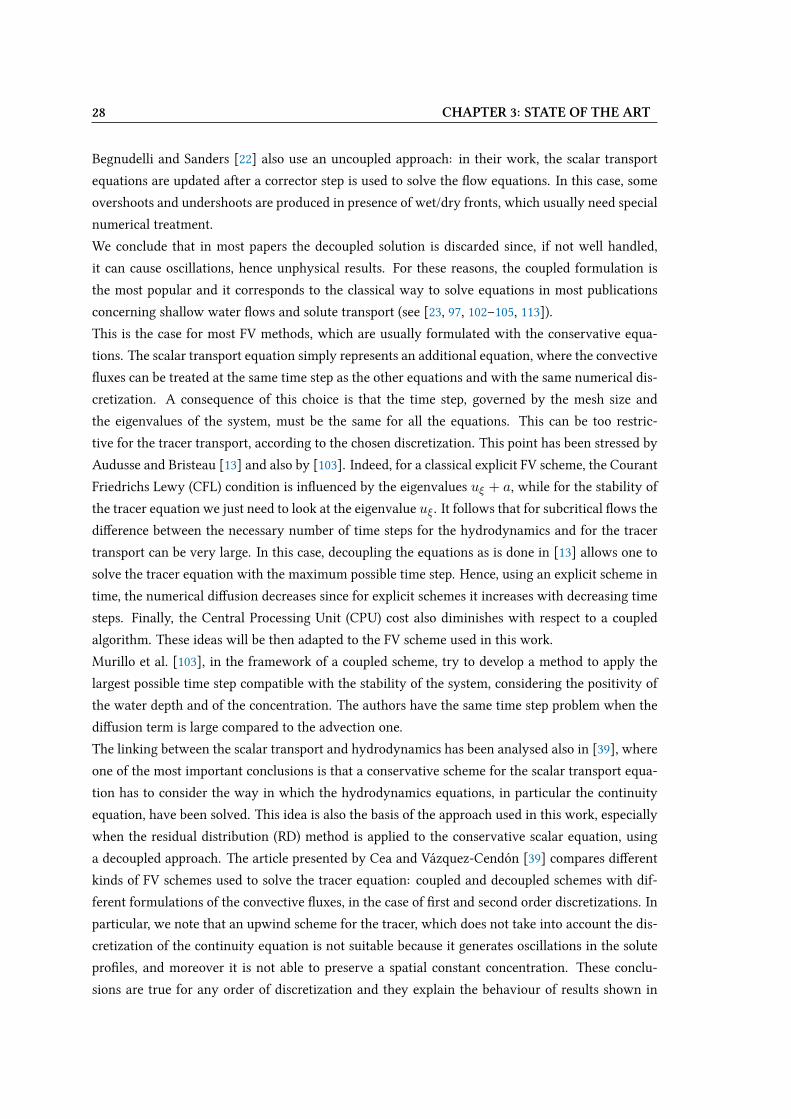
28 CHAPTER 3: STATE OF THE ART
Begnudelli and Sanders [22] also use an uncoupled approach: in their work, the scalar transport
equations are updated after a corrector step is used to solve the Wow equations. In this case, some
overshoots and undershoots are produced in presence of wet/dry fronts, which usually need special
numerical treatment.
We conclude that in most papers the decoupled solution is discarded since, if not well handled,
it can cause oscillations, hence unphysical results. For these reasons, the coupled formulation is
the most popular and it corresponds to the classical way to solve equations in most publications
concerning shallow water Wows and solute transport (see [23, 97, 102–105, 113]).
This is the case for most FV methods, which are usually formulated with the conservative equa-
tions. The scalar transport equation simply represents an additional equation, where the convective
Wuxes can be treated at the same time step as the other equations and with the same numerical dis-
cretization. A consequence of this choice is that the time step, governed by the mesh size and
the eigenvalues of the system, must be the same for all the equations. This can be too restric-
tive for the tracer transport, according to the chosen discretization. This point has been stressed by
Audusse and Bristeau [13] and also by [103]. Indeed, for a classical explicit FV scheme, the Courant
Friedrichs Lewy (CFL) condition is inWuenced by the eigenvalues uξ + a, while for the stability of
the tracer equation we just need to look at the eigenvalue uξ . It follows that for subcritical Wows the
diUerence between the necessary number of time steps for the hydrodynamics and for the tracer
transport can be very large. In this case, decoupling the equations as is done in [13] allows one to
solve the tracer equation with the maximum possible time step. Hence, using an explicit scheme in
time, the numerical diUusion decreases since for explicit schemes it increases with decreasing time
steps. Finally, the Central Processing Unit (CPU) cost also diminishes with respect to a coupled
algorithm. These ideas will be then adapted to the FV scheme used in this work.
Murillo et al. [103], in the framework of a coupled scheme, try to develop a method to apply the
largest possible time step compatible with the stability of the system, considering the positivity of
the water depth and of the concentration. The authors have the same time step problem when the
diUusion term is large compared to the advection one.
The linking between the scalar transport and hydrodynamics has been analysed also in [39], where
one of the most important conclusions is that a conservative scheme for the scalar transport equa-
tion has to consider the way in which the hydrodynamics equations, in particular the continuity
equation, have been solved. This idea is also the basis of the approach used in this work, especially
when the residual distribution (RD) method is applied to the conservative scalar equation, using
a decoupled approach. The article presented by Cea and Vázquez-Cendón [39] compares diUerent
kinds of FV schemes used to solve the tracer equation: coupled and decoupled schemes with dif-
ferent formulations of the convective Wuxes, in the case of Vrst and second order discretizations. In
particular, we note that an upwind scheme for the tracer, which does not take into account the dis-
cretization of the continuity equation is not suitable because it generates oscillations in the solute
proVles, and moreover it is not able to preserve a spatial constant concentration. These conclu-
sions are true for any order of discretization and they explain the behaviour of results shown in
3.2 FIRST ORDER SCHEMES WITH LOW NUMERICAL DIFFUSION 29
[102],[106]. In addition, the authors show that this type of scheme does not conserve mass.
Concerning the coupled and decoupled approach, Cea and Vázquez-Cendón [39] demonstrate that
the two approaches can be equivalent in absence of source terms and under a particular choice of
the non conservative variable transported by the convective Wux. In any case the decoupled ap-
proach, if well formulated, represents a valid solution to model the depth-averaged scalar transport.
Contrary to the explicit FV case, when using semi-implicit schemes for hydrodynamics, decoupling
the tracer equation is useful to keep accurate and bounded solutions for tracer at a low cost for the
hydrodynamic part (which often represents the most expensive side of the whole computation).
Indeed, the semi-implicit method for hydrodynamics allows one to choose large time steps for long
computations, so the CPU cost is smaller than that of an explicit scheme. It follows that the hy-
drodynamic time step could be too large for the tracer stability, so the tracer equation is solved
through a sub-iteration system which enables obtaining physical and bounded solutions. A similar
philosophy will be adopted for the RD scheme used in this work, whose details will be given in
Chapter 5.
3.2 First order schemes with low numerical diUusion
Beyond high-order schemes, other solutions can be considered in order to improve the accuracy
of transport schemes. Indeed, numerical results for the advection of discontinuous proVles can be
disappointing despite the use of an high-order scheme. Representing a discontinuity over a mesh
can be a very diXcult task independent of the numerical method used. This is often one of the
reasons for which techniques called ‘anti-dissipative’ schemes [57] are developed in the framework
of FV schemes. However, even for the transport of smooth initial proVles, we Vnd in the literature
a series of schemes which are Vrst order in space and time but with very low numerical diUusion
with respect the classical FV or FE methods.
3.2.1 Method of characteristics
The method of characteristics is a typical example of such a scheme. This method can be very
accurate in spite of the low convergence rate. The idea of applying this lagrangian method to
transport quantities in the eulerian framework comes from Courant et al. [46], for Vnite diUerence
schemes. The popularity of the method is due to its simplicity. For each point of the mesh, the
method consists of two steps [82]:
1. Vnding the foot of the characteristic by tracing the trajectory that passes by the interested
point at time tn+1;
2. using an arbitrary interpolation at the arrival time.
However, one diXculty is the trajectory construction in the mesh and the parallelization of this
technique can be a very diXcult issue, though it has been resolved. On the other hand, this method
gets rid of the typical severe time step condition that is necessary for classical methods applied

30 CHAPTER 3: STATE OF THE ART
to the transport equations. The unconditional stability is one of the most important advantage,
together with the respect of the monotonicity condition.
Unfortunately, the two steps of the method do not lead to a mass conservative scheme because of
the interpolation of the function at the foot of characteristic.
The latter is the major drawback that eliminates this method from the list of possible candidates
for pollutant transport in shallow water.
3.2.2 Eulerian-Lagrangian localized adjoint method
To solve the mass conservation problem, a weak formulation of the method of characteristics was
Vrst proposed by Benque et al. [24], then studied in other reports at EDF (Electricité de France)
[78, 79]. The method is also known as ELLAM (Eulerian-Lagrangian localized adjoint method), a
name given in the work presented by Celia, Russel and his collaborators [27, 41, 150], who also
proposed a good overview and revision of the method in [127].
The key idea is the application of the weak formulation in space and time, which is responsable for
the advection of the test functions (beyond that of the transported quantities). The Vnal formulation
of the scheme is conservative but a product of test functions at time tn+1 and at time tn appear and
its computation represents a technical problem since the functions are based on diUerent meshes.
The integral can be computed with Gauss points, as done in [80], but in this way the number of
Gauss points becomes a parameter which inWuences the mass conservation of the method. At the
same time the method allows getting very accurate results close to exact solutions. Indeed, the Vnal
conservative form of the scheme is a linear system which, to be solved, needs the inversion of a
mass-matrix composed of the product of test functions at time tn+1. This particular mass-matrix
that contains time information is the key point that reduces the artiVcial diUusion of the scheme.
However, this Vnal linear system of the technique breaks monotonicity.
Hence, the violation of the maximum principle prevents the use of this method for scalar transport
application in Wows.
3.2.3 Anti-dissipative transport schemes
The VoVre method is presented in [59] as an anti-dissipative transport scheme. This scheme seems
to be a valid alternative for transport problems thus we deem it is necessary to mention it. The
method is based on the construction of an anti-dissipative Wux and is the result of previous works
[57, 58]. The procedure used in this work could seem similar to the Monotonic Upwind Scheme
for Conservation Law (MUSCL) approach since in the present method the reconstruction step is
a key point. However, the authors clarify that it is not the same approach since in this case the
reconstructions are piecewise-constant instead of piecewise-linear.
The main idea is to reduce the numerical diUusion by dividing the problem into two steps. In the
Vrst step the transverse reconstruction is applied in order to diminish the diUusion which appears
when the velocity Veld is not aligned with the mesh i.e. transverse diUusion (see Figure 3.1). In the
second, the problem of the longitudinal diUusion which appears when the velocity Veld is aligned
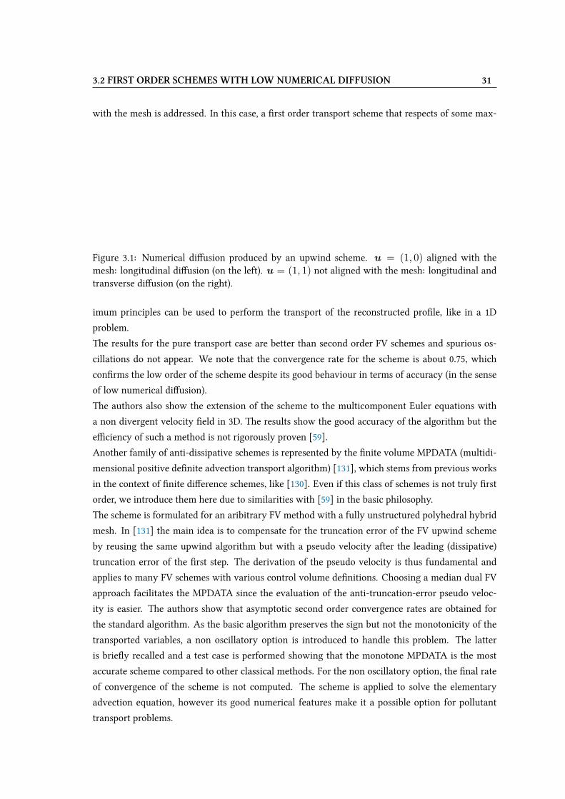
3.2 FIRST ORDER SCHEMES WITH LOW NUMERICAL DIFFUSION 31
with the mesh is addressed. In this case, a Vrst order transport scheme that respects of some max-
Figure 3.1: Numerical diUusion produced by an upwind scheme. u = (1, 0) aligned with themesh: longitudinal diUusion (on the left). u = (1, 1) not aligned with the mesh: longitudinal andtransverse diUusion (on the right).
imum principles can be used to perform the transport of the reconstructed proVle, like in a 1D
problem.
The results for the pure transport case are better than second order FV schemes and spurious os-
cillations do not appear. We note that the convergence rate for the scheme is about 0.75, which
conVrms the low order of the scheme despite its good behaviour in terms of accuracy (in the sense
of low numerical diUusion).
The authors also show the extension of the scheme to the multicomponent Euler equations with
a non divergent velocity Veld in 3D. The results show the good accuracy of the algorithm but the
eXciency of such a method is not rigorously proven [59].
Another family of anti-dissipative schemes is represented by the Vnite volume MPDATA (multidi-
mensional positive deVnite advection transport algorithm) [131], which stems from previous works
in the context of Vnite diUerence schemes, like [130]. Even if this class of schemes is not truly Vrst
order, we introduce them here due to similarities with [59] in the basic philosophy.
The scheme is formulated for an aribitrary FV method with a fully unstructured polyhedral hybrid
mesh. In [131] the main idea is to compensate for the truncation error of the FV upwind scheme
by reusing the same upwind algorithm but with a pseudo velocity after the leading (dissipative)
truncation error of the Vrst step. The derivation of the pseudo velocity is thus fundamental and
applies to many FV schemes with various control volume deVnitions. Choosing a median dual FV
approach facilitates the MPDATA since the evaluation of the anti-truncation-error pseudo veloc-
ity is easier. The authors show that asymptotic second order convergence rates are obtained for
the standard algorithm. As the basic algorithm preserves the sign but not the monotonicity of the
transported variables, a non oscillatory option is introduced to handle this problem. The latter
is brieWy recalled and a test case is performed showing that the monotone MPDATA is the most
accurate scheme compared to other classical methods. For the non oscillatory option, the Vnal rate
of convergence of the scheme is not computed. The scheme is applied to solve the elementary
advection equation, however its good numerical features make it a possible option for pollutant
transport problems.
32 CHAPTER 3: STATE OF THE ART
3.3 Conservative high order schemes
As previously stated, major challenge when solving the pollutant transport equation is high accu-
racy, which is expected as well as maintaining other properties like conservation of the mass and
respect of the maximum principle. For industrial applications, it is essential to have an accurate
prediction of the pollutant path for long distances (order of hundred kilometers), typical of rivers.
In this case, the numerical diUusion as well as the order of accuracy of the scheme, play a funda-
mental role. Thus, a natural choice is to increase the space and time accuracy of the scheme.
We recall that the local truncation error of a numerical scheme represents the discretization error,
which is generated by the speciVc numerical scheme, due to the truncation of the inVnite Taylor se-
ries to form the discrete algorithm [95]. We deVne Lh as an operator acting on the discrete solution
ch = ch(xh, th), in the form Lh(ch) = 0, where xh = (xi−l, ..., xi, ..., xi+r) and th = (tn, tn+1)
are the discretizations of space and time with l and r the integer numbers that deVne the size of
the stencil (support) of the numerical method. The local truncation error is deVned as [62]:
τ =Lh(c(xh, th))
∆t(3.1)
where c(xh, th) is the exact solution of the PDE computed at the discrete point (xh, th) and ∆t =
tn+1 − tn is the discrete time step. If, for a suXciently smooth solution of the PDE, we have:
τ(∆t, x) = O(∆tp + ∆xq) (3.2)
where ∆x is the average mesh size, then we will say that the scheme is p-th order accurate in time
and q-th order accurate in space. The error, using the harmonic analysis of Fourier applied to the
modiVed equation (i.e. the equation which is exactly solved by the numerical method) can also be
interpreted as diUusion and dispersion errors (see [96, 146]).
For pollutant transport problems in hydraulic applications, a requirement can be Vxed in order to
have discrete agreement between numerical solutions and real data. It is necessary to reduce the
signiVcant impact of numerical diUusion on the results. For industrial applications it would be
suitable to have numerical methods that are at least second order accurate in space and in time, to
handle steady and unsteady problems. Higher order methods are not considered for the moment,
due to the prohibitive computational cost and the lack of a robust mathematical theory, which is
necessary for industrial applications to strictly keep true the numerical properties of the equations
at the discrete level.
3.3.1 Finite volumes schemes
The FV methods are widely used to solve the SW system and also the tracer equation. In this case,
a complete literature review would be quite cumbersome, and our analysis focuses on the existing
techniques used to get second order accurate schemes in the FV context. To start, the overview
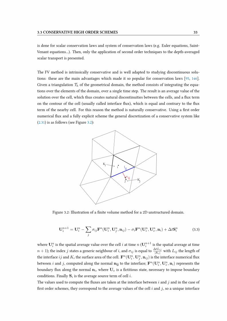
3.3 CONSERVATIVE HIGH ORDER SCHEMES 33
is done for scalar conservation laws and system of conservation laws (e.g. Euler equations, Saint-
Venant equations...). Then, only the application of second order techniques to the depth-averaged
scalar transport is presented.
The FV method is intrinsically conservative and is well adapted to studying discontinuous solu-
tions: these are the main advantages which made it so popular for conservation laws [95, 146].
Given a triangulation Th of the geometrical domain, the method consists of integrating the equa-
tions over the elements of the domain, over a single time step. The result is an average value of the
solution over the cell, which thus creates natural discontinuities between the cells, and a Wux term
on the contour of the cell (usually called interface Wux), which is equal and contrary to the Wux
term of the nearby cell. For this reason the method is naturally conservative. Using a Vrst order
numerical Wux and a fully explicit scheme the general discretization of a conservative system like
(2.31) is as follows (see Figure 3.2):
Ki
Kj
nij
i
j
lij
Figure 3.2: Illustration of a Vnite volume method for a 2D unstructured domain.
Un+1i = Un
i −∑j
σijFn(Un
i ,Unj ,nij)− σiFn(Un
i ,Une ,ni) + ∆tSni (3.3)
whereUni is the spatial average value over the cell i at time n (Un+1
i is the spatial average at time
n+ 1); the index j states a generic neighbour of i, and σij is equal to∆tLij|Ki| with Lij the length of
the interface ij andKi the surface area of the cell. Fn(Uni ,U
nj ,nij) is the interface numerical Wux
between i and j, computed along the normal nij to the interface; Fn(Uni ,U
ne ,ni) represents the
boundary Wux along the normal ni, where Ue is a Vctitious state, necessary to impose boundary
conditions. Finally Si is the average source term of cell i.
The values used to compute the Wuxes are taken at the interface between i and j and in the case of
Vrst order schemes, they correspond to the average values of the cell i and j, so a unique interface
34 CHAPTER 3: STATE OF THE ART
value is used for every interface of the cell. Equation (3.3) should in general satisfy a CFL condition
[45, 46] for stability reasons.
3.3.1.1 Second order techniques
For the Godunov theorem, linear schemes can not be monotone and second (or higher) order accu-
rate at the same time. Thus, to overcome this theorem and to improve the accuracy of Vnite volume
schemes, the values at the interfaces between cells are reconstructed considering piecewise linear
approximations and then limited using non linear functions (called limiters) of the data themselves.
These functions make the scheme non linear even if the equation to solve is linear (e.g. the scalar
linear transport equation), and they are necessary to avoid oscillatory solutions.
When solving the augmented SW system, it is important to use a general method that guaran-
tees the preservation of a convex invariant domain (D ), as described in [28]. Indeed a second
order scheme, satisfying a half original CFL condition, will be able to preserve a convex invariant
domain, if:
• the numerical Wux of the Vrst order scheme preserves a convex invariant domain under a
CFL condition. This means that the scheme itself, under a CFL condition, preserves a convex
invariant domain: Uni ∈ D ∀ i→ Un+1
i ∈ D ∀ i.
• the reconstruction also preserves a convex invariant domain:
Ui ∈ D ∀ i ⇒ Ui+1/2± ∈ D ∀ i, where Ui+1/2± are the reconstructed values at the
interfaces of the cell i.
In multidimensional cases, it is more diXcult to check the second condition, while the Vrst condi-
tion is easily veriVed if we have a Vrst order monotone scheme.
In a 1D framework we call xi+1/2 the interface point between cell i and i+ 1, and i+ 1/2−, i+
1/2+, the left and the right side of the interface, respectively. The reconstructed states are second
order in the sense that for some smooth function U(x), we have Ui+1/2− = U(xi+1/2) +O(∆x2)
and Ui+1/2+ = U(xi+1/2) + O(∆x2). With these reconstructed values (called Uij in 2D) the
scheme (3.3) becomes:
Un+1i = Un
i −mi∑j=1
σijF(Unij ,U
nji,nij)− σiF(Un
i ,Une ,ni) + ∆tSni (3.4)
For one dimensional scalar equations, in the case of second order schemes, an option to enforce the
maximum principle is to use the Minmod limiter. In 1D cases the way to apply the linear recon-
struction and the limiters is well deVned, owing to the reduced dimensionality of the problem, and
it is based on a robust theory which guarantees the preservation of some important properties (e.g.
the maximum principle).
On the other hand, in 2D unstructured domains, several techniques have been proposed during
3.3 CONSERVATIVE HIGH ORDER SCHEMES 35
the last 30 years to perform the linear reconstruction and to limit the interface values. The large
number of available techniques and the lack of a unique procedure is related to diUerent reasons:
the theorems for the 1D cases have not been completely extended to the 2D cases; criteria to apply
limiters change depending on the type of numerical Wux used; use of cell-centred or vertex-centred
scheme generates diUerences in gradient computations and consequently on limiting approaches.
In addition, several kinds of limiters can be chosen: Minmod, van Albada, Superbee and many oth-
ers [92, 137]. All of them have diUerent characteristics in terms of the stability (or monotonicity)
region, and the Vnal solution can be more or less smoothed by the limiter. It follows that strictly
preserving the maximum principle in convection problems can be very diXcult. The fact that in
many papers describing pollutant transport in shallow water Wows, the monotonicity of the solu-
tion is not strictly veriVed or ensured might then be related to these reasons.
The MUSCL (Monotonic Upwind Scheme for Conservation Law) technique is the Vrst method
known in the literature to achieve second order accuracy with Vnite diUerence schemes and has
then been extended to Vnite volumes schemes. Even if this method has usually been attributed
to van Leer [149], we remember that it is Vrstly due to N.E. Kolgan [93]. Kolgan conceived the
gradient reconstruction and the slope limiter when he was at the Central Aerodynamical National
Laboratory near Moscow, but since he died young his work wasn’t noticed outside his laboratory.
This was later acknowledged by van Leer [65].
The method is the most popular in industrial codes, since it is more Wexible, simples and easier to
implement than other high order methods like ENO [75], WENO [100] or Discontinuous Galerkin
methods [129].
The MUSCL method with limiters can be applied to 1D scalar cases very easily: the L∞ stability
and the Total Variation Diminishing (TVD) condition have been proven [109, 148], and the method
results are eUectively second order accurate. Clear explanations and examples can also be found
in [95, 146]. For the one-dimensional scalar case, the method consists of the evaluation of the edge
value through the appropriate computation of the upwind and downwind slope in a way that the
TVD property or the maximum principle have been fulVlled. Hence the approach consists of two
steps: in the Vrst step a cell gradient is computed while in the second step the gradient is modiVed
by some limiter functions in order to guarantee the maximum principle or the TVD property.
The extension of the gradient reconstruction to the 2D case is straightforward when using carte-
sian meshes and applying the procedure to each direction, yet it has been shown that the TVD
stability condition reduces the method to a Vrst order scheme [70]. This problem was overcome by
Spekreijse [134], who proposed positive coeXcients schemes.
The Vrst attempts to generalize the 1D monotone reconstruction to the multidimensional case over
unstructured grids were made by Barth and Jespersen [18], Batten et al. [19], Hubbard [87], Liu
[99]. All of these studies deal with cell-centred FV schemes (except Barth who also show some re-
sults for a vertex-centred scheme), where the reconstructed gradients are limited imposing diUerent
conditions in order to respect a local maximum principle. These eUorts aimed at generalizing the
one-dimensional technique to the 2D case.
36 CHAPTER 3: STATE OF THE ART
In [18], the idea is to Vnd the largest admissible value for the limiter while invoking a monotonicity
principle stating that values of the linearly reconstructed function must not exceed the maximum
and minimum neighbouring centroid values (including the cell itself). For a reconstruction of the
type:
u(x, y)A = u(x0, y0)A + ΦA∇uA · 4rA (3.5)
where u(x, y)A is the variable to limit,(x0, y0) is the centroid of the cell,Φ is the limiter and rA is
the distance from the centroid to the point A; the requirement is that:
uminA ≤ u(x, y)A ≤ umaxA (3.6)
with uminA and umaxA the minimum and the maximum values of the cell itself and the neighbouring
cells. In [87], Hubbard tries to take into account to the maximum the multidimensionality of the
problem, improving the old limiting techniques. Limited gradient operators are constructed by
constraining the gradients to lie within a ‘Maximum principle region’ and a cell-centred scheme is
used, for which an exact gradient operator for linear data can be deVned. The region is constructed
using the inequality:
min(uk − u0, 0) ≤ r0k · ∇u ≤ max(uk − u0, 0) (3.7)
where r0k is the vector from the centroid of cell 0 to the midpoint of the edge between cells 0 and
k. The inequality ensures the desired properties: no new extrema and sign preservation of the re-
constructed variables. Besides the gradient computation, the cell-centred scheme is advantageous
also because it does not need a further correction of the reconstructed values to enforce mass con-
servation. On the contrary, this is not true in a vertex-centred framework, as explained in [112].
Perthame and Qiu [112], in 1994, proposed a variant of the classical MUSCL approach in a vertex-
centred FV framework. The novelty of their method consists of using interpolation rather than
slope reconstruction and the robustness of the approach is proven through numerical tests where
stability and the non-negativity of some variables (pressure and density, since they solve the Euler
equations) are veriVed. Because of interpolation, the solution is represented by piece-wise constant
subcell functions, which dictate the limitation to perform on the reconstructed value in order to
guarantee a conservation constraint. We note that in this case the interpolated values are placed
at the vertex of the control volume (and not at the mid point of the interfaces) since a simple in-
terpolation of the numerical Wux is performed using the vertex values. Due to the vertex-centred
framework, a supplementary correction of the interpolated values is necessary for conservation
reasons. This is due to some geometrical aspects, since the centre of mass of the vertex-centred
cell i does not correspond to the node of the mesh used to indicate the cell i (from which then the
gradients are computed). In [14], the correction of the second order values has been transposed for
a classical case where slopes are computed to approximate the gradient at the middle point of the
interface. The correction is successful since mass is conserved and the positivity of the interested
values is preserved too.

3.3 CONSERVATIVE HIGH ORDER SCHEMES 37
More recently other studies [26, 33, 36, 44, 86, 94] of MUSCL methods for unstructured grids ap-
peared in the literature.
The work of Berthon [26] focuses on the application of a variant of the classical MUSCL technique
in a vertex-centred FV framework. Since the method is used on the Euler equations, the preserva-
tion of invariant domains and the satisfaction of a set of entropy inequalities is analysed in detail
in the gradient reconstruction step. The authors present a scheme which turns out to be the same
as in [112], even if the procedure to reconstruct and to limit the interface values is diUerent.
To write the second order scheme as a relevant average of states obtained by a Vrst-order scheme,
a particular geometrical framework is considered: the classical dual cell of a vertex-centred context
is decomposed in sub-cells. The paper aims to prove that the solution given by the second-order 2D
scheme is able to guarantee the preservation of a convex set and the satisfaction of the discrete form
of the entropy inequalities, if a relevant CFL condition and a special limitation process are applied.
Theoretical and numerical proofs are given in the paper. Demanding tests show the robustness of
the scheme proposed, stressing the positivity of pressure and density, yet the non-oscillatory char-
acter of the solution is not controlled by the proposed technique.
BuUard and Clain [33] propose two new MUSCL techniques for cell-centred FV schemes. The
methods are based on a mesh assumption: the barycenter of a triangle is always contained by a
convex set deVned by the barycenters of the three neighboring volumes.
The Vrst technique proposed is called the monoslope method as only one gradient is used per el-
ement, which means that the three values reconstructed at the interfaces are generated by the
same gradient. The novelty with respect to the classical monoslope approach is that the gradient is
constructed in only one procedure. The technique consists of optimizing the slope under the TVD
constraint, hence the slope is the result of the minimizing procedure. A new variable is introduced
and deVned at the interface: it is called the reference variable since it represents the reference
reconstructed value at the intersection between the segment joining the barycenters and the line
containing the edge of the cell. The reference variable is equal for the two nearby cells (i and j).
In the minimization procedure, the objective is for the reconstructed values the be as equal as pos-
sible to the reference values, respecting the TVD condition.
The second technique proposed for the MUSCL approach is a multislope method since a diUerent
slope is provided for each interface of the same triangle. In this case two requirements have to be
satisVed: the reconstruction must be consistent for linear functions and the slope has to vanish in
case of a local extremum at point i. For both techniques, the authors consider two ways to deVne
the interface values: the midpoint of the interface or the intersection point between the interface
and the segment linking the two barycenters of the two triangles. A large number of tests are pre-
sented and the techniques are tested for the scalar advection equation and for the Euler equations
for diUerent kinds of meshes and for diUerent initial conditions (continuous and discontinuous
functions). Due to the large number of combinations of limiters and of types of reconstruction
methods, it is diXcult to retain a unique general conclusion from the test cases. However, the most
important conclusions are:
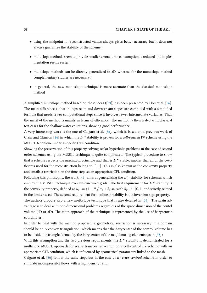
38 CHAPTER 3: STATE OF THE ART
• using the midpoint for reconstructed values always gives better accuracy but it does not
always guarantee the stability of the scheme;
• multislope methods seem to provide smaller errors, time consumption is reduced and imple-
mentation seems easier;
• multislope methods can be directly generalized to 3D, whereas for the monoslope method
complementary studies are necessary;
• in general, the new monoslope technique is more accurate than the classical monoslope
method
A simpliVed multislope method based on these ideas ([33]) has been presented by Hou et al. [86].
The main diUerence is that the upstream and downstream slopes are computed with a simpliVed
formula that needs fewer computational steps since it involves fewer intermediate variables. Thus
the merit of the method is mainly in terms of eXciency. The method is then tested with classical
test cases for the shallow water equations, showing good performance.
A very interesting work is the one of Calgaro et al. [36], which is based on a previous work of
Clain and Clauzon [44] in which the L∞ stability is proven for a cell-centred FV scheme using the
MUSCL technique under a speciVc CFL condition.
Showing the preservation of this property solving scalar hyperbolic problems in the case of second
order schemes using the MUSCL techinque is quite complicated. The typical procedure to show
that a scheme respects the maximum principle and that is L∞ stable, implies that all of the coef-
Vcients used for the reconstruction belong to [0, 1]. This is also known as the convexity property
and entails a restriction on the time step, so an appropriate CFL condition.
Following this philosophy, the work [44] aims at generalizing the L∞ stability for schemes which
employ the MUSCL technique over unstructured grids. The Vrst requirement for L∞ stability is
the convexity property, deVned as uij = (1− θij)ui + θijuj with θij ∈ [0, 1] and strictly related
to the limiter used. The second requirement for nonlinear stability is the inversion sign property.
The authors propose also a new multislope technique that is also detailed in [33]. The main ad-
vantage is to deal with one-dimensional problems regardless of the space dimension of the contol
volume (2D or 3D). The main approach of the technique is represented by the use of barycentric
coordinates.
In order to deal with the method proposed, a geometrical restriction is necessary: the domain
should be an α convex triangulation, which means that the barycenter of the control volume has
to be inside the triangle formed by the barycenters of the neighbouring elements (as in [33]).
With this assumption and the two previous requirements, the L∞ stability is demonstrated for a
multislope MUSCL approach for scalar transport advection on a cell-centred FV scheme with an
appropriate CFL condition, which is inWuenced by geometrical parameters linked to the mesh.
Calgaro et al. [36] follow the same steps but in the case of a vertex-centred scheme in order to
simulate incompressible Wows with a high density ratio.
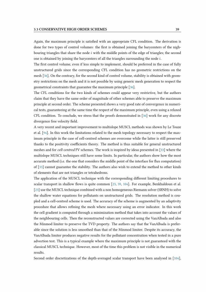
3.3 CONSERVATIVE HIGH ORDER SCHEMES 39
Again, the maximum principle is satisVed with an appropriate CFL condition. The derivation is
done for two types of control volumes: the Vrst is obtained joining the barycenters of the nigh-
bouring triangles that share the node i with the middle points of the edge of triangles; the second
one is obtained by joining the barycenters of all the triangles surrounding the node i.
The Vrst control volume, even if less simple to implement, should be preferred in the case of fully
unstructured grids since the corresponding CFL condition has no geometric restrictions on the
mesh [36]. On the contrary, for the second kind of control volume, stability is obtained with geom-
etry restrictions on the mesh and it is not possible by using generic mesh generation to respect the
geometrical constraints that guarantee the maximum principle [36].
The CFL conditions for the two kinds of schemes could appear very restrictive, but the authors
claim that they have the same order of magnitude of other schemes able to preserve the maximum
principle at second order. The scheme presented shows a very good rate of convergence in numeri-
cal tests, guaranteeing at the same time the respect of the maximum principle, even using a relaxed
CFL condition. To conclude, we stress that the proofs demonstrated in [36] work for any discrete
divergence free velocity Veld.
A very recent and important improvement to multislope MUSCL methods was shown by Le Touze
et al. [94]. In this work the limitations related to the mesh topology necessary to respect the max-
imum principle in the case of cell-centred schemes are overcome while the latter is still preserved
thanks to the positivity coeXcients theory. The method is thus suitable for general unstructured
meshes and for cell-centred FV schemes. The work is inspired by ideas presented in [33] where the
multislope MUSCL techniques still have some limits. In particular, the authors show how the most
accurate method (i.e. the one that considers the middle point of the interface for Wux computation)
of [33] cannot guarantee the stability. The authors also wish to extend the method to other kinds
of elements that are not triangles or tetrahedrons.
The application of the MUSCL technique with the corresponding diUerent limiting procedures to
scalar transport in shallow Wows is quite common [23, 39, 104]. For example, Benkhaldoun et al.
[23] use the MUSCL technique combined with a non homogeneous Riemann solver (SRNH) to solve
the shallow water equations for pollutants on unstructured grids. The resolution method is cou-
pled and a cell-centred scheme is used. The accuracy of the scheme is augmented by an adaptivity
procedure that allows reVning the mesh where necessary using an error indicator. In this work
the cell gradient is computed through a minimization method that takes into account the values of
the neighbouring cells. Then the reconstructed values are corrected using the VanAlbada and also
the Minmod limiter to preserve the TVD property. The authors say that the VanAlbada is prefer-
able since the solution is less smoothed than that of the Minmod limiter. Despite its accuracy, the
VanAlbada limiter produces negative results for the pollutant concentration when tested in a pure
advection test. This is a typical example where the maximum principle is not guaranteed with the
classical MUSCL technique. However, most of the time this problem is not visible in the numerical
results.
Second order discretizations of the depth-averaged scalar transport have been analysed in [104],
40 CHAPTER 3: STATE OF THE ART
for a cell centred scheme, on an unstructured grid. The paper considers the advection-diUusion
phenomena for tracers, under steady and unsteady Wow conditions. The authors use a fully explicit
upwind method for the advection part, where Wuxes are based on the Jacobian matrix, while an
implicit method is used for the diUusion term (which only involves the tracer equation). The ex-
tension to second order is achieved through the MUSCL-Hancock method, for the convection part.
Two diUerent limiting gradient techniques are used and then compared in the test cases.
The inWuence of the source terms on the stability condition is analysed and included in the deVni-
tion of the maximum time step. The respect of the maximum principle for the tracer is another issue
discussed in the paper. In this case, an eXcient technique is proposed to avoid unbounded values
of concentration for the second order case. In particular, second order accuracy can be achieved for
the tracer variables, while the hydrodynamic scheme is reduced to Vrst order. The numerical tests
show the qualitative improvement for the second order schemes, under various Wow conditions.
Other second order discretizations for the solute transport in shallow water Wows are tested in [39]
in the framework of a Roe-type FV Wux. The authors compare three diUerent high-order discretiza-
tions for the non conservative variable c transported by the convective Wuxes: one is a centred
discretization, another is the centred discretization where a dissipative term is added for stability
reasons (presented in [40]), and the last one is given by the Gamma scheme [91]. Numerical tests
show that the centred high order discretization produces strong oscillations in the solution, as ex-
pected. The other two high order discretizations show good behaviour and the results are more
accurate than the Vrst order cases. The least diUusive scheme is the Gamma scheme and the dis-
continuous proVle of tracers are qualitatively better when using this scheme.
The Harten-Lax-van Leer Contact (HLLC) Riemann solver is very popular in the framework of
FV schemes. The solver has been presented in [143, 144], and the application to the SW system
is described in [142]. The HLLC solver is a modiVcation of the HLL solver, which is a two-wave
model insuXcient for correct solute transport modeling. In the HLLC scheme the missing contact
and shear waves are included in the structure of the solution. Due to its popularity it has also
been extended to turbulent Wow applications [21], to Magnetohydrodynamics equations [74], to
two-phase Wow [141] and to the Navier-Stokes equations [115].
Other works using the HLLC RS in shallow water Wows are [98], where dynamically adaptive
quadtree grids are used and [101], where the classical formulation is extended to include source
terms.
Second order extensions of FV schemes using an HLLC RS, have been presented in [85, 86, 132, 133].
These works concern mainly the problem of wetting and drying phenomena, as well as the well-
balanced property, for second order schemes. For passive scalar transport, a sesitivity analysis for
MUSCL schemes using HLLC RS is presented in [73].
Canestrelli and Toro [37] use a FV FORCE-Contact scheme to discretize the augmented shallow
water system in a coupled way. In the paper, the authors show the impact of the restoration of the
Contact wave on the solution. Indeed, more accurate results are reached with the presented model,
for the Vrst, second and third order case. Here the higher orders are obtained with the ADER
3.3 CONSERVATIVE HIGH ORDER SCHEMES 41
approach presented in [63], and the theoretical rates of convergence are conVrmed in numerical
tests. In addition a comparison with the Vrst order HLLC scheme is also presented, showing that
the FORCE-contact model is slightly better in terms of accuracy. The paper stresses the importance
of capturing the contact or shear waves when linearly degenerate characteristic Velds play an im-
portant role in the physical phenomenon.
Higher order methods more than second-order like the WENO scheme are alternatives that we do
not consider here. There are several reasons for which these schemes are not implemented in in-
dustrial codes for real life problems. One is the high computational cost, which increases with the
order select and with the multidimensionality of the problem. Another motivation is that, often,
the shock capturing technique is hardly compatible with the higher order techniques. Improve-
ments in this Veld can be found in [63, 64], where the WENO reconstruction technique is used in
the framework of the one-step ADER approach, initially proposed in [145] by Toro and his collab-
orators. In particular, the application of the ADER approach to solve pollutant transport problems
is presented in [140].
3.3.2 Residual distribution schemes
The RD technique is less popular and less developed than the FV and FE methods. This is due
to the very limited formal understanding available with respect to the other classical techniques
[120]. However, due to the good properties (especially the linearity preservation condition) shown
by this method, the scientiVc community continues to remain interested in future developments of
this technique, which have been conducted in the recent years mainly by a team working at the
research centre INRIA-Bordeaux.
Works concerning the discretization of the SW equations using RD methods have been carried out
mainly by Ricchiuto and his co-workers [118–122, 128], while other previous works, with almost
non-conservative RD schemes, are [68, 88]. In fact, most of the time, the method has been used for
the discretization of the Euler equations rather than the Saint-Venant equations.
The overview given in this section focuses on the existing techniques to achieve second (or higher)
order schemes in space and in time, for a general conservation law. It is worth noticing that up to
now this technique, as far as we know, has not yet been used for pollutant transport problems in
shallow water Wows, except in [111] and here. However, as for FV method, it should be quite easy
to use the method proposed, for example in [121], for solving the coupled augmented SW system,
yet no papers appear on this topic. However, this is not the approach chosen in this work.
In the framework of the RD method, the solution is approximated in the piecewise linear Vnite-
element space over an arbitrary unstructured grid: ch(x, y, t) =npoin∑ic(xi, yi, t)ψi(x, y) where
npoin is the total number of nodes in the mesh, c(xi, yi, t) is the time dependent nodal value of
the solution at node i and ψi(x, y) is the piecewise linear shape function that beneVts from the
classical properties of linear P 1 FE basis functions.
42 CHAPTER 3: STATE OF THE ART
The integration of the scalar advection equation (2.38b) (without sources) over a single time step,
using an explicit time integration, leads to the following form:
cn+1i = cni −
∆t
Si
∑T3i
φEi (3.8)
where cni is the nodal value at time n and cn+1i is the nodal value at time n + 1, Si represents
the area of the cell around the point i, equal to∑T3i
T3 and φEi is the splitting residual at node i,
computed for every element that contains the node i and then summed up.
The quantity φE , called the residual, is computed as:
φE =
∫Eu · ∇ch dxdy (3.9)
By construction, the consistency relation: ∑i∈T
φEi = φT (3.10)
is satisVed. Another fundamental relation is φTi = βiφT , where βi represents the distribution
coeXcient. The way to distribute the residual to the nodes (i.e. through the distribution coeXcients)
inWuences a series of properties of the scheme like the positivity, the linearity preservation and the
multidimensional character. Hence diUerent schemes with diUerent properties can be created with
a diUerent residual distribution.
Every property characterizes the solution in a certain way and they are brieWy recalled here below
[54]:
• Positivity. A scheme of the form:
φEi =∑j∈T
λEij(cni − cnj ) with λEij ≥ 0 (3.11)
and able to respect the maximum principle, under the time step condition:
Si −∆t∑T3i
∑j∈T
λEij ≥ 0 ∀i ∈ Th (3.12)
is said to be positive. This property is thus related to the non-oscillatory character of the
solutions.
• Linearity Preserving. A scheme is linearity preserving if its distribution coeXcients βi are
uniformly bounded with respect to the solution and the data of the problem:
maxT∈Th
maxj∈T|βj | < C <∞ ∀φE , ch, c0
h (3.13)
3.3 CONSERVATIVE HIGH ORDER SCHEMES 43
where C is a constant. Linearity preserving schemes satisfy by construction the necessary
condition for second order accuracy, hence this property is related to the accuracy of the
scheme.
• Genuinely Multidimensional Upwind procedure: multidimensional upwind schemes only
send portions of φE to downstream nodes. This property corresponds to the generalization
of the 1D upwind idea. It is related to the stability of the scheme.
The origin of these schemes traces back to Ni [107] and Roe [125], who, in 1987, proposed the name
of Wuctuation splitting schemes. In [125], the upwind treatment of the scalar convection equation
was generalized in two space dimensions, deVning the multidimensional upwind character of these
schemes. In the same work, also the most successful Vrst order scheme was introduced. It is the
N (narrow) scheme, also known as the optimum Vrst order scheme, since among the Vrst order
schemes it is the least diUusive. The scheme is positive, multidimensional upwind and linear be-
cause of the Godunov theorem, it is limited to be only of Vrst order accuracy.
However, due to its properties, the scheme plays an important role in the construction of second
order schemes.
3.3.2.1 Second order techniques
In the RD scheme, the truncation error is deVned following a variational approach, see for example
[2, 8, 54]. From the consistency analysis it is possible to show that, in two spaces, a RD scheme
veriVes the truncation error estimate:
TE(wh) :=∑i∈Th
ϕi∑T3i
φi(wh) = O(∆xk) (3.14)
provided that the following condition is met:
φi(wh) = O(∆xk+1) ∀i ∈ T and T ∈ Th (3.15)
with ϕ a smooth compact function ϕ ∈ Ck0 (Ω), wh the k− th order accurate continuous piecewise
polynomial of degree k − 1 interpolant of w, a smooth exact solution of the PDE. This condition
guarantees formally that the scheme has an O(∆xk) error [54].
The N scheme only preserves O(∆x1) and does not guarantee the LP property since the distribu-
tion coeXcients are unbounded, but it can be the basis for a second order scheme.
Indeed, in order to obtain bounded distribution coeXcients and thus meet the condition φi =
O(∆x3), the non linear limiter PSI is introduced. The original PSI scheme was presented in 1994
by Struijs [136] in his PhD, and it met a large success (see [110, 125, 126]) due to its good per-
formance, which is better than FV schemes, especially on irregular grids [54] for steady scalar
44 CHAPTER 3: STATE OF THE ART
problems. The scheme is related to the N scheme since the limiter is applied on the distribution
coeXcients of the N scheme.
Later, a more general framework to construct non linear limited second order schemes was pre-
sented in [7, 8, 110]. In the RD method, the limiter is used in a completely diUerent manner than in
the FV method. In this case, the role of the limiter is to bound the coeXcients and to preserve the
positivity of the Vrst order scheme coeXcients, while in the FV context the limiter is used to limit
the slopes and so to avoid oscillations in the solution.
This technique, which is the one commonly used in practice, has been known for a very long time
(1995), and improved constructions have not been published since then [54].
In the RD framework the Vrst order scheme is critically important in the construction of the second
order one. Beyond the N scheme, the Lax–Friedrichs scheme is often used as basis for the construc-
tion of a limited non linear variant [3, 117, 121, 122].
However, all these formulations, which are based on the prototype (3.8) are only Vrst order accu-
rate in time dependent problems. This is due to an inconsistency in the spatial discretization [54],
which is independent of the order of the time discretization. Essentially, whatever the choice of
the discretization of the time derivative, the scheme has a discretization error bounded by O(∆x)
[120]. This can be demonstrated performing a time continuous consistency analysis (see [54, 118]).
To overcome this issue, several solutions have been tested based on a new concept of residual. The
diUerence consists of including the time derivative in the computation of the residual, which thus
becomes a space-time residual. This operation is necessary to recover second order accuracy in
space and it leads to the formation of a mass-matrix of the time derivative, exactly like in the FE
context, except that in this case the problem has not been formulated using a variational approach.
The various approaches proposed to solve time dependent problems can be classiVed in three fam-
ilies of schemes:
• space-time schemes,
• implicit in space schemes,
• explicit predictor-corrector schemes.
Schemes proposed in [47, 48, 54] and the more recent versions [89, 128] belong to the Vrst class.
Each element in the mesh deVnes a prism in space-time. In this case the problem is solved comput-
ing a space-time residual on the prism, which corresponds to [54]:
ΦPn+1/2E =
∫Pn+1/2C
(∂ch∂t
+ u · ∇ch)dx dy dt =
∫E
∫ t+1
t
(∂ch∂t
+ u · ∇ch)dx dy dt
(3.16)
Then, the fractions of ΦPn+1/2E are distributed to the nodes of E through the distribution coeX-
cients, like in the steady case, respecting the multidimensional character. Finally the solution is
3.3 CONSERVATIVE HIGH ORDER SCHEMES 45
found solving the system: ∑Pn+1/2E 3i
ΦPn+1/2E = 0 (3.17)
The extension of the multidimensional upwind scheme in the space-time context, yields a CFL
condition, called the past-shield condition. This condition, for prismatic space-time elements, is
exactly equivalent to the time step restriction ensuring the local positivity of the N scheme with
trapezium integration [54].
The resulting scheme is quite expensive from a computational point of view, due to the very re-
stricting time-marching condition coupled to the solution of a non linear system at every iteration.
In [123] a better condition for the time step is presented, and the Vnal cost is comparable to that of
an unconditionally implicit second order Runge-Kutta scheme.
The second approach for time dependent problem is represented by implicit space schemes. They
deal with unsteady problems Vrstly discretizing in time the residual and then applying the spatial
discretization. Schemes belonging to this family have been presented in [6, 38, 118]. The space-time
residual can be recast as [118]:
Φh =ST3
∑j∈T
(cn+1i − cni ) +
∆t
2φh(cn+1
h ) +∆t
2φh(cnh) (3.18)
Then the splitting is operated following the same design criteria for steady problems: positiv-
ity, multidimensional upwind and linearity preservation for the second order case. The accuracy
analysis for time problems [54, 118] shows that the scheme respects an error estimate of the type
ε(wh, tf ) = O(∆x2), if Φi(wh) = O(∆x4). Hence, even for unsteady cases, the non linear limiter
is applied on positive linear schemes to obtain bounded distribution coeXcients.
However, as for the steady case, the condition for Φi(wh) is only necessary and not suXcient to
get the desired convergence rate, since other stability conditions are necessary.
Once the splitting is completed, a set of non linear algebraic equations has to be solved to Vnd cn+1i :∑
T3iΦEi = 0 (3.19)
The formulation of the N scheme in this implicit in time framework then helps to construct the PSI
version for time dependent problems.
The monotonicity condition is derived from the N scheme and corresponds to the past-shields
condition of [54]. The non linear system obtained when the βPSI are applied can be solved through
non linear solvers like the Newton-Raphson method [6] or through an explicit pseudo-time iterative
procedure [47, 48, 123]. The latter seems to converge faster in terms of CPU time [61], however the
implicit in space formulation is tied down by the non linear system.
It is worth noting that for the two families of schemes presented, the restrictive stability constraints
can sometimes be removed when using a two-layer formulation, see [6, 47, 123].
The genuinely explicit schemes, like the predictor-corrector, represent another approach to handle
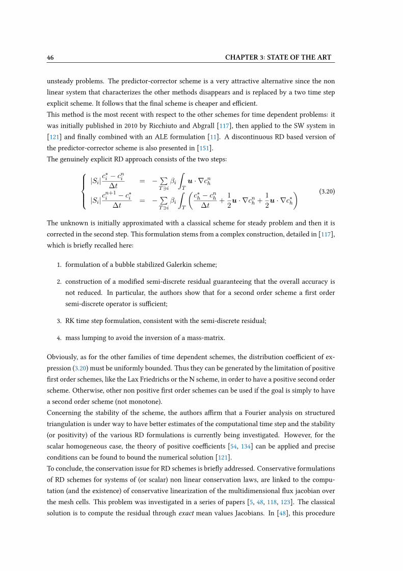
46 CHAPTER 3: STATE OF THE ART
unsteady problems. The predictor-corrector scheme is a very attractive alternative since the non
linear system that characterizes the other methods disappears and is replaced by a two time step
explicit scheme. It follows that the Vnal scheme is cheaper and eXcient.
This method is the most recent with respect to the other schemes for time dependent problems: it
was initially published in 2010 by Ricchiuto and Abgrall [117], then applied to the SW system in
[121] and Vnally combined with an ALE formulation [11]. A discontinuous RD based version of
the predictor-corrector scheme is also presented in [151].
The genuinely explicit RD approach consists of the two steps:|Si|
c∗i − cni∆t
= −∑T3i
βi
∫Tu · ∇cnh
|Si|cn+1i − c∗i
∆t= −
∑T3i
βi
∫T
(c∗h − cnh
∆t+
1
2u · ∇cnh +
1
2u · ∇c∗h
) (3.20)
The unknown is initially approximated with a classical scheme for steady problem and then it is
corrected in the second step. This formulation stems from a complex construction, detailed in [117],
which is brieWy recalled here:
1. formulation of a bubble stabilized Galerkin scheme;
2. construction of a modiVed semi-discrete residual guaranteeing that the overall accuracy is
not reduced. In particular, the authors show that for a second order scheme a Vrst order
semi-discrete operator is suXcient;
3. RK time step formulation, consistent with the semi-discrete residual;
4. mass lumping to avoid the inversion of a mass-matrix.
Obviously, as for the other families of time dependent schemes, the distribution coeXcient of ex-
pression (3.20) must be uniformly bounded. Thus they can be generated by the limitation of positive
Vrst order schemes, like the Lax Friedrichs or the N scheme, in order to have a positive second order
scheme. Otherwise, other non positive Vrst order schemes can be used if the goal is simply to have
a second order scheme (not monotone).
Concerning the stability of the scheme, the authors aXrm that a Fourier analysis on structured
triangulation is under way to have better estimates of the computational time step and the stability
(or positivity) of the various RD formulations is currently being investigated. However, for the
scalar homogeneous case, the theory of positive coeXcients [54, 134] can be applied and precise
conditions can be found to bound the numerical solution [121].
To conclude, the conservation issue for RD schemes is brieWy addressed. Conservative formulations
of RD schemes for systems of (or scalar) non linear conservation laws, are linked to the compu-
tation (and the existence) of conservative linearization of the multidimensional Wux jacobian over
the mesh cells. This problem was investigated in a series of papers [5, 48, 118, 123]. The classical
solution is to compute the residual through exact mean values Jacobians. In [48], this procedure
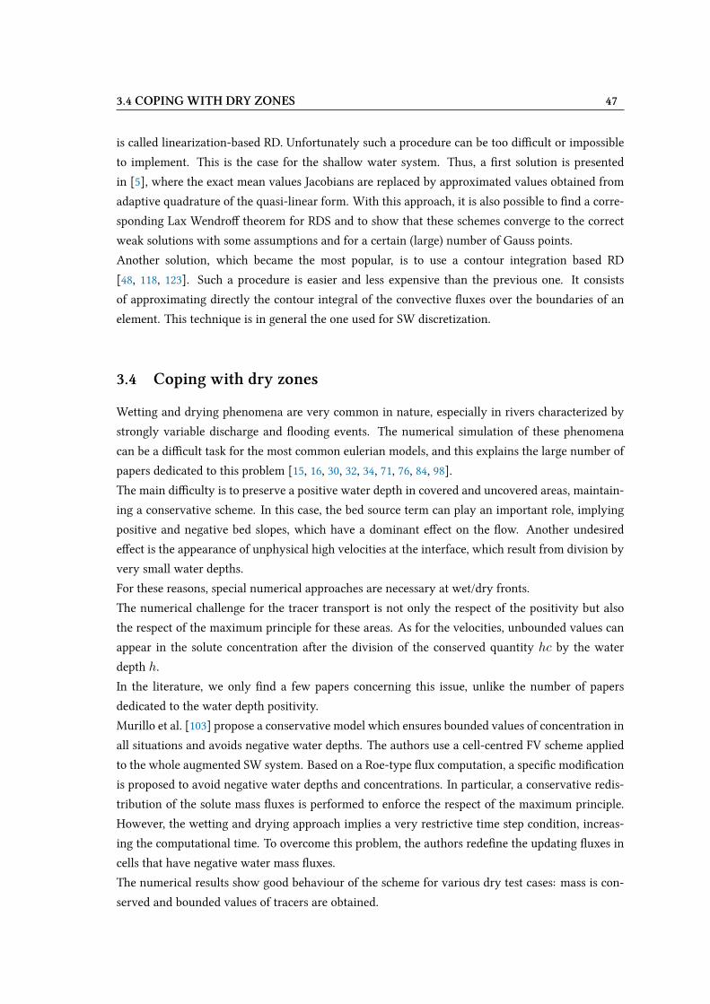
3.4 COPING WITH DRY ZONES 47
is called linearization-based RD. Unfortunately such a procedure can be too diXcult or impossible
to implement. This is the case for the shallow water system. Thus, a Vrst solution is presented
in [5], where the exact mean values Jacobians are replaced by approximated values obtained from
adaptive quadrature of the quasi-linear form. With this approach, it is also possible to Vnd a corre-
sponding Lax WendroU theorem for RDS and to show that these schemes converge to the correct
weak solutions with some assumptions and for a certain (large) number of Gauss points.
Another solution, which became the most popular, is to use a contour integration based RD
[48, 118, 123]. Such a procedure is easier and less expensive than the previous one. It consists
of approximating directly the contour integral of the convective Wuxes over the boundaries of an
element. This technique is in general the one used for SW discretization.
3.4 Coping with dry zones
Wetting and drying phenomena are very common in nature, especially in rivers characterized by
strongly variable discharge and Wooding events. The numerical simulation of these phenomena
can be a diXcult task for the most common eulerian models, and this explains the large number of
papers dedicated to this problem [15, 16, 30, 32, 34, 71, 76, 84, 98].
The main diXculty is to preserve a positive water depth in covered and uncovered areas, maintain-
ing a conservative scheme. In this case, the bed source term can play an important role, implying
positive and negative bed slopes, which have a dominant eUect on the Wow. Another undesired
eUect is the appearance of unphysical high velocities at the interface, which result from division by
very small water depths.
For these reasons, special numerical approaches are necessary at wet/dry fronts.
The numerical challenge for the tracer transport is not only the respect of the positivity but also
the respect of the maximum principle for these areas. As for the velocities, unbounded values can
appear in the solute concentration after the division of the conserved quantity hc by the water
depth h.
In the literature, we only Vnd a few papers concerning this issue, unlike the number of papers
dedicated to the water depth positivity.
Murillo et al. [103] propose a conservative model which ensures bounded values of concentration in
all situations and avoids negative water depths. The authors use a cell-centred FV scheme applied
to the whole augmented SW system. Based on a Roe-type Wux computation, a speciVc modiVcation
is proposed to avoid negative water depths and concentrations. In particular, a conservative redis-
tribution of the solute mass Wuxes is performed to enforce the respect of the maximum principle.
However, the wetting and drying approach implies a very restrictive time step condition, increas-
ing the computational time. To overcome this problem, the authors redeVne the updating Wuxes in
cells that have negative water mass Wuxes.
The numerical results show good behaviour of the scheme for various dry test cases: mass is con-
served and bounded values of tracers are obtained.
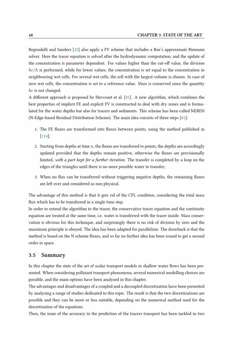
48 CHAPTER 3: STATE OF THE ART
Begnudelli and Sanders [22] also apply a FV scheme that includes a Roe’s approximate Riemann
solver. Here the tracer equation is solved after the hydrodynamic computation, and the update of
the concentration is parameter dependent. For values higher than the cut-oU value, the division
hc/h is performed, while for lower values, the concentration is set equal to the concentration in
neighbouring wet cells. For several wet cells, the cell with the largest volume is chosen. In case of
zero wet cells, the concentration is set to a reference value. Mass is conserved since the quantity
hc is not changed.
A diUerent approach is proposed by Hervouet et al. [81]. A new algorithm, which combines the
best properties of implicit FE and explicit FV is constructed to deal with dry zones and is formu-
lated for the water depths but also for tracers and sediments. This scheme has been called NERDS
(N-Edge-based Residual Distribution Scheme). The main idea consists of three steps [81]:
1. The FE Wuxes are transformed into Wuxes between points, using the method published in
[114];
2. Starting from depths at time n, the Wuxes are transferred to points, the depths are accordingly
updated provided that the depths remain positive, otherwise the Wuxes are provisionally
limited, with a part kept for a further iteration. The transfer is completed by a loop on the
edges of the triangles until there is no more possible water to transfer;
3. When no Wux can be transferred without triggering negative depths, the remaining Wuxes
are left over and considered as non physical.
The advantage of this method is that it gets rid of the CFL condition, considering the total mass
Wux which has to be transferred in a single time step.
In order to extend the algorithm to the tracer, the conservative tracer equation and the continuity
equation are treated at the same time, i.e. water is transferred with the tracer inside. Mass conser-
vation is obvious for this technique, and surprisingly there is no risk of division by zero and the
maximum principle is obeyed. The idea has been adapted for parallelism. The drawback is that the
method is based on the N scheme Wuxes, and so far no further idea has been issued to get a second
order in space.
3.5 Summary
In this chapter the state of the art of scalar transport models in shallow water Wows has been pre-
sented. When considering pollutant transport phenomena, several numerical modelling choices are
possible, and the main options have been analysed in this chapter.
The advantages and disadvantages of a coupled and a decoupled discretization have been presented
by analysing a range of studies dedicated to this topic. The result is that the two discretizations are
possible and they can be more or less suitable, depending on the numerical method used for the
discretization of the equations.
Then, the issue of the accuracy in the prediction of the tracers transport has been tackled in two
3.5 SUMMARY 49
diUerent parts. In the Vrst part, some Vrst order numerical methods with low numerical diUusion
have been presented. Among these methods, we Vnd some possible candidates for the solution of
the depth-averaged tracer equation.
In the second part, conservative and second order accurate methods have been presented. Since
these are the methods used in the remainder of this work, an in-depth analysis has been provided
for the reader. In particular, cutting-edge studies of second order techniques have been introduced,
showing the progression of these techniques from the 80’s to today.
Finally, the problem of wetting and drying phenomena in the presence of tracers has been ad-
dressed, presenting the studies available in the literature that analyse this issue.

50 CHAPTER 3: STATE OF THE ART

Chapter 4
A second order Vnite volume scheme
with larger time step
Dans ce chapitre un schéma aux volumes Vnis, formellement d’ordre deux et carac-
térisé par un grand pas de temps est présenté.
D’abord la solution du système de Saint-Venant couplé avec une loi de conservation
scalaire, qui se base sur un solveur de type HLLC, est décrite pour le schéma d’ordre
un. Ainsi, la positivité de la hauteur d’eau et de la concentration sont montrées.
L’analyse de l’équation du traceur simple permet de montrer que la positivité, ainsi
que la monotonie de la solution, demandent un pas de temps qui est plus grand par
rapport à celui qui est nécessaire pour résoudre le système de Saint-Venant.
Pour cette raison, la solution de l’équation du traceur est découplée de l’hydrodynamique,
aVn d’exploiter le plus grand pas de temps admissible, avec des bénéVces sur les coûts
de calcul et la diUusion numérique.
La méthode utilisée pour la reconstruction d’ordre deux est ensuite introduite, pour
les variables hydrodynamiques et pour le traceur. DiUérents limiteurs sont choisis en
fonction des propriétés mathématiques, pour chaque variable.
L’algorithme utilisé pour découpler traceur et hydrodynamique est aussi détaillé.
EnVn, le problème des bancs découvrants et une ébauche de solution sont présentés
dans la dernière partie du chapitre.
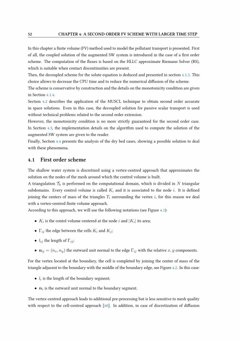
52 CHAPTER 4: A SECOND ORDER FV SCHEME WITH LARGER TIME STEP
In this chapter a Vnite volume (FV) method used to model the pollutant transport is presented. First
of all, the coupled solution of the augmented SW system is introduced in the case of a Vrst order
scheme. The computation of the Wuxes is based on the HLLC approximate Riemann Solver (RS),
which is suitable when contact discontinuities are present.
Then, the decoupled scheme for the solute equation is deduced and presented in section 4.1.3. This
choice allows to decrease the CPU time and to reduce the numerical diUusion of the scheme.
The scheme is conservative by construction and the details on the monotonicity condition are given
in Section 4.1.4.
Section 4.2 describes the application of the MUSCL technique to obtain second order accurate
in space solutions. Even in this case, the decoupled solution for passive scalar transport is used
without technical problems related to the second order extension.
However, the monotonicity condition is no more strictly guaranteed for the second order case.
In Section 4.3, the implementation details on the algorithm used to compute the solution of the
augmented SW system are given to the reader.
Finally, Section 4.4 presents the analysis of the dry bed cases, showing a possible solution to deal
with these phenomena.
4.1 First order scheme
The shallow water system is discretized using a vertex-centred approach that approximates the
solution on the nodes of the mesh around which the control volume is built.
A triangulation Th is performed on the computational domain, which is divided in N triangular
subdomains. Every control volume is called Ki and it is associated to the node i. It is deVned
joining the centers of mass of the triangles Ti surrounding the vertex i, for this reason we deal
with a vertex-centred Vnite volume approach.
According to this approach, we will use the following notations (see Figure 4.1):
• Ki is the contol volume centered at the node i and |Ki| its area;
• Γij the edge between the cellsKi andKj ;
• lij the length of Γij ;
• nij = (nx, ny) the outward unit normal to the edge Γij with the relative x, y components.
For the vertex located at the boundary, the cell is completed by joining the center of mass of the
triangle adjacent to the boundary with the middle of the boundary edge, see Figure 4.2. In this case:
• li is the length of the boundary segment;
• ni is the outward unit normal to the boundary segment.
The vertex-centred approach leads to additional pre-processing but is less sensitive to mesh quality
with respect to the cell-centred approach [60]. In addition, in case of discretization of diUusion
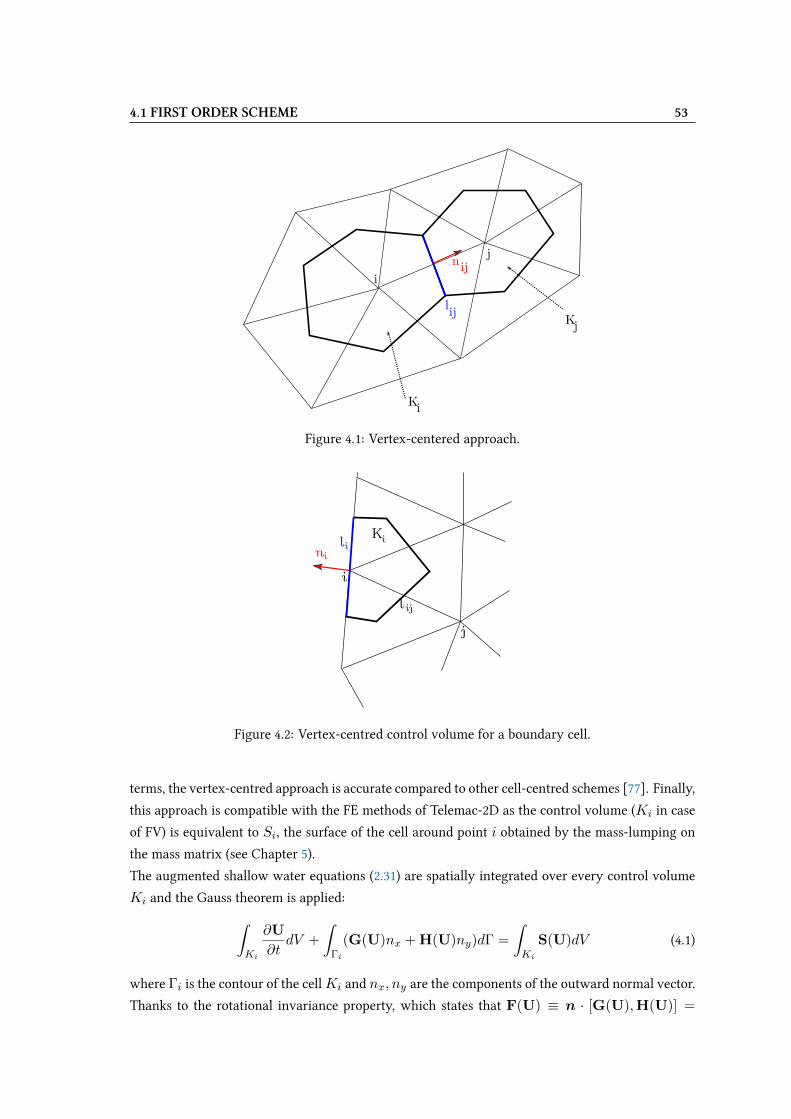
4.1 FIRST ORDER SCHEME 53
Ki
Kj
niji
j
lij
Figure 4.1: Vertex-centered approach.
ni
Kili
l ij
i
j
Figure 4.2: Vertex-centred control volume for a boundary cell.
terms, the vertex-centred approach is accurate compared to other cell-centred schemes [77]. Finally,
this approach is compatible with the FE methods of Telemac-2D as the control volume (Ki in case
of FV) is equivalent to Si, the surface of the cell around point i obtained by the mass-lumping on
the mass matrix (see Chapter 5).
The augmented shallow water equations (2.31) are spatially integrated over every control volume
Ki and the Gauss theorem is applied:∫Ki
∂U
∂tdV +
∫Γi
(G(U)nx + H(U)ny)dΓ =
∫Ki
S(U)dV (4.1)
where Γi is the contour of the cellKi and nx, ny are the components of the outward normal vector.
Thanks to the rotational invariance property, which states that F(U) ≡ n · [G(U),H(U)] =
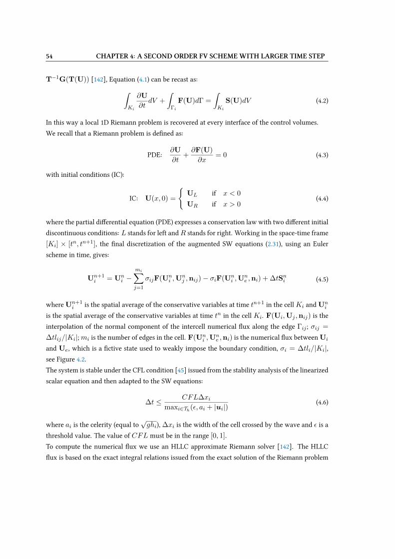
54 CHAPTER 4: A SECOND ORDER FV SCHEME WITH LARGER TIME STEP
T−1G(T(U)) [142], Equation (4.1) can be recast as:∫Ki
∂U
∂tdV +
∫Γi
F(U)dΓ =
∫Ki
S(U)dV (4.2)
In this way a local 1D Riemann problem is recovered at every interface of the control volumes.
We recall that a Riemann problem is deVned as:
PDE:∂U
∂t+∂F(U)
∂x= 0 (4.3)
with initial conditions (IC):
IC: U(x, 0) =
UL if x < 0
UR if x > 0(4.4)
where the partial diUerential equation (PDE) expresses a conservation law with two diUerent initial
discontinuous conditions: L stands for left andR stands for right. Working in the space-time frame
[Ki] × [tn, tn+1], the Vnal discretization of the augmented SW equations (2.31), using an Euler
scheme in time, gives:
Un+1i = Un
i −mi∑j=1
σijF(Uni ,U
nj ,nij)− σiF(Un
i ,Une ,ni) + ∆tSni (4.5)
whereUn+1i is the spatial average of the conservative variables at time tn+1 in the cellKi andUn
i
is the spatial average of the conservative variables at time tn in the cell Ki. F(Ui,Uj ,nij) is the
interpolation of the normal component of the intercell numerical Wux along the edge Γij ; σij =
∆tlij/|Ki|;mi is the number of edges in the cell. F(Uni ,U
ne ,ni) is the numerical Wux betweenUi
and Ue, which is a Vctive state used to weakly impose the boundary condition, σi = ∆tli/|Ki|,see Figure 4.2.
The system is stable under the CFL condition [45] issued from the stability analysis of the linearized
scalar equation and then adapted to the SW equations:
∆t ≤ CFL∆ximaxi∈Th(ε, ai + |ui|)
(4.6)
where ai is the celerity (equal to√ghi), ∆xi is the width of the cell crossed by the wave and ε is a
threshold value. The value of CFL must be in the range [0, 1].
To compute the numerical Wux we use an HLLC approximate Riemann solver [142]. The HLLC
Wux is based on the exact integral relations issued from the exact solution of the Riemann problem
4.1 FIRST ORDER SCHEME 55
(see Figure 4.3). It is deVned as:
F(Uni ,U
nj ,nij) =
FL, if 0 ≤ SLF∗L, if SL ≤ 0 ≤ S∗F∗R, if S∗ ≤ 0 ≤ SRFR, if 0 ≥ SR
, (4.7)
Looking at the 1D case, F(Uni ,U
nj ,nij) is also called Fi+1/2 since is the Wux at the interface
between the cell i and the cell i + 1. Formula (4.7) means that we have 4 possible solutions for
the Wux, according to the wave speeds SK with K = L, ∗, R which stands for left, star and right.
Integration over appropriate control volume gives:
t
xi+1/2
F
F F
F
**
L
LR
R
UL
U U
UR
t
x
S S SLR
*
L**R
star region
0
Figure 4.3: HLLC approximate Riemann solver and solutions in the 4 regions: left, left star, rightstar, right (on the left); approximate HLLC Wux (on the right).
F∗L = FL + SL(U∗L −UL) (4.8)
F∗R = F∗L + S∗(U∗R −U∗L) (4.9)
F∗R = FR + SR(U∗R −UR) (4.10)
The wave speeds SL, S∗, SR are computed with appropriate formulas which will be speciVed later.
Note that manipulating equations (4.8) ,(4.10) and using condition u∗ = S∗ we Vnd the approximate
states, necessary to compute (4.7):
U∗K = hK
(SK − uKSK − S∗
)1
S∗
vK
cK
, (4.11)
withK = L,R.
Before estimating the wave speeds, we recall some basic conditions that are enforced to solve the
algebraic problem. These conditions are issued from the exact Riemann problem and correspond
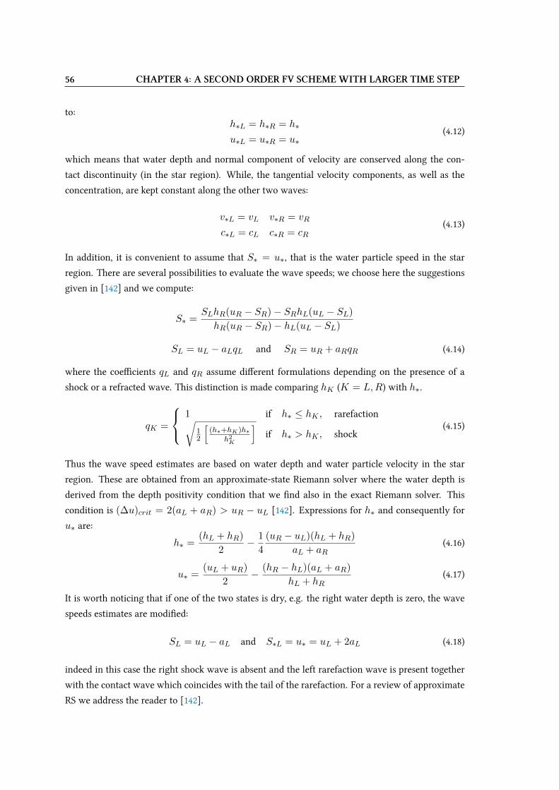
56 CHAPTER 4: A SECOND ORDER FV SCHEME WITH LARGER TIME STEP
to:h∗L = h∗R = h∗
u∗L = u∗R = u∗(4.12)
which means that water depth and normal component of velocity are conserved along the con-
tact discontinuity (in the star region). While, the tangential velocity components, as well as the
concentration, are kept constant along the other two waves:
v∗L = vL v∗R = vR
c∗L = cL c∗R = cR(4.13)
In addition, it is convenient to assume that S∗ = u∗, that is the water particle speed in the star
region. There are several possibilities to evaluate the wave speeds; we choose here the suggestions
given in [142] and we compute:
S∗ =SLhR(uR − SR)− SRhL(uL − SL)
hR(uR − SR)− hL(uL − SL)
SL = uL − aLqL and SR = uR + aRqR (4.14)
where the coeXcients qL and qR assume diUerent formulations depending on the presence of a
shock or a refracted wave. This distinction is made comparing hK (K = L,R) with h∗.
qK =
1 if h∗ ≤ hK , rarefaction√12
[(h∗+hK)h∗
h2K
]if h∗ > hK , shock
(4.15)
Thus the wave speed estimates are based on water depth and water particle velocity in the star
region. These are obtained from an approximate-state Riemann solver where the water depth is
derived from the depth positivity condition that we Vnd also in the exact Riemann solver. This
condition is (∆u)crit = 2(aL + aR) > uR − uL [142]. Expressions for h∗ and consequently for
u∗ are:
h∗ =(hL + hR)
2− 1
4
(uR − uL)(hL + hR)
aL + aR(4.16)
u∗ =(uL + uR)
2− (hR − hL)(aL + aR)
hL + hR(4.17)
It is worth noticing that if one of the two states is dry, e.g. the right water depth is zero, the wave
speeds estimates are modiVed:
SL = uL − aL and S∗L = u∗ = uL + 2aL (4.18)
indeed in this case the right shock wave is absent and the left rarefaction wave is present together
with the contact wave which coincides with the tail of the rarefaction. For a review of approximate
RS we address the reader to [142].
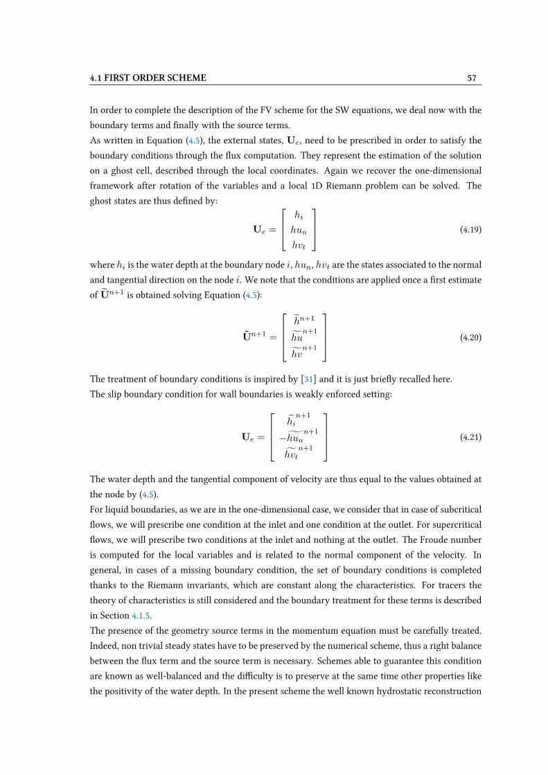
4.1 FIRST ORDER SCHEME 57
In order to complete the description of the FV scheme for the SW equations, we deal now with the
boundary terms and Vnally with the source terms.
As written in Equation (4.5), the external states, Ue, need to be prescribed in order to satisfy the
boundary conditions through the Wux computation. They represent the estimation of the solution
on a ghost cell, described through the local coordinates. Again we recover the one-dimensional
framework after rotation of the variables and a local 1D Riemann problem can be solved. The
ghost states are thus deVned by:
Ue =
hi
hun
hvt
(4.19)
where hi is the water depth at the boundary node i, hun, hvt are the states associated to the normal
and tangential direction on the node i. We note that the conditions are applied once a Vrst estimate
of Un+1 is obtained solving Equation (4.5):
Un+1 =
hn+1
hun+1
hvn+1
(4.20)
The treatment of boundary conditions is inspired by [31] and it is just brieWy recalled here.
The slip boundary condition for wall boundaries is weakly enforced setting:
Ue =
hin+1
−hunn+1
hvtn+1
(4.21)
The water depth and the tangential component of velocity are thus equal to the values obtained at
the node by (4.5).
For liquid boundaries, as we are in the one-dimensional case, we consider that in case of subcritical
Wows, we will prescribe one condition at the inlet and one condition at the outlet. For supercritical
Wows, we will prescribe two conditions at the inlet and nothing at the outlet. The Froude number
is computed for the local variables and is related to the normal component of the velocity. In
general, in cases of a missing boundary condition, the set of boundary conditions is completed
thanks to the Riemann invariants, which are constant along the characteristics. For tracers the
theory of characteristics is still considered and the boundary treatment for these terms is described
in Section 4.1.5.
The presence of the geometry source terms in the momentum equation must be carefully treated.
Indeed, non trivial steady states have to be preserved by the numerical scheme, thus a right balance
between the Wux term and the source term is necessary. Schemes able to guarantee this condition
are known as well-balanced and the diXculty is to preserve at the same time other properties like
the positivity of the water depth. In the present scheme the well known hydrostatic reconstruction
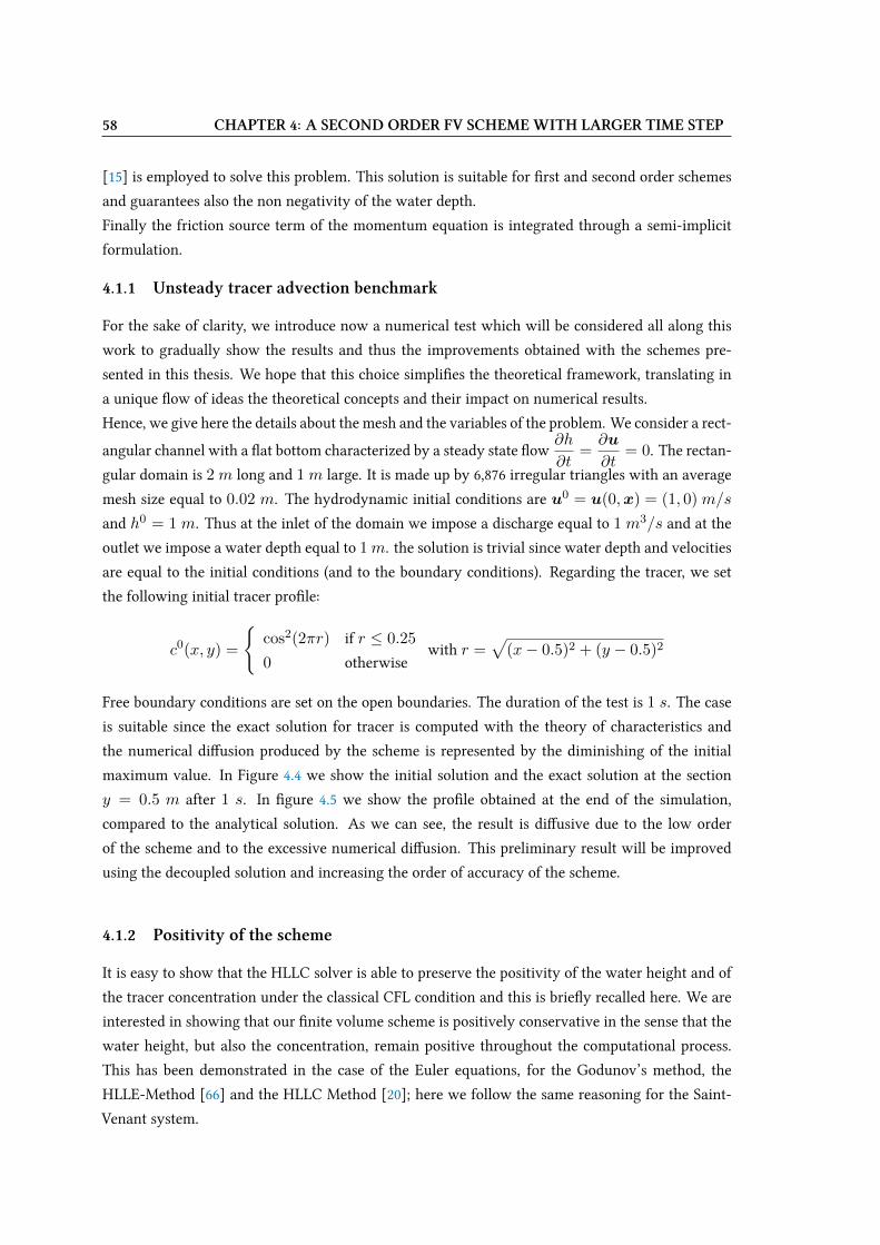
58 CHAPTER 4: A SECOND ORDER FV SCHEME WITH LARGER TIME STEP
[15] is employed to solve this problem. This solution is suitable for Vrst and second order schemes
and guarantees also the non negativity of the water depth.
Finally the friction source term of the momentum equation is integrated through a semi-implicit
formulation.
4.1.1 Unsteady tracer advection benchmark
For the sake of clarity, we introduce now a numerical test which will be considered all along this
work to gradually show the results and thus the improvements obtained with the schemes pre-
sented in this thesis. We hope that this choice simpliVes the theoretical framework, translating in
a unique Wow of ideas the theoretical concepts and their impact on numerical results.
Hence, we give here the details about the mesh and the variables of the problem. We consider a rect-
angular channel with a Wat bottom characterized by a steady state Wow∂h
∂t=∂u
∂t= 0. The rectan-
gular domain is 2 m long and 1 m large. It is made up by 6,876 irregular triangles with an average
mesh size equal to 0.02 m. The hydrodynamic initial conditions are u0 = u(0,x) = (1, 0) m/s
and h0 = 1 m. Thus at the inlet of the domain we impose a discharge equal to 1 m3/s and at the
outlet we impose a water depth equal to 1m. the solution is trivial since water depth and velocities
are equal to the initial conditions (and to the boundary conditions). Regarding the tracer, we set
the following initial tracer proVle:
c0(x, y) =
cos2(2πr) if r ≤ 0.25
0 otherwisewith r =
√(x− 0.5)2 + (y − 0.5)2
Free boundary conditions are set on the open boundaries. The duration of the test is 1 s. The case
is suitable since the exact solution for tracer is computed with the theory of characteristics and
the numerical diUusion produced by the scheme is represented by the diminishing of the initial
maximum value. In Figure 4.4 we show the initial solution and the exact solution at the section
y = 0.5 m after 1 s. In Vgure 4.5 we show the proVle obtained at the end of the simulation,
compared to the analytical solution. As we can see, the result is diUusive due to the low order
of the scheme and to the excessive numerical diUusion. This preliminary result will be improved
using the decoupled solution and increasing the order of accuracy of the scheme.
4.1.2 Positivity of the scheme
It is easy to show that the HLLC solver is able to preserve the positivity of the water height and of
the tracer concentration under the classical CFL condition and this is brieWy recalled here. We are
interested in showing that our Vnite volume scheme is positively conservative in the sense that the
water height, but also the concentration, remain positive throughout the computational process.
This has been demonstrated in the case of the Euler equations, for the Godunov’s method, the
HLLE-Method [66] and the HLLC Method [20]; here we follow the same reasoning for the Saint-
Venant system.
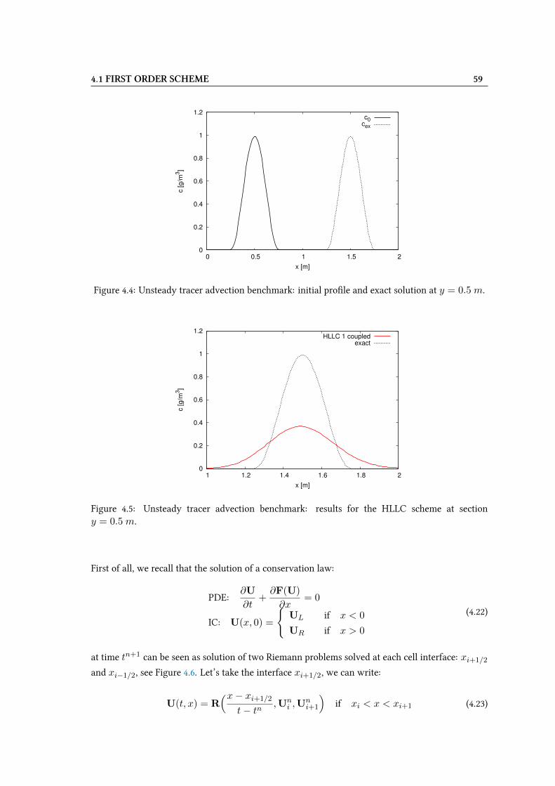
4.1 FIRST ORDER SCHEME 59
0
0.2
0.4
0.6
0.8
1
1.2
0 0.5 1 1.5 2
c [
g/m
3]
x [m]
c0cex
Figure 4.4: Unsteady tracer advection benchmark: initial proVle and exact solution at y = 0.5 m.
0
0.2
0.4
0.6
0.8
1
1.2
1 1.2 1.4 1.6 1.8 2
c [
g/m
3]
x [m]
HLLC 1 coupledexact
Figure 4.5: Unsteady tracer advection benchmark: results for the HLLC scheme at sectiony = 0.5 m.
First of all, we recall that the solution of a conservation law:
PDE:∂U
∂t+∂F(U)
∂x= 0
IC: U(x, 0) =
UL if x < 0
UR if x > 0
(4.22)
at time tn+1 can be seen as solution of two Riemann problems solved at each cell interface: xi+1/2
and xi−1/2, see Figure 4.6. Let’s take the interface xi+1/2, we can write:
U(t, x) = R(x− xi+1/2
t− tn,Un
i ,Uni+1
)if xi < x < xi+1 (4.23)
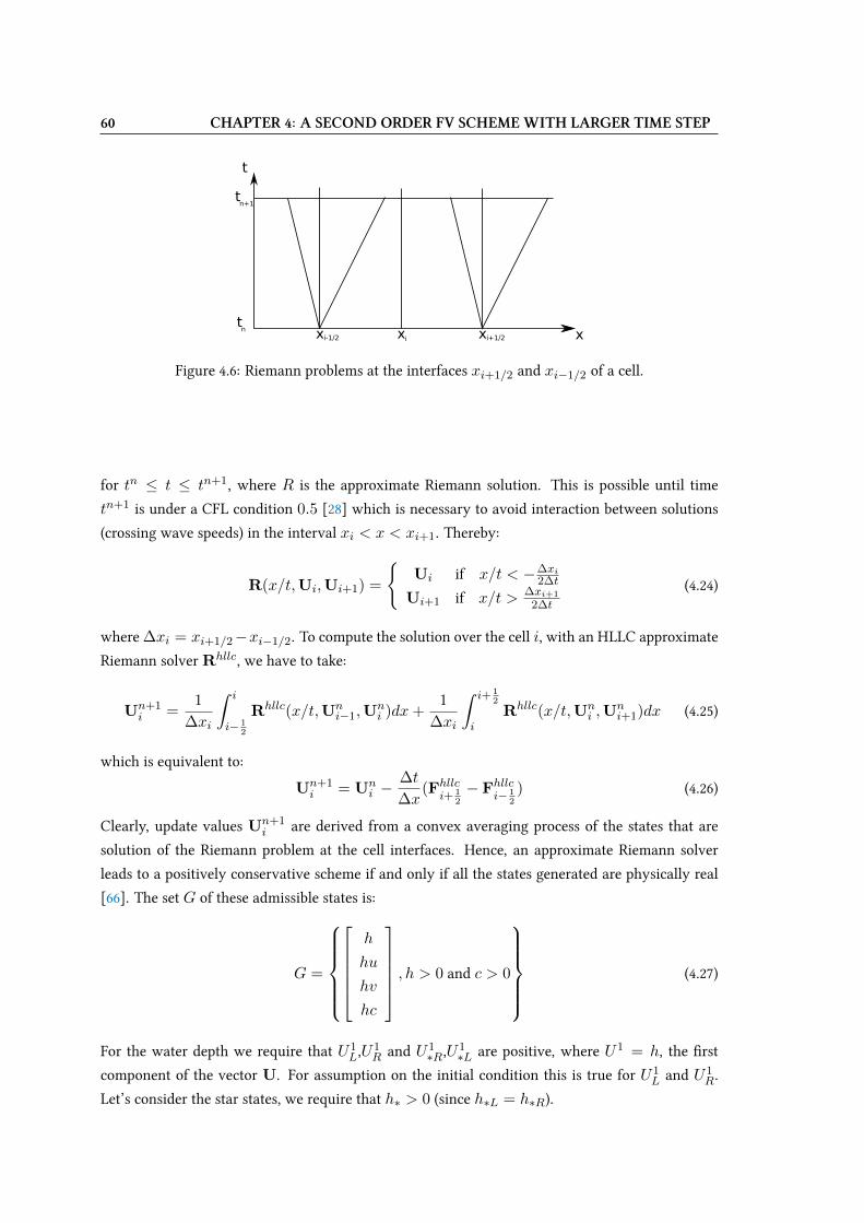
60 CHAPTER 4: A SECOND ORDER FV SCHEME WITH LARGER TIME STEP
x x xi-1/2 i+1/2
t
t
i
n+1
n
t
x
Figure 4.6: Riemann problems at the interfaces xi+1/2 and xi−1/2 of a cell.
for tn ≤ t ≤ tn+1, where R is the approximate Riemann solution. This is possible until time
tn+1 is under a CFL condition 0.5 [28] which is necessary to avoid interaction between solutions
(crossing wave speeds) in the interval xi < x < xi+1. Thereby:
R(x/t,Ui,Ui+1) =
Ui if x/t < −∆xi
2∆t
Ui+1 if x/t > ∆xi+1
2∆t
(4.24)
where ∆xi = xi+1/2−xi−1/2. To compute the solution over the cell i, with an HLLC approximate
Riemann solver Rhllc, we have to take:
Un+1i =
1
∆xi
∫ i
i− 12
Rhllc(x/t,Uni−1,U
ni )dx+
1
∆xi
∫ i+ 12
iRhllc(x/t,Un
i ,Uni+1)dx (4.25)
which is equivalent to:
Un+1i = Un
i −∆t
∆x(Fhllc
i+ 12
− Fhllci− 1
2
) (4.26)
Clearly, update values Un+1i are derived from a convex averaging process of the states that are
solution of the Riemann problem at the cell interfaces. Hence, an approximate Riemann solver
leads to a positively conservative scheme if and only if all the states generated are physically real
[66]. The set G of these admissible states is:
G =
h
hu
hv
hc
, h > 0 and c > 0
(4.27)
For the water depth we require that U1L,U
1R and U1
∗R,U1∗L are positive, where U1 = h, the Vrst
component of the vector U. For assumption on the initial condition this is true for U1L and U1
R.
Let’s consider the star states, we require that h∗ > 0 (since h∗L = h∗R).

4.1 FIRST ORDER SCHEME 61
From (4.11) we have:
h∗L = hL
(SL − uLSL − S∗
)(4.28)
Positivity is satisVed because:
• SL < S∗ since S∗ is an average velocity between SL and SR;
• SL < uL since SL = uL − aLq with q ≥ 0.
For the tracer, we have to demonstrate that [(hc)L, (hc)L∗, (hc)R∗, (hc)R] are positive. The left
and right states are positive by assumption and in the star region we will have a single value of h∗
but two diUerent values of c. We know that:
(hc)L∗ = hL
(SL − uLSL − S∗
)cL = h∗cL
(hc)R∗ = hR
(SR − uRSR − S∗
)cR = h∗cR
(4.29)
Since h∗ is positive under the CFL condition, (hc)∗L and (hc)∗R are also positive. Indeed, the
positivity is anyway subjected to the CFL condition (4.24). In practice this condition is not used
and the CFL condition is instead:
∆t ≤ CFL∆x
a(Ui,Ui+1)(4.30)
with CFL = 0.9 and a(Ui,Ui+1) the maximum local speed. For the shallow water system the
maximum speed is evaluated as maxi∈Th(ε, ai + |ui|) where ε is a threshold value. This conditionallows to avoid the interaction between solutions over the cell, that is xi−1/2 ≤ x ≤ xi+1/2. This
is suXcient because in practice the solution is updated with formula (4.26), so we look to Wuxes on
the lines x = xi+1/2 and x = xi−1/2.
In the presence of a non-Wat bottom, the non-negativity of the water depth is guaranteed by the
hydrostatic reconstruction [15], which is used to take into account the geometric source terms and
to preserve the C-property.
4.1.3 Decoupling the tracer equation
The decoupling of the tracer equation follows the ideas of Audusse and Bristeau [13], who proposed
a two time step kinetic scheme for pollutant transport. These ideas can be straightforwardly applied
to this scheme, providing that for a positive star wave speed we will have a positive water mass
Wux and for a negative star wave speed we will have a negative water mass Wux.
We focus on the tracer equation and we look at the one-dimensional problem (F 4 being the tracer
Wux):
(hc)n+1i = (hc)ni −
∆t
∆x(F 4
i+1/2 − F4i−1/2) (4.31)
62 CHAPTER 4: A SECOND ORDER FV SCHEME WITH LARGER TIME STEP
The Wux for tracer given by (4.7) can be written as:
F 4i+1/2 = F 1
i+1/2ci+1/2 (4.32)
where ci+1/2 is equal to ci or ci+1, depending on the speed S*:
ci+1/2 =
ci if S∗ ≥ 0
ci+1 if S∗ < 0(4.33)
This formulation shows clearly the upwind in the treatment of the tracer and this choice is equiv-
alent to:
ci+1/2 =
ci if F 1
i+1/2 ≥ 0
ci+1 if F 1i+1/2 < 0
(4.34)
The study of the Wux function F 1i+1/2 shows that a positive star wave speed implies a positive Wux
for water depth, so expressions (4.33) and (4.34) are equivalent.
We give in the following the proof, considering the 4 possible cases of Wux, given by formula (4.7).
For simplicity F 1i+1/2 will be called F 1
K withK = L,L∗, R∗, R according to the case.
We consider the expression (4.7):
• For SL ≥ 0. In this case F 1L = (hu)L. Since SL ≥ 0, using (4.14) we Vnd that also uL ≥ 0.
It follows that F 1 ≥ 0 for SL ≥ 0.
• For SL ≤ 0 ≤ S∗ the expression for the water mass Wux is equal to:
F 1∗L = F 1
L + SL(U1∗L − U1
L
)= F 1
L + SL
[hL
(SL − uLSL − S∗
)− hL
]= hL
[uL + SL
(SL − uLSL − S∗
)− SL
]Since hL ≥ 0, we prove that the quantity inside the squared brackets is positive. This
quantity is rewritten as:
uL (SL − S∗) + SL (SL − uL)− SL (SL − S∗)SL − S∗
=S∗ (SL − uL)
SL − S∗
Since SL ≤ 0 ≤ S∗ for assumption, then the denominator is certainly negative. The numer-
ator is also negative since S∗ is positive while SL−uL is negative: SL−uL = −aLqL using
Equation (4.14). Hence, F 1 ≥ 0 for SL ≤ 0 ≤ S∗.
4.1 FIRST ORDER SCHEME 63
• For S∗ ≤ 0 ≤ SR we want to show that F 1 < 0 since S∗ < 0. We have:
F 1∗R = F 1
R + SR(U1∗R − U1
R
)= F 1
R + SR
[hR
(SR − uRSR − S∗
)− hR
]= hR
[uR + SR
(SR − uRSR − S∗
)− SR
]Since hR ≥ 0, the term in the squared bracket must be negative. The latter, after some
algebraic simpliVcations becomes:
S∗ (SR − uR)
SR − S∗
The denominator is positive for assumption since S∗ ≤ 0 ≤ SR. The numerator is negative
since S∗ ≤ 0 and SR − aR = aRqR is positive. Hence F 1 ≤ 0 for SL ≤ 0 ≤ S∗.
• For SR ≤ 0, we want to show that the numerical water mass Wux is negative (or null) again.
This is true since SR ≤ 0 means that uR ≤ 0. The latter implies F 1R = (hu)R thus F 1 ≤ 0
and the proof is achieved.
We take now the upwind formulation (4.34) and going back to the 2D formulation we write:
F 4(Ui, Uj ,nij) = F 1+ci + F 1−cj (4.35)
with F+ = max(0, F (Ui, Uj ,nij)) and F− = min(0, F (Ui, Uj ,nij)). Taking the outward nor-
mal as reference, F+ represents the outgoing Wuxes and F− the ingoing Wuxes. Thus the scheme
for tracer becomes:
(hc)n+1i = (hc)ni −
∆t
Ki
mi∑j=1
(F 1+(Ui, Uj ,nij)ci + F 1−(Ui, Uj ,nij)cj
)lij (4.36)
We deduce that:
(hc)n+1i ≥ cni
hni − ∆t
Ki
mi∑j=1
F 1+(Ui, Uj ,nij)lij
(4.37)
This means that the positivity of the tracer will be ensured if:
hni −∆t
Ki
mi∑j=1
F 1+(Ui, Uj ,nij)lij > 0 (4.38)
Physically it means that the maximum time step is the one that causes a cell to be emptied by
exiting Wuxes. This condition is less restrictive than Equation (4.6) and thus advantageous for the

64 CHAPTER 4: A SECOND ORDER FV SCHEME WITH LARGER TIME STEP
tracer transport.
Inspired by the work of [13], we disconnect the hydrodynamic part from the transport and we use
an algorithm that computes hydrodynamics and tracer transport in parallel but with diUerent time
steps. Hence, the tracer solution is decoupled yet it is still dependent on the hydrodynamics through
condition (4.38). Indeed, the idea is that the tracer is updated only when the above condition is not
fulVlled, which can happen after several hydrodynamic time steps. Hence, the computational cost
for the solution of the augmented SW system is decreased. In addition, as we deal with explicit
schemes in time, taking the maximum time step admissible for the tracer transport allows to reduce
the numerical diUusion which is larger for a coupled solution.
In order to clearly show the eUect of the decoupled scheme, we show the results obtained with the
decoupled scheme for the unsteady advection test case. Figure 4.7 compares the decoupled solution
to the coupled solution for the unsteady tracer advection benchmark. We see that the numerical
diUusion is reduced by the decoupled scheme, indeed the maximum value of the tracer at the end
of the simulation is larger than the one of the coupled scheme. To explain this improvement, we
recall that a numerical scheme produces a numerical error at every discrete time step. When using
explicit schemes for advection it is important to exploit the maximum admissible time step in order
to reduce this numerical error. This is realised by the decoupled algorithm.
0
0.2
0.4
0.6
0.8
1
1.2
1 1.2 1.4 1.6 1.8 2
c [
g/m
3]
x [m]
HLLC 1 coupledHLLC 1 decoupled
exact
Figure 4.7: Unsteady tracer advection benchmark: results for the coupled and the decoupled HLLCscheme at section y = 0.5 m.
The choice of a decoupled solution is related to the fact that the transport phenomena are regulated
by the velocity of the Wow and not by the speed waves, as the hydrodynamic system. Indeed, as
we have seen in Chapter 2 the eigenvalue corresponding to the transport is just uξ while for the
hydrodynamic system they are uξ ± a. The case of steady Wow (h = const and q = const) shows
clearly that the new condition for the positivity of the tracer is less limiting than the classical one.
Indeed it becomes ∆t ≤ min(
∆xmaxi∈Th (ε,|uni |)
)[13]. Details on the algorithm will be given later.
For this FV scheme the hydrodynamics can be too restrictive for the tracer equation, which is thus
solved after some hydrodynamic steps with the minimum number of time step necessary. This is
4.1 FIRST ORDER SCHEME 65
strictly related to the explicit discretizations in time used here.
It is worth noticing that this situation is exactly the contrary of what happens for RD schemes,
as we will see later in the Section 5.1.2. Indeed, when using FE schemes on hydrodynamics and
RD schemes on tracer, the latter are more constraining than hydrodynamics. Hence, sub-iterations
within the hydrodynamic steps are used to solve the tracer equation.
4.1.4 Monotonicity analysis
The theory of positive coeXcient [134] is used to guarantee the respect of the maximum principle.
Indeed, the theorem on the positivity of coeXcients [146] for a linear advection equation establishes
that, considering a numerical scheme given by:
cn+1i =
∑k
bkcnj(k) (4.39)
then the scheme will be monotone if and only if:∑k
bk = 1 and bk ≥ 0, ∀k (4.40)
cnj(k) are the concentration values on the nodes j(k) involved in the sum; bk are their coeXcients
and k is an integer which represents the support (or the stencil) of the scheme. Dividing Equation
(4.36) by hn+1i we obtain:
cn+1i =
cnihn+1i
hni − ∆t
Ki
mi∑j=1
F 1+(Ui, Uj ,nij)lij
− ∆t
hn+1i Ki
mi∑j=1
F 1−(Ui, Uj ,nij)lijcnj (4.41)
The second term on the RHS is surely positive and the positivity of the Vrst term is ensured through
condition (4.38), thus the discrete maximum principle is respected. In the proof we assume that
hn+1i is positive, which is the case when using the present scheme.
4.1.5 Boundaries and sources
We now add to the basic formulation (4.36) the boundary terms and the sources. For the theory of
characteristics, if the boundary is an inlet it will be necessary to prescribe a boundary condition for
the tracer, while if the boundary is an outlet, then no condition is necessary.
For convention, we consider the outward normal to the boundary, hence the boundary Wux F 1bound
will be positive at the outlet and negative at the inlet. Thus the equation becomes:
(hc)n+1i =(hc)ni −
∆t
Ki
mi∑j=1
(F 1+(Ui, Uj ,nij)ci + F 1−(Ui, Uj ,nij)cj
)lij
− ∆t
Ki
(F 1+boundci + F 1−
boundcbound)li
(4.42)

66 CHAPTER 4: A SECOND ORDER FV SCHEME WITH LARGER TIME STEP
Source terms are added following the same philosophy: a positive source of water mass carries in
the tracer source while a negative source (sink term) carries away the existing value of tracer. The
scheme with boundaries and sources is:
(hc)n+1i =(hc)ni −
∆t
Ki
mi∑j=1
(F 1+(Ui, Uj ,nij)ci + F 1−(Ui, Uj ,nij)cj
)lij
− ∆t
Ki
(F 1+boundci + F 1−
boundcbound)li
+∆t
Ki
(sce+
i csce + sce−i ci)
(4.43)
These additional terms modify the previous positivity and monotonicity condition, which now
reads as follows:
hni −∆t
Ki
mi∑j=1
F 1+(Ui, Uj ,nij)lij + F 1+boundli − sce
−i
> 0 (4.44)
Indeed, only the coeXcient of cni could represent a problem for the positivity. All the other coeX-
cients are instead positive and do not need any additional condition.
4.2 Second order scheme
To improve the accuracy of the Vnite volume scheme, the values at the interfaces between cells are
reconstructed considering piecewise linear approximations. The reconstruction is second order in
the sense that for a smooth function U(x) we have:
Ui+1/2− = U(xi+1/2) +O(∆x2) (4.45)
and
Ui+1/2+ = U(xi+1/2) +O(∆x2) (4.46)
Given the Vrst order Wux and the reconstructed values Uij the scheme is now:
Un+1i = Un
i −mi∑j=1
σijF(Unij ,U
nji,nij)− σiF(Un
i ,Une ,ni) + ∆tSni (4.47)
From theory [28] we know that if under a CFL condition the numerical Wux preserves a convex
invariant domain D and if the reconstruction also preserves this invariant domain, then under the
half original CFL condition, the second-order scheme also preserves this invariant domain.
In practice, as mentioned in Chapter 3 it is diXcult to verify that the reconstruction preserves the
invariant domain. On the other hand, as in the Vrst order case, the CFL condition can be relaxed.
To perform the reconstruction, we use here a multislope MUSCL technique since a diUerent value
of slope is used for every interface of the same control volume. The reconstruction technique is
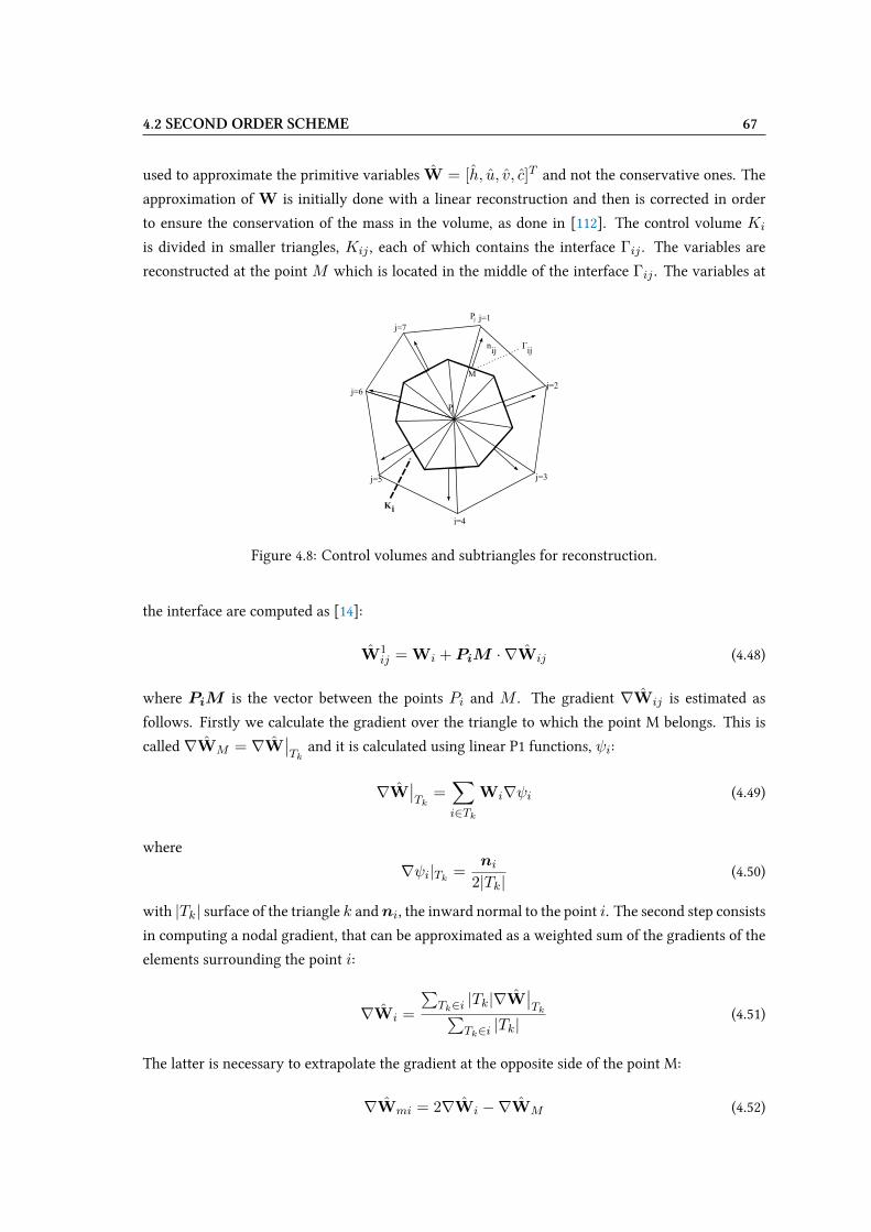
4.2 SECOND ORDER SCHEME 67
used to approximate the primitive variables W = [h, u, v, c]T and not the conservative ones. The
approximation of W is initially done with a linear reconstruction and then is corrected in order
to ensure the conservation of the mass in the volume, as done in [112]. The control volume Ki
is divided in smaller triangles, Kij , each of which contains the interface Γij . The variables are
reconstructed at the pointM which is located in the middle of the interface Γij . The variables at
j=1
j=2
j=3
j=4
j=5
j=6
j=7
nij
Γij
Ki
M
Pi
Pj
Figure 4.8: Control volumes and subtriangles for reconstruction.
the interface are computed as [14]:
W1ij = Wi + PiM · ∇Wij (4.48)
where PiM is the vector between the points Pi and M . The gradient ∇Wij is estimated as
follows. Firstly we calculate the gradient over the triangle to which the point M belongs. This is
called∇WM = ∇W∣∣Tk
and it is calculated using linear P1 functions, ψi:
∇W∣∣Tk
=∑i∈Tk
Wi∇ψi (4.49)
where
∇ψi|Tk =ni
2|Tk|(4.50)
with |Tk| surface of the triangle k andni, the inward normal to the point i. The second step consists
in computing a nodal gradient, that can be approximated as a weighted sum of the gradients of the
elements surrounding the point i:
∇Wi =
∑Tk∈i |Tk|∇W
∣∣Tk∑
Tk∈i |Tk|(4.51)
The latter is necessary to extrapolate the gradient at the opposite side of the point M:
∇Wmi = 2∇Wi −∇WM (4.52)
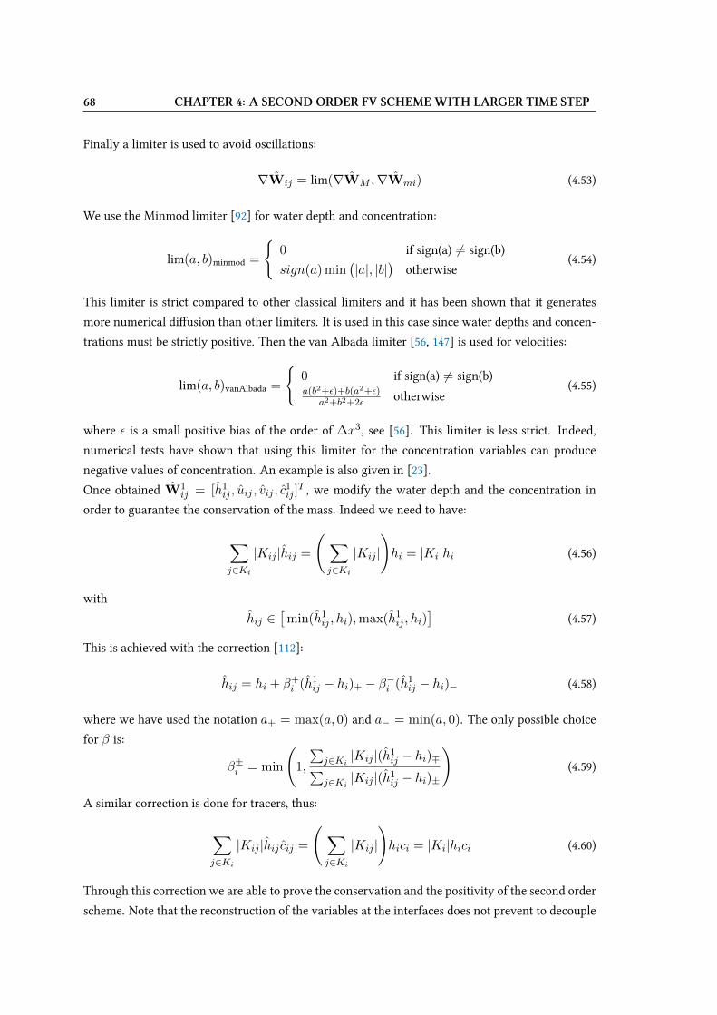
68 CHAPTER 4: A SECOND ORDER FV SCHEME WITH LARGER TIME STEP
Finally a limiter is used to avoid oscillations:
∇Wij = lim(∇WM ,∇Wmi) (4.53)
We use the Minmod limiter [92] for water depth and concentration:
lim(a, b)minmod =
0 if sign(a) 6= sign(b)
sign(a) min(|a|, |b|
)otherwise
(4.54)
This limiter is strict compared to other classical limiters and it has been shown that it generates
more numerical diUusion than other limiters. It is used in this case since water depths and concen-
trations must be strictly positive. Then the van Albada limiter [56, 147] is used for velocities:
lim(a, b)vanAlbada =
0 if sign(a) 6= sign(b)a(b2+ε)+b(a2+ε)
a2+b2+2εotherwise
(4.55)
where ε is a small positive bias of the order of ∆x3, see [56]. This limiter is less strict. Indeed,
numerical tests have shown that using this limiter for the concentration variables can produce
negative values of concentration. An example is also given in [23].
Once obtained W1ij = [h1
ij , uij , vij , c1ij ]T , we modify the water depth and the concentration in
order to guarantee the conservation of the mass. Indeed we need to have:
∑j∈Ki
|Kij |hij =
( ∑j∈Ki
|Kij |
)hi = |Ki|hi (4.56)
with
hij ∈[
min(h1ij , hi),max(h1
ij , hi)]
(4.57)
This is achieved with the correction [112]:
hij = hi + β+i (h1
ij − hi)+ − β−i (h1ij − hi)− (4.58)
where we have used the notation a+ = max(a, 0) and a− = min(a, 0). The only possible choice
for β is:
β±i = min
(1,
∑j∈Ki |Kij |(h1
ij − hi)∓∑j∈Ki |Kij |(h1
ij − hi)±
)(4.59)
A similar correction is done for tracers, thus:
∑j∈Ki
|Kij |hij cij =
( ∑j∈Ki
|Kij |
)hici = |Ki|hici (4.60)
Through this correction we are able to prove the conservation and the positivity of the second order
scheme. Note that the reconstruction of the variables at the interfaces does not prevent to decouple
4.3 GENERAL RESOLUTION ALGORITHM 69
the tracer solution, which becomes:
(hc)n+1i = (hc)ni −
∆t
Ki
mi∑j=1
(F 1+(Uij , Uji,nij)cij + F 1−(Uij , Uji,nij)cji
)(4.61)
In this case, the solution obtained with the second order decoupled scheme for the unsteady tracer
advection benchmark case is shown in Figure 4.9. The improvement obtained using the linear
reconstruction is very clear. The tracer proVle is closer to the exact solution than the other previous
schemes. The theoretical condition (4.38) is now computed with the Wuxes based on reconstructed
0
0.2
0.4
0.6
0.8
1
1.2
1 1.2 1.4 1.6 1.8 2
c [
g/m
3]
x [m]
HLLC 1 coupledHLLC 1 decoupledHLLC 2 decoupled
exact
Figure 4.9: Unsteady tracer advection benchmark: results at section y = 0.5 m for the coupledversion of the Vrst order HLLC, the decoupled version of the Vrst order HLLC, the decoupledversion of the second order HLLC.
states:
hni −∆t
Ki
mi∑j=1
F 1+(Uij , Uji,nij) > 0 (4.62)
The whole procedure described here to obtain the reconstructed values cij is not suXcient to strictly
ensure the monotonicity principle. This is mainly related to the fact that we cannot prove that the
reconstructed values are generated by a convex sum of the neighbouring values, which is deVni-
tively dependent on the way to compute the gradients, on the limiters used and their properties, as
explained in [36].
The boundary and source terms are treated like in the Vrst order case without technical problems.
4.3 General resolution algorithm
The algorithm used to compute the solutions of the system for the Vrst and the second order FV
scheme will be detailed. We remark that the tracer time step will not be directly calculated with
formula (4.38) but it will be simply the sum of several hydrodynamic time steps until the condition
expressed by (4.38) will not be trespassed. So, the test for the positivity of the tracer is a key point
70 CHAPTER 4: A SECOND ORDER FV SCHEME WITH LARGER TIME STEP
in the algorithm. Compared to the one proposed by Audusse [13], the algorithm is just adapted to
our hydrodynamic computation where the Wuxes are calculated in a diUerent way and some details
are added to the description. We call i (superscript) the step indicator for the hydrodynamic part
and k the one for the tracer part. The index i represents instead the node i of the computational
domain.
The algorithm consists of:
1. Initialization
• Set i = 0, k = 0;
• Set the initial conditions on variables [h, hu, hv]0 and c0;
• Set [Ftr(Ui, Uj ,nij)]−1,0 = 0, (Sce)−1,0
i , hi,ki = hii;
2. Hydrodynamic computation and update
• Take into account the boundary conditions: [hb, ub, vb]i and ckb ;
• Start from [h, hu, hv]i and compute the time step ∆tiCFL necessary for stability;
• Compute the hydrodynamic Wuxes [F h,hu,hv(Ui, Uj ,nij)]i for internal and boundary
nodes;
• Update the hydrodynamic values [h, hu, hv]i+1 considering sources if present;
3. Tracer computation
• Compute the cumulated mass Wuxes:
[F tr(Ui, Uj ,nij)]i,k =[F tr(Ui, Uj ,nij)]
i−1,k
+ ∆tiCFL
([F h(Ui, Uj ,nij)]
+,i + [F h(Ui, Uj ,nij)]−,i)
Note that here again − and + indicate the negative and the positive Wuxes;
• Compute cumulated sources if present:
(Sce)i,ki = (Sce)i−1,ki + ∆tiCFL(sce−,ii + sce+,i
i );
• Test based on the positivity condition (4.44):
Note that the test should be positive at least at the Vrst iteration, since the Vrst time
step issued by the CFL condition is suXcient to satisfy the positivity of the tracer.
(a) The test is false: update the tracer
• Update the tracer with Wuxes of the old time step:
[hc]i,k+1 =[hc]i−1,k − 1
Ki
mi∑j=1
[F tr(Ui, Uj ,nij)]+,i−1,kci−1,k
i + F tr(Ui, Uj ,nij)]−,i−1,kci−1,k
j
+1
Ki
(sce+,i−1,k
i csce + sce−,i−1,ki ci−1,k
i
)
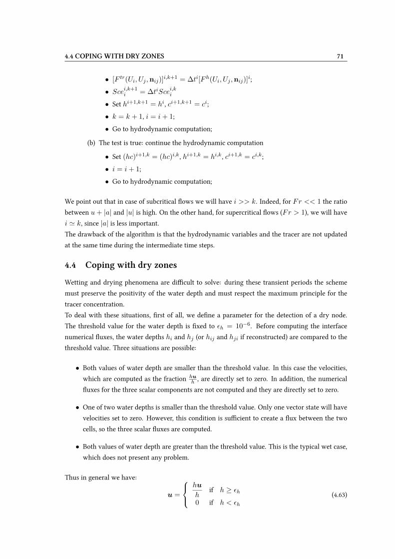
4.4 COPING WITH DRY ZONES 71
• [F tr(Ui, Uj ,nij)]i,k+1 = ∆ti[F h(Ui, Uj ,nij)]
i;
• Scei,k+1i = ∆tiScei,ki
• Set hi+1,k+1 = hi, ci+1,k+1 = ci;
• k = k + 1, i = i+ 1;
• Go to hydrodynamic computation;
(b) The test is true: continue the hydrodynamic computation
• Set (hc)i+1,k = (hc)i,k, hi+1,k = hi,k, ci+1,k = ci,k;
• i = i+ 1;
• Go to hydrodynamic computation;
We point out that in case of subcritical Wows we will have i >> k. Indeed, for Fr << 1 the ratio
between u+ |a| and |u| is high. On the other hand, for supercritical Wows (Fr > 1), we will have
i ' k, since |a| is less important.
The drawback of the algorithm is that the hydrodynamic variables and the tracer are not updated
at the same time during the intermediate time steps.
4.4 Coping with dry zones
Wetting and drying phenomena are diXcult to solve: during these transient periods the scheme
must preserve the positivity of the water depth and must respect the maximum principle for the
tracer concentration.
To deal with these situations, Vrst of all, we deVne a parameter for the detection of a dry node.
The threshold value for the water depth is Vxed to εh = 10−6. Before computing the interface
numerical Wuxes, the water depths hi and hj (or hij and hji if reconstructed) are compared to the
threshold value. Three situations are possible:
• Both values of water depth are smaller than the threshold value. In this case the velocities,
which are computed as the fraction huh , are directly set to zero. In addition, the numerical
Wuxes for the three scalar components are not computed and they are directly set to zero.
• One of two water depths is smaller than the threshold value. Only one vector state will have
velocities set to zero. However, this condition is suXcient to create a Wux between the two
cells, so the three scalar Wuxes are computed.
• Both values of water depth are greater than the threshold value. This is the typical wet case,
which does not present any problem.
Thus in general we have:
u =
hu
hif h ≥ εh
0 if h < εh(4.63)
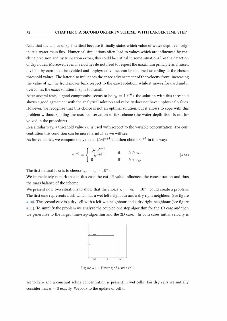
72 CHAPTER 4: A SECOND ORDER FV SCHEME WITH LARGER TIME STEP
Note that the choice of εh is critical because it Vnally states which value of water depth can orig-
inate a water mass Wux. Numerical simulations often lead to values which are inWuenced by ma-
chine precision and by truncation errors, this could be critical in some situations like the detection
of dry nodes. Moreover, even if velocities do not need to respect the maximum principle as a tracer,
division by zero must be avoided and unphysical values can be obtained according to the chosen
threshold values. The latter also inWuences the space advancement of the velocity front: increasing
the value of εh, the front moves back respect to the exact solution, while it moves forward and it
overcomes the exact solution if εh is too small.
After several tests, a good compromise seems to be εh = 10−6 : the solution with this threshold
shows a good agreement with the analytical solution and velocity does not have unphysical values.
However, we recognize that this choice is not an optimal solution, but it allows to cope with this
problem without spoiling the mass conservation of the scheme (the water depth itself is not in-
volved in the procedure).
In a similar way, a threshold value εtr is used with respect to the variable concentration. For con-
centration this condition can be more harmful, as we will see.
As for velocities, we compute the value of (hc)n+1 and then obtain cn+1 in this way:
cn+1 =
(hc)n+1
hn+1if h ≥ εtr
0 if h < εtr
(4.64)
The Vrst natural idea is to choose εtr = εh = 10−6.
We immediately remark that in this case the cut-oU value inWuences the concentration and thus
the mass balance of the scheme.
We present now two situations to show that the choice εtr = εh = 10−6 could create a problem.
The Vrst case represents a cell which has a wet left neighbour and a dry right neighbour (see Vgure
4.10). The second case is a dry cell with a left wet neighbour and a dry right neighbour (see Vgure
4.11). To simplify the problem we analyze the coupled one step algorithm for the 1D case and then
we generalize to the larger time-step algorithm and the 2D case. In both cases initial velocity is
h
C
i-1 i i+1
Figure 4.10: Drying of a wet cell.
set to zero and a constant solute concentration is present in wet cells. For dry cells we initially
consider that h = 0 exactly. We look to the update of cell i.
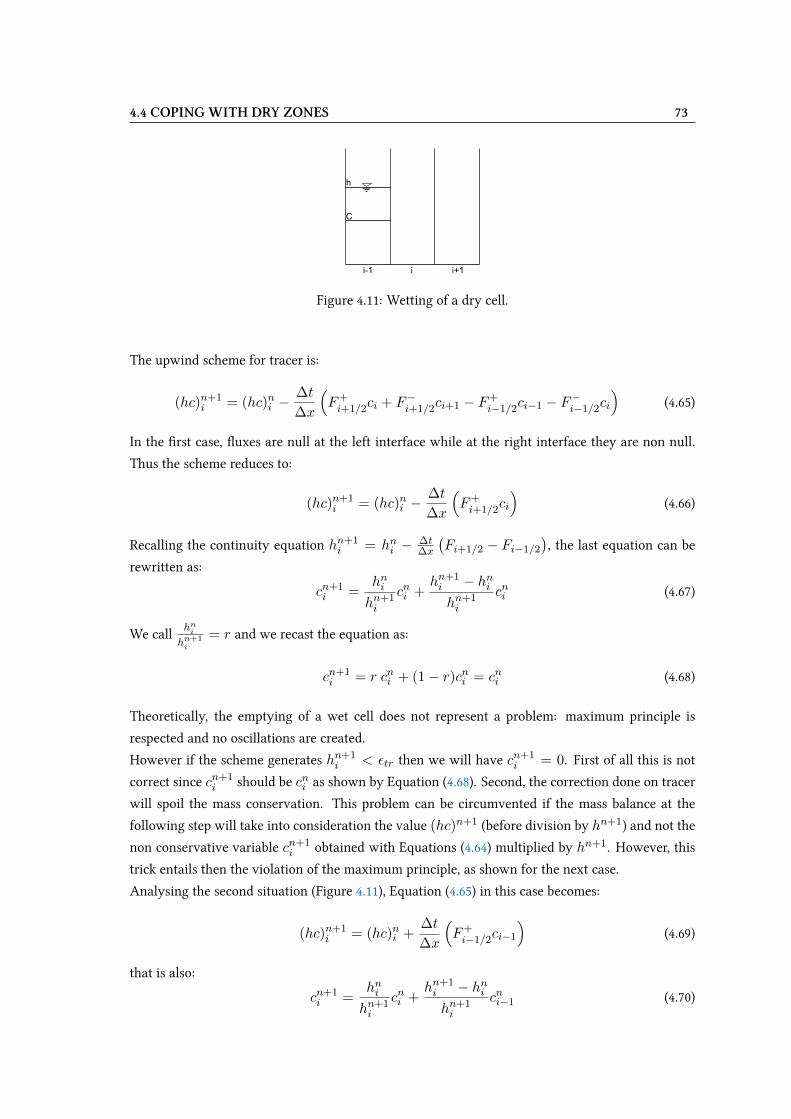
4.4 COPING WITH DRY ZONES 73
h
C
i-1 i i+1
Figure 4.11: Wetting of a dry cell.
The upwind scheme for tracer is:
(hc)n+1i = (hc)ni −
∆t
∆x
(F+i+1/2ci + F−i+1/2ci+1 − F+
i−1/2ci−1 − F−i−1/2ci
)(4.65)
In the Vrst case, Wuxes are null at the left interface while at the right interface they are non null.
Thus the scheme reduces to:
(hc)n+1i = (hc)ni −
∆t
∆x
(F+i+1/2ci
)(4.66)
Recalling the continuity equation hn+1i = hni − ∆t
∆x
(Fi+1/2 − Fi−1/2
), the last equation can be
rewritten as:
cn+1i =
hnihn+1i
cni +hn+1i − hnihn+1i
cni (4.67)
We call hnihn+1i
= r and we recast the equation as:
cn+1i = r cni + (1− r)cni = cni (4.68)
Theoretically, the emptying of a wet cell does not represent a problem: maximum principle is
respected and no oscillations are created.
However if the scheme generates hn+1i < εtr then we will have cn+1
i = 0. First of all this is not
correct since cn+1i should be cni as shown by Equation (4.68). Second, the correction done on tracer
will spoil the mass conservation. This problem can be circumvented if the mass balance at the
following step will take into consideration the value (hc)n+1 (before division by hn+1) and not the
non conservative variable cn+1i obtained with Equations (4.64) multiplied by hn+1. However, this
trick entails then the violation of the maximum principle, as shown for the next case.
Analysing the second situation (Figure 4.11), Equation (4.65) in this case becomes:
(hc)n+1i = (hc)ni +
∆t
∆x
(F+i−1/2ci−1
)(4.69)
that is also:
cn+1i =
hnihn+1i
cni +hn+1i − hnihn+1i
cni−1 (4.70)

74 CHAPTER 4: A SECOND ORDER FV SCHEME WITH LARGER TIME STEP
or also (remember that hi and also ci are null at time n):
cn+1i = rcni + (1− r)cni−1 = cni−1 (4.71)
So, even this case is theoretically well handled by a simple upwind scheme.
We suppose again that at time n+1 the water depth in i is smaller than εtr , while in i−1 the water
depth is bigger than εtr . So, cn+1i is set to zero, like velocities. Then, at time step n+ 2, the values
of hi will increase, but we suppose that it will continue to be hn+2i < εtr . Again concentrations
and velocities will be then set to zero, even if the scheme reads as:
(hc)n+2i = hn+1
i cn+1i + (hn+2
i − hn+1i )cn+1
i−1 (4.72)
hence (hc)n+2i 6= 0 and errors can thus cumulate over several time steps.
As stated before, to have a correct mass balance, the scheme could take into consideration the latter
value of the conservative variable hc, used to update the solution. Otherwise, computing the mass
at the end of the time step with the non conservative variable cn+1 and hn+1 will spoil the mass
balance.
On the other hand, choosing to update the solution using the conservative variable will create
unbounded concentration values, indeed at time n+ 2 the scheme will produce:
cn+2i =
(hc)n+1i
hn+2i
+ (1− r)cn+1i−1 (4.73)
with r = hn+1i /hn+2
i . The coeXcient of ci−1 is bounded between [0, 1], but (hc)n+1i is not
bounded, so we cannot ensure that the sum of the two coeXcients will respect the maximum prin-
ciple. It is easy to generalize this problem when we use the larger time step algorithm. Oscillations
could be even greater due to the fact that several hydrodynamic iterations are done and the fractionhnihn+1i
can be bigger than the one obtained with the one step algorithm.
In order to deal with the maximum principle and the mass conservation problems, a very simple
solution for the wet/dry interface with tracer is proposed.
The basic idea is that every Wux able to create a non-null water depth, included h < 10−6, will also
transport a quantity of solute, according to the upwind scheme (4.65). For this reason we choose
to diminish the threshold value and to Vx εtr < εh and in particular we take εtr = 10−14 which
corresponds also to the machine precision. Taking εtr < εh allows to be numerically consistent
with the continuity equation and the Wux computation, that is avoided if hi < εh or hj < εh.
Considering again the second situation (wetting of a dry cell) we will exactly respect equations
(4.69) and (4.70) to eventually Vnd cn+1i = ci−1, at every wet/dry interface. This proves that the
maximum principle will be respected, depending on the threshold and so on the machine precision.
Then, we also choose to set cn+1 = cn if h < εtr . The latter has a consequence in case of drying
of a wet zone: the algorithm will continue to detect tracer values in the space where hn+1 < εh
4.5 SUMMARY 75
(which is thus theoretically dry). This choice allows to not spoil the conservation of the mass.
It will be later shown in the numerical tests (Chapter 6) that the problem linked to the maximum
principle is no longer observed with the new choice of εtr .
To sum up, the new condition is:
cn+1i =
(hc)n+1
i
hn+1i
if h ≥ εtr
cni if h < εtr
(4.74)
with εtr = 10−14.
4.5 Summary
This chapter presents the FV model used in this thesis. The theoretical property of positivity for
the water depth and concentration has been shown under a classical CFL condition. Concerning
the scalar transport, the main idea is the decoupling of the transport equation when employing
an HLLC approximate Riemann solver. The decoupling is possible thanks to the properties of the
HLLC solver. The decoupled algorithm is described and it considers also boundary terms and
sources, with respect to the one presented by [13]. These additional terms are included in the
monotonicity condition.
The second order extension is achieved using a MUSCL approach, for hydrodynamics and for
tracers. In this case the theoretical stability is not strictly preserved; however as we will show
later the solution remains stable. Even in this case the decoupled algorithm is used to reduce the
numerical diUusion.
For dry zones problems, an analysis clearly shows which solutions must be avoided and which
ones must be preferred with respect to a cut-oU parameter.

76 CHAPTER 4: A SECOND ORDER FV SCHEME WITH LARGER TIME STEP
Chapter 5
New residual distribution
predictor-corrector schemes for time
dependent problems
L’objectif de ce chapitre est de présenter la formulation des schémas aux résidus dis-
tribués pour la solution de l’équation découplée du traceur.
La méthode utilisée pour la solution de l’équation de continuité du Wuide est détaillée
puisqu’elle représente une étape préalable à la discrétisation de l’équation du traceur.
Les schémas de type résidus distribués pour la solution de l’équation stationnaire du
traceur sont ensuite présentés à partir d’une formulation variationnelle du problème.
Ainsi, les propriétés numériques des schémas telles que la conservation, la précision et
la monotonie sont énoncées et établies.
A partir de cette formulation, les schémas aux résidus distribués appropriés pour les
cas non stationnaires et les propriétés numériques correspondantes sont aussi décrites
de manière systématique. En particulier, trois types diUérents de schémas sont con-
struits : un schéma semi-implicite, un schéma prédicteur-correcteur d’ordre un et un
autre d’ordre deux. Les diUérences et les ressemblances entre ces schémas et les sché-
mas classiques RD, seront mises en évidence.
La Vn du chapitre est dédiée aux problèmes des bancs découvrants qui sont gérés avec
une formulation semi-implicite locale.

78 CHAPTER 5: NEW RD PC SCHEMES FOR TIME DEPENDENT PROBLEMS
In this chapter we present the residual distribution (RD) method applied to the scalar transport
equation in the shallow water context.
Unlike the Vnite volume method presented in the previous chapter, here the RD method is only ap-
plied to discretize the tracer equation: the solution of the equation is decoupled with respect to the
shallow water system but a compatibility with the discretized continuity equation is guaranteed.
Details on this choice are given in Section 5.1, where the formulation of some explicit transport
schemes for steady problems is also included. In particular, the N scheme which is Vrst order accu-
rate and the PSI scheme which is second order accurate in space are presented.
Section 5.2 focuses on the formulation of the scheme in case of unsteady problems. For these
problems three diUerent solutions are shown: a semi-implicit scheme, which will be also useful
to cope with wetting and drying problems; a Vrst order predictor-corrector scheme and a second
order predictor-corrector scheme. The numerical properties of these schemes, like positivity and
monotonicity, are then analyzed in Section 5.3.
The monotonicity analysis also allows to formulate and to solve the problem through an iterative
scheme, which is introduced in Section 5.4. The latter allows improving the accuracy of the basic
scheme and it is a novelty with respect to classical RDS.
Finally, the wetting and drying problem is presented in Section 5.5. In this case, a new locally
semi-implicit predictor-corrector scheme is introduced to cope with this problem.
5.1 Preliminaries
The formulation of the residual distribution model only concerns the scalar transport equation
which is thus solved with a decoupled approach.
This choice is related to diUerent causes. On one hand, this work has been realized in an open
source hydroinformatic system, called Telemac, where the shallow water equations can be solved
by a Vnite element (FE) kernel or a Vnite volume one. The solution oUered by the Vnite element
method guarantees all the numerical properties stated in Chapter 2 and several tests have shown
that this method is very eXcient, Wexible and it has a computational cost which is lower than other
classical numerical methods [82]. In particular, large time steps can be used to solve the system
of equations since, in general, it is not submitted to a strict CFL condition like the explicit FV
schemes. In addition, a semi-implicit method can be employed on velocities and on water depth,
giving more accurate results. The FE formulation of the continuity equation is compatible with
the RD formulation of the tracer equation. This explains why the decoupled approach has been
preferred to the coupled approach.
On the other hand, this choice is more challenging since, as discussed in Chapter 3, the decoupled
modeling of the scalar transport implies some special numerical tricks. In particular, the continuity
equation has to be considered to enforce the mass conservation and the monotonicity.
The reader may consult the work of Hervouet [82] for details about the solution of the SW system
using a FE method.

5.1 PRELIMINARIES 79
5.1.1 Continuity equation
We present here the discretization of the continuity equation, which will be necessary in the tracer
equation. For simplicity, the source term will be neglected for the moment and considered later on.
In the Vnite element context, the continuity equation is transformed into a weak form, Vrst by
multiplying with test functions ψ from an appropriate space V and then applying integration by
parts. Using the FE method, we employ a Vnite dimensional space V h. Then we consider that the
variables of the problem are approximated with linear P1 Vnite element basis functions, ϕi, such
that for example the water depth function is equal to h ≈npoin∑ihiϕ
hi , where npoin is the number
of points in the domain (see for example [67, 153]).
In this work the Bubnov-Galerkin technique is employed: test functions and the basis functions be-
long to the same Vnite dimensional space. However, for the sake of clarity, test and basis functions
will always be distinguished.
For every degree of freedom i, we want to solve:∫Ωψi∂h
∂tdΩ +
∫Ωψi∇ · (hu)dΩ = 0 0 ≤ i ≤ Nh (5.1)
where Nh represents the number of degrees of freedom. For mass conservation it is important to
avoid the splitting of the divergence term, thus integrating by parts we obtain:∫Ωψi∂h
∂tdΩ +
∫Γψihu · ndΓ−
∫Ωhu · ∇ψidΩ = 0 0 ≤ i ≤ Nh (5.2)
This integration by parts will allow to Vnd a strict proof of mass conservation at discrete level. It is
not done in the literature of RD schemes, where the conservation issue is diUerently addressed.
Using an explicit discretization in time and projecting the functions onto the basis, the equation
leads to the following matrix form:
M
∆t(Hn+1 −Hn) = CV 1 (5.3)
whereM is the mass matrix;Hn+1−Hn is the vector of dimension npoin containing the unknown
hn+1; CV 1 is the right-hand side vector of dimension npoin, which contains the boundary Wuxes,
the sources and the other explicit terms. In particular we have:
Mij =
∫ΩϕjψidΩ (5.4)
CV 1 = BM1 Un +BM2 V n + TB1 (5.5)
with:
BM1ij =
∫Ωϕjh
n∂ψi∂x
dΩ (5.6)
80 CHAPTER 5: NEW RD PC SCHEMES FOR TIME DEPENDENT PROBLEMS
BM2ij =
∫Ωϕjh
n∂ψi∂y
dΩ (5.7)
TB1 = −∫
Γψih
nun · ndΓ (5.8)
Another discrete version of the continuity equation can be obtained introducing a Crank-Nicholson
θ-scheme for the treatment of the velocity Veld:∫Ωψi∂h
∂tdΩ +
∫Ωψi∇ ·
[h(θuun+1 + (1− θu)un
)]dΩ = 0 0 ≤ i ≤ Nh (5.9)
which in a discrete matrix form becomes:
M
∆t(Hn+1 −Hn)−BM1 Un+1 −BM2 V n+1 = CV 1 (5.10)
with BM1, BM2, CV 1 the appropriate vectors, function of θu and 1− θu.The term TB1 is given explicitly as boundary conditions on liquid boundaries and is zero on
solid boundaries (impermeability condition). Equation (5.3) (or Equation (5.10)) is then combined
with the other two discretized momentum equations and in this way a linear system of the form
AX = B is solved. Hence, a Vrst approximation of [hn+1, un+1, vn+1] is obtained.
We note that performing a mass-lumping on h, Equation (5.10) becomes:
Si∆t
(Hn+1 −Hn)−BM1Un+1 −BM2V n+1 = CV 1 (5.11)
where Si is obtained by the mass-lumping and it is the surface of the cell around the point of the
mesh i, called volume of basis i (see Figure 5.1), equal to∑T3i
ST /3 with ST the area of the triangle.
We now recast the continuity equation in a diUerent form, which will be useful for the tracer
equation. We deVne a vector of modiVed water depths, so that:
MHn+1 = DHn+1 (5.12)
where D is the diagonal obtained by the mass-lumping of M . In this way we can deal with the
following form:Si∆t
(hn+1i − hni
)= CV 1i (5.13)
even if Equation (5.3) (or (5.10)) is not solved with mass-lumping. To simplify notations, hi are
replaced by hi from here on out.
The RHS term is:
CV 1i =
∫Ωhun · ∇ψidΩ−
∫Γψihu
n · ndΓ (5.14)
Computing the integrals over the singular triangular elements T , the internal boundary integrals
eliminate each others thanks to the continuous polynomial test functions, while they have to be
computed on open boundaries. This also means that no mass is gained or lost in single internal
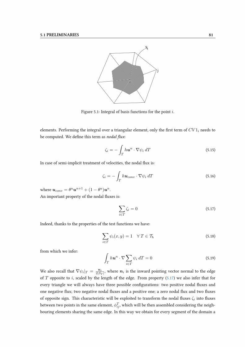
5.1 PRELIMINARIES 81
i
Si
j
Figure 5.1: Integral of basis functions for the point i.
elements. Performing the integral over a triangular element, only the Vrst term of CV 1i needs to
be computed. We deVne this term as nodal Wux:
ζi = −∫Thun · ∇ψi dT (5.15)
In case of semi-implicit treatment of velocities, the nodal Wux is:
ζi = −∫Thuconv · ∇ψi dT (5.16)
where uconv = θuun+1 + (1− θu)un.
An important property of the nodal Wuxes is:∑i∈T
ζi = 0 (5.17)
Indeed, thanks to the properties of the test functions we have:∑i∈T
ψi(x, y) = 1 ∀ T ∈ Th (5.18)
from which we infer: ∫Thun · ∇
∑i∈T
ψi dT = 0 (5.19)
We also recall that ∇ψi|T = ni2|ST | , where ni is the inward pointing vector normal to the edge
of T opposite to i, scaled by the length of the edge. From property (5.17) we also infer that for
every triangle we will always have three possible conVgurations: two positive nodal Wuxes and
one negative Wux; two negative nodal Wuxes and a positive one; a zero nodal Wux and two Wuxes
of opposite sign. This characteristic will be exploited to transform the nodal Wuxes ζi into Wuxes
between two points in the same element, φTij , which will be then assembled considering the neigh-
bouring elements sharing the same edge. In this way we obtain for every segment of the domain a
82 CHAPTER 5: NEW RD PC SCHEMES FOR TIME DEPENDENT PROBLEMS
singular value of Wux, called φij . The transformation of ζi into φTij is explained in [114] and it is
done following the so called “nearest projection method“. Here we just recall the main formula:
φTij =
−ζj if |ζi| > |ζj | and |ζi| > |ζk|+ζi if |ζj | > |ζi| and |ζj | > |ζk|0 otherwise
(5.20)
where + and − are chosen in order to store a positive value for a Wux going from node i to node j.
Note that in formula (5.20), i, j, k are the local node numbers in the element T .
The same Wuxes can be obtained through a diUerent method, which will be useful to relate the
scheme to the RD classical schemes. This method consists in computing from ζi an intermediary
Wux, called λNij and then the Vnal Wux φTij . The main formula is [82]:
λNij = max(min(−ζi, ζj), 0) (5.21)
Here the Wuxes between i and j are local Wuxes since i and j are the local node numbers, so that
we have 6 local Wuxes for every element. Then we use the formula:
φTij = +λNji − λNij (5.22)
where + and − are chosen like in the previous case (a positive value of φTij means that the Wux is
going from i to j). We note that formula (5.22) and (5.20) exactly give the same values of φTij .
Finally φTij is transformed into an assembled Wux, φij , considering the contribution of the nearby
elements. Equation (5.13) can be rewritten with the new Wuxes:
Si(hn+1i − hni )
∆t+∑j
φij + bi = 0 (5.23)
The sum over j represents the sum over all the neighbours j of point i and bi is the boundary Wux:
bi =∫
Γ ψihu · ndΓ. Note that in presence of sources we will have scei in the RHS.
Equation (5.13) and Equation (5.23) are the same but recast in a diUerent way. The Wuxes between
points of Equation (5.23) are directly used by the scheme called NERDS [81]. The NERD scheme
solves the continuity equation in a particular way which allows to get rid of the stability condi-
tion on the time step and to preserve the positivity of the water depths, as already explained in
Chapter 3. Indeed, in the hydrodynamic part, Equation (5.3) (or (5.10)) is Vrst solved regardless
of the positivity of depth. Then, a posteriori, the NERD scheme is used to give a set of positive
hn+1 and Wuxes φij that exactly solve Equation (5.23). In case of wet cases, formulation (5.3) and
(5.23) are equivalent, however very small diUerences arise in the values of hn+1 and in the mass
balance, which is exact at the machine precision when the NERD scheme is employed. Probably
the diUerences are due to the linear solvers used for the solution of Equation (5.3). Thus, for mass
conservation reasons, once the SW system is solved, only the continuity equation is played again
5.1 PRELIMINARIES 83
using the form (5.23), before solving the tracers equations. The proof of mass conservation is ob-
tained taking Equation (5.23) and summing over all the points of the domain, obtaining at discrete
level:npoin∑i=1
(Sih
n+1i − Sihni
)= −∆t
npoin∑i=1
bi (5.24)
The equation states that the variation of mass in the domain can be generated only by the presence
of boundary Wuxes (or possibly sources). It is important to note that the interior Wuxes φij eliminate
each other.
5.1.2 Explicit schemes for steady problems
We present in this section the discretization of the tracer equation suitable for steady problems.
Two diUerent explicit schemes are formulated: the N and the PSI scheme. Their numerical proper-
ties are introduced as well.
The tracer equation is discretized following the same steps used for the continuity equation.
For every degree of freedom i we have:∫Ωψi∂hc
∂tdΩ +
∫Ωψi∇ · (hcu)dΩ = 0 0 ≤ i ≤ Nh (5.25)
An integration by parts gives:∫Ωψi∂(hc)
∂tdΩ +
∫Γψihcu · ndΓ−
∫Ωhcu · ∇ψidΩ = 0 (5.26)
In accordance to the continuity equation, for the tracer equation (5.26) we choose to have:
−∫
Ωhcu · ∇ψidΩ =
∑j
φijcnij (5.27)
where cij is a quantity to be deVned, which represents the tracer carried by the Wuxes φij . Per-
forming a mass-lumping on c, the discrete tracer equation reads as:
Si(hn+1i cn+1
i − hni cni )
∆t+∑j
φijcnij + bicbound = 0 (5.28)
cbound is the boundary concentration, carried by the boundary Wux.
It is worth to notice that for the tracer equation, a boundary value is necessary at the inlet for any
kind of Wows (torrential or Wuvial), for the theory of characteristics. In order to have a correct mass
balance, ingoing Wuxes are multiplied by the boundary value of tracer, while outgoing Wuxes are
multiplied by the values on the boundaries given by the scheme:
bicbound = min(bi, 0)cbound + max(bi, 0)cni (5.29)
84 CHAPTER 5: NEW RD PC SCHEMES FOR TIME DEPENDENT PROBLEMS
The intermediate value of concentration is deVned choosing an upwind value, that is:
cnij =
cni if φij ≥ 0
cnj if φij < 0(5.30)
Hence, Equation (5.28) can be rewritten as:
Si(hn+1i cn+1
i − hni cni )
∆t+∑j
(max(φij , 0)cni + min(φji, 0)cnj
)+min(bi, 0)cbound+max(bi, 0)cni = 0
(5.31)
Before the next step, we note that this scheme is conservative since, summing over all the nodes of
the domain we have:
npoin∑i=1
(Sih
n+1i cn+1
i − Sihni cni)
= −∆t
npoin∑i=1
bicbound (5.32)
Then we plug the discrete continuity equation (5.23) into the tracer equation (5.31) to replace hn
with hn+1 we get:
cn+1i = cni +
∆t
Sihn+1i
∑j
min(φNij , 0)(cni − cnj )−min(bi, 0)(cbound − cni )
(5.33)
Let us suppose that hn+1 is positive for the moment. Note that to Vnd Equation (5.33) we also use
the fact that φNij = max(φNij , 0) + min(φNij , 0). We add the superscript N to the Wuxes φij (which
are computed as we have explained in the previous section) since, as we will see hereafter, this
scheme corresponds to the N scheme. Equation (5.33) can be rewritten with a residual distribution
formalism as:
cn+1i = cni −
∆t
Sihn+1i
∑T3i
3∑j=1
λNij (cni − cnj ) + min(bi, 0)(cbound − cni )
(5.34)
where∑T3i
represents the sum over all the triangles which contains the node i and j represents in
this case the local neighbours on a triangle. Alternatively, Equation (5.34) can be rewritten as:
cn+1i = cni −
∆t
Sihn+1i
(∑T3i
βNi φT + min(bi, 0)(cbound − cni )
)(5.35)
where the βNi are called distribution coeXcients of the N scheme:
βNi =φNiφT
(5.36)
5.1 PRELIMINARIES 85
φT is the residual, which represents the total mass Wux to distribute to the nodes within an element.
It stems from the passage between the conservative tracer equation and the non conservative form:
it corresponds to the diUerence between the divergence term integrated by parts (5.27) and the
divergence term of the continuity equation, integrated by parts and multiplied by ci. Indeed it is:
φT =
∫Th(cn − cni )u∇ψi dT =
3∑i=1
3∑j=1
φTijcnij −
3∑i=1
3∑j=1
φTijcni
=
3∑i=1
3∑j=1
[max(φTij , 0)cni + min(φTij , 0)cnj
]−
3∑i=1
3∑j=1
[max(φTij , 0) + min(φTij , 0)
]cni
= −3∑i=1
3∑j=1
min(φTij , 0)(cni − cnj ) =3∑i=1
3∑j=1
λNij (cni − cnj )
(5.37)
and φNi is the contribution received by node i of element T :
φNi =3∑j=1
λNij (cni − cnj ) = βNi φT (cn)
= ζ+i (cni − cnin)
(5.38)
where, according to the classical notations of the RD methods, we have:
ζ+i = max(0, ζi) ζ−i = min(0, ζi) (5.39)
and
cin =
∑j∈T
ζ−i cnj∑
j∈Tζ−i
(5.40)
The scheme (5.35) is conservative, however now we deal with the non conservative form and thus
the sum over all the nodes of the domain will give:
npoin∑i=1
Sihn+1i
(cn+1i − cni
)= −∆t
∑T∈Th
φT (cn) +
npoin∑i=1
min(bi, 0) (cbound − cni )
(5.41)
In order to Vnd the mass balance (5.32) it is necessary to use again the discrete continuity equation
yet the Equation (5.41) is useful to directly check the mass conservation when solving a non con-
servative form of the tracer equation.
For second order accurate schemes, the distribution coeXcients must be bounded with respect to
the solution and the data of the problem, in order to guarantee that φi = O(h3) [54]. It should be
remarked that the N scheme (5.35) is only Vrst order accurate as shown by the fact that the βNi are
in general unbounded.
86 CHAPTER 5: NEW RD PC SCHEMES FOR TIME DEPENDENT PROBLEMS
Formula (5.21) guarantees the Local Extremum Diminishing property (see [54, 119]) for the semi-
discrete scheme:∂c
∂t= − 1
Sihn+1i
∑T3i
3∑j=1
λNij (cni − cnj ) (5.42)
Indeed, it leads to positive or null values of λNij . Another fundamental relation which will be often
used in this work is:
∑j
min(φNij , 0)(cni − cnj ) = −∑T3i
3∑j=1
λNij (cni − cnj ) = −∑T3i
βNi φT (5.43)
From Equation (5.33), the time step condition necessary to guarantee the monotonicity can be
computed. We use the theory of positive coeXcients schemes recalled also in Chapter 4: the
coeXcients of ci and cj must be in the range [0, 1] and their summust be equal to 1. This also means
to have a convex sum of the neighbouring values. Hence, in Equation (5.33) only the coeXcient of
ci could create a problem. Imposing the positivity of this coeXcient we obtain:
∆t ≤hn+1i Si
−∑
j min(φNij , 0)−min(bi, 0)(5.44)
The values hn+1i (or hni if the criterion depends on hn) are then substituted with hend (or hstart) if
we are iterating within an hydrodynamic time step. Indeed, the discrete continuity equation (5.23)
is satisVed at any intermediate time level, provided that the water depths at the intermediate level
are linearly interpolated between hni and hn+1i . If nsub is the number of sub-iterations within the
hydrodynamic time step ∆tcas and isub is the i-th iteration, we will have:
hendi = hstarti − ∆tcasnsub
1
Si
∑j
φNij + bi
(5.45)
hendi =(nsub− isub)hni + isub hn+1
i
nsub(5.46)
We consider now again the equation (5.35) and we observe that if we do not change the total
residual φT over an element T , the Wuxes can be modiVed without spoiling the mass conserva-
tion. Indeed the relation∑i∈T
φi =∑i∈T
βiφT = φT is always fulVlled at element level and thus
Equation (5.41) holds true for diUerent kinds of distribution coeXcients. We choose to use the PSI
distribution, for which the scheme reads as follows:
cn+1i = cni −
∆t
Sihn+1i
(∑T3i
βPSIi φT + min(bi, 0)(cbound − cni )
)(5.47)
The distribution coeXcients of the PSI scheme, βPSIi , have the fundamental property to be bounded
between 0 and 1, and of providing discretization coeXcients of the same sign as those of the N
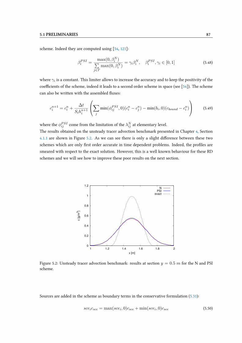
5.1 PRELIMINARIES 87
scheme. Indeed they are computed using [54, 121]:
βPSIi =max(0, βNi )∑
j∈Tmax(0, βNi )
= γiβNi , βPSIi , γi ∈ [0, 1] (5.48)
where γi is a constant. This limiter allows to increase the accuracy and to keep the positivity of the
coeXcients of the scheme, indeed it leads to a second order scheme in space (see [54]). The scheme
can also be written with the assembled Wuxes:
cn+1i = cni +
∆t
Sihn+1i
∑j
min(φPSIij , 0)(cni − cnj )−min(bi, 0)(cbound − cni )
(5.49)
where the φPSIij come from the limitation of the λNij at elementary level.
The results obtained on the unsteady tracer advection benchmark presented in Chapter 4, Section
4.1.1 are shown in Figure 5.2. As we can see there is only a slight diUerence between these two
schemes which are only Vrst order accurate in time dependent problems. Indeed, the proVles are
smeared with respect to the exact solution. However, this is a well known behaviour for these RD
schemes and we will see how to improve these poor results on the next section.
0
0.2
0.4
0.6
0.8
1
1.2
1 1.2 1.4 1.6 1.8 2
c [
g/m
3]
x [m]
NPSI
exact
Figure 5.2: Unsteady tracer advection benchmark: results at section y = 0.5 m for the N and PSIscheme.
Sources are added in the scheme as boundary terms in the conservative formulation (5.31):
sceicsce = max(scei, 0)csce + min(scei, 0)csce (5.50)
88 CHAPTER 5: NEW RD PC SCHEMES FOR TIME DEPENDENT PROBLEMS
Then plugging the continuity equation into the conservative formulation, the N scheme becomes:
cn+1i =cni +
∆t
Sihn+1i
∑j
min(φNij , 0)(cni − cnj )
− ∆t
Sihn+1i
min(bi, 0)(cbound − cni ) +∆t
Sihn+1i
max(scei, 0)(csce − cni )
(5.51)
To formulate the PSI scheme with source terms it is suXcient to replace φNij with φPSIij . Hence,
sources are also included in the time step condition:
∆t ≤hn+1i Si
−∑
j min(φNij , 0)−min(bi, 0) + max(scei, 0)(5.52)
5.2 Distribution schemes for time dependent problems
Following the ideas of the RD theory, the schemes presented in the previous section are extended to
the unsteady cases. Among the various forms suitable for the time dependent problems presented
in Chapter 3, the semi-implicit formulation and then the predictor-corrector schemes are studied
in this work.
The semi-implicit formulation represents the Vrst attempt to overcome the accuracy limitations of
the N and the PSI schemes. Actually, a simple semi-implicitness is not enough to have second order
scheme in time, if not associated with the upwind of the derivative in time [54]. However, such a
formulation results interesting for tackling wetting and drying problems.
A Vrst order form of the predictor-corrector scheme is introduced, before the Vnal second order
form. Both schemes are based on the ideas of Ricchiuto and Abgrall [117]. Adapting these schemes
to the tracer equation in the shallow water context represents a novelty in the literature.
5.2.1 Semi-implicit formulation
We present in this section a semi-implicit formulation of the N scheme which will be useful for the
wetting and drying problems. In addition, it represents also a Vrst attempt to face unsteady cases.
We start by changing the time integration scheme for the semi-discrete conservative equation
(sce = 0 for the moment):∂(hc)
∂t= −
∑j
cnijφij − bicbound (5.53)
where the values cij have still to be deVned.
The fully discrete version is obtained introducing an intermediate value of concentration:
cn+θ = (1− θ)cn + θcn+1 θ ∈ [0, 1] (5.54)
5.2 DISTRIBUTION SCHEMES FOR TIME DEPENDENT PROBLEMS 89
and adding ∆t∑
j cn+θi φij and ∆t bic
n+θi on both sides:
Sihn+1i cn+1
i − Sihni cni + ∆t
∑j
cn+θi φij + bicn+θi
= + ∆t
∑j
(cn+θi − cnij)φij
+ ∆tbi
(cn+θi − cbound
) (5.55)
Developing the terms cn+θ of the LHS we obtain:
Fcn+1i −Gcni = +∆t
∑j
(cn+θi − cnij)φij
+ ∆tbi(cn+θi − cbound) (5.56)
where F =(Sih
n+1i + θ∆t
(∑j φij + bi
))and G =
(Sih
ni − (1− θ)∆t
(∑j φij + bi
)).
Using the continuity equation:
hni = hn+1i +
∆t
Si
∑j
φij + bi
(5.57)
and the deVnition of hn+θi :
hni = hn+θi +
θ∆t
Si
∑j
φij + bi
(5.58)
which is also:
hn+θi = (1− θ)hni + θhn+1
i
we obtain the tracer equation in the form:
Sihn+1−θi cn+1
i − Sihn+1−θi cni = +∆t
∑j
(cn+θi − cnij)φij + bi(c
n+θi − cbound)
(5.59)
We do a semi-implicit upwind: cij is equal to cn+θi if φij is positive and cij is equal to c
n+θj if φij
is negative. Then we also consider that for positive boundary terms, which are the outgoing Wuxes
we will have a value of cbound equal to cn+θ . Indeed, for outgoing Wuxes there is nothing special to
do, since the information is provided in the interior by the numerical scheme. On the contrary, the
ingoing Wuxes will be multiplied by the prescribed value cbound. So we Vnd:
Sihn+1−θi
(cn+1i − cni
)= +∆t
−∑j
(cn+θj − cn+θ
i
)min (φij , 0)−min(bi, 0)
(cbound − cn+θ
i
)(5.60)
90 CHAPTER 5: NEW RD PC SCHEMES FOR TIME DEPENDENT PROBLEMS
Developing again the terms cn+θ we obtain:
Sihn+1−θi (cn+1
i − cni ) =−∆tθ∑j
min (φij , 0)(cn+1j − cn+1
i
)−∆t(1− θ)
∑j
min (φij , 0)(cnj − cni
)−∆t
(min(bi, 0)
(cbound −
(θcn+1i + (1− θ)cni
)))(5.61)
These operations generate a linear system. Using the notation introduced in section 5.1.2, in par-
ticular Equation (5.43), the scheme can also be recast as a so called space-time N scheme (proposed
in [6] for the scalar and the Euler equations), which reads as follows:∑T3i
ΦNi = 0 ∀i ∈ Th (5.62)
where the values cn+1i are the solution of the system and:
ΦNi =
ST3hn+1−θi
cn+1i − cni
∆t+ (1− θ)φNi (cn) + θφNi (cn+1) (5.63)
with ST the area of triangle T (we remember that∑T3i
ST /3 = Si). Note that boundary terms are
neglected here for simplicity.
We insist on the new notation: Φi represents the splitting residual where the derivative in time is
included, while φi represents the splitting residual of the spatial Wuxes.
The equation above, which for θ = 0.5 corresponds to the N scheme (5.35) with the trapezium
scheme in time, is the Vrst step to achieve second order scheme in time for unsteady problems. The
importance of this scheme lies in the fact that it is a positivity preserving scheme (choosing the ap-
propriate time condition) and on this basis, a space-time limited scheme with bounded coeXcients
can be obtained.
As for the steady case, we Vnd for every triangle a residual, which in this case will be called
space-time residual, since it includes also the derivative in time:
ΦT =∑i∈T
ΦNi =
ST3
∑i∈T
hn+1−θi
cn+1i − cni
∆t+ (1− θ)φT (cn) + θφT (cn+1) (5.64)
Again we stress the diUerence between ΦT and φT , respectively the space-time residual and the
space residual.
The formulation of the N splitting residual with the assembled spatial Wuxes is (boundaries are
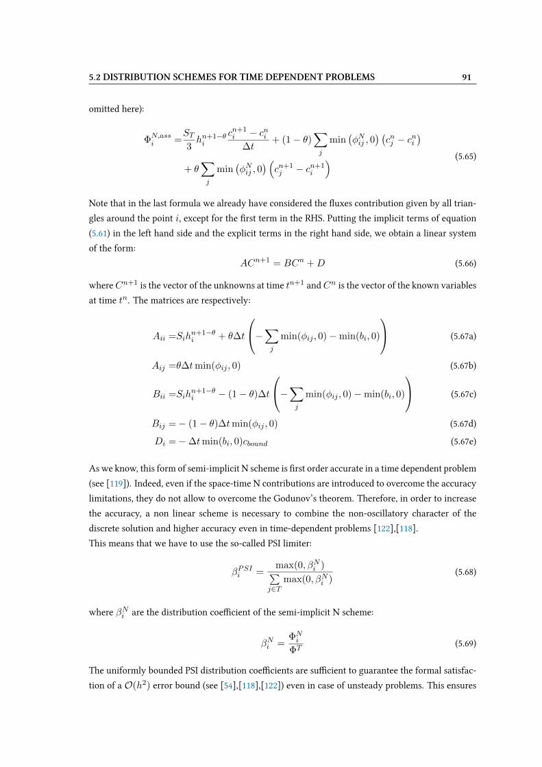
5.2 DISTRIBUTION SCHEMES FOR TIME DEPENDENT PROBLEMS 91
omitted here):
ΦN,assi =
ST3hn+1−θi
cn+1i − cni
∆t+ (1− θ)
∑j
min(φNij , 0
) (cnj − cni
)+ θ
∑j
min(φNij , 0
) (cn+1j − cn+1
i
) (5.65)
Note that in the last formula we already have considered the Wuxes contribution given by all trian-
gles around the point i, except for the Vrst term in the RHS. Putting the implicit terms of equation
(5.61) in the left hand side and the explicit terms in the right hand side, we obtain a linear system
of the form:
ACn+1 = BCn +D (5.66)
whereCn+1 is the vector of the unknowns at time tn+1 andCn is the vector of the known variables
at time tn. The matrices are respectively:
Aii =Sihn+1−θi + θ∆t
−∑j
min(φij , 0)−min(bi, 0)
(5.67a)
Aij =θ∆tmin(φij , 0) (5.67b)
Bii =Sihn+1−θi − (1− θ)∆t
−∑j
min(φij , 0)−min(bi, 0)
(5.67c)
Bij =− (1− θ)∆tmin(φij , 0) (5.67d)
Di =−∆tmin(bi, 0)cbound (5.67e)
As we know, this form of semi-implicit N scheme is Vrst order accurate in a time dependent problem
(see [119]). Indeed, even if the space-time N contributions are introduced to overcome the accuracy
limitations, they do not allow to overcome the Godunov’s theorem. Therefore, in order to increase
the accuracy, a non linear scheme is necessary to combine the non-oscillatory character of the
discrete solution and higher accuracy even in time-dependent problems [122],[118].
This means that we have to use the so-called PSI limiter:
βPSIi =max(0, βNi )∑
j∈Tmax(0, βNi )
(5.68)
where βNi are the distribution coeXcient of the semi-implicit N scheme:
βNi =ΦNi
ΦT(5.69)
The uniformly bounded PSI distribution coeXcients are suXcient to guarantee the formal satisfac-
tion of a O(h2) error bound (see [54],[118],[122]) even in case of unsteady problems. This ensures
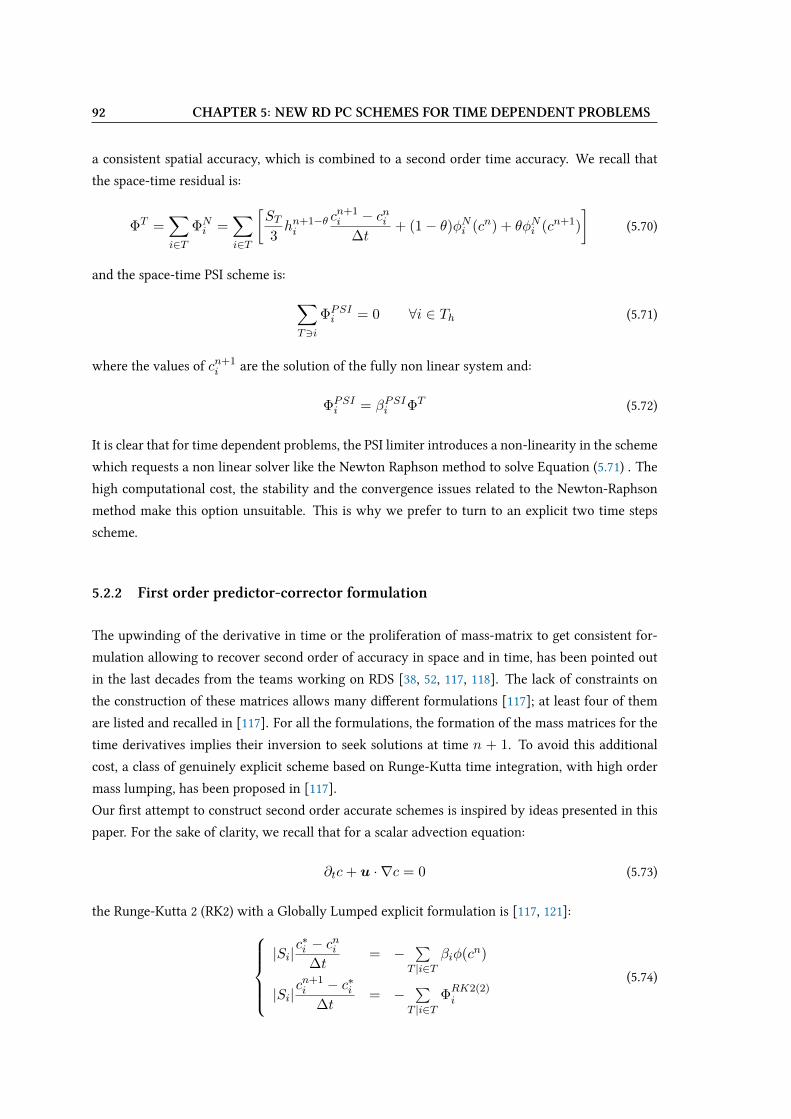
92 CHAPTER 5: NEW RD PC SCHEMES FOR TIME DEPENDENT PROBLEMS
a consistent spatial accuracy, which is combined to a second order time accuracy. We recall that
the space-time residual is:
ΦT =∑i∈T
ΦNi =
∑i∈T
[ST3hn+1−θi
cn+1i − cni
∆t+ (1− θ)φNi (cn) + θφNi (cn+1)
](5.70)
and the space-time PSI scheme is: ∑T3i
ΦPSIi = 0 ∀i ∈ Th (5.71)
where the values of cn+1i are the solution of the fully non linear system and:
ΦPSIi = βPSIi ΦT (5.72)
It is clear that for time dependent problems, the PSI limiter introduces a non-linearity in the scheme
which requests a non linear solver like the Newton Raphson method to solve Equation (5.71) . The
high computational cost, the stability and the convergence issues related to the Newton-Raphson
method make this option unsuitable. This is why we prefer to turn to an explicit two time steps
scheme.
5.2.2 First order predictor-corrector formulation
The upwinding of the derivative in time or the proliferation of mass-matrix to get consistent for-
mulation allowing to recover second order of accuracy in space and in time, has been pointed out
in the last decades from the teams working on RDS [38, 52, 117, 118]. The lack of constraints on
the construction of these matrices allows many diUerent formulations [117]; at least four of them
are listed and recalled in [117]. For all the formulations, the formation of the mass matrices for the
time derivatives implies their inversion to seek solutions at time n + 1. To avoid this additional
cost, a class of genuinely explicit scheme based on Runge-Kutta time integration, with high order
mass lumping, has been proposed in [117].
Our Vrst attempt to construct second order accurate schemes is inspired by ideas presented in this
paper. For the sake of clarity, we recall that for a scalar advection equation:
∂tc+ u · ∇c = 0 (5.73)
the Runge-Kutta 2 (RK2) with a Globally Lumped explicit formulation is [117, 121]:|Si|
c∗i − cni∆t
= −∑
T |i∈Tβiφ(cn)
|Si|cn+1i − c∗i
∆t= −
∑T |i∈T
ΦRK2(2)i
(5.74)

5.2 DISTRIBUTION SCHEMES FOR TIME DEPENDENT PROBLEMS 93
where
ΦRK2(2)i =
∑j∈T
mTij
c∗j − cnj∆t
+1
2βi (φ(c∗) + φ(cn)) (5.75)
The Vrst step consists of a classical explicit RD scheme, which can be the N, the PSI or any other
classical RD scheme. The upwind on the derivative in time appears in the corrector step, combined
to a semi-implicit scheme (with θ already set to 1/2) on the space residual φ(c).
The main ingredients to end up with this formulation are [117]:
• recast the RD discretization as a stabilized Galerkin scheme;
• use a shifted time discretization in the stabilization operator;
• apply high order mass lumping on the Galerkin component of the discretization.
In our case, since the RD formulation is employed to solve the non conservative discrete equation
which makes use of the discrete continuity equation (5.35), the equations (5.74) and (5.75) have to
be modiVed. In addition, we remember that several formulations are possible for (5.75) and in our
Vrst attempt we end up with a very diUerent form of (5.75).
To recover a similar scheme for the tracer equation, we look for a predictor-corrector scheme of
this type: Sih
n+1i
c∗i − cni∆t
= −∑T3i
βPSIi φT −min(bi, 0)(cbound − cni )
Sihn+1i
cn+1i − c∗i
∆t= −
∑T3i
βPSIi ΦT −min(bi, 0)(cbound − cni )(5.76)
where:
βPSIi ΦT = βPSIi
(∑i∈T
ΦNi
)= βPSIi
(∑i∈T
[T
3hn+1i
c∗i − cni∆t
+ βPSIi φ(cn)
])(5.77)
Note that when summing over i ∈ T , βPSIi φ(cn) = βNi φ(cn).
As we can see the latter is diUerent from (5.75), since in particular the prediction c∗ is only used to
estimate the derivative in time while in (5.75) it also necessary to estimate a semi-implicit residual.
In particular we would have:
ΦT =∑i∈T
ΦNi =
∑i∈T
T
3hn+1i
c∗i − cni∆t
+1
2
(βPSIi φ(cn) + βPSIi φ(c∗)
)(5.78)
The problem is that using the space-time residual (5.78) in Equation (5.76) will spoil the mass
conservation, which is related to the term hn+1 that multiplies the mass matrix and the derivative
in time.
To prove the mass conservation of the two steps scheme (5.76), we want that the sum of both steps
summed over all points gives the right conservation (i.e. like in the explicit schemes for steady
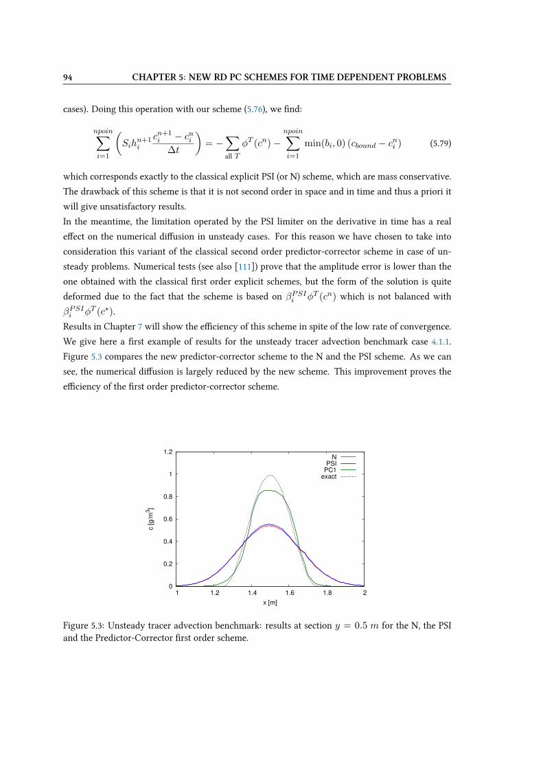
94 CHAPTER 5: NEW RD PC SCHEMES FOR TIME DEPENDENT PROBLEMS
cases). Doing this operation with our scheme (5.76), we Vnd:
npoin∑i=1
(Sih
n+1i
cn+1i − cni
∆t
)= −
∑all T
φT (cn)−npoin∑i=1
min(bi, 0) (cbound − cni ) (5.79)
which corresponds exactly to the classical explicit PSI (or N) scheme, which are mass conservative.
The drawback of this scheme is that it is not second order in space and in time and thus a priori it
will give unsatisfactory results.
In the meantime, the limitation operated by the PSI limiter on the derivative in time has a real
eUect on the numerical diUusion in unsteady cases. For this reason we have chosen to take into
consideration this variant of the classical second order predictor-corrector scheme in case of un-
steady problems. Numerical tests (see also [111]) prove that the amplitude error is lower than the
one obtained with the classical Vrst order explicit schemes, but the form of the solution is quite
deformed due to the fact that the scheme is based on βPSIi φT (cn) which is not balanced with
βPSIi φT (c∗).
Results in Chapter 7 will show the eXciency of this scheme in spite of the low rate of convergence.
We give here a Vrst example of results for the unsteady tracer advection benchmark case 4.1.1.
Figure 5.3 compares the new predictor-corrector scheme to the N and the PSI scheme. As we can
see, the numerical diUusion is largely reduced by the new scheme. This improvement proves the
eXciency of the Vrst order predictor-corrector scheme.
0
0.2
0.4
0.6
0.8
1
1.2
1 1.2 1.4 1.6 1.8 2
c [
g/m
3]
x [m]
NPSI
PC1exact
Figure 5.3: Unsteady tracer advection benchmark: results at section y = 0.5 m for the N, the PSIand the Predictor-Corrector Vrst order scheme.
5.2 DISTRIBUTION SCHEMES FOR TIME DEPENDENT PROBLEMS 95
The Vnal scheme containing sources is:
Sihn+1i
c∗i − cni∆t
= −∑T3i
βPSIi φT −min(bi, 0)(cbound − cni )
+ max(scei, 0)(cscei − cni )
Sihn+1i
cn+1i − c∗i
∆t= −
∑T3i
βPSIi ΦT −min(bi, 0)(cbound − cni )
+ max(scei, 0)(cscei − cni )
(5.80)
5.2.3 Second order predictor-corrector scheme
We show here how to apply the second order predictor-corrector scheme to the pollutant transport
equation in shallow Wows. Three main steps are necessary:
1. choose the explicit second order scheme in space (5.47) as predictor to approximate the value
of c∗ (or possibly the Vrst order scheme (5.35));
2. construct two possible Vrst order in time mass-conservative corrector schemes: one with the
upwind of hn+1i
c∗i−cni∆t , which corresponds to (5.77) and one with the upwind of hni
c∗i−cni∆t ;
3. average the two variants in order to obtain a second order in time corrector step.
As before, choosing an explicit second order scheme in space to Vnd c∗ means solving:
Sihn+1i
c∗i − cni∆t
= −∑T3i
βPSIi φT −min(bi, 0)(cbound − cni ) (5.81)
which corresponds to the PSI scheme.
For the corrector step, we construct now a Vrst order scheme in time but performing the upwind of
the derivative in time on the term hn+1i
∂c
∂tand neglecting the boundary terms. The corrector thus
reads as follows:
Sihn+1i
cn+1i − c∗i
∆t= −
∑T3i
βPSIi ΦT (5.82)
where the ΦT is the new space-time residual, constructed in order to be conservative, thus with
the factor hn+1 on the time derivative:
ΦT =∑i∈T
(ST3hn+1i
c∗i − cni∆t
+ βPSIi φT (cn)
)(5.83)
and
ΦNi =
(ST3hn+1i
c∗i − cni∆t
+ βPSIi φT (cn)
)(5.84)
If we try now to construct a corrector step which includes the Wuxes of c∗, considering expression
(5.41) we will Vnd that the only possibility in order to guarantee the conservation of the mass is to
96 CHAPTER 5: NEW RD PC SCHEMES FOR TIME DEPENDENT PROBLEMS
change the residual in:
ΦT =∑i∈T
(ST3hnic∗i − cni
∆t+ βPSIi φT (c∗)
)(5.85)
The average of these two possible schemes, will always give a conservative scheme which consists
in taking:
ΦT =∑i∈T
(θST3hnic∗i − cni
∆t+ (1− θ)ST
3hn+1i
c∗i − cni∆t
+ θβPSIi φT (cn) + (1− θ)βPSIi φT (c∗)
)(5.86)
which is equivalent to:
ΦT =∑i∈T
(ST3hn+1−θi
c∗i − cni∆t
+ θβPSIi φT (cn) + (1− θ)βPSIi φT (c∗)
)(5.87)
and with:
ΦNi =
(ST3hn+1−θi
c∗i − cni∆t
+ θβPSIi φT (cn) + (1− θ)βPSIi φT (c∗)
)(5.88)
Note that expression (5.88) is exactly the same as (5.70), where c∗ is known and it replaces cn+1.
The complete scheme includes also the boundary terms, so the corrector step becomes:
Sihn+1i
cn+1i − c∗i
∆t= −
∑T3i
βPSIi ΦT − bi (cbound − (1− θ) cni − θc∗i ) (5.89)
The Vnal scheme reads as follows:Sih
n+1i
c∗i − cni∆t
= −∑T3i
βPSIi φT (cn)−min(bi, 0)(cbound − cni )
Sihn+1i
cn+1i − c∗i
∆t= −
∑T3i
βPSIi ΦT (cn, c∗)−min(bi, 0) (cbound − (1− θ) cni − θc∗i )
(5.90)
with φT computed with Equation (5.37), ΦT as in Equation (5.87), and βPSIi computed using (5.68)
and (5.36) in combination with (5.38) in the predictor step, while (5.68) and (5.69) in combina-
tion with (5.88) in the corrector step. This scheme will be called second order predictor-corrector
scheme.
The second order discretization of the space time residual, together with the limitation given by the
PSI limiter, allows to improve the convergence of the scheme with respect to the Vrst order scheme
(5.76). However, for a given mesh, the diUerence between the two schemes can be negligible, as we
can see in Figure 5.4 where the RD schemes presented until now are compared. Results show that
both the predictor-corrector schemes improve the precision, thus the numerical results are closer to
the exact solution and a large diUerence exists between the N or the PSI scheme and the predictor-
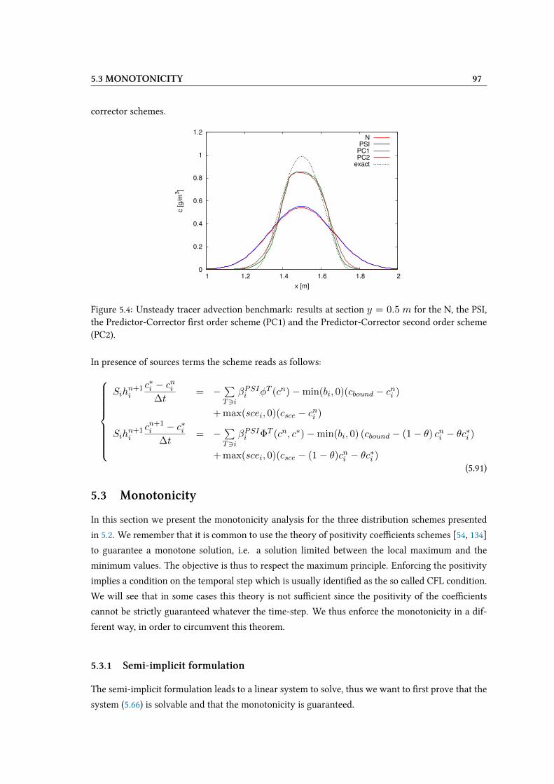
5.3 MONOTONICITY 97
corrector schemes.
0
0.2
0.4
0.6
0.8
1
1.2
1 1.2 1.4 1.6 1.8 2
c [
g/m
3]
x [m]
NPSI
PC1PC2
exact
Figure 5.4: Unsteady tracer advection benchmark: results at section y = 0.5 m for the N, the PSI,the Predictor-Corrector Vrst order scheme (PC1) and the Predictor-Corrector second order scheme(PC2).
In presence of sources terms the scheme reads as follows:
Sihn+1i
c∗i − cni∆t
= −∑T3i
βPSIi φT (cn)−min(bi, 0)(cbound − cni )
+ max(scei, 0)(csce − cni )
Sihn+1i
cn+1i − c∗i
∆t= −
∑T3i
βPSIi ΦT (cn, c∗)−min(bi, 0) (cbound − (1− θ) cni − θc∗i )
+ max(scei, 0)(csce − (1− θ)cni − θc∗i )(5.91)
5.3 Monotonicity
In this section we present the monotonicity analysis for the three distribution schemes presented
in 5.2. We remember that it is common to use the theory of positivity coeXcients schemes [54, 134]
to guarantee a monotone solution, i.e. a solution limited between the local maximum and the
minimum values. The objective is thus to respect the maximum principle. Enforcing the positivity
implies a condition on the temporal step which is usually identiVed as the so called CFL condition.
We will see that in some cases this theory is not suXcient since the positivity of the coeXcients
cannot be strictly guaranteed whatever the time-step. We thus enforce the monotonicity in a dif-
ferent way, in order to circumvent this theorem.
5.3.1 Semi-implicit formulation
The semi-implicit formulation leads to a linear system to solve, thus we want to Vrst prove that the
system (5.66) is solvable and that the monotonicity is guaranteed.
98 CHAPTER 5: NEW RD PC SCHEMES FOR TIME DEPENDENT PROBLEMS
The system is solvable because theAmatrix is non singular and it is a L-matrix, i.e. Aii > 0 ∀i andAij < 0 forj 6= i. We consider thus at (5.67a) and (5.67b) and we Vrst show that A is a L-matrix.
This is easy to prove since Aii is the sum of positive terms while Aij is negative thanks to the term
min(φij , 0).
Then to prove that the matrix is not singular we can show that A has a positive dominant diagonal.
Indeed:
|Aii| −∑j 6=i|Aij | > 0
since:
Sihn+1−θi + θ∆t
−∑j
min(φij , 0)−min(bi, 0)
−∑j
θ∆tmin(φij , 0) > 0
The monotonicity is ensured ifB is a matrix with positive elements. A CFL condition can be found
to ensure the positivity of Bii:
∆t ≤ 1
(1− θ)−Sihn+1−θ
i∑j min(φij , 0) + min(bi, 0)
(5.92)
Then we can state that the scheme is monotone under this CFL condition. We note that this
condition is slightly better than the one found in [6, 54] for the scalar case, which is with our
notation:
∆t ≤ minT,T3i
1
1− θST3
1∑j∈T
λNij(5.93)
where cij are the positive coeXcients which correspond to λNij in our case. Indeed the authors
say in [6] that this condition is certainly not optimal and computations with CFL greater than one
have shown that monotonicity is preserved. In order to show that our condition is larger than the
latter, we omit the depth and the boundaries in our formula, then we Vx θ = 0.5 and we consider
a regular mesh (all the triangles have the same area). Condition (5.93) becomes:
∆t1 ≤ minT,T3i
2
3
ST∑j∈T
λNij(5.94)
and our condition (5.92) becomes:
∆t2 ≤ 2
∑T3i
ST /3∑T3i
∑j∈T
λNij=
2
3
∑T3i
ST∑T3i
∑j∈T
λNij(5.95)
In the worst situation we will have two positive Wuxes for every triangle (the cell i is emptying),
thus ∆t2 = ∆t1 and in the best situation we will have only one positive Wuxes in one triangle,
thus ∆t2 = n∆t1 where n is the number of triangles around the point i. Thus if we have for
5.3 MONOTONICITY 99
example 7 triangles around the point i, our time step can be 7 times larger then ∆t1. In addition if
we consider an unstructured mesh with irregular triangles, the factor minT,T3i
ST in ∆t1 will be very
restrictive with respect to∑T3i
ST = SaverageT > minT,T3i
ST in ∆t2.
5.3.2 First order predictor-corrector scheme
In case of a Vrst order predictor-corrector scheme, the solution is approximated by a two time step
explicit scheme and the theory of positivity coeXcients can be easily used.
A Vrst approach consists in taking advantage of the known stability condition for the predictor
step which is given by equation (5.44) and only study the stability of the corrector step. Once
established the time step condition on the corrector, the minimum time-step between the predictor
and the corrector will be chosen as Vnal condition.
We rewrite the corrector step as:
Sihn+1i
cn+1i − c∗i
∆t= −
∑T3i
βPSIi
βNiβNi ΦT −min(bi, 0)(cbound − cni ) (5.96)
= −∑T3i
γi
(T
3hn+1j
c∗j − cnj∆t
+ βPSIi φ(cn)
)−min(bi, 0)(cbound − cni )
(5.97)
= −∑T3i
γi
T3hn+1j
c∗j − cnj∆t
+∑j
λPSIij (cni − cnj )
−min(bi, 0)(cbound − cni )
(5.98)
We make explicit the coeXcients of every variable:
Sihn+1i cn+1
i =∑T3i
(1− γi)ST3hn+1i c∗i + ∆t
∑T3i
γi∑j
λPSIij cnj
+
∑T3i
γi
ST3hn+1i −∆t
∑j
λPSIij
+ min(bi, 0)
cni −∆tmin(bi, 0)cbound
And we arrive at the restrictive condition:
∆t = minT3i
ST /3 hn+1i∑
jλPSIij −min(bi, 0)
(5.99)
Note that the boundary term has been included in the denominator for security reasons. This con-
dition is surely too restrictive and indeed we can Vnd a larger condition using a diUerent method.
The second approach takes into consideration in the analysis also the predictor step, in order to
eliminate the dependence on c∗ and uses the assembled Wuxes φij to replace the elementary Wuxes
100 CHAPTER 5: NEW RD PC SCHEMES FOR TIME DEPENDENT PROBLEMS
λij . Using the notations of section 5.1.2, especially−βNi φT =3∑j=1
min(φN,elij , 0)(ci−cj), we write:
Sihn+1i
(cn+1i − c∗i
)= −∆t
∑T3i
γi
ST3hn+1i
(c∗i − cni
∆t
)+
3∑j=1
min(φN,elij , 0)(cnj − cni )
−∆t min(bi, 0) (cbound − cni )
Note that for security reasons we take φNij since they are larger than φPSIij . The demonstration
works also for φPSIij . Then we set:
∑T3i
γi
(ST3hn+1i
(c∗i − cni
∆t
))= fiSih
n+1i
(c∗i − cni
∆t
)(5.100)
where fi represents the PSI reduction on the derivative in time: fi = 1Si
∑T3i
γiST3 and fi ∈ [0, 1].
This simpliVcation is possible since the diUerence c∗ − cn has the same sign on all the elements
around node i. Then we set:
−∆t∑T3i
γi
3∑j=1
min(φN,elij , 0)(cnj − cni )
= −∆t∑j
µij(min(φNij , 0)(cnj − cni ) (5.101)
where µij ∈ [0, 1] takes into account the limitation γi applied on the two nearby elements which
share the edge ij.
We do the same simpliVcation on the other terms and we obtain:
Sihn+1i cn+1
i =Sihn+1i c∗i − fiSihn+1
i (c∗i − cni )−∆t∑j
µij(cnj − cni
)min(φNij , 0)
−∆tmin(bi, 0) (cbound − cni )
(5.102)
which, considering that c∗−cn∆t is the result of the predictor step, becomes:
Sihn+1i cn+1
i =Sihn+1i c∗i − fi∆t
∑j
min(φNij , 0)(cni − cnj )−min(bi, 0)(cbound − cni )
−∆t
∑j
µij(cnj − cni
)min(φNij , 0)−∆tmin(bi, 0) (cbound − cni )
(5.103)
5.3 MONOTONICITY 101
Even in this case we have used the N Wuxes at the predictor step but it is just for security reasons.
We now sum the predictor and the corrector step and we obtain:
Sihn+1i cn+1
i =Sihn+1i cni + ∆t
∑j
(1− fi + µij) min(φNij , 0)(cni − cnj )
+ ∆t(fi − 2) min(bi, 0) (cbound − cni )
(5.104)
Studying the coeXcients of all values of c, we see that they are all positive except the ones of cniwhich could create a problem:
Sihn+1i + ∆t
∑j
(1− fi + µij) min(φNij , 0) + ∆t(2− fi) min(bi, 0) > 0 (5.105)
We note that the coeXcient (1− fi + µij) and 2− fi are positive and not larger than 2. We thus
arrive at the criterion:
∆t <Sih
n+1i
−2
[∑j
min(φNij , 0) + min(bi, 0)
] (5.106)
We note that this condition is less restrictive than (5.99), like in the case of a semi-implicit scheme.
The criterion can also be written in function of hn, using the continuity equation:
∆t <Sih
ni∑
jmax(φNij , 0)−min(φNij , 0) + max(bi, 0)−min(bi, 0)
(5.107)
Provided the time step (5.106), we can Vnd that the predicted values naturally respects:
cni + cmin
2≤ c∗i ≤
cni + cmax
2(5.108)
where cmin = minj(cnj , c
ni ) and cmax = maxj(c
nj , c
ni ). This condition will be useful later.
If sources are present, then the time step condition (5.106) becomes:
∆t <Sih
n+1i
−2
[∑j
min(φNij , 0) + min(bi, 0)−max(scei, 0)
] (5.109)
102 CHAPTER 5: NEW RD PC SCHEMES FOR TIME DEPENDENT PROBLEMS
5.3.3 Second order predictor-corrector scheme
We use again the same approach to study the monotonicity of the second order scheme. We start
rewriting the corrector in the following way:
Sihn+1i
(cn+1i − c∗i
)= −∆t
∑T3i
γi
ST3hn+1−θi
(c∗i − cni
∆t
)+ (1− θ)
3∑j=1
min(φN,elij , 0)(cnj − cni )
−∆t
∑T3i
γi
θ 3∑j=1
min(φN,elij , 0)(c∗j − c∗i )
−∆t bi (cbound − (1− θ) cni − θc∗i ) (5.110)
We set: ∑T3i
γi
(ST3hn+1−θi
(c∗i − cni
∆t
))= fiSih
n+1−θi
(c∗i − cni
∆t
)(5.111)
where fi represents the PSI reduction on the derivative in time: fi = 1Si
∑T3i
γiST3 and fi ∈ [0, 1].
This simpliVcation is possible since the diUerence c∗ − cn has the same sign on all the elements
around node i. Then we set:
− (1− θ)∆t∑T3i
γi
3∑j=1
min(φN,elij , 0)(cnj − cni )
= −(1− θ)∆t∑j
µij(min(φNij , 0)(cnj − cni )
(5.112)
where µij ∈ [0, 1] takes into account the limitation γi applied on the two nearby elements which
share the edge ij.
We do the same simpliVcation on the other terms and we obtain:
Sihn+1i cn+1
i =Sihn+1i c∗i − fiSihn+1−θ
i (c∗i − cni )− θ∆t∑j
µij(c∗j − c∗i
)min(φNij , 0)
− (1− θ)∆t∑j
µij(cnj − cni
)min(φNij , 0)
−∆tmin(bi, 0) (cbound − (1− θ) cni − θc∗i )
(5.113)
Looking at coeXcients of c in equation (5.113), we see that only coeXcients of c∗i and cni may be
negative. Indeed these coeXcients are, respectively:
• Sihn+1i − fiSihn+1−θ
i + θ∆t∑
j µij min(φNij , 0) + θ∆tmin(bi, 0) = a∗
• fiSihn+1−θi + (1− θ)∆t
∑j µij min(φNij , 0) + (1− θ) ∆tmin(bi, 0) = an
We see that the two conditions are not compatible and nothing guarantees that Sihn+1i −fiSihn+1−θ
i
is positive. So, we conclude that we cannot Vnd a time step condition for the corrector step which
ensures the positivity of the two coeXcients at the same time.
5.3 MONOTONICITY 103
However, if we consider that c∗i is issued by the predictor step with a time step given by (5.44), we
can say that the sum of the coeXcients of cni and c∗i is certainly positive, as we have:
a∗ + an = Sihn+1i + ∆t
∑j
µij min(φNij , 0) + min(bi, 0)
(5.114)
Taking µij = 1, which is the worst case, it becomes:
a∗ + an = Sihn+1i + ∆t
∑j
min(φNij , 0) + min(bi, 0)
(5.115)
We know that c∗ and cn are included in the range [cmin, cmax], with cmin = minj
(cj , ci) and
cmax = maxj
(cj , ci), thus we write:
c∗i = cmin + α(cmax − cmin
)cni = cmin + β
(cmax − cmin
)with α and β in the range [0,1] and we want to Vnd the solutions under which:
a∗c∗i + ancni = (a∗ + an)caveragei (5.116)
with: caveragei = cmin + γ(cmax − cmin
), and γ in the range [0,1]. The idea is that the coeXcient
of caveragei is the sum of c∗i and cni coeXcients, so that we are sure that the sum of all coeXcients
giving cn+1i remains 1. If caveragei is included in the range [cmin, cmax] then the monotonicity of
cn+1 can be demonstrated.
From (5.116) we get:
γ =αa∗ + βan
a∗ + an
We must thus ensure that:
0 ≤ αa∗ + βan ≤ a∗ + an
γ will be positive if: αa∗ + βan ≥ 0 and it will be less than 1 if: αa∗ + βan ≤ a∗ + an, i.e. if
(1− α) a∗ + (1− β) an ≥ 0. So we have to Vnd a condition on c∗i , i.e. on α depending on β and
then we shall have the same condition for (1− α) depending on (1− β). Only the positivity of γ
is then to be studied. We are sure that γ will be positive if:
αSihn+1i + (β − α) fiSih
n+1−θi + [αθ + β (1− θ)]
∆t∑j
min(ΦNij , 0) + ∆tmin(bi, 0)
≥ 0

104 CHAPTER 5: NEW RD PC SCHEMES FOR TIME DEPENDENT PROBLEMS
We now assume that the time step is chosen with the condition:
∆t ≤ 1
2
Sihn+1i(
−∑
j min(
ΦNij , 0
)−min (bi, 0)
)This is the classical condition for the N scheme, divided by 2, which also corresponds to (5.106).
The positivity will be thus ensured if:
αSihn+1i + (β − α) fiSih
n+1−θi ≥ [αθ + β (1− θ)]
Sihn+1i
2
If α ≤ β the worst case happens when fi = 0 and we must have:
α ≥ 1− θ2− θ
β
If α ≥ β the worst case happens when fi = 1 and we must have:
αSihn+1i ≥ [αθ + β (1− θ)]
Sihn+1i
2+ (α− β)Sih
n+1−θi
We can use the property:
hn+1i
(1− θ
2
)≤ hn+1−θ
i ≤ hn+1i
(1 +
θ
2
)and we get a stronger condition if we replace hn+1−θ
i by hn+1i
(1 + θ
2
):
α ≥ [αθ + β (1− θ)] 1
2+ (α− β)
(1 +
θ
2
)which is:
α ≤ β (1 + 2θ)
2θ
and we arrive at:
β
(1− 1
2− θ
)≤ α ≤ β
(1 +
1
2θ
)The condition for γ ≤ 1 will give in the same way:
(1− β)
(1− 1
2− θ
)≤ 1− α ≤ (1− β)
(1 +
1
2θ
)or:
1 + (β − 1)
(1 +
1
2θ
)≤ α ≤ 1 + (β − 1)
(1− 1
2− θ
)We arrive thus at two conditions:
5.4 ITERATIVE PREDICTOR-CORRECTOR SCHEMES 105
β(
1− 12−θ
)≤ α ≤ β
(1 + 1
2θ
)1 + (β − 1)
(1 + 1
2θ
)≤ α ≤ 1 + (β − 1)
(1− 1
2−θ
) (5.117)
We translate now conditions (5.117) into limitations on c∗. To simplify the problem, we restrict to
the case θ = 1/2. It gives: β
3≤ α ≤ 2β
2β − 1 ≤ α ≤ 1 +(β − 1)
3
Which for symmetry reason we rather combine in the form: 2β − 1 ≤ α ≤ 2ββ
3≤ α ≤ 2
3+β
3
This is equivalent to: 2cni − cmax ≤ c∗i ≤ 2cni − cmin
2cmin
3+cni3≤ c∗i ≤
2cmax
3+cni3
(5.118)
This limitation will be performed after the predictor step in order to ensure the monotonicity of the
Vnal value cn+1. To sum up we can conclude that:
Given a time step ∆t such that:
∆t ≤ 1
2
Sihn+1i(
−∑
j min(
ΦNij , 0
)−min (bi, 0)
) (5.119)
and choosing θ = 1/2 for the corrector step, the approximate discrete solution cn+1i respects the
maximum principle, under the following conditions on c∗i : 2cni − cmax ≤ c∗i ≤ 2cni − cmin
2cmin
3+cni3≤ c∗i ≤
2cmax
3+cni3
(5.120)
where cmax = maxj(cnj , c
ni ) and cmin = minj(c
nj , c
ni ). Again the criterion (5.119) can be adapted
to the source terms in the following way:
∆t ≤ 1
2
Sihn+1i(
−∑
j min(
ΦNij , 0
)−min (bi, 0) + max(scei, 0)
) (5.121)
5.4 Iterative predictor-corrector schemes
Both the Vrst order and the second order predictor-corrector schemes can take advantage of a
further improvement: an iterative procedure can be applied on the corrector step.
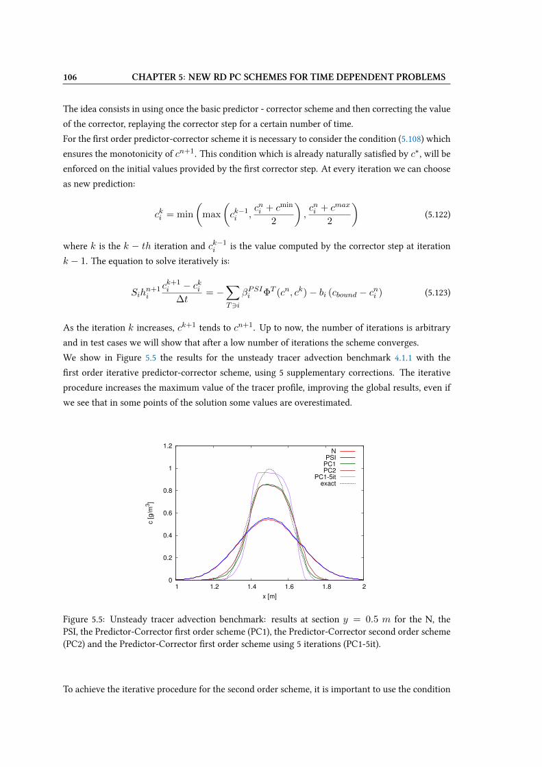
106 CHAPTER 5: NEW RD PC SCHEMES FOR TIME DEPENDENT PROBLEMS
The idea consists in using once the basic predictor - corrector scheme and then correcting the value
of the corrector, replaying the corrector step for a certain number of time.
For the Vrst order predictor-corrector scheme it is necessary to consider the condition (5.108) which
ensures the monotonicity of cn+1. This condition which is already naturally satisVed by c∗, will be
enforced on the initial values provided by the Vrst corrector step. At every iteration we can choose
as new prediction:
cki = min
(max
(ck−1i ,
cni + cmin
2
),cni + cmax
2
)(5.122)
where k is the k − th iteration and ck−1i is the value computed by the corrector step at iteration
k − 1. The equation to solve iteratively is:
Sihn+1i
ck+1i − cki
∆t= −
∑T3i
βPSIi ΦT (cn, ck)− bi (cbound − cni ) (5.123)
As the iteration k increases, ck+1 tends to cn+1. Up to now, the number of iterations is arbitrary
and in test cases we will show that after a low number of iterations the scheme converges.
We show in Figure 5.5 the results for the unsteady tracer advection benchmark 4.1.1 with the
Vrst order iterative predictor-corrector scheme, using 5 supplementary corrections. The iterative
procedure increases the maximum value of the tracer proVle, improving the global results, even if
we see that in some points of the solution some values are overestimated.
0
0.2
0.4
0.6
0.8
1
1.2
1 1.2 1.4 1.6 1.8 2
c [
g/m
3]
x [m]
NPSI
PC1PC2
PC1-5itexact
Figure 5.5: Unsteady tracer advection benchmark: results at section y = 0.5 m for the N, thePSI, the Predictor-Corrector Vrst order scheme (PC1), the Predictor-Corrector second order scheme(PC2) and the Predictor-Corrector Vrst order scheme using 5 iterations (PC1-5it).
To achieve the iterative procedure for the second order scheme, it is important to use the condition
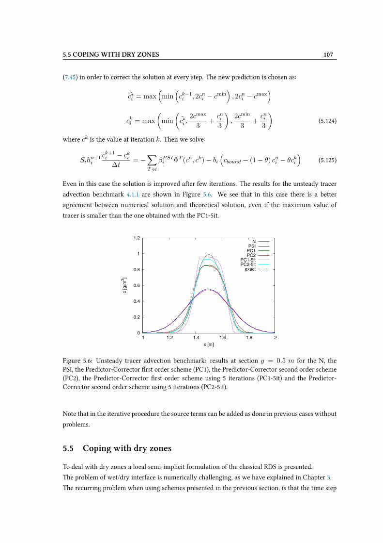
5.5 COPING WITH DRY ZONES 107
(7.45) in order to correct the solution at every step. The new prediction is chosen as:
c∗i = max(
min(ck−1i , 2cni − cmin
), 2cni − cmax
)cki = max
(min
(c∗i ,
2cmax
3+cni3
),2cmin
3+cni3
)(5.124)
where ck is the value at iteration k. Then we solve:
Sihn+1i
ck+1i − cki
∆t= −
∑T3i
βPSIi ΦT (cn, ck)− bi(cbound − (1− θ) cni − θcki
)(5.125)
Even in this case the solution is improved after few iterations. The results for the unsteady tracer
advection benchmark 4.1.1 are shown in Figure 5.6. We see that in this case there is a better
agreement between numerical solution and theoretical solution, even if the maximum value of
tracer is smaller than the one obtained with the PC1-5it.
0
0.2
0.4
0.6
0.8
1
1.2
1 1.2 1.4 1.6 1.8 2
c [
g/m
3]
x [m]
NPSI
PC1PC2
PC1-5itPC2-5it
exact
Figure 5.6: Unsteady tracer advection benchmark: results at section y = 0.5 m for the N, thePSI, the Predictor-Corrector Vrst order scheme (PC1), the Predictor-Corrector second order scheme(PC2), the Predictor-Corrector Vrst order scheme using 5 iterations (PC1-5it) and the Predictor-Corrector second order scheme using 5 iterations (PC2-5it).
Note that in the iterative procedure the source terms can be added as done in previous cases without
problems.
5.5 Coping with dry zones
To deal with dry zones a local semi-implicit formulation of the classical RDS is presented.
The problem of wet/dry interface is numerically challenging, as we have explained in Chapter 3.
The recurring problem when using schemes presented in the previous section, is that the time step

108 CHAPTER 5: NEW RD PC SCHEMES FOR TIME DEPENDENT PROBLEMS
is water depth dependent:
∆t ≤ f h
g(5.126)
f represents in general an area (of a cell or triangle) and g represents the sum of Wuxes which
empties a cell, including boundaries and sources. In case of dry zones, we thus obtain a zero time
step as minimum value and the scheme will not work.
A common solution used to treat this problem is to make use of a cut-oU value of the water depth,
below which the computation of the concentration (or velocities) is avoided and zero values are put
instead as solution. In particular this solution is also used for FV schemes presented in this work.
Here we would like to construct a scheme for dry zones which is completely water depth free, that
is a scheme with a time step computation independent on the value of the water depth. In this way
the scheme does not need a cut-oU parameter, which can create instabilities. The general idea is to
avoid situations in which a division by a zero water depth arises.
The new idea used in this work, consists in exploiting the unconditional stability of the implicit
scheme to face the wet/dry interface and to keep the accuracy of the predictor-corrector explicit
schemes in the wet zones. The method is presented in two steps:
• Formulation of a local semi-implicit scheme for steady problems
• Formulation of a local semi-implicit predictor-corrector scheme for unsteady problems (the
upwind of the derivative in time is included in the local semi-implicit formulation)
5.5.1 Local semi-implicit N scheme
We Vrst transform the global semi-implicit scheme presented in section 5.2.1 into a local semi-
implicit scheme, where the choice of θ is local, i.e. locally chosen for every point. To do this, special
attention is required on the upwind choice when deVning cij . The derivation is done starting from
the conservative Equation (5.59), expliciting cn+θ and with a local θi:
Sihn+1−θii cn+1
i − Sihn+1−θii cni = + ∆t
∑j
[((1− θi)cni + θic
n+1)− cnij
]φij
+ ∆tbi((1− θi)cni + θic
n+1i − cbound
) (5.127)
Note that here we omit the superscript N on φij but we consider that we deal with N Wuxes. In order
to deVne cij we choose θicn+1i + (1− θi)cni if φij is positive (from i to j) and θjc
n+1j + (1− θj)cnj
if φij is negative. Accordingly we also consider that for ingoing boundary terms bi > 0 we will
have θicn+1i + (1− θi)cni . Thus the scheme reads as follows:
Sihn+1−θii (cn+1
i − cni ) =−∆t∑j
[θjc
n+1j + (1− θj)cnj − θicn+1
i − (1− θi)cni]
min(φij , 0)
−∆tmin(bi, 0)(cbound − (θic
n+1i + (1− θi)cni )
)(5.128)
5.5 COPING WITH DRY ZONES 109
And in presence of sources becomes:
Sihn+1−θii (cn+1
i − cni ) =−∆t∑j
[θjc
n+1j + (1− θj)cnj − θicn+1
i − (1− θi)cni]
min(φij , 0)
−∆tmin(bi, 0)(cbound − (θic
n+1i + (1− θi)cni )
)+ ∆tmax(scei, 0)
(csce − (θic
n+1i + (1− θi)cni )
)(5.129)
Putting the implicit terms of (5.128) in the left-hand side and explicit terms in the right-hand side,
the equation can again be written in the form of a linear system:
ACn+1 = BCn +D (5.130)
where the matrices are:
Aii =Sihn+1−θii + θi∆t
−∑j
min(φij , 0)−min(bi, 0)
(5.131a)
Aij =θj∆tmin(φij , 0) (5.131b)
Bii =Sihn+1−θii − (1− θi)∆t
−∑j
min(φij , 0)−min(bi, 0)
(5.131c)
Bij =− (1− θj)∆tmin(φij , 0) (5.131d)
Di =−∆tmin(bi, 0)cbound (5.131e)
5.5.1.1 Monotonicity analysis
As for the global semi-implicit scheme, the stability of the scheme is given by the positivity of Bii.
We obtain a stability condition:
∆t ≤ 1
1− θiSih
ni∑
jmax(φji, 0) + max(bi, 0)
(5.132)
Sources do not add theoretical problems if well taken into account, thus the time step condition
becomes:
∆t ≤ 1
1− θiSih
ni∑
jmax(φji, 0) + max(bi, 0)−min(scei, 0)
(5.133)
110 CHAPTER 5: NEW RD PC SCHEMES FOR TIME DEPENDENT PROBLEMS
Note that we have transformed hn+1−θii into hni thanks to the continuity equation:
Sihn+1−θii = Sih
ni − (1− θi)∆t
∑j
φij + bi
(5.134)
5.5.1.2 Choosing the local semi-implicitation
Formula (5.132) gives rise to an interesting question: which local θi can we choose?
The minimum acceptable time step for every point is obtained when θi = 0:
∆tstab(i) =Sih
ni∑
jmax(φji, 0) + max(bi, 0)
(5.135)
and it can be increased by the implicitation.
The goal is to do the whole process in n sub-steps, with n an arbitrary parameter. Indeed it is
necessary to get the same time step for all points.
We thus would like to have:1
1− θi∆tstab(i) =
∆tcasn
(5.136)
where ∆tcas represents the time-step chosen for hydrodynamics. Bounding the coeXcient to 0, we
Vnd:
θi = max
(0, 1− n∆tstab(i)
∆tcas
)(5.137)
The latter tends to give 0 if n is large enough or if ∆tcasn ' ∆tstab(i), except in the wet/dry front
where ∆tstab(i) = 0, so θi = 1. The scheme is thus stabilised on dry zones by a full implicitation.
In completely wet steady cases, for n large enough, the scheme falls into the classical N explicit
scheme.
Once the θi are computed, we can solve equation (5.128) enforcing ∆t = ∆tcasn .
5.5.1.3 Local semi-implicit PSI scheme
We write now a variation of this scheme in order to fall into the PSI scheme in case of wet steady
state. To do this we consider Equation (5.128) and we take the term on the LHS:
−∆t∑j
[θjc
n+1j + (1− θj)cnj − θicn+1
i − (1− θi)cni]
min(φij , 0) (5.138)
5.5 COPING WITH DRY ZONES 111
which is rewritten it in the equivalent form:
−∆t∑j
[θj(c
n+1j − cnj )− θi(cn+1
i − cni ) + cnj − cni]
min(φij , 0) (5.139)
then we split it into two parts, with φij changed into φPSIij for the last term, since it does not spoil
the mass conservation:
−∆t∑j
[θj(c
n+1j − cnj )− θi(cn+1
i − cni )]
min(φij , 0)−∆t∑j
(cnj −cni ) min(φPSIij , 0) (5.140)
This change involves a change in the matrix B, while the other matrices will not change. In partic-
ular we will have:
Bii =Sihn+1−θii − (1− θi)∆t (−min(bi, 0)) + ∆t
∑j
min(φPSIij , 0)− θi∆t∑j
min(φij , 0)
(5.141a)
Bij =−∆tmin(φPSIij , 0) + θj∆tmin(φij , 0) (5.141b)
Since min(φPSIij , 0) ≤ min(φij , 0) the monotonicity analysis can be done replacing φPSIij with φijin the matrix B. Then Bii and Bij are equal to Bii and Bij of (5.131) and the same monotonicity
condition can be used. The local parameter θi is chosen again with formula (5.137) and the linear
system is solved choosing ∆t = ∆tcasn .
We have now obtained a local semi-implicit scheme able to deal with dry zones and also able to
fall back into a classical PSI scheme in case of steady wet cases.
The new goal is to construct a scheme which is still capable to tackle dry zones but which is also
suitable for the unsteady cases. We thus would like to apply the local method to the predictor-
corrector scheme.
5.5.2 Local semi-implicit predictor-corrector scheme
To build a semi-implicit predictor-corrector scheme, we use the local semi-implicit scheme (5.128)
as predictor step, to give a Vrst approximation of cn+1i denoted c∗i .
Then we would like to construct a local corrector step where the derivative in time is upwinded
and limited thanks to the PSI limiter.
To do this the Vrst step consists in writing a semi-implicit corrector, splitting the original derivative
112 CHAPTER 5: NEW RD PC SCHEMES FOR TIME DEPENDENT PROBLEMS
in time:
Sihn+1−θii (cn+1
i − c∗i ) =− Sihn+1−θii (c∗i − cni )
−∆t∑j
((θjc
n+1j − θicn+1
i ) + ((1− θj)cnj − (1− θi)cni ))
min(φij , 0)
−∆tmin(bi, 0)(cbound − (θic
n+1i + (1− θi)cni )
)(5.142)
The second steps consists in choosing the space-time residual over which applying the PSI limiter.
Since we want to avoid non-linearities, we choose to limit the derivative in time and the explicit
Wuxes. Thus we end up with this kind of corrector:
Sihn+1−θii (cn+1
i − c∗i ) =−∆t∑j
(θjcn+1j − θicn+1
i ) min(φij , 0)
−∆tβPSIi ΦT −∆tmin(bi, 0)(cbound − (θic
n+1i + (1− θi)cni )
)(5.143)
where the space-time residual is :
ΦT =∑i∈T
ΦNi =
ST3
∑i∈T
hn+1−θii
c∗i − cni∆t
+3∑i=1
3∑j=1
((1− θj)cnj − (1− θi)cni
)min(φNij , 0)
(5.144)
The Vnal predictor-corrector scheme reads:
Sihn+1−θii
c∗i − cni∆t
= −∆t∑j
[θjc∗j + (1− θj)cnj − θic∗i − (1− θi)cni
]min(φij , 0)
−∆tmin(bi, 0) (cbound − (θic∗i + (1− θi)cni ))
Sihn+1−θii
cn+1i − c∗i
∆t= −
∑T∈i
βPSIi ΦT −∆t∑j
(θjcn+1j − θicn+1
i ) min(φij , 0)
−∆tmin(bi, 0)(cbound − (θic
n+1i + (1− θi)cni )
)(5.145)
The scheme presented here is similar to the Vrst order predictor-corrector scheme, since the space
time residual does not correspond to a second order discretization in time of the spatial Wuxes since
only the explicit part is upwinded.

5.5 COPING WITH DRY ZONES 113
Considering additional sources the Vnal scheme becomes:
Sihn+1−θii
c∗i − cni∆t
= −∆t∑j
[θjc∗j + (1− θj)cnj − θic∗i − (1− θi)cni
]min(φij , 0)
−∆tmin(bi, 0) (cbound − (θic∗i + (1− θi)cni ))
+∆tmax(scei, 0) (csce − (θic∗i + (1− θi)cni ))
Sihn+1−θii
cn+1i − c∗i
∆t= −
∑T∈i
βPSIi ΦT −∆t∑j
(θjcn+1j − θicn+1
i ) min(φij , 0)
−∆tmin(bi, 0)(cbound − (θic
n+1i + (1− θi)cni )
)+∆tmax(scei, 0)
(csce − (θic
n+1i + (1− θi)cni )
)(5.146)
5.5.2.1 Monotonicity analysis
We now study the monotonicity of the corrector step without sources, taking into account the
limitation (like fi and µij) that stems from the PSI limiter:
an+1i cn+1
i + an+1j cn+1
j = +d∗i c∗i − dnj cnj + dni c
ni −∆tmin(bi, 0)cbound
where:
an+1i = Sih
n+1−θii −∆tθi
∑j
min(φij , 0)−∆tθi min(bi, 0) (5.147a)
an+1j = ∆t
∑j
θj min(φij , 0) (5.147b)
d∗i = Sihn+1−θii − fiSihn+1−θi
i (5.147c)
dnj = −µij∆t∑j
(1− θj) min(φij , 0) (5.147d)
dni = fiSihn+1−θii + (1− θi)∆t
∑j
µij min(φij , 0) + min(bi, 0)
(5.147e)
The system is solvable since, like in the previous case, the Amatrix, made up by ai on the diagonal
and aj on the extra-diagonal terms, is non singular and it is a L-matrix i.e. Aii > 0 ∀i andAij < 0 forj 6= i, thanks to the stability condition of the predictor step.
Only the coeXcients of cni could be negative, indeed the extra derivative in time with the limitation
given by the PSI limiter could be a problem. This coeXcient is:
fiSihn+1−θii + (1− θi)∆t
∑j
µij min(φij , 0) + min(bi, 0)
(5.148)
114 CHAPTER 5: NEW RD PC SCHEMES FOR TIME DEPENDENT PROBLEMS
If fi = 1, we Vnd the previous condition, (5.132), on the time step. Yet, in this case fi could also be
zero, thus in order to keep the positivity, the value of c∗i is considered.
As for the second order predictor-corrector scheme, an average value of concentration caveragei is
introduced to guarantee the monotonicity of the scheme. The demonstration follows the same steps
of the predictor-corrector schemes.
We can show that, for a time step chosen so that:
∆tstab <1
2
1
1− θiSih
starti(∑
jmax(φNij , 0) + max(bi, 0)
) (5.149)
the approximate discrete solution cn+1i respects the maximum principle under the following con-
dition on c∗i :
cni +1
2
(cmini − cni
)< c∗i < cni +
1
2(cmaxi − cni ) (5.150)
where cmax = maxj(cnj , c
ni ) and cmin = minj(c
nj , c
ni ). The proof is reported in Appendix A.
This statement is true also in presence of sources, but the time step to consider is:
∆tstab <1
2
1
1− θiSih
starti(∑
jmax(φNij , 0) + max(bi, 0)−min(scei, 0)
) (5.151)
5.5.2.2 A correct sum of coeXcients
The Vnal value of cn+1 is monotone only if the sum of the interpolation coeXcients is equal to 1.
However, the last term on the RHS of Equation (5.144) could create problems in the global balance
of coeXcients of c after the reduction operated by the PSI limiter. Indeed, before the PSI reduction,
the balance of (1−θj)cnj −(1−θi)cni is ensured by the term−θjcn+1j −θicn+1
i . This does not hold
true after the PSI reduction. To have a right balance of coeXcients, the solution consists in applying
the limiter only on the terms which can be balanced. Thus, denoting θij = min(1 − θi, 1 − θj),we replace:
3∑i=1
3∑j=1
((1− θj)cnj − (1− θi)cni
)min(φNij , 0)
by:
3∑i=1
3∑j=1
θij(cni − cnj
)min(φij , 0)+
3∑i=1
3∑j=1
[((1− θj)− θij) cnj − ((1− θi)− θij) cni
]min(φNij , 0)
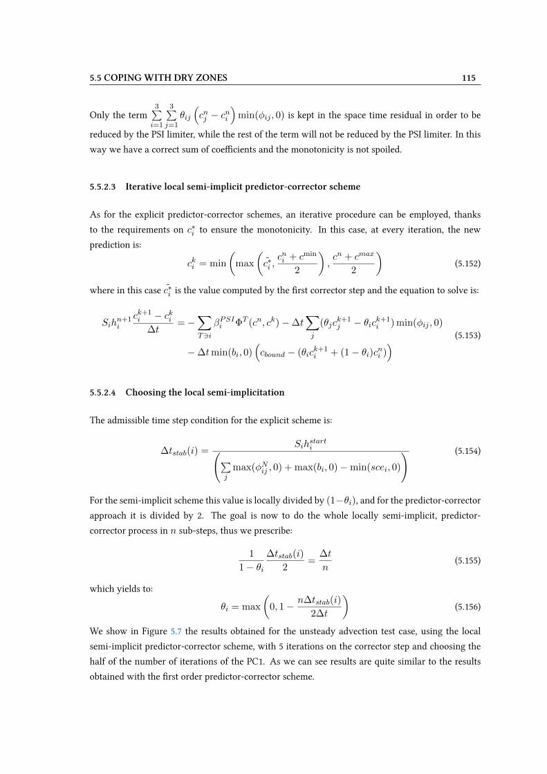
5.5 COPING WITH DRY ZONES 115
Only the term3∑i=1
3∑j=1
θij
(cnj − cni
)min(φij , 0) is kept in the space time residual in order to be
reduced by the PSI limiter, while the rest of the term will not be reduced by the PSI limiter. In this
way we have a correct sum of coeXcients and the monotonicity is not spoiled.
5.5.2.3 Iterative local semi-implicit predictor-corrector scheme
As for the explicit predictor-corrector schemes, an iterative procedure can be employed, thanks
to the requirements on c∗i to ensure the monotonicity. In this case, at every iteration, the new
prediction is:
cki = min
(max
(c∗i ,
cni + cmin
2
),cn + cmax
2
)(5.152)
where in this case c∗i is the value computed by the Vrst corrector step and the equation to solve is:
Sihn+1i
ck+1i − cki
∆t=−
∑T3i
βPSIi ΦT (cn, ck)−∆t∑j
(θjck+1j − θick+1
i ) min(φij , 0)
−∆tmin(bi, 0)(cbound − (θic
k+1i + (1− θi)cni )
) (5.153)
5.5.2.4 Choosing the local semi-implicitation
The admissible time step condition for the explicit scheme is:
∆tstab(i) =Sih
starti(∑
jmax(φNij , 0) + max(bi, 0)−min(scei, 0)
) (5.154)
For the semi-implicit scheme this value is locally divided by (1−θi), and for the predictor-correctorapproach it is divided by 2. The goal is now to do the whole locally semi-implicit, predictor-
corrector process in n sub-steps, thus we prescribe:
1
1− θi∆tstab(i)
2=
∆t
n(5.155)
which yields to:
θi = max
(0, 1− n∆tstab(i)
2∆t
)(5.156)
We show in Figure 5.7 the results obtained for the unsteady advection test case, using the local
semi-implicit predictor-corrector scheme, with 5 iterations on the corrector step and choosing the
half of the number of iterations of the PC1. As we can see results are quite similar to the results
obtained with the Vrst order predictor-corrector scheme.
116 CHAPTER 5: NEW RD PC SCHEMES FOR TIME DEPENDENT PROBLEMS
0
0.2
0.4
0.6
0.8
1
1.2
1 1.2 1.4 1.6 1.8 2
c [
g/m
3]
x [m]
NPSI
PC1PC2
PC1-5itPC2-5itLIPS-5it
exact
Figure 5.7: Unsteady tracer advection benchmark: results at section y = 0.5 m for the N,the PSI, the Predictor-Corrector Vrst order scheme (PC1), the Predictor-Corrector second orderscheme (PC2), the Predictor-Corrector Vrst order scheme using 5 iterations (PC1-5it), the Predictor-Corrector second order scheme using 5 iterations (PC2-5it) and the Locally Implicit Predictor cor-rector Scheme with 5 iterations (LIPS-5it).
5.5.2.5 Optimisation
At every new correction, the mass of c∗ added at the previous correction is removed by the term
−Sihn+1−θi (c∗i − cni ) /∆t in the RHS. A consequence is that only the monotonicity is requested
for intermediate c∗i , mass conservation is not mandatory. This allows to solve only partially the
intermediate linear system. In practice we do only one iteration of the Jacobi iterative solver. It
consists in writing a matrix A in the form A = D + E, splitting the diagonal (D) and the extra-
diagonal terms (E). Solving the system:
AX = B (5.157)
with an initial guess X0, the Vrst iteration of the Jacobi method reads:
X1 =B − EX0
D(5.158)
given our matrices, such an iteration keeps the monotonicity.
5.6 Summary
In this chapter the RD schemes have been tailored to the depth-averaged scalar transport equation
showing the compatibility with the discretized continuity equation of the Wuid. The main ingre-
dients of the RD schemes, like the concept of positive schemes and of limited non linear schemes
are used here. However, diUerences with respect to the classical RD formulation arise due to the
depth-averaged context (e.g. the conservation issue is not treated like in classical RD schemes).
5.6 SUMMARY 117
The chapter focuses then on accurate schemes for unsteady problems where the upwinding of the
derivative in time plays the most important role for accuracy. The Vrst and second order predictor-
corrector schemes are the schemes suitable for time dependent problems. The preservation of the
monotonicity has been shown for both schemes and yields diUerent time step conditions with
respect to the classical predictor-corrector RD schemes presented in [117] where the theoretical
monotonicity is not deeply discussed, even if the results shown are monotone. In addition, the
iterative version of the predictor-corrector schemes improves the accuracy and represents a new
contribution in the development of schemes for unsteady tracer transport.
A new locally semi-implicit scheme is presented to solve the wetting and drying problems. This
scheme tries to mix the good properties in terms of accuracy of the predictor-corrector schemes and
the unconditional stability of the implicit scheme. Even in this case an enhanced iterative version
is build. An optimisation is proposed to avoid the resolution of a linear system at every iteration.

118 CHAPTER 5: NEW RD PC SCHEMES FOR TIME DEPENDENT PROBLEMS
Chapter 6
VeriVcation and validation of the
numerical schemes
Ce chapitre présente la validation des nouveaux schémas proposés dans cette thèse.
Une batterie de cas tests a été choisie pour valider les diUérentes propriétés numériques
des schémas.
Dans un premier temps on estime les ordres de convergence des schémas pour des
problèmes stationnaires et non stationnaires. Ensuite, des cas plus complexes comme
la convection d’un proVl gaussien dans un champ rotationel, une rupture de barrage
sur fond mouillé ou encore un canal avec des piles de pont, sont utilisés pour vériVer
la monotonie de la solution et la conservation de la masse. Les résultats obtenus par
les nouveaux schémas sont assez satisfaisants et comparables à ceux obtenus dans
[13, 117]. Ces résultats montrent qu’eUectivement les nouveaux schémas sont plus pré-
cis et assurent au niveau discret la conservation de la masse et la monotonie.
Le traitement des zones avec des bancs découvrants est testé avec une rupture de bar-
rage sur fond sec et avec le test de Thacker. Dans les deux cas, les schémas se montrent
appropriés à ce type de problèmes.
Des comparaisons en termes de nombre d’itérations ou temps de calcul, sont aussi ef-
fectuées de manière systématique aVn de donner une idée de l’eXcacité des schémas.
L’inWuence du maillage sur la solution pour les schémas aux VF et aux RD est aussi
soulignée dans le premier cas test.
Le chapitre se termine avec un cas réel où les résultats numériques sont comparés à
des mesures. Le but de ce dernier test est la validation d’un des schémas sur un cas
industriel.
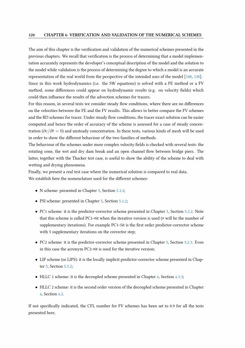
120 CHAPTER 6: VERIFICATION AND VALIDATION OF THE NUMERICAL SCHEMES
The aim of this chapter is the veriVcation and validation of the numerical schemes presented in the
previous chapters. We recall that veriVcation is the process of determining that a model implemen-
tation accurately represents the developer’s conceptual description of the model and the solution to
the model while validation is the process of determining the degree to which a model is an accurate
representation of the real world from the perspective of the intended uses of the model [108, 138].
Since in this work hydrodynamics (i.e. the SW equations) is solved with a FE method or a FV
method, some diUerences could appear on hydrodynamic results (e.g. on velocity Velds) which
could then inWuence the results of the advection schemes for tracers.
For this reason, in several tests we consider steady Wow conditions, where there are no diUerences
on the velocities between the FE and the FV results. This allows to better compare the FV schemes
and the RD schemes for tracer. Under steady Wow conditions, the tracer exact solution can be easier
computed and hence the order of accuracy of the scheme is assessed for a case of steady concen-
tration (∂c/∂t = 0) and unsteady concentration. In these tests, various kinds of mesh will be used
in order to show the diUerent behaviour of the two families of methods.
The behaviour of the schemes under more complex velocity Velds is checked with several tests: the
rotating cone, the wet and dry dam break and an open channel Wow between bridge piers. The
latter, together with the Thacker test case, is useful to show the ability of the scheme to deal with
wetting and drying phenomena.
Finally, we present a real test case where the numerical solution is compared to real data.
We establish here the nomenclature used for the diUerent schemes:
• N scheme: presented in Chapter 5, Section 5.1.2;
• PSI scheme: presented in Chapter 5, Section 5.1.2;
• PC1 scheme: it is the predictor-corrector scheme presented in Chapter 5, Section 5.2.2. Note
that this scheme is called PC1-#it when the iterative version is used (# will be the number of
supplementary iterations). For example PC1-5it is the Vrst order predictor-corrector scheme
with 5 supplementary iterations on the corrector step;
• PC2 scheme: it is the predictor-corrector scheme presented in Chapter 5, Section 5.2.3. Even
in this case the acronym PC2-#it is used for the iterative version;
• LIP scheme (or LIPS): it is the locally implicit predictor-corrector scheme presented in Chap-
ter 5, Section 5.5.2;
• HLLC 1 scheme: it is the decoupled scheme presented in Chapter 4, Section 4.1.3;
• HLLC 2 scheme: it is the second order version of the decoupled scheme presented in Chapter
4, Section 4.2.
If not speciVcally indicated, the CFL number for FV schemes has been set to 0.9 for all the tests
presented here.
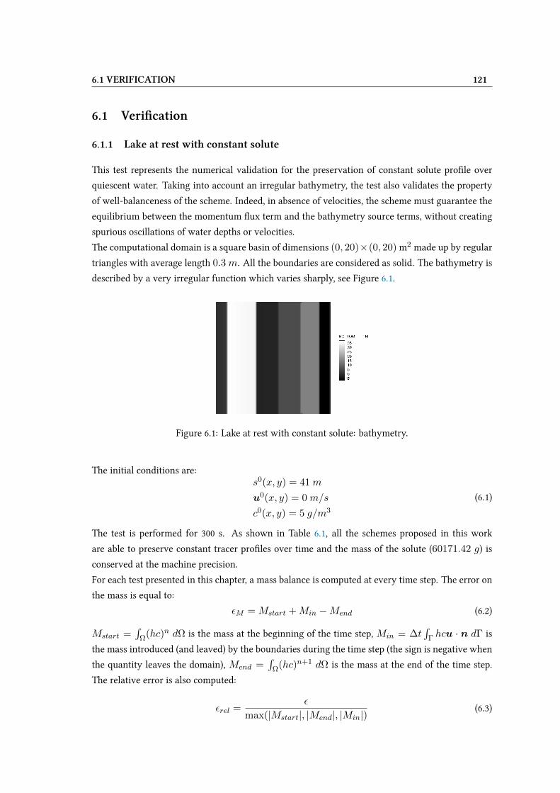
6.1 VERIFICATION 121
6.1 VeriVcation
6.1.1 Lake at rest with constant solute
This test represents the numerical validation for the preservation of constant solute proVle over
quiescent water. Taking into account an irregular bathymetry, the test also validates the property
of well-balanceness of the scheme. Indeed, in absence of velocities, the scheme must guarantee the
equilibrium between the momentum Wux term and the bathymetry source terms, without creating
spurious oscillations of water depths or velocities.
The computational domain is a square basin of dimensions (0, 20)×(0, 20) m2 made up by regular
triangles with average length 0.3 m. All the boundaries are considered as solid. The bathymetry is
described by a very irregular function which varies sharply, see Figure 6.1.
Figure 6.1: Lake at rest with constant solute: bathymetry.
The initial conditions are:s0(x, y) = 41 m
u0(x, y) = 0 m/s
c0(x, y) = 5 g/m3
(6.1)
The test is performed for 300 s. As shown in Table 6.1, all the schemes proposed in this work
are able to preserve constant tracer proVles over time and the mass of the solute (60171.42 g) is
conserved at the machine precision.
For each test presented in this chapter, a mass balance is computed at every time step. The error on
the mass is equal to:
εM = Mstart +Min −Mend (6.2)
Mstart =∫
Ω(hc)n dΩ is the mass at the beginning of the time step, Min = ∆t∫
Γ hcu · n dΓ is
the mass introduced (and leaved) by the boundaries during the time step (the sign is negative when
the quantity leaves the domain), Mend =∫
Ω(hc)n+1 dΩ is the mass at the end of the time step.
The relative error is also computed:
εrel =ε
max(|Mstart|, |Mend|, |Min|)(6.3)
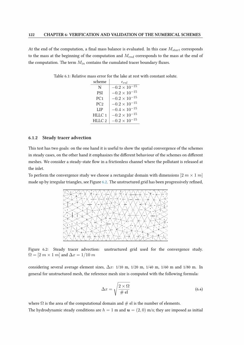
122 CHAPTER 6: VERIFICATION AND VALIDATION OF THE NUMERICAL SCHEMES
At the end of the computation, a Vnal mass balance is evaluated. In this caseMstart corresponds
to the mass at the beginning of the computation and Mend corresponds to the mass at the end of
the computation. The termMin contains the cumulated tracer boundary Wuxes.
Table 6.1: Relative mass error for the lake at rest with constant solute.scheme εrel
N −0.2× 10⁻¹⁵
PSI −0.2× 10⁻¹⁵
PC1 −0.2× 10⁻¹⁵
PC2 −0.2× 10⁻¹⁵
LIP −0.4× 10⁻¹⁵
HLLC 1 −0.2× 10⁻¹⁵
HLLC 2 −0.2× 10⁻¹⁵
6.1.2 Steady tracer advection
This test has two goals: on the one hand it is useful to show the spatial convergence of the schemes
in steady cases, on the other hand it emphasizes the diUerent behaviour of the schemes on diUerent
meshes. We consider a steady-state Wow in a frictionless channel where the pollutant is released at
the inlet.
To perform the convergence study we choose a rectangular domain with dimensions [2 m× 1 m]
made up by irregular triangles, see Figure 6.2. The unstructured grid has been progressively reVned,
Figure 6.2: Steady tracer advection: unstructured grid used for the convergence study.Ω = [2 m× 1 m] and ∆x = 1/10 m
considering several average element sizes, ∆x: 1/10 m, 1/20 m, 1/40 m, 1/60 m and 1/80 m. In
general for unstructured mesh, the reference mesh size is computed with the following formula:
∆x =
√2× Ω
# el(6.4)
where Ω is the area of the computational domain and # el is the number of elements.
The hydrodynamic steady conditions are h = 1 m and u = (2, 0) m/s; they are imposed as initial
6.1 VERIFICATION 123
Table 6.2: Steady tracer advection: order of accuracy.
∆x #el ON OHLLC1 OPSI OHLLC2
0.1 4400.05 1749 0.95 0.53 1.84 1.430.025 6876 0.95 0.75 1.7 1.570.016 16739 1.01 0.79 1.16 1.630.0125 26842 -0.46 1.19 1.52 1.59
and boundary conditions. Since the truncation error analysis holds true for smooth solutions, we
choose the following boundary inlet tracer proVle:
cbound = c(x = 0, y) = e(−2y) sin(πy)2 g/l
At the outlet we leave a free boundary condition for the tracer. The duration of the test is set to 2,5
s such that at the Vnal time, tf , all schemes have converged to the steady solution.
The exact solution given by the method of characteristics is simply:
cex = c(x, y) = e(−2y) sin(πy)2 g/l
To measure the accuracy of the numerical schemes, we take the L2 norm of the error in space:
||ε||L2 =
√1
npoin
∑i∈Th
(cex(tf )− cnum(tf ))2
where npoin is the total number of nodes, cex is the exact solution, cnum is the numerical solution
and tf is the Vnal time. The convergence rates of the diUerent schemes and the tracer proVles
obtained at the end of the simulation at the transversal section x = 2 m are shown in Figure 6.3.
This test is important to assess the order of the already existing schemes (N and PSI) and of the
new schemes. For the new RD schemes, which are more appropriate for time dependent problems,
we just want to verify that in steady cases they are able to revert to the PSI scheme. The curves are
exactly superimposed for the PSI, PC1, PC2 and LIP scheme. Thus they are not shown. The choice
of the number of sub-steps n for the locally implicit scheme (see Section 5.5.2.4) is not trivial and
in general it must be related to the arbitrary time step chosen to solve the hydrodynamics.
In this case, to choose the parameter n, Vrstly we consider that in wet cases we are not interested
in having θi = 1 and we prefer to have θi = 0 in steady cases, in order to recover the PSI scheme.
Then, in order to be comparable to the other RD schemes, n is chosen so as the number of iterations
is the same as the N and the PSI scheme. Hence, in this way, the results of the LIP schemes are
equal to the results of the PSI scheme.
The tracer proVles shown in Figure 6.3 agree with the convergence rates, indeed the most diUusive
schemes are the HLLC 1 and the N, while the HLLC 2 and the PSI are the most accurate.
The order of convergence for the diUerent schemes are shown in Table 6.2. The N and the HLLC
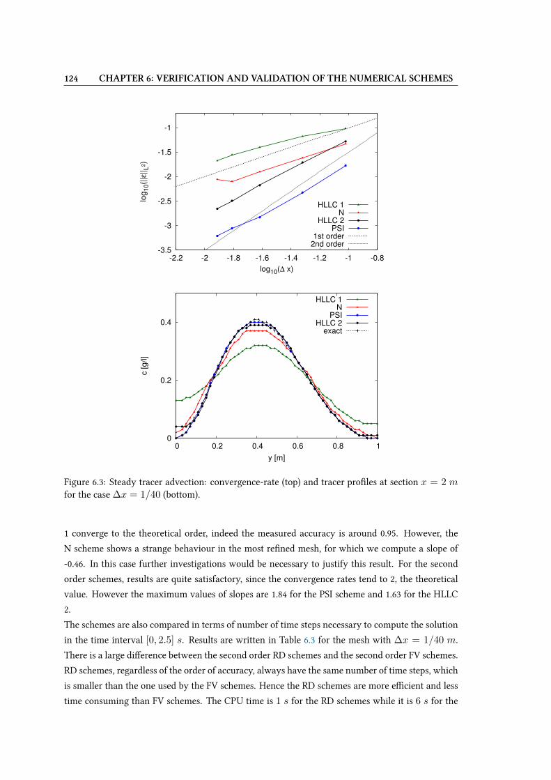
124 CHAPTER 6: VERIFICATION AND VALIDATION OF THE NUMERICAL SCHEMES
-3.5
-3
-2.5
-2
-1.5
-1
-2.2 -2 -1.8 -1.6 -1.4 -1.2 -1 -0.8
log
10(|
|ε||
L2)
log10(∆ x)
HLLC 1N
HLLC 2PSI
1st order2nd order
0
0.2
0.4
0 0.2 0.4 0.6 0.8 1
c [
g/l]
y [m]
HLLC 1N
PSIHLLC 2
exact
Figure 6.3: Steady tracer advection: convergence-rate (top) and tracer proVles at section x = 2 mfor the case ∆x = 1/40 (bottom).
1 converge to the theoretical order, indeed the measured accuracy is around 0.95. However, the
N scheme shows a strange behaviour in the most reVned mesh, for which we compute a slope of
-0.46. In this case further investigations would be necessary to justify this result. For the second
order schemes, results are quite satisfactory, since the convergence rates tend to 2, the theoretical
value. However the maximum values of slopes are 1.84 for the PSI scheme and 1.63 for the HLLC
2.
The schemes are also compared in terms of number of time steps necessary to compute the solution
in the time interval [0, 2.5] s. Results are written in Table 6.3 for the mesh with ∆x = 1/40 m.
There is a large diUerence between the second order RD schemes and the second order FV schemes.
RD schemes, regardless of the order of accuracy, always have the same number of time steps, which
is smaller than the one used by the FV schemes. Hence the RD schemes are more eXcient and less
time consuming than FV schemes. The CPU time is 1 s for the RD schemes while it is 6 s for the
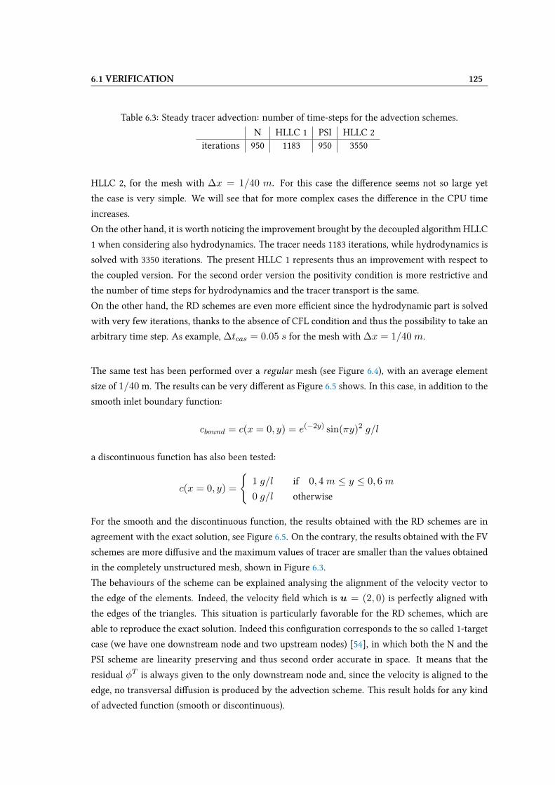
6.1 VERIFICATION 125
Table 6.3: Steady tracer advection: number of time-steps for the advection schemes.
N HLLC 1 PSI HLLC 2iterations 950 1183 950 3550
HLLC 2, for the mesh with ∆x = 1/40 m. For this case the diUerence seems not so large yet
the case is very simple. We will see that for more complex cases the diUerence in the CPU time
increases.
On the other hand, it is worth noticing the improvement brought by the decoupled algorithm HLLC
1 when considering also hydrodynamics. The tracer needs 1183 iterations, while hydrodynamics is
solved with 3350 iterations. The present HLLC 1 represents thus an improvement with respect to
the coupled version. For the second order version the positivity condition is more restrictive and
the number of time steps for hydrodynamics and the tracer transport is the same.
On the other hand, the RD schemes are even more eXcient since the hydrodynamic part is solved
with very few iterations, thanks to the absence of CFL condition and thus the possibility to take an
arbitrary time step. As example, ∆tcas = 0.05 s for the mesh with ∆x = 1/40 m.
The same test has been performed over a regular mesh (see Figure 6.4), with an average element
size of 1/40 m. The results can be very diUerent as Figure 6.5 shows. In this case, in addition to the
smooth inlet boundary function:
cbound = c(x = 0, y) = e(−2y) sin(πy)2 g/l
a discontinuous function has also been tested:
c(x = 0, y) =
1 g/l if 0, 4 m ≤ y ≤ 0, 6 m
0 g/l otherwise
For the smooth and the discontinuous function, the results obtained with the RD schemes are in
agreement with the exact solution, see Figure 6.5. On the contrary, the results obtained with the FV
schemes are more diUusive and the maximum values of tracer are smaller than the values obtained
in the completely unstructured mesh, shown in Figure 6.3.
The behaviours of the scheme can be explained analysing the alignment of the velocity vector to
the edge of the elements. Indeed, the velocity Veld which is u = (2, 0) is perfectly aligned with
the edges of the triangles. This situation is particularly favorable for the RD schemes, which are
able to reproduce the exact solution. Indeed this conVguration corresponds to the so called 1-target
case (we have one downstream node and two upstream nodes) [54], in which both the N and the
PSI scheme are linearity preserving and thus second order accurate in space. It means that the
residual φT is always given to the only downstream node and, since the velocity is aligned to the
edge, no transversal diUusion is produced by the advection scheme. This result holds for any kind
of advected function (smooth or discontinuous).

126 CHAPTER 6: VERIFICATION AND VALIDATION OF THE NUMERICAL SCHEMES
On the contrary, this mesh is inconvenient for FV because, as we use a vertex-centred scheme,
the control volumes are distorted and an artiVcial Wux is developed along faces which cross the
diagonals of the squares.
We suppose that the use of a cell-centred method, in this particular case (with regular mesh and
constant horizontal velocities) could probably improve the results in terms of transversal diUusion.
Indeed, where the face element is aligned with velocities we will have zero-Wux faces, so the scheme
should be less diUusive. However, this kind of scheme has not been tested yet.
Finally the conservation of mass is veriVed through a mass balance. The relative error at the end
Figure 6.4: Steady tracer advection: regular mesh. Ω = [2 m× 1 m] and ∆x = 1/40 m
of the computation is about 10−15 for all the RD and FV schemes.
6.1.3 Unsteady tracer advection benchmark
This test was already presented in Chapter 4 and it is here recalled in order to measure the accu-
racy of the schemes and to give a more detailed comparison of all the schemes. The domain is a
rectangular channel of (0, 2)× (0, 1) m2 made up by irregular triangles (as the one of Figure 6.2).
The convergence test is performed on a series of Vve unstructured meshes, like in the steady case.
The mesh sizes are, from the coarsest to the Vnest: 1/10 m, 1/20 m, 1/40 m, 1/80 m, 1/160 m.
The water depth in the channel is constant and equal to 1 m, and the Wow rate is 1 m3/s. The
simulation time is set to 1 s. The initial tracer proVle is described by the function:
c0(x, y) =
cos2(2πr) g/m3 if r ≤ 0.25
0 g/m3 otherwisewith r =
√(x− 0.5)2 + (y − 0.5)2 m
In Figure 6.6 we show the rates of convergence for all schemes, the orders of accuracy are displayed
in Table 6.4 and Figure 6.7 shows the tracer proVles obtained at the end of the simulation at the
section y = 0.5 for the mesh with h = 1/40 m.
Figure 6.6 shows that the HLLC 1, the N and the PSI schemes are the most diUusive schemes with
a rate of convergence lower than one. This behaviour is normal since all these schemes are Vrst
order in space and in time, hence they are not suitable for time dependent problems like this one.
On the contrary the new schemes introduced in this work occupy the region with lower magnitude

6.1 VERIFICATION 127
0
0.2
0.4
0.6
0.8
1
1.2
0 0.2 0.4 0.6 0.8 1
c [
g/l]
y [m]
HLLC 1N
PSIHLLC 2
exact
0
0.2
0.4
0 0.2 0.4 0.6 0.8 1
c [
g/l]
y [m]
HLLC 1N
PSIHLLC 2
exact
Figure 6.5: Steady tracer advection: results at section x = 2 m for the advection of a discontinuousfunction (top) and a continuous function (bottom) over a regular grid.
error and according to the scheme chosen, the slope is between 1 and 2. Analyzing the Figure 6.6
we note that the average convergence rates for the PC1 and the PC1-5it are about 1. Indeed, both
schemes are only Vrst order accurate in time. However, we note that they are more accurate than
the N and the PSI and they give a better estimate of the maximum tracer value, as shown in Figure
6.7. The reason is related to the upwind of the derivative in time which is done in the PC schemes
while it is absent in the N and PSI schemes.
In addition, comparing the scheme without iteration (PC1) and the scheme with Vve supplementary
iterations on the corrector steps (PC1-5it), we note that the maximum value of tracer increases
thanks to the supplementary iterations.
We consider now the PC2 and the PC2-5it. The convergence rate of these schemes is more regular:
the PC2 gives a slope of about 1.4, while the PC2-5it tends to 1.7. These schemes are formally
second order accurate in space and in time, however their convergence rate is less than two. In
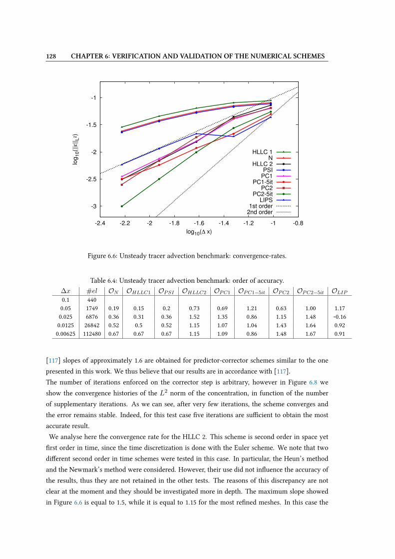
128 CHAPTER 6: VERIFICATION AND VALIDATION OF THE NUMERICAL SCHEMES
-3
-2.5
-2
-1.5
-1
-2.4 -2.2 -2 -1.8 -1.6 -1.4 -1.2 -1 -0.8
log
10(|
|ε||
L2)
log10(∆ x)
HLLC 1N
HLLC 2PSI
PC1PC1-5it
PC2PC2-5it
LIPS1st order
2nd order
Figure 6.6: Unsteady tracer advection benchmark: convergence-rates.
Table 6.4: Unsteady tracer advection benchmark: order of accuracy.∆x #el ON OHLLC1 OPSI OHLLC2 OPC1 OPC1−5it OPC2 OPC2−5it OLIP0.1 4400.05 1749 0.19 0.15 0.2 0.73 0.69 1.21 0.63 1.00 1.170.025 6876 0.36 0.31 0.36 1.52 1.35 0.86 1.15 1.48 -0.160.0125 26842 0.52 0.5 0.52 1.15 1.07 1.04 1.43 1.64 0.920.00625 112480 0.67 0.67 0.67 1.15 1.09 0.86 1.48 1.67 0.91
[117] slopes of approximately 1.6 are obtained for predictor-corrector schemes similar to the one
presented in this work. We thus believe that our results are in accordance with [117].
The number of iterations enforced on the corrector step is arbitrary, however in Figure 6.8 we
show the convergence histories of the L2 norm of the concentration, in function of the number
of supplementary iterations. As we can see, after very few iterations, the scheme converges and
the error remains stable. Indeed, for this test case Vve iterations are suXcient to obtain the most
accurate result.
We analyse here the convergence rate for the HLLC 2. This scheme is second order in space yet
Vrst order in time, since the time discretization is done with the Euler scheme. We note that two
diUerent second order in time schemes were tested in this case. In particular, the Heun’s method
and the Newmark’s method were considered. However, their use did not inWuence the accuracy of
the results, thus they are not retained in the other tests. The reasons of this discrepancy are not
clear at the moment and they should be investigated more in depth. The maximum slope showed
in Figure 6.6 is equal to 1.5, while it is equal to 1.15 for the most reVned meshes. In this case the

6.1 VERIFICATION 129
0
0.2
0.4
0.6
0.8
1
1 1.2 1.4 1.6 1.8 2
c [
g/m
3]
x [m]
HLLC 1N
HLLC 2PSI
PC1PC1-5it
PC2PC2-5it
LIPSexact
Figure 6.7: Unsteady tracer advection benchmark: tracer proVles at tf = 1 s and for y = 0.5 m.
error in time is bigger than the error in space, thus the scheme is not able to reproduce the second
order rate. However the results are clearly better with respect to the HLLC 1.
Finally the convergence study for the LIP scheme is more complicated due to the local implicitation
coeXcient. In order to compare this scheme to the others, the parameter n has been Vxed to obtain
the same number of iteration of the PSI scheme. As we can see the rate of convergence is almost 1
and this agrees with the formal accuracy of the scheme. However, as for the PC1, for a given mesh
size the error is smaller than the error produced by the N and the PSI thanks to the upwind of the
derivative in time.
Concerning the monotonicity, we observe that all schemes presented give a monotone solution.
Figure 6.9 shows the results obtained with the HLLC schemes when using the coupled and the
decoupled formulation. The mesh size is Vxed at ∆x = 1/40 m and the proVles are obtained
at the section y = 0.5 m. For both the Vrst and the second order schemes, we note that the
decoupled formulation proposed in this work allows to decrease the numerical diUusion of the
coupled formulation. The decoupled formulation is also convenient from a computational point of
view, indeed for the Vrst order case the decoupled scheme updates the tracer in 191 iterations while
the coupled one needs 1143 iterations (see Table 6.5).
In Table 6.6 we show the variation of the ratio between the hydrodynamic time steps and the
transport time steps according to various Froude numbers, for the Vrst order HLLC. The test is
performed on the mesh ∆x = 1/40 m and the water depth varies in order to recover diUerent
Froude number. It is clear that the ratio between the hydrodynamic time step and the transport
time step decreases when the Froude number grows up. These results are similar to the one shown

130 CHAPTER 6: VERIFICATION AND VALIDATION OF THE NUMERICAL SCHEMES
0.006
0.008
0.01
0.012
0.014
0.016
0.018
0.02
0.1 1 10 100
||E
||L
2
# supplementary iterations
PC2-#iter
Figure 6.8: Unsteady tracer advection benchmark: convergence for the PC2 scheme.
Table 6.5: Unsteady tracer advection benchmark: number of time-steps for the FV schemes.
HLLC 1 HLLC 2hydrodynamics 1143 1143
tracer 191 381
in [13]. The comparison in terms of number of iterations for all schemes is presented in Table 6.7.
Table 6.6: Unsteady tracer advection benchmark: hydrodynamic and transport iterations for diUer-ent Froude numbers, for the HLLC 1.
Fr hydrodynamic iterations transport iterations0.66 720 2310.95 580 1881.42 480 235
It is worth noticing that even if the number of time steps is the same for the PC1 (or PC2) and the
PC1-5it (or PC2-5it), the computational time is larger when more iterations are added. Examples
about the CPU time will be more clear for complex cases, indeed in this test, due to the simple
conditions and the short duration, the computational time is 1s for both the PC2 and the PC2-5it.
In this test the FV and RD schemes which are Vrst order accurate in space and in time, have
approximately the same time step, thus the total number of iterations are equal.
6.1.4 Rotating cone
The rotating cone case is a diXcult test because the velocity varies in space: the tracer is submitted
to a rotational velocity Veld. For this test we do not solve the Saint-Venant system, but just the
tracer equation, using a constant value of water depth. The aim is to show howmuch the numerical
6.1 VERIFICATION 131
0
0.2
0.4
0.6
0.8
1
1 1.2 1.4 1.6 1.8 2
c [g/m
3]
x [m]
HLLC 1HLLC 1 coupled
HLLC 2HLLC 2 coupled
Figure 6.9: Unsteady tracer advection benchmark: tracer proVles for the coupled and the decoupledHLLC scheme at section y = 0.5 m.
Table 6.7: Unsteady case: number of time-steps for the advection schemes.
N HLLC 1 PSI HLLC 2 PC1 PC1-5it PC2 PC2-5it LIPiterations 180 191 180 381 396 396 396 396 180
scheme is diUusive in a time dependent case. The maximum value of the cone after one rotation
can be considered a good indicator of the numerical diUusion. The velocity Veld is constant in time
and equal to:
u =
u(x, y) = −(y − 10.05) m/s
v(x, y) = (x− 10.05) m/s
The initial condition for the tracer is a Gaussian function:
c0(x, y) = e−[(x−15)2+(y−10.2)2]
2 g/l
which bounds the solution between 0 and 1. The problem is solved on a square domain of dimen-
sions [20.1 × 20.1] m2 and formed by squares of side 0.3 m split into two triangles. After one
period the cone is again at the initial position but the maximum value is diminished due to the
numerical diUusion produced by the schemes.
The maximum and the minimum values are presented in Table 6.8. The better estimates of the
maximum are obtained with the LIP scheme, the PC1-5it and the PC2-5it schemes. However the
Vrst two schemes are only Vrst order accurate in time and the good estimate of the maximum is
mostly due to the upwind of the derivative in time.
Again, the improvement brought by the new RD schemes presented in this work is clear. Con-
cerning the FV schemes, we note that the HLLC 2 computes a maximum which is about the triple
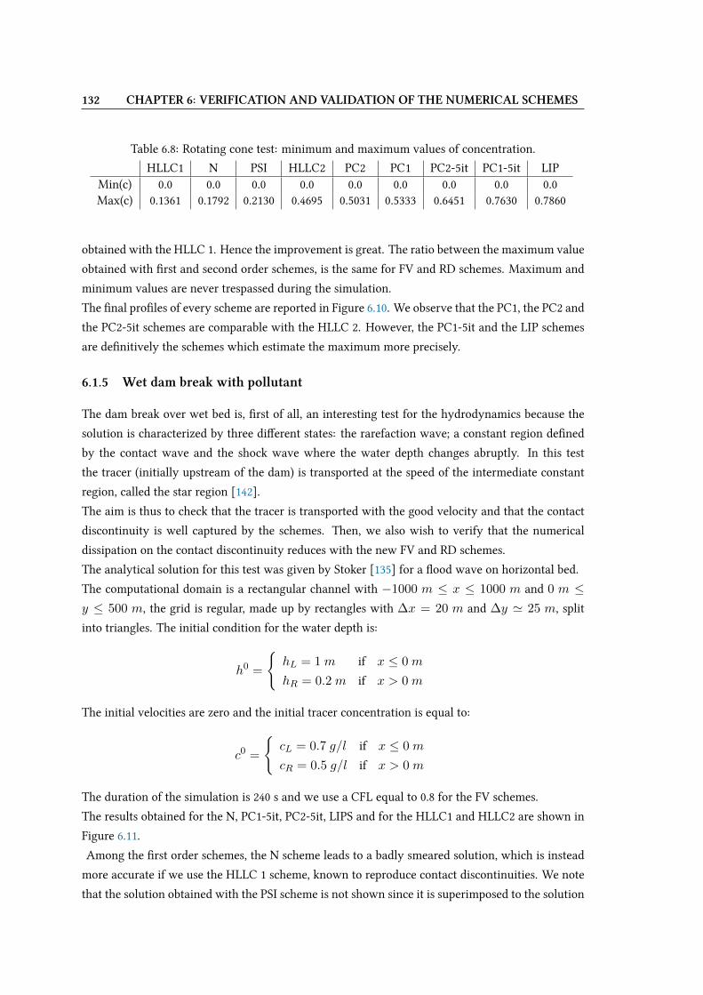
132 CHAPTER 6: VERIFICATION AND VALIDATION OF THE NUMERICAL SCHEMES
Table 6.8: Rotating cone test: minimum and maximum values of concentration.
HLLC1 N PSI HLLC2 PC2 PC1 PC2-5it PC1-5it LIPMin(c) 0.0 0.0 0.0 0.0 0.0 0.0 0.0 0.0 0.0Max(c) 0.1361 0.1792 0.2130 0.4695 0.5031 0.5333 0.6451 0.7630 0.7860
obtained with the HLLC 1. Hence the improvement is great. The ratio between the maximum value
obtained with Vrst and second order schemes, is the same for FV and RD schemes. Maximum and
minimum values are never trespassed during the simulation.
The Vnal proVles of every scheme are reported in Figure 6.10. We observe that the PC1, the PC2 and
the PC2-5it schemes are comparable with the HLLC 2. However, the PC1-5it and the LIP schemes
are deVnitively the schemes which estimate the maximum more precisely.
6.1.5 Wet dam break with pollutant
The dam break over wet bed is, Vrst of all, an interesting test for the hydrodynamics because the
solution is characterized by three diUerent states: the rarefaction wave; a constant region deVned
by the contact wave and the shock wave where the water depth changes abruptly. In this test
the tracer (initially upstream of the dam) is transported at the speed of the intermediate constant
region, called the star region [142].
The aim is thus to check that the tracer is transported with the good velocity and that the contact
discontinuity is well captured by the schemes. Then, we also wish to verify that the numerical
dissipation on the contact discontinuity reduces with the new FV and RD schemes.
The analytical solution for this test was given by Stoker [135] for a Wood wave on horizontal bed.
The computational domain is a rectangular channel with −1000 m ≤ x ≤ 1000 m and 0 m ≤y ≤ 500 m, the grid is regular, made up by rectangles with ∆x = 20 m and ∆y ' 25 m, split
into triangles. The initial condition for the water depth is:
h0 =
hL = 1 m if x ≤ 0 m
hR = 0.2 m if x > 0 m
The initial velocities are zero and the initial tracer concentration is equal to:
c0 =
cL = 0.7 g/l if x ≤ 0 m
cR = 0.5 g/l if x > 0 m
The duration of the simulation is 240 s and we use a CFL equal to 0.8 for the FV schemes.
The results obtained for the N, PC1-5it, PC2-5it, LIPS and for the HLLC1 and HLLC2 are shown in
Figure 6.11.
Among the Vrst order schemes, the N scheme leads to a badly smeared solution, which is instead
more accurate if we use the HLLC 1 scheme, known to reproduce contact discontinuities. We note
that the solution obtained with the PSI scheme is not shown since it is superimposed to the solution
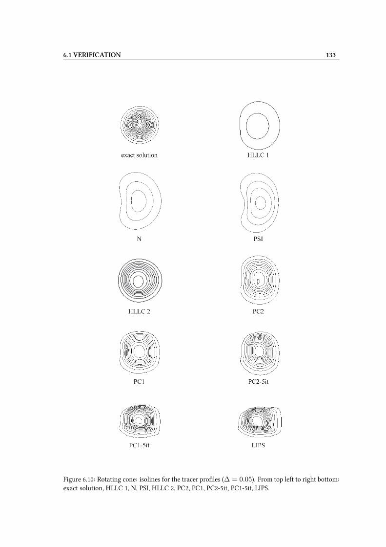
6.1 VERIFICATION 133
Figure 6.10: Rotating cone: isolines for the tracer proVles (∆ = 0.05). From top left to right bottom:exact solution, HLLC 1, N, PSI, HLLC 2, PC2, PC1, PC2-5it, PC1-5it, LIPS.

134 CHAPTER 6: VERIFICATION AND VALIDATION OF THE NUMERICAL SCHEMES
0.45
0.5
0.55
0.6
0.65
0.7
0.75
200 300 400 500 600 700
c [
g/l]
x [m]
HLLC 1N
HLLC 2PC1-5itPC2-5it
LIPSexact
Figure 6.11: Wet dam break: solutions for the contact discontinuity computed with the numericalschemes at time 240 s at the channel axis.
obtained with the N scheme.
Among the new schemes, the HLLC 2 and the PC1-5it are the most accurate schemes while the
PC2-5it and the LIP scheme are slightly less accurate and little diUerences between these schemes
are observed in Figure 6.11. We conclude that the new schemes are more appropriate to represent
contact discontinuities with very small numerical diUusion. In order to better appreciate the inWu-
ence of the decoupled algorithm for the FV schemes, we show in Figure 6.12, the results obtained
with the coupled and the decoupled scheme for the Vrst and the second order schemes. We observe
that the numerical diUusion is decreased by the decoupled algorithm, however, the diUerences are
smaller for the second order scheme. In table 6.9 we write the number of hydrodynamic steps and
0.45
0.5
0.55
0.6
0.65
0.7
0.75
200 300 400 500 600 700
c [g/l]
x [m]
exactHLLC 1
HLLC 1 coupledHLLC 2
HLLC 2 coupled
0.45
0.5
0.55
0.6
0.65
0.7
0.75
200 300 400 500 600 700
c [g/l]
x [m]
PC1PC1-5it
PC2PC2-5it
exact
Figure 6.12: Wet dam break: solutions solution at the channel axis at time 240 s for the contactdiscontinuity computed with the HLLC schemes (left) and the RD schemes (right).
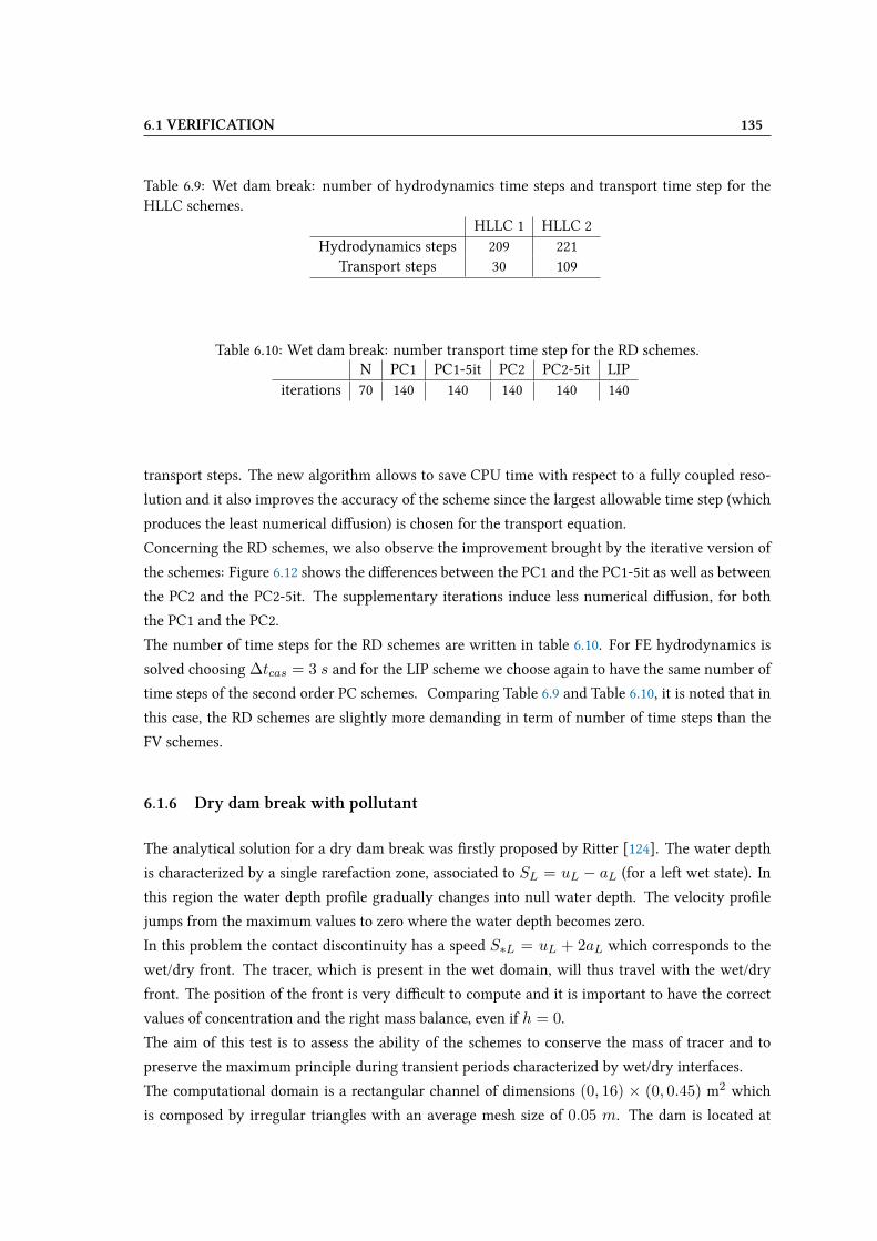
6.1 VERIFICATION 135
Table 6.9: Wet dam break: number of hydrodynamics time steps and transport time step for theHLLC schemes.
HLLC 1 HLLC 2Hydrodynamics steps 209 221
Transport steps 30 109
Table 6.10: Wet dam break: number transport time step for the RD schemes.N PC1 PC1-5it PC2 PC2-5it LIP
iterations 70 140 140 140 140 140
transport steps. The new algorithm allows to save CPU time with respect to a fully coupled reso-
lution and it also improves the accuracy of the scheme since the largest allowable time step (which
produces the least numerical diUusion) is chosen for the transport equation.
Concerning the RD schemes, we also observe the improvement brought by the iterative version of
the schemes: Figure 6.12 shows the diUerences between the PC1 and the PC1-5it as well as between
the PC2 and the PC2-5it. The supplementary iterations induce less numerical diUusion, for both
the PC1 and the PC2.
The number of time steps for the RD schemes are written in table 6.10. For FE hydrodynamics is
solved choosing ∆tcas = 3 s and for the LIP scheme we choose again to have the same number of
time steps of the second order PC schemes. Comparing Table 6.9 and Table 6.10, it is noted that in
this case, the RD schemes are slightly more demanding in term of number of time steps than the
FV schemes.
6.1.6 Dry dam break with pollutant
The analytical solution for a dry dam break was Vrstly proposed by Ritter [124]. The water depth
is characterized by a single rarefaction zone, associated to SL = uL − aL (for a left wet state). In
this region the water depth proVle gradually changes into null water depth. The velocity proVle
jumps from the maximum values to zero where the water depth becomes zero.
In this problem the contact discontinuity has a speed S∗L = uL + 2aL which corresponds to the
wet/dry front. The tracer, which is present in the wet domain, will thus travel with the wet/dry
front. The position of the front is very diXcult to compute and it is important to have the correct
values of concentration and the right mass balance, even if h = 0.
The aim of this test is to assess the ability of the schemes to conserve the mass of tracer and to
preserve the maximum principle during transient periods characterized by wet/dry interfaces.
The computational domain is a rectangular channel of dimensions (0, 16) × (0, 0.45) m2 which
is composed by irregular triangles with an average mesh size of 0.05 m. The dam is located at
136 CHAPTER 6: VERIFICATION AND VALIDATION OF THE NUMERICAL SCHEMES
x = 8 m. The initial conditions for the wet part of the domain, on the left of the dam, are:hL = 0.4 m
uL = 0 m/s
cL = 1 g/l
(6.5)
All the variables are set to zero in the dry part, on the right of the dam:hR = 0 m
uR = 0 m/s
cR = 0 g/l
(6.6)
The duration of the test is 1.5 s.
In this case, we only compare the schemes able to handle dry states that are the HLLC 1 , the HLLC
2 and the LIP scheme. In Vgure 6.13 the results obtained with these schemes are plotted. The FV
schemes seems more appropriate to solve this problem than the RD schemes. Indeed the water
depth proVle is better approximated, since there is a smooth transition into zero. However, the
second order HLLC exhibits a very small oscillation in the front. Even the velocity proVle is better
estimated with the FV schemes.
On the contrary, the FE schemes cannot reproduce the continuous water depth proVle and they
show instead a jump in h preceded by some oscillations. For the FE scheme we set ∆tcas = 0.01 s,
in order to get enough accurate results for hydrodynamics. Since in this case the tracer solution
is generated by the wet/dry front advancement, the choice of the parameter n for the LIP scheme
is not so signiVcant. Indeed, at the wet/dry interface the LIP scheme is characterized by θi = 1,
hence taking n = 1 is enough in this case to get correct solutions. The total number of time-steps
for the hydrodynamics and the LIP scheme is thus 150.
The solutions obtained with the diUerent schemes for the tracer, can be easily justiVed consider-
ing the results obtained for hydrodynamics. The wet/dry front, thus the tracer proVle, is better
estimated with the FV schemes. The tracer proVle computed by the LIP scheme is far from the
analytical solution, however, the monotonicity of the tracer is strictly ensured. We prove with this
test that the LIP scheme is perfectly able to handle dry problems.
The HLLC 2 is less accurate in the prediction of the wet/dry front than the HLLC 1. The rea-
son is not very clear at the moment and further investigations should be done to understand this
behaviour. However we consider that both schemes are able to treat the wetting and drying inter-
faces.
The comparison of the time-steps for Vrst and second order solutiono for FV is done in Table 6.11.
Even for the dry dam break is clear the advantage of a decoupled solution for the tracer transport,
when using the HLLC solver.
Regarding the FV schemes, we recall the formula for the dry interfaces introduced at Chapter 4.
We note that computing c = hc/h if h > εtr with εtr = 10−6, the results show small oscillation
(cmax = 1.14) at the wet/dry front which indicate a slight loss of monotonicity. Using instead
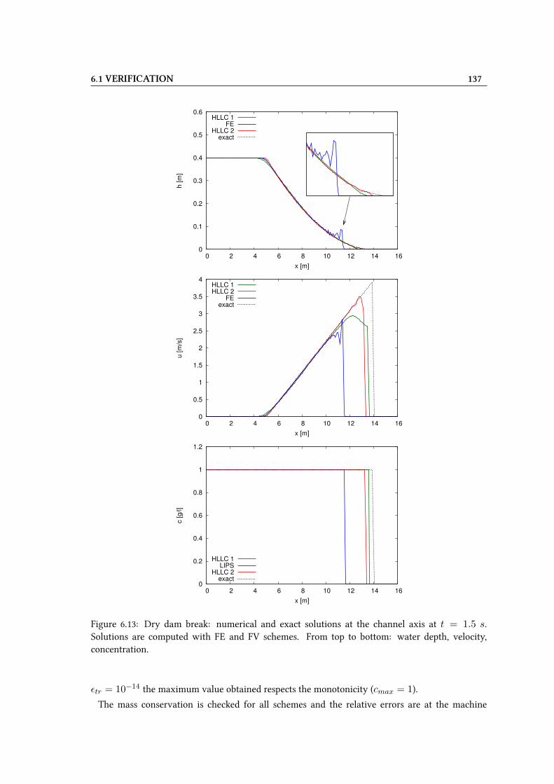
6.1 VERIFICATION 137
0
0.1
0.2
0.3
0.4
0.5
0.6
0 2 4 6 8 10 12 14 16
h [
m]
x [m]
HLLC 1FE
HLLC 2exact
0
0.5
1
1.5
2
2.5
3
3.5
4
0 2 4 6 8 10 12 14 16
u [
m/s
]
x [m]
HLLC 1HLLC 2
FEexact
0
0.2
0.4
0.6
0.8
1
1.2
0 2 4 6 8 10 12 14 16
c [
g/l]
x [m]
HLLC 1LIPS
HLLC 2exact
Figure 6.13: Dry dam break: numerical and exact solutions at the channel axis at t = 1.5 s.Solutions are computed with FE and FV schemes. From top to bottom: water depth, velocity,concentration.
εtr = 10−14 the maximum value obtained respects the monotonicity (cmax = 1).
The mass conservation is checked for all schemes and the relative errors are at the machine

138 CHAPTER 6: VERIFICATION AND VALIDATION OF THE NUMERICAL SCHEMES
Table 6.11: Dry dam break: number of hydrodynamics time steps and transport time step for theHLLC schemes.
HLLC 1 HLLC 2Hydrodynamics steps 500 600
Transport steps 165 531
precision.
6.1.7 Thacker test case with tracer
This test assesses the ability of the scheme to handle wetting and drying phenomena. As described
in Chapter 2, the solution was published by Thacker [139]. The test shows nonlinear periodic
oscillations in a basin with a frictionless paraboloid topography. The initial solution corresponds to
the exact solution at time t = 0, then the free surface oscillates with moving wet/dry boundaries
and goes back to the initial position after one period. The duration of the simulation is set to 1000
s and one period is about 237,77 s. The accuracy of the scheme can also be veriVed, indeed, the
decrease of the free surface with time corresponds to the amount of numerical diUusion produced
by the scheme.
The computational domain is a square of dimensions [4000×4000]m2 and it is made up by squares
of sides 25 m split into triangles. The parameters used for this test are: h0 = 20 m, r0 = 1200 m,
a = 1500 m and L = 4000 m. The addition of the tracer variable which moves with the water
surface was proposed in [103] and we consider the same set of parameter. The initial condition for
the tracer is:
c(r, 0) = c0exp
(− r
200r0
)g/l
where c0 = 100 and r = (x− L/2)2 − (y − L/2)2.
To compare the FV results to the RD results, we choose to enforce for the LIP scheme the same
number of iterations of the Vrst and the second order scheme. The diUerent number of iterations,
with the corresponding CPU time, are shown in table 6.12. For the LIP diUerent combinations of
time steps and sub-time steps can be chosen since hydrodynamic is solvable with a theoretically
arbitrary time step. In this case, a good compromise is represented by ∆t = 2 s for hydrodynamics.
Thus to have the same number of iterations of FV schemes, we choose once n = 1 to be comparable
with the Vrst order scheme and then n = 2 to be comparable with the second order scheme.
First of all, we stress again the large diUerence of iterations between hydrodynamics and transport
Table 6.12: Thacker test case: number of iterations for the advection schemes.HLLC 1 HLLC 2 LIP n = 1 LIP n = 2
Hydrodynamic iterations 4515 4520 500 500Transport iterations 571 1077 500 1000
CPU times 55 s 1 min 41 s 26 s 30 s
for the HLLC schemes. This justiVes the decoupled approach. Second, we note that the CPU time

6.1 VERIFICATION 139
is almost the double for the second order HLLC scheme. This is related to the reconstruction of
the interface states, done for every cell, which is very time consuming. Then, we note that the
diUerence of CPU time for the LIP with n = 1 or n = 2 is negligible, while it is very large if
compared to the HLLC 2. This example highlights the eXciency in terms of computational costs of
the LIP scheme.
In Figure 6.14 we plot the evolution of the water depth in the central point of the domain, which is
the one with the maximum value. We note that the maximum decreases with time for all schemes,
which is normal because of the numerical diUusion. The variation after 4 periods is limited to about
4 m for the HLLC 1, which is the most diUusive. For the FE scheme, the maximum variation of the
water depth is 3 m, while for the HLLC 2, the most accurate scheme, we only Vnd a diUerence of
1 m, which is a very good result.
On the contrary, the phase error seems more pronounced for FV schemes, especially for the HLLC
1 for which the phase error increases largely with time. Figure 6.15 shows the tracer and water
12
14
16
18
20
22
24
26
28
0 200 400 600 800 1000
h [
m]
t [s]
exactHLLC 1HLLC 2
FE
Figure 6.14: Thacker test case: evolution of the maximum water depth in the centre of the domain.
depth proVles obtained after 4 periods on the central axis of the domain. All schemes show a good
agreement with the theoretical solution for tracer and the values obtained also agree with the water
depth proVles. The maximum and minimum values are respected along all the simulation and the
maximum values of concentration after 4 periods are shown in Table 6.13. As expected, the second
order HLLC is more accurate then the Vrst order version and indeed we observe that the exact
solution and the computed solution are almost superimposed.
For the LIP schemes, there is no diUerence among the solution obtained with n = 1 and the one
obtained with n = 2. This behaviour is normal since, regardless of n, at the wet/dry interfaces θiwill be equal to 1 everywhere.
The schemes are mass conservative: the relative error at the end of the computation is about 10−8.
A global comparison of the advection schemes is shown in Figure 6.16. As for the water depth, the
most diUusive scheme is the HLLC 1, while the most accurate is the HLLC 2. The LIP is between
the HLLC 1 and the HLLC 2. Results demonstrate that these schemes are suitable for problems
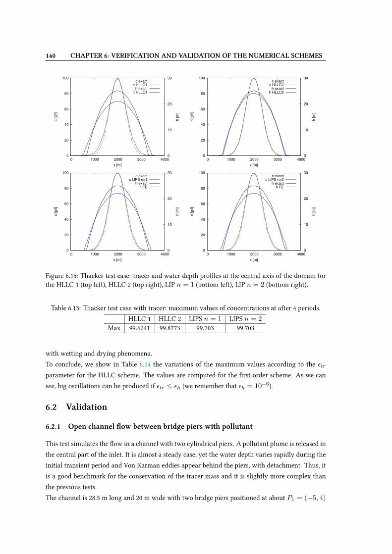
140 CHAPTER 6: VERIFICATION AND VALIDATION OF THE NUMERICAL SCHEMES
0
20
40
60
80
100
0 1000 2000 3000 4000 0
10
20
30
c [
g/l]
h [
m]
x [m]
c exactc HLLC1
h exacth HLLC1
0
20
40
60
80
100
0 1000 2000 3000 4000 0
10
20
30
c [
g/l]
h [
m]
x [m]
c exactc HLLC2
h exacth HLLC2
0
20
40
60
80
100
0 1000 2000 3000 4000 0
10
20
30
c [
g/l]
h [
m]
x [m]
c exactc LIPS n=1
h exacth FE
0
20
40
60
80
100
0 1000 2000 3000 4000 0
10
20
30
c [
g/l]
h [
m]
x [m]
c exactc LIPS n=2
h exacth FE
Figure 6.15: Thacker test case: tracer and water depth proVles at the central axis of the domain forthe HLLC 1 (top left), HLLC 2 (top right), LIP n = 1 (bottom left), LIP n = 2 (bottom right).
Table 6.13: Thacker test case with tracer: maximum values of concentrations at after 4 periods.
HLLC 1 HLLC 2 LIPS n = 1 LIPS n = 2
Max 99.6241 99.8773 99.703 99.703
with wetting and drying phenomena.
To conclude, we show in Table 6.14 the variations of the maximum values according to the εtrparameter for the HLLC scheme. The values are computed for the Vrst order scheme. As we can
see, big oscillations can be produced if εtr ≤ εh (we remember that εh = 10−6).
6.2 Validation
6.2.1 Open channel Wow between bridge piers with pollutant
This test simulates the Wow in a channel with two cylindrical piers. A pollutant plume is released in
the central part of the inlet. It is almost a steady case, yet the water depth varies rapidly during the
initial transient period and Von Karman eddies appear behind the piers, with detachment. Thus, it
is a good benchmark for the conservation of the tracer mass and it is slightly more complex than
the previous tests.
The channel is 28.5 m long and 20 m wide with two bridge piers positioned at about P1 = (−5, 4)

6.2 VALIDATION 141
0
20
40
60
80
100
0 1000 2000 3000 4000
c [g/l]
x [m]
exactHLLC 1HLLC 2
LIPS
Figure 6.16: Thacker test case: numerical and exact solutions for the tracer proVle after 4 periods atthe central axis.
Table 6.14: Thacker test case with tracer: maximum and minimum values of concentration accord-ing to diUerent εtr after 1 period.
εtr Max(c) Min(c)10−3 265 010−6 174 010−7 100 010−13 100 0
and P2 = (−5,−4), and a radius of 2 m. Note that x ∈ [−14, 14.5] and y ∈ [−10, 10]. The
channel section is trapezoidal (see the bottom in the Figure 6.17) and the minimum value of the
bottom is equal to -4 m in the main channel.
At the inlet of the channel, we impose as upstream boundary conditions a Wow discharge equal to
Figure 6.17: Open channel Wow between bridge piers with pollutant: topography of the channelwith the cylindrical piers sketch.
62 m3/s, while at the outlet a null free surface is imposed, which is also the initial condition.
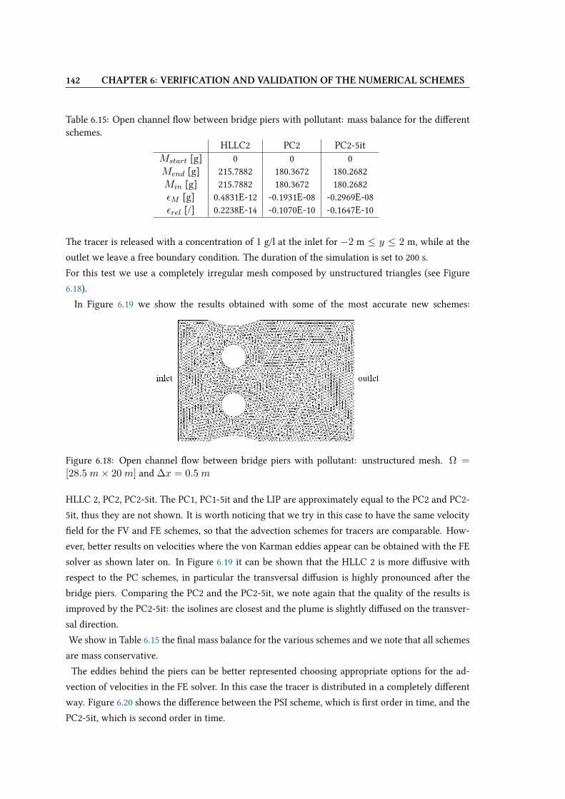
142 CHAPTER 6: VERIFICATION AND VALIDATION OF THE NUMERICAL SCHEMES
Table 6.15: Open channel Wow between bridge piers with pollutant: mass balance for the diUerentschemes.
HLLC2 PC2 PC2-5itMstart [g] 0 0 0Mend [g] 215.7882 180.3672 180.2682Min [g] 215.7882 180.3672 180.2682εM [g] 0.4831E-12 -0.1931E-08 -0.2969E-08εrel [/] 0.2238E-14 -0.1070E-10 -0.1647E-10
The tracer is released with a concentration of 1 g/l at the inlet for −2 m ≤ y ≤ 2 m, while at the
outlet we leave a free boundary condition. The duration of the simulation is set to 200 s.
For this test we use a completely irregular mesh composed by unstructured triangles (see Figure
6.18).
In Figure 6.19 we show the results obtained with some of the most accurate new schemes:
Figure 6.18: Open channel Wow between bridge piers with pollutant: unstructured mesh. Ω =[28.5 m× 20 m] and ∆x = 0.5 m
HLLC 2, PC2, PC2-5it. The PC1, PC1-5it and the LIP are approximately equal to the PC2 and PC2-
5it, thus they are not shown. It is worth noticing that we try in this case to have the same velocity
Veld for the FV and FE schemes, so that the advection schemes for tracers are comparable. How-
ever, better results on velocities where the von Karman eddies appear can be obtained with the FE
solver as shown later on. In Figure 6.19 it can be shown that the HLLC 2 is more diUusive with
respect to the PC schemes, in particular the transversal diUusion is highly pronounced after the
bridge piers. Comparing the PC2 and the PC2-5it, we note again that the quality of the results is
improved by the PC2-5it: the isolines are closest and the plume is slightly diUused on the transver-
sal direction.
We show in Table 6.15 the Vnal mass balance for the various schemes and we note that all schemes
are mass conservative.
The eddies behind the piers can be better represented choosing appropriate options for the ad-
vection of velocities in the FE solver. In this case the tracer is distributed in a completely diUerent
way. Figure 6.20 shows the diUerence between the PSI scheme, which is Vrst order in time, and the
PC2-5it, which is second order in time.

6.2 VALIDATION 143
Figure 6.19: Open channel Wow between bridge piers with pollutant: isolines for the tracer (∆ =0.05). From top to bottom: HLLC2, PC2, PC2-5it.
Figure 6.20: Open channel Wow between bridge piers with pollutant: isolines (∆ = 0.05) for thePSI scheme (left) and the PC2-5it scheme (right).
6.2.2 Real river with tracer injection
In this test case we evaluate the robustness, the eXciency and the accuracy of the new LIP scheme
on a real study case.
144 CHAPTER 6: VERIFICATION AND VALIDATION OF THE NUMERICAL SCHEMES
A tracer is released in a river with an irregular topography (Figure 6.21), where the Wow often
changes its path between the minor bed and the major bed, according to the season and the meteo-
rological events. Several small islands are present along the river channel. Hence, the wetting and
drying phenomena occur often on these zones, as well as on the major bed.
The tracer is released through seven source points in the upstream part of the river and a series of
data measures is available in order to compare the numerical results.
The river is approximately 40 km long and the computational domain is discretized with an un-
structured grid, made up by 1,281,717 elements that correspond to 652,412 nodes. The mesh has an
average mesh size of 4 m and decreases to 1.7 m in the zones with the source points. The Strickler
coeXcients (Ks) are Vxed after a calibration study and six diUerent zones are identiVed with Ks
in the range [22, 40]m1/3s−1. A Wow rate is imposed at the inlet while the free surface is set on
the outlet through a stage-discharge curve, which is part of the measurements. The Wow rate used
is equal to 87 m3/s while the free surface at the outlet varies in the range [60.912, 62.4939] m
according to the computed Wow rate. The initial condition corresponds to the steady condition,
previously computed with the calibration study.
A constant quantity of tracer is injected along all the duration of the simulation, through seven
sources. The Wow rate of every source is 0.3 m3/s and the value of tracer at the source is
csce = 1 g/l.
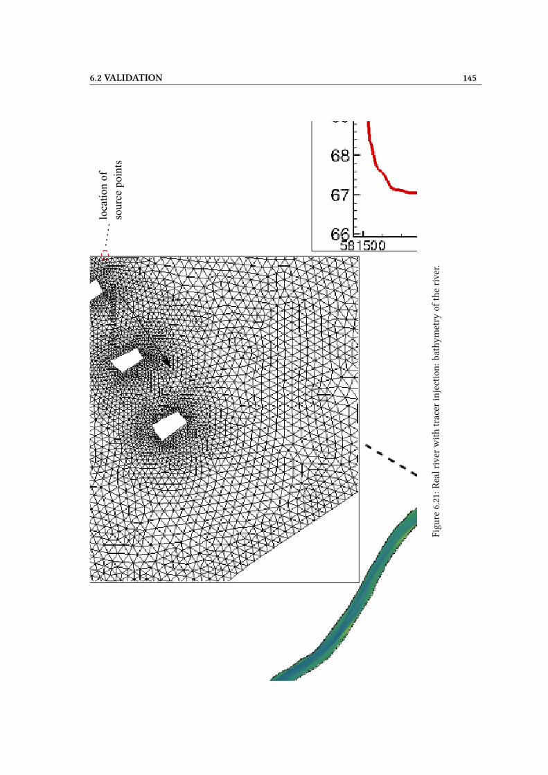
6.2 VALIDATION 145
loca
tion
of
sour
ce p
oint
sfl
ow d
irec
tion
Figure
6.21:R
ealriver
with
tracer
injection:
bathym
etry
oftheriver.
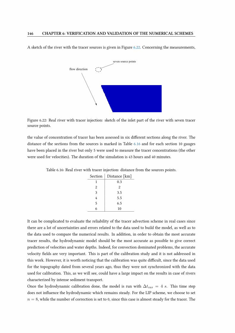
146 CHAPTER 6: VERIFICATION AND VALIDATION OF THE NUMERICAL SCHEMES
A sketch of the river with the tracer sources is given in Figure 6.22. Concerning the measurements,
flow direction
seven source points
Figure 6.22: Real river with tracer injection: sketch of the inlet part of the river with seven tracersource points.
the value of concentration of tracer has been assessed in six diUerent sections along the river. The
distance of the sections from the sources is marked in Table 6.16 and for each section 10 gauges
have been placed in the river but only 5 were used to measure the tracer concentrations (the other
were used for velocities). The duration of the simulation is 43 hours and 40 minutes.
Table 6.16: Real river with tracer injection: distance from the sources points.
Section Distance [km]1 0.32 23 3.54 5.55 6.56 10
It can be complicated to evaluate the reliability of the tracer advection scheme in real cases since
there are a lot of uncertainties and errors related to the data used to build the model, as well as to
the data used to compare the numerical results. In addition, in order to obtain the most accurate
tracer results, the hydrodynamic model should be the most accurate as possible to give correct
prediction of velocities and water depths. Indeed, for convection dominated problems, the accurate
velocity Velds are very important. This is part of the calibration study and it is not addressed in
this work. However, it is worth noticing that the calibration was quite diXcult, since the data used
for the topography dated from several years ago, thus they were not synchronized with the data
used for calibration. This, as we will see, could have a large impact on the results in case of rivers
characterized by intense sediment transport.
Once the hydrodynamic calibration done, the model is run with ∆tcas = 4 s. This time step
does not inWuence the hydrodynamic which remains steady. For the LIP scheme, we choose to set
n = 8, while the number of correction is set to 0, since this case is almost steady for the tracer. The
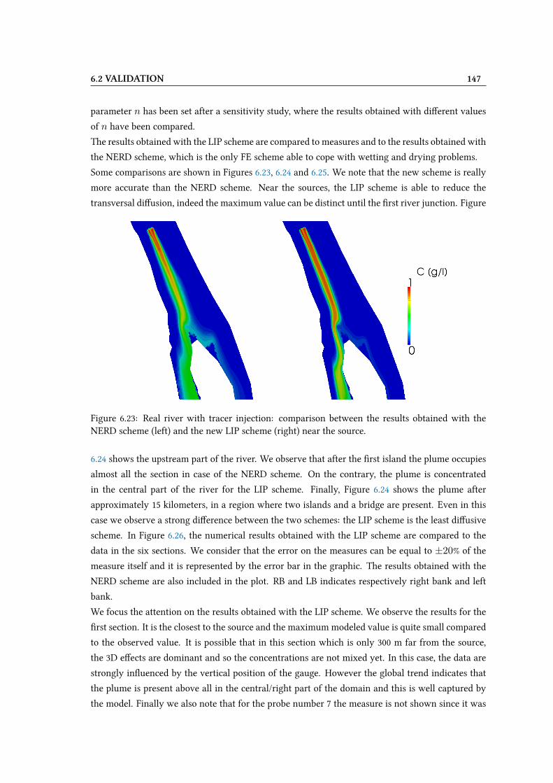
6.2 VALIDATION 147
parameter n has been set after a sensitivity study, where the results obtained with diUerent values
of n have been compared.
The results obtained with the LIP scheme are compared to measures and to the results obtained with
the NERD scheme, which is the only FE scheme able to cope with wetting and drying problems.
Some comparisons are shown in Figures 6.23, 6.24 and 6.25. We note that the new scheme is really
more accurate than the NERD scheme. Near the sources, the LIP scheme is able to reduce the
transversal diUusion, indeed the maximum value can be distinct until the Vrst river junction. Figure
Figure 6.23: Real river with tracer injection: comparison between the results obtained with theNERD scheme (left) and the new LIP scheme (right) near the source.
6.24 shows the upstream part of the river. We observe that after the Vrst island the plume occupies
almost all the section in case of the NERD scheme. On the contrary, the plume is concentrated
in the central part of the river for the LIP scheme. Finally, Figure 6.24 shows the plume after
approximately 15 kilometers, in a region where two islands and a bridge are present. Even in this
case we observe a strong diUerence between the two schemes: the LIP scheme is the least diUusive
scheme. In Figure 6.26, the numerical results obtained with the LIP scheme are compared to the
data in the six sections. We consider that the error on the measures can be equal to ±20% of the
measure itself and it is represented by the error bar in the graphic. The results obtained with the
NERD scheme are also included in the plot. RB and LB indicates respectively right bank and left
bank.
We focus the attention on the results obtained with the LIP scheme. We observe the results for the
Vrst section. It is the closest to the source and the maximummodeled value is quite small compared
to the observed value. It is possible that in this section which is only 300 m far from the source,
the 3D eUects are dominant and so the concentrations are not mixed yet. In this case, the data are
strongly inWuenced by the vertical position of the gauge. However the global trend indicates that
the plume is present above all in the central/right part of the domain and this is well captured by
the model. Finally we also note that for the probe number 7 the measure is not shown since it was
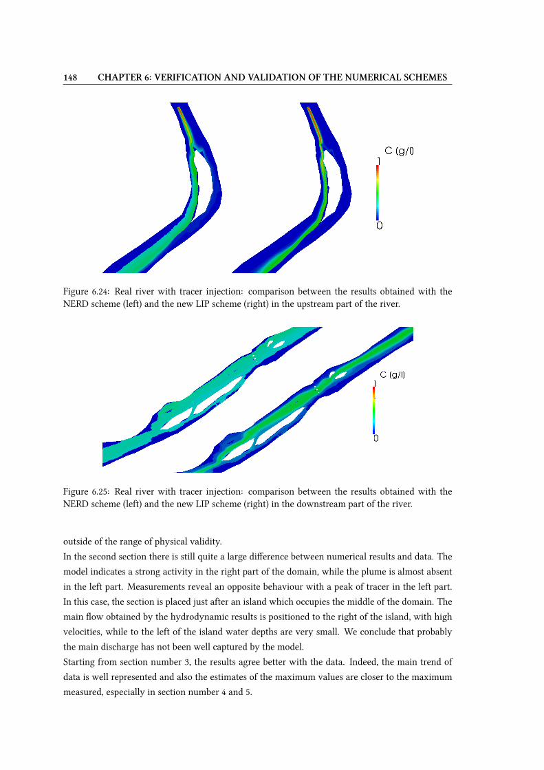
148 CHAPTER 6: VERIFICATION AND VALIDATION OF THE NUMERICAL SCHEMES
Figure 6.24: Real river with tracer injection: comparison between the results obtained with theNERD scheme (left) and the new LIP scheme (right) in the upstream part of the river.
Figure 6.25: Real river with tracer injection: comparison between the results obtained with theNERD scheme (left) and the new LIP scheme (right) in the downstream part of the river.
outside of the range of physical validity.
In the second section there is still quite a large diUerence between numerical results and data. The
model indicates a strong activity in the right part of the domain, while the plume is almost absent
in the left part. Measurements reveal an opposite behaviour with a peak of tracer in the left part.
In this case, the section is placed just after an island which occupies the middle of the domain. The
main Wow obtained by the hydrodynamic results is positioned to the right of the island, with high
velocities, while to the left of the island water depths are very small. We conclude that probably
the main discharge has not been well captured by the model.
Starting from section number 3, the results agree better with the data. Indeed, the main trend of
data is well represented and also the estimates of the maximum values are closer to the maximum
measured, especially in section number 4 and 5.
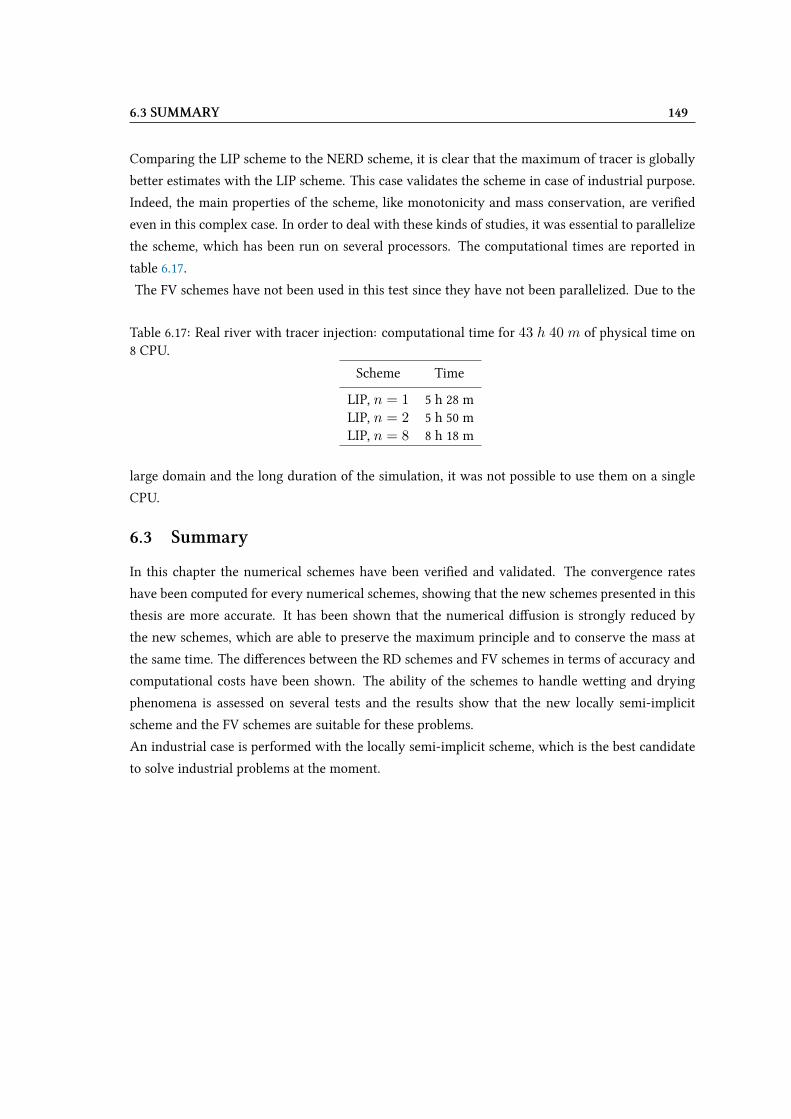
6.3 SUMMARY 149
Comparing the LIP scheme to the NERD scheme, it is clear that the maximum of tracer is globally
better estimates with the LIP scheme. This case validates the scheme in case of industrial purpose.
Indeed, the main properties of the scheme, like monotonicity and mass conservation, are veriVed
even in this complex case. In order to deal with these kinds of studies, it was essential to parallelize
the scheme, which has been run on several processors. The computational times are reported in
table 6.17.
The FV schemes have not been used in this test since they have not been parallelized. Due to the
Table 6.17: Real river with tracer injection: computational time for 43 h 40 m of physical time on8 CPU.
Scheme Time
LIP, n = 1 5 h 28 mLIP, n = 2 5 h 50 mLIP, n = 8 8 h 18 m
large domain and the long duration of the simulation, it was not possible to use them on a single
CPU.
6.3 Summary
In this chapter the numerical schemes have been veriVed and validated. The convergence rates
have been computed for every numerical schemes, showing that the new schemes presented in this
thesis are more accurate. It has been shown that the numerical diUusion is strongly reduced by
the new schemes, which are able to preserve the maximum principle and to conserve the mass at
the same time. The diUerences between the RD schemes and FV schemes in terms of accuracy and
computational costs have been shown. The ability of the schemes to handle wetting and drying
phenomena is assessed on several tests and the results show that the new locally semi-implicit
scheme and the FV schemes are suitable for these problems.
An industrial case is performed with the locally semi-implicit scheme, which is the best candidate
to solve industrial problems at the moment.
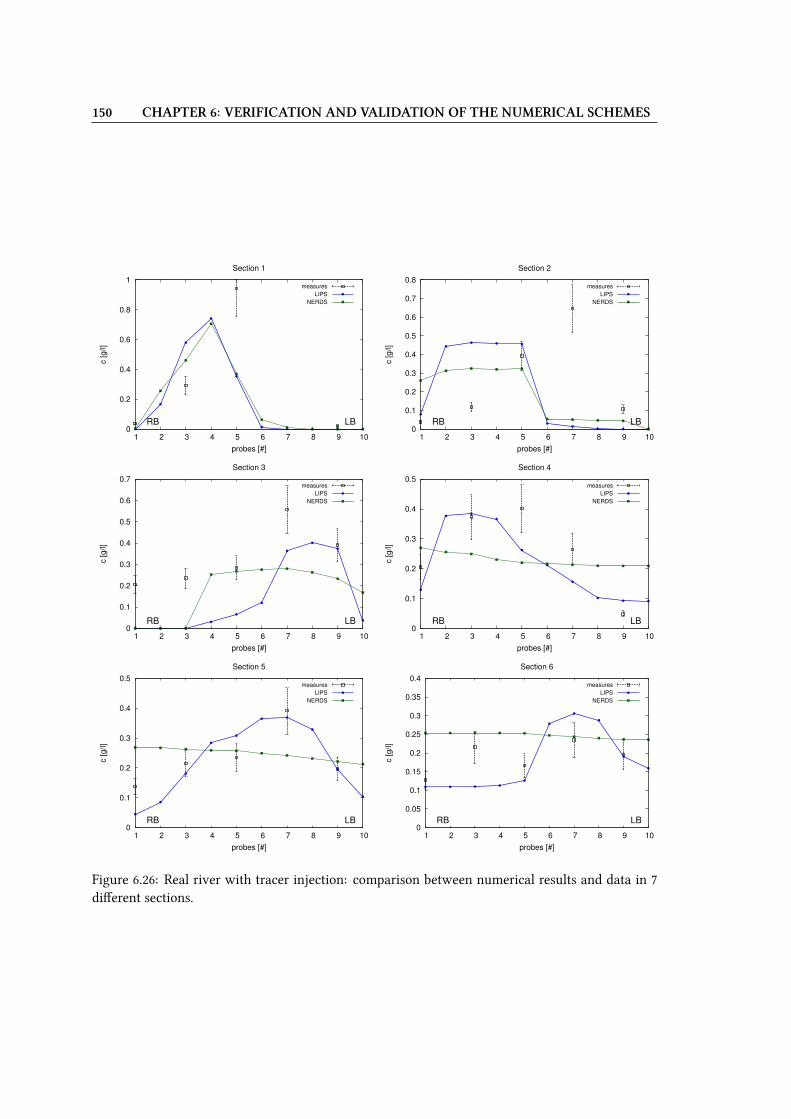
150 CHAPTER 6: VERIFICATION AND VALIDATION OF THE NUMERICAL SCHEMES
0
0.2
0.4
0.6
0.8
1
1 2 3 4 5 6 7 8 9 10
c [g/l]
probes [#]
Section 1
RB LB
measures
LIPS
NERDS
0
0.1
0.2
0.3
0.4
0.5
0.6
0.7
0.8
1 2 3 4 5 6 7 8 9 10
c [g/l]
probes [#]
Section 2
RB LB
measures
LIPS
NERDS
0
0.1
0.2
0.3
0.4
0.5
0.6
0.7
1 2 3 4 5 6 7 8 9 10
c [g/l]
probes [#]
Section 3
RB LB
measures
LIPS
NERDS
0
0.1
0.2
0.3
0.4
0.5
1 2 3 4 5 6 7 8 9 10
c [g/l]
probes [#]
Section 4
RB LB
measures
LIPS
NERDS
0
0.1
0.2
0.3
0.4
0.5
1 2 3 4 5 6 7 8 9 10
c [g/l]
probes [#]
Section 5
RB LB
measures
LIPS
NERDS
0
0.05
0.1
0.15
0.2
0.25
0.3
0.35
0.4
1 2 3 4 5 6 7 8 9 10
c [g/l]
probes [#]
Section 6
RB LB
measures
LIPS
NERDS
Figure 6.26: Real river with tracer injection: comparison between numerical results and data in 7diUerent sections.
Chapter 7
Residual distribution schemes in three
dimensions and validation
Dans ce chapitre les schémas RD sont formulés pour des problèmes 3D. L’extension au
3D est assez simple, grâce à la compatibilité entre l’équation de continuité du Wuide
et l’équation conservative du traceur. De plus, en 3D les volumes d’eau autour des
points peuvent être interprétés comme des hauteurs d’eau en 2D. Les schémas N et PSI
sont introduits d’abord, et les schémas prédicteur correcteur d’ordre un et deux sont
présentés ensuite. Les propriétés obtenues en 2D sont conservées en 3D, avec des con-
ditions de monotonie similaires.
Les schémas sont testés sur des cas simples qui visent à vériVer la monotonie de la so-
lution et la conservation de la masse. La précision des schémas est évaluée de manière
qualitative et d’autres cas tests seraient nécessaires pour avoir une validation complète
des ces nouveaux schémas.
152 CHAPTER 7: RESIDUAL DISTRIBUTION SCHEMES IN 3D AND VALIDATION
7.1 Three dimensional formulation
The explicit predictor-corrector schemes introduced in Chapter 5 can be directly adapted to a three
dimensional (3D) case. This is due to the fact that, in 3D free surface Wows, the varying volumes
around points play the role of the varying depth in 2D. The Navier-Stokes equations are solved
using a Vnite element method as far the 2D case and the discretization of the continuity equation
is presented, in order to deal with the tracer equation. The N and the PSI explicit schemes are later
formulated for a 3D case and Vnally the predictor-corrector schemes are introduced.
The locally implicit predictor-corrector scheme could be adapted to the 3D case as well and this
step is foreseen after this thesis.
7.1.1 Preliminaries
To solve the Navier-Stokes equations, a sigma transform on the free surface is used. We recall here
some basic notions related to this transformation, which are further analyzed in [53, 82]. We limit
ourselves to the fundamental expressions useful to deal with the 3D tracer transport equation. For
this reason, the solution of the continuity equation is detailed.
As in the 2D case, the tracer equation is decoupled from the Wuid equations and the Bubnov-
Galerkin technique is used again to discretize the equations. The Vnite elements are in this case
prisms made up by 6 nodes and characterized by 3 vertical quadrangular sides. The bilinear basis
functions ϕi can be broken down as ϕi = ϕhi ϕvi , where ϕ
hi is the horizontal basis function which
depends only on coordinates x and y, while ϕvi is the vertical basis function which depends only
on coordinate z. We note that the horizontal basis function corresponds to the one used in 2D,
presented in Chapter 5. The properties of the linear P1 Vnite element basis functions are thus un-
changed for the vertical and the horizontal directions. This notion will be useful for the resolution
of the continuity equation.
A sigma transform (as well as a generalised sigma transform) is used in order to deal with the prob-
lem of the free surface evolution with time. Indeed, with the sigma transform a change of variable
is done so that the bottom elevation is zero and the free surface elevation is equal to 1. The new
variable z∗ is thus deVned as:
z∗ =z − bs− b
=z − bh
(7.1)
In case of a generalised sigma transform this is done layer by layer and we have:
z∗ =z − zip
zip+1 − zip=z − zip
∆z(7.2)
where zip is the bottom elevation of layer ip at point i, zip+1 is the elevation of the top of the layer
ip at point i and ∆z is the height of layer ip, deVned by ∆z =∂z
∂z∗. The transformed domain
is called Ω∗ and considering an unstructured 2D mesh, the corresponding 3D mesh is made up by
prisms whose basis are the 2D triangles. The boundary of the transformed domain in Γ∗.
The advection part of the Navier-Stokes equations (and of the tracer equation) is solved, to take
7.1 THREE DIMENSIONAL FORMULATION 153
into account the movement of the mesh due to the free surface evolution, in the transformed mesh.
As a matter of fact the relocalisation is naturally done in this mesh. Then the diUusion step and the
pressure-continuity step are solved on the real mesh, in a further fractional step.
The choice of solving the advection in the transformed mesh implies that some terms of the original
partial diUerential equations are modiVed by the new variable z∗. The advection equations are thus
rewritten in order to deal with this issue.
In addition, in the new mesh the velocity vector is diUerent from the one on the real mesh. Indeed
it is deVned as U∗ = (U∗, V ∗,W ∗) where U∗ = U , V ∗ = V and W ∗ 6= W sincedz∗
dt6= dz
dt.
Note thatW ∗ takes into account the movement of the mesh which triggers the relocalisation.
As the advection terms of the Navier-Stokes equations are treated the transformed mesh, it is
necessary to compute at every time step the vertical velocity:
W ∗ =dz∗
dt=∂z
∂t+ U
∂z∗
∂x+ V
∂z∗
∂y+W
∂z∗
∂z(7.3)
The velocityW ∗ appears in the continuity equation ∇ · U = 0 written in the transformed mesh
(further details can be found in [82]):
1
∆z
[∂∆z
∂t+
(∂(∆zU)
∂x
)y,z∗,t
+
(∂(∆zV )
∂y
)x,z∗,t
+
(∂(∆zW ∗)
∂z∗
)x,y,t
]= 0 (7.4)
Hence, multiplying the equation by a test function on the transformed domain ψ∗i and integrating
by Ω∗ we obtain:
∫Ω∗
1
∆z
[∂∆z
∂t+
(∂(∆zU)
∂x
)y,z∗,t
+
(∂(∆zV )
∂y
)x,z∗,t
+
(∂(∆zW ∗)
∂z∗
)x,y,t
]ψ∗i dΩ∗ = 0
(7.5)
Discretized as such, the equation whose unknown is W ∗ or ∆zW ∗ leads to a system that is ill-
conditioned (since there are more unknowns than equations). To overcome this problem we choose
as unknown the variable ∆zW ∗ for which we give a speciVc deVnition. This particular deVnition
allows to get the compatibility with the RD schemes used for tracer advection. In this way Equation
(7.5) is recast using the divergence operator and then is integrated by parts in order to obtain ∆zW ∗
solving:∫Ω∗
(∆zn+1−∆zn)ψ∗i dΩ∗ = ∆t
∫Ω∗
∆zU∗∇ψ∗i dΩ∗−∆t
∫Γ∗
∆zU∗ ·nψ∗i dΓ∗ 0 ≤ i ≤ Nh
(7.6)
where Nh represents the number of degrees of freedom. The unknowns are the average of ∆zW ∗
along the vertical of each prism, thus the problem is well-posed. Equation (7.6) is strictly satisVed
by ∆zW ∗.
In order to be consistent with the 2D continuity equation, ∆z on the RHS of Equation (7.6) is
chosen at time tn. The continuity equation can also be written distinguishing the vertical and the
154 CHAPTER 7: RESIDUAL DISTRIBUTION SCHEMES IN 3D AND VALIDATION
horizontal gradients of the test functions:∫Ω∗
∆zW ∗∂ψ∗i∂z∗
dΩ∗ =1
∆t
∫Ω∗
(∆zn+1 −∆zn)ψ∗i dΩ∗ −∫
Ω∗∆z
(U∂ψ∗i∂x
+ V∂ψ∗i∂y
)
)dΩ∗
+
∫Γ∗
∆zU∗ · nψ∗i dΓ∗
(7.7)
Now we assume that the boundary integral is known (through the imposition of boundary con-
ditions), so that the RHS of the above equation is known and the only unknown is on the LHS.
The idea is to simplify the LHS, using the fact that ψ∗i = ψhi ψvi and thus
∂ψ∗i∂z∗
= ψhi∂ψvi∂z∗
and to
compute at every layer ip, the average of ∆zW ∗. The details about the computation of this terms
can be found in [82]. After manipulation, we arrive at a series of linear systems, one per plane,
whose form is:
npoin2∑j=1
∫Ω2D
ψhi ψhj dΩ2D
[¯∆zw∗
jip+1/2 − ¯∆zw∗
jip−1/2
]=− 1
∆t
∫Ω∗
(∆zn+1 −∆zn
)ψ∗i dΩ∗
+
∫Ω∗
∆z
(U∂ψ∗i∂x
+ V∂ψ∗i∂y
)
)dΩ∗
−∫
Γ∗liq
∆zU∗ · nψ∗i dΓ∗
(7.8)
where:
¯∆zw∗jip+1/2 =
1
z∗ip − z∗ip−1
∫ z∗ip
z∗ip−1
[∆zW ∗(∆z∗)]j dz∗ (7.9)
npoin2 indicates the number of points on the 2Dmesh, as well as Ω2D indicates the 2D domain and
Γ∗liq is the liquid boundary (on solid boundary the Wux is zero for the impermeability condition).
We show now that Equation (7.8) can be rewritten similarly as Equation (5.23). At node i, Equation
(7.8) can be recast as:
φvip+1/2 − φvip−1/2 = − Si
∆t
(∆zn+1
i −∆zni)−∑j
φhij − bi (7.10)
The sum over j represents the sum over all the neighbours j of point i on the 2D domain. Then:
• φvip±1/2 = ¯∆zw∗iip±1/2 are the assembled vertical Wuxes at point i computed for the layers
upper and below the node i, solution of Equation (7.8);
• Si =∫
Ω∗ ψ∗i dΩ∗ is the volume of the test functions around the point i in 3D obtained by the
mass-lumping;
• φhij are the horizontal assembled Wuxes, which stem from the assembly of the intermediary
Wuxes computed on every prism: φh,P∗
ij . As in 2D we have: φh,P∗
ij = λNji − λNij and
7.1 THREE DIMENSIONAL FORMULATION 155
λNij = max(min(ai,−aj), 0) with ai = −∫P ∗ ∆zU
∂ψ∗i∂x dP
∗ −∫P ∗ ∆zV
∂ψ∗i∂y dP
∗ and P ∗
the prism on the transformed mesh;
• bi =∫
Γ∗liq∆zU∗ · nψ∗i dΓ∗ is the boundary term
Reorganising the terms we obtain:
Si∆t
(∆zn+1
i −∆zni)
+ φvip+1/2 − φvip−1/2 +
∑j
φhij + bi = 0 (7.11)
or in a more compact form:
Si∆t
(∆zn+1
i −∆zni)
+∑j
(φhij + φvij) + bi = 0 (7.12)
with φvij = φvip+1/2 for j = ip + 1/2 or φvij = −φvip−1/2 for j = ip − 1/2. Note that here j
indicates the horizontal as well as the vertical neighbours of node i. We note that respect to the
2D case (Equation (5.23)), Equation (7.12) presents two additional Wuxes (the vertical ones) and the
variable h is replaced by ∆z. Once the Navier-Stokes equations are solved, the tracer equation is
solved.
7.1.2 Explicit schemes for steady problems
Firstly we deVne the two explicit Vrst order schemes in time, the N and the PSI. The basis to apply
the RD schemes in 3D dealing with a Vnite element formulation, were already established by Janin
[90] and Hervouet [82]. Their work deVnes how to build the N and the PSI schemes and it is just
recalled here to simplify the explanations on the application of the predictor-corrector schemes in
3D.
However, unlike the 2D case, the initial derivation for the 3D case was based on the direct dis-
cretization of the non conservative continuous transport equation. We present here a formulation
based instead on the conservative equation, where the divergence term is integrated by parts, as
done for the continuity equation. This operation allows to do exactly the same passages done for
the 2D case, where h, the 2D water depth is replaced by ∆z, the height of a layer in 3D. The mass
conservation for the tracer on the transformed mesh is written as:∫Ω∗
(∆zn+1Cn+1 −∆znCn)dΩ∗ + ∆t
∫Γ∗
∆zCU∗ · ndΓ∗ = 0 (7.13)
which is equivalent to:∫Ω∗
(∆zn+1Cn+1 −∆znCn)dΩ∗ + ∆t
∫Ω∗∇ ·∆zCU∗dΩ∗ = 0 (7.14)
156 CHAPTER 7: RESIDUAL DISTRIBUTION SCHEMES IN 3D AND VALIDATION
For every degree of freedom i, we solve:∫Ω∗
(∆zn+1Cn+1 −∆znCn)ψ∗i dΩ∗ + ∆t
∫Ω∗∇ ·∆zCU∗dΩ∗ψ∗i = 0 (7.15)
As for the continuity equation, we integrate by parts and we obtain:∫Ω∗
(∆zn+1Cn+1 −∆znCn)ψ∗i dΩ∗ −∆t
∫Ω∗
∆zCU∗∇ψ∗i dΩ∗ +
∫Γ∗ψ∗i ∆zCU
∗ · ndΓ∗ = 0
(7.16)
We perform a mass-lumping on the Vrst term of the LHS and we get:∫Ω∗
(∆zn+1Cn+1 −∆znCn)ψ∗i dΩ∗ ≈ Si(∆zn+1Cn+1
i −∆znCni)
(7.17)
In order to employ the Wuxes of the continuity equation, we choose:
−∫
Ω∗∆zCU∗∇ψ∗i dΩ∗ =
∑j
(φhij + φvij)Cij (7.18)
Note that j includes the vertical and the horizontal neighbours of i and Cij is still a general value
of C , in the range [Ci, Cj ].
Finally the last term of Equation (7.16) becomes as in 2D:∫Γ∗ψ∗i ∆zCU
∗ · ndΓ∗ = biCbound (7.19)
These boundary Wuxes are treated like in the 2D case: therefore the ingoing Wuxes are multiplied by
the boundary value of tracer, while outgoing Wuxes are multiplied by the values on the boundaries
given by the scheme. This is summarised as:
biCbound = min(bi, 0)Cbound + max(bi, 0)Ci (7.20)
The conservative equation now reads as:
Si(∆zn+1Cn+1
i −∆znCni)+∆t
∑j
(φhij + φvij)Cij + min(bi, 0)Cbound + max(bi, 0)Ci
= 0
(7.21)
We now repeat all the passages done in 2D, which means that we choose an upwind value for the
variable Cij , that is Ci if φij is leaving the node i and Cj if φij is entering in i. Then the value of
∆zn in Equation (7.21) is replaced by ∆zn+1 by the use of the discrete continuity equation (7.12).
7.1 THREE DIMENSIONAL FORMULATION 157
Hence, we obtain:
Cn+1i =Cni +
∆t
Si∆zn+1i
∑j
min(φh,Nij , 0)(Cni − Cnj ) +∑j
min(φv,Nij , 0)(Cni − Cnj )
− ∆t
Si∆zn+1i
min(bi, 0)(Cbound − Cni )
(7.22)
where φh,Nij (and φv,Nij ) correspond to the φhij (and φvij) of the continuity equation (7.12). The
superscriptN has been added since the scheme obtained corresponds to the N scheme. Indeed this
equation is equivalent to:
Cn+1i = Cni −
∆t
Si∆zn+1i
(∑P ∗3i
βNi φP ∗ + min(bi, 0)(Cbound − Cni )
)(7.23)
where φP∗is the space residual computed on the prism P ∗, βNi are the distribution coeXcients
and∑P ∗3i
represents the sum over all the prism containing the node i. The space residual is equal
to:
φP∗
=6∑i=1
6∑j=1
λNij (Cni − Cnj ) (7.24)
In the 3D case the computation of coeXcients λNij is more complicated than for the 2D case; their
expressions can be found in [82]. The derivation for prisms was presented by Janin [90], based on
the work of Bourgois et al. [29] for tetrahedral meshes. As in 2D, the main characteristic of λNij is
that they are positive or null. The expression for the N distribution coeXcients is:
βNi =φNiφP ∗
(7.25)
where φNi is the contribution received by node i of the prism P ∗:
φNi =
6∑j
λNij (Cni − Cnj ) = βNi φP ∗ (7.26)
Note that expression (7.22) and expression (7.23) are related by:∑j
min(φh,Nij , 0)(Cni − Cnj ) +∑j
min(φv,Nij , 0)(Cni − Cnj ) = −∑P ∗3i
βNi φP ∗ (7.27)
158 CHAPTER 7: RESIDUAL DISTRIBUTION SCHEMES IN 3D AND VALIDATION
As in the 2D case, the N and the PSI scheme diUers in the distribution of the residual φP∗to the
nodes of the prism. The PSI scheme is deVned as:
Si∆zn+1C
n+1i − Cni
∆t= −
∑P ∗3i
βPSIi φP∗
+ min(bi, 0)(Cbound − Cni ) (7.28)
with the PSI limiter equal to:
βPSIi =max(0, βNi )∑
i∈Pmax(0, βNi )
(7.29)
The scheme can also be written directly using the λPSIij , which are reduced respect to the λNij . The
conservation is therefore guaranteed:
6∑i=1
6∑j=1
λNij (Cni − Cnj ) =6∑i=1
6∑j=1
λPSIij (Cni − Cnj ) (7.30)
Both schemes are subject to a monotonicity condition, determined by the study of the positive
coeXcients. The time step condition for the N scheme is equal to:
∆t ≤ Si∆zn+1∑
P ∗3i
6∑j=1
λNij −min(bi, 0)
(7.31)
For the PSI scheme we obtain:
∆t ≤ Si∆zn+1∑
P ∗3i
6∑j=1
λPSIij −min(bi, 0)
(7.32)
It is worth noticing that the time step for the PSI scheme will be larger than the one for the N
scheme and the stability of the PSI scheme can be ensured also by the λNij .
In this section we have shown that the work done in 2D to show that the RD schemes are conser-
vative and monotone, is equivalent in 3D if we replace h by ∆z (it is mandatory taking them at
the same time).
7.1.3 Predictor-corrector schemes
The predictor-corrector schemes can be built in 3D, once the compatibility between the 2D and the
3D formulations has been shown for the explicit N and PSI schemes. Indeed, the eUorts done in 2D
to show that the predictor-corrector schemes are monotone and conservative, hold true in 3D. This
is mainly due to the fact that the advection schemes are based on the conservative tracer equations
where the divergence form is treated with an integration by parts as it is done for the continuity
equation, in 2D as well as in 3D.
7.1 THREE DIMENSIONAL FORMULATION 159
7.1.3.1 First order predictor-corrector scheme
The Vrst order predictor-corrector scheme is:Si∆z
n+1C∗i − Cni
∆t= −
∑P ∗3i
βPSIi φP∗(Cn)−min(bi, 0)(Cbound − Cni )
Si∆zn+1C
n+1i − C∗i
∆t= −
∑P ∗3i
βPSIi ΦP ∗(Cn, C∗)−min(bi, 0)(Cbound − Cni )(7.33)
The PSI distribution coeXcients are retrieved with Equation (7.29), but we insist on the fact that the
space residual φP∗(Cn) is diUerent from the space-time residual ΦP ∗(Cn, C∗). Indeed the space
residual is computed with Equation (7.24) and the contributions φNi are computed with formula
(7.26). The space time residual is instead equal to:
ΦP ∗(Cn, C∗) =∑i∈P ∗
ST6
∆zn+1C∗i − Cni
∆t+
6∑i=1
6∑j=1
λij(Cni − Cnj ) (7.34)
where ST is the surface of the triangle which is the basis of the prism. We also have:
ΦP ∗(Cn, C∗) =∑i∈P ∗
ΦNi (7.35)
with:
ΦNi =
ST6
∆zn+1C∗i − Cni
∆t+
6∑j=1
λij(Cni − Cnj ) (7.36)
Since the monotonicity analysis is based on the study of the positive coeXcients and on the idea
that the PSI limiter operates a reduction of the type:
βPSIi = γiβNi βPSIi , γPSIi ∈ [0, 1] (7.37)
then, the results obtained for the 2D case can be straightforwardly applied to the 3D case.
The time step criterion to preserve the monotonicity is written as:
∆t ≤ Si∆zn+1
−2
[∑j
min(φh,Nij , 0) +∑j
min(φv,Nij , 0) + min(bi, 0)
] (7.38)
The iterative version of the scheme presented in Chapter 5, Section 5.4, is also possible in 3D.
160 CHAPTER 7: RESIDUAL DISTRIBUTION SCHEMES IN 3D AND VALIDATION
7.1.3.2 Second order predictor-corrector scheme
The second order predictor-corrector scheme reads as:Si∆z
n+1C∗i − Cni
∆t= −
∑P3i
βPSIi φP (Cn)−min(bi, 0)(Cbound − Cni )
Si∆zn+1C
n+1i − C∗i
∆t= −
∑P3i
βPSIi ΦP (Cn, C∗)−min(bi, 0)(Cbound − (1− θ)Cni − θC∗i )
(7.39)
with:
φP∗(Cn) =
∑i∈P ∗
φP∗
i,N (Cn) =∑i∈P ∗
6∑j=1
λij(Cni − Cnj ) =
6∑i=1
6∑j=1
λij(Cni − Cnj ) (7.40)
and
ΦP (Cn, C∗) =∑i∈P ∗
ΦP ∗i,N (7.41)
=∑i∈P ∗
ST6
∆zn+1−θC∗i − Cni
∆t+ (1− θ)
6∑i=1
6∑j=1
λij(Cni − Cnj ) + θ
6∑i=1
6∑j=1
λij(C∗i − C∗j )
(7.42)
As before, the contributions of the N scheme are:
ΦPi,N (Cn, C∗) =
ST6
∆zn+1−θC∗i − Cni
∆t+(1−θ)
6∑j=1
λij(Cni −Cnj )+θ
6∑j=1
λij(C∗i −C∗j ) (7.43)
Given the following time step:
∆t ≤ 1
2
Si∆zn+1
−∑j
min(φN,hij , 0)−∑j
min(φN,vij , 0)−min(bi, 0)(7.44)
and choosing θ = 1/2 in Equation (7.39), the scheme preserves the monotonicity under the follow-
ing conditions on C∗: 2Cni − Cmax ≤ C∗i ≤ 2Cni − Cmin
2Cmin
3+Cni3≤ C∗i ≤
2Cmax
3+Cni3
(7.45)
where Cmax = maxj(Cnj , C
ni ) and Cmin = minj(C
nj , C
ni ). The iterative version of the second-
order scheme can be straightforwardly applied to the 3D case.
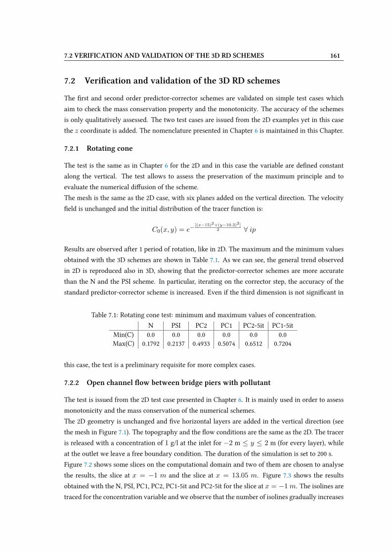
7.2 VERIFICATION AND VALIDATION OF THE 3D RD SCHEMES 161
7.2 VeriVcation and validation of the 3D RD schemes
The Vrst and second order predictor-corrector schemes are validated on simple test cases which
aim to check the mass conservation property and the monotonicity. The accuracy of the schemes
is only qualitatively assessed. The two test cases are issued from the 2D examples yet in this case
the z coordinate is added. The nomenclature presented in Chapter 6 is maintained in this Chapter.
7.2.1 Rotating cone
The test is the same as in Chapter 6 for the 2D and in this case the variable are deVned constant
along the vertical. The test allows to assess the preservation of the maximum principle and to
evaluate the numerical diUusion of the scheme.
The mesh is the same as the 2D case, with six planes added on the vertical direction. The velocity
Veld is unchanged and the initial distribution of the tracer function is:
C0(x, y) = e−[(x−15)2+(y−10.2)2]
2 ∀ ip
Results are observed after 1 period of rotation, like in 2D. The maximum and the minimum values
obtained with the 3D schemes are shown in Table 7.1. As we can see, the general trend observed
in 2D is reproduced also in 3D, showing that the predictor-corrector schemes are more accurate
than the N and the PSI scheme. In particular, iterating on the corrector step, the accuracy of the
standard predictor-corrector scheme is increased. Even if the third dimension is not signiVcant in
Table 7.1: Rotating cone test: minimum and maximum values of concentration.
N PSI PC2 PC1 PC2-5it PC1-5itMin(C) 0.0 0.0 0.0 0.0 0.0 0.0Max(C) 0.1792 0.2137 0.4933 0.5074 0.6512 0.7204
this case, the test is a preliminary requisite for more complex cases.
7.2.2 Open channel Wow between bridge piers with pollutant
The test is issued from the 2D test case presented in Chapter 6. It is mainly used in order to assess
monotonicity and the mass conservation of the numerical schemes.
The 2D geometry is unchanged and Vve horizontal layers are added in the vertical direction (see
the mesh in Figure 7.1). The topography and the Wow conditions are the same as the 2D. The tracer
is released with a concentration of 1 g/l at the inlet for −2 m ≤ y ≤ 2 m (for every layer), while
at the outlet we leave a free boundary condition. The duration of the simulation is set to 200 s.
Figure 7.2 shows some slices on the computational domain and two of them are chosen to analyse
the results, the slice at x = −1 m and the slice at x = 13.05 m. Figure 7.3 shows the results
obtained with the N, PSI, PC1, PC2, PC1-5it and PC2-5it for the slice at x = −1m. The isolines are
traced for the concentration variable and we observe that the number of isolines gradually increases

162 CHAPTER 7: RESIDUAL DISTRIBUTION SCHEMES IN 3D AND VALIDATION
Figure 7.1: Open channel Wow between bridge piers with pollutant: 3D mesh.
Figure 7.2: Open channel Wow between bridge piers with pollutant: location of the slices.
from N to PSI, as well as from PSI to PC1 or PC2, for which the maximum value of concentration
is equal to 0.6 after the bridge piers. The PC1 and PC2 show however very similar results, almost
identical. We note that the maximum value is better estimated with the PC1-5it and the PC2-5it.
Figure 7.4 shows the results obtained with the N, PSI, PC1, PC2, PC1-5it and PC2-5it for the slice at
x = 13.075m. Even in this case the numerical diUusion is strongly reduced with the new schemes,
in particular we note that the iterated version of the PC1 and the PC2 improve the results obtained
with the other schemes. The mass balance is computed as in the 2D case: Mstart is the mass at
the beginning of the time step,Min is the mass introduced (and leaved) by the boundaries during
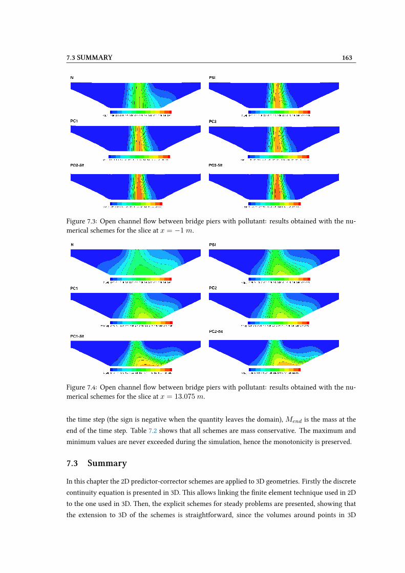
7.3 SUMMARY 163
Figure 7.3: Open channel Wow between bridge piers with pollutant: results obtained with the nu-merical schemes for the slice at x = −1 m.
Figure 7.4: Open channel Wow between bridge piers with pollutant: results obtained with the nu-merical schemes for the slice at x = 13.075 m.
the time step (the sign is negative when the quantity leaves the domain), Mend is the mass at the
end of the time step. Table 7.2 shows that all schemes are mass conservative. The maximum and
minimum values are never exceeded during the simulation, hence the monotonicity is preserved.
7.3 Summary
In this chapter the 2D predictor-corrector schemes are applied to 3D geometries. Firstly the discrete
continuity equation is presented in 3D. This allows linking the Vnite element technique used in 2D
to the one used in 3D. Then, the explicit schemes for steady problems are presented, showing that
the extension to 3D of the schemes is straightforward, since the volumes around points in 3D
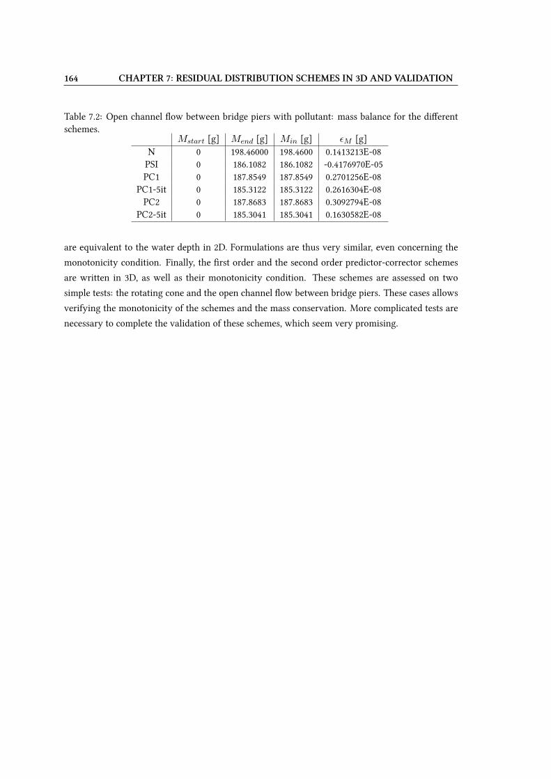
164 CHAPTER 7: RESIDUAL DISTRIBUTION SCHEMES IN 3D AND VALIDATION
Table 7.2: Open channel Wow between bridge piers with pollutant: mass balance for the diUerentschemes.
Mstart [g] Mend [g] Min [g] εM [g]N 0 198.46000 198.4600 0.1413213E-08PSI 0 186.1082 186.1082 -0.4176970E-05PC1 0 187.8549 187.8549 0.2701256E-08
PC1-5it 0 185.3122 185.3122 0.2616304E-08PC2 0 187.8683 187.8683 0.3092794E-08
PC2-5it 0 185.3041 185.3041 0.1630582E-08
are equivalent to the water depth in 2D. Formulations are thus very similar, even concerning the
monotonicity condition. Finally, the Vrst order and the second order predictor-corrector schemes
are written in 3D, as well as their monotonicity condition. These schemes are assessed on two
simple tests: the rotating cone and the open channel Wow between bridge piers. These cases allows
verifying the monotonicity of the schemes and the mass conservation. More complicated tests are
necessary to complete the validation of these schemes, which seem very promising.
Chapter 8
Conclusions and future work
Dans cette thèse des nouveaux schémas de convection pour le transport scalaire dans
un écoulement à surface libre ont été proposés.
Les diUérentes problématiques liées à la discretisation de l’équation de transport avec
des méthodes aux volumes Vnis et aux résidus distribués ont été exposées. Concernant
les schémas VF, une amélioration est trouvée en utilisant un schéma découplé avec un
solveur HLLC. Cette solution permet de réduire la diUusion numérique et d’alléger les
coûts de calcul. De plus la technique MUSCL est utilisée pour augmenter l’ordre en
espace du schéma.
L’application des schémas RD au transport scalaire dans le cadre des équation de
Saint-Venant représente une nouveauté. Les techniques pour améliorer l’ordre dans
des cas non stationnaires sont appliquées avec succès. De plus des améliorations pour
augmenter la précision des schémas sont développées. Par rapport aux schémas exis-
tants, les conditions de monotonie des schémas sont diUérentes. Pour traiter des cas
réels avec des bancs découvrants, un nouvau schéma RD localement implicite est aussi
proposé.
Les diUérents schémas sont testés sur une série de cas tests et les résultats montrent qu’
ils sont eUectivement beaucoup plus précis, avec cependant des ordres de convergence
assez variés. En particulier, le schéma adapté aux bancs découvrants n’est pas d’ordre
deux et un système linéaire doit être résolu.
Les schémas RD 2D sont facilement adaptés au cas 3D. Cette extension est validée
sur des cas préliminaires simples mais leurs bonnes propriétés en font des schémas
prometteurs sur des cas plus complexes.
Des études sont en cours pour améliorer encore le caractère upwind des schémas ou
pour s’aUranchir de systèmes linéaires à résoudre.
166 CHAPTER 8: CONCLUSIONS AND FUTURE WORK
8.1 Concluding remarks
In this thesis, advanced numerical schemes for convection problems have been developed and
assessed. The focus is kept on two numerical methods: the Vnite volumes and the residual distri-
bution.
For the Vnite volume HLLC scheme, the major novelty consists in decoupling the tracer equation
from the hydrodynamic equations, obtaining better eXciency in terms of accuracy and numerical
costs. To increase the space accuracy a MUSCL scheme has also been introduced in the decoupled
formulation.
The application of the residual distribution schemes to the depth-averaged transport equation rep-
resents a novelty for this family of schemes, even if they have been already applied to the shallow
water equations. The existing schemes are reformulated in order to be compatible with the dis-
cretized continuity equation. DiUerent strategies to reduce the numerical diUusion in time depen-
dent problems have been studied and compared in this work. A new iterative procedure has been
introduced to enhance the accuracy of the scheme. For the schemes proposed in this thesis, speciVc
monotonicity conditions have been found and proved. These conditions are diUerent from the one
proposed in the literature, due to the depth-averaged context and to a diUerent monotonicity anal-
ysis. In order to treat real cases, a new locally implicit scheme able to deal with wetting and drying
phenomena has been proposed and the number of linear systems that really need to be solved has
been reduced. The locally implicit scheme scheme has the properties that were specially looked for
in this thesis:
• free surface context;
• mass conservation;
• monotonicity;
• unconditional stability even in dry zones;
• compatibility with domain decomposition parallelism.
It can thus be considered as the best candidate for industrial application.
A number of test cases are presented to validate and compare the new convection schemes. Re-
sults show that these schemes are suitable to steady and unsteady transport problems. In addition
the schemes are all mass conservative and they preserve the maximum principle, which is very
important in convection phenomena. The dam-break with dry bed and the Thacker test case are
presented to validate the schemes in case of wetting and drying problems, in presence of tracers.
A good agreement between the numerical results and the exact solution is shown. An industrial
case of a real river characterized by wetting and drying phenomena is carried out to check the
robustness of the code under real conditions. In general, the numerical results agree with the
8.2 PERSPECTIVES 167
experimental data, showing in particular that the scheme is able to capture with accuracy the max-
imum measured values of tracer.
An overall comparison between the FV and the RD methods shows that the RD schemes are more
eXcient than the FV schemes for the same degree of accuracy. However, in terms of precision
the schemes are comparable. The extra value of the new RD schemes is the speciVc monotonicity
condition which is not too much restrictive.
The application of the RD schemes to the 3D case is also presented in this work. As explained, the
3D extension does not present issues from a theoretical and numerical point of view. The validation
is done on preliminary test cases.
The new RD schemes presented here improve the existing N, PSI and NERD schemes. This is also
an advancement in the Telemac system and the new schemes have already been used in a real
study which could not be done before due to numerical diUusion problems.
8.2 Perspectives
The numerical schemes presented in this thesis could be improved in various ways.
For the FV schemes, other formulations (like [33]) to apply the limiter should be taken into account.
Then, second order schemes in time (other than the Newmark and the Heun method) should also
be tested in order to avoid spoiling the second order space accuracy. This point should be addressed
with particular attention to the cost of second order discretization techniques. Regarding mono-
tonicity, an appropriate condition when using the MUSCL technique could be found following the
ideas of Calgaro et al. [36]. In addition, in order to apply the scheme on real cases the paralleliza-
tion should be done.
For the RD schemes, additional work would be necessary to improve the local implicit formulation
for wetting and drying phenomena. The solution of a linear system represents at the moment a
drawback for this scheme in terms of CPU time. It would be suitable to replace the linear system
by a completely explicit scheme, still able to cope with wetting and drying problems. Besides, the
scheme is still not perfectly second order in space and in time. This is another drawback which
should be improved. Other improvements concern thus a better upwinding (so far only the explicit
part of the Wuxes is upwinded), or optimisation, e.g. by avoiding to solve a linear system.
To better improve the accuracy of the second order RD schemes, third order schemes, as proposed
in [4] could be tailored to the depth-averaged transport. Yet in this case even more attention should
be focused on the monotonicity which is still a problem for these schemes.
A possible improvement of existing schemes could be obtained exploiting the good accuracy prop-
erties when the edges of the mesh are aligned with the Wow. An adaptive mesh which follows the
Wow paths could thus mainly reduce the numerical diUusion.
For the 3D case, the model should be tested on several and more complex cases, where also diUusion
and turbulence are involved. In general, the behaviour of the scheme should be checked coupling
the convection to the other possible phenomena like diUusion, reaction, adsorption or other more

168 CHAPTER 8: CONCLUSIONS AND FUTURE WORK
complex kinetic models which should be appropriate modeled.
Finally, the extension of the locally implicit scheme for wetting and drying phenomena should also
be adapted to the 3D and tested, it was not done here for lack of time.
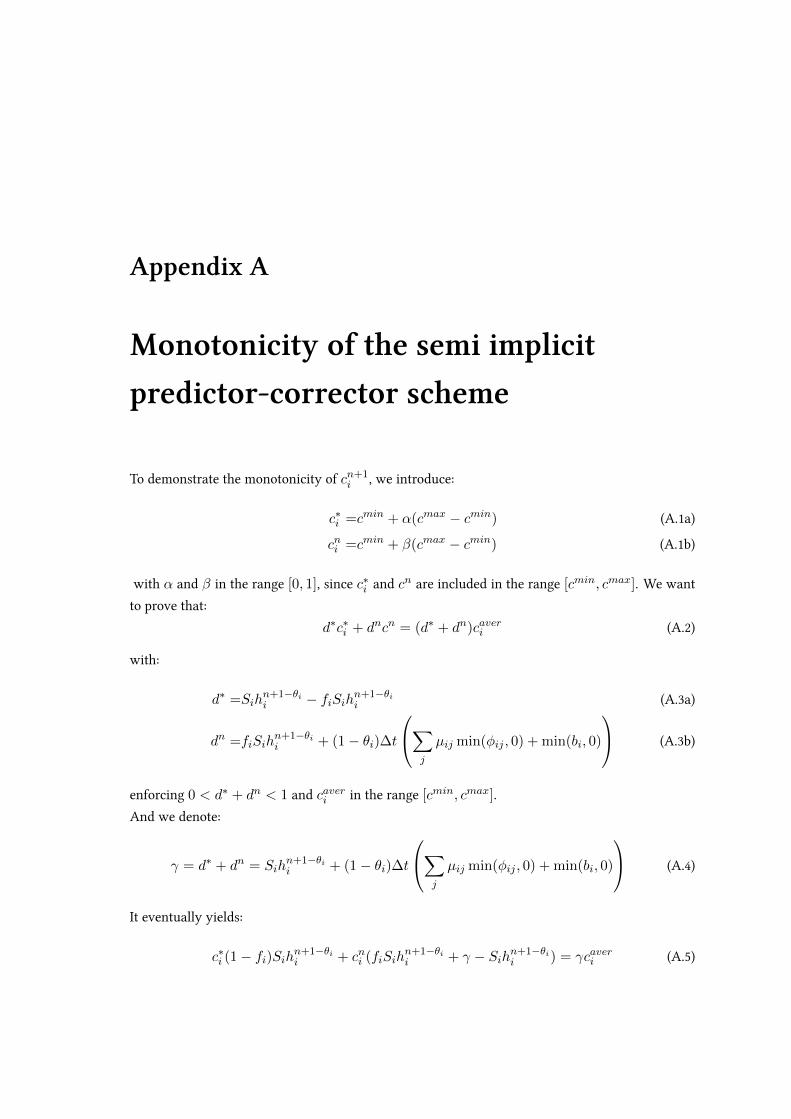
Appendix A
Monotonicity of the semi implicit
predictor-corrector scheme
To demonstrate the monotonicity of cn+1i , we introduce:
c∗i =cmin + α(cmax − cmin) (A.1a)
cni =cmin + β(cmax − cmin) (A.1b)
with α and β in the range [0, 1], since c∗i and cn are included in the range [cmin, cmax]. We want
to prove that:
d∗c∗i + dncn = (d∗ + dn)caveri (A.2)
with:
d∗ =Sihn+1−θii − fiSihn+1−θi
i (A.3a)
dn =fiSihn+1−θii + (1− θi)∆t
∑j
µij min(φij , 0) + min(bi, 0)
(A.3b)
enforcing 0 < d∗ + dn < 1 and caveri in the range [cmin, cmax].
And we denote:
γ = d∗ + dn = Sihn+1−θii + (1− θi)∆t
∑j
µij min(φij , 0) + min(bi, 0)
(A.4)
It eventually yields:
c∗i (1− fi)Sihn+1−θii + cni (fiSih
n+1−θii + γ − Sihn+1−θi
i ) = γcaveri (A.5)
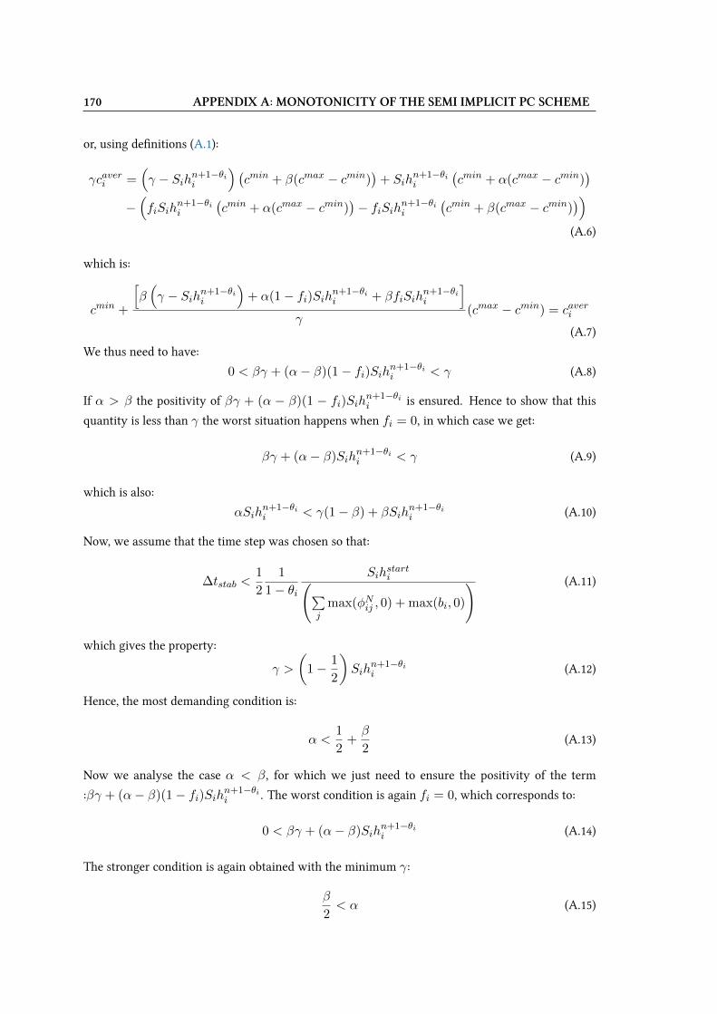
170 APPENDIX A: MONOTONICITY OF THE SEMI IMPLICIT PC SCHEME
or, using deVnitions (A.1):
γcaveri =(γ − Sihn+1−θi
i
) (cmin + β(cmax − cmin)
)+ Sih
n+1−θii
(cmin + α(cmax − cmin)
)−(fiSih
n+1−θii
(cmin + α(cmax − cmin)
)− fiSihn+1−θi
i
(cmin + β(cmax − cmin)
))(A.6)
which is:
cmin +
[β(γ − Sihn+1−θi
i
)+ α(1− fi)Sihn+1−θi
i + βfiSihn+1−θii
]γ
(cmax − cmin) = caveri
(A.7)
We thus need to have:
0 < βγ + (α− β)(1− fi)Sihn+1−θii < γ (A.8)
If α > β the positivity of βγ + (α − β)(1 − fi)Sihn+1−θii is ensured. Hence to show that this
quantity is less than γ the worst situation happens when fi = 0, in which case we get:
βγ + (α− β)Sihn+1−θii < γ (A.9)
which is also:
αSihn+1−θii < γ(1− β) + βSih
n+1−θii (A.10)
Now, we assume that the time step was chosen so that:
∆tstab <1
2
1
1− θiSih
starti(∑
jmax(φNij , 0) + max(bi, 0)
) (A.11)
which gives the property:
γ >
(1− 1
2
)Sih
n+1−θii (A.12)
Hence, the most demanding condition is:
α <1
2+β
2(A.13)
Now we analyse the case α < β, for which we just need to ensure the positivity of the term
:βγ + (α− β)(1− fi)Sihn+1−θii . The worst condition is again fi = 0, which corresponds to:
0 < βγ + (α− β)Sihn+1−θii (A.14)
The stronger condition is again obtained with the minimum γ:
β
2< α (A.15)
APPENDIX A: MONOTONICITY OF THE SEMI IMPLICIT PC SCHEME 171
Hence, the general condition which must be ensured is:
β
2< α <
1
2+β
2(A.16)
This condition corresponds to:
cni +1
2
(cmini − cni
)< c∗i < cni +
1
2(cmaxi − cni ) (A.17)
Here below, we also show that this property is already ensured by c∗i when using a semi-implicit
predictor. Indeed the predictor step is:
Sihn+1−θii (c∗i − cni ) =−∆t
∑j
[θjc∗j + (1− θj)cnj − θic∗i − (1− θi)cni
]min(φij , 0)
−∆tmin(bi, 0) (cbound − (θic∗i + (1− θi)cni ))
(A.18)
The latter is equivalent to:[Sih
n+1−θii + θi∆t (−min(φij , 0)−min(bi, 0))
](c∗i − cni ) = −∆tmin(bi, 0) (cbound − cni )
−∆t∑j
(θjc∗j + (1− θj)cnj − cni
)min(φij , 0)
(A.19)
Denoting λ = ∆t (−min(φij , 0)−min(bi, 0)), we can write:
λ(cmin − cni ) <(Sih
n+1−θii + θiλ
)c∗i −
(Sih
n+1−θii + θiλ
)cni < λ(cmax − cni ) (A.20)
that is:
cni +λ
Sihn+1−θii + θiλ
(cmin − cni ) < c∗i < cni +λ
Sihn+1−θii + θiλ
(cmax − cni ) (A.21)
The maximum of λ
Sihn+1−θii +θiλ
(cmin − cni ) is obtained with the maximum of λ.
Under condition (A.11), the maximum is 12+θi
which is less than 1k . Hence we get:
cni +1
2
(cmini − cni
)< c∗i < cni +
1
2(cmaxi − cni ) (A.22)
which is exactly the condition (A.17), found for the corrector, but also the condition found to do
iterations on the Vrst order predictor corrector scheme.

172 APPENDIX A: MONOTONICITY OF THE SEMI IMPLICIT PC SCHEME

Bibliography
[1] URL http://opentelemac.org/.
[2] R. Abgrall. Toward the Ultimate Conservative Scheme: Following the Quest. Journal of
Computational Physics, 167(2):277–315, March 2001. ISSN 00219991. doi: 10.1006/jcph.2000.
6672. URL http://linkinghub.elsevier.com/retrieve/pii/S0021999100966725.
[3] R. Abgrall. Essentially non-oscillatory Residual Distribution schemes for hyperbolic prob-
lems. Journal of Computational Physics, 214(2):773–808, May 2006. ISSN 00219991.
doi: 10.1016/j.jcp.2005.10.034. URL http://linkinghub.elsevier.com/retrieve/pii/
S0021999105004730.
[4] R. Abgrall, G. Baurin, P. Jacq, and M. Ricchiuto. Some examples of high order simu-
lations parallel of inviscid Wows on unstructured and hybrid meshes by residual distri-
bution schemes. Computers & Fluids, 61:6–13, May 2012. ISSN 00457930. doi: 10.
1016/j.compWuid.2011.05.014. URL http://linkinghub.elsevier.com/retrieve/pii/
S0045793011001848.
[5] Rémi Abgrall and Timothy Barth. Residual distribution schemes for conservation laws via
adaptive quadrature. SIAM Journal on ScientiVc Computing, 24(3):732–769, 2003. URL http:
//epubs.siam.org/doi/abs/10.1137/S106482750138592X.
[6] Rémi Abgrall and Mohamed Mezine. Construction of second order accurate monotone and
stable residual distribution schemes for unsteady Wow problems. Journal of Computational
Physics, 188(1):16–55, June 2003. ISSN 00219991. doi: 10.1016/S0021-9991(03)00084-6. URL
http://linkinghub.elsevier.com/retrieve/pii/S0021999103000846.
[7] Rémi Abgrall and Mohamed Mezine. Construction of second-order accurate monotone and
stable residual distribution schemes for steady problems. Journal of Computational Physics,
195(2):474–507, April 2004. ISSN 00219991. doi: 10.1016/j.jcp.2003.09.022. URL http://
linkinghub.elsevier.com/retrieve/pii/S0021999103005400.
[8] Rémi Abgrall and Philip L. Roe. High order Wuctuation schemes on triangular meshes.
Journal of ScientiVc Computing, 19(1-3):3–36, 2003. URL http://link.springer.com/
article/10.1023/A:1025335421202.
174 BIBLIOGRAPHY
[9] F. Angrand, A. Dervieux, J.A. Désidéri, and R. Glowinski, editors. Numerical methods for
the Euler Equations for Wuid dynamics. SIAM, 1985.
[10] V. I Arnold. Lectures on Partial DiUerential Equations. PHASIS, Moskva, 1997. ISBN 978-5-
7036-0035-1.
[11] L. Arpaia, M. Ricchiuto, and R. Abgrall. An ALE Formulation for Explicit Runge–Kutta
Residual Distribution. Journal of ScientiVc Computing, 63(2):502–547, May 2015. ISSN 0885-
7474, 1573-7691. doi: 10.1007/s10915-014-9910-5. URL http://link.springer.com/10.
1007/s10915-014-9910-5.
[12] Emmanuel Audusse. Modélisation hyperbolique et analyse numérique pour les écoulements
en eaux peu profondes. PhD thesis, Université Paris VI Pierre et Marie Curie, 2004.
[13] Emmanuel Audusse and Marie-Odile Bristeau. Transport of Pollutant in Shallow Water. A
Two Time Steps Kinetic Method. ESAIM: Mathematical Modelling and Numerical Analysis,
37(2):389–416, March 2003. ISSN 0764-583X, 1290-3841. doi: 10.1051/m2an:2003034. URL
http://www.esaim-m2an.org/10.1051/m2an:2003034.
[14] Emmanuel Audusse and Marie-Odile Bristeau. A well-balanced positivity preserving
“second-order” scheme for shallow water Wows on unstructured meshes. Journal of Com-
putational Physics, 206(1):311–333, June 2005. ISSN 00219991. doi: 10.1016/j.jcp.2004.12.016.
URL http://linkinghub.elsevier.com/retrieve/pii/S0021999104005157.
[15] Emmanuel Audusse, François Bouchut, Marie-Odile Bristeau, Rupert Klein, and Benoit
Perthame. A Fast and Stable Well-Balanced Scheme with Hydrostatic Reconstruction for
Shallow Water Flows. SIAM Journal on ScientiVc Computing, 25(6):2050–2065, January 2004.
ISSN 1064-8275, 1095-7197. doi: 10.1137/S1064827503431090. URL http://epubs.siam.
org/doi/abs/10.1137/S1064827503431090.
[16] Andrea Balzano. Evaluation of methods for numerical simulation of wetting and dry-
ing in shallow water Wow models. Coastal Engineering, 34(1-2):83–107, July 1998. ISSN
03783839. doi: 10.1016/S0378-3839(98)00015-5. URL http://linkinghub.elsevier.com/
retrieve/pii/S0378383998000155.
[17] A.J.C. Barré de Saint Venant. Théorie du mouvement non-permanent des eaux, avec appli-
cation aux crues des rivières et à l’introduction des marées dans leur lit. Comptes Rendus des
séances de l’Académie des Sciences, Paris, (73):147–154, 1871.
[18] Timothy Barth and Dennis Jespersen. The design and application of upwind schemes on
unstructured meshes. In 27th Aerospace Sciences Meeting. American Institute of Aeronautics
and Astronautics, January 1989. doi: 10.2514/6.1989-366. URL http://arc.aiaa.org/
doi/abs/10.2514/6.1989-366.
BIBLIOGRAPHY 175
[19] P. Batten, C. Lambert, and D. M. Causon. POSITIVELY CONSERVATIVE HIGH-
RESOLUTION CONVECTION SCHEMES FOR UNSTRUCTURED ELEMENTS. Interna-
tional Journal for Numerical Methods in Engineering, 39(11):1821–1838, June 1996. ISSN
0029-5981, 1097-0207. doi: 10.1002/(SICI)1097-0207(19960615)39:11<1821::AID-NME929>3.0.
CO;2-E. URL http://doi.wiley.com/10.1002/%28SICI%291097-0207%2819960615%
2939%3A11%3C1821%3A%3AAID-NME929%3E3.0.CO%3B2-E.
[20] P. Batten, N. Clarke, C. Lambert, and D. M. Causon. On the choice of wavespeeds for the
HLLC Riemann solver. SIAM Journal on ScientiVc Computing, 18(6):1553–1570, 1997. URL
http://epubs.siam.org/doi/abs/10.1137/S1064827593260140.
[21] P. Batten, M.A. Leschziner, and U.C. Goldberg. Average-State Jacobians and Implicit Meth-
ods for Compressible Viscous and Turbulent Flows. Journal of Computational Physics,
137(1):38–78, October 1997. ISSN 00219991. doi: 10.1006/jcph.1997.5793. URL http:
//linkinghub.elsevier.com/retrieve/pii/S0021999197957934.
[22] Lorenzo Begnudelli and Brett F. Sanders. Unstructured Grid Finite-Volume Algorithm
for Shallow-Water Flow and Scalar Transport with Wetting and Drying. Journal of Hy-
draulic Engineering, 132(4):371–384, April 2006. ISSN 0733-9429, 1943-7900. doi: 10.
1061/(ASCE)0733-9429(2006)132:4(371). URL http://ascelibrary.org/doi/10.1061/
%28ASCE%290733-9429%282006%29132%3A4%28371%29.
[23] Fayssal Benkhaldoun, Imad Elmahi, and Mohammed Seaid. Well-balanced Vnite vol-
ume schemes for pollutant transport by shallow water equations on unstructured meshes.
Journal of Computational Physics, 226(1):180–203, September 2007. ISSN 00219991.
doi: 10.1016/j.jcp.2007.04.005. URL http://linkinghub.elsevier.com/retrieve/pii/
S0021999107001490.
[24] J.-P. Benque, G. Labadie, and J. Ronat. Une méthode d’éléments Vnis pour la résolution
des équations de Navier-Stokes couplées à une équation thermique. In Proceedings of 4th
International Symposium on Vnite element methods for Wuid mechanics problems, Tokyo,
Japan, July 1982.
[25] Alfredo Bermudez and María Elena Vázquez-Cendón. Upwind methods for hyperbolic con-
servation laws with source terms. Computers & Fluids, 23(8):1049–1071, November 1994.
ISSN 00457930. doi: 10.1016/0045-7930(94)90004-3. URL http://linkinghub.elsevier.
com/retrieve/pii/0045793094900043.
[26] Christophe Berthon. Robustness of MUSCL schemes for 2D unstructured meshes. Journal
of Computational Physics, 218(2):495–509, 2006. URL http://www.sciencedirect.com/
science/article/pii/S0021999106001161.
[27] P. Binning and M.A. Celia. A forward particle tracking Eulerian–Lagrangian Localized
Adjoint Method for solution of the contaminant transport equation in three dimensions.

176 BIBLIOGRAPHY
Advances in Water Resources, 25(2):147–157, February 2002. ISSN 03091708. doi: 10.
1016/S0309-1708(01)00051-3. URL http://linkinghub.elsevier.com/retrieve/pii/
S0309170801000513.
[28] François Bouchut. Nonlinear Stability of Finite Volume Methods for Hyperbolic Conservation
Laws. Frontiers in Mathematics. Birkhäuser Basel, Basel, 2004. ISBN 978-3-7643-6665-0 978-
3-7643-7792-2. URL http://link.springer.com/10.1007/b93802.
[29] G. Bourgois, H. Deconinck, P.L. Roe, and R. Struijs. Multidimensional upwind schemes
for scalar advection on tetrahedral meshes. In Hirsch et al., editor, Computational Fluid
Dynamics. Elsevier Science Publisher, 1992.
[30] Scott F. Bradford and Brett F. Sanders. Finite-Volume Model for Shallow-Water
Flooding of Arbitrary Topography. Journal of Hydraulic Engineering, 128(3):289–
298, March 2002. ISSN 0733-9429, 1943-7900. doi: 10.1061/(ASCE)0733-9429(2002)
128:3(289). URL http://ascelibrary.org/doi/10.1061/%28ASCE%290733-9429%
282002%29128%3A3%28289%29.
[31] M.O. Bristeau and B. Coussin. Boundary conditions for the shallow water equations solved
by kinetic schemes. Report no 4282, INRIA, 2001.
[32] P. Brufau, P. García-Navarro, and M. E. Vázquez-Cendón. Zero mass error using unsteady
wetting–drying conditions in shallow Wows over dry irregular topography. International
Journal for Numerical Methods in Fluids, 45(10):1047–1082, August 2004. ISSN 0271-2091,
1097-0363. doi: 10.1002/Wd.729. URL http://doi.wiley.com/10.1002/fld.729.
[33] Thierry BuUard and Stéphane Clain. Monoslope and multislope MUSCL methods for
unstructured meshes. Journal of Computational Physics, 229(10):3745–3776, May 2010.
ISSN 00219991. doi: 10.1016/j.jcp.2010.01.026. URL http://linkinghub.elsevier.com/
retrieve/pii/S0021999110000495.
[34] Shintaro Bunya, Ethan J. Kubatko, Joannes J. Westerink, and Clint Dawson. A wetting and
drying treatment for the Runge–Kutta discontinuous Galerkin solution to the shallow water
equations. Computer Methods in Applied Mechanics and Engineering, 198(17-20):1548–1562,
April 2009. ISSN 00457825. doi: 10.1016/j.cma.2009.01.008. URL http://linkinghub.
elsevier.com/retrieve/pii/S0045782509000383.
[35] J. Burguete, Pilar García-Navarro, and J. Murillo. Preserving bounded and conservative solu-
tions of transport in one-dimensional shallow-water Wow with upwind numerical schemes:
Application to fertigation and solute transport in rivers. International journal for numerical
methods in Wuids, 56(9):1731–1764, 2008. URL http://onlinelibrary.wiley.com/doi/
10.1002/fld.1576/abstract.
BIBLIOGRAPHY 177
[36] Caterina Calgaro, Emile Chane-Kane, Emmanuel Creusé, and Thierry Goudon. L-∞ sta-
bility of vertex-based MUSCL Vnite volume schemes on unstructured grids: Simulation
of incompressible Wows with high density ratios. Journal of Computational Physics, 229
(17):6027–6046, August 2010. ISSN 00219991. doi: 10.1016/j.jcp.2010.04.034. URL http:
//linkinghub.elsevier.com/retrieve/pii/S0021999110002214.
[37] Alberto Canestrelli and Eleuterio F. Toro. Restoration of the contact surface in FORCE-type
centred schemes I: Homogeneous two-dimensional shallow water equations. Advances in
Water Resources, 47:88–99, October 2012. ISSN 03091708. doi: 10.1016/j.advwatres.2012.03.
019. URL http://linkinghub.elsevier.com/retrieve/pii/S0309170812000747.
[38] D. Caraeni and L. Fuchs. Compact third-order multidimensional upwind discretization for
steady and unsteady Wow simulations. Computers & Fluids, 34(4-5):419–441, May 2005. ISSN
00457930. doi: 10.1016/j.compWuid.2004.03.002. URL http://linkinghub.elsevier.
com/retrieve/pii/S0045793004000416.
[39] L. Cea and M.E. Vázquez-Cendón. Unstructured Vnite volume discretisation of bed fric-
tion and convective Wux in solute transport models linked to the shallow water equa-
tions. Journal of Computational Physics, 231(8):3317–3339, April 2012. ISSN 00219991.
doi: 10.1016/j.jcp.2012.01.007. URL http://linkinghub.elsevier.com/retrieve/pii/
S0021999112000289.
[40] L. Cea and M. E. Vázquez-Cendón. Unstructured Vnite volume discretization of two-
dimensional depth-averaged shallow water equations with porosity. International Jour-
nal for Numerical Methods in Fluids, pages 903–930, 2009. ISSN 02712091, 10970363. doi:
10.1002/Wd.2107. URL http://doi.wiley.com/10.1002/fld.2107.
[41] Michael A. Celia, Thomas F. Russell, Ismael Herrera, and Richard E. Ewing. An
Eulerian-Lagrangian localized adjoint method for the advection-diUusion equation. Ad-
vances in Water Resources, 13(4):187–206, December 1990. ISSN 03091708. doi: 10.
1016/0309-1708(90)90041-2. URL http://linkinghub.elsevier.com/retrieve/pii/
0309170890900412.
[42] Alina Chertock and Alexander Kurganov. On a hybrid Vnite-volume-particle method.
ESAIM: Mathematical Modelling and Numerical Analysis, 38(6):1071–1091, November 2004.
ISSN 0764-583X, 1290-3841. doi: 10.1051/m2an:2004051. URL http://www.esaim-m2an.
org/10.1051/m2an:2004051.
[43] Alina Chertock, Alexander Kurganov, and Guergana Petrova. Finite-Volume-Particle Meth-
ods for Models of Transport of Pollutant in Shallow Water. Journal of ScientiVc Computing,
27(1-3):189–199, June 2006. ISSN 0885-7474, 1573-7691. doi: 10.1007/s10915-005-9060-x. URL
http://link.springer.com/10.1007/s10915-005-9060-x.
178 BIBLIOGRAPHY
[44] Stephane Clain and Vivien Clauzon. L-∞ stability of the MUSCL methods. URL https:
//hal.archives-ouvertes.fr/hal-00329588/.
[45] R. Courant, K.O. Friedrichs, and H. Lewy. On the partial diUerential equations of mathemat-
ical physics. IBM Journal, (11):215–234, 1967.
[46] Richard Courant, Eugene Isaacson, and Mina Rees. On the solution of nonlinear hyperbolic
diUerential equations by Vnite diUerences. Communications on Pure and Applied Mathemat-
ics, 5(3):243–255, August 1952. ISSN 00103640, 10970312. doi: 10.1002/cpa.3160050303. URL
http://doi.wiley.com/10.1002/cpa.3160050303.
[47] Á. Csík and H. Deconinck. Space-time residual distribution schemes for hyperbolic con-
servation laws on unstructured linear Vnite elements. International Journal for Numeri-
cal Methods in Fluids, 40(3-4):573–581, September 2002. ISSN 0271-2091, 1097-0363. doi:
10.1002/Wd.315. URL http://doi.wiley.com/10.1002/fld.315.
[48] Árpád Csík, Mario Ricchiuto, and Herman Deconinck. A Conservative Formulation of the
Multidimensional Upwind Residual Distribution Schemes for General Nonlinear Conserva-
tion Laws. Journal of Computational Physics, 179(1):286–312, June 2002. ISSN 00219991.
doi: 10.1006/jcph.2002.7057. URL http://linkinghub.elsevier.com/retrieve/pii/
S0021999102970579.
[49] J.A. Cunge, F.M.Jr. Holly, and A. Verwey. Practical aspects of computational river hydraulics.
Pitman Advanced Publishing Program, London, 1980.
[50] Clint Dawson and Jennifer Proft. Coupling of continuous and discontinuous Galerkin meth-
ods for transport problems. Computer Methods in Applied Mechanics and Engineering, 191
(29-30):3213–3231, May 2002. ISSN 00457825. doi: 10.1016/S0045-7825(02)00257-8. URL
http://linkinghub.elsevier.com/retrieve/pii/S0045782502002578.
[51] Clint Dawson and Jennifer Proft. Discontinuous and coupled continuous/discontinuous
Galerkin methods for the shallow water equations. Computer Methods in Applied Me-
chanics and Engineering, 191(41-42):4721–4746, September 2002. ISSN 00457825. doi:
10.1016/S0045-7825(02)00402-4. URL http://linkinghub.elsevier.com/retrieve/
pii/S0045782502004024.
[52] P. De Palma, G. Pascazio, G. Rossiello, and M. Napolitano. A second-order-accurate mono-
tone implicit Wuctuation splitting scheme for unsteady problems. Journal of Computational
Physics, 208(1):1–33, September 2005. ISSN 00219991. doi: 10.1016/j.jcp.2004.11.023. URL
http://linkinghub.elsevier.com/retrieve/pii/S002199910400484X.
[53] Astrid Decoene. Hydrostatic model for three-dimensional free surface Wows and numerical
schemes. Theses, Université Pierre et Marie Curie - Paris VI ; Laboratoire Jacques-Louis
Lions, May 2006. URL https://tel.archives-ouvertes.fr/tel-00180003.
BIBLIOGRAPHY 179
[54] Herman Deconinck and Mario Ricchiuto. Residual Distribution Schemes: Foundations and
Analysis. In Erwin Stein, René de Borst, and Thomas J. R. Hughes, editors, Encyclopedia of
Computational Mechanics. John Wiley & Sons, Ltd, Chichester, UK, October 2007. ISBN 0-
470-84699-2 978-0-470-84699-5 0-470-09135-5 978-0-470-09135-7. URL http://doi.wiley.
com/10.1002/0470091355.ecm054.
[55] Olivier Delestre, Carine Lucas, Pierre-Antoine Ksinant, Frédéric Darboux, Christian La-
guerre, T.-N.-Tuoi Vo, François James, and Stéphane Cordier. SWASHES: a compilation
of shallow water analytic solutions for hydraulic and environmental studies: ANALYTIC
SOLUTIONS FOR SHALLOW WATER EQUATIONS. International Journal for Numerical
Methods in Fluids, 72(3):269–300, May 2013. ISSN 02712091. doi: 10.1002/Wd.3741. URL
http://doi.wiley.com/10.1002/fld.3741.
[56] A. Dervieux and G. Vijayasundaram. Numerical methods for the Euler Equations for Wuid
dynamics, chapter On numerical schemes for solving Euler equations of Fluid Dynamics,
pages 121–144. In Angrand et al. [9], 1985.
[57] Bruno Després and Frédéric Lagoutière. Contact discontinuity capturing schemes for linear
advection and compressible gas dynamics. Journal of ScientiVc Computing, 16(4):479–524,
2001. URL http://link.springer.com/article/10.1023/A:1013298408777.
[58] Bruno Després and Frédéric Lagoutière. Generalized Harten formalism and longitudinal
variation diminishing schemes for linear advection on arbitrary grids. ESAIM: Mathemat-
ical Modelling and Numerical Analysis, 35(06):1159–1183, 2001. URL http://journals.
cambridge.org/abstract_S0764583X01001522.
[59] Bruno Després, Emmanuel Labourasse, and Frédéric Lagoutière. The VoVre method for
multicomponent Wows on unstructured meshes. Jacques-Louis Lions Report R07052, 2007.
URL http://www.ann.jussieu.fr/~lagoutie/Papiers/vofire.pdf.
[60] Boris Diskin and James L. Thomas. Comparison of Node-Centered and Cell-Centered Un-
structured Finite-Volume Discretizations: Inviscid Fluxes. AIAA Journal, 49(4):836–854,
April 2011. ISSN 0001-1452, 1533-385X. doi: 10.2514/1.J050897. URL http://arc.aiaa.
org/doi/abs/10.2514/1.J050897.
[61] Jiří Dobeš, Mario Ricchiuto, and Herman Deconinck. Implicit space–time residual distribu-
tion method for unsteady laminar viscous Wow. Computers & Fluids, 34(4-5):593–615, May
2005. ISSN 00457930. doi: 10.1016/j.compWuid.2003.09.007. URL http://linkinghub.
elsevier.com/retrieve/pii/S0045793004000337.
[62] Michael Dumbser. Advanced numerical methods for hyperbolic equations and applications.
Lecture notes, 2011.
180 BIBLIOGRAPHY
[63] Michael Dumbser and Martin Käser. Arbitrary high order non-oscillatory Vnite volume
schemes on unstructured meshes for linear hyperbolic systems. Journal of Computational
Physics, 221(2):693–723, February 2007. ISSN 00219991. doi: 10.1016/j.jcp.2006.06.043. URL
http://linkinghub.elsevier.com/retrieve/pii/S0021999106003123.
[64] Michael Dumbser, Martin Käser, Vladimir A. Titarev, and Eleuterio F. Toro. Quadrature-
free non-oscillatory Vnite volume schemes on unstructured meshes for nonlinear hyperbolic
systems. Journal of Computational Physics, 226(1):204–243, September 2007. ISSN 00219991.
doi: 10.1016/j.jcp.2007.04.004. URL http://linkinghub.elsevier.com/retrieve/pii/
S0021999107001520.
[65] Denys Dutykh. Modélisation mathématique des tsunamis. PhD thesis, Ecole nor-
male supérieure de Cachan, 2007. URL https://tel.archives-ouvertes.fr/
tel-00194763/.
[66] B Einfeldt, C.D Munz, P.L Roe, and B Sjögreen. On Godunov-type methods near low den-
sities. Journal of Computational Physics, 92(2):273–295, February 1991. ISSN 00219991.
doi: 10.1016/0021-9991(91)90211-3. URL http://linkinghub.elsevier.com/retrieve/
pii/0021999191902113.
[67] A. Ern and J.L. Guermond. Theory and Practice of Finite Elements. Applied Mathematical
Sciences. Springer New York, 2004. ISBN 9780387205748. URL https://books.google.
fr/books?id=CCjm79FbJbcC.
[68] P. Garcia-Navarro, M.E. Hubbard, and A. Priestley. Genuinely Multidimensional Upwind-
ing for the 2D Shallow Water Equations. Journal of Computational Physics, 121(1):79–93,
October 1995. ISSN 00219991. doi: 10.1006/jcph.1995.1180. URL http://linkinghub.
elsevier.com/retrieve/pii/S0021999185711801.
[69] P. García-Navarro, E. Playán, and G. Zapata. Solute transport modeling in overland Wow
applied to fertigation. Journal of Irrigation and Drainage Engineering, 126(1):33–40, 2000.
[70] Jonathan B. Goodman and Randall J. LeVeque. On the accuracy of stable schemes for 2D
scalar conservation laws. Mathematics of Computation, 45(171):15–15, September 1985. ISSN
0025-5718. doi: 10.1090/S0025-5718-1985-0790641-4. URL http://www.ams.org/jourcgi/
jour-getitem?pii=S0025-5718-1985-0790641-4.
[71] Olivier Gourgue, Richard Comblen, Jonathan Lambrechts, Tuomas Kärnä, Vincent Legat,
and Eric Deleersnijder. A Wux-limiting wetting–drying method for Vnite-element shallow-
water models, with application to the Scheldt Estuary. Advances in Water Resources, 32
(12):1726–1739, December 2009. ISSN 03091708. doi: 10.1016/j.advwatres.2009.09.005. URL
http://linkinghub.elsevier.com/retrieve/pii/S0309170809001493.

BIBLIOGRAPHY 181
[72] J. M. Greenberg and A. Y. Leroux. A well-balanced scheme for the numerical processing of
source terms in hyperbolic equations. SIAM Journal on Numerical Analysis, 33(1):pp. 1–16,
1996. ISSN 00361429. URL http://www.jstor.org/stable/2158421.
[73] Vincent Guinot and Carole Delenne. MUSCL schemes for the shallow water sensitivity
equations with passive scalar transport. Computers & Fluids, 59:11–30, April 2012. ISSN
00457930. doi: 10.1016/j.compWuid.2012.02.001. URL http://linkinghub.elsevier.
com/retrieve/pii/S004579301200045X.
[74] K. F. Gurski. An HLLC-Type Approximate Riemann Solver for Ideal Magnetohydrodynam-
ics. SIAM Journal on ScientiVc Computing, 25(6):2165–2187, January 2004. ISSN 1064-8275,
1095-7197. doi: 10.1137/S1064827502407962. URL http://epubs.siam.org/doi/abs/10.
1137/S1064827502407962.
[75] Ami Harten, Bjorn Engquist, Stanley Osher, and Sukumar R Chakravarthy. Uniformly high
order accurate essentially non-oscillatory schemes, III. Journal of Computational Physics, 71
(2):231–303, August 1987. ISSN 00219991. doi: 10.1016/0021-9991(87)90031-3. URL http:
//linkinghub.elsevier.com/retrieve/pii/0021999187900313.
[76] Mourad Heniche, Yves Secretan, Paul Boudreau, and Michel Leclerc. A two-dimensional V-
nite element drying-wetting shallow water model for rivers and estuaries. Advances in Water
Resources, 23(4):359–372, January 2000. ISSN 03091708. doi: 10.1016/S0309-1708(99)00031-7.
URL http://linkinghub.elsevier.com/retrieve/pii/S0309170899000317.
[77] R. Herbin and F. Hubert. Benchmark on discretization schemes for anisotropic diUusion
problems on general grids. In R. Eymard and J.-M. Hérard, editors, Finite volumes for com-
plex applications V: proceedings of the 5th International Symposium on Finite Volumes for
Complex Applications, pages 659–692. ISTE ; Wiley, London : Hoboken, NJ, 2008.
[78] J.-M. Hervouet. Application de la méthode des charactéristiques en formulation faible à la
résolution des equations d’advection bidimensionnelles sur des maillages grilles. Technical
report HE-43/92-41, EDF R&D, 1992.
[79] J.-M. Hervouet. Characteristics and mass conservation. New developments in Telemac-2D.
Technical report HE-43/92-41, EDF R&D, 1992.
[80] J.-M. Hervouet. The weak form of the method of characteristics, an amazing advection
scheme. In Proceedings of XXth TELEMAC-MASCARET User Conference 2013, Karlsruhe,
Germany, 16-18 October 2013.
[81] J-M Hervouet, E. RazaVndrakoto, and C. Villaret. Dealing with dry zones in free surface
Wows: a new class of advection schemes. In International Association of Hydraulic En-
gineering and Research, Congress, Eric M Valentine, C. J Apelt, International Association
for Hydro-Environment Engineering and Research, Congress, International Association for
182 BIBLIOGRAPHY
Hydro-Environment Engineering and Research, Hydrology and Water Resources Sympo-
sium, and National Conference on Hydraulics in Water Engineering, editors, Proceedings of
the 34th IAHR World Congress 33rd Hydrology and Water Resources Symposium, 10th Con-
ference on Hydraulics in Water Engineering: balance and uncertainty - water in a changing
world, 26 June - 1 July 2011, Brisbane Australia. Engineers Australia, 2011. ISBN 978-0-
85825-868-6.
[82] Jean-Michel Hervouet. Hydrodynamics of Free Surface Flows. John Wiley & Sons, Ltd,
Chichester, UK, April 2007. ISBN 978-0-470-31962-8 978-0-470-03558-0. URL http://doi.
wiley.com/10.1002/9780470319628.
[83] Charles Hirsch. Numerical computation of internal and external Wows: fundamentals of
computational Wuid dynamics. Elsevier/Butterworth-Heinemann, Oxford ; Burlington, MA,
2nd ed edition, 2007. ISBN 978-0-7506-6594-0.
[84] M. S. Horritt. Evaluating wetting and drying algorithms for Vnite element models of shallow
water Wow. International Journal for Numerical Methods in Engineering, 55(7):835–851,
November 2002. ISSN 0029-5981, 1097-0207. doi: 10.1002/nme.529. URL http://doi.
wiley.com/10.1002/nme.529.
[85] Jingming Hou, Qiuhua Liang, Franz Simons, and Reinhard Hinkelmann. A 2D well-
balanced shallow Wow model for unstructured grids with novel slope source term treat-
ment. Advances in Water Resources, 52:107–131, February 2013. ISSN 03091708. doi:
10.1016/j.advwatres.2012.08.003. URL http://linkinghub.elsevier.com/retrieve/
pii/S0309170812002230.
[86] Jingming Hou, Qiuhua Liang, Hongbin Zhang, and Reinhard Hinkelmann. Multis-
lope MUSCL method applied to solve shallow water equations. Computers & Mathe-
matics with Applications, 68(12):2012–2027, December 2014. ISSN 08981221. doi: 10.
1016/j.camwa.2014.09.018. URL http://linkinghub.elsevier.com/retrieve/pii/
S0898122114004672.
[87] M.E. Hubbard. Multidimensional Slope Limiters for MUSCL-Type Finite Volume Schemes
on Unstructured Grids. Journal of Computational Physics, 155(1):54–74, October 1999.
ISSN 00219991. doi: 10.1006/jcph.1999.6329. URL http://linkinghub.elsevier.com/
retrieve/pii/S0021999199963295.
[88] M.E. Hubbard and M.J. Baines. Conservative Multidimensional Upwinding for the Steady
Two-Dimensional Shallow Water Equations. Journal of Computational Physics, 138(2):
419–448, December 1997. ISSN 00219991. doi: 10.1006/jcph.1997.5823. URL http:
//linkinghub.elsevier.com/retrieve/pii/S002199919795823X.
[89] M.E. Hubbard and M. Ricchiuto. Discontinuous upwind residual distribution: A route to
unconditional positivity and high order accuracy. Computers & Fluids, 46(1):263–269, July
BIBLIOGRAPHY 183
2011. ISSN 00457930. doi: 10.1016/j.compWuid.2010.12.023. URL http://linkinghub.
elsevier.com/retrieve/pii/S0045793010003798.
[90] J.-M. Janin. Conservativité et positivité dans le module de transport scalaire écrit en éléments
Vnis. Application à TELEMAC-3D. Technical report HE-42/95/054/a, EDF R&D, 1996.
[91] H. Jasak, H.G. Weller, and A.D. Gosman. High resolution NVD diUerencing scheme for ar-
bitrarily unstructured meshes. International Journal for Numerical Methods in Fluids, 31(2):
431–449, September 1999. ISSN 0271-2091, 1097-0363. doi: 10.1002/(SICI)1097-0363(19990930)
31:2<431::AID-FLD884>3.0.CO;2-T. URL http://doi.wiley.com/10.1002/%28SICI%
291097-0363%2819990930%2931%3A2%3C431%3A%3AAID-FLD884%3E3.0.CO%3B2-T.
[92] Friedemann Kemm. A comparative study of TVD-limiters-well-known limiters and an intro-
duction of new ones. International Journal for Numerical Methods in Fluids, 67(4):404–440,
October 2011. ISSN 02712091. doi: 10.1002/Wd.2357. URL http://doi.wiley.com/10.
1002/fld.2357.
[93] N.E. Kolgan. Application of the minimum-derivative principle in the construction of Vnite-
diUerence schemes for numerical analysis of discontinuous solutions in gas dynamics. Tech-
nical Report 3(6):68-77, Uchenye Zapiski TsaGI (Sci. Notes Central Inst.Aerodyn), 1972.
[94] C. Le Touze, A. Murrone, and H. Guillard. Multislope MUSCL method for general unstruc-
tured meshes. Journal of Computational Physics, 284:389–418, March 2015. ISSN 00219991.
doi: 10.1016/j.jcp.2014.12.032. URL http://linkinghub.elsevier.com/retrieve/pii/
S0021999114008493.
[95] Randall J. LeVeque. Finite volume methods for hyperbolic problems. Cambridge texts in
applied mathematics. Cambridge University Press, Cambridge ; New York, 2002. ISBN 978-
0-521-81087-6 978-0-521-00924-9.
[96] Randall J. LeVeque. Finite diUerence methods for ordinary and partial diUerential equations:
steady-state and time-dependent problems. Society for Industrial and Applied Mathematics,
Philadelphia, PA, 2007. ISBN 978-0-89871-629-0.
[97] Shuangcai Li and Christopher J. DuUy. Fully-Coupled Modeling of Shallow Water Flow
and Pollutant Transport on Unstructured Grids. Procedia Environmental Sciences, 13:2098–
2121, 2012. ISSN 18780296. doi: 10.1016/j.proenv.2012.01.200. URL http://linkinghub.
elsevier.com/retrieve/pii/S1878029612002010.
[98] Qiuhua Liang and Alistair G.L. Borthwick. Adaptive quadtree simulation of shallow Wows
with wet–dry fronts over complex topography. Computers & Fluids, 38(2):221–234, February
2009. ISSN 00457930. doi: 10.1016/j.compWuid.2008.02.008. URL http://linkinghub.
elsevier.com/retrieve/pii/S0045793008000479.

184 BIBLIOGRAPHY
[99] Xu-Dong Liu. A Maximum Principle Satisfying ModiVcation of Triangle Based Adapative
Stencils for the Solution of Scalar Hyperbolic Conservation Laws. SIAM Journal on Numeri-
cal Analysis, 30(3):701–716, June 1993. ISSN 0036-1429, 1095-7170. doi: 10.1137/0730034. URL
http://epubs.siam.org/doi/abs/10.1137/0730034.
[100] Xu-Dong Liu, Stanley Osher, and Tony Chan. Weighted Essentially Non-oscillatory
Schemes. Journal of Computational Physics, 115(1):200–212, November 1994. ISSN 00219991.
doi: 10.1006/jcph.1994.1187. URL http://linkinghub.elsevier.com/retrieve/pii/
S0021999184711879.
[101] J. Murillo and P. García-Navarro. Augmented versions of the HLL and HLLC Riemann
solvers including source terms in one and two dimensions for shallow Wow applica-
tions. Journal of Computational Physics, 231(20):6861–6906, August 2012. ISSN 00219991.
doi: 10.1016/j.jcp.2012.06.031. URL http://linkinghub.elsevier.com/retrieve/pii/
S0021999112003464.
[102] J. Murillo, J. Burguete, P. Brufau, and P. García-Navarro. Coupling between shallow wa-
ter and solute Wow equations: analysis and management of source terms in 2D. In-
ternational Journal for Numerical Methods in Fluids, 49(3):267–299, 2005. URL http:
//onlinelibrary.wiley.com/doi/10.1002/fld.992/abstract.
[103] J. Murillo, P. García-Navarro, J. Burguete, and P. Brufau. A conservative 2Dmodel of inunda-
tion Wow with solute transport over dry bed. International journal for numerical methods in
Wuids, 52(10):1059–1092, 2006. URL http://onlinelibrary.wiley.com/doi/10.1002/
fld.1216/abstract.
[104] J. Murillo, P. García-Navarro, and J. Burguete. Analysis of a second-order upwind method
for the simulation of solute transport in 2D shallow water Wow. International Journal for
Numerical Methods in Fluids, 56(6):661–686, February 2008. ISSN 02712091, 10970363. doi:
10.1002/Wd.1546. URL http://doi.wiley.com/10.1002/fld.1546.
[105] J. Murillo, P. García-Navarro, and J. Burguete. Conservative numerical simulation of multi-
component transport in two-dimensional unsteady shallow water Wow. Journal of Computa-
tional Physics, 228(15):5539–5573, August 2009. ISSN 00219991. doi: 10.1016/j.jcp.2009.04.039.
URL http://linkinghub.elsevier.com/retrieve/pii/S0021999109002290.
[106] J. Murillo, P. García-Navarro, and J. Burguete. Conservative numerical simulation of multi-
component transport in two-dimensional unsteady shallow water Wow. Journal of Computa-
tional Physics, 228(15):5539–5573, August 2009. ISSN 00219991. doi: 10.1016/j.jcp.2009.04.039.
URL http://linkinghub.elsevier.com/retrieve/pii/S0021999109002290.
[107] R.-H. Ni. A multiple grid scheme for solving the Euler equation. AIAA Journal, (20):1565–
1571, 1981.
BIBLIOGRAPHY 185
[108] Naomi Oreskes, Kristin Shrader-Frechette, Kenneth Belitz, et al. VeriVcation, validation, and
conVrmation of numerical models in the earth sciences. Science, 263(5147):641–646, 1994.
[109] Stanley Osher. Convergence of Generalized MUSCL Schemes. SIAM Journal on Numerical
Analysis, 22(5):947–961, October 1985. ISSN 0036-1429, 1095-7170. doi: 10.1137/0722057. URL
http://epubs.siam.org/doi/abs/10.1137/0722057.
[110] Henri Paillère. Multidimensional Upwind Residual Distribution Schemes for the Euler and
Navier-Stokes Equations on Unstructured Grids. PhD thesis, Université Libre de Bruxelles,
1995.
[111] Sara Pavan, Riadh Ata, and Jean-Michel Hervouet. Finite volume schemes and residual
distribution schemes for pollutant transport on unstructured grids. Environmental Earth
Sciences, 74(11):7337–7356, December 2015. ISSN 1866-6280, 1866-6299. doi: 10.1007/
s12665-015-4760-5. URL http://link.springer.com/10.1007/s12665-015-4760-5.
[112] B. Perthame and Y. Qiu. A variant of van Leer’s method for multidimensional system of
conservation laws. Journal of Computational Physics, 112(1):370–381, 1994.
[113] Marco Petti and Silvia Bosa. Accurate shock-capturing Vnite volume method for advection-
dominated Wow and pollution transport. Computers & Fluids, 36(2):455–466, February
2007. ISSN 00457930. doi: 10.1016/j.compWuid.2005.11.008. URL http://linkinghub.
elsevier.com/retrieve/pii/S0045793006000387.
[114] Leo Postma and Jean-Michel Hervouet. Compatibility between Vnite volumes and Vnite ele-
ments using solutions of shallowwater equations for substance transport. International Jour-
nal for Numerical Methods in Fluids, 53(9):1495–1507, March 2007. ISSN 02712091, 10970363.
doi: 10.1002/Wd.1373. URL http://doi.wiley.com/10.1002/fld.1373.
[115] L. Remaki, O. Hassan, and K. Morgan. New limiter and gradient reconstruction
method for HLLC-Vnite volume scheme to solve Navier-Stokes equations. In TECCO-
MAS, the Vfth European Congress on Computational in Fluid Dynamics, Lisbon, Portugal,
pages 14–17, 2010. URL http://www.bcamath.org/documentos_public/archivos/
publicaciones/CFD2010_Hllc.pdf.
[116] Michael Renardy and Robert C. Rogers. An introduction to partial diUerential equations.
Number 13 in Texts in applied mathematics. Springer, New York, 2nd ed edition, 2004. ISBN
978-0-387-00444-0.
[117] M. Ricchiuto and R. Abgrall. Explicit Runge–Kutta residual distribution schemes for time de-
pendent problems: Second order case. Journal of Computational Physics, 229(16):5653–5691,
August 2010. ISSN 00219991. doi: 10.1016/j.jcp.2010.04.002. URL http://linkinghub.
elsevier.com/retrieve/pii/S0021999110001786.
186 BIBLIOGRAPHY
[118] M. Ricchiuto, R. Abgrall, and H. Deconinck. Application of conservative residual
distribution schemes to the solution of the shallow water equations on unstructured
meshes. Journal of Computational Physics, 222(1):287–331, March 2007. ISSN 00219991.
doi: 10.1016/j.jcp.2006.06.024. URL http://linkinghub.elsevier.com/retrieve/pii/
S0021999106002853.
[119] Mario Ricchiuto. Contributions to the development of residual discretizations for hyperbolic
conservation laws with application to shallow water Wows. PhD thesis, Université Libre de
Bruxelles, Faculté de Sciences Appliquées, 2005.
[120] Mario Ricchiuto. Contributions to the development of residual discretizations for hyper-
bolic conservation laws with application to shallow water Wows. PhD thesis, Université
Sciences et Technologies-Bordeaux I, 2011. URL http://tel.archives-ouvertes.fr/
tel-00651688/.
[121] Mario Ricchiuto. An explicit residual based approach for shallow water Wows. Journal of
Computational Physics, 280:306–344, January 2015. ISSN 00219991. doi: 10.1016/j.jcp.2014.09.
027. URL http://linkinghub.elsevier.com/retrieve/pii/S0021999114006639.
[122] Mario Ricchiuto and Andreas Bollermann. Stabilized residual distribution for shallow water
simulations. Journal of Computational Physics, 228(4):1071–1115, 2009. URL http://www.
sciencedirect.com/science/article/pii/S0021999108005391.
[123] Mario Ricchiuto, Árpád Csík, and Herman Deconinck. Residual distribution for general time-
dependent conservation laws. Journal of Computational Physics, 209(1):249–289, October
2005. ISSN 00219991. doi: 10.1016/j.jcp.2005.03.003. URL http://linkinghub.elsevier.
com/retrieve/pii/S002199910500118X.
[124] A. Ritter. Die fortpWanzung der wasserwellen. Zeitschrift des Vereines Deuscher Ingenieure,
36(33):947–954, 1892.
[125] P. L. Roe. Linear advection schemes on triangular meshes. Technical report coa 8720, Cran-
Veld Institute of Technology, 1987.
[126] P. L. Roe and D. Sidilkover. Optimum Positive Linear Schemes for Advection in Two and
Three Dimensions. SIAM Journal on Numerical Analysis, 29(6):1542–1568, December 1992.
ISSN 0036-1429, 1095-7170. doi: 10.1137/0729089. URL http://epubs.siam.org/doi/
abs/10.1137/0729089.
[127] Thomas F. Russell and Michael A. Celia. An overview of research on Eulerian–Lagrangian
localized adjoint methods (ELLAM). Advances in Water Resources, 25(8-12):1215–1231, Au-
gust 2002. ISSN 03091708. doi: 10.1016/S0309-1708(02)00104-5. URL http://linkinghub.
elsevier.com/retrieve/pii/S0309170802001045.

BIBLIOGRAPHY 187
[128] Domokos Sarmany, M. E. Hubbard, and Mario Ricchiuto. Unconditionally stable space–time
discontinuous residual distribution for shallow-water Wows. Journal of Computational
Physics, 253:86–113, 2013. URL http://www.sciencedirect.com/science/article/
pii/S0021999113004816.
[129] Chi-Wang Shu. Discontinuous Galerkin methods: general approach and stability. Numerical
Solutions of Partial DiUerential Equations, pages 149–201, 2009. URL http://eaton.math.
rpi.edu/csums/Papers/PorousMedia/DGReview_Shu.pdf.
[130] Piotr K. Smolarkiewicz. A fully multidimensional positive deVnite advection transport al-
gorithm with small implicit diUusion. Journal of Computational Physics, 54(2):325–362,
May 1984. ISSN 00219991. doi: 10.1016/0021-9991(84)90121-9. URL http://linkinghub.
elsevier.com/retrieve/pii/0021999184901219.
[131] Piotr K. Smolarkiewicz and Joanna Szmelter. MPDATA: An edge-based unstructured-grid
formulation. Journal of Computational Physics, 206(2):624–649, July 2005. ISSN 00219991.
doi: 10.1016/j.jcp.2004.12.021. URL http://linkinghub.elsevier.com/retrieve/pii/
S0021999105000082.
[132] Lixiang Song, Jianzhong Zhou, Jun Guo, Qiang Zou, and Yi Liu. A robust well-balanced
Vnite volume model for shallow water Wows with wetting and drying over irregular ter-
rain. Advances in Water Resources, 34(7):915–932, July 2011. ISSN 03091708. doi:
10.1016/j.advwatres.2011.04.017. URL http://linkinghub.elsevier.com/retrieve/
pii/S0309170811000819.
[133] Lixiang Song, Jianzhong Zhou, Qingqing Li, Xiaoling Yang, and Yongchuan Zhang. An
unstructured Vnite volume model for dam-break Woods with wet/dry fronts over complex
topography. International Journal for Numerical Methods in Fluids, 67(8):960–980, November
2011. ISSN 02712091. doi: 10.1002/Wd.2397. URL http://doi.wiley.com/10.1002/fld.
2397.
[134] Stefan Spekreijse. Multigrid solution of monotone second-order discretizations of hyperbolic
conservation laws. Mathematics of Computation, 49(179):135–135, September 1987. ISSN
0025-5718. doi: 10.1090/S0025-5718-1987-0890258-9. URL http://www.ams.org/jourcgi/
jour-getitem?pii=S0025-5718-1987-0890258-9.
[135] J. J. Stoker. Water Waves: the Mathematical Theory with Applications. Interscience Publish-
ers, New York, USA, 1957.
[136] R. Struijs. A Multi-Dimensional Upwind Discretization Method for the Euler Equations on
Unstructured Grids. PhD thesis, University of Delft, Netherlands, 1994.
[137] P. K. Sweby. High Resolution Schemes Using Flux Limiters for Hyperbolic Conservation
Laws. SIAM Journal on Numerical Analysis, 21(5):995–1011, October 1984. ISSN 0036-1429,
188 BIBLIOGRAPHY
1095-7170. doi: 10.1137/0721062. URL http://epubs.siam.org/doi/abs/10.1137/
0721062.
[138] Ben H Thacker, Scott W Doebling, Francois M Hemez, Mark C Anderson, Jason E Pepin, and
Edward A Rodriguez. Concepts of model veriVcation and validation. Technical report, Los
Alamos National Lab., Los Alamos, NM (US), 2004.
[139] William Carlisle Thacker. Some exact solutions to the nonlinear shallow-water wave equa-
tions. Journal of Fluid Mechanics, 107(-1):499, June 1981. ISSN 0022-1120, 1469-7645. doi:
10.1017/S0022112081001882. URL http://www.journals.cambridge.org/abstract_
S0022112081001882.
[140] V A Titarev and E F Toro. Ader schemes for shallow water equations with pollutant trans-
port. In Proceedings of the XXIX Convegno di Idraulica e Costruzioni Idrauliche, pages 909–
914, 2004.
[141] S.A. Tokareva and E.F. Toro. HLLC-type Riemann solver for the Baer–Nunziato equations
of compressible two-phase Wow. Journal of Computational Physics, 229(10):3573–3604, May
2010. ISSN 00219991. doi: 10.1016/j.jcp.2010.01.016. URL http://linkinghub.elsevier.
com/retrieve/pii/S0021999110000318.
[142] E. F. Toro. Shock-capturing methods for free-surface shallow Wows. John Wiley, Chichester ;
New York, 2001. ISBN 978-0-471-98766-6.
[143] E. F. Toro, M. Spruce, and W. Speares. Restoration of the contact surface in the HLL-
Riemann solver. Shock Waves, 4(1):25–34, July 1994. ISSN 0938-1287, 1432-2153. doi:
10.1007/BF01414629. URL http://link.springer.com/10.1007/BF01414629.
[144] E.F. Toro, M. Spruce, and W. Speares. Restoration of the contact surface in the HLL Riemann
Solver. Report coa 9204, Department of Aerospace Science, College of Aeronautics, CranVeld
Institute of Technology, 1992.
[145] E.F. Toro, R.C. Millington, and L.A.M. Nejad. Godunov Methods: Theory and Applications.
Edited Review, chapter Towards Very High–Order Godunov Schemes, pages 905–937. Kluwer
Academic/Plenum Publishers, 2001.
[146] Eleuterio F. Toro. Riemann Solvers and Numerical Methods for Fluid Dynamics. Springer
Berlin Heidelberg, Berlin, Heidelberg, 2009. ISBN 978-3-540-25202-3 978-3-540-49834-6. URL
http://link.springer.com/10.1007/b79761.
[147] G. D. van Albada, B. van Leer, and W. W. Jr. Roberts. A comparative study of computational
methods in cosmic gas dynamics. Astronomy and Astrophysics, 108(1):76–84, 1982.
[148] Bram van Leer. Towards the ultimate conservative diUerence scheme. II. Monotonicity and
conservation combined in a second-order scheme. Journal of Computational Physics, 14
BIBLIOGRAPHY 189
(4):361–370, March 1974. ISSN 00219991. doi: 10.1016/0021-9991(74)90019-9. URL http:
//linkinghub.elsevier.com/retrieve/pii/0021999174900199.
[149] Bram van Leer. Towards the ultimate conservative diUerence scheme. V. A second-order
sequel to Godunov’s method. Journal of Computational Physics, 32(1):101–136, July 1979.
ISSN 00219991. doi: 10.1016/0021-9991(79)90145-1. URL http://linkinghub.elsevier.
com/retrieve/pii/0021999179901451.
[150] Hong Wang, Richard E. Ewing, and Michael A. Celia. Eulerian-Lagrangian localized ad-
joint methods for reactive transport with biodegradation. Numerical Methods for Par-
tial DiUerential Equations, 11(3):229–254, May 1995. ISSN 0749-159X, 1098-2426. doi:
10.1002/num.1690110305. URL http://doi.wiley.com/10.1002/num.1690110305.
[151] Andrzej Warzyński, Matthew E. Hubbard, and Mario Ricchiuto. Runge–Kutta Residual Dis-
tribution Schemes. Journal of ScientiVc Computing, 62(3):772–802, March 2015. ISSN 0885-
7474, 1573-7691. doi: 10.1007/s10915-014-9879-0. URL http://link.springer.com/10.
1007/s10915-014-9879-0.
[152] Weiming Wu, Dalmo A. Vieira, and Sam S. Y. Wang. One-Dimensional Numerical Model
for Nonuniform Sediment Transport under Unsteady Flows in Channel Networks. Journal of
Hydraulic Engineering, 130(9):914–923, September 2004. ISSN 0733-9429, 1943-7900. doi: 10.
1061/(ASCE)0733-9429(2004)130:9(914). URL http://ascelibrary.org/doi/10.1061/
%28ASCE%290733-9429%282004%29130%3A9%28914%29.
[153] O.C. Zienkiewicz and R.L. Taylor. The Finite Element Method: Solid mechanics. Referex
collection. Mecánica y materiales. Butterworth-Heinemann, 2000. ISBN 9780750650557. URL
https://books.google.fr/books?id=MhgBfMWFVHUC.