multiscale data assimilation approaches and error...
TRANSCRIPT
Thèse présentée pour obtenir le grade de
Docteur de l’Université Paris-Est
Spécialité: Sciences et Techniques de l’Environnement
par
Mohammad Reza Koohkan
École Doctorale : SCIENCES, INGÉNIERIE ET ENVIRONNEMENT
Multiscale data assimilation approaches and error
characterisation applied to the inverse modelling of
atmospheric constituent emission fields.
Thèse soutenue le 20 décembre 2012 devant le jury composé de:
Dr Olivier Talagrand CNRS/LMD Président
Dr Slimane Bekki CNRS/LATMOS Rapporteur
Dr Frédéric Chevallier CEA/LSCE Rapporteur
Dr Gilles Forêt UPEC/LISA Examinateur
Dr Sébastien Massart ECMWF Examinateur
Dr Marc Bocquet École des Ponts ParisTech/CEREA Directeur de thèse
past
el-0
0807
468,
ver
sion
1 -
3 Ap
r 201
3

past
el-0
0807
468,
ver
sion
1 -
3 Ap
r 201
3

"with all the affection, devotion and love thata son can ever express to his dear mum".
À ma petite maman
past
el-0
0807
468,
ver
sion
1 -
3 Ap
r 201
3

past
el-0
0807
468,
ver
sion
1 -
3 Ap
r 201
3

Acknowledgment
This Ph.D. thesis was made possible through an École des Ponts ParisTech scholarship withthe help of the Agence Nationale de la Recherche (MSDAG project), the INSU/LEFE coun-cil (ADOMOCA-2 project) and finally the French Ministry of Ecology and ADEME (CAR-BOSOR project, Primequal research program). Many thanks to all these institutions.
Though only my name appears on the cover of this dissertation, a great many people havecontributed to its production. First and foremost, I would like to express my sincere gratitudeto my supervisor Marc Bocquet for his patience, motivation, enthusiasm and immense knowl-edge. His guidance helped me in all the time of research and writing of this thesis. I could nothave imagined having a better mentor.
Besides my supervisor, I am truly indebted to Christian Signieur and Yelva Roustan for thelong discussions that helped me sorting out the technical details of my work.
I am also deeply grateful to my thesis committee, Dr Slimane Bekki, Dr Frédéric Cheval-lier, Dr Sébastien Massart, Dr Gilles Forêt and Dr Olivier Talagrand, for their encouragement.
I would like to thank sincerely my fellow lab-mates of École des Pont ParisTech, Lin Wu,Victor Winiarek, Kim Younsoub and my office-mate, Nora Duhanyan for her moral supportthroughout these three years. Many thanks also to Monika Krysta and Stéphane Sauvage andeveryone who helped me writing my dissertation.
Finally, I would like to dedicate this entire work to the one and unique person who, wher-ever I could be, guides me through life: my Mother.
past
el-0
0807
468,
ver
sion
1 -
3 Ap
r 201
3

past
el-0
0807
468,
ver
sion
1 -
3 Ap
r 201
3
7
Abstract
Data assimilation in geophysical sciences aims at optimally estimating the state of the systemor some parameters of the system’s physical model. To do so, data assimilation needs threetypes of information: observations and background information, a physical/numerical model,and some statistical description that prescribes uncertainties to each componenent of the sys-tem.
In my dissertation, new methodologies of data assimilation are used in atmospheric chem-istry and physics: the joint use of a 4D-Var with a subgrid statistical model to consistentlyaccount for representativeness errors, accounting for multiple scale in the BLUE estimationprinciple, and a better estimation of prior errors using objective estimation of hyperparameters.These three approaches will be specifically applied to inverse modelling problems focussingon the emission fields of tracers or pollutants.
First, in order to estimate the emission inventories of carbon monoxide over France, in-situstations which are impacted by the representativeness errors are used. A subgrid model is in-troduced and coupled with a 4D-Var to reduce the representativeness error. Indeed, the resultsof inverse modelling showed that the 4D-Var routine was not fit to handle the representative-ness issues. The coupled data assimilation system led to a much better representation of theCO concentration variability, with a significant improvement of statistical indicators, and moreconsistent estimation of the CO emission inventory.
Second, the evaluation of the potential of the IMS (International Monitoring System) ra-dionuclide network is performed for the inversion of an accidental source. In order to assessthe performance of the global network, a multiscale adaptive grid is optimised using a criterionbased on degrees of freedom for the signal (DFS). The results show that several specific regionsremain poorly observed by the IMS network.
Finally, the inversion of the surface fluxes of Volatile Organic Compounds (VOC) are car-ried out over Western Europe using EMEP stations. The uncertainties of the background valuesof the emissions, as well as the covariance matrix of the observation errors, are estimated ac-cording to the maximum likelihood principle. The prior probability density function of the con-trol parameters is chosen to be Gaussian or truncated Gaussian distributed. Grid-size emissioninventories are inverted under these two statistical assumptions. The two kinds of approachesare compared. With the Gaussian assumption, the departure between the posterior and theprior emission inventories is higher than when using the truncated Gaussian assumption, butthat method does not provide better scores than the truncated Gaussian in a forecast experiment.
Keywords: Data assimilation, inverse modelling, 4D-Var, multiscale, representativenesserrors, maximum likelihood principle.
past
el-0
0807
468,
ver
sion
1 -
3 Ap
r 201
3
8
Résumé
Dans les études géophysiques, l’assimilation de données a pour but d’estimer l’état d’unsystème ou les paramètres d’un modèle physique de façon optimale. Pour ce faire, l’assimila-tion de données a besoin de trois types d’informations : des observations, un modèle physique/-numérique et une description statistique de l’incertitude associée aux paramètres du système.
Dans ma thèse, de nouvelles méthodes d’assimilation de données sont utilisées pour l’étudede la physico-chimie de l’atmosphère : (i) On y utilise de manière conjointe la méthode 4D-Varavec un modèle sous-maille statistique pour tenir compte des erreurs de représentativité. (ii)Des échelles multiples sont prises en compte dans la méthode d’estimation BLUE. (iii) Enfin,la méthode du maximum de vraisemblance est appliquée pour estimer des hyper-paramètresqui paramètrisent les erreurs à priori. Ces trois approches sont appliquées de manière spéci-fique à des problèmes de modélisation inverse des sources de polluant atmosphérique.
Dans une première partie, la modélisation inverse est utilisée afin d’estimer les émissionsde monoxyde de carbone sur un domaine représentant la France. Les stations du réseau d’ob-servation considérées sont impactées par les erreurs de représentativité. Un modèle statistiquesous-maille est introduit. Il est couplé au système 4D-Var afin de réduire les erreurs de représen-tativité. En particulier, les résultats de la modélisation inverse montrent que la méthode 4D-Varseule n’est pas adaptée pour gérer le problème de représentativité. Le système d’assimilationdes données couplé conduit à une meilleure représentation de la variabilité de la concentrationde CO avec une amélioration très significatives des indicateurs statistiques.
Dans une deuxième partie, on évalue le potentiel du réseau IMS (International MonitoringSystem) du CTBTO (preparatory commission for the Comprehensive nuclear-Test-Ban TreatyOrganization) pour l’inversion d’une source accidentelle de radionucléides. Pour évaluer laperformance du réseau, une grille multi-échelle adaptative de l’espace de contrôle est optimi-sée selon un critère basé sur les degrés de liberté du signal (DFS). Les résultats montrent queplusieurs régions restent sous-observées par le réseau IMS.
Dans la troisième et dernière partie, sont estimés les émissions de Composés OrganiquesVolatils (COVs) sur l’Europe de l’ouest. Cette étude d’inversion est faite sur la base des obser-vations de 14 COVs extraites du réseau EMEP. L’évaluation des incertitudes des valeurs desinventaires d’émission et des erreurs d’observation sont faites selon le principe du maximum devraisemblance. La distribution des inventaires d’émission a été supposée tantôt gaussienne ettantôt gaussienne tronquée. Ces deux hypothèses sont appliquées pour inverser le champs desinventaires d’émission. Les résultats de ces deux approches sont comparés. Bien que la cor-rection apportée sur les inventaires est plus forte avec l’hypothèse gaussienne que gaussiennetronquée, les indicateurs statistiques montrent que l’hypothèse de la distribution gaussiennetronquée donne de meilleurs résultats de concentrations que celle gaussienne.
Mots-clés : assimilation de données, modélisation inverse, 4D-Var, multi-échelle, erreursde représentativité, principe du maximum de vraisemblance.
past
el-0
0807
468,
ver
sion
1 -
3 Ap
r 201
3

List of Figures
2.1 The computed concentrations via the adjoint model due to (a) the surface emis-sions, (b) the volume emissions, (c) the initial conditions and (d) the boundaryconditions, versus the measured concentrations. . . . . . . . . . . . . . . . . . 45
2.2 The perturbation test: Variation of the gradient ratio ρ with respect to the per-turbation coefficient β. . . . . . . . . . . . . . . . . . . . . . . . . . . . . . . 46
2.3 Scale factor test: Variation of the gradient and cost function with respect to thescale factor β. . . . . . . . . . . . . . . . . . . . . . . . . . . . . . . . . . . . 47
3.1 The carbon monoxide monitoring stations of the BDQA network, sorted out bytheir official type. . . . . . . . . . . . . . . . . . . . . . . . . . . . . . . . . . 53
3.2 Possible physical interpretation of the subgrid model. This mesh represents theCO inventory of a spatial domain. The darker the blue shade, the bigger theemission in the grid-cell. Notice the high emission zone in the south-east cor-ner. A zoom is performed on one of the central grid-cell (see in the magnifier).Inside this grid-cell is represented a finer scale inventory inaccessible to themodeller that may represent the true multiscale inventory. Two CO monitor-ing stations are considered. Station A is under the direct influence of a nearbyactive emission zone that represents a significant contribution to the grid-cellflux. The model, operating at coarser scales cannot scale the influence of thisactive zone onto station A, even though it has an estimation of its total con-tribution through the grid-cell total emission. Differently, station B which islocated in the same grid-cell, does not feel the active zone as much as stationA. Our subgrid statistical model assumes that the influence of the active subgridzone onto A or B has a magnitude quantified by the influence factors ξA andξB . Obviously, in this case, one has ξA ≫ ξB . Notice that both station A andstation B are under the influence of the south-east corner of the whole domain.But this influence is meant to be represented through the Eulerian coarser ATM. 59
3.3 Schematic of the minimisation algorithm for the 4D-Var-ξ system. . . . . . . . 613.4 Iterative decrease of the full cost function (black lines), of the background term
of the cost function Jb (blue lines), and of the observation departure term of thecost function Jo (red lines). For the sake of clarity, the Jb values are to be readon the right y-axis. Two optimisations are considered: with 4D-Var (dashedlines), and joint 4D-Var and ξ optimisation (full lines), within the assimilationwindow of the first 8 weeks of 2005. . . . . . . . . . . . . . . . . . . . . . . . 62
3.5 Time-integrated spatial distribution of the carbon monoxide EMEP+MEGANinventory over the first 8 weeks of 2005. . . . . . . . . . . . . . . . . . . . . . 63
3.6 Ratio of the time-integrated CO flux retrieval to the EMEP+MEGAN time-integrated CO flux for each grid-cell, in the 4D-Var case (a) and in the joint4D-Var and subgrid model case (b). . . . . . . . . . . . . . . . . . . . . . . . 64
past
el-0
0807
468,
ver
sion
1 -
3 Ap
r 201
3
10 LIST OF FIGURES
3.7 Scatterplot during 8-week: (a) comparison between the concentrations via themodel and the observations, (b) comparison between the concentrations via themodel using the a posteriori emissions retrieved from 4D-Var and the observa-tions, (c) comparison between the concentrations diagnosed by the 4D-Var-ξsystem and the observations. The colour bars show the correspondence be-tween the blue shade and the density of points of the scatterplot. This densityhas been normalised so that its maximum is 1. Dashed lines are the FA5 divid-ing lines, and dashed-dotted lines are the FA2 dividing lines. . . . . . . . . . . 65
3.8 Time series of CO concentrations for the first 300 hours of 2005, at four sta-tions: observations (blue), simulation using the prior emissions (red), simula-tion using the posterior emissions of data assimilation (green) and simulationusing the posterior emissions of 4D-Var-ξ (black) with adjusted observationsusing the statistical subgrid model. . . . . . . . . . . . . . . . . . . . . . . . . 68
3.9 The training (triangle) and validation (circle) subnetworks that partition theBDQA stations measuring carbon monoxide. This partition is randomly gen-erated for the cross-validation experiment. . . . . . . . . . . . . . . . . . . . . 69
3.10 Scatterplot of the 49 ξi of the training network inferred from either the trainingnetwork or the full network (89 stations). Four ξi = 0 crosses are missing. Inthe four cases, they were concordantly diagnosed to be 0 by the two inferences. 70
3.11 Monthly RMSE (left panel) and Pearson correlation (right panel) of four runs:a pure forecast, a ten-month forecast initialised by an 8-week 4D-Var assimi-lation, a ten-month forecast initialised by an 8-week window where the ξ areoptimised and a ten-month forecast initialised with an 8-week joint 4D-Var andξ optimisation. The vertical dashed line indicates the end of the assimilationwindow and the start of the forecasts. . . . . . . . . . . . . . . . . . . . . . . 73
4.1 Schematic for the projector Πω which operates in the finest regular grid cell. . . 82
4.2 Fisher criterion (a), and degrees of freedom for the signal (b,c) of optimaltilings and regular grids against the number of grid-cells in the representation.Upper panel (a): χ/m is arbitrary (just a multiplicative factor). Middle panel(b): with χ/m = 100. Lower panel (c): with χ/m = 1. The illustrations ofFig. 4.3 correspond to the points indicated by double circles. . . . . . . . . . . 85
4.3 Optimal adaptive grids for N = 4096 grid-cells. Upper panel (a): from theFisher criterion optimisation, (b): from the DFS optimisation in the realisticcase χ/m = 100. Lower panel (c): from the DFS optimisation with littleerror χ/m = 1. The stations of the IMS radionuclide network are indicated bytriangles. . . . . . . . . . . . . . . . . . . . . . . . . . . . . . . . . . . . . . . 86
4.4 Degrees of freedom for the signal of optimal tilings and regular grids againstthe number of grid-cells in the representation, in the case of the noble gassubnetwork (χ/m = 100). The illustrations of Fig. 4.5 correspond to the pointsindicated by double circles. . . . . . . . . . . . . . . . . . . . . . . . . . . . . 88
4.5 Optimal adaptive grids for the 39-station noble gas network, for (a): N = 4096and (b): 32768 grid-cells, using χ/m = 100. The 39 stations of the noble gasnetwork are indicated by triangles. . . . . . . . . . . . . . . . . . . . . . . . . 89
4.6 Degrees of freedom for the signal of optimal tilings and regular grids againstthe number of grid-cells in the representation, in the case of the limited areamodels (χ/m = 100). The illustrations of Fig. 4.7 correspond to the pointsemphasised by a double circle and a double square. . . . . . . . . . . . . . . . 90
past
el-0
0807
468,
ver
sion
1 -
3 Ap
r 201
3
LIST OF FIGURES 11
4.7 Optimal adaptive grids in the limited-area domain with N = 16384 grid-cells,computed from a Jacobian matrix H obtained from the influence function of(a): a Lagrangian model and (b): a Eulerian model, using χ/m = 100. Withinthis domain only 18 stations away from the borders are considered. This helpsto avoid re-entries of tracer in the Eulerian case. . . . . . . . . . . . . . . . . . 91
5.1 The 11 monitoring stations of the EMEP network for volatile organic com-pounds whose observations are assimilated are indicated with a circle. TheKollumerwaard station in the Netherlands used for validation only is indicatedby a rhombus. . . . . . . . . . . . . . . . . . . . . . . . . . . . . . . . . . . . 100
5.2 Comparison of the source contributions estimated with the direct model andthe adjoint model. . . . . . . . . . . . . . . . . . . . . . . . . . . . . . . . . . 103
5.3 This density plot displays a monotonic transform of the likelihood of the hyper-parameters for NBUT in the Gaussian case. The monotonic transform is usedto obtain a better contrast in the density plot. The abscissa and ordinate arenormalised according to the optimal parameters obtained from the fixed-pointmethod. . . . . . . . . . . . . . . . . . . . . . . . . . . . . . . . . . . . . . . 105
5.4 A monotonic transform of the likelihood of the hyperparameters for C2H6 inthe truncated Gaussian case. The abscissa and ordinate are normalised accord-ing to the fixed-point method. . . . . . . . . . . . . . . . . . . . . . . . . . . . 106
5.5 Comparison between the a priori and a posteriori OH concentration fields. . . . 1075.6 The total emitted mass correction, normalised with respect to the total emitted
mass of the EMEP inventory for cases B1, B2 and C. . . . . . . . . . . . . . . 1095.7 Gridded ratios of time-integrated retrieved flux to EMEP time-integrated flux
for C2H6, (a,b), IPEN (c,d), OXYL (e,f) and ISO (g,h). Green and blue colourscorrespond to reduction of the emission fluxes, whereas red and pink colourscorrespond to increase of the emission fluxes. The left column (a,c,e,g) corre-sponds to case B2 and the right column (b,d,f,h) corresponds to case C. Thespecies are ordered by decreasing lifetime. . . . . . . . . . . . . . . . . . . . . 111
C.1 Gridded ratios of time-integrated retrieved flux to EMEP time-integrated fluxfor VOC species . . . . . . . . . . . . . . . . . . . . . . . . . . . . . . . . . . 146
D.1 comparison between the observations and the simulated concentrations (for theyear 2005) in four cases: case A (blue), case B1 (black), case B2 (red), case C(green). . . . . . . . . . . . . . . . . . . . . . . . . . . . . . . . . . . . . . . 148
past
el-0
0807
468,
ver
sion
1 -
3 Ap
r 201
3

12 LIST OF FIGURES
past
el-0
0807
468,
ver
sion
1 -
3 Ap
r 201
3
List of Tables
3.1 Comparison of the observations and the simulated or analysed concentrations.C is the mean concentration, O is the mean observation, and NB= 2(C −O)/(C + O) is the normalised bias. RMSE stands for root-mean square error.R is the Pearson correlation. FAx is the fraction of the simulated concentrationsthat are within a factor x of the corresponding observations. C, O, and theRMSE are given in µg m−3. . . . . . . . . . . . . . . . . . . . . . . . . . . . 57
3.2 The values of the influence factors ξi for the stations. . . . . . . . . . . . . . . 663.3 Comparison of the observations and the forecasted concentrations on the val-
idation network for the first 8 weeks of 2005. The statistical indicators aredescribed in Tab.3.1. Additionally, the total retrieved emitted mass is given (inTg). The corresponding value for the retrieved mass using the full network isrecalled in parenthesis. . . . . . . . . . . . . . . . . . . . . . . . . . . . . . . 70
4.1 Distribution of the DFS over hemispheres and seasons. . . . . . . . . . . . . . 87
5.1 The volatile organic compounds, their (indicative) lifetime and reactions. . . . . 975.2 Number of observations for each species (Nobs
species) and number of observation
dates for each station (Nobsstation). The numbers 1-12 are given to help locate the
stations on the map of Fig. 5.1. . . . . . . . . . . . . . . . . . . . . . . . . . . 1015.3 Factors applied to MOZART 2 explicit species concentrations to determine the
initial and boundary conditions of the model species. . . . . . . . . . . . . . . 1025.4 Estimated standard deviations of the observation error and background error,
under the Gaussian likelihood and truncated-Gaussian likelihood. The units ofrs and r+
s are µg/m3. . . . . . . . . . . . . . . . . . . . . . . . . . . . . . . 1045.5 Scores from the comparison between the observations and the simulated con-
centrations for four simulations. For each species, the first line represents thescores for the simulations with the a priori fluxes (case A). The scores of thesecond line and third lines are related to the simulations with the a posteri-ori emissions from Gaussian hyper parameters estimation (case B1 and caseB2 respectively). The scores of the fourth line are related to the simulationsperformed with the a posteriori emissions under the truncated Gaussian as-sumption (case C). The means and the RMSE are in µg/m3. Bold numberscompared to the best agreement with the observations. . . . . . . . . . . . . . 108
5.6 For all species, the total emitted mass (in Gg) for the EMEP inventory run (caseA), the a posteriori emissions under Gaussian assumption (cases B1 and B2)and the a posteriori emissions under the truncated Gaussian assumption (case C).109
5.7 Scores of the forecast test (year 2006) from the comparison of the observationsand the simulated concentrations for four simulations: case A, case B1, caseB2 and case C. . . . . . . . . . . . . . . . . . . . . . . . . . . . . . . . . . . 113
past
el-0
0807
468,
ver
sion
1 -
3 Ap
r 201
3

14 LIST OF TABLES
5.8 Scores at the Kollumerwaard station (for the year 2006) from the comparisonof the observations and the simulated concentrations for three simulations: caseA, case B2 and case C. . . . . . . . . . . . . . . . . . . . . . . . . . . . . . . 114
5.9 The ratio of DFS to the cost function for each species. . . . . . . . . . . . . . . 115
B.1 Comparison of the observations and the simulated concentrations. . . . . . . . 135B.2 Comparison of the observations and the simulated concentrations diagnosed by
the 4D-Var system. . . . . . . . . . . . . . . . . . . . . . . . . . . . . . . . . 137B.3 Comparison of the observations and the simulated concentrations diagnosed by
the 4D-Var-ξ system. . . . . . . . . . . . . . . . . . . . . . . . . . . . . . . . 139
past
el-0
0807
468,
ver
sion
1 -
3 Ap
r 201
3

Contents
1 Introduction 19
1.1 Chemistry-transport models . . . . . . . . . . . . . . . . . . . . . . . . . . . . 201.1.1 Eulerian models . . . . . . . . . . . . . . . . . . . . . . . . . . . . . 201.1.2 Lagrangian models . . . . . . . . . . . . . . . . . . . . . . . . . . . . 221.1.3 Uncertainty of the parameters of the model . . . . . . . . . . . . . . . 23
1.2 Observations . . . . . . . . . . . . . . . . . . . . . . . . . . . . . . . . . . . 231.2.1 Air pollution observations . . . . . . . . . . . . . . . . . . . . . . . . 231.2.2 Measurement stations: strengths and weaknesses . . . . . . . . . . . . 24
1.3 Inverse modelling . . . . . . . . . . . . . . . . . . . . . . . . . . . . . . . . . 261.3.1 General description . . . . . . . . . . . . . . . . . . . . . . . . . . . . 261.3.2 Bayesian approach . . . . . . . . . . . . . . . . . . . . . . . . . . . . 271.3.3 Prior error estimation . . . . . . . . . . . . . . . . . . . . . . . . . . . 301.3.4 Multiscale data assimilation . . . . . . . . . . . . . . . . . . . . . . . 31
1.4 Outline . . . . . . . . . . . . . . . . . . . . . . . . . . . . . . . . . . . . . . 34
2 Four-Dimensional Variational Data Assimilation 37
2.1 Introduction . . . . . . . . . . . . . . . . . . . . . . . . . . . . . . . . . . . . 382.2 The adjoint model . . . . . . . . . . . . . . . . . . . . . . . . . . . . . . . . . 392.3 The 4D-Var model . . . . . . . . . . . . . . . . . . . . . . . . . . . . . . . . 40
2.3.1 The control space . . . . . . . . . . . . . . . . . . . . . . . . . . . . . 412.3.2 The optimisation algorithm . . . . . . . . . . . . . . . . . . . . . . . . 43
2.4 The verification of the 4D-Var routine . . . . . . . . . . . . . . . . . . . . . . 442.4.1 Validation of the approximate adjoint model . . . . . . . . . . . . . . . 442.4.2 Verification of the gradient . . . . . . . . . . . . . . . . . . . . . . . . 46
2.5 Conclusion . . . . . . . . . . . . . . . . . . . . . . . . . . . . . . . . . . . . 46
3 Inversion of regional carbon monoxide fluxes: Coupling 4D-Var with a simple
subgrid statistical model 49
3.1 Introduction . . . . . . . . . . . . . . . . . . . . . . . . . . . . . . . . . . . . 503.2 Inverse modelling setup . . . . . . . . . . . . . . . . . . . . . . . . . . . . . . 523.3 Experiment setup . . . . . . . . . . . . . . . . . . . . . . . . . . . . . . . . . 52
3.3.1 Observations . . . . . . . . . . . . . . . . . . . . . . . . . . . . . . . 523.3.2 Inventory and control variables . . . . . . . . . . . . . . . . . . . . . . 533.3.3 4D-Var . . . . . . . . . . . . . . . . . . . . . . . . . . . . . . . . . . 543.3.4 Error modelling . . . . . . . . . . . . . . . . . . . . . . . . . . . . . . 54
3.4 Application of 4D-Var . . . . . . . . . . . . . . . . . . . . . . . . . . . . . . 563.5 Coupling 4D-Var with a subgrid statistical model . . . . . . . . . . . . . . . . 57
3.5.1 A simple subgrid statistical model . . . . . . . . . . . . . . . . . . . . 573.5.2 Coupling to the 4D-Var system . . . . . . . . . . . . . . . . . . . . . . 60
past
el-0
0807
468,
ver
sion
1 -
3 Ap
r 201
3

16 CONTENTS
3.6 Application of 4D-Var-ξ . . . . . . . . . . . . . . . . . . . . . . . . . . . . . 603.6.1 Analysis . . . . . . . . . . . . . . . . . . . . . . . . . . . . . . . . . 603.6.2 Validation . . . . . . . . . . . . . . . . . . . . . . . . . . . . . . . . . 67
3.7 Conclusion . . . . . . . . . . . . . . . . . . . . . . . . . . . . . . . . . . . . 72
4 Potential of the International Monitoring System radionuclide network for inverse
modelling 75
4.1 Introduction . . . . . . . . . . . . . . . . . . . . . . . . . . . . . . . . . . . . 764.1.1 The IMS network and the CTBT enforcement . . . . . . . . . . . . . . 764.1.2 Inverse modelling of tracers . . . . . . . . . . . . . . . . . . . . . . . 774.1.3 Objectives and outline . . . . . . . . . . . . . . . . . . . . . . . . . . 78
4.2 Methodology of data assimilation . . . . . . . . . . . . . . . . . . . . . . . . 784.2.1 Inverse modelling with Gaussian statistical assumptions . . . . . . . . 784.2.2 Information content and DFS . . . . . . . . . . . . . . . . . . . . . . . 804.2.3 Multiscale data assimilation . . . . . . . . . . . . . . . . . . . . . . . 81
4.3 Application to the IMS radionuclide network . . . . . . . . . . . . . . . . . . 834.3.1 Setup . . . . . . . . . . . . . . . . . . . . . . . . . . . . . . . . . . . 834.3.2 Daily-averaged criteria . . . . . . . . . . . . . . . . . . . . . . . . . . 834.3.3 Dependence of the DFS in the number of grid-cells . . . . . . . . . . . 844.3.4 Interpretation of optimal grids . . . . . . . . . . . . . . . . . . . . . . 864.3.5 Distribution of the DFS over hemispheres and seasons . . . . . . . . . 874.3.6 Implication on the design of the network . . . . . . . . . . . . . . . . 884.3.7 Noble gas network . . . . . . . . . . . . . . . . . . . . . . . . . . . . 884.3.8 Eulerian and Lagrangian models . . . . . . . . . . . . . . . . . . . . . 89
4.4 Conclusion . . . . . . . . . . . . . . . . . . . . . . . . . . . . . . . . . . . . 91
5 Estimation of volatile organic compound emissions for Europe using data assimi-
lation 93
5.1 Introduction . . . . . . . . . . . . . . . . . . . . . . . . . . . . . . . . . . . . 945.2 Methodology . . . . . . . . . . . . . . . . . . . . . . . . . . . . . . . . . . . 95
5.2.1 Full chemical transport model and reduced VOC model . . . . . . . . . 955.2.2 The source receptor model . . . . . . . . . . . . . . . . . . . . . . . . 965.2.3 Control space . . . . . . . . . . . . . . . . . . . . . . . . . . . . . . . 985.2.4 Inversion method . . . . . . . . . . . . . . . . . . . . . . . . . . . . . 985.2.5 Estimation of hyperparameters . . . . . . . . . . . . . . . . . . . . . . 99
5.3 Setup of the numerical experiments . . . . . . . . . . . . . . . . . . . . . . . 1005.3.1 Observations . . . . . . . . . . . . . . . . . . . . . . . . . . . . . . . 1005.3.2 Inversion and validation setup . . . . . . . . . . . . . . . . . . . . . . 1015.3.3 Verification of the adjoint solutions . . . . . . . . . . . . . . . . . . . 1025.3.4 Values of the hyperparameters . . . . . . . . . . . . . . . . . . . . . . 102
5.4 Inversion results . . . . . . . . . . . . . . . . . . . . . . . . . . . . . . . . . . 1035.4.1 Analysis of the inversion results . . . . . . . . . . . . . . . . . . . . . 1045.4.2 Forecast test . . . . . . . . . . . . . . . . . . . . . . . . . . . . . . . 1105.4.3 Cross-validation test . . . . . . . . . . . . . . . . . . . . . . . . . . . 1125.4.4 Information content and DFS . . . . . . . . . . . . . . . . . . . . . . . 115
5.5 Conclusion . . . . . . . . . . . . . . . . . . . . . . . . . . . . . . . . . . . . 115
past
el-0
0807
468,
ver
sion
1 -
3 Ap
r 201
3

CONTENTS 17
6 Summary and perspectives 117
6.1 Conclusion . . . . . . . . . . . . . . . . . . . . . . . . . . . . . . . . . . . . 1176.1.1 Adjoint of chemistry transport model . . . . . . . . . . . . . . . . . . 1176.1.2 4D-Var algorithm . . . . . . . . . . . . . . . . . . . . . . . . . . . . . 1176.1.3 Representativeness error and subgrid model . . . . . . . . . . . . . . . 1186.1.4 Multiscale method data assimilation and application to network design 1186.1.5 Emission flux estimation for Volatile Organic Compounds . . . . . . . 118
6.2 Outlook . . . . . . . . . . . . . . . . . . . . . . . . . . . . . . . . . . . . . . 1196.2.1 A more complex subgrid model . . . . . . . . . . . . . . . . . . . . . 1206.2.2 Network design through the minimisation of representativeness error . 1206.2.3 Multiscale data assimilation for VOC species . . . . . . . . . . . . . . 1206.2.4 Inversion of the boundary conditions fields for long lifetime VOC species121
Appendix A A posteriori formalism of the cost function 133
Appendix B Carbon monoxide scores for each of the stations 135
B.1 Simulation scores . . . . . . . . . . . . . . . . . . . . . . . . . . . . . . . . . 135B.2 4D-Var scores . . . . . . . . . . . . . . . . . . . . . . . . . . . . . . . . . . . 137B.3 4D-Var-ξ scores . . . . . . . . . . . . . . . . . . . . . . . . . . . . . . . . . . 139
Appendix C VOC emission scaling factor maps 143
Appendix D VOC scatterplots 147
past
el-0
0807
468,
ver
sion
1 -
3 Ap
r 201
3

18 CONTENTS
past
el-0
0807
468,
ver
sion
1 -
3 Ap
r 201
3
Chapter 1
Introduction
Contents
1.1 Chemistry-transport models . . . . . . . . . . . . . . . . . . . . . . . . 20
1.1.1 Eulerian models . . . . . . . . . . . . . . . . . . . . . . . . . . . 20
1.1.2 Lagrangian models . . . . . . . . . . . . . . . . . . . . . . . . . . 22
1.1.3 Uncertainty of the parameters of the model . . . . . . . . . . . . . 23
1.2 Observations . . . . . . . . . . . . . . . . . . . . . . . . . . . . . . . . . 23
1.2.1 Air pollution observations . . . . . . . . . . . . . . . . . . . . . . 23
1.2.2 Measurement stations: strengths and weaknesses . . . . . . . . . . 24
1.3 Inverse modelling . . . . . . . . . . . . . . . . . . . . . . . . . . . . . . 26
1.3.1 General description . . . . . . . . . . . . . . . . . . . . . . . . . . 26
1.3.2 Bayesian approach . . . . . . . . . . . . . . . . . . . . . . . . . . 27
1.3.3 Prior error estimation . . . . . . . . . . . . . . . . . . . . . . . . . 30
1.3.4 Multiscale data assimilation . . . . . . . . . . . . . . . . . . . . . 31
1.4 Outline . . . . . . . . . . . . . . . . . . . . . . . . . . . . . . . . . . . . 34
In the present study, data assimilation methods are used to estimate the sources of pollu-tants which are part of the input data in a model of atmospheric physics. Such methods are veryuseful because they provide reliable information on some physical parameters which would bedifficult or impossible to access otherwise (for instance experimentally) and help to calibratethe numerical models to predict the future. These methods are not only in need of a physicalmodel, but also of observations and of some knowledge of the statistics on the errors related tothe model and to the observations.
During the two last decades, many studies have been published on the assimilation of in-situand satellite observations of pollutant concentrations. In particular, the present study focuseson the assimilation of the in-situ observations of concentrations. The objective pursued is toestimate the emission fluxes of carbon monoxide (CO) and the ability of the IMS (InternationalMonitoring System) of Comprehensive Nuclear-Test-Ban Treaty (CTBTO) to reconstruct ra-dionuclide sources. A final purpose is to correct the emission inventories of Volatile OrganicCompounds (VOCs) with the help of the hyper-parameters (the errors related to the parameters
past
el-0
0807
468,
ver
sion
1 -
3 Ap
r 201
3

20 Chapter 1 – Introduction
and related to the observations) computed via the maximum likelihood method.
This chapter aims at introducing the necessary elements of data assimilation. Section 1.1presents the different physical models of the atmosphere, as well as, the sources of uncertaintyrelated to them. In Section 1.2, the observations and their importance are discussed. The dif-ferent kinds of errors between the observations and the simulations (modelling errors) will alsobe explained. Section 1.3 gives a detailed description of inverse modelling, of the estimation ofthe hyper-parameters of the objective function for data assimilation and finally, of the methodof multiscale data assimilation. The outline of the study will be presented in Section 1.4.
1.1 Chemistry-transport models
The assessment of the pollutant concentrations in the atmospheric boundary layer is essentialto improve air quality and prevent harmful impacts on human health. For many years, numer-ical codes have been developed to compute the spatio-temporal concentrations of atmosphericspecies. Most of them use Eulerian, Lagrangian and Gaussian numerical models. As will beexplained below, each have their strengths and weaknesses and are used in different, thoughcomplementary, simulation contexts.
• The Eulerian models- are deterministic models. The pollutant motion is studied at spe-cific locations in space (control volumes), through which air flows as time passes. Inthese models each physical quantity such as velocity and acceleration of the fluid isexpressed as a function depending on space and time. As the Eulerian models are notfocused directly on each particle, the computed concentrations are continuous quantities.
• The Lagrangian models- are stochastic models which follow the particle (the pollutants)trajectories in time. Each particle is labelled with a number. The concentration of apollutant is computed with the help of the number and mass of the particle in a specificarea. The computed concentrations that are discrete quantities are accurate near thesources. The computational load increases linearly with the number of sources. Thus, inan air quality context, Lagrangian models are suitable for accidental case studies.
• The Gaussian models- are based on analytical approximate solutions of the advection-diffusion equation. The latter is not solved and the physical and chemical processes aretaken into account through parametrisations. They are suitable for operational studiesas the computing time required is short. However, they cannot easily handle complexphysical and chemical processes.
In this study the Eulerian code POLAIR3D of the POLYPHEMUS platform [Boutahar et al.,2004; Quélo et al., 2007] and the Lagrangian code FLEXPART [Stohl et al., 2005] will be used.
1.1.1 Eulerian models
An Eulerian model is based on the spatial and temporal resolution of the equations describinga physical system. In atmospheric studies, the equations are solved under the assumption ofincompressible flow and for diluted species (neglecting the pollutant actions on the fluid flow).The concentration of the studied species is computed taking the flux, the production and theloss of the species in the cell into account according to the following equation:
past
el-0
0807
468,
ver
sion
1 -
3 Ap
r 201
3

Section 1.1 – Chemistry-transport models 21
∂c(x, t)
∂t= −div (u(x, t)c(x, t)) + ∇ ·
(ρK(x, t)∇
c(x, t)
ρ
)
−Λ(x, t)c(x, t) + χ(c(x, t),x, t) + σ(x, t) . (1.1)
In this equation, c(x, t) is the average concentration of the species at coordinate x and timet and u their average velocity. K is the turbulent diffusion matrix. ρ is the density of the fluid.Λ is the scavenging coefficient. Finally, χ and σ are the chemical reaction and the emissionterms, respectively. The different terms in Eq. (1.1) are:
• the transport term following two principles:
– the advection (div (u(x, t)c(x, t))) which accounts for the transport of the specieswith the average fluid motion.
– the turbulent diffusion (∇·(ρK(x, t)∇ c(x,t)
ρ
)) which accounts for the transport of
the species with the fluctuating fluid motion assuming a first order closure model.The molecular diffusion of the species is neglected compared to their turbulentdiffusion.
• the wet scavenging term (Λ(x, t)c(x, t)) models the loss of species by absorption inhydrometeors. The pollutants incorporated, for instance, in raindrops are transferredfrom the atmosphere to the ground. The scavenging term is a sink term in the masstransport equation.
• the chemistry term (χ(c(x, t),x, t)) accounts for the chemical reactions the species un-dergo. It is a source term when the species are produced or a sink term when they areconsumed, however, it is zero for the inert pollutants.
• the volume emission term (σ(x, t)); it is a source of species in the mentioned equation.It includes the emissions of pollutants due to human activities (anthropogenic sources),e.g., traffic and industries, and due to natural (biogenic) sources, e.g., vegetation emissionand uplake biomass burning and volcanic eruptions.
One can show the existence and the uniqueness of the solution for the above evolutionaryequation (Eq. (1.1)) under the following conditions:
• The initial conditions are the concentrations at time t=0,
c(x, 0) = c0(x) , (1.2)
and show the state of the atmosphere at the beginning of the modelling process.
• The boundary conditions are the concentrations at the borders of the numerical domain:
– Boundary conditions at the ground level (z = 0):
K(xz=0, t)∇c(xz=0, t) · n = vdc(xz=0, t) − E(xz=0, t) , (1.3)
where, n is the unity vector normal to the surface z = 0 and directed towardsthe outside of the domain. vd is the dry deposition velocity. The left side of Eq.(1.3) displays the variation of the concentration at the ground with respect to time.E(xz=0, t) is the surface emission.
past
el-0
0807
468,
ver
sion
1 -
3 Ap
r 201
3
22 Chapter 1 – Introduction
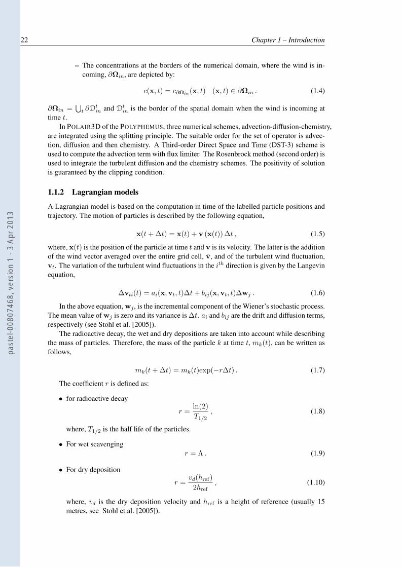
– The concentrations at the borders of the numerical domain, where the wind is in-coming, ∂Ωin, are depicted by:
c(x, t) = c∂Ωin(x, t) (x, t) ∈ ∂Ωin . (1.4)
∂Ωin =⋃
t ∂Dtin and Dt
in is the border of the spatial domain when the wind is incoming attime t.
In POLAIR3D of the POLYPHEMUS, three numerical schemes, advection-diffusion-chemistry,are integrated using the splitting principle. The suitable order for the set of operator is advec-tion, diffusion and then chemistry. A Third-order Direct Space and Time (DST-3) scheme isused to compute the advection term with flux limiter. The Rosenbrock method (second order) isused to integrate the turbulent diffusion and the chemistry schemes. The positivity of solutionis guaranteed by the clipping condition.
1.1.2 Lagrangian models
A Lagrangian model is based on the computation in time of the labelled particle positions andtrajectory. The motion of particles is described by the following equation,
x(t + ∆t) = x(t) + v (x(t)) ∆t , (1.5)
where, x(t) is the position of the particle at time t and v is its velocity. The latter is the additionof the wind vector averaged over the entire grid cell, v, and of the turbulent wind fluctuation,vt. The variation of the turbulent wind fluctuations in the ith direction is given by the Langevinequation,
∆vti(t) = ai(x,vt, t)∆t + bij(x,vt, t)∆wj . (1.6)
In the above equation, wj , is the incremental component of the Wiener’s stochastic process.The mean value of wj is zero and its variance is ∆t. ai and bij are the drift and diffusion terms,respectively (see Stohl et al. [2005]).
The radioactive decay, the wet and dry depositions are taken into account while describingthe mass of particles. Therefore, the mass of the particle k at time t, mk(t), can be written asfollows,
mk(t + ∆t) = mk(t)exp(−r∆t) . (1.7)
The coefficient r is defined as:
• for radioactive decay
r =ln(2)
T1/2, (1.8)
where, T1/2 is the half life of the particles.
• For wet scavengingr = Λ . (1.9)
• For dry deposition
r =vd(href)
2href, (1.10)
where, vd is the dry deposition velocity and href is a height of reference (usually 15metres, see Stohl et al. [2005]).
past
el-0
0807
468,
ver
sion
1 -
3 Ap
r 201
3
Section 1.2 – Observations 23
The sources of emission are also taken into account with the mass of particles in a grid cellat each instant.
Finally, the average concentration of pollutants at time t and position x is given by thefollowing Lagrangian formula,
c(x, t) =1
|∆V (x)|
N∑
k=1
δk(x)mk(t) . (1.11)
Eq. (1.11) |∆V (x)|, is the volume of the grid cell to which the vector x is pointing. δk(x)is the Dirac distribution that is unity if the particle k is located inside the grid cell to which x ispointing and zero otherwise. N is the total number of particles. mk is the mass of the specieswhich are produced inside the mentioned grid cell. This is the source/sink term for the particlek. Eq. (1.11) shows that the concentration is a discrete quantity in the Lagrangian model.
Instead of Eqs. (1.5) and (1.6), one can also use the following Fokker-Planck equation inwhich the turbulent diffusion matrix, K (described in Sec. 1.1.1) appears:
xi(t + ∆t) = xi(t) +
(vi(t) +
∂Ki
∂xi
)∆t +
√2Ki∆wi , (1.12)
where, i is the vector component index.
1.1.3 Uncertainty of the parameters of the model
The accuracy of any of the previously presented models depends strongly on the uncertaintyof the parameters [Mallet and Sportisse, 2006] and the sensitivity of the models to them. As itis difficult to correct each source of uncertainty, it is important to identify those of them whichhave the strongest effect on the results.
Here are listed the sources of uncertainty that can be met in the numerical simulations ofair quality:
• Input data: boundary and initial conditions, dry deposition velocity, emission inven-tories, meteorological fields (temperature, pressure, wind, etc). These parameters areclosely dependent on the spatial and temporal domain which is chosen for the computa-tion.
• Sub-grid parameterisations : mesoscale meteorological parameterisations, mesoscaleemission fields, etc.
• The accuracy in the description of the physical phenomena : the lack of understandingof some phenomena can lead to a non comprehensive and incorrect theoretical represen-tation of the reality.
• The numerical errors: errors due to the methods of discretisation and to the solvers.
It is important to know the sensitivity of the model to each of the above mentioned points inorder to get numerical results as close to reality as possible.
1.2 Observations
1.2.1 Air pollution observations
Measurements are necessary to quantify the state and quality of the atmosphere. They areuseful to estimate the needed parameters to run the numerical simulations and also to validate
past
el-0
0807
468,
ver
sion
1 -
3 Ap
r 201
3

24 Chapter 1 – Introduction
their results. The measurements can be performed by ground based stations, marine monitor-ing buoy networks, airplanes, radiosondes, LIDARs and satellites. The in-situ stations providemeasurements at one single place and a network of several of them is needed to have wider spa-tial sight of the air quality. The other instruments (airplane, Lidar, radiosonde and satellites)can provide a spatial (vertical and horizontal) picture of the state of the atmosphere [Lahozet al., 2010]. The fixed measurement stations usually provide information with a greater ac-curacy. Furthermore, at a given place, they can describe the evolution in time of the collectedinformation. They remain necessary in boundary layer studies.
1.2.2 Measurement stations: strengths and weaknesses
Stations provide in-situ measurements (observations) of a given pollutant in air at a given lo-cation. The pollutant concentrations can be monitored in real time or samples of air can becollected and analysed in laboratories. The relevance of the measurements depends on theinstruments which are used and also on the spatial representativity of the stations for the moni-tored pollutant. The stations are organised into networks which enables regular, if not continu-ous, temporal information for a whole surface area. The spatial relevance of the measurementsis increased with the density of the stations in the network.
To perform a numerical simulation and check its results with the help of the in-situ mea-surements, the following points should be investigated:
• Assessment of the instrumental error.
• Spatial and temporal representativeness of the observations for the selected numericalspatio-temporal domain.
• Observability or the ability of the measurement network, to provide as much informationas possible useful for the numerical model.
1.2.2.1 Instrumental error
The errors of measurement can arise from the data-recording facilities, the methods or pro-cesses carried out and even from the interference of inexpert operators.
If µtrue is a vector of physical parameters (for instance, concentrations) dependent on somecontinuous fields xtrue (for instance in the frame work of air quality studies, emission invento-ries and meteorological data ), the following relation can be written,
µtrue = H(xtrue) , (1.13)
where H is a continuous operator linking µtrue to the continuous true state xtrue. The instru-mental error (ǫmeas) is the departure of the measured value of µ from its true value.
µ = µtrue + ǫmeas . (1.14)
1.2.2.2 Representativeness error
Errors of representativeness arises of shifting from a continuous space to a discrete one. Fornumerical modelling purposes, the continuous operator H is replaced by the discrete operatorH and the continuous true state xtrue by the discrete one xt. In that purpose, the restrictionoperator Γs enables to shift from the continuous to the discrete spaces with a resolution s,
xtrueΓs−→ xt . (1.15)
past
el-0
0807
468,
ver
sion
1 -
3 Ap
r 201
3
Section 1.2 – Observations 25
The discrete operator H can be formalised as follows:
H = HΓ⋆s , (1.16)
where Γ⋆s is the prolognation operator (see section 1.3.4).
While writing the vector of physical parameters, µtrue, this time in the discrete space, anadditional error is brought into the theoretical relation, where ǫrep is called the representative-ness error:
µtrue = Hxt + ǫrep . (1.17)
The summation of ǫmeas and ǫrep gives:
µ = Hxt + ǫmeas + ǫrep . (1.18)
Note that in data assimilation textbooks, the above equation is written as:
µ = Hxt + ǫt , (1.19)
where, the modelling error, ǫt, does not only include the measurement and representativenesserrors but also the error, ǫmodel, due to the physical model H(xtrue).
Let us specify that the loss of information arises from the discretisation of xtrue only, andnot from the operator H. In other words, the error of representativeness is generated by therestriction operation.
As long as the results of the discrete model (at the available measurement points) remainunaffected by the grid resolution (Γs), the representativeness error (ǫrep) can be assumed to besmall. Therefore, in the frame of air quality modelling, two categories of measurement stationscan be identified :
• The background stations- are located far from the pollution sources (for instance, re-gional and rural stations). These stations help to measure the average quality of ambientair and are not affected by the immediate impact of pollution sources. These are goodstations to fulfil the statement just above.
• The proximity stations- are located close to the pollution sources (for instance, urban,traffic and industrial stations). The discrete model results at these stations are stronglydependent on the grid resolution.
The proximity stations cannot be used for regional and global scale modelling as theycan not provide relevant information at low grid resolution. To use the proximity stations,the resolution needs to be higher, which at global scale modelling this would challenge theperformances of the computer. Furthermore, at large scale, there won’t be enough availablemeteorological and emission related data.
1.2.2.3 Observability
The observability of a network of stations for a given study is its ability to provide relevantmeasurements for that particular study.
The observability of a network depends on the climatology of the area covered by thenetwork [Mason and Bohlin, 1995]. It also depends on the location of the sources of pollutionand their distance from the measurement stations. For instance, for pollutants with a small lifetime, the network should be dense enough to be able to detect the pollution plume.
past
el-0
0807
468,
ver
sion
1 -
3 Ap
r 201
3
26 Chapter 1 – Introduction
The observability of the networks is an essential issue in inverse modelling to reconstructthe sources of pollution from the observations. Furthermore, inverse modelling can help tocheck the observability of the network and improve the network design. For instance, com-bination of optimisation studies can be performed in order to design the spread of a network[Abida and Bocquet, 2009]. Geostatistical methods, such as Kriging, are among the simplestmethods used for network design. Data assimilation can also be used at a higher level of com-plexity.
1.3 Inverse modelling
Inverse modelling is a way to use the available information (e.g. measurements) in order todetermine some specific parameters of the model (e.g. emissions fields, initial conditions,vertical diffusion, etc). The space of these parameters is called control space. Inverse modellingis not only applied to estimate the parameters of the model, but also it is used to increasethe ability of the model of predicting a physical phenomena. For instance, in atmosphericchemistry, inversion studies are focused on the estimation of the parameters that impact thespecies concentration fields. The parameters of the model which should be estimated are theinitial state for short time simulations, or the emission fields, boundary conditions or diffusionfields in long simulations.
In geophysical literature, data assimilation is the word commonly used for the methodsthat help to find the true state of the parameters describing a phenomenon. Data assimilationis a technique of inverse modelling for very large scale systems which are ill-posed. Although,inverse modelling focuses on the parameters, data assimilation focuses on the outputs of themodel. The main problem in inverse modelling is the lack of data or the lack of observability ofthe computed parameters. Therefore, having an initial idea about the background informationis essential. The latter are used to regulate (or adjust) the model parameters.
1.3.1 General description
In order to estimate the vector x ∈ Rn, n being the number of model parameters, from a set of
m observations represented by a vector µ ∈ Rm, the linear map H ∈ R
m×n (which depicts alinear physical model) is used to link the model parameters to the observation vector,
µ = Hx + ǫ . (1.20)
In Eq.(1.20), ǫ ∈ Rm is the modelling error. The latter represents the mismatch between the
observations and the model results. The information arising from the observations is the keyto get reliable results from the model. However, the extraction of information using inversemodelling in atmospheric studies is difficult for several reasons.
As it is often question in geophysical data assimilations, the system under study is oftenlargely underdetermined: i.e. m ≪ n. One of the techniques commonly used is to aggregatethe control parameters x into coarser variables to reduce the number of effective parameters.One can assume a map g : R
n → Rl, where: x = g(α). The dimension of α ∈ R
l is anip-and-tuck of the dimension of the observations vector, µ. Although this methodology helpsto reduce the control parameters, it may lead to a loss in the resolution of the results.
Moreover, the results of the model (H) are not always sensitive enough with respect to allthe model parameters. In that case, the extraction of significant information in order to adjustthe parameters from the observations is difficult. For instance, in atmospheric studies, whileassimilating the source emission parameters, the model does not always retrieve the informa-tion far from the observation. In atmospheric transport models, this is a common problem dueto the effective diffusion term generated by the turbulent mixing.
past
el-0
0807
468,
ver
sion
1 -
3 Ap
r 201
3
Section 1.3 – Inverse modelling 27
Furthermore, the errors coming from the estimations of the model make it still more com-plicated to find a reliable solution for x.
For all these reasons, the inverse problem is often ill-posed in atmospheric studies. There-fore, it is mandatory that the a priori information (background or first guess) should be ac-counted for, in order to resolve the inverse problem. The Bayesian approach (based on theBayes formalism) allows to consistantly include the statistics of the errors and the model pa-rameters in the inversion system [Bennett, 1992; Kaipio and Somersalo, 2010; Rodgers, 2000].
1.3.2 Bayesian approach
1.3.2.1 Bayesian inference and maximum likelihood
The Bayesian inference is based on two antecedents, the probability of the a priori model pa-rameters, denoted pb(x), and the modelling error probability, denoted pe(ǫ). The approachleads to compute the posterior probability following the Bayes’ rule. The difficulties encoun-tered by this approach are the estimations of the distribution, the uncertainties involved in thebackground of the parameters and the statistical parameters of the modelling error. The prob-ability density function (pdf ) of the modelling error (or observation mismatch) is called thelikelihood function. The latter can be interpreted as the probability of the observations, given avector of parameters evidence, pe(µ|x) = pe(µ − Hx). According to the Bayes’ rule
p(x|µ) =pe(µ|x)pb(x)
p(µ)
=pe(µ − Hx)pb(x)
p(µ).
(1.21)
The denominator term in Eq. (1.21), p(µ), is disconnected from the models and the controlparameters. This is the so-called marginal-likelihood or model evidence.
Different methods can be used to compute a reliable value for the vector x. One of them,stands on maximising the probability of the variable x. The maximum a posteriori estimator(MAP) specifies the solution of the parameters of the model according to
xa = argminx p(x|µ) . (1.22)
Often, the log-likelihood method is used for that purpose. Therefore, one can define the objec-tive cost function as follows:
J(x) = −ln (pe(µ − Hx)) − ln (pb(x)) . (1.23)
The marginal log-likelihood term appears as a constant term in the cost function which can beeliminated. Eq. (1.23) is a simple form of the cost function, normally used in the three dimen-sional and four dimensional variational data assimilation (3D-Var and 4D-Var, respectively)approaches [Sasaki, 1958; Lorenc, 1986; Le Dimet and Talagrand, 1986].
1.3.2.2 Gaussian statistics
The argument of the minimum of Eq. (1.23), is closely dependent on the statistical assump-tions for the likelihood function pdf, pe, and the pdf of the prior model parameters, pb. Theassumption is commonly used for the modelling error in curve fitting method, such as the least
past
el-0
0807
468,
ver
sion
1 -
3 Ap
r 201
3
28 Chapter 1 – Introduction
squares. Let us assume that E(ǫ) = 0 and the model error covariance matrix is R = E[ǫtǫTt ].
As a result, the pdf pe is
pe(µ|x) =e−
12ǫTR−1ǫ
√(2π)m|R|
. (1.24)
The pdf of the a priori control variables can be chosen following different distributions.Specifically, the selection of the distribution depends on the nature of the parameters. In mostdata assimilation textbooks, this pdf is chosen to be Gaussian. Assume that xb is the vectorof a first guess of the control parameters such that E
[xb − xt
]= 0. Let’s also assume that
B = E[(xb − xt)(xb − xt)T
]is the background error covariance matrix which represents the
information about the uncertainty of the first guess. Therefore
pb(x) =e−
12(x−xb)
TB−1(x−xb)
√(2π)n|B|
. (1.25)
Using these two pdf, the cost function, Eq.(1.23), can be rewritten as:
J(x) =1
2(µ − Hx)TR−1(µ − Hx) +
1
2(x − xb)
TB−1(x − xb) +1
2ln((2π)m+n|R||B|
).
(1.26)The very last term in Eq. (1.26) is independent from x, and the cost function can be reformu-lated as
J(x) =1
2(µ − Hx)TR−1(µ − Hx) +
1
2(x − xb)
TB−1(x − xb) . (1.27)
The argument of the minimum of Eq. (1.27) is equivalent to the solution of the maximumlikelihood method. The Gaussian assumption on the pdf of the a priori control variables leadsto the creation of a regulation term of the Tikhonov kind [Tikhonov and Arsenin, 1977]. Thatregulation term guarantees the existence of a unique solution for the problem, even though theinverse problem is ill-defined. This solution can be written as
xa = xb + BHT(R + HBHT
)−1(µ − Hxb) , (1.28)
where,
K = BHT(R + HBHT
)−1. (1.29)
K is the so-called gain matrix. This solution (Eq. (1.28)) is known as the Best Linear UnbiasedEstimator (BLUE).
1.3.2.3 The posterior distribution
If x and ǫ are two independent normal random vectors, then the posterior distribution p(x|µ)follows the same distribution. According to Eq. (1.28),
xa − xt = (I − KH)(xb − xt) + Kǫt . (1.30)
The above equation is the key to estimate the statistical parameters of the posterior distributionp(x|µ). Using Eq. (1.29), one can easily deduce that
E[xa − xt
]= 0 , (1.31)
past
el-0
0807
468,
ver
sion
1 -
3 Ap
r 201
3
Section 1.3 – Inverse modelling 29
and,
Pa = E[(xa − xt)(xa − xt)
T]
= (I − KH)B
= B − BHT(R + HBHT)−1HB .
(1.32)
The a posteriori pdf, which constitutes the probabilistic Bayes’ interference result reads
p(x|µ) =e−
12(x−xa)TP
−1a (x−xa)
√(2π)n|Pa|
. (1.33)
1.3.2.4 The marginal likelihood
The likelihood of the observation set, p(µ), is a key to estimate of the uncertainty matrix, B
and R [Desroziers and Ivanov, 2001]. That’s why its computation is important. According tothe law of total probability:
p(µ) =
∫
Rn×Rm
δ(µ − Hx)pe(ǫ)pb(x)dxdǫ =
∫
Rn
pe(µ|x)pb(x)dx , (1.34)
where δ is Dirac delta function. Replacing Eq. (1.24) and Eq. (1.25) in the above formula gives
p(µ) =1√
(2π)m+n|R||B|
∫
Rn
e−12((µ−Hx)TR−1(µ−Hx)+(x−xb)
TB−1(x−xb))dx . (1.35)
The above equation (Eq. 1.24) can be reformulated as below (see Appendix A)
p(µ) =1√
(2π)m+n|R||B|
∫
Rn
e−12((µ−Hxb)
T(R+HBHT)−1(µ−Hxb)+(x−xa)TP−1a (x−xa))dx .
(1.36)Finally:
p(µ) =e−
12(µ−Hxb)
T(R+HBHT)−1(µ−Hxb)
√(2π)m|R + HBHT|
∫
Rn
e−12(x−xa)TP
−1a (x−xa)
√(2π)n|Pa|
dx . (1.37)
The term presented in the integral denotes the a posteriori pdf, p(x|µ). The integral in theabove formulation (Eq. (1.37)) is equal to unity. Then the pdf of the observation reads
p(µ) =e−
12(µ−Hxb)
T(R+HBHT)−1(µ−Hxb)
√(2π)m|R + HBHT|
. (1.38)
1.3.2.5 Degrees of freedom for the signal
The goal of inverse modelling is to estimate the model parameters as reliably as possible.That means the posterior uncertainty of the model parameters, compacted in the term Pa, issmaller for a given prior uncertainty B. According to Eq. (1.32), if the term KH is close tothe identity matrix, the posterior value of the model parameters becomes more certain. Thesymmetric matrix, A = KH, is the so-called averaging kernel. The degrees of freedom for thesignal (DFS) is a quantity closed to the a posteriori uncertainty of the model parameters. Thisvalue extracts the fraction of the observations used in the data assimilation system to retrievethe solution. It reads,
DFS = E[(xa − xb)
TB−1(xa − xb)]
= Tr(A) = Tr(HK) = Tr(KH) . (1.39)
past
el-0
0807
468,
ver
sion
1 -
3 Ap
r 201
3
30 Chapter 1 – Introduction
The singular vector decomposition of the averaging kernel gives:
DFS =
m∑
l=1
wl . (1.40)
where wl is the lth eigenvalue of A.When the observations are representative enough, the value of the DFS shows the quality of
the analysis. The higher is the DFS, the higher is the information recovered from the observa-tions. The computation of the DFS is inconsistent under the non-Gaussian assumption for thea priori pdf of the control parameters. However, under the positivity enforcing, in the presenceof the positive background of the control parameters and when the uncertainty of the controlparameters is not very high, that can be also applied. Note that, in a non-Gaussian context, thecomputation of relative entropy can be used in order to understand the quality of assimilation[Bocquet, 2008].
1.3.3 Prior error estimation
The results of the inverse system depend not only on the model and on the observations butalso on the prior error estimations. One of the difficulties for inverse modelling studies is theassessment of the error covariance matrix, R and B. This section introduces the maximumlikelihood method in order to estimate the prior errors.
1.3.3.1 Gaussian assumption
Let us assume that the two error covariance matrix, B and R, are as follows
R = r2R0 , B = β2B0 . (1.41)
where R0 and B0 are the first estimation of the information about the prior parameters. r and β,called hyper-parameters, are the parameters used to fix these two covariance matrices. In orderto obtain the more likely values for r and β, one has to maximise the pdf of the observations,Eq. (1.38), with respect to r and β. The log-likelihood can be written as
lnp(µ|r, β) = −1
2(µ−Hxb)
T(R + HBHT)−1(µ−Hxb)− ln|R + HBHT|+ C , (1.42)
where C is a constant parameter. The optimisation of the above log-likelihood function, Eq.(1.42), with respect to the hyper-parameters, gives
r2 =(µ − Hxa)
TR−10 (µ − Hxa)
Tr(Im − HK), (1.43)
and,
β2 =(xa − xb)
TB−10 (xa − xb)
Tr(KH). (1.44)
The above two equations (1.43 and 1.43) can be used in an iterative system which convergesto a fixed point. At each iteration, xa and K are obtained from equations (1.28 and 1.29). Thismethod was first presented by Desroziers and Ivanov [2001]. They also show that the methodis equivalent to the maximum likelihood.
The χ2 method (see Ménard et al. [2000]; Tarantola [2005]) can be derived from Deroziersmethod (see Chapnik et al. [2006]) and when one of the hyper-parameters is assumed to befixed. The method is useful in the variational data assimilation method [Koohkan and Bocquet,2012; Michalak et al., 2005].
past
el-0
0807
468,
ver
sion
1 -
3 Ap
r 201
3
Section 1.3 – Inverse modelling 31
1.3.3.2 Semi-normal assumption
When the model parameters that should be retrieved are all positive, the Gaussian pdf is notappropriate. In that case, we assume the following Gaussian truncated pdf for the a priori modelparameters, is assumed:
pb(x) =e−
12(x−xb)
TB−1(x−xb)
√(2π)n|B| (1 − Φ(B,xb,0))
Ix≥0 . (1.45)
In Eq. (1.45), Φ(B,xb,0) is the cumulative distribution function (cdf ), N(xb,B), computedover the integral from minus infinity to zero. Ix≥0 is a function with the value zero if xi < 0 foreach i = 0, .., n and with the value unity elsewise. According to the semi-normal assumption,the marginal probability function can be written as
p(µ|r, β) =e−
12(µ−Hxb)
T(R+HBHT)−1(µ−Hxb)
(1 − Φ(B,xb,0))√
(2π)m|R + HBHT|
∫e−
12(x−xa)TP
−1a (x−xa)
√(2π)n|Pa|
Ix≥0dx .
(1.46)The analytical computation of the hyper-parameters is difficult from Eq. (1.46). However, thelatter can be used by choosing the input values from within an allowed set of hyper-parametersand computing the value of the function (Winiarek et al. [2011]; also in chapter 5). This methodis expensive for very large systems, but it can be used for a few thousand variables.
1.3.4 Multiscale data assimilation
1.3.4.1 Scaling operators
For a given domain, a regular grid, Ω, can be defined by a discretisation in space and time.For instance, in a surface space and time discretisation (2D+T), Nx denotes the number ofgrid cells along the longitude, Ny denotes the number of grid cells along the latitudes axis,and Nt is the number of time step. Let us assume that Nfg = Nx × Ny × Nt is the finestgrid resolution of the spatio-temporal domain. x ∈ R
Nfg is the vector which gives the controlparameters for the finest resolution. Now, let us assume that R(Ω) is the dictionary of allof the adaptative grids representing the domain. A representation ω is a member of R(Ω),which gives a spatio-temporal discretisation of the domain, such that, xω ∈ R
N , N ≤ Nfg
(see Bocquet et al. [2011]; Bocquet [2009]). A restriction operator, Γω : RN → R
Nfg denoteshow the vector of control parameters x is coarse-grained into the vector xω. Vice-versa, theprolongation operator, Γ⋆
ω : RNfg → R
N , refines the vector xω into x ∈ RNfg , where
xω = Γωx , x = Γ⋆ωxω . (1.47)
Since N ≤ Nfg, the loss of information occurs during the restriction operation. The com-position of the prolongation and the restriction operator is the identity ΓωΓ⋆
ω = IN . Theoperator Γ⋆
ω is ambiguous since additional information is needed to reconstruct the vector x
from x. A simplest choice for that operator is to set Γ⋆ω = ΓT
ω . The best choice to determinethis operator is the use of the Bayes’ rule. The method is based on maximising the probabilityof x, for a given representation xω. As mentioned before (Eq. (1.25)), the random variable x
can be assumed to be Gaussian: x ∼ N(xb,B). From Bayes’ rule, one can write
p(x|xω) =p(x)δ(xω − Γωx)
pω(xω), (1.48)
past
el-0
0807
468,
ver
sion
1 -
3 Ap
r 201
3
32 Chapter 1 – Introduction
where δ is the Dirac distribution. For a linear operator Γω, the pdf of x in a representation ω,pω(xω) remains Gaussian: xw ∼ N(xω
b ,Bω),
xωb = Γωxb , Bω = ΓωBΓT
ω . (1.49)
The optimum solution of Eq. (1.48) can be computed with the help of the BLUE analysis
x⋆ = xb + Λ⋆ω(xω − Γωxb) , (1.50)
whereΛ⋆
ω = BΓTω (ΓωBΓT
ω )−1 . (1.51)
Moreover, the projection operator is defined as,
Πω = Λ⋆ωΓω , (1.52)
so that, we can choose the prolongation operator to be:
Γ⋆ω : xω → (INfg
− Πω)xb + Λ⋆ωxω . (1.53)
The composition of the restriction and the prolongation operator gives
Γ⋆ωΓω : x → (INfg
− Πω)xb + Πωx . (1.54)
When xb = 0, the projection operator Πω is equal to Γ⋆ωΓω. This operator satisfies the follow-
ing equations:
Π2ω = Πω , ΠωB = BΠT
ω (1.55)
If the representation ω is coarse, Tr(Πω) ≪ Nfg. For a representation ω close to the finestgrid Ncg ≪ Tr(Πω) (Ncg is the number of cells in the coarsest grid resolution). The higherTr(Πω), the better the recovered information. However, this operator cannot be the identitybecause the coarse-graining implies a loss of information.
1.3.4.2 Multiscale source receptor model
The source receptor model, Eq. (1.20), can be written in any representation ω. The Jacobianmatrix H in the representation ω changes to Hω = HΓ⋆
ω. The scale-dependent source-receptormodel is defined as:
µ = Hx + ǫ
= HΓ⋆ωΓωx + H(INfg
− Γ⋆ωΓω)x + ǫ
= Hωxω + ǫω .
(1.56)
Where, the ǫω is a scale-made dependent error:
ǫω = H(INfg− Γ⋆
ωΓω)x + ǫ = H(INfg− Πω)(x − xb) + ǫ (1.57)
Using Eq. (1.54), the source receptor model can be reformulated as
µ = Hxb + HΠω(x − xb) + ǫω . (1.58)
The observation covariance matrix in a representation ω is different from that one in thefinest grid
Rω = R + H(INfg− Πω)BHT . (1.59)
The term H(INfg− Πω)BHT, in the above equation, Eq. (1.59), leads to an increase of the
observation covariance matrix term. The term H(INfg− Πω)(x − xb) is identified as the
aggregation error.
past
el-0
0807
468,
ver
sion
1 -
3 Ap
r 201
3
Section 1.3 – Inverse modelling 33
1.3.4.3 Design criteria
DFS criterion
The degrees of freedom for the signal quantify the quality of the analysis. As presented inSection 1.3.2.5, the DFS value is computed by the trace of the averaging kernel (Tr(KH)). Ina multi-scale context, one hopes to find a representation ω, which maximises the DFS. Thiscriterion is expressed as:
Jω = Tr(IN − B−1ω Pω
a ) = Tr(ΠωBHT(R + HBHT)−1H
)(1.60)
Fisher criterion
This criterion measures the reduction of uncertainty granted by the observations. This criterioncan be computed in the finest grid, Ω, according to
J = Tr(BP−1
a
)= Tr
(BHTR−1H
). (1.61)
For a given representation ω, the criterion reads
Jω = Tr(BωHT
ωR−1ω Hω
)= Tr
(ΠωBHTR−1H
). (1.62)
The aggregation error is related to the representation. The two equations above (1.61-1.62) givean assessment of that error. The following equation (1.63), presents the normalised aggregationerror for a given representation ω [Koohkan et al., 2012; Wu et al., 2011]:
Tr(R−1(Rω − R)
)= Tr
(BHTR−1H
)− Tr(ΠωBHTR−1H) . (1.63)
Note that the Fisher criterion is the limiting case of the DFS criterion when R is inflating or B
is vanishing.
1.3.4.4 Adaptive tiling
To apply the multiscale extension in 2D+T, the dictionary of representations, R(Ω) should behandled mathematically. Let us assume that Nx, Ny and Nt are multiples of 2nx , 2ny and2nt , respectively. For each scale l = (lx, ly, lt), such that 0 ≤ lx ≤ nx, 0 ≤ ly ≤ ny and0 ≤ lt ≤ nt, the domain is presented with Nfg×2−(lx+ly+lt) coarser cells. The latter are calledthe tiles. In all directions, a coarser grid is made when two adjacent grids in each direction aregathered into one. The physical quantities of the coarser cell are the average of those from thefinest grid cells.
A physical quantity in each cell of the finest grid, indexed by k is attached to a base vectorui,j,h ∈ R
Nfg with 1 ≤ i ≤ Nx, 1 ≤ j ≤ Ny and 1 ≤ h ≤ Nt. At a coarser scalel, this quantity in the finest grid, which is enumerated by k, attaches to the vector: vl,k =∑2lx−1
δi=0
∑2ly−1δj=0
∑2lt−1δh=0 uik+δi,jk+δj ,hk+δh
, where (ik, jk, hk) denotes the index of cell k inthe coarser representation. For a representation ω of Ω, the projection operator defines:
Πω =∑
l
nl∑
k=1
αωl,k
vl,kvTl,k
vTl,kvl,k
, (1.64)
where αωl,k are the coefficients which define the representation ω. To obtain an admissible
representation ω, each parameter αωl,k is set to 0 or 1. Each cell of the finest grid cell should be
attached in the representation ω. Therefore,
∑
l
nl∑
k=1
αωl,kvl,k = (1, ..., 1)T . (1.65)
past
el-0
0807
468,
ver
sion
1 -
3 Ap
r 201
3
34 Chapter 1 – Introduction
The number of multiscale grid cells N should be imposed
Nfg × 2−(nx+ny+nt) ≤
nl∑
k=1
αωl,k = N ≤ Nfg . (1.66)
1.3.4.5 Optimisation
In order to optimise the cost function, Jω, in a fixed number of tiles, the following Lagrangianfunction is defined:
L(ω) =∑
l
nl∑
k=1
αωl,k
vl,kQvTl,k
vTl,kvl,k
+
Nfg∑
k=1
λk
(∑
l
αωl,k − 1
)+ ξ
(∑
l
nl∑
k=1
αωl,k − N
). (1.67)
The first term on the right hand side of this equation stands for Jω. Q is the average kernelmatrix for the DFS criterion and is equal to BHTR−1H for the Fisher criterion. Since thevalue of αω
l,k should be 0 or 1, a second term is added to the right hand side of Eq. (1.67). Thevector λ is the Lagrangian multiplier. The very last term of the above equation aims to satisfythe condition of Eq. (1.66). ξ is a scalar and is called the Lagrange multiplier. The Lagrangianobjective function can be also written as follows:
L(ω) =∑
l
nl∑
k=1
(vl,kQvT
l,k
vTl,kvl,k
+ vTl,kλ + ξ
)αω
l,k −
Nfg∑
k=1
λk − ξN (1.68)
The optimisation of the representation ω can be done by minimising the dual function ofL. Therefore, it comes:
L(λ, ξ) =∑
l
nl∑
k=1
max
(0,
vl,kQvTl,k
vTl,kvl,k
+ vTl,kλ + ξ
)αω
l,k −
Nfg∑
k=1
λk − ξN (1.69)
The above introduced cost function, L(λ, ξ), cannot be optimised directly using a gradient-based minimisation algorithm. Besides, the uniqueness of the solution is not guaranteed.To overcome that difficulty, a regularisation method for the cost function is used in Bocquet[2009].
1.4 Outline
New methodologies of data assimilation are presented in the following chapters:
• In chapter 2 are detailed the adjoint of the Eulerian Chemistry Transport Model and the4D-Var method.
• In chapter 3, the 4D-Var model is used to invert the emission inventories of carbonmonoxide provided by the EMEP (European Monitoring and Evaluation Program). Theobservations used for the inversion are impacted with the representativeness error. Asthe 4D-Var routine is not fit to handle the representativeness error, a subgrid model isdeveloped and coupled to the 4D-Var algorithm.
• chapter 4- introduces the observations to be retrieved from the International MonitoringSystem (IMS) radionuclide network. The compatibility of the observation network withdata assimilation, in other words, the ability of the network to observe the radionuclide
past
el-0
0807
468,
ver
sion
1 -
3 Ap
r 201
3

Section 1.4 – Outline 35
pollutants, is discussed. In order to build the Jacobian matrix of the atmospheric transportmodel, the Lagrangian FLEXPART model and also the adjoint of the Eulerian POLAIR3Dmodel of POLYPHEMUSare used.
• In chapter 5 is shown the application which can be made of the maximum likelihoodmethod in order to estimate the uncertainty of the model parameters, as well as, thecovariance matrix of the model errors. A fast version of POLAIR3D CTM and its adjointare developed. The emission inventories of the Volatile Organic Compounds (VOCs) areinverted. The observations extracted from the EMEP database are assimilated.
• Chapter 6 concludes on the achievements of this work and presents some interestingpoints to investigate.
The points dealt with in chapter 2 and 3 are presented in Koohkan and Bocquet [2012].The contents of chapter 4 was published in Koohkan et al. [2012]. Chapter 5 was submitted toAtmospheric Chemistry and Physics.
past
el-0
0807
468,
ver
sion
1 -
3 Ap
r 201
3

36 Chapter 1 – Introduction
past
el-0
0807
468,
ver
sion
1 -
3 Ap
r 201
3
Chapter 2
Four-Dimensional Variational Data
Assimilation
Summary
The present chapter describes the 4D-Var method that we have used. First of all, an approxi-mate adjoint model of the chemistry transport model is introduced and developed. The adjointsolution is validated via a duality test. Then, the way this adjoint is taken into account in the4D-Var algorithm is described. The latter algorithm is also checked through two gradient tests.The duality test shows that the concentrations computed with the help of the adjoint solutionare in good agreement with the concentrations computed using the CTM, directly. The Pearsoncorrelation between the solutions of the two models for a tracer species is of 99.8%. The gradi-ent of the cost function obtained with the adjoint model is compared with the one obtained withthe finite difference method. The results show that the gradient of the cost function obtainedvia the adjoint solution is correct enough to be used in the optimisation algorithm.
Contents
2.1 Introduction . . . . . . . . . . . . . . . . . . . . . . . . . . . . . . . . . 38
2.2 The adjoint model . . . . . . . . . . . . . . . . . . . . . . . . . . . . . . 39
2.3 The 4D-Var model . . . . . . . . . . . . . . . . . . . . . . . . . . . . . . 40
2.3.1 The control space . . . . . . . . . . . . . . . . . . . . . . . . . . . 41
2.3.2 The optimisation algorithm . . . . . . . . . . . . . . . . . . . . . . 43
2.4 The verification of the 4D-Var routine . . . . . . . . . . . . . . . . . . . 44
2.4.1 Validation of the approximate adjoint model . . . . . . . . . . . . . 44
2.4.2 Verification of the gradient . . . . . . . . . . . . . . . . . . . . . . 46
2.5 Conclusion . . . . . . . . . . . . . . . . . . . . . . . . . . . . . . . . . . 46
past
el-0
0807
468,
ver
sion
1 -
3 Ap
r 201
3
38 Chapter 2 – 4D-Var
2.1 Introduction
Five decades after the appearance of data assimilation [Cressman, 1959; Gandin, 1963], Four-Dimensional Variational method (4D-Var) has become one of the most important tools to esti-mate the parameters of a physical model. Data assimilation combines experimental data, infor-mation coming from models (chemistry and transport model in our case) and statistics of theerrors in order to find the optimum values of the parameters which minimise the observationsmismatch.
Variational data assimilation is a powerful method when it comes to constraining dynamicalsystems by numerous observations. In variational data assimilation, all types of informationmentioned above are accounted for altogether in a two-term objective cost function J = Jo +Jb. The first term Jo is a measure of the discrepancy between the observed and simulatedconcentrations. The second term Jb evaluates the departure of the control parameters fromtheir first guess (background). By minimising the sum of these two terms, 4D-Var makes inour case an optimal compromise while enforcing the fact that the simulated concentrations areobtained from a given numerical transport model.
One way to minimise the cost function, J, is to use an analytical method, granted that thefunction in question is continuous and derivable. That way supposes to solve the algebraicequations equal to zero of the gradient function. The solution obtained is a minimum point ifthe function is locally convex. This analytical method includes a system of n equations, wheren is the number of control parameters. It leads to find an analytical solution for the optimalcontrol parameters and actually performs well when the dimension of the problem is small.Another way to minimise the cost function consists in using an iterative descent algorithm,such as, the conjugate gradient or the quasi-Newton algorithm. In the descent algorithm, aninitial value for the control parameters is chosen and the local gradient of the cost function iscomputed. The latter gradient shows the direction of decrease of the cost function. Therefore,the optimal point (control parameters) for the cost function in that direction can be found by theline search method. Using the updated parameters, the above described procedure is repeateduntil the cost function is minimised.
In order to find the gradient of the cost function with respect to the control parameters, anadjoint of the numerical model is needed. To compute that adjoint, besides hand calculationwhich is almost impossible in air quality context, two methods can be used: the automaticdifferentiation and the approximated adjoint [Krysta and Bocquet, 2007]. The former is used toevaluate the derivative of a function specified by a computer program. The latter is an analyticalmethod which gives the adjoint solution of the chemistry transport model. The adjoint of adynamical model was first used by Kontarev [1980] and Hall and Cacuci [1983] for sensitivitystudies. Le Dimet and Talagrand [1986] proposed an algorithm for minimising the 4D-Var costfunction with the help of the adjoint dynamical equation in the framework of meteorology.
The adjoint model is described in Section 2.2. In Section 2.3, a continuous expansion ofthe control optimal problem is introduced and control variables space are defined. Then, thenumerical discretisation of the 4D-Var system is presented. Finally, the optimisation algorithmis described. The adjoint model, as well as, the descent algorithm are validated in Section 2.4.A short conclusion follows in section 2.5.
past
el-0
0807
468,
ver
sion
1 -
3 Ap
r 201
3
Section 2.2 – The adjoint model 39
2.2 The adjoint model
In air quality modelling, the concentrations of pollutants at each time and location can beobtained by a chemistry transport model (CTM). For the species with a linear chemistry andphysics, the Jacobian of the CTM can be computed either using the solution generated by theCTM, or the one generated by the adjoint CTM model. For instance, in the studies of accidentalcases, when the source is pointwise, the Jacobian matrix of the model is easier to computeusing the solution of the CTM. In case the number of sources is higher than the number ofmeasurements, the Jacobian is easier to build via the adjoint model. Furtheremore, the adjointmodel can be used in the 4D-Var algorithm to compute the gradient of the cost function. Thatis why, a particular attention has to be paid to the adjoint model when assimilating atmosphericobservations.
We can assume that c(x, t) is continuously differentiable on the space-time domain Ω =D× [0, T ] (D denotes the spatial domain) and the chemical reaction operator χ is linear (whichis not always the case). Then Eq. (1.1) is multiplied by a sufficiently smooth function φ(x, t)and integrated. The “weak” form of the CTM is:
∫
Ωφ
(∂c
∂t+ ∇ · (uc) −∇ · (K∇c) + Λc − χ(c) − σ
)dxdt = 0 (2.1)
Note that the density of air is assumed to be constant. The above equation can be trans-formed into (see Roustan and Bocquet [2006a]):
∫
Ωc
(−
∂φ
∂t−∇ · (uφ) −∇ · (K∇φ) + Λφ − χ†(φ)
)dxdt =
−
∫
D
φ(T )c(T ) − φ(0)c(0)dx −
∫
∂Dbc×[0,T ](φcu) · dSdt
−
∫
∂Db×[0,T ](cK∇φ − φK∇c) · dSdt +
∫
Ωφσdxdt
(2.2)
where χ† denotes the adjoint operator of the chemical reactions term, χ. ∂Db stands for theground surface boundary of the domain. ∂Dbc are the boundaries of the domain with theexception of the ground surface. Note also that dS = dSn.
Before further developping Eq. (2.2), let us assume the following equation:
∂φ(x, τ)
∂τ= div (u(x, τ)φ(x, τ)) + ∇ ·
(ρK(x, τ)∇
φ(x, τ)
ρ
)
−Λ(x, τ)φ(x, τ) + χ†(φ(x, τ),x, τ) + π(x, τ) . (2.3)
πi(x, τ) is a continuous sampling function defined over the time-space domain and τ is thereverse time variable: τ = T − t. Eq.(2.3) can be seen as a CTM, backward in time witha reversed wind direction. One can set the following conditions for the above equation (Eq.(2.3):
• final conditions:
φ(x, T ) = 0 x ∈ D (2.4)
past
el-0
0807
468,
ver
sion
1 -
3 Ap
r 201
3
40 Chapter 2 – 4D-Var
• border conditions (top, left, right, front and back sides):
φ(x, τ) = 0 ∀(x, τ) ∈ ∂Ωout (2.5)
∂Ωout =⋃
t ∂Dtout denotes the border when the wind is outgoing. Dt
out is the border ofthe spatial domain when the wind is outgoing at instance t.
• Boundary conditions at ground level (z = 0):
K(xz=0, τ)∇φ(xz=0, τ) · n = vdφ(xz=0, τ) (2.6)
Using Eqs. (2.3 to 2.6), Eq. (2.2) can be rewritten as follows:
∫
Ωcπdxdt =
∫
D
φ(0)c(0)dx −
∫
∂Ωin
(φcu) · dSdt
+
∫
∂Db×[0,T ]φE · dSdt +
∫
Ωφσdxdt ,
(2.7)
where, E = −E · n is the surface emission vector. Note that in the above equation, the termK∇c and K∇φ are assumed to be zero at the top and around the domain.
2.3 The 4D-Var model
Four dimensional variational data assimilation (4D-Var) is used to invert the surface fluxes ofnon-reactive species (tracers). The analysis of the emissions is achieved by computing theminimum value of the following Lagrangian cost function:
J =1
2
∫
D×Ω(σ(x, t) − σb(x, t))B−1
σ (x, x, t)(σ(x, t) − σb(x, t))dxdxdt
+1
2
∫
Db×Ωb
(E(xp, t) − Eb(xp, t))B−1E (xp, xp, t)(E(xp, t) − Eb(xp, t))dxpdxpdt
+1
2
∫ T
0(y(t) − Ht,x[c])R−1(t) (y(t) − Ht,x[c]) dt
+
∫
Ωφ
(∂c
∂t+ ∇ · (uc) −∇ · (K∇c) + Λc − σ
)dxdt .
(2.8)
The first and the second terms on the right hand-side of the equation above are represen-tative of the cost of the background emissions. σ(x, t) is the volume emission inventories attime t and coordinate x. σb(x, t) denotes its first guess. Bσ(x, x, t) is called the backgroundcovariance of the volume emissions. E(xp, t) and Eb(xp, t) are the surface emission func-tion and the background surface emission function at time t and at the surface coordinate xp.BE(xp, xp, t) is called the background covariance of the surface emissions. Ωb denotes thesurface-time domain Db × [0, T ]. The third term represents the cost of the observation mis-match. y(t) is the vector of observations at time t and Ht,x denotes the observation operator.R(t) is the application related to the observations error covariance. The integral in the very last
past
el-0
0807
468,
ver
sion
1 -
3 Ap
r 201
3
Section 2.3 – The 4D-Var model 41
term is the model constraint. φ is the Lagrange multiplicatier. One can assume that φ belongsto the following set:
φ ∈w ∈ H2(Ω)|K∇w = vdw, w(T ) = 0
(2.9)
In the above set, H2(Ω) is a Sobolev space [Nikodym, 1933]. According to Sec. 2.2, theequation (2.10) can be transformed into:
J =1
2
∫
D×Ω(σ(x, t) − σb(x, t))B−1
σ (x, x, t)(σ(x, t) − σb(x, t))dxdxdt
+1
2
∫
Db×Ωb
(E(xp, t) − Eb(xp, t))B−1E (xp, xp, t)(E(xp, t) − Eb(xp, t))dxpdxpdt
+1
2
∫ T
0(y(t) − Ht,x[c])R−1(t) (y(t) − Ht,x[c]) dt
+
∫
Ωc
(−
∂φ
∂t−∇ · (uφ) −∇ · (K∇φ) + Λφ + χ†(φ)
)dxdt
−
∫
D
φ(0)c(0)dx +
∫
∂Din×[0,T ](φcu) · dSdt −
∫
∂Db×[0,T ]E · dSdt −
∫
Ωφσdxdt .
(2.10)
The optimisation of Eq. (2.10) with respect to the concentrations at time t and point x,gives:
δJ
δc(x, t)= −H
†x,tR(t)−1 (y(t) − Ht,x[c])
−∂φ∂t
−∇ · (uφ) −∇ · (K∇φ) + Λφ = 0 .(2.11)
The positivity of the operator H†x,tR(t)−1Ht,x shows that the extrema function, c(x, t), is
a minimiser solution for the cost function. Setting
π(x, t) = H†t,xR(t)−1 (y(t) − Hx,t[c]) , (2.12)
Eq. (2.11) can be seen as the adjoint of the CTM (Eq. (2.3)) and φ is the solution of the adjointmodel. The gradient of the cost function, Eq. (2.10), with respect to the initial conditions, tothe surface and to the volume emissions, can be obtained with the following set of equations:
∂J
∂c0= −
∫
Ωφ0dx (2.13)
and,
δJ
δσ(t,x)= −
∫
Ωφdx +
∫
ΩB−1
σ (x, x, t)(σ(x, t) − σb(x, t))dx (2.14)
δJ
δE(t,xp)= −
∫
∂Ωb
φdxp +
∫
Ωb
B−1E (xp, xp, t)(E(xp, t) − Eb(xp, t))dxp . (2.15)
2.3.1 The control space
The dimension of the observation space is often smaller than that of the control space. Thesystem of equations is then under-determined. The background term of the cost function guar-anties the uniqueness of the optimum solution for control parameters. Now, even though thatsolution is found, the high uncertainty on the model parameters which should be optimised,impacts on its reliability. Therefore, an alternate way for estimating it is to aggregate some of
past
el-0
0807
468,
ver
sion
1 -
3 Ap
r 201
3
42 Chapter 2 – 4D-Var
the parameters (of the same nature) together with the help of a secondary and coarser parametercalled a scaling factor. This choice leads to parameters which are less uncertain and decreasethe number of unknown parameters in the system. Besides, this methodology helps to estimatethe parameters through an extrapolation, even though there is a lack of observability at a spe-cific moment and location. When estimating the emission inventories, one can assume that theemission fields at a specific location depend on time and change periodically. Therefore, thefollowing changes are brought to the expression of σ and E.
σ(t,x) = α(t,xp)σb(t,x) , (2.16)
E(t,xp) = α(t,xp)Eb(t,xp) . (2.17)
In the equations above, xp is the image of the point x on the ground surface. α(t,xp) isa time-periodic function (with the period Tα ). The scale factor function, α(t,xp), is the newstate vector which will be optimised instead of σ and E.
2.3.1.1 Numerical discretisation
The analysis and equations introduced in section 2.3 are based on a continuous model. To builda numerical model, a discretisation of the equations is needed. First of all, a 3D grid is built todiscretise the continuous geometric space. Let’s consider a continuous function f(t,x). Thevector fk includes the discrete values of the function f at time tk all over the grid cells. Theobservation operator at time tk can then be written as follows :
yk = Hkck + ǫk (2.18)
Hk is the linear observation operator that maps the concentrations from the state space to theobservation space. In Eq. (2.18), yk ∈ R
mk is the vector of the observed concentrations (mk
observations at time tk), ǫk is the vector of the observation errors at time tk, and ck is the vectorof the concentrations. The discrete form of the CTM equation, Eq. (1.1), can be written as:
ck = Mkck−1 + ∆tek , (2.19)
where Mk denotes the dynamical operator of the model from tk−1 to tk and ∆t is the modelintegration time step. When there is no observation at the intermediate time tk, mk = 0. Vectorek is representative of both the volume sources σk and of the fluxes Ek. Assuming eb
k is thefirst guess of the emissions, one has:
ebk,l = σb
k,l + δl,1Ebk
∆, (2.20)
where, ∆ is the height of the surface layer and l is the layer number. δ is the Kronecker’s delta:
δi,j =
0, if i 6= j
1, if i = j(2.21)
According to Eq. (2.16) and Eq. (2.16):
ek =∑
i∈∂Db
α(k−Nh[k/Nh]),iebk,i (2.22)
where Nh is the number of time steps included in the time discretisation of α.The 4D-Var data assimilation is used to invert the non-dimensional control variable vector
past
el-0
0807
468,
ver
sion
1 -
3 Ap
r 201
3
Section 2.3 – The 4D-Var model 43
α. Setting the same uncertainty for the surface and for the volume emissions, the first twoterms of equation (2.10) can be included in a term dependent on α. The cost function to beminimised over the time-window [t0, tN ] becomes:
J(α) =1
2
Nh−1∑
h=0
(αh − 1)T B−1αh
(αh − 1)
+1
2
N∑
k=0
(yk − Hkck)T
R−1k (yk − Hkck)
+
N∑
k=1
φTk (ck − Mkck−1 − ∆tek) . (2.23)
Rk = E[ǫk(ǫk)
T]
is the observation error covariance matrix, Bαh= E
[ǫbh(ǫb
h)T]
is thebackground error covariance matrix, and 1 is the vector with entries 1. The vector αh is aset of [α]i,j,h for which 0 ≤ i ≤ Nx − 1, 0 ≤ j ≤ Ny − 1, and 0 ≤ h ≤ Nh − 1. Inaddition, ǫb
h = αth −1 is the background error, where αt
h is the unknown true state of the scalefactors at a given h. In order to minimise the cost function J with respect to α, with an iterativegradient-based minimiser, the gradient of the cost function can be computed as follows:
∇αJ =∂J
∂α+
N−1∑
k=0
(∂ek
∂α
)∂J
∂ek
= B−1α (α − 1) −
N−1∑
k=0
∆t
(∂ek
∂α
)φk . (2.24)
∂ek
∂αis a matrix which describes the dependence of the source σ and emission E on the control
variable vector α. Its entries can be read out from Eq. (2.16) and Eq. (2.17), and depend on ebk.
The optimisation of Eq. (2.23) with respect to the concentrations field at time tk gives:
φk = MTk+1φk+1 + ∆k , (2.25)
where the normalised innovation ∆k is:
∆k = HTk R−1
k (yk − Hkck) . (2.26)
Equation (2.25) is the adjoint model equation.
2.3.2 The optimisation algorithm
The limited memory Broyden-Fletcher-Goldfarb-Shanno (L-BFGS) is an efficient quasi-Newtonoptimisation method which can used in 4D-Var. The optimisation procedure uses a limitedmemory variation update to approximate the inverse of the Hessian matrix. L-BFGS storesonly a few vectors that represent the approximation of the Hessian matrix, implicitly, by keep-ing a history of the past m updates of the input variables and never explicitly forming it.
Let us assume that αk is the position at the kth iteration and gk = ∇J(αk). Updating∆αk = αk+1 − αk and ∆gk = gk+1 − gk, one can define ρk = 1
(∆gk)Tαk. The initial
approximate of the inverse Hessian at iteration k is set to H0k . The algorithm starts with
• set q = gk
past
el-0
0807
468,
ver
sion
1 -
3 Ap
r 201
3
44 Chapter 2 – 4D-Var
• for i = k − 1, k − 2, . . . , k − m repeat:ri = ρi(∆αi)
Tqq = q − ri∆gi
• put z = H0kq
• for i = k − m, k − 2, . . . , k − 1 repeat:βi = ρi(∆gi)
Tzz = z + ∆αk(ri − βi)
• set Hkgk = z
• obtain λ⋆ = argmin (J(αk + λHkgk)), using the line search minimisation.
• αk+1 = αk + λ⋆Hkgk.
• repeat the algorithm for the next iteration, k + 1, until the convergence of the solutionαk.
2.4 The verification of the 4D-Var routine
2.4.1 Validation of the approximate adjoint model
Following Bocquet [2012], an approximate but fast POLAIR3D adjoint model of the platformPOLYPHEMUS can be built. That adjoint model is the discretisation of the continuous adjoint.This allows to use the CTM model, but propagating the concentrations backward in time withreversed wind fields.
A simulated observation yi can be computed with both the forward model and the adjointmodel. When the numerical adjoint is correct, the results from the two method should coincideto the numerical round-off errors. Hence, the discrepancy between the two can be viewed as ameasure of the quality of the adjoint. This is the so-called duality test [Davoine and Bocquet,2007]. The duality test was generalised following Roustan and Bocquet [2006a]. The simulatedobservation can be computed according to the two following equations:
yi =∑
j∈D,k
ck,jπik,j∆vj∆t , (2.27)
yi =∑
j∈D
φi0,jc0,j∆vj +
∑
j∈∂Din,k
φik,jck,juk,j · ∆Sj∆t
+∑
j∈∂Db,k
φik,jEk,j · ∆Sj∆t +
∑
j∈D,k
φik,jσk,j∆vj∆t . (2.28)
In Eq. (2.27), πi is the sampling function of the measurement i. It describes the measurementprocess. ∆vj is the volume of the grid-cell j. ck,j is the concentration in cell j at time tk.Hence, Eq. (2.27) connects the observation yi to the simulated concentration field. The secondequality Eq. (2.28) describes the same observation but using the adjoint model. φi
k,j is the valueof the solution of the adjoint model forced with the sampling ∆k = πi
k in cell j and time tk.In Eq. (2.28), the first term of the right-hand side describes the contribution of the initial
conditions to yi. D is the space domain. The second, the third and the fourth terms represent thecontributions of the boundary conditions, of the surface emissions and of the volume emissionsrespectively, to the measurement yi. ∂Din is the boundary where the wind field is incoming.∂Db represents the ground.
past
el-0
0807
468,
ver
sion
1 -
3 Ap
r 201
3
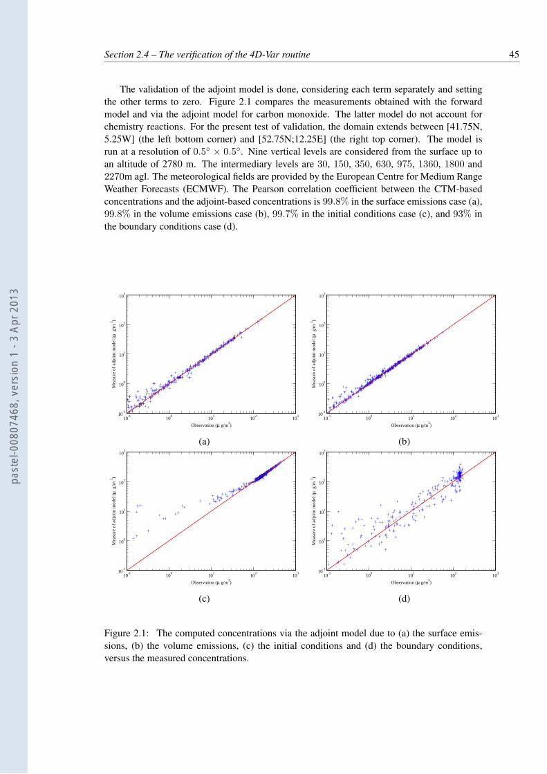
Section 2.4 – The verification of the 4D-Var routine 45
The validation of the adjoint model is done, considering each term separately and settingthe other terms to zero. Figure 2.1 compares the measurements obtained with the forwardmodel and via the adjoint model for carbon monoxide. The latter model do not account forchemistry reactions. For the present test of validation, the domain extends between [41.75N,5.25W] (the left bottom corner) and [52.75N;12.25E] (the right top corner). The model isrun at a resolution of 0.5 × 0.5. Nine vertical levels are considered from the surface up toan altitude of 2780 m. The intermediary levels are 30, 150, 350, 630, 975, 1360, 1800 and2270m agl. The meteorological fields are provided by the European Centre for Medium RangeWeather Forecasts (ECMWF). The Pearson correlation coefficient between the CTM-basedconcentrations and the adjoint-based concentrations is 99.8% in the surface emissions case (a),99.8% in the volume emissions case (b), 99.7% in the initial conditions case (c), and 93% inthe boundary conditions case (d).
10-1
100
101
102
103
Observation (µ g/m3)
10-1
100
101
102
103
Mea
sure
of a
djoi
nt m
odel
(µ g
/m 3 )
10-1
100
101
102
103
Observation (µ g/m3)
10-1
100
101
102
103
Mea
sure
of a
djoi
nt m
odel
(µ g
/m 3 )
(a) (b)
10-1
100
101
102
103
Observation (µ g/m3)
10-1
100
101
102
103
Mea
sure
of a
djoi
nt m
odel
(µ g
/m 3 )
10-1
100
101
102
103
Observation (µ g/m3)
10-1
100
101
102
103
Mea
sure
of a
djoi
nt m
odel
(µ g
/m 3 )
(c) (d)
Figure 2.1: The computed concentrations via the adjoint model due to (a) the surface emis-sions, (b) the volume emissions, (c) the initial conditions and (d) the boundary conditions,versus the measured concentrations.
past
el-0
0807
468,
ver
sion
1 -
3 Ap
r 201
3
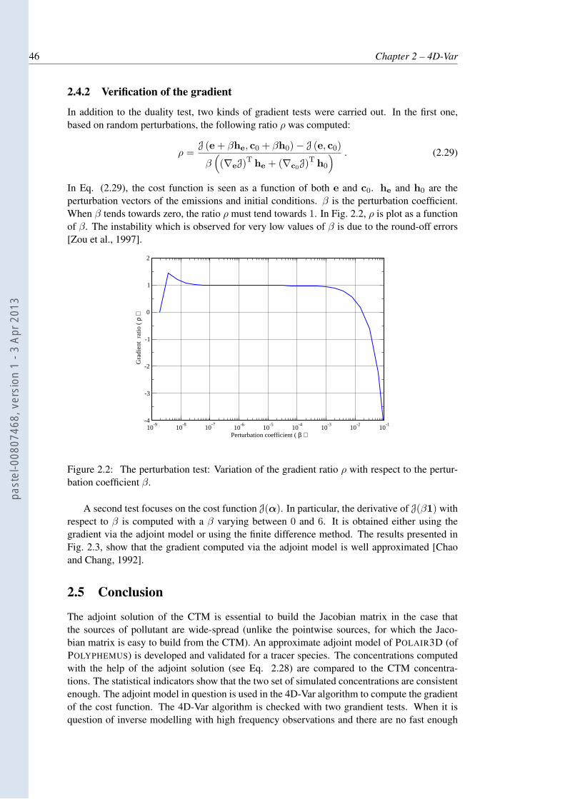
46 Chapter 2 – 4D-Var
2.4.2 Verification of the gradient
In addition to the duality test, two kinds of gradient tests were carried out. In the first one,based on random perturbations, the following ratio ρ was computed:
ρ =J (e + βhe, c0 + βh0) − J (e, c0)
β((∇eJ)T he + (∇c0
J)T h0
) . (2.29)
In Eq. (2.29), the cost function is seen as a function of both e and c0. he and h0 are theperturbation vectors of the emissions and initial conditions. β is the perturbation coefficient.When β tends towards zero, the ratio ρ must tend towards 1. In Fig. 2.2, ρ is plot as a functionof β. The instability which is observed for very low values of β is due to the round-off errors[Zou et al., 1997].
10-9
10-8
10-7
10-6
10-5
10-4
10-3
10-2
10-1
Perturbation coefficient ( β )
-4
-3
-2
-1
0
1
2
Gra
dien
t ra
tio (
ρ )
Figure 2.2: The perturbation test: Variation of the gradient ratio ρ with respect to the pertur-bation coefficient β.
A second test focuses on the cost function J(α). In particular, the derivative of J(β1) withrespect to β is computed with a β varying between 0 and 6. It is obtained either using thegradient via the adjoint model or using the finite difference method. The results presented inFig. 2.3, show that the gradient computed via the adjoint model is well approximated [Chaoand Chang, 1992].
2.5 Conclusion
The adjoint solution of the CTM is essential to build the Jacobian matrix in the case thatthe sources of pollutant are wide-spread (unlike the pointwise sources, for which the Jaco-bian matrix is easy to build from the CTM). An approximate adjoint model of POLAIR3D (ofPOLYPHEMUS) is developed and validated for a tracer species. The concentrations computedwith the help of the adjoint solution (see Eq. 2.28) are compared to the CTM concentra-tions. The statistical indicators show that the two set of simulated concentrations are consistentenough. The adjoint model in question is used in the 4D-Var algorithm to compute the gradientof the cost function. The 4D-Var algorithm is checked with two grandient tests. When it isquestion of inverse modelling with high frequency observations and there are no fast enough
past
el-0
0807
468,
ver
sion
1 -
3 Ap
r 201
3
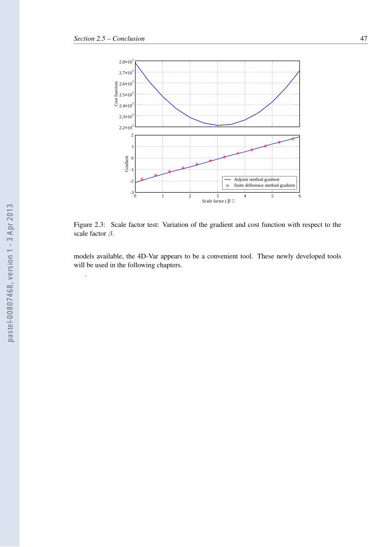
Section 2.5 – Conclusion 47
0 1 2 3 4 5 6Scale factor ( β )
-3
-2
-1
0
1
2
Gra
dien
t
Adjoint method gradientfinite difference method gradient
2.2×10³
2.3×10³
2.4×10³
2.5×10³
2.6×10³
2.7×10³
2.8×10³
Cos
t fun
ctio
n
Figure 2.3: Scale factor test: Variation of the gradient and cost function with respect to thescale factor β.
models available, the 4D-Var appears to be a convenient tool. These newly developed toolswill be used in the following chapters.
.
past
el-0
0807
468,
ver
sion
1 -
3 Ap
r 201
3

48 Chapter 2 – 4D-Var
past
el-0
0807
468,
ver
sion
1 -
3 Ap
r 201
3
Chapter 3
Inversion of regional carbon monoxide
fluxes: Coupling 4D-Var with a simple
subgrid statistical model
Summary
A four-dimensional variational data assimilation system (4D-Var) is employed to retrieve car-bon monoxide (CO) fluxes at regional scale, using an air quality network. The air qualitystations that monitor CO are proximity stations located close to industrial, urban or trafficsources. The mismatch between the coarsely discretized Eulerian transport model and the ob-servations, inferred to be mainly due to representativeness errors in this context, lead to a bias(average simulated concentrations minus observed concentrations) of the same order of mag-nitude as the concentrations. 4D-Var leads to a mild improvement in the bias because it doesnot adequately handle the representativeness issue. For this reason, a simple statistical sub-grid model is introduced and is coupled to 4D-Var. In addition to CO fluxes, the optimisationseeks to jointly retrieve influence coefficients, which quantify each station’s representativeness.The method leads to a much better representation of the CO concentration variability, with asignificant improvement of statistical indicators. The resulting increase in the total inventoryestimate is close to the one obtained from remote sensing data assimilation. This methodologyand experiments suggest that information useful at coarse scales can be better extracted fromatmospheric constituent observations strongly impacted by representativeness errors.
Contents
3.1 Introduction . . . . . . . . . . . . . . . . . . . . . . . . . . . . . . . . . 50
3.2 Inverse modelling setup . . . . . . . . . . . . . . . . . . . . . . . . . . . 52
3.3 Experiment setup . . . . . . . . . . . . . . . . . . . . . . . . . . . . . . 52
3.3.1 Observations . . . . . . . . . . . . . . . . . . . . . . . . . . . . . 52
3.3.2 Inventory and control variables . . . . . . . . . . . . . . . . . . . . 53
3.3.3 4D-Var . . . . . . . . . . . . . . . . . . . . . . . . . . . . . . . . 54
3.3.4 Error modelling . . . . . . . . . . . . . . . . . . . . . . . . . . . . 54
3.4 Application of 4D-Var . . . . . . . . . . . . . . . . . . . . . . . . . . . . 56
3.5 Coupling 4D-Var with a subgrid statistical model . . . . . . . . . . . . . 57
past
el-0
0807
468,
ver
sion
1 -
3 Ap
r 201
3
50 Chapter 3 – Coupled model
3.5.1 A simple subgrid statistical model . . . . . . . . . . . . . . . . . . 57
3.5.2 Coupling to the 4D-Var system . . . . . . . . . . . . . . . . . . . . 60
3.6 Application of 4D-Var-ξ . . . . . . . . . . . . . . . . . . . . . . . . . . . 60
3.6.1 Analysis . . . . . . . . . . . . . . . . . . . . . . . . . . . . . . . 60
3.6.2 Validation . . . . . . . . . . . . . . . . . . . . . . . . . . . . . . . 67
3.7 Conclusion . . . . . . . . . . . . . . . . . . . . . . . . . . . . . . . . . . 72
3.1 Introduction
In tracer transport studies, observations are infrequent in time and, for ground-measurements,sparse in space. Furthermore, they do not intrinsically carry any information about the future.That is why, complementarity, numerical models are used to assess the meteorological andchemical state of the atmosphere. In air quality modelling, input data, such as initial andboundary conditions, emission fluxes, and vertical diffusion coefficients are necessary to runproper simulations. The uncertainties of these input data and perhaps the lack of understandingof the underlying physical processes induce model errors in the simulations. To minimisethem, data assimilation (DA) methods can be used. They combine observational data, andinformation coming from chemistry and transport models and their related error statistics inorder to find the optimal values of the parameters which minimise the errors.
Introducing optimal control theory ideas in geophysics, Le Dimet and Talagrand [1986]used 4D-Var to assimilate meteorological observations. Fisher and Leny [1995] used 4D-Varfor the analysis of some chemically active tracer species. Lately, variational data assimilationstudies have focused on the inverse modelling of pollutant emission fields (e.g. Elbern et al.[2007] and other references within Zhang et al. [2012]).
Focusing on carbon monoxide (CO), several modelling studies pointed out to the discrep-ancy between the observations and the simulated concentrations. Using the Emission Databasefor Global Atmospheric Research 3 (EDGAR3) inventory, before any correction, the modelglobal run of Fortems-Cheiney et al. [2011] underestimates the CO concentrations of about5 to 10% with respect to the satellite observations for January, February and March 2005.Emmons et al. [2010] compared the satellite observations to simulations of the the Model forOZone And Related chemical Tracers, version 4 (MOZART-4), using the EDGAR3 inventory.Displaying a similar trend, their results exhibit an underestimation of the CO concentrationsover Europe of about 10 to 20% for the same period.
That is why inverse modelling experiments have been carried out to update the CO fluxinventories. For instance, Mulholland and Seinfeld [1995]; Saide et al. [2011] focused onurban scale. Yumimotoa and Uno [2006]; Kopacz et al. [2009] used 4D-Var or analyticalmethods to invert the emissions at regional scale. Other studies have also been performed onglobal scale: e.g. Pétron et al. [2002]; Stavrakou and Müller [2006]; Arellano and Hess [2006];Fortems-Cheiney et al. [2009]; Kopacz et al. [2010]. These studies make use of ground-basedinstruments that measure concentrations, or they make use of satellite instruments to infersatellite-derived retrieval of CO. The former instruments are mostly used in conjunction withregional scale models whereas the latter instruments are mostly used with global scale models.
In the case of an assimilation of observations over a short period (i.e. a few hours toa few days), the parameters to be optimised are usually the initial conditions. With largerdata assimilation windows (i.e. a few days to a few months), the model is more sensitive toother parameters, such as the emissions inventory, the meteorological fields and the boundaryconditions.
past
el-0
0807
468,
ver
sion
1 -
3 Ap
r 201
3
Section 3.1 – Introduction 51
In most top-down (i.e. inverse modelling) studies related to the global scale, the CO emis-sions fluxes were found to be underestimated in the Northern hemisphere whereas they arequite consistent with the measurements in the Southern hemisphere (e.g. Müller and Stavrakou[2005]), or slightly overestimated (e.g. Arellano and Hess [2006]). This underestimation in theNorthern hemisphere is also found in the modelling studies (e.g. Emmons et al. [2010]).
Satellite and in-situ measurements require specific care when compared to transport mod-els. The discrepancy between the observations and the model forecast of these observationsare known to be due to instrumental errors, deficiencies of the model and of the forcing fields(model error), and the representativeness error. The assessment of this representativeness errorbecomes a key issue when assimilating in-situ observations, which are the focus of this study.Indeed, the model is operative at coarser scale and by construction cannot simulate subgridevents. The in-situ observations do capture both the coarser scale pollutant plumes, but alsosubgrid plumes that are not accounted for by the model. Therefore, there is a residual mismatchdue to unresolved scales known as the representativeness error. In data assimilation, it is oftenconsidered part of model error, but formally ascribed to the observation error.
Due to the complexity of its estimation, an experience-based value is usually assumed forthat error. This value is often chosen to be the same for all measurements. Yet that is certainlynot true, because the nature of the measurements can be different (urban, rural, etc.). Themaximum possible representativeness error is often chosen for all observations. Alternativelya χ2 criterion (used by Ménard et al. [2000] in tracer studies) can be implemented to estimatethe proper magnitude of the observational errors.
In this chapter, our goal is to estimate carbon monoxide surface emissions with inversemodelling, using in-situ measurements from an air quality network. This network operates inFrance and we wish to retrieve the emissions over France. Hence, as opposed to most of thestudies mentioned earlier, the focus is on mesoscale and lower troposphere modelling. Thesemeasurements are abundant, but strongly impacted by representativeness errors since manyof them are influenced by nearby industrial, traffic or urban sources. Most of them aim atmeasuring (some of) those influential sources. To perform emission inverse modelling in thiscontext, this lack of representativeness must be accounted for. One needs to demonstrate thatobservations obtained at fine scale, and strongly impacted by representativeness errors, can beassimilated with the aim of correcting a pollutant inventory defined at larger scale.
In Section 4.2, the atmospheric transport model (ATM) is introduced, as well as, a detaileddescription of the observational data. The specifications of the control space are presented. Aninvestigation of the modelling of errors and of the uncertainties of the control parameters isalso reported. In Section 3.4, 4D-Var is used to optimise the spatio-temporal parameters of theinventories with unsatisfactory results. Since there is a dramatic lack of representativeness ofthe measurements, a simple subgrid statistical model is built in order to improve the 4D-Varnumerical results. The statistical model aims at taking into account the impact of close-bysources on monitoring stations. Section 3.5 introduced and justifies this statistical model andits tight coupling to 4D-Var. In Section 4.3, the inverse modelling experiment is performed withthe combination of 4D-Var and the subgrid statistical model, which will be called 4D-Var-ξ.The analysis produced by the retrieval is studied. Validations with independent observations areperformed, notably using cross-validation and a long-term forecast of the CO concentrations.In Section 5.5, the findings of this study are summarised. The potential and limitation of theapproach are discussed.
past
el-0
0807
468,
ver
sion
1 -
3 Ap
r 201
3
52 Chapter 3 – Coupled model
3.2 Inverse modelling setup
First, details are given about the necessary ingredients of the inverse modelling study: thetransport model setup, the observations, the control variables (which are the scale factors of theemission inventories) and the first guess provided by the initial inventory. How to incorporatethem in a 4D-Var-ξ system is then described, as well as the necessary statistical assumptionson the errors present in the system.
3.3 Experiment setup
All runs of the model will be performed over France. The domain extends between [41.75N,5.25W] (the left bottom corner) and [52.75N;12.25E] (the right top corner). The grid hasthe resolution of 0.25 × 0.25. Nine vertical levels are considered from the surface up toan altitude of 2780 m. The intermediary levels are 30, 150, 350, 630, 975, 1360, 1800 and2270 m. The meteorological fields are provided by the European Centre for Medium RangeWeather Forecasts (ECMWF). These fields have a resolution of 0.36 × 0.36 and 60 verticallevels. The time step is 3 hours. Concentrations from the global chemistry-transport modelMOZART, version 2 [Horowitz et al., 2003] are used to provide boundary conditions, and theinitial condition. A calibration factor of 1.2 is used to correct a global underestimation ofincoming carbon monoxide, following the global estimations of Emmons et al. [2010].
It has initially been examined that within our regional, lower troposphere setup, and for ourtimescale, carbon monoxide is barely reactive. To do so, we have compared the photochemicalversion of POLAIR3D to the tracer version (validated in Quélo et al. [2007]). A small bias of5.8 µg m−3 is observed between the CO concentrations with or without reactions, i.e. about2% of the average measurements. As a consequence, neglecting the reactions, we chose to usethe faster tracer version of the model.
3.3.1 Observations
The BDQA (Base de Données de la Qualité de l’Air1) is a database listing the concentrationsof several air quality pollutants over France. The (mostly hourly) collected observations areprovided by 600 monitoring stations distributed all over France. For carbon monoxide, 89stations provide hourly measurements at ground level (with an average of 75 observations perhour for the year 2005). These stations belong to one of the four different categories: industrial,traffic, urban and suburban. This gives an indication of their environment but not necessarily oftheir representativeness in an ATM. Larssen et al. [1999] define an area of representativenessfor a station as being an area in which the concentrations do not differ from the ones measuredat the station by more than a specified amount. This amount can be set to the total uncertaintyof the measurement or to a value not to be exceeded in order to fulfil data quality objectives.Nappo et al. [1982] further precise that more than 90% of the concentrations measured in thatarea should satisfy that definition. When these conditions cannot be satisfied for a station, thelatter is not deemed representative of its area.
In the case of carbon monoxide, the stations belonging to the BDQA network are far fromrepresentative as it is very difficult to determine an area of representativeness for most of them.These receptors are likely to be influenced by nearby surface fluxes [Henne et al., 2010]. Back-ground stations, far from pollution sources, are missing.
For the experiments performed in this study, 8 weeks of BDQA observations will be assim-ilated from January the 1st 2005 to February the 26th 2005, for a total of 107, 914 observations,
1details available at http://www.atmonet.org
past
el-0
0807
468,
ver
sion
1 -
3 Ap
r 201
3
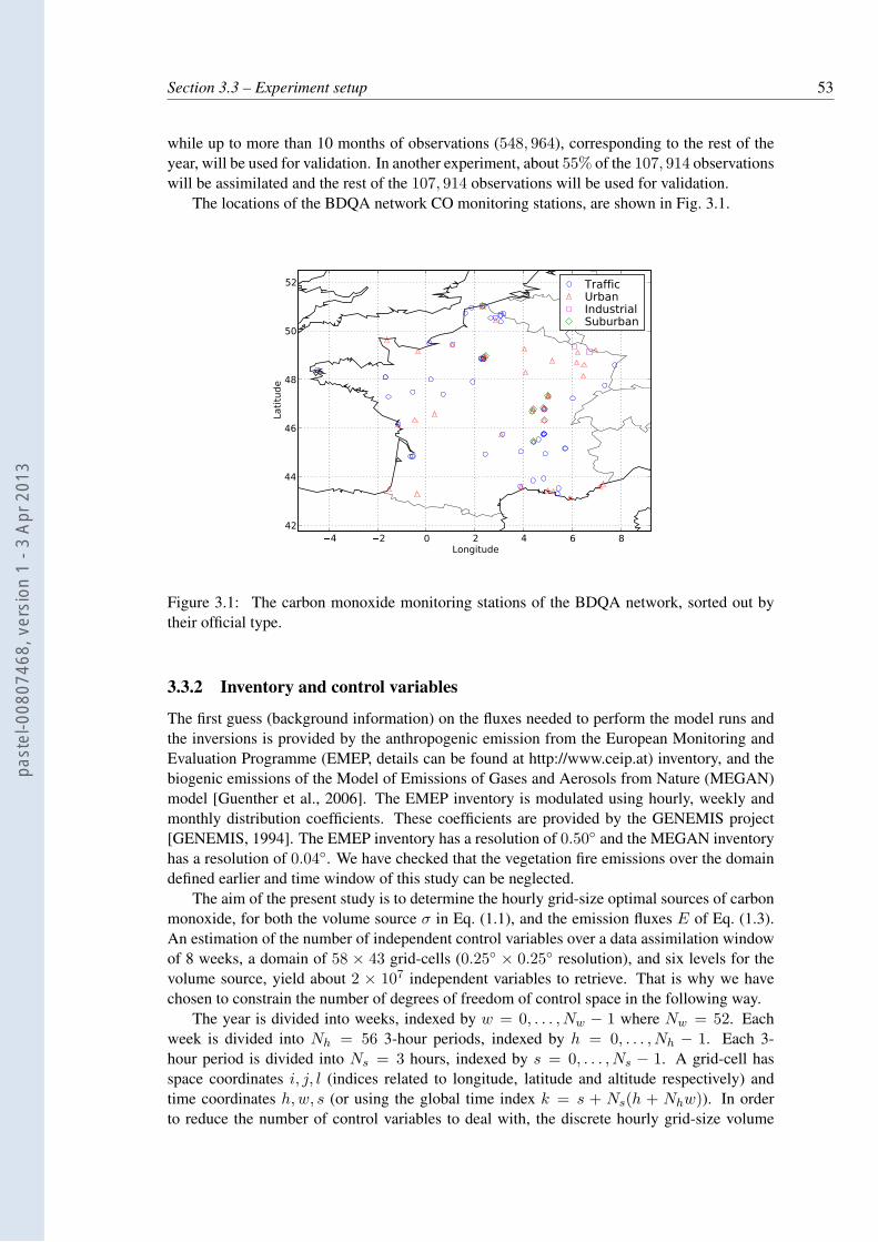
Section 3.3 – Experiment setup 53
while up to more than 10 months of observations (548, 964), corresponding to the rest of theyear, will be used for validation. In another experiment, about 55% of the 107, 914 observationswill be assimilated and the rest of the 107, 914 observations will be used for validation.
The locations of the BDQA network CO monitoring stations, are shown in Fig. 3.1.
4 2 0 2 4 6 8Longitude
42
44
46
48
50
52La
titude
TrafficUrbanIndustrialSuburban
Figure 3.1: The carbon monoxide monitoring stations of the BDQA network, sorted out bytheir official type.
3.3.2 Inventory and control variables
The first guess (background information) on the fluxes needed to perform the model runs andthe inversions is provided by the anthropogenic emission from the European Monitoring andEvaluation Programme (EMEP, details can be found at http://www.ceip.at) inventory, and thebiogenic emissions of the Model of Emissions of Gases and Aerosols from Nature (MEGAN)model [Guenther et al., 2006]. The EMEP inventory is modulated using hourly, weekly andmonthly distribution coefficients. These coefficients are provided by the GENEMIS project[GENEMIS, 1994]. The EMEP inventory has a resolution of 0.50 and the MEGAN inventoryhas a resolution of 0.04. We have checked that the vegetation fire emissions over the domaindefined earlier and time window of this study can be neglected.
The aim of the present study is to determine the hourly grid-size optimal sources of carbonmonoxide, for both the volume source σ in Eq. (1.1), and the emission fluxes E of Eq. (1.3).An estimation of the number of independent control variables over a data assimilation windowof 8 weeks, a domain of 58 × 43 grid-cells (0.25 × 0.25 resolution), and six levels for thevolume source, yield about 2 × 10⁷ independent variables to retrieve. That is why we havechosen to constrain the number of degrees of freedom of control space in the following way.
The year is divided into weeks, indexed by w = 0, . . . , Nw − 1 where Nw = 52. Eachweek is divided into Nh = 56 3-hour periods, indexed by h = 0, . . . , Nh − 1. Each 3-hour period is divided into Ns = 3 hours, indexed by s = 0, . . . , Ns − 1. A grid-cell hasspace coordinates i, j, l (indices related to longitude, latitude and altitude respectively) andtime coordinates h, w, s (or using the global time index k = s + Ns(h + Nhw)). In orderto reduce the number of control variables to deal with, the discrete hourly grid-size volume
past
el-0
0807
468,
ver
sion
1 -
3 Ap
r 201
3

54 Chapter 3 – Coupled model
sources σ and emissions E are parameterised according to
[σ]i,j,l,h,w,s = [α]i,j,h [σb]i,j,l,h,w,s , (3.1)
[E]i,j,h,w,s = [α]i,j,h[Eb]i,j,h,w,s , (3.2)
where [α]i,j,h are the non-dimensional effective control variables corresponding to the residualdegrees of freedom. They represent 58 × 43 × 56 = 139, 664 scalars. The first guesses σb
and Eb are the background sources stemming from the inventory. Let us make a remark onthe temporal cycles of the inventory, that are for instance due to vehicles traffic, urban heating,industry, etc. Because the control variables [α]i,j,h are indexed by h, the intra-week temporalcycles will be solved for in the inverse modelling experiments. However the longer cycleswill not be solved for, but are determined by the built-in cycles of the inventory: [σb]i,j,l,h,w,s
depends on the indexes w and s. For instance, seasonal cycles of urban heating are prescribedby [σb]i,j,l,h,w,s.
The surface E and volume emission σ variables have a similar local signature and wouldhave a similar impact on a distant observation site, so that they would appear as ill-determinedvariables in an inverse problem. That is the reason why they were parameterised in Eq. (3.1)and Eq. (3.2) in terms of the same control vector α. It is convenient to introduce a compositeemission vector e, defined in the surface layer by
el=0 = σl=0 +E
∆, (3.3)
where ∆ is the height of the surface layer. Note that this equality assumes a well-mixed surfacelayer. In the upper layers l ≥ 1, it is defined by
el = σl . (3.4)
In the following, the first guess about e (background) will be denoted eb. Correspondingly, onehas:
[eb]i,j,l=0,h,w,s = [σb]i,j,l=0,h,w,s +[Eb]i,j,h,w,s
∆and [eb]i,j,l 6=0,h,w,s = [σb]i,j,l 6=0,h,w,s .
(3.5)As a result, Eq. (3.1) and Eq. (3.2) can be synthesised into
[e]i,j,l,h,w,s = [α]i,j,h[eb]i,j,l,h,w,s . (3.6)
3.3.3 4D-Var
In spite of the quasi-linear physics of carbon monoxide (at these space and time scales), thecomputation of the Jacobian matrix is difficult to afford because of the very large set of data andcontrol variables we intend to use. 4D-Var is meant to handle such a computational problem[Chevallier et al., 2005]. The details of the 4D-Var are reported in chapter 2.
3.3.4 Error modelling
In this section, we describe how the background and observation errors are statistically mod-eled. The background errors on the independent variables α are first related to the traditionalbackground errors on e (hence σ and E). While the background error variances will be chosena priori, the observation errors will be determined through a χ2 diagnosis.
past
el-0
0807
468,
ver
sion
1 -
3 Ap
r 201
3
Section 3.3 – Experiment setup 55
3.3.4.1 Background error covariance matrix
The background error covariance matrix Bα defines the variances-covariances between thedifferent components of the departure of the scale factors α from αb = 1. In the inventory,anthropogenic emissions significantly dominates the biogenic emissions (1.8% of the total in-ventory over France). Assuming the anthropogenic sources (such as the individual industrialsources, or urban heating sources) have errors that are barely spatially correlated, the error cor-relation between grid-cells are taken as negligible, so that the covariance terms of that matrixare set to zero. Note that other sources of anthropogenic sources, such as traffic might have ex-tended correlated errors. We also neglect temporal correlations, which is a weaker assumptioneven though the emission are mostly anthropogenic. As a consequence of our assumptions,the prior errors are essentially represented by the variances of the prior emissions (diagonalassumption for Bα).
Assuming that the emission errors are not time dependent, the variance of control variable[α]i,j,h is:
[Bα]i,j,h =
Nw−1∑
w=0
Ns−1∑
s=0
Nl−1∑
l=0
[Be]i,j,l,h,w,s
(Nw−1∑
w=0
Ns−1∑
s=0
Nl−1∑
l=0
[eb]i,j,l,h,w,s
)2 , (3.7)
where
[Be]i,j,l,h,w,s = E
[([e]i,j,l,h,w,s − [eb]i,j,l,h,w,s
)2]
(3.8)
is the background error variance of the emission fluxes in the grid-cell of coordinates i, j, l attime h, w, s. Since the data assimilation window of the experiments ahead is 8-week long, Nw
is now set to 8.
3.3.4.2 Observation error covariance matrix
In Eq. (2.18), ǫk includes the instrumental error and representativeness error of the observa-tions. It is assumed that they are independent from site to site, and from observation time toobservation time. At this stage the variances are assumed to be the same for all observations,which is crude since the representativeness error is expected to significantly vary between sta-tions. Accordingly, Rk is modeled as a diagonal matrix:
Rk = r2Imk, (3.9)
where Imkis the identity matrix in observation space at time tk, and
r2 = ε2repr + ε2
meas . (3.10)
εmeas is the standard deviation of instrumental error, and εrepr is the standard deviation of therepresentativeness errors, which depends on the species, the station type, and the grid size[Elbern et al., 2007].
To estimate the standard deviation parameter r, we resort to a χ2 diagnosis ([Ménard et al.,2000; Elbern et al., 2007] for instance in the context of atmospheric chemistry). When thestatistics of the errors are consistent with the innovations, then one should expect that theaverage value of the cost function is equal to half of the number of assimilated observations.Accordingly r should be chosen such that:
min
αJ(α)
(r) ≃
m
2(3.11)
past
el-0
0807
468,
ver
sion
1 -
3 Ap
r 201
3
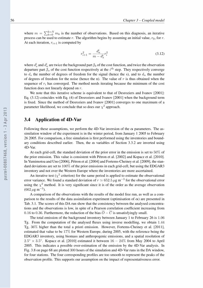
56 Chapter 3 – Coupled model
where m =∑k=N
k=0 mk is the number of observations. Based on this diagnosis, an iterativeprocess can be used to estimate r. The algorithm begins by assuming an initial value, r0, for r.At each iteration, ri+1 is computed by
r2i+1 =
din
m − dis
r2i (3.12)
where dis and di
n are twice the background part Jb of the cost function, and twice the observationdeparture part Jo of the cost function respectively at the ith step. They respectively convergeto ds the number of degrees of freedom for the signal (hence the s), and to dn the numberof degrees of freedom for the noise (hence the n). The value of r is thus obtained when thesequence of ri has converged. The method needs iterating because the minimum of the costfunction does not linearly depend on r.
We note that this iterative scheme is equivalent to that of Desroziers and Ivanov [2001]:Eq. (3.12) coincides with Eq. (4) of Desroziers and Ivanov [2001] when the background termis fixed. Since the method of Desroziers and Ivanov [2001] converges to one maximum of aparameter likelihood, we conclude that so does our χ2 approach.
3.4 Application of 4D-Var
Following these assumptions, we perform the 4D-Var inversion of the α parameters. The as-similation window of the experiment is in the winter period, from January 1 2005 to February26 2005. For comparison, a free simulation is first performed using the inventories and bound-ary conditions described earlier. Then, the α variables of Section 3.3.2 are inverted using4D-Var.
At each grid-cell, the standard deviation of the prior error in the emission is set to 50% ofthe prior emission. This value is consistent with Pétron et al. [2002] and Kopacz et al. [2010].In Yumimotoa and Uno [2006], Pétron et al. [2004] and Fortems-Cheiney et al. [2009], the stan-dard deviations are set to 100% of the prior emissions in each grid-cell, but using the EDGAR3inventory and not over the Western Europe where the inventories are more ascertained.
An iterative test (χ2 criterion) for the same period is applied to estimate the observationalerror variance. We found a standard deviation of r ≃ 652.5 µg m−3 for the observational errorusing the χ2 method. It is very significant since it is of the order as the average observation(662 µg m−3).
A comparison of the observations with the results of the model free run, as well as a com-parison to the results of the data assimilation experiment (optimisation of α) are presented inTab. 3.1. The scores of this DA run show that the consistency between the analysed concentra-tions and the observations is low, in spite of a Pearson correlation coefficient increasing from0.16 to 0.36. Furthermore, the reduction of the bias O − C is unsatisfyingly small.
The total emission of the background inventory between January 1 to February 26 is 1.06Tg. From the computation of the analysed fluxes using inverse modelling, we obtain 1.44Tg, 36% higher than the total a priori emission. However, Fortems-Cheiney et al. [2011],estimated that value to be 17% for Western Europe, during 2005, with the reference being theEDGAR3 inventory, using biomass and anthropogenic emissions, and a spatial resolution of2.5 × 3.5. Kopacz et al. [2010] estimated it between 16 − 24% from May 2004 to April2005. This indicates a possible over-estimation of the emission by the 4D-Var analysis. InFig. 3.8 on page 68 are plotted 300 hours of the simulation and 4D-Var runs in the DA window,for four stations. The four corresponding profiles are too smooth to represent the peaks of theobservation profile. This supports our assumption on the impact of representativeness error.
past
el-0
0807
468,
ver
sion
1 -
3 Ap
r 201
3
Section 3.5 – Coupling 4D-Var with a subgrid statistical model 57
Table 3.1: Comparison of the observations and the simulated or analysed concentrations. Cis the mean concentration, O is the mean observation, and NB= 2(C − O)/(C + O) is thenormalised bias. RMSE stands for root-mean square error. R is the Pearson correlation. FAx
is the fraction of the simulated concentrations that are within a factor x of the correspondingobservations. C, O, and the RMSE are given in µg m−3.
C O NB RMSE R FA2 FA5
Simulation (01/01–02/26 2005) 303 662 -0.74 701 0.16 0.52 0.90
Optimisation of α (4D-Var) 396 662 -0.50 633 0.36 0.59 0.92
Optimisation of ξ 615 662 -0.07 503 0.57 0.73 0.96
Coupled optimisation of α, ξ (4D-Var-ξ) 671 662 0.01 418 0.73 0.79 0.97
The BDQA CO network is mostly composed of proximity stations, whose observations arelikely to be influenced by local sources. Therefore, the lack of consistency between the modeland the observations could be explained by the direct impact of nearby pollution sources onobservations. The 4D-Var analysis cannot account for the local peaks of CO concentrationssince it uses a model that cannot resolve those subgrid-scale processes. However, we believethat there is some useful signal to extract from these observations. To do so, one needs toaccount for the subgrid processes. At least two state-of-the-art options are possible. The de-terministic route consists in using explicit representations of partial information that one mayhave about the subgrid processes, emissions, etc. These representations are incorporated intothe coarser model. This is what typically does a plume-in-grid model that uses some additionalinformation about short-range dispersion (e.g. Karamchandani et al. [2009] for an applicationto CO subgrid traffic emission). A second route is of statistical nature. The aim is to make astatistical regression between the observations and the coarse resolution model output, whichresults in a fitted linear correspondence between the model to the observations. In geosciences,downscaling techniques have taken this path (e.g. Guillas et al. [2008] for an application toozone concentrations). In this study, a statistical approach is chosen to represent the subgrideffects. A deterministic modelling approach of the subgrid processes would theoretically bedesirable, but it requires additional subgrid information that we do not have here, and it wouldbe computationally more expensive.
3.5 Coupling 4D-Var with a subgrid statistical model
3.5.1 A simple subgrid statistical model
Assume that s is a continuous source field: it describes the emission at any spatial scale. Recallthat e is the discrete coarse-grained source that we use to drive the model. Ideally, s and e
should be related through a restriction, coarse-graining operator Γ, which acts as a low-passfilter, filtering out the fine details of the source:
e = Γs . (3.13)
Following Bocquet et al. [2011], we can consider a prolongation operator Γ⋆, which refines acoarse emission field e to a continuous field s⋆:
s⋆ = Γ⋆e . (3.14)
There is freedom in choosing Γ⋆. It could be a basic subgrid spatial interpolation operator, or itcould rely on additional subgrid information, or it could be obtained from a Bayesian inference
past
el-0
0807
468,
ver
sion
1 -
3 Ap
r 201
3
58 Chapter 3 – Coupled model
[Bocquet et al., 2011]. For the purpose of this derivation, we do not have to specify a preciseform for Γ⋆. However, it is reasonable to assume ΓΓ⋆ = I. Besides, Γ⋆Γ is a projectionoperator, not the identity, because of some details of the real fine scale emission field are lostin the restriction process Γ.
If H is the Jacobian of a continuous multiscale hypothetical carbon monoxide model thatrelates s to the measurements y, the vector collecting all measurements, then
y = Hs + ǫ
= HΓ⋆Γs + H (I − Γ⋆Γ) s + ǫ
= (HΓ⋆) e + H (I − Γ⋆Γ) s + ǫ . (3.15)
Assume Γ operates the coarse-graining at the finest scale accessible by the model. ThereforeHΓ⋆ could be identified with the Jacobian of our Eulerian ATM. Since I − Γ⋆Γ is a high-pass projector (it retains the short-scale fluctuations of the real emission field), H(I − Γ⋆Γ)stheoretically stands for the representativeness error [Wu et al., 2011].
Unfortunately, we do not have access to s or a multiscale model H, and one needs a simplesubgrid scale model to approximate H(I−Γ⋆Γ)s and close the equation. We assume this rep-resentativeness error is mostly due to subgrid/nearby sources that have a strong impact on themeasurements which are not representative of the background carbon monoxide concentrationlevel. Another possibly significant source of error is the weakness of current vertical turbu-lent diffusion parameterisations. Notice that part of it may be categorised as representativenesserrors when for instance the boundary layer height varies significantly within grid-cells.
Guided by the structure of H(I−Γ⋆Γ)s, we choose to model this nearby source influenceby the term
ξiΠi,ke (3.16)
where ξi is a positive scalar attached to a station indexed by i. Similarly to H(I − Γ⋆Γ)s,ξiΠi,ke has a linear explicit dependence on the emission e. The influence coefficient ξi quan-tifies the influence of local nearby sources onto the station. It can be interpreted as the time(given in hours in the following) required to reach a CO concentration level equivalent to thesubgrid part of the measurement [y − Hc]i,k, by emitting Πi,ke which is based on the coarse-grained inventory. This influence factor is assumed constant in time and it is a priori unknown.Πi,k is an operator that linearly interpolates e at the station location and at time tk. If ξi isvanishing, then the representativeness of the station is deemed good. Otherwise, a significantξi (a few hours and beyond) indicates a possible significant impact of nearby sources. Figure3.2 illustrates this rationale.
This term is enforced in the observation model Eq. (2.18), which becomes, at any giventime:
y = Hc + ξ · Πe + ǫ , (3.17)
where ξ · Πe is the vector of entries [ξ · Πe]i,k = ξiΠi,ke. The residual error ǫ should statis-tically be smaller than ǫ of Eq. (2.18) since part of the representativeness error should now be
accounted for by the subgrid term. We denote its covariance matrix with R = E[ǫǫT]. Under
independence assumptions, the two are connected by
R = E[ǫǫT]
= ξ · ΠE[eeT
]ΠT · ξT + R . (3.18)
past
el-0
0807
468,
ver
sion
1 -
3 Ap
r 201
3
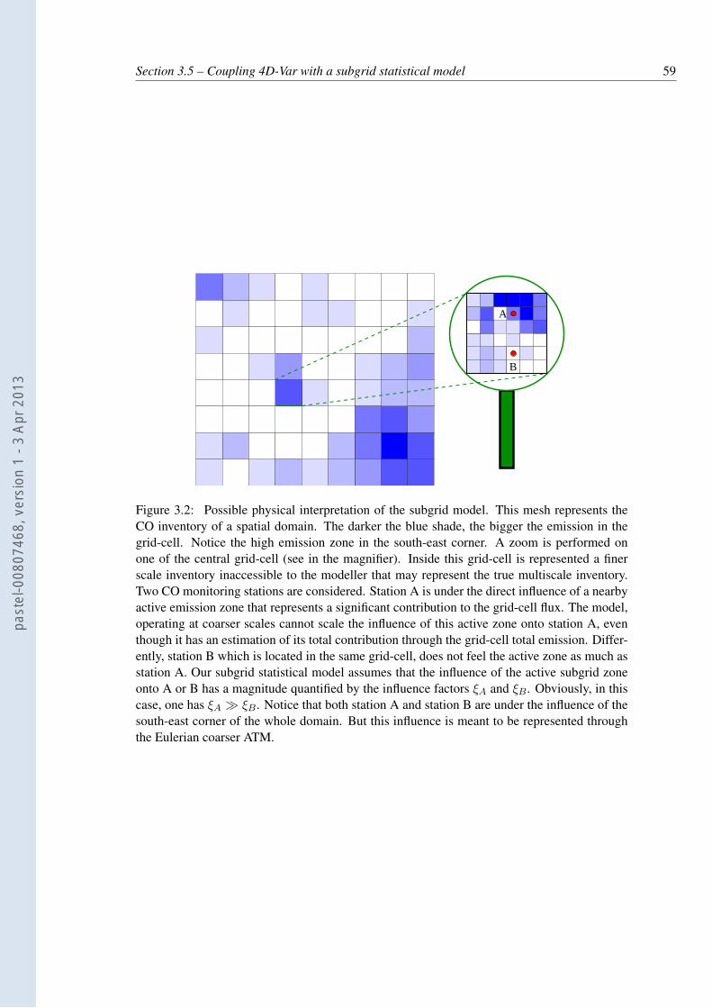
Section 3.5 – Coupling 4D-Var with a subgrid statistical model 59
A
B
Figure 3.2: Possible physical interpretation of the subgrid model. This mesh represents theCO inventory of a spatial domain. The darker the blue shade, the bigger the emission in thegrid-cell. Notice the high emission zone in the south-east corner. A zoom is performed onone of the central grid-cell (see in the magnifier). Inside this grid-cell is represented a finerscale inventory inaccessible to the modeller that may represent the true multiscale inventory.Two CO monitoring stations are considered. Station A is under the direct influence of a nearbyactive emission zone that represents a significant contribution to the grid-cell flux. The model,operating at coarser scales cannot scale the influence of this active zone onto station A, eventhough it has an estimation of its total contribution through the grid-cell total emission. Differ-ently, station B which is located in the same grid-cell, does not feel the active zone as much asstation A. Our subgrid statistical model assumes that the influence of the active subgrid zoneonto A or B has a magnitude quantified by the influence factors ξA and ξB . Obviously, in thiscase, one has ξA ≫ ξB . Notice that both station A and station B are under the influence of thesouth-east corner of the whole domain. But this influence is meant to be represented throughthe Eulerian coarser ATM.
past
el-0
0807
468,
ver
sion
1 -
3 Ap
r 201
3
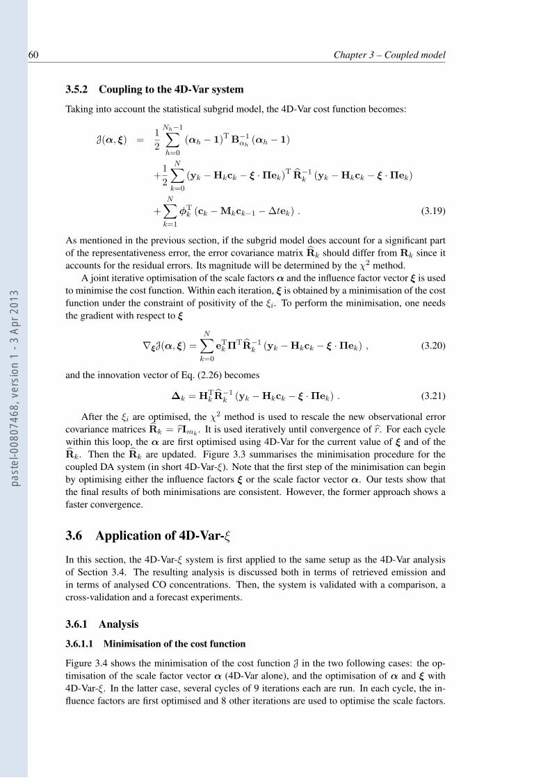
60 Chapter 3 – Coupled model
3.5.2 Coupling to the 4D-Var system
Taking into account the statistical subgrid model, the 4D-Var cost function becomes:
J(α, ξ) =1
2
Nh−1∑
h=0
(αh − 1)T B−1αh
(αh − 1)
+1
2
N∑
k=0
(yk − Hkck − ξ · Πek)T
R−1k (yk − Hkck − ξ · Πek)
+
N∑
k=1
φTk (ck − Mkck−1 − ∆tek) . (3.19)
As mentioned in the previous section, if the subgrid model does account for a significant partof the representativeness error, the error covariance matrix Rk should differ from Rk since itaccounts for the residual errors. Its magnitude will be determined by the χ2 method.
A joint iterative optimisation of the scale factors α and the influence factor vector ξ is usedto minimise the cost function. Within each iteration, ξ is obtained by a minimisation of the costfunction under the constraint of positivity of the ξi. To perform the minimisation, one needsthe gradient with respect to ξ
∇ξJ(α, ξ) =
N∑
k=0
eTk ΠTR−1
k (yk − Hkck − ξ · Πek) , (3.20)
and the innovation vector of Eq. (2.26) becomes
∆k = HTk R−1
k (yk − Hkck − ξ · Πek) . (3.21)
After the ξi are optimised, the χ2 method is used to rescale the new observational errorcovariance matrices Rk = rImk
. It is used iteratively until convergence of r. For each cyclewithin this loop, the α are first optimised using 4D-Var for the current value of ξ and of theRk. Then the Rk are updated. Figure 3.3 summarises the minimisation procedure for thecoupled DA system (in short 4D-Var-ξ). Note that the first step of the minimisation can beginby optimising either the influence factors ξ or the scale factor vector α. Our tests show thatthe final results of both minimisations are consistent. However, the former approach shows afaster convergence.
3.6 Application of 4D-Var-ξ
In this section, the 4D-Var-ξ system is first applied to the same setup as the 4D-Var analysisof Section 3.4. The resulting analysis is discussed both in terms of retrieved emission andin terms of analysed CO concentrations. Then, the system is validated with a comparison, across-validation and a forecast experiments.
3.6.1 Analysis
3.6.1.1 Minimisation of the cost function
Figure 3.4 shows the minimisation of the cost function J in the two following cases: the op-timisation of the scale factor vector α (4D-Var alone), and the optimisation of α and ξ with4D-Var-ξ. In the latter case, several cycles of 9 iterations each are run. In each cycle, the in-fluence factors are first optimised and 8 other iterations are used to optimise the scale factors.
past
el-0
0807
468,
ver
sion
1 -
3 Ap
r 201
3
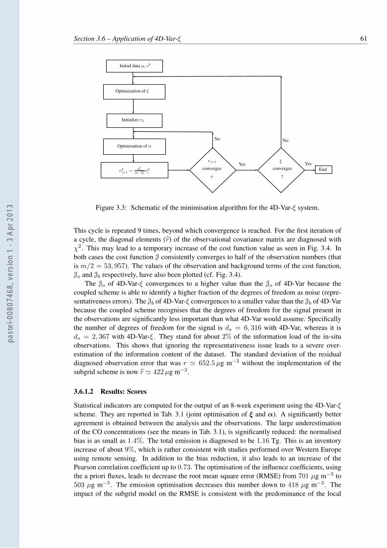
Section 3.6 – Application of 4D-Var-ξ 61
Initial data µ, eb
Optimization of ξ
Initialize r0
Optimisation of α
r2i+1 =
di
n
m−dis
r2i
ri+1 ξ
converges converges
? ?
EndYes
No No
Yes
Figure 3.3: Schematic of the minimisation algorithm for the 4D-Var-ξ system.
This cycle is repeated 9 times, beyond which convergence is reached. For the first iteration ofa cycle, the diagonal elements (r) of the observational covariance matrix are diagnosed withχ2. This may lead to a temporary increase of the cost function value as seen in Fig. 3.4. Inboth cases the cost function J consistently converges to half of the observation numbers (thatis m/2 = 53, 957). The values of the observation and background terms of the cost function,Jo and Jb respectively, have also been plotted (cf. Fig. 3.4).
The Jo of 4D-Var-ξ convergences to a higher value than the Jo of 4D-Var because thecoupled scheme is able to identify a higher fraction of the degrees of freedom as noise (repre-sentativeness errors). The Jb of 4D-Var-ξ convergences to a smaller value than the Jb of 4D-Varbecause the coupled scheme recognises that the degrees of freedom for the signal present inthe observations are significantly less important than what 4D-Var would assume. Specificallythe number of degrees of freedom for the signal is ds = 6, 316 with 4D-Var, whereas it isds = 2, 367 with 4D-Var-ξ. They stand for about 2% of the information load of the in-situobservations. This shows that ignoring the representativeness issue leads to a severe over-estimation of the information content of the dataset. The standard deviation of the residualdiagnosed observation error that was r ≃ 652.5 µg m−3 without the implementation of thesubgrid scheme is now r ≃ 422 µg m−3.
3.6.1.2 Results: Scores
Statistical indicators are computed for the output of an 8-week experiment using the 4D-Var-ξscheme. They are reported in Tab. 3.1 (joint optimisation of ξ and α). A significantly betteragreement is obtained between the analysis and the observations. The large underestimationof the CO concentrations (see the means in Tab. 3.1), is significantly reduced: the normalisedbias is as small as 1.4%. The total emission is diagnosed to be 1.16 Tg. This is an inventoryincrease of about 9%, which is rather consistent with studies performed over Western Europeusing remote sensing. In addition to the bias reduction, it also leads to an increase of thePearson correlation coefficient up to 0.73. The optimisation of the influence coefficients, usingthe a priori fluxes, leads to decrease the root mean square error (RMSE) from 701 µg m−3 to503 µg m−3. The emission optimisation decreases this number down to 418 µg m−3. Theimpact of the subgrid model on the RMSE is consistent with the predominance of the local
past
el-0
0807
468,
ver
sion
1 -
3 Ap
r 201
3
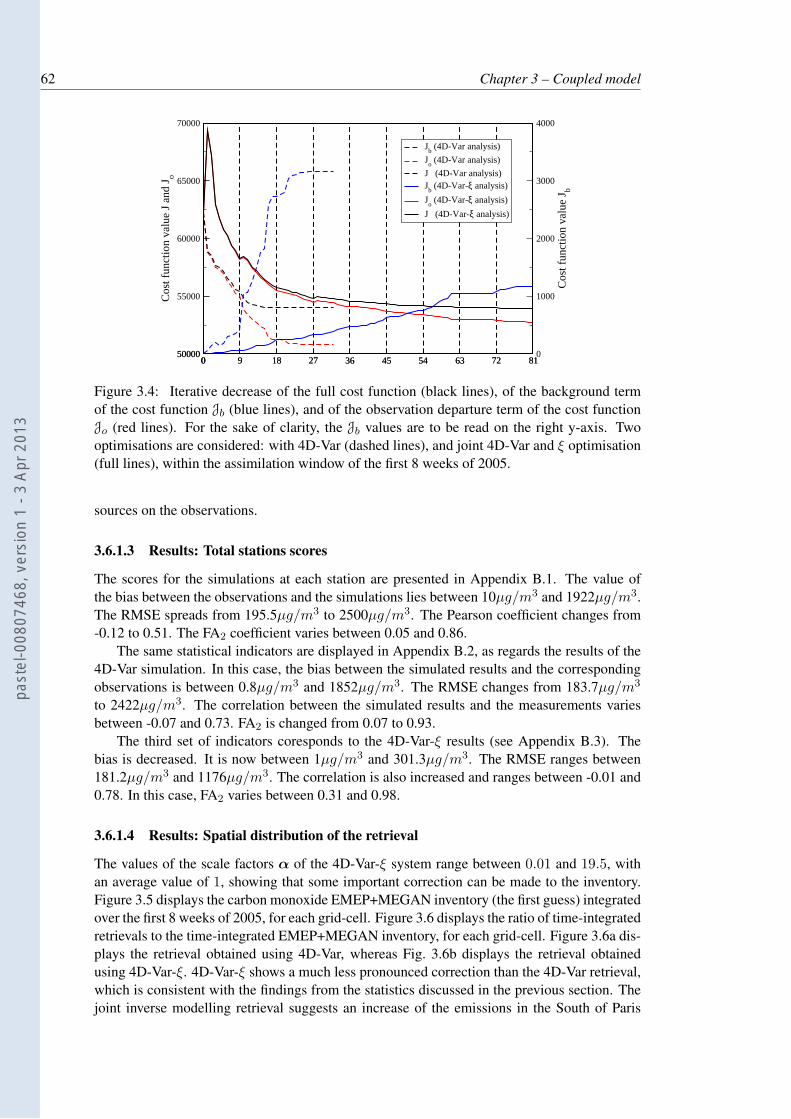
62 Chapter 3 – Coupled model
0 9 18 27 36 45 54 63 72 8150000
55000
60000
65000
70000
Cos
t fun
ctio
n va
lue
J an
d J
o
050000
Jb (4D-Var analysis)
Jo (4D-Var analysis)
J (4D-Var analysis)Jb (4D-Var-ξ analysis)
Jo (4D-Var-ξ analysis)
J (4D-Var-ξ analysis)
0 9 18 27 36 45 54 63 72 810
1000
2000
3000
4000
Cos
t fun
ctio
n va
lue
J b
Figure 3.4: Iterative decrease of the full cost function (black lines), of the background termof the cost function Jb (blue lines), and of the observation departure term of the cost functionJo (red lines). For the sake of clarity, the Jb values are to be read on the right y-axis. Twooptimisations are considered: with 4D-Var (dashed lines), and joint 4D-Var and ξ optimisation(full lines), within the assimilation window of the first 8 weeks of 2005.
sources on the observations.
3.6.1.3 Results: Total stations scores
The scores for the simulations at each station are presented in Appendix B.1. The value ofthe bias between the observations and the simulations lies between 10µg/m3 and 1922µg/m3.The RMSE spreads from 195.5µg/m3 to 2500µg/m3. The Pearson coefficient changes from-0.12 to 0.51. The FA2 coefficient varies between 0.05 and 0.86.
The same statistical indicators are displayed in Appendix B.2, as regards the results of the4D-Var simulation. In this case, the bias between the simulated results and the correspondingobservations is between 0.8µg/m3 and 1852µg/m3. The RMSE changes from 183.7µg/m3
to 2422µg/m3. The correlation between the simulated results and the measurements variesbetween -0.07 and 0.73. FA2 is changed from 0.07 to 0.93.
The third set of indicators coresponds to the 4D-Var-ξ results (see Appendix B.3). Thebias is decreased. It is now between 1µg/m3 and 301.3µg/m3. The RMSE ranges between181.2µg/m3 and 1176µg/m3. The correlation is also increased and ranges between -0.01 and0.78. In this case, FA2 varies between 0.31 and 0.98.
3.6.1.4 Results: Spatial distribution of the retrieval
The values of the scale factors α of the 4D-Var-ξ system range between 0.01 and 19.5, withan average value of 1, showing that some important correction can be made to the inventory.Figure 3.5 displays the carbon monoxide EMEP+MEGAN inventory (the first guess) integratedover the first 8 weeks of 2005, for each grid-cell. Figure 3.6 displays the ratio of time-integratedretrievals to the time-integrated EMEP+MEGAN inventory, for each grid-cell. Figure 3.6a dis-plays the retrieval obtained using 4D-Var, whereas Fig. 3.6b displays the retrieval obtainedusing 4D-Var-ξ. 4D-Var-ξ shows a much less pronounced correction than the 4D-Var retrieval,which is consistent with the findings from the statistics discussed in the previous section. Thejoint inverse modelling retrieval suggests an increase of the emissions in the South of Paris
past
el-0
0807
468,
ver
sion
1 -
3 Ap
r 201
3
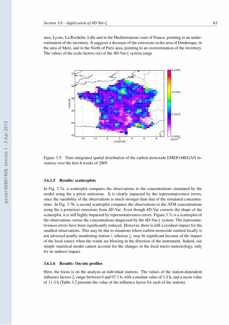
Section 3.6 – Application of 4D-Var-ξ 63
area, Lyons, La Rochelle, Lille and in the Mediterranean coast of France, pointing to an under-estimation of the inventory. It suggests a decrease of the emissions in the area of Dunkerque, inthe area of Metz, and in the North of Paris area, pointing to an overestimation of the inventory.The values of the scale factors (α) of the 4D-Var-ξ system range
4 2 0 2 4 6 8Longitude
42
44
46
48
50
52
Lati
tude
kg.km20.0001
0.0010
0.0100
0.1000
Figure 3.5: Time-integrated spatial distribution of the carbon monoxide EMEP+MEGAN in-ventory over the first 8 weeks of 2005.
3.6.1.5 Results: scatterplots
In Fig. 3.7a, a scatterplot compares the observations to the concentrations simulated by themodel using the a priori emissions. It is clearly impacted by the representativeness errors,since the variability of the observations is much stronger than that of the simulated concentra-tions. In Fig. 3.7b, a second scatterplot compares the observations to the ATM concentrationsusing the a posteriori emissions from 4D-Var. Even though 4D-Var corrects the shape of thescatterplot, it is still highly impacted by representativeness errors. Figure 3.7c is a scatterplot ofthe observations versus the concentrations diagnosed by the 4D-Var-ξ system. The representa-tiveness errors have been significantly reduced. However, there is still a residual impact for thesmallest observations. This may be due to situations where carbon monoxide emitted locally isnot advected nearby monitoring station i, whereas ξi may be significant because of the impactof the local source when the winds are blowing in the direction of the instrument. Indeed, oursimple statistical model cannot account for the changes in the local micro-meteorology, onlyfor its indirect impact.
3.6.1.6 Results: On-site profiles
Here, the focus is on the analysis at individual stations. The values of the station-dependentinfluence factors ξi range between 0 and 97.5 h, with a median value of 5.9 h, and a mean valueof 11.3 h (Table 3.2 presents the value of the influence factor for each of the station).
past
el-0
0807
468,
ver
sion
1 -
3 Ap
r 201
3
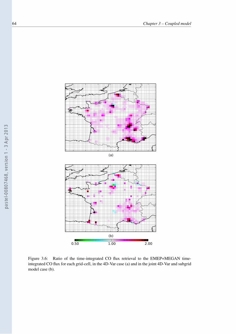
64 Chapter 3 – Coupled model
(a)
(b)
0.50 1.00 2.00
Figure 3.6: Ratio of the time-integrated CO flux retrieval to the EMEP+MEGAN time-integrated CO flux for each grid-cell, in the 4D-Var case (a) and in the joint 4D-Var and subgridmodel case (b).
past
el-0
0807
468,
ver
sion
1 -
3 Ap
r 201
3
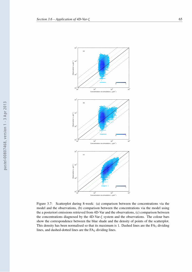
Section 3.6 – Application of 4D-Var-ξ 65
101
102
103
104
Concentration via simulation ( g/m3
)
101
102
103
104
Obse
rvati
on (
g/m3)
(a)
0 1
101
102
103
104
Concentration via simulation ( g/m3
)
101
102
103
104
Obse
rvati
on (
g/m3)
(b)
0 1
101
102
103
104
Concentration via simulation ( g/m3
)
101
102
103
104
Obse
rvati
on (
g/m3)
(c)
0 1
Figure 3.7: Scatterplot during 8-week: (a) comparison between the concentrations via themodel and the observations, (b) comparison between the concentrations via the model usingthe a posteriori emissions retrieved from 4D-Var and the observations, (c) comparison betweenthe concentrations diagnosed by the 4D-Var-ξ system and the observations. The colour barsshow the correspondence between the blue shade and the density of points of the scatterplot.This density has been normalised so that its maximum is 1. Dashed lines are the FA5 dividinglines, and dashed-dotted lines are the FA2 dividing lines.
past
el-0
0807
468,
ver
sion
1 -
3 Ap
r 201
3
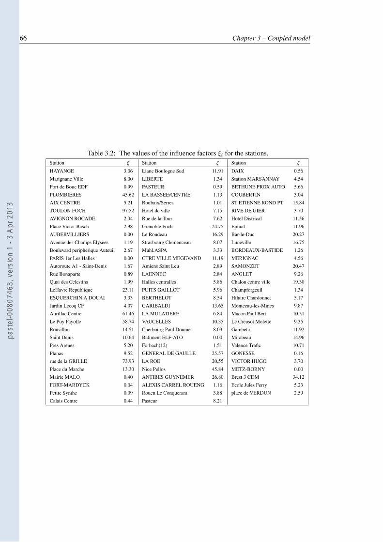
66 Chapter 3 – Coupled model
Table 3.2: The values of the influence factors ξi for the stations.Station ξ Station ξ Station ξ
HAYANGE 3.06 Liane Boulogne Sud 11.91 DAIX 0.56
Marignane Ville 8.00 LIBERTE 1.34 Station MARSANNAY 4.54
Port de Bouc EDF 0.99 PASTEUR 0.59 BETHUNE PROX AUTO 5.66
PLOMBIERES 45.62 LA BASSEE/CENTRE 1.13 COUBERTIN 3.04
AIX CENTRE 5.21 Roubaix/Serres 1.01 ST ETIENNE ROND PT 15.84
TOULON FOCH 97.52 Hotel de ville 7.15 RIVE DE GIER 3.70
AVIGNON ROCADE 2.34 Rue de la Tour 7.62 Hotel Districal 11.56
Place Victor Basch 2.98 Grenoble Foch 24.75 Epinal 11.96
AUBERVILLIERS 0.00 Le Rondeau 16.29 Bar-le-Duc 20.27
Avenue des Champs Elysees 1.19 Strasbourg Clemenceau 8.07 Luneville 16.75
Boulevard peripherique Auteuil 2.67 Muhl.ASPA 3.33 BORDEAUX-BASTIDE 1.26
PARIS 1er Les Halles 0.00 CTRE VILLE MEGEVAND 11.19 MERIGNAC 4.56
Autoroute A1 - Saint-Denis 1.67 Amiens Saint Leu 2.89 SAMONZET 20.47
Rue Bonaparte 0.89 LAENNEC 2.84 ANGLET 9.26
Quai des Celestins 1.99 Halles centralles 5.86 Chalon centre ville 19.30
LeHavre Republique 23.11 PUITS GAILLOT 5.96 Champforgeuil 1.34
ESQUERCHIN A DOUAI 3.33 BERTHELOT 8.54 Hilaire Chardonnet 5.17
Jardin Lecoq CF 4.07 GARIBALDI 13.65 Montceau-les-Mines 9.87
Aurillac Centre 61.46 LA MULATIERE 6.84 Macon Paul Bert 10.31
Le Puy Fayolle 58.74 VAUCELLES 10.35 Le Creusot Molette 9.35
Rousillon 14.51 Cherbourg Paul Doume 8.03 Gambeta 11.92
Saint Denis 10.64 Batiment ELF-ATO 0.00 Mirabeau 14.96
Pres Arenes 5.20 Forbach(12) 1.51 Valence Trafic 10.71
Planas 9.52 GENERAL DE GAULLE 25.57 GONESSE 0.16
rue de la GRILLE 73.93 LA ROE 20.55 VICTOR HUGO 3.70
Place du Marche 13.30 Nice Pellos 45.84 METZ-BORNY 0.00
Mairie MALO 0.40 ANTIBES GUYNEMER 26.80 Brest 3 CDM 34.12
FORT-MARDYCK 0.04 ALEXIS CARREL ROUENG 1.16 Ecole Jules Ferry 5.23
Petite Synthe 0.09 Rouen Le Conquerant 3.88 place de VERDUN 2.59
Calais Centre 0.44 Pasteur 8.21
past
el-0
0807
468,
ver
sion
1 -
3 Ap
r 201
3
Section 3.6 – Application of 4D-Var-ξ 67
In Fig. 3.8, four different time series of concentrations are displayed for four differentstations: the observations, the concentrations simulated with the a priori emissions, the con-centrations obtained from 4D-Var, and 4D-Var-ξ concentrations. The traffic station of LillePasteur, can be cited as an example of small influence factor value with ξi = 0.6 h. In thatstation, the simulation concentrations are in quite good agreement with the observations. Thecorrelation between the observations and the simulated concentrations reaches 0.49. It is 0.74for the 4D-Var-ξ results. At the station Paris, boulevard périphérique Auteuil (suburban), forwhich ξi is of 2.7 h, the correlation increases from 0.29 up to 0.77. Orléans Gambetta (trafficzone) station can be cited as an example with a moderate influence factor value of ξi = 11.9 h.At this station, the Pearson correlation coefficient increases from 0.11 to 0.67 when using the4D-Var-ξ system. The dependence of the observations and the local emissions is clearly shownin Fig. 3.8c. The model simulation gives a smooth curve, whereas the observations are highlyfluctuating. The 4D-Var system is able to anticipate the trend of the concentrations, but cannotpredict the peaks. Furthermore, it over-estimates the inventory by trying to adjust to the peaks.
Figure 3.8d shows the concentrations in Nice Pellos (urban station) with a high influencefactor value of ξ = 45.8 h. The results of 4D-Var-ξ are in good agreement with the observationswhereas neither the simulation, nor 4D-Var are able to match the observations. The correlationvalue is significantly increased from 0.32 to 0.68. It is also clear that although 4D-Var-ξ is ableto account for a substantial part of the peaks, it underestimates their maxima and overestimatesthe minima, which may be due to residual representativeness error.
3.6.1.7 Results: sensitivity to the background standard deviation
The whole inverse modelling study using a background standard deviation is performed for thecarbon monoxide of 100%, instead of 50%. The results are qualitatively unchanged. They arebarely quantitatively changed. For instance, one retrieves a total of 1.18 Tg instead of 1.16 Tgover the 8-week winter period. This relative insensitivity is mostly due to the use of the χ2
criterion.
3.6.2 Validation
A direct and reliable validation of a spatial emission inventory is currently out of reach for mostpollutants (see the in-depth discussion of Vestreng et al. [2007] about SO2). It is only possibleto compare with another independent estimation (top-down or bottom-up), which, as a relativecomparison approach, may not be as satisfying as a straight comparison to observations. Localflux measurements are possible (e.g. for CO2) in some media but these are sparse and cannotfully validate a spatial inventory. Therefore, a CO emission inventory can only be indirectlyvalidated. For instance one can compare the CO concentrations simulated with the inventoryto real measurements.
We shall first compare the total emitted carbon monoxide to an independent bottom-upinventory over France. We will then compare simulated concentrations obtained with an in-ventory retrieved from a training network, on a distinct validation network. Finally, after anassimilation period of 8 weeks, we shall make a 10-month CO concentration forecast. Theforecasted concentrations will be compared to independent observations (that have not beenassimilated).
past
el-0
0807
468,
ver
sion
1 -
3 Ap
r 201
3
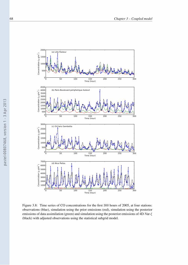
68 Chapter 3 – Coupled model
0 50 100 150 200 250 300Time (hour)
0
500
1000
1500
2000
Conce
ntr
ati
on (
g/m3) (a) Lille Pasteur
0 50 100 150 200 250 300Time (hour)
0
500
1000
1500
2000
2500
3000
3500
4000
4500
Conce
ntr
ati
on (
g/m3) (b) Paris Boulevard p
riphrique Auteuil
0 50 100 150 200 250 300Time (hour)
0
500
1000
1500
2000
2500
3000
Conce
ntr
ati
on (
g/m3) (c) Orl
ans Gambetta
0 50 100 150 200 250 300Time (hour)
0
1000
2000
3000
4000
5000
6000
7000
Conce
ntr
ati
on (
g/m3) (d) Nice Pellos
Figure 3.8: Time series of CO concentrations for the first 300 hours of 2005, at four stations:observations (blue), simulation using the prior emissions (red), simulation using the posterioremissions of data assimilation (green) and simulation using the posterior emissions of 4D-Var-ξ(black) with adjusted observations using the statistical subgrid model.
past
el-0
0807
468,
ver
sion
1 -
3 Ap
r 201
3
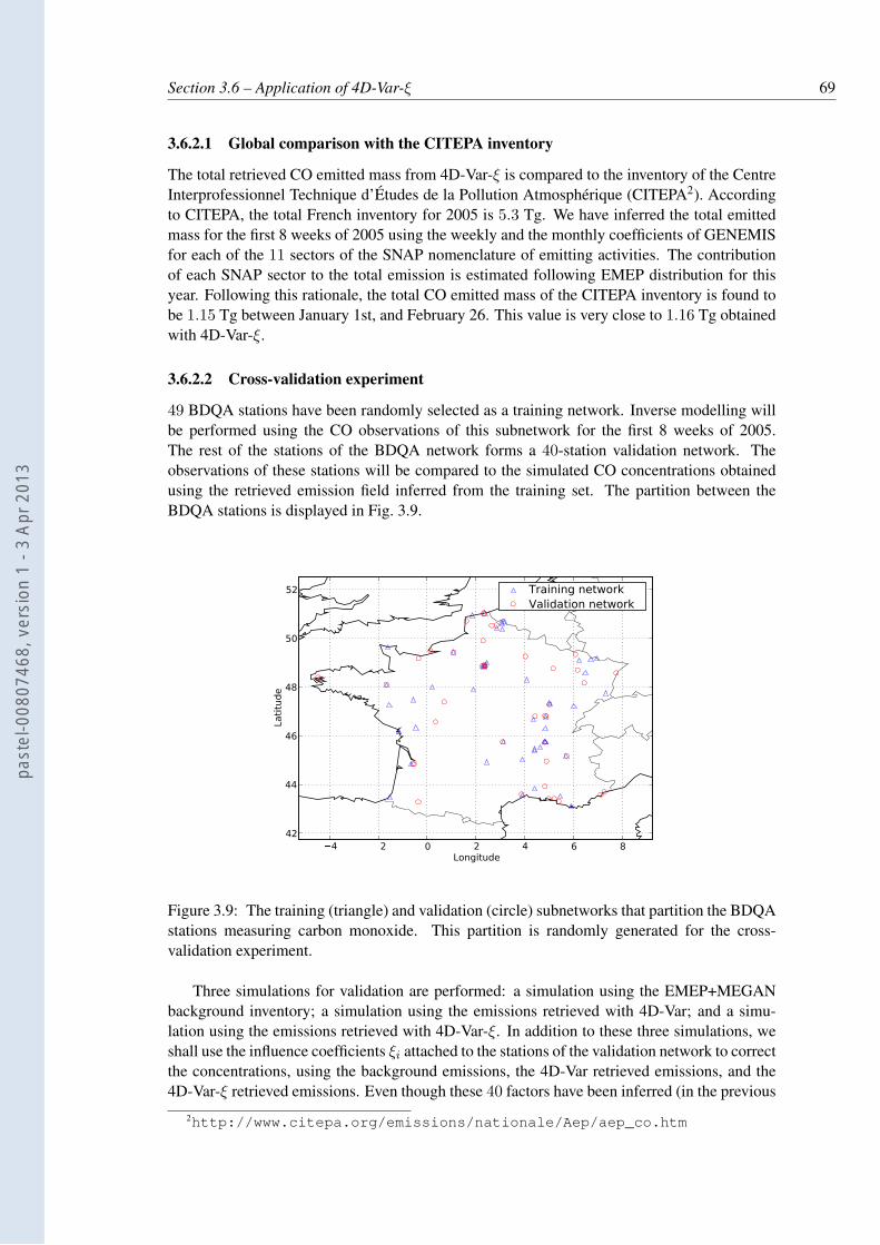
Section 3.6 – Application of 4D-Var-ξ 69
3.6.2.1 Global comparison with the CITEPA inventory
The total retrieved CO emitted mass from 4D-Var-ξ is compared to the inventory of the CentreInterprofessionnel Technique d’Études de la Pollution Atmosphérique (CITEPA2). Accordingto CITEPA, the total French inventory for 2005 is 5.3 Tg. We have inferred the total emittedmass for the first 8 weeks of 2005 using the weekly and the monthly coefficients of GENEMISfor each of the 11 sectors of the SNAP nomenclature of emitting activities. The contributionof each SNAP sector to the total emission is estimated following EMEP distribution for thisyear. Following this rationale, the total CO emitted mass of the CITEPA inventory is found tobe 1.15 Tg between January 1st, and February 26. This value is very close to 1.16 Tg obtainedwith 4D-Var-ξ.
3.6.2.2 Cross-validation experiment
49 BDQA stations have been randomly selected as a training network. Inverse modelling willbe performed using the CO observations of this subnetwork for the first 8 weeks of 2005.The rest of the stations of the BDQA network forms a 40-station validation network. Theobservations of these stations will be compared to the simulated CO concentrations obtainedusing the retrieved emission field inferred from the training set. The partition between theBDQA stations is displayed in Fig. 3.9.
4 2 0 2 4 6 8Longitude
42
44
46
48
50
52
Lati
tude
Training networkValidation network
Figure 3.9: The training (triangle) and validation (circle) subnetworks that partition the BDQAstations measuring carbon monoxide. This partition is randomly generated for the cross-validation experiment.
Three simulations for validation are performed: a simulation using the EMEP+MEGANbackground inventory; a simulation using the emissions retrieved with 4D-Var; and a simu-lation using the emissions retrieved with 4D-Var-ξ. In addition to these three simulations, weshall use the influence coefficients ξi attached to the stations of the validation network to correctthe concentrations, using the background emissions, the 4D-Var retrieved emissions, and the4D-Var-ξ retrieved emissions. Even though these 40 factors have been inferred (in the previous
2http://www.citepa.org/emissions/nationale/Aep/aep_co.htm
past
el-0
0807
468,
ver
sion
1 -
3 Ap
r 201
3
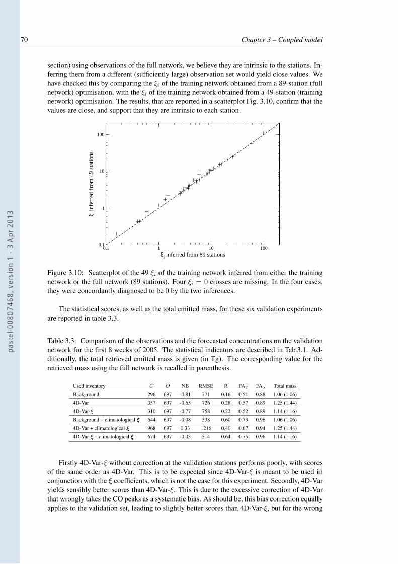
70 Chapter 3 – Coupled model
section) using observations of the full network, we believe they are intrinsic to the stations. In-ferring them from a different (sufficiently large) observation set would yield close values. Wehave checked this by comparing the ξi of the training network obtained from a 89-station (fullnetwork) optimisation, with the ξi of the training network obtained from a 49-station (trainingnetwork) optimisation. The results, that are reported in a scatterplot Fig. 3.10, confirm that thevalues are close, and support that they are intrinsic to each station.
0.1 1 10 100ξ
i inferred from 89 stations
0.1
1
10
100
ξ i infe
rred
from
49
stat
ions
Figure 3.10: Scatterplot of the 49 ξi of the training network inferred from either the trainingnetwork or the full network (89 stations). Four ξi = 0 crosses are missing. In the four cases,they were concordantly diagnosed to be 0 by the two inferences.
The statistical scores, as well as the total emitted mass, for these six validation experimentsare reported in table 3.3.
Table 3.3: Comparison of the observations and the forecasted concentrations on the validationnetwork for the first 8 weeks of 2005. The statistical indicators are described in Tab.3.1. Ad-ditionally, the total retrieved emitted mass is given (in Tg). The corresponding value for theretrieved mass using the full network is recalled in parenthesis.
Used inventory C O NB RMSE R FA2 FA5 Total mass
Background 296 697 -0.81 771 0.16 0.51 0.88 1.06 (1.06)
4D-Var 357 697 -0.65 726 0.28 0.57 0.89 1.25 (1.44)
4D-Var-ξ 310 697 -0.77 758 0.22 0.52 0.89 1.14 (1.16)
Background + climatological ξ 644 697 -0.08 538 0.60 0.73 0.96 1.06 (1.06)
4D-Var + climatological ξ 968 697 0.33 1216 0.40 0.67 0.94 1.25 (1.44)
4D-Var-ξ + climatological ξ 674 697 -0.03 514 0.64 0.75 0.96 1.14 (1.16)
Firstly 4D-Var-ξ without correction at the validation stations performs poorly, with scoresof the same order as 4D-Var. This is to be expected since 4D-Var-ξ is meant to be used inconjunction with the ξ coefficients, which is not the case for this experiment. Secondly, 4D-Varyields sensibly better scores than 4D-Var-ξ. This is due to the excessive correction of 4D-Varthat wrongly takes the CO peaks as a systematic bias. As should be, this bias correction equallyapplies to the validation set, leading to slightly better scores than 4D-Var-ξ, but for the wrong
past
el-0
0807
468,
ver
sion
1 -
3 Ap
r 201
3
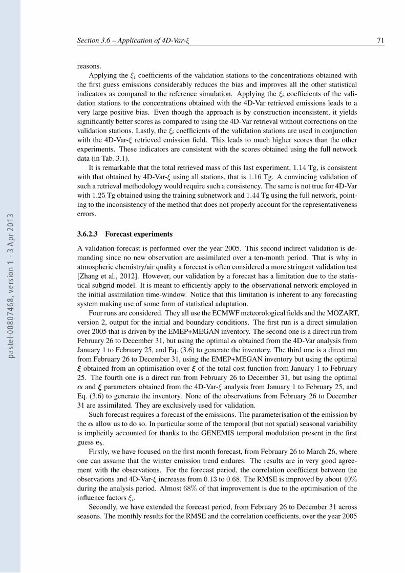
Section 3.6 – Application of 4D-Var-ξ 71
reasons.Applying the ξi coefficients of the validation stations to the concentrations obtained with
the first guess emissions considerably reduces the bias and improves all the other statisticalindicators as compared to the reference simulation. Applying the ξi coefficients of the vali-dation stations to the concentrations obtained with the 4D-Var retrieved emissions leads to avery large positive bias. Even though the approach is by construction inconsistent, it yieldssignificantly better scores as compared to using the 4D-Var retrieval without corrections on thevalidation stations. Lastly, the ξi coefficients of the validation stations are used in conjunctionwith the 4D-Var-ξ retrieved emission field. This leads to much higher scores than the otherexperiments. These indicators are consistent with the scores obtained using the full networkdata (in Tab. 3.1).
It is remarkable that the total retrieved mass of this last experiment, 1.14 Tg, is consistentwith that obtained by 4D-Var-ξ using all stations, that is 1.16 Tg. A convincing validation ofsuch a retrieval methodology would require such a consistency. The same is not true for 4D-Varwith 1.25 Tg obtained using the training subnetwork and 1.44 Tg using the full network, point-ing to the inconsistency of the method that does not properly account for the representativenesserrors.
3.6.2.3 Forecast experiments
A validation forecast is performed over the year 2005. This second indirect validation is de-manding since no new observation are assimilated over a ten-month period. That is why inatmospheric chemistry/air quality a forecast is often considered a more stringent validation test[Zhang et al., 2012]. However, our validation by a forecast has a limitation due to the statis-tical subgrid model. It is meant to efficiently apply to the observational network employed inthe initial assimilation time-window. Notice that this limitation is inherent to any forecastingsystem making use of some form of statistical adaptation.
Four runs are considered. They all use the ECMWF meteorological fields and the MOZART,version 2, output for the initial and boundary conditions. The first run is a direct simulationover 2005 that is driven by the EMEP+MEGAN inventory. The second one is a direct run fromFebruary 26 to December 31, but using the optimal α obtained from the 4D-Var analysis fromJanuary 1 to February 25, and Eq. (3.6) to generate the inventory. The third one is a direct runfrom February 26 to December 31, using the EMEP+MEGAN inventory but using the optimalξ obtained from an optimisation over ξ of the total cost function from January 1 to February25. The fourth one is a direct run from February 26 to December 31, but using the optimalα and ξ parameters obtained from the 4D-Var-ξ analysis from January 1 to February 25, andEq. (3.6) to generate the inventory. None of the observations from February 26 to December31 are assimilated. They are exclusively used for validation.
Such forecast requires a forecast of the emissions. The parameterisation of the emission bythe α allow us to do so. In particular some of the temporal (but not spatial) seasonal variabilityis implicitly accounted for thanks to the GENEMIS temporal modulation present in the firstguess eb.
Firstly, we have focused on the first month forecast, from February 26 to March 26, whereone can assume that the winter emission trend endures. The results are in very good agree-ment with the observations. For the forecast period, the correlation coefficient between theobservations and 4D-Var-ξ increases from 0.13 to 0.68. The RMSE is improved by about 40%during the analysis period. Almost 68% of that improvement is due to the optimisation of theinfluence factors ξi.
Secondly, we have extended the forecast period, from February 26 to December 31 acrossseasons. The monthly results for the RMSE and the correlation coefficients, over the year 2005
past
el-0
0807
468,
ver
sion
1 -
3 Ap
r 201
3
72 Chapter 3 – Coupled model
are presented in Fig. 3.11. Using 4D-Var-ξ, the RMSE decreases decreases by 282 µg m−3
within the analysis period, January 1 to February 26 (left side of the vertical dashed line). Itdecreases by 172 µg m−3 during the forecast period, from February 26 to December 31 (rightside of the vertical dashed line). The improvement is remarkably persistent during the whole10-month forecast period. It shows that choosing α and ξ as control vectors has a good prog-nostic value. In spring and summer, the RMSE decreases for all four experiments. This canbe due to the decrease of urban heating during that period which is accounted for in the cyclesof the inventory but which reduces a source of uncertainty. It can also be seen that the RMSEgain in the spring and summer is essentially due to the subgrid model identification, and notthe emission estimation, since 4D-Var-ξ and the optimal-ξ forecast yield the same RMSE. Un-surprisingly, this means that the emission retrieval carried out over two winter months are notoptimal for the spring and summer months. Another possible explanation is the emergence ofnew source of errors in the spring-summer time, such as the higher OH concentration that leadsto a higher reactivity of CO, or a stronger turbulent mixing in the boundary layer. However,this should be balanced by a persistent gain in the spring-summer period of the correlation dueto the emission retrieval.
3.7 Conclusion
In this article, a 4D-Var data assimilation system was developed to estimate carbon monoxidefluxes at regional scale. An approximate adjoint of the POLAIR3D model has been built andvalidated for this 4D-Var system. A study over France, at a resolution of 0.25 × 0.25 isconducted. We used the in-situ observations of the BDQA database that includes the observa-tions from industrial, traffic, urban and suburban stations. They are strongly impacted by localsources that the stations are meant to monitor. Hence, although the number of observationsis very significant, their information load is impacted by large representativeness errors. ThePearson correlation coefficient between the simulated concentrations and the observations iscomputed to be 0.16. A first 4D-Var inversion of the CO fluxes leads to a mild improvementof the skill. The Pearson correlation climbs to 0.36. However looking at stations profile, it isclear that the representativeness errors are not accounted for, since the analysis from 4D-Varcannot reproduce the intense CO peaks. Besides, it leads to an artificially large increase of theretrieved emissions.
Therefore, a simple model is developed to statistically represent the subgrid effects ofnearby sources. A coefficient attached to each station is used to estimate this influence. The4D-Var system is coupled to this subgrid model and the fluxes are determined altogether withthe influence coefficients. The correlation coefficient reaches 0.73, while the bias betweenthe observations and the analysed concentrations is considerably reduced. The net increaseof the CO inventory is estimated to be 9%, consistent with other top-down approaches usingsatellite data. Cross-validation experiments using a training subnetwork and a validation sub-network demonstrates the consistency of the inventory estimation, whereas, in this context, thetraditional 4D-Var does not deliver consistent estimations with different training subnetworks.Forecast experiments with the analysed coefficients and fluxes over 10 months, after an as-similation window of 8 weeks, show remarkably persistent scores throughout the year. Thisemphasises the relevance of the choice of ξ and α as joint control parameter vectors of the4D-Var-ξ analysis.
We believe that this methodology and experiment show that, in this context, it is possible toextract relevant information from observations strongly impacted by representativeness errors.One limitation which is inherent to the statistical adaptation component of the system is that itis meant to be used on a given monitoring network. A validation forecast can safely be made
past
el-0
0807
468,
ver
sion
1 -
3 Ap
r 201
3
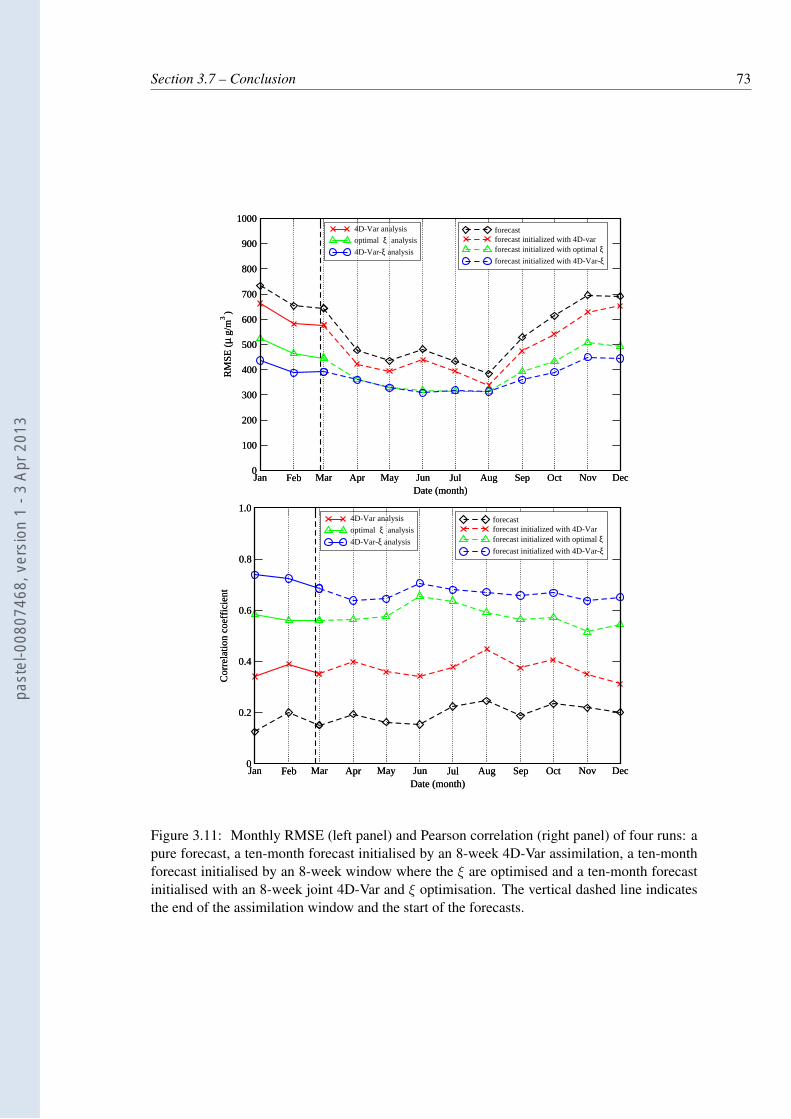
Section 3.7 – Conclusion 73
Jan Feb Mar Apr May Jun Jul Aug Sep Oct Nov DecDate (month)
0
100
200
300
400
500
600
700
800
900
1000R
MS
E (µ
g/m
3 )
4D-Var analysis
optimal ξ analysis
4D-Var-ξ analysis
Jan Feb Mar Apr May Jun Jul Aug Sep Oct Nov DecDate (month)
0
100
200
300
400
500
600
700
800
900
1000R
MS
E (µ
g/m
3 )
forecastforecast initialized with 4D-varforecast initialized with optimal ξforecast initialized with 4D-Var-ξ
Jan Feb Mar Apr May Jun Jul Aug Sep Oct Nov DecDate (month)
0
0.2
0.4
0.6
0.8
1.0
Cor
rela
tion
coef
ficie
nt
4D-Var analysis
optimal ξ analysis
4D-Var-ξ analysis
Jan Feb Mar Apr May Jun Jul Aug Sep Oct Nov DecDate (month)
0
0.2
0.4
0.6
0.8
1.0
Cor
rela
tion
coef
ficie
nt
forecastforecast initialized with 4D-Varforecast initialized with optimal ξforecast initialized with 4D-Var-ξ
Figure 3.11: Monthly RMSE (left panel) and Pearson correlation (right panel) of four runs: apure forecast, a ten-month forecast initialised by an 8-week 4D-Var assimilation, a ten-monthforecast initialised by an 8-week window where the ξ are optimised and a ten-month forecastinitialised with an 8-week joint 4D-Var and ξ optimisation. The vertical dashed line indicatesthe end of the assimilation window and the start of the forecasts.
past
el-0
0807
468,
ver
sion
1 -
3 Ap
r 201
3

74 Chapter 3 – Coupled model
to additional stations, but statistical adaptation cannot be performed to these stations, if therelated influence factor ξi were not previously estimated.
To improve the present statistical subgrid model, which uses the influence factors to esti-mate the immediate impact of the emissions on the observations, a more comprehensive sta-tistical subgrid model could be used. For instance, that model could include the effects of thewind direction, deposition parameters, etc, that are used or diagnosed in the coarse resolutionmodel. Computationally, it would not be as cheap as the subgrid model used here.
Beyond the carbon monoxide context of this study, it is believed that the integration of thesimple statistical subgrid scale into a 4D-Var can be generalised to pollutants whose observa-tions could highly be impacted by representativeness errors.
past
el-0
0807
468,
ver
sion
1 -
3 Ap
r 201
3
Chapter 4
Potential of the International
Monitoring System radionuclide
network for inverse modelling
Summary
The International Monitoring System (IMS) radionuclide network enforces the ComprehensiveNuclear-Test-Ban Treaty which bans nuclear explosions. We have evaluated the potential of theIMS radionuclide network for inverse modelling of the source, whereas it is usually assessed byits detection capability. To do so, we have chosen the degrees of freedom for the signal (DFS),a well established criterion in remote sensing, in order to assess the performance of an inversemodelling system. Using a recent multiscale data assimilation technique, we have computedoptimal adaptive grids of the source parameter space by maximising the DFS. This optimisa-tion takes into account the monitoring network, the meteorology over one year (2009) and therelationship between the source parameters and the observations derived from the FLEXPARTLagrangian transport model. Areas of the domain where the grid-cells of the optimal adaptivegrid are large emphasise zones where the retrieval is more uncertain, whereas areas where thegrid-cells are smaller and denser stress regions where more source variables can be resolved.
The observability of the globe through inverse modelling is studied in strong, realistic andsmall model error cases. The strong error and realistic error cases yield heterogeneous adaptivegrids, indicating that information does not propagate far from the monitoring stations, whereasin the small error case, the grid is much more homogeneous. In all cases, several specificcontinental regions remain poorly observed such as Africa as well as the tropics, because ofthe trade winds. The northern hemisphere is better observed through inverse modelling (morethan 60% of the total DFS) mostly because it contains more IMS stations. This unbalanceleads to a better performance of inverse modelling in the northern hemisphere winter. Themethodology is also applied to the subnetwork composed of the stations of the IMS networkwhich measure noble gases.
past
el-0
0807
468,
ver
sion
1 -
3 Ap
r 201
3
76 Chapter 4 – CTBTO
Contents
4.1 Introduction . . . . . . . . . . . . . . . . . . . . . . . . . . . . . . . . . 76
4.1.1 The IMS network and the CTBT enforcement . . . . . . . . . . . . 76
4.1.2 Inverse modelling of tracers . . . . . . . . . . . . . . . . . . . . . 77
4.1.3 Objectives and outline . . . . . . . . . . . . . . . . . . . . . . . . 78
4.2 Methodology of data assimilation . . . . . . . . . . . . . . . . . . . . . . 78
4.2.1 Inverse modelling with Gaussian statistical assumptions . . . . . . 78
4.2.2 Information content and DFS . . . . . . . . . . . . . . . . . . . . . 80
4.2.3 Multiscale data assimilation . . . . . . . . . . . . . . . . . . . . . 81
4.3 Application to the IMS radionuclide network . . . . . . . . . . . . . . . 83
4.3.1 Setup . . . . . . . . . . . . . . . . . . . . . . . . . . . . . . . . . 83
4.3.2 Daily-averaged criteria . . . . . . . . . . . . . . . . . . . . . . . . 83
4.3.3 Dependence of the DFS in the number of grid-cells . . . . . . . . . 84
4.3.4 Interpretation of optimal grids . . . . . . . . . . . . . . . . . . . . 86
4.3.5 Distribution of the DFS over hemispheres and seasons . . . . . . . 87
4.3.6 Implication on the design of the network . . . . . . . . . . . . . . 88
4.3.7 Noble gas network . . . . . . . . . . . . . . . . . . . . . . . . . . 88
4.3.8 Eulerian and Lagrangian models . . . . . . . . . . . . . . . . . . . 89
4.4 Conclusion . . . . . . . . . . . . . . . . . . . . . . . . . . . . . . . . . . 91
4.1 Introduction
4.1.1 The IMS network and the CTBT enforcement
The Comprehensive Nuclear-Test-Ban Treaty (CTBT) signed by 182 states bans nuclear ex-plosions [United Nations, 1996]. The monitoring of the treaty is implemented by the UnitedNations CTBT Organisation (CTBTO), based in Vienna, Austria. It operates an InternationalMonitoring System (IMS) and collects seismic, infrasound, hydroacoustic data as well as ra-dionuclide (particulate matter and noble gases) activity concentrations. This article focuses onthe latter. Upon completion of the installation, the radionuclide IMS network will have 80 sta-tions. As of June 2011, 60 stations are certified and operational. The instruments are radionu-clide gamma detectors coupled to particle filters. They allow to deliver 24 hour-averaged activ-ity concentrations for several particulate/aerosol species: caesium-137, caesium-134, iodine-131 (aerosol form), etc. In the long term, 40 of those stations will also be able to measure noblegases (xenon-131m, xenon-133, xenon-133m, xenon-135), among which 24 are operating asof June 2011.
The locations of 79 (among 80) stations are detailed in the treaty, even though the actual lo-cations could slightly differ (see http://www.ctbto.org/map). The design of the networkhas been validated using dispersion modelling. For instance, using a global atmospheric trans-port model (ATM), one can compute the ability of the monitoring network to detect a releasestemming from any location on Earth [Ringbom and Miley, 2009]. Recently, the radionuclideIMS network has measured the Fukushima Dai-ichi plume throughout the world, although onlypart of the observations has been disclosed.
past
el-0
0807
468,
ver
sion
1 -
3 Ap
r 201
3
Section 4.1 – Introduction 77
The observations of the IMS network can be used to detect a nuclear tests, and to discrim-inate nuclear test among underground explosions. They could also help to characterise a test(location, signature and intensity) using inverse modelling techniques. The objective of this ar-ticle is to determine the potential of the IMS radionuclide network for inverse modelling of thesource term, using rigorous mathematical tools in conjunction with global or regional ATMs.
4.1.2 Inverse modelling of tracers
The application of inverse modelling techniques to the reconstruction of the source term is re-cent in atmospheric dispersion. The European Tracer Experiment (ETEX, Nodop et al. [1998]),initially triggered by the Chernobyl accident, served as a playground to test inverse methodolo-gies [Robertson and Langner, 1998; Pudykiewicz, 1998; Seibert and Stohl, 2000; Issartel andBaverel, 2003; Bocquet, 2005a, b]. Full reconstructions using real data with results close to theknown characteristics of the source have been obtained [Bocquet, 2007; Krysta et al., 2008].These authors used methodologies inspired by geophysical data assimilation techniques: thefield to retrieve is discretised into a spatially organised large set of source variables/parameters.Alternatively, the so-called parametric methods rely on the optimisation of a restricted set ofvariables that parametrise the source term. In the specific case of accidental dispersion, thelat-lon coordinates and the emission rate parametrise the source [Delle Monache et al., 2008;Yee et al., 2008].
As far as real radionuclide dispersion events are concerned, these methodologies have beentested on the Algeciras dispersion event [Krysta and Bocquet, 2007; Delle Monache et al.,2008], with about hundred caesium-137 integrated activity concentration measurements. Theresults are satisfying but mostly because of the very simple shape of the source (a single peak).The inverse modelling approach was also applied to the atmospheric source term of Cher-nobyl (caesium-137, caesium-134, and iodine-131) by Davoine and Bocquet [2007]; Bocquet[2012] with an estimation of the source terms consistent with the official UNSCEAR source term[United Nations, 2000]. Reconstruction of the source term was also performed for a North Ko-rea nuclear test measured by the IMS radionuclide network [Becker et al., 2010], although thereconstruction was not strictly based on inverse modelling.
In this context, the inverse modelling approach remains a difficult one, because:
• the observations are ground-based and local. Activity concentration measurements aresparse, infrequent or integrated, as opposed to gamma dose measurements. Moreover,point-wise observations may lead to representativeness errors, depending on whether thedispersion model is Eulerian or Lagrangian.
• The dispersion models remain imprecise. They are driven by meteorological fields of in-creasing precision and reliability at a given resolution, but the planetary boundary layerremains difficult to model, and the vertical turbulent diffusion is still uncertain. With onlya few documented field experiments, the microphysical properties of the radionuclides inthe atmosphere, are still difficult to grasp. Therefore the physical parametrisations imple-mented in the ATMs (dry deposition, wet scavenging, aerosol modelling, granulometryof particles) remain gross.
Beyond its own interest, inverse modelling of the source term is also the sine qua noncondition for a proper forecasting of the resulting plume, as was illustrated by Politis andRobertson [2004]; Bocquet [2007]; Abida and Bocquet [2009].
past
el-0
0807
468,
ver
sion
1 -
3 Ap
r 201
3
78 Chapter 4 – CTBTO
4.1.3 Objectives and outline
Detectability has been used to assess the performance of the IMS radionuclide network [Hour-din and Issartel, 2000; Wotawa et al., 2003; Ringbom and Miley, 2009]. A more complexcriterion is a measure of the ability to interpolate activity concentrations in between the sta-tions of the network, using geostatistical techniques (Wu and Bocquet [2011] and referencestherein). It has been used to assess and even design a radionuclide monitoring network [Abidaet al., 2008]. One step further in complexity, our goal is to evaluate the potential of the IMS ra-dionuclide network for inverse modelling, using an objective quantitative criterion: the degreesof freedom for the signal.
In Section 4.2, we define the typical inverse modelling experiment that could serve theCTBT enforcement. The average quality of an inversion is rigorously defined by the the de-grees of freedom for the signal. We do not focus on the particular results of specific inversemodelling experiments. This was done for instance by Winiarek et al. [2011] in the samecontext. Instead, we focus on the average ability of inverse modelling to extract informationfrom the measurements. A multiscale formalism is used to rigorously diagnose how the in-formation contained in the observations should optimally be spread in regions of the world.In Section 4.3, the formalism is applied to the IMS radionuclide network using all influencefunctions of year 2009 computed by the CTBTO. Adaptive grids that maximise the degrees offreedom for the signal are computed. By construction, they are optimal for the assimilation ofobservations. For a given number of grid-cells, they are numerically more efficient, and bearless aggregation errors than regular grids with the same number of grid-cells. They rigorouslydetermine the ability of the monitoring network to resolve source variables through data assim-ilation. Consequently, they allow to pinpoint well observed (from inverse modelling) as well aspoorly observed regions of the world. They have indirect implications on the way to optimisethe design of the network. The technique is also applied to the subnetwork of the stations thatmonitor noble gases. The difference between an Eulerian and a Lagrangian model in the designof those adaptive grids is examined, using a specific region of the globe. Conclusions are givenin Section 5.5.
4.2 Methodology of data assimilation
4.2.1 Inverse modelling with Gaussian statistical assumptions
The source parameters are the unknown variables. Each one of them is attached to a grid-cellin a domain Ω, and to a time interval. At first, Ω will be the globe. At the end of Section 4.3,Ω will be a limited area of the globe. We assume that the domain Ω is discretised. We shalluse unprojected (lat-lon) coordinates in the following, with Nx meridians and Ny −1 parallels.The source vector σ is defined on this grid. It has an extension in time of Nt time-steps, so thatσ is a vector of dimension NxNyNt. The radionuclide plume is observed by the monitoringnetwork. The observations yield a measurement vector µ in R
d.The physics of dispersion is assumed linear. This is the case for most transport and physical
processes: advection, diffusion, radioactive decay, dry deposition, and wet scavenging. Thisassumption is true for noble gases or particulate matter, but could be breached for aged parcelsof radionuclides which can lead to the formation of aerosols, whose modelling implies complexnonlinear equations.
With this assumption of linearity, and in the absence of boundary conditions, or using cleanair boundary conditions which are suitable for accidental release, a source-receptor relationshipbetween the observation vector µ and the source σ is established. It is formalised by the
past
el-0
0807
468,
ver
sion
1 -
3 Ap
r 201
3

Section 4.2 – Methodology of data assimilation 79
Jacobian matrix H
µ = Hσ + ǫ , (4.1)
where the vector ǫ represents errors of all kinds: instrumental error, representativeness error,and model errors.
The simplest approach for non-parametric inverse modelling is to minimise the discrepancy
L(σ) =1
2(µ − Hσ)T R−1 (µ − Hσ) , (4.2)
where R = E[ǫǫT]
is the observation error covariance matrix, which, in this ground obser-vation context, is almost always assumed diagonal, even though transport model errors couldinduce some cross-correlations. Following the Bayesian paradigm of geophysical data assim-ilation, a background term (also called regularisation term in this inverse modelling context)should be added to the cost function Eq. (4.2). This term is obviously unavoidable when thenumber of variables to retrieve is greater than the number of observations. However, even witha larger set of observations, a regularisation may be needed because of the errors that impov-erish the information content of the observations, and because of the lack of observability ofsome regions of the source space. It is often said that these inverse problems are ill-posed.
It was shown in Winiarek et al. [2011], that even when the location of the source is wellknown (anticipated in the case of Fukushima Dai-ichi, or with delay in the case of the Cher-nobyl) so that only a temporal rate profile should be retrieved, and even when the observationsare abundant, a background term is still necessary in a significant fraction of the cases. In thecase of Chernobyl, where the location is supposed to be known in re-analysis, Bocquet [2012]has demonstrated that a problem without a properly defined background but with much moreobservations than source parameters can lead to aberrant total retrieved activity for the sourceterm.
Therefore, it is often safer to use the objective function with a regularisation term:
L(σ) =1
2(µ − Hσ)T R−1 (µ − Hσ)
+1
2(σ − σb)
TB−1 (σ − σb) , (4.3)
where σb is the first guess (or background), an estimation of the source before the observationsare assimilated, and B is the background error covariance matrix. In the context of an acciden-tal release, it is reasonable to assume σb = 0 for the accidental source, since so little is knownabout it. In the case of noble gases, there could be significant diffuse natural (radon) or anthro-pogenic (xenon) emissions, that would have to be taken into account through an offset termin Eq. (4.1), or incorporated into the inverse modelling scheme. In that latter case, a non-zerodiffuse background σb would be defined from their emission inventories.
Matrix B is a rather well studied object in meteorological and oceanographical data assim-ilation, even though its modelling is complex. In our context, B is very poorly known, since itis meant to measure our ignorance on the source term before the accident or the nuclear test,which is difficult to quantify. The B matrix related to noble gas with an estimated backgroundwhich measures the errors in the inventory, may be better known. In the following, we arenot considering such non-trivial background, and we will focus on the accidental release part.However the formalism used in this article can cope with more complex situations.
A posteriori parameter estimation techniques, such as L-curve, maximum-likelihood, gen-eralised cross-validation [Vogel, 2002; Hansen, 2010], can efficiently help to assess the back-ground term in an accidental context [Davoine and Bocquet, 2007; Krysta et al., 2008; Saideet al., 2011], where a single realisation of the set of observations is available (as opposed to
past
el-0
0807
468,
ver
sion
1 -
3 Ap
r 201
3
80 Chapter 4 – CTBTO
routine pollution). However it should be clear that the errors represented by R and B are verydifficult to assess in this context.
In the absence of any constraint such as the positivity of σ, the best linear unbiased esti-mator of the source is given by the argument of the minimum of Eq. (4.3)
σa = σb + BHT(R + HBHT
)−1(µ − Hσb) . (4.4)
The uncertainty of this estimator is given by the analysis error covariance matrix
Pa =(B−1 + HTR−1H
)−1. (4.5)
which is obtained as the inverse matrix of the Hessian of Eq. (4.3), which represents the preci-sion matrix of the estimator. It is often equivalently rewritten as
Pa = B − BHT(R + HBHT
)−1HB , (4.6)
which is to be used later.More advanced methodologies that are able to handle the non-Gaussianity of errors, can
lead to more sophisticated estimators of the a posteriori errors (see Bocquet et al. [2010] andreferences therein). However, second-order moments of the error distribution still provide anapproximation of the posterior error statistics. In this case, Pa is approximately obtained asthe inverse of the Hessian of the cost function,
4.2.2 Information content and DFS
After the analysis, a scalar residual posterior uncertainty is given by Tr(Pa). The reduction ofuncertainty in the data assimilation process can be measured by a related quantity: Tr(IN −PaB
−1), which identifies with the degrees of freedom for the signal, abbreviated DFS in thefollowing [Rodgers, 2000]. The DFS are often used in the inversion of satelite-based instrumentradiances. In our context, it measures the fractional number of observations that are effectivelyused in the inversion to retrieve the source. Explicitly, one has
JDFS = Tr(IN − PaB
−1)
= Tr(BHT
(R + HBHT
)−1H)
. (4.7)
It is always lower or equal to the total number of observations d: 0 ≤ JDFS ≤ d.As explained earlier, it is difficult to specify R and B, especially in the retrieval of sources
in atmospheric dispersion. Besides these matrices are context-dependent. In the absence ofsignificant correlations in-between observation errors, and in-between background errors, theycan be both chosen proportional to the identity matrix: R = χ2Id and B = m2IN . Yet, χand especially m still need to be estimated. However, in this article, we are not interested inthe precise values of χ and m. We are more interested in the degrees of freedom for the signalavailable for the inversion. They depend on the ratio χ/m as can be checked on Eq. (4.7). Tosome extent, reasoning in terms of DFS circumvents the necessity to reason on R and B.
Using the results of inverse modelling of actual dispersion problems: ETEX, Chernobyl,Algeciras, or from the results of carbon dioxide inverse modelling [Krysta and Bocquet, 2007;Krysta et al., 2008; Wu et al., 2011], we have found that the DFS usually represents 5% to 15%for the total number of observation, for this kind of dispersion problem. In the following ofthis study, rather than specifying χ, m, or the ratio χ/m, we shall assume that when dealingwith real observations, one should expect to reach a DFS of about 10% of the total numberof observations. In the future, with the reduction of model errors, this fraction of the DFSmay increase. However a strong reduction of the model or representativeness errors may notnecessarily lead to a strong increase of the ratio ρ = DFS/d, because of the ill-posed nature ofdispersion.
past
el-0
0807
468,
ver
sion
1 -
3 Ap
r 201
3
Section 4.2 – Methodology of data assimilation 81
4.2.3 Multiscale data assimilation
One usually considers a regular mesh, with grid-cells of constant size in one system of coordi-nates, to discretise the source σ. However, adaptive grids can also be considered to model thetransport of pollutant [Constantinescu et al., 2008], or to perform source inversion [Bocquet,2009; Bocquet et al., 2011; Bocquet and Wu, 2011]. Such grids are relevant to atmosphericchemistry modelling because of the high heterogeneity of the emission fields. They are espe-cially relevant in data assimilation for atmospheric dispersion when the observations are sparse,because the (adjoint) model can carry information from the observations in a very heteroge-neous manner. We shall adopt such an adaptive grid formalism following the methodologydeveloped in [Bocquet, 2009; Bocquet et al., 2011]. Details can be found in these references,and we shall focus here on what is necessary to interpret the results.
The activity concentrations of the numerical transport model are defined on, or interpolatedto, a regular grid, which is the finest available grid in the rest of this article. In the case of theCTBT problematic, the finest grid will be lat-lon, with Nx = 512 and Ny = 256. In particularthe Jacobian H computed with the numerical model, or possibly its adjoint, is defined in thisgrid. The background error covariance matrix B is defined in this grid too.
One can define a restriction operator that coarse-grains a source σ defined in the finest gridinto a coarser σω defined in an adaptive grid ω with grid-cells of various sizes but all assembledfrom grid-cells of the finest regular grid. A prolongation operator refines a coarse σω defined inthe adaptive grid ω into a source σ defined in the finest regular grid. Coarse-graining a vectorσ defined in the finest grid, then refining the result to project back to the finest grid does notgive σ back, because information is lost in the coarse-graining. Rather, it gives
σ −→ (INfg− Πω)σb + Πωσ (4.8)
where Πω is a projection operator that can be defined from the action of the restriction andthe prolongation operators. Nfg is the number of grid-cells in the finest grid, so that INfg
is the identify operator defined in the corresponding vector space. A Bayesian constructionof the prolongation operator leads to a Πω which is B−symmetric: ΠωB = BΠT
ω . In theaccidental context, the assumption σb = 0 sets the constant term in Eq. (4.8) to zero. Aschematic representation of the action of Πω is drawn in Fig. 4.1. The errors caused only bythe aggregation of grid-cells can be formally computed [Bocquet et al., 2011]
ǫω = H(INfg
− Πω
)(σ − σb) . (4.9)
Performing inverse modelling in the finest regular grid yields the DFS given by Eq. (4.7).Bocquet et al. [2011] have shown that performing inverse modelling in the adaptive grid ωyields the DFS
JωDFS = Tr
(ΠωBHT
(R + HBHT
)−1H)
. (4.10)
This result assumes that representativeness errors, such as Eq. (4.9), are taken into accountwhen changing resolution. The DFS can be used as a criterion to find the optimal adaptivegrid given a fixed total number of grid-cells N . The algorithm to perform this optimisation isdescribed in Bocquet [2009]; Bocquet et al. [2011]. In the context of atmospheric dispersionwith ground-based point-wise observations, an optimal adaptive grid can deliver much moreDFS than a regular grid with about the same number of grid-cells. The grid is usually refinedclose to the observation sites. It also depends on the dispersion itself and the meteorology. Thesize of a grid-cell offers a rigorous measure of the resolution defined by Rodgers [2000], that isto say the capacity to resolve a variable from the observations. As opposed to using the inverseof the diagonal entries of Pa, this measure does not rely on any approximation. In practice,
past
el-0
0807
468,
ver
sion
1 -
3 Ap
r 201
3
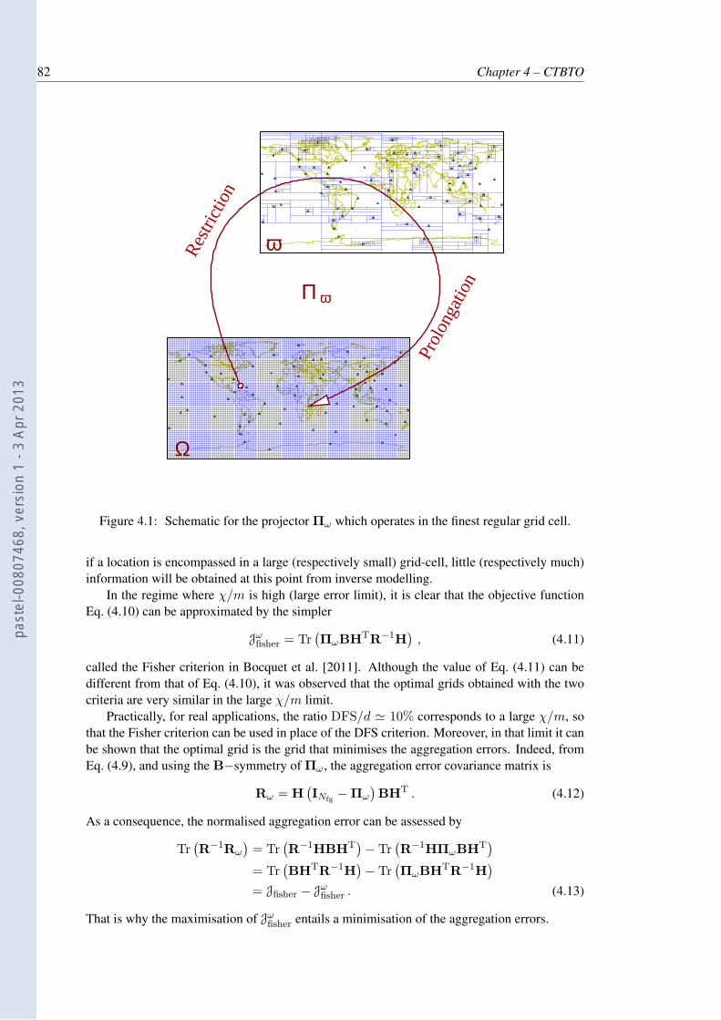
82 Chapter 4 – CTBTO
Π ω
ω
Ω
Res
trict
ion
Pro
long
atio
n
Figure 4.1: Schematic for the projector Πω which operates in the finest regular grid cell.
if a location is encompassed in a large (respectively small) grid-cell, little (respectively much)information will be obtained at this point from inverse modelling.
In the regime where χ/m is high (large error limit), it is clear that the objective functionEq. (4.10) can be approximated by the simpler
Jωfisher = Tr
(ΠωBHTR−1H
), (4.11)
called the Fisher criterion in Bocquet et al. [2011]. Although the value of Eq. (4.11) can bedifferent from that of Eq. (4.10), it was observed that the optimal grids obtained with the twocriteria are very similar in the large χ/m limit.
Practically, for real applications, the ratio DFS/d ≃ 10% corresponds to a large χ/m, sothat the Fisher criterion can be used in place of the DFS criterion. Moreover, in that limit it canbe shown that the optimal grid is the grid that minimises the aggregation errors. Indeed, fromEq. (4.9), and using the B−symmetry of Πω, the aggregation error covariance matrix is
Rω = H(INfg
− Πω
)BHT . (4.12)
As a consequence, the normalised aggregation error can be assessed by
Tr(R−1Rω
)= Tr
(R−1HBHT
)− Tr
(R−1HΠωBHT
)
= Tr(BHTR−1H
)− Tr
(ΠωBHTR−1H
)
= Jfisher − Jωfisher . (4.13)
That is why the maximisation of Jωfisher entails a minimisation of the aggregation errors.
past
el-0
0807
468,
ver
sion
1 -
3 Ap
r 201
3
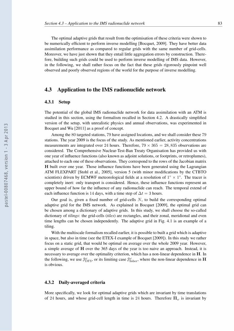
Section 4.3 – Application to the IMS radionuclide network 83
The optimal adaptive grids that result from the optimisation of these criteria were shown tobe numerically efficient to perform inverse modelling [Bocquet, 2009]. They have better dataassimilation performance as compared to regular grids with the same number of grid-cells.Moreover, we have just shown that they entail little aggregation errors by construction. There-fore, building such grids could be used to perform inverse modelling of IMS data. However,in the following, we shall rather focus on the fact that these grids rigorously pinpoint wellobserved and poorly observed regions of the world for the purpose of inverse modelling.
4.3 Application to the IMS radionuclide network
4.3.1 Setup
The potential of the global IMS radionuclide network for data assimilation with an ATM isstudied in this section, using the formalism recalled in Section 4.2. A drastically simplifiedversion of the setup, with unrealistic physics and annual observations, was experimented inBocquet and Wu [2011] as a proof of concept.
Among the 80 targeted stations, 79 have assigned locations, and we shall consider these 79stations. The year 2009 is the focus of the study. As mentioned earlier, activity concentrationsmeasurements are integrated over 24 hours. Therefore, 79 × 365 = 28, 835 observations areconsidered. The Comprehensive Nuclear-Test-Ban Treaty Organisation has provided us withone year of influence functions (also known as adjoint solutions, or footprints, or retroplumes),attached to each one of these observations. They correspond to the rows of the Jacobian matrixH built over one year. Those influence functions have been generated using the LagrangianATM FLEXPART [Stohl et al., 2005], version 5 (with minor modifications by the CTBTOscientists) driven by ECMWF meteorological fields at a resolution of 1 × 1. The tracer iscompletely inert: only transport is considered. Hence, these influence functions represent anupper bound of how far the influence of any radionuclide can reach. The temporal extend ofeach influence function is 14 days, with a time step of ∆t = 3 hours.
Our goal is, given a fixed number of grid-cells N , to build the corresponding optimaladaptive grid for the IMS network. As explained in Bocquet [2009], the optimal grid canbe chosen among a dictionary of adaptive grids. In this study, we shall choose the so-calleddictionary of tilings: the grid-cells (tiles) are rectangles, and their zonal, meridional and eventime lengths can be chosen independently. The adaptive grid in Fig. 4.1 is an example of atiling.
With the multiscale formalism recalled earlier, it is possible to built a grid which is adaptivein space, but also in time (see the ETEX-I example of Bocquet [2009]). In this study we ratherfocus on a static grid, that would be optimal on average over the whole 2009 year. However,a simple average of H over the 365 days of the year is too naive an approach. Instead, it isnecessary to average over the optimality criterion, which has a non-linear dependence in H. Inthe following, we use Jω
DFS, or its limiting case Jωfisher, where the non-linear dependence in H
is obvious.
4.3.2 Daily-averaged criteria
More specifically, we look for optimal adaptive grids which are invariant by time translationsof 24 hours, and whose grid-cell length in time is 24 hours. Therefore Πω is invariant by
past
el-0
0807
468,
ver
sion
1 -
3 Ap
r 201
3
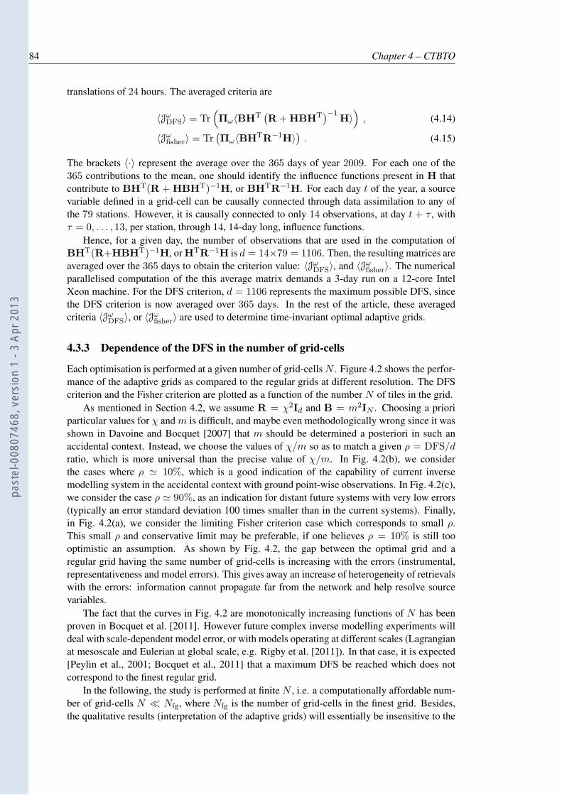
84 Chapter 4 – CTBTO
translations of 24 hours. The averaged criteria are
〈JωDFS〉 = Tr
(Πω〈BHT
(R + HBHT
)−1H〉)
, (4.14)
〈Jωfisher〉 = Tr
(Πω〈BHTR−1H〉
). (4.15)
The brackets 〈·〉 represent the average over the 365 days of year 2009. For each one of the365 contributions to the mean, one should identify the influence functions present in H thatcontribute to BHT(R + HBHT)−1H, or BHTR−1H. For each day t of the year, a sourcevariable defined in a grid-cell can be causally connected through data assimilation to any ofthe 79 stations. However, it is causally connected to only 14 observations, at day t + τ , withτ = 0, . . . , 13, per station, through 14, 14-day long, influence functions.
Hence, for a given day, the number of observations that are used in the computation ofBHT(R+HBHT)−1H, or HTR−1H is d = 14×79 = 1106. Then, the resulting matrices areaveraged over the 365 days to obtain the criterion value: 〈Jω
DFS〉, and 〈Jωfisher〉. The numerical
parallelised computation of the this average matrix demands a 3-day run on a 12-core IntelXeon machine. For the DFS criterion, d = 1106 represents the maximum possible DFS, sincethe DFS criterion is now averaged over 365 days. In the rest of the article, these averagedcriteria 〈Jω
DFS〉, or 〈Jωfisher〉 are used to determine time-invariant optimal adaptive grids.
4.3.3 Dependence of the DFS in the number of grid-cells
Each optimisation is performed at a given number of grid-cells N . Figure 4.2 shows the perfor-mance of the adaptive grids as compared to the regular grids at different resolution. The DFScriterion and the Fisher criterion are plotted as a function of the number N of tiles in the grid.
As mentioned in Section 4.2, we assume R = χ2Id and B = m2IN . Choosing a prioriparticular values for χ and m is difficult, and maybe even methodologically wrong since it wasshown in Davoine and Bocquet [2007] that m should be determined a posteriori in such anaccidental context. Instead, we choose the values of χ/m so as to match a given ρ = DFS/dratio, which is more universal than the precise value of χ/m. In Fig. 4.2(b), we considerthe cases where ρ ≃ 10%, which is a good indication of the capability of current inversemodelling system in the accidental context with ground point-wise observations. In Fig. 4.2(c),we consider the case ρ ≃ 90%, as an indication for distant future systems with very low errors(typically an error standard deviation 100 times smaller than in the current systems). Finally,in Fig. 4.2(a), we consider the limiting Fisher criterion case which corresponds to small ρ.This small ρ and conservative limit may be preferable, if one believes ρ = 10% is still toooptimistic an assumption. As shown by Fig. 4.2, the gap between the optimal grid and aregular grid having the same number of grid-cells is increasing with the errors (instrumental,representativeness and model errors). This gives away an increase of heterogeneity of retrievalswith the errors: information cannot propagate far from the network and help resolve sourcevariables.
The fact that the curves in Fig. 4.2 are monotonically increasing functions of N has beenproven in Bocquet et al. [2011]. However future complex inverse modelling experiments willdeal with scale-dependent model error, or with models operating at different scales (Lagrangianat mesoscale and Eulerian at global scale, e.g. Rigby et al. [2011]). In that case, it is expected[Peylin et al., 2001; Bocquet et al., 2011] that a maximum DFS be reached which does notcorrespond to the finest regular grid.
In the following, the study is performed at finite N , i.e. a computationally affordable num-ber of grid-cells N ≪ Nfg, where Nfg is the number of grid-cells in the finest grid. Besides,the qualitative results (interpretation of the adaptive grids) will essentially be insensitive to the
past
el-0
0807
468,
ver
sion
1 -
3 Ap
r 201
3
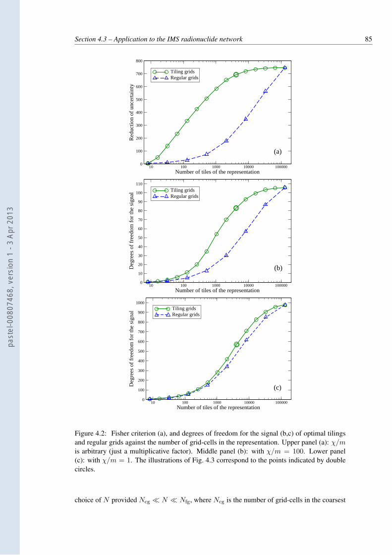
Section 4.3 – Application to the IMS radionuclide network 85
10 100 1000 10000 100000Number of tiles of the representation
0
100
200
300
400
500
600
700
800
Red
uctio
n of
unc
erta
inty
Tiling gridsRegular grids
(a)
10 100 1000 10000 100000Number of tiles of the representation
0
10
20
30
40
50
60
70
80
90
100
110
Deg
rees
of f
reed
om fo
r th
e si
gnal Tiling grids
Regular grids
(b)
10 100 1000 10000 100000Number of tiles of the representation
0
100
200
300
400
500
600
700
800
900
1000
Deg
rees
of f
reed
om fo
r th
e si
gnal Tiling grids
Regular grids
(c)
Figure 4.2: Fisher criterion (a), and degrees of freedom for the signal (b,c) of optimal tilingsand regular grids against the number of grid-cells in the representation. Upper panel (a): χ/mis arbitrary (just a multiplicative factor). Middle panel (b): with χ/m = 100. Lower panel(c): with χ/m = 1. The illustrations of Fig. 4.3 correspond to the points indicated by doublecircles.
choice of N provided Ncg ≪ N ≪ Nfg, where Ncg is the number of grid-cells in the coarsest
past
el-0
0807
468,
ver
sion
1 -
3 Ap
r 201
3
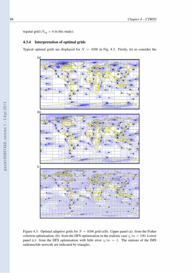
86 Chapter 4 – CTBTO
regular grid (Ncg = 8 in this study).
4.3.4 Interpretation of optimal grids
Typical optimal grids are displayed for N = 4096 in Fig. 4.3. Firstly, let us consider the
(a)
(b)
(c)
Figure 4.3: Optimal adaptive grids for N = 4096 grid-cells. Upper panel (a): from the Fishercriterion optimisation, (b): from the DFS optimisation in the realistic case χ/m = 100. Lowerpanel (c): from the DFS optimisation with little error χ/m = 1. The stations of the IMSradionuclide network are indicated by triangles.
past
el-0
0807
468,
ver
sion
1 -
3 Ap
r 201
3
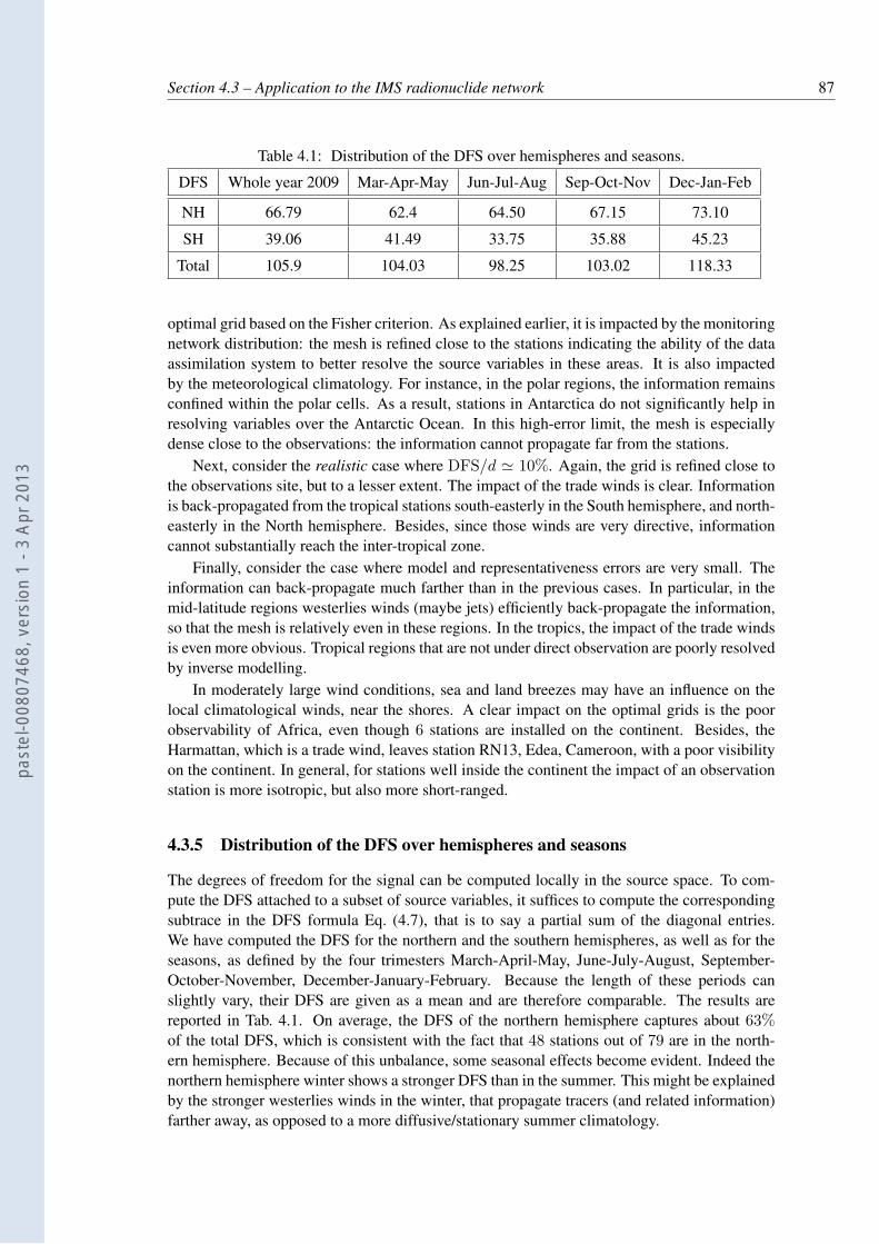
Section 4.3 – Application to the IMS radionuclide network 87
Table 4.1: Distribution of the DFS over hemispheres and seasons.
DFS Whole year 2009 Mar-Apr-May Jun-Jul-Aug Sep-Oct-Nov Dec-Jan-Feb
NH 66.79 62.4 64.50 67.15 73.10
SH 39.06 41.49 33.75 35.88 45.23
Total 105.9 104.03 98.25 103.02 118.33
optimal grid based on the Fisher criterion. As explained earlier, it is impacted by the monitoringnetwork distribution: the mesh is refined close to the stations indicating the ability of the dataassimilation system to better resolve the source variables in these areas. It is also impactedby the meteorological climatology. For instance, in the polar regions, the information remainsconfined within the polar cells. As a result, stations in Antarctica do not significantly help inresolving variables over the Antarctic Ocean. In this high-error limit, the mesh is especiallydense close to the observations: the information cannot propagate far from the stations.
Next, consider the realistic case where DFS/d ≃ 10%. Again, the grid is refined close tothe observations site, but to a lesser extent. The impact of the trade winds is clear. Informationis back-propagated from the tropical stations south-easterly in the South hemisphere, and north-easterly in the North hemisphere. Besides, since those winds are very directive, informationcannot substantially reach the inter-tropical zone.
Finally, consider the case where model and representativeness errors are very small. Theinformation can back-propagate much farther than in the previous cases. In particular, in themid-latitude regions westerlies winds (maybe jets) efficiently back-propagate the information,so that the mesh is relatively even in these regions. In the tropics, the impact of the trade windsis even more obvious. Tropical regions that are not under direct observation are poorly resolvedby inverse modelling.
In moderately large wind conditions, sea and land breezes may have an influence on thelocal climatological winds, near the shores. A clear impact on the optimal grids is the poorobservability of Africa, even though 6 stations are installed on the continent. Besides, theHarmattan, which is a trade wind, leaves station RN13, Edea, Cameroon, with a poor visibilityon the continent. In general, for stations well inside the continent the impact of an observationstation is more isotropic, but also more short-ranged.
4.3.5 Distribution of the DFS over hemispheres and seasons
The degrees of freedom for the signal can be computed locally in the source space. To com-pute the DFS attached to a subset of source variables, it suffices to compute the correspondingsubtrace in the DFS formula Eq. (4.7), that is to say a partial sum of the diagonal entries.We have computed the DFS for the northern and the southern hemispheres, as well as for theseasons, as defined by the four trimesters March-April-May, June-July-August, September-October-November, December-January-February. Because the length of these periods canslightly vary, their DFS are given as a mean and are therefore comparable. The results arereported in Tab. 4.1. On average, the DFS of the northern hemisphere captures about 63%of the total DFS, which is consistent with the fact that 48 stations out of 79 are in the north-ern hemisphere. Because of this unbalance, some seasonal effects become evident. Indeed thenorthern hemisphere winter shows a stronger DFS than in the summer. This might be explainedby the stronger westerlies winds in the winter, that propagate tracers (and related information)farther away, as opposed to a more diffusive/stationary summer climatology.
past
el-0
0807
468,
ver
sion
1 -
3 Ap
r 201
3
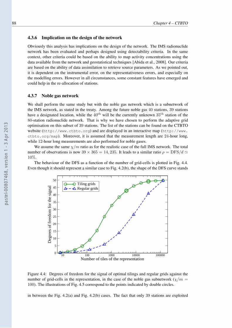
88 Chapter 4 – CTBTO
4.3.6 Implication on the design of the network
Obviously this analysis has implications on the design of the network. The IMS radionuclidenetwork has been evaluated and perhaps designed using detectability criteria. In the samecontext, other criteria could be based on the ability to map activity concentrations using thedata available from the network and geostatistical techniques [Abida et al., 2008]. Our criteriaare based on the ability of data assimilation to retrieve source parameters. As we pointed out,it is dependent on the instrumental error, on the representativeness errors, and especially onthe modelling errors. However in all circumstances, some constant features have emerged andcould help in the re-allocation of stations.
4.3.7 Noble gas network
We shall perform the same study but with the noble gas network which is a subnetwork ofthe IMS network, as stated in the treaty. Among the future noble gas 40 stations, 39 stationshave a designated location, while the 40th will be the currently unknown 35th station of the80-station radionuclide network. That is why we have chosen to perform the adaptive gridoptimisation on this subset of 39 stations. The list of the stations can be found on the CTBTOwebsite (http://www.ctbto.org) and are displayed in an interactive map (http://www.ctbto.org/map). Moreover, it is assumed that the measurement length are 24-hour long,while 12-hour long measurements are also performed for noble gases.
We assume the same χ/m ratio as for the realistic case of the full IMS network. The totalnumber of observations is now 39 × 365 = 14, 235. It leads to a similar ratio ρ = DFS/d ≃10%.
The behaviour of the DFS as a function of the number of grid-cells is plotted in Fig. 4.4.Even though it should represent a similar case to Fig. 4.2(b), the shape of the DFS curve stands
10 100 1000 10000 100000Number of tiles of the representation
0
5
10
15
20
25
30
35
40
45
50
Deg
rees
of f
reed
om fo
r th
e si
gnal Tiling grids
Regular grids
Figure 4.4: Degrees of freedom for the signal of optimal tilings and regular grids against thenumber of grid-cells in the representation, in the case of the noble gas subnetwork (χ/m =100). The illustrations of Fig. 4.5 correspond to the points indicated by double circles.
in between the Fig. 4.2(a) and Fig. 4.2(b) cases. The fact that only 39 stations are exploited
past
el-0
0807
468,
ver
sion
1 -
3 Ap
r 201
3
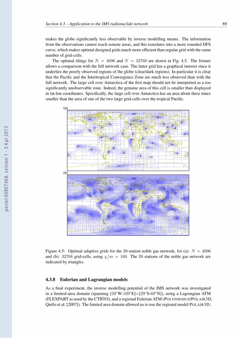
Section 4.3 – Application to the IMS radionuclide network 89
makes the globe significantly less observable by inverse modelling means. The informationfrom the observations cannot reach remote areas, and this translates into a more rounded DFScurve, which makes optimal designed grids much more efficient than regular grid with the samenumber of grid-cells.
The optimal tilings for N = 4096 and N = 32768 are drawn in Fig. 4.5. The formerallows a comparison with the full network case. The latter grid has a graphical interest since itunderlies the poorly observed regions of the globe (clear/dark regions). In particular it is clearthat the Pacific and the Intertropical Convergence Zone are much less observed than with thefull network. The large cell over Antarctica of the first map should not be interpreted as a toosignificantly unobservable zone. Indeed, the genuine area of this cell is smaller than displayedin lat-lon coordinates. Specifically, the large cell over Antarctica has an area about three timessmaller than the area of one of the two large grid-cells over the tropical Pacific.
(a)
(b)
Figure 4.5: Optimal adaptive grids for the 39-station noble gas network, for (a): N = 4096and (b): 32768 grid-cells, using χ/m = 100. The 39 stations of the noble gas network areindicated by triangles.
4.3.8 Eulerian and Lagrangian models
As a final experiment, the inverse modelling potential of the IMS network was investigatedin a limited-area domain (spanning [59W-109E]×[29S-69N]), using a Lagrangian ATM(FLEXPART as used by the CTBTO), and a regional Eulerian ATM (POLYPHEMUS/POLAIR3D,Quélo et al. [2007]). The limited area domain allowed us to use the regional model POLAIR3D,
past
el-0
0807
468,
ver
sion
1 -
3 Ap
r 201
3
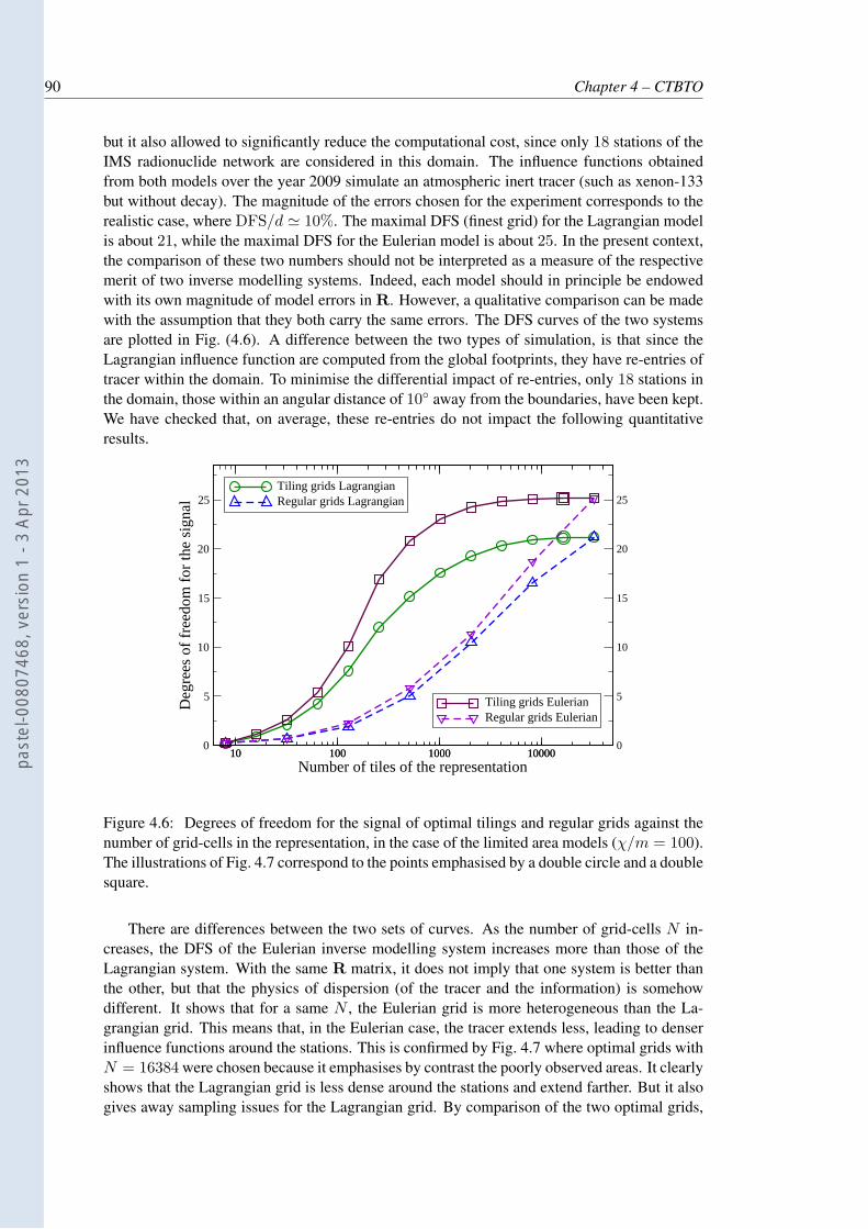
90 Chapter 4 – CTBTO
but it also allowed to significantly reduce the computational cost, since only 18 stations of theIMS radionuclide network are considered in this domain. The influence functions obtainedfrom both models over the year 2009 simulate an atmospheric inert tracer (such as xenon-133but without decay). The magnitude of the errors chosen for the experiment corresponds to therealistic case, where DFS/d ≃ 10%. The maximal DFS (finest grid) for the Lagrangian modelis about 21, while the maximal DFS for the Eulerian model is about 25. In the present context,the comparison of these two numbers should not be interpreted as a measure of the respectivemerit of two inverse modelling systems. Indeed, each model should in principle be endowedwith its own magnitude of model errors in R. However, a qualitative comparison can be madewith the assumption that they both carry the same errors. The DFS curves of the two systemsare plotted in Fig. (4.6). A difference between the two types of simulation, is that since theLagrangian influence function are computed from the global footprints, they have re-entries oftracer within the domain. To minimise the differential impact of re-entries, only 18 stations inthe domain, those within an angular distance of 10 away from the boundaries, have been kept.We have checked that, on average, these re-entries do not impact the following quantitativeresults.
10 100 1000 10000Number of tiles of the representation
0
5
10
15
20
25
Deg
rees
of f
reed
om fo
r th
e si
gnal Tiling grids Lagrangian
Regular grids Lagrangian
10 100 1000 100000
5
10
15
20
25
Tiling grids EulerianRegular grids Eulerian
Figure 4.6: Degrees of freedom for the signal of optimal tilings and regular grids against thenumber of grid-cells in the representation, in the case of the limited area models (χ/m = 100).The illustrations of Fig. 4.7 correspond to the points emphasised by a double circle and a doublesquare.
There are differences between the two sets of curves. As the number of grid-cells N in-creases, the DFS of the Eulerian inverse modelling system increases more than those of theLagrangian system. With the same R matrix, it does not imply that one system is better thanthe other, but that the physics of dispersion (of the tracer and the information) is somehowdifferent. It shows that for a same N , the Eulerian grid is more heterogeneous than the La-grangian grid. This means that, in the Eulerian case, the tracer extends less, leading to denserinfluence functions around the stations. This is confirmed by Fig. 4.7 where optimal grids withN = 16384 were chosen because it emphasises by contrast the poorly observed areas. It clearlyshows that the Lagrangian grid is less dense around the stations and extend farther. But it alsogives away sampling issues for the Lagrangian grid. By comparison of the two optimal grids,
past
el-0
0807
468,
ver
sion
1 -
3 Ap
r 201
3
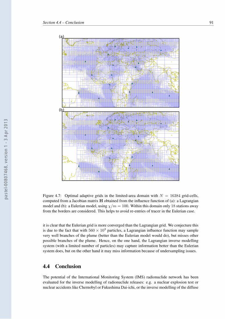
Section 4.4 – Conclusion 91
(a)
(b)
Figure 4.7: Optimal adaptive grids in the limited-area domain with N = 16384 grid-cells,computed from a Jacobian matrix H obtained from the influence function of (a): a Lagrangianmodel and (b): a Eulerian model, using χ/m = 100. Within this domain only 18 stations awayfrom the borders are considered. This helps to avoid re-entries of tracer in the Eulerian case.
it is clear that the Eulerian grid is more converged than the Lagrangian grid. We conjecture thisis due to the fact that with 560 × 103 particles, a Lagrangian influence function may samplevery well branches of the plume (better than the Eulerian model would do), but misses otherpossible branches of the plume. Hence, on the one hand, the Lagrangian inverse modellingsystem (with a limited number of particles) may capture information better than the Euleriansystem does, but on the other hand it may miss information because of undersampling issues.
4.4 Conclusion
The potential of the International Monitoring System (IMS) radionuclide network has beenevaluated for the inverse modelling of radionuclide releases: e.g. a nuclear explosion test ornuclear accidents like Chernobyl or Fukushima Dai-ichi, or the inverse modelling of the diffuse
past
el-0
0807
468,
ver
sion
1 -
3 Ap
r 201
3
92 Chapter 4 – CTBTO
sources of xenon radio-isotopes. We have proposed an evaluation methodology accountingfor the performance of the inversion (or data assimilation) system. This methodology differsfrom the detection capability approach and the geostatistics approach in that: i) the degrees offreedom for the signal (DFS) is chosen to be the criterion that assesses the information gainfrom the observations to the whole domain through inversion; ii) optimal multiscale adaptivegrids of sources are constructed by maximising the DFS criterion; and iii) the radionuclidenetwork is evaluated by the spatial distribution of the grid-cells of the optimal adaptive grids.
For optimal grids, the inverse of the size of a grid cell measures the resolution defined asthe capacity to locally resolve the source by the inversion system. Therefore the dense meshindicates the regions where the source variables are well resolved. By contrast, for sparsemesh, the over-aggregations of the regular grid cells at finer scale result in high uncertaintiesof inverted sources.
We have constructed global optimal grids with the IMS radionuclide network for its evalu-ation. The influence functions, which relate the observations with the sources, were generatedusing the Lagrangian transport model FLEXPART driven by ECMWF meteorological fields ata resolution of 1 × 1 over the 365 days of year 2009. The ratio ρ between the DFS and thetotal number of observations was used to control different error levels in the inversion, i.e. theerror of a priori sources and the observational error that encapsulates the instrumental error, therepresentativity error and the transport model error.
Grid optimisations have been performed for three cases with ρ ≃ 0 (very large observa-tional error), ρ ≃ 10% (realistic observational error), and ρ ≃ 90% (accurate transport) re-spectively. Some stable spatial patterns have emerged in the optimal grids with these differentsettings. In all cases, the trade winds carry information towards the Intertropical ConvergenceZone along straight paths, leaving large unobserved areas in the tropics. For the case of largeobservational errors, the optimal grid is very heterogeneous. The mesh is dense close to mostobservation sites. The information propagation is not obvious except for the polar areas dueto the impact of the polar vortices. For realistic observational errors, there are still many areasaway from the information propagation path, e.g. the African continent.
When accurate atmospheric transport representation is assumed, the optimal grids becomemore uniformly distributed, especially for the mid-latitude regions where westerlies winds pre-vail. Such coverage is desirable. However, we do not believe current state-of-the-art ATM canreach that accuracy level. Moreover, even with high accuracy and a good coverage of the globeon average, the tropics will remain difficult to probe with inverse modelling.
The results obtained in this study can also serve as a basis for reallocation or installationof stations using the size of the adaptive grid-cells as an indication. It would be interesting tocompare the results of this approach with the results based on the detectability criterion.
past
el-0
0807
468,
ver
sion
1 -
3 Ap
r 201
3
Chapter 5
Estimation of volatile organic
compound emissions for Europe using
data assimilation
Summary
The emission of volatile organic compounds (VOCs) over western Europe for the year 2005 areestimated via inverse modelling, by assimilation of in situ observations of concentration andcompared to a standard emission inventory. The study focuses on fifteen VOC species: fivearomatics, six alkanes, two alkenes, one alkyne and one biogenic diene. The inversion relieson a validated fast adjoint of the chemistry transport model used to simulate the fate and trans-port of these VOCs. The assimilated ground-based measurements over Europe are providedby the European Monitoring and Evaluation Programme (EMEP) network. The backgroundemissions errors and the prior observational errors are estimated by maximum likelihood ap-proaches. The positivity assumptions on the VOC emission fluxes is pivotal for a successfulinversion and this maximum likelihood approach consistently accounts for the positivity of thefluxes. For most species, the retrieval leads to a significant reduction of the bias, which under-lines the misfit between the standard inventories and the observed concentrations. The resultsare validated through a forecast test and a cross-validation test. It is shown that the statisticallyconsistent non-Gaussian approach based on a reliable estimation of the errors offers the bestperformance. The efficiency in correcting the inventory depends on the lifetime of the VOCs.In particular, it is shown that the use of in-situ observations using a sparse monitoring networkto estimate emissions of isoprene is inadequate because its short chemical lifetime significantlylimits the spatial radius of influence of the monitoring data. For species with longer lifetime (afew days), successful, albeit partial, emission corrections can reach regions hundreds of kilo-metres away from the stations. Domainwide corrections of the emissions inventories of someVOCs are significant, with underestimations on order of a factor of two of propane, ethane,ethylene and acetylene.
past
el-0
0807
468,
ver
sion
1 -
3 Ap
r 201
3
94 Chapter 5 – VOC
Contents
5.1 Introduction . . . . . . . . . . . . . . . . . . . . . . . . . . . . . . . . . 94
5.2 Methodology . . . . . . . . . . . . . . . . . . . . . . . . . . . . . . . . . 95
5.2.1 Full chemical transport model and reduced VOC model . . . . . . . 95
5.2.2 The source receptor model . . . . . . . . . . . . . . . . . . . . . . 96
5.2.3 Control space . . . . . . . . . . . . . . . . . . . . . . . . . . . . . 98
5.2.4 Inversion method . . . . . . . . . . . . . . . . . . . . . . . . . . . 98
5.2.5 Estimation of hyperparameters . . . . . . . . . . . . . . . . . . . . 99
5.3 Setup of the numerical experiments . . . . . . . . . . . . . . . . . . . . 100
5.3.1 Observations . . . . . . . . . . . . . . . . . . . . . . . . . . . . . 100
5.3.2 Inversion and validation setup . . . . . . . . . . . . . . . . . . . . 101
5.3.3 Verification of the adjoint solutions . . . . . . . . . . . . . . . . . 102
5.3.4 Values of the hyperparameters . . . . . . . . . . . . . . . . . . . . 102
5.4 Inversion results . . . . . . . . . . . . . . . . . . . . . . . . . . . . . . . 103
5.4.1 Analysis of the inversion results . . . . . . . . . . . . . . . . . . . 104
5.4.2 Forecast test . . . . . . . . . . . . . . . . . . . . . . . . . . . . . 110
5.4.3 Cross-validation test . . . . . . . . . . . . . . . . . . . . . . . . . 112
5.4.4 Information content and DFS . . . . . . . . . . . . . . . . . . . . . 115
5.5 Conclusion . . . . . . . . . . . . . . . . . . . . . . . . . . . . . . . . . . 115
5.1 Introduction
Volatile organic compounds (VOCs) are of particular environmental concern because they areprecursors of secondary pollutants, such as ozone and fine particulate matter (PM2.5), andsome VOCs are pollutants in their own right due to their adverse carcinogenic and/or non-carcinogenic health effects. Therefore, it is essential to have accurate emission inventories ofVOCs to conduct air quality modelling studies for the development of optimal emission con-trol strategies and for air quality forecasting as well as to follow their temporal emission trendsover the years as emission control strategies get implemented. The large number of emissionsources, both anthropogenic and biogenic, and processes leading to those emissions (combus-tion, evaporation, vegetation metabolism) make the development of accurate VOC emissioninventories difficult. Furthermore, VOC emissions cannot be derived from mass balances andthey must be obtained from experimental measurements conducted at the source of the emis-sions. Also, emission testing is costly and some emission factors are developed for total VOCsrather than for individual VOCs. Therefore, a chemical speciation must be applied to total VOCemission factors using speciation data that are limited and uncertain. Although uncertaintiesin anthropogenic emissions have been reduced over the years as a result of better characteri-sation of major emission sources, uncertainties still remain. Furthermore, large uncertaintiesare associated with biogenic emissions due to the difficulty of estimating the meteorology-dependent emission rates for a large number of vegetation species as well as characterising theland-use/land-cover of the area of interest. Therefore, several approaches have been used toevaluate the accuracy of VOC emission inventories and, if appropriate, apply some correction.
past
el-0
0807
468,
ver
sion
1 -
3 Ap
r 201
3
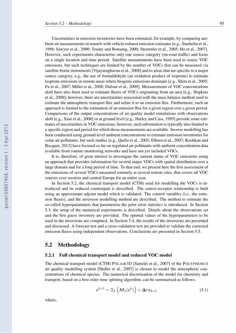
Section 5.2 – Methodology 95
Uncertainties in emission inventories have been estimated, for example, by comparing am-bient air measurements in tunnels with vehicle exhaust emission estimates [e.g., Staehelin et al.,1998; Sawyer et al., 2000; Touaty and Bonsang, 2000; Stemmler et al., 2005; Ho et al., 2007].However, such experiments characterise only one source category (on-road traffic) and focuson a single location and time period. Satellite measurements have been used to assess VOCemissions, but such techniques are limited by the number of VOCs that can be measured viasatellite-borne instruments [Vijayaraghavan et al., 2008] and to areas that are specific to a majorsource category, e.g., the use of formaldehyde (an oxidation product of isoprene) to estimateisoprene emissions in remote areas where biogenic emissions dominate [e.g., Shim et al., 2005;Fu et al., 2007; Millet et al., 2008; Dufour et al., 2009]. Measurements of VOC concentrationsaloft have also been used to estimate fluxes of VOCs originating from an area [e.g., Hopkinset al., 2009]; however, there are uncertainties associated with the mass balance method used toestimate the atmospheric transport flux and relate it to an emission flux. Furthermore, such anapproach is limited to the estimation of an emission flux for a given region over a given period.Comparisons of the output concentrations of air quality model simulations with observationsaloft [e.g., Xiao et al., 2008] or at ground level [e.g., Harley and Cass, 1995] provide some esti-mates of uncertainties in VOC emissions; however, such information is typically also limited toa specific region and period for which those measurements are available. Inverse modelling hasbeen conducted using ground-level ambient concentrations to estimate emission inventories forsome air pollutants, but such studies [e.g., Quélo et al., 2005; Elbern et al., 2007; Koohkan andBocquet, 2012] have focused so far on regulated air pollutants with ambient concentration dataavailable from routine monitoring networks and have not yet included VOCs.
It is, therefore, of great interest to investigate the current status of VOC emissions usingan approach that provides information for several major VOCs with spatial distribution over alarge domain and for a long period of time. To that end, we present here the first assessment ofthe emissions of several VOCs measured routinely at several remote sites, that covers all VOCsources over western and central Europe for an entire year.
In Section 5.2, the chemical transport model (CTM) used for modelling the VOCs is in-troduced and its reduced counterpart is described. The source-receptor relationship is builtusing an approximate adjoint model which is validated. The control variables (i.e., the emis-sion fluxes), and the inversion modelling method are described. The method to estimate theso-called hyperparameters that parametrise the prior error statistics is introduced. In Section5.3, the setup of the numerical experiments is described. Details about the observations setand the first guess inventory are provided. The optimal values of the hyperparameters to beused in the inversions are computed. In Section 5.4, the results of the inversions are presentedand discussed. A forecast test and a cross-validation test are provided to validate the correctedemission fluxes using independent observations. Conclusions are presented in Section 5.5.
5.2 Methodology
5.2.1 Full chemical transport model and reduced VOC model
The chemical transport model (CTM) POLAIR3D [Sartelet et al., 2007] of the POLYPHEMUS
air quality modelling system [Mallet et al., 2007] is chosen to model the atmospheric con-centrations of chemical species. The numerical discretisation of the model for chemistry andtransport, based on a first order time splitting algorithm, can be summarised as follows:
ck+1 = Xk
(Mk(c
k))
+ ∆t ek+1 (5.1)
where,
past
el-0
0807
468,
ver
sion
1 -
3 Ap
r 201
3
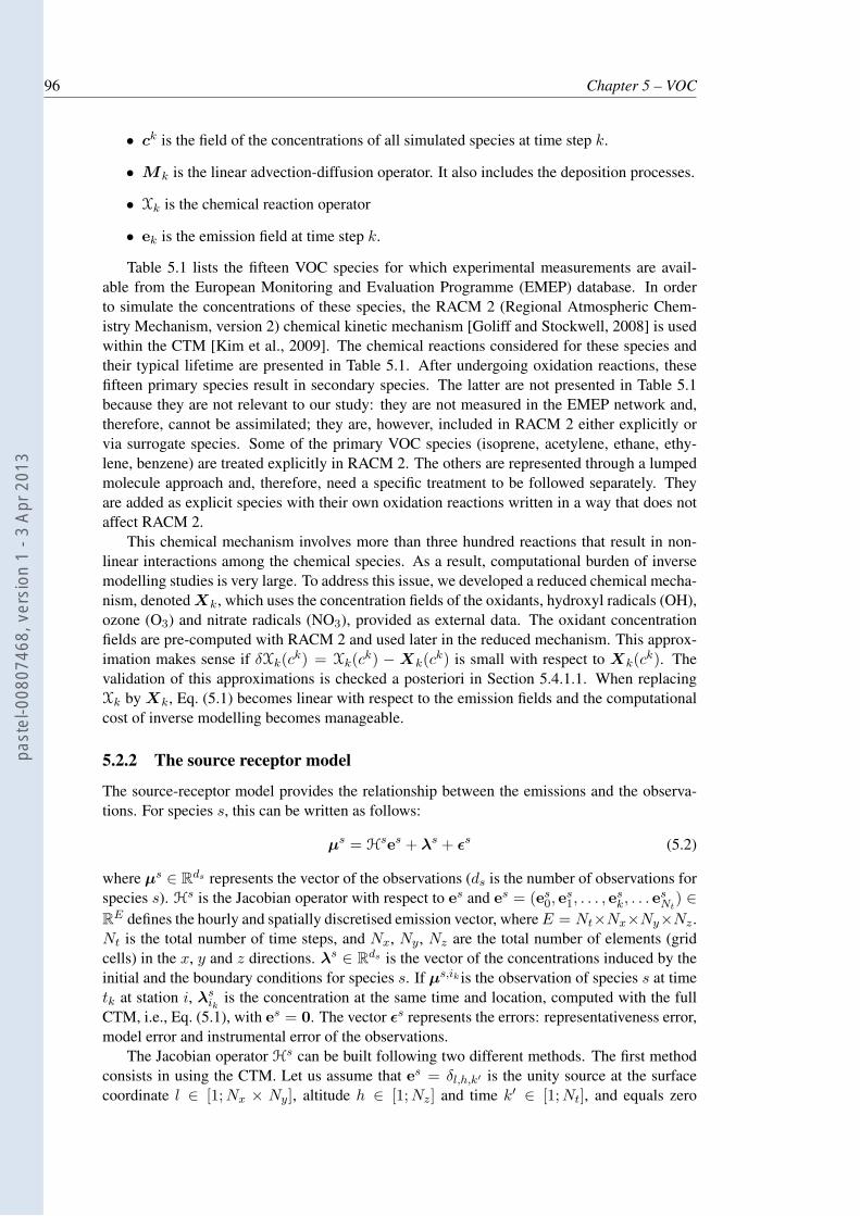
96 Chapter 5 – VOC
• ck is the field of the concentrations of all simulated species at time step k.
• Mk is the linear advection-diffusion operator. It also includes the deposition processes.
• Xk is the chemical reaction operator
• ek is the emission field at time step k.
Table 5.1 lists the fifteen VOC species for which experimental measurements are avail-able from the European Monitoring and Evaluation Programme (EMEP) database. In orderto simulate the concentrations of these species, the RACM 2 (Regional Atmospheric Chem-istry Mechanism, version 2) chemical kinetic mechanism [Goliff and Stockwell, 2008] is usedwithin the CTM [Kim et al., 2009]. The chemical reactions considered for these species andtheir typical lifetime are presented in Table 5.1. After undergoing oxidation reactions, thesefifteen primary species result in secondary species. The latter are not presented in Table 5.1because they are not relevant to our study: they are not measured in the EMEP network and,therefore, cannot be assimilated; they are, however, included in RACM 2 either explicitly orvia surrogate species. Some of the primary VOC species (isoprene, acetylene, ethane, ethy-lene, benzene) are treated explicitly in RACM 2. The others are represented through a lumpedmolecule approach and, therefore, need a specific treatment to be followed separately. Theyare added as explicit species with their own oxidation reactions written in a way that does notaffect RACM 2.
This chemical mechanism involves more than three hundred reactions that result in non-linear interactions among the chemical species. As a result, computational burden of inversemodelling studies is very large. To address this issue, we developed a reduced chemical mecha-nism, denoted Xk, which uses the concentration fields of the oxidants, hydroxyl radicals (OH),ozone (O3) and nitrate radicals (NO3), provided as external data. The oxidant concentrationfields are pre-computed with RACM 2 and used later in the reduced mechanism. This approx-imation makes sense if δXk(c
k) = Xk(ck) − Xk(c
k) is small with respect to Xk(ck). The
validation of this approximations is checked a posteriori in Section 5.4.1.1. When replacingXk by Xk, Eq. (5.1) becomes linear with respect to the emission fields and the computationalcost of inverse modelling becomes manageable.
5.2.2 The source receptor model
The source-receptor model provides the relationship between the emissions and the observa-tions. For species s, this can be written as follows:
µs = Hses + λs + ǫs (5.2)
where µs ∈ Rds represents the vector of the observations (ds is the number of observations for
species s). Hs is the Jacobian operator with respect to es and es = (es0, e
s1, . . . , e
sk, . . . e
sNt
) ∈
RE defines the hourly and spatially discretised emission vector, where E = Nt×Nx×Ny×Nz .
Nt is the total number of time steps, and Nx, Ny, Nz are the total number of elements (gridcells) in the x, y and z directions. λs ∈ R
ds is the vector of the concentrations induced by theinitial and the boundary conditions for species s. If µs,ik is the observation of species s at timetk at station i, λs
ikis the concentration at the same time and location, computed with the full
CTM, i.e., Eq. (5.1), with es = 0. The vector ǫs represents the errors: representativeness error,model error and instrumental error of the observations.
The Jacobian operator Hs can be built following two different methods. The first methodconsists in using the CTM. Let us assume that es = δl,h,k′ is the unity source at the surfacecoordinate l ∈ [1;Nx × Ny], altitude h ∈ [1;Nz] and time k′ ∈ [1;Nt], and equals zero
past
el-0
0807
468,
ver
sion
1 -
3 Ap
r 201
3
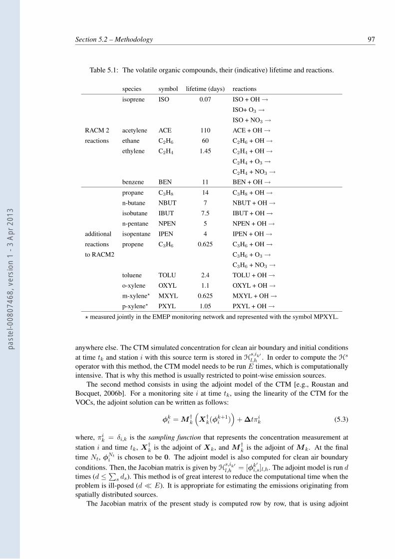
Section 5.2 – Methodology 97
Table 5.1: The volatile organic compounds, their (indicative) lifetime and reactions.
species symbol lifetime (days) reactions
isoprene ISO 0.07 ISO + OH →
ISO+ O3 →
ISO + NO3 →
RACM 2 acetylene ACE 110 ACE + OH →
reactions ethane C2H6 60 C2H6 + OH →
ethylene C2H4 1.45 C2H4 + OH →
C2H4 + O3 →
C2H4 + NO3 →
benzene BEN 11 BEN + OH →
propane C3H8 14 C3H8 + OH →
n-butane NBUT 7 NBUT + OH →
isobutane IBUT 7.5 IBUT + OH →
n-pentane NPEN 5 NPEN + OH →
additional isopentane IPEN 4 IPEN + OH →
reactions propene C3H6 0.625 C3H6 + OH →
to RACM2 C3H6 + O3 →
C3H6 + NO3 →
toluene TOLU 2.4 TOLU + OH →
o-xylene OXYL 1.1 OXYL + OH →
m-xylene⋆ MXYL 0.625 MXYL + OH →
p-xylene⋆ PXYL 1.05 PXYL + OH →
⋆ measured jointly in the EMEP monitoring network and represented with the symbol MPXYL.
anywhere else. The CTM simulated concentration for clean air boundary and initial conditionsat time tk and station i with this source term is stored in H
s,ik′l,h . In order to compute the Hs
operator with this method, the CTM model needs to be run E times, which is computationallyintensive. That is why this method is usually restricted to point-wise emission sources.
The second method consists in using the adjoint model of the CTM [e.g., Roustan andBocquet, 2006b]. For a monitoring site i at time tk, using the linearity of the CTM for theVOCs, the adjoint solution can be written as follows:
φki = M
†k
(X
†k(φ
k+1i )
)+ ∆tπi
k (5.3)
where, πik = δi,k is the sampling function that represents the concentration measurement at
station i and time tk, X†k is the adjoint of Xk, and M
†k is the adjoint of Mk. At the final
time Nt, φNt
i is chosen to be 0. The adjoint model is also computed for clean air boundary
conditions. Then, the Jacobian matrix is given by Hs,ik′l,h = [φk′
i,s]l,h. The adjoint model is run dtimes (d ≤
∑s ds). This method is of great interest to reduce the computational time when the
problem is ill-posed (d ≪ E). It is appropriate for estimating the emissions originating fromspatially distributed sources.
The Jacobian matrix of the present study is computed row by row, that is using adjoint
past
el-0
0807
468,
ver
sion
1 -
3 Ap
r 201
3
98 Chapter 5 – VOC
solutions.
5.2.3 Control space
In order to reduce the dimension of the control space, that is the space of the fluxes to beestimated via inverse modelling, we introduce a relation between the effective control variablesαs and the emission es:
[esk]l,h = [αs]l[e
s,bk ]l,h . (5.4)
In this equation, es,b is the a priori (first guess or background) vector of emission for speciess. Obviously the first guess value of the scaling factors αs, is αs
b = 1, where 1 = (1, . . . , 1)T.Indices k, l, h are respectively related to the time sequence, the horizontal space grid, andthe vertical grid. The αs factors, rather than the full 3D time-dependent emission fields ofEq. (5.1), will be optimised. This choice of control parameters, which is only a function ofl, implies that the correction of the emission fluxes is spatially distributed in the horizontaldirections but that the vertical and the temporal distribution of the emission fluxes are notmodified by the data assimilation analysis.
5.2.4 Inversion method
Combining Eq. (5.2) with Eq. (5.4), one obtains
µs = Hsαs + λs + ǫs (5.5)
where Hs is the Jacobian matrix that relates µs to αs:
Hsik,l =
∑
k
[φks,i]l[e
s,bk ]l . (5.6)
In order to optimise the α parameters, the following objective function with a regularisationterm is used:
Ls(αs) =
1
2(µs − Hsαs − λs)T R−1
s (µs − Hsαs − λs)
+1
2(αs − 1)T B−1
s (αs − 1) . (5.7)
The vector αsb = 1 = (1, . . . , 1)T is the first guess of αs. Rs is the observation error co-
variance matrix. Bs is the background error covariance matrix. For each species, these twomatrices are both chosen to be diagonal with uniform variances, that is, Bs = m2
sINx×Ny ,Rs = r2
sIds. These statistical assumptions imply that we neglect any spatial and temporal
correlations between grid cells in the errors. The anthropogenic emissions of VOCs are notexpected to induce long-range correlation in the errors. However, potential important reasonsfor this hypothesis to fail are when the biogenic VOC emissions have correlated errors duefor some VOCs common sources and similar emission model formulations, or when trans-port model errors induce temporal correlation in the error covariance matrix. That is why ourdiagonal assumption is an approximation.
In the following, two solutions of Eq. (5.7) are considered and compared. The first oneassumes that the errors are Gaussian-distributed and the analysed parameters αs
a are given bythe Best Linear Unbiased Estimator (BLUE):
αsa = 1 + Ks (µs − Hs1 − λs) (5.8)
past
el-0
0807
468,
ver
sion
1 -
3 Ap
r 201
3
Section 5.2 – Methodology 99
where Ks is the gain matrix:
Ks = BsHsT(Rs + HsBsH
sT)−1
(5.9)
The second solution of Eq. (5.7) is obtained assuming a truncated Gaussian distribution for thebackground error statistics, so that α is optimised under a positivity constraint of each one ofits entry [αs]l. As opposed to the Gaussian case, the retrieved scaling factors [αs]l cannot benegative.
5.2.5 Estimation of hyperparameters
The parameters of the prior statistics, such as rs and ms, usually coined hyperparameters, oftenneed to be estimated because their first guess is usually inaccurate, while the dependence of theretrieval on the hyperparameters can be dramatic [Davoine and Bocquet, 2007].
The estimation method for the hyperparameters depends on the statistical assumptions un-derlying Eq. (5.7). In the first case, the error ǫs (in Eq. (5.5)) is assumed to be Gaussian-distributed, ǫs ∼ N(0,Rs). The same assumption applies to the control parameters: αs ∼N(1,Bs). The probability density function (pdf) of the observation vector can be computed asfollows:
p(µs|rs, ms) =
∫p(µs|αs, rs, ms)p(αs|rs, ms)dαs =
∫p(ǫs|rs)p(αs|ms)dαs (5.10)
or analytically,
p(µs|rs, ms) =e−
12(µs−Hs1−λs)T(Rs+HsBsH
sT)−1(µs−Hs1−λs)
√(2π)ds |Rs + HsBsHsT|
. (5.11)
This pdf is also proportional to the likelihood of rs and ms. In order to estimate the hyperpa-rameters rs and ms, Desroziers and Ivanov [2001] suggested an iterative method to convergetowards a fixed point. Chapnik et al. [2006] showed that this approach converges to one localmaximum of the likelihood. The maximisation of log (p(µs|rs, ms)) with respect to the twohyperparameters gives the stationary conditions:
r2s =
‖ µs − Hsαsa ‖2
Tr (Ids− HsKs)
, m2s =
‖ αsa − 1 ‖2
Tr (HsKs)(5.12)
where ‖ · ‖ is the Euclidean norm.However, the Desroziers method relies on Gaussian assumptions, and, for the sake of con-
sistency, one needs another approach to compute the likelihood under the truncated Gaussianassumption [Winiarek et al., 2012]. In this case, the prior on the scaling factors is:
p(αs) =e−
12(αs−1)TB
−1s (αs−1)
√(2π)Nx×Ny |Bs| (1 − Φ1,Bs(0))
Iαs≥0 (5.13)
where Φ1,Bs(0) is the Gaussian cumulative density function (cdf) of N(1,Bs). Iαs≥0 is afunction equal to unity when [αs]l ≥ 0 for each l, and equal to zero otherwise. This pdf is re-ferred to as N(1,Bs,0) or the truncated Gaussian distribution. From Eq. (5.10) and Eq. (5.13),one can derive:
p(µs|r+s , m+
s ) =e−
12(µs−Hs1−λs)T(Rs+HsBsH
sT)−1(µs−Hs1−λs)
√(2π)ds |Rs + HsBsHsT|
×
∫αs≥0
e−12(αs−1)T(Pa
s )−1(αs−1)
√(2π)Nx×Ny |Bs| (1 − Φ1,Bs(0))
(5.14)
past
el-0
0807
468,
ver
sion
1 -
3 Ap
r 201
3
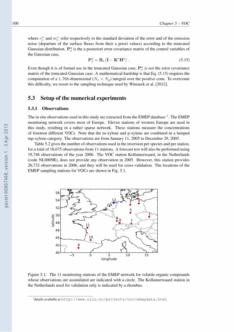
100 Chapter 5 – VOC
where r+s and m+
s refer respectively to the standard deviation of the error and of the emissionnoise (departure of the surface fluxes from their a priori values) according to the truncatedGaussian distribution. Pa
s is the a posteriori error covariance matrix of the control variables ofthe Gaussian case,
Pas = Bs (I − KsHs) . (5.15)
Even though it is of formal use in the truncated Gaussian case, Pas is not the error covariance
matrix of the truncated Gaussian case. A mathematical hardship is that Eq. (5.15) requires thecomputation of a 1, 768-dimensional (Nx × Ny) integral over the positive cone. To overcomethis difficulty, we resort to the sampling technique used by Winiarek et al. [2012].
5.3 Setup of the numerical experiments
5.3.1 Observations
The in situ observations used in this study are extracted from the EMEP database 1. The EMEPmonitoring network covers most of Europe. Eleven stations of western Europe are used inthis study, resulting in a rather sparse network. These stations measure the concentrationsof fourteen different VOCs. Note that the m-xylene and p-xylene are combined in a lumpedmp-xylene category. The observations are from January 11, 2005 to December 29, 2005.
Table 5.2 gives the number of observations used in the inversion per species and per station,for a total of 18,675 observations from 11 stations. A forecast test will also be performed using19,746 observations of the year 2006. The VOC station Kollumerwaard, in the Netherlands(code NL0009R), does not provide any observation in 2005. However, this station provides26,732 observations in 2006, and they will be used for cross-validation. The locations of theEMEP sampling stations for VOCs are shown in Fig. 5.1.
5 0 5 10 15longitude
40
42
44
46
48
50
52
54
56
latitude 1
2
3
4
5
6
7
8
9
10
11
12
Figure 5.1: The 11 monitoring stations of the EMEP network for volatile organic compoundswhose observations are assimilated are indicated with a circle. The Kollumerwaard station inthe Netherlands used for validation only is indicated by a rhombus.
1details available at http://www.nilu.no/projects/ccc/emepdata.html
past
el-0
0807
468,
ver
sion
1 -
3 Ap
r 201
3
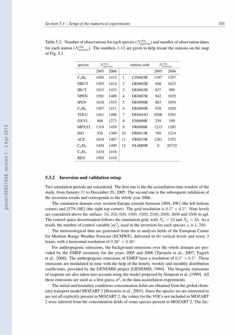
Section 5.3 – Setup of the numerical experiments 101
Table 5.2: Number of observations for each species (Nobsspecies) and number of observation dates
for each station (Nobsstation). The numbers 1-12 are given to help locate the stations on the map
of Fig. 5.1.
species Nobsspecies station code Nobs
station
2005 2006 2005 2006
C3H8 1505 1415 1 CZ0003R 1397 1297
NBUT 1503 1414 2 DE0002R 948 1023
IBUT 1033 1453 3 DE0003R 837 990
NPEN 1501 1409 4 DE0007R 942 1029
IPEN 1610 1553 5 DE0008R 883 1054
C3H6 1497 1411 6 DE0009R 938 1020
TOLU 1441 1408 7 DE0043G 9206 9283
OXYL 868 1273 8 ES0009R 259 199
MPXYL 1318 1459 9 FR0008R 1215 1285
ISO 936 1309 10 FR0013R 769 1214
ACE 1034 1407 11 FR0015R 1281 1352
C2H6 1494 1409 12 NL0009R 0 26732
C2H4 1434 1416
BEN 1503 1410
5.3.2 Inversion and validation setup
Two simulation periods are considered. The first one is the the assimilation time window of thestudy, from January 11 to December 29, 2005. The second one is the subsequent validation ofthe inversion results and corresponds to the whole year 2006.
The simulation domain over western Europe extends between [40N, 8W] (the left bottomcorner) and [57N;18E] (the right top corner). The grid resolution is 0.5 × 0.5. Nine levelsare considered above the surface: 50, 250, 600, 1000, 1500, 2100, 2800, 3600 and 4500 m agl.The control space discretisation follows the simulation grid, with Nx = 52 and Ny = 34. As aresult, the number of control variable [αs]l used in the inversion for each species s, is 1, 768.
The meteorological data are generated from the re-analysis fields of the European Centrefor Medium Range Weather Forecast (ECMWF), delivered in 60 vertical levels and every 3hours, with a horizontal resolution of 0.36 × 0.36.
For anthropogenic emissions, the background emissions over the whole domain are pro-vided by the EMEP inventory for the years 2005 and 2006 [Tarrasón et al., 2007; Fagerliet al., 2008]. The anthropogenic emissions of EMEP have a resolution of 0.5 × 0.5. Theseemissions are modulated in time with the help of the hourly, weekly and monthly distributioncoefficients, provided by the GENEMIS project [GENEMIS, 1994]. The biogenic emissionsof isoprene are also taken into account using the model proposed by Simpson et al. [1999]. Allthese emissions are used as a first guess, eb, in the data assimilation experiments.
The initial and boundary conditions concentration fields are obtained from the global chem-istry transport model MOZART 2 [Horowitz et al., 2003]. Since the species we are interested inare not all explicitly present in MOZART 2, the values for the VOCs not included in MOZART2 were inferred from the concentration fields of some species present in MOZART 2. The fac-
past
el-0
0807
468,
ver
sion
1 -
3 Ap
r 201
3
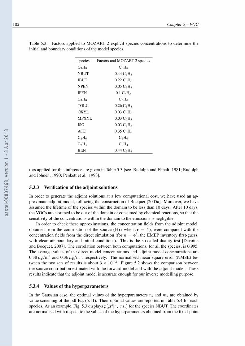
102 Chapter 5 – VOC
Table 5.3: Factors applied to MOZART 2 explicit species concentrations to determine theinitial and boundary conditions of the model species.
species Factors and MOZART 2 species
C3H8 C3H8
NBUT 0.44 C3H8
IBUT 0.22 C3H8
NPEN 0.05 C3H8
IPEN 0.1 C3H8
C3H6 C3H6
TOLU 0.26 C3H8
OXYL 0.03 C3H8
MPXYL 0.03 C3H8
ISO 0.03 C3H8
ACE 0.35 C3H8
C2H6 C2H6
C2H4 C2H4
BEN 0.44 C3H8
tors applied for this inference are given in Table 5.3 [see Rudolph and Ehhalt, 1981; Rudolphand Johnen, 1990; Penkett et al., 1993].
5.3.3 Verification of the adjoint solutions
In order to generate the adjoint solutions at a low computational cost, we have used an ap-proximate adjoint model, following the construction of Bocquet [2005a]. Moreover, we haveassumed the lifetime of the species within the domain to be less than 10 days. After 10 days,the VOCs are assumed to be out of the domain or consumed by chemical reactions, so that thesensitivity of the concentrations within the domain to the emissions is negligible.
In order to check these approximations, the concentration fields from the adjoint model,obtained from the contribution of the source (Hα when α = 1), were compared with theconcentration fields from the direct simulation (for e = eb, the EMEP inventory first-guess,with clean air boundary and initial conditions). This is the so-called duality test [Davoineand Bocquet, 2007]. The correlation between both computations, for all the species, is 0.995.The average values of the direct model concentrations and adjoint model concentrations are0.38 µg/m3 and 0.36 µg/m3, respectively. The normalised mean square error (NMSE) be-tween the two sets of results is about 3 × 10⁻³. Figure 5.2 shows the comparison betweenthe source contribution estimated with the forward model and with the adjoint model. Theseresults indicate that the adjoint model is accurate enough for our inverse modelling purpose.
5.3.4 Values of the hyperparameters
In the Gaussian case, the optimal values of the hyperparameters rs and ms are obtained byvalue screening of the pdf Eq. (5.11). Their optimal values are reported in Table 5.4 for eachspecies. As an example, Fig. 5.3 displays p(µs|rs, ms) for the species NBUT. The coordinatesare normalised with respect to the values of the hyperparameters obtained from the fixed-point
past
el-0
0807
468,
ver
sion
1 -
3 Ap
r 201
3
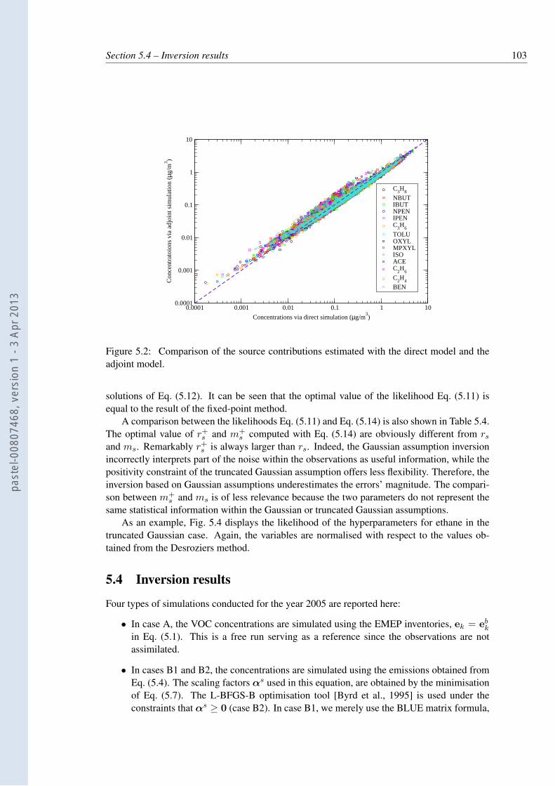
Section 5.4 – Inversion results 103
0.0001 0.001 0.01 0.1 1 10
Concentrations via direct simulation (µg/m3)
0.0001
0.001
0.01
0.1
1
10
Con
cent
rato
ions
via
adj
oint
sim
ulat
ion
(µg
/m3 )
C3H
8
NBUTIBUTNPENIPENC
3H
6
TOLUOXYLMPXYLISOACEC
2H
6
C2H
4
BEN
Figure 5.2: Comparison of the source contributions estimated with the direct model and theadjoint model.
solutions of Eq. (5.12). It can be seen that the optimal value of the likelihood Eq. (5.11) isequal to the result of the fixed-point method.
A comparison between the likelihoods Eq. (5.11) and Eq. (5.14) is also shown in Table 5.4.The optimal value of r+
s and m+s computed with Eq. (5.14) are obviously different from rs
and ms. Remarkably r+s is always larger than rs. Indeed, the Gaussian assumption inversion
incorrectly interprets part of the noise within the observations as useful information, while thepositivity constraint of the truncated Gaussian assumption offers less flexibility. Therefore, theinversion based on Gaussian assumptions underestimates the errors’ magnitude. The compari-son between m+
s and ms is of less relevance because the two parameters do not represent thesame statistical information within the Gaussian or truncated Gaussian assumptions.
As an example, Fig. 5.4 displays the likelihood of the hyperparameters for ethane in thetruncated Gaussian case. Again, the variables are normalised with respect to the values ob-tained from the Desroziers method.
5.4 Inversion results
Four types of simulations conducted for the year 2005 are reported here:
• In case A, the VOC concentrations are simulated using the EMEP inventories, ek = ebk
in Eq. (5.1). This is a free run serving as a reference since the observations are notassimilated.
• In cases B1 and B2, the concentrations are simulated using the emissions obtained fromEq. (5.4). The scaling factors αs used in this equation, are obtained by the minimisationof Eq. (5.7). The L-BFGS-B optimisation tool [Byrd et al., 1995] is used under theconstraints that αs ≥ 0 (case B2). In case B1, we merely use the BLUE matrix formula,
past
el-0
0807
468,
ver
sion
1 -
3 Ap
r 201
3
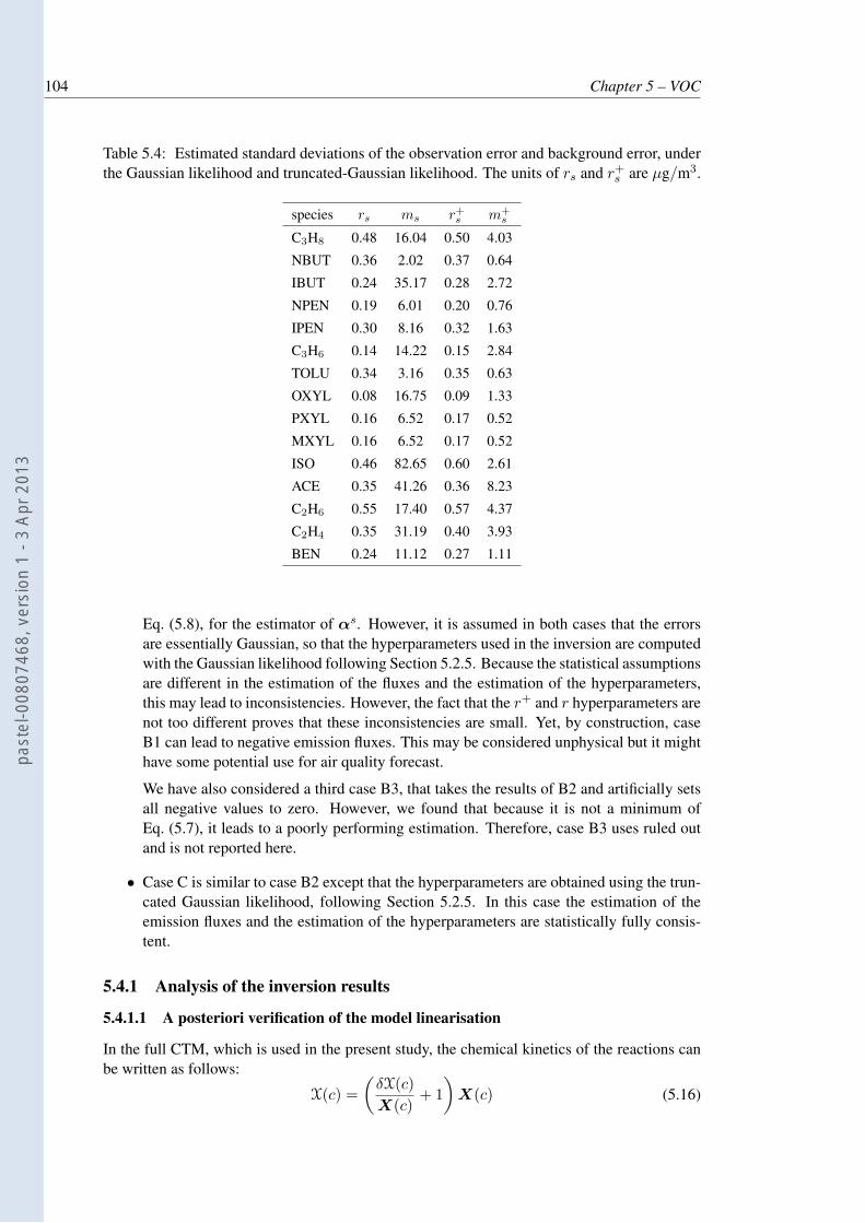
104 Chapter 5 – VOC
Table 5.4: Estimated standard deviations of the observation error and background error, underthe Gaussian likelihood and truncated-Gaussian likelihood. The units of rs and r+
s are µg/m3.
species rs ms r+s
m+s
C3H8 0.48 16.04 0.50 4.03
NBUT 0.36 2.02 0.37 0.64
IBUT 0.24 35.17 0.28 2.72
NPEN 0.19 6.01 0.20 0.76
IPEN 0.30 8.16 0.32 1.63
C3H6 0.14 14.22 0.15 2.84
TOLU 0.34 3.16 0.35 0.63
OXYL 0.08 16.75 0.09 1.33
PXYL 0.16 6.52 0.17 0.52
MXYL 0.16 6.52 0.17 0.52
ISO 0.46 82.65 0.60 2.61
ACE 0.35 41.26 0.36 8.23
C2H6 0.55 17.40 0.57 4.37
C2H4 0.35 31.19 0.40 3.93
BEN 0.24 11.12 0.27 1.11
Eq. (5.8), for the estimator of αs. However, it is assumed in both cases that the errorsare essentially Gaussian, so that the hyperparameters used in the inversion are computedwith the Gaussian likelihood following Section 5.2.5. Because the statistical assumptionsare different in the estimation of the fluxes and the estimation of the hyperparameters,this may lead to inconsistencies. However, the fact that the r+ and r hyperparameters arenot too different proves that these inconsistencies are small. Yet, by construction, caseB1 can lead to negative emission fluxes. This may be considered unphysical but it mighthave some potential use for air quality forecast.
We have also considered a third case B3, that takes the results of B2 and artificially setsall negative values to zero. However, we found that because it is not a minimum ofEq. (5.7), it leads to a poorly performing estimation. Therefore, case B3 uses ruled outand is not reported here.
• Case C is similar to case B2 except that the hyperparameters are obtained using the trun-cated Gaussian likelihood, following Section 5.2.5. In this case the estimation of theemission fluxes and the estimation of the hyperparameters are statistically fully consis-tent.
5.4.1 Analysis of the inversion results
5.4.1.1 A posteriori verification of the model linearisation
In the full CTM, which is used in the present study, the chemical kinetics of the reactions canbe written as follows:
X(c) =
(δX(c)
X(c)+ 1
)X(c) (5.16)
past
el-0
0807
468,
ver
sion
1 -
3 Ap
r 201
3
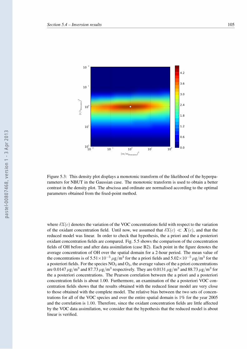
Section 5.4 – Inversion results 105
102
101
100
101
102
(m/mDesroziers)2
102
101
100
101
102
(r/r D
esroziers)
2
0.0
0.6
1.2
1.8
2.4
3.0
3.6
4.2
Figure 5.3: This density plot displays a monotonic transform of the likelihood of the hyperpa-rameters for NBUT in the Gaussian case. The monotonic transform is used to obtain a bettercontrast in the density plot. The abscissa and ordinate are normalised according to the optimalparameters obtained from the fixed-point method.
where δX(c) denotes the variation of the VOC concentrations field with respect to the variationof the oxidant concentration field. Until now, we assumed that δX(c) ≪ X(c), and that thereduced model was linear. In order to check that hypothesis, the a priori and the a posteriorioxidant concentration fields are compared. Fig. 5.5 shows the comparison of the concentrationfields of OH before and after data assimilation (case B2). Each point in the figure denotes theaverage concentration of OH over the spatial domain for a 2-hour period. The mean value ofthe concentrations is of 5.51×10⁻⁵ µg/m3 for the a priori fields and 5.02×10⁻⁵ µg/m3 for thea posteriori fields. For the species NO3 and O3, the average values of the a priori concentrationsare 0.0147 µg/m3 and 87.73 µg/m3 respectively. They are 0.0131 µg/m3 and 88.73 µg/m3 forthe a posteriori concentrations. The Pearson correlation between the a priori and a posterioriconcentration fields is about 1.00. Furthermore, an examination of the a posteriori VOC con-centration fields shows that the results obtained with the reduced linear model are very closeto those obtained with the complete model. The relative bias between the two sets of concen-trations for all of the VOC species and over the entire spatial domain is 1% for the year 2005and the correlation is 1.00. Therefore, since the oxidant concentration fields are little affectedby the VOC data assimilation, we consider that the hypothesis that the reduced model is aboutlinear is verified.
past
el-0
0807
468,
ver
sion
1 -
3 Ap
r 201
3
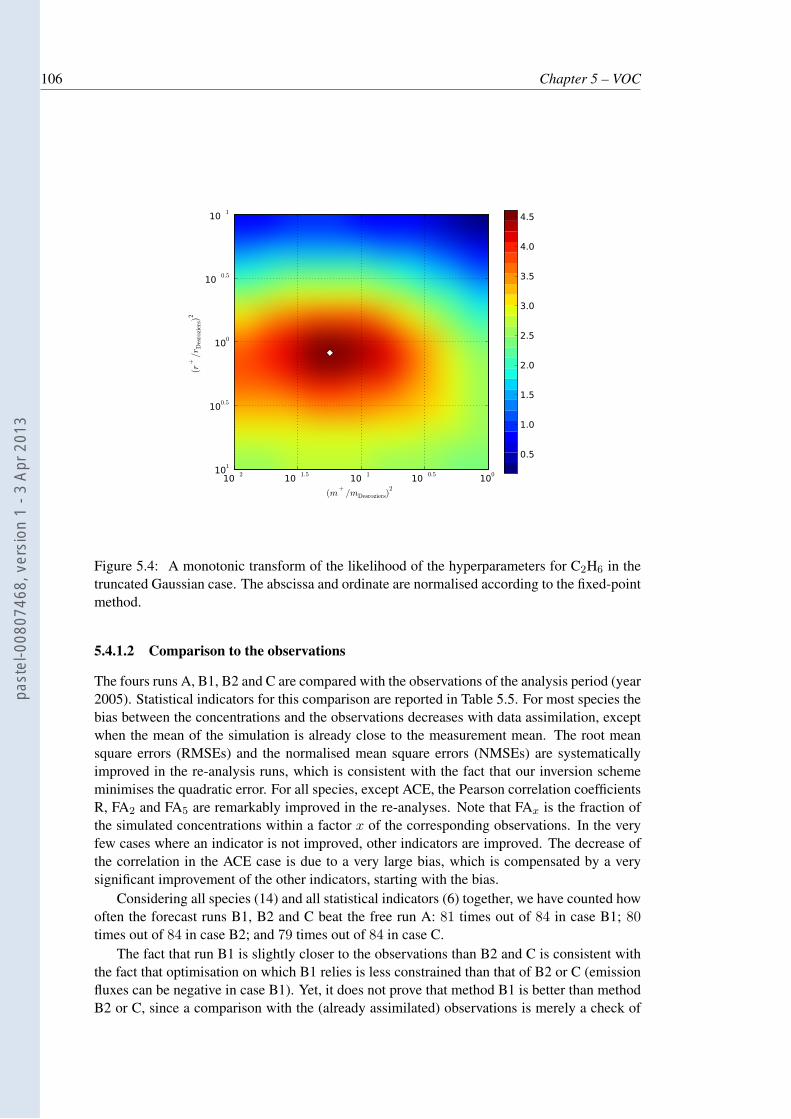
106 Chapter 5 – VOC
102
101.5
101
100.5
100
(m+/mDesroziers)
2
101
100.510
0
100.5
101
(r+/r D
esroziers)2
0.5
1.0
1.5
2.0
2.5
3.0
3.5
4.0
4.5
Figure 5.4: A monotonic transform of the likelihood of the hyperparameters for C2H6 in thetruncated Gaussian case. The abscissa and ordinate are normalised according to the fixed-pointmethod.
5.4.1.2 Comparison to the observations
The fours runs A, B1, B2 and C are compared with the observations of the analysis period (year2005). Statistical indicators for this comparison are reported in Table 5.5. For most species thebias between the concentrations and the observations decreases with data assimilation, exceptwhen the mean of the simulation is already close to the measurement mean. The root meansquare errors (RMSEs) and the normalised mean square errors (NMSEs) are systematicallyimproved in the re-analysis runs, which is consistent with the fact that our inversion schememinimises the quadratic error. For all species, except ACE, the Pearson correlation coefficientsR, FA2 and FA5 are remarkably improved in the re-analyses. Note that FAx is the fraction ofthe simulated concentrations within a factor x of the corresponding observations. In the veryfew cases where an indicator is not improved, other indicators are improved. The decrease ofthe correlation in the ACE case is due to a very large bias, which is compensated by a verysignificant improvement of the other indicators, starting with the bias.
Considering all species (14) and all statistical indicators (6) together, we have counted howoften the forecast runs B1, B2 and C beat the free run A: 81 times out of 84 in case B1; 80times out of 84 in case B2; and 79 times out of 84 in case C.
The fact that run B1 is slightly closer to the observations than B2 and C is consistent withthe fact that optimisation on which B1 relies is less constrained than that of B2 or C (emissionfluxes can be negative in case B1). Yet, it does not prove that method B1 is better than methodB2 or C, since a comparison with the (already assimilated) observations is merely a check of
past
el-0
0807
468,
ver
sion
1 -
3 Ap
r 201
3
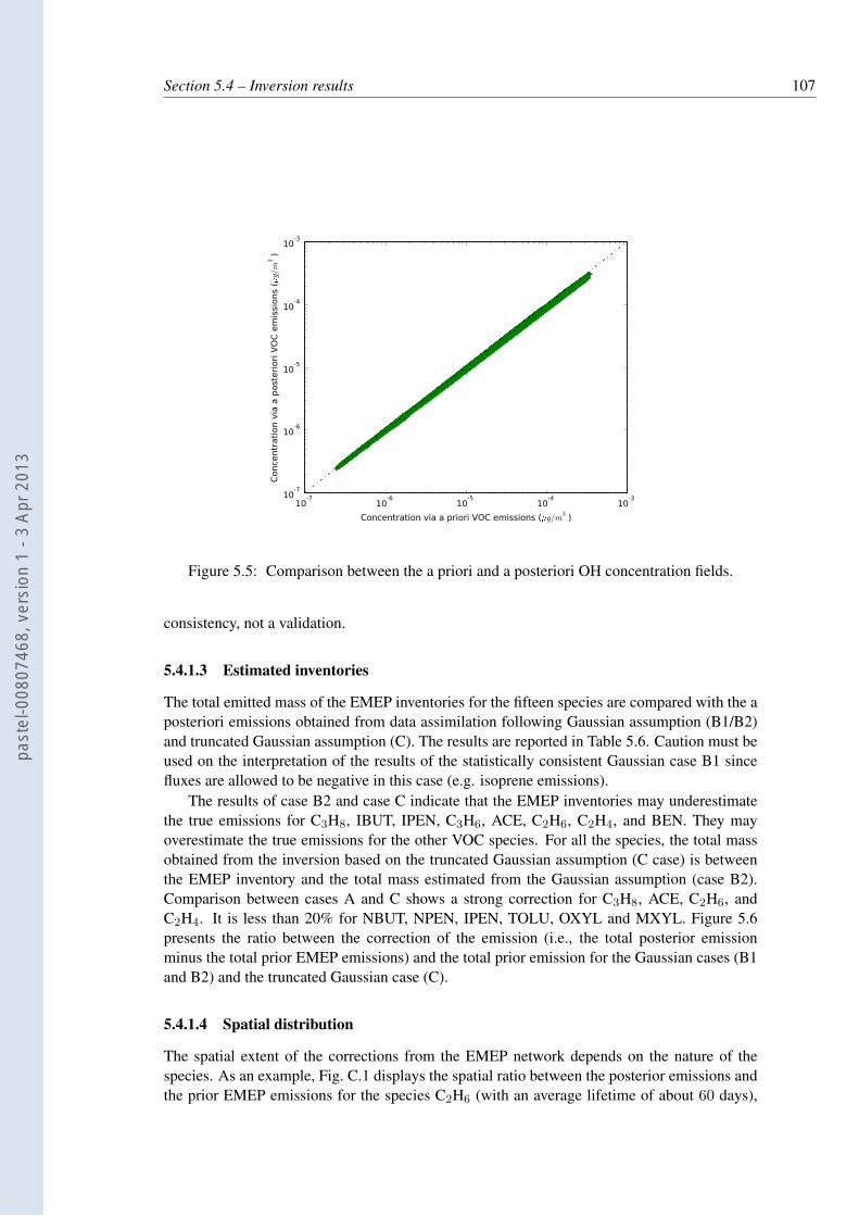
Section 5.4 – Inversion results 107
10-7
10-6
10-5
10-4
10-3
Concentration via a priori VOC emissions (g/m3)
10-7
10-6
10-5
10-4
10-3
Conce
ntr
ati
on v
ia a
post
eri
ori
VO
C e
mis
sions
(g/m3
)
Figure 5.5: Comparison between the a priori and a posteriori OH concentration fields.
consistency, not a validation.
5.4.1.3 Estimated inventories
The total emitted mass of the EMEP inventories for the fifteen species are compared with the aposteriori emissions obtained from data assimilation following Gaussian assumption (B1/B2)and truncated Gaussian assumption (C). The results are reported in Table 5.6. Caution must beused on the interpretation of the results of the statistically consistent Gaussian case B1 sincefluxes are allowed to be negative in this case (e.g. isoprene emissions).
The results of case B2 and case C indicate that the EMEP inventories may underestimatethe true emissions for C3H8, IBUT, IPEN, C3H6, ACE, C2H6, C2H4, and BEN. They mayoverestimate the true emissions for the other VOC species. For all the species, the total massobtained from the inversion based on the truncated Gaussian assumption (C case) is betweenthe EMEP inventory and the total mass estimated from the Gaussian assumption (case B2).Comparison between cases A and C shows a strong correction for C3H8, ACE, C2H6, andC2H4. It is less than 20% for NBUT, NPEN, IPEN, TOLU, OXYL and MXYL. Figure 5.6presents the ratio between the correction of the emission (i.e., the total posterior emissionminus the total prior EMEP emissions) and the total prior emission for the Gaussian cases (B1and B2) and the truncated Gaussian case (C).
5.4.1.4 Spatial distribution
The spatial extent of the corrections from the EMEP network depends on the nature of thespecies. As an example, Fig. C.1 displays the spatial ratio between the posterior emissions andthe prior EMEP emissions for the species C2H6 (with an average lifetime of about 60 days),
past
el-0
0807
468,
ver
sion
1 -
3 Ap
r 201
3
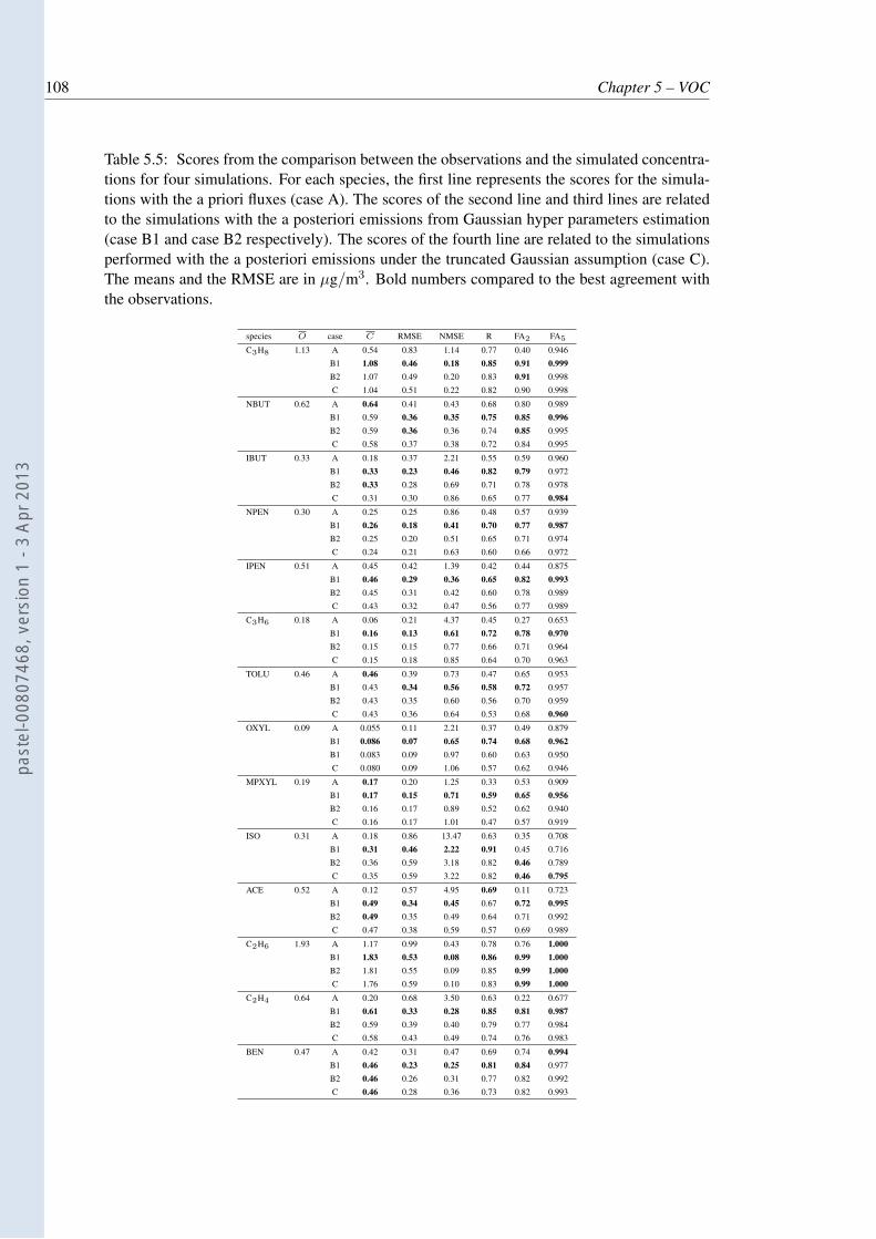
108 Chapter 5 – VOC
Table 5.5: Scores from the comparison between the observations and the simulated concentra-tions for four simulations. For each species, the first line represents the scores for the simula-tions with the a priori fluxes (case A). The scores of the second line and third lines are relatedto the simulations with the a posteriori emissions from Gaussian hyper parameters estimation(case B1 and case B2 respectively). The scores of the fourth line are related to the simulationsperformed with the a posteriori emissions under the truncated Gaussian assumption (case C).The means and the RMSE are in µg/m3. Bold numbers compared to the best agreement withthe observations.
species O case C RMSE NMSE R FA2 FA5
C3H8 1.13 A 0.54 0.83 1.14 0.77 0.40 0.946
B1 1.08 0.46 0.18 0.85 0.91 0.999
B2 1.07 0.49 0.20 0.83 0.91 0.998
C 1.04 0.51 0.22 0.82 0.90 0.998
NBUT 0.62 A 0.64 0.41 0.43 0.68 0.80 0.989
B1 0.59 0.36 0.35 0.75 0.85 0.996
B2 0.59 0.36 0.36 0.74 0.85 0.995
C 0.58 0.37 0.38 0.72 0.84 0.995
IBUT 0.33 A 0.18 0.37 2.21 0.55 0.59 0.960
B1 0.33 0.23 0.46 0.82 0.79 0.972
B2 0.33 0.28 0.69 0.71 0.78 0.978
C 0.31 0.30 0.86 0.65 0.77 0.984
NPEN 0.30 A 0.25 0.25 0.86 0.48 0.57 0.939
B1 0.26 0.18 0.41 0.70 0.77 0.987
B2 0.25 0.20 0.51 0.65 0.71 0.974
C 0.24 0.21 0.63 0.60 0.66 0.972
IPEN 0.51 A 0.45 0.42 1.39 0.42 0.44 0.875
B1 0.46 0.29 0.36 0.65 0.82 0.993
B2 0.45 0.31 0.42 0.60 0.78 0.989
C 0.43 0.32 0.47 0.56 0.77 0.989
C3H6 0.18 A 0.06 0.21 4.37 0.45 0.27 0.653
B1 0.16 0.13 0.61 0.72 0.78 0.970
B2 0.15 0.15 0.77 0.66 0.71 0.964
C 0.15 0.18 0.85 0.64 0.70 0.963
TOLU 0.46 A 0.46 0.39 0.73 0.47 0.65 0.953
B1 0.43 0.34 0.56 0.58 0.72 0.957
B2 0.43 0.35 0.60 0.56 0.70 0.959
C 0.43 0.36 0.64 0.53 0.68 0.960
OXYL 0.09 A 0.055 0.11 2.21 0.37 0.49 0.879
B1 0.086 0.07 0.65 0.74 0.68 0.962
B1 0.083 0.09 0.97 0.60 0.63 0.950
C 0.080 0.09 1.06 0.57 0.62 0.946
MPXYL 0.19 A 0.17 0.20 1.25 0.33 0.53 0.909
B1 0.17 0.15 0.71 0.59 0.65 0.956
B2 0.16 0.17 0.89 0.52 0.62 0.940
C 0.16 0.17 1.01 0.47 0.57 0.919
ISO 0.31 A 0.18 0.86 13.47 0.63 0.35 0.708
B1 0.31 0.46 2.22 0.91 0.45 0.716
B2 0.36 0.59 3.18 0.82 0.46 0.789
C 0.35 0.59 3.22 0.82 0.46 0.795
ACE 0.52 A 0.12 0.57 4.95 0.69 0.11 0.723
B1 0.49 0.34 0.45 0.67 0.72 0.995
B2 0.49 0.35 0.49 0.64 0.71 0.992
C 0.47 0.38 0.59 0.57 0.69 0.989
C2H6 1.93 A 1.17 0.99 0.43 0.78 0.76 1.000
B1 1.83 0.53 0.08 0.86 0.99 1.000
B2 1.81 0.55 0.09 0.85 0.99 1.000
C 1.76 0.59 0.10 0.83 0.99 1.000
C2H4 0.64 A 0.20 0.68 3.50 0.63 0.22 0.677
B1 0.61 0.33 0.28 0.85 0.81 0.987
B2 0.59 0.39 0.40 0.79 0.77 0.984
C 0.58 0.43 0.49 0.74 0.76 0.983
BEN 0.47 A 0.42 0.31 0.47 0.69 0.74 0.994
B1 0.46 0.23 0.25 0.81 0.84 0.977
B2 0.46 0.26 0.31 0.77 0.82 0.992
C 0.46 0.28 0.36 0.73 0.82 0.993
past
el-0
0807
468,
ver
sion
1 -
3 Ap
r 201
3
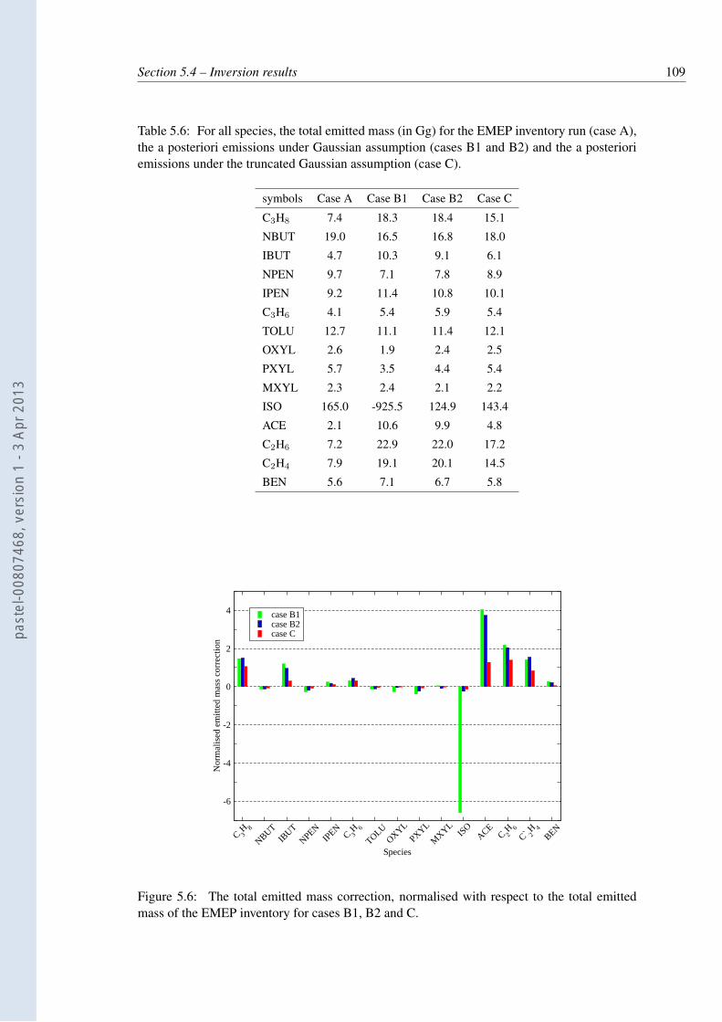
Section 5.4 – Inversion results 109
Table 5.6: For all species, the total emitted mass (in Gg) for the EMEP inventory run (case A),the a posteriori emissions under Gaussian assumption (cases B1 and B2) and the a posterioriemissions under the truncated Gaussian assumption (case C).
symbols Case A Case B1 Case B2 Case C
C3H8 7.4 18.3 18.4 15.1
NBUT 19.0 16.5 16.8 18.0
IBUT 4.7 10.3 9.1 6.1
NPEN 9.7 7.1 7.8 8.9
IPEN 9.2 11.4 10.8 10.1
C3H6 4.1 5.4 5.9 5.4
TOLU 12.7 11.1 11.4 12.1
OXYL 2.6 1.9 2.4 2.5
PXYL 5.7 3.5 4.4 5.4
MXYL 2.3 2.4 2.1 2.2
ISO 165.0 -925.5 124.9 143.4
ACE 2.1 10.6 9.9 4.8
C2H6 7.2 22.9 22.0 17.2
C2H4 7.9 19.1 20.1 14.5
BEN 5.6 7.1 6.7 5.8
C 3H 8
NBUTIB
UTNPEN
IPEN
C 3H 6
TOLUOXYL
PXYL
MXYL
ISO
ACEC 2
H 6
C` 2H 4
BEN
Species
-6
-4
-2
0
2
4
Nor
mal
ised
em
itted
mas
s co
rrec
tion
case B1case B2case C
Figure 5.6: The total emitted mass correction, normalised with respect to the total emittedmass of the EMEP inventory for cases B1, B2 and C.
past
el-0
0807
468,
ver
sion
1 -
3 Ap
r 201
3
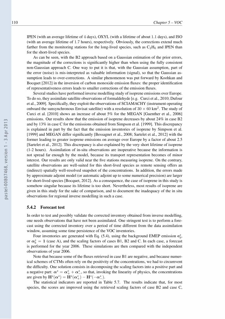
110 Chapter 5 – VOC
IPEN (with an average lifetime of 4 days), OXYL (with a lifetime of about 1.1 days), and ISO(with an average lifetime of 1.7 hours), respectively. Obviously, the corrections extend muchfarther from the monitoring stations for the long-lived species, such as C2H6 and IPEN thanfor the short-lived species.
As can be seen, with the B2 approach based on a Gaussian estimation of the prior errors,the magnitude of the corrections is significantly higher than when using the fully consistentnon-Gaussian approach C. One way to put it is that, with the Gaussian assumption, part ofthe error (noise) is mis-interpreted as valuable information (signal), so that the Gaussian as-sumption leads to over-corrections. A similar phenomenon was put forward by Koohkan andBocquet [2012] in the inversion of carbon monoxide emission fluxes: the proper identificationof representativeness errors leads to smaller corrections of the emission fluxes.
Several studies have performed inverse modelling study of isoprene emissions over Europe.To do so, they assimilate satellite observations of formaldehyde [e.g. Curci et al., 2010; Dufouret al., 2009]. Specifically, they exploit the observations of SCIAMACHY (instrument operatingonboard the sunsynchronous Envisat satellite) with a resolution of 30 × 60 km2. The study ofCurci et al. [2010] shows an increase of about 5% for the MEGAN [Guenther et al., 2006]emissions. Our results show that the emission of isoprene decreases by about 24% in case B2and by 13% in case C for the emissions obtained from Simpson et al. [1999]. This discrepancyis explained in part by the fact that the emission inventories of isoprene by Simpson et al.[1999] and MEGAN differ significantly [Bessagnet et al., 2008; Sartelet et al., 2012] with theformer leading to greater isoprene emissions on average over Europe by a factor of about 2.5[Sartelet et al., 2012]. This discrepancy is also explained by the very short lifetime of isoprene(1-2 hours). Assimilation of in-situ observations are inoperative because the information isnot spread far enough by the model, because its transport representation becomes of minorinterest. Our results are only valid near the five stations measuring isoprene. On the contrary,satellite observations are well-suited for this short-lived species as remote sensing offers an(indirect) spatially well-resolved snapshot of the concentrations. In addition, the errors madeby approximate adjoint model (or automatic adjoint up to some numerical precision) are largerfor short-lived species [Bocquet, 2012]. As a consequence, the case of isoprene in this study issomehow singular because its lifetime is too short. Nevertheless, most results of isoprene aregiven in this study for the sake of comparison, and to document the inadequacy of the in situobservations for regional inverse modelling in such a case.
5.4.2 Forecast test
In order to test and possibly validate the corrected inventory obtained from inverse modelling,one needs observations that have not been assimilated. One stringent test is to perform a fore-cast using the corrected inventory over a period of time different from the data assimilationwindow, assuming some time persistence of the VOC inventories.
Four inventories are generated with Eq. (5.4), using the background EMEP emission esb,
or αsb = 1 (case A), and the scaling factors of cases B1, B2 and C. In each case, a forecast
is performed for the year 2006. These simulations are then compared with the independentobservations of year 2006.
Note that because some of the fluxes retrieved in case B1 are negative, and because numer-ical schemes of CTMs often rely on the positivity of the concentrations, we had to circumventthe difficulty. One solution consists in decomposing the scaling factors into a positive part anda negative part: αs = αs
+ + αs−, so that, invoking the linearity of physics, the concentrations
are given by Hs(αs) = Hs(αs+) − Hs(−αs
−).The statistical indicators are reported in Table 5.7. The results indicate that, for most
species, the scores are improved using the retrieved scaling factors of case B2 and case C,
past
el-0
0807
468,
ver
sion
1 -
3 Ap
r 201
3
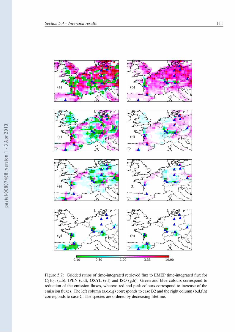
Section 5.4 – Inversion results 111
(a)
0.10 0.30 1.00 3.33 10.00
(b)
(c) (d)
(e) (f)
(g) (h)
Figure 5.7: Gridded ratios of time-integrated retrieved flux to EMEP time-integrated flux forC2H6, (a,b), IPEN (c,d), OXYL (e,f) and ISO (g,h). Green and blue colours correspond toreduction of the emission fluxes, whereas red and pink colours correspond to increase of theemission fluxes. The left column (a,c,e,g) corresponds to case B2 and the right column (b,d,f,h)corresponds to case C. The species are ordered by decreasing lifetime.
past
el-0
0807
468,
ver
sion
1 -
3 Ap
r 201
3
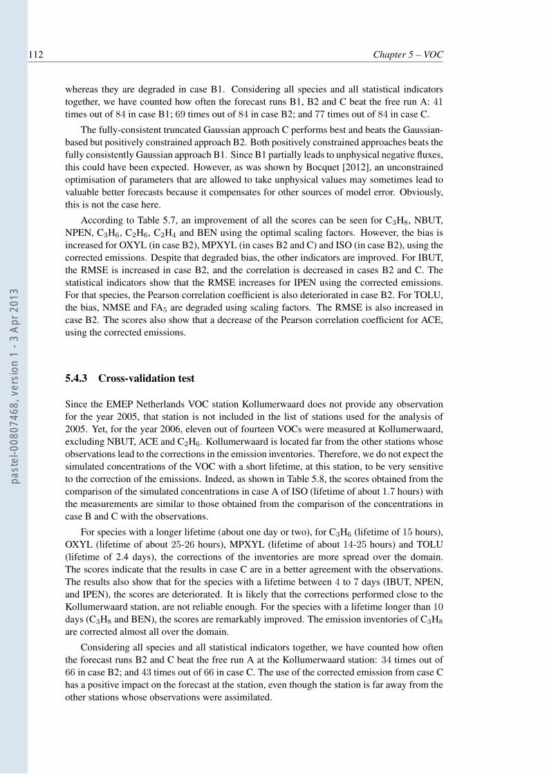
112 Chapter 5 – VOC
whereas they are degraded in case B1. Considering all species and all statistical indicatorstogether, we have counted how often the forecast runs B1, B2 and C beat the free run A: 41times out of 84 in case B1; 69 times out of 84 in case B2; and 77 times out of 84 in case C.
The fully-consistent truncated Gaussian approach C performs best and beats the Gaussian-based but positively constrained approach B2. Both positively constrained approaches beats thefully consistently Gaussian approach B1. Since B1 partially leads to unphysical negative fluxes,this could have been expected. However, as was shown by Bocquet [2012], an unconstrainedoptimisation of parameters that are allowed to take unphysical values may sometimes lead tovaluable better forecasts because it compensates for other sources of model error. Obviously,this is not the case here.
According to Table 5.7, an improvement of all the scores can be seen for C3H8, NBUT,NPEN, C3H6, C2H6, C2H4 and BEN using the optimal scaling factors. However, the bias isincreased for OXYL (in case B2), MPXYL (in cases B2 and C) and ISO (in case B2), using thecorrected emissions. Despite that degraded bias, the other indicators are improved. For IBUT,the RMSE is increased in case B2, and the correlation is decreased in cases B2 and C. Thestatistical indicators show that the RMSE increases for IPEN using the corrected emissions.For that species, the Pearson correlation coefficient is also deteriorated in case B2. For TOLU,the bias, NMSE and FA5 are degraded using scaling factors. The RMSE is also increased incase B2. The scores also show that a decrease of the Pearson correlation coefficient for ACE,using the corrected emissions.
5.4.3 Cross-validation test
Since the EMEP Netherlands VOC station Kollumerwaard does not provide any observationfor the year 2005, that station is not included in the list of stations used for the analysis of2005. Yet, for the year 2006, eleven out of fourteen VOCs were measured at Kollumerwaard,excluding NBUT, ACE and C2H6. Kollumerwaard is located far from the other stations whoseobservations lead to the corrections in the emission inventories. Therefore, we do not expect thesimulated concentrations of the VOC with a short lifetime, at this station, to be very sensitiveto the correction of the emissions. Indeed, as shown in Table 5.8, the scores obtained from thecomparison of the simulated concentrations in case A of ISO (lifetime of about 1.7 hours) withthe measurements are similar to those obtained from the comparison of the concentrations incase B and C with the observations.
For species with a longer lifetime (about one day or two), for C3H6 (lifetime of 15 hours),OXYL (lifetime of about 25-26 hours), MPXYL (lifetime of about 14-25 hours) and TOLU(lifetime of 2.4 days), the corrections of the inventories are more spread over the domain.The scores indicate that the results in case C are in a better agreement with the observations.The results also show that for the species with a lifetime between 4 to 7 days (IBUT, NPEN,and IPEN), the scores are deteriorated. It is likely that the corrections performed close to theKollumerwaard station, are not reliable enough. For the species with a lifetime longer than 10days (C3H8 and BEN), the scores are remarkably improved. The emission inventories of C3H8
are corrected almost all over the domain.
Considering all species and all statistical indicators together, we have counted how oftenthe forecast runs B2 and C beat the free run A at the Kollumerwaard station: 34 times out of66 in case B2; and 43 times out of 66 in case C. The use of the corrected emission from case Chas a positive impact on the forecast at the station, even though the station is far away from theother stations whose observations were assimilated.
past
el-0
0807
468,
ver
sion
1 -
3 Ap
r 201
3
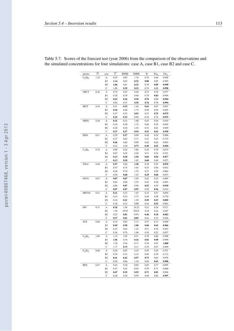
Section 5.4 – Inversion results 113
Table 5.7: Scores of the forecast test (year 2006) from the comparison of the observations andthe simulated concentrations for four simulations: case A, case B1, case B2 and case C.
species O case C RMSE NMSE R FA2 FA5
C3H8 1.10 A 0.55 0.85 1.19 0.76 0.46 0.958
B1 1.14 0.63 0.32 0.80 0.85 0.992
B2 1.06 0.61 0.32 0.78 0.89 0.998
C 1.00 0.59 0.32 0.79 0.88 0.998
NBUT 0.56 A 0.75 0.45 0.49 0.72 0.70 0.977
B1 0.38 0.39 0.40 0.78 0.83 0.994
B2 0.62 0.36 0.38 0.76 0.80 0.994
C 0.65 0.37 0.38 0.76 0.79 0.994
IBUT 0.34 A 0.21 0.33 1.46 0.61 0.67 0.967
B1 0.36 0.46 1.73 0.49 0.56 0.825
B2 0.37 0.35 0.93 0.55 0.75 0.975
C 0.32 0.33 0.98 0.54 0.74 0.975
NPEN 0.29 A 0.31 0.31 1.08 0.45 0.56 0.919
B1 0.18 0.30 1.72 0.48 0.39 0.692
B2 0.26 0.28 1.03 0.51 0.61 0.949
C 0.27 0.27 0.94 0.52 0.62 0.950
IPEN 0.47 A 0.29 0.37 0.99 0.49 0.54 0.906
B1 0.37 0.62 2.17 0.31 0.43 0.733
B2 0.46 0.46 0.99 0.42 0.64 0.963
C 0.42 0.38 0.73 0.49 0.65 0.969
C3H6 0.19 A 0.08 0.24 3.86 0.44 0.39 0.674
B1 0.07 0.24 4.40 0.51 0.24 0.521
B2 0.13 0.20 1.58 0.60 0.50 0.877
C 0.13 0.20 1.62 0.60 0.49 0.873
TOLU 0.66 A 0.57 0.69 1.28 0.28 0.55 0.876
B1 0.47 0.73 1.65 0.25 0.56 0.852
B2 0.48 0.70 1.55 0.27 0.58 0.864
C 0.50 0.68 1.42 0.29 0.60 0.875
OXYL 0.07 A 0.07 0.07 1.05 0.42 0.54 0.885
B1 0.04 0.08 2.35 0.42 0.36 0.693
B2 0.06 0.07 0.98 0.52 0.54 0.918
C 0.07 0.07 0.95 0.50 0.56 0.910
MPXYL 0.21 A 0.21 0.25 1.45 0.32 0.51 0.856
B1 0.10 0.23 2.73 0.49 0.38 0.720
B2 0.16 0.21 1.38 0.50 0.53 0.885
C 0.18 0.22 1.33 0.44 0.53 0.863
ISO 0.31 A 0.35 1.04 10.25 0.21 0.26 0.571
B1 1.39 19.95 939.9 -0.18 0.16 0.287
B2 0.25 0.81 8.59 0.46 0.34 0.682
C 0.27 0.81 8.05 0.44 0.33 0.656
ACE 0.68 A 0.14 0.83 7.17 0.57 0.17 0.649
B1 0.49 0.58 1.00 0.60 0.63 0.966
B2 0.47 0.62 1.22 0.51 0.54 0.952
C 0.36 0.70 1.98 0.39 0.52 0.837
C2H6 1.89 A 1.15 1.05 0.51 0.78 0.80 0.998
B1 1.96 0.76 0.16 0.81 0.98 0.999
B2 1.78 0.76 0.17 0.78 0.97 1.000
C 1.71 0.75 0.17 0.79 0.97 0.999
C2H4 0.66 A 0.26 0.87 4.43 0.59 0.36 0.751
B1 0.39 0.74 2.15 0.65 0.39 0.713
B2 0.61 0.62 0.97 0.73 0.64 0.978
C 0.56 0.66 1.18 0.69 0.65 0.980
BEN 0.47 A 0.44 0.38 0.69 0.65 0.77 0.995
B1 0.57 0.42 0.65 0.70 0.71 0.966
B2 0.47 0.35 0.55 0.71 0.81 0.994
C 0.46 0.36 0.59 0.69 0.80 0.997
past
el-0
0807
468,
ver
sion
1 -
3 Ap
r 201
3

114 Chapter 5 – VOC
Table 5.8: Scores at the Kollumerwaard station (for the year 2006) from the comparison of theobservations and the simulated concentrations for three simulations: case A, case B2 and caseC.
species case O C RMSE NMSE R FA2 FA5
A 0.82 2.12 3.24 0.05 0.39 0.799
C3H8 B2 1.69 0.97 1.81 2.08 0.43 0.63 0.936
C 0.81 1.87 2.56 0.47 0.56 0.932
A 0.44 0.33 1.32 0.54 0.60 0.868
IBUT B2 0.33 0.41 0.39 1.19 0.34 0.60 0.927
C 0.36 0.34 0.98 0.37 0.62 0.948
A 0.28 0.42 1.53 0.52 0.50 0.899
NPEN B2 0.42 0.18 0.48 2.99 0.48 0.45 0.859
C 0.23 0.44 2.00 0.53 0.52 0.917
A 0.43 0.59 1.32 0.20 0.48 0.868
IPEN B2 0.61 0.37 0.63 2.04 0.13 0.41 0.770
C 0.33 0.65 1.75 0.12 0.36 0.814
A 0.08 0.30 6.10 0.65 0.36 0.719
C3H6 B2 0.17 0.14 0.26 2.79 0.63 0.44 0.780
C 0.13 0.26 2.97 0.66 0.39 0.734
A 0.52 0.43 0.68 0.48 0.67 0.886
TOLU B2 0.53 0.35 0.35 0.64 0.72 0.61 0.937
C 0.39 0.33 0.52 0.73 0.67 0.942
A 0.06 0.10 1.51 0.52 0.39 0.847
OXYL B2 0.11 0.05 0.10 1.76 0.59 0.36 0.818
C 0.06 0.09 1.58 0.60 0.38 0.829
A 0.15 0.22 1.44 0.72 0.39 0.881
MPXYL B2 0.22 0.11 0.23 2.26 0.75 0.36 0.875
C 0.14 0.21 1.48 0.75 0.38 0.888
A 0.05 0.35 14.3 0.33 0.19 0.445
ISO B2 0.18 0.05 0.35 13.29 0.32 0.20 0.463
C 0.05 0.35 13.29 0.32 0.20 0.463
A 0.14 0.44 4.33 0.57 0.24 0.609
C2H4 B2 0.18 0.17 0.45 3.58 0.44 0.33 0.691
C 0.20 0.40 2.42 0.55 0.31 0.662
A 0.54 0.83 2.92 0.00 0.48 0.772
BEN B2 0.44 0.24 0.67 4.26 0.23 0.43 0.816
C 0.30 0.65 3.25 0.27 0.52 0.869
past
el-0
0807
468,
ver
sion
1 -
3 Ap
r 201
3
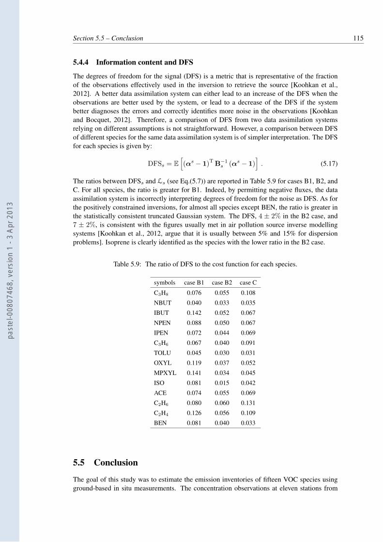
Section 5.5 – Conclusion 115
5.4.4 Information content and DFS
The degrees of freedom for the signal (DFS) is a metric that is representative of the fractionof the observations effectively used in the inversion to retrieve the source [Koohkan et al.,2012]. A better data assimilation system can either lead to an increase of the DFS when theobservations are better used by the system, or lead to a decrease of the DFS if the systembetter diagnoses the errors and correctly identifies more noise in the observations [Koohkanand Bocquet, 2012]. Therefore, a comparison of DFS from two data assimilation systemsrelying on different assumptions is not straightforward. However, a comparison between DFSof different species for the same data assimilation system is of simpler interpretation. The DFSfor each species is given by:
DFSs = E
[(αs − 1)T B−1
s (αs − 1)]
. (5.17)
The ratios between DFSs and Ls (see Eq.(5.7)) are reported in Table 5.9 for cases B1, B2, andC. For all species, the ratio is greater for B1. Indeed, by permitting negative fluxes, the dataassimilation system is incorrectly interpreting degrees of freedom for the noise as DFS. As forthe positively constrained inversions, for almost all species except BEN, the ratio is greater inthe statistically consistent truncated Gaussian system. The DFS, 4 ± 2% in the B2 case, and7 ± 2%, is consistent with the figures usually met in air pollution source inverse modellingsystems [Koohkan et al., 2012, argue that it is usually between 5% and 15% for dispersionproblems]. Isoprene is clearly identified as the species with the lower ratio in the B2 case.
Table 5.9: The ratio of DFS to the cost function for each species.
symbols case B1 case B2 case C
C3H8 0.076 0.055 0.108
NBUT 0.040 0.033 0.035
IBUT 0.142 0.052 0.067
NPEN 0.088 0.050 0.067
IPEN 0.072 0.044 0.069
C3H6 0.067 0.040 0.091
TOLU 0.045 0.030 0.031
OXYL 0.119 0.037 0.052
MPXYL 0.141 0.034 0.045
ISO 0.081 0.015 0.042
ACE 0.074 0.055 0.069
C2H6 0.080 0.060 0.131
C2H4 0.126 0.056 0.109
BEN 0.081 0.040 0.033
5.5 Conclusion
The goal of this study was to estimate the emission inventories of fifteen VOC species usingground-based in situ measurements. The concentration observations at eleven stations from
past
el-0
0807
468,
ver
sion
1 -
3 Ap
r 201
3
116 Chapter 5 – VOC
the EMEP network over western Europe were assimilated to perform inverse modelling of theemission field for each one of the fifteen species, for the year 2005.
For that purpose, the Jacobian matrix, i.e., the source-receptor relationship, was built us-ing the POLAIR3D CTM. To compute that matrix, a fast version of this CTM, as well as itsvalidated approximate adjoint model have been developed. The chemistry module of this fastversion only includes the chemical reactions between the VOC species and three oxidants (OH,NO3 and O3), the concentrations of which are pre-computed with the full CTM.
For each species and each grid cell, a scaling factor that multiplies the local EMEP emissionflux, is computed. The uncertainty attached to the prior scaling factors and the covariancematrix of the observation errors, which are crucial statistical components of the inversion, areobtained using the maximum likelihood principle. The principle was implemented using twodifferent assumptions: (1) the errors attached to the scaling factors follow a Gaussian pdf or (2)the scaling factor follows a truncated Gaussian pdf.
In the Gaussian case, the simulated concentrations for the year 2005 using the correctedemissions lead to a significant improvement in most statistical indicators. However the factthat the VOC fluxes are positive is not statistically accounted for, and this is shown to leadto a probable over-fitting to the observations, and to over-corrections of the EMEP emissions.Using a fully consistent truncated Gaussian assumption for the emission fluxes, including theuse of a non-Gaussian likelihood for the estimation of the hyperparameters, the corrections aresignificantly smaller.
For short-lived species, it is shown that information cannot propagate far from the moni-toring stations, so that the corrections are rather local to the stations. That is why we deem theisoprene inversion to be unreliable. That is a typical case where remote sensing assimilation isnecessary to offer a satisfying coverage.
The corrected emissions have been partly validated thanks to a forecast conducted for theyear 2006 using independent observations. The simulations using the corrected emissions oftenled to significant improvements in the statistical indicators. Considering all statistical indica-tors, the fully consistent truncated Gaussian approach emerged as the best approach from thistest.
The 2006 forecasts have also been compared to the observations at the Kollumerwaard sta-tion, the Netherlands. The Kollumerwaard station is not part of the 11 stations used in theanalysis of 2005. Even though this station is far away from the 2005 network, and its surround-ings fluxes little affected by the 2005 analysis, some improvements are noticed for severallong-lived VOC species using the statistically consistent positively constrained inversion.
past
el-0
0807
468,
ver
sion
1 -
3 Ap
r 201
3
Chapter 6
Summary and perspectives
6.1 Conclusion
This study introduces new applications of data assimilation in air quality modelling. It isdivided in three different studies for which a brief description is presented hereafter.
In the first part of this PhD thesis, an adjoint model to the chemistry transport model,as well as a 4D-Var routine are developed and validated. The 4D-Var routine developed isused to invert the carbon monoxide emissions. The data assimilation approach to correct theemission fields leading to a mild improvement only in the bias and the correlation (since it doesnot handle the representativeness issue), a simple statistical subgrid model is introduced andcoupled to the 4D-Var routine.
In a second part, data assimilation is used as a decision-making support in order to assessthe ability of a monitoring network (as a matter of fact, the International Monitoring Systemnetwork of radionuclides) to reconstruct accidental sources.
In the third and last part, the maximum likelihood method is used to assess the hyper-parameters of a cost function. In particular, that method is applied to invert the emissions ofVolatile Organic Compounds (VOCs).
6.1.1 Adjoint of chemistry transport model
The adjoint of the chemistry transport model based on the POLAIR3D Eulerian code ofPOLYPHEMUS is validated in four steps, using the duality test, involving one term of the equa-tion at a time (source terms of surface and volume emissions, initial and boundary conditions).The concentrations computed using the CTM and its adjoint model are in good agreement.The pearson coefficient is 99.8% when validating the surface and volume emission fields. Itis of 98.7% and 93% when validating the initial conditions and boundary conditions, respec-tively. This shows that the developed adjoint model is reliable enough as the errors it yields aremuch smaller than the modelling errors (departure between the observation and the simulatedconcentrations).
6.1.2 4D-Var algorithm
The 4D-Var algorithm, using the newly developed adjoint model, is validated with the help oftwo kinds of unity tests. In that aim, the gradient of the cost function computed within the4D-var subroutine is compared to the one computed with the finite difference method. The firsttest (perturbation) enabled to validate the gradient with respect to the emission fields and to theinitial conditions. The second test validated the gradient with respect to the control parameters(periodical scale factors of the emissions).
past
el-0
0807
468,
ver
sion
1 -
3 Ap
r 201
3
118 Chapter 6 – conclusion
6.1.3 Representativeness error and subgrid model
The stations of BDQA recording carbon monoxide concentrations are impacted by representa-tiveness errors. Comparisons between the observations and simulated concentrations show thatthe variability of the observations is much stronger than that of the simulated concentrations.The scores of a preliminary assimilation run via the 4D-Var method, for carbon monoxide andduring 8 weeks from January 1 2005, show that the consistency between the analysed concen-trations and the observations is low, in spite of a Pearson correlation coefficient increasing from0.16 to 0.36. The results also show that the 4D-Var method artificially over-estimates the totalemitted mass in the first 8 weeks of the year 2005. In order to take the representativeness issueinto account, which is an unresolved part of the model, a statistical subgrid model is developedand is coupled to the CTM. That new subgrid model provides a coefficient ξi to each stationi. This statistical coefficient ξi links the average of the variation of the representativeness errorto the variation of the emission inventories. The subgrid model in question, although simpleremoves an important part of the observation mismatch. The correlation between the observa-tions and the simulated results of the coupled model , 4D-Var-ξ, increases to 0.73. The biasbetween the simulated concentrations and the measurements is also eliminated using the 4D-Var-ξ algorithm. The amount of the total emitted mass of CO is computed either with 4D-Varand 4D-Var-ξ. That value is independent on the station locations for the network in case using4D-Var-ξ, while it is sensitive to the network when using 4D-Var. This results is consistentwith the one obtained from CITEPA.
This study shows that the 4D-Var system is not able to assess the emission fluxes of CTMfor the case in which in-situ measurements are impacted by the representativeness errors. Thatis why the estimation of representativeness errors is important for the assimilation of the mea-surements of the proximity stations.
6.1.4 Multiscale method data assimilation and application to network design
Beyond the detection capability of an observation network and the geostatistics approaches, itis crucial to evaluate the potential of a monitoring system for inverse modelling. To do so, mul-tiscale adaptative grids of the IMS radionuclide network sources are built and optimised underthe DFS criterion. The influence functions linked to the observations are generated using theLagrangian transport model FLEXPART (driven by ECMWF meteorological fields) over theyear 2009. The ratio DFS/d (d is the total number of observations), which is used to controlthe error of the a priori source and the modelling error (instrumental, representativeness andtransport model) is carried out for the system performance level. At each level of performace,the adaptative grids are optimised. The results of the optimisation show that the IMS radionu-clide network is not quite able to construct the source in the Intertropical Convergence Zone.In case of the large modelling errors, the system is not able to construct the sources far from theobservation point. Considering the realistic case where DFS/d is about 10%, the informationfrom many locations, such as African continent, cannot be sufficiently propageted.
The same test is performed for the noble gas network. The results of the realistic case showthat the network does not perform well enough to detect the informations coming from theIntertropical Convergence Zone, from the African continent and the central Asia.
6.1.5 Emission flux estimation for Volatile Organic Compounds
In this study, the method of data assimilation is used in order to estimate the emission fluxes offifteen Volatile Organic Compounds (five aromatics, six alkanes, two alkenes, one alkyne andone biogenic diene). To begin with, it can be notice that the results of the CTM simulation show
past
el-0
0807
468,
ver
sion
1 -
3 Ap
r 201
3
Section 6.2 – Outlook 119
the discrepancies between the computed concentrations and the ground-based observationsprovided by the European Monitoring and Evaluation Programme (EMEP) for the year 2005.Furthermore, the RACM 2 (Regional Atmospheric Chemistry Mechanism, version 2) chemicalkinetic mechanism used within this CTM and contains more than three hundreds reactions.The mentioned CTM is not fast enough. Therefore, a new version of that chemical kineticmechanism is built which uses pre-computed fields of oxidants (OH,NO3 and O3). The adjointof this fast CTM version is also developed and validated. As the concentrations of the computedVOCs change linearly with respect to the emission fluxes, the Jacobian matrix of the model canbe built to be used in inversion problems. In the present data assimilation system, the numberof the unknown variables (gridded emissions) is higher than the number of the observations. Inorder to reduce the dimension of the control space (the space of the gridded emission fluxes)in the inverse problem, the scaling factors attached to each grid cell are introduced for theemission fluxes. These are the very factors which would be estimated in the inversion systeminstead of the gridded emission fluxes. The parameters of the errors (the uncertainty of thecontrol parameters and the observational error), used in the inversion system are obtained via amaximum likelihood method. Three types of distributions for the prior flux errors are assumed:Gaussian, Gaussian under positivity assumption and truncated Gaussian. The DA method leadsto a significant reduction of the bias between the observations and the simulated concentrations.The statistical indicators show that the results of the model under the Gaussian assumption is inbetter agreement with the observations of the year 2005 than the results of the models under theGaussian positive or under the truncated Gaussian assumptions. A forecast test is performedfor the observations of the year 2006. The statistical indicators of the model under truncatedGaussian assumption outperform those of the Gaussian assumptions. The observations of theyear 2006 done in a single station in the Netherlands is used for a validation test. It is alsoshown that the non-Gaussian approach provides the best scores.
The positivity assumption on the VOC emission fluxes is crucial for a successful inversion.The Gaussian assumption on the VOC emissions leads to unrealistic emission fields. Duringthe analysis period, DA system without the positivity assumption on the emission fields morereduce the departure between the observations and model compared to the system taking thepositivity assumption on the emission fields into account. However, the model is not physicallyadmissible (since the emission flux value can be negative): therefore, it does not able to modela new set of observations. Although DA with Gaussian positive assumption on the emissions isphysically allowable, but it is not performance enough. Because the error parameters (Rs andBs) used for DA system are not compatible with the positivity assumption. DA system withtruncated Gaussian assumption on the emissions gives the best performance, not only due tothe positivity of the posterior emissions, but also to the accurate estimation of error parametersused for DA system.
The test results also show that the efficiency in correcting the inventory depends on the life-time of the VOCs, when using the in-situ observations. For instance, using a sparse monitoringnetwork to estimate the emissions of isoprene is not suitable because its short chemical life-time significantly limits the spatial radius of influence of the monitoring data. For species withlonger lifetimes (a few days), emission corrections can reach regions hundreds of kilometresaway from the stations.
6.2 Outlook
The new applications of data assimilation presented in this study can be generalised to theother pollutant species. For instance, the subgrid statistical model can be used for pollutantswhose observations are impacted by representativeness errors. The multiscale method is an
past
el-0
0807
468,
ver
sion
1 -
3 Ap
r 201
3
120 Chapter 6 – conclusion
advantageous method which helps to optimise the control space for inverse modelling. Thehyper-parameters (or error parameters) estimation under the positivity constraint is useful toinvert the initial condition, boundary condition, emission fluxes, etc.Some perspectives for this thesis are presented in this section. The methodologies used in thisthesis can be optimised and extended. The DA method can be also used to estimate otherparameters of the model such as vertical diffusion and boundary conditions.
6.2.1 A more complex subgrid model
In chapter 3 a statistical subgrid model is introduced to take the representativeness issue intoaccount. Although simple, that statistical model significantly helps to better estimate modelerrors. That subgrid model could also take the effects of the mesoscale wind direction intoaccount. Let us assume that the θt angle defines the wind direction at time t in a grid cellwhere the station i is located. The subgrid model can be written as:
ξif(θt, θi)Πi,ke (6.1)
where f is the effective wind function and the angle θi accounts for the effective wind direction.If θt = θi, then the impact of the nearby source on the station is maximum. A simple form forfunction f can be:
f(θt, θi) = cos2(
θt − θi
2
). (6.2)
The use of a such function can help to produce a more accurate physical model. In addition toξi, the unknown parameter θi is also estimated in the optimisation algorithm.
6.2.2 Network design through the minimisation of representativeness error
Comparison between model output and in-situ measurements are more or less impacted byrepresentativeness errors. The accessibility to the background station observations is essentialfor inverse modelling [Koohkan and Bocquet, 2012] if one cannot precisely estimate repre-sentativeness errors. The mismatch between the model results and the measurements done inproximity stations (due to the local emission sources) decreases by increasing the resolution ofthe model. This can be expressed by the representativeness term, H (I − Γ⋆Γ) s, mentionedin chapter 3. If the mismatch between the observations and the simulation results remainsunchanged by choosing finer or coarser grid resolutions, then it can be concluded that the mea-surements at the station of interest are not directly impacted by nearby sources. Therefore,in order to minimise the representativeness errors, the choice of the in-situ stations (used tocompare their measurements with the computations) could be done by finding out the stationlocations for which the results of the CTM remain unchanged with respect to the grid resolu-tion. This kind of study can be made possible if emission inventories with fine resolution areavailable (for example, using the EDGAR3 inventory with a resolution of 10km × 10km). Togive an example, this methodology can be used to set up a background observation network ofCO over France. Alternatively, one can pick up the stations with the lower ξi for a provisionalmonitoring network.
6.2.3 Multiscale data assimilation for VOC species
One of the challenges in inverse problem studies is finding an optimal control space. In otherwords, to decrease the cost of computation, instead of the real number of model parameters asmaller number of parameters called the effective parameters are used for the computations.
past
el-0
0807
468,
ver
sion
1 -
3 Ap
r 201
3

Section 6.2 – Outlook 121
Of course, the computations run with the real and effective number of parameters must givealmost the same results at each observational time and location. The choice of optimal spacecan be determined by multiscale data assimilation. The multiscale DA can be effective toinvert the emissions of the VOC species with short lifetime. The spatial distribution (Fig. C.1)of these species show that the effective number of parameters which should be estimated issmaller than the dimension of the control space. Furtheremore, this type of study helps tobetter understand the quality of the assimilation performed in chapter 5. It also shows theperformance of the EMEP monitoring network for inverse modelling of VOCs. The Jacobianmatrices and the error parameters (Rs and Bs) computed for inverse modelling of VOCs canbe used for multiscale inverse modelling.
6.2.4 Inversion of the boundary conditions fields for long lifetime VOC species
In chapter 5, the emission fluxes of Volatile Organic Compounds are estimated using dataassimilation. For long lifetime species such as C3H8, ACE, C2H4and C2H6, the emissionfluxes are corrected even far from the in-situ stations and almost all over the domain (westernEurope). For these species, the influence of the boundary conditions on the observations shouldnot be neglected. To better estimate the simulated concentrations, a more accurate assessmentof the boundary conditions is needed. One of the additional challenges could be to invert theboundary conditions field for long-range VOCs.
past
el-0
0807
468,
ver
sion
1 -
3 Ap
r 201
3

past
el-0
0807
468,
ver
sion
1 -
3 Ap
r 201
3
Bibliography
Abida, R. and Bocquet, M. (2009). Targeting of observations for accidental atmospheric releasemonitoring. Atmospheric Environment, 43. 26, 77
Abida, R., Bocquet, M., Vercauteren, N., and Isnard, O. (2008). Design of a monitoring net-work over France in case of a radiological accidental release. Atmos. Env., 42:5205–5219.78, 88
Arellano, A. and Hess, P. (2006). Sensitivity of top-down estimates of co sources to gctmtransport. J. Geophys. Res., 33:L21807. 50, 51
Becker, A., Wotawa, G., Ringbom, A., and Saey, P. (2010). Backtracking of noble gas mea-surements taken in the aftermath of the announced october 2006 event in North Korea bymeans of PTS methods in nuclear source estimation and reconstruction. Pure and AppliedGeophysics, 167:581–599. 77
Bennett, A. (1992). Inverse Methods in Physical Oceanography. Cambridge Unversity Press.27
Bessagnet, B., Menut, L., Curci, G., Hodzic, A., Guillaume, B., Liousse, C., Moukhtar, S.,Pun, B., C., S., and Schulz, M. (2008). Regional modeling of carbonaceous aerosols overeurope-focus on secondary organic aerosols. Journal of Atmospheric Chemistry, 61:175–202. 110
Bocquet, M. (2005a). Reconstruction of an atmospheric tracer source using the principle ofmaximum entropy. I: Theory. Q. J. Roy. Meteor. Soc., 131:2191–2208. 77, 102
Bocquet, M. (2005b). Reconstruction of an atmospheric tracer source using the principle ofmaximum entropy. II: Applications. Q. J. Roy. Meteor. Soc., 131:2209–2223. 77
Bocquet, M. (2007). High resolution reconstruction of a tracer dispersion event. Q. J. Roy.Meteor. Soc., 133:1013–1026. 77
Bocquet, M. (2008). Inverse modelling of atmospheric tracers: Non-Gaussian methods andsecond-order sensitivity analysis. Nonlin. Processes Geophys., 15:127–143. 30
Bocquet, M. (2009). Towards optimal choices of control space representation for geophysicaldata assimilation. Mon. Wea. Rev., 137:2331–2348. 31, 34, 81, 83
Bocquet, M. (2012). Parameter field estimation for atmospheric dispersion: Application to theChernobyl accident using 4D-Var. Q. J. Roy. Meteor. Soc., 138:664–681. 44, 77, 79, 110,112
Bocquet, M., Pires, C. A., and Wu, L. (2010). Beyond Gaussian statistical modeling in geo-physical data assimilation. Mon. Wea. Rev., 138:2997–3023. 80
past
el-0
0807
468,
ver
sion
1 -
3 Ap
r 201
3
124 BIBLIOGRAPHY
Bocquet, M. and Wu, L. (2011). Bayesian design of control space for optimal assimilation ofobservations. II: Asymptotics solution. Q. J. Roy. Meteor. Soc., 0:0–0. in press. 81, 83
Bocquet, M., Wu, L., and Chevallier, F. (2011). Bayesian design of control space for optimalassimilation of observations. I: Consistent multiscale formalism. Q. J. Roy. Meteor. Soc.,137:1340–1356. 31, 57, 58, 81, 82, 84
Boutahar, J., Lacour, S., Mallet, V., Musson-Genon, L., Quélo, D., Roustan, Y., and Sportisse,B. (2004). Development and validation of a fully modular platform for the numerical mod-eling of air pollution: POLAIR. Int. J. of Environ. and Pollution, 22:17–28. 20
Byrd, R. H., Lu, P., and Nocedal, J. (1995). A limited memory algorithm for bound constrainedoptimization. SIAM Journal on Scientific and Statistical Computing, 16:1190–1208. 103
Chao, W. and Chang, L. (1992). Development of a four dimensional variational analysis systemusing the adjoint method at at GLA. Part 1: Dynamics. Mon. Wea. Rev., 120:1661–1674. 46
Chapnik, B., Desroziers, G., Rabier, F., and Talagrand, O. (2006). Properties and first applica-tion of an error-statistics tuning method in variational assimilation. Q. J. Roy. Meteor. Soc.,130:2253–2275. 30, 99
Chevallier, F., Fisher, M., Peylin, P., Serrar, A., Bousquet, P., Bréon, F.-M., Chédin, A., andP., C. (2005). Inferring CO2 sources and sinks from satellite observations: Method andapplication to TOVS data. J. Geophys. Res., 110:D24309. 54
Constantinescu, E. M., Sandu, A., and Carmichael, G. R. (2008). Modeling atmosphericchemistry and transport with dynamic adaptive resolution. Computational Geosciences,12(2):133–151. 81
Cressman, G. P. (1959). An operational objective analysis system. American MeteorologicalSociety, 87(10):367–374. 38
Curci, G., Palmer, P. I., Kurosu, T. P., Chance, K., and Visconti, G. (2010). Estimating Eu-ropean volatile organic compound emissions using satellite observations of formaldehydefrom the Ozone Monitoring Instrument. Atmos. Chem. Phys., 10:11501–11517. 110
Davoine, X. and Bocquet, M. (2007). Inverse modelling-based reconstruction of the Chernobylsource term available for long-range transport. Atmos. Chem. Phys., 7:1549–1564. 44, 77,79, 84, 99, 102
Delle Monache, L., Lundquist, J. K., Kosovic, B., Johannesson, G., Dyer, K. M., Aines, R. D.,Chow, F. K., Belles, R. D., Hanley, W. G., Larsen, S. C., Loosmore, G. A., Nitao, J. J.,Sugiyama, G. A., and Vogt, P. J. (2008). Bayesian inference and Markov chain Monte Carlosampling to reconstruct a contaminant source on a continental scale. Journal of AppliedMeteorology and Climatology, 47:2600–2613. 77
Desroziers, G. and Ivanov, S. (2001). Diagnosis and adaptive tuning of observation-error pa-rameters in a variational assimilation. Q. J. Roy. Meteor. Soc., 127:1433–1452. 29, 30, 56,99
Dufour, G., Wittrock, F., Camredon, M., Beekmann, M., Richter, A., Aumont, B., and Burrows,J. P. (2009). SCIAMACHY formaldehyde observations: constraint for isoprene emissionestimates over Europe? Atmos. Chem. Phys., 9:1647–1664. 95, 110
past
el-0
0807
468,
ver
sion
1 -
3 Ap
r 201
3
BIBLIOGRAPHY 125
Elbern, H., Strunk, A., Schmidt, H., and Talagrand, O. (2007). Emission rate and chemicalstate estimation by 4-dimensional variational inversion. Atmos. Chem. Phys., 7:3749–3769.50, 55, 95
Emmons, L. K., Walters, S., Hess, P. G., Lamarque, J.-F., Pfister, G. G., Fillmore, D., Granier,C., Guenther, A., Kinnison, D., Laepple, T., Orlando, J., Tie, X., Tyndall, G., Wiedinmyer,C., Baughcum, S. L., and Kloster, S. (2010). Description and evaluation of the model forOzone and related chemical tracers, version 4 (MOZART-4). Geosci. Model Dev., 3:43–67.50, 51, 52
Fagerli, H., Gauss, M., Jonson, J., Nyíri, Á., Simpson, D., Tarrasón, L., Tsyro, S., and Wind,P. (2008). Transboundary acidification, euthrophication and ground level ozone in Europe.Part I: Unified EMEP model description. Technical report, EMEP. 101
Fisher, M. and Leny, D. J. (1995). Lagrangian four-dimensional variational data assimilationof chemical species. Q. J. Roy. Meteor. Soc., 121:1681–1704. 50
Fortems-Cheiney, A., Chevallier, F., Pison, I., Bousquet, F., Carouge, C., Clerbaux, C., Coheur,P.-F., and George, M. (2009). On the capability of IASI measurements to inform about COsurface emissions. Atmos. Chem. Phys., 9:8735–8743. 50, 56
Fortems-Cheiney, A., Chevallier, F., Pison, I., Bousquet, P., Szopa, S., Deeper, N. M., andClerbaux, C. (2011). Ten years of CO emissions as seen from measurements of pollution inthe troposphere (MOPITT). J. Geophys. Res., 116:D05304. 50, 56
Fu, T.-M., Jacob, D., Palmer, P., Chance, K., Wang, Y., Barletta, B., Blake, D., Stanton, J.,and Pilling, M. (2007). Space-based formaldehyde measurements as constraints on volatileorganic compound emissions in east and south asia and implications for ozone. J. Geophys.Res., 112:D06312. 95
Gandin, L. S. (1963). Objective analysis of meteorological fields. Leningrad. Hydromet. Press.Translated from Russian by Israel Program for Scientific Translations. Jerusalem 1965. 38
GENEMIS (1994). Generation of european emission data for episodes (GENEMIS) project.Technical report, EUROTRAC annual report 1993, Garmisch-Partenkirchen, Germany. 53,101
Goliff, W. S. and Stockwell, W. R. (2008). The regional atmospheric chemistry mechanism,version 2, an update. International con- ference on Atmospheric Chemical Mechanisms,University of California, Davis. 96
Guenther, A., Karl, T., Harley, P., Wiedinmyer, C., Palmer, P., and Geron, C. (2006). Esti-mates of global terrestrial isoprene emissions using megan (Model of Emissions of Gasesand Aerosols from Nature). Atmos. Chem. Phys., 6:3181–3210. 53, 110
Guillas, S., Bao, J., Choi, Y., and Wang, Y. (2008). Statistical correction and downscaling ofchemical transport model ozone forecasts over atlanta. Atmos. Env., 42:1338–1348. 57
Hall, M. C. G. and Cacuci, D. G. (1983). Physical interpretation of the adjoint functions forsensitivity analysis of atmospheric models. J. Atmos. Sci., 40:2537–2546. 38
Hansen, P. C. (2010). Discrete Inverse Problems: Insight and Algorithms. SIAM. 79
Harley, R. and Cass, G. (1995). Modeling the atmospheric concentrations of individual volatileorganic compounds. Atmos. Env., 29:905–922. 95
past
el-0
0807
468,
ver
sion
1 -
3 Ap
r 201
3
126 BIBLIOGRAPHY
Henne, S., Brunner, D., Folini, D., Solberg, S., Klausen, J., and Buchmann, B. (2010). Assess-ment of parameters describing representativeness of air quality in-situ measurement sites.Atmos. Chem. Phys., 10:3561–3581. 52
Ho, K., Ho, S., Cheng, Y., Lee, S., and Yu, J. (2007). Real-world emission factors of fifteencarbonyl compounds measured in a hong kong tunnel. Atmos. Env., 41:1747–1758. 95
Hopkins, J. R., Evans, M. J., Lee, J. D., Lewis, A. C., H Marsham, J., McQuaid, J. B., Parker,D. J., Stewart, D., Reeves, C. E., and Purvis, R. M. (2009). Direct estimates of emissionsfrom the meacity of lagos. Atmos. Chem. Phys., 9:8471–8477. 95
Horowitz, L. W., Walters, S., Mauzerall, D. L., Emmons, L. K., Rasch, P. J., Granier, C., Tie,X., Lamarque, J. F., Schultz, M. G., Tyndall, G. S., Orlando, J. J., and Brasseur, G. P. (2003).A global simulation of tropospheric ozone and related tracers: Description and evaluation ofMOZART, version 2. J. Geophys. Res., 108:D24. 52, 101
Hourdin, F. and Issartel, J.-P. (2000). Sub-surface nuclear tests monitoring through the ctbtxenon network. Geophys. Res. Lett., 27:2245–2248. 78
Issartel, J.-P. and Baverel, J. (2003). Inverse transport for the verification of the ComprehensiveNuclear Test Ban Treaty. Atmos. Chem. Phys., 3:475–486. 77
Kaipio, J. and Somersalo, E. (2010). Statistical and Computational Inverse Problems. Springer.27
Karamchandani, P., Lohman, K., and Seigneur, C. (2009). Using a sub-grid scale modelingapproach to simulate the transport and fate of toxic air pollutants. Environ. Fluid. Mech.,9:59–71. 57
Kim, Y., Sartelet, K., and Seigneur, C. (2009). Comparison of two gas-phase chemical kineticmechanisms of ozone formation over europe. Journal of Atmospheric Chemistry, 62:89–119.96
Kontarev, G. (1980). The adjoint equation technique applied to meteorological problems. Tech-nical Report 21, European Centre for Medium-Range Weather Forecasts, Shinfield Park,Reading RG2 9AX, UK. 38
Koohkan, M. and Bocquet, M. (2012). Accounting for representativeness errors in the inver-sion of atmospheric constituent emissions: Application to the retrieval of regional carbonmonoxide fluxes. Tellus-B, 64. 30, 35, 95, 110, 115, 120
Koohkan, M. R., Bocquet, M., Wu, L., and Krysta, M. (2012). Potential of the internationalmonitoring system radionuclide network for inverse modelling. Atmos. Env., 54:557–567.33, 35, 115
Kopacz, M., Jacob, D. J., Fisher, J. A., Logan, J. A., Zhang, L., Megretskaia, I. A., Yan-tosca, R. M., Singh, K., Henze, D. K., Burrows, J. P., Buchwitz, M., Khlystova, I., McMil-lan, W. W., Gille, J. C., Edwards, D. P., Eldering, A., Thouret, V., and Nedelec, P. (2010).Global estimates of CO sources with high resolution by adjoint inversion of multiple satellitedatasets MOPITT, AIRS, SCIAMACHY, TES. Atmos. Chem. Phys., 10:855–876. 50, 56
Kopacz, M., Jacob, D. J., Henze, D. K., Heald, C., Streets, D., and Zhang, Q. (2009). A com-parison of analytical and adjoint bayesian inversion methods for constraining asian sourcesof co using satellite (mopitt) measurements of co columns. J. Geophys. Res., 114:D04305.50
past
el-0
0807
468,
ver
sion
1 -
3 Ap
r 201
3
BIBLIOGRAPHY 127
Krysta, M. and Bocquet, M. (2007). Source reconstruction of an accidental radionuclide releaseat european scale. Q. J. Roy. Meteor. Soc., 133. 38, 77, 80
Krysta, M., Bocquet, M., and Brandt, J. (2008). Probing ETEX-II data set with inverse mod-elling. Atmos. Chem. Phys., 8:3963–3971. 77, 79, 80
Lahoz, W., Khattatov, B., Ménard, R., and (Eds.) (2010). Data Assimilation: Making Sense ofObservations. Springer. 24
Larssen, S., Sluyter, R., and Helmis, C. (1999). Criteria for EUROAIRNET: The EEA air qual-ity monitoring and information network. Technical report, European Environment Agency.52
Le Dimet, F.-X. and Talagrand, O. (1986). Variational algorithms for analysis and assimilationof meteorological observations: Theoretical aspects. Tellus A, 38:97–110. 27, 38, 50
Lorenc, A. (1986). Analysis methods for numerical weather prediction. Q. J. Roy. Meteor.Soc., 112:1177–1194. 27
Mallet, V., Quélo, D., Sportisse, B., Ahmed de Biasi, M., Debry, É., Korsakissok, I., Wu, L.,Roustan, Y., Sartelet, K., Tombette, M., and Foudhil, H. (2007). Technical note: The airquality modeling system polyphemus. Atmos. Chem. Phys., 7:5479–5497. 95
Mallet, V. and Sportisse, B. (2006). Uncertainty in a chemistry-transport model due to physicalparameterizations and numerical approximations: An ensemble approach applied to ozonemodeling. J. Geophys. Res., 111:D01302. 23
Mason, L. R. and Bohlin, J. B. (1995). Network optimization of a radionuclide monitoringsystem for the comprehensive nuclear test ban treaty. Technical Report 2585. 25
Ménard, R., Cohn, S. E., Chang, L.-P., and Lyster, P. M. (2000). Assimilation of stratosphericchemical tracer observations using a kalman filter. Part I: Formulation. Mon. Wea. Rev.,128:2654–2671. 30, 51, 55
Michalak, A., Hirsch, A., Bruhwiler, L., Gurney, K., Peters, W., and Tans, P. (2005). Maximumlikelihood estimation of covariance parameters for bayesian atmospheric trace gas surfaceflux inversions. J. Geophys. Res., 110:D24107. 30
Millet, D., Jacob, D., Boersma, K., Fu, T.-M. Kurosu, T., Chance, K., Heald, C., and Guen-ther, A. (2008). Spatial distribution of isoprene emissions from north america derived fromformaldehyde column measurements by the omi satellite sensor. J. Geophys. Res., 113. 95
Mulholland, M. and Seinfeld, J. (1995). Inverse air pollution modelling of urban-scale carbonmonoxide emissions. atmoenv, 4:497–516. 50
Müller, J.-F. and Stavrakou, T. (2005). Inversion of CO abd NOx emissions using the adjointof the Image model. Atmos. Chem. Phys., 5:1157–1186. 51
Nappo, C. J., Caneill, J. Y., Furman, R. W., Gifford, F. A., Kaimal, J. C., Kramer, M. L., Lock-hart, T. J., Pendergast, M. M., Pielke, R. A., Randerson, D., Shreffler, J. H., and Wyngaard,J. C. (1982). Workshop on the representativeness of meteorological observations. B. Am.Meteorol.Soc., pages 761–764. 52
Nikodym, O. (1933). Sur une classe de fonctions considérée dans l’étude du problème dedirichlet. Fund. Math., 21:129–150. 41
past
el-0
0807
468,
ver
sion
1 -
3 Ap
r 201
3
128 BIBLIOGRAPHY
Nodop, K., Connolly, R., and Girardi, F. (1998). The field campaigns of the European TracerExperiment (ETEX): Overview and results. Atmos. Env., 32:4095–4108. 77
Penkett, S. A., J., B. N., Lightman, P., Marsh, A. R. W., Anwyl, P., and Butcher, G. (1993).The seasonal variation of nonmethane hydrocarbons in the free troposphere over the northatlantic ocean: Possible evidence for extensive reaction of hydrocarbons with the nitrateradical. J. Geophys. Res., 98:2865–2885. 102
Pétron, G., Granier, C., Khattatov, B., Lamarque, J.-F., Yudin, V., Müller, J.-F., and Gille, J.(2002). Inverse modeling of carbon monoxide surface emissions using Climate Monitoringand Diagnostics Laboratory network observations. J. Geophys. Res., 107:4761. 50, 56
Pétron, G., Granier, C., Khattatov, B., Yudin, V., Lamarque, J.-F., Emmons, L., Gille, J., andEdwards, D. P. (2004). Monthly CO surface sources inventory based on the 2000-2001MOPITT satellite data. Geophys. Res. Lett., 31:L21107. 56
Peylin, P., Bousquet, P., and Ciais, P. (2001). Inverse modeling of atmospheric carbon dioxidfluxes - response. Science, 294:2292–2292. 84
Politis, K. and Robertson, L. (2004). Bayesian updating of atmospheric dispersion after anuclear accident. Appl. Statist., 53:583–600. 77
Pudykiewicz, J. A. (1998). Application of adjoint transport tracer equations for evaluatingsource parameters. Atmos. Env., 32:3039–3050. 77
Quélo, D., Krysta, M., Bocquet, M., Isnard, O., Minier, Y., and Sportisse, B. (2007). Validationof the Polyphemus platform on the ETEX, Chernobyl and Algeciras cases. Atmos. Env.,41:5300–5315. 20, 52, 89
Quélo, D., Mallet, V., and Sportisse, B. (2005). Inverse modeling of nox emissions at re-gional scale over northern france: Preliminary investigation of the second-order sensitivity.J. Geophys. Res., 110:D24310. 95
Rigby, M., Manning, A. J., and Prinn, R. G. (2011). Inversion of long-lived trace gas emissionsusing combined Eulerian and Lagrangian chemical transport models. Atmos. Chem. Phys.Discuss., 11:14689–14717. 84
Ringbom, A. and Miley, H. (2009). Radionuclide Monitoring. Science for Security: Verifyingthe Comprehensive Nuclear-Test-Ban Treaty, pages 23–28. Preparatory Commission for theComprehensive Nuclear-Test-Ban Treaty Organization, Vienna, Austria. 76, 78
Robertson, L. and Langner, J. (1998). Source function estimate by means of adjoint variationaldata assimilation applied to the ETEX-I tracer experiment. Atmos. Env., 32(24):4219–4225.77
Rodgers, C. (2000). Inverse Methods for Atmospheric Sounding: Theory and Practice. WorldScientific, Series on Atmospheric, Oceanic and Planetary Physics: Volume 2. 27, 80, 81
Roustan, Y. and Bocquet, M. (2006a). Inverse modeling for mercury over europe. Atmos.Chem. Phys., 6:3085–3098. 39, 44
Roustan, Y. and Bocquet, M. (2006b). Sensitivity analysis for mercury over europe. J. Geophys.Res., 111:D14304. 97
past
el-0
0807
468,
ver
sion
1 -
3 Ap
r 201
3
BIBLIOGRAPHY 129
Rudolph, J. and Ehhalt, D. (1981). Measurements of c2-c5 hydrocarbons over the north atlantic.J. Geophys. Res., 86:11959–11964. 102
Rudolph, J. and Johnen, F. J. (1990). Measurements of light atmospheric hydrocarbons overthe atlantic in regions of low biological activity. J. Geophys. Res., 95:20583–20591. 102
Saide, P., Bocquet, M., Osses, A., and Gallardo, L. (2011). Constraining surface emissions ofair pollutants using inverse modeling: method intercomparison and a new two-step multi-scale approach. Tellus B, 63:360–370. 50, 79
Sartelet, K., Couvidat, F., Seigneur, C., and Roustan, Y. (2012). Impact of biogenic emissionson air quality over europe and north america. Atmos. Env., 53:131–141. 110
Sartelet, K., Debry, E., Fahey, K., Roustan, Y., Tombette, M., and Sportisse, B. (2007). Sim-ulation of aerosols and gas-phase species over europe with the polyphemus system. part i:model-to-data comparison for 2001. Atmos. Env., 41:6116–6131. 95
Sasaki, Y. (1958). An objective analysis based on the variational method. J. Meteor. Soc.Japan, pages 77–88. 27
Sawyer, R., Harley, R., Cadle, S., Norbeck, J., Slott, R., and Bravo, H. (2000). Mobile sourcescritical review: 1998 narsto assessment. Atmos. Env., 34:2161–2181. 95
Seibert, P. and Stohl, A. (2000). Inverse modelling of the ETEX-1 release with a Lagrangianparticle model. In Proceedings of the Third GLOREAM Workshop, September 1999, Ischia,Italy. 77
Shim, C., Wang, Y., Choi, Y., Palmer, P., Abbot, D., and Chance, K. (2005). Constrainingglobal isoprene emissions with global ozone monitoring experiment (gome) formaldehydecolumn measurements. J. Geophys. Res., 110:D24301. 95
Simpson, D., Winiwarter, W., Börjesson, G., Cinderby, S., Ferreiro, A., Guenther, A., Hewitt,C., Janson, R., Khalil, M., Owen, S., Pierce, T., Puxbaum, H., Shearer, M., Skiba, U.,Steinbrecher, R., Tarrason, L., and Oquist, M. (1999). Inventorying emissions from naturein Europe. J. Geophys. Res., 104(D7):8113–8152. 101, 110
Staehelin, J., Keller, C., Stahel, W., Schläpfer, K., and Wunderli, S. (1998). Emission factorsfrom road traffic from a tunnel study (gubris tunnel, switzerland), part iii: results of organiccompounds, so2 and speciation of organic exhaust emission. Atmos. Env., 32:999–1009. 95
Stavrakou, T. and Müller, J.-F. (2006). Grid-based versus big region approach for inverting coemissions using measurement of pollution in the troposphere (mopitt) data. jgr, 111:D15304.50
Stemmler, K., Bugmann, S., Buchmann, B., Reimann, S., and Staehelin, J. (2005). Largedecrease of voc emissions of switzerland’s car fleet during the past decade: results from ahighway tunnel study. Atmos. Env., 39:1009–1018. 95
Stohl, A., Forster, C., Frank, A., Seibert, P., and Wotawa, G. (2005). Technical note : Thelagrangian particle dispersion model FLEXPART version 6.2. Atmos. Chem. Phys., 5:2461–2474. 20, 22, 83
Tarantola, A. (2005). Inverse problem theory and methods for model parameter estimation.SIAM. 30
past
el-0
0807
468,
ver
sion
1 -
3 Ap
r 201
3
130 BIBLIOGRAPHY
Tarrasón, L., Fagerli, H., Jonson, J., Simpson, D., Benedictow, A., Klein, H., and Vestreng, V.(2007). Transboundary acidification, euthrophication and ground level ozone in Europe in2005. Technical report, EMEP. 101
Tikhonov, A. and Arsenin, V. (1977). Solutions of Ill Posed Problems. Winston, WashingtonDC. 28
Touaty, M. and Bonsang, B. (2000). Hydrocarbon emissions in a highway tunnel in the parisarea. Atmos. Env., 34:985–996. 95
United Nations (1996). Protocol of the Comprehensive Nuclear-Test-Ban Treaty. PreparatoryCommission for the Comprehensive Nuclear-Test-Ban Treaty Organization, Vienna, Aus-tria. 76
United Nations (2000). United nations: Sources and effects of ionizing radiation. United Na-tions scientific commitee on the effects of atomic radiation. Report to general assembly.Technical report, United Nations, New-York. 77
Vestreng, V., Myhre, G., Fagerli, H., Reis, S., and Terrasón, L. (2007). Twenty-five years ofcontinuous sulphir dioxide emission reduction in europe. Atmos. Chem. Phys., 7:3663–3681.67
Vijayaraghavan, K., Snell, H., and Seigneur, C. (2008). Practical aspects of using satellite datain air quality modeling. Environ. Sci. Technol., 42:8187–8192. 95
Vogel, C. R. (2002). Computational Methods for Inverse Problems. SIAM, Frontiers in AppliedMathematics. 79
Winiarek, V., M. Bocquet, M., Saunier, O., and Mathieu, A. (2012). Estimation of errorsin the inverse modeling of accidental release of atmospheric pollutant: Application to thereconstruction of the cesium-137 and iodine-131 source terms from the fukushima daiichipower plant. J. Geophys. Res., pages in–press. 99, 100
Winiarek, V., Vira, J., Bocquet, M., Sofiev, M., and Saunier, O. (2011). Towards the operationalestimation of a radiological plume using data assimilation after a radiological accidentalatmospheric release. Atmos. Env., 45:2944–2955. 31, 78, 79
Wotawa, G., De Geer, L.-E., Denier, P., Kalinowski, M., Toivonen, H., D’Amours, R., Desiato,F., Issartel, J.-P., Langer, M., Seibert, P., Frank, A., Sloan, C., and Yamazawa, H. (2003).Atmospheric transport modelling in support of CTBT verification–overview and basic con-cepts. Atmos. Env., 37:2529–2537. 78
Wu, L. and Bocquet, M. (2011). Optimal redistribution of the background ozone monitoringstations over France. Atmos. Env., 45:772–783. 78
Wu, L., Bocquet, M., Lauvaux, T., Chevallier, F., Rayner, P., and Davis, K. (2011). Optimalrepresentation of source-sink fluxes for mesoscale carbon dioxide inversion with syntheticdata. J. Geophys. Res., 116:D21304. 33, 58, 80
Xiao, Y., Logan, J., Jacob, D., Hudman, R., Yantosca, R., and Blake, D. (2008). Global budgetof ethane and regional constraints on u.s. sources. J. Geophys. Res., 113:D21306. 95
Yee, E., Lien, F.-S., Keats, A., and D’Amours, R. (2008). Bayesian inversion of concentrationdata: Source reconstruction in the adjoint representation of atmospheric diffusion. Journalof Wind Engineering and Industrial Aerodynamics, 96:1805–1816. 77
past
el-0
0807
468,
ver
sion
1 -
3 Ap
r 201
3

BIBLIOGRAPHY 131
Yumimotoa, K. and Uno, I. (2006). Adjoint inverse modeling of CO emissions over EasternAsia using four-dimensional variational data assimilation. Atmos. Env., 40:6836–6845. 50,56
Zhang, Y., Bocquet, M., Mallet, V., Seigneur, C., and Baklanov, A. (2012). Real-time airquality forecasting, part ii: State of the science, current research needs, and future prospects.Atmos. Env. 50, 71
Zou, X., Vandenberghe, F., Pondeca, M., and Kuo, Y.-H. (1997). Introduction to adjoint tech-niques and the MM5 adjoint modeling system. Technical report, NCAR. 46
past
el-0
0807
468,
ver
sion
1 -
3 Ap
r 201
3

132 BIBLIOGRAPHY
past
el-0
0807
468,
ver
sion
1 -
3 Ap
r 201
3
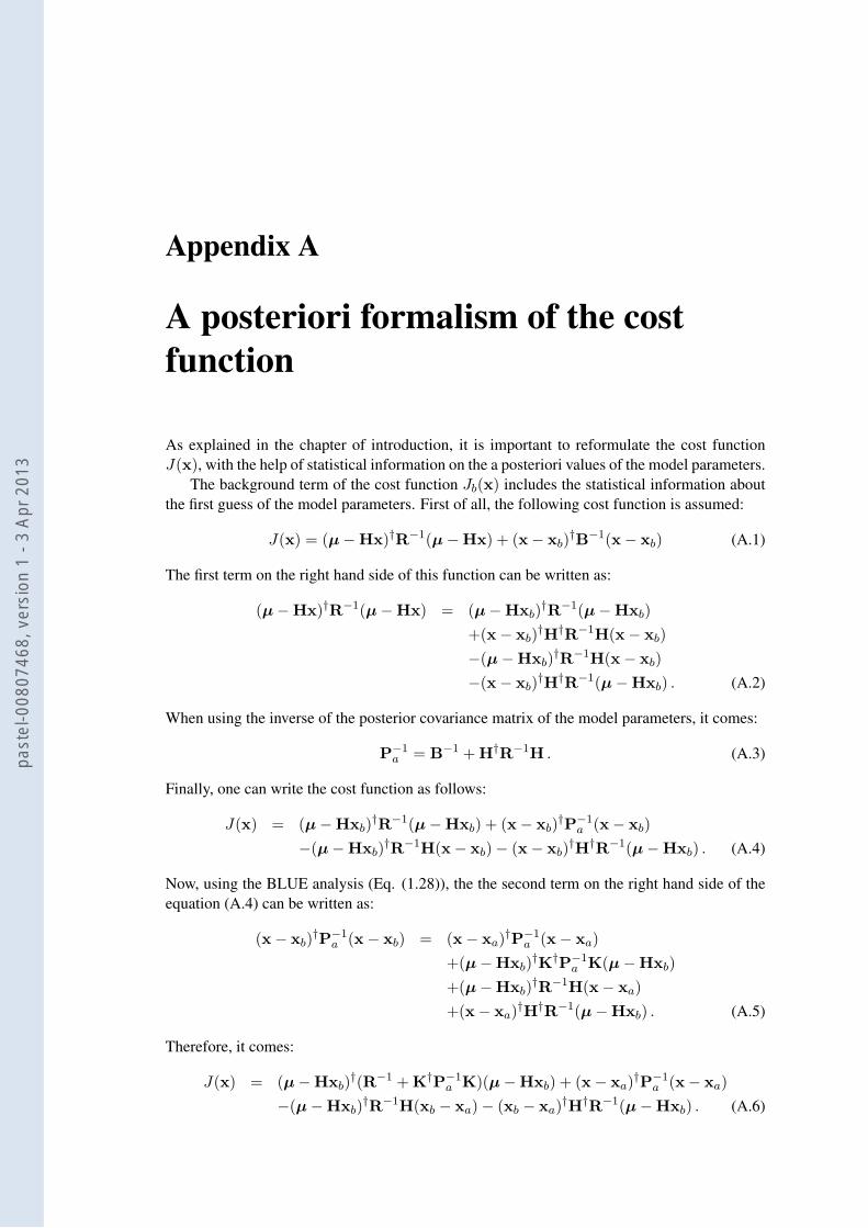
Appendix A
A posteriori formalism of the cost
function
As explained in the chapter of introduction, it is important to reformulate the cost functionJ(x), with the help of statistical information on the a posteriori values of the model parameters.
The background term of the cost function Jb(x) includes the statistical information aboutthe first guess of the model parameters. First of all, the following cost function is assumed:
J(x) = (µ − Hx)†R−1(µ − Hx) + (x − xb)†B−1(x − xb) (A.1)
The first term on the right hand side of this function can be written as:
(µ − Hx)†R−1(µ − Hx) = (µ − Hxb)†R−1(µ − Hxb)
+(x − xb)†H†R−1H(x − xb)
−(µ − Hxb)†R−1H(x − xb)
−(x − xb)†H†R−1(µ − Hxb) . (A.2)
When using the inverse of the posterior covariance matrix of the model parameters, it comes:
P−1a = B−1 + H†R−1H . (A.3)
Finally, one can write the cost function as follows:
J(x) = (µ − Hxb)†R−1(µ − Hxb) + (x − xb)
†P−1a (x − xb)
−(µ − Hxb)†R−1H(x − xb) − (x − xb)
†H†R−1(µ − Hxb) . (A.4)
Now, using the BLUE analysis (Eq. (1.28)), the the second term on the right hand side of theequation (A.4) can be written as:
(x − xb)†P−1
a (x − xb) = (x − xa)†P−1
a (x − xa)
+(µ − Hxb)†K†P−1
a K(µ − Hxb)
+(µ − Hxb)†R−1H(x − xa)
+(x − xa)†H†R−1(µ − Hxb) . (A.5)
Therefore, it comes:
J(x) = (µ − Hxb)†(R−1 + K†P−1
a K)(µ − Hxb) + (x − xa)†P−1
a (x − xa)
−(µ − Hxb)†R−1H(xb − xa) − (xb − xa)
†H†R−1(µ − Hxb) . (A.6)
past
el-0
0807
468,
ver
sion
1 -
3 Ap
r 201
3

134 Chapter A – A posteriori formalism of the cost function
The BLUE analysis can be still formulated as:
xb − xa = −K(µ − Hxb) . (A.7)
Finally, the following cost function is detailed, this time, using the BLUE analysis,
J(x) = (µ − Hxb)†(R−1 + K†P−1
a K − R−1HK − K†H†R−1)(µ − Hxb)
+(x − xa)†P−1
a (x − xa) . (A.8)
The gain matrix, K, can be derived as a function of B and R (Eq. (1.29)). Then,
R−1 + K†P−1a K − R−1HK − K†H†R−1 = (R + HBH†)−1. (A.9)
This leads to the following from of the cost function.
J(x) = (µ − Hxb)†(R + HBH†)−1(µ − Hxb) + (x − xa)
†P−1a (x − xa) . (A.10)
past
el-0
0807
468,
ver
sion
1 -
3 Ap
r 201
3

Appendix B
Carbon monoxide scores for each of
the stations
B.1 Simulation scores
Table B.1: Comparison of the observations and the simulated concentrations.
N C O RMSE R FA2 FA5
HAYANGE (industrial) 1273 343 584.3 545.5 0.28 0.51 0.91
Brest 3 CDM (traffic) 954 256.5 649.6 621.6 -0.01 0.44 0.87
SAMONZET (urban) 780 222.8 673.4 562.8 -0.04 0.24 0.88
TOULON FOCH (urban) 1330 239.1 995.9 1123 0.07 0.25 0.72
ALEXIS CARREL ROUENG (urban) 1275 295 356.3 263.3 0.25 0.72 0.95
Jardin Lecoq CF (urban) 1137 236.4 283.9 478.9 -0.09 0.36 0.69
VICTOR HUGO (traffic) 1320 271.6 367.3 465.3 0.16 0.39 0.75
Roubaix/Serres (traffic) 1244 357.6 539.3 378.2 0.47 0.71 0.98
Cherbourg Paul Doume (urban) 1341 244 342.1 226.7 0 0.81 0.99
Station MARSANNAY (urban) 1285 280 437.1 282.4 0.16 0.73 0.99
Saint Denis (traffic) 1341 252 895.7 903.2 0.28 0.29 0.79
Mirabeau (traffic) 1340 276.7 754.5 667.3 0.08 0.35 0.89
Grenoble Foch (traffic) 1323 247 1064 1053 0.14 0.15 0.7
Muhl.ASPA (traffic) 1308 298.5 451.5 425.7 0.16 0.68 0.96
Hotel de ville (urban) 1296 296.8 428.9 571.5 0.09 0.81 0.99
MERIGNAC (traffic) 781 260.9 581.9 477 0.19 0.53 0.96
Nice Pellos (urban) 1242 233.8 2156 2500 0.04 0.06 0.34
Ecole Jules Ferry (urban) 578 273.7 520.2 410.5 -0.04 0.63 0.96
GONESSE (periurban) 1073 472.3 554.7 293.7 0.48 0.86 0.99
Liane Boulogne Sud (traffic) 1141 270.6 367.8 351.3 0.32 0.51 0.89
VAUCELLES (urban) 1243 262.1 585 549.3 0.04 0.45 0.89
COUBERTIN (periurban) 1331 243.3 312.9 239.7 0 0.7 0.95
Gambeta (traffic) 1333 286.1 715.9 635.4 0.04 0.39 0.92
ANGLET (urban) 710 228.5 602.7 589.5 -0.08 0.4 0.89
Bar-le-Duc (urban) 1231 285 521.4 450.7 -0.02 0.65 0.96
Aurillac Centre (traffic) 1327 228.3 698.1 833.2 -0.09 0.35 0.78
CTRE VILLE MEGEVAND (traffic) 1337 266.5 457.8 367.9 0.13 0.62 0.95
LA ROE (traffic) 1316 267 755.8 668.3 0.05 0.32 0.9
AVIGNON ROCADE (traffic) 1341 317.7 683 658.7 0.51 0.57 0.96
past
el-0
0807
468,
ver
sion
1 -
3 Ap
r 201
3
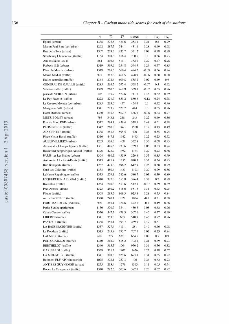
136 Chapter B – Carbon monoxide scores for each of the stations
N C O RMSE R FA2 FA5
Epinal (urban) 1338 275.6 431.6 253.1 0.21 0.8 0.99
Macon Paul Bert (periurban) 1292 287.7 544.1 431.1 0.28 0.69 0.98
Rue de la Tour (urban) 1307 279.3 435.7 331.2 0.07 0.78 0.99
Strasbourg Clemenceau (traffic) 1164 308.3 816.4 700.5 0.1 0.36 0.93
Amiens Saint Leu () 584 299.4 511.1 382.9 0.29 0.77 0.98
Forbach (12) (urban) 1319 319.6 354.8 394.5 0.29 0.57 0.85
Place du Marche (urban) 1319 265.3 560.4 494.2 -0.09 0.56 0.94
Mairie MALO (traffic) 975 387.3 461.5 498.9 -0.06 0.68 0.88
Halles centralles (traffic) 1344 272.4 609.8 585.2 0.02 0.49 0.9
GENERAL DE GAULLE (traffic) 1285 264.5 597.4 568.2 -0.07 0.5 0.92
Valence traffic (traffic) 1329 260.6 462.9 359.1 -0.02 0.65 0.96
place de VERDUN (urban) 102 195.7 522.6 741.8 0.45 0.62 0.89
Le Puy Fayolle (traffic) 1222 221.7 831.2 880.8 -0.12 0.24 0.78
Le Creusot Molette (periurban) 1295 263.6 457 454.4 0.1 0.72 0.96
Marignane Ville (urban) 1341 273.9 527.7 444 0.3 0.65 0.96
Hotel Districal (urban) 1330 293.6 562.7 436.8 -0.08 0.64 0.97
METZ-BORNY (urban) 786 343.1 248 243 0.22 0.49 0.86
Port de Bouc EDF (urban) 1312 294.1 459.4 378.1 0.44 0.61 0.98
PLOMBIERES (traffic) 1342 260.8 1463 1500 0.17 0.13 0.49
AIX CENTRE (traffic) 1338 281.4 595.5 490 0.24 0.55 0.95
Place Victor Basch (traffic) 1316 447.1 1642 1463 0.22 0.23 0.72
AUBERVILLIERS (urban) 1203 505.3 408 332.8 0.35 0.68 0.95
Avenue des Champs Elysees (traffic) 1331 445.6 933.6 739.3 0.03 0.53 0.94
Boulevard peripherique Auteuil (traffic) 1326 423.7 1392 1164 0.29 0.23 0.86
PARIS 1er Les Halles (urban) 1304 480.5 435.9 229.8 0.35 0.85 0.99
Autoroute A1 - Saint-Denis (traffic) 1313 481.4 1255 970.3 0.32 0.34 0.93
Rue Bonaparte (traffic) 1267 473.3 896.2 642.9 0.25 0.58 0.99
Quai des Celestins (traffic) 1333 480.4 1420 1193 0.29 0.29 0.86
LeHavre Republique (traffic) 1333 259.1 582.6 580.7 0.03 0.39 0.89
ESQUERCHIN A DOUAI (traffic) 1340 327.3 555.8 396.4 0.32 0.7 0.99
Rousillon (traffic) 1254 240.3 553.6 512.1 -0.07 0.39 0.89
Pres Arenes (urban) 1323 250.2 518.6 581.3 0.31 0.63 0.95
Planas (traffic) 1308 283.5 869.3 925.8 0.28 0.35 0.84
rue de la GRILLE (traffic) 1320 240.1 1022 1054 -0.1 0.21 0.68
FORT-MARDYCK (industrial) 990 385.1 374.6 422.7 -0.1 0.49 0.88
Petite Synthe (periurban) 1130 370.7 384.1 450.3 0.08 0.62 0.96
Calais Centre (traffic) 1330 347.3 478.3 307.6 0.46 0.77 0.99
LIBERTE (traffic) 1341 353.3 603 540.8 0.45 0.72 0.96
PASTEUR (traffic) 1338 355.1 494.7 289.9 0.49 0.81 1
LA BASSEE/CENTRE (traffic) 1337 327.4 413.1 281 0.49 0.76 0.98
Le Rondeau (traffic) 1315 245.9 793.7 707.5 0.02 0.23 0.84
LAENNEC (traffic) 605 277 679.1 634.5 0.08 0.5 0.9
PUITS GAILLOT (traffic) 1340 318.7 815.2 702.2 0.21 0.39 0.93
BERTHELOT (traffic) 1340 315.3 1004 970.2 0.36 0.36 0.82
GARIBALDI (traffic) 1339 321.7 1407 1426 0.22 0.18 0.67
LA MULATIERE (traffic) 1341 308.8 829.6 693.1 0.34 0.35 0.92
Batiment ELF-ATO (industrial) 1075 328.1 257.3 196 0.24 0.62 0.92
ANTIBES GUYNEMER (urban) 1275 233.4 1279 1363 0.11 0.05 0.54
Rouen Le Conquerant (traffic) 1340 292.6 503.6 382.7 0.25 0.62 0.97
past
el-0
0807
468,
ver
sion
1 -
3 Ap
r 201
3
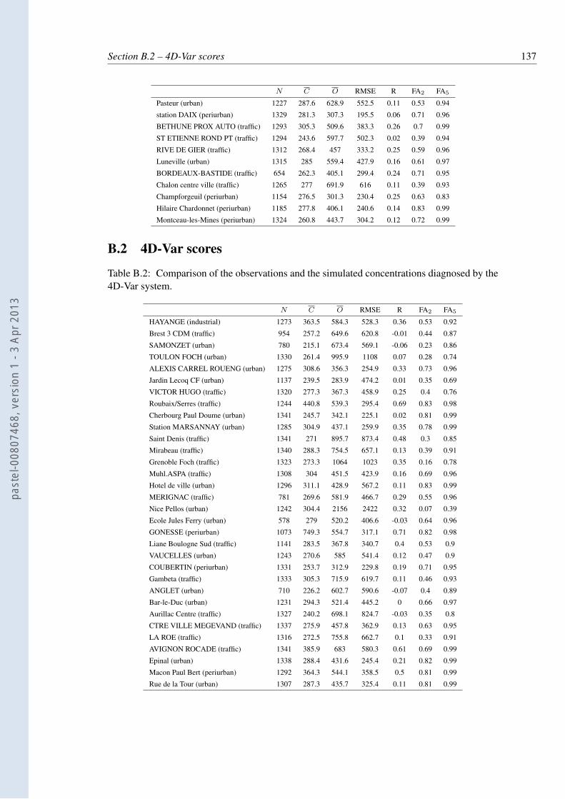
Section B.2 – 4D-Var scores 137
N C O RMSE R FA2 FA5
Pasteur (urban) 1227 287.6 628.9 552.5 0.11 0.53 0.94
station DAIX (periurban) 1329 281.3 307.3 195.5 0.06 0.71 0.96
BETHUNE PROX AUTO (traffic) 1293 305.3 509.6 383.3 0.26 0.7 0.99
ST ETIENNE ROND PT (traffic) 1294 243.6 597.7 502.3 0.02 0.39 0.94
RIVE DE GIER (traffic) 1312 268.4 457 333.2 0.25 0.59 0.96
Luneville (urban) 1315 285 559.4 427.9 0.16 0.61 0.97
BORDEAUX-BASTIDE (traffic) 654 262.3 405.1 299.4 0.24 0.71 0.95
Chalon centre ville (traffic) 1265 277 691.9 616 0.11 0.39 0.93
Champforgeuil (periurban) 1154 276.5 301.3 230.4 0.25 0.63 0.83
Hilaire Chardonnet (periurban) 1185 277.8 406.1 240.6 0.14 0.83 0.99
Montceau-les-Mines (periurban) 1324 260.8 443.7 304.2 0.12 0.72 0.99
B.2 4D-Var scores
Table B.2: Comparison of the observations and the simulated concentrations diagnosed by the4D-Var system.
N C O RMSE R FA2 FA5
HAYANGE (industrial) 1273 363.5 584.3 528.3 0.36 0.53 0.92
Brest 3 CDM (traffic) 954 257.2 649.6 620.8 -0.01 0.44 0.87
SAMONZET (urban) 780 215.1 673.4 569.1 -0.06 0.23 0.86
TOULON FOCH (urban) 1330 261.4 995.9 1108 0.07 0.28 0.74
ALEXIS CARREL ROUENG (urban) 1275 308.6 356.3 254.9 0.33 0.73 0.96
Jardin Lecoq CF (urban) 1137 239.5 283.9 474.2 0.01 0.35 0.69
VICTOR HUGO (traffic) 1320 277.3 367.3 458.9 0.25 0.4 0.76
Roubaix/Serres (traffic) 1244 440.8 539.3 295.4 0.69 0.83 0.98
Cherbourg Paul Doume (urban) 1341 245.7 342.1 225.1 0.02 0.81 0.99
Station MARSANNAY (urban) 1285 304.9 437.1 259.9 0.35 0.78 0.99
Saint Denis (traffic) 1341 271 895.7 873.4 0.48 0.3 0.85
Mirabeau (traffic) 1340 288.3 754.5 657.1 0.13 0.39 0.91
Grenoble Foch (traffic) 1323 273.3 1064 1023 0.35 0.16 0.78
Muhl.ASPA (traffic) 1308 304 451.5 423.9 0.16 0.69 0.96
Hotel de ville (urban) 1296 311.1 428.9 567.2 0.11 0.83 0.99
MERIGNAC (traffic) 781 269.6 581.9 466.7 0.29 0.55 0.96
Nice Pellos (urban) 1242 304.4 2156 2422 0.32 0.07 0.39
Ecole Jules Ferry (urban) 578 279 520.2 406.6 -0.03 0.64 0.96
GONESSE (periurban) 1073 749.3 554.7 317.1 0.71 0.82 0.98
Liane Boulogne Sud (traffic) 1141 283.5 367.8 340.7 0.4 0.53 0.9
VAUCELLES (urban) 1243 270.6 585 541.4 0.12 0.47 0.9
COUBERTIN (periurban) 1331 253.7 312.9 229.8 0.19 0.71 0.95
Gambeta (traffic) 1333 305.3 715.9 619.7 0.11 0.46 0.93
ANGLET (urban) 710 226.2 602.7 590.6 -0.07 0.4 0.89
Bar-le-Duc (urban) 1231 294.3 521.4 445.2 0 0.66 0.97
Aurillac Centre (traffic) 1327 240.2 698.1 824.7 -0.03 0.35 0.8
CTRE VILLE MEGEVAND (traffic) 1337 275.9 457.8 362.9 0.13 0.63 0.95
LA ROE (traffic) 1316 272.5 755.8 662.7 0.1 0.33 0.91
AVIGNON ROCADE (traffic) 1341 385.9 683 580.3 0.61 0.69 0.99
Epinal (urban) 1338 288.4 431.6 245.4 0.21 0.82 0.99
Macon Paul Bert (periurban) 1292 364.3 544.1 358.5 0.5 0.81 0.99
Rue de la Tour (urban) 1307 287.3 435.7 325.4 0.11 0.81 0.99
past
el-0
0807
468,
ver
sion
1 -
3 Ap
r 201
3
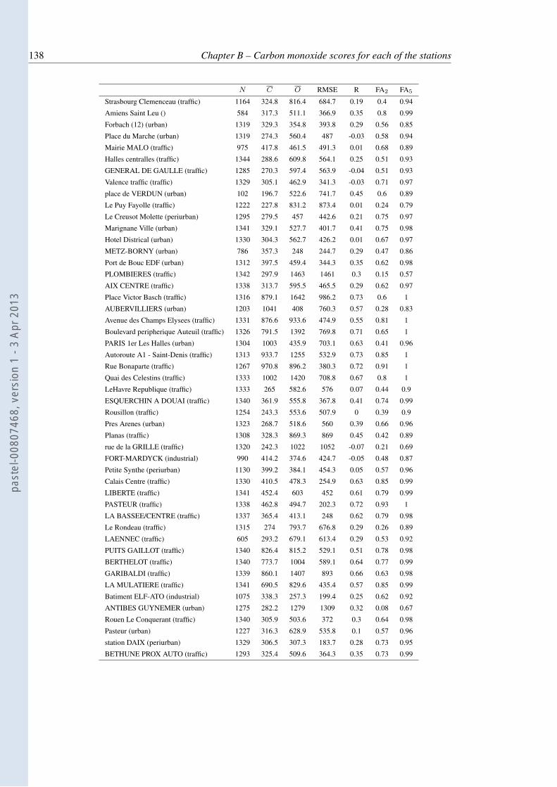
138 Chapter B – Carbon monoxide scores for each of the stations
N C O RMSE R FA2 FA5
Strasbourg Clemenceau (traffic) 1164 324.8 816.4 684.7 0.19 0.4 0.94
Amiens Saint Leu () 584 317.3 511.1 366.9 0.35 0.8 0.99
Forbach (12) (urban) 1319 329.3 354.8 393.8 0.29 0.56 0.85
Place du Marche (urban) 1319 274.3 560.4 487 -0.03 0.58 0.94
Mairie MALO (traffic) 975 417.8 461.5 491.3 0.01 0.68 0.89
Halles centralles (traffic) 1344 288.6 609.8 564.1 0.25 0.51 0.93
GENERAL DE GAULLE (traffic) 1285 270.3 597.4 563.9 -0.04 0.51 0.93
Valence traffic (traffic) 1329 305.1 462.9 341.3 -0.03 0.71 0.97
place de VERDUN (urban) 102 196.7 522.6 741.7 0.45 0.6 0.89
Le Puy Fayolle (traffic) 1222 227.8 831.2 873.4 0.01 0.24 0.79
Le Creusot Molette (periurban) 1295 279.5 457 442.6 0.21 0.75 0.97
Marignane Ville (urban) 1341 329.1 527.7 401.7 0.41 0.75 0.98
Hotel Districal (urban) 1330 304.3 562.7 426.2 0.01 0.67 0.97
METZ-BORNY (urban) 786 357.3 248 244.7 0.29 0.47 0.86
Port de Bouc EDF (urban) 1312 397.5 459.4 344.3 0.35 0.62 0.98
PLOMBIERES (traffic) 1342 297.9 1463 1461 0.3 0.15 0.57
AIX CENTRE (traffic) 1338 313.7 595.5 465.5 0.29 0.62 0.97
Place Victor Basch (traffic) 1316 879.1 1642 986.2 0.73 0.6 1
AUBERVILLIERS (urban) 1203 1041 408 760.3 0.57 0.28 0.83
Avenue des Champs Elysees (traffic) 1331 876.6 933.6 474.9 0.55 0.81 1
Boulevard peripherique Auteuil (traffic) 1326 791.5 1392 769.8 0.71 0.65 1
PARIS 1er Les Halles (urban) 1304 1003 435.9 703.1 0.63 0.41 0.96
Autoroute A1 - Saint-Denis (traffic) 1313 933.7 1255 532.9 0.73 0.85 1
Rue Bonaparte (traffic) 1267 970.8 896.2 380.3 0.72 0.91 1
Quai des Celestins (traffic) 1333 1002 1420 708.8 0.67 0.8 1
LeHavre Republique (traffic) 1333 265 582.6 576 0.07 0.44 0.9
ESQUERCHIN A DOUAI (traffic) 1340 361.9 555.8 367.8 0.41 0.74 0.99
Rousillon (traffic) 1254 243.3 553.6 507.9 0 0.39 0.9
Pres Arenes (urban) 1323 268.7 518.6 560 0.39 0.66 0.96
Planas (traffic) 1308 328.3 869.3 869 0.45 0.42 0.89
rue de la GRILLE (traffic) 1320 242.3 1022 1052 -0.07 0.21 0.69
FORT-MARDYCK (industrial) 990 414.2 374.6 424.7 -0.05 0.48 0.87
Petite Synthe (periurban) 1130 399.2 384.1 454.3 0.05 0.57 0.96
Calais Centre (traffic) 1330 410.5 478.3 254.9 0.63 0.85 0.99
LIBERTE (traffic) 1341 452.4 603 452 0.61 0.79 0.99
PASTEUR (traffic) 1338 462.8 494.7 202.3 0.72 0.93 1
LA BASSEE/CENTRE (traffic) 1337 365.4 413.1 248 0.62 0.79 0.98
Le Rondeau (traffic) 1315 274 793.7 676.8 0.29 0.26 0.89
LAENNEC (traffic) 605 293.2 679.1 613.4 0.29 0.53 0.92
PUITS GAILLOT (traffic) 1340 826.4 815.2 529.1 0.51 0.78 0.98
BERTHELOT (traffic) 1340 773.7 1004 589.1 0.64 0.77 0.99
GARIBALDI (traffic) 1339 860.1 1407 893 0.66 0.63 0.98
LA MULATIERE (traffic) 1341 690.5 829.6 435.4 0.57 0.85 0.99
Batiment ELF-ATO (industrial) 1075 338.3 257.3 199.4 0.25 0.62 0.92
ANTIBES GUYNEMER (urban) 1275 282.2 1279 1309 0.32 0.08 0.67
Rouen Le Conquerant (traffic) 1340 305.9 503.6 372 0.3 0.64 0.98
Pasteur (urban) 1227 316.3 628.9 535.8 0.1 0.57 0.96
station DAIX (periurban) 1329 306.5 307.3 183.7 0.28 0.73 0.95
BETHUNE PROX AUTO (traffic) 1293 325.4 509.6 364.3 0.35 0.73 0.99
past
el-0
0807
468,
ver
sion
1 -
3 Ap
r 201
3
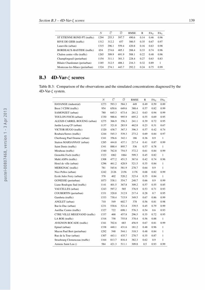
Section B.3 – 4D-Var-ξ scores 139
N C O RMSE R FA2 FA5
ST ETIENNE ROND PT (traffic) 1294 255.3 597.7 490.6 0.14 0.46 0.96
RIVE DE GIER (traffic) 1312 312.2 457 300.5 0.35 0.67 0.97
Luneville (urban) 1315 296.1 559.4 420.8 0.16 0.63 0.98
BORDEAUX-BASTIDE (traffic) 654 274.6 405.1 288.4 0.33 0.74 0.96
Chalon centre ville (traffic) 1265 309.9 691.9 588.1 0.22 0.48 0.96
Champforgeuil (periurban) 1154 311.1 301.3 228.4 0.27 0.63 0.83
Hilaire Chardonnet (periurban) 1185 312.5 406.1 216.3 0.32 0.89 1
Montceau-les-Mines (periurban) 1324 274.1 443.7 292.2 0.24 0.75 0.99
B.3 4D-Var-ξ scores
Table B.3: Comparison of the observations and the simulated concentrations diagnosed by the4D-Var-ξ system.
N C O RMSE R FA2 FA5
HAYANGE (industrial) 1273 593.3 584.3 449 0.49 0.59 0.89
Brest 3 CDM (traffic) 954 650.6 649.6 388.4 0.57 0.82 0.99
SAMONZET (urban) 780 645.3 673.4 261.2 0.63 0.94 0.99
TOULON FOCH (urban) 1330 988.6 995.9 695.2 0.55 0.69 0.95
ALEXIS CARREL ROUENG (urban) 1275 366.9 356.3 241.1 0.39 0.72 0.95
Jardin Lecoq CF (urban) 1137 321.8 283.9 462.8 0.23 0.31 0.67
VICTOR HUGO (traffic) 1320 438.7 367.3 396.3 0.57 0.42 0.74
Roubaix/Serres (traffic) 1244 545.3 539.3 273.2 0.69 0.84 0.97
Cherbourg Paul Doume (urban) 1341 356.6 342.1 186 0.36 0.9 1
Station MARSANNAY (urban) 1285 444.8 437.1 217.4 0.41 0.87 0.99
Saint Denis (traffic) 1341 888.4 895.7 536 0.57 0.78 1
Mirabeau (traffic) 1340 762.8 754.5 372.2 0.61 0.84 0.99
Grenoble Foch (traffic) 1323 1062 1064 599.3 0.45 0.82 1
Muhl.ASPA (traffic) 1308 477.2 451.5 367.6 0.42 0.74 0.96
Hotel de ville (urban) 1296 461.2 428.9 521.5 0.35 0.84 1
MERIGNAC (traffic) 781 545.6 581.9 278.7 0.64 0.9 1
Nice Pellos (urban) 1242 2126 2156 1176 0.68 0.82 0.99
Ecole Jules Ferry (urban) 578 402 520.2 323.4 0.35 0.84 1
GONESSE (periurban) 1073 538.1 554.7 240.7 0.66 0.9 0.99
Liane Boulogne Sud (traffic) 1141 401.5 367.8 309.2 0.57 0.55 0.85
VAUCELLES (urban) 1243 597.2 585 376.9 0.53 0.71 0.93
COUBERTIN (periurban) 1331 320.8 312.9 217.4 0.28 0.7 0.95
Gambeta (traffic) 1333 730.4 715.9 349.5 0.67 0.86 0.99
ANGLET (urban) 710 549 602.7 378 0.56 0.81 0.98
Bar-le-Duc (urban) 1231 530.6 521.4 339.5 0.45 0.79 0.99
Aurillac Centre (traffic) 1327 722 698.1 576.3 0.54 0.6 0.93
CTRE VILLE MEGEVAND (traffic) 1337 468 457.8 296.5 0.35 0.72 0.95
LA ROE (traffic) 1316 758 755.8 378.4 0.56 0.88 1
AVIGNON ROCADE (traffic) 1341 702.6 683 456.9 0.67 0.81 0.99
Epinal (urban) 1338 440.1 431.6 181.2 0.48 0.96 1
Macon Paul Bert (periurban) 1292 548 544.1 318.3 0.48 0.84 1
Rue de la Tour (urban) 1307 443.1 435.7 270.7 0.35 0.87 1
Strasbourg Clemenceau (traffic) 1164 813.7 816.4 382.3 0.62 0.9 1
Amiens Saint Leu () 584 421.3 511.1 309.8 0.5 0.93 0.99
past
el-0
0807
468,
ver
sion
1 -
3 Ap
r 201
3

140 Chapter B – Carbon monoxide scores for each of the stations
N C O RMSE R FA2 FA5
Forbach (12) (urban) 1319 379.9 354.8 387.1 0.35 0.52 0.85
Place du Marche (urban) 1319 569.8 560.4 352.2 0.42 0.8 0.99
Mairie MALO (traffic) 975 446.4 461.5 477 0.14 0.68 0.89
Halles centralles (traffic) 1344 668.4 609.8 385.8 0.6 0.75 0.97
GENERAL DE GAULLE (traffic) 1285 624.4 597.4 370.1 0.59 0.82 0.99
Valence traffic (traffic) 1329 472.8 462.9 283.5 0.24 0.79 0.99
place de VERDUN (urban) 102 221.3 522.6 725.7 0.55 0.66 0.9
Le Puy Fayolle (traffic) 1222 811 831.2 574.6 0.41 0.78 0.99
Le Creusot Molette (periurban) 1295 472.6 457 384.5 0.35 0.78 0.99
Marignane Ville (urban) 1341 572.4 527.7 335.4 0.49 0.74 1
Hotel Districal (urban) 1330 568.5 562.7 318.2 0.32 0.89 1
METZ-BORNY (urban) 786 340.3 248 237.4 0.29 0.49 0.86
Port de Bouc EDF (urban) 1312 504.2 459.4 321.2 0.5 0.64 0.95
PLOMBIERES (traffic) 1342 1464 1463 653.8 0.69 0.86 1
AIX CENTRE (traffic) 1338 620.6 595.5 333.1 0.51 0.81 0.99
Place Victor Basch (traffic) 1316 1618 1642 542.8 0.78 0.96 1
AUBERVILLIERS (urban) 1203 531.9 408 295.9 0.61 0.72 0.96
Avenue des Champs Elysees (traffic) 1331 953.1 933.6 432.5 0.6 0.88 1
Boulevard peripherique Auteuil (traffic) 1326 1374 1392 431.6 0.77 0.98 1
PARIS 1er Les Halles (urban) 1304 516.2 435.9 216.1 0.59 0.88 0.99
Autoroute A1 - Saint-Denis (traffic) 1313 1219 1255 448.3 0.69 0.96 1
Rue Bonaparte (traffic) 1267 897.3 896.2 363 0.69 0.93 1
Quai des Celestins (traffic) 1333 1416 1420 527.6 0.73 0.96 1
LeHavre Republique (traffic) 1333 619.2 582.6 369.6 0.65 0.72 0.95
ESQUERCHIN A DOUAI (traffic) 1340 573.6 555.8 277.5 0.59 0.89 0.99
Rousillon (traffic) 1254 556.6 553.6 362.2 0.39 0.68 0.95
Pres Arenes (urban) 1323 537.2 518.6 479.3 0.46 0.7 0.98
Planas (traffic) 1308 899.2 869.3 574.6 0.64 0.78 0.99
rue de la GRILLE (traffic) 1320 1012 1022 621.8 0.46 0.81 1
FORT-MARDYCK (industrial) 990 380.3 374.6 413.5 -0.01 0.5 0.88
Petite Synthe (periurban) 1130 376.3 384.1 448.2 0.1 0.6 0.96
Calais Centre (traffic) 1330 485.7 478.3 237.9 0.65 0.86 0.99
LIBERTE (traffic) 1341 618 603 404.8 0.64 0.75 0.99
PASTEUR (traffic) 1338 499.8 494.7 195.1 0.74 0.93 1
LA BASSEE/CENTRE (traffic) 1337 432.7 413.1 238.4 0.66 0.79 0.97
Le Rondeau (traffic) 1315 783 793.7 408 0.41 0.8 0.97
LAENNEC (traffic) 605 476.3 679.1 454.3 0.65 0.81 1
PUITS GAILLOT (traffic) 1340 806 815.2 452.1 0.45 0.81 0.98
BERTHELOT (traffic) 1340 988.5 1004 629.4 0.45 0.69 0.99
GARIBALDI (traffic) 1339 1447 1407 738.7 0.62 0.82 0.99
LA MULATIERE (traffic) 1341 827.5 829.6 424 0.45 0.81 1
Batiment ELF-ATO (industrial) 1075 330.1 257.3 192.7 0.31 0.63 0.92
ANTIBES GUYNEMER (urban) 1275 1243 1279 753.7 0.52 0.89 0.99
Rouen Le Conquerant (traffic) 1340 521 503.6 269.8 0.58 0.8 0.97
Pasteur (urban) 1227 638.6 628.9 372.7 0.53 0.79 0.99
station DAIX (periurban) 1329 314.6 307.3 185.9 0.24 0.73 0.95
BETHUNE PROX AUTO (traffic) 1293 525.6 509.6 281.6 0.56 0.83 1
ST ETIENNE ROND PT (traffic) 1294 615.1 597.7 293.8 0.56 0.89 1
RIVE DE GIER (traffic) 1312 490.3 457 250.7 0.48 0.76 0.95
past
el-0
0807
468,
ver
sion
1 -
3 Ap
r 201
3

Section B.3 – 4D-Var-ξ scores 141
N C O RMSE R FA2 FA5
Luneville (urban) 1315 569.3 559.4 287.7 0.51 0.86 1
BORDEAUX-BASTIDE (traffic) 654 383.2 405.1 227.3 0.57 0.86 0.96
Chalon centre ville (traffic) 1265 693.4 691.9 390.6 0.52 0.81 0.99
Champforgeuil (periurban) 1154 317.2 301.3 222.7 0.36 0.64 0.82
Hilaire Chardonnet (periurban) 1185 400 406.1 190.2 0.35 0.92 1
Montceau-les-Mines (periurban) 1324 448.9 443.7 218.7 0.45 0.89 1
past
el-0
0807
468,
ver
sion
1 -
3 Ap
r 201
3

142 Chapter B – Carbon monoxide scores for each of the stations
past
el-0
0807
468,
ver
sion
1 -
3 Ap
r 201
3
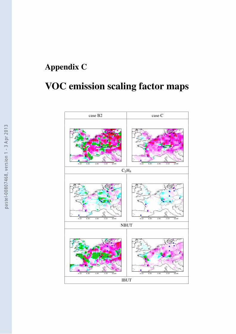
Appendix C
VOC emission scaling factor maps
case B2 case C
0.10 0.30 1.00 3.33 10.00 0.10 0.30 1.00 3.33 10.00
C3H8
0.10 0.30 1.00 3.33 10.00 0.10 0.30 1.00 3.33 10.00
NBUT
0.10 0.30 1.00 3.33 10.00 0.10 0.30 1.00 3.33 10.00
IBUT
past
el-0
0807
468,
ver
sion
1 -
3 Ap
r 201
3
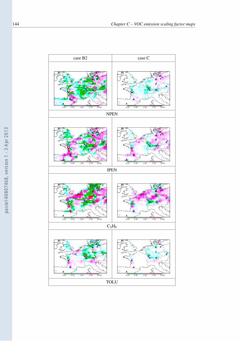
144 Chapter C – VOC emission scaling factor maps
case B2 case C
0.10 0.30 1.00 3.33 10.00 0.10 0.30 1.00 3.33 10.00
NPEN
0.10 0.30 1.00 3.33 10.00 0.10 0.30 1.00 3.33 10.00
IPEN
0.10 0.30 1.00 3.33 10.00 0.10 0.30 1.00 3.33 10.00
C3H6
0.10 0.30 1.00 3.33 10.00 0.10 0.30 1.00 3.33 10.00
TOLU
past
el-0
0807
468,
ver
sion
1 -
3 Ap
r 201
3
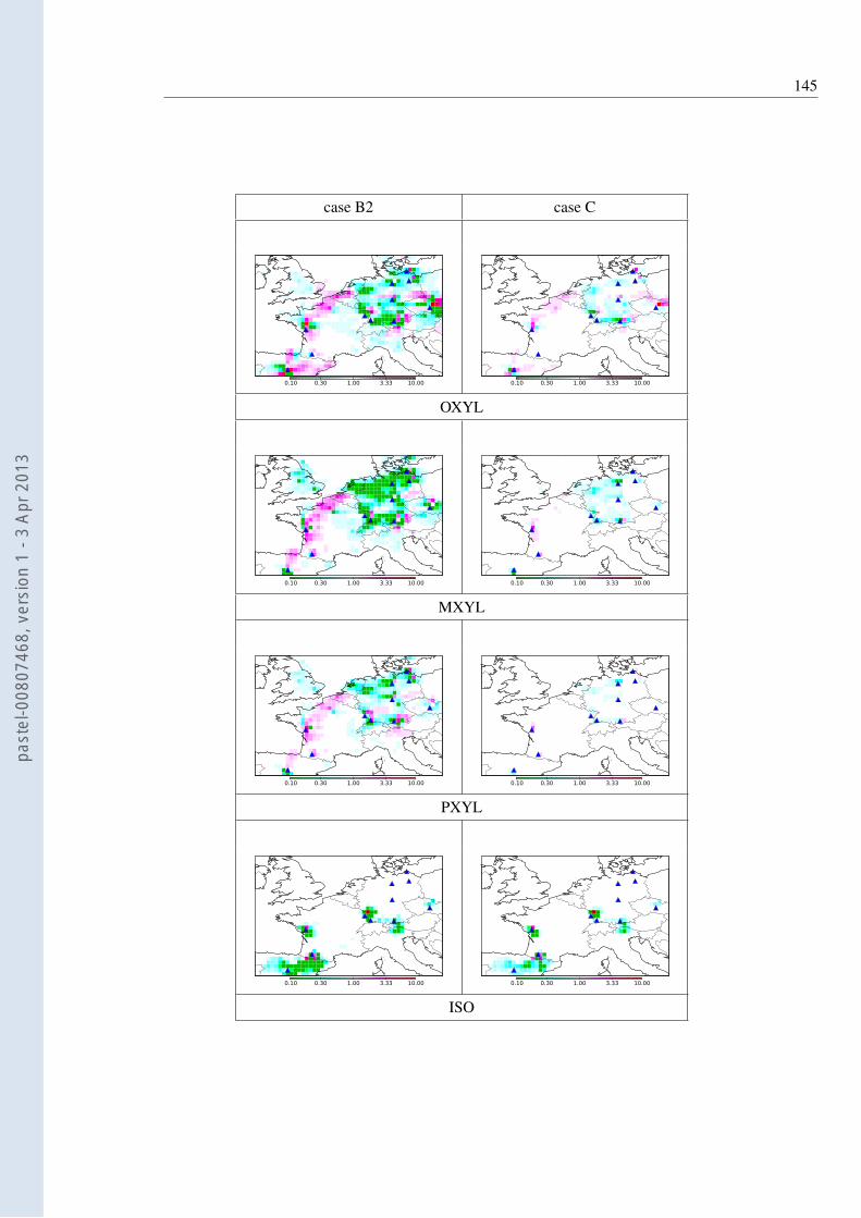
145
case B2 case C
0.10 0.30 1.00 3.33 10.00 0.10 0.30 1.00 3.33 10.00
OXYL
0.10 0.30 1.00 3.33 10.00 0.10 0.30 1.00 3.33 10.00
MXYL
0.10 0.30 1.00 3.33 10.00 0.10 0.30 1.00 3.33 10.00
PXYL
0.10 0.30 1.00 3.33 10.00 0.10 0.30 1.00 3.33 10.00
ISO
past
el-0
0807
468,
ver
sion
1 -
3 Ap
r 201
3
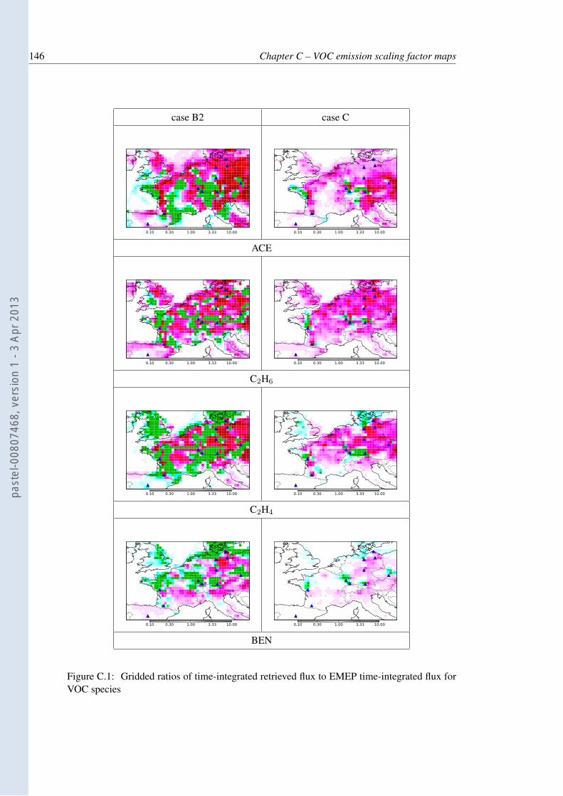
146 Chapter C – VOC emission scaling factor maps
case B2 case C
0.10 0.30 1.00 3.33 10.00 0.10 0.30 1.00 3.33 10.00
ACE
0.10 0.30 1.00 3.33 10.00 0.10 0.30 1.00 3.33 10.00
C2H6
0.10 0.30 1.00 3.33 10.00 0.10 0.30 1.00 3.33 10.00
C2H4
0.10 0.30 1.00 3.33 10.00 0.10 0.30 1.00 3.33 10.00
BEN
Figure C.1: Gridded ratios of time-integrated retrieved flux to EMEP time-integrated flux forVOC species
past
el-0
0807
468,
ver
sion
1 -
3 Ap
r 201
3
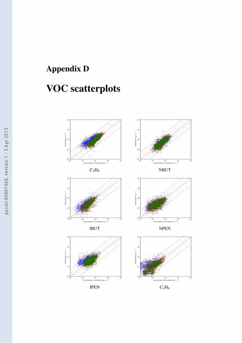
Appendix D
VOC scatterplots
10-2
10-1
100
101
102
Concentration via simulation (g/m3)
10-2
10-1
100
101
102
Obse
rvati
on (
g/m3)
10-2
10-1
100
101
102
Concentration via simulation (g/m3)
10-2
10-1
100
101
102
Obse
rvati
on (
g/m3)
C3H8 NBUT
10-2
10-1
100
101
102
Concentration via simulation (g/m3)
10-2
10-1
100
101
102
Obse
rvati
on (
g/m3)
10-2
10-1
100
101
102
Concentration via simulation (g/m3)
10-2
10-1
100
101
102
Obse
rvati
on (
g/m3)
IBUT NPEN
10-2
10-1
100
101
102
Concentration via simulation (g/m3)
10-2
10-1
100
101
102
Obse
rvati
on (
g/m3)
10-2
10-1
100
101
102
Concentration via simulation (g/m3)
10-2
10-1
100
101
102
Obse
rvati
on (
g/m3)
IPEN C3H6
past
el-0
0807
468,
ver
sion
1 -
3 Ap
r 201
3
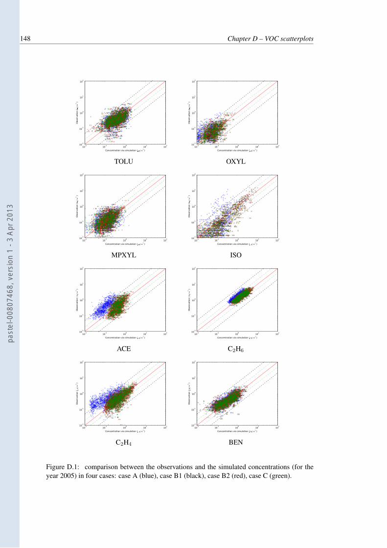
148 Chapter D – VOC scatterplots
10-2
10-1
100
101
102
Concentration via simulation (g/m3)
10-2
10-1
100
101
102
Obse
rvati
on (
g/m3)
10-2
10-1
100
101
102
Concentration via simulation (g/m3)
10-2
10-1
100
101
102
Obse
rvati
on (
g/m3)
TOLU OXYL
10-2
10-1
100
101
102
Concentration via simulation (g/m3)
10-2
10-1
100
101
102
Obse
rvati
on (
g/m3)
10-2
10-1
100
101
102
Concentration via simulation (g/m3)
10-2
10-1
100
101
102
Obse
rvati
on (
g/m3)
MPXYL ISO
10-2
10-1
100
101
102
Concentration via simulation (g/m3)
10-2
10-1
100
101
102
Obse
rvati
on (
g/m3)
10-2
10-1
100
101
102
Concentration via simulation (g/m3)
10-2
10-1
100
101
102
Obse
rvati
on (
g/m3)
ACE C2H6
10-2
10-1
100
101
102
Concentration via simulation (g/m3)
10-2
10-1
100
101
102
Obse
rvati
on (
g/m3)
10-2
10-1
100
101
102
Concentration via simulation (g/m3)
10-2
10-1
100
101
102
Obse
rvati
on (
g/m3)
C2H4 BEN
Figure D.1: comparison between the observations and the simulated concentrations (for theyear 2005) in four cases: case A (blue), case B1 (black), case B2 (red), case C (green).
past
el-0
0807
468,
ver
sion
1 -
3 Ap
r 201
3