modèles mathématiques et simulation numérique de...

Modeles mathematiques et simulation numerique de dispositifsphotovoltaıques

Athmane Bakhta

Athmane Bakhta CERMICS - Dec 2017 1 / 34

Motivation and context

©IRDEP-Gilles Renou

Collaboration with IRDEP (Institutde Recherche et Developpement surl’Energie Photovoltaıque, EDF,CNRS, Chimie ParisTech).

Study of CIGS (Copper, Indium,Gallium, Selenium) thin film solarcells:

Optimization of the productionprocessElectronic properties (forinverse design purpose)


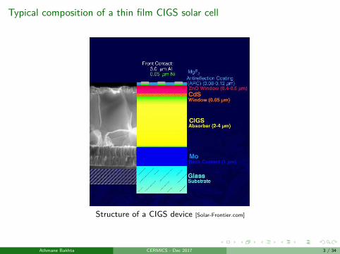
Typical composition of a thin film CIGS solar cell

Structure of a CIGS device [Solar-Frontier.com]


Outline

1 Cross diffusion equationsSimplified 1D model for the production process of CIGS layersWithout external fluxesWith external fluxesApplications

2 Electronic structureBloch-FloquetInverse problem of band structure

3 Other works and perspectives


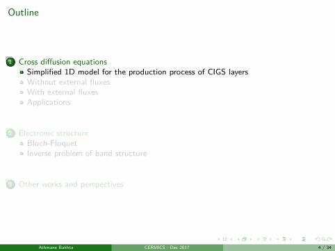
Production process of the CIGS layer

Physical Vapor Deposition (PVD) [Mattox, 2010]

[manmadediamondinfo.com]

[azonano.com]


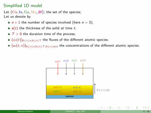
Simplified 1D modelLet Cu, In,Ga,Mo,Se; the set of the species;Let us denote by

n + 1 the number of species involved (here n = 3);e(t) the thickness of the solid at time t;T > 0 the duration time of the process;(φi (t))0≤i≤n,0≤t≤T the fluxes of the different atomic species.(ui (t, x))0≤i≤n,0≤t≤T ,0≤x≤e(t) the concentrations of the different atomic species.

u0(t, x) u1(t, x)

u3(t, x)u2(t, x)

0(t) 1(t) 2(t) 3(t)

0 x e(t)

SUBSTRAT


Simplified 1D model

One has to model:the evolution of the surface of the solid due to the imposition of external fluxes.the cross-diffusion occurring inside the bulk due to the high temperature;

The aim is to optimize the fluxes of the different atomic species (φi (t))0≤i≤n,0≤t≤Tin order to obtain a desired thickness etar (T ) and desired profile of concentrations(utar

i (x))0≤i≤n, 0≤x≤etar(T ) at time t = T .


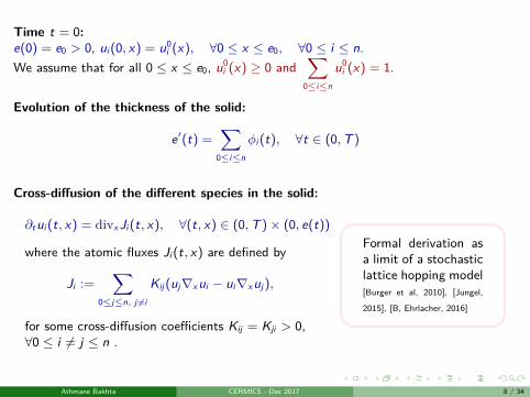
Time t = 0:e(0) = e0 > 0, ui (0, x) = u0

i (x), ∀0 ≤ x ≤ e0, ∀0 ≤ i ≤ n.We assume that for all 0 ≤ x ≤ e0, u0

i (x) ≥ 0 and∑

0≤i≤n

u0i (x) = 1.

Evolution of the thickness of the solid:

e′(t) =∑

0≤i≤n

φi (t), ∀t ∈ (0,T )

Cross-diffusion of the different species in the solid:

∂tui (t, x) = divx Ji (t, x), ∀(t, x) ∈ (0,T )× (0, e(t))

where the atomic fluxes Ji (t, x) are defined by

Ji :=∑

0≤j≤n, j 6=i

Kij (uj∇x ui − ui∇x uj ),

for some cross-diffusion coefficients Kij = Kji > 0,∀0 ≤ i 6= j ≤ n .

Formal derivation asa limit of a stochasticlattice hopping model[Burger et al, 2010], [Jungel,2015], [B, Ehrlacher, 2016]


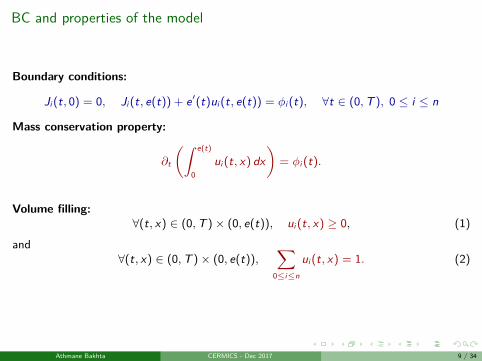
BC and properties of the model

Boundary conditions:

Ji (t, 0) = 0, Ji (t, e(t)) + e′(t)ui (t, e(t)) = φi (t), ∀t ∈ (0,T ), 0 ≤ i ≤ n

Mass conservation property:

∂t

(∫ e(t)

0ui (t, x) dx

)= φi (t).

Volume filling:∀(t, x) ∈ (0,T )× (0, e(t)), ui (t, x) ≥ 0, (1)

and∀(t, x) ∈ (0,T )× (0, e(t)),

∑0≤i≤n

ui (t, x) = 1. (2)


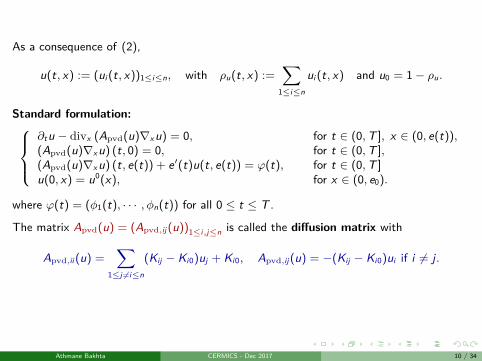
As a consequence of (2),

u(t, x) := (ui (t, x))1≤i≤n, with ρu(t, x) :=∑

1≤i≤n

ui (t, x) and u0 = 1− ρu.

Standard formulation:∂tu − divx (Apvd(u)∇x u) = 0, for t ∈ (0,T ], x ∈ (0, e(t)),(Apvd(u)∇x u) (t, 0) = 0, for t ∈ (0,T ],(Apvd(u)∇x u) (t, e(t)) + e′(t)u(t, e(t)) = ϕ(t), for t ∈ (0,T ]u(0, x) = u0(x), for x ∈ (0, e0).

where ϕ(t) = (φ1(t), · · · , φn(t)) for all 0 ≤ t ≤ T .

The matrix Apvd(u) = (Apvd,ij (u))1≤i,j≤n is called the diffusion matrix with

Apvd,ii (u) =∑

1≤j 6=i≤n

(Kij − Ki0)uj + Ki0, Apvd,ij (u) = −(Kij − Ki0)ui if i 6= j.


Outline





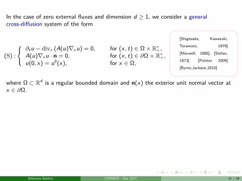
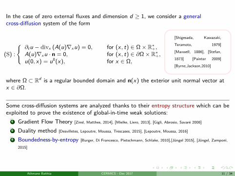
In the case of zero external fluxes and dimension d ≥ 1, we consider a generalcross-diffusion system of the form

(S) :

∂tu − divx (A(u)∇x u) = 0, for (x , t) ∈ Ω× R∗+,A(u)∇x u · n = 0, for (x , t) ∈ ∂Ω× R∗+,u(0, x) = u0(x), for x ∈ Ω,

[Shigesada, Kawazaki,Teramoto, 1979][Maxwell, 1886], [Stefan,1873] [Painter 2009][Byrne,Jackson,2010]

where Ω ⊂ Rd is a regular bounded domain and n(x) the exterior unit normal vector atx ∈ ∂Ω.

Some cross-diffusion systems are analyzed thanks to their entropy structure which can beexploited to prove the existence of global-in-time weak solutions:

1 Gradient Flow Theory [Zinsl, Matthes, 2014], [Mielke, Liero, 2013], [Gigli, Abrosio, Savare 2008]

2 Duality method [Desvilletes, Lepoutre, Moussa, Trescases, 2015], [Lepoutre, Moussa, 2016]

3 Boundedness-by-entropy [Burger, Di Francesco, Pietschmann, Schlake, 2010],[Jungel 2015], [Jungel, Zamponi,2015]


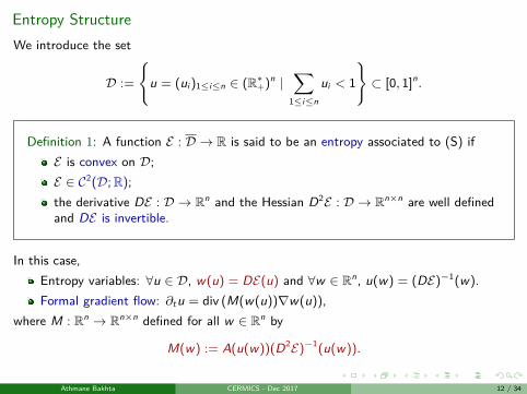
Entropy StructureWe introduce the set

D :=

u = (ui )1≤i≤n ∈ (R∗+)n |

∑1≤i≤n

ui < 1

⊂ [0, 1]n.

Definition 1: A function E : D → R is said to be an entropy associated to (S) ifE is convex on D;E ∈ C2(D;R);the derivative DE : D → Rn and the Hessian D2E : D → Rn×n are well definedand DE is invertible.

In this case,Entropy variables: ∀u ∈ D, w(u) = DE(u) and ∀w ∈ Rn, u(w) = (DE)−1(w).Formal gradient flow: ∂tu = div (M(w(u))∇w(u)),

where M : Rn → Rn×n defined for all w ∈ Rn by

M(w) := A(u(w))(D2E)−1(u(w)).


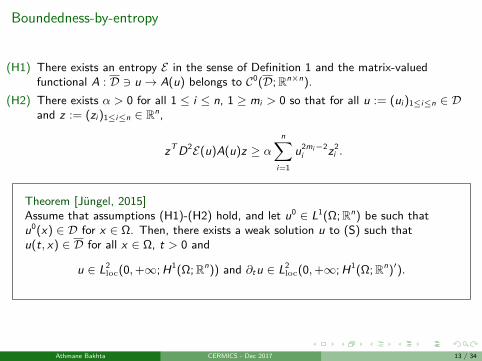
Boundedness-by-entropy

(H1) There exists an entropy E in the sense of Definition 1 and the matrix-valuedfunctional A : D 3 u → A(u) belongs to C0(D;Rn×n).

(H2) There exists α > 0 for all 1 ≤ i ≤ n, 1 ≥ mi > 0 so that for all u := (ui )1≤i≤n ∈ Dand z := (zi )1≤i≤n ∈ Rn,

zT D2E(u)A(u)z ≥ αn∑

i=1

u2mi−2i z2

i .

Theorem [Jungel, 2015]Assume that assumptions (H1)-(H2) hold, and let u0 ∈ L1(Ω;Rn) be such thatu0(x) ∈ D for x ∈ Ω. Then, there exists a weak solution u to (S) such thatu(t, x) ∈ D for all x ∈ Ω, t > 0 and

u ∈ L2loc(0,+∞; H1(Ω;Rn)) and ∂tu ∈ L2

loc(0,+∞; H1(Ω;Rn)′).


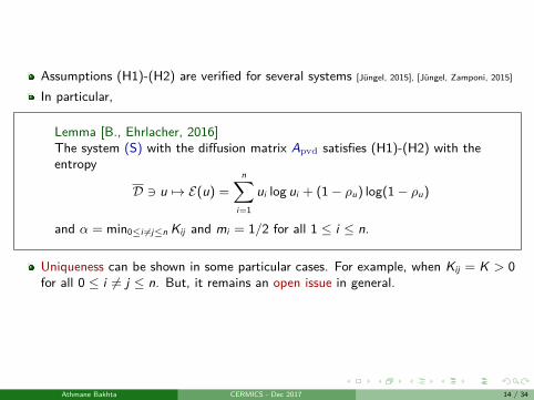
Assumptions (H1)-(H2) are verified for several systems [Jungel, 2015], [Jungel, Zamponi, 2015]

In particular,

Lemma [B., Ehrlacher, 2016]The system (S) with the diffusion matrix Apvd satisfies (H1)-(H2) with theentropy

D 3 u 7→ E(u) =n∑

i=1

ui log ui + (1− ρu) log(1− ρu)

and α = min0≤i 6=j≤n Kij and mi = 1/2 for all 1 ≤ i ≤ n.

Uniqueness can be shown in some particular cases. For example, when Kij = K > 0for all 0 ≤ i 6= j ≤ n. But, it remains an open issue in general.


Outline





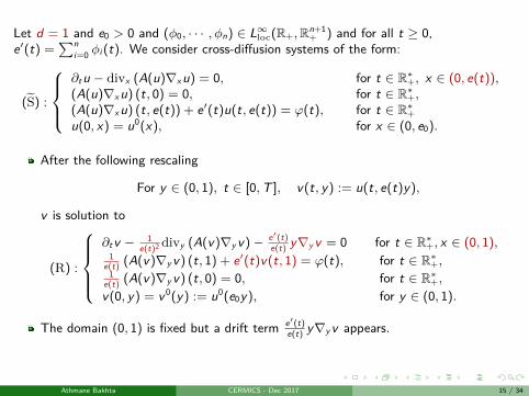
Let d = 1 and e0 > 0 and (φ0, · · · , φn) ∈ L∞loc(R+,Rn+1+ ) and for all t ≥ 0,

e′(t) =∑n

i=0 φi (t). We consider cross-diffusion systems of the form:

(S) :

∂tu − divx (A(u)∇x u) = 0, for t ∈ R∗+, x ∈ (0, e(t)),(A(u)∇x u) (t, 0) = 0, for t ∈ R∗+,(A(u)∇x u) (t, e(t)) + e′(t)u(t, e(t)) = ϕ(t), for t ∈ R∗+u(0, x) = u0(x), for x ∈ (0, e0).

After the following rescaling

For y ∈ (0, 1), t ∈ [0,T ], v(t, y) := u(t, e(t)y),

v is solution to

(R) :

∂tv − 1

e(t)2 divy (A(v)∇y v)− e′(t)e(t) y∇y v = 0 for t ∈ R∗+, x ∈ (0, 1),

1e(t) (A(v)∇y v) (t, 1) + e′(t)v(t, 1) = ϕ(t), for t ∈ R∗+,

1e(t) (A(v)∇y v) (t, 0) = 0, for t ∈ R∗+,v(0, y) = v 0(y) := u0(e0y), for y ∈ (0, 1).

The domain (0, 1) is fixed but a drift term e′(t)e(t) y∇y v appears.


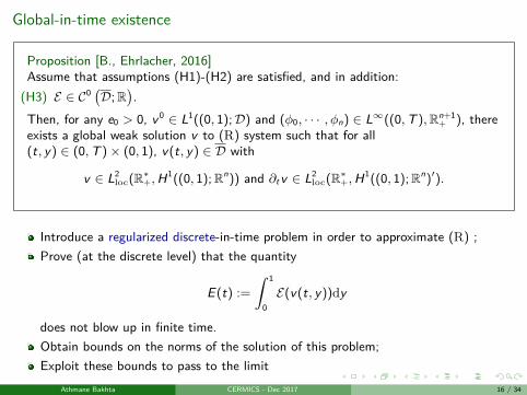
Global-in-time existence

Proposition [B., Ehrlacher, 2016]Assume that assumptions (H1)-(H2) are satisfied, and in addition:

(H3) E ∈ C0 (D;R)

.Then, for any e0 > 0, v 0 ∈ L1((0, 1);D) and (φ0, · · · , φn) ∈ L∞((0,T ),Rn+1

+ ), thereexists a global weak solution v to (R) system such that for all(t, y) ∈ (0,T )× (0, 1), v(t, y) ∈ D with

v ∈ L2loc(R∗+,H1((0, 1);Rn)) and ∂tv ∈ L2

loc(R∗+,H1((0, 1);Rn)′).

Introduce a regularized discrete-in-time problem in order to approximate (R) ;Prove (at the discrete level) that the quantity

E(t) :=∫ 1

0E(v(t, y))dy

does not blow up in finite time.Obtain bounds on the norms of the solution of this problem;Exploit these bounds to pass to the limit


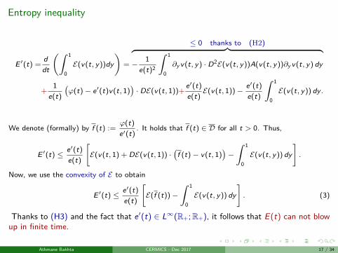
Entropy inequality

E ′(t) = ddt

(∫ 1

0E(v(t, y))dy

)=

≤ 0 thanks to (H2)︷︸︸︷−

1e(t)2

∫ 1

0∂y v(t, y) · D2E(v(t, y))A(v(t, y))∂y v(t, y) dy

+ 1e(t)

(ϕ(t)− e′(t)v(t, 1)

)· DE(v(t, 1))+ e′(t)

e(t)E(v(t, 1))− e′(t)

e(t)

∫ 1

0E(v(t, y)) dy .

We denote (formally) by f (t) := ϕ(t)e′(t)

. It holds that f (t) ∈ D for all t > 0. Thus,

E ′(t) ≤ e′(t)e(t)

[E(v(t, 1) + DE(v(t, 1)) ·

(f (t)− v(t, 1)

)−∫ 1

0E(v(t, y)) dy

].

Now, we use the convexity of E to obtain

E ′(t) ≤ e′(t)e(t)

[E(f (t))−

∫ 1

0E(v(t, y)) dy

]. (3)

Thanks to (H3) and the fact that e′(t) ∈ L∞(R+;R+), it follows that E(t) can not blowup in finite time.


Long-time behavior with constant fluxes

Proposition [B., Ehrlacher, 2016]Under the assumptions of the existencetheorem, we suppose moreover that forall t ≥ 0, φi (t) = φi > 0 for all0 ≤ i ≤ n. Let us denote by

f i := φi∑nj=0 φj

∀0 ≤ i ≤ n.

Then, there exists a constant C > 0such that

‖vi (t, ·)− f i‖L1(0,1) ≤C√

t + 1.

We perform a simulation of (R) with n = 3and plot the quantities

ηi (t) := 1‖vi (t, ·)− f i‖2

L1(0,1)

1400 1500 1600 1700 1800 1900 20000

0.5

1

1.5

2

2.5

3

3.5x 10

7

t

ηi(

t)

i = 0

i = 1

i = 2

i = 3

Long time behavior with constant fluxes


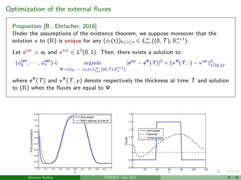
Optimization of the external fluxes

Proposition [B., Ehrlacher, 2016]Under the assumptions of the existence theorem, we suppose moreover that thesolution v to (R) is unique for any (φi (t))0≤i≤n ∈ L∞loc((0,T );Rn+1

+ ).

Let etar > e0 and v tar ∈ L2(0, 1). Then, there exists a solution to:

(φopt0 , · · · , φopt

n ) ∈ argminΨ:=(φ0,··· ,φn)∈L∞loc((0,T );Rn+1

+ )|etar − eΨ(T )|2 + ‖vΨ(T , ·)− v tar‖2

L2(0,1),

where eΨ(T ) and vΨ(T , y) denote respectively the thickness at time T and solutionto (R) when the fluxes are equal to Ψ.

0 0.1 0.2 0.3 0.4 0.5 0.6 0.7 0.8 0.9 10.23

0.24

0.25

0.26

0.27

0.28

0.29

0.3

0.31

0.32

y

Fin

al c

once

ntr

atio

n

Simulated

With optimal fluxes Φ*

20 40 60 80 100 1200.8

0.9

1

1.1

1.2

1.3

1.4

1.5

t

Flu

xes

Simulated

Optimal

Initial guess


Outline





Numerical scheme

Space discretization (step ∆y > 0): finite differences of order 2 for the diffussivepart and up-winding order 1 for the drift term;Time discretization (step ∆t > 0): implicit Euler scheme;At each time iteration m ≥ 1, we project the discrete solutions (vm

i )0≤i≤n to ensurethe volume filling property:

vmi = max (0,min(1, vm

i ))∑0≤i≤n

max (0,min(1, vmi ))

, ∀0 ≤ i ≤ n;

The scheme is numerically observed to be unconditionally stable with respect to thechoice of the parameters ∆y and ∆t.Numerical optimization with a quasi-Newton gradient descent.The gradient of ‖vΨ(T , ·)− v tar‖2

L2(0,1) with respect to Ψ is in practice computed bymeans of a dual method.


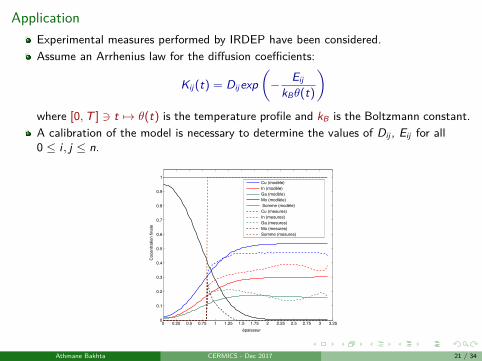
ApplicationExperimental measures performed by IRDEP have been considered.Assume an Arrhenius law for the diffusion coefficients:

Kij (t) = Dijexp(− Eij

kBθ(t)

)where [0,T ] 3 t 7→ θ(t) is the temperature profile and kB is the Boltzmann constant.A calibration of the model is necessary to determine the values of Dij , Eij for all0 ≤ i , j ≤ n.

0 0.25 0.5 0.75 1 1.25 1.5 1.75 2 2.25 2.5 2.75 3 3.250

0.1

0.2

0.3

0.4

0.5

0.6

0.7

0.8

0.9

1

épaisseur

Coc

entra

tion

final

e

Cu (modèle)In (modèle)Ga (modèle)Mo (modlèle) Somme (modèle)Cu (mesures)In (mesures)Ga (mesures)Mo (mesures)Somme (mesures)


Outline





Perfect crystals

[wikipedia]

A crystalline solid is a material composed of an infinite number of atoms that arearranged periodically in space.The study of the states of electrons in the crystal (electronic structure) enables tounderstand the macroscopic behavior of the solid.Understanding the electronic properties of a photovoltaic cell is crucial to improveits efficiency.


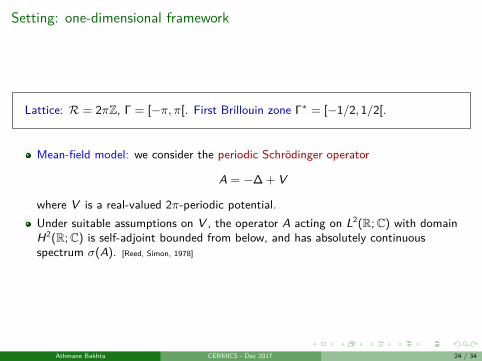
Setting: one-dimensional framework

Lattice: R = 2πZ, Γ = [−π, π[. First Brillouin zone Γ∗ = [−1/2, 1/2[.

Usual Hilbert spaces: a function f : R→ C belongs to:L2 if ‖f ‖2

2 :=∫R |f (x)|2dx < +∞;

L2loc if

∫K |f (x)|2dx <∞, ∀K ⊂ R compact;

L2per if f ∈ L2

loc(R;C) and f (x + 2π) = f (x), ∀x ∈ R.

Regular Sobolev spaces: Let s ∈ N∗. A function f : R→ C belongs to:Hs if f , f ′, · · · , f (s) ∈ L2(R;C);Hs

loc if f , f ′, · · · , f (s) ∈ L2loc(R;C);

Hsper if f ∈ Hs

loc(R;C) ∩ L2per.

Distributional spaces: Let s ∈ Z. A distribution u ∈ S ′(R), whose k th Fouriercoefficients for k ∈ Z is denoted by u(k), belongs to:

D′per if u is 2π − periodic;Hs

per if u ∈ D′per(R;C), ‖u‖2Hs

per:=∑

k∈Z(1 + |k|2)s |u(k)|2 < +∞.

Real-valued functions: We distinguish the spaces of real-valued functions by the index r:L2

per,r,Hsper,r.


Setting: one-dimensional framework

Lattice: R = 2πZ, Γ = [−π, π[. First Brillouin zone Γ∗ = [−1/2, 1/2[.

Mean-field model: we consider the periodic Schrodinger operator

A = −∆ + V

where V is a real-valued 2π-periodic potential.Under suitable assumptions on V , the operator A acting on L2(R;C) with domainH2(R;C) is self-adjoint bounded from below, and has absolutely continuousspectrum σ(A). [Reed, Simon, 1978]


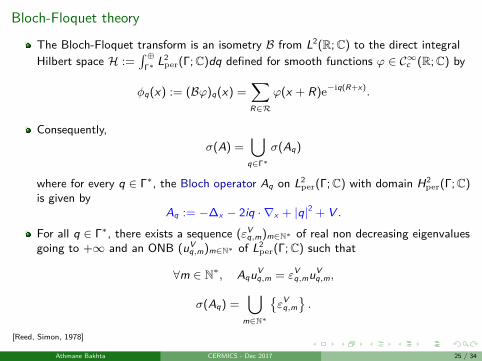
Bloch-Floquet theory

The Bloch-Floquet transform is an isometry B from L2(R;C) to the direct integralHilbert space H :=

∫ ⊕Γ∗ L2

per(Γ;C)dq defined for smooth functions ϕ ∈ C∞c (R;C) by

φq(x) := (Bϕ)q(x) =∑R∈R

ϕ(x + R)e−iq(R+x).

Consequently,σ(A) =

⋃q∈Γ∗

σ(Aq)

where for every q ∈ Γ∗, the Bloch operator Aq on L2per(Γ;C) with domain H2

per(Γ;C)is given by

Aq := −∆x − 2iq · ∇x + |q|2 + V .

For all q ∈ Γ∗, there exists a sequence (εVq,m)m∈N∗ of real non decreasing eigenvalues

going to +∞ and an ONB (uVq,m)m∈N∗ of L2

per(Γ;C) such that

∀m ∈ N∗, AquVq,m = εV

q,muVq,m,

σ(Aq) =⋃

m∈N∗

εV

q,m.

[Reed, Simon, 1978]


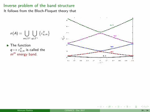
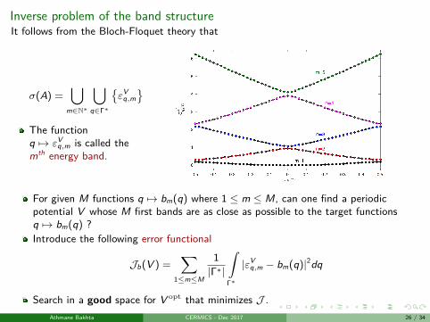
Inverse problem of the band structureIt follows from the Bloch-Floquet theory that

σ(A) =⋃

m∈N∗

⋃q∈Γ∗

εV

q,m

The functionq 7→ εV

q,m is called themth energy band.

For given M functions q 7→ bm(q) where 1 ≤ m ≤ M, can one find a periodicpotential V whose M first bands are as close as possible to the target functionsq 7→ bm(q) ?Introduce the following error functional

Jb(V ) =∑

1≤m≤M

1|Γ∗|

∫Γ∗

|εVq,m − bm(q)|2dq

Search in a good space for V opt that minimizes J .


Inverse problem of the band structureIt follows from the Bloch-Floquet theory that

σ(A) =⋃

m∈N∗

⋃q∈Γ∗

εV

q,m

The functionq 7→ εV

q,m is called themth energy band.

For given M functions q 7→ bm(q) where 1 ≤ m ≤ M, can one find a periodicpotential V whose M first bands are as close as possible to the target functionsq 7→ bm(q) ?Introduce the following error functional

Jb(V ) =∑

1≤m≤M

1|Γ∗|

∫Γ∗

|εVq,m − bm(q)|2dq

Search in a good space for V opt that minimizes J .Athmane Bakhta CERMICS - Dec 2017 26 / 34

Outline





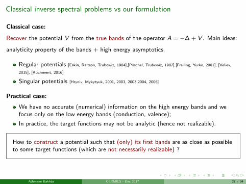
Classical inverse spectral problems vs our formulation

Classical case:

Recover the potential V from the true bands of the operator A = −∆ + V . Main ideas:

analyticity property of the bands + high energy asymptotics.

Regular potentials [Eskin, Raltson, Trubowiz, 1984],[Poschel, Trubowiz, 1987],[Freiling, Yurko, 2001], [Veliev,2015], [Kuchment, 2016]

Singular potentials [Hryniv, Mykytyuk, 2001, 2003, 2003,2004, 2006]

Practical case:

We have no accurate (numerical) information on the high energy bands and wefocus only on the low energy bands (conduction, valence);In practice, the target functions may not be analytic (hence not realizable).

How to construct a potential such that (only) its first bands are as close as possibleto some target functions (which are not necessarily realizable) ?


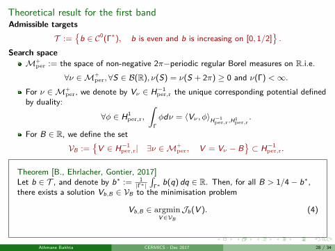
Theoretical result for the first bandAdmissible targets

T :=

b ∈ C0(Γ∗), b is even and b is increasing on [0, 1/2].

Search spaceM+

per := the space of non-negative 2π−periodic regular Borel measures on R.i.e.∀ν ∈M+

per, ∀S ∈ B(R), ν(S) = ν(S + 2π) ≥ 0 and ν(Γ) <∞.For ν ∈M+

per, we denote by Vν ∈ H−1per,r the unique corresponding potential defined

by duality:

∀φ ∈ H1per,r,

∫Γφdν = 〈Vν , φ〉H−1

per,r,H1per,r

.

For B ∈ R, we define the setVB :=

V ∈ H−1

per,r| ∃ν ∈M+per, V = Vν − B

⊂ H−1

per,r.

Theorem [B., Ehrlacher, Gontier, 2017]Let b ∈ T , and denote by b∗ := 1

|Γ∗|∫

Γ∗ b(q) dq ∈ R. Then, for all B > 1/4− b∗,there exists a solution Vb,B ∈ VB to the minimisation problem

Vb,B ∈ argminV∈VB

Jb(V ). (4)


Elements of the proof

Classical strategy : minimizing sequence, compactness, convergence.

Proposition [B., Ehrlacher, Gontier, 2017]Let B ∈ R and let (Vn)n∈N∗ ⊂ VB . For all n ∈ N∗, let νn ∈M+

per such thatVn := Vνn − B. Let us assume that the sequence

(εVn

0)

n∈N∗is bounded and such

that νn(Γ) −→n→+∞

+∞. Then, up to a (non-relabeled) subsequence, the functions

q 7→ εVnq converge uniformly to a constant function ε ∈ R, with ε ≥ 1

4 − B. In otherwords, there is ε ≥ 1

4 − B such that

maxq∈[0,1/2]

∣∣εVnq − ε

∣∣ −−−→n→∞

0. (5)

Conversely, for all ε ≥ 14 −B, there is a sequence (Vn)n∈N∗ ⊂ VB such that (5) holds.


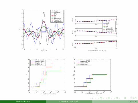
Numerical results

Admissible targets: Let M ∈ N∗ and b1, · · · , bM : Γ∗ → R be target functions.Brillouin zone grid: : Let Q ∈ N∗ and set

Γ∗Q :=−1

2 + jQ , 0 ≤ j ≤ Q − 1

.

Plane-wave approximation: The eigenvalues εVq,m are approximated by εV ,s

q,m usingGalerkin discretization method with the space

Xs := Span

x 7→ ek (x) := 1√2π

eikx , k ∈ Z, |k| ≤ s, s ∈ R+.

Search space:

Yp := Span

x 7→∑

k∈Z, |k|≤p

Vkek (x), ∀k ∈ Z, |k| ≤ p, V−k = Vk

, p ∈ R+.


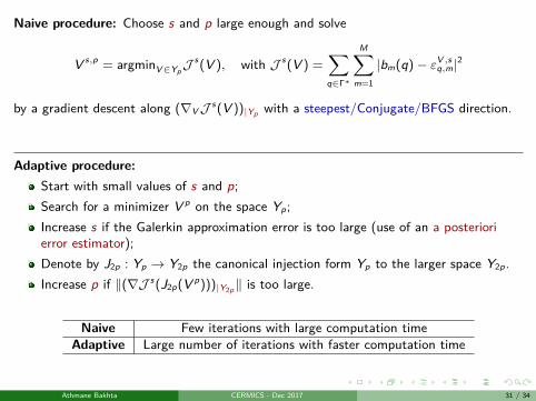
Naive procedure: Choose s and p large enough and solve

V s,p = argminV∈YpJs(V ), with J s(V ) =

∑q∈Γ∗

M∑m=1

|bm(q)− εV ,sq,m|2

by a gradient descent along (∇VJ s(V ))|Yp with a steepest/Conjugate/BFGS direction.

Adaptive procedure:Start with small values of s and p;Search for a minimizer V p on the space Yp ;Increase s if the Galerkin approximation error is too large (use of an a posteriorierror estimator);Denote by J2p : Yp → Y2p the canonical injection form Yp to the larger space Y2p .Increase p if ‖(∇J s(J2p(V p)))|Y2p‖ is too large.

Naive Few iterations with large computation timeAdaptive Large number of iterations with faster computation time


−3 −2 −1 0 1 2 3−2

−1.5

−1

−0.5

0

0.5

1

1.5

2

2.5

3

x ∈ [−π, π ]

V(x

)

Target

Initial guess

BFGS

PR

SD

Adaptive SD

Adaptive PR

Adaptive BFGS

0 0.25 0.5−0.2

0

0.2

band

1

recuced Brillouin zone [0, 1/2]

0 0.25 0.50

0.5

1

band

2

0 0.25 0.51

2

3

band

3

Target

BFGS

PR

SD

Adaptive SD

Adaptive PR

Adaptive BFGS

100

101

102

103

104

105

0

1

2

3

4

5

6

7

8

sn

n:= number of iterations

Adaptive BFGS

Adaptive PR

Adaptive SD

100

101

102

103

104

105

0

1

2

3

4

5

6

7

8

n:= number of iterations

pn

Adaptive BFGS

Adaptive PR

Adaptive SD


Outline





Perspectives

Cross-diffusion:Cross diffusion systems with non-zero external fluxes in higher dimension;Include reaction terms;Numerical schemes preserving the volume filling property.

Inverse Hill’s problem [work in progress]:Numerical results in higher dimension;Consider the inverse problem of band gap location/size.


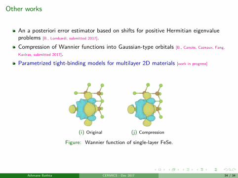
Other works

An a posteriori error estimator based on shifts for positive Hermitian eigenvalueproblems [B., Lombardi, submitted 2017].Compression of Wannier functions into Gaussian-type orbitals [B., Cances, Cazeaux, Fang,Kaxiras, submitted 2017].Parametrized tight-binding models for multilayer 2D materials [work in progress]

(i) Original (j) Compression

Figure: Wannier function of single-layer FeSe.


MERCI


modèles mathématiques et simulation numérique de...

Documents