mémoire présenté le : srxuo¶rewhqwlrqgx 'lso
TRANSCRIPT

Mémoire présenté le :
pour l’obtention du Diplôme Universitaire d’actuariat de l’ISFA
et l’admission à l’Institut des Actuaires
Par : SAYAH Mabelle
Titre Comparing standardized and internal models in computing the interest rate risk capital charge in a bank’s trading book
Confidentialité : NON OUI (Durée : 1 an 2 ans)
Les signataires s’engagent à respecter la confidentialité indiquée ci-dessus
Membre présents du jury de l’Institut
des Actuaires signature
Entreprise :
Nom :
Signature :
Membres présents du jury de l’ISFA Directeur de mémoire en entreprise :
Nom : ROBERT Christian
Signature :
Invité :
Nom :
Signature :
Autorisation de publication et de mise
en ligne sur un site de diffusion de
documents actuariels (après expiration
de l’éventuel délai de confidentialité)
Signature du responsable entreprise
Secrétariat : DRIGUZZI Christine Signature du candidat
Bibliothèque : BARTOLO Patricia

Contents
Introduction 5
I Banking Risk Management Function 10
1 Banks 101.1 Objectives and roles . . . . . . . . . . . . . . . . . . . . . . . 101.2 Balance Sheet Composition . . . . . . . . . . . . . . . . . . . 101.3 Banking vs trading book . . . . . . . . . . . . . . . . . . . . . 14
2 Financial Risk Management 142.1 Market Risk . . . . . . . . . . . . . . . . . . . . . . . . . . . . 142.2 Credit Risk . . . . . . . . . . . . . . . . . . . . . . . . . . . . 142.3 Operational Risk . . . . . . . . . . . . . . . . . . . . . . . . . 152.4 Liquidity Risk . . . . . . . . . . . . . . . . . . . . . . . . . . . 15
3 Basel implementation 153.1 Basel I . . . . . . . . . . . . . . . . . . . . . . . . . . . . . . . 153.2 Basel II . . . . . . . . . . . . . . . . . . . . . . . . . . . . . . 153.3 Basel III . . . . . . . . . . . . . . . . . . . . . . . . . . . . . . 16
4 On the interest rate risk in the trading book 164.1 Definition of the interest rate risk . . . . . . . . . . . . . . . . 164.2 Net interest income (NII) . . . . . . . . . . . . . . . . . . . . . 174.3 General Interest rate risk in the trading book . . . . . . . . . 174.4 Basel III perception (January 2016) . . . . . . . . . . . . . . . 17
4.4.1 SBA impact on banks . . . . . . . . . . . . . . . . . . 19
II Tools and Models used 20
1 Yield Curves 201.1 Introduction to yield curves . . . . . . . . . . . . . . . . . . . 201.2 Term structure estimation models . . . . . . . . . . . . . . . . 201.3 Yield curves across central banks . . . . . . . . . . . . . . . . 211.4 Different methodologies . . . . . . . . . . . . . . . . . . . . . . 23
1.4.1 Nelson Siegel method . . . . . . . . . . . . . . . . . . . 241.4.2 Dynamic Nelson Siegel . . . . . . . . . . . . . . . . . . 24

2 Statistical tools 252.1 PCA . . . . . . . . . . . . . . . . . . . . . . . . . . . . . . . . 252.2 ICA . . . . . . . . . . . . . . . . . . . . . . . . . . . . . . . . 26
3 Econometrical tools 273.1 GARCH(p,q) model specification . . . . . . . . . . . . . . . . 273.2 Different GARCH Models . . . . . . . . . . . . . . . . . . . . 29
4 Forecasting models 294.1 Constant Conditional Correlation models . . . . . . . . . . . . 304.2 Dynamic Conditional Correlation models . . . . . . . . . . . . 304.3 CCC vs DCC . . . . . . . . . . . . . . . . . . . . . . . . . . . 31
5 Sensitivity Based approach (SBA) 325.1 Introducing the approach . . . . . . . . . . . . . . . . . . . . . 325.2 Implementation reasons . . . . . . . . . . . . . . . . . . . . . 325.3 Computational steps . . . . . . . . . . . . . . . . . . . . . . . 325.4 Hypothetical example . . . . . . . . . . . . . . . . . . . . . . . 34
6 Risk measures 356.1 Value at risk . . . . . . . . . . . . . . . . . . . . . . . . . . . . 35
6.1.1 Different VaRs . . . . . . . . . . . . . . . . . . . . . . 366.2 Expected Shortfall . . . . . . . . . . . . . . . . . . . . . . . . 376.3 VaR vs ES . . . . . . . . . . . . . . . . . . . . . . . . . . . . . 38
7 Value at Risk Backtesting Methods 397.1 Introduction . . . . . . . . . . . . . . . . . . . . . . . . . . . . 397.2 Backtesting strategies . . . . . . . . . . . . . . . . . . . . . . . 41
7.2.1 Frequency Based Tests . . . . . . . . . . . . . . . . . . 417.2.2 Magnitude Based Tests . . . . . . . . . . . . . . . . . . 427.2.3 Independence Tests . . . . . . . . . . . . . . . . . . . . 427.2.4 Duration Based Tests . . . . . . . . . . . . . . . . . . . 437.2.5 Martingale Difference Based Tests . . . . . . . . . . . . 437.2.6 Regression models Based Tests . . . . . . . . . . . . . 447.2.7 Loss function Based Tests . . . . . . . . . . . . . . . . 45
7.3 Practical Issues . . . . . . . . . . . . . . . . . . . . . . . . . . 457.4 Remarks . . . . . . . . . . . . . . . . . . . . . . . . . . . . . . 46
III Numerical Application 47
3

1 Data used 471.1 Data statistics . . . . . . . . . . . . . . . . . . . . . . . . . . . 47
2 Portfolios’ duration and capital requirements 492.1 Single currency portfolios . . . . . . . . . . . . . . . . . . . . . 502.2 Multiple currencies portfolios . . . . . . . . . . . . . . . . . . 58
3 Backtesting Results 63
IV Conclusion 64
V References 67
VI Appendices 72
4
IntroductionCommercial banks are a key component of today’s financial and economicsystem. Banks allocate funds from depositors to borrowers, convert maturi-ties, and provide financial products. These services among others enhancesthe efficiency of the overall economy. Given this crucial role, adequate regu-lations should apply to monitor banks risks.
Since its first issuance in 1988, Basel has been the main banking regula-tion authority initializing with some main credit risk rules. In 1996, themarket amendment was issued setting the basic standards regarding tradingassets and the value at risk computation methodology. It also divided therisk into market and credit risk; market risk being divided between equity,interest rate, foreign exchange, commodity, and option risk with a standard-ized capital computation approach treating each asset class separately. In2006, Basel II came along with more ’personalised’ approaches such as Inter-nal Rating Based (IRB) for credit risk, internal models for Over The Counter(OTC) derivatives exposure along with the introduction of the operationalrisk charge.
However these regulations did not prevent major crisis hitting the inter-national market causing huge losses in different sectors (cf. Baptistab et al.(2012)). As a response to this shortage, Basel 2.5 was created beginning2011 as a response adding more capital to the trading book (especially onthe poorly modeled products). Basel 2.5 additions target the stressed VaRconcept, the incremental risk charge and few new standard rules regardingthe banking book.
In 2013, after a thorough observation of the consequences of the crisis andthe attempt for correction made by 2.5, Basel III was introduced. The mainfunctions of this issuance are: increasing capital for counterpart exposures,tightening the definition of the bank’s capital, adding buffer for liquidity andintroducing a new leverage ratio (cf. BCBS (2014)). In parallel, increasingthe trading book capital requirement under Basel 2.5 was required follow-ing the crisis and was not well designed: the calculation remains non-risksensitive and highly conservative, and differences in model approval persistbetween jurisdictions (cf. Babel (2012))
As a result, in May 2012 the Basel Committee published a ConsultativePaper on a ’Fundamental Review of the Trading Book’ (FRTB) to improve
5

this framework, then in December 2014, ”Fundamental review of the tradingbook: outstanding issues”, and its comments March 2015,the BCBS exposedthe weaknesses of Basel’s previous approaches. It suggested some majorchanges to the trading book to be implemented by 2018: scope and approvalprocess (boundary of the trading book, desk level model approval, modeltesting, model independent assessment tool), modeling Issues (stressed ex-pected shortfall, liquidity adjustments, diversification, default and migrationrisk, and non-modelable risk factors), and new standard rules for capitalcharges computation.
The standard rule suggested by the FRTB is based on sensitivities, henceit is called the ”Sensitivity based approach” (SBA): it was implemented asthe ’homogeneous’ method for capital charge computation across all banks.The SBA is based on percentages and correlations between different matu-rities and currencies (cf. BCBS (2015)). The existing standard rules poorlyreflected hedging or diversification thus inflating the trading book capitallevel. The SBA is simple yet risk sensitive which is already a big improve-ment. SBA is a standardized method that reflects the risk resulting from:Interest rate, credit spread, equity, commodity, foreign exchange, options riskand default.
Comparing regulatory approaches, an obvious contrast between Basel andSolvency is noted: Solvency II has a similar three pillar structure as Basel’sAccords. The capital requirements are described under the first pillar andrefer to all types of risks: an insurance is exposed to: market risk (inter-est rate risks, equity risk, property risk, spread risk, concentration risk andcurrency risk) and counterpart default risk. Both frameworks take diversi-fication effects into account and use square root formulas. However, theseaggregation approaches are applied at different levels: a considerably strongerrisk differentiation is shown under Basel III. For example, the SBA equityrisk distinguishes 10 risk categories in order to assign the risk weights, incontrast to one single shock for all listed equities under Solvency II. Underthe interest rate risk, SBA is Basel’s III approach whereas in solvency II ashocked scenarios based computation sets the capital charge (cf. LAAS andSiegel (2015)).
Seemingly, the SBA has several add-ons regarding sensitivity and diversify-ing considerations however it still has some issues (specifying the coefficients)and details concerning the aggregations that need to be tweaked; for instancethe figure under the square root is sometimes negative (cf. ISDA (2015)).In this dissertation, we aim to focus on the suggested standard rule by the
6

FRTB in order to compare it with other econometric models to find an equiv-alent capital charge computation technique with few additional details suchas time horizon and confidence level for a given capital. Among the differentrisk modulations, we chose to focus on the interpretation of the interest raterisk capital charge calculation.
According to Oxford Dictionary of Economics, interest rate is defined as”The charge made for the loan of financial capital expressed as a proportionof the loan”. More formally, Basel Committee on Banking Supervision (cf.BCBS (2004)) indicated that interest rate risk (IRR) is the exposure of abank’s financial condition to adverse movements in interest rate.
The sound IRR management conducted by Basel Committee on BankingSupervision had been the source on which analysts rely to evaluate the ac-tivities of bank’s risk management of interest rate (cf. BCBS (2004)). Inthe guideline, the committee offers four basic elements of IRR: appropriateboard oversight, comprehensive internal controls, adequate policies and ap-propriate risk measure. The SBA falls under this forth element in modelingthe interest rate risk in the trading book.
Our aim in this work is to understand the computation of the interest raterisk in banks based on BASEL’s III approach. However, the SBA remainsrelatively vague and the choices of its coefficient and correlation parametersare not robustly detailed and documented. Hence, studying the interest raterisk from an econometric point of view in order to compare and contrast theresults is critical and highly important.
Based on different central banks approaches for term structure interest rate,we selected few econometric models. The main idea was to reduce the di-mensions of the database, study the dynamics of these ’reduced’ factors andthen conclude on the wider data range dynamic. We introduce the methodsused to derive capital requirement and compare them with SBA’s in orderto conclude on some equivalence between them.
Having this objective in mind, the structure of the work is as follows: Westarted by modeling each interest rate curve on a stand-alone maturity basisusing a Generalized Auto regressive Conditional Heteroskedasticity (GARCH)approach. It is worth noting that by doing so, we dropped a crucial infor-mation which is the strong correlation between these maturities, however weneeded this phase as a starting point and a comparison threshold. Modelingthe volatility of term structures using GARCH processes has become a cur-
7

rent practice due to its numerous advantages relative to alternative models.GARCH-methods are a way of investigating how a function of past returns, ina specific financial series, should be constructed and mapped onto the secondmoment (cf. Hull (2000)). Proposed by Engle (1982) and then generalized byBollerslev (1986), GARCH models explain high frequency financial data se-ries through the auto regressive conditional heteroskedasticity and can modelsimultaneously conditional mean and conditional variance (cf. Edison andLiang, 1999). Two parameters for orders could be used in order to optimizethe results of the tests regarding GARCH coefficients convergence. However,in practice, low orders are more frequently used. The first-order (p=q=1)GARCH model (cf. Taylor (1986)) has become the most popular GARCHmodel.
Secondly, we introduced the component approaches starting with the Prin-cipal component analysis (PCA) which is one of the multivariate analysistechniques usually used for correlation studies, data reduction and efficiencyassessment (cf. Levieuge et al. (2010)). This method incorporates the inter-dependence between term structures maturities: it considers the correlatedcurves and generates new non-correlated variables. Each factor is related toa loading and a cumulative variance defining the variance explained by eachone of the new variables. PCA creates the same number of term structuresincluded in the model however, we need to choose the reduced number offactors that we want to handle. In this work, we chose to cover 98% of thevariance, by considering two or three factors. Using a GARCH model, weonly project the chosen factors and not the loadings; then we re-create theentire data from the projected factors and previously observed loadings.
Thirdly, we introduced the implementation of the Independent componentanalysis (ICA): it provides a mechanism of decomposing a given signal intostatistically independent components. PCA uses only second order statisti-cal information however, ICA uses higher order (kurtosis) for separating thesignals which permits more conclusive results in financial data (cf. Comon(1994)). A drawback in the ICA is its inability to indicate the data variancecoverage for each factor, therefore the modeler has to define the number offactors to be considered; in this dissertation we chose to include three ICAfactors.
Regarding the last approach, a factor model is suggested: the Dynamic Nel-son Siegel. No GARCH processes are used, instead a mix of Nelson Siegelestimation and Autoregressive Integrated Moving Average (ARIMA) pro-cesses projection are put in practice. Yield curve factor models, such as
8

Nelson-Siegel (1988), its dynamic version (cf. Diebold and Li (2006)) and itsarbitrage-free counterpart proposed by Christensen, Diebold and Rudebusch(2011), have been extensively applied to forecast bond yields. We used theDynamic Nelson Siegel due to its flexibility in representation especially forthe long term projection. By fitting the curves, projecting the factors usingDiebold method and the loadings employing an ARIMA process, we are ableto reconstruct the curves from which we concluded the capital requirement.
The capital charge using the previously mentioned methods, except SBA,can be computed on a certain confidence level basis and for a given timehorizon; therefore comparing these methods to SBA would determine a com-mon time horizon and confidence level, reaching the purpose of this work.We start by explaining in details the procedure of the SBA, the correlationbetween the duration of the portfolios and the capital charge required by thisprocedure then compare the methods using different approaches. These latterwill be based on bonds portfolios denoted in: euros, dollars and Turkish lirafrom the French, German, US and Turkish governments yields respectively,for maturities between 1 month and 30 years.
9

Part I
Banking Risk ManagementFunction
1 Banks
1.1 Objectives and roles
Banking is about managing different risks and making the most profit outof it. The skills that banks use to balance their numerous assets and lia-bilities reflect the risk exposure and the expected returns. Nowadays, com-mercial banks are becoming more complex including different instrumentsin their portfolio and expanding their work circle. In addition regulatoryrequirements have been adding strict restrictions and requirements in orderto reevaluate the risk management tasks. This might induce that they aremore able to withstand the business fluctuation and risks, however, recentevents showed that this might not be the case.
Based on the recent crises, in a systemic sense, the financial sector is be-coming more risky. Indeed, if numerous banks invest in similar positions orfollow parallel strategies the whole sector becomes more exposed. In orderto explain how to handle the entire banking risk, compute it and minimizeit, a certain full comprehension of a commercial bank portfolio should be intitle.
1.2 Balance Sheet Composition
To begin with, let us demonstrate the components of its balance sheet andbriefly explain each:
10
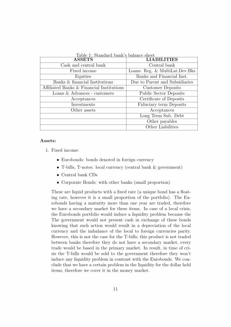
Table 1: Standard bank’s balance sheetASSETS LIABILITIES
Cash and central bank Central bankFixed income Loans: Reg. & MultiLat.Dev.Bks
Equities Banks and Financial Inst.Banks & financial Institutions Due to Parent and Subsidiaries
Affiliated Banks & Financial Institutions Customer DepositsLoans & Advances - customers Public Sector Deposits
Acceptances Certificate of DepositsInvestments Fiduciary term DepositsOther assets Acceptances
Long Term Sub. DebtOther payables
Other Liabilities
Assets:
1. Fixed income:
• Eurobonds: bonds denoted in foreign currency
• T-bills, T-notes: local currency (central bank & government)
• Central bank CDs
• Corporate Bonds: with other banks (small proportion)
These are liquid products with a fixed rate (a unique bond has a float-ing rate, however it is a small proportion of the portfolio). The Eu-robonds having a maturity more than one year are traded, thereforewe have a secondary market for these items. In case of a local crisis,the Eurobonds portfolio would induce a liquidity problem because theThe government would not present cash in exchange of these bondsknowing that such action would result in a depreciation of the localcurrency and the imbalance of the local to foreign currencies parity.However, this is not the case for the T-bills; this product is not tradedbetween banks therefore they do not have a secondary market, everytrade would be based in the primary market. In result, in time of cri-sis the T-bills would be sold to the government therefore they won’tinduce any liquidity problem in contrast with the Eurobonds. We con-clude that we have a certain problem in the liquidity for the dollar helditems, therefore we cover it in the money market.
11

2. Money Market: This item is included in the assets and liabilities, butis mainly covered in the assets part including all kinds of currencies(LBP, USD, EURO, JPY...). Mainly, the placements are divided uponthree categories relatively to the counterpart of each: affiliated, non-affiliated and the central bank. The purpose of this money marketshare is, as previously mentioned, covering the liquidity in case of alocal crisis (mainly due to the foreign currency held Eurobonds). Onthe assets part we have:
• Nostro: current account with another foreign bank: this is a coston the bank because, when a client beholds money in the bank, wetake a certain proportion of the amount and place it in a Nostroaccount presenting a low interest rate. Therefore, I am losingin term of interest rate however gaining in terms of covering theliquidity risk.
• Loan: Blocked account with a foreign bank
• Loan term: Blocked account with a foreign bank having an amor-tization option at the banks blocked accounts with the centralbank are included here (secret repo agreement for ten years).
• Central bank reserve: in local and foreign currencies
• Subordinated debt: it mainly include the main entity debt to otherentities, it is another category of debt with a priority of collectingmoney in case of failure or bankruptcy.
• Reverse Repo: loans given to financial institution, paying low in-terest rate and receiving collateral for guarantee (ex: collateralcovering 120% of the loan amount in CDs), they are qualified asover collateralized products.
3. Loans
• Corporate and Commercial loans
– Term loan: x amount on n years, payments divided over theyears
– Overdraft: a certain fixed amount but the client has the lib-erty to choose when and how much money to spend condi-tioned by the reimbursement of the amount
– Post financing: corporate having different payments with clientsbut in need of money right away, the bank provide the liquid-ity and get to be the recipient of the clients bills (with acertain profit margin)
12

– Syndicated loan: a loan divided between different banks
• Retail
– Personal
– Car
– Home: divided between the banks proportion and the housingservice (provided by the government)
– Credit card
– Educational
– Others
It is important to note what a SUBSIDIED loan is: a loan in-cluding a proportion held by the government such as the housingloan.
Liabilities:
1. Deposits:
• Demand
• Term
• Credit linked deposit: using a number of deposits we buy a bond,with the same maturity as the deposits, the coupons of the bondare distributed on the depositors and an additional commission isretained by the bank.
2. Money Market:
• Vostro: another bank places money in our portfolio
• Deposit: idem as the loan but reversely
• Deposit term: idem as the loan term but reversely
• Deposit fiduciaries: deposits from affiliated banks on which wepay interests (rather than them paying in their home country ahigher rate)
3. Sub debt: When we need to increase the capital, the investors give thebank a loan, the bank pays them the coupons from the benefits. Inthat way, we increase the capital from the investors.
13

1.3 Banking vs trading book
Trading and banking book are accounting terms that categories instrumentsin a bank: Based on the purpose the bank is holding this product, a decisionis made whether it is in the banking or the trading book. We note that thedistinction between these two books is rather ambiguous in some cases, toconfirm, some financial institutions have used this to juggle products betweenthis or that book in order to reduce the capital charge or enhance the capitaladequacy ratio.
The trading book, as its name shows, refers to all assets held by the bankand that are regularly traded, it is required to be marked to market daily.
The banking book however, is the assets that the bank is supposed to holduntil maturity. It is not marked to market.
2 Financial Risk Management
Financial risk management has known a large boost over the last decades dueto consecutive crisis that emphasis the crucial need of having a robust riskmanagement function. Corporations need to manage their risk rather thanavoiding them: quantitative approaches have been widely adopted howevera full reliance on these figures without considering the exogenous conditionsa financial institution is exposed to would not be very representative.
In banks, financial risk is divided between several types: market, credit,operational and more recently liquidity. Briefly, we introduce each type:
2.1 Market Risk
This risk is due to market prices movement: stock prices, FX rates, interestrates, commodity prices or credit spreads. It is this, overly studied risk, thatled to the birth of the value-at-risk concept.
2.2 Credit Risk
The credit risk is related to a counterpart: this latter might not be ableto fulfill his contractual obligations: as default or just devaluation of therequired amount. The key aspect in this type is the probability of defaultand the exposure at default.
14

2.3 Operational Risk
Operational risk is divided between sources: people, systems and externalevents. An employee fraud, an ATM malfunction or a civil war fit in the op-erational risk category. This is the most hard to quantify type of risks whichleads to the use of more qualitative techniques, score cards and professionalsassessments.
2.4 Liquidity Risk
Liquidity risk represent the risk that a transaction cannot be executed onthe market due to the illiquidity of the underlying or size of the transactionsor the risk of not being able to fund payments. This risk gained the notationof the ’death risk’ in 2008 crisis once liquidity is missing it’s a vicious circlenot only for the concerned institutions but for the whole system.
3 Basel implementation
3.1 Basel I
In 1988, Basel was created in his first version in order to unify the interna-tional banking system (cf. BIS).
It divided the required capital into two tiers: tier I (Core capital) and TierII (Supplementary capital).
The tier I consists shareholders equity, held stocks and all declared reserveswhereas tier II includes gains and long-term maturing debts. The Capitalcharge is divided between two risk typologies: Market risks (interest rates,fx, equity derivatives) and credit risk (including default risk).
3.2 Basel II
Basel II implemented the minimal capital adequacy ratio which is the capitalheld to the assets for an 8% figure. The risks acknowledged became three:the operational risk was added. Plus, under Basel II internal approachessuch as the internal ratings-based approach were recognized. This new Baselversion is more risk sensitive and more representative of the risk mitigationadvantages therefore it was seen as an improvement to the previous Baselaccord until enormous financial crisis such as the Sub-crime crisis in 2008.
15

3.3 Basel III
Basel III was created in an attempt to improve capacity of absorbing shocksdue to the rise of the instability in the financial markets, improve risk man-agement and strengthen transparency among banks: it increases the marketrisk requirement, adjusts the credit risk computation and adds disclosures tobe provided regularly. Basel III also added two main concepts: the liquidityratio and leverage ratio.
4 On the interest rate risk in the trading
book
4.1 Definition of the interest rate risk
Previous studies show that the market risk factor dominates in term of sta-tistical significance on the entire portfolio risk, therefore we chose to managethe interest rate risk in order to get a broader view on the consolidated risk(cf. Schuermann (2010)).
P.S: A careful analysis of the portfolio risk suggests that the use of fewfactors accounting for the largest proportion of returns will underestimatethe risk, adding to that leaving out factors with high expected return willguide to misleading results as well (cf. Kambhu, Rodriguez). A banks inter-est rate risk reflects the extent to which its financial condition is affected bychanges in market interest rates. There are two different ways of thinkingabout such effects. The first approach focuses on the impact of changes inmarket interest rates on the value of bank assets, liabilities and off-balancesheet positions (potentially including those that are not marked to marketfor reporting purposes). The second approach focuses on the implications ofmovements in market rates for the future cash flows that the bank will ob-tain. Since the present discounted value of the banks cash flows must equalthe economic value of the bank, these two approaches are consistent and bothcan be useful (cf. BIS paper (2010)).
To assess directly the extent detailed information about a number of possiblesources of interest rate risk is needed. Clearly, one would need to understandthe mechanism of the bank and the detailed characteristics of each prod-uct: pricing assets and liabilities, including repricing periods and base rates,the likelihood that bank customers would choose to repay loans or withdrawfunds early as a result of changes in market rates, the interest sensitivity of
16

fee income and off-balance sheet exposures...
In addition to being very complex, the feasibility of this study depends onthe availability of the data therefore we try to choose an alternative way byresorting to well-chosen benchmarks. A universally used tool to measure thiskind of risk is the NII, net interest income.
4.2 Net interest income (NII)
The net interest income of a bank is defined as the excess of interest receivedover interest paid (cf. Hull (2012)).
Net interest income = interest revenue - interest expense
• Daily computed
• Deposits basis: 365 days
• Loans basis: 360 days
• Calculation for each product and then aggregated
• The change of NII for a giving change in rate: the computation is onlyaffected by the items that matures within this year or the floating itemswhich rates can change during this one year.
4.3 General Interest rate risk in the trading book
In the trading book, two different notations are assigned to the interest raterisk: the general aspect and the specific genre.
Simply, the general interest rate risk is the risk arising from general mar-ket movements Such as fluctuations in interest rate levels or equity priceschanges on the market; whereas specific interest rate risk is the risk relatedto the credit quality of issuers.
4.4 Basel III perception (January 2016)
In December 2014 Basel Committee issued its third consultative paper onoutstanding issues related to the fundamental review of trading book capitalrequirements. Recognizing the significant operational burden posed by cer-tain features of the proposed framework, including the revised standardizedapproach (cashflows needed) , several alternative treatments were tested in
17

the 2014 QIS and will be further assessed through a follow-up QIS in early2015. This document sets:
• the treatment of internal risk transfers of equity risk and interest raterisk between the banking book and the trading book
• a sensitivities-based methodology in the revised standardized approach
• a simpler method for incorporating the concept of liquidity horizons inthe internal models approach
Three main objectives for the revised standardized approach:
1. The approach must provide a method for calculating capital require-ments for banks with a level of trading activity that does not requiresophisticated measurement of market risk.
2. It provides a fallback in the event that a bank’s internal model isdeemed inadequate, including the potential use as an add-on or floorto an internal models-based charge.
3. The approach should facilitate consistent and comparable reporting ofmarket risk across banks and jurisdictions.
A previous consultative paper proposed a cash flow-based method which re-quired banks to decompose financial instruments into their constituent cashflows and then discount each cash flow using the risk-free curve for each cur-rency plus the credit spread of each instrument. Banks had many constraintsand issues regarding this method (data wise), therefore following these con-cerns, the Committee agreed on a sensitivity-based approach (SBA) as analternative to cash flow-based calculations for the standardized approach.
This new method would require banks to use price and rate sensitivities thatare more likely to be available in their systems as inputs into the differentasset class treatments. The use of sensitivities thus reduces the implementa-tion cost of the revised standardized approach.
The standardized approach trading book capital requirement is the sum of:
The linear (delta and Vega) risk and curvature requirements for the generalinterest rate risk (GIRR) capital charge, Credit Spread Risk (non-securitisations),CSR (securitisation non-correlation trading portfolio), Equity capital charge,Commodity capital charge, FX risks and additional requirements for defaultrisk (non-securitizations), default risk (securitization non-correlation trading
18

portfolio) and default risk (correlation trading portfolio).
In the following, we are discussing the SBA for the GIRR in the tradingbook.
4.4.1 SBA impact on banks
in a study led by BCBS (cf. BCBS (2015))based on a sample of 44 banks thatprovided usable data for the study and assumed that the proposed marketrisk framework was fully in force as of 31 December 2014; the results showthe following: market risk capital charges would produce a 4.7% increase inthe overall Basel III minimum capital requirement. When the bank with thelargest value of market risk-weighted assets is excluded from the sample, thechange in total market risk capital charges leads to a 2.3% increase in overallBasel III minimum regulatory capital. Compared with the current marketrisk framework, the proposed standard would result in a weighted averageincrease of 74% in aggregate market risk capital. When measured as a simpleaverage, the increase in the total market risk capital requirement is 41%. Forthe median bank in the same sample, the capital increase is 18%. Comparedwith the current internally modelled approaches for market risk, the capitalrequirement under the proposed internally modelled approaches would resultin an increase of 54%. For the median bank, the capital requirement underthe proposed internally modelled approaches is 13% higher. Compared withthe current standardised approach for market risk, the capital requirementunder the proposed standardised approach is 128% higher. For the medianbank, the capital requirement under the proposed standardised approach is51% higher.
19

Part II
Tools and Models used
1 Yield Curves
1.1 Introduction to yield curves
The relationship between the yields of default-free zero coupon bonds andtheir length to maturity is defined as the term structure of interest rates andis shown pictorially in the yield curve. This relation can be used for riskmanagement and has an important role in pricing fixed-income securitiesand interest rate derivatives, as well as other financial assets. Because of itsnumerous uses, an accurate estimate of the term structure has constituted amajor question in the empirical literature in economics and finance.
There are two distinct approaches to estimate the term structure of interestrates: the equilibrium models and the statistical techniques. Examples of thefirst approach include Vasicek (1977), Dothan (1978), Brenan and Schwartz(1979), Cox and Ingersoll Ross (1985) and Dufie and Kan (1996).
1.2 Term structure estimation models
Term Structure static models are usually spot rate models that weaves to-gether zero yields of different maturities as they are observed in the market.Major criticism of static spot rate models are adjustments and data overfitting. These models simply calculate the interest rate that fits the observedprice.
The first step in any financial scenario aiming to measure risk, anticipatefuturistic losses, gain or returns is the construction of an appropriate inter-est rate model especially when the existing yield curve is insufficient and lackof precision. A wide variety of models is available for long and short term;yet not a single model has proven to be worthy and valuable for all kindsof application, different purposes and different approaches. There is a veryimportant issue to consider when choosing among different models related tothe background, data and concept of the model: equilibrium and arbitragefree models(cf. Chen et al. (2010)).
20

Arbitrage free models Arbitrage-free structure projects future interestrates based on the historical yield curve. Therefore, the new anticipatedprices respect the non arbitrage concept and are useful for pricing deriva-tives. In this approach, we consider that individual agents are risk-neutraland have no preferences reaching by that a ’theoretical’ partial equilibrium(cf. Damino, Fabio (2000)). The no-arbitrage approach is an exact fit tothe observed market yield. Some of these models include: Hull and White,CIR++ and Karasinki’s extended model.
Equilibrium models In contrast with the no arbitrage methods, the gen-eral equilibrium model allows the investor’s risk preference to enroll in pricingthe instruments, in that kind of assumptions a more realistic equilibrium isreached. Equilibrium models typically begin with an assumption for theshort term interest rate behavior, which are usually derived from more gen-eral assumptions such as state variable or any significant factor that describethe overall economy. Using these assumptions, the model can determine thelong term behavior based on the possible paths (cf. Longstaff (1989)). Thesemodels are fairly easy to use however, they generate yield curve inconsistentwith the current market prices. In addition, the market price of risk used inthese models is very hard to obtain. Some of these models include: Vasicek,CIR, Dothan and exponential Vasicek.
1.3 Yield curves across central banks
Most central banks use either the Nelson-Siegel or the extended version sug-gested by Svensson. Exceptions are Canada, Japan, Sweden, the UnitedKingdom, and the United States of America which all apply variants of thesmoothing splines method. They employ government bonds in the estima-tions since they carry no default risk.
21

Rudy J. DACCACHE PhD Thesis
Appendix 1.B- Yield Curve Models in Cen-tral Banks
Table 1.7: Yield Curve Models in Central Banks
Centra Bank EstimationMethod
Minimised Er-ror
Availability(BIS)
Belgium Svensson orNelson-Siegel
Weighted Prices up to 16 years
Canada Merrill LynchExponentialSpline
Weighted Prices up to 30 years
Finland Nelson-Siegel Weighted Prices up to 12 yearsFrance Svensson or
Nelson-SiegelWeighted Prices up to 10 years
Germany Svensson Yields up to 10 yearsItaly Nelson-Siegel Weighted Prices up to 30 yearsJapan Smoothing
SplinesPrices up to 10 years
Norway Svensson Yields up to 10 yearsSpain Svensson Weighted Prices up to 10 yearsSweeden Smoothing
Splines andSvensson
Yields up to 10 years
Switzerland Svensson Yields up to 30 yearsUK VRP Yields up to 30 yearsUSA Smoothing
SplinesWeighted Pricesor Prices
up to 10 years
40
Table 2: Yield Curve methodologies across central banks
22

1.4 Different methodologies
noMo
del Na
meSte
psEqu
ation
Advant
ages
Disadv
antage
s
1Sup
er Bell
(Bootst
raping
)extr
acting t
he zero
-coupo
n and fo
rward i
nterest
rates
using an
OLS re
gressio
n to fit
a par yie
ld curv
e from
exis
ting bo
nd em
ploying
bootst
rapping
to der
ive zero
-coupo
n rates
For les
s than o
ne year
Cubic In
terpolat
ion1. T
he mode
l is not c
oncept
ually di
fficult.
2. The m
odel is p
arame
trized a
nalytica
lly and i
s thus s
traight
forward
to solv
e.1. le
ngthy p
rocess
2. focu
ses exc
lusively
on YTM
rather
than o
n the ac
tual ca
sh flow
s of the
underly
ing bon
ds.3. n
ot enou
gh flexi
bility
2Nel
son-Sie
gel Con
vert th
e bond p
rices to
forwar
d rates
(using F
ama-b
liss me
thod)
Conver
t to zer
o yields
1.The av
erage y
ield cur
ve is in
creasin
g and co
ncave.
2.Coul
d assum
e a var
iety of
shapes
(sloping
upward
, sloping
downw
ard, hu
mped o
r inver
sely hum
ped).
3.Yield
dynam
ics are p
ersisten
t (\beta
_1) and
less pe
rsisten
t (weak
er for \
beta_2
).4.Th
e short
end is m
ore vol
atile th
an the l
ong end
(short
end dep
ends on
\beta_
1 and \b
eta_2 w
hereas
the lon
g end
depend
s only o
n \beta
_1).
5.Long r
ates ar
e more
persist
ent tha
n short
rates (lo
ng end d
epends
on \be
ta_1 o
nly).
non line
ar estim
ation fo
r the la
mbda f
actor
3Sm
ith- Wi
lsonGoi
ng from
the ob
served Z
C on th
e mark
et, Com
pute ot
her ma
turities
ZC via
interpo
lation an
d extrap
olation
using a
long U
ltimate
Forwar
Rate
1.perfe
ct fit o
f the es
timate
d term
structu
re to th
e liquid
marke
t data
2.base
d on so
lving a
linear s
ystem o
f equat
ions an
alytical
ly. This
is an ad
vantag
e comp
ared to
metho
ds that
are bas
ed on m
inimizin
g sums
of leas
t squar
e deviat
ions, a
s the
se are s
uscept
ible to
“catast
rophic”
jumps w
hen the
least-sq
uares f
it jump
s from o
ne set o
f param
eters t
o anoth
er set o
f quite d
ifferen
t values
.3.In
this m
ethod
the ult
imate f
orward
rate w
ill be re
ached a
sympto
tically.
1.The pa
ramete
r alpha
has to
be chos
en outsi
de the m
odel. Th
us, in g
eneral,
expert
judgm
ent wo
uld be n
eeded t
o assess
this
input p
arame
ter for
each cu
rrency a
ndeac
h point
in time
separa
tely.
2.The pr
ice mig
ht be ne
gative.
4Nel
son-Sie
gel Sve
nsson
Conver
t the bo
nd price
s to for
ward ra
tes(usi
ng Fam
a-bliss
metho
d)Con
vert to
zero yi
eldsmo
re flexi
ble with
the cur
ve move
ments
estima
tion err
ors lea
ds to fu
rther de
viation
6Me
rrill Lyn
ch Expo
nential
spline
Specifie
s a fun
ctional
form for
the dis
count f
unction
a zero c
oupon
interest
rate fu
nction
is deriv
ed from
this
latter
1. high
flexibili
ty2. m
akes no
underly
ing eco
nomic a
ssump
tions
No assu
mption
s regar
ding infl
ation, f
uture
econom
ic grow
th, and
the dyn
amics o
f the sh
ort rate
over tim
e
7Sm
oothing
splines
assume
a linea
r funct
ionmin
imise th
e distan
ce betw
een est
imatet
and ob
served
data
1. Com
putatio
nal spe
d 2. c
larity in
control
ling cur
vature
behavio
rnot
easy to
progra
m
Model
s for co
nstruc
ting yie
ld curv
es
P
1
0, 1exp
1exp
exp
Table 3: Yield curves constuction methods
23

1.4.1 Nelson Siegel method
The interest rate curve is essential for pricing, hedging and evaluating aportfolio. Various curve fitting spline methods have been introduced suchas quadratic and cubic splines (McCulloch (1971, 1975)), exponential splines(Vasicek and Fong (1982)), B splines (Shea (1984))... However, these meth-ods were criticized for not being too representative of the economic situations.Therefore, Nelson and Siegel (1987) and Svensson (1994, 1996) suggestedparametric curves that are flexible enough to describe the large frame of thefinancial conditions in a static method overview.
Nelson Siegel method consists of estimating three parameters using the max-imum likelihood process or OLS to rebuild the yield curve (cf. Siegel andNelson (1988)): the three Nelson-Siegel components have a clear interpreta-tion as short, medium and long-term components. These labels are the resultof each element’s contribution to the yield curve.
y(τ) = β1 + β21−e−λτλτ
+ β31−e−λτλτ−e−λτ
Where β1 > 0, β1 + β2 > 0 and λ > 0 The Nelson Siegel model is extensivelyused by central banks and monetary policy makers (ex: Bank of InternationalSettlements (2005), European Central Bank (2008)).
1.4.2 Dynamic Nelson Siegel
As a development to the traditional fitting approach, Diebold and Li (2006)introduce the Dynamic Nelson-Siegel (DNS) model by estimating the classi-cal formula with time-varying factors and model them using autoregressivespecifications projecting therefore the yield curves by adding dynamism tothe parameters.Diebold and Li (2006) interpret β1t, β2tandβ3t as the slope, curvature andlevel of the curve. This method shows very encouraging results especially ona long time horizon.
yt(τ) = β1t + β2t1−e−λtτλtτ
+ β3t1−e−λtτλtτ−e−λtτ
Our chosen approach in this work is to fit the yield curves using the tra-ditional Nelson Siegel and to project it afterwards: estimating the differentyields using the Nelson Siegel function in R, R-package: YieldCurve, project-ing the betas computed using adequate ARIMA processes (based on best-fitapproach); maintaining the loadings as calculated historically, rebuilding theprojected yields based on Diebold and Li’s dynamic approach. Having theprojected yields, a new portfolio evaluating could be placed, a value at riskand therefore a capital charge is computed.
24

2 Statistical tools
2.1 PCA
The principal component method summarizes the numerous factors affectinga system by a few uncorrelated variables, called principal components, whichprovide a description of the systems dynamics.
Principal component analysis is a process used to reduce the dimension ofthe data (cf. Jackson (1991)): This is useful in extracting a visual represen-tation i.e. by reducing the considered dimensions to a much more compactones enabling the researcher to represent visually the points. PCA trans-forms a number of starting points to a much reduced one using optimizationcriteria. Used criteria might be, among others, minimization of the mean-square error in data compression or finding mutually orthogonal directionsin the data explaining a maximal variance.
This reduction in dimensionality is particularly useful in finance, since assetprices are affected by thousands of economic variables that are difficult totranslate into a rigorous price model therefore this technique is commonlyapplied in banks to interest rate markets to describe the yield curves behaviorto be used for scenario analysis and risk estimation (cf. Nath, Dalvi (2013)).
The benenefits of PCA may be divided into: risk estimation, risk report-ing and scenario analysis. This method allow a new representation of thesame data however with a much more compact distribution that retains thesame characteristics. It helps understanding the dynamics and the shifts ofthe curves. The chosen model has to explain at least 95% of the variation andinclude the fewest components possible. For factor analysis to be efficient, itis important that an appropriate sample size should be used (cf. Novosyolov,Scatchkov (2009)).
To apply the principal component analysis, p vectors representing the weightsor loadings will be considered such as: wk = (w1, . . . , wp)k . These lattersmap each row vector xi of X to a new vector of principal component scoresti = (t1, .., tp)i , given by tki = xi.wk.
Therefore instead of having 15 yield curves with different maturities, usingthe PCA process we reduce it to a number of principle factors that representmore than 98% of our data. Having these factors (in most cases 2 or 3) weproject them on a one year basis using GARCH models and choose their
25

parameters based on the previously mentioned details. After rebuilding thefifteen maturities using the projected factors and the previously computedloadings, we generate the VaR and capital charge of our portfolios using thesame way selected in the previous methodology for the capital charge com-putation. This process adds the correlation between different maturities andshows the interdependency between all tenors even when the portfolio doesnot include the entirety of maturities.
2.2 ICA
Independent components analysis, (cf. Comon (1994)), is another methodto reduce dimensions that has the same functionality as PCA except for thedifference in the determination of the components and the loadings: In PCA,the aim is to find vectors that best explain the variance of the data whereas inICA the kurtosis is in focus. The latent variables are assumed non-Gaussianand mutually independent(cf. Bugli (2007), Burgos (2013)).
ICA could be used in different fields such as digital imaging, stocks databases,economic indicators, geologic measurements or even psychometric indicators.Initially, the process was mostly used to ‘un-mix’ several signals: differentwaves recorded at the same time, two time series interfering for a certainprocess, underwater signals. . . (cf. Amari (1996), Bell (1995)). In this ICAmethod follows the same process as PCA’s: ICA to the full data panel,GARCH projection, rebuilding of the data, determining the VaR, capital re-quirement computation.
ICA is a data processing technique that aims to transform a certain setof data to another reduced, linear functions of statistically independent com-ponent variables:Having an m−dimensional vector xt = (x1t, x2t, . . . , xmt) , using the ICAmethod we generate a matrix A and another set of vector st verifying thefollowing:
xt = A ∗ st
Having A is a m ∗ n matrix with elements that explains the effect (weight)of st on our original data xt, and st a n−vector with mutually independentcomponents.
Again this model includes correlation as well as GARCH estimations howeverit is an add-on to the previous method due to the following: ICA does not
26

assume the non-correlation of the factors instead it supposes the indepen-dence, such that the normality of the data is not a must; on the contrary,non-Gaussian factors have an added-value.
3 Econometrical tools
3.1 GARCH(p,q) model specification
ARCH methods were introduced by Engle in 1982 (cf. Engle (1982)) thengeneralized by Bollerslev in 1986 (cf. Bollerslev and Tim (1986,2008)) as aconditional variance prediction model, especially useful when the volatilityof the financial data is the main issue.
Let Xt denote a real-time stochastic process and σt its conditional variance;GARCH (p, q) process is given by:
Xt|σt N(0, σ|t2)
σ2t = α0 +
∑pi=1 αiX
2t−i +
∑qj=1 βjσt−j(4)
Where p > 0, q > 0, α0 > 0, αi > 0 and βj > 0∀i, j
The GARCH approach has been used in modeling financial time series, test fi-nancial theories and interpret key features of a given data in a time-dependentmatter.
In our bonds portfolio we consider government yield curves with maturitiesranging from 3 months to 30 years, compute the return and apply GARCHmodels for each maturity.
The orders of a GARCH process play a major role in determining the re-sults: q can be based on model selection tests such as the auto correlationfunction of the squared residuals; however with large q, estimation errormight increase. Finding both p and q parameters can be facilitated throughtime series testing.
In our work GARCH models are determined on the basis of coefficients signif-icance and Jarque Berra test (cf. Bollerslev (2008)): skewness and kurtosisare used for constructing Jarque Berra’s test statistic to find whether thecoefficients of skewness and excess kurtosis are jointly null (cf. Jarque andBera (1981)).
27

When estimating GARCH models, computer-based softwares have to beused. Different softwares have different functionalities, drawbacks and fea-tures. Several works present these GARCH estimating software packages andcompare them (cf. Brooks et al. (2003)). In our work, the ’tseries’ R-packageis used to estimate these models.
We start by estimating the GARCH process for each maturity, after hav-ing adequately selected the parameters. Since the projection requires initialvalues for each yield curve, we adopted the traditional way of having the lastobserved yield as the first data point of projection and the volatility as thehistorically observed volatility for each curve. We project for one year, fixinga year as 252 days, using Monte Carlo simulations then extract the value atrisk for different confidence levels from 95% to 99.9 %. The capital chargepercentage was computed on a mean relative figure basis, i.e. the mean of allsimulations is extracted of the VaR and divided again by the mean (10,000simulations were in order).
28

3.2 Different GARCH Models
Table 4: Different GARCH models
4 Forecasting models
Projecting time series relies mostly on the volatility of the considered data.The correlation is a critical point to tackle too which led to different ap-proaches in forecasting models: non-conditional modals, constant conditionalcorrelation and dynamic conditional correlations approach.
29

4.1 Constant Conditional Correlation models
Model where time-varying covariances are proportional to the conditionalstandard deviation
In the CCC model the conditional covariance matrix consists of two com-ponents that are estimated separately: sample correlations and the diagonalmatrix of time-varying volatilities.
Advantages of a CCC model:
• Guarantees the positive definiteness of the co-variance matrix forecast
• Simple model, easy to implement
• Since we obtain a diagonal matrix for volatilities, we can estimate eachvolatility separately.
Disadvantages of a CCC model:
• The assumption of correlations being constant over time is at odds withthe vast amount of empirical evidence supporting nonlinear dependence
4.2 Dynamic Conditional Correlation models
DCC model is an extension of the the CCC model that corrects the latter’smain defect: constant correlations. Such models let the correlation matrixbe time dependent.
Advantages of a DCC model:
• Large covariance matrices can be consistently estimated using DCCtwo-step estimation technique without requiring too much computa-tional power.
Disadvantages of a DCC model:
• This method implies that the conditional correlations of all assets aredriven by the same underlying dynamics which is often an unrealisticassumption.
30

4.3 CCC vs DCC
Author
year
Title
Publica
tionCCC
DCC
1Ext
reme
Value
Theory
EVTF. X
. Diebo
ldT.
Schuer
mann
J. D.
Strough
air199
8Pitf
alls and
Oppor
tunitie
s in t
he Use
of Ext
reme
Value
Theory
in Risk
Manag
ement
Journa
l of
Risk
Finance
, 1 (Wi
nter
2000),
30-36.
comput
ation o
f the r
are
events
' proba
bility of
occ
urence
Estima
tes ext
reme q
uantile
s and
probab
ilities b
y fitting
a mo
del to
the em
pirical
surviva
l fun
ction o
f a set
of data
using
only th
e extrem
e event
data
rather t
han all
of it.
1. Selec
t a thre
shold u
2. Fit th
e excee
dent da
ta of th
is thre
shold y
={y1,y2
,…,yn} t
o a gen
eralise
d Pare
to distr
ibution
GPD for
a sam
ple of n
esceed
ing dat
a points
maxim
um like
lihood
for esti
mating
s and
eAlt
ernativ
e estim
ators
are av
ailable
(meth
od of
mome
nts, H
ill,or o
ther)
daily re
turns of
the
Nikkei
225 ma
rket
index f
or the
period
from
07 Jan
uary 19
70 to 1
7 Augu
st 2010
~ it foc
cusses
on the
'critica
l' par
t ~ r
easona
ble fun
ctions a
re gen
erated
that ar
e well s
uited
for the
tail fit
tings an
d esti
mation
s
~ conve
rgence
of (Ma
ximum
Likelih
ood) es
timate
d par
amete
rs is no
t guara
nteed.
~ M
ight req
uire Mo
nte Ca
rlo sim
ulations
when
applied
to por
tfolios.
~ Pa
rametri
c bootst
rappin
g could
be con
sidered
, but
is com
putatio
nally ex
pensive
.~ W
orks on
ly with
very lo
w prob
ability q
uantile
2His
torical
Simulat
ion
VaRHS-
VaRDow
d K.
2002
Measu
ring Ma
rket Ri
skChi
chester
: Joh
n Wiley
& S
onssup
posedl
y norma
l dist
ribution
sord
ered Lo
ss and
Profit
observ
ations
choose
the cor
respond
ant
quantil
eno
calculat
ion ne
eded
(P&L)^(
number
of obs
ervatio
ns * con
fidence
level)
no esti
mation
neede
d1000
given
P&L~ fa
st com
putatio
n~ ea
sy imp
liment
ation
~ Only
allows
us to e
stimate
VaRs a
t discre
te con
fidence
interv
als det
ermine
d by th
e size o
f our
data se
t~ P
oor app
roxima
tions of
small q
uantile
s
3Filt
ered
historic
al sim
ulation
VaR
FHS-Va
RBar
one-Ad
esi G.,
Gianno
poulos
K. and
Vosper
L.
2002
Backte
sting D
erivativ
e Por
tfolios
with Fi
ltered
Histori
cal Sim
ulation
(FHS)
Europe
an Fina
ncial
Manag
eme
nt, Vol
. 8, nº 1
, pp. 31
-58
time-v
arying
volatilit
iesimp
rovem
ent of
the HS
me
thod
Using t
he HS
Garch m
odels a
re fitte
d resi
duals a
re filte
redretu
rns are
regene
rated
doing s
o on m
ultiple
passes
resu
lts in a
VaR com
putatio
n
1. GARC
H mode
l on his
torical
data
2. Para
meters
comput
ation
3. Norm
alize th
e residu
als4. C
omput
e the fo
recasti
ng volat
ility5. C
omput
e the st
ock for
ecast
1) 3) 4) 5)
based
on the
hist
orical d
ata, ga
rch
param
eters a
re esti
mated
Germa
n Bund
, BTP,
Long G
ilt, Eur
omark
, 3 m
onth sw
iss inte
rest rat
es con
tracts
4 jan 1
996 un
til 12
novem
ber 199
7
~ takes
into ac
count c
hanges
in pas
t volati
lities
~ reduc
ed num
ber of
assum
ptions a
bout th
e future
pric
es
~ not e
nough a
ttention
to ext
reme o
bserva
tions
~ negle
cts tim
e-vary
ing cor
relation
s
4Gen
eralize
d dyn
amic
GDCC
C. M. Ha
fner
Philip a
nd H.
Franse
s200
3A G
enerali
zed Dy
namic
Conditi
onal Co
rrelatio
n Mo
del for
Many A
sset
Return
s
Econom
etric In
stitute
Rep
ort EI
2003–1
8larg
e num
ber of
assets
returns
(co
rrelatio
n sensit
ivity)
Genera
lize the
DCC m
odel by
allo
wing an
assest-
specific
vola
tility
It does
so by i
ndexing
one o
f the
ARMA
param
eters t
o the
asset
1. On h
istorica
l data e
stimate
Garch
mo
del2. B
uild a d
iagonal
matrix
with th
e var
iances e
stimate
d3. C
omput
e an int
ermedia
te matri
x4. C
alculate
the con
ditionn
al cova
riance
matrix
5. Appl
y Garc
h using
this m
atrix
quasi m
aximum
like
lihood
18 Germ
an stoc
k retu
rns (DA
X) and
25 UK
stocks
in the
FTSE
7800 (x
2) retr
uns
observ
ations
~ allow
s for as
set-spe
cific
hetero
geneity
in the
correla
tion
structu
re~ fl
exibility
gain fo
r the
dynam
ics of t
he cor
relation
s
~ no as
ymptoti
c propr
eties
~ quick
ly incre
asing di
mensio
ns
5Con
ditionn
al aut
oregre
ssive va
lue at
riskCaV
iarEng
le R. an
d Ma
nganel
li S. 200
4(19
9 9)
CAViaR
: Condi
tional
Autore
gressiv
e Value
at Risk
by Reg
ression
Qua
ntiles
Journa
l of
Busine
ss &
Econom
ic Sta
tistics,
Vol
. 22, nº
4, p
p. 367-
381
to capt
ure lev
erage e
ffects
and oth
er nonl
inear
charact
eristics
of the
financ
ial retu
rn
Instead
of mo
deling
the wh
ole
distribu
tion, we
model
the
quantil
e direc
tly
Choose
the app
roach f
or the f
unction
f :1. A
daptive
2. Prop
ortiona
l symm
etric ad
aptive
3. Sym
metric
absolut
e value
4. Asym
metric
absolu
te value
5. Assy
metric
slope
6. Indi
rect GA
RCH(1,1
)
genetic
algorit
hm to
optimi
ze a no
n-diff
erentia
ble
object
ive fun
ction
(cannot
be op
timized
usin
g tradit
ional
estima
tion me
thods)
3392 d
aily pri
ces fro
m Dat
astream
for Ge
neral
Motors
, IBM a
nd S&P
500
From A
pril 7, 1
986 to
April 7,
1999
(includ
ing the
crash o
f the 19
87)
~ ability
to ada
pt to n
ew risk
environ
ments
~ diffic
ulties c
hoosing
the app
roprait
e CaVi
aR mo
del (un
less usi
ng diffe
rent te
sts)
6Dyn
amic
Additiv
e Qua
ntile
DAQC. G
ouriero
ux and
J. Jasia
k200
6Dyn
amic q
uantile
model
sManus
cript
, Univer
sity
of Toro
ntouni
variate
return
scom
putatio
n of Va
RIt is
an imp
rovem
ent to
the
quantil
e mode
ls that
incopor
ates dy
namic e
ffects
1. Choo
se the
quantil
e funct
ion2. A
ppliyin
g the es
timatio
n meth
od,
we get
the par
amete
rs3. S
imulate
future
values
Optimi
zation
criterio
n bas
ed on
the inv
erse
KLIC me
thod
Stock r
eturn f
rom
Toront
o Stock
exchan
ge247
daily o
bserva
tions
Betwee
n octo
ber 20
02 and
octobe
r 2003
~ easy e
stimable
~ ensur
es the
monot
onicity
of con
ditinal
quantil
e estim
ates
(in opp
osition
with p
reviou
s mo
dels)
~ many
tests r
ecomm
ended
in orde
r to cho
ose
the ade
quate q
uantile
functio
n
7Qua
ntile
Factor
Model
QFMC. G
ouriero
ux and
J. Jasia
k200
6Dyn
amic q
uantile
model
sManus
cript
, Univer
sity
of Toro
nto
Dynam
ics of c
ross-se
ctional
distribu
tions of
return
sind
ividiual
incom
escor
porate
ratings
It is an
improv
ement
to the
qua
ntile m
odels th
at inco
porate
s dynam
ic effec
ts for
a panel
frame
work
1. Facto
r analys
is to de
termine
K2. E
stimate
the qu
antiles
(kalma
n filte
r)3. C
omput
e the m
odel of
the fac
tors
(AR)
4. Get t
he qua
ntile
where F
are fac
tors (po
sitif) an
d Q are
the qu
antiles
Kalman f
ilter
Log-like
lihood
optimi
zation
40 larg
est sto
cks tra
ded
on the
TSX247
daily o
bserva
tions
Betwee
n octo
ber 20
02 and
octobe
r 2003
~ prese
rves th
e orde
ring of
succes
sive qu
antiles
~ idd o
n the p
ast ass
umptio
ns
8Gen
eralise
d Smo
oth
transitio
n con
ditiona
l cor
relation
GSTCC
T. Shio
hama,
M. Hal
lin, D.
Vereda
s and
M. Tan
iguchi
2010
Dynam
ic portf
olio
optimi
zation
using
genera
lized d
ynamic
con
ditiona
l het
eroske
dastic f
actor
model
s
J. Japan
Sta
tist. So
c. Vol
. 40 No
. 1 14
5–166
large p
anels o
f financ
ial time
seri
es
The aim
is find
ing the
perfec
t ass
ets allo
cation
via wor
king
on the
idiosyn
cratic p
art of t
he risk
, and n
ot the
return a
s a who
le
1. Extra
ct the
idiosyn
cratic
compon
ents
2. Com
pute th
e VaR
of each
com
ponent
3. C
onstruc
t the p
ortfolio
by min
imising
the Va
R (with
respect
to the
weight
s)
1)
where
is th
e comm
on fact
or, is
the
idiosyn
cratic c
ompon
ent and
the m
ean of
2) Dete
rmine t
he num
ber of
commo
n shock
(for th
e idiosy
ncratic
com
ponent
, using
Hallin a
nd Las
ka (200
7) proc
edure
3) Reco
nstruc
t estim
ators f
or each
compon
ent
4) Assu
me tha
t
wher
e H is t
he con
ditionn
al cova
riance
matrix
and z w
hite no
ise idd
5) Appl
y multi
variate
GARCH
on the
idiosyn
cratic p
art to g
et the
correla
tions (D
CC or C
CC) ?
Hallan
and Lis
ka com
mon sh
ock fac
tor esti
mator
daily re
turns of
the
Tokyo s
tock ex
change
from Jan
uary 4,
2001
to Jun
e 29, 20
07 159
7 days
33
indust
ries
~ few r
estrictio
ns on th
e data
(on
ly seco
nd ord
er stat
ionnar
ity)
~ since
the idio
syncrat
ic com
ponent
s are n
ot obs
erved,
they ha
ve to b
e estim
ated an
d henc
e the
results
may be
affect
ed by t
he cho
ice of t
he mo
del
9Dyn
amic
Factor
Model
DFM-Va
RS.A
ramont
e,M.
Rodrigu
ezy
and J. W
u201
2Dyn
amic fa
ctor Va
lue-at-
Risk for
large
hetero
skedas
tic portf
olioshttp
://ssrn
.com
/abstra
ct=184
5846
applied
to por
tfolios
with ti
me-
varying
weight
s
Capturi
ng the
time-v
arying
volatilit
ies and
correla
tions of
a larg
e num
ber of
financia
l var
iables t
hrough
other l
atent
factors
to red
uce siz
e for an
ade
quate V
aR esti
mation
1. Appl
y a com
ponent
decom
positio
n to
the ret
urns (t
o reduc
e the si
ze and
work
on late
nt facto
rs)2. T
he volat
ility of
the ret
urn is m
odelled
3. Q
is mode
lled as
a DCC
specific
ation
4. Fore
cast th
e return
s using
the DC
C par
amete
rs
1) 2) 3) 4)
whe
re A,H,Q
and z a
re defin
ed in th
e DCC
model
six step
s estim
ation
proced
ure de
tailed
in the
relativ
e pape
r
daily re
turns on
the
stocks i
n CRSP
that
commo
nly trad
e on the
NYS
E, AME
X, and
NASDAQ
non-mi
ssing re
turns on
all t
rading
days (2
007-
2009)
~ well r
eprese
ntative
in case
of syst
ematic
risk~ co
mputa
tional e
fficien
cy~ d
o not a
llow for
foreca
sting m
odels th
at are
non-lin
ear
10Ind
epende
nt Com
ponent
ana
lysis
GARCH
model
ICA-
GARCH
D. Xu an
d T.
S. Wirja
nto201
4On
the Co
mputa
tion of
Large P
ortfolio
's VaRs
und
er Multi
variate
GARCH
Vol
atility
not
publish
edlarg
e num
ber of
assets
portfol
ios tha
t are
charact
erized
by nonl
inearit
y and
nonno
rmality
Model
ing a m
ultivar
iate
GARCH
compos
ition u
sing a
linear c
ombin
ation o
f sever
al uni
variate
GARCH
model
s using
the ICA
decom
positio
n
1. Appl
y the IC
A techn
ique to
the
multiv
ariate a
sset re
turns da
ta2. F
it the G
ARCH m
odel to
each IC
3. G
enerate
the res
ultinng
foreca
sted
returns
1) 2) 3)
severa
l estim
ation
algorith
ms for
the ICA
pro
cess
tests fo
r IC's
indepe
ndence
~ 1st p
ortfolio
: 6 cur
rency e
xchang
e rates
~ 2nd p
ortfolio
: 4 stoc
k ind
ices (Ja
n 1998
to Dec
200
5) ~ 3
rd portf
olio: 18
ind
ividual
stocks
traded
in the
New Y
ork Sto
ck Exc
hange (
NYSE)
~ comp
utation
ally tra
ctable
metho
d~ m
ore sta
ble tha
n othe
r~ ex
plain th
e non-
gaussia
n beh
aviour o
f financ
ial data
compar
able mo
dels
~ Garch
model
s only a
re sens
itive to
thema
gnitude
of the
excess
of retu
rns and
not to
the
sign o
f this e
xcess o
f return
Inconve
nients
Idea
VaR cal
culation
steps
noMo
del Na
meSho
rtSou
rceTyp
eAdv
antage
sSui
table f
or Con
ditionn
al Non
-con
ditionn
alEqu
ation
Estima
tions
Applica
tions
~
0,
√1,
∀2
1√
1
1
,,
,,
,
;
,,
,
,
,,
χ
ϵ
/
/ ∗
∗ = A
/
~ 0,
1 ,
,
Table 5: Different forecasting methodologies

5 Sensitivity Based approach (SBA)
5.1 Introducing the approach
This new method would require banks to use prices and rate sensitivitiesin order to compute their capital charge. This revised (sensitivity-based)standardized approach would capture more granular or complex risk factorsacross different asset classes in the trading book (cf. BCBS (2015)).
It builds on the standardized framework tested in the trading book QISconducted in the second half of 2014 (cf. Basel (2014)).
The proposed methodology covers the delta and optionality risk: generalinterest rate risk, credit spread risk of non-securitization and securitizationexposures, equity, commodity and FX risk.
Vega and curvature risk measurements are under development in order tomeasure the sensitivity of the value of an option with respect to a modifica-tion in volatility and the rate of change of delta.
5.2 Implementation reasons
• The approach must provide a method for calculating capital require-ments for banks with a level of trading activity that does not requiresophisticated measurement of market risk.
• It provides a fall back in the event that a bank′s internal model isdeemed inadequate, including the potential use as add-on or floor toan internal model-based charge.
• The approach should facilitate consistent and comparable reporting ofmarket risk across banks and jurisdictions.
5.3 Computational steps
We first compute the net sensitivity of the bond (relative 1 bps change)and multiply it by its corresponding risk weight in order to get the weightedsensitivity. We note that for each maturity a different risk weight is allocatedbased on a matrix provided by the Basel committee. For each currency, the’average’ is computed as the square root of the sum of squared single weightedsensitivities and double products of these latter weighted by given, maturitybased, correlation coefficients. Aggregation on a portfolio level is another

sum of the squared capital charges computed for each currency plus thedouble products weighted by a factor of 0.5 fixed by Basel. The method isas follows:
1. Get the observed yield and price on the market.
2. Compute the net sensitivity of each instrument and recalculate theprice.
3. Based on the matrix imposed by Basel, get the weighted sensitivities(WS), i and j refer to the maturity: we notice an decreasing trendin weights i.e. for short maturities high volatility is implied there-fore higher risk weights are implemented rather than the relatively lowweights for the more stable, longer maturities.
4. Form buckets by sorting each currency in a separate bucket.
5. For each bucket compute the following using the correlations coeffi-cients sited in the following table by Basel.
Kbucket =√∑N
i=1WS2i +
∑Ni=1
∑j 6=i ρijWSiWSj
ρ represents the correlation between the weighted sensitivities for prod-ucts that have the same behavior vis a vis a market risk: for shortmaturities the correlation is tight between ’near’ maturing products.However, this correlation parameter decreases slightly in med-term con-ditions to rise again and become a full 100% correlation among the 15years instruments and above.
6. Compute the capital charge (having M buckets:
Capital Charge =√∑M
l=1 K2i + 0.5
∑Mi=1
∑p 6=l Sp ∗ Sl where
Sl =∑l
d=1 WSdfor all maturities in bucket l

Table 6: Implemented correlation matrices and weights by Basel III
5.4 Hypothetical example
Let us consider a hypothetical portfolio composed of only one zero couponbond. The portfolio is studied on a rolling basis and the bond does notinclude optionality. In this work, we do not consider the effect of currencyor default risk.
Price P = 100e−rTT
Modified price P ′ = 100e−rTT−0.0001T
Sensitivity S = P ′−P0.0001
Weighed sensitivity WS = RW ∗ SCapital Charge WS
P
The previous example proves that the capital charge under the SBA is onlydependent of the zero bond maturity (therefore duration) and the associatedrisk weight of this particular maturity.
We analyzed the three following cases: a portfolio consisting of one bond,two same currency bonds and different currencies bond in order to come up

with one generalized approach. Step by step computation and numerical ex-amples can be found in Appendix 1 .
Hereafter we consider a portfolio combining three bonds: two in a samecurrency and a third in a different one, we obtain the following:
Let α1 denote the first currency and α2 the second one, P1,P2 the priceof the two bonds in α1 and P3 the bond in α2; τ1,τ2 and τ3 their respectivematurities.
• For i ∈ 1, 2, 3 and ti ∈ 0, . . . , τi,the prices and durations are shown
as follows: Pi =∑Cite
−ritt and Di =∑tCite
−ritt
Piwith Cit being the
cashflows and rit the interest rate for bond i at time t.
• We compute the net sensitivity NSi and the weighted sensitivity WSi:
NSi =∑t Cite
−ritt−∑t Cite
(−rit−0.01%)t
0.0001and
WSi = RWi
0.0001
∑tCite
−ritt(1− e−0.0001t) = RWi ∗Di ∗ Pi.
• Having two different currencies, two buckets are created and a Kαi iscomputed for each:Kα1 =
√WS2
1 +WS22 + 2ρ12WS1WS2 , in the second bucket having
only one bond Kα2 = WS3
• Bringing these together, SBA demands a 0.5 coefficient for the corre-lation and a sum of square to compute the capital charge:
CC =∑3i=1RW
2i P
2i D
2i∑3
i=1 Pi(1+2ρ1,2RW1D1P1RW2D2P2+RW1D1P1RW3D3P3+RW2D2P2RW3D3P3
2(∑3i=1RW
2i D
2i P
2i )
).
6 Risk measures
6.1 Value at risk
A reliable quantitative tool is needed for risk management: the Value at Risk(VaR). This figure places an upper bond on losses meaning that these latterwill exceed the VaR threshold only by a small previously fixed probability(usually 1 to 5%). Regulatory requirements focus almost exclusively on thisfigure. Var functions:
• Risk reporting for senior management and shareholders
• Allocating financial resources
• Risk-adjusted performance evaluation

• Calculating internal VaR models for regulatory market-risk capital re-quirements
Var shortcomings:
• Leads to inferior allocations if agents is risk averse
• Fails to account for portfolio risk diversification
6.1.1 Different VaRs
This work compares different VaR calculations methods for a delta-hedgedportfolio (offsetting long and short positions).
Historical VaR All historical observations are equal scenarios that projectthe historical return percentile of the portfolio.
+ Easy, no complicated model
- Assumes the normality and independency of the returns.
Delta normal VaR
+ In delta normal VaR calculation, it assumes change in stock ∆S followsa normal central distribution. Thus the change in option price ∆V canbe approximated as the product of delta and ∆S, hence can be seen asnormal distributed random variable.
+ Simple to evaluate.
- The drawback is that the empirical financial returns exhibit fat tail orleft kurtosis in reality and the approximation does not reflect that.
Monte Carlo VaR In order to generate predictions of the returns we needto rely on the historical data to provide these estimations. Plus, in order toreflect a better image we need to take the correlation structure into accountby using multiple time series.
Bootstrapping could be used for a single time series, instead the Choleskydecomposition could be used: from the historical returns of multiple stocks,the covariance matrix is estimated and the Cholesky decomposition methodis to be applied on this latter matrix.

The remaining step would be converting the multivariate normal samplesto samples that follow the empirical distributions.
Having demonstrated this, and given its practical importance, we need tocompute a reliable VaR estimation and prediction methodologies.
no Model Name Short Source Type Suitable for Estimation method Test Application1 Variance-
CovarianceVaR-
CoVaR Darbha CCC quick results no estimationback testing with a cetain window of
timeasset portifolios
2 Historical Simualation VaR HS-VaR Aramonte CCC supposedly normal
distributions no estimationback testing with a cetain window of
timeoil prices (performance depends on the size)
3Filtered
historical simulation VaR
FHS-VaR Barone-Adesi DCC time-varying volatilities GARCH Coverage and
independence test equity portfolios
4Dynamic Additive Quantile
DAQ Gourieroux DCC univariate returnscomputation of VaR
Optimization criterion based on the inverse KLIC
methodhit variable Stock return from Toronto Stock exchange
5 Quantile Factor Model QFM Gourieroux DCC
Dynamics of cross-sectional distributions of returns
individiual incomescorporate ratings
Optimization criterion based on the inverse KLIC
methodBack-tests Stock return from Toronto Stock exchange
6 Generalized dynamic GDCC Hafner DCC
large number of assets returns (correlation
sensitivity)quasi miximium likelihood Back-tests 18 German stock returns (DAX) and 25 UK stocks in the FTSE
7800 (x 2) retruns observations
7Conditional
Autoregressive Value at Risk
CAViaR Engle univariatefinding the quantile
distribution of a time series return
minimizing the RQ loss function DQ test 3 392 daily prices from S&P, IBM and General Motors, daily
returns
8Generalised
Smooth transition
conditional correlation
GSTCC Shiohama DCC large panels of financial time series explained methodology back-tests daily returns of the Tokyo stock exchange over 500 days
9 Extreme Value Theory EVT Darbha -
computation of the rare events' probability of
occurence
generalized moments method or the maximum
likelihood after having fitted a distribution
Kolmogorov-Smirnov Kupiec test
and Wald testfixed income or equity portfolio
10 Dynamic Nelson-Siegel DNS Caldeira DCC bond potfolio management
for heteroskedatic dataJungbacker and Koopman
proposed approachindependence,
unconditional and conditional coverage test of Christoffersen
a panel of monthly time series of U.S. zero-coupon bonds with maturities up to 10 years
over the period from Jan 1970 to December 2009
11Independent Component
analysis GARCH model
ICA-GARCH Dinghai DCC
large number of assets portfolios that are
characterized by nonlinearity and nonnormality
several estimation algorithms for the ICA
processLikelihood-Ratio test
~ 1st portfolio: 6 currency exchange rates~ 2nd portfolio: 4 stock indices (Jan 1998 to Dec 2005) ~ 3rd portfolio: 18 individual stocks traded in the New York Stock Exchange (NYSE)
12 Dynamic Factor Model
DFM-VaR Aramonte DCC applied to portfolios with
time-varying weightsexplained 6 steps
methodology CAViaR testdaily returns on the stocks in CRSP that commonly trade on the NYSE, AMEX, and NASDAQnon-missing returns on all trading days (2007- 2009)daily returns on 3,376 stocks across 750 trading days
Table 7: VaR computation methodologies
6.2 Expected Shortfall
The expected shortfall was implemented after the VaR to resolve some of theincapacities of this later measure. On one hand, it added some importantcharacteristics however, on a second hand it lacks few important proprieties.
To simply it, conditionnal Value at Risk, mean shortfall or mean excessLoss are several terminologies for a measure: the expected shortfall. ES is

the mean of the expected values beyond VaR. The value at risk had given thethreshold that we might exceed for a certain confidence level, the expectedshortfall is here to identify the amount by which we are going to exceed thisthreshold on average.
6.3 VaR vs ES
Since 1996, the Basel Committee has proposed to use the Value-at-Risk(VaR) as an easy to grasp extreme event measure with a certain confidencelevel. However, better measures of risk are desired for an extra robust riskmanagement such as the expected shortfall.
While Basel II was considering a VaR approach, Basel 2.5 and 3 rejectedthis method due to several arguments dismissing it as inaccurate in favorof the tailed VaR or, as more commonly known, the expected shortfall. Inpractice many evidences could question both methods and many evidencescould support each.
Comparing these two risk measures we note the following:
• The Value at risk can be misleading: it is seen as ’the maximum loss’therefore it is giving a false sense of security, whilst it is real significationis the threshold of losses in the chosen confidence level meaning thatthe loss will exceed this VaR, without noting the amount of this excess,the ES covers this shortage.
• ES has better theoretical properties than VaR. If two portfolios arecombined, the total ES usually decreases -reflecting the benefits ofdiversification- and certainly never increases. By contrast, the totalVaR can and in practice occasionally does increase: VaR is said to benot coherent because it does not have this particular property.
• The expected shortfall has its shortcomings against the VaR too: First,it is difficult to back-test. A key point is that back-testing a stressedmodel, whether VaR or ES, is not possible because we are interestedin whether the model performs well for another stressed period, but wedo not have another such period to use for testing.
• Another disadvantage of ES is that estimates of the measure may notbe as accurate as estimates of VaR. The accuracy of VaR and ES isabout the same when the loss is normally distributed, but that VaRestimates are more accurate than ES estimates when the losses have fat

tails. This means capital calculated from ES may be less stable thancapital calculated from VaR.
The knowledge of relationship between different risk measures is importantfor selecting appropriate risk control strategies.
• On the first hand, for a given risk level p, the ES can be derived bymultiplying the VaR with an amplifying factor. In their paper Sensitiv-ity Analysis of Distortion Risk Measures, Gourieroux and Liu (2006),show that this amplifying factor is mostly a function of p and onlyindependent of p if the underlying distribution is Pareto.
• On the other hand, this same publication, proves that the VaR and Tail-VaR can be related through their risk levels by some transformationthat could be linear or not.
For parametric distributions several tests and modeling can be made in or-der to contrast and compare ES and VaR and find the link between thesetwo measures however, in other ’real’ situations and dynamic portfolios suchapproaches are not that easy due to the difficulty of estimating the ES. Inthis work, we compare the Basel III approach to our models: Basel III leanson an expected shortfall approach whereas we use the value at risk tool.Equivalences will show the convergence between these methods on differingconfidence level and time horizons.
7 Value at Risk Backtesting Methods
7.1 Introduction
Backtesting is a statistical procedure where actual profits and losses are sys-tematically compared to corresponding VaR estimates.
Backtesting is, or at least it should be, an integral part of VaR reportingin today’s risk management. Without proper model validation one can neverbe sure that the VaR system yields accurate risk estimates. The topic is es-pecially important in the current market environment where volatile marketprices tend to make investors and more interested in portfolio risk figures aslosses accumulate. On the other hand, VaR is known to have severe problemsin estimating losses at times of turbulent markets. As a matter of fact, bydefinition, VaR measures the expected loss only under normal market condi-tions (c.f. Jorion (2001)). This limitation is one of the major drawbacks of

VaR and it makes the backtesting procedures very interesting and challeng-ing.
Banks with substantial trading activity are required to set aside a certainamount of capital to cover potential portfolio losses. The size of this marketrisk capital is defined by the bank’s VaR estimates. The current regulatoryframework requires that banks compute VaR for a 10-day horizon using aconfidence level of 99 % (Basel Committee, 2006). Under this framework, itis obvious that a strict backtesting mechanism is required to prevent banksunderstating their risk estimates. This is why backtesting played a signifi-cant role in Basel Committee’s decision allowing banks to use their internalVaR models for capital requirements calculation (c.f. Jorion (2001)).
Market risk capital requirements are directly linked to both the estimatedlevel of portfolio risk as well as the VaR model’s performance on backtests.
MCR = max[V aRt(0.01), St1N
∑N−1i=0 V aRt−i(0.01)] + c
Importantly, the multiplication factor, St, varies with backtesting results.Therefore, we acknowledge the importance of such procedures.
A variety of testing methods have been proposed for backtesting purposes.
Basic tests, examine the frequency of losses in excess of VaR. This so calledfailure rate should be in line with the selected confidence level: we wouldthen examine whether the observed amount of exceptions is reasonable com-pared to the expected amount.
In addition to the acceptable amount of exceptions, another equally impor-tant aspect is to make sure that the observations exceeding VaR levels areserially independent, i.e. spread evenly over time. A good model is capableof avoiding exception clustering by reacting quickly to changes in instrumentvolatilities and correlations. These types of tests that take into account theindependence of exceptions.
Unconditional coverage are straightforward tests to implement since theydo not take into account for when the exceptions occur.
In theory, however, a good VaR model not only produces the ’correct’ amountof exceptions but also exceptions that are evenly spread over time i.e. areindependent of each other. Clustering of exceptions indicates that the model

does not accurately capture the changes in market volatility and correla-tions. Tests of conditional coverage therefore examine also conditioning, ortime variation, in the data.
7.2 Backtesting strategies
7.2.1 Frequency Based Tests
Basel Committee’s (1996) traffic light approach Knowing the MRC,the committee proposed a three step ’light traffic’ approach in order to de-termine the St parameter used in the computation, as follows:
St =
3, if x ≤ 4→ green
3 + 0.2× (x− 4), if 5 ≤ x ≤ 9→ yellow
4, if 10 ≤ x→ red
• Red zone: Rejection of the model
• Green zone: Acceptance of the model
• Yellow zone: further study to determine incoherence reasons
Drawback: Does not take into account neither the dependence of the ex-ceptions nor their severity.
Kupiec’s (1995) proportion of failures-test (POF-test) The propor-tion of failures tests measures whether the number of exceptions is consis-tent with the confidence level. The only information required to implementa POF-test is the number of observations (T), number of exceptions (x) andthe confidence level (c).
H0 : p = p = xT
LRPOF = −2 ln[ (1−p)x−T px[1− x
T]T−x x
Tx ] ∼ χ2(1)
Where T is the number of observations, x the number of exceptions, p being1% and (1-p) the 99% (per example). If LRPOF > χ2(1), H0 is rejected.
Good VaR models are capable of reacting to changing volatility and corre-lations in a way that exceptions occur independently of each other, whereasbad models tend to produce a sequence of consecutive exceptions. Therefore,opposing to Kupiec’s and the traffic light approach (that cannot capture timeseries dependences in the violations) different new methodologies were sug-gested.

7.2.2 Magnitude Based Tests
Super exception
• Choose a certain α′ such as α′ < α
• H0 : E[It(α)] = α and E[It(α′)] = α′
• Risk Map that accounts for the number and the severity of VaR excep-tions: loss greater thanV aRt(α
′).
7.2.3 Independence Tests
Using the same log-likelihood testing framework as Kupiec, Christoffersen’sextends the test to include also a separate statistic for independence of ex-ceptions. (cf. Christoffersen (1998))
The test goes as follow:
• Step 1: It =
{1, if violation occurs
0, if no violation occur
• Step 2: nij is the number of days j occurred assuming that i occurred
on the previous day:
(n00 n10
n01 n11
)• Step 3: Π0 = n01
n00+n01,Π1 = n11
n10+n11and Π = n01+n11
n00+n11+n01+n10
• Step 4:
H0 : Π0 = Π1
LRind = −2 ln[ (1−Π)n00+n10Πn01+n11
(1−Π)n00Πn010 (1−Π1)n10Π
n111
]
• Step 5: Combine the two tests:
LRCC = LRPOF + LRind
LRCC ∼ χ2(2)
• Step 6: LRCC < χ2(2)→The model is accepted
Drawback: Only takes into account the dependence between two consecu-tive dates.

7.2.4 Duration Based Tests
This kind of models try to estimate the duration between violations, opposingit to a geometric variable with α as its parameter.
TUFF test The time until first failure test (TUFF) measures the time (ν)it takes for the first exception to occur and it is based on similar assumptionsas the POF-test.
LRTUFF = −2 ln[ p(1−p)ν−1
1ν
(1− 1ν
)ν−1 ] ∼ χ2(1)
If LRTUFF < χ2(1) we accept the model.
Mixed Kupiec-test Haas (2001) proposed a mixed Kupiec-test whichmeasures the time between exceptions instead of observing only weather anexception today depends on the outcome of the previous day. It uses theTUFF-test to measure the time between two exceptions.
• Step 1: For each exception, having νi the time between exceptions iand i− 1
LRi = −2 ln[ p(1−p)νi−1
1νi
(1− 1νi
)νi−1 ]
• Step 2: Having calculated this, we compute the following:
LRind =∑n
i=2−2 ln[ p(1−p)νi−1
1νi
(1− 1νi
)νi−1 ]− 2 ln[ p(1−p)ν−1
1ν
(1− 1ν
)ν−1 ] ∼ χ2(n)
• Step 3: We combine this test with the POF test:
LRmix = LRPOF + LRind ∼ χ2(n+ 1)
• Step 4: If LRmix < χ2(n+ 1)→ We accept the model.
7.2.5 Martingale Difference Based Tests
Berkowitz test (2005) This method, proposed by Berkowitz (2005) sug-gests looking into the auto-correlation of the violations process.
It defines Hitα = It(α) − α Having K the number of the first autocorre-lation of violations measured and ri the autocorrelation of order i of Hitα,the statistic used is:
LB(K) = T (T + 2)∑K
i=1r2iT−i ∼ χ2(K)

7.2.6 Regression models Based Tests
Engle and Manganelli test (2004) This models aim to study the cor-relation between current and past hits.
We redefine the hit function as: Hitt(α) =
{1− α, ifrt < V aRt|t−1(α)
−α, otherwiseEn-
gle and Manganelli suppose that:
Hitt(α) = δ +∑K
k=1 βkHitt−k(α) +∑K
k=1 γkg[Hitt−k(α), zt−k] + εt
With g the function of past violations and εt =
{1− α, with a probability of α
−α, with a probability of 1− αThe test:
H0 : δ = βk = γk = 0∀k = 1, . . . , K
We construct: Ψ
γβ1
...βk...γ1
...γk
and Z is a matrix of variables (Wald statistic)
DQCC = Ψ′Z′ZΨα(1−α)
∼ χ2(2K + 1)
Paton (2002) This model reject the linear model consideration of Engleand replace it with a Logit model in order to consider the heteroscedasticity.
According to this model, the probability of a violation occurrence is:
Πt = Λ[βZt − ln 1−αα
]whereΛ(w) = exp(w)1+exp(w)
H0 : β = 0
The statistic used is:
LRLogitCC = −2 ln(L(α,I1(α),...,IT (α))
L(Π,I1(α),...,IT (α))) ∼ χ2(dimZ)

7.2.7 Loss function Based Tests
Backtesting Based on Lopez Loss Function Instead of only observingwhether VaR estimate is exceeded or not, one might be interested, for ex-ample, in the magnitude of the excess(cf. Campbell (2005)). Lopez (1998,1999) suggests a method to examine this aspect of VaR estimates.
The idea is to gauge the performance of VaR models by how well they min-imize a loss function that represents the evaluator’s concerns. Unlike mostother backtesting methods, loss function approach is not based on hypothesis-testing framework. Dowd (2006) argues that this makes loss functions at-tractive for backtesting with relatively small amount of observations.
The general form of the loss functions is such that an exception is givena higher score than no exception.
For example, the loss function may take the following quadratic form:
L(V aRt(α), xt,t+1) =
{1 + (xt,t+1 − V aRt)
2, ifxt,t+1 ≤ −V aRt(α)
0, ifxt,t+1 > −V aRt(α)
where xt,t+1is the realized return and V aRt the corresponding VaR esti-mate
A backtest based on this approach would then be conducted by calculatingthe sample average loss (with T observations):
L = 1T
∑Tt=1 L(V aRt(α), xt,t+1)
What is this average compared too? Here is the advantage of this method:it could be very flexible and tailored of the need of the bank’s policy. Onebenchmark could be the mean of the empirical distribution of these returns.
Or another benchmark could be fixed by generating 10000Li and choosingthe corresponding quantile.
7.3 Practical Issues
• 99th percentile risk measures from the internal models capital require-ment with actual ten-day trading outcomes would probably not be ameaningful exercise. In particular, in any given ten day period, signif-icant changes in portfolio composition relative to the initial positions

are common at major trading institutions. For this reason, the back-testing framework should involve the use of risk measures calibrated toa one-day holding period.
• Given the use of one-day risk measures, it is appropriate to employone-day trading outcomes as the benchmark to use in the backtestingprogram. However, there is a concern that the overall one-day tradingoutcome is not a suitable point of comparison, because it reflects theeffects of intra-day trading, possibly including fee income that is bookedin connection with the sale of new products.
7.4 Remarks
• Concerning a GARCH based VaR computation, Statistical adequacyis usually tested based on Kupiec’s and Christoffersen’s backtestingmeasures.
• Moreover, in order to compare between two different ’accepted’ models,a loss function is used: the model that has the minimal distance viathis function is the most adequate model.
• Note that all testing should be in a robust sub-sampling conditions.

Part III
Numerical Application
1 Data used
The data is fetched from Bloomberg: Government yield curves 3 monthsup till 30 years maturities on a daily basis for: France, Germany, USA andTurkey. We chose to go with this selection in order to cover a heterogeneoussample having three different market conditions: two European stable mar-kets, the American market and an emerging case such as Turkey. For eachcountry, different dates are available, France data starts on 04/30/1998, Ger-man on 10/04/1991, US on 11/24/2003 and Turkey on 04/01/2005; all thedata ending point is on 05/15/2015.
1.1 Data statistics
Table 8: FRANCE data statistics
Maturity mean std min max
3m 0.021 0.016 -0.002 0.0516m 0.022 0.016 -0.004 0.0531y 0.023 0.016 -0.002 0.0532y 0.025 0.015 -0.002 0.0533y 0.027 0.015 -0.002 0.0534y 0.029 0.014 -0.001 0.0545y 0.031 0.013 0.000 0.0546y 0.032 0.013 0.000 0.0547y 0.034 0.012 0.001 0.0558y 0.036 0.012 0.001 0.0579y 0.037 0.012 0.002 0.05710y 0.038 0.011 0.004 0.05915y 0.042 0.010 0.006 0.05920y 0.045 0.011 0.008 0.06730y 0.045 0.010 0.010 0.065

Table 9: GERMAN data statistics
Maturity mean std min max
3m 0.030 0.024 -0.003 0.0996m 0.030 0.023 -0.002 0.1001y 0.031 0.022 -0.003 0.0952y 0.032 0.022 -0.003 0.0913y 0.034 0.021 -0.002 0.0894y 0.037 0.021 -0.002 0.0885y 0.038 0.020 -0.002 0.0876y 0.040 0.020 -0.001 0.0867y 0.042 0.020 -0.001 0.0858y 0.043 0.020 0.000 0.0849y 0.044 0.019 0.000 0.08310y 0.044 0.019 0.001 0.08215y 0.048 0.017 0.002 0.08220y 0.051 0.017 0.004 0.08430y 0.051 0.018 0.005 0.086
Table 10: US data statistics
Maturity mean std min max
3m 0.018 0.019 0.002 0.0576m 0.019 0.019 0.002 0.0581y 0.020 0.019 0.003 0.0582y 0.022 0.018 0.003 0.0573y 0.025 0.017 0.004 0.0574y 0.027 0.016 0.006 0.0585y 0.029 0.015 0.007 0.0586y 0.031 0.014 0.009 0.0587y 0.033 0.013 0.011 0.0588y 0.034 0.013 0.013 0.0599y 0.036 0.012 0.014 0.05910y 0.037 0.012 0.015 0.05915y 0.040 0.011 0.019 0.06020y 0.041 0.011 0.021 0.06130y 0.042 0.010 0.021 0.061

Table 11: TRY data statistics
Maturity mean std min max
3m 0.112 0.042 0.044 0.2276m 0.118 0.046 0.045 0.2401y 0.123 0.049 0.046 0.2542y 0.126 0.050 0.049 0.2673y 0.127 0.048 0.052 0.2734y 0.125 0.046 0.055 0.2715y 0.123 0.044 0.057 0.2676y 0.124 0.044 0.058 0.2677y 0.124 0.044 0.059 0.2678y 0.124 0.044 0.061 0.2679y 0.125 0.043 0.063 0.26710y 0.125 0.043 0.064 0.26715y 0.125 0.043 0.063 0.26720y 0.126 0.043 0.063 0.26730y 0.126 0.043 0.063 0.267
Comparing these statistics, we can see that France, Germany and USA haverelatively low interest rates compared to an average of 12% rate for the Turk-ish market. In addition, whereas the standard deviation representing roughlythe volatility of a market is larger by a factor of four in the emerging market.
Comparing the European markets to the American status, we can clearlysee a large resemblance in trends and volatilities; however US remains thegovernment with the lowest rates.
2 Portfolios’ duration and capital requirements
In order to compare these methods, we build portfolios using either oneunique currency or multiple currencies. The following plots represent thedifferent yields for each currency:

In these plots we can distinguish four phases:
1. The normal phase up until 2004.
2. The moderation phase as called by Basel between 2004 and 2007, endingwith the beginning of the financial crisis (low volatility).
3. The liquidity crisis between 2007 and 2008.
4. The zero bound phase where the volatility decreases going from 2008up till the end of the sample: low short term volatility, high long termvolatility.
Data statics can be found in Appendix 2.
2.1 Single currency portfolios
We consider four portfolios, for each governmental yield, with the same com-position, consisting of 12 zero coupons each: 3 one year ZC, 3 two years ZC,2 three years ZC, 1 five years ZC, 1 ten years ZC and 2 fifteen years ZC.
Sensitivity Based Approach: SBA capital requirement is comparedbelow to the portfolio′s duration at every date:

2006 2008 2010 2012 2014
3.5
4.0
4.5
5.0
French duration vs SBA
time
DurationSBA
2006 2008 2010 2012 2014
3.5
4.0
4.5
5.0
German duration vs SBA
time
DurationSBA
2006 2008 2010 2012 2014
3.5
4.0
4.5
5.0
US duration vs SBA
time
DurationSBA
2006 2008 2010 2012 2014
2.5
3.0
3.5
TRY duration vs SBA
time
DurationSBA
As previously shown by the three cases equations, the plots above reflect thecorrelation between the duration of the four chosen portfolios and the capitalrequirement computed using the SBA method.
It is clear that the coefficient depends on a certain factor reflected by therisk weight used. Having the same portfolio composition, the factor betweenthe duration and the capital charge is the same. After noting the obviousresemblance between the behavior of the SBA capital requirement and theduration of these single currency portfolios, we proceed in applying the maingoal of this dissertation.
Our aim is to define an equivalent to the SBA capital requirement usinga VaR on a given confidence level and time horizon; we proceed as follows:For each chosen methodology, we compute the VaR of the portfolios price(Monte-Carlo simulations basis) and compare these VaRs to the SBA require-ment; the interception between these figures will simulate the confidence leveland time horizon equivalent to Basel’s requirement. We initiate this com-parative work by computing the GARCH process value at risk.

Please note that in the following plots red represent the SBA capital charge,black a 99.8 % confidence level, green a 99%, blue the 97.5% and magenta a95 % confidence level. The term ’cc’ denotes the capital charge.
GARCH model:
For each currency, we have 15 yield curves with different maturities; we com-pute: ∆it = it − it−1. Building on these differences, we estimate them usingan GARCH model; projecting this model one year ahead (252 days) we buildour ’future’ portfolios. Repeating this process 10000 times, based on a MonteCarlo logic, we conclude the VaR and therefore the capital charge. Note thatfor all methods the SBA capital charge is computed as a percentage of theinitial portfolio, in the other methods capital charge is computed as the rel-ative change between the projected mean and values at risk of the initialportfolio value.
For the following part, we presented a detailed review of the described modelfor one given case. Supplementary material in the Appendix show a full de-scription of the integrality of currencies and maturities for each methodology.
French government one year yield: The raw data (∆i) is representedbelow.
0 1000 2000 3000 4000
−20
−10
010
20
delta_i_FR 1y
Index
delta
_i_F
R[,
3]
Analysing the autocorrelation functions and partial autocorrelation functionsof both the first differential and its squared values allow us to judge thestationarity of the manipulated data.

0 5 10 15 20 25 30 35
0.0
0.2
0.4
0.6
0.8
1.0
Lag
AC
F
acf delta_i_FR 1y
0 5 10 15 20 25 30 35
0.0
0.2
0.4
0.6
0.8
1.0
Lag
AC
F
acf squarred delta_i_FR 1y
0 5 10 15 20 25 30 35
−0.
04−
0.02
0.00
0.02
0.04
0.06
0.08
Lag
Par
tial A
CF
pacf delta_i_FR 1y
0 5 10 15 20 25 30 35
0.00
0.05
0.10
0.15
Lag
Par
tial A
CF
pacf squarred delta_i_FR 1y
Having the adequate conditions we estimate a GARCH model:
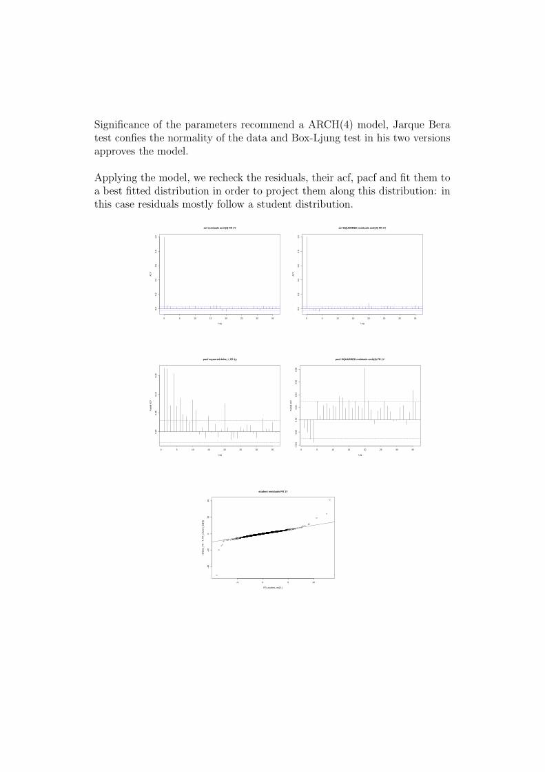
Significance of the parameters recommend a ARCH(4) model, Jarque Beratest confies the normality of the data and Box-Ljung test in his two versionsapproves the model.
Applying the model, we recheck the residuals, their acf, pacf and fit them toa best fitted distribution in order to project them along this distribution: inthis case residuals mostly follow a student distribution.
0 5 10 15 20 25 30 35
0.0
0.2
0.4
0.6
0.8
1.0
Lag
AC
F
acf residuals arch(4) FR 1Y
0 5 10 15 20 25 30 35
0.0
0.2
0.4
0.6
0.8
1.0
Lag
AC
F
acf SQUARRED residuals arch(4) FR 1Y
0 5 10 15 20 25 30 35
0.00
0.05
0.10
0.15
Lag
Par
tial A
CF
pacf squarred delta_i_FR 1y
0 5 10 15 20 25 30 35
−0.
04−
0.02
0.00
0.02
0.04
0.06
0.08
Lag
Par
tial A
CF
pacf SQUARRED residuals arch(4) FR 1Y
−5 0 5 10
−40
−20
020
40
student residuals FR 1Y
FR_student_res[3, ]
rt(N
obs_
FR
− 4
, FR
_cho
sen_
ddl[3
])

Resulting plots
0 50 100 150 200 250
01
23
45
time horizon
capi
tal c
harg
e (%
)
Figure 1: French GARCH cc
0 50 100 150 200 250
01
23
45
time horizon
capi
tal c
harg
e (%
)
Figure 2: German GARCH cc
0 50 100 150 200 250
02
46
810
time horizon
capi
tal c
harg
e (%
)
Figure 3: US GARCH cc
0 50 100 150 200 250
02
46
810
12
time horizon
capi
tal c
harg
e (%
)
Figure 4: Turkish GARCH cc
Not accounting for the inter-correlation in our GARCH approach, the capitalcharge is expected to fall mostly below the SBA approach. We can observethe resemblance between the French, German and US market, however avery unstable behavior in the Turkish data: Turkey is located in a very frag-ile environment quickly influenced by numerous factors making its currencyvolatile.
PCA-GARCH model:
Applying the PCA on the 15 maturities of each currency, we reduce the datainto two components covering at least 98 % of the data. We project thefirst differential of these components using an adequate GARCH model thenrebuild the entire maturities using the projected factors and the previouslycomputed loadings. Monte Carlo simulations permits the extraction of the

VaR at different levels and the capital charge.
0 50 100 150 200 250
02
46
8
time horizon
capi
tal c
harg
e (%
)
Figure 5: French PCA cc
0 50 100 150 200 250
02
46
8
time horizon
capi
tal c
harg
e (%
)
Figure 6: German PCA cc
0 50 100 150 200 250
02
46
810
time horizon
capi
tal c
harg
e (%
)
Figure 7: US PCA cc
0 50 100 150 200 250
05
1015
20
time horizon
capi
tal c
harg
e (%
)
Figure 8: Turkish PCA cc
Once again EU and US data show the same behavior, whereas the Turkishdata being very volatile shows different results (emerging market status).Quickly comparing GARCH and PCA, a clear increase in the required capitalis showing in the PCA figures due to the incorporation of the inter-maturitiescorrelation.
ICA-GARCH model:
This method is similar to the PCA, but instead of using the principal com-ponents approach we used the independent components approach to increasethe precision and reduce the assumptions.

0 50 100 150 200 250
02
46
time horizon
capi
tal c
harg
e (%
)
Figure 9: French ICA cc
0 50 100 150 200 250
02
46
810
12
time horizon
capi
tal c
harg
e (%
)
Figure 10: German ICA cc
0 50 100 150 200 250
05
1015
20
time horizon
capi
tal c
harg
e (%
)
Figure 11: US ICA capital charge
0 50 100 150 200 250
05
1015
20
time horizon
capi
tal c
harg
e (%
)
Figure 12: Turkish ICA cc
DNS-ARIMA model:
After estimating the curves using NS model, we projected the beta param-eters using the best fitted ARIMA(p,d,q) process. Along with the mean ofthe historically observed lambda’s and the projected beta’s, we rebuild thecurves, estimate the VaR and capital charge.
0 50 100 150 200 250
02
46
810
1214
time horizon
capi
tal c
harg
e (%
)
Figure 13: French DNS cc
0 50 100 150 200 250
02
46
810
time horizon
capi
tal c
harg
e (%
)
Figure 14: German DNS cc

0 50 100 150 200 250
02
46
810
12
time horizon
capi
tal c
harg
e (%
)
Figure 15: US DNS capital charge
The results show a quicker convergence in this method. However, in anunstable market such as the Turkish case, we do not observe any convergencein the Nelson Siegel parameter, therefore no projection could be applied.
2.2 Multiple currencies portfolios
Denoting the previous portfolios by their government yield we have: Port FRANCE,Port GERMANY , Port US and Port TURKEY .
In this section we consider multiple currencies combining the previously men-tioned portfolios: Port FR GR,Port FR US, Port FR TRY, Port FR GR US,Port GR US TRY and Port FR GR US TRY
Sensitivity Based Approach
In this section, having multiple currencies, the correlation parameters be-tween different curves at different tenors will be added. Note that bothFrance and Germany are held in euros therefore they are part of the samebucket. SBA capital requirement vs duration:
2006 2008 2010 2012 2014
3.0
3.5
4.0
4.5
5.0
FR−GR duration vs SBA
time
DurationSBA
2006 2008 2010 2012 2014
3.0
3.5
4.0
4.5
5.0
FR−US duration vs SBA
time
DurationSBA

2006 2008 2010 2012 2014
3.0
3.5
4.0
4.5
5.0
FR−TRY duration vs SBA
time
DurationSBA
2006 2008 2010 2012 2014
3.0
3.5
4.0
4.5
5.0
FR−GR−US duration vs SBA
time
DurationSBA
2006 2008 2010 2012 2014
3.0
3.5
4.0
4.5
5.0
GR−US−TRY duration vs SBA
time
DurationSBA
2006 2008 2010 2012 2014
3.0
3.5
4.0
4.5
5.0
FR−GR−US−TRY duration vs SBA
time
DurationSBA
Similar remarks could be presented here regarding the parallel movementof the duration and capital requirement of these portfolios. This could beinterpreted using the equations in appendix 1,case 3.
FR-GR portfolio
0 50 100 150 200 250
01
23
45
time horizon
capi
tal c
harg
e (%
)
Figure 16: GARCH capital charge
0 50 100 150 200 250
02
46
8
time horizon
capi
tal c
harg
e (%
)
Figure 17: PCA capital charge

0 50 100 150 200 250
02
46
810
1214
time horizon
capi
tal c
harg
e (%
)
Figure 18: ICA capital charge
0 50 100 150 200 250
02
46
8
time horizon
capi
tal c
harg
e (%
)
Figure 19: DNS capital charge
FR-US portfolio
0 50 100 150 200 250
01
23
4
time horizon
capi
tal c
harg
e (%
)
Figure 20: GARCH capital charge
0 50 100 150 200 250
02
46
8
time horizon
capi
tal c
harg
e (%
)
Figure 21: PCA capital charge
0 50 100 150 200 250
02
46
810
12
time horizon
capi
tal c
harg
e (%
)
Figure 22: ICA capital charge
0 50 100 150 200 250
02
46
810
time horizon
capi
tal c
harg
e (%
)
Figure 23: DNS capital charge

FR-TRY portfolio
0 50 100 150 200 250
01
23
45
6
time horizon
capi
tal c
harg
e (%
)
Figure 24: GARCH
0 50 100 150 200 250
02
46
810
1214
time horizon
capi
tal c
harg
e (%
)
Figure 25: PCA
0 50 100 150 200 250
05
1015
time horizon
capi
tal c
harg
e (%
)
Figure 26: ICA
FR-GR-US portfolio
0 50 100 150 200 250
01
23
4
time horizon
capi
tal c
harg
e (%
)
Figure 27: GARCH capital charge
0 50 100 150 200 250
02
46
8
time horizon
capi
tal c
harg
e (%
)
Figure 28: PCA capital charge
0 50 100 150 200 250
02
46
810
1214
time horizon
capi
tal c
harg
e (%
)
Figure 29: ICA capital charge
0 50 100 150 200 250
02
46
8
time horizon
capi
tal c
harg
e (%
)
Figure 30: DNS capital charge

GR-US-TRY portfolio
0 50 100 150 200 250
01
23
45
time horizon
capi
tal c
harg
e (%
)
Figure 31: GARCH
0 50 100 150 200 250
02
46
810
1214
time horizon
capi
tal c
harg
e (%
)
Figure 32: PCA
0 50 100 150 200 250
05
1015
time horizon
capi
tal c
harg
e (%
)
Figure 33: ICA
FR-GR-US-TRY portfolio
0 50 100 150 200 250
01
23
4
time horizon
capi
tal c
harg
e (%
)
Figure 34: GARCH
0 50 100 150 200 250
02
46
810
time horizon
capi
tal c
harg
e (%
)
Figure 35: PCA Figure 36: ICA

3 Backtesting Results
In order to decide on the best approach for the capital requirement compu-tation, a backtest analysis is a must. We used the typical ’number of hits’approach (number of violations) based on a scrolling window of 252 datesprojecting them 100 notches (daily or weekly) and comparing the resultswith the actually observed rates. Our findings are summarized in the follow-ing table.Results reject the GARCH model being too unrealistic and raises questionmarks regarding the DNS model for the daily projection.Number of violations
expected daily weekly
ARCH
FR 5.00% 7.00% 8.00%
GR 5.00% 0.00% 5.00%
US 5.00% 20.00% 11.00%
TRY 5.00% 22.00% 14.50%
PCA
FR 5.00% 2.00% 4.00%
GR 5.00% 3.00% 4.00%
US 5.00% 4.00% 3.50%
TRY 5.00% 0.00% 4.00%
ICA
FR 5.00% 0.00% 0.50%
GR 5.00% 0.00% 2.50%
US 5.00% 0.00% 0.00%
TRY 5.00% 0.00% 0.00%
DNS
FR 5.00% 1.00% 0.00%
GR 5.00% 9.00% 1.00%
US 5.00% 9.00% 0.50%
TRY 5.00% 0.00% 0.00%
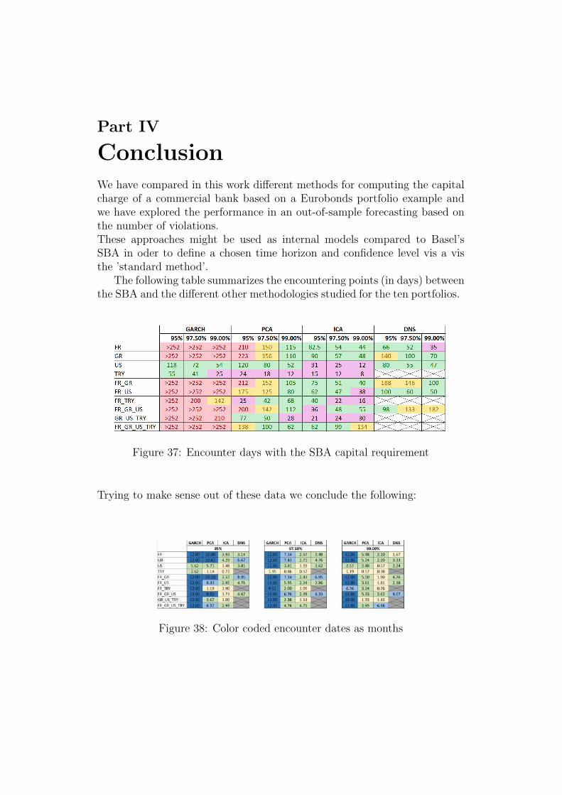
Part IV
ConclusionWe have compared in this work different methods for computing the capitalcharge of a commercial bank based on a Eurobonds portfolio example andwe have explored the performance in an out-of-sample forecasting based onthe number of violations.These approaches might be used as internal models compared to Basel’sSBA in oder to define a chosen time horizon and confidence level vis a visthe ’standard method’.
The following table summarizes the encountering points (in days) betweenthe SBA and the different other methodologies studied for the ten portfolios.
Figure 37: Encounter days with the SBA capital requirement
Trying to make sense out of these data we conclude the following:
Figure 38: Color coded encounter dates as months

Approaching Basel’s method, the results show:
• Except for the Turkish market, GARCH method computes a similarcapital requirement as the SBA for a minimum of one year time horizon.
• Comparing PCA and ICA we can conclude that the ICA is more re-strictive for single currency denoted and mixed portfolios.
• PCA gives an eight months, 97.5% adequacy parallel to the five monthsgiven by the ICA for FR and GR portfolios. We add a PCA requirementof 4 months horizon for the US portfolio facing a two months limit givenby the ICA.
• In the mixed portfolios PCA sets (at 97.5%) a limit of one year exceptwhen the Turkish lira is involved, ICA shows a lower encounter pointof two months.
• The DNS on the 97.5% gives an adequate capital charge between twoand four months.
• In the mixed portfolios DNS method on the 97.5% requires a timehorizon between three and seven months.
Based on the previous, our recommendations are:
→ For the Eurozone:
- GARCH capital charge would be equivalent to the SBA for a levelof 97.5 %.
- GARCH does not account for inter-maturities correlations there-fore an ICA or PCA approach would be more rational:
* 7 months PCA 97.5 % on a country level and 6 months whencombined.
* 3 months ICA 97.5 %on a country level and 2 months whencombined.
- DNS would inquire an average of 3 months for each country and6 months for a multi-European portfolio.
→ For the US:
- GARCH imposes a 1 year horizon for 97.5% confidence level.

- 97.5% PCA for less than 4 months capital charge would do it anda 1 month ICA.
- An average of 2 months DNS results in a close capital charge asthe SBA’s requirement.
→ For the Turkish market:
- TRY is too volatile to be adequately represented by ICA or DNSmodels: it can be used for very short term : one month or lessPCA (97.5%).
→ When combining US and Euro markets:
- GARCH results could remain applicable.
- PCA method time horizons’ is half a year.
- ICA and DNS methods time horizons’ is 2 months.
→ When combining the Turkish lira with any of the US dollar or Europortfolio: PCA approaches an average of 4 months and ICA an averageof 2 months.
The goal of this work was to provide banks with a tool that explainsthe econometric concept behind Basel’s SBA approach in order to fix thetime horizon and confidence level of their capital requirement in the tradingportfolio. In addition, these models could provide an internal approach withcustomized coefficients and parameters.
In June 2015, a new consultative document was issued by the BCBS on the’Interest rate risk in the banking book, presenting new approaches to handlethis book’s capital charge computation and suggests dividing this amountbetween the first and second pillar. Incorporating the banking book in thefirst pillar is a new approach, because that segment was reserved for the trad-ing book. Doing so, a similar methodology to the SBA would be inquired forthe banking book. Our next step would be to construct an internal modelthat mimics the proposed approach to compute the local parameters for thecapital charge computation and interest rate shock scenarios applications.

Part V
References
References
[1] A. Feuerverger, A. Wong, Computation of value-at-risk for nonlinearportfolios, Toronto
[2] Amari S. , A. Cichocki, and H.H. Yang, 1996, A new learning algorithmfor blind signal separation, Advances in Neural Information ProcessingSystems 8 (NIPS*95), pages 757-763, Cambridge, The MIT Press.
[3] B. Scherer, B. Balachander, R. Falk, B. Yen, 2010, Introducing CapitalIQ’s fundamental US equity Risk Models, Quantitative research
[4] B. Yang, S. Liao, Y. Su,Interest Rates term Structure Forecasting andbond portfolio Risk Management, Tianjin University, China
[5] Babel B., Gius D., Grawert A., Luders E., Natale A., Nilsson B., Schnei-der S., 2012,McKinsey Working Papers on Risk, Number 38, Capitalmanagement: Banking’s new imperative.
[6] Bank For International Settlements, Basel Committee on Banking Su-pervisions, http://www.bis.org/bcbs/index.htm
[7] Baptistab A. , Alexandera G., 2012,A comparison of the original andrevised Basel market risk frameworks for regulating bank capital, ShuYanc. Journal of Economic Behavior and Organisation.
[8] Barone-Adesi G., Giannopoulos K. and Vosper L. ,2002, Backtestingderivative portfolios with filtered historical simulation,European Finan-cial Management, Vol. 8, no 1, pp. 31-58
[9] Basel Committee on Banking Supervision (BCBS), 2012, FundamentalReview of the Trading Book,Consultative Document.
[10] Basel Committee on Banking Supervision (BCBS), 2014, FrequentlyAsked Questions on Basel III Monitoring.
[11] Basel Committee on Banking Supervision (BCBS), 2015, Fundamentalreview of the trading book: outstanding issues.

[12] Basel Committee on Banking Supervision (BCBS),2014, Analysis of thetrading book hypothetical portfolio exercise, QIS.
[13] Basel Committee on Banking Supervison (BCBS), 2004, ConsultativeDocument: Principles for Management and Supervision of Interest RateRisk.
[14] Basel Committee on Banking Supervison (BCBS),2015,Fundamental re-view of the trading book - interim impact analysis.
[15] Basel Committee on Banking Supervision (BCBS), 1996, Supervisoryframework for the use of “backtesting” in conjunction with the internalmodels approach to market risk capital requirements
[16] Bell A.J. and Sejnowski T.J., 1995, An information maximization ap-proach to blind separation and blind deconvolution, pp. 1129-1159.
[17] Bollerslev T. , 1986, Generalized Autoregressive Conditional Het-eroskedasticity, Journal of econometrics.
[18] Bollerslev T., 2008, Glossary to ARCH (GARCH), CREATES researchpaper, ssrn.com.
[19] Brooks C., Burke S., Persand G., 2003, Multivariate GARCH Models:Software Choice and Estimation Issues, ICMA Centre Discussion Papersin Finance icma-dp2003-07, Henley Business School, Reading University.
[20] Bugli C., 2007, Comparison between principal component analysis andindependent component analysis in electroencephalograms modeling.
[21] Burgos T. DA, 2013, Principal component Analysis vs Independent com-ponent analysis for damage detection, 6th European workshop on struc-tural health monitoring.
[22] C. Gourieroux and J. Jasiak,2006,Dynamic quantile models,Manuscript,University of Toronto
[23] C. Gourieroux and J. Jasiak,2006,Dynamic quantile models,Manuscript,University of Toronto
[24] C. M. Hafner Philip and H. Franses,2003,A Generalized Dynamic Condi-tional Correlation Model for Many Asset Returns,Econometric InstituteReport EI 2003–18

[25] Campbell S. , 2005, A Review of Backtesting and Backtesting Proce-dures, Finance and Economics Discussion Series, Divisions of Research& Statistics and Monetary Affairs Federal Reserve Board, Washington,D.C.
[26] Comon P. ,1994, Independent component analysis - a new con-cept?Signal Processing, 36(3):287-314.
[27] Diebold F. X. and Li C. , 2006, Forecasting the Term structure of gov-ernment bond yields, journal of econometrics.
[28] Dowd K. , 2002 ,Measuring Market Risk,Chichester: John Wiley & Sons
[29] Edison H.J. and Liang H., 1999, Foreign Exchange Intervention and theAustralian Dollar: Has It Mattered?, IMF Working Paper. ”
[30] Engle R. and Manganelli S. ,2004 ,1999,CAViaR: Conditional Autore-gressive Value at Risk by Regression Quantiles, Journal of Business &Economic Statistics, Vol. 22, n. 4, pp. 367-381”
[31] Engle R. F., 1982, Autoregressive conditional heteroscedasticity with es-timates of the variance of United Kingdom inflation, Econometrica.
[32] F. X. Diebold, T. Schuermann and J. D. Stroughair,1998,Pitfallsand opportunities in the use of extreme value theory in risk manage-ment,Journal of Risk Finance, 1 (Winter 2000), 30-36.
[33] G. Darbha, 2001, Value at risk for fixed income portfolios: A comparisonof alternative models, National Stock exchange, Mumbai, India
[34] G.Hanweck, L. Ryu, 2005, The sensitivity of Bank net interest marginsand profitability to credit, interest-rate, and term-structure shocks acrossbank product specializations, Working paper
[35] Gilli M. , Schumann, Grobe,2010, Calibrating the Nelson Siegel Svenssonmodel,Comisef working papers series,WPS-031.
[36] Hull J., 2000, Options, Futures and Other Derivatives, 4th ed. New York:Prentice- Hall.
[37] Hurlin C., 2013, Backtesting value at risk models, University of Orleans,Seminaire Validation des Modeles Financiers.
[38] Hurlin C., 2008, Value-at-Risk et Backtesting, Christophe Hurlin, Uni-versite d.Orleans, Laboratoire d.Economie d.Orleans

[39] ISDA, 2015,Fundamental Review of the Trading Book, briefing notes.
[40] J. Caldeira, G. Moura, A. Santos, 2012, Bond portfolio managementusing the dynamic Nelson-Siegel model, Catarina
[41] J. Caldeira, G. Moura, A. Santos, 2012, Bond portfolio optimization: adynamic heteroskedastic factor model approach, Catarina
[42] J. Carlos Escanciano & Jose Olmo, 2011, Robust Backtesting Tests forValue-at-risk Models,Journal of Financial Econometrics, Society for Fi-nancial Econometrics, vol. 9(1), pages 132-161, Winter
[43] Jackson J.E., 1991, A user’s guide to principal components, Wiley.
[44] Jarque C.and Bera, A., 1981, Efficient tests for normality, homoscedas-ticity and serial independence of regression residuals: Monte Carlo evi-dence, Economics Letters 7 (4),p. 313–318.
[45] Laas D. and Siegel C, 2015, Basel III versus Solvency II: An analysisof regulatory consistency under the new capital standards, University ofSt. Gallen, Working papers on risk management and insurance no.132
[46] Levieuge G. and Badarau-Semenescu C. ,2010, Assessing the PotentialStrength of a Bank Capital Channel in Europe: A Principal ComponentAnalysis,The Review of Finance and Banking, Vol. 02, Issue 1, pp. 5-16.
[47] M. Pesaran, P. Zaffaroni, 2008, Optimal asset allocation with factor mod-els for large portfolios, Cambridge
[48] Nath G. and Dalvi M. , 2013, Estimating Term Structure Changes usingPCA in Indian Soverign Bond Market, International Journal of Bank-ing,Risk and insurance, Vol. 1, No 1.
[49] Novosyolov A. and Scatchkov D. , 2009, Global Term Structure Modelingusing Principal Component Analysis, Factset.
[50] Olli N. , 2009, Backtesting Value-at-Risk Models, University of Helsinki
[51] Pelletier, D. The geometric VaR backtesting method
[52] P. Glasserman, P. Heidelberger, P. Shahabuddin, Efficient Monte Carlomethods for value at risk
[53] R. Best, 2008, An introduction to error correction models, Oxford springschool for quantitative methods in social research

[54] R. Engle, S. Manganelli, 2004, CAViaR: Conditional AutoregressiveValue at Risk by Regression Quantiles, Journal of business & EconomicStatistics, vol. 22, no. 4
[55] S. Aramonte, M. Rodriguez, J. Wu, 2012, Dynamic factor Value-at-Riskfor large heteroskedastic portfolios
[56] S. Pichler, K. Selitsch, 1999, A comparison of analytical VaR methodolo-gies for portfolios that include options, Vienna University of Technology
[57] S. Zenios, M. Holmer, R. Mckendall, C. Vassiadou-Zeniou, 1996-1997,Dynamic models for fixed income portfolio management under uncer-tainty, journal of economic dynamics and control, 22, pages 1517-1541
[58] S. Aramonte,M. Rodriguezy and J. Wu,2012,Dynamicfactor Value-at-Risk for large heteroskedastic portfolios,http://ssrn.com/abstract=1845846
[59] Siegel A.F., Nelson C.R., 1988, Long-term behavior of yield curves, Jour-nal of financial and quantitative analysis.
[60] T. Angelidis, A. Benos and S. Degiannakis, 2003, The use of GARCHModels in VaR Estimation
[61] T. Shiohama, M. Hallin, D. Veredas and M. Taniguchi,2010,Dynamicportfolio optimization using generalized dynamic conditional het-eroskedastic factor models,J. Japan Statist. Soc. Vol. 40 No. 1 145–166
[62] T. Shiohama, M. Hallin, D. Veredas, M. Taniguchi, 2010, Dynamic port-folio optimization using generalized dynamic conditional heteroskedasticfactor models, J. Japan Statistic soc., vol 40, no. 1, 145-166
[63] Taylor S. J., 1986, Modelling financial time series, Wiley, New York,NY.
[64] X. Dinghai and T. Wirjanto , 2014, On the computation of Large Port-folio’s VaRs under Multivariate GARCH volatility, Dep. of Economics,Univ. of Waterloo
[65] X. Zhang, J. Xu, D. Lim, 2012, Approaches to computing value-at-riskfor equity portfolios
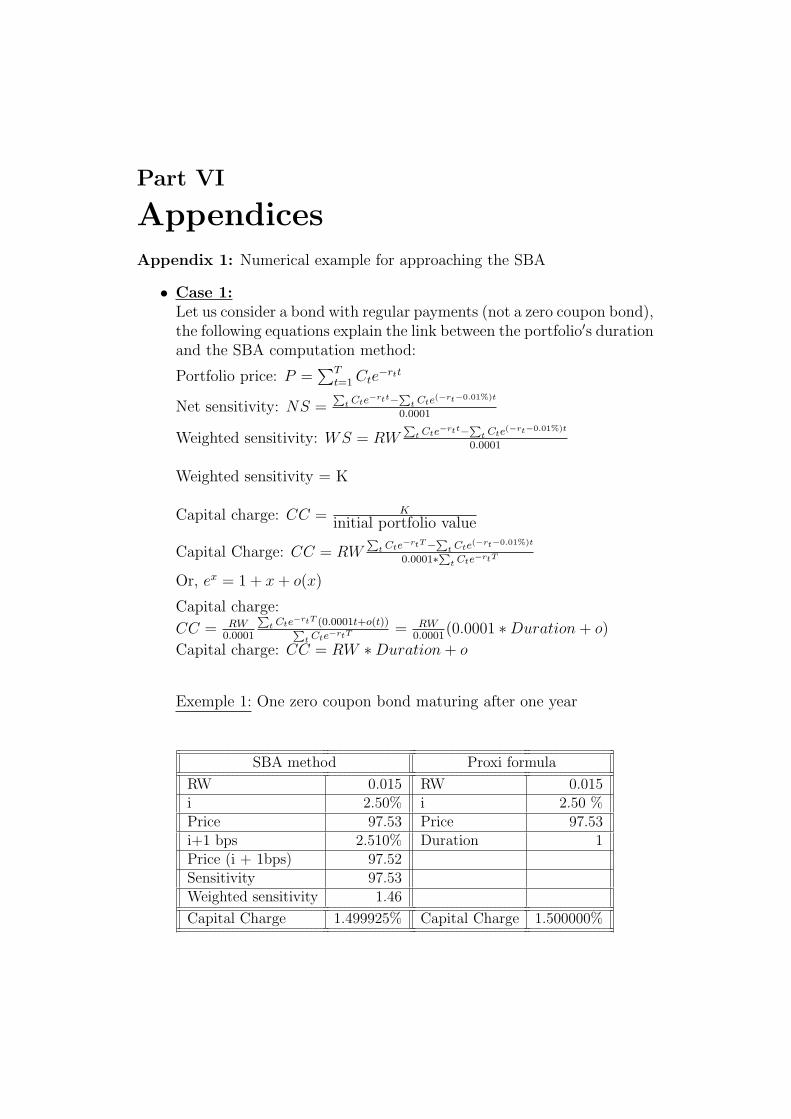
Part VI
AppendicesAppendix 1: Numerical example for approaching the SBA
• Case 1:Let us consider a bond with regular payments (not a zero coupon bond),the following equations explain the link between the portfolio′s durationand the SBA computation method:
Portfolio price: P =∑T
t=1Cte−rtt
Net sensitivity: NS =∑t Cte
−rtt−∑t Cte
(−rt−0.01%)t
0.0001
Weighted sensitivity: WS = RW∑t Cte
−rtt−∑t Cte
(−rt−0.01%)t
0.0001
Weighted sensitivity = K
Capital charge: CC = K
initial portfolio value
Capital Charge: CC = RW∑t Cte
−rtT−∑t Cte
(−rt−0.01%)t
0.0001∗∑t Cte
−rtT
Or, ex = 1 + x+ o(x)
Capital charge:
CC = RW0.0001
∑t Cte
−rtT (0.0001t+o(t))∑t Cte
−rtT = RW0.0001
(0.0001 ∗Duration+ o)
Capital charge: CC = RW ∗Duration+ o
Exemple 1: One zero coupon bond maturing after one year
SBA method Proxi formula
RW 0.015 RW 0.015i 2.50% i 2.50 %Price 97.53 Price 97.53i+1 bps 2.510% Duration 1Price (i + 1bps) 97.52Sensitivity 97.53Weighted sensitivity 1.46
Capital Charge 1.499925% Capital Charge 1.500000%

• Case 2:Considering two different bonds with the same currency the resultsare as follow:
Bond 1: P1 =∑Cte
−rtt, D1 =∑tCte−rtt
P1
Bond 2: P2 =∑Bje
−rjj, D2 =∑jBje
−rjj
P2
Net sensitivity:
NS1 =∑t Cte
−rtt−∑t Cte
(−rt−0.01%)t
0.0001
NS2 =∑j Bje
−rjj−∑j Bje
(−rj−0.01%)j
0.0001
Weighted sensitivity: WS1 = RW1
0.0001
∑tCte
−rtt(1− e−0.0001t)
WS1 = RW1 ∗D1 ∗ P1
WS2 = RW2
0.0001
∑j Cje
−rjj(1− e−0.0001j)
WS2 = RW2 ∗D2 ∗ P2
K =√WS2
1 +WS22 + 2ρ1,2WS1WS2
Capital charge:
CC = RW1P1D1+RW2D2P2
P1+P2(1 + (ρ1,2 − 1) RW1D1P1RW2D2P2
(RW1D1P1+RW2D2P2)2)
Exemple: two zero coupon bonds, maturities one and two yearshaving the same currency
SBA method Proxi formula
RW1 0.015 RW1 0.015i1 2.50% i1 2.50%Price1 97.53 Price1 97.53i1+1 bps 2.51% RW2 0.0115Price1 (i1 + 1bps) 97.52 i2 3.00%RW2 0.0115 Price2 94.18i2 3.00% Duration 1 1Price2 94.18 Duration 2 2i2+1 bps 3.01% Correlation 0.75Price2 (i2 + 1bps) 94.16Sensitivity1 97.53WS1 1.46Sensitivity2 188.33WS2 2.166
Capital Charge 1.775338% Capital Charge 1.779129%

• Case 3:In order to see the influence of the diversity in currencies, we consider2 bonds with different currencies therefore we consider two buckets:
Bond 1: P1 =∑Cte
−rtt, D1 =∑tCte−rtt
P1; Bond 2:
P2 =∑Bje
−rjj, D2 =∑jBje
−rjj
P2
Net sensitivity: NS1 =∑t Cte
−rtt−∑t Cte
(−rt−0.01%)t
0.0001;
NS2 =∑j Bje
−rjj−∑j Bje
(−rj−0.01%)j
0.0001
Weighted sensitivity:
WS1 = RW1
0.0001
∑tCte
−rtt(1− e−0.0001t) = RW1 ∗D1 ∗ P1
WS2 = RW2
0.0001
∑j Cje
−rjj(1− e−0.0001j) = RW2 ∗D2 ∗ P2
Having two currencies results in having two buckets:K1 = WS1andK2 = WS2
Basel SBA implements a correlation factor of 0.5 between currencies:
Capital Charge: Ktotal =√K2
1 +K22 + 0.5 ∗ (S1S2 + S2S1) where
Si =∑WSi
Capital Charge: CC = RW1P1D1+RW2D2P2
P1+P2(1− RW1D1P1RW2D2P2
2(RW1D1P1+RW2D2P2)2)
Example: two zero coupon bonds, maturities one and three yearshaving different currencies
SBA method Proxi formula
RW1 0.015 RW1 0.015i1 2.53% i1 2.53%Price1 97.50 Price1 97.50i1+1 bps 2.54% RW2 0.0115Price1 (i1 + 1bps) 97.49 i2 12.67%RW2 0.0115 Price2 68.38i2 12.67% Duration 1 1Price2 68.38 Duration 2 3i2+1 bps 12.68% Inter-buckets 0.5Price2 (i2 + 1bps) 68.36Sensitivity1 97.50WS1 1.46Sensitivity2 205.11WS2 2.36
Capital Charge 2.013159% Capital Charge 2.031698%

Supplementary Material: Models details: GARCH
French portfolio1 year
0 1000 2000 3000 4000
−20
−10
010
20
delta_i_FR 1y
Index
delta
_i_F
R[,
3]
3 years
0 1000 2000 3000 4000
−30
−20
−10
010
2030
delta_i_FR 3y
Index
delta
_i_F
R[,
5]
Data:
0 5 10 15 20 25 30 35
0.0
0.2
0.4
0.6
0.8
1.0
Lag
AC
F
acf delta_i_FR 1y
0 5 10 15 20 25 30 35
0.0
0.2
0.4
0.6
0.8
1.0
Lag
AC
F
acf squarred delta_i_FR 1y
0 5 10 15 20 25 30 35
−0.
04−
0.02
0.00
0.02
0.04
0.06
0.08
Lag
Par
tial A
CF
pacf delta_i_FR 1y
0 5 10 15 20 25 30 35
0.00
0.05
0.10
0.15
Lag
Par
tial A
CF
pacf squarred delta_i_FR 1y
Residuals:
0 5 10 15 20 25 30 35
0.0
0.2
0.4
0.6
0.8
1.0
Lag
AC
F
acf residuals arch(4) FR 1Y
Figure 39: French data 1y
0 5 10 15 20 25 30 35
0.0
0.2
0.4
0.6
0.8
1.0
Lag
AC
F
acf SQUARRED residuals arch(4) FR 1Y
0 5 10 15 20 25 30 35
0.00
0.05
0.10
0.15
Lag
Par
tial A
CF
pacf squarred delta_i_FR 1y
0 5 10 15 20 25 30 35
−0.
04−
0.02
0.00
0.02
0.04
0.06
0.08
Lag
Par
tial A
CF
pacf SQUARRED residuals arch(4) FR 1Y
−5 0 5 10
−40
−20
020
40
student residuals FR 1Y
FR_student_res[3, ]
rt(N
obs_
FR
− 4
, FR
_cho
sen_
ddl[3
])
Data:
0 5 10 15 20 25 30 35
0.0
0.2
0.4
0.6
0.8
1.0
Lag
AC
F
acf delta_i_FR 3y
0 5 10 15 20 25 30 35
0.0
0.2
0.4
0.6
0.8
1.0
Lag
AC
F
acf squarred delta_i_FR 3y
0 5 10 15 20 25 30 35
−0.
04−
0.02
0.00
0.02
0.04
0.06
Lag
Par
tial A
CF
pacf delta_i_FR 3y
0 5 10 15 20 25 30 35
0.00
0.05
0.10
Lag
Par
tial A
CF
pacf squarred delta_i_FR 3y
Residuals:
0 5 10 15 20 25 30 35
0.0
0.2
0.4
0.6
0.8
1.0
Lag
AC
F
acf residuals garch(1,1) FR 5Y
0 5 10 15 20 25 30 35
0.0
0.2
0.4
0.6
0.8
1.0
Lag
AC
F
acf SQUARRED residuals garch(1,1) FR 5Y
0 5 10 15 20 25 30 35
0.00
0.05
0.10
Lag
Par
tial A
CF
pacf squarred delta_i_FR 3y
0 5 10 15 20 25 30 35
−0.
03−
0.02
−0.
010.
000.
010.
020.
03
Lag
Par
tial A
CF
pacf SQUARRED residuals garch(1,1) FR 5Y
−10 0 10 20
−15
−10
−5
05
1015
student residuals FR 3m
FR_student_res[1, ]
rt(N
obs_
FR
− 2
, FR
_cho
sen_
ddl[1
])

French portfolio5 years
0 1000 2000 3000 4000
−30
−20
−10
010
2030
delta_i_FR 5y
Index
delta
_i_F
R[,
7]
10 years
0 1000 2000 3000 4000
−20
−10
010
2030
delta_i_FR 10y
Index
delta
_i_F
R[,
12]
Data:
0 5 10 15 20 25 30 35
0.0
0.2
0.4
0.6
0.8
1.0
Lag
AC
F
acf delta_i_FR 5y
0 5 10 15 20 25 30 35
0.0
0.2
0.4
0.6
0.8
1.0
Lag
AC
F
acf squarred delta_i_FR 5y
0 5 10 15 20 25 30 35
−0.
04−
0.02
0.00
0.02
0.04
0.06
Lag
Par
tial A
CF
pacf delta_i_FR 5y
0 5 10 15 20 25 30 35
0.00
0.05
0.10
0.15
Lag
Par
tial A
CF
pacf squarred delta_i_FR 5y
Residuals:
0 5 10 15 20 25 30 35
0.0
0.2
0.4
0.6
0.8
1.0
Lag
AC
F
acf residuals garch(1,1) FR 5Y
Figure 40: French data 5y
0 5 10 15 20 25 30 35
0.0
0.2
0.4
0.6
0.8
1.0
Lag
AC
F
acf SQUARRED residuals garch(1,1) FR 5Y
0 5 10 15 20 25 30 35
−0.
020.
000.
020.
04
Lag
Par
tial A
CF
pacf residuals garch(1,1) FR 5Y
0 5 10 15 20 25 30 35
−0.
03−
0.02
−0.
010.
000.
010.
020.
03
Lag
Par
tial A
CF
pacf SQUARRED residuals garch(1,1) FR 5Y
−4 −2 0 2 4 6
−6
−4
−2
02
46
student residuals FR 5Y
FR_student_res[7, ]
rt(N
obs_
FR
− 2
, FR
_cho
sen_
ddl[7
])
Data:
0 5 10 15 20 25 30 35
0.0
0.2
0.4
0.6
0.8
1.0
Lag
AC
F
acf delta_i_FR 10y
0 5 10 15 20 25 30 35
0.0
0.2
0.4
0.6
0.8
1.0
Lag
AC
F
acf squarred delta_i_FR 10y
0 5 10 15 20 25 30 35
−0.
03−
0.02
−0.
010.
000.
010.
020.
030.
04
Lag
Par
tial A
CF
pacf delta_i_FR 10y
0 5 10 15 20 25 30 35
0.00
0.05
0.10
0.15
Lag
Par
tial A
CF
pacf squarred delta_i_FR 10y
Residuals:
0 5 10 15 20 25 30 35
0.0
0.2
0.4
0.6
0.8
1.0
Lag
AC
F
acf residuals arch(4) FR 10Y
0 5 10 15 20 25 30 35
0.0
0.2
0.4
0.6
0.8
1.0
Lag
AC
F
acf squarred delta_i_FR 10y
0 5 10 15 20 25 30 35
−0.
03−
0.02
−0.
010.
000.
010.
020.
030.
04
Lag
Par
tial A
CF
pacf residuals arch(4) FR 10Y
0 5 10 15 20 25 30 35
0.00
0.05
0.10
0.15
Lag
Par
tial A
CF
pacf squarred delta_i_FR 10y
−5 0 5
−5
05
student residuals FR 10Y
FR_student_res[12, ]
rt(N
obs_
FR
− 4
, FR
_cho
sen_
ddl[1
2])

Supplementary Material: Models details: PCA
French portfolio1stcomponent
0 1000 2000 3000 4000
−50
050
composante 1 FR
Index
PC
A_d
elta
_i_F
R[,
1]
2ndcomponent
0 1000 2000 3000 4000
−40
−20
020
40
composante 2 FR
Index
PC
A_d
elta
_i_F
R[,
2]
Data:
0 5 10 15 20 25 30 35
0.0
0.2
0.4
0.6
0.8
1.0
Lag
AC
F
acf composante 1 FR
0 5 10 15 20 25 30 35
0.0
0.2
0.4
0.6
0.8
1.0
Lag
AC
F
acf squarred composante 1 FR
0 5 10 15 20 25 30 35
−0.
020.
000.
020.
04
Lag
Par
tial A
CF
pacf composante 1 FR
0 5 10 15 20 25 30 35
0.00
0.05
0.10
0.15
Lag
Par
tial A
CF
pacf squarred composante 1 FR
Residuals:
0 5 10 15 20 25 30 35
0.0
0.2
0.4
0.6
0.8
1.0
Lag
AC
F
acf residuals arch(4) FR composante 1
0 5 10 15 20 25 30 35
0.0
0.2
0.4
0.6
0.8
1.0
Lag
AC
F
acf SQUARRED residuals arch(4) FR composante 1
0 5 10 15 20 25 30 35
−0.
020.
000.
020.
04
Lag
Par
tial A
CF
pacf residuals arch(4) FR composante 1
0 5 10 15 20 25 30 35
−0.
020.
000.
020.
040.
060.
08
Lag
Par
tial A
CF
pacf SQUARRED residuals arch(4) FR composante 1
−3 −2 −1 0 1 2 3
−6
−4
−2
02
4
qqplot residuals ARCH FR composante 1
rnorm(Nobs_FR − 5)
PC
A_r
eg1_
FR
$res
[5:(
Nob
s_F
R −
1)]
Data:
0 5 10 15 20 25 30 35
0.0
0.2
0.4
0.6
0.8
1.0
Lag
AC
F
acf composante 2 FR
0 5 10 15 20 25 30 35
0.0
0.2
0.4
0.6
0.8
1.0
Lag
AC
F
acf squarred composante 2 FR
0 5 10 15 20 25 30 35
0.00
0.05
0.10
0.15
Lag
Par
tial A
CF
pacf composante 2 FR
0 5 10 15 20 25 30 35
−0.
050.
000.
050.
100.
150.
20
Lag
Par
tial A
CF
pacf squarred composante 2 FR
Residuals:
0 5 10 15 20 25 30 35
0.0
0.2
0.4
0.6
0.8
1.0
Lag
AC
F
acf residuals arch(3) FR composante 2
0 5 10 15 20 25 30 35
0.0
0.2
0.4
0.6
0.8
1.0
Lag
AC
F
acf SQUARRED residuals arch(3) FR composante 2
0 5 10 15 20 25 30 35
0.00
0.05
0.10
Lag
Par
tial A
CF
pacf residuals arch(3) FR composante 2
0 5 10 15 20 25 30 35
−0.
020.
000.
020.
040.
06
Lag
Par
tial A
CF
pacf SQUARRED residuals arch(3) FR composante 2
−2 0 2 4
−10
−5
05
qqplot residuals ARCH FR composante 2
rnorm(Nobs_FR − 4)
PC
A_r
eg2_
FR
$res
[4:(
Nob
s_F
R −
1)]
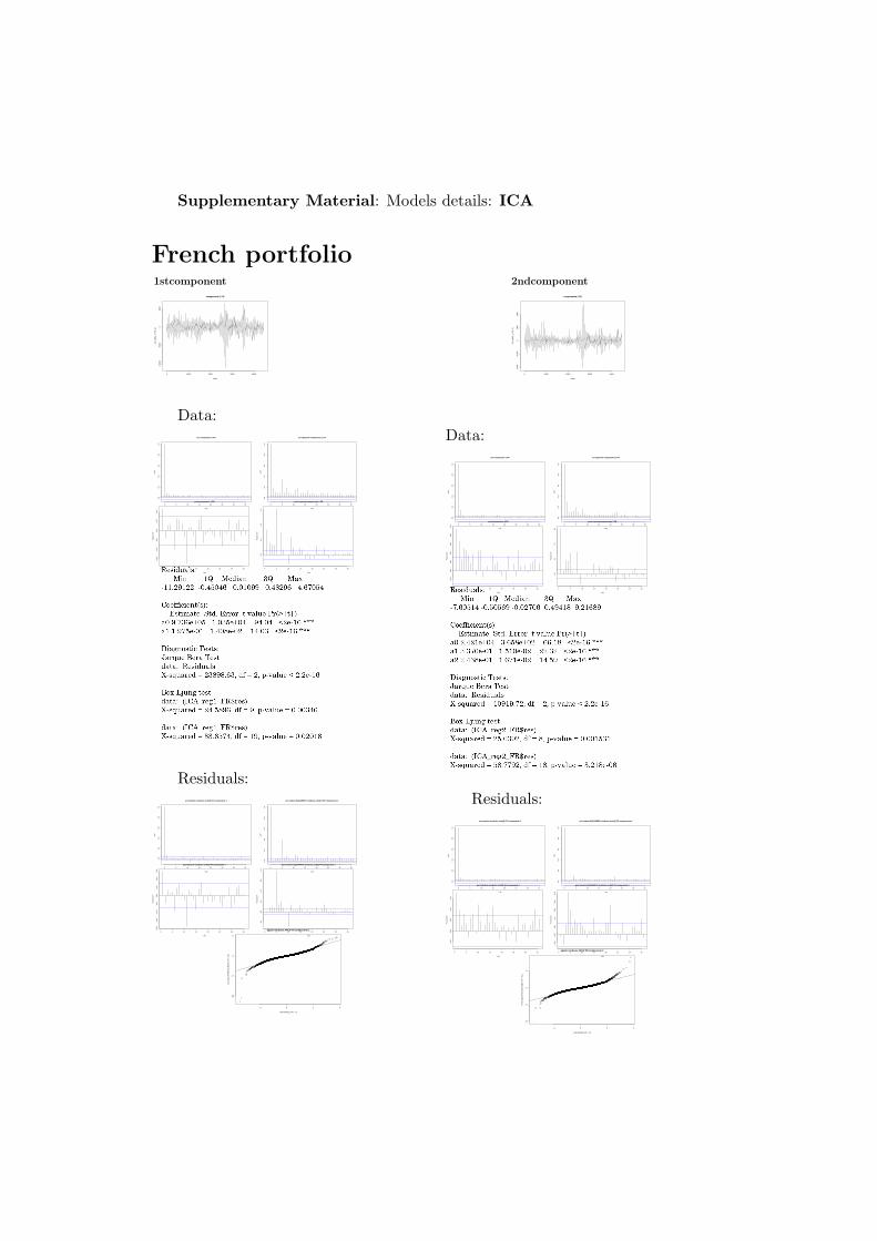
Supplementary Material: Models details: ICA
French portfolio1stcomponent
0 1000 2000 3000 4000
−10
000
−50
000
5000
composante 1 FR
Index
ICA
_del
ta_i
_FR
[, 1]
2ndcomponent
0 1000 2000 3000 4000
−20
00−
1000
010
0020
00
composante 2 FR
Index
ICA
_del
ta_i
_FR
[, 2]
Data:
0 5 10 15 20 25 30 35
0.0
0.2
0.4
0.6
0.8
1.0
Lag
AC
F
acf composante 2 FR
0 5 10 15 20 25 30 35
0.0
0.2
0.4
0.6
0.8
1.0
Lag
AC
F
acf squarred composante 1 FR
0 5 10 15 20 25 30 35
−0.
06−
0.04
−0.
020.
000.
020.
04
Lag
Par
tial A
CF
pacf composante 1 FR
0 5 10 15 20 25 30 35
0.0
0.1
0.2
0.3
Lag
Par
tial A
CF
pacf squarred composante 1 FR
Residuals:
0 5 10 15 20 25 30 35
0.0
0.2
0.4
0.6
0.8
1.0
Lag
AC
F
acf student residuals arch(1) FR composante 1
0 5 10 15 20 25 30 35
0.0
0.2
0.4
0.6
0.8
1.0
Lag
AC
F
acf student SQUARRED residuals arch(1) FR composante 1
0 5 10 15 20 25 30 35
−0.
08−
0.06
−0.
04−
0.02
0.00
0.02
0.04
0.06
Lag
Par
tial A
CF
pacf student residuals arch(1) FR composante 1
0 5 10 15 20 25 30 35
−0.
10.
00.
10.
20.
30.
4
Lag
Par
tial A
CF
pacf student SQUARRED residuals arch(1) FR composante 1
−2 0 2 4
−10
−5
05
qqplot residuals ARCH FR composante 1
rnorm(Nobs_FR − 2)
ICA
_reg
1_F
R$r
es[2
:(N
obs_
FR
− 1
)]
Data:
0 5 10 15 20 25 30 35
0.0
0.2
0.4
0.6
0.8
1.0
Lag
AC
F
acf composante 2 FR
0 5 10 15 20 25 30 35
0.0
0.2
0.4
0.6
0.8
1.0
Lag
AC
F
acf squarred composante 2 FR
0 5 10 15 20 25 30 35
−0.
020.
000.
020.
040.
060.
080.
10
Lag
Par
tial A
CF
pacf composante 2 FR
0 5 10 15 20 25 30 35
0.0
0.1
0.2
0.3
Lag
Par
tial A
CF
pacf squarred composante 2 FR
Residuals:
0 5 10 15 20 25 30 35
0.0
0.2
0.4
0.6
0.8
1.0
Lag
AC
F
acf student residuals arch(2) FR composante 2
0 5 10 15 20 25 30 35
0.0
0.2
0.4
0.6
0.8
1.0
Lag
AC
F
acf student SQUARRED residuals arch(2) FR composante 2
0 5 10 15 20 25 30 35
−0.
020.
000.
020.
040.
06
Lag
Par
tial A
CF
pacf student residuals arch(2) FR composante 2
0 5 10 15 20 25 30 35
−0.
020.
000.
020.
040.
060.
080.
10
Lag
Par
tial A
CF
pacf student SQUARRED residuals arch(2) FR composante 2
−2 0 2 4
−10
−5
05
qqplot residuals ARCH FR composante 2
rnorm(Nobs_FR − 4)
PC
A_r
eg2_
FR
$res
[4:(
Nob
s_F
R −
1)]

Supplementary Material: Models details: DNS
French portfolioBeta1
Jun 13 2013 Oct 01 2013 Jan 01 2014 Apr 01 2014 Jul 01 2014 Oct 01 2014 Jan 01 2015 Apr 01 2015
0.01
50.
020
0.02
50.
030
0.03
50.
040
0.04
5
Beta1 FR
Beta2
Jun 13 2013 Oct 01 2013 Jan 01 2014 Apr 01 2014 Jul 01 2014 Oct 01 2014 Jan 01 2015 Apr 01 2015
−0.
045
−0.
040
−0.
035
−0.
030
−0.
025
−0.
020
−0.
015
Beta2 FR
Beta3
Jun 13 2013 Oct 01 2013 Jan 01 2014 Apr 01 2014 Jul 01 2014 Oct 01 2014 Jan 01 2015 Apr 01 2015
−0.
06−
0.05
−0.
04−
0.03
−0.
02
Beta3 FR
Model:
Residuals:
Beta1
2014 2015
−0.
002
−0.
001
0.00
00.
001
FR_int[, 1]
arF
R1$
resi
dual
s
Beta2
2014 2015
−0.
002
−0.
001
0.00
00.
001
0.00
20.
003
FR_int[, 1]
arF
R2$
resi
dual
s
Beta3
2014 2015
−0.
004
−0.
002
0.00
00.
002
0.00
40.
006
FR_int[, 1]
arF
R3$
resi
dual
s
Beta1
−5 0 5 10
−6
−4
−2
02
46
qqplot residus FR NSParameters[,1] arima student
(a_FR[1] * rt(Nsim, ddl_FR[1]) + b_FR[1])
rt(N
obs_
FR
, ddl
_FR
[1])
Beta2
−8 −6 −4 −2 0 2 4 6
−4
−2
02
46
qqplot residus FR NSParameters[,2] arima student
(a_FR[2] * rt(Nsim, ddl_FR[2]) + b_FR[2])
rt(N
obs_
FR
, ddl
_FR
[2])
Beta3
−4 −2 0 2 4
−4
−2
02
46
qqplot residus FR NSParameters[,3] arima student
(a_FR[3] * rt(Nsim, ddl_FR[3]) + b_FR[3])
rt(N
obs_
FR
, ddl
_FR
[3])

Supplementary Material: Models details: GARCH
German portfolio1 year
0 1000 2000 3000 4000 5000 6000
−40
−20
020
40
delta_i_GR 1y
Index
delta
_i_G
R[,
3]
5 years
0 1000 2000 3000 4000 5000 6000
−20
−10
010
2030
delta_i_GR 3y
Index
delta
_i_G
R[,
5]
Data:
0 10 20 30
0.0
0.2
0.4
0.6
0.8
1.0
Lag
AC
F
acf delta_i_GR 1y
0 10 20 30
0.0
0.2
0.4
0.6
0.8
1.0
Lag
AC
F
acf squarred delta_i_GR 1y
0 5 10 15 20 25 30 35
−0.
020.
000.
020.
04
Lag
Par
tial A
CF
pacf delta_i_GR 1y
0 5 10 15 20 25 30 35
0.00
0.05
0.10
Lag
Par
tial A
CF
pacf squarred delta_i_GR 1y
Residuals:
Figure 41: French data 1y
Data:
0 10 20 30
0.0
0.2
0.4
0.6
0.8
1.0
Lag
AC
F
acf delta_i_GR 3y
0 10 20 30
0.0
0.2
0.4
0.6
0.8
1.0
Lag
AC
F
acf squarred delta_i_GR 3y
0 5 10 15 20 25 30 35
−0.
04−
0.02
0.00
0.02
0.04
0.06
Lag
Par
tial A
CF
pacf delta_i_GR 3y
0 5 10 15 20 25 30 35
0.00
0.05
0.10
Lag
Par
tial A
CF
pacf squarred delta_i_GR 3y
Residuals:

German portfolio10 years
0 1000 2000 3000 4000 5000 6000
−20
−10
010
2030
delta_i_GR 5y
Index
delta
_i_G
R[,
7]
15 years
0 1000 2000 3000 4000 5000 6000
−40
−20
020
40
delta_i_GR 10y
Index
delta
_i_G
R[,
12]
Data:
0 10 20 30
0.0
0.2
0.4
0.6
0.8
1.0
Lag
AC
F
acf delta_i_GR 10y
0 10 20 30
0.0
0.2
0.4
0.6
0.8
1.0
Lag
AC
F
acf squarred delta_i_GR 10y
0 5 10 15 20 25 30 35
−0.
03−
0.02
−0.
010.
000.
010.
020.
03
Lag
Par
tial A
CF
pacf delta_i_GR 10y
0 5 10 15 20 25 30 35
−0.
050.
000.
050.
100.
15
Lag
Par
tial A
CF
pacf squarred delta_i_GR 10y
Residuals:

Supplementary Material: Models details: PCA
German portfolio1stcomponent
0 1000 2000 3000 4000 5000 6000
−10
0−
500
50
composante 1 GR
Index
PC
A_d
elta
_i_G
R[,
1]
2ndcomponent
0 1000 2000 3000 4000 5000 6000
−40
−20
020
40
composante 2 GR
Index
PC
A_d
elta
_i_G
R[,
2]
Data:
0 10 20 30
0.0
0.2
0.4
0.6
0.8
1.0
Lag
AC
F
acf composante 1 GR
0 10 20 30
0.0
0.2
0.4
0.6
0.8
1.0
Lag
AC
F
acf squarred composante 1 GR
0 5 10 15 20 25 30 35
−0.
02−
0.01
0.00
0.01
0.02
0.03
0.04
Lag
Par
tial A
CF
pacf composante 1 GR
0 5 10 15 20 25 30 35
0.00
0.05
0.10
0.15
Lag
Par
tial A
CF
pacf squarred composante 1 GR
Residuals:
Data:
0 10 20 30
0.0
0.2
0.4
0.6
0.8
1.0
Lag
AC
F
acf composante 2 GR
0 10 20 30
0.0
0.2
0.4
0.6
0.8
1.0
Lag
AC
F
acf squarred composante 2 GR
0 5 10 15 20 25 30 35
−0.
020.
000.
020.
040.
06
Lag
Par
tial A
CF
pacf composante 2 GR
0 5 10 15 20 25 30 35
0.00
0.05
0.10
0.15
0.20
Lag
Par
tial A
CF
pacf squarred composante 2 GR
Residuals:

Supplementary Material: Models details: ICA
German portfolio1stcomponent
0 1000 2000 3000 4000 5000 6000
−10
000
−50
000
5000
composante 1 GR
Index
ICA
_del
ta_i
_GR
[, 1]
2ndcomponent
0 1000 2000 3000 4000 5000 6000
−20
00−
1000
010
0020
00
composante 2 GR
Index
ICA
_del
ta_i
_GR
[, 2]
Data:
0 10 20 30
0.0
0.2
0.4
0.6
0.8
1.0
Lag
AC
F
acf composante 1 GR
0 10 20 30
0.0
0.2
0.4
0.6
0.8
1.0
Lag
AC
F
acf squarred composante 1 GR
0 5 10 15 20 25 30 35
−0.
03−
0.02
−0.
010.
000.
010.
020.
03
Lag
Par
tial A
CF
pacf composante 1 GR
0 5 10 15 20 25 30 35
0.00
0.05
0.10
0.15
0.20
0.25
Lag
Par
tial A
CF
pacf squarred composante 1 GR
Residuals:
0 10 20 30
0.0
0.2
0.4
0.6
0.8
1.0
Lag
AC
F
acf student residuals arch(2) GR composante 1
0 10 20 30
0.0
0.2
0.4
0.6
0.8
1.0
Lag
AC
F
acf student SQUARRED residuals arch(1) GR composante 1
0 5 10 15 20 25 30 35
−0.
02−
0.01
0.00
0.01
0.02
0.03
0.04
Lag
Par
tial A
CF
pacf residuals arch(2) GR composante 1
0 5 10 15 20 25 30 35
−0.
020.
000.
020.
040.
060.
080.
10
Lag
Par
tial A
CF
pacf SQUARRED residuals arch(2) GR composante 1
−4 −3 −2 −1 0 1 2 3
−10
−5
05
qqplot residuals ARCH GR composante 1
rnorm(Nobs_GR − 3)
ICA
_reg
1_G
R$r
es[3
:(N
obs_
GR
− 1
)]
Data:
0 10 20 30
0.0
0.2
0.4
0.6
0.8
1.0
Lag
AC
F
acf composante 2 GR
0 10 20 30
0.0
0.2
0.4
0.6
0.8
1.0
Lag
AC
F
acf squarred composante 2 GR
0 5 10 15 20 25 30 35
−0.
04−
0.03
−0.
02−
0.01
0.00
0.01
0.02
0.03
Lag
Par
tial A
CF
pacf composante 2 GR
0 5 10 15 20 25 30 35
0.00
0.05
0.10
0.15
0.20
Lag
Par
tial A
CF
pacf squarred composante 2 GR
Residuals:
0 10 20 30
0.0
0.2
0.4
0.6
0.8
1.0
Lag
AC
F
acf student residuals arch(1) GR composante 2
0 10 20 30
0.0
0.2
0.4
0.6
0.8
1.0
Lag
AC
F
acf student SQUARRED residuals arch(1) GR composante 2
0 5 10 15 20 25 30 35
−0.
04−
0.02
0.00
0.02
Lag
Par
tial A
CF
pacf residuals arch(1) GR composante 2
0 5 10 15 20 25 30 35
−0.
020.
000.
020.
040.
060.
080.
10
Lag
Par
tial A
CF
pacf SQUARRED residuals arch(1) GR composante 2
−4 −2 0 2 4
−5
05
10
qqplot residuals ARCH GR composante 2
rnorm(Nobs_GR − 2)
ICA
_reg
2_G
R$r
es[2
:(N
obs_
GR
− 1
)]
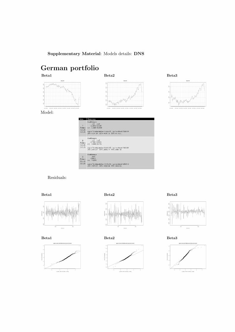
Supplementary Material: Models details: DNS
German portfolioBeta1
Jun 13 2013 Oct 01 2013 Jan 01 2014 Apr 01 2014 Jul 01 2014 Oct 01 2014 Jan 01 2015 Apr 01 2015
0.01
00.
015
0.02
00.
025
0.03
00.
035
Beta1 GR
Beta2
Jun 13 2013 Oct 01 2013 Jan 01 2014 Apr 01 2014 Jul 01 2014 Oct 01 2014 Jan 01 2015 Apr 01 2015
−0.
035
−0.
030
−0.
025
−0.
020
−0.
015
−0.
010
Beta2 GR
Beta3
Jun 13 2013 Oct 01 2013 Jan 01 2014 Apr 01 2014 Jul 01 2014 Oct 01 2014 Jan 01 2015 Apr 01 2015
−0.
05−
0.04
−0.
03−
0.02
Beta3 GR
Model:
Residuals:
Beta1
2014 2015
−0.
002
−0.
001
0.00
00.
001
GR_int[, 1]
arG
R1$
resi
dual
s
Beta2
2014 2015
−0.
002
−0.
001
0.00
00.
001
0.00
2
GR_int[, 1]
arG
R2$
resi
dual
s
Beta3
2014 2015
−0.
006
−0.
004
−0.
002
0.00
00.
002
0.00
4
GR_int[, 1]
arG
R3$
resi
dual
s
Beta1
−4 −2 0 2
−4
−2
02
46
qqplot residus GR NSParameters[,1] arima student
(a_GR[1] * rt(Nsim, ddl_GR[1]) + b_GR[1])
rt(N
obs_
GR
, ddl
_GR
[1])
Beta2
−4 −2 0 2 4
−6
−4
−2
02
46
8
qqplot residus GR NSParameters[,2] arima student
(a_GR[2] * rt(Nsim, ddl_GR[2]) + b_GR[2])
rt(N
obs_
GR
, ddl
_GR
[2])
Beta3
−4 −2 0 2 4 6
−4
−2
02
4
qqplot residus GR NSParameters[,3] arima student
(a_GR[3] * rt(Nsim, ddl_GR[3]) + b_GR[3])
rt(N
obs_
GR
, ddl
_GR
[3])

Supplementary Material: Models details: GARCH
US portfolio1 year
0 500 1000 1500 2000 2500
−40
−30
−20
−10
010
20
delta_i_US 1y
Index
delta
_i_U
S[,
3]
5 years
0 500 1000 1500 2000 2500
−40
−20
020
delta_i_US 3y
Index
delta
_i_U
S[,
5]
Data:
0 5 10 15 20 25 30 35
0.0
0.2
0.4
0.6
0.8
1.0
Lag
AC
F
acf delta_i_US 1y
0 5 10 15 20 25 30 35
0.0
0.2
0.4
0.6
0.8
1.0
Lag
AC
F
acf squarred delta_i_US 1y
0 5 10 15 20 25 30 35
−0.
050.
000.
05
Lag
Par
tial A
CF
pacf delta_i_US 1y
0 5 10 15 20 25 30 35
0.00
0.05
0.10
0.15
0.20
Lag
Par
tial A
CF
pacf squarred delta_i_US 1y
Residuals:
0 5 10 15 20 25 30 35
0.0
0.2
0.4
0.6
0.8
1.0
Lag
AC
F
acf student residuals arch(1) US 1Y
Figure 42: French data 1y
0 5 10 15 20 25 30 35
0.0
0.2
0.4
0.6
0.8
1.0
Lag
AC
F
acf student SQUARRED residuals arch(1) US 1Y
0 5 10 15 20 25 30 35
−0.
050.
000.
05
Lag
Par
tial A
CF
pacf student residuals arch(1) US 1Y
0 5 10 15 20 25 30 35
−0.
04−
0.02
0.00
0.02
0.04
0.06
0.08
Lag
Par
tial A
CF
pacf student SQUARRED residuals arch(1) US 1Y
−2 0 2 4
−15
−10
−5
05
qqplot residuals ARCH US 1Y
rnorm(Nobs_US − 2)
reg3
_US
$res
[2:(
Nob
s_U
S −
1)]
Data:
0 5 10 15 20 25 30 35
0.0
0.2
0.4
0.6
0.8
1.0
Lag
AC
F
acf delta_i_US 3y
0 5 10 15 20 25 30 35
0.0
0.2
0.4
0.6
0.8
1.0
Lag
AC
F
acf squarred delta_i_US 3y
0 5 10 15 20 25 30 35
−0.
050.
000.
05
Lag
Par
tial A
CF
pacf delta_i_US 3y
0 5 10 15 20 25 30 35
0.00
0.05
0.10
0.15
0.20
Lag
Par
tial A
CF
pacf squarred delta_i_US 3y
Residuals:
0 5 10 15 20 25 30 35
0.0
0.2
0.4
0.6
0.8
1.0
Lag
AC
F
acf student residuals arch(2) US 5Y
0 5 10 15 20 25 30 35
0.0
0.2
0.4
0.6
0.8
1.0
Lag
AC
F
acf student SQUARRED residuals arch(2) US 5Y
0 5 10 15 20 25 30 35
−0.
06−
0.04
−0.
020.
000.
020.
04
Lag
Par
tial A
CF
pacf student residuals arch(2) US 5Y
0 5 10 15 20 25 30 35
0.00
0.05
0.10
Lag
Par
tial A
CF
pacf student SQUARRED residuals arch(2) US 5Y
−2 0 2 4
−6
−4
−2
02
4
qqplot residuals ARCH US 5Y
rnorm(Nobs_US − 3)
reg7
_US
$res
[3:(
Nob
s_U
S −
1)]

US portfolio10 years
0 500 1000 1500 2000 2500
−40
−20
020
delta_i_US 5y
Index
delta
_i_U
S[,
7]
15 years
0 500 1000 1500 2000 2500
−40
−20
020
delta_i_US 10y
Index
delta
_i_U
S[,
12]
Data:
0 5 10 15 20 25 30 35
0.0
0.2
0.4
0.6
0.8
1.0
Lag
AC
F
acf delta_i_US 10y
0 5 10 15 20 25 30 35
0.0
0.2
0.4
0.6
0.8
1.0
Lag
AC
F
acf squarred delta_i_US 10y
0 5 10 15 20 25 30 35
−0.
08−
0.06
−0.
04−
0.02
0.00
0.02
0.04
Lag
Par
tial A
CF
pacf delta_i_US 10y
0 5 10 15 20 25 30 35
0.00
0.05
0.10
0.15
0.20
0.25
Lag
Par
tial A
CF
pacf squarred delta_i_US 10y
Residuals:
−4 −3 −2 −1 0 1 2 3
−6
−4
−2
02
4
qqplot residuals ARCH US 10Y
rnorm(Nobs_US − 3)
reg1
2_U
S$r
es[3
:(N
obs_
US
− 1
)]

Supplementary Material: Models details: PCA
US portfolio1stcomponent
0 1000 2000 3000 4000 5000 6000
−10
0−
500
50
composante 1 GR
Index
PC
A_d
elta
_i_G
R[,
1]
2ndcomponent
0 500 1000 1500 2000 2500
−30
−20
−10
010
2030
composante 2 US
Index
PC
A_d
elta
_i_U
S[,
2]
Data:
0 5 10 15 20 25 30 35
0.0
0.2
0.4
0.6
0.8
1.0
Lag
AC
F
acf composante 1 US
0 5 10 15 20 25 30 35
0.0
0.2
0.4
0.6
0.8
1.0
Lag
AC
F
acf squarred composante 1 US
0 5 10 15 20 25 30 35
−0.
06−
0.04
−0.
020.
000.
020.
04
Lag
Par
tial A
CF
pacf composante 1 US
0 5 10 15 20 25 30 35
0.00
0.05
0.10
0.15
0.20
Lag
Par
tial A
CF
pacf squarred composante 1 US
Residuals:
−6 −4 −2 0 2 4 6 8
−5
05
student residuals US PCA 1 composante
PCA_US_student_res[1, ]
rt(N
obs_
US
− 2
, PC
A_U
S_c
hose
n_dd
l[1])
Data:
0 5 10 15 20 25 30 35
0.0
0.2
0.4
0.6
0.8
1.0
Lag
AC
F
acf composante 2 US
0 5 10 15 20 25 30 35
0.0
0.2
0.4
0.6
0.8
1.0
Lag
AC
F
acf squarred composante 2 US
0 5 10 15 20 25 30 35
−0.
050.
000.
050.
10
Lag
Par
tial A
CF
pacf composante 2 US
0 5 10 15 20 25 30 35
0.00
0.05
0.10
0.15
0.20
0.25
Lag
Par
tial A
CF
pacf squarred composante 2 US
Residuals:
−5 0 5 10
−5
05
10
student residuals US PCA 2 composante
PCA_US_student_res[2, ]
rt(N
obs_
US
− 2
, PC
A_U
S_c
hose
n_dd
l[2])

Supplementary Material: Models details: ICA
US portfolio1stcomponent
0 500 1000 1500 2000 2500
−0.
4−
0.2
0.0
0.2
0.4
composante 1 US
Index
ICA
_del
ta_i
_US
[, 1]
2ndcomponent
0 500 1000 1500 2000 2500
−0.
50.
00.
5
composante 2 US
Index
ICA
_del
ta_i
_US
[, 2]
Data:
0 5 10 15 20 25 30 35
0.0
0.2
0.4
0.6
0.8
1.0
Lag
AC
F
acf composante 1 US
0 5 10 15 20 25 30 35
0.0
0.2
0.4
0.6
0.8
1.0
Lag
AC
F
acf squarred composante 1 US
0 5 10 15 20 25 30 35
−0.
04−
0.02
0.00
0.02
0.04
0.06
Lag
Par
tial A
CF
pacf composante 1 US
0 5 10 15 20 25 30 35
0.00
0.05
0.10
0.15
0.20
0.25
Lag
Par
tial A
CF
pacf squarred composante 1 US
Residuals:
0 5 10 15 20 25 30 35
0.0
0.2
0.4
0.6
0.8
1.0
Lag
AC
F
acf residuals arch(4) US composante 1
0 5 10 15 20 25 30 35
0.0
0.2
0.4
0.6
0.8
1.0
Lag
AC
F
acf SQUARRED residuals arch(4) US composante 1
0 5 10 15 20 25 30 35
−0.
04−
0.02
0.00
0.02
0.04
Lag
Par
tial A
CF
pacf residuals arch(4) US composante 1
0 5 10 15 20 25 30 35
−0.
04−
0.02
0.00
0.02
0.04
0.06
Lag
Par
tial A
CF
pacf SQUARRED residuals arch(4) US composante 1
−4 −2 0 2 4
−4
−2
02
46
8
qqplot residuals ARCH US composante 1
rnorm(Nobs_US − 5)
ICA
_reg
1_U
S$r
es[5
:(N
obs_
US
− 1
)]
Data:
0 5 10 15 20 25 30 35
0.0
0.2
0.4
0.6
0.8
1.0
Lag
AC
F
acf composante 2 US
0 5 10 15 20 25 30 35
0.0
0.2
0.4
0.6
0.8
1.0
Lag
AC
F
acf squarred composante 2 US
0 5 10 15 20 25 30 35
−0.
06−
0.04
−0.
020.
000.
020.
040.
06
Lag
Par
tial A
CF
pacf composante 2 US
0 5 10 15 20 25 30 35
0.00
0.05
0.10
0.15
0.20
Lag
Par
tial A
CF
pacf squarred composante 2 US
Residuals:
0 5 10 15 20 25 30 35
0.0
0.2
0.4
0.6
0.8
1.0
Lag
AC
F
acf residuals garch(1,1) US composante 2
0 5 10 15 20 25 30 35
0.0
0.2
0.4
0.6
0.8
1.0
Lag
AC
F
acf SQUARRED residuals garch(1,1) US composante 2
0 5 10 15 20 25 30 35
−0.
04−
0.02
0.00
0.02
0.04
Lag
Par
tial A
CF
pacf residuals garch(1,1) US composante 2
0 5 10 15 20 25 30 35
−0.
04−
0.02
0.00
0.02
0.04
Lag
Par
tial A
CF
pacf SQUARRED residuals garch(1,1) US composante 2
−2 0 2 4
−6
−4
−2
02
4
qqplot residuals ARCH US composante 2
rnorm(Nobs_US − 2)
ICA
_reg
2_U
S$r
es[2
:(N
obs_
US
− 1
)]

Supplementary Material: Models details: DNS
US portfolioBeta1
May 03 2013 Sep 03 2013 Jan 02 2014 May 01 2014 Sep 02 2014 Jan 02 2015 May 01 2015
0.02
50.
030
0.03
50.
040
0.04
5
Beta1 US
Beta2
May 03 2013 Sep 03 2013 Jan 02 2014 May 01 2014 Sep 02 2014 Jan 02 2015 May 01 2015
−0.
040
−0.
035
−0.
030
−0.
025
Beta2 US
Beta3
May 03 2013 Sep 03 2013 Jan 02 2014 May 01 2014 Sep 02 2014 Jan 02 2015 May 01 2015
−0.
07−
0.06
−0.
05−
0.04
−0.
03−
0.02
Beta3 US
Model:
Residuals:
Beta1
2014 2015
−0.
002
−0.
001
0.00
00.
001
0.00
20.
003
US_int[, 1]
arU
S1$
resi
dual
s
Beta2
2014 2015
−0.
004
−0.
002
0.00
00.
002
US_int[, 1]
arU
S2$
resi
dual
s
Beta3
2014 2015
−0.
010
−0.
005
0.00
00.
005
0.01
0
US_int[, 1]
arU
S3$
resi
dual
s
Beta1
−4 −2 0 2
−4
−2
02
4
qqplot residus US NSParameters[,1] arima student
(a_US[1] * rt(Nsim, ddl_US[1]) + b_US[1])
rt(N
obs_
US
, ddl
_US
[1])
Beta2
−4 −2 0 2 4
−4
−2
02
46
qqplot residus US NSParameters[,2] arima student
(a_US[2] * rt(Nsim, ddl_US[2]) + b_US[2])
rt(N
obs_
US
, ddl
_US
[2])
Beta3
−4 −2 0 2
−4
−2
02
4
qqplot residus US NSParameters[,3] arima student
(a_US[3] * rt(Nsim, ddl_US[3]) + b_US[3])
rt(N
obs_
US
, ddl
_US
[3])

Supplementary Material: Models details: GARCH
TRY portfolio1 year
0 500 1000 1500 2000 2500
−10
0−
500
5010
015
020
0
delta_i_TRY 1y
Index
delta
_i_T
RY
[, 3]
5 years
0 500 1000 1500 2000 2500
−10
0−
500
5010
015
0
delta_i_TRY 3y
Index
delta
_i_T
RY
[, 5]
Data:
0 5 10 15 20 25 30 35
0.0
0.2
0.4
0.6
0.8
1.0
Lag
AC
F
acf delta_i_TRY 1y
0 5 10 15 20 25 30 35
0.0
0.2
0.4
0.6
0.8
1.0
Lag
AC
F
acf squarred delta_i_TRY 1y
0 5 10 15 20 25 30 35
−0.
050.
000.
050.
100.
15
Lag
Par
tial A
CF
pacf delta_i_TRY 1y
0 5 10 15 20 25 30 35
−0.
10.
00.
10.
2
Lag
Par
tial A
CF
pacf squarred delta_i_TRY 1y
Residuals:
0 5 10 15 20 25 30 35
0.0
0.2
0.4
0.6
0.8
1.0
Lag
AC
F
acf student residuals arch(3) TRY 1Y
Figure 43: French data 1y
0 5 10 15 20 25 30 35
0.0
0.2
0.4
0.6
0.8
1.0
Lag
AC
F
acf student SQUARRED residuals arch(3) TRY 1Y
0 5 10 15 20 25 30 35
−0.
050.
000.
050.
10
Lag
Par
tial A
CF
pacf student residuals arch(3) TRY 1Y
0 5 10 15 20 25 30 35
−0.
050.
000.
050.
100.
150.
20
Lag
Par
tial A
CF
pacf student SQUARRED residuals arch(3) TRY 1Y
−3 −2 −1 0 1 2 3
−5
05
1015
qqplot residuals ARCH TRY 1Y
rnorm(Nobs_TRY − 2)
reg3
_TR
Y$r
es[2
:(N
obs_
TR
Y −
1)]
Data:
0 5 10 15 20 25 30 35
0.0
0.2
0.4
0.6
0.8
1.0
Lag
AC
F
acf delta_i_TRY 3y
0 5 10 15 20 25 30 35
0.0
0.2
0.4
0.6
0.8
1.0
Lag
AC
F
acf squarred delta_i_TRY 3y
0 5 10 15 20 25 30 35
0.00
0.05
0.10
0.15
Lag
Par
tial A
CF
pacf delta_i_TRY 3y
0 5 10 15 20 25 30 35
−0.
050.
000.
050.
100.
15
Lag
Par
tial A
CF
pacf squarred delta_i_TRY 3y
Residuals:
−3 −2 −1 0 1 2 3
−6
−4
−2
02
46
qqplot residuals ARCH TRY 5Y
rnorm(Nobs_TRY − 2)
reg6
_TR
Y$r
es[2
:(N
obs_
TR
Y −
1)]

TRY portfolio10 years
0 500 1000 1500 2000 2500
−20
0−
100
010
020
0
delta_i_TRY 5y
Index
delta
_i_T
RY
[, 7]
15 years
0 500 1000 1500 2000 2500
−20
0−
100
010
020
0
delta_i_TRY 10y
Index
delta
_i_T
RY
[, 12
]
Data:
0 5 10 15 20 25 30 35
0.0
0.2
0.4
0.6
0.8
1.0
Lag
AC
F
acf delta_i_TRY 10y
0 5 10 15 20 25 30 35
0.0
0.2
0.4
0.6
0.8
1.0
Lag
AC
F
acf squarred delta_i_TRY 10y
0 5 10 15 20 25 30 35
−0.
050.
000.
050.
10
Lag
Par
tial A
CF
pacf delta_i_TRY 10y
0 5 10 15 20 25 30 35
0.00
0.05
0.10
0.15
0.20
Lag
Par
tial A
CF
pacf squarred delta_i_TRY 10y
Residuals:
−3 −2 −1 0 1 2 3
−5
05
1015
qqplot residuals ARCH TRY 10Y
rnorm(Nobs_TRY − 2)
reg1
2_T
RY
$res
[2:(
Nob
s_T
RY
− 1
)]

Supplementary Material: Models details: PCA
TRY portfolio1stcomponent
0 1000 2000 3000 4000 5000 6000
−10
0−
500
50
composante 1 GR
Index
PC
A_d
elta
_i_G
R[,
1]
2ndcomponent
0 500 1000 1500 2000 2500
−40
0−
300
−20
0−
100
010
020
030
0
composante 2 TRY
Index
PC
A_d
elta
_i_T
RY
[, 2]
Data:
0 5 10 15 20 25 30 35
0.0
0.2
0.4
0.6
0.8
1.0
Lag
AC
F
acf composante 1 TRY
0 5 10 15 20 25 30 35
0.0
0.2
0.4
0.6
0.8
1.0
Lag
AC
F
acf squarred composante 1 TRY
0 5 10 15 20 25 30 35
−0.
050.
000.
050.
100.
15
Lag
Par
tial A
CF
pacf composante 1 TRY
0 5 10 15 20 25 30 35
−0.
050.
000.
050.
100.
150.
20
Lag
Par
tial A
CF
pacf squarred composante 1 TRY
Residuals:
−4 −3 −2 −1 0 1 2 3
−10
−5
05
qqplot residuals ARCH TRY composante 1
rnorm(Nobs_TRY − 3)
PC
A_r
eg1_
TR
Y$r
es[3
:(N
obs_
TR
Y −
1)]
Data:
0 5 10 15 20 25 30 35
0.0
0.2
0.4
0.6
0.8
1.0
Lag
AC
F
acf composante 2 TRY
0 5 10 15 20 25 30 35
0.0
0.2
0.4
0.6
0.8
1.0
Lag
AC
F
acf squarred composante 2 TRY
0 5 10 15 20 25 30 35
−0.
10−
0.05
0.00
0.05
0.10
Lag
Par
tial A
CF
pacf composante 2 TRY
0 5 10 15 20 25 30 35
0.00
0.05
0.10
0.15
Lag
Par
tial A
CF
pacf squarred composante 2 TRY
Residuals:
−3 −2 −1 0 1 2 3
−10
−5
05
1015
20
qqplot residuals ARCH TRY composante 2
rnorm(Nobs_TRY − 3)
PC
A_r
eg2_
TR
Y$r
es[3
:(N
obs_
TR
Y −
1)]

Supplementary Material: Models details: ICA
TRY portfolio1stcomponent
0 500 1000 1500 2000 2500
−2
−1
01
2
composante 1 TRY
Index
ICA
_del
ta_i
_TR
Y[,
1]
2ndcomponent
0 500 1000 1500 2000 2500
−0.
6−
0.4
−0.
20.
00.
20.
40.
6
composante 2 TRY
Index
ICA
_del
ta_i
_TR
Y[,
2]
Data:
0 5 10 15 20 25 30 35
0.0
0.2
0.4
0.6
0.8
1.0
Lag
AC
F
acf composante 1 TRY
0 5 10 15 20 25 30 35
0.0
0.2
0.4
0.6
0.8
1.0
Lag
AC
F
acf squarred composante 1 TRY
0 5 10 15 20 25 30 35
−0.
050.
000.
050.
10
Lag
Par
tial A
CF
pacf composante 1 TRY
0 5 10 15 20 25 30 35
−0.
050.
000.
050.
100.
150.
20
Lag
Par
tial A
CF
pacf squarred composante 1 TRY
Residuals:
0 5 10 15 20 25 30 35
0.0
0.2
0.4
0.6
0.8
1.0
Lag
AC
F
acf student residuals garch(1,1) TRY composante 1
0 5 10 15 20 25 30 35
0.0
0.2
0.4
0.6
0.8
1.0
Lag
AC
F
acf student SQUARRED residuals garch(1,1) TRY composante 1
0 5 10 15 20 25 30 35
−0.
04−
0.02
0.00
0.02
0.04
0.06
Lag
Par
tial A
CF
pacf student residuals garch(1,1) TRY composante 1
0 5 10 15 20 25 30 35
−0.
04−
0.02
0.00
0.02
0.04
0.06
0.08
0.10
Lag
Par
tial A
CF
pacf student SQUARRED residuals garch(1,1) TRY composante 1
−4 −2 0 2
−15
−10
−5
05
10
qqplot residuals ARCH TRY composante 1
rnorm(Nobs_TRY − 2)
ICA
_reg
1_T
RY
$res
[2:(
Nob
s_T
RY
− 1
)]
Data:
0 5 10 15 20 25 30 35
0.0
0.2
0.4
0.6
0.8
1.0
Lag
AC
F
acf composante 2 TRY
0 5 10 15 20 25 30 35
0.0
0.2
0.4
0.6
0.8
1.0
Lag
AC
F
acf squarred composante 2 TRY
0 5 10 15 20 25 30 35
−0.
050.
000.
050.
100.
15
Lag
Par
tial A
CF
pacf composante 2 TRY
0 5 10 15 20 25 30 35
−0.
050.
000.
050.
100.
150.
200.
25
Lag
Par
tial A
CF
pacf squarred composante 2 TRY
Residuals:
0 5 10 15 20 25 30 35
0.0
0.2
0.4
0.6
0.8
1.0
Lag
AC
F
acf student residuals garch(1,1) TRY composante 2
0 5 10 15 20 25 30 35
0.0
0.2
0.4
0.6
0.8
1.0
Lag
AC
F
acf student SQUARRED residuals garch(1,1) TRY composante 2
0 5 10 15 20 25 30 35
−0.
04−
0.02
0.00
0.02
0.04
0.06
0.08
0.10
Lag
Par
tial A
CF
pacf student residuals garch(1,1) TRY composante 2
0 5 10 15 20 25 30 35
−0.
04−
0.02
0.00
0.02
0.04
Lag
Par
tial A
CF
pacf student SQUARRED residuals garch(1,1) TRY composante 2
−4 −3 −2 −1 0 1 2 3
−5
05
qqplot residuals ARCH TRY composante 2
rnorm(Nobs_TRY − 2)
ICA
_reg
2_T
RY
$res
[2:(
Nob
s_T
RY
− 1
)]

Supplementary Material: Models details: DNS
TRY portfolioBeta1
Jun 13 2013 Oct 01 2013 Jan 01 2014 Apr 01 2014 Jul 01 2014 Oct 01 2014 Jan 01 2015 Apr 01 2015
0.07
0.08
0.09
0.10
0.11
0.12
0.13
Beta1 TRY
Beta2
Jun 13 2013 Oct 01 2013 Jan 01 2014 Apr 01 2014 Jul 01 2014 Oct 01 2014 Jan 01 2015 Apr 01 2015
−0.
04−
0.03
−0.
02−
0.01
0.00
0.01
0.02
Beta2 TRY
Beta3
Jun 13 2013 Oct 01 2013 Jan 01 2014 Apr 01 2014 Jul 01 2014 Oct 01 2014 Jan 01 2015 Apr 01 2015
−0.
04−
0.02
0.00
0.02
0.04
0.06
0.08
Beta3 TRY
Model:
Residuals:
Beta1
2014 2015
−0.
02−
0.01
0.00
0.01
0.02
0.03
0.04
TRY_int[, 1]
arT
RY
1$re
sidu
als
Beta2
2014 2015
−0.
020.
000.
02
TRY_int[, 1]
arT
RY
2$re
sidu
als
Beta3
2014 2015
−0.
06−
0.04
−0.
020.
000.
020.
040.
06
TRY_int[, 1]
arT
RY
3$re
sidu
als
Beta1
−2 0 2 4
−4
−2
02
qqplot residus TRY NSParameters[,1] arima student
(a_TRY[1] * rt(Nsim, ddl_TRY[1]) + b_TRY[1])
rt(N
obs_
TR
Y, d
dl_T
RY
[1])
Beta2
−2 0 2 4 6
−4
−2
02
4
qqplot residus TRY NSParameters[,2] arima student
(a_TRY[2] * rt(Nsim, ddl_TRY[2]) + b_TRY[2])
rt(N
obs_
TR
Y, d
dl_T
RY
[2])
Beta3
−4 −2 0 2 4
−4
−2
02
4
qqplot residus TRY NSParameters[,3] arima student
(a_TRY[3] * rt(Nsim, ddl_TRY[3]) + b_TRY[3])
rt(N
obs_
TR
Y, d
dl_T
RY
[3])