LIF

Laboratoire d’Informatique Fondamentale

de Marseille

Unite Mixte de Recherche 6166CNRS – Universite de Provence – Universite de la Mediterranee

Resource Control for SynchronousCooperative Threads

Roberto M. Amadio and Silvano Dal Zilio

Rapport/Report 22-2004

4 mai 2004

Les rapports du laboratoire sont telechargeables a l’adresse suivante

Reports are downloadable at the following address

http://www.lif.univ-mrs.fr

Resource Control for SynchronousCooperative Threads

Roberto M. Amadio and Silvano Dal Zilio

LIF – Laboratoire d’Informatique Fondamentale de Marseille

UMR 6166

CNRS – Universite de Provence – Universite de la Mediterranee

{amadio,dalzilio}@lif.univ-mrs.fr

Abstract/Resume

We develop new methods to statically bound the resources needed for the execution of systemsof concurrent, interactive threads.

Our study is concerned with a synchronous model of interaction based on cooperativethreads whose execution proceeds in synchronous rounds called instants. Our contribution isa system of compositional static analyses to guarantee that each instant terminates and tobound the size of the values computed by the system as a function of the size of its parametersat the beginning of the instant.

Our method generalises an approach designed for first-order functional languages thatrelies on a combination of standard termination techniques for term rewriting systems andan analysis of the size of the computed values based on the notion of quasi-interpretation.

We show that these two methods can be combined to obtain an explicit polynomial boundon the space needed for the execution of the system during an instant. We also provide ev-idence for the expressivity of our synchronous programming model and describe a bytecodefor a related virtual machine.

Keywords: resource control, synchronous programming, quasi-interpretation, termination,term rewriting systems.

Nous presentons une nouvelle approche permettant de borner statiquement les ressourcesnecessaires a l’execution de systemes de threads interactifs et concurrents.

Notre etude porte sur un modele d’interaction synchrone base sur des threads cooperatifsdont l’execution procede par “segments synchrones” successifs appeles instants. Notre con-tribution est un systeme d’analyses statiques (toutes compositionnelles) qui garantissent quechaque instant se termine et qui permettent de borner la taille des valeurs calculees par lesysteme en fonction de la taille de ses parametres au debut de l’instant.

Notre methode generalise une approche concue pour des langages de programmation fonc-tionnels de premier ordre qui se fonde sur la combinaison de techniques standards pour lapreuve de terminaison de systemes de reecriture et d’une analyse de la taille des valeurs

calculees basee sur la notion de quasi-interpretation.Nous prouvons que ces methodes peuvent etre combinees pour extraire de chaque pro-

gramme un polynome qui borne l’espace requis pour l’execution du systeme pendant uninstant. Nous montrons egalement, a l’aide d’exemples, l’expressivite de notre modele de pro-grammation synchrone et nous decrivons un possible langage de bytecode pour une machinevirtuelle associee.

Mots-cles : controle de ressources, programmation synchrone, quasi-interpretations, ter-minaison, systemes de reecriture.

Relecteurs/Reviewers: Frederic Dabrowski and Gerard Boudol.

Notes: The authors are partly supported by ACI CRISS.

3

1 Introduction

The problem of bounding the usage made by programs of their resources has already attractedconsiderable attention. Automatic extraction of resource bounds has mainly focused on (first-order) functional languages starting from Cobham’s characterisation [13] of polynomial timefunctions by bounded recursion on notation. Following work, see, e.g., [5, 19, 17, 15], hasdeveloped various inference techniques that allow for efficient analyses while capturing asufficiently large range of practical algorithms.

Previous work [20, 8] has shown that polynomial time or space bounds can be obtainedby combining traditional termination techniques for term rewriting systems with an analysisof the size of computed values based on the notion of quasi-interpretation. In [2], we haveconsidered the problem of automatically inferring quasi-interpretations in the space of multi-variate max-plus polynomials. In [1], we have presented a virtual machine and a correspondingbytecode for a first-order functional language and shown how size and termination annotationscan be formulated and verified at the level of the bytecode. In particular, we can derivefrom the verification an explicit polynomial bound on the space required to execute a givenbytecode.

In this work, we aim at extending and adapting these results to a concurrent framework.Our starting point, is a quite basic and popular model of parallel threads interacting onshared variables. The kind of concurrency we consider is a cooperative one. This means thatby default a running thread cannot be preempted unless it explicitly decides to return thecontrol to the scheduler. In preemptive threads, the opposite hypothesis is made: by defaulta running thread can be preempted at any point unless it explicitly requires that a seriesof actions is atomic. We refer to, e.g., [24] for an extended comparison of the cooperativeand preemptive models. Our viewpoint is pragmatic: the cooperative model is closer to thesequential one and many applications are easier to program in the cooperative model thanin the preemptive one. Thus, as a first step, it makes sense to develop a resource controlanalysis for the cooperative model.

In models based on preemptive threads, it is difficult to foresee the behaviour of the sched-uler which might depend on timing information not available in the model. For this reasonand in spite of the fact that most schedulers are deterministic, the scheduler is often modelledas a non-deterministic process. In cooperative threads, the interrupt points are explicit inthe program and it is possible to think of the scheduler as a deterministic process. Thenthe resulting model is deterministic and this fact considerably simplifies its programming,debugging, and analysis.

The second major design choice is to assume that the computation is regulated by anotion of instant. An instant lasts as long as a thread can make some progress in the currentinstant. In other terms, an instant ends when the scheduler realizes that all threads are eitherstopped, or waiting for the next instant, or waiting for a value that no thread can produce inthe current instant. Because of this notion of instant, we regard our model as synchronous.Because the model includes a logical notion of time, it is possible for a thread to react to theabsence of an event.

The reaction to the absence of an event, is typical of synchronous languages such asEsterel [7]. Boussinot et al. have proposed a weaker version of this feature where thereaction to the absence happens in the following instant [6] and they have implemented itin various programming environments based on C, Java, and Scheme [26]. They have alsoadvocated the relevance of this concept for the programming of mobile code and demonstrated

4

that the possibility for a ‘synchronous’ mobile agent to react to the absence of an event isan added factor of flexibility for programs designed for open distributed systems, whosebehaviours are inherently difficult to predict.

Recently, Boudol [4] has proposed a formalisation of this programming model. Our anal-ysis will essentially focus on a small fragment of this model where higher-order functions,dynamic thread creation, and dynamic memory allocation are ruled out. We believe thatwhat is left is still expressive and challenging enough as far as resource control is concerned.Our analysis goes in three main steps. A first step is to guarantee that each instant terminates(Section 4). A second step, is to bound the size of the computed values as a function of thesize of the parameters at the beginning of the instant (Section 5). A third step, is to combinethe termination and size analyses in order to obtain polynomial bounds on the space neededfor the execution of the system during an instant as a function of the size of the parametersat the beginning of the instant (Section 6).

A characteristic of our static analyses is that to a great extent they make abstractionof the memory and the scheduler. This means that each thread can be analysed separately,that the complexity of the analyses grows linearly in the number of threads, and that anincremental analysis of a dynamically changing system of threads is possible. Preliminary tothese analyses, is a control flow analysis (Section 3) that guarantees that each thread readseach register at most once in an instant. We will see that without this condition, it is veryeasy to achieve an exponential growth of the space needed for the execution. From a technicalpoint of view, the benefit of this read once condition is that it allows to regard behaviours asfunctions of their initial parameters and the registers they may read in the instant. Takingthis functional viewpoint, we are able to adapt the main techniques developed for provingtermination and size bounds in the first-order functional setting.

We point out that our static size analyses are not intended to predict the size of the systemafter arbitrary many instants. This is a harder problem which in general seems to require anunderstanding of the global behaviour of the system: typically one has to find an invariantthat shows that the parameters of the system stay within certain bounds. For this reason,we believe that in practice our static analyses should be combined with a dynamic controllerthat at the end of each instant checks the size of the parameters of the system.

Along the way and in appendix A, we provide a number of programming examples illustrat-ing how certain synchronous and/or concurrent programming paradigms can be representedin our model. These examples suggest that the constraints imposed by the static analyses arenot too severe and that their verification can be automated.

Finally, we describe a bytecode for a simple virtual machine implementing our program-ming model (Section 7). This provides a more precise description of the resources needed forthe execution of the systems we consider and opens the way to the verification of resourcebounds at the bytecode level, following the ‘typed assembly language’ approach adopted in [1]for the purely functional fragment of the language. Proofs are available in appendix B.

2 A Model of Synchronous Cooperative Threads

A system of synchronous cooperative threads is described by: (1) a list of mutually recursivetype definitions, (2) a list of shared registers (or global variables) with a type and a defaultvalue, and (3) a list of mutually recursive functions and behaviours definitions relying onpattern matching. In this respect, the resulting programming language is reminiscent of

5

Erlang [3], which is a practical language to develop concurrent applications.The set of instructions a behaviour can execute is rather minimal. Indeed, our language

is already in a pre-compiled form where registers are assigned constant values and behavioursdefinitions are tail recursive. However, it is quite possible to extend the language and ouranalyses to have registers’ names as first-class values and general recursive behaviours.

Expressions. We rely on standard notation. If α, β are formal terms then Var(α) is the setof free variables in α (variables in patterns are not free) and [α/x]β denotes the substitutionof α for x in β. If h is a function, h[u/i] denotes a function update.

Expressions and values are built from a finite number of constructors, ranged over byc, c′, . . . We use f, f ′, . . . to range over function identifiers and x, x′, . . . for variables, anddistinguish the following three syntactic categories:

v ::= c(v, . . . , v) (values)p ::= x || c(p, . . . , p) (patterns)e ::= x || c(e, . . . , e) || f(e, . . . , e) (expressions)

The size of an expression |e| is defined as 0 if e is a constant or a variable and 1 + Σi∈1..n|ei|if e is of the form c(e1, . . . , en) or f(e1, . . . , en).

A function of arity n is defined by a sequence of pattern-matching rules of the formf(~p1) = be1, . . . , f(~pk) = bek, where bei is either an expression or a thread behaviour (seebelow), and ~p1, . . . , ~pk are sequences of length n of patterns. We follow the usual hypothesisthat the patterns in ~p1, . . . , ~pn are linear (a variable appears at most once). For the sake ofsimplicity, we will also assume that in a function definition a sequence of values ~v matchesexactly a sequence of patterns ~pi in a function definition. This hypothesis can be relaxed.

Inductive types are defined by equations of the shape t = · · · | c of (t1 ∗ · · · ∗ tn) | · · · .For instance, the type of natural numbers in unary format can be defined as follows: nat =z | s of nat . Functions, values, and expressions are assigned first order types of the shape(t1 ∗ · · · ∗ tn) → t where t, t1, . . . , tn are inductive types.

Behaviours. Some function symbols may return a thread behaviour b, b′, . . . rather than avalue. In contrast to ‘pure’ expressions, a behaviour does not return a result but producesside-effects by reading and writing a set of global registers, ranged over by r, r ′, . . . A behaviourmay also affect the scheduling status of the thread executing it (see below).

be, . . . ::= e || bb, b′, . . . ::= stop || yield.b || f(~e) || next.f(~e) || r := e.b ||

match r with p1 ⇒ b1 | · · · | pk ⇒ bk | [x] ⇒ f(~e)

The effect of the various instructions is informally described as follows: stop, terminates theexecuting thread for ever; yield.b, halts the execution and hands over the control to the sched-uler — the control should return to the thread later in the same instant and execution resumeswith b; f(~e) and next.f(~e) switch to another behaviour immediately or at the beginning ofthe following instant; r := e.b, evaluates the expression e, assigns its value to r and proceedswith the evaluation of b; match r with p1 ⇒ b1 | · · · | pk ⇒ bk | [x] ⇒ f(~e), waits until the valueof r matches one of the patterns p1, . . . , pk (there could be no delay) and yields the controlotherwise. At the end of the instant, if the value of r is v and no rules filter v then startthe next instant with the behaviour [v/x]f(~e). By convention, when the [x] ⇒ . . . branch isomitted, it is intended that if the match conditions are not satisfied in the current instant,then they are checked again in the following one.

6

Systems. Every thread has a status, denoted X,X ′, . . . , ranging over {N,R, S,W} — whereN stands for next, R for run, S for stop, and W for wait. A system of synchronous threadsB,B′, . . . is a finite mapping from thread indexes to pairs (behaviour, status). Each registerhas a type and a default value — its value at the beginning of an instant — and we uses, s′, . . . to denote a store, an association between registers and their values. We suppose thethread indexes i, k, . . . range over Zn = {0, 1, . . . , n − 1} and that at the beginning of eachinstant the store is so, such that each registers is assigned its default value. If B is a systemand i ∈ Zn a valid thread index then we denote with B1(i) the behaviour executed in thethread i and with B2(i) its current status. Initially, all threads have status R, the currentthread index is 0, and B1(i) is a behaviour expression of the shape f(~v). It is a standardexercise to formalise a type system of simple first-order functional types for such a languageand, in the following, we assume that all systems we consider are well typed.

Operational semantics. The operational semantics is described by three relations of grow-ing complexity, presented in Table 1:

• e ⇓ v, the closed expression e evaluates to the value v,

• (b, s)X→ (b′, s′), the behaviour b with store s runs an atomic sequence of actions till b′,

producing a store s′, and returning the control to the scheduler with status X.

• (B, s, i) → (B ′, s′, i′) the system B with store s and current thread (index) i runs anatomic sequence of actions (read from B1(i)) and becomes (B ′, s′, i′).

Behaviour reduction (b, s)X→ (b′, s′) is described by 7 rules, (b1) to (b7). We note that

during the instant, a thread may undergo the following status transitions: R → S,W,N andW → R. Also, the status of a thread may change from R to W if and only if the executedbehaviour is of the form match r with . . . and no filters match the value of r. System reduction(B, s, i) → (B ′, s′, i′) is described by 2 rules, (s1) and (s2), and relies on: (1) a partial functionN that computes the index of the next thread that will run in the current instant; (2) Afunction U that updates the status of the threads at the end of an instant. In particular, itactivates the branches [x] ⇒ f(~e) of threads in status W .

Scheduler. The scheduler is determined by the functions N and U . To ensure progress ofthe scheduling, we assume that if N returns an index then it must be possible to run thecorresponding thread in the current instant and that if N is undefined (denoted N (. . . ) ↑)then no thread can be run in the current instant. In addition, one could arbitrarily enrichthe functional behaviour of the scheduler by considering extensions such that N depends onthe history, the store, and/or is defined by means of probabilities. When no more thread canrun, the instant ends and the function U performs the following status transitions: N → R,W → R. For simplicity, we assume here that every thread in status W takes the [x] ⇒ . . .branch. Note that the function N is undefined on the updated system if and only if all threadsare stopped.

The cooperative fragment. The ‘cooperative’ fragment of the model with no synchronyis obtained by removing the next instruction and assuming that for all match instructions thebranch [x] ⇒ f(~e) is such that f(. . . ) = stop. Then all the interesting computation happensin the first instant, and in the second instant all the threads terminate. This fragment isalready powerful enough to simulate, e.g., Kahn networks (see appendix A.1).

7

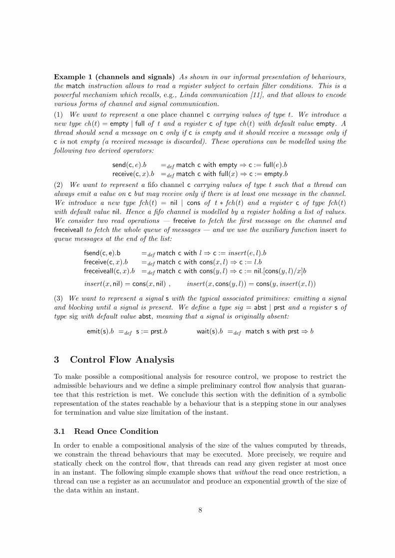
Example 1 (channels and signals) As shown in our informal presentation of behaviours,the match instruction allows to read a register subject to certain filter conditions. This is apowerful mechanism which recalls, e.g., Linda communication [11], and that allows to encodevarious forms of channel and signal communication.

(1) We want to represent a one place channel c carrying values of type t. We introduce anew type ch(t) = empty | full of t and a register c of type ch(t) with default value empty. Athread should send a message on c only if c is empty and it should receive a message only ifc is not empty (a received message is discarded). These operations can be modelled using thefollowing two derived operators:

send(c, e).b =def match c with empty ⇒ c := full(e).breceive(c, x).b =def match c with full(x) ⇒ c := empty.b

(2) We want to represent a fifo channel c carrying values of type t such that a thread canalways emit a value on c but may receive only if there is at least one message in the channel.We introduce a new type fch(t) = nil | cons of t ∗ fch(t) and a register c of type fch(t)with default value nil. Hence a fifo channel is modelled by a register holding a list of values.We consider two read operations — freceive to fetch the first message on the channel andfreceiveall to fetch the whole queue of messages — and we use the auxiliary function insert toqueue messages at the end of the list:

fsend(c, e).b =def match c with l ⇒ c := insert(e, l).bfreceive(c, x).b =def match c with cons(x, l) ⇒ c := l.bfreceiveall(c, x).b =def match c with cons(y, l) ⇒ c := nil.[cons(y, l)/x]b

insert(x, nil) = cons(x, nil) , insert(x, cons(y, l)) = cons(y, insert(x, l))

(3) We want to represent a signal s with the typical associated primitives: emitting a signaland blocking until a signal is present. We define a type sig = abst | prst and a register s oftype sig with default value abst, meaning that a signal is originally absent:

emit(s).b =def s := prst.b wait(s).b =def match s with prst ⇒ b

3 Control Flow Analysis

To make possible a compositional analysis for resource control, we propose to restrict theadmissible behaviours and we define a simple preliminary control flow analysis that guaran-tee that this restriction is met. We conclude this section with the definition of a symbolicrepresentation of the states reachable by a behaviour that is a stepping stone in our analysesfor termination and value size limitation of the instant.

3.1 Read Once Condition

In order to enable a compositional analysis of the size of the values computed by threads,we constrain the thread behaviours that may be executed. More precisely, we require andstatically check on the control flow, that threads can read any given register at most oncein an instant. The following simple example shows that without the read once restriction, athread can use a register as an accumulator and produce an exponential growth of the size ofthe data within an instant.

8

Expression evaluation:

(e1)~e ⇓ ~v

c(~e) ⇓ c(~v)(e2)

~e ⇓ ~v, f(~p) = e, σ~p = ~v, σ(e) ⇓ v

f(~e) ⇓ v

Behaviour reduction:

(b1)(stop, s)

S→ (stop, s)

(b2)(yield.b, s)

R→ (b, s)

(b3)(next.f(~e), s)

N→ (f(~e), s)

(b4)no pattern matches s(r)

(match r with . . . , s)W→ (match r with . . . , s)

(b5)σp = s(r), (σb, s)

X→ (b′, s′)

(match r with · · · | p ⇒ b | . . . , s)X→ (b′, s′)

(b6)~e ⇓ ~v, f(~p) = b, σ~p = ~v, (σb, s)

X→ (b′, s′)

(f(~e), s)X→ (b′, s′)

(b7)e ⇓ v, (b, s[v/r])

X→ (b′, s′)

(r := e.b, s)X→ (b′, s′)

System reduction:

(s1)(B1(i), s)

X→ (b′, s′), B2(i) = R, B′ = B[(b′, X)/i], N (B′, s′, i) = k

(B, s, i) → (B′[(B′

1(k), R)/k], s′, k)

(s2)(B1(i), s)

X→ (b′, s′), B2(i) = R, B′ = B[(b′, X)/i], N (B′, s′, i) ↑,

B′′ = U(B′, s′), N (B′′, so, 0) = k

(B, s, i) → (B′′, so, k)

Conditions on the scheduler:

If N (B, s, i) = j then B2(k) = R or ( B2(k) = W andB1(k) = match r with · · · | p ⇒ b | . . . , σp = s(r) )

If N (B, s, i) ↑ then ∀k ∈ Zn, B2(k) ∈ {N, S} or ( B2(k) = W,B1(k) = match r with . . . and no pattern matches s(r) )

U(B, s)(i) =

(b, S) if B(i) = (b, S)(b, R) if B(i) = (b, N)([s(r)/x](f(~e)), R) if B(i) = (match r with · · · | [x] ⇒ f(~e), W )

Table 1: Operational semantics

9

Example 2 Let nat = z | s of nat be the type of tally natural numbers. The function dble,defined by the two rules dble(z) = z and dble(s(n)) = s(s(d(n))) doubles a number so that|dble(n)| = 2|n|. We assume r is a register of type nat with initial value s(z). Now considerthe following recursive behaviour:

exp(z) = stop , exp(s(n)) = match r withm ⇒ r := dble(m).exp(n)

The evaluation of exp(n) involves |n| reads to the register r and, after each read operation,the size of the value stored in r doubles. Hence, at end of the instant, the register contains avalue of size 2|n|.

The read once condition is comparable to the restriction on the absence of immediate cyclicdefinitions in Lustre and does not appear to be a severe limitation on the expressiveness ofthe language. An important consequence of the read once condition is that a behaviour canbe described as a function of its parameters and the registers it may read during an instant.We stress that we retain the read once condition for its simplicity, however it is clear that onecould weaken the condition and adapt the analysis in the following section 3.2 to allow thereading of a register at most a constant number of times.

3.2 Enforcing the Read Once Condition

We now describe a simple analysis that guarantees the read once condition. Consider the setReg = {r1, . . . , rm} of the registers as an alphabet. To every function symbol f whose resultis a behaviour, we associate the least language R(f) of words over Reg such that ε, the emptyword, is in R(f) and the following conditions are satisfied:

if f(~p1) = b1, . . . , f(~pn) = bn are the rules of f then R(f) =def R(f) ·⋃

i∈1..n R(bi) ,

R(match r with p1 ⇒ b1 | · · · | pn ⇒ bn | [x] ⇒ g(~e)) =def {r} ·⋃

i∈1..n R(bi) ,R(stop) = {ε} , R(g(~e)) = R(g) , R(r := e.b) = R(b) ,R(yield.b) = R(b), R(next.g(~e)) = {ε} .

Looking at the words in R(f), we get an over-approximation of the sequences of registers thata thread can read in an instant starting from the control point f with arbitrary parametersand store. Note that an expression can never read or write a register.

To determine the sets R(f), we perform an iterative computation according to the equa-tions above. The iteration stops when either (1) we reach a fixpoint — and we are sure thatthe property holds — or (2) we notice that a word in the current approximation of R(f)contains the same register twice — thus we never need to consider words whose length isgreater than the number of registers. Since there is only a finite number of registers, it iseasy to prove that the computation of E (f) always terminates. If situation (1) occurs, thenfor every function symbol f that returns a behaviour we can obtain a list of registers ~rf thata thread starting from control point f may read. We are going to consider these registers ashidden parameters (variables) of the function f . If situation (2) occurs, we cannot guaranteethe read once property and we stop analysing the code.

Example 3 This will be the running example for this section. We consider the representationof signals as in Example 1(3). We assume two signals sig and ring. The behaviour alarm(n,m)

10

will emit a signal on ring if it detects that no signal is emitted on sig for m consecutive instants.The alarm delay is reset to n if the signal sig is present.

alarm(x, z) = ring := prst.stop ,alarm(x, s(y)) = match sig with prst ⇒ next.alarm(x, x) | [ ] ⇒ alarm(x, y)

By computing R on this example, we obtain: R(alarm) = {ε} · (R(ring := prst.stop) ∪R(match sig with . . . )) = {ε} · ({ε} ∪ ({sig} · {ε})) = {ε, sig}.

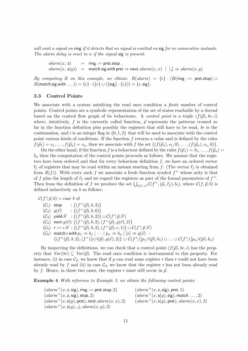
3.3 Control Points

We associate with a system satisfying the read once condition a finite number of controlpoints. Control points are a symbolic representation of the set of states reachable by a threadbased on the control flow graph of its behaviours. A control point is a triple (f(~p), be , i)where, intuitively, f is the currently called function, ~p represents the patterns crossed sofar in the function definition plus possibly the registers that still have to be read, be is thecontinuation, and i is an integer flag in {0, 1, 2} that will be used to associate with the controlpoint various kinds of conditions. If the function f returns a value and is defined by the rulesf(~p1) = e1, . . . , f(~pn) = en, then we associate with f the set {(f(~p1), e1, 0), . . . , (f(~pn), en, 0)}.

On the other hand, if the function f is a behaviour defined by the rules f(~p1) = b1, . . . , f(~pn) =bn then the computation of the control points proceeds as follows. We assume that the regis-ters have been ordered and that for every behaviour definition f , we have an ordered vector~rf of registers that may be read within an instant starting from f . (The vector ~rf is obtainedfrom R(f)). With every such f we associate a fresh function symbol f + whose arity is thatof f plus the length of ~rf and we regard the registers as part of the formal parameters of f +.Then from the definition of f we produce the set

⋃

i∈1..n C(f+, (~pi,~rf ), bi), where C(f, ~p, b) isdefined inductively on b as follows:

C(f+, ~p, b) = case b of

(C1) stop : {(f+(~p), b, 2)}(C2) g(~e) : {(f+(~p), b, 0)}(C3) yield.b′ : {(f+(~p), b, 2)} ∪ C(f+, ~p, b′)(C4) next.g(~e): {(f+(~p), b, 2), (f+(~p), g(~e), 2)}(C5) r := e.b′ : {(f+(~p), b, 2), (f+(~p), e, 1)} ∪ C(f+, ~p, b′)(C6) match r with p1 ⇒ b1 | · · · | pn ⇒ bn | [x] ⇒ g(~e) :

{(f+(~p), b, 2), (f+([x/r]~p), g(~e), 2)} ∪ C(f+, ([p1/r]~p), b1) ∪ . . . ∪ C(f+, ([pn/r]~p), bn)

By inspecting the definitions, we can check that a control point (f(~p), be , i) has the prop-erty that Var (be) ⊆ Var(~p). The read once condition is instrumental to this property. Forinstance, (i) in case C2, we know that if g can read some register r then r could not have beenalready read by f and (ii) in case C6, we know that the register r has not been already readby f . Hence, in these two cases, the register r must still occur in ~p.

Example 4 With reference to Example 3, we obtain the following control points:

(alarm+(x, z, sig), ring := prst.stop, 2) (alarm+(x, z, sig), prst, 1)(alarm+(x, z, sig), stop, 2) (alarm+(x, s(y), sig),match . . . , 2)(alarm+(x, s(y), prst), next.alarm(x, x), 2) (alarm+(x, s(y), prst), alarm(x, x), 2)(alarm+(x, s(y), ), alarm(x, y), 2)

11

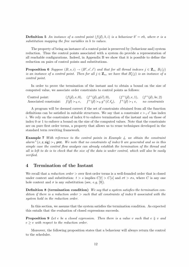
Definition 5 An instance of a control point (f(~p), b, i) is a behaviour b′ = σb, where σ is asubstitution mapping the free variables in b to values.

The property of being an instance of a control point is preserved by (behaviour and) systemreduction. Thus the control points associated with a system do provide a representation ofall reachable configurations. Indeed, in Appendix B we show that it is possible to define thereduction on pairs of control points and substitutions.

Proposition 6 Suppose (B, s, i) → (B ′, s′, i′) and that for all thread indexes j ∈ Zn, B1(j)is an instance of a control point. Then for all j ∈ Zn, we have that B ′

1(j) is an instance of acontrol point.

In order to prove the termination of the instant and to obtain a bound on the size ofcomputed value, we associate order constraints to control points as follows:

Control point: (f(~p), e, 0), (f+(~p), g(~e), 0), (f+(~p), e, 1), (f+(~p), be, 2)Associated constraint: f(~p) �0 e, f+(~p) �0 g+(~e,~rg), f+(~p) �1 e, no constraints

A program will be deemed correct if the set of constraints obtained from all the functiondefinitions can be satisfied in suitable structures. We say that a constraint e �i e′ has indexi. We rely on the constraints of index 0 to enforce termination of the instant and on those ofindex 0 or 1 to enforce a bound on the size of the computed values. Note that the constraintsare on pure first order terms, a property that allows us to reuse techniques developed in thestandard term rewriting framework.

Example 7 With reference to the control points in Example 4, we obtain the constraintalarm+(x, z, sig) �1 prst. We note that no constraints of index 0 are generated and so in thissimple case the control flow analysis can already establish the termination of the thread andall is left to do is to check that the size of the data is under control, which will also be easilyverified.

4 Termination of the Instant

We recall that a reduction order > over first-order terms is a well-founded order that is closedunder context and substitution: t > s implies C[t] > C[s] and σt > σs, where C is any onehole context and σ is any substitution (see, e.g, [9]).

Definition 8 (termination condition) We say that a system satisfies the termination con-dition if there is a reduction order > such that all constraints of index 0 associated with thesystem hold in the reduction order.

In this section, we assume that the system satisfies the termination condition. As expectedthis entails that the evaluation of closed expressions succeeds.

Proposition 9 Let e be a closed expression. Then there is a value v such that e ⇓ v ande ≥ v with respect to the reduction order.

Moreover, the following proposition states that a behaviour will always return the controlto the scheduler.

12

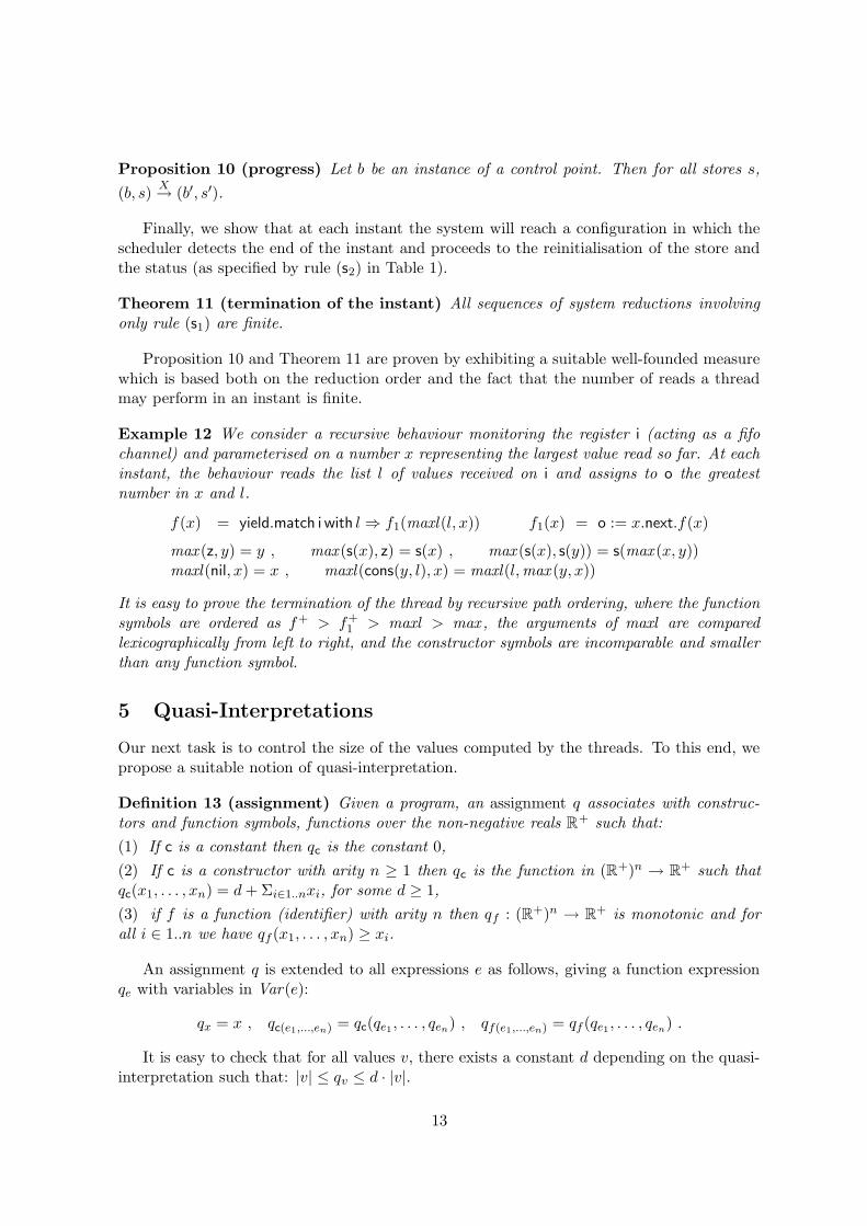
Proposition 10 (progress) Let b be an instance of a control point. Then for all stores s,

(b, s)X→ (b′, s′).

Finally, we show that at each instant the system will reach a configuration in which thescheduler detects the end of the instant and proceeds to the reinitialisation of the store andthe status (as specified by rule (s2) in Table 1).

Theorem 11 (termination of the instant) All sequences of system reductions involvingonly rule (s1) are finite.

Proposition 10 and Theorem 11 are proven by exhibiting a suitable well-founded measurewhich is based both on the reduction order and the fact that the number of reads a threadmay perform in an instant is finite.

Example 12 We consider a recursive behaviour monitoring the register i (acting as a fifochannel) and parameterised on a number x representing the largest value read so far. At eachinstant, the behaviour reads the list l of values received on i and assigns to o the greatestnumber in x and l.

f(x) = yield.match i with l ⇒ f1(maxl (l, x)) f1(x) = o := x.next.f(x)

max (z, y) = y , max (s(x), z) = s(x) , max (s(x), s(y)) = s(max (x, y))maxl (nil, x) = x , maxl (cons(y, l), x) = maxl(l,max (y, x))

It is easy to prove the termination of the thread by recursive path ordering, where the functionsymbols are ordered as f+ > f+

1 > maxl > max , the arguments of maxl are comparedlexicographically from left to right, and the constructor symbols are incomparable and smallerthan any function symbol.

5 Quasi-Interpretations

Our next task is to control the size of the values computed by the threads. To this end, wepropose a suitable notion of quasi-interpretation.

Definition 13 (assignment) Given a program, an assignment q associates with construc-tors and function symbols, functions over the non-negative reals R

+ such that:

(1) If c is a constant then qc is the constant 0,

(2) If c is a constructor with arity n ≥ 1 then qc is the function in (R+)n → R+ such that

qc(x1, . . . , xn) = d + Σi∈1..nxi, for some d ≥ 1,

(3) if f is a function (identifier) with arity n then qf : (R+)n → R+ is monotonic and for

all i ∈ 1..n we have qf (x1, . . . , xn) ≥ xi.

An assignment q is extended to all expressions e as follows, giving a function expressionqe with variables in Var(e):

qx = x , qc(e1,...,en) = qc(qe1, . . . , qen) , qf(e1,...,en) = qf (qe1

, . . . , qen) .

It is easy to check that for all values v, there exists a constant d depending on the quasi-interpretation such that: |v| ≤ qv ≤ d · |v|.

13

Definition 14 (quasi-interpretation) An assignment is a quasi-interpretation, if for allconstraints associated with the system of the shape f(~p) �i e, with i ∈ {0, 1}, the inequalityqf(~p) ≥ qe holds over the non-negative reals.

Quasi-interpretations are designed so as to provide a bound on the size of the computedvalues as a function of the size of the input data. In the following, we assume given a suitablequasi-interpretation, q, for the system under investigation.

Example 15 With reference to Examples 2 and 12, the following assignment is a quasi-interpretation (we give no quasi-interpretations for the function exp because it fails the readonce condition):

qnil = qz = 0 , qs(x) = x + 1 , qcons(x, l) = x + l + 1 , qdble(x) = 2 · x ,qf+(x, i) = x + i + 1 , q

f+

1

(x) = x , qmaxl (x, y) = qmax(x, y) = max (x, y) .

One can show [2] that in the purely functional fragment of our language every value vcomputed during the evaluation of an expression f(v1, . . . , vn) satisfies the following condition:

|v| ≤ qv ≤ qf(v1,...,vn) = qf (qv1, . . . , qvn) ≤ qf (d|v1|, . . . , d|vn|) . (1)

We generalise this result to threads as follows.

Theorem 16 Given a system of synchronous threads B, suppose that at the beginning of theinstant B1(i) = f(~v) for some thread index i. Then the size of the values computed by thethread i during an instant is bound by qf+(~v,~u) where ~u are the values contained in the registers~rf when they are read by the thread (or some constant value, otherwise).

Theorem 16 is proven by showing that quasi-interpretations satisfy a suitable invariant.In the following corollary, we note that it is possible to express a bound on the size of thecomputed values which depends only on the size of the parameters at the beginning of theinstant. This is possible because the number of reads a system may perform in an instant isbound by a constant.

Corollary 17 Let B be a system with m registers and n threads. Suppose B1(i) = fi(~vi) fori ∈ Zn. Let c be a bound of the size of the largest parameter of the functions fi and the largestdefault value of the registers. Suppose h is a function bounding all the quasi-interpretations,that is, for all the functions f+

i we have h(x) ≥ qf+

i(x, . . . , x) over the non-negative reals.

Then the size of the values computed by the system B during an instant is bound by hn·m+1(c).

Example 18 The n ·m iterations of the function h predicted by Corollary 17 correspond to atight bound, as shown by the following example. We assume n threads and m registers (withdefault value z). The control of each thread is described as follows, where writeall (e).b standsfor the behaviour r1 := e. · · · .rm := e.b :

f(x0) = match r1 withx1 ⇒ writeall (dble(max (x1, x0))).match r2 withx2 ⇒ writeall (dble(x2)).

. . . . . .match rm withxm ⇒ writeall (dble(xm)).next.f(dble(xm)) .

For this system we have c ≥ |x0| and h(x) = qdble(x) = 2 · x. It is easy to show that, at theend of an instant, there have been m · n assignments to each register (m for every thread inthe system) and that the value stored in each register is dblem·n(x0) of size 2m·n · |x0|.

14

6 Combining Termination and Quasi-Interpretations

To bound the space needed for the execution of a system during an instant we also need tobound the number of nested recursive calls, i.e., the number of frames that can be found on thestack (a precise definition of frame is given in the following Section 7). Unfortunately, quasi-interpretations provide a bound on the size of the frames but not on their number (at leastnot in a direct way). One way to cope with this problem is to combine quasi-interpretationswith various families of reduction orders [20, 8]. In the following, we provide an example ofthis approach based on recursive path orders which is a widely used and fully mechanizabletechnique to prove termination [9].

Definition 19 We say that a system terminates by LPO, if the reduction order associatedwith the system is a recursive path order where: (1) function symbols are compared lexico-graphically; (2) constructor symbols are always smaller than function symbols and two distinctconstructor symbols are incomparable; (3) the arguments of constructor symbols are comparedcomponentwise (product order).

Definition 20 We say that a system admits a polynomial quasi-interpretation if it has aquasi-interpretation where all functions are bound by a polynomial.

Theorem 21 If a system B terminates by LPO and admits a polynomial quasi-interpretationthen the computation of the system in an instant runs in space polynomial in the size of theparameters of the threads at the beginning of the instant.

The proof of Theorem 21 is based on Corollary 17 that provides a polynomial bound onthe size of the computed values and on an analysis of nested calls in the LPO order that canbe found in [8]. The point is that the depth of such nested calls is polynomial in the sizeof the values and that this allows to effectively compute a polynomial bounding the spacenecessary for the execution of the system. We stress that beyond proving that a system‘runs in PSPACE’, we can extract a definite polynomial that bounds the size needed to runa system during an instant. For each thread (in a verified system) running the behaviour fwith n parameters, we obtain a polynomial q(x1, . . . , xn) such that for all values v1, . . . , vn ofthe appropriate types, the size needed for the evaluation of the thread [v1/x1, . . . , vn/xn]b isbounded by q(|v1|, . . . , |vn|), where |v| stands for the size of the value v.

Example 22 With reference to Example 12, we can check that the order used there is indeeda LPO. From the quasi-interpretation in Example 15, we can deduce that the function h(x)has the shape a · x + b (it is affine). More precisely, we can choose h(x) = 2 · x + 1. Inpractice, many useful functions admit quasi-interpretations bound by an affine function suchas the max-plus polynomials considered in [2]. Note that the parameter of the thread is thelargest value received so far. Clearly, bounding the value of this parameter for arbitrary manyinstants requires a global analysis of the system.

7 A Virtual Machine

We describe a simple virtual machine for our language thus providing a concrete intuition forthe data structures required for the execution of the programs and the scheduler.

15

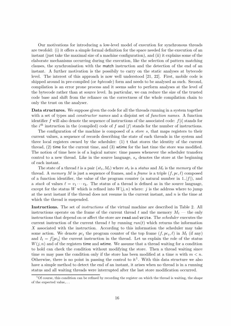
Our motivations for introducing a low-level model of execution for synchronous threadsare twofold: (i) it offers a simple formal definition for the space needed for the execution of aninstant (just take the maximal size of a machine configuration), and (ii) it explains some of theelaborate mechanisms occurring during the execution, like the selection of pattern matchingclauses, the synchronisation with the match instruction and the detection of the end of aninstant. A further motivation is the possibily to carry on the static analyses at bytecodelevel. The interest of this approach is now well understood [21, 22]. First, mobile code isshipped around in pre-compiled (or bytecode) form and needs to be analysed as such. Second,compilation is an error prone process and it seems safer to perform analyses at the level ofthe bytecode rather than at source level. In particular, we can reduce the size of the trustedcode base and shift from the reliance on the correctness of the whole compilation chain toonly the trust on the analyser.

Data structures. We suppose given the code for all the threads running in a system togetherwith a set of types and constructor names and a disjoint set of function names. A functionidentifier f will also denote the sequence of instructions of the associated code: f [i] stands forthe ith instruction in the (compiled) code of f and |f | stands for the number of instructions.

The configuration of the machine is composed of a store s, that maps registers to theircurrent values, a sequence of records describing the state of each threads in the system andthree local registers owned by the scheduler: (1) t that stores the identity of the currentthread, (2) time for the current time, and (3) wtime for the last time the store was modified.The notion of time here is of a logical nature: time passes whenever the scheduler transferscontrol to a new thread. Like in the source language, so denotes the store at the beginningof each instant.

The state of a thread t is a pair (st t,Mt) where st t is a status and Mt is the memory of thethread. A memory M is just a sequence of frames, and a frame is a triple (f, pc, `) composedof a function identifier, the value of the program counter (a natural number in 1..|f |), anda stack of values ` = v1 · · · vk. The status of a thread is defined as in the source language,except for the status W which is refined into W (j, n) where: j is the address where to jumpat the next instant if the thread does not resume in the current instant, and n is the time atwhich the thread is suspended.

Instructions. The set of instructions of the virtual machine are described in Table 2. Allinstructions operate on the frame of the current thread t and the memory Mt — the onlyinstructions that depend on or affect the store are read and write. The scheduler executes thecurrent instruction of the current thread t by running run(t) which returns the informationX associated with the instruction. According to this information the scheduler may takesome action. We denote pc t the program counter of the top frame (f, pc t, `) in Mt (if any)and It = f [pct] the current instruction in the thread. Let us explain the role of the statusW (j, n) and of the registers time and wtime. We assume that a thread waiting for a conditionto hold can check the condition without modifying the store. Then a thread waiting sincetime m may pass the condition only if the store has been modified at a time n with m < n.Otherwise, there is no point in passing the control to it1. With this data structure we alsohave a simple method to detect the end of an instant, it arises when no thread is in a runningstatus and all waiting threads were interrupted after the last store modification occurred.

1Of course, this condition can be refined by recording the register on which the thread is waiting, the shapeof the expected value,. . .

16

Instructions:

f [pc] Current memory Following memory

load i M · (f, pc, v1 · · · vi · `) → M · (f, pc + 1, v1 · · · vi · ` · vi)pop i M · (f, pc, ` · v1 · · · vi) → M · (f, pc + 1, `)branch c j M · (f, pc, ` · c(v1, . . . , vn)) → M · (f, pc + 1, ` · v1 · · · vn)branch c j M · (f, pc, ` · d(. . .)) → M · (f, j, ` · d(. . .)) c 6= d

build c n M · (f, pc, ` · v1 · · · vn) → M · (f, pc + 1, ` · c(v1, . . . , vn))call g n M · (f, pc, ` · v1 · · · vn) → M · (f, pc, `) · (g, 1, v1 · · · vn)tcall g n M · (f, pc, ` · v1 · · · vn) → M · (g, 1, v1 · · · vn)return M · (g, pc ′, `′) · (f, pc, ` · v) → M · (g, pc ′ + 1, `′ · v)read r (M · (f, pc, `), s) → (M · (f, pc + 1, ` · s(r)), s)write r (M · (f, pc, ` · v), s) → (M · (f, pc + 1, ` · v), s[v/r])

stop M · (f, pc, `)S→ ε

yield M · (f, pc, `)R→ M · (f, pc + 1, `)

next M · (f, pc, `)N→ M · (f, pc + 1, `)

wait j M · (f, pc, `)W→ M · (f, pc + 1, `)

Scheduler:

for t inZn do { st t := R; }s := so; t := time := wtime := 0;repeat forever {

if It = (write ) thenwtime := time; /* retain that the store has been modified */X := run(t); /* run the current thread */case X ofN, R, S, W : {

if It = (wait j ) then st t := W (j, time); else st t := X;t′ := N (t, st); /* compute the index of the next active thread */if t′ ∈ Zn /* test whether all threads are blocked */

then { t := t′; st t := R; time := time + 1; }else { s := so; wtime := time; /* initialisation of the new instant */

forall i inZn do {if st i = W (j, ) then pci := j;if st i 6= S then st i := R; } } }

}

Conditions on N :

If N (t, st) = k ∈ Zn then stk = R or (stk = W (j, n) and n < wtime)If N (t, st) /∈ Zn then ∀k ∈ Zn (stk 6= R and (stk = W (j, n) implies n ≥ wtime))

Table 2: Virtual machine

17

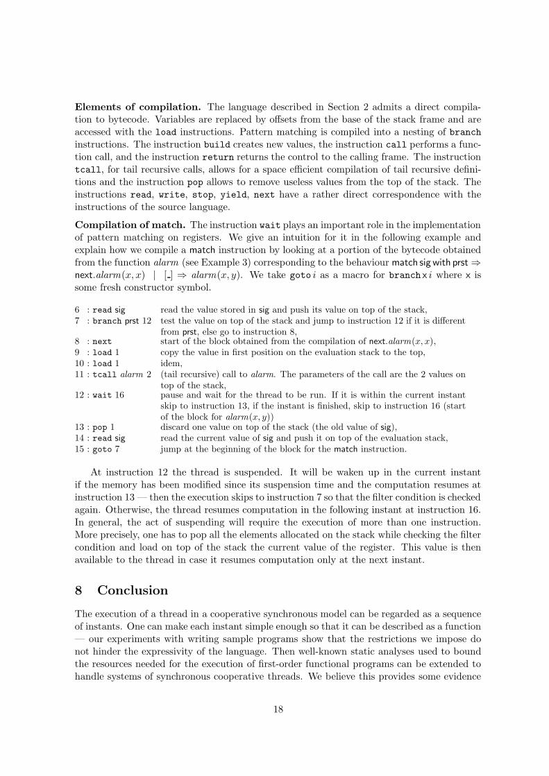
Elements of compilation. The language described in Section 2 admits a direct compila-tion to bytecode. Variables are replaced by offsets from the base of the stack frame and areaccessed with the load instructions. Pattern matching is compiled into a nesting of branchinstructions. The instruction build creates new values, the instruction call performs a func-tion call, and the instruction return returns the control to the calling frame. The instructiontcall, for tail recursive calls, allows for a space efficient compilation of tail recursive defini-tions and the instruction pop allows to remove useless values from the top of the stack. Theinstructions read, write, stop, yield, next have a rather direct correspondence with theinstructions of the source language.

Compilation of match. The instruction wait plays an important role in the implementationof pattern matching on registers. We give an intuition for it in the following example andexplain how we compile a match instruction by looking at a portion of the bytecode obtainedfrom the function alarm (see Example 3) corresponding to the behaviour match sig with prst ⇒next.alarm(x, x) | [ ] ⇒ alarm(x, y). We take goto i as a macro for branch x i where x issome fresh constructor symbol.

6 : read sig read the value stored in sig and push its value on top of the stack,7 : branch prst 12 test the value on top of the stack and jump to instruction 12 if it is different

from prst, else go to instruction 8,8 : next start of the block obtained from the compilation of next.alarm(x, x),9 : load 1 copy the value in first position on the evaluation stack to the top,10 : load 1 idem,11 : tcall alarm 2 (tail recursive) call to alarm. The parameters of the call are the 2 values on

top of the stack,12 : wait 16 pause and wait for the thread to be run. If it is within the current instant

skip to instruction 13, if the instant is finished, skip to instruction 16 (startof the block for alarm(x, y))

13 : pop 1 discard one value on top of the stack (the old value of sig),14 : read sig read the current value of sig and push it on top of the evaluation stack,15 : goto 7 jump at the beginning of the block for the match instruction.

At instruction 12 the thread is suspended. It will be waken up in the current instantif the memory has been modified since its suspension time and the computation resumes atinstruction 13 — then the execution skips to instruction 7 so that the filter condition is checkedagain. Otherwise, the thread resumes computation in the following instant at instruction 16.In general, the act of suspending will require the execution of more than one instruction.More precisely, one has to pop all the elements allocated on the stack while checking the filtercondition and load on top of the stack the current value of the register. This value is thenavailable to the thread in case it resumes computation only at the next instant.

8 Conclusion

The execution of a thread in a cooperative synchronous model can be regarded as a sequenceof instants. One can make each instant simple enough so that it can be described as a function— our experiments with writing sample programs show that the restrictions we impose donot hinder the expressivity of the language. Then well-known static analyses used to boundthe resources needed for the execution of first-order functional programs can be extended tohandle systems of synchronous cooperative threads. We believe this provides some evidence

18

for the relevance of these techniques in concurrent/embedded programming. We also expectthat our approach can be extended to a richer programming model including, e.g., referencesas first-class values, transactions-like primitives for error recovery, more elaborate mechanismsfor preemption, . . .

The static analyses we have considered do not try to analyse the whole system. On thecontrary, they focus on each thread separately and can be carried out incrementally. Onthe basis of our previous work [1] and the virtual machine presented in Section 7, we expectthat these analyses can be performed at bytecode level. These characteristics are particularlyinteresting in the framework of ‘mobile code’ where threads can enter or leave the system atthe end of each instant as described in [4].

References

[1] R. Amadio, S. Coupet-Grimal, S. Dal-Zilio, and L. Jakubiec. A functional scenario forbytecode verification of resource bounds. Research Report LIF 17-2004, 2004.

[2] R. Amadio. Max-plus quasi-interpretations. In Proc. Typed Lambda Calculi and Appli-cations (TLCA ’03), Springer LNCS 2701, 2003.

[3] J. Armstrong, R. Virding, C. Wikstrom, M. Williams. Concurrent Programming inErlang. Prentice-Hall 1996.

[4] G. Boudol, ULM, a core programming model for global computing. In Proc. of ESOP,Springer LNCS, 2004.

[5] S. Bellantoni and S. Cook. A new recursion-theoretic characterization of the poly-timefunctions. Computational Complexity, 2:97–110, 1992.

[6] F. Boussinot and R. De Simone, The SL Synchronous Language. IEEE Trans. onSoftware Engineering, 22(4):256–266, 1996.

[7] G. Berry and G. Gonthier, The Esterel synchronous programming language. Science ofcomputer programming, 19(2):87–152, 1992.

[8] G. Bonfante, J.-Y. Marion, and J.-Y. Moyen. On termination methods with space boundcertifications. In Proc. Perspectives of System Informatics, Springer LNCS, 2001.

[9] F. Baader and T. Nipkow. Term rewriting and all that. Cambridge University Press,1998.

[10] J. Buck. Scheduling dynamic dataflow graphs with bounded memory using the token flowmodel. PhD thesis, University of Berkeley, 1993.

[11] N. Carriero and D. Gelernter. Linda in Context. Commun. ACM, 32(4): 444-458, 1989.

[12] P. Caspi. Clocks in data flow languages. Theoretical Computer Science, 94:125–140,1992.

[13] A. Cobham. The intrinsic computational difficulty of functions. In Proc. Logic, Method-ology, and Philosophy of Science II, North Holland, 1965.

19

[14] P. Caspi and M. Pouzet. Synchronous Kahn networks. In Proc. ACM Conf. on FunctionalProgramming, 1996.

[15] M. Hofmann. The strength of non size-increasing computation. In Proc. POPL, ACMPress, 2002.

[16] G. Kahn. The semantics of a simple language for parallel programming. In Proc. IFIPCongress, North-Holland, 1974.

[17] N. Jones. Computability and complexity, from a programming perspective. MIT-Press,1997.

[18] E. Lee and D. Messerschmitt. Static scheduling of synchronous data flow programs fordigital signal processing. IEEE Trans. on Computers, 1:24–35, 1987.

[19] D. Leivant. Predicative recurrence and computational complexity i: word recurrence andpoly-time. Feasible mathematics II, Clote and Remmel (eds.), Birkhauser:320–343, 1994.

[20] J.-Y. Marion. Complexite implicite des calculs, de la theorie a la pratique. Universite deNancy, 2000. Habilitation a diriger des recherches.

[21] G. Morriset, D. Walker, K. Crary and N. Glew. From system F to typed assemblylanguage. In ACM Transactions on Programming Languages and Systems, 21(3):528-569, 1999.

[22] G. Necula. Proof carrying code. In Proc. POPL, ACM Press, 1997.

[23] M. Odersky. Functional nets. In Proc. ESOP, Springer Lecture Notes in Comp. Sci.1782, 2000.

[24] J. Ousterhout. Why threads are a bad idea (for most purposes). Invited talk at the 1996USENIX Technical Conference.

[25] Th. Park. Bounded scheduling of process networks. PhD thesis, University of Berkeley,1995.

[26] Reactive Programming, INRIA, Mimosa Project. http://www-sop.inria.fr/mimosa/rp.

20

A Examples

We illustrate how certain synchronous and/or concurrent programming paradigms can berepresented in our model.

A.1 Kahn and Lustre Networks

In Kahn networks [16] sequential threads communicate through unbounded, first-in-first-out,point-to-point channels. A thread can always send a message on a channel but reception willblock until there is a message actually present in the channel. Also, it is not possible to testwhether a channel is empty.

These fifo channels can be simulated as shown in Example 1(2). Since there is no notionof instant in Kahn networks, it is possible to rely just on the cooperative fragment (cf. section2) of our model and to perform the whole simulation during a single instant.

In the general Kahn model there is no bound on the number of messages that can bewritten in a fifo channel nor on the size of the messages. Much effort has been put into thestatic scheduling of Kahn networks (see, e.g., [18, 12, 14]). This analysis can be regarded asa form of resource control since it guarantees that the number of messages in fifo channels isbounded (but says nothing about their size). The static scheduling of Kahn network is alsomotivated by performance issues, since it eliminates the need to schedule threads at run time.

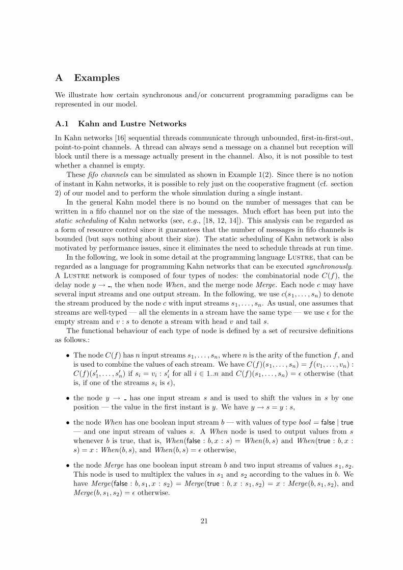
In the following, we look in some detail at the programming language Lustre, that can beregarded as a language for programming Kahn networks that can be executed synchronously.A Lustre network is composed of four types of nodes: the combinatorial node C(f), thedelay node y → , the when node When, and the merge node Merge. Each node c may haveseveral input streams and one output stream. In the following, we use c(s1, . . . , sn) to denotethe stream produced by the node c with input streams s1, . . . , sn. As usual, one assumes thatstreams are well-typed — all the elements in a stream have the same type — we use ε for theempty stream and v : s to denote a stream with head v and tail s.

The functional behaviour of each type of node is defined by a set of recursive definitionsas follows.:

• The node C(f) has n input streams s1, . . . , sn, where n is the arity of the function f , andis used to combine the values of each stream. We have C(f)(s1, . . . , sn) = f(v1, . . . , vn) :C(f)(s′1, . . . , s

′n) if si = vi : s′i for all i ∈ 1..n and C(f)(s1, . . . , sn) = ε otherwise (that

is, if one of the streams si is ε),

• the node y → has one input stream s and is used to shift the values in s by oneposition — the value in the first instant is y. We have y → s = y : s,

• the node When has one boolean input stream b — with values of type bool = false | true

— and one input stream of values s. A When node is used to output values from swhenever b is true, that is, When(false : b, x : s) = When(b, s) and When(true : b, x :s) = x : When(b, s), and When(b, s) = ε otherwise,

• the node Merge has one boolean input stream b and two input streams of values s1, s2.This node is used to multiplex the values in s1 and s2 according to the values in b. Wehave Merge(false : b, s1, x : s2) = Merge(true : b, x : s1, s2) = x : Merge(b, s1, s2), andMerge(b, s1, s2) = ε otherwise.

21

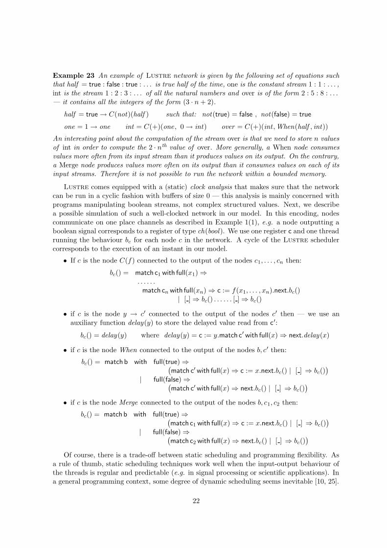
Example 23 An example of Lustre network is given by the following set of equations suchthat half = true : false : true : . . . is true half of the time, one is the constant stream 1 : 1 : . . . ,int is the stream 1 : 2 : 3 : . . . of all the natural numbers and over is of the form 2 : 5 : 8 : . . .— it contains all the integers of the form (3 · n + 2).

half = true → C(not)(half ) such that: not(true) = false , not(false) = true

one = 1 → one int = C(+)(one , 0 → int) over = C(+)(int ,When(half , int))

An interesting point about the computation of the stream over is that we need to store n valuesof int in order to compute the 2 · nth value of over. More generally, a When node consumesvalues more often from its input stream than it produces values on its output. On the contrary,a Merge node produces values more often on its output than it consumes values on each of itsinput streams. Therefore it is not possible to run the network within a bounded memory.

Lustre comes equipped with a (static) clock analysis that makes sure that the networkcan be run in a cyclic fashion with buffers of size 0 — this analysis is mainly concerned withprograms manipulating boolean streams, not complex structured values. Next, we describea possible simulation of such a well-clocked network in our model. In this encoding, nodescommunicate on one place channels as described in Example 1(1), e.g. a node outputting aboolean signal corresponds to a register of type ch(bool ). We use one register c and one threadrunning the behaviour bc for each node c in the network. A cycle of the Lustre schedulercorresponds to the execution of an instant in our model.

• If c is the node C(f) connected to the output of the nodes c1, . . . , cn then:

bc() = match c1 with full(x1) ⇒. . . . . .

match cn with full(xn) ⇒ c := f(x1, . . . , xn).next.bc()| [ ] ⇒ bc() . . . . . . [ ] ⇒ bc()

• if c is the node y → c′ connected to the output of the nodes c′ then — we use anauxiliary function delay(y) to store the delayed value read from c′:

bc() = delay(y) where delay(y) = c := y.match c′ with full(x) ⇒ next.delay(x)

• if c is the node When connected to the output of the nodes b, c′ then:

bc() = match b with full(true) ⇒(

match c′ with full(x) ⇒ c := x.next.bc() | [ ] ⇒ bc())

| full(false) ⇒(

match c′ with full(x) ⇒ next.bc() | [ ] ⇒ bc())

• if c is the node Merge connected to the output of the nodes b, c1, c2 then:

bc() = match b with full(true) ⇒(

match c1 with full(x) ⇒ c := x.next.bc() | [ ] ⇒ bc())

| full(false) ⇒(

match c2 with full(x) ⇒ next.bc() | [ ] ⇒ bc())

Of course, there is a trade-off between static scheduling and programming flexibility. Asa rule of thumb, static scheduling techniques work well when the input-output behaviour ofthe threads is regular and predictable (e.g. in signal processing or scientific applications). Ina general programming context, some degree of dynamic scheduling seems inevitable [10, 25].

22

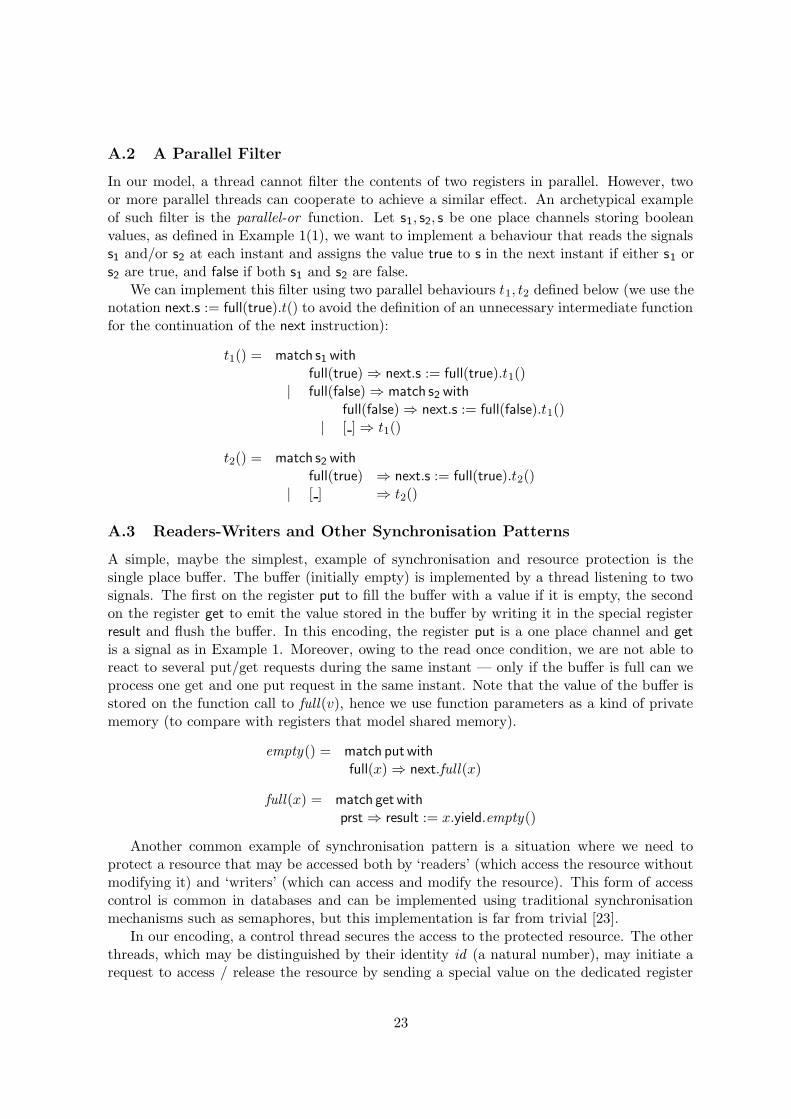
A.2 A Parallel Filter

In our model, a thread cannot filter the contents of two registers in parallel. However, twoor more parallel threads can cooperate to achieve a similar effect. An archetypical exampleof such filter is the parallel-or function. Let s1, s2, s be one place channels storing booleanvalues, as defined in Example 1(1), we want to implement a behaviour that reads the signalss1 and/or s2 at each instant and assigns the value true to s in the next instant if either s1 ors2 are true, and false if both s1 and s2 are false.

We can implement this filter using two parallel behaviours t1, t2 defined below (we use thenotation next.s := full(true).t() to avoid the definition of an unnecessary intermediate functionfor the continuation of the next instruction):

t1() = match s1 with

full(true) ⇒ next.s := full(true).t1()| full(false) ⇒ match s2 with

full(false) ⇒ next.s := full(false).t1()| [ ] ⇒ t1()

t2() = match s2 with

full(true) ⇒ next.s := full(true).t2()| [ ] ⇒ t2()

A.3 Readers-Writers and Other Synchronisation Patterns

A simple, maybe the simplest, example of synchronisation and resource protection is thesingle place buffer. The buffer (initially empty) is implemented by a thread listening to twosignals. The first on the register put to fill the buffer with a value if it is empty, the secondon the register get to emit the value stored in the buffer by writing it in the special registerresult and flush the buffer. In this encoding, the register put is a one place channel and get

is a signal as in Example 1. Moreover, owing to the read once condition, we are not able toreact to several put/get requests during the same instant — only if the buffer is full can weprocess one get and one put request in the same instant. Note that the value of the buffer isstored on the function call to full(v), hence we use function parameters as a kind of privatememory (to compare with registers that model shared memory).

empty() = match putwith

full(x) ⇒ next.full(x)

full(x) = match get with

prst ⇒ result := x.yield.empty()

Another common example of synchronisation pattern is a situation where we need toprotect a resource that may be accessed both by ‘readers’ (which access the resource withoutmodifying it) and ‘writers’ (which can access and modify the resource). This form of accesscontrol is common in databases and can be implemented using traditional synchronisationmechanisms such as semaphores, but this implementation is far from trivial [23].

In our encoding, a control thread secures the access to the protected resource. The otherthreads, which may be distinguished by their identity id (a natural number), may initiate arequest to access / release the resource by sending a special value on the dedicated register

23

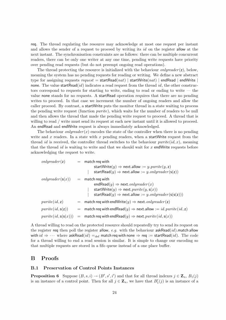
req. The thread regulating the resource may acknowledge at most one request per instantand allows the sender of a request to proceed by writing its id on the register allow at thenext instant. The synchronisation constraints are as follows: there can be multiple concurrentreaders, there can be only one writer at any one time, pending write requests have priorityover pending read requests (but do not preempt ongoing read operations).

The thread protecting the resource is initialized with the behaviour onlyreader (z), below,meaning the system has no pending requests for reading or writing. We define a new abstracttype for assigning requests request = startRead(nat) | startWrite(nat) | endRead | endWrite |none. The value startRead(id) indicates a read request from the thread id , the other construc-tors correspond to requests for starting to write, ending to read or ending to write — thevalue none stands for no requests. A startRead operation requires that there are no pendingwrites to proceed. In that case we increment the number of ongoing readers and allow thecaller proceed. By contrast, a startWrite puts the monitor thread in a state waiting to processthe pending write request (function pwrite), which waits for the number of readers to be nulland then allows the thread that made the pending write request to proceed. A thread that iswilling to read / write must send its request at each new instant until it is allowed to proceed.An endRead and endWrite request is always immediately acknowledged.

The behaviour onlyreader (x) encodes the state of the controller when there is no pendingwrite and x readers. In a state with x pending readers, when a startWrite request from thethread id is received, the controller thread switches to the behaviour pwrite(id, x), meaningthat the thread id is waiting to write and that we should wait for x endWrite requests beforeacknowledging the request to write.

onlyreader (z) = match req with

startWrite(y) ⇒ next.allow := y.pwrite(y, z)| startRead(y) ⇒ next.allow := y.onlyreader (s(z))

onlyreader (s(x)) = match req with

endRead(y) ⇒ next.onlyreader (x)| startWrite(y) ⇒ next.pwrite(y, s(x))| startRead(y) ⇒ next.allow := y.onlyreader (s(s(z)))

pwrite(id , z) = match req with endWrite(y) ⇒ next.onlyreader (z)

pwrite(id , s(z)) = match req with endRead(y) ⇒ next.allow := id .pwrite(id , z)

pwrite(id , s(s(x))) = match req with endRead(y) ⇒ next.pwrite(id , s(x))

A thread willing to read on the protected resource should repeatedly try to send its request onthe register req then poll the register allow, e.g. with the behaviour askRead(id).match allow

with id ⇒ · · · where askRead(id) =def match req with none ⇒ req := startRead(id). The codefor a thread willing to end a read session is similar. It is simple to change our encoding sothat multiple requests are stored in a fifo queue instead of a one place buffer.

B Proofs

B.1 Preservation of Control Points Instances

Proposition 6 Suppose (B, s, i) → (B ′, s′, i′) and that for all thread indexes j ∈ Zn, B1(j)is an instance of a control point. Then for all j ∈ Zn, we have that B ′

1(j) is an instance of a

24

control point.

We note that (f+(~p), b, i) ∈ C(f+, ~p, b), for some i ∈ {0, 1, 2}. We start by proving thepreservation of instances for behaviour reduction, that is, if b is an instance and (b, s)

X→(b′, s′)

then b′ is an instance.

Proof. We prove this auxiliary property by induction on the derivation of (b, s)X→ (b′, s′). We

proceed by case analysis on the last reduction rule used.

(b1) We can use the same control point.

(b2) Suppose yield.b is an instance of the control point (f +(~p), yield.b0, i). This control pointmust be generated by rule (C3) and then (f+(~p), b0, j) is also a symbolic control point and bis one of its instances.

(b3) We proceed as in the previous case, applying (C4).

(b4) We can use the same control point.

(b5) Suppose match r with . . . p ⇒ b . . . is an instance of (f +(~p),match r with . . . p ⇒ b0 . . . , j).By (C6), (f+([p/r]~p), b0, j

′) is a control point and σb is one of its instances if σp = s(r). Weconclude by applying the inductive hypothesis on σb.

(b6) Suppose f(~e) is an instance of (g+(~q), f(~e0), i). If ~e ⇓ ~v, f(~p) = b and σ~p = ~v, then(f+(~p,~rf ), b, i) is a control point by definition of C and σb is one of its instances. We concludeby applying the inductive hypothesis on σb.

(b7) Suppose r := e.b is an instance of (f+(~p), r := e0.b0, j), then by (C5) (f+(~p), b0, j′) is a

control point and b one of its instances. 2

Next we show the main property, namely that being an instance is preserved at the levelof system reduction. We proceed by case analysis on the last reduction rule used in thederivation of (B, s, i) → (B ′, s′, i′).

Proof. (s1) One of the threads performs one step. The property follows by the analysis

carried on above.

(s2) One of the threads performs one step. Moreover, the threads in waiting status take the[x] ⇒ g(~e) branch of the match instructions that were blocking. A thread match r . . . | [x] ⇒g(~e) in waiting status is an instance of a control point (f +(~p),match r . . . | [x] ⇒ g(~e0), j).By (C6), (f+([x/r]~p), g(~e0), 2) is a control point, and for any value v, [v/x]g(~e) is one of itsinstances. 2

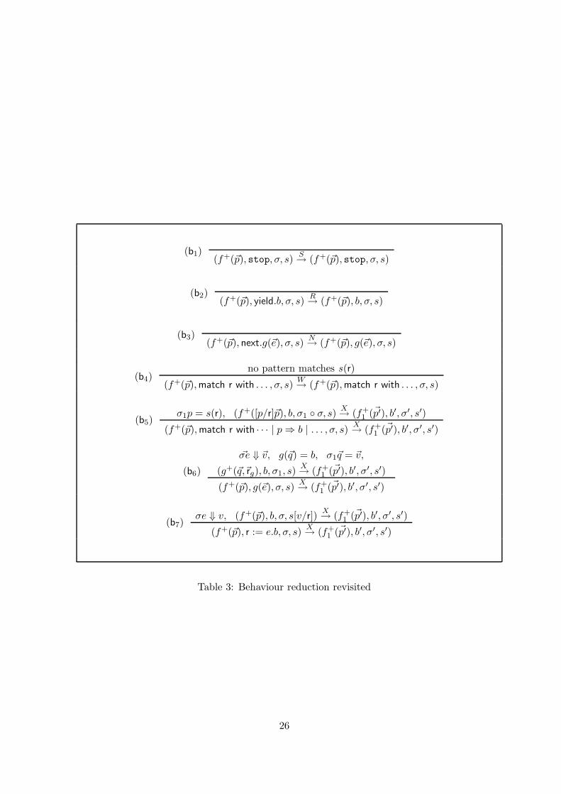
Our analysis has shown that if b is an instance of a control point and bX→ b′ then we

can effectively build a control point of which b′ is an instance. We can make this remarkprecise by redefining the behaviour reduction on quadruples (f +(~p), b, σ, s), where for some i,(f+(~p), b, i) is a control point, σ is a substitution mapping the variables in b to values, and sis a store. The revised system for behaviour reduction is described in table 3.

25

(b1)(f+(~p), stop, σ, s)

S→ (f+(~p), stop, σ, s)

(b2)(f+(~p), yield.b, σ, s)

R→ (f+(~p), b, σ, s)

(b3)(f+(~p), next.g(~e), σ, s)

N→ (f+(~p), g(~e), σ, s)

(b4)no pattern matches s(r)

(f+(~p),match r with . . . , σ, s)W→ (f+(~p),match r with . . . , σ, s)

(b5)σ1p = s(r), (f+([p/r]~p), b, σ1 ◦ σ, s)

X→ (f+

1 (~p′), b′, σ′, s′)

(f+(~p),match r with · · · | p ⇒ b | . . . , σ, s)X→ (f+

1 (~p′), b′, σ′, s′)

(b6)

~σe ⇓ ~v, g(~q) = b, σ1~q = ~v,

(g+(~q,~rg), b, σ1, s)X→ (f+

1 (~p′), b′, σ′, s′)

(f+(~p), g(~e), σ, s)X→ (f+

1 (~p′), b′, σ′, s′)

(b7)σe ⇓ v, (f+(~p), b, σ, s[v/r])

X→ (f+

1 (~p′), b′, σ′, s′)

(f+(~p), r := e.b, σ, s)X→ (f+

1 (~p′), b′, σ′, s′)

Table 3: Behaviour reduction revisited

26

B.2 Evaluation of Closed Expressions

Proposition 9 Let e be a closed expression. Then there is a value v such that e ⇓ v ande ≥ v with respect to the reduction order.

Proof. By induction on the structure of e and the reduction order >.

case e ≡ c(e1, . . . , en) If the arity of c is 0 then c ⇓ c and c ≥ c. If n > 0 then by inductivehypothesis ei ⇓ vi and ei ≥ vi for i = 1, . . . , n. Thus c(e1, . . . , en) ⇓ c(v1, . . . , vn). Moreover,since > is closed under context and transitivity, it follows that c(e1, . . . , en) ≥ c(v1, . . . , vn).

case e ≡ f(e1, . . . , en) By inductive hypothesis, ei ⇓ vi and ei ≥ vi for i = 1, . . . , n. Thisimplies f(~e) ≥ f(~v). Since the patterns used in function definitions are total, there is a rulef(~p) = e and a substitution σ such that σ~p = ~v. We know that f(~p) > e, thus f(σ~p) = f(~v) >σe. By inductive hypothesis, σe ⇓ v and σe ≥ v. Thus f(~e) ⇓ v and f(~e) ≥ f(~v) > σe ≥ v. 2

B.3 Progress

Proposition 10 Let b be an instance of a control point. Then for all stores s, there exists

a store s′ and a status X such that (b, s)X→ (b′, s′).

Proof. We restrict our attention to behaviours which are instances of control point. We have

seen in proposition 6 that if b is an instance of a control point and (b, s)X→ (b′, s′) then we

can effectively determine a control point of which b′ is an instance. Thus we can think ofthe behaviour reduction as acting on both a behaviour and a control point as formalised inTable 3.

We start by defining a suitable well-founded order. If b is a behaviour, then let nr(b) bethe maximum number of reads that b may perform in an instant:

nr(b) = max{ |w| | w ∈ R(b) }

Moreover, let ln(b) be the length of b inductively defined as follows:

ln(stop) = ln(f(~e)) = 0 ln(yield.b) = ln(r := e.b) = 1 + ln(b) ln(next.f(~e)) = 2ln(match r with . . . | pi ⇒ bi | . . . | [x] ⇒ f(~e)) = 1 + max (. . . , ln(bi), . . .)

If the behaviour b is an instance of the control point γ ≡ (f +(~p), b0, i) via a substitution σthen we associate to the pair (b, γ) a measure

µ(b, γ) = (nr (b), f+(σ~p), ln(b))

We assume that measures are lexicographically ordered from left to right, where the orderon the first and third component is the standard one on natural numbers and the order onthe second component is the one given by the reduction order considered in the terminationcondition. This is a well-founded order.

Now we show the assertion by induction on µ(b, γ). We proceed by case analysis on thestructure of b.

stop Apply (b1). Here X = S and the measure stays the same.

yield.b′ Apply (b2). Here X = R and the measure decreases because ln(b) decreases.

27

next.b′ Apply (b3). Here X = N and the measure decreases because ln(b) decreases.

match . . . If no pattern matches then apply (b4). The measure is unchanged. If a pat-tern matches then apply (b5). The measure decreases because nr (b) decreases and then theinduction hypothesis applies.

g(~e) Suppose g(~e) is an instance of the control point (f +(~p), g(~e0), 0) via the substitution σ.Note that ~e = σ~e0. By proposition 9, we know that ~e ⇓ ~v and ~e ≥ ~v in the reduction order.We also know that for some ~q, b, σ′~q = ~v and g(~q) = b. Finally, the constraint associated withthe control point requires f+(~p) > g+(~e0,~rg). Then using the properties of reduction orderswe observe:

f+(σ~p) > g+(σ~e0,~rg) = g+(~e,~rg)≥ g+(~v,~rg) = g+(σ′~q,~rg) .

Thus the measure decreases because f+(σ~p) > g+(σ′~q,~rg), and then the induction hypothesisapplies.

r := e.b′ By proposition 9, e ⇓ v. Apply (b7). The measure decreases because ln(b) decreases,and then the induction hypothesis applies. 2

Remark 24 We point out that in the proof of proposition 10, if X = R then the measuredecreases and if X ∈ {N,S,W} then the measure decreases or stays the same. This will beused in the following proof of Theorem 11.

B.4 Termination of the Instant

Theorem 11 All sequences of system reductions involving only rule (s1) are finite.

Proof. We order the status of threads as follows: R > N,S,W . With a behaviour B1(i)coming with a control point γi, we associate the pair µ′(i) = (µ(B1(i), γi), B2(i)) where µ isthe measure in the proof of Proposition 10. Thus µ′(i) can be regarded as a quadruple witha lexicographic order from left to right. With a system B of n threads (threads indexes arein Zn we associate the tuple (µ′(0), . . . , µ′(n − 1)). On such tuples, we consider the productorder. We prove that every system reduction sequence involving only rule (s1) terminates byinduction on this product order. We recall the rule below:

(B1(i), s)X→ (b′, s′), B2(i) = R, B′ = B[(b′, X)/i], N (B ′, s′, i) = k

(B, s, i) → (B ′[(B′1(k), R)/k], s′, k)

Let B′′ = B′[(B′1(k), R)/k]. We proceed by case analysis on X and B ′

2(k).We remark that if B ′

2(k) = W then the conditions on the scheduler tell us that i 6= kand that the thread k resuming the computation can read at least one register without beingsuspended. Then, if the measure on i is stable or decreasing, the induction hypothesis can beapplied to the continuation of the read operation, and from this, we can conclude that everyreduction sequence from (B ′′, s′, k) terminates. We proceed by case analysis on the status X

in the reduction (B1(i), s)X→ (b′, s′).

S Then µ′(i) decreases by Remark 24. If B ′2(k) = R then µ′(k) is unchanged. If B ′

2(k) = Wthen the argument above applies.

N Then µ′(i) decreases by Remark 24. If B ′2(k) = R then µ′(k) is unchanged. If B ′

2(k) = Wthen the argument above applies.

28

W Then µ′(i) decreases by Remark 24. If B ′2(k) = R then µ′(k) is unchanged. If B ′

2(k) = Wthen the argument above applies.

R Then µ′(i) decreases by Remark 24. If B ′2(k) = R then µ′(k) is unchanged. If B ′

2(k) = Wthen the argument above applies. 2

B.5 Bounding the Size of Values for Threads

Theorem 16 Given a system of synchronous threads B, suppose that at the beginning ofthe instant B1(i) = f(~v) for some thread index i. Then the size of the values computed bythe thread i during an instant is bound by qf+(~v,~u) where ~u are the values contained in theregisters ~rf when they are read by the thread (or some constant value, otherwise).

In Tables 1 and 3, we define the reduction of behaviours as a big step semantics. Wereformulate the rules in Table 3, following a small step approach:

(b′2) (f+(~p), yield.b, σ, s) → (f+(~p), b, σ, s)

(b′5) (f+(~p),match r with · · · | p ⇒ b | . . . , σ, s) → (f+([p/r]~p), b, σ1 ◦ σ, s) if σ1p = s(r)

(b′6) (f+(~p), g(~e), σ, s) → (g+(~q,~rg), b, σ1, s) if σ~e ⇓ ~v, g(~q) = b, σ1~q = ~v

(b′7) (f+(~p), r := e.b, σ, s) → (f+(~p), b, σ, s[v/r]) if σe ⇓ v

Note that there are no rules corresponding to (b1), (b3), (b4) since these rules eitherterminate or suspend the computation of the thread in the instant. If (f +(~p), b, σ, s) →∗

(g+(~q), b′, σ′, s′) by the rules above then some register variables r1, . . . , rk in ~p can be instan-tiated. Because of the read once condition, we know that each register can be instantiatedat most once. Thus we can uniquely determine a substitution δ = [u1/r1, . . . , uk/rk] thatassociates the values read with the registers.

Next, we prove the following invariant: if (f +(~p), b, σ, s) → (g+(~q), b′, σ′, s′) then we haveqδ(f+(σ(~p))) ≥ qg+((σ′(~q))) over the non-negative reals.

Proof. By case analysis on the small step rules.

(b′2) Then δ is the identity substitution and qf+(σ(~p)) = qf+(σ(~p)).

(b′5) Then δ = [s(r)/r] = [σ1(p)/r] and recalling that patterns are linear, we note that:

δ(f+(σ(~p))) = f+((δ ◦ σ)(~p)) = f+((σ1 ◦ σ)[p/r]~p) .

(b′6) Then δ is the identity substitution. By the properties of quasi-interpretations, we knowthat qσ~e ≥ q~v. By the constraints generated by the control points, we derive that qf+(~p) ≥qg+(~e,~rg) over the non-negative reals. By the substitutivity property of quasi-interpretations,this implies that qf+(σ~p) ≥ qg+(σ~e,~rg). Thus we derive, as required:

qf+(σ~p) ≥ qg+(σ~e,~rg) ≥ qg+(~v,~rg) = qg+(σ1~q,~rg)

(b′7) Then δ is the identity substitution and the conclusion follows as in (b′2). 2

29

It remains to support our claim that all values computed by the thread i during an instanthave a size bound by qf(~v,~u) where ~u are either the values read by the thread in the registersor some constant value.

Proof. By inspecting the shape of behaviours we see that a thread computes values eitherwhen writing into a register or in recursive calls. We consider in turn the two cases.

Writing Suppose (f+(~p,~rf ), b, σ, s) →∗ (g+(~q), r := e.b′, σ′, s′) by reading a series of registersrecorded by the substitution δ and assuming σ~p = ~v. Then the invariant we have proved aboveimplies that: qf+((δ◦σ)(~p,~rf )) ≥ qg+(σ′~q) over the non-negative reals. If some of the registers~rf are not instantiated by the substitution δ, then we may replace them by some constant.Next, we observe that the constraint of index 0 associated with the control point requiresthat qg+(~q) ≥ qe and that if σe ⇓ v then this implies qg+(σ′~q) ≥ qσ′e ≥ qv ≥ |v|.

Recursive call Suppose (f+(~p,~rf ), b, σ, s) →∗ (g+(~q), h(~e), σ′, s′) by reading a series of reg-isters recorded by the substitution δ and assuming σ~p = ~v. Then the invariant we haveproved above implies that: qf+((δ◦σ)(~p,~rf )) ≥ qg+(σ′~q) over the non-negative reals. Again,if some of the registers ~rf are not instantiated by the substitution δ, then we may re-place them by some constant value. Next we observe that the constraint of index 1 as-sociated with the control point requires that qg+(~q) ≥ qh+(~e,~rh). Moreover, if σ~e ⇓ ~v thenqg+(σ′~q) ≥ qh+(σ′~e,~rh) ≥ qh+(~v,~rh) ≥ qvi

≥ |vi|, where vi is any of the values in ~v (this uses theproperty qf (x1, . . . , xn) ≥ xi of assignments, cf. Definition 13). 2

B.6 Bounding the Size of Values for Systems

Corollary 17 Let B be a system with m registers and n threads. Suppose B1(i) = fi(~vi) fori ∈ Zn. Let c be a bound of the size of the largest parameter of the functions fi and the largestdefault value of the registers. Suppose h is a function bounding all the quasi-interpretations,that is, for all the functions f+

i we have h(x) ≥ qf+

i(x, . . . , x) over the non-negative reals. Then

the size of the values computed by the system B during an instant is bound by hn·m+1(c).

Proof. Because of the read once condition, during an instant a system can perform a (suc-cessful) read at most n · m times. We proceed by induction on the number k of registers thesystem has read so far to prove that the size of the values is bound by hk+1(c).

k = 0 If no register has been read, then Theorem 16 can be applied to show that all valueshave size bound by h(c).

k > 0 Inductively, the size of the values in the parameters and the registers is bound by hk(c).Theorem 16 says that all the values that can be computed before reading a new register havea size bound by h(hk(c)) = hk+1(c). 2

B.7 Proof of theorem 21

Theorem 21 If a system B terminates by LPO and admits a polynomial quasi-interpretationthen the computation of the system in an instant runs in space polynomial in the size of theparameters of the threads at the beginning of the instant.

Proof. We can always choose a polynomial for the function h in corollary 17. Hence, hnm+1

is also a polynomial. This shows that the size of all the values computed by the system is

30

bound by a polynomial. The number of values in a frame depends on the number of formalparameters and local variables and it can be statically bound. It remains to bound the numberof frames on the stack. Note that behaviours are tail recursive. This means that the stack ofeach thread contains a frame that never returns a value plus possibly a sequence of framesthat relate to the evaluation of expressions.

From this point on, one can follow the proof in [8]. The idea is to exploit the characteristicsof the LPO order: a nested sequence of recursive calls f1(~v1), . . . , fn(~vn) must satisfy f1(~v1) >· · · > fn(~vn), where > is the LPO order on terms. Because of the polynomial bound on thesize of the values, one can provide a polynomial bound on the length of such strictly decreasingsequences and therefore a polynomial bound on the size of the stack needed to execute thesystem. 2

31