lec1

Advanced Electric Drives

Prof. S. P. Das

Department of Electrical Engineering

Indian Institution of Technology, Kanpur

Lecture - 1

Hello. Welcome to the course on advanced electric drives. To do this course, you should

have some basic background about electrical machines, and some background about

mathematics, which is expected in the first year and second year level of an electrical

engineering course.

(Refer Slide Time: 00:44)

Now, before I start, let me just highlight the main objective of this particular course. We

must have drawn a first course in electric machines. So, in that course, you have some

basic idea about DC machines, AC machines, transformer and various other machines

also. Now, in this particular course, we will be only concentrating on rotating machines.

And we will also concentrate on basically the modeling and control of rotating machines

– rotating electrical machines. Now, before I start about this particular course, just I have

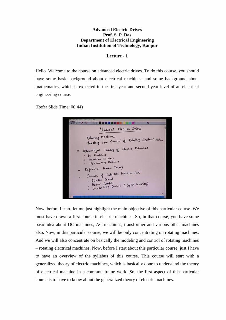
to have an overview of the syllabus of this course. This course will start with a

generalized theory of electric machines, which is basically done to understand the theory

of electrical machine in a common frame work. So, the first aspect of this particular

course is to have to know about the generalized theory of electric machines.

Now, by generalized theory, we mean we have a theory, which can be used to analyze

various types of machines in a common frame work. We know that we have DC

machines, we have AC machines. DC machines – we may have shunt machine, series

DC machine, compound machine. Similarly, in AC machine, we may have induction

machine, synchronous machine, reluctance machine. So, we have so many types of

machines. So, can we understand this machine in a common frame work? Can we

develop a common framework for all these machines.

So, that is done using generalized theory of electric machines. And under this, we will be

discussing about the modeling aspect. This will also help us to model. Modeling aspect is

one of the very important aspects of electrical machine simulation. So, in this case, we

will be talking about the modeling of DC machines. It is the most easiest machine to

model. And then we will be also discussing about the modeling of induction machines –

primarily, the three-phase induction machines and then about the synchronous machines.

Now, remember that, when we want to control the machine, we have to understand the

behavior of the machine. And modeling will help us understand the behavior of the

machine. And we can simulate it in a computer. We can also develop some control

principle based on the machine model. So, the generalized theory will help us develop

the machine model, which can be used for the advance control of electric machines. So,

this is the first part of the course, that is, the generalized theory of electric machines.

Now, after we finish this, we will be talking about the reference frame theory. Now, in

the reference frame theory, we will be talking about the various types of reference frames

we have and which are very useful to understand the control aspect of the electrical

machines. For example, if you talk about electrical motors, we know that, the DC

motors, AC motors are constructionally different. But, if you understand the principle of

torque production in DC motor, it will not be very difficult to understand the principle of

torque production in an AC motor or an induction motor.

But, to analyze an induction motor just like a DC motor, you have to take a very special

reference frame. So, the reference frame will help us analyze the machine prospective of

control. So, this is the second aspect of this particular course – the reference frame

theory. And then this ((Refer Time: 05:43)) the background; but the advanced control of

electrical machines, mainly, the rotating machine. And this course will be primarily be

focused on the control of AC machines, because the DC machine is the scope of the

course, which is a fundamental of electric drive. This is an advanced electric drive. So,

this will be only focusing on the control of AC machines. So, we will be taking the

control of induction machine subsequently.

Control of induction machine – we call this induction machine as IM. So, this is a control

of induction machine. And under this, we start with a scalar control, which is basically

the control of the speed and the torque by controlling the frequency and the voltage. So,

under this, we will have the scalar control, which is the control of mere amplitude and

voltage without any reference to phase angle. So, this is a simple control, which is very

good in steady state; but this has some problem in the transient condition. So, one of the

objectives of controlling AC motors is to have faster dynamic torque and speed response.

Whenever we have a drive, the objective is that, we should have a very fast control; we

should be able to control the torque with a fast dynamic response.

Now, the scalar control will give the response, which is good in steady state condition.

But, under the transient condition, the response may not be desirable; there may be

((Refer Time: 07:28)) response in the transient condition. So, to have good transient

response also, we will go for vector control. The vector control of induction machine or

induction motors especially are controls similar to that of a separately excited fully

compensated DC machine. We know that, in case of DC machine, we have a separate

((Refer Time: 07:52)) and the field axis. We have armature and we have field. So, we

can control the current of the armature and current of the field to have independent

control. And the field and the armature are orthogonal to each other to ensure good

dynamic response. So, we will have something similar in case of induction machine

when you talk about vector control.

And then we will have some advanced control aspect like sensor less control. Now, in

this case, we will be talking about the speed sensor less control. It is seen that, in

industrial drive, having a speed encoded or having a speed sensor is not always good for

the overall robustness of the drive. The robustness reduces whenever you have a speed

sensor. So, can we have a drive without a speed sensor? Can we have a sensor less drive?

It means can we have a drive without a speed encoder. And this will increase the

robustness of the drive. And that is why we will talk about sensor less control. And for

the sensor less control, we have to estimate the speed; we have to observe the speed from

the terminal variables like voltage and current. This we will be taking up in the topic

under control of induction machine.


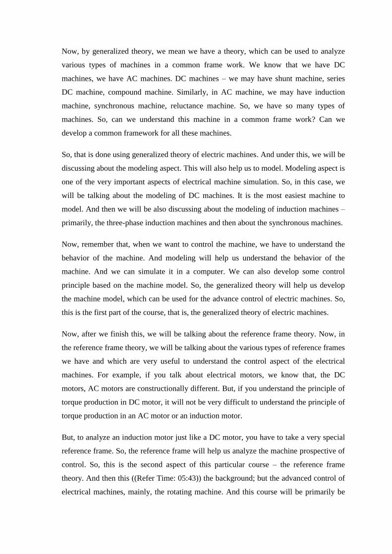
And then we have some advanced control of induction machines like direct torque and

flux control. Now, this actually is an advanced control, which was patented by Asea

Brown Boveri – ABB way back sometimes in early 90s. Now, this way of control aims

are controlling the torque and the flux of an induction machine directly using hysteresis

control. So, the implementation is quite simple; you can have hysteresis control for the

torque and flux; and you can control the torque and flux independently as we do in case

of a DC machine. This actually finishes the control aspect of induction machine.

And then we will be talking about the control aspect of synchronous machine. So, under

this synchronous motor control, we have something similar to that we have already

talked, discussed in induction machine. In synchronous machine, what we have; we can

have a self controlled synchronous motor control. We know that, in a synchronous

machine, the rotor should always run at synchronous speed, which is the speed of the

rotating mmf. Now, in the transient condition, there is always instability; whenever the

load changes or whenever the stator frequency changes, there is the tendency of the rotor

to hunt around the main position. That is called hunting. And hunting is a type of

instability. So, if you suddenly change the torque or if you suddenly increase the supply

of frequency, there is a possibility that, the drive may become unstable.

Now, we are talking about drive; we are talking about electric motor. And in motor, we

have to have continuous speed variation. The speed should start very smoothly from the

rest to the rated value. Even we should have… We can also have reversible speed

operation. Now, under this condition, you know it is not possible to supply the

synchronous motor from a constant frequency source. Now, when the frequency is

variable, the rotor speed is also variable. And the rotor speed decides the stator

frequency; it means the rotor always rotate at synchronous speed, which is variable. And

the synchronous speed is decided by the rotor frequency. This is called self controlled

machine; it means the machine is controlling itself. So, this avoids the instability or

sound in a normal conventional synchronous motor, that is, the self controlled

synchronous motor.

Now, we will have some advanced feature in this. A self controlled synchronous motor

can also be a vector control synchronous motor; where, the control aims are high

transient torque and speed response just like DC machine. So, we will be discussing on

vector control of synchronous motor after we have finish self controlled synchronous

motor. And the synchronous motors are basically used for very limited applications; they

are not very widely used in industry. Majority of the motors used in industry are

induction motors. Induction motors are called the workers of industry.

Now, the synchronous motors are limited to very high power and low speed applications;

sometimes, at a very high power range ranging from a few megawatts to a few tens of

megawatts. For example, synchronous motors can be used in a drive like steel rolling

mill, cement kiln; very low speed, but huge. Cement kiln can be rotating otherwise 15

rpm. And the rating of the cement kiln can be as high as few tens of megawatts; mine

winders; very large drive, but low speed. So, these are basically typical application of

synchronous machine.

Now, when we talk about the synchronous machine control, we will also be talking about

this kind of application. And one of this application is cycloconverter-fed synchronous

motor drive – cycloconvertor-fed synchronous motor drive. Cycloconverters are

naturally commutated; they have SCR thyristors; they are very very robust; there is no

commutation circuit; they are line commutated or naturally commutated. And they can

be rated for megawatt range without any problem. So, when we have a combination of

cycloconverter and synchronous motor, the complete drive can be configured for very

high power and low speed drive, because output of a cycloconvertor is the low frequency

output. And hence, the drive speed is low. The frequency output is low and the speed of

the drive is low.

And then we will be discussing something on control of synchronous reluctance motor.

The synchronous reluctance motors are used for applications, where there is a need of

low rotor weight. The rotor winding here – there is no rotor winding; the rotor is a salient

pole rotor; the rotor inertia is very low. And hence, the rotor can have higher speed

response. The acceleration and the deceleration of the rotor can be very fast. So, when

there is a need of having a low weight drive at high power application, we can go for

synchronous reluctance motor. The stator construction is of course similar to a

conventional synchronous motor. The rotor construction does not have any winding and

the torque is only produced based on the saliency of the motor. And hence, is called

synchronous reluctance motor.

And then we will be discussing something on very special drive – control aspect of very

special drives like permanent magnet synchronous motor. We just used for automobile

application for electric vehicles. This has got very high torque to weight ratio, because

the rotor is a permanent magnet; does not have any winding there. We can have very

high energy density. We have a special type of drive used for low to medium power

application. They are known as brushless DC motors. They are also synchronous motors.

This brushless DC motors – we call them BLDC – brushless DC motor – BLDCM.

And, they are used for low power application and as well as medium power application.

For example, if you talk about any computer drives, computer disk drives; they should

not be having brushes. One of the drawbacks of DC motor is that, there is commutator

and brushes. And its mechanical contact – it is a fixed contact, which creates the problem

very often. It cannot be operated in an environment full of dust. So, the DC motors are

not very robust. But, the brushless DC motors – they are just like a synchronous motor;

we have permanent magnet on the rotor. And there is close look feedback; and the motor

behavior is just like a DC motor. Since we do not have any brush on commutators here,

these drives are known as brushless DC motor drive, which are used for low power

application like computer peripherals, computer power supply as well as medium power

applications in some vehicles, automobiles, electric vehicles and so on.

We also have another special type of motor called switched reluctance motor. This is

abbreviated as SRM. The switched reluctance motor is supposed to be good motor; is

something like a competitor of induction motor. In this case, the rotor and the stator –

both the structures have saliency. The rotor is a salient structure having no windings, just

having slots and teeth. The stator is also a salient structure having slots and teeth. And

the stator has got concentric winding as opposed to distributed winding in case of normal

induction motor or synchronous motor. But, in this case, the stator current has been

switched in conjunction with rotor position, so that the torque is maximized. And since

the rotor currents are switched using a convertor, these type of motors are called

switched reluctance motor.

They are used for those applications, where there is a need of low weight, because the

rotor does not carry any winding; it is very very robust. And the robustness is

comparable to that of induction motor. And the torque is also sometimes comparable to

that of induction motor. So, these motors in a limited way could be a competitor to

induction motor in few applications. But, the drawback of this type of motor is higher

torque repels. So, we will be discussing about this motor at the end. So, this is actually

roughly about the syllabus of the course on advanced electric drives. Now, before we go

to the various aspects of the drive system, let us talk about the generalized theory of

rotating machine. What you understand by generalized theory of rotating machine?


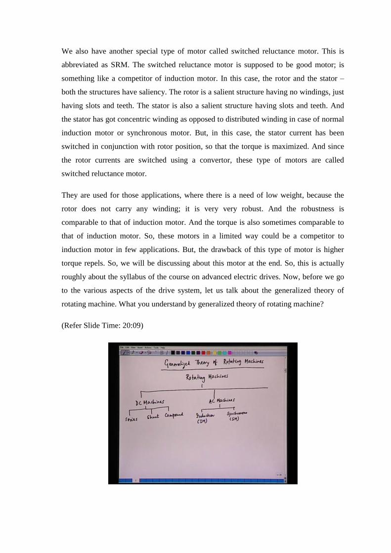
So, what we are trying to do is that, we have so many types of machines; and we are

trying to bring all these machines into a common framework. So, what are the types of

machines? Now, we have the rotating machines. And these are the types of machines we

have. We have DC machines. And what are the types of DC machines we have? We

have… This is series machine and then we have DC shunt machines, which also have

their own applications. And then we have compound machines, where both the series and

shunt windings are present. So, this series, shunt and compound machines have their own

applications. So, these are three types of DC machines we have. And then we have AC

machines. And under the AC machines, we have primarily very popularly used two types

of machines. One is an induction machine; we call this to be IM. And then we have

synchronous machine – SM.


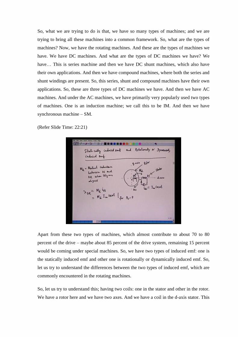
Apart from these two types of machines, which almost contribute to about 70 to 80

percent of the drive – maybe about 85 percent of the drive system, remaining 15 percent

would be coming under special machines. So, we have two types of induced emf: one is

the statically induced emf and other one is rotationally or dynamically induced emf. So,

let us try to understand the differences between the two types of induced emf, which are

commonly encountered in the rotating machines.

So, let us try to understand this; having two coils: one in the stator and other in the rotor.

We have a rotor here and we have two axes. And we have a coil in the d-axis stator. This

we call as capital DS. And we have a coil in the d-axis rotor. This we call as capital DR.

And these two coils are magnetically coupled. Naturally, when the two coils are aligned,

there is a maximum coupling. So, these two coils are maximally coupled. And we can

have a dot convention. So, this is the dot here and this is also the dot here. So, this

terminal is corresponding to this terminal of the stator. And what we do here; this is the

d-axis and this is q-axis. d stands for the direct axis; q stands for the quadrature axis.

And, we define an inductance called M d. M d is the mutual inductance between DS

winding and DR winding when they are aligned. When the two windings are aligned, let

us say that, the mutual inductance is M d. So, this inductance between these two – this

capital M subscript d. Now, what we do here is that, in the d-axis stator, we inject a

current; and this current is a time ((Refer Time: 24:42)) current. So, maybe we have

current source here; we can have the current source in this case. And this current is

injected into the d-axis stator; and the current is i d s. And what is the nature of this

current? This current is given as I m cos omega t. So, it is a time varying current; it is a

function of time; and it is given as I m cos omega t. This structure is a rotor. This is free

to rotate. And this one is in the stator.

And, when this is having this current I m cos omega t, what about the flux linkage? We

are finding out the flux linkage lambda D R. The flux linkage with d-axis rotor, that is,

winding D R; that is equal to… The rotor is not carrying any current; rotor is open

circuited. So, we are finding out the flux linkage in the rotor due to the d-axis stator

current. And this flux linkage is given as M d. M d is the mutual inductance between the

rotor and the stator when they are aligned. And the current in the stator is i d s. So, M d

into i d s. And that is equal to… What is i d s? i d s is I m cos omega t. So, we can say

that, M d into I m cos omega t is the flux linkage with the d-axis rotor because of the

current in the d-axis stator.

So, now, what happens here is that, we give the rotor a motion. The rotor is rotated now;

it is not stationary; it is free to rotate. And it rotates at a speed of omega r. So, when the

rotor rotates, the flux linkage will change; the flux linkage lambda D R is the flux

linkage when they are aligned. So, we can say that, this is for theta r equal to 0; theta r is

the rotor angle. The angle between the rotor and the d-axis stator is theta r. Now, when it

is rotated, what happens? This is given a motion. So, if this is given a motion and the

speed is equal to omega r; what happens?


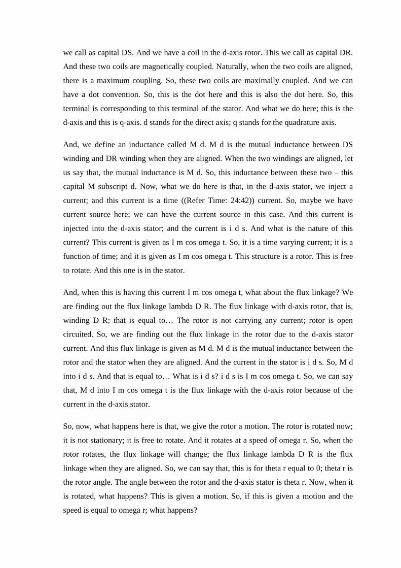
Let me draw another picture here. This is the rotor. This is centre of the rotor. And then

we have the d-axis stator; it is excited with a current source. And this current – this is the

DS winding; and i d s is given as I m cos omega t. So, this is the d-axis and this is the q-

axis. And the rotor is now rotating. After sometime, this is rotating in the clockwise

direction – omega r; speed is omega r here. The winding which was aligned with the

stator at t equal to 0 has now moved to different position. Now, if I see the new position

of the rotor winding, the position will be somewhere here. So, this is DR; this is the

winding that is DR. Now, the DR axis is this. Now, this angle – angle between the d-axis

stator and the rotor winding is now is known as theta r.

Now, if we want to find out the flux linkage in the d-axis rotor or DR winding rotor due

to the stator winding current, which is i d s; that is equal to I m sin omega t; we can we

can write down the flux linkage as follows. The flux linkage in the winding DR due to

the stator current is given as M d i d s. Now, the rotor has moved to on angle that is theta

r into cos of theta. So, this is the flux linkage with the winding that is DR. And the DR

winding is now rotating at a speed of omega r. Now, if I want to find out the induced emf

in the rotor; suppose I have voltmeter here; I can connect a voltmeter here; and I can

measure the induced emf by having a voltmeter. So, if I have a voltmeter to find out the

induced emf, the induced emf – e D R – as per the Faraday’s law, this will be given as

minus d by d t of lambda D R. The rate of change of flux linkage and the negative side is

due to the Lenz's law.

Now, I have to differentiate this lambda D R to find out the total induced emf. Now,

what is lambda D R? Lambda D R is given as M d I m cos omega t into cos of theta r.

So, this is also a function of time. Lambda D R is also a function of time; it is also a

function of position. And the position is also constantly changing; theta r – the rotor

angle; this angle is not constant; it is constantly changing.

So, if I differentiate this with respect to time, what I have here is the following that, this

will be a differentiation by parts. So, minus of M d i d s d by d t of cos theta r – I will

first differentiate the cos theta r and then I will differentiate M d cos theta r d by d t of i d

s. So, this is the induced emf. Now, if I differentiate cos theta r, it will be minus of sin

theta r into d theta r by d t. And if I differentiates i d s with respect to time, i d s is I m

cos omega t; it will I m sin omega t with a negative sign into omega. So, let me just try to

write down the result of this. So, if I differentiate this and simplify, what I will have is

the following. I will have M d I m omega r cos omega t into sin theta r plus M d I m

omega cos theta r into sin omega t. So, this is the expression for the induced emf.

Now, I can express again sin theta r in terms of cos theta r; sin omega t in terms of cos

omega t. So, if I do that, I will have the final expression M d I m omega r cos omega t

into sin theta r is cos theta r minus pi by 2. I can replace this sin theta r by cos theta r

minus pi by 2. Similarly, I can also replace sin theta r by cos omega t minus pi by 2. So, I

can just write down here – M d I m omega cos theta r into cos omega t minus pi by 2. So,

this is a very interesting equation. It is an interesting expression in the sense that, the

induced emf, which we know that, it is equal to minus d lambda by dt has got two

different terms. The first term; you can see that, this is actually a function of speed. So,

this is a function of speed. This speed is equal to 0; this term will be equal to 0. So, we

would like to call this as the rotationally induced emf or e DR – Rot. It is called the

rotationally induced emf or dynamically induced emf. This is basically coming up due to

the motion. So, this is called the rotationally induced emf. And the second term, which is

given here, is called the statically induced emf or e D R – stat.

Now, if you see, this is interesting to note that, the rotationally induced emf is the

function of omega r. It means if the speed is equal to 0, the rotationally induced emf will

be equal to 0. So, that emf is coming because of the rotation. The statically induced emf

is a function of the frequency. Omega here – if you see this omega; omega is the

electrical frequency of the current. If the frequency of the applied current is equal to 0,

this component will be equal to 0. So, this is the statically induced emf because this is

induced because of the coupling between the rotor and the stator.

Furthermore, you will see that, there is another interesting feature between the two emfs.

You can see that, the rotationally induced emf is in the same time phase, because the

time phase angle is cos omega t. Omega t is the phase angle here. Cos omega t is the

phase angle at the phase of the time. So, you can see here the rotationally induced emf is

in the same time phase. It is also cos omega t; this is also function of time and it is cos

omega t. So, it is in the same time phase, but it is pi by 2 lagging behind the space phase.

It is cos theta r minus pi by 2.

And, the statically induced emf is in the same space phase, because this is cos theta r;

theta r is this angle. So, this will be maximum when these two windings are aligned. So,

whenever theta r is equal to 0, it means this winding is aligned along this; you have

maximum statically induced emf; the coupling will be maximum; the induced emf will

be maximum. And if theta r is pi by 2; when this winding is along the q-axis, the

statically induced emf will be 0. So, the statically induced emf will be in the same space

phase, but pi by 2 lagging in the time phase. You can see here also, we have expression

of time; it is cos of omega t minus pi by 2.


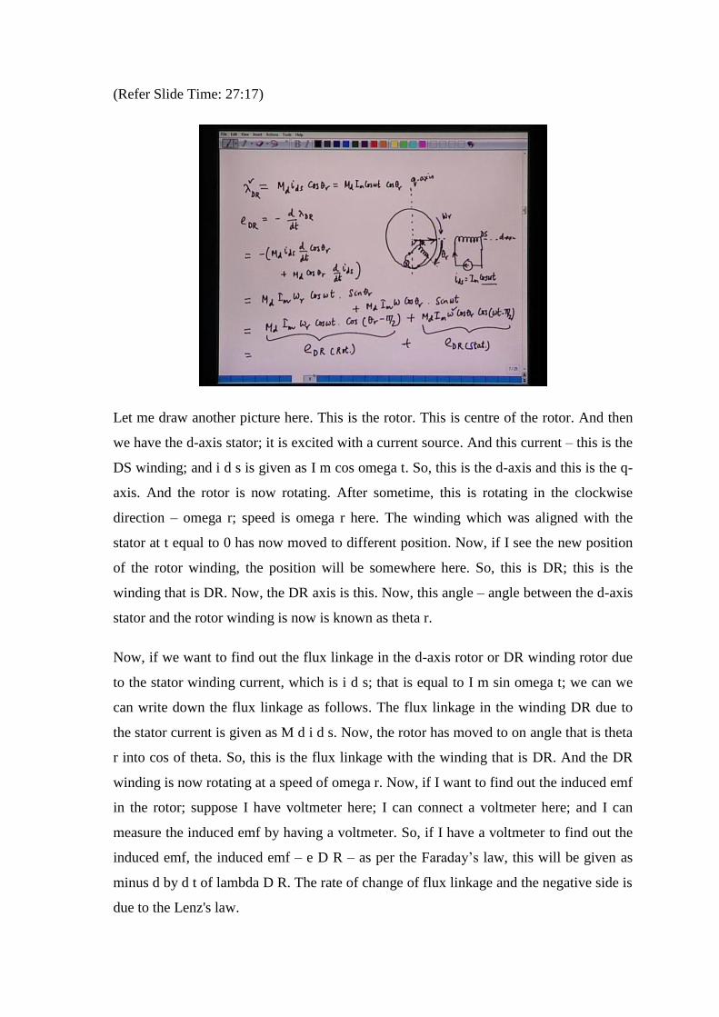
So, I summarize here that, if you talk about the statically induced emf, this is in the same

space phase; it means the statically induced emf will be maximum whenever two coils

are aligned along each other. Axis of the two coils are aligned; then only we will have

maximum coupling; then only we will have maximum statically induced emf. So, if I

have a winding here; if the other winding is also having the same axis, I have the

maximum coupling; and hence, I have maximum statically induced emf. This is in the

same space phase, but pi by 2 lagging in time phase. Although the second coil here will

have the same space phase with respect to this; if I connect a voltmeter here and measure

the induced emf here because of the current variation in the first coil and that is I m cos

omega t, this induced emf will be lagging behind this flux by pi by 2. Whenever I have a

current, I will have a flux production. And this induced emf will be lagging behind the

flux in time by pi by 2. So, this is an important aspect of statically induced emf.

Now, if we talk about the dynamically induced emf of rotationally induced emf –

dynamically or rotationally induced emf; now, this will be maximum when the two coils

are in quadrature. It means if I have one coil here and this coil is being excited by a

current; and if I have other coil and the two axes are orthogonal to each other; this axis is

here and this axis is right angle to this axis; then I will have maximum rotationally

induced emf. Here the coupling is 0, but the rate of change of flux linkage is maximum

due to rotation.

So, we can say that, in the same time phase, if I have – this is I m cos omega t; this

induced emf with the rotationally induced emf; the component of that induced emf,

which is called rotationally induced emf; that means, in the same time phase as cos

omega t, but it will be shifted in space by pi by 2; but pi by 2 lagging in space phase.

This is a very important conclusion. It means a coil which is right angle to the other coil

will have maximum rotationally induced emf.

And, that is the reason why in case of the DC machine, we have seen that, the brush axis

is orthogonal to the field axis; they are not in the same axis; the brush axis and the field

axis are orthogonal. If you align the brush axis with the field axis, the rotationally

induced emf will be equal to 0, because in a DC machine, we have only rotationally

induced emf. The field winding is not having any alternating current. So, in a DC

machine, if you have seen that, we have a DC machine structure, we have the brush here

and we have the field winding here. This is the field winding.

And, this is the armature. And whenever I have perpendicular relationship between the

two coils, I may have hypothetical coils here, because the brushes are in the q-axis. So,

this axis is orthogonal to this axis and the brush will have the maximum rotationally

induced emf. That is the induced emf in case of DC machine. And that is the reason why

in case of DC machine, the brush axis and the field axis are orthogonal to each other.

Now, after having said this, we are now talking about the generalized theory of electric

machine. And we know that, we have two different types of induced emf: one is the

statically induced emf and the other one is the rotationally induced emf or dynamically

induced emf.


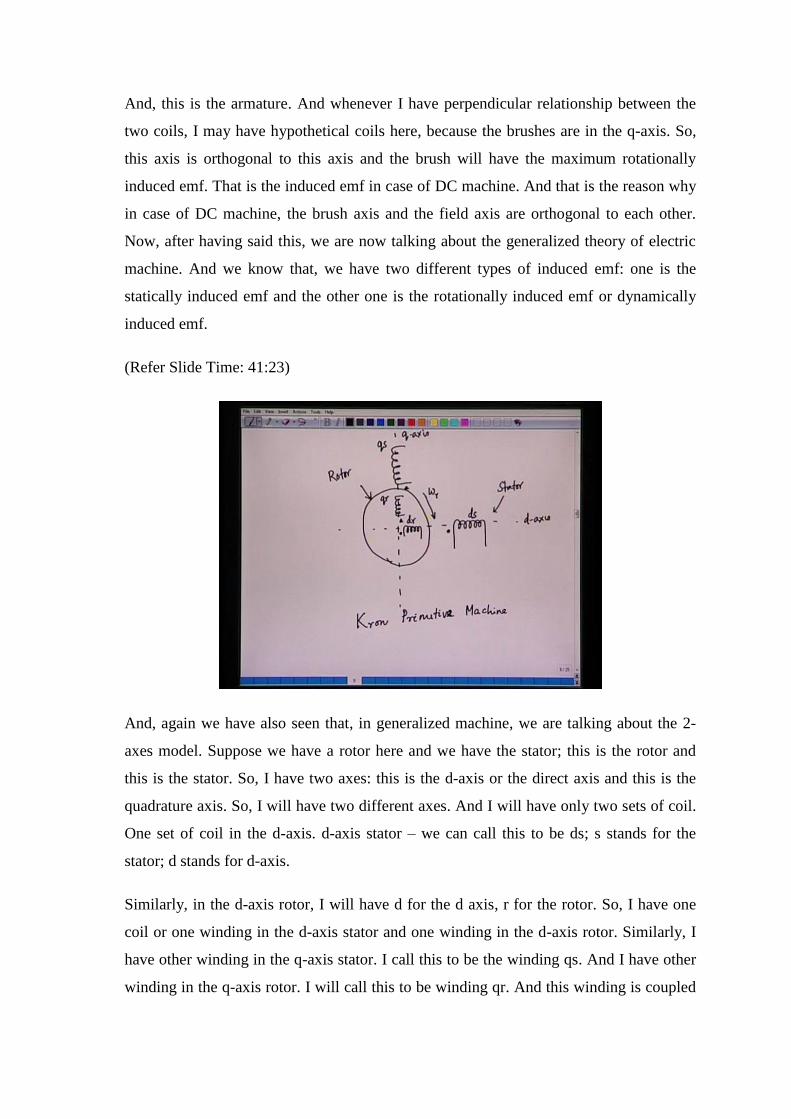
And, again we have also seen that, in generalized machine, we are talking about the 2-

axes model. Suppose we have a rotor here and we have the stator; this is the rotor and

this is the stator. So, I have two axes: this is the d-axis or the direct axis and this is the

quadrature axis. So, I will have two different axes. And I will have only two sets of coil.

One set of coil in the d-axis. d-axis stator – we can call this to be ds; s stands for the

stator; d stands for d-axis.

Similarly, in the d-axis rotor, I will have d for the d axis, r for the rotor. So, I have one

coil or one winding in the d-axis stator and one winding in the d-axis rotor. Similarly, I

have other winding in the q-axis stator. I call this to be the winding qs. And I have other

winding in the q-axis rotor. I will call this to be winding qr. And this winding is coupled

with this winding. So, I will show it by dot convention. This winding is coupled with this

winding. And similarly, in the q-axis also, this winding is coupled with this winding. So,

this thing – the q-axis is coupled with q-axis and the d-axis is coupled with d-axis. And

then the rotor is rotating in the clockwise direction. This is the direction of rotation. And

the speed is omega r.

Now, this is generalized machine that we are talking about. And this was given – the

concept was given by scientist called Kron; and this is called the Kron primitive

machine. So, I have two axes; I have one stator, one rotor in the d-axis; one stator and

one rotor in the q-axis. And the d-axis is coupled with d-axis. And this d-axis is

stationary; it is fixed; q-axis is also fixed. The q-axis stator is coupled with the q-axis

rotor and it is rotating in the clockwise direction. We will be discussing the remaining

part in the next lecture.