Le rotateur frappé: Rapport avec la localisation d’Anderson et réalisation

expérimentale

Équipe Chaos Quantique

1

Groupe de travail NLSE-CEMPI

10/9/2012

Matthias Lopez Benoît Vermersch Radu Chicireanu J.F. Clément Véronique Zehnlé Pascal Szriftgiser JCG

Dominique Delande Nicolas Cherroet

Gabriel Lemarié

PhLAM LKB LPT

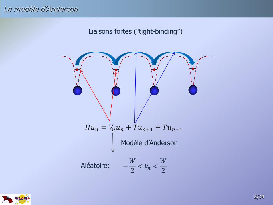
Le modèle d’Anderson

2 /34

𝐻𝑢𝑛 = 𝑉𝑛𝑢𝑛 + 𝑇𝑢𝑛+1 + 𝑇𝑢𝑛−1

Liaisons fortes (“tight-binding”)

Aléatoire: −𝑊

2< 𝑉𝑛 <

𝑊

2

Modèle d’Anderson

Quantum dynamics in (perfect) lattices

3

-2

-1

0

1

2

0

5

10

15

20

25

300

5

10

15

20

25

30

Perfect crystal: Delocalized Bloch waves → diffusive dynamics

Conducteur

/34

Ordered crystal

Cliquer sur la figure pour voir l’animation

Quantum dynamics in disordered lattices

4

Disordered crystal

Insulator

-2

-1

0

1

2

3

0

5

10

15

20

25

300

5

10

15

20

25

30

/34

Disordered crystal: Localized states (3D: mobility edge)

Cliquer sur la figure pour voir l’animation

Simple picture of Anderson dynamics

5 /34

∆𝐸

𝑡~ℏ/∆𝐸

~ℏ/𝑊

ℏ/𝑇=

𝑇

𝑊 Nombre de sites visités ~

𝑇

𝑊≪ 1 Localisation

𝑇

𝑊≫ 1 Diffusion

Temps de tunneling

Temps de séjour

Impact of the Anderson model

6 /34

5300 citations

Increase of computer power

« End of citing life »

Cold-atom experiments

One-parameter scaling

Impact of the Anderson model

7 /34

S. Redner arXiv:physics/0407137

Consequences and limitations

8

• 1D : Exponential localization of the eigenfunctions 𝜓~exp 𝑥 − 𝑥0 /ℓ • Suppression of the diffusion → Insulator

• 3D → « Mobility edge » → Metal-insulator transition

• “One-particle” model → No particle interactions

• Zero-temperature

• Oversimplified description of a crystal lattice

Limitations of the Anderson model

/34

Consequences of the Anderson model

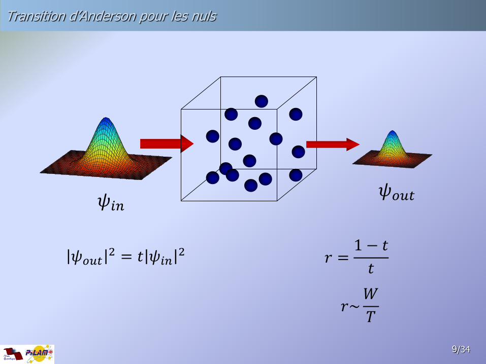
Transition d’Anderson pour les nuls

9 /34 9

𝜓𝑜𝑢𝑡2 = 𝑡 𝜓𝑖𝑛

2 𝑟 =1 − 𝑡

𝑡

𝜓𝑖𝑛 𝜓𝑜𝑢𝑡

𝑟~𝑊

𝑇

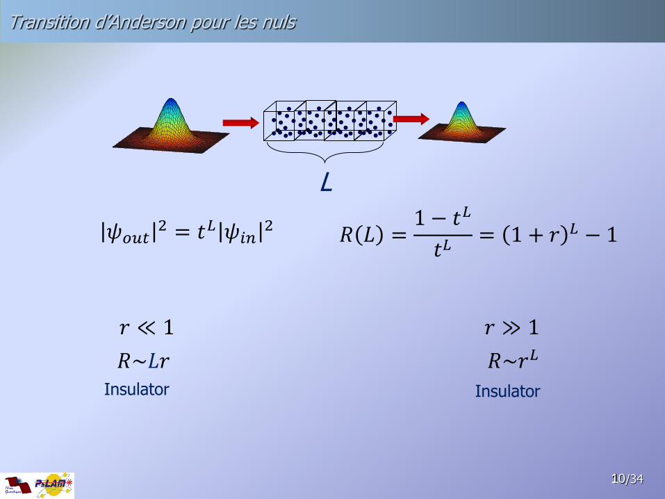
Transition d’Anderson pour les nuls

10 /34 10

L

𝑅~𝐿𝑟

𝜓𝑜𝑢𝑡2 = 𝑡𝐿 𝜓𝑖𝑛

2 𝑅 𝐿 =1 − 𝑡𝐿

𝑡𝐿= 1 + 𝑟 𝐿 − 1

𝑟 ≪ 1

𝑅~𝑟𝐿

𝑟 ≫ 1

Insulator Insulator

La transition d’Anderson pour les nuls

11 /34

L

L

L

𝑅~𝐿𝑟

𝑟 ≪ 1

Conductor

/𝐿2 ~𝐿−1 𝑅~𝑟𝐿

𝑟 ≫ 1

Insulator

/𝐿2 𝑟 = 𝑟𝑐

𝑅~𝐿𝛼

𝛼 =𝑑 ln𝑅

𝑑 ln 𝐿

𝛼 < 0 𝛼 > 0

La transition d’Anderson pour les nuls

12 /34

2D

4D

5D

rln

Ld

Rd

ln

ln

Insu

lato

r Conduct

or

1D

3D

𝑅 = 𝐿𝑟

𝑅 = 𝐿𝑟/𝐿

𝑅 = 𝐿𝑟/𝐿2

𝑅 = 𝐿𝑟/𝐿3

𝑅 = 𝐿𝑟/𝐿4

Experiments in condensed-matter and ultracold atoms

13

Condensed matter

• Decoherence (ill-defined quantum phases)

• No access to the wave function

• Electron-electron coulombian interactions

/34

Ultracold atoms

• Control of decoherence

• Access to probability distributions (and even the full wavefunction)

• Control of interactions (Feschbach resonance)

Experiments with ultracold atoms

14

“3D”: S. S. Kondov et al., Three-Dimensional Anderson Localization of Ultracold Fermionic Matter, Science 334, 66 (2011)

1D: J. Billy et al., Direct observation of Anderson localization of matter-waves in a controlled disorder, Nature 453, 891 (2008)

“3D” : F. Jendrzejewski et al., Three-dimensional localization of ultracold atoms in an optical disordered potential, Nature Physics 8, 398 (2012)

/34

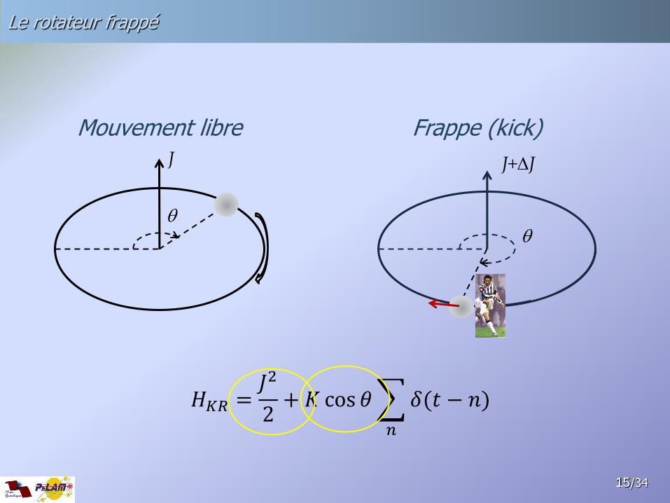
Le rotateur frappé

15 /34 15

Mouvement libre

J

q q

J+DJ

Frappe (kick)

𝐻𝐾𝑅 =𝐽2

2+ 𝐾 cos 𝜃 𝛿(𝑡 − 𝑛)

𝑛

Le rotateur frappé “déplié”

16 /34 16

Mouvement libre

p

Frappe (kick)

𝐻𝐾𝑅 =𝑝2

2+ 𝐾 cos 𝑥 𝛿(𝑡 − 𝑛)

𝑛

p+Dp

Comment faire cela avec des atomes froids?

17 /34 17 17

“Potentiel optique” 𝑉~𝐼(𝑥)

Δ→ 𝐼0 cos 2𝑘𝑥

𝑝𝑎𝑓𝑡𝑒𝑟 = 𝑝𝑏𝑒𝑓𝑜𝑟𝑒 + 2ℏ𝑘

Cliquer sur la figure pour voir l’animation

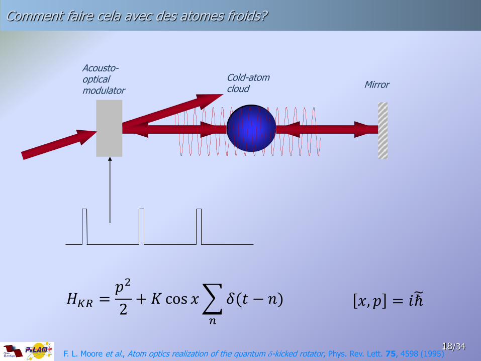
Comment faire cela avec des atomes froids?

18 /34 18 18

Acousto-optical modulator

Cold-atom cloud Mirror

𝐻𝐾𝑅 =𝑝2

2+ 𝐾 cos 𝑥 𝛿(𝑡 − 𝑛)

𝑛

𝑥, 𝑝 = 𝑖ℏ

F. L. Moore et al., Atom optics realization of the quantum d-kicked rotator, Phys. Rev. Lett. 75, 4598 (1995)

Problème

19 /34 19 19

Limite la durée de la manip à quelques ms

Solution

20 /34 20 20

Ce n’est pas un rotateur frappé (kicked accelerator)

𝜔

𝜔 − 𝛼𝑡

𝑒−𝑖(𝑘𝑧−𝜔𝑡) + 𝑒−𝑖(−𝑘𝑧−𝜔𝑡+𝛼𝑡2)

2

1 + cos 2𝑘𝑧 − 𝛼𝑡2

𝑧𝑛 =𝑛𝜋 + 𝛼𝑡2

2𝑘

g′ =𝛼𝑡2

2𝑘

−𝑣

Mesurer la vitesse des atomes

21 /34 21 21

𝑣

Mesure directe de la “norme de Sobolev 2,1”

Le rotateur frappé “simule” le modèle d’Anderson 1D

22 /34 22 S. Fishman et al., Chaos, quantum recurrences, and Anderson localization, PRL 49, 509 (1982)

22

Anderson Kicked rotor

nax

Time periodicity: Floquet analysis

𝑉𝑛𝑢𝑛 + 𝑇𝑟𝑟

𝑢𝑛+𝑟 = 𝐸𝑢𝑛

𝑈 𝑇 = 1 = exp −𝑖𝐾 sin 𝑥

ℏ exp −

𝑖𝑛 2

2ℏ 𝑣(𝜑) = exp −𝑖𝜑 𝑣(𝜑)

𝑣(𝜑) = 𝑣𝑛𝑛

exp −𝑖𝑛𝑥

𝑉𝑛 = tan𝜑 − 𝑛2ℏ /2

2 tan

𝐾 cos 𝑥

2ℏ = 𝑇𝑟

𝑟

exp −𝑖𝑟𝑥

𝑝0 → 𝑝0 + 𝑛 2ℏ𝑘

𝑝 = 𝑛 2ℏ𝑘

Le rotateur frappé “simule” le modèle d’Anderson 1D

23 /34 23 S. Fishman et al., Chaos, quantum recurrences, and Anderson localization, PRL 49, 509 (1982)

23

• Each Floquet state is a realization of the fixed disorder ~ W = cte

“Pseudo” disorder

𝑉𝑛 = tan𝜑 − 𝑛2ℏ /2

2

Random Eq. (1)

Comment simuler le modèle d’Anderson 3D ?

24 /34 24 24

g

Rotateur frappé quasi-périodique

25 /34 25 G. Casati et al., Anderson transition in a one-dimensional system with three incommensurate frequencies, PRL 62, 345 (1989)

25

𝐻3𝐹 =𝑝2

2+ 𝐾 cos 𝑥 1 + 휀 cos 𝜔2𝑡 cos 𝜔3𝑡 𝛿(𝑡 − 𝑛)

𝑛

𝜔2, 𝜔3 irrational

H3F NOT periodic: NO Floquet states

NO Fishman-Grempel-Prangue equivalence

Rotateur frappé quasi-périodique

26 /34 26 26

Good news: H3D is periodic in time : Floquet analysis

Apply Fishman-Grempel-Prangue trick all over again

𝑇𝒏𝑢𝒏 + 𝑉𝒓𝒓

𝑢𝒏+𝒓 = 𝐸𝑢𝒏 𝒏 = 𝑛, 𝑛2, 𝑛3

H3D is equivalent to a 3D Anderson model

𝑇𝒏 = tan𝜑 −

𝑛2ℏ

2− 𝑛2𝜔2 − 𝑛3𝜔3

2ℏ

tan𝐾 cos 𝑥 1 + 𝜖 cos 𝑥2 cos 𝑥3

2ℏ = 𝑉𝒓

𝒓

exp −𝑖𝒓 ⋅ 𝐱

𝐻3𝐷 =𝑝2

2+ 𝜔2𝑝2 + 𝜔3𝑝3 + 𝐾 cos 𝑥 1 + 휀 cos 𝑥2 cos 𝑥3 𝛿(𝑡 − 𝑛)

𝑛

H3D et H3F sont-ils équivalents ?

27 /34 27 27

Ψ 𝑥, 𝑥2, 𝑥3; 0 = 𝜓(𝑥, 0)𝛿(𝑥2)𝛿(𝑥3)

Ψ 𝑥, 𝑥2, 𝑥3; 𝑡 = 𝑈3𝐷(𝑡)Ψ 𝑥, 𝑥2, 𝑥3; 0

≡ 𝑈3𝐹 (𝑡)𝜓(𝑥, 0)

The “underlying unit of nature”: different systems described by the same equations Feynman Lectures in Physics, vol.2 ch. 12

La transition d’Anderson (enfin!)

28 /34 28 28

Localized

Critical

Diffusive

e

K 4 9 0.1

0.8 Metal

Insulator

𝐻3𝐹 =𝑝2

2+ 𝐾 cos 𝑥 1 + 휀 cos 𝜔2𝑡 cos 𝜔3𝑡 𝛿(𝑡 − 𝑛)

𝑛

Caractérisée

29 /34 29 29 29

Caractérisée

30 /34 30 30 30

Fonction d’onde critique

31 /34 31 31 31 31

Fonction d’onde critique

32 /34 32 32 32 32

Universalité

33 /34 33 33 33 33

La suite…

34 /34 34 34 34 34

Utiliser un condensat de Bose-Einstein

Atomes individuels Onde de matière collective

𝑖𝜕𝜓

𝜕𝑡= −

∆𝜓

2+ 𝑉𝜓 𝑖

𝜕𝜓

𝜕𝑡= −

∆𝜓

2+ 𝑉𝜓 + 𝑔 𝜓 2𝜓

Mécanique quantique non linéaire !

𝐻𝑢𝑛 = 𝑉𝑛𝑢𝑛 + 𝑇𝑢𝑛+1 + 𝑇 + 𝑔 𝑢𝑛2𝑢𝑛