large-scale image collections
TRANSCRIPT
Yimeng Zhang and Henry Shu
10/6/11
Large-Scale Image Collections
Adapted Slides from Feifei’s and Rob’s slides
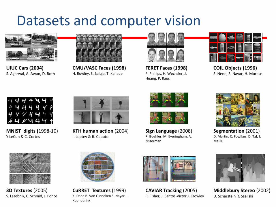
Datasets and computer vision
UIUC Cars (2004)S. Agarwal, A. Awan, D. Roth
3D Textures (2005)S. Lazebnik, C. Schmid, J. Ponce
CuRRET Textures (1999)K. Dana B. Van Ginneken S. Nayar J. Koenderink
CAVIAR Tracking (2005)R. Fisher, J. Santos-Victor J. Crowley
FERET Faces (1998)P. Phillips, H. Wechsler, J. Huang, P. Raus
CMU/VASC Faces (1998)H. Rowley, S. Baluja, T. Kanade
MNIST digits (1998-10)Y LeCun & C. Cortes
KTH human action (2004)I. Leptev & B. Caputo
Sign Language (2008)P. Buehler, M. Everingham, A. Zisserman
Segmentation (2001)D. Martin, C. Fowlkes, D. Tal, J. Malik.
Middlebury Stereo (2002)D. Scharstein R. Szeliski
COIL Objects (1996)S. Nene, S. Nayar, H. Murase

1 2 3 4 5
1
2
3
4
Caltech101/256MRSC
PASCAL1 LabelMe
Tiny Images2
# of visual concept categories (log_10)
# o
f cl
ean
imag
es p
er c
ateg
ory
(lo
g_1
0)
1. Excluding the Caltech101 datasets from PASCAL2. No image in this dataset is human annotated. The # of clean images per category is a rough estimation
Datasets
12 million
80 million
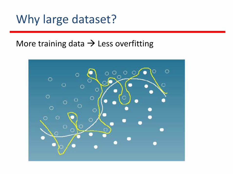
Why large dataset?
More training data Less overfitting
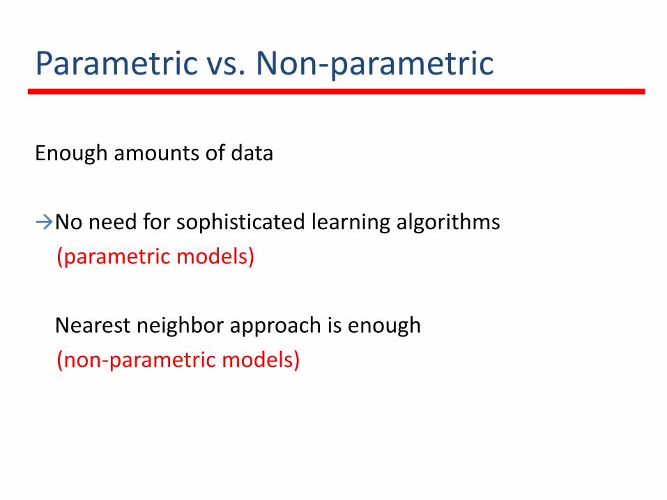
Enough amounts of data
No need for sophisticated learning algorithms
(parametric models)
Nearest neighbor approach is enough
(non-parametric models)
Parametric vs. Non-parametric
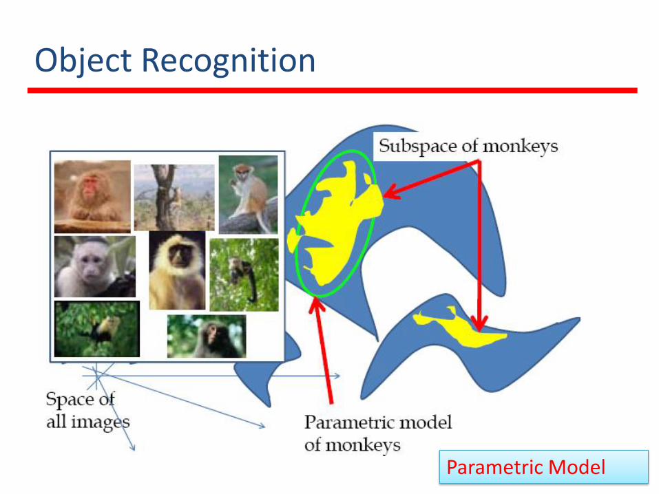
Object Recognition
Parametric Model
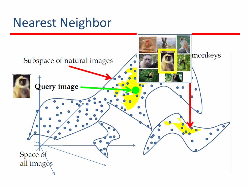
Nearest Neighbor
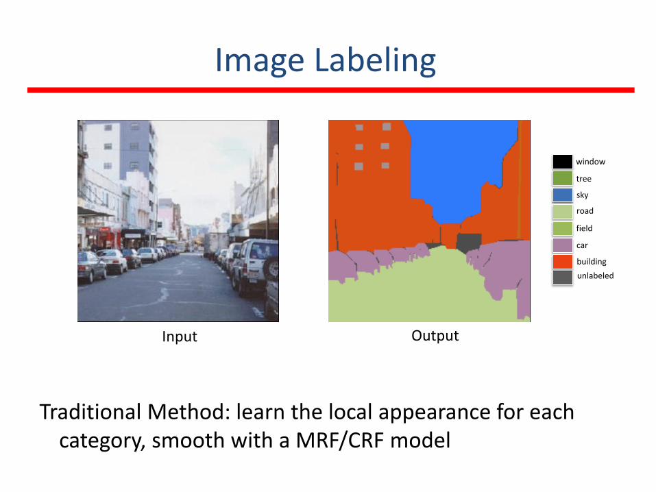
Image Labeling
Traditional Method: learn the local appearance for each category, smooth with a MRF/CRF model
tree
sky
road
field
car
unlabeled
building
window
Input Output
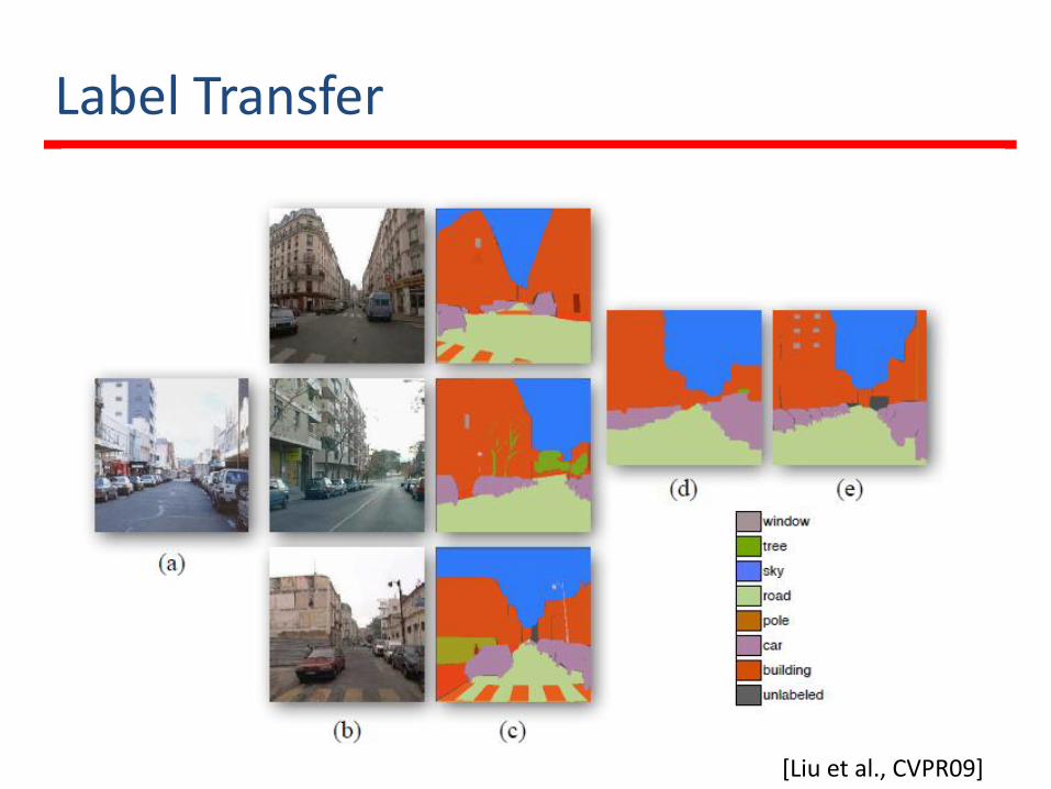
Label Transfer
[Liu et al., CVPR09]
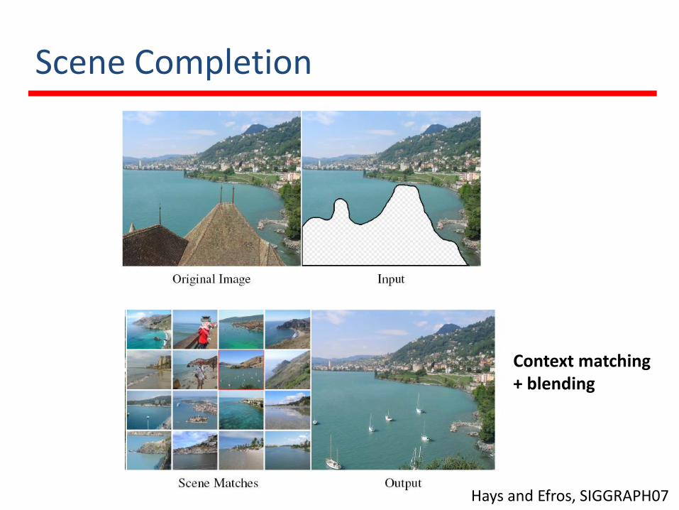
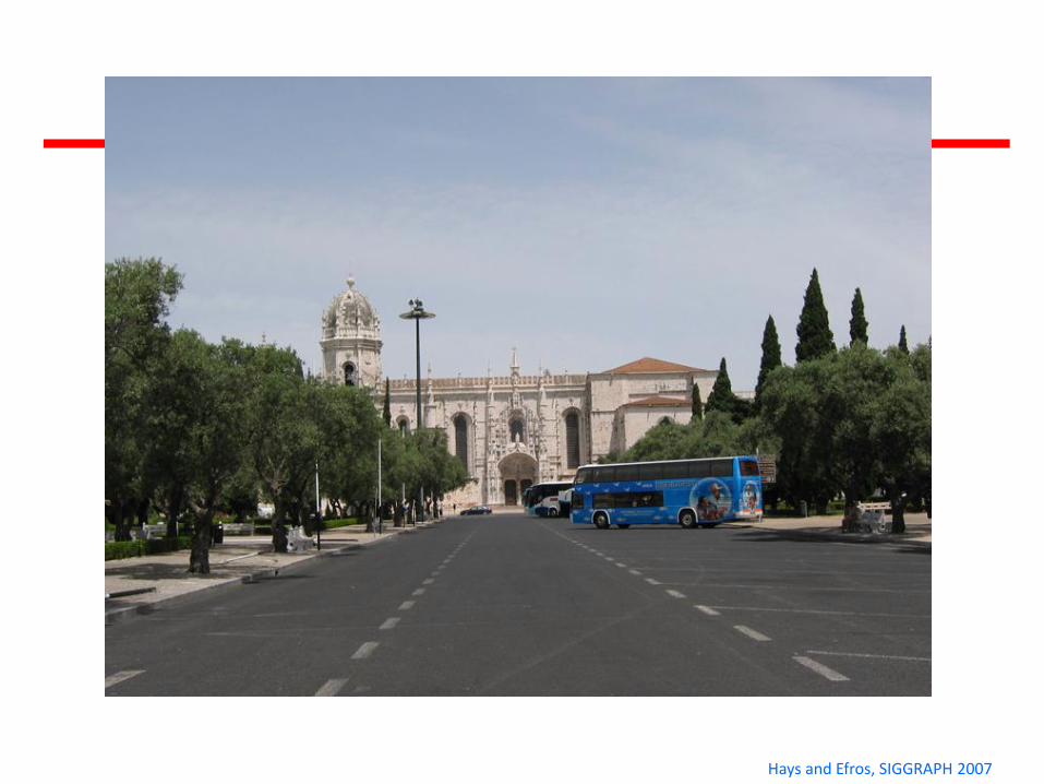
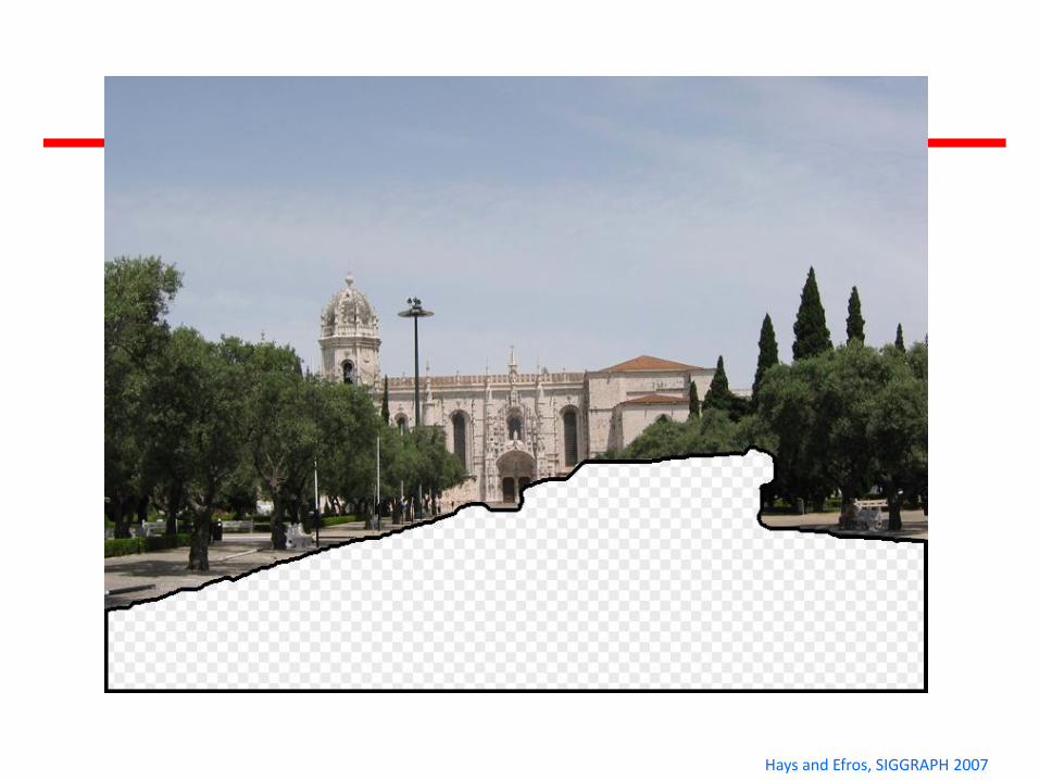
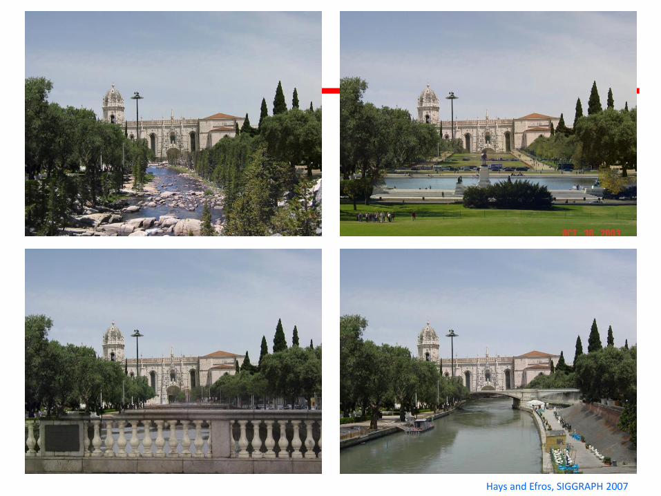
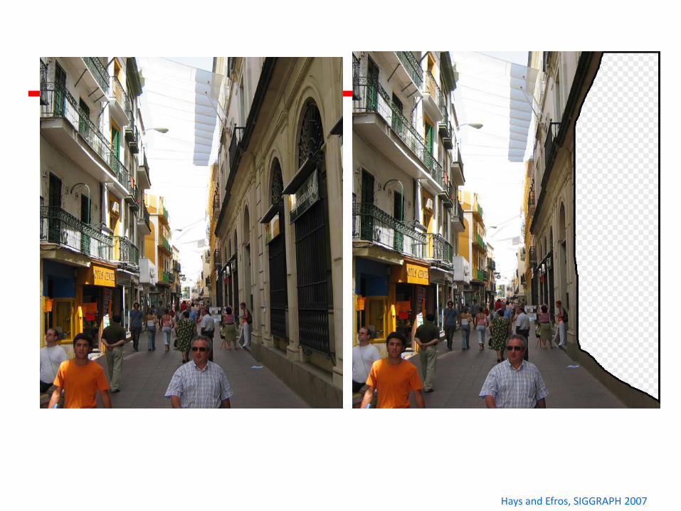
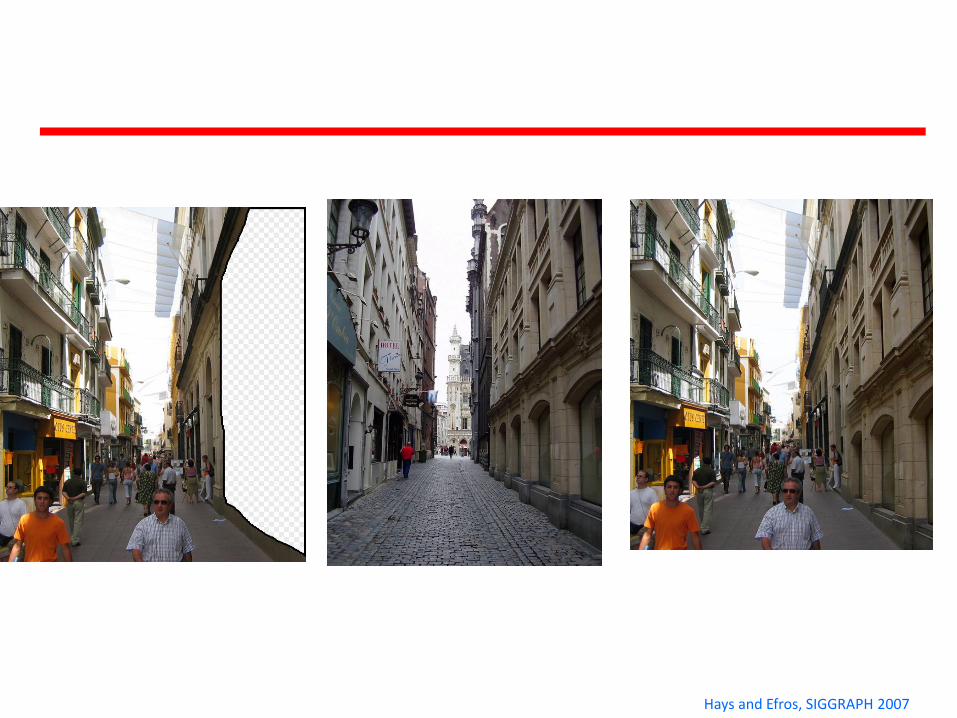
Scene Completion
Hays and Efros, SIGGRAPH07
Context matching+ blending
Hays and Efros, SIGGRAPH 2007
Hays and Efros, SIGGRAPH 2007
Hays and Efros, SIGGRAPH 2007
Hays and Efros, SIGGRAPH 2007
Hays and Efros, SIGGRAPH 2007
Image Representation
80 million tiny images: a large dataset for non-parametric object and scene recognition. Torralba et al., PAMI 2008.
Small Codes and Large Image Databases for Recognition, Torralba et al., CVPR 2008
Slides adapted from Rob and Antonio’s slides
How much memory do we need?
For computation, representation must fit in memory
Google has few billion images (109)
Big PC has ~10 Gbytes
Budget of 100 bits/image
1 Megapixel image (107 bits)
Need serious dimension reduction
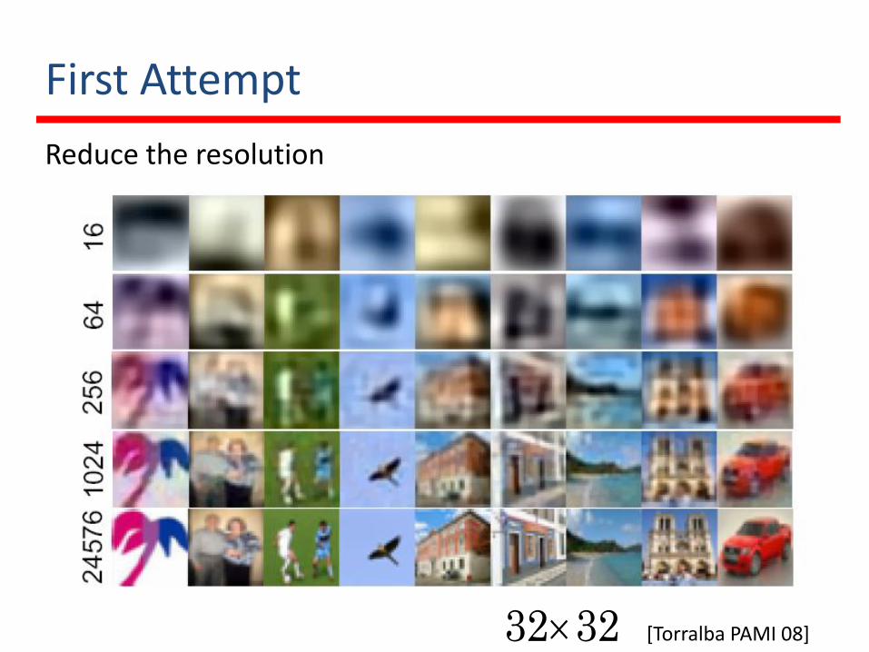
First Attempt
Reduce the resolution
[Torralba PAMI 08] 3232
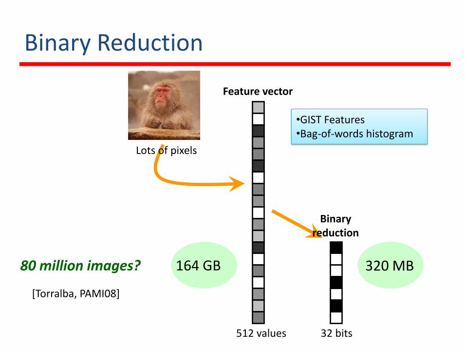
Binary Reduction
Lots of pixels
512 values
Feature vector
32 bits
Binaryreduction
164 GB 320 MB80 million images?
•GIST Features•Bag-of-words histogram
[Torralba, PAMI08]
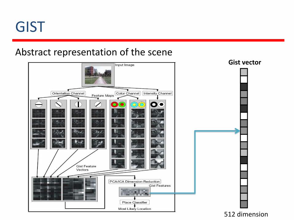
GIST
Abstract representation of the sceneGist vector
512 dimension
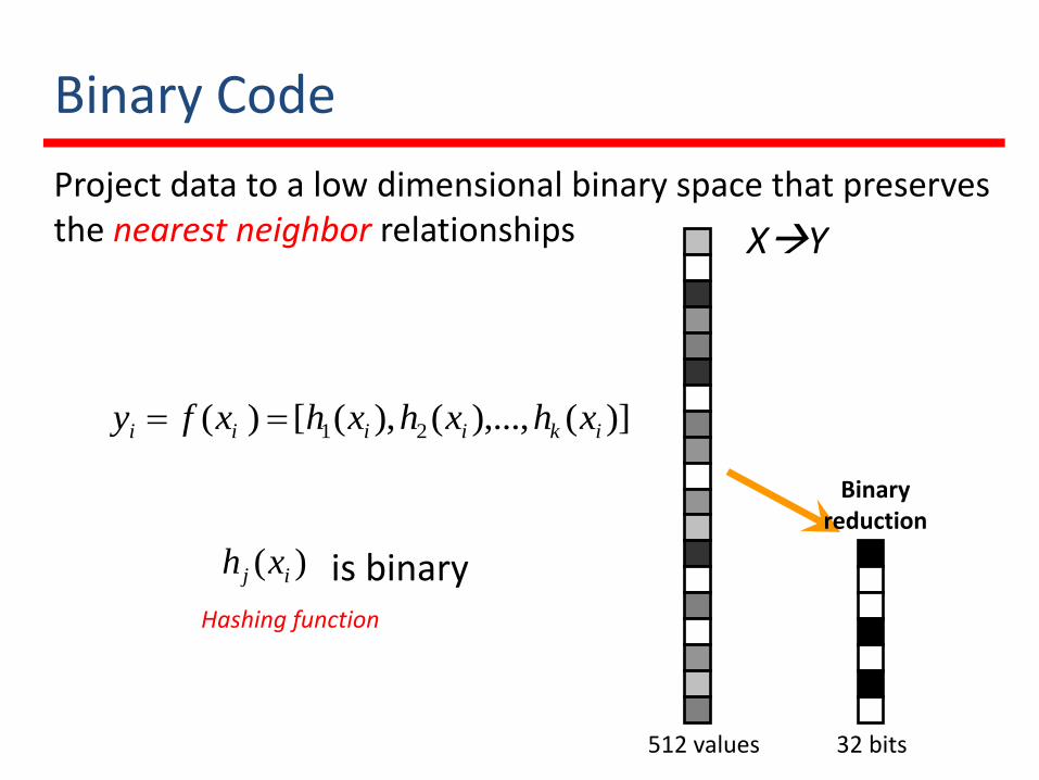
Binary Code
Project data to a low dimensional binary space that preserves the nearest neighbor relationships
)](),...,(),([)( 21 ikiiii xhxhxhxfy
XY
)( ij xh is binary
512 values 32 bits
Binaryreduction
Hashing function
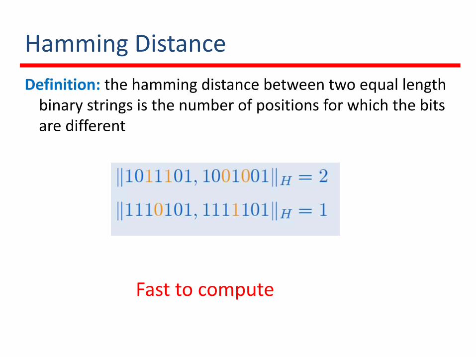
Hamming Distance
Definition: the hamming distance between two equal length binary strings is the number of positions for which the bits are different
Fast to compute
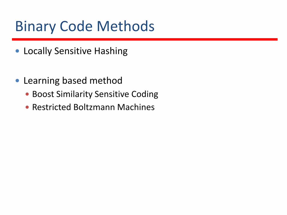
Binary Code Methods
Locally Sensitive Hashing
Learning based method
Boost Similarity Sensitive Coding
Restricted Boltzmann Machines
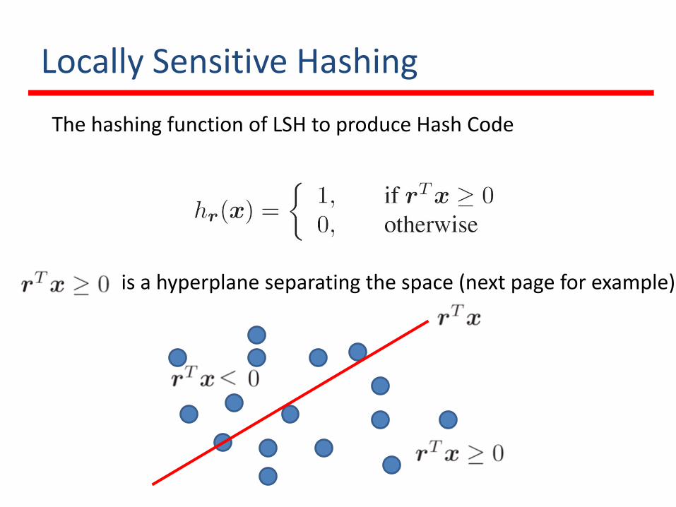
Locally Sensitive Hashing
The hashing function of LSH to produce Hash Code
is a hyperplane separating the space (next page for example)
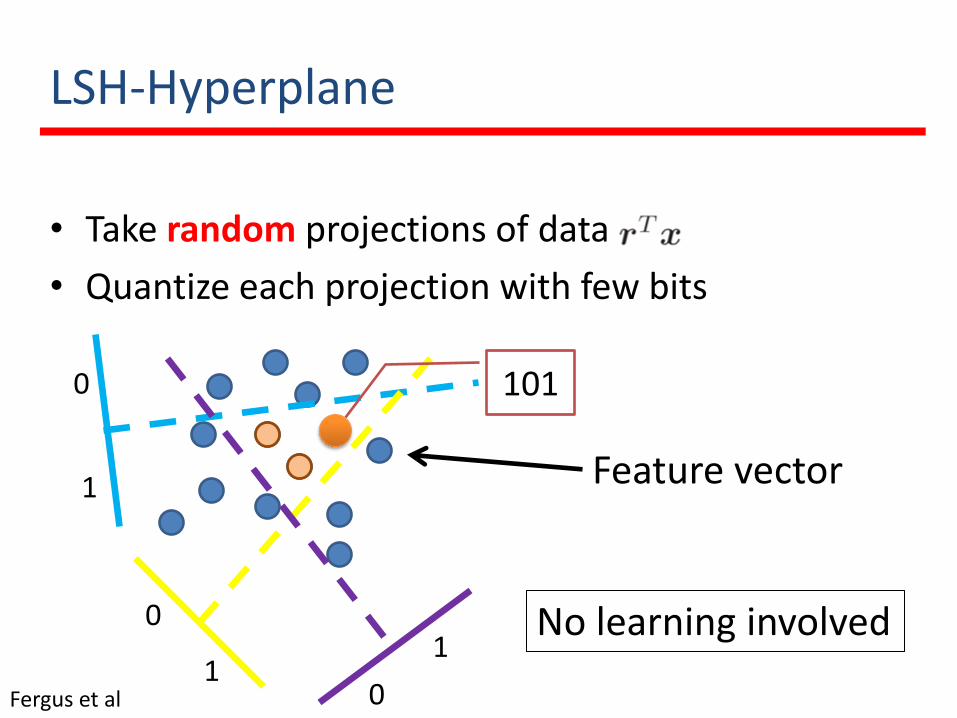
LSH-Hyperplane
• Take random projections of data
• Quantize each projection with few bits
0
1
0
10
1
101
No learning involved
Feature vector
Fergus et al
Binary Code Methods
Locally Sensitive Hashing
Learning based method
Boost Similarity Sensitive Coding
Restricted Boltzmann Machines
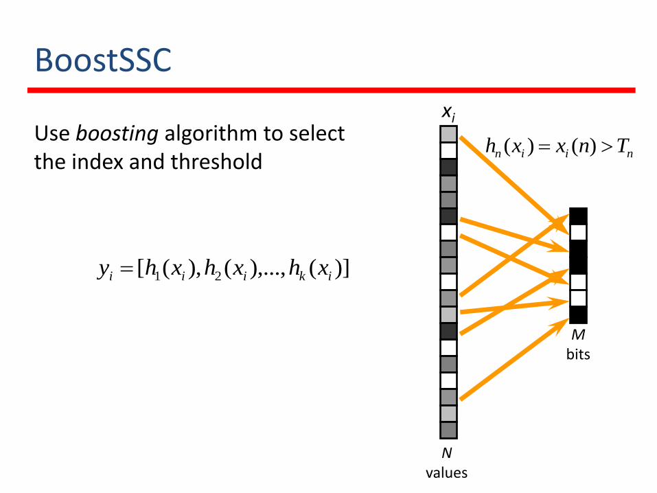
BoostSSC
Use boosting algorithm to select the index and threshold niin Tnxxh )()(
)](),...,(),([ 21 ikiii xhxhxhy
xi
Nvalues
Mbits
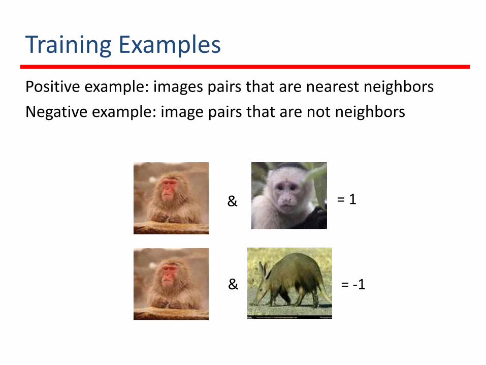
Training Examples
Positive example: images pairs that are nearest neighbors
Negative example: image pairs that are not neighbors
&
&
= 1
= -1
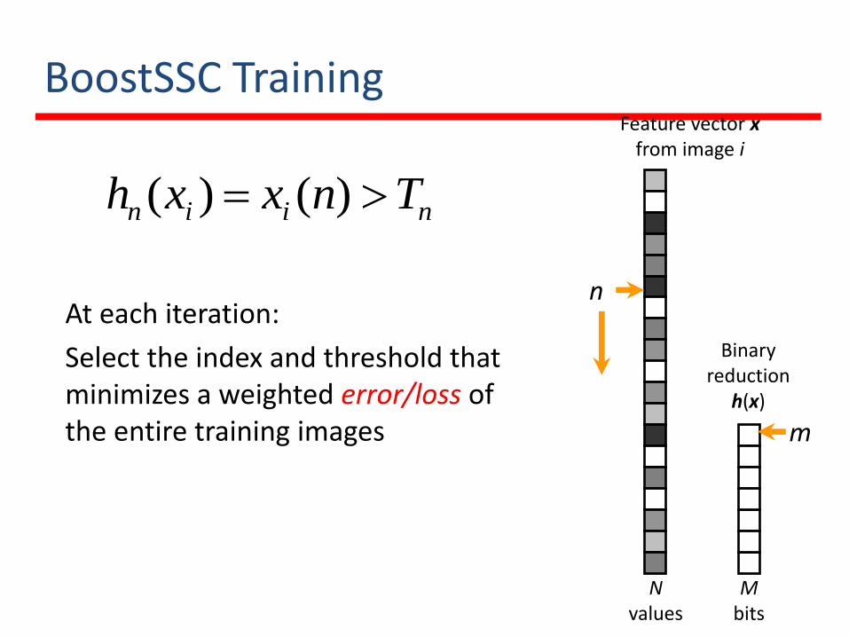
BoostSSC Training
At each iteration:
Select the index and threshold that minimizes a weighted error/loss of the entire training images
Feature vector xfrom image i
Binaryreduction
h(x)
Nvalues
Mbits
m
n
niin Tnxxh )()(
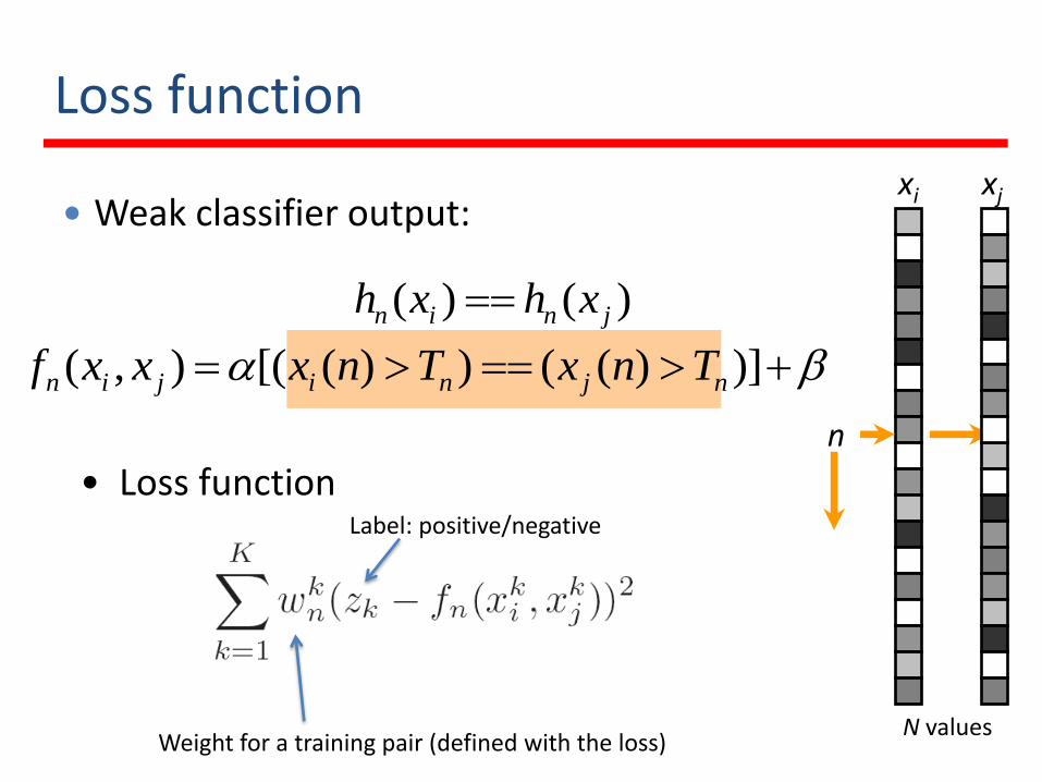
Loss function
Weak classifier output:xi
N values
n
xj
)])(())([(),( njnijin TnxTnxxxf
• Loss function
Weight for a training pair (defined with the loss)
Label: positive/negative
)()( jnin xhxh
Binary Code Methods
Locally Sensitive Hashing
Learning based method
Boost Similarity Sensitive Coding
Restricted Boltzmann Machines
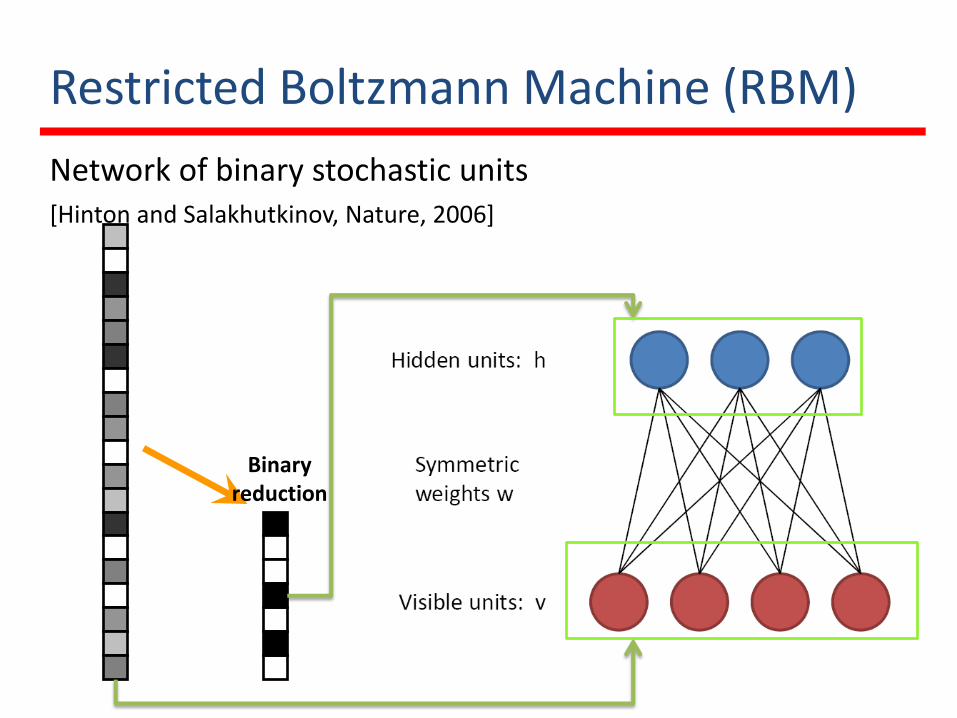
Restricted Boltzmann Machine (RBM)
Network of binary stochastic units[Hinton and Salakhutkinov, Nature, 2006]
Binaryreduction
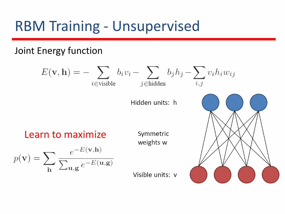
RBM Training - Unsupervised
Joint Energy function
Learn to maximize
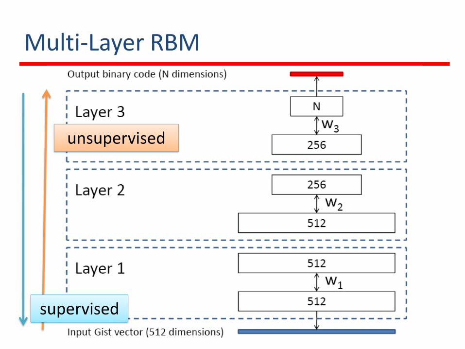
Multi-Layer RBM
unsupervised
supervised
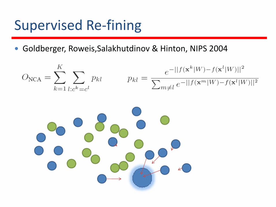
Supervised Re-fining
Goldberger, Roweis,Salakhutdinov & Hinton, NIPS 2004
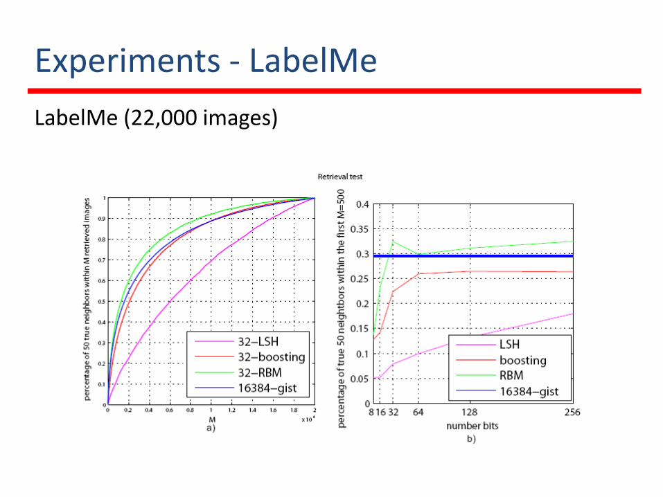
Experiments - LabelMe
LabelMe (22,000 images)
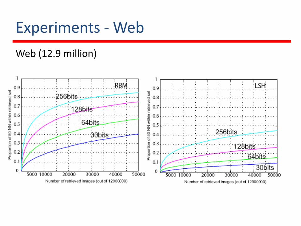
Experiments - Web
Web (12.9 million)
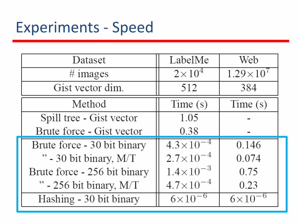
Experiments - Speed
Large Scale Dataset
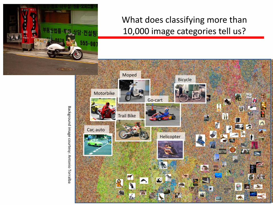
ImageNet: A Large-Scale Hierarchical Image Database. J. Deng et al., CVPR, 2009.What does classifying more than 10,000 image categories tell us? J. Deng et al., ECCV. 2010
Trail Bike
Motorbike
Moped
Go-cart
Helicopter
Car, auto
Bicycle
Backgro
un
d im
age cou
rtesy: An
ton
io To
rralba
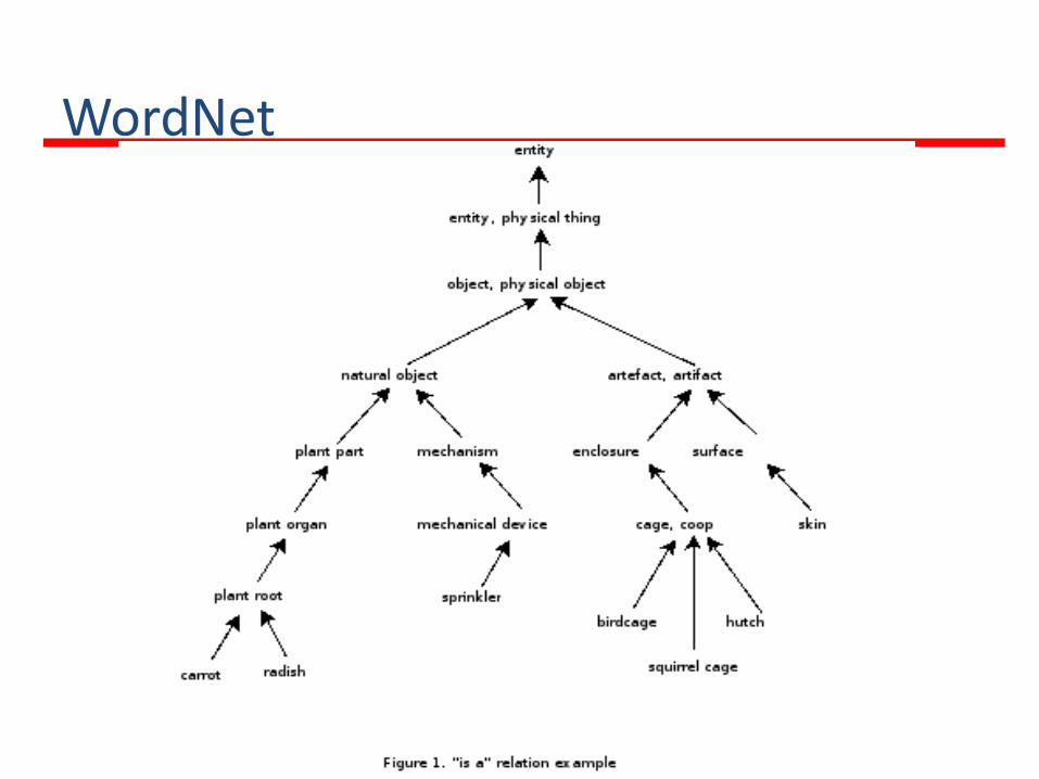
WordNet
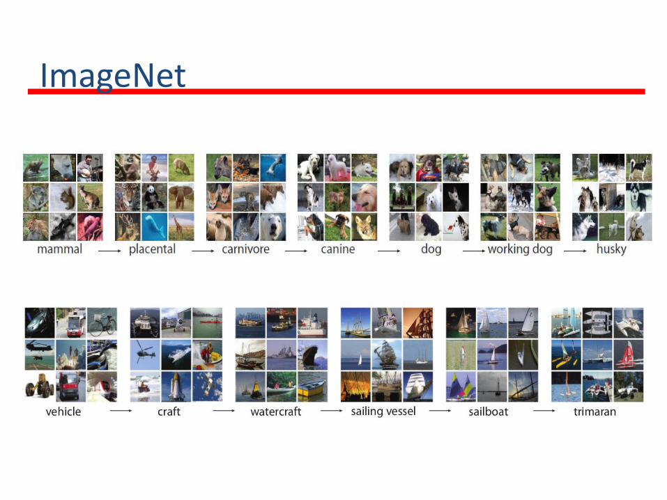
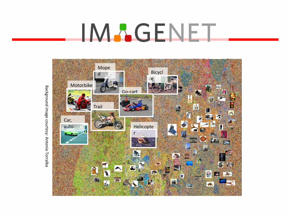
ImageNet
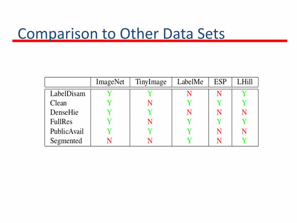
Comparison to Other Data Sets
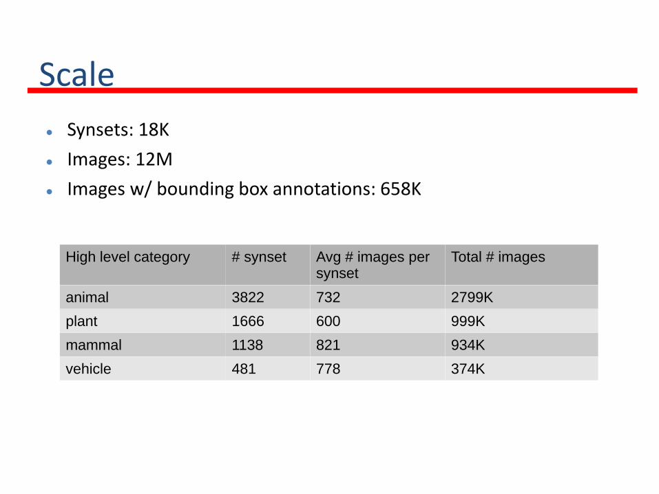
Scale
Synsets: 18K
Images: 12M
Images w/ bounding box annotations: 658K
High level category # synset Avg # images per synset
Total # images
animal 3822 732 2799K
plant 1666 600 999K
mammal 1138 821 934K
vehicle 481 778 374K
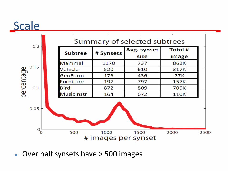
Scale
Over half synsets have > 500 images
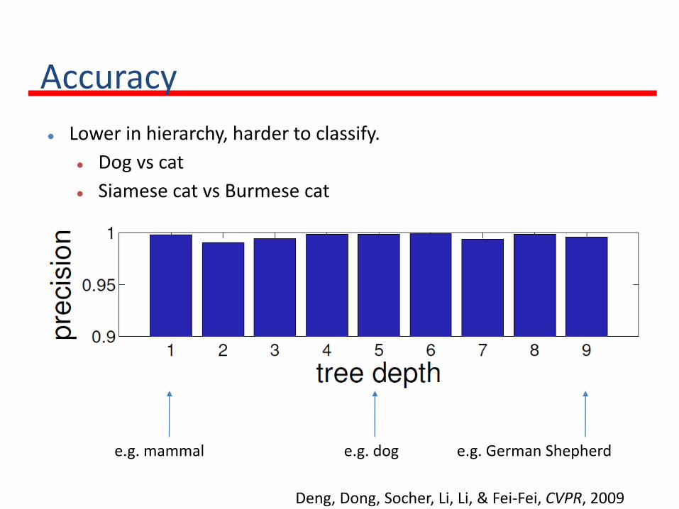
Accuracy
Lower in hierarchy, harder to classify.
Dog vs cat
Siamese cat vs Burmese cat
e.g. German Shepherde.g. doge.g. mammal
Deng, Dong, Socher, Li, Li, & Fei-Fei, CVPR, 2009
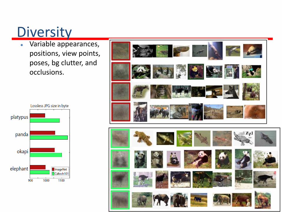
Diversity Variable appearances,
positions, view points, poses, bg clutter, and occlusions.
Constructing ImageNet
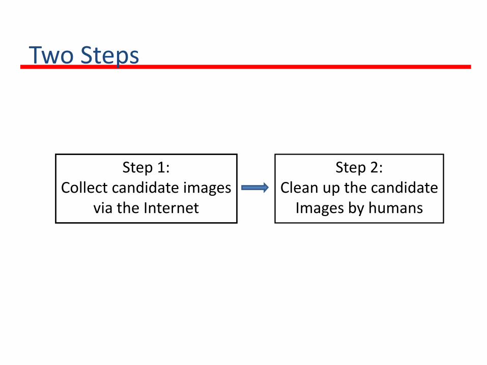
Two Steps
Step 1:Collect candidate images
via the Internet
Step 2:Clean up the candidate
Images by humans
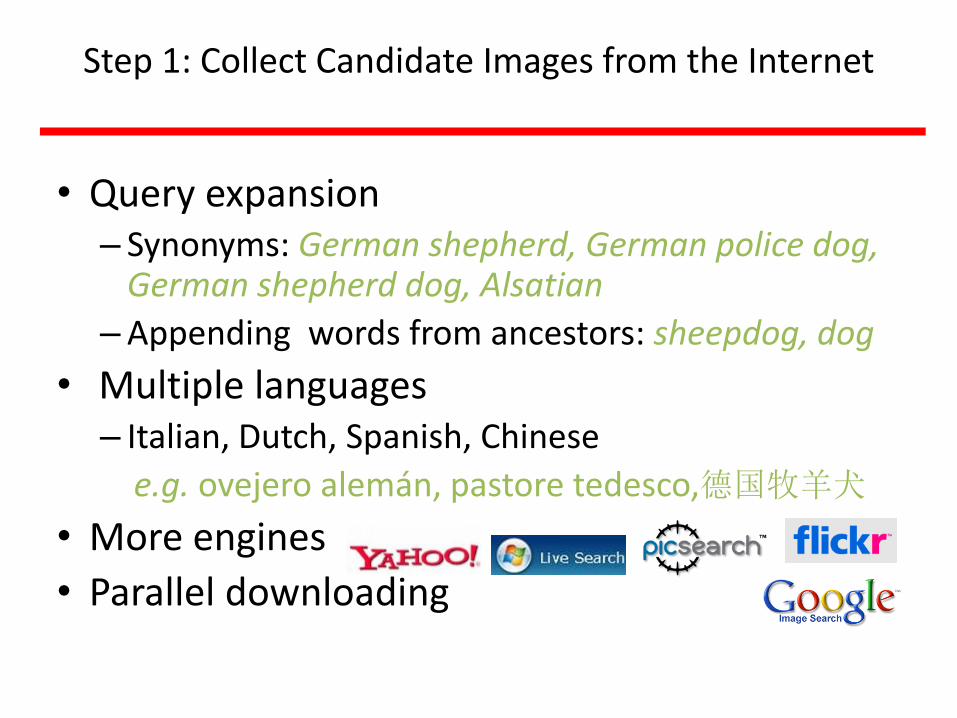
• Query expansion– Synonyms: German shepherd, German police dog,
German shepherd dog, Alsatian
– Appending words from ancestors: sheepdog, dog
• Multiple languages– Italian, Dutch, Spanish, Chinese
e.g. ovejero alemán, pastore tedesco,德国牧羊犬
• More engines
• Parallel downloading
Step 1: Collect Candidate Images from the Internet
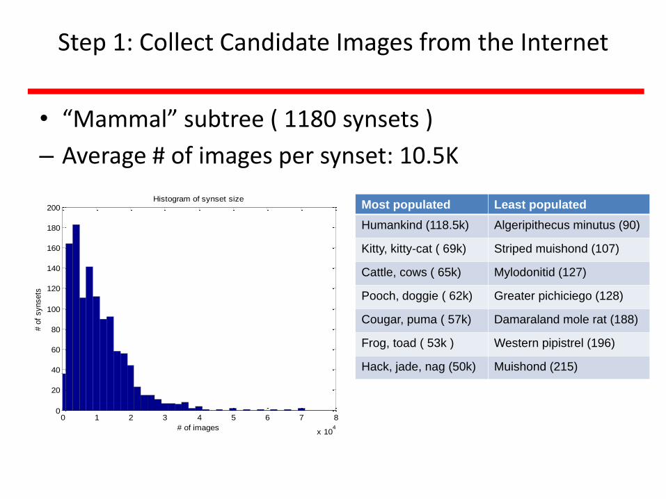
• “Mammal” subtree ( 1180 synsets )
– Average # of images per synset: 10.5K
0 1 2 3 4 5 6 7 8
x 104
0
20
40
60
80
100
120
140
160
180
200
# of images
# o
f synsets
Histogram of synset sizeMost populated Least populated
Humankind (118.5k) Algeripithecus minutus (90)
Kitty, kitty-cat ( 69k) Striped muishond (107)
Cattle, cows ( 65k) Mylodonitid (127)
Pooch, doggie ( 62k) Greater pichiciego (128)
Cougar, puma ( 57k) Damaraland mole rat (188)
Frog, toad ( 53k ) Western pipistrel (196)
Hack, jade, nag (50k) Muishond (215)
Step 1: Collect Candidate Images from the Internet
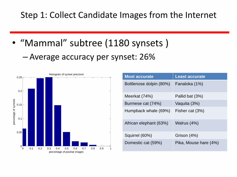
• “Mammal” subtree (1180 synsets )
– Average accuracy per synset: 26%
0 0.1 0.2 0.3 0.4 0.5 0.6 0.7 0.8 0.9 10
0.05
0.1
0.15
0.2
0.25
percentage of positive images
perc
enta
ge o
f synsets
Histogram of synset precisionMost accurate Least accurate
Bottlenose dolpin (80%) Fanaloka (1%)
Meerkat (74%) Pallid bat (3%)
Burmese cat (74%) Vaquita (3%)
Humpback whale (69%) Fisher cat (3%)
African elephant (63%) Walrus (4%)
Squirrel (60%) Grison (4%)
Domestic cat (59%) Pika, Mouse hare (4%)
Step 1: Collect Candidate Images from the Internet
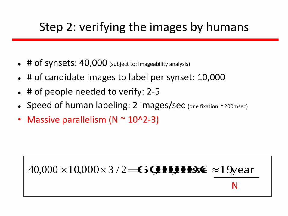
Step 2: verifying the images by humans
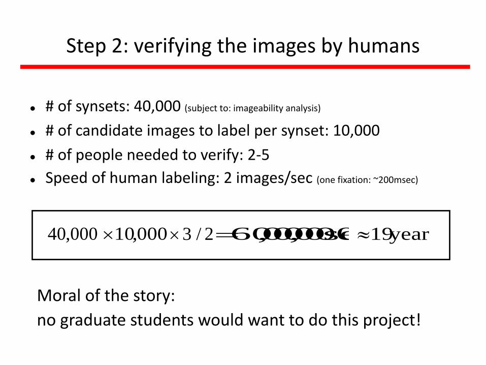
# of synsets: 40,000 (subject to: imageability analysis)
# of candidate images to label per synset: 10,000
# of people needed to verify: 2-5
Speed of human labeling: 2 images/sec (one fixation: ~200msec)
Moral of the story:
no graduate students would want to do this project!
000,40 000,10 3 2/ sec000,000,600 years19
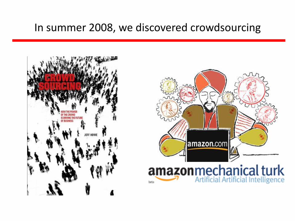
In summer 2008, we discovered crowdsourcing

# of synsets: 40,000 (subject to: imageability analysis)
# of candidate images to label per synset: 10,000
# of people needed to verify: 2-5
Speed of human labeling: 2 images/sec (one fixation: ~200msec)
• Massive parallelism (N ~ 10^2-3)
000,40 000,10 3 2/ sec000,000,600 years19
N
Step 2: verifying the images by humans
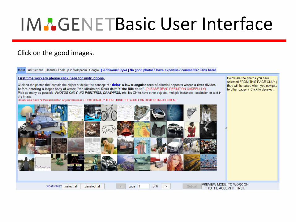
Basic User Interface
Click on the good images.
Basic User Interface
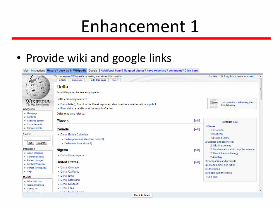
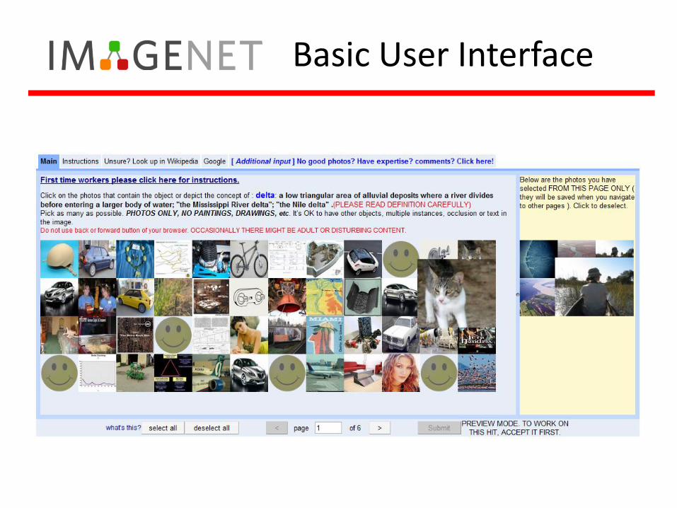
Enhancement 1
• Provide wiki and google links
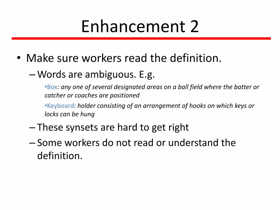
Enhancement 2
• Make sure workers read the definition.
– Words are ambiguous. E.g.•Box: any one of several designated areas on a ball field where the batter or catcher or coaches are positioned
•Keyboard: holder consisting of an arrangement of hooks on which keys or locks can be hung
– These synsets are hard to get right
– Some workers do not read or understand the definition.
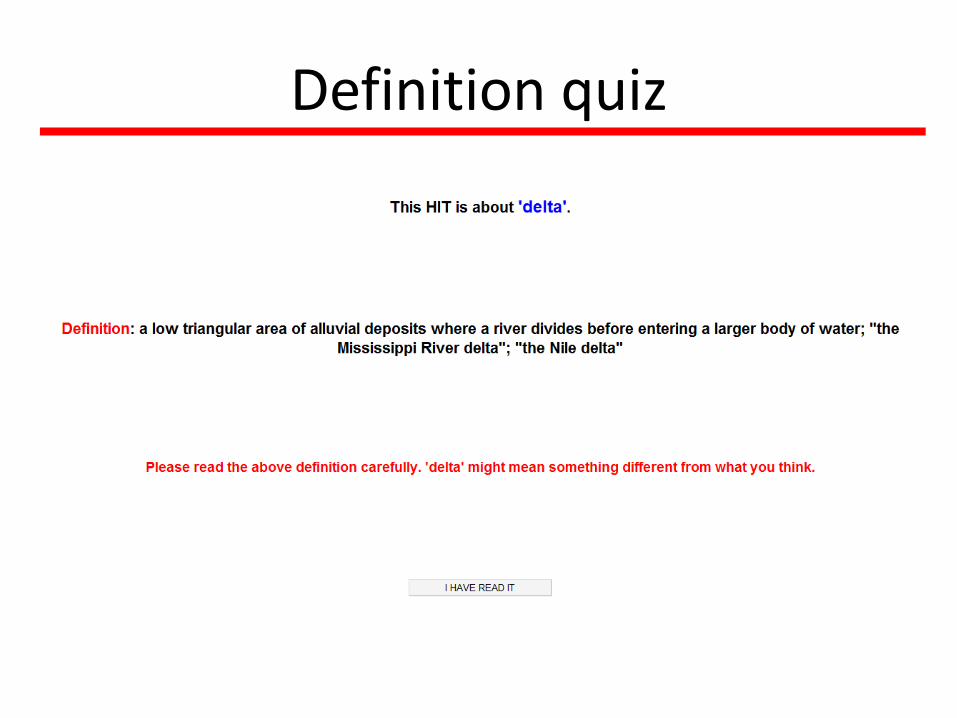
Definition quiz
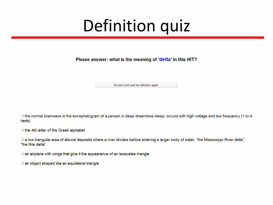
Definition quiz
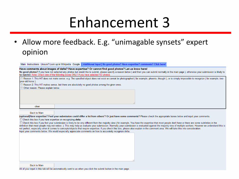
Enhancement 3• Allow more feedback. E.g. “unimagable synsets” expert
opinion
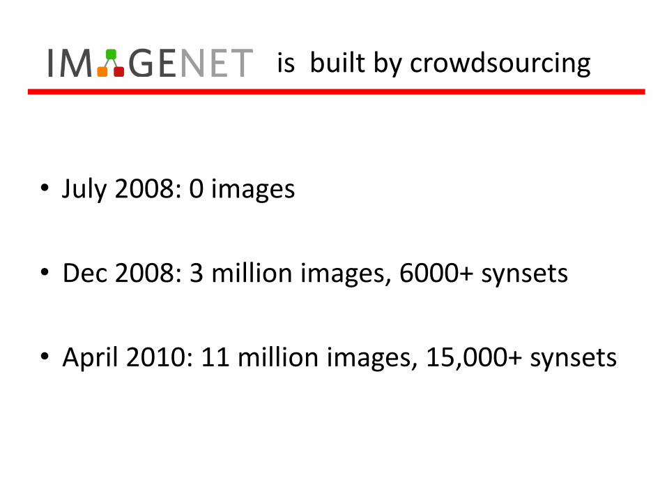
is built by crowdsourcing
• July 2008: 0 images
• Dec 2008: 3 million images, 6000+ synsets
• April 2010: 11 million images, 15,000+ synsets

Demography of AMT workers
Panos Ipeirotis, NYU, Feb, 2010
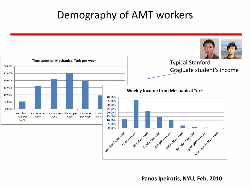
Typical StanfordGraduate student’s income
Demography of AMT workers
Panos Ipeirotis, NYU, Feb, 2010
Use Large Dataset Smartly
80 million tiny images: a large dataset for non-parametric object and scene recognition. Torralba, Fergus, Freeman. PAMI 2008.
Nonparametric scene parsing: Label transfer via dense scene alignment , C. Liu, J. Yuen and A. Torralba. CVPR, 2009.
Trail Bike
Motorbike
Moped
Go-cart
Helicopter
Car, auto
Bicycle
Backgro
un
d im
age cou
rtesy: An
ton
io To
rralba
What does classifying more than 10,000 image categories tell us?
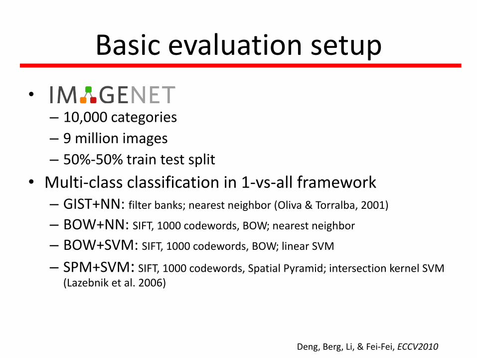
Basic evaluation setup
•
– 10,000 categories
– 9 million images
– 50%-50% train test split
• Multi-class classification in 1-vs-all framework– GIST+NN: filter banks; nearest neighbor (Oliva & Torralba, 2001)
– BOW+NN: SIFT, 1000 codewords, BOW; nearest neighbor
– BOW+SVM: SIFT, 1000 codewords, BOW; linear SVM
– SPM+SVM: SIFT, 1000 codewords, Spatial Pyramid; intersection kernel SVM (Lazebnik et al. 2006)
Deng, Berg, Li, & Fei-Fei, ECCV2010
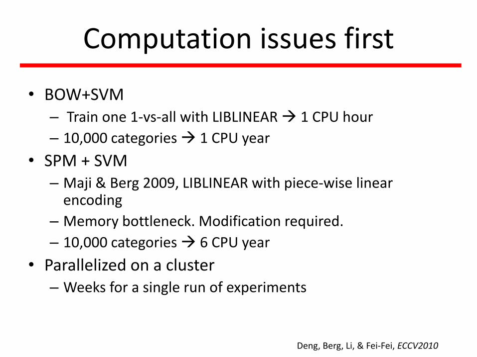
Computation issues first
Deng, Berg, Li, & Fei-Fei, ECCV2010
• BOW+SVM– Train one 1-vs-all with LIBLINEAR 1 CPU hour
– 10,000 categories 1 CPU year
• SPM + SVM– Maji & Berg 2009, LIBLINEAR with piece-wise linear
encoding
– Memory bottleneck. Modification required.
– 10,000 categories 6 CPU year
• Parallelized on a cluster– Weeks for a single run of experiments
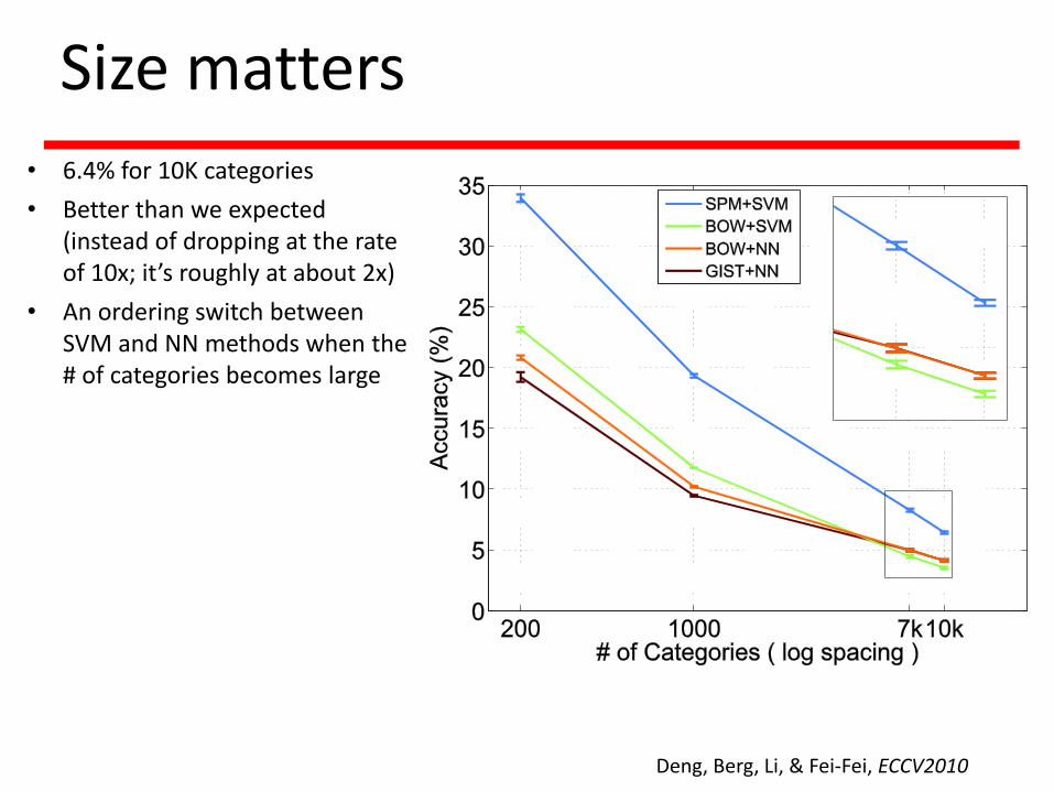
Size matters
• 6.4% for 10K categories
• Better than we expected (instead of dropping at the rate of 10x; it’s roughly at about 2x)
• An ordering switch between SVM and NN methods when the # of categories becomes large
Deng, Berg, Li, & Fei-Fei, ECCV2010
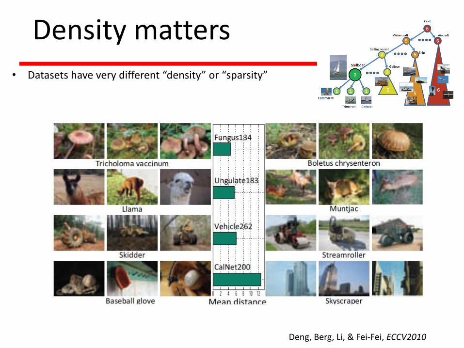
Density matters
• Datasets have very different “density” or “sparsity”
Deng, Berg, Li, & Fei-Fei, ECCV2010
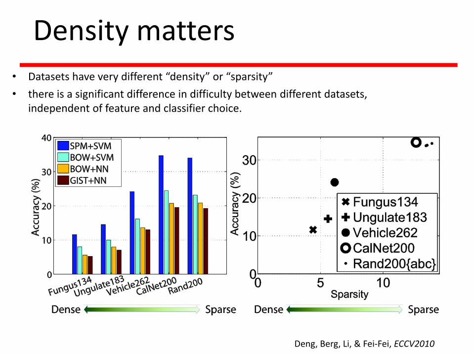
Density matters
• Datasets have very different “density” or “sparsity”
• there is a significant difference in difficulty between different datasets, independent of feature and classifier choice.
Deng, Berg, Li, & Fei-Fei, ECCV2010
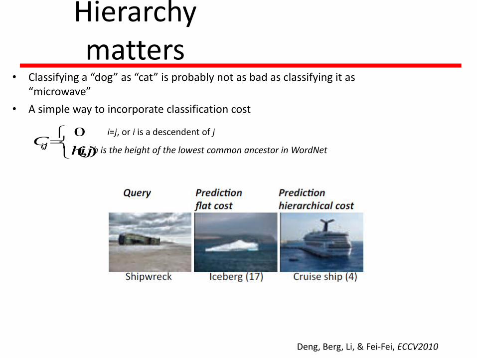
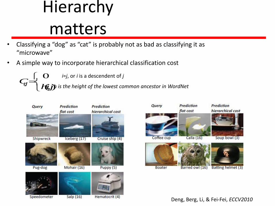
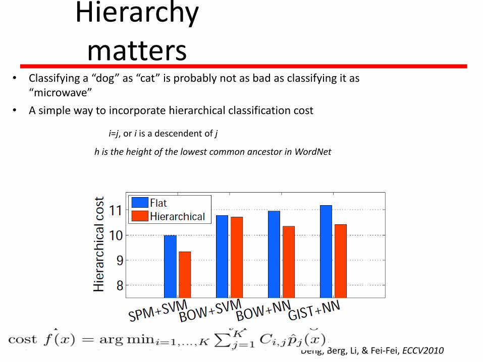
Hierarchy matters
• Classifying a “dog” as “cat” is probably not as bad as classifying it as “microwave”
• A simple way to incorporate classification cost
),(
0,
jihCji
i=j, or i is a descendent of j
h is the height of the lowest common ancestor in WordNet
Deng, Berg, Li, & Fei-Fei, ECCV2010
Hierarchy matters
• Classifying a “dog” as “cat” is probably not as bad as classifying it as “microwave”
• A simple way to incorporate hierarchical classification cost
i=j, or i is a descendent of j
h is the height of the lowest common ancestor in WordNet
Deng, Berg, Li, & Fei-Fei, ECCV2010

Image Labeling
Traditional Method: learn the local appearance for each category, smooth with a MRF/CRF model
tree
sky
road
field
car
unlabeled
building
window
Input Output
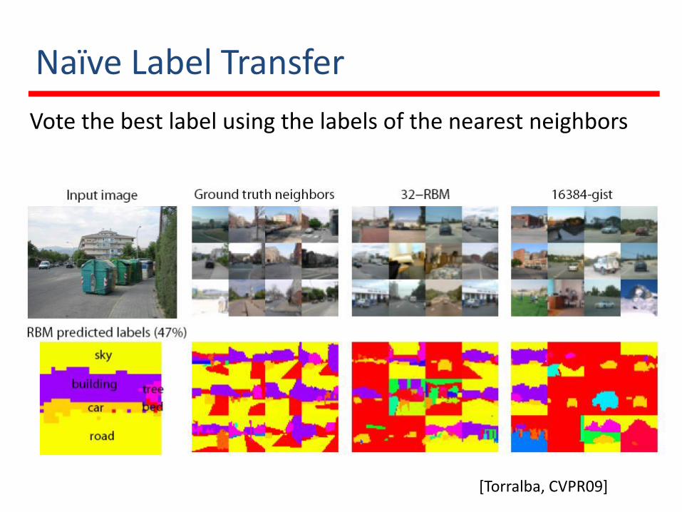
Naïve Label Transfer
Vote the best label using the labels of the nearest neighbors
[Torralba, CVPR09]
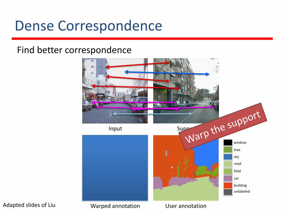
Dense Correspondence
Find better correspondence
tree
sky
road
field
car
unlabeled
building
window
Input Support
User annotationWarped annotationAdapted slides of Liu
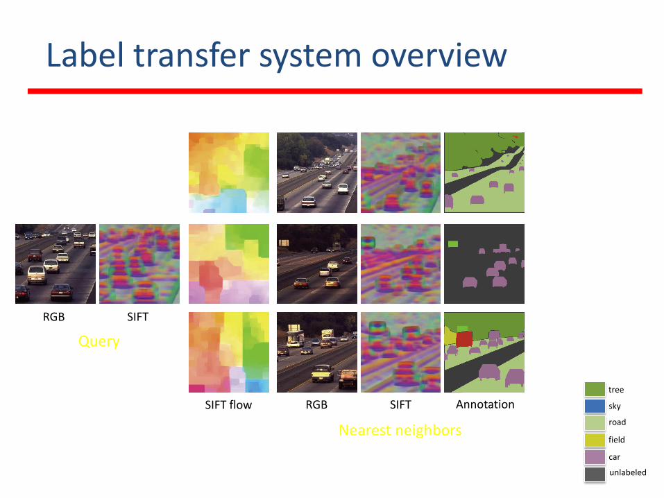
Label transfer system overview
Query
RGB SIFT
RGB SIFT AnnotationSIFT flow
Nearest neighbors
tree
sky
road
field
car
unlabeled
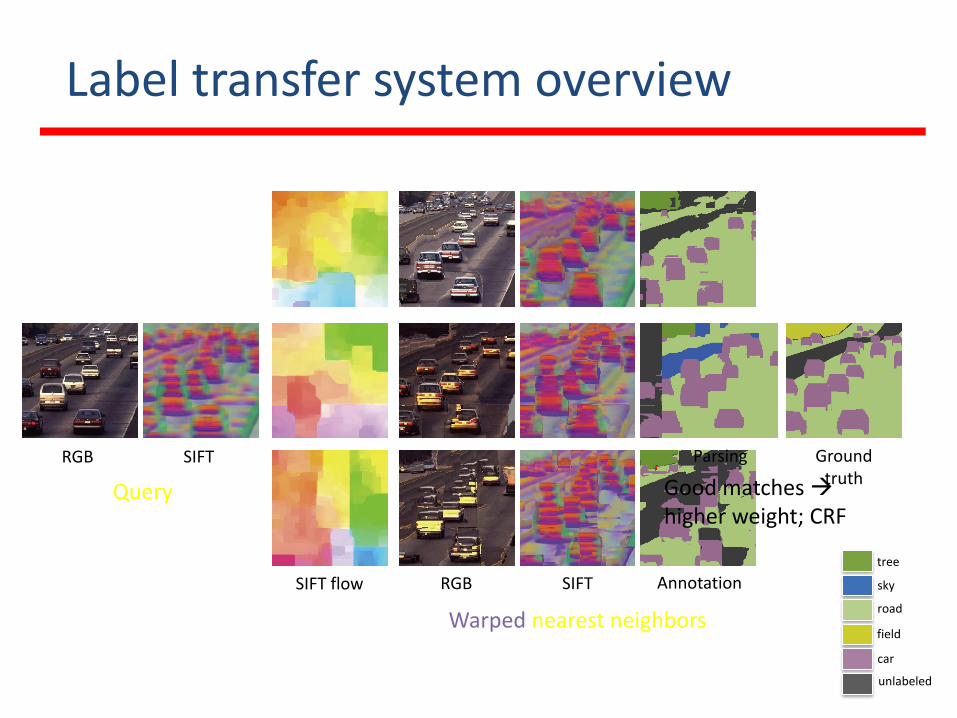
Label transfer system overview
SIFT flow RGB SIFT Annotation
Warped nearest neighbors
Query
RGB SIFT Parsing Ground truth
tree
sky
road
field
car
unlabeled
Good matches higher weight; CRF
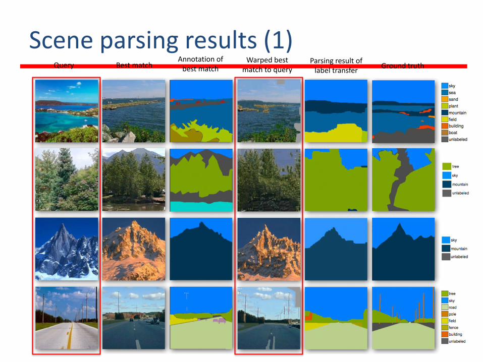
Scene parsing results (1)Query Best match
Annotation of best match
Warped best match to query
Parsing result of label transfer
Ground truth
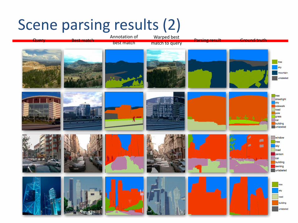
Scene parsing results (2)Query Best match
Annotation of best match
Warped best match to query
Parsing result Ground truth
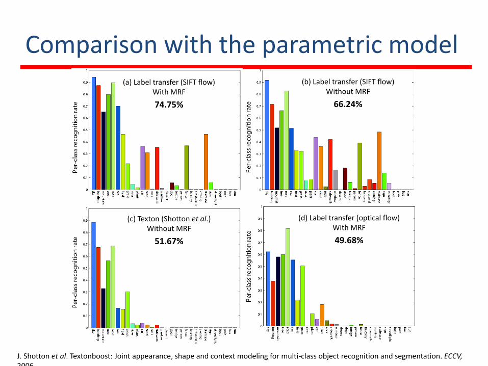
Comparison with the parametric model
J. Shotton et al. Textonboost: Joint appearance, shape and context modeling for multi-class object recognition and segmentation. ECCV, 2006
(a) Label transfer (SIFT flow)With MRF
74.75%
(b) Label transfer (SIFT flow)Without MRF
66.24%
(c) Texton (Shotton et al.)Without MRF
51.67%
(d) Label transfer (optical flow)With MRF
49.68%
Conclusion
Image Dataset is getting larger (tens of millions)
Memory usage is essential for storing large scale dataset
Non-parametric models are effective and popular for large dataset
Hierarchical structure of the object categories can be effectively utilized
Discussion
How many images do we need?
What about the quality of the data [Torralba and Efros, CVPR11]
Is nearest neighbor really the best?
New research problem How to do learning with the large scale dataset?
Fine-grained object categorization
Other interesting things with large dataset?

Thank you