introduction to rheology
TRANSCRIPT
ÉC OL E POL Y T EC H N I Q U EFÉ DÉRA LE D E L A U SAN N E
Christophe Ancey
Laboratoire hydraulique environnementale (LHE)
École Polytechnique Fédérale de LausanneÉcublens
CH-1015 Lausanne
Notebook
Introduction to Fluid Rheology
version 1.0 of 4th July 2005
2
C. Ancey,EPFL, ENAC/ICARE/LHE,
Ecublens, CH-1015 Lausanne, Suisse
[email protected], lhe.epfl.ch
Introduction to Fluid Rheology / C. Ancey
Ce travail est soumis aux droits d’auteurs. Tous les droits sont réservés ; toute copie, partielleou complète, doit faire l’objet d’une autorisation de l’auteur.
La gestion typographique a été réalisée à l’aide du package french.sty de Bernard Gaulle.
Remerciements : à Sébastien Wiederseiner et Martin Rentschler pour la relecture dumanuscrit.
3
« Le physicien ne peut demander à l’analyste de lui révéler une vérité nouvelle ; toutau plus celui-ci pourrait-il l’aider à la pressentir. Il y a longtemps que personne nesonge plus à devancer l’expérience, ou à construire le monde de toutes pièces surquelques hypothèses hâtives. De toutes ces constructions où l’on se complaisaitencore naïvement il y a un siècle, il ne reste aujourd’hui plus que des ruines.Toutes les lois sont donc tirées de l’expérience, mais pour les énoncer, il fautune langue spéciale ; le langage ordinaire est trop pauvre, elle est d’ailleurs tropvague, pour exprimer des rapports si délicats, si riches et si précis. Voilà donc unepremière raison pour laquelle le physicien ne peut se passer des mathématiques ;elles lui fournissent la seule langue qu’il puisse parler.»
Henri Poincaré, in La Valeur de la Science

4
TABLE OF CONTENTS 5
Table of contents
1 Rheometry 17
1.1 How does a rheometer operate? . . . . . . . . . . . . . . . . . . . . . . . . . . . . 18
1.1.1 A long history . . . . . . . . . . . . . . . . . . . . . . . . . . . . . . . . . 18
1.1.2 Anatomy of a modern rheometer . . . . . . . . . . . . . . . . . . . . . . . 18
1.1.3 Typical performance of modern lab rheometers . . . . . . . . . . . . . . . 21
1.2 Principles of viscometry . . . . . . . . . . . . . . . . . . . . . . . . . . . . . . . . 22
1.2.1 Fundamentals of rheometry . . . . . . . . . . . . . . . . . . . . . . . . . . 22
1.2.2 Flow down an inclined channel . . . . . . . . . . . . . . . . . . . . . . . . 24
1.2.3 Standard geometries . . . . . . . . . . . . . . . . . . . . . . . . . . . . . . 27
1.3 Inverse problems in rheometry . . . . . . . . . . . . . . . . . . . . . . . . . . . . . 28
1.3.1 A typical example: the Couette problem . . . . . . . . . . . . . . . . . . . 28
1.3.2 Earlier attempts at solving the Couette problem . . . . . . . . . . . . . . 28
1.3.3 The wavelet-vaguelette decomposition . . . . . . . . . . . . . . . . . . . . 30
1.3.4 Practical example . . . . . . . . . . . . . . . . . . . . . . . . . . . . . . . . 31
1.4 Rheometers and rheometrical procedures . . . . . . . . . . . . . . . . . . . . . . . 33
1.4.1 How to determine the flow curve? . . . . . . . . . . . . . . . . . . . . . . . 33
1.4.2 Stress/strain step . . . . . . . . . . . . . . . . . . . . . . . . . . . . . . . . 34
1.5 Typical rheological behaviors . . . . . . . . . . . . . . . . . . . . . . . . . . . . . 37
1.5.1 Outlining a flow curve . . . . . . . . . . . . . . . . . . . . . . . . . . . . . 37
1.5.2 Shear-thinning/thickening . . . . . . . . . . . . . . . . . . . . . . . . . . . 37
1.5.3 Yield stress . . . . . . . . . . . . . . . . . . . . . . . . . . . . . . . . . . . 38
1.5.4 Viscoelasticity . . . . . . . . . . . . . . . . . . . . . . . . . . . . . . . . . 39
1.5.5 Normal stress effects . . . . . . . . . . . . . . . . . . . . . . . . . . . . . . 45
1.5.6 Thixotropy . . . . . . . . . . . . . . . . . . . . . . . . . . . . . . . . . . . 46
1.6 Problems encountered in rheometry . . . . . . . . . . . . . . . . . . . . . . . . . . 51
1.6.1 Problems with rheometers . . . . . . . . . . . . . . . . . . . . . . . . . . . 51
1.6.2 Limitations of the viscometric treatment . . . . . . . . . . . . . . . . . . . 53
1.6.3 Technical issues related to the derivation of the flow curve . . . . . . . . . 54
1.6.4 Problems related to sample preparation . . . . . . . . . . . . . . . . . . . 55
6 TABLE OF CONTENTS
1.7 Non-standard techniques: what can be done without a rheometer? . . . . . . . . . 56
1.7.1 Viscosity: free fall of a bead . . . . . . . . . . . . . . . . . . . . . . . . . . 56
1.7.2 Yield stress: Slump test . . . . . . . . . . . . . . . . . . . . . . . . . . . . 56
2 Rheology and Continuum Mechanics 59
2.1 Why is continuum mechanics useful? An historical perspective . . . . . . . . . . . 60
2.1.1 Paradoxical experimental results? . . . . . . . . . . . . . . . . . . . . . . . 60
2.1.2 How to remove the paradox? . . . . . . . . . . . . . . . . . . . . . . . . . 61
2.2 Fundamentals of Continuum Mechanics . . . . . . . . . . . . . . . . . . . . . . . 63
2.2.1 Kinematics . . . . . . . . . . . . . . . . . . . . . . . . . . . . . . . . . . . 63
2.2.2 Stress tensor . . . . . . . . . . . . . . . . . . . . . . . . . . . . . . . . . . 67
2.2.3 Admissibility of a constitutive equations . . . . . . . . . . . . . . . . . . . 69
2.2.4 Specific properties of material . . . . . . . . . . . . . . . . . . . . . . . . . 70
2.2.5 Representation theorems . . . . . . . . . . . . . . . . . . . . . . . . . . . . 70
2.2.6 Balance equations . . . . . . . . . . . . . . . . . . . . . . . . . . . . . . . 72
2.2.7 Conservation of energy . . . . . . . . . . . . . . . . . . . . . . . . . . . . . 74
2.2.8 Jump conditions . . . . . . . . . . . . . . . . . . . . . . . . . . . . . . . . 76
2.3 Phenomenological constitutive equations . . . . . . . . . . . . . . . . . . . . . . . 79
2.3.1 Newtonian behavior . . . . . . . . . . . . . . . . . . . . . . . . . . . . . . 79
2.3.2 Viscoplastic behavior . . . . . . . . . . . . . . . . . . . . . . . . . . . . . . 79
2.3.3 Viscoelasticity . . . . . . . . . . . . . . . . . . . . . . . . . . . . . . . . . 81
3 Rheophysics 83
3.1 Fundamentals of rheophysics . . . . . . . . . . . . . . . . . . . . . . . . . . . . . . 84
3.1.1 Movement of a single sphere and consequences on the flow regime . . . . . 84
3.1.2 From a single sphere to a bulk: averaging . . . . . . . . . . . . . . . . . . 90
3.1.3 Averaged balance equations . . . . . . . . . . . . . . . . . . . . . . . . . . 92
3.1.4 Passing from volume averages to ensemble averages . . . . . . . . . . . . . 95
3.2 Dilute suspensions . . . . . . . . . . . . . . . . . . . . . . . . . . . . . . . . . . . 99
3.2.1 Dilute suspension in a Stokes regime: Stokesian theory . . . . . . . . . . . 99
3.2.2 Computations of the constitutive equation . . . . . . . . . . . . . . . . . . 104
3.3 Concentrated suspensions . . . . . . . . . . . . . . . . . . . . . . . . . . . . . . . 105
3.3.1 Constitutive equations for concentrated suspensions . . . . . . . . . . . . 105
3.3.2 Regime diagram and computation of individual contributions . . . . . . . 107
References 111
TABLE OF CONTENTS 7
Foreword
Objective of the course
The objective of this course held in the framework of the doctoral school Mechanics of Solidsand Fluids et EPFL is to provide the student with the modern tools needed to investigate therheological behavior of complex fluids. Emphasis will be given to particle suspensions. The coursewill start with an introduction of experimental procedures. Phenomenological description of howmatter flows will then be presented. The last part of the course will be devoted to the rheophysicalapproach to modelling the rheological behavior of particle suspensions.
This notebook will focus on materials encountered by geophysicists (mud, snow, magma, etc.)and in industrial or civil-engineering applications (concrete, slurries, etc.): in most cases we willconsider only homogeneous and suspensions of particles within an interstitial fluid without lossof generality. Other complex fluids such as polymeric liquids are rarely encountered in geophysicsand therefore they will not be addressed here.
Content of the notebook
The mere description of what the term rheology embraces in terms of scientific areas is noteasy. Roughly speaking, rheology distinguishes different areas and offshoots such as the following:rheometry, formulation of constitutive equation, computational rheometry, microstructural ana-lysis and interpretation of bulk rheological behavior, etc. Here we will focus on the followingpoints 1:
Rheometry. The term “rheometry” is usually used to refer to a group of experimentaltechniques for investigating the rheological behavior of materials. It is of great importance indetermining the constitutive equation of a fluid or in assessing the relevance of any proposedconstitutive law. Most of the textbooks on rheology deal with rheometry. The books by Colemanet al. (1966), Walters (1975), and by Bird et al. (1987) provide a complete introduction to theviscometric theory used in rheometry for inferring the constitutive equation. The book by Coussot& Ancey (1999b) gives practical information concerning rheometrical measurements with naturalfluids. Though primarily devoted to food processing engineering, Steffe’s book presents a detaileddescription of rheological measurements; a free sample is available on the web (Steffe, 1996).
In Chapter 1, we will review the different techniques that are suitable to studying variousfluids. Emphasis is given both to describing the methods and the major experimental problemsencountered with materials made up of particles and fluids.
1. Other aspects of rheology, such as complex flow modelling and computational rheology, are notaddressed in this introductory notebook.
8 TABLE OF CONTENTS
Continuummechanics. The formulation of constitutive equations is probably the early goalof rheology. At the beginning of the 20th century, the non-Newtonian character of many fluidsof practical interest motivated Professor Bingham to coin the term rheology and to define it asthe study of the deformation and flow of matter. The development of a convenient mathematicalframework occupied the attention of rheologists for a long time after the Second World War. Atthat time, theoreticians such as Coleman, Markovitz, Noll, Oldroyd, Reiner, Toupin, Truesdell,etc. sought to express rheological behavior through equations relating suitable variables andparameters representing the deformation and stress states. This gave rise to a large number ofstudies on the foundations of continuummechanics (Bird et al., 1987). Nowadays the work of thesepioneers is pursued through the examination of new problems such as the treatment of multiphasesystems or the development of nonlocal field theories. For examples of current developmentsand applications to geophysics, the reader may consult papers by Hutter and coworkers onthe thermodynamically consistent continuum treatment of soil-water systems (Wang & Hutter,1999; Hutter et al., 1999), the book by Vardoulakis & Sulem (1995) on soil mechanics, andthe review by Bedford & Dumheller (1983) on suspensions. A cursory glance at the literatureon theoretical rheology may give the reader the impression that all this literature is merely anoverly sophisticated mathematical description of the matter with little practical interest. In fact,excessive refinements in the tensorial expression of constitutive equations lead to prohibitivedetail and thus substantially limit their utility or predictive capabilities. This probably explainswhy there is currently little research on this topic. Such limitations should not prevent the reader(and especially the newcomer) from studying the textbooks in theoretical rheology, notably toacquire the basic principles involved in formulating constitutive equations.
Two simple problems related to these principles will be presented in Chapter 2 to illustratethe importance of an appropriate tensorial formulation of constitutive equations.
Rheophysics. For many complex fluids of practical importance, bulk behavior is not easilyoutlined using a continuum approach. It may be useful to first examine what happens at a micro-scopic scale and then infer the bulk properties using an appropriate averaging process. Kinetictheories give a common example for gases (Chapman & Cowling, 1970) or polymeric liquids(Bird et al., 1987), which infer the constitutive equations by averaging all the pair interactionsbetween particles. Such an approach is called microrheology or rheophysics. Here we prefer touse the latter term to emphasize that the formulation of constitutive equations is guided by aphysical understanding of the origins of bulk behavior. Recent developments in geophysics arebased on using kinetic theories to model bed load transport (Jenkins & Hanes, 1998), floatingbroken ice fields (Savage, 1994), and rockfall and granular debris flows (Savage, 1989). It is impli-citly recognized that thoroughly modelling the microstructure would require prohibitive detail,especially for natural fluids. It follows that a compromise is generally sought between capturingthe detailed physics at the particle level and providing applicable constitutive equations. Usingdimensionless groups and approximating constitutive equations are commonly used operationsfor that purpose. In Chap. 3, we will consider suspensions of rigid particles within a Newtonianfluid to exemplify the different tools used in rheophysics. Typical examples of such fluids in ageophysical context include magma and mud.
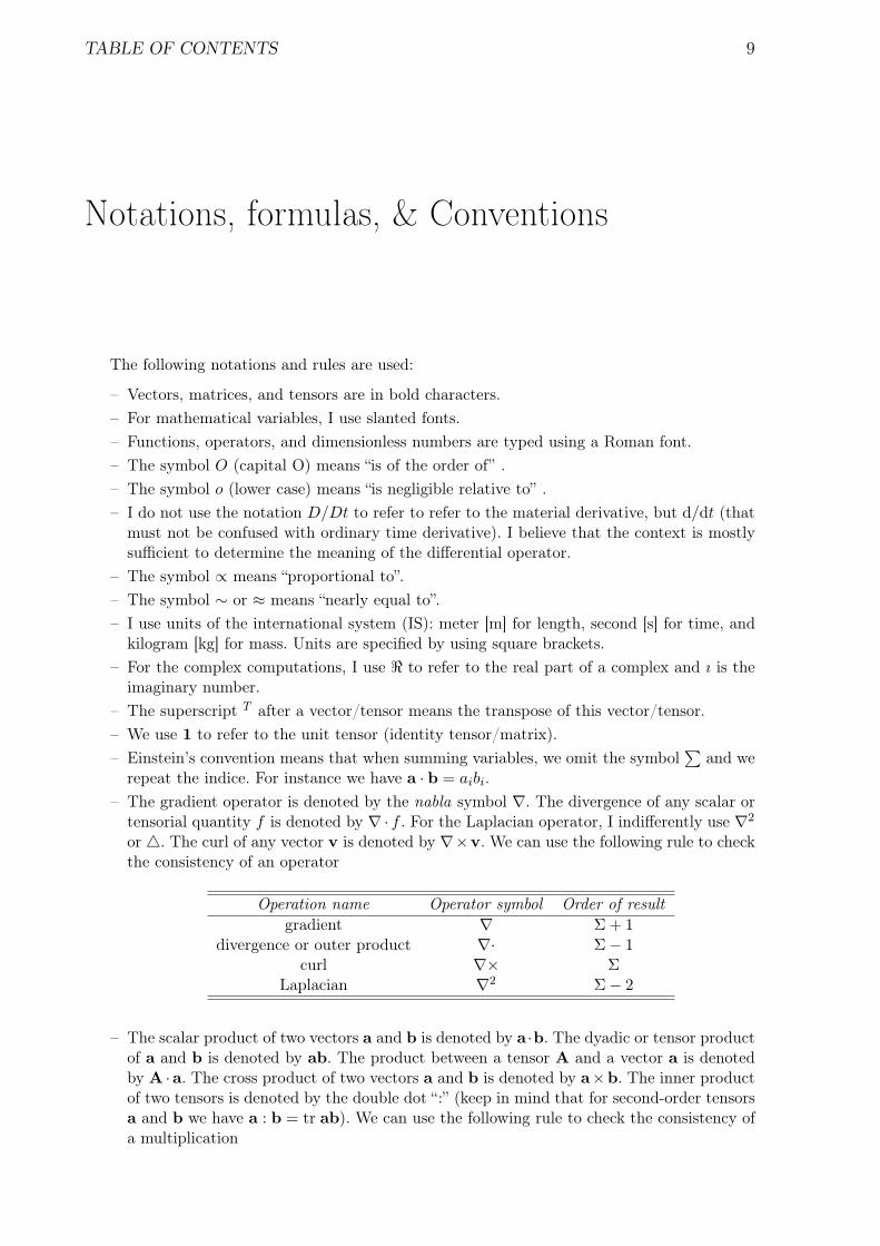
TABLE OF CONTENTS 9
Notations, formulas, & Conventions
The following notations and rules are used:
– Vectors, matrices, and tensors are in bold characters.– For mathematical variables, I use slanted fonts.– Functions, operators, and dimensionless numbers are typed using a Roman font.– The symbol O (capital O) means “is of the order of” .– The symbol o (lower case) means “is negligible relative to” .– I do not use the notation D/Dt to refer to refer to the material derivative, but d/dt (that
must not be confused with ordinary time derivative). I believe that the context is mostlysufficient to determine the meaning of the differential operator.
– The symbol ∝ means “proportional to”.– The symbol ∼ or ≈ means “nearly equal to”.– I use units of the international system (IS): meter [m] for length, second [s] for time, and
kilogram [kg] for mass. Units are specified by using square brackets.– For the complex computations, I use < to refer to the real part of a complex and ı is the
imaginary number.– The superscript T after a vector/tensor means the transpose of this vector/tensor.– We use 1 to refer to the unit tensor (identity tensor/matrix).– Einstein’s convention means that when summing variables, we omit the symbol
∑and we
repeat the indice. For instance we have a · b = aibi.– The gradient operator is denoted by the nabla symbol ∇. The divergence of any scalar or
tensorial quantity f is denoted by ∇· f . For the Laplacian operator, I indifferently use ∇2
or 4. The curl of any vector v is denoted by ∇×v. We can use the following rule to checkthe consistency of an operator
Operation name Operator symbol Order of resultgradient ∇ Σ + 1
divergence or outer product ∇· Σ− 1curl ∇× Σ
Laplacian ∇2 Σ− 2
– The scalar product of two vectors a and b is denoted by a ·b. The dyadic or tensor productof a and b is denoted by ab. The product between a tensor A and a vector a is denotedby A ·a. The cross product of two vectors a and b is denoted by a×b. The inner productof two tensors is denoted by the double dot “:” (keep in mind that for second-order tensorsa and b we have a : b = tr ab). We can use the following rule to check the consistency ofa multiplication
10 TABLE OF CONTENTS
Operation name Multiplication sign Order of resultdyadic or tensorial product none Σ
cross or outer product × Σ− 1scalar or inner product · Σ− 2scalar or inner product : Σ− 4
Recall that the order of a scalar is 0, a vector is of order 1, and a tensor is of order at least2. For instance, if a and b denotes vectors and T is a tensor, T · a is order 2 + 1− 1 = 2;T : a is order 2 + 1− 2 = 1.
– The gradient of a vector a is a tensor ∇a, whose components in a Cartesian frame xi are
∂aj
∂xi.
The divergence of a second-order tensor Mij is a vector ∇ ·M, whose jth component in aCartesian frame xi is
∂Mij
∂xi.
– The tensorial product of two vectors a and b provides a tensor ab such that for any vectorc, we have (ab)c = (b · c)a.
– A vector field such that ∇ · v = 0 is said to be solenoidal. A function f satisfying theLaplace equation ∇2f = 0 is said to be harmonic. A function f such that ∇4f = 0 is saidto be biharmonic. A vectorial field v such ∇× v = 0 is said to be irrotational.
– An extensive use is made of the Green-Ostrogradski theorem (also called the divergencetheorem): ∫
V∇ · udV =
∫
Su · n dS,
where S is the surface bounding the volume V and n is the unit normal to the infinitesimalsurface dS. A closely allied theorem for scalar quantities f is
∫
V∇f dV =
∫
SfndS.
– For some algebraic computations, we need to use– Cartesian coordinates (x, y, z),– or spherical coordinates (x = r cosϕ sin θ) , y = r sin θ sinϕ, z = r cos θ) with 0 ≤ θ ≤
π and −π ≤ ϕ ≤ π, dS = r2 sin θdθdϕ on a sphere of radius r, dV = r2 sin θdrdθdϕ.– Some useful formulas on vector and tensor products
N : M = M : N,
a× (b× c) = (a · c)b− (a · b)c,
(M · a) · b = M : (ab) and a · (b ·M) = M : (ab),
ab : cd = a · (b · cd) = a · ((b · c)d) = (a · b)(c · d) = ac : bd
∇(fg) = g∇f + f∇g,
∇ · (fa) = a · ∇f + f∇ · a,
∇ · (a× b) = b(∇× a)− a(∇× b),
∇ · ∇a =12∇(a · a)− a× (∇× a),
∇ · ab = a∇b + b∇ · a1 : ∇a = ∇ · a,
∇ · (f1) = ∇f,
TABLE OF CONTENTS 11
– and on derivatives(a · ∇)b = a · (∇b)T ,
∂f(x)∂x
=xx
∂f(x)∂x
,
ab : (∇c) = a · (b∇) c,
with x = |x|.– For some computations, we need the use the Dirac function
∫R3 δ(x)dx = 1,
∫R3 δ(x −
x0)g(x)dx = g(x0), and δ(x) = −∇2(4πx)−1 = −∇4x(8π)−1, where x = |x|. The lasttwo expressions are derived by applying the Green formula to the function 1/x (see anytextbook on distributions).
– The Fourier transform in an n-dimensional space is defined as
f(ξ) =∫
Rn
f(x)e−ıξ·xdx,
for any continuous function. Conversely, the inverse Fourier transform is defined as
f(x) =∫
Rn
f(x)eıξ·xdξ.

12 TABLE OF CONTENTS
TABLE OF CONTENTS 13
Further reading
This notebook gives an overview of the major current issues in rheology through a series ofdifferent problems of particular relevance to particle-suspension rheology. For each topic consi-dered here, we will outline the key elements and point the student toward the most helpfulreferences and authoritative works. The student is also referred to available books introducingrheology (Barnes, 1997; Tanner, 1988) for a more complete presentation; the tutorials writtenby Middleton & Wilcock (1994) on mechanical and rheological applications in geophysics and byBarnes (2000) provide a shorter introduction to rheology.
Continuum Mechanics, rheology
– K. Hutter and K. Jöhnk, Continuum Methods of Physical Modeling (Springer, Berlin, 2004)635 p.
– H.A. Barnes, J.F. Hutton and K. Walters, An introduction to rheology (Elsevier, Amster-dam, 1997).
– H.A. Barnes, A Handbook of Elementary Rheology (University of Wales, Aberystwyth,2000).
– K. Walters, Rheometry (Chapman and Hall, London, 1975).– D.V. Boger and K. Walters, Rheological Phenomena in Focus (Elsevier, Amsterdam, 1993)
156 p.– B.D. Coleman, H. Markowitz and W. Noll, Viscometric flows of non-Newtonian fluids
(Springer-Verlag, Berlin, 1966) 130 p.– C. Truesdell, Rational Thermodynamics (Springer Verlag, New York, 1984).– C. Truesdell, The meaning of viscometry in fluid dynamics, Annual Review of Fluid Me-
chanics, 6 (1974) 111–147.
Fluid mechanics
– S.B. Pope, Turbulent Flows (Cambridge University Press, Cambridge, 2000) 771 p.– W. Zdunkowski and A. Bott, Dynamics of the Atmosphere (Cambridge University Press,
Cambridge, 2003) 719 p.– C. Pozrikidis, Boundary Integral and Singularity Methods for Linearized Viscous Flows
(Cambridge University Press, Cambridge, 1992) 259 p.– G.K. Batchelor, An introduction to fluid dynamics (Cambridge University Press, 1967)
614 p.– H. Lamb, Hydrodynamics (Cambridge University Press, Cambridge, 1932).
14 TABLE OF CONTENTS
Polymeric fluid rheology– R.B. Bird, R.C. Armstrong and O. Hassager, Dynamics of Polymeric Liquids (John Wiley
& Sons, New York, 1987) 649 p.– R.I. Tanner, Engineering Rheology (Clarendon Press, Oxford, 1988) 451 p.– F.A. Morrison, Understanding Rheology (Oxford University Press, New York, 2001) 545 p.– W.R. Schowalter, Mechanics of non-Newtonian fluids (Pergamon Press, Oxford, 1978)
300 p.
Suspensions and multi-phase materials– W.B. Russel, D.A. Saville and W.R. Schowalter, Colloidal dispersions (Cambridge Uni-
versity Press, Cambridge, 1995) 525.– P. Coussot and C. Ancey, Rhéophysique des pâtes et des suspensions (EDP Sciences, Les
Ulis, 1999) 266.– D.L. Koch and R.J. Hill, “Inertial effects in suspension and porous-media flows”, Annual
Review of Fluid Mechanics, 33 (2001) 619-647.– R. Herczynski and I. Pienkowska, “Toward a statistical theory of suspension”, Annual
Review of Fluid Mechanics, 12 (1980) 237–269.– S. Kim and S.J. Karrila,Microhydrodynamics: Principles and Selected Applications (Butterworth-
Heinemann, Stoneham, 1991) 507 p.– D.A. Drew and S.L. Passman, Theory of Multicomponent Fluids (Springer, New York,
1999) 308 p.– Jean-Pierre Minier and Eric Peirano, “The pdf approach to turbulent polydispersed two-
phase flows”, Physics Reports, 352 (2001) 1–214.– S. Dartevelle, “Numerical modeling of geophysical granular flows: 1. A comprehensive ap-
proach to granular rheologies and geophysical multiphase flows”, Geochemistry GeophysicsGeosystems, 5 (2004) 2003GC000636.
– D.A. Drew, “Mathematical modeling of two-phase flows”, Annual Review of Fluid Mecha-nics, 15 (1983) 261–291.
– Y.A. Buyevich and I.N. Shchelchkova, “Flow of dense suspension”, Progress in AerospaceScience, 18 (1978) 121–150.
Resources on the web
Proceedings of the Porquerolles summer school organized by the CNRS, look at
http://www.lmgc.univ-montp2.fr/MIDI/
Granular stuffs and geophysical flows, a site managed by Sébastien Dartevelle, MichiganTechnology University
http://www.granular.org
The book on rheology (with emphasis on food rheology) is freely available at
http://www.egr.msu.edu/~steffe/freebook/offer.html
Of great interest is also the free-book distribution initiated by John Scaled and Martin Smith(School of Mines, Colorado, USA). Take a closer look at
http//samizdat.mines.edu,
where there are several books on continuum mechanics and inverse theory including thee-books by Jean Garrigues (in French) also available at
http://esm2.imt-mrs.fr/gar/pagePerso.html.
TABLE OF CONTENTS 15
Of the same vein, but in French: http://www.librecours.org
together with: http://www.sciences.ch

16 TABLE OF CONTENTS
17
Chapter 1Rheometry
Prerequisites– fluid mechanics: conservation law– mathematics: differential analysis, tensorial analysis, algebra tools
Objectives– to provide the mathematical basis underpinning viscometry theory– to review the different techniques used in rheometry– to deal with approximate methods for evaluating some rheological properties– to introduce the readers with some techniques used for solving inverse problems
in rheometry– to pinpoint the commonly observed rheological behaviors (e;g., viscosity, visco-
plasticity, viscoelasticity)
Content
Rheometry refers to a set of standard techniques that are used to experimentally determinerheological properties of materials (fluid or solid). The idea underpinning rheometry is to realizeflows, where the stress and/or strain fields are known in advance, which makes it possible todeduce rheological properties from measurements of flow properties. A rheometer is usually anengine, which can exert a torque/force on a material and accurately measures its response withtime (or conversely, it can impose a strain and measures the resulting torque). In this chapter,we start with a presentation of how a rheometer operates and how measurements can be usedto infer the rheological properties of the material tested. Then, the experimental procedures andthe typical behaviors observed are reviewed. Emphasis is also given to providing a general viewon issues encountered in rheometry, either because of rheometer limitations or as a result ofdisturbing phenomena in the material tested.
18 CHAPTER 1. RHEOMETRY
1.1 How does a rheometer operate?
1.1.1 A long history
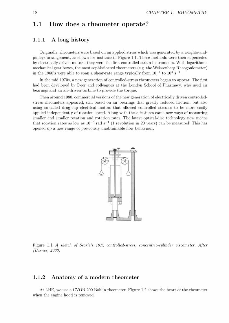
Originally, rheometers were based on an applied stress which was generated by a weights-and-pulleys arrangement, as shown for instance in Figure 1.1. These methods were then supersededby electrically driven motors; they were the first controlled-strain instruments. With logarithmicmechanical gear boxes, the most sophisticated rheometers (e.g. the Weissenberg Rheogoniometer)in the 1960’s were able to span a shear-rate range typically from 10−4 to 104 s−1.
In the mid 1970s, a new generation of controlled-stress rheometers began to appear. The firsthad been developed by Deer and colleagues at the London School of Pharmacy, who used airbearings and an air-driven turbine to provide the torque.
Then around 1980, commercial versions of the new generation of electrically driven controlled-stress rheometers appeared, still based on air bearings that greatly reduced friction, but alsousing so-called drag-cup electrical motors that allowed controlled stresses to be more easilyapplied independently of rotation speed. Along with these features came new ways of measuringsmaller and smaller rotation and rotation rates. The latest optical-disc technology now meansthat rotation rates as low as 10−8 rad s−1 (1 revolution in 20 years) can be measured! This hasopened up a new range of previously unobtainable flow behaviour.
Figure 1.1 A sketch of Searle’s 1912 controlled-stress, concentric-cylinder viscometer. After(Barnes, 2000)
1.1.2 Anatomy of a modern rheometer
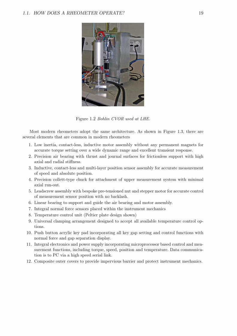
At LHE, we use a CVOR 200 Bohlin rheometer. Figure 1.2 shows the heart of the rheometerwhen the engine hood is removed.
1.1. HOW DOES A RHEOMETER OPERATE? 19
Figure 1.2 Bohlin CVOR used at LHE.
Most modern rheometers adopt the same architecture. As shown in Figure 1.3, there areseveral elements that are common in modern rheometers
1. Low inertia, contact-less, inductive motor assembly without any permanent magnets foraccurate torque setting over a wide dynamic range and excellent transient response.
2. Precision air bearing with thrust and journal surfaces for frictionless support with highaxial and radial stiffness.
3. Inductive, contact-less and multi-layer position sensor assembly for accurate measurementof speed and absolute position.
4. Precision collett-type chuck for attachment of upper measurement system with minimalaxial run-out.
5. Leadscrew assembly with bespoke pre-tensioned nut and stepper motor for accurate controlof measurement sensor position with no backlash.
6. Linear bearing to support and guide the air bearing and motor assembly.7. Integral normal force sensors placed within the instrument mechanics8. Temperature control unit (Peltier plate design shown)9. Universal clamping arrangement designed to accept all available temperature control op-
tions.10. Push button acrylic key pad incorporating all key gap setting and control functions with
normal force and gap separation display.11. Integral electronics and power supply incorporating microprocessor based control and mea-
surement functions, including torque, speed, position and temperature. Data communica-tion is to PC via a high speed serial link.
12. Composite outer covers to provide impervious barrier and protect instrument mechanics.

20 CHAPTER 1. RHEOMETRY
1
2
3
4
5
5
6
7
8
9
10
11
12
Figure 1.3 Bohlin CVOR used at LHE.

1.1. HOW DOES A RHEOMETER OPERATE? 21
1.1.3 Typical performance of modern lab rheometers
Modern rheometer capabilities include
– control on sample temperature;– quite a wide range of tools (parallel-plate, cone-plane, etc.);– wide shear-rate range (> 10 orders of magnitude);– directional (including reverse flow) and oscillatory flow;– high accuracy and resolution;– direct monitoring via a PC.
Here are the typical features of modern high-performance rheometer (Bohlin CVOR) :
– Torque range 0.05× 10−6200× 10−3 mN.m– Torque resolution 1× 10⁻⁹ Nm– Rotational-velocity range 1× 10⁻⁷ − 600 rad/s– Resolution in angular position 5× 10⁻⁸ rad– Frequency range 1× 10⁻⁵ − 150 Hz– Normal force range 1× 10⁻³ − 20 N
22 CHAPTER 1. RHEOMETRY
1.2 Principles of viscometry
1.2.1 Fundamentals of rheometry
Rheometry and viscometry
At the very beginning, the term rheometry referred to a set of standard techniques for mea-suring shear viscosity. Then, with the rapid increase of interest in non-Newtonian fluids, othertechniques for measuring the normal stresses and the elongational viscosity were developed. Vis-cometry is an important offshoot of rheometry, which applies to incompressible simple fluids.When the ‘simple-fluid’ approximation holds, it is possible to derive the flow curve and otherrheological functions (e.g., normal stress differences) from the geometrical measurements: torque,rotational velocity, and thrust.
Nowadays, rheometry is usually understood as the area encompassing any technique thatinvolves measuring mechanical or rheological properties of a material. This includes :
– visualization techniques (such as photoelasticimetry for displaying stress distribution wi-thin a sheared material);
– nonstandard methods (such as the slump test for evaluating the yield stress of a viscoplasticmaterial).
In most cases for applications, shear viscosity is the primary variable characterizing the behaviorof a fluid. Thus in the following, we will mainly address this issue, leaving aside all the problemsrelated to the measurement of elongational viscosity.
The basic principle of rheometry is to perform simple experiments where the flow characte-ristics such as the shear stress distribution and the velocity profile are known in advance and canbe imposed. Under these conditions, it is possible to infer the flow curve, that is, the variationof the shear stress as a function of the shear rate, from measurements of flow quantities such astorque and the rotational velocity for a rotational viscometer. In fact, despite its apparent sim-plicity, putting this principle into practice for natural or industrial fluids raises many issues thatwe will discuss below. Most rheometers rely on the achievement of viscometric flow (Colemanet al., 1966).
The simplest curvilinear flow is the simple shear flow achieved by shearing a fluid betweentwo plates in a way similar to Newton’s experiment depicted in Chap. 2. However, in practicemany problems (fluid recirculation, end effect, etc.) arise, which preclude using such a shearingbox to obtain accurate measurements. Another simple configuration consists of an inclined planeor a parallel-plate rheometer.
For many fluids of practical interest, viscometry is then an indispensable theory that under-pins rheometrical investigation by making a clear connection between bulk measurements andrheological data. We shall see later that an incompressible simple fluid is defined as follows:
1. only isochoric motions are permitted: bulk density is constant;2. the stress tensor σ is determined, to within a pressure term, by the history of the relative
deformation gradient 1 Fs = σ + p1 = F(F(t)),
with s the extra-stress tensor, p the pressure, σ the stress tensor, and F a tensor-valuedfunctional of F. Time is denoted by t. This expression is called the constitutive equationor rheological law.Some specific material classes can be defined (see Chap. 2):
– If the functional F involves the time derivative of F alone 2, the material is a fluid.
1. See Chap. 2 for further information.2. i.e., the strain-rate tensor d = − 1
2 (F + FT )
1.2. PRINCIPLES OF VISCOMETRY 23
– If the functional F does not involve the time derivative of F, the material is a solid.– If the functional F is a one-to-one function, then the fluid has no memory since the
stress depends on the current state of deformation alone.– If F is an integral function, then the fluid behavior is characterized by memory
effects: the stress state depends on the past states of deformation experienced by thematerial.
More complicated behaviors can be imagined, but the important point here is to recallthat a wide range of behavior can be described using this formulation. For instance, if Finvolves F and d, the material is said to be visco-elastic.
Viscometric flows
On many occasions, it is possible to create flows that induces a relative deformation gradientthat is linear with time, that is, the distance between two neighboring points varies linearly withtime (this distance may be zero) at any time and any point of the material. In this case, it canbe shown (Coleman et al., 1966) that
– There is a tensor M, which can be interpreted as the velocity gradient and the matrixrepresentation of which takes the form
M =
0 0 0γ 0 00 0 0
,
for some orthogonal basis B and such that the relative deformation gradient F is F(t) =R(t) · (1 − tM), where R is an arbitrary orthogonal tensor, which is a function of timeand satisfies R(0) = 1. In the basis B, the strain-rate and stress tensors takes the form
d =
0 γ 0γ 0 00 0 0
and σ =
σ11 σ12 0σ21 σ22 00 0 σ33
.
– In these expressions, γ is the shear rate and is assumed to a control parameter. If the fluidis a simple fluid, then there is a functional F such that
σ + p1 = F(M) = F(γ).
To get rid of the pressure term (which can be determined only by solving the equations ofmotion, thus does not reflect any rheological property, but only isochoric constraint), weintroduce
– the shear-stress function τ(γ) = σ21;– the first normal-stress difference N1 = σ11 − σ22;– the second normal-stress difference N2 = σ22 − σ33.
These functions are called material functions since they reflect the rheological behavior ofthe material tested.
If a flow satisfies these conditions, it is called viscometric. Two subclasses are particularly im-portant in practice:
– A simple shear flow is a particular case, where the shear rate is constant at any point anddoes vary with time. The Couette flow between two parallel, infinite, horizontal planesprovides a typical example.
– More generally, curvilinear flows can be seen a generalized variant of simple-shear flows:the shear rate is permitted to vary with position, but the deformation field remains steadyand two-dimensional for a certain basis.
24 CHAPTER 1. RHEOMETRY
Current geometries that allow realizing curvilinear flows are:
– simple shear flow: pressure-driven flow through parallel plates or gravity-driven flow downan inclined channel;
– vertical cylindrical tubes (Poiseuille flow): capillary rheometers;– torsional flows: cone-and-plate and parallel-plate rheometers;– helical flows such as flows between concentric cylinders (Couette flow): coaxial rheometers.
1.2.2 Flow down an inclined channel
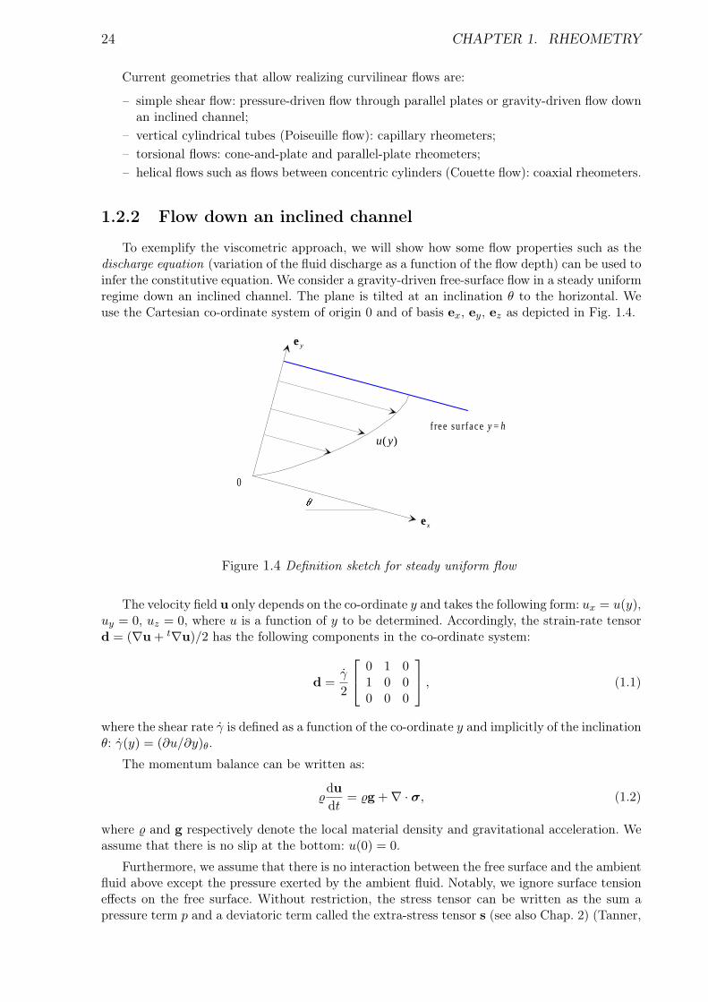
To exemplify the viscometric approach, we will show how some flow properties such as thedischarge equation (variation of the fluid discharge as a function of the flow depth) can be used toinfer the constitutive equation. We consider a gravity-driven free-surface flow in a steady uniformregime down an inclined channel. The plane is tilted at an inclination θ to the horizontal. Weuse the Cartesian co-ordinate system of origin 0 and of basis ex, ey, ez as depicted in Fig. 1.4.
f ree su rface y = h( )u y
0
xe
ye
Figure 1.4 Definition sketch for steady uniform flow
The velocity field u only depends on the co-ordinate y and takes the following form: ux = u(y),uy = 0, uz = 0, where u is a function of y to be determined. Accordingly, the strain-rate tensord = (∇u + t∇u)/2 has the following components in the co-ordinate system:
d =γ
2
0 1 01 0 00 0 0
, (1.1)
where the shear rate γ is defined as a function of the co-ordinate y and implicitly of the inclinationθ: γ(y) = (∂u/∂y)θ.
The momentum balance can be written as:
%dudt
= %g +∇ · σ, (1.2)
where % and g respectively denote the local material density and gravitational acceleration. Weassume that there is no slip at the bottom: u(0) = 0.
Furthermore, we assume that there is no interaction between the free surface and the ambientfluid above except the pressure exerted by the ambient fluid. Notably, we ignore surface tensioneffects on the free surface. Without restriction, the stress tensor can be written as the sum apressure term p and a deviatoric term called the extra-stress tensor s (see also Chap. 2) (Tanner,
1.2. PRINCIPLES OF VISCOMETRY 25
1988; Coleman et al., 1966): σ = −p1 + s. For a homogeneous and isotropic simple fluid, theextra-stress tensor depends on the strain rate only: s = G(d), where G is a tensor-valued isotropicfunctional. In the present case, it is straightforward to show that the stress tensor must have theform
σ = −p1 +
sxx sxy 0sxy syy 00 0 szz
. (1.3)
Thus, the stress tensor is fully characterized by three functions:
– the shear stress τ = σxy = sxy
– the normal stress differences: N1 = sxx−syy and N2 = syy−szz called the first and secondnormal stress differences, respectively.
Since for steady flows acceleration vanishes and the components of s only depend on y, theequations of motion (1.2) reduce to
0 =∂sxy
∂y− ∂p
∂x+ %g sin θ, (1.4)
0 =∂syy
∂y− ∂p
∂y− %g cos θ, (1.5)
0 =∂p
∂z. (1.6)
It follows from (1.6) that the pressure p is independent of z. Accordingly, integrating (1.5) betweeny and h imply that p must be written: p(x,y)− p(x,h) = syy(y)− syy(h) + %g(h− y) cos θ. It ispossible to express Eq. (1.4) in the following form:
∂
∂y(sxy + %gy sin θ) =
∂p(x,h)∂x
. (1.7)
This is possible only if both terms of this equation are equal to a function of z, whichwe denote b(z). Moreover, Eq. (1.6) implies that b(z) is actually independent of z; thus, in thefollowing we will note: b(z) = b. The solutions to (1.7) are: p (x,h) = bx+c, where c is a constant,and sxy(h) − sxy(y) + %g(h − y) sin θ = b(h − y), which we will determine. To that end, let usconsider the free surface. It is reasonable and usual to assume that the ambient fluid frictionis negligible. The stress continuity at the interface implies that the ambient fluid pressure p0
exerted on an elementary surface at y = h (oriented by ey) must equal the stress exerted by thefluid. Henceforth, the boundary conditions at the free surface may be expressed as: −p0ey = σey,which implies in turn that: sxy(h) = 0 and p0 = p(x,h)− syy(h). Comparing these equations toformer forms leads to b = 0 and c = p0 +syy(h). Accordingly, we obtain for the shear and normalstress distributions
τ = %g(h− y) sin θ, (1.8)
σyy = syy − (p− p0) = −%g(h− y) cos θ. (1.9)
The shear and normal stress profiles are determined regardless of the form of the constitutiveequation. For simple fluids, the shear stress is a one-to-one function of the shear rate: τ = f(γ).Using the shear stress distribution (1.8) and the inverse function f−1, we find: γ = f−1(τ). Adouble integration leads to the flow rate (per unit width):
q =∫ h
0
∫ y
0f−1(τ(ξ))dξ =
h∫
0
u(y)dy. (1.10)
26 CHAPTER 1. RHEOMETRY
An integration by parts leads to:
q(h, θ) = [(y − h)u(y)]h0 +
h∫
0
(h− y)(
∂u
∂y
)
θ
dy.
In this equation, the first expression of the right-hand term is hug if the slip condition at thebottom is relaxed. Making use of the shear stress equation leads to
q(h,θ) = hug +
h∫
0
(h− y)f (%g sin θ(h− y)) dy
By making the variable change: ζ = h− y, we also obtain
q(h,θ) =
h∫
0
ζf (%g sin θυ) dζ + hug.
Thus the partial derivative of q with respect to h (at a given channel slope θ) is(
∂q
∂h
)
θ
= hf(%gh sin θ) + ug + h
(∂ug
∂h
)
θ
,
or equivalently
f(τp) =1h
(∂q
∂h
)
θ
− ug
h−
(∂ug
∂h
)
θ
.
where τp = %g sin θ is the bottom shear shear. In the case (often encountered) of no-slip, thisexpression reduces to
γ = f−1(τ(h)) =1h
(∂q
∂h
)
θ
. (1.11)
This relation allows us to directly use a channel as a rheometer.
The other normal components of the stress tensor cannot be easily measured. The curvature ofthe free surface of a channelled flow may give some indication of the first normal stress difference.Let us imagine the case where it is not equal to zero. Substituting the normal component syy bysyy = sxx −N1 in (1.5), after integration we find:
sxx = p + %gy cos θ + N1 + c, (1.12)
where c is a constant. Imagine that a flow section is isolated from the rest of the flow and theadjacent parts are removed. In order to hold the free surface flat (it will be given by the equationy = h, ∀z), the normal component σxx must vary and balance the variations of N1 due to thepresence of the sidewalls (for a given depth, the shear rate is higher in the vicinity of the wallthan in the center). But at the free surface, the boundary condition forces the normal stress σxx
to vanish and the free surface to bulge out. To first order, the free surface equation is:
−%gy cos θ = N1 + c. (1.13)
If the first normal stress difference vanishes, the boundary condition −p0ey = σey is automati-cally satisfied and the free surface is flat. In the case where the first normal stress difference doesnot depend on the shear rate, there is no curvature of the shear free surface. The observationof the free surface may be seen as a practical test to examine the existence and sign of the firstnormal stress difference and to quantify it by measuring both the velocity profile at the freesurface and the free-surface equation.
1.2. PRINCIPLES OF VISCOMETRY 27
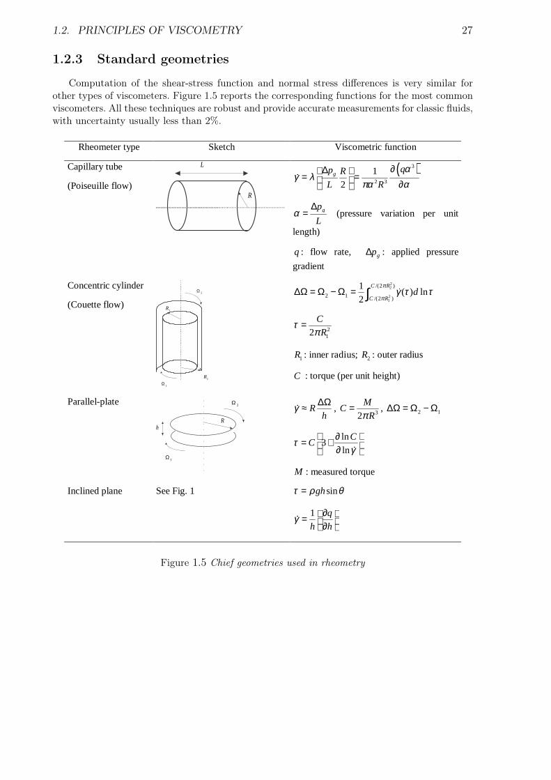
1.2.3 Standard geometries
Computation of the shear-stress function and normal stress differences is very similar forother types of viscometers. Figure 1.5 reports the corresponding functions for the most commonviscometers. All these techniques are robust and provide accurate measurements for classic fluids,with uncertainty usually less than 2%.
Rheometer type Sketch Viscometric function
Capillary tube
(Poiseuille flow)
L
R
( )3
2 3
1
2g
qp R
L R
αγ λ
πα α∂∆ = = ∂
gp
Lα
∆= (pressure variation per unit
length)
q : flow rate, gp∆ : applied pressure
gradient
Concentric cylinder
(Couette flow)1R
2R
2Ω
1Ω
22
21
/(2 )
2 1 /(2 )
1( ) ln
2
C R
C Rd
π
πγ τ τ∆Ω = Ω − Ω = ∫
212
C
Rτ
π=
1R : inner radius; 2R : outer radius
C : torque (per unit height)
Parallel-plate
R
1Ω
2Ω
h
Rh
γ ∆Ω≈, 32
MC
Rπ= , 2 1∆Ω = Ω − Ω
ln3
ln
CCτ
γ ∂= + ∂
M : measured torque
Inclined plane See Fig. 1 singhτ ρ θ=
1 q
h hγ ∂ = ∂
Figure 1.5 Chief geometries used in rheometry
28 CHAPTER 1. RHEOMETRY
1.3 Inverse problems in rheometry
1.3.1 A typical example: the Couette problem
A longstanding problem in rheometry is the so-called Couette inverse problem, in which onetries to derive the flow curve τ(γ) from the torque measurements M(ω) in a coaxial cylinder(Couette) rheometer, where τ is the shear stress, γ denotes the shear rate, ω is the rotationalvelocity of the inner cylinder, and M represents the torque per unit height (Coleman et al.,1966). The shear stress τ exerted on the inner cylinder of radius R1 can be directly related tothe measured torque M by τ = α1M , with α1 = 1/(2πR2
1), independently of the form of theconstitutive equation. The shear rate is related to the rotational velocity ω by
ω =∫ R2
R1
γ(r)r
dr, (1.14)
where R2 denotes the outer-cylinder radius and it is assumed that (i) the rotational velocity ofthe outer cylinder is zero and (ii) there is no slip between the inner cylinder and the shearedmaterial at r = R1. In order to recover the flow curve from measurements of the rotationalvelocity ω(M), one must be able to
(i) relate the function γ(r) to τ(r),(ii) find out a means of inverting the integral relationship (1.14),(iii) estimate the continuous function γ(τ) from a set of discrete values (ωi, Mi).
For a broad class of fluids (simple fluids), the first step is systematically achieved since thereis a one-to-one relation between the shear stress and the shear rate for steady viscometric flows:γ = γ(τ). Moreover, the momentum equations imply that the shear stress distribution across thegap is given by S(r) = M/(2πr2) = τ(R1/r)2, where r denotes the distance from the verticalrotation axis of the cylinders. Under these conditions, which are not too stringent, it is possibleto make the variable change r = R1
√τ/S in the integral above; we then derive the well-known
equation (Krieger & Elrod, 1953; Coleman et al., 1966)
ω(τ) =12
∫ τ
βτ
γ(S)S
dS, (1.15)
where β = (R1/R2)2. The next step is to recover γ from ω(τ).
1.3.2 Earlier attempts at solving the Couette problem
Scientific statement and mathematical strategies
In the Couette inverse problem, Eq. (1.15) can be represented in the generic form: ω(τ) =(Kγ)(τ), where K is the integral operator
(Kf)(z) =∫ z
βz
f(x)x
dx, (1.16)
with β a constant parameter (β < 1). A considerable body of literature has been publishedover the last three decades on ill-posed inverse problems in this form (Bertero et al., 1985, 1988;O’Sullivan, 1986; Tenorio, 2001). Schematically, we can split the various methods for solving
1.3. INVERSE PROBLEMS IN RHEOMETRY 29
Couette-like problems into three main categories 3.
– Least-square approach: instead of solving ω = Kγ, an attempt is made to minimize theresidual ||ω−Kγ||, usually with an additional constraint on the norm of ||f || or its deriva-tive(s), to control the smoothness of the solution. Tikhonov’s regularization method usedby Yeow et al. (2000) and Landweber’s iterative procedure used by Tanner & Williams(1970) come within this category. The advantages of this method are its robustness againstcomputation inaccuracies and measurement errors, its versatility, its fast convergence whenthe function to be recovered behaves reasonably well, and the relative facility of its imple-mentation. The drawbacks are that it relies on an arbitrary selection of the regularizationoperator (even though specific procedures have been established) and its limited capacityto retrieve irregular functions.
– Projection approach: the idea here is to discretize the problem by projecting the functionover a finite space spanned by a family of functions enjoying specific properties (such asorthogonality) ui. Equation (1.15) is then replaced by the finite set of equations 〈Kγ, ui〉 =〈ω, ui〉 for 1 ≤ i ≤ p, where 〈f, g〉 =
∫R f(x)g(x)dx denotes the inner product in the
function space (Dicken & Maass, 1996; Louis et al., 1997; Rieder, 1997). Galerkin’s method,used by Macsporran (1989) with spline functions, provides a typical example for Couetterheometry. Irregular functions can be recovered by these methods provided appropriateprojection functions are chosen in advance.
– Adjoint operator approach: for many reasons, it is usually either not possible or not ad-vantageous to compute the inverse operator K−1. In some cases, however, it is possible toprovide a weak inverse formulation, in which the function γ is expressed as
γ =∑
i∈J
〈Kγ, ui〉Ψi,
where the summation is made over a set J , Ψi is an orthonormal basis of functions, and ui
denotes a family of function solutions of the adjoint problem K∗ui = Ψi, where K∗ is theadjoint operator of K (Golberg, 1979). Typical examples include singular-value decomposi-tion (Bertero et al., 1985, 1988), a generalized formulation based on reconstruction kernels(Louis, 1999), wavelet-vaguelette decomposition (Donoho, 1995), and vaguelette-wavelet de-composition (Abramovich & Silverman, 1998). The solution to the inverse problem is foundby replacing Kγ with ω in the equation above and filtering or smoothing the inner products〈Kγ, ui〉 and/or truncating the sum.
Mooney’s and Krieger’s approximation
Although the Couette problem admits an analytical theoretical solution in the form of aninfinite series (Coleman et al., 1966), deriving the shear rate remains a difficult task in practicebecause the derivation enters the class of ill-posed problems (Friedrich et al., 1996). In rheometry,the first attempt at solving Eq. (1.15) can be attributed to Mooney (1931), Krieger & Maron(1952), and Krieger & Elrod (1953). When β is close to unity, it is possible to directly approximatethe integral to the first order by
ω(τ) =1− β
2γ(τ) + o(βγ).
3. This partitioning is a bit arbitrary because there are interconnections between the three categories[e.g., Tikhonov’s regularization can be viewed as a special case of singular-value decomposition (Berteroet al., 1988)]. This is, however, sufficient in the present paper to outline the main approaches used so farand to situate the previous attempts at solving the Couette problem. Alternative methods, e.g., stochasticmethods (Gamboa & Gassiat, 1997; Mosegaard & Sambridge, 2002), are also possible, but have neverbeen used in rheometry as far as we know.
30 CHAPTER 1. RHEOMETRY
When β moves away from unity, further terms are needed in the expansion of the integralinto a β series. One of the most common approximations is attributed to Krieger who proposedfor Newtonian and power-law fluids (Yang & Krieger, 1978; Krieger, 1968):
γ =2Ω(1 + α)
1− βff, (1.17)
with
f =d ln Ωd lnC
, α =f ′
f2χ1(−f log β), and χ1(x) =
x
2(xex − 2ex + x + 2)(ex − 1)−2.
However, this method can give poor results with yield stress fluids, especially if it is partiallysheared within the gap. In this case, Nguyen & Boger (1992) have proposed using
γ = 2Ωd ln Ωd ln C
.
A few rheologists used an alternative consisting of an expansion into a power series of (1.15).They obtained:
γ = 2Ω∑∞
n=0f
(βnC/(2πR2
1)).
Although refined to achieve higher accuracy (Yang & Krieger, 1978), Krieger’s approach wasunable to provide reliable results for viscoplastic flows (Darby, 1985; Nguyen & Boger, 1992) orfor data contaminated by noise (Borgia & Spera, 1990).
Tikhonov’s regularization technique
Alternative methods have been proposed: Tanner & Williams (1970) developed an iterativeprocedure, whereas Macsporran (1989), Yeow et al. (2000), and Leong & Yeow (2003) used aregularized least-square approach, which involves discretizing the integral term and regularizingit.
These methods are very efficient for a wide range of well-behaved rheological equations.However, when the rheological behavior exhibits singularities such as a yield stress or a rapidshear-thickening, the regularization procedure can lead to unrealistic results by smoothing outthe singularities or to complicated trial-and-error loops. For instance, when testing Tikhonov’smethod with viscoplastic flows, Yeow et al. (2000) had to evaluate the yield stress iteratively,which may involve a large number of computations and slow convergence. This undesired behavioris to a large extent the result of attempting to evaluate a continuous function (γ(τ)) from a finiteset of discrete values representing measurements of bulk quantities. This task is more delicatethan believed, especially when data are noisy. For a well-behaved rheological equation, imposinga certain degree of smoothness in the regularization procedures does not entail many problems.On the contrary, for complex rheological responses, it becomes increasingly difficult to discerngenuine rheological properties, noise effects, and discretization errors.
1.3.3 The wavelet-vaguelette decomposition
We will begin by exposing the principle in a very simple manner. A more rigorous mathema-tical derivation follows in the Appendix. Let us assume that we can approximate any shear ratefunction γ(τ) with a finite series of terms
γ(τ) ≈∑
k
akΨk(τ),
1.3. INVERSE PROBLEMS IN RHEOMETRY 31
where Ψk denotes the kth member of a family of orthogonal functions, i.e.,∫
Ψk(τ)Ψi(τ)dτ = δik;making use of this property, we could compute the coefficients ak as ak =
∫γ(τ)Ψi(τ)dτ if the
function γ(τ) were known.
Using the linearity of the integral operator K, we have
ω(τ) = (Kγ)(τ) ≈∑
k
ak (KΨk)(τ).
Note that the function ω(τ) shares the same coefficients ak as the shear-rate function, implyingthat if we were able to expand ω(τ) into a (KΨk) series, we could determine the coefficients ak,then find an approximation of γ(τ).
Unfortunately, the functions (KΨk)(τ) are not orthogonal, making it difficult to numericallycompute ak. Specific procedures such as the Schmidt orthogonalization procedure could be used toderive an orthogonal family of functions from (KΨk)(τ), but here this involves overly complicatedcomputations. We will envisage another technique based on dual bases. A dual basis of thefunction basis Ψk is a set of functions ui such that
∫ui(τ)(KΨk)(τ)dτ = δik, implying that
ak =∫
ω(τ)uk(τ)dτ . Therefore the crux of the issue lies in the derivation of the dual basis uk.In the following, we will show that the functions uk can be built from the functions Ψi.
1.3.4 Practical example
Baudez et al. (2004) investigated the rheological properties of a polymeric suspension (com-mercial hair gel made of Carbopol) using a stress-controlled Paar Physica MC1+ rheometerequipped with a Couette geometry (R1 = 1.25 cm and β = 0.26). In addition they carried outvelocity-profile measurements in a similar geometry (R1 = 4 cm and β = 0.44) using magneticresonance imaging (MRI) techniques. Further rheometrical tests were also done with a BohlinCVOR200 rheometer (R1 = 0.0125 cm and β = 0.06). Carbopol suspensions usually exhibit aviscoplastic behavior (Roberts & Barnes, 2001). MRI techniques made it possible to obtain anaccurate estimation of the flow curve and then to compare the different methods.
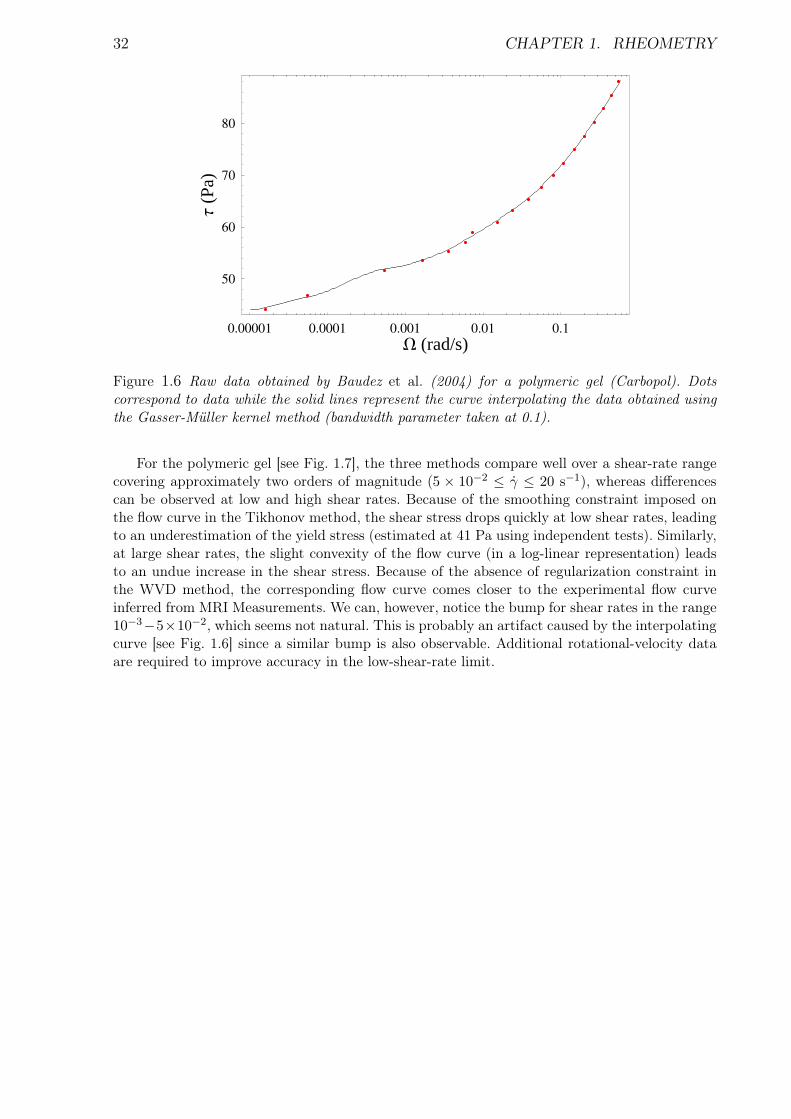
The data obtained by Baudez et al. (2004) are reported in a log-linear plot in Fig. 1.6. Theywere slightly noisy and a specific procedure was used to denoise and interpolate the raw data.Different nonparametric regression techniques can be used for this purpose: kernel estimator(Hart, 1999), spline smoothing (Wahba, 1990), Fourier series estimator, wavelet regression andshrinkage (Donoho & Johnstone, 1995; Kovac, 1998; Cai, 1999, 2002), Bayesian inference (Wer-man & Keren, 2001), etc. There is not a universal method because, depending on the noise level,the number of data, and the properties of the function to be recovered, the performance of eachmethod in terms of denoising efficiency can vary significantly. Here, because of the small sizeof the data samples, the optimized Gasser-Müller kernel method (included in the Mathematicapackage) was used to denoise and interpolate the data [for details in the implementation, see(Hart, 1999)]. The resulting interpolating curves are plotted in Fig. 1.6.
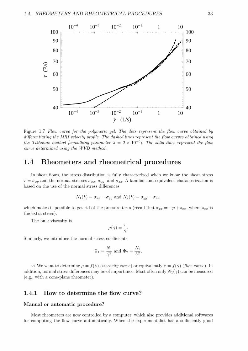
Figure 1.7 shows the flow curves deduced by the Tikhonov regularization method (dashedline) and the wavelet-vaguelette decomposition method (solid line) for the polymeric gel. Forthe Tikhonov method, we used the method described in (Yeow et al., 2000) with nk = 400discretization points and a smoothing parameter λ = 2 × 10⁻⁶ and 5 × 10⁻⁶. For the WVDmethod, Daubechies D8 wavelet and the functional formulation were used.
For the polymeric gel, it was possible to independently obtain a reference flow curve byusing the velocity profile determined by Baudez et al. (2004) using MRI techniques. Indeed, ina Couette geometry, the shear stress distribution across the gap is imposed: τ(r) = M/(2πr2);the shear rate can be computed by differentiating the velocity profile v(r): γ(r) = −r∂(v/r)/∂r.Reporting a parametric plot (γ(r), τ(r)) as a function of the radial distance r makes it possibleto have a clearer idea on the flow curve for the material tested. The dots in Fig. 1.7 representthe flow curve determined in this way.
32 CHAPTER 1. RHEOMETRY
0.00001 0.0001 0.001 0.01 0.1
W (rad/s)
50
60
70
80
Τ(P
a)
Figure 1.6 Raw data obtained by Baudez et al. (2004) for a polymeric gel (Carbopol). Dotscorrespond to data while the solid lines represent the curve interpolating the data obtained usingthe Gasser-Müller kernel method (bandwidth parameter taken at 0.1).
For the polymeric gel [see Fig. 1.7], the three methods compare well over a shear-rate rangecovering approximately two orders of magnitude (5 × 10⁻² ≤ γ ≤ 20 s−1), whereas differencescan be observed at low and high shear rates. Because of the smoothing constraint imposed onthe flow curve in the Tikhonov method, the shear stress drops quickly at low shear rates, leadingto an underestimation of the yield stress (estimated at 41 Pa using independent tests). Similarly,at large shear rates, the slight convexity of the flow curve (in a log-linear representation) leadsto an undue increase in the shear stress. Because of the absence of regularization constraint inthe WVD method, the corresponding flow curve comes closer to the experimental flow curveinferred from MRI Measurements. We can, however, notice the bump for shear rates in the range10−3−5×10⁻², which seems not natural. This is probably an artifact caused by the interpolatingcurve [see Fig. 1.6] since a similar bump is also observable. Additional rotational-velocity dataare required to improve accuracy in the low-shear-rate limit.
1.4. RHEOMETERS AND RHEOMETRICAL PROCEDURES 33
10-1
10-2
10-3
10-4
1 10
Γ. (1/s)
40
50
60
70
80
90
100
Τ(P
a)
10-1
10-2
10-3
10-4
1 10
40
50
60
70
80
90
100
Figure 1.7 Flow curve for the polymeric gel. The dots represent the flow curve obtained bydifferentiating the MRI velocity profile. The dashed lines represent the flow curves obtained usingthe Tikhonov method [smoothing parameter λ = 2 × 10⁻⁶]. The solid lines represent the flowcurve determined using the WVD method.
1.4 Rheometers and rheometrical procedures
In shear flows, the stress distribution is fully characterized when we know the shear stressτ = σxy and the normal stresses σxx, σyy, and σzz. A familiar and equivalent characterization isbased on the use of the normal stress differences
N1(γ) = σxx − σyy and N2(γ) = σyy − σzz,
which makes it possible to get rid of the pressure term (recall that σxx = −p + sxx, where sxx isthe extra stress).
The bulk viscosity isµ(γ) =
τ
γ.
Similarly, we introduce the normal-stress coefficients
Ψ1 =N1
γ2and Ψ2 =
N2
γ2.
à We want to determine µ = f(γ) (viscosity curve) or equivalently τ = f(γ) (flow curve). Inaddition, normal stress differences may be of importance. Most often only N1(γ) can be measured(e;g., with a cone-plane rheometer).
1.4.1 How to determine the flow curve?
Manual or automatic procedure?
Most rheometers are now controlled by a computer, which also provides additional softwaresfor computing the flow curve automatically. When the experimentalist has a sufficiently good
34 CHAPTER 1. RHEOMETRY
knowledge of the rheological properties of the material tested and the viscometric geometry usedin the testing is standard, these softwares are very helpful.
For complex materials or for non-standard geometries, it is usually better to directly extractthe measurement data (torque, rotational velocity) and use specific methods to determine theflow curves, which makes it possible:
– to use a specific experimental protocole in data acquisition or processing;– to modify the data to take disturbing phenomena into account;– to obtain more accurate solutions (e.g., in the inverse problem for wide-gap rheometers,
by controlling the smoothness of the solution sought).
For complex fluids (the general case for natural fluids studied in geophysics and in industry),rheometry is far from being an ensemble of simple and ready-for-use techniques. On the contrary,investigating the rheological properties of a material generally requires many trials using differentrheometers and procedures. In some cases, visualization techniques (such as nuclear magnetic re-sonance imagery, transparent interstitial fluid and tools, birefringence techniques) may be helpfulto monitor microstructure changes.
How to measure the flow curve?
In most modern rheometers, the standard technique involves imposing a step-like ramp, i.e.,a succession of stress steps (respectively, strain steps), and measuring the resulting deformation(respectively, stress). It is difficult to prescribe the duration of each step in advance because itbasically depends on how quickly the material reaches its steady state.
Plotting the data
The data obtained by using a rheometer usually cover a wide range of shear rate, typically3 or more orders of magnitude. For this reason, it is usually recommended to plot the data on alogarithmic basis. When the data are plotted, different things can be done:
– simple mathematical expressions can be fitted to the data, e.g., a power-law relation:τ = Kγn ;
– a yield stress can be evaluated by extrapolating the experimental curve to γ = 0 and givean apparent intercept on the τ -axis that can be interpreted as a yield stress.
Note that the flow curve τ = f(γ) can be plotted as:
– shear stress as a function of shear rate– bulk viscosity µ = τ/γ as a function of shear rate
Recall that the units used in viscometry are the following
– strain in %– stress in Pascal [Pa] 1 Pa = kg×m2×s−2
– shear rate in 1/s (and not Hertz)– dynamical viscosity µ in [Pa.s] 1 Pa.s = kg×m2×s−1 (avoid Poise, centiPoise, etc.)– density % in [kg/m3]– dynamical viscosity ν = µ/% in [m2/s] (avoid Stokes, centiStokes [cS], etc.)
1.4.2 Stress/strain step
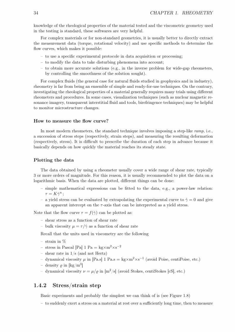
Basic experiments and probably the simplest we can think of is (see Figure 1.8)
– to suddenly exert a stress on a material at rest over a sufficiently long time, then to measure
1.4. RHEOMETERS AND RHEOMETRICAL PROCEDURES 35
the strain output after flow cessation: recovery test.
– to suddenly exert a stress on a material at rest over a sufficiently long time, then to measurethe strain output after flow inception: creep test.
– to suddenly impose a steady shear flow, then to monitor the stress variation with time todetermine how the shear stress reaches its steady value: stress growth test.
– to suddenly impose a steady shear flow, keep it constant over a given time interval, thencease the flow and monitor the stress variation with time after flow cessation (fluid at rest):stress relaxation test.
– to realize a steady shear flow over a given time interval, then remove the shear stressand monitor the strain variation with time: constrained recoil test. A viscoelastic materialrecoils because of elasticity, whereas a Newtonian fluid stops immediately.
γ
t
τ
0τ
(a) (b)
0γ
t
τ
0τ
(c)(d)
γ
0γ
fluid at rest
fluid at rest fluid at rest
fluid at rest
Figure 1.8 Basic tests: (a) Creep. (b) Stress relaxation. (c) Recovery. (d) Stress growth.
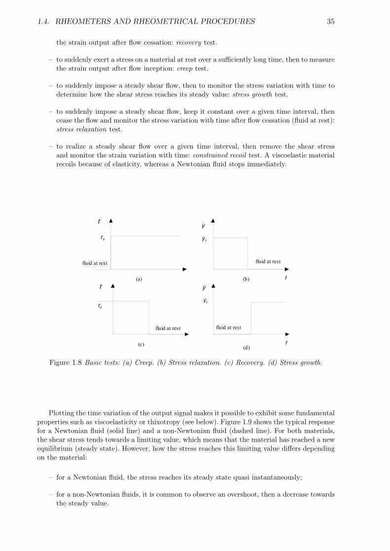
Plotting the time variation of the output signal makes it possible to exhibit some fundamentalproperties such as viscoelasticity or thixotropy (see below). Figure 1.9 shows the typical responsefor a Newtonian fluid (solid line) and a non-Newtonian fluid (dashed line). For both materials,the shear stress tends towards a limiting value, which means that the material has reached a newequilibrium (steady state). However, how the stress reaches this limiting value differs dependingon the material:
– for a Newtonian fluid, the stress reaches its steady state quasi instantaneously;
– for a non-Newtonian fluids, it is common to observe an overshoot, then a decrease towardsthe steady value.
36 CHAPTER 1. RHEOMETRY
τ
t
γ
eqτ
0γ
(a)
(b)
Figure 1.9 Stress growth: shear rate imposed at t = 0 and stress response measured upon flowinception. (a) Input: constant shear rate imposed at t = 0. (b) Output: time variation of τmonitored upon flow inception. How the shear stress reaches the steady-state value τeq dependson the rheological properties: the typical response of a Newtonian fluid (solid line) and a visco-elastic material (dashed line) is depicted.
For a non-Newtonian fluid, the overshoot can be understood as follows: when the material hasa structure on the microscopic scale (e.g., polymers connection, particle network, etc.), deformingthe material implies that the structure must be re-organized, e.g., by breaking contacts betweenparticles in close contact for a suspension: more energy must be provided to the system for it toreach a new equilibrium. For a thixotropic material, the time needed to reach this equilibriumdepends on the previous states (intensity of the shear rate, duration of the resting procedure).
1.5. TYPICAL RHEOLOGICAL BEHAVIORS 37
1.5 Typical rheological behaviors
1.5.1 Outlining a flow curve
The flow curve is the relation between the shear rate γ and shear stress τ established fromexperimental measurements taken in a viscometric flow (i.e., meaning that a simple shear flowwas realized by appropriate means and that we are able to derive the γ − τ curve). On manyoccasions, the flow curve is represented in the form
µ =τ
γ= f(γ),
where f is a function that we want to characterize.
1.5.2 Shear-thinning/thickening
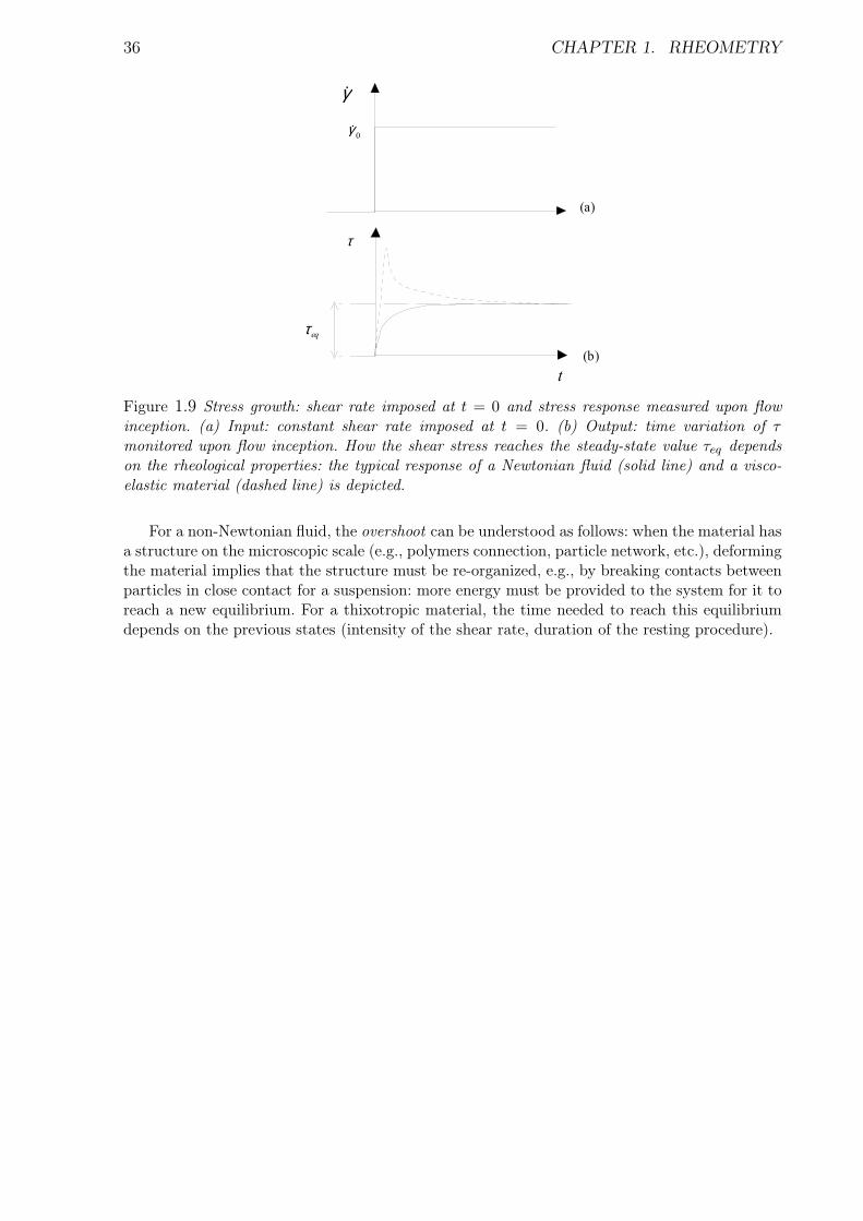
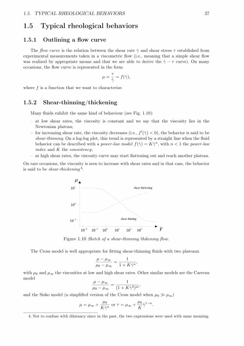
Many fluids exhibit the same kind of behaviour (see Fig. 1.10):
– at low shear rates, the viscosity is constant and we say that the viscosity lies in theNewtonian plateau;
– for increasing shear rate, the viscosity decreases (i.e., f ′(γ) < 0), the behavior is said to beshear-thinning. On a log-log plot, this trend is represented by a straight line when the fluidbehavior can be described with a power-law model f(γ) = Kγn, with n < 1 the power-lawindex and K the consistency ;
– at high shear rates, the viscosity curve may start flattening out and reach another plateau.
On rare occasions, the viscosity is seen to increase with shear rates and in that case, the behavioris said to be shear-thickening 4.
µ
γ110
− 010
210
310
110
210
−
110−
010
110
shear thinning
shear thickening
Figure 1.10 Sketch of a shear-thinning/thikening flow.
The Cross model is well appropriate for fitting shear-thinning fluids with two plateaux
µ− µ∞µ0 − µ∞
=1
1 + Kγn,
with µ0 and µ∞ the viscosities at low and high shear rates. Other similar models are the Carreaumodel
µ− µ∞µ0 − µ∞
=1
(1 + Kγ2)m,
and the Sisko model (a simplified version of the Cross model when µ0 À µ∞)
µ = µ∞ +µ0
Kγnor τ = µ∞ +
µ0
Kγ1−n.
4. Not to confuse with dilatancy since in the past, the two expressions were used with same meaning.
38 CHAPTER 1. RHEOMETRY
1.5.3 Yield stress
Definition
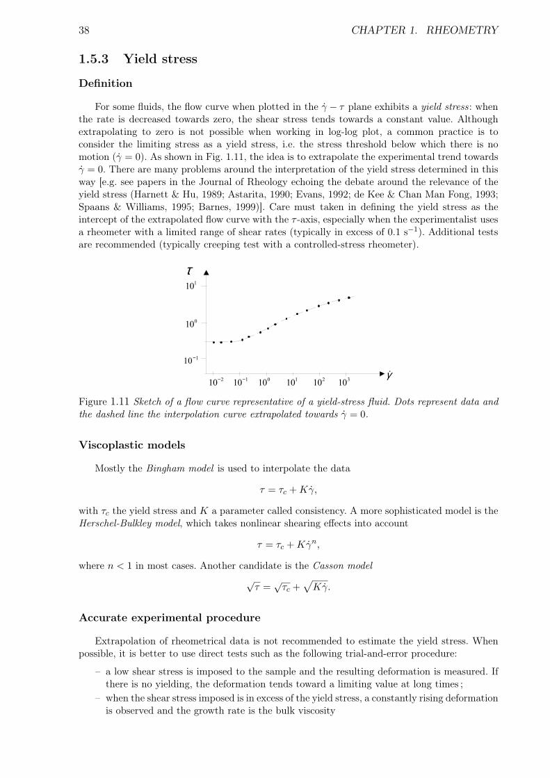
For some fluids, the flow curve when plotted in the γ − τ plane exhibits a yield stress: whenthe rate is decreased towards zero, the shear stress tends towards a constant value. Althoughextrapolating to zero is not possible when working in log-log plot, a common practice is toconsider the limiting stress as a yield stress, i.e. the stress threshold below which there is nomotion (γ = 0). As shown in Fig. 1.11, the idea is to extrapolate the experimental trend towardsγ = 0. There are many problems around the interpretation of the yield stress determined in thisway [e.g. see papers in the Journal of Rheology echoing the debate around the relevance of theyield stress (Harnett & Hu, 1989; Astarita, 1990; Evans, 1992; de Kee & Chan Man Fong, 1993;Spaans & Williams, 1995; Barnes, 1999)]. Care must taken in defining the yield stress as theintercept of the extrapolated flow curve with the τ -axis, especially when the experimentalist usesa rheometer with a limited range of shear rates (typically in excess of 0.1 s−1). Additional testsare recommended (typically creeping test with a controlled-stress rheometer).
τ
γ1
10− 0
102
103
101
102
10−
110
−
010
110
Figure 1.11 Sketch of a flow curve representative of a yield-stress fluid. Dots represent data andthe dashed line the interpolation curve extrapolated towards γ = 0.
Viscoplastic models
Mostly the Bingham model is used to interpolate the data
τ = τc + Kγ,
with τc the yield stress and K a parameter called consistency. A more sophisticated model is theHerschel-Bulkley model, which takes nonlinear shearing effects into account
τ = τc + Kγn,
where n < 1 in most cases. Another candidate is the Casson model√
τ =√
τc +√
Kγ.
Accurate experimental procedure
Extrapolation of rheometrical data is not recommended to estimate the yield stress. Whenpossible, it is better to use direct tests such as the following trial-and-error procedure:
– a low shear stress is imposed to the sample and the resulting deformation is measured. Ifthere is no yielding, the deformation tends toward a limiting value at long times ;
– when the shear stress imposed is in excess of the yield stress, a constantly rising deformationis observed and the growth rate is the bulk viscosity
1.5. TYPICAL RHEOLOGICAL BEHAVIORS 39
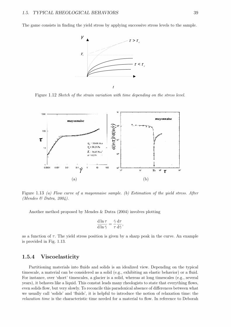
The game consists in finding the yield stress by applying successive stress levels to the sample.
γ
cγ
t
cτ τ<
cτ τ>
Figure 1.12 Sketch of the strain variation with time depending on the stress level.
(a) (b)
Figure 1.13 (a) Flow curve of a mayonnaise sample. (b) Estimation of the yield stress. After(Mendes & Dutra, 2004).
Another method proposed by Mendes & Dutra (2004) involves plotting
d ln τ
d ln γ=
γ
τ
dτ
dγ,
as a function of τ . The yield stress position is given by a sharp peak in the curve. An exampleis provided in Fig. 1.13.
1.5.4 Viscoelasticity
Partitioning materials into fluids and solids is an idealized view. Depending on the typicaltimescale, a material can be considered as a solid (e.g., exhibiting an elastic behavior) or a fluid.For instance, over ‘short’ timescales, a glacier is a solid, whereas at long timescales (e.g., severalyears), it behaves like a liquid. This constat leads many rheologists to state that everything flows,even solids flow, but very slowly. To reconcile this paradoxical absence of differences between whatwe usually call ‘solids’ and ‘fluids’, it is helpful to introduce the notion of relaxation time: therelaxation time is the characteristic time needed for a material to flow. In reference to Deborah
40 CHAPTER 1. RHEOMETRY
in the Bible, rheologists also introduce the Deborah number, which is the ratio between thecharacteristic time/duration of an observation/experiment tobs. and the relaxation time tr
De =tobs.
tr.
When De ¿ 1, the observer/experimentalist has not the time to register any fluid/creep motionand the material behavior can be considered as solid. When De À 1, the material has time torelax and modify its structure as a response to the applied forces; the material behaves like afluid.
Using this definition and using usual timescales for observation/experiments, most materialsbelong to either the solid or fluid classes. However, for some materials, the Deborah numberis of order of unity, which means that the material can exhibit both solid and fluid properties.Viscoelasticity is a typical trait of materials exhibiting fluid/solid properties.
Linear viscoelasticity
In most textbooks and courses on rheology, the simplest way to introduce the notion ofviscoelasticity is to make use of analogies with simple mechanical models consisting of springs(elastic behavior) and dashpot (viscous behavior). These analogues make it possible to have someconceptual insight into the physical behavior of complex materials by breaking down the dissi-pative viscous processes (time-dependent) and energy-storage processes. Two basic ingredientsare used
– spring: according to Hooke’s law, the strain γ is proportional to the applied stress τ , whichreads
τ = Gγ,
with G the elastic modulus. Note that: (i) for a given stress, there is a limiting deformationγ = G−1τ , (ii) the behavior is independent of time. Physically, elastic elements representthe possibility of storing energy. This storage can be achieved by different processes (e.g.,polymer recoil).
– dashpot: the response of the dashpot, the plunger of which is pushed at the velocity γ is
τ = µγ,
where µ is the viscosity. Note that if we switch on a stress τ , the material response isimmediate and the deformation rate is proportional to the applied rate. Physically, dash-pots represent dissipative processes that occur as a result of the relative motion betweenmolecules, particles, or polymer chains. This motion induce friction when there is contactbetween elements or viscous dampening if there is an interstitial fluid.
The simplest representation of a visco-elastic fluid is to combine a spring and a dashpot inseries and this combination is called the Maxwell model. If the two elements are mounted inparallel, the combination is called a Kelvin-Voight model and is the simplest representation of aviscoelastic solid. There are a number of possible combinations of these two elementary models,the simplest one is the Burgers model, which is the association of a Maxwell and Kelvin-Voightmodels. These models are empirical in essence; experimentation showed that these simple modelscapture the basic properties of a number of viscoelastic materials, but they have their limitations.
Maxwell model. – Let us consider the response given by a Maxwell model: since the springand the dashpot are in series, the total deformation is the sum of the elementary deformation.We deduce
dγ
dt=
1G
dτ
dt+
τ
µ,
1.5. TYPICAL RHEOLOGICAL BEHAVIORS 41
whose general solution is
τ(t) = Ke−Gt
µ +∫ t
−∞Ge
G(t′−t)µ γ(t′)dt′,
where K is an integration constant, the lower boundary in the integral is arbitrary. If we requirethat the stress in the fluid is finite at t = −∞, then we must set K = 0. Note that:
– for steady state, this equation simplifies to the Newtonian equation τ = µγ;– for sudden changes in stress, the time derivative dominates;– the general solution can be cast into the following form
τ(t) =∫ t
−∞
[µ
tre
t′−ttr
]γ(t′)dt′ =
∫ t
−∞Γ(t− t′)γ(t′)dt,
where tr = µ/G is a relaxation time. The term within the brackets is called the relaxationmodulus and the integral takes the form of a convolution product of Γ(t) = µe−t/tr/tr andγ. When written in this form, the Maxwell model says that the stress at the present timet depends on the strain rate at t as well as on the strain rate at all past time t′ but towithin a weighting factor that decays exponentially. This is the simplest representation offading memory. This way of representing the stress is particularly interesting because theintegrands is written as the product of two functions: the first one Γ represents the fluidproperties, while the second depends on the nature of the flow (via the shear rate). Allgeneralized viscoelastic models are specified in this form.
If we apply this model to the creep testing (see below), the deformation is described by thecurve
γ = τ
(1G
+t
µ
).
Kelvin-Voight model. – The deformation is described by the curve
γ =τ
G
(1− e−
ttr
),
where tr = µ/G is once again the relaxation time.
Burgers model. – The deformation is described by the curve
γ = τ
(1
G1+
1G2
(1− e−
ttr +
t
µ1
)),
where tr = µ2/G2 is the relaxation time.
Creep testing
The simplest test we can imagine is the creeping test: a constant stress is suddenly appliedto the material and the strain variation with time is then monitored. The ratio
J(t) =γ(t)τ
,
is usually referred to as the compliance.
42 CHAPTER 1. RHEOMETRY
γ
t
τ
eγ
0τ
(a)
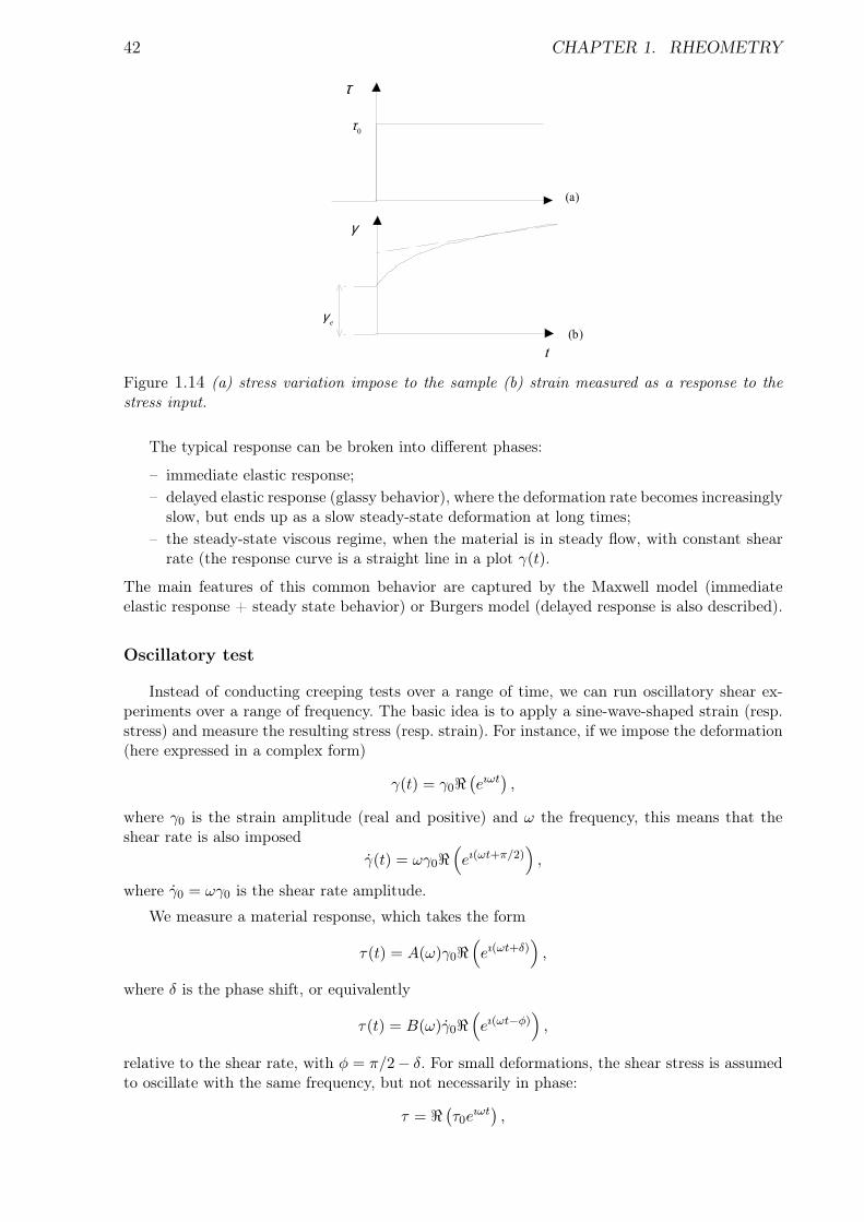
(b)
Figure 1.14 (a) stress variation impose to the sample (b) strain measured as a response to thestress input.
The typical response can be broken into different phases:
– immediate elastic response;– delayed elastic response (glassy behavior), where the deformation rate becomes increasingly
slow, but ends up as a slow steady-state deformation at long times;– the steady-state viscous regime, when the material is in steady flow, with constant shear
rate (the response curve is a straight line in a plot γ(t).
The main features of this common behavior are captured by the Maxwell model (immediateelastic response + steady state behavior) or Burgers model (delayed response is also described).
Oscillatory test
Instead of conducting creeping tests over a range of time, we can run oscillatory shear ex-periments over a range of frequency. The basic idea is to apply a sine-wave-shaped strain (resp.stress) and measure the resulting stress (resp. strain). For instance, if we impose the deformation(here expressed in a complex form)
γ(t) = γ0<(eıωt
),
where γ0 is the strain amplitude (real and positive) and ω the frequency, this means that theshear rate is also imposed
γ(t) = ωγ0<(eı(ωt+π/2)
),
where γ0 = ωγ0 is the shear rate amplitude.
We measure a material response, which takes the form
τ(t) = A(ω)γ0<(eı(ωt+δ)
),
where δ is the phase shift, or equivalently
τ(t) = B(ω)γ0<(eı(ωt−φ)
),
relative to the shear rate, with φ = π/2− δ. For small deformations, the shear stress is assumedto oscillate with the same frequency, but not necessarily in phase:
τ = < (τ0e
ıωt),
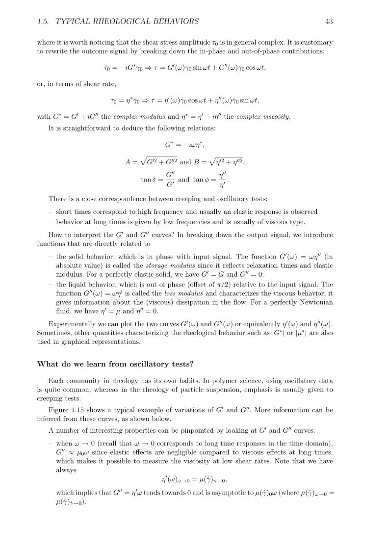
1.5. TYPICAL RHEOLOGICAL BEHAVIORS 43
where it is worth noticing that the shear stress amplitude τ0 is in general complex. It is customaryto rewrite the outcome signal by breaking down the in-phase and out-of-phase contributions:
τ0 = −ıG∗γ0 ⇒ τ = G′(ω)γ0 sinωt + G′′(ω)γ0 cosωt,
or, in terms of shear rate,
τ0 = η∗γ0 ⇒ τ = η′(ω)γ0 cosωt + η′′(ω)γ0 sinωt,
with G∗ = G′ + ıG′′ the complex modulus and η∗ = η′ − ıη′′ the complex viscosity.
It is straightforward to deduce the following relations:
G∗ = −ıωη∗,
A =√
G′2 + G′′2 and B =√
η′2 + η′′2,
tan δ =G′′
G′ and tanφ =η′′
η′.
There is a close correspondence between creeping and oscillatory tests:
– short times correspond to high frequency and usually an elastic response is observed– behavior at long times is given by low frequencies and is usually of viscous type.
How to interpret the G′ and G′′ curves? In breaking down the output signal, we introducefunctions that are directly related to
– the solid behavior, which is in phase with input signal. The function G′(ω) = ωη′′ (inabsolute value) is called the storage modulus since it reflects relaxation times and elasticmodulus. For a perfectly elastic solid, we have G′ = G and G′′ = 0;
– the liquid behavior, which is out of phase (offset of π/2) relative to the input signal. Thefunction G′′(ω) = ωη′ is called the loss modulus and characterizes the viscous behavior; itgives information about the (viscous) dissipation in the flow. For a perfectly Newtonianfluid, we have η′ = µ and η′′ = 0.
Experimentally we can plot the two curves G′(ω) and G′′(ω) or equivalently η′(ω) and η′′(ω).Sometimes, other quantities characterizing the rheological behavior such as |G∗| or |µ∗| are alsoused in graphical representations.
What do we learn from oscillatory tests?
Each community in rheology has its own habits. In polymer science, using oscillatory datais quite common, whereas in the rheology of particle suspension, emphasis is usually given tocreeping tests.
Figure 1.15 shows a typical example of variations of G′ and G′′. More information can beinferred from these curves, as shown below.
A number of interesting properties can be pinpointed by looking at G′ and G′′ curves:
– when ω → 0 (recall that ω → 0 corresponds to long time responses in the time domain),G′′ ≈ µ0ω since elastic effects are negligible compared to viscous effects at long times,which makes it possible to measure the viscosity at low shear rates. Note that we havealways
η′(ω)ω→0 = µ(γ)γ→0,
which implies that G′′ = η′ω tends towards 0 and is asymptotic to µ(γ)0ω (where µ(γ)ω→0 =µ(γ)γ→0).
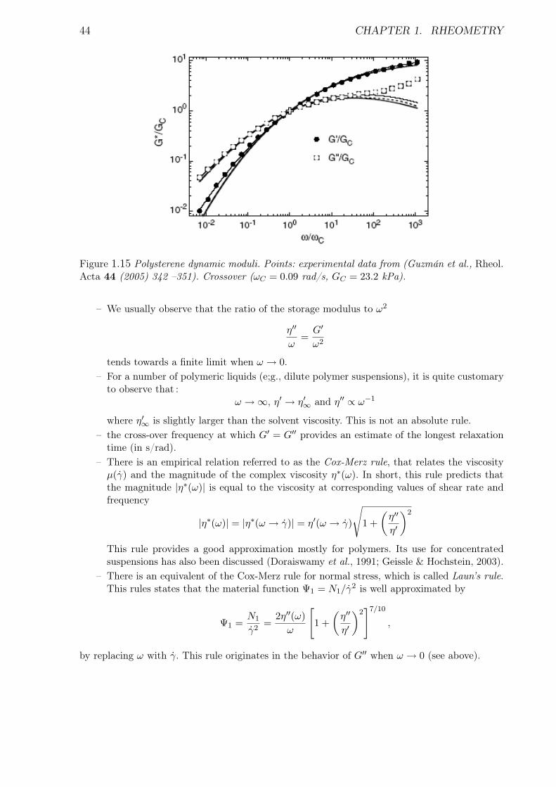
44 CHAPTER 1. RHEOMETRY
Figure 1.15 Polysterene dynamic moduli. Points: experimental data from (Guzmán et al., Rheol.Acta 44 (2005) 342 –351). Crossover (ωC = 0.09 rad/s, GC = 23.2 kPa).
– We usually observe that the ratio of the storage modulus to ω2
η′′
ω=
G′
ω2
tends towards a finite limit when ω → 0.– For a number of polymeric liquids (e;g., dilute polymer suspensions), it is quite customary
to observe that :ω →∞, η′ → η′∞ and η′′ ∝ ω−1
where η′∞ is slightly larger than the solvent viscosity. This is not an absolute rule.– the cross-over frequency at which G′ = G′′ provides an estimate of the longest relaxation
time (in s/rad).– There is an empirical relation referred to as the Cox-Merz rule, that relates the viscosity
µ(γ) and the magnitude of the complex viscosity η∗(ω). In short, this rule predicts thatthe magnitude |η∗(ω)| is equal to the viscosity at corresponding values of shear rate andfrequency
|η∗(ω)| = |η∗(ω → γ)| = η′(ω → γ)
√1 +
(η′′
η′
)2
This rule provides a good approximation mostly for polymers. Its use for concentratedsuspensions has also been discussed (Doraiswamy et al., 1991; Geissle & Hochstein, 2003).
– There is an equivalent of the Cox-Merz rule for normal stress, which is called Laun’s rule.This rules states that the material function Ψ1 = N1/γ2 is well approximated by
Ψ1 =N1
γ2=
2η′′(ω)ω
[1 +
(η′′
η′
)2]7/10
,
by replacing ω with γ. This rule originates in the behavior of G′′ when ω → 0 (see above).
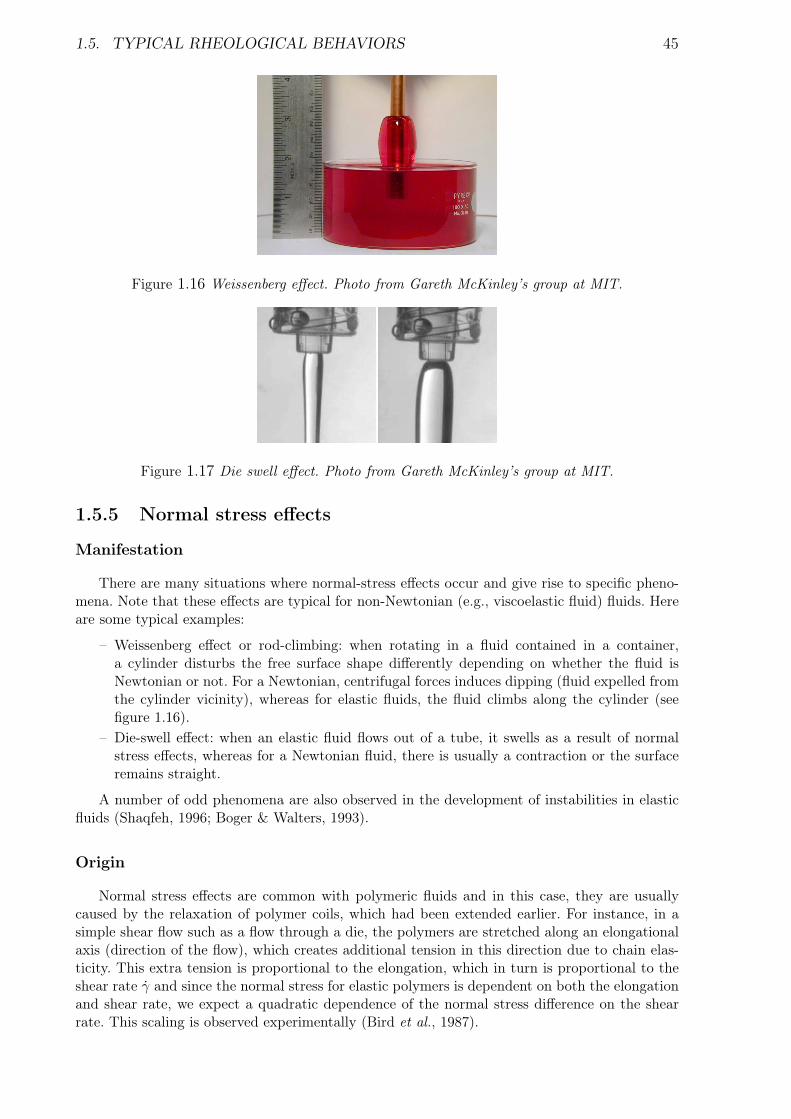
1.5. TYPICAL RHEOLOGICAL BEHAVIORS 45
Figure 1.16 Weissenberg effect. Photo from Gareth McKinley’s group at MIT.
Figure 1.17 Die swell effect. Photo from Gareth McKinley’s group at MIT.
1.5.5 Normal stress effects
Manifestation
There are many situations where normal-stress effects occur and give rise to specific pheno-mena. Note that these effects are typical for non-Newtonian (e.g., viscoelastic fluid) fluids. Hereare some typical examples:
– Weissenberg effect or rod-climbing: when rotating in a fluid contained in a container,a cylinder disturbs the free surface shape differently depending on whether the fluid isNewtonian or not. For a Newtonian, centrifugal forces induces dipping (fluid expelled fromthe cylinder vicinity), whereas for elastic fluids, the fluid climbs along the cylinder (seefigure 1.16).
– Die-swell effect: when an elastic fluid flows out of a tube, it swells as a result of normalstress effects, whereas for a Newtonian fluid, there is usually a contraction or the surfaceremains straight.
A number of odd phenomena are also observed in the development of instabilities in elasticfluids (Shaqfeh, 1996; Boger & Walters, 1993).
Origin
Normal stress effects are common with polymeric fluids and in this case, they are usuallycaused by the relaxation of polymer coils, which had been extended earlier. For instance, in asimple shear flow such as a flow through a die, the polymers are stretched along an elongationalaxis (direction of the flow), which creates additional tension in this direction due to chain elas-ticity. This extra tension is proportional to the elongation, which in turn is proportional to theshear rate γ and since the normal stress for elastic polymers is dependent on both the elongationand shear rate, we expect a quadratic dependence of the normal stress difference on the shearrate. This scaling is observed experimentally (Bird et al., 1987).
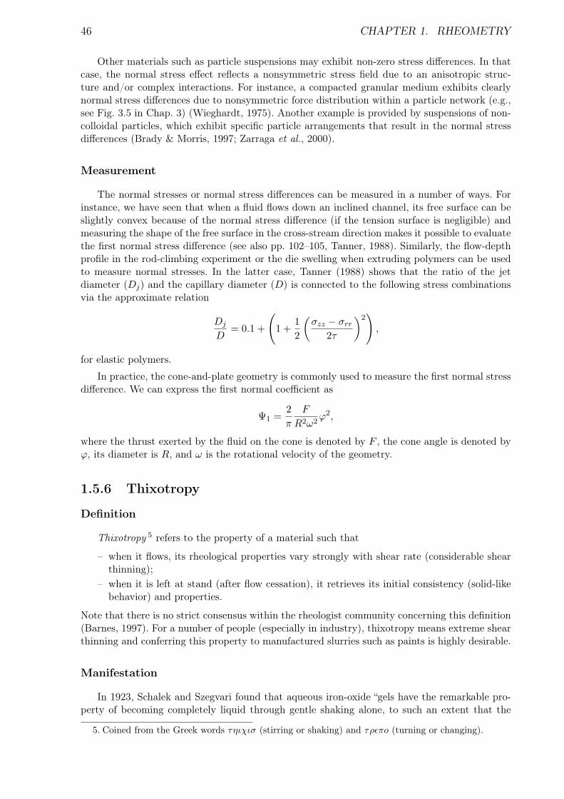
46 CHAPTER 1. RHEOMETRY
Other materials such as particle suspensions may exhibit non-zero stress differences. In thatcase, the normal stress effect reflects a nonsymmetric stress field due to an anisotropic struc-ture and/or complex interactions. For instance, a compacted granular medium exhibits clearlynormal stress differences due to nonsymmetric force distribution within a particle network (e.g.,see Fig. 3.5 in Chap. 3) (Wieghardt, 1975). Another example is provided by suspensions of non-colloidal particles, which exhibit specific particle arrangements that result in the normal stressdifferences (Brady & Morris, 1997; Zarraga et al., 2000).
Measurement
The normal stresses or normal stress differences can be measured in a number of ways. Forinstance, we have seen that when a fluid flows down an inclined channel, its free surface can beslightly convex because of the normal stress difference (if the tension surface is negligible) andmeasuring the shape of the free surface in the cross-stream direction makes it possible to evaluatethe first normal stress difference (see also pp. 102–105, Tanner, 1988). Similarly, the flow-depthprofile in the rod-climbing experiment or the die swelling when extruding polymers can be usedto measure normal stresses. In the latter case, Tanner (1988) shows that the ratio of the jetdiameter (Dj) and the capillary diameter (D) is connected to the following stress combinationsvia the approximate relation
Dj
D= 0.1 +
(1 +
12
(σzz − σrr
2τ
)2)
,
for elastic polymers.
In practice, the cone-and-plate geometry is commonly used to measure the first normal stressdifference. We can express the first normal coefficient as
Ψ1 =2π
F
R2ω2ϕ2,
where the thrust exerted by the fluid on the cone is denoted by F , the cone angle is denoted byϕ, its diameter is R, and ω is the rotational velocity of the geometry.
1.5.6 Thixotropy
Definition
Thixotropy 5 refers to the property of a material such that
– when it flows, its rheological properties vary strongly with shear rate (considerable shearthinning);
– when it is left at stand (after flow cessation), it retrieves its initial consistency (solid-likebehavior) and properties.
Note that there is no strict consensus within the rheologist community concerning this definition(Barnes, 1997). For a number of people (especially in industry), thixotropy means extreme shearthinning and conferring this property to manufactured slurries such as paints is highly desirable.
Manifestation
In 1923, Schalek and Szegvari found that aqueous iron-oxide “gels have the remarkable pro-perty of becoming completely liquid through gentle shaking alone, to such an extent that the
5. Coined from the Greek words τηιχισ (stirring or shaking) and τρεπo (turning or changing).
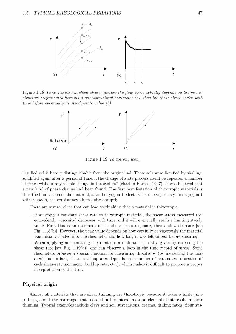
1.5. TYPICAL RHEOLOGICAL BEHAVIORS 47
τ
γ
0λ
λ∞
0t
1 0t t>
1i it t −>
1n nt t −>
τ
t(b)(a)
0t nti
t
Figure 1.18 Time decrease in shear stress: because the flow curve actually depends on the micro-structure (represented here via a microstructural parameter (a), then the shear stress varies withtime before eventually its steady-state value (b).
γ
t(a)
fluid at rest
τ
t(b)
Figure 1.19 Thixotropy loop.
liquified gel is hardly distinguishable from the original sol. These sols were liquified by shaking,solidified again after a period of time. . . the change of state process could be repeated a numberof times without any visible change in the system” (cited in Barnes, 1997). It was believed thata new kind of phase change had been found. The first manifestation of thixotropic materials isthus the fluidization of the material, a kind of yoghurt effect: when one vigorously mix a yoghurtwith a spoon, the consistency alters quite abruptly.
There are several clues that can lead to thinking that a material is thixotropic:
– If we apply a constant shear rate to thixotropic material, the shear stress measured (or,equivalently, viscosity) decreases with time and it will eventually reach a limiting steadyvalue. First this is an overshoot in the shear-stress response, then a slow decrease [seeFig. 1.18(b)]. However, the peak value depends on how carefully or vigorously the materialwas initially loaded into the rheometer and how long it was left to rest before shearing.
– When applying an increasing shear rate to a material, then at a given by reversing theshear rate [see Fig. 1.19(a)], one can observe a loop in the time record of stress. Somerheometers propose a special function for measuring thixotropy (by measuring the looparea), but in fact, the actual loop area depends on a number of parameters (duration ofeach shear-rate increment, buildup rate, etc.), which makes it difficult to propose a properinterpretation of this test.
Physical origin
Almost all materials that are shear thinning are thixotropic because it takes a finite timeto bring about the rearrangements needed in the microstructural elements that result in shearthinning. Typical examples include clays and soil suspensions, creams, drilling muds, flour sus-
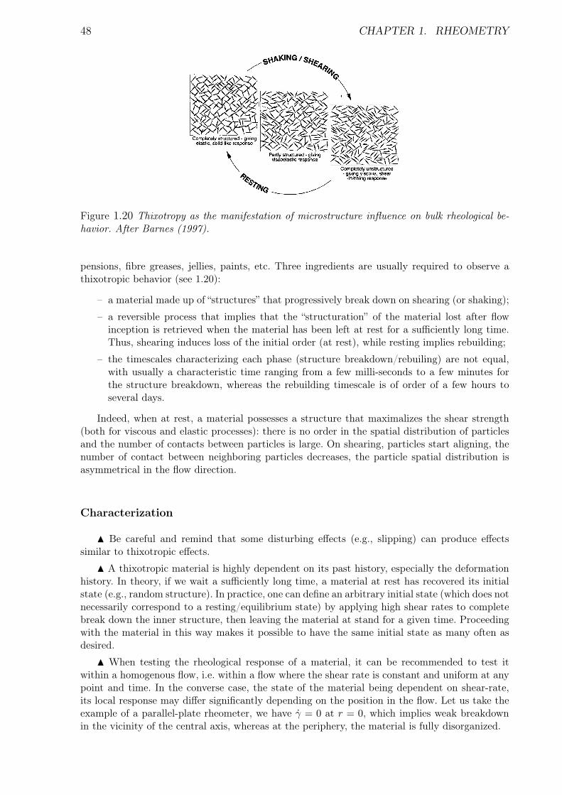
48 CHAPTER 1. RHEOMETRY
Figure 1.20 Thixotropy as the manifestation of microstructure influence on bulk rheological be-havior. After Barnes (1997).
pensions, fibre greases, jellies, paints, etc. Three ingredients are usually required to observe athixotropic behavior (see 1.20):
– a material made up of “structures” that progressively break down on shearing (or shaking);
– a reversible process that implies that the “structuration” of the material lost after flowinception is retrieved when the material has been left at rest for a sufficiently long time.Thus, shearing induces loss of the initial order (at rest), while resting implies rebuilding;
– the timescales characterizing each phase (structure breakdown/rebuiling) are not equal,with usually a characteristic time ranging from a few milli-seconds to a few minutes forthe structure breakdown, whereas the rebuilding timescale is of order of a few hours toseveral days.
Indeed, when at rest, a material possesses a structure that maximalizes the shear strength(both for viscous and elastic processes): there is no order in the spatial distribution of particlesand the number of contacts between particles is large. On shearing, particles start aligning, thenumber of contact between neighboring particles decreases, the particle spatial distribution isasymmetrical in the flow direction.
Characterization
N Be careful and remind that some disturbing effects (e.g., slipping) can produce effectssimilar to thixotropic effects.
N A thixotropic material is highly dependent on its past history, especially the deformationhistory. In theory, if we wait a sufficiently long time, a material at rest has recovered its initialstate (e.g., random structure). In practice, one can define an arbitrary initial state (which does notnecessarily correspond to a resting/equilibrium state) by applying high shear rates to completebreak down the inner structure, then leaving the material at stand for a given time. Proceedingwith the material in this way makes it possible to have the same initial state as many often asdesired.
N When testing the rheological response of a material, it can be recommended to test itwithin a homogenous flow, i.e. within a flow where the shear rate is constant and uniform at anypoint and time. In the converse case, the state of the material being dependent on shear-rate,its local response may differ significantly depending on the position in the flow. Let us take theexample of a parallel-plate rheometer, we have γ = 0 at r = 0, which implies weak breakdownin the vicinity of the central axis, whereas at the periphery, the material is fully disorganized.
1.5. TYPICAL RHEOLOGICAL BEHAVIORS 49
We suggest the following procedure:
1. Let us assume that we start from a well-specified initial state, the material being at rest.We apply a constant shear rate γ0 [see Fig. 1.21(a)] and measure the shear stress.
2. On applying a shear rate, the inner structure is disorganized, which requires energy. Thisis reflected by a shear-stress overshoot, which is followed by a slow decrease towards alimiting value corresponding to the new equilibrium induced by the new strain rate [seeFig. 1.21(b)] if we wait a sufficiently long time.
3. If we remove the shear rate, the shear stress drops to zero instantaneously (no viscoelas-ticity).
4. After a resting time, we apply the same rate as earlier, but since the inner structure wasaltered, less energy is needed to break the particle network or realign the particles, whichimplies that the shear-stress overshoot is less pronounced and the steady state is reachedmore quickly [see Fig. 1.21(b)].
5. If the overshoot is denoted by ∆τ , we can determine the function ∆τ(trest relating theovershoot to the resting time [see Fig. 1.21(c)].
Modelling
The simplest mode we can imagine is to assume that the viscosity is dependent on a structuralparameter. As a first approximation and for the sake of simplicity, we assume that (i) thisparameter is scalar, (ii) it reflects the microstructure state (e.g., the floc size in a flocculatedsuspension, the number of contact in a colloid, available energy for a given particle configuration,etc.), (iii) it satisfies a kinetic equation in the form
dλ
dt=
F (λ)tb
− G(λ)te
,
where tb is the buildup timescale, te = γ−1 is a typical characteristic of the flow, F representsthe increase of the scalar parameter induced by buildup, whereas G stands for the λ as a resultof microstructure disorganization. These functions can de determined experimentally. Typicalexamples include F = (1−λ)a and G = bλ, with a and b two reals (see pp. 24–25, Barnes, 1997)
In short, we have µ = µ(γ,λ), with λ variations controlled by the kinetic equation above.When solving a problem, we have to solve the momentum equations together with the kineticequation.
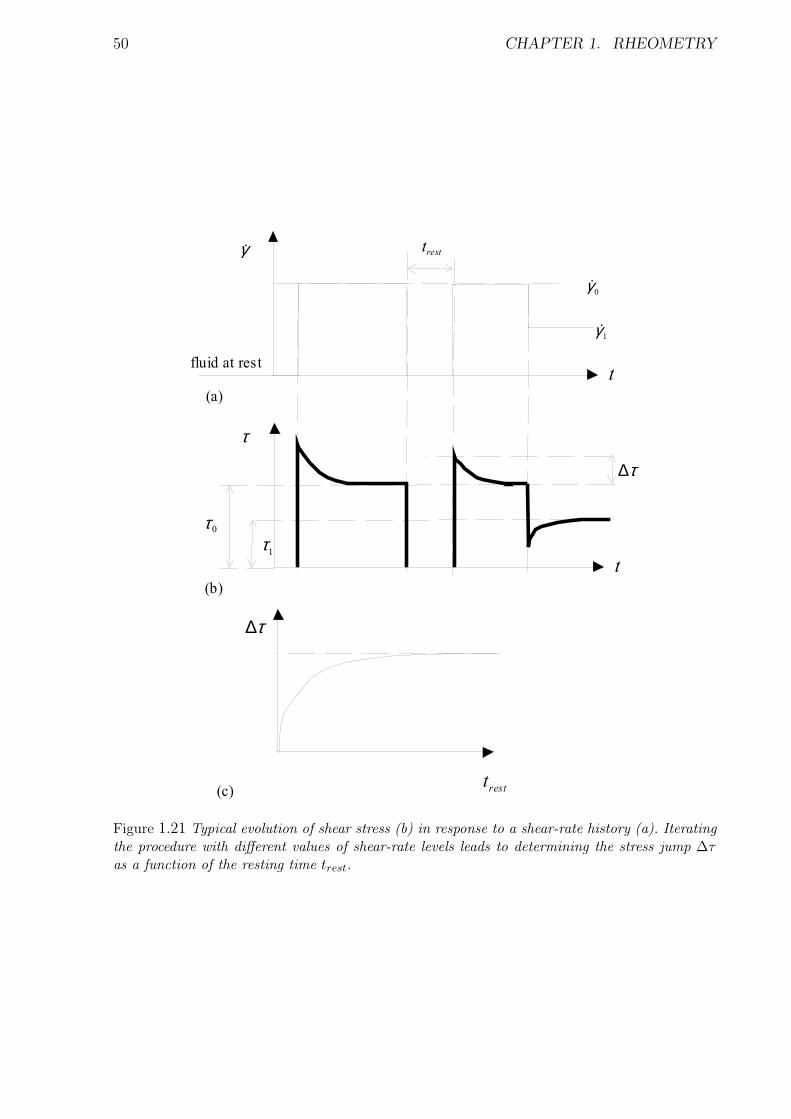
50 CHAPTER 1. RHEOMETRY
γ
t
(a)
0γ
fluid at rest
1γ
τ
t
0τ
(b)
restt
1τ
τ∆
τ∆
restt
(c)
Figure 1.21 Typical evolution of shear stress (b) in response to a shear-rate history (a). Iteratingthe procedure with different values of shear-rate levels leads to determining the stress jump ∆τas a function of the resting time trest.
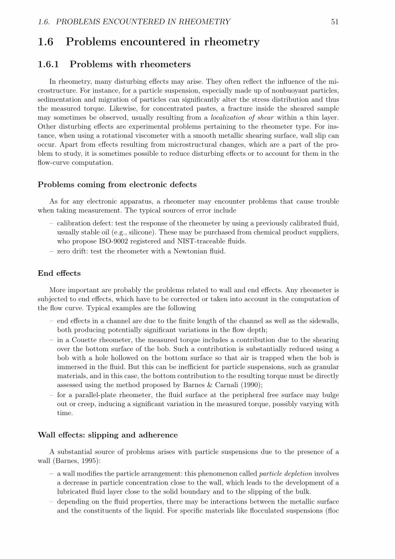
1.6. PROBLEMS ENCOUNTERED IN RHEOMETRY 51
1.6 Problems encountered in rheometry
1.6.1 Problems with rheometers
In rheometry, many disturbing effects may arise. They often reflect the influence of the mi-crostructure. For instance, for a particle suspension, especially made up of nonbuoyant particles,sedimentation and migration of particles can significantly alter the stress distribution and thusthe measured torque. Likewise, for concentrated pastes, a fracture inside the sheared samplemay sometimes be observed, usually resulting from a localization of shear within a thin layer.Other disturbing effects are experimental problems pertaining to the rheometer type. For ins-tance, when using a rotational viscometer with a smooth metallic shearing surface, wall slip canoccur. Apart from effects resulting from microstructural changes, which are a part of the pro-blem to study, it is sometimes possible to reduce disturbing effects or to account for them in theflow-curve computation.
Problems coming from electronic defects
As for any electronic apparatus, a rheometer may encounter problems that cause troublewhen taking measurement. The typical sources of error include
– calibration defect: test the response of the rheometer by using a previously calibrated fluid,usually stable oil (e.g., silicone). These may be purchased from chemical product suppliers,who propose ISO-9002 registered and NIST-traceable fluids.
– zero drift: test the rheometer with a Newtonian fluid.
End effects
More important are probably the problems related to wall and end effects. Any rheometer issubjected to end effects, which have to be corrected or taken into account in the computation ofthe flow curve. Typical examples are the following
– end effects in a channel are due to the finite length of the channel as well as the sidewalls,both producing potentially significant variations in the flow depth;
– in a Couette rheometer, the measured torque includes a contribution due to the shearingover the bottom surface of the bob. Such a contribution is substantially reduced using abob with a hole hollowed on the bottom surface so that air is trapped when the bob isimmersed in the fluid. But this can be inefficient for particle suspensions, such as granularmaterials, and in this case, the bottom contribution to the resulting torque must be directlyassessed using the method proposed by Barnes & Carnali (1990);
– for a parallel-plate rheometer, the fluid surface at the peripheral free surface may bulgeout or creep, inducing a significant variation in the measured torque, possibly varying withtime.
Wall effects: slipping and adherence
A substantial source of problems arises with particle suspensions due to the presence of awall (Barnes, 1995):
– a wall modifies the particle arrangement: this phenomenon called particle depletion involvesa decrease in particle concentration close to the wall, which leads to the development of alubricated fluid layer close to the solid boundary and to the slipping of the bulk.
– depending on the fluid properties, there may be interactions between the metallic surfaceand the constituents of the liquid. For specific materials like flocculated suspensions (floc
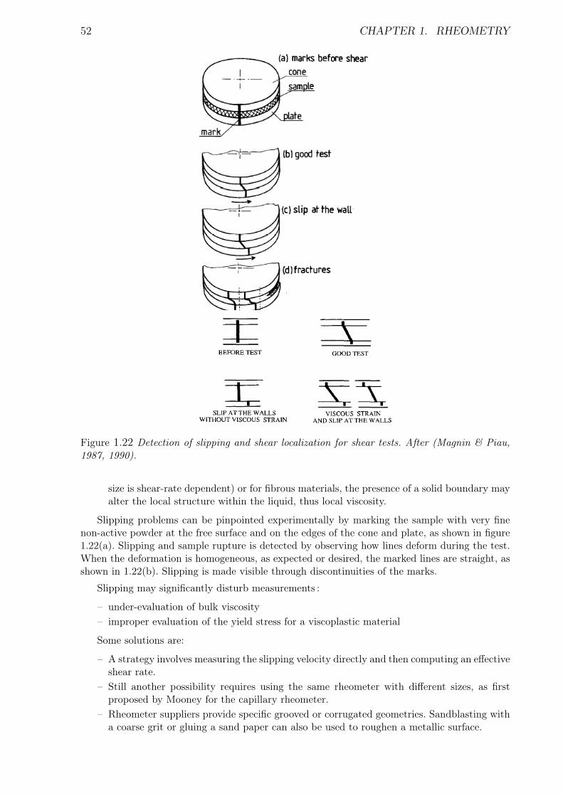
52 CHAPTER 1. RHEOMETRY
Figure 1.22 Detection of slipping and shear localization for shear tests. After (Magnin & Piau,1987, 1990).
size is shear-rate dependent) or for fibrous materials, the presence of a solid boundary mayalter the local structure within the liquid, thus local viscosity.
Slipping problems can be pinpointed experimentally by marking the sample with very finenon-active powder at the free surface and on the edges of the cone and plate, as shown in figure1.22(a). Slipping and sample rupture is detected by observing how lines deform during the test.When the deformation is homogeneous, as expected or desired, the marked lines are straight, asshown in 1.22(b). Slipping is made visible through discontinuities of the marks.
Slipping may significantly disturb measurements :
– under-evaluation of bulk viscosity– improper evaluation of the yield stress for a viscoplastic material
Some solutions are:
– A strategy involves measuring the slipping velocity directly and then computing an effectiveshear rate.
– Still another possibility requires using the same rheometer with different sizes, as firstproposed by Mooney for the capillary rheometer.
– Rheometer suppliers provide specific grooved or corrugated geometries. Sandblasting witha coarse grit or gluing a sand paper can also be used to roughen a metallic surface.
1.6. PROBLEMS ENCOUNTERED IN RHEOMETRY 53
– A growing number of applications are based on vane shear cell Barnes & Nguyen (2001).– When there are chemical interactions (chemical attack with ion production) or physical
interactions (van der Waals force) between the fluid constituents and the walls, specificsurface treatment must be used.
Be careful: some techniques such as using rough surfaces do not remove the slipping problem,but only shift it: instead of slipping, the material undergoes shear localization within the sample.
Rupture within the sample
With rupture, we mean:
– shear localization: shear is concentrated within a narrow strip inside the sample, whichimplies a jump in shear rate on the bulk scale
– slipping between two layers of material.
Deformation of the free surface
In most viscometric flows, there is a free surface. This surface may deform as a result ofdifferent processes:
– normal stress effect: rod-climbing effect or bulging of the free surface for flows down inclines– inertial effect: for the coaxial cylinder rheometer at high velocities, there is a gradient in
the flow depth to balance the inertial centrifuge forces. For the parallel-plate rheometer,fluid may be expelled because of radial acceleration
– evaporation, particle migration etc. at the periphery of the sample for parallel-plate rheo-meter.
Finite-size effects
Furthermore, many natural fluids encountered in geophysics are suspensions with a large sizedistribution. The size of the rheometer should be determined such that its typical size (e.g., thegap in a rotational viscometer) is much larger than the largest particle size.
The solution involves using large-sized rheometers, e.g., wide gap Couette cells.
1.6.2 Limitations of the viscometric treatment
The ‘simple-fluid’ assumption
The viscometric treatment relies on the crucial assumption that the extra-stress tensor isa one-to-one function of the strain-rate tensor only (class of simple fluids). Many classes ofmaterial studied in geophysics are not in fact incompressible, homogeneous, isotropic, or merelyexpressible in the form σ = −p1 + s(d).
For instance, for materials with time-dependent properties (thixotropic materials, viscoelasticmaterials), the constitutive equation can be expressed in the form σ = −p1 + s(d) only for asteady state. Another example is provided by granular flows. In this case, when applied toexperimental data obtained by studying dry granular flows down an inclined channel (Anceyet al., 1996), the viscometric treatment leads to the conclusion that the flow curve should be adecreasing function of the shear rate in violation of a stability criterion imposing that the flowcurve be an increasing function. Although such a decrease in the flow curve cannot be directlyinterpreted in terms of a constitutive equation, it provides interesting rheological informationthat can be explained on the basis of microstructural theories (Ancey & Evesque, 2000).
54 CHAPTER 1. RHEOMETRY
Development of instabilities
At high speed, a number of instabilities occur:
– development of secondary flow and recirculation cell, e.g., Saffman-Taylor instability inCouette cells
– turbulence development– particle migration, particle jamming or settling
The possible solution is to
– visualize the internal flow structure to detect secondary flow;– place tracers in the fluid to determine their trajectory, then the streamlines;– check the consistency of the data. For instance for a parallel-plate rheometer, the visco-
metric treatment is valid provided centrifugal forces are negligible compared to the secondnormal stress difference: %R2w2 ¿ N2, where w is the orthoradial component of the velo-city. Such an effect can be detected experimentally either by observing secondary flows orby noticing that doubling both the gap and the rotational velocity (thus keeping the shearrate constant) produces a significant variation in the measured torque.
1.6.3 Technical issues related to the derivation of the flow curve
Recall that:
– The softwares provided by rheometer manufacturers for computing the flow curve or otherrheological properties makes use of standard methods. For instance, for the Couette cell(coaxial cylinder rheometer), the narrow-gap approximation is used, which implies thatthe user should develop his own software to deal with wide-gap rheometer.
– For most viscometers, computing the shear rate from experimental data can raise seriousproblems. A major source of uncertainty is that in most viscometric procedures the shearrate is expressed as a derivative – for instance ∂q/∂h in (1.11) – which must be estimatedfrom experimental data. To do so, different procedures are available but they do not alwaysprovide the same results, especially when data are noisy (Borgia & Spera, 1990).
A typical example of these problems is given by the concentric-cylinder rheometer (or Couetterheometer). The shear rate is inferred from the rotational velocity Ω and the torque (per unitdepth) C using the following relationship:
Ω = −12
∫ C/(2πR22)
C/(2πR21)
γ(τ)d ln τ . (1.18)
When the gap between the two cylinders is narrow, it is possible to approximate the shear rateas: γ = R1Ω/(R2 −R1) + o(1−R2/R1).
However, such a geometry is not very suitable to studying particle suspensions (slipping, sizeeffects, etc.) and usually a wide gap is preferred. For methods of this kind, computing the shearrate requires:
– specifying the type of constitutive equation in advance, integrating it to obtain the relationbetween the torque and the rotational velocity, and fitting the relation to experimentaldata.
– using a more effective and practical method of solving the inverse problem such as– the Tikhonov regularization method proposed by Yeow et al. (2000): this procedure
does not require the algebraic form of the τ − γ curve to be specified and has theadvantage of filtering out noise.
1.6. PROBLEMS ENCOUNTERED IN RHEOMETRY 55
– the wavelet-vaguelette decomposition method proposed by Ancey (2005) which is notbased on a regularization step and thus is more appropriate for complex fluids.
The only viscometer which poses no problem in converting experimental data into a τ − γcurve is the parallel-plate rheometer. In this case, the shear rate distribution is imposed by theexperimentalist: γ = ΩR/h. But such a relationship holds provided centrifugal forces are negli-gible compared to the second normal stress difference: %R2w2 ¿ N2, where w is the orthoradialcomponent of the velocity. Such an effect can be detected experimentally either by observingsecondary flows or by noticing that doubling both the gap and the rotational velocity (thuskeeping the shear rate constant) produces a significant variation in the measured torque.
1.6.4 Problems related to sample preparation
A sample that will be tested in a rheometer must be representative of large batches ofmaterial from which it is extracted. Specific care should be taken in obtaining and preparingparticle suspensions when the sample has been collected in the field (e.g., a sample of debrisflow) or in industrial facilities due to segregation effects.
56 CHAPTER 1. RHEOMETRY
1.7 Non-standard techniques: what can be done wi-thout a rheometer?
1.7.1 Viscosity: free fall of a bead
Consider an isolated spherical particule of radius a falling under the action of gravity in afluid that is assumed to be Newtonian with viscosity µ and unbounded (no wall close to theparticle). If the sphere moves very slowly, its Reynolds number
Re =%pau
µ,
with %p the particle density and u the particle velocity relative to the fluid. When Re ¿ 1, thenthe force exerted by the fluid on the particle is given by Stokes’ law
F = 6πµau.
If we can measure the velocity u when the particle reaches a steady regime, we can determine thefluid viscosity from the force balance 0 = −%pg + %fg + F , where fluid density has been denotedby %f
µ =29(%p − %f )
ga2
u.
A practical version of this measurement technique is the rolling-ball viscometer (Bird et al.,1987).
1.7.2 Yield stress: Slump test
In the laboratory, it is frequently impossible to investigate the rheological properties of aparticle suspension using a rheometer. For instance, with snow or magma, such tests are al-most always impractical. For debris suspensions, it is usually impossible to carry out measu-rements with the complete range of particle size. This has motivated researchers to developedapproximate rheometric procedures and to investigate the relations between field observationsand rheological properties. For instance, given the sole objective of determining the yield stress,the semi-empirical method referred to as a slump test can provide an estimate of the yield stressfor a viscoplastic material. This method involves filling a cylinder with the material to be tested,lifting the cylinder off and allowing the material to flow under its own weight. The profile of thefinal mound of material as well as the difference (δ) between the initial and final heights is linkedto the yield stress. Pashias & Boger (1996) have found:
δ
h= 1− 2
τc
%gh
(1− ln
(2
τc
%gh
)), (1.19)
where h is the cylinder height, % the material density (see also Schowalter & Christensen, 1999).Close examination of experimental data published by Pashias and Boger shows a deviation fromthe theoretical curve for yield stress values in excess of approximately 0.15%gh. For yield stressvalues lower than 0.15%gh (or for δ/h > 0.4), uncertainty was less than 10% for their tests.The explanation of the deviation for higher yield stress values lies perhaps in the weakness ofthe assumption on the elastoplastic behavior for very cohesive materials. Coussot et al. (1996)developed an alternative approach based on an interpretation of the deposit shape. They showedthat the free surface profile (the relationship between the material height y and the distancefrom the edge x) depends on the yield stress only. On a flat horizontal surface, the free surfaceprofile has the following expression
%gy
τc=
√2%gx
τc. (1.20)
1.7. NON-STANDARDTECHNIQUES: WHAT CAN BE DONEWITHOUTA RHEOMETER?57
Comparisons between rheological data deduced from a parallel-plate rheometer and free surfaceprofile measurements showed an acceptable agreement for fine mud suspensions and debris flowmaterials. Uncertainty was less than 20%, within the boundaries of acceptable uncertainty forrheometrical measurement. The major restriction in the use of equation (1.20) stems from thelong-wave approximation, which implies that the mound height must far outweigh the extensionof the deposit: h− δ À τc/(%g). The method proposed by Coussot et al. (1996) can be extendedto different rheologies and boundary conditions. In the field, such a method applied to leveeprofiles of debris flow can provide estimates of the bulk yield stress provided that the assumptionof viscoplastic behavior holds.
A number of other tests have been developed in civil engineering tests (e.g., Abram’s test forevaluating concrete workability) and in the industry (e.g., Bostwick’s test in food engineering),which usually provide information on how easily a material flows. More recently, some theoreticalanalyses have tried to elaborate on the interpretations that can be done with these empirical(McKarthy & Seymour, 1994; Piau & Debiane, 2005).

58 CHAPTER 1. RHEOMETRY
59
Chapter 2Rheology and Continuum Mechanics
Prerequisites– fluid mechanics: mass, momentum, energy balance equations– mathematics: differential analysis, tensorial analysis, algebra tools
Objectives– to provide the mathematical ground supporting continuum mechanics– to review the fundamental principles used in formulating a constitutive equations– to provide physical insight into the mathematical operators used in mechanics
Content
Within the framework of continuum mechanics, the details of the material microstructureare forgotten and we only examine the bulk behavior, e.g. how does a material deform when itexperiences a given state of stress? Mathematically, we introduce the constitutive equation, whichrelates deformations and/or rates of deformation to stresses. Essentially continuum mechanicsprovides tools and rules that make it possible to:
– express constitutive equations in a proper form, i.e., in a tensorial form that satisfies therules of physics;
– obtain equations that govern the bulk motion.
Most phenomenological laws we can infer from experiments are in a scalar form. For instance,in rheometry, the only information we obtain in most cases is the flow curve, i.e., the relationτ = f(γ), whereas we need more information to model the three-dimensional behavior of fluids.The question is how to express a 3D constitutive equations. We shall see that the reply is notas easy as it can be thought at first glance. We start with the Newtonian case, the simplestcase that we can imagine. We then continue by reviewing the basic equations used in continuummechanics (conservation of mass, momentum, and energy). Emphasis is then given to providinga few examples of application.
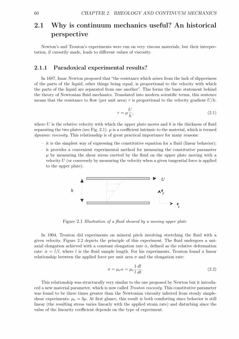
60 CHAPTER 2. RHEOLOGY AND CONTINUUM MECHANICS
2.1 Why is continuum mechanics useful? An historicalperspective
Newton’s and Trouton’s experiments were run on very viscous materials, but their interpre-tation, if cursorily made, leads to different values of viscosity.
2.1.1 Paradoxical experimental results?
In 1687, Isaac Newton proposed that “the resistance which arises from the lack of slipperinessof the parts of the liquid, other things being equal, is proportional to the velocity with whichthe parts of the liquid are separated from one another”. This forms the basic statement behindthe theory of Newtonian fluid mechanics. Translated into modern scientific terms, this sentencemeans that the resistance to flow (per unit area) τ is proportional to the velocity gradient U/h:
τ = µU
h, (2.1)
where U is the relative velocity with which the upper plate moves and h is the thickness of fluidseparating the two plates (see Fig. 2.1). µ is a coefficient intrinsic to the material, which is termeddynamic viscosity. This relationship is of great practical importance for many reasons:
– it is the simplest way of expressing the constitutive equation for a fluid (linear behavior);– it provides a convenient experimental method for measuring the constitutive parameter
µ by measuring the shear stress exerted by the fluid on the upper plate moving with avelocity U (or conversely by measuring the velocity when a given tangential force is appliedto the upper plate).
h
U
ex
ey
Figure 2.1 Illustration of a fluid sheared by a moving upper plate
In 1904, Trouton did experiments on mineral pitch involving stretching the fluid with agiven velocity. Figure 2.2 depicts the principle of this experiment. The fluid undergoes a uni-axial elongation achieved with a constant elongation rate α, defined as the relative deformationrate: α = l/l, where l is the fluid sample length. For his experiments, Trouton found a linearrelationship between the applied force per unit area σ and the elongation rate:
σ = µeα = µe1l
dl
dt. (2.2)
This relationship was structurally very similar to the one proposed by Newton but it introdu-ced a new material parameter, which is now called Trouton viscosity. This constitutive parameterwas found to be three times greater than the Newtonian viscosity inferred from steady simple-shear experiments: µe = 3µ. At first glance, this result is both comforting since behavior is stilllinear (the resulting stress varies linearly with the applied strain rate) and disturbing since thevalue of the linearity coefficient depends on the type of experiment.
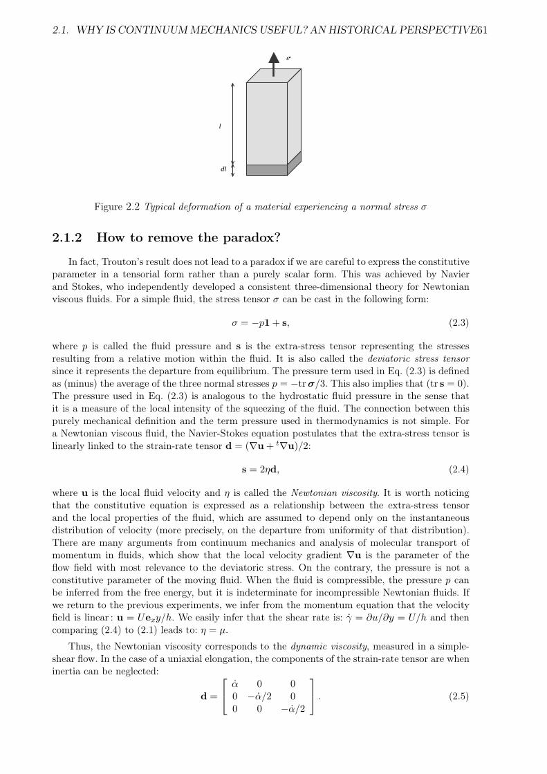
2.1. WHY IS CONTINUUMMECHANICS USEFUL? AN HISTORICAL PERSPECTIVE61
l
dl
Figure 2.2 Typical deformation of a material experiencing a normal stress σ
2.1.2 How to remove the paradox?
In fact, Trouton’s result does not lead to a paradox if we are careful to express the constitutiveparameter in a tensorial form rather than a purely scalar form. This was achieved by Navierand Stokes, who independently developed a consistent three-dimensional theory for Newtonianviscous fluids. For a simple fluid, the stress tensor σ can be cast in the following form:
σ = −p1 + s, (2.3)
where p is called the fluid pressure and s is the extra-stress tensor representing the stressesresulting from a relative motion within the fluid. It is also called the deviatoric stress tensorsince it represents the departure from equilibrium. The pressure term used in Eq. (2.3) is definedas (minus) the average of the three normal stresses p = −trσ/3. This also implies that (tr s = 0).The pressure used in Eq. (2.3) is analogous to the hydrostatic fluid pressure in the sense thatit is a measure of the local intensity of the squeezing of the fluid. The connection between thispurely mechanical definition and the term pressure used in thermodynamics is not simple. Fora Newtonian viscous fluid, the Navier-Stokes equation postulates that the extra-stress tensor islinearly linked to the strain-rate tensor d = (∇u + t∇u)/2:
s = 2ηd, (2.4)
where u is the local fluid velocity and η is called the Newtonian viscosity. It is worth noticingthat the constitutive equation is expressed as a relationship between the extra-stress tensorand the local properties of the fluid, which are assumed to depend only on the instantaneousdistribution of velocity (more precisely, on the departure from uniformity of that distribution).There are many arguments from continuum mechanics and analysis of molecular transport ofmomentum in fluids, which show that the local velocity gradient ∇u is the parameter of theflow field with most relevance to the deviatoric stress. On the contrary, the pressure is not aconstitutive parameter of the moving fluid. When the fluid is compressible, the pressure p canbe inferred from the free energy, but it is indeterminate for incompressible Newtonian fluids. Ifwe return to the previous experiments, we infer from the momentum equation that the velocityfield is linear : u = Uexy/h. We easily infer that the shear rate is: γ = ∂u/∂y = U/h and thencomparing (2.4) to (2.1) leads to: η = µ.
Thus, the Newtonian viscosity corresponds to the dynamic viscosity, measured in a simple-shear flow. In the case of a uniaxial elongation, the components of the strain-rate tensor are wheninertia can be neglected:
d =
α 0 00 −α/2 00 0 −α/2
. (2.5)
62 CHAPTER 2. RHEOLOGY AND CONTINUUM MECHANICS
At the same time, the stress tensor can be written as:
σ =
σ 0 00 0 00 0 0
. (2.6)
Comparing (2.3), (2.5), and (2.6) leads to: p = −ηα and σ = 3ηα, that is: µe = 3η, confirmingthat the Trouton elongational viscosity is three times greater than the Newtonian viscosity. Itturns out that Trouton’s and Newton’s experiments reflect the same constitutive behavior. Thisexample shows the importance of an appropriate tensorial form for expressing the stress tensor.In the present case, the tensorial form (2.4) may be seen as a simple generalization of the simpleshear expression (2.1).
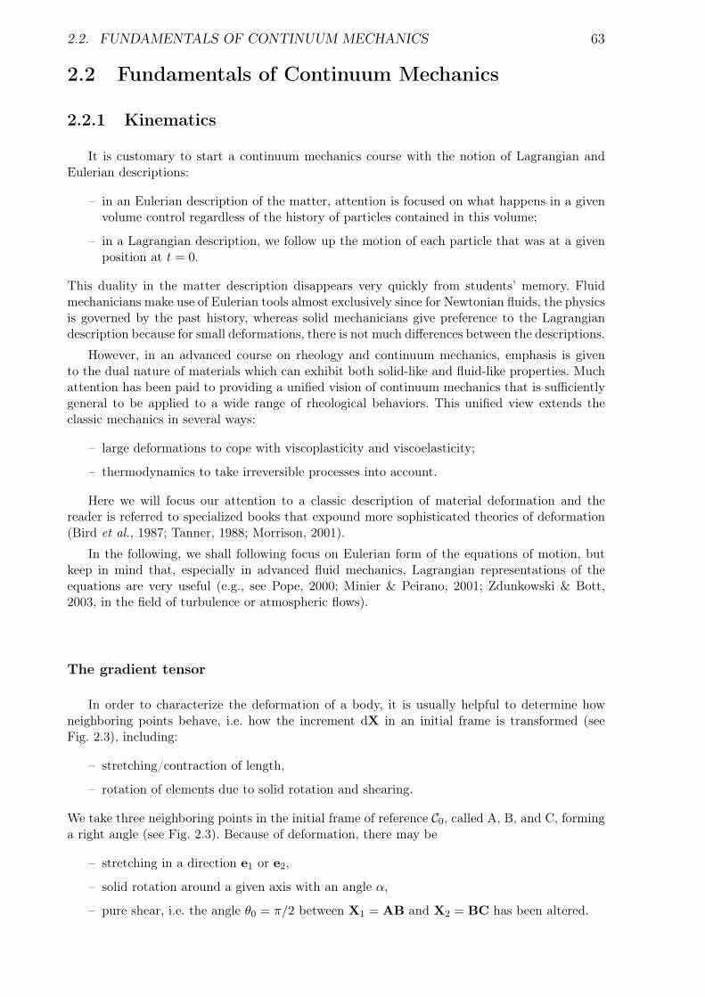
2.2. FUNDAMENTALS OF CONTINUUM MECHANICS 63
2.2 Fundamentals of Continuum Mechanics
2.2.1 Kinematics
It is customary to start a continuum mechanics course with the notion of Lagrangian andEulerian descriptions:
– in an Eulerian description of the matter, attention is focused on what happens in a givenvolume control regardless of the history of particles contained in this volume;
– in a Lagrangian description, we follow up the motion of each particle that was at a givenposition at t = 0.
This duality in the matter description disappears very quickly from students’ memory. Fluidmechanicians make use of Eulerian tools almost exclusively since for Newtonian fluids, the physicsis governed by the past history, whereas solid mechanicians give preference to the Lagrangiandescription because for small deformations, there is not much differences between the descriptions.
However, in an advanced course on rheology and continuum mechanics, emphasis is givento the dual nature of materials which can exhibit both solid-like and fluid-like properties. Muchattention has been paid to providing a unified vision of continuum mechanics that is sufficientlygeneral to be applied to a wide range of rheological behaviors. This unified view extends theclassic mechanics in several ways:
– large deformations to cope with viscoplasticity and viscoelasticity;
– thermodynamics to take irreversible processes into account.
Here we will focus our attention to a classic description of material deformation and thereader is referred to specialized books that expound more sophisticated theories of deformation(Bird et al., 1987; Tanner, 1988; Morrison, 2001).
In the following, we shall following focus on Eulerian form of the equations of motion, butkeep in mind that, especially in advanced fluid mechanics, Lagrangian representations of theequations are very useful (e.g., see Pope, 2000; Minier & Peirano, 2001; Zdunkowski & Bott,2003, in the field of turbulence or atmospheric flows).
The gradient tensor
In order to characterize the deformation of a body, it is usually helpful to determine howneighboring points behave, i.e. how the increment dX in an initial frame is transformed (seeFig. 2.3), including:
– stretching/contraction of length,
– rotation of elements due to solid rotation and shearing.
We take three neighboring points in the initial frame of reference C0, called A, B, and C, forminga right angle (see Fig. 2.3). Because of deformation, there may be
– stretching in a direction e1 or e2,
– solid rotation around a given axis with an angle α,
– pure shear, i.e. the angle θ0 = π/2 between X1 = AB and X2 = BC has been altered.
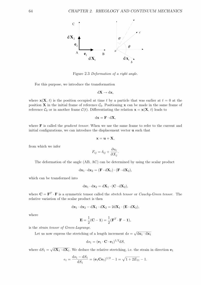
64 CHAPTER 2. RHEOLOGY AND CONTINUUM MECHANICS
AB
C
a
c
b
1e
2e θ
α
1dX
2dX
1d x
Figure 2.3 Deformation of a right angle.
For this purpose, we introduce the transformation
dX → dx,
where x(X, t) is the position occupied at time t by a particle that was earlier at t = 0 at theposition X in the initial frame of reference C0. Positioning x can be made in the same frame ofreference C0 or in another frame C(t). Differentiating the relation x = x(X, t) leads to
dx = F · dX,
where F is called the gradient tensor. When we use the same frame to refer to the current andinitial configurations, we can introduce the displacement vector u such that
x = u + X,
from which we inferFij = δij +
∂ui
∂Xj.
The deformation of the angle (AB, AC) can be determined by using the scalar product
dx1 · dx2 = (F · dX1) · (F · dX2),
which can be transformed into
dx1 · dx2 = dX1 · (C · dX2),
where C = FT ·F is a symmetric tensor called the stretch tensor or Cauchy-Green tensor. Therelative variation of the scalar product is then
dx1 · dx2 − dX1 · dX2 = 2dX1 · (E · dX2),
whereE =
12(C− 1) =
12(FT · F− 1),
is the strain tensor of Green-Lagrange.
Let us now express the stretching of a length increment ds =√
dx1 · dx1
ds1 = (e1 ·C · e1)1/2dS,
where dS1 =√
dX1 · dX1. We deduce the relative stretching, i.e. the strain in direction e1
ε1 =ds1 − dS1
dS1= (e1Ce1)1/2 − 1 =
√1 + 2E11 − 1.
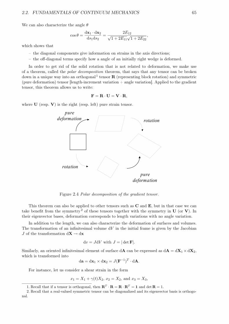
2.2. FUNDAMENTALS OF CONTINUUM MECHANICS 65
We can also characterize the angle θ
cos θ =dx1 · dx2
ds1ds2=
2E12√1 + 2E11
√1 + 2E22
,
which shows that
– the diagonal components give information on strains in the axis directions;– the off-diagonal terms specify how a angle of an initially right wedge is deformed.
In order to get rid of the solid rotation that is not related to deformation, we make useof a theorem, called the polar decomposition theorem, that says that any tensor can be brokendown in a unique way into an orthogonal 1 tensor R (representing block rotation) and symmetric(pure deformation) tensor [length-increment variation + angle variation]. Applied to the gradienttensor, this theorem allows us to write:
F = R ·U = V ·R,
where U (resp. V) is the right (resp. left) pure strain tensor.
rotation
rotation
pure
deformation
pure
deformation
Figure 2.4 Polar decomposition of the gradient tensor.
This theorem can also be applied to other tensors such as C and E, but in that case we cantake benefit from the symmetry 2 of these tensors together with the symmetry in U (or V). Intheir eigenvector bases, deformation corresponds to length variations with no angle variation.
In addition to the length, we can also characterize the deformation of surfaces and volumes.The transformation of an infinitesimal volume dV in the initial frame is given by the JacobianJ of the transformation dX → dx
dv = JdV with J = | detF|.Similarly, an oriented infinitesimal element of surface dA can be expressed as dA = dX1×dX2,which is transformed into
da = dx1 × dx2 = J(F−1)T · dA.
For instance, let us consider a shear strain in the form
x1 = X1 + γ(t)X2, x2 = X2, and x3 = X3,
1. Recall that if a tensor is orthogonal, then RT ·R = R ·RT = 1 and detR = 1.2. Recall that a real-valued symmetric tensor can be diagonalized and its eigenvector basis is orthogo-
nal.
66 CHAPTER 2. RHEOLOGY AND CONTINUUM MECHANICS
where γ(t) is called the shear amplitude and (x1, x2, x3) is the coordinates in a Cartesian frame.We find that this transformation keeps the volumes constant (J = 1) and
F =
1 γ 00 1 00 0 1
, C =
1 γ 0γ 1 + γ2 00 0 1
, and E =
0 γ/2 0γ/2 γ2/2 00 0 1
.
Small deformations
When deformations are small, we can linearize the tensors to get rid of nonlinear terms.Essentially this means that the displacement u = x−X between the current and initial positionsis very small. We can deduce that
– there is not much differences between the frame C0 and C(t), which can then be assumedto be the same;
– we can write F = 1 + H with H = ∇Xx with “small” entries.
We deduce that the Cauchy-Green tensor can be linearized in the following way
C = FT · F = 1 + H + HT = 1 + 2ε,
where ε is called the (linearized) strain tensor and is defined as the symmetric part of H
ε =12(H + HT ) =
12
(∇Xx +∇XxT)
= E.
Rate of strain
In order to characterize the velocity, we introduce the time derivative of x(X, t). In a La-grangian system, X corresponds to the initial condition at t = 0, whereas in an Eulerian system,X is the position previously occupied by a particle and is a function of time.
The time derivative of an infinitesimal length increment is
ddt
dx = F · dX = F · F−1 · dx = L · dx,
where L = F · F−1 = ∇xv is called the velocity gradient tensor. It is customary to break downinto a symmetric and antisymmetric contribution
d =12(L + LT ) and w =
12(L− LT ).
The symmetric part d describes the strain rate and hence is called the strain-rate tensor (so-metimes the stretching tensor), whereas the antisymmetric part w called the vorticity tensor(sometimes the spin tensor) corresponds to the rotational of the velocity field.
Recall that when a tensor w is antisymmetric, this implies the existence of a vector ω suchthat for any vector n, we have w · n = ω × n. Let us expand the velocity v(x + dx)
v(x + dx) = v(x) +∇xv · dx + · · · = v(x) + d(x) · dx + w(x) · dx + · · · ,
which means that to first order, we have
v(x + dx) = v(x) + d · dx + ω × dx.
This means that the local variation in the velocity field can be broken down into a strain-ratecontribution and another contribution corresponding to solid rotation
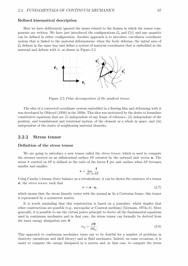
2.2. FUNDAMENTALS OF CONTINUUM MECHANICS 67
Refined kinematical description
Here we have deliberately ignored the issues related to the frames in which the tensor com-ponents are written. We have just introduced the configurations C0 and C(t) and any quantitycan be defined in either configuration. Another approach is to introduce curvilinear coordinatesystem that is linked to the material deformations: when the body deforms, the initial axes ofC0 deform in the same way and define a system of material coordinates that is embedded in thematerial and deform with it, as shown in Figure 2.5.
1e
2e
2′e
1′e
Figure 2.5 Polar decomposition of the gradient tensor.
The idea of a convected coordinate system embedded in a flowing film and deforming with itwas developed by Oldroyd (1950) in the 1950s. This idea was motivated by the desire to formulateconstitutive equations that are (i) independent of any frame of reference, (ii) independent of theposition, and translational and rotational motion, of the element as a whole in space, and (iii)independent of the states of neighboring material elements.
2.2.2 Stress tensor
Definition of the stress tensor
We are going to introduce a new tensor called the stress tensor, which is used to computethe stresses exerted on an infinitesimal surface δS oriented by the outward unit vector n. Thestress τ exerted on δS is defined as the ratio of the forces f per unit surface when δS becomessmaller and smaller:
τ = limδS→0
fδS
.
Using Cauchy’s lemma (force balance on a tetrahedron), it can be shown the existence of a tensorσ, the stress tensor, such that
τ = σ · n, (2.7)
which means that the stress linearly varies with the normal n. In a Cartesian frame, this tensoris represented by a symmetric matrix.
It is worth reminding that this construction is based on a postulate, which implies thatother constructions are possible (e.g., micropolar or Cosserat medium) (Germain, 1973a,b). Moregenerally, it is possible to use the virtual power principle to derive all the fundamental equationsused in continuum mechanics and in that case, the stress tensor can formally be derived fromthe inner energy dissipation rate Φ
σij =∂Φ∂dij
. (2.8)
This approach to continuum mechanics turns out to be fruitful for a number of problems inelasticity (membrum and shell theory) and in fluid mechanics. Indeed, on some occasions, it iseasier to compute the energy dissipated in a system and, in that case, to compute the stress
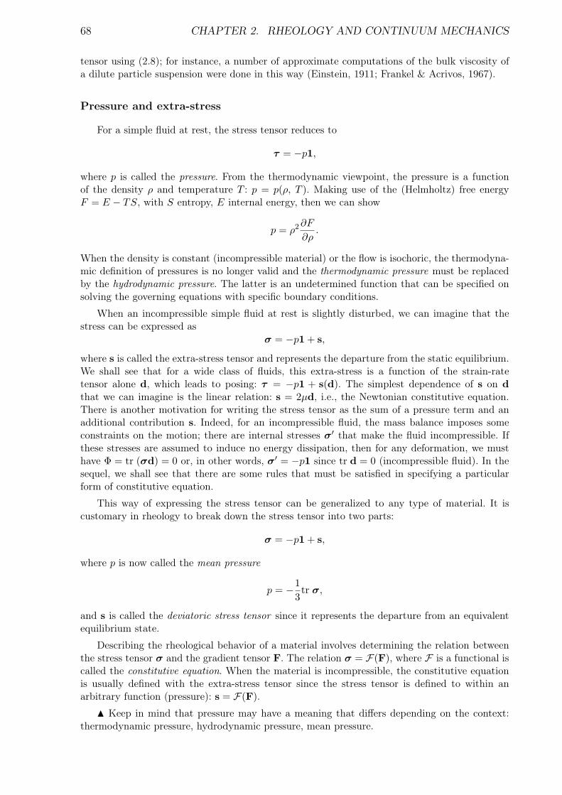
68 CHAPTER 2. RHEOLOGY AND CONTINUUM MECHANICS
tensor using (2.8); for instance, a number of approximate computations of the bulk viscosity ofa dilute particle suspension were done in this way (Einstein, 1911; Frankel & Acrivos, 1967).
Pressure and extra-stress
For a simple fluid at rest, the stress tensor reduces to
τ = −p1,
where p is called the pressure. From the thermodynamic viewpoint, the pressure is a functionof the density ρ and temperature T : p = p(ρ, T ). Making use of the (Helmholtz) free energyF = E − TS, with S entropy, E internal energy, then we can show
p = ρ2 ∂F
∂ρ.
When the density is constant (incompressible material) or the flow is isochoric, the thermodyna-mic definition of pressures is no longer valid and the thermodynamic pressure must be replacedby the hydrodynamic pressure. The latter is an undetermined function that can be specified onsolving the governing equations with specific boundary conditions.
When an incompressible simple fluid at rest is slightly disturbed, we can imagine that thestress can be expressed as
σ = −p1 + s,
where s is called the extra-stress tensor and represents the departure from the static equilibrium.We shall see that for a wide class of fluids, this extra-stress is a function of the strain-ratetensor alone d, which leads to posing: τ = −p1 + s(d). The simplest dependence of s on dthat we can imagine is the linear relation: s = 2µd, i.e., the Newtonian constitutive equation.There is another motivation for writing the stress tensor as the sum of a pressure term and anadditional contribution s. Indeed, for an incompressible fluid, the mass balance imposes someconstraints on the motion; there are internal stresses σ′ that make the fluid incompressible. Ifthese stresses are assumed to induce no energy dissipation, then for any deformation, we musthave Φ = tr (σd) = 0 or, in other words, σ′ = −p1 since tr d = 0 (incompressible fluid). In thesequel, we shall see that there are some rules that must be satisfied in specifying a particularform of constitutive equation.
This way of expressing the stress tensor can be generalized to any type of material. It iscustomary in rheology to break down the stress tensor into two parts:
σ = −p1 + s,
where p is now called the mean pressure
p = −13tr σ,
and s is called the deviatoric stress tensor since it represents the departure from an equivalentequilibrium state.
Describing the rheological behavior of a material involves determining the relation betweenthe stress tensor σ and the gradient tensor F. The relation σ = F(F), where F is a functional iscalled the constitutive equation. When the material is incompressible, the constitutive equationis usually defined with the extra-stress tensor since the stress tensor is defined to within anarbitrary function (pressure): s = F(F).
N Keep in mind that pressure may have a meaning that differs depending on the context:thermodynamic pressure, hydrodynamic pressure, mean pressure.
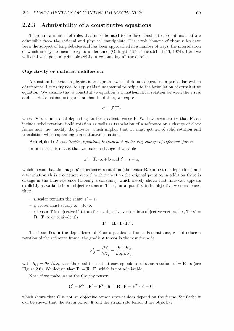
2.2. FUNDAMENTALS OF CONTINUUM MECHANICS 69
2.2.3 Admissibility of a constitutive equations
There are a number of rules that must be used to produce constitutive equations that areadmissible from the rational and physical standpoints. The establishment of these rules havebeen the subject of long debates and has been approached in a number of ways, the interrelationof which are by no means easy to understand (Oldroyd, 1950; Truesdell, 1966, 1974). Here wewill deal with general principles without expounding all the details.
Objectivity or material indifference
A constant behavior in physics is to express laws that do not depend on a particular systemof reference. Let us try now to apply this fundamental principle to the formulation of constitutiveequation. We assume that a constitutive equation is a mathematical relation between the stressand the deformation, using a short-hand notation, we express
σ = F(F)
where F is a functional depending on the gradient tensor F. We have seen earlier that F caninclude solid rotation. Solid rotation as wells as translation of a reference or a change of clockframe must not modify the physics, which implies that we must get rid of solid rotation andtranslation when expressing a constitutive equation.
Principle 1: A constitutive equations is invariant under any change of reference frame.
In practice this means that we make a change of variable
x′ = R · x + b and t′ = t + a,
which means that the image x′ experiences a rotation (the tensor R can be time-dependent) anda translation (b is a constant vector) with respect to the original point x; in addition there ischange in the time reference (a being a constant), which merely shows that time can appearsexplicitly as variable in an objective tensor. Then, for a quantity to be objective we must checkthat:
– a scalar remains the same: s′ = s,– a vector must satisfy x = R · x– a tensor T is objective if it transforms objective vectors into objective vectors, i.e., T′ ·x′ =
R ·T · x or equivalentlyT′ = R ·T ·RT .
The issue lies in the dependence of F on a particular frame. For instance, we introduce arotation of the reference frame, the gradient tensor is the new frame is
F ′ij =
∂x′i∂Xj
=∂x′i∂xk
∂xk
∂Xj,
with Rik = ∂x′i/∂xk an orthogonal tensor that corresponds to a frame rotation: x′ = R · x (seeFigure 2.6). We deduce that F′ = R · F, which is not admissible.
Now, if we make use of the Cauchy tensor
C′ = F′T · F′ = FT ·RT ·R · F = FT · F = C,
which shows that C is not an objective tensor since it does depend on the frame. Similarly, itcan be shown that the strain tensor E and the strain-rate tensor d are objective.
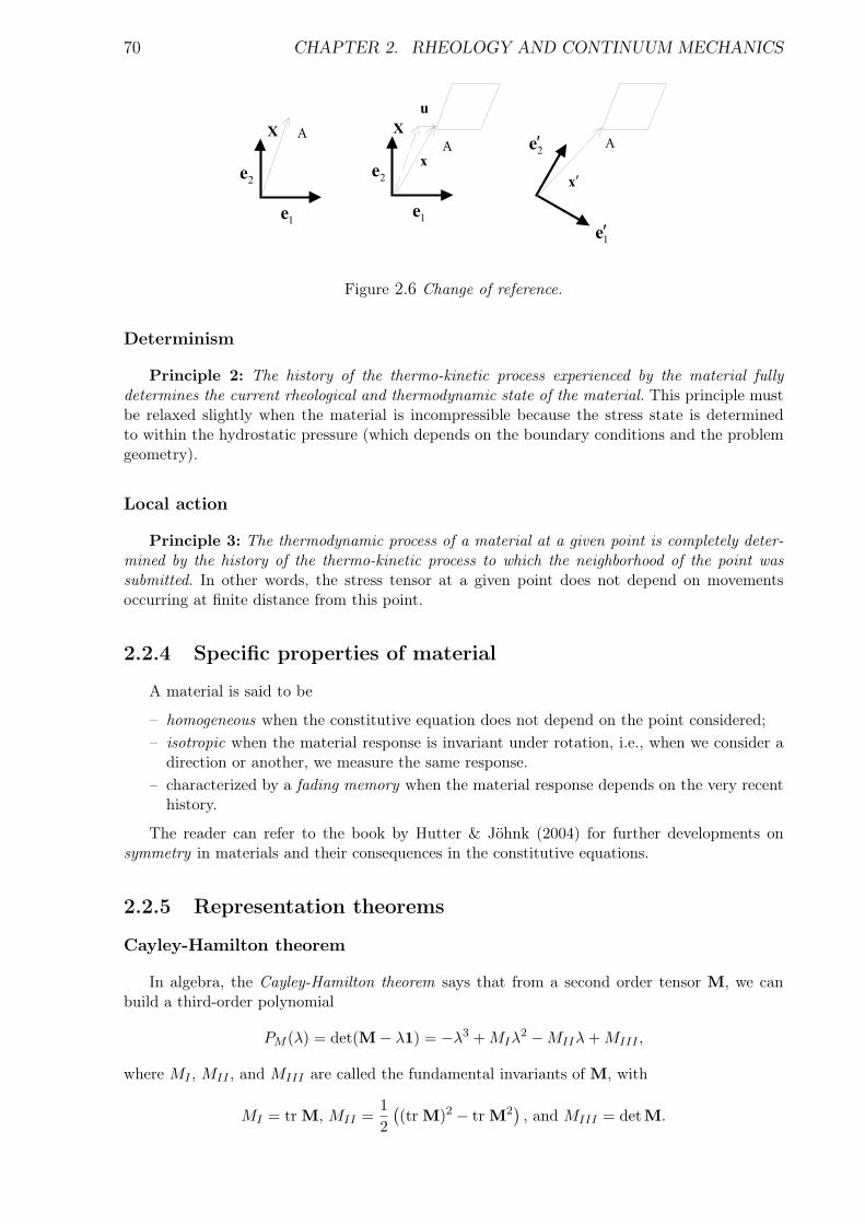
70 CHAPTER 2. RHEOLOGY AND CONTINUUM MECHANICS
1e
2e
1e
2e
2′e
1′e
A
A AX X
x
′x
u
Figure 2.6 Change of reference.
Determinism
Principle 2: The history of the thermo-kinetic process experienced by the material fullydetermines the current rheological and thermodynamic state of the material. This principle mustbe relaxed slightly when the material is incompressible because the stress state is determinedto within the hydrostatic pressure (which depends on the boundary conditions and the problemgeometry).
Local action
Principle 3: The thermodynamic process of a material at a given point is completely deter-mined by the history of the thermo-kinetic process to which the neighborhood of the point wassubmitted. In other words, the stress tensor at a given point does not depend on movementsoccurring at finite distance from this point.
2.2.4 Specific properties of material
A material is said to be
– homogeneous when the constitutive equation does not depend on the point considered;– isotropic when the material response is invariant under rotation, i.e., when we consider a
direction or another, we measure the same response.– characterized by a fading memory when the material response depends on the very recent
history.
The reader can refer to the book by Hutter & Jöhnk (2004) for further developments onsymmetry in materials and their consequences in the constitutive equations.
2.2.5 Representation theorems
Cayley-Hamilton theorem
In algebra, the Cayley-Hamilton theorem says that from a second order tensor M, we canbuild a third-order polynomial
PM (λ) = det(M− λ1) = −λ3 + MIλ2 −MIIλ + MIII ,
where MI , MII , and MIII are called the fundamental invariants of M, with
MI = tr M, MII =12
((tr M)2 − tr M2
), and MIII = detM.
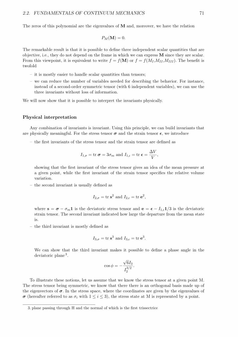
2.2. FUNDAMENTALS OF CONTINUUM MECHANICS 71
The zeros of this polynomial are the eigenvalues of M and, moreover, we have the relation
PM (M) = 0.
The remarkable result is that it is possible to define three independent scalar quantities that areobjective, i.e., they do not depend on the frame in which we can express M since they are scalar.From this viewpoint, it is equivalent to write f = f(M) or f = f(MI ,MII ,MIII). The benefit istwofold
– it is mostly easier to handle scalar quantities than tensors;– we can reduce the number of variables needed for describing the behavior. For instance,
instead of a second-order symmetric tensor (with 6 independent variables), we can use thethree invariants without loss of information.
We will now show that it is possible to interpret the invariants physically.
Physical interpretation
Any combination of invariants is invariant. Using this principle, we can build invariants thatare physically meaningful. For the stress tensor σ and the strain tensor ε, we introduce
– the first invariants of the stress tensor and the strain tensor are defined as
I1,σ = tr σ = 3σm and I1,ε = tr ε =∆V
V,
showing that the first invariant of the stress tensor gives an idea of the mean pressure ata given point, while the first invariant of the strain tensor specifies the relative volumevariation.
– the second invariant is usually defined as
I2,σ = tr s2 and I2,ε = tr e2,
where s = σ − σm1 is the deviatoric stress tensor and e = ε − I1,ε1/3 is the deviatoricstrain tensor. The second invariant indicated how large the departure from the mean stateis.
– the third invariant is mostly defined as
I3,σ = tr s3 and I3,ε = tr e3.
We can show that the third invariant makes it possible to define a phase angle in thedeviatoric plane 3.
cosφ = −√
6I3
I3/22
.
To illustrate these notions, let us assume that we know the stress tensor at a given point M.The stress tensor being symmetric, we know that there there is an orthogonal basis made up ofthe eigenvectors of σ. In the stress space, where the coordinates are given by the eigenvalues ofσ (hereafter referred to as σi with 1 ≤ i ≤ 3), the stress state at M is represented by a point.
3. plane passing through H and the normal of which is the first trissectrice
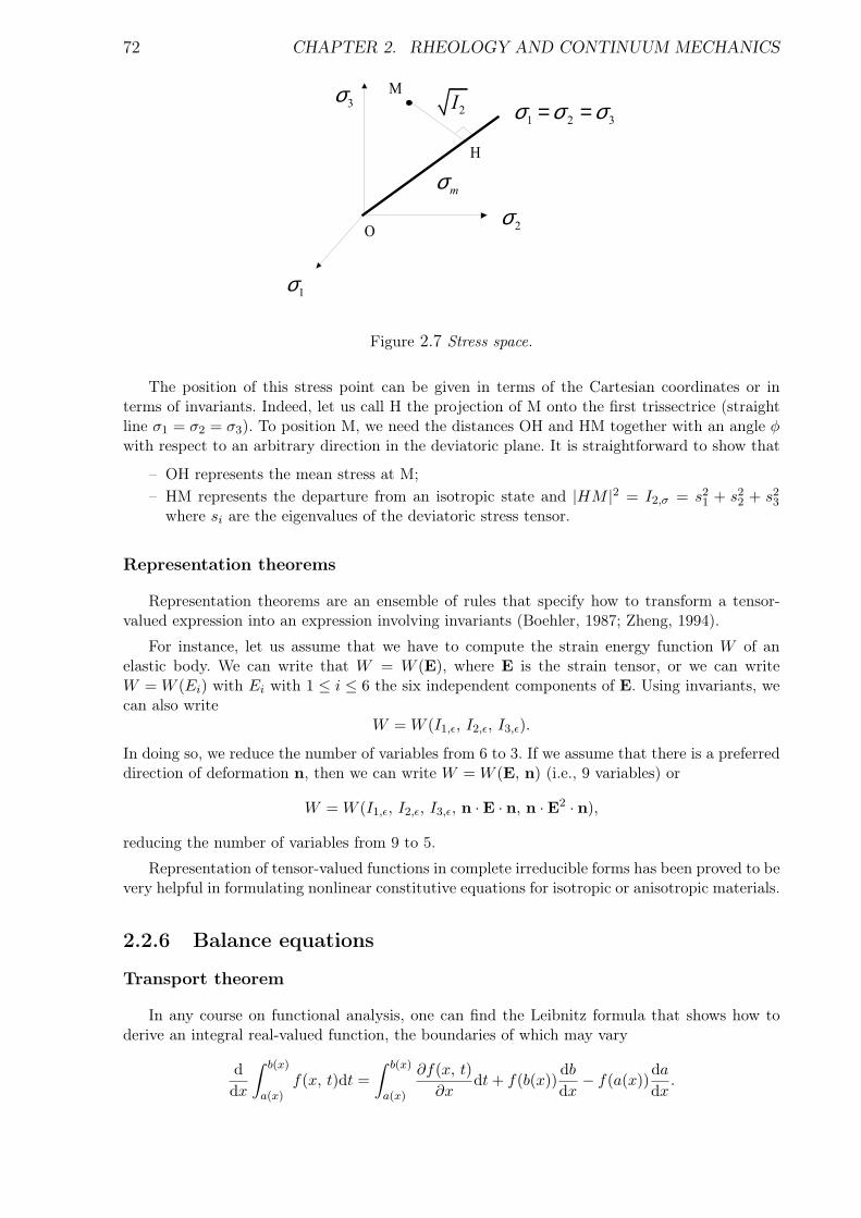
72 CHAPTER 2. RHEOLOGY AND CONTINUUM MECHANICS
O
3σ
2σ
1σ
1 2 3σ σ σ= =
M
mσ
H
2I
Figure 2.7 Stress space.
The position of this stress point can be given in terms of the Cartesian coordinates or interms of invariants. Indeed, let us call H the projection of M onto the first trissectrice (straightline σ1 = σ2 = σ3). To position M, we need the distances OH and HM together with an angle φwith respect to an arbitrary direction in the deviatoric plane. It is straightforward to show that
– OH represents the mean stress at M;– HM represents the departure from an isotropic state and |HM |2 = I2,σ = s2
1 + s22 + s2
3
where si are the eigenvalues of the deviatoric stress tensor.
Representation theorems
Representation theorems are an ensemble of rules that specify how to transform a tensor-valued expression into an expression involving invariants (Boehler, 1987; Zheng, 1994).
For instance, let us assume that we have to compute the strain energy function W of anelastic body. We can write that W = W (E), where E is the strain tensor, or we can writeW = W (Ei) with Ei with 1 ≤ i ≤ 6 the six independent components of E. Using invariants, wecan also write
W = W (I1,ε, I2,ε, I3,ε).
In doing so, we reduce the number of variables from 6 to 3. If we assume that there is a preferreddirection of deformation n, then we can write W = W (E, n) (i.e., 9 variables) or
W = W (I1,ε, I2,ε, I3,ε, n ·E · n, n ·E2 · n),
reducing the number of variables from 9 to 5.
Representation of tensor-valued functions in complete irreducible forms has been proved to bevery helpful in formulating nonlinear constitutive equations for isotropic or anisotropic materials.
2.2.6 Balance equations
Transport theorem
In any course on functional analysis, one can find the Leibnitz formula that shows how toderive an integral real-valued function, the boundaries of which may vary
ddx
∫ b(x)
a(x)f(x, t)dt =
∫ b(x)
a(x)
∂f(x, t)∂x
dt + f(b(x))db
dx− f(a(x))
da
dx.
2.2. FUNDAMENTALS OF CONTINUUM MECHANICS 73
Leibnitz relation can be generalized to multiple integrals, i.e. integration is made on volumesinstead of intervals. One obtains the following relation called transport theorem
ddt
∫
VfdV =
∫
V
∂f
∂tdV +
∫
Sfu · ndS, (2.9)
where V is the control volume containing a given mass of fluid, S is the surface bounding thisvolume, and n is the vector normal to the surface S ; n is unitary (|n| = 1) and outwardlyoriented. This relation written here for a scalar function f holds for any vectorial function f .
Equation (2.9) is fondamental since it makes it possible to derive all the equations needed incontinuum mechanics. It can be interpreted as follows Any variation in f with time within thecontrol volume V results from
– local change in f with time;– flux of f through S (flux = inflow – outflow through V ).
An helpful variant of the transport theorem is obtained by using the Green-Ostrogradskitheorem :
ddt
∫
VfdV =
∫
V
(∂f
∂t+∇ · (fu)
)dV .
This expression shall be used to derive local equations in the following.
N Be careful: a control volume is most often a material volume, i.e., it is made up ofa collection of particles that are followed up in their motion; its borders are fluid and movewith the fluid, which means that the boundary velocity corresponds to the local velocity at theboundary. On some occasions, we can also define an arbitrary control volume, the velocity ofwhich u at the border surface S does not correspond to that of the fluid.
Another important variant of the transport theorem is the Reynolds theorem that applies tointegrands that take the form ρf , with ρ the fluid density.
ddt
∫
VρfdV =
∫
Vρ
ddt
fdV. (2.10)
Conservation of mass
Let us apply the transport theorem (2.9) to f = ρ:
ddt
∫
VρdV =
∫
V
∂ρ(x, t)∂t
dV +∫
Sρu · ndS.
Making use of the divergence theorem (Green-Ostrogradski), we find
ddt
∫
VρdV =
∫
V
(∂ρ(x, t)
∂t+∇ · (ρu)
)dV = 0.
Note that the total mass is constant because we follow up a finite number of particles and thereis no production or loss of particles.
When ρ is continuous, then we can pass from a control-volume formulation to a local equation
∂ρ(x, t)∂t
+∇ · ρu = 0. (2.11)
This equation is often called continuity equation. It can also be cast in the following form:
1ρ
dρ
dt= −ρ∇ · u.
74 CHAPTER 2. RHEOLOGY AND CONTINUUM MECHANICS
N Recall that passing from global to local equations is permitted only if the field is continuous.This is not always the case, e.g. when there is a shock inside the control volume. Specific equationmust be used (see below).
Here are other helpful definitions
– a flow is said isochoric when 1ρ
dρdt = 0 (e.g., when the Mach number is less than unity, air
flow is isochoric);– a material is said incompressible when ρ is constant at any point and any time (water can
be considered as incompressible under normal flow conditions).
Conservation of momentum
One applies the transport theorem (2.9) tho the momentum f = ρu :
ddt
∫
VρudV =
∫
V
∂ρu∂t
dV +∫
Sρu(u · n)dS.
There are many variants of this equation, based either on different ways of expressing the ma-terial derivative of ρu or on different ways of expressing the velocity (e.g., streamline function,vorticity). On applying the divergence theorem, one gets :
ddt
∫
VρudV =
∫
V
(∂ρu∂t
+∇ · ρuu)
dV,
or equivalentlyddt
∫
VρudV =
∫
Vρ
(∂u∂t
+∇ · uu)
dV.
The fundamental principle of Mechanics is that any time variation in momentum results fromapplying body or surface force(s) on the control volume
ddt
∫
VρudV = forces applied on V.
Once again, we can obtain a local expression of the momentum balance equation if the fieldsare continuous:
∂ρu∂t
+∇ · ρuu = ρg +∇ · σ,
or
ρ∂u∂t
+ ρu · ∇u = ρg +∇ · σ = ρg −∇p +∇ · s (2.12)
N Be aware that u·∇u does not mean the product between u and the tensor ∇u. Rigorouslyspeaking, it would be better to write (u · ∇)u, the parentheses are used to say that u · ∇ is adifferential operator applied to u.
2.2.7 Conservation of energy
Kinetic energy
The transport theorem (2.9) is now applied to the kinetic energy f = Ec = 12ρ|u|2:
ddt
∫
V
12ρ|u|2dV =
∫
V
∂Ec
∂tdV +
∫
S
12ρ|u|2(u · n)dS.
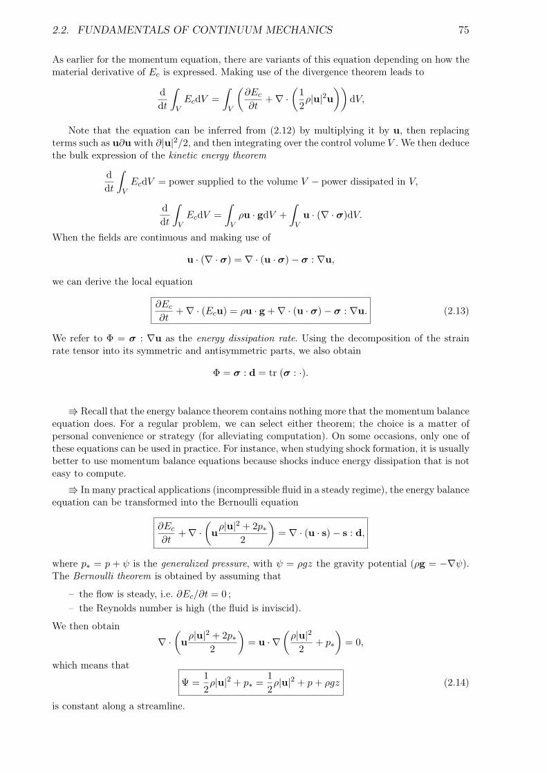
2.2. FUNDAMENTALS OF CONTINUUM MECHANICS 75
As earlier for the momentum equation, there are variants of this equation depending on how thematerial derivative of Ec is expressed. Making use of the divergence theorem leads to
ddt
∫
VEcdV =
∫
V
(∂Ec
∂t+∇ ·
(12ρ|u|2u
))dV,
Note that the equation can be inferred from (2.12) by multiplying it by u, then replacingterms such as u∂u with ∂|u|2/2, and then integrating over the control volume V . We then deducethe bulk expression of the kinetic energy theorem
ddt
∫
VEcdV = power supplied to the volume V − power dissipated in V,
ddt
∫
VEcdV =
∫
Vρu · gdV +
∫
Vu · (∇ · σ)dV.
When the fields are continuous and making use of
u · (∇ · σ) = ∇ · (u · σ)− σ : ∇u,
we can derive the local equation
∂Ec
∂t+∇ · (Ecu) = ρu · g +∇ · (u · σ)− σ : ∇u. (2.13)
We refer to Φ = σ : ∇u as the energy dissipation rate. Using the decomposition of the strainrate tensor into its symmetric and antisymmetric parts, we also obtain
Φ = σ : d = tr (σ : ·).
V Recall that the energy balance theorem contains nothing more that the momentum balanceequation does. For a regular problem, we can select either theorem; the choice is a matter ofpersonal convenience or strategy (for alleviating computation). On some occasions, only one ofthese equations can be used in practice. For instance, when studying shock formation, it is usuallybetter to use momentum balance equations because shocks induce energy dissipation that is noteasy to compute.
V In many practical applications (incompressible fluid in a steady regime), the energy balanceequation can be transformed into the Bernoulli equation
∂Ec
∂t+∇ ·
(u
ρ|u|2 + 2p∗2
)= ∇ · (u · s)− s : d,
where p∗ = p + ψ is the generalized pressure, with ψ = ρgz the gravity potential (ρg = −∇ψ).The Bernoulli theorem is obtained by assuming that
– the flow is steady, i.e. ∂Ec/∂t = 0 ;– the Reynolds number is high (the fluid is inviscid).
We then obtain
∇ ·(u
ρ|u|2 + 2p∗2
)= u · ∇
(ρ|u|2
2+ p∗
)= 0,
which means that
Ψ =12ρ|u|2 + p∗ =
12ρ|u|2 + p + ρgz (2.14)
is constant along a streamline.
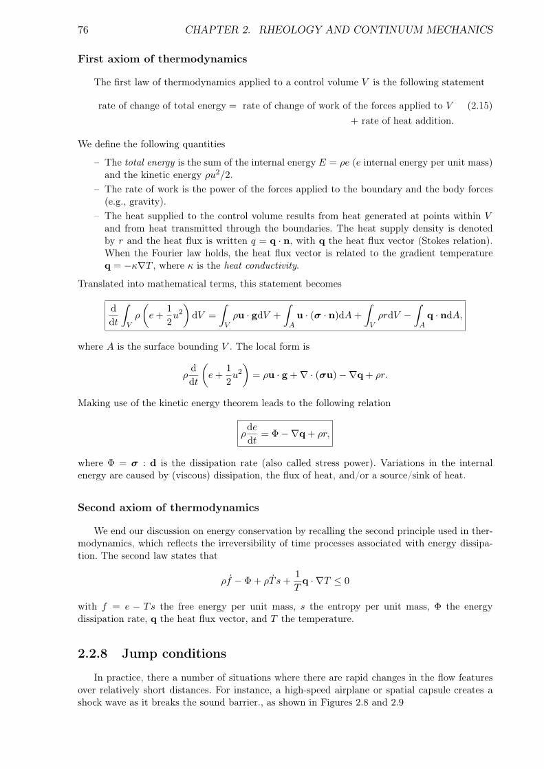
76 CHAPTER 2. RHEOLOGY AND CONTINUUM MECHANICS
First axiom of thermodynamics
The first law of thermodynamics applied to a control volume V is the following statement
rate of change of total energy = rate of change of work of the forces applied to V (2.15)+ rate of heat addition.
We define the following quantities
– The total energy is the sum of the internal energy E = ρe (e internal energy per unit mass)and the kinetic energy ρu2/2.
– The rate of work is the power of the forces applied to the boundary and the body forces(e.g., gravity).
– The heat supplied to the control volume results from heat generated at points within Vand from heat transmitted through the boundaries. The heat supply density is denotedby r and the heat flux is written q = q · n, with q the heat flux vector (Stokes relation).When the Fourier law holds, the heat flux vector is related to the gradient temperatureq = −κ∇T , where κ is the heat conductivity.
Translated into mathematical terms, this statement becomes
ddt
∫
Vρ
(e +
12u2
)dV =
∫
Vρu · gdV +
∫
Au · (σ · n)dA +
∫
VρrdV −
∫
Aq · ndA,
where A is the surface bounding V . The local form is
ρddt
(e +
12u2
)= ρu · g +∇ · (σu)−∇q + ρr.
Making use of the kinetic energy theorem leads to the following relation
ρde
dt= Φ−∇q + ρr,
where Φ = σ : d is the dissipation rate (also called stress power). Variations in the internalenergy are caused by (viscous) dissipation, the flux of heat, and/or a source/sink of heat.
Second axiom of thermodynamics
We end our discussion on energy conservation by recalling the second principle used in ther-modynamics, which reflects the irreversibility of time processes associated with energy dissipa-tion. The second law states that
ρf − Φ + ρT s +1T
q · ∇T ≤ 0
with f = e − Ts the free energy per unit mass, s the entropy per unit mass, Φ the energydissipation rate, q the heat flux vector, and T the temperature.
2.2.8 Jump conditions
In practice, there a number of situations where there are rapid changes in the flow featuresover relatively short distances. For instance, a high-speed airplane or spatial capsule creates ashock wave as it breaks the sound barrier., as shown in Figures 2.8 and 2.9
2.2. FUNDAMENTALS OF CONTINUUM MECHANICS 77
Figure 2.8 A U.S. Navy airplane creates a shock wave as it breaks the sound barrier. The shockwave is visible as a large cloud of condensation formed by the cooling of the air. A smaller shockwave can be seen forming on top of the canopy.(U.S. Navy photo by John Gay).
Figure 2.9 A shadowgraph of the Project Mercury reentry capsule, showing the bow-shock wavein front of it and the flow fields behind the capsule. Photograph from NASA).
In theory, it is usually appropriate to consider the shock as a discontinuity surface, i.e. asurface through the flow variables (density, velocity, etc.) may be become discontinuous. Thelocal balance equations are valid on either side of the jump, but not at the shock surface. Thisimplies that we have to specify the jump conditions on the flow variables induced by a shock.Note that a discontinuity surface may be an existing boundary (e.g. a free surface) or it may becreated under some flow conditions. Spontaneous creation or disappearance of a shock surface istypical for hyperbolic partial differential equations (Courant & Friedrich, 1948). We will focushere on the latter case.
Let us first consider the scalar case. We have to solve a hyperbolic problem in the form:
∂f(x, t)∂t
+∂G[f(x, t)]
∂x= a(x, t),
where G is a function and a another function called the source term. Note that the equationslooks like the balance equations we have seen earlier. Usually such an equation originates fromthe conservation of a quantity in a given control volume, i.e. an equation in the following integralform
ddt
∫
Vf(x, t)dx = G[f(x2, t)]−G[f(x1, t)] +
∫
Va(x, t)dx,
78 CHAPTER 2. RHEOLOGY AND CONTINUUM MECHANICS
where the control volume corresponds to the range [x1, x2] in the scalar case. When f is continuousover V , the two equations are equivalent. Let us assume that there is a moving point x = s(t)within [x1, x2] at which f admits a discontinuity. Making use of the Leibnitz rule, we have
ddt
∫ x2
x1
f(x, t)dx =∫ s(t)
x1
∂f(x, t)∂t
dx +∫ x2
s(t)
∂f(x, t)∂t
dx− sJfK,
where have broken down [x1, x2] = [x1, s(t)] + [s, x2(t)] and where JfK is the jump experiencedby f :
JfK = limx−>s, x>0
f(x)− limx−>s, x<0
f(x).
Then taking the limits x1 → s and x2 → s, leads to
JG[f(x, t)]− sf(x, t)K = 0,
where A =∫
a(x, t)dx. The quantity is G[f ] − fs is conserved through the shock. We can alsodeduce the shock velocity
s =JG[f(x, t)]KJf(x, t)K .
For instance, we can retrieve the Rankine-Hugoniot shock conditions used in gas dynamics ifwe take
– f = ρu (u being a velocity and ρ a density), G[f ] = 12ρu2 + p, and a = 0 (with p the
pressure), we have the (scalar) momentum equation along an axis. The shock condition isthen Jp + 1
2ρu2K = sJρuK at x = s(t).– f = ρ, G[f ] = ρu, and a = 0, we have the (scalar) mass equation along an axis. The shock
condition is then JρuK = sJρK at x = s(t). If we introduce the relative velocity u′ = u− s,we have also Jρu′K = 0, which means that in the frame relative to the shock, the mass fluxis conserved.
This equation can be generalized to higher dimensions without any problem.
N When dealing with shocks, it is very important to use the original conservation equations(in an integral form) from which the local equation has been derived. Typically, when the fieldare continuous, the equations
∂ρu
∂t+ u
∂ρu
∂x= 0,
and∂u
∂t+ u
∂u
∂x= 0,
are equivalent because of the continuity equation. However, the former equation comes directlyfrom the conservation of momentum (hence it is called the conservative form and ρu a conser-vative variable), whereas the latter is a simplification (called non-conservative form). It we rein-tegrate these equations to obtain the shock conditions, we will not find the same shock velocity.For this reason, care must be taken in computing shock conditions related to a hyperbolic partialdifferential equation.
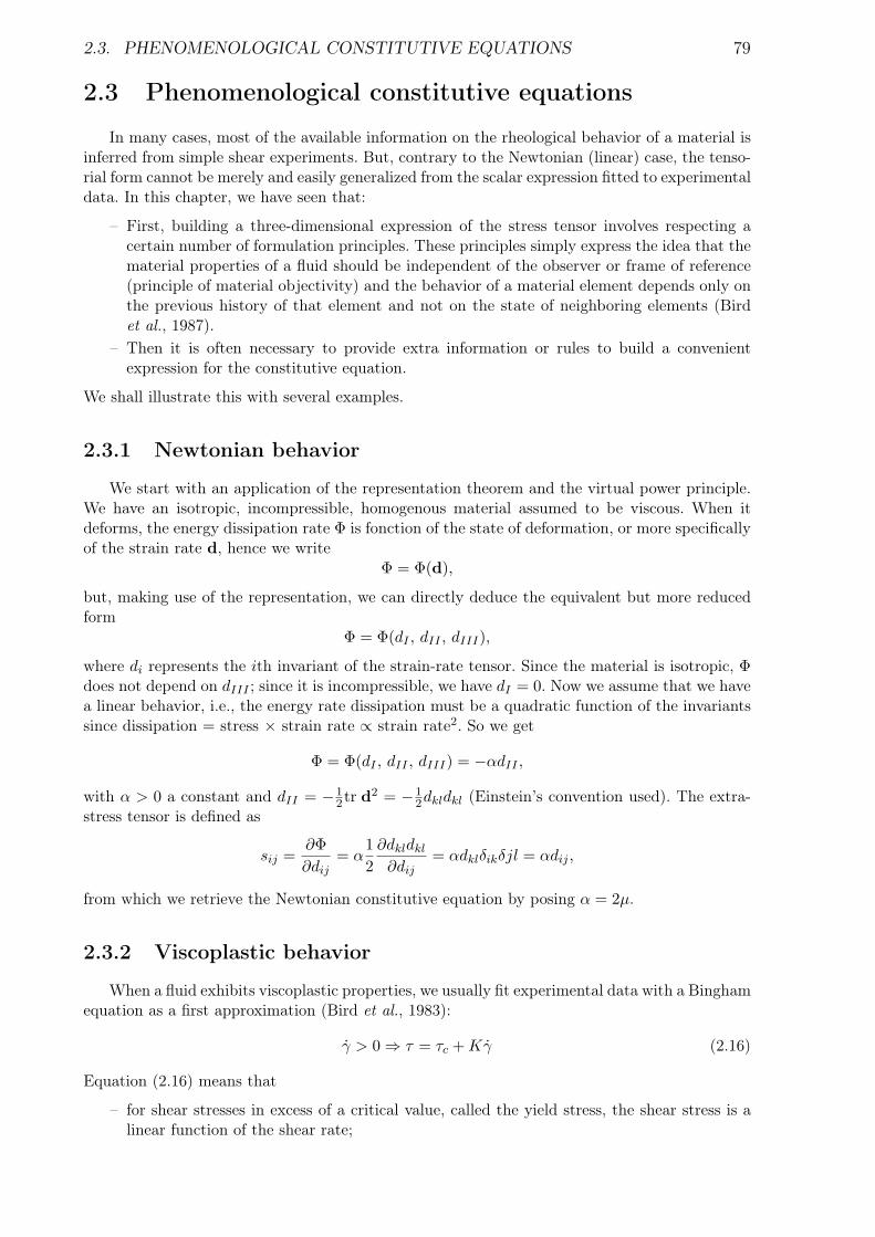
2.3. PHENOMENOLOGICAL CONSTITUTIVE EQUATIONS 79
2.3 Phenomenological constitutive equations
In many cases, most of the available information on the rheological behavior of a material isinferred from simple shear experiments. But, contrary to the Newtonian (linear) case, the tenso-rial form cannot be merely and easily generalized from the scalar expression fitted to experimentaldata. In this chapter, we have seen that:
– First, building a three-dimensional expression of the stress tensor involves respecting acertain number of formulation principles. These principles simply express the idea that thematerial properties of a fluid should be independent of the observer or frame of reference(principle of material objectivity) and the behavior of a material element depends only onthe previous history of that element and not on the state of neighboring elements (Birdet al., 1987).
– Then it is often necessary to provide extra information or rules to build a convenientexpression for the constitutive equation.
We shall illustrate this with several examples.
2.3.1 Newtonian behavior
We start with an application of the representation theorem and the virtual power principle.We have an isotropic, incompressible, homogenous material assumed to be viscous. When itdeforms, the energy dissipation rate Φ is fonction of the state of deformation, or more specificallyof the strain rate d, hence we write
Φ = Φ(d),
but, making use of the representation, we can directly deduce the equivalent but more reducedform
Φ = Φ(dI , dII , dIII),
where di represents the ith invariant of the strain-rate tensor. Since the material is isotropic, Φdoes not depend on dIII ; since it is incompressible, we have dI = 0. Now we assume that we havea linear behavior, i.e., the energy rate dissipation must be a quadratic function of the invariantssince dissipation = stress × strain rate ∝ strain rate2. So we get
Φ = Φ(dI , dII , dIII) = −αdII ,
with α > 0 a constant and dII = −12tr d2 = −1
2dkldkl (Einstein’s convention used). The extra-stress tensor is defined as
sij =∂Φ∂dij
= α12
∂dkldkl
∂dij= αdklδikδjl = αdij ,
from which we retrieve the Newtonian constitutive equation by posing α = 2µ.
2.3.2 Viscoplastic behavior
When a fluid exhibits viscoplastic properties, we usually fit experimental data with a Binghamequation as a first approximation (Bird et al., 1983):
γ > 0 ⇒ τ = τc + Kγ (2.16)
Equation (2.16) means that
– for shear stresses in excess of a critical value, called the yield stress, the shear stress is alinear function of the shear rate;
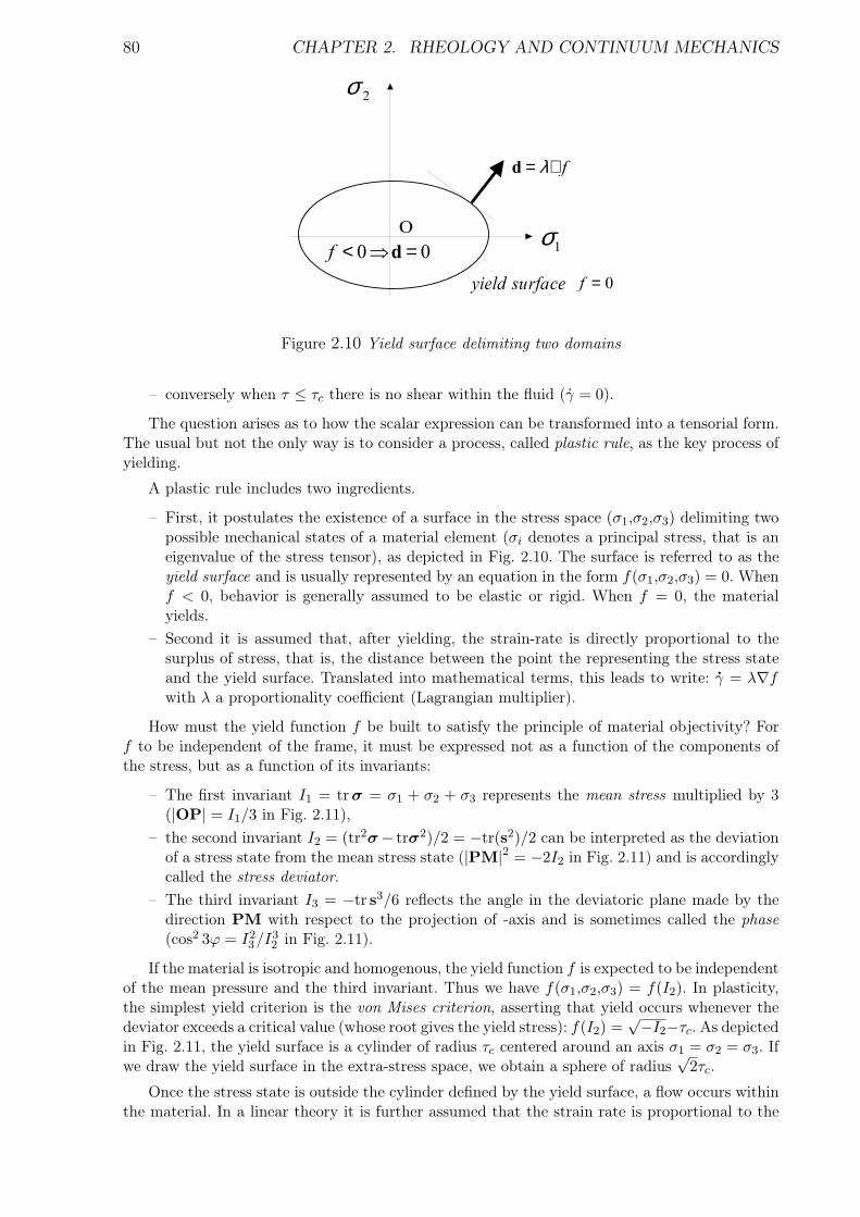
80 CHAPTER 2. RHEOLOGY AND CONTINUUM MECHANICS
O
1σ
2σ
yield surface
0 0f < ⇒ =d0f =
fλ= ∇d
Figure 2.10 Yield surface delimiting two domains
– conversely when τ ≤ τc there is no shear within the fluid (γ = 0).
The question arises as to how the scalar expression can be transformed into a tensorial form.The usual but not the only way is to consider a process, called plastic rule, as the key process ofyielding.
A plastic rule includes two ingredients.
– First, it postulates the existence of a surface in the stress space (σ1,σ2,σ3) delimiting twopossible mechanical states of a material element (σi denotes a principal stress, that is aneigenvalue of the stress tensor), as depicted in Fig. 2.10. The surface is referred to as theyield surface and is usually represented by an equation in the form f(σ1,σ2,σ3) = 0. Whenf < 0, behavior is generally assumed to be elastic or rigid. When f = 0, the materialyields.
– Second it is assumed that, after yielding, the strain-rate is directly proportional to thesurplus of stress, that is, the distance between the point the representing the stress stateand the yield surface. Translated into mathematical terms, this leads to write: γ = λ∇fwith λ a proportionality coefficient (Lagrangian multiplier).
How must the yield function f be built to satisfy the principle of material objectivity? Forf to be independent of the frame, it must be expressed not as a function of the components ofthe stress, but as a function of its invariants:
– The first invariant I1 = trσ = σ1 + σ2 + σ3 represents the mean stress multiplied by 3(|OP| = I1/3 in Fig. 2.11),
– the second invariant I2 = (tr2σ− trσ2)/2 = −tr(s2)/2 can be interpreted as the deviationof a stress state from the mean stress state (|PM|2 = −2I2 in Fig. 2.11) and is accordinglycalled the stress deviator.
– The third invariant I3 = −tr s3/6 reflects the angle in the deviatoric plane made by thedirection PM with respect to the projection of -axis and is sometimes called the phase(cos2 3ϕ = I2
3/I32 in Fig. 2.11).
If the material is isotropic and homogenous, the yield function f is expected to be independentof the mean pressure and the third invariant. Thus we have f(σ1,σ2,σ3) = f(I2). In plasticity,the simplest yield criterion is the von Mises criterion, asserting that yield occurs whenever thedeviator exceeds a critical value (whose root gives the yield stress): f(I2) =
√−I2−τc. As depictedin Fig. 2.11, the yield surface is a cylinder of radius τc centered around an axis σ1 = σ2 = σ3. Ifwe draw the yield surface in the extra-stress space, we obtain a sphere of radius
√2τc.
Once the stress state is outside the cylinder defined by the yield surface, a flow occurs withinthe material. In a linear theory it is further assumed that the strain rate is proportional to the
2.3. PHENOMENOLOGICAL CONSTITUTIVE EQUATIONS 81
1
2
3
yield surface
-2I3I
O
P
M2
Q
1
s1
s2
s3
-2I
PM
2
Q
Figure 2.11 On the left, the yield surface in the stress space when the von Mises criterion isselected as yield function. A stress state is characterized by its three principal stresses and thuscan be reported in the stress space. The three invariants of the stress tensor can be interpreted interms of co-ordinates
increment in stress (distance from the point representing the stress state M to the yield surface)and collinear to the normal ∂f/∂s. This leads to the expression:
d = λ(√
I2 − τc
) s√I2
(2.17)
For convenience, we define the proportionality coefficient as: λ−1 = 2η. It is generally more usualto express the constitutive equation in the converse form. First, the second invariant of the strainrate tensor J2 can be expressed as J2 = −tr(d2)/2 =
(λ
(√−I2 − τc
))2. Then we deduce theusual form of the Bingham constitutive equation:
d = 0 ⇔√−I2 ≤ τc (2.18)
d 6= 0 ⇔ σ = −p1 +(
2η +τc√−J2
)d (2.19)
It is worth noting that contrary to the Newtonian case, the general tensorial expression (2.18)cannot not easily be extrapolated from the steady simple-shear equation (2.16).
2.3.3 Viscoelasticity
When studying the linear 1D Maxwell model in § 1.5.4, we obtained an equation in the form
dγ
dt=
1G
dτ
dt+
τ
µ,
where G is the elastic modulus and µ denotes viscosity. We would like to transform this empiricalequation into a 3D tensorial expression and naively we write
2µd =µ
G
dσ
dt+ σ,
but it is not difficult to see that this expression does not satisfy the objectivity principle. Ac-cording to this principle, the stress tensor does not depend on the frame in which we use it (orits components) or, in other words, it must be invariant under any rotation. Let us consider thestress tensor when the frame of reference is rotated. We have
σ′ = R · σ ·RT
82 CHAPTER 2. RHEOLOGY AND CONTINUUM MECHANICS
the image of σ, where R is an orthogonal tensor. Taking the time derivative leads to
ddt
σ′ =dRdt
· σ ·RT + R · dσ
dt·RT + R · σ · dRT
dt6= R · dσ
dt·RT ,
which shows that σ is not objective. To overcome this issue, we have to define a kind of timederivative that satisfies the objectivity principle. For this purpose, note that if we replace σ withRT · σ′ ·R and introduce Ω = R ·RT , we have σ′ = R · σ ·R + Ω · σ′ + σ′ · ΩT , which canbe transformed by making use of the antisymmetry of Ω: σ′ = R · σ · RT + Ω · σ′ − σ′ · Ω.If we want to transform this derivative into an objective derivative, we have to get rid of thelast two contributing terms. There are different possibilities. Oldroyd introduced the Oldroyd (orconvective contravariant) derivative as follows:
Mσ= σ − L · σ − σ · LT ,
where L is the velocity gradient tensor. In this way, it is possible to
– provide a proper tensorial formulation of the constitutive equation;– make an empirical law (primarily valid for small deformations) consistent with large de-
formations.
The stress tensor is then solution to
2µd =µ
G
Ms +s.
Note that in this particular case, we do not have necessarily tr s, which is a typical example ofa fluid for which the extra-stress tensor differs from the deviatoric the stress tensor.
83
Chapter 3Rheophysics
Prerequisites– fluid mechanics: conservation law– mathematics: differential analysis, probability, algebra tools
Objectives– to provide the mathematical basis underpinning kinetic theory– to review a few averaging techniques– to deal with approximate methods for finding tractable analytical expressions– to introduce the readers with the modelling of particle suspension
Content
My presentation focuses on dynamic properties of particle suspensions. Because the behavioris complex, study of idealized situations makes it easier to understand the physics behind. Westart the chapter by outlining the relationship existing between a single particle and a fluidphase. Dimensionless numbers such as the Reynolds and the Stokes numbers are very helpful incharacterizing the strength of the phase coupling. On extreme cases, when the particle is the slaveor completely independent of the fluid phase, fully analytical derivations of the bulk constitutiveequation are possible. We show that using appropriate averaging procedures make it possible toconstruct the bulk stress tensor from the governing equations describing the motion on the bulkscale. At the end of this chapter, we give some clues to understand the physics of concentratedsuspensions that offer a substantial and challenging field of investigations.
84 CHAPTER 3. RHEOPHYSICS
3.1 Fundamentals of rheophysics
3.1.1 Movement of a single sphere and consequences on the flowregime
An overview
In the rheology of particle suspensions, the starting point in any rheophysical approach isto examine the behavior of individual components on a particle scale, then to infer the bulkrheological behavior by using an appropriate average process. In order to avoid overly generalexplanations, we assume that
(i) the interstitial fluid is Newtonian, with viscosity µ and density ρf ;(ii) the particles are rigid, spherical, and of equal size (radius a, density ρp).
Fluid motion is described by the Navier-Stokes equations:
∂uf
∂t+ uf · ∇uf = − 1
ρf∇p +
1ρf∇ · σf , (3.1)
∇ · uf = 0, (3.2)
where uf is the fluid velocity, p is the generalized pressure (including the fluid pressure andgravity potential), and σf is the stress tensor (here σf = 2µd where d denotes the strain-ratetensor). The equation of motion for the particle can be written in the following Lagrangian form:
dup
dt= g +
1mp
F(up,uf ), (3.3)
where F(up,uf ) is the force field resulting from the interaction between the fluid and the particle,mp is the particle mass, and up the velocity of the mass center. The boundary conditions at thesolid/fluid interface reflect non-penetration and fluid adherence: uf · k = 0, where k denotes theoutwardly-oriented unit normal.
Note that
– the force field F(up,uf ) is not yet defined;– when expressing the dependence of F on the flow variables, we assume that it depends on
the instantaneous particle velocity and the (Eulerian) velocity field (given by the Navier-Stokes equations).
The interplay between the two sets of equations is obvious since to solve the Navier-Stokesequations, we need to know the boundary conditions, hence the particle position, and in themeantime, to know this particle position, we have to determine the fluid velocity field.
To obtain a more physical picture of the fluid/particle interplay, we introduce dimensionlessnumbers and transform the equations above into dimensionless expressions. Let us introducea velocity scale U for the fluid. The timescale for the fluid motion near the particle is then:tf = a/U . The characteristic time for the particle is defined as a relaxation time, that is, thetime needed for its velocity to vary substantially as a result of the fluid action. If F is the order ofmagnitude of the fluid-particle interaction, examining Eq. (3.3) leads to selecting: tp = mpU/F .The equations of motion can now be written in dimensionless form as follows (dimensionlessvariables have a tilde) :
Rep
(∂uf
∂t+ uf · ∇uf
)= −Pρfa
µU∇p + ∆uf (3.4)
where P is the pressure scale [here P = µU/(ρfa)] and
Rep = ρfUa/µ,
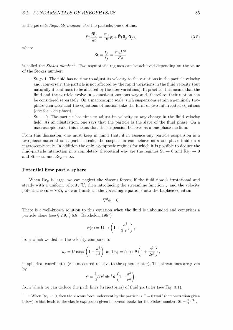
3.1. FUNDAMENTALS OF RHEOPHYSICS 85
is the particle Reynolds number. For the particle, one obtains:
Stdup
dt=
mp
Fg + F(up,uf ), (3.5)
where
St =tptf
=mpU
2
Fa,
is called the Stokes number 1. Two asymptotic regimes can be achieved depending on the valueof the Stokes number:
– St À 1. The fluid has no time to adjust its velocity to the variations in the particle velocityand, conversely, the particle is not affected by the rapid variations in the fluid velocity (butnaturally it continues to be affected by the slow variations). In practice, this means that thefluid and the particle evolve in a quasi-autonomous way and, therefore, their motion canbe considered separately. On a macroscopic scale, such suspensions retain a genuinely two-phase character and the equations of motion take the form of two interrelated equations(one for each phase).
– St → 0. The particle has time to adjust its velocity to any change in the fluid velocityfield. As an illustration, one says that the particle is the slave of the fluid phase. On amacroscopic scale, this means that the suspension behaves as a one-phase medium.
From this discussion, one must keep in mind that, if in essence any particle suspension is atwo-phase material on a particle scale, the suspension can behave as a one-phase fluid on amacroscopic scale. In addition the only asymptotic regimes for which it is possible to deduce thefluid-particle interaction in a completely theoretical way are the regimes St → 0 and Rep → 0and St →∞ and Rep →∞.
Potential flow past a sphere
When Rep is large, we can neglect the viscous forces. If the fluid flow is irrotational andsteady with a uniform velocity U, then introducing the streamline function ψ and the velocitypotential φ (u = ∇φ), we can transform the governing equations into the Laplace equation
∇2φ = 0.
There is a well-known solution to this equation when the fluid is unbounded and comprises aparticle alone (see § 2.9, § 6.8, Batchelor, 1967)
φ(r) = U · r(
1 +a3
2|r|3)
,
from which we deduce the velocity components
ur = U cos θ
(1− a3
r3
)and uθ = U cos θ
(1 +
a3
2r3
),
in spherical coordinates (r is measured relative to the sphere center). The streamlines are givenby
ψ =12Ur2 sin2 θ
(1− a3
r3
),
from which we can deduce the path lines (trajectories) of fluid particles (see Fig. 3.1).
1. When Rep → 0, then the viscous force underwent by the particle is F = 6πµaU (demonstration givenbelow), which leads to the classic expression given in several books for the Stokes number: St = 2
9a2U
ν .
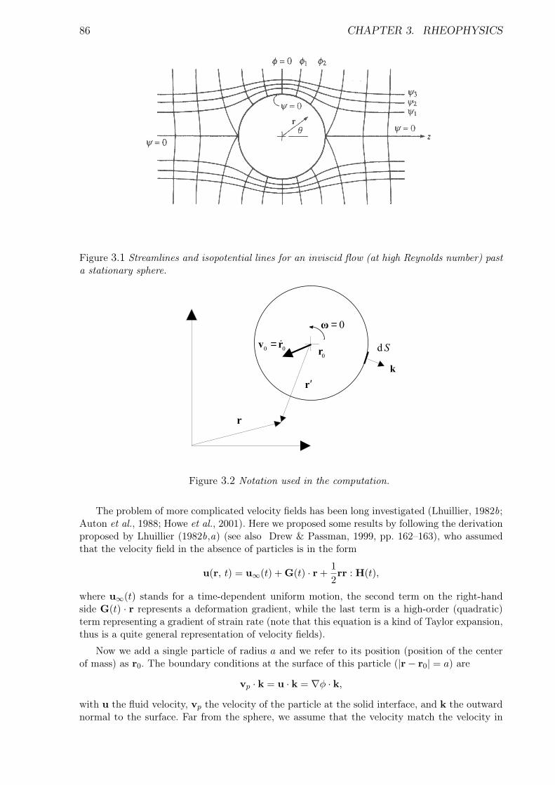
86 CHAPTER 3. RHEOPHYSICS
Figure 3.1 Streamlines and isopotential lines for an inviscid flow (at high Reynolds number) pasta stationary sphere.
0r
r
k
0 0=v r d S
0=ω
′r
Figure 3.2 Notation used in the computation.
The problem of more complicated velocity fields has been long investigated (Lhuillier, 1982b;Auton et al., 1988; Howe et al., 2001). Here we proposed some results by following the derivationproposed by Lhuillier (1982b,a) (see also Drew & Passman, 1999, pp. 162–163), who assumedthat the velocity field in the absence of particles is in the form
u(r, t) = u∞(t) + G(t) · r +12rr : H(t),
where u∞(t) stands for a time-dependent uniform motion, the second term on the right-handside G(t) · r represents a deformation gradient, while the last term is a high-order (quadratic)term representing a gradient of strain rate (note that this equation is a kind of Taylor expansion,thus is a quite general representation of velocity fields).
Now we add a single particle of radius a and we refer to its position (position of the centerof mass) as r0. The boundary conditions at the surface of this particle (|r− r0| = a) are
vp · k = u · k = ∇φ · k,
with u the fluid velocity, vp the velocity of the particle at the solid interface, and k the outwardnormal to the surface. Far from the sphere, we assume that the velocity match the velocity in
3.1. FUNDAMENTALS OF RHEOPHYSICS 87
the absence of the particle. The potential function related to the disturbed velocity field andconsistent with the boundary conditions at the free surface of a particle is found to be
φ(r, t|r0) = u∞(t) · r +12G(t) : rr +
a3
2r′3
(u0 − dr0
dt
)· r′ + a5
3r′5G : r′r′,
where for simplicity, we omit the H-dependent terms and where r′ = |r− r0|, u0 = u(r0), r0 isthe position of the center of mass of the particle, i.e, the fluid velocity at the position actuallyoccupied by the center of mass (see Fig. 3.2). The first two terms on the right-hand side representthe potential in the absence of the particle (i.e., the velocity field very far from the particle),whereas the two other contributions represent how the particle disturbs the fluid velocity field.Taking the gradient of the potential function provided the velocity field disturbed by a particlelocated at r0 and moving at velocity r0
u(r, t|r0) = u(r, t) +12
( a
r′)3
(u0 − r0) ·(1− 3
r′r′
r′2
)+
23
( a
r′)5
r′ ·G ·(1− 5
2r′r′
r′2
).
We can compute the force exerted by the fluid on the particle, which arises from the pressureat the body surface
F =∫
A(−p)kdA.
Using the Bernoulli equation for unsteady irrotational flows, we infer that the pressure is
∂φ
∂t+
12|u|2 +
p
ρf− g · r = constant,
where we note that the potential functions cannot be steady because of the motion of the sphereand the constant can be embedded in φ. We then deduce
F = ρf
∫
A
∂φ
∂tkdA +
12ρf
∫
Au · ukdA− ρf
∫
Ag · rkdA.
We finally obtainF
4π3 a3ρf
= −g +dudt
+12
(dudt− r0
),
where du/dt represents the acceleration of the undisturbed flow at the center of mass of thesphere. The last term on the right-hand side is called the added-mass effect. Note that in theabsence of fluid acceleration, the net force (i.e., ignoring the gravity force) is zero. This result iswell-known in fluid mechanics and is often referred to as the d’Alembert paradox.
Stokes flow past a sphere
Conversely, when the Reynolds number comes close to zero Rep → 0, a good approximationto the equations of motion is provided by the Stokes equation
∇ · u = 0, (3.6)
∇p = µ∇2u. (3.7)
These equations exhibit two specific properties that deserve a few comments:
– since the time derivative has been removed, the equations provide a pseudo-static descrip-tion of the motion;
– the equations are linear, hence we can use the superposition principle to find solutionsto complicated boundary-value problems. This is the key point in most analytical andnumerical treatment used for solving the Stokes equations.
88 CHAPTER 3. RHEOPHYSICS
By taking the divergence of the momentum equation, it can be shown that the pressure is aharmonic function while the velocity field is biharmonic:
∇2p = 0 and ∇4u = 0,
which may simplify the problem, especially when there is a free surface (e.g., see Garabedian,1966; Pozrikidis, 1992).
We are trying to determine the viscous force exerted on a particle by the surrounding fluidas a function of the particle velocity. There are two sub-problems encompassed in the originalformulation:
– mobility problem: we assume that we know the viscous force and torque experienced bythe particle and we seek its velocity;
– resistance problem: we seek the force and torque experienced by the particle when itsvelocity is prescribed.
The former solutions to the Stokes equations were constructed by using the method called ‘theseparation of variables’ (Lamb, 1932). Nowadays, it is more usual to use the singular solution me-thod (Green’s function) extensively used in elasticity and electrostatics. The original momentumequations is replaced by
∇p = µ∇2u + δ(x− x0)f(x), (3.8)
where f is a singular point force and δ is the Dirac function. Physically this equation means thatwhen a force F is exerted on a sphere immersed in a unbounded Newtonian fluid, one expectsthat sufficiently far from the sphere, the velocity and pressure fields are the same as those causedby a force of the same magnitude concentrated at point x0, i.e., the details of the flow in closevicinity around the sphere are lost. The first building block for constructing the solution is toseek a ‘far-field’ approximation. Using the Fourier transform of the modified momentum equation(3.8) or using the vorticity formulation of this momentum equation (Landau & Lifschitz, 1987),we can show that the fluid velocity field is
u(x) =1
8πµ
(1x
+xxx3
)· f ,
while the pressure field takes the form
p(x) =1
4πx3x · f ,
where for the sake of simplicity, we have posed x0 = 0 (see pp. 32–33, Russel et al., 1995), (seepp. 36–39, Kohr & Pop, 2004). In the velocity field expression, the multiplier of f is called theOseen tensor (or Oseen-Burgers tensor) or the free-space Green function 2
u(x) = I · f , with I =1
8πµ
(1x
+xxx3
).
The linearity of the solution appears clearly in this expression. This singular solution to themodified Stokes equations is usually called the Stokeslet. In the literature, Stokeslet refers toboth the force density f and the velocity field induced by this force. Sometimes, f is introducedas f = 8πµα, with α the strength (Kim & Karrila, 1991).
2. There is a classification of Green functions depending on the topology of the domain of flow (boun-ded, unbounded, semi-bounded). The free-space Green function corresponds to an infinite fluid domain.
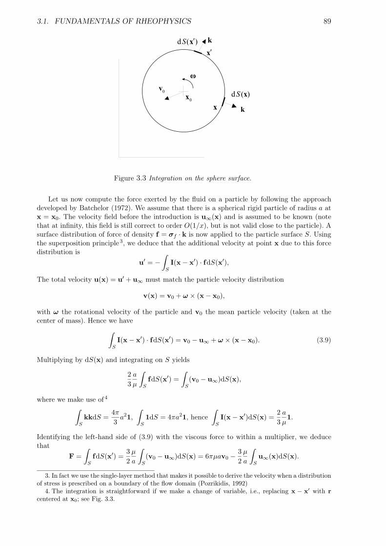
3.1. FUNDAMENTALS OF RHEOPHYSICS 89
k
0x
′x
x
d ( )S ′x
k
0v
d ( )S x
ω
Figure 3.3 Integration on the sphere surface.
Let us now compute the force exerted by the fluid on a particle by following the approachdeveloped by Batchelor (1972). We assume that there is a spherical rigid particle of radius a atx = x0. The velocity field before the introduction is u∞(x) and is assumed to be known (notethat at infinity, this field is still correct to order O(1/x), but is not valid close to the particle). Asurface distribution of force of density f = σf · k is now applied to the particle surface S. Usingthe superposition principle 3, we deduce that the additional velocity at point x due to this forcedistribution is
u′ = −∫
SI(x− x′) · fdS(x′),
The total velocity u(x) = u′ + u∞ must match the particle velocity distribution
v(x) = v0 + ω × (x− x0),
with ω the rotational velocity of the particle and v0 the mean particle velocity (taken at thecenter of mass). Hence we have
∫
SI(x− x′) · fdS(x′) = v0 − u∞ + ω × (x− x0). (3.9)
Multiplying by dS(x) and integrating on S yields
23
a
µ
∫
SfdS(x′) =
∫
S(v0 − u∞)dS(x),
where we make use of 4∫
SkkdS =
4π
3a21,
∫
S1dS = 4πa21, hence
∫
SI(x− x′)dS(x) =
23
a
µ1.
Identifying the left-hand side of (3.9) with the viscous force to within a multiplier, we deducethat
F =∫
SfdS(x′) =
32
µ
a
∫
S(v0 − u∞)dS(x) = 6πµav0 − 3
2µ
a
∫
Su∞(x)dS(x).
3. In fact we use the single-layer method that makes it possible to derive the velocity when a distributionof stress is prescribed on a boundary of the flow domain (Pozrikidis, 1992)
4. The integration is straightforward if we make a change of variable, i.e., replacing x − x′ with rcentered at x0; see Fig. 3.3.
90 CHAPTER 3. RHEOPHYSICS
By using a Taylor series of the velocity field u∞ at x = x0, we get
u∞(x) = u∞(x0) + ((x− x0) · ∇)u∞(x0) +12
((x− x0) · ∇)2 u∞(x0) + · · · ,
where we can transform the second-order operator ((x− x0) · ∇)2 on the right-hand side into((x− x0)(x− x0)∇∇ :) (do not forget the double dot for the inner product). Integrating on S,we get
F = 6πµa
(u∞(x0) +
16((a2∇2)u∞)|x0 − v0
).
This equation is known as the Faxén equation, which is a second-order correction to the Stokesforce: identifying vg = u∞(x0)−v0 as the particle velocity relative to the fluid, we can interpretthis equation as:
– a zero-order term F = 6πµavg + O(a2) which is referred to as the Stokes force;– a second-order contribution taking into account the perturbation of the fluid velocity field
as a result of shearing.
The key points to keep in mind are
– When the velocity u is known, we can derive the force F, which is linearly linked to u andvice versa. In the latter case, the mobility tensor of the sphere is M = (6πµa)−11 and wecan express vg = M · F. This is the key ingredient used in Stokesian-dynamics numericalmodels (Brady & Bossis, 1988).
– The method based on the singular solutions to the Stokes equation, which was used toobtain the results above, are likely to be the simplest one we can imagine. For comparisonsee the more complete, but more complicated boundary integral methods (Pozrikidis, 1992)or the proofs provided in fluid-mechanics textbooks (Lamb, 1932; Happel & Brenner, 1965;Batchelor, 1967; Bird et al., 1987).
General solution to the Stokes problem for unsteady flow conditions 5 have also been found(Mazur & Bedeaux, 1974; Coimbra & Rangel, 1998). The resulting equation is often called theBasset-Boussinesq-Oseen equation.
3.1.2 From a single sphere to a bulk: averaging
There are several fundamental properties that an averaging operator should satisfy to behelpful in deriving averaged equations. Let us represent the operator by a angular brackets: 〈f〉reads the averaged value of f . Here are these fundamental properties:
– First Reynolds rule: let c1 and c2 two constants and f1 and f2 two fields. Linearity of theaveraging procedure implies that
〈c1f1 + c2f2〉 = c1〈f1〉+ c2〈f2〉.
– Second Reynolds rule:〈g〈f〉〉 = 〈g〉〈f〉,
which also implies that averaging twice does not alter the outcome since taking g = 1, weget 〈〈f〉〉 = 〈f〉.
– Leibnitz rule: we can interchange time derivative and operating operator⟨
∂f
∂t
⟩=
∂〈f〉∂t
,
5. i.e., by assuming that the convective acceleration term in the Navier-Stokes momentum equation(2.3) alone vanishes
3.1. FUNDAMENTALS OF RHEOPHYSICS 91
but be aware that f may be admit jump within the material volume, which implies thataveraging such a function requires a bit more attention (see §9, Drew & Passman, 1999).
– Gauss rule: we can interchange space derivative and operating operator⟨
∂f
∂x
⟩=
∂〈f〉∂x
.
There are several ways of averaging a heterogenous medium. A great deal of literature hasbeen devoted to averaging procedures (e.g., see Jongschaap & Doeksen, 1983; Murdoch & Be-deaux, 1994; Drew & Passman, 1999). Data acquisition based on time averaging is probably apervasive way of measuring averaged quantities since it is the easiest method in practice, butfor theoretical purposes, volume or ensemble averaging is more appropriate. We will outline thedefinition and fundamental properties of these two operators in the following.
Volume averaging
Averaging any quantity f consists in
f(x,t) =1V
∫
Vf(x,t)dV. (3.10)
This operator is advantageous in that it can be permuted with time or space derivation, withthe subtlety that the integration volume includes both fluid and solid phases (see below).
Ensemble averaging
One of the most robust and efficient procedures is to consider (fictitiously) that we are able tocarry out as many runs as desired (we will refer to them as realizations) with the same conditionsat the macroscopic scale (same boundary conditions, same number of particles, etc.):
〈f〉 (x,t) =∫
Pf(x,t|R)dP (R), (3.11)
where R denotes a particular configuration/state of the system and P (R) the probability ofobserving the system in this configuration/state. f(x,t|R) is the value taken by f when the systemis in a given state R. Statistical mechanics provides a good examples of ensemble averaging; inthis case, a system is characterized by its energy E and the probability is of an exponential formdP = e−cEdE, with c a constant.
For suspensions in a Stokes regime, the configuration of the system can be related to theposition of the N particles within the suspension. Indeed, the system is entirely determinedwhen the particle positions and velocities are known since the fluid velocity can be deduceddirectly from this information. The ensemble average is then the average over all the possiblerealizations; the ensemble CN of all possible realizations constitute the space of states of thesystem at hand, i.e. CN is the set of parameters required to describe the setting. The dimensionof CN is the degree of freedom of the system studied. We introduce the probability P of observingN particles in a given configuration CN . The ensemble average of any quantity f is then:
〈f〉 (x,t) =∫
CN
dCNP (CN )f(x,t|CN ), (3.12)
where CN = (x1, x1, · · · , xN , xN ).
For a granular material, for which interstitial fluid effects can be ignored (or decoupled),it is also possible to use ensemble averages by utilizing the notion of configuration. However,
92 CHAPTER 3. RHEOPHYSICS
in that case, more information is needed since particles are in close contact and can transmitforces over long distances. The space of states must accordingly of higher dimension: CN =(x1, x1, x1 · · · , xN , xN , xN ), where we can replace replace the acceleration x with forces Fexerted on particles. If in the model we have to use the rotational velocity, we must once againincrease the dimension of the space of states by including the particle spin as a state variable:CN = (xi, xi, Fi, ωi)1≤i≤N , and so forth.
Compared to volume averaging, ensemble averaging does not require the notion of volume ofcontrol that can be cumbersome when dealing with finite-size samples (see below for an examplerelated to concentrated suspensions). An inconvenient is that it involves assigning probabilitiesto configurations of the systems, which may require a very large quantity of information to dealwith continuous phases. Another potential drawback is that ensemble averaging can only be usedfor finite systems, i.e., it is not possible to consider an unbounded volume.
3.1.3 Averaged balance equations
We consider equal-size spherical rigid particles (of radius a) within a Newtonian fluid. Thesuspension is assumed to be statistically homogeneous. The number of particles per unit volume(density number) is n and is related to the solid concentration φ (φ = volume occupied byparticles to total volume) since we have n = φ/(4πa3/3).
The approach first involves averaging the local equations of motion (volume averaging), thenusing an ensemble average, when required, to go farther in the interpretation of individual contri-butions. The operator “volume average” is constructed by taking a control volume V assumedto sufficiently wide to contain a large number of articles, but in the meantime sufficiently smallwith the respect to a typical lengthscale of the bulk for it to be considered as a continuum.
Bulk mass balance equation
For solid and fluid phases, the local mass balance equation is in the form
∂ρi
∂t+∇ · (ρiu) = 0,
with i = p (particle) or i = f (fluid). We define the bulk (volume-averaged) density as ρ = φρp +(1 − φ)ρf with φ the solid concentration. We also define a characteristic function (Lundgren,1972):
– H(x) = 1 if x is inside a particle;– H(x) = 0 if x lies within the fluid.
We call Vp the sub-volume of V containing the particles and Ap the surface bounding Vp.
Multiplying the mass equation for solid particles by the characteristic function H and themass equation for the continuous phase by 1−H and integrating over the control volume V, weobtain ∫
V
(H
∂ρp
∂t+ (1−H)
∂ρf
∂t+ H∇ · (ρpu) + (1−H)∇ · (ρfu)
)dV = 0,
that can be transformed into∫
V
(∂ρ
∂t+∇ · (ρu)− ρp
∂H
∂t− ρf
∂(1−H)∂t
− ρp∇ · (Hu)− ρf∇ · ((1−H)u))
dV = 0,
where we need to characterize how the characteristic function H varies with time and space.
For this purpose, it is worth noting that particle suspensions are characterized by the presenceof solid/fluid interfaces, which implies discontinuities in the material property (e.g., the local
3.1. FUNDAMENTALS OF RHEOPHYSICS 93
density may vary between a solid particle and the bounding fluid). Usually the fields studiedhere are smooth and can undergo jumps at material interfaces, which means that their timeand/or space derivative may be meaningless. This issue is overcome by using generalized functions(i.e., distributions). It is customary to introduce test functions, which have a finite support, arecontinuous, and admit derivative at all orders. For instance, if ψ denotes a test function with asupport D included in a larger domain B (i.e., ψ(x, t) = 0 for x ∈ B, but x /∈ D), we have
∫ψ(x, t)f(x, t)dx = 0 =
∫∂ψ(x, t)
∂tf(x, t)dxdt +
∫∂f(x, t)
∂tψ(x, t)dx,
which leads to the formula∫
∂f(x, t)∂t
ψ(x, t)dx = −∫
∂ψ(x, t)∂t
f(x, t)dx,
which is very helpful in getting rid of discontinuous derivatives. This equation remains nearly thesame when we replace the time derivative with a space derivative. Here, applying this procedureto the characteristic functions leads to
∂Hi
∂t+ u · ∇(Hi) = 0,
with i = f or p and where the following short-hand notations Hp = H and Hf = 1 − H havebeen used. This equation is sometimes referred to as the topological equation (Drew & Passman,1999). Then, applying the Gauss and Leibnitz rules to interchange the time/space derivativeswith the volume averaging operator, we deduce the bulk mass equation
∂ρ
∂t+∇ · (ρu) = 0.
Bulk momentum balance equation
Multiplying Equation (3.1) with 1−H, then integrating over the control volume V, makinguse of the mass conservation (∂H/∂t+u ·∇H = 0), the relation ∇H = k over Ap with k the unitoutward normal to Ap (and ∇H = 0 otherwise), and the Reynolds decomposition uf = uf +u′f ,we eventually obtain
ρf
(∂uf
∂t+∇ · uf uf
)= −∇p +
1V
∫
Ap
(σf − p1) · kdA+∇ · 1V
∫
Vf
(σf − ρfu′fu′f )dV. (3.13)
In this equation, the mean fluid velocity is
uf (x,t) =1V
∫
V(1−H(x,t))uf (x,t)dV =
1− φ
Vf
∫
Vf
uf (x,t)dV,
where we used∫V
(1−H)dV = 1−φ. Here, the mean fluid velocity is 1−φ the mean bulk velocity.
For the solid phase, we have to transform the Lagrangian equation of motion into an Eule-rian equivalent. The rigid-sphere assumption implies that the solid kinematic field is: up(x,t) =up(y,t) + ωp × (x − y), with y the position of the center of mass and ωp the rotation velo-city. Since the gradient of a rotational field is zero, the local equation is for a solid particle:ρp∂up/∂t = ρpg +∇ ·σp, with the following difficulty: the particle being rigid, the stress field isundetermined. This is in fact a minor issue since we will integrate the stress field over the particlevolume, the Green-Ostrogradski allows us to connect this field to the forces acting on the particle
94 CHAPTER 3. RHEOPHYSICS
surface. Proceeding as earlier by multiplying the equation above by H, then integrating it on V,we find
ρp
(∂up
∂t+∇ · upup
)= φρpg +∇ · (σp − ρpu′pu′p)−∇ · 1
V∫
Ap
σp · kdA. (3.14)
Since at the particle surface we have σp ·k = (σf − p1) · k, the last term on the right-hand side,representing the stresses exerted on the particle surface, is equivalent to the term in (??). Theseterms reflect momentum transfer between phases through their interface.
The local bulk velocity is defined as follows: u(x,t) = Hup(x,t) + (1 −H)uf (x,t). The bulkvolume-averaged velocity is then: u(x,t) = up(x,t) + uf (x,t). We can also define a bulk velocitybased on mass averaging (rather than volume): ρum = ρpup + ρf uf , with ρ = φρp + (1− φ)ρf .The two velocities coincide when the solid and fluid densities are equal. A helpful approximationcan be used when one of the densities is very low compared to the other and the velocities ofeach phase are of same magnitude. Using the same dimensional argument as earlier, we can showthat we meet such a case for a suspension of particles within a gas with St À 1 and ρp À ρf ;the same situation is met with emulsions (ρp ¿ ρf and St À 1 or St → 0). Note that the massconservation is satisfied ∇ · u = ∇ · um = 0 (φ is assumed to be constant).
Summing (??) et (??) leads to the bulk momentum equation:
ρ
(∂um
∂t+∇ · umu
)= −∇p? +∇ · 1
V∫
V(σ − ρu′u′)dV, (3.15)
with p? = Φ + pf (where ∇Φ = −ρg). This equation is not very helpful as long as we are notable to give it the classic form of momentum balance equation for a continuum; here this meansthat we must have um ≈ u so that the terms on the left-hand side can be identified as a materialderivative. If this condition is satisfied, then we can identify the term on the right-hand sideunder the divergence operator as a stress tensor. We refer to it as the bulk extra-stress tensor :
σ =1V
∫
V(σ − ρu′u′)dV, (3.16)
which is the definition used by Batchelor (1970) for the bulk stress tensor. Further computationreveals that this stress tensor can be divided into a fluid contribution (Batchelor, 1970; Anceyet al., 1999):
σ(f) = 2µd− 1V
∫
Vf
ρfu′u′dV, (3.17)
and a solid contribution (Ancey et al., 1999):
σ(p) =1V
∫
Ap
σ · xkdA− 1V
∫
Vp
ρpu′u′dV + G(ωp), (3.18)
where G(ωp) represents an antisymmetric function ωp, which is not detailed here because in mostcases of practical interest, G vanishes (Ancey et al., 1999; Batchelor, 1970; Prosperetti, 2004).
Energy balance equation
Let us focus our attention on particle suspensions that behave as one-phase material at thebulk scale. Similarly to the momentum balance, we can derive the energy balance equation. Here
3.1. FUNDAMENTALS OF RHEOPHYSICS 95
ε = e + u2/2 denotes the total energy per unit volume, where e is the internal energy and u2/2is the kinetic energy per unit volume. It can be shown that (Ancey et al., 1999):
dρe
dt+
12
d
dtρu′2 = σ : d +∇ · q +
∫
Ap
k · Jσ · uKdA. (3.19)
The first term on the left-hand side represents the variation in internal energy, while thesecond one is related to the fluctuating kinetic energy (where appears a “granular temperature”T = u′ · u′/3 representing particle agitation). On the right-hand side member, the first termrepresents the work supplied during the simple shear motion (for the simple shear motion, wehave σ · d = τ γ with τ the shear stress and γ the shear rate), the second term q = −σ · u′ is aflux of energy related to velocity fluctuations, whereas the third one reflects energy dissipationinduced by contact between particles (this term originates from the sliding between particles incontact).
Another interpretation is drawn from (3.19) on a control volume de V bounded by A. Rear-ranging the terms, we deduce (Ancey & Evesque, 2000) :
∫
Vσ : ddV =
∫
A
(12ρTu · k + q · k
)dA+
∫
V( ˙ε− 〈k · Jσ · uK〉)dV. (3.20)
The first term represents energy production resulting from shear. There are two ways ofdissipating energy
– energy diffusion, which acts as a redistribution of energy (no real creation). Here thisdiffusion operates through the advection of fluctuating kinetic energy (budget6 betweenthe fluctuating kinetic energy supplied to or provided by the control volume) and, on theother hand, the fluctuating kinetic energy dissipate energy at the boundaries7.
– The second mode of dissipation is related to processes of internal dissipation through anincrease:
– in internal energy (heat production resulting from viscous dissipation or inelasticdeformations inside particles, hence increase in thermodynamic temperature),
– dissipation resulting from slipping contacts between particles.
For dilute suspensions, there is no energy dissipation induced by solid particles, which impliesthat the primary mode of energy dissipation is related to internal energy. For concentratedsuspensions, there are
– energy dissipation at the solid boundaries when particle agitation is sufficiently high;– energy dissipation induced by slipping contacts between particles
Concerning energy dissipation, concentrated and dilute suspensions behave differently. A strikingproperty results from this difference: for Newtonian fluids, there is equivalence between energyand momentum balance equations; notably we can derive the stress in this way: σij = ∂Φ/∂dij .For concentrated suspensions, such a procedure requires that we specify the energy dissipatedby particle contact, which is not easy to determine.
3.1.4 Passing from volume averages to ensemble averages
While volume averaging is likely to be the more appropriate method for averaging equationsof motion, ensemble averaging turns out to be more efficient when pushing the computation ofindividual contributions farther.
6. Note that this budget is zero for a uniform steady flow, as shown in la figure 3.5, because either thevelocity vanishes on the volume boundary or there is a balance between inward flux and outward flux ofenergy.
7. This is the case when the boundaries contain a solid wall.
96 CHAPTER 3. RHEOPHYSICS
Conditional averaging
We start with the simplest description of the configuration of a system made up of particles,i.e., we want to describe the position of N particles. Earlier, we have introduced the characteristicfunction H(x), which takes the value 1 when x lies inside a particle and 0 otherwise. If we considerthat all particles have the same radius a and the position of their center of mass is given by yi,then we can write
H(x, t) =N∑
i=1
H(a− |x− yi|),
whereH is the Heaviside function. The number density carries the same information by providingthe position of the centers of mass
n(x, t) =N∑
i=1
δ(x− yi),
where δ is the Dirac function. What we want know is to reduce the amount of informationrequired to describe the system. For this purpose, we introduce the distribution function PN ,which is the probability of observing N particles occupying the position yi.
PN (t, y1, y2, · · · , yN ) = probability that at position yi, there is the center of mass of one particle.
The information contained in P is still very large and we can define reduced distribution functions,which are the marginal probability distribution of finding a finite number of particles at givenplace. For instance, P1(t, y1) gives the probability that the center of mass of one particles isplaced at y1
P1(t, y1) =∫
DN−1
PN (t, y1, y2, · · · ,yN )dy2dy3 · · · dyN ,
where D is the domain of integration. We can also define the conditional probability, which theprobability of observing N − 1 particles when the position of one particle is known to be at y1
P cN−1(t, y2, · · · ,yN |y1) =
PN (t, y1, y2, · · · ,yN )P1(t, y1)
.
Armed with these distribution functions, we can transform the ensemble average of a quantity f
〈f(x, t)〉 =∫
Df(x, t|CN )PN (t, y1, y2, · · · ,yN )dy1dy2 · · ·dyN
with the help of the conditional average of f
〈f(x, t|y1)〉 =∫
DN−1
f(x, t|CN )P cN−1(t, y1, y2, · · · ,yN |y1)dy2 · · ·dyN .
We obtain〈f(x, t)〉 =
∫
D〈f(x, t|y1)〉P1(t, y1)dy1.
The result can be extended to two particles or more
〈f(x, t)〉 =∫
D2
〈f(x, t|y1, y2)〉P2(t, y1, y2)dy1dy2,
P2 is the pair distribution function defined as the probability that simultaneously the centers oftwo spheres lie respectively in y1 and y2. The physical meaning of these equations is clear: wehave to average a quantity f , which takes its values on both the solid and fluid phases and isinfluenced by the configuration CN of the N spheres. The ensemble average of f is the meanvalue of f over all the possible configurations. By introducing conditional probabilities on one
3.1. FUNDAMENTALS OF RHEOPHYSICS 97
or more particle(s), we can focus our attention on a finite set of ‘test’ sphere(s). The notationf(x, t|y1) reads “variation of f(x, t) given that one particle is located at y1”.
Further simplification is obtained by posing some assumptions on the configuration of thesystem. For instance, for a dilute suspension (φ small), the number of particles per unit volumeis the density number n. Within a volume r3, the number of particles is on average nr3; if weassume that the distribution of the number of particles lying within a unit volume follows aPoisson distribution (an assumption that seems realistic for dilute suspensions), the probabilityP that k spheres are located at a distance lower than r from the test sphere is given by
P(k) = e−nr3 (nr3)k
k!,
which shows that the probability of finding one particle around the test particle is of the orderφ(r/a)3, thus is a small quantity. Likewise the probability of finding two spheres simultaneouslyis of the order φ2(r/a)6 and so forth. If the function f is such that f(x, t) ∝ (a/x)n, with n > 3,then it decreases to zero more rapidly than 1/P, this means that the influence of other spherescan be neglected. In this case, in the definition of the conditional average
〈f(x, t|y1, y2)〉 =∫
DN−2
f(x, t)P cN−1(t, y1, y2, · · · ,yN |y1, y2)dy3 · · ·dyN ,
we can consider that f(x, t) is independent of the position of the N − 2 remaining particles,which implies that we can extract f(x, t) from the integrand. To order O(φ2), we have
〈f(x, t|y1, y2)〉 = f(x, t|CN )∫
DN−2
P cN−1(t, y1, y2, · · · ,yN |y1, y2)dy3 · · ·dyN = f(x, t|y1, y2),
thus
〈f(x, t)〉 =∫
DN−2
f(x, t|y1, y2)P2(t, y1, y2)dy1dy2.
Furthermore, if we assume that there is no preferential direction for f (isotropy) and no explicittime dependence, then P2(t, y1, y2) reduces to the radial distribution function g(r) with r =|y1 − y2|. In a number of kinetic theories or microstructural models, all the information on themicrostructure is contained in the function g(r).
In the developments above, emphasis has been given to defining the configuration of thesystem via the position of the N spheres. Obviously, we can extend the number of state para-meters for refining the description, e.g., by including the velocity, the orientation, the spin, theacceleration, etc.
Boltzmann equation
One of the major achievements of microstructural theories was the kinetic theory for dilutegases proposed by Boltzmann in 1872. It took a long while to recognize that this theory was adecisive breakthrough in our way of thinking about the connection between molecules and bulkbehavior of gases. One of the fundamental building block of this theory is the so-called Boltzmannequation that teaches us how the probability density function P describing the states of a systemvaries with time.
Let us consider particles that move at velocity v and experience forces F. The governingequation is given by equation (3.3). The number of particles at time t within a small volume draround r and with velocities v is denoted by f(x, v, t). The normalizing constraint is
∫
Ddx
∫
Rf(x, v, t)dv = N
98 CHAPTER 3. RHEOPHYSICS
when there are N molecules in the domain D. Differentiating with respect to time leads to∫
Ddx
∫
R3
(∂
∂tf +
∂x∂t· ∇xf +
∂v∂t
· ∇vf
)dv =
∫
Ddx
∫
R3
(∂
∂tf + v · ∇xf +
Fmp
· ∇vf
)= 0,
from which we deduce that if there is no jump in f , then
∂
∂tf + v · ∇xf +
Fmp
· ∇vf = 0.
This derivation is valid solely for particles that do not interact. If particles interact (e;g., collisionin a gas made up of molecules), then we have to take into account a source term due representingparticle interactions. In kinetic theory, making allowance for particle interactions leads to anexpression in the form
∂
∂tf + v · ∇xf +
Fmp
· ∇vf =∂
∂tf
∣∣∣∣collisions
,
where the new contribution on the right-hand side indicates how collisions modify the timevariations of the distribution function f . It can be shown (Chapman & Cowling, 1970; Drew &Passman, 1999)
∂
∂tf
∣∣∣∣collisions
=∫
dΩ∫
R3
dv1|v − v1|Se(Ω,|v − v1|(f(r, v′,t)f(r, v′1,t)− f(r, v,t)f(r, v1,t)
),
where Ω is the solid angle indicating the deflection of molecules after collision, the prime is usedto refer to post-collision velocities, Se is the efficient section (ISe(Ω,|v)dΩ represents the numberof molecules flying in the direction represented by the solid angle Ω where I is the number ofparticles per unit time crossing a unit surface normal to u). The Boltzmann is the prototype ofa kinetic equation describing the variations of the probability distribution f . Although it is oneout of the simplest kinetic equations we can imagine, it is markedly difficult to solve becausethe equation is of integro-differential type. Usually, one restricts to steady or nearly steady flowconditions, which implies that
∂
∂tf
∣∣∣∣collisions
≈ 0,
or more precisely f(r, v′,t)f(r, v′1,t)− f(r, v,t)f(r, v1,t). Simple inspection the function f in asteady state must satisfy
ln f = Ae−B(v−c)2 ,
where A, B, and c are unknown quantities that can be determined using the normalizingconstraint. By introducing the temperature T as
12mp
∫
R3
dv|v|2f(v) =32ρkBT,
with ρ the gas density, kB Boltzmann’s constant, we deduce that the steady-state function is
fss(r, v,t) = ρ
(mp
ρkBT
)3/2
e− 1
2
mp|v|2kBT ,
which is known as the Maxwellian distribution of velocities at temperature T
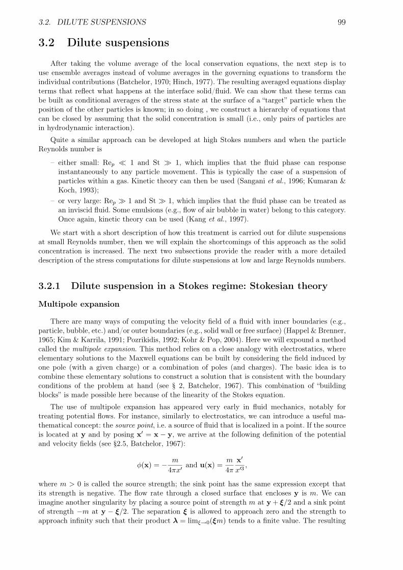
3.2. DILUTE SUSPENSIONS 99
3.2 Dilute suspensions
After taking the volume average of the local conservation equations, the next step is touse ensemble averages instead of volume averages in the governing equations to transform theindividual contributions (Batchelor, 1970; Hinch, 1977). The resulting averaged equations displayterms that reflect what happens at the interface solid/fluid. We can show that these terms canbe built as conditional averages of the stress state at the surface of a “target” particle when theposition of the other particles is known; in so doing , we construct a hierarchy of equations thatcan be closed by assuming that the solid concentration is small (i.e., only pairs of particles arein hydrodynamic interaction).
Quite a similar approach can be developed at high Stokes numbers and when the particleReynolds number is
– either small: Rep ¿ 1 and St À 1, which implies that the fluid phase can responseinstantaneously to any particle movement. This is typically the case of a suspension ofparticles within a gas. Kinetic theory can then be used (Sangani et al., 1996; Kumaran &Koch, 1993);
– or very large: Rep À 1 and St À 1, which implies that the fluid phase can be treated asan inviscid fluid. Some emulsions (e.g., flow of air bubble in water) belong to this category.Once again, kinetic theory can be used (Kang et al., 1997).
We start with a short description of how this treatment is carried out for dilute suspensionsat small Reynolds number, then we will explain the shortcomings of this approach as the solidconcentration is increased. The next two subsections provide the reader with a more detaileddescription of the stress computations for dilute suspensions at low and large Reynolds numbers.
3.2.1 Dilute suspension in a Stokes regime: Stokesian theory
Multipole expansion
There are many ways of computing the velocity field of a fluid with inner boundaries (e.g.,particle, bubble, etc.) and/or outer boundaries (e.g., solid wall or free surface) (Happel & Brenner,1965; Kim & Karrila, 1991; Pozrikidis, 1992; Kohr & Pop, 2004). Here we will expound a methodcalled the multipole expansion. This method relies on a close analogy with electrostatics, whereelementary solutions to the Maxwell equations can be built by considering the field induced byone pole (with a given charge) or a combination of poles (and charges). The basic idea is tocombine these elementary solutions to construct a solution that is consistent with the boundaryconditions of the problem at hand (see § 2, Batchelor, 1967). This combination of “buildingblocks” is made possible here because of the linearity of the Stokes equation.
The use of multipole expansion has appeared very early in fluid mechanics, notably fortreating potential flows. For instance, similarly to electrostatics, we can introduce a useful ma-thematical concept: the source point, i.e. a source of fluid that is localized in a point. If the sourceis located at y and by posing x′ = x − y, we arrive at the following definition of the potentialand velocity fields (see §2.5, Batchelor, 1967):
φ(x) = − m
4πx′and u(x) =
m
4π
x′
x′3,
where m > 0 is called the source strength; the sink point has the same expression except thatits strength is negative. The flow rate through a closed surface that encloses y is m. We canimagine another singularity by placing a source point of strength m at y + ξ/2 and a sink pointof strength −m at y − ξ/2. The separation ξ is allowed to approach zero and the strength toapproach infinity such that their product λ = limξ→0(ξm) tends to a finite value. The resulting
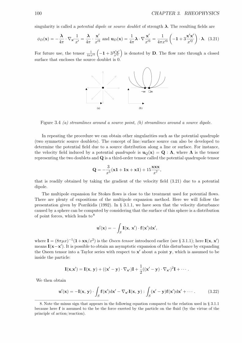
100 CHAPTER 3. RHEOPHYSICS
singularity is called a potential dipole or source doublet of strength λ. The resulting fields are
φD(x) = − λ
4π· ∇x′
1x′
=λ
4π· x′
x′3and uD(x) =
14π
λ · ∇ x′
x′3=
14πx′3
(−1 + 3
x′x′
x′2
)· λ. (3.21)
For future use, the tensor 14πx′3
(−1 + 3x′x′
x′2
)is denoted by D. The flow rate through a closed
surface that encloses the source doublet is 0.
m+m−
(a) (b)
Figure 3.4 (a) streamlines around a source point, (b) streamlines around a source dipole.
In repeating the procedure we can obtain other singularities such as the potential quadruple(two symmetric source doublets). The concept of line/surface source can also be developed todetermine the potential field due to a source distribution along a line or surface. For instance,the velocity field induced by a potential quadrupole is uQ(x) = Q : Λ, where Λ is the tensorrepresenting the two doublets and Q is a third-order tensor called the potential quadrupole tensor
Q = − 3x5
(x1 + 1x + x1) + 15xxxx7
,
that is readily obtained by taking the gradient of the velocity field (3.21) due to a potentialdipole.
The multipole expansion for Stokes flows is close to the treatment used for potential flows.There are plenty of expositions of the multipole expansion method. Here we will follow thepresentation given by Pozrikidis (1992). In § 3.1.1, we have seen that the velocity disturbancecaused by a sphere can be computed by considering that the surface of this sphere is a distributionof point forces, which leads to 8
u′(x) = −∫
SI(x, x′) · f(x′)dx′,
where I = (8πµx)−1(1+xx/x2) is the Oseen tensor introduced earlier (see § 3.1.1); here I(x, x′)means I(x−x′). It is possible to obtain an asymptotic expansion of this disturbance by expandingthe Oseen tensor into a Taylor series with respect to x′ about a point y, which is assumed to beinside the particle:
I(x,x′) = I(x, y) + ((x′ − y) · ∇x′)I +12((x′ − y) · ∇x′)2I + · · · .
We then obtain
u′(x) = −I(x, y) ·∫
Sf(x′)dx′ −∇x′I(x, y) :
∫
S(x′ − y)f(x′)dx′ + · · · . (3.22)
8. Note the minus sign that appears in the following equation compared to the relation used in § 3.1.1because here f is assumed to the be the force exerted by the particle on the fluid (by the virtue of theprinciple of action/reaction).
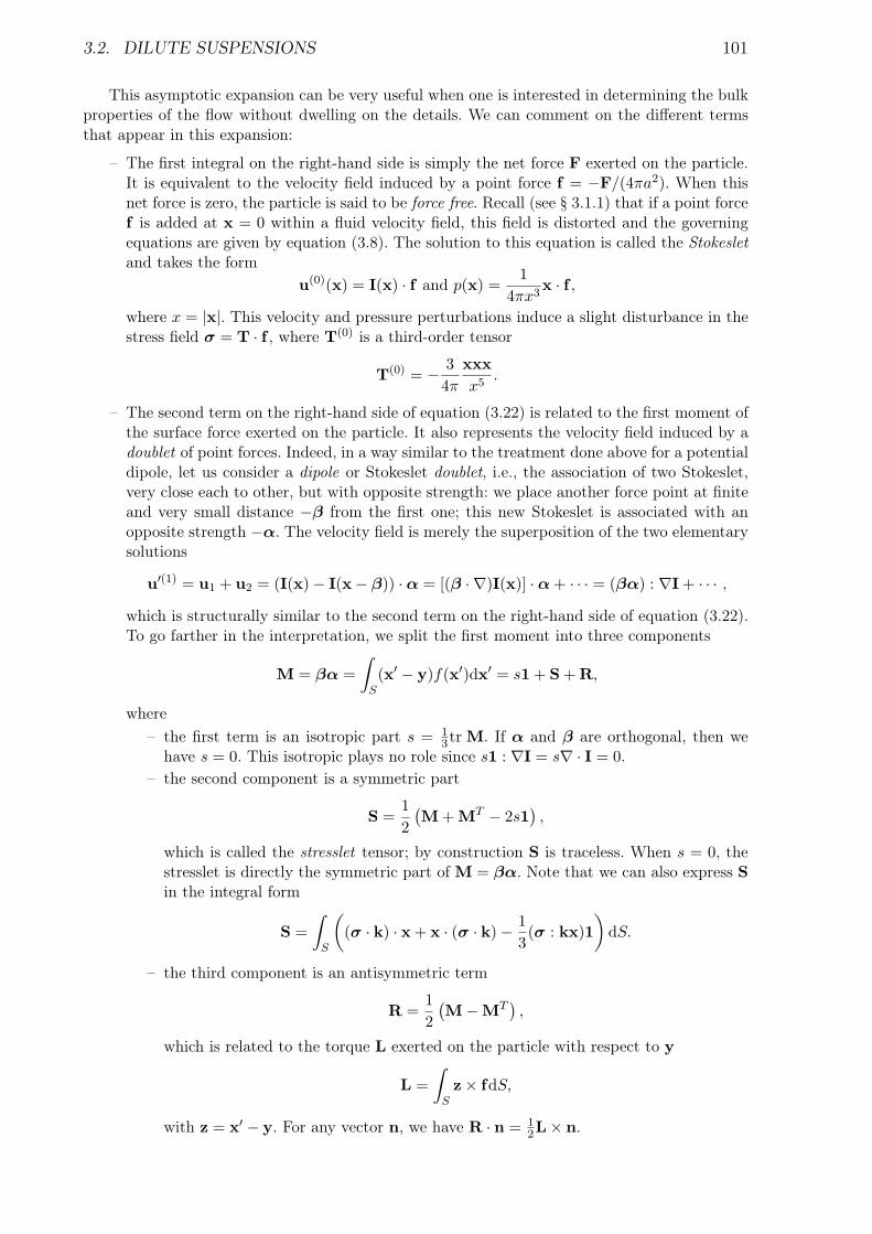
3.2. DILUTE SUSPENSIONS 101
This asymptotic expansion can be very useful when one is interested in determining the bulkproperties of the flow without dwelling on the details. We can comment on the different termsthat appear in this expansion:
– The first integral on the right-hand side is simply the net force F exerted on the particle.It is equivalent to the velocity field induced by a point force f = −F/(4πa2). When thisnet force is zero, the particle is said to be force free. Recall (see § 3.1.1) that if a point forcef is added at x = 0 within a fluid velocity field, this field is distorted and the governingequations are given by equation (3.8). The solution to this equation is called the Stokesletand takes the form
u(0)(x) = I(x) · f and p(x) =1
4πx3x · f ,
where x = |x|. This velocity and pressure perturbations induce a slight disturbance in thestress field σ = T · f , where T(0) is a third-order tensor
T(0) = − 34π
xxxx5
.
– The second term on the right-hand side of equation (3.22) is related to the first moment ofthe surface force exerted on the particle. It also represents the velocity field induced by adoublet of point forces. Indeed, in a way similar to the treatment done above for a potentialdipole, let us consider a dipole or Stokeslet doublet, i.e., the association of two Stokeslet,very close each to other, but with opposite strength: we place another force point at finiteand very small distance −β from the first one; this new Stokeslet is associated with anopposite strength −α. The velocity field is merely the superposition of the two elementarysolutions
u′(1) = u1 + u2 = (I(x)− I(x− β)) ·α = [(β · ∇)I(x)] ·α + · · · = (βα) : ∇I + · · · ,
which is structurally similar to the second term on the right-hand side of equation (3.22).To go farther in the interpretation, we split the first moment into three components
M = βα =∫
S(x′ − y)f(x′)dx′ = s1 + S + R,
where– the first term is an isotropic part s = 1
3tr M. If α and β are orthogonal, then wehave s = 0. This isotropic plays no role since s1 : ∇I = s∇ · I = 0.
– the second component is a symmetric part
S =12
(M + MT − 2s1
),
which is called the stresslet tensor; by construction S is traceless. When s = 0, thestresslet is directly the symmetric part of M = βα. Note that we can also express Sin the integral form
S =∫
S
((σ · k) · x + x · (σ · k)− 1
3(σ : kx)1
)dS.
– the third component is an antisymmetric term
R =12
(M−MT
),
which is related to the torque L exerted on the particle with respect to y
L =∫
Sz× fdS,
with z = x′ − y. For any vector n, we have R · n = 12L× n.
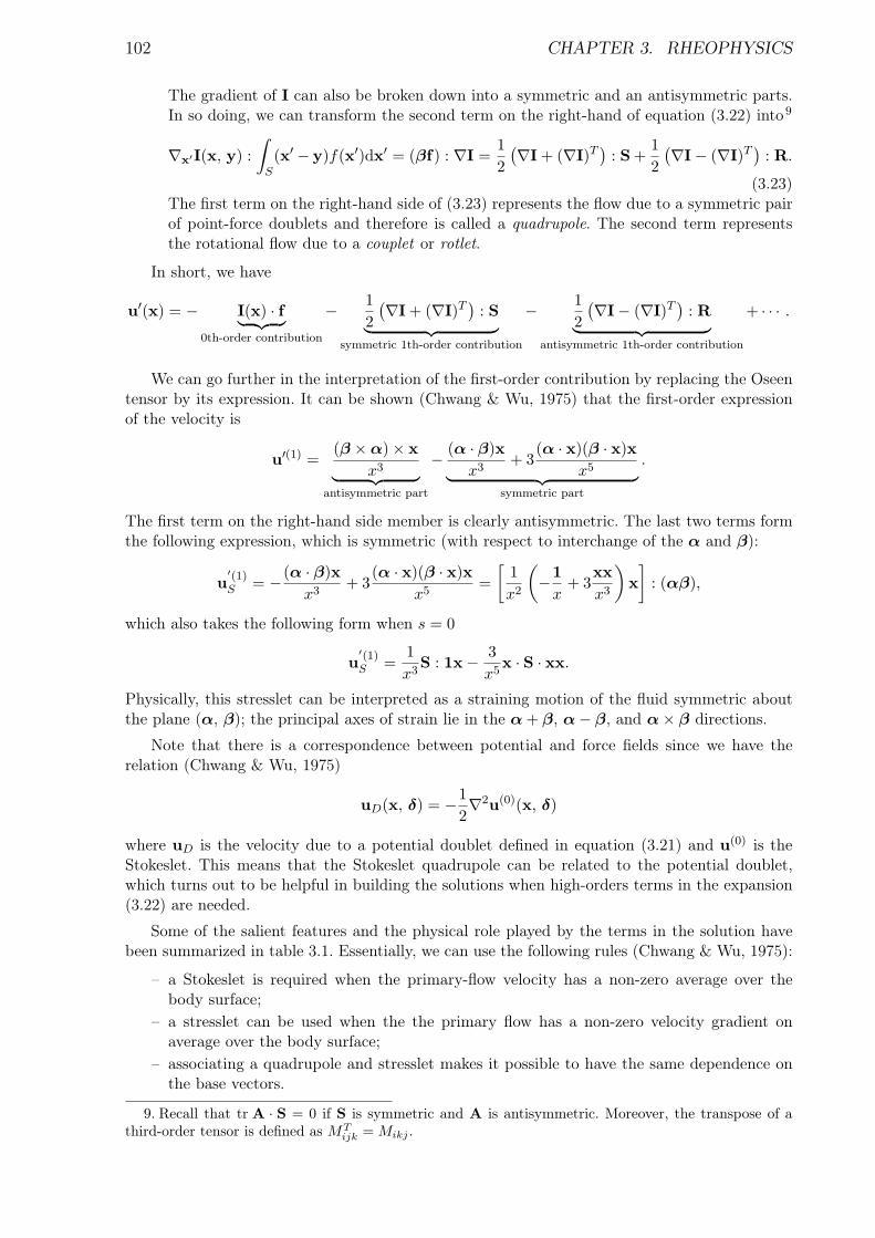
102 CHAPTER 3. RHEOPHYSICS
The gradient of I can also be broken down into a symmetric and an antisymmetric parts.In so doing, we can transform the second term on the right-hand of equation (3.22) into9
∇x′I(x, y) :∫
S(x′ − y)f(x′)dx′ = (βf) : ∇I =
12
(∇I + (∇I)T)
: S +12
(∇I− (∇I)T)
: R.
(3.23)The first term on the right-hand side of (3.23) represents the flow due to a symmetric pairof point-force doublets and therefore is called a quadrupole. The second term representsthe rotational flow due to a couplet or rotlet.
In short, we have
u′(x) = − I(x) · f︸ ︷︷ ︸0th-order contribution
− 12
(∇I + (∇I)T)
: S︸ ︷︷ ︸
symmetric 1th-order contribution
− 12
(∇I− (∇I)T)
: R︸ ︷︷ ︸
antisymmetric 1th-order contribution
+ · · · .
We can go further in the interpretation of the first-order contribution by replacing the Oseentensor by its expression. It can be shown (Chwang & Wu, 1975) that the first-order expressionof the velocity is
u′(1) =(β ×α)× x
x3︸ ︷︷ ︸antisymmetric part
− (α · β)xx3
+ 3(α · x)(β · x)x
x5︸ ︷︷ ︸symmetric part
.
The first term on the right-hand side member is clearly antisymmetric. The last two terms formthe following expression, which is symmetric (with respect to interchange of the α and β):
u′(1)S = −(α · β)x
x3+ 3
(α · x)(β · x)xx5
=[
1x2
(−1
x+ 3
xxx3
)x]
: (αβ),
which also takes the following form when s = 0
u′(1)S =
1x3
S : 1x− 3x5
x · S · xx.
Physically, this stresslet can be interpreted as a straining motion of the fluid symmetric aboutthe plane (α, β); the principal axes of strain lie in the α + β, α− β, and α× β directions.
Note that there is a correspondence between potential and force fields since we have therelation (Chwang & Wu, 1975)
uD(x, δ) = −12∇2u(0)(x, δ)
where uD is the velocity due to a potential doublet defined in equation (3.21) and u(0) is theStokeslet. This means that the Stokeslet quadrupole can be related to the potential doublet,which turns out to be helpful in building the solutions when high-orders terms in the expansion(3.22) are needed.
Some of the salient features and the physical role played by the terms in the solution havebeen summarized in table 3.1. Essentially, we can use the following rules (Chwang & Wu, 1975):
– a Stokeslet is required when the primary-flow velocity has a non-zero average over thebody surface;
– a stresslet can be used when the the primary flow has a non-zero velocity gradient onaverage over the body surface;
– associating a quadrupole and stresslet makes it possible to have the same dependence onthe base vectors.
9. Recall that tr A · S = 0 if S is symmetric and A is antisymmetric. Moreover, the transpose of athird-order tensor is defined as MT
ijk = Mikj .
3.2. DILUTE SUSPENSIONS 103
Table 3.1 Construction of the solution to specific boundary-value problems from the singularsolutions. After (Chwang & Wu, 1975).
Primary flow Singularitiesuniform flow Stokeslet + potential dipoleshear flow Stokeslet dipole + potential quadrupoleextensional flow stresslet + quadrupole
Application to the multipole expansion
Example 1: According to table 3.1, the disturbance induced by a translating rigid (solid)sphere (with no spin) in a quiescent fluid is a combination of a Stokeslet and a potential doublet
u′ = I · f + D · λ
where I is reduced the Oseen tensor 10, D is the potential-doublet tensor introduced in equation(3.21), and λ and f are two unknown vectors to be determined. These vectors are determined byimposing that the velocity at the particle surface equals the particle velocity vp at x = a. Since
u′ =(
1x1 +
xxx3
)· f +
(− 1
x31 + 3
xxx5
)· λ
λ and f must be collinear with vp. Solving the system we find:
f =34avp and λ = −1
4a3vp.
Since the net force due to a potential dipole is zero, we retrieve the Stokes force
F =∫
SfdS = −8πµf = −6πµavp.
Example 2: According to table 3.1, the disturbance induced by a linear flow u∞ = G · xpast a rigid (solid) sphere (with no spin) is given by a combination of a potential quadrupoleand a Stokes doublet. We assume that this flow at infinity is irrotational, implying that G issymmetric and traceless (because of the continuity equation). Thus we write
u′(x) = Q : Λ +∇I : M.
The boundary condition is u′ = −G · x when x = a. We obtain
M = − 5a2
Λ,
and after a few computations, we find
Λ =a5
6G and M = −5
6a3G.
The stresslet S is M to within the multiplicative factor −(8πµ)−1
S =203
πµa3G. (3.24)
Making allowance of the relation between the potential quadrupole velocity disturbance can bewritten
10. Here, to simplify the computations, we get rid of the multiplier (4πµ)−1 and (8πµ)−1 that can beembodied in the unknown vectors, e.g., we simply pose I = (8πµ)I and D = (4πµ)D.
104 CHAPTER 3. RHEOPHYSICS
3.2.2 Computations of the constitutive equation
We consider a dilute suspension of rigid spherical solid particles within a Newtonian fluid.We assume that the particles are force-free and torque-free, i.e., in a Stokesian regime St → 0,the solid phase is the slave of the fluid phase. We have shown in § 3.1.3 that the bulk stresstensor σ can be broken into a fluid and solid contributions
σ = σ(f) = +σ(p),
where the solid contribution is given by equation (3.18) while the fluid contribution is given byequation (3.17). Neglecting the Reynolds stress tensor, we have
σ(p) =1V
∫
Sσ · xkdS and σ(f) = −p1 + 2µd.
In the solid contribution, the integral term is nothing but the first moment of the stresses exertedon the particle surface, which corresponds to the stresslet in the case of force-free and torque-free particles. This result holds because we neglect pairwise interactions between particles in thelow-concentration limit. Since in the volume V , the number of particles is φV [(4πa3/3)]−1
σ(p) =1V
∫
Sσ · xkdS = φ
34πa3
S,
and making use of equation (3.24) with G = d, we arrive at the following constitutive equation
σ = −p1 + 2µ
(1 +
52φ
)d.
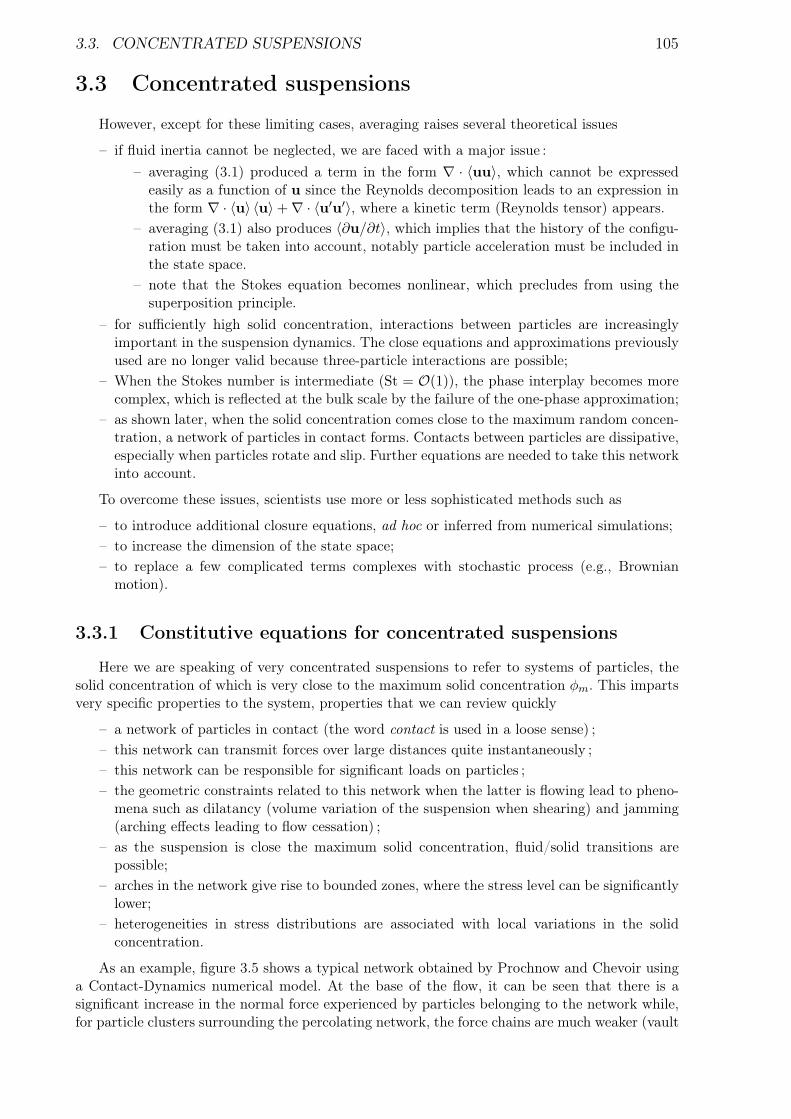
3.3. CONCENTRATED SUSPENSIONS 105
3.3 Concentrated suspensions
However, except for these limiting cases, averaging raises several theoretical issues
– if fluid inertia cannot be neglected, we are faced with a major issue :– averaging (3.1) produced a term in the form ∇ · 〈uu〉, which cannot be expressed
easily as a function of u since the Reynolds decomposition leads to an expression inthe form ∇ · 〈u〉 〈u〉+∇ · 〈u′u′〉, where a kinetic term (Reynolds tensor) appears.
– averaging (3.1) also produces 〈∂u/∂t〉, which implies that the history of the configu-ration must be taken into account, notably particle acceleration must be included inthe state space.
– note that the Stokes equation becomes nonlinear, which precludes from using thesuperposition principle.
– for sufficiently high solid concentration, interactions between particles are increasinglyimportant in the suspension dynamics. The close equations and approximations previouslyused are no longer valid because three-particle interactions are possible;
– When the Stokes number is intermediate (St = O(1)), the phase interplay becomes morecomplex, which is reflected at the bulk scale by the failure of the one-phase approximation;
– as shown later, when the solid concentration comes close to the maximum random concen-tration, a network of particles in contact forms. Contacts between particles are dissipative,especially when particles rotate and slip. Further equations are needed to take this networkinto account.
To overcome these issues, scientists use more or less sophisticated methods such as
– to introduce additional closure equations, ad hoc or inferred from numerical simulations;– to increase the dimension of the state space;– to replace a few complicated terms complexes with stochastic process (e.g., Brownian
motion).
3.3.1 Constitutive equations for concentrated suspensions
Here we are speaking of very concentrated suspensions to refer to systems of particles, thesolid concentration of which is very close to the maximum solid concentration φm. This impartsvery specific properties to the system, properties that we can review quickly
– a network of particles in contact (the word contact is used in a loose sense) ;– this network can transmit forces over large distances quite instantaneously ;– this network can be responsible for significant loads on particles ;– the geometric constraints related to this network when the latter is flowing lead to pheno-
mena such as dilatancy (volume variation of the suspension when shearing) and jamming(arching effects leading to flow cessation) ;
– as the suspension is close the maximum solid concentration, fluid/solid transitions arepossible;
– arches in the network give rise to bounded zones, where the stress level can be significantlylower;
– heterogeneities in stress distributions are associated with local variations in the solidconcentration.
As an example, figure 3.5 shows a typical network obtained by Prochnow and Chevoir usinga Contact-Dynamics numerical model. At the base of the flow, it can be seen that there is asignificant increase in the normal force experienced by particles belonging to the network while,for particle clusters surrounding the percolating network, the force chains are much weaker (vault
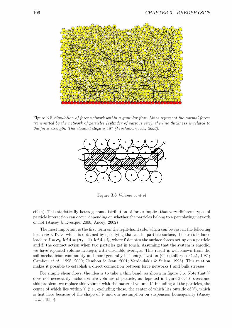
106 CHAPTER 3. RHEOPHYSICS
Figure 3.5 Simulation of force network within a granular flow. Lines represent the normal forcestransmitted by the network of particles (cylinder of various size); the line thickness is related tothe force strength. The channel slope is 18 (Prochnow et al., 2000).
Figure 3.6 Volume control
effect). This statistically heterogenous distribution of forces implies that very different types ofparticle interaction can occur, depending on whether the particles belong to a percolating networkor not (Ancey & Evesque, 2000; Ancey, 2002)
The most important is the first term on the right-hand side, which can be cast in the followingform: na < fk >, which is obtained by specifying that at the particle surface, the stress balanceleads to f = σp ·kdA = (σf −1) ·kdA+ fc, where f denotes the surface forces acting on a particleand fc the contact action when two particles get in touch. Assuming that the system is ergodic,we have replaced volume averages with ensemble averages. This result is well known from thesoil-mechanician community and more generally in homogenization (Christoffersen et al., 1981;Cambou et al., 1995, 2000; Cambou & Jean, 2001; Vardoulakis & Sulem, 1995). This relationmakes it possible to establish a direct connection between force networks f and bulk stresses.
For simple shear flows, the idea is to take a thin band, as shown in figure 3.6. Note that Vdoes not necessarily include entire volumes of particle, as depicted in figure 3.6. To overcomethis problem, we replace this volume with the material volume V ′ including all the particles, thecenter of which lies within V (i.e., excluding those, the center of which lies outside of V), whichis licit here because of the shape of V and our assumption on suspension homogeneity (Anceyet al., 1999).
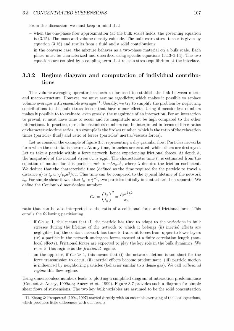
3.3. CONCENTRATED SUSPENSIONS 107
From this discussion, we must keep in mind that
– when the one-phase flow approximation (at the bulk scale) holds, the governing equationis (3.15). The mass and volume density coincide. The bulk extra-stress tensor is given byequation (3.16) and results from a fluid and a solid contributions;
– in the converse case, the mixture behaves as a two-phase material on a bulk scale. Eachphase must be characterized and described using specific equations (3.13–3.14). The twoequations are coupled by a coupling term that reflects stress equilibrium at the interface.
3.3.2 Regime diagram and computation of individual contribu-tions
The volume-averaging operator has been so far used to establish the link between micro-and macro-structure. However, we must assume ergodicity, which makes it possible to replacevolume averages with ensemble averages 11. Usually, we try to simplify the problem by neglectingcontributions to the bulk stress tensor that have minor effects. Using dimensionless numbersmakes it possible to to evaluate, even grossly, the magnitude of an interaction. For an interactionto prevail, it must have time to occur and its magnitude must be high compared to the otherinteractions. In practice, most dimensionless numbers can be interpreted in terms of force ratiosor characteristic-time ratios. An example is the Stokes number, which is the ratio of the relaxationtimes (particle/ fluid) and ratio of forces (particles’ inertia/viscous forces).
Let us consider the example of figure 3.5, representing a dry granular flow. Particles networksform when the material is sheared. At any time, branches are created, while others are destroyed.Let us take a particle within a force network, hence experiencing frictional forces. At depth h,the magnitude of the normal stress σn is ρpgh. The characteristic time tp is estimated from theequation of motion for this particle: mv ≈ −λσna2, where λ denotes the friction coefficient.We deduce that the characteristic time (defined as the time required for the particle to travel adistance a) is tp ∝
√ρpa2/σn. This time can be compared to the typical lifetime of the network
tn. For simple shear flows, after tn ≈ γ−1, two particles initially in contact are then separate. Wedefine the Coulomb dimensionless number:
Co =(
tptn
)2
=ρpa
2γ2
σn
ratio that can be also interpreted as the ratio of a collisional force and frictional force. Thisentails the following partitioning
– if Co ¿ 1, this means that (i) the particle has time to adapt to the variations in bulkstresses during the lifetime of the network to which it belongs (ii) inertial effects arenegligible, (iii) the contact network has time to transmit forces from upper to lower layers(iv) a particle in the network undergoes forces created at a finite correlation length (non-local effects). Frictional forces are expected to play the key role in the bulk dynamics. Werefer to this regime as the frictional regime.
– on the opposite, if Co À 1, this means that (i) the network lifetime is too short for theforce transmission to occur, (ii) inertial effects become predominant, (iii) particle motionis influenced by neighboring particles (behavior similar to a dense gas). We call collisionalregime this flow regime.
Using dimensionless numbers leads to plotting a simplified diagram of interaction predominance(Coussot & Ancey, 1999b,a; Ancey et al., 1999). Figure 3.7 provides such a diagram for simpleshear flows of suspensions. The two key bulk variables are assumed to be the solid concentration
11. Zhang & Prosperetti (1994, 1997) started directly with an ensemble averaging of the local equations,which produces little differences with our results
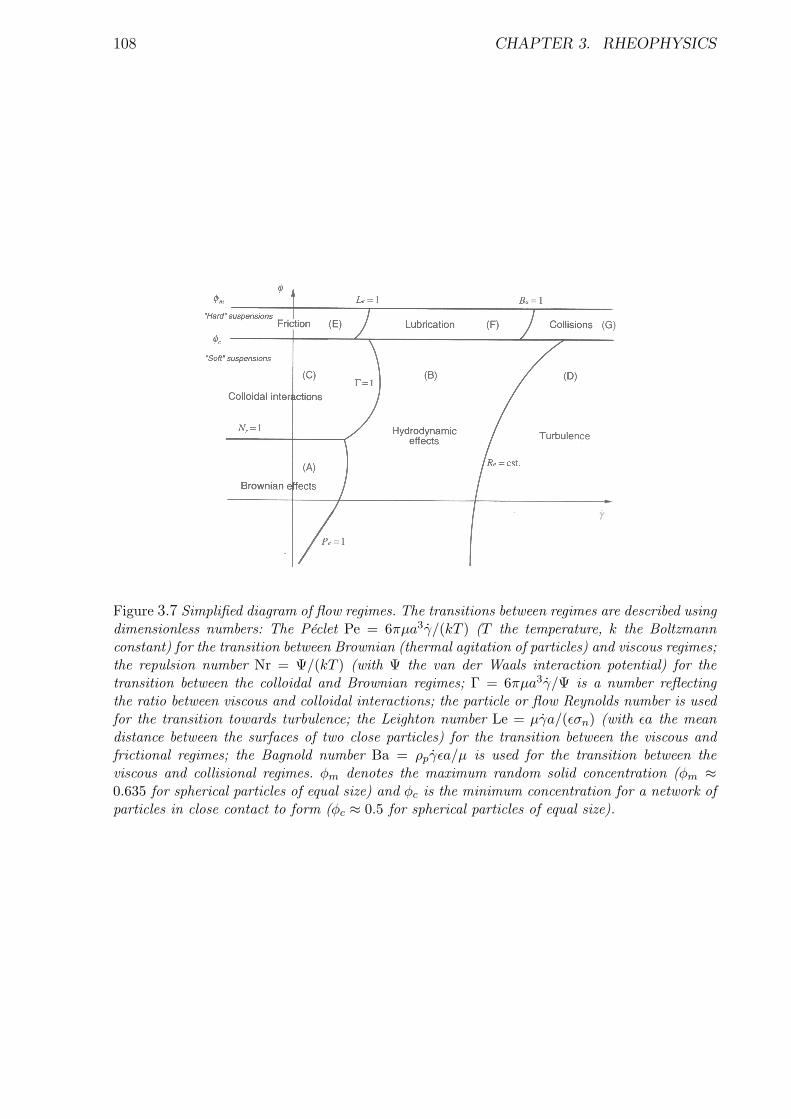
108 CHAPTER 3. RHEOPHYSICS
Figure 3.7 Simplified diagram of flow regimes. The transitions between regimes are described usingdimensionless numbers: The Péclet Pe = 6πµa3γ/(kT ) (T the temperature, k the Boltzmannconstant) for the transition between Brownian (thermal agitation of particles) and viscous regimes;the repulsion number Nr = Ψ/(kT ) (with Ψ the van der Waals interaction potential) for thetransition between the colloidal and Brownian regimes; Γ = 6πµa3γ/Ψ is a number reflectingthe ratio between viscous and colloidal interactions; the particle or flow Reynolds number is usedfor the transition towards turbulence; the Leighton number Le = µγa/(εσn) (with εa the meandistance between the surfaces of two close particles) for the transition between the viscous andfrictional regimes; the Bagnold number Ba = ρpγεa/µ is used for the transition between theviscous and collisional regimes. φm denotes the maximum random solid concentration (φm ≈0.635 for spherical particles of equal size) and φc is the minimum concentration for a network ofparticles in close contact to form (φc ≈ 0.5 for spherical particles of equal size).
3.3. CONCENTRATED SUSPENSIONS 109
φ and the shear rate γ. For dilute and moderately concentrated suspensions, the flow regimesare usually well established (Russel et al., 1995). However, at high solid concentrations, thedetermination of the constitutive equation is much more difficult. We can cite:
– for the regime dominated by colloidal interactions (regime C on the diagram) the worksby Kapur et al. (1997); Scales et al. (1998) and Zhou et al. (1999).
– for the regime dominated by lubricated-contact interactions, the work by van der Brule &Jongshaap (1991).
– for the collisional regime, an abundant literature can be found on the application of kinetictheory to dry granular flows (Savage & Jeffrey, 1981; Savage, 1984; Campbell, 1990; Jenkins& Savage, 1983). For wetted materials, less works are available Jenkins & Hanes (1998) ;
– for the frictional regime, the papers by Cambou & Jean (2001); Cambou et al. (1995,2000).

110 CHAPTER 3. RHEOPHYSICS
REFERENCES 111
References
Abramovich, F. & Silverman, B. 1998 Wavelet decomposition approaches to statistical in-verse problems. Biometrika 85, 115–129.
Ancey, C. 2002 Dry granular flow down an inclined channel: Experimental investigations onthe frictional-collisional regime. Phys. Rev. E 65, 11304.
Ancey, C. 2005 Solving the Couette inverse problem by using a wavelet-vaguelette decomposi-tion. J. Rheol. 49, 441–460.
Ancey, C., Coussot, P. & Evesque, P. 1996 Examination of the possibility of a fluid-mechanics treatment for dense granular flows. Mech. Cohesive-Frict. Mater. 1, 385–403.
Ancey, C., Coussot, P. & Evesque, P. 1999 A theoretical framework for very concentratedgranular suspensions in a steady simple shear flow. J. Rheol. 43, 1673–1699.
Ancey, C. & Evesque, P. 2000 Frictional-collisional regime for granular suspension flows downan inclined channel. Phys. Rev. E 62, 8349–8360.
Astarita, G. 1990 The engineering reality of the yield stress. J. Rheol. 34, 275–277.Auton, T., Hunt, J. & Prud’homme, M. 1988 The force exerted on a body in inviscid
unsteady non-uniform flow rotational flow. J. Fluid Mech. 197, 241–257.Barnes, H. 1995 A review of the slip (wall depletion) of polymer solutions, emulsions and
particle suspensions in viscometers: its cause, character, and cure. J. Non-Newtonian FluidMech. 56, 221–251.
Barnes, H. 1997 Thixotropy - a review. J. Non-Newtonian Fluid Mech. 70, 1–33.Barnes, H. 1999 The yield stress –a review or ’παντα ρει’ – everything flows? J. Non-Newtonian
Fluid Mech. 81, 213–217.Barnes, H. 2000 A Handbook of Elementary Rheology. Aberystwyth: University of Wales.Barnes, H. & Carnali, J. 1990 The vane-in-cup as a novel rheometer geometry for shear
thinning and thixotropic materials. J. Rheol. 34, 851–866.Barnes, H. & Nguyen, Q. 2001 Rotating vane rheometry - a review. J. Non-Newtonian Fluid
Mech. 98, 1–14.Batchelor, G. 1967 An introduction to fluid dynamics. Cambridge University Press.Batchelor, G. 1970 The stress system in a suspension of free-forces particles. J. Fluid Mech.41, 545–570.
Batchelor, G. 1972 Sedimentation in a dilute dispersion of spheres. J. Fluid Mech. 52, 245–268.
Baudez, J., Rodts, S., Chateau, X. & Coussot, P. 2004 New technique for reconstructinginstantaneous profiles from viscometric tests: application to pasty materials. J. Rheol. 48,69–82.
Bedford, A. & Dumheller, D. 1983 Theories of immiscible and structured mixtures. Int. J.Eng. Sci. 21, 863–960.
Bertero, M., De Mol, C. & Pike, E. 1985 Linear inverse problems with discrete data. I:General formulation and singular system analysis. Inverse Prob. 1, 301–330.
112 REFERENCES
Bertero, M., De Mol, C. & Pike, E. 1988 Linear inverse problems with discrete data. II:Stability and regularization. Inverse Prob. 4, 573–594.
Bird, R., Armstrong, R. & Hassager, O. 1987 Dynamics of Polymeric Liquids. New York:John Wiley & Sons.
Bird, R., Dai, G. & Yarusso, B. 1983 The rheology and flow of viscoplastic materials. Rev.Chem. Eng. 1, 1–70.
Boehler, J., ed. 1987 Applications of tensor functions in solid mechanics, International Centrefor Mechanical Sciences, Courses and Lectures, vol. 292. New York: Springer Verlag.
Boger, D. & Walters, K. 1993 Rheological Phenomena in Focus. Amsterdam: Elsevier.Borgia, A. & Spera, F. 1990 Error analysis for reducing noisy wide-gap concentric cylinder
rheometric data for nonlinear fluids: theory and applications. J. Rheol. 34, 117–135.Brady, J. & Bossis, G. 1988 Stokesian dynamics. Annu. Rev. Fluid Mech. 20, 111–157.Brady, J. & Morris, J. 1997 Microstructure of strongly sheared suspensions and its impact
on rheology and diffusion. J. Fluid Mech. 348, 103–139.van der Brule, B. & Jongshaap, R. 1991 Modeling of concentrated suspensions. J. Stat.
Phys. 62, 1225–1237.Cai, T. 1999 Adaptative wavelet estimation: a block thresholding and oracle inequality approach.
Ann. Stat. 27, 898–924.Cai, T. 2002 On adaptive wavelet estimation of a derivative and other related linear inverse
problems. J. Stat. Planning Infer. 108, 329–349.Cambou, B., Chaze, M. & Dedecker, F. 2000 Change of scale in granular materials. Eur.
J. Mech. A 19 (6), 999–1014, tY - JOUR.Cambou, B., Dubujet, P., Emeriault, F. & Sidoroff, F. 1995 Homogenization for granular
materials. Eur. J. Mech. A 14, 255–276.Cambou, B. & Jean, M., ed. 2001 Micromécanique des matériaux granulaires. Paris: Hermès
Science, tY - JOUR.Campbell, C. 1990 Rapid granular flows. Annu. Rev. Fluid Mech. 22, 57–92.Chapman, S. & Cowling, T. 1970 The mathematical theory of non-uniform gases, 3rd edn.
Cambrige: Cambrige University Press.Christoffersen, J., Mehrabadi, M. & Nemat-Nasser, S. 1981 A micromechanical des-
cription of granular behavior. J. Appl. Mech. 48, 339–344.Chwang, A. & Wu, T. Y.-T. 1975 Hydrodynamics of low-Reynolds-number flow. Part 2.
Singularity method for Stokes flow. J. Fluid Mech. 67, 787–815.Coimbra, C. & Rangel, R. 1998 General solution of the particle momentum equation in
unsteady Stokes flows. J. Fluid Mech. 370, 53–72.Coleman, B., Markowitz, H. & Noll, W. 1966 Viscometric flows of non-Newtonian fluids,
Springer Tracts in natural philosophy, vol. 5. Berlin: Springer-Verlag.Courant, R. & Friedrich, K. 1948 Supersonic Flow and Shock Waves. New York: Inter-
sciences Publishers.Coussot, P. & Ancey, C. 1999a Rheophysical classification of concentrated suspensions and
granular pastes. Phys. Rev. E 59, 4445–4457.Coussot, P. & Ancey, C. 1999b Rhéophysique des pâtes et des suspensions. Les Ulis: EDP
Sciences.Coussot, P., Proust, S. & Ancey, C. 1996 Rheological interpretation of deposits of yield
stress fluids. J. Non-Newtonian Fluid Mech. 66, 55–70.Darby, R. 1985 Couette viscometer data reduction for materials with a yield stress. J. Rheol.29, 369–378.
Dicken, V. & Maass, P. 1996 Wavelet-Galerkin methods for ill-posed problems. J. Inv. Ill-Posed Problems 4, 203–221.
REFERENCES 113
Donoho, D. 1995 Nonlinear solution of linear inverse problems by wavelet-vaguelette decom-position. Appl. Comp. Harmonic Anal. 2, 101–126.
Donoho, D. & Johnstone, I. 1995 Wavelet shrinkage: asymptotia? J. Royal. Stat. Soc. B 57,301–369.
Doraiswamy, D., Mujumdar, A., Taso, I., Beris, A., Danforth, S. & Metzner, A.1991 The Cox-Merz rule extended: a rheological model for concentrated suspensions and othermaterials with a yield stress. J. Rheol. 35, 647–685.
Drew, D. & Passman, S. 1999 Theory of Multicomponent Fluids. New York: Springer.Einstein, A. 1911 Berichtigung zu meiner Arbeit “Eine neue Bestimmung der Moleküldimen-
sionen”. Annalen der Physik 34, 591–592.Evans, I. 1992 On the nature of the yield stress. J. Rheol. 36, 131–1318.Frankel, N. & Acrivos, A. 1967 On the viscosity of a concentrated suspension of solid
spheres. Chemical Engineering Science 22, 847–853.Friedrich, C., Honerkamp, J. & Weese, J. 1996 New ill-posed problems in rheology. Rheol.
Acta 35, 186–193.Gamboa, F. & Gassiat, E. 1997 Bayesian methods and maximum entropy for ill-posed inverse
problems. Ann. Stat. 25, 328–350.Garabedian, P. 1966 Free boundary flows of a viscous liquid. Comm. Pure Appl. Math. 19,
421–434.Geissle, W. & Hochstein, B. 2003 Validity of the Cox-Merz rule for concentrated suspensions.
J. Rheol. 47, 897–910.Germain, P. 1973a La méthode des puissances virtuelles en mécanique des milieux continus.
Journal de Mécanique 12, 235–274.Germain, P. 1973b The method of virtual power in continuum mechanics, Part 2: Microstruc-
ture. SIAM J. Appl. Math. 25 (3), 556–575.Golberg, M. 1979 A method of adjoints for solving some ill-posed equations of the first kind.
Appl. Math. Comput. 5, 123–130.Happel, J. & Brenner, H. 1965 Low Reynolds number hydrodynamics. Englewood Cliffs:
Prentice Hall.Harnett, J. & Hu, R. 1989 The yield stress-An engineering reality. J. Rheol. 33, 671–679.Hart, J. 1999 Nonparametric Smoothing and Lack-of-Fit Tests. New York: Springer.Hinch, E. 1977 An averaged-equation approach to particle interactions in a fluid suspension. J.
Fluid Mech. 83, 695–720.Howe, M., Lauchke, G. & Wang, J. 2001 Aerodynamic lift and drag fluctuations of a sphere.
J. Fluid Mech. 436, 41–57.Hutter, K. & Jöhnk, K. 2004 Continuum Methods of Physical Modeling. Berlin: Springer.Hutter, K., Laloui, L. & Vulliet, L. 1999 Thermodynamically based mixture models of
saturated and unsaturated soils. Mech. Cohesive-Frict. Mater. 4, 295–338.Jenkins, J. & Hanes, H. 1998 Collisional sheet flows of sediment driven by a turbulent fluid.
J. Fluid Mech. 370, 29–52.Jenkins, J. & Savage, S. 1983 A theory for the rapid flow identical, smooth, nearly elastic,
spherical particles. J. Fluid Mech. 130, 187–202.Jongschaap, R. & Doeksen, D. 1983 The average stress tensor in systems with interacting
particles. Rheol. Acta 22, 4–11.Kang, S., Sangani, A., Tsao, H. & Koch, D. 1997 Rheology of dense bubble suspensions.
Phys. Fluids 9, 1540–1561.Kapur, P., Scales, P., Boger, B. & Healy, T. . 1997 A theoretical framework for the yield
stress of suspensions loaded with size distributed particles. AIChE J. 43, 1171–1179.de Kee, D. & Chan Man Fong, C. 1993 A true yield stress? J. Rheol. 37, 775–776.
114 REFERENCES
Kim, S. & Karrila, S. 1991 Microhydrodynamics: Principles and Selected Applications. Sto-neham: Butterworth-Heinemann.
Kohr, M. & Pop, I. 2004 Viscous incompressible flow for low Reynolds numbers. Southampton:WIT press.
Kovac, A. 1998 Wavelet Thresholding for Unequally Spaced Data. Phd thesis, University ofBristol.
Krieger, I. 1968 Shear rate in the Couette viscometer. Trans. Soc. Rheol. 12, 5–11.Krieger, I. & Elrod, H. 1953 Direct determination of the flow curves of non-Newtonian fluids.
II Shearing rate in the concentric cylinder viscometer. J. Appl. Phys. 24, 134–136.Krieger, I. & Maron, S. 1952 Direct determination of the flow curves of non-Newtonian
fluids. J. Appl. Phys. 23, 147–149.Kumaran, V. & Koch, D. 1993 Properties of a bidisperse particle-gas suspension. Part 2.
Viscous relaxation time small compared with collision time. J. Fluid Mech. 247, 643–660.Lamb, H. 1932 Hydrodynamics. Cambridge: Cambridge University Press.Landau, L. & Lifschitz, E. 1987 Fluid Mechanics. London: Pergamon.Leong, Y. & Yeow, Y. 2003 Obtaining the shear stress shear rate relationship and yield of
liquid foods from Couette viscometry data. Rheol. Acta 42, 365–371.Lhuillier, D. 1982a Forces d’inertie sur une bulle en expansion se déplac,ant dans un fluide.
Comptes Rendus de l’Académie des Sciences, série II 295, 95–98.Lhuillier, D. 1982b On the equation of motion of a rigid sphere in a non uniform and accelerated
inviscid fluid. Incidence on two-phase flow equations. Mechanics Research Communications 9,295–299.
Louis, A. 1999 A unified approach to regularization methods for linear and ill-posed problems.Inverse Prob. 15, 489–498.
Louis, A., Maass, P. & Rieder, A. 1997 Wavelets, Theory and Applications. Chichester:John Wiley & Sons.
Lundgren, T. 1972 Slow flow through stationary random beads and suspensions of spheres. J.Fluid Mech. 51, 273–299.
Macsporran, W. 1989 Direct numerical evaluation of shear rates in concentric cylinder visco-metry using least-squares cubic splines. J. Rheol. 33, 745–755.
Magnin, A. & Piau, J. 1987 Shear rheometry of fluids with a yield stress. J. Non-NewtonianFluid Mech. 23, 91–106.
Magnin, A. & Piau, J. 1990 Cone-and-plate rheometry of yield stress fluids. Study of anaqueous gel. J. Non-Newtonian Fluid Mech. 36, 85–108.
Mazur, P. & Bedeaux, D. 1974 A generalization of Faxén’s theorem to nonsteady motion ofa sphere through an incompressible fluid in arbitrary flow. Physica 76, 235–246.
McKarthy, K. & Seymour, J. 1994 Gravity current analysis of the Bostwick consistometerfor power-law foods. Journal of Texture Studies 25, 207–220.
Mendes, P. & Dutra, E. 2004 Viscosity function for yield-stress liquids. Applied Rheology 14,296–302.
Middleton, G. & Wilcock, P. 1994 Mechanics in the Earth and Environmental Sciences.Cambridge: Cambridge University Press.
Minier, J.-P. & Peirano, E. 2001 The pdf approach to turbulent polydispersed two-phaseflows. Physics Reports 352 (1-3), 1–214.
Mooney, M. 1931 Explicit formulas for slip and fluidity. J. Rheol. 2, 210–222.Morrison, F. 2001 Understanding Rheology . New York: Oxford University Press.Mosegaard, K. & Sambridge, M. 2002 Monte Carlo analysis of inverse problems. Inverse
Prob. 18, R29–R54.Murdoch, A. & Bedeaux, D. 1994 Continuum equations of balance via weighted averages of
microscopic quantities. Proc. Roy. Soc. London 445, 157–179.
REFERENCES 115
Nguyen, Q. & Boger, D. 1992 Measuring the flow properties of yield stress fluids. Annu. Rev.Fluid Mech. 24, 47–88.
Oldroyd, J. 1950 On the formulation of rheological equations of state. Proc. Roy. Soc. LondonA 200, 523–541.
O’Sullivan, F. 1986 A statistical perpective on ill-posed inverse problems. Stat. Sci. 1, 502–527.Pashias, N. & Boger, D. 1996 A fifty cent rheometer for yield stress measurement. J. Rheol.40, 1179–1189.
Piau, J.-M. & Debiane, K. 2005 Consistometers rheometry of power-law viscous fluids. J.Non-Newtonian Fluid Mech. 127, 213–224.
Pope, S. 2000 Turbulent Flows. Cambridge: Cambridge University Press.Pozrikidis, C. 1992 Boundary Integral and Singularity Methods for Linearized Viscous Flows.
Cambridge: Cambridge University Press.Prochnow, M., Chevoir, F., Mills, P. & Jenkins, J. 2000 Ecoulements granulaires denses
sur un plan incliné : microstructure et loi de comportement. In Physique et Mecanique desMateriaux Granulaires (ed. F. Chevoir), p. 425. Champ-sur-Marne: Presses du LCPC, Paris.
Prosperetti, A. 2004 The average stress in incompressible disperse flow. Int. J. MultiphaseFlow 30, 1011–1036.
Rieder, A. 1997 A wavelet multilevel method for ill-posed problems stabilized by Tikhonovregularization. Numer. Math 75, 501–522.
Roberts, G. & Barnes, H. 2001 New measurements of the flow-curves for Carbopol dispersionswithout slip artefacts. Rheol. Acta 40, 499–503.
Russel, W., Saville, D. & Schowalter, W. 1995 Colloidal dispersions. Cambridge: Cam-bridge University Press.
Sangani, A., Mo, G., Tsao, H. & Koch, D. 1996 Simple shear flows of dense gas-solidsuspensions at finite Stokes numbers. J. Fluid Mech. 313, 309–341.
Savage, S. 1984 The mechanics of rapid granular flows. Adv. Appl. Mech. 24, 289–366.Savage, S. 1989 Flow of granular materials. In Theoretical and Applied Mechanics (ed. P. Ger-
main, J.-M. Piau & D. Caillerie), pp. 241–266. Amsterdam: Elsevier.Savage, S. 1994 Marginal ice zone dynamics modelled by computer simulations involving floe
collisions. In Mobile particulate systems (ed. E. Guazelli & L. Oger), pp. 305–330. Carghese:Kluwer Academic Publishers.
Savage, S. & Jeffrey, D. 1981 The stress tensor in a granular flow at high shear stress rates.J. Fluid Mech. 110, 255–272.
Scales, P., Kapur, P., Johnson, S. & Healy, T. 1998 The shear yield stress of partiallyflocculated colloidal suspensions. AIChE J. 44, 538–544.
Schowalter, W. & Christensen, G. 1999 Toward a rationalization of the slump test forfresh concrete: comparisons of calculations and experiments. J. Rheol. 42, 865–870.
Shaqfeh, E. 1996 Purely elastic instabilities in viscometric flows. Annu. Rev. Fluid Mech. 28,129–185.
Spaans, R. & Williams, M. 1995 At last, a true liquid-phase yield stress. J. Rheol. 39, 241–246.Steffe, J. 1996 Rheological methods in food process engineering, 2nd edn. East Langing, USA:
Freeman Press.Tanner, R. 1988 Engineering Rheology . Oxford: Clarendon Press.Tanner, R. & Williams, G. 1970 Iterative numerical methods for some integral equations
arising in rheology. Trans. Soc. Rheol. 14, 19–38.Tenorio, L. 2001 Statistical regularization of inverse problems. SIAM Rev. 43, 347–366.Truesdell, C. 1966 Six Lectures on Modern Natural Philosophy. New York: Springer Verlag.Truesdell, C. 1974 The meaning of viscometry in fluid dynamics. Annu. Rev. Fluid Mech. 6,
111–147.
116 REFERENCES
Vardoulakis, I. & Sulem, J. 1995 Bifurcation Analysis in Geomechanics. Glasgow: BlackieAcademic & Professional.
Wahba, G. 1990 Spline Models for Observational Data. Philadelphia: Society for Industrial andApplied Mathematics.
Walters, K. 1975 Rheometry . London: Chapman and Hall.Wang, Y. & Hutter, K. 1999 A constitutive model of multiphase mixtures and its application
in shearing flows of saturated solid-fluid mixtures. Granul. Matter 1, 163–181.Werman, M. & Keren, D. 2001 A Bayesian method for fitting parametric and nonparametric
models to noisy data. IEEE Transactions on Pattern Analysis and Machine Intelligence 23,528–534.
Wieghardt, K. 1975 Experiments in granular flow. Annu. Rev. Fluid Mech. 7, 89–114.Yang, T. & Krieger, I. 1978 Comparison of methods for calculating shear rates in coaxial
viscometers. J. Rheol. 22, 413–421.Yeow, Y., Ko, W. & Tang, P. 2000 Solving the inverse problem of Couette viscometry by
Tikhonov regularization. J. Rheol. 44, 1335–1351.Zarraga, I., Hill, D. & Leighton, D. 2000 The characterization of the total stress of concen-
trated suspensions of noncolloidal spheres in Newtonian fluids. J. Rheol. 44, 185–221.Zdunkowski, W. & Bott, A. 2003 Dynamics of the Atmosphere. Cambridge: Cambridge
University Press.Zhang, D. & Prosperetti, A. 1994 Averaged equations for inviscid disperse two-phase flow.
J. Fluid Mech. 267, 185–219.Zhang, D. & Prosperetti, A. 1997 Momentum and energy equations for disperse two-phase
flows and their closure for dilute suspensions. Int. J. Multiphase Flow 23, 425–453.Zheng, Q.-S. 1994 Theory of representations for tensor functions- A unified invariant approach
to constitutive equation. Appl. Mech. Rev. 47, 545–586.Zhou, Z., Solomon, M., Scales, P. & Boger, D. 1999 The yield stress of concentrated
flocculated suspensions of size distributed particles. J. Rheol. 43, 651–671.
Index
adherence, 51average
ensemble, 90, 91, 99volume, 91, 92, 99
biharmonic, 11
compliance, 41creep, 41cross-over frequency, 44curl, 11
density number, 92depletion, 51description
Eulerian, 63Lagrangian, 63
Dirac, 11divergence, 11doublet, 102
effectadded mass, 87die-swell, 33end, 51wall, 51Weissenberg, 33, 53
energyfree, 68kinetic, 75, 76total, 76
energy dissipation rate, 75, 76, 79equation
Basset-Boussinesq-Oseen, 90Bernoulli, 75Boltzmann, 97conservative, 78constitutive, 22, 68continuity, 73Faxén, 90Navier-Stokes, 61, 84non-conservative, 78Stokes, 87
topological, 93
fading memory, 41, 70flow curve, 37fluid
inviscid, 75Newtonian, 29, 34, 36, 43, 60, 68, 79polymeric, 34power-law, 29simple, 22, 23, 28, 53, 61, 68
Fourier transform, 11function
characteristic, 92, 96Maxwellian (velocity distribution), 98pair distribution, 97radial distribution, 97
gradient, 11
harmonic, 11heat, 76
incompressible, 74invariant, 70, 71irrotational, 11isochoric, 74
jump, 78
Laplacian, 11law
thermodynamics, 76
materialhomogeneous, 70isotropic, 70
modelBingham, 38, 79Burgers, 40Carreau, 37Casson, 38Cross, 37Herschel-Bulkley, 38Kelvin-Voight, 40
117

118 INDEX
Maxwell, 40, 81power-law, 37Sisko, 37
moduluscomplex, 43elastic, 40loss, 43relaxation, 41storage, 43
multipole expansion, 90
numberCoulomb, 107Deborah, 39Reynolds, 84Stokes, 84
overshoot, 36, 48
pointforce, 88, 100source, 99source doublet, 99
pressure, 61, 68generalized, 75hydrostatic, 68mean, 68thermodynamic, 68
realization, 90rheometer, 18, 21, 51rheometry, 7, 17, 22rotlet, 102rule
Cox-Merz, 44Gauss, 90Laun, 44Leibnitz, 90plastic, 80Reynolds, 90
shear localization, 53shear thickening, 37shear thinning, 37, 46shock, 74slipping, 48, 51, 53solid concentration, 92Stokeslet, 88, 99, 100stresslet, 102symmetry, 70
tensorbulk extra-stress, 94Cauchy-Green, 64
deviatoric strain, 71deviatoric stress, 61, 68, 71extra-stress, 61, 68gradient, 63Green-Lagrange, 64Oseen, 99Reynolds, 105strain, 71strain rate, 66stress, 67, 71stretch, 64velocity gradient, 66
testBostwick, 57constrained recoil, 34creep, 34Pashias, 57recovery, 34slump, 56stress growth, 34stress relaxation, 34
theoremCayley-Hamilton, 70Green-Ostrogradski, 11kinetic energy, 75Leibnitz, 72representation, 79Reynolds, 73transport, 72
thixotropy, 46, 48
viscoelasticity, 40viscometers, 51viscometric treatment, 51viscometry, 22viscoplastic, 79viscosity
complex, 43dynamic, 60Newtonian, 60, 61Trouton, 60
volumecontrol, 73material, 73
von Mises criterion, 80
yield stress, 31, 38, 79