institut national polytechnique de …hydrologie.org/the/ali.pdfrésumé cette thèse se place dans...
TRANSCRIPT
INSTITUT NATIONAL POLYTECHNIQUE DE GRENOBLE
N° attribué par la bibliothèque |__|__|__|__|__|__|__|__|__|__|
T H E S E
pour obtenir le grade de
DOCTEUR DE L’INPG
Spécialité : « Océan, Atmosphère, Hydrologie»
préparée au
Laboratoire d’étude des Transferts en Hydrologie et Environnement (LTHE, UMR 5564, CNRS-INPG-IRD-UJF)
dans le cadre de l’Ecole Doctorale Terre, Univers, Environnement
présentée et soutenue publiquement par
Abdou ALI
le 21/12/2004
Titre :
Modélisation de l’invariance d’échelle des champs de pluie sahéliens Application aux algorithmes d’estimation et aux études de variabilité climatique
_______
Directeur de thèse :
Thierry LEBEL
JURY
M. Philippe BOIS Professeur Émérite, INPG, Grenoble Président M. Christian ONOF Professeur, Imperial College, Londres Rapporteur M. Michel DESBOIS DR CNRS, LMD, Paris Rapporteur M. Gilles GUILLOT CR, INRA, Paris Examinateur M. Abou AMANI PhD, Expert CRA, Niamey Examinateur M. Thierry LEBEL DR, IRD, LTHE, Grenoble Directeur de thèse
Résumé
Cette thèse se place dans une perspective de modélisation intégrée des champs de pluie sahéliens en considérant l’événement pluvieux comme l’élément de base de la variabilité pluviométrique. La première partie porte sur le développement d’un modèle géostatistique permettant de caractériser la variabilité spatiale des champs de pluie sur une large gamme d'échelles temporelles. Pour ce faire, les variabilités interne et externe des événements pluvieux ont été identifiées comme des invariants climatologiques et caractérisées par leurs variogrammes respectifs �e et �I. A partir de ces deux éléments constituant le noyau
du modèle, une relation analytique permet de déduire le variogramme �Z des champs pluri-événementiels en fonction du nombre d’événements. La deuxième partie combine l’expression théorique de la variance de krigeage déduite du modèle développé dans la première partie et le résultat d’une intercomparaison de méthodes d’interpolation optimale pour étendre sur toute la bande sahélienne une fonction de l’erreur d’estimation des pluies initialement établie sur la zone expérimentale EPSAT-Niger. Cette fonction d’erreur a servi à évaluer les réseaux pluviométriques des pays sahéliens et à intercomparer des estimations de pluie par satellite sur la région. La troisième partie présente les bases d’un modèle conceptuel régional de simulation des pluies en zone sahélienne, prenant en compte la formation et la dynamique des systèmes convectifs pluviogènes. Le modèle est basé sur le formalisme des processus de point et exploite une base de données satellitales établie à partir d’un suivi automatique des systèmes convectifs de méso-échelle. A terme, il servira à produire des scénarios pluviométriques aux échelles régionales pour tester l’impact hydrologique ou agronomique de la variabilité climatique.
Abstract
This thesis concerns an integrated modeling approach to Sahelian rainfields by considering rain events as the basic elements of rainfall variability. The first part relates to the development of a geostatistical model, allowing the characterization of the spatial variability of rainfields over a broad range of time scales. For this, the internal and external variability of rain events have been identified as climatological invariants and have been characterized by their respective variograms �e and �I. From these two elements which constitute the core of the model, an analytical relation makes it possible to deduce the variogram �Z of the multi-event rainfields as a function of the number of events. The second part combines the theoretical expression of the kriging variance deduced from the model developed in the first part and the result of an intercomparison of optimal interpolation methods to extend an estimation error function initially established on the EPSAT-Niger experiment region to all the Sahelian region. This error function has been used to evaluate the rainfall networks in the Sahelian countries and to intercompare various satellite rainfall products for the region. The third part presents the basis of a conceptual simulation model for Sahelian rainfields at regional scale, taking into account the initiation and the dynamics of convective rain systems. The model is based on the formalism of the point processes and uses a satellite data base established from an automatic tracking of meso-scale convective systems. Upon completion, this model will be used to produce rainfall scenarios at regional scales in order to test the hydrological or agronomic impact of climatic variability.
i

Remerciements Le financement de ce travail de recherche a été assuré par l’Institut de Recherche pour le
Développement (IRD) auquel je tiens à exprimer toute ma gratitude, ainsi qu’au service d’action culturelle et scientifique de l’ambassade de France au Niger qui a initialement financé mes études de DEA.
Il a été réalisé au Laboratoire d’étude des Transferts en Hydrologie et Environnement (LTHE) en collaboration avec le Centre Régional AGRHYMET. Je remercie les deux directeurs successifs du LTHE, Michel Vauclin et Jean-Dominique Creutin ainsi que les responsables de AGRHYMET, en particulier Sidibé Ibrahima, responsable du Programme Majeur Information. Le Centre AGRHYMET a fourni une partie des données utilisées dans ce travail
Au cours de cette thèse, j’ai bénéficié du soutien et de l’appui de nombreuses personnes que je tiens à remercier très sincèrement.
En premier lieu, je tiens à exprimer ma profonde gratitude à Thierry Lebel et Abou Amani pour tout ce que je leur dois. Ils m’ont fait confiance depuis le premier stage que j’ai effectué au Centre AGRHYMET dans le cadre d’un projet commun AGRHYMET/IRD. Leur expérience et leur compréhension de la variabilité des pluies au Sahel ont beaucoup marqué ce travail et je les remercie de l’efficacité de leur réponse à mes questions. Thierry Lebel a su, tout au long de ce travail, m’accorder une liberté académique, ce qui m’a permis de développer certaines idées. Merci à Abou pour nos nombreuses discussions les implications opérationnelles de mes travaux.
J’exprime ma reconnaissance à Philippe Bois d’avoir assuré la présidence de mon Jury de thèse et aussi parce qu’il a été mon enseignant d’Hydrologie statistique au DEA.
Je tiens à remercier Michel Desbois d'avoir accepté d'être rapporteur de cette thèse. Les préoccupations exprimées au cours des réunions du groupe Précipitations Amma qu'il dirige m’ont aidé dans l'orientation des applications de ce travail.
Je remercie vivement Christian Onof, Professeur à l’Imperial College de Londres, pour le plaisir qu'il m'a fait en rapportant cette thèse. Il lui a ajouté un œil extérieur et les travaux sur les processus de point de son équipe m'ont inspiré dés le début de ma thèse
Gilles Guillot m’a fait l’amitié de faire partie de ce jury. Au-delà de ce que je lui dois scientifiquement, je tiens à le remercier tout spécialement pour son conseil précieux sur le choix des outils adaptés à mon travail. Mes discussions avec lui restent toujours des sujets de réflexion très enrichissants.
Une mention particulière doit être accordée à Henri Laurent sans qui il ne m’aurait pas été possible d’utiliser les données satellitales issues du suivi des systèmes convectifs. Il a relu mon manuscrit en français, qu’il trouve ici l’expression de ma reconnaissance.
J’ai partagé pendant quatre ans, du DEA à la soutenance de thèse, le bureau et les mêmes préoccupations de l’étude la variabilité pluviométrique au Sahel que Maud Balme. Je lui adresse ma satisfaction et mon amitié pour ces temps passés ensemble. Je suis reconnaissant de l’aide qu’elle m’a apporté avec Théo Vischel dans la préparation de ma soutenance.
Il ne serait sans doute pas possible de mentionner toutes les personnes impliquées dans ce travail et je voudrais tout simplement dire grand merci à toutes. Je garde un bon souvenir des réunions enthousiastes du groupe Amma du LTHE et l’équipe d’hydrométéorologie dont je tiens à remercier tous les membres : Charles Obled, Christian Depraetere, Guy Delrieu, Isabelle Braud, Isabella Zin, Marielle Gosset, Nadine Dessay, Nick Hall, Sylvie Galle, Sandrine Anquetin…
ii

J’exprime mon amitié à tous les doctorants du LTHE : Christophe Lavaysse, David Gélard, Deveraj De Condappa, Eddy Yates, Guillaume Fourquet, Guillaume Nord, Laétitia Michel, Matthieu Lelay, Noémie Varado, Romain Ramel, Véronique Guine,…ainsi qu’à Gaël Derive et Abdoulatif Djerboua.
Merci à tous les membres du LTHE en particulier ceux de l’administration dont Agnès Agarla, Brossier Martine, Elif Baggad, Odette Nave et Sylviane Fabry ainsi que l’informaticien Bruno Galabertier. Je remercie Anne-Marie Boulier responsable de l’école doctorale Terre Univers Environnement et Martine Barreau secrétaire pour leur gentillesse et leur disponibilité.
Je souhaite du courage à Moctar, Emmunel, Eric et Mohamed, thésards « africains » au LTHE.
La recherche se nourrit de collaborations. Je remercie très sincèrement les experts du Centre Régional AGRHYMET avec qui j’ai eu des échanges très fructueux. Je remercie en particulier Somé Bonaventure pour la mise à disposition des données. Patrick Bisson a suivi mon travail de recherche depuis mon DEA, qu’il trouve ici l’expression de ma reconnaissance.
Je remercie l’équipe IRD de Niamey pour l’accueil réservé lors mes séjours à Niamey, en particulier Arona Diedhiou et Luc Descroix .
Que John Nicol, Ludovic Diasso et Harvey Harder qui ont relu les documents en anglais de ce mémoire trouvent ici l’expression de ma gratitude..
Ma pensée va à Achène Semar, Enseignant à l’Ecole Nationale Polytechnique d’Alger qui m’a ouvert la voie à la géostatistique à travers mon mémoire d’ingénieur. Je remercie mes enseignants de L’INPG Grenoble, en particulier Rémy Garçon qui a été mon Professeur d’hydrologie approfondie.
Alain Morel a effectué le déplacement pour assister à ma soutenance, cela m’a beaucoup touché et qu’il en remercié.
Enfin grand merci à Abbas Mahamane et du courage à Nassirou.
iii

TABLES DES MATIERES
Résumé - Abstract i
Remerciements ii
Tables des matières iv
I. Présentation générale 1
I.1 Introduction 3
I.2 Contexte climatologique 5
I.2.1 Climatologie actuelle 5
I.2.2 Les systèmes pluvieux sahéliens : les systèmes convectifs au cœur
d’une interaction complexe 5
I.2.3 Quelques éléments essentiels du régime pluviométrique sahélien 7
I.3 Problématique scientifique de la thèse 8
I.3.1 Problématique de la modélisation 8
I.3.1 Intégration des données disponibles 9
I.4 Composition du mémoire 10
II. Modélisation de l’invariance d’échelle des champs de pluie sahéliens 13
II.1. introduction 15
II.2 Etapes clés du développement mathématique du modèle d’invariance d’échelle 16
II.3. Le modèle d’invariance d’échelle 17
4. Enjeux et portées d’un tel développement 19
Article: Invariance in the Spatial Structure of Sahelian Rain Fields
at Climatological Scales 21
III. Evaluation des incertitudes d’estimation et validation
des produits pluviométriques 39
III.1 Introduction 41
III. 2 Fonction d’erreur 42
III.2.1 Interpolation optimale des champs de pluie au Sahel 43
III.2.2 Evaluation et intercomparaison des méthodes
d’interpolation optimale 44
III.2.3 Dérivation de la fonction d’erreur 45
III.3 Evaluation des réseaux sol et intercomparaison de produits satellitaux 48
III.3.1 Evaluation du réseau CILSS 48
III.3.2 Evaluation et intercomparaison des produits pluviométriques 49
iv
Article : Rainfall Estimation in the Sahel. Part 1 : Error Function 53
Article : Rainfall Estimation in the Sahel. Part 2 : Evaluation of Raingauge
Networks in the CILSS Countries and Objective Intercomparison
of Satellite Rainfall Products 77
IV Modèle conceptuel pour des études climatiques régionales 97
IV.1 Introduction 99
IV.2 Méthodes de simulation des champs de pluie 99
IV.2.1 Les modèles déterministes 99
IV.2.2 Les modèles statistiques mécanistes 100
IV.2.3 Les modèles géostatistiques : au delà du cadre gaussien
ou gaussien anamorphosé 100
IV.2.4 Les algorithmes passe-partout 102
IV.2.5 Les modèles fractals 103
IV.2.6. Les processus de poisson 103
IV.3 Modèle conceptuel régional des systèmes pluvieux au Sahel 105
IV.3.1 Modèle conceptuel 105
IV.3.2 Structures spatio-temporelles des naissances 105
IV.3.3 Conception du modèle 106
Article : Towards a Conceptual Regional Model for Sahelian Rainfields 109
V. Conclusion 121
V.1 Principaux résultats 123
V.2 Perspectives 125
v

I. Présentation Générale
Présentation générale 3
I.1 Introduction
Une analyse à l’échelle mondiale, sur les changements annuels et saisonniers des précipitations (Hume et al. 1992), suggèrent que les deux traits les plus marquants de la deuxième moitié du vingtième siècle seraient l’accroissement des précipitations, allant jusqu'à 20%, en Russie septentrionale, mais surtout la réduction des pluies sur l’Afrique de l’Ouest, comprise entre 20 et 50%.
La vulnérabilité de l’Afrique de l’Ouest à cette sécheresse qui sévit depuis les années 1970
(Nicholson et al. 1998 ; Le Barbé et al. 2002) et les préoccupations croissantes sur une possible modification durable du régime pluviométrique (Lebel et al. 2003) mènent hydrologues et climatologues à se poser deux grands types de questions : i) comment et avec quel degré de précision peut-on procéder à un suivi en temps réel ou peu différé de la pluie au Sahel, ceci afin de répondre aux besoins d’une large communauté d’utilisateurs confrontée aux effets de cette sécheresse persistante (suivi des campagnes agricoles, gestion des ressources en eau, programmes d’aide alimentaire) ; ii) comment et avec quel degré de signification peut-on caractériser les fluctuations interannuelles et intra-saisonnières des champs de pluie au Sahel et d’éventuelles modifications du régime pluviométrique.
L’étude du régime pluviométrique sahélien et du cycle hydrologique associé est liée à trois
enjeux majeurs. Le premier est d’ordre socio-économique à l’échelle de la région. L’agriculture non irriguée est de loin la première activité des pays de cette zone et la sécheresse persistante a conduit à des situations très dramatiques. Les séquences sèches les plus intenses (celles de 1972-1973 et 1983-1984) ont décimé la moitié du cheptel sahélien et causé des milliers de victimes, ainsi qu’un exode durable vers les centres urbains. Cette situation a conduit à la création d’institutions régionales pour mieux gérer les effets des accidents climatiques, dont le Centre régional AGHYMET, mis en place par le Comité Inter-Etats de Lutte Contre la Sécheresse au Sahel (CILSS) et basé à Niamey au Niger. Le second enjeu résulte du rôle joué par la ceinture sahélo-saharienne dans le climat global de la planète. Les modifications de grande échelle du bilan d’énergie associées aux sécheresses peuvent en effet avoir des répercussions sur le climat d’autres régions. Le troisième enjeu tient à la configuration particulière de la région. Les caractéristiques géographiques (plus de 3 millions de km² en un seul tenant, répartition zonale de la végétation, fort contraste Océan-Continent) de la région concernée font du climat sahélien un cas d’étude particulièrement intéressant pour la communauté scientifique. Alors que les processus individuels constituant le noyau de ce système climatique sont raisonnablement bien connus et compris, leurs interactions restent à étudier de manière systématique.
Une abondante littérature existe sur les tentatives d’explication des causes et des mécanismes de la variabilité pluviométrique au Sahel. Les rôles des surfaces des océans (Palmer 1986 ; Lmab and Peppler 1992 ; Janicot et al. 1996 ; Fontaine et al. 1998 ; Ward 1998 ; Rowell 2001), des surfaces continentales (Charney et al. 1997 ; Semazzi and Sun 1997, Zheng and Eltahir 1998 ; Wang and Eltahir 2000) et des structures atmosphériques (Burpee 1972 ; Reed et al. 1977 ; Cook 1997 ; Thornroft and Blackburn 1999 ; Diedhiou et al. 1998, 1999) ont été examinés. Tous ces facteurs interagissent de façon complexe et Lebel et al. (2003) ont proposé de distinguer un "régime océanique" et un "régime continental" dans le cycle saisonnier. Le premier correspond à
Présentation générale 4
la phase préliminaire de la saison des pluies où dominent les apports d’énergie liés au chauffage sur le golfe de Guinée, tandis que le second est associé à la domination des gros systèmes convectifs mobiles comme source principale de pluviométrie.
Par ailleurs, cette littérature s’accompagne d’une quantité sans cesse croissante de données de
nature et d’échelle variées. Ces données proviennent, d’une part, de diverses observations de terrain. Les expériences GATE (Global Atmosphere Tropical Experience, 1974) et COPT81 (COnvection Profonde Tropicale, 1981) ont produit des données essentielles à la compréhension et à la paramétrisation de la convection dans la Mousson Africaine (MA). En zone sahélienne, d’un côté, Hapex-Sahel (Hydrological and Atmospheric Pilot Experiment in the Sahel, 1992), était focalisé sur les interactions entre surfaces continentales et atmosphère, et de l’autre, EPSAT (Estimation des Précipitations par Satellite, initié en 1990 et qui se poursuit encore) se concentrait sur la caractérisation des systèmes précipitants. D’autre part, diverses missions satellitales (METEOSAT, NOAA, TRMM, GOES, LANDSAT, SPOT, ENVISAT…), dotées de capteurs de plus en plus sophistiqués, fournissent des données précieuses sur l’atmosphère et l’environnement terrestre qui peuvent être combinées aux données climatologiques, archivées de longue date par les pays nationaux. Il faut souligner néanmoins que, malgré ces progrès, aucun moyen de mesure ne peut prétendre couvrir à lui seul toutes les échelles intervenant pour décrire la variabilité pluviométrique et son impact.
Cette situation impose de mettre en œuvre des modélisations de pluie capables d’intégrer des données d’échelles et de portées différentes. Cette thèse, dont l’objectif général est de rendre compte de la variabilité pluviométrique en identifiant des invariants, se place dans cette perspective. Elle s’appuie, dans un premier temps, sur des observations fines de champs pluviométriques acquises à partir de 1990 grâce à l’expérience EPSAT-Niger. Ces données permettent d'accéder à la variabilité d'échelle kilométrique (échelle des cellules convectives) et intra-saisonnière (liée à la montée de la mousson et à la fréquence de formation des systèmes convectifs). Ensuite, les données pluviométriques journalières des réseaux nationaux, archivées depuis 1950, donnent une idée de la structure des champs pluvieux sur toute la sous-région sahélienne. La combinaison des ces deux sources d'informations de résolution différente permet d'étudier des propriétés d'invariance d'échelle, caractérisant la variabilité interne des champs pluvieux. Enfin, on dispose d'une base de données issue d'un suivi ("tracking") des systèmes convectifs de méso-échelle (SCM) observés par satellite géostationnaire sur la région. On peut ainsi étudier les naissances, le cycle de vie et la taille de ces systèmes convectifs et modéliser les propriétés externes des champs de pluie associés. A partir de ces deux éléments, l'objectif est de construire un modèle intégré de la variabilité pluviométrique permettant, d’une part, d’aborder des questions d’estimation de la pluie et, d’autre part, d’étudier les variations du régime pluviométrique en cas de modification de telle ou telle composante de la circulation atmosphérique. Ces modifications peuvent soit correspondre à une variabilité climatique déjà observée dans le passé (exemple : la sécheresse des années 70 et 80), soit à des scénarios pour le futur.
Présentation générale 5
I.2 Contexte climatologique
I.2.1. Climatologie actuelle
Après deux décennies (1971-1990) particulièrement sèches au Sahel, la période actuelle
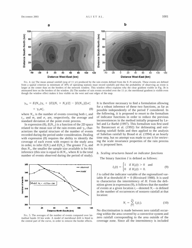
(1991-2002) n’a pas vu le retour aux conditions humides des années 1950-1970 – mais des différences avec la période précédente sont tout de même à signaler. Tout d’abord on a observé deux années très pluvieuses (1994 et 1999) – proches des records observés et une année bien arrosée (1998). Ensuite, comme le montre la figure I.1, une opposition est apparue entre le Sahel Ouest – qui reste très sec – et le Sahel Est qui a vu, pour ce qui est de la moyenne interannuelle, un retour à une meilleure pluviométrie.
Fig. I.1 Comparaison des isohyètes moyennes (200 mm, 500 mm, 1000 mm) pour les
périodes humide (1950-1969), sèche (1970-1989) et récente (1990-2002). On note l’apparition de deux comportements différents entre le Sahel Est et le Sahel Ouest. Sur le Sahel Ouest, la dernière décennie est très proche de 1970-1989, alors que sur le Sahel Est, elle est souvent plus humide que la période 1970-1989, avec des valeurs proches de la moyenne long terme (1950-2002). Entre la période humide 1950-1969 et la période sèche 1970-1989, on assiste une descente d’environ un 1° en latitude des isohyètes vers le Sud. Le décalage est assez important sur l’ensemble de la zone. Par contre à compter du début des années 1990, on note une remontée des isohyètes de la partie Est par rapport à la partie Sud.
I.2.2 Les systèmes pluvieux sahéliens : les Systèmes convectifs de Méso-échelle au cœur d’une interaction complexe
Les précipitations sahéliennes, essentiellement d’origine convective, résultent de l’interaction
complexe de multiples facteurs d’échelles différentes : i) facteurs régionaux (gradients d’énergie liés au contraste entre l’océan et le continent et aux gradients de végétation sur le continent), ii)

Présentation générale 6
éléments synoptiques (ondes du jet d’Est africain), iii) facteurs de méso-échelle (systèmes convectifs) et localisés (végétation et reliefs).
Facteurs régionaux). La circulation méridienne advecte de l’air humide dans la couche de la Mousson et ce à partir du Golfe de Guinée. De l’air plus sec est simultanément advecté dans la troposphère moyenne en provenance du Sahara. Le conflit et le mélange des ces deux masses d’air ont principalement lieu dans les basses couches de la Zone de Convergence Inter-Tropicale (ZCIT). Il en résulte des gradients d’énergie dans la couche limite (e.g. Eltahir and Gong 1996 ; Zheng and Eltahir, 1998 ; Fontaine et al. 1999). Ces gradients sont modulés par les conditions de surface aussi bien océaniques que continentales et dépendent donc de la surface des mers et des propriétés des paramètres de surface sur le continent tels que l’albédo, l’humidité des sols et le couvert végétal. Notons par ailleurs que les précipitations saisonnières sur l’Afrique de l’Ouest dépendent non seulement de la température de surface de la mer (TSM) dans l’Atlantique tropical (Lamb 1978), mais aussi de la TSM à l’échelle globale (Folland et al. 1986 ; Rowell et al. 1995). Des études récentes (Janicot et al. 2001 ; Rowell 2001 ) tendent à montrer que ce forçage par l’océan a pu changer de nature à compter du début des années 70.
Éléments synoptiques). Sur le continent, la surface continentale rétroagit sur la pluviométrie à différentes échelles spatiales et temporelles. Charney (1975) fut le premier à évoquer une possible rétroaction de la dégradation du couvert végétal sur les pluies au Sahel, par le biais de la modification de l’albédo. Plusieurs simulations à l’aide des Modèles de Circulation Générale Atmosphérique (MCGA) ont montré par la suite, une certaine sensibilité de la Mousson Africaine aux conditions de la surface continentale (champ des humidités des sols par exemple, voir Douville et al. 2000). D’autre part les ondes 3-5 jours et 6-9 jours liées au Jet d’Est Africain interagissent avec la convection (Thorncroft and Blackburn 1999 ; Diedhiou et al. 1999) en modulant la localisation des systèmes convectifs et des précipitations.
Ces interactions d’échelles régionale et synoptique se résume en un régime moyen constitué par deux sous-régimes (Lebel et al. 2003) : un régime océanique caractérisé par une augmentation progressive du flux de l’humidité des océans sur le continent et un régime continental dans lequel la pluie provient essentiellement de gros systèmes associés aux instabilités dans le Jet d’Est Africain (JEA). Ce régime continental se met en place avec un saut brusque des pluies vers le nord. Les précipitations dans ce régime sont apportées pour l’essentiel par quelques systèmes très bien organisés, du type lignes de grains. 90% des pluies sont produites par 12% du nombre total des systèmes (Mathon et al. 2002).
Éléments de méso-échelle). En ce qui concerne la méso-échelle, les reliefs constituent un
terrain privilégié pour l’initiation des systèmes convectifs, susceptibles d’évoluer en ligne de grains (figure I.2). Mais le rôle des gradients d’humidité dans leur initiation et le maintien de leur dynamique n’est pas encore bien étudié. Un aspect important souligné par plusieurs auteurs (Desbois et al. 1988 ; Polcher 1995) est la distinction à établir entre systèmes convectifs de Méso-échelle (SCM) et systèmes convectifs locaux. Les SCM sont des systèmes mobiles se déplaçant d’est en ouest, avec éventuellement une composante nord-sud, à une vitesse moyenne de 50 à 60 km/h. Parmi ces SCM, c’est seulement une catégorie, appelés systèmes convectifs organisés (SCO) représentant 12% des systèmes, qui est responsable de l’essentiel de la pluie de la saison. Ces SCO comprennent les complexes convectifs de méso-échelle, ainsi que les lignes de grain. Les SCO se distinguent des autres SCM par des caractéristiques tant dynamiques que morphologiques (vitesse de déplacement, taille, forme).
Téléconnexions à l’échelle globale. A ces interactions d’échelle sur la région, s’ajoutent des possibles téléconnexions à l’échelle du globe. La simultanéité de la canicule de 2003 en Europe et
Présentation générale 7
d’une année exceptionnellement pluvieuse sur le nord du Sahel pourrait être une manifestation des liens dynamiques entre le climat sahélien et le climat de l’Europe.
Comme déjà mentionné, ces différents facteurs sont aujourd’hui relativement bien documentés, mais leur interaction est mal connue. Ces questions d’interaction sont au cœur du programme AMMA.
Fig. I.2 : Répartition spatiale de la probabilité de naissance des systèmes convectifs organisés, valeurs calculées sur la période 1990-1999. Les zones vertes représentent les lieux de forte probabilité de naissance. On note une forte hétérogénéité spatiale. L’effet du relief est bien présent (Plateau de Joss, Aïr), mais il existe aussi des zones de maxima sans relief marqué, au Mali par exemple.
I.2.3 Quelques éléments essentiels du régime pluviométrique sahélien.
Le Sahel est correctement instrumenté en pluviomètres sur une zone comprise entre les latitudes 11°N et 15°-16°N. Le cumul moyen de la pluviométrie interannuelle sur cette zone a une organisation zonale quasi parfaite (figure I.1). La période sèche (1971-1990) a été caractérisée par un glissement assez régulier des isohyètes vers le sud de 1° environ. La durée de la saison des pluies, contrôlée par le mouvement saisonnier de la ZCIT, est d’environ 7 mois (avril à octobre) sur le Sud de la région et de trois mois sur le Nord. A la latitude de Niamey (13°N), la saison des pluies dure en moyenne un peu plus de 5 mois. La moyenne interannuelle du cumul saisonnier a été de 650 mm sur la période humide 1950-1969 et de 490 mm sur la période sèche 1970-1989. Sur les années récentes (1990-2002) analysées dans ce travail, la pluviométrie moyenne est remontée à 515 mm, essentiellement du fait de quelques années plus humides en fin de période. Le cumul de l’année la plus sèche (1990) a été de 400 mm et celui de l’année la plus humide (1998, l’année du plus fort El-nino) d’environ 680 mm. Il faut noter que plus de 50% de ce cumul annuel tombe sur une durée cumulée de moins de 4 h (Balme 2004). Quant à la variabilité intra-saisonnière, elle est caractérisée par un maximum de pluie pour les mois de juillet et août. La dynamique saisonnière est marquée par un saut brutal vers le Nord pendant la dernière décade de juin. Ce phénomène est appelé saut de Mousson (Sultan and Janicot 2000 ; Le Barbé et al. 2002). Contrairement à une vision classique qui suppose un fort lissage spatial des champs de pluie pour des pas de temps de cumul assez grands, la variabilité spatiale du champ de pluie saisonnier
Présentation générale 8
demeure très forte comme le montre Balme (2004) dans son analyse synthétique du jeu de données EPSAT-Niger. En 1992 par exemple, un gradient de 270 mm sur 9 km a été enregistré dans le champ du cumul annuel. Ceci pose des problèmes d’interpolation, les réseaux nationaux étant peu denses. Cette grande variabilité pourrait provenir en partie d’un effet de persistance comme suggéré par Taylor and Lebel (1998). Par contre, la pluviométrie associée aux événements pluvieux est caractérisée par une faible variabilité interannuelle des paramètres tels que la fréquence de pluie nulle (26%), la moyenne événementielle (14 mm) et la variance (205 mm²). La variabilité interannuelle du nombre d’évènements pluvieux est, elle, beaucoup plus importante et explique la majeure partie de la variabilité interannuelle des cumuls saisonniers. Ces résultats que nous avons obtenus à partir des données couvrant la période 1990-2002, confirment ceux de Lebel et al. (2002) obtenus pour la variabilité décennale, la période sèche 1970-1997 s’étant caractérisée par une forte baisse, surtout en août et septembre, du nombre moyen d’évènements pluvieux.
I.3 Problématique scientifique de la thèse
I.3.1 Problématique de la modélisation
La modélisation climatique, à travers des outils comme les modèles de circulation générale atmosphérique (MCGA), rend bien compte de la dynamique grande échelle de l’atmosphère. Par contre, elle n’est pas encore capable de produire des sorties de précipitation réalistes aux échelles d’intérêt pour les hydrologues et les agronomes à cause des limites de la résolution. Dans ce contexte, la modélisation stochastique se présente soit comme une approche alternative produisant stochastiquement des séquences de situations humides ou sèches correspondant à des situations déjà observées, soit comme une approche complémentaire – et c’est la plus prometteuse – en reproduisant la variabilité pluviométrique requise dans la planification des ressources en eau et agricole, tout en la conditionnant aux valeurs moyennes prédites par les MCGA ou estimées par l’observation satellitale. Cela peut se faire soit par le biais de désagrégation des sorties des MCGA, soit par le biais d’agrégation des modèles hydrologiques à qui on impose de respecter les moyennes prédites par les MCGA. Donc, et loin de vouloir faire ressurgir ici un débat qui a le plus souvent opposé partisans d’une modélisation mécaniste, soucieux de représenter la genèse des phénomènes en cause et ceux d’une approche plus probabiliste, convaincus que les lois déterministes ne peuvent décrire correctement des phénomènes complexes et hétérogènes, nous dirons que le recours à des modèles probabilistes n'implique pas une foi en un hasard qui régenterait le monde. Comme il est évoqué ci-dessus, il y a une vraie complémentarité entre la modélisation stochastique et celle déterministe. Une même modélisation peut intégrer les deux volets.
C’est avec cet esprit que nous abordons ce travail, en considérant l’événement pluvieux comme l’élément de base d’une modélisation stochastique intégrée. Ce choix a un fondement climatologique important au Sahel. Plus que nulle part ailleurs, les événements pluvieux se présentent comme des objets individuels, facilement identifiables et dotés de caractéristiques stables dans le temps et dans l’espace. A l’échelle événementielle proprement dite, des acquis importants sont à souligner. La typologie des événements pluvieux sahéliens a d’abord été étudiée par Amani (1995) et Amani et al. (1996). Sur cette base, Lebel et al. (1998) ont proposé un
Présentation générale 9
premier modèle adapté à leur désagrégation spatio-temporelle. Guillot (1998) et Guillot and Lebel (1999) généralisèrent ce travail dans un cadre mathématique rigoureux, qui maintient la cohérence des différents aspects (spatiaux, cinématiques, hyétogrammes) des champs événementiels. La désagrégation est conditionnée aux données ponctuelles mesurées. Onibon et al. (2004) ont parachevé ce travail en conditionnant la désagrégation spatiale à la moyenne de l’événement via l’algorithme de Gibbs. Pour capitaliser ces travaux aux échelles supérieures de temps et d’espace, il convient de mener un travail de fond pour assurer les fondements théoriques de nouveaux algorithmes.
Le problème est posé de deux manières. Tout d’abord, le cadre des travaux cités ci-dessus
relevant de la géostatistique, il s’agit d’exprimer la structure des champs de pluie issus des cumuls d’événements en fonction des paramètres du champ de pluie événementiel. Le cadre géostatistique a été choisi car, moyennant des hypothèses d’homogénéité, il permet de quantifier les incertitudes associées aux estimations. Le passage de la structure événementielle à la structure multi-événementielle fait appel à la notion d’invariance d’échelle. L’invariance d’échelle dans son sens strict (auto-similarité et formalisme multifractal) implique toute absence d’échelles caractéristiques dans le système étudié. Or il est bien clair que dans notre cas, l’échelle événementielle est une échelle caractéristique. La notion d’invariance d’échelle est prise ici dans un sens général, en la prolongeant dans un cadre plus souple, donc plus adaptable à des situations réelles. Le cœur de notre démarche va donc consister à relier la géostatistique aux questions d’invariance d’échelle.
Une seconde approche doit être envisagée pour passer à de grands domaines (tout le Sahel par
exemple), l’hypothèse de continuité spatiale de la variable régionalisée (le champ événementiel) n’étant plus adaptée. On aura alors recours aux modèles objets, ce qui nous place dans le cadre plus général des ensembles aléatoires. I.3.2 Intégration des données disponibles
Les données disponibles pour ce travail se prêtent bien à la problématique décrite dans la section ci-dessus. Nous avons trois sources de données différentes mais très complémentaires et chacune apporte sa pierre dans la construction de l’édifice.
Données de Meso-échelle. A cette échelle, nous avons accès à la base de données de l’expérience EPSAT-Niger (Estimation des précipitations par Satellite) qui a débuté en 1990 dans la région de Niamey au Niger et qui se poursuit encore (Balme 2004). Le réseau de pluviographes comptait entre 1990 et 1993 plus 100 appareils à acquisition numérique couvrant une superficie de 16,000 km². Un dispositif de suivi à long terme comprenant 30 pluviographes, a été maintenu depuis lors et constitue un réseau de base. Cette instrumentation de méso-échelle a permis de documenter la variabilité des champs de pluie aux échelles kilométriques dans l’espace et de façon quasi continue dans le temps. Ce réseau, qui fournit un échantillonnage dense mais de couverture spatiale limitée, est référencé ici par la notation E-N.
Au niveau régional, nous utilisons les données du réseau pluviométrique du Centre Régional AGRHYMET, à Niamey (CRA) qui centralise les données des réseaux opérationnels des pays du CILSS (Comité Inter-Etas de Lutte contre la Sécheresse au Sahel). Ce réseau (référencé ici par la
Présentation générale 10
notation CILSS) couvre environ trois millions de km² et est constitué de près de 1200 stations, mais 750 seulement en moyenne font parvenir leurs données au CRA chaque année. Sur ces 750, une centaine présentent des lacunes qui les rendent inexploitables et on dispose donc en moyenne de 650 stations réellement utilisables chaque année. Ces données constituent une longue chronique temporelle (depuis 1950). Par conséquent, bien que beaucoup moins dense que le réseau précédent (1 station tous les 5000 km² en moyenne sur le Sahel et 1.5 station tous les 2500 km² sur la partie Sud, contre 1 station pour 400 km² pour le réseau E-N), le réseau CILSS constitue une source d’informations complémentaire indispensable pour, d’une part, appréhender la variabilité interannuelle ou décennale et, d’autre part, pour disposer d’une vision spatiale des champs de pluie à des échelles plus larges. Chacun de ces deux réseaux représente à son échelle, le meilleur de la région.
A partir du réseau CILSS, on sera amené à distinguer deux sous-réseaux. Les données du réseau CILSS ne sont totalement disponibles que plusieurs semaines après la fin de la saison des pluies. C’est pourquoi les experts du centre AGRHYMET s’appuient sur un réseau moins fourni, constitué par les données qui leur parviennent en cours de saison (théoriquement chaque 10 jours), pour effectuer le suivi opérationnel de la compagne hydro-agro-sylvo-pastorale. Ce réseau d’environ 250 postes est le réseau de suivi, noté CRA. Le deuxième sous-réseau est le réseau synoptique. Ses données sont en principe transmises quotidiennement à tous les opérateurs nationaux et régionaux dans le monde via le Système Mondial de Télécommunication (SMT). Dans la réalité, toutes les stations synoptiques (environ 80) des pays sahéliens ne sont pas transmises sur le SMT, pour différentes raisons techniques ou organisationnelles. Le sous-réseau SYN considéré ici est celui de toutes les stations synoptiques, correspondant à l’échantillonnage qui pourrait être obtenu des champs pluviométriques si le SMT fonctionnait à son niveau optimal.
Données satellites. Un suivi ("tracking") des systèmes convectifs de méso-échelle (SCM) réalisé à partir des images du satellite METEOSAT (Mathon and Laurent 2001) donne accès aux paramètres suivants des SCM: durée de vie, taille, vitesse de déplacement, direction, lieu de naissance. De plus, une analyse croisée de cette base avec celle d’EPSAT-Niger a permis de discriminer les SCM pluviogènes responsables de plus de 90% de la pluie sur la zone. Cette catégorie de SCM a reçu le nom des systèmes convectifs organisés (SCO) et les caractéristiques de ces SCO serviront pour identifier à partir de la seule donnée satellite un événement pluvieux (Mathon et al. 2002). Un SCO est un SCM dont la vitesse moyenne de déplacement est supérieure à 10 ms-1, la taille atteinte au seuil en température de 213 K est supérieure à 5000 km² et la durée de vie est supérieure à 3 h.
Un des objectifs majeurs de ce travail est d’élaborer une modélisation multi-échelle capable d’intégrer de façon cohérente ces données de natures et d’échelles différentes à des fins d’estimation et de simulation .
Présentation générale 11
-15 -10 -5 0 5 10 15 20 25 300
5
10
15
20
25
30Réseaux nationauxRéseaux nationaux Tracking Tracking des événements des événements pluviogènespluviogènes (SCO) (SCO)
par image satellitepar image satellite
MésoMéso--échelle: réseau dense EPSATéchelle: réseau dense EPSAT--NigerNiger
-15 -10 -5 0 5 10 15 20 25 300
5
10
15
20
25
30
-15 -10 -5 0 5 10 15 20 25 300
5
10
15
20
25
30
-15 -10 -5 0 5 10 15 20 25 300
5
10
15
20
25
30Réseaux nationauxRéseaux nationaux Tracking Tracking des événements des événements pluviogènespluviogènes (SCO) (SCO)
par image satellitepar image satellite
MésoMéso--échelle: réseau dense EPSATéchelle: réseau dense EPSAT--NigerNiger
Fig. I.3. Les trois sources de données utilisées dans ce travail.
I.4 Composition du mémoire
Le mémoire est rédigé sous forme d’articles. Il est articulé en trois parties. La première propose une modélisation par invariance d’échelle des champs de pluie, dans un cadre géostatistique. L’essentiel de cette partie est contenu dans un article paru dans Journal of Hydrometeoroloy (2003) et intitulé « Invariance in the Spatial Structure of Sahelian Rainfields at Climatological Scale ». Cette partie constitue le fondement conceptuel de la thèse. L’intérêt à la fois théorique et pratique du modèle proposé est analysé. Les applications de ce formalisme constitue la deuxième partie du mémoire consacrée au développement d’un modèle d’erreur qui a servi à évaluer des produits pluviométriques opérationnels sur la région. Ce travail est présenté dans une série de deux articles soumis à Journal of Applied Meteorology : « Rainfall estimation in the Sahel. Part 1: Error Function » et « Rainfall estimation in the Sahel. Part 2: Evaluation of CILSS countries Raingauge Networks and Objective Intercomparison of Satellite Rainfall Products ». La troisième et dernière partie de la thèse porte sur le développement d’un modèle conceptuel pour des études climatiques régionales. Cette partie n’est pas encore soumise pour publication, mais une ébauche d’article, « Towards a Conceptual Regional Model for Sahelian Rainfields », en constitue la trame.

II. Modélisation de l’invariance d’échelle des champs de pluie sahéliens 1
1 Article : Invariance in the Spatial Structure of Sahelian Rain fields at Climatological Scales . Ali, Lebel, Amani, 2003. Journal of hydrometeorology 4(6), 996-1011.
Modélisation de l’Invariance d’échelle des champs de pluie sahéliens 15
II.1 Introduction
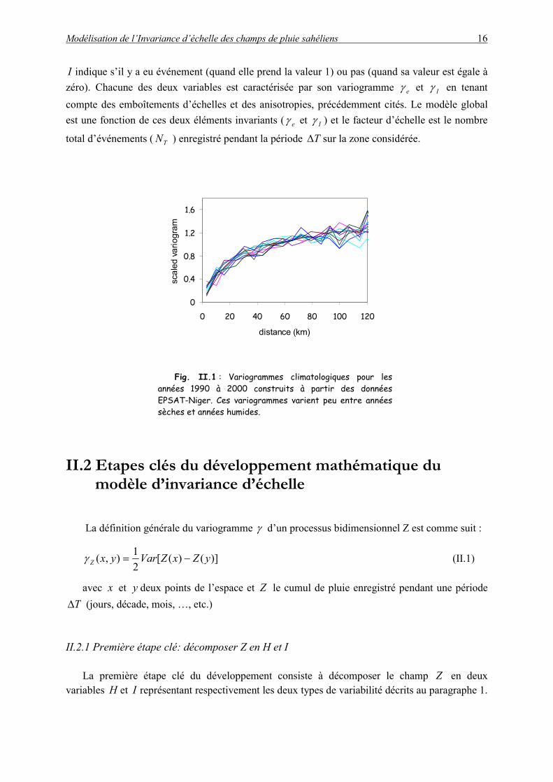
Les systèmes convectifs matérialisent le lien entre l’environnement grande échelle et la pluie. La pluviométrie associée à ces systèmes convectifs a des caractères relativement stables, qu’on soit en année humide ou sèche, même si par ailleurs les champs de pluie constitués par des cumuls d’événements, présentent eux une grande variabilité sur une large gamme d'échelles temporelles: variabilité décennale associée à la sécheresse 1970-1997; variabilité interannuelle incarnée par l'année 1994, seule année humide au sein de la période précédente; variabilité intra-saisonnière (arrêt brutal de la mousson de l'année 2000) et enfin intermittence au sein des événements pluvieux. Le Barbé et al. (2002) montrent que la différence entre années sèches et humides est liée à une fluctuation importante du nombre d’événements pluvieux, leur intensité moyenne demeurant relativement constante. La figure II.1 montre également que les différents variogrammes climatologiques annuels des cumuls événementiels sont assez semblables pour la période 1990-2000, qui comprend autant d’années très humides (1994, 1998, 1999), très sèches (1990, 1997, 200) et d’années moyennes (1991, 1992, 1995, 1996).
L’organisation spatiale des cumuls de pluie au Sahel est, en fait, commandée par deux processus dominants. Tout d’abord, les événements pluvieux sont associés à des systèmes convectifs organisés (Mathon et al. 2002) en nombre relativement faible (12% seulement de l’effectif total des systèmes), mais qui apportent plus de 90% de la pluie totale de la saison. Ils sont identifiables par satellite (Mathon and Laurent 2001). Ces systèmes se développent dans une circulation d’Est, ce qui engendre une anisotropie marquée des champs de pluie événementiels : les distances de corrélation sont plus importantes selon l’axe Est-Ouest que selon l’axe Nord-Sud. Aussi, conformément au schéma de Austin et Houze (1972), les systèmes convectifs de méso-échelle pluviogènes, sont organisés en un emboîtement de structures d’échelles différentes (cellules convectives, front convectif, partie stratiforme). La variabilité des pluies associée à ces processus constitue la variabilité interne de l’événement pluvieux (ou variabilité interne, tout court). A plus grande échelle de temps, et c’est le deuxième processus important, la climatologie régionale est contrôlée par les mouvements saisonniers de la ZCIT, ce qui implique des structures d’échelles dominées par une dérive Nord-Sud. Cette variabilité peut être qualifiée de variabilité externe aux événements.
Se basant sur ces deux variabilités caractérisant l’organisation interne et externe des événements pluvieux au Sahel, le but recherché dans cette première partie de la thèse, est de développer un modèle d’invariance d’échelle dans un contexte géostatistique qui, d’une part, soit capable de décrire la variabilité totale des champs de pluie pour des pas de temps supérieurs à l’événement pluvieux et, d’autre part, servira d’outil permettant de lier la variabilité climatique et la variabilité spatiale des pluies aux échelles hydrologiques. Le modèle est calé de manière robuste à l’échelle de l’événement pluvieux (la taille des échantillons étant grande à cette échelle, par exemple 470 contre 11 à l’échelle du pas de temps annuel, quand on considère les 11 années de EPSAT-Niger). Il permet ensuite le passage aux échelles supérieures (pluri-journalière à pluri-annuelle). Pour ce faire, les deux variabilités (interne et externe) sont considérées comme des invariants climatologiques des systèmes pluvieux. Elles sont représentées par les variables H (cumul de pluie événementielle) et I (variable indicatrice l’événement pluvieux). La variable
Modélisation de l’Invariance d’échelle des champs de pluie sahéliens 16
I indique s’il y a eu événement (quand elle prend la valeur 1) ou pas (quand sa valeur est égale à zéro). Chacune des deux variables est caractérisée par son variogramme � et � en tenant compte des emboîtements d’échelles et des anisotropies, précédemment cités. Le modèle global est une fonction de ces deux éléments invariants (� et � ) et le facteur d’échelle est le nombre
total d’événements ( ) enregistré pendant la période
e I
e I
TN T� sur la zone considérée.
0
ce (k
80
)
([Z
�
Z
0
0.4
0.8
1.2
1.6
0 20 40 6 100 120
distan m
scal
ed v
ario
gram
Fig. II.1 : Variogrammes climatologiques pour les années 1990 à 2000 construits à partir des données EPSAT-Niger. Ces variogrammes varient peu entre années sèches et années humides.
II.2 Etapes clés du développement mathématique du modèle d’invariance d’échelle
La définition générale du variogramme � d’un processus bidimensionnel Z est comme suit :
)]()21),( yZxVaryxZ ��� (II.1)
avec x et deux points de l’espace et y Z le cumul de pluie enregistré pendant une période T (jours, décade, mois, …, etc.)
II.2.1 Première étape clé: décomposer Z en H et I
La première étape clé du développement consiste à décomposer le champ en deux variables H et I représentant respectivement les deux types de variabilité décrits au paragraphe 1.
Modélisation de l’Invariance d’échelle des champs de pluie sahéliens 17
H est le cumul de pluie par événement et I la variable indicatrice de l’événement (1 ou 0 selon que l’événement est passé à la station x ou pas). On pose alors :
kI
)
(x
x
�
I
~]~I�emZNe
�
��
�
)(
1)()(
xN
kk xHxZ et (II.2) �
�
�
TN
k
xxN1
)()(
II.2.1 Deuxième étape clé: décomposer en , )N xyN 'xN
Le nombre d’événements touchant le point (xN x est décomposé en un nombre
d’événements qui touchent à la fois xyN et , et qui touchent seulement y 'xN x mais pas .
Au point , est également décomposé en , et qui touchent seulement .
Autrement dit :
y
yy )(yN xyN 'yN
')( xxy NNxN �� et . (I.3) ')( yxy NNyN �
Après ces deux étapes de décomposition clé, la variable Z est remplacée dans l’expression
(I.1) par les différentes sous-variables ( H , et ) et le reste du problème devient une question de calcul mathématique. L’hypothèse fondamentale qui est faite, est l’indépendance entre les cumuls de pluie enregistrés en un point d’un événement à l’autre. Cette hypothèse est tout à fait soutenable et elle diffère de celle considérant l’indépendance entre les événements, qui, elle, est moins soutenable comme nous le verrons dans la partie 3 de cette thèse.
N
II.3 Le modèle d’invariance d’échelle
Le résultat final du calcul dont les détails se trouvent dans Ali et al. 2003, donne le modèle d’invariance d’échelle de la structure spatiale des champs de pluie, résumé par la relation suivante :
� � � �222
1222
1 )()()1(~~)()[(~][1221 IIeTTIeeeIIT mmmNNmmN �������� ���� (I.4)
(1) (2)
NeZ�~ est le variogramme pour un champ Z composé de événements. N
, et � sont la moyenne, la variance et le variogramme de l’événement pluvieux,
et � sont la moyenne et le variogramme de l’indicatrice. Tous ces éléments sont
considérés climatologiquement invariants. est le nombre total d’événements sur la zone pendant la période
em
Ime� e
I
TNT� considérée et représente le facteur d’échelle de cette relation
d’invariance d’échelle.
Modélisation de l’Invariance d’échelle des champs de pluie sahéliens 18
Dans cette équation on peut noter que est effectivement un facteur d’échelle qui permet à
lui seul de passer de l’échelle événementielle aux échelles -événementielles. Mais ce facteur intervient de deux manières : i) si le champ est stationnaire le second terme s’annule et le facteur d’échelle est simplement en ; ii) si le champ est non stationnaire, le facteur d’échelle est une
fonction quadratique de [i.e en ]. La stationnarité ou non dépend seulement de
(qui est la moyenne de l’indicatrice). La stationnarité correspond à m indépendant de la position du point dans l’espace, ce qui revient à dire que la probabilité d’avoir un événement est constante dans l’espace. Cette hypothèse est valable dans la direction Est-Ouest, où nous pouvons considérer qu’il n’y a pas de gradient systématique en m . Par contre dans la direction Nord-Sud, la probabilité d’avoir un événement diminue systématiquement du Sud vers le Nord. La dérive étant alors une fonction quadratique de , devient rapidement prépondérante quand devient grand. C’est la situation observée en analysant les données réelles.
TN
)1�
T
TN
TN
TN ( TT NN
N
Im
I
I
TN
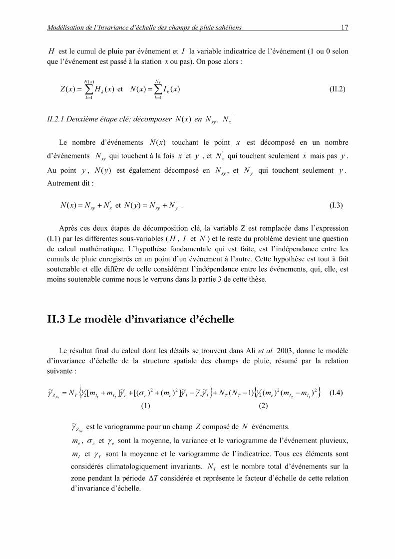
La validation a été effectuée avec succès sur les données EPSAT-Niger et celles de Centre
Régional AGRHYMET (figure II.2). Il n’était pas possible, sans utilisation de données satellitaires, de différencier l’intermittence interne de l’intermittence externe ; H représentait la variable conditionnelle : , c’est-à dire les valeurs de pluie non nulles et 0/*
�� HHHI indiquait si la pluie enregistrée était nulle ( ) ou non (0�I 1�I ).
Fig. II.2. Exemple de validation du modèle d’invariance d’échelle. Le variogramme expérimental correspond au variogramme moyen décadaire calculé à partir des données du réseau pluviométrique du Niger pour la période (JAS). Le nombre d’événements dans le modèle théorique est pris égal à 4.
TN

Modélisation de l’Invariance d’échelle des champs de pluie sahéliens 19
II.4 Enjeux et portées d’un tel développement
Les enjeux d’une telle modélisation sont multiples. On va en passer quelques uns en revue ci-après.
4.1) Robustesse et cohérence des variogrammes aux différentes échelles. La robustesse de la méthode proposée vient du fait que le modèle est calé à une échelle où l’information est abondante (échelle événementielle). Cette information est ensuite transférée vers les échelles supérieures où on en a moins (échelle annuelle par exemple) par la relation d’invariance. La cohérence est garantie de deux manières. D’abord de manière statistique : les champs de pluie étant très variables, les variogrammes expérimentaux à partir d’une seule réalisation sont peu robustes et mal structurés. Pour pallier cela, le variogramme moyen (Guillot and Lebel 1999) ou le variogramme climatologique (Bastin et al. 1988) sont utilisés. Or le nombre d’événements variant fortement d’un champ à un autre (par exemple d’un cumul mensuel à un autre), le variogramme moyen n’est pas statistiquement cohérent. Cet inconvénient disparaît dans cette nouvelle approche, le nombre d’événements étant explicitement pris en compte. Ensuite la cohérence des variogrammes est garantie entre les différentes échelles, car ils sont liés par un facteur d’échelle.
4.2) Quantification de l’erreur d’estimation. Traditionnellement les approches d’invariance d’échelle sont abordées dans le domaine fractal. Dans ce travail, il est mené dans un cadre géostatistique, ce qui permet d’aborder de manière optimale les questions de l’estimation et de la quantification des incertitudes associées. En effet, grâce au réseau dense de pluviographes de l’expérience EPSAT-Niger, il est démontré que cette variabilité temporelle des pluies est associée à une forte variabilité spatiale dont l’impact hydrologique et agronomique est extrêmement important (Peugeot et al. 1997 ; Balme et al. 2004 ; Lebel and Vischel 2004). Cette variabilité spatiale pose des problèmes d'interpolation des champs pluvieux (les réseaux nationaux étant peu denses), il est donc fondamental de disposer d’une fonction quantifiant l’erreur d’estimation. Cette fonction d’erreur peut être déduite de la relation d’invariance. La deuxième partie de ce mémoire est consacrée à l’exploitation de cette voie.
4.3) Estimation des pluies par satellite. La performance des algorithmes d’estimation des pluies par satellite au Sahel est encore très insuffisante. La quantité de pluie qui arrive au sol est très mal estimée. Mais des travaux récents (Mathon et al. 2002) permettent d’envisager la possibilité de déterminer assez efficacement le nombre d’événements pluvieux à partir uniquement de l’imagerie satellitaire. Il serait par conséquent possible de déterminer assez objectivement la fonction de structure des champs de pluie pour une période donnée, uniquement à partir de l’imagerie satellitaire. Ceci permet d’envisager de nouveaux algorithmes d’estimation des pluies par satellite en combinant de manière optimale les possibilités du satellite et les quelques informations pouvant être obtenues au sol, dans la perspective d’un suivi en temps réel ou peu différé de la saison des pluies au Sahel.
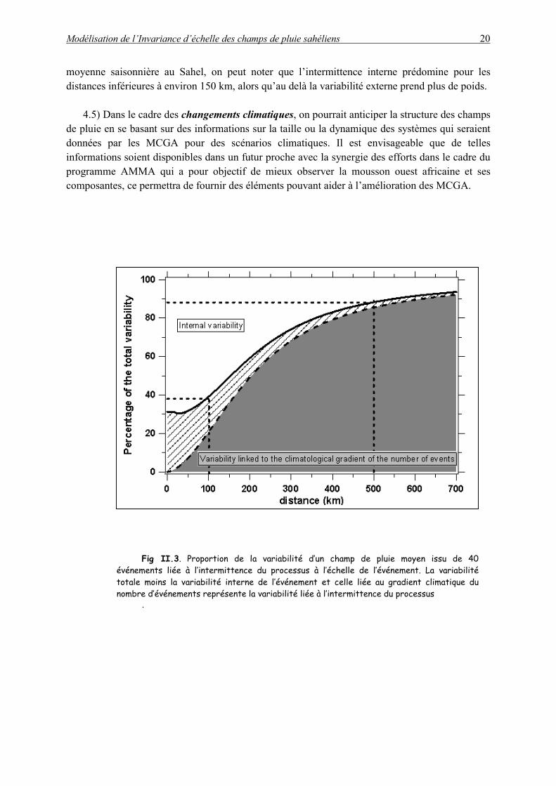
4.4) Diagnostique des différentes échelles de variabilité. Le poids associé à chaque type de variabilité (interne ou externe) pour une échelle donnée peut être quantifié directement à partir du modèle. Par exemple en figure II.3, pour un cumul moyen de 40 évènements qui correspond à la
Modélisation de l’Invariance d’échelle des champs de pluie sahéliens 20
moyenne saisonnière au Sahel, on peut noter que l’intermittence interne prédomine pour les distances inférieures à environ 150 km, alors qu’au delà la variabilité externe prend plus de poids.
4.5) Dans le cadre des changements climatiques, on pourrait anticiper la structure des champs de pluie en se basant sur des informations sur la taille ou la dynamique des systèmes qui seraient données par les MCGA pour des scénarios climatiques. Il est envisageable que de telles informations soient disponibles dans un futur proche avec la synergie des efforts dans le cadre du programme AMMA qui a pour objectif de mieux observer la mousson ouest africaine et ses composantes, ce permettra de fournir des éléments pouvant aider à l’amélioration des MCGA.
Fig II.3. Proportion de la variabilité d’un champ de pluie moyen issu de 40
événements liée à l’intermittence du processus à l’échelle de l’événement. La variabilité totale moins la variabilité interne de l’événement et celle liée au gradient climatique du nombre d’événements représente la variabilité liée à l’intermittence du processus
.
Article
Invariance in the Spatial Structure of Sahelian Rain fields at Climatological Scales
996 VOLUME 4J O U R N A L O F H Y D R O M E T E O R O L O G Y
q 2003 American Meteorological Society
Invariance in the Spatial Structure of Sahelian Rain Fields at Climatological Scales
ABDOU ALI
IRD, LTHE, Grenoble, France, and Centre AGRHYMET, Niamey, Niger
THIERRY LEBEL
IRD, LTHE, Grenoble, France
ABOU AMANI
Centre AGRHYMET, Niamey, Niger
(Manuscript received 8 November 2002, in final form 21 March 2003)
ABSTRACT
The occurrence of rainfall in the semiarid regions is notoriously unreliable and characterized by great spatialvariability over a large spectrum of timescales. Based on analytical considerations, an integrated approach ispresented here in order to describe the spatial structure of rain fields for timescales used in climatological studies,that is from the daily to the seasonal scales and beyond to the interannual scale. At the scale of the rain event,two factors determine the spatial structure of rain fields. One is the spatial variability of the conditional rainfallH* (H . 0), represented by its variogram . The other is the intermittency, its spatial structure being describedg*eby the indicator variogram g1. It is shown that the spatial structure of rain fields for time steps larger than theevent may be analytically derived from and g1, taking into account the anisotropy and nonstationarity thatg*emay affect either of these two functions, which are thus two timescale invariants of the rainfall process. Theupscaling factor used to obtain the structure at large timescales is the number of rain events recorded over theperiod under consideration. An application using a large dataset of 450 Sahelian rain events observed with theEstimation des Precipitations par Satellite (EPSAT)–Niger monitoring network is presented. The theoreticalmodel provides a good representation of the spatial variability observed in the data. The validation of the modelconfirms that knowledge of the average event rain field structure and the number of events N is sufficient todetermine the structure of the N-event rain fields.
1. Introduction
Rainfall monitoring in semiarid regions of the worldremains a challenging problem, mostly because of theintermittency of the rain process. This intermittency isa source of great variability for rainfall in space, havingimportant consequences on agriculture, which is oftenentirely composed of rain-based crops. This variabilityalso influences the water cycle and it is a main concernfor hydrologists and climatologists alike to understandhow this influence evolves depending on the timescaleconsidered. Are there critical spatial scales when up-scaling from the daily scale used in water resourcesmodeling to the 10-day scale used in many crop modelsand beyond to the seasonal scale used in many clima-tological studies? Another question is related to thestrong interannual variability characterizing the tropicalclimates: are the characteristics of intermittency chang-
Corresponding author address: Thierry Lebel, LTHE, BP 53,38041 Grenoble Cedex 9, France.E-mail: [email protected]
ing from a dry year to a wet year and if yes, in whatway?
Intermittency may be defined as an accumulation ofzero values in a given part of a study area. As such, itis mostly apparent at the scale of the rain event. At thisscale, especially when convective rain is dominant, largeareas of zero rainfall are commonly embedded in rainareas. When rainfall is accumulated over several events,these areas of zero rainfall tend to disappear. At theseasonal scale, for instance, there will be rainfall ev-erywhere and, strictly speaking, intermittency has van-ished. It is easy to conceive, however, that the inter-mittency of the underlying rainfall process must havean influence on the structure of the rain fields at largerscales: in the Sahel, Lebel et al. (1997) have observedseasonal rainfall gradients of nearly 300 mm over 10km in an area where rain average is about 500 mm. Thepurpose of this article is to propose a framework allow-ing for a coherent representation of rain fields at thevarious timescales of interest for climatological and wa-ter resources studies, taking into account the variability
DECEMBER 2003 997A L I E T A L .
associated with areas of nonzero-event rainfall and thatassociated to areas of zero-event rainfall.
Four elements led to the development of the approachproposed here. First, in many regions of the world, es-pecially where rainfall unreliability is a daily threat topeople, there is no radar monitoring of rainfall due tothe high cost of this technology. Therefore the dataavailable for the modeling are point data. Second, abasic need for water resources management and watercycle modeling is to be able to interpolate these pointmeasurements in order to produce areal rainfall esti-mates along with the uncertainty attached to these es-timates. Third, in many water resources applications thetimescale of interest is the rain event and beyond. Afinal and important point is that the algorithms used forthe interpolation should not be based on ad hoc param-eters derived separately for various time steps; rather,there must be some coherency in the interpolation mod-els used, whatever the time step considered.
Scale invariance in rainfall modeling has become afruitful field of investigation over the past 15 years. Awhole corpus of theories emerged from the use of mul-tifractal representations of rain fields, the focus beingon the small- time and space scales [see, e.g., Holleyand Waymire (1992); Gupta and Waymire (1993) for amathematical representation of rain fields as a randomcascade; and Foufoula-Georgiou and Krajewski (1995)for a review of rainfall models based on concepts ofscale invariance]. The scaling properties at these scalesare essentially inferred from the study of spatial rainfalldata, mostly obtained from radar measurements (e.g.,Wheater et al. 2000). As mentioned above, the contextof the study presented in this paper is somewhat dif-ferent, the emphasis being on larger timescales docu-mented from point observations. Previous work (e.g.,Creutin and Obled 1982; Bastin et al. 1984; Kassim andKottegoda 1991) demonstrated that in such a contextgeostatistics provide a convenient and efficient way ofcharacterizing some key properties of the rain fields thatneed to be inferred for interpolation purposes. Howeverupscaling the geostatistical model characterizing a giventimescale to obtain models at larger time steps is notvery common in rainfall modeling, even though thereare well-known links between the multifractal theoryand the geostatistical theory (Federico and Neuman1997; Deidda 2000). The use of the geostatistical frame-work in this paper results from a few theoretical andpractical considerations that are expressed in the fol-lowing section 2, where point rainfall data are used asillustration. Then in section 3, an analytical derivationis given for indicator functions—describing the spatialstructure of the intermittency—used in the estimationof the spatial structure of rain fields over a range ofscales. Some aspects of the model implementation areexamined in section 4 and a validation is presented insection 5. Section 6 synthesizes the results obtained andpresents some possible applications.
2. General framework
The scaling approach proposed here was developedin the context of a long-term monitoring program carriedout in the region of Niamey, Niger, where a network ofa 100 recording rain gauges was installed over a 16 000km2 area in 1990 (see map and details in section 5).One important requirement of this approach is to pro-vide a simple and direct computation of the uncertaintyassociated with rainfall estimation (Lebel and Amani1999). This is especially important in order to take intoaccount the effect of input errors in hydrological modelsused to study the impact of rainfall variability on waterresources [see, e.g., Troutman (1983) for theoreticalconsiderations on how input rainfall errors produce bi-ased estimates of mean runoff and of physical param-eters in rainfall-runoff models]. This requirement is metby identifying the covariance function—or for that mat-ter the associated variogram—characterizing the spatialstructure of the rainfall process at the timescale of in-terest. The first step consists in identifying the variogramat the scale of the rain event, using point sampling ofrainfall accumulation H over a rain event [see D’Amatoand Lebel (1998) for a definition of a rain event, typ-ically lasting for less than 1 day].
The challenge is then to deduce the covariance func-tions at larger timescales, with a minimum of hypothesisand parameters.
The variogram of a random process X is defined as2g(t , t ) 5 1/2{Var[X(t ) 2 X(t )] },1 2 2 1 (1a)
where t1(x1, y1) and t2(x2, y2) are two points in the 2Dspace.
The variogram of the event rainfall (H) will be de-noted here g e:
g (t , t ) 5 1/2{Var[H(t ) 2 H(t )]}.e 1 2 2 1 (1b)
The inference of the theoretical variogram g is basedon the computation of an experimental variogram g av-eraged for classes of distances {h to h 1 Dh} using theavailable realizations of the random process:
JN h12g(h; h 1 Dh) 5 [X (t ) 2 X (t )] , (2)O O k j k i2NJ k51 1h
where Jh is the number of pairs (ti, tj) belonging to theclass {h to h 1 Dh} and N is the number of realizations.
The variogram provides a simple representation ofthe spatial structure of a rain field at a given temporalscale. It is conveniently used as a basis for interpolationand estimation purposes [see Bacchi and Kottegoda(1995) for a review on the identification of rainfall spa-tial correlation patterns with reference to the theory ofvariograms]. In many applications, the inference of thevariogram is carried out directly on data accumulatedat the time step of interest. This may generate two typesof difficulties: (i) the greater the time step, the smallerthe number N of available realizations (in the case studytreated here, the value of N decreases from 450 at the
998 VOLUME 4J O U R N A L O F H Y D R O M E T E O R O L O G Y
event scale to 11 at the annual scale), thus making theinference less and less robust; (ii) there is no guaranteeof consistency between the different variograms inferredfor different time steps. Considering that the large num-ber of realizations make the inference of g e robust, theobjective is then to find a theoretical framework thatwill allow the derivation of the variogram of ZT fromthe variogram of H, where ZT is the rainfall accumulatedover a period of length T (T being larger than 1 day).
This will be done by following the approach proposedby Bras and Rodriguez-Iturbe (1976), which consists indistinguishing the variability linked to the internal struc-ture of the event rain fields from the external variabilitylinked to the life cycle of the convective systems. Thisrequires taking into account three important factors in-fluencing the organization of rain fields—namely, in-termittency, stationarity, and anisotropy—knowing thatthe influence of these three factors changes dependingon the temporal scale considered. The method proposedto upscale from the event scale to the T-scale (T varyingfrom a few days to 1 yr) must therefore be able tocorrectly reproduce these changes.
a. Intermittency
T-day rain fields are the accumulation of a numberNT of event rain fields, that is at each location t(x, y),the T-day rainfall ZT is expressed as
NT
Z (t) 5 H (t), (3)OT kk51
where Hk(t) is the rainfall of event k at location t(x, y).The value H is an unconditional variable that can takezero or nonzero values at point t.
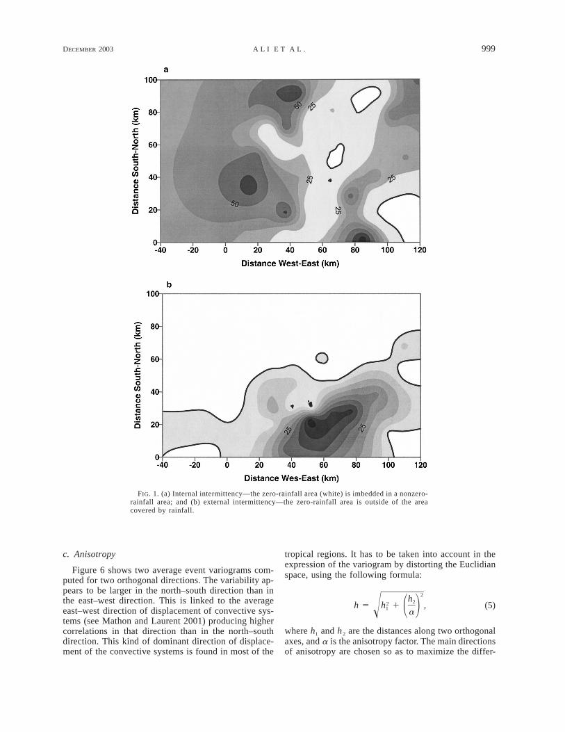
An important point to stress here is that NT is a ran-dom function of T both in space and time. This impliesthat, for a given period of length T, NT is a regionalizedvariable. In other words not all the points of the studyarea will record the same number of rain events, due tothe intermittent nature of the rain process at the eventscale. As visible in Fig. 1, intermittency is linked totwo factors: (i) there are areas of zero rainfall embeddedin the rainy areas (internal intermittency), and (ii) thereare areas that are not covered by the convective system(external intermittency). One difficulty that will be ad-dressed later in the paper is to separate the effects ofthe internal intermittency from that of the external in-termittency. They generally do not have the same spatialstructure and their respective weight in the spatial var-iability of a T-day rain field is a function of T. In theNiamey region the average intermittency of the eventrainfall process over the study area is equal to 0.26. Thisstatistic is strongly dependent on the size of the studyarea. The smaller the study area with respect to theaverage size of the convective systems, the smaller theexternal intermittency. On the other hand, if the studyarea is too small, the sampling of the variability of the
rain fields is limited to a range of space scales that aretoo small for hydrological applications. It is difficult tofind a proper trade-off between these two (E–N) con-straints but the experience gained from Estimation desPrecipitations par Satellite (EPSAT)–Niger is that thesize of the study area should be of the same order ofmagnitude as the average size of the rain-efficient con-vective systems. From the study of Mathon et al. (2002)it can be deduced that the average size of the activearea of the convective systems producing 90% of therain over the Niamey region is around 20 000 km2,compared to a study area of 16 000 km2.
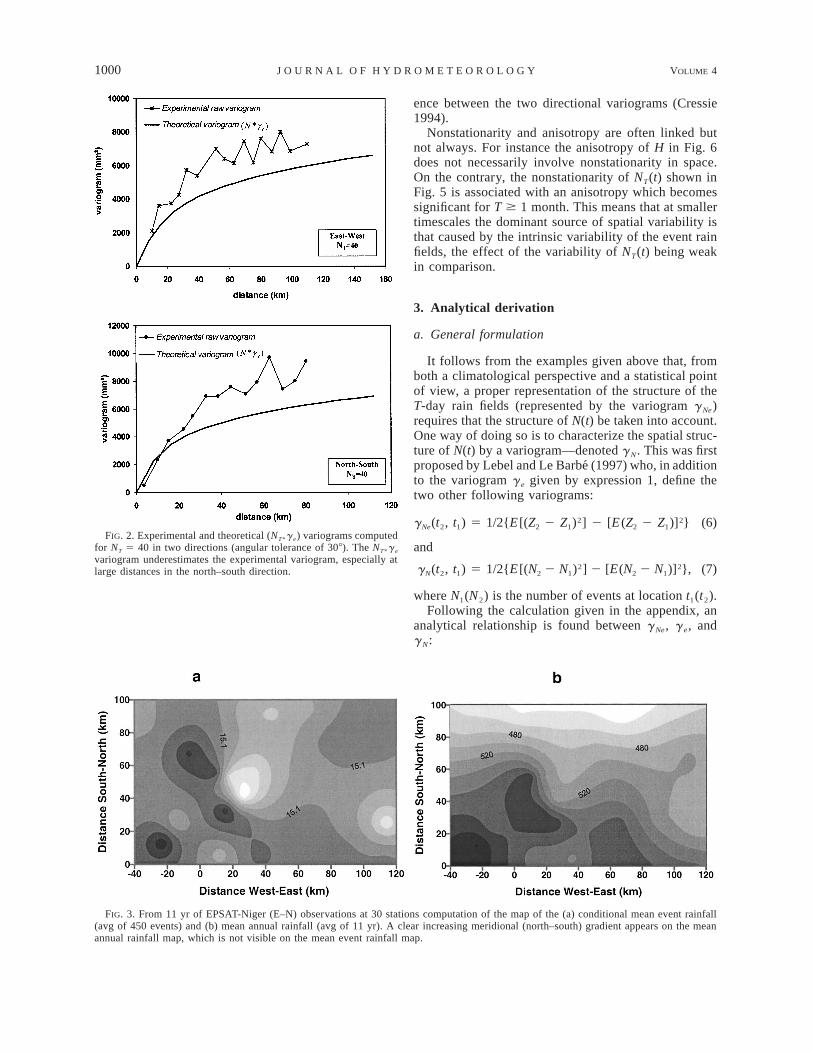
A direct consequence of intermittency on the esti-mation of the variogram at the T-day scale may be ob-served in Fig. 2. Theoretically, if the T-day rain fieldwas the accumulation of a constant number NT of in-dependent events with the same spatial structure char-acterized by the variogram g e, then the spatial structureof ZT, denoted g Ne, would be
g (h) 5 N g (h)Ne T* e (4)
since the variances of independent realizations of a ran-dom process are additive.
Consequently the theoretical variogram NT*g e shouldfit the experimental variogram gNe computed from theobservations. This is clearly not the case in Fig. 2 wherethe variograms were computed directionally in order toeliminate possible anisotropy effects (see later for thatquestion). It is seen that in both directions NT*g e un-derestimates the experimental gNe variogram. The der-ivation of g Ne from g e, is thus not straightforward andrequires some analytical work.
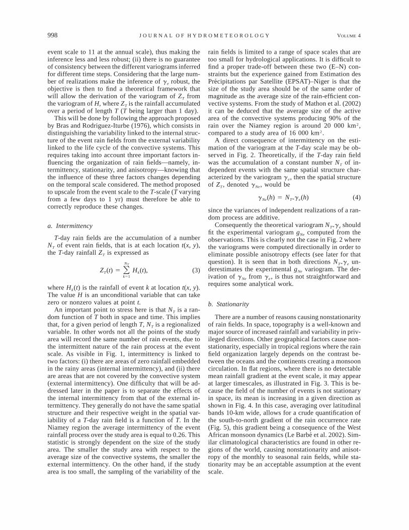
b. Stationarity
There are a number of reasons causing nonstationarityof rain fields. In space, topography is a well-known andmajor source of increased rainfall and variability in priv-ileged directions. Other geographical factors cause non-stationarity, especially in tropical regions where the rainfield organization largely depends on the contrast be-tween the oceans and the continents creating a monsooncirculation. In flat regions, where there is no detectablemean rainfall gradient at the event scale, it may appearat larger timescales, as illustrated in Fig. 3. This is be-cause the field of the number of events is not stationaryin space, its mean is increasing in a given direction asshown in Fig. 4. In this case, averaging over latitudinalbands 10-km wide, allows for a crude quantification ofthe south-to-north gradient of the rain occurrence rate(Fig. 5), this gradient being a consequence of the WestAfrican monsoon dynamics (Le Barbe et al. 2002). Sim-ilar climatological characteristics are found in other re-gions of the world, causing nonstationarity and anisot-ropy of the monthly to seasonal rain fields, while sta-tionarity may be an acceptable assumption at the eventscale.
DECEMBER 2003 999A L I E T A L .
FIG. 1. (a) Internal intermittency—the zero-rainfall area (white) is imbedded in a nonzero-rainfall area; and (b) external intermittency—the zero-rainfall area is outside of the areacovered by rainfall.
c. Anisotropy
Figure 6 shows two average event variograms com-puted for two orthogonal directions. The variability ap-pears to be larger in the north–south direction than inthe east–west direction. This is linked to the averageeast–west direction of displacement of convective sys-tems (see Mathon and Laurent 2001) producing highercorrelations in that direction than in the north–southdirection. This kind of dominant direction of displace-ment of the convective systems is found in most of the
tropical regions. It has to be taken into account in theexpression of the variogram by distorting the Euclidianspace, using the following formula:
2h22h 5 h 1 , (5)1 1 2! a
where h1 and h2 are the distances along two orthogonalaxes, and a is the anisotropy factor. The main directionsof anisotropy are chosen so as to maximize the differ-
1000 VOLUME 4J O U R N A L O F H Y D R O M E T E O R O L O G Y
FIG. 2. Experimental and theoretical (NT*g e) variograms computedfor NT 5 40 in two directions (angular tolerance of 308). The NT*g e
variogram underestimates the experimental variogram, especially atlarge distances in the north–south direction.
FIG. 3. From 11 yr of EPSAT-Niger (E–N) observations at 30 stations computation of the map of the (a) conditional mean event rainfall(avg of 450 events) and (b) mean annual rainfall (avg of 11 yr). A clear increasing meridional (north–south) gradient appears on the meanannual rainfall map, which is not visible on the mean event rainfall map.
ence between the two directional variograms (Cressie1994).
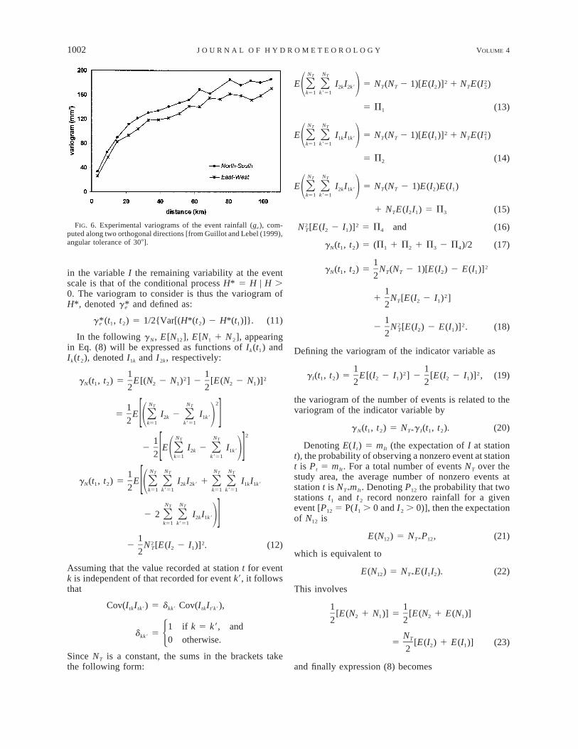
Nonstationarity and anisotropy are often linked butnot always. For instance the anisotropy of H in Fig. 6does not necessarily involve nonstationarity in space.On the contrary, the nonstationarity of NT(t) shown inFig. 5 is associated with an anisotropy which becomessignificant for T $ 1 month. This means that at smallertimescales the dominant source of spatial variability isthat caused by the intrinsic variability of the event rainfields, the effect of the variability of NT(t) being weakin comparison.
3. Analytical derivation
a. General formulation
It follows from the examples given above that, fromboth a climatological perspective and a statistical pointof view, a proper representation of the structure of theT-day rain fields (represented by the variogram g Ne)requires that the structure of N(t) be taken into account.One way of doing so is to characterize the spatial struc-ture of N(t) by a variogram—denoted g N. This was firstproposed by Lebel and Le Barbe (1997) who, in additionto the variogram g e given by expression 1, define thetwo other following variograms:
2 2g (t , t ) 5 1/2{E [(Z 2 Z ) ] 2 [E (Z 2 Z )] } (6)Ne 2 1 2 1 2 1
and2 2g (t , t ) 5 1/2{E [(N 2 N ) ] 2 [E(N 2 N )] }, (7)N 2 1 2 1 2 1
where N1(N2) is the number of events at location t1(t2).Following the calculation given in the appendix, an
analytical relationship is found between g Ne, g e, andg N:
DECEMBER 2003 1001A L I E T A L .
FIG. 4. (a) The mean annual rainfall (avg of 11 yr) produced by the rain events defined from the E–N network. These events are definedfrom a spatial criterion (a minimum of 30% of operating stations must record rainfall) and thus the probability of observing an event islarger at the center than on the borders of the network window. This window effect explains why the clear gradient visible in Fig. 3b isattenuated here on the borders of the window. (b) The number of rain events recorded over the 11 yr; the meridional gradient is visible eventhough the window effect makes it less visible on the west and east edges of the map.
FIG. 5. The averages of the number of events computed over lat-itudinal bands 10 km wide. A model of meridional drift is fitted tothe central part of the curve, in order to remove the border effects.
2g 5 E(N )g 1 {E [(N 1 N )/2] 2 [E(N )]}sNe 12 e 1 2 12 e
21 g m , (8)N e
where N12 is the number of events covering both t1 andt2, and me and se are, respectively, the average andstandard deviation of the point event process.
In expression (8), E(N12) is a function of the 2D spacerelated to the mean size of the rain events and g N char-acterizes the spatial structure of the number of eventsrecorded during the period under consideration. Dealingwith expression (8) requires the ability to identify thecoverage of each event with respect to the study areain order, to infer E(Ni) and E(Nij). The greater T is, andthus NT, the smaller the sample size available is for thisinference (this size is equal to K/NT, where K is the totalnumber of events observed during the period of study).
It is therefore necessary to find a formulation allowingfor a robust inference of these two functions, as far aspossible independently of the period T considered. Inthe following, it is proposed to resort to the formalismof indicator functions in order to reduce the previousinconveniences in the method initially proposed by Le-bel and Le Barbe (1997). This formalism was first usedby Barancourt et al. (1992) for delineating and esti-mating rainfall fields and then applied to the analysisof Sahelian rainfall by Braud et al. (1994) at an hourlytime step, but no attempt was made to use it for retriev-ing the scale invariance properties of the rain processas is proposed here.
b. Scaling structures based on indicator functions
The binary function I is defined as follows:
1 if H (t) . 0 andkI (t) 5 (9)k 50 if H (t) 5 0.k
I is called the indicator variable of the regionalized var-iable H at threshold H 5 0 (Rivoirard 1988). It is usedto characterize the intermittency of H. From the defi-nition given in expression (9), it follows that the numberof events at a given location ti—denoted Ni—is definedas the number of occurrences of nonzero rainfall at thatlocation:
NT
N 5 I (t ). (10)Oi k ik51
No discrimination is made between zero rainfall occur-ring within the area covered by a convective system andzero rainfall corresponding to the area outside of thecoverage zone. Since all the intermittency is included
1002 VOLUME 4J O U R N A L O F H Y D R O M E T E O R O L O G Y
FIG. 6. Experimental variograms of the event rainfall (ge), com-puted along two orthogonal directions [from Guillot and Lebel (1999),angular tolerance of 308].
in the variable I the remaining variability at the eventscale is that of the conditional process H* 5 H | H .0. The variogram to consider is thus the variogram ofH*, denoted and defined as:g*e
g*(t , t ) 5 1/2{Var[(H*(t ) 2 H*(t )]}.e 1 2 2 1 (11)
In the following g N, E[N12], E[N1 1 N2], appearingin Eq. (8) will be expressed as functions of Ik(t1) andIk(t2), denoted I1k and I2k, respectively:
1 12 2g (t , t ) 5 E [(N 2 N ) ] 2 [E(N 2 N )]N 1 2 2 1 2 12 2
2N NT T15 E I 2 IO O2k 1k91 2[ ]2 k51 k951
2N NT T12 E I 2 IO O2k 1k91 2[ ]2 k51 k951
N N N NT T T T1g (t , t ) 5 E I I 1 I IO O O ON 1 2 2k 2k9 1k 1k91[2 k51 k951 k51 k951
N NT T
2 2 I IO O 2k 1k92]k51 k951
12 22 N [E(I 2 I )] . (12)T 2 12
Assuming that the value recorded at station t for eventk is independent of that recorded for event k9, it followsthat
Cov(I I ) 5 d Cov(I I ),tk tk9 kk9 tk t9k9
1 if k 5 k9, andd 5kk9 50 otherwise.
Since NT is a constant, the sums in the brackets takethe following form:
N NT T
2 2E I I 5 N (N 2 1)[E(I )] 1 N E(I )O O 2k 2k9 T T 2 T 21 2k51 k951
5 P (13)1
N NT T
2 2E I I 5 N (N 2 1)[E(I )] 1 N E(I )O O 1k 1k9 T T 1 T 11 2k51 k951
5 P (14)2
N NT T
E I I 5 N (N 2 1)E(I )E(I )O O 2k 1k9 T T 2 11 2k51 k951
1 N E(I I ) 5 P (15)T 2 1 3
2 2N [E(I 2 I )] 5 P and (16)T 2 1 4
g (t , t ) 5 (P 1 P 1 P 2 P )/2 (17)N 1 2 1 2 3 4
12g (t , t ) 5 N (N 2 1)[E(I ) 2 E(I )]N 1 2 T T 2 12
121 N [E(I 2 I ) ]T 2 12
12 22 N [E(I ) 2 E(I )] . (18)T 2 12
Defining the variogram of the indicator variable as
1 12 2g (t , t ) 5 E [(I 2 I ) ] 2 [E(I 2 I )] , (19)I 1 2 2 1 2 12 2
the variogram of the number of events is related to thevariogram of the indicator variable by
g (t , t ) 5 N g (t , t ).N 1 2 T* I 1 2 (20)
Denoting E(It) 5 mIt (the expectation of I at stationt), the probability of observing a nonzero event at stationt is Pt 5 mIt. For a total number of events NT over thestudy area, the average number of nonzero events atstation t is NT*mIt. Denoting P12 the probability that twostations t1 and t2 record nonzero rainfall for a givenevent [P12 5 P(I1 . 0 and I2 . 0)], then the expectationof N12 is
E(N ) 5 N P , (21)12 T* 12
which is equivalent to
E(N ) 5 N E(I I ). (22)12 T* 1 2
This involves
1 1[E(N 1 N )] 5 [E(N 1 E(N )]2 1 2 12 2
NT5 [E(I ) 1 E(I )] (23)2 12
and finally expression (8) becomes
DECEMBER 2003 1003A L I E T A L .
g (t , t ) 5 N ^E(I I )g*(t , t )Ne 1 2 T 1 2 e 1 2
21 {[E(I ) 1 E(I )]/2 2 E(I I )}(s*)1 2 1 2 e
21 (m*) g (t , t )&. (24)e I 1 2
All the elements of this expression are invariant withthe period T considered except for NT. While ands*e
characterize the probability density function (pdf )m*eof the conditional point event process, characterizesg*eits spatial structure and g I the spatial structure of theintermittency. Expression (24) may thus be viewed asa scale-invariant characterization of the structure of therain fields at timescales larger than the event scale, withNT being the upscaling parameter. One important ad-vantage of this formulation is that the indicator variableis defined at the scale of the rain event. Consequentlythe inference of its parameters will be based on a largenumber of realizations and it is independent of the time-scale of interest.
Before validating the method on observations, thereare a few practical points to consider, as will be dis-cussed in the next section.
4. Implementation and inference
a. Intermittency
In the theoretical development presented above noseparation is made between the internal and the externalintermittency of the process even though they may havevery different characteristics. A theoretical separationbetween the internal intermittency and the external in-termittency can be made as follows. For a given eventk, let Vk be the set of 2D space points t(x, y) belongingto the domain covered by the event k. For any t(x, y)∈ Vk if Hk(t) 5 0, this is the internal intermittency. Ift(x, y) ∈ Vk, Hk(t) is by definition equal to 0, whichleads to the definition of the binary function I as
1 if t(x, y) ∈ V andkI (t) 5 (25)k 50 if t(x, y) ¸ V .k
Thus the variable H includes zero values when they areobserved within the area covered by the rain event andthe indicator variable I represents the external inter-mittency only. In pratice it is not easy to identify Vk
although satellite data may be used to define the areacovered on the ground by a convective system duringits entire lifetime (see an example of this in Mathon andLaurent 2001). Therefore in most applications the in-termittency will have to be treated globally. When thewindow of ground observation is sufficiently large theexternal intermittency will usually be the predominantfactor, though it will be difficult to exactly assess inwhat proportion.
b. Stationarity
Nonstationarity may affect either H, I, or both. Inmany regions of flat topography the nonstationarity of
I is stronger than that of H. This is especially the casein semiarid regions where rainfall variability at clima-tological scales may primarily be caused by the fluc-tuations of the number of events rather than by thoseof the mean event rainfall (Le Barbe et al. 2002).
The transformation of expression (24) is given belowfor two cases: stationarity or nonstationarity of I.
1) STATIONARITY OF I
When I is stationary, g I, defined in expression (19),reduces to
2g (t , t ) 5 E[(I 2 I )] /2.I 1 2 2 1 (26)
In addition the probability Pt is constant and equalto the mean of the indicator function mI. For a totalnumber of events NT over the study area, the averagenumber of nonzero events at any station t is constantand equal to NT*mI. The stationarity of I also impliesthat its covariance can be computed as
Cov(I , I ) 5 E(I I ) 2 E(I )[E(I )],1 2 1 2 1 2
2Cov(I I ) 5 E(I , I ) 2 (m ) . (27)1 2 1 2 I
For a stationary process, the variogram and the covari-ance are related as follows:
g (t , t ) 5 Var(I ) 2 Cov(I , I ) and (28)I 1 2 1 2
2 2Var(I ) 5 s 5 E(I ) 2 [E(I )] 5 m (1 2 m ). (29)I I I
Thus,
2g (t , t ) 5 m (1 2 m ) 2 E(I I ) 1 m , (30)I 1 2 I I 1 2 I
E(I I ) 5 m 2 g (t t ) and (31)1 2 I I 1 2
1[E(I ) 1 E(I )] 5 m . (32)1 2 I2
Introducing expressions (31) and (32) in expression (24)it gives
2 2g 5 N {(m 2 g )g* 1 [(s*) 1 (m*) ]g }. (33)Ne T* I I e e e I
Note also that in this stationary case the probabilityP12 that two stations t1 and t 2 record nonzero rainfallis equal to
P 5 m 2 g (t , t ),12 I I 1 2 (34)
and using expression (29), it may be easily shown that
2P (h 5 0) 5 m and limP (h → `) 5 m . (35)12 12 I 12 12 I
2) NONSTATIONARITY OF I
In the case of nonstationarity we are led to considertwo distinct variograms. One is the ‘‘true’’ variogramg defined in Eq. (1a). The other is the raw variogramdefined as
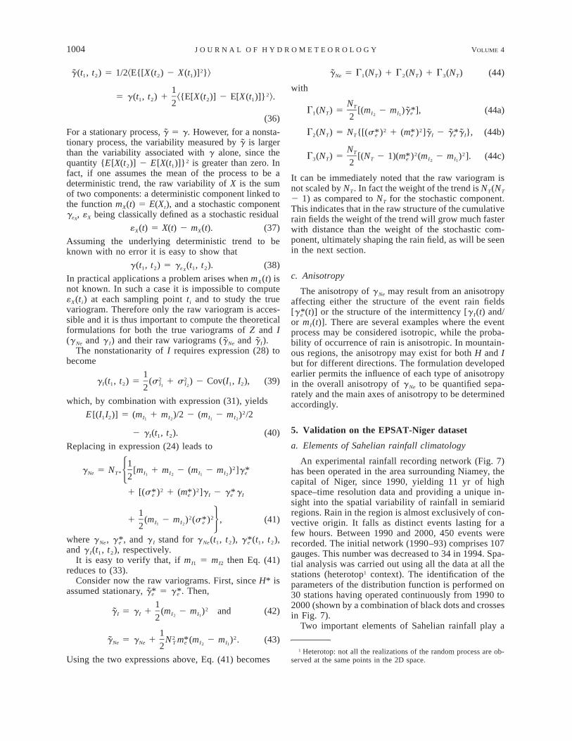
1004 VOLUME 4J O U R N A L O F H Y D R O M E T E O R O L O G Y
2g(t , t ) 5 1/2^E{[X(t ) 2 X(t )] }&1 2 2 1
125 g(t , t ) 1 ^{E[X(t )] 2 E[X(t )]} &.1 2 2 12
(36)
For a stationary process, 5 g. However, for a nonsta-gtionary process, the variability measured by is largergthan the variability associated with g alone, since thequantity {E[X(t2)] 2 E[X(t1)]}2 is greater than zero. Infact, if one assumes the mean of the process to be adeterministic trend, the raw variability of X is the sumof two components: a deterministic component linked tothe function mX(t) 5 E(Xt), and a stochastic componentg , «X being classically defined as a stochastic residual«X
« (t) 5 X(t) 2 m (t).X X (37)
Assuming the underlying deterministic trend to beknown with no error it is easy to show that
g(t , t ) 5 g (t , t ).1 2 « 1 2X(38)
In practical applications a problem arises when mX(t) isnot known. In such a case it is impossible to compute«X(ti) at each sampling point ti and to study the truevariogram. Therefore only the raw variogram is acces-sible and it is thus important to compute the theoreticalformulations for both the true variograms of Z and I(g Ne and g I) and their raw variograms ( Ne and I).g g
The nonstationarity of I requires expression (28) tobecome
12 2g (t , t ) 5 (s 1 s ) 2 Cov(I , I ), (39)I 1 2 I I 1 21 22
which, by combination with expression (31), yields2E [(I I )] 5 (m 1 m )/2 2 (m 2 m ) /21 2 I I I I1 2 1 2
2 g (t , t ). (40)I 1 2
Replacing in expression (24) leads to
12g 5 N [m 1 m 2 (m 2 m ) ]g*Ne T* I I I I e1 2 1 252
2 21 [(s*) 1 (m*) ]g 2 g*ge e I e I
12 21 (m 2 m ) (s*) , (41)I I e1 2 62
where g Ne, , and g I stand for g Ne(t1, t2), (t1, t2),g* g*e e
and g I(t1, t2), respectively.It is easy to verify that, if mI1 5 mI2 then Eq. (41)
reduces to (33).Consider now the raw variograms. First, since H* is
assumed stationary, 5 . Then,g* g*e e
12g 5 g 1 (m 2 m ) and (42)I I I I2 12
12 2g 5 g 1 N m*(m 2 m ) . (43)Ne Ne T e I I2 12
Using the two expressions above, Eq. (41) becomes
g 5 G (N ) 1 G (N ) 1 G (N )Ne 1 T 2 T 3 T (44)
with
NTG (N ) 5 [(m 2 m )g*], (44a)1 T I I e2 122 2G (N ) 5 N {[(s*) 1 (m*) ]g 2 g*g }, (44b)2 T T e e I e I
NT 2 2G (N ) 5 [(N 2 1)(m*) (m 2 m ) ]. (44c)3 T T e I I2 12
It can be immediately noted that the raw variogram isnot scaled by NT. In fact the weight of the trend is NT(NT
2 1) as compared to NT for the stochastic component.This indicates that in the raw structure of the cumulativerain fields the weight of the trend will grow much fasterwith distance than the weight of the stochastic com-ponent, ultimately shaping the rain field, as will be seenin the next section.
c. Anisotropy
The anisotropy of g Ne may result from an anisotropyaffecting either the structure of the event rain fields[ (t)] or the structure of the intermittency [g I(t) and/g*eor mI(t)]. There are several examples where the eventprocess may be considered isotropic, while the proba-bility of occurrence of rain is anisotropic. In mountain-ous regions, the anisotropy may exist for both H and Ibut for different directions. The formulation developedearlier permits the influence of each type of anisotropyin the overall anisotropy of g Ne to be quantified sepa-rately and the main axes of anisotropy to be determinedaccordingly.
5. Validation on the EPSAT-Niger dataset
a. Elements of Sahelian rainfall climatology
An experimental rainfall recording network (Fig. 7)has been operated in the area surrounding Niamey, thecapital of Niger, since 1990, yielding 11 yr of highspace–time resolution data and providing a unique in-sight into the spatial variability of rainfall in semiaridregions. Rain in the region is almost exclusively of con-vective origin. It falls as distinct events lasting for afew hours. Between 1990 and 2000, 450 events wererecorded. The initial network (1990–93) comprises 107gauges. This number was decreased to 34 in 1994. Spa-tial analysis was carried out using all the data at all thestations (heterotop1 context). The identification of theparameters of the distribution function is performed on30 stations having operated continuously from 1990 to2000 (shown by a combination of black dots and crossesin Fig. 7).
Two important elements of Sahelian rainfall play a
1 Heterotop: not all the realizations of the random process are ob-served at the same points in the 2D space.
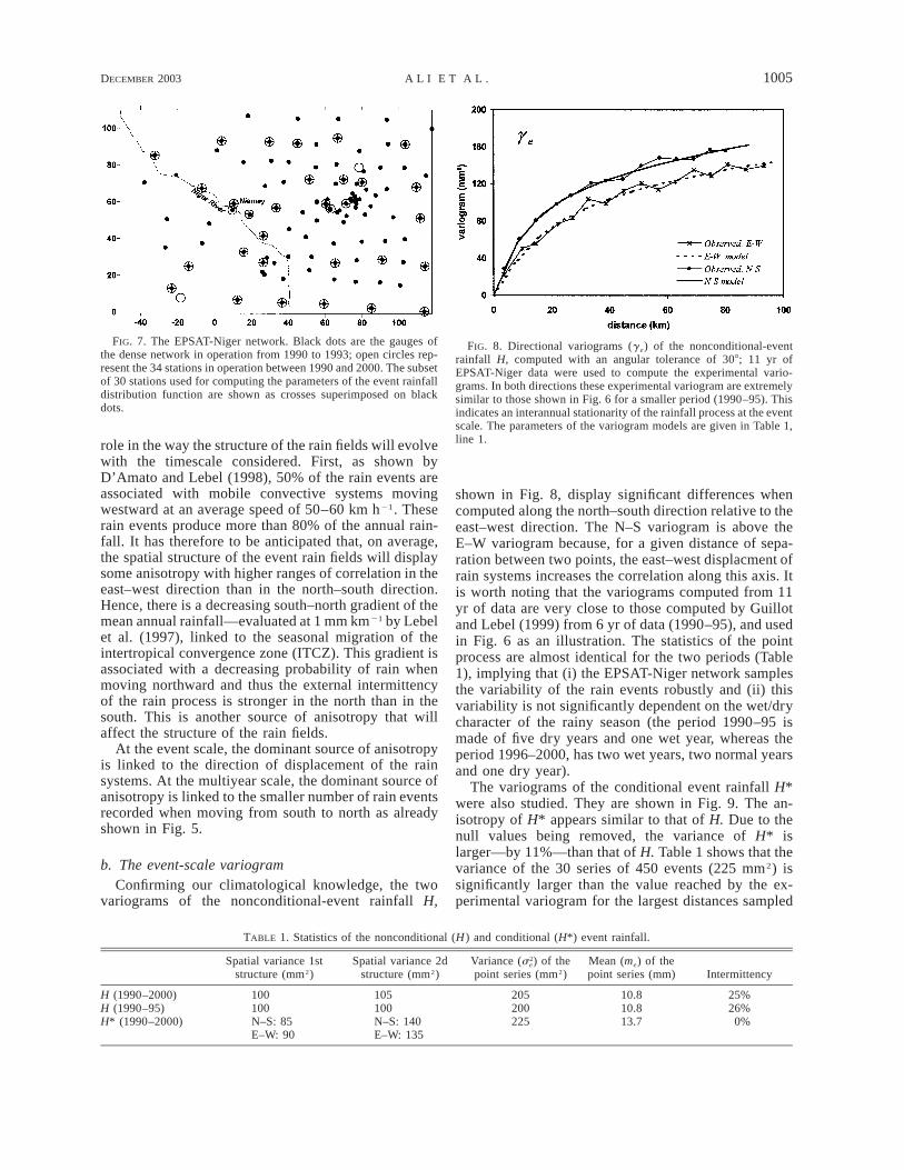
DECEMBER 2003 1005A L I E T A L .
FIG. 7. The EPSAT-Niger network. Black dots are the gauges ofthe dense network in operation from 1990 to 1993; open circles rep-resent the 34 stations in operation between 1990 and 2000. The subsetof 30 stations used for computing the parameters of the event rainfalldistribution function are shown as crosses superimposed on blackdots.
FIG. 8. Directional variograms (g e) of the nonconditional-eventrainfall H, computed with an angular tolerance of 308; 11 yr ofEPSAT-Niger data were used to compute the experimental vario-grams. In both directions these experimental variogram are extremelysimilar to those shown in Fig. 6 for a smaller period (1990–95). Thisindicates an interannual stationarity of the rainfall process at the eventscale. The parameters of the variogram models are given in Table 1,line 1.
TABLE 1. Statistics of the nonconditional (H ) and conditional (H*) event rainfall.
Spatial variance 1ststructure (mm2)
Spatial variance 2dstructure (mm2)
Variance (s ) of the2e
point series (mm2)Mean (me) of thepoint series (mm) Intermittency
H (1990–2000)H (1990–95)H* (1990–2000)
100100N–S: 85E–W: 90
105100N–S: 140E–W: 135
205200225
10.810.813.7
25%26%
0%
role in the way the structure of the rain fields will evolvewith the timescale considered. First, as shown byD’Amato and Lebel (1998), 50% of the rain events areassociated with mobile convective systems movingwestward at an average speed of 50–60 km h21. Theserain events produce more than 80% of the annual rain-fall. It has therefore to be anticipated that, on average,the spatial structure of the event rain fields will displaysome anisotropy with higher ranges of correlation in theeast–west direction than in the north–south direction.Hence, there is a decreasing south–north gradient of themean annual rainfall—evaluated at 1 mm km21 by Lebelet al. (1997), linked to the seasonal migration of theintertropical convergence zone (ITCZ). This gradient isassociated with a decreasing probability of rain whenmoving northward and thus the external intermittencyof the rain process is stronger in the north than in thesouth. This is another source of anisotropy that willaffect the structure of the rain fields.
At the event scale, the dominant source of anisotropyis linked to the direction of displacement of the rainsystems. At the multiyear scale, the dominant source ofanisotropy is linked to the smaller number of rain eventsrecorded when moving from south to north as alreadyshown in Fig. 5.
b. The event-scale variogramConfirming our climatological knowledge, the two
variograms of the nonconditional-event rainfall H,
shown in Fig. 8, display significant differences whencomputed along the north–south direction relative to theeast–west direction. The N–S variogram is above theE–W variogram because, for a given distance of sepa-ration between two points, the east–west displacment ofrain systems increases the correlation along this axis. Itis worth noting that the variograms computed from 11yr of data are very close to those computed by Guillotand Lebel (1999) from 6 yr of data (1990–95), and usedin Fig. 6 as an illustration. The statistics of the pointprocess are almost identical for the two periods (Table1), implying that (i) the EPSAT-Niger network samplesthe variability of the rain events robustly and (ii) thisvariability is not significantly dependent on the wet/drycharacter of the rainy season (the period 1990–95 ismade of five dry years and one wet year, whereas theperiod 1996–2000, has two wet years, two normal yearsand one dry year).
The variograms of the conditional event rainfall H*were also studied. They are shown in Fig. 9. The an-isotropy of H* appears similar to that of H. Due to thenull values being removed, the variance of H* islarger—by 11%—than that of H. Table 1 shows that thevariance of the 30 series of 450 events (225 mm2) issignificantly larger than the value reached by the ex-perimental variogram for the largest distances sampled
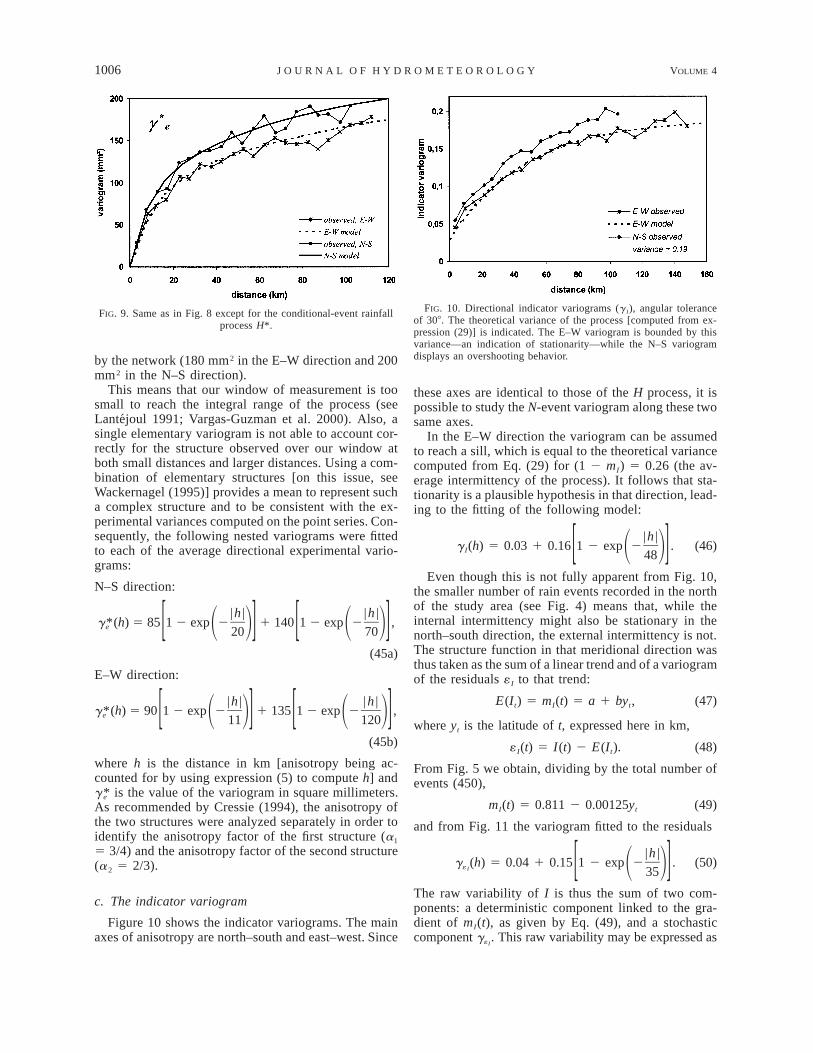
1006 VOLUME 4J O U R N A L O F H Y D R O M E T E O R O L O G Y
FIG. 9. Same as in Fig. 8 except for the conditional-event rainfallprocess H*.
FIG. 10. Directional indicator variograms (g I), angular toleranceof 308. The theoretical variance of the process [computed from ex-pression (29)] is indicated. The E–W variogram is bounded by thisvariance—an indication of stationarity—while the N–S variogramdisplays an overshooting behavior.by the network (180 mm2 in the E–W direction and 200
mm2 in the N–S direction).This means that our window of measurement is too
small to reach the integral range of the process (seeLantejoul 1991; Vargas-Guzman et al. 2000). Also, asingle elementary variogram is not able to account cor-rectly for the structure observed over our window atboth small distances and larger distances. Using a com-bination of elementary structures [on this issue, seeWackernagel (1995)] provides a mean to represent sucha complex structure and to be consistent with the ex-perimental variances computed on the point series. Con-sequently, the following nested variograms were fittedto each of the average directional experimental vario-grams:
N–S direction:
|h | |h |g*(h) 5 85 1 2 exp 2 1 140 1 2 exp 2 ,e 1 2 1 2[ ] [ ]20 70
(45a)
E–W direction:
|h | |h |g*(h) 5 90 1 2 exp 2 1 135 1 2 exp 2 ,e 1 2 1 2[ ] [ ]11 120
(45b)
where h is the distance in km [anisotropy being ac-counted for by using expression (5) to compute h] and
is the value of the variogram in square millimeters.g*eAs recommended by Cressie (1994), the anisotropy ofthe two structures were analyzed separately in order toidentify the anisotropy factor of the first structure (a1
5 3/4) and the anisotropy factor of the second structure(a2 5 2/3).
c. The indicator variogram
Figure 10 shows the indicator variograms. The mainaxes of anisotropy are north–south and east–west. Since
these axes are identical to those of the H process, it ispossible to study the N-event variogram along these twosame axes.
In the E–W direction the variogram can be assumedto reach a sill, which is equal to the theoretical variancecomputed from Eq. (29) for (1 2 mI) 5 0.26 (the av-erage intermittency of the process). It follows that sta-tionarity is a plausible hypothesis in that direction, lead-ing to the fitting of the following model:
|h |g (h) 5 0.03 1 0.16 1 2 exp 2 . (46)I 1 2[ ]48
Even though this is not fully apparent from Fig. 10,the smaller number of rain events recorded in the northof the study area (see Fig. 4) means that, while theinternal intermittency might also be stationary in thenorth–south direction, the external intermittency is not.The structure function in that meridional direction wasthus taken as the sum of a linear trend and of a variogramof the residuals «I to that trend:
E(I ) 5 m (t) 5 a 1 by , (47)t I t
where y is the latitude of t, expressed here in km,t
« (t) 5 I(t) 2 E(I ). (48)I t
From Fig. 5 we obtain, dividing by the total number ofevents (450),
m (t) 5 0.811 2 0.00125yI t (49)
and from Fig. 11 the variogram fitted to the residuals
|h |g (h) 5 0.04 1 0.15 1 2 exp 2 . (50)«I 1 2[ ]35
The raw variability of I is thus the sum of two com-ponents: a deterministic component linked to the gra-dient of mI(t), as given by Eq. (49), and a stochasticcomponent g . This raw variability may be expressed as«I
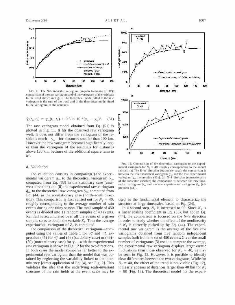
DECEMBER 2003 1007A L I E T A L .
FIG. 11. The N–S indicator variogram (angular tolerance of 308):comparison of the raw variogram and of the variogram of the residualsto the trend shown in Fig. 5. The theoretical model fitted to the rawvariogram is the sum of the trend and of the theoretical model fittedto the variogram of the residuals.
FIG. 12. Comparison of the theoretical variogram to the experi-mental variogram for NT 5 40, roughly corresponding to the annualrainfall. (a) The E–W direction (stationary case): the comparison isbetween the true theoretical variogram gNe and the true experimentalvariogram gNe [expression (33)]; (b) N–S direction (nonstationarityof the indicator variable) the comparison is between the raw theo-retical variogram Ne and the raw experimental variogram gNe [ex-gpression (44)].
26 2g (t , t ) 5 g (t , t ) 1 0.5 3 10 (y 2 y ) . (51)I 1 2 « 1 2 t tI 1 2
The raw variogram model obtained from Eq. (51) isplotted in Fig. 11. It fits the observed raw variogramwell. It does not differ from the variogram of the re-siduals much—g —for distances smaller than 100 km.«I
However the raw variogram becomes significantly larg-er than the variogram of the residuals for distancesabove 150 km, because of the additional square term inh2.
d. Validation
The validation consists in comparing(i)-the experi-mental variogram gNe to the theoretical variogram g Ne
computed from Eq. (33) in the stationary case (east–west direction) and (ii) the experimental raw variogramgNe to the theoretical raw variogram Ne computed fromgEq. (44) in the nonstationary case (north–south direc-tion). This comparison is first carried out for NT 5 40,roughly corresponding to the average number of rainevents during one rainy season. The total sample of 450events is divided into 11 random samples of 40 events.Rainfall is accumulated over all the events of a givensample, so as to obtain the variable ZT. Then the averageexperimental variogram of ZT is computed.
The comparison of the theoretical variogram—com-puted using the values of Table 1 for and , ex-s* m*e e
pression (45) for and (46) (stationary case) or (49)–g*e(50) (nonstationary case) for g I —with the experimentalraw variogram is shown in Fig. 12 for the two directions.In both cases the model compares far better to the ex-perimental raw variogram than the model that was ob-tained by neglecting the variability linked to the inter-mittency [direct application of Eq. (4), see Fig. 2]. Thisvalidates the idea that the underlying scale-invariantstructure of the rain fields at the event scale may be
used as the fundamental element to characterize thestructure at large timescales, based on Eq. (24).
In a second step, NT is increased to 90. Since NT isa linear scaling coefficient in Eq. (33), but not in Eq.(44), the comparison is focused on the N–S directionin order to study whether the effect of the nonlinearityin NT is correctly picked up by Eq. (44). The experi-mental raw variogram is the average of the five rawvariograms obtained from five random independentsamples built from the set of 450 events. Given the smallnumber of variograms (5) used to compute the average,the experimental raw variogram displays larger erraticfluctuations than those observed for NT 5 40, as maybe seen in Fig. 13. However, it is possible to identifyclear differences between the two variograms. While forNT 5 40, the effect of the trend is not visible (Fig. 12),it clearly appears at distances larger than 40 km for NT
5 90 (Fig. 13). The theoretical model fits the experi-
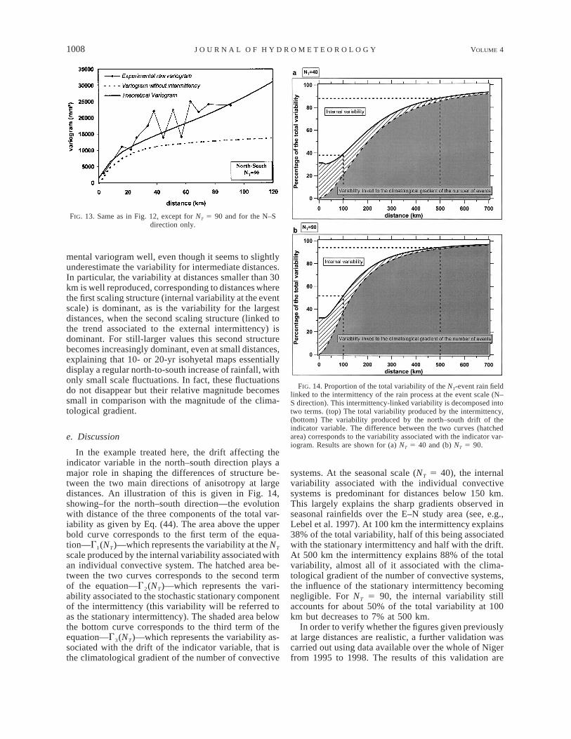
1008 VOLUME 4J O U R N A L O F H Y D R O M E T E O R O L O G Y
FIG. 13. Same as in Fig. 12, except for NT 5 90 and for the N–Sdirection only.
FIG. 14. Proportion of the total variability of the NT-event rain fieldlinked to the intermittency of the rain process at the event scale (N–S direction). This intermittency-linked variability is decomposed intotwo terms. (top) The total variability produced by the intermittency,(bottom) The variability produced by the north–south drift of theindicator variable. The difference between the two curves (hatchedarea) corresponds to the variability associated with the indicator var-iogram. Results are shown for (a) NT 5 40 and (b) NT 5 90.
mental variogram well, even though it seems to slightlyunderestimate the variability for intermediate distances.In particular, the variability at distances smaller than 30km is well reproduced, corresponding to distances wherethe first scaling structure (internal variability at the eventscale) is dominant, as is the variability for the largestdistances, when the second scaling structure (linked tothe trend associated to the external intermittency) isdominant. For still-larger values this second structurebecomes increasingly dominant, even at small distances,explaining that 10- or 20-yr isohyetal maps essentiallydisplay a regular north-to-south increase of rainfall, withonly small scale fluctuations. In fact, these fluctuationsdo not disappear but their relative magnitude becomessmall in comparison with the magnitude of the clima-tological gradient.
e. Discussion
In the example treated here, the drift affecting theindicator variable in the north–south direction plays amajor role in shaping the differences of structure be-tween the two main directions of anisotropy at largedistances. An illustration of this is given in Fig. 14,showing–for the north–south direction—the evolutionwith distance of the three components of the total var-iability as given by Eq. (44). The area above the upperbold curve corresponds to the first term of the equa-tion—G1(NT)—which represents the variability at the NT
scale produced by the internal variability associated withan individual convective system. The hatched area be-tween the two curves corresponds to the second termof the equation—G2(NT)—which represents the vari-ability associated to the stochastic stationary componentof the intermittency (this variability will be referred toas the stationary intermittency). The shaded area belowthe bottom curve corresponds to the third term of theequation—G3(NT)—which represents the variability as-sociated with the drift of the indicator variable, that isthe climatological gradient of the number of convective
systems. At the seasonal scale (NT 5 40), the internalvariability associated with the individual convectivesystems is predominant for distances below 150 km.This largely explains the sharp gradients observed inseasonal rainfields over the E–N study area (see, e.g.,Lebel et al. 1997). At 100 km the intermittency explains38% of the total variability, half of this being associatedwith the stationary intermittency and half with the drift.At 500 km the intermittency explains 88% of the totalvariability, almost all of it associated with the clima-tological gradient of the number of convective systems,the influence of the stationary intermittency becomingnegligible. For NT 5 90, the internal variability stillaccounts for about 50% of the total variability at 100km but decreases to 7% at 500 km.
In order to verify whether the figures given previouslyat large distances are realistic, a further validation wascarried out using data available over the whole of Nigerfrom 1995 to 1998. The results of this validation are
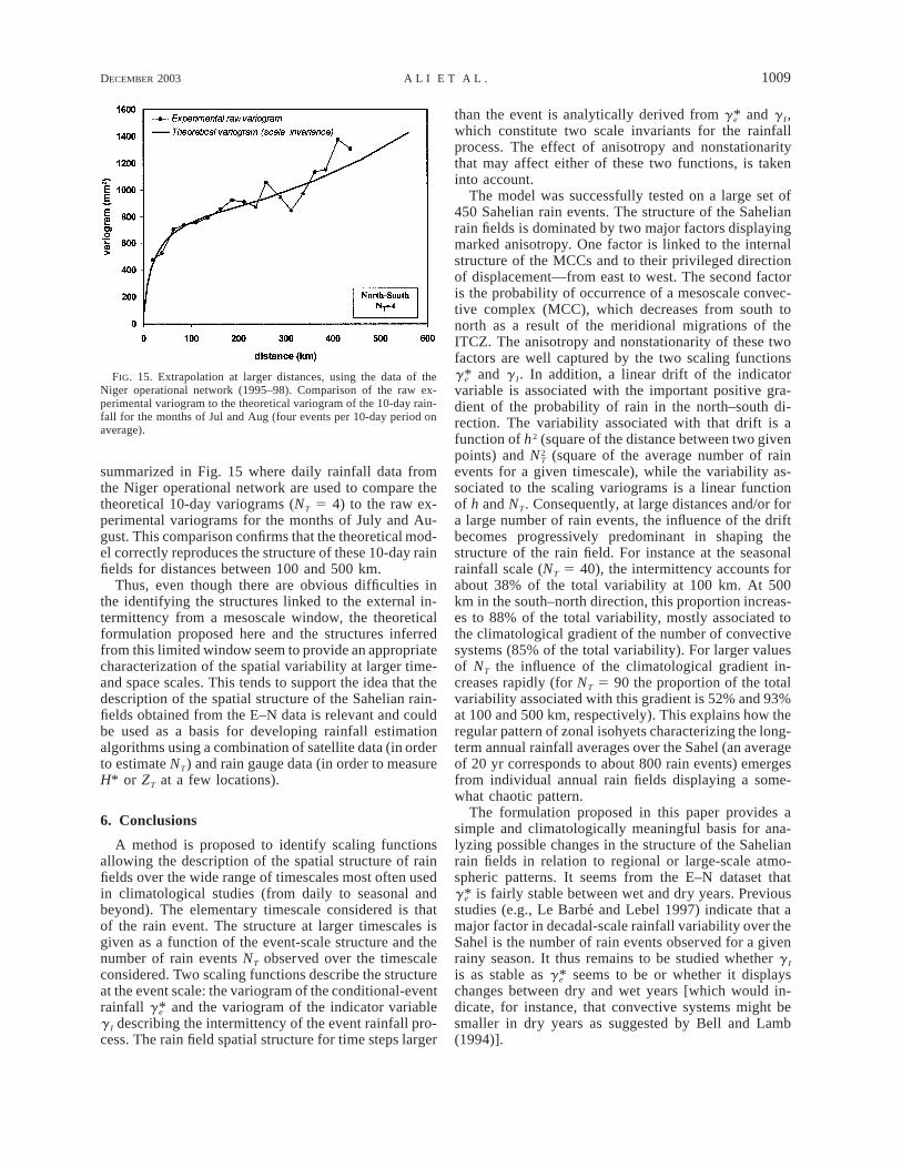
DECEMBER 2003 1009A L I E T A L .
FIG. 15. Extrapolation at larger distances, using the data of theNiger operational network (1995–98). Comparison of the raw ex-perimental variogram to the theoretical variogram of the 10-day rain-fall for the months of Jul and Aug (four events per 10-day period onaverage).
summarized in Fig. 15 where daily rainfall data fromthe Niger operational network are used to compare thetheoretical 10-day variograms (NT 5 4) to the raw ex-perimental variograms for the months of July and Au-gust. This comparison confirms that the theoretical mod-el correctly reproduces the structure of these 10-day rainfields for distances between 100 and 500 km.
Thus, even though there are obvious difficulties inthe identifying the structures linked to the external in-termittency from a mesoscale window, the theoreticalformulation proposed here and the structures inferredfrom this limited window seem to provide an appropriatecharacterization of the spatial variability at larger time-and space scales. This tends to support the idea that thedescription of the spatial structure of the Sahelian rain-fields obtained from the E–N data is relevant and couldbe used as a basis for developing rainfall estimationalgorithms using a combination of satellite data (in orderto estimate NT) and rain gauge data (in order to measureH* or ZT at a few locations).
6. Conclusions
A method is proposed to identify scaling functionsallowing the description of the spatial structure of rainfields over the wide range of timescales most often usedin climatological studies (from daily to seasonal andbeyond). The elementary timescale considered is thatof the rain event. The structure at larger timescales isgiven as a function of the event-scale structure and thenumber of rain events NT observed over the timescaleconsidered. Two scaling functions describe the structureat the event scale: the variogram of the conditional-eventrainfall and the variogram of the indicator variableg*eg I describing the intermittency of the event rainfall pro-cess. The rain field spatial structure for time steps larger
than the event is analytically derived from and g I,g*ewhich constitute two scale invariants for the rainfallprocess. The effect of anisotropy and nonstationaritythat may affect either of these two functions, is takeninto account.
The model was successfully tested on a large set of450 Sahelian rain events. The structure of the Sahelianrain fields is dominated by two major factors displayingmarked anisotropy. One factor is linked to the internalstructure of the MCCs and to their privileged directionof displacement—from east to west. The second factoris the probability of occurrence of a mesoscale convec-tive complex (MCC), which decreases from south tonorth as a result of the meridional migrations of theITCZ. The anisotropy and nonstationarity of these twofactors are well captured by the two scaling functions
and g I. In addition, a linear drift of the indicatorg*evariable is associated with the important positive gra-dient of the probability of rain in the north–south di-rection. The variability associated with that drift is afunction of h2 (square of the distance between two givenpoints) and (square of the average number of rain2NT
events for a given timescale), while the variability as-sociated to the scaling variograms is a linear functionof h and NT. Consequently, at large distances and/or fora large number of rain events, the influence of the driftbecomes progressively predominant in shaping thestructure of the rain field. For instance at the seasonalrainfall scale (NT 5 40), the intermittency accounts forabout 38% of the total variability at 100 km. At 500km in the south–north direction, this proportion increas-es to 88% of the total variability, mostly associated tothe climatological gradient of the number of convectivesystems (85% of the total variability). For larger valuesof NT the influence of the climatological gradient in-creases rapidly (for NT 5 90 the proportion of the totalvariability associated with this gradient is 52% and 93%at 100 and 500 km, respectively). This explains how theregular pattern of zonal isohyets characterizing the long-term annual rainfall averages over the Sahel (an averageof 20 yr corresponds to about 800 rain events) emergesfrom individual annual rain fields displaying a some-what chaotic pattern.
The formulation proposed in this paper provides asimple and climatologically meaningful basis for ana-lyzing possible changes in the structure of the Sahelianrain fields in relation to regional or large-scale atmo-spheric patterns. It seems from the E–N dataset that
is fairly stable between wet and dry years. Previousg*estudies (e.g., Le Barbe and Lebel 1997) indicate that amajor factor in decadal-scale rainfall variability over theSahel is the number of rain events observed for a givenrainy season. It thus remains to be studied whether g I
is as stable as seems to be or whether it displaysg*echanges between dry and wet years [which would in-dicate, for instance, that convective systems might besmaller in dry years as suggested by Bell and Lamb(1994)].
1010 VOLUME 4J O U R N A L O F H Y D R O M E T E O R O L O G Y
Another more immediate application of this formu-lation is in the area of rainfall estimation. The inter-polation functions derived from the theoretical formu-lation do not depend in any manner on the time stepconsidered and the coherency of the interpolation car-ried out for different time steps is guaranteed. The ac-curacy of the estimation procedure is directly given; theuncertainty linked to the internal variability and thatlinked to the intermittency may be quantified dependingon the time- and space scales considered. Based on this,geostationary satellite data can be used to count thenumber of convective systems and to estimate the up-scaling factor NT, while ground data provide local ac-curate measurements of the rainfall accumulation.
APPENDIX
Calculation of the N-Event Variogram
Starting from the definition of the N-event variogram
2 2g (t , t ) 5 1/2{E[(Z 2 Z ) ] 2 [E(Z 2 Z )] }, (A1)Ne 1 2 2 1 2 1
it follows that
2N N2 11g (t , t ) 5 E H 2 HO ONe 1 2 2 j 1i1 2[ ]2 j51 i51
2N N2 112 E H 2 H or (A2)O O2 j 1i1 2[ ]2 j51 i51
g (t , t ) 5 J 2 D (A3)Ne 1 2
with
2N N2 11J 5 E H 2 H , and (A4)O O2 j 1i1 2[ ]2 j51 i51
2N N2 11D 5 E H 2 H . (A5)O O2 j 1i1 2[ ]2 j51 i51
In case of stationarity D is equal to zero and g Ne 5 J.Defining N12 as the number of events covering both
t1 and t 2 , and 5 N1 2 N12 ( 5 N 2 2 N12 ) as theN 9 N 91 2
number of events covering t1 only (t 2 ), J may be writ-ten as
2N N9 N N912 2 12 111i9J 5 E H 1 H 2 H 2 H , (A6)O O O O2 j 2 j9 1i1 2[ ]2 j51 j951 i51 i951
2N N N9 N912 12 2 11J 5 E H 2 H 1 H 2 H 1 · · ·O O O O2 j 1i 2 j9 1i91 2 1 2[ ]2 j51 i51 j951 i951
N N N9 N912 12 2 111 E H 2 H H 2 H . (A7)O O O O2 j 1i 2 j9 1i91 21 2[ ]2 j51 i51 j9519 i9
Expressing J 5 J1 1 J2 1 J3 and assuming indepen-dence between the events, Lebel and Le Barbe (1997)showed that
2N N12 121J 5 E H 2 HO O1 2 j 1i1 2[ ]2 j51 i51
12 25 E(N )E(H 1 H ) 2 E(N )E(H H )12 1 2 12 1 22
5 E(N )g (t , t ), (A8)12 e 1 2
9 9 2N N2 11J 5 E H 2 HO O2 2 j9 1i91 2[ ]2 j951 i951
15 {[E(N 1 N 2 2N )] Var(H )1 2 122
2 21 [E(N 2 N ) ][E(H )] }, (A9)2 1
9 9N N N N12 12 2 1
J 5 E H 2 H H 2 H 5 0.O O O O3 2 j 1i 2 j9 1i91 21 2[ ]j51 i51 j951 i951
(A10)
In case of nonstationarity D is written as2N N2 11
D 5 E H 2 HO O2 j 1i1 2[ ]2 j51 i51
2E(N ) E(N )2 115 E(H ) 2 E(H ) ,O O2 j 1i5 6[ ]2 j51 i51
12 2D 5 [E(N 2 N )] [E(H )] . (A11)2 12
Combining expressions (A3), (A8), (A9), (A10), and(A11), it gives
2g (t , t ) 5 2E(N )g (t , t )Ne 1 2 12 e 1 2
1 [E(N 1 N 2 2N )] Var(H )1 2 12
2 21 E(N 2 N ) [E(H )]2 1
2 22 · · · [E (N 2 N )] [E (H )] . (A12)2 1
Using the following notations:2s 5 Var(H ), m 5 E(H ), ande e
2 2g 5 E(N 2 N ) 2 [E(N 2 N )]N 2 1 2 1
it follows finally that
g (t , t ) 5 E(N )g (t , t )Ne 1 2 12 e 1 2
21 {E [(N 1 N )/2] 2 [E(N )]}s1 2 12 e
21 m g (t , t ). (A13)e N 1 2
REFERENCES
Bacchi, B., and N. T. Kottegoda, 1995: Identification and calibrationof spatial correlation patterns of rainfall. J. Hydrol., 165, 311–348.
Barancourt, C., J. D. Creutin, and J. Rivoirard, 1992: A method fordelineating and estimating rainfall fields. Water Resour. Res.,28, 1133–1143.
DECEMBER 2003 1011A L I E T A L .
Bastin, G., B. Lorent, C. Duque, and M. Gevers, 1984: Optimal es-timation of the average areal rainfall and optimal selection ofrain guage locations. Water Resour. Res., 20, 463–470.
Bell, M. A., and P. J. Lamb, 1994: Temporal variations in the rainfallcharacteristics of the disturbance lines over Subsaharan WestAfrica: 1951–90. Proc. Int. Conf. on Monsoon Variability andPrediction, Vol. I, Trieste, Italy, World Meteorological Orga-nization, 35–41.
Bras, R. L., and I. Rodriguez-Iturbe, 1976: Rainfall generation: Anon stationary time-varying multidimensional model. Water Re-sour. Res., 12, 450–456.
Braud, I., P. Crochet, and J.-D. Creutin, 1994: A method for estimatingmean areal rainfall using moving trend functions of the inten-sities. J. Appl. Meteor., 33, 1551–1561.
Cressie, N. A. C., 1994: Statistics for Spatial Data. Wiley Series inProbability and Mathematical Statistics, John Wiley, 900 pp.
Creutin, J. D., and C. Obled, 1982: Objective analyses and mappingtechniques for rainfall fields: An objective comparison. WaterResour. Res., 18, 413–431.
D’Amato, N., and T. Lebel, 1998: On the characteristics of the rainfallevents in the Sahel with a view to the analysis of climatic var-iability. Int. J. Climatol., 18, 955–974.
Deidda, R., 2000: Rainfall downscaling in a space–time multifractalframework. Water Resour. Res., 36, 1779–1794.
Federico, V. D., and S. P. Neuman, 1997: Scaling of random fieldsby means of truncated power variograms and associated spectra.Water Resour. Res., 33, 1075–1085.
Foufoula-Georgiou, E., and W. Krajewski, 1995: Recent advances inrainfall modeling, estimation and forecasting. Rev. Geophys., 33,1125–1137.
Guillot, G., and T. Lebel, 1999: Approximation of Sahelian rainfallfields with meta-Gaussian random functions. Part 2: Parameterestimation and comparison to data. Stochastic Environ. Res. RiskAssess., 13, 113–130.
Gupta, V. K., and E. Waymire, 1993: A statistical analysis of me-soscale rainfall as a random cascade. J. Appl. Meteor., 32, 251–267.
Holley, R., and E. C. Waymire, 1992: Multifractal dimensions and
scaling exponents for strongly bounded random cascades. Ann.Appl. Probab., 2, 819–845.
Kassim, A. H. M., and N. T. Kottegoda, 1991: Rainfall network designthrough comparative kriging methods. Hydrol. Sci. J., 36, 223–240.
Lantejoul, C., 1991: Ergodicity and integral range. J. Microsc., 161,387–404.
Le Barbe, L., and T. Lebel, 1997: Rainfall climatology of the HAPEX-Sahel region during the years 1950–1990. J. Hydrol., 188–189,43–73.
——, ——, and D. Tapsoba, 2002: Rainfall variability in West Africaduring the years 1950–90. J. Climate, 15, 187–202.
Lebel, T., and L. Le Barbe, 1997: Rainfall monitoring during HAPEX-Sahel. 2. Point and areal estimation at the event and seasonalscales. J. Hydrol., 188–189, 97–122.
——, and A. Amani, 1999: Rainfall estimation in the Sahel: Whatis the ground truth? J. Appl. Meteor., 38, 555–568.
——, J. D. Taupin, and N. D’Amato, 1997: Rainfall monitoring duringHAPEX-Sahel. 1. General rainfall conditions and climatology.J. Hydrol., 188–189, 74–96.
Mathon, V., and H. Laurent, 2001: Life cycle of mesoscale convectivecloud systems. Quart. J. Roy. Meteor. Soc., 127, 377–406.
——, ——, and T. Lebel, 2002: Mesoscale convective system rainfallin the Sahel. J. Appl. Meteor., 41, 1081–1092.
Rivoirard, J. C., 1988: Model with orthogonal indicator residuals.Proceedings of the Third International Geostatistics Congress,M. Armstrong, Ed., Vol. 1, Kluwer, 256–273.
Troutman, B., 1983: Runoff prediction errors and bias in parameterestimation induced by spatial variability of precipitation. WaterResour. Res., 19, 791–810.
Vargas-Guzman, J. A., D. E. Myers, and A. W. Warrick, 2000: De-rivatives of spatial variances of growing windows and the var-iogram. Math. Geol., 32, 851–871.
Wackernagel, H., 1995: Multivariate Geostatistics: An Introductionwith Application. Springer-Verlag, 256 pp.
Wheater, H. S., and Coauthors, 2000: Spatial–temporal rainfall fields:Modeling and statistical aspects. Hydrol. Earth Syst. Sci., 4, 581–601.

III. Evaluation des incertitudes d’estimation et validation des produits
pluviométriques 1
1 Cette partie fait l’objet d’une série de deux articles.

Evaluation des incertitudes d'estimation et validation des produits pluviométriques 41
III.1 Introduction
Les difficultés rencontrées pour estimer correctement les précipitations au Sahel font l’objet
depuis quelques années d’une attention renouvelée. La dégradation des réseaux (figure III.1), la difficulté pour accéder aux données, la vulnérabilité de l’Afrique de l’Ouest à la sécheresse qui sévit depuis les années 1970 et les préoccupations croissantes sur une possible modification durable du régime pluviométrique (Lebel et al. 2003), les performances encore modestes des algorithmes satellitaires (Jobard 2001) sont autant de facteurs qui ont motivé des études récentes sur le sujet (Ramage 2002 ; Nicholson et al. 2003, Grimes and Diop 2003). D’une manière générale, la problématique de l’estimation quantitative des précipitations a fait l’objet de nombreux travaux au cours des 20 dernières années et on pourra notamment se référer aux synthèses sur : i) les méthodes disponibles (Kidder and Vonder 1995), ii) le statut des satellites dédiés à l’estimation des pluies (Petty 1995) et iii) les perspectives qui s’offrent aujourd’hui (Levizzani et al. 2001). Ces différents points sont également abordés dans le contexte Ouest –Africain par Ramage (2002).
Le problème posé est bien cerné : d’une part, on dispose de données pluviométriques ponctuelles – considérées comme étant de « vraies » valeurs de pluie, après évaluation d’un certain nombre d’erreurs possibles (Sevruk 1982; WMO 1994); d’autre part, il existe également des mesures obtenues par télédétection qui sont reliées à la pluie de manière indirecte. L’utilisateur est, lui, intéressé par une valeur moyenne sur un domaine, valeur que ne fournissent directement ni les réseaux de pluviomètres, ni les mesures par télédétection. Part exemple, la pluie spatialisée est l’entrée principale de nombreux outils (systèmes d’alerte précoce, de gestion de ressource en eau, de suivi hydrologique et agronomique) utilisés actuellement en mode opérationnel au Centre régional AGHYMET, qui est la principale institution spécialisée du CILSS pour mieux gérer les effets de la sécheresse. Cependant, quelles que soient les sources d’information et la procédure utilisées pour estimer cette pluie, l’erreur associée est rarement évaluée avec rigueur, et encore moins utilisée dans les modèles.
Or, pour obtenir une valeur moyenne sur un domaine à partir d’un réseau de pluviomètres, il faut spatialiser des valeurs ponctuelles, c'est-à-dire reconstituer de l’information manquante, ce qui implique des erreurs. Pour faire de même à partir de données satellitales, il faut convertir une réflectance ou une température de brillance en pluie, via des modèles plus ou moins complexes dont l’utilisation entraîne également des erreurs, parfois importantes. Dans un tel contexte deux questions deviennent centrales. i) Peut-on disposer d’une estimation de pluie qui, à défaut d’être exacte, soit utilisable comme valeur de référence pour départager les autres estimations entre elles ? ii) Comment peut-on évaluer la précision réelle d’un produit par rapport à une valeur de référence elle-même entachée d’erreur ?
Pour y répondre, il convient d’estimer deux quantités. L’une est la valeur de référence dont la qualité est supposée être meilleure que celle des autres produits évalués. L’autre est une fonction d’erreur qui permet, d’une part, de juger objectivement que la qualité de la valeur de référence est effectivement meilleure que celle des produits évalués et, d’autre part, d’accéder à la précision réelle de ces produits. Pour accéder à cette précision réelle, les statistiques doivent être rapportées
Evaluation des incertitudes d'estimation et validation des produits pluviométriques 42
à la vraie valeur de la pluie moyenne sur la zone considérée, même si par ailleurs cette valeur demeure en elle-même inconnue.
La deuxième partie de ce mémoire est consacrée à cette problématique, s’appuyant sur une série de deux articles. Le premier traite du calcul d’une fonction d’erreur. Pour ce faire, elle combine les méthodes d’interpolation optimale basées sur la théorie des « Best Linear Unbiased Estimators, (BULEs) » et une approche expérimentale de validation. Les besoins de la communauté s’étendant sur une large gamme d’échelles spatiales et temporelles, la fonction d’erreur s’appuie sur les propriétés d’invariance d’échelle des champs de pluie décrites dans la partie I. Dans un deuxième article, la fonction d’erreur est utilisée pour évaluer les réseaux sol et intercomparer différents produits pluviométriques. Avant de présenter ces deux articles, un élément important de contexte est à souligner. Comme le montre la figure III.1, le réseau pluviométrique des pays sahéliens a tendance à se dégrader depuis le milieu des années 80. Par ailleurs, malgré la disponibilité de capteurs satellitaires de plus en plus sophistiqués (e.g., TRMM, MSG), la précision des estimations satellitaires est encore loin d’être parfaite. Quantifier la qualité des réseaux sol et des produits satellitaires reste donc un sujet d’actualité, en particulier dans la perspective du projet AMMA.
Fig. III.1. Evolution du nombre moyen de stations pluviométriques (période de cinq ans) de la base de données du Centre AGRHYMET. Réseau mensuel (pour qu’une station soit prise en compte il faut qu’il y ait au minimum un cumul mensuel non manquant). La tendance est à la baisse à partir des années 1985.

Evaluation des incertitudes d'estimation et validation des produits pluviométriques 43
III.2 Fonction d’erreur2
III.2.1 Interpolation optimale des champs de pluie au Sahel
Plusieurs travaux (e.g., WMO 1994) notent, après évaluation d’un certain nombre d’erreurs possibles, que les mesures ponctuelles des pluviomètres (placés en quelques endroits seulement), peuvent être admises comme étant les «vraies » valeurs de la pluie ponctuelle en ces endroits. Pour connaître la pluie aux points où il n’y a pas de mesure ou pour calculer la moyenne sur un certain domaine, il faut l’estimer. Pour ce faire il existe de nombreux outils et l’utilisateur perd souvent plus de temps en amont, dans le choix des outils à utiliser que dans l’exécution des travaux de spatialisation proprement dits. Une analyse détaillée et spécifique à chaque zone climatique est donc utile pour fournir à l’utilisateur une méthode s’adaptant bien à cette zone.
Les méthodes d’interpolation se basent sur une hypothèse fondamentale: la continuité dans
l’espace de la variable à interpoler, ce qui implique que la position dans l’espace des points est un élément essentiel à prendre en compte. Si on exclut la moyenne arithmétique, qui ne fait aucun cas de cette considération élémentaire, les méthodes d’interpolation prennent en compte la distribution spatiale des points de mesure, mais le font de deux manières très différentes (déterministe et stochastique). L’approche déterministe procède indépendamment de la structure spatiale propre au phénomène analysé, ne prenant en compte que la structure du réseau de mesure : des champs de températures, de pluie ou d’ensoleillement seront traités d’une manière équivalente si ils sont observés sur un même réseau de mesure. Le groupe des méthodes déterministes comporte notamment la méthode du plus proche voisin, les méthodes de pondération par distance inverse, la méthode des isohyètes, la méthode des splines. Outre que ces méthodes ne donnent pas d’écart-type sur l’estimation réalisée, elles sont en général univariées et ne peuvent donc tenir compte de l’information apportée par une variable auxiliaire.
A l’opposé, les approches stochastiques s’appuient sur une modélisation statistique de la
structure spatiale des champs de pluie pour calculer un modèle d’erreur associé à l’interpolation. Elles se rapportent plus ou moins à la notion d’interpolation optimale, initialement promue par Gandin (1965), en ce sens qu’elles travaillent à partir d’une fonction de corrélation spatiale, les deux premiers moments du processus ponctuel étant supposés connus. La théorie des variables régionalisées de Matheron (1971) fournit un cadre plus général qui tient compte des incertitudes introduites dans la connaissance de la fonction aléatoire par un échantillonnage sur un espace nécessairement limité.
Cette section capitalise nos connaissances en terme de spatialisation des pluies au Sahel et aboutit au choix d’une méthode de krigeage. Les algorithmes d’interpolation, d’une part, prennent en compte les structures emboîtées (les modèles de variogramme sont la somme de deux modèles élémentaires) et anisotropes (les variogrammes n’ont pas la même portée dans chaque direction) qui caractérisent de façon marquée les champs de pluie sahéliens, voir par exemple Guillot and Lebel (1999). D’autre part, ils exploitent la description intégrée et cohérente de la fonction de structure, basée sur la formulation d’invariance d’échelle proposée par Ali et al. (2003). La prise en compte de la connaissance de la variance du processus, déterminée ponctuellement à partir de la série de 13 années de données EPSAT-Niger (1990-2002), est testée par rapport aux approches classiques du krigeage où la variance du processus est estimée à partir du champ spatial. Une évaluation globale des différentes méthodes de krigeage est effectuée pour chaque pas de temps, non seulement en terme de valeurs estimées, mais aussi et surtout en terme de l’erreur
2 Article : Estimation of Rainfall in the Sahel. Part 1 : Error Function. Article accepté pour publication au Journal of Applied Meteorology.
Evaluation des incertitudes d'estimation et validation des produits pluviométriques 44
d’estimation. Le travail initié à la méso-échelle, région densément instrumentée, est étendu à l’échelle régionale où une analyse structurale fine est menée. Huit années de données sont utilisées pour l’échelle régionale.
L’analyse variographique sur la zone CILSS a confirmé que les structures spatiales des
champs de pluie sont caractérisées, à l’échelle régionale également, par de fortes anisotropies à tous les pas de temps examinés (jour, décade, mois, année) et sont constituées de deux structures emboîtées. L’anisotropie de la seconde structure (avec 0.3 comme coefficient d’anisotropie) est plus forte que celle de la première structure (0.5). La portée de la première est très stable (60 km dans la direction est-ouest quelque soit le pas de temps). Au Sahel, les cumuls de pluie, au delà du pas de temps événementiel, sont tous entachés d’une dérive spatiale (gradient systématique), dont l’importance augmente avec le pas de temps. Par ailleurs, la pente de cette dérive est plus faible dans la direction Est-Ouest et augmente progressivement pour atteindre son maximum dans la direction Nord-Sud (figure III.2). III.2.2 Evaluation et intercomparaison des méthodes d’interpolation optimale
L’évaluation des méthodes d’interpolation réalisée ici traite du cas stationnaire et du cas non stationnaire. A l’échelle de l’événement (cas stationnaire) deux interpolateurs de krigeage ordinaire sont comparés. L’un avec un variogramme climatologique isotrope et sans structure emboîtée (Lebel and Le Barbé 1997). Il est noté OK-NAN (ordinary kriging with no anisotropic and nested variogram). L’autre considère un variogramme anisotrope et emboîté (Guillot and Lebel 1999) avec la variance ponctuelle des événements (205 mm²) comme palier. Il est noté OK-NA (ordinary kriging with nested and anisotropic varioram). Notons que la variance spatiale moyenne des événements sur EPSAT-Niger est de 120 mm². Pour le cas non-stationnaire (i.e. pour les pas de temps plus grands que l’événement : décade, mois, année), trois méthodes sont considérées. Elles utilisent toutes des fonctions de structure anisotropes et emboîtées. Ce sont le krigeage universel (Universal Kriging, UK), le krigeage des résidus (Regression Kriging, RK), et un krigeage universel utilisant la fonction de structure dérivée de la méthode d’invariance d’échelle. Il est appelé « scaling kriging » (SC). L’évaluation dans le cas stationnaire, vise plutôt à évaluer l’apport de l’un par rapport à l’autre des deux types de variogrammes utilisés, alors que dans le cas non stationnaire, elle vise à trouver la meilleure méthode de krigeage. Les données utilisées couvrent deux échelles spatiales différentes. La comparaison de différentes méthodes d’interpolation débouche sur le choix des outils les mieux adaptés. Ces outils fournissent des valeurs de référence pour la calibration et la validation de la fonction d’erreur qui servira de métrique opérationnelle utile à la fois pour l’estimation des pluies et pour la validation des produits pluviométriques.
Les critères utilisés pour évaluer les méthodes sont calculés à partir d’une procédure de validation croisée : la pluie est estimée en un point où la mesure est connue en utilisant les autres stations différentes de celle du point concerné et le résultat est comparé avec la mesure réellement observée. Ces critères sont: le biais (b) de la valeur interpolée par rapport à la valeur mesurée, l’erreur expérimentale ou erreur quadratique moyenne entre valeur interpolée et valeur mesurée (notée RMSE), l’erreur théorique fournie par la méthode d’interpolation à travers l’écart type de krigeage (ksd) et un indice I quantifiant la co-fluctuation entre erreur théorique et expérimentale. Une valeur de I = 1 indique une parfaite égalité des deux erreurs et I = 0 indique une absence totale de relation entre ces deux quantités.
1. Notons tout d’abord que les deux réseaux utilisés (E-N et CILSS) sont suffisamment robustes face aux méthodes de krigeage, il n’y a aucune différence significative concernant la valeur interpolée en elle même. Le biais calculé pour l’ensemble des méthodes est pratiquement
Evaluation des incertitudes d'estimation et validation des produits pluviométriques 45
nul (il est inférieur à 0.1%). Le RMSE également n’est pas significativement différent d’une méthode à l’autre; la différence est inférieure à 3%.
2. Par contraste, les valeurs théoriques de l’erreur fournies par les différentes méthodes varient fortement d’une méthode à l’autre (dans certains cas, l’erreur théorique de certaines méthodes est deux fois plus faibles que celle fournie par d’autres). On peut tout d’abord noter que quand la taille de la zone est assez petite par rapport à la portée du processus, la variance spatiale sous-estime la variance réelle du processus, et donc sous-estime l’erreur d’estimation. L’écart-type de krigeage fourni par OK-NAN est de 7 mm, celui de OK-NA est de 8.2 mm et l’erreur observée est de 8.3 mm à l’échelle événementielle sur la zone E-N. Le réseau E-N est suffisamment dense et la taille de l’échantillon suffisamment grande pour que la différence entre ces valeurs soit considérée très significative. Par ailleurs, si le nombre d’événements3 (KT) est connu avec une assez bonne précision, comme cela est le cas sur la zone E-N, la méthode SC est meilleure pour évaluer l’erreur d’estimation ( I = 1.02 pour SC contre 1.08 pour RK et 1.09 pour UK). Pour ce qui est de l’estimation de l’erreur à l’échelle régionale, RK est apparu comme étant la meilleure méthode. I est proche de 1 pour tous les pas de temps considérés et l’erreur théorique fournie par cette méthode est très proche des erreurs expérimentales. Par exemple à l’échelle du mois sur la zone CILSS, RMSE = 53.9, ksd = 52.3, et I = 1.07, alors que pour UK ces statistiques sont respectivement égales à 54.1, 33.6, 1.61. Cette performance de RK est due, d’une part, à une meilleure représentation de la dérive qui a non seulement une composante Nord-Sud mais aussi Est-Ouest. Bien que le gradient Est-Ouest soit beaucoup plus faible que celui de la direction Nord-Sud, son influence sur la variance de krigeage est assez significative. Cette dérive n’est pas homogène sur la zone CILSS et différentes zones sont considérées : la partie centrale du Sahel (14° W - 12° E en longitude et 12° N -15° N en latitude), la zone Nord (latitudes supérieures à 15° N), la partie Ouest (longitudes inférieures à 14° W), la partie Est (longitudes supérieures à 12° E), et la partie Sud (latitudes inférieures à 12° N). D’autre part, cette performance de RK s’explique par le fait que la distribution statistique des résidus (obtenus après avoir soustrait la dérive) est beaucoup plus gaussienne que celle des valeurs brutes mesurées. Un test normalité de Shapiro-Wilk au seuil de 0.1 effectué sur les valeurs brutes des cumuls mensuels de la période JAS est accepté pour seulement 35% des 135 stations du réseau CILSS qui ont fonctionné sur toute la période 1950-2002. Ce pourcentage devient 82% si le test est effectué sur les résidus. Ces derniers sont calculés par les moindres carrés généralisés afin de tenir compte de leur corrélation spatiale. Pour ce qui est de l’interpolateur SC, la difficulté à estimer correctement le nombre d’événement à cette échelle régionale sera examinée ci-après. TK III.2.3 Dérivation de la fonction d’erreur
Pour évaluer réseau sol et produits satellites, il est nécessaire de disposer d’une fonction d’erreur. A travers l’analyse des données EPSAT-Niger, Lebel and Amani (1999) ont établi de manière expérimentale la fonction d’erreur dont la forme générale est présentée par la relation suivante :
432
2.0
1),,,( CNALogCC
KP
KNCPKNAe
ST
T
TSTTS ��
�
���
���
���
���
���
��
�
(III.1)
avec : la surface en km² ; le nombre de stations que contient A ; le nombre
d’événements pendant la période considérée ;A sN TK
TP le cumul de pluie pendant la même période en mm ; l’erreur relative de l’estimation de la pluie moyenne sur la surface A.e
3 La notation du nombre d’événements par NT de la première partie est remplacée par KT pour garder la même notation que celle utilisée dans les travaux de Lebel et Amani, 1999.
Evaluation des incertitudes d'estimation et validation des produits pluviométriques 46
Cette fonction offre un moyen de calcul direct de l’erreur associée à l’estimation de la valeur
moyenne sur une zone A et résume l’essentiel des facteurs dont elle dépend. Elle a été calibrée et validée avec succès sur la zone EPSAT-Niger. La densité du réseau EPSAT-Niger permet cela.
La question qui se pose est de vérifier sa validité à l’échelle régionale, et si nécessaire de réajuster ses paramètres, afin de tenir compte des effets d’échelle. Pour cela il est nécessaire de disposer d’une valeur de référence à cette échelle régionale. L’évaluation des méthodes d’interpolation a montré, dans la section précédente, que RK estimait correctement l’erreur d’estimation avec une erreur inférieure à 3%. Elle sert donc de référence à l’échelle régionale, pour la mise en œuvre de la fonction. Cette mise en œuvre passe par deux étapes. Dans un premier temps, il s’agit d’estimer le nombre d’événements , à une échelle où on ne dispose au mieux que du cumul journalier. Dans un second temps, il s’agit d’optimiser les paramètres de la fonction d’erreur à partir de cette référence.
TK
1) ESTIMER LE NOMBRE D’EVENEMENTS: TKLa méthode d’interpolation SC (scaling) a été moins performante à l’échelle régionale,
essentiellement à cause d’une mauvaise estimation du nombre d’événements K , le jour pluvieux ayant été directement pris à la place de l’événement pluvieux. A l’échelle de EPSAT-Niger, où un comptage direct de est possible, la méthode SC est meilleure. L’adaptation de SC sur la zone CILSS fournit un moyen d’estimer . Une méthodologie rigoureuse a d’abord été utilisée pour filtrer les jours pluvieux associés à des systèmes convectifs isolés. Le nombre de jours pluvieux majeurs obtenus après ce filtrage est noté . La relation (III.2) est ensuite considérée pour déterminer le nombre d’événements .
T
TK
TK
TKJN
)],(),(),()(),([),( 22222 ACACmACmACmNACKsd IeIIeeeIJRK ������ ���� (III.2)
avec la variance de krigeage fournie par RK pour une surface A
échantillonnée par un réseau C ; � et � sont les variances de krigeage du
cumul événementiel et de l’indicatrice pour le même réseau; et � représentent la
moyenne et la variance de l’événement ; m et � moyenne et variance de l’indicatrice ; � est le paramètre qui permet d’ajuster le nombre d’événements sur le nombre de jours pluvieux majeurs , i.e. .
),(2 ACKsdRK
JN
),(2 ACe
I
JN
),(2 ACI
2I
em
TK
2e
TK ��*
Le second membre de la relation (III.2) représente la variance théorique de krigeage déduite
de la relation d’invariance d’échelle. Dans cette équation tous les termes, en dehors du paramètre , peuvent être calculés à partir des données. On peut alors déduire la valeur de � et donc
d’estimer le nombre d’événements avec . Notons que les échantillons utilisés sont très robustes. Par exemple, pour une résolution spatiale de 1°x1° à l’échelle du mois, la taille de l’échantillon est de 8(années)x3(mois)x400(mailles) soit 9600. Le résultat de la résolution de l’équation (III.2) donne
�
TK JT NK ��*
2.1�� pour A=1°x1° et 5.1�� pour A=2.5°x2.5°. Comme on peut le constater, � est un paramètre d’échelle. L’espérance du nombre d’événements sur une grille de 1°x1° (1.2 fois le nombre de jours pluvieux majeurs) est inférieure à celle de 2.5°x2.5° (1.5 fois le nombre de jours pluvieux majeurs).
Evaluation des incertitudes d'estimation et validation des produits pluviométriques 47
2) OPTIMISER LES PARAMETRES DU MODELE D’ERREUR A L’ECHELLE REGIONALE La valeur du paramètre de la fonction d’erreur (relation III.1) est fixée à la valeur calculée
par Lebel et Amani 1999 (C =1.05), car elle est indépendante de l’échelle considérée. Pour obtenir les valeurs des paramètres , et la relation (III.3) est optimisée à partir des moindres carrés non linéaires (Bates and Watts, 1988 ; Bates and Chambers, 1992).
1C
1
2C 3C 4C
432
2.0
**
05.1 CNALogCC
KP
KNPKsd
ST
T
TST
RK ���
���
���
���
���
���
�
�
(III.3)
Le résultat de l’optimisation donne C ; ; pour la résolution de
1°x1° et C ; C ; C pour 2.5°x2.5°. 25.02 �
011.03 �C 03.04 �C
28.02 � 17.03 � 4 �
Une utilisation très simplifiée du modèle d’erreur (relation III.1) consiste à considérer le
nombre d’événements égal au rapport TKmPT avec la moyenne climatologique de
l’événement. Cette simplification donne une bonne approximation de l’erreur d’estimation (voir Ali et al. 2004 a).
m
a) b)
Fig III.2. Comportement de la dérive des champs de pluie sahéliens analysé à partir des données CILSS. a) représente le rapport en pourcentage entre la pluie moyenne sur une bande de 0.5° et celle calculée sur toute la zone considérée en fonction de la latitude. Les différentes courbes correspondent à différents nombres de jours cumulés variant entre 1 et 80 jours. On peut noter que la dérive existe à tous les pas de temps de cumuls et que son gradient augmente avec le nombre de jours cumulés. b) représente la dérive à l’échelle mensuelle dans différentes directions. De la direction Est-Ouest (0°) – l’origine est prise en -15° en longitude – on tourne jusqu’à la direction Nord-Sud (90°). Les pluies sont moyennées sur des bandes perpendiculaires à la direction considérée avec des largeurs diminuant linéairement de 1.5° dans la direction Est-Ouest à 0.5° dans la direction Nord-Sud. On peut noter que la dérive est maximale dans la direction Nord-Sud (90°) et minimale dans la direction Est-Ouest (0°).
Evaluation des incertitudes d'estimation et validation des produits pluviométriques 48
III.3 Evaluation des réseaux sol et intercomparaison des Produits satellitaux4
III.3.1 Evaluation du réseau CILSS
En dehors de son application directe pour le calcul de l’erreur d’estimation, la fonction d’erreur peut être utilisée pour définir un réseau "optimum" et évaluer le réseau existant par rapport à celui-ci. La notion de réseau optimum est contingente d’une échelle de travail (temps K et espace A) et renvoie à la définition d’un critère d’erreur qui ne doit pas être dépassé. Dans ce travail, ce critère est le RMSE, dont la valeur seuil a été fixée à 10%.
Pour ce qui est de l’erreur d’estimation sur la zone CILSS à l’échelle du mois, la moyenne des valeurs calculées par la fonction d’erreur sur toutes les cellules de 2.5°x2.5° est de 12%. Cette valeur est de 9% pour les latitudes inférieures à 15° N. A cette résolution de 2.5°x2.5°, 80% des erreurs sont comprises entre 5% et 22%, alors qu’à la résolution de 1°x1°, l’intervalle est 8% - 28%.
Par cohérence avec la résolution des produits satellites qui seront intercomparés par la suite, l’optimalité du réseau a été analysée à la résolution de 2.5°x2.5° et à l’échelle du mois pour le seuil d’erreur de 10%. Il ressort de l’analyse que la différence entre le nombre total de stations existant et le nombre total de stations optimal n’est pas significative (568 contre 561). Par contre 42% seulement des mailles ont un nombre de stations supérieur ou égal au nombre de stations optimal. La non-optimalité du réseau CILSS à cette échelle s’explique donc principalement par la mauvaise distribution spatiale des stations plutôt qu’à un déficit de leur nombre total. Quand on considère la zone située de 15° N et à l’Ouest de 11° E, toutes les mailles ont un nombre de stations qui garantit en moyenne une erreur d’estimation inférieure à 10%.
Fig. III.3. Différence entre le nombre de stations par maille de 1°x1° du réseau CILSS existant et le nombre optimal de stations pour la même résolution spatiale garantissant une erreur d’estimation de la pluie moyenne décadaire inférieure à 10%. Cette échelle est acceptable pour les applications hydrologiques ou agronomiques au niveau régional. On observe que la différence est négative sur la presque totalité de la zone CILSS, montrant ainsi l’insuffisance du réseau CILSS à cette échelle décadaire pour le seuil d’erreur considéré.
4 Article : Estimation of Rainfall in the Sahel. Part 2: Evaluation of CILSS countries Raingauge Networks and Objective Intercomparison of Satellite Rainfall Products. Soumis au Journal of Applied Meteorology, 2004.
Evaluation des incertitudes d'estimation et validation des produits pluviométriques 49
D’un point de vue agronomique ou hydrologique, le critère d’optimalité à viser serait plutôt une erreur inférieure à 10% à l’échelle décadaire sur 1°x1°. Le nombre total de stations requis sur toute la zone serait alors de 3074. Pour respecter ce critère sur la zone située au sud de 15°N seulement, il faudrait 1725 stations. Comme l’illustre la carte de la figure III.3, la presque totalité de la zone CILSS est alors déficitaire, seulement 1.5% contient un nombre de stations supérieur ou égal au nombre requis. Actuellement on est donc loin d’un réseau "hydrologiquement" optimal pour le CILSS. Or il n’y a pas que les zones agricoles ou fortement habitées qui présentent un intérêt. L’invasion récente des criquets sur la partie Nord du Sahel, montre que la mesure de la pluie est importante même dans le désert.
III.3.2 Evaluation et intercomparaison des produits pluviométriques
On appelle produit pluviométrique tout type de combinaison de données provenant de différentes sources et procédés pour une résolution donnée. Cette section est composée de trois sous-sections. Premièrement les estimations satellitales internationales CMAP, GPCC, GPCP et GPI sont évaluées par rapport à une référence calculée par krigeage à partir du réseau total CILSS. Notons que si, par commodité, tous ces produits sont ici qualifiés de "satellitaux", ils incluent, tous, sauf GPI, des données mesurées au sol et GPCC est même élaboré uniquement à partir de données pluviométriques. Deuxièmement, l’intercomparaison englobe non seulement ces produits internationaux, mais aussi l’estimation des pluies par satellite du Centre Régional AGRHYMET ainsi que des "produits sol". Ces produits sol sont obtenus uniquement par interpolation optimale des données pluviométriques de deux sous-réseaux du CILSS : le réseau de suivi (CRA) qui compte environ 250 stations et dont les données parviennent au Centre AGRHYMET chaque décade, et le réseau synoptique (SYN) dont les données sont reçues chaque jour et qui compte environ 85 stations. Troisièmement, une approche est proposée pour tenir compte, dans l’évaluation des produits satellitaux, de l’erreur de la valeur référence qui est elle-même une estimation. Les produits internationaux sont considérés à l’échelle mensuelle et à la résolution spatiale de 2.5°x2.5° long� lat sur la période 1986 - 1999. Les produits CILSS, CRA, SYN sont élaborés à partir du krigeage des résidus.
1) EVALUATION DES PRODUITS SATELLITES Dans cette évaluation plusieurs statistiques sont calculées, car un seul critère ne peut prétendre
rendre utilement compte de tous les aspects d’un produit: biais, erreur moyenne, valeurs centrales, valeurs extrêmes. L’analyse des distributions expérimentales a montré que les produits satellitaux sous-estiment la fréquence des valeurs faibles (intermittence) ainsi que celle des très fortes pluies, par contre ils surestiment fortement les fréquences des valeurs centrales. Cette situation peut conduire à des biais hydrologiques ou agronomiques importants (surévaluation de la ressource en eau, de la croissance des plantes, les grandes crues liées à des pluies exceptionnelles peuvent échapper, comme on peut également avoir le contraire de ces situations). Les modes des distributions des produits satellites, en dehors de GPI, et des produits CILSS coïncident dans les parties centrales et sud de la zone CILSS, mais sont complètement décalés dans la partie Nord. En moyenne pour la période JAS, CMAP est apparu comme étant le meilleur produit comparé aux autres estimations internationales, tant sur le plan du biais que sur celui du RMSE ou des distributions. Le RMSE de CMAP est toutefois le double de l’erreur de spatialisation du CILSS :
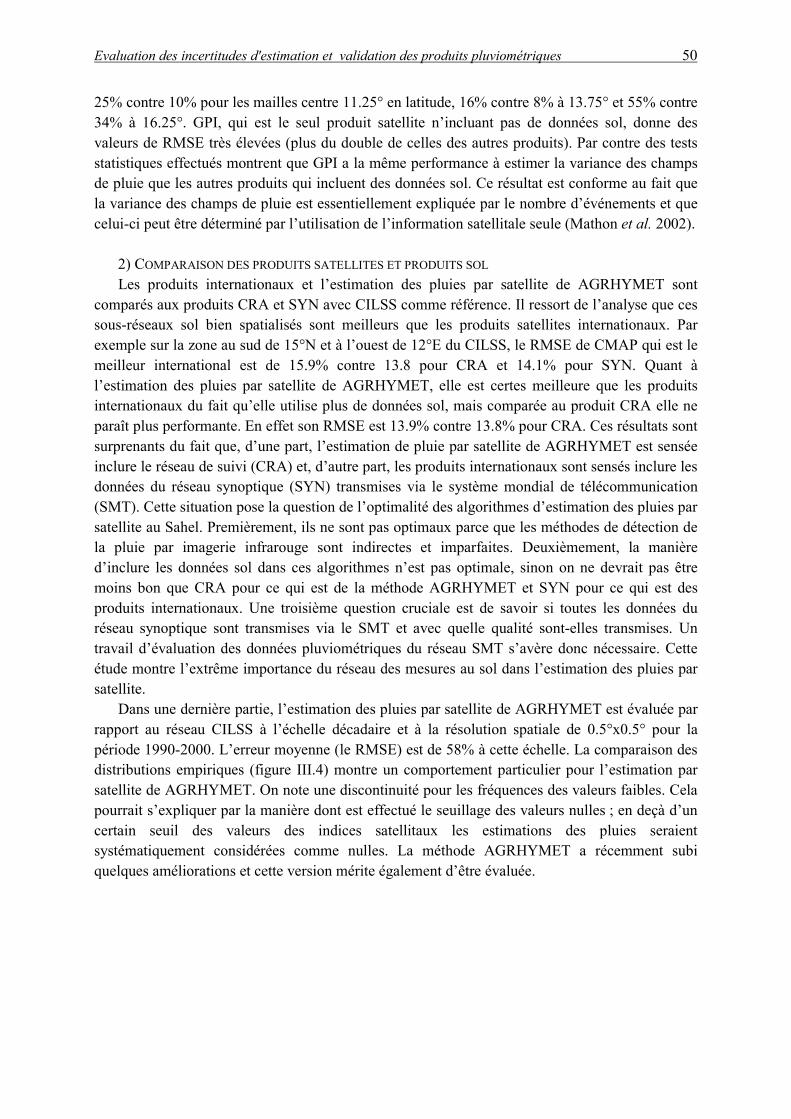
Evaluation des incertitudes d'estimation et validation des produits pluviométriques 50
25% contre 10% pour les mailles centre 11.25° en latitude, 16% contre 8% à 13.75° et 55% contre 34% à 16.25°. GPI, qui est le seul produit satellite n’incluant pas de données sol, donne des valeurs de RMSE très élevées (plus du double de celles des autres produits). Par contre des tests statistiques effectués montrent que GPI a la même performance à estimer la variance des champs de pluie que les autres produits qui incluent des données sol. Ce résultat est conforme au fait que la variance des champs de pluie est essentiellement expliquée par le nombre d’événements et que celui-ci peut être déterminé par l’utilisation de l’information satellitale seule (Mathon et al. 2002).
2) COMPARAISON DES PRODUITS SATELLITES ET PRODUITS SOL Les produits internationaux et l’estimation des pluies par satellite de AGRHYMET sont
comparés aux produits CRA et SYN avec CILSS comme référence. Il ressort de l’analyse que ces sous-réseaux sol bien spatialisés sont meilleurs que les produits satellites internationaux. Par exemple sur la zone au sud de 15°N et à l’ouest de 12°E du CILSS, le RMSE de CMAP qui est le meilleur international est de 15.9% contre 13.8 pour CRA et 14.1% pour SYN. Quant à l’estimation des pluies par satellite de AGRHYMET, elle est certes meilleure que les produits internationaux du fait qu’elle utilise plus de données sol, mais comparée au produit CRA elle ne paraît plus performante. En effet son RMSE est 13.9% contre 13.8% pour CRA. Ces résultats sont surprenants du fait que, d’une part, l’estimation de pluie par satellite de AGRHYMET est sensée inclure le réseau de suivi (CRA) et, d’autre part, les produits internationaux sont sensés inclure les données du réseau synoptique (SYN) transmises via le système mondial de télécommunication (SMT). Cette situation pose la question de l’optimalité des algorithmes d’estimation des pluies par satellite au Sahel. Premièrement, ils ne sont pas optimaux parce que les méthodes de détection de la pluie par imagerie infrarouge sont indirectes et imparfaites. Deuxièmement, la manière d’inclure les données sol dans ces algorithmes n’est pas optimale, sinon on ne devrait pas être moins bon que CRA pour ce qui est de la méthode AGRHYMET et SYN pour ce qui est des produits internationaux. Une troisième question cruciale est de savoir si toutes les données du réseau synoptique sont transmises via le SMT et avec quelle qualité sont-elles transmises. Un travail d’évaluation des données pluviométriques du réseau SMT s’avère donc nécessaire. Cette étude montre l’extrême importance du réseau des mesures au sol dans l’estimation des pluies par satellite.
Dans une dernière partie, l’estimation des pluies par satellite de AGRHYMET est évaluée par rapport au réseau CILSS à l’échelle décadaire et à la résolution spatiale de 0.5°x0.5° pour la période 1990-2000. L’erreur moyenne (le RMSE) est de 58% à cette échelle. La comparaison des distributions empiriques (figure III.4) montre un comportement particulier pour l’estimation par satellite de AGRHYMET. On note une discontinuité pour les fréquences des valeurs faibles. Cela pourrait s’expliquer par la manière dont est effectué le seuillage des valeurs nulles ; en deçà d’un certain seuil des valeurs des indices satellitaux les estimations des pluies seraient systématiquement considérées comme nulles. La méthode AGRHYMET a récemment subi quelques améliorations et cette version mérite également d’être évaluée.
Evaluation des incertitudes d'estimation et validation des produits pluviométriques 51
CILSS
Fig. III.4 : Comparaison des distributions de fréquence observées pour les pluies spatialisées à partir réseau total du CILSS (CILSS) et l’estimations de pluie par satellite de AGRHYMET (CRA ST) à l’échelle de la décade et à la résolution spatiale 0.5°x0.5° pour la période 1992-1999.
Evaluation des incertitudes d'estimation et validation des produits pluviométriques 52
3) PRISE EN COMPTE DE L’ERREUR DE LA REFERENCE DANS L’EVALUATION DES PRODUITS SATELLITES
Soit la relation (III.4) suivante :
2STRMSE = (III.4) 2
SRRMSE 2RTRMSE� RTSTRTST bbCov 2),(2 ����
avec le RMSE du produit satellite par rapport à la vraie valeur mais inconnue de
la pluie moyenne. est le RMSE du produit satellite par rapport à la référence
considérée. est l’erreur (RMSE) de la référence par rapport à la vraie valeur. et
sont les biais de l’estimation satellite et de la référence par rapport à la vraie valeur.
est l’écart entre estimation satellite et vraie valeur ; � écart entre référence et vraie valeur.
STRMSE
RMSE
TS R�
SRRMSE
RT STb
RTb
SR� R� TRSR RR ��
Cette relation (III.4) montre comment l’erreur de la référence, qui est elle-même une
estimation, intervient dans l’évaluation d’un produit satellital. Pour avoir accès à l’erreur réelle des produits satellites, il convient de disposer, d’une part, d’une fonction d’erreur pour calculer
, et d’autre part, de pouvoir estimer ; le biais peut être négligé. Du
fait de la difficulté de l’estimer, la covariance a toujours été négligée dans les études qui ont tenté d’appliquer la relation (III.4) pour corriger l’erreur d’évaluation des estimations satellitales. Dans ce travail nous avons utilisé la zone du CILSS où le réseau est le plus dense pour l’estimer. Voir Ali et al. (2004b) pour des détails sur la comparaison des résultats obtenus en estimant cette covariance et en la négligeant. Notons simplement que le fait d’estimer ce terme donne des erreurs d’évaluation des produits satellites plus objectives que le fait de le négliger. L’erreur d’évaluation est ainsi indépendante de la référence utilisée et demeure constante. Alors que dans le cas où il est négligé, l’erreur d’évaluation dépend du réseau de référence, surtout quand sa densité est faible ou quand il a un fort lien avec le réseau utilisé dans l’élaboration du produit satellite. L’application de la relation III.4 fait chuter l’erreur brute d’évaluation des produits satellites, par exemple elle passe de 15.9% à 11% pour CMAP. Par contre elle n’a pas changé l’ordre de classement des produits, obtenu avec le calcul direct à partir de la référence CILSS.
RTRMSE ),( RTSRCov ��
,( RTSRCov ��
RTb
)
Rainfall estimation in the Sahel. Part 1: Error Function 53
Article Rainfall estimation in the Sahel.
Part 1: Error Function
Rainfall estimation in the Sahel. Part 1: Error Function 55
Rainfall estimation in the Sahel. Part 1: Error Function
Abdou ALI1,2, Thierry LEBEL1, Abou AMANI2
Accepted for publication in the Journal of Applied Meteorology
Abstract Rainfall estimation in semi-arid regions remains a challenging issue since it displays great spatial
and temporal variability and networks available for monitoring are often of low density. This is especially the case in the Sahel, a 3 million km² region where the life of populations is still heavily dependent on rain for agriculture. Whatever the data and sensors available for rainfall estimation – including satellite IR and microwave data and possibly weather radar systems – it is necessary to define objective error functions to be used in comparing various rainfall products. This first paper of a series of two presents a theoretical framework for the development of such an error function and the optimization of its parameters for the Sahel. A range of time scales – from rain event to annual – are considered, using two data sets covering two different spatial scales. The mesoscale (E-N) is documented over a period of 13 years (1990-2002) on a 16,000 km² area covered by 30 recording rain gauges; the regional scale is documented by the CRA (Centre Regional AGRHYMET) data set, with an annual average of between 600 to 650 rain gauges available over a period of 8 years. The data analysis showed that the spatial structure of the Sahelian rain fields is markedly anisotropic, nonstationary and dominated by the nesting of two elementary structures. A cross validation procedure on point rainfall values leads to the identification of an optimal interpolation algorithm. Using the error variances computed from this algorithm on 1°x1° and 2.5°x2.5° cells, an error function is derived, allowing the calculation of standard errors of estimation for the region. Typical standard errors for monthly rainfall estimation are 11% (10%) for a 10-station network on a 2.5°x2.5° (1°x1°); 40% (30%) for a single station on a 2.5°x2.5° (1°x1°). In a companion paper, this error function is used to investigate the differences between satellite rainfall products and how they compare with ground based estimates.
* Corresponding author address: Abdou ALI, LTHE, BP 53 38041 Grenoble Cedex 9, France [email protected]
1IRD, LTHE, Grenoble, France 2Centre AGRHYMET, Niamey, Niger
Rainfall estimation in the Sahel. Part 1: Error Function 56
1. Introduction
The possible long-term modification of the Sahelian precipitation regime (e.g., Lebel et al. 2003), makes hydrologists and climatologists ask themselves two major types of questions: i) how and to what degree of accuracy can Sahelian rainfall be monitored in real or near real time in order to meet the needs of a large community of users faced with the effects of persistent drought (seasonal crop monitoring, water resource management, food aid programs)?; ii) how and to what degree of significance can the interannual fluctuations of Sahelian rain fields and possible modifications of the precipitation regime be charac-terized?. Considering the deterioration of rain gauge networks (Fig. 1), data access problems, and the significant variability in time and space of Sahelian rainfall, satellite estimates are looked to as a substitute – or complement– of ground-based network estimates particularly as satellite borne sensors become increa-singly efficient. This problem is not specific to the Sahel: the past decade has seen the development of rain products intended for a large community of users aiming to summarize as well as possible the informa-tion from ground-based networks and satellites for a given region. Monitoring rainfall performance is nevertheless a particularly sensitive issue in the Sahel and this work aims at developing an objective method for evaluating the quality of rainfall estimates over the region. The emphasis is on the determination of an error function, inferred from the analysis of several years of data – years that can be considered to be representative of the region’s current climate – and on a range of scales meeting the needs of a large commu-nity of users. The requirements to be met by a clima-tological product are different enough from those of products that will be described here as "hydrological", in the sense that they should especially serve as input data for water balance or water resource quantification models. Yet, intuitively speaking – and it is clearly shown in this study – the errors depend heavily on rain field variability and this variability is far from being consistent from one year to the next. Moreover, this variability naturally depends on the time scale on which our work is based.
Accordingly, this series of two articles deals with two closely related issues. The first, which is the subject of this article, consists of determining an error function, used to: i) develop reference rainfields by minimizing this function; ii) provide criteria for the intercomparison of various rain products. The second issue is addressed in a companion paper and relates to the intercomparison of various rain products, while focusing more on error distributions than on mean values.
The vulnerability of West Africa to the drought that has been prevailing since the 70s has resulted in the creation of regional institutions in order to better manage its effects. The AGRHYMET Regional Centre based in Niamey, Niger, is one of the major bodies
among them, which currently uses many tools for operational activities: systems for early warning, resource water management, hydrological and agrono-mic monitoring. Areal rainfall is the main input data for these tools. Yet, whatever the sources of informa-tion and procedure used for estimating this rainfall are, the associated error is seldom evaluated with rigour and less often used in the models.
The main objective of this paper is thus to provide a general framework for users who need to build or to evaluate rain products. In this respect, the results are felt to extend beyond the Sahelian region itself and to apply to most semi-arid regions of the inter-tropical belt. Great care is paid to account for all the informa-tion provided by various sources of rain gauge data, whether from operational or research origins. Using the wide conceptual possibilities of geostatistics, a refined characterization of the Sahelian rain fields is used to compare several estimation methods. This in turn proposes a coherent interpolation approach and an operational metrics for the evaluation of rain products that are presented in the companion paper.
Section 2 briefly reviews the general question of rainfall estimation and the methods available for a quantitative evaluation of the errors associated with any estimation procedure. The application of these methods to the interpolation of Sahelian rain fields (characterized by a strong intermittency in time and space) is then the object of section 3. Section 4 presents a comparison of results between different for-mulations of kriging, showing that the non stationarity and anisotropy of the Sahelian rain fields heavily influence the performance of these methods. This leads in section 5 to the derivation of an error function associated with the choice of an optimal model of covariance, before concluding in section 6.
2. Rainfall estimation from ground data a. General framework
For the problem treated here, stochastic interpo-lation methods are the most relevant, since they provide an error evaluation of the estimation made. Apart from some empirical-statistical studies (e.g., Huff 1970; Rudolf et al. 1994; Huffman 1997), almost the entire group of statistical methods refer more or less to the concept of optimal interpolation, initially promoted by Gandin (1965). Matheron’s theory of regionalized variables (1971) expands the framework of optimal interpolation, by taking into account the uncertainties related to sampling over a necessarily limited area. As a matter of fact, the empirical mean and spatial variance (i.e., inferred from data) may be highly biased estimators of the mean and variance of the process. Geostatistical methods are widely reco-gnized as performing better than conventional methods (see e.g., Creutin and Obled 1982; Boussières and Hogg 1989; Philips et al. 1992; Zimmerman et al. 1999). This is particularly the case with anisotropic
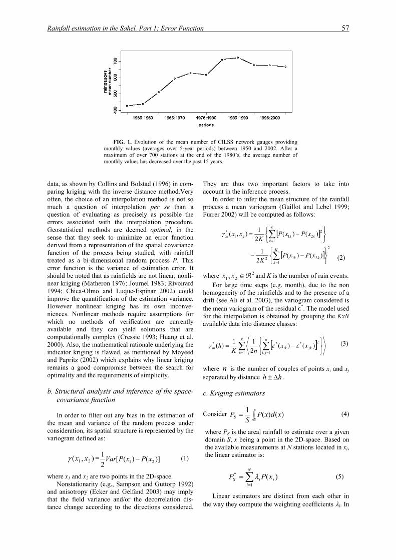
Rainfall estimati in the Sahel. Part 1: Error Function 57
data, as shown byparing kriging wioften, the choice much a questioquestion of evalerrors associatedGeostatistical mesense that they sderived from a refunction of the ptreated as a bi-derror function is should be noted tnear kriging (Mat1994; Chica-Olmimprove the quanHowever nonlineniences. Nonlinewhich no methavailable and thcomputationally c2000). Also, the mindicator kriging and Papritz (2002remains a good optimality and the
b. Structural ancovariance fu
In order to fil
the mean and vaconsideration, its variogram defined
),( 21 xx�
where x1 and x2 arNonstationarit
and anisotropy (Ethat the field vatance change acc
on
FIG. 1. Evolution of the mean number of CILSS network gauges providing monthly values (averages over 5-year periods) between 1950 and 2002. After a maximum of over 700 stations at the end of the 1980’s, the average number of monthly values has decreased over the past 15 years.
Collins and Bolstad (1996) in com-th the inverse distance method.Very of an interpolation method is not so n of interpolation per se than a uating as precisely as possible the with the interpolation procedure. thods are deemed optimal, in the eek to minimize an error function
presentation of the spatial covariance rocess being studied, with rainfall
imensional random process P. This the variance of estimation error. It
hat as rainfields are not linear, nonli-heron 1976; Journel 1983; Rivoirard o and Luque-Espinar 2002) could tification of the estimation variance. ar kriging has its own inconve-
ar methods require assumptions for ods of verification are currently ey can yield solutions that are omplex (Cressie 1993; Huang et al. athematical rationale underlying the
is flawed, as mentioned by Moyeed ) which explains why linear kriging
compromise between the search for requirements of simplicity.
alysis and inference of the space-nction
ter out any bias in the estimation of riance of the random process under spatial structure is represented by the as:
= )]()([21
21 xPxPVar � (1)
e two points in the 2D-space. y (e.g., Sampson and Guttorp 1992) cker and Gelfand 2003) may imply
riance and/or the decorrelation dis-ording to the directions considered.
They are thus two important factors to take into account in the inference process.
In order to infer the mean structure of the rainfall process a mean variogram (Guillot and Lebel 1999; Furrer 2002) will be computed as follows:
� �
� �2
1212
1
22121
*
)()(2
1
)()(21),(
���
���
��
���
���
��
�
�
�
�
K
kkk
K
kkkm
xPxPK
xPxPK
xx�
where and K is the number of rain e221, ��xx
For large time steps (e.g. month), due to thhomogeneity of the rainfields and to the presencdrift (see Ali et al. 2003), the variogram considethe mean variogram of the residual �*. The modefor the interpolation is obtained by grouping theavailable data into distance classes:
� �� �� � �
��
���
��K
k
n
jijkikm xx
nKh
1 1,
2*** )()(211)( ���
where is the number of couples of points xn i separated by distance . hh ��
c. Kriging estimators
Consider ��
SS xdxPS
P )()(1
where PS is the areal rainfall to estimate over a domain S, x being a point in the 2D-space. Basthe available measurements at N stations locatedthe linear estimator is:
)(1
*i
N
iiS xPP �
�
� �
Linear estimators are distinct from each oththe way they compute the weighting coefficients
(2)
vents. e non e of a red is l used KxN
(3)
and xj
(4)
given ed on in xi,
(5)
er in �i. In
Rainfall estimation in the Sahel. Part 1: Error Function 58
Kriging the weighting coefficients are computed in such a way as:
�� The estimate is unbiased : = 0 )( *SS PPE �
(6a) �� Its variance (the Kriging variance) is minimi-
zed: min [Var(P*S -PS)] (6b)
Whereas at small time scales, rainfields may be treated as a purely stochastic process, at larger time scales (daily and over) a deterministic component – m(x) – may be present (linked to the topography or any other geographical forcing factor) along with a stochastic component – �(x):
)()()( xxmxP ��� (7)
The stochastic component is assumed to be second-order stationary and E[�(x)] =0. The various formulations of kriging depend on the nature of m(x).
If m(x) is constant and known, the kriging formulation is called simple kriging (SK). If it is constant but unknown, the kriging formulation is called ordinary kriging (OK). One can refer to Cressie 1993 and Chilès and Delfiner 1999 for example, for a full presentation of these methods. The kriging variance of estimation error at point for SK and OK are:
0x
��
�
N
iiSKSK xx
i1
02 ),(
���� (8)
��
��
N
iOKiOKOK xx
i1
002 ),( ����
� (9)
with the variogram of the underlying process �
which in this case is also the variogram of P; is the Lagrange multiplier accounting for the constraint on the weights of the OK system.
��
OK�
If m(x) depends on the 2-D coordinates x, nonstationary geostatistical methods must be consi-dered (Matheron 1969). The two following methods are tested1 here: i) The Universal kriging (UK) was firstly formulated by Matheron (1969) and further developed by several authors (Journel and Huijbregts 1978 ; Papritz and Stein 1999), and is based on a global resolution of the kriging system, assuming a polynomial form for the drift, that is to say:
1 Note that only the univariate form of kriging is considered here since the Sahel is a fairly flat region and no direct relation between vegetation and rainfall is known; bivariate kriging, such as cokriging (Wackernagel, 1998) may be more suitable in other contexts.
�� )()( xfaxm ll (10)
The estimation variance of the UK is obtained as follows:
� ��
��
Ni l
llUKiUK
iUK xfxx
,10*0
2 )(),( �����
(11)
In the UK system the variogram � of the underlying process � is unfortunately not known in practice, because the coefficients of the drift [m(x)] model are not known. Several authors (Cressie 1993; Goovaerts 1997; Chilès and Delfiner 1999) draw attention to the biased behavior of the variogram used in the universal kriging system.
�
ii) The second approach, in case of non stationarity, is regression kriging, RK (Ahmed and De Marsily 1987; Odeh et al. 1995; Goovaerts 1997). Here the predictions are made separately for the drift and the residuals and then added back together. The method consists of three steps: a) subtracting the drift values {m(xi)} from the observations{P(xi)}, b) kriging the obtained residuals {��(xi)} and c) for each point x0 where an estimation is sought, combining the estimated value of the drift to the kriged
residual :
)(ˆ 0xm)(ˆ 0x�
)(ˆ)(ˆ)(ˆ00,0 xxmxPRK ��� (12)
The drift model coefficients are optimally estimated using the generalized least squares (GLS) in order to account for the spatial correlation of residuals (Cressie 1993; Hengl et al. 2003). This idea resolves the problem mentioned for UK , since only the variogram of the residuals is required, which can be estimated from the experimental residuals. However the experimental residuals contain the drift estimation error which produces a nugget effect on the residual variogram:
2ˆ mRK ������ (13)
where � is the regression error variance assumed to be stationary over the study area.
2m
Numerically residual kriging is thus comparable to kriging data affected by a measurement error. The residual kriging variance represents the global error associated with the estimation by the RK system i.e., the sum of two errors, one linked to the regression estimation and the other to the undersampling of the underlying process � :
)](ˆ[)](ˆ[)( 0
20
20
2 xxmxRK ���� �� (14)
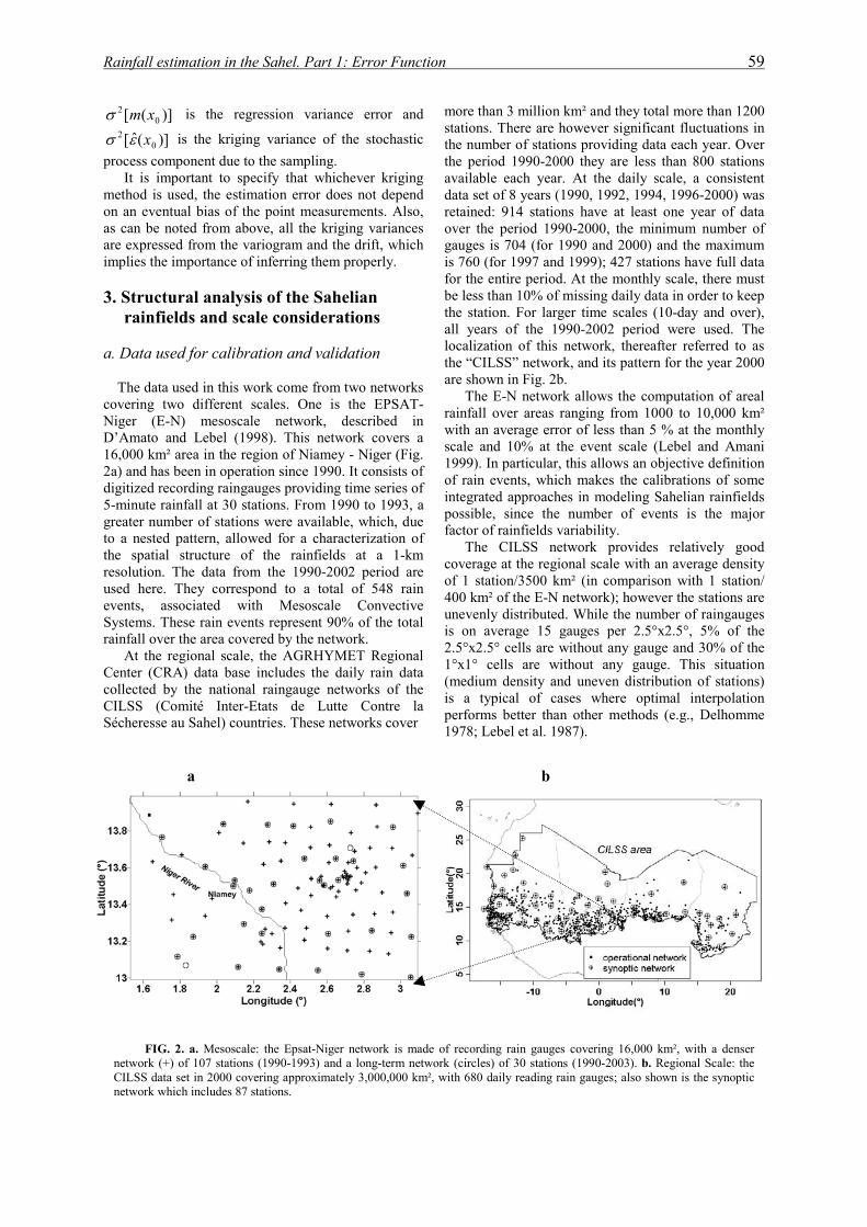
Rainfall estimation in the Sahel. Part 1: Error Function 59
)]([ 02 xm�
)](ˆ[ 02 x��
is the regression variance error and
is the kriging variance of the stochastic process component due to the sampling.
It is important to specify that whichever kriging method is used, the estimation error does not depend on an eventual bias of the point measurements. Also, as can be noted from above, all the kriging variances are expressed from the variogram and the drift, which implies the importance of inferring them properly.
3. Structural analysis of the Sahelian
rainfields and scale considerations a. Data used for calibration and validation
The data used in this work come from two networks covering two different scales. One is the EPSAT-Niger (E-N) mesoscale network, described in D’Amato and Lebel (1998). This network covers a 16,000 km² area in the region of Niamey - Niger (Fig. 2a) and has been in operation since 1990. It consists of digitized recording raingauges providing time series of 5-minute rainfall at 30 stations. From 1990 to 1993, a greater number of stations were available, which, due to a nested pattern, allowed for a characterization of the spatial structure of the rainfields at a 1-km resolution. The data from the 1990-2002 period are used here. They correspond to a total of 548 rain events, associated with Mesoscale Convective Systems. These rain events represent 90% of the total rainfall over the area covered by the network.
At the regional scale, the AGRHYMET Regional Center (CRA) data base includes the daily rain data collected by the national raingauge networks of the CILSS (Comité Inter-Etats de Lutte Contre la Sécheresse au Sahel) countries. These networks cover
more than 3 million km² and they total more than 1200 stations. There are however significant fluctuations in the number of stations providing data each year. Over the period 1990-2000 they are less than 800 stations available each year. At the daily scale, a consistent data set of 8 years (1990, 1992, 1994, 1996-2000) was retained: 914 stations have at least one year of data over the period 1990-2000, the minimum number of gauges is 704 (for 1990 and 2000) and the maximum is 760 (for 1997 and 1999); 427 stations have full data for the entire period. At the monthly scale, there must be less than 10% of missing daily data in order to keep the station. For larger time scales (10-day and over), all years of the 1990-2002 period were used. The localization of this network, thereafter referred to as the “CILSS” network, and its pattern for the year 2000 are shown in Fig. 2b.
The E-N network allows the computation of areal rainfall over areas ranging from 1000 to 10,000 km² with an average error of less than 5 % at the monthly scale and 10% at the event scale (Lebel and Amani 1999). In particular, this allows an objective definition of rain events, which makes the calibrations of some integrated approaches in modeling Sahelian rainfields possible, since the number of events is the major factor of rainfields variability.
The CILSS network provides relatively good coverage at the regional scale with an average density of 1 station/3500 km² (in comparison with 1 station/ 400 km² of the E-N network); however the stations are unevenly distributed. While the number of raingauges is on average 15 gauges per 2.5°x2.5°, 5% of the 2.5°x2.5° cells are without any gauge and 30% of the 1°x1° cells are without any gauge. This situation (medium density and uneven distribution of stations) is a typical of cases where optimal interpolation performs better than other methods (e.g., Delhomme 1978; Lebel et al. 1987).
a
FIG. 2. a. Mesoscale: the Epsat-Niger network is madnetwork (+) of 107 stations (1990-1993) and a long-term netwCILSS data set in 2000 covering approximately 3,000,000 kmnetwork which includes 87 stations.
b
e of recording rain gauges covering 16,000 km², with a denser ork (circles) of 30 stations (1990-2003). b. Regional Scale: the
², with 680 daily reading rain gauges; also shown is the synoptic
b)
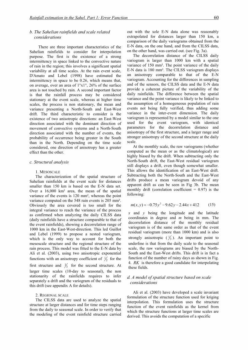
Rainfall estimation in the Sahel. Part 1: Error Function 60
b. The Sahelian rainfields and scale related considerations
There are three important characteristics of the
Sahelian rainfields to consider for interpolation purpose. The first is the existence of a strong intermittency in space linked to the convective nature of rain in the region; this involves a significant spatial variability at all time scales. At the rain event scale, D'Amato and Lebel (1998) have estimated the intermittency in space to be 0.26, which means that, on average, over an area of 1°x1°, 26% of the surface area is not touched by rain. A second important factor is that the rainfall process may be considered stationary at the event scale, whereas at higher time scales, the process is non stationary, the mean and variance presenting a North-South and East-West drift. The third characteristic to consider is the existence of two anisotropic directions: an East-West direction associated with the dominant direction of movement of convective systems and a North-South direction associated with the number of events, the probability of occurrence being greater in the South than in the North. Depending on the time scale considered, one direction of anisotropy has a greater effect than the other.
c. Structural analysis
1. MESOSCALE The characterization of the spatial structure of
Sahelian rainfields at the event scale for distances smaller than 150 km is based on the E-N data set. Over a 16,000 km² area, the mean of the spatial variance of the events is 120 mm², whereas the point variance computed on the 548 rain events is 205 mm². Obviously the area covered is too small for the integral variance to reach the variance of the process as confirmed when analyzing the daily CILSS data (daily rainfields have a structure comparable to that of the event rainfields), showing a decorrelation range of 1000 km in the East-West-direction. This led Guillot and Lebel (1999) to propose a nested variogram, which is the only way to account for both the mesoscale structure and the regional structure of the rain process. This model was fitted to the E-N data by Ali et al. (2003), using two anisotropic exponential functions with an anisotropy coefficient of 2
1 for the first structure and 3
1 for the second structure. At larger time scales (10-day to seasonal), the non stationarity of the rainfields requires to infer separately a drift and the variogram of the residuals to this drift (see appendix A for details).
2. REGIONAL SCALE The CILSS data are used to analyze the spatial
structure at larger distances and for time steps ranging from the daily to seasonal scale. In order to verify that the modeling of the event rainfield structure carried
out with the sole E-N data alone was reasonably extrapolated for distances larger than 150 km, a comparison of the daily variograms obtained from the E-N data, on the one hand, and from the CILSS data, on the other hand, was carried out. (see Fig. 3a).
The decorrelation distance of the CILSS daily variogram is larger than 1000 km with a spatial variance of 150 mm². The point variance of the daily E-N data is 180 mm². The CILSS variogram displays an anisotropy comparable to that of the E-N variogram. Accounting for the differences in sampling and of the sensors, the CILSS data and the E-N data provide a coherent picture of the variability of the daily rainfields. The difference between the spatial variance and the point variance is likely to be linked to the assumption of a homogeneous population of rain events not being fully verified, thus adding some variance in the inter-event dimension. The daily variogram is represented by a model similar to the one used for the event variogram, with identical parameters for the decorrelation distance and anisotropy of the first structure, and a larger range and stronger anisotropy of the second structure at the daily scale.
At the monthly scale, the raw variograms (whether computed as the mean or as the climatological) are highly biased by the drift. When subtracting only the North-South drift, the East-West residual variogram still displays a drift, even though somewhat smaller. This allows the identification of an East-West drift. Subtracting both the North-South and the East-West drifts produce a mean variogram devoid of any apparent drift as can be seen in Fig 3b. The mean monthly drift (correlation coefficient = 0.97) is the following:
41244.262.975.0),( 2����� xyyyxm (15)
x and y being the longitude and the latitude coordinates in degree and m being in mm. The decorrelation distance of the monthly residual variogram is of the same order as that of the event residual variogram (more than 1000 km) and is also strongly anisotropic ( 3
1 ). An important point to underline is that from the daily scale to the seasonal scale, the raw variograms are biased by the North-South and the East-West drifts. This drift is in fact a function of the number of rainy days as shown in Fig. 4. RK is therefore a good candidate for interpolating these fields.
d. A model of spatial structure based on scale considerations
Ali et al. (2003) have developed a scale invariant
formulation of the structure function used for kriging interpolation. This formulation uses the structure function of the event rainfields as the kernel from which the structure functions at larger time scales are derived. This avoids the computation of a specific
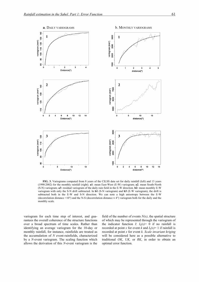
Rainfall estimation in the Sahel. Part 1: Error Function 61
variograrantees tover a bidentifyimonthlythe accuby a N-eallows th
b. MONTHLY VARIOGRAMS a. DAILY VARIOGRAMS
1 1
FIG. 3. Variograms computed from 8 years of the CILS(1990:2002) for the monthly rainfall (right). a1: mean East-(S-N) variogram; a3: residual variogram of the daily rain fielvariogram with only the S-N drift subtracted. In b1 (S-N vasubtracted both in the E-W and S-N direction. We can(decorrelation distance >10°) and the N-S (decorrelation distmonthly scale.
m for each time step of interest, and gua-he overall coherence of the structure functions road spectrum of time scales. Rather than
ng an average variogram for the 10-day or rainfall, for instance, rainfields are treated as mulation of N event-rainfields, characterized vent variogram. The scaling function which e derivation of this N-event variogram is the
fieldof wthe recorecowilltradopti
2
3
2
S data set for daily rainfall (left) and 13 years West (E-W) variogram; a2. mean South-North d in the E-W direction. b2: mean monthly E-W riogram) and b3 (E-W variogram), the drift is note a high anisotropy between the E-W
ance � 4°) variogram both for the daily and the
of the number of events N(x), the spatial structure hich may be represented through the variogram of indicator function I: Ik(x)= 0 if no rainfall is rded at point x for event k and Ik(x)= 1 if rainfall is rded at point x for event k. Scale invariant kriging be considered here as a possible alternative to itional OK, UK, or RK, in order to obtain an mal error function.
3
Rainfall estimation in the Sahel. Part 1: Error Function 62
FIG. 4. The drift along progressive time scales. Each curve repthe cumulative number of rainy days by band, normalized by the width 0.5° in latitude or 1° in longitude. We can note a progressnumber of rainy days, both in latitude (left) and longitude (right). gradient is smallest at one-day scale. The gradient is stronger as a fu80 cumulative rainy days) than as a function of longitude (around 0.1
4. Optimal interpolation of the Sahelian rainfields
a. Possible interpolation functions
Five formulations of kriging are considered in what follows for selecting an optimal interpolation function of Sahelian rainfields. The tradeoff between ordinary kriging and more sophisticated methods is that the latter usually imply a greater number of parameters to infer, which in turn means a lack of robustness of the estimated parameters.
The first two formulations retained for the comparison are thus two ordinary kriging methods (corresponding to a stationarity assumption, assumed to hold only at the event scale): i) ordinary kriging with a simple climatological variogram (no anisotropy and no nesting), denoted OK-NAN, ii) ordinary kriging with a nested and anisotropic mean variogram denoted OK-NA.
Three formulations are retained for the non stationary case, all three using a nested and anisotropic variogram (NAV) corresponding to the main features of the empirical variograms (Fig 3b). As already mentioned the number of rain events varies from month to month (or from one season to another), which makes the cumulative monthly (or seasonal) rainfields inhomogeneous with respect to the underlying stochastic process. To overcome this problem, the NAV is scaled in order to account for the variability of number of events. As kriging utilizes this normalized variogram in this case, the “true” kriging variance is obtained for a given rainfield by multiplying the estimated (normalized) kriging variance by the spatial variance of the field concerned. Note that this problem of non-homogeneity does not arise in the scaling approach since the number of events is explicitly and directly taken into account in its formulation (see Ali et al. 2003). In the application
ofneInbydiEmfoapcosiison
b
calainasus(1peRprlathanmacco(Mpe
inunbe
resents the conditional (on non-zero values) mean rainfall for corresponding overall mean rainfall. The bands are either of ive augmentation of the rainfall gradient with an increasing The drift exists at all the cumulative time scales, thought the nction of latitude (around 6% at the one-day scale to 23% for 3% at the one-day scale to 3% for 80 cumulative rainy days).
UK, it is assumed that the East-West drift is gligible in comparison with the North-South drift. the application of RK, the drift is computed month month. Also, recent analyses show that there are fferences in the average rainfall pattern between the astern and the Western Sahel. Consequently, the drift odel used reflects these differences. The last rmulation selected for the comparison is the scaling proach referred to hereafter as SC. For the regional mparison, the SC formulation was used in a
mplified way by assuming that the number of events equal to the number of rainy days, since at this scale ly daily raingauges are available.
. Cross validation and criteria used for the intercomparison
A cross-validation procedure (Seaman 1983) is
rried out to determine which of the five formu-tions under consideration can produce: i) the best terpolation and ii) the more realistic value for the sociated errors. Several statistical indicators will be ed to that end, referring to the work of Willmott 984) who used five statistical criteria to evaluate the rformances of various interpolation methods. The
MSE is sensitive to extreme values, though this oblem is attenuated in this study by the extremely rge size of the samples used. It was underlined that e relationship between the correlation coefficient (r²) d model performance is not well defined and the agnitudes of r² are not consistently related to the curacy of prediction. It was suggested that in nclusion, that the RMSE and the mean bias error E) are among the "best" overall measures of model rformance for intercomparison. The ME and the RMSE will thus be used here as
dicators of the overall coherency between the fields der comparison. Defining ei as the difference tween the estimate Pi* and the observed value Pi :
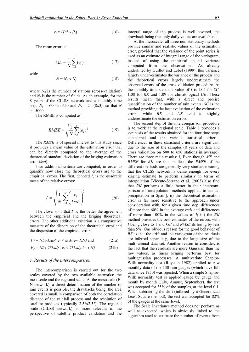
Rainfall estimation in the Sahel. Part 1: Error Function 63
ei = (Pi* - Pi) (16)
The mean error is:
��
�
N
iie
NME
1)(1 (17)
with: N = NS x Nf (18)
where NS is the number of stations (cross-validation) and Nf is the number of fields. As an example, for the 8 years of the CILSS network and a monthly time step, NS = 600 to 650 and Nf = 24 (8x3), so that N ��15000.
The RMSE is computed as:
��
�
N
iie
NRMSE
1
2)(1 (19)
The RMSE is of special interest to this study since it provides a mean value of the estimation error that can be directly compared to the average of the theoretical standard deviation of the kriging estimation error (ksd).
Two additional criteria are computed, in order to quantify how close the theoretical errors are to the empirical errors. The first, denoted I, is the quadratic mean of the relative errors:
��
���
����
��
N
i i
i
ksde
NI
1
21
(20)
The closer to 1 that I is, the better the agreement between the empirical and the kriging theoretical errors. The other additional criterion is a comparative measure of the dispersion of the theoretical error and the dispersion of the empirical errors:
P1 = Nb{-ksdi< ei < ksdi; i= 1,N} and (21a)
P2 = Nb{-2*ksdi< ei < 2*ksdi; i= 1,N} (21b)
c. Results of the intercomparison The intercomparison is carried out for the two
scales covered by the two available networks: the mesoscale and the regional scale. At the mesoscale (E-N network), a direct determination of the number of rain events is possible, the drawbacks being, the area covered is small in comparison of both the correlation distance of the rainfall process and the resolution of satellite products (typically 2.5°x2.5°). The regional scale (CILSS network) is more relevant in the perspective of satellite product validation and the
integral range of the process is well covered, the drawback being that only daily values are available.
At the mesoscale, all three non stationary methods provide similar and realistic values of the estimation error, provided that the variance of the point series is used as an estimate of integral range of the variogram, instead of using the empirical spatial variance computed from the observations. As already underlined by Guillot and Lebel (1999), this variance largely under-estimates the variance of the process and the theoretical errors largely underestimate the observed errors of the cross-validation procedure. At the monthly time step, the value of I is 1.02 for SC, 1.08 for RK and 1.09 for climatological UK. These results mean that, with a direct and precise quantification of the number of rain events, SC is the method providing the best evaluation of the estimation errors, while RK and UK tend to slightly underestimate the estimation errors.
The second step of the intercomparison procedure is to work at the regional scale. Table 1 provides a synthesis of the results obtained for the four time steps considered and the various statistical criteria. Differences in these statistical criteria are significant due to the size of the samples (8 years of data and cross validation on 600 to 650 stations in average). There are three main results: i) Even though ME and RMSE for RK are the smallest, the RMSE of the different methods are generally very similar, meaning that the CILSS network is dense enough for every kriging estimate to perform similarly in terms of interpolation [Vicente-Serrano et al. (2003) also find that RK performs a little better in their intercom-parison of interpolation methods applied to annual precipitation in Spain]; ii) the theoretical estimation error is far more sensitive to the approach under consideration with, for a given time step, differences of more than 60% in the average ksds and differences of more than 100% in the values of I; iii) the RK method provides the best estimates of the errors, with I being close to 1 and ksd and RMSE differing by less than 5%. One obvious reason for the good behavior of RK is that the drift and the variogram of the residuals are inferred separately, due to the large size of the multi-annual data set. Another reason to consider, is the fact that the residuals are more Gaussian than the raw values, as linear kriging performs best for multigaussian processses. A multivariate Shapiro-Wilk normality test (Royston 1982) applied to raw monthly data of the 130 rain gauges (which have full data since 1950) was rejected. When a simple Shapiro-Wilk normality test is applied gauge by gauge and month by month (July, August, September), the test was accepted for 35% of the samples, at the level 0.1. When subtracting the drift (inferred by a Generalized Least Square method), the test was accepted for 82% of the gauges at the same level.
The Scale Invariance method does not perform as well as expected, which is obviously linked to the algorithm used to estimate the number of events from
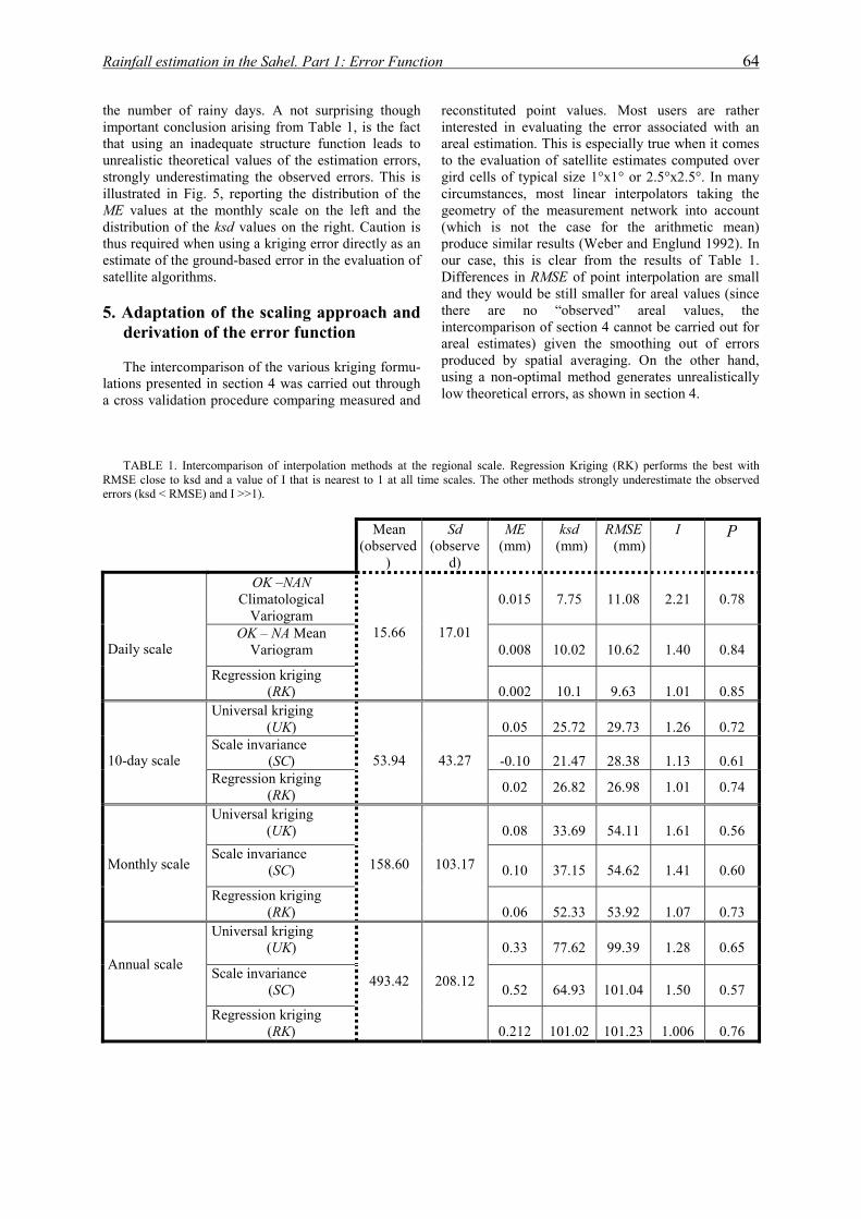
Rainfall estimation in the Sahel. Part 1: Error Function 64
the number of rainy days. A not surprising though important conclusion arising from Table 1, is the fact that using an inadequate structure function leads to unrealistic theoretical values of the estimation errors, strongly underestimating the observed errors. This is illustrated in Fig. 5, reporting the distribution of the ME values at the monthly scale on the left and the distribution of the ksd values on the right. Caution is thus required when using a kriging error directly as an estimate of the ground-based error in the evaluation of satellite algorithms.
5. Adaptation of the scaling approach and
derivation of the error function
The intercomparison of the various kriging formu-lations presented in section 4 was carried out through a cross validation procedure comparing measured and
reconstituted point values. Most users are rather interested in evaluating the error associated with an areal estimation. This is especially true when it comes to the evaluation of satellite estimates computed over gird cells of typical size 1°x1° or 2.5°x2.5°. In many circumstances, most linear interpolators taking the geometry of the measurement network into account (which is not the case for the arithmetic mean) produce similar results (Weber and Englund 1992). In our case, this is clear from the results of Table 1. Differences in RMSE of point interpolation are small and they would be still smaller for areal values (since there are no “observed” areal values, the intercomparison of section 4 cannot be carried out for areal estimates) given the smoothing out of errors produced by spatial averaging. On the other hand, using a non-optimal method generates unrealistically low theoretical errors, as shown in section 4.
TABLE 1. Intercomparison of interpolation methods at the regional scale. Regression Kriging (RK) performs the best with
RMSE close to ksd and a value of I that is nearest to 1 at all time scales. The other methods strongly underestimate the observed errors (ksd < RMSE) and I >>1).
Mean (observed
)
Sd (observe
d)
ME (mm)
ksd (mm)
RMSE (mm)
I P
OK –NAN Climatological
Variogram
0.015
7.75
11.08
2.21
0.78
OK – NA Mean Variogram
0.008
10.02
10.62
1.40
0.84
Daily scale
Regression kriging (RK)
15.66
17.01
0.002
10.1
9.63
1.01
0.85
Universal kriging (UK)
0.05
25.72
29.73
1.26
0.72
Scale invariance (SC)
-0.10
21.47
28.38
1.13
0.61
10-day scale Regression kriging
(RK)
53.94
43.27
0.02 26.82 26.98 1.01 0.74
Universal kriging (UK)
0.08
33.69
54.11
1.61
0.56
Scale invariance (SC)
0.10
37.15
54.62
1.41
0.60
Monthly scale
Regression kriging (RK)
158.60
103.17
0.06
52.33
53.92
1.07
0.73
Universal kriging (UK)
0.33
77.62
99.39
1.28
0.65
Scale invariance (SC)
0.52
64.93
101.04
1.50
0.57
Annual scale
Regression kriging (RK)
493.42
208.12
0.212
101.02
101.23
1.006
0.76
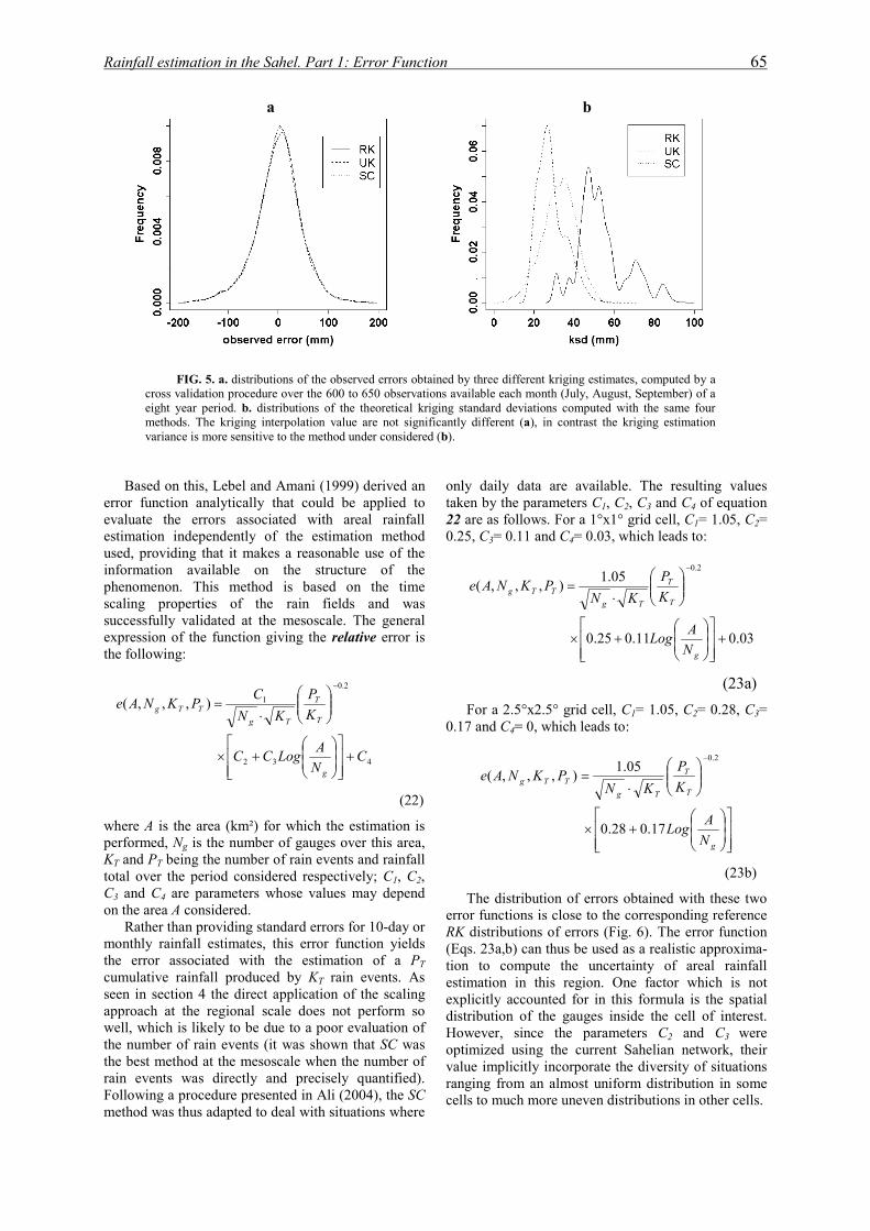
Rainfall estimation in the Sahel. Part 1: Error Function 65
Berroevalestimusedinfophenscalsuccexprthe f
(e
wheperfKT atotalC3 aon t
Rmonthe cumseenapprwellthe the rainFollmeth
a
FIG. 5. a. distributions of the observed errors obtaincross validation procedure over the 600 to 650 observationseight year period. b. distributions of the theoretical kriginmethods. The kriging interpolation value are not significavariance is more sensitive to the method under considered (b
ased on this, Lebel and Amani (1999) derived an r function analytically that could be applied to uate the errors associated with areal rainfall
ation independently of the estimation method , providing that it makes a reasonable use of the rmation available on the structure of the omenon. This method is based on the time
ing properties of the rain fields and was essfully validated at the mesoscale. The general ession of the function giving the relative error is ollowing:
432
2.0
1),,,
CNALogCC
KP
KNCPKNA
g
T
T
TgTTg
����
�
���
�
��
��
�
��
��
���
��
�
(22)
re A is the area (km²) for which the estimation is ormed, Ng is the number of gauges over this area, nd PT being the number of rain events and rainfall over the period considered respectively; C1, C2, nd C4 are parameters whose values may depend
he area A considered. ather than providing standard errors for 10-day or
thly rainfall estimates, this error function yields error associated with the estimation of a PT ulative rainfall produced by KT rain events. As in section 4 the direct application of the scaling oach at the regional scale does not perform so , which is likely to be due to a poor evaluation of number of rain events (it was shown that SC was best method at the mesoscale when the number of events was directly and precisely quantified). owing a procedure presented in Ali (2004), the SC od was thus adapted to deal with situations where
b
ed by three different kriging estimates, computed by a available each month (July, August, September) of a g standard deviations computed with the same four ntly different (a), in contrast the kriging estimation ).
only daily data are available. The resulting values taken by the parameters C1, C2, C3 and C4 of equation 22 are as follows. For a 1°x1° grid cell, C1= 1.05, C2= 0.25, C3= 0.11 and C4= 0.03, which leads to:
03.011.025.0
05.1),,,(2.0
����
�
���
�
��
��
�
��
��
���
��
�
g
T
T
TgTTg
NALog
KP
KNPKNAe
(23a) For a 2.5°x2.5° grid cell, C1= 1.05, C2= 0.28, C3=
0.17 and C4= 0, which leads to:
���
�
���
�
��
�
�
� �
���
�
�
��
�
g
T
T
TgTTg
NALog
KP
KNPKNAe
17.028.0
05.1),,,(2.0
(23b)
The distribution of errors obtained with these two error functions is close to the corresponding reference RK distributions of errors (Fig. 6). The error function (Eqs. 23a,b) can thus be used as a realistic approxima-tion to compute the uncertainty of areal rainfall estimation in this region. One factor which is not explicitly accounted for in this formula is the spatial distribution of the gauges inside the cell of interest. However, since the parameters C2 and C3 were optimized using the current Sahelian network, their value implicitly incorporate the diversity of situations ranging from an almost uniform distribution in some cells to much more uneven distributions in other cells.
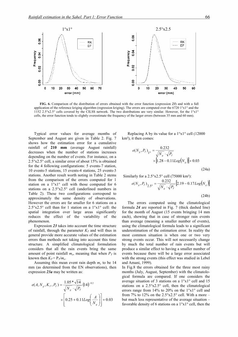
Rainfall estimation in the Sahel. Part 1: Error Function 66
1°x1°
FIG. 6. Comparison of the distribution of errors obtained with the error function
application of the reference kriging algorithm (regression kriging). The errors are comp1152 2.5°x2.5° cells covered by the CILSS network. The two distributions are very cells, the error function tends to slightly overestimate the frequency of the larger errors
Typical error values for average months of
September and August are given in Table 2. Fig. 7 shows how the estimation error for a cumulative rainfall of 210 mm (average August rainfall) decreases when the number of stations increases depending on the number of events. For instance, on a 2.5°x2.5° cell, a similar error of about 15% is obtained for the 4 following configurations: 5 events-7 station, 10 events-5 stations, 15 events-4 stations, 25 events-3 stations. Another result worth noting in Table 2 stems from the comparison of the errors computed for 1 station on a 1°x1° cell with those computed for 6 stations on a 2.5°x2.5° cell (underlined numbers in Table 2). These two configurations correspond to approximately the same density of observations. However the errors are far smaller for 6 stations on a 2.5°x2.5° cell than for 1 station on a 1°x1° cell: the spatial integration over large areas significantly reduces the effect of the variability of the phenomenon.
Expression 23 takes into account the time structure of rainfall, through the parameter KT and will thus in general provide more accurate values of the estimation errors than methods not taking into account this time structure. A simplified climatological formulation considers that all the rain events bring the same amount of point rainfall me, meaning that when PT is known then KT = PT/me.
Assuming this mean event rain depth me to be 14 mm (as determined from the EN observations), then expression 23a may be written as:
� �
03.011.025.0
1414*05.1),,,( 2.0
����
�
���
�
��
��
�
��
��
�
g
TgTTg
NALog
PNPKNAe
Replacing A by km²), it then comes
),(1
��
Tg PNe
Similarly for a 2.5°
Tg PNe ),(5.2 �
The errors comformula 24 are repfor the month of Aeach), showing thathan average (meanusing the climatolounderestimation of most common situstrong events occurby much the totalproduce a similar efevents because thewith the strong evenand Amani, 1999). In Fig.8 the errors months (July, Augugical formula are average situation ostations on a 2.5°xerrors range from 1from 7% to 12% onbut much less reprefavorable density of
2.5°x2.5
(expression 23) and with a full uted over the 6720 1°x1° and the similar. However, for the 1°x1° (between 35 mm and 60 mm).
its value for a 1°x1° cell (12000 :
� �� � 03.011.0821.
232.0
���
�
g
Tg
NLog
PN
(24a)
x2.5° cell (75000 km²):
� �� �gTg
NLogPN
17.02.19232.0�
�
�
(24b)
puted using the climatological orted in Fig. 7 (thick dashed line) ugust (15 events bringing 14 mm t in case of stronger rain events ing a smaller number of events),
gical formula leads to a significant the estimation error. In reality the ation is when one or two very . This will not necessarily change number of rain events but will fect to having a smaller number of
re will be a large error associated ts (this effect was studied in Lebel
obtained for the three most rainy st, September) with the climatolo-compared. If one considers the
f 3 stations on a 1°x1° cell and 15 2.5° cell, then the climatological 4% to 20% on the 1°x1° cell and the 2.5°x2.5° cell. With a more – sentative of the average situation – 6 stations on a 1°x1° cell, then the
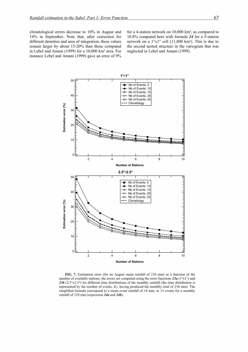
Rainfall estimation in the Sahel. Part 1: Error Function 67
climatological errors decrease to 10% in August and 14% in September. Note that, after correction for different densities and area of integration, these values remain larger by about 15-20% than those computed in Lebel and Amani (1999) for a 10,000 km² area. For instance Lebel and Amani (1999) gave an error of 9%
for a 4-station network on 10,000 km², as compared to 10.8% computed here with formula 24 for a 5-station network on a 1°x1° cell (11,800 km²). This is due to the second nested structure in the variogram that was neglected in Lebel and Amani (1999).
50
40
30
20
10
0
Estim
atio
n er
ror (
%)
108642
Number of Stations
Nb of Events: 5 Nb of Events: 10 Nb of Events: 15 Nb of Events: 20 Nb of Events: 25 Climatology
1°*1°
50
40
30
20
10
0
Estim
atio
n er
ror (
%)
108642
Number of Stations
Nb of Events: 5 Nb of Events: 10 Nb of Events: 15 Nb of Events: 20 Nb of Events: 25 Climatology
2.5°*2.5°
FIG. 7. Estimation error (for an August mean rainfall of 210 mm) as a function of the
number of available stations; the errors are computed using the error functions 23a (1°x1°) and 23b (2.5°x2.5°) for different time distributions of the monthly rainfall (the time distribution is represented by the number of events, KT, having produced the monthly total of 210 mm). The simplified formula correspond to a mean event rainfall of 14 mm, or 15 events for a monthly rainfall of 210 mm (expression 24a and 24b).
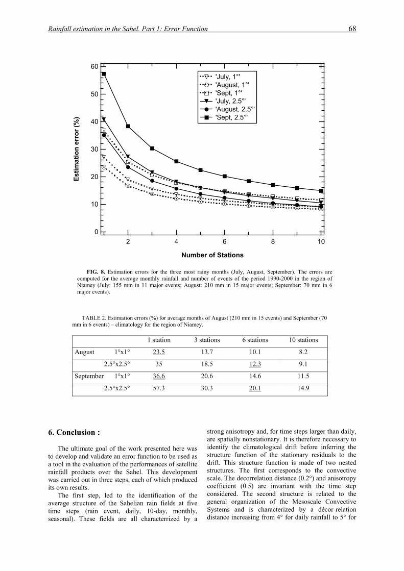
Rainfall estimation in the Sahel. Part 1: Error Function 68
60
50
40
30
20
10
0
Estim
atio
n er
ror (
%)
108642
Number of Stations
'July, 1°' 'August, 1°' 'Sept, 1°' 'July, 2.5°' 'August, 2.5°' 'Sept, 2.5°'
FIG. 8. Estimation errors for the three most rainy months (July, August, September). The errors are computed for the average monthly rainfall and number of events of the period 1990-2000 in the region of Niamey (July: 155 mm in 11 major events; August: 210 mm in 15 major events; September: 70 mm in 6 major events).
TABLE 2. Estimation errors (%) for average months of August (210 mm in 15 events) and September (70
mm in 6 events) – climatology for the region of Niamey.
1 station 3 stations 6 stations 10 stations
August 1°x1° 23.5 13.7 10.1 8.2
2.5°x2.5° 35 18.5 12.3 9.1
September 1°x1° 36.6 20.6 14.6 11.5
2.5°x2.5° 57.3 30.3 20.1 14.9
6. Conclusion :
The ultimate goal of the work presented here was
to develop and validate an error function to be used as a tool in the evaluation of the performances of satellite rainfall products over the Sahel. This development was carried out in three steps, each of which produced its own results.
The first step, led to the identification of the average structure of the Sahelian rain fields at five time steps (rain event, daily, 10-day, monthly, seasonal). These fields are all characterrized by a
strong anisotropy and, for time steps larger than daily, are spatially nonstationary. It is therefore necessary to identify the climatological drift before inferring the structure function of the stationary residuals to the drift. This structure function is made of two nested structures. The first corresponds to the convective scale. The decorrelation distance (0.2°) and anisotropy coefficient (0.5) are invariant with the time step considered. The second structure is related to the general organization of the Mesoscale Convective Systems and is characterized by a décor-relation distance increasing from 4° for daily rainfall to 5° for
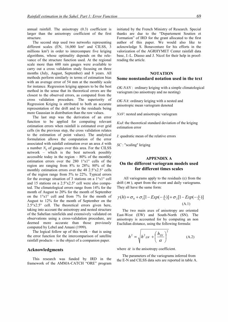
Rainfall estimation in the Sahel. Part 1: Error Function 69
annual rainfall. The anisotropy (0.3) coefficient is larger than the anisotropy coefficient of the first structure.
The second step used two networks representing different scales (EN, 16,000 km² and CILSS, 3 millions km²) in order to intercompare five kriging algorithms, whose optimality depends on the rele-vance of the structure function used. At the regional scale more than 600 rain gauges were available to carry out a cross validation study focusing on three months (July, August, September) and 8 years. All methods perform similarly in terms of estimation bias with an average error of 54 mm at the monthly scale for instance. Regression kriging appears to be the best method in the sense that its theoretical errors are the closest to the observed errors, as computed from the cross validation procedure. The superiority of Regression Kriging is attributed to both an accurate representation of the drift and to the residuals being more Gaussian in distribution than the raw values.
The last step was the derivation of an error function to be applied for computing relevant estimation errors when rainfall is estimated over grid cells (in the previous step, the cross validation relates to the estimation of point values). The analytical formulation allows the computation of the error associated with rainfall estimation over an area A with a number Ng of gauges over this area. For the CILSS network – which is the best network possibly accessible today in the region – 80% of the monthly estimation errors over the 280 1°x1° cells of the region are ranging from 8% to 28%; 80% of the monthly estimation errors over the 48 2.5°x2.5° cells of the region range from 5% to 22%. Typical errors for the average situation of 3 stations on a 1°x1° cell and 15 stations on a 2.5°x2.5° cell were also compu-ted. The climatological errors range from 14% for the month of August to 20% for the month of September on the 1°x1° cell and from 7% for the month of August to 12% for the month of September on the 2.5°x2.5° cell. The theoretical errors given here, taking into account the anisotropy and nested structure of the Sahelian rainfields and extensively validated on observations using a cross-validation procedure, are deemed more accurate than those previously computed by Lebel and Amani (1999).
The logical follow up of this work – that is using the error function for the intercomparison of satellite rainfall products – is the object of a companion paper. Acknowledgments
This research was funded by IRD in the
framework of the AMMA-CATCH “ORE” program
initiated by the French Ministry of Research. Special thanks are due to the “Departement Soutien et Formation” of IRD for the grant allocated to the first author of this paper. We would also like to acknowledge S. Bonaventure for his efforts in the valorization of the AGRHYMET Center rainfall data base, J.-L. Diasso and J. Nicol for their help in proof-reading the article.
NOTATION Some nonstandard notation used in the text OK-NAN : ordinary kriging with a simple climatological variogram (no anisotropy and no nesting) OK-NA: ordinary kriging with a nested and anisotropic mean variogram denoted NAV: nested and anisotropic variogram Ksd: the theoretical standard deviation of the kriging estimation error I: quadratic mean of the relative errors SC : "scaling" kriging
APPENDIX A On the different variogram models used
for different times scales All variograms apply to the residuals (�) from the drift ( ), apart from the event and daily variograms. They all have the same form:
m
)](1[)](1[)(
21 210 Sh
Sh ExpExph ������� ����
(A.1)
The two main axes of anisotropy are oriented East-West (EW) and South-North (SN). The anisotropy is accounted for by computing an non Euclidian distance, using the following formula:
222 �
�
���
���
�
SNEW
hhh (A.2)
where � is the anisotropy coefficient.
The parameters of the variograms inferred from the E-N and CILSS data sets are reported in table A.
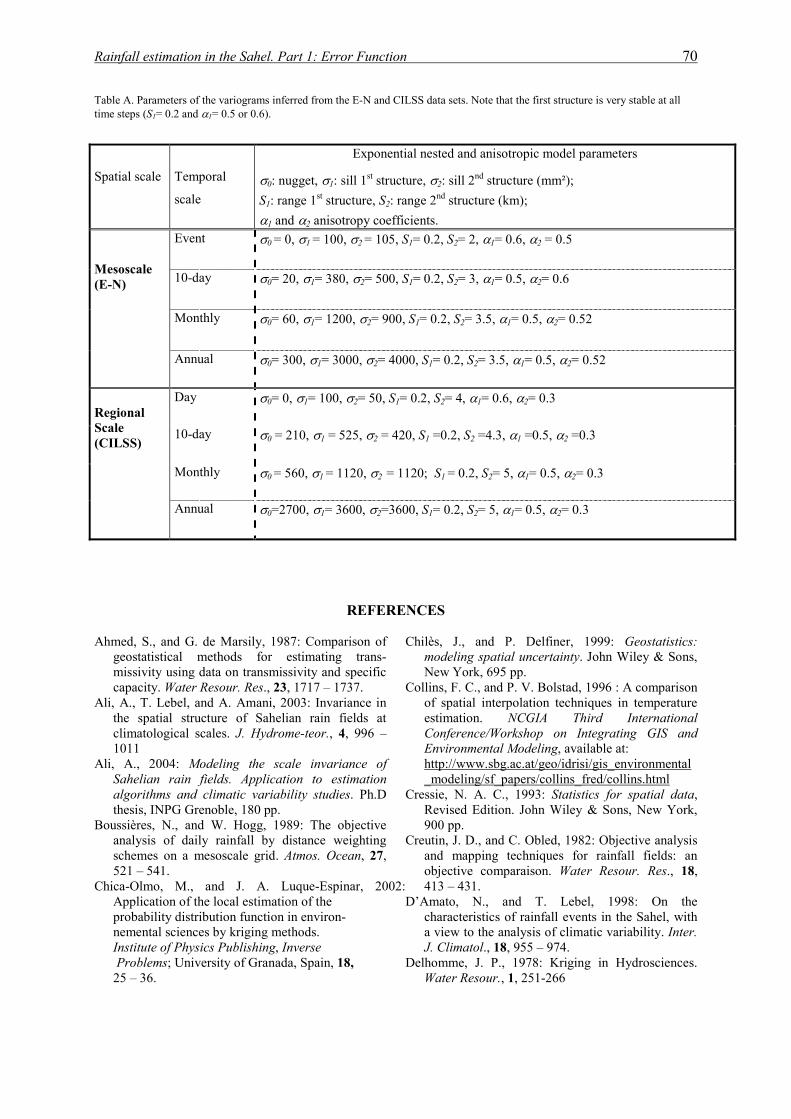
Rainfall estimation in the Sahel. Part 1: Error Function 70
Table A. Parameters of the variograms inferred from the E-N and CILSS data sets. Note that the first structure is very stable at all time steps (S1= 0.2 and �1= 0.5 or 0.6).
Spatial scale
Temporal
scale
Exponential nested and anisotropic model parameters
�0: nugget, �1: sill 1st structure, �2: sill 2nd structure (mm²); S1: range 1st structure, S2: range 2nd structure (km); �1 and �2 anisotropy coefficients.
Event �0 = 0, �1 = 100,��2 = 105, S1= 0.2, S2= 2,��1= 0.6, �2 = 0.5
10-day �0= 20, �1= 380,��2= 500, S1= 0.2, S2= 3,��1= 0.5, �2= 0.6
Monthly �0= 60, �1= 1200,��2= 900, S1= 0.2, S2= 3.5,��1= 0.5, �2= 0.52
Mesoscale (E-N)
Annual �0= 300, �1= 3000,��2= 4000, S1= 0.2, S2= 3.5,��1= 0.5, �2= 0.52
Day �0= 0, �1= 100,��2= 50, S1= 0.2, S2= 4,��1= 0.6, �2= 0.3
10-day �0 = 210, �1 = 525,��2 = 420, S1 =0.2, S2 =4.3,��1 =0.5, �2 =0.3
Monthly �0 = 560, �1 = 1120,��2 = 1120; S1 = 0.2, S2= 5,��1= 0.5, �2= 0.3
Regional Scale (CILSS)
Annual �0=2700, �1= 3600,��2=3600, S1= 0.2, S2= 5,��1= 0.5, �2= 0.3
REFERENCES Ahmed, S., and G. de Marsily, 1987: Comparison of
geostatistical methods for estimating trans-missivity using data on transmissivity and specific capacity. Water Resour. Res., 23, 1717 – 1737.
Ali, A., T. Lebel, and A. Amani, 2003: Invariance in the spatial structure of Sahelian rain fields at climatological scales. J. Hydrome-teor., 4, 996 – 1011
Ali, A., 2004: Modeling the scale invariance of Sahelian rain fields. Application to estimation algorithms and climatic variability studies. Ph.D thesis, INPG Grenoble, 180 pp.
Boussières, N., and W. Hogg, 1989: The objective analysis of daily rainfall by distance weighting schemes on a mesoscale grid. Atmos. Ocean, 27, 521 – 541.
Chica-Olmo, M., and J. A. Luque-Espinar, 2002: Application of the local estimation of the probability distribution function in environ- nemental sciences by kriging methods. Institute of Physics Publishing, Inverse Problems; University of Granada, Spain, 18, 25 – 36.
Chilès, J., and P. Delfiner, 1999: Geostatistics: modeling spatial uncertainty. John Wiley & Sons, New York, 695 pp.
Collins, F. C., and P. V. Bolstad, 1996 : A comparison of spatial interpolation techniques in temperature estimation. NCGIA Third International Conference/Workshop on Integrating GIS and Environmental Modeling, available at: http://www.sbg.ac.at/geo/idrisi/gis_environmental_modeling/sf_papers/collins_fred/collins.html
Cressie, N. A. C., 1993: Statistics for spatial data, Revised Edition. John Wiley & Sons, New York, 900 pp.
Creutin, J. D., and C. Obled, 1982: Objective analysis and mapping techniques for rainfall fields: an objective comparaison. Water Resour. Res., 18, 413 – 431.
D’Amato, N., and T. Lebel, 1998: On the characteristics of rainfall events in the Sahel, with a view to the analysis of climatic variability. Inter. J. Climatol., 18, 955 – 974.
Delhomme, J. P., 1978: Kriging in Hydrosciences. Water Resour., 1, 251-266
Rainfall estimation in the Sahel. Part 1: Error Function 71
Ecker, M. D., and A. E. Gelfand, 2003: Spatial Modeling and Prediction Under Range Aniso-tropy. Environ. Ecolog. Stat., 10, 165 – 178.
Furrer, R., 2002 : Aspects of modern geostatistics : nonstationarity, covariance estimation and state-space decompositions. Ph.D Thesis, Federal Institute of Technology in Lausanne (EPFL), Swiss, 139 pp.
Gandin, L. S., 1965: Objective analysis of meteorological fields, translated from Russian by R. Hardin, Israel Program for Scientific Translation, Jerusalem, 242 pp.
Guillot, G., and T. Lebel, 1999 : Approximation of Sahelian rainfall fields with metaGaussian random functions. Part 2: Parameter estimation and comparison to data. Stochastic Environmental Research and Risk Assessment, 13, 113-130.
Hengl, T., G. B. M. Geuvelink, and A. Stein, 2003: Comparison of kriging with external drift and regressing kriging. Technical note, ITC, available at: http://www.itc.nl/library/Academic_output/.
Huang, H. C., N. Cressie, and J. Gabrosek, 2000: Fast spatial prediction of global processes from satellite data. Technical Report, Department of statistics, the Ohio State University.
Huff, F. A., 1970: Sampling errors in measurement of mean precipitation. J. Appl. Meteor., 9, 35-44.
Huffman, G. J., 1997: Estimation of root-mean-square random error for finite samples of estimated precipitation. J. Appl. Meteor., 124, 939 – 963.
Goovaerts, P., 1997: Geostatistics for Natural Resources Evaluation. Oxford University Press, New York; 483 pp.
Journel, A. G., 1983: Nonparametric estimation of spatial distributions. Math. Geol., 15, 445 – 468.
Journel A. G., and C. J. Huijbregts, 1978: Mining geostatistics. Academic Press, London, 597 pp.
Lebel, T., and A. Amani, 1999: Rainfall Estimation in the Sahel : What is the ground truth? J Applied Meteor., 38 : 555 – 568.
Lebel, T., G. Bastin, C. Obled and J. D. Creutin, 1987: On the accuracy of areal rainfall estimation: a case study. Water Resour. Res., 23, 2123 – 2134.
Lebel T, A. Diedhiou and H. Laurent, 2003: Seasonal cycle and interannual variability of the Sahelian rainfall at hydrological scales. J Geophys Res, 108 , 8389 – 8392.
Matheron, G., 1969: Le krigeage universel. Cahiers du Centre de Morphologie Mathematique, Ecole de Mines de Paris, N°1, Fontainebleau.
Matheron, G., 1971: The theory of regionalised variables and its applications. Cahiers du Centre de Morphologie Mathematique Ecole de Mines de Paris, N° 5, Fontainebleau.
Matheron, G., 1976: A simple substitute for conditional expectation: The disjunctive kriging.
Advanced geostatistics in the mining industry, M., Guarascio, M., David, and Ch. J. Huijbregts, Eds., Reidel, Dordrecht, 221 – 236.
Moyeed, R.A., and A. Papritz, 2002: An empirical comparison of kriging methods for nonlinear spatial point prediction. Math. Geol., 34, 365 – 386.
Odeh, I., A. McBractney, D. Chittleborough, 1994: Further results on prediction of soil proprieties from terrain attributes: heterotopic cokriging and regression-kriging. Geoderma, 67, 215-226.
Papritz, A., and Stein, A., 1999: Spatial prediction by linear kriging. Spatial statistics for remote sensing, A., Stein, F. Van der Meer, and B. Gorte, Eds., Kluwer Academic publishers, Dodrecht, 83 – 113.
Philips, R. H., J. Dolph, and D. Marks, 1992: A comparison of geostatistical procedures for spatial analysis of precipitation in mountainous terrain. Agr. Forest Meteor., 58, 119 – 141.
Rivoirard, J. 1994. Introduction to disjunctive and Non-Linear Geostatistics. Oxford University Press, Oxford, 181 pp.
Royston, P., 1982 : An Extension of Shapiro and Wilk's W Test for Normality to Large Samples. Applied Statistics, 31, 115–124.
Rudolf, B., H. Hauschild, W. Rueth, and U. Schneider, 1994: Terrestrial precipitation analysis: operational methods and required density of point measurements. Global Precipitation and climate change, NATO ASI ser., M. Desbois and F. Desalmand, Eds., Vol.1, Springer-Verlag, New York, 173 – 186.
Sampson P., and P. Guttorp, 1992: Nonparametric estimation of Nonstationary Spatial Covariance Structure. J. Am. Stat. Assoc., 87, 108 – 119.
Seaman, R. S., 1983: Objective analysis accuracies of statistical interpolation and successive correction schemes. Aust. Met. Mag., 31, 225 – 240.
Vicente-Serrano, S. M., M. A. Saz-Sanchez, J. M. Cuadrat, 2003: Comparative analysis of interpo-lation methods in the middle Ebro Valley (Spain): application to annual precipitation and tempe-rature. Clim. Res., 24, 161-180.
Weber, D. D., and E. J. Englund, 1992: Evaluation and comparison of spatial interpolators. Math. Geol., 24, 381 – 391.
Willmott, C. J., 1984: On the evaluation of model performance in physical geography. Spatial Statistics and Models, G. L. Galle and C. J. Willmott, Eds., D. Reidel, 443 – 460.
Zimmerman, D. L., C. Pavlik, A. Ruggles and M. P. Armstrong, 1999: An experimental comparison of ordinary and universal kriging and inverse distance weighting. Math. Geol., 31, 375-390

Rainfall estimation in the Sahel. Part 1: Error Function 72
Complement* à l’article : “Rainfall estimation in the Sahel. Part 1: Error Function”
The scaling approach and its implementation at regional scale
* Ce complément n’est pas publié avec l’article, mais il détaille la procédure de mise en œuvre de la fonction d’erreur à l’échelle de toute la bande sahélienne utilisée dans l’article. On y notamment trouve la procédure de calcul du nombre d’événements à partir des cumuls de pluie journaliers.
a. Theoretical estimation error derived from the scaling approach
Ali et al. (2003) proposed a scaling approach to
describe the structure of Sahelian rainfields over a range of time scales. For any value of KT (KT = total number of rain events over the whole region during the period considered), the scale invariant approach permits a direct computation of the associated variogram �K for the KT event cumulative rainfields: �
�
�)(])()[(
)()]([)(22 hm
hhmKh
Iee
eIITK
��
���
��
��
�����������(B.1)
where �e(h) is the event variogram (see Table B) and �I(h) is the indicator variogram (see Table B); me, �e², mI, �I² represent respectively the mean and the variance of the rain process at the event time scale, and the mean and the variance of the indicator, also at the event time scale.
The estimation error associated with the estimation of the areal rainfall over an area A sampled by a network C is defined as (Journel and Huijbregts, 1978):
�K²(C,A)= –��00 –��NN –2�0N (B.2)
with
���
AK Adh
A2
200 )(1�� (B.2a)
��� �
�
N
i
N
jijKjiNN h
1 1
)(���� (B.2b)
���
�
A ixK
N
iiON dAh
A)(1
1��� (B.2c)
Assuming that the event variogram and the
indicator variogram are independent, relation (B.2) yields:
)],(),(),()(),([),( 22222
ACACmACmACmKAC
IeI
IeeeITK
��
����
�
���
(B.3)
where �e²(C,A) is the event kriging variance, and �I²(C,A) is the indicator kriging variance. The knowledge of KT is sufficient to compute the error at any time scale. Note that the scale relation can be used for kriging or for the direct computation of the error associated with a given network C, after evaluating the error at the event scale. �e²(C,A) and �I²(C,A) are computed using expressions B.2 through B.2c where �K is replaced by �e and �I respectively. The application of the scaling approach at the regional scale and for large grids encounters two major difficulties: i) when only daily reading gauges are available, a direct determination of the rain event is not possible, and the hypothesis is made that the number of rain events over a grid can be determined from the number of rainy days, ii) it has to be determined how a given day will be considered as a rainy day for a given cell.
TABLE B. Parameters of the daily indictor variogram model (expression A.1)
Spatial scale
Temporal scale
Exponential nested and anisotropic model parameters
�0: nugget, �1: sill 1st structure, �2: sill 2nd structure (mm²); S1: range 1st structure, S2: range 2nd structure (km); �1 and �2 anisotropy coefficients.
Regional (CRA) Daily Indicator �0= 0.085, �1= 0.06,��2= 0.095, S1= 0.12, S2= 4.1,��1= 1, �2= 0.5
Rainfall estimation in the Sahel. Part 1: Error Function 73
b. Adaptation of the scaling approach when only daily observation are available
1. FILTERING OUT THE ISOLATED SMALL RAIN EVENTS
Five approaches to determine the number of events
have been tested in order to filter out small isolated systems whose contribute less than 10% of the total JAS rainfall.
The first three approaches are based on the exploration of the 8 cells surrounding the cell of interest (Fig. B.1), thus forming a 3x3 window. In the first approach 2x2-cell windows are taken into account (case 1 in Fig. B.1). In the second approach 2x3-cell windows are used (case 2 in Fig. B.1). In both cases there are four possible configurations. In the third approach the whole 3x3 window is considered (case 3 in Fig. B.1). For each of these three cases, all the windows are explored and the percentage p of gauges reporting rainfall in each of them is computed. A threshold �p is then determined. If p>�p, for at least one of the four possible configurations of cases 1 and 2 the day is counted as being “rainy” for the central cell of the 3x3 window. For case 3 the criterion applies to the whole 3x3 window.
The fourth method consists of kriging the indicator for the cell under consideration (value = 1 at the gauge if daily rainfall is larger than 0.5 mm; value = 0 otherwise). Using the E-N area as a test area it was then shown that the cell could be considered as associated with a major rain event if the integral of the indicator over the cell is larger or equal to 0.4.
The fifth approach consists in kriging the indicator at 50 nodes into the grid. The day is considered as associated with a major rain event if the percentage of nodes with value 1 is over a threshold (threshold values of 20 and 30% were tested).
The criterion to determine the optimal threshold for each method and then to determine the best of the five approaches was the capacity of reproducing the number of rainy days computed on the E-N study area (where a major rainy day can be precisely known). The best method is the first approach with a threshold value �p =20%. The correlation coefficients between the number of major rainy days during a month determined by these approaches with the CRA data and the number of the rainy days directly
computed from the E-N data is 0.96 for the best approach, 0.91 for the fourth approach and 0.87 for the fifth approach.
2. ADDITIONAL CORRECTION FOR TWO DIFFERENT
SYSTEMS BEING PRESENT IN THE WINDOW
Another bias in the computation of the number of rain events from the number of rainy days is linked to the possibility of having two different systems in the window the same day. When comparing the error distribution of SC to that of RK, it is seen that the SC distribution is shifted to the left (Fig B2), indicating an underestimation of the errors that can be attributed to an underestimation of KT in expression B.3. This is consistent with the results obtained in Table 1 for the estimation of point values (non adapted SC tends to underestimate the estimation errors). The following procedure was followed in order to compute an optimal value of KT ( ) TT KK **
��
Since RK was shown to be the best linear unbiased estimator for the region studied here, it is used as a reference. The theoretical RK monthly estimation errors associated with the CRA network are computed for each grid cell of the regional study area (280 1°x1° cells and 48 2.5°x2.5° cells) and for 24 months (JAS for 8 years). The distributions of the 1° errors (6720 values) and of the 2.5° errors (1152 values) are the references to which the SC distribution of errors is compared. The optimal value �� is the one for which the best matching is obtained
between the RK and SC theoretical distributions of errors. As may be seen from Fig. B2, the values �� = 1.2 for 1°x1° grid cells and �� = 1.5 for 2.5°*2.5° grid cells provide a good matching between the RK and SC theoretical distributions of errors. As expec-ted the optimal value �� is scale dependant, since the probability of having two different rain events occurring on a grid cell for a given day increases with the size of the cell.
Replacing KT by K*T in expression B.3 leads to
expression B.4 which allows the computation of more realistic estimation errors with the SC method and to the calculation of the error function presented in section 5 of this paper.
)],(),(),()(),([),( 2222*2 ACACmACmACmKAC IeIIeeeITK ������ ���� (B.4)

Rainfall estimation in the Sahel. Part 1: Error Function 74
1.
2.
3.
FIG. B1. Different approaches to filter out the rainy days associated with small isolated rain events.
Rainfall estimation in the Sahel. Part 1: Error Function 75
1°x1°
FIG. B2. adaptation of the scaling approach. After optimal d(see appendix B for detail), the distribution of the ksd from the SC and 2.5°x2.5° grid, which is conform with the table 1: the SC un
adaptation yields = 1.2 over 1°x1° and = 1.5
figure show a good agreement between the SC adapted and the RK op
*TK dayN *
TK N
2.5°x2.5
etermination of the major rainy day is left shifted both for the 1°x1° grid derestimates the error variance. The
over 1.5°x1.5° . And the final
timal reference value. day

Rainfall estimation in the Sahel. Part 1: Error Function 76
Rainfall Estimation in the Sahel. Part 2 7
Article Rainfall Estimation in the Sahel. Part 2
Evaluation of Raingauge Networks in the CILSS Countries anObjective Intercomparison of Satellite Rainfall Products
7
d
Rainfall Estimation in the Sahel. Part 2 9
Rainfall Estimation in the Sahel. Part 2: Evaluation of RaingauNetworks in the CILSS Countries and Objective Intercomparis
of Satellite Rainfall Products.
Abdou ALI1,2, Abou AMANI2, Arona DIEDHIOU1, Thierry LEBEL1
Submitted for publication in Journal of Applied Meteorology
Abstract
This study concerns the accuracy of ground-based precipitation estimates and those of various satelliteproducts in the Sahelian region covering the period 1986 to 2000. The evaluation of the entire operationanetwork of Sahelian countries indicates that on average the monthly estimation error for the July, AugustSeptember period (JAS) is around 12% at spatial scale 2.5°x2.5°. The estimation error increases fromsouth to north and remains below 10% for the area south of 15°N and west of 11°E (representing 42% othe region studied). In the Southern Sahel (South of 15°N) the rain gauge density needs to be at least 10gauges per 2.5°x2.5° grid cell for a monthly error of less than 10%. In the Northern Sahel this densityincreases to more than 20 gauges, due to the large intermittency of rainfall. In contrast, for othecontinental regions outside Africa, some authors have found that only 5 gauges per 2.5°x2.5°grid cell areneeded to give a monthly error of less than 10%.
The satellite products considered in this comparison are: CMAP, GPCP, GPCC and GPI*. Twooperational networks (CRA* and synoptic) of smaller density than the entire reference network are alsoconsidered. Several methods (scatter plots, distribution comparisons, root mean square error, bias, NashIndex, significance test for the mean, variance and distribution function and the standard deviationapproach for the kriging interval) are first used for the intercomparison. All these methods lead to thesame conclusion that CMAP is the best product overall, followed by GPCC, GPCP and GPI with largeerrors for GPI. However, based on the root mean square error, it is found that the ground rainfall producobtained from the CRA and synoptic networks are better than the four satellite products in the regionFinally, based on the error function developed in a companion paper, an approach is proposed to take intoaccount the uncertainty due to the fact that the reference values are not the real ground truth. This methodwas applied to the most densely sampled region in the Sahel and led to a significant decrease of the rawevaluation errors. The re-evaluated error is independent of the gauge references.
* For acronyms see section 3
* Corresponding author address: Abdou ALI, LTHE, BP 53 38041 Grenoble Cedex 9, France [email protected]
1IRD, LTHE, Grenoble, France 2Centre AGRHYMET, Niamey, Niger
7
ge on
l ,
f
r
t .
Rainfall Estimation in the Sahel. Part 2 0
1. Introduction
Various rainfall products, widely available through Internet, are increasingly used as standard input to run hydrological and crop models or to validate atmospheric model outputs. In general, these products combine information from satellites – Infrared imagers (IR), Microwave Imager (such as SSM/I), Radars (TRMM) – and/or raingauges. In recognition of the necessity to evaluate these rainfall products as rigorously as possible, several studies (e.g., Morrissey and Greene 1993; Chiu et al. 1993; Xie and Arkin 1995; Ebert and Maton 1998; Bell et al. 2001; Adler et al. 2001; Ha et al. 2002) have assessed the quality of products from different parts of the world and have shown that the performance of algorithms and the added value of rainfall products may depend on the region concerned (Kummerow 2004).
For at least three main reasons, such a validation is especially needed in West-Africa: i) the severe drought that started in the beginning of the 1970’s, has made precipitation more irregular and more difficult to estimate; ii) after reaching a peak in the early 1980’s, in situ networks are now becoming less dense iii) West-Africa is one of the world's most sensitive regions in terms of precipitation variability because its economy is still largely dependent on rain-fed agriculture.
Several papers dealing with rainfall estimation in Africa were published in recent years, such as those of Thorne et al. (2001) for South Africa and McCollum (2000) in equatorial Africa. In West Africa, Laurent et al. (1998) compared and discussed the validation of estimates resulting from five satellites methods, while Ramage et al. (2000) compared rainfall products with different resolutions in Niger. Jobard (2001) reviewed satellite-based rainfall retrieval using multi-source data. However, a comprehensive evaluation of various rainfall products remains to be carried out for Africa. The work presented here may be considered as one step in that direction. Focusing on the Sahel, it adds to previous work in several ways. Firstly it explicitly addresses the problem that the reference values are not the real ground truth (section 2). Secondly, as explained in section 3, this study covers a longer period (1986-2000) than any previous work carried out in West Africa, thus dealing with a much larger range of climatological conditions. Thirdly, based on the error function developed in a companion paper (Ali et al. 2004), this study deals with both ground-based estimates and satellite products (sections 4 and 5). Finally, a way of incorporating the uncertainty associated with reference rainfields into the assessment of the quality of satellite estimates is tested in section 6. 2. Problem Statement and Methodology a. Generalities
Satellite-based rainfall estimates have beeimportant research topic since the first operamethods were proposed in the early 1980’s [e.g.the initial review of Barret and Martin 1981, more recent analyses of Petty 1995, dealingsatellite rainfall estimation over land, and Levizzal. 2001, dealing with future perspectives]. important points must be considered with respsatellite-based estimate evaluation and intercomson. First, satellite-based estimates are areal vwhile ground based references are point vraising the question of the significance of stacomputed using a reference estimate instead ounknown true value. The second concern is linkthe objectives of the evaluation and intercomparaising the question of which statistics should beIn others words, which products give theestimates and in what ways these estimates are bSeveral statistics will be used here to substantiatanalysis. Traditionally, estimate evaluation haemphasis on bias (correspondence between values), co-fluctuation (the strength of the relationship between the estimate and a refevalue) and accuracy (the point by point levagreement between the estimate and the referHowever, other performance characteristicsimportant in assessing the quality of an estimatexample, a difference in the frequency of low vfor two products having similar mean statisticsgreat importance for agricultural applications. Oother hand, upper extreme values are of gimportance in hydrology. b. Relationship between statistics computed a reference value and those of the unknownvalue
The most usual statistics used in satellite pr
evaluation relate to the bias (b), the root mean serror (RMSE) and the correlation coefficient (rmore details and discussion of these stastatistics, see, for example, Stanski et al. (1These statistics are in general computed froestimated reference value (bSR, RMSESR, rSR). Ifollowing, the bias and the root mean square errcomputed using the true reference value RMSEST). As this true reference is unknownstatistics will be expressed as a function of derived from the estimated reference value.
Considering that RS is a satellite estimate, Rtrue unknown value and RR the reference valuwill be the bias of RS with respect to RT, bSR the bRS with respect to RR and bRT the bias of RRrespect to RT. Also RMSEST, RMSESR, RMSERT wthe respective RMSEs. Thus:
�� bST = )( TS RRE �
= E )()( TRRS RRERR ���
= bSR + bRT
8
n an tional from to the with ani et Two
ect to pari-alues
alues, tistics f the ed to rison, used. best etter. e this s laid mean linear rence el of ence). are e. For alues is of n the reater
using true
oduct quare ). For ndard 989).
m an n the or are
(bST, , the those
T the e, bST ias of with ill be
(1)
Rainfall Estimation in the Sahel. Part 2 1
So if the reference value is unbiased, the bias of the satellite estimate with respect to this reference value is the true bias. �� Computation of RMSEST Denoting: �SR = RS –RR ; �ST = RS -RT ; �RT = RR -RT and:
2SR�
� = = ( ; 2)( RS RRE �
2)SRRMSE2ST�
� = = ; 2)( TS RRE �
2)( STRMSE2RT�
� = = and 2)( TR RRE �2)( RTRMSE
since RS –RR = (RS – RT ) – (RR –RT), we have:
� )()(2)(
),(2)(2
22
TRTSTR
TRTSTSSR
RRERRERRE
RRRRCovRRE
�����
������
(2) or:
��
2ST� � -� + 2 Cov2
SR�
2RT�
),( RTST ��
+ 2bST�bRT (3) The relationships above show how the bias and the
random error of the reference value can have a significant influence on the computation of the raw statistics. The evaluation of the reference value is thus a crucial part of any objective validation and inter-comparison exercise.
Using these relationships, two approaches are possible. First, one can directly base the analysis on the raw statistics computed using the estimated reference values, without taking into account their uncertainty. This means that more confidence is given to the reference value than to the evaluated products. This is acceptable if the reference value error is much smaller than the expected error of the evaluated product.
This is, for example, the implicit assumption of Nicholson et al. (2003) in their comparison of rain products, which does not include a quantification of the possible error of the reference. This makes it difficult to assess the degree of significance of the statistics obtained. Thorne et al. (2001), on the other hand, evaluate the reference uncertainty to draw attention to the significance of their statistics, but do not use it directly in their calculation.
The second approach is more objective but also more complicated. The statistics (bST, RMSEST) are related to the true unknown values. Considering Eqs. (1), and (3), this approach first requires estimation of the following associated statistics: bRT, RMSERT,
. Correction of the raw RMSE (RMSE
),( RTSTCov ��
SR) has been attempted by some authors. Branston (1991), Ciach and Krajewski (1999), Gebremichael et al. (2003), for instance, have used Eq. (3) in which they assume and b
),( RTSTCov ��
ST�bRT to be equal to zero. The method has been called EVS (error variance separation) and Eq. (3) becomes:
��
2ST� � - � 2
SR�
2RT�
In others words, the satellite product error
ground product errors are assumed to be indepenSince “satellite” products often consist of a mergraingauge data and satellite information, the referaingauge and satellite products have some cominformation, which implies that Covnot be equal to zero and its influence masignificant in relation (3). The importanc
may depend on the relation bethe gauges used for validation and the gauges are included in satellite estimates. This situatiocritical point for large scale validation exercissatellite products in West-Africa, since the avaraingauge network generally used to createreference value is often not dense and notdifferent from the network used to create the msatellite products. Moreover, the nongaussianirain-fields accentuates the effects of the compbias. The application of the assumption that thecovariance is equal to zero must be consideredmuch attention. We analyze below how to accouground-based sampling error in the evaluation ersatellite products i.e how can RMSE
),( RTST ��
),( RTSTCov ��
ST be computapplication of Eq. (3) without neglectingcovariance. The results obtained with and wtaking into account the reference uncertainty wcompared.
a. Estimation of the terms of equation (3)
In order to assess the RMSEST from Eq. (3terms bRT, RMSERT, are estimatfollow.
),( RTSTCov ��
1) ESTIMATION OF THE TERM RMSERT The question of computing RMSERT has
treated in the companion paper, Ali et al. (200cross validation procedure has been useinvestigate different kriging methods designeimprove the calculation of the ground-based (RMSERT). A relative error function [Eq. (5) bhas been established and will be used here focomputation of RMSERT.
���
�
��
�
�
� �
���
�
�
��
�
g
T
T
TgTTg
NALog
KP
KNPKNAe
17.028.0
05.1),,,(2.0
with: AA
grid area in km², number of raingauges in
, number of events during the consiperiod, cumulative rainfall over the same per
gN
TKPT
8
(4)
s and dent.
ing of rence mon
may y be e of tween which n is a es of ilable the
very erged ty of uting
error with nt for ror of ed by the ithout ill be
), the ed as
been 4). A d to d to error
elow] r the
���
�
(5)
area
dered iod in
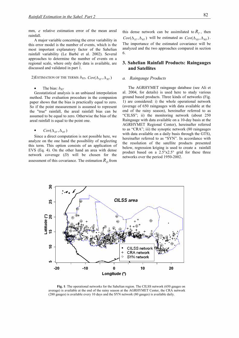
Rainfall Estimation in the Sahel. Part 2 2
mm, relative estimation error of the mean areal rainfall.
e
A major variable concerning the error variability in this error model is the number of events, which is the most important explanatory factor of the Sahelian rainfall variability (Le Barbé et al. 2002). Several approaches to determine the number of events on a regional scale, where only daily data is available, are discussed and validated in part 1.
2)ESTIMATION OF THE TERMS: bRT, Cov ),( RTST ��
�� The bias: bRT Geostatistical analysis is an unbiased interpolation
method. The evaluation procedure in the companion paper shows that the bias is practically equal to zero. So if the point measurement is assumed to represent the "true" rainfall, the areal rainfall bias can be assumed to be equal to zero. Otherwise the bias of the areal rainfall is equal to the point one.
�� ),( RTSTCov ��
Since a direct computation is not possible here, we analyze on the one hand the possibility of neglecting this term. This option consists of an application of EVS (Eq. 4). On the other hand an area with dense network coverage (D) will be chosen for the assessment of this covariance. The estimation from
this dense network can be assimilated to , will be estimated as Cov
The importance of the estimated covariance wanalyzed and the two approaches compared in se6.
DR
TR,SD�),( RTSTCov �� ( �
3. Sahelian Rainfall Products: Rainga
and Satellites a. Raingauge Products
The AGRHYMET raingauge database (see
al. 2004, for details) is used here to study vaground based products. Three kinds of networks1) are considered: i) the whole operational ne(average of 650 raingauges with data available end of the rainy season), hereinafter referred “CILSS”; ii) the monitoring network (aboutRaingauge with data available on a 10-day basis AGRHYMET Regional Center), hereinafter reto as “CRA”; iii) the synoptic network (80 raingwith data available on a daily basis through the Ghereinafter referred to as “SYN”. In accordancethe resolution of the satellite products presbelow, regression kriging is used to create a raproduct based on a 2.5°x2.5° grid for these networks over the period 1950-2002.
Fig. 1: The operational networks for the Sahelian region. The CILSS network (650 gauges on average) is available at the end of the rainy season at the AGRHYMET Center, the CRA network (280 gauges) is available every 10 days and the SYN network (80 gauges) is available daily.
8
then .
ill be ction
)RD
uges
Ali et rious (Fig. twork at the to as 250 at the ferred auges
TS), with ented infall three
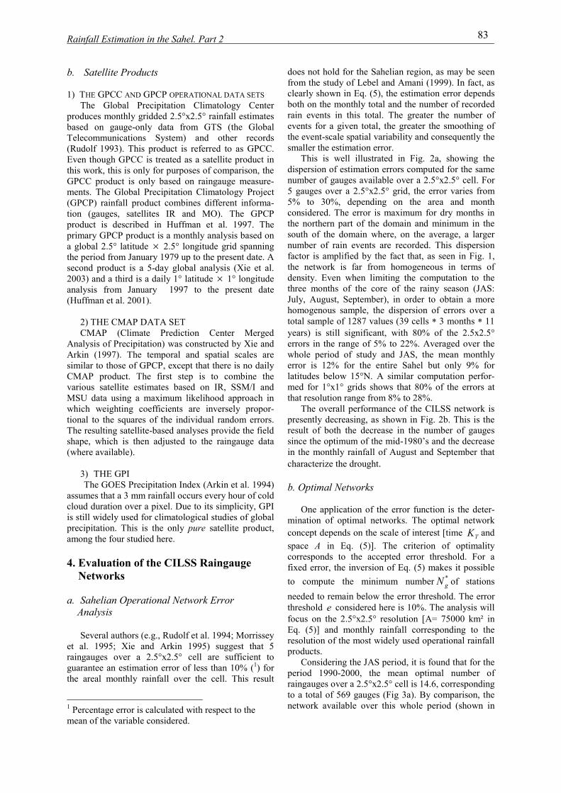
Rainfall Estimation in the Sahel. Part 2 - 3
b. Satellite Products 1) THE GPCC AND GPCP OPERATIONAL DATA SETS
The Global Precipitation Climatology Center produces monthly gridded 2.5°x2.5° rainfall estimates based on gauge-only data from GTS (the Global Telecommunications System) and other records (Rudolf 1993). This product is referred to as GPCC. Even though GPCC is treated as a satellite product in this work, this is only for purposes of comparison, the GPCC product is only based on raingauge measure-ments. The Global Precipitation Climatology Project (GPCP) rainfall product combines different informa-tion (gauges, satellites IR and MO). The GPCP product is described in Huffman et al. 1997. The primary GPCP product is a monthly analysis based on a global 2.5° latitude 2.5° longitude grid spanning the period from January 1979 up to the present date. A second product is a 5-day global analysis (Xie et al. 2003) and a third is a daily 1° latitude � 1° longitude analysis from January 1997 to the present date (Huffman et al. 2001).
�
2) THE CMAP DATA SET CMAP (Climate Prediction Center Merged
Analysis of Precipitation) was constructed by Xie and Arkin (1997). The temporal and spatial scales are similar to those of GPCP, except that there is no daily CMAP product. The first step is to combine the various satellite estimates based on IR, SSM/I and MSU data using a maximum likelihood approach in which weighting coefficients are inversely propor-tional to the squares of the individual random errors. The resulting satellite-based analyses provide the field shape, which is then adjusted to the raingauge data (where available).
3) THE GPI The GOES Precipitation Index (Arkin et al. 1994)
assumes that a 3 mm rainfall occurs every hour of cold cloud duration over a pixel. Due to its simplicity, GPI is still widely used for climatological studies of global precipitation. This is the only pure satellite product, among the four studied here. 4. Evaluation of the CILSS Raingauge Networks
a. Sahelian Operational Network Error Analysis
Several authors (e.g., Rudolf et al. 1994; Morrissey
et al. 1995; Xie and Arkin 1995) suggest that 5 raingauges over a 2.5°x2.5° cell are sufficient to guarantee an estimation error of less than 10% (1) for the areal monthly rainfall over the cell. This result
does not hold for the Sahelian region, as may befrom the study of Lebel and Amani (1999). In faclearly shown in Eq. (5), the estimation error deboth on the monthly total and the number of recrain events in this total. The greater the numbevents for a given total, the greater the smoothithe event-scale spatial variability and consequentsmaller the estimation error.
1 Percentage error is calculated with respect to the mean of the variable considered.
This is well illustrated in Fig. 2a, showindispersion of estimation errors computed for thenumber of gauges available over a 2.5°x2.5° cel5 gauges over a 2.5°x2.5° grid, the error varies5% to 30%, depending on the area and mconsidered. The error is maximum for dry monthe northern part of the domain and minimum south of the domain where, on the average, a number of rain events are recorded. This dispfactor is amplified by the fact that, as seen in Fthe network is far from homogeneous in termdensity. Even when limiting the computation tthree months of the core of the rainy season July, August, September), in order to obtain a homogenous sample, the dispersion of errors ototal sample of 1287 values (39 cells * 3 monthsyears) is still significant, with 80% of the 2.5errors in the range of 5% to 22%. Averaged ovwhole period of study and JAS, the mean moerror is 12% for the entire Sahel but only 9%latitudes below 15°N. A similar computation pmed for 1°x1° grids shows that 80% of the errthat resolution range from 8% to 28%.
The overall performance of the CILSS netwpresently decreasing, as shown in Fig. 2b. This result of both the decrease in the number of gsince the optimum of the mid-1980’s and the decin the monthly rainfall of August and Septembecharacterize the drought.
b. Optimal Networks
One application of the error function is the mination of optimal networks. The optimal neconcept depends on the scale of interest [time space A in Eq. (5)]. The criterion of optimcorresponds to the accepted error threshold. fixed error, the inversion of Eq. (5) makes it poto compute the minimum number of stneeded to remain below the error threshold. Thethreshold considered here is 10%. The analysifocus on the 2.5°x2.5° resolution [A= 75000 kEq. (5)] and monthly rainfall corresponding tresolution of the most widely used operational raproducts.
K
*gN
e
Considering the JAS period, it is found that fperiod 1990-2000, the mean optimal numbraingauges over a 2.5°x2.5° cell is 14.6, correspoto a total of 569 gauges (Fig 3a). By comparisonetwork available over this whole period (sho
8
seen ct, as pends orded er of ng of ly the
g the same l. For from
onth ths in in the larger ersion ig. 1, s of
o the (JAS: more ver a * 11 x2.5° er the nthly for
erfor-ors at
ork is is the auges rease r that
deter-twork
and ality
For a ssible ations error s will m² in o the infall
T
or the er of nding n, the wn in
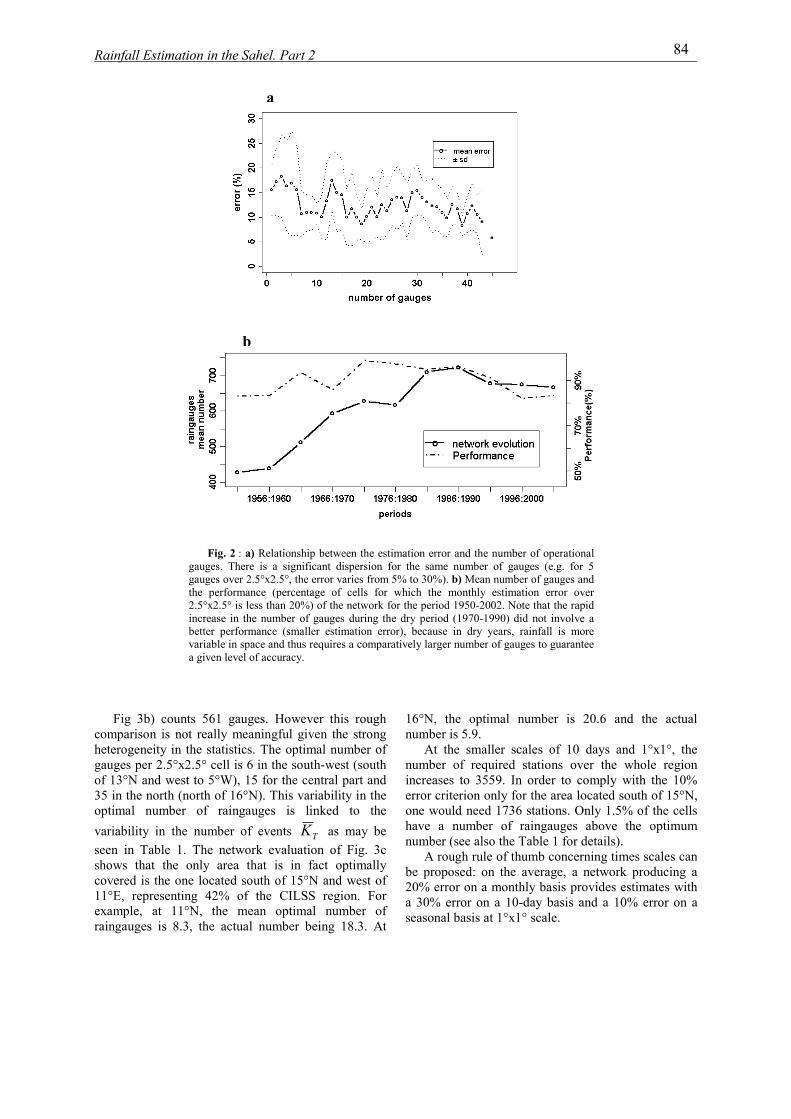
Rainfall Estimation in the Sahel. Part 2 - 4
a
Fig. 2gauges. Tgauges ovthe perfor2.5°x2.5° increase inbetter pervariable ina given lev
Fig 3b) counts 561 gcomparison is not really mheterogeneity in the statistgauges per 2.5°x2.5° cell iof 13°N and west to 5°W)35 in the north (north of 1optimal number of rainvariability in the numberseen in Table 1. The netshows that the only areacovered is the one located11°E, representing 42% example, at 11°N, the raingauges is 8.3, the act
b
: a) Relationship between the estimation error and the number of operational here is a significant dispersion for the same number of gauges (e.g. for 5 er 2.5°x2.5°, the error varies from 5% to 30%). b) Mean number of gauges and mance (percentage of cells for which the monthly estimation error over is less than 20%) of the network for the period 1950-2002. Note that the rapid the number of gauges during the dry period (1970-1990) did not involve a
formance (smaller estimation error), because in dry years, rainfall is more space and thus requires a comparatively larger number of gauges to guarantee el of accuracy.
auges. However this rough eaningful given the strong
ics. The optimal number of s 6 in the south-west (south , 15 for the central part and 6°N). This variability in the gauges is linked to the
of events TK as may be work evaluation of Fig. 3c that is in fact optimally south of 15°N and west of of the CILSS region. For mean optimal number of ual number being 18.3. At
16°N, the optimal number is 20.6 and the number is 5.9.
At the smaller scales of 10 days and 1°x1number of required stations over the whole rincreases to 3559. In order to comply with theerror criterion only for the area located south of one would need 1736 stations. Only 1.5% of thehave a number of raingauges above the optnumber (see also the Table 1 for details).
A rough rule of thumb concerning times scalebe proposed: on the average, a network produc20% error on a monthly basis provides estimatesa 30% error on a 10-day basis and a 10% errorseasonal basis at 1°x1° scale.
8
actual
°, the egion 10% 15°N, cells imum
s can ing a with on a
Rainfall Estimation in the Sahel. Part 2 5
Fig. 3: a) Mean optimal number of gauges per grid cell (2.5°x2.5°) which provide the estimation error of less than 10% at the monthly scale for the period 1990-2000. b) Actual mean number of gauges of the CILSS operational network for the same period. c) The difference between a) and b). The CILSS operational network guarantees a monthly error smaller than 10% for 42 % of the grid cells, located south to 15°N and west of 11° E.
c
b
a
Table 1: Details on the characteristics of optimal networks and the evaluation of the CILSS operational network for differenand for two scales: monthly values over 2.5°x2.5° grid cells and 10-day values over 1°x1° grid cells. The only area over whCILSS network is optimal everywhere for the 2.5°x2.5° resolution is the area lying south of 15°N and west of 11°E. is the a
number of gauges per cell satisfying the optimality criterion and is the average number of gauges per cell of the CILSS n
over the sub-area. Optimality corresponds to grid cells for which the error is less than 10%.
*gN
realgN
area TK *gN real
gN real
g
greal
g
NNN *
�
Number optimal c
total 11.8 14.6 14.4 -1% 42%
10-12.5° lat 16.3 8.2 18.3 55% 72%
12.5°-15° lat 12.1 11.2 21.1 47% 69%
15°-17.5° lat 7 20.6 5.9 -248% 0%
Monthly
values
(JAS)
2.5°x2.5°
<15° lat & West of 11°E
11.27 9.9 27.1 82% 100%
total 5.6 16.7 2.6 -538% 1.5%
10°-13°lat 7.33 11 3.4 -223% 2%
13-15° lat 6 14.25 3.6 -296 2.8%
15-18° lat 3.9 23.4 1.2 -1900% 0%
10-day
values
1°x1° <15° lat & West of 11°E
6.8 12.2 4.5 -169% 3.2%
8
t areas ich the verage
etwork
of ells
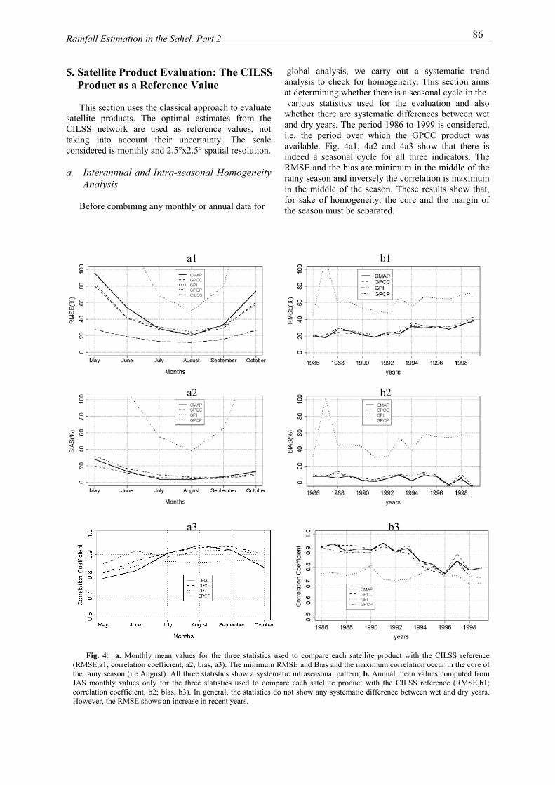
Rainfall Estimation in the Sahel. Part 2 - 6
5. Satellite Product Evaluation: The CILSS Product as a Reference Value
This section uses the classical approach to evaluate satellite products. The optimal estimates from the CILSS network are used as reference values, not taking into account their uncertainty. The scale considered is monthly and 2.5°x2.5° spatial resolution.
a. Interannual and Intra-seasonal Homogeneity
Analysis
Before combining any monthly or annual data for
global analysis, we carry out a systematic trend analysis to check for homogeneity. This section aims at determining whether there is a seasonal cycle in the various statistics used for the evaluation and also whether there are systematic differences between wet and dry years. The period 1986 to 1999 is considered, i.e. the period over which the GPCC product was available. Fig. 4a1, 4a2 and 4a3 show that there is indeed a seasonal cycle for all three indicators. The RMSE and the bias are minimum in the middle of the rainy season and inversely the correlation is maximum in the middle of the season. These results show that, for sake of homogeneity, the core and the margin of the season must be separated.
Fig. 4: a. Monthly mean values for the three statistics used (RMSE,a1; correlation coefficient, a2; bias, a3). The minimum RMSthe rainy season (i.e August). All three statistics show a systematicJAS monthly values only for the three statistics used to compare correlation coefficient, b2; bias, b3). In general, the statistics do noHowever, the RMSE shows an increase in recent years.
a1 b1
a2 b2
a3
to compare each satellite product with the CILSS refE and Bias and the maximum correlation occur in the
intraseasonal pattern; b. Annual mean values computeeach satellite product with the CILSS reference (RMt show any systematic difference between wet and dry
b3
8
erence core of d from SE,b1; years.
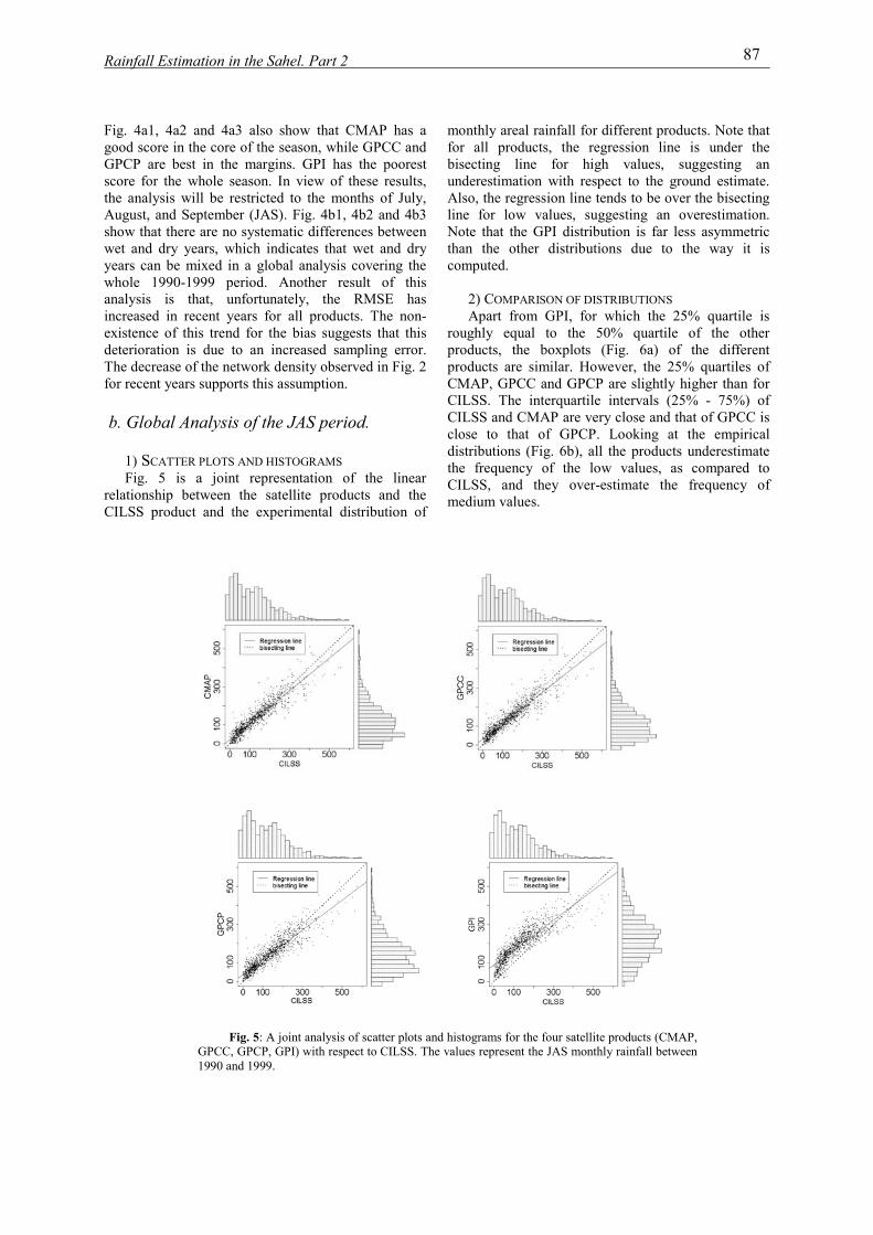
Rainfall Estimation in the Sahel. Part 2 7
Fig. 4a1, 4a2 and 4a3 also show that CMAP has a good score in the core of the season, while GPCC and GPCP are best in the margins. GPI has the poorest score for the whole season. In view of these results, the analysis will be restricted to the months of July, August, and September (JAS). Fig. 4b1, 4b2 and 4b3 show that there are no systematic differences between wet and dry years, which indicates that wet and dry years can be mixed in a global analysis covering the whole 1990-1999 period. Another result of this analysis is that, unfortunately, the RMSE has increased in recent years for all products. The non-existence of this trend for the bias suggests that this deterioration is due to an increased sampling error. The decrease of the network density observed in Fig. 2 for recent years supports this assumption. b. Global Analysis of the JAS period.
1) SCATTER PLOTS AND HISTOGRAMS Fig. 5 is a joint representation of the linear
relationship between the satellite products and the CILSS product and the experimental distribution of
monthly areal rainfall for different products. Note that for all products, the regression line is under the bisecting line for high values, suggesting an underestimation with respect to the ground estimate. Also, the regression line tends to be over the bisecting line for low values, suggesting an overestimation. Note that the GPI distribution is far less asymmetric than the other distributions due to the way it is computed.
2) COMPARISON OF DISTRIBUTIONS Apart from GPI, for which the 25% quartile is
roughly equal to the 50% quartile of the other products, the boxplots (Fig. 6a) of the different products are similar. However, the 25% quartiles of CMAP, GPCC and GPCP are slightly higher than for CILSS. The interquartile intervals (25% - 75%) of CILSS and CMAP are very close and that of GPCC is close to that of GPCP. Looking at the empirical distributions (Fig. 6b), all the products underestimate the frequency of the low values, as compared to CILSS, and they over-estimate the frequency of medium values.
Fig. 5: A joint analysis of scatter plots and GPCC, GPCP, GPI) with respect to CILSS. The v1990 and 1999.
hia
stograms for the four satellite products (CMAP, lues represent the JAS monthly rainfall between
8
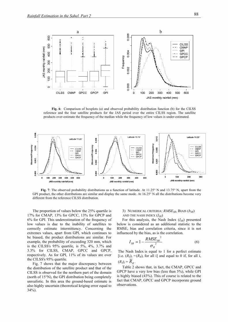
Rainfall Estimation in the Sahel. Part 2 - 8
GPI pdiffer
The p17% for6% for Glow valcorrectlyextremesbe biaseexampleis the C3.3% frespectivthe CILS
Fig. the distrCILSS is(north ofunrealistalso high34%).
a
Fig. 6: Comparison of boxplots (a) and observreference and the four satellite products for the JASproducts over-estimate the frequency of the median wh
Fig. 7: The observed probability distributions as a functroduct, the other distributions are similar and display theent from the reference CILSS distribution.
roportion of values below the 25% quartile is CMAP, 13% for GPCC, 13% for GPCP and
PI. This underestimation of the frequency of ues is due to the inability of satellites to estimate intermittency. Concerning the values, apart from GPI, which continues to d, the product distributions are similar. For , the probability of exceeding 320 mm, which ILSS's 95% quartile, is 5%, 4%, 3.7% and or CILSS, CMAP, GPCC and GPCP, ely. As for GPI, 11% of its values are over S's 95% quartile.
7 shows that the major discrepancy between ibution of the satellite product and that of the observed for the northern part of the domain 15°N), the GPI distribution being completely ic. In this area the ground-based estimate is ly uncertain (theoretical kriging error equal to
beRin
T[(
Gisfaob
b
ed probability distribution function (b) for the CILSS period over the entire CILSS region. The satellite
ile the frequency of low values is under-estimated.
ion of latitude. At 11 same mode. At 16.25
3) NUMERICAL C AND THE NASH IND
For this analysis,low is considered
MSE, bias and cofluenced by the bias
1SRRMI ��
he Nash Index is ei.e. (RS)i =(RR)i for RS)i = RR .
Table 2 shows thaPCP have a very lo highly biased (43%ct that CMAP, GPCservations.
.25° N and 13.75° N, apart fro° N all the distributions becom
RITERIA: RMSESR, BIAIS (bSEX (ISR)
the Nash Index (ISR) presas an additional statistic t
rrelation criteria, since it i, as is the correlation.
2
2
R
SRSE�
qual to 1 for a perfect estall i] and equal to 0 if, for
t, in fact, the CMAP, GPCw bias (less than 5%), whil). This of course is related C and GPCP incorporate g
8
m the e very
R)
ented o the s not
(6)
imate all i,
C and e GPI to the round
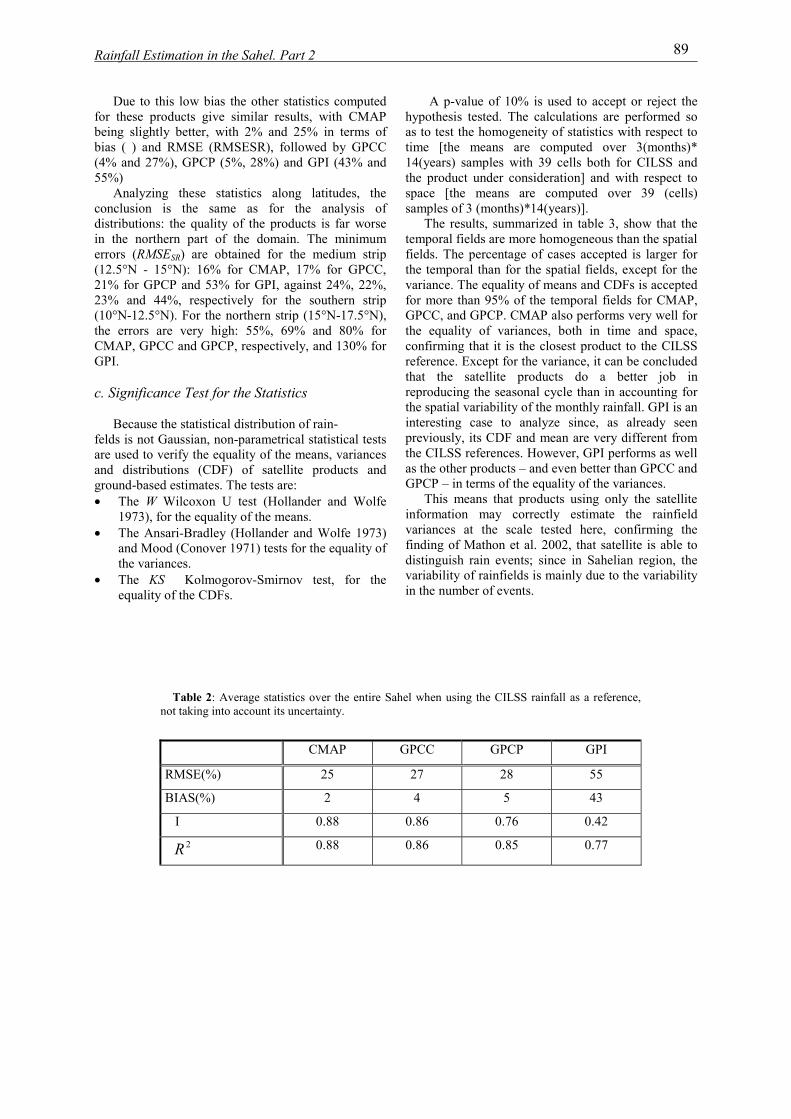
Rainfall Estimation in the Sahel. Part 2 9
Due to this low bias the other statistics computed for these products give similar results, with CMAP being slightly better, with 2% and 25% in terms of bias ( ) and RMSE (RMSESR), followed by GPCC (4% and 27%), GPCP (5%, 28%) and GPI (43% and 55%)
Analyzing these statistics along latitudes, the conclusion is the same as for the analysis of distributions: the quality of the products is far worse in the northern part of the domain. The minimum errors (RMSESR) are obtained for the medium strip (12.5°N - 15°N): 16% for CMAP, 17% for GPCC, 21% for GPCP and 53% for GPI, against 24%, 22%, 23% and 44%, respectively for the southern strip (10°N-12.5°N). For the northern strip (15°N-17.5°N), the errors are very high: 55%, 69% and 80% for CMAP, GPCC and GPCP, respectively, and 130% for GPI.
c. Significance Test for the Statistics
Because the statistical distribution of rain- felds is not Gaussian, non-parametrical statistical tests are used to verify the equality of the means, variances and distributions (CDF) of satellite products and ground-based estimates. The tests are: �� The W Wilcoxon U test (Hollander and Wolfe
1973), for the equality of the means. �� The Ansari-Bradley (Hollander and Wolfe 1973)
and Mood (Conover 1971) tests for the equality of the variances.
�� The KS Kolmogorov-Smirnov test, for the equality of the CDFs.
A p-value of 10% is used to accept or rejehypothesis tested. The calculations are performas to test the homogeneity of statistics with resptime [the means are computed over 3(mon14(years) samples with 39 cells both for CILSthe product under consideration] and with respspace [the means are computed over 39 (samples of 3 (months)*14(years)].
The results, summarized in table 3, show thtemporal fields are more homogeneous than the sfields. The percentage of cases accepted is largthe temporal than for the spatial fields, except fvariance. The equality of means and CDFs is accfor more than 95% of the temporal fields for CGPCC, and GPCP. CMAP also performs very wethe equality of variances, both in time and sconfirming that it is the closest product to the Creference. Except for the variance, it can be concthat the satellite products do a better joreproducing the seasonal cycle than in accountinthe spatial variability of the monthly rainfall. GPIinteresting case to analyze since, as alreadypreviously, its CDF and mean are very differentthe CILSS references. However, GPI performs aas the other products – and even better than GPCGPCP – in terms of the equality of the variances.
This means that products using only the sainformation may correctly estimate the raivariances at the scale tested here, confirminfinding of Mathon et al. 2002, that satellite is adistinguish rain events; since in Sahelian regiovariability of rainfields is mainly due to the variain the number of events.
Table 2: Average statistics over the entire Sahel when using the CILSS rainfall as a reference, not taking into account its uncertainty.
CMAP GPCC GPCP GPI
RMSE(%) 25 27 28 55
BIAS(%) 2 4 5 43
I 0.88 0.86 0.76 0.42
2R 0.88 0.86 0.85 0.77
8
ct the ed so ect to ths)*
S and ect to cells)
at the patial er for or the epted MAP, ll for pace, ILSS luded b in g for is an
seen from s well C and tellite nfield g the ble to n, the bility
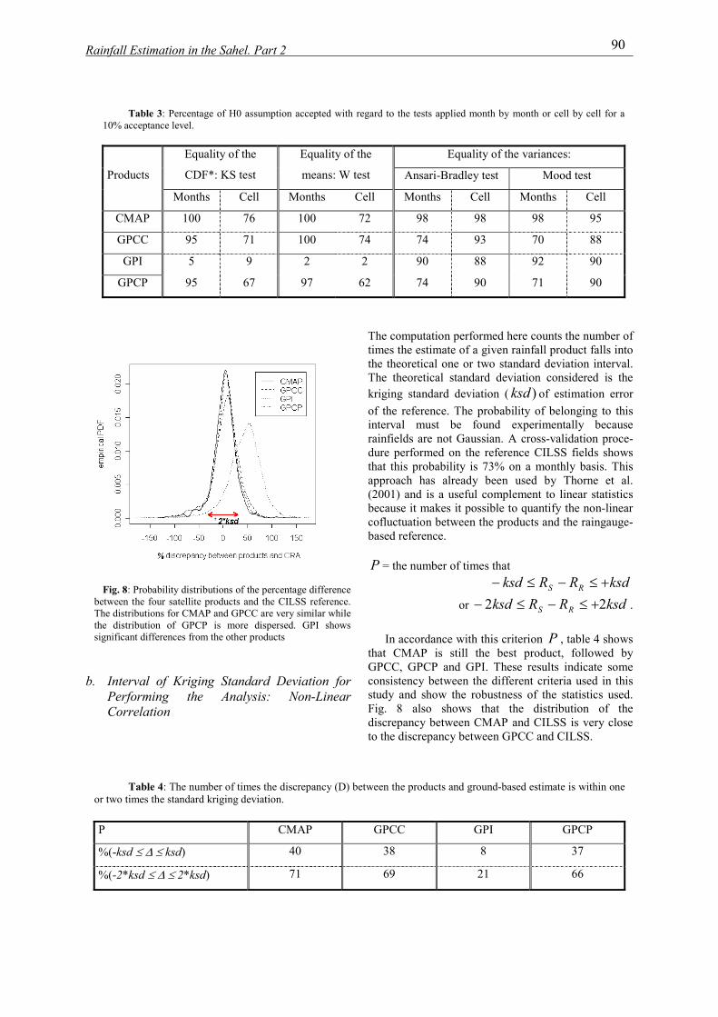
Rainfall Estimation in the Sahel. Part 2 0
Table 3: Percentage of H0 assumption accepted with regard to the tests applied month by month or cell by cell
10% acceptance level.
Equality of the variances: Equality of the
CDF*: KS test
Equality of the
means: W test Ansari-Bradley test Mood test
Products
Months Cell Months Cell Months Cell Months Cell
CMAP 100 76 100 72 98 98 98 95
GPCC 95 71 100 74 74 93 70 88
GPI 5 9 2 2 90 88 92 90
GPCP 95 67 97 62 74 90 71 90
Fig. 8: Probability distributions of the percentage difference between the four satellite products and the CILSS reference. The distributions for CMAP and GPCC are very similar while the distribution of GPCP is more dispersed. GPI shows significant differences from the other products
b. Interval of Kriging Standard Deviation for Performing the Analysis: Non-Linear Correlation
The computation performed here counts the numtimes the estimate of a given rainfall product fallthe theoretical one or two standard deviation intThe theoretical standard deviation considered kriging standard deviation ( of estimationof the reference. The probability of belonging tinterval must be found experimentally berainfields are not Gaussian. A cross-validation pdure performed on the reference CILSS fields sthat this probability is 73% on a monthly basisapproach has already been used by Thorne (2001) and is a useful complement to linear stabecause it makes it possible to quantify the non-cofluctuation between the products and the raingbased reference.
)ksd
P = the number of times that
RRksd RS �����
or RRksd RS 22 �����
In accordance with this criterion P , table 4 s
that CMAP is still the best product, followeGPCC, GPCP and GPI. These results indicate consistency between the different criteria used istudy and show the robustness of the statistics Fig. 8 also shows that the distribution odiscrepancy between CMAP and CILSS is veryto the discrepancy between GPCC and CILSS.
Table 4: The number of times the discrepancy (D) between the products and ground-based estimate is within
or two times the standard kriging deviation.
P CMAP GPCC GPI GPCP
%(-ksd � � � ksd) 40 38 8 37
%(-2*ksd � � � 2*ksd) 71 69 21 66
9
for a
ber of s into erval. is the error o this cause roce-hows
. This et al. tistics linear auge-
ksd. ksd
hows d by some n this used.
f the close
one
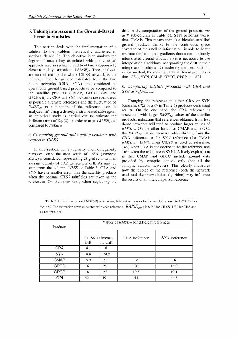
Rainfall Estimation in the Sahel. Part 2 1
6. Taking into Account the Ground-Based Error in Statistics
This section deals with the implementation of a solution to the problem theoretically addressed in sections 2b and 2c. The objective is to analyze the degree of uncertainty associated with the classical approach used in section 5 and to obtain a supposedly closer to reality estimation of RMSEST. Three analyses are carried out: i) the whole CILSS network is the reference and the gridded estimates from the two others networks (CRA, SYN) are considered as operational ground-based products to be compared to the satellite products (CMAP, GPCC, GPI and GPCP); ii) the CRA and SYN networks are considered as possible alternate references and the fluctuation of RMSESR as a function of the reference used is analyzed; iii) using a densely instrumented sub-region, an empirical study is carried out to estimate the different terms of Eq. (3), in order to assess RMSEST as compared to RMSESR. a. Comparing ground and satellite products with respect to CILSS
In this section, for stationarity and homogeneity
purposes, only the area south of 15°N (southern Sahel) is considered, representing 23 grid cells with an average density of 19.2 gauges per cell. As may be seen from the column CILSS of Table 5, CRA and SYN have a smaller error than the satellite products when the optimal CILSS rainfields are taken as the references. On the other hand, when neglecting the
drift in the computation of the ground productdrift sub-column in Table 5), SYN performs than CMAP. This means that: i) a blended satground product, thanks to the continuous coverage of the satellite information, is able to restitute the latitudinal gradients than a non-optiinterpolated ground product; ii) it is necessary tinterpolation algorithms incorporating the drift ininterpolation scheme. Considering the best spzation method, the ranking of the different produthus: CRA, SYN, CMAP, GPCC, GPCP and GPI b. Comparing satellite products with CRASYN as references
Changing the reference to either CRA or
(columns CRA or SYN in Table 5) produces contresults. On the one hand, the CRA referenassociated with larger RMSESR values of the saproducts, indicating that references obtained fromdense networks will tend to produce larger valuRMSESR. On the other hand, for CMAP and Gthe RMSESR values decrease when shifting froCRA reference to the SYN reference (for CRMSESR= 15.9% when CILSS is used as refe18% when CRA is considered to be the referenc16% when the reference is SYN). A likely explanis that CMAP and GPCC include ground provided by synoptic stations only (not alsynoptic stations however). This clearly illushow the choice of the reference (both the neused and the interpolation algorithm) may inflthe results of an intercomparison exercise.
Table 5: Estimation errors (RMSESR) when using different references for the area lying south to 15°N. Values
are in %. The estimation error associated with each reference ( ) is 8.2% for CILSS, 12% for CRA and 13.6% for SYN.
RTRMSE
Values of RMSESR for different references
Products
CILSS Reference drift no drift
CRA Reference
SYN Reference
CRA 14.1 18 SYN 14.4 24.5
CMAP 15.9 21 18 16 GPCC 16 25 18 15.9 GPCP 18 27 19.5 19.1 GPI 42 45 44 44.5
9
s (no worse ellite/ space better mally o use their atiali-cts is .
and
SYN rasted ce is tellite less es of PCC,
m the MAP
rence, e and ation data
l the trates twork uence
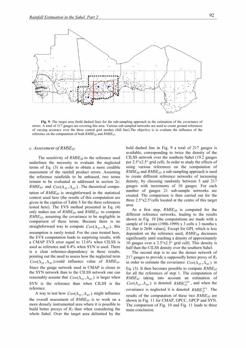
Rainfall Estimation in the Sahel. Part 2 2
Fig. 9. The target area (bold dashed line) for the sub-sampling approach in the estimation of the covariance of errors. A total of 217 gauges are covering this area. Various sub-sampled networks are used to create ground references of varying accuracy over the three central grid meshes (full line).The objective is to evaluate the influence of the reference on the computation of both RMSESR and RMSEST.
c. Assessment of RMSEST
The sensitivity of RMSESR to the reference used underlines the necessity to evaluate the neglected terms of Eq. (3) in order to obtain a more credible assessment of the rainfall product errors. Assuming the reference rainfields to be unbiased, two terms remain to be evaluated as addressed in section 2c: RMSERT and . The theoretical compu-tation of RMSE
),( RTSTCov ��
)
(
RT is straightforward in the statistical context used here (the results of this computation are given in the caption of Table 5 for the three references tested here). The EVS method presented in Eq. (4) only makes use of RMSERS and RMSERT to compute RMSEST, assuming the covariance to be negligible in comparison of these terms. Because there is no straightforward way to compute , this assumption is rarely tested. For the case treated here, the EVS computation leads to surprising results, with a CMAP EVS error equal to 13.6% when CILSS is used as reference and 8.4% when SYN is used. There is a clear reference-dependency in these results, pointing out the need to assess how the neglected term
could influence value of RMSE
),( RTSTCov ��
), RT�
,( RTSTCov �� ST. Since the gauge network used in CMAP is closer to the SYN network than to the CILSS network one can reasonably assume that Cov is larger when SYN is the reference than when CILSS is the reference.
ST�
A way to test how Cov might influence the overall assessment of RMSE
),( RTST ��
ST is to work on a more densely instrumented area where it is possible to build better proxys of RT than when considering the whole Sahel. Over the target area delimited by the
bold dashed line in Fig. 9 a total of 217 gaugavailable, corresponding to twice the density oCILSS network over the southern Sahel (19.2 gper 2.5°x2.5° grid cell). In order to study the effeusing various references on the computatioRMSESR and RMSEST, a sub-sampling approach isto create different reference networks of incredensity, by choosing randomly between 5 andgauges with increments of 10 gauges. For number of gauges 21 sub-sample networkcreated. The comparison is then carried out fothree 2.5°x2.5°cells located at the centre of this area.
As a first step, RMSESR is computed fodifferent reference networks, leading to the rshown in Fig. 10 [the computations are made wsample of 14 years (1986-1999) x 3 cells x 3 mo21, that is 2646 values]. Except for GPI, which idependent on the reference used, RMSESR decsignificantly until reaching a density of approxim10 gauges over a 2.5°x2.5° grid cell). This denshalf than the CILSS density over the southern Sa
The second step is to use the denser netwo217 gauges to provide a supposedly better proxyin order to estimate the covariance CovEq. (3). It then becomes possible to compute RM
,( RST ��
COVST
EVSSTRMSE
for all the references of step 1. The computatiRMSEST taking into account an estimatio
is denoted , and whecovariance is neglected it is denoted results of the computation of these two RMSE
),( RTSTCov �� RMSE
shown in Fig. 11 for CMAP, GPCC, GPCP and The comparison of Fig. 10 and Fig. 11 leads tomain conclusion.
9
es is f the
auges cts of n of used asing 217 each
s are r the
target
r the esults ith a
nths x s less reases ately ity is
hel. rk of
of RT in
SE)T
ST on of n of n the . The
ST are SYN. three
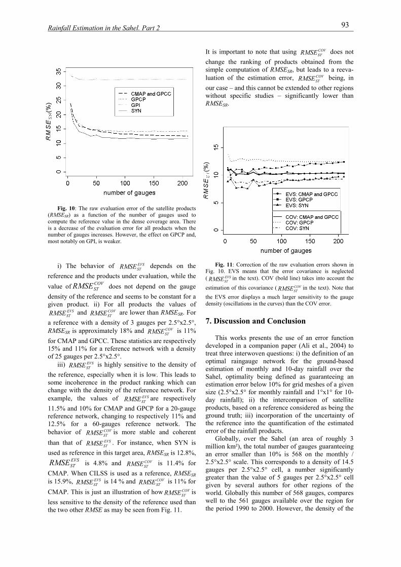
Rainfall Estimation in the Sahel. Part 2 3
Fig. 10: The raw evaluation error of the satellite products (RMSESR) as a function of the number of gauges used to compute the reference value in the dense coverage area. There is a decrease of the evaluation error for all products when the number of gauges increases. However, the effect on GPCP and, most notably on GPI, is weaker.
i) The behavior of depends on the
reference and the products under evaluation, while the value of does not depend on the gauge density of the reference and seems to be constant for a given product. ii) For all products the values of
and are lower than RMSE
EVSSTRMSE
COVSTRMSE
EVS RMSESTRMSE COVST SR. For
a reference with a density of 3 gauges per 2.5°x2.5°, RMSESR is approximately 18% and is 11% for CMAP and GPCC. These statistics are respectively 15% and 11% for a reference network with a density of 25 gauges per 2.5°x2.5°.
COVSTRMSE
iii) is highly sensitive to the density of the reference, especially when it is low. This leads to some incoherence in the product ranking which can change with the density of the reference network. For example, the values of are respectively 11.5% and 10% for CMAP and GPCP for a 20-gauge reference network, changing to respectively 11% and 12.5% for a 60-gauges reference network. The behavior of is more stable and coherent than that of . For instance, when SYN is used as reference in this target area, RMSE
EVSSTRMSE
RMSERMSE
EVSST
STRMSE
EVSSTRMSE
COVSTRMSE
RMSE
COVSTEVSST
EVS
SR is 12.8%, is 4.8% and is 11.4% for
CMAP. When CILSS is used as a reference, RMSERMSE
SR is 15.9%, is 14 % and is 11% for CMAP. This is just an illustration of how is less sensitive to the density of the reference used than the two other RMSE as may be seen from Fig. 11.
COVST
COVSTRMSE
It is important to note that using doechange the ranking of products obtained fromsimple computation of RMSE
COVSTRMSE
COVSTRMSE
SR, but leads to a rluation of the estimation error, beinour case – and this cannot be extended to other rewithout specific studies – significantly lowerRMSESR.
Fig. 11: Correction of the raw evaluation errors sho
Fig. 10. EVS means that the error covariance is neg( in the text). COV (bold line) takes into acco
estimation of this covariance ( in the text). Nothe EVS error displays a much larger sensitivity to thedensity (oscillations in the curves) than the COV error.
EVSSTRMSE
COVSTRMSE
7. Discussion and Conclusion
This works presents the use of an error fundeveloped in a companion paper (Ali et al., 200treat three interwoven questions: i) the definitionoptimal raingauge network for the ground-estimation of monthly and 10-day rainfall oveSahel, optimality being defined as guaranteeinestimation error below 10% for grid meshes of a size (2.5°x2.5° for monthly rainfall and 1°x1° foday rainfall); ii) the intercomparison of saproducts, based on a reference considered as beinground truth; iii) incorporation of the uncertainthe reference into the quantification of the estierror of the rainfall products.
Globally, over the Sahel (an area of rougmillion km²), the total number of gauges guarantan error smaller than 10% is 568 on the mon2.5°x2.5° scale. This corresponds to a density ogauges per 2.5°x2.5° cell, a number significgreater than the value of 5 gauges per 2.5°x2.5given by several authors for other regions oworld. Globally this number of 568 gauges, comwell to the 561 gauges available over the regiothe period 1990 to 2000. However, the density
9
s not the
eeva-g, in gions than
wn in lected
unt the
te that gauge
ction 4) to
of an based r the g an
given r 10-
tellite g the ty of
mated
hly 3 eeing thly / f 14.5 antly ° cell f the pares n for
of the
Rainfall Estimation in the Sahel. Part 2 4
optimal network should increase when moving North due to the gradient of the average number of rain events. The distribution of the present network does not conform to this pattern. For instance, the “optimal” network should count 238 gauges south of 15°N – or 10.3 gauges per 2.5°x2.5°cell – while the actual network counts 465 gauges (19.2 per cell), meaning that the South Sahel is well covered. Over the whole region however, only 42% of the 39 2.5°x2.5° meshes satisfy the optimality criterion for monthly rainfall, the Northern and Eastern areas being undersampled. North of 15°N, the average estimation error is 34%, which makes the validation of satellite products very difficult there (the density should be 20.6 gauges per cell in this area). On the 10-day / 1°x1° scale, 1736 gauges would be needed to ensure a good coverage of the area located South of 15°N, as compared to the 465 available. Accordingly it is not surprising that the optimality criterion is satisfied for only 3.2% of the 135 cells in this area.
In a second step, four rainfall products (GPCC, CMAP, GPCP, GPI) were compared, using the rainfields produced by the entire raingauge network (CILSS) as a reference. All these products (CMAP and GPCP blend satellite and ground information, GPCC is ground-based and GPI is satellite-based only) highly under-estimate the frequency of small rainfall, linked to the high spatial intermittency, which is better documented by direct point measurements. Only 17% of the CMAP values, 13% of the GPCC values and GPCP values and 6% of the GPI values are under the 25% CILSS quantile. Satellite products also slightly underestimate the frequency of the high values.
Two ground-based products were also considered: the CRA monitoring network (about 250 gauges providing data in real time on a 10-day basis) and the synoptic network (about 80 gauges, available daily). Comparison of these two ground products to satellite products have been carried out for the CILSS area with latitudes less than 15°N. At the coarser resolution (1 month, 2.5°x2.5°) the synoptic network performs quite well, its RMSE (14.4%) with respect to the CILSS reference being smaller than the RMSE of the four satellite products. The best satellite product is CMAP with a 15.9% RMSE. This result is somewhat surprising since, in principle, the mixed products incorporating ground information make use of the synoptic information available on the GTS and should therefore perform at least as well as the synoptic-only product. An explanation may reside in the fact that
mixed products do not use all the synoptic stbecause not all of them transmit their data on the
The last part of the paper was devoted to assehow using a reference value that is not the true might influence the computation of evaluation eThis leads us to take into account two quantities are usually neglected in the computation: the erthe reference and the covariance between the satto-truth errors and the reference-to-truth errors. a denser instrumented zone an empirical evaluatthese two quantities was performed, leading estimation that the “true” evaluation errors of boground and satellite products might be significlower than when these two terms are neglectedinstance, the re-evaluated value of RMSE for CMaround 11%, as compared to the above mentvalue of 15.9% when the simplified computatused. This difference is due both to the referenceand to the non-zero covariance existing betweesatellite-to-truth errors and the reference-toerrors. Note also that this re-evaluation of the Rdoes not change the ranking of methods estabfrom the simplified computation. The ground proremain, in this region, superior to the blended proanalyzed here.
It is clear that ample room remains for imprthe quality of satellite rainfall estimates oveSahel. The availability of new Infrared (e.g., Mand microwave (e.g., TRMM, GPM) sensorsundoubtedly lead to more accurate satellite raproducts. This study shows however, that a cand optimal use of ground information is needorder to evaluate and intercompare any raproducts, especially in regions of high ravariability. Acknowledgments
This research was funded by IRD in
framework of the AMMA-CATCH "ORE" proinitiated by the French Ministry of Research. Sthanks are due to the "Departement SoutiFormation" of IRD for the grant allocated to thauthor of this paper. We would also likacknowledge S. Bonaventure for his efforts ivalorization of the AGRHYMET Center rainfalbase, H. Harder for his help in proof-readinarticle.
REFERENCES
Adler, R. F., C. Kidd, G. Petty, M. Morissey, and H.
M. Goodman, 2001: Intercomparison of Global Precipitation Products: The Third Precipitation Intercomparison Project (PIP-3). Bulletin of the American Meteorological Society , 82, 1377-1396.
Ali, A., T. Lebel, and A. Amani, 2004: Raestimation in the Sahel. Part 1 : Error FunJ. Appl. Meteor. (submitted).
Arkin, P. A., R. Joyce, and J. E. Janowiak, 199techniques: GOES Precipitation Index. RSens. Rev., 11, 107–124.
9
ations GTS. ssing value rrors.
which ror of ellite-Using ion of to an th the antly . For AP is ioned ion is error n the -truth MSE
lished ducts ducts
oving r the
SG) will infall areful ed in infall infall
the gram
pecial en et e first e to n the l data g the
infall ction.
4: IR emote
Rainfall Estimation in the Sahel. Part 2 5
Barrett, E. C., and D. W. Martin, 1981: The Use of Satellite Data in Rainfall Monitoring. Academic Press, 340 pp.
Bell, T. L., P. K. Kundu, and C. D. Kummerow, 2001: Sampling errors of SSM/I and TRMM rainfall averages: Comparison with error estimates from surface data and a simple model. J. Appl. Meteor., 40, 938– 954.
Barnston, A. G., 1991: An empirical method of estimating raingage and radar rainfall measure-ment bias and resolution. J. Appl. Meteor., 30, 282–296.
Chiu, L., A. Chang, and J. Janowiak, 1993: Comparison of monthly rain rates derived from GPI and SSM/I using probability distribution functions. J. Appl. Meteor., 32, 323–334.
Ciach, J. G., and W. F. Krajewski, 1999 : On the estimation of radar rainfall error variance. Adv. Water Resour., 22, 585–595.
Conover, W. J., 1971 : Practical nonparametric statistics. John Wiley & Sons, New York, 234 PP.
Ebert, E. E., and M. J. Manton, 1998: Performance of satellite rainfall estimation algorithms during TOGA COARE. J. Atmos. Sci., 55, 1537–1557.
Gebremichael, M., W. F. Krajewski, M. Morrissey, D. Langerud and G. J. Huffman, 2003: error uncer-tainty Analysis of GPCP Monthly Rainfall Products: A Data-Based Simulation Study. J. Appl. Meteor., 42, 1837-1848.
Ha, E., G. R. North, C. Yoo, and K.-J. Ha, Evaluation of some ground truth designs for satellite estimates of rain rate, J. Atmos. Oceanic Technol., 19, 65– 73, 2002.
Hollander, M., and D. A. Wolfe, 1973 : Nonpa-rametric statistical inference. John Wiley & Sons, New York, 250 PP.
Huffman, G. J., and Coauthors, 1997 : The Global Precipitation Climatology Project (GPCP) Combined Precipitation Data Set. Bull. Amer. Meteor. Soc., 78, 5–20.
Huffman, G. J, M. Morrissey, D. T. Bolvin, S. Curtis, R. Joyce, B. McGavock, and J. Susskind, 2001: Global precipitation at one degree daily resolution from multisatellite observations. J. Hydrometeor., 2, 36–50.
Jobard, I., status of satellite retrieval of rainfall at different scales using multi-source data, 2001. MEGHA-TROPIQUES Scientific Workshop, 2-6 July 2001, Paris, France.
Kummerow, C., P. Poyner, W. Berg and J. Thomas-Sthale, 2004. The effects of rainfall inhomogeneity on climate variability of rainfall estimated from passive microwave sensors. J. Atmos. Oceanic technol., 21, 624-638.
Laurent H., I. Jobard and A. Toma, 1998. Validation of satellite and ground-based estimates of precipitation over the Sahel. Atmospheric Research, 47-48, 651-670.
Le Barbé, L., T. Lebel, and D. Tapsoba, Ravariability in West Africa during the years 11990, J. Clim., 15, 187–202, 2002.
Lebel, T., and A. Amani, 1999: Rainfall Estimatthe Sahel : What is the ground truth? J ApMeteor., 38 : 555 – 568.
Levizzani, V., P. Bauer, A. Buzzi, S. Davolio, Hinsman, C. Kidd, F. S. MarzanoMeneguzzo, A. Mugnai, J. P. V. PBaptista, F. Porcù, F. Prodi, J. F. W. PurdoRosenfeld, J. Schmetz, E. A. Smith, F. TamF. J. Turk, and G. A. Vicente, EURAINSAT - Looking into the futusatellite rainfall estimations. Proc. The EUMETSAT Meteorological Satellite Users' Conf., EUMETSAT, Antalya, 1-5 375-384.
Mathon V., H. Laurent and T. Lebel, 2002: MesoConvective System Rainfall in the SahApplied Meteor., 41, (1081-1092).
McCollum, J. R., A.Gruber, and M. B. Ba, Discrepancy between gauges and saestimates of rainfall in equatorial AfriAppl. Meteor., 39, 666-679.
Morrissey, M. L., and J. S. Greene, 1993: Compof two satellite based rainfall algorithms atoll rain gauge data. J. Appl Meteor., 32, 425.
Morrissey, M. L., J. A. Malikekal, J. S. Greene, Wang, 1995: The uncertainty in spatial aveusing raingauge networks. Water Resour.31, 2011 – 2017.
Nicholson, S. E., B. Some, J. Mccollum, E. ND. Klotter, Y. Berte, B. M. Diallo, I. GayKpabeba, O. Ndiaye, J. N. NoukpozounkoM. Tanu, A. Thiam, A. A. Toure , and Traore; 2003. Validation of TRMM and Rainfall Estimates with a High-Density GDataset for West Africa. Part I: ValidatiGPCC Rainfall Product and Pre-TRMM Saand Blended Products. , J. Appl. Meteoro1337-1354.
Petty, G. W., 1995. The status of satellite-rainfall estimation over land. Remote Environ., 51, 125-137.
Ramage K., I. Jobard, T. Lebel and M. Desbois, Satellite estimation of 1-day to10-day prection : Comparison and validation over TrAfrica of TRMM, METEOSAT and Gproducts. Proc. The 2000 EUMEMeteorological Satellite data User’s conferBologna, Italy, 29 May – 2 June 2000. 363-
Rudolf, B., 1993: Management and analysprecipitation data on a routine basis. ProcWMO/IAHS/ETH Symp. on PrecipitationEvaporation, Bratislava, Slovakia, SHydrometeorology Institute, 69–76.
Rudolf, H. Hauschild, W. Rüth, and U. Schn1994: Terrestrial precipitation analysis: Otional method and required density of
9
infall 950–
ion in plied
D. E. , F. oiares m, D. pieri, 2001. re of 2001 Data Oct.,
scale el. J.
2000: tellite ca. J.
arison using 411 –
and J. rages
Res.,
elkin, e, G. u, M. A. K. Other auge
on of tellite l., 42,
based Sens.
2000. ipita-
opical PCP
TSAT ence,
369. is of . Int. and lovak
eider, pera-point

Rainfall Estimation in the Sahel. Part 2 6
measurements. Global Precipitations and Climate Change, M. Dubois and F. Desalmand, Eds., Springer Verlag, 173–186.
Stanski, H. R., L. J. Wilson and W. R. Burrows, 1989. Survey of common verification methods in meteorology. WMO/TD-N°. 358, Wold Meteoro-logical Organization, Geneva, 114 pp.
Thorne V., P. Coakeley, D. Grimes and G. Dugdale, 2001. Comparison of TAMSAT and CPC rainfall estimates with raingauges, for southern Africa. Int. J. Remote Sensing, 22, n° 10, 1951-1974.
Xie, P., and P. A. Arkin, 1995: An intercomparison of gauge observations and satellite estimates of
monthly precipitation. J. Appl. Meteor.1143–1160.
Xie, P., and P. A. Arkin, 1997: Global precipitati17-year monthly analysis based on observations, satellite estimates, and nummodel outputs. Bull. Amer. Meteor. Soc2539– 2558.
Xie, P., J. E. Janowiak, P. A. Arkin, R. F. AdlGruber, R. Ferraro, G. J. Huffman, and S. C2003: GPCP pentad precipitation analyseexperimental dataset based on observations and satellite estimates. J. Cli16, 2197–2214.
9
, 34,
on: A gauge erical ., 78,
er, A. urtis,
s: An gauge mate,

Modèle conceptuel pour des études climatiques régionales 97
IV. Modèle conceptuel pour des études climatiques régionales
Modèle conceptuel pour des études climatiques régionales 99
IV.1 Introduction
Il y a plusieurs façons d’approcher la modélisation et la simulation des précipitations. Cox and
Isham (1994) ont classé les modèles de pluie en trois catégories principales. Les modélisations "statistiques empiriques", comme leur nom l’indique, sont essentiellement basées sur l’analyse des caractéristiques empiriques des données des stations et aucune tentative de modélisation explicite du processus n’est réalisée. Elles traitent généralement des donnés d’un seul site pour un seul pas de temps. Ces modèles ont été largement utilisés pour la caractérisation mono-site des précipitations.
Les modèles déterministes, au contraire, intègrent de façon explicite des paramétrisations des processus atmosphériques qui vérifient la conservation de la masse, de la quantité de mouvement et de l’énergie. Ces modèles sont largement utilisés dans la prévision du temps et du changement global du climat. Ils regroupent les Modèles de Circulation Générale Atmosphérique (MCGA), les modèles climatiques régionaux et les modèles de Méso-échelle pour la prévision à court terme.
Les modèles conceptuels constituent la troisième catégorie et peuvent être agrégés pour n’importe quelle échelle spatiale ou temporelle. Une représentation conceptuelle simplifiée du processus des pluies est définie, utilisant des hypothèses probabilistes simples mais peuvent nécessiter un nombre important de paramètres. Les paramètres du modèle représentent des propriétés physiques observables du processus (par exemple durée de vie des événements, taille, vitesse, direction, etc.) et peuvent être utilisés pour une simulation quasi-physique.
Quelque soit l’approche utilisée, les modèles hydrologiques ou agronomiques exigent des entrées pluviométriques de "bonnes" propriétés spatio-temporelles ; en effet la variabilité du champ spatial (lisse, erratique, intermittent) à l’échelle considérée joue un rôle important. De même, le champ temporel doit être conforme aux séquences sèches et humides, aux persistances et dérives de ces séquences. Ces caractéristiques sont particulièrement importantes, d’autant plus que la réponse hydrologique ou agronomique au forçage pluviométrique est non linéaire.
IV.2 Méthodes de simulation des champs de pluie IV.2.1 Les modèles déterministes.
Du fait de leur faible résolution spatiale, les MCGA actuellement disponibles fournissent des sorties pluviométriques inadéquates aux applications hydrologiques ou agronomiques. Par exemple, Lebel et al. (2000) ont montré que les MCGA tendaient à produire au Sahel, un nombre trop grand de jours de pluvieux au cumul de pluie élevé. Cette surestimation conduit à des biais amplifiés en sortie des modèles hydrologiques où l’intermittence spatio-temporelle joue un rôle important. La modélisation climatique régionale était susceptible d’apporter une réponse à ce problème de résolution spatiale. Fonctionnant à des résolutions de l’ordre de 40 km x 40 km, ces modèles, forcés aux frontières par des modèles globaux, fournissent une image plus réaliste des champs de pluie que ces derniers et avec une résolution qui devrait permettre d’envisager un forçage direct des modèles hydrologiques (Messager 2004). Cependant, des simulations réalisées à l’aide du modèle MAR (Gallée and Schayes 1994) montrent également des biais importants des sorties pluviométriques aux échelles hydrologiques (surestimation des jours pluvieux, lissage de
Modèle conceptuel pour des études climatiques régionales 100
l’intermittence spatiale), même si quelques améliorations sont à noter (Moufouma 2003 ; Ramel 2004). Cette inadéquation des scénarios climatiques des modèles atmosphériques à la variabilité pluviométrique s’explique essentiellement par leur incapacité à modéliser les systèmes convectifs. Ajouté à cette inadéquation, Il faut noter que la simulation à travers ces modèles déterministes nécessite des moyens de calcul importants (Mason 1986). En vue de combler le fossé entre les MCGA et les modèles hydrologiques, des recherches importantes devraient se poursuivre dans le domaine de la désagrégation (communément appelée downscaling dans la littérature). IV.2.2 Les modèles statistiques "mécanistes"
Considérant la pluie comme une variable aléatoire , ils conduisent le plus souvent à l’ajustement d’une loi statistique. En général, ce sont des modèles ponctuels et ne traitent que de l’aspect temporel des champs de pluie. Parmi ces modèles, on peut noter les modèles de la variable hauteur de pluie non nulle et les modèles d’occurrence de pluie. La loi de poisson (caractère aléatoire de l’occurrence de la pluie) et les chaînes de Markov (dépendance temporelle entre les occurrences) sont deux exemples de modèles fréquemment utilisés. Bien qu’on rencontre des applications de ces deux types de modèles sous un même climat, ils impliquent des hypothèses contraires sur le processus physique. Pour ce qui est des champs de pluie sahéliens, Gozé (1990) a élaboré un générateur des jours pluvieux sur la base d’une Chaîne de Markov d’ordre 1 pour l’occurrence et un modèle exponentiel pour les hauteurs de pluie journalière. Ce modèle est actuellement utilisé en opérationnel au Centre AGRHYMET. Deux points sont à souligner : i) les modèles purement stochastiques (modèles boîtes noires) sont moins pertinents pour la modélisation des champs de pluie où l’on possède des connaissances a priori sur le phénomène (par exemple la hiérarchie des structures établie par Austin and Houze 1972) ; ii) la nécessité de disposer des champs spatio-temporels rend les simulations mono-sites moins pertinentes pour les applications hydrologiques. Et la prise en compte de la dépendance des champs de pluie entre les sites lorsqu’on génère des séries chronologiques à plusieurs sites semble requise.
)(tP
)(tH )(tI
)(tI
IV.2.3 Les modèles géostatistiques : au delà du cadre gaussien ou gaussien anamorphosé
La construction de simulations géostatistiques est extrêmement commode dans le cadre des fonctions aléatoires de loi spatiale multigaussienne, c’est-à-dire telles que toute combinaison linéaire de valeurs suit une distribution gaussienne. La distribution multigaussienne ne dépend que des moments d’ordre un et deux (espérance et fonction de covariance ou variogramme), ce qui facilite la tâche d’inférence statistique. De nombreux algorithmes ont été développés pour simuler des variables gaussiennes : e.g. décompositions matricielles, bandes tournantes, méthode séquentielle (Matheron 1972 ; Journel 1974 ; Davis 1987; Chilès 1995 ; Lantuéjoul 2002). Si la variable régionalisée n’est pas gaussienne, elle doit être préalablement transformée en une variable dont la distribution marginale est gaussienne, laquelle est supposée posséder une loi spatiale multigaussienne. Cette transformation est connue sous le nom “d’anamorphose” gaussienne (Journel and Huijbregts 1978 ; Rivoirard 1994). Une fois la procédure de simulation achevée dans le cadre gaussien, l’anamorphose inverse est appliquée pour revenir à la variable initiale. Pour ce qui est des champs de pluie sahéliens, Guillot (1998) a construit une anamorphose atomisée par la fréquence des valeurs nulles des champs qui a servi de cadre pour une simulation
Modèle conceptuel pour des études climatiques régionales 101
des champs de pluie événementiels, conditionnée aux valeurs ponctuelles mesurées. L’algorithme des bandes tournantes a été utilisé. Onibon et al. (2001) ont conditionné cette anamorphose par rapport à la moyenne évènementielle à l’aide de l’algorithme de Gibbs.
Toutefois, la simulation dans le cadre gaussien ou gaussien anamorphosé présente plusieurs
caractéristiques limitatives. Par exemple il est difficile de réaliser l’anamorphose lorsque l’histogramme de la variable régionalisée est fortement dissymétrique (Rivoirard 1994). Le cadre gaussien ne s’adapte pas quand il y a discontinuité de la variable régionalisée (voir exemple de la figure IV. 1). Ces situations motivent la recherche d’algorithmes de simulation non gaussienne.
On peut d’abord noter les méthodes de simulation non gaussienne qualifiées d’exactes. Les
simulations exactes sont définies à partir des procédés de construction de fonctions aléatoires. Parmi celles-ci on peut citer i) les modèles mosaïques où l’espace est partitionné en cellules aléatoires stationnaires et la fonction aléatoire générée (dite “mosaïque”) est stationnaire d’ordre deux et sa covariance est proportionnelle au covariogramme géométrique des cellules, lequel mesure la probabilité que deux sites appartiennent à la même cellule en fonction de leur séparation (e.g. Rivoirard 1994). ii) Les modèles construits par implantation d’objets où la construction de la simulation est réalisée de manière “dynamique”. Des points de position aléatoire apparaissent au cours du temps. En général, ils sont issus d’un processus ponctuel de Poisson dont la densité peut être uniforme ou variable dans l’espace ou dans le temps. Chaque point est le centre de gravité d’un “objet”, par exemple une forme géométrique prédéterminée, de taille et orientation aléatoires. Les points sont appelés germes et les objets grains primaires. Lorsqu’un objet nouveau rencontre un objet ancien, une convention est adoptée pour définir la valeur des sites où les deux objets se chevauchent, par exemple : valeur du dernier objet ou du premier objet : modèle des feuilles mortes ; somme des valeurs des objets : modèle de dilution ; valeur maximale : modèle booléen (Serra, 1968, 1988). iii) La technique des gaussiennes tronquées simule un ensemble aléatoire, que l’on représente par une variable binaire ou “indicatrice”, par seuillage d’une fonction aléatoire de loi spatiale multigaussienne (Journel and Isaaks 1984). Cette approche peut être étendue pour simuler une partition de l’espace en plusieurs ensembles aléatoires en travaillant sur plusieurs fonctions aléatoires gaussiennes. Cette généralisation, connue sous le nom de méthode des plurigaussiennes (Armstrong et al. 2003), fournit une vaste classe de modèles capables de reproduire de nombreuses caractéristiques morphologiques des ensembles aléatoires à simuler, notamment les relations de contiguïté et d’emboîtement.
Une méthode intermédiaire de simulation non gaussienne est la simulation isofactorielle. Elle est intermédiaire par rapport aux simulations exactes en ce sens qu’elle repose sur la spécification d’un modèle, mais cette spécification reste incomplète (lois bivariables au lieu de multivariables pour les cas ci-dessus). Elle est basée sur les techniques du krigeage disjonctif (Emery 2002), dont les équations peuvent être résolues analytiquement lorsque la loi bivariable est isofactorielle, c’est-à-dire lorsqu’il existe une famille complète de fonctions sans corrélations spatiales croisées appelées facteurs (Delfiner and Chilès 1999).
Le choix de telle ou telle méthode est dicté par les propriétés structurales observées sur la variable régionalisée. Cependant, traiter à la fois la variabilité spatiale des champs de pluie, l’occurrence temporelle et la dynamique des événements pluvieux, tel que cela nous préoccupe
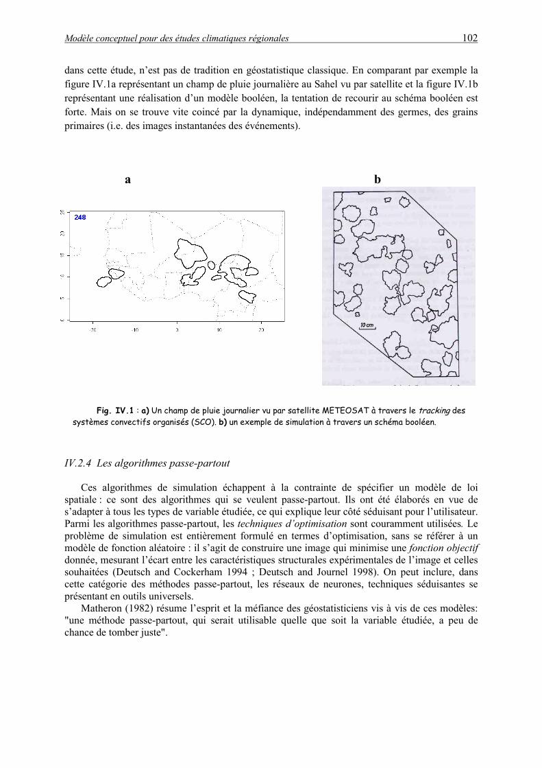
Modèle conceptuel pour des études climatiques régionales 102
dans cette étude, n’est pas de tradition en géostatistique classique. En comparant par exemple la figure IV.1a représentant un champ de pluie journalière au Sahel vu par satellite et la figure IV.1b représentant une réalisation d’un modèle booléen, la tentation de recourir au schéma booléen est forte. Mais on se trouve vite coincé par la dynamique, indépendamment des germes, des grains primaires (i.e. des images instantanées des événements).
Fig. Isystèmes co
IV.2.4 Les a
Ces algospatiale : ce s’adapter à toParmi les algproblème de modèle de fodonnée, mesusouhaitées (Dcette catégorprésentant en
Matheron"une méthodchance de tom
a
V.1 : a) Un champ de pluie journalier vu par satellite METEOSATnvectifs organisés (SCO). b) un exemple de simulation à travers un
lgorithmes passe-partout
rithmes de simulation échappent à la contrainte de spésont des algorithmes qui se veulent passe-partout. Ils onus les types de variable étudiée, ce qui explique leur côté séorithmes passe-partout, les techniques d’optimisation sont simulation est entièrement formulé en termes d’optimisanction aléatoire : il s’agit de construire une image qui minirant l’écart entre les caractéristiques structurales expérimeeutsch and Cockerham 1994 ; Deutsch and Journel 1998
ie des méthodes passe-partout, les réseaux de neurones, t outils universels. (1982) résume l’esprit et la méfiance des géostatisticiens e passe-partout, qui serait utilisable quelle que soit la vber juste".
b
à travers le tracking des schéma booléen.
cifier un modèle de loi t été élaborés en vue de duisant pour l’utilisateur. couramment utilisées. Le tion, sans se référer à un mise une fonction objectif ntales de l’image et celles ). On peut inclure, dans echniques séduisantes se
vis à vis de ces modèles: ariable étudiée, a peu de
Modèle conceptuel pour des études climatiques régionales 103
IV.2.5 Les modèles fractals
L’avantage essentiel, qui est aussi une limite, des modèles fractals vient du fait qu’ils sont indépendants de toute échelle considérée dans le système et sont caractérisés par un nombre très faible de paramètres. Ils essaient de représenter au mieux le degré d’irrégularité des phénomènes à travers un paramètre invariant d’échelle : « la dimension fractale ». Une revue de ces modèles peut être trouvée dans Foufoula-Georgiou and Krajewski (1995). Elles ont fait l’objet d’intense recherche ces deux dernières décennies et continuent de mobiliser des énergies. Cependant, la précision avec laquelle sont restituées les périodes sèches et humides par ces modèles fractals (scaling en anglais), peut être jugée insuffisante (Gupta and Waymire 1993). Par ailleurs, l’application de la théorie des cascades multi-fractales à des données réelles requiert un nombre important de réalisations disponibles. Une modélisation complète espace-temps des processus des précipitations utilisant ces cascades multi-fractales est un domaine encore en développement du point de vue théorique. IV.2.6 Les processus de Poisson
L’utilisation des processus ponctuels a été un terrain fructueux pour la modélisation stochastique des pluies depuis les travaux pionniers de Le Cam (1961). Waymire and Gupta (1981a, b, c) ont traité, de façon détaillée, la représentation mathématique des pluies à travers les processus ponctuels. Les processus ponctuels de Poisson sont le prototype des processus ponctuels. Ils sont pour ces processus ce qu’est la loi normale pour les distributions statistiques. La modélisation à travers les processus de Poisson groupés (Poisson-cluster processes) a permis de rendre compte avec succès de certaines propriétés intéressantes des champs des pluies, notamment les agrégations dans l’espace et le temps. Une revue des développements des modèles des processus de Poisson composés (PPC) peut être trouvée dans Onof et al. (2000). Afin de définir un PPC, il est nécessaire de spécifier le processus qui génère les centres des groupes d’agrégation et les mécanismes qui gouvernent chaque groupe. La modélisation des pluies à travers les PPC a principalement concerné deux échelles: l’événement pluvieux et les cellules pluvieuses. Il s’agit d’associer à chaque réalisation d’un événement pluvieux (processus mère) un nombre aléatoire de cellules pluvieuses (processus fils). Deux schémas spécifiques ont été les plus utilisés: le schéma de Neyman-Scott et celui de Bartlett-Lewis. Pour un PPC de Neyman-Scott les cellules pluvieuses associées à un événement pluvieux sont identiquement et indépendamment distribuées autour de son centre, alors que pour un PPC de Bartlett-Lewis les intervalles de temps séparant deux cellules successives de chaque événement suivent une distribution statistique quelconque.
Il y a eu beaucoup de développements et de validations des PPC. On peut regrouper les modèles en i) mono-site (e.g. Rodriguez-Iturbe et al. 1987, 1988 ; Cowpertwait 1991 ; Cowpertwait et al. 1996a ; Onof and Wheater 1993 ; Onof and Wheater 1994a, b ; Kakou 1997 ; Khaliq and Cunnane 1996, Gyasi-Agyei and Willgoose 1997, Calenda and Napolitano 1999). ii) En multi-site (e.g. Wheater et al. 1991a, b ; Cox and Isham 1994; Cowpertwait 1995; Cowpertwait et al. 1996b ; Kakou 1997 ; Gyasi-Agyei 1999). Ceux-ci incluent les modèles linéaires généralisés, GLMs en anglais (Generalized Linear Models) et s’attachent à générer des séries chronologiques en plusieurs points dans l’espace en tenant compte des corrélations spatiales entre ces points. iii) En spatio-temporels continus (e.g. Cox and Isham 1994 ; Northrop 1996 , 1998).
Le modèle développé par Northrop (1998) considère des événements pluvieux qui arrivent suivant un processus de Poisson bidimensionnel dans l’espace d’intensité � . Suivant chaque événement de centre (u ) arrivent des cellules convectives suivant un schéma d’agrégation temporel de Bartlett-Lewis. Les cellules sont dotées d’une durée de vie, d’une vitesse de déplacement et d’une taille (de forme elliptique).
00 ,t

Modèle conceptuel pour des études climatiques régionales 104
Ce modèle correspond à l’idée de génération des SCO qui peuvent être assimilés au processus fils et le processus mère correspondrait à une situation synoptique favorisant leur naissance (cette situation synoptique peut être une Onde d’Est). Cependant vu l’information disponible, il ne nous est pas possible de déterminer l’intensité de ce processus mère qui serait responsable du déclenchement des SCO. Le modèle Northrop (1998) n’est donc pas applicable aux échelles de cette étude eu égard à l’information disponible.
A l’inverse de ce modèle, Le Barbé and Lebel (1997) ont développé un modèle mixte (occurrence et hauteur de pluie) adapté à la variabilité des champs des pluies à l’échelle de l’événement. Ce modèle de loi de fuite est cependant un modèle mono-site et utilise une loi de Poisson homogène. Signalons qu’une autre catégorie de modèles n’ayant pas été rappelés dans la brève revue ci-dessus porte sur les modèles d’état, utilisant les chaînes de Markov cachées (Huges et al. 1994, 1999 ; Lambert et al. 2003). Ces modèles ont un avenir du fait qu’ils combinent l’information sur l’état de l’atmosphère fournie pour les MCGA et une approche stochastique de la modélisation.
Modèle conceptuel pour des études climatiques régionales 105
IV.3 Modèle conceptuel régional des systèmes pluvieux au Sahel
L’objectif est de développer un modèle conceptuel s’étendant à l’échelle régionale et qui soit capable de simuler la pluviométrie associée aux SCO. Le modèle doit pouvoir intégrer les informations relevant de la variabilité climatique. IV.3.1 Modèle conceptuel
La dénomination de modèle conceptuel fait référence au fait que, quand la structure du système et les lois le régissant sont mal connues ou lorsque la pauvreté des informations et la complexité des phénomènes en jeu prévalent, le comportement du système en question est simplifié. Ainsi les modèles conceptuels intègrent des facteurs complexes en essayant de décrire le concept physique du comportement du système par une représentation plus simple, qui bien qu’ayant un sens physique, est dépourvue de réalité physique. A travers ce type de modélisation, on reproduit au mieux le comportement d’un système, plutôt que d’avancer des explications causales sur son comportement. Notons qu’un modèle conceptuel n’implique pas forcément une modélisation stochastique (comme cela est le cas dans cette étude). IV.3.2 Structures spatio-temporelles des naissances
Pour analyser la structure spatio-temporelle des naissances des SCO la fonction espace-temps de Ripley (Diggle et al. 1995) est utilisée ; où est la distance spatiale et t le temps.
Cette fonction espace-temps de Ripley (),( tdK d
K ) quantifie le nombre de naissances par unité d’espace et de temps suivant diverses valeurs de et t . Les figure IV.2a et b représentent la moyenne de cette fonction ; calculée à partir des 9 années de données (1990 à 1999 sauf 1995) issues du tracking des systèmes convectifs pluviogènes. Les courbes continues viennent des données et celles qui sont discontinues représentent un processus de Poisson homogène (HPP en anglais). Si la fonction calculée pour le processus analysé est au dessus de celle de HPP, les données présentent un clustering, si elle est en dessous c’est une répulsion.
d
On observe à travers les figure III a et b que "localement" le processus spatial de naissance des SCO est assimilable à un processus de poisson homogène; par contre dans le temps la courbe des naissances est nettement au dessus de celle de HPP, ce qui indique une forte agrégation temporelle. L’agrégation spatiale observée pour les grandes distances peut être interprétée comme un effet de relief. La figure IV.2 de l’introduction générale montre des zones privilégiées de naissance. Cette situation nous amène à adopter le modèle d’intensité des naissances représenté par l’équation IV.1
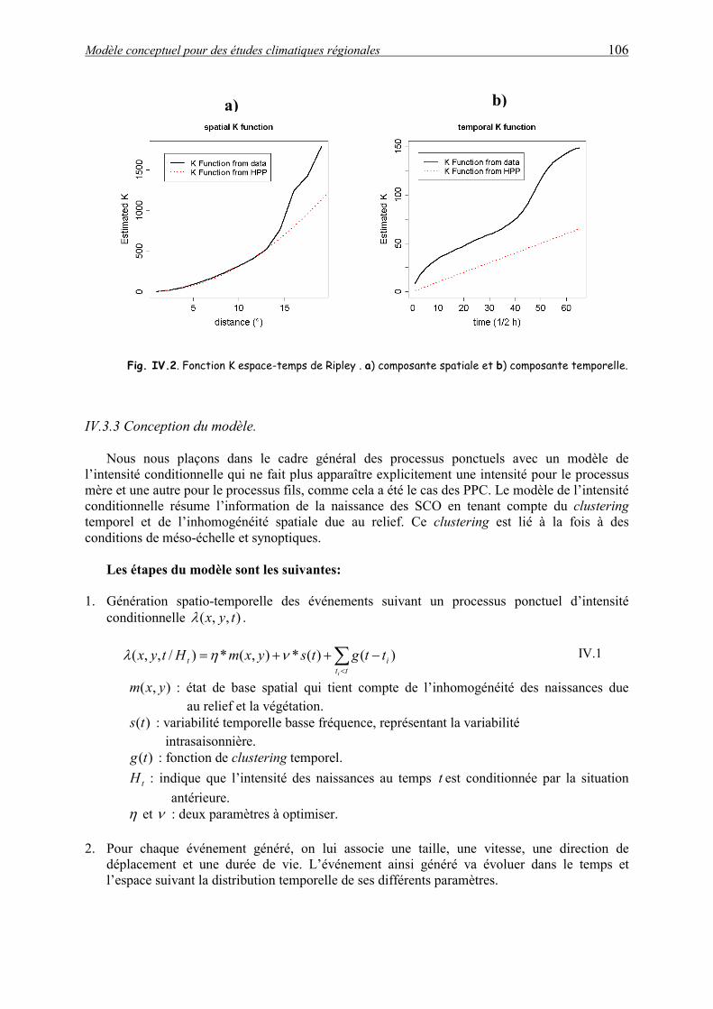
Modèle conceptuel pour des études climatiques régionales 106
)
Fig. IV.2. Fonctio IV.3.3 Conception du m
Nous nous plaçonsl’intensité conditionnellmère et une autre pour leconditionnelle résume ltemporel et de l’inhomconditions de méso-éche
Les étapes du modè
1. Génération spatio-tconditionnelle ,(x�
�tHtyx )/,,( ��
),( yxm : état dau rel
)(ts : variabilité intrasaiso
)(tg : fonction d
tH : indique quantérieur
� et � : deux pa 2. Pour chaque événe
déplacement et unel’espace suivant la d
a)
n K espace-temps de Ripley . a) composante spatiale e
odèle.
dans le cadre général des processus ponctue qui ne fait plus apparaître explicitement une in processus fils, comme cela a été le cas des PPC’information de la naissance des SCO en tenaogénéité spatiale due au relief. Ce clusteringlle et synoptiques.
le sont les suivantes:
emporelle des événements suivant un proces), ty .
��
���
tti
i
ttgtsyxm )()(*),(* �
e base spatial qui tient compte de l’inhomogéief et la végétation. temporelle basse fréquence, représentant la varinnière. e clustering temporel. e l’intensité des naissances au temps t est cone. ramètres à optimiser.
ment généré, on lui associe une taille, une v durée de vie. L’événement ainsi généré va éistribution temporelle de ses différents paramètre
b
t b) composante temporelle.
els avec un modèle de tensité pour le processus . Le modèle de l’intensité nt compte du clustering est lié à la fois à des
sus ponctuel d’intensité
IV.1
néité des naissances due
abilité
ditionnée par la situation
itesse, une direction de voluer dans le temps et s.
Modèle conceptuel pour des études climatiques régionales 107
3. Une hauteur de pluie correspondant à sa moyenne lui est associée. Et enfin ce cumul sera désagrégé via l’algorithme de Gibbs pour obtenir une distribution spatiale suivant la trace au sol de l’événement durant son cycle de vie.
iH iH
4. Pour un temps T� donné, le cumul de pluie est la somme des pluies apportées par les différents événements. En espérance cette pluie est égale :
]/)[())](,([ 0 VDADT yyHTyxPE ����� ���� IV.2
Où
T�� : espérance du nombre de naissance pendant la période T�
D� : espérance de la durée des événements
A� : espérance de la taille des événements
0y : limite nord du Sahel, qui représente la limite de la zone des naissances
V� : espérance de la vitesse
Une des caractéristiques importantes de ce modèle est qu’il doit pouvoir restituer le gradient climatologique connu des cumuls de pluie au Sahel, à travers la limite qu’impose le Sahara. La prise en compte de ce gradient était un challenge, puisqu’il n’existe ni sur les cumuls événementiels pouvant donner des intensités plus faibles au Nord qu’au Sud, ni sur le nombre de naissances. Cette non-existence de dérive sur le nombre de naissances correspond bien au saut de Mousson qui fait qu’à une certaine période, brusquement tout le Sahel devient favorable aux naissances des événements. Précisons que l’équation IV.2 n’est valable que pour la zone comprise entre les latitudes et . Au sud de cette zone, le facteur ( de l’équation disparaît et il n’y a plus de gradient dans le régime pluviométrique dû aux SCO.
0y VDy ���0 VDyy ��/)0 �
En dehors de l’effet du relief et de la végétation prise en compte à travers une inhomogénéité
spatiale du potentiel des naissances des événements, le modèle prend également en compte la variabilité intra-saisonnière à travers la composante basse fréquence de l’intensité conditionnelle et la variabilité inter-annuelle à travers une typologie des années sèches et des années humides. La figure IV.3 présente une image instantanée des SCOs vus par satellite Meteosat et les lieux des naissances des SCOs pour la période 1990-1994 et 1996-1999. La mise en œuvre numérique et la validation du modèle proposé, constitue une suite à ce travail.
0y
a) b)
Fig. IV.3. a) une image temporelle (image en un instant donné) des systèmes convectifs organisés (SCOs) vus par satellite Meteosat et modélisés sous forme d’ellipses et b) l’ensemble des lieux de naissances des SCOs pour la période comprise entre 1990-1999 mais sans 1995.

Modèle conceptuel pour des études climatiques régionales 108
Towards a Conceptual Regional Model for Sahelian Rainfields 109
Article Towards a Conceptual Regional Model
for Sahelian Rainfields
109

Towards a Conceptual Regional Model for Sahelian Rainfields 110
110
Towards a Conceptual Regional Model for Sahelian Rainfields 111
Towards a Conceptual Regional Model for Sahelian Rainfields
Ali A*. et al.
Not Submitted for publication * Corresponding author address:
Abdou ALI
LTHE
BP 53
38041 Grenoble Cedex 9, France
Abdou [email protected]
111
Towards a Conceptual Regional Model for Sahelian Rainfields 112
1. Introduction
The spatio-temporal variability of rainfall is a key component in studying the impact of climatic fluctuations on water resources and agronomic monitoring in the Sahel. The spatial intermittence and the sequence of wet and dry periods are of great importance. The main tools in climate scenario fore-casting are the general circulation models (GCMs). These numerical models are based on large systems of non-linear partial differential equations. These equations are chosen to represent the physical processes involved fairly realistically (Mason 1986). However rainfall outputs of GCMs are unrealistically biased at hydrological and agronomic scales. For example, in the Sahelian region, Lebel et al. (2000) showed that GCMs provide poor representation of the seasonal rainfall cycle, which is probably linked to problems in representing the large scale rain-fall system. Also, GCMs are not able to simulate the rainfall of mesoscale convective systems, which represent 90% of the total seasonal rainfall. Since rainfall is a complex phenomena and because it is difficult to explicitly represent all the components of the rainfall process and their interactions, stochastic modelling is a complementary alternative. The objective of this study is to propose the basis, for the Sahelian region, of a conceptual stochastic rainfall model at the regional scale, based on a generation of Mesoscale Convective Systems (MCSs). 2. Problem statement
Space-time rain event generation, when the area considered is too large, is faced with high spatial intermittence and a complex temporal wet and dry sequence. This situation is due to the fact that the resulting rainfield cannot be considered as a continuous variable. It is composed of two forms of variability: the internal variability of the rain event and that of its indicator. It is not indicated in such a context to analyze the variability of the phenomenon by considering the realization point by point. The rain event must be considered as an object and the process of its generation which constitutes the external varia-bility, must be analyzed first, before analyzing the internal variability. In this study, multi-dimensional point processes will be considered for the generation of rain event initiation. The problem of applying clustered Poisson point processes is that it is difficult to estimate explicitly the density of the master process generating the rain events. 3. Spatio-temporal point process
A spatio-temporal point process is a random collection of points, where each point represents the
time and location of an event. A spatial-temporal point process is mathematically defined as a random measure on a region of space-time, taking values in the non-negative integers
N3RRS ��
�Z . In this framework the measure represents the number of points falling in the subset of . The two-dimensional space (longitude and latitude) and time are considered in this study, so . A marked spatial-temporal point process is a spatial-temporal point process where each point has a further random variable associated with it, called a mark.
)(AN
S
A
�
S
2RR�
a. Conditional rate
Any analytic spatial-temporal point process is uniquely characterized by its conditional rate process � (Fishman and Snyder 1976). ),,( tyx� may be thought of as the frequency with which events are expected to occur around a particular location
in space-time, conditional on the prior
history of the point process up to time t . Note that in the statistical literature (e.g. Daley and Vere-Jones 1988; Karr 1991),
),ty,(x
tH
� is more commonly referred to as the conditional intensity rather than conditional rate. Formally, the conditional rate
),, tyx(� associated with a spatial-temporal point may be defined as the limiting conditional expectation:
N
� �
tyxHtttyyyxxxNE
lim t
tyx ���
��������
����
)],(),(),[(0
provided that the limit exists.
The conditional rate represents the infinitesimal increment of the expected rate of events at time t and location , given all the observations up to time
. ),( yx
t b. Models for the conditional rate
The behavior of a spatial-temporal point process is typically modeled by specifying a functional
form for N
),,( tyx� . Although this may be estimated nonparametrically (Diggle 1985; Guttorp and Thompson 1990), it is more common to estimate � via a parametric model. ),,( tyx� generally depends not only on x , , y t but also on the times and locations of preceding events. When is a Poisson process,
N� is deterministic; i.e. )( t,, yx� depends
only on x , and y t . The simplest model is the stationary Poisson process, where the conditional rate is constant: �� ,,( tyx �) for all x , and y t . In this
112
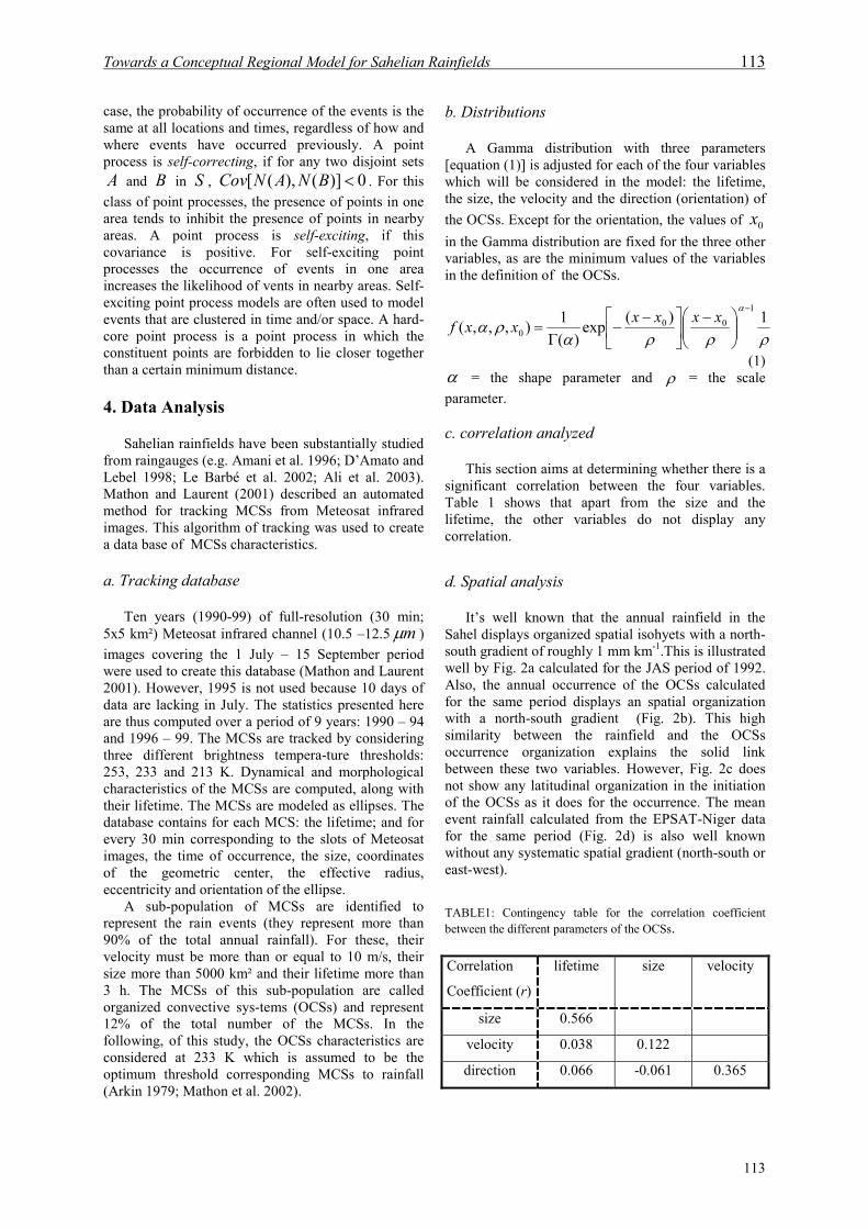
Towards a Conceptual Regional Model for Sahelian Rainfields 113
case, the probability of occurrence of the events is the same at all locations and times, regardless of how and where events have occurred previously. A point process is self-correcting, if for any two disjoint sets
and A B in , . For this class of point processes, the presence of points in one area tends to inhibit the presence of points in nearby areas. A point process is self-exciting, if this covariance is positive. For self-exciting point processes the occurrence of events in one area increases the likelihood of vents in nearby areas. Self-exciting point process models are often used to model events that are clustered in time and/or space. A hard-core point process is a point process in which the constituent points are forbidden to lie closer together than a certain minimum distance.
S 0)](),([ �BNANCov
4. Data Analysis
Sahelian rainfields have been substantially studied from raingauges (e.g. Amani et al. 1996; D’Amato and Lebel 1998; Le Barbé et al. 2002; Ali et al. 2003). Mathon and Laurent (2001) described an automated method for tracking MCSs from Meteosat infrared images. This algorithm of tracking was used to create a data base of MCSs characteristics.
a. Tracking database
Ten years (1990-99) of full-resolution (30 min;
5x5 km²) Meteosat infrared channel (10.5 –12.5 ) images covering the 1 July – 15 September period were used to create this database (Mathon and Laurent 2001). However, 1995 is not used because 10 days of data are lacking in July. The statistics presented here are thus computed over a period of 9 years: 1990 – 94 and 1996 – 99. The MCSs are tracked by considering three different brightness tempera-ture thresholds: 253, 233 and 213 K. Dynamical and morphological characteristics of the MCSs are computed, along with their lifetime. The MCSs are modeled as ellipses. The database contains for each MCS: the lifetime; and for every 30 min corresponding to the slots of Meteosat images, the time of occurrence, the size, coordinates of the geometric center, the effective radius, eccentricity and orientation of the ellipse.
m�
A sub-population of MCSs are identified to represent the rain events (they represent more than 90% of the total annual rainfall). For these, their velocity must be more than or equal to 10 m/s, their size more than 5000 km² and their lifetime more than 3 h. The MCSs of this sub-population are called organized convective sys-tems (OCSs) and represent 12% of the total number of the MCSs. In the following, of this study, the OCSs characteristics are considered at 233 K which is assumed to be the optimum threshold corresponding MCSs to rainfall (Arkin 1979; Mathon et al. 2002).
b. Distributions
A Gamma distribution with three parameters [equation (1)] is adjusted for each of the four variables which will be considered in the model: the lifetime, the size, the velocity and the direction (orientation) of the OCSs. Except for the orientation, the values of in the Gamma distribution are fixed for the three other variables, as are the minimum values of the variables in the definition of the OCSs.
0x
������
�
1)(exp)(
1),,,(1
000
�
���
����
� ��
��
��
��
xxxxxxf
(1) � = the shape parameter and � = the scale parameter. c. correlation analyzed
This section aims at determining whether there is a significant correlation between the four variables. Table 1 shows that apart from the size and the lifetime, the other variables do not display any correlation.
d. Spatial analysis
It’s well known that the annual rainfield in the Sahel displays organized spatial isohyets with a north-south gradient of roughly 1 mm km-1.This is illustrated well by Fig. 2a calculated for the JAS period of 1992. Also, the annual occurrence of the OCSs calculated for the same period displays an spatial organization with a north-south gradient (Fig. 2b). This high similarity between the rainfield and the OCSs occurrence organization explains the solid link between these two variables. However, Fig. 2c does not show any latitudinal organization in the initiation of the OCSs as it does for the occurrence. The mean event rainfall calculated from the EPSAT-Niger data for the same period (Fig. 2d) is also well known without any systematic spatial gradient (north-south or east-west). TABLE1: Contingency table for the correlation coefficient between the different parameters of the OCSs. Correlation
Coefficient (r)
lifetime size velocity
size 0.566
velocity 0.038 0.122
direction 0.066 -0.061 0.365
113
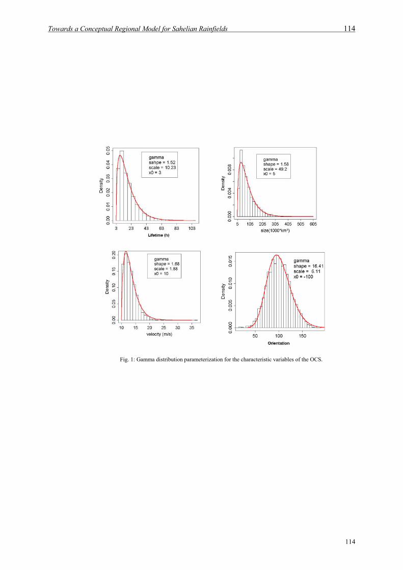
Towards a Conceptual Regional Model for Sahelian Rainfields 114
Fig. 1: Gamma distribution parameterization for the characteristic variables of the OCS.
114
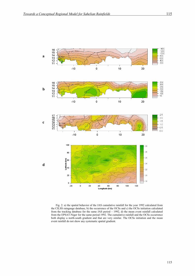
Towards a Conceptual Regional Model for Sahelian Rainfields 115
a
b
c
d
Fig. 2: a) the spatial behavior of the JAS cumulative rainfall for the year 1992 calculated from the CILSS raingauge database, b) the occurrence of the OCSs and c) the OCSs initiation calculated from the tracking database for the same JAS period – 1992, d) the mean event rainfall calculated from the EPSAT-Niger for the same period 1992. The cumulative rainfall and the OCSs occurrence both display a north-south gradient and that are very similar. The OCSs initiation and the mean event rainfall do not show any systematic spatial gradient.
115
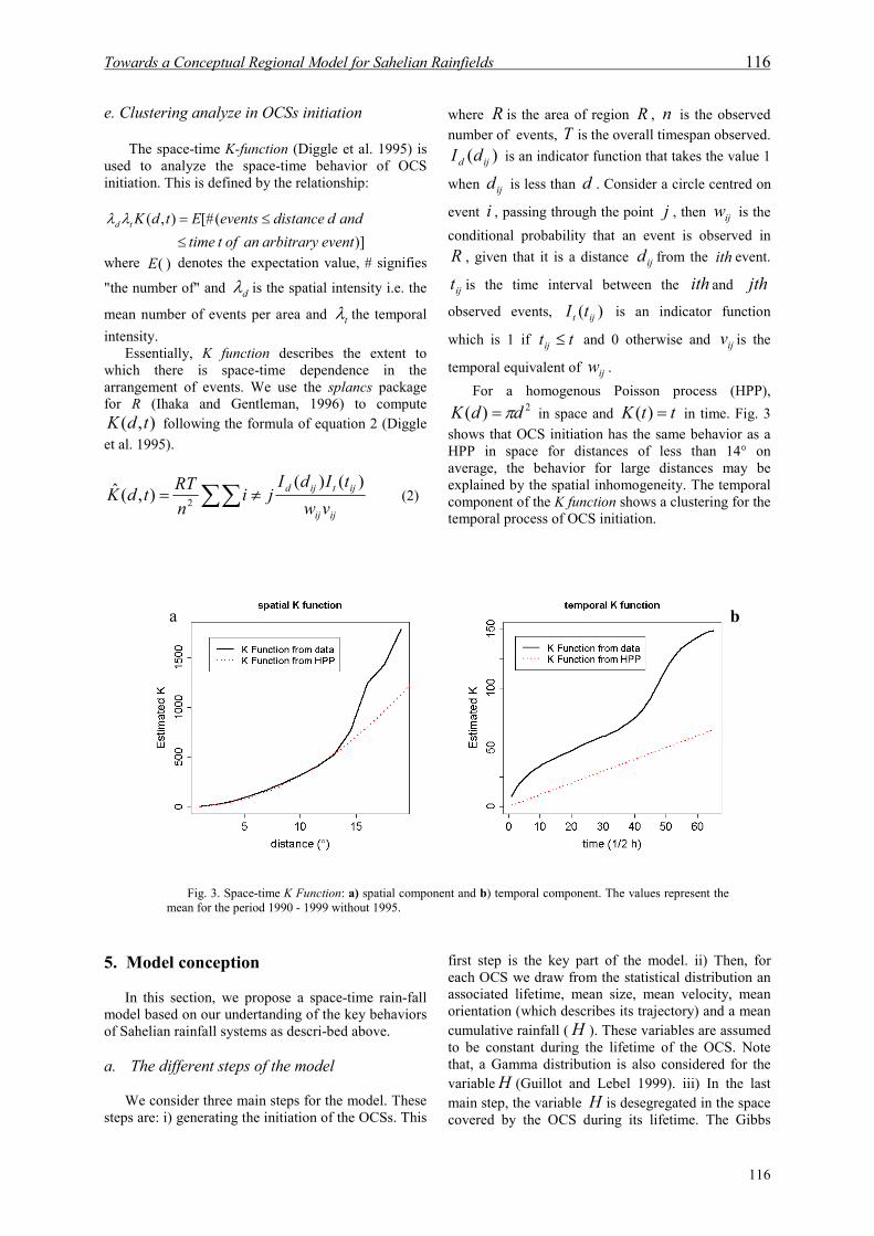
Towards a Conceptual Regional Model for Sahelian Rainfields 116
e. Clustering analyze in OCSs initiation
The space-time K-function (Diggle et al. 1995) is used to analyze the space-time behavior of OCS initiation. This is defined by the relationship:
)]([#),(
eventarbitrary an of t time and d distanceeventsEtdKtd
�
����
where denotes the expectation value, # signifies
"the number of" and is the spatial intensity i.e. the
mean number of events per area and � the temporal intensity.
)( E
d�
t
Essentially, K function describes the extent to which there is space-time dependence in the arrangement of events. We use the splancs package for R (Ihaka and Gentleman, 1996) to compute
following the formula of equation 2 (Diggle et al. 1995).
),( tdK
�� ��
ijij
ijtijd
vwtIdI
jinRTtdK
)()(),(ˆ
2 (2)
where R is the area of region R , is the observed number of events,
nT is the overall timespan observed.
is an indicator function that takes the value 1
when is less than . Consider a circle centred on
event , passing through the point
)
ijdi
( ijd dId
j , then is the conditional probability that an event is observed in
ijw
R , given that it is a distance from the ith event.
is the time interval between the and
observed events, is an indicator function
which is 1 if t and 0 otherwise and v is the
temporal equivalent of .
ijd
ijt ith jth)
ij
( ijt
w
tI
t�ij ij
For a homogenous Poisson process (HPP), in space and in time. Fig. 3
shows that OCS initiation has the same behavior as a HPP in space for distances of less than 14° on average, the behavior for large distances may be explained by the spatial inhomogeneity. The temporal component of the K function shows a clustering for the temporal process of OCS initiation.
2)( ddK �� ttK �)(
a b
Fig. 3. Space-time K Function: a) spatial component and b) temporal component. The values represent the
mean for the period 1990 - 1999 without 1995. 5. Model conception
In this section, we propose a space-time rain-fall model based on our undertanding of the key behaviors of Sahelian rainfall systems as descri-bed above. a. The different steps of the model
We consider three main steps for the model. These
steps are: i) generating the initiation of the OCSs. This
first step is the key part of the model. ii) Then, for each OCS we draw from the statistical distribution an associated lifetime, mean size, mean velocity, mean orientation (which describes its trajectory) and a mean cumulative rainfall ( H ). These variables are assumed to be constant during the lifetime of the OCS. Note that, a Gamma distribution is also considered for the variable H (Guillot and Lebel 1999). iii) In the last main step, the variable H is desegregated in the space covered by the OCS during its lifetime. The Gibbs
116
Towards a Conceptual Regional Model for Sahelian Rainfields 117
algorithm will be used to allow a spatial desegregation of H , which is performed conditionally on its mean (see Onibon et al. 2004).
), y
T
,( yx
yx,(
y
The expectation value of the cumulative rain-fall P , for a given T� period and a given spatial location
is expressed by equation (3). A demonstration of this equation for a non-limited area can be found in Northrop 1998. Only the factor in square brackets which is linked to the Sahara limit is not considered in its demonstration.
(x
]/)[())](,([
0 VD
ADT
yyHTyxPE
��
���
��
���
(3) where : expected number of initiation during the T��
� period; : expectation value of the lifetime of
the OCSs; : expectation value of the size of the
OCSs; : northern limit in OCS initiation (this is
the southern border of the Sahara, see Fig. 4); : expectation value of the velocity.
D�
A�
0y
V�
b. A model for the conditional rate
The key part of equation (3) is the function )., t� In prescribing a model for the conditional
rate )/ tHt,,( yx� , we use three components:
i) a spatial background m which takes into account the spatial inhomogeneity of the probability of OCS initiations. This component can be thought of as incorporating the effect of the relief and other local conditions that can have an impact of OCS initiation. For this component, a simple two-dimensional kernel smoother is used.
),( yx
� �� � �
�
�
�
��
�
�
��
�
�
�
��
�
�
� �
N
i
n
j y
ij
x
ji
i
i yyK
xxK
nNm
1 1
00
0
011)��
(4) In estimating the spatial background, the data must
be separated into two subsets. The spatial locations of the initiations are smoothed for the first data subset, guaranteeing that the estimate of the conditional intensity at time t is based strictly on information before t .
In equation (4) is the number of years constituting the first data subset used to compute the smoothing function; is the number of initiations
for the year i and represents the spatial
coordinates of the initiation in that subset. �
and � are the bandwidth parameters.
N
in0
,0i
j yth
)( 0i
jx
J x
K is a suitable kernel function (i.e positive, symmetric and integrates to 1). Similar approaches using kernel smoothing have
been taken in the area of seismology (see e.g. Zhuang et al. 2002). We use a Normal density kernel function:
� �2exp21)( 2zz ��
�
K (5)
For the bandwidth selection, see the discussion in Choi and Hall 1998.
ii) A seasonal component is used to describe the overall seasonal variation of the OCS initiation activity.
� �� �
��
�
�
��
�
� ��
N
i
n
j seas
ij
i
i ttK
nNts
1 1
0
0
011)(�
(6)
Here, the terms have the same signification as above.
iii) Finally, we use a one-dimensional Hawkes-type cluster model (Ogata, 1998) for describing the instantaneous temporal probability of OCS initiation. Thus, the component of the conditional rate is: (7) �
�
�
tti
i
ttg )(
where g is the trigger function
(8) ��
��
�
M
m
cmmm ezazg
1
1)(
The parameters and control the level of the clustering.
Maa ,...,1 cM represents the order of the trigger
function.
The final conditional rate is expressed as:
��
��
��
tti
t
i
ttgtSyxmHtyx
)()(*),(*)/,,( ���
(9) � and � are two parameters.
c. Parameters estimation
All the parameters of the models are estimated by maximizing the log-likelihood function.
� � dxdydtyxtyxtT
T S
n
iiii ),,,(,,,log)(
2
11
� ��� ��
�
������
(10) where is the vector of free parameters and is
the total number of events in the second
dataset, observed in the time interval over the area . The parameters to be estimated are: � , � , as
well as , , and
�
,...,1
n),,( iii tyxT� 21,T �
S
Maa c M . Under fairly general conditions, maximum likelihood estimates have shown to be consistent (e.g. Rathbun and Cressie, 1994). When optimizing the log-likelihood function some restrictions must be placed on the parameters in order to maintain a positive conditional intensity
117
Towards a Conceptual Regional Model for Sahelian Rainfields 118
function and ensure the numerical stability of the optimization procedure. The critical point is the selection of the value of M . This is allowed to take various values and that which gives the minimum value for the Akaike Information Criteria
(Akaike 1983) is chosen. AIC d. Accounting for dry and wet years
Fig. 5 represents the composite spatial distributions
of OCS initiations for wet and dry years, along
with the intraseasonal variability of these initiations. This shows a distinct spatial behavior between wet and dry years. The maximum initiations during wet years in the North-East of Niger is not present during dry years. It may also be seen that there is a large decrease in the number of initiations in the middle of the rainy season (i.e. August). The model must therefore take this variability between wet and dry years into account.
6. Conclusion
This work has a space-time rainfOrganized Convecmodel is able to tageneity, the seasclustering of OCS
Composite of Dry years Composite of Wet years
Figbetweeseason
addressed a theoretical conception of all model, based on the initiation of tive Systems (OCSs). The proposed ke into account the spatial inhomo-onal variability and the temporal initiations. The interannual variability
must be taken into account by considering the different behavior observed between wet and dry years, both in terms of the spatial and temporal characteristics.
However, the practical implementation and validation of this study have not been addressed here. These will constitute one of the immediate extensions of this thesis.
. 4. OCS initiation typology for wet and dry years. The spatial distribution of initiations n wet and dry years do not display the same behavior and a distinct difference is shown in al behavior.
118
Towards a Conceptual Regional Model for Sahelian Rainfields 119
REFERENCES Akaike, H., 1983 : Information Measure and Model
Selection. Bulletin of the International Statistical Institute, 50, 277–291.
Ali, A., T. Lebel and A. Amani : Invariance in the Spatial Structure of Sahelian Rain fields at Climatological Scales . Ali, Lebel, Amani, 2003. J. hydrometeor 4(6), 996-1011
Amani, A., T. Lebel, J. Rousselle and J. D. Taupin, 1996 : Typology of rainfall fields to improve rainfall estimation in the Sahel by the area threshold method. Water Resour. Res., 32, 2473-2488.
Arkin, P., 1979: The relationship between fractional coverage of high cloud and rainfall accumulations during GATE over the B-scale array. Mon. Wea. Rev., 107, 1382-1387.
Choi, E. and P. Hall, 1998 : Nonparametric Approach to Analysis of Space-Time Data on Earthquake Occurrences. Journal of Computational and Graphical Statistics, 8, 733–748.
Daley, D. J. and D. Vere-Jones 1988 : An Introduction to the Theory of Point. Processes, Springer, NY. 147 pp.
D'Amato, N., and T. Lebel, 1998: On the characteristics of the rainfall events in the sahel with a view to the analysis of climatic variability. Int. J. Climatol., 18, 955-974.
Diggle, P., 1985: A kernel method for smoothing point process data. Appl. Stat. 34, 138-147.
Diggle P., A. Chetwynd, R. Haggkvist, and S. Morris, 1995: Second-order analysis of space-time clustering. Statistical Methods in Medical Research, 4, 124-136.
Fishman, P. M. and , D. L. Snyder, 1976 : The statistical analysis of spacetime point processes. IEEE Trans. Inf. Theory IT, 22(3), 257-274.
Guillot, G., and T. Lebel 1999 : Disaggregation of Sahelian mesoscale convective system rain fields: Further developments and validation, J. Geophys. Res., 104, 533–31,552.
Guttorp, P., and M. Thompson 1990 : Nonparametric estimation of intensities for sampled counting processes. J. Royal Stat. Soc. B 52, 157-173.
Ihaka, R., and R. Gentleman, 1996 : R: A Language for Data Analysis and Graphics. Journal of Computational and Graphical Statistics, 5, 299–314.
Karr, A. 1991 : Point Processes and Their Statistical Inference, second ed.
Le Barbé, L., T. Lebel, and D. Tapsoba, 2002 : Rainfall variability in West Africa during the years 1950–1990, J. Clim., 15, 187–202.
Lebel, T., F. Delclaux, L. Le Barbé, J. Polcher, 2000. From GCM scales to hydirlogical scales: rainfall variability in West Africa. Stochastic Envir. Res. Risk Assessm., 14 275-295.
Mason, J., 1986 : Numerical weather prediction. Proc. Roy. Soc. London, A407, 51-60.
Mathon V. and H. Laurent, 2001: Life cycle of mesoscale convective cloud systems. Q.J.R. Meteorology. Society, 127, 377-406.
Mathon V., H. Laurent and T. Lebel, 2002: Mesoscale Convective System Rainfall in the Sahel. J. Applied Meteor., 41(11), (1081-1092).
Northrop, P. J. 1998 : A clustered spatial-temporal model of rainfall. Proc. Roy. Soc. London, A454 : 1875-1888
Ogata, Y. (1998). Space-time point process models for earthquake occurrences.Ann. Inst. Statist. Math. 50(2), 379–402.
Onibon H., T. Lebel, A. Afouda, and G. Guillot 2004 : Gibbs sampling for conditional spatial disaggregation of rain fields, Water Resour. Res., 40, 10.1029/2003WR002009.
Rathbun, S. L. and Cressie, N. (1994), “Asymptotic Properties of Estimators for the Parameters of Spatial Inhomogeneous Poisson Point Processes,” Advances in Applied Probability, 26, 122–154.
Zhuang, J., Y. Ogata and D. Vere-Jones, 2002 : Stochastic Declustering of Space-Time Earthquake Occurrences,” Journal of the American Statistical Association, 97, 369–380
119

Towards a Conceptual Regional Model for Sahelian Rainfields 120
120

Conclusion 121
V - Conclusion
Conclusion 123
V.1 Principaux Résultats
Trois principaux objectifs étaient assignés à cette thèse. Il s’agissait dans un premier temps de
modéliser dans un contexte géostatistique, la variabilité interne �e et externe �I des événements pluvieux, considérées comme des invariants, et de les intégrer pour décrire la structure spatiale des champs de pluie pour tous pas de temps supérieurs à l’événement. Dans un second temps, le modèle ainsi développé devait être testé dans le domaine de l’estimation des pluies. Enfin, le troisième objectif portait sur le développement d’un modèle stochastique régional pour étudier la variabilité climatique aux échelles hydrologiques. Les données utilisées sont issues de deux échelles différentes, une échelle locale, densément instrumentée par le réseau EPSAT-Niger, et une échelle régionale, couverte par les données rassemblées dans la base du Centre Régional AGRHYMET.
Le premier et le deuxième objectifs ont été atteints. Un modèle d’invariance d’échelle basé sur les éléments invariants �e et �I avec NT (nombre d’événements) comme seul paramètre d’échelle, a été développé et validé avec succès sur des données réelles. Cette validation a eu lieu à la fois à la méso-échelle (avec les données de EPSAT-Niger) et à l’échelle régionale (avec les données du Centre Régional AGRHYMET). En dehors de son usage pour l’interpolation des champs de pluies, le modèle a permis de diagnostiquer les différentes échelles de variabilité. Ainsi à l’échelle de la saison (NT = 40, nombre moyen d’événements pour une année de pluviométrie moyenne), la variabilité interne est prédominante pour des distances inférieures à 150 km sur le variogramme. Par exemple à 100 km, l’intermittence de la pluie explique 38% de la variabilité totale et à 500 km elle en explique 88%. Il a aussi été montré que la dérive spatiale des champs de pluie sahéliens s’explique essentiellement par le nombre d’événements, NT, qui intervient dans le modèle d’invariance d’échelle en forme quadratique dans la direction Nord-Sud. La dérive liée à ce gradient devient alors rapidement prépondérante quand NT augmente. Cette situation correspond aux structures des isohyètes observés sur la région.
Dans la deuxième partie axée sur les applications, nos connaissances sur la structure spatiale des champs de pluie sahéliens (structures emboîtées et anisotropes, modèle d’invariance d’échelle, dérive spatiale) ont été capitalisées en terme de spatialisation. Ainsi, l’évaluation des méthodes d’interpolation optimale basées sur ces structures, a montré que le réseau CILSS, a fortiori celui de EPSAT-Niger, sont suffisamment denses pour fournir des valeurs de référence robustes pour tous les interpolateurs utilisés. En procédant par validation croisée sur les 650 postes disponibles on constate que les estimations fournies par quatre variantes de krigeage ne diffèrent entre elles que d’un maximum de 4%. En revanche, l’estimation théorique de l’erreur d’estimation varie fortement en fonction de la méthode considérée (elle va du simple au double dans certains cas). On peut noter tout d’abord que si NT est correctement estimé, comme cela est le cas sur la zone EPSAT-Niger, l’interpolateur utilisant la fonction de structure déduite du modèle d’invariance d’échelle a donné la meilleure estimation de la variance de krigeage. A l’échelle régionale, où on ne disposait au mieux que des données journalières, le krigeage des résidus (Regression Kriging, RK) est apparu comme fournissant la meilleure évaluation de l’erreur d’interpolation, les trois autres méthodes testées la sous-estimant fortement. La différence entre l’erreur théorique fournie par RK et l’erreur expérimentale calculée par une procédure de validation croisée est inférieure à
Conclusion 124
3% à tous les pas de temps considérés. Cette excellente performance de RK s’explique à la fois par une bonne représentation de la dérive spatiale, qui n’est pas homogène sur toute la zone CILSS, et le fait que les résidus sont plus gaussiens que les valeurs brutes : un test de normalité montre que 35% des distributions des valeurs brutes peuvent être considérées comme gaussiennes contre 82% pour les résidus. Les hypothèses sur lesquelles repose le calcul de l’écart-type de l’erreur de krigeage sont alors mieux respectées et les valeurs ainsi calculées sont plus réalistes.
L’estimateur RK a donc été considéré comme la référence à l’échelle régionale. L’erreur théorique de krigeage associée est considérée comme une valeur approchée réaliste de l’incertitude liée à cette référence. Cela a permis, dans un premier temps, de mieux estimer NT à partir de la relation d’invariance d’échelle et, dans un second temps, d’optimiser une fonction d’erreur, initialement définie et validée à partir des données EPSAT-Niger. Cette fonction d’erreur a été par la suite utilisée pour évaluer les réseaux pluviométriques des pays du CILSS et intercomparer plusieurs estimations satellites. Il ressort de cette analyse que les réseaux des pays sahéliens sont certes capables de fournir des valeurs de référence mensuelles à moins de 10% d’erreur à l’échelle de 2.5°x2.5°, mais ils sont complètement inaptes aux échelles hydrologiques. S’il s’agit par exemple de garantir une erreur d’estimation inférieure à 10% à l’échelle de la décade pour une résolution spatiale de 1°x1° – qui est l’échelle des modèles hydrologiques ou des bilans hydriques régionaux – la presque totalité de la zone CILSS est déficitaire (seulement 2% des cellules répondent à cette condition).
Pour ce qui est des produits satellitaux, ils sous-estiment tous la fréquence des valeurs faibles (intermittence) et celle des très fortes pluies. Par contre ils surestiment largement la fréquence des valeurs centrales. Cette situation peut conduire à des biais « hydrologiques » importants. L’erreur d’évaluation du meilleur produit satellite (CMAP) est le double de l’erreur théorique de la référence (obtenue à partir du réseau CILSS) : 15.9% contre 8% pour la zone bien couverte située au sud de 15°N. GPI, qui est le seul produit satellite n’incluant pas de données pluviométriques, conduit à des estimations totalement inadaptées (40% d’erreur au sud de 15°N et plus de 80% au nord de 15°N). Mais GPI a montré la même performance à estimer la variance des champs de pluie que les autres produits incluant des données sol, du fait de sa capacité à détecter les événements pluvieux. Ce résultat oriente vers des nouvelles approches d’estimation des pluies par satellite au Sahel, basées sur une exploitation optimale de la capacité des capteurs satellitaires à identifier les événements pluvieux. Par ailleurs une intercomparaison par rapport à l’estimation utilisant le réseau total du CILSS, considérée comme référence, montre que les estimations obtenues uniquement par interpolation optimale de deux réseaux moins denses que le réseau CILSS (CRA, 250 postes et SYN, 80 stations) s’avèrent meilleurs que les produits satellites. Le fait que SNY soit meilleur que les produits internationaux est un peu surprenant du fait que ces produits internationaux sont sensés inclure les données du réseau synoptique transmises via le système mondial de télécommunications (SMT). Une explication de ce résultat peut venir, d’une part, du fait que toutes les données du réseau synoptique sont ne transmises sur le SMT et, d’autres part, d’une mauvaise qualité des données du SMT.
Dans une dernière partie, une approche est proposée pour tenir compte, dans l’évaluation des produits satellites, de l’erreur de la valeur de référence qui est elle même une estimation. La mise en œuvre de cette approche est basée sur l’estimation de la covariance entre l’erreur du produit satellite et celle de la référence dans la zone CILSS où le réseau est le plus dense. Les résultats obtenus donnent des erreurs d’évaluation des produits satellites et des produits sol plus faibles que
Conclusion 125
celles qui n’intègrent pas l’erreur de la référence. Par exemple l’erreur de CMAP passe de 15.9% à 11%. Les nouvelles erreurs n’ont cependant pas changé le classement des produits établi sans tenir compte de l’erreur de la référence. Notons enfin que l’approche proposée donne des erreurs d’évaluation objectives, car elles sont indépendantes de la référence considérée.
Le but visé dans la troisième partie de cette thèse était d’élaborer un modèle conceptuel de simulation stochastique du régime pluviométrique sahélien à l’échelle régionale. L’essentiel est acquis, mais des développements restent à poursuivre. La base des données issue du suivi (tracking) des systèmes convectifs organisés (SCO) a été utilisée à cet effet. Les systèmes ont été considérés comme des objets dont il faut générer la naissance, ensuite la taille et la durée de vie, ainsi que les directions, vitesses de déplacement et la quantité de pluie associée à ces systèmes. L’analyse des données du tracking a d’abord montré une certaine inhomogénéité spatiale de la probabilité de naissance des SCO, principalement liée à l’effet du relief. Par contre il n’y a pas de gradient systématique (Nord-Sud ou Est-Ouest par exemple) de cette probabilité. La structure des naissances montre un phénomène d’agrégation temporelle. L’analyse des corrélations inter-paramètres (taille, durée de vie, vitesse, direction) a montré qu’en dehors de la taille et de la durée de vie, il y a une certaine indépendance entre les paramètres du système. Le modèle, basé sur le formalisme des processus de point, prend en compte ces caractéristiques de formation et de dynamique des systèmes convectifs pluviogènes. Pour tenir compte de la variabilité interannuelle, le modèle utilise une typologie effectuée entre année et année sèche.
V.2 Perspectives
Les perspectives de ce travail se situent dans trois directions. La plus évidente est de finaliser le modèle conceptuel et de tester des scénarios hydrologiques ou agronomiques pour le Sahel. Ces scénarios constitueront des outils d’aide à la décision pour les décideurs nationaux et internationaux dans le cadre par exemple d’un programme d’adaptation des pays sahéliens aux changements climatiques. Ce travail peut se faire de deux manières. Soit en générant stochastiquement le nombre des SCO sur la base des tendances déjà observées dans le régime pluviométrique Sahélien ; soit en procédant par approche de downscaling en liant la grande échelle et l’échelle des systèmes convectifs. Un travail en cours (en collaboration avec Nick Hall, figure V) montre par exemple une bonne relation entre des paramètres de la dynamique grande échelle et le nombre de systèmes convectifs.
La deuxième perspective consiste à adapter les outils de désagrégation développés à l’échelle de l’événement pluvieux aux échelles des cumuls de plusieurs événements. Cette adaptation s’avère particulièrement intéressante car la possibilité actuelle des MCGA, qui sont les seuls outils capables de prédire des tendances climatiques, porte sur des cumuls de plusieurs événements, typiquement des cumuls mensuels à la résolution spatiale 2.5°x2.5°. Une telle adaptation est possible à travers le modèle d’invariance d’échelle, mais nécessite un développement mathématique préalable pour pouvoir lier les paramètres des algorithmes de désagrégation calculés pour l’échelle de l’événement à des paramètres adaptés pour des échelles spatio-temporelles plus grandes.
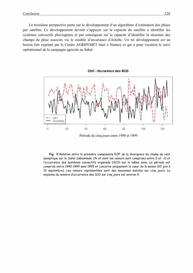
Conclusion 126
La troisième perspective porte sur le développement d’un algorithme d’estimation des pluies par satellite. Ce développement devrait s’appuyer sur la capacité du satellite à identifier les systèmes convectifs pluviogènes et par conséquent sur la capacité d’identifier la structure des champs de pluie associés via le modèle d’invariance d’échelle. Un tel développement est un besoin fort exprimé par le Centre AGRHYMET basé à Niamey et qui a pour vocation le suivi opérationnel de la campagne agricole au Sahel.
Période de cinq jours entre 1990 et 1999
Fig. V Relation entre la première composante EOF de la divergence du champ de vent synoptique sur le Sahel (dénommée Chi et dont les valeurs sont comprises entre 0 et -1) et l’occurrence des systèmes convectifs organisés (SCO) sur la même zone. La période est comprise entre 1990-1999 sans 1995 et concerne uniquement le cœur de la saison (20 juin à 10 septembre). Les valeurs représentées sont des moyennes mobiles sur cinq jours. La moyenne du nombre d’occurrence des SCO sur cinq jours est environ 9.
Références bibliographiques5 Ali A., T. Lebel and A. Amani 2004a: Estimation of Rainfall in the Sahel. Part 1 : Error Function.
J. Appl. Meteor. (article accepté) Ali A., A. Amani, A. Diedhiou, and T. Lebel 2004b: Evaluation of CILSS countries Raingauge
Networks and Objective Intercomparison of Satellite Rainfall Products. J. Appl. Meteor. (soumis)
Ali, A., T. Lebel and A. Amani : Invariance in the Spatial Structure of Sahelian Rain fields at Climatological Scales . Ali, Lebel, Amani, 2003. J. hydrometeor 4(6), 996-1011
Amani, A., T. Lebel, J. Rousselle and J. D. Taupin, 1996 : Typology of rainfall fields to improve rainfall estimation in the Sahel by the area threshold method. Water Resour. Res., 32, 2473-2488.
Amani, A., 1995 : Estimation des pluies au Sahel : quelques problèmes de modélisation analysés à partir des données Epsat-Niger. PhD Thesis, Ecole Polytechnique, Université de Montréal.
Armstrong M., A. Galli, G. Le Loc’h, F. Geffroy and R. Eschard, 2003 : Plurigaussian simulations in geosciences, Berlin: Springer-Verlag, 160 pp.
Austin, P. and R. Houze, 1972 : Analysis of the precipitation partterns of New England. J. Appl. Meteor., 11, 926-935.
Balme, M., 2004 : Analyse du régime pluviométrique Sahélien et de son impact sur le rendement du mil à l’aide des données de l’Observatoire AMMA-CATCH, Niger. Thèse de Doctorat l’Institut National Polytechnique de Grenoble, 158 pages.
Balme, M., S. Galle, et T. Lebel, 2004 : Démarrage de la saison des pluies au Sahel: variabilité à des échelles hydrologique et agronomique analysée à partir des données EPSAT-Niger. Sécheresse, (article accepté).
Bastin, G., B. Lorent, C. Duqué, and M. Gevers, 1984: Optimal estimation of the average areal rainfall and optimal selection of rain gauge locations. Water Resour. Res., 20, 463-470.
Bates, D. M. and D. G. Watts, 1988 : Nonlinear Regression Analysis and Its Applications. Wiley, 233p
Bates, D. M. and J. M. Chambers, 1992 : Nonlinear models. Statistical Models in S. J. M. Chambers and T. J. Hastie, Eds, Wadsworth & Brooks/Cole.
Burpee, R. W., 1972 : The origin and structure of easterly waves in the lower troposphere in North Africa, J. Atmos. Sci., 29, 77–90.
Calenda, G. and F. Napolitano, 1999 : Parameter estimation of Neyman-Scott processes for temporal point rainfall simulation. J. Hydrol., 225, 45-66.
Charney, J. G., 1975 : Dynamics of deserts and drought in the Sahel. Quart. J. Roy. Meteor. Soc., 101, 193-202.
Charney, J. G., W. J. Quirk, S. H. Chow, and J. Kornfield, 1977 : A comparative study of the effects of albedo change on drought in semi-arid regions; J. Atmos. Sci., 34, 1366–1385.
Chilès J. P., 1995 : Quelques méthodes de simulation de fonctions aléatoires intrinsèques. Cahiers de géostatistique. Fontainebleau, Paris, Fascicule 5, 97-112.
Chilès J. P. and Delfiner P., 1999 : Geostatistics: Modeling Spatial Uncertainty. New York: Wiley, 696 pp.
Cook, K. H., 1997 : Large scale atmospheric dynamics and Sahelian precipitation, J. Clim., 10, 1137–1152.
Cox, D. R., and V. Isham, 1994 : stochastic model of precipitation. Statistics for the environment 2: Water Related Issues, Eds. V. Barnett and K. Turkman, 3-18. Wiley, Chichester, UK.
5 Ces références bibliographiques sont celles citées dans la présentation en français de ce mémoire
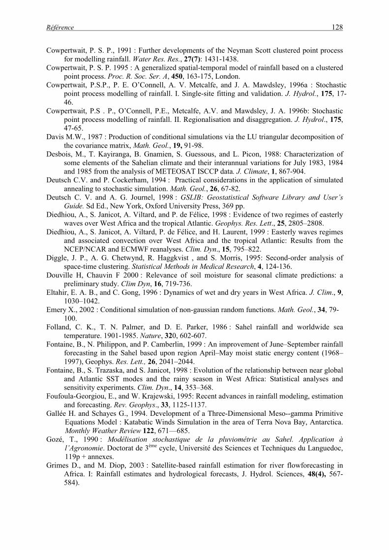
Référence 128
Cowpertwait, P. S. P., 1991 : Further developments of the Neyman Scott clustered point process for modelling rainfall. Water Res. Res., 27(7): 1431-1438.
Cowpertwait, P. S. P. 1995 : A generalized spatial-temporal model of rainfall based on a clustered point process. Proc. R. Soc. Ser. A, 450, 163-175, London.
Cowpertwait, P.S.P., P. E. O’Connell, A. V. Metcalfe, and J. A. Mawdsley, 1996a : Stochastic point process modelling of rainfall. I. Single-site fitting and validation. J. Hydrol., 175, 17-46.
Cowpertwait, P.S . P., O’Connell, P.E., Metcalfe, A.V. and Mawdsley, J. A. 1996b: Stochastic point process modelling of rainfall. II. Regionalisation and disaggregation. J. Hydrol., 175, 47-65.
Davis M.W., 1987 : Production of conditional simulations via the LU triangular decomposition of the covariance matrix, Math. Geol., 19, 91-98.
Desbois, M., T. Kayiranga, B. Gnamien, S. Guessous, and L. Picon, 1988: Characterization of some elements of the Sahelian climate and their interannual variations for July 1983, 1984 and 1985 from the analysis of METEOSAT ISCCP data. J. Climate, 1, 867-904.
Deutsch C.V. and P. Cockerham, 1994 : Practical considerations in the application of simulated annealing to stochastic simulation. Math. Geol., 26, 67-82.
Deutsch C. V. and A. G. Journel, 1998 : GSLIB: Geostatistical Software Library and User’s Guide. Sd Ed., New York, Oxford University Press, 369 pp.
Diedhiou, A., S. Janicot, A. Viltard, and P. de Félice, 1998 : Evidence of two regimes of easterly waves over West Africa and the tropical Atlantic. Geophys. Res. Lett., 25, 2805–2808.
Diedhiou, A., S. Janicot, A. Viltard, P. de Félice, and H. Laurent, 1999 : Easterly waves regimes and associated convection over West Africa and the tropical Atlantic: Results from the NCEP/NCAR and ECMWF reanalyses. Clim. Dyn., 15, 795–822.
Diggle, J. P., A. G. Chetwynd, R. Haggkvist , and S. Morris, 1995: Second-order analysis of space-time clustering. Statistical Methods in Medical Research, 4, 124-136.
Douville H, Chauvin F 2000 : Relevance of soil moisture for seasonal climate predictions: a preliminary study. Clim Dyn, 16, 719-736.
Eltahir, E. A. B., and C. Gong, 1996 : Dynamics of wet and dry years in West Africa. J. Clim., 9, 1030–1042.
Emery X., 2002 : Conditional simulation of non-gaussian random functions. Math. Geol., 34, 79-100.
Folland, C. K., T. N. Palmer, and D. E. Parker, 1986 : Sahel rainfall and worldwide sea temperature. 1901-1985. Nature, 320, 602-607.
Fontaine, B., N. Philippon, and P. Camberlin, 1999 : An improvement of June–September rainfall forecasting in the Sahel based upon region April–May moist static energy content (1968–1997), Geophys. Res. Lett., 26, 2041–2044.
Fontaine, B., S. Trazaska, and S. Janicot, 1998 : Evolution of the relationship between near global and Atlantic SST modes and the rainy season in West Africa: Statistical analyses and sensitivity experiments. Clim. Dyn., 14, 353–368.
Foufoula-Georgiou, E., and W. Krajewski, 1995: Recent advances in rainfall modeling, estimation and forecasting. Rev. Geophys., 33, 1125-1137.
Gallée H. and Schayes G., 1994. Development of a Three-Dimensional Meso--gamma Primitive Equations Model : Katabatic Winds Simulation in the area of Terra Nova Bay, Antarctica. Monthly Weather Review 122, 671—685.
Gozé, T., 1990 : Modélisation stochastique de la pluviométrie au Sahel. Application à l’Agronomie. Doctorat de 3ème cycle, Université des Sciences et Techniques du Languedoc, 119p + annexes.
Grimes D., and M. Diop, 2003 : Satellite-based rainfall estimation for river flowforecasting in Africa. I: Rainfall estimates and hydrological forecasts, J. Hydrol. Sciences, 48(4), 567-584).
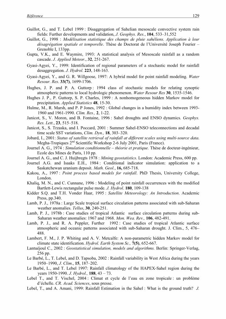
Référence 129
Guillot, G., and T. Lebel 1999 : Disaggregation of Sahelian mesoscale convective system rain fields: Further developments and validation, J. Geophys. Res., 104, 533–31,552
Guillot, G., 1998 : Modélisation statistique des champs de pluie sahéliens. Application à leur désagrégation spatiale et temporelle. Thèse de Doctorat de l’Université Joseph Fourier – Grenoble I, 133pp.
Gupta, V.K., and E. Waymire, 1993: A statistical analysis of Mesoscale rainfall as a random cascade. J. Applied Meteor., 32, 251-267.
Gyasi-Agyei, Y., 1999: Identification of regional parameters of a stochastic model for rainfall desaggregation. J. Hydrol. 223, 148-163.
Gyasi-Agyei, Y., and G. R. Willgoose, 1997: A hybrid model for point rainfall modeling. Water Resour. Res. 33(7), 1699-1706.
Hughes, J. P. and P. A. Guttorp : 1994 class of stochastic models for relating synoptic atmospheric patterns to local hydrologic phenomenon. Water Resour Res 30, 1535-1546.
Hughes J. P., P. Guttorp, S. P. Charles, 1999 : A nonhomogeneous hidden Markov model for precipitation. Applied Statistics 48, 15-30.
Hulme, M., R. Marsh, and P. P Jones, 1992 : Global changes in a humidity index between 1993-1960 and 1961-1990. Clim. Res., 2, 1-22.
Janicot, S., V. Moron, and B. Fontaine, 1996 : Sahel droughts and ENSO dynamics. Geophys. Res. Lett., 23, 515–518.
Janicot, S., S. Trzaska, and I. Poccard, 2001 : Summer Sahel-ENSO teleconnections and decadal time scale SST variations, Clim. Dyn., 18, 303–320.
Jobard, I., 2001: Status of satellite retrieval of rainfall at different scales using multi-source data. Megha-Tropiques 2nd Scientific Workshop 2-6 July 2001, Paris (France).
Journel A. G., 1974 : Simulation conditionnelle – théorie et pratique. Thèse de docteur-ingénieur, Ecole des Mines de Paris, 110 pp.
Journel A. G., and C. J. Huijbregts 1978 : Mining geostatistics. London: Academic Press, 600 pp. Journel A.G. and Isaaks E.H., 1984 : Conditional indicator simulation: application to a
Saskatchewan uranium deposit. Math. Geol., 16, 685-718. Kakou, A., 1997 : Point process based models for rainfall. PhD Thesis, University College,
London. Khaliq, M. N., and C. Cunnane, 1996 : Modeling of point rainfall occurrences with the modified
Bartlett-Lewis rectangular pulse mode. J. Hydrol. 180, 109-138 Kidder S.Q. and T.H. Vonder Haar, 1995 : Satellite Meteorology: An Introduction. Academic
Press, pp.340. Lamb, P. J., 1978a : Large Scale tropical surface circulation patterns associated with sub-Saharan
weather anomalies. Tellus, 30, 240-251. Lamb, P. J., 1978b : Case studies of tropical Atlantic surface circulation patterns during sub-
Saharan weather anomalies: 1967 and 1968. Mon. Wea. Rev., 106, 482-491. Lamb, P. J., and R. A. Peppler, Further 1992 : Case studies of tropical Atlantic surface
atmospheric and oceanic patterns associated with sub-Saharan drought. J. Clim., 5, 476–488.
Lambert, F. M., J. P. Whiting and A. V. Metcalfe: A non-parametric hidden Markov model for climate state identification. Hydrol. Earth System Sc., 7(5), 652-667.
Lantuéjoul C., 2002 : Geostatistical simulation, models and algorithms. Berlin: Springer-Verlag, 256 pp.
Le Barbé, L., T. Lebel, and D. Tapsoba, 2002 : Rainfall variability in West Africa during the years 1950–1990, J. Clim., 15, 187–202.
Le Barbé, L., and T. Lebel 1997: Rainfall climatology of the HAPEX-Sahel region during the years 1950-1990. J. Hydrol., 188, 43 – 73.
Lebel T., and T. Vischel, 2004 : Climat et cycle de l’eau en zone tropicale : un problème d’échelle. CR. Acad. Sciences, sous presse.
Lebel, T., and A. Amani, 1999: Rainfall Estimation in the Sahel : What is the ground truth? J.
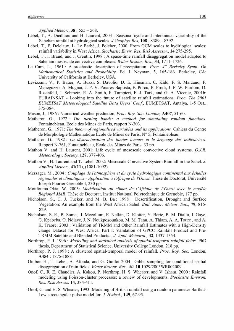
Référence 130
Applied Meteor., 38 : 555 – 568. Lebel, T., A. Diedhiou and H. Laurent, 2003 : Seasonal cycle and interannual variability of the
Sahelian rainfall at hydrological scales. J Geophys Res, 108 , 8389 – 8392. Lebel, T., F. Delclaux, L. Le Barbé, J. Polcher, 2000. From GCM scales to hydirlogical scales:
rainfall variability in West Africa. Stochastic Envir. Res. Risk Assessm., 14 275-295. Lebel, T., I. Braud, and J. Creutin, 1998 : A space-time rainfall disaggregation model adapted to
Sahelian mesoscale convective complexes. Water Resour. Res., 34, 1711–1726. Le Cam, L., 1961 : A stochastic description of precipitation. Proc. 4th Berkeley Symp. On
Mathematical Statistics and Probability. Ed. J. Neyman, 3, 165-186. Berkeley, CA: University of California at Berkeley, USA.
Levizzani, V., P. Bauer, A. Buzzi, S. Davolio, D. E. Hinsman, C. Kidd, F. S. Marzano, F. Meneguzzo, A. Mugnai, J. P. V. Poiares Baptista, F. Porcù, F. Prodi, J. F. W. Purdom, D. Rosenfeld, J. Schmetz, E. A. Smith, F. Tampieri, F. J. Turk, and G. A. Vicente, 2001b: EURAINSAT - Looking into the future of satellite rainfall estimations. Proc. The 2001 EUMETSAT Meteorological Satellite Data Users' Conf., EUMETSAT, Antalya, 1-5 Oct., 375-384.
Mason, J., 1986 : Numerical weather prediction. Proc. Roy. Soc. London, A407, 51-60. Matheron G., 1972 : The turning bands: a method for simulating random functions.
Fontainebleau, Ecole des Mines de Paris, rapport N-303. Matheron, G., 1971: The theory of regionalised variables and its applications. Cahiers du Centre
de Morphologie Mathematique Ecole de Mines de Paris, N° 5, Fontainebleau. Matheron G., 1982 : La déstructuration des hautes teneurs et le krigeage des indicatrices.
Rapport N-761, Fontainebleau, Ecole des Mines de Paris, 33 pp. Mathon V. and H. Laurent, 2001: Life cycle of mesoscale convective cloud systems. Q.J.R.
Meteorology. Society, 127, 377-406. Mathon V., H. Laurent and T. Lebel, 2002: Mesoscale Convective System Rainfall in the Sahel. J.
Applied Meteor., 41(11), (1081-1092). Messager. M., 2004 : Couplage de l'atmosphère et du cycle hydrologique continental aux échelles
régionales et climatiques - Application à l'Afrique de l'Ouest. Thèse de Doctorat, Université Joseph Fourier Grenoble I, 230 pp.
Moufouma-Okia, W. 2003: Modélisation du climat de l’Afrique de l’Ouest avec le modèle Régional MAR. Thèse de Doctorat, Institut National Polytechnique de Grenoble, 177 pp.
Nicholson, S., C. J. Tucker, and M. B. Ba : 1998 : Desertification, Drought and Surface Vegetation: An example from the West African Sahel. Bull. Amer. Meteor. Soc., 79, 816-829.
Nicholson, S. E., B. Some, J. Mccollum, E. Nelkin, D. Klotter, Y. Berte, B. M. Diallo, I. Gaye, G. Kpabeba, O. Ndiaye, J. N. Noukpozounkou, M. M. Tanu, A. Thiam, A. A. Toure , and A. K. Traore; 2003 : Validation of TRMM and Other Rainfall Estimates with a High-Density Gauge Dataset for West Africa. Part I: Validation of GPCC Rainfall Product and Pre-TRMM Satellite and Blended Products. , J. Appl. Meteorol., 42, 1337-1354.
Northrop, P. J. 1996 : Modelling and statistical analysis of spatial-temporal rainfall fields. PhD thesis, Department of Statistical Science, University College London, 218 pp.
Northrop, P. J. 1998 : A clustered spatial-temporal model of rainfall. Proc. Roy. Soc. London, A454 : 1875-1888
Onibon H., T. Lebel, A. Afouda, and G. Guillot 2004 : Gibbs sampling for conditional spatial disaggregation of rain fields, Water Resour. Res., 40, 10.1029/2003WR002009.
Onof, C., R. E. Chandler, A. Kakou, P. Northrop, H. S. Wheater, and V. Isham, 2000 : Rainfall modeling using Poisson-cluster processes: a review of developments. Stochastic Environ. Res. Risk Assess. 14, 384-411.
Onof, C. and H. S. Wheater, 1993 :Modeling of British rainfall using a random parameter Bartlett-Lewis rectangular pulse model for. J. Hydrol., 149, 67-95.
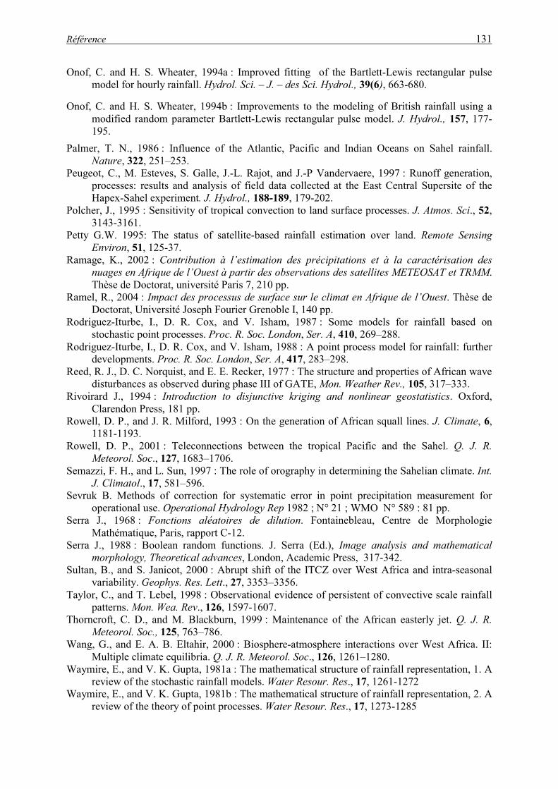
Référence 131
Onof, C. and H. S. Wheater, 1994a : Improved fitting of the Bartlett-Lewis rectangular pulse model for hourly rainfall. Hydrol. Sci. – J. – des Sci. Hydrol., 39(6), 663-680.
Onof, C. and H. S. Wheater, 1994b : Improvements to the modeling of British rainfall using a modified random parameter Bartlett-Lewis rectangular pulse model. J. Hydrol., 157, 177-195.
Palmer, T. N., 1986 : Influence of the Atlantic, Pacific and Indian Oceans on Sahel rainfall. Nature, 322, 251–253.
Peugeot, C., M. Esteves, S. Galle, J.-L. Rajot, and J.-P Vandervaere, 1997 : Runoff generation, processes: results and analysis of field data collected at the East Central Supersite of the Hapex-Sahel experiment. J. Hydrol., 188-189, 179-202.
Polcher, J., 1995 : Sensitivity of tropical convection to land surface processes. J. Atmos. Sci., 52, 3143-3161.
Petty G.W. 1995: The status of satellite-based rainfall estimation over land. Remote Sensing Environ, 51, 125-37.
Ramage, K., 2002 : Contribution à l’estimation des précipitations et à la caractérisation des nuages en Afrique de l’Ouest à partir des observations des satellites METEOSAT et TRMM. Thèse de Doctorat, université Paris 7, 210 pp.
Ramel, R., 2004 : Impact des processus de surface sur le climat en Afrique de l’Ouest. Thèse de Doctorat, Université Joseph Fourier Grenoble I, 140 pp.
Rodriguez-Iturbe, I., D. R. Cox, and V. Isham, 1987 : Some models for rainfall based on stochastic point processes. Proc. R. Soc. London, Ser. A, 410, 269–288.
Rodriguez-Iturbe, I., D. R. Cox, and V. Isham, 1988 : A point process model for rainfall: further developments. Proc. R. Soc. London, Ser. A, 417, 283–298.
Reed, R. J., D. C. Norquist, and E. E. Recker, 1977 : The structure and properties of African wave disturbances as observed during phase III of GATE, Mon. Weather Rev., 105, 317–333.
Rivoirard J., 1994 : Introduction to disjunctive kriging and nonlinear geostatistics. Oxford, Clarendon Press, 181 pp.
Rowell, D. P., and J. R. Milford, 1993 : On the generation of African squall lines. J. Climate, 6, 1181-1193.
Rowell, D. P., 2001 : Teleconnections between the tropical Pacific and the Sahel. Q. J. R. Meteorol. Soc., 127, 1683–1706.
Semazzi, F. H., and L. Sun, 1997 : The role of orography in determining the Sahelian climate. Int. J. Climatol., 17, 581–596.
Sevruk B. Methods of correction for systematic error in point precipitation measurement for operational use. Operational Hydrology Rep 1982 ; N° 21 ; WMO N° 589 : 81 pp.
Serra J., 1968 : Fonctions aléatoires de dilution. Fontainebleau, Centre de Morphologie Mathématique, Paris, rapport C-12.
Serra J., 1988 : Boolean random functions. J. Serra (Ed.), Image analysis and mathematical morphology, Theoretical advances, London, Academic Press, 317-342.
Sultan, B., and S. Janicot, 2000 : Abrupt shift of the ITCZ over West Africa and intra-seasonal variability. Geophys. Res. Lett., 27, 3353–3356.
Taylor, C., and T. Lebel, 1998 : Observational evidence of persistent of convective scale rainfall patterns. Mon. Wea. Rev., 126, 1597-1607.
Thorncroft, C. D., and M. Blackburn, 1999 : Maintenance of the African easterly jet. Q. J. R. Meteorol. Soc., 125, 763–786.
Wang, G., and E. A. B. Eltahir, 2000 : Biosphere-atmosphere interactions over West Africa. II: Multiple climate equilibria. Q. J. R. Meteorol. Soc., 126, 1261–1280.
Waymire, E., and V. K. Gupta, 1981a : The mathematical structure of rainfall representation, 1. A review of the stochastic rainfall models. Water Resour. Res., 17, 1261-1272
Waymire, E., and V. K. Gupta, 1981b : The mathematical structure of rainfall representation, 2. A review of the theory of point processes. Water Resour. Res., 17, 1273-1285

Référence 132
Waymire, E., and V. K. Gupta, 1981c : The mathematical structure of rainfall representation, 3. Some applications of the point process theory to rainfall processes. Water Resour. Res., 17, 1287-1294
Ward, M. N., 1998 : Diagnosis and short-lead time prediction of summer rainfall in tropical North Africa at interannual and multi-decadal time scales. J. Clim., 11, 3167–3191.
Wheater, H.S., A. P. Butler, E. J. Stewart, and G. S. Hamilton, 1991a : A multivariate spatial-temporal model of rainfall in South-West Saudi Arabia. I. Data characteristics and model formulation. J. Hydrol., 125, 175-99.
Wheater, H.S., C. Onof, A. P. Butler, and G. S. Hamilton 1991b : A multivariate spatial-temporal model of rainfall in South-West Saudi Arabia. II. Regional analysis and model validation. J. Hydrol., 125, 201-20.
World Meteorological Organization (WMO), 1994: Guide to hydrological practices. WMO Publication No. 168. Geneva : WMO, 735 pp.
Zheng, X., and E. A. B. Eltahir, 1998 : The role of vegetation in the dynamics of West African monsoons. J. Clim., 11, 2078–2096.