Improving Coverage Estimation for Cellular Networks withSpatial Bayesian Prediction based on Measurements

Berna Sayrac�, Janne Riihijärvi�, Petri Mähönen�,Sana Ben Jemaa�, Eric Moulines��, Sébastien Grimoud�

�Orange Labs, Issy-Les-Moulineaux, France�Institute for Networked Systems, RWTH Aachen University, Aachen, Germany

��Telecom ParisTech, Paris, Franceemail: berna.sayrac@orange-ftgroup.com

ABSTRACTCellular operators routinely use sophisticated planning toolsto estimate the coverage of the network based on build-ing and terrain data combined with detailed propagationmodeling. Nevertheless, coverage holes still emerge due toequipment failures, or unforeseen changes in the propaga-tion environment. For detecting these coverage holes, drivetests are typically used. Since carrying out drive tests isexpensive and time consuming, there is significant interestin both improving the quality of the coverage estimates ob-tained from a limited number of drive test measurements, aswell as enabling the incorporation of measurements from mo-bile terminals. In this paper we introduce a spatial Bayesianprediction framework that can be used for both of these pur-poses. We show that using techniques from modern spatialstatistics we can significantly increase the accuracy of cov-erage predictions from drive test data. Further, we carryout a detailed evaluation of our framework in urban andrural environments, using realistic coverage data obtainedfrom an operator planning tool for an operational cellularnetwork. Our results indicate that using spatial predictiontechniques can more than double the likelihood of detect-ing coverage holes, while retaining a highly acceptable falsealarm probability.

Categories and Subject DescriptorsC.2 [Computer-Communication Networks]: Miscella-neous; G.3 [Probability and Statistics]: Statistical com-puting; I.6.4 [Simulation and Modeling]: Model Vali-dation and Analysis; I.6.5 [Simulation and Modeling]:Model Development

KeywordsCoverage estimation, minimization of drive tests, Bayesiankriging, spatial statistics

Permission to make digital or hard copies of all or part of this work forpersonal or classroom use is granted without fee provided that copies arenot made or distributed for profit or commercial advantage and that copiesbear this notice and the full citation on the first page. To copy otherwise, torepublish, to post on servers or to redistribute to lists, requires prior specificpermission and/or a fee.CellNet’12, August 13, 2012, Helsinki, Finland.Copyright 2012 ACM 978-1-4503-1475-6/12/08 ...$15.00.

1. INTRODUCTIONCoverage estimation is one of the key problems in de-

ployment and operation of cellular networks. While so-phisticated planning tools incorporating building and ter-rain aware propagation models typically result in accuratecoverage estimates, coverage holes are nevertheless occasion-ally formed. These can result from changes in the propaga-tion environment, equipment failures, or other causes. Drivetests are then used to discover these coverage holes, eitheras routine part of network diagnostics, or in a targeted fash-ion based on information obtained from the customers andstatistics gathered from the network. However, drive testsare in general both expensive and time consuming. There-fore, operators have keen interest in both maximizing theutility of information obtained from drive tests, and alsominimizing the need for them. To achieve the latter, recentwork in 3GPP has targeted harnessing the measurement ca-pabilities of mobile terminals for the purposes of networkdiagnostics. The related work item goes by the name of“minimization of drive tests” (MDT) [1].

In this paper we show how coverage estimation based oneither drive tests or data obtained through the MDT ap-proach can be improved using Bayesian spatial statistics [7].This extends our earlier work on spatial estimation problemsin wireless networks [2, 10], and also illustrates how radioenvironment map (REM) techniques [9, 12] can be appliedin the cellular network context as discussed in [3]. Whileconventional drive tests can only uncover coverage holes inregions where the measurements are actively conducted, ourapproach can estimate their presence in adjacent regions aswell, based on the use of spatial prediction techniques. TheBayesian nature of our scheme also allows to take into ac-count prior knowledge the operator has on their networksetup, increasing the accuracy of the results. We show usingrealistic coverage data that spatial prediction techniques cansignificantly increase the likelihood of discovering coverageholes for a given number of measurements conducted, whileretaining low probability of false alarms.

The rest of this paper is structured as follows. In Section 2we give an overview of our spatial estimation approach, in-cluding the necessary mathematical foundations. We thenintroduce in Section 3 our evaluation scenarios, includingthe coverage data sets used together with the metrics ap-plied to quantify the performance of our scheme. Resultsof the performance evaluation are given in Section 4, andconclusions in Section 5.

43

2. COVERAGE PREDICTIONWITHBAYESIAN KRIGING

We consider the DownLink (DL) transmission of a cellu-lar radio access where there is only one BaseStation (BS)transmitter equipped with an omnidirectional antenna. Lety(xi) denote the DL received power (in dB) at location xi.Assuming that the fast fading effects are averaged out bythe receivers, y(xi) can be expressed as:

y(xi) = p0 − 10α log10 di + s(xi) + zi, (1)

where p0 is the transmitted power (in dBm), α is the pathlosscoefficient, di is the distance between the transmitter andthe receiver location xi, s(xi) is the shadowing (in dB), andzi is the zero-mean noise term which incorporates the un-certainties of the measurement process and all other randomeffects due to the propagation environment.

Equation (1) is the well-known channel model in the dBscale, which models the wireless channel as the sum of adeterministic linear pathloss term and two stochastic terms:shadowing and noise. This model is one of the most widelyused wireless channel models due to its simplicity and to itsoverall ability to represent the main characteristics of thewireless channel behaviour in a variety of important wire-less environments. The random noise process is assumed toconsist of independent and identically distributed Gaussiansamples, which are also independent of the shadowing term.Shadowing is a zero-mean Gaussian random variable that isspatially correlated according to the exponential correlationmodel [5]

E {s(xi), s(xj)} = rij =1

θexp

„−dij

φ

«, (2)

where 1θ

is the shadowing variance in dB, dij is the distancebetween locations xi and xj and φ is the correlation distanceof the shadowing.

Such power measurements are carried out by a set ofN receiving terminals, located at the set of locations x ={x1,x2, . . . ,xN}. Arranging these measurements in a N × 1column vector y(x), we obtain the vector-matrix relation

y = Xβ + u, (3)

where

X =

26641 −10 log10(d1)

......

1 −10 log10(dN )

3775 , β =

"p0

α

#,u =

2664

s(x1) + z1

...

s(xN) + zN

3775 .

(4)

Here, X is a N×2 deterministic matrix of known functions ofthe measurement locations x, β is the 2×1 parameter vectorof the spatial mean and u is a N × 1 multivariate Gaussianvector whose covariance matrix is Qyy(θ, φ, τ ) = 1

θ(Ryy(φ)+

τIN) where 1θRyy(φ) is the N ×N covariance matrix of the

spatially correlated shadowing term whose (i, j)th entry isequal to rij of equation (2), IN is the N ×N identity matrix

and [.]T denotes vector/matrix transpose. Note that thevariance of the noise process is τ

θ. Note also that y, X and

u are functions of the locations x. The aim is to predictthe received power values at locations where we do not havemeasurements. Let x0 denote the M × 1 vector of thoselocations. The same underlying model is assumed for the

predictions, given by

y0 = X0β + u0, (5)

where y0 is the M × 1 vector of received power values atlocations x0, X0 is the M × 2 matrix of deterministic effectsfor y0 and u0 is the M×1 stochastic vector whose covariancematrix is denoted by Q00(θ, φ, τ ). Note that for notationalconvenience, the dependence of y, X and u (y0, X0 and u0

resp.) on x (x0 resp.) is not shown in equations (3) and (5).The model parameters β, θ, φ and τ are unknown. There-

fore, they have to be estimated from the existing measure-ment dataset. However, those parameters are not completelyunknown to us: we have some prior knowledge on theirprobable values. For example, we can say that the radi-ated power p0 is close to the power at the antenna feeder,the propagation pathloss coefficient α is around 3.5 in ur-ban areas [6] and the shadowing standard deviation 1/

√θ

typically ranges between 8 and 11 dB for typical outdoorAbove RoofTop to Below RoofTop scenarios [11]. Includingthose prior information into the model helps us enhance theprediction quality, so we prefer using a Bayesian approach inthis paper. Besides, the Gaussian assumption of the stochas-tic component vector u in the chosen model provides easeand tractability in the complex analytical derivations of theBayesian inference framework.

The task of predicting the received power values at lo-cations x0 is equivalent to finding an estimator y0 of therandom vector y0 given measurements y. This estimator ispreferably a linear function of measurements y which mini-mizes a given loss/risk/cost function. In Bayesian context,this is equivalent to the Bayes estimator which minimizes agiven posterior expected loss/risk/cost (a.k.a. Bayes risk).The most commonly used risk function is the squared errorrisk (or the Mean Squared Error - MSE ) for which the Bayesestimator is the posterior mean E {y0|y} given by

y0 = arg miny∗0

E

n(y0 − y∗

0)T (y0 − y∗

0)|yo

, = E {y0|y} , (6)

and the Bayes risk (or MSE) is the posterior variance:

1

ME

n(y0 − y0)

T (y0 − y0)|yo

=1

Mvar {y0|y}. (7)

For the MSE Bayes estimator, we need to calculate themarginal posterior (or Bayesian) pdf p(y0|y), or at leastits moments such as the posterior mean E {y0|y} and co-variance cov {y0|y}. The derivation of these quantities arequite lengthy, therefore we will only give the main points inthe following and omit the details due to space limitations.

We start by writing the Bayesian pdf p(y0|y) as

p(y0|y) =

ZZZZτ,φ,θ,β

p(y0|β, θ, φ, τ,y)

× p(β, θ, φ, τ |y) dβ dθ dφ dτ.

(8)

The first integrand in equation (8) is the conditional pdf ofy0 given y and the model parameters. Assuming that Qyy

is non-singular, it can be shown that this pdf is Gaussianwith mean X0β + Q0yQ−1

yy (y − Xβ) and covariance matrixQ00 − Q0yQ−1

yy Qy0 [4] where Q0y and Qy0 are the cross-covariance matrices between y0 and y. Note that for nota-tional convenience, the dependence of Q0y and Qy0 on themodel parameters is not shown.

44

The second integrand in equation (8) is the joint posteriorof the model parameters which can be decomposed into theproduct of two joint posteriors:

p(β, θ, φ, τ |y) = p(β, θ|φ, τ, y)p(φ, τ |y). (9)

The first joint posterior p(β, θ|φ, τ,y) is proportional to theproduct of a likelihood term and a prior as in

p(β, θ|φ, τ,y) ∝ p(y|β, θ, φ, τ )p(β, θ|φ, τ ), (10)

where p(β, θ|φ, τ ) is the joint (conditional) prior of β and θ,and p(y|β, θ, φ, τ ) is the likelihood term which is Gaussianwith mean y − Xβ and covariance Qyy.

An important issue in Bayesian inference is the choice ofprior distributions. It is common practice to choose func-tional forms that facilitate the involved analytical treat-ments. Such functional forms are called as conjugate priors,meaning conjugate to the likelihood function, such that theposterior distribution has the same functional form as theprior distribution. Conjugate priors have been identified forthe most widely used distribution functions [8].

Reformulating the likelihood term p(y|β, θ, φ, τ ) and match-ing the pdf parameters through several algebraic manip-ulations (whose details are omitted here for brevity rea-sons), the conjugate prior for p(β, θ|φ, τ ) can be found asthe Normal-Gamma-2 density [8]. The Normal-Gamma-2density represents a multivariate Gaussian random vectorβ whose covariance matrix is scaled with a random vari-able whose inverse (θ) is Gamma-2 distributed. This im-plies that p(β|θ, φ, τ ) is Gaussian and p(θ|φ, τ ) is Gamma-2distributed.

The choice of the conjugate prior yields the same func-tional form for the joint posterior, so p(β, θ|φ, τ, y) is alsoNormal-Gamma-2. Its exact expression (and moments) canbe calculated using equation (10) which is followed by sev-eral algebraic manipulations that are again skipped here forbrevity purposes.

As for the second joint posterior of equation (9), p(φ, τ |y),it can be calculated by combining the Gaussian likelihoodp(y|β, θ, φ, τ ) and the two Normal-Gamma-2 pdfs, p(β, θ|φ, τ ),p(β, θ|φ, τ, y) with the following expression:

p(φ, τ |y) =p(y|β, θ, φ, τ )p(β, θ|φ, τ )

p(β, θ|φ, τ,y)p(φ, τ ). (11)

The joint prior p(φ, τ ) can be written as the product of themarginal densities p(φ) and p(τ ), since the noise is assumedindependent of the shadowing. Furthermore, we assume dis-crete pdfs for p(φ) and p(τ ). Therefore,

p(φ, τ ) =X

k

Xlφkτlδ(φ − φk)δ(τ − τl), (12)

where δ(.) is the Dirac delta function. Thus, replacing equa-tion (12) in equation (11), p(φ, τ |y) can also be calculatedas a discrete pdf, i.e. a weighted sum of delta functions.

We can now go back to the Bayesian pdf of equation (8).Applying the chain rule to p(β, θ, φ, τ |y), it can be writtenas

p(y0|y) =

ZZZτ,φ,θ

»Zβ

p(y0|β, θ, φ, τ, y)p(β|θ, φ, τ,y) dβ

–

× p(θ|φ, τ,y)p(φ, τ |y) dθ dφdτ. (13)

The inner integral, p(y0|θ, φ, τ,y), can be recognized as themarginalisation (wrt β) of a joint Gaussian pdf. Therefore,

it is also Gaussian whose mean and variance can be easilycalculated by analytical integration. Proceeding with theintegration with respect to θ, we can write

p(y0|y) =ZZτ,φ

»Zθ

p(y0|θ, φ, τ, y)p(θ|φ, τ,y)dθ

–p(φ, τ |y) dφdτ.

(14)

Here, the inner integral can be recognized as a Student dis-tribution whose mean E{y0|φ, τ,y} and covariance matrixcov{y0|φ, τ,y} can be calculated analytically [8]. Thesestatistics can be readily used in equation (14) together withthe discrete posterior p(φ, τ |y) to calculate the posteriormean and covariance of the MSE Bayes estimator given by

E{y0|y} =Xφ,τ

p(φ, τ |y)E{y0|φ, τ,y} (15)

and

cov{y0|y} =Xφ,τ

p(φ, τ |y)[cov{y0|φ, τ,y} + (E{y0|φ, τ,y}

− E{y0|y})(E{y0|φ, τ,y} − E{y0|y})T ].(16)

Estimation of the model parameters β and θ is carried outby calculating their posterior expectations, obtained from

E {β|y} =

ZZφ,τ

E {β|φ, τ,y} p(φ, τ |y) dφ dτ (17)

and

E {θ|y} =

ZZφ,τ

E {θ|φ, τ,y} p(φ, τ |y) dφdτ. (18)

The marginal posteriors p(β|φ, τ,y) and p(θ|φ, τ,y) neededto calculate E {β|φ, τ, y} and E {θ|φ, τ,y} can be obtainedby integrating p(β, θ|φ, τ,y) with respect to θ and β respec-tively. The former integration results in a multivariate Stu-dent distribution while the latter yields a Gamma-2 distri-bution whose first two moments can be analytically calcu-lated [8].

Considering the discrete nature of p(φ, τ |y), the two in-tegrals of equations (17) and (18) become weighted sumsof pdfs, hence the posterior parameter expectations becomeweighted averages of the conditional parameter expectationsgiven by

E {β|y} =X

φk

Xτl

p(φk, τl|y)E {β|φk, τl, y}, (19)

and

E {θ|y} =X

φk

Xτl

p(φk, τl|y)1

E {θ|φk, τl,y} . (20)

3. EVALUATION SCENARIOANDMETRICSWe shall now introduce the evaluation scenarios and met-

ric used to evaluate the performance of the proposed spatialprediction scheme for coverage estimation. As a foundationfor our evaluation work, we have used signal strength mapsobtained from a highly accurate planning tool used also foroperational network planning within Orange. The coveragemaps are for an operational 3G network and the received

45

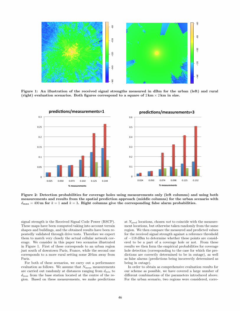
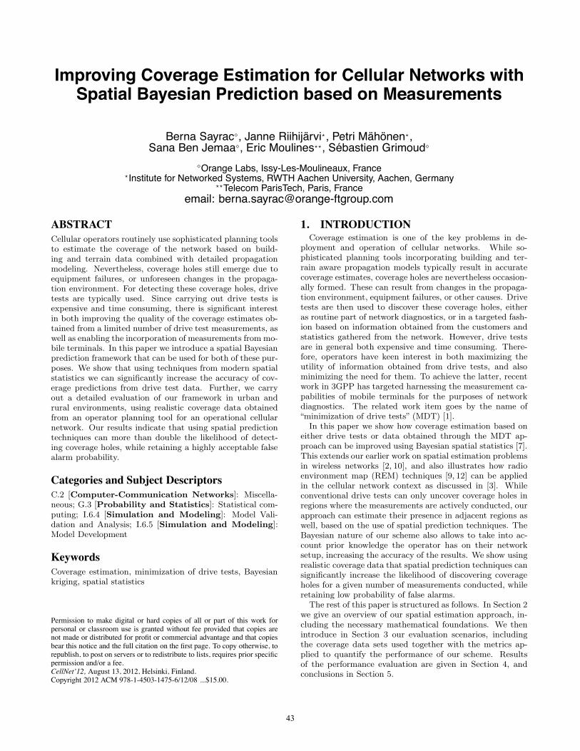
Figure 1: An illustration of the received signal strengths measured in dBm for the urban (left) and rural(right) evaluation scenarios. Both figures correspond to a square of 2km× 2km in size.

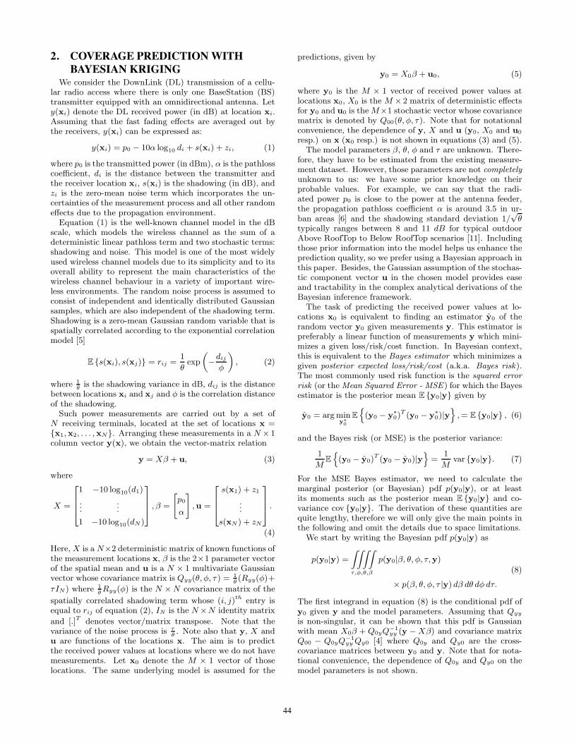
Figure 2: Detection probabilities for coverage holes using measurements only (left columns) and using bothmeasurements and results from the spatial prediction approach (middle columns) for the urban scenario withdmax = 400m for k = 1 and k = 3. Right columns give the corresponding false alarm probabilities.

signal strength is the Received Signal Code Power (RSCP).These maps have been computed taking into account terrainshapes and buildings, and the obtained results have been re-peatedly validated through drive tests. Therefore we expectthem to match very closely the actual cellular network cov-erage. We consider in this paper two scenarios illustratedin Figure 1. First of these corresponds to an urban regionjust south of downtown Paris, France, while the second onecorresponds to a more rural setting some 20 km away fromParis.

For both of these scenarios, we carry out a performanceevaluation as follows. We assume that Nmeas measurementsare carried out randomly at distances ranging from dmin todmax from the base station located at the centre of the re-gion. Based on these measurements, we make predictions

at Npred locations, chosen not to coincide with the measure-ment locations, but otherwise taken randomly from the sameregion. We then compare the measured and predicted valuesfor the received signal strength against a reference thresholdof −118 dBm to determine whether these points are consid-ered to be a part of a coverage hole or not. From theseresults we then form the empirical probabilities for coveragehole detection (corresponding to the case for which the pre-dictions are correctly determined to be in outage), as wellas false alarms (predictions being incorrectly determined asbeing in outage).

In order to obtain as comprehensive evaluation results forour scheme as possible, we have covered a large number ofdifferent combinations of the parameters introduced above.For the urban scenario, two regions were considered, corre-

46

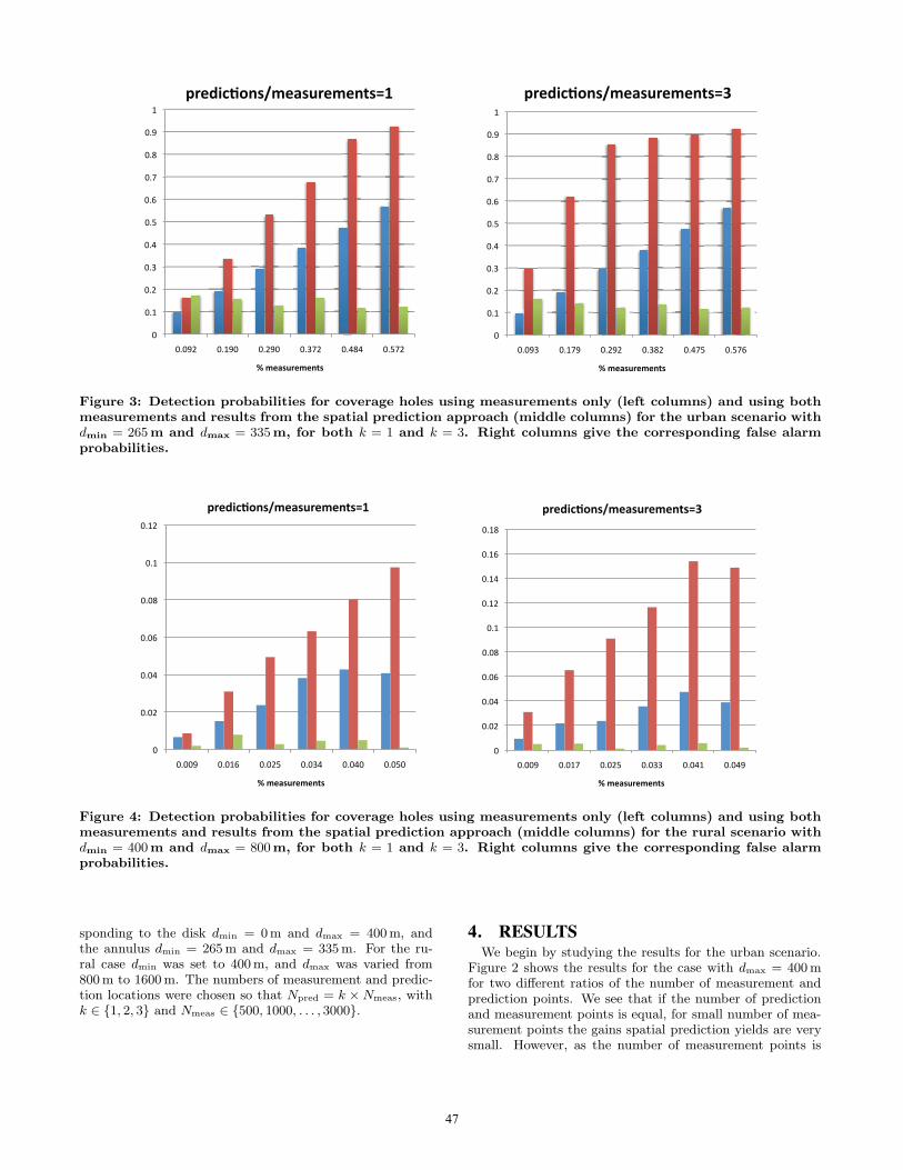
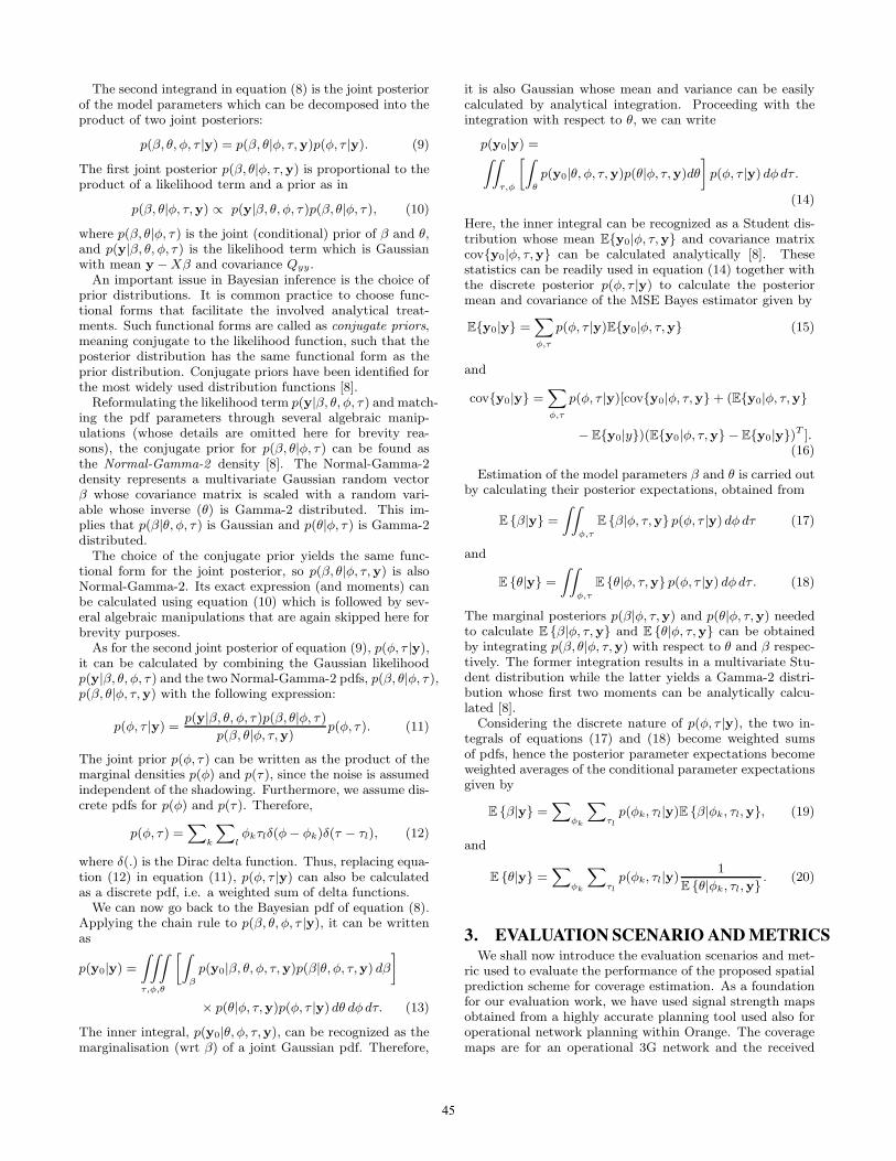
Figure 3: Detection probabilities for coverage holes using measurements only (left columns) and using bothmeasurements and results from the spatial prediction approach (middle columns) for the urban scenario withdmin = 265m and dmax = 335m, for both k = 1 and k = 3. Right columns give the corresponding false alarmprobabilities.

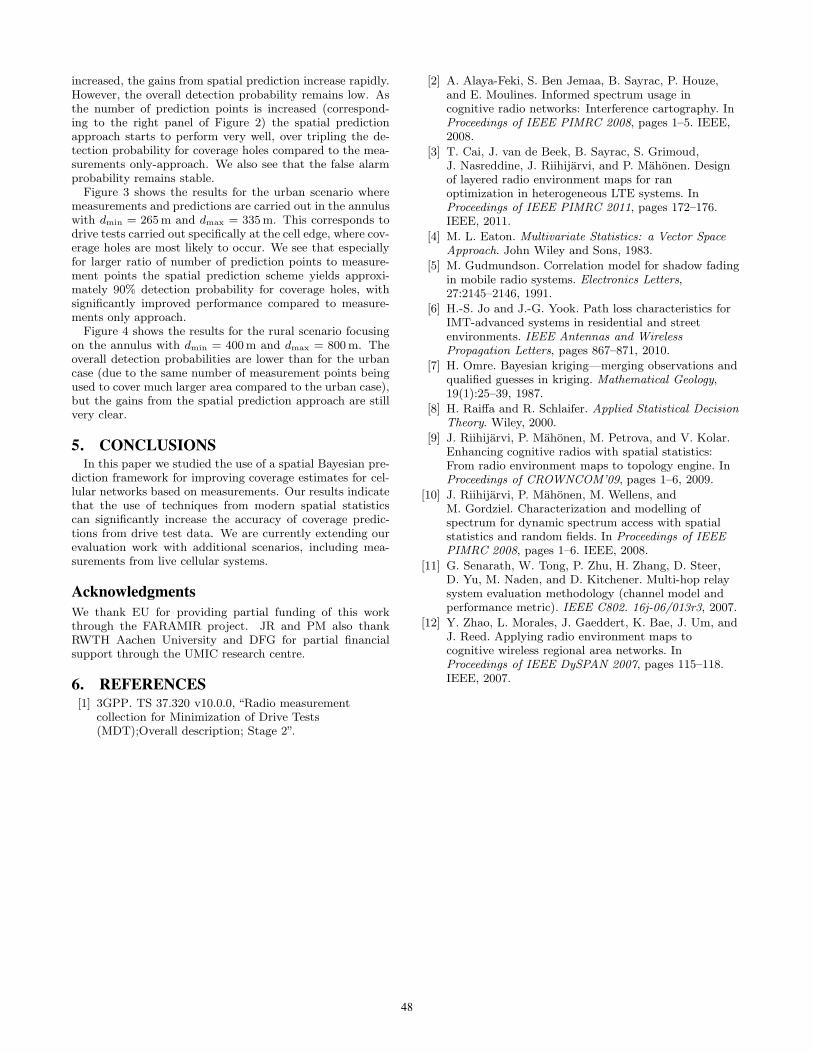
Figure 4: Detection probabilities for coverage holes using measurements only (left columns) and using bothmeasurements and results from the spatial prediction approach (middle columns) for the rural scenario withdmin = 400m and dmax = 800m, for both k = 1 and k = 3. Right columns give the corresponding false alarmprobabilities.

sponding to the disk dmin = 0m and dmax = 400 m, andthe annulus dmin = 265 m and dmax = 335 m. For the ru-ral case dmin was set to 400 m, and dmax was varied from800 m to 1600 m. The numbers of measurement and predic-tion locations were chosen so that Npred = k × Nmeas, withk ∈ {1, 2, 3} and Nmeas ∈ {500, 1000, . . . , 3000}.

4. RESULTSWe begin by studying the results for the urban scenario.

Figure 2 shows the results for the case with dmax = 400 mfor two different ratios of the number of measurement andprediction points. We see that if the number of predictionand measurement points is equal, for small number of mea-surement points the gains spatial prediction yields are verysmall. However, as the number of measurement points is

47

increased, the gains from spatial prediction increase rapidly.However, the overall detection probability remains low. Asthe number of prediction points is increased (correspond-ing to the right panel of Figure 2) the spatial predictionapproach starts to perform very well, over tripling the de-tection probability for coverage holes compared to the mea-surements only-approach. We also see that the false alarmprobability remains stable.

Figure 3 shows the results for the urban scenario wheremeasurements and predictions are carried out in the annuluswith dmin = 265 m and dmax = 335 m. This corresponds todrive tests carried out specifically at the cell edge, where cov-erage holes are most likely to occur. We see that especiallyfor larger ratio of number of prediction points to measure-ment points the spatial prediction scheme yields approxi-mately 90% detection probability for coverage holes, withsignificantly improved performance compared to measure-ments only approach.

Figure 4 shows the results for the rural scenario focusingon the annulus with dmin = 400 m and dmax = 800 m. Theoverall detection probabilities are lower than for the urbancase (due to the same number of measurement points beingused to cover much larger area compared to the urban case),but the gains from the spatial prediction approach are stillvery clear.

5. CONCLUSIONSIn this paper we studied the use of a spatial Bayesian pre-

diction framework for improving coverage estimates for cel-lular networks based on measurements. Our results indicatethat the use of techniques from modern spatial statisticscan significantly increase the accuracy of coverage predic-tions from drive test data. We are currently extending ourevaluation work with additional scenarios, including mea-surements from live cellular systems.

AcknowledgmentsWe thank EU for providing partial funding of this workthrough the FARAMIR project. JR and PM also thankRWTH Aachen University and DFG for partial financialsupport through the UMIC research centre.

6. REFERENCES[1] 3GPP. TS 37.320 v10.0.0, “Radio measurement

collection for Minimization of Drive Tests(MDT);Overall description; Stage 2”.

[2] A. Alaya-Feki, S. Ben Jemaa, B. Sayrac, P. Houze,and E. Moulines. Informed spectrum usage incognitive radio networks: Interference cartography. InProceedings of IEEE PIMRC 2008, pages 1–5. IEEE,2008.

[3] T. Cai, J. van de Beek, B. Sayrac, S. Grimoud,J. Nasreddine, J. Riihijarvi, and P. Mahonen. Designof layered radio environment maps for ranoptimization in heterogeneous LTE systems. InProceedings of IEEE PIMRC 2011, pages 172–176.IEEE, 2011.

[4] M. L. Eaton. Multivariate Statistics: a Vector SpaceApproach. John Wiley and Sons, 1983.

[5] M. Gudmundson. Correlation model for shadow fadingin mobile radio systems. Electronics Letters,27:2145–2146, 1991.

[6] H.-S. Jo and J.-G. Yook. Path loss characteristics forIMT-advanced systems in residential and streetenvironments. IEEE Antennas and WirelessPropagation Letters, pages 867–871, 2010.

[7] H. Omre. Bayesian kriging—merging observations andqualified guesses in kriging. Mathematical Geology,19(1):25–39, 1987.

[8] H. Raiffa and R. Schlaifer. Applied Statistical DecisionTheory. Wiley, 2000.

[9] J. Riihijarvi, P. Mahonen, M. Petrova, and V. Kolar.Enhancing cognitive radios with spatial statistics:From radio environment maps to topology engine. InProceedings of CROWNCOM’09, pages 1–6, 2009.

[10] J. Riihijarvi, P. Mahonen, M. Wellens, andM. Gordziel. Characterization and modelling ofspectrum for dynamic spectrum access with spatialstatistics and random fields. In Proceedings of IEEEPIMRC 2008, pages 1–6. IEEE, 2008.

[11] G. Senarath, W. Tong, P. Zhu, H. Zhang, D. Steer,D. Yu, M. Naden, and D. Kitchener. Multi-hop relaysystem evaluation methodology (channel model andperformance metric). IEEE C802. 16j-06/013r3, 2007.

[12] Y. Zhao, L. Morales, J. Gaeddert, K. Bae, J. Um, andJ. Reed. Applying radio environment maps tocognitive wireless regional area networks. InProceedings of IEEE DySPAN 2007, pages 115–118.IEEE, 2007.

48