IMACLIM-R

A modeling framework for sustainable development issues

Renaud CRASSOUS, Jean-Charles HOURCADE, Olivier SASSI, Vincent GITZ,

Sandrine MATHY, Meriem HAMDI-CHERIF *#

April 2006

* CIRED - Centre International de Recherche sur l’Environnement et le Développement 45 bis avenue de la Belle Gabrielle 94736 Nogent sur Marne Cedex contact : crassous@centre-cired.fr # The development of this modeling architecture benefited from the early participation of Philippe Ambrosi and from the development of IMACLIM-S by Frédéric Ghersi.

Contents

CONTENTS ...................................................................................................... 3

RATIONALE OF THE IMACLIM-R MODELING BLUEPRINT............... 5

TECHNICAL DESCRIPTION ........................................................................ 8

A. Static Equilibrium ............................................................................................................ 11 1. Households demand of goods, services and energy ....................................................................11

1.1. Income and savings.....................................................................................................................11 1.2. Utility function.............................................................................................................................11 1.3. Maximization program ...............................................................................................................12

2. Governments ....................................................................................................................................13 3. Purchase of goods for building productive capacities.................................................................14 4. Production constraints and supply curves ....................................................................................14 5. Market mechanisms and equilibrium constraints.........................................................................16

5.1. Labor market................................................................................................................................16 5.2. Goods markets and international trade ....................................................................................17 5.3. International capital flows..........................................................................................................21

B. Dynamic Linkages: Growth engine and technical change ............................................. 23 6. Demographic trends and overall labor productivity....................................................................23 7. Capacity, Infrastructures and equipments.....................................................................................24

7.1. Productive capacity expansions ................................................................................................24 7.2. Transportation infrastructures...................................................................................................25 7.3. Households equipments .............................................................................................................26

8. Energy-related technical change.....................................................................................................27 8.1. Supply of energy ..........................................................................................................................27 8.2. Demand of Energy......................................................................................................................29

APPENDIX A: EQUATIONS OF THE STATIC EQUILIBRIUM ..............31

APPENDIX B: REFERENCES...................................................................... 35

APPENDIX C: MAIN FEATURES OF THE BASELINE SCENARIO...... 37

LEVELS ........................................................................................................... 39

- 4 -

Rationale of the IMACLIM-R modeling blueprint

or economic modelers, the feverishness in the demands for studying sustainability issues represents an exciting challenge: how can we put some rationale in public debates in spite of the uncertainty surrounding the unprecedented time horizons necessary to understand

whether, when and why certain development pathways may be proven unsustainable? F

This challenge led to the concept of integrated modeling (Weyant et al., 1996). Issues like

climate change, energy transition, energy security, food security, migration, cannot indeed be responded to without embarking in economic models information coming from demography, engineering sciences and natural sciences at various scale levels. In the same way, it is increasingly demanded to account for lessons from other social sciences about the institutional determinants of private and collective economic behaviors.

Scientifically, the main difficulty is how to integrate in a consistent manner such diverse,

fragile and controversial information from many different disciplinary fields. But this challenge cannot be tackled without a prior clarification of three sources of long-standing controversies between economists and specialists of other disciplines and amongst economic modelers themselves whenever they deal with long term studies:

- the bottom-up vs. top-down debate which relates to the gap between the engineering view of technology and its description by economists;

- the interpretation of the concepts of general equilibrium and of equilibrated growth pathways: analytically very powerful, these notions are often suspected to be ideologically biased by non-economists and even some economists;

- the assumption of rational expectations vs. the consideration of myopic behaviors, information asymmetry and decision routines in given institutional contexts.

Motivated by lessons of a three-decennial involvement of the CIRED on energy-

environment and development issues, the primary aim of IMACLIM-R is to provide a common language to avoid that these legitimate controversies constitute an obstacle to the efficacy of modeler’s contribution to public decision. To do so, IMACLIM-R follows a modeling blueprint supported by three major principles:

First, to be based on an explicit description of the economy both in money metric values

and in physical quantities linked by a price vector, so as to ensure that long run simulations are

- 5 -

based on a consistent and plausible future physical world. This dual vision of the economy, which comes back to the inspiration of the Arrow-Debreu axiomatic, is a precondition to guarantee that the projected economy is supported by a realistic technical background, or, conversely, that any projected vision of the technical systems corresponds to realistic economic flows and sets of relative prices.

Second to be capable to incorporate information from sector based analysis about how final demand and technical systems can be transformed by various sets of economic incentives for very large departures from the reference scenario. This information can be applied to physical variables corresponding to those of top-down models under provision of appropriate aggregations. It incorporates (i) engineering based analysis about these technical systems including economies of scale, learning by doing mechanisms and saturations in efficiency progress that may occur at any given time horizons; (ii) explicit views about the efficiency of alternative incentive systems, on the rationality of economic behaviours and on the pre-existence of market and institutional imperfections.

Third to model a growth engine fueled by the investment/consumption ratio but the functioning of which is governed by (i) structural changes explicitly dependent on consistent pictures of the interplay between consumption styles, technology and land-use patterns1; (ii) overall productivity driven by endogenous growth mechanisms; (iii) investments decisions function of expected profits at each point in time and which, in case of imperfect expectations and technical inertia, generate second best growth pathways; (iv) trade patterns and international capital flows which depend on assumptions about the future organization of world markets.

The fundamental methodological choice made in IMACLIM-R and which explains its

structure is that this blueprint imposes to overcome difficulties stemming from the usual production functions. These functions indeed are critical for the dialogue between engineers and economists and for the description of the economic engine itself over the long run.

According to (Berndt and Wood, 1975) and (Jorgenson, 1981), KLE or KLEM production

functions were admitted to mimic the real set of available techniques in macroeconomic models and, by paralipsis, the technical constraints impinging upon an economy. Whatever their specifications, these functions are calibrated on cost-shares data and the Shepard's lemma is used to reveal their parameters by duality. Beyond and independently from ancient and recent questions about the economic interpretation of these functions2, it remains that the domain within which this

1 Land-use is not currently treated in the existing versions of the model. 2 Having assessed one thousand econometric works on the capital-energy substitution, Frondel and Schmidt conclude that “inferences obtained from previous empirical analyses appear to be largely an artefact of cost shares and have little to do with statistical inference about technology relationship” (Frondel and Schmidt, 2002, p.72). This comes back to the Solow’s warning that this ‘wrinkle’ is acceptable only at an aggregate level

- 6 -

use of the envelop theorem provides a robust approximation of real technical sets is limited by (i) the necessary assumption that economic data, at each point of time, result from an optimal response to the current price vector3; (ii) the assumption that constant elasticities can be used over the entire space of relative prices, production levels and time horizons under examination in sustainability issues; (iii) the increasing necessity to address technical change as endogenously determined by economic decisions, which makes the production function at t+n path-dependent.

The premise of IMACLIM-R is that it is difficult to find functions with mathematical

properties allowing for covering large departures from reference equilibrium over one century and flexible enough to embark information from sector-based analysis and different views of structural change. Indeed, it is unlikely that the resulting drastic changes in the structure of energy supply and demand will only have a marginal effect on the structure of household consumption, on the input-output matrix or on the rate and direction of technical change, which ultimately govern the structure of economic growth and the needs in primary production factors. To picture large structural changes, the challenge is to capture in a consistent manner the interplays between consumption styles (C), technological patterns (T) and localization patterns (L). As pointed out in (Hourcade, 1993), this in turn implies to embark in a common framework information coming not only from specialists in the energy field but from experts from industry, transportation, urban planning and land-use. To avoid the trap of the ‘scale one map’, a modular structure is needed whereby sector based information is translated into a set of reduced forms.

We tried earlier to overcome the potential impossibility of finding a single functional form

for production functions over a very long time horizon and a large spectrum of hypothesis in a static version of the model IMACLIM-S (Hourcade, 1993; Hourcade and Ghersi, 2000), where this is done through an envelope of production functions generated between t and t+n by a set of price signals. This approach is very flexible but cannot represent transient pathways. The dynamic recursive model IMACLIM-R now proceeds in two steps by articulating a static equilibrium and dynamic equations which changes the production frontier between each equilibrium:

- at the static equilibrium, the production function is a Leontief function, with fixed equipment stocks, and fixed intensity of labor, energy and other intermediary inputs;

- changes between t and t+1 in the level and productivity of equipments stocks and in the intensity of other production factors depend on the amount of investments and on variations of relative prices of production factors. The set of corresponding equations translate both bottom-up sector-based information and assumptions about the evolution of labor productivity.

(for specific purposes) and implies to be cautious about the interpretation of the macroeconomic productions functions as referring to a specific technical content’ (Solow, 1988, p. 313) . 3 “[...] total-factor-productivity calculations require not only that market prices can serve as a rough-and-ready approximation of marginal products, but that aggregation does not hopelessly distort these relationships [...] over-interpretation is the endemic econometric vice.” (Solow, 1988, p. 314)

- 7 -

Technical Description

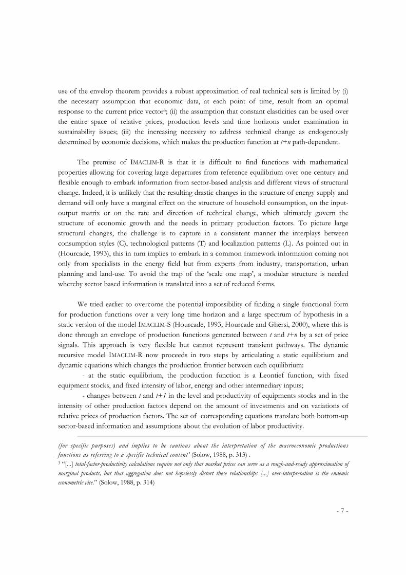
Technically IMACLIM-R is a multi-sector multi-region dynamic recursive growth model (see

Table 1 and Table 2 for regional and sector disaggregation). The growth path is described as a sequence of static short-term equilibria, on a yearly base, articulated with dynamic equations giving the new conditions for the following equilibria, as sketched in Figure 1.

Updated parameters (tech. coef., stocks, etc.)

Price-signals, rate of return Physical flows

Static Equilibrium t Static equilibrium t+1

Bottom-up sub-models

Capital and

technology dynamics

Demography

Time path

Figure 1 : The recursive dynamic framework of IMACLIM-R

At each point of time, a static equilibrium links regional inter-dependent supplies and

demands for goods. This is done by solving a general walrasian equilibrium following behavioral equations for all agents, namely households, firms and states, and accounting for regional and international flows of goods in quantities and values, as well as international investment flows. The

- 8 -

crucial point is that behavioral equations encompass some constraints: specific installed capital, technologies (input-output coefficients), household’s equipments, public infrastructures. It means that there is no substitution of factors in a given year4. Some factor markets may not be perfectly cleared in this process, allowing for unemployment, excess or shortage of production capacities, unequal rates of profitability of capital across sectors and regions.

Then the economic values derived from the equilibrium at t (relative prices, level of output, profitability rates, allocation of investments across sectors) inform both:

- the macroeconomic growth engine, composed of (i) exogenous demographic trends derived from UN estimations and corrected with migration flows capable to stabilize populations in low fertility regions; (ii) labor productivity changes governed by exogenous or endogenous trends of global productivity (depending on the version of the model) and by capital deepening mechanisms; (iii) dynamics of production capacities obeying the usual law of capital accumulation, with a full description of vintages and sector-specific lifetimes for some sectors.

- various submodels concerning energy systems, transport infrastructures or end-use equiments and which are reduced forms of more detailed models. Producers’ and consumers’ behavioral parameters that are fixed in each static equilibrium are here subject to changes. Dynamic submodels describe how each economic agent will adapt, on the demand or supply side, in response to past economic signals (variables obtained as result of former static equilibria such as relative prices or investment flows). Demographic changes follow exogenous pathways. Structural parameters of the static equilibrium (structure of demand, input-output coefficients and state of embodied technologies, installed capacities, infrastructures) are thus updated for the following time step.

Then we calculate the following equilibrium on the basis of these new coefficients. The long-term growth pathway result from how the economy adjusts to the successive changes of the level of equipments and of the technical frontier. Beyond its advantages in terms of computation, this recursive structure rests on a useful schematic representation of the growth process, made of both short-term economic variations (inside the static equilibrium) and long-term evolutions of growth drivers (in the dynamic modules).

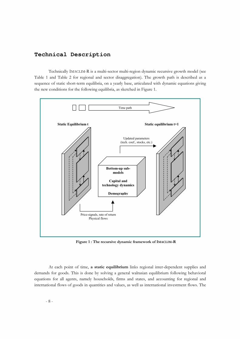
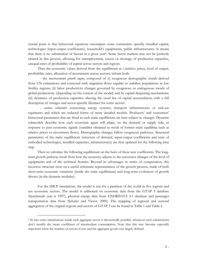
For the IMCP simulations, the model is run for a partition of the world in five regions and

ten economic sectors. The model is calibrated on economic data from the GTAP 5 database (benchmark year is 1997), physical energy data from ENERDATA 4.1 database and passenger transportation data from (Schafer and Victor, 2000). The mapping of regional and sectoral aggregation of the original regions and sectors of GTAP 5 can be found in Table 1 and Table 2.

4 In fact some substitutions inside each aggregate sector is theoretically possible, whenever such substitutions don’t modify the mean coefficient of intermediate consumption. Note that this may become especially important when the number of sectors is low and the aggregate goods very largely defined.

- 9 -

IMACLIM-R Regions GTAP regions

OECD90 Australia, New-Zealand, Japan, Canada, USA, Austria, Belgium, Denmark, Finland, France, Germany, United Kingdom, Greece, Ireland, Italy, Luxembourg, Netherlands, Portugal, Spain, Sweden, Switzerland, Turkey, Rest of EFTA, Rest Of World.

ASIA China, Hong Kong, Korea, Taiwan, Malaysia, Philippines, Singapore, Thailand, Vietnam, Bangladesh, India, Sri Lanka, Rest of South Asia.

REF Hungary , Poland , Rest of Central European Assoc., Former Soviet Union.

ALM Mexico , Central America, Caribbean, Colombia, Peru, Rest of Andean Pact, Argentina, Brazil, Chile, Uruguay, Rest of South America, Morocco, Botswana, Rest of SACU (Namibia,RSA), Malawi, Mozambique, Tanzania, Zambia, Zimbabwe, Other Southern Africa(Ang,Maur), Uganda, Rest of Sub-Saharan Africa.

OPEP Indonesia, Venezuela, Rest of North Africa, Rest of Middle-East.

Table 1 : Regional aggregation

Imaclim-R sectors GTAP sectors

Coal Coal

Oil Oil

Gas Gas

Transformed energy Petroleum and coal products

Electricity Electricity

Construction Construction

Composite good Rest of sectors

Air transport Air transport

Water transport Sea transport

Terrestrial transport Other transport

Table 2 : Sector aggregation

In the following pages, index k refers to regions, indexes i and j refer to goods or sectors, index t refers to the current year and t0 to the benchmark year 1997.

- 10 -

A. STATIC EQUILIBRIUM 5

The static equilibrium results from short-term interactions between decisions of firms,

households and public administration under constraints of existing equipment and of techniques embodied in this equipment. Variables involved in the calculation of this equilibrium are relative prices, wages, labor, quantities of goods and services, money flows. At the equilibrium, all are set to satisfy market clearing conditions for all goods under budget constraints of agents and countries while respecting the mass conservation principle of physical flows. 1. Households demand of goods, services and energy

Households are described through a representative consumer at the regional level, whose aggregate utility function is maximized under income and time constraints.6

1.1. Income and savings

Households income is equal to the sum of wages received from all sectors i in region k (non mobile labor supply), dividends (a fixed share divk,i of profits) and lump-sum public transfers, as shown in equation [1]. Savings are set as a proportion (1-ptck,i) of this income (equation [2]) 7:

k k, j k, j , k, j , , k, j k, j kIncome Ω w Q p Q transfersk j k j k jj j

l div π= ⋅ ⋅ ⋅ + ⋅ ⋅ ⋅ +∑ ∑ [1]

( )k ksaving 1 ptc income= − ⋅ k

[2]

1.2. Utility function

The households utility function is written considering that energy products contribute to utility only indirectly through the services to which it gives access (heating, cooling, cooking, mobility etc.). The arguments of the utility function are the difference (Ck,i - bnk,i) between the consumption and basic needs of a composite goods, an aggregate mobility service Sk,mobility and housing services Sk,housing. (equation [3]). Sk,mobility is a CES function of passengers-kilometers pkmk,j traveled by four transportation modes: air, public terrestrial, private cars, non motorized (equation

5 A memento of the equations of the static equilibrium can be found in Appendix A. 6 Here we follow (Muellbauer, 1976) who states that the legitimacy of the representative consumer assumption is only to provide ‘an elegant and striking informational economy’, by capturing the aggregate behavior of final demand through a utility maximization. This specification remains valid as long as the dispersion of individual consumers characteristics are not evolving significantly (Hildenbrand, 1994). 7 In the IMCP simulations these rates are fixed for all regions in order to concentrate on the induction of technical change. The endogeneisation of the saving rates is a critical challenge which should be taken up together with a better description of the loop between demography and economic growth such as in INGENUE 2 (CEPII, 2003).

- 11 -

[4]). This is a way to endogenize modal choices and to translate the fact that transport modes can not be considered as fully substitutable.

( ) ( ) ( ) ( ),

k k k k,i , k,mobilitygoods services

U C ,S C Smobility housingC

k i k k

k i k,housingi

j

bn Sξ ξξ

= −Πr r

[3]

1

k,publick,air k,cars k,nonmotorizedk,mobility

, , , ,

pkmpkm pkm pkmS

kk k k

k air k public k cars k nonmotorizedb b b b

ηη η kη η⎛ ⎞⎛ ⎞⎛ ⎞ ⎛ ⎞ ⎛ ⎞⎜ ⎟= + + +⎜ ⎟⎜ ⎟ ⎜ ⎟ ⎜ ⎟⎜ ⎟ ⎜ ⎟ ⎜ ⎟⎜ ⎟⎜ ⎟⎝ ⎠ ⎝ ⎠ ⎝ ⎠⎝ ⎠⎝ ⎠

[4]

The energy demand is derived from the levels of Sk,housing and pkmk,cars through equation [5]: cars ² ²

, k ,pkmi

cars m mk E k Ei k k EiC ,Sα α= ⋅ + ⋅ [5]

where αcars are coefficients describing the mean amount of each energy needed to travel one passenger-kilometer with the current stock of private cars; Sm² is the total surface of housing and αm² is the consumption of each energy product per square meter of housing. These parameters are held constant during the resolution of the static equilibrium and only adjusted between two equilibriums, depending on the changes in nature of end-use equipments and their energy requirements.

1.3. Maximization program

The originality of IMACLIM-R is to capture the induction of final demand by technical change and infrastructures policies in the transportation and energy sectors. This is done by considering that consumers maximize their utility under two constraints:

(i) an income constraint which imposes that purchases of non-energy goods and services Ck,i and of energy (induced by transportation by private cars and end-use services in housing) are equal to the income available for consumption (equation [6]), for a given set of consumers prices pCk,i,

( )cars ² ²k,i k,i k,Ei k , ,

Energies

Income pC C pC pkm cars m mk k k Ei k

i Ei

ptc Sα α⋅ = ⋅ + ⋅ ⋅ + ⋅∑ ∑ k Ei [6]

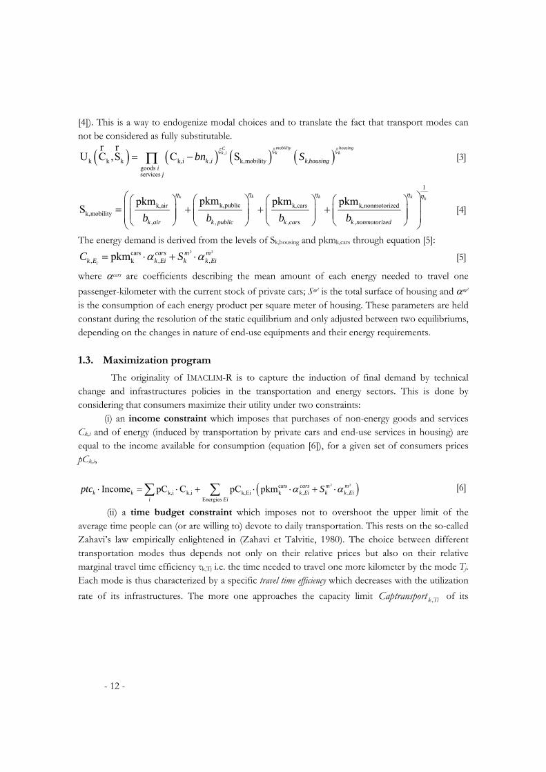
(ii) a time budget constraint which imposes not to overshoot the upper limit of the average time people can (or are willing to) devote to daily transportation. This rests on the so-called Zahavi’s law empirically enlightened in (Zahavi et Talvitie, 1980). The choice between different transportation modes thus depends not only on their relative prices but also on their relative marginal travel time efficiency τk,Tj i.e. the time needed to travel one more kilometer by the mode Tj. Each mode is thus characterized by a specific travel time efficiency which decreases with the utilization rate of its infrastructures. The more one approaches the capacity limit of its ,k TiCaptransport

- 12 -

infrastructures (expressed in kilometers of road or rail, or seat-kilometers), the less each mode will be time-efficient because of congestion (Figure 2). The Zahavi constraint thus reads8:

k,Tj

j

pkm

,means of transport T ,0

k k Tjk Tj

uTdisp duCaptransport

τ⎛ ⎞

= ⎜⎜⎝ ⎠

∑ ∫ ⎟⎟ [7]

,k Tjτ

,k TjCaptransportPkmk,Tj

Congestion, relevance of

the mode

Figure 2: Marginal time efficiency of the mode Tj

Connected with the dynamic module described here below, this optimization program under double constraint allows for representing the induction of mobility. The investments in transportation infrastructures will lower congestion of transportation networks and increase their time-efficiency, while more efficient vehicles will lower fuel costs. Thus more mobility can be ‘demanded’ by households at constant income and time budget.

2. Governments

The governments ressources are composed by the sum of all taxes. They are equal to the sum of public administrations expenditures Gk,i, transfers to households transfersk and public investments in transportation infrastructures InvInfrak 9. As Gk,i k and InvInfra are fixed in the static

k

8 Assuming a 1.1 hour per day traveling, the total annual time devoted to transportation is given by where L1.1 365kTdisp L= ⋅ ⋅ k is the total population.

9 Given the objective of this paper and given that the development of transportation infrastructures is ultimately dictated by public policies, we assume for simplicity sake that it is funded by public expenditure.

- 13 -

equilibrium, governments adjusts transfers to households to balance their budget (equation [8]). Public administrations expenditures are assumed to follow population growth.

k , k,i ktaxes pG transfersk i ki

G InvInfra= ⋅ + +∑ ∑ [8]

3. Purchase of goods for building productive capacities

As explained in (5.3), InvFink,i is the total amount of money available for investment in each sector i in the region k. This amount allows to build new capacities ∆Capk,i at a cost pCapk,i (equation [9]). The cost pCapk,i depends on the quantities βj,i,k and the prices pIk,j of goods j required by the construction of a new unit of capacity in sector i and in region k (equation [10]). Coefficient βj,i,k is the amount of good j necessary to build the equipment10 corresponding to one new unit of production capacity in the sector i of the region k. As the β-matrix represents the intensity of the productive capacities in investment goods, it is modified in the dynamic equations to be consistent with shifts to more or less capital intensive techniques.

Finally, in each region, the total demand of goods for building new capacities in all sectors is given by equation [11].

k,ik,i

k,i

InvFin∆Cap

pCap= [9]

(k,i , , j,i,kpCap pIj i kjβ= ⋅∑ )

[10]

k, j , , k,isectors

I ∆Capj i kiβ= ⋅∑ [11]

4. Production constraints and supply curves

On the short-run, producers operate under constraints of fixed technologies and production capacities. Their only margin of freedom is their utilization rate of installed capacities in function of the relative market prices of inputs and output.

The fact that physical input-ouput coefficients are held constant for a given static equilibrium translates the assumption that all investments are putty-clay. At a given point of time, a fixed set of techniques is embodied in the current stock of production capacities, and no substitution is achievable between inputs without additional investments. Therefore the production of one unit of a good i in region k requires fixed amounts of intermediate goods ICj,i,k and labor lk,i.

Physical capacities of production are also fixed, sector-specific and non malleable. Capacities are defined as the maximum levels of physical output that are achievable with the

10 In practice, due to sector aggregation in this version of the model, building a new unit of capacity only requires construction and composite good (for the other inputs, i.e. energy and transportation goods, β coefficients are null).

- 14 -

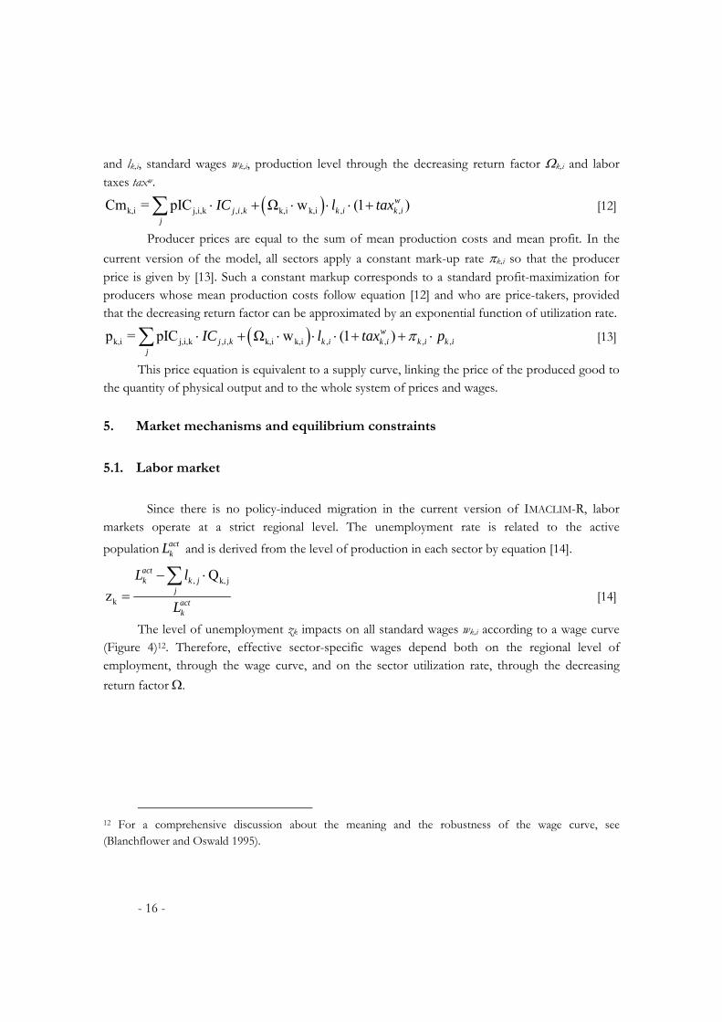
equipments build and accumulated previously. They represent a slightly different paradigm from usual production specifications, since the ‘capital’ factor is not fully operated at any time, which is realistic, especially in capital-intensive industry highly sensitive to business cycles. Indeed producers keep the ability to adjust the utilization rate of installed capacities to the market conditions. This under-utilization of capacities comes from the fact that fixed capacities imply the existence of static decreasing returns: production costs increase when the capacity utilization rate of equipments approaches one (Figure 3). Following (Corrado and Mattey 1997), we state that this is generally caused by higher labor costs due to extra hours with lower productivity, costly night work and more maintenance works11. For sake of simplicity, we assume that a decreasing return parameter Ωk,i=Ω(Qk,i/Capk,i) weighs only on wages at each sector level (see [13]), even though these incremental costs may be also caused by lower mean labor productivity and to a lesser extent by higher intermediary consumption. Sector-specific wages are thus determined by (i) regional levels of unemployment that modify standard wages wk,i (standard wage is the level of wage when the decreasing cost factor is equal to one, which occurs for a utilization rate equal to 0.8) homogeneously in all sectors (see 5.1 for details) and (ii) capacity utilization rate in each sector that impact on the static decreasing return factor.

Ω

1 Capacity utilization rate

decreasing mean

efficiency

capacity shortage

Figure 3: Static decreasing returns

We derive from the previous assumptions an expression of mean production costs Cmk,i

(equation [12]), depending on prices of intermediate goods pICj,i,k, input-ouput coefficients ICj,i,k

11 More generally, mean costs increase because less efficient units are switched on at last at the aggregate level. By default the increasing factor is attached to wages.

- 15 -

and lk,i, standard wages wk,i, production level through the decreasing return factor Ωk,i and labor taxes taxw.

( )k,i j,i,k , , k,i k,i , ,Cm = pIC Ω w (1 wj i k k i k i

j)IC l⋅ + ⋅ ⋅ ⋅ +∑ tax [12]

Producer prices are equal to the sum of mean production costs and mean profit. In the current version of the model, all sectors apply a constant mark-up rate πk,i so that the producer price is given by [13]. Such a constant markup corresponds to a standard profit-maximization for producers whose mean production costs follow equation [12] and who are price-takers, provided that the decreasing return factor can be approximated by an exponential function of utilization rate.

( )k,i j,i,k , , k,i k,i , , , ,p = pIC Ω w (1 )wj i k k i k i k i k i

jIC l tax π⋅ + ⋅ ⋅ ⋅ + + ⋅∑ p [13]

This price equation is equivalent to a supply curve, linking the price of the produced good to the quantity of physical output and to the whole system of prices and wages.

5. Market mechanisms and equilibrium constraints

5.1. Labor market

Since there is no policy-induced migration in the current version of IMACLIM-R, labor

markets operate at a strict regional level. The unemployment rate is related to the active

population actkL and is derived from the level of production in each sector by equation [14].

, k,

k

Qz

actk k j

jactk

L l

L

− ⋅=

∑ j

[14]

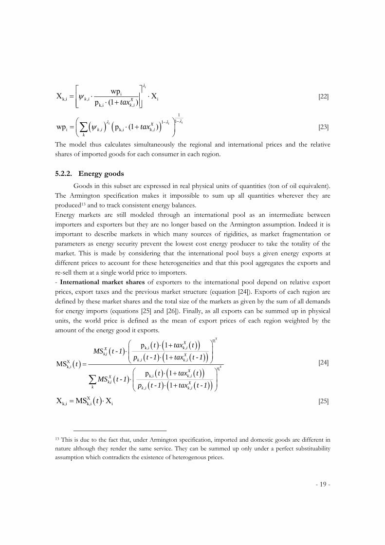
The level of unemployment zk impacts on all standard wages wk,i according to a wage curve (Figure 4)12. Therefore, effective sector-specific wages depend both on the regional level of employment, through the wage curve, and on the sector utilization rate, through the decreasing return factor Ω.

12 For a comprehensive discussion about the meaning and the robustness of the wage curve, see (Blanchflower and Oswald 1995).

- 16 -

Real wage w

Unemployment rate z

Figure 4: Wage curve

5.2. Goods markets and international trade

To represent inter-regional flows imposes to track imported and locally produced goods. In doing so, we treat ‘energy commodities’ in a different manner from all other goods and services, for which we use a usual Armington specification.

All intermediate and final demands are satisfied by a mix of domestic and imported goods. Because of the existence of different set of taxes and different preferences, the share of domestic goods in consumption is different for households, government, investment and intermediary consumption (denoted C, G, I and IC respectively). In the following section, for clarity sake, we use the index C only but all expressions are valid for the other indexes.

5.2.1. Armington goods

Composite, construction, sea transport, air transport, and terrestrial transport are assumed to follow the Armington assumption (Armington, 1969) that states that goods of the same kind produced in different regions may not be perfect substitutes. Regional demand of any Armington good (Ck,i) is thus satisfied with domestic and imported goods, which means that we do not track all bilateral flows, as it is usually the case in models designed to study trade policies. Instead, we assume that imported goods are sold by an international pool who sells an international good of the same nature, composed of the exports of the same good by all regions. We thus decompose commercial flows in two steps, the first one representing the choice of regional consumers between domestic and imported goods, the second one picturing the choice of the international pool across exporters. Regional consumers (households, governments, investors, producers) are willing to purchase an aggregate (equation [15]) of domestic and imported goods. The respective amount of domestic and

- 17 -

imported goods in that aggregate depend on their relative prices. The price of imports (equation [16]) is derived from the world prices of the international goods wpi plus import taxes taximp and international transportation costs, themselves dependent on an aggregate price for international transport wpit and on a fixed international transport requirement nitk,i for conveying good i to the region k.

( ) ( )( )1

, , , , ,dom dom imp imp

k i k i k i k i k iC b C b Cρ ρ ρ

−− −= ⋅ + ⋅ [15]

( )impk,i i , it ,p wp 1 wpimp

k i k itax nit= ⋅ + + ⋅ [16]

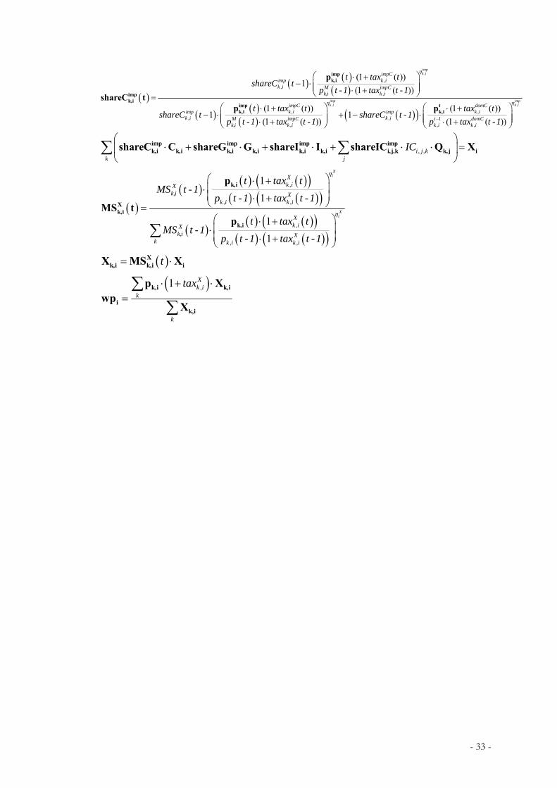
Assuming that consumers maximize the composed index Ci that they can purchase facing these prices, we derive the following its price pCk,i (equation [17]) and shares of domestic (equation [18]) and imported (equation [19]) products in demand (with taxdomC and taximpC the consumption taxes on domestic and imported goods):

( ) ( )( ) ( )

, , ,

, ,

11 1

, k,i ,

k,i 1imp, k,i ,

p (1 )pC

1 p (1 )

k i k i k i

k i k i

dom domCk i k i

dom impCk i k i

b tax

b tax

σ σ σ

σ

− −

−

⎛ ⎞⋅ +⎜= ⎜⎜ ⎟+ − ⋅ +⎝ ⎠σ

⎟⎟ [17]

,

k,idomk,i ,

k,i ,

pCshareC

p (1 )

k i

domk i domC

k i

btax

σ⎛ ⎞

= ⋅⎜⎜ ⋅ +⎝ ⎠⎟⎟ [18]

( ),

k,iimpk,i , imp

k,i ,

pCshareC 1

p (1 )

k i

domk i impC

k i

btax

σ⎛ ⎞

= − ⋅⎜⎜ ⋅ +⎝ ⎠⎟⎟

⎟⎟

[19]

The international pool thus has to provide a total amount of international good Xi equal to the sum of the regional demand for imports as shown in equation [20]. This amount of international goods is assumed to be a CES index of exports from all regions (equation [21]), in order to translate the fact that on the exporters’ side substituability is also not perfect. By minimizing the price at which the total demand Xi can be satisfied by a set of regional exports, we derive the regional exports Xk,i (equation [22]) that enter in the international good and the corresponding world price wpi (equation [23]) that allows consistent total money flows on the two sides of exports and imports.

imp impk,i k,i k,i k,i

imp impik,i k,i i, j,k , , k, j

shareC C shareG GX shareI I shareIC Qi j kk

j

IC

⎛ ⎞⋅ + ⋅⎜= + ⋅ + ⋅ ⋅⎜⎜ ⎟⎝ ⎠

∑ ∑ [20]

k,i

1

i ,X Xi

ik i

k

θθψ

−−⎡

= ⋅⎢⎣ ⎦∑ ⎤

⎥ [21]

- 18 -

ik,i , i

k,i ,

wpXp (1 )

i

k i Xk itax

λ

ψ⎡ ⎤

= ⋅ ⋅⎢⋅ +⎢ ⎥⎣ ⎦

X⎥ [22]

( ) ( )1

11

i , k,i ,wp p (1 )ii X

k i k ik

tax i λλψ

λ −−⎛ ⎞= ⋅ +⎜⎝ ⎠∑ ⎟ [23]

The model thus calculates simultaneously the regional and international prices and the relative shares of imported goods for each consumer in each region.

5.2.2. Energy goods

Goods in this subset are expressed in real physical units of quantities (ton of oil equivalent). The Armington specification makes it impossible to sum up all quantities wherever they are produced13 and to track consistent energy balances. Energy markets are still modeled through an international pool as an intermediate between importers and exporters but they are no longer based on the Armington assumption. Indeed it is important to describe markets in which many sources of rigidities, as market fragmentation or parameters as energy security prevent the lowest cost energy producer to take the totality of the market. This is made by considering that the international pool buys a given energy exports at different prices to account for these heterogeneities and that this pool aggregates the exports and re-sell them at a single world price to importers. - International market shares of exporters to the international pool depend on relative export prices, export taxes and the previous market structure (equation [24]). Exports of each region are defined by these market shares and the total size of the markets as given by the sum of all demands for energy imports (equations [25] and [26]). Finally, as all exports can be summed up in physical units, the world price is defined as the mean of export prices of each region weighted by the amount of the energy good it exports.

( )( )

( ) ( )( )( ) ( )( )

( )( ) ( )( )

( ) ( )( )

k,i ,

, ,Xk,i

k,i ,

, ,

p 1

1MS

p 1

1

Xi

Xi

Xk iX

k,i Xk i k i

Xk iX

k,i Xk k i k i

t tax tMS t -1

p t -1 tax t -1t

t tax tMS t -1

p t -1 tax t -1

η

η

⎛ ⎞⋅ +⎜ ⎟⋅⎜ ⎟⋅ +⎝=⎛ ⎞⋅ +⎜ ⎟⋅⎜ ⎟⋅ +⎝ ⎠

∑

⎠

⋅

[24]

( )Xk,i k,i iX MS Xt= [25]

13 This is due to the fact that, under Armington specification, imported and domestic goods are different in nature although they render the same service. They can be summed up only under a perfect substituability assumption which contradicts the existence of heterogenous prices.

- 19 -

imp impk,i k,i k,i k,i

imp impik,i k,i i, j,k , , k, j

shareC C shareG GX shareI I shareIC Qi j kk

j

IC

⎛ ⎞⋅ + ⋅⎜= + ⋅ + ⋅ ⋅⎜⎜ ⎟⎝ ⎠

∑ ∑⎟⎟

[26]

- Regional market shares of domestic and imported energy goods depend on the domestic and import prices of energy (equations [27] and [28]). As opposed to the Armington case, the sum of both shares is equal to 1. The consumer price of energy is simply defined as the mean between domestic and import prices weighted by the respective shares of domestic and imported flows of energy in consumption.

( )( ) ( )

( )

( ) ( )( )

,

,

impk,i ,

,,imp

k,iimpk,i ,

,,

,

p (1 ( ))1

(1 ( ))shareC t

p (1 ( ))(1 ( ))

1

impk i

impk i

impCk iimp

k i imp impCk,i k i

impCk iimp

k i imp impCk,i k i

k i

t tax tshareC t

p t -1 tax t -1

t tax tshareC t -1

p t -1 tax t -1

shareC

η

η

⎛ ⎞⋅ +− ⋅⎜ ⎟⎜ ⋅ +⎝=⎛ ⎞⋅ +⋅⎜ ⎟⎜ ⎟⋅ +⎝ ⎠

+ − ( )( ) ( )( )

⎟⎠

,

k,i ,

, ,

p (1 ( ))(1 ( ))

impk idomC

k iimpdomC

k i k i

t tax tt -1

p t -1 tax t -1

η

⎛ ⎞⎜ ⎟⎜ ⎟⎜ ⎟⎜ ⎟⎛ ⎞⋅ +⎜ ⎟⋅⎜ ⎟⎜ ⎟⎜ ⎟⋅ +⎝ ⎠⎝ ⎠

[27]

dom impk,i k,ishareC 1 shareC= − [28]

Note that this treatment allows for reproducing exact energy balances as reported by IEA, and avoid energy and emissions accounting errors.

5.2.3. Equilibrium constraints on physical flows

Equations [29] and [30] are market closure equations which secure physical balance respectively for domestic and imported goods for all kind of goods.14

dom dom domk,i k,i k,i k,i k,i k,i k,i

domk, j , , i, j,k k,i

Q shareC C shareG G shareI I

[ Q shareIC ] Xi j kj

IC

= ⋅ + ⋅ +

+ ⋅ ⋅ +∑

⋅

⋅

[29]

imp imp imp

k,i k,i k,i k,i k,i k,i k,i

impk, j , , i, j,k

M shareC C shareG G shareI I

[ Q share ]impi j k

j

IC

= ⋅ + ⋅ +

+ ⋅ ⋅∑ [30]

14 Note that for energy goods the two equations can be summed in a unique balance constraints, whereas it is not feasible for Armington goods.

- 20 -

5.3. International capital flows

5.3.1. Regional and international allocation of savings

Profits from all sectors regions are partially rebated to households according to a fixed dividend rate. Equation [31] adds up residual profits and household savings to give gross regional savings GRBk. A fixed part shareExpKk of this amount is sent to an international capital pool which re-allocates its total funds to regions according to their expected profitability rreg (equation [32]). This results is the amount of net regional savings NRBk given by equation [33]. The index of expected regional profitability (equation [34]) is computed as a weighted sum of expected sector profitability, which are themselves dependent on current cost of capacities, previous profit rate and previous utilization rate of installed capacities (equation [35]). In each region net savings are invested across sectors according to shares (equation [36]) derived from sectors’ expected profitability rsec. The global amount of investment InvFink,i for each sector is then given by equation [37]

( ) ( )k k , k, j k, jGRB Income 1 p Q 1k k jj

ptc divπ= ⋅ − + ⋅ ⋅ ⋅ −∑ ,k j [31]

''

( )( )

ImpK

k

ImpK

k

regk ImpK

k regk' ImpK

k

r bshareImpK

r b

σ

σ=∑

[32]

k k k' ''

NRB GRB (1 ) GRBk kk

shareExpK shareExpK shareImpK⎛ ⎞= ⋅ − + ⋅ ⋅⎜ ⎟⎝ ⎠∑ k [33]

sec,

,

k j kjreg

kk j

j

VA rr

VA

⋅=∑∑

[34]

1.5, , , ,

,, 0.8

k j k j k i k iseck j

k j

p Q Capr

pCapπ⎛ ⎞⋅ ⎛ ⎞

= ⋅⎜ ⎟ ⎜⎜ ⎟ ⎝ ⎠⎝ ⎠⎟ [35]

,

,

( )

( )

InvFink

k i

InvFink

k j

seck,i InvFin

k,i seck, j InvFin

j

r bshareInvFin

r b

ε

ε=∑

[36]

k,i kInvFin NRB k,ishareInvFin= ⋅ [37]

5.3.2. Commercial and capital balances

Capital balance is defined by the difference between capital exports and capital imports as shown in equation [38]. By construction, the general equilibrium demands that the capital balance

- 21 -

and the commercial balance compensate each other15. We do not need to write this equation in the model since it is fulfilled as soon as the budget balances equations of all economic agents across each regional economy are all satisfied.

''

k k kk

kBCap shareExpK shareImpK shareExpK⎛ ⎞= ⋅ ⋅ − ⋅⎜ ⎟⎝ ⎠∑ k' kGRB GRB [38]

5.3.3. Choice of a numeraire

The static equilibrium consists in a full set of quantities and relative prices fulfilling all equations above. The absolute level of prices is not determined by the model, which is completely homogenous in prices. One price has to be fixed as a numeraire and we chose to set the price of the composite good in the OECD region equal to one.

15 This rule also holds in the real world but is satisfied through mechanisms that are not modeled in this version of IMACLIM-R and that would modify the capital account, especially changes in the money stocks of central banks or variations of the external debt.

- 22 -

B. DYNAMIC LINKAGES: GROWTH ENGINE AND TECHNICAL CHANGE

Solving the static equilibrium is done by taking prices and capital flows as variables and

technical constraints as given. The dynamic equations do the reverse, considering prices and investments as fixed and the technical constraints as variables. These equations serve to calculate the evolution of parameters equipments which will be used to calculate the new equilibrium at t+1: labor productivity, input-output coefficients (including the energy mix), installed capacity and energy requirements of new equipments.

In IMACLIM-R all dimensions of technical change are putty-clay which means that, at each point in time the new techniques are optimal for prevailing economic signals but that this is not the case for total equipment stocks. This is this feature which allows for (i) representing the consequences of the interplay between inertia and the volatility of economic signals (ii) disposing of a computable endogenous growth framework since, demographic trends excepted, all technical change parameters are driven by the cumulated effect of economic choices over the projected period. Because of the embodiement of technical change in equipments, endogenous technical change captured in IMACLIM-R has to be interpreted as encompassing both R&D and learning-by-doing.

For the IMCP exercise, the model was run both under an endogenous and an exogenous technical change mode (ETC and ATC). For clarity sake, we give hereafter the dynamic equations under the ETC mode only; the ATC equations can be easily derived by making all technical parameters and functions dependant of time.

6. Demographic trends and overall labor productivity

Demography is the only exogenous parameter of the growth engine in IMACLIM; it does not change between the reference and policy scenarios. Trends are basically taken from UN estimations but allow for some migration flows in order to stabilize populations in regions in which their natural replacement is not predicted (e.g. European Union). This accounts for the fact that these regions have already planned to call for migrant workers to provide missing workforce in the future. The total and active population for the year t+1 is thus given by equations [39] and [40].

( ) ( ) ( )(1k k kL t +1 L t rL t= ⋅ + ) [39]

( ) ( ) ( )( )1act act actk k kL t +1 L t rL t= ⋅ + [40]

where rLk(t) and ( )actkrL t are respectively the annual growth rate of the total and active population

in region k at year t.. In IMACLIM-R, labor productivity is inversely proportional to parameter lk,i in equation [13]

for each sector in each region, which represents how many units of work (man-year) are needed to produce one unit of good i in the region k. Trends of productivity growth (decreasing lk,i) are

- 23 -

endogenous and equation [41] says that they depend on cumulated investment in composite good. We also paid attention to produce productivity trends consistent with historic trajectories (Maddison, 1998) and current knowledge of long-term trends (Oliveira, 2005). The updated value of parameter lk,i is then given by equation [42] ; where rLk(t) is the annual growth rate of labor productivity in region k at year t.

( )0

,..

( )k k Compop t t

rl t f Inv p=

⎛ ⎞= ⎜⎜

⎝ ⎠∑ site ⎟⎟

)

)

[41]

( ) ( ) ( )(, , 1k i k i kl t +1 l t rl t= ⋅ + [42]

As apparent labor productivity growth is partially associated with substitution between

capital and labor, equation [44] is modifying the ‘equipment-intensity’ of productive capacity by increasing coefficients of the β-matrix. The rate rβ depends on the rate of growth of labor productivity (equation [43]). This relation between the increasing rate of β-coefficients and the decreasing rate of l is calibrated from historical data (Maddison, 1998). We also assume that the general level of wages follows the increase of labor productivitythe same dynamic, shifting the wage curve upward according to equations [45] and [46].

(( ) ( )k kr t f rl tβ = [43]

( ) ( ) (, , , , 1j i k j i k kt +1 t r tβ β β= ⋅ + ( ))

)

[44]

( ) ( )( )(1

wkw

kk

a ta t +1

rl t=

+ [45]

( ) ( )( )( )1

wkw

kk

b tb t +1

rl t=

+ [46]

7. Capacity, Infrastructures and equipments

At the sector level technical change is related to the dynamics of equipments in the households, industry (the composite goods) and infrastructures (transportation, buildings).

7.1. Productive capacity expansions 16

For all sectors, except composite and electricity, the production capacity obeys to the usual law of capital accumulation (equation [47]) with a depreciation rate δk,i.

( ) ( ) ( ), , ,k i k i k i k iCap t +1 1 Cap t Capδ= − ⋅ + ∆ ,

. [47]

16 There is more time lag between the investment decision and the building of any particular investment, but we reason here at an aggregated level and not on discrete decisions.

- 24 -

For composite and electricity sectors, we track the composition of all capital vintages with their explicit operating lifetime to better capture inertia effects

( ) ,k,i k iCapvintage t Cap= ∆ [48]

These vintages embody new techniques (given by technology choices sub-modules described here

below), characterized by new intermediate consumption coefficients ( ), ,vintagej i kIC t . Equation [49]

states that productive capacity at year t+1 is the sum of capacity vintages from year t-Lifetimek,i+1 to year t, Lifetimek,i denoting the operating lifetime of equipments in these sectors. The mean of intermediate consumption coefficients weighted by the size of each vintage will give the new input-ouput coefficient (equation [50]).

( ) (,

,1

k iLifetime

k i k ip

Cap t +1 Capvintages t +1- p=

= ∑ ),

)

[49]

( )( ) (

( )

,

,

, , ,1

, ,

,1

=

=

⋅=∑

∑

k i

k i

Lifetimevintage

k i j i kp

j i k Lifetime

k ip

Capvintages t +1- p IC t +1- pIC t +1

Capvintages t +1- p [50]

7.2. Transportation infrastructures

As presented in equation [7] each transportation mode is caracterized by a capacity index (potential capacity of mobility generated in the different modes): For air transport and other transport it is calculated in the same way as productive capacity expansion (equation [47]). For private transport it is calculated in a more complex manner. Equation [51] makes it dependent on both the stock of vehicles Cark(t) and the length of available roads kminfrak(t). As indicated by equation [52], the length of roads ∆kminfrak(t) built at year t is proportional to the amount of construction good for infrastructures purchased by the government in the static equilibrium. It is added to global stock of road infrastructure ∆kminfrak which is

depreciated at an annual rate infrakδ (equation [53]). The evolution of the stock of vehicles Cark(t) will

be described in the following section.

( ) ( ) ( )(, ,k cars k kCaptransport t g Car t kminfra t= ) [51]

( ) ( ) ( )( )

,0

, 0

∆ = ∆ ⋅ k infrak k

k infra

I tkminfra t kminfra t

I t [52]

( ) ( ) ( ) ( )δ= − ⋅ + ∆infrak k kkminfra t +1 1 kminfra t kminfra tk [53]

Since in the IMPC simulations road infrastructures are taken as a policy variable, enacted by public investments, we simulated two policy cases. In the reference case, the amount of public investment

- 25 -

devoted to road building follows steadily the final demand for mobility by private cars as indicated in equation [54], whereas in the alternative policy case it is voluntarily capped.

( ) ( ) ( )( )0

0

= ⋅carsk

k k carsk

pkm tInvInfra t +1 InvInfra t

pkm t [54]

7.3. Households equipments

Equation [55] indicates that the surface of new dwellings ∆m2housingk(t) evolves in proportion of the level of consumption of construction goods computed in the static equilibrium. In equation [56] this surface is added to the global stock of housing surfaces ∆m2housingk which is depreciated with an annual rate δm2. These new dwellings incorporate new energy end-use equipments as explained in section 8.2.3.

( ) ( ) ( )( )

,2 20

, 0

∆ = ∆ ⋅ k constructionk k

k construction

C tm housing t m housing t

C t [55]

( ) ( ) ( ) ( )22 2δ= − ⋅ + ∆mk k km housing t+1 1 m housing t m housing t2

k [56]

As for the stock of private vehicles, we track the composition of each vintage of the fleet with their explicit lifetime. The fleet vintage at year t equals the amount of cars purchased during the previous static equilibrium. This amount Carvintagek(t) is proportional to the consumption of composite good and is given by equation [57]. Equation [58] states that the stock of private vehicles at year t+1 is equal to the sum of fleet vintages from year t-Lifetimekcari+1 to year t, Lifetimek,cars denoting the operating lifetime of cars. The energy requirements per kilometer are then given by

the mean of energy requirements per kilometer associated with each car vintages

weighted by the number of cars in each vintage (equation [59]). ,

carsk Eivintagesα

( ) ( ) ( )( )

,0

, 0

= ⋅ k compositek k

k composite

C tCarvintage t Carvintage t

C t [57]

( ) (,

1== ∑

k carsLifetime

kp

Car t +1 Carvintages t +1- p)k

)

[58]

( )( ) (

( )

,

,

,1

,

1

αα =

=

⋅=

∑

∑

k cars

k cars

Lifetimecars

k k Eipcars

k Ei Lifetime

kp

Carvintages t +1- p vintages t +1- pt +1

Carvintages t +1- p [59]

- 26 -

8. Energy-related technical change

The following sub-models represent technical choices and innovation dynamics that triggers technical change for energy supply and demand. Since the transformation from fossil fuels to gasoline is captured by a single i/o coefficient, we concentrate hereafter on the techniques used in the electricity sector, in fossil fuels extraction, and on energy demand by the composite sector, private transportation and residential end-uses.

8.1. Supply of energy

8.1.1. Electricity sector

The production of electricity is performed with fossil fuel based technologies (coal, gas, and oil), nuclear technologies, and renewable technologies. Market shares of these technologies in new investments are calculated through a reduced form of an electric investment module and triggered by relative evolution of the fuel prices. This module is calibrated on the POLES model and encapsulates many specifics of electric markets. Equation [60] shows the relation of the market shares of each technology to fuels prices pArmICFUELS,elec,k. Once the technology mix is determined for new vintages of electric sector equipment, equation [61] shows out how to derive the i/o coefficient of each primary energy in electricity production from its share and its mean

efficiency 17,

elecTECH kEE .

( ) ( ),elecTECH k FUELS elec kshare t f pArmIC= , , [60]

For TECH Fossil Fuel based technologies∈

( ) ( ) ( )( )

,, ,

,

=elecTECH kvintage

E TECH elec k elecTECH k

share tIC t

EE t [61]

At the same time, changes in the technology mix in the new vintage of electric capacity

impact on the price of productive capacity in the electric sector. Equation [62] shows how the β-coefficients are modified according to (i) the share of technologies in the current equipment vintage and (ii) capital costs of these technologies CAPITAL_COSTj,k.

( )( ) ( )

( ) ( )

( ), ,

, , , , 0, 0 , 0

_

_β β∈

∈

⋅= ⋅

⋅

∑

∑

elec elecj k j k

j TECHNOLOGIESi elec k i elec kelec elec

j k j kj TECHNOLOGIES

share t CAPITAL COST tt +1 t

share t CAPITAL COST t [62]

17 Other intermediate consumption coefficients (composite, construction, etc.) are assumed constant over time.

- 27 -

For each technology TECH, the evolution of energy efficiency depends on

cumulated investments in this technology (learning by doing, equation [63]). A similar learning by doing rule is adopted for the evolution of capital costs, which decrease with cumulated investments ([64]).

,elecTECH kEE

( ) ( ), , 0 ( ( ),..., ( ))elec elec elec eleck TECH k TECH TECH,k TECH,kEE t +1 EE t f Inv t Inv t= ⋅ 0 [63]

( ) ( ),

0

_ _

( ( ),..., ( ))

elec elecTECH k TECH k

elec elecTECH,k TECH,k

CAPITAL COST t +1 CAPITAL COST t, 0

f Inv t Inv t

=

⋅ [64]

8.1.2. Fossil energy extraction

Over the 21st century fossil fuels (oil, gas and coal) prices will be highly impacted by (i) increasing extraction costs due to the depletion of cheap reserves and (ii) increasing scarcity rent caused by the decrease of the Reserves/Production ratio. To capture these two drivers, we calibrate curves linking fossil fuel prices to cumulated extraction in each region on data from IFP (Institut Français du Pétrole). These curves allow us to derive the IFP’s prediction of the increase of regional fossil fuel prices at each date from the amount of cumulated production (Equation [65]). The increasing rate rFF is used to modify the parameters which will drive in IMACLIM-R both fixed equipment costs and variable extraction costs (equation [66] and [67] respectively). The markup of fossil sectors are also adjusted to fit the expected increase of the market price, taking into account the new values of i/o coefficients (equation [68]).

For , ,i oil gas coal∈ ,

( ) ( )(, , ,_k i k i k irFF t f Q Cum t= ) [65]

where Q_Cumk,i(t) is the cumulated quantity of the fossil resource i extracted during the period between the base year t0 and the current year t.

For , ,i oil gas coal∈ ,

( ) ( ) (, , , , ,j i k j i k k it +1 t 1+rFF tβ β= ⋅ ( )) [66]

( ) ( ) ( )(, , , , ,j i k j i k k i )IC t +1 IC t 1+rFF t= ⋅ [67]

( )

( )( ) ( )

( ) ( )( )( )

, ,

, ,,

,

( )

k,i k i j,i,k j i kj

wk,i k,i k i k i

k ik,i k i

,p 1+rFF t pArmIC IC t +1

- w l t +1 1+taxt +1

p 1+rFF tπ

⎛ ⎞⋅ ⋅⎜ ⎟⎜ ⎟⎜ ⎟Ω ⋅ ⋅ ⋅⎝ ⎠=

⋅

∑-

[68]

- 28 -

8.2. Demand of Energy

For the evolution of demand-side systems, we distinguish specific mechanisms for industry, transportation and residential consumptions.

8.2.1. Composite sector

Changes in energy consumption for the composite sectors are related to (i) a general energy efficiency coefficient that affects energy consumption of all vintages (ii) the energy mix embodied in the new vintage of productive capacity. The energy efficiency improvements EEIk(t) impacts on total energy intermediate consumption of the composite sector (equation [70]) and depends on cumulative investments in the composite good (equation [69]).

( )0

,..

( )k k Compositep t t

EEI t +1 f Inv j=

⎛ ⎞= ⎜⎜

⎝ ⎠∑ ⎟⎟ [69]

For i Energies∈ ,

( ) ( ) ( ), , , , 0= ⋅i composite k i composite k kIC t+1 IC t EEI t [70]

The shares of energies in new vintages of productive capacity are described by a logit function of the variation of energy prices between the previous and the current year (equation [71]) and

coefficients for the new vintage of productive capacity are computed as in equation [72]. ICFor i Energies∈ ,

( )( ) ( )

( )

( ) ( )( )

, ,, 0

, , 0,

, ,, 0

, , 0

γ

γ

∈

⎛ ⎞⋅⎜ ⎟⎜ ⎟⎝ ⎠=

⎛ ⎞⎛ ⎞⎜ ⎟⋅⎜ ⎟⎜ ⎟⎜ ⎟⎝ ⎠⎝ ⎠∑

indusk

indusk

i composite kcompositei k

i composite kcompositei k

j composite kcompositej k

j ENERGIES j composite k

pArmIC tshare t

pArmIC tshare t

pArmIC tshare t

pArmIC t

[71]

( ) ( ) ( )( )

,, , , , 0

, 0

= ⋅compositei kvintage vintage

i composite k i composite k compositei k

share tIC t IC t

share t [72]

8.2.2. Transportation by private cars

The transformed energy requirement per kilometer ( ),α carsk Etvintages t corresponding to

the new vintage of vehicles is evolving in function of the past evolution of fuel prices (equation [73]

- 29 -

). This evolution takes into account for technical progress on energy efficiency, it is calibrated on bottom up models information including technical asymptotes on gains.

( ) ( ), , 0 ,( ( ),..., ( ))cars carsk Et k Et k Et k Etvintages t+1 vintages t f pC t pC tα α= ⋅ , 0 [73]

8.2.3. Residential end-uses

End-use consumption of energy per square meter in the residential sector (parameter ²,

mk Eiα

in equation [6]) is evolving through a price-reaction function (equation [74]), which encompasses the evolution of the level of end-use equipment per square meter, the shift between energy sources and end-use energy efficiency gains.

( ) ( )2 2

, , 0 , ,( ( ),..., ( ))m mk Ei k Ei k Ei k Eit +1 t f pC t pC tα α= ⋅ 0 [74]

- 30 -

Appendix A: Equations of the static equilibrium

Core equations (Bold=variable) Income formation

, , ,k j k j k jj j

l div π= ⋅ ⋅ ⋅ + ⋅ ⋅ ⋅ +∑ ∑k k,j k,j k,j k,j k,j kIncome Ω w Q p Q transfers

nvInfra

Governments’ budget

,k i ki

G I= ⋅ + +∑ ∑ k,i ktaxes pG transfers

Utility maximisation

( ) ( ) ( ) ,,

, ,goods services

,SCk ik i

k i k ji

j

bn bnξξ

= − −Π

k k k k,i k,jU C S C S

, , , ,

kkk k

k air k public k cars k nonmotorizedb b b b

kηηη η η −

⎛ ⎞⎛ ⎞⎛ ⎞ ⎛ ⎞ ⎛ ⎞⎜ ⎟= + + +⎜ ⎟⎜ ⎟ ⎜ ⎟ ⎜ ⎟⎜ ⎟ ⎜ ⎟ ⎜ ⎟⎜ ⎟⎜ ⎟⎝ ⎠ ⎝ ⎠ ⎝ ⎠⎝ ⎠⎝ ⎠

k,publick,air k,cars k,nonmotorizedk,mobility

pkmpkm pkm pkmS

Income constraint

( )² ², ,

Energies

cars m mk k k Ei k

i Ei

ptc Sα α⋅ = ⋅ + ⋅ ⋅ + ⋅∑ ∑ carsk,i k,i k,Ei kIncome pC C pC pkm k Ei

Time budget constraint

( )jmeans of transport T 0

k jTdisp u duτ= ∑ ∫k,Tjpkm

Sector budget (supply curve)

( ), , , , ,(1 )wj i k k i k i k i

j

IC l tax π⋅ + ⋅ ⋅ ⋅ + + ⋅∑k,i j,i,k k,i k,i k,ip = pIC Ω w p

Labor market (wage curve)

,actk k j

jactk

L l

L

− ⋅=

∑ k,j

k

Qz

( ),refk i w w w

k k krefk

wa b tanh c

pind⎡ ⎤= ⋅ + ⋅ ⋅⎣ ⎦

k,ik

k

wz

pind

Equilibrium constraints on physical flows

, ,[ ]impi j k

jIC= ⋅ + ⋅ + ⋅ + ⋅ ⋅∑imp imp imp imp

k,i k,i k,i k,i k,i k,i k,i k,j i,j,kM shareC C shareG G shareI I Q share

( )k

=∑ k,i iM X

, ,[ ]i j kj

IC= ⋅ + ⋅ + ⋅ + ⋅ ⋅ +∑dom dom dom domk,i k,i k,i k,i k,i k,i k,i k,j i,j,k k,iQ shareC C shareG G shareI I Q shareIC X

Investment formation

''

( )k kk

1- shareExpK shareExpK shareImpK⎛ ⎞= ⋅ + ⋅ ⋅⎜ ⎟⎝ ⎠∑k k k'NRB GRB GRB k

- 31 -

( ) ( ), ,1k k jj

1- ptc divπ= ⋅ + ⋅ ⋅ ⋅ − k j∑k k k,j k,jGRB Income p Q

k,ishareInvFin= ⋅k,i kInvFin NRB

( ), ,j i kj

β= ⋅∑k,i j,i,kpCap pI

= k,ik,i

k,i

InvFin∆Cap

pCap

, ,sectors

j i kiβ= ⋅∑k,j k,iI ∆Cap

Intermediate variables Armington goods

( ) ( )( )1

, ,dom impk i k ib b

ρ ρ ρ−− −

= ⋅ + ⋅dom impk,i k,i k,iC C C

( ), ,1 Mk i k itaxe nit= ⋅ + + ⋅imp

k,i i itp wp wp

( ) ( ) ( ) ( )( ), , , ,

11 1 1

, , , ,(1 ) 1 (1 )k i k i k i k i k idom domC dom impCk i k i k i k ib tax b tax

σ σ σ ,σ σ− − −= ⋅ + + − ⋅ +impk,i k,i k,ipC p p

,

,,(1 )

k i

domk i domC

k i

btax

σ⎛ ⎞

= ⋅⎜ ⎟⎜ ⎟⋅ +⎝ ⎠

k,idomk,i

k,i

pCshareC

p

( ),

,,

1(1 )

k i

domk i impC

k i

btax

σ⎛ ⎞

= − ⋅⎜ ⎟⎜ ⎟⋅ +⎝ ⎠

k,iimpk,i imp

k,i

pCshareC

p

1

, , ,

ii

i j k k ik j k

ICθ

θψ−

−⎛ ⎞ ⎡ ⎤⋅ + ⋅ + ⋅ + ⋅ ⋅ = = ⋅⎜ ⎟ ⎢ ⎥⎣ ⎦⎝ ⎠∑ ∑ k,i

imp imp imp impk,i k,i k,i k,i k,i k,i i,j,k k,j ishareC C shareG G shareI I shareIC Q X X∑

,,(1 )

i

k i Xk itax

λ

ψ⎡ ⎤

= ⋅ ⋅⎢ ⎥⋅ +⎣ ⎦i

k,i ik,i

wpX Xp

( ) ( )1

11

, ,(1 )ii iX

k i k ik

taxλλ λ

ψ−−⎛ ⎞

= ⋅ +⎜ ⎟⎝ ⎠∑i k,iwp p

Energy goods

= +dom impk,i k,i k,iC C C

, ,(1 ) (1 )domC impCk i k itax tax= ⋅ ⋅ + + ⋅ ⋅ +dom imp imp

k,i k,i k,i k,i k,ipC shareC p shareC p

( ), ,1 Mk i k itaxe nit= ⋅ + + ⋅imp

k,i i itp wp wp

- 32 -

( )( ) ( )

( )

( ) ( )( )

,

,

,,

,

,, ,

,

(1 ( ))1

(1 ( ))

(1 ( ))1 1

(1 ( ))

impk i

impk i

impCk iimp

k i M impCk,i k i

impCk iimp imp

k i k iM impCk,i k i

t tax tshareC t

p t -1 tax t -1

t tax tshareC t shareC t

p t -1 tax t -1

η

η

⎛ ⎞⋅ +− ⋅⎜ ⎟⎜ ⎟⋅ +⎝ ⎠=

⎛ ⎞⋅ +− ⋅ + −⎜ ⎟⎜ ⎟⋅ +⎝ ⎠

impk,i

impk,i

impk,i

p

shareC tp ( )( )

,

,1

, ,

(1 ( ))(1 ( ))

impk idomC

k it domCk i k i

tax t-1

p tax t -1

η

−

⎛ ⎞⋅ +⋅⎜ ⎟⎜ ⎟⋅ +⎝ ⎠

tk,ip

, ,i j kk j

IC⎛ ⎞

⋅ + ⋅ + ⋅ + ⋅ ⋅⎜ ⎟⎝ ⎠

∑ ∑imp imp imp impk,i k,i k,i k,i k,i k,i i,j,k k,j ishareC C shareG G shareI I shareIC Q X=

( )( )

( ) ( )( )( ) ( )( )

( )( ) ( )( )

( ) ( )( )

,

, ,

,

, ,

1

1

1

1

Xi

Xi

Xk iX

k,i Xk i k i

Xk iX

k,i Xk k i k i

t tax tMS t -1

p t -1 tax t -1

t tax tMS t -1

p t -1 tax t -1

η

η

⎛ ⎞⋅ +⎜ ⎟⋅⎜ ⎟⋅ +⎝ ⎠=⎛ ⎞⋅ +⎜ ⎟⋅⎜ ⎟⋅ +⎝ ⎠

∑

k,i

Xk,i

k,i

p

MS tp

( )t= ⋅Xk,i k,i iX MS X

( ),1 Xk i

k

k

tax⋅ + ⋅=∑

∑k,i k,i

ik,i

p Xwp

X

- 33 -

Appendix B: References

Armington, P. S. (1969). "A Theory of Demand for Products Distinguished by Place of Production." IMF, International Monetary Fund Staff Papers 16: 170-201. Berndt, E. and Wood, D. (1975). “Technology, Prices and the Derived Demand for Energy”, The Review of Economics and Statistics, August, pp 259-268 Blanchflower, D. G. and A. J. Oswald (1995). “An introduction to the Wage Curve.” Journal of Economic Perspectives 9(3): 153-167.

CEPII, (2001), Croissance Economique Mondiale: un scénario de référence à l’horizon 2030, CEPII working papers, Nina Kousnetzoff, PARIS, décembre 2001.

Corrado, C. and Mattey, J. (1997). “Capacity Utilization”, Journal of Economic Perspectives, Vol. 11, No. 1, pp. 151-167. Frondel, M. and Schmidt M. C. (2002). “The Capital-Energy Controversy: An Artifact of Cost Shares?”, The Energy Journal Vol.23, Issue 3, 53-79.

Hildenbrand, W. (1994). “Market Demand : theory and empirical evidence”, Princeton University Press.

Hourcade, J.C. (1993). “Modelling long-run scenarios. Methodology lessons from a prospective study on a low CO2 intensive country”. Energy Policy 21(3): 309-326.

Hourcade, J.C. and Ghersi, F. (2000). “Le Rôle du Changement Technique dans le Double Dividende d’Écotaxes“. Économie et Prévision (143-144) : 47-68. Jorgenson, D.W. and Fraumeini, B. (1981). “Relative Prices and Technical Change.” In E.R. Berndt and B.C. Field (eds.), Modeling and Measuring Natural Resource Substitution. MIT Press, Cambridge MA, United States. Maddison, A. (1995). Monitoring the world economy: 1820 – 1992, OECD Development Center, August 1995, 260 p.

Muellbauer, J., 1976. “Community Preferences and the Representative Consumer”, Econometrica, 44(5):979-999.

Oliveira Martins, J., F. Gonand, P. Antolin, C. de la Maisonneuve, and Kwang-Y (2005). "The impact of ageing on demand, factor markets and growth”, OECD Economics Department Working Papers, #420, OECD Economics Department

Schäfer, A. and D.G. Victor (2000). “The future mobility of future population”, Transportation Research Part A 34:171-205.

- 35 -

Solow, R. (1990). “Reactions to Conference Papers” in Diamond, P. (ed.), Growth, Productivity, Unemployment: Essays to Celebrate Bob Solow’s Birthday, The MIT Press. Solow, R., (1988), “Growth theory and after”, The American Economic Review, 78:3, 307-317. Weyant et al., (1996). “Integrated Assessment of Climate Change: An Overview and Comparison of Approaches and Results,” in Climate Change 1995: Economic and Social Dimensions of Climate Change, J.P. Bruce, H. Lee, E.F. Haites (eds), Cambridge University Press, Cambridge, UK, Chapter 10: Sections 10.1-10.3, pp. 374-380.

Zahavi, Y. and A. Talvitie (1980). “Regularities in travel time and money expenditures”. Transportation Research Record 750, 13±19.

- 36 -

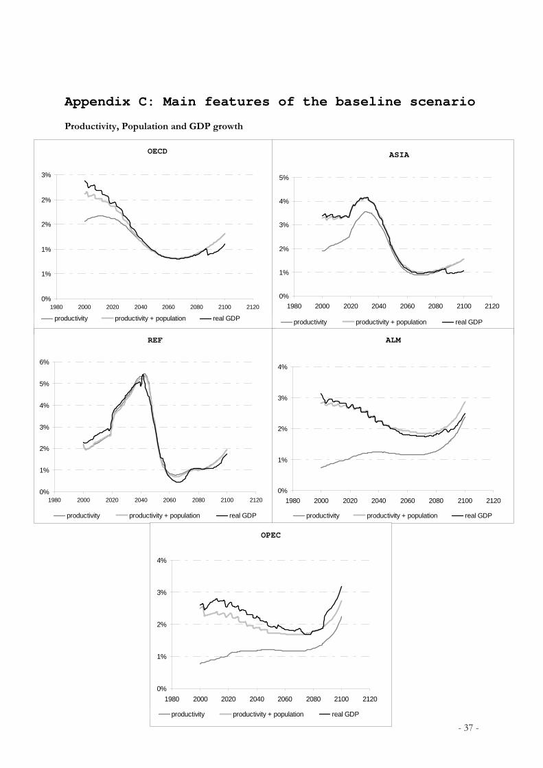
Appendix C: Main features of the baseline scenario

Productivity, Population and GDP growth

- 37 -

OECD

0%

1%

1%

2%

2%

3%

1980 2000 2020 2040 2060 2080 2100 2120

productivity productivity + population real GDP

ASIA

0%

1%

2%

3%

4%

5%

1980 2000 2020 2040 2060 2080 2100 2120

productivity productivity + population real GDP

REF

0%

1%

2%

3%

4%

5%

6%

1980 2000 2020 2040 2060 2080 2100 2120

productivity productivity + population real GDP

ALM

0%

1%

2%

3%

4%

1980 2000 2020 2040 2060 2080 2100 2120

productivity productivity + population real GDP

OPEC

0%

1%

2%

3%

4%

1980 2000 2020 2040 2060 2080 2100 2120

productivity productivity + population real GDP

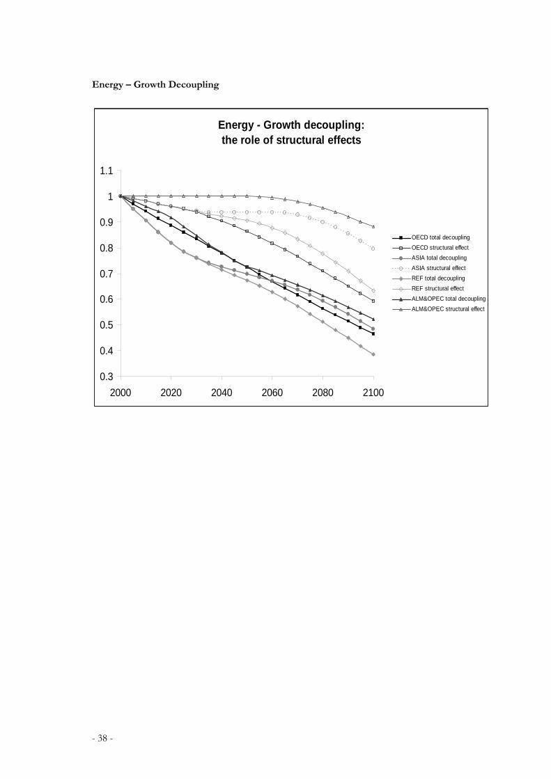
Energy – Growth Decoupling

Energy - Growth decoupling:the role of structural effects

0.3

0.4

0.5

0.6

0.7

0.8

0.9

1

1.1

2000 2020 2040 2060 2080 2100

OECD total decouplingOECD structural effectASIA total decouplingASIA structural effectREF total decouplingREF structural effect ALM&OPEC total decouplingALM&OPEC structural effect

- 38 -

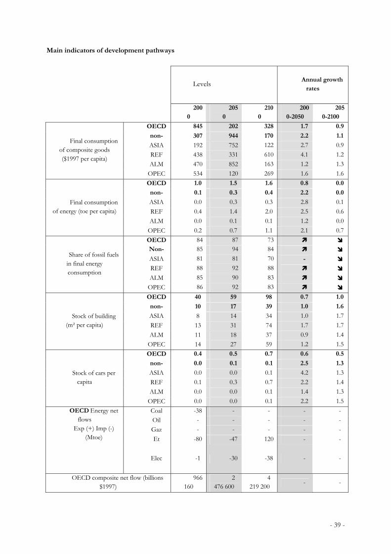
Main indicators of development pathways

Levels Annual growth rates

200

0 205

0 210

0 200

0-2050 205

0-2100

OECD 845 202 328 1.7 0.9

non- 307 944 170 2.2 1.1

ASIA 192 752 122 2.7 0.9REF 438 331 610 4.1 1.2ALM 470 852 163 1.2 1.3

Final consumption of composite goods ($1997 per capita)

OPEC 534 120 269 1.6 1.6OECD 1.0 1.5 1.6 0.8 0.0

non- 0.1 0.3 0.4 2.2 0.0

ASIA 0.0 0.3 0.3 2.8 0.1REF 0.4 1.4 2.0 2.5 0.6ALM 0.0 0.1 0.1 1.2 0.0

Final consumption of energy (toe per capita)

OPEC 0.2 0.7 1.1 2.1 0.7OECD 84 87 73 Non- 85 94 84 ASIA 81 81 70 -

REF 88 92 88

ALM 85 90 83

Share of fossil fuels in final energy consumption

OPEC 86 92 83

OECD 40 59 98 0.7 1.0

non- 10 17 39 1.0 1.6

ASIA 8 14 34 1.0 1.7REF 13 31 74 1.7 1.7ALM 11 18 37 0.9 1.4

Stock of building (m² per capita)

OPEC 14 27 59 1.2 1.5OECD 0.4 0.5 0.7 0.6 0.5

non- 0.0 0.1 0.1 2.5 1.3

ASIA 0.0 0.0 0.1 4.2 1.3REF 0.1 0.3 0.7 2.2 1.4ALM 0.0 0.0 0.1 1.4 1.3

Stock of cars per capita

OPEC 0.0 0.0 0.1 2.2 1.5Coal -38 - - - - Oil - - - - - Gaz - - - - - Et -80 -47 120 - -

OECD Energy net flows

Exp (+) Imp (-) (Mtoe)

Elec -1 -30 -38 - -

OECD composite net flow (billions $1997)

966 160

2 476 600

4 219 200

- -

- 39 -

OECD Net Capital Flows Exp (-) Imp (+) (billions $1997)

-29200

-98000

-44000

- -

- 40 -