from the desert to the glaciers: exploring interregional … · from the desert to the glaciers:...
TRANSCRIPT
From the Desert to the Glaciers:
Exploring Interregional Connections
of the Chilean Economy
International Workshop on General Equilibrium
Modeling, Universidad Adolfo Ibañez
Viña del Mar, December 3-4, 2018
Eduardo Haddad Denise Li Karina Sass Keyi Ussami Sofia Arantes
2
Research team – NEREUS
Eduardo Amaral Haddad (coordinator)
Ademir Antônio Moreira Rocha
Bruno Proença Pacheco Pimenta
Denise Leyi Li
Karina Simone Sass
Keyi Ando Ussami
Lucas Cardoso Correa Dias
Raphael Pinto Fernandes
Sofia Marques Arantes
Department of Economics, University of Sao Paulo
Outline
1. Introduction
2. Structure of the interregional data
3. Basic socioeconomic indicators
4. Theoretical background
5. Multiplier analysis
6. Linkage analysis
7. Next steps
Department of Economics, University of Sao Paulo 3
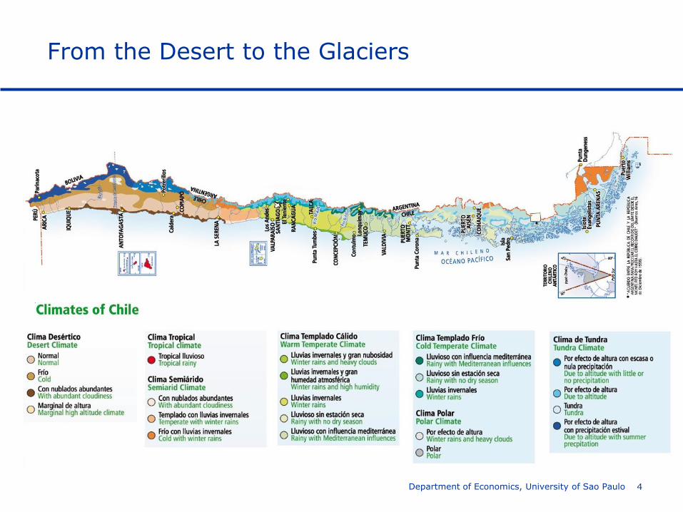
From the Desert to the Glaciers
Department of Economics, University of Sao Paulo 4
5
Introduction
As part of the development of an interregional CGE (ICGE) model
for Chile, a fully specified interregional input-output database was
developed under conditions of limited information.
Such database is needed for calibration of the ICGE model.
Lack of adequate data is a problem: but do you wait until the data
have improved sufficiently, or do you start with existing data, no
matter how imperfect, and improve the database gradually?
Department of Economics, University of Sao Paulo
6
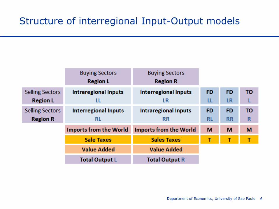
Structure of interregional Input-Output models
Department of Economics, University of Sao Paulo
7
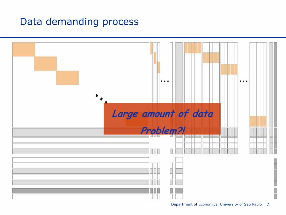
Data demanding process
Department of Economics, University of Sao Paulo
Large amount of data
Problem?!
8
Chilean interregional input-output system, 2014
Department of Economics, University of Sao Paulo
9
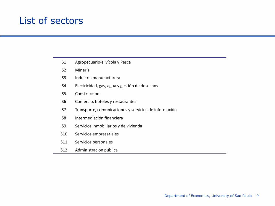
List of sectors
Department of Economics, University of Sao Paulo
S1 Agropecuario-silvícola y Pesca
S2 Minería
S3 Industria manufacturera
S4 Electricidad, gas, agua y gestión de desechos
S5 Construcción
S6 Comercio, hoteles y restaurantes
S7 Transporte, comunicaciones y servicios de información
S8 Intermediación financiera
S9 Servicios inmobiliarios y de vivienda
S10 Servicios empresariales
S11 Servicios personales
S12 Administración pública
10
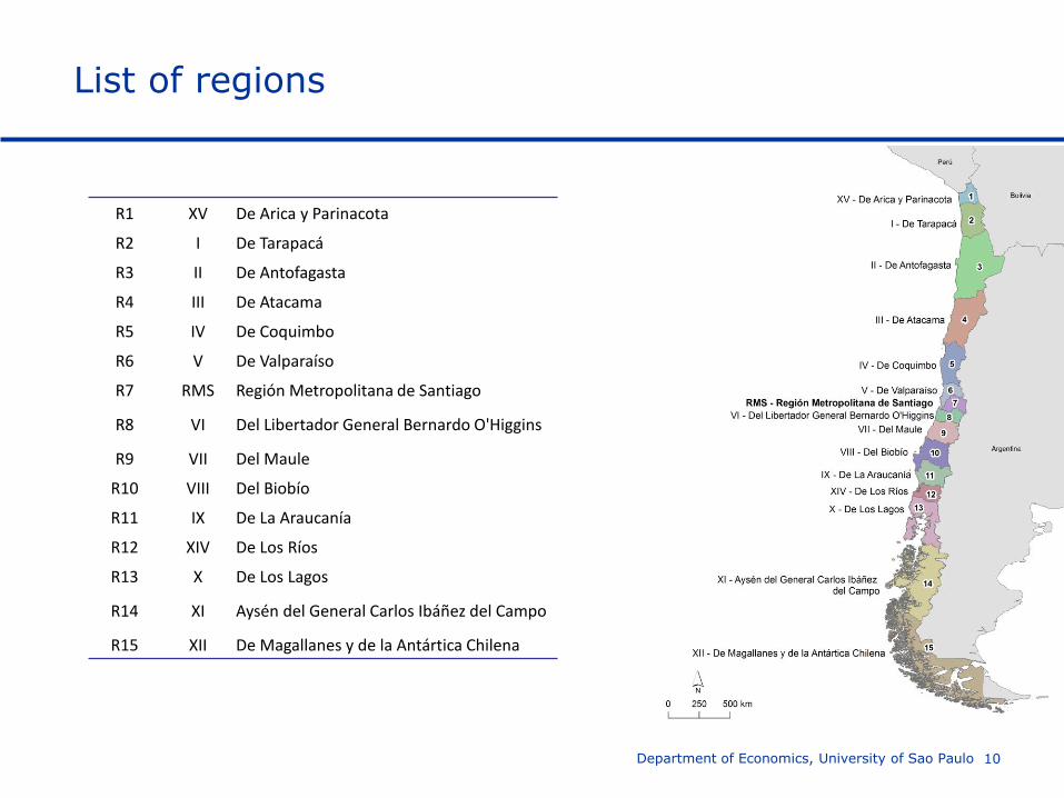
List of regions
Department of Economics, University of Sao Paulo
R1 XV De Arica y Parinacota
R2 I De Tarapacá
R3 II De Antofagasta
R4 III De Atacama
R5 IV De Coquimbo
R6 V De Valparaíso
R7 RMS Región Metropolitana de Santiago
R8 VI Del Libertador General Bernardo O'Higgins
R9 VII Del Maule
R10 VIII Del Biobío
R11 IX De La Araucanía
R12 XIV De Los Ríos
R13 X De Los Lagos
R14 XI Aysén del General Carlos Ibáñez del Campo
R15 XII De Magallanes y de la Antártica Chilena
11
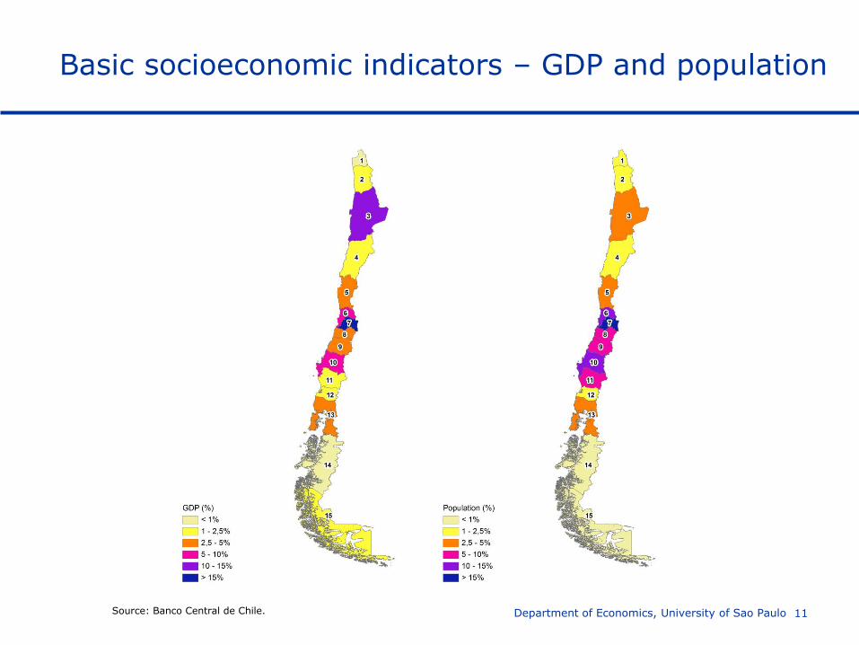
Basic socioeconomic indicators – GDP and population
Department of Economics, University of Sao Paulo Source: Banco Central de Chile.
12
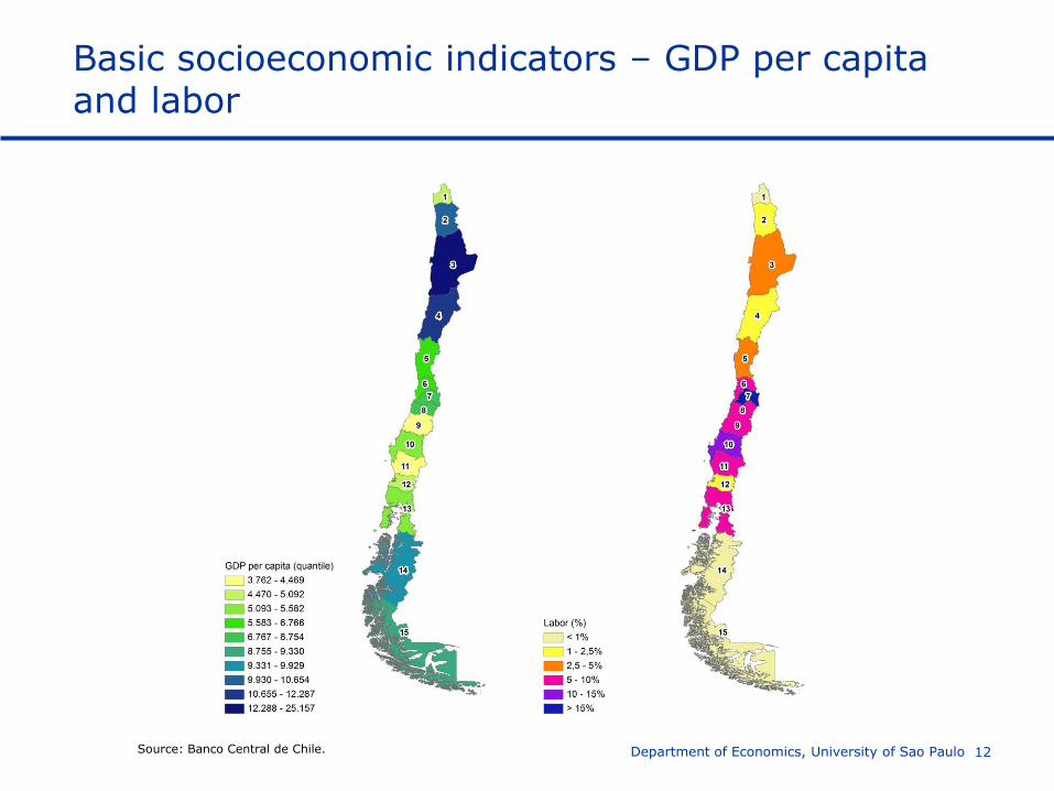
Basic socioeconomic indicators – GDP per capita and labor
Department of Economics, University of Sao Paulo Source: Banco Central de Chile.
13
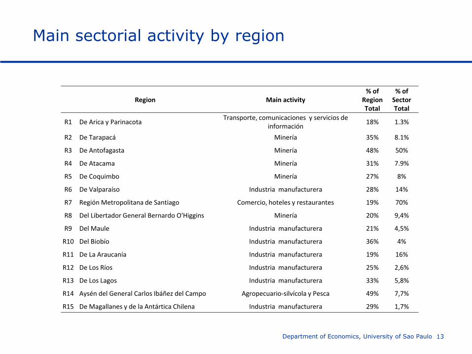
Main sectorial activity by region
Department of Economics, University of Sao Paulo
Region Main activity % of
RegionTotal
% of Sector Total
R1 De Arica y Parinacota Transporte, comunicaciones y servicios de
información 18% 1.3%
R2 De Tarapacá Minería 35% 8.1%
R3 De Antofagasta Minería 48% 50%
R4 De Atacama Minería 31% 7.9%
R5 De Coquimbo Minería 27% 8%
R6 De Valparaíso Industria manufacturera 28% 14%
R7 Región Metropolitana de Santiago Comercio, hoteles y restaurantes 19% 70%
R8 Del Libertador General Bernardo O'Higgins Minería 20% 9,4%
R9 Del Maule Industria manufacturera 21% 4,5%
R10 Del Biobío Industria manufacturera 36% 4%
R11 De La Araucanía Industria manufacturera 19% 16%
R12 De Los Ríos Industria manufacturera 25% 2,6%
R13 De Los Lagos Industria manufacturera 33% 5,8%
R14 Aysén del General Carlos Ibáñez del Campo Agropecuario-silvícola y Pesca 49% 7,7%
R15 De Magallanes y de la Antártica Chilena Industria manufacturera 29% 1,7%
14
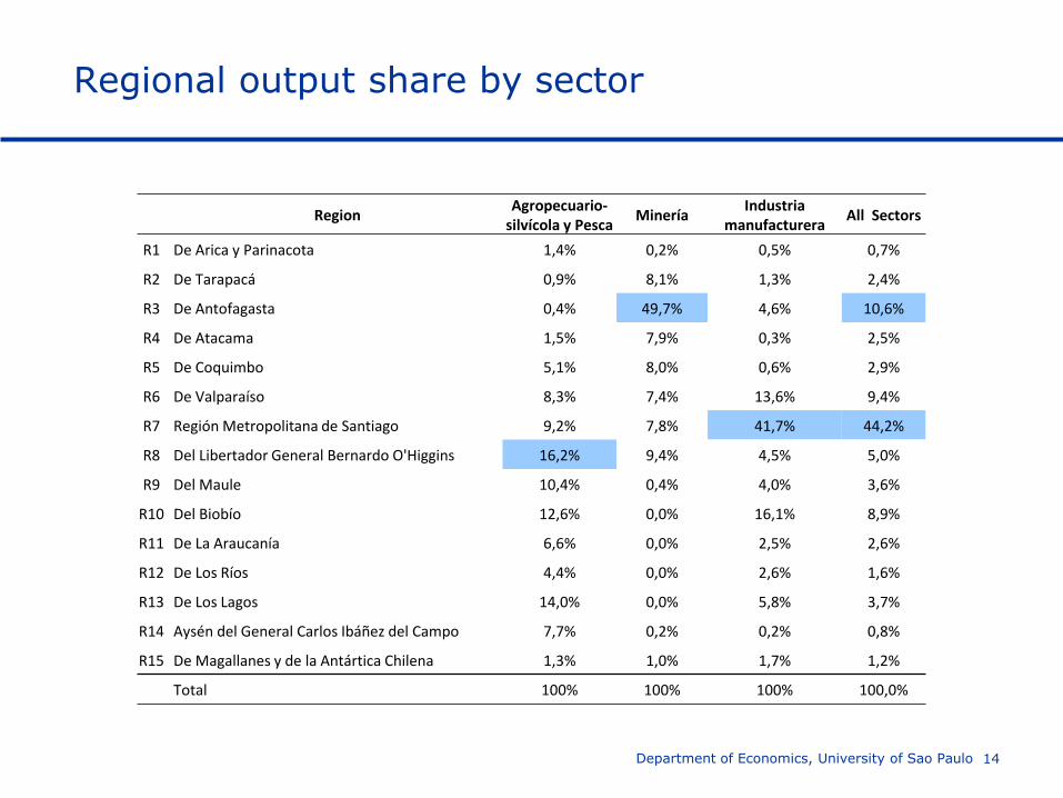
Regional output share by sector
Department of Economics, University of Sao Paulo
Region Agropecuario-
silvícola y Pesca Minería
Industria manufacturera
All Sectors
R1 De Arica y Parinacota 1,4% 0,2% 0,5% 0,7%
R2 De Tarapacá 0,9% 8,1% 1,3% 2,4%
R3 De Antofagasta 0,4% 49,7% 4,6% 10,6%
R4 De Atacama 1,5% 7,9% 0,3% 2,5%
R5 De Coquimbo 5,1% 8,0% 0,6% 2,9%
R6 De Valparaíso 8,3% 7,4% 13,6% 9,4%
R7 Región Metropolitana de Santiago 9,2% 7,8% 41,7% 44,2%
R8 Del Libertador General Bernardo O'Higgins 16,2% 9,4% 4,5% 5,0%
R9 Del Maule 10,4% 0,4% 4,0% 3,6%
R10 Del Biobío 12,6% 0,0% 16,1% 8,9%
R11 De La Araucanía 6,6% 0,0% 2,5% 2,6%
R12 De Los Ríos 4,4% 0,0% 2,6% 1,6%
R13 De Los Lagos 14,0% 0,0% 5,8% 3,7%
R14 Aysén del General Carlos Ibáñez del Campo 7,7% 0,2% 0,2% 0,8%
R15 De Magallanes y de la Antártica Chilena 1,3% 1,0% 1,7% 1,2%
Total 100% 100% 100% 100,0%
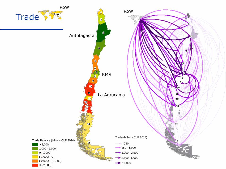
Trade Balance (billions CLP 2014)
> 2,000
1,000 - 2,000
0 - 1,000
(-1,000) - 0
(-2,000) - (-1,000)
≤ (-2,000)
RoW
3
4
14
5
2
9
13
10
11
1
12
15
8
6
7
Trade (billions CLP 2014)
< 250
250 - 1,000
1,000 - 2,500
2,500 - 5,000
> 5,000
3
4
14
5
2
9
10
11
1
12
15
13
8
6
7
Trade
Antofagasta
RMS
RoW
La Araucanía
RoW
16
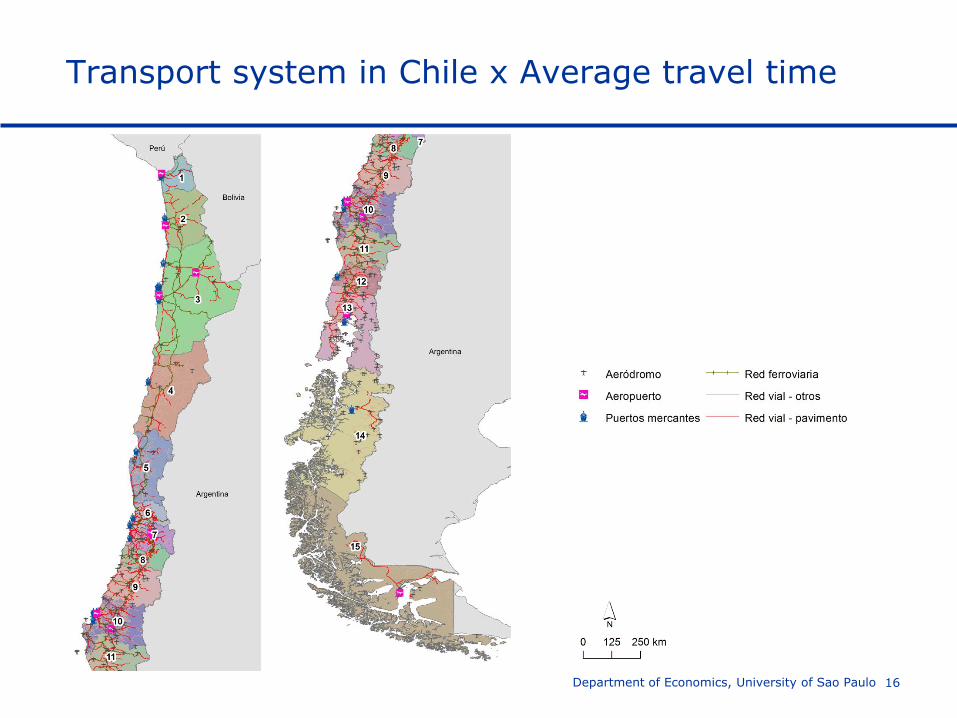
Transport system in Chile x Average travel time
Department of Economics, University of Sao Paulo
17
Theoretical background – Conventional Input-Output model
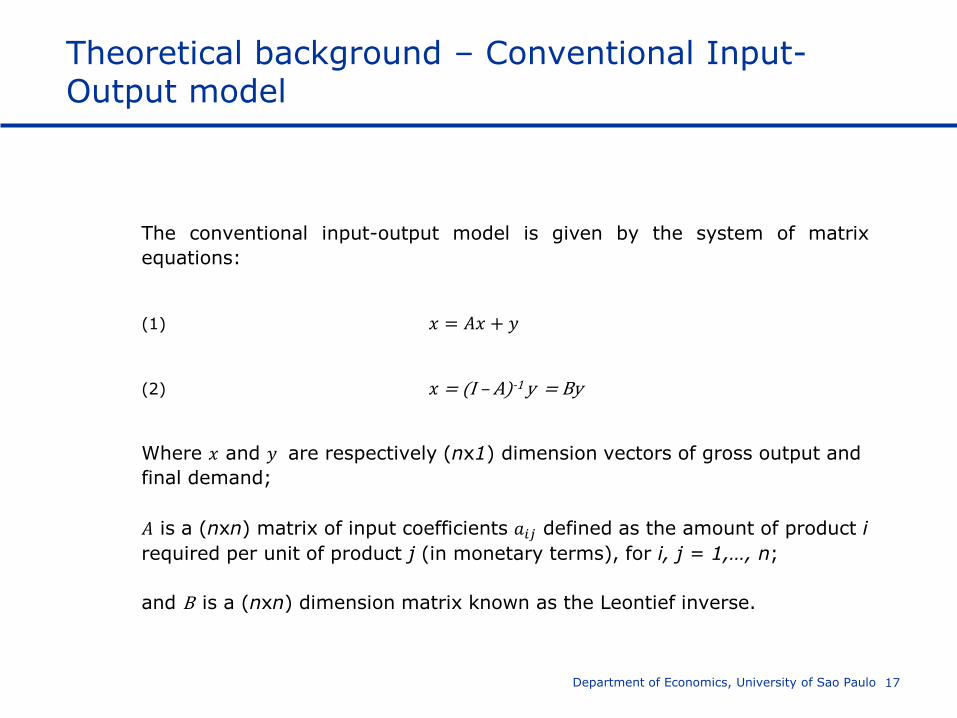
The conventional input-output model is given by the system of matrix
equations:
(1) 𝑥 = 𝐴𝑥 + 𝑦
(2) 𝑥 = (I – A)-1 y = By
Where 𝑥 and 𝑦 are respectively (nx1) dimension vectors of gross output and
final demand;
𝐴 is a (nxn) matrix of input coefficients 𝑎𝑖𝑗 defined as the amount of product i
required per unit of product j (in monetary terms), for i, j = 1,…, n;
and B is a (nxn) dimension matrix known as the Leontief inverse.
Department of Economics, University of Sao Paulo
18
Theoretical background – Interregional Input-Output model
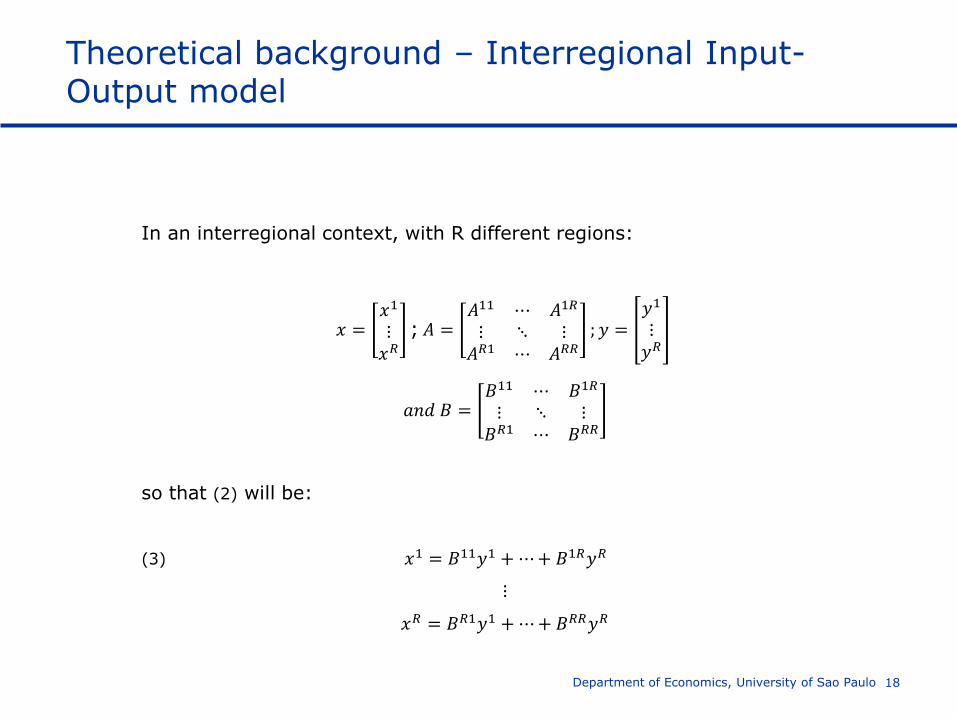
In an interregional context, with R different regions:
𝑥 =𝑥1
⋮𝑥𝑅
; 𝐴 =𝐴11 ⋯ 𝐴1𝑅
⋮ ⋱ ⋮𝐴𝑅1 ⋯ 𝐴𝑅𝑅
; 𝑦 =𝑦1
⋮𝑦𝑅
𝑎𝑛𝑑 𝐵 =𝐵11 ⋯ 𝐵1𝑅
⋮ ⋱ ⋮𝐵𝑅1 ⋯ 𝐵𝑅𝑅
so that (2) will be:
(3) 𝑥1 = 𝐵11𝑦1 + ⋯ + 𝐵1𝑅𝑦𝑅
⋮
𝑥𝑅 = 𝐵𝑅1𝑦1 + ⋯ + 𝐵𝑅𝑅𝑦𝑅
Department of Economics, University of Sao Paulo
19
Theoretical background – Interregional Input Output model
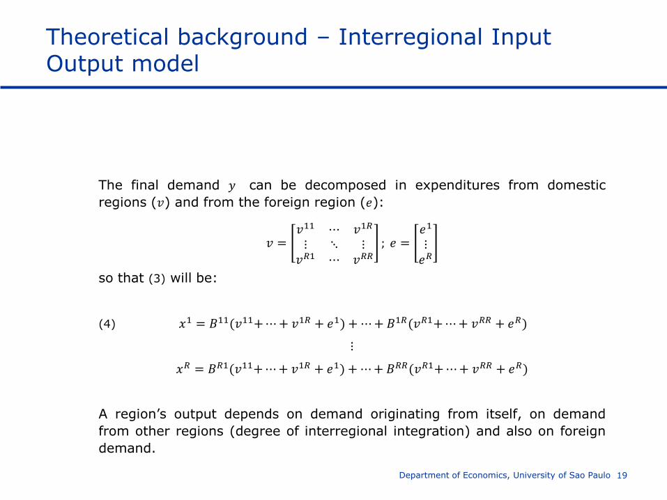
The final demand 𝑦 can be decomposed in expenditures from domestic
regions (𝑣) and from the foreign region (𝑒):
𝑣 =𝑣11 ⋯ 𝑣1𝑅
⋮ ⋱ ⋮𝑣𝑅1 ⋯ 𝑣𝑅𝑅
; 𝑒 =𝑒1
⋮𝑒𝑅
so that (3) will be:
(4) 𝑥1 = 𝐵11(𝑣11+ ⋯ + 𝑣1𝑅 + 𝑒1) + ⋯ + 𝐵1𝑅(𝑣𝑅1+ ⋯ + 𝑣𝑅𝑅 + 𝑒𝑅)
⋮
𝑥𝑅 = 𝐵𝑅1(𝑣11+ ⋯ + 𝑣1𝑅 + 𝑒1) + ⋯ + 𝐵𝑅𝑅(𝑣𝑅1+ ⋯ + 𝑣𝑅𝑅 + 𝑒𝑅)
A region’s output depends on demand originating from itself, on demand
from other regions (degree of interregional integration) and also on foreign
demand.
Department of Economics, University of Sao Paulo
20
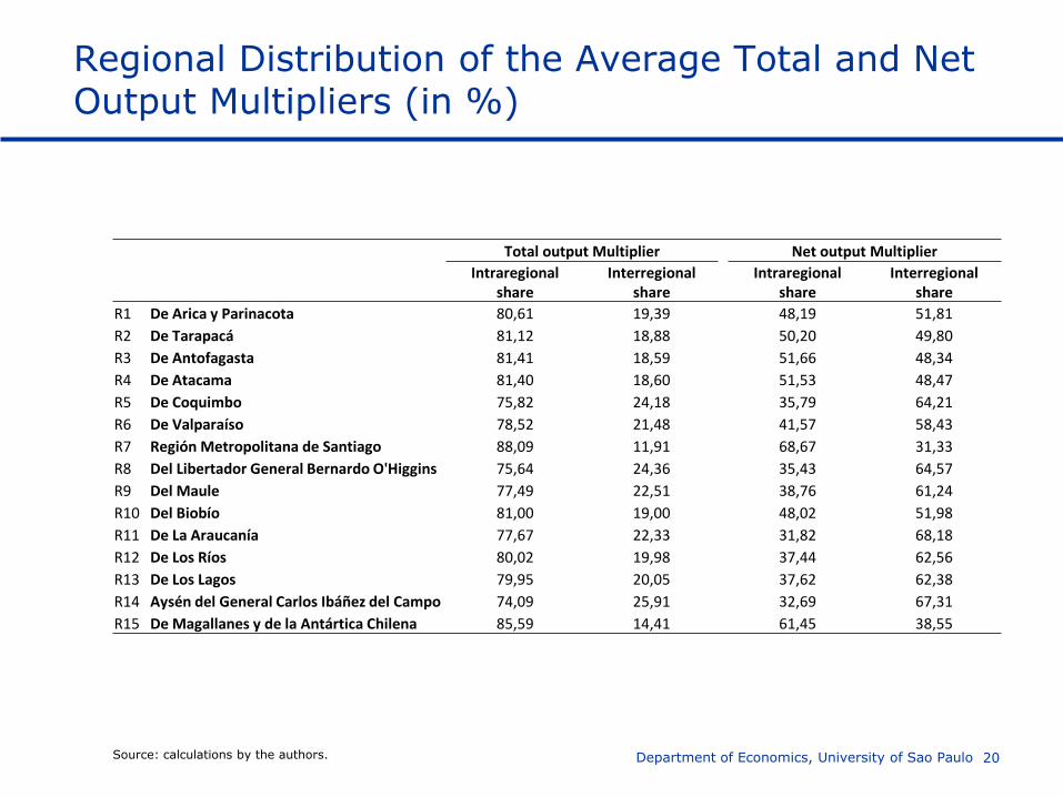
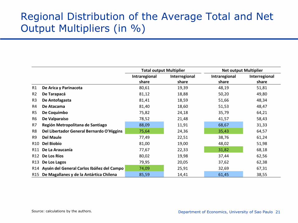
Regional Distribution of the Average Total and Net Output Multipliers (in %)
Department of Economics, University of Sao Paulo Source: calculations by the authors.
Total output Multiplier Net output Multiplier
Intraregional share
Interregional share
Intraregional share
Interregional share
R1 De Arica y Parinacota 80,61 19,39 48,19 51,81
R2 De Tarapacá 81,12 18,88 50,20 49,80
R3 De Antofagasta 81,41 18,59 51,66 48,34
R4 De Atacama 81,40 18,60 51,53 48,47
R5 De Coquimbo 75,82 24,18 35,79 64,21
R6 De Valparaíso 78,52 21,48 41,57 58,43
R7 Región Metropolitana de Santiago 88,09 11,91 68,67 31,33
R8 Del Libertador General Bernardo O'Higgins 75,64 24,36 35,43 64,57
R9 Del Maule 77,49 22,51 38,76 61,24
R10 Del Biobío 81,00 19,00 48,02 51,98
R11 De La Araucanía 77,67 22,33 31,82 68,18
R12 De Los Ríos 80,02 19,98 37,44 62,56
R13 De Los Lagos 79,95 20,05 37,62 62,38
R14 Aysén del General Carlos Ibáñez del Campo 74,09 25,91 32,69 67,31
R15 De Magallanes y de la Antártica Chilena 85,59 14,41 61,45 38,55
21
Regional Distribution of the Average Total and Net Output Multipliers (in %)
Department of Economics, University of Sao Paulo Source: calculations by the authors.
Total output Multiplier Net output Multiplier
Intraregional share
Interregional share
Intraregional share
Interregional share
R1 De Arica y Parinacota 80,61 19,39 48,19 51,81
R2 De Tarapacá 81,12 18,88 50,20 49,80
R3 De Antofagasta 81,41 18,59 51,66 48,34
R4 De Atacama 81,40 18,60 51,53 48,47
R5 De Coquimbo 75,82 24,18 35,79 64,21
R6 De Valparaíso 78,52 21,48 41,57 58,43
R7 Región Metropolitana de Santiago 88,09 11,91 68,67 31,33
R8 Del Libertador General Bernardo O'Higgins 75,64 24,36 35,43 64,57
R9 Del Maule 77,49 22,51 38,76 61,24
R10 Del Biobío 81,00 19,00 48,02 51,98
R11 De La Araucanía 77,67 22,33 31,82 68,18
R12 De Los Ríos 80,02 19,98 37,44 62,56
R13 De Los Lagos 79,95 20,05 37,62 62,38
R14 Aysén del General Carlos Ibáñez del Campo 74,09 25,91 32,69 67,31
R15 De Magallanes y de la Antártica Chilena 85,59 14,41 61,45 38,55
22
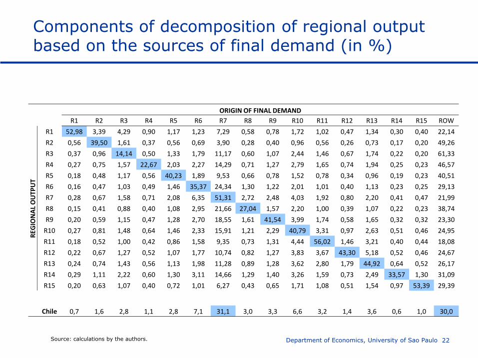
Components of decomposition of regional output based on the sources of final demand (in %)
Department of Economics, University of Sao Paulo Source: calculations by the authors.
ORIGIN OF FINAL DEMAND
R1 R2 R3 R4 R5 R6 R7 R8 R9 R10 R11 R12 R13 R14 R15 ROW
REG
ION
AL
OU
TPU
T
R1 52,98 3,39 4,29 0,90 1,17 1,23 7,29 0,58 0,78 1,72 1,02 0,47 1,34 0,30 0,40 22,14
R2 0,56 39,50 1,61 0,37 0,56 0,69 3,90 0,28 0,40 0,96 0,56 0,26 0,73 0,17 0,20 49,26
R3 0,37 0,96 14,14 0,50 1,33 1,79 11,17 0,60 1,07 2,44 1,46 0,67 1,74 0,22 0,20 61,33
R4 0,27 0,75 1,57 22,67 2,03 2,27 14,29 0,71 1,27 2,79 1,65 0,74 1,94 0,25 0,23 46,57
R5 0,18 0,48 1,17 0,56 40,23 1,89 9,53 0,66 0,78 1,52 0,78 0,34 0,96 0,19 0,23 40,51
R6 0,16 0,47 1,03 0,49 1,46 35,37 24,34 1,30 1,22 2,01 1,01 0,40 1,13 0,23 0,25 29,13
R7 0,28 0,67 1,58 0,71 2,08 6,35 51,31 2,72 2,48 4,03 1,92 0,80 2,20 0,41 0,47 21,99
R8 0,15 0,41 0,88 0,40 1,08 2,95 21,66 27,04 1,57 2,20 1,00 0,39 1,07 0,22 0,23 38,74
R9 0,20 0,59 1,15 0,47 1,28 2,70 18,55 1,61 41,54 3,99 1,74 0,58 1,65 0,32 0,32 23,30
R10 0,27 0,81 1,48 0,64 1,46 2,33 15,91 1,21 2,29 40,79 3,31 0,97 2,63 0,51 0,46 24,95
R11 0,18 0,52 1,00 0,42 0,86 1,58 9,35 0,73 1,31 4,44 56,02 1,46 3,21 0,40 0,44 18,08
R12 0,22 0,67 1,27 0,52 1,07 1,77 10,74 0,82 1,27 3,83 3,67 43,30 5,18 0,52 0,46 24,67
R13 0,24 0,74 1,43 0,56 1,13 1,98 11,28 0,89 1,28 3,62 2,80 1,79 44,92 0,64 0,52 26,17
R14 0,29 1,11 2,22 0,60 1,30 3,11 14,66 1,29 1,40 3,26 1,59 0,73 2,49 33,57 1,30 31,09
R15 0,20 0,63 1,07 0,40 0,72 1,01 6,27 0,43 0,65 1,71 1,08 0,51 1,54 0,97 53,39 29,39
Chile 0,7 1,6 2,8 1,1 2,8 7,1 31,1 3,0 3,3 6,6 3,2 1,4 3,6 0,6 1,0 30,0
23
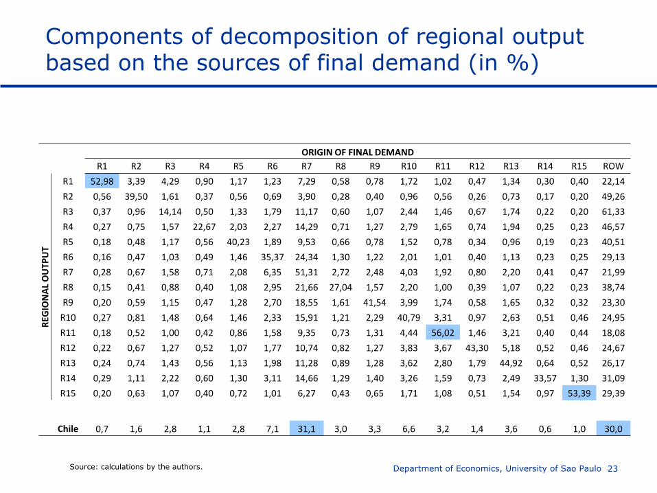
Components of decomposition of regional output based on the sources of final demand (in %)
Department of Economics, University of Sao Paulo Source: calculations by the authors.
ORIGIN OF FINAL DEMAND
R1 R2 R3 R4 R5 R6 R7 R8 R9 R10 R11 R12 R13 R14 R15 ROW
REG
ION
AL
OU
TPU
T
R1 52,98 3,39 4,29 0,90 1,17 1,23 7,29 0,58 0,78 1,72 1,02 0,47 1,34 0,30 0,40 22,14
R2 0,56 39,50 1,61 0,37 0,56 0,69 3,90 0,28 0,40 0,96 0,56 0,26 0,73 0,17 0,20 49,26
R3 0,37 0,96 14,14 0,50 1,33 1,79 11,17 0,60 1,07 2,44 1,46 0,67 1,74 0,22 0,20 61,33
R4 0,27 0,75 1,57 22,67 2,03 2,27 14,29 0,71 1,27 2,79 1,65 0,74 1,94 0,25 0,23 46,57
R5 0,18 0,48 1,17 0,56 40,23 1,89 9,53 0,66 0,78 1,52 0,78 0,34 0,96 0,19 0,23 40,51
R6 0,16 0,47 1,03 0,49 1,46 35,37 24,34 1,30 1,22 2,01 1,01 0,40 1,13 0,23 0,25 29,13
R7 0,28 0,67 1,58 0,71 2,08 6,35 51,31 2,72 2,48 4,03 1,92 0,80 2,20 0,41 0,47 21,99
R8 0,15 0,41 0,88 0,40 1,08 2,95 21,66 27,04 1,57 2,20 1,00 0,39 1,07 0,22 0,23 38,74
R9 0,20 0,59 1,15 0,47 1,28 2,70 18,55 1,61 41,54 3,99 1,74 0,58 1,65 0,32 0,32 23,30
R10 0,27 0,81 1,48 0,64 1,46 2,33 15,91 1,21 2,29 40,79 3,31 0,97 2,63 0,51 0,46 24,95
R11 0,18 0,52 1,00 0,42 0,86 1,58 9,35 0,73 1,31 4,44 56,02 1,46 3,21 0,40 0,44 18,08
R12 0,22 0,67 1,27 0,52 1,07 1,77 10,74 0,82 1,27 3,83 3,67 43,30 5,18 0,52 0,46 24,67
R13 0,24 0,74 1,43 0,56 1,13 1,98 11,28 0,89 1,28 3,62 2,80 1,79 44,92 0,64 0,52 26,17
R14 0,29 1,11 2,22 0,60 1,30 3,11 14,66 1,29 1,40 3,26 1,59 0,73 2,49 33,57 1,30 31,09
R15 0,20 0,63 1,07 0,40 0,72 1,01 6,27 0,43 0,65 1,71 1,08 0,51 1,54 0,97 53,39 29,39
Chile 0,7 1,6 2,8 1,1 2,8 7,1 31,1 3,0 3,3 6,6 3,2 1,4 3,6 0,6 1,0 30,0
24
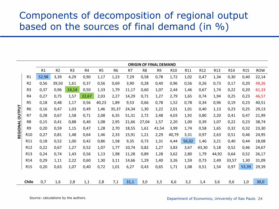
Components of decomposition of regional output based on the sources of final demand (in %)
Department of Economics, University of Sao Paulo Source: calculations by the authors.
ORIGIN OF FINAL DEMAND
R1 R2 R3 R4 R5 R6 R7 R8 R9 R10 R11 R12 R13 R14 R15 ROW
REG
ION
AL
OU
TPU
T
R1 52,98 3,39 4,29 0,90 1,17 1,23 7,29 0,58 0,78 1,72 1,02 0,47 1,34 0,30 0,40 22,14
R2 0,56 39,50 1,61 0,37 0,56 0,69 3,90 0,28 0,40 0,96 0,56 0,26 0,73 0,17 0,20 49,26
R3 0,37 0,96 14,14 0,50 1,33 1,79 11,17 0,60 1,07 2,44 1,46 0,67 1,74 0,22 0,20 61,33
R4 0,27 0,75 1,57 22,67 2,03 2,27 14,29 0,71 1,27 2,79 1,65 0,74 1,94 0,25 0,23 46,57
R5 0,18 0,48 1,17 0,56 40,23 1,89 9,53 0,66 0,78 1,52 0,78 0,34 0,96 0,19 0,23 40,51
R6 0,16 0,47 1,03 0,49 1,46 35,37 24,34 1,30 1,22 2,01 1,01 0,40 1,13 0,23 0,25 29,13
R7 0,28 0,67 1,58 0,71 2,08 6,35 51,31 2,72 2,48 4,03 1,92 0,80 2,20 0,41 0,47 21,99
R8 0,15 0,41 0,88 0,40 1,08 2,95 21,66 27,04 1,57 2,20 1,00 0,39 1,07 0,22 0,23 38,74
R9 0,20 0,59 1,15 0,47 1,28 2,70 18,55 1,61 41,54 3,99 1,74 0,58 1,65 0,32 0,32 23,30
R10 0,27 0,81 1,48 0,64 1,46 2,33 15,91 1,21 2,29 40,79 3,31 0,97 2,63 0,51 0,46 24,95
R11 0,18 0,52 1,00 0,42 0,86 1,58 9,35 0,73 1,31 4,44 56,02 1,46 3,21 0,40 0,44 18,08
R12 0,22 0,67 1,27 0,52 1,07 1,77 10,74 0,82 1,27 3,83 3,67 43,30 5,18 0,52 0,46 24,67
R13 0,24 0,74 1,43 0,56 1,13 1,98 11,28 0,89 1,28 3,62 2,80 1,79 44,92 0,64 0,52 26,17
R14 0,29 1,11 2,22 0,60 1,30 3,11 14,66 1,29 1,40 3,26 1,59 0,73 2,49 33,57 1,30 31,09
R15 0,20 0,63 1,07 0,40 0,72 1,01 6,27 0,43 0,65 1,71 1,08 0,51 1,54 0,97 53,39 29,39
Chile 0,7 1,6 2,8 1,1 2,8 7,1 31,1 3,0 3,3 6,6 3,2 1,4 3,6 0,6 1,0 30,0
Linkage analysis - Theoretical background
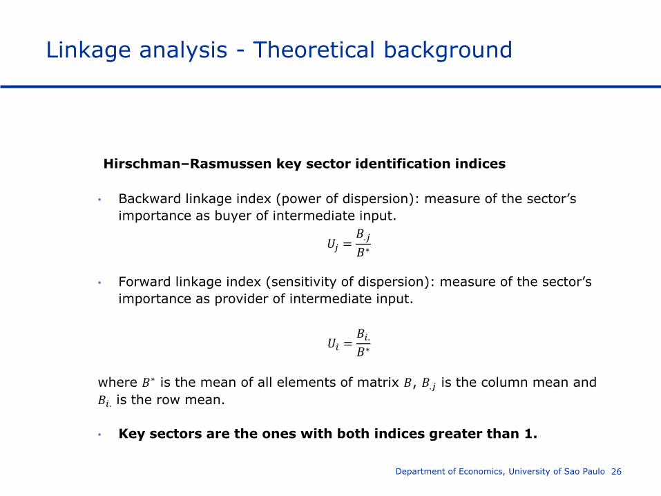
Hirschman–Rasmussen key sector identification indices
• Backward linkage index (power of dispersion): measure of the sector’s
importance as buyer of intermediate input.
𝑈𝑗 =𝐵.𝑗
𝐵∗
• Forward linkage index (sensitivity of dispersion): measure of the sector’s
importance as provider of intermediate input.
𝑈𝑖 =𝐵𝑖.
𝐵∗
where 𝐵∗ is the mean of all elements of matrix 𝐵, 𝐵.𝑗 is the column mean and
𝐵𝑖. is the row mean.
• Key sectors are the ones with both indices greater than 1.
Department of Economics, University of Sao Paulo 26
Linkage analysis - Theoretical background
Pure Linkage Approach
Measure the importance of the sectors in terms of production generation in
the economy.
Pure Total Linkage = PTL = PBL + PFL
• PBL – Pure Backward Linkage index: measure the pure impact of the
sector’s gross output in the economy, i.e., the impact that is free from
the demand inputs that the region makes from itself, and the feedbacks
from the rest of the economy to the region and vice-versa.
• PFL – Pure Forward Linkage index: measure the pure impact of the gross
output of the economy in the sector.
Department of Economics, University of Sao Paulo 27
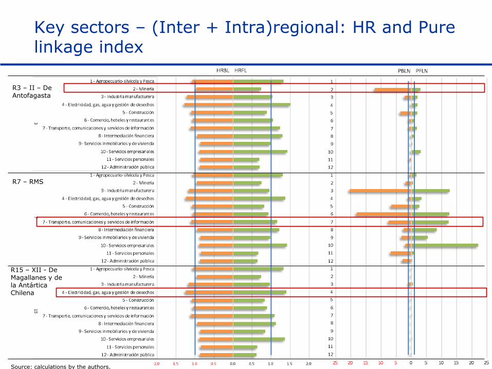
Key sectors – (Inter + Intra)regional: HR and Pure linkage index
Source: calculations by the authors.
R3 – II – De Antofagasta
R7 – RMS
R15 – XII - De Magallanes y de la Antártica Chilena
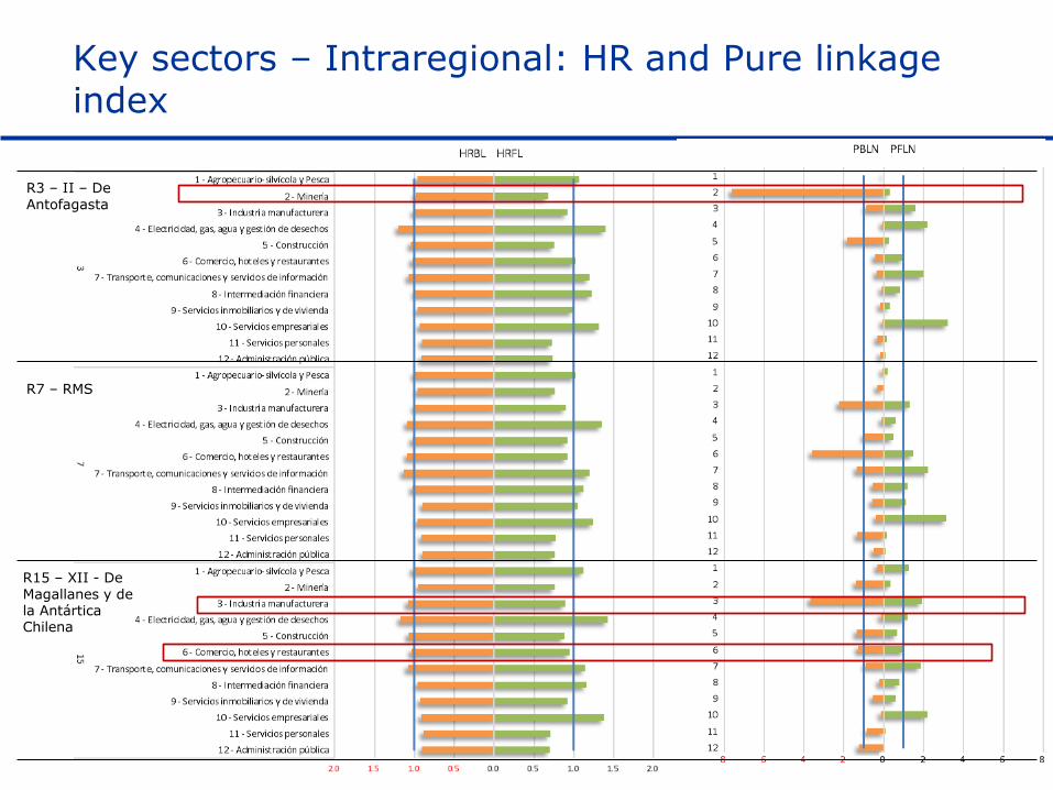
Key sectors – Intraregional: HR and Pure linkage index
R3 – II – De Antofagasta
R7 – RMS
R15 – XII - De Magallanes y de la Antártica Chilena
Next Steps
• Disaggregation
• Sectors
• Products
Fipe - Fundação Instituto de Pesquisas Econômicas 30
www.usp.br/nereus
Department of Economics, University of Sao Paulo 31