Étude probabiliste des équations de smoluchowski; … · 1.1.3.2 analysis of the continuous case...
TRANSCRIPT
UFR S.T.M.I.A.École Doctorale IAE + M
Université Henri Poincaré - Nancy ID.F.D. Mathématiques
Étude probabiliste des équations deSmoluchowski ;
Schéma d'Euler pour des fonctionnelles ;Amplitude du mouvement brownien avec
dérive.
THÈSE
présentée et soutenue publiquement le 13 septembre 2001
pour l'obtention du
Doctorat de l'Université Henri Poincaré Nancy I(Spécialité Mathématiques appliquées)
par
Étienne TANRÉ
Composition du jury
Président et Rapporteur : James NORRIS, Professeur à l'Université de CambridgeRapporteur : Damien LAMBERTON, Professeur à l'Université de Marne la ValléeÉxaminateurs : Vlad BALLY, Professeur à l'Université du Maine
Jean BERTOIN, Professeur à l'Université Pierre et Marie Curie Paris 6Philippe LAURENÇOT, Chargé de recherche CNRS à l'Université
Paul Sabatier ToulouseDirecteurs de thèse : Bernard ROYNETTE, Professeur à l'Université Henri Poincaré Nancy 1
Pierre VALLOIS, Professeur à l'Université Henri Poincaré Nancy 1
Institut Élie Cartan Nancy

Mis en page avec la classe TheseCRIN.

À Muriel,À Elsa ...
i

ii

Remerciements
Je tiens avant tout à remercier Bernard ROYNETTE et Pierre VALLOIS quim'ont dirigé dans la préparation de cette thèse. Je leur suis extrêmement reconnais-sant de m'avoir initié à la recherche avec des sujets aussi intéressants. Leurs connais-sances en probabilité me laisse admiratif ; leur manière d'encadrer et de conseillerm'a été très agréable.
Je tiens à remercier James NORRIS pour avoir accepté de rapporter cette thèse.L'honneur qu'il m'a fait en présidant ce jury me touche particulièrement.
Je remercie également Damien LAMBERTON pour la charge de travail impor-tante qu'il a accepté en rapportant ma thèse. En particulier, ses remarques et conseilsm'ont aidé.
Je souhaite remercier Philippe LAURENÇOT pour plusieurs raisons : il est lapremière personne qui m'ait parlé des équations de coagulation de Smoluchowski.J'ai toujours eu un grand plaisir à discuter avec lui de ses travaux de recherche.Merci d'avoir fait un long déplacement pour participer au jury.
Vlad BALLY et Jean BERTOIN ont accepté de faire partie de ce jury, je les enremercie. Leurs travaux ont inspiré une partie de ma thèse.
Je tiens également à remercier très chaleureusement Madalina DEACONU, Ni-colas FOURNIER et Jean-Sébastien GIET avec qui j'ai eu l'occasion de travailler.Le plaisir a été immense. Merci également pour la bonne humeur...
Je souhaite également remercier l'ensemble des institutions qui m'ont permisd'eectuer ce travail dans de telles conditions. Cette thèse a été réalisée grâce ausoutien nancier du Conseil Régional de Lorraine et de l'INRIA. L'accueil au seinde l'IECN, la disponibilité de ses secrétaires et bibliothécaires est précieuse.
Je tiens à remercier Bruno PINÇON et Mireille BOSSY pour leurs conseils etleur aide pour les simulations numériques.
Je souhaite remercier les collègues du laboratoire et tout particulièrement ceuxde l'équipe de Probabilité pour l'ambiance amicale qui peut y régner. En particu-lier, je retiens les discussions que j'ai pu avoir avec Madalina, Jean-Sébastien, Jean-François, Nicolas, Marie-Pierre, Samuel, André, Fabrice, Vincent, Bruno, Francis...tant en mathématiques que sur le reste.
Je souhaite également ici remercier mes amis, ma famille et surtout mes parentspour tout ce qu'ils ont su m'apporter.
iii

La place qu'occupe Muriel dans ma vie est immense. Je me contente ici de laremercier pour tout le bonheur que nous viv(r)ons.
Enn, j'ai une pensée pour Stéphane HOGUET, c'est lui qui m'a montré à lafois la rigueur et la beauté des Mathématiques ainsi que les plaisirs que l'on peut ytrouver ; il ne le saura pas, ça ne m'empêche pas de le remercier.
iv
Table des matières
Table des gures ix
Introduction 1
I Phénomènes de coagulation 13
1 Smoluchowski's Eq. : probabilistic interpretation for particular
kernels 15
1.1 Introduction . . . . . . . . . . . . . . . . . . . . . . . . . . . . . . 16
1.1.1 Paper's Plan . . . . . . . . . . . . . . . . . . . . . . . . . 16
1.1.2 Heuristic Motivation of the Problem . . . . . . . . . . . . 16
1.1.3 Some Known Results . . . . . . . . . . . . . . . . . . . . . 17
1.1.3.1 Analysis of the Discrete Case . . . . . . . . . . . 18
1.1.3.2 Analysis of the Continuous Case . . . . . . . . . 21
1.1.3.3 Probabilistic Approach for the Smoluchowski'sCoagulation Equation . . . . . . . . . . . . . . . 22
1.2 Connection Between the Discrete Smoluchowski's Equ and Bran-ching Processes . . . . . . . . . . . . . . . . . . . . . . . . . . . . 23
1.2.1 Discrete Coagulation Equation with K(i,j) = i j . . . . . . 23
1.2.2 Discrete Coagulation Equation with K(i,j) = i+ j . . . . 25
1.2.3 Discrete Coagulation Equation with K(i,j) = 1 . . . . . . 26
1.3 Continuous Smoluchowski's CoagulationEquation (SC) . . . . . . . . . . . . . . . . . . . . . . . . . . . . 28
v
Table des matières
1.3.1 General Results for (SC) . . . . . . . . . . . . . . . . . . 28
1.3.2 Continuous Coagulation Equation with Constant Kernel . 30
1.3.3 Additive and Multiplicative Kernels for the ContinuousCoagulation Equation . . . . . . . . . . . . . . . . . . . . 33
1.3.3.1 Existence of Solutions for (SC+) and (SC∗) . . 36
1.3.3.2 Convergence of Solutions . . . . . . . . . . . . . 39
1.4 Appendix . . . . . . . . . . . . . . . . . . . . . . . . . . . . . . . 43
2 Generalization of the Connection Between Additive and Multi-
plicative kernels 45
2.1 Introduction . . . . . . . . . . . . . . . . . . . . . . . . . . . . . . 45
2.1.1 Norris results and construction . . . . . . . . . . . . . . . 46
2.2 Connection between the additive and multiplicative case in termsof measures . . . . . . . . . . . . . . . . . . . . . . . . . . . . . . 48
3 A pure jump Markov process associated with Smoluchowski's
equation 55
3.1 Introduction . . . . . . . . . . . . . . . . . . . . . . . . . . . . . . 56
3.2 Framework . . . . . . . . . . . . . . . . . . . . . . . . . . . . . . 59
3.3 Existence results for (SDE) . . . . . . . . . . . . . . . . . . . . . 66
3.4 Pathwise behaviour of (SDE) . . . . . . . . . . . . . . . . . . . . 77
3.5 About the uniqueness for (SDE) . . . . . . . . . . . . . . . . . . . 81
3.6 Study of the exact multiplicative kernel . . . . . . . . . . . . . . . 85
3.7 Appendix . . . . . . . . . . . . . . . . . . . . . . . . . . . . . . . 88
4 Study of a stochastic particle system 91
4.1 Introduction . . . . . . . . . . . . . . . . . . . . . . . . . . . . . . 92
4.2 Notations and previous results . . . . . . . . . . . . . . . . . . . . 95
4.3 An associated particle system . . . . . . . . . . . . . . . . . . . . 99
4.4 The simulation algorithm . . . . . . . . . . . . . . . . . . . . . . 110
4.5 A central limit theorem in the discrete case . . . . . . . . . . . . 113
4.6 Numerical results . . . . . . . . . . . . . . . . . . . . . . . . . . . 128
vi
4.7 Appendix . . . . . . . . . . . . . . . . . . . . . . . . . . . . . . . 133
II
Approximation de l'espérance de fonctionnelles de la tra-
jectoire d'une diusion par le schéma d'Euler 135
5 Introduction 137
5.1 Quelques exemples de fonctionnelles intéressantes . . . . . . . . . 137
5.1.1 L'équation de la chaleur . . . . . . . . . . . . . . . . . . . 137
5.1.2 Le problème de Cauchy avec potentiel et Lagrangien . . . 138
5.1.3 Le problème de Dirichlet . . . . . . . . . . . . . . . . . . . 139
5.2 Calcul de l'espérance des fonctionnelles . . . . . . . . . . . . . . . 140
5.2.1 Principe . . . . . . . . . . . . . . . . . . . . . . . . . . . . 140
5.2.2 Études réalisées dans la littérature . . . . . . . . . . . . . 140
5.2.3 Fonctionnelles étudiées . . . . . . . . . . . . . . . . . . . . 140
5.2.4 Résultats . . . . . . . . . . . . . . . . . . . . . . . . . . . 141
5.2.5 Plan de l'étude . . . . . . . . . . . . . . . . . . . . . . . . 142
6 Notations et hypothèses 143
6.1 Le processus de diusion . . . . . . . . . . . . . . . . . . . . . . . 143
6.2 La fonctionnelle de la trajectoire . . . . . . . . . . . . . . . . . . 145
7 Développement en δ de l'erreur pour des fonctionnelles à n
points 147
7.1 Résultat principal . . . . . . . . . . . . . . . . . . . . . . . . . . . 147
7.2 Dérivation de l'espérance d'une fonction du processus Xδr (.) . . . 148
7.3 Limite en δ . . . . . . . . . . . . . . . . . . . . . . . . . . . . . . 154
7.4 Expression du coecient devant δ . . . . . . . . . . . . . . . . . . 158
8 Majoration en δ et n de l'erreur pour l'intégrale de la trajec-
toire 161
vii
Table des matières
8.1 Majorations des dérivées du noyau de la diusion . . . . . . . . . 1628.2 Les moments d'ordre l . . . . . . . . . . . . . . . . . . . . . . . . 1628.3 Convergence des sommes de Riemann . . . . . . . . . . . . . . . . 1658.4 Convergence du schéma d'Euler pour le moment d'ordre l . . . . 1678.5 Démonstration dans le cas du moment d'ordre un . . . . . . . . . 1678.6 Démonstration dans le cas du moment d'ordre deux . . . . . . . . 1708.7 Démonstration dans le cas général . . . . . . . . . . . . . . . . . 1748.8 Les moments exponentiels . . . . . . . . . . . . . . . . . . . . . . 177
9 Majoration en δ = 1nde l'erreur pour l'intégrale de la trajec-
toire 181
9.2 Résultats numériques . . . . . . . . . . . . . . . . . . . . . . . . . 195
III Amplitude du mouvement brownien avec dérive 197
10 Amplitude du mouvement brownien avec dérive 199
10.1 Introduction . . . . . . . . . . . . . . . . . . . . . . . . . . . . . . 19910.2 Résultats préliminaires . . . . . . . . . . . . . . . . . . . . . . . . 20010.3 Preuve du théorème 10.1.1 . . . . . . . . . . . . . . . . . . . . . . 204
10.3.1 Une première décomposition . . . . . . . . . . . . . . . . . 20410.3.2 Une deuxième décomposition : étude de (Bδ(t))t≤T δ
a. . . . 208
10.3.3 Preuve du théorème 10.1.1 . . . . . . . . . . . . . . . . . . 21210.4 Quelques applications . . . . . . . . . . . . . . . . . . . . . . . . 213
10.4.1 Descriptions des densités . . . . . . . . . . . . . . . . . . . 213
Bibliographie 217
Annexe 221
viii
Table des gures
1 Bt + δt . . . . . . . . . . . . . . . . . . . . . . . . . . . . . . . . . . . 12
1.1 Behaviour of t0(λ0) . . . . . . . . . . . . . . . . . . . . . . . . . . . . 391.2 Path description . . . . . . . . . . . . . . . . . . . . . . . . . . . . . . 44
4.1 K(x,y)=1. . . . . . . . . . . . . . . . . . . . . . . . . . . . . . . . . . 1304.2 K(x,y)=x+y. . . . . . . . . . . . . . . . . . . . . . . . . . . . . . . . 1304.3 K(x,y)=xy. . . . . . . . . . . . . . . . . . . . . . . . . . . . . . . . . 1304.4 a : K(x,y) = 1, b : K(x,y) = x+ y, c : K(x,y) = xy . . . . . . . . . . 1314.5 K(x,y)=1+x+y+xy. . . . . . . . . . . . . . . . . . . . . . . . . . . . . 1324.6 K(x,y)=1+x+y+xy. . . . . . . . . . . . . . . . . . . . . . . . . . . . . 132
9.1 Approximation par le schéma d'Euler . . . . . . . . . . . . . . . . . . 195
ix

Table des gures
x

Introduction
1

INTRODUCTION
Mon travail s'articule autour de trois thèmes de recherche en probabilité :
A- les phénomènes de coagulation régis par les équations de Smoluchowski,B- une méthode d'approximation de diusions irrégulières par le schéma d'Euler,C- l'amplitude du mouvement brownien avec dérive.
Ces trois sujets étant indépendants, je vais les introduire séparément.
A : Phénomènes de coagulation
Cette partie traite des résultats obtenus par des méthodes probabilistes sur lessolutions des équations de coagulation de Smoluchowski. Il s'agit d'équations déter-ministes. L'utilisation des probabilités pour étudier certaines E.D.P. est bien souventune méthode simple et rapide : elle permet de retrouver des résultats connus et d'enmontrer d'autres qui n'étaient que conjectures pour les analystes [36]. Le dernierchapitre de cette partie explicitera un algorithme de simulation des solutions de cesE.D.P. dans un cadre assez large.
Les équations de coagulation de Smoluchowski décrivent de nombreux phénomè-nes de coalescence aussi bien physiques que chimiques. Ils modélisent, par exemple,la formation des gouttes d'eau dans l'atmosphère, la formation des étoiles et des pla-nètes ou encore la polymérisation en chimie. C'est dans ce dernier cadre que nouschoisissons de les présenter :Considérons un récipient dans lequel on souhaite observer une réaction de poly-mérisation. Pour nous, un polymère est un assemblage de monomères qui sont desparticules identiques. Le polymère est caractérisé par le nombre de monomères quile forment. La géométrie de cet assemblage n'est pas prise en compte. Lorsque desparticules sont assez proches, elles peuvent se lier pour former un polymère de tailleplus grande. Les hypothèses faites sur cette réaction sont :
1. Le mélange est spatialement homogène.2. Les réactions ne font intervenir que deux polymères pour en donner un troi-
sième.3. La masse du polymère après la réaction est égale à la somme des masses des
deux polymères qui le constituent.
La première hypothèse nous permet de décrire le comportement dans une unité devolume. La troisième nous donne une information essentielle, la conservation de la
3
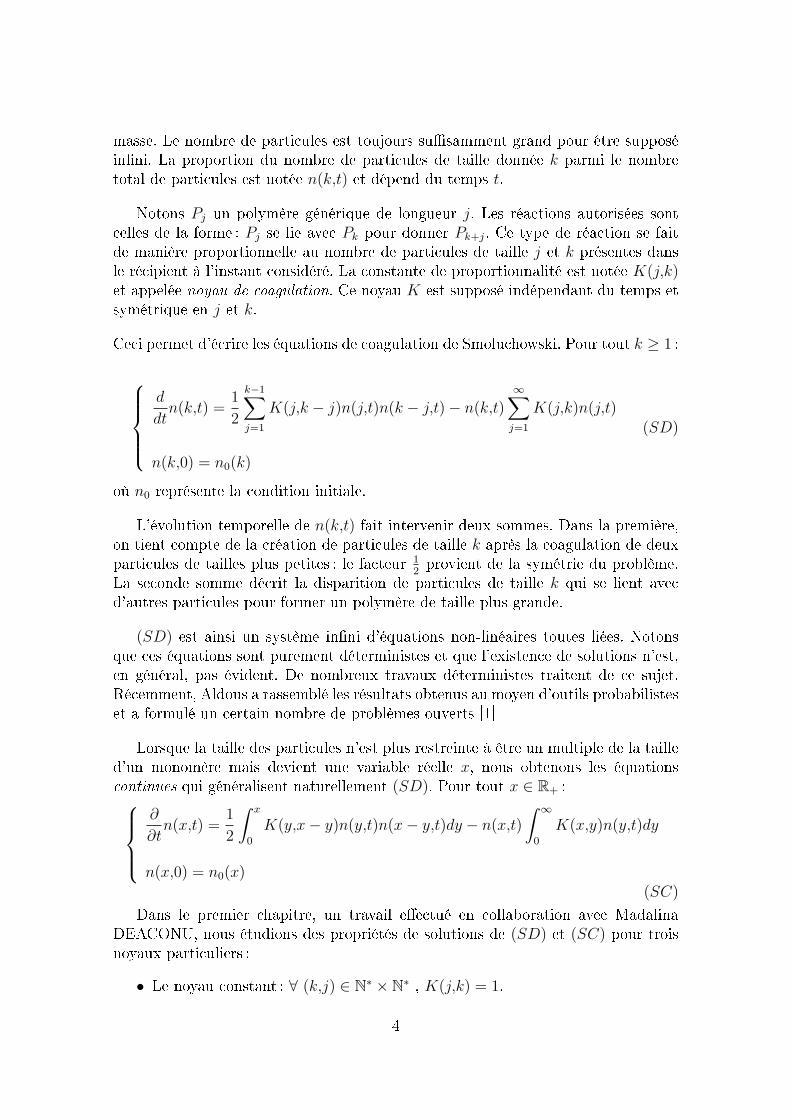
masse. Le nombre de particules est toujours susamment grand pour être supposéinni. La proportion du nombre de particules de taille donnée k parmi le nombretotal de particules est notée n(k,t) et dépend du temps t.
Notons Pj un polymère générique de longueur j. Les réactions autorisées sontcelles de la forme : Pj se lie avec Pk pour donner Pk+j. Ce type de réaction se faitde manière proportionnelle au nombre de particules de taille j et k présentes dansle récipient à l'instant considéré. La constante de proportionnalité est notée K(j,k)et appelée noyau de coagulation. Ce noyau K est supposé indépendant du temps etsymétrique en j et k.
Ceci permet d'écrire les équations de coagulation de Smoluchowski. Pour tout k ≥ 1 :
d
dtn(k,t) =
1
2
k−1∑j=1
K(j,k − j)n(j,t)n(k − j,t)− n(k,t)∞∑
j=1
K(j,k)n(j,t)
n(k,0) = n0(k)
(SD)
où n0 représente la condition initiale.
L'évolution temporelle de n(k,t) fait intervenir deux sommes. Dans la première,on tient compte de la création de particules de taille k après la coagulation de deuxparticules de tailles plus petites ; le facteur 1
2provient de la symétrie du problème.
La seconde somme décrit la disparition de particules de taille k qui se lient avecd'autres particules pour former un polymère de taille plus grande.
(SD) est ainsi un système inni d'équations non-linéaires toutes liées. Notonsque ces équations sont purement déterministes et que l'existence de solutions n'est,en général, pas évident. De nombreux travaux déterministes traitent de ce sujet.Récemment, Aldous a rassemblé les résultats obtenus au moyen d'outils probabilisteset a formulé un certain nombre de problèmes ouverts [1]
Lorsque la taille des particules n'est plus restreinte à être un multiple de la tailled'un monomère mais devient une variable réelle x, nous obtenons les équationscontinues qui généralisent naturellement (SD). Pour tout x ∈ R+ :
∂
∂tn(x,t) =
1
2
∫ x
0
K(y,x− y)n(y,t)n(x− y,t)dy − n(x,t)
∫ ∞
0
K(x,y)n(y,t)dy
n(x,0) = n0(x)(SC)
Dans le premier chapitre, un travail eectué en collaboration avec MadalinaDEACONU, nous étudions des propriétés de solutions de (SD) et (SC) pour troisnoyaux particuliers :
• Le noyau constant : ∀ (k,j) ∈ N∗ × N∗ , K(j,k) = 1.
4
• Le noyau additif : ∀ (k,j) ∈ N∗ × N∗ , K(j,k) = j + k.• Le noyau multiplicatif : ∀ (k,j) ∈ N∗ × N∗ , K(j,k) = jk.
Ces trois noyaux ont l'avantage de permettre des calculs explicites.
Dans le cas particulier où la condition initiale n0 est la masse de Dirac en 1(n0(k) = δ1(k)), on peut obtenir les solutions exactes pour ces trois noyaux. Cettecondition initiale correspond à la présence uniquement de monomères dans le ré-cipient au début de la polymérisation. Nous retrouvons les solutions exactes grâceà une interprétation probabiliste de ces équations. Nous avons également su lierles solutions des équations de Smoluchowski à la population totale d'un processusde branchement de type Galton-Watson. Grâce à cela, nous établissons une cor-respondance entre les solutions des équations de coagulation de Smoluchowski avecnoyau additif et celles avec noyau multiplicatif, sans restriction sur les conditionsinitiales. Ce résultat important permet d'obtenir les propriétés pour les deux noyauxlorsqu'elles ne sont pas aisées à prouver directement.
Nous décrivons par ailleurs le comportement asymptotique des solutions de (SC),toujours pour les noyaux constant, additif et multiplicatif. Après une bonne renor-malisation, nous montrons que les solutions convergent vers une variable aléatoire,la limite dépendant peu de la condition initiale (uniquement par ses premiers mo-ments). L'ensemble de ces résultats constitue le Chapitre 1.
Le Chapitre 2 a fait l'objet d'une publication à la suite de la conférence in-ternationale Monte Carlo 2000. Dans ce court travail, (en collaboration avec Mada-lina DEACONU), nous montrons comment l'on peut exploiter notre correspondanceentre les solutions liées aux noyaux additif et multiplicatif au travers des solutionsà valeur mesure, données par Norris [52], [53].
Les Chapitres 3 et 4 sont le fruit d'un travail en collaboration avec MadalinaDEACONU et Nicolas FOURNIER.Tout comme dans le Chapitre 1, nous nous intéressons à une forme faible de solutionsdes équations de coagulation de Smoluchowski.
Une propriété physique très importante des solutions de (SD) et (SC) que nousétudions est qu'elles conservent la masse : pour toute solution de (SC), jusqu'à uninstant T0, on a, pour tout t ∈ [0,T0[ :∫
R+
xn(x,t) dx =
∫R+
xn(x,0) dx.
De même, pour toute solution de (SD), il existe un instant T0 tel que pour toutt ∈ [0,T0[ : ∑
k≥1
kn(k,t) =∑k≥1
kn(k,0).
5
De ce fait, la quantité
Qt(dx) =∑k≥1
k n(k,t)δk(dx) resp. Qt(dx) = xn(x,t) dx
est une mesure de probabilité sur R+.
Cette notation permet de traiter ensemble les problèmes (SC) et (SD) de lamanière suivante : nous dirons que la famille de probabilités (Qt)t∈[0,T0[ est solutionfaible de l'équation (MS) si pour toute fonction test ϕ ∈ C1
0(R+) et pour toutt ∈ [0,T0[, on a :∫ ∞
0
ϕ(x)Qt(dx) =
∫ ∞
0
ϕ(x)Q0(dx)
+
∫ t
0
∫R+
∫R+
[ϕ(x+ y)− ϕ(x)]K(x,y)
yQs(dy)Qs(dx)ds.
Nous réussissons ainsi à établir un lien entre les équations de Smoluchowski etles processus vériant l'équation diérentielle stochastique à sauts, dirigée par unprocessus de Poisson :
Xt = X0 +
∫ t
0
∫ 1
0
∫ ∞
0
Xs−(α)11z≤K(Xs−,Xs−(α))
Xs−(α)
N(ds,dα,dz). (EDS)
Le processus X vit sur l'espace de probabilité (Ω,F ,P) alors que X est un pro-cessus sur l'espace de probabilité auxiliaire [0,1] muni de la mesure (de probabilité)de Lebesgue.
On cherche les solutions de (EDS) telles que les processus X et X aient mêmeloi. La quantité N(ω,dt,dα,dz) est une mesure de Poisson sur [0,T0[×[0,1] × R+ demesure d'intensité dt dα dz et est indépendante de X0.
Le lien entre les solutions de cette équation et les équations de coagulation deSmoluchowski est le suivant : toute solution (X,X) de cette équation est telle queles marginales temporelles Qt de X. sont solutions de (MS) :
Qt = L(Xt).
Dans le Chapitre 3, l'équation (EDS) est étudiée (existence des solutions, unicité,propriétés trajectorielles). Dès à présent, nous pouvons expliquer le comportementdes solutions de (EDS). Nous partons d'une variable aléatoire distribuée suivant laloi X0. Le rôle de la mesure de Poisson est le suivant : à des instants aléatoires, nouschoisissons une particule au hasard dans la solution - c'est le choix de α - et unniveau z. La particule Xt(α) se colle ou non sur la particule que l'on observe suivantla valeur du niveau z. L'indicatrice dans cette E.D.S. non linéaire est un contrôle dela coagulation en fonction du noyau.
6
Dans le Chapitre 4, les résultats (théoriques) du Chapitre 3 sont utilisés pourapprocher les solutions des équations de Smoluchowski par un système de particules.Nous prouvons la convergence du système de particules et montrons qu'il est parfai-tement simulable dès que la condition initiale l'est. Nous présentons également desrésultats numériques qui valident l'étude.
De plus, un théorème de la limite centrale est démontré sous les hypothèsessuivantes :
• Q0 a un moment d'ordre 2 ni.• Q0 a son support inclus dans N.• Le noyau K est borné.
Les résultats numériques laissent à penser que le champ d'application du théorèmeest plus large et que chacune de ces hypothèses peut être aaiblie.
B : Approximation de diusions irrégulières
Dans la deuxième partie de ce travail, en collaboration avec Jean-SébastienGIET, nous étudions la validité du schéma d'Euler pour approcher des diusionsirrégulières.
La quantité que l'on souhaite estimer est :
E∫ T
0
f(Xs)ds
lorsque X est une diusion régulière, f une fonction quelconque (mesurable et bor-née) et T un temps xe déterministe.
L'apport des processus stochastiques dans la résolution des E.D.P. est bien connu.Commençons par rappeler l'exemple de l'équation de la chaleur :
∂u
∂t(t,x) = 1
2∆u(t,x)
u(0,x) = u0(x),
où u0 est une fonction continue. La solution s'exprime sous la forme :
u(t,x) = E u0 (x+Bt)
où B est un mouvement brownien issu de 0.
Lorsque l'on considère une diusion X solution de l'équation :
Xt = X0 +
∫ t
0
σ(Xs) dBs +
∫ t
0
b(Xs) ds.
7
La fonction u(t,x) = E u0(Xxt ) est solution de l'E.D.P. (équation de la chaleur
généralisée) : ∂u
∂t(t,x) = Au(t,x)
u(0,x) = u0(x)
Le lien entre la diusion X et l'opérateur A intervenant dans l'E.D.P. est :
Ag(x) =1
2
d∑i,j=1
ai,j(x)∂2
∂xi∂xj
(x) +d∑
i=1
bi(x)∂g
∂xi
(x).
Donnons ici un exemple d'E.D.P. pour laquelle la solution fait intervenir unefonctionnelle de la totalité de la trajectoire d'un processus stochastique : le problèmede Cauchy avec potentiel r et Lagrangien g, qui est une extension de l'équation dela chaleur :
∂u
∂t(t,x) = Au(t,x)− r(x)u(t,x) + g(x)
u(0,x) = u0(x)
où les fonctions r et g sont continues ; r est de plus supposée minorée.
La formule de Feynman-Kac permet d'exprimer la solution du problème de Cau-chy sous la forme suivante :
u(t,x) = E
u0(X
xt ) exp
(−∫ t
0
r(Xxs ) ds
)+
∫ t
0
g(Xxθ ) exp
(−∫ θ
0
r(Xxs ) ds
)dθ
.
L'approximation des solutions de l'équation de la chaleur généralisée grâce à soninterprétation probabiliste a déjà été étudiée. Par exemple, Talay et Tubaro [61],Bally et Talay [6], [5] donnent un développement de l'erreur commise en approchantE f(XT ) par E
f(XT )
où X désigne l'approximation deX obtenue par le schéma
d'Euler.T est un temps xé, X est une diusion régulière et f est une fonction régulière
dans [61], seulement mesurable bornée dans [6] et [5].
Précisons maintenant le cadre dans lequel notre travail est eectué :• X est solution de l'équation :
Xt = X0 +
∫ t
0
σ(Xs) dBs +
∫ t
0
b(Xs) ds.
• σ et b sont des fonctions C∞.• σ′ , σ′′ , b′, b′′ sont des fonctions bornées.
8
• La diusion est uniformément elliptique, on note a = σσt :
∃η ∈ R∗ t.q. ∀ξ 6= 0 , ξta(x)ξ ≥ η||ξ||2
• f est une fonction mesurable et bornée.
Nous pouvons formuler diéremment ce problème en augmentant la dimension dela diusion :
dXt = σ(Xt) dBt + b(Xt) dtdYt = f(Xt) dt
(EDS2)
Ainsi écrit, le but de ce travail est d'approcher E(YT ), Y étant ici une diusionirrégulière.
Les résultats connus pour la méthode de discrétisation par le schéma d'Eulers'appliquent si la fonction f est elle-même régulière. La diusion (Xt,Yt) l'est alorsaussi et l'approximation de E(YT ) par le schéma d'Euler converge vers E(YT ) à unevitesse d'ordre 1
noù T
nest le pas de discrétisation.
Ici, nous étendons ce résultat pour f mesurable bornée quelconque :∣∣∣∣∣E(∫ T
0
f(Xs) ds
)− 1
n
n∑i=1
Ef(X
Tn
(iT
n
))∣∣∣∣∣ ≤ K
n;
XTn désigne l'approximation de X obtenue par le schéma d'Euler de pas T
n.
Pour estimer E∫ T
0
f(Xs) ds, on rencontre 3 types de problèmes :
• L'espérance est approchée par une méthode de Monte-Carlo classique : on ef-fectue un grand nombre de réalisations et on en prend la moyenne. Nous nedéveloppons pas davantage cette partie dont les résultats sont connus.
• La diusion n'est connue qu'en tant que solution de l'E.D.S. et nous sommesdonc amenés à l'approcher. Nous avons privilégié l'approximation par le sché-ma d'Euler assez facile à mettre en oeuvre.
• La totalité de la trajectoire de l'approximation par le schéma d'Euler n'est pasconnue or nous devons en calculer l'intégrale sur [0,T ]. Nous remplaçons cetteintégrale par les sommes de Riemann associées.
C'est ainsi que nous approchons E(∫ T
0f(Xs) ds
)par 1
n
∑ni=1 Ef
(X
Tn
(iTn
)).
Notons ici que lorsque la fonction f est régulière, nous avons vu que le problèmese ramène à estimer E(YT ) pour (X.,Y.) solution de (EDS2). Dans ce cas, l'approxi-mation donnée par le schéma d'Euler est précisément : 1
n
∑ni=1 Ef
(X
Tn
(iTn
)).
9
Nous avons découpé l'erreur commise en deux parts : l'une vient des sommes deRiemann, l'autre du schéma d'Euler.∣∣∣∣∣E
(∫ T
0
f(Xs) ds
)− 1
n
n∑i=1
Ef(X
Tn
(i
n
))∣∣∣∣∣ ≤∣∣∣∣∣E(∫ T
0
f(Xs) ds
)− 1
n
n∑i=1
Ef(X i
n
)∣∣∣∣∣+
∣∣∣∣∣ 1nn∑
i=1
Ef(X i
n
)− 1
n
n∑i=1
Ef(X
Tn
(i
n
))∣∣∣∣∣ .Pour majorer la première erreur, nous utilisons essentiellement la régularité de
la diusion X et la propriété pour f d'être bornée.
Pour majorer la seconde partie, la technique utilisée repose sur une idée de Kurtzet Protter consistant à introduire la famille d'approximations de X (Xδ
r (t),0 ≤ t ≤T ) dénie ainsi :
• δ désigne le pas de discrétisation.• Xδ
r (t) = Xδ(t) pour t ∈ [0,r].• Xδ
r (t) = Xr,Xδr (r)(t) pour t ∈ [r,T ].
La diusion Xδr est donnée par le schéma d'Euler jusqu'à l'instant r puis est gou-
vernée par les coecients σ et b entre r et T .
Ainsi Xδ0(.) = X. et Xδ
T (.) = Xδ(.).
La diérence ϕ(Xδ(.))− ϕ(X.) peut donc être vue comme l'intégrale :∫ T
0
∂
∂rϕ(Xδ
r (.)) dr
pour tout fonctionnelle ϕ de la trajectoire.
C : Amplitude du mouvement brownien avec dérive
Cette dernière partie de ma thèse a fait l'objet d'une collaboration avec PierreVALLOIS, un de mes directeurs de thèse. Le mouvement brownien avec dériveconstante est un objet qui apparaît naturellement dans un certain nombres de pro-blèmes comme, par exemple, en mathématiques nancières. En eet, le logarithme
10
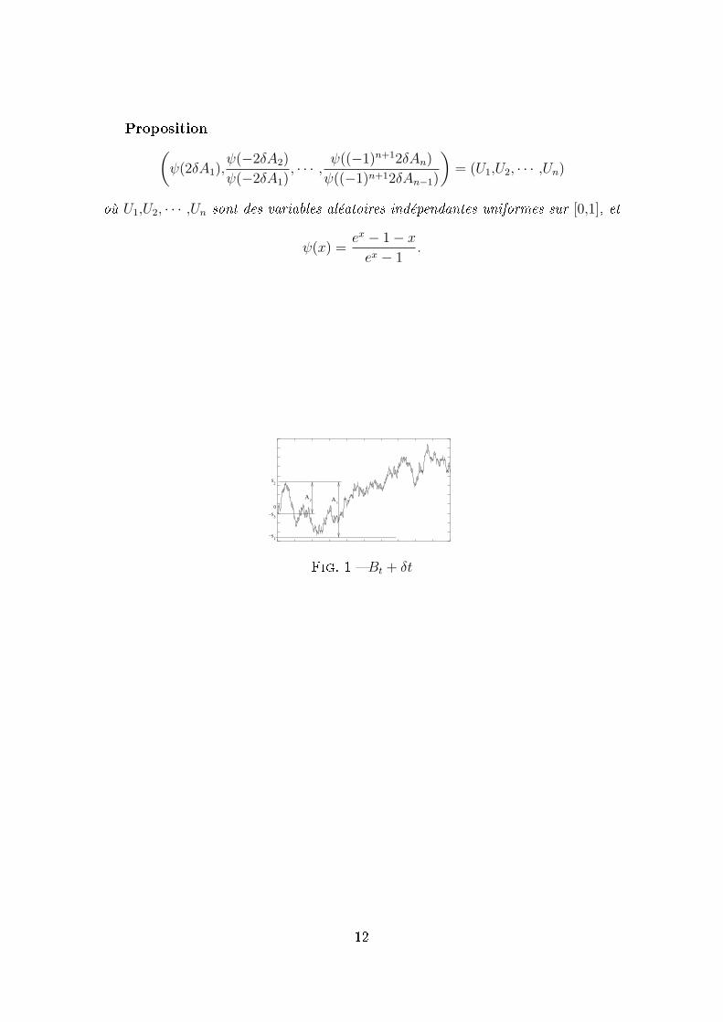
du cours d'un actif qui suit le modèle de Black et Scholes est précisément un mou-vement brownien avec dérive.L'étude des uctuations des cours dans ce modèle amène à s'intéresser aux ampli-tudes de ce processus.On dénit l'amplitude At par :
At = sups∈[0,t]
Bs + δs − infs∈[0,t]
Bs + δs
Dans ce travail, nous donnons une description des trajectoires du mouvementbrownien avec dérive en le décomposant suivant ses extremums successifs. Laquantité Bt +δt est presque sûrement minorée (resp. majorée) si δ > 0 (resp. δ < 0).On note −S1 le minimum (resp. S1 le maximum) absolu de Bt+δt sur une trajectoireet ρ1 le dernier instant où il est atteint. Nous retrouvons au moyen d'une techniquede grossissement de ltration un résultat de Williams [66] qui décrit :
• La loi de S1.• Conditionnellement à S1 = x1,
la loi de (Bt + δt , 0 ≤ t ≤ ρ1), la loi de (Bt + δt , t ≥ ρ1).
Notre technique permet de poursuivre cette décomposition : sur [0,ρ1] , Bt + δt estpresque sûrement majoré (resp. minoré). On note S2 l'extremum correspondant et ρ2
le dernier instant où il est atteint. Nous obtenons alors (toujours conditionnellementà S1 = x1) :
• La loi de S2.• Conditionnellement à S2 = x2,
la loi de (Bt + δt , 0 ≤ t ≤ ρ2), la loi de (Bt + δt , ρ2 ≤ t ≤ ρ1).
Et nous poursuivons cette décomposition.
Nous décrivons complètement les trajectoires à l'aide des lois des extremums suc-cessifs, du mouvement brownien avec dérive et de la diusion Z(δ), solution positivede l'équation diérentielle stochastique suivante :
Z(δ)(t) = Bt + δ
∫ t
0
coth(δZ(δ)(s)
)ds.
En particulier nous obtenons la loi des n-uples (A1,A2, · · · ,An) où Ak = Sk + Sk+1.Proposition (A1, · · · ,An) a pour densité :
δn
[n−1∏k=1
e(−1)kδak
sh(δak)
]e(−1)n2δan − 1 + (−1)n+12δan
sh2 δan
110≤an≤···≤a1
Nous obtenons également une représentation plus probabiliste de ses variablesaléatoires :
11
Proposition(ψ(2δA1),
ψ(−2δA2)
ψ(−2δA1), · · · , ψ((−1)n+12δAn)
ψ((−1)n+12δAn−1)
)= (U1,U2, · · · ,Un)
où U1,U2, · · · ,Un sont des variables aléatoires indépendantes uniformes sur [0,1], et
ψ(x) =ex − 1− x
ex − 1.
1A
3−S
2A
S
1
2
−S
0
Fig. 1 Bt + δt
12
Première partie
Phénomènes de coagulation
13

1
Smoluchowski's CoagulationEquation : Probabilistic
Interpretation of Solutions forConstant, Additive andMultiplicative Kernels
Une grande partie de ce chapitre a fait l'objet d'une publication à Annali dellaScuola Normale Superiore di Pisa, Serie IV, Vol. XXIX (3) : 549-580, 2000.
Abstract
This paper is devoted to the study of the Smoluchowski's coagulationequation, discrete and continuous version, for the case of constant, ad-ditive and multiplicative kernels. Even though, for the discrete case theresults stated in this work are not new, our approach allows the simpli-cation of existing proofs. For the continuous case we obtain new results :a connection between the solutions of the additive and multiplicativecases and renormalisation theorems which show that after a convenientscaling, the solution converges to a limit which depends on the initialcondition only through its moments of order 1, 2 and 3.
Key Words : Smoluchowski's coagulation equation, branching processes, stochastic pro-cesses, partial dierential equations, Laplace transform.
AMS 2000 subject classication : 60J80, 44A10
15
Chapitre 1. Smoluchowski's Eq. : probabilistic interpretation for particular kernels
1.1 Introduction
1.1.1 Paper's Plan
The aim of this paper is to provide a probabilistic representation for some solu-tions of the Smoluchowski's coagulation equation.In the introduction we give the heuristic motivation of this problem. Afterwards wefurnish a survey of some results that we can nd in the literature on the Smolu-chowski's equation, without any intention of being exhaustive, but by pointing outthe results obtained by using probabilistic methods. For a more detailed survey werefer to Aldous ([1]).The two following parts discuss three particular kernels : constant, additive and mul-tiplicative. This choice for the kernel allows the development of the computation.The second part recalls briey some known results on the discrete case for this threeparticular kernels. We obtain the explicit form of these solutions via branching pro-cesses. The results we give on this part are not new but our approach allows thesimplication of existing proofs.The last part deals with the continuous case. We express here our main results : atransformation which connects the solution of the additive case with the one of themultiplicative case (theorems 1.3.9 and 1.3.11), and some renormalisation theorems(theorems 1.3.6, 1.3.20 and 1.3.24). These last theorems insure the convergence ofthe solution to a limit, which depends weakly on the initial condition.
1.1.2 Heuristic Motivation of the Problem
The Smoluchowski's coagulation equation models various kind of phenomena asfor example : in chemistry (polymerisation), in physics (aggregation of colloidal par-ticles), in astrophysics (formation of stars and planets), in engineering (behaviourof fuel mixtures in engines), in genetics, in random graphs theory etc.In order to x the ideas, we present the appearance of this equation, in polymerisa-tion.For k ∈ N∗, let Pk denote a polymer of mass k, that is a set of k identical particles(monomers). As time advances, the polymers evolve and, if they are sucientlyclose, there is some chance that they merge into a single polymer whose mass equalsthe sum of the two polymers' masses which take part in this binary reaction. Byconvention, we admit only binary reactions. This phenomenon is called coalescenceand we write formally
Pk + Pj −→ Pk+j,
for the coalescence of a polymer of mass k with a polymer of mass j.Let n(k,t) denote the average number of polymers of mass k per unit volume, attime t. The expression k n(k,t) denotes the part of mass consisting on polymers of
16
1.1. Introduction
length k, per unit volume.It is thus natural to consider that the coalescence phenomenon (Pk + Pj −→ Pk+j),is proportional to n(k,t)n(j,t) with a proportionality constant K(k,j), called coa-lescence kernel.In the sequel we employ for the discrete case letters i, j, k ... while for the continuouscase we use x, y, z .... Furthermore, throughout this paper, time t is always conti-nuous, discrete and continuous refer to polymers' masses.Hereafter (discrete and continuous case), the coagulation kernel K will satisfy thefollowing hypothesis :
(H1) K is positive i.e., K : (N∗)2 or (R+)2 → R+,and(H2) K is symmetric i.e., K(i,j) = K(j,i).
The Smoluchowski's coagulation equation, in the discrete case, is the equation onn(k,t), for k ∈ N∗. It is usually written on the following form
d
dtn(k,t) =
1
2
k−1∑j=1
K(j,k − j)n(j,t)n(k − j,t)− n(k,t)∞∑
j=1
K(j,k)n(j,t)
n(k,0) = n0(k), k ≥ 1.
(SD)
This system describes a non linear evolution equation of innite dimension, withinitial condition (n0(k))k≥1. Due to the presence of the innite series, (SD) is not aclassical initial value problem for a system of non linear ordinary dierential equa-tions, and even the existence of a local solution is not guaranteed by the theory ofordinary dierential equations. According to the form of the coalescence kernel Kand the one of the initial condition, we obtain or not solutions for this system. Inthe rst line of (SD), the rst term on the right hand side describes the creation ofpolymers of mass k by coagulation of polymers of mass j and k−j. The coecient 1
2
is due to the fact that K is symmetric. The second term corresponds to the depletionof polymers of mass k after coalescence with other polymers.The notion of solution will be given in the following section (denitions 1.1.1, 1.1.2for the discrete case and denitions 1.1.3, 1.1.4 for the continuous case).The continuous analogue of the equation (SD) can be written naturally
∂
∂tn(x,t)=
1
2
∫ x
0
K(y,x− y)n(y,t)n(x− y,t)dy − n(x,t)
∫ ∞
0
K(x,y)n(y,t)dy
n(x,0) = n0(x).(SC)
1.1.3 Some Known Results
The references, while numerous, are not intended to be complete, except that wehave sought to represent the major direction of research from a probabilistic pointof view. In this study on the Smoluchowski's coagulation equation we consider threekernels : constant, additive and multiplicative.
17
Chapitre 1. Smoluchowski's Eq. : probabilistic interpretation for particular kernels
1.1.3.1 Analysis of the Discrete Case
Let us consider the discrete case. Introduce rst of all the notion of weak solutionfor the system (SD) (we can nd this denition for example in Laurençot ([43])).
Denition 1.1.1 Let T ∈ (0,∞] and (n0(k))k≥1 be a sequence of positive realnumbers. We call weak solution of the system (SD) on [0,T ), a sequence of nonne-gative continuous functions such that, for all t ∈ (0, T ) and k ≥ 1 :
(a) n(k,.) ∈ C([0,T ]) and∞∑
j=1
K(j,k)n(j,t) ∈ L1(0,t),
and(b)
n(k,t)=n0(k) +
∫ t
0
(12
k−1∑j=1
K(j,k − j)n(j,s)n(k − j,s)−n(k,s)∞∑
j=1
K(j,k)n(j,s))ds.
For our study we shall consider rather the notion of strong solution.
Denition 1.1.2 Let T ∈ (0,∞] and (n0(k))k≥1 be a sequence of positive realnumbers. We call strong solution of (SD) on [0,T ), a sequence of positive functionssuch that, for all t ∈ (0, T ) and k ≥ 1 : the derivative of n(k,t) with respect to t
exists,∞∑
j=1
K(j,k)n(j,t) <∞ and (SD) is veried.
A global solution is a solution with T = ∞. The solution will be called local in theopposite case.Hereafter, we denote by C a constant whose value changes from line to line.Let us make the following remark. Formal computations give
d
dt
∞∑k=1
k n(k,t) = 0. (1.1)
Therefore it is natural to ask if (1.1) is preserved on time. From a physical point ofview the equality (1.1) is equivalent to the conservation of the mass for the system(SD). As far as (1.1) is true we have
∞∑k=1
k n(k,t) =∞∑
k=1
k n(k,0). (1.2)
The rst moment for which (1.2) is not longer valid is called gelication time and isdened by
Tgel = inft ≥ 0;∞∑
k=1
k n(k,t) <∞∑
k=1
k n(k,0). (1.3)
18
1.1. Introduction
In polymerisation this time corresponds to the appearance of an innite polymercalled gel (and is equivalent to mass removal). From a physical point of view thegelation phenomenon might be interpreted as follows : the process of formation oflarge polymers takes place at suciently large rate so that a part of monomers istransfered to larger and larger polymers, and eventually gives rise to a huge polymercalled gel. This gel can be regarded as a polymer formed by an innite number ofmonomers so it is not accounted into (SD).Let us introduce also, the space of real positive sequences dened by
E = x = (xi)i≥1, xi ≥ 0,∞∑i=1
i xi <∞. (1.4)
Constant KernelsIn 1916 Smoluchowski ([56]) studied (SD) for the constant kernel and gave an ex-plicit solution. More generally, Melzak ([51]) proved that, for
K(i,j) ≤ C, for i,j ≥ 1 and C > 0, (1.5)
one can obtain existence and uniqueness of a global solution for (SD), for any initialcondition in E.
Additive KernelsBall and Carr ([4]) were interested on kernels satisfying
K(i,j) ≤ C(i+ j), i, j ≥ 1. (1.6)
They got the existence of a global solution for (SD), which conserves the mass, forany initial condition from E. In order to get uniqueness of this solution we haveeither to impose
K(i,j) ≤ C√ij, (1.7)
or to restrict the class of initial conditions to E. This last situation was treated byHeilmann ([33]). For kernels satisfying the inequality (1.6) and with initial condition(n(k,0))k≥1, from E, such that
∞∑k=1
k2n(k,0) <∞, (1.8)
Heilmann ([33]) proved the existence and uniqueness of a global solution for (SD),which satises for all T ∈ [0,+∞)
supt∈[0,T ]
∞∑k=1
k2n(k,t) <∞. (1.9)
Previously, the case K(i,j) = C(i+ j) was considered by Golovin ([28]).For "additive" kernels K of the form
K(i,j) = iα + jα (1.10)
19
Chapitre 1. Smoluchowski's Eq. : probabilistic interpretation for particular kernels
with α > 1, Carr and da Costa ([8]) proved that there is no solution (even local)of (SD). This result holds for any initial condition in E, dierent from the 0 function.
Multiplicative KernelsThe case of the kernel K(i,j) = i j under the initial condition n(k,0) = δ1(k), for allk ∈ N∗, was treated by McLeod ([48]). This initial condition insures that, at t = 0,there are only monomers. McLeod deduced the existence and uniqueness of a localsolution for all t ∈ [0,1) verifying
sups∈(0,t]
∞∑k=1
k2n(k,s) <∞, ∀t ∈ (0,1). (1.11)
For the same kernel and under the same initial condition, Kokholm ([40]) provedthe existence of an unique global solution for (SD), satisfying for all T ∈ [0,+∞)
supt∈[0,T ]
∞∑k=1
kn(k,t) <∞. (1.12)
This solution is given by
n(k,t) =
kk−3
(k − 1)!tk−1e−kt for t ∈ [0,1]
kk−3
(k − 1)!
e−t
tfor t ∈ [1,+∞).
Leyvraz and Tschudi ([45]), obtained a more general result. More precisely, forK(i,j) ≥ Cij, ∀i,j ≥ 1, (1.13)
any solution of (SD), when it exists, cannot satisfy the mass conservation for all t.Furthermore, for the initial condition n(k,0) = δ1(k) they constructed a solution forwhich :
∞∑k=1
k n(k,t) =
1 for t ≤ 11
tfor t ≥ 1.
Obviously, in this particular case Tgel = 1. Their result explains also the local solutionobtained previously by McLeod ([48]).Furthermore, Leyvraz ([44]) treated the case K(i,j) = iα jα, and proved that for allα ∈ (1
2, 1], there exists an initial condition such that Tgel = 0 (that is the total mass
decreases from the beginning).Several works in the literature were concentrated on kernels which combine theadditive, constant and multiplicative kernels, of the following form :
K(i,j) = A+B(i+ j) + Cij, (1.14)where A,B and C are given constants.For these kernels, the existence of a solution for the Smoluchowski's coagulationequation was obtained by using various techniques : Flory ([21], [22], [23]) and Spouge([58], [59]), from a combinatorial point of view, Gordon ([29]) and Spouge ([57]), byusing branching processes.
20
1.1. Introduction
1.1.3.2 Analysis of the Continuous Case
Let us introduce rst the notion of weak solution in the continuous case.Denition 1.1.3 Let T ∈ (0,∞] and (n0(x))x≥0 be a positive real function. We
call weak solution of (SC) on [0,T ), a set of continuous and positive functions sa-tisfying, for all t ∈ (0, T ) and x ≥ 0 :
(a) n(x,.) ∈ C([0,T ]) and
∫ ∞
0
K(x,y)n(y,t)dy ∈ L1(0,t)
and(b)
n(x,t) = n0(x)
+
∫ t
0
(1
2
∫ x
0
K(y,x− y)n(y,s)n(x− y,s)dy−n(x,s)
∫ ∞
0
K(x,y)n(y,s)dy)ds.
The notion of strong solution becomes then :
Denition 1.1.4 Let T ∈ (0,∞] and (n(x,0))x≥0 be a real positive function. Wecall strong solution of (SC) on [0,T ), a set of positive and continuous functions suchthat, for all t ∈ (0, T ) and x ≥ 0 : the derivative with respect to t of n(x,t) exists,∫ ∞
0
K(x,y)n(y,t)dy <∞ and (SC) is veried.
For the additive, constant and multiplicative kernels, in the continuous case, theuniqueness is far of being obvious. We can obtain it for some special kernels, as forexample, those satisfying ([1])
K(x,y) ≤ C(1 + x+ y), (1.15)
More precisely, if the condition (Ct)∫ ∞
0
n(x,t)dx <∞,
∫ ∞
0
xn(x,t)dx = 1 and∫ ∞
0
x2n(x,t)dx <∞, (Ct)
is satised for t = 0, then the solution of the continuous Smoluchowski's coagulationequation (SC), exists and is unique. Furthermore (Ct) is valid for all t ∈ [0,∞).The work of Drake ([12]) and Aldous ([1]) gave examples of kernels K which haveappeared in physics and chemistry. The model initially proposed by Smoluchowski([56]) in 1916 had a kernel of the form
K(x,y) = C(x13 + y
13 )(x−
13 + y−
13 ), (1.16)
and corresponds to a coagulation controled by the Brownian diusion.Ernst, Zi and Hendricks ([16]) gave in their paper the construction of a solution
21
Chapitre 1. Smoluchowski's Eq. : probabilistic interpretation for particular kernels
for (SC) after the gelication time, for kernels admitting a nite gelication time,of the form
K(x,y) = (xy)α, with 1
2< α ≤ 1. (1.17)
For kernels of the form
K(x,y) = A+B(x+ y) + Cxy, (1.18)
Spouge ([60]) studied the "critical" time
tc = inft;∫ ∞
0
x2 n(x,t)dx <∞, (1.19)
and proved that it corresponds to a critical branching process. Times t > tc corres-pond to super-critical branching processes.
1.1.3.3 Probabilistic Approach for the Smoluchowski's Coagulation Equa-tion
Many authors have treated the Smoluchowski's coagulation equation by usingprobabilistic methods.In his paper, Aldous ([1]) made a survey of the present situation for (SD) and (SC)from a probabilistic point of view. He brought also to the fore some open problemswhich can be solved by using probabilistic methods.Lang and Nguyen ([42]) used the propagation of chaos method in order to provethe convergence of an innite particles system, directed by 3 dimensional BrownianMotions, to the initial model of coagulation proposed by Smoluchowski ([56]).Recently, Jeon ([36]) approached the solution of a more general equation than (SD),in that, we have also the fragmentation of polymers, by a sequence of nite Markovchains. Jeon gave a general result. More precisely, if we have
K(i,j) ≥ (ij)α, with α ∈(1
2,1), (1.20)
and furthermorelim
i+j→∞
K(i,j)
ij= 0, (1.21)
then we have gelication in nite time (Tgel <∞), for a large class of initial condi-tions. This result was generalised to the continuous situation by Norris ([52]).The equation for the kernel K(i,j) = ij can be connected to studies on coagulationvia random graphs and forests ([1], [17]).Another interesting direction in the present study of the Smoluchowski's coagulationequation is the approximation of the solution by using Monte Carlo methods ([32],[3]).
22
1.2. Connection Between the Discrete Smoluchowski's Equ and Branching Processes
1.2 Connection Between the Discrete Smoluchows-
ki's Coagulation Equation (SD) and Branching
Processes
Let us consider the discrete Smoluchowski's coagulation equation (SD). We aregoing to study three coagulation kernels K : constant, additive and multiplicative.The initial condition that we consider for these three cases is n(k,0) = δ1(k). Itcorresponds to an initial conguration in which there are only monomers. In thesequel we shall use the notion of solution in the sense of strong solution, given inthe denition 1.1.2.For each one of these cases we shall emphasise a connection between the solutionn(k,t) of (SD) and a branching process. This allows to obtain explicit solutions(corollaries 1.2.3, 1.2.5 and 1.2.7). The choice of this initial condition is essentialand it corresponds, for the branching process, to the fact that it has one ancestor.On one hand, our results are not new, we can nd them for example in Aldous([1]). On the other hand, our approach is new and consists in using generatingfunctions, which allow the simplication of existing proofs. The goal of this sectionis to exhibit clearly the breadth and importance of branching processes in the studyof the discrete Smoluchowski's coagulation equation.A formal calculation allows the following remark.
Lemma 1.2.1 Before the gelication time (t < Tgel), we have for (SD)
d
dt
∞∑k=1
k n(k,t) = 0. (1.22)
By re-normalising the initial condition, we can always suppose that
∞∑k=1
k n(k,t) = 1. (1.23)
1.2.1 Discrete Coagulation Equation with K(i,j) = i j
For this particular case the equation (SD) can be writtend
dtn(k,t) =
1
2
k−1∑j=1
j(k − j)n(j,t)n(k − j,t)− kn(k,t)∞∑
j=1
jn(j,t)
n(k,0) = δ1(k), k ≥ 1.
(SD∗)
The choice of this initial condition corresponds to consider that at t = 0 we haveonly monomers. It is essential for the results which follow. We have Tgel = 1 (cf.
23
Chapitre 1. Smoluchowski's Eq. : probabilistic interpretation for particular kernels
Leyvraz and Tschudi ([45])), and we shall consider only t ≤ Tgel. By using lemma1.2.1, we have the conservation of mass
∞∑k=1
k n(k,t) =∞∑
k=1
k n(k,0) = 1, ∀t ≤ Tgel = 1. (1.24)
Let us denote byp(k,t) = k n(k,t), (1.25)
such that (p(k,t))k≥1 form a probability distribution on N∗. The generating functionof this probability,
G(t,s) =∞∑
k=1
p(k,t) sk, |s| ≤ 1, (1.26)
veries
Proposition 1.2.2 The function G, given by (1.26), is the unique solution ofthe non linear partial dierential equation
∂G
∂t(t,s) =
s
2
∂G2
∂s(t,s)− s
∂G
∂s(t,s)
G(t,1) = 1G(0,s) = s,
(1.27)
for all t ≤ 1 = Tgel and |s| ≤ 1.
The proof of this proposition is obvious in view of the equation (SD∗), on n(k,t).The solution of the equation (1.27) is also the generating function of the total popu-lation of a particular branching process. Indeed, let us consider a branching processwith one ancestor and ospring distribution a Poisson distribution of parameter t.Denote by Xt its total population. We consider the situation Xt < ∞ which isequivalent with t ≤ 1 (by using classical properties of branching processes). Thegenerating function of Xt satises the equation (1.27). We remark that on one hand,from a probabilistic point of view, t = 1 is a critical time in that, for t > 1 theprobability that the total population of the branching process be nite is strictlyless than 1 (that is PXt < ∞ < 1). On the other hand, for the Smoluchowski'scoagulation equation (SD∗), this time is the gelication time. It becomes thus na-tural to consider for both cases t ≤ 1.
The equality (via uniqueness), of these two generating functions allows us to ex-press the solution of (SD∗)
Corollary 1.2.3 For t ≤ 1, the solution of the equation (SD∗), is given by :
n(k,t) =1
k2
(kt)k−1
(k − 1)!e−kt, ∀k ∈ N∗. (1.28)
24
1.2. Connection Between the Discrete Smoluchowski's Equ and Branching Processes
Proof This result follows immediately from a remarkable property of branchingprocesses, which connects the law of the total population to the law of the ospring(Athreya and Ney ([2])). More precisely, if Xt denotes the total population of theprevious branching process, we have
P (Xt = k) =1
kP (Y 1
t + ...+ Y kt = k − 1),
where Y it are i.i.d. random variables having a Poisson distribution of parameter t.
Thus, we have obtained for the total populationXt, a Borel distribution of parametert.
The previous corollary implicitly gives an existence and uniqueness result for thesolution of the equation (SD∗). We observe that, the connection between the solutionof (SD∗) and the branching process with one ancestor and ospring distribution aPoisson distribution of parameter t, denoted by P(t), allows to nd the explicit formfor the solution of (SD∗), by using a generating function argument.
1.2.2 Discrete Coagulation Equation with K(i,j) = i+ j
The form of the equation (SD) becomes in this cased
dtn(k,t) =
k
2
k−1∑j=1
n(j,t)n(k − j,t)− k n(k,t)∞∑
j=1
n(j,t)− n(k,t)
n(k,0) = δ1(k), k ≥ 1.
(SD+)
We have now Tgel = ∞ and the solution will be dened on the real positive line. Bysumming over k in (SD+) we deduce
∞∑k=1
n(k,t) = e−t. (1.29)
This leads us to choose the normalisationp(k,t) = etn(k,t). (1.30)
The generating function associated with (p(k,t))k≥1
G(t,s) =∞∑
k=1
p(k,t)sk, |s| ≤ 1, (1.31)
satises
Proposition 1.2.4 The function G(t,s), given by (1.31), is the unique solutionof the following partial dierential equation :
∂G
∂t(t,s) = s e−t(G(t,s)− 1)
∂G
∂s(t,s)
G(t,1) = 1G(0,s) = s,
(1.32)
25
Chapitre 1. Smoluchowski's Eq. : probabilistic interpretation for particular kernels
for all t ∈ [0,+∞) and |s| ≤ 1.
We don't prove this proposition. It follows easily from the equation (SD+). Letus construct a branching process for which the generating function of its total po-pulation is G. In order to do this, consider a branching process with one ancestorand ospring distribution a Poisson distribution of parameter 1 − e−t, t ≥ 0. Thegenerating function of its total population Xt, is the unique solution of (1.32). Clas-sical results on branching processes allow to express the distribution of Xt. We candeduce thus the solution of the equation (SD+) :
Corollary 1.2.5 The solution n(k,t) of the equation (SD+), is given by
n(k,t) =1
k
(k(1− e−t))k−1
(k − 1)!e−t e−k(1−e−t), k ≥ 1, t ≥ 0. (1.33)
Let us also remark that the previous corollary furnishes an existence and uniquenessresult for the solution of (SD+).
1.2.3 Discrete Coagulation Equation with K(i,j) = 1
The equation (SD) can be written in this cased
dtn(k,t) =
1
2
k−1∑j=1
n(j,t)n(k − j,t)− n(k,t)∞∑
j=1
n(j,t)
n(k,0) = δ1(k), k ≥ 1.
(SD1)
By summing over k in (SD1) we deduce∞∑
k=1
n(k,t) =2
t+ 2.
This leads us to consider
p(k,t) =
(1 +
t
2
)n(k,t), (1.34)
such that (p(k,t))k≥1 form a probability distribution. The generating function asso-ciated with this probability :
G(t,s) =∞∑
k=1
p(k,t)sk, |s| ≤ 1, (1.35)
satises the following equation :
26
1.2. Connection Between the Discrete Smoluchowski's Equ and Branching Processes
Proposition 1.2.6 The function G, given in (1.35), is the unique solution ofthe partial dierential equation
(2 + t)∂G
∂t(t,s) = G(t,s)(G(t,s)− 1)
G(t,1) = 1G(0,s) = s,
(1.36)
for all t ∈ [0,+∞) and |s| ≤ 1.
Again we observe that the proof of this result is obvious in view of the equation(SD1). Associate with G a branching process. While we are on the subject, considera branching process with one ancestor and ospring distribution a Bernoulli distri-bution of parameter pt =
t
2 + t. Denote by Xt its total population. The generating
function of Xt is solution of (1.36) and, by uniqueness, we are able to express n(k,t)with respect to P (Xt = k). This remark gives us the form of the solution of theSmoluchowski's coagulation equation for K(i,j) = 1.
Corollary 1.2.7 The solution n(k,t) of the equation (SD1), is given by
n(k,t) =
(1 +
t
2
)−2 (t
t+ 1
)k−1
, k ≥ 1, t ≥ 0. (1.37)
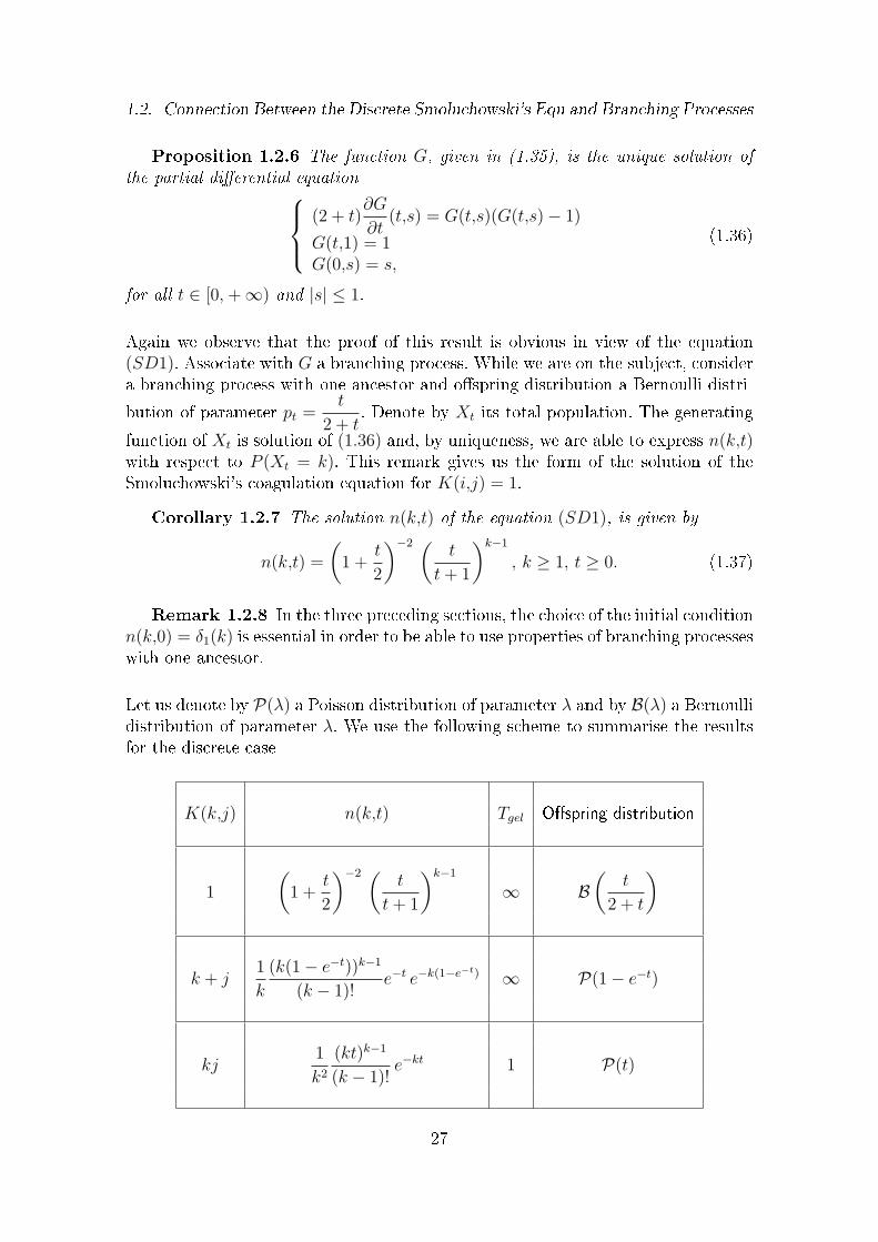
Remark 1.2.8 In the three preceding sections, the choice of the initial conditionn(k,0) = δ1(k) is essential in order to be able to use properties of branching processeswith one ancestor.
Let us denote by P(λ) a Poisson distribution of parameter λ and by B(λ) a Bernoullidistribution of parameter λ. We use the following scheme to summarise the resultsfor the discrete case
K(k,j) n(k,t) Tgel Ospring distribution
1
(1 +
t
2
)−2 (t
t+ 1
)k−1
∞ B(
t
2 + t
)
k + j1
k
(k(1− e−t))k−1
(k − 1)!e−t e−k(1−e−t) ∞ P(1− e−t)
kj1
k2
(kt)k−1
(k − 1)!e−kt 1 P(t)
27
Chapitre 1. Smoluchowski's Eq. : probabilistic interpretation for particular kernels
Remark 1.2.9 We have presented in this section a simple manner which allowsto obtain a probabilistic representation of solutions for the equation (SD), by makinguse of the PDEs veried by a generating function associated with (SD).Our approach gives a construction for each xed time t. We refer to the Aldous' paper([1]) for a dynamic construction in t, via processes for the constant, additive andmultiplicative coalescence (see section 3, constructions 5, 6 and 8 of his paper). Jeon([36]) gives also an interesting construction for a general coagulation-fragmentationequation as a limit of a sequence of nite state Markov chains.
1.3 Continuous Smoluchowski's Coagulation
Equation (SC)
We shall now be interested on the Smoluchowski's coagulation equation (SC),for which the mass is a continuous parameter. First of all we present some generalresults for (SC), which are independent from the kernel K. Part of these results(proposition 1.3.1), are taken from Aldous ([1]).Afterwards, as for the discrete case we shall consider the constant, additive andmultiplicative kernels.The aim of this part is to present some new results, more precisely : a duality resultconnecting the solutions of the multiplicative case with those of the additive case(theorems 1.3.9 and 1.3.11) and also some renormalisation theorems (theorems 1.3.6,1.3.20 and 1.3.24), which insure the convergence of the solution, for a large class ofinitial conditions, to a limit, which depends weakly on the initial condition.
1.3.1 General Results for (SC)
Hereafter we shall use for solution the notion of strong solution introduced indenition 1.1.4.
Proposition 1.3.1 Let K be a symmetric and positive kernel and n(x,t) be thesolution of (SC). Denote, for i ∈ N
φi(t) =
∫ ∞
0
xin(x,t) dx.
When these expressions are well dened, φ0 is non-increasing, φ1 is constant and φ2
is increasing. Furthermore
φ′0(t) = −1
2
∫ ∞
0
∫ ∞
0
K(x,y)n(x,t)n(y,t) dy dx. (1.38)
These results can be found for example in Dubovskii ([13]). We shall usually consider,for normalisation reasons
φ1(0) = φ1(t) = 1. (1.39)
28
1.3. Continuous Smoluchowski's Coagulation Equation (SC)
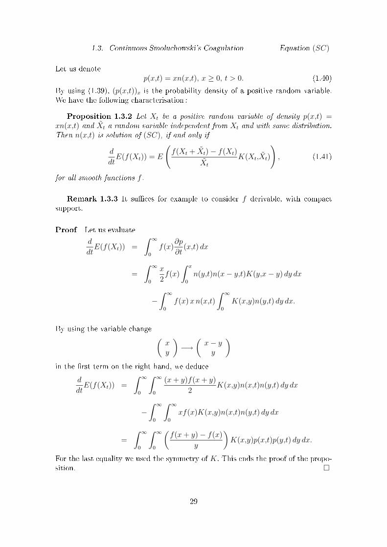
Let us denotep(x,t) = xn(x,t), x ≥ 0, t > 0. (1.40)
By using (1.39), (p(x,t))x is the probability density of a positive random variable.We have the following characterisation :
Proposition 1.3.2 Let Xt be a positive random variable of density p(x,t) =xn(x,t) and Xt a random variable independent from Xt and with same distribution.Then n(x,t) is solution of (SC), if and only if
d
dtE(f(Xt)) = E
(f(Xt + Xt)− f(Xt)
Xt
K(Xt,Xt)
), (1.41)
for all smooth functions f .
Remark 1.3.3 It suces for example to consider f derivable, with compactsupport.
Proof Let us evaluated
dtE(f(Xt)) =
∫ ∞
0
f(x)∂p
∂t(x,t) dx
=
∫ ∞
0
x
2f(x)
∫ x
0
n(y,t)n(x− y,t)K(y,x− y) dy dx
−∫ ∞
0
f(x)xn(x,t)
∫ ∞
0
K(x,y)n(y,t) dy dx.
By using the variable change (xy
)−→
(x− yy
)in the rst term on the right hand, we deduce
d
dtE(f(Xt)) =
∫ ∞
0
∫ ∞
0
(x+ y)f(x+ y)
2K(x,y)n(x,t)n(y,t) dy dx
−∫ ∞
0
∫ ∞
0
xf(x)K(x,y)n(x,t)n(y,t) dy dx
=
∫ ∞
0
∫ ∞
0
(f(x+ y)− f(x)
y
)K(x,y)p(x,t)p(y,t) dy dx.
For the last equality we used the symmetry of K. This ends the proof of the propo-sition.
29
Chapitre 1. Smoluchowski's Eq. : probabilistic interpretation for particular kernels
1.3.2 Continuous Coagulation Equation with Constant Ker-nel
For the constant kernel, a time normalisation is more interesting than the massnormalisation that we have announced in the general case. For this case we shall usethis normalisation.Let us rst remark that the result in (1.15) applies in particular for constant andadditive kernels, once the initial condition satises (C0). We can deduce thus anexistence and uniqueness result for the solution of (SC1) and (SC+).The equation (SC) becomes, for K(x,y) = 1
∂
∂tn(x,t) =
1
2
∫ x
0
n(y,t)n(x− y,t) dy − n(x,t)
∫ ∞
0
n(y,t) dy
n(x,0) = n0(x).
(SC1)
For the same kernel, the dierential equation (1.38), can be written
φ′0(t) = −φ20(t)
2. (1.42)
We obtain
φ0(t) =2
t+ α
where α > 0 is given by
α =2
φ0(0).
Let us denote by
p(x,t) =t+ α
2n(x,t), (1.43)
such that (p(x,t))x≥0 is the probability distribution of a positive random variable.There is a similar result to the proposition 1.3.2 and it writes, for this particularcase
Proposition 1.3.4 Let Xt denote a random variable with probability densityp(x,t) given by (1.43), and Xt an independent copy of Xt. Then, n(x,t) is solutionof (SC1) if and only if, for any smooth function f we have :
d
dtE(f(Xt)) =
1
t+ α(E(f(Xt + Xt))− E(f(Xt))). (1.44)
30
1.3. Continuous Smoluchowski's Coagulation Equation (SC)
Proof We proceed as for the proof of the proposition 1.3.2. Let us evaluated
dtE[f(Xt)] =
=1
2
∫ ∞
0
f(x)n(x,t) dx+t+ α
2
∫ ∞
0
f(x)
2
(∫ x
0
n(y,t)n(x− y,t) dy
)dx
−t+ α
2
∫ ∞
0
f(x)n(x,t) dx
∫ ∞
0
n(y,t) dy
= −1
2
∫ ∞
0
f(x)n(x,t) dx+t+ α
4
∫ ∞
0
∫ ∞
0
f(x+ y)n(y,t)n(x,t) dy dx
=1
t+ α
∫ ∞
0
∫ ∞
0
f(x+ y)p(y,t)p(x,t) dy dx− 1
t+ α
∫ ∞
0
f(x)p(x,t) dx
This achieves the proof.
This result allows us to describe entirely, for any initial condition, the solutionof the Smoluchowski's coagulation equation with constant kernel, (SC1).
Theorem 1.3.5 Let Tt be a random variable of geometric law, with parametert
t+ αi.e.
∀k ≥ 1, P (Tt = k) =α
t+ α
(t
t+ α
)k−1
. (1.45)
Let (Yi)i≥1 denote a sequence of i.i.d. random variables having same law as X0, ofprobability density p(x,0), and independent from Tt.Dene
Xt =Tt∑
i=1
Yi,
and denote by p(x,t) the distribution of the random variable Xt. Then
n(x,t) =2
t+ αp(x,t),
is the solution of the Smoluchowski's coagulation equation corresponding to theconstant kernel (SC1).
Proof We prove this result by using Laplace transforms. Let us apply the equation(1.44) with fλ(x) = e−λx. Denote by ψ(λ,t) = E(e−λXt), the Laplace transform ofXt and by g(λ) = ψ(λ,0), the Laplace transform of the initial condition. We deduce
∂
∂tψ(λ,t) =
1
t+ α(ψ2(λ,t)− ψ(λ,t))
ψ(λ,0) = g(λ).(1.46)
31
Chapitre 1. Smoluchowski's Eq. : probabilistic interpretation for particular kernels
After integration we get1
(t+ α)ψ(λ,t)=
1
t+ α+ d(λ), (1.47)
where d(λ) is a function depending only on λ. We obtain so the form of the Laplacetransform
ψ(λ,t) =1
(t+ α)d(λ) + 1(1.48)
under the initial condition
ψ(λ,0) = g(λ) =1
αd(λ) + 1. (1.49)
Let us also remark that the equation (1.47) insures that(t+ α) d(λ) + 1 6= 0.
From (1.49) we deduce the expression of d
d(λ) =
(1
g(λ)− 1
)1
α. (1.50)
By reporting in (1.48) the form of d found in (1.50), we obtain for ψ the followingformula :
ψ(λ,t) =αg(λ)
(t+ α)(1− g(λ) + αt+α
g(λ))=
αg(λ)
(t+ α)(1− tt+α
g(λ)). (1.51)
As g(λ) < 1, we can expand in integer series this expression and obtain
ψ(λ,t) =αg(λ)
t+ α
∑k≥1
(t
t+ α
)k−1
(g(λ))k−1. (1.52)
g(λ) being a Laplace transform it is not dicult to verify that ψ(λ,t) is also aLaplace transform (we can use the structure of ψ in terms of convolution). We havethus construct a solution of (1.46) ; more precisely, the equation (1.44) is satisedfor all exponential functions fλ(x) = e−λx. This family is suciently large in orderthat (1.44) be veried by all smooth functions. This ends the proof of the theorem1.3.5, because the equation (1.44) is nothing else that the integral version of theSmoluchowski's coagulation equation (SC1).
Let us focus now on the asymptotic behaviour of the random variables introducedin the theorem 1.3.5.
Theorem 1.3.6 Consider the notations of theorem 1.3.5. For any random va-riable X0 with probability density p(x,0) = α
2n(x,0), we have, independently of the
initial condition and for all xed t
aX ta
(d)−→a→0
R t2,
where Rt is the square of a two-dimensional Bessel process starting from the origin.
32
1.3. Continuous Smoluchowski's Coagulation Equation (SC)
Proof We shall prove this convergence by using Laplace transforms. Let us remarkrst that, if the initial condition has a rst order moment, we can write
g(λ) = E(e−λ X0) = 1− E(X0) + o(λ).
We obtain, by using (1.51)
ψ(λa,t
a) =
αg(λa)ta
+ α− tag(λa)
=α(1 + o(1))
ta
+ α− ta(1− λaα
2+ o(a))
=1 + o(1)
1 + λt2
+ o(1).
By letting a goes to zero we obtain the result of the theorem.
Remark 1.3.7 Rt "corresponds" to the solution of (SC1) with initial conditiona Dirac mass, δ0. Consequently, for any initial condition, the scaled solution of thecontinuous Smoluchowski's coagulation equation, with constant kernel, converges tothe solution of (SC1), with initial condition the Dirac mass.
By applying known results on the density of the square of a Bessel process, wededuce an exact solution for the Smoluchowski's coagulation equation (SC1)
n(x,t) =4
t2exp
(−2x
t
). (1.53)
1.3.3 Additive and Multiplicative Kernels for the ContinuousCoagulation Equation
We shall prove in this section that the solutions of the additive and multiplicativekernels are connected. We make rst some remarks that simplify these equations.We will suppose in what follows, that
φ1(0) =
∫ ∞
0
xn(x,0) dx = 1. (1.54)
In the sequel we will denote by +n(x,t) (respectively ∗
n(x,t)), a solution for the Smo-luchowski's coagulation equation with additive kernel (respectively multiplicative).
Remark 1.3.8 For the additive kernel K(x,y) = x + y, the equation (1.38)becomes
φ′0(t) = −φ0(t) and so φ0(t) = βe−t,
whereβ = φ0(0) =
∫ ∞
0
+n(x,0) dx.
33
Chapitre 1. Smoluchowski's Eq. : probabilistic interpretation for particular kernels
The equation (SC) can be written in this case
∂
+n
∂t(x,t) =
x
2
∫ x
0
+n(y,t)
+n(x− y,t) dy − x
+n(x,t)
∫ ∞
0
+n(y,t) dy − +
n(x,t)
=x
2
∫ x
0
+n(y,t)
+n(x− y,t) dy − x
+n(x,t)βe−t − +
n(x,t)
+n(x,0) =
+n0(x).
(SC+)Let us also write the equation (SC) for the multiplicative kernel.
∂∗n
∂t(x,t) =
1
2
∫ x
0
y(x− y)∗n(y,t)
∗n(x− y,t) dy − x
∗n(x,t)
∫ ∞
0
y∗n(y,t) dy
=1
2
∫ x
0
y(x− y)∗n(y,t)
∗n(x− y,t) dy − x
∗n(x,t)
∗n(x,0) =
∗n0(x).
(SC∗)We can now express the connection between the solutions of the equations (SC+)and (SC∗).
Theorem 1.3.9 Let+n(x,t) denote a solution of the Smoluchowski's coagulation
equation with additive kernel (SC+), and initial condition+n0(x). Then
∗n(x,t) is a
solution for the equation with multiplicative kernel (SC∗), where we have denotedby
∗n(x,t) =
1
T − t
1
x
+n
(x,− ln(1− t
T)
),∀t < T, (1.55)
and T =
∫ ∞
0
+n0(y) dy.
Proof We remark rst that the initial condition (1.54), that we usually impose,is really satised for ∗
n. We have
∫ ∞
0
x∗n(x,0) dx =
1
T
∫ ∞
0
+n(x,0) dx
= 1.
34
1.3. Continuous Smoluchowski's Coagulation Equation (SC)
We prove now that ∗n satises the Smoluchowski's equation (SC∗). We have
∂
∂t
∗n(x,t) =
1
(T − t)2
1
x
+n(x,− ln(1− t
T)) +
1
(T − t)2
1
x
∂
∂t
+n(x,− ln(1− t
T))
=1
(T − t)2
1
x
+n(x,− ln(1− t
T))
+1
2
1
(T − t)2
1
x
∫ x
0
x+n(y,− ln(1− t
T))
+n(x− y,− ln(1− t
T)) dy
− 1
(T − t)2
1
x
+n(x,− ln(1− t
T))
− 1
(T − t)2
+n(x,− ln(1− t
T))
∫ ∞
0
+n(y,− ln(1− t
T)) dy,
because +n is solution of (SC+). We conclude that
∂
∂t
∗n(x,t) =
1
2
∫ x
0
y(x− y)∗n(y,t)
∗n(x− y,t) dy − x
∗n(x,t).
Here we have used that for the additive solution∫ ∞
0
+n(y,t) dy = Te−t with T =
∫ ∞
0
+n(x,0) dx.
This ends the proof of the theorem 1.3.9.
Remark 1.3.10 The transformation in theorem 1.3.9 emphasises a nite timeexistence interval for the solution in the multiplicative case. We nd thus alreadyknown results for this kernel (Tgel <∞, Norris ([52]))
We have also the inverse transformation.
Theorem 1.3.11 If∗n(x,t) is a solution of the Smoluchowski's coagulation equa-
tion with multiplicative kernel (SC∗) and initial condition∗n0(x), then
+n(x,t) is a
solution of the Smoluchowski's equation with additive kernel (SC+), where we havedenoted by :
+n(x,t) = xT e−t ∗n(x,T (1− e−t))
and T =
(∫ ∞
0
x2 ∗n0(x) dx
)−1
.
Proof The proof of this theorem is similar to the one of the theorem 1.3.9. Thechoice of T insures that (1.54) is satised, i.e.∫ ∞
0
x+n(x,0) = 1.
35
Chapitre 1. Smoluchowski's Eq. : probabilistic interpretation for particular kernels
Remark 1.3.12 These transformations (theorems 1.3.9 and 1.3.11), apply alsoto the discrete case. It suces to replace integrals by sums.
1.3.3.1 Existence of Solutions for (SC+) and (SC∗)
The aim of this part is to prove existence of solutions for (SC+) and (SC∗)by employing probabilistic methods and the preceding transformations. We shallrst recall an existence result which can be found for example in Dubovskii ([13]).Consider the equation (SC∗). We have
Theorem 1.3.13 For any initial condition∗n(x,0), x ≥ 0 which satises∫ ∞
0
x∗n(x,0) dx = 1 and 0 <
∫ ∞
0
x2 ∗n(x,0) dx < ∞, there exists an unique solution
of (SC∗) dened for t ∈ [0,T ) where
T =
(∫ ∞
0
x2 ∗n(x,0) dx
)−1
.
Proof The aim of what follows is to prove this theorem by using probabilistictechniques. In order to obtain this result, we apply the proposition 1.3.2 on thisparticular case. We deduce that
d
dtE(f(Xt)) = E((f(Xt + Xt)− f(Xt))Xt), (1.56)
where Xt has density x∗n(x,t) and Xt is an independent copy of the random variable
Xt. We apply the equation (1.56) to functions of the form fλ(x) = e−λx. Denote byψ(λ,t) = E
(e−λXt
)the Laplace transform of Xt. ψ satises the non linear hyperbolic
partial dierential equation : ∂ψ
∂t= (1− ψ)
∂ψ
∂λψ(λ,0) = g(λ).
(1.57)
We will construct a solution for this equation under the initial condition
ψ(λ,0) =
∫ ∞
0
e−λxx∗n(x,0) dx
and prove that it conserves, for all t, the property of being a Laplace transform oncethat g(λ) = ψ(λ,0) is a Laplace transform.Let us denote, for t ∈
[0,− 1
g′(0)
[ψ(λ0 + (g(λ0)− 1)t,t) = g(λ0). (1.58)
36
1.3. Continuous Smoluchowski's Coagulation Equation (SC)
Remark 1.3.14 Similar techniques, based on Laplace transform, have beenused by Ernst, Zi and Hendricks ([16]) for the multiplicative kernel, in order tond the expression of
∫ ∞
0
x∗n(x,t)dx beyond the gelication time.
Proposition 1.3.15 The function ψ dened by (1.58) is a solution of the partialdierential equation (1.57).
Proof This proposition doesn't really need a proof. By construction the result istrue. Indeed, we constructed this solution by using the level sets of the equation(1.57).
We want to prove that ψ(λ,t), solution of (1.57), is a Laplace transform. We shalluse the Karamata theorem (cf. ([18]), p. 439). In order to apply it we need someauxiliary results (lemmas 1.3.16 and 1.3.17).
Lemma 1.3.16 The function ψ, solution of (1.57), is completely monotone, thatis
∀k ≥ 0, (−1)k ∂kψ
∂λk≥ 0. (1.59)
Proof The proof will be done by recurrence on k : the result is true for k = 0, byconstruction of ψ.Let us denote by fk(t) =
∂kψ
∂λk(λ(t),t) where λ(t) = λ0 + (g(λ0)− 1)t.
We suppose that :∀j ∈ J1,k − 1K, (−1)jfj(t) ≥ 0. (1.60)
We get then :
f ′k(t) = λ′(t)∂k+1
∂λk+1ψ(λ(t),t) +
∂k+1
∂λk ∂tψ(λ(t),t). (1.61)
By taking the derivative in the equation (1.57), k times with respect to λ, we obtain
∂k+1ψ
∂λk ∂t(λ,t)=(1−ψ(λ,t))
∂k+1
∂λk+1ψ(λ,t)−
k∑j=1
(k
j
)∂j
∂λjψ(λ,t)
∂k−j+1
∂λk−j+1ψ(λ,t). (1.62)
This gives, by using (1.61) and recalling that we are on a level set (1− ψ(λ(t),t) +λ′(t) = 0)
f ′k(t) =−(k+1)∂
∂λψ(λ(t),t)fk(t)−
k−1∑j=2
(k
j
)∂j
∂λjψ(λ(t),t)
∂k−j+1
∂λk−j+1ψ(λ(t),t)
= −(k+1)f1(t)fk(t)−k−1∑j=2
(k
j
)fj(t)fk+1−j(t).
(1.63)
37
Chapitre 1. Smoluchowski's Eq. : probabilistic interpretation for particular kernels
We remark now that each term in the previous sum has same sign as (−1)k+1, by therecurrence hypothesis (1.60). In conclusion, we have a rst order partial dierentialequation, that is :
u′(t) = a(t)u(t) + b(t) (1.64)with u(0) and b(t) of same sign.In this case, the sign of u(t) is conserved, for all t in the denition domain of thefunction u, solution of the equation (1.64).
Furthermore :
Lemma 1.3.17 For all t ∈[0,− 1
g′(0)
[, we have
limλ→0
ψ(λ,t) = 1.
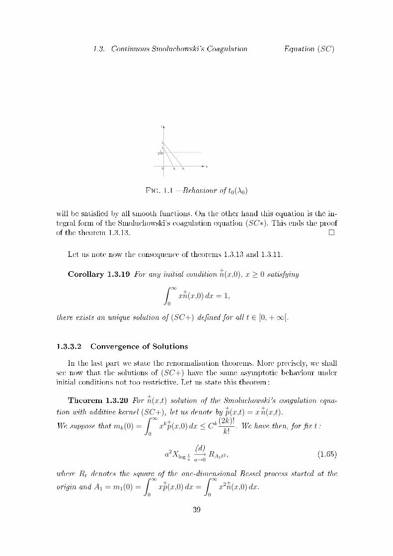
Proof We calculate the ordinate of the intersection between the level set and theaxis λ = 0. Call t0(λ0) the intersection point of the level set passing through thepoint (λ0,0), with this axis. We have
t0(λ0) =λ0
1− g(λ0).
By taking derivatives in this expression we get
t′0(λ0) =1− g(λ0)− λ0g
′(λ0)
(1− g(λ0))2.
This last expression is obviously positive (g(λ) is a Laplace transform). Thus t0(λ0)
is increasing (see the picture) and equals − 1
g′(0)in 0. We deduce that, for all t ∈[
0,− 1
g′(0)
[,
limλ→0
ψ(λ,t) = 1.
The results of lemmas 1.3.16 and 1.3.17 prove (by the Karamata theorem, ([18]),p. 439) the following proposition :
Proposition 1.3.18 For all t ∈[0,− 1
g′(0)
[, ψ is the Laplace transform of a
probability density.
By using the resolution of the partial dierential equation satised by the Laplacetransform, we have proved that the equation (1.56) is true for all exponential func-tions fλ(x) = e−λx. This family forms a large family of functions and the equation
38
1.3. Continuous Smoluchowski's Coagulation Equation (SC)
λλ λ
t
t
t
0 1 2
2
g’(0)1
1
Fig. 1.1 Behaviour of t0(λ0)
will be satised by all smooth functions. On the other hand this equation is the in-tegral form of the Smoluchowski's coagulation equation (SC∗). This ends the proofof the theorem 1.3.13.
Let us note now the consequence of theorems 1.3.13 and 1.3.11.
Corollary 1.3.19 For any initial condition+n(x,0), x ≥ 0 satisfying∫ ∞
0
x+n(x,0) dx = 1,
there exists an unique solution of (SC+) dened for all t ∈ [0,+∞[.
1.3.3.2 Convergence of Solutions
In the last part we state the renormalisation theorems. More precisely, we shallsee now that the solutions of (SC+) have the same asymptotic behaviour underinitial conditions not too restrictive. Let us state this theorem :
Theorem 1.3.20 For+n(x,t) solution of the Smoluchowski's coagulation equa-
tion with additive kernel (SC+), let us denote by+p(x,t) = x
+n(x,t).
We suppose that mk(0) =
∫ ∞
0
xk+p(x,0) dx ≤ Ck (2k)!
k!. We have then, for x t :
a2Xlog ta
(d)−→a→0
RA1t2 , (1.65)
where Rt denotes the square of the one-dimensional Bessel process started at the
origin and A1 = m1(0) =
∫ ∞
0
x+p(x,0) dx =
∫ ∞
0
x2+n(x,0) dx.
39
Chapitre 1. Smoluchowski's Eq. : probabilistic interpretation for particular kernels
Remark 1.3.21 The condition of this theorem on the initial condition is satis-ed by all random variables whose moments are dominated by the moments of thesquare of a Gaussian random variable. This is true for example for random variableshaving compact support.
Proof In order to make the proof we need some auxiliary results and remarks.Proposition 1.3.2 gives in this particular case, the following result : for Xt a randomvariable with probability density p(x,t) and f a smooth function, we have
d
dtE(f(Xt)) = E
(Xt + Xt
Xt
(f(Xt + Xt)− f(Xt))
), (1.66)
where Xt denotes an independent copy of the random variable Xt.To get existence we used functions f of the form e−λx. Another way to treat theproblem is to nd the moments of Xt, by using a recurrence formula.Let us apply formula (1.66) for power functions fk(x) = xk. Denote by
mk(t) =
∫ ∞
0
xk+p(x,t) dx. (1.67)
For f1(x) = x, (1.66) writesm′
1(t) = 2m1(t),
that ism1(t) = A1e
2t where A1 = m1(0).
Furthermore, by using (1.66) for fk(x) = xk, we obtain
m′k(t) = (k + 1)mk(t) +
k−1∑j=1
(k + 1
j
)mj(t)mk−j(t). (1.68)
Simple computation for rst order moments gives
m1(t) = A1e2t, A1 = m1(0),
m2(t) = 3A12e4t + A2e
3t, A2 = m2(0)− 3A21,
m3(t) = 15A13e6t + 10A1A2e
5t + A3e4t, A3 = m3(0)− 15A3
1 − 10A1A2.
These results and formula (1.68) allow us to obtain the general form of mk.
Lemma 1.3.22 For all integer k, mk(log t) is a polynomial on t of degree 2k,
with valuation greater or equal to k + 1 and dominating coecient :(2k)!
2kk!Ak
1, where
A1 = m1(0).
Proof We have already test this result for k = 1 (and even for k = 0). Supposeit valid until k − 1 and solve the equation (1.68) by using the method of constantvariation. We obtain
mk(t) = e(k+1)tΓ(t), (1.69)
40
1.3. Continuous Smoluchowski's Coagulation Equation (SC)
where Γ(t) is such that :
e(k+1)tΓ′(t) =k−1∑j=1
(k + 1j
)mj(t)mk−j(t). (1.70)
By using the recurrence hypothesis, Γ′(log t) is a polynomial of degree k − 1 and
dominating coecient A1k
2k
k−1∑j=1
(k + 1
j
)(2j)!(2k − 2j)!
j!(k − j)!.
We can prove also the following result (see lemma 1.4.1, given in the appendix) :k−1∑j=1
(k + 1
j
)(2j)!(2k − 2j)!
j!(k − j)!= (k − 1)
(2k)!
k!.
We deduce that Γ(log t) is a polynomial on t of degree k−1 and dominating coecient(2k)!
2kk!Ak
1. This ends the proof.
Let us write down the Laplace transform of the random variable Xt.
ψ(λ,t) =∑k≥0
(−1)kλk
k!mk(t). (1.71)
Evaluate this function at (λa2, log ta).
ψ(λa2, logt
a) =
∑k≥0
(−1)kλka2k
k!mk(log
t
a). (1.72)
By using the result in lemma 1.3.22 we can remark that, each term of this seriessatises
lima→0
((λa2)
kmk(log
t
a)
)= A1
k (2k)!
2kk!λkt2k. (1.73)
We shall prove that we can consider the limit as a goes to 0 in the sum of (1.72). Inorder to obtain this convergence, we need the following result :
Lemma 1.3.23 For any initial condition of the Smoluchowski's coagulation equa-
tion (SC+), such that mk(0) ≤ Ck (2k)!
k!for xed C and for all k, we have
mk(t) ≤ Ck (2k)!
k!e2kt, ∀t ≥ 0.
Proof We shall use the same method as the one used in order to obtain the formof mk. We get from (1.69) and (1.70)
Γ′(t) ≤ Ck
k − 1
(2k)!
k!e(k−1)t. (1.74)
41
Chapitre 1. Smoluchowski's Eq. : probabilistic interpretation for particular kernels
We have alsoΓ(t) = Γ(0) +
∫ t
0
Γ′(s)ds,
which yieldsΓ(t) ≤ Ck (2k)!
k!e(k−1)t + Γ(0)− (2k)!
k!Ck,
and Γ(0) = mk(0). The result is then proved.
Lemma 1.3.23 insures the normal convergence, with respect to a, of the seriesappearing in the expression of ψ(λa2, log
t
a) (see (1.72)), as soon as 4λt2
C≤ 1. We
can now conclude the proof of the theorem 1.3.20.
By using the previous normal convergence, we easily deduce
lima→0
ψ(λa2, logt
a) =
∑k≥0
(2k)!
(k!)2
(−1)kA1kλkt2k
2k=
1√1 + 2A1λt2
. (1.75)
This last limit is also the Laplace transform of the square of a one-dimensional Besselprocess starting from the origin.
As in the previous section, this convergence allows us to nd a particular solutionof (SC+) :
n1(x,t) =1√2πe−tx−
32 e−
x2e−2t
.
We can obtain other solutions by scaling, more precisely, consider
nA1(x,t) =1
A21
n1
(x
A1
,t
)so
nA1(x,t) =1√A1
1√2πe−tx−
32 e− x
2A1e−2t
is a solution of (SC+).Let us also express the similar result for the solutions of (SC∗). By using theorem1.3.9 we have
Theorem 1.3.24 Let∗n(x,t) be a solution of the Smoluchowski's coagulation
equation with multiplicative kernel (SC∗). Let∗p(x,t) = x2 (T − t)
∗n(x,t),
and denote by Yt a random variable with probability density∗p(x,t).
We suppose also that mk(0) =
∫ ∞
0
xk ∗p(x,0) dx ≤ Ck (2k)!
k!, where
T =
(∫ ∞
0
x2 ∗n(x,0) dx
)−1
.
42
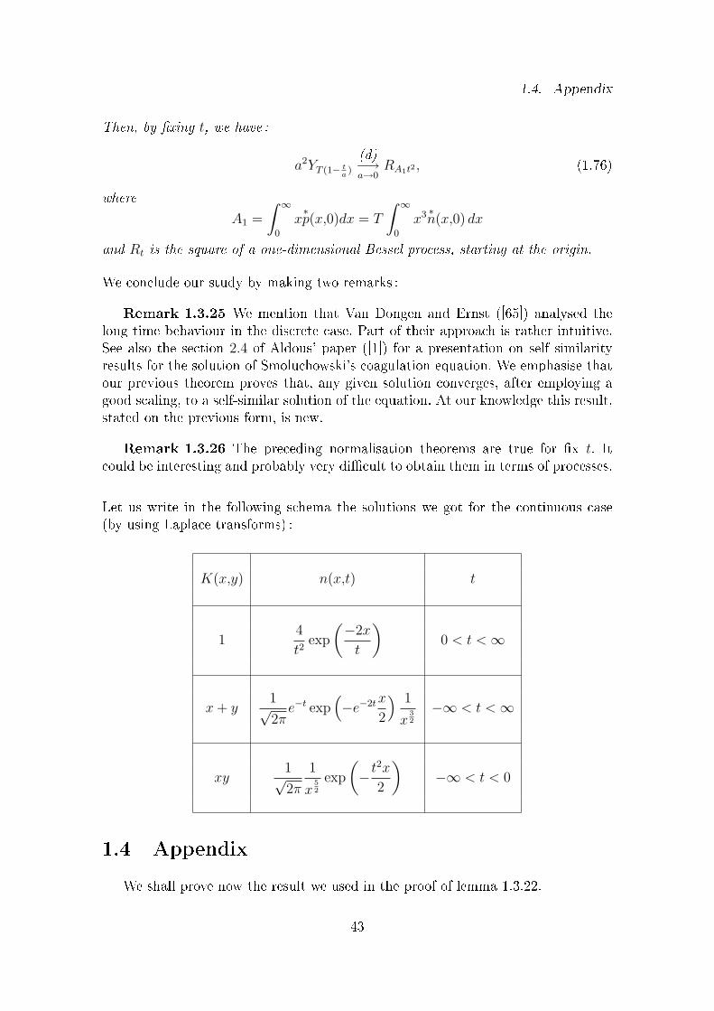
1.4. Appendix
Then, by xing t, we have :
a2YT (1− ta)
(d)−→a→0
RA1t2 , (1.76)
where
A1 =
∫ ∞
0
x∗p(x,0)dx = T
∫ ∞
0
x3 ∗n(x,0) dx
and Rt is the square of a one-dimensional Bessel process, starting at the origin.
We conclude our study by making two remarks :
Remark 1.3.25 We mention that Van Dongen and Ernst ([65]) analysed thelong time behaviour in the discrete case. Part of their approach is rather intuitive.See also the section 2.4 of Aldous' paper ([1]) for a presentation on self similarityresults for the solution of Smoluchowski's coagulation equation. We emphasise thatour previous theorem proves that, any given solution converges, after employing agood scaling, to a self-similar solution of the equation. At our knowledge this result,stated on the previous form, is new.
Remark 1.3.26 The preceding normalisation theorems are true for x t. Itcould be interesting and probably very dicult to obtain them in terms of processes.
Let us write in the following schema the solutions we got for the continuous case(by using Laplace transforms) :
K(x,y) n(x,t) t
14
t2exp
(−2x
t
)0 < t <∞
x+ y1√2πe−t exp
(−e−2tx
2
) 1
x32
−∞ < t <∞
xy1√2π
1
x52
exp
(−t
2x
2
)−∞ < t < 0
1.4 Appendix
We shall prove now the result we used in the proof of lemma 1.3.22.
43
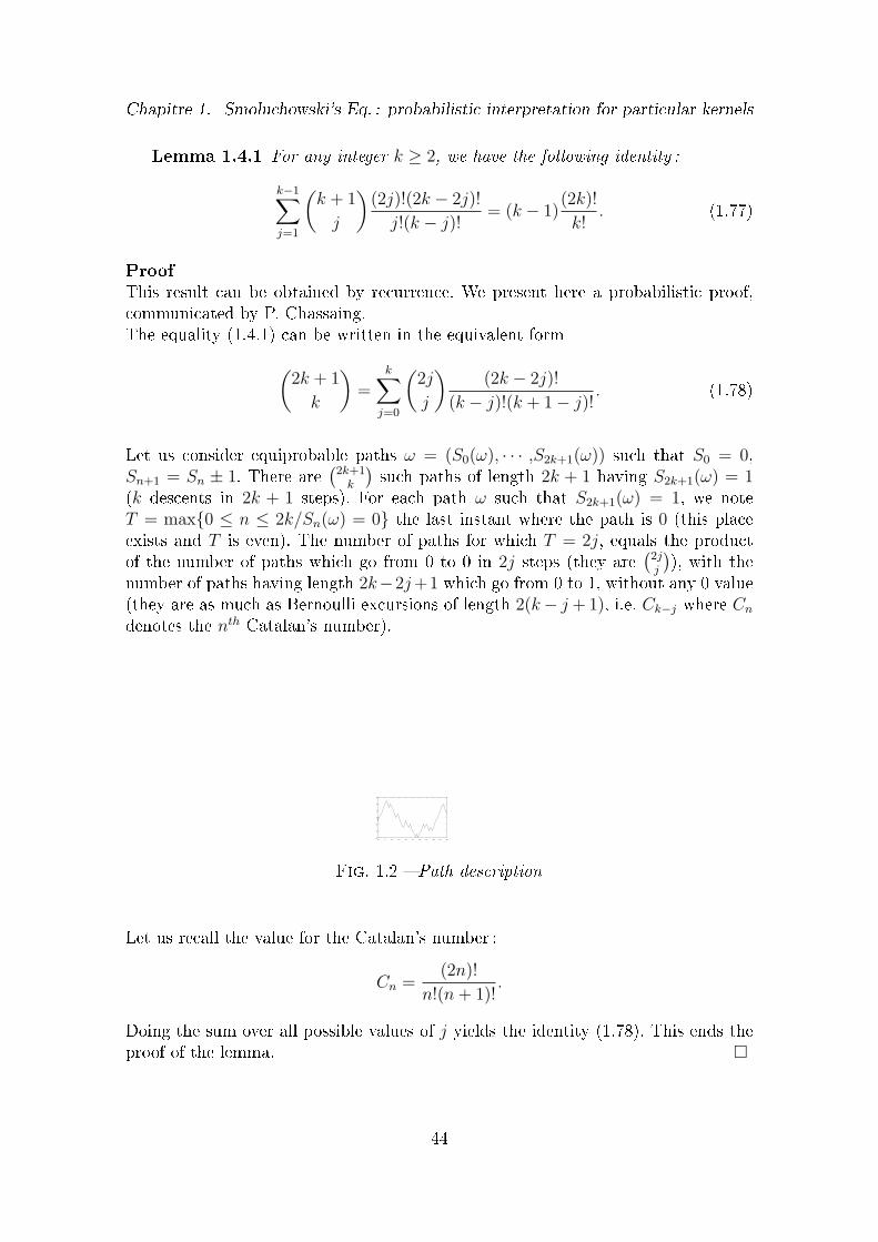
Chapitre 1. Smoluchowski's Eq. : probabilistic interpretation for particular kernels
Lemma 1.4.1 For any integer k ≥ 2, we have the following identity :
k−1∑j=1
(k + 1
j
)(2j)!(2k − 2j)!
j!(k − j)!= (k − 1)
(2k)!
k!. (1.77)
ProofThis result can be obtained by recurrence. We present here a probabilistic proof,communicated by P. Chassaing.The equality (1.4.1) can be written in the equivalent form(
2k + 1
k
)=
k∑j=0
(2j
j
)(2k − 2j)!
(k − j)!(k + 1− j)!. (1.78)
Let us consider equiprobable paths ω = (S0(ω), · · · ,S2k+1(ω)) such that S0 = 0,Sn+1 = Sn ± 1. There are
(2k+1
k
)such paths of length 2k + 1 having S2k+1(ω) = 1
(k descents in 2k + 1 steps). For each path ω such that S2k+1(ω) = 1, we noteT = max0 ≤ n ≤ 2k/Sn(ω) = 0 the last instant where the path is 0 (this placeexists and T is even). The number of paths for which T = 2j, equals the productof the number of paths which go from 0 to 0 in 2j steps (they are
(2jj
)), with the
number of paths having length 2k−2j+1 which go from 0 to 1, without any 0 value(they are as much as Bernoulli excursions of length 2(k− j + 1), i.e. Ck−j where Cn
denotes the nth Catalan's number).
−6
−4
−2
0
2
4
6
0 5 10 15 20 25 30 35 40 45 50
Fig. 1.2 Path description
Let us recall the value for the Catalan's number :
Cn =(2n)!
n!(n+ 1)!.
Doing the sum over all possible values of j yields the identity (1.78). This ends theproof of the lemma.
44
2
A generalization of the ConnectionBetween the Additive and
Multiplicative Solutions for theSmoluchowski's Coagulation
Equation
Ce chapitre a été publié à Monte Carlo Methods and Applications,Vol.7 , No.1-2 : 141-147, 2001.
Abstract This study will reformulate part of our previous results ([10]) obtained for theSmoluchowski's coagulation equation for the additive, multiplicative and constant kernelsfor xed time, in terms of measures. In order to obtain this, we use a construction intro-duced by Norris ([52]).Key Words : Smoluchowski's coagulation equation, stochastic processes, partial dieren-tial equations.AMS 2000 subject classication : 60J80, 44A10
2.1 Introduction
Let us consider the coagulation phenomenon described as follows. Consider alarge system of particles and allow only the coagulation of particles in pairs. Forphysical reasons, the rate at which pairs of particles aggregate depends on somepositive parameter associated with each particles, such as mass or size.We can write down the continuous Smoluchowski's coagulation equation in the fol-
45
Chapitre 2. Generalization of the Connection Between Additive and Multiplicative kernels
lowing form : ∂
∂tn(x,t) =
1
2
∫ x
0
K(y,x− y)n(y,t)n(x− y,t)dy
−n(x,t)
∫ ∞
0
K(x,y)n(y,t)dy
n(x,0) = n0(x).
(SC)
where K : R2+ → R+ is a symmetric kernel and n(x,t) denotes the average number
of particles with mass [x, x+ dx] per unit volume.In the equation (SC) the rst term on the right corresponds to the creation ofparticles of mass x while the second stands for the disappearance of particles ofmass x after coagulation with other particles.
2.1.1 Norris results and construction
We shall present here the construction and some of results in Norris ([52]).Let K : (R∗
+)2 → R+ be a symmetric measurable function and M the space ofsigned Radon measures on R∗
+. Denote by M+ the set of non negative measures onM. Let µ ∈M+ be such that, for every compact set B ⊆ R∗
+ :∫B
∫ ∞
0
K(x,y)µ(dx)µ(dy) <∞.
For such µ we consider the following weak form of the Smoluchowski's coagulationequation :
µt = µ0 +
∫ t
0
L(µs)ds, (SCW )
where L(µ) ∈M is dened by the relation
< f,L(µ) >=1
2
∫ ∞
0
∫ ∞
0
(f(x+ y)− f(x)− f(y))K(x,y)µ(dx)µ(dy), (2.1)
for all bounded measurable functions f of compact support.
Denition 2.1.1 We call local solution of (SCW ) any map t 7→ µt : [0,T ) 7→M+ such that :
(i)
∫ ∞
0
x11x≤1µ0(dx) <∞
(ii) For all B ⊆ R∗+ compact, the map t 7→ µt(B) : [0,T ) 7→ [0,∞) is measurable.
(iii) For all t < T and B ⊆ R∗+ compact∫ t
0
∫B
∫ ∞
0
K(x,y)µs(dx)µs(dy)ds <∞.
(iv) For all measurable function f with compact support and for f(x) = x11x≤1 andfor all t < T ∫ ∞
0
f(x)µt(dx) =
∫ ∞
0
f(x)µ0(dx)
46
2.1. Introduction
+1
2
∫ t
0
ds
∫ ∞
0
∫ ∞
0
(f(x+ y)− f(x)− f(y))K(x,y)µs(dx)µs(dy).
For T = ∞ we have a solution.We make also the following hypothesis on K
K(x,y) ≤ ϕ(x)ϕ(y), ∀x,y ∈ R∗+, (2.2)
where ϕ : R∗+ 7→ R∗
+ is a continuous sub-linear function (that is ϕ(λx) ≤ λϕ(x), forall x ∈ R∗
+ and λ ≥ 1).Further hypothesis ∫ ∞
0
ϕ(x)µ0(dx) <∞. (2.3)
Any local solution such that∫ t
0
∫ ∞
0
ϕ2(x)µs(dx)ds <∞, (2.4)
is called strong solution.Under assumptions (2.2) and (2.3), Norris ([52]) proved that, starting from µ0, wehave uniqueness of a strong solution.If ϕ(x) ≥ εx for all x and some ε > 0, then any strong solution is conservative.If∫ ∞
0
ϕ2(x)µ0(dx) <∞ then there exists a unique maximal strong solution (µt)t≤ξ(µ0)
where ξ(µ0) ≥(∫ ∞
0
ϕ2(x)µ0(dx)
)−1
.
Furthermore, if ϕ2 is sub-linear or K(x,y) ≤ ϕ(x) + ϕ(y), for all x, y ∈ R∗+ then
ξ(µ0) = ∞.
Markov process associated with (SCW )We shall introduce now a particle system connected to the Smoluchowski's coagu-lation equation.Let X0 be a nite, integer valued measure on R∗
+
X0 =m∑
i=1
δxi,
for some x1, . . . ,xm ∈ R∗+. X0 is a system of m particles labelled by their masses.
We construct a Markov process (Xt)t≥0 of nite, integer valued measures on R∗+ as
follows : for each pair i < j take Tij an independent exponential random variable ofparameter K(xi,xj) and dene
T = mini<j
Tij.
Set Xt = X0 for t < T and, if T = Tij set
XT = X0 + δxi+xj− δxi
− δxj
47
Chapitre 2. Generalization of the Connection Between Additive and Multiplicative kernels
and then begin the construction afresh from XT .In the process described above each pair of particles xi, xj coalesces at a rateK(xi, xj) to form a new particle xi +xj. We call (Xt)t≥0 a stochastic coalescent withcoagulation kernel K.Let d be a metric on M such that(a) d(µn,µ) 7→ 0 if and only if
∫ ∞
0
f(x)µn(dx) 7→∫ ∞
0
f(x)µ(dx), for all boundedcontinuous functions f : R∗
+ 7→ R.(b) d(µ,µ′) ≤ ‖µ− µ′‖, for all µ,µ′ ∈M.When we consider f of bounded support we obtain a weaker topology, also metri-zable, and we denote by d0 some compatible metric with d0 ≤ d.We have the following weak convergence result :
Theorem 2.1.2 (see Norris ([52]), theorem 4.1)Let K : R∗
+ × R∗+ 7→ [0,∞) be a symmetric continuous function and µ0 a measure
on R∗+. Assume that for ϕ : R∗
+ 7→ R∗+ continuous and sublinear we have
K(x,y) ≤ ϕ(x)ϕ(y), ∀x,y ∈ R∗+
lim(x,y)→(∞,∞)
K(x,y)
ϕ(x)ϕ(y)= 0.
Assume also that
∫ ∞
0
ϕ(x)µ0(dx) <∞.
Let (Xnt )t≥0 be a sequence of stochastic coalescents with coagulation kernel K. Set
Xnt :=
1
nXn
tn
and suppose that
limn→∞
d0(ϕXn0 , ϕµ0) = 0
and that, for some constant C <∞ and for all n∫ ∞
0
ϕ(x)dXn0 ≤ C.
Then the sequence of laws of ϕXn on D([0,∞),(M,d0)) is tight. Moreover, for anyweak limit point ϕX, almost surely, (Xt)t≥0 is a solution of Smoluchowski's coagu-lation equation (SCW ). In particular, this equation has at least one solution.
2.2 Connection between the additive and multipli-
cative case in terms of measures
Let us denote by (SCW+) and (SCW∗) the weak form for the Smoluchowski'scoagulation equation for K(x,y) = x+y and K(x,y) = xy respectively. The previous
48
2.2. Connection between the additive and multiplicative case in terms of measures
results from Norris ([52]) apply with ϕ(x) = x. We express in the following theoremthe connection between the additive and the multiplicative kernels.
Theorem 2.2.1 Let Xt be solution for the multiplicative equation with initialcondition X0. Then Yt dened as
dYt(x) = xTe−tdXT (1−e−t)(x) (2.5)
is solution for the additive equation (SCW+), where T =
(∫ ∞
0
x2dX0(x)
)−1
.
Proof We remark rst of all that Xt and Yt are obtained as weak limit points ofthe corresponding coalescents. As Xt is solution for K(x,y) = xy we have, by usingdenition 2.1, that for any function f with compact support
∫ ∞
0
f(x)dXt(x) =
∫ ∞
0
f(x)dX0(x)
+1
2
∫ t
0
ds
∫ ∞
0
∫ ∞
0
(f(x+ y)− f(x)− f(y))xydXs(x)dXs(y).(2.6)
We shall prove that we can write a similar formula for a function of the form g(t,x) =α(t)f(x). In order to make rigorous the calculus to follow, we have to prove that wecan use time-dependent test functions. We can justify this by using a result due toNorris (see proposition 2.3. in [52]).First remark that, for any smooth functions α(t), β(t) we have, after integration byparts
α(t)
∫ t
0
β(s)ds =
∫ t
0
α(s)β(s)ds+
∫ t
0
α′(s)
∫ s
0
β(u)duds. (2.7)
Let us also denote, in order to simplify notations
Γf (s) =
∫ ∞
0
∫ ∞
0
(f(x+ y)− f(x)− f(y))xydXs(x)dXs(y). (2.8)
With this notation equation (2.6) writes
∫ ∞
0
f(x)dXt(x) =
∫ ∞
0
f(x)dX0(x) +1
2
∫ t
0
Γf (s)ds. (2.9)
49
Chapitre 2. Generalization of the Connection Between Additive and Multiplicative kernels
Multiplying equality (2.9) by α(t) and using (2.7) one gets
α(t)
∫ ∞
0
f(x)dXt(x)
= α(t)
∫ ∞
0
f(x)dX0(x) +1
2α(t)
∫ t
0
Γf (s)ds
= α(t)
∫ ∞
0
f(x)dX0(x) +1
2
∫ t
0
α(s)Γf (s)ds+1
2
∫ t
0
α′(s)
∫ s
0
Γf (u)duds
= α(t)
∫ ∞
0
f(x)dX0(x) +1
2
∫ t
0
α(s)Γf (s)ds
+
∫ t
0
α′(s)ds
[∫ ∞
0
f(x)dXs(x)−∫ ∞
0
f(x)dX0(x)
]= α(t)
∫ ∞
0
f(x)dX0(x) +1
2
∫ t
0
α(s)Γf (s)ds
+
∫ t
0
α′(s)ds
∫ ∞
0
f(x)dXs(x)−∫ ∞
0
f(x)dX0(x)(α(t)− α(0))
= α(0)
∫ ∞
0
f(x)dX0(x) +1
2
∫ t
0
α(s)Γf (s)ds+
∫ t
0
α′(s)ds
∫ ∞
0
f(x)dXs(x).
(2.10)Recall that g(t,x) = α(t)f(x) so the last equality writes
∫ ∞
0
g(t,x)dXt(x) =
∫ ∞
0
g(0,x)dX0(x)
+1
2
∫ t
0
ds
∫ ∞
0
∫ ∞
0
(g(s,x+ y)− g(s,x)− g(s,y))xydXs(x)dXs(y)
+
∫ t
0
ds
∫ ∞
0
∂g
∂s(s,x)dXs(x).
(2.11)
Apply rst the equality (2.11) for g(t,x) = (T − t)f(x). This yields
∫ ∞
0
(T − t)f(x)dXt(x) =
∫ ∞
0
Tf(x)dX0(x)
+1
2
∫ t
0
(T − s)ds
∫ ∞
0
∫ ∞
0
(f(x+ y)− f(x)− f(y))xydXs(x)dXs(y)
−∫ t
0
ds
∫ ∞
0
f(x)dXs(x).
(2.12)
50
2.2. Connection between the additive and multiplicative case in terms of measures
Replacing t by T (1− e−t) in (2.12) we get
∫ ∞
0
Te−tf(x)dXT (1−e−t)(x) =
∫ ∞
0
Tf(x)dX0(x)
+1
2
∫ T (1−e−t)
0
(T − s)ds
∫ ∞
0
∫ ∞
0
(f(x+ y)− f(x)− f(y))xydXs(x)dXs(y)
−∫ T (1−e−t)
0
ds
∫ ∞
0
f(x)dXs(x).
(2.13)Make in the last two terms on the right side of (2.13) the change of variable s =T (1− e−u). This gives 0 ≤ u ≤ t and
∫ ∞
0
Te−tf(x)dXT (1−e−t)(x) =
∫ ∞
0
Tf(x)dX0(x)
+T 2
2
∫ t
0
e−2udu
∫ ∞
0
∫ ∞
0
(f(x+ y)− f(x)− f(y))xydXT (1−e−u)(x)dXT (1−e−u)(y)
−∫ t
0
Te−udu
∫ ∞
0
f(x)dXT (1−e−u)(x).
(2.14)Further, apply (2.14) to f(x) = xh(x).
∫ ∞
0
Te−txh(x)dXT (1−e−t)(x) =
∫ ∞
0
Txh(x)dX0(x)
+T 2
2
∫ t
0
e−2udu
∫ ∞
0
∫ ∞
0
[(x+y)h(x+y)−xh(x)−yh(y)]xydXT (1−e−u)(x)dXT (1−e−u)(y)
−∫ t
0
Te−udu
∫ ∞
0
xh(x)dXT (1−e−u)(x).
(2.15)
51
Chapitre 2. Generalization of the Connection Between Additive and Multiplicative kernels
Replace now dYt(x) = xTe−tdXT (1−e−t)(x) (as asked in the theorem) to obtain∫ ∞
0
h(x)dYt(x) =
∫ ∞
0
h(x)dY0(x)
+1
2
∫ t
0
ds
∫ ∞
0
∫ ∞
0
(h(x+ y)− h(x)− h(y))(x+ y)dYs(x)dYs(y)
+1
2
∫ t
0
ds
∫ ∞
0
∫ ∞
0
(xh(y) + yh(x))dYs(x)dYs(y)−∫ t
0
ds
∫ ∞
0
h(x)dYs(x)
=
∫ ∞
0
h(x)dY0(x) +
∫ t
0
ds
∫ ∞
0
h(x)dYs(x)
(∫ ∞
0
xdYs(x)− 1
)
+1
2
∫ t
0
ds
∫ ∞
0
∫ ∞
0
(h(x+ y)− h(x)− h(y))(x+ y)dYs(x)dYs(y).
(2.16)
Once we have proved that ∫ ∞
0
xdYt(x) = 1, ∀t < T (2.17)
we can conclude from (2.16) that∫ ∞
0
h(x)dYt(x) =
∫ ∞
0
h(x)dY0(x)
+1
2
∫ t
0
ds
∫ ∞
0
∫ ∞
0
(h(x+ y)− h(x)− h(y))(x+ y)dYs(x)dYs(y),
(2.18)
which shows that Yt dened by using Xt is a solution for the additive kernel. Let usprove that (2.17) holds. Evaluate (2.6) for f(x) = x2
∫ ∞
0
x2dXt(x) =
∫ ∞
0
x2dX0(x) +
∫ t
0
(∫ ∞
0
x2dXs(x)
)2
ds. (2.19)
Recalling that T =
(∫ ∞
0
x2dX0(x)
)−1
, we get
m∗2(t) :=
∫ ∞
0
x2dXt(x) =1
T − t, ∀t < T. (2.20)
Introducing (2.20) into (2.17) yields∫ ∞
0
xdYt(x) = Te−t
∫ ∞
0
x2dXT (1−e−t)(x)
= m∗2(T (1− e−t))Te−t
= 1.
(2.21)
52
2.2. Connection between the additive and multiplicative case in terms of measures
This ends the proof of the theorem 2.2.1.We can refer to the paper of Norris ([53]) for much more on the multiplicative kernel.
There is a similar result once we know the additive solution. More precisely
Theorem 2.2.2 Let Yt be solution of the additive equation with initial conditionY0. Then Xt given by
dXt(x) =1
1− T
1
xdY− ln(1− t
T)(x), ∀t < T. (2.22)
is solution for the multiplicative equation (SCW∗), where T =
∫ ∞
0
dY0(x).
53

Chapitre 2. Generalization of the Connection Between Additive and Multiplicative kernels
54
3
A pure jump Markov processassociated with Smoluchowski's
coagulation equation
Ce chapitre est soumis à Annals of Probability
AbstractThe Smoluchowski coagulation equation models the evolution of the den-
sity n(x,t) of the particles of size (or mass) x at the instant t ≥ 0 for a system inwhich a coalescence phenomenon occurs. Two versions of this equation exist :the case of discrete sizes (when x ∈ N∗) and the case of continuous sizes (whenx ∈ R∗).The aim of the present paper is to construct a stochastic process, whose law isthe solution of the Smoluchowski's coagulation equation. This approach is atour knowledge the rst in this direction, in that, for the rst time the solutionof Smoluchowski's coagulation equation is obtained as the law of a stochasticprocess.We rst introduce a modied equation, dealing with the evolution of the re-partition Qt(dx) of the mass in the system. The advantage we take on this isthat we can do an unied study for both continuous and discrete models.The integro-partial-dierential equation satised by Qtt≥0 can be interpre-ted as the evolution equation of the time marginals of a Markov pure jumpprocess. At this end we introduce a nonlinear Poisson driven stochastic die-rential equation related to the Smoluchowski equation in the following way : ifXt satises this stochastic equation, then the law of Xt satises the modiedSmoluchowski equation. Existence, uniqueness, and pathwise behaviour of asolution to this S.D.E. are studied.
Key words : Smoluchowski's coagulation equations, nonlinear stochastic dieren-tial equations, Poisson measures.
MSC 2000 : 60H30, 60K35, 60J75.
55
Chapitre 3. A pure jump Markov process associated with Smoluchowski's equation
3.1 Introduction
Smoluchowski's coagulation equation governs various phenomenons as for example :polymerisation, aggregation of colloidal particles, formation of stars and planets, be-haviour of fuel mixtures in engines etc.We describe this equation as modelling the polymerisation phenomenon.For k ∈ N∗, let Pk denote a polymer of mass k, that is a set of k identical particles(monomers). As time advances, the polymers evolve and, if they are sucientlyclose, there is some chance that they merge into a single polymer whose mass equalsthe sum of the two polymers' masses which take part in this binary reaction. Weadmit here only binary reactions.Denote by n(k,t) the average number of polymers of mass k per unit volume, at timet so k n(k,t) stands for the part of mass consisting on polymers of length k, per unitvolume. The coalescence phenomenon of a polymer of mass k with a polymer of massj, can be written formally as Pk + Pj −→ Pk+j, and is proportional to n(k,t)n(j,t)with a proportionality constant K(k,j), called coalescence kernel.Throughout this paper, time t is always continuous, discrete and continuous referto polymers' masses.Hereafter (discrete and continuous case), the coagulation kernel K will satisfy thefollowing hypothesis : K is positive (i.e., K : (N∗)2 or (R+)2 → R+) and symmetric(i.e., K(i,j) = K(j,i)).
The Smoluchowski coagulation equation, in the discrete case, is the equation onn(k,t), for k ∈ N∗. It writes :
d
dtn(k,t) =
1
2
k−1∑j=1
K(j,k − j)n(j,t)n(k − j,t)
−n(k,t)∞∑
j=1
K(j,k)n(j,t)
n(k,0) = n0(k).
(SD)
This system describes a non linear evolution equation of innite dimension, withinitial condition (n0(k))k≥1. In the rst line of (SD), the rst term on the righthand side describes the creation of polymers of mass k by coagulation of polymersof mass j and k − j. The coecient 1
2is due to the fact that K is symmetric. The
second term corresponds to the depletion of polymers of mass k after coalescencewith other polymers.The continuous analog of the equation (SD) can be written naturally :
∂
∂tn(x,t) =
1
2
∫ x
0
K(y,x− y)n(y,t)n(x− y,t)dy
−n(x,t)
∫ ∞
0
K(x,y)n(y,t)dy
n(x,0) = n0(x)
(SC)
56
3.1. Introduction
for all x ∈ R+.
We present briey some recent results on the existence and uniqueness for the Smo-luchowski coagulation equation, obtained by employing a probabilistic approach.These results furnish answers to some phenomenon that seems to be accepted asgranted by the physicists.A detailed survey on the present situation of the research on this equation is provi-ded in Aldous [1].In the discrete case few situations allow to conclude to the existence and uniquenessof the solution of (SD). If the kernel K satises :
K(i,j) ≤ C(i+ j), i, j ≥ 1. (3.1)
and the initial condition is such that∞∑
k=1
kn(k,0) <∞ then existence (see Ball and
Carr [4]) and uniqueness (see Heilmann [33]) are known.Jeon [36] approached the solution of a more general equation than (SD), in that,we have also the fragmentation of polymers, by a sequence of nite Markov chains.Jeon gave a general result about the gelication time Tgel, i.e. the rst instant whenparticles of innite mass appear. More precisely, if we have
K(i,j) ≥ (ij)α, with α ∈]12,1[
(3.2)
and furthermorelim
i+j→∞
K(i,j)
ij= 0 (3.3)
then we have gelication in nite time (Tgel <∞), for a large class of initial condi-tions.For the continuous case, Aldous [1], states hypotheses which insure existence anduniqueness of the solution of the Smoluchowski coagulation equation. More preciselyexistence and uniqueness hold for (SC) if the kernel K satises, for all x and y inR+ :
K(x,y) ≤ C(1 + x+ y) (3.4)and the initial condition is such that∫ ∞
0
n(x,0)dx <∞ and∫ ∞
0
x2n(x,0)dx <∞ (3.5)
and furthermore we have conservation of mass∫ ∞
0
xn(x,0)dx = 1. (3.6)
Our conditions will be less restrictive because we don't need to impose∫ ∞
0
n(x,0)dx <∞. (3.7)
57
Chapitre 3. A pure jump Markov process associated with Smoluchowski's equation
Norris [52], [53] obtains recently some new results on (SC) by generalising to thecontinuous case the results in Jeon [36]. Norris has two kinds of hypotheses :either K(x,y)
xy→ 0 as (x,y) →∞
orK(x,y) ≤ ϕ(x)ϕ(y) where ϕ : R+ → R+ is sub-linear and∫∞
0ϕ2(x)n(0,x)dx <∞.
Under one of this conditions he proved existence and uniqueness of the solution of(SC). The last hypothesis includes the case where K(x,y) explodes as x 7→ 0 ory 7→ 0 and allows also to obtain uniqueness in some cases when the initial conditionhas no second, or even rst, moment. These results are also interesting because oneneeds no local regularity on K.Norris constructs a sequence of stochastic processes which converges to a determi-nistic limit which is a solution of (SC).Deaconu and Tanré [10] furnish a probabilistic interpretation for the additive, mul-tiplicative and constant kernels in both discrete and continuous cases. They nd aduality between the additive and multiplicative solutions which permits to obtainthe results for one of this solutions by those on the other one. They have also pre-sented a long time behaviour for the solution.
Our approach of (SC) or (SD) is new and purely stochastic. We construct a purejump stochastic process (Xt)t≥0 whose law is the solution of the Smoluchowski coa-gulation equation in the following sense : in the discrete case, P [Xt = k] = kn(k,t)for all t ≥ 0 and all k ∈ N∗, while in the continuous case, P [Xt ∈ dx] = xn(x,t)dxfor all t ≥ 0. For each ω, Xt(ω) may be seen as the evolution of the size of one mean particle in the system.The jump process satises a non linear Poisson driven stochastic dierential equa-tion.This approach is strongly inspired by probabilistic works on the Boltzmann equa-tion. The Boltzmann equation deals with the distribution of the speeds in a gas, andcan be related to the Smoluchowski equation for two reasons : rst, it concerns theevolution of the density of particles of speed v at the instant t , while the Smolu-chowski equation deals with the density of particles of mass x at the instant t .Second, the phenomenon is discontinuous : in each case, a particle moves instantlyfrom a mass x (or a speed v) to a new mass x′ (or a speed v′) after a coagulation(or a collision).
Let us rst mention Tanaka [63], who rst introduced a non linear jump processin order to study the Boltzmann equation of Maxwell molecules. Many new resultsabout this equation has been obtained thanks to this approach, as regularity, posi-tivity, and numerical approximation : Desvillettes, Graham and Méléard [11], [31],have initiated a new way for studying non linear P.D.E.s, by using recent probabi-listic tools, such as Malliavin Calculus and propagation of chaos.Very recently, Tanaka's approach has been extended, in Fournier, Méléard [25], [26],to the case of non Maxwell molecules, which is technically much less easy. We followessentially here the approach of [25]. We will transpose it here in order to give a
58
3.2. Framework
probabilistic interpretation to the Smoluchowski equations.The main fact that makes the Maxwell molecules easy is that the rate of collisionsof a particle does not depend on its speed, which is not the case for non Maxwellmolecules. In the Smoluchowski equation, the rate of coagulation of a particledepends on its size.We get rid of this problem by using a sort of reject procedure : as in [25], thereis, in our stochastic equation, an indicator function which allows to control the rateof coagulation.
Let us nally describe the plan of the present paper.In Section 3.2, we introduce our notations, we state a modied Smoluchowski equa-tion (MS) which allows to study equations (SC) and (SD) together. This equation(MS) describes the evolution of the repartition Qt(dx) (either discrete or conti-nuous) of the sizes : for each t, Qt is a probability measure on R∗
+. Afterwards werelate (MS) to a nonlinear martingale problem (MP ) : for Q a solution to (MP ),its time marginals Qt satisfy the modied Smoluchowski equation (MS). We nallyexhibit a non linear Poisson driven stochastic dierential equation (SDE), whichgives a pathwise representation of (MP ). If Xt satises (SDE), then its law is asolution to (MP ). Notice that Xt can be seen as the evolution of a particle chosenrandomly in the system, which coagulates randomly with other particles also chosenrandomly. In other words, Xt is the evolution of the mass of a mean particle . InSection 3.3, we state and prove an existence result for (SDE), under quite generalassumptions. The pathwise properties of the solution to (SDE) are briey discussedin Section 3.4. Section 3.5 deals with uniqueness results for (SDE). In Section 3.6,we study the case where K(x,y) = xy. This case drives to very simple computa-tions, and the results we obtain are of course easy and satisfactory. The last sectioncontains an appendix which includes some useful classical results.
In the sequel A and B stand for universal constants whose values may change fromline to line.
A forthcoming paper will present a stochastic particle system associated with theprocess constructed in the present paper, which will permit to solve numerically theSmoluchowski's coagulation equation.
3.2 Framework
Our probabilistic approach is based on the following remark : there is conser-vation of mass in (SC) and (SD). This means in the discrete case that a solution(n(k,t))t≥0,k∈N∗ of (SD) will satisfy until a time T0 ≤ ∞,
for all t ∈ [0,T0[,∑k≥1
k n(k,t) = 1 (3.8)
59
Chapitre 3. A pure jump Markov process associated with Smoluchowski's equation
and in the continuous one that a solution (n(x,t))t≥0,x∈R∗+ of (SC) will satisfy untila time T0 ≤ ∞,
for all t ∈ [0,T0[,
∫ ∞
0
xn(x,t)dx = 1. (3.9)
Thus, either in the discrete or continuous case, the quantity
Qt(dx) =∑k≥1
k n(k,t)δk(dx) or Qt(dx) = xn(x,t) dx (3.10)
(where δk denotes the Dirac mass at k) is a probability measure on R+ for allt ∈ [0,T0[
Let us rst dene the weak solution for (SC) (or (SD)).Denition 3.2.1 We say that n(x,t)x,t≥0 is a weak solution of (SC) on [0,T0[
if for all test function ϕ ∈ C10(R+) and all t ∈ [0,T0[ we have∫
R+
ϕ(x)n(x,t) dx =
∫R+
ϕ(x)n(x,0) dx
+
∫ t
0
ds
∫R+
ϕ(x)[12
∫ x
0
n(x− y,s)n(y,s)K(x− y,y)dy
−∫
R+
n(x,s)n(y,s)K(x,y)dy]dx. (3.11)
For any t, Qt(dx) can be seen as the repartition of the mass of the particles atinstant t. This leads us to dene a modied Smoluchowski equation. We begin withsome notations.
Notation 3.2.2 1. We denote by P1 the set of probability measures Q on R+
such that
Q (]0,∞[) = 1 ;
∫R+
xQ(dx) <∞. (3.12)
2. Let Q0 ∈ P1. We denote by
HQ0 =
n∑
i=1
xi ; xi ∈ Supp Q0 , n ∈ N∗
R+
. (3.13)
Notice that HQ0 is a closed subset of R+ which contains the support of Q0.
Since Q0 is the repartition of the sizes of the particles in the initial system, HQ0
simply represents the smallest closed subset of R+ in which the sizes of the particleswill always take their values.
Denition 3.2.3 Let Q0 be a probability measure on R+ belonging to P1 and letT0 ≤ ∞. We will say that (Qt(dx))t∈[0,T0[ is a weak solution to (MS) on [0,T0[ with
60
3.2. Framework
initial condition Q0 if :for all t ∈ [0,T0[, Supp Qt ⊂ HQ0 and Qt ∈ P1, and for all ϕ ∈ C1
0(R+) and allt ∈ [0,T0[, ∫ ∞
0
ϕ(x)Qt(dx) =
∫ ∞
0
ϕ(x)Q0(dx)
+
∫ t
0
∫R+
∫R+
[ϕ(x+ y)− ϕ(x)]K(x,y)
yQs(dy)Qs(dx)ds. (3.14)
It is obvious the procedure to pass from (SC) to (MS). It suces to multiplyby ϕ(x) and integrate over R+. This denition allows us to consider together bothdiscrete and continuous cases. To make this assertion clear, let us state the followingresult :
Proposition 3.2.4 Let (Qt(dx))t∈[0,T0[ be a weak solution to (MS), with initialcondition Q0 ∈ P1, for some T0 ≤ ∞.
1. If Supp Q0 ⊂ N∗, then clearly HQ0 ⊂ N∗. Thus for all t ∈ [0,T0[, Supp Qt ⊂N∗, and we can write Qt as :
Qt(dx) =∑k≥1
αk(t) δk(dx) where αk(t) = Qt(k). (3.15)
Then, the function n(k,t) = αk(t)/k is a solution to (SD) on [0,T0[, with initialcondition n0(k) = αk(0)/k
2. Assume now that for all t ∈ [0,T0[, the probability measure Qt is absolutelycontinuous with respect to the Lebesgue measure on R+. We can thus writeQ0(dx) = f0(x) dx and for any t ∈]0,T0[, Qt(dx) = f(x,t) dx. Then n(x,t) =f(x,t)/x is a weak solution to (SC) on [0,T0[, with initial condition n0(x) =f0(x)/x.
3. Other cases, as mixed cases, are contained in (MS).
Notice that the assumption Q0 ∈ P1 simply means that the initial condition tothe Smoluchowski equation admits a moment of order 2 : in the discrete case thiswrites
∑k k
2n0(k) <∞, while in the continuous case we have,∫x2n0(x)dx <∞.
Proof 1. Since Qt(dx) =∑
k≥1 αk(t) δk(dx), with αk(t) = k n(k,t), is a weaksolution to (MS), we may apply (3.14) with ϕk(x) ∈ C1
c (R∗+) such that for some
k ≥ 1
ϕk(x) =
0 if x /∈
[k − 1
2,k + 1
2
]1
kif x = k.
(3.16)
We obtain :αk(t)
k=αk(0)
k+
∫ t
0
1
k
∑i≥1
αi(s)∑j≥1
αj(s)[11i+j=k − 11i=k
] K(i,j)
jds (3.17)
61
Chapitre 3. A pure jump Markov process associated with Smoluchowski's equation
and thus
n(k,t) = n0(k) +
∫ t
0
[ k−1∑i=1
αi(s)n(k − i,s)K(i,k − i)
k
−∑j≥1
n(k,s)n(j,s)K(k,j)]ds
= n0(k) +
∫ t
0
[12
k−1∑i=1
n(i,s)n(k − i,s)K(i,k − i)
−∑j≥1
n(k,s)n(j,s)K(k,j)]ds (3.18)
where the last equality comes from the facts that αi(s) = in(i,s) and K(i,j) is asymmetric kernel.
2. We now assume that Qt(dx) = f(x,t) dx for all t ∈ [0,T0[ ; let ϕ ∈ C1c (R∗
+).Let ψ(x) = ϕ(x)/x. Applying (3.14) to ψ, we obtain Q0(dx) = f(x,0)dx = xn0(x)dxand : ∫
R+
ϕ(x)n(x,t) dx =
∫R+
ϕ(x)n0(x) dx
+
∫ t
0
∫R+
∫R+
ϕ(x+ y)
x+ y
K(x,y)
yf(x,s)f(y,s) dxdyds
−∫ t
0
∫R+
∫R+
ϕ(x)
x
K(x,y)
yf(x,s)f(y,s) dxdyds. (3.19)
Using a symmetry argument, we obtain :
I =
∫ t
0
∫R+
∫R+
ϕ(x+ y)
x+ y
K(x,y)
yf(x,s)f(y,s) dxdyds
=1
2
∫ t
0
∫R+
∫R+
ϕ(x+ y)K(x,y)f(x,s)f(y,s)(1
y(x+ y)+
1
x(x+ y)
)dxdyds
=1
2
∫ t
0
∫R+
∫R+
ϕ(x+ y)K(x,y)n(x,s)n(y,s)dxdyds.
(3.20)
62
3.2. Framework
Using the substitution x′ = x+ y, y′ = y, we obtain :
I =1
2
∫ t
0
∫R+
dx′∫ x′
0
dy′ϕ(y′)K(x′ − y′,y′)n(x′ − y′,s)n(y′,s)ds.
(3.21)
We have proved that for any ϕ ∈ C1c (R∗
+),∫R+
ϕ(x)n(x,t) dx =
∫R+
ϕ(x)n(x,0) dx
+
∫ t
0
ds
∫R+
ϕ(x)[12
∫ x
0
n(x− y,s)n(y,s)K(x− y,y)dy
−∫
R+
n(x,s)n(y,s)K(x,y)dy]dx (3.22)
which is the denition of a weak solution for (SC). This ends the proof.
Equation (MS) has to be understood as the evolution equation of the timemarginals of a pure jump Markov process. In order to exploit this remark, we willassociate to (MS) a martingale problem. We begin with some notations.
Notation 3.2.5 Let T0 ≤ ∞ and Q0 ∈ P1 be xed. We denote by D↑([0,T0[, HQ0)the set of positive increasing càdlàg functions from [0,T0[ to HQ0. We denote by
P↑1 ([0,T0[, HQ0) the set of probability measures Q on D↑([0,T0[, HQ0) such that
Q(x ∈ D↑([0,T0[, HQ0) ; x(0) > 0
)= 1 (3.23)
and for all t < T0,∫x∈D↑([0,T0[, HQ0
)
x(t)Q(dx) =
∫x∈D↑([0,T0[, HQ0
)
(sup
s∈[0,t]
x(s)
)Q(dx) <∞. (3.24)
The last equality comes naturally from the fact that x(t) is increasing.
Denition 3.2.6 Let T0 ≤ ∞, and Q0 ∈ P1 be xed. ConsiderQ ∈ P↑
1 ([0,T0[, HQ0). Let Z be the canonical process of D↑([0,T0[, HQ0). We say thatQ is a solution to the martingale problem (MP ) on [0,T0[ if for all ϕ ∈ C1
b (R+) andt ∈ [0,T0[ ,
ϕ(Zt)− ϕ(Z0)−∫ t
0
∫R+
[ϕ(Zs + y)− ϕ(Zs)]K(Zs,y)
yQs(dy)ds (3.25)
is a Q−martingale, where Qs denotes the law of Zs under Q.
63
Chapitre 3. A pure jump Markov process associated with Smoluchowski's equation
Taking expectations in (3.25), we obtain the following remark :
Remark 3.2.7 Let Q be a solution to the martingale problem (MP ) on [0,T0[.For t ∈ [0,T0[, let Qt be its time marginal. Then (Qt)t∈[0,T0[ is a weak solution of(MS) with initial condition Q0.
We are now seeking for a pathwise representation of the martingale problem(MP ). To this aim, let us introduce some notations. The main ideas of the followingnotations and denition are taken from Tanaka [63].
Notation 3.2.8 1. We consider two probability spaces : (Ω,F ,P) is an abs-tract space and ([0,1],B[0,1],dα) is an auxiliary space (here, dα denotes theLebesgue measure). In order to avoid confusion, the expectation on [0,1] willbe denoted Eα, the laws Lα, the processes will be said to be α-processes, etc.
2. Let T0 ≤ ∞ and Q0 ∈ P1 be xed. An increasing positive càdlàg process(Xt(ω))t∈[0,T0[ is said to belong to L
T0,↑1 ( HQ0) if its law belongs to P↑
1 ([0,T0[, HQ0).
In the same way, an increasing positive càdlàg α-process (Xt(x))t∈[0,T0[ is said
to belong to LT0,↑1 ( HQ0)-α if its α-law belongs to P↑
1 ([0,T0[, HQ0).
Denition 3.2.9 Let T0 ≤ ∞ and Q0 ∈ P1 be xed. We say that (X0,X,X,N)is a solution to the problem (SDE) on [0,T0[ if :
1. X0 : Ω → R+ is a random variable whose law is Q0.
2. Xt(ω) : [0,T0[×Ω → R+ is a LT0,↑1 ( HQ0)-process
3. Xt(α) : [0,T0[×[0,1] → R+ is a LT0,↑1 ( HQ0)-α-process.
4. N(ω,dt,dα,dz) is a Poisson measure on [0,T0[×[0,1]×R+ with intensity mea-sure dt dα dz and is independent of X0.
5. X and X have the same law on their respective probability spaces :L(X) = Lα(X) (this equality holds in P↑
1 ([0,T0[, HQ0)).
6. Finally, the following S.D.E. is satised on [0,T0[ :
Xt = X0 +
∫ t
0
∫ 1
0
∫ ∞
0
Xs−(α)11z≤K(Xs−,Xs−(α))
Xs−(α)
N(ds,dα,dz). (3.26)
The motivation of this denition is the following :
Proposition 3.2.10 Let (X0,X,X,N) be a solution to (SDE) on [0,T0[. Thenthe law L(X) = Lα(X) satises the martingale problem (MP ) on [0,T0[ with initialcondition Q0 = L(X0). Hence L(Xt)t∈[0,T0[ is a solution to the modied Smolu-chowski equation (MS) with initial condition Q0.
Before proving rigorously this result, we explain its main intuition : why is itnatural to choose (Xt) satisfying (SDE), in order to obtain a stochastic processwhose law satises the modied Smoluchowski equation (MS)?
64
3.2. Framework
We wish that the law Qt of Xt describes the evolution of the repartition particles'masses in the system. A natural way to do this is to choose one particle randomly,and to use a random (but natural) coagulation dynamic. Thus, Xt should be un-derstood as the evolution of the size of a sort of mean particle. Of course, X0
has to follow the initial distribution Q0. Then, at some random instants, which aretypically Poissonian instants (for Markovian reasons), coalescence phenomenons oc-cur. Let τ be one of these instants. We choose another particle, randomly, and wedenote by Xτ (α) its size. Then we describe the coagulation as Xτ = Xτ− + Xτ (α).The indicator function in (3.26) allows to control the frequency of the coagulations.Thus, from a time-evolution point of view, X. mimics randomly the evolution of thesize of one particle, thus its law is given by the (deterministic) true repartitionof the sizes in the system at the instant t, which is exactly the solution of (MS).For xed t, Xt may be understood as a random variable representing the followingexperience : we choose randomly one particle in the system, at the instant t, (accor-ding to an uniform law ), and we denote by Xt its size.
Let us now prove Proposition 3.2.10.
Proof Let ϕ be a C1c (R+) function. Then for all t ∈ [0,T0[,
ϕ(Xt) = ϕ(X0) +∑s≤t
[ϕ(Xs)− ϕ(Xs−)] (3.27)
= ϕ(X0) +
∫ t
0
∫ 1
0
∫ ∞
0
[ϕ
(Xs− + Xs−(α)11
z≤K(Xs−,Xs−(α))
Xs−(α)
)− ϕ(Xs−)
]
N(ds,dα,dz)
= ϕ(X0) +
∫ t
0
∫ 1
0
∫ ∞
0
[ϕ(Xs− + Xs−(α)
)− ϕ(Xs−)
]11
z≤K(Xs−,Xs−(α))
Xs−(α)
N(ds,dα,dz).
Hence :
Mϕt = ϕ(Xt)− ϕ(X0) (3.28)
−∫ t
0
∫ 1
0
∫ ∞
0
[ϕ(Xs + Xs(α)
)− ϕ(Xs)
]11
z≤ K(Xs,Xs(α))
Xs(α)
dz dα ds
can be written as a stochastic integral with respect to the compensated Poisson
65
Chapitre 3. A pure jump Markov process associated with Smoluchowski's equation
measure, and thus is a martingale. But
Mϕt = ϕ(Xt)− ϕ(X0) (3.29)
−∫ t
0
Eα
[(ϕ(Xs + Xs(α))− ϕ(Xs)
) K(Xs,Xs(α))
Xs(α)
]ds
= ϕ(Xt)− ϕ(X0)−∫ t
0
∫R+
[ϕ(Xs + y)− ϕ(y)]K(Xs,y)
yQs(dy)ds
whereQs = Lα(Xs) = L(Xs). We have proved that L(X) satises (MP ) on [0,T0[.
Let us now state hypotheses which will allow to prove existence results for(SDE). In the sequel, we will always suppose that the coagulation kernel K sa-tises the following hypothesis :
(Hβ) : The initial condition Q0 belongs to P1. The symmetric kernel K :R+×R+ 7→ R+ is locally Lipschitz continuous on ( HQ0)
2, and satises,for some constant C <∞,
K(x,y) ≤ C(1 + x+ y + xβyβ). (3.30)
Two dierent cases will appear according with β = 1/2 or β = 1. We will alwaysprove the results for the case β = 1 the other one being similar and easier to treat.Let us also remark that all results for β = 1/2 apply also for 0 ≤ β ≤ 1/2 andsimilarly the ones for β = 1 are true for 1/2 < β ≤ 1.Notice that in the discrete case, HQ0 is contained in N∗, so that we don't need thelocal Lipschitz continuity condition.
3.3 Existence results for (SDE)
The aim of this section is to prove the following result.
Theorem 3.3.1 Let Q0 ∈ P1 satisfy∫x2Q0(dx) <∞. Assume (Hβ).
1. If β = 1/2 then there exists a solution (X0,X,X,N) to (SDE), on [0,T0[, whereT0 = ∞.
2. If β = 1 then there exists a solution (X0,X,X,N) to (SDE), on [0,T0[, whereT0 = 1/C(1 + E(X0)).
Remark 3.3.2 From now on we state that under (Hβ) if β = 1/2 then T0 = ∞and if β = 1 we put T0 = 1/C(1 + E(X0)).
66
3.3. Existence results for (SDE)
Thus, under (Hβ), if β = 1/2 we obtain an existence result on [0,∞[. This is notthe case if β = 1, but this is not a limitation. It is classical that for β = 1, there maybe a gelication time : for example, in the discrete case, Jeon has proved in [36] thatif K(x,y) ≥ xβyβ for some β ∈]1/2,1[, then a solution n(k,t) to (SD) will satisfy
Tgel = inf
t ≥ 0 ;
∑k≥1
k2n(k,t) = ∞
<∞ (3.31)
which writes, with our notations,
Tgel = inf t ≥ 0 ; E(Xt) = ∞ <∞. (3.32)
It is thus clear that an existence result on [0,∞[ can not be proved under the generalassumption (Hβ) for β = 1.Finally, notice that for β = 1, T0 = 1/C(1 + E(X0)) is not the exact gelicationtime, except if K(x,y) = C(1 + x+ y + xy) : since we only assume an upper boundon K, we are able only to prove an existence result for (SDE) on [0,T0[, for someT0 ≤ Tgel. We however will give exact gelication times corresponding to a classof coagulation kernels for which explicit computations are easy. In such cases, ourexistence result will easily extend to [0,Tgel[.
Technically, Theorem 3.3.1 is not easy to prove, because the coecients of (SDE)are not globally Lipschitz continuous. Due to the nonlinearity, a direct constructionis dicult. Thus, in a rst proposition, we prove a result, which combined withProposition 3.2.10 shows that the existence (resp. uniqueness in law) for (SDE)is equivalent to existence (resp. uniqueness) for (MP ). It will thus be sucient toprove an existence result for (MP ).Next, we use a cuto procedure, which transforms the coecients of our equationglobally Lipschitz continuous : we obtain the existence of a solution Xε to a cutoequation (SDE)ε. Then we prove tightness and uniform integrability results, whichallow to prove that the family L(Xε) has limiting points, and that these limitingpoints satisfy (MP ).
As said previously, we begin with a proposition, which, combined with Proposi-tion 3.2.10, shows a sort of equivalence between (MP ) and (SDE).
Proposition 3.3.3 Let Q0 belong to P1. Assume that Q ∈ P↑1 ([0,T0[, HQ0) is a
solution to (MP ) with initial condition Q0 ∈ P1 on [0,T0[ for some T0 ≤ ∞.Consider any LT0,↑
1 ( HQ0)-α-process X such that Lα(X) = Q. Consider also thecanonical process Z of D↑([0,T0[, HQ0)). Then there exists, on an enlarged probabilityspace (from the canonical one), a Poisson measure N(ω,dt,dα,dz), independent ofZ0 (all of this under Q), such that (Z0,Z,X,N) is a solution to (SDE) (still underQ).
67
Chapitre 3. A pure jump Markov process associated with Smoluchowski's equation
Proof It follows from (MP ), since Lα(Xs) = Qs for all s, that for any ϕ ∈ C1b (R+),
Mϕt = ϕ(Zt)− ϕ(Z0) (3.33)
−∫ t
0
∫ 1
0
[ϕ(Zs + Xs(α))− ϕ(Zs)
] K(Zs,Xs(α))
Xs(α)dα ds
= ϕ(Zt)− ϕ(Z0)
−∫ t
0
∫ 1
0
∫ ∞
0
[ϕ
(Zs + Xs(α)11
z≤K(Zs,Xs(α))
Xs(α)
)− ϕ(Zs)
]dz dα ds
is a martingale under Q. Applying this result with ϕ(x) = x, we deduce that
Zt = Z0 +Mt +
∫ t
0
∫ 1
0
∫ ∞
0
Xs(α)11z≤K(Zs,Xs(α))
Xs(α)
dz dα ds (3.34)
whereMt is a martingale (under Q). This decomposition is unique, in the sense thatif Zt = Z0 + Lt + Ft, where Lt is a local martingale and Ft has bounded variations,then Lt = Mt and
Ft =
∫ t
0
∫ 1
0
∫ ∞
0
Xs(α)11z≤K(Zs,Xs(α))
Xs(α)
dz dα ds (3.35)
(see Jacod-Shiryaev [35], p 43). Hence, applying the Itô formula for jump processes(see e.g. [35]), we see that for any ϕ ∈ C2
b (R+) and t ∈ [0,T0[,
ϕ(Zt) = ϕ(Z0) +
∫ t
0
ϕ′(Zs−) dZs +1
2
∫ t
0
ϕ′′(Zs) dMcs
+∑s≤t
[ϕ(Zs− + ∆Zs)− ϕ(Zs−)−∆Zsϕ′(Zs−)] (3.36)
where M c denotes the continuous martingale part of M . A comparison with (3.33)shows that M c ≡ 0, and hence that M is a pure jump martingale.A second comparison between (3.33) and (3.36) shows that the compensator of thejump measure µ =
∑s≤T0
δ(s,∆Ms) of M is the image measure of the Lebesgue measure
ds dα dz by the map :
(s,α,z) → Xs−(α)11z≤K(Zs−,Xs−(α))
Xs−(α)
. (3.37)
Using a representation theorem for point processes (see El Karoui, Lepeltier [39]) wesee that there exists, on an enlarged probability space, a Poisson measureN(ω,dt,dα,dz),with intensity measure dt dα dz, such that :
Mt =
∫ t
0
∫ 1
0
∫R+
Xs−(α)11z≤K(Zs−,Xs−(α))
Xs−(α)
N(ds,dα,dz), (3.38)
68
3.3. Existence results for (SDE)
N(ds,dα,dz) denoting the compensated Poisson measure of N , i.e.
N(ds,dα,dz) = N(ds,dα,dz)− ds dα dz. (3.39)
We nally obtain :
Zt = Z0 +
∫ t
0
∫ 1
0
∫R+
Xs−(α)11z≤K(Zs−,Xs−(α))
Xs−(α)
N(ds,dα,dz). (3.40)
Since we work under Q and since Lα(X) = Q, we deduce that (Z0,Z,X,N) satises(SDE). This was our aim.
In order to prove Theorem 3.3.1, we rst consider a simpler problem with cuto.For Q0 in P1, we dene a solution (X0,X
ε,Xε,N) to (SDE)ε exactly in the sameway as in Denition 3.2.9, but replacing (3.26) by
Xεt = X0 +
∫ t
0
∫ 1
0
∫ ∞
0
(Xε
s−(α) ∨ ε ∧ 1
ε
)11
z≤K(Xε
s−∧1ε ,Xε
s−(α)∧ 1ε )
Xεs−(α)∨ε∧ 1
ε
N(ds,dα,dz)
(3.41)with the conditions that L(Xε) ∈ P↑
1 ([0,T0[, HQ0) and that Lα(Xε) = L(Xε).
We begin with an important remark :Remark 3.3.4 We need that for each ε > 0 and for (X0,X
ε,Xε,N) a solutionto (SDE)ε, X
ε takes its values in HQ0. Indeed, the regularity assumption (Hβ) onK holds only on HQ0. Hence, in (3.41), x ∨ ε ∧ (1/ε) is only a notation, of whichthe rigorous denition is, for any x ∈ HQ0, any ε > 0,
x ∨ ε ∧ (1/ε) =
infy ∈ HQ0 ; y ≥ ε if 0 ≤ x ≤ εx if x ∈ [ε,1/ε]supy ∈ HQ0 ; y ≤ 1/ε if 1/ε ≤ x.
(3.42)
Of course, x∧ (1/ε) is dened in the same way. With these denitions, x∨ ε∧ (1/ε)and x ∧ (1/ε) belong to HQ0 for any x ∈ HQ0, ε > 0.
We now prove an existence result for (SDE)ε.
Proposition 3.3.5 Let Q0 ∈ P1 and ε > 0. Assume (Hβ). Let X0 be a randomvariable whose law is Q0 and N be a Poisson measure independent of X0. Then thereexists a solution (X0,X
ε,Xε,N) to (SDE)ε.
Proof The proof mimics that of Tanaka, who proved in [63] a similar result inthe case of a nonlinear S.D.E. related to a Boltzmann equation (and with globallyLipschitz coecients). To this end, we introduce the following non-classical Picardapproximations. First, we consider the process X0,ε ≡ X0, and any α-process X0,ε
69
Chapitre 3. A pure jump Markov process associated with Smoluchowski's equation
such that Lα(X0,ε) = L(X0,ε).Once everything is built up to n, we set
Xn+1,εt = X0 +
∫ t
0
∫ 1
0
∫ ∞
0
(Xn,ε
s− (α) ∨ ε ∧ 1
ε
)11
z≤K(X
n,εs− ∧ 1
ε ,Xn,εs− (α)∧ 1
ε )
Xn,εs− (α)∨ε∧ 1
ε
N(ds,dα,dz)
(3.43)
and we consider any α-process Xn+1,ε such that
Lα(Xn+1,ε|X0,ε, . . . ,Xn,ε) = L(Xn+1,ε|X0,ε, . . . ,Xn,ε). (3.44)
One easily checks recursively that for each n, Xn,ε is an L∞,↑1 ( HQ0)-process.
Let us show now that the sequence Xn,εn is Cauchy in L∞,↑1 ( HQ0). A simple
computation gives
Xn+1,εt −Xn,ε
t =
∫ t
0
∫ 1
0
∫ ∞
0
(Xn,ε
s− (α) ∨ ε ∧ 1
ε− Xn−1,ε
s− (α) ∨ ε ∧ 1
ε
)11
z≤K(X
n,εs− ∧ 1
ε ,Xn,εs− (α)∧ 1
ε )
Xn,εs− (α)∨ε∧ 1
ε
N(ds,dα,dz)
+
∫ t
0
∫ 1
0
∫ ∞
0
(Xn−1,ε
s− (α) ∨ ε ∧ 1
ε
).
11z≤
K(Xn,εs− ∧ 1
ε ,Xn,εs− (α)∧ 1
ε )
Xn,εs− (α)∨ε∧ 1
ε
− 11z≤
K(Xn−1,εs− ∧ 1
ε ,Xn−1,εs− (α)∧ 1
ε )
Xn−1,εs− (α)∨ε∧ 1
ε
N(ds,dα,dz).
(3.45)
Let us for example present the proof under (Hβ) when β = 1. Then
∣∣Xn+1,εt −Xn,ε
t
∣∣ ≤ ∫ t
0
∫ 1
0
∫ ∞
0
∣∣∣Xn,εs− (α)− Xn−1,ε
s− (α)∣∣∣ (3.46)
11z≤Cε
(1+2/ε+1/ε2)N(ds,dα,dz)
+1
ε
∫ t
0
∫ 1
0
∫ ∞
0
∣∣∣∣∣∣11z≤
K(Xn,εs− ∧ 1
ε ,Xn,εs− (α)∧ 1
ε )
Xn,εs− (α)∨ε∧ 1
ε
− 11z≤
K(Xn−1,εs− ∧ 1
ε ,Xn−1,εs− (α)∧ 1
ε )
Xn−1,εs− (α)∨ε∧ 1
ε
∣∣∣∣∣∣
N(ds,dα,dz).
70
3.3. Existence results for (SDE)
By setting ϕn(t) := E
[sup
s∈[0,t]
∣∣Xn+1,εs −Xn,ε
s
∣∣], we obtain, for some constant A, de-
pending only on ε,
ϕn(t) ≤ A
∫ t
0
ϕn−1(s) ds (3.47)
+A
∫ t
0
EEα
∣∣∣∣∣K(Xn,εs ∧ 1
ε,Xn,ε
s ∧ 1ε)
Xn,εs ∨ ε ∧ 1
ε
−K(Xn−1,ε
s ∧ 1ε,Xn−1,ε
s ∧ 1ε)
Xn−1,εs ∨ ε ∧ 1
ε
∣∣∣∣∣ ds.Since K is locally Lipschitz continuous on ( HQ0)
2, it is clear that the map
(x,y) 7→K(x ∧ 1
ε,y ∧ 1
ε
)x ∨ ε ∧ 1
ε
(3.48)
is globally Lipschitz continuous on ( HQ0)2. Hence, using the fact that∫ 1
0|Xn,ε(α)− Xn−1,ε(α)| dα ≤ ϕn−1(s), we obtain
ϕn(t) ≤ A
∫ t
0
ϕn−1(s) ds. (3.49)
We conclude, thanks to the usual Picard Lemma, that there exists a L∞,↑1 ( HQ0)-
process Xε such that, for any T <∞, when n tends to innity,
E
[sup
t∈[0,T ]
|Xn,εt −Xε
t |
]−→ 0. (3.50)
By construction, the α-law of the sequence of processes X0,ε, . . . ,Xn,ε, . . . is thesame as the law of the sequence X0,ε, . . . ,Xn,ε, . . . . We thus deduce the existenceof an L∞,↑
1 ( HQ0)-α-process Xε such that Lα(Xε) = L(Xε), and such that for allT <∞, when n tends to innity,
Eα
[sup
t∈[0,T ]
|Xn,εt − Xε
t |
]−→ 0. (3.51)
Letting n go to innity in (3.43) concludes the proof.
We now prove the tightness of the family L(Xε)ε.
Lemma 3.3.6 Let Q0 ∈ P1. Assume (Hβ). For β = 1/2 set T0 = ∞, while forβ = 1 set T0 = 1/C
(1 +
∫xQ0(dx)
), where C is the constant which appear in the
hypothesis (Hβ).Consider a family (X0,X
ε,Xε,N) of solutions to (SDE)ε. Then, for all T < T0,
supε>0
E
[sup
t∈[0,T ]
|Xεt |
]= sup
ε>0Eα
[sup
t∈[0,T ]
|Xεt |
]<∞. (3.52)
71
Chapitre 3. A pure jump Markov process associated with Smoluchowski's equation
Furthermore, the family L(Xε) = Lα(Xε) of probability measures on D↑([0,T0[, HQ0)is tight, and any limiting point Q of a convergent subsequence is the law of a quasi-left continuous process (for the denition see Jacod, Shiryaev [35] ). .
Proof Let us again prove the result under (Hβ) for β = 1, the case of β = 1/2being similar. We rst check (3.52). Setting
fε(t) = E
[sup
s∈[0,t]
|Xεs |
](3.53)
it is immediate, since the processes are positive and increasing and since for each ε,Lα(Xε) = L(Xε), that :
fε(t) = E [Xεt ] = Eα
[Xε
t
](3.54)
A simple computation, using (3.41), yields that
fε(t) = E(X0) +
∫ t
0
EEα
[K
(Xε
s ∧1
ε,Xε
s ∧1
ε
)]ds. (3.55)
But since we are under (Hβ) with β = 1, it is clear that
EEα
[K
(Xε
s ∧1
ε,Xε
s ∧1
ε
)]≤ C
(1 + 2fε(s) + f 2
ε (s))
= C (1 + fε(s))2 . (3.56)
Lemma 3.7.3 of the appendix, applied to the function gε = 1 + fε, which is clearlycontinuous thanks to (3.55) allows to conclude that for any t < T0 = 1/C(1+E(X0)),
fε(t) ≤1 + E(X0)
1− t/T0
− 1 (3.57)
from which (3.52) is straightforward.
In order to obtain the tightness of the family L(Xε)ε, we use the Aldouscriterion, which is recalled in the appendix (Theorem 3.7.1).We just have to check (for example) that for all T < T0 xed, there exists a constantAT such that for all δ > 0, all couple of stopping times S and S ′ satisfying a.s.0 ≤ S ≤ S ′ ≤ (S + δ) ∧ T , and all ε,
E|XεS′ −Xε
S| ≤ AT δ (3.58)the constant AT being independent of ε, δ, S and S ′. This is not hard. Indeed,
|XεS′ −Xε
S| =∫ S′
S
(Xε
s−(α) ∨ ε ∧ 1
ε
)11
z≤K(Xε
s−∧1ε ,Xε
s−(α)∧ 1ε )
Xεs−(α)∨ε∧ 1
ε
N(ds,dα,dz). (3.59)
Hence
E [|XεS′ −Xε
S|] = EEα
[∫ S′
S
K(Xεs ,X
εs (α))ds
]
≤ δ sups∈[0,T ]
EEα
[K(Xε
s ,Xεs )]. (3.60)
72
3.3. Existence results for (SDE)
But thanks to (Hβ) for β = 1 and to (3.52) (since T < T0),
sups∈[0,T ]
EEα
[K(Xε
s ,Xεs )]
≤ C sups∈[0,T ]
EEα
[1 +Xε
s + Xεs +Xε
sXεs
]≤ AT (3.61)
which concludes the proof.
To prove that any limiting point Q of L(Xε) satises (MP ), we will also need aproperty of uniform integrability, which will be obtained in the next lemma.
Lemma 3.3.7 Assume that Q0 ∈ P1, and that∫x2Q0(dx) <∞. Assume (Hβ),
and following the value of β consider the associated T0. Consider a family (X0,Xε,Xε,N)
of solutions to (SDE)ε. Then for all T < T0 xed,
supε>0
E
[sup
t∈[0,T ]
|Xεt |2]<∞. (3.62)
Proof For k ∈ N∗, we dene
gεk(t) = E
[sup
t∈[0,T ]
|Xεt |k]
= E[(Xε
T )k]. (3.63)
For all t < T0,
(Xεt )
2 = (X0)2 +
∑s≤t
((Xε
s− + ∆Xεs
)2 − (Xεs−)2) (3.64)
= (X0)2 +
∑s≤t
(2Xε
s−∆Xεs + (∆Xε
s )2)
= (X0)2 +
∫ t
0
∫ 1
0
∫ ∞
0
(2Xε
s−
(Xε
s−(α) ∨ ε ∧ 1
ε
)+
(Xε
s−(α) ∨ ε ∧ 1
ε
)2)
11z≤
K(Xεs−∧
1ε ,Xε
s−(α)∧ 1ε )
Xεs−(α)∨ε∧ 1
ε
N(ds,dα,dz).
Hence
gε2(t) = E(X2
0 ) + 2
∫ t
0
EEα
[Xε
sK
(Xε
s ∧1
ε,Xε
s ∧1
ε
)]ds
+
∫ t
0
EEα
[(Xε
s ∨ ε)K(Xε
s ∧1
ε,Xε
s ∧1
ε
)]ds (3.65)
73
Chapitre 3. A pure jump Markov process associated with Smoluchowski's equation
Let us nish the proof for (Hβ) with β = 1, the other case being similar. Using (Hβ)with β = 1, the fact that L(Xε) = Lα(Xε) and (3.52), we obtain the existence of aconstant AT , not depending on ε, such that for all t ≤ T ,
gε2(t) ≤ E(X2
0 ) + 3C
∫ t
0
EEα
[(Xε
s + ε)(
1 +Xεs + Xε
s +XεsX
εs
)]ds
≤ E(X20 ) + AT
∫ t
0
[1 + gε2(s)] ds. (3.66)
The usual Gronwall Lemma allows to conclude.
The following lemma, associated with Proposition 3.3.3, will conclude the proofof Theorem 3.3.1.
Lemma 3.3.8 Let Q0 belong to P1 and satisfy∫x2Q0(dx) <∞. Assume (Hβ)
and consider the corresponding T0. Consider a family (X0,Xε,Xε,N) of solutions to
(SDE)ε, and a limiting point Q of the tight family L(Xε) = Lα(Xε). Then Q is asolution to (MP ) on [0,T0[, with initial condition Q0 = L(X0).
Proof We prove the result for β = 1. The other case is simpler. Let Q be thelimit of a sequence of Qk = L(Xεk), εk being a sequence of positive real numbersdecreasing to 0.We have to check that for any φ ∈ C1
b (R+), any g1, . . . ,gl ∈ Cb(R+) and any 0 ≤s1 ≤ · · · ≤ sl < s < t < T0,
〈Q⊗Q,F 〉 = 0 (3.67)
where F is the map from D↑([0,T0[, HQ0)× D↑([0,T0[, HQ0) dened by
F (x,y) = g1(x(s1))× · · · × gl(x(sl))×(3.68)
φ(x(t))− φ(x(s))−∫ t
s
[φ(x(u) + y(u))− φ(x(u))]K(x(u),y(u))
y(u)du.
It is clear from the denition of the process Xεk that for any k,⟨Qk ⊗Qk,F k
⟩= 0, (3.69)
where F k is dened by :
F k(x,y) = g1(x(s1))× · · · × gl(x(sl))×φ(x(t))− φ(x(s))
(3.70)
−∫ t
s
[φ(x(u) + y(u) ∨ εk ∧
1
εk
)− φ(x(u))
]K(x(u) ∧ 1
εk,y(u) ∧ 1
εk)
y(u) ∨ εk ∧ 1εk
du
.
74
3.3. Existence results for (SDE)
It thus suces to prove that⟨Qk ⊗Qk,F k
⟩tends to 〈Q⊗Q,F 〉 as k tends to in-
nity. We split the proof in two steps.
Step 1 : Let us rst check that, as k goes to innity,⟨Qk ⊗Qk,|F − F k|
⟩−→ 0. (3.71)
By denition,⟨Qk ⊗Qk,|F − F k|
⟩= EEα
[∣∣∣g1(Xεk(s1))× · · · × gl(X
εk(sl))
∫ t
s
[ϕ(Xεk
u + Xεku ∨ εk ∧
1
εk
)− ϕ(Xεku )
]K(Xεk
u ∧ 1εk,Xεk
u ∧ 1εk
)
Xεku ∨ εk ∧ 1
εk
−[ϕ(Xεk
u + Xεku )− ϕ(Xεk
u )] K(Xεk
u ,Xεku )
Xεku
du∣∣∣]. (3.72)
Hence, for some constant A,⟨Qk ⊗Qk,|F − F k|
⟩is smaller than
AEEα
[ ∫ t
s
∣∣∣∣∣ϕ(Xεku + Xεk
u ∨ εk ∧ 1εk
)− ϕ(Xεku )
Xεku ∨ εk ∧ 1
εk
− ϕ(Xεku + Xεk
u )− ϕ(Xεku )
Xεku
∣∣∣∣∣K(Xεk
u ,Xεku )du
]
+AEEα
[ ∫ t
s
∣∣∣∣∣ϕ(Xεku + Xεk
u ∨ εk ∧ 1εk
)− ϕ(Xεku )
Xεku ∨ εk ∧ 1
εk
∣∣∣∣∣ (3.73)
∣∣∣∣K(Xεku ,X
εku )−K(Xεk
u ∧ 1
εk
,Xεku ∧ 1
εk
)
∣∣∣∣ du]= A(Iεk
+ Jεk),
with obvious notations for Iεkand Jεk
. Since ϕ′ is bounded, we obtain, using (Hβ)for β = 1,
Jεk≤ 2||ϕ′||∞EEα
[ ∫ t
s
(11Xεk
u > 1εk + 11Xεk
u > 1εk
)(1 +Xεk
u + Xεku +Xεk
u Xεku )du
]≤ A
∫ t
s
P(Xεk
u >1
εk
) + Eα(Xεku )P(Xεk
u >1
εk
) + E(Xεku 11Xεk
u > 1εk)
+E(Xεku 11Xεk
u > 1εk)Eα(Xεk
u ))du. (3.74)
75
Chapitre 3. A pure jump Markov process associated with Smoluchowski's equation
Since the processes are increasing, and thanks to (3.52), we deduce that
Jεk≤ A
[P(Xεk
t > 1/εk) + E[Xεk
t 11Xεkt >1/εk
]]. (3.75)
The uniform integrability obtained in Lemma 3.3.7 allows to conclude that Jεktends
to 0.Let us now bound Iεk
from above. First,
Iεk≤ AEEα
[ ∫ t
s
11Xεk
u <εkK(Xεku ,X
εku )∣∣∣∣∣ϕ(Xεk
u + εk)− ϕ(Xεku )
εk
− ϕ(Xεku + Xεk
u )− ϕ(Xεku )
Xεku
∣∣∣∣∣+11Xεk
u > 1εkK(Xεk
u ,Xεku )∣∣∣∣∣ϕ(Xεk
u + 1εk
)− ϕ(Xεku )
1εk
− ϕ(Xεku + Xεk
u )− ϕ(Xεku )
Xεku
∣∣∣∣∣ du]= I1
εk+ I2
εk, (3.76)
with obvious notations. The second term is similar to Jεk, and thus goes to 0 as k
tends to innity. Using (Hβ) with β = 1 and (3.52), we see that the rst term issmaller than
I1εk
≤ 2A||ϕ′||∞∫ t
s
EEα
[11Xεk
u <εk(1 +Xεku + Xεk
u + Xεku X
εku )]du
≤ A
∫ t
s
EEα
[(1 +Xεk
u )(1 + εk)11Xεku <εk
]du
≤ A
∫ t
s
E(1 +Xεku )Eα(11Xεk
u <εk)du
≤ A
∫ t
0
P(Xεku < εk)du
≤ AtP(X0 < εk)
where the last inequality comes from the fact that the process Xεk is increasing.This goes to 0, because X0 > 0 a.s. Step 1 is nished.
Step 2 : It remains to prove that as k goes to innity,⟨Qk ⊗Qk,F
⟩−→ 〈Q⊗Q,F 〉 . (3.78)
76
3.4. Pathwise behaviour of (SDE)
This convergence would be obvious if F was continuous and bounded onD↑([0,T0[, HQ0) × D↑([0,T0[, HQ0), thanks to the denition of the convergence inlaw. The map F is not continuous on D↑([0,T0[, HQ0) × D↑([0,T0[, HQ0), but onlyon C × C, where
C =x ∈ D↑([0,T0[, HQ0) ; ∆x(s1) = . . .∆x(sl) = ∆x(s) = ∆x(t) = 0
. (3.79)
Thanks to Lemma 3.3.6, Q is the law of a quasi-left continuous process, thus Q(C) =1, and hence F is Q⊗Q-a.e. continuous. This implies that for any positive constantA, ⟨
Qk ⊗Qk,F ∧ A ∨ (−A)⟩−→ 〈Q⊗Q,F ∧ A ∨ (−A)〉 (3.80)
because F ∧A∨ (−A) is Q⊗Q-a.e. continuous and bounded. Thus (3.78) will holdif we prove that
supk
⟨Qk ⊗Qk,|F |11|F |≥A
⟩−→ 0 (3.81)
as A tends to innity. One can check, after many but easy computations, that⟨Qk ⊗Qk,|F |11|F |≥A
⟩≤ BE
[Xε
t 11Xεt >ζ(A)
](3.82)
for some constants B and some function ζ(A) tending to innity with A. The uniformintegrability obtained in Lemma 3.3.7 allows to conclude that (3.81) holds. Hence(3.78) is valid. This concludes the proof of Step 2 and thus the proof of the lemma.
Let us nally give the proof of the main result of this section.
Proof of Theorem 3.3.1 Thanks to Lemma 3.3.5, there exists a solution(X0,X
ε,Xε,N) to (SDE)ε for each ε. Due to Lemma 3.3.6, the sequence L(Xε) istight, and in particular there exists a sequence εk decreasing to 0 such that L(Xεk)tends to some Q. From Lemma 3.3.8, Q satises (MP ). Finally, Proposition 3.3.3allows us to build a solution (X0,X,X,N) to (SDE).
3.4 Pathwise behaviour of (SDE)
In this short section, we would like to give an idea on the pathwise properties ofXt, for (X0,X,X,N) a solution to (SDE). We have very few results on this topic,and the study seems to be dicult. However, we hope that new results will arise in aforthcoming paper. Let us begin with a remark concerning the long time behaviour.
Remark 3.4.1 Let Q0 belong to P1, and satisfy∫x2Q0(dx) <∞. Let us assume
(Hβ) with β = 1/2, and let (X0,X,X,N) be a solution to the corresponding (SDE).A natural question is the following. Does the size of every particle in the system tendto innity when the time grows to innity? In other words, does Xt tend to innitya.s. with t? This result, which seems to hold in the cases where K(x,y) = 1 and
77
Chapitre 3. A pure jump Markov process associated with Smoluchowski's equation
K(x,y) = x+y (for which explicit computations are easy), is not obvious. It is clearthat a lower bound of K has to be supposed. Indeed, if we assume for example thatK(x,y) vanishes for all x, y such that x∨y ≥ n then it is clear that a.s., lim
tXt <∞.
This comes from the fact that in such a case, if we set
τ = inft > 0 ; Xt ≥ n (3.83)then either τ = ∞ (and hence lim
tXt < ∞) or τ is nite, and then it is easily
deduced from (3.26) that limtXt = Xτ <∞.
We are not able yet to express properly the lower bound which has to be assumed onK.
We now present an idea about the frequency of the jumps of Xt. How often doesa particle in the system coagulate?The following result, which says that the number of jumps is nite on every compactinterval, is not a priori obvious in the continuous case.
Proposition 3.4.2 Let Q0 ∈ P1 satisfy∫x2Q0(dx) < ∞. Assume (Hβ) and
consider the corresponding T0. Let (X0,X,X,N) be a solution to the corresponding(SDE). Assume furthermore that∫
R+
1
xQ0(dx) <∞ (3.84)
which always holds in the discrete case, and which simply means, in the continuouscase, that
∫n0(x)dx <∞.
Denote by Jt =∑
s≤t 11∆Xs 6=0 the number of jumps of X on [0,t]. Then for allt < T0, E[Jt] <∞.
Proof Let us again prove the result for β = 1. Thanks to (3.26), we see that
Jt =
∫ t
0
∫ 1
0
∫ ∞
0
11z≤K(Xs−,Xs−(α))
Xs−(α)
N(ds,dα,dz) (3.85)
and hence
E[Jt] = E
[∫ t
0
∫ 1
0
∫ ∞
0
11z≤K(Xs,Xs(α))
Xs(α)
dzdαds]
=
∫ t
0
EEα
[K(Xs,Xs)
Xs
]ds. (3.86)
Using (Hβ) with β = 1, we obtain
E[Jt] ≤ C
∫ t
0
EEα
[1/Xs +Xs/Xs + 1 +Xs
]ds
≤ C
∫ t
0
[E[1/Xs] + E[Xs]E[1/Xs] + 1 + E[Xs]] ds
≤ Ct [E[1/X0] + E[Xt]E[1/X0] + 1 + E[Xt]] (3.87)
78
3.4. Pathwise behaviour of (SDE)
where the last inequality comes from the fact that X is a.s. increasing. This last up-per bound is clearly nite, since t < T0, and since we have assumed that E(1/X0) <∞. The proof is complete.
Remark 3.4.3 If we do not assume (3.84), we do not know what happens.It however seems that in the (non explosive) case where K(x,y) = 1 and whereE(1/X0) = ∞, then X. has innitely many jumps immediately after 0, but that forany 0 < s < t <∞, X. has an a.s. nite number of jumps on [s,t].
Let us nally talk about the gelication time :
Tgel = inf t ≥ 0 ; E(Xt) = ∞ . (3.88)
This quantity, which can be seen as a L1-gelication time, has been much studiedby the analysts and physicists. It is easily deduced from Theorem 3.3.1 that under(Hβ) with β = 1/2, Tgel = ∞ for any initial condition (satisfying Q0 ∈ P1 and∫x2Q0(dx) <∞).
In the case of β = 1, under the same assumptions on Q0, Theorem 3.3.1 yields thatTgel ≥ T0 = 1/C(1 +
∫xQ0(dx)). Of course, we have only proved the existence for
(SDE) on [0,T0[, because we have only assumed an upper bound for K. But in anyparticular case where explicit computations can be done, solutions to (SDE) maybe built on [0,Tgel[. For example, the following proposition holds.
Proposition 3.4.4 Assume that Q0 ∈ P1 and that∫x2Q0(dx) < ∞. Assume
that K(x,y) = A + B(x + y) + Cxy, for some nonnegative constants A and B,and for some C > 0. Then Theorem 3.3.1 still holds replacing T0 by Tgel, where, ifa0 =
∫xQ0(dx),
1. If ∆ = 4(B2 − AC) = 0, then Tgel =1
C(a0 +B),
2. If ∆ = 4(B2 − AC) < 0, then Tgel = 2πC−∆
− 4C−∆
arctan
(4C
a0 +B
−∆
),
3. If ∆ = 4(B2 − AC) > 0, then Tgel = 12∆
ln(
a0+B/C+√
∆/C
a0+B/C−√
∆/C
).
Proof This is not hard. It suces to replace the use of the extended GronwallLemma 3.7.3 by solving classical ODEs. The result is easily understood a posteriori.If (X0,X,X,N) is a solution to (SDE), one easily checks that
E[Xt] = a0 +
∫ t
0
EEα
[K(Xs,Xs)
]ds. (3.89)
In the present case, by setting f(t) = E[Xt], one easily gets
f(t) = a0 +
∫ t
0
[A+ 2Bf(s) + Cf 2(s)
]ds. (3.90)
79
Chapitre 3. A pure jump Markov process associated with Smoluchowski's equation
This equation has an unique solution, which can be explicitly computed, and Tgel,which corresponds to its explosion time, can also be computed. We obtain the ex-pressions given in the statement.
From a probabilistic point of view, the L1-gelication time is of course important,but we want also to study the stochastic gelication time :
τgel = inf t ≥ 0 ; Xt = ∞ . (3.91)
Obviously, τgel ≥ Tgel a.s. An interesting question is the following. Under whichconditions on Q0 and K do we have
P (τgel > Tgel) ∈]0,1[, P (τgel > Tgel) = 0 or P (τgel > Tgel) = 1 ? (3.92)
In other words, are there particles of which the mass is nite (resp. innite) at theinstant Tgel? Do all particles have a nite (resp. innite) mass at the instant Tgel?We are not able to give a complete answer for the moment. Let us however stateand prove the following result.
Proposition 3.4.5 Let Q0 ∈ P1 with∫x2Q0(dx) <∞, and let us assume (Hβ)
with β = 1. Assume furthermore that Tgel <∞, and that there exists a function ζ :Supp Q0 7→ R+ such that for all x ∈ Supp Q0,
supy∈ HQ0
K(x,y)
y≤ ζ(x). (3.93)
Consider a solution (X0,X,X,N) to (SDE). Then for any t ∈ [0,∞[,
P (τgel > t) > 0. (3.94)
This means in particular that there are many particles which have a nite mass atthe instant Tgel.
Notice that (3.93) is always satised in the discrete case, and more generally forany kernel satisfying (Hβ) with β = 1 if [0,ε[∩Supp Q0 = ∅ for some ε > 0.Notice also that (3.93) is satised with any initial condition, if K(x,y) ≤ Cxy forsome constant C ∈ R+.
Proof We will prove a much stronger result : for any t > 0,
P (Xt = X0) > 0. (3.95)
To this end, we study the rst jump time
T1 = inf s ≥ 0 ; ∆Xs 6= 0 . (3.96)
80
3.5. About the uniqueness for (SDE)
By remarking that thanks to (3.93) and (3.26),
X0 ≤ Xt ≤ X0 +
∫ t
0
∫ 1
0
∫ ∞
0
Xs−(α)11z≤ζ(Xs−)N(ds,dα,dz) (3.97)
we deduce that T1 ≥ S1 a.s., where
S1 = inf
s ≥ 0 ;
∫ t
0
∫ 1
0
∫ ∞
0
11z≤ζ(X0)N(ds,dα,dz) > 0
. (3.98)
Since N is a Poisson measure independent of X0, the random variable∫ t
0
∫ 1
0
∫ ∞
0
11z≤ζ(X0)N(ds,dα,dz) (3.99)
follows, conditionally to X0, a Poisson distribution of parameter∫ t
0
∫ 1
0
∫ ∞
0
11z≤ζ(X0)dsdαdz = tζ(X0). (3.100)
HenceP (S1 > t) = E [P (S1 ≥ t|X0)] = E
[e−tζ(X0)
]> 0. (3.101)
Finally, we conclude that
P (τgel > t) ≥ P (Xt = X0) = P (T1 > t) ≥ P (S1 > t) > 0 (3.102)
which was our aim.
This concludes the section.
3.5 About the uniqueness for (SDE)
In this section, we deal with the uniqueness in law for (SDE), which is equivalentto the uniqueness for (MP ) (see Propositions 3.2.10 and 3.3.3). We are not able toprove such uniqueness results by ourselves (except in the case where K(x,y) = xy,see the next section). However, we may prove uniqueness by using the results of theanalysts. In other words, we may prove uniqueness in law for (SDE) once we knowthe uniqueness for the Smoluchowski equation.
We rst consider the discrete case.
Proposition 3.5.1 Let Q0 ∈ P1 satisfy∫x2Q0(dx) < ∞. Assume (Hβ) and
consider the corresponding T0.Assume that Q0(N∗) = 1, and write Q0 as
∑k≥1 αkδk(dx). Set n0(k) = αk/k. As-
sume that the uniqueness of a solution to (SC) with the kernel K and the initialcondition n0 holds on [0,T0[. Then the uniqueness of a solution Q to (MP ), on [0,T0[holds. Hence the uniqueness in law holds for (SDE), in the sense that any solution(X0,X,X,N) to (SDE) with L(X0) = Q0, satises L(X) = Q.
81
Chapitre 3. A pure jump Markov process associated with Smoluchowski's equation
As we will prove below a similar result in the continuous case, we just sketch theproof.
Proof Let (X0,X,X,N) be any solution to (SDE) corresponding to the initialcondition Q0 and to the kernel K. It is clear that for all t ∈ [0,T0[, L(Xt) has its sup-port in N∗, and thus can be written as
∑k≥1 f(k,t)δk(dx). Then, n(k,t) = f(k,t)/k
satises (SD), thanks to Proposition 3.2.4 and Remark 3.2.7. Thus L(Xt) is com-pletely determined for each t ∈ [0,T0[, since the uniqueness holds for (SD). This isof course not sucient, but one can conclude exactly as in the proof of Proposition3.5.4 below.
The following corollary is immediately deduced from Proposition 3.5.1 and fromHeilmann [33].
Corollary 3.5.2 Assume that Q0 ∈ P1 and that∫x2Q0(dx) < ∞. Assume
also that Q0 is discrete, i.e. that its support is contained in N∗. Then, if K(x,y) ≤C(1+x+ y) for all x, y in N∗, uniqueness holds for (MP ), and we have uniquenessin law for (SDE).
In order to use the results of the analysts in the continuous case, we rst have tocheck that for (X0,X,X,N) a solution to (SDE), L(Xt) is really a modied solutionto (SC) : we have to prove that if Q0 has a density, then for all t ≥ 0, the law of Xt
admits a density.
Proposition 3.5.3 Assume that X0 > 0 is a random variable of which the lawQ0 belongs to P1, and such that E(X2
0 ) <∞.Assume (Hβ) and consider the corresponding T0. Assume also that Q0 is absolutelycontinuous w.r.t. the Lebesgue measure on R+, and that K(x,y) is (not necessarily) increasing (for example in x when y is xed).Consider a solution (X0,X,X,N) to (SDE). Then for all t ∈ [0,T0[, the law of Xt
is also absolutely continuous w.r.t. the Lebesgue measure on R+. Hence the law ofXt is really a weak solution to (SC), in the sense that if f(x,t) denotes the densityof Xt, then n(x,t) = f(x,t)/x is a weak solution to (SC).
Proof Let us denote by f0(x) the density of the law of X0. Let t ∈]0,T0[ be xed.Consider a Lebesgue-null set A. Our aim is to check thatP(Xt ∈ A) = 0. First notice that
P(Xt ∈ A) =
∫ ∞
0
P(Xt ∈ A | X0 = x
)f0(x)dx
=
∫ ∞
0
P(Xx
t ∈ A)f0(x)dx
= E
(∫ ∞
0
11A(Xxt )f0(x)dx
)(3.103)
82
3.5. About the uniqueness for (SDE)
where Xx is a solution, on [0,T0[, of the following standard S.D.E. (here X is known,is xed and behaves as a parameter) :
Xxt = x+
∫ t
0
∫ 1
0
∫ ∞
0
Xs−(α)11z≤
K(Xxs−,Xs−(α))
Xs−(α)
N(ds,dα,dz). (3.104)
We will prove that for almost all ω, the map x 7→ Xxt (ω) can be written as Xx
t (ω) =x+ φt,ω(x), for some increasing function φt,ω. This will allow to conclude, thanks toLemma 3.7.2 of the appendix, that for almost all ω,∫ ∞
0
11A(Xxt )dx = 0 (3.105)
thus that ∫ ∞
0
11A(Xxt )f0(x)dx = 0 (3.106)
and hence, using (3.103) that P(Xt ∈ A) = 0, which was our aim.
It remains to check that for almost all ω, Xxt (ω) = x+φt,ω(x), for some increasing
function φt,ω. It of course suces to prove that for all x > y,Xx
t −Xyt ≥ x− y.
Let thus x > y be xed. Consider the following stopping time :
τ = inf s ∈ [0,T0[ | Xxs < Xy
s . (3.107)
Then it is clear that for all t < τ , since K is increasing,∫ t
0
∫ 1
0
∫ ∞
0
Xs−(α)11z≤
K(Xxs−,Xs−(α))
Xs−(α)
N(ds,dα,dz)
≥∫ t
0
∫ 1
0
∫ ∞
0
Xs−(α)11z≤
K(Xys−,Xs−(α))
Xs−(α)
N(ds,dα,dz) (3.108)
from which we deduce that for all s < τ ,
Xxs −Xy
s ≥ x− y (3.109)
It remains to prove that τ = T0. Let us assume that for some ω, τ(ω) < T0. Wededuce from (3.109) that
Xxτ− −Xy
τ− ≥ x− y. (3.110)Hence, still using the fact that K is increasing, we obtain that, for some randomατ ∈ [0,1], zτ ∈ [0,∞[,
∆Xxτ = Xτ−(ατ )11
zτ≤K(Xx
τ−,Xτ−(ατ ))
Xτ−(ατ )
≤ Xτ−(ατ )11zτ≤
K(Xyτ−,Xτ−(ατ ))
Xτ−(ατ )
= ∆Xyτ . (3.111)
83
Chapitre 3. A pure jump Markov process associated with Smoluchowski's equation
We deduce that
Xxτ = Xx
τ− + ∆Xxτ ≥ x− y +Xy
τ− + ∆Xyτ ≥ x− y +Xy
τ (3.112)
which contradicts the denition of τ .
Thanks to the previous Proposition, we are able to state the following uniquenessresult :
Proposition 3.5.4 Let Q0 ∈ P1 satisfy∫x2Q0(dx) < ∞. Assume (Hβ) and
consider the corresponding T0. Assume also that K is increasing and satises theregularity condition : there exists a locally bounded function ζ on [0,∞[2 such thatfor all x,x′,y ∈ R+,
|K(x,y)−K(x′,y)| ≤ |x− x′|ζ(x,x′)(1 + y2). (3.113)
Assume also that Q0 admits a density f0(x), and set n0(x) = f0(x)/x. Assume thatthe uniqueness of a weak solution to (SC) with initial condition n0 and kernel Kholds. Then there exists a unique solution Q to (MP ) with initial condition Q0. Thusuniqueness in law holds for (SDE), in the sense that any solution (X0,X,X,N) to(SDE) with L(X0) = Q0 satises L(X) = Q.
Notice that (3.113) always holds when K(x,y) is of the form A+B(x+y)+Cxy,for some nonnegative constants A,B,C.
Proof Let Q be a solution to (MP ). Thanks to Propositions 3.5.3 and 3.3.3, weknow that for all t, Qt(dx) = f(t,x) dx, for some function f : [0,T0[×R+ → R+.Hence, Proposition 3.2.4 (2) and Remark 3.2.7 show that f(x,t) = xn(x,t), wheren is the unique solution of (SC). Since Q0 ∈ P1 and
∫x2Q0(dx) < ∞, it is easily
deduced that for all T < T0,
supt∈[0,T ]
∫ ∞
0
(x+ x2 + x3
)n(x,t)dx
= supt∈[0,T ]
[1 + E(Xt) + E(X2
t )]<∞ (3.114)
The uniqueness of Qtt∈[0,T0[ is proved, but we need more : we want to prove theuniqueness of Q ∈ P↑
1 ([0,T0[, HQ0).As Q satises (MP ) it also satises the simple (because linear) martingale problem(MPS) : for all φ ∈ C1
b (R+),
φ(Zt)− φ(Z0)−∫ t
0
∫R+
(φ(Zs + y)− φ(Zs))K(Zs,y)n(y,s) dyds (3.115)
is a Q-martingale, Z standing for the canonical process of D↑([0,T0[, HQ0). We willprove the uniqueness for (MPS). In this way, we will deduce that Q is entirely
84
3.6. Study of the exact multiplicative kernel
determined, since any solution to (MP ) satises also (MPS). This will concludethe proof.The uniqueness for (MPS) is equivalent to the uniqueness in law for the followingS.D.E. :
Yt = X0 +
∫ t
0
∫R+
∫ ∞
0
y11z≤K(Ys−,y)
y
µ(ds,dy,dz) (3.116)
µ(ds,dy,dz) being a Poisson measure on [0,T0[×R+ × [0,∞[ with intensity measureds (yn(y,s)dy) dz. But the strong uniqueness (which implies the uniqueness in law)holds for this equation, thanks to standard arguments : local Lipschitz continuityand at most linear growth. Indeed, for all u ≥ 0, all T < T0, we obtain, using (Hβ)and (3.114),
sups∈[0,T ]
∫R+
∫ ∞
0
y11z≤K(u,y)y dz yn(y,s) dy
≤ A(1 + u) sups∈[0,T ]
∫R+
(y + y3)n(y,s) dy
≤ AT (1 + u)
(3.117)
the constant AT depending only on T . We also have, for all u,u′ in [0,∞[, all T < T0,by using (3.113) and (3.114),
sups∈[0,T ]
∫R+
∫ ∞
0
∣∣∣∣y11z≤K(u,y)y − y11
z≤K(u′,y)y
∣∣∣∣ dz yn(y,s) dy
≤ sups∈[0,T ]
∫R+
|K(u,y)−K(u′,y)| yn(y,s) dy
≤ ζ(u,u′)|u− u′| sups∈[0,T ]
∫R+
(y + y3)n(y,s)dy
≤ AT ζ(u,u′)|u− u′|.
(3.118)
Using these properties, the strong uniqueness is easily checked for equation (3.116).This implies the uniqueness for (MPS) and concludes the proof.
We nally deduce the following corollary from Aldous [1], Principle 1.
Corollary 3.5.5 Assume that Q0 belongs to P1 and that∫x2Q0(dx) <∞. As-
sume that K(x,y) ≤ C(1 + x + y), that K is increasing, and that the regularitycondition (3.113) holds.In addition, assume that Q0 admits a density f0(x) and that
∫1xQ0(dx) <∞.
Then uniqueness in law holds for (SDE), and so does uniqueness for (MP ).
3.6 Study of the exact multiplicative kernel
In this short section, we will make explicit computations for the case K(x,y) =xy. In this explicit case, we obtain very satisfying results. In particular, we get ridof the assumption
∫x2Q0(dx) <∞. We build directly a solution by using a Picard
85
Chapitre 3. A pure jump Markov process associated with Smoluchowski's equation
iteration without cuto. Uniqueness for (SDE) is proved without using the resultsof the analysts. Let us begin with the statement.
Theorem 3.6.1 Assume that K(x,y) = xy. Let Q0 belong to P1 and T0 =1/∫xQ0(dx). Then the following results hold.
1. For any random variable X0 of law Q0, any independent Poisson measureN(dt,dα,dz) with intensity measure dtdαdz, there exists a solution (X0,X,X,N)to (SDE) on [0,T0[.
2. The obtained law L(X) = Lα(X) is unique, and depends only on Q0.
3. Hence existence and uniqueness for (MP ) hold.
Proof 1. Let X0 and N be xed. We consider the following Picard iterations : rst,we consider the process X0 ≡ X0. Then we consider any α-process X0 such thatLα(X0) = L(X0). Once everything is built up to n, we consider
Xn+1t = X0 +
∫ t
0
∫ 1
0
∫ ∞
0
Xns−(α)11z≤Xn
s−N(ds,dα,dz) (3.119)
and we build an α-process Xn+1 such that
Lα(Xn+1|X0,...,Xn) = L(Xn+1|X0,...,Xn). (3.120)
One can check that if fn(t) = E(Xnt ) = Eα(Xn
t ), then f0(t) = a = E(X0), and forall n ≥ 0,
fn+1(t) = a+
∫ t
0
f 2n(s)ds (3.121)
which easily implies that for all t ≤ T0 = 1/a,
supnfn(t) ≤ a
1− at. (3.122)
Let now gn(t) = E
[sup
s∈[0,t]
|Xn+1s −Xn
s |
]= Eα
[sup
s∈[0,t]
|Xn+1s − Xn
s |
]. A simple com-
putation shows that
gn(t) ≤∫ t
0
EEα
(∫ ∞
0
∣∣Xns 11z≤Xn
s − Xn−1s 11z≤Xn−1
s ∣∣dz)ds
≤∫ t
0
EEα
(Xn
s
∣∣∣Xns − Xn−1
s
∣∣∣+ Xn−1s
∣∣Xns −Xn−1
s
∣∣ )ds≤
∫ t
0
2a
1− as× gn−1(s)ds. (3.123)
It is now clear that for all T < T0,∑n≥1
gn(T ) <∞. (3.124)
86
3.6. Study of the exact multiplicative kernel
Hence there exist a process X ∈ LT0,↑1 ( HQ0) and an α-process X such that for all
T < T0,
E
[sup
s∈[0,T ]
|Xs −Xns |
]= Eα
[sup
s∈[0,T ]
|Xs − Xns |
](3.125)
goes to 0 when n tends to innity. One easily concludes that (X0,X,X,N) satises(SDE).
2. The uniqueness is much more dicult to prove. We can follow the proof ofDesvillettes, Graham, Méléard [11] which concerns the Boltzmann equation, and weonly give the main steps of the proof.
Step 1 : it is clear that in the existence proof, the obtained law L(X) = L(X)
does not depend on the possible choices for Ω, X0, N and Xn(α), but only on thelaw of the initial condition L(X0) = Q0.
Step 2 : let thus Ω, X0 and N be xed. Consider two solutions (X0,X,X,N)
and (X0,Y,Y ,N) of (SDE). We have to prove that L(X) = L(Y ). Let us denoteQ = L(X) = Lα(X) and Q′ = L(Y ) = Lα(Y ). For T < T0, we consider the quantity
ρT (Q,Q′) = infZ,Z′
Eα
(sup
s∈[0,T ]
|Zs − Z ′s|
); Lα(Z) = Q, Lα(Z ′) = Q′
. (3.126)
For some ε > 0 xed, we consider α-processes Xε and Y ε such that Lα(Xε) = Q,Lα(Y ε) = Q′, and
ρT (Q,Q′) ≤ Eα
(sup
s∈[0,T ]
|Xεs − Y ε
s |
)+ ε. (3.127)
Then we build Xε and Y ε, in such a way that (X0,Xε,Xε,N) and (X0,Y
ε,Y ε,N) besolutions to (SDE). This can be done by solving linear S.D.E.s (because Xε and Y ε
are xed processes). For all T < T0, one easily obtains the existence of a constantAT , not depending on ε, such that
E
[sup
s∈[0,T ]
Xεs
]+ E
[sup
s∈[0,T ]
Y εs
]≤ AT . (3.128)
Finally, we obtain, for any t ≤ T < T0,
E
(sup
s∈[0,t]
|Xεs − Y ε
s |
)≤
∫ t
0
EEα
(Xε
s
∣∣∣Xεs − Y ε
s
∣∣∣+ Y εs |Xε
s − Y εs |)ds
≤ AT
∫ t
0
[ρT (Q,Q′) + ε+ E(|Xεs − Y ε
s |)] ds (3.129)
87
Chapitre 3. A pure jump Markov process associated with Smoluchowski's equation
which yields that for any t ≤ T
E
(sup
s∈[0,t]
|Xεs − Y ε
s |
)≤ ATT (ρT (Q,Q′) + ε)eAT T . (3.130)
The left hand side member is greater than ρT (Q,Q′). We thus obtain, making ε goto 0,
ρT (Q,Q′) ≤ ATTρT (Q,Q′)eAT T . (3.131)ButXT is increasing in T . Hence, we can choose τ small enough, such that Aττe
Aτ τ <1 and thus ρτ (Q,Q
′) = 0. The Markov property of the Poisson measure allows toprove that the result remains true on [0,T0[, i.e. that ρT (Q,Q′) = 0 for all T < T0.
3.7 Appendix
First, we recall the Aldous criterion for tightness (see Jacod, Shiryaev [35]).
Theorem 3.7.1 Let Xnt t∈[0,T0[ be a family of càdlàg adapted processes on
[0,T0[, for some T0 ≤ ∞. Denote by Qn ∈ P (D([0,T0[,R)) the law of Xn. Assumethat :
1. For all T < T0,
supnE
[sup
t∈[0,T ]
|Xnt |
]<∞ (3.132)
2. For all T < T0, all η > 0,
supn
sup(S,S′)∈STT (δ)
P [|XnS′ −Xn
S | ≥ η] −→ 0 (3.133)
when δ goes to 0, where STT (δ) is the set of couples (S,S ′) of stopping timessatisfying a.s. 0 ≤ S ≤ S ′ ≤ (S + δ) ∧ T .
Then the family Qn is tight. Furthermore, any limiting point Q of this family isthe law of a quasi-left continuous process, i.e. for all t ∈ [0,T0[ xed,∫
D([0,T0[,R)
11∆x(t) 6=0Q(dx) = 0. (3.134)
We now prove an easy absolute continuity result.
Lemma 3.7.2 Let ϕ be an increasing map from R+ into itself. Let A be aLebesgue-null subset of R+. Then∫ ∞
0
11A(x+ ϕ(x)
)dx = 0. (3.135)
88
3.7. Appendix
Proof We set f(x) = x+ϕ(x). Since ϕ is increasing, the Stieljes measure df−1(x) isclearly smaller than the Lebesgue measure dx on R+. In particular, df−1(x) << dx.Hence, ∫ ∞
0
11A(x+ ϕ(x)
)dx =
∫Adf−1(x) = 0 (3.136)
which was our aim.
We carry on with a generalised Gronwall Lemma (see Beesack [7]).
Lemma 3.7.3 Let a, b ≥ 0. Consider a continuous function g on [0,T ], satis-fying for all t ∈ [0,T ],
g(t) ≤ a+ b
∫ t
0
g2(s)ds. (3.137)
Then, for all t < T0 = 1/ab,
g(t) ≤ a
1− abt. (3.138)
Proof Let us denoteU(t) = a+ b
∫ t
0
g2(s)ds.
Clearly for all t, x(t) ≤ U(t). Let G(x) = − 1x. We have :
d
dsG(U(s)) = b
x2(s)
U2(s)≤ b
thus :G(U(t)) ≤ G(a) + bt
which yieldsU(t) ≤ a
1− abt.
This inequality ends the proof.
89

Chapitre 3. A pure jump Markov process associated with Smoluchowski's equation
90
4
Study of a stochastic particle systemassociated with the Smoluchowski
coagulation equation
Ce chapitre est soumis à Annals of Applied Probability
AbstractThe Smoluchowski coagulation equation models the evolution of the den-
sity n(x,t) of the particles of size x at the instant t ≥ 0 for a system in which acoalescence phenomenon occurs. Two versions of this equation exist : the sizescan be discrete (x ∈ N∗) or continuous (x ∈ R+).In Deaconu, Fournier and Tanré [9], we constructed a nonlinear pure jumpMarkov process X = (Xt, t ≥ 0) which is related to the Smoluchowski equa-tion in the following way : its marginal ow (L(Xt))t≥0 satises, in a certainsense, the (discrete or continuous) Smoluchowski equation.In the present paper, we linearise the Markov process X by using a si-mulable interacting particle system. We obtain thus an approximation schemefor the law of X, and also for the solution to the Smoluchowski equation : theempirical probability measure, associated with the particle system converges,as the size of the system grows to innity, to the solution of the Smoluchowskiequation. This convergence result is obtained under satisfying assumptions,and the proof covers both discrete and continuous equations.Afterwards, for the discrete case and under a quite stringent hypothesis, weprove a central limit theorem associated with our Monte Carlo method.Numerical results on this approximation scheme are included at the end of thepaper.
Key words : Smoluchowski's coagulation equations, interacting stochastic particlesystems, Monte Carlo methods.
MSC 2000 : 82C22, 60H30, 60J75, 35M10.
91
Chapitre 4. Study of a stochastic particle system
4.1 Introduction
Smoluchowski's coagulation equation writes in the discrete cased
dtn(k,t) =
1
2
k−1∑j=1
K(j,k − j)n(j,t)n(k − j,t)− n(k,t)∞∑
j=1
K(j,k)n(j,t)
n(k,0) = n0(k)
(SD)
and describes the time evolution of the average number of particles of mass k ∈ N∗,in a dynamic particle system where coagulation phenomenons occur. K(i,j) denotesthe coagulation rate of clusters of size i and j, we call it coagulation kernel and it issupposed symmetric and positive. In this model we allow only coagulation by pairs.If the clusters' mass take their values in the continuous set R+, we obtain thecontinuous version of the Smoluchowski coagulation equation. It writes easily afterreplacing sums by integrals in (SD) :
∂
∂tn(x,t) =
1
2
∫ x
0
K(y,x− y)n(y,t)n(x− y,t)dy − n(x,t)
∫ ∞
0
K(x,y)n(y,t)dy
n(x,0) = n0(x)
for all x ∈ R+.
Smoluchowski's coagulation equations govern various phenomenons as polymerisa-tion, aggregation of colloidal particles, formation of stars and planets, behaviour offuel mixtures in engines etc.
The rst model of stochastic coalescent was introduced by Marcus [47] and Lushni-kov [46] as a model of gelation. Intuitively, the Smoluchowski's coagulation equationis an innite volume mean eld description of coalescence in term of a deterministicequation.In order to approach this innite volume mean eld description the natural idea is toconsider the nite volume mean eld description corresponding to. Let us describeit in the discrete situation :Fix N ∈ N∗ and consider the state space of the form
E = ∃m,x = (x1, . . . ,xm);xi ∈ N∗,
m∑i=1
xi = N.
So x is a possible conguration of the system with clusters of masses x1, . . . ,xm.We can dene a continuous time Markov chain by saying that each pair of clusters(xi,xj) for j 6= i coalesces into a cluster of size xi + xj at rate K(xi,xj)
N.
Let us express this elementary idea by considering the state space :F = (n1,n2, . . . ,nN) where nx represents the number of clusters of mass x.
92
4.1. Introduction
Obviously,∑
x nx = N .We can regard a coalescence as a transition of the form, for i < j :
(n1, . . . ,nN) −→ (n1, . . . ,ni−1,ni − 1,ni+1,
. . . ,nj−1,nj − 1,nj+1, . . . ,ni+j−1,ni+j + 1,ni+j+1, . . . ,nN)
at rate K(i,j)ninj
N.
This process is called the Marcus-Lushnikov process and we denote it by ML(N).We can regard either ML(N)(i,t) the random number of mass i cluster or ML
(N)l (t)
the mass of the l'th largest cluster in the system.This process is the natural stochastic analog for the discrete Smoluchowski equation,when we are interested in nite-sized clusters.We can generalise the previous construction, by a normalisation technique. See thesurvey of Aldous [1] for further details.In their paper, Lang and Nguyen [42] derived a version of Smoluchowski's coagula-tion equation from a system driven by a Brownian motion.Aldous [1] provides a very interesting and up to date survey on what has been doneand has to be done from a probabilistic point of view for the Smoluchowski's coa-gulation equation.Recently many rigorous results have been obtained for the stochastic approxima-tion of the coagulation equation. Jeon [36] proved that, for a discrete coagulation-fragmentation equation, with coagulation kernel K, and under the hypothesis
limi+j→∞
K(i,j)
ij= 0 (4.1)
weak limit points of some stochastic particle system exist and they provide a solu-tion to the equation. This result was extended to the continuous case by Norris [52],[53].Guias [32] introduced a fast method of direct simulation for the stochastic processcorresponding to the coagulation-fragmentation dynamics with multiplicative coa-gulation kernel. Babovsky [3] proposed a Monte Carlo simulation scheme for theSmoluchowski's coagulation equation.
In Deaconu, Fournier and Tanré [9], we have introduced a new stochastic approachto (SD) and (SC). We have built a pure jump Markov process X = (Xt, t ≥ 0)whose law is related to the solution of the Smoluchowski equation in the follo-wing sense : in the discrete case P (Xt = k) = kn(k,t), while in the continuous caseP (Xt ∈ dx) = xn(x,t)dx.For each ω, Xt(ω) has to be understood as the evolution of the size of one particlein the system (which has of course an innite number of particles). At the initialinstant t = 0 we choose randomly one particle among all the particles. The sto-chastic dynamic (close to the deterministic usual dynamic) is described as follow :we consider rst that, the instant of coagulation of particles are Poissonian, with ajump rate depending on Xt(ω) and on the coagulation kernel K. At one of thesejump instants τ , we choose randomly another particle in the system, and consider
93
Chapitre 4. Study of a stochastic particle system
its size Xτ . It is obvious that Xτ has to be a random variable whose law coincideswith the law of Xτ . This approach get ride to a nonlinearity. We control the rateof coagulation between particles of size x and y, by using an acceptance-rejectionprocedure involving the coagulation kernel K.The process X is thus naturally the solution of a nonlinear Poisson driven stochasticdierential equation.
Our aim in this paper is to present and to study an approximation scheme forthe law of X. Due to the nonlinearity of the process X we cannot apply a direct ap-proximation for it. In order to avoid this diculty, we introduce a particle system,which satises a linearised version of the S.D.E. veried by X. Furthermore,instead of considering an innite system of particles, we consider a nite system ofparticles.This particle system is not physically reasonable , because we will see that whena coagulation occurs, the total mass of the system grows. It is however naturallyrelated to the Markov process introduced in [9], which was naturally derived fromthe expression of the Smoluchowski equation.The simulation algorithm we obtain is quite simple : the main dierence with otherparticle systems is that the number of particle is constant on any time interval, andalso that we are able to treat the continuous situation.
Our approach is closely related to the one introduced recently by Eibeck and Wagner[14], [15]. Eibeck and Wagner introduced a new class of stochastic algorithms for ap-proximation of stochastic dynamics, in which the number of particles is also constantin time. These algorithms are based on the introduction of jumps (expressing thecoagulation phenomenon) and an acceptance-rejection technique for distributionsdepending on particle size. In one of their papers, they studied also numerically thegelation phenomena.
The method used in [9] and also in the present paper are strongly inspired byprobabilistic works on the Boltzmann equation, which deals with the distributionof the speeds in a gas. An associated Markov process was initially introduced byTanaka [62]. Many qualitative results have been derived from this approach. Theuse of Tanaka's representation in order to introduce particle systems can be founde.g. in Graham, Méléard [30], see also Fournier and Méléard [24] for the physical3D Boltzmann equation without cuto, and Méléard [50] for a central limit theorem.
The present paper is structured as follows. In Section 4.2, we recall the main nota-tions and results obtained in [9]. We introduce the nonlinear stochastic dierentialequation, and denote by (Xt,t ≥ 0) its solution. (Xt,t ≥ 0) has for law the solutionof the Smoluchowski equation (in some sense to be dened).Section 4.3 is devoted to "linearise" the nonlinear SDE. After linearisation we ob-tain a particle system, easily simulable, whose law converges to the solution of theSmoluchowski's coagulation equation, as the size of the system goes to innity. Weobtain these convergence results under natural and satisfying assumptions. Section
94
4.2. Notations and previous results
4.4 describes the simulation of the particle system previously introduced. We provethat this procedure is nite in time.In Section 4.5, we prove a central limit theorem associated to our Monte Carlo me-thod. We consider only the discrete case, because the arguments are very technical,and seem to be much more complicated in the continuous case. We obtain a veryprecise result, under the quite stringent assumption that the coagulation kernel Kis bounded.Section 4.6 gives numerical results. We remark in these simulations that the centrallimit theorem seems to apply also in cases of unbounded kernels and continuousones.An appendix lies at the end of the paper.
4.2 Notations and previous results
Let us recall in this section the probabilistic interpretation introduced in [9].We construct a pure jump stochastic process (Xt,t ≥ 0) whose law is the solutionof the Smoluchowski coagulation equation in the following sense : in the discretecase P (Xt = k) = kn(k,t) for all t ≥ 0 and k ∈ N∗, while in the continuous caseP (Xt ∈ dx) = xn(x,t)dx for all t ≥ 0 and x ∈ R+. For each ω, Xt(ω) can beregarded as the evolution of the size of one mean particle in the system.The jump process satises a nonlinear Poisson driven stochastic dierential equation.The main property which allows us a probabilistic and unied treatment for (SC)and (SD) is that we have conservation of mass in the system. This means in thediscrete case that a solution (n(k,t), t ≥ 0, k ∈ N∗) of (SD) will satisfy until a timeT0 ≤ ∞,
for all t ∈ [0,T0[,∑k≥1
k n(k,t) = 1. (4.2)
Similarly, in the continuous case, a solution (n(x,t), t ≥ 0, x ∈ R+) of (SC) willsatisfy until a time T0 ≤ ∞,
for all t ∈ [0,T0[,
∫ ∞
0
xn(x,t)dx = 1. (4.3)
Thus, either in the discrete or continuous case, the quantity
Qt(dx) =∑k≥1
k n(k,t)δk(dx) or Qt(dx) = xn(x,t) dx (4.4)
(where δk denotes the Dirac mass at k) is a probability measure on R+ for allt ∈ [0,T0[, and has to be understood as the repartition of particles mass' at someinstant t. This leads us to dene a modied Smoluchowski equation. Let
P1 =
Q probability measure on R∗
+, and∫
R+
xQ(dx) <∞. (4.5)
95
Chapitre 4. Study of a stochastic particle system
For Q0 ∈ P1, we denote by
HQ0 =
n∑
i=1
xi ; xi ∈ Supp Q0 , n ∈ N∗
R+
. (4.6)
HQ0 represents the smallest closed subset of R+ in which the sizes of the particleswill always take their values.
Denition 4.2.1 Let Q0 belong to P1 and T0 ≤ ∞. We will say that(Qt(dx), t ∈ [0,T0[) is a weak solution to (MS) on [0,T0[ with initial conditionQ0 if : for all t ∈ [0,T0[, Supp Qt ⊂ HQ0 and Qt ∈ P1, and for all test functionϕ ∈ C1
0(R+) ∫ ∞
0
ϕ(x)Qt(dx) =
∫ ∞
0
ϕ(x)Q0(dx)
+
∫ t
0
∫R+
∫R+
[ϕ(x+ y)− ϕ(x)]K(x,y)
yQs(dy)Qs(dx)ds. (4.7)
This denition allows us to treat together both discrete and continuous cases. Tomake this assertion clear, let us recall the following result (see [9]) :
Proposition 4.2.2 Let (Qt(dx), t ∈ [0,T0[) be a weak solution to (MS), withinitial condition Q0 ∈ P1, for some T0 ≤ ∞.
1. If Supp Q0 ⊂ N∗ then HQ0 ⊂ N∗. Thus for all t ∈ [0,T0[, Supp Qt ⊂ N∗, andwe can write Qt as :
Qt(dx) =∑k≥1
αk(t) δk(dx) where αk(t) = Qt(k). (4.8)
Then, the function n(k,t) = αk(t)/k is a solution to (SD) on [0,T0[, with initialcondition n0(k) = αk(0)/k.
2. Assume now that for all t ∈ [0,T0[, the probability measure Qt is absolutelycontinuous with respect to the Lebesgue measure on R+. We can thus writeQ0(dx) = f0(x) dx and for any t ∈]0,T0[, Qt(dx) = f(x,t) dx. Then n(x,t) =f(x,t)/x is a weak solution to (SC) on [0,T0[, with initial condition n0(x) =f0(x)/x.
3. Other cases, as mixed cases, are contained in (MS).
Notice that the assumption Q0 ∈ P1 simply means that the initial condition associa-ted with the Smoluchowski equation admits a second order moment : in the discretecase,
∑k k
2n0(k) < ∞, while in the continuous case we write∫x2n0(x)dx < ∞.
This hypothesis appears to be classical in the study of the Smoluchowski's coagula-tion equation.
96
4.2. Notations and previous results
Equation (MS) can be seen as the evolution equation of the time marginals ofa pure jump Markov process. In order to exploit this remark, we associate to (MS)a martingale problem.
Notation 4.2.3 Let T0 ≤ ∞ and Q0 ∈ P1 be xed. We denote byD↑([0,T0[, HQ0) the set of positive increasing càdlàg functions from [0,T0[ to HQ0.
We denote by P↑1 ([0,T0[, HQ0) the set of probability measures Q on D↑([0,T0[, HQ0)
such that
Q(x ∈ D↑([0,T0[, HQ0) ; x(0) > 0
)= 1 (4.9)
and such that for all t < T0,∫x∈D↑([0,T0[, HQ0
)
x(t)Q(dx) <∞. (4.10)
Denition 4.2.4 Let T0 ≤ ∞, and Q0 ∈ P1 be xed. ConsiderQ ∈ P↑
1 ([0,T0[, HQ0). Let Z be the canonical process of D↑([0,T0[, HQ0). We say thatQ is a solution to the martingale problem (MP ) on [0,T0[ if for all ϕ ∈ C1
b (R+) andt ∈ [0,T0[ ,
ϕ(Zt)− ϕ(Z0)−∫ t
0
∫R+
[ϕ(Zs + y)− ϕ(Zs)]K(Zs,y)
yQs(dy)ds (4.11)
is a Q−martingale, where Qs denotes the law of Zs under Q.
Taking expectations in (4.11), we obtain :
Remark 4.2.5 Let Q be a solution to the martingale problem (MP ) on [0,T0[.For t ∈ [0,T0[, let Qt denote its time marginal. Then (Qt)t∈[0,T0[ is a weak solutionof (MS) with initial condition Q0.
We are now seeking for a pathwise representation of the martingale problem (MP ).To this aim, let us introduce some notations. The main ideas of the following nota-tions and denition are taken from Tanaka [62], who was dealing with the Boltzmannequation of Maxwell molecules.
Notation 4.2.6 1. We consider two probability spaces : (Ω,F ,P) is an abs-tract space and ([0,1],B[0,1],dα) is an auxiliary space (here dα denotes theLebesgue measure). In order to avoid confusions, the expectation on [0,1] willbe denoted Eα, the laws Lα, the processes will be called α-processes, etc.
2. Let T0 ≤ ∞ and Q0 ∈ P1 be xed. An increasing positive càdlàg process(Xt(ω), t ∈ [0,T0[) is said to belong to L
T0,↑1 ( HQ0) if its law belongs to P↑
1 ([0,T0[, HQ0).In the same way, an increasing positive càdlàg α-process (Xt(α), t ∈ [0,T0[) issaid to belong to LT0,↑
1 ( HQ0)-α if its α-law belongs to P↑1 ([0,T0[, HQ0).
97
Chapitre 4. Study of a stochastic particle system
Denition 4.2.7 Let T0 ≤ ∞ and Q0 ∈ P1 be xed. We say that (X0,X,X,N)is a solution to the problem (SDE) on [0,T0[ if :
1. X0 : Ω → R+ is a random variable whose law is Q0.
2. Xt(ω) : [0,T0[×Ω → R+ is a LT0,↑1 ( HQ0)-process
3. Xt(α) : [0,T0[×[0,1] → R+ is a LT0,↑1 ( HQ0)-α-process.
4. N(ω,dt,dα,dz) is a Poisson measure on [0,T0[×[0,1]×R+ with intensity mea-sure dt dα dz and is independent of X0.
5. X and X have same law on their respective probability spaces :L(X) = Lα(X) (this equality holds in P↑
1 ([0,T0[, HQ0)).
6. Finally, the following S.D.E. is satised on [0,T0[ :
Xt = X0 +
∫ t
0
∫ 1
0
∫ ∞
0
Xs−(α)11z≤K(Xs−,Xs−(α))
Xs−(α)
N(ds,dα,dz). (SDE)
We recall the following result (see [9]) :
Proposition 4.2.8 Let (X0,X,X,N) be a solution to (SDE) on [0,T0[. Thenthe law L(X) = Lα(X) satises the martingale problem (MP ) on [0,T0[ with initialcondition Q0 = L(X0). Hence (L(Xt))t∈[0,T0[ is a solution to the modied Smolu-chowski equation (MS) with initial condition Q0.
Let us now write the assumption supposed in [9].
Hypothesis (Hβ) : The initial condition Q0 belongs to P1.The symmetric kernel K : R+ ×R+ → R+ is locally Lipschitzcontinuous on ( HQ0)
2, and satises, for some constant C <∞and β ∈ [0,1]
K(x,y) ≤ C(1 + x+ y + xβyβ). (4.12)Notice that (Hβ) is less and less stringent as β grows : if it is satised with β1 > 0,then it also holds for any β2 ≥ β1.The solutions of (SD) or (SC) have dierent behaviours according to the value of β.In the case β ∈ [0,1/2], the solution is dened on the time interval [0,∞[. This is notthe case when β > 1/2, since it is known that the solution n(x,t) to the Smoluchowskiequation may gel at some time T0 < ∞. This time T0 is called the gelicationtime, and can be written e.g. as the rst instant where
∑k≥1 k
2n(k,t) = ∞ (in thediscrete case) or
∫x2n(x,t)dx = ∞ (in the continuous case). After the gelication
time, the Smoluchowski equation is no more physical, and we are not treating thesituation t > T0 here.In the sequel, we will always assume (Hβ) either with β = 1/2 or β = 1.
The following existence result is proved in [9].
98
4.3. An associated particle system
Theorem 4.2.9 Let Q0 ∈ P1 satisfy∫x2Q0(dx) <∞. Assume (Hβ).
1. If β = 1/2 then there exists a solution (X0,X,X,N) to (SDE) on [0,∞[.
2. If β = 1 then there exists a solution (X0,X,X,N) to (SDE) on [0,T0[, whereT0 = 1/C(1 +
∫xQ0(dx)).
Remark that this result also furnishes existence results for (MP ) and (MS).
We have also obtained uniqueness results (by making use of those of analysts). Letus state them here. The hypothesis we take is the sub-additive one.
Corollary 4.2.10 Assume that Q0 ∈ P1, SuppQ0 ⊂ N∗ and that it has a secondorder moment. Then, if K(i,j) ≤ C(1 + i + j) for all i, j in N∗, uniqueness holdsfor (MS), (MP ) and we have also uniqueness in law for (SDE).
Corollary 4.2.11 Assume that Q0 belongs to P1 and that∫x2Q0(dx) < ∞.
Assume that K(x,y) ≤ C(1 + x + y), that K is increasing and that the followingregularity condition holds : there exists a locally bounded function ζ on [0,∞[2 suchthat for all x,x′,y ∈ R+,
|K(x,y)−K(x′,y)| ≤ |x− x′|ζ(x,x′)(1 + y2). (4.13)In addition, assume that Q0 admits a density f0(x) and that
∫x−1Q0(dx) <∞.
Then uniqueness holds for (MS), (MP ), and we have uniqueness in law for (SDE).
4.3 An associated particle system
The aim of this section is to solve numerically Smoluchowski's coagulation equa-tion, by building an approximation scheme for L(X) = Lα(X), where (X0,X,X,N)is a solution to (SDE).Due to the presence of X, the system is nonlinear so we cannot directly simulate X.The natural way to get rid of this nonlinearity is to construct an interacting particlesystem.For technical (but rather serious) reasons, we restrict our study, for the moment, tothe case of (Hβ) with β = 1/2. We explain at the end of this section how to treatβ = 1.Let us dene a linearised version of the nonlinear stochastic dierential equation(SDE).
Denition 4.3.1 Let K : R+ × R+ → R+ be a symmetric kernel. Let Q0 ∈ P1
and let n ∈ N∗ be xed. Consider a family(X i,n
0
)i∈1,...,n of i.i.d. Q0-distributed
random variables. Consider also a family (N i(dt,dj,dz))i∈1,...,n of i.i.d. Poissonmeasures on [0,∞[×1, . . . ,n × [0,∞[ with intensity measures
ds1
n
n∑k=1
δk(dj)dz. (4.14)
99
Chapitre 4. Study of a stochastic particle system
A process Xn = (X1,n, . . . ,Xn,n) with values in[D↑([0,∞[, HQ0)
]nis said to solve
(PS)n if for all i ∈ 1, . . . ,n and all t ∈ [0,∞[
X i,nt = X i,n
0 +
∫ t
0
∫j
∫ ∞
0
Xj,ns− 11
z≤K(X
i,ns− ,X
j,ns− )
Xj,ns−
N i(ds,dj,dz). (PS)n
For Xn a solution to (PS)n, we will denote by
µn =1
n
n∑i=1
δXi,n (4.15)
the associated empirical measure.µn is a random probability measure on D↑([0,∞[, HQ0).
Let us rst prove that (PS)n is well-dened.
Proposition 4.3.2 Let Q0 ∈ P1. Assume (Hβ) with β = 1/2 and let n ∈ N∗
be xed. Then there exists an unique solution Xn = (X1,n, . . . ,Xn,n) to (PS)n. Thissolution satises, for all t ∈ [0,∞[
supiE
[sup
s∈[0,t]
X i,ns
]= E
[X1,n
t
]<∞ (4.16)
Proof The proof is obvious, and thus will just be sketched. For ε > 0, we considerthe following system of S.D.E.s : for all i ∈ 1, . . . ,n and all t ∈ [0,∞[
X i,n,εt = X i,n
0 +
∫ t
0
∫j
∫ ∞
0
Xj,n,εs− 11
z≤K(X
i,n,εs− ∧ 1
ε ,Xj,n,εs− ∧ 1
ε)X
j,n,εs−
N i(ds,dj,dz). (4.17)
Thanks to (Hβ) with β = 1/2, we deduce that in this equation, the integral on[0,∞[ may be replaced by an integral on [0,C(1+3/ε)/min X1,n
0 , . . . ,Xn,n0 ]. Hence,
conditionally to the σ-eld generated by the initial system, the Poisson measuresN i can be considered as i.i.d. Poisson measures, whose intensities measures areintegrable on every compact time interval. S.D.E.s driven by such Poisson measuresare easily solved, and the strong existence and uniqueness of (4.17) is deduced.Furthermore, (Hβ) with β = 1/2 allows to prove that
supε>0
supi∈1,...,n
E
[sup
s∈[0,t]
|X i,n,εs |
]= sup
ε>0E[X1,n,ε
t
]<∞. (4.18)
Hence, if we consider the stopping times
τε = inft ≥ 0 ; maxX1,n,ε
t , . . . ,Xn,n,εt > 1/ε
(4.19)
100
4.3. An associated particle system
it can be easily seen that τε increases a.s. to innity when ε decreases to 0. Fromthe uniqueness for (4.17), we deduce that for all ε < ε′, for all i ∈ 1, . . . ,n and allt < τε′ ,
X i,n,εt = X i,n,ε′
t . (4.20)
The existence is now easy : for all t and all ω, there exists ε such that τε(ω) > t. Weset X i,n
t = X i,n,εt for all i. This denition is correct thanks to (4.20).
The uniqueness is also clear, because one can check that any solution Y n to (PS)n
will satisfy Y i,nt = X i,n,ε
t on the set t < τε.Finally, (4.16) also follows easily.
We will see in the next section that this particle system is exactly simulable on [0,T ],for any T <∞ xed.Our aim is now to prove the following result.
Theorem 4.3.3 Let Q0 ∈ P1. Assume (Hβ) with β = 1/2, and suppose that∫x2Q0(dx) <∞. Consider, for each n, the solution Xn to (PS)n, and its associated
empirical measure µn.
1. The sequence (L(µn))n≥1 is tight in P(P(D↑([0,∞[, HQ0)
))(the set
P(D↑([0,∞[, HQ0)
)being endowed with the weak convergence topology asso-
ciated with the Skorokhod topology on D↑([0,∞[, HQ0)).
2. Any limiting point π of (L(µn))n≥1 satises
Supp π ⊂ solutions to (MP ) . (4.21)
This implies that there exists a subsequence µnk which converges in law, for theweak topology of P
(D↑([0,∞[, HQ0)
)(associated with the Skorokhod topology
on D↑([0,∞[, HQ0)), to some random probability measure µ, and that µ is a.s.a solution to (MP ).
Let us comment this result.
Remark 4.3.4 1. If uniqueness holds for (MP ), see e.g. Corollaries 4.2.10and 4.2.11, then we deduce from Theorem 4.3.3 that µn goes in law to theunique solution Q of (MP ). Since Q is deterministic, we nally conclude thatµn goes to Q in probability.
2. In the discrete case, one are able to obtain approximations of the solutionn(k,t), for any k and t, by using
1
kµn
t (k) =1
kn
n∑i=1
11Xi,nt =k. (4.22)
101
Chapitre 4. Study of a stochastic particle system
3. In the continuous case, we cannot approximate directly the solution n(x,t) of(SC), for t and x xed, but we are able to obtain approximations of∫ϕ(x)n(x,t) dx by using
〈µnt ,ϕ(x)/x〉 =
1
n
n∑i=1
ϕ(X i,nt )
X i,nt
. (4.23)
In [14], Eibeck and Wagner have introduced a similar interacting particle system.There are however important dierences here : rst, Eibeck and Wagner were trun-cating the kernel K, by replacing K(x,y) by K(x,y)∧bn, for some bn going to innityas the size of the system tends to innity. We will see that this cuto procedure isnot useful here, since the particle system we introduce is well dened and directlysimulable.Secondly, they proved their convergence result under the assumptions thatK(x,y) ≤h(x)h(y) for some positive function satisfying that h(x)/x is non-increasing, and that
limx+y→∞
K(x,y)
h(x)h(y)= 0.
It seems that the standard additive kernel K(x,y) = x + y does not satisfy theseassumptions.Finally (this is of course much less important), we do not have to assume, in thecontinuous case, that
∫x−1Q0(dx) <∞, but only that Q0(]0,∞[) = 1.
Proof of Theorem 4.3.3. Notice that for evident reasons of symmetry, L(X i,n) isindependent of i ∈ 1, . . . ,n, L(X i,n,Xj,n) is independent of(i,j) ∈ 1, . . . ,n2 ; i 6= j, etc.We break the proof in several steps. The tightness is proved in Steps 1 and 2, andan uniform integrability result is checked in Step 3. Point 2 of the theorem is provedin Steps 4 to 7.
Step 1 : We rst prove that for all T <∞, supn hn(T ) <∞, where
hn(T ) = E[X1,n
T
]= sup
i∈1,...,nE
[sup
s∈[0,T ]
X i,ns
]. (4.24)
Let us compute, using (PS)n, (4.14) and (Hβ) with β = 1/2.
hn(t) = E(X1,n0 ) +
∫ t
0
1
n
n∑j=1
E(K(X1,n
s ,Xj,ns
))ds (4.25)
≤ E(X1,n0 ) + C
∫ t
0
1
n
n∑j=1
E
(1 +X1,n
s +Xj,ns +
√X1,n
s Xj,ns
)ds.
102
4.3. An associated particle system
Cauchy-Schwarz inequality yieldsE(√
X1,ns Xj,n
s
)≤√E(X1,n
s
)E(Xj,n
s
)= E (X1,n
s ).Hence, setting a0 = E(X1,n
0 ), we obtain
hn(t) ≤ a0 + C
∫ t
0
[1 + 3hn(s)] ds (4.26)
which suces to conclude, by using the usual Gronwall Lemma. We get sosup
nE[X1,n
T
]<∞.
Step 2 : It is known (see Méléard [49], Lemma 4.5), that the tightness of µn isequivalent to that of X1,n. We can thus apply the Aldous criterion (see Theorem4.7.1 of the appendix). Thanks to Step 1, we only have to prove that if S and S ′ aretwo stopping times such that a.s., 0 ≤ S ≤ S ′ ≤ (S + δ) ∧ T , for some T <∞ andδ > 0, then
E[|X1,n
S′ −X1,nS |]≤ CT δ (4.27)
the constant CT not depending on n, S, S ′, nor δ. But, using (4.14), (PS)n and(Hβ) with β = 1/2.
E[|X1,n
S′ −X1,nS |]
=1
n
n∑j=1
E
[∫ S′
S
K(X1,n
s ,Xj,ns
)ds
]
≤ 1
n
n∑j=1
δ sups∈[0,T ]
E
[C
(1 +X1,n
s +Xj,ns +
√X1,n
s Xj,ns
)]≤ δ C
(1 + 3E(X1,n
T ))
≤ δ CT (4.28)where the last inequality is deduced from Step 1. We conclude thus with the tight-ness of (µn)n≥1.
Step 3 : We will also need a condition of uniform integrability. We deduce it fromthe following claim : for all T <∞, supn fn(T ) <∞, where
fn(T ) = E[(X1,n
T
)2]= sup
i∈1,...,nE
[sup
s∈[0,T ]
(X i,n
s
)2]. (4.29)
Let us prove (4.29). We have(X1,n
T
)2=
(X1,n
0
)2+∑s≤t
2X1,n
s− ∆X1,ns +
(∆X1,n
s
)2 (4.30)
=(X1,n
0
)2+
∫ t
0
∫j
∫ ∞
0
[2X1,n
s−Xj,ns− +
(Xj,n
s−)2]
11z≤
K(X1,ns− ,X
j,ns− )
Xj,ns−
N1(ds,dj,dz).
103
Chapitre 4. Study of a stochastic particle system
Setting b0 = E[(X1,n
0
)2], using (Hβ) with β = 1/2 and the Hölder inequality, weobtain
fn(t) ≤ b0 +1
n
n∑j=1
C
∫ t
0
E[ (
2X1,ns +Xj,n
s
)(
1 +X1,ns +Xj,n
s +
√X1,n
s Xj,ns
)]ds
≤ b0 +1
n
n∑j=1
C
∫ t
0
3E(X1,n
s ) + 9fn(s)ds
≤ b0 + C
∫ t
0
3E(X1,n
s ) + 9fn(s)ds (4.31)
which allows to conclude thanks to Step 1 and the usual Gronwall Lemma.
Step 4 : Let us consider a convergent subsequence of µn, that we still denote by µn,whose limit is µ, a probability measure on D↑([0,∞[, HQ0).We want to prove that µ satises a.s. the martingale problem (MP ). To this aim,we consider φ ∈ C1
b (R+), g1,. . . ,gk ∈ Cb(R+) and 0 ≤ s1 ≤ · · · ≤ sk < s < t < T0.Let F be the map from D↑([0,∞[, HQ0)× D↑([0,∞[, HQ0) into R dened by
F (x,y) = g1(x(s1))× · · · × gk(x(sk))×(4.32)
φ(x(t))− φ(x(s))−∫ t
s
[φ(x(u) + y(u))− φ(x(u))]K(x(u),y(u))
y(u)du
.
We have to prove that a.s.,〈µ⊗ µ,F 〉 = 0. (4.33)
If this equality is proved for all F satisfying the previous condition, we can deduceeasily that a.s., µ solves the martingale problem (MP ).
In Step 5, we will prove that
E[⟨µn ⊗ µn,F 2
⟩]−→n→∞
0. (4.34)
Steps 6 and 7 will conclude the proof since we obtain that
E [|〈µn ⊗ µn,F 〉|] −→n→∞
E [|〈µ⊗ µ,F 〉|] . (4.35)
Step 5 : Let us prove (4.34). We set αn = 〈µn ⊗ µn,F 2〉. Then
αn =[ 1
n2
n∑i,j=1
g1(Xi,ns1
) . . . gk(Xi,nsk
)φ(X i,n
t )− φ(X i,ns ) (4.36)
−∫ t
s
[φ(X i,n
u +Xj,nu )− φ(X i,n
u )] K (X i,n
u ,Xj,nu )
Xj,nu
du]2
104
4.3. An associated particle system
which can be rewritten as
αn =[ 1
n
n∑i=1
g1(Xi,ns1
) . . . gk(Xi,nsk
)φ(X i,n
t )− φ(X i,ns ) (4.37)
− 1
n
n∑j=1
∫ t
s
[φ(X i,n
u +Xj,nu )− φ(X i,n
u )] K (X i,n
u ,Xj,nu )
Xj,nu
du]2
.
Now we set, for i xed,
M i,nt (φ) = φ(X i,n
t )− φ(X i,n0 ) (4.38)
− 1
n
n∑j=1
∫ t
0
[φ(X i,n
u +Xj,nu )− φ(X i,n
u )] K (X i,n
u ,Xj,nu )
Xj,nu
du.
Applying the Itô formula to compute φ(X i,nt ), we see that
M i,nt (φ) =
∫ t
0
∫j
∫ ∞
0
[φ(X i,n
u− +Xj,nu− )− φ(X i,n
u−)]
(4.39)
11z≤
K(Xi,nu− ,X
j,nu−)
Xj,nu−
N i(ds,dj,dz)
where N i(ds,dj,dz) = N i(ds,dj,dz)− ds 1n
∑nk=1 δk(dj)dz is the compensated Poisson
measure associated with N i. It is easily seen, using Step 3, that M i,n(φ) is an L2-martingale, for each i. Hence
E(αn) = E
1
n
n∑i=1
g1(Xi,ns1
)× · · · × gk(Xi,nsk
)[M i,n
t (φ)−M i,ns (φ)
]2
=1
n2E
[n∑
i=1
g1(X
i,ns1
)× · · · × gk(Xi,nsk
)[M i,n
t (φ)−M i,ns (φ)
]2
]
+1
n2E[ n∑
i=1
∑j 6=i
g1(Xi,ns1
)× · · · × gk(Xi,nsk
)[M i,n
t (φ)−M i,ns (φ)
]×g1(X
j,ns1
)× · · · × gk(Xj,nsk
)[M j,n
t (φ)−M j,ns (φ)
] ]= α1
n + α2n (4.40)
105
Chapitre 4. Study of a stochastic particle system
with obvious notations for α1n and α2
n. But, using (4.39) and (Hβ) with β = 1/2, wesee that for some constant A,
α1n ≤ 1
n2n||g1||∞ . . . ||gk||∞E
[M1,n
t (φ)−M1,ns (φ)
2]
≤ A
n
∫ t
s
1
n
n∑j=1
∫ ∞
0
||φ′||2∞E
(Xj,n
u
)211
z≤K(X1,nu ,X
j,nu )
Xj,nu
dzdu
≤ A
n
∫ t
s
1
n
n∑j=1
E[Xj,n
u K(X1,n
u ,Xj,nu
)]du
≤ A
n
(1 + sup
t∈[0,T ]
E[(X1,n
t
)2])
≤ A
n(4.41)
thanks to Step 2. Thus α1n goes to 0 as n goes to ∞. On the other hand,
α2n =
n(n− 1)
n2E(g1(X
1,ns1
)× · · · × gk(X1,nsk
)× g1(X2,ns1
)× · · · × gk(X2,nsk
)
×[M1,n
t (φ)−M1,ns (φ)
] [M2,n
t (φ)−M2,ns (φ)
] )=
n(n− 1)
n2E(g1(X
1,ns1
)× · · · × gk(X1,nsk
)× g1(X2,ns1
)× · · · × gk(X2,nsk
)
×E[M1,n
t (φ)−M1,ns (φ)
] [M2,n
t (φ)−M2,ns (φ)
]∣∣Fns
), (4.42)
where Fns is the σ-eld generated by the initial particles X i,n
0 , and by the Poissonmeasures N i until s.To conclude, we will prove that (M1,n
. (φ)M2,n. (φ)). is a martingale for the ltra-
tion Fns . Applying Itô formula and using that M1,n(φ) and M2,n(φ) are pure jump
martingales (their continuous part is 0), we obtain
M1,nt (φ)M2,n
t (φ) =
∫ t
0
M1,ns− (φ)dM2,n
s (φ) +
∫ t
0
M2,ns− (φ)dM1,n
s (φ)
+∑s≤t
∆M1,ns (φ)∆M2,n
s (φ). (4.43)
Since the Poisson measures N1 and N2 are independent, we deduce that M1,n(φ)and M2,n(φ) do never jump at same time a.s.. Hence, a.s.,
sups∈R+
|∆M1,ns (φ)∆M2,n
s (φ)| = 0. (4.44)
106
4.3. An associated particle system
We deduce thatM1,n(φ)M2,n(φ) is a martingale. Thus α2n vanishes identically, which
concludes the proof of Step 5.
Step 6 : We now prove (4.35). One can verify that the map from P↑1 ([0,∞[, HQ0)
into R, dened byQ 7→ 〈Q⊗Q,F 〉 (4.45)
is continuous for any Q ∈ E , where E is dened as the set of all probability measuresQ in P↑
1 ([0,∞[, HQ0) satisfying
Qx(0) > 0, ∆x(s1) = · · · = ∆x(sk) = ∆x(s) = ∆x(t) = 0
= 1. (4.46)
It will be shown in the next step that the limiting point µ belongs a.s. to E . It isthus clear that for any C <∞, when n tends to innity,
E [|〈µn ⊗ µn,F ∧ C ∨ (−C)〉|] −→ E [|〈µ⊗ µ,F ∧ C ∨ (−C)〉|] . (4.47)
It only remains to check that
supnE[⟨µn ⊗ µn,|F |11|F |≥C
⟩]−→C→∞
0. (4.48)
Using (Hβ) with β = 1/2, we obtain for some constants A and B, that for all x andy in D↑([0,∞[, HQ0),
|F (x,y)| ≤ A
[2||φ||∞ + ||φ′||∞
∫ t
s
K(x(u),y(u))du
]≤ A+B
(x(t) + y(t) +
√x(t)y(t)
). (4.49)
Thus, by settingZn
C =⟨µn ⊗ µn,|F |11|F |≥C
⟩(4.50)
we obtain
ZnC ≤ 1
n2
n∑i,j=1
[A+B
(X i,n
t +Xj,nt +
√X i,n
t Xj,nt
)]×11
A+B(Xi,n
t +Xj,nt +
√Xi,n
t Xj,nt
)≥C
. (4.51)
One easily concludes that (4.48) holds, thanks to the uniform integrability obtainedin Step 3.
Step 7 : We nally prove that µ belongs a.s. to the set E dened in Step 6. First,it is clear that a.s., ∫
x∈D↑([0,∞[, HQ0)
11x(0)=0µ(dx) = 0 (4.52)
107
Chapitre 4. Study of a stochastic particle system
because the initial condition Q0 of our particle system belongs to P1. In order toprove that µ belongs to E a.s., it thus suces to show that for any t0 ∈]0,∞[ xed∫
x∈D↑([0,∞[, HQ0)
11∆x(t0) 6=0µ(dx) = 0 (4.53)
a.s., or equivalently that a.s.,∫x∈D↑([0,∞[, HQ0
)
|∆x(t0)| ∧ 1µ(dx) = 0. (4.54)
One easily checks that (4.54) holds as soon as
E
[∫x∈D↑([0,∞[, HQ0
)
sups∈[t0−r,t0+r]
|∆x(s)| ∧ 1µ(dx)
]−→r→0
0. (4.55)
But, for any r > 0 xed, the mapping from D↑([0,∞[, HQ0) into R+ dened by
x 7→ sups∈[t0−r,t0+r]
|∆x(s)| ∧ 1 (4.56)
is known to be continuous and bounded, which implies, since µn tends to µ in law,that (4.55) holds as soon as
supnE
[∫x∈D↑([0,∞[, HQ0
)
sups∈[t0−r,t0+r]
|∆x(s)| ∧ 1µn(dx)
]−→r→0
0. (4.57)
But
γn = E
[∫x∈D↑([0,∞[, HQ0
)
sups∈[t0−r,t0+r]
|∆x(s)| ∧ 1µn(dx)
]
=1
n
n∑i=1
E
[sup
s∈[t0−r,t0+r]
|∆X i,n
s | ∧ 1]
= E
[sup
s∈[t0−r,t0+r]
|∆X1,n
s | ∧ 1]
≤ E[X1,n
t0+r −X1,nt0−r
](4.58)
the last inequality coming from the fact that X1,n is an increasing process.Using the denition of X1,n, using (Hβ) with β = 1/2 and Step 1, we deduce thatfor all r < 1,
γn ≤∫ t0+r
t0−r
1
n
n∑j=1
E[K(X1,n
s ,Xj,ns )]ds
≤ 2r C(1 + 3E(X1,n
t0+1))
≤ Ar (4.59)
108
4.3. An associated particle system
the constant A depending only on t0. Finally, (4.57) is veried. This concludes theproof of Step 7 and ends the proof of Theorem 4.3.3.
We now prove the following corollary, which is not far obvious, since the projectionsx 7→ x(t) are not continuous on D↑([0,∞[, HQ0). We cannot a priori conclude, onlyby Theorem 4.3.3, that for each t xed, µn
t tends to Qt.
Corollary 4.3.5 Let Q0 ∈ P1. Assume (Hβ) with β = 1/2, and suppose that∫x2Q0(dx) < ∞. Assume also that uniqueness holds for (MP ) (see e.g. Corolla-
ries 4.2.10 and 4.2.11). We thus know from Remark 4.3.4 (2) that the empiricalmeasure µn goes to the unique solution Q of (MP ) in probability. Then the P(R+)-
valued process (µnt )t≥0 =
(1n
∑ni=1 δXi,n
t
)t≥0
converges in probability to (Qt)t≥0 in
D([0,∞[,P(R+)) (endowed with the topology of the uniform convergence on everycompact associated with the weak topology of P(R+)).
To prove this result, we will use Lemma 4.7.2 of the Appendix, which is due toMéléard, [49].
Proof of Corollary 4.3.5 Thanks to Lemma 4.7.2, we just have to prove thatfor Q the unique solution to (MP ) and any T <∞
supt∈[0,T ]
∫x∈D↑([0,T ], HQ0
)
sups∈[t−r,t+r]
(|∆x(s)| ∧ 1)Q(dx) −→r→0
0. (4.60)
To this end, we use the fact that Q is the law of X, (X0,X,X,N) being a solutionto (SDE). We thus have to show that
supt∈[0,T ]
E
(sup
s∈[t−r,t+r]
(|∆Xs| ∧ 1)
)−→r→0
0. (4.61)
Since X is a.s. increasing, we obtain, by using (Hβ) with β = 1/2,
supt∈[0,T ]
E
(sup
s∈[t−r,t+r]
(|∆Xs| ∧ 1)
)≤ sup
t∈[0,T ]
E (Xt+r −Xt−r)
≤ supt∈[0,T ]
∫ t+r
t−r
EEα
[K(Xs,Xs)
]ds
≤ 2r × C sups∈[0,T+r]
E (1 + 3Xs) (4.62)
which clearly goes to 0 as r goes to 0, thanks to the fact that for all T <∞,
sups∈[0,T ]
E (Xs) <∞. (4.63)
The corollary is now proved.
109
Chapitre 4. Study of a stochastic particle system
In order to conclude this section, we present the approximation scheme for thesolution of the Smoluchowski equation in the case of (Hβ) with β = 1, by using theprevious results.As a matter of fact, we are not able (and this might be false) to prove that theparticle system is well-dened when β > 1/2, nor that it is simulable. That's whywe are led to introduce a double approximation.
Remark 4.3.6 Assume (Hβ) with β = 1, that Q0 ∈ P1 and∫x2Q0(dx) < ∞.
Let T0 = 1/C(1 +∫xQ0(dx)).
Consider a kernel with cuto Kε(x,y) = K(x∧ 1ε,y∧ 1
ε). Then Kε satises (Hβ) with
β = 1/2, and we may dene the associated particle system : we obtain an empiricalmeasure µε,n. We know from Theorem 4.3.3 that the sequence L(µε,n) is tight, andthat any limiting point µε satises a.s. the martingale problem with cuto (MP )ε,obtained for (MP ) by replacing K with Kε.On the other hand, the following result holds, and can be proved by following lineby line the proofs of Lemmas 3.6, 3.7 and 3.8 of [9] : the sequence Qε is tight inP(D↑([0,T0[, HQ0)), and any limiting point Q is a solution to (MP ).Hence, if ε is small enough, and n large enough, µε,n approximates a solution Qto (MP ).
4.4 The simulation algorithm
The aim of this section is to show how to simulate (on [0,T ], for T < ∞) theparticle system described in Denition 4.3.1. We assume (Hβ) with β = 1/2.Let Xn = (X1,n, . . . ,Xn,n) be the unique solution to (PS)n associated with the Pois-son randommeasures N i(ds,dj,dz)i∈1,...,n and with the initial particles
(X i,n
0
)i∈1,...,n.
Then Xn belongs a.s. to[D↑([0,∞[, HQ0)
]n.The rst thing to do is to write a n-dimensional equation satised by this system. Thefundamental idea is that instead of simulating n Poisson measures and reorder thejump instants, it is more convenient to construct one global Poisson measure. To thisaim, we introduce the random measure N on [0,∞[×1, . . . ,n × 1, . . . ,n × [0,∞[dened by :
N (ds,di,dj,dz) =n∑
k=1
δk(di)Nk(ds,dj,dz). (4.64)
Since the Poisson measures Nk are i.i.d., it is not hard to prove that N is a Poissonmeasure whose intensity measure is
ds
(n∑
k=1
δk(di)
)(1
n
n∑l=1
δl(dj)
)dz. (4.65)
110
4.4. The simulation algorithm
The particle system can be seen as the solution of the following n-dimensional S.D.E.
Xnt = Xn
0 +
∫ t
0
∫i
∫j
∫ ∞
0
⟨Xn
s−,ej
⟩.ei11
z≤K(〈Xn
s−,ei〉,〈Xns−,ej〉)
〈Xns−,ej〉
N (ds,di,dj,dz) (4.66)
where ei = (0, . . . ,0,1,0, . . . ,0), 1 being at the i-th place. < .,. > denotes the scalarproduct of Rn and Xn = (X1,n, . . . ,Xn,n) is a random vector.
The numerical algorithm for Xnt for t ∈ [0,T ] is the following :
Step 0 : At the beginning, we simulate X1,n0 , . . . ,Xn,n
0 i.i.d., according to Q0.
Step 1 : Compute
m1 = supi,j
K(X i,n
0 ,Xj,n0
)Xj,n
0
. (4.67)
Further, simulate a random variable S1, following an exponential distribution withparameter nm1, and set T1 = S1. T1 is the rst instant when a coagulation mayoccur. State for all k ∈ 1, . . . ,n and all t ∈ [0,T1[
Xk,nt = Xk,n
0 . (4.68)
At T1 choose uniformly a couple (i1,j1) in 1, . . . ,n2 (one may have i1 = j1).Simulate a random variable Z1, according to the uniform distribution over [0,m1].Compare Z1 with K
(X i1,n
0 ,Xj1,n0
)/Xj1,n
0 .If Z1 ≤ K
(X i1,n
0 ,Xj1,n0
)/Xj1,n
0 , then "accept" the jump and set
X i1,nT1
= X i1,n0 +Xj1,n
0
Xk,nT1
= Xk,n0 for all k 6= i1. (4.69)
Otherwise "reject" the jump and set
Xk,nT1
= Xk,n0 for all k ∈ 1, . . . ,n. (4.70)
Step p : More generally, suppose that all is constructed up to Tp−1. At step pcompute
mp = supi,j
K(X i,n
Tp−1,Xj,n
Tp−1
)Xj,n
Tp−1
. (4.71)
Simulate a random variable Sp, following an exponential distribution with parameternmp and set Tp = Tp−1 + Sp. Until Tp, nothing happens and for all k ∈ 1, . . . ,nand all t ∈ [Tp−1,Tp[ put
Xk,nt = Xk,n
Tp−1. (4.72)
111
Chapitre 4. Study of a stochastic particle system
At Tp, we choose, uniformly, a couple (ip,jp) in 1, . . . ,n2 and simulate a randomvariable Zp, according to the uniform distribution over [0,mp].If Zp ≤ K
(X
ip,nTp−1
,Xjp,nTp−1
)/X
jp,nTp−1
, then"accept" the jump and set
Xip,nTp
= Xip,nTp−1
+Xjp,nTp−1
Xk,nTp
= Xk,nTp−1
for all k 6= ip. (4.73)Else "reject" the jump and set
Xk,nTp
= Xk,nTp−1
for all k ∈ 1, . . . ,n. (4.74)
The algorithm stops when Tp > T , in which case we just set, for all t ∈ [Tp−1,T ],
Xk,nt = Xk,n
Tp−1for all k ∈ 1, . . . ,n. (4.75)
Let us remark that the jumps in the system correspond to the coagulation of par-ticles. Also once we choose a couple (ip,jp) the components do not play a symmetricalrole. Indeed, if coalescence occurs we replace the ipth particle with the cluster obtai-ned by coalescing the ipth particle with the jpth particle and keeping the jp particleunchanged. The number of particles is constant in time.
Proposition 4.4.1 Let T > 0 be xed. Then there exists a.s. p such that Tp > T .The particle system is thus simulable.
Proof Let n ∈ N∗ and T ∈ [0,∞[ be xed. Consider the random variablesLmax = X1,n
T + · · ·+Xn,nT (4.76)
which is nite a.s. thanks to Proposition 4.3.2, andLmin = inf
iX i,n
0 (4.77)
which is strictly positive a.s., since Q0 ∈ P1. For k ≥ 0, we denote by µk the numberof ctive collisions between the (k − 1)-th and k-th eective collisions. This canbe written rigorously by induction. We also denote by S1, . . . , Sk,. . . the instantsof eective collisions : S1 = Tµ1+1, . . . , Sk = T(µ1+1)+···+(µk+1),. . . Then there were νeective collisions between 0 and T , where ν =
∑∞i=1 11Si≤T.
The random variable ν is smaller than Lmax/Lmin. Indeed, at every real collision,the minimum mass added to the system is Lmin, and hence the maximum possiblenumber of eective collisions is clearly smaller than the total mass of the system atthe instant T divided by its minimum mass Lmin.Hence ν is a.s. nite.On the other hand, for each k, the random variable µk follows a Poisson distribu-tion (with nite and explicitly computable parameter) conditionally to the σ-eldgenerated by the whole system up to Sk−1. It is thus clear that for each k, µk is a.s.nite. Hence, the total number of (eective or ctive) collisions on [0,T ], given byν + µ1 + · · ·+ µν , is a.s. nite. This concludes the proof.
112

4.5. A central limit theorem in the discrete case
4.5 A central limit theorem in the discrete case
Our aim in this section is to prove a central limit type theorem, i.e. to show thatthe rate of convergence associated with our simulation algorithm is of order 1/
√n.
Let us mention the works of Ferland, Fernique and Giroux [19] and Méléard [50] forsimilar results concerning the Boltzmann equation and its particles approximatingsystem.We consider only the discrete case for simplicity, but it seems reasonable that a si-milar result may hold in the continuous case. However, the technical arguments areclearly much more easy in the discrete case. We will assume the strong hypothesis :
Assumption (A) : The initial condition Q0 has its support in N∗ andadmits a second order moment. The positive symmetric coagulation ker-nel K is bounded.
This assumption is clearly not satisfying : K is in general unbounded. However, weare not able to get rid of this stringent hypothesis.
Under (A), one knows (see Corollary 4.2.10) that uniqueness of a solution Q holdsfor (MP ), and that its marginal ow (Qt, t ≥ 0) is the unique solution to (MS).We use here the notations of Denition 4.3.1. Consider, for each n, a solutionXn = (X1,n, . . . ,Xn,n) to (PS)n, lying a.s. in
(D↑([0,∞[,N∗)
)n, associated withthe Poisson random measures N i(ds,dj,dz)i∈1,...,n and with the initial particles(X i,n
0
)i∈1,...,n. Denote by µ
n. =
1
n
n∑i=1
δXi,n.. µn takes its values in P
(D↑([0,∞[,N∗)
).
For each t ∈ [0,∞[, denote by µnt =
1
n
n∑i=1
δXi,nt, the time marginal of µn
. . µnt takes
its values in P (N∗).We know (see Remark 4.3.4) that the empirical measures µn converge in law to Q.P(D↑([0,∞[,N∗)) is endowed with the weak topology associated with the Skorohodtopology on D↑([0,∞[,N∗). We also know from Corollary 4.3.5 that the P(N∗)-valuedprocess (µn
t , t ≥ 0) goes in probability to (Qt, t ≥ 0) in D([0,∞[,P(N∗)) endowedwith the topology of the uniform convergence on every compact subset (of [0,∞[)for the weak topology of P(N∗).Let us now consider the uctuation process :
ηn =√n(µn −Q) (4.78)
which, for each n, can be seen as a stochastic process with values in the set M(N∗)of signed measures on N∗. The aim is to prove that ηn converges weakly to a Gaus-sian process η, as n goes to innity. In order to obtain this convergence, we have tointroduce a better space than M(N∗).
113
Chapitre 4. Study of a stochastic particle system
Remark 4.5.1 Let l2 = (uk)k≥0, uk ∈ R,∑
k u2k < ∞. l2 endowed with the
norm :
||u||l2 =
√∑k≥1
u2k (4.79)
is an Hilbert space. Notice that any bounded (signed) measure ν = (ν(k))k≥1 can beseen as an element of l2. Remark also that l2 is not Polish when endowed with theweak topology.Finally notice that for each n, each t, ηn
t belongs a.s. to l2, and that, since µnt and
Qt are probability measures,||ηn
t ||l2 ≤√
2n. (4.80)
We need to introduce some random objects in order to formulate properly the mainresult. These objects will serve to dene the limit law of ηn.
Denition 4.5.2 Assume (A) and let (Qt, t ≥ 0) be the unique solution of(MS). Let η0 = (η0(k))k≥0 be an l2-valued random variable, and consider an l2-valued stochastic process, W = (Ws(k), k ∈ N∗, s ≥ 0). We say that (η0,W ) is of law(GP) if :
1. The random innite vector (η0(1), . . . ,η0(k), . . . ) is a centered Gaussian vectorof covariance : for all k, l in N∗,
E(η0(k)η0(l)) =
Q0(k)−Q2
0(k) if k = l−Q0(k)Q0(l) if k 6= l.
(4.81)
2. The real-valued stochastic process (Wt(k), t ≥ 0, k ≥ 1) is a centered Gaus-sian process with covariance :
E (Wt(k)Ws(l)) =
∫ s∧t
0
∑i≥1
∑j≥1
Qu(i)Qu(j) (4.82)
(11i+j=k − 11i=k
) (11i+j=l − 11i=l
) K(i,j)
jdu.
3. The random objects η0 and W are independent.
The standard theory of Gaussian processes insures that the law (GP) is unique andcompletely dened.
Let us carry on with the denition of a limit S.D.E.
Proposition 4.5.3 Assume (A). Let (η0,W ) be a process of law (GP). Then uni-queness of a strongly continuous l2-valued process η satisfying the following S.D.E.
ηt(.) = η0(.) +Wt(.) +
∫ t
0
∑i≥1
∑j≥1
L(.)(i,j) [ηs(i)Qs(j) +Qs(i)ηs(j)] ds (4.83)
114
4.5. A central limit theorem in the discrete case
holds. L(k) being, for each k ∈ N∗, a map on N∗ × N∗ dened by
L(k)(i,j) =11i+j=k − 11i=k
jK(i,j). (4.84)
In particular, the law of the process η is unique.
Let us now state the main result.
Theorem 4.5.4 Assume (A). Then for each n, the process ηn is a.s. stronglycàdlàg from [0,∞[ into l2.Furthermore, ηn converges weakly to the solution η of (4.83) as n goes to innity.By ηn converges weakly to η , we mean the convergence of law of ηn to that ofη in the weak topology of P(D([0,∞[,l2)), the space D([0,∞[,l2) being endowed herewith the Skorohod topology associated with the weak topology of l2.
Let us now sketch briey the main ideas of the proof. First, we will give an usefulcharacterisation of the law (GP). After a technical lemma we will be able to provethe uniqueness result stated in Proposition 4.5.3.As usual we split the process ηn into satisfying terms, study the tightness and weakconvergence of these terms. This technique allows to conclude the proof of Theorem4.5.4.
We begin with a characterisation of the law (GP).
Proposition 4.5.5 Assume (A) and let (Qt, t ≥ 0) be the unique solution of(MS). Let η0 = (η0(k))k≥0 be an l2-valued random variable, and letW = (Ws(k), k ≥ 1, s ≥ 0) be an l2-valued stochastic process. Then (η0,W ) has thelaw (GP) as soon as the following condition are satised.
1. For each k0 ≥ 1, the random vector (η0(1), . . . ,η0(k0)) is a centered Gaussianvector of covariance : for all k, l in N∗,
E(η0(k)η0(l)) =
Q0(k)−Q2
0(k) if k = l−Q0(k)Q0(l) if k 6= l.
(4.85)
2. The process W is strongly continuous from [0,∞[ into l2. For all k0 ∈ N∗, thereal-valued process W.(k0) is an (Ft, t ≥ 0)-martingale starting from 0, wherefor each t ≥ 0,
Ft = σ η0(k) ; k ∈ N∗ ∨ σ Ws(k) ; 0 ≤ s ≤ t, k ∈ N∗ . (4.86)
For all k1, k2 in N∗, W (k1) and W (k2) have the following (deterministic)
115
Chapitre 4. Study of a stochastic particle system
Doob-Meyer bracket
〈W (k1),W (k2)〉t =
∫ t
0
∑i≥1
∑j≥1
Qs(i)Qs(j) (4.87)
(11i+j=k1 − 11i=k1
) (11i+j=k2 − 11i=k2
) K(i,j)
jds.
Proof We consider a couple (η0,W ) satisfying the conditions in the proposition,and prove that its law is (GP).We rst prove that for each k1, . . . , kl in N∗, and each α1, . . . , αl in R, the Rl-valuedprocess Z = (α1W (k1), . . . ,αlW (kl)) has (Ft, t ≥ 0)-independent increments andis Gaussian. This is immediate, by using the usual theory of martingales : Z is acontinuous (Ft, t ≥ 0)-martingale starting from 0 and of which all the Doob-Meyerbrackets are deterministic, hence it is a centered Gaussian process with (Ft, t ≥ 0)-independent increments. Let us now verify these results.Let us rst check that the real valued process (Wt(k), t ≥ 0, k ≥ 1) is Gaussian.Let k1, . . . , kl in N∗, α1, . . . , αl in R, and 0 < t1 < t2 < . . . < tl be xed. Thenthe random variable V = α1Wt1(k1) + · · · + αlWtl(kl) is Gaussian, since it can bewritten as the sum of l independent Gaussian random variables :
V = α1Wt1(k1) + · · ·+ αlWt1(kl)
+α2 (Wt2(k2)−Wt1(k2)) + · · ·+ αl (Wt2(kl)−Wt1(kl))
+ . . .
+αl
(Wtl(kl)−Wtl−1
(kl)). (4.88)
It remains to prove (4.82). Let 0 ≤ s ≤ t and k, l in N∗ be xed. Since the R2-valuedprocess (W (k),W (l)) has independent increments and is centered, we deduce that
E [Wt(k)Ws(l)] = E [Ws(k)Ws(l)] = E [〈W (k),W (l)〉s] . (4.89)(4.87) allows to conclude.We nally notice that W and η0 are obviously independent, since W has (Ft, t ≥ 0)-independent increments, starts from 0, and since for each t, Ft contains the σ-eldgenerated by η0.
We now state a technical lemma. The hypothesis K bounded appears to be use-ful in this statement only.
Lemma 4.5.6 Assume (A). There exists a constant A such that for every coupleof probability measures q, µ in P(N∗) and all α ∈ l2, we have∣∣∣∣∣
∣∣∣∣∣∑i≥1
∑j≥1
L(.)(i,j) [α(i)q(j) + µ(i)α(j)]
∣∣∣∣∣∣∣∣∣∣l2
≤ A ||α||l2 (4.90)
116
4.5. A central limit theorem in the discrete case
and ∣∣∣∣∣∣∣∣∣∣∑
i≥1
∑j≥1
L(.)(i,j)α(i) [q(j)− µ(j)]
∣∣∣∣∣∣∣∣∣∣l2
≤ A ||α||l2 ||q − µ||l2 . (4.91)
Proof Let us rst check (4.90). First notice that∣∣∣∣∣∣∣∣∣∣∑
i≥1
∑j≥1
L(.)(i,j) [α(i)q(j) + µ(i)α(j)]
∣∣∣∣∣∣∣∣∣∣2
l2
≤ 2I1 + 2I2 (4.92)
where
I1 =∑k≥1
∑i≥1
∑j≥1
11i+j=k − 11i=k
jK(i,j)α(i)q(j)
2
(4.93)
and
I2 =∑k≥1
∑i≥1
∑j≥1
11i+j=k − 11i=k
jK(i,j)µ(i)α(j)
2
. (4.94)
Thanks to the Cauchy-Schwarz inequality applied to the probability measure q,
I1 ≤∑k≥1
∑j≥1
q(j)
∑i≥1
11i+j=k − 11i=k
jK(i,j)α(i)
2
=∑k≥1
∑j≥1
q(j)
j2
K(k − j,j)α(k − j)11k>j −K(k,j)α(k)
2
≤ A∑j≥1
q(j)∑k≥1
[α2(k − j)11k>j + α2(k)
]≤ A ||α||2l2 (4.95)
since K is bounded and since q is a probability measure. On the other hand, usingtwice the Cauchy-Schwarz inequality, one obtains
I2 ≤∑k≥1
∑i≥1
µ(i)
∑j≥1
11i+j=k − 11i=k
jK(i,j)α(j)
2
≤ A∑k≥1
∑i≥1
µ(i)
(∑j≥1
α2(j)
)∑j≥1
11i+j=k + 11i=k
j2K(i,j)
≤ A ||α||2l2∑i≥1
µ(i)∑j≥1
1
j2
∑k≥1
[11i+j=k + 11i=k
]≤ A ||α||2l2 . (4.96)
Let us now check (4.91). Since K is bounded, we obtain, using the Cauchy-Schwarzinequality, that for some constant A, the square of the left hand side member of
117
Chapitre 4. Study of a stochastic particle system
(4.91) is smaller than
A∑k≥1
(∑i≥1
∑j≥1
11i+j=k + 11i=k
j|α(i)||q(j)− µ(j)|
)2
≤ A∑k≥1
(∑j≥1
1
j2
)∑j≥1
(∑i≥1
[11i+j=k + 11i=k
]|α(i)||q(j)− µ(j)|
)2
≤ A∑k≥1
∑j≥1
[q(j)− µ(j)]2[α2(k − j)11k>j + α2(k)
]≤ A ||q − µ||2l2 ||α||
2l2 , (4.97)
the last inequality being immediate when exchanging the order of the sums. Thelemma is proved.
The uniqueness for (4.83) is now straightforward.
Proof of Proposition 4.5.3 Consider two solutions η and η′ of the equation(4.83), and let T > 0 be xed. Then one gets immediately the existence of a constantAT such that
sup[0,t]
||ηs − η′s||2l2
≤ AT
∫ t
0
∣∣∣∣∣∣∣∣∣∣∑
i≥1
∑j≥1
L(.)(i,j) [(ηs(i)− η′s(i))Qs(j) +Qs(i)(ηs(j)− η′s(j)]
∣∣∣∣∣∣∣∣∣∣2
l2
ds
≤ AT
∫ t
0
||ηs − η′s||2l2 ds (4.98)
thanks to Lemma 4.5.6. Gronwall's Lemma allows to conclude.
In order to prove Theorem 4.5.4, we have to split ηn into satisfying terms.
Notation 4.5.7 Thanks to Denition 4.3.1 and the fact that (Qt, t ≥ 0) satises(MS), we can write for any k ≥ 1
ηnt (k) = ηn
0 (k) +Mnt (k) + F n
t (k) (4.99)
where
ηn0 (k) =
1√n
n∑i=1
(11Xi,n
0 =k −Q0(k)), (4.100)
118
4.5. A central limit theorem in the discrete case
where
Mnt (k) =
1√n
n∑i=1
∫ t
0
∫j
∫ ∞
0
(11Xi,n
s−+Xj,ns−=k − 11Xi,n
s−=k
)11
z≤K(X
i,ns− ,X
j,ns− )
Xj,ns−
N i(ds,dj,dz). (4.101)
N i denotes the Poisson compensated measure associated with N i and where
F nt (k) =
∫ t
0
∑i≥1
∑j≥1
L(k)(i,j) [ηns (i)µn
s (j) +Qs(i)ηns (j),] ds, (4.102)
L(k) being dened in (4.84).
Let us study rst the asymptotic behaviour of the initial condition.
Lemma 4.5.8 Assume (A). For all n,
E[||ηn
0 ||2l2
]≤ 1. (4.103)
Furthermore, ηn0 converges weakly (for the weak topology on l2) to a random variable
η0 with the law dened in Denition 4.5.2 1.
Proof The rst estimate is easily proved, using an independence argument. Indeed,
E[||ηn
0 ||2l2
]≤ 1
nE
∑k≥1
n∑
i=1
(11Xi,n
0 =k −Q0(k))2
=
∑k≥1
E
[(11X1,n
0 =k − E[11X1,n
0 =k
])2]
≤∑k≥1
P(X1,n
0 = k)
= 1. (4.104)
To prove the convergence result, it suces to check that the sequence ηn0 is tight in
l2 (endowed with the weak topology), and that for any k0 xed, the random vector(ηn
0 (1), . . . ,ηn0 (k0)) converges weakly to (η0(1), . . . ,η0(k0)). The rst point is obvious
thanks to (4.103), since the balls are weakly compact in l2. This is an essentialproperty of l2 that we use here. The second point is a straightforward consequence ofthe standard central limit theorem. Indeed, for each n, the vector (ηn
0 (1), . . . ,ηn0 (k0))
can be written as
1√n
n∑i=1
11Xi,n
0 =1. . .
11Xi,n0 =k0
− E
11Xi,n0 =1. . .
11Xi,n0 =k0
(4.105)
119
Chapitre 4. Study of a stochastic particle system
and thus converges weakly to a centered Gaussian distribution on Rk0 with cova-riance matrix [
Cov(11Xi,n
0 =k,11Xi,n0 =l
)]k,l∈1,...,k0
(4.106)
which is the same as (4.81)
We now state some easy moment calculus and trajectorial estimates for Mn andηn.
Lemma 4.5.9 Assume (A).
1. For all T > 0, there exists a constant AT , such that for any n
E
[sup[0,T ]
||Mnt ||
2l2
]≤ E
[∑k≥1
sup[0,T ]
(Mnt (k))2
]≤ AT . (4.107)
2. For all T > 0, there exists a constant AT , such that for any n
E
[sup[0,T ]
||ηnt ||
2l2
]≤ AT . (4.108)
3. For all n, Mn and ηn are a.s. strongly càdlàg from [0,∞[ into l2.
4. For each T > 0, there exists a constant AT , such that for any n and k0 ∈ N∗
E
[sup[0,T ]
(Mnt (k0))
4
]≤ AT . (4.109)
Proof 1. A simple computation using Doob's inequality and the expression ofMn
shows that
∑k≥1
E
[sup[0,T ]
(Mnt (k))2
]
≤ A∑k≥1
1
nE
[n∑
i=1
1
n
n∑j=1
∫ T
0
(11Xi,n
s +Xj,ns =k − 11Xi,n
s =k
)2 K(X i,ns ,Xj,n
s )
Xj,ns
ds
]
≤ A1
n2
n∑i,j=1
∫ T
0
∑k≥1
(11Xi,n
s +Xj,ns =k + 11Xi,n
s =k
)ds
≤ AT (4.110)
since K is bounded, and since X i,n takes its values in N∗ and thus is greater than 1.
120
4.5. A central limit theorem in the discrete case
2. We deduce from 1, equation (4.99), Lemmas 4.5.8 and 4.5.6 that for any n andt ≤ T ,
E
[sup[0,t]
||ηns ||
2l2
]≤ AT + AT
∫ t
0
E[||ηn
s ||2l2
]ds. (4.111)
Gronwall's Lemma allows to conclude.
3. Recall that ηnt = ηn
0 + Mnt + F n
t . Let us rst notice that thanks to Lemma4.5.6, we obtain, for all s < t
||F nt − F n
s ||2l2 ≤ t
∫ t
0
||ηnu ||
2l2 du (4.112)
and it is clear from 1 that F n is strongly continuous.We thus just have to check that Mn is càdlàg. Let us for example show that it iscàd. Let tm be a sequence decreasing to t and ε > 0 be xed. Then for all q ∈ N,∣∣∣∣Mn
tm −Mnt
∣∣∣∣2l2≤
q∑k=1
(Mn
tm(k)−Mnt (k)
)2+ 2
∞∑k=q+1
sup[0,t+1]
(Mnu (k))2 (4.113)
(at least if m is large enough, which ensures that tm ≤ t+ 1). Now, choosing q largeenough will imply that the second term of the right hand side member is smallerthan ε/2, thanks to 1. It is also clear that for each k xed Mn(k) is càdlàg, sinceit is a nite sum of integrals against Poisson measures. We can now conclude : it issucient to choose m large enough, in order to obtain that for all k in 1, . . . ,q,(Mn
tm(k)−Mnt (k))2 ≤ ε/(2q).
4. First notice that the quadratic variation of Mn(k0) is given, since the Poissonmeasures N i are independent (and thus never jump at the same moment a.s.), by
[Mn(k0)]t =1
n
n∑i=1
∫ t
0
∫j
∫ ∞
0
(11Xi,n
s−+Xj,ns−=k − 11Xi,n
s−=k
)2
11z≤
K(Xi,ns− ,X
j,ns− )
Xj,ns−
N i(ds,dj,dz). (4.114)
In particular, since K is bounded and Xj,n takes its values in N∗ (and is thus inparticular greater than 1),
[Mn(k0)]t ≤1
n
n∑i=1
∫ t
0
∫j
∫ ∞
0
11z≤||K||∞Ni(ds,dj,dz). (4.115)
But the random variables∫ t
0
∫j
∫ ∞
0
11z≤||K||∞Ni(ds,dj,dz) are independent and
have a Poisson law of parameter t ||K||∞. Hencen∑
i=1
∫ t
0
∫j
∫ ∞
0
11z≤||K||∞Ni(ds,dj,dz) (4.116)
121
Chapitre 4. Study of a stochastic particle system
has a Poisson law of parameter nt ||K||∞, from which we deduce that
E[[Mn(k0)]
2t
]≤ 1
n2
(nt ||K||∞ + [nt ||K||∞]2
)≤ AT . (4.117)
Finally, using the Burkholder-Davis-Gundy inequality, we obtain
E
[sup[0,T ]
(Mnt (k0))
4
]≤ AE
([Mn(k0)]
2T
)≤ AT . (4.118)
The Lemma 4.5.9 is proved.
It remains to prove tightness results. Notice that l2, endowed with the weak topo-logy, is not Polish. We thus have to use a specic Lemma which is due to Fernique[20] (see lemma 4.7.3 in the appendix). This lemma allows us to state and prove thefollowing result.
Lemma 4.5.10 Assume (A).
1. The sequences of processes ηn and Mn are tight in D([0,∞[,l2), (endowed withthe Skorohod topology associated with the weak topology of l2).
2. Any limit point η (resp. M) of the sequence ηn (resp. Mn) is a.s. stronglycontinuous from [0,∞[ into l2.
Proof 1. We prove rst 1. We apply Lemma 4.7.3 to the sequences ηn and Mn.Condition (i) is satised thanks to Lemma 4.5.9, 1 and 2.To prove the second condition, we x k, and apply the Aldous criterion. We justhave to show, for example, that there exists a constant AT such that for all n, allδ > 0, all couple of stopping times 0 < S < S ′ < (S + δ) ∧ T ,
E[(Mn
S′(k)−MnS (k))2
]+ E
[(ηn
S′(k)− ηnS(k))2
]≤ AT δ. (4.119)
First, using (4.101),
E[(Mn
S′(k)−MnS (k))2
]≤ 1
n2
n∑i=1
n∑j=1
E
[∫ S′
S
11Xi,n
s +Xj,ns =k − 11Xi,n
s =k
2 K(X i,ns ,Xj,n
s )
Xj,ns
ds
]
≤ ATE [S ′ − S] ≤ AT δ (4.120)
thanks to (A). Using (4.99), Lemmas 4.5.6 and 4.5.9, we obtain
E[(ηn
S′(k)− ηnS(k))2
]≤ 2E
[(Mn
S′(k)−MnS (k))2
]+2E
[∫ S′
S
ds× sup[0,T ]
||ηns ||
2l2
]≤ AT δ (4.121)
122
4.5. A central limit theorem in the discrete case
which was our aim.
2. To prove the continuity results, it suces to check that
E
[sup[0,∞[
||∆Mnt ||l2
]−→n→0
0 (4.122)
and that the same limit result holds for ηn. First notice that for any ω, n, t, ∆Mnt =
∆ηnt , so that it suces to prove (4.122). Remark also that as the Poisson measures
N i are independent, it is obvious using (4.101) that any jump of Mn is of the form
∆Mnt (.) =
1√n
[11Xi,n
t− +Xj,nt− =. − 11Xi,n
t− =.
](4.123)
from which we deduce that
||∆Mnt ||
2l2 ≤
1
n
∑k≥1
[11Xi,n
t− +Xj,nt− =k − 11Xi,n
t− =k
]2≤ 1
n, (4.124)
which implies (4.122). The Lemma is now proved.
Let us study now the law of the limiting points.
Lemma 4.5.11 Assume (A). Consider a subsequence ηnk of ηn, weaklyconvergent to a strongly continuous l2-valued process η , in D([0,∞[,l2) (endowedwith the Skorohod topology associated with the weak topology on l2). Consider theprocesses
Mn = ηn − ηn0 − F n (4.125)
and
W.() = η.()− η0()−∫ .
0
∑i≥1
∑j≥1
L()(i,j) ηs(i)Qs(j) +Qs(i)ηs(j) ds. (4.126)
Finally set, for t ≥ 0,
Ft = σ η0(k) ; k ∈ N∗ ∨ σ Ws(k) ; 0 ≤ s ≤ t, k ∈ N∗ . (4.127)
We have :
1. (ηnk0 ,Mnk) converges weakly to (η0,W ) in l2 × D([0,∞[,l2) (endowed with the
product topology, l2 being endowed with the weak topology and D([0,∞[,l2) withthe associated Skorohod topology).
2. The processW is a.s. strongly continuous from [0,∞[ into l2. For each k0 ∈ N∗,the real-valued process W (k0) is an (Ft, t ≥ 0)-martingale.
123
Chapitre 4. Study of a stochastic particle system
3. For each q1, q2 in N∗, the Doob-Meyer bracket of W (q1) and W (q2) is given by
〈W (q1),W (q2)〉t =
∫ t
0
∑i≥1
∑j≥1
Qs(i)Qs(j) (4.128)
(11i+j=q1 − 11i=q1
) (11i+j=q2 − 11i=q2
) K(i,j)
jds.
Proof 1. We divide the proof of 1 in two steps. Consider the process
Gn. () = ηn
. ()− ηn0 ()−
∫ .
0
∑i≥1
∑j≥1
L()(i,j) ηns (i)Qs(j) +Qs(i)η
ns (j) ds. (4.129)
(i)We will rst prove that for any T > 0, the processMn−Gn goes to 0, as n tendsto innity, in L1 (and thus in probability), for the uniform norm on [0,T ] and thestrong norm of l2.(ii) Then we will check that (ηnk
0 ,Gnk) goes in law, as k tends to innity, to (η0,W )in l2×D([0,∞[,l2), the space l2 being endowed (twice) with the weak topology. Oncethe two points are proved, 1 is straightforward.Let us check the rst point (i). We deduce from the expression of F n (see (4.102))that
E
[sup[0,T ]
||Mnt −Gn
t ||l2
]
≤ E
∫ T
0
∣∣∣∣∣∣∣∣∣∣∑
i≥1
∑j≥1
L(.)(i,j)ηns (i) µn
s (j)−Qs(j)
∣∣∣∣∣∣∣∣∣∣l2
ds
. (4.130)
Using Lemma 4.5.6, we get the existence of a constant AT such that
E
[sup[0,T ]
||Mnt −Gn
t ||l2
]≤ ATE
[∫ T
0
||ηns ||l2 ||µ
ns −Qs||l2 ds
]
≤ 1
n1/2ATE
[sup[0,T ]
||ηns ||
2l2
](4.131)
which goes to 0 as n tends to innity thanks to Lemma 4.5.9.To prove that (ηnk
0 ,Mnk) goes in law to (η0,W ), it suces to prove that the map Gfrom D([0,∞[,l2) into l2 × D([0,∞[,l2), dened by
G(α) = (G(1),G(2)) (4.132)
=
(α0,α− α0 −
∫ .
0
∑i≥1
∑j≥1
L()(i,j) αs(i)Qs(j) +Qs(i)αs(j) ds
)
124
4.5. A central limit theorem in the discrete case
is continuous at any point α that is strongly continuous. Indeed, we know that ηnk
goes to η and that η is strongly continuous.We thus consider a sequence αn of D([0,∞[,l2), converging (for the Skorohod to-pology associated with the weak topology of l2) to a strongly continuous l2-valuedfunction α. It is well-known that since the limit α is continuous, the convergenceholds also for the topology of the uniform convergence on compacts, i.e. that forany T > 0, any γ in l2,
sup[0,T ]
∣∣∣∣∣∑k≥1
γ(k)(αnt (k)− αt(k))
∣∣∣∣∣ −→n→00. (4.133)
We rst deduce that G(1)(αn) tends to G(1)(α) for the weak topology of l2. It remainsto prove that for any β in l2 and any T > 0
δn = sup[0,T ]
∣∣∣∣∣∑k≥1
β(k)(G(2)
t (αn)− G(2)t (α)
)∣∣∣∣∣ −→n→∞0. (4.134)
First, it is clear that
δn ≤ 2 sup[0,T ]
∣∣∣∣∣∑k≥1
β(k)(αnt (k)− αt(k))
∣∣∣∣∣+
∫ T
0
∣∣∣∣∣∑k≥1
β(k)
(∑i≥1
∑j≥1
L(k)(i,j)(αns (i)− αs(i))Qs(j)
)∣∣∣∣∣ ds+
∫ T
0
∣∣∣∣∣∑k≥1
β(k)
(∑i≥1
∑j≥1
L(k)(i,j)Qs(i)(αns (j)− αs(j))
)∣∣∣∣∣ ds= 2δ(1)
n + δ(2)n + δ(3)
n (4.135)
with obvious notations in the last equality. First, δ(1)n tends to 0 thanks to (4.133)
applied with γ = β. On the other hand,
δ(2)n =
∫ T
0
∣∣∣∣∣∑k≥1
β(k)∑i≥1
∑j≥1
(11i+j=k − 11i=k
) K(i,j)
j[αn
s (i)− αs(i)]Qs(j)
∣∣∣∣∣ ds=
∫ T
0
∣∣∣∑i≥1
[αns (i)− αs(i)] (4.136)
×
∑j≥1
β(i+ j)K(i,j)
jQs(j)− β(i)
∑j≥1
K(i,j)
jQs(j)
∣∣∣ds.For each s, the integrand tends to 0, thanks to (4.133) applied with
γ(i) =∑j≥1
β(i+ j)K(i,j)
jQs(j)− β(i)
∑j≥1
K(i,j)
jQs(j), (4.137)
125
Chapitre 4. Study of a stochastic particle system
which belongs to l2. On the other hand, the Cauchy-Schwarz inequality and Lemma4.5.6 allow to obtain that the integrand in (4.136) is smaller thanA×||β||l2 ||αn
s − αs||l2which is clearly bounded (uniformly in n) on [0,T ]. By Lebesgue theorem we get thatδ(2)n tends to 0. One proves in the same way that δ(3)
n tends to 0. This ends the proofof 1.
2. From Lemma 4.5.10 the process W is strongly continuous since it is a limitpoint of Mn. To check that W (k0) is a (Ft, t ≥ 0)-martingale, let us consider0 ≤ s1 ≤ · · · ≤ sl ≤ t, k1, . . . , kl, m1, . . . , mp in N∗, and a family φ1, . . . , φl,ψ1, . . . , ψp of continuous bounded functions from R into itself. We have to checkthat
E[Wt(k0)−Wsl
(k0)ψ1(η0(m1)) . . . ψp(η0(mp))
φ1(Ms1(k1)) . . . φl(Msl(kl))
]= 0. (4.138)
By notation 4.5.7, we see that for each n,
E[ Mn
t (k0)−Mnsl(k0)
ψ1(η
n0 (m1)) . . . ψp(η
n0 (mp))
φ1(Mns1
(k1)) . . . φl(Mnsl(kl))
]= 0, (4.139)
so that we just have to take the limit. We know from 1 that (ηnk0 ,Mnk) converges
weakly to (η0,W ), and that W is strongly continuous. Furthermore, the map F :l2 × D([0,∞[,l2) → R, dened by
F (ζ,α) = αt(k0)− αsl(k0)ψ1(ζ(m1)) . . . ψp(ζ(mp))φ1(αs1(k1)) . . . φl(αsl
(kl))(4.140)
is continuous at any point (ζ,α) such that α is strongly continuous. We deduce thatfor each 0 ≤ A <∞,
E [F (ηnk0 ,Mnk) ∧ A ∨ (−A)] −→
k→∞E [F (η0,W ) ∧ A ∨ (−A)] . (4.141)
Finally, using the fact that for some constant B, |F (ζ,α)| ≤ B sup[0,t] |αs(k0)| andthe uniform integrability (concerning Mn) obtained in Lemma 4.5.9, we can makeA go to innity, and obtain that
E [F (ηnk0 ,Mnk)] −→
k→∞E [F (η0,W )] . (4.142)
By using (4.139), we get E [F (η0,W )] = 0, which was our aim.
3. To prove (4.128) it suces to check that, for Y the process denoting the righthand side member of (4.128), W (q1)W (q2) − Y is a (Ft, t ≥ 0)-martingale. To this
126
4.5. A central limit theorem in the discrete case
aim, we proceed exactly as in 2. We have to prove, with the same notations as in 2,that
E[Wt(q1)Wt(q2)− Yt −Wsl
(q1)Wsl(q2) + Ysl
ψ1(η0(m1)) . . . ψp(η0(mp))φ1(Ms1(k1)) . . . φl(Msl(kl))
]= 0 (4.143)
This equality holds when replacing everywhere W by Mnk , Y by〈Mnk(q1),M
nk(q2)〉, and η0 by ηnk0 . We just have to make k tend to innity. Using
(4.101) we obtain for each n
〈Mn(q1),Mn(q2)〉t =
∫ t
0
∑i≥1
∑j≥1
µns (i)µn
s (j) (4.144)
(11i+j=q1 − 11i=q1
) (11i+j=q2 − 11i=q2
) K(i,j)
jds.
A simple computation shows that for any T > 0, for some constant A,
E
[sup[0,T ]
|〈Mn(q1),Mn(q2)〉t − Yt|
]≤ E
[ ∫ T
0
∑i≥1
∑j≥1
∣∣11i+j=q1 − 11i=q1∣∣ ∣∣11i+j=q2 − 11i=q2
∣∣ K(i,j)
j
|Qs(i)||Qs(j)− µns (j)|+ |Qs(j)||Qs(i)− µn
s (i)| ds]
≤ AE[ ∫ T
0
∑j≥1
1
j
∑i≥1
11i+j=q1 + 11i=q1 + 11i+j=q2 + 11i=q2
|Qs(i)||Qs(j)− µn
s (j)|+ |Qs(j)||Qs(i)− µns (i)| ds
]≤ AE
[ ∫ T
0
∑j≥1
1
j4 sup
i≥1
|Qs(i)||Qs(j)− µn
s (j)|+ |Qs(j)||Qs(i)− µns (i)|
ds]
≤ AE[ ∫ T
0
∑j≥1
1
j|Qs(j)− µn
s (j)|+Qs(j) ||µns −Qs||l2 ds
]≤ AE
[∫ T
0
||µns −Qs||l2 ds
]≤ AT
1√nE
[sup[0,T ]
||ηns ||l2
]which tends to 0 thanks to Lemma 4.5.9. Finally notice that for any T > 0,
supnE
[sup[0,T ]
|Mnt (q1)M
nt (q2)− 〈Mnk(q1),M
nk(q2)〉t|2
]
≤ 2 supnE
[sup[0,T ]
(Mnt (q1))
4
]E
[sup[0,T ]
(Mnt (q2))
4
]
+2 supnE[|Mn
t (q1)Mnt (q2)|2
]<∞ (4.145)
127
Chapitre 4. Study of a stochastic particle system
thanks to Lemma 4.5.9 4. and since one obviously deduces from (4.144) (recall thatµn is a probability measure) that for all t ∈ [0,T ],
| < Mn(q1),Mn(q2) >t | ≤ T ||K||∞ .
Using the convergence in L1 of < Mn(q1),Mn(q2) > to Y , the convergence in law of
(ηnk0 ,Mnk) to (η0,W ), the uniform integrability obtained in (4.145) and the equality
E[Mnk
t (q1)Mnkt (q2)− 〈Mnk(q1),M
nk(q2)〉t (4.146)
−Mnksl
(q1)Mnksl
(q2) + 〈Mnk(q1),Mnk(q2)〉sl
×ψ1(η
nk0 (m1)) . . . ψp(η
nk0 (mp))φ1(M
nks1
(k1)) . . . φl(Mnksl
(kl))]
= 0,
we obtain (4.143) by letting k go to innity. This concludes the proof of the lemma.
We nally are able to provide the
Proof of Theorem 4.5.4 Recall the Notation 4.5.7, for each n, ηn = ηn0 +Mn+F n.
We know from Lemma 4.5.10 that the sequence ηn is tight, and that any limit pointis strongly continuous. Let us consider a converging subsequence ηnk , going to someprocess η. From Lemma 4.5.11 we know that ηnk
t − ηnk0 − F nk
t goes to the process
W.() = η.()− η0()−∫ .
0
∑i≥1
∑j≥1
L()(i,j) ηs(i)Qs(j) +Qs(i)ηs(j) ds. (4.147)
It is clear from Lemmas 4.5.11, 4.5.8, and Denition 4.5.2 that (η0,W ) has the law(GP). Hence, η can be written as a solution to equation (4.83). Since the uniquenessin law for this S.D.E. holds thanks to Proposition 4.5.3, we deduce that the wholesequence ηn goes, in law, to the solution η of equation (4.83), which concludes theproof of Theorem 4.5.4.
4.6 Numerical results
In this section we test numerically our algorithm. The main questions we treathere are :
(i) test the convergence of the particle system for classical kernels for which thesolution is known,(ii) we answer numerically the question : is the particle system still simulable whenthe coagulation kernel K does not satisfy (H1/2) but only (H1)?
128
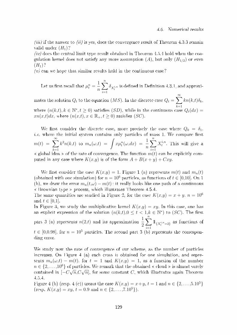
4.6. Numerical results
(iii) if the answer to (ii) is yes, does the convergence result of Theorem 4.3.3 remainvalid under (H1)?(iv) does the central limit type result obtained in Theorem 4.5.4 hold when the coa-gulation kernel does not satisfy any more assumption (A), but only (H1/2) or even(H1)?(v) can we hope that similar results hold in the continuous case?
Let us rst recall that µnt =
1
n
n∑i=1
δXi,nt
is dened in Denition 4.3.1, and approxi-
mates the solution Qt to the equation (MS). In the discrete case Qt =∞∑
k=1
kn(k,t)δk,
where (n(k,t), k ∈ N∗, t ≥ 0) satises (SD), while in the continuous case Qt(dx) =xn(x,t)dx, where (n(x,t), x ∈ R+, t ≥ 0) satises (SC).
We rst consider the discrete case, more precisely the case where Q0 = δ1,i.e. where the initial system contains only particles of mass 1. We compare rst
m(t) =∞∑
k=1
k2n(k,t) to mn(ω,t) =
∫xµn
t (ω,dx) =1
n
n∑i=1
X i,nt . This will give a
global idea of the rate of convergence. The function m(t) can be explicitly com-puted in any case where K(x,y) is of the form A+B(x+ y) + Cxy.
We rst consider the case K(x,y) = 1. Figure 1 (a) represents m(t) and mn(t)(obtained with one simulation) for n = 106 particles, as functions of t ∈ [0,10]. On 1(b), we draw the error mn(t,ω)−m(t) : it really looks like one path of a continuous Brownian type process, which illustrates Theorem 4.5.4.The same quantities are studied in Figure 2, for the case K(x,y) = x + y, n = 106
and t ∈ [0,1].In Figure 3, we study the multiplicative kernel K(x,y) = xy. In this case, one hasan explicit expression of the solution (n(k,t),0 ≤ t < 1,k ∈ N∗) to (SC). The rst
part 3 (a) represents n(2,t) and its approximation 1
2
n∑i=1
11Xi,nt =2 as functions of
t ∈ [0,0.98], for n = 105 particles. The second part 3 (b) represents the correspon-ding error.
We study now the rate of convergence of our scheme, as the number of particlesincreases. On Figure 4 (a) each cross is obtained for one simulation, and repre-sents mn(ω,t) − m(t), for t = 1 and K(x,y) = 1, as a function of the numbern ∈ 2, . . . ,106 of particles. We remark that the obtained cloud is almost surelycontained in [−C
√n,C
√n], for some constant C, which illustrates again Theorem
4.5.4.Figure 4 (b) (resp. 4 (c)) treats the case K(x,y) = x+y, t = 1 and n ∈ 2, . . . ,5.105(resp. K(x,y) = xy, t = 0.9 and n ∈ 2, . . . ,7.105).
129

Chapitre 4. Study of a stochastic particle system
a. 1
2
3
4
5
6
7
8
9
10
11
12
0 1 2 3 4 5 6 7 8 9 10
’cons10E6.dat’ using 2:3’cons10E6.dat’ using 2:4
b. -0.002
-0.001
0
0.001
0.002
0.003
0.004
0.005
0.006
0.007
0.008
0 1 2 3 4 5 6 7 8 9 10
Fig. 4.1 K(x,y)=1.
a. 1
2
3
4
5
6
7
8
0 0.1 0.2 0.3 0.4 0.5 0.6 0.7 0.8 0.9 1
’adddis3.dat’ using 2:3’adddis3.dat’ using 2:4
b. -0.002
0
0.002
0.004
0.006
0.008
0.01
0.012
0.014
0.016
0.018
0 0.1 0.2 0.3 0.4 0.5 0.6 0.7 0.8 0.9 1
Fig. 4.2 K(x,y)=x+y.
a. 0
0.01
0.02
0.03
0.04
0.05
0.06
0.07
0.08
0.09
0.1
0 0.1 0.2 0.3 0.4 0.5 0.6 0.7 0.8 0.9 1
’mul.dat’ using 2:11’mul.dat’ using 2:12
b. -0.0004
-0.0003
-0.0002
-0.0001
0
0.0001
0.0002
0.0003
0.0004
0.0005
0.0006
0 0.1 0.2 0.3 0.4 0.5 0.6 0.7 0.8 0.9 1
Fig. 4.3 K(x,y)=xy.
130
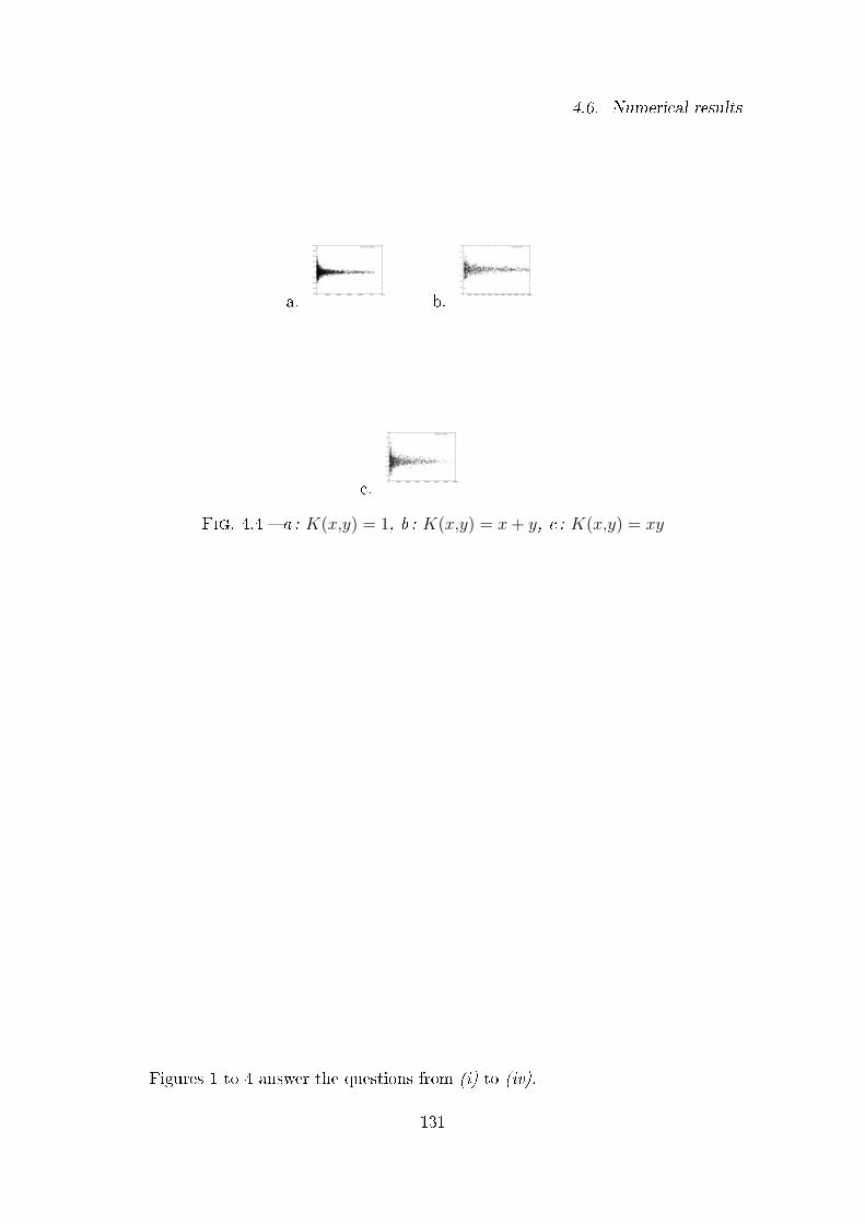
4.6. Numerical results
a.-0.04
-0.03
-0.02
-0.01
0
0.01
0.02
0.03
0.04
0.05
0 200000 400000 600000 800000 1e+06 1.2e+06
’fluctucon.dat’ using 5:6
b.-0.4
-0.3
-0.2
-0.1
0
0.1
0.2
0.3
0.4
0 50000 100000 150000 200000 250000 300000 350000 400000 450000 500000
’test.dat’ using 5:6
c.-2
-1.5
-1
-0.5
0
0.5
1
1.5
2
2.5
3
0 100000 200000 300000 400000 500000 600000 700000
’multiwe.dat’ using 5:6
Fig. 4.4 a : K(x,y) = 1, b : K(x,y) = x+ y, c : K(x,y) = xy
Figures 1 to 4 answer the questions from (i) to (iv).
131
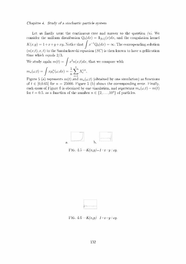
Chapitre 4. Study of a stochastic particle system
Let us nally treat the continuous case and answer so the question (v). Weconsider the uniform distribution Q0(dx) = 11[0,1](x)dx, and the coagulation kernelK(x,y) = 1+x+y+xy. Notice that
∫x−1Q0(dx) = ∞. The corresponding solution
(n(x,t), x, t) to the Smoluchowski equation (SC) is then known to have a gelicationtime which equals 2/3.We study again m(t) =
∫x2n(x,t)dx, that we compare with
mn(ω,t) =
∫xµn
t (ω,dx) =1
n
n∑i=1
X i,nt .
Figure 5 (a) represents m(t) and mn(ω,t) (obtained by one simulation) as functionsof t ∈ [0,0.65] for n = 25000. Figure 5 (b) shows the corresponding error. Finally,each cross of Figure 6 is obtained by one simulation, and represents mn(ω,t)−m(t)for t = 0.5, as a function of the number n ∈ 2, . . . ,104 of particles.
a. 0
10
20
30
40
50
60
0 0.1 0.2 0.3 0.4 0.5 0.6 0.7
’betaun25000.dat’ using 2:3’betaun25000.dat’ using 2:4
b. -0.3
-0.2
-0.1
0
0.1
0.2
0.3
0.4
0.5
0.6
0.7
0 0.1 0.2 0.3 0.4 0.5 0.6 0.7
’betaun25000.dat’ using 2:6
Fig. 4.5 K(x,y)=1+x+y+xy.
-4
-2
0
2
4
6
8
10
0 1000 2000 3000 4000 5000 6000 7000 8000 9000 10000
Fig. 4.6 K(x,y)=1+x+y+xy.
132
4.7. Appendix
The main conclusion of this numerical study is that our assumptions in Theorems4.3.3 and 4.5.4 are too stringent, and that these results seem to hold true in a moregeneral context. Indeed, the particle system really seems to be simulable under (H1)(we have not used any cuto procedure to obtain Figures 3, 4 (c), 5 and 6). Theconvergence result of Theorem 4.3.3 seems to hold also under (H1).Finally, Figures 1 (b), 2 (b), 3 (b) and 4 show that the result of Theorem 4.5.4 mayhold, in the discrete case, under (H1), while Figures 5 (b) and 6 show that a similarresult might remain true in the continuous case.
4.7 Appendix
First, we recall the Aldous criterion for tightness (see Jacod, Shiryaev [35]).Theorem 4.7.1 Let (Xn
t , t ∈ [0,T0[) be a family of càdlàg adapted processes on[0,T0[, for some T0 ≤ ∞. Denote by Qn ∈ P (D([0,T0[,R)) the law of Xn. Assumethat :
1. For all T < T0,
supnE
[sup
t∈[0,T ]
|Xnt |
]<∞. (4.148)
2. For all T < T0, all η > 0,
supn
sup(S,S′)∈STT (δ)
P [|XnS′ −Xn
S | ≥ η] −→δ→0
0 (4.149)
where STT (δ) is the set of couples (S,S ′) of stopping times satisfying a.s.0 ≤ S ≤ S ′ ≤ (S + δ) ∧ T .
Then the family (Qn)n is tight. Furthermore, any limiting point Q of this family isthe law of a quasi-left continuous process, i.e. for all t ∈ [0,T0[ xed,∫
D([0,T0[,R)
11∆x(t) 6=0Q(dx) = 0. (4.150)
The following Lemma can be found in Méléard [49].Lemma 4.7.2 Let T > 0 be xed and let νn be a sequence of random probabi-
lity measures on D([0,T ],R), which converges in law to a deterministic probabilitymeasure R ∈ P(D([0,T ],R)). Assume moreover that
supt∈[0,T ]
∫x∈D([0,T ],R)
sups∈[t−r,t+r]
(|∆x(s)| ∧ 1)R(dx) −→r→0
0. (4.151)
Then (νnt , t ∈ [0,T ]) converges in probability to (Rt, t ∈ [0,T ]) in D([0,T ],P(R)) en-
dowed with the topology of the uniform convergence.
133
Chapitre 4. Study of a stochastic particle system
We state here a Lemma due to Fernique [20], which we write in the particular si-tuation of l2-valued processes.
Lemma 4.7.3 Let αn be a sequence of strongly càdlàg processes with values inl2. Then the sequence αn is tight in D([0,∞[,l2) (endowed with the Skorohod topologyassociated with the weak topology of l2) if the following conditions are satised :(i) For any T <∞, there exists a sequence of weakly compact subsets Km of l2 suchthat for any n, any m,
P (∀ t ∈ [0,T ], αnt ∈ Km) ≥ 1− 2−m. (4.152)
In particular this condition is always satised if for all T ,
supnE
[sup[0,T ]
||αnt ||
2l2
]<∞. (4.153)
(ii) For each k ≥ 1, the sequence of real-valued processes αn(k) is tight (for the usualSkorohod topology on D([0,∞[,R).
134
Deuxième partie
Approximation de l'espérance defonctionnelles de la trajectoire d'une
diusion par le schéma d'Euler
135

5
Introduction
Cette étude a fait l'objet d'une collaboration avec Jean-Sébastien Giet.Pour certaines fonctionnelles Φ : C([0,∞[ ; Rd) → R, l'espérance de la variablealéatoireΦ (X(s)s≥0), où (X(s))s≥0 est la solution de l'E.D.S. (6.1), représente une quantitéintervenant dans de nombreux problèmes d'E.D.P. et de mathématiques nancières.
X(t) = X(0) +
∫ t
0
σ(X(s)) dB(s) +
∫ t
0
b(X(s)) ds (t ≥ 0). (6.1)
La section suivante rappelle diérentes équations dont les solutions peuvent s'ex-primer comme l'espérance de fonctionnelles de trajectoires stochastiques, ainsi quecertaines grandeurs liées à la nance.
5.1 Quelques exemples de fonctionnelles intéressantes
5.1.1 L'équation de la chaleur
L'exemple le plus simple est sans doute celui d'un mouvement brownien (B(s)s≥0)issu de zéro.La solution de l'équation de la chaleur,
∂u
∂t(t,x) = 1
2∆u(t,x) (t > 0 , x ∈ Rd)
u(0,x) = f(x) (x ∈ Rd),(5.1)
où f est une fonction continue, s'exprime sous la forme d'une espérance de ce mou-vement brownien :
u(t,x) = E f(x+B(t)) (t ≥ 0 , x ∈ Rd). (5.2)
137
Chapitre 5. Introduction
En considérant la diusion (X(t))t≥0 à la place du mouvement brownien, on obtientla solution de l'équation de la chaleur généralisée, au sens où le Laplacien ∆ estremplacé par l'opérateur de diérentiation A associé à l'E.D.S. (6.1) :
Ag(x) =1
2
d∑i,j=1
ai,j(x)∂2g
∂xi∂xj
(x) +d∑
i=1
bi(x)∂g
∂xi
(x) (g ∈ C2) (x ∈ Rd), (5.3)
où
ai,j(x) =l∑
k=1
(σi,kσj,k) (x) (x ∈ Rd). (5.4)
Si on note (Xx(t))t≥0 la solution de l'E.D.S. (6.1) pour laquelle X(0) = x, la solutionde l'équation,
∂u
∂t(t,x) = Au(t,x) (t > 0 , x ∈ Rd)
u(0,x) = f(x) (x ∈ Rd),(5.5)
où f est une fonction continue, s'écrit d'une manière analogue à la solution (5.2) del'équation (5.1) :
u(t,x) = E f(Xx(t)) (t ≥ 0 , x ∈ R). (5.6)
Il est également possible d'interpréter le membre de droite de (5.6) en terme de prixd'options nancières européennes en particularisant la fonction f : f(y) = (K−y)+.
Tous ces exemples présentent le même type de fonctionnelles qui ne dépendent quede la seule valeur à un instant t de la trajectoire. Ces fonctionnelles élémentairesne sont toutefois pas les seules à fournir des solutions d'E.D.P. ou des grandeurséconomiques.
5.1.2 Le problème de Cauchy avec potentiel et Lagrangien
Deux exemples, où la totalité de la trajectoire du processus stochastique intervient,peuvent être considérés en parallèle : ils utilisent le même type de fonctionnelles. Ils'agit des solutions du problème de Cauchy présentant un potentiel non nul et duprix des options asiatiques.
Le problème de Cauchy avec potentiel r et Lagrangien g, est une extension del'équation de la chaleur (5.5) :
∂u
∂t(t,x) = Au(t,x)− r(x)u(t,x) + g(x) (t > 0 , x ∈ Rd)
u(0,x) = u0(x) (x ∈ Rd),(5.7)
138
5.1. Quelques exemples de fonctionnelles intéressantes
où les fonctions r et g sont continues ; r est de plus supposée minorée.La formule de Feynman-Kac [38] permet d'exprimer la solution du problème deCauchy sous la forme suivante :
u(t,x) = E
u0(X
x(t)) exp
(−∫ t
0
r(Xx(s)) ds
)+
∫ t
0
g(Xx(θ)) exp
(−∫ θ
0
r(Xx(s)) ds
)dθ
(t ≥ 0 , x ∈ Rd),
(5.8)Quant aux prix des options asiatiques, l'allure de leur expression ressemble à celledes solutions ci-dessus. Plus précisément, soit (r(t)0≤t≤T ) un processus stochastiquereprésentant le taux d'intérêt. On suppose, pour ne pas avoir à changer de proba-bilité, qu'il compense exactement le taux de croissance de l'ensemble des actions.On considère une option ("contingent claim") de valeur terminale de paiement uT
et de taux de paiement (g(t)0≤t≤T ) ; il est alors démontré [38] que le prix initial qu'ilfaut investir dans un portefeuille d'actions pour couvrir le paiement de l'option estdonné par :
E
exp
(−∫ T
0
r(u) du
)uT +
∫ T
0
exp
(−∫ s
0
r(u) du
)g(s) ds
. (5.9)
5.1.3 Le problème de Dirichlet
D'autres types de fonctionnelles apparaissent à la fois dans l'analyse des E.D.P. etdans les mathématiques nancières.Si D est un domaine régulier de l'espace d'état d'un processus Xx issu de x, letemps de sortie τx
D de l'ensemble D est une information contenue dans l'ensemblede la trajectoire du processus : τx
D = inf s > 0 ; Xxs /∈ D.
La solution du problème de Dirichlet (5.10) :Au = 0 (x ∈ D)u(x) = f(x) (x ∈ ∂D),
(5.10)
où f est une fonction continue sur ∂D, s'exprime sous la forme suivante :
u(x) = Ef(Xx
τxD). (5.11)
Contenant lui aussi la v.a. τxD du temps de sortie du domaine D pour la diusion
issue de x, le prix d'une option barrière admet comme expression :E11T<τx
Df(Xx
T ). (5.12)
Ces diérents exemples illustrent l'intérêt qu'il peut y avoir à estimer, à défaut decalculer, des espérances de fonctionnelles de la trajectoire de diusions puisque cesquantités représentent des solutions d'E.D.P. ou des prix de couverture d'optionsnancières.
139
Chapitre 5. Introduction
5.2 Calcul de l'espérance des fonctionnelles
5.2.1 Principe
Le point de vue adopté ici ne consiste pas à résoudre numériquement les éven-tuelles E.D.P. dont ces espérances sont solutions. D'ailleurs, l'existence et l'unicitédes solutions des E.D.P. décrites ci-dessus ne sont assurées que si la fonction f estsusamment régulière. L'optique est d'approcher ces quantités par des méthodesprobabilistes, moins sensibles à la régularité des fonctions mises en jeu.
La méthode de Monte-Carlo constitue un moyen classique pour calculer des espé-rances de v.a., et il est naturel d'y avoir recours pour estimer ces espérances defonctionnelles de la trajectoire de processus. Toutefois, cette approche présente unproblème : il est en eet impossible de simuler des trajectoires du processus initial(X(s)s≥0). On est alors amené à remplacer ce dernier par un processus proche de Xet que l'on peut simuler. Une méthode est privilégiée par sa simplicité : le schémad'Euler.
L'objectif est donc ici d'apprécier les vitesses de convergence de quantités calculables,en faisant intervenir le schéma d'Euler et des approximations de fonctionnelles, versles espérances contenant le processus initial de diusion.
5.2.2 Études réalisées dans la littérature
Plusieurs travaux ont déjà été conduits dans cette voie. En particulier, les étudesdes cas où la fonctionnelle est réduite à la valeur en un seul point de la trajectoireont permis d'obtenir des développements en δ de l'erreur commise en remplaçantle processus initial par celui obtenu grâce au schéma d'Euler de pas δ [61], [6]. Cedernier article se distingue du premier par un aaiblissement des hypothèses portantsur la fonction f qui apparaît dans (5.6). En eet, aucune régularité n'est demandéeà cette fonction si ce n'est la mesurabilité ; une hypothèse de bornitude peut êtrerelaxée pour ne conserver qu'une croissance polynomiale en −∞ et +∞.Plus récemment, des travaux portant sur l'erreur lors de l'évaluation du prix desoptions barrière par une méthode impliquant le schéma d'Euler conduisent égalementà des développements de l'erreur [Seumen, (1997)], [Gobet, (1998)].
5.2.3 Fonctionnelles étudiées
L'étude présentée ici s'articule autour de plusieurs sortes de fonctionnelles. Dans unpremier temps, une étude de fonctionnelles faisant intervenir plusieurs points de latrajectoire est réalisée. Cette extension, sans applications directes, permet dans unsecond temps d'aboutir à des résultats concernant des fonctionnelles plus intéres-santes, qui reprennent l'information de l'intégrale de la trajectoire de la diusion.Ceci permet alors de connaître les comportements de l'erreur, lors du calcul du prix
140
5.2. Calcul de l'espérance des fonctionnelles
d'options tel que le laisse apparaître (5.9), ou lors du calcul de solutions de l'équation(5.7) qui s'expriment par (5.8).
5.2.4 Résultats
Plus précisément, on démontre (théorème 7.1.1) que pour un nombre xé n depoints de la trajectoire, l'écart existant entre les espérances E Φ(X(t1), . . . ,X(tn))et E
Φ(Xδ(t1), . . . ,X
δ(tn)), où Φ désigne une fonction réelle dénie sur
(Rd)n
et (ti)(0≤i≤n) une subdivision, se comporte en δ. Cette démonstration a déjà étéprésentée lorsque ces espérances se ramènent au membre de droite de (5.6), avec ftrès régulière [61] et avec f seulement supposée mesurable et bornée [6]. C'est cettedernière hypothèse qui est imposée dans le cadre de cette étude.
Ce premier résultat permet d'aboutir à des fonctionnelles ayant la forme x(.) 7−→(∫ 1
0
f(x(s)) ds
)l
et x(.) 7−→ exp
(∫ 1
0
f(x(s)) ds
)au travers de l'étude des conver-
gences des fonctionnelles du type précédent x(.) 7−→(
1
n
n∑i=1
f
(x(i
n)
))l
et x(.) 7−→
exp
(1
n
n∑i=1
f
(x(i
n)
)).
Il est ensuite démontré dans les théorèmes 8.2.1, 8.4.1 et 8.8.1 que chaque erreur estmajorée par une quantité comportant un terme en δ et un autre en 1
n. Toutefois, si
l'on sait majorer uniformément en n le coecient devant δ, il n'a pas été possible decontrôler uniformément le reste εδ,n. Par conséquent, la vitesse de convergence desquantités contenant l'approximation d'Euler du processus n'est pas connue.
Enn, en imposant l'égalité n =1
δ, on obtient une majoration de l'erreur, énoncée
dans le théorème 9.1, concernant l'intégrale de la trajectoire du processus.
Théorème 5.2.1 Soit f une fonction mesurable et bornée.Soit X(.) la solution de (6.1) ; soit X
1n (.) l'approximation de cette solution donnée
par le schéma d'Euler ; X1n (.) est la solution de (6.2).
Alors il existe C tel que :∣∣∣∣∣E∫ 1
0
f(X(s)) ds
− E
1
n
n∑i=1
f(X1n (i
n))
∣∣∣∣∣ ≤ C ‖f‖∞1
n. (5.13)
Ce théorème fournit des majorations des vitesses de convergence pour les algorithmespermettant de calculer des prix d'options ou des solutions du problème de Cauchy.
141
Chapitre 5. Introduction
5.2.5 Plan de l'étude
• Quelques notations et hypothèses intervenant dans l'ensemble de l'étude sontprécisées dans la partie 6.
• À partir de là, le théorème 7.1.1, indiquant la vitesse de convergence pour desfonctionnelles faisant intervenir plusieurs points de la trajectoire, est énoncé dans lapartie 7.1. Sa démonstration s'articule autour de trois parties : 7.2, 7.3 et 7.4.
• Avant l'étude des fonctionnelles de la trajectoire, qui sont cette fois-ci des fonctionsde l'intégrale de la trajectoire, la partie 8.1 est consacrée au rappel d'un résultatconcernant la dérivation des noyaux de transition pour des diusions suivant leshypothèses décrites en 6.1. On y démontre la majoration de noyaux dérivés que l'onpeut trouver dans les travaux de Kusuoka-Stroock [41] ou Sanchez-Calle [55].Ensuite, un développement de l'erreur par rapport à δ est établi pour les momentsd'ordre l de l'intégrale de la trajectoire (partie 8.2) ainsi que pour les moments ex-ponentiels (partie 8.8). La démonstration de ce développement pour les moments(théorème 8.4.1) est réalisée dans le cas des ordres 1, 2, puis l dans les para-graphes 8.5, 8.6 et 8.7 respectivement. La partie 8.3 est réservée à la majoration
de la vitesse de convergence des sommes de Riemann 1
n
n∑i=1
Ef
(X(
i
n)
)vers∫ 1
0
E f(X(s)) ds.
• La partie 9 est réservée à l'étude de majorations uniformes en δ = 1n.
142
6
Notations et hypothèses
6.1 Le processus de diusion
Soit B(t)t≥0 un mouvement brownien de dimension 1, issu de zéro et déni sur unespace de probabilité (Ω,F ,P).
Dénition :
On désigne par X(.) la solution de l'E.D.S. :
X(t) = X(0) +
∫ t
0
σ(X(s)) dB(s) +
∫ t
0
b(X(s)) ds (t ≥ 0), (6.1)
où X(0) est une v.a. possédant des moments de tout ordre, et où σ, b et a = σσt
(5.3) sont des fonctions vériant les hypothèses suivantes :
(H 1)
b : Rd → Rd et σ : Rd → Rd sont de classe C∞
les dérivées b′, b′′, σ′, σ′′ sont bornées sur Rd
il existe η tel que∑i,j
ξiai,j(x)ξj ≥ η > 0 (x ∈ Rd) (ξ ∈ Rd ; ‖ξ‖ = 1).
Notation :
On note, pour r ∈ [0,1] et x ∈ Rd, Xr,x(.) la diusion correspondant à X(.) partantà l'instant r du point x ; Xr,x(.) est la solution de l'E.D.S. :
Xr,x(t) = x+
∫ t
r
σ(Xr,x(s)) dB(s) +
∫ t
r
b(Xr,x(s)) ds (t ≥ r) (x ∈ Rd). (6.2)
Dénitions :
i) ϕδδ>0 désigne une famille de fonctions réelles, dénies sur [0,1] vériant leshypothèses :
143
Chapitre 6. Notations et hypothèses
(H 2)Pour tout δ > 0, ϕδ est une fonction en escalier croissantetelle que pour tout t ∈ [0,1], ϕδ(t) ≤ t et t−ϕδ(t)
δ≤ 1,
limδ→0
ϕδ(t) = t
ii) On dénit, pour toute fonction ϕδ, le processus Xδ(.) comme la solution del'E.D.S. :
Xδ(t) = X(0) +
∫ t
0
σ(Xδ ϕδ(s)) dB(s) +
∫ t
0
b(Xδ ϕδ(s)) ds (t ≥ 0). (6.3)
Xδ(.) correspond à la solution approchée par le schéma d'Euler de l'équation (6.1)si ϕδ(t) =
⌊t
δ
⌋δ, où bvc représente la partie entière de v ∈ [0,+∞[.
Notation :
On note t(δ) la quantité⌊t
δ
⌋δ.
Remarque :
On ne s'interdit pas, sauf mention contraire, de choisir des familles de fonctionsvériant seulement les hypothèses (H 2).
Un résultat classique (voir par exemple [27] ou [38]) consiste en une majoration desmoments de Y (t) où (Y,W ) est une solution faible de l'E.D.S. générale :
Y (t) = Y (0) +
∫ t
0
f(s,Y ) dW (s) +
∫ t
0
g(s,Y ) ds, (6.4)
les fonctionnelles f et g étant dénies sur [0,+∞[×C([0,+∞[,Rd).
Proposition 6.1.1 On suppose que les fonctionnelles f et g vérient l'hypothèsede majoration suivante :il existe K ∈ R tel que :
‖f(t,y)‖2 + ‖g(t,y)‖2 ≤ K
(1 + sup
0<s<t‖y(s)‖2)
). (6.5)
Alors pour toute solution faible (Y,W ) de (6.4) :
E
sup0≤s≤t
‖Y (s)‖2m
≤ C(1 + E
‖Y (0)‖2m
) exp(Ct) (0 ≤ t ≤ T ), (6.6)
le nombre C dépendant uniquement de m, T et K.
Les E.D.S. (6.3) entrent dans le cadre des E.D.S. (6.4), puisqu'il sut de choisirf(s,y) = σ(y(ϕδ(s))) et g(s,y) = b(y(ϕδ(s))) pour obtenir l'équation suivie par Xδ.
144
6.2. La fonctionnelle de la trajectoire
Les conclusions de la proposition 6.5 permettent d'établir un résultat concernant lafamille de processus
(Xδ(.)
)δ>0
:
Corollaire 6.1.2 Sous les hypothèses (H 1) vériées par b et σ, il existe unnombre C tel que pour tout δ > 0 :
E
sup0≤s≤t
‖Xδ(s)‖2m
≤ C(1 + E
‖X(0)‖2m
) exp(Ct) (0 ≤ t ≤ T ). (6.7)
Démonstration du corollaire 6.1.2.
L'hypothèse (6.5) de la proposition 6.1.1 est réalisée pour la famille(Xδ(.)
)δ>0
:
‖σ(y(ϕδ(t)))‖2 + ‖b(y(ϕδ(t)))‖2
≤ K
(1 + sup
0<s<t‖y(s)‖2)
) (y ∈ C([0,+∞[,Rd)
)(t ≥ 0), (6.8)
où K est un réel indépendant de δ.Donc la majoration (6.8) est uniforme en δ > 0, et le nombre C de la majoration(6.7) ne dépend pas de δ. 2
Dénition :
Pour toute famille ϕδδ>0 et tout r ∈ ]0,1[, on dénit le processus Xδr (.) comme
étant la solution Xδ(.) de l'équation (6.3) jusqu'au temps r, puis la solution Xr,Xδ(r)
de l'équation (6.2) au-delà de l'instant r.Xδ
r (.) est ainsi la solution de l'E.D.S. suivante :
Xδr (t) = X(0) +
∫ t
0
(σ(Xδ
r ϕδ(s))11]0,r[(s) + σ(Xδr (s))11]r,1[(s)
)dB(s)
+
∫ t
0
(b(Xδ
r ϕδ(s))11]0,r[(s) + b(Xδr (s))11]r,1[(s)
)ds
(t ≥ 0).
(6.9)Cette famille de processus a été introduite par Kurtz et Protter. Elle est au c÷urdu principe de la démonstration du théorème 7.1.1.
6.2 La fonctionnelle de la trajectoire
Les résultats des parties 7, 8 et 9 correspondent à un horizon de temps ni. Poursimplier les notations, ils sont énoncés et démontrés sur l'intervalle [0,1].
Nous nous intéressons, dans un premier temps (partie 7), à des fonctionnelles qui nefont intervenir qu'un nombre ni de points de la trajectoire.
Dénition :
145
Chapitre 6. Notations et hypothèses
Une fonctionnelle Φ : C([0,1],Rd) → R, ne dépendant que d'un nombre ni n depoints de la trajectoire, est entièrement déterminée par la donnée :- d'une subdivision ti ; 1 ≤ i ≤ n de l'intervalle [0,1] avec 0 ≤ t1 < . . . < tn ≤ 1,- d'une fonction Φ :
(Rd)n → R.
Ainsi,Φ(x(.)) = Φ(x(t1), . . . ,x(tn))
(x(.) ∈ C([0,1],Rd)
). (6.10)
La fonction Φ vérie l'hypothèse (H 3) :
(H 3) Φ est une fonction mesurable,il existe C ∈ R et p > 0 tels que :
|Φ(x1, . . . ,xn)| ≤ C
(1 + sup
1≤j≤n‖xj‖p
). (Mp)
146
7
Développement en δ de l'erreur pourdes fonctionnelles à n points
7.1 Résultat principal
Le théorème 7.1.1 propose un développement de l'erreur induite par le remplacementde X par Xδ dans l'expression E Φ(X(t1), . . . ,X(tn)). La dimension de la diusionest restreinte à d = 1. Cependant, lors de la démonstration du théorème 7.1.1, lethéorème 7.2.1 dont le résultat sera également utilisé dans la partie 9 est énoncédans le cas général d ∈ N∗.
Théorème 7.1.1 On considère une fonctionnelle Φ dénie à partir d'une fonc-tionΦ : Rn −→ R et d'une subdivision ti ; 1 ≤ i ≤ n de [0,1].On suppose que Φ vérie l'hypothèse (H 3).Soit X(.) la solution de (6.1) avec d = 1 ; soit Xδ(.) l'approximation de cette solutiondonnée par le schéma d'Euler.Alors,
E Φ(X(t1), . . . ,X(tn)) − EΦ(Xδ(t1), . . . ,X
δ(tn))
= R(Φ)δ + εδ,n, (7.1)
la quantité εδ,n vériant pour tout entier n : limδ→0
εδ,n
δ= 0, et la quantité R(Φ)
pouvant s'exprimer comme la somme de trois intégrales faisant intervenir la fonctionHr,n dénie plus avant par (7.3) :
R(Φ) =
∫ 1
0
E∂Hr,n
∂z(X(t1), . . . ,X(tnr),X(r))
(ab′′
2+ bb′
)(X(r))
dr
+
∫ 1
0
E∂2Hr,n
∂z2(X(t1), . . . ,X(tnr),X(r))(
ab′ +aa′′
4+ba′
2
)(X(r))
dr
+
∫ 1
0
E∂3Hr,n
∂z3(X(t1), . . . ,X(tnr),X(r))
aa′
2(X(r))
dr.
(7.2)
147
Chapitre 7. Développement en δ de l'erreur pour des fonctionnelles à n points
Lorsque k est égal à 1, ce théorème est une version assez proche du théorème 3.1de Bally-Talay [6]. Il faut noter que nos hypothèses concernant les coecients de ladiusion sont plus restrictives, et que celles portant sur la fonction f sont identiques ;l'hypothèse (H 3), dans le cas k = 1, correspond à la mesurabilité de f et à sacroissance polynomiale.
Par contre, la démonstration du théorème 7.1.1 ne reprend pas celle de Bally-Talay[6] mais s'inspire d'une idée de Kurtz et Protter. En particulier, l'introduction de lafamille de processus paramétrés, qui sont les solutions de l'E.D.S. (6.9), leur revient.De plus, le théorème 7.2.1 et le lemme 7.3.2 ont été adaptés ici à des valeurs de nsupérieures à 1.
Plan de la démonstration du théorème 7.1.1.
La démonstration qui suit se compose de trois parties.Dans une première partie, l'écart entre E Φ(X(t1, . . . ,tn)) et E
Φ(Xδ(t1, . . . ,tn))
est représenté comme l'intégrale d'une dérivée ; cette dérivée est calculée, dans lethéorème 7.2.1, en fonction du seul processus Xδ.Une seconde partie est consacrée au calcul des limites des quotients des termesobtenus au théorème 7.2.1 pour cette dérivée par δ, quand δ tend vers zéro.Une dernière partie regroupe les résultats précédents pour établir (7.1) et l'expression(7.2) de R(Φ).
7.2 Dérivation de l'espérance d'une fonction du pro-
cessus Xδr (.)
Les processus Xδr (.), lorsque r décrit [0,1], constituent une paramétrisation dans
l'espace des solutions des équations (6.3) où ϕδ vérie (H 2), allant de la solutionX(.) de (6.1) pour r = 0 à la solution Xδ(.) de (6.3) pour r = 1. La diérenceE Φ(X(t1), . . . ,X(tn))−E
Φ(Xδ(t1), . . . ,X
δ(tn))peut ainsi s'écrire comme l'in-
tégrale entre r = 0 et r = 1 de la dérivée ∂
∂rEΦ(Xδ
r (t1), . . . ,Xδr (tn))
.
Le théorème suivant exprime cette dérivée en fonction des coecients σ et b.
Théorème 7.2.1 On considère une fonctionnelle Φ dénie à partir d'une fonc-tion Φ :
(Rd)n −→ R et d'une subdivision ti ; 1 ≤ i ≤ n de [0,1].
On suppose que Φ vérie l'hypothèse (H 3).Soit X(.) la solution de (6.1) avec d ∈ N∗ ; soit Xδ(.) l'approximation de cette so-lution donnée par le schéma d'Euler. On dénit la famille de fonctions à valeursréelles indexées par r et n :
Hr,n :(Rd)nr × Rd −→ R
(x1, . . . ,xnr ,z) 7−→ E Φ(x1, . . . ,xnr ,Xr,z(tnr+1), . . . ,X
r,z(tn)) , (7.3)
148
7.2. Dérivation de l'espérance d'une fonction du processus Xδr (.)
où nr = supi ; ti ≤ r.Alors pour tout r ∈]0,1[\ti ; 1 ≤ i ≤ n,
∂
∂r
(EΦ(Xδ
r (t1), . . . ,Xδr (tn))
)= E
d∑
i=1
[bi(X
δ ϕδ(r))− bi(Xδ(r))
] ∂Hr,n
∂zi
(Xδ(t1), . . . ,Xδ(tnr),X
δ(r))
+1
2E
d∑
i,j=1
[aij(X
δ ϕδ(r))− aij(Xδ(r))
] ∂2Hr,n
∂zi∂zj
(Xδ(t1), . . . ,Xδ(tnr),X
δ(r))
.
(7.4)
Notations :
Si g désigne une fonction réelle C∞ dénie pour x = (y,z) ∈(Rd)i ×Rd dans R, on
écrira dans la suite :
b(x)∂g
∂z(x) pour
d∑i=1
bi(x)∂g
∂zi
(x),
a(x)∂2g
∂z2(x) pour
d∑i,j=1
aij(x)∂2g
∂zi∂zj
(x).
La conclusion du théorème 7.2.1 s'écrit alors :∂
∂r
(EΦ(Xδ
r (t1), . . . ,Xδr (tn))
)= E
[b(Xδ ϕδ(r))− b(Xδ(r))
] ∂Hr,n
∂z(Xδ(t1), . . . ,X
δ(tnr),Xδ(r))
+
1
2E[a(Xδ ϕδ(r))− a(Xδ(r))
] ∂2Hr,n
∂z2(Xδ(t1), . . . ,X
δ(tnr),Xδ(r))
.
(7.5)L'énoncé du théorème appelle quelques commentaires avant d'aborder sa démons-tration.
• Premièrement, la fonction Hr,n est correctement dénie en tant qu'espérance d'unev.a. intégrable. En eet, en appliquant successivement (Mp) et (6.6), on obtient :
E |Φ(x1, . . . ,xnr ,Xr,z(tnr+1), . . . ,X
r,z(tn))|
≤ C
(1 + sup
1≤j≤nr
‖xj‖p + E
supnr+1≤j≤n
‖Xr,z(tj)‖p
)≤ C
(1 + sup
1≤j≤nr
‖xj‖p + ‖z‖p
),
où C et C sont des constantes.
• Deuxièmement, la fonction Hr,n est dérivable par rapport à la dernière variable. Il
149
Chapitre 7. Développement en δ de l'erreur pour des fonctionnelles à n points
sut d'utiliser le théorème de dérivation sous le signe d'intégration pour le démon-trer.Plus précisément, soit a > 0, les fonctions Φ(x1, . . . ,xnr ,X
r,z(tnr+1), . . . ,Xr,z(tn))
sont P-intégrables pour tout z ∈]− a,a[.En introduisant le noyau de transition du processus Xr,z(.) entre les temps r ettnr+1, on isole le paramètre z par rapport auquel on veut dériver.
Notation :
La densité de la probabilité de transition du processus X(.) entre les instants s1 ets2 est notée qs1,s2 , parfois qs2−s1 :
P (Xs1,x(s2) ∈ dy) = qs1,s2(x,y) dy. (7.6)
La fonction Hr,n s'écrit alors :
Hr,n(x1, . . . ,xnr ,z) = E
∫R
Φ(x1, . . . ,xnr+1,Xtnr+1,xnr+1(tnr+2), . . . ,X
tnr+1,xnr+1(tn))
qr,tnr+1(z,xnr+1) dxnr+1
.
Pour tout entier strictement positif γ, l'application de l'inégalité (8.2) permet demajorer la famille des dérivées∂γ
∂zγ
(Φ(x1, . . . ,xnr+1,X
tnr+1,xnr+1(tnr+2), . . . ,Xtnr+1,xnr+1(tn))qr,tnr+1(z,xnr+1)
)z∈]−a,a[
par :
C∣∣Φ(x1, . . . ,xnr+1,X
tnr+1,xnr+1(tnr+2), . . . ,Xtnr+1,xnr+1(tn))
∣∣× 1
(tnr+1 − r)γ+12
exp
(−x2
nr+1 − 2|a|xnr+1
2M(tnr+1 − r)
)√
2πM;
cette fonction est intégrable par rapport à P⊗ dxnr+1.Par conséquent, pour γ ∈ N∗,
∂γHr,n
∂zγ(x1, . . . ,xnr ,z) = E
∫R
Φ(x1, . . . ,xnr+1,Xtnr+1,xnr+1(tnr+2),
. . . ,X tnr+1,xnr+1(tn))∂lqr,tnr+1
∂zl(z,xnr+1)dxnr+1
.
(7.7)
• Enn, le lemme suivant, qui interviendra lors de la démonstration du lemme 7.3.2,démontre en outre que les espérances apparaissant dans le membre de droite de(7.4), impliquant les dérivées ∂
γHr,n
∂zγ, sont nies.
150
7.2. Dérivation de l'espérance d'une fonction du processus Xδr (.)
Lemme 7.2.1 Les hypothèses du théorème 7.2.1 sont restreintes à d = 1 ; qdésigne un entier naturel non nul.Alors, pour γ ∈ N∗, il existe un réel C et un entier N tels que :
E
sup0≤θ≤1
∣∣∣∣∂γHr,n
∂zγ(Xδ(t1), . . . ,X
δ(tnr),(1− θ)Xδ ϕδ(r) + θXδ(r))
∣∣∣∣q≤ C E
1 + sup
0≤s≤r
∣∣Xδ(s)∣∣N . (7.8)
Démonstration du lemme 7.2.1.
On note :
I =
∣∣∣∣∂γHr,n
∂zγ(x1, . . . ,xnr ,z)
∣∣∣∣ .Par (7.7), I s'exprime sous la forme suivante :
I =
∣∣∣∣∣E∫
RΦ(x1, . . . ,xnr+1,X
tnr+1,xnr+1(tnr+2), . . . ,Xtnr+1,xnr+1(tn))
∂γqr,tnr+1
∂zγ(z,xnr+1)dxnr+1
∣∣∣∣∣.On majore la fonction Φ et la dérivée du noyau qr,tnr+1 en utilisant respectivement(Mp) et (8.2) :
I ≤ C1 E
∫R
(1 + sup
1≤j≤nr
|xj|p + supnr+2≤j≤n
∣∣X tnr+1,xnr+1(tj)∣∣p)
exp
(− (xnr+1 − z)2
2M(tnr+1 − r)
)√
2πM(tnr+1 − r)γ+12
dxnr+1
.
On échange espérance et intégrale, puis on utilise la majoration (6.6) avant qu'unchangement de variable dans l'intégrale ne conduise à :
I ≤ C2
1 + sup1≤j≤nr
|xj|p +
∫R|x|p
exp
(−(x− z)2
2
)√
2πdx
,
où le réel C2 dépend de M et du temps tnr+1 − r.L'intégrale en x est clairement dominée par une fonction polynomiale en |z| de degrép.On obtient alors successivement :
I ≤ C3
(1 + sup
1≤j≤nr
|xj|p + |z|p)
151
Chapitre 7. Développement en δ de l'erreur pour des fonctionnelles à n points
et
E
sup0≤θ≤1
∣∣∣∣∂γHr,n
∂zγ(Xδ(t1), . . . ,X
δ(tnr),(1− θ)Xδ ϕδ(r) + θXδ(r))
∣∣∣∣q≤ C E
1 + sup
0≤s≤r
∣∣Xδ(s)∣∣qp.
2
Démonstration du théorème 7.2.1.
On considère la diérence suivante dans laquelle le réel strictement positif h estchoisi pour que r + h < tnr+1, de sorte que nr+h = nr :
EΦ(Xδ
r+h(t1), . . . ,Xδr+h(tn))
− E
Φ(Xδ
r (t1), . . . ,Xδr (tn))
. (7.9)
Chacun des deux termes peut s'exprimer au moyen de la fonction Hr+h,n.En eet, la variable aléatoire Xδ
r+h(s) étant égale à Xδ(s) ou à Xr+h,Xδ(r+h)(s),suivant que le temps s est respectivement inférieur ou supérieur à r + h, le premierterme s'écrit :
EΦ(Xδ
r+h(t1), . . . ,Xδr+h(tn))
= E
Φ(Xδ(t1), . . . ,X
δ(tnr),Xr+h,Xδ
r+h(r+h)(tnr+1), . . . ,Xr+h,Xδ
r+h(r+h)(tn)).
Un conditionnement par rapport à la tribu Fr+h laisse apparaître la fonction Hr+h,n :
EΦ(Xδ
r+h(t1), . . . ,Xδr+h(tn))
= E
Hr+h,n(Xδ(t1), . . . ,X
δ(tnr),Xδr+h(r + h))
.
(7.10)En procédant à l'identique, on peut écrire le second terme de (7.9) comme suit :
EΦ(Xδ
r (t1), . . . ,Xδr (tn))
= E
Hr+h,n(Xδ(t1), . . . ,X
δ(tnr),Xδr (r + h))
.
On applique alors à la fonction Hr+h,n la formule d'Itô [38] avec les processus Xδr (.)
et Xδr+h(.), entre les instants r et r + h :
Hr+h,n(Xδ(t1), . . . ,Xδ(tnr),X
δr+h(r + h)) = Hr+h,n(Xδ(t1), . . . ,X
δ(tnr),Xδr+h(r))
+
∫ r+h
r
∂Hr+h,n
∂z(Xδ(t1), . . . ,X
δ(tnr),Xδr+h(s)) σ(Xδ
r+h(s(δ))) dB(s)
+
∫ r+h
r
∂Hr+h,n
∂z(Xδ(t1), . . . ,X
δ(tnr),Xδr+h(s)) b(X
δr+h(s
(δ))) ds
+1
2
∫ r+h
r
∂2Hr+h,n
∂z2(Xδ(t1), . . . ,X
δ(tnr),Xδr+h(s)) a(X
δr+h(s
(δ))) ds,
(7.11)
152
7.2. Dérivation de l'espérance d'une fonction du processus Xδr (.)
Hr+h,n(Xδ(t1), . . . ,Xδ(tnr),X
δr (r + h)) = Hr+h,n(Xδ(t1), . . . ,X
δ(tnr),Xδ(r))
+
∫ r+h
r
∂Hr+h,n
∂z(Xδ(t1), . . . ,X
δ(tnr),Xδr (s)) σ(Xδ
r (s)) dB(s)
+
∫ r+h
r
∂Hr+h,n
∂z(Xδ(t1), . . . ,X
δ(tnr),Xδr (s)) b(X
δr (s)) ds
+1
2
∫ r+h
r
∂2Hr+h,n
∂z2(Xδ(t1), . . . ,X
δ(tnr),Xδr (s)) a(X
δr (s)) ds.
(7.12)On choisit le réel positif h susamment petit pour que s(δ) ≤ r lorsque r < s < r+h ;ainsi, on peut remplacer Xδ
r+h(s(δ)) par Xδ(s(δ)) dans les intégrales de (7.11).
Par ailleurs, comme s < r + h dans les intégrales de (7.11), on peut remplacerXδ
r+h(s) par Xδ(s).Soustrayant (7.12) à (7.11), on obtient :
Hr+h,n(Xδ(t1), . . . ,Xδ(tnr),X
δr+h(r+h))−Hr+h,n(Xδ(t1), . . . ,X
δ(tnr),Xδr (r+h))
=
∫ r+h
r
∂Hr+h,n
∂z(Xδ(t1), . . . ,X
δ(tnr),Xδ(s))
[σ(Xδ(s(δ))) dB(s) + b(Xδ(s(δ))) ds
]−∫ r+h
r
∂Hr+h,n
∂z(Xδ(t1), . . . ,X
δ(tnr),Xδr (s))
[σ(Xδ
r (s)) dB(s) + b(Xδr (s)) ds
]+
1
2
∫ r+h
r
∂2Hr+h,n
∂z2(Xδ(t1), . . . ,X
δ(tnr),Xδ(s)) a(Xδ(s(δ))) ds
− 1
2
∫ r+h
r
∂2Hr+h,n
∂z2(Xδ(t1), . . . ,X
δ(tnr),Xδr (s)) a(X
δr (s)) ds.
(7.13)Il resulte du lemme 7.2.1 et du corollaire 6.1.2 que les intégrales en dB(s) sont desmartingales de carré intégrable. Par conséquent, en prenant l'espérance dans l'égalité(7.13), on fait disparaître ces intégrales en dB(s), et par (7.10) on obtient :
EΦ(Xδ
r+h(t1), . . . ,Xδr+h(tn))
− E
Φ(Xδ
r (t1), . . . ,Xδr (tn))
= E
∫ r+h
r
(∂Hr+h,n
∂z(Xδ(t1), . . . ,X
δ(tnr),Xδ(s))b(Xδ(s(δ)))
− ∂Hr+h,n
∂z(Xδ(t1), . . . ,X
δ(tnr),Xδr (s))b(X
δr (s))
) ds
+1
2E
∫ r+h
r
(∂2Hr+h,n
∂z2(Xδ(t1), . . . ,X
δ(tnr),Xδ(s)) a(Xδ(s(δ)))
− ∂2Hr+h,n
∂z2(Xδ(t1), . . . ,X
δ(tnr),Xδr (s)) a(X
δr (s))
)ds
.
(7.14)
La conclusion du théorème s'obtient en divisant cette dernière égalité par h et enfaisant tendre h vers zéro. 2
153
Chapitre 7. Développement en δ de l'erreur pour des fonctionnelles à n points
Les résultats de cette première partie sont utilisés dans la dernière partie de ladémonstration. Par ailleurs, l'égalité (7.4) oriente les calculs menés dans la deuxièmepartie.
7.3 Limite en δ
L'égalité (7.4) fournit une expression de la dérivée par rapport au paramètre r, dela fonctionnelle Φ appliquée au processus Xδ
r . L'écriture de cette dérivée ne faitapparaître que le seul processus Xδ.Le but de cette section est de préciser les comportements des espérances du membrede droite de l'égalité (7.4), lorsque le paramètre δ converge vers zéro. Les résultatsde cette section sont restreints au cas où la diusion est de dimension un.
Avant d'étudier ces comportements, nous comparons les vitesses de convergence verszéro, de la norme Lp de Xδ(r)− Xδ ϕδ(r) et de r − ϕδ(r).
Lemme 7.3.1 Soit un réel p ≥ 1. Il existe un nombre C tel que pour tout δ > 0 :
E∣∣Xδ(r)− Xδ ϕδ(r)
∣∣2p≤ C (r − ϕδ(r))
p . (7.15)
Démonstration du lemme 7.3.1.
La fonction ϕδ reste constante entre ϕδ(r) et r ; par conséquent, l'équation (6.3) sesimplie :
Xδ(r)−Xδϕδ(r) = σ(Xδϕδ(r))(B(r)−B ϕδ(r))+b(Xδϕδ(r))(r−ϕδ(r)). (7.16)
||Xδ(r)−Xδϕδ(r)||p ≤ ||σ(Xδϕδ(r))(B(r)−Bϕδ(r))||p+||b(Xδϕδ(r))(r−ϕδ(r))||p(7.17)
Le corollaire 6.1.2 et le contrôle des moments d'ordre p d'une gaussienne nous per-mettent de conclure. 2
Remarque :
L'application de l'inégalité de Cauchy-Schwarz et de la majoration (7.15) lorsquep = 1 implique l'existence d'un nombre C tel que pour tout δ > 0 :
E∣∣Xδ(r)− Xδ ϕδ(r)
∣∣ ≤ C√r − ϕδ(r). (7.18)
Lemme 7.3.2 Soit g une fonction dénie de R dans R, de classe C2 telle qu'ilexiste une constante C :
|g(x)− g(y)| ≤ C|x− y|(1 + |x|+ |y|)((x,y) ∈ R2
). (7.19)
154
7.3. Limite en δ
Soient n ∈ N∗, γ ∈ 1,2 et r ∈]0,1[\ti ; 1 ≤ i ≤ n.Alors :
limδ→0
1
r−ϕδ(r)E[g(Xδ
r (r))−g(Xδr ϕδ(r))
]∂γHr,n
∂zγ(Xδ
r (t1), . . . ,Xδr (tnr),X
δr (r))
= E
(ag′′
2+ bg′
)(X(r))
∂γHr,n
∂zγ(X(t1), . . . ,X(tnr),X(r))
+ E
a(X(r))g′(X(r))
∂γ+1Hr,n
∂zγ+1(X(t1), . . . ,X(tnr),X(r))
.
(7.20)
Démonstration du lemme 7.3.2.
On développe l'expression apparaissant dans la limite à calculer, en utilisant ladérivée par rapport à la dernière variable de la fonction Hr,n.
[g(Xδ(r))− g(Xδ ϕδ(r))
] ∂γHr,n
∂zγ(Xδ(t1), . . . ,X
δ(tnr),Xδ(r))
=[g(Xδ(r))− g(Xδ ϕδ(r))
]∂γHr,n
∂zγ(Xδ(t1), . . . ,X
δ(tnr),Xδ(r))
− ∂γHr,n
∂zγ(Xδ(t1), . . . ,X
δ(tnr),Xδ ϕδ(r))
− ∂γ+1Hr,n
∂zγ+1(Xδ(t1), . . . ,X
δ(tnr),Xδ ϕδ(r))(X
δ(r)− Xδ ϕδ(r))
+[g(Xδ(r))− g(Xδ ϕδ(r))
]∂γ+1Hr,n
∂zγ+1(Xδ(t1), . . . ,
Xδ(tnr),Xδ ϕδ(r))(X
δ(r)− Xδ ϕδ(r))
+[g(Xδ(r))− g(Xδ ϕδ(r))
] ∂γHr,n
∂zγ(Xδ(t1), . . . ,X
δ(tnr),Xδ ϕδ(r))
.
(7.21)
Chacun des termes du membre de droite de (7.21) va être étudié.
• On va démontrer que l'espérance du premier terme du membre de droite de (7.21)divisée par r − ϕδ(r) converge vers zéro lorsque δ tend vers zéro.L'espérance de ce premier terme s'écrit :
E
(g(Xδ(r))− g(Xδ ϕδ(r)))[
∂γHr,n
∂zγ(Xδ(t1), . . . ,X
δ(tnr),Xδ(r))− ∂γHr,n
∂zγ(Xδ(t1), . . . ,X
δ(tnr),Xδ ϕδ(r))
−(Xδ(r)− Xδ ϕδ(r)
) ∂γ+1Hr,n
∂zγ+1(Xδ(t1), . . . ,X
δ(tnr),Xδ ϕδ(r))
]. (7.22)
155
Chapitre 7. Développement en δ de l'erreur pour des fonctionnelles à n points
En appliquant à plusieurs reprises l'inégalité de Cauchy-Schwarz et en utilisant l'hy-pothèse (7.19) suivie par g, on obtient une majoration de (7.22) par :
C(E(Xδ(r)− Xδ ϕδ(r))
4) 1
4
(E(
1 +∣∣Xδ(r)
∣∣+ ∣∣Xδ ϕδ(r)∣∣)4) 1
4(E(∂γHr,n
∂zγ(Xδ(t1), . . . ,X
δ(tnr),Xδ(r))
−∂γHr,n
∂zγ(Xδ(t1), . . . ,X
δ(tnr),Xδ ϕδ(r))
−(Xδ(r)− Xδ ϕδ(r)
) ∂γ+1Hr,n
∂zγ+1(Xδ(t1), . . . ,X
δ(tnr),Xδ ϕδ(r))
)2) 12
.
(7.23)
Le premier facteur de (7.23) se comporte comme√r − ϕδ(r) lorsque δ tend vers zéro.
Le second facteur est borné en vertu de la proposition 6.1.1. Il reste à démontrerque le dernier facteur converge vers zéro avec δ.Le développement de Taylor à l'ordre 2 permet d'écrire :
(∂γHr,n
∂zγ(Xδ(t1), . . . ,X
δ(tnr),Xδ(r))− ∂γHr,n
∂zγ(Xδ(t1), . . . ,X
δ(tnr),Xδ ϕδ(r))
−(Xδ(r)− Xδ ϕδ(r)
) ∂γ+1Hr,n
∂zγ+1(Xδ(t1), . . . ,X
δ(tnr),Xδ ϕδ(r))
)2
=
((Xδ(r)− Xδ ϕδ(r)
)2 ∫ 1
0
(1− θ)∂γ+2Hr,n
∂zγ+2(Xδ(t1), . . . ,X
δ(tnr),
(1− θ)Xδ ϕδ(r) + θXδ(r)) dθ
)2
≤(Xδ(r)− Xδ ϕδ(r)
)4sup
0≤θ≤1
(∂γ+2Hr,n
∂zγ+2(Xδ(t1), . . . ,X
δ(tnr),(1− θ)Xδ ϕδ(r) + θXδ(r))
)2
.
(7.24)En prenant l'espérance et en appliquant l'inégalité de Cauchy-Schwarz, puis la ma-joration (7.8), on obtient :
E(∂γHr,n
∂zγ(Xδ(t1), . . . ,X
δ(tnr),Xδ(r))− ∂γHr,n
∂zγ(Xδ(t1), . . . ,X
δ(tnr),Xδ ϕδ(r))
−(Xδ(r)− Xδ ϕδ(r)
) ∂γ+1Hr,n
∂zγ+1(Xδ(t1), . . . ,X
δ(tnr),Xδ ϕδ(r))
)2≤ C
(E(Xδ(r)− Xδ ϕδ(r)
)8) 14
(1 + E
sup
0≤s≤r
∣∣Xδ(s)∣∣N) .
Le corollaire 6.1.2 et le lemme 7.15 impliquent l'existence d'une constante C per-mettant la majoration de l'espérance ci-dessus par C
√r − ϕδ(r).
• L'espérance du second terme du membre de droite de (7.21) est développée grâce
156
7.3. Limite en δ
à la formule d'Itô.
E
∂γ+1Hr,n
∂zγ+1(Xδ(t1), . . . ,X
δ(tnr),Xδ ϕδ(r))
[g(Xδ(r)− g(Xδ ϕδ(r))
](Xδ(r)− Xδ ϕδ(r))
= E
∂γ+1Hr,n
∂zγ+1(Xδ(t1), . . . ,X
δ(tnr),Xδ ϕδ(r))
∫ r
ϕδ(r)
(Xδ(s)− Xδ ϕδ(r))[g′(Xδ(s))b(Xδ ϕδ(s)) +
1
2g′′(Xδ(s))a(Xδ ϕδ(s))
]ds
+ E
∂γ+1Hr,n
∂zγ+1(Xδ(t1), . . . ,X
δ(tnr),Xδ ϕδ(r))∫ r
ϕδ(r)
(g(Xδ(s))− g(Xδ ϕδ(r)))b(Xδ ϕδ(s)) ds
+ E
∂γ+1Hr,n
∂zγ+1(Xδ(t1), . . . ,X
δ(tnr),Xδ ϕδ(r))∫ r
ϕδ(r)
g′(Xδ(s))a(Xδ ϕδ(s)) ds
.
(7.26)
Dans le membre de droite de (7.26), l'application du lemme 7.2.1 et du corollaire6.1.2 permet de vérier les hypothèses des théorèmes de Fubini et de Lebesgue ; ilest alors possible d'echanger les signes d'intégration et d'espérance, puis d'obtenir lalimite lorsque δ converge vers zéro des espérances. Les deux premiers termes diviséspar r−ϕδ(r) convergent vers zéro avec δ. Seul le troisième terme divisé par r−ϕδ(r)possède une limite non nulle :
Ea(X(r))g′(X(r))
∂γ+1Hr,n
∂zγ+1(X(t1), . . . ,X(tnr),X(r))
.
• L'espérance du troisième terme du membre de droite de (7.21) s'écrit grâce à laformule d'Itô :
E∂γHr,n
∂zγ(Xδ(t1), . . . ,X
δ(tnr),Xδ ϕδ(r))(g(X
δ(r))− g(Xδ ϕδ(r)))
= E
∂γHr,n
∂zγ(Xδ(t1), . . . ,X
δ(tnr),Xδ ϕδ(r)) (7.27)
∫ r
ϕδ(r)
[g′(Xδ(s))b(Xδ ϕδ(r)) +
1
2g′′(Xδ(s))a(Xδ ϕδ(r))
]ds
.
157
Chapitre 7. Développement en δ de l'erreur pour des fonctionnelles à n points
L'égalité (7.27) et le troisième terme de (7.26) donnent les termes de (7.20) ; ce quiachève la démonstration du lemme 7.3.2 et clôt la deuxième partie de la démonstra-tion du théorème 7.1.1. 2
7.4 Expression du coecient devant δ
Il reste à établir l'expression (7.2) de la quantité R(Φ) pour achever la démonstrationdu théorème 7.1.1.Le lemme 7.3.2 appliqué à g = b puis g = a et le théorème 7.2.1 permettent demajorer R(Φ), pour tout n ∈ N∗ :
∣∣∣R(Φ)∣∣∣ = lim
δ→0
1
δ
∣∣EΦ(Xδ(t1), . . . ,Xδ(tn))
− E Φ(X(t1), . . . ,X(tn))
∣∣= lim
δ→0
1
δ
∣∣∣∣∫ 1
0
∂
∂rEΦ(Xδ
r (t1), . . . ,Xδr (tn))
dr
∣∣∣∣= lim
δ→0
∣∣∣∣∣∫ 1
0
r − ϕδ(r)
δ
1
r − ϕδ(r)
E
(b(Xδ ϕδ(r))−b(Xδ(r)))
∂Hr,n
∂z(Xδ(t1), . . . ,X
δ(tnr),Xδ(r))
+1
2(a(Xδ ϕδ(r))−a(Xδ(r)))
∂2Hr,n
∂z2(Xδ(t1), . . . ,X
δ(tnr),Xδ(r))
dr
∣∣∣∣∣≤
∣∣∣∣∣∫ 1
0
E
∂Hr,n
∂z(X(t1), . . . ,X(tnr),X(r))
(ab′′
2+ bb′
)(X(r))
dr
+
∫ 1
0
E
∂2Hr,n
∂z2(X(t1), . . . ,X(tnr),X(r))(
ab′ +aa′′
4+ba′
2
)(X(r))
dr
+
∫ 1
0
E
∂3Hr,n
∂z3(X(t1), . . . ,X(tnr),X(r))
(aa′
2
)(X(r))
dr
∣∣∣∣∣.(7.28)
Si l'on choisit la fonction ϕδ correspondant au schéma d'Euler, c'est-à-dire si ϕδ(r) =⌊rδ
⌋δ = r(δ), on peut établir un lemme qui permettra d'obtenir une égalité dans
(7.28) :Lemme 7.4.1 Soit gδ ; δ > 0 une famille uniformément bornée de fonctions
réelles continues sur [0,1] convergeant simplement vers une fonction continue g ;c'est-à-dire que pour tout r ∈ [0,1], lim
δ→0gδ(r) = g(r).
158
7.4. Expression du coecient devant δ
Alors
limδ→0
∫ 1
0
r − r(δ)
δgδ(r) dr =
1
2
∫ 1
0
g(r) dr. (7.29)
Démonstration du lemme 7.4.1.
La famille de fonctions gδ ; δ > 0 étant bornée, la convergence simple de gδ versg entraîne la convergence en norme L1.Ce qui, après que la quantité r − r(δ)
δest majorée par 1, permet d'établir :
limδ→0
[∫ 1
0
r − r(δ)
δgδ(r) dr −
∫ 1
0
r − r(δ)
δg(r) dr
]= 0.
On calcule maintenant la limite du second terme :
limδ→0
∫ 1
0
r − r(δ)
δg(r) dr = lim
δ→0 1
δ∈N
1δ∑
i=1
∫ iδ
(i−1)δ
(rδ− (i− 1)
)g(r) dr
= limN→∞
N∑i=1
∫ iN
i−1N
(rN − (i− 1)) g(r) dr
On peut remplacer dans cette expression g(r) par g(
i−1N
). En eet, en majorant
rN − (i− 1) par 1 et la diérence impliquant la fonction g, on obtient :
N∑i=1
∫ iN
i−1N
(rN − (i− 1))
∣∣∣∣g(r)− g
(i− 1
N
)∣∣∣∣ dr ≤ sup|s−t|≤ 1
N
|g(s)− g(t)| ,
et comme la fonction g est uniformément continue puisque continue sur un compact,le module de continuité converge vers zéro lorsque N tend vers l'inni.
Il reste à remplacer l'intégrale∫ i
N
i−1N
(rN − (i− 1)) dr par sa valeur 1
2Npour obtenir :
limδ→0
∫ 1
0
r − r(δ)
δg(r) dr =
1
2lim
N→∞
1
N
N∑i=1
g
(i− 1
N
)=
1
2
∫ 1
0
g(r) dr.
2
159
Chapitre 7. Développement en δ de l'erreur pour des fonctionnelles à n points
On peut reprendre le calcul de la limite (7.28) sans avoir recours à des majorations :
R(Φ) = limδ→0
1
δEΦ(Xδ(t1), . . . ,X
δ(tn))− E Φ(X(t1), . . . ,X(tn))
= limδ→0
1
δ
∫ 1
0
∂
∂rEΦ(Xδ
r (t1), . . . ,Xδr (tn))
dr
= limδ→0
∫ 1
0
r − r(δ)
δ
1
r − r(δ)E
(b(Xδ(r(δ)))− b(Xδ(r)))
∂Hr,n
∂z(Xδ(t1), . . . ,X
δ(tnr),Xδ(r))
+1
2(a(Xδ(r(δ)))− a(Xδ(r)))
∂2Hr,n
∂z2(Xδ(t1), . . . ,X
δ(tnr),Xδ(r))
dr
=
∫ 1
0
E
∂Hr,n
∂z(X(t1), . . . ,X(tnr),X(r))
(ab′′
2+ bb′
)(X(r))
dr
+
∫ 1
0
E
∂2Hr,n
∂z2(X(t1), . . . ,X(tnr),X(r))(
ab′ +aa′′
4+b(σ2)′
2
)(X(r))
dr
+
∫ 1
0
E
∂3Hr,n
∂z3(X(t1), . . . ,X(tnr),X(r))
(aa′
2
)(X(r))
dr.
(7.30)Pour tout entier naturel n xé, les trois intégrales composant la quantité R(Φ) etapparaissant dans (7.30) sont nies.Le théorème 7.1.1 est démontré. 2
Le paramètre n reste xé dans toute la partie précédente. Notre objectif est d'obtenirdes résultats de convergence pour des fonctionnelles qui dépendent de la trajectoirecomplète du processus stochastique et non plus d'un nombre ni de points de latrajectoire. Pour cela, on va étudier l'inuence de n dans le coecient R(Φ).
160
8
Majoration en δ et n de l'erreur pourl'intégrale de la trajectoire
Ce qui suit est consacré à plusieurs exemples de fonctionnelles dépendant de la tota-lité de la trajectoire. Imaginons que les fonctionnelles Φ soient des approximationsd'une fonctionnelle Ψ. Il est alors possible de faire tendre n vers l'inni dans lemembre de gauche de (7.1). Le membre de droite de (7.1) possède donc une limite,mais on ignore s'il en est de même pour chacun de ses deux termes R(Φ)δ et εδ,n.La suite de l'étude se restreint à l'utilisation de l'approximation usuelle Xδ donnéepar le schéma d'Euler. C'est-à-dire que la famille de fonctions (ϕδ)δ>0 est déniepar :
ϕδ(r) =⌊rδ
⌋δ (r ∈ [0,1])
Les deux sections 8.2 et 8.3 ont pour objet de démontrer que la quantité R(Φ) restebornée uniformément en n, pour plusieurs types de fonctionnelles spéciques. Eneet, toutes les v.a. Φ(X(.)) étudiées ne dépendent que de l'intégrale de la trajectoires 7−→ f(X(s)).
Mais auparavant, on va énoncer le résultat fondamental permettant de contrôler lecoecient R(Φ) par rapport au paramètre n.Le développement (7.1) de l'erreur E Φ(X(t1), . . . ,X(tn))−E
Φ(Xδ(t1), . . . ,X
δ(tn))
présente une expression du coecient R(Φ) devant le paramètre δ. Au vu de (7.2),le comportement de R(Φ) lorsque n tend vers l'inni est lié à ceux des trois pre-mières dérivées de la fonction Hr,n. La fonction Hr,n, dénie par (7.3), est égale àl'espérance de la fonctionnelle Φ sur une trajectoire, aléatoire seulement au-delà dutemps r. Ce morceau de trajectoire aléatoire est (Xr,z(s))r≤s≤1. Ainsi, les dérivées dela fonction Hr,n mesure l'impact d'une variation du point de départ de la diusion àl'instant r. Ces dérivations pourront être contrôlées au travers des majorations desdérivées du noyau de transition du processus X.
161
Chapitre 8. Majoration en δ et n de l'erreur pour l'intégrale de la trajectoire
8.1 Majorations des dérivées du noyau de la diu-
sion
Une des conséquences de la dénition (7.3) de Hr,n est que l'expression (7.2) ducoecient R(Φ) fait intervenir des dérivées de l'espérance de la trajectoire de ladiusion Xr,z par rapport à son point de départ z. Et si l'on utilise le noyau detransition qt(x,y) de la diusion X(.) pour écrire la fonction Hr,n,
Hr,n(x1, . . . ,xnr ,z) =
∫Rn−nr
Φ(x1, . . . ,xn)qr,tnr+1(z,xnr+1) . . . (8.1)
qtn−1,tn(xn − xn−1) dxnr+1 . . . dxn,
cette dérivation se concentre exclusivement sur un des noyaux de transition. C'estclairement le cas pour l'expression (8.31) correspondant à l'un des trois termes deR(Φ).
Par conséquent, il est possible de contrôler R(Φ) si l'on peut majorer les dérivéesen espace du noyau de transition. Les hypothèses imposées à l'opérateur diérentielA =
1
2a∂2
∂x2+ b
∂
∂xau travers des fonctions σ et b (H 1) permettent d'obtenir de
telles majorations. L'opérateur A est en eet uniformément elliptique. Il s'ensuit quel'on peut utiliser des résultats classiques sur les noyaux [41] ou [55]. Le théorème IIde ce dernier article démontre la proposition suivante dans un cadre plus général.
Proposition 8.1.1 Sous les hypothèses (H 1) de régularité des coecients del'opérateur associé à l'E.D.S. (6.1) et de son uniforme ellipticité,pour tout entier naturel l, il existe deux constantes C et M telles que :∥∥∥∥∂lqt
∂zl(z,x)
∥∥∥∥ ≤ C
tl2
1√2πMt
exp
(−(z − x)2
2Mt
), (8.2)∥∥∥∥ ∂l
∂tl(qt(z,x)
)∥∥∥∥ ≤ C
tl1√
2πMtexp
(−(z − x)2
2Mt
). (8.3)
Le fait remarquable tient à ce que l'ordre de la dérivation en espace apparaît, audénominateur du majorant, comme exposant de la racine carrée du temps. C'estcette racine qui évite l'explosion de R(Φ), lorsque n tend vers l'inni et que lesdérivations portent sur des noyaux dont le paramètre du temps converge vers zéro.La majoration (8.3) de la dérivée par rapport au temps intervient lors de l'étude surla convergence des fonctionnelles Φn,l, dénies à partir de la fonction (8.4) et de lasubdivision
i
n; 1 ≤ i ≤ n
, vers l'intégrale de la trajectoire.
8.2 Les moments d'ordre l
On se propose d'étudier le coecient R(Φ) au travers des dérivées de la fonction Hr,n
dans le cas où la fonctionnelle Φ représente la moyenne arithmétique considérée aux
162
8.2. Les moments d'ordre l
pointsi
n; 1 ≤ i ≤ n
de la trajectoire de (f(X(s)))(0≤s≤1). Lorsque n tend vers
l'inni, cette moyenne converge vers l'intégrale de (f(X(s)))(0≤s≤1). Les hypothèsesà imposer et la vitesse de convergence sont discutées dans la section (8.3).
Dénition :
Soit f une fonction borélienne, dénie sur Rd, vériant la condition de croissance(Mp) :
(Mp) Il existe une constante C > 0 et un entier naturel p tels que :|f(x)| ≤ C (1 + ‖x‖p) pour tout x ∈ Rd.
Pour l ∈ N∗ et n ∈ N∗, on considère la fonction réelle Φn,l dénie sur(Rd)n par :
Φn,l(x1, . . . ,xn) =
(f(x1) + · · ·+ f(xn)
n
)l
. (8.4)
Φn,l désigne la fonctionnelle associée à la fonction Φn,l et à la subdivisioni
n; 1 ≤ i ≤ n
.
Ainsi dénie, la fonction Φn,l vérie la condition (Mlp). Il sut en eet d'appliquerla majoration (Mp) à chaque fonction f rencontrée dans l'expression de Φn,l :
|Φn,l(x1, . . . ,xn)| ≤(|f(x1)|+ · · ·+ |f(xn)|
n
)l
≤ C l
(1 +
‖x1‖p + · · ·+ ‖xn‖p
n
)l
≤ C l
(1 + sup
1≤j≤n‖xj‖p
)l
≤ C
(1 + sup
1≤j≤n‖xj‖lp
).
L'application du théorème 7.1.1 permet d'obtenir (7.1) qui s'écrit pour la fonction-nelle Φn,l associée à la fonction Φn,l et à la subdivision
ti =
i
n; 1 ≤ i ≤ n
:
E
(
1
n
n∑i=1
f(X(i
n))
)l− E
(
1
n
n∑i=1
f(Xδ(i
n))
)l = R(Φn,l) δ + εδ,n,l, (8.5)
avecsup
n,l∈N∗limδ→0
|εδ,n,l|δ
= 0. (8.6)
Le théorème suivant explique dans quelle mesure on peut faire tendre n vers +∞dans le premier terme du membre de gauche de (8.5) pour obtenir l'intégrale de latrajectoire s 7−→ f(X(s)).
163
Chapitre 8. Majoration en δ et n de l'erreur pour l'intégrale de la trajectoire
Théorème 8.2.1 Soit f une fonction mesurable et bornée.Soit X(.) la solution de (6.1) avec d = 1 ; soit Xδ(.) l'approximation de cette solutiondonnée par le schéma d'Euler .Alors il existe C, (εδ,n,l)n,l∈N∗
0<δ<1
et (Cn,l)n,l∈N∗ tels que :∣∣∣∣∣∣E(∫ 1
0
f(X(s)) ds
)l− E
(
1
n
n∑i=1
f(Xδ(i
n))
)l∣∣∣∣∣∣ ≤ Cn,l δ + εδ,n,l
+ C l2 ‖f‖l∞
1
n(0 < δ < 1) (n,l ∈ N∗) (1 ≤ l ≤ n
6).
(8.7)
Le nombre C est indépendant de l, n et δ ; les quantités Cn,l et εδ,n,l vérient :
supn,l
Cn,l
l2<∞ , sup
δ,n,l
εδ,n,l
l2(‖f‖l∞ ∨ 1)
<∞, (8.8)
supn,l
limδ→0
εδ,n,l
δ= 0. (8.9)
Démonstration du théorème 8.2.1.
L'inégalité triangulaire appliquée au membre de gauche de (8.7) dénit le schémade la démonstration.∣∣∣∣∣∣E
(∫ 1
0
f(X(s)) ds
)l− E
(
1
n
n∑i=1
f(Xδ(i
n))
)l∣∣∣∣∣∣
≤
∣∣∣∣∣∣E(∫ 1
0
f(X(s)) ds
)l− E
(
1
n
n∑i=1
f(X(i
n))
)l∣∣∣∣∣∣ (8.10)
+
∣∣∣∣∣∣E(
1
n
n∑i=1
f(X(i
n))
)l− E
(
1
n
n∑i=1
f(Xδ(i
n))
)l∣∣∣∣∣∣ .
Cette inégalité décompose l'erreur en une partie indépendante du schéma d'Euler(et donc du pas δ), et en une autre sans l'intégrale sur [0,1].
Le second terme du membre de droite de (8.10), sans la valeur absolue, est égalà R(Φn,l)δ + εδ,n,l d'après (8.5) ; cette expression est transformée dans le théorème8.4.1 pour appréhender le comportement en l et n. Il est ainsi démontré que
E
(
1
n
n∑i=1
f(X(i
n))
)l− E
(
1
n
n∑i=1
f(Xδ(i
n))
)l = Cn,l δ + εδ,n,l ; (8.11)
et par conséquent que sont réalisées l'inégalité (8.12) et les conditions (8.8) et (8.9).
164
8.3. Convergence des sommes de Riemann
∣∣∣∣∣∣E(∫ 1
0
f(X(s)) ds
)l− E
(
1
n
n∑i=1
f(Xδ(i
n))
)l∣∣∣∣∣∣ ≤ Cn,l δ + εδ,n,l. (8.12)
La majoration du premier terme est liée à l'évaluation de la vitesse de conver-gence des sommes de Riemann vers l'intégrale, pour la fonction C∞ sur ]0,1], s 7−→E f(X(s)).Cette majoration est réalisée dans le lemme (8.3.1) et ainsi (8.7) est une conséquencede (8.10), (8.11) et (8.13). 2
8.3 Convergence des sommes de Riemann
La partie de la majoration de l'erreur comportant le facteur 1
nprovient de l'approxi-
mation de l'intégrale∫ 1
0
f(X(s)) ds par les sommes de Riemann 1
n
n∑i=1
f
(X(
i
n)
),
ou plus exactement de∫ 1
0
E f(X(s)) ds par 1
n
n∑i=1
Ef
(X(
i
n)
).
Lemme 8.3.1 Soit f une fonction mesurable et bornée.Soit X(.) la solution de (6.1) avec d ∈ N∗.Alors il existe un réel C tel que :∣∣∣∣∣E
∫ 1
0
f(X(s)) ds
− E
1
n
n∑i=1
f(X(i
n))
∣∣∣∣∣ ≤ C ‖f‖∞1
n(8.13)
Démonstration du lemme 8.3.1.
Notons ϕ(t) = E(f(X(t))). La régularité de X assure que :• ϕ est bornée,
• |ϕ′(s)| ≤ C
s
• |ϕ′′(s)| ≤ C
s2.
Notons à présent I1 la quantité suivante :
I1 =
∫ 1
0
f(X(s)) ds− 1
n
n∑i=1
f(X(i
n)). (8.14)
165
Chapitre 8. Majoration en δ et n de l'erreur pour l'intégrale de la trajectoire
Nous avons :E(I1) =
∫ t
0
ϕ(s) ds− 1
n
n∑i=1
ϕ
(i
n
)=
n∑i=1
∫ in
i−1n
ϕ(s)− ϕ
(i
n
)ds
(8.15)
Écrivons ici le développement de Taylor de ϕ :
ϕ(s)− ϕ(i
n) = ϕ′(
i
n)
(s− i
n
)+ ϕ′′(y)
(s− i
n
)2
(8.16)
où y ∈ [s, in]. Bien entendu, y dépend de s. On déduit que :
|E(I1)| ≤
∣∣∣∣∣∫ 1
n
0
ϕ(s)− ϕ(1
n) ds
∣∣∣∣∣+∣∣∣∣∣
n∑i=2
∫ in
i−1n
ϕ′(i
n)
(s− i
n
)ds
∣∣∣∣∣+
n∑i=2
∫ in
i−1n
|ϕ′′(y)|(s− i
n
)2
ds
≤ 2||f ||∞n
+1
2n2
∣∣∣∣∣n∑
i=2
ϕ′(i
n)
∣∣∣∣∣+
n∑i=2
n2
(i− 1)2
1
3n3
≤ C
n+
1
2n2
∣∣∣∣∣n∑
i=2
ϕ′(i
n)
∣∣∣∣∣ .
(8.17)
On montre maintenant que 1
n
n∑i=2
ϕ′(i
n) est borné.
1
n
n∑i=2
ϕ′(i
n)−
∫ 1
1n
ϕ′(s) ds =n∑
i=2
∫ in
i−1n
ϕ′(i
n)− ϕ′(s) ds
=n∑
i=2
∫ in
i−1n
ϕ′′(y)
(i
n− s
)ds∣∣∣∣∣ 1n
n∑i=2
ϕ′(i
n)−
∫ 1
1n
ϕ′(s) ds
∣∣∣∣∣ ≤n∑
i=2
n2
(i− 1)2
1
2n2
≤ 1
2
∑i>0
1
i2.
(8.18)
On a de plus : ∣∣∣∣∣∫ T
Tn
ϕ′(s) ds
∣∣∣∣∣ =
∣∣∣∣ϕ(T )− ϕ(T
n)
∣∣∣∣ ≤ 2||f ||∞. (8.19)
Ce dernier résultat achève la preuve.
166
8.4. Convergence du schéma d'Euler pour le moment d'ordre l
8.4 Convergence du schéma d'Euler pour le moment
d'ordre l
Comme annoncé dans la démonstration du théorème 8.2.1, le théorème 8.4.1 permetd'obtenir l'erreur commise en remplaçant X par Xδ dans l'expression du momentd'ordre l de la somme de Riemann d'ordre n.
Théorème 8.4.1 Soit f une fonction mesurable et bornée.Soit X(.) la solution de (6.1) avec d = 1 ; soit Xδ(.) l'approximation de X(.) donnéepar le schéma d'Euler.Alors l'erreur commise en remplaçant X par Xδ, pour calculer le moment d'ordre l
de la v.a.1
n
n∑i=1
f(X(i
n)), s'exprime sous la forme suivante :
E
(
1
n
n∑i=1
f(X(i
n))
)l− E
(
1
n
n∑i=1
f(Xδ(i
n))
)l = Cn,l δ + εδ,n,l, (8.20)
les quantités Cn,l et εδ,n,l vériant les conditions (8.8) et (8.9) du théorème 8.2.1 :
supn,l
|Cn,l|l2
<∞ , supδ,n,l
|εδ,n,l|l2(‖f‖l
∞ ∨ 1)<∞, (8.8)
supn,l
limδ→0
|εδ,n,l|δ
= 0. (8.9)
8.5 Démonstration dans le cas du moment d'ordre
un
Lorsque l = 1, les résultats (8.20), (8.8) et (8.9) du théorème 8.4.1 s'écrivent :
E
1
n
n∑i=1
f(X(i
n))
− E
1
n
n∑i=1
f(Xδ(i
n))
= Cn δ + εδ,n, (8.21)
supn∈N∗
|Cn| <∞ , supδ∈]0,1],n∈N∗
|εδ,n| <∞, (8.22)
supn∈N∗
limδ→0
|εδ,n|δ
= 0. (8.23)
Compte-tenu de (8.5) et (8.6), il sut de montrer que la quantité R(Φn,1), quicorrespond à Cn dans (8.21), est bornée uniformément en n.En eet, on peut alors transformer (8.21) pour obtenir :
εδ,n = E
1
n
n∑i=1
f(X(i
n))
− E
1
n
n∑i=1
f(Xδ(i
n))
− Cn δ,
167
Chapitre 8. Majoration en δ et n de l'erreur pour l'intégrale de la trajectoire
puis
|εδ,n| ≤ 2‖f‖∞ + δ supn∈N∗
|Cn|,
et ainsisup
δ∈]0,1],n∈N∗|εδ,n| <∞. (8.24)
Démontrons donc que R(Φn,1) est bornée en n.L'expression de R(Φn,1) apparaissant en (7.2) conduit à examiner la fonction Hr,n
dénie en (7.3) et associée à la fonction Φn,1.Pour tout r ∈]0,1[ et tout entier strictement positif n, la fonction Hr,n s'écrit pourΦn,1 :
Hr,n(x1, . . . ,xnr ,z) =1
n
[f(x(t1)) + · · ·+ f(x(tnr))
+E f(Xr,z(tnr+1)) + · · ·+ f(Xr,z(tn))].
(8.25)
La linéarité de l'expression de Hr,n élimine les nr premiers termes des dérivées parrapport à z ; pour γ = 1, 2, ou 3 :
∂γHr,n
∂zγ(x1, . . . ,xnr ,z) =
1
n
n∑j=nr+1
∂γ
∂zγE f(Xr,z(tj)) . (8.26)
Le lemme suivant permet de contrôler les trois termes apparaissant dans le membrede droite de l'égalité (7.2).
Lemme 8.5.1 Soit g une fonction réelle dénie sur R, de classe C3 à croissanceau plus polynomiale ainsi que ses dérivées ; c'est-à-dire qu'il existe β ∈ N et C ∈ Rtels que : ∣∣g(j)(x)
∣∣ ≤ C(1 + |x|β
)(x ∈ R) (j ∈ 0,1,2,3). (8.27)
Sous les hypothèses du théorème 8.4.1 et si la fonction∂γHr,n
∂zγest dénie par (8.26).
Alors pour γ = 1, 2 ou 3, la famille d'intégrales∫ 1
0
E∂γHr,n
∂zγ(X(t1), . . . ,X(tnr),X(r))g(X(r))
dr paramétrée par n est uniformé-
ment bornée.
Démonstration du lemme 8.5.1.
Si ]a,b[ désigne un intervalle de ]0,1[, on note :
Iγ(]a,b[) =
∫ b
a
E∂γHr,n
∂zγ(X(t1), . . . ,X(tnr),X(r))g(X(r))
dr. (8.28)
168
8.5. Démonstration dans le cas du moment d'ordre un
En tenant compte de (8.26) et en remarquant que nr = i lorsque ti < r < ti+1, onobtient :
Iγ(]ti,ti+1[) =1
n
n∑j=i+1
∫ ti+1
ti
E Iγ,j(X(r)) dr,
où
Iγ,j(z) = g(z)∂γ
∂zγ
(E f(Xr,z(tj))
).
On écrit Iγ(]ti,ti+1[) en utilisant les noyaux de transition :
Iγ(]ti,ti+1[) =1
n
n∑j=i+1
∫ ti+1
ti
∫Ri×R
qt1(x0,x1) . . . qti−ti−1(xi−1,xi) g(z) qr−ti(xi,z)
∂γ
∂zγ
(∫Rn−i
f(xj)qti+1−r(z,xi+1)qti+2−ti+1(xi+1,xi+2) . . .
qtn−tn−1(xn−1,xn) dxi+1 . . . dxn
)dx1 . . . dxn dz dr.
L'application successive de l'égalité de Chapman-Kolmogorov permet d'établir :
Iγ(]ti,ti+1[) =1
n
n∑j=i+1
∫ ti+1
ti
∫Rqr(x0,z)g(z)
∂γ
∂zγ
(∫Rqtj−r(z,xj)f(xj) dxj
)dz dr.
En sommant les contributions de chaque intervalle ]ti,ti+1[, et en inversant les sommesen i et j, on obtient :
Iγ(]0,1[) =1
n
n∑j=1
∫ tj
0
∫R
∂γ
∂zγ
(∫Rqtj−r(z,xj)f(xj) dxj
)qr(x0,z)g(z) dz dr.
L'intégrale en temps est scindée en deux parties et l'une d'elles est transformée parune intégration par parties. Les termes de bord sont nuls puisqu'ils comportent lefacteur qr(x0,z) qui tendent vers zéro à une vitesse exponentielle lorsque z tend versl'inni.
Iγ(]0,1[) =1
n
n∑j=1
(∫ tj2
0
∫R
∂γ
∂zγ
(∫Rqtj−r(z,xj)f(xj) dxj
)qr(x0,z)g(z) dz dr
+ (−1)γ
∫ tj
tj2
∫R
∫Rqtj−r(z,xj)f(xj) dxj
∂γ
∂zγ(qr(x0,z)g(z)) dz dr
).
169
Chapitre 8. Majoration en δ et n de l'erreur pour l'intégrale de la trajectoire
On utilise la majoration (8.2) de la valeur absolue de la dérivée en la variable d'espacedu noyau qt(x,y). Il existe par conséquent un réel K indépendant de r, j et n telque :
Iγ(]0,1[) ≤ K
n
n∑j=1
(∫ tj2
0
1
(tj − r)γ2
dr +
γ∑i=0
∫ tj
tj2
1
ri2
dr
).
Par deux changements de variables, on obtient :
Iγ(]0,1[) ≤ K
n
n∑j=1
(t1− γ
2j
∫ 1
12
1
uγ2
du+
γ∑i=0
t1− i
2j
∫ 1
12
1
ui2
du
).
On majore alors les intégrales par 1 et les sommes par des intégrales.
Iγ(]0,1[) ≤ K
(∫ 1
0
x1− γ2 dx+
γ∑i=0
∫ 1
0
x1− i2 dx
),
Iγ(]0,1[) ≤ K
(2
4− γ+
γ∑i=0
2
4− i
).
2
8.6 Démonstration dans le cas du moment d'ordre
deux
La démonstration se diérencie du cas l = 1 par l'expression de la fonction ∂γHr,n
∂zγ.
En particulier, ∂γHr,n
∂zγ(x1, . . . ,xnr ,z) ne dépend plus seulement de z comme il appa-
raissait dans (8.26).
Nous allons démontrer un lemme, analogue au lemme 8.5.1, mais où la fonction Hr,n
est dénie par :
Hr,n(x1, . . . ,xnr ,z) =1
n2
[f(x(t1)) + · · ·+ f(x(tnr))
+E f(Xr,z(tnr+1)) + · · ·+ f(Xr,z(tn))]2.
(8.29)
Lemme 8.6.1 Soit g une fonction réelle dénie sur R, de classe C3 à croissancepolynomiale ainsi que ses dérivées ; c'est-à-dire qu'il existe β ∈ N et C ∈ R tels que :∣∣g(j)(x)
∣∣ ≤ C(1 + |x|β
)(x ∈ R) (j ∈ 0,1,2,3). (8.27)
Sous les hypothèses du théorème 8.4.1 et si la fonction Hr,n est dénie par (8.29).Alors pour γ = 1, 2 ou 3 :
supn∈N∗
∣∣∣∣∫ 1
0
E∂γHr,n
∂zγ(X(t1), . . . ,X(tnr),X(r))g(X(r))
dr
∣∣∣∣ <∞. (8.30)
170
8.6. Démonstration dans le cas du moment d'ordre deux
Démonstration du lemme 8.6.1.
En utilisant les noyaux de transition, on peut écrire la quantité Iγ(]0,1[) commesuit :
Iγ(]0,1[) =n−1∑i=0
∫ ti+1
ti
∫Ri×R
∂γ
∂zγ
(∫Rn−i
(f(x1) + · · ·+ f(xn)
n
)2
qti+1−r(z,xi+1)
qti+2−ti+1(xi+1,xi+2) . . . qtn−tn−1(xn−1,xn) dxi+1 . . . dxn
)g(z) (8.31)
qt1(x0,x1) . . . qti−ti−1(xi−1,xi)qr−ti(xi,z) dx1 . . . dxi dz dr.
Le carré de la somme peut se développer de la façon suivante :
(f(x1) + · · ·+ f(xn))2 =∑
1≤j1≤j2≤n
Cj1,j2f(xj1)f(xj2), (8.32)
où les coecients Cj1,j2 valent 1 ou 2 suivant que j1 = j2 ou non.L'interversion des sommes et des intégrales entraîne :
Iγ(]0,1[) =1
n2
∑1≤j1≤j2≤n
Cj1,j2
n∑i=0
∫ ti+1
ti
∫Ri×R
∂γ
∂zγ
(∫Rn−i
f(xj1)f(xj2)qti+1−r(z,xi+1)
qti+2−ti+1(xi+1,xi+2) . . . qtn−tn−1(xn−1,xn) dxi+1 . . . dxn
)g(z)
qt1(x0,x1) . . . qti−ti−1(xi−1,xi)qr−ti(xi,z) dx1 . . . dxi dz dr.
En distinguant les sommes sur les indices vériant 0 ≤ i ≤ j1 − 1, j1 ≤ i ≤ j2 − 1et j2 ≤ i ≤ n, on applique plusieurs fois l'identité de Chapman-Kolmogorov poursimplier l'écriture des deux premières sommes et montrer que la dernière est nulle :
Iγ(]0,1[) =1
n2
∑1≤j1≤j2≤n
Cj1,j2
[j1−1∑i=0
∫ ti+1
ti
∫R
∂γ
∂zγ
(∫R2
f(xj1)f(xj2)qtj1−r(z,xj1)
qtj2−tj1(xj1 ,xj2) dxj1 dxj2
)g(z)qr(x0,z) dz dr
+
j2−1∑i=j1
∫ ti+1
ti
∫R2
∂γ
∂zγ
(∫Rf(xj1)f(xj2)qtj2−r(z,xj2)dxj2
)
g(z)qtj1 (x0,xj1)qr−tj1(xj1 ,z) dxj1 dz dr
].
(8.33)On remarque que l'indice de sommation i n'apparaît plus que dans les bornes desintégrales en temps. On peut, par conséquent, faire totalement disparaître l'indice i
171
Chapitre 8. Majoration en δ et n de l'erreur pour l'intégrale de la trajectoire
de l'expression ci-dessus.Par ailleurs, on découpe chacune des intégrales de temps en deux. En prenant soind'intégrer par parties en la variable z deux des quatre termes obtenus, on échangeensuite les signes d'intégration et de dérivation.
Iγ(]0,1[) =1
n2
∑1≤j1≤j2≤n
Cj1,j2
[∫ tj12
0
∫R
∫R2
f(xj1)f(xj2)∂γ
∂zγ(qtj1−r(z,xj1)
)qtj2−tj1
(xj1 ,xj2) dxj1 dxj2g(z)qr(x0,z) dz dr
+(−1)γ
∫ tj1
tj12
∫R
∫R2
f(xj1)f(xj2)
×qtj1−r(z,xj1)qtj2−tj1(xj1 ,xj2) dxj1 dxj2
∂γ
∂zγ(g(z)qr(x0,z)) dz dr
+
∫ tj1+tj22
tj1
∫R2
∫Rf(xj1)f(xj2)
∂γ
∂zγ
(qtj2−r(z,xj2)
)dxj2g(z)
×qtj1 (x0,xj1)qr−tj1(xj1,z) dxj1 dz dr
+(−1)γ
∫ tj2
tj1+tj22
∫R2
∫Rf(xj1)f(xj2)qtj2−r(z,xj2) dxj2qtj1 (x0,xj1)
∂γ
∂zγ
(g(z)qr−tj1
(xj1 ,z))dxj1 dz dr
].
On utilise la majoration (8.2) de la valeur absolue de la dérivée en la variable d'espacedu noyau qt(x,y). On est alors en mesure de majorer les intégrales en les variablesd'espace xj1 , xj2 et z ; par exemple pour la première des quatre intégrales, on peutécrire :
∣∣∣∣∫R3
f(xj1)f(xj2)g(z)qr(x0,z)∂γqtj1−r
∂zγ(z,xj1)qtj2−tj1
(xj1 ,xj2) dz dxj1 dxj2
∣∣∣∣≤ C
(tj1 − r)l2
∫R3
|f(xj1)f(xj2)g(z)| qr(x0,z)
exp(− (z−xj1
)2
2M(tj1−r)
)√
2πM(tj1 − r)qtj2−tj1
(xj1 ,xj2) dz dxj1 dxj2 ,
et cette dernière intégrale peut s'interpréter en terme de l'espérance d'une diusionX(.) solution de l'équation :
X(t) = X(0) +
∫ t
0
(σ(X(s))11[0,r[∪]tj1 ,1](s) +
√M11[r,tj1 ](s)
)dB(s)
+
∫ t
0
(b(X(s))11[0,r[∪]tj1 ,1](s)
)ds
(t ≥ 0),
172
8.6. Démonstration dans le cas du moment d'ordre deux
ainsi,
∫R3
|f(xj1)f(xj2)g(z)| qr(x0,z)exp
(− (z−xj1
)2
2M(tj1−r)
)√
2πM(tj1 − r)qtj2−tj1
(xj1 ,xj2) dz dxj1 dxj2
= E∣∣∣f(X(tj1))f(X(tj2))g(X(r)
∣∣∣ .Comme la fonction f est bornée et la fonction g à croissance polynomiale, la majora-tion (6.6) implique que cette espérance est contrôlée par une quantité indépendantede j1, j2, n ou r. Il s'ensuit l'existence d'un nombre K ne dépendant que de f , b etσ permettant d'écrire :
|Iγ(]0,1[)| ≤ K
n2
∑1≤j1≤j2≤n
Cj1,j2
[∫ tj12
0
1
(tj1 − r)γ2
dr +
∫ tj1
tj12
γ∑i=0
1
ri2
dr
+
∫ tj1+tj22
tj1
1
(tj2 − r)γ2
dr +
∫ tj2
tj1+tj22
γ∑i=0
1
(r − tj1)i2
dr
].
(8.34)
Ce qui s'écrit, après quatre changements de variables :
|Iγ(]0,1[)| ≤ K
n2
∑1≤j1≤j2≤n
Cj1,j2
[t1− γ
2j1
∫ 1
12
1
uγ2
du+
γ∑i=0
t1− i
2j1
∫ 1
12
1
ui2
du
]
+K
n2
∑1≤j1<j2≤n
Cj1,j2
[(tj2 − tj1)
1− γ2
∫ 1
12
1
uγ2
du+
γ∑i=0
(tj2 − tj1)1− i
2
∫ 1
12
1
ui2
du
].
Toutes les intégrales ci-dessus sont majorées par 1.Les sommes en j1, j2 divisées par n2 possèdent des limites simples à calculer lorsquen tend vers l'inni.
1
n2
∑1≤j1≤j2≤n
(j1n
)1− γ2
=1
n
n∑j1=1
(j1n
)1− γ2(
1− j1n
)'
∫ 1
0
x1− γ2 (1− x) dx =
4
(4− γ)(6− γ),
et
1
n2
∑1≤j1<j2≤n
(j2 − j1n
)1− γ2
'∫ 1
0
∫ 1
y
(x− y)1− γ2 dx dy =
4
(4− γ)(6− γ).
173
Chapitre 8. Majoration en δ et n de l'erreur pour l'intégrale de la trajectoire
Par conséquent, |Iγ(]0,1[)| est majorée par un nombre indépendant de n et le lemme8.6.1 est démontré. 2
La réunion de (7.2) et (8.30) entraîne que R(Φn,2) = Cn,2 est uniformément bornéeen n.
8.7 Démonstration dans le cas général
Démonstration du théorème 8.4.1.
Il sut de démontrer que la valeur absolue de la quantité R(Φn,l) = Cn,l est majoréepar une quantité indépendante de n et inférieure à un polynôme de degré deux enl :
supn,l
|Cn,l|l2
<∞. (8.35)
En eet, si l'on exprime εδ,n,l grâce à (8.20) et que l'on majore :
εδ,n,l = E
(
1
n
n∑i=1
f(X(i
n))
)l− E
(
1
n
n∑i=1
f(Xδ(i
n))
)l− Cn,l δ,
|εδ,n,l| ≤ 2(‖f‖l
∞ ∨ 1)
+ l2 δ|Cn,l|l2
,
|εδ,n,l|l2 (‖f‖l
∞ ∨ 1)≤ 2
l2+ δ sup
n,l
|Cn,l|l2
,
et ainsi, (8.8) est démontrée.
Nous allons maintenant démontrer (8.35) en reprenant la démonstration du lemme8.6.1.
On exprime Iγ(]0,1[) à l'aide des noyaux de transition, comme il a été fait en (8.31)dans le cas l = 2 :
Iγ(]0,1[) =n−1∑i=0
∫ ti+1
ti
∫Ri×R
∂γ
∂zγ
(∫Rn−i
(f(x1) + · · ·+ f(xn)
n
)l
qti+1−r(z,xi+1)
qti+2−ti+1(xi+1,xi+2) . . . qtn−tn−1(xn−1,xn) dxi+1 . . . dxn
)g(z) . . .(8.36)
qt1(x0,x1)qti−ti−1(xi−1,xi)qr−ti(xi,z) dx1 . . . dxi dz dr.
La puissance l se développe comme suit :
(f(x1) + · · ·+ f(xn))l =∑
1≤j1≤···≤jl≤n
Cj1,...,jlf(xj1) . . . f(xjl
), (8.37)
174
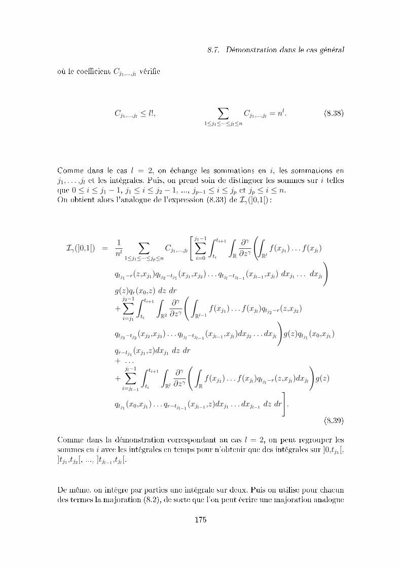
8.7. Démonstration dans le cas général
où le coecient Cj1,...,jlvérie
Cj1,...,jl≤ l!,
∑1≤j1≤···≤jl≤n
Cj1,...,jl= nl. (8.38)
Comme dans le cas l = 2, on échange les sommations en i, les sommations enj1, . . . ,jl et les intégrales. Puis, on prend soin de distinguer les sommes sur i tellesque 0 ≤ i ≤ j1 − 1, j1 ≤ i ≤ j2 − 1, ..., jp−1 ≤ i ≤ jp et jp ≤ i ≤ n.On obtient alors l'analogue de l'expression (8.33) de Iγ(]0,1[) :
Iγ(]0,1[) =1
nl
∑1≤j1≤···≤jp≤n
Cj1,...,jl
[j1−1∑i=0
∫ ti+1
ti
∫R
∂γ
∂zγ
(∫Rl
f(xj1) . . . f(xjl)
qtj1−r(z,xj1)qtj2−tj1(xj1 ,xj2) . . . qtjl
−tjl−1(xjl−1
,xjl) dxj1 . . . dxjl
)g(z)qr(x0,z) dz dr
+
j2−1∑i=j1
∫ ti+1
ti
∫R2
∂γ
∂zγ
(∫Rl−1
f(xj1) . . . f(xjl)qtj2−r(z,xj2)
qtj3−tj2(xj2 ,xj3) . . . qtjl
−tjl−1(xjl−1
,xjl)dxj2 . . . dxjl
)g(z)qtj1 (x0,xj1)
qr−tj1(xj1 ,z)dxj1 dz dr
+ . . .
+
jl−1∑i=jl−1
∫ ti+1
ti
∫Rl
∂γ
∂zγ
(∫Rf(xj1) . . . f(xjl
)qtjl−r(z,xjl
)dxjl
)g(z)
qtj1 (x0,xj1) . . . qr−tjl−1(xjl−1
,z)dxj1 . . . dxjl−1dz dr
].
(8.39)
Comme dans la démonstration correspondant au cas l = 2, on peut regrouper lessommes en i avec les intégrales en temps pour n'obtenir que des intégrales sur ]0,tj1 [,]tj1 ,tj2 [, ..., ]tjl−1
,tjl[.
De même, on intègre par parties une intégrale sur deux. Puis on utilise pour chacundes termes la majoration (8.2), de sorte que l'on peut écrire une majoration analogue
175
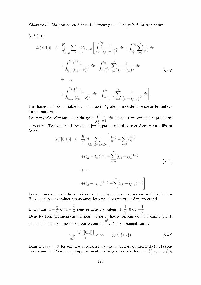
Chapitre 8. Majoration en δ et n de l'erreur pour l'intégrale de la trajectoire
à (8.34) :
|Iγ(]0,1[)| ≤ K
nl
∑1≤j1≤···≤jl≤n
Cj1,...,jl
[∫ tj12
0
1
(tj1 − r)γ2
dr +
∫ tj1
tj12
γ∑i=0
1
ri2
dr
+
∫ tj1+tj22
tj1
1
(tj2 − r)γ2
dr +
∫ tj2
tj1+tj22
γ∑i=0
1
(r − tj1)i2
dr
+ . . .
+
∫ tjl−1+tjl
2
tjl−1
1
(tjl− r)
γ2
dr +
∫ tjl
tjl−1+tjl
2
γ∑i=0
1(r − tjl−1
) i2
dr
].
(8.40)
Un changement de variable dans chaque intégrale permet de faire sortir les indicesde sommations.Les intégrales obtenues sont du type
∫ 1
12
1
uα2
du où α est un entier compris entre
zéro et γ. Elles sont ainsi toutes majorées par 1 ; ce qui permet d'écrire en utilisant(8.38) :
|Iγ(]0,1[)| ≤ K
nll!
∑1≤j1≤···≤jl≤n
[t1− γ
2j1
+
γ∑i=0
t1− i
2j1
+(tj2 − tj1)1− γ
2 +
γ∑i=0
(tj2 − tj1)1− i
2
+ . . .
+(tjl− tjl−1
)1− γ2 +
γ∑i=0
(tjl− tjl−1
)1− i2
].
(8.41)
Les sommes sur les indices croissants j1, . . . ,jl vont compenser en partie le facteurl!. Nous allons examiner ces sommes lorsque le paramètre n devient grand.
L'exposant 1− γ
2ou 1− i
2peut prendre les valeurs 1, 1
2, 0 ou −1
2.
Dans les trois premiers cas, on peut majorer chaque facteur de ces sommes par 1,et ainsi chaque somme se comporte comme n
l
l!. Par conséquent, on a :
supn,l
|Iγ(]0,1[)|l
<∞ (γ ∈ 1,2). (8.42)
Dans le cas γ = 3, les sommes apparaissant dans le membre de droite de (8.41) sontdes sommes de Riemann qui approximent des intégrales sur le domaine (x1, . . . ,xl) ∈
176
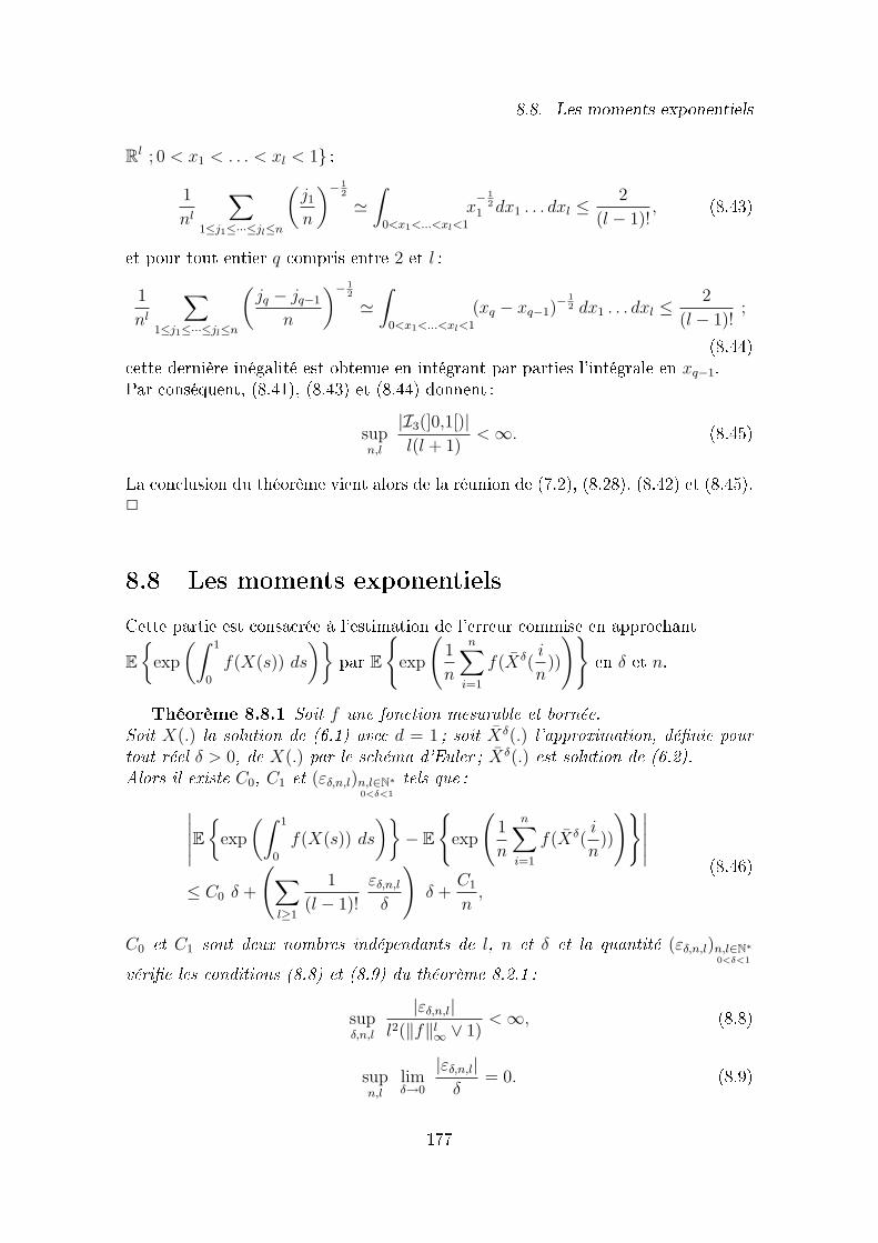
8.8. Les moments exponentiels
Rl ; 0 < x1 < . . . < xl < 1 :
1
nl
∑1≤j1≤···≤jl≤n
(j1n
)− 12
'∫
0<x1<...<xl<1
x− 1
21 dx1 . . . dxl ≤
2
(l − 1)!, (8.43)
et pour tout entier q compris entre 2 et l :
1
nl
∑1≤j1≤···≤jl≤n
(jq − jq−1
n
)− 12
'∫
0<x1<...<xl<1
(xq − xq−1)− 1
2 dx1 . . . dxl ≤2
(l − 1)!;
(8.44)cette dernière inégalité est obtenue en intégrant par parties l'intégrale en xq−1.Par conséquent, (8.41), (8.43) et (8.44) donnent :
supn,l
|I3(]0,1[)|l(l + 1)
<∞. (8.45)
La conclusion du théorème vient alors de la réunion de (7.2), (8.28), (8.42) et (8.45).2
8.8 Les moments exponentiels
Cette partie est consacrée à l'estimation de l'erreur commise en approchant
E
exp
(∫ 1
0
f(X(s)) ds
)par E
exp
(1
n
n∑i=1
f(Xδ(i
n))
)en δ et n.
Théorème 8.8.1 Soit f une fonction mesurable et bornée.Soit X(.) la solution de (6.1) avec d = 1 ; soit Xδ(.) l'approximation, dénie pourtout réel δ > 0, de X(.) par le schéma d'Euler ; Xδ(.) est solution de (6.2).Alors il existe C0, C1 et (εδ,n,l)n,l∈N∗
0<δ<1
tels que :∣∣∣∣∣E
exp
(∫ 1
0
f(X(s)) ds
)− E
exp
(1
n
n∑i=1
f(Xδ(i
n))
)∣∣∣∣∣≤ C0 δ +
(∑l≥1
1
(l − 1)!
εδ,n,l
δ
)δ +
C1
n,
(8.46)
C0 et C1 sont deux nombres indépendants de l, n et δ et la quantité (εδ,n,l)n,l∈N∗0<δ<1
vérie les conditions (8.8) et (8.9) du théorème 8.2.1 :
supδ,n,l
|εδ,n,l|l2(‖f‖l
∞ ∨ 1)<∞, (8.8)
supn,l
limδ→0
|εδ,n,l|δ
= 0. (8.9)
177
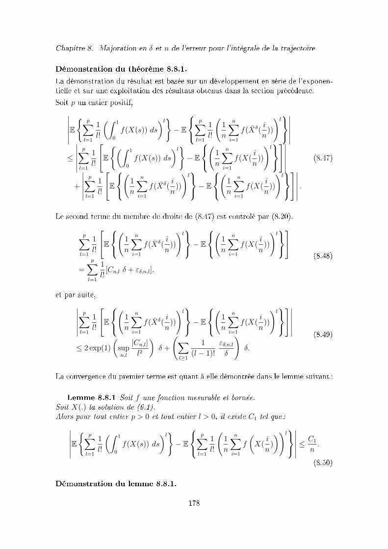
Chapitre 8. Majoration en δ et n de l'erreur pour l'intégrale de la trajectoire
Démonstration du théorème 8.8.1.
La démonstration du résultat est basée sur un développement en série de l'exponen-tielle et sur une exploitation des résultats obtenus dans la section précédente.Soit p un entier positif,∣∣∣∣∣∣E
p∑
l=1
1
l!
(∫ 1
0
f(X(s)) ds
)l− E
p∑
l=1
1
l!
(1
n
n∑i=1
f(Xδ(i
n))
)l∣∣∣∣∣∣
≤
∣∣∣∣∣∣p∑
l=1
1
l!
E
(∫ 1
0
f(X(s)) ds
)l− E
(
1
n
n∑i=1
f(X(i
n))
)l∣∣∣∣∣∣
+
∣∣∣∣∣∣p∑
l=1
1
l!
E
(
1
n
n∑i=1
f(Xδ(i
n))
)l− E
(
1
n
n∑i=1
f(X(i
n))
)l∣∣∣∣∣∣ .
(8.47)
Le second terme du membre de droite de (8.47) est contrôlé par (8.20).
p∑l=1
1
l!
E
(
1
n
n∑i=1
f(Xδ(i
n))
)l− E
(
1
n
n∑i=1
f(X(i
n))
)l
=
p∑l=1
1
l![Cn,l δ + εδ,n,l],
(8.48)
et par suite,∣∣∣∣∣∣p∑
l=1
1
l!
E
(
1
n
n∑i=1
f(Xδ(i
n))
)l− E
(
1
n
n∑i=1
f(X(i
n))
)l∣∣∣∣∣∣
≤ 2 exp(1)
(supn,l
|Cn,l|l2
)δ +
(∑l≥1
1
(l − 1)!
εδ,n,l
δ
)δ.
(8.49)
La convergence du premier terme est quant à elle démontrée dans le lemme suivant :
Lemme 8.8.1 Soit f une fonction mesurable et bornée.Soit X(.) la solution de (6.1).Alors pour tout entier p > 0 et tout entier l > 0, il existe C1 tel que :∣∣∣∣∣∣E
p∑
l=1
1
l!
(∫ 1
0
f(X(s)) ds
)l− E
p∑
l=1
1
l!
(1
n
n∑i=1
f
(X(
i
n)
))l∣∣∣∣∣∣ ≤ C1
n.
(8.50)
Démonstration du lemme 8.8.1.
178
8.8. Les moments exponentiels
Si pn désigne une suite d'entiers positifs, on peut écrire :
E
p∑
l=1
1
l!
(∫ 1
0
f(X(s)) ds
)l− E
p∑
l=1
1
l!
(1
n
n∑i=1
f
(X(
i
n)
))l
=
p∑l=1
1
l!
∫ 1
0
. . .
∫ 1
0
E f(X(s1)) . . . f(X(sl)) ds1 . . . dsl
− 1
nl
n∑il=1
· · ·n∑
i1=1
Ef
(X(
i1n
)
). . . f
(X(
iln
)
)
=
p∧(pn−1)∑l=1
1
l!Dn,l +
∑pn≤l≤p
1
l!Dn,l.
(8.51)
On utilise (8.13) pour majorer la somme dont l'indice l va de zéro à p ∧ (pn − 1).
pn−1∑l=1
1
l!|Dn,l| ≤ ‖f‖∞ exp(‖f‖∞)
(C1
n+ (C2 + C3‖f‖∞)
1
n
) (pn ≤
n
6
). (8.52)
Pour la somme allant de pn à p, on choisit pn tel que l'on puisse se contenter de lamajoration triviale |Dn,l| ≤ 2‖f‖l
∞ ; ainsi :
p∑l=pn
1
l!|Dn,l| ≤ 2
p∑l=pn
‖f‖l∞
l!≤ 2 exp(‖f‖∞)
‖f‖pn∞
pn!. (8.53)
On remarque que ces deux majorations (8.52) et (8.53) sont indépendantes de p. Enles réunissant dans (8.51), on obtient :∣∣∣∣∣∣E
p∑
l=1
1
l!
(∫ 1
0
f(Xs) ds
)l− E
p∑
l=1
1
l!
(1
n
n∑i=1
f
(X(
i
n)
))l∣∣∣∣∣∣
≤ 2 exp(‖f‖∞)‖f‖pn
∞pn!
+ ‖f‖∞ exp(‖f‖∞)
(C1
n+ (C2 + C3‖f‖∞)
1
n
).
(8.54)
Il reste à choisir la suite (pn)n>0 pour préciser la vitesse de convergence en n. Laseule restriction concernant cette suite est la majoration pn ≤ n
6. En choisissant
cette borne pour pn, on obtient∣∣∣∣∣∣E
p∑l=1
1
l!
(∫ 1
0
f(X(s)) ds
)l− E
p∑
l=1
1
l!
(1
n
n∑i=1
f(Xδ(i
n))
)l∣∣∣∣∣∣
≤ 2 exp(‖f‖∞)‖f‖
n6∞(
n6
)!
+ ‖f‖∞ exp(‖f‖∞)
(C1
n+ (C2 + C3‖f‖∞)
1
n
) (8.55)
et la conclusion (8.50) du lemme. 2
179
Chapitre 8. Majoration en δ et n de l'erreur pour l'intégrale de la trajectoire
Remarque :
Le terme ‖f‖n6∞(
n6
)!est négligeable devant les autres termes du membre de droite de
(8.55) lorsque n tend vers l'inni : par exemple, dès que n ≥ 12 ‖f‖∞ e, on a lamajoration suivante :
‖f‖n6∞(
n6
)!≤ 1
2n6
. (8.56)
En injectant (8.48) et (8.55) dans (8.47), on obtient l'existence de trois nombres C1,C2 et C3 tels que :∣∣∣∣∣∣E
p∑
l=1
1
l!
(∫ 1
0
f(X(s)) ds
)l− E
p∑
l=1
1
l!
(1
n
n∑i=1
f(Xδ(i
n))
)l∣∣∣∣∣∣
≤ 2 exp(1)
(supn,l
|Cn,l|l2
)δ +
(∑l≥1
1
(l − 1)!
εδ,n,l
δ
)δ
+ 2 exp(‖f‖∞)‖f‖
n6∞(
n6
)!
+ ‖f‖∞ exp(‖f‖∞)
(C1
n+ (C2 + C3‖f‖∞)
1
n
).
(8.57)
Le membre de droite est indépendant de p. En faisant tendre p vers +∞ dans (8.57)et en ne conservant que les termes dominants, on obtient la conclusion (8.46). 2
180
9
Majoration en δ= 1n de l'erreur pour
l'intégrale de la trajectoire
Dans la section précédente, nous avons présenté un développement en δ de l'erreur.Il a été montré que le coecient R(Φ(n,l)) devant δ est borné par rapport à n. Maisceci ne sut pas pour obtenir la vitesse de convergence de l'erreur puisque l'on necontrôle pas le reste εδ,n,l
δuniformément en n.
Nous allons reprendre l'étude de l'erreur en faisant tendre, en même temps et à lamême vitesse (δ = 1
n), les paramètres δ vers zéro et n vers l'inni.
Théorème 9.1.2 Soit f une fonction mesurable et bornée.Soit X(.) la solution de (6.1) avec d ∈ N∗ ; soit X
1n (.) l'approximation de cette
solution donnée par le schéma d'Euler .Alors il existe C tel que :∣∣∣∣∣E
∫ 1
0
f(X(s)) ds
− E
1
n
n∑i=1
f(X1n (i
n))
∣∣∣∣∣≤ C ‖f‖∞
1
n.
(9.1)
Démonstration du théorème 9.1.2.
On applique l'inégalité triangulaire (8.10) au membre de gauche de (9.1), puis laconclusion (8.13) du lemme 8.3.1 et enn celle (9.3) du théorème 9.1.3 ci-dessous.Ainsi il existe C1 et C2 tels que :∣∣∣∣∣E
∫ 1
0
f(X(s)) ds
− E
1
n
n∑i=1
f(X1n (i
n))
∣∣∣∣∣≤ ‖f‖∞
(C1
1
n+ C2
1
n
).
(9.2)
2
181
Chapitre 9. Majoration en δ= 1nde l'erreur pour l'intégrale de la trajectoire
Théorème 9.1.3 Soit f une fonction mesurable et bornée.Soit X(.) la solution de (6.1) ; soit X
1n (.) l'approximation de cette solution donnée
par le schéma d'Euler .Alors il existe un réel C tel que pour tous les entiers strictement positifs n :∣∣∣∣∣E
1
n
n∑i=1
f(X(i
n))
− E
1
n
n∑i=1
f(X1n (i
n))
∣∣∣∣∣ ≤ C ‖f‖∞1
n. (9.3)
Démonstration du théorème 9.1.3.
Le théorème 7.2.1 donne une expression de la dérivée de l'erreur comprenant deuxtermes où interviennent les dérivées première et seconde de la fonction Hr,n. Cesdeux termes sont de la forme suivante, où tantôt g = b et γ = 1, tantôt g = a
2et
γ = 2 :
I =
∫ 1
0
E[g(Xδ(r))− g(Xδ(r(δ)))
] ∂γHr,n
∂zγ(Xδ(t1), . . . ,X
δ(tnr),Xδ(r))
dr. (9.4)
Notation 9.1.2 Pour γ = 1 ou 2, on pose :
Q(n)γ (i,j,r) = E
∫
Rf(xj)
[gγ(X(r))− gγ(X(
i
n))
]∂γ
∂zγ
(qr, j
n(z,xj)
) ∣∣∣∣∣z=X(r)
dxj
(9.5)
où les entiers i, j, n et le réel r vérient les conditions :n ≥ 1 et 0 ≤ i/n < r < (i+ 1)/n ≤ j/n ≤ 1 ;
g1 et g2 désignent respectivement les fonctions b eta
2.
Avec ces notations, l'erreur commise en utilisant le schéma d'Euler de pas 1/n est
la somme des intégrales 1
n
∫ (i+1)/n
i/n
Q(n)1 (i,j,r) dr et 1
n
∫ (i+1)/n
i/n
Q(n)2 (i,j,r) dr où (i,j)
décrivent ∆(n) = (i,j) ; 0 ≤ i ≤ j − 1, 1 ≤ j ≤ n.Ce domaine peut être découpé en deux parties :
∆1(n) =k+1⋃p=2
(i,j) ; 0 ≤ i ≤ 2p−1 − 2, 2p−1 ≤ j ≤ 2p − 1
,
∆2(n) =k+1⋃p=2
(i,j) ; 2p−1 − 1 ≤ i ≤ j − 1, 2p−1 ≤ j ≤ 2p − 1
.
où k =
⌊log n
log 2
⌋. (bxc désigne la partie entière de x)
Nous avons : ∆(n) ⊂ (∆1(n) ∪∆2(n)) .Les deux lemmes suivants donnent des majorations de Q(n)
γ (i,j,r). Le Lemme 9.1.3sera utile pour la somme sur ∆1(n), le Lemme 9.1.4 pour celle sur ∆2(n).
182
Lemme 9.1.3 Il existe un entier n0 et une constante K1 indépendante de n, i,j et r tels que :
|Q(n)γ (i,j,r)| ≤ K1 ||f ||∞
(r − i
n
)(
jn− r) γ+1
2
(γ ∈ 1,2) (n > n0) (9.6)
Lemme 9.1.4 Il existe un entier n0 et une constante K2 indépendante de n, i,j et r tels que :
|Q(n)γ (i,j,r)| ≤ K2 ||f ||∞
(r − i
n
)√jn− r
(ni
) γ2
(γ ∈ 1,2) (n > n0) (9.7)
Montrons ici que ces deux majorations permettent de conclure.
Somme sur ∆1(n)
Comme r−i/n et j/n−r sont plus petit que 1, le terme dominant dans la majorationobtenue dans le Lemme 9.1.3 provient du cas γ = 2 et son ordre est (r− i/n)(j/n−r)−3/2. Ainsi il existe une constante K1 indépendante de n, i, j et r telle que pourtout n > n0 :
K−11
1
n
∑(i,j)∈∆1(n)
∣∣∣∣∣∫ (i+1)/n
i/n
Q(n)γ (i,j,r) dr
∣∣∣∣∣ ≤ 1
n
∑(i,j)∈∆1(n)
∫ i+1n
in
r − in(
jn− r) 3
2
dr
≤ 1
n2
k+1∑p=2
2p−1∑j=2p−1
2p−1−2∑i=0
2√jn− r
i+1n
in
≤ 2
n32
k+1∑p=2
2p−1∑j=2p−1
1√j − 2p−1 + 1
− 1√j
≤ 2
n32
k+1∑p=2
(∫ 2p−1
0
1√xdx−
∫ 2p
2p−1
1√xdx
)≤ 8
n32
√2
k
Le choix de k nous permet de conclure pour la somme sur ∆1(n) :
1
n
∑(i,j)∈∆1(n)
∣∣∣∣∣∫ (i+1)/n
i/n
Q(n)γ (i,j,r) dr
∣∣∣∣∣ ≤ 8 K1
n(γ ∈ 1,2) (n > n0) (9.8)
Somme sur ∆2(n)
183
Chapitre 9. Majoration en δ= 1nde l'erreur pour l'intégrale de la trajectoire
La majoration obtenue dans le Lemme 9.1.4 va nous permettre de contrôler lasomme sur ∆2(n) de la manière suivante : le terme prédominant est à nouveau obtenupour γ = 2 et l'on obtient l'existence d'une constante K2 indépendante de n, i, j etr telle que pour tout n > n0 :
K−12
1
n
∑(i,j)∈∆2(n)
∣∣∣∣∣∫ (i+1)/n
i/n
Q(n)γ (i,j,r) dr
∣∣∣∣∣ ≤ 1
n
∑(i,j)∈∆2(n)
∫ i+1n
in
n
i
r − in√
jn− r
dr
≤ 1
n
k+1∑p=2
2p−1∑j=2p−1
j−1∑i=2p−1−1
1
i
[−2
√j
n− r
] i+1n
in
≤ 2
n32
k+1∑p=2
2p−1∑i=2p−1−1
√2p − i− 1
i
≤ 2
n32
(2√
2 +k+1∑p=3
√2
p−1∫ 2p−1
2p−1−2
1
xdx
)
≤ 2
n32
(2√
2 +k+1∑p=3
√2
p−12 log 2
)
≤ 4
n32
(√
2 + 2 log 2
√2
k−2 − 1√2− 1
)
Le choix de k nous donne la majoration suivante :
1
n
∑(i,j)∈∆2(n)
∣∣∣∣∣∫ (i+1)/n
i/n
Q(n)γ (i,j,r) dr
∣∣∣∣∣ ≤ 4K2 log 2√2− 1
1
n+
4K2
√2
n32
(γ ∈ 1,2) (n > n0)
(9.9)
Les majorations (9.8) et (9.9) donnent un majorant de l'erreur en 1n.
Avant de prouver les Lemmes 9.1.3 et 9.1.4, montrons un lemme préliminaire
Notation 9.1.5 Soit G une variable aléatoire gaussienne centrée réduite. Onpose pour tout x ∈ R :
H(x) = σ(x)√r − i/nG+ b(x) (r − i/n) , (9.10)
Ψ(x) = (gγ(x+H(x))− gγ(x)) q(n)i/n(x0,x). (9.11)
184
Lemme 9.1.6 Sous les hypothèses (H 1) sur les fonctions σ et b, les fonctionsH et Ψ vérient :pour tout α, β, β1, β2 ∈ 0,1,2, q, q1, q2 ∈ N, la suite suivante est bornée :
(sup(i,r)∈Jn
∫RE
(i
n
)α/2∣∣∣∣∣ Ψ(α)(x)√
r − i/n
∣∣∣∣∣∣∣∣∣∣ H(β)(x)√
r − i/n
∣∣∣∣∣q
∣∣a(β1)(x)∣∣q1∣∣b(β2)(x)
∣∣q211
|G|≤ (r−i/n)−1/2
2||σ′||∞
dx
)n≥1
où Jn = (i,r) ∈ N× [0,1] ; i/n < r < (i+ 1)/n
Preuve du Lemme 9.1.6
D'après la dénition (9.11) de Ψ, il est immédiat que :
|Ψ(x)| ≤ |H(x)| ||g′γ||∞ q(n)i/n(x0,x) (9.12)
De la même manière, on calcule les deux premières dérivées de Ψ :
Ψ′(x) =((1 +H ′(x))g′γ(x+H(x))− g′γ(x)
)q(n)i/n(x0,x)
+ (gγ(x+H(x))− gγ(x))∂q
(n)i/n
∂x(x0,x)
Ψ′(x) =(g′γ(x+H(x))− g′γ(x)
)q(n)i/n(x0,x)
+H ′(x)g′γ(x+H(x))q(n)i/n(x0,x)
+ (gγ(x+H(x))− gγ(x))∂q
(n)i/n
∂x(x0,x).
Ceci nous donne la majoration suivante :
|Ψ′(x)| ≤ |H(x)| ||g′γ||∞
∣∣∣∣∣∂q(n)i/n
∂x(x0,x)
∣∣∣∣∣+ (|H(x)| ||g′′γ ||∞ + |H ′(x)| ||g′γ||∞)q(n)i/n(x0,x),
(9.13)
185
Chapitre 9. Majoration en δ= 1nde l'erreur pour l'intégrale de la trajectoire
Calculons à présent la dérivée seconde de Ψ :
Ψ′′(x) =((1 +H ′(x))g′′γ(x+H(x))− g′′γ(x)
)q(n)i/n(x0,x)
+(g′γ(x+H(x))− g′γ(x)
) ∂q(n)i/n
∂x(x0,x)
+H ′′(x)g′γ(x+H(x))q(n)i/n(x0,x)
+H ′(x)(1 +H ′(x))g′′γ(x+H(x))q(n)i/n(x0,x)
+H ′(x)g′γ(x+H(x))∂q
(n)i/n
∂x(x0,x)
+((1 +H ′(x))g′γ(x+H(x))− g′γ(x)
) ∂q(n)i/n
∂x(x0,x)
+ (gγ(x+H(x))− gγ(x))∂2q
(n)i/n
∂x2(x0,x).
Après factorisation, on obtient :
Ψ′′(x) =( (g′′γ(x+H(x))− g′′γ(x)
)+ 2H ′(x)g′′γ(x+H(x)) +
H ′′(x)g′γ(x+H(x)) +H ′(x)2g′′γ(x+H(x)))q(n)i/n(x0,x)
+2( (g′γ(x+H(x))− g′γ(x)
)+H ′(x)g′γ(x+H(x))
)∂q(n)i/n
∂x(x0,x)
+(gγ(x+H(x))− gγ(x)
)∂2q(n)i/n
∂x2(x0,x).
Nous obtenons ainsi :
|Ψ′′(x)| ≤(|H(x)| ||g(3)
γ ||∞ + |(H ′(x) + 2)H ′(x)| ||g′′γ ||∞ + |H ′′(x)| ||g′γ||∞)q(n)i/n(x0,x)
+2(|H(x)| ||g′′γ ||∞ + |H ′(x)| ||g′γ||∞
) ∣∣∣∣∂q(n)i/n
∂x(x0,x)
∣∣∣∣+ |H(x)| ||g′γ||∞∣∣∣∣∂2q
(n)i/n
∂x2 (x0,x)
∣∣∣∣(9.14)
Dans un premier temps, on peut remplacer dans (9.13) et (9.14) les dérivéesd'ordre κ du noyau q(n)
i/n(x0,x) par les majorations données dans (8.2) : C(ni
)κ/2
pMi/n(x−x0). (pσ2(x) désigne la densité d'une gaussienne centrée de variance σ2).
Par ailleurs, sur l'événement|G| ≤
(2||σ′||∞
√r − i/n
)−1, on obtient les majo-
rations des dérivées de H :
H ′(x) = σ′(x)(r − i/n)1/2G+ b′(x)(r − i/n)
|H ′(x)| ≤ 1
2+||b′||∞n
(9.15)
186
On obtient également|H ′′(x)| ≤ ||σ′′||∞
2||σ′||∞+||b′′||∞n
(9.16)
On sait donc que H ′ et H ′′ sont bornées sur l'événement considéré.
On en déduit l'existence d'une constante C indépendante de i,n,r tel que pour toutα ∈ 0,1,2 et pour n assez grand, on ait :(
i
n
)α/2∣∣Ψ(α)(x)∣∣ ≤ C |H(x)| ||g′γ||∞pMi/n(x− x0), (9.17)
ainsi, la famille du Lemme 9.1.6 est majorée par la famille suivante :(C ||g′γ||∞ sup(i,r)∈Jn
∫RE∣∣∣∣ H(x)√
r−i/n
∣∣∣∣ ∣∣∣∣ H(β)(x)√r−i/n
∣∣∣∣q∣∣a(β1)(x)∣∣q1∣∣b(β2)(x)
∣∣q2
pMi/n(x− x0) dx
)n≥1
Grâce à un changement de variable, l'intégrale précédente s'écrit :∫R2
∣∣∣∣∣σ(x0 + x
√Mi
n)y + b(x0 + x
√Mi
n)
√r− i
n
∣∣∣∣∣∣∣∣∣∣a(β1)(x0 + x
√Mi
n)
∣∣∣∣∣q1
×
∣∣∣∣∣σ(β)(x0 + x
√Mi
n)y + b(β)(x0 + x
√Mi
n)
√r− i
n
∣∣∣∣∣q
×∣∣∣b(β2)(x0 + x
√Min
)∣∣∣q2
p1(x)p1(y) dx dy
où p1 désigne la densité de la gaussienne centrée réduite. Le noyau p1(x)p1(y) assureque l'intégrale est uniformément bornée en r, i et n.
Remarque 9.1.7 Une petite variante dans la preuve précédente nous permet deconclure que sous les hypothèses du Lemme 9.1.6, la famille suivante est égalementbornée :
(sup(i,r)∈Jn
∫RE
(i
n
)α/2∣∣∣∣∣∂
αp(n)i/n
∂xα(x0,x)
∣∣∣∣∣∣∣∣∣∣ H(β)(x)√
r − i/n
∣∣∣∣∣q
∣∣a(β1)(x)∣∣q1∣∣b(β2)(x)
∣∣q211
|G|≤ (r−i/n)−1/2
2||σ′||∞
dx
)n≥1
Montrons à présent les Lemmes 9.1.3 et 9.1.4.Preuve du Lemme 9.1.3
187
Chapitre 9. Majoration en δ= 1nde l'erreur pour l'intégrale de la trajectoire
Nous allons écrire l'expression (9.5) de Q(n)γ (i,j,r) en utilisant une variable aléatoire
gaussienne : en eet, conditionnellement à X(i
n) = x, la v.a. X(r) s'écrit :
x+ σ(x)
√r − i
nG+ b(x)
(r − i
n
)︸ ︷︷ ︸
H(x)
où G désigne une gaussienne centrée réduite.L'expression (9.5) de Q(n)
γ (i,j,r) devient :
Q(n)γ (i,j,r) =
∫R
E
∫Rf(xj) [gγ(x+H(x))− gγ(x)]
∂γ
∂zγ
(qr, j
n(z,xj)
) ∣∣∣∣∣z=x+H(x)
dxj
q(n)in
(x0,x) dx
(9.18)
Écrivons le développement de Taylor avec reste intégrale des fonctions gγ etz 7−→ ∂γ
∂zγ
(qr, j
n(z,xj)
), nous obtenons alors :
Q(n)γ (i,j,r) =
∫R
E
∫Rf(xj)
[g′γ(x)H(x) +
∫ x+H(x)
x
g′′γ(u) (x+H(x)−u) du
][∂γ
∂xγ
(qr, j
n(x,xj)
)+
∫ x+H(x)
x
∂γ+1
∂uγ+1
(qr, j
n(u,xj)
)du
]dxj
q(n)in
(x0,x) dx
(9.19)Le développement du produit des deux crochets donne quatre termes T1, T2, T3 etT4.Dans T1, une simplication apparaît grâce à la symétrie de G.
T1 =
∫R
E∫
Rf(xj)g
′γ(x)H(x)
∂γ
∂xγ
(qr, j
n(x,xj)
)dxj q
(n)in
(x0,x) dx
=
∫R
∫Rf(xj)g
′γ(x)b(x)
(r − i
n
)∂γ
∂xγ
(qr, j
n(x,xj)
)dxj q
(n)in
(x0,x) dx(9.20)
On obtient alors une majoration de T1 :
|T1| ≤ K||f ||∞(r − i
n
)1(
jn− r) γ
2
(9.21)
188
Intéressons nous maintenant à T2 :
T2 =
∫R
E∫
Rf(xj)g
′γ(x)H(x)
∫ x+H(x)
x
∂γ+1
∂uγ+1
(qr, j
n(u,xj)
)du dxj q
(n)in
(x0,x) dx
|T2| ≤||f ||∞||g′γ||∞(
jn− r) γ+1
2
∫R
E(H2(x)
)q(n)in
(x0,x) dx
≤ K||f ||∞(r − i
n
)1(
jn− r) γ+1
2
(9.22)
Nous obtenons pour T3 et T4 :
T3 =
∫R
E∫
Rf(xj)
∂γ
∂xγ
(qr, j
n(x,xj)
)∫ x+H(x)
x
g′′γ(u) (x+H(x)−u) du dxj q(n)in
(x0,x) dx
|T3| ≤ K||f ||∞(r − i
n
)1(
jn− r) γ
2
(9.23)
T4 =
∫R
E∫
Rf(xj)
∫ x+H(x)
x
∂γ+1
∂uγ+1
(qr, j
n(u,xj)
)du∫ x+H(x)
x
g′′γ(u) (x+H(x)−u) du dxj q(n)in
(x0,x) dx
|T4| ≤ K||f ||∞(r − i
n
) 32 1(
jn− r) γ+1
2
(9.24)
Grâce aux inégalités (9.21),(9.22),(9.23) et (9.24), nous avons terminé la preuve duLemme 9.1.3.
Preuve du Lemme 9.1.4
La majoration obtenue dans le Lemme 9.1.3 n'est pas bonne lorsque i et j sonttrop proches ; on ne peut pas intégrer en r à cause du terme 1
(j/n−r)3/2 . Le but de ceLemme 9.1.4 est de trouver une majoration de Q(n)
γ (i,j,r) qui soit 'bonne' pour lesindices i et j dans ∆2(n).Dans ce cas, nous allons grâce à une intégration par partie faire porter l'irrégularitédue à la dérivée sur la transition entre l'instant initial et l'instant i
n.
Nous allons écrire la preuve complète dans le cas γ = 2. (le cas γ = 1 étant similaireet plus simple)
189
Chapitre 9. Majoration en δ= 1nde l'erreur pour l'intégrale de la trajectoire
On découpe Q(n)2 (i,j,r) en une somme de deux termes suivant que l'événement
|G| ≤(2||σ′||∞
√r − i/n
)−1
est réalisé ou non.
Q(n)2 (i,j,r) = Q2,1 +Q2,2 (9.25)
En suivant l'écriture de (9.18), on obtient :
Q2,1 = E
∫R2
f(xj)∂2
∂z2
(qr, j
n(z,xj)
)∣∣∣∣∣z=x+H(x)
Ψ(x)11|G|≤ ||σ′||−1
∞2
√r− i
n
dxj
dx (9.26)
Q2,2 =
∫R3
f(xj) [g2(z)− g2(x)]∂2
∂z2
(qr, j
n(z,xj)
)11B(i,n,r,x)(z)pσ2(x)(r−i/n)(z − x− b(x)(r − i/n)) dz dxj q
(n)in
(x0,x) dx
(9.27)
avec B(i,n,r,x) =
z ∈ R ;
∣∣∣∣∣z−x−b(x)(r − i
n
)σ(x)
∣∣∣∣∣ > 1
2||σ′||∞
.
Majoration de |Q2,1|D'abord on scinde l'expression (9.26) de Q2,1 en une somme de trois termes.
Q2,1 = E
∫R2
∂2qr, jn
∂x2(x,xj)g
′2(x)H(x)11
|G|≤ ||σ′||−1∞
2
√r− i
n
q(n)in
(x0,x) dx f(xj) dxj
+E
∫R2
∂2qr, jn
∂x2(x,xj)
∫ x+H(x)
x
g′′2(u)(x+H(x)−u) du11|G|≤ ||σ′||−1
∞2
√r− i
n
q(n)in
(x0,x) dx f(xj) dxj
+E
∫R2
∂2
∂z2
(qr, j
n(z,xj)
)∣∣∣∣∣z=x+H(x)
−∂2qr, j
n
∂x2(x,xj)
11|G|≤ ||σ′||−1
∞2
√r− i
n
Ψ(x) dx f(xj) dxj
(9.28)
Avec des notations évidentes, Q2,1 = I1 + I2 + I3.Dans I1, on utilise l'expression (9.10) de H.On remarque que la v.a. G 11
|G|≤(2||σ′||∞
√r− i
n
)−1 est centrée et il vient :
I1 = E
∫R2
∂2qr, jn
∂x2(x,xj)g
′2(x)(r −
i
n)b(x)11
|G|≤ ||σ′||−1∞
2
√r− i
n
q(n)in
(x0,x) dx f(xj) dxj
190
Intégrons par parties en x :
I1 = −E
∫R2
∂qr, jn
∂x(x,xj)(r −
i
n)g′2(x)b(x)11
|G|≤ ||σ′||−1
∞2
√r− i
n
∂q(n)in
∂x(x0,x) dx f(xj) dxj
−E
∫R2
∂qr, jn
∂x(x,xj)(r −
i
n)(g′′2(x)b(x) + g′2(x)b
′(x))
×11|G|≤ ||σ′||−1
∞2
√r− i
n
q(n)in
(x0,x) dx f(xj) dxj
La remarque 9.1.7 et les majorations sur les dérivées des noyaux permettentd'obtenir le contrôle suivant sur I1 : il existe une constante K indépendant de i, j,n et r telle que :
|I1| ≤K ||f ||∞√
jn− r
(r − i
n
)(1 +
√n
i
)(9.29)
Pour estimer un majorant de I2, nous allons à nouveau procéder à une intégration
par parties en x et nous allons avoir besoin de la dérivée de ϕ(x) =
∫ x+H(x)
x
g′′2(u)(x+
H(x)−u) du.
ϕ(x) = (x+H(x))
∫ x+H(x)
x
g′′2(u) du−∫ x+H(x)
x
ug′′2(u) du
ϕ′(x) = (1 +H ′(x))
∫ x+H(x)
x
g′′2(u) du
+(x+H(x))((1 +H ′(x))g′′2(x+H(x))− g′′2(x))
−(1 +H ′(x))(x+H(x))g′′2(x+H(x)) + xg′′2(x)
ϕ′(x) = (1 +H ′(x))
∫ x+H(x)
x
g′′2(u) du−H(x)g′′2(x)
Nous obtenons alors
|I2| ≤K ||f ||∞√
jn− r
(r − i
n
)(1 +
√n
i
)(9.30)
L'expression (9.15) nous assure que sur l'événement|G| ≤
(2||σ′||∞
√r − i/n
)−1,
la quantité 1 + H ′(x) est susamment éloignée de 0 pour n assez grand. On peutainsi procéder à une intégration par partie (double) dans I3.
191
Chapitre 9. Majoration en δ= 1nde l'erreur pour l'intégrale de la trajectoire
I3 = E
∫R2
∂2
∂z2
(qr, j
n(z,xj)
)∣∣∣∣∣z=x+H(x)
−∂2qr, j
n
∂x2(x,xj)
Ψ(x)11|G|≤ ||σ′||−1
∞2
√r− i
n
dx f(xj) dxj
= −E
∫R2
∂
∂z
(qr, j
n(z,xj)
)∣∣∣∣∣z=x+H(x)
(Ψ
1 +H ′
)′(x)11
|G|≤ ||σ′||−1∞
2
√r− i
n
dx f(xj) dxj
+E
∫R2
∂
∂z
(qr, j
n(z,xj)
)Ψ′(x)11
|G|≤ ||σ′||−1∞
2
√r− i
n
dx f(xj)dxj
= E
∫R2
qr, jn(x+H(x),xj)
(1
1 +H ′
(Ψ
1 +H ′
)′)′(x)11
|G|≤ ||σ′||−1∞
2
√r− i
n
dx f(xj) dxj
−E
∫R2
qr, jn(x,xj)Ψ
′′(x)11|G|≤ ||σ′||−1
∞2
√r− i
n
dx f(xj) dxj
(9.31)
Dans (9.31), on remplace qr, jn(x+H(x),xj) par l'expression :
qr, jn(x,xj) +
∫ x+H(x)
x
∂qr, jn
∂u(u,xj) du
Nous obtenons ainsi :
I3 = E
∫R
[∫Rqr, j
n(x,xj)
((1
1+H ′
(Ψ
1+H ′
)′)′−Ψ′′
)(x) dx (9.32)
+
∫R
∫ x+H(x)
x
∂qr, jn
∂u(u,xj) du
((1
1+H ′
(Ψ
1+H ′
)′)′)(x) dx
]
11|G|≤ ||σ′||−1
∞2
√r− i
n
f(xj) dxj
Un calcul des dérivées dans (9.32) et l'application des majorations du Lemme 9.1.6nous donne le contrôle suivant sur I3 :
|I3| ≤K||f ||∞√
jn− r
(r − i
n
)(ni
)(9.33)
En rassemblant les résultats obtenus par (9.29), (9.30) et (9.33) nous avons nale-ment
192
|Q2,1| ≤ K
(r − i
n
) (ni
) 1√jn− r
(9.34)
Majoration de |Qγ,2|Nous allons à nouveau prouver le résultat pour γ = 2, le cas γ = 1 se faisant d'unemanière analogue et plus simple. Q2,2 est donnée par l'expression (9.27) :
Q2,2 =
∫R3
f(xj) [g2(z)− g2(x)]∂2
∂z2
(qr, j
n(z,xj)
)11B(i,n,r,x)(z)pσ2(x)(r−i/n)(z − x− b(x)(r − i/n)) dz dxj q
(n)in
(x0,x) dx
On découpe l'intégrale en z suivant le signe de z − x− b(x)(r − i/n).On dénit :
Q+2,2 =
∫R2
f(xj) q(n)in
(x0,x)
∫ ∞
|σ(x)|2||σ′||∞
+x+b(x)(r− in
)
[g2(z)− g2(x)]∂2
∂z2
(qr, j
n(z,xj)
)pσ2(x)(r−i/n)(z − x− b(x)(r − i/n)) dz dxj dx
(9.35)et Q−
2,2 d'une manière analogue. Ainsi,
Q2,2 = Q−2,2 +Q+
2,2 (9.36)
Pour Q+2,2, une intégration par parties en z donne :
Q+2,2 =
∫R2
dxj dx f(xj) q(n)in
(x0,x)[(g2(z)− g2(x))pσ2(x)(r−i/n)(z − x− b(x)(r − i/n))
∂
∂zqr, j
n(z,xj)
]∞|σ(x)|
2||σ′||∞+x+b(x)(r− i
n)
−∫ ∞
|σ(x)|2||σ′||∞
+x+b(x)(r− in
)
∂
∂zqr, j
n(z,xj)(
(g2(z)− g2(x))p′σ2(x)(r−i/n)(z − x− b(x)(r − i/n))
+g′2(z) pσ2(x)(r−i/n)(z − x− b(x)(r − i/n)))
193
Chapitre 9. Majoration en δ= 1nde l'erreur pour l'intégrale de la trajectoire
Après un changement de variable, nous obtenons :
Q+2,2 =
∫R2
dxj dx f(xj) q(n)in
(x0,x)[(g2(x)− g2(
|σ(x)|2||σ′||∞
+ x+ b(x)(r − i
n))) exp(− 1
8||σ′||∞(r − i/n))
]∂
∂zqr, j
n(|σ(x)|
2||σ′||∞+ x+ b(x)(r − i
n),xj)
−∫ ∞
12||σ′||∞
√r− i
n
∂1
∂z1qr, j
n(y|σ(x)|
√r − i
n+ x+ b(x)(r − i
n),xj)[
(g2(x)− g2(y|σ(x)|√r − i
n+ x+ b(x)(r − i
n)))
y
|σ(x)|√r − i/n
+g′2(y|σ(x)|√r − i
n+ x+ b(x)(r − i
n))]e− y2
2
√2π
dy
On utilise la majoration de la dérivée du noyau q donnée par (8.2) et l'on intègre enxj, ce qui nous donne :
∣∣Q+2,2
∣∣ ≤ C||f ||∞||g′2||∞(jn− r) 1
2
∫Rdx q
(n)in
(x0,x)
∣∣∣∣ |σ(x)|2||σ′||∞
+ x+ b(x)
(r − i
n
)∣∣∣∣exp(− 1
8||σ′||∞(r−i/n))
+
∫ ∞
12||σ′||∞
√r− i
n
(∣∣∣∣∣y2 + yb(x)
|σ(x)|
√r − i
n
∣∣∣∣∣+ 1
)e−
y2
2
√2π
dy
On peut donc trouver des constantes C1 et C2 telles que :
∣∣Q+2,2
∣∣ ≤ ||f ||∞(jn− r) 1
2
exp(− 1
8||σ′||∞(r − i/n))
C1 + C2
√r − i
n+
1√r − i
n
(9.37)
On procède de la même manière pour majorer∣∣Q−
2,2
∣∣∣∣Q−
2,2
∣∣ ≤ ||f ||∞(jn− r) 1
2
exp(− 1
8||σ′||∞(r − i/n))
C1 + C2
√r − i
n+
1√r − i
n
(9.38)
La conclusion (9.7) du Lemme 9.1.4 découle de (9.25), (9.34), (9.36), (9.37) et (9.38).
194
9.2. Résultats numériques
9.2 Résultats numériques
Nous allons illustrer dans cette partie le résultat que nous venons de montrer.Nous approchons la quantité E(
∫ 1
0f(X(s))ds) où la diusion X(.) est donnée par
l'E.D.S. suivante :
X(t) =1
2+
∫ t
0
X(s)
1 +X2(s)ds+
∫ t
0
X(s) dBs.
La fonction f que l'on considère est la fonction indicatrice de l'évênement le pre-mier chire après la virgule est un 5 :
f(x) =∑m∈Z
11[0.5,0.6[(x−m).
0.22
0.222
0.224
0.226
0.228
0.23
0.232
0.234
0.236
0.238
0 0.02 0.04 0.06 0.08 0.1
Fig. 9.1 Approximation par le schéma d'Euler
Nous représentons sur cette gure l'approximation obtenue par notre méthodeen fonction de l'inverse du pas de discrétisation.Cette simulation amène plusieurs remarques :
• l'erreur semble être une fonction linéaire de l'inverse du pas de discrétisation ;nous avons seulement montré qu'elle est majorée par une fonction linéaire.
• la condition d'uniforme ellipticité imposée pour la diusion semble pouvoirêtre relaxée puisque la diusion X que nous considérons ici ne l'est pas.
195

Chapitre 9. Majoration en δ= 1nde l'erreur pour l'intégrale de la trajectoire
196

Troisième partie
Amplitude du mouvement brownienavec dérive
197

10
Amplitude du mouvement brownienavec dérive
10.1 Introduction
Le but est d'étudier le processus de l'amplitude d'un mouvement brownien réelavec dérive δ. Le cas δ = 0 a été étudié par Imhof [34], Vallois [64].Nous donnerons les résultats avec δ > 0, le cas δ < 0 s'en déduisant immédiatementpar symétrie.
Puisque limt→∞
Bδ(t) = +∞, nous allons décrire les amplitudes successives de Bδ
en remontant le temps à partir de l'instant où Bδ a atteint son minimum absolu.Pour cela, on va considérer :
S1 = − inft≥0Bδ(t)
ρ1 = supt ≥ 0,Bδ(t) = −S1(10.1)
S2 = sup0≤t≤ρ1
Bδ(t)
ρ2 = sup0 ≤ t ≤ ρ1,Bδ(t) = S2(10.2)
et plus généralement pour tout k ∈ N∗ :
Sk = supt∈[0,ρk−1]
(−1)kBδ(t)
ρk = supt ∈ [0,ρk−1],Bδ(t) = (−1)k Sk(10.3)
(avec la convention ρ0 = +∞).
Remarque 10.1.1 S1 est le minimum absolu de Bδ(t) pour t ≥ 0,
ρ1 est le dernier instant où ce minimum est atteint,
S2 est le maximum absolu de Bδ(t) pour t ≤ ρ1,
ρ2 est le dernier instant dans [0,ρ1] où ce maximum est atteint.
199
Chapitre 10. Amplitude du mouvement brownien avec dérive
An d'énoncer le résultat principal, introduisons la notation :Notation 10.1.2 Z(δ)(t) désigne la solution positive de l'équation diérentielle
stochastique suivante :
Z(δ)(t) = B(t) + δ
∫ t
0
coth(δZ(δ)(s)
)ds. (10.4)
Théorème 10.1.1 Soit Bδ un mouvement brownien avec dérive positive δ.
1. S1 suit une loi exponentielle de paramètre 2δ (i.e. de densité 2δe−2δx11x≥0).
2. Conditionnellement à S1 = a1, S2 a pour densité
δeδa1 sh(δa1)1
sh2(δ(x+ a1))11x≥0 (10.5)
3. Pour tout k ≥ 3, conditionnellement à S1 = a1, . . . ,Sk−1 = ak−1 :Sk a pour densité :
δsh δak−1 sh δ(ak−1 + ak−2)
sh δak−2
1
sh2 δ(ak−1 + x)110≤x≤ak−2
4. Pour tout k ≥ 1, conditionnellement à Sk = ak, . . . ,S1 = a1,• (Bδ(t))t≤ρk
et (Bδ(t+ ρk)−Bδ(ρk))0≤t≤ρk−1−ρksont indépendants
• (Bδ(t))t≤ρka même loi qu'un mouvement brownien avec dérive (−1)kδ
arrêté au premier temps d'atteinte du niveau (−1)kak et conditionné àne pas atteindre (−1)k+1ak−1
•((−1)k+1(Bδ(t+ ρk)−Bδ(ρk))
)0≤t≤ρk−1−ρk
est un processus (positif) qui
a même loi que Z(δ) déni par (10.4) arrêté au premier instant où ilatteint le niveau ak + ak−1.
Remarque 10.1.3 On a pris comme convention : a0 = ρ0 = +∞.
La suite du travail s'articulera ainsi :dans la partie 10.2, nous donnerons les résultats connus que nous utiliserons, puisnous donnerons les deux propositions centrales dans la partie suivante, enn nousprouverons le théorème 10.1.1.
10.2 Résultats préliminaires
Donnons ici les notations utilisées par la suite.
Notation 10.2.1 • B(t) est un mouvement brownien de dimension 1 par-tant de 0
• F = (Ft)t≥0 désigne la ltration engendrée par (B(t))t≥0
200
10.2. Résultats préliminaires
• Bα(t) désigne un mouvement brownien avec dérive α issu de 0Bα(t) = B(t) + α t
• Tαa est le temps d'atteinte d'un niveau a par Bα :Tα
a = inf t > 0 , Bα(t) = a• Aδ désigne le processus de l'amplitude de Bδ :Aδ(t) = sup
s∈[0,t]
Bδ(s)− infs∈[0,t]
Bδ(s).
• θδ est l'inverse continu à droite de Aδ :θδ(a) = inf u ≥ 0;Aδ(u) > a
Donnons ici un premier résultat classique ([54] page 301) relatif aux temps d'atteinted'un niveau donné par un processus de Markov en fonction de sa fonction d'échelle :
Lemme 10.2.2 Soit (Xt) un processus de Markov réel continu, s une fonctiond'échelle associée à X.On note Ta = inf t > 0,Xt = a.On a :
Px(Tb < Ta) =s(x)− s(a)
s(b)− s(a), pour x compris entre a et b.
En appliquant le lemme 10.2.2 au mouvement brownien avec dérive non nulle, on a :Corollaire 10.2.3 Soit α 6= 0. On a :
Px (Tαb < Tα
a ) =e−2αx − e−2αa
e−2αb − e−2αa, pour x compris entre a et b. (10.6)
Démonstration Une fonction d'échelle associée au mouvement brownien avec dé-rive α 6= 0 est :
s(y) = e−2αy.
Donnons une conséquence de ce corollaire 10.2.3 :Corollaire 10.2.4 Soit δ > 0. Alors
Px
(T δ
b <∞)
= e−2δ(x−b) , pour b < x (10.7)
Ajoutons ici un résultat d'égalité en loi qui nous sera utile par la suite :Proposition 10.2.5 Soient δ, x et y des réels positifs.
Les 2 processus suivants ont même loi :
• (Bδ(t),0 ≤ t ≤ T δx ) conditionné par
T δ
x < T δ−y
• (B−δ(t),0 ≤ t ≤ T−δ
x ) conditionné parT−δ
x < T−δ−y
201
Chapitre 10. Amplitude du mouvement brownien avec dérive
Démonstration Nous allons montrer ce résultat en appliquant le théorème de Gir-sanov.Soit F une fonction test.
A = E[F(B(t) + δt,0 ≤ t ≤ T δ
x
)|T δ
x < T δ−y
]= E
[F(B(t) + δt,0 ≤ t ≤ T δ
x
)11T δ
x<T δ−y
] 1
P(T δx < T δ
−y).
On utilise le corollaire 10.2.3 et on applique le théorème de Girsanov en remarquantque F
(B(t) + δt,0 ≤ t ≤ T δ
x
)11T δ
x<T δ−y est FT δ
xmesurable et T δ
x <∞ presque sûre-ment ([54] proposition VIII 1.3 ).
A = E[F(B(t),0 ≤ t ≤ T 0
x
)11T 0
x<T 0−y exp
(δB(T 0
x )− δ2
2T 0
x
)]e−2δx − e2δy
1− e2δy
= E[F(B(t),0 ≤ t ≤ T 0
x
)11T 0
x<T 0−y exp
(−δ
2
2T 0
x
)]e−δx − e2δy+δx
1− e2δy
Eectuons le même calcul pour B(t)− δt.
A = E[F(B(t)− δt,0 ≤ t ≤ T−δ
x
)|T−δ
x < T−δ−y
]= E
[F(B(t)− δt,0 ≤ t ≤ T−δ
x
)11T−δ
x <T−δ−y
] 1
P(T−δx < T−δ
−y )
= E[F(B(t),0 ≤ t ≤ T 0
x
)11T 0
x<T 0−y exp
(−δB(T 0
x )− δ2
2T 0
x
)]e2δx − e−2δy
1− e−2δy
= E[F(B(t),0 ≤ t ≤ T 0
x
)11T 0
x<T 0−y exp
(−δ
2
2T 0
x
)]eδx − e−2δy−δx
1− e−2δy
= A
On déduit de la proposition 10.2.5 leCorollaire 10.2.6 Soit δ > 0 et x > 0.
Les deux processus suivants ont même loi :
• (Bδ(t),0 ≤ t ≤ T δx )
• (B−δ(t),0 ≤ t ≤ T−δx ) conditionné par T−δ
x <∞
Donnons ici une conséquence immédiate de la proposition 10.2.5 (et du corollaire10.2.6) :
Corollaire 10.2.7 Soient δ, x et y des réels positifs.Les 2 processus suivants ont même loi :
• (Bδ(t),0 ≤ t ≤ T δ−x) conditionné par
T δ−x < T δ
y
• (B−δ(t),0 ≤ t ≤ T−δ
−x ) conditionné parT−δ−x < T−δ
y
.
202
10.2. Résultats préliminaires
D'autre part, les deux processus suivants ont même loi :
• (Bδ(t),0 ≤ t ≤ T δ−x) conditionné par T−δ
−x <∞• (B−δ(t),0 ≤ t ≤ T−δ
−x )
Démonstration Le résultat est immédiat en utilisant la proposition 10.2.5, le co-rollaire 10.2.6 et la symétrie du mouvement brownien.
Nous rappelons brièvement quelques résultats concernant la projection duale pré-visible et le grossissement de ltration.
Rappel : Soit A(0)t un processus croissant, nul en 0, continu à droite.
La projection duale prévisible de A(0)t est le processus prévisible croissant
continu à droite At caractérisé par :
E[∫ ∞
0Us dA(0)
s
]= E
[∫ ∞
0Us dAs
]. (10.8)
pour tout processus U prévisible positif.Puisque nous travaillons avec la ltration brownienne, un processus est prévi-sible si et seulement s'il est adapté.Soit T un temps d'arrêt borné, le processus U = 11[0,T ] est un processus prévi-sible, (10.8) s'écrit :
E[A
(0)T
]= E [AT ] . (10.9)
En raisonnant par classe monotone, il est facile de montrer que si un processus(At)t≥0 croissant et adapté, nul en 0, vérie (10.9) pour tout temps d'arrêtborné T , alors A est la projection duale prévisible de A(0).
Pour nir, nous rappelons un résultat de grossissement progressif que l'on peuttrouver dans Jeulin ([37] théorème 5.10 page 80). Pour cela, nous avons besoin dela dénition suivante :
Denition 10.2.8 Une variable aléatoire ρ est dite honnête si pour tout t > 0,ρ est égale à une variable Ft-mesurable sur ρ < t.
Théorème 10.2.1 [Jeulin] Soit ρ une variable aléatoire honnête. On note (Fρt )t≥0
la plus petite ltration continue à droite contenant (Ft)t≥0 pour laquelle ρ est untemps d'arrêt.Soit (Y ρ
t )t≥0 le processusY ρ
t = P (ρ ≤ t|Ft) ; t ≥ 0. (10.10)(Y ρ
t )t≥0 est une sous-martingale de partie martingale (Mρt )t≥0
χ(t) = −∫ t∧ρ
0
1
1− Y ρsd 〈B,Mρ〉s +
∫ t
0
11ρ<s1
Y ρsd 〈B,Mρ〉s (10.11)
B − χ = B est un Fρ mouvement brownien.
203
Chapitre 10. Amplitude du mouvement brownien avec dérive
10.3 Preuve du théorème 10.1.1
10.3.1 Une première décomposition
Dans un premier temps, nous allons prouver les résultats du théorème 10.1.1 pourk = 1 ; ils font l'objet de la proposition 10.3.1.Rappelons les notations :
S1 = − inft≥0Bδ(t)
ρ1 = supt ≥ 0,Bδ(t) = −S1(10.1)
Comme δ > 0, S1 est p.s. ni.On cherche : la loi de (S1,(Bδ(t),0 ≤ t ≤ ρ1),(Bδ(t),ρ1 ≤ t)) en conditionnant par lesvaleurs de S1.Le résultat qui suit n'est pas nouveau, il gure par exemple dans Williams [66],toutefois, notre approche est diérente, elle repose sur le grossissement progressif ;elle présente l'avantage de pouvoir s'appliquer à l'étude du processus Bδ arrêté auxtemps ρk.
Proposition 10.3.1 Soit S1 et ρ1 les deux variables aléatoires dénies par (10.1).Alors
• S1 suit une loi exponentielle de paramètre 2δ (i.e. de densité 2δe−2δx11x≥0).
• Conditionnellement à S1 = a1,1. (Bδ(t))t≤ρ1 et (Bδ(t+ ρ1)−Bδ(ρ1))t>0 sont deux processus indépendants
2. (Bδ(t))t≤ρ1 a même loi qu'un mouvement brownien avec dérive −δ arrêtéau premier temps d'atteinte du niveau −a1
3. (Bδ(t+ ρ1)− Bδ(ρ1))t≥0 est un processus (positif) qui a même loi que leprocessus (Z(δ)) déni par (10.4).
Notre approche repose sur la théorie du grossissement ; plus précisément nous réa-lisons un grossissement progressif avec ρ1. D'après le rappel, nous sommes conduitsdans un premier temps à calculer la projection duale prévisible de 11t≥ρ1.
Lemme 10.3.2 La projection duale prévisible de A(0)t = 11t≥ρ1
est : At = −2δBδ(t) où : Bδ(t) = infs≤t
Bδ(s)
Démonstration D'après le rappel, on cherche At processus croissant tel que pourtout temps d'arrêt borné T ,
E [AT ] = P(ρ1 ≤ T ).
ρ1 ≤ T signie qu'après l'instant T , Bδ ne va plus visiter Bδ(T ).On utilise le corollaire 10.2.4 :
P (ρ1 ≤ T |FT ) =e−2δBδ(T ) − e−2δBδ(T )
e−2δBδ(T ).
204
10.3. Preuve du théorème 10.1.1
On pose :
Y ρ1t =
e−2δBδ(t) − e−2δBδ(t)
e−2δBδ(t)
= 1− e−2δ(Bδ(t)−Bδ(t)). (10.12)(Y ρ1
t ) est une semi-martingale continue ; on cherche sa décomposition canonique enremarquant que exp(−2δBδ(t)) = exp(−2δB(t)− 2δ2t) est une martingale.
dY ρ1t = 2δe−2δ(Bδ(t)−Bδ(t)) dB(t)− 2δe−2δ(Bδ(t)−Bδ(t)) dBδ(t) (10.13)
Remarquons que (Bδ(t)− Bδ(t)) ≥ 0 donc exp(−2δ(Bδ(t)− Bδ(t))) ≤ 1 et on peutappliquer le théorème d'arrêt. On obtient :
E [Y ρ1
T ] = −2δE[∫ T
0
exp(−2δ(Bδ(t)−Bδ(t))) dBδ(t)
]= −2δE
[∫ T
0
dBδ(t)
]. (10.14)
Ce résultat provient du fait que la mesure aléatoire dBδ ne charge que les instantst tels que Bδ(t) = Bδ(t).
E [Y ρ1
T ] = −2δE[Bδ(T )
]
Introduisons la notation suivante :
Mρ1t =
∫ t
0
2δ exp(−2δ(Bδ(s)−Bδ(s))) dB(s). (10.15)
Mρ1 est la partie martingale de Y ρ1 .
Démonstration de la proposition 10.3.11) Nous allons dans un premier temps montrer les deux résultats suivants :
• S1 suit une loi exponentielle de paramètre 2δ .• Conditionnellement à S1 = a1 (Bδ(t))t≤ρ1 a même loi qu'un mouvementbrownien avec dérive δ arrêté au premier temps d'atteinte du niveau −a1 etconditionné par T δ
−a1<∞
Soit f et F des fonctions test. Posons :θ = E [f(S1)F (Bδ(s),0 ≤ s ≤ ρ1)] = E
[f(−Bδ(ρ1))F (Bδ(s),0 ≤ s ≤ ρ1)
]On pose : Ut = f(−Bδ(t))F (Bδ(s),0 ≤ s ≤ t) ; Ut est un processus prévisible doncon applique le lemme 10.3.2 et (10.8) :
θ = E [Uρ1 ] = E[∫ ∞
0
Ut dA(0)t
]= E
[∫ ∞
0
Ut dAt
]θ = −2δE
[∫ ∞
0
f(−Bδ(t))F (Bδ(s),0 ≤ s ≤ t) dBδ(t)
](10.16)
205
Chapitre 10. Amplitude du mouvement brownien avec dérive
Particularisons avec F = 1 pour obtenir la loi de S1.
E [f(S1)] = −2δE[∫ ∞
0
f(−Bδ(t)) dBδ(t)
]Puisque −Bδ est une fonction croissante continue, le 'changement de variable' u =−Bδ(t) donne :
E [f(S1)] = 2δE[∫ S1
0
f(u) du
]
= 2δ
∫ ∞
0
f(u) P(S1 ≥ u) du.
On déduit de ce calcul :
P(S1 ∈ du) = 2δP(S1 ≥ u) du.
Donc S1 admet pour densité 2δe−2δu11u≥0. Revenons à (10.16) ; (T δ−u,u ≥ 0) est
l'inverse continu à droite de −Bδ donc le 'changement de variable' u = −Bδ(t) nouspermet d'obtenir :
θ = 2δE[∫ +∞
0
f(u)F(Bδ(s),0 ≤ s ≤ T δ
−u
)11T δ
−u<∞ du
]= 2δ
∫ ∞
0
f(u) E[F(Bδ(s),0 ≤ s ≤ T δ
−u
)11T δ
−u<∞
]du
= 2δ
∫ ∞
0
f(u) E[F(Bδ(s),0 ≤ s ≤ T δ
−u
)|T δ−u <∞
]P(T δ−u <∞
)du
=
∫ ∞
0
f(u) E[F(Bδ(s),0 ≤ s ≤ T δ
−u
)|T δ−u <∞
]2δe−2δu du (10.17)
Cette dernière égalité termine la preuve de ces premiers résultats. Notons qu'uneapplication immédiate du corollaire 10.2.7 donne le deuxième résultat de la propo-sition 10.3.1.2) Nous nous intéressons à présent à l'étude de (Bδ(t+ ρ1)−Bδ(t))t≥0, nous allonsappliquer le théorème 10.2.1 avec ρ1. Remarquons que la variable aléatoire ρ1 estun dernier temps de passage donc est une variable aléatoire honnête : sur ρ1 ≤ t,ρ1 = sup
u ∈ [0,t],Bδ(u) = Bδ(t)
.
Nous obtenons :
χ(t) = −∫ t∧ρ1
0
1
e−2δ(Bδ(t)−Bδ(t))2δe−2δ(Bδ(s)−Bδ(s)) ds
+
∫ t
0
11ρ1<se−2δBδ(s)
e−2δBδ(s) − e−2δBδ(s)2δe−2δ(Bδ(s)−Bδ(s)) ds
χ(t) = −2δ(t ∧ ρ1) + 2δ
∫ t
0
11ρ1<se−2δBδ(s)
e−2δBδ(s) − e−2δBδ(s)ds (10.18)
206
10.3. Preuve du théorème 10.1.1
Utilisons (10.18) pour étudier (Bδ(t))t≥ρ1
χ(t+ ρ1)− χ(ρ1) = 2δ
∫ ρ1+t
ρ1
e−2δBδ(s)
e−2δBδ(s) − e−2δBδ(s)ds (10.19)
On obtient ainsi (B(t)− χ(t) = B1(t)) est un Fρ1 mouvement brownien.
Bδ(t) = B(t) + δt = B1(t) + δt+ χ(t)
Bδ(t+ ρ1)−Bδ(ρ1) = B1(t+ ρ1)−B1(ρ1) + δt+ χ(t+ ρ1)− χ(ρ1)
Posons :Z1(t) = Bδ(t+ ρ1)−Bδ(ρ1) = Bδ(t+ ρ1) + S1 (10.20)
Z1(t) = B1(t+ ρ1)−B1(ρ1)
+ δ
∫ ρ1+t
ρ1
1 + 2exp (−2δBδ(s))
exp (−2δBδ(s))− exp (−2δBδ(s))ds
= B1(t+ ρ1)−B1(ρ1)
+ δ
∫ ρ1+t
ρ1
exp (−2δBδ(s)) + exp (−2δBδ(s))
exp (−2δBδ(s))− exp (−2δBδ(s))ds
= B1(t+ ρ1)−B1(ρ1) (10.21)
+ δ
∫ ρ1+t
ρ1
exp (2δBδ(s)− 2δBδ(s)) + 1
exp (2δBδ(s)− 2δBδ(s))− 1ds
Puisque ρ1 est un Fρ1 temps d'arrêt, le processus
B1(t) = B1(t+ ρ1)−B1(ρ1) (10.22)
est un Fρ1 mouvement brownien indépendant de Fρ1ρ1.
Revenons à (10.21) en nous souvenant que pour t ≥ ρ1, Bδ(t) = −S1
Z1(t) = B1(t) + δ
∫ t
0
exp (2δZ1(s)) + 1
exp (2δZ1(s))− 1ds (10.23)
Z1(t) = B1(t) + δ
∫ t
0
coth (δZ1(s)) ds (10.24)
Z1 est la solution forte de (10.24) à valeurs dans R+ et est donc indépendant de Fρ1ρ1
donc de (Bδ(t))t≤ρ1 .
D'après la proposition 10.3.1, l'étude de (B−δ(t))t≤T−δ−a1
nous donnera le comporte-ment de Bδ sur [0,ρ1] où
T−δ−a1
= inft > 0,B−δ(t) = −a1
207
Chapitre 10. Amplitude du mouvement brownien avec dérive
10.3.2 Une deuxième décomposition : étude de (Bδ(t))t≤T δa
Pour des raisons de symétrie, nous allons étudier le processus (Bδ(t))t≤T δapour ob-
tenir (B−δ(t))t≤T−δ−a1
comme indiqué a la n de la partie précédente.Les techniques seront très proches de celles utilisées pour la proposition 10.3.1.On notera :
S = − inft∈[0,T δ
a ]Bδ(t) (10.25)
On souhaite étudier le processus (Bδ(t),0 ≤ t ≤ T δa ) conditionnellement à S. L'outil
sera à nouveau le grossissement progressif de ltration. A cet eet, on introduit :
ρ = supt ∈ [0,T δa ],Bδ(t) = −S. (10.26)
Donnons ici le résultat principal :Proposition 10.3.3 Soient S et ρ les variables aléatoires dénies par (10.25)
et (10.26). Alors :
• S a pour densité
ϕ(x) = δeδa sh δa1
sh2 δ(x+ a)11x≥0 (10.5)
• Conditionnellement à S = b,1. (Bδ(t))t≤ρ et (Bδ(t+ ρ)−Bδ(ρ))0≤t≤T δ
a−ρsont indépendants,
2. (Bδ(t))t≤ρ a même loi qu'un mouvement brownien avec dérive −δ ar-rêté au premier temps d'atteinte du niveau −b et conditionné à ne pasatteindre a
3. (Bδ(t+ ρ)−Bδ(ρ) = Z(t)) est un processus (positif) qui a même loi quele processus (Z(δ)) déni par (10.4) arrêté au premier instant où il atteintle niveau a+ b
ρ est un temps honnête, il s'agit de calculer la projection duale prévisible de 11[ρ,∞[. :Lemme 10.3.4 La projection duale prévisible de A
(0)t = 11t≥ρ
est : At = ln
(e−2δBδ(t∧T δ
a ) − e−2δa
1− e−2δa
)
où : Bδ(t) = − infs≤t
Bδ(s)
Démonstration Soit T un temps d'arrêt. Us = 11[0,T ] est un processus prévisibleélémentaire.
E[∫ ∞
0
Us dA(0)s
]= E [Uρ] = P(ρ ≤ T )
On a :11ρ≤T = 11ρ≤T≤T δ
a + 11T δa <T (10.27)
208
10.3. Preuve du théorème 10.1.1
Sur T ≤ T δa, ρ ≤ T signie qu'après l'instant T , Bδ va visiter a avant min
u≤TBδ(u).
En utilisant le corollaire 10.2.3, nous obtenons :
P(ρ ≤ T ≤ T δa |FT ) =
e−2δBδ(T ) − e−2δBδ(T )
e−2δBδ(T ) − e−2δa11T≤T δ
a (10.28)
On pose :
Y ρt =
e−2δBδ(t) − e−2δBδ(t)
e−2δBδ(t) − e−2δapour t ≥ 0 (10.29)
Mais Y ρT δ
a= 1 donc
P(ρ ≤ T |F) = Y ρT∧T δ
a(10.30)
On sait que e−2δBδ(t) = e−2δB(t)−2δ2t est une martingale, on trouve ainsi la décompo-sition canonique de la semi-martingale (Y ρ
t ) :
dY ρt =
1
e−2δBδ(t) − e−2δae−2δBδ(t)2δdB(t)
− e−2δBδ(t) − e−2δa(e−2δBδ(t) − e−2δa
)2 2δe−2δBδ(t)dBδ(t)
(10.31)
On utilise maintenant le fait que la mesure aléatoire dBδ ne charge que les points ttels que Bδ(t) = Bδ(t) et l'on obtient :
E(Y ρT∧T δ
a) = −2δE
[∫ T∧T δa
0
e−2δBδ(t)
e−2δBδ(t) − e−2δadBδ(t)
]
= E [AT ] = E[∫ ∞
0
Us dAs
] (10.32)
Soit Mρt la partie martingale intervenant dans la décomposition de Y ρ :
Mρt = 2δ
∫ t
0
1
e−2δBδ(s) − e−2δae−2δBδ(s) dB(s). (10.33)
Démonstration de la proposition 10.3.3
1) Soient f et F des fonctions tests et θ = E [f(S)F (Bδ(s),0 ≤ s ≤ ρ)].On a :
θ = E[f(−Bδ(ρ))F (Bδ(s),0 ≤ s ≤ ρ)
]Posons Ut = f(−Bδ(t))F (Bδ(s),0 ≤ s ≤ t).
209
Chapitre 10. Amplitude du mouvement brownien avec dérive
θ = E [Uρ] = E[∫ ∞
0
Ut dA(0)t
](Ut,t ≥ 0) est un processus prévisible donc :
θ = E[∫ ∞
0
Ut dAt
](10.34)
= −2δE
[∫ T δa
0
f(−Bδ(t))F (Bδ(s),0 ≤ s ≤ t)e−2δBδ(t)
e−2δBδ(t) − e−2δadBδ(t)
]
Particularisons avec F = 1 et eectuons le 'changement de variable' : x = −Bδ(t).
E [f(S)] = 2δE[∫ S
0
f(x)e2δx
e2δx − e−2δadx
]
= 2δE[∫ ∞
0
f(x)e2δx
e2δx − e−2δaP(S ≥ x) dx
] (10.35)
On en déduit que :
P(S ∈ dx) = 2δe2δx
e2δx − e−2δaP(S ≥ x) dx.
Donc S admet une densité φ et :
φ(x) = 2δe2δx
e2δx − e−2δa
∫ ∞
x
φ(s) ds (10.36)
Soit Φ déni par Φ(x) =∫∞
xφ(s) ds.
(10.36) est l'équation diérentielle vériée par Φ. On la résout sachant que Φ(0) = 1 :
Φ(x) =
∫ ∞
x
φ(s) ds =1− e−2δa
e2δx − e−2δa.
Par dérivation, nous obtenons :
φ(x) = 2δ(1− e−2δa)e2δx
(e2δx − e−2δa)2 11x≥0.
Le résultat annoncé sur la densité de S en découle.Revenons à (10.34) ; (T δ
−x,x ≥ 0) est l'inverse continu à droite de −Bδ donc le
210
10.3. Preuve du théorème 10.1.1
'changement de variable' x = −Bδ(t) nous permet d'obtenir :
θ = 2δ
∫ ∞
0
f(x)E[F (Bδ(s),0 ≤ s ≤ T δ
−x)11T δ−x<T δ
a
] e2δx
e2δx − e−2δadx
= 2δ
∫ ∞
0
f(x)E[F (Bδ(s),0 ≤ s ≤ T δ
−x)|T δ−x < T δ
a
]× e2δx
e2δx − e−2δaP(T δ
−x < T δa ) dx
= 2δ
∫ ∞
0
f(x)E[F (Bδ(s),0 ≤ s ≤ T δ
−x)|T δ−x < T δ
a
]× e2δx
e2δx − e−2δa
1− e−2δa
e2δx − e−2δadx
On utilise la proposition 10.2.5 et l'on obtient la loi de (Bδ(t),t ≤ ρ) conditionnelle-ment à S.2) On s'intéresse à présent au processus (Bδ(t + ρ) − Bδ(ρ),0 ≤ t ≤ T δ
a ). On note(Fρ
t )t≥0 la plus petite ltration contenant (Ft)t≥0 pour laquelle ρ est un temps d'ar-rêt. On applique le théorème 10.2.1, compte tenu du lemme 10.3.4, de (10.29) et(10.33), on a :
χ(t) = −∫ t∧ρ
0
(e−2δBδ(s) − e−2δa)2δe−2δBδ(s)
(e−2δBδ(s) − e−2δa)(e−2δBδ(s) − e−2δa)ds
+
∫ t
0
11ρ<s(e−2δBδ(s) − e−2δa)2δe−2δBδ(s)
(e−2δBδ(s) − e−2δBδ(s))(e−2δBδ(s) − e−2δa)ds
= −∫ t∧ρ
0
2δe−2δBδ(s)
e−2δBδ(s) − e−2δads
+
∫ t
0
11ρ<s2δe−2δBδ(s)
e−2δBδ(s) − e−2δBδ(s)ds
(10.37)
On en déduit :
χ(t+ ρ)− χ(ρ) = 2δ
∫ ρ+t
ρ
e−2δBδ(s)
e−2δBδ(s) − e−2δBδ(s)ds (10.38)
On sait que (B2(t) = B(t)− χ(t)) est un Fρ mouvement brownien.Soit Z(t) = Bδ(ρ+ t)−Bδ(ρ). Ce processus vérie l'équation :
Z(t) = B2(t) + δ
∫ t
0
coth (δZ(s)) ds (10.39)
où B2(t) = B2(t+ ρ)−B2(ρ) est un Fρ mouvement brownien indépendant de Fρρ .
De plus, T δa − ρ = inft ≥ 0,Z(t) = a+ b, avec b = −S.
211
Chapitre 10. Amplitude du mouvement brownien avec dérive
Il reste à remarquer que Z est une solution forte de (10.39) pour terminer la preuve.
Nous allons donner un résultat annexe ici qui sera utile pour calculer la loi de(S1,S2, · · · ,Sk) :
Corollaire 10.3.5 Soit S déni par :
S = − inft∈[0,T δ
a ]Bδ(t). (10.25)
Conditionnellement à S ≤ z, S a pour densité :
δ sh δa sh δ(z + a)
sh δz
1
sh2 δ(x+ a)110≤x≤z (10.40)
Démonstration On utilise le résultat de la proposition 10.3.3, S a pour densité lafonction ϕ donnée par (10.5) :
ϕ(x) = δeδa sh δa1
sh2 δ(x+ a)11x≥0.
Soit z > 0, soit ϕz(x) la densité de S, sachant S < z ; par dénition :
ϕz(x) =ϕ(x)∫ z
0
ϕ(y) dy
11x≤z. (10.41)
∫ z
0
ϕ(y) dy = δeδa sh δa
∫ z
0
1
sh2 δ(y + a)dy
= −eδa sh δa
[ch δ(y + a)
sh δ(y + a)
]z
y=0
= −eδa sh δa
(ch δ(z + a)
sh δ(z + a)− ch δa
sh δa
)=
eδa
sh δ(z + a)(ch δa sh δ(z + a)− ch δ(z + a) sh δa)∫ z
0
ϕ(y) dy =eδa
sh δ(z + a)sh δz (10.42)
Ce qui termine la preuve.
10.3.3 Preuve du théorème 10.1.1
Comme annoncé, les résultats du théorème 10.1.1 pour k = 2 sont une consé-quence immédiate des propositions 10.3.1 et 10.3.2 et de la symétrie du mouvementbrownien.Pour obtenir les résultats pour k ≥ 3, on raisonne par récurrence en appliquant lecorollaire 10.3.5.
212
10.4. Quelques applications
10.4 Quelques applications
10.4.1 Descriptions des densités
Nous allons donner ici une interprétation probabiliste des amplitudes :
Ak = Sk + Sk+1 (10.43)
Dans cette première proposition, nous allons donner la densité du vecteur (A1, . . . ,An)pour tout n ∈ N∗
Proposition 10.4.1 (A1, . . . ,An) a pour densité :
δn
[n−1∏k=1
e(−1)kδak
sh(δak)
]e(−1)n2δan − 1 + (−1)n+12δan
sh2 δan
110≤an≤···≤a1 (10.44)
Démonstration Soit F une fonction test.
E [F (A1, . . . ,An)] = E [F (S1 + S2, . . . ,Sn + Sn+1)]
=
∫F (x1 + x2, . . . ,xn + xn+1)δ
n+12e−2δx1
eδx1sh(δx1)
sh2 δ(x2 + x1)
n+1∏k=3
sh δxk−1 sh δ(xk−1 + xk−2)
sh δxk−2 sh2 δ(xk + xk−1)110≤xk≤xk−2dx1 . . . dxn+1
=
∫F (x1 + x2, . . . ,xn + xn+1)2δ
n+1 e−δx1 sh δxn∏n−1k=1 sh δ(xk+1 + xk)
1
sh2 δ(xn+1 + xn)11x1≥x3≥···≥011x2≥x4≥···≥0dx1 . . . dxn+1
On eectue maintenant le changement de variable :
x1 = x1
a1 = x1 + x2
. . .an = xn + xn+1
(10.45)
E [F (A1, . . . ,An)] =
∫F (a1, . . . ,an)2δn+1e−δx1
sh δ(an−1 − an−2 + · · ·+ (−1)na1 + (−1)n+1x1)(∏n−1k=1 sh δak
)sh2 δan
110≤an≤an−1≤···≤a111a1−a2+···+(−1)n+1an≤x1≤a1−a2+···+(−1)nan−1
dx1da1 . . . dan
213
Chapitre 10. Amplitude du mouvement brownien avec dérive
Reste alors à calculer la quantité suivante :
I =
∫ a1−a2+···+(−1)nan−1
a1−a2+···+(−1)n+1an
e−δx1 sh δ(an−1 − an−2 + · · ·+ (−1)na1 + (−1)n+1x1) dx1
= e−δa1eδa2 . . . e(−1)n−1an−1
∫ an
0
eδy sh δy dy
= e−δa1eδa2 . . . e(−1)n−1an−11
2δ
e(−1)n2δan − 1 + (−1)n+12δan
sh2 δan
Ainsi, nous obtenons :
E [F (A1, . . . ,An)] =
∫F (a1, . . . ,an)δn
[n−1∏k=1
e(−1)kδak
sh(δak)
](10.46)
e(−1)n2δan − 1 + (−1)n+12δan
sh2 δan
110≤an≤···≤a1 da1 . . . dan
Donnons maintenant une représentation probabiliste de ses variables aléatoires :Proposition 10.4.2(
ψ(2δA1),ψ(−2δA2)
ψ(−2δA1), . . . ,
ψ((−1)n+12δAn)
ψ((−1)n+12δAn−1)
)= (U1,U2, . . . ,Un) (10.47)
où U1,U2, . . . ,Un sont des variables aléatoires indépendantes uniformes sur [0,1],
ψ(x) =ex − 1− x
ex − 1(10.48)
Démonstration On connaît la densité h1 de A1 par rapport à la mesure de Le-besgue :
h1(x) =δ
2 sh2 δx
(e−2δx − 1 + 2δx
)(10.49)
Donnons ici le lemme calculatoire suivant :Lemme 10.4.3 ∫ x
0
e2y − 1− 2y
sh2 ydy =
ex
sh x
(e−2x − 1 + 2x
)(10.50)
Notons H1 la fonction de répartition de A1, on a :
H1(x) =δ
2
∫ x
0
e−2δu − 1 + 2δu
sh2 δudu
214
10.4. Quelques applications
On utilise le lemme, et on obtient :
H1(x) =δ
2 sh(−δx)e−δx
−δ(e2δx − 1− 2δx
)=
e2δx − 1− 2δx
e2δx − 1= ψ(2δx). (10.51)
On montre aisément que ψ est bijective et l'on obtient ainsi :
A1 ∼1
2δψ−1(U1) (10.52)
où U1 est une variable aléatoire uniforme sur [0,1].On calcule ici la densité h(x)
2 de A2 sachant A1 = x
h(x)2 (y) =
δ2
2
e2δy − 1− 2δy
sh2 δy
e−δx
sh δx110≤y≤x
2 sh2 δx
δ
1
e−2δx − 1 + 2δx
= δe−δx sh δx
e−2δx − 1 + 2δx
e2δy − 1− 2δy
sh2 δy110≤y≤x (10.53)
On note H(x)2 la fonction de répartition associée :
H(x)2 (y) =
e−δx sh δx
e−2δx − 1 + 2δxδ
∫ y
0
e2δt − 1− 2δt
sh2 δtdt. (10.54)
On applique à nouveau le lemme et l'on obtient :
H(x)2 (y) =
e−δx sh δx
e−2δx − 1 + 2δx
eδy
sh δy
(e−2δy − 1 + 2δy
)(10.55)
=ψ(−2δy)
ψ(−2δx). (10.56)
On a ainsi prouvé : (ψ(2δA1),
ψ(−2δA2)
ψ(−2δA1)
)∼ (U1,U2).
La proposition se démontre alors sans diculté par récurrence.
215

Chapitre 10. Amplitude du mouvement brownien avec dérive
216
Bibliographie
[1] D.J. Aldous. Deterministic and Stochastic Models for Coalescence (Aggre-gation, Coagulation) : A Review of the Mean-Field Theory for Probabilists.Bernoulli, 5 :348, 1999.
[2] K.B. Athreya and P.E. Ney. Branching Processes. Springer, 1972.[3] H. Babovsky. On a monte carlo scheme for smoluchowski's coagulation equation.
Monte Carlo Methods and Appl., 5(1) :118, 1999.[4] J.M. Ball and J. Carr. The discrete coagulation-fragmentation equations : exis-
tence, uniqueness and density conservation. J. Stat. Phys., 61(1-2) :203234,1990.
[5] V. Bally and D. Talay. The Euler scheme for stochastic dierential equations :error analysis with Malliavin calculus. Math. Comput. Simulation, 38(1-3) :3541, 1995. Probabilités numériques (Paris, 1992).
[6] V. Bally and D. Talay. The law of the Euler scheme for stochastic dierentialequations. I. Convergence rate of the distribution function. Probab. TheoryRelated Fields, 104(1) :4360, 1996.
[7] P. Beesack. Gronwall inequalities. Carleton University, Ottawa, Ont., 1975.Carleton Mathematical Lecture Notes, No. 11.
[8] J. Carr and F.P. da Costa. Instantaneous gelation in coagulation dynamics. Z.Angew. Math. Phys., 43 :974983, 1992.
[9] M. Deaconu, N. Fournier, and E. Tanré. A pure jump Markov process associatedwith Smoluchowski's coagulation equation. Prépublication de l'Institut ElieCartan, Nancy, (6), 2001.
[10] M. Deaconu and E. Tanré. Smoluchowski's Coagulation Equation : ProbabilisticInterpretation of Solutions for Constant, Additive and Multiplicative Kernels.Ann. Scuola Norm. Sup. Pisa Cl. Sci. (4), 29(3) :549579, 2000.
[11] L. Desvillettes, C. Graham, and S. Méléard. Probabilistic interpretation andnumerical approximation of a Kac equation without cuto. Stochastic Process.Appl., 84(1) :115135, 1999.
[12] R. Drake. A general mathematical survey of the coagulation equation. volume 3,pages 201376. Oergamon Press, Oxford, 1962.
[13] P.B. Dubovskii. Mathematical theory of coagulation. volume 23. Global Ana-lysis Research Center, Seoul National University, 1994.
[14] A. Eibeck and W. Wagner. An ecient stochastic algorithm for studying coa-
217
Bibliographie
gulation dynamics and gelation phenomena. SIAM J. Sci. Comput., 22(6) :921948, 2000.
[15] A. Eibeck and W. Wagner. Stochastic algorithms for studying coagulationdynamics and gelation phenomena. Monte Carlo Methods Appl., Special Issueof Monte Carlo Methods, 2000.
[16] M.H. Ernst, R.M. Zi, and E.M. Hendriks. Coagulation Processes with phasetransition. J. Colloid Interface Sci, 97(1) :266277, 1984.
[17] S.N. Evans and J. Pitman. Construction of Markovian coalescents. Ann. I.H.P.,Probabilités et Statistiques, 34 :339383, 1998.
[18] W. Feller. An Introduction to Probability Theory and Its Applications, volume 2.John Willey and Sons, 1966.
[19] R. Ferland, X. Fernique, and G. Giroud. Compactness of the uctuations asso-ciated with some generalized nonlinear Boltzmann equations. Canad. J. Math.,44 :11921205, 1992.
[20] X. Fernique. Convergence en loi de fonctions aleatoires continues ou càdlàg,propriétés de compacité des lois. In Séminaire de Probabilités XX, LNM, volume1485, pages 178195. Springer, 1991.
[21] P.J. Flory. Molecular size distribution in three dimensional polymers. I. Gela-tion. J. Amer. Chem. Soc., 63 :30913096, 1941.
[22] P.J. Flory. Molecular size distribution in three dimensional polymers. II. Tri-functional branching units. J. Amer. Chem. Soc., 63 :30833090, 1941.
[23] P.J. Flory. Molecular size distribution in three dimensional polymers. III. Te-trafunctional branching units. J. Amer. Chem. Soc., 63 :30963100, 1941.
[24] N. Fournier and S. Méléard. A stochastic particle numerical method for 3DBoltzmann equations without cuto. to appear in Mathematics of computation,2000.
[25] N. Fournier and S. Méléard. A Markov process associated with a Boltzmannequation without cuto and for non Maxwell molecules. Prépublication duLaboratoire de probabilités et modèles aléatoires, Paris 6 et 7, (608), 2000.
[26] N. Fournier and S. Méléard. Existence results for 2D homogeneous Boltzmannequations without cuto and for non Maxwell molecules by use of Malliavincalculus. Prépublication du Laboratoire de probabilités et modèles aléatoires,Paris 6 et 7, (622), 2000.
[27] I. I. Ghman and A. V. Skorohod. Stochastic dierential equations. Springer-Verlag, New York, 1972. Translated from the Russian by Kenneth Wickwire,Ergebnisse der Mathematik und ihrer Grenzgebiete, Band 72.
[28] A.M. Golovin. The solution of the coagulating equation for cloud droplets in arising air current. Izv. Geophys., 5 :482487, 1963.
[29] M. Gordon. Good's theory of cascade processes applied to the statistics ofpolymer distribution. Proc. R. Soc. London, 268 :240259, 1962.
[30] C. Graham and S. Méléard. Stochastic particle approximations for generalizedboltzmann models and convergence estimates. Ann. Probab., 25(1) :115132,1997.
218
[31] C. Graham and S. Méléard. Existence and regularity of a solution of a Kacequation without cuto using the stochastic calculus of variations. Comm.Math. Phys., 205(3) :551569, 1999.
[32] F. Guias. Coagulation-fragmentation processes : relations between nite particlemodels and dierential equations. PhD thesis, Universitat Heidelberg, 1998.
[33] O.J. Heilmann. Analytical solutions of Smoluchowski's coagulation equation.J. Phys. A, 25(13) :37633771, 1992.
[34] J.P. Imhof. On the range of Brownain motion and its inverse process. Ann.Prob., 13 :10111017, 1985.
[35] J. Jacod and A.N. Shiryaev. Limit theorems for stochastic processes. Springer-Verlag, Berlin, 1987.
[36] I. Jeon. Existence of gelling solutions for coagulation-fragmentation equations.Comm. Math. Phys., 194(3) :541567, 1998.
[37] T. Jeulin. Semi-Martingales et Grossissement d'une Filtration. Springer Verlag,1980.
[38] I. Karatzas and S. E. Shreve. Brownian motion and stochastic calculus.Springer-Verlag, New York, second edition, 1991.
[39] N. El Karoui and J-P. Lepeltier. Représentation des processus ponctuels mul-tivariés à l'aide d'un processus de Poisson. Z. Wahrscheinlichkeitstheorie undVerw. Gebiete, 39(2) :111133, 1977.
[40] N.J. Kokholm. On Smoluchowski's coagulation equation. J. Phys. A, 21 :839842, 1988.
[41] S. Kusuoka and D. Stroock. Applications of the Malliavin calculus. III. J. Fac.Sci. Univ. Tokyo Sect. IA Math., 34(2) :391442, 1987.
[42] R. Lang and X.X. Nguyen. Smoluchowski's theory of coagulation in colloidsholds rigorously in the Boltzmann-Grad-Limit. Z. Wahrscheinlichkeitstheorieverw. Gebiete, 54 :227280, 1980.
[43] P. Laurençot. The discrete coagulation equations : existence of solutions andgelation. Private Communication, 1999.
[44] F. Leyvraz. Phys. Rev. A, 29 :854, 1984.[45] F. Leyvraz and H.R. Tschudi. Singularities in the kinetics of coagulation pro-
cesses. J. Phys. A : Math. Gen., 14 :33893405, 1981.[46] A. A. Lushnikov. Some new aspects of coagulation theory. Izv. Akad. Nauk
SSSR, Ser. Fiz. Atmosfer. I Okeana, 14(10) :738743, 1978.[47] A. H. Marcus. Stochastic coalescence. Technometrics, 10(1) :133148, 1968.[48] J.B. McLeod. On an innite set of non-linear dierential equations. Quart, J.
Math. Oxford Ser, 13(2) :119128, 1962.[49] S. Méléard. Asymptotic behaviour of some interacting particle systems ;
McKean-Vlasov and Boltzmann models. In Probabilistic models for nonlinearpartial dierential equations (Montecatini Terme, 1995), pages 4295. Springer,Berlin, 1996.
219
Bibliographie
[50] S. Méléard. Convergence of the uctuations for interacting diusion with jumpsassociated with Boltzmann equations. Stochastics and Stoch. Rep., 63 :195225,1998.
[51] Z.A. Melzak. A scalar transport equation. Trans. Amer. Math. Soc., 85 :547560, 1957.
[52] J.R. Norris. Smoluchowski's coagulation equation : uniqueness, nonuniquenessand a hydrodynamic limit for the stochastic coalescent. Ann. Appl. Probab.,9(1) :78109, 1999.
[53] J.R. Norris. Cluster coagulation. Comm. Math. Phys., 209(2) :407435, 2000.[54] D. Revuz and M. Yor. Continuous Martingales and Brownian Motion. Springer
Verlag, 1998.[55] A. Sánchez-Calle. Fundamental solutions and geometry of the sum of squares
of vector elds. Invent. Math., 78(1) :143160, 1984.[56] M.V. Smoluchowski. Drei Vortage uber Diusion, Brownsche Bewegung und
Koagulation von Kolloidteilchen. Physik., 17 :557585, 1916.[57] J.L. Spouge. Asymmetric bonding of identical units : a general AgRBf−g poly-
mer model. Macromolecules, 16 :831835, 1983.[58] J.L. Spouge. Equilibrium polymer distributions. Macromolecules, 16 :121127,
1983.[59] J.L. Spouge. The size distribution for the AgRBf−g model of polymerization.
J. Stat. Phys., 31(2) :363378, 1983.[60] J.L. Spouge. A branching-process solution of the polydisperse coagulation equa-
tion. Adv. Appl. Prob., 16 :5669, 1984.[61] D. Talay and L. Tubaro. Expansion of the global error for numerical schemes
solving stochastic dierential equations. Stochastic Anal. Appl., 8(4) :483509(1991), 1990.
[62] H. Tanaka. Probabilistic treatment of the Boltzmann equation of Maxwellianmolecules. Z. Wahrscheinlichkeitstheorie verw. Gebiete, 46 :67105, 1978.
[63] H. Tanaka. Probabilistic treatment of the Boltzmann equation of Maxwellianmolecules. Z. Wahrsch. Verw. Gebiete, 46(1) :67105, 1978/79.
[64] P. Vallois. Decomposing the Brownian path via the range process. Stoch. proc.and their app., 55 :211226, 1995.
[65] P.G.J van Dongen and M. H. Ernst. Cluster size distribution in irreversibleaggregation at large times. J. Phys. A : Math. Gen., 18 :27792793, 1985.
[66] D. Williams. Path Decomposition and Continuity of Local Time for one-dimensional diusions, I. Proc. London Math. Soc., 28 :738768, 1974.
220

.
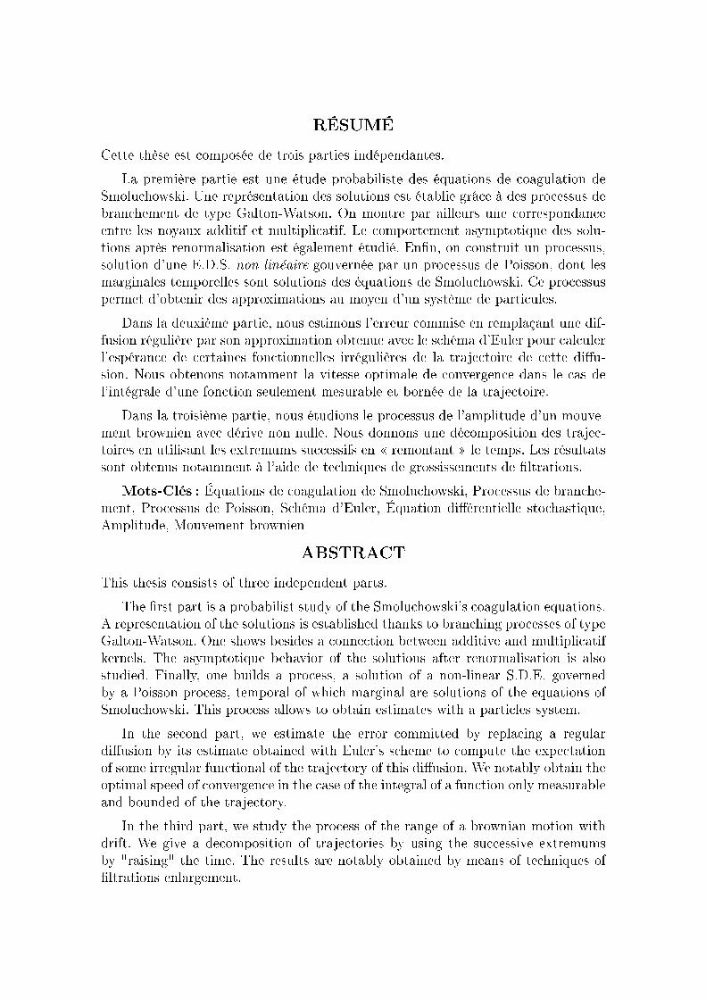
RÉSUMÉ
Cette thèse est composée de trois parties indépendantes.La première partie est une étude probabiliste des équations de coagulation de
Smoluchowski. Une représentation des solutions est établie grâce à des processus debranchement de type Galton-Watson. On montre par ailleurs une correspondanceentre les noyaux additif et multiplicatif. Le comportement asymptotique des solu-tions après renormalisation est également étudié. Enn, on construit un processus,solution d'une E.D.S. non-linéaire gouvernée par un processus de Poisson, dont lesmarginales temporelles sont solutions des équations de Smoluchowski. Ce processuspermet d'obtenir des approximations au moyen d'un système de particules.
Dans la deuxième partie, nous estimons l'erreur commise en remplaçant une dif-fusion régulière par son approximation obtenue avec le schéma d'Euler pour calculerl'espérance de certaines fonctionnelles irrégulières de la trajectoire de cette diu-sion. Nous obtenons notamment la vitesse optimale de convergence dans le cas del'intégrale d'une fonction seulement mesurable et bornée de la trajectoire.
Dans la troisième partie, nous étudions le processus de l'amplitude d'un mouve-ment brownien avec dérive non nulle. Nous donnons une décomposition des trajec-toires en utilisant les extremums successifs en remontant le temps. Les résultatssont obtenus notamment à l'aide de techniques de grossissements de ltrations.
Mots-Clés : Équations de coagulation de Smoluchowski, Processus de branche-ment, Processus de Poisson, Schéma d'Euler, Équation diérentielle stochastique,Amplitude, Mouvement brownien
ABSTRACT
This thesis consists of three independent parts.The rst part is a probabilist study of the Smoluchowski's coagulation equations.
A representation of the solutions is established thanks to branching processes of typeGalton-Watson. One shows besides a connection between additive and multiplicatifkernels. The asymptotique behavior of the solutions after renormalisation is alsostudied. Finally, one builds a process, a solution of a non-linear S.D.E. governedby a Poisson process, temporal of which marginal are solutions of the equations ofSmoluchowski. This process allows to obtain estimates with a particles system.
In the second part, we estimate the error committed by replacing a regulardiusion by its estimate obtained with Euler's scheme to compute the expectationof some irregular functional of the trajectory of this diusion. We notably obtain theoptimal speed of convergence in the case of the integral of a function only measurableand bounded of the trajectory.
In the third part, we study the process of the range of a brownian motion withdrift. We give a decomposition of trajectories by using the successive extremumsby "raising" the time. The results are notably obtained by means of techniques ofltrations enlargement.