Étude formelle des distributions de logiciel libre · a formal study of free software...
TRANSCRIPT
Université Paris Diderot — Paris 7École doctorale de Sciences Mathématiques de Paris Centre
THÈSEpour obtenir le grade de
DOCTEUR DE L’UNIVERSITÉ PARIS DIDEROTSpécialité : Informatique
présentée parJacob Pieter BOENDER
Directeur : Roberto DI COSMO
Étude formelle des distributions de logiciel libre
A formal study of Free Software Distributions
soutenue le 24 mars 2011devant le jury composé de :
M. Roberto DI COSMO directeurM. Jesús M. GONZÁLEZ-BARAHONA examinateur
M. Carsten SINZ rapporteurM. Diomidis SPINELLIS examinateur
M. Jean-Bernard STEFANI examinateurM. Ralf TREINEN examinateur
M. Peter VAN ROY rapporteur

2
Contents CRésumé 5La théorie des paquets . . . . . . . . . . . . . . . . . . . . . . . . . . . . . 6Algorithmes et outils . . . . . . . . . . . . . . . . . . . . . . . . . . . . . . 8Formalisation . . . . . . . . . . . . . . . . . . . . . . . . . . . . . . . . . . 9Validation et analyse . . . . . . . . . . . . . . . . . . . . . . . . . . . . . . 9Conclusions et perspectives . . . . . . . . . . . . . . . . . . . . . . . . . . 10
1 Introduction 111.1 F/OSS Software Distributions . . . . . . . . . . . . . . . . . . . . . . 111.2 Contributions . . . . . . . . . . . . . . . . . . . . . . . . . . . . . . . 121.3 Structure . . . . . . . . . . . . . . . . . . . . . . . . . . . . . . . . . . 14
2 Definitions 172.1 Existing package formats . . . . . . . . . . . . . . . . . . . . . . . . . 172.2 Definitions . . . . . . . . . . . . . . . . . . . . . . . . . . . . . . . . . 282.3 Installability . . . . . . . . . . . . . . . . . . . . . . . . . . . . . . . . 302.4 Dependencies . . . . . . . . . . . . . . . . . . . . . . . . . . . . . . . 32
3 Strong dependencies and conflicts 373.1 Strong dependencies . . . . . . . . . . . . . . . . . . . . . . . . . . . 373.2 Dominators . . . . . . . . . . . . . . . . . . . . . . . . . . . . . . . . 393.3 Dominators in strong dependency graphs and control flow graphs 413.4 Strong conflicts . . . . . . . . . . . . . . . . . . . . . . . . . . . . . . 46
4 Algorithms 534.1 Installability . . . . . . . . . . . . . . . . . . . . . . . . . . . . . . . . 534.2 Strong dependencies . . . . . . . . . . . . . . . . . . . . . . . . . . . 544.3 Dominators . . . . . . . . . . . . . . . . . . . . . . . . . . . . . . . . 594.4 Strong conflicts . . . . . . . . . . . . . . . . . . . . . . . . . . . . . . 60
5 Tools 635.1 distcheck . . . . . . . . . . . . . . . . . . . . . . . . . . . . . . . . . . 635.2 dose . . . . . . . . . . . . . . . . . . . . . . . . . . . . . . . . . . . . . 635.3 Ceve . . . . . . . . . . . . . . . . . . . . . . . . . . . . . . . . . . . . 655.4 Pkglab . . . . . . . . . . . . . . . . . . . . . . . . . . . . . . . . . . . 66
6 Formalisation 716.1 Repository . . . . . . . . . . . . . . . . . . . . . . . . . . . . . . . . . 716.2 Dependencies . . . . . . . . . . . . . . . . . . . . . . . . . . . . . . . 726.3 The dependency cone . . . . . . . . . . . . . . . . . . . . . . . . . . . 766.4 Repository properties . . . . . . . . . . . . . . . . . . . . . . . . . . . 786.5 Installability . . . . . . . . . . . . . . . . . . . . . . . . . . . . . . . . 806.6 Strong dependencies and conflicts . . . . . . . . . . . . . . . . . . . 82
3
6.7 Triangle conflicts . . . . . . . . . . . . . . . . . . . . . . . . . . . . . 84
7 Experimentation and validation 917.1 Repositories . . . . . . . . . . . . . . . . . . . . . . . . . . . . . . . . 917.2 Run time of the installability algorithm . . . . . . . . . . . . . . . . 937.3 Run time of the strong dependency algorithm . . . . . . . . . . . . 957.4 The dominator graph . . . . . . . . . . . . . . . . . . . . . . . . . . . 967.5 Run time of the strong conflict algorithm . . . . . . . . . . . . . . . 98
8 Graph properties of distributions 1098.1 Small world properties . . . . . . . . . . . . . . . . . . . . . . . . . . 1098.2 Distributions as small world networks . . . . . . . . . . . . . . . . . 111
9 Conclusion 1259.1 Summary . . . . . . . . . . . . . . . . . . . . . . . . . . . . . . . . . . 1259.2 Practical usage . . . . . . . . . . . . . . . . . . . . . . . . . . . . . . . 1269.3 Related works . . . . . . . . . . . . . . . . . . . . . . . . . . . . . . . 1279.4 Future work . . . . . . . . . . . . . . . . . . . . . . . . . . . . . . . . 130
Acknowledgements 131
4
Résumé RDe quoi s’agit-il ?
— FERDINAND FOCH
Comme l’indique le titre, dans cette thèse, il sera beaucoup question desdistributions du logiciel libre (aussi connu sous l’abréviation F/OSS, free andopen source software).
Ces distributions sont extrêmement hétérogènes. Elles contiennent des lo-giciels de différentes provenances ; écrits dans des langages différents, avec descalendriers de publication différents et avec des procédures différentes.
Pour gérer cette hétérogénéité, et pour avoir une façon simple et uniqued’installer des logiciels, les systèmes de paquetage ont été développés. Ceux-ciconsistent en l’emballage d’un logiciel dans un paquet, qui contient des don-nées supplémentaires utilisées par un logiciel approprié, un gestionnaire de pa-quets. Le gestionnaire sert à installer les paquets et le logiciel qu’il contient defaçon presque automatique.
Les systèmes de paquetage diffèrent selon les distributions, mais les prin-cipes sont communs : une distribution a plusieurs dépôts, dont chacun contientplusieurs paquets, reliés entre eux par des relations spécifiques, notamment lesdépendances et les conflits. Une dépendance d’un paquet a un autre indique quele premier paquet ne peut pas être installé sans que l’autre soit installé aussi ;un conflit entre deux paquets indique que ces deux paquets ne pourront jamaisêtre installés en même temps.
Les dépendances peuvent être disjonctives, c’est à dire qu’un paquet peutspécifier une dépendance sur plusieurs paquets, dont au moins un doit êtreinstallé pour satisfaire à la dépendance.
Tout ceci fait que le problème de l’installabilité d’un paquet est d’une com-plexité comparable au problème SAT. Quand on y ajoute le fait que les distri-butions d’aujourd’hui ont une taille importante (la version la plus récente deDebian contient 22 000 paquets), il devient clair qu’il est très important d’avoirdes algorithmes rapides et efficaces.
Les quatre sujets principaux abordés dans cette thèse se résument commesuit :
• D’abord, nous présentons un modèle formel qui réunit les propriétésprincipales des systèmes de paquetage les plus courantes, et nous iden-tifions des relations sémantiques entre paquets qui peuvent être utiliséespour trouver des erreurs et assurer la qualité des distributions de logiciellibre ;
• Ensuite, nous présentons des algorithmes efficaces pour manipuler desdépôts de paquets et calculer les relations mentionnées ci-dessus ; tousces algorithmes ont été implémentés dans la langage de programmationOCaml, et incorporés dans une librairie de manipulation et analyse depaquets qui s’appelle dose3 ;
5
• Nous avons encodé notre modèle dans l’assistant de preuves Coq, et uti-lisé cet encodage pour vérifier quelques-uns des théorèmes les plus im-portants qui correspondent aux étapes les plus compliquées des algo-rithmes déjà présentés ;
• Finalement, nous avons validé nos algorithmes sur des distributions delogiciel libre existantes, et nous présentons une analyse extensive de lastructure générale de ces distributions, notamment les caractéristiquesdites «petit monde» de la structure du graphe sous-jacent.
La théorie des paquets
Dans cette partie de la thèse, qui correspond aux chapitres 2 et 3, nous com-mençons par expliquer les concepts communs entre les différents systèmes depaquetage.
Systèmes de paquetage
bravo
alpha
charlie delta foxtrot
echo
#
(a) Dépendances et conflits
alpha charliedelta echozulubravo #(b) Paquet virtuel
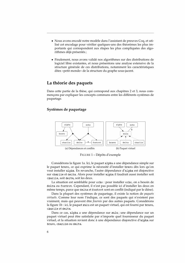
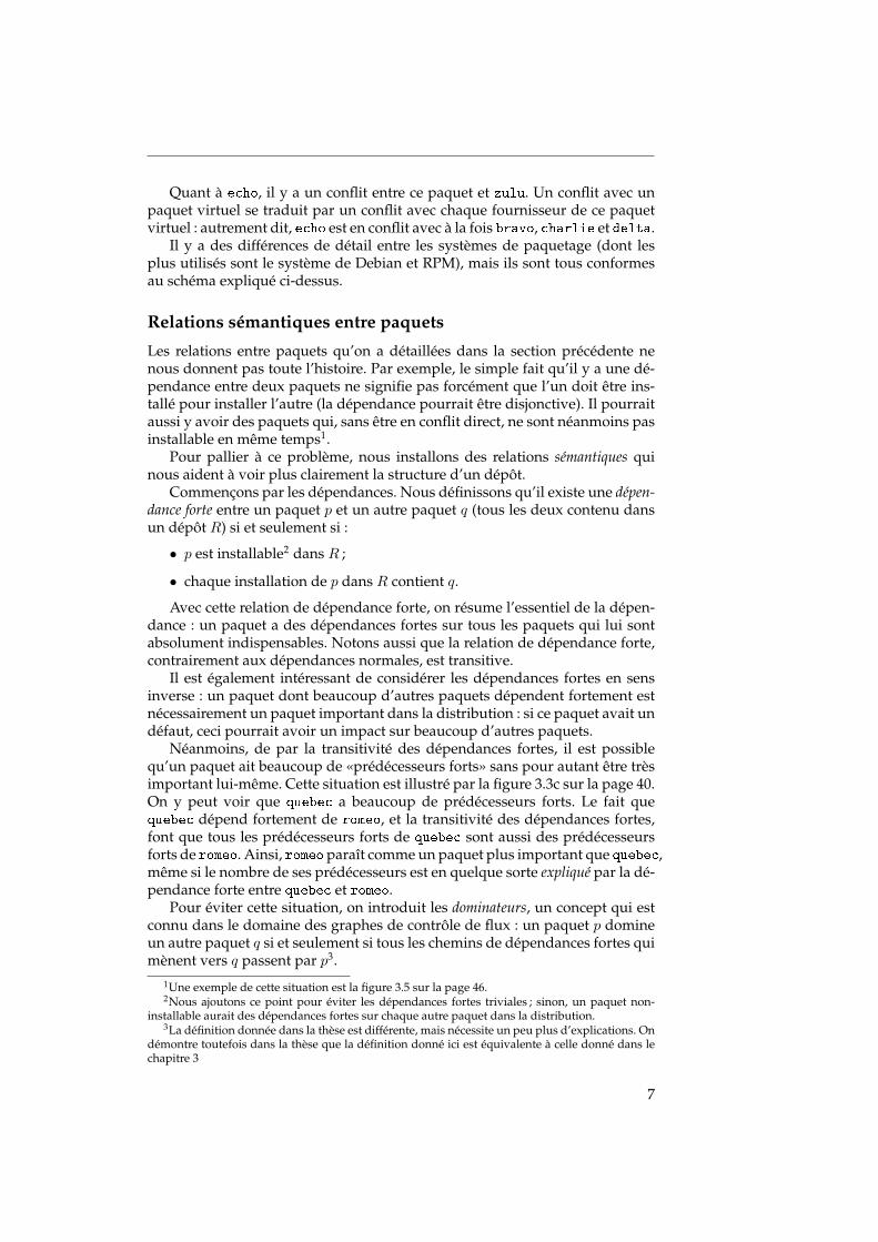
FIGURE 1 – Dépôts d’exemple
Considérons la figure 1a. Ici, le paquet alpha a une dépendance simple surle paquet bravo, ce qui exprime la nécessité d’installer bravo dès lors qu’onveut installer alpha. En revanche, l’autre dépendance d’alpha est disjonctivesur charlie et delta. Alors pour installer alpha il faudrait aussi installer soitcharlie, soit delta, soit les deux.
La situation est semblable pour echo : pour installer echo, on a besoin dedelta ou foxtrot. Cependant, il n’est pas possible ici d’installer les deux enmême temps, parce que delta et foxtrot sont en conflit (indiqué par le dièse).
Dans la plupart des systèmes de paquetage, il existe la notion de paquetsvirtuels. Comme leur nom l’indique, ce sont des paquets qui n’existent pasvraiment, mais qui peuvent être fournis par des autres paquets. Considéronsla figure 1b : ici, le paquet zulu est un paquet virtuel, qui est fourni par bravo,charlie et delta.
Dans ce cas, alpha a une dépendance sur zulu ; une dépendance sur unpaquet virtuel peut être satisfaite par n’importe quel fournisseur du paquetvirtuel, et la situation revient donc à une dépendance disjonctive d’alpha surbravo, charlie ou delta.
6
Quant à echo, il y a un conflit entre ce paquet et zulu. Un conflit avec unpaquet virtuel se traduit par un conflit avec chaque fournisseur de ce paquetvirtuel : autrement dit, echo est en conflit avec à la fois bravo, charlie et delta.
Il y a des différences de détail entre les systèmes de paquetage (dont lesplus utilisés sont le système de Debian et RPM), mais ils sont tous conformesau schéma expliqué ci-dessus.
Relations sémantiques entre paquets
Les relations entre paquets qu’on a détaillées dans la section précédente nenous donnent pas toute l’histoire. Par exemple, le simple fait qu’il y a une dé-pendance entre deux paquets ne signifie pas forcément que l’un doit être ins-tallé pour installer l’autre (la dépendance pourrait être disjonctive). Il pourraitaussi y avoir des paquets qui, sans être en conflit direct, ne sont néanmoins pasinstallable en même temps1.
Pour pallier à ce problème, nous installons des relations sémantiques quinous aident à voir plus clairement la structure d’un dépôt.
Commençons par les dépendances. Nous définissons qu’il existe une dépen-dance forte entre un paquet p et un autre paquet q (tous les deux contenu dansun dépôt R) si et seulement si :
• p est installable2 dans R ;
• chaque installation de p dans R contient q.
Avec cette relation de dépendance forte, on résume l’essentiel de la dépen-dance : un paquet a des dépendances fortes sur tous les paquets qui lui sontabsolument indispensables. Notons aussi que la relation de dépendance forte,contrairement aux dépendances normales, est transitive.
Il est également intéressant de considérer les dépendances fortes en sensinverse : un paquet dont beaucoup d’autres paquets dépendent fortement estnécessairement un paquet important dans la distribution : si ce paquet avait undéfaut, ceci pourrait avoir un impact sur beaucoup d’autres paquets.
Néanmoins, de par la transitivité des dépendances fortes, il est possiblequ’un paquet ait beaucoup de «prédécesseurs forts» sans pour autant être trèsimportant lui-même. Cette situation est illustré par la figure 3.3c sur la page 40.On y peut voir que quebec a beaucoup de prédécesseurs forts. Le fait quequebec dépend fortement de romeo, et la transitivité des dépendances fortes,font que tous les prédécesseurs forts de quebec sont aussi des prédécesseursforts de romeo. Ainsi, romeo paraît comme un paquet plus important que quebec,même si le nombre de ses prédécesseurs est en quelque sorte expliqué par la dé-pendance forte entre quebec et romeo.
Pour éviter cette situation, on introduit les dominateurs, un concept qui estconnu dans le domaine des graphes de contrôle de flux : un paquet p domineun autre paquet q si et seulement si tous les chemins de dépendances fortes quimènent vers q passent par p3.
1Une exemple de cette situation est la figure 3.5 sur la page 46.2Nous ajoutons ce point pour éviter les dépendances fortes triviales ; sinon, un paquet non-
installable aurait des dépendances fortes sur chaque autre paquet dans la distribution.3La définition donnée dans la thèse est différente, mais nécessite un peu plus d’explications. On
démontre toutefois dans la thèse que la définition donné ici est équivalente à celle donné dans lechapitre 3
7
En utilisant les dominateurs, on peut nettoyer la structure des dépendancesfortes de façon que les paquets qui paraissent importants, mais ne le sont pasvraiment, comme expliqué ci-dessus, soient enlevés.
Ce qu’on peut faire pour les dépendances, on peut faire pour les conflits :deux paquets p et q d’un dépôt R sont en conflit fort si et seulement si on peutinstaller p et q séparément dans R, mais non pas ensemble.
Ici encore, on résume l’essentiel de la relation de conflit : deux paquets quine peuvent pas être installés en même temps ; pour avoir cette situation, il n’estpoint nécessaire qu’il y ait un conflit direct entre les deux paquets. Par contre,nous avons démontré que pour qu’un conflit fort existe entre deux paquets,il doit exister un chemin de dépendances (normales) entre chacun des deuxpaquets et un conflit (théorème 3.25).
Algorithmes et outils
Dans la section précédente, nous avons noté que le problème de déterminer siun paquet est installable dans un dépôt est de complexité égale au problèmeSAT, c’est à dire NP-complet.
On a également vu que les relations sémantiques dépendent aussi de l’ins-tallabilité des paquets. Vu la taille des distributions, il n’est pas envisageablede simplement calculer la totalité des relations en vérifiant l’existence d’unerelation pour chaque paire de paquets.
Dans le chapitre 4, nous proposons donc des algorithmes plus efficaces,dont le fonctionnement repose sur des théorèmes présentés dans le chapitre 3.
Pour les dépendances fortes, l’algorithme proposé utilise d’abord le fait quepour qu’une dépendance forte existe entre deux paquets p et q, q doit êtreprésent dans n’importe lequel installation de p ; pour trouver toutes les dé-pendances fortes de p, on peut donc se borner à contrôler tous les membresd’un ensemble d’installation de p quelconque. En plus, nous utilisons le faitqu’une dépendance conjonctive est automatiquement une dépendance forte(corollaires 3.7 et 3.2).
Le calcul efficace des conflits forts repose essentiellement sur le théorème 3.25.Puisque, pour avoir un conflit fort entre deux paquets p et q, il est nécessairequ’il existe un chemin de dépendances (normales) de p et q jusqu’à deux pa-quets qui sont en conflit, on peut rassembler tous les conflits forts en commen-çant par les conflits directs (dont il y a relativement peu), et en remontant lesdépendances en sens inverse. Ainsi, on obtient tous les paires de paquets quipourraient être en conflit fort, ce qui réduit l’espace de recherche de façon im-portante.
Pour les dominateurs, on utilise le théorème 3.19 qui démontre que notrenotion des dominateurs est équivalent à celle utilisée dans le domaine desgraphes de contrôle de flux. On peut ensuite utiliser l’algorithme de Tarjan [LT79]pour calculer rapidement le graphe des dominateurs.
Dans le chapitre 5, nous présentons les outils qui ont été crées en faisantusage de ces algorithmes. Notamment, il s’agit de dose, qui a été conçu commeune librairie de manipulation et analyse de distributions, et qui inclut tous lesalgorithmes présentés ci-dessus.
8
Formalisation
Comme on a vu dans la section précédente, les algorithmes présentés ont étéoptimisés en utilisant des théorèmes qui permettent de réduire l’espace de re-cherche.
Pour être sûr qu’on ne réduit pas trop l’espace de recherche, il faut s’as-surer de la validité des théorèmes utilisés. Pour ce faire, nous avons utilisél’assistant de preuves Coq pour formaliser une partie de la théorie des paquets,et notamment pour vérifier les théorèmes les plus importants utilisés dans nosalgorithmes.
Une explication des méthodes utilisées dans cette formalisation est le sujetdu chapitre 6.
Validation et analyse
Dans les chapitres 7 et 8, nous présentons des résultats d’expériences faitesavec les outils présentés précédemment.
D’abord, nous parlons des temps d’exécution des algorithmes. Théorique-ment, ce sont toujours des algorithmes de complexité NP-complet ou assimilé,mais en utilisant les optimisations mentionnées, on peut obtenir des réductionsassez importantes qui permettent de calculer les graphes de relations séman-tiques dans un temps raisonnable ; ainsi, il devient possible de faire un calculquotidien.
Ensuite, nous nos intéressons à la structure de la distribution. Dans despublications précédentes ([LW04] et [NNR09], il a déjà été démontré que lesdistributions de logiciel libre ont un graphe sous-jacent qui présente le phéno-mène du petit monde ; nous affirmons que c’est le cas en bien précisant notreméthodologie, ce qui n’a pas été le cas dans les publications citées.
Le phénomène du petit monde est surtout intéressant pour les conclusionsqu’on peut en tirer sur la structure de la distribution. Un graphe petit mondeest un graphe qui a des chemins relativement court entre ses noeuds ; on peutaussi diviser les noeuds d’un graphe petit monde dans deux catégories : lesnoeuds a forte connectivité (il y en a peu), et les noeuds a faible connectivité (ily en a beaucoup).
Les graphes de distribution de logiciel libre ont la particularité d’être diri-gée ; on peut alors distinguer trois types de noeuds distincts :
• Des noeuds avec beaucoup d’arêtes sortantes, mais peu d’arêtes rentrantes ;ces noeuds présentent des paquets de haut niveau, appelés les meta-paquets,qui sont utilisées pour installer facilement une famille de logiciels, commeKDE ou GNOME ;
• Des noeuds avec beaucoup d’arêtes rentrantes, mais peu d’arêtes sor-tantes ; ces noeuds présentent des paquets de bas niveau, des librairesnotamment, comme par exemple la librairie standard de C qui est néces-saire pour une grande partie des autres paquets ;
• Des noeuds avec peu d’arêtes, rentrantes ou sortants.
Dans le chapitre 8, il y a plus d’informations qui confirment l’existence decette structure.
9
Contributions et perspectives
Dans cette thèse, nous avons présenté une modélisation formelle des distribu-tions de logiciel libre, avec des méthodes pour améliorer la gestion de qualitéqui utilise cette modélisation. Ces méthodes ont été implémentées en utilisantle langage OCaml, et partiellement vérifiées. Finalement, nous avons utiliséles outils implémentés pour faire des analyses sur des distributions existantes,notamment Debian et Mandriva.
Nous avons présenté des cas réels des erreurs qui ont pu être détectées enutilisant nos méthodes ; leur application quotidienne est rendue possible parles optimisations que nous avons ajoutés. Ceci peut beaucoup aider les éditeursde distributions à éviter des erreurs, par exemple des paquets non installables.
En continuant ce travail, notamment en complétant la vérification des al-gorithmes, et en les intégrant dans un langage spécifique, on peut aboutir surune suite complète d’outils pour la manipulation et l’analyse des distributions.Ceci pourrait aider à garder la qualité des distributions de logiciel libre, mêmesi dans le futur ils continueront à grandir et devenir plus complexes.
10
Introduction 1Het zal waarachtig wel gaan!
— CORNELIS TROMP
It has long been a standard method in computing science to divide complexsystems into components [Szy02].
The basic reason for this is that smaller programs are easier for a humanto comprehend, and therefore to design, write, verify, test and maintain. Thismakes for a quicker design phase, less time spent in implementation, and fewerbugs.
Components can also be reused, especially the more generic ones. Thisagain saves time, because components do not have to be implemented twice.It also results in fewer errors, for the same reason. It is even possible to re-usecomponents developed elsewhere, for example by a third party (for exampleby using COTS, commercial off-the-shelf products).
Unfortunately, component-based systems have their disadvantages as well,notably in maintenance and evolution. The foremost problem here is the factthat components, as their name already indicates, do not stand alone: theyinteract with each other.
This interaction brings forth the relations between components: these caneither be positive (i.e. a component needs another component to function; thisis commonly called a dependency relation) or negative (i.e. a component can notfunction together with another component; this is commonly called a conflictrelation).
A component-based system, by its nature, is not stable: components areadded, removed and upgraded as a matter of routine. These changes, however,can easily break relationships between components, thus corrupting the stateof the entire system or even rendering it unusable.
One specific instance of component-based systems that has become moreand more widely adopted over the last two decades are the operating systemsbased on Free and Open Source Software (F/OSS).
These systems are extremely heterogeneous: every part of the system isdeveloped by a different group; components therefore are implemented in dif-ferent programming languages, use different release cycles, and have differentmodalities for downloading and installing. It is easy to see that this can giverise to many compatibility problems.
1.1 F/OSS Software Distributions
In order to at least partially solve these problems, F/OSS operating systemsare assembled into distributions. This is especially true for the operating sys-tems based on the Linux kernel: there is a great number of distributions based
11
1. Introduction
on this kernel, each with its own specificities. However, other F/OSS oper-ating systems, such as the different varieties of BSD, or OpenSolaris, are alsoprovided in distribution form.
The idea of a distribution is that it creates a coherent system out of the largeamount of available software: it allows for a single method of downloadingand installing software, and there is one person (the maintainer) responsible forintegrating the software into the distribution and updating the distribution if anew release is published.
1.1.1 Components as packages
In a distribution, every piece of software becomes a package. This packagecontains the software itself, plus some extra data (known as metadata) that de-scribes the package, its dependencies and all the specifics needed to install it ona user’s machine. In this way, the user can simply install the package, withouthaving to worry about how exactly to do this: all the necessary information iscontained in the package.
The tool used to install a package (using the metadata) is called a packagemanager. The package manager takes care of downloading the package, verify-ing contents, installing eventual dependencies, making sure there are no con-flicts and all actions that are needed to correctly install the software containedin the package (creating specific user accounts, for example).
The packaging format and package manager used vary widely between dis-tributions; in the Linux world, RPM (the RedHat Package Manager) is usedby many systems (Fedora, Mandriva, and SUSE, to name a few); another well-known system is Debian’s package manager APT with its package format (usedby Debian and Ubuntu, amongst others).
1.1.2 The challenge of scale
One of the most important problems that plagues F/OSS distributions todayis one of scale. The latest stable version of the Debian distribution (5.0.6, re-leased in October 2010) contains 22 000 packages; the latest version of Man-driva (2010.1) has over 7 500 packages.
Unfortunately, the tools used on both the user side and the distribution sidehave not notably changed since the first appearance of distributions, now sometwo decades ago: the SUSE distribution has recently integrated a SAT solver inits package manager, for dependency checking, but most distributions do notyet use even this basic technology.
On the distribution side, the situation is comparable: there are some toolsthat aid distribution editors in their tasks (one example is Debian’s britney,which takes care of integration of new version of packages), but these are slowand not formally proven.
1.2 Contributions
The main contributions of this work can be summarised in four broad areas:
12
• We present a formal framework that captures the essential features of themost common package models, and identify some new semantic relation-ships among packages that are relevant for finding errors and maintain-ing quality in F/OSS distributions;
• We present efficient algorithms for manipulating package repositoriesand compute the relationships mentioned above; all of these algorithmshave been implemented in the OCaml programming language, and in-corporated in a generic package manipulation and analysis library calleddose3;
• We encode our formal framework in the Coq proof assistant, and use it tomechanically verify some of the key lemmas corresponding to the mostcomplicated steps in the aforementioned algorithms;
• We have validated our algorithms on real-world F/OSS distributions,and have performed an extensive analysis of the general structure ofthese distributions, notably the small world characteristics of the under-lying graph structure.
1.2.1 Theory of packages
The details of how packages are represented and manipulated differ quite sig-nificantly from one Free Software distribution to the other, but when choosingthe right level of abstraction, one can find a remarkably simple and elegantcommon model that is able to accommodate all the metadata which is relev-ant for maintaining the quality of a repository. This model has already beenpresented in [MBDC+06] and is reproduced here with some extensions.
Subsequently, we extend this model with some new semantic relationshipsbetween packages. These relationships, in highlighting specific properties ofpackages, help distribution editors in quickly spotting potential errors and infinding means to correct these errors.
The simplest example is the broken package, a package that cannot be in-stalled under any circumstances. By not only providing a list of such packages,but also an explanation of why they cannot be installed, we help distributionengineers in correcting such packages.
In the same vein, packages that are installable but that, when installed,render a large subset of the distribution non-installable, also are a potentialsource of errors. Again, since we provide an explanation, distribution editorscan easily isolate the source of the problem, and correct it if necessary.
Another way to spot potential trouble is to identify packages that are insome way important to the distribution—for example, because they are de-pended on by many other packages. We offer a way to identify such packages,so that distribution editors know which packages need extra care and testingin case of changes to the distribution.
Some of the material presented in this part has already been publishedin [MBDC+06], [ADCBZ09] and [DCB10]; this thesis presents this previous ma-terial in its general context, and contains some new additions besides.
13
1. Introduction
1.2.2 Algorithms and tools
The problem of determining whether a package is installable is NP-complete,as already shown in [MBDC+06].
Since the computation of all of the semantic relationships mentioned in theprevious section depends ultimately on this installability problem, a naive im-plementation that checks the existence of a relationship for every pair of pack-ages will take a very long time.
In this thesis, we present algorithms that use the various properties of thepackages and their relationships to avoid any superfluous computations. Inthis way, it becomes feasible to compute the relationships with every majorchange in the distribution, so that errors can be found as early as possible.
Furthermore, we discuss the implementation of our algorithms as a part ofa general distribution manipulation and analysis framework.
1.2.3 Formalisation
For our algorithms, we use several lemmas that allow us to skip a lot of SATcomputations. Needless to say, it is very important that these computationscan indeed be skipped; in other words, that the lemmas are actually valid.
In order to assure ourselves of this, we have formalised the theory of pack-ages as provided in the previous parts using the Coq proof assistant, and wehave formally proven several of the lemmas presented.
1.2.4 Validation and analysis
In this part, we present some practical results obtained by applying our al-gorithms to some common F/OSS distributions.
To start with, we show that the run time of the algorithms remains reason-able in practical cases: a daily run of the algorithms is in all cases possible.
Then, we present the insights we have obtained on the structure of the un-derlying graphs. First we note that the underlying graph of a F/OSS distri-bution can be generated in different ways, and that the method of generationchanges the characteristics.
We also talk about the small world properties of the underlying graphs,and discuss the ramifications for the structure of the graph. It turns out thatthe graph of a distribution has a distinct structure: there are few packageswith many dependencies, and many packages with just a few dependencies.The packages with many dependencies again fall into two distinct categories:high-level packages with many outgoing dependencies (but few or no incom-ing dependencies), and low-level packages with many incoming dependencies(but few or no outgoing dependencies). See also figure 8.3 on page 115.
1.3 Structure
The contents of the thesis are as follows: first, in chapter 2, we shall presentan overview of the basics of Linux distribution management: its most-usedpackage formats (Debian and RPM), and we shall recall the formalisation ofF/OSS distributions devised in the EDOS project [MBDC+06, DCMB+06].
14
In chapter 3, we shall extend this formalisation with the concepts of strongdependencies and strong conflicts, as well as an application of dominators (a conceptalready known from flow control graphs) which allow for more extensive qual-ity control over distributions. We shall also specify and prove some theoremsthat allow for more efficient computation of these concepts.
Then, in chapter 4, we present algorithms that use these theorems to effi-ciently compute strong dependencies, strong conflicts and dominators over adistribution. The actual implementation of these algorithms during the EDOSand MANCOOSI projects will be discussed in chapter 5.
The formalisation in Coq of the definitions and theorems from chapters 2and 3 is the subject of chapter 6.
In chapter 7, we present the results of several experiments that have beenexecuted using the tools from chapter 5. These results offer insights into thestructure of the distributions; in chapter 8, we continue on this subject by dis-cussing distributions when seen as graphs—this view offers other insights intothe structure of distributions that can aid in managing them.
Finally, in chapter 9, I discuss the relevance of the subjects presented in thisthesis, as well as related work and possible directions for future research.
15
1. Introduction
16
Definitions 2‘And why is it called the Carrock?’ asked Bilbo as he went along at the wizard’s side.
‘He called it the Carrock, because carrock is his word for it. He calls things like that carrocks,and this one is the Carrock because it is the only one near his home and he knows it well.’
— J.R.R. TOLKIEN, The Hobbit
In this preliminary chapter, we shall first specify in detail the package formatscurrently used for most Linux distributions: the Debian format and RPM. Thesetwo formats are very different in syntax; the difference in semantics, however,is much smaller, which is why it has been possible during the MANCOOSIproject to devise a common format, called CUDF [TZ09], to which both formatscan be translated.
After this, we shall discuss a package format from a different environment:the metadata format used for Eclipse plugins. Even though the environmentin which this format is used is very different from RPM or the Debian format,we shall see that the basic metadata contents and semantics remain the same.
Having thus presented the existing package formats, we shall recall thedefinitions proposed in the EDOS project [DCMB+06]. These definitions areintended to be usable as a way of reasoning about any F/OSS distribution:they are sufficiently abstract to be used to represent packages from the Debianformat, from RPM and even from Eclipse.
The main object of the EDOS formalisation is to reason about package in-stallability. The effect of this is that a large part of the package metadata canbe ignored, because it has no influence on installability. Examples of this aredata like the name of the package maintainer, the package description or thepackage classification.
2.1 Existing package formats
2.1.1 Basic ideas
As discussed in the introduction, in F/OSS distributions, there exist interrela-tionships between packages. There are two main types: dependencies and con-flicts. There are other types of relationships, but these are either equivalentto dependencies or conflicts, or can be safely ignored as far as installability isconcerned.
For example, in Debian there is a pre-dependency relationship, which is like anormal dependency, except that it enforces an order of installation on the pack-ages (a pre-dependency must be installed before configuration of the packagesbegins). Examples of relationships that can be ignored are the recommendationor suggestion relationships found in both Debian and RPM: these specify op-tional dependencies and thus do not influence installability.
17
2. Definitions
A dependency relationship specifies that one package needs another tofunction; if package A depends on package B, the package manager takes carethat when installing package A, package B also will be installed (but not theother way around).
Sometimes, it is possible to have alternative (or disjunctive) dependencies: inthis case, a package can specify a list of other packages, of which at least onemust be installed (it is allowed to have more than one package from the listinstalled as well; the disjunction is not exclusive).
A conflict specifies that one package cannot function when another packageis installed. If package A conflicts with package B, the package manager takescare that package A is never installed at the same time as package B. Unlikethe dependency relationship, the conflict relationship is symmetric (at least forDebian, RPM and Eclipse).
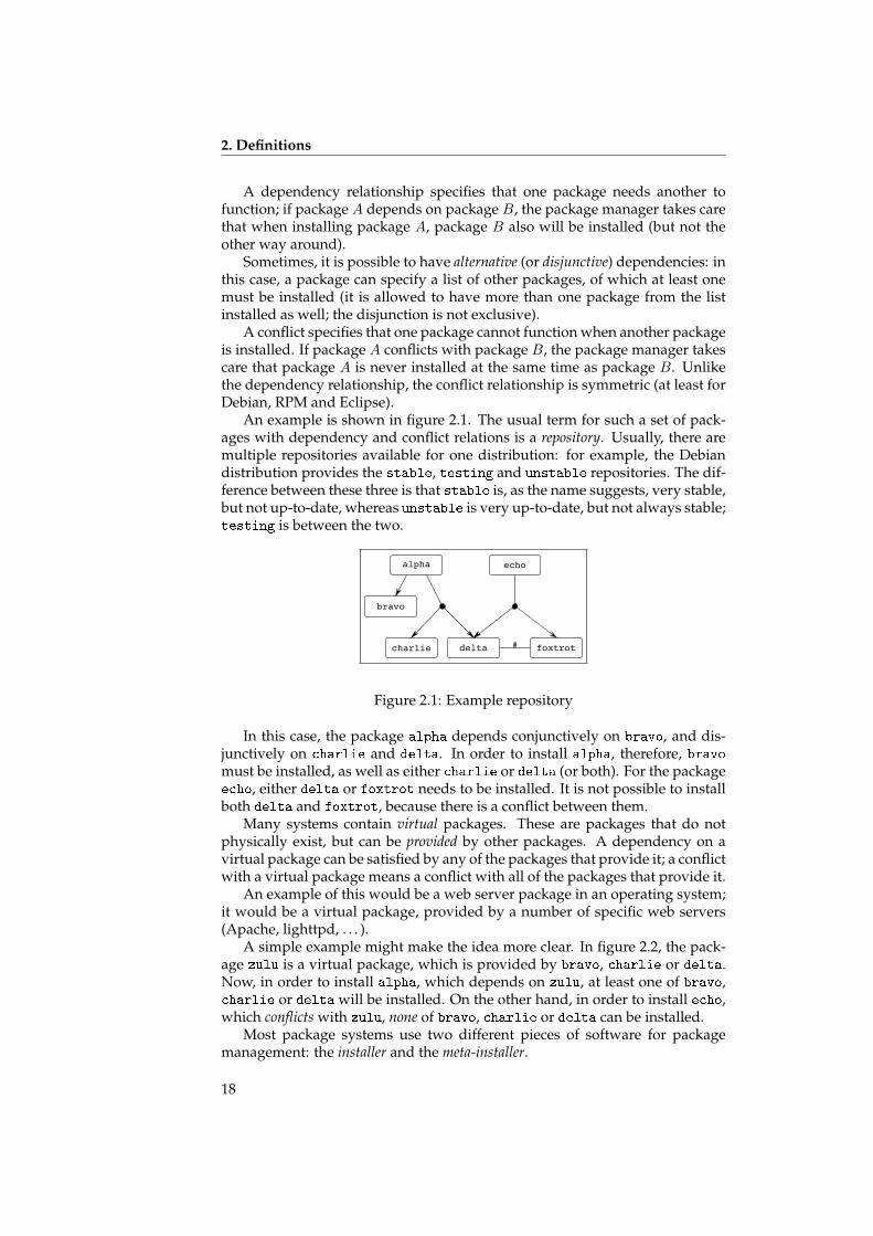
An example is shown in figure 2.1. The usual term for such a set of pack-ages with dependency and conflict relations is a repository. Usually, there aremultiple repositories available for one distribution: for example, the Debiandistribution provides the stable, testing and unstable repositories. The dif-ference between these three is that stable is, as the name suggests, very stable,but not up-to-date, whereas unstable is very up-to-date, but not always stable;testing is between the two.
bravo
alpha
charlie delta foxtrot
echo
#
Figure 2.1: Example repository
In this case, the package alpha depends conjunctively on bravo, and dis-junctively on charlie and delta. In order to install alpha, therefore, bravomust be installed, as well as either charlie or delta (or both). For the packageecho, either delta or foxtrot needs to be installed. It is not possible to installboth delta and foxtrot, because there is a conflict between them.
Many systems contain virtual packages. These are packages that do notphysically exist, but can be provided by other packages. A dependency on avirtual package can be satisfied by any of the packages that provide it; a conflictwith a virtual package means a conflict with all of the packages that provide it.
An example of this would be a web server package in an operating system;it would be a virtual package, provided by a number of specific web servers(Apache, lighttpd, . . . ).
A simple example might make the idea more clear. In figure 2.2, the pack-age zulu is a virtual package, which is provided by bravo, charlie or delta.Now, in order to install alpha, which depends on zulu, at least one of bravo,charlie or delta will be installed. On the other hand, in order to install echo,which conflicts with zulu, none of bravo, charlie or delta can be installed.
Most package systems use two different pieces of software for packagemanagement: the installer and the meta-installer.
18
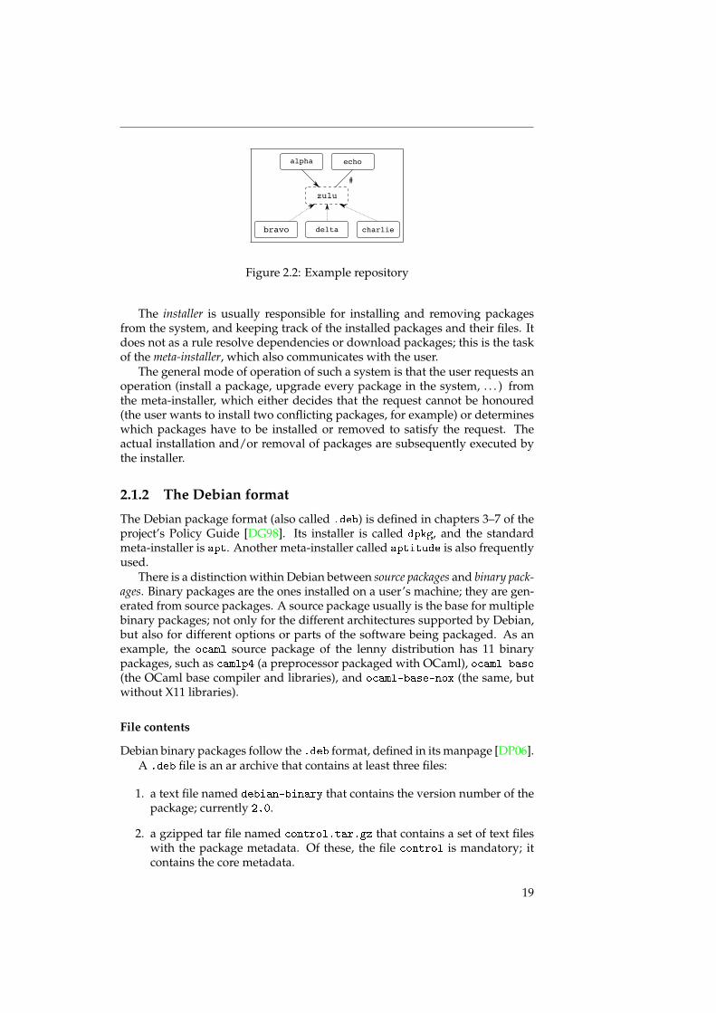
alpha charliedelta echozulubravo #Figure 2.2: Example repository
The installer is usually responsible for installing and removing packagesfrom the system, and keeping track of the installed packages and their files. Itdoes not as a rule resolve dependencies or download packages; this is the taskof the meta-installer, which also communicates with the user.
The general mode of operation of such a system is that the user requests anoperation (install a package, upgrade every package in the system, . . . ) fromthe meta-installer, which either decides that the request cannot be honoured(the user wants to install two conflicting packages, for example) or determineswhich packages have to be installed or removed to satisfy the request. Theactual installation and/or removal of packages are subsequently executed bythe installer.
2.1.2 The Debian format
The Debian package format (also called .deb) is defined in chapters 3–7 of theproject’s Policy Guide [DG98]. Its installer is called dpkg, and the standardmeta-installer is apt. Another meta-installer called aptitude is also frequentlyused.
There is a distinction within Debian between source packages and binary pack-ages. Binary packages are the ones installed on a user’s machine; they are gen-erated from source packages. A source package usually is the base for multiplebinary packages; not only for the different architectures supported by Debian,but also for different options or parts of the software being packaged. As anexample, the ocaml source package of the lenny distribution has 11 binarypackages, such as camlp4 (a preprocessor packaged with OCaml), ocaml-base(the OCaml base compiler and libraries), and ocaml-base-nox (the same, butwithout X11 libraries).
File contents
Debian binary packages follow the .deb format, defined in its manpage [DP06].A .deb file is an ar archive that contains at least three files:
1. a text file named debian-binary that contains the version number of thepackage; currently 2.0.
2. a gzipped tar file named control.tar.gz that contains a set of text fileswith the package metadata. Of these, the file control is mandatory; itcontains the core metadata.
19
2. Definitions
3. a gzipped tar file named data.tar.gz that contains the files that belongto the package.
In order to easily allow access to the metadata of all packages in a distri-bution, there is also a file format that consists of the concatenation of controlfiles from an entire distribution (as a text file). This type of file will from nowon be referred to as a Packages file.
Package metadata
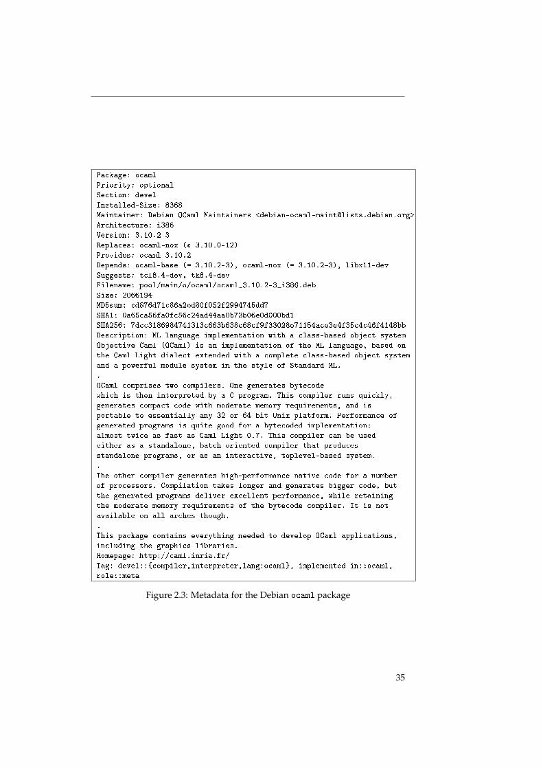
The package control file contains one or more paragraphs of fields, separatedby blank lines. Each paragraph contains a list of fields: the field name, followedby a colon, followed by the field value. A field value may span several lines,in which case the second and following lines start with a space or tab. Otherwhitespace is ignored. Figure 2.3 is an example of the package control file forthe ocaml package:
For a binary package, the Package, Version, Architecture, Maintainer,and Description fields are mandatory; Section and Priority are recommen-ded. A list of the different fields and their meanings (for binary packages)follows:
Maintainer The name and e-mail address of the package maintainer.
Section This field is used for package classifications, as defined in the PolicyManual, Section 2.4.
Priority Package priority, as defined in the Policy Manual, Section 2.5.
Package The name of the package.
Architecture The architecture the package is intended for. If the value all isspecified, the package is architecture-independent.
Essential If this field is set to yes, then the package is considered to be indis-pensable for a functioning system, and it should be installed at all times.
Depends This field specifies the dependency relationship mentioned in theprevious section; its syntax will be explained in more detail below.
Pre-Depends This field specifies a special sort of dependency; it means thatthe package depended on must be installed before the package specifyingthe dependency.
Recommends This field specifies “a strong, but not absolute, dependency”.The standard Debian package manager apt installs recommended pack-ages by default.
Suggests This field specifies a weaker sort of dependency than a Recommends
dependency; suggested packages are not installed by default by apt.
Enhances This field specifies the same sort of dependency as the Suggests
field, but in the opposite direction.
20
Conflicts This field specifies a conflict between two packages, as explained inthe previous section; the Debian package manager refuses to install twopackages together if there is a conflict between them.
Breaks This field specifies a special, slightly weaker, kind of conflict: packagesthat break each other can be physically present on the system at the sametime, but must not both be active (“configured”).
Provides This field specifies that the package provides a virtual package, asexplained in the previous section.
Replaces This field has two distinct uses:
• Normally, two packages cannot share the same file. However, ifone package replaces the other, the Debian package manager willreplace the file from the old package by the file from the new pack-age.
• If two packages conflict with each other, and one of the packages isspecified as replacing the other, instead of refusing to install themboth, the Debian package manager will remove the replaced pack-age and install the replacing package.
Version The package version.
Description A description of the contents of the package.
Installed-Size The estimated size of the package when installed, in kilobytes.
Homepage The URL for the home page of the software packaged.
Package interrelationships
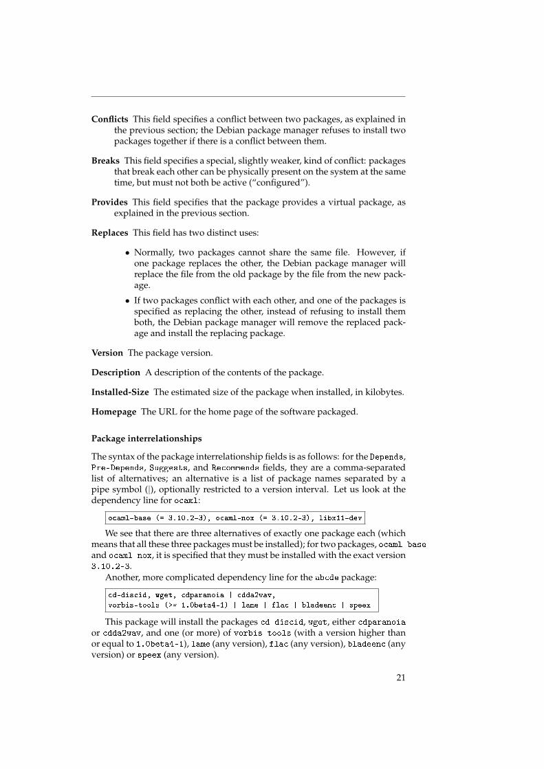
The syntax of the package interrelationship fields is as follows: for the Depends,Pre-Depends, Suggests, and Recommends fields, they are a comma-separatedlist of alternatives; an alternative is a list of package names separated by apipe symbol (|), optionally restricted to a version interval. Let us look at thedependency line for ocaml:
ocaml-base (= 3.10.2-3), ocaml-nox (= 3.10.2-3), libx11-dev
We see that there are three alternatives of exactly one package each (whichmeans that all these three packages must be installed); for two packages, ocaml-baseand ocaml-nox, it is specified that they must be installed with the exact version3.10.2-3.
Another, more complicated dependency line for the abcde package:
cd-discid, wget, cdparanoia | cdda2wav,
vorbis-tools (>= 1.0beta4-1) | lame | flac | bladeenc | speex
This package will install the packages cd-discid, wget, either cdparanoiaor cdda2wav, and one (or more) of vorbis-tools (with a version higher thanor equal to 1.0beta4-1), lame (any version), flac (any version), bladeenc (anyversion) or speex (any version).
21
2. Definitions
The syntax for the other interrelationship fields (Conflicts, Breaks) is sim-ilar, except that alternatives are not allowed here, the values are just a comma-separated list of package names, with eventual version restrictions.
Finally, the Provides field is just a comma-separated list of names, withoutany version specification.
Version comparison algorithm
A Debian package version number consists of three parts: the epoch, the ver-sion proper and, optionally, the revision. When comparing two versions,these three are compared in order: the epochs first, then the versions properif there is no difference between the epochs, and finally the releases if there isno difference between the versions.
The epoch is an unsigned integer. If not specified, it is assumed to be 0.The version proper (separated from the epoch by a colon) is an alphanu-
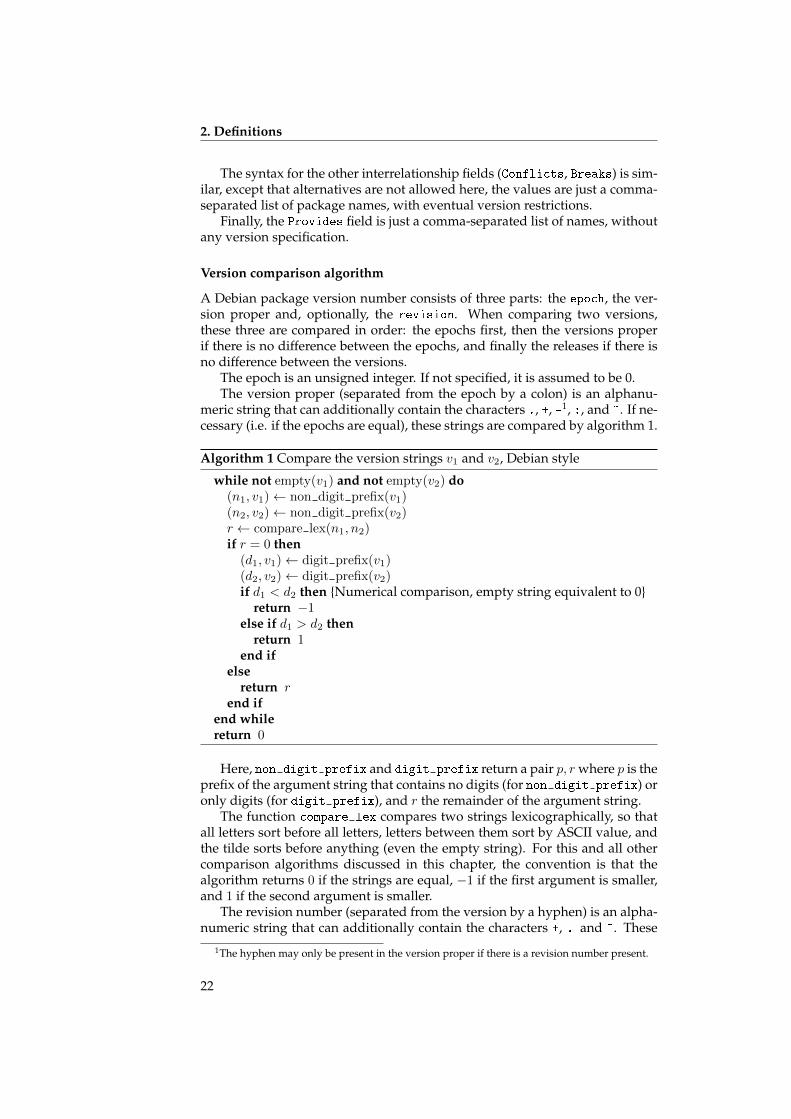
meric string that can additionally contain the characters ., +, -1, :, and �. If ne-cessary (i.e. if the epochs are equal), these strings are compared by algorithm 1.
Algorithm 1 Compare the version strings v1 and v2, Debian style
while not empty(v1) and not empty(v2) do(n1, v1)← non digit prefix(v1)(n2, v2)← non digit prefix(v2)r ← compare lex(n1, n2)if r = 0 then
(d1, v1)← digit prefix(v1)(d2, v2)← digit prefix(v2)if d1 < d2 then {Numerical comparison, empty string equivalent to 0}
return −1else if d1 > d2 then
return 1end if
elsereturn r
end ifend whilereturn 0
Here, non digit prefix and digit prefix return a pair p, r where p is theprefix of the argument string that contains no digits (for non digit prefix) oronly digits (for digit prefix), and r the remainder of the argument string.
The function compare lex compares two strings lexicographically, so thatall letters sort before all letters, letters between them sort by ASCII value, andthe tilde sorts before anything (even the empty string). For this and all othercomparison algorithms discussed in this chapter, the convention is that thealgorithm returns 0 if the strings are equal, −1 if the first argument is smaller,and 1 if the second argument is smaller.
The revision number (separated from the version by a hyphen) is an alpha-numeric string that can additionally contain the characters +, . and �. These
1The hyphen may only be present in the version proper if there is a revision number present.
22
strings are only compared if both the epochs and versions proper are equal; thealgorithm is the same as that used for the version proper.
The rationale behind this version numbering scheme (which, as we shallsee, is very similar to the one used for RPM) is that the version specified bythe original author of the software should become the version of the package;this comparison algorithm works well with most versioning schemes used inpractice.
However, it is possible that the original author decides to change the ver-sion numbering scheme (for example, to pass from a date-based scheme to amore classic x.y.z scheme). In such a case, to make sure that the new version isdeemed larger than the old version, the epoch can be raised.
The release part is used by the distribution to be able to make changes tothe package, while keeping the same version of the original software.
Special semantics
In Debian, virtual packages do not have versions; hence, a dependency with aversion restriction can never be satisfied by a virtual package.
Furthermore, a package can never conflict with itself. Thus, a special case oc-curs when a package both provides a virtual package and conflicts with it. Sup-pose a package has both Provides: mail-transport-agent and Conflicts: mail-transport-agent
in its metadata. In this case, the package conflicts with any other packageproviding the same virtual package, in effect specifying that it should be theonly package installed that provides mail-transport-agent.
If the package also has Replaces: mail-transport-agent in its metadata(in addition to the Provides and Conflicts) mentioned above, any packagealso providing mail-transport-agent will be removed by the Debian packagemanager.
In Debian, two versions of the same package implicitly conflict with eachother, which means that it is not possible to have two packages that have thesame name installed at the same time.
Installer and meta-installer
As said before, the tools used to install Debian packages are dpkg, the installer,and apt, the meta-installer.
In this section, we shall note some salient facts about apt and its most inter-esting part (for our purposes, anyway), the dependency solver. More extensiveinformation on apt can be found in [DCMB+06].
Let us note first that the problem that apt tries to solve is indeed quitecomplicated, even beyond simple installability. In fact, apt has to deal withan existing system, one or more available distributions, and try to execute userrequests while trying to maintain the system in a consistent state.
As we shall show later on, the installation problem itself is NP-complete.Since this means that dependency solving can take a very long time, apt doesnot try to be complete: if at some point in the calculation multiple optionspresent itself (which is the case when a disjunctive dependency is encountered,none of whose packages are already installed), it just takes the first packagefrom the list of alternatives and tries to install that. No backtracking is attemp-ted.
23
2. Definitions
In fact, this behaviour of apt has become something of a de facto stand-ard, since it allows package managers to specify a preference in alternativedependencies: the package specified first in the alternative will be installed,unless another package from the alternative is already installed.
Furthermore, if multiple versions of the same package are available, onlythe highest version is installed; the idea being that the highest version of anypackage should always be the most advanced and bug-free one.
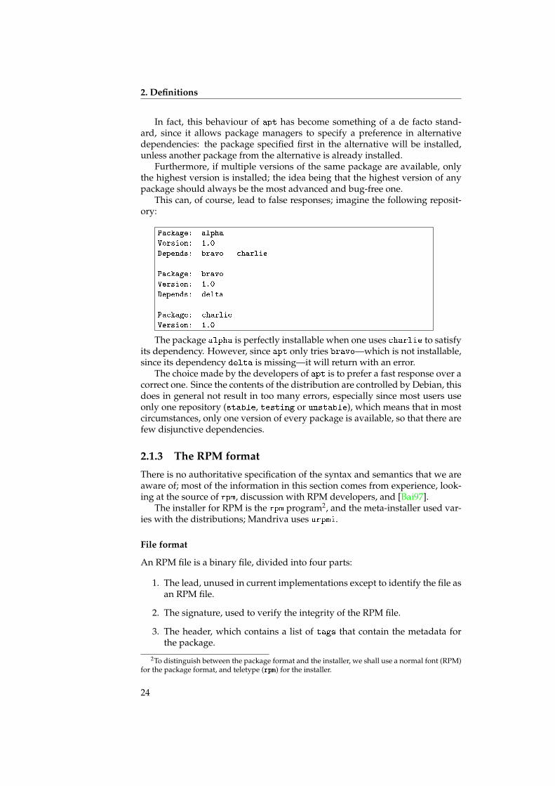
This can, of course, lead to false responses; imagine the following reposit-ory:
Package: alpha
Version: 1.0
Depends: bravo | charlie
Package: bravo
Version: 1.0
Depends: delta
Package: charlie
Version: 1.0
The package alpha is perfectly installable when one uses charlie to satisfyits dependency. However, since apt only tries bravo—which is not installable,since its dependency delta is missing—it will return with an error.
The choice made by the developers of apt is to prefer a fast response over acorrect one. Since the contents of the distribution are controlled by Debian, thisdoes in general not result in too many errors, especially since most users useonly one repository (stable, testing or unstable), which means that in mostcircumstances, only one version of every package is available, so that there arefew disjunctive dependencies.
2.1.3 The RPM format
There is no authoritative specification of the syntax and semantics that we areaware of; most of the information in this section comes from experience, look-ing at the source of rpm, discussion with RPM developers, and [Bai97].
The installer for RPM is the rpm program2, and the meta-installer used var-ies with the distributions; Mandriva uses urpmi.
File format
An RPM file is a binary file, divided into four parts:
1. The lead, unused in current implementations except to identify the file asan RPM file.
2. The signature, used to verify the integrity of the RPM file.
3. The header, which contains a list of tags that contain the metadata forthe package.
2To distinguish between the package format and the installer, we shall use a normal font (RPM)for the package format, and teletype (rpm) for the installer.
24
4. The archive, which is a compressed cpio archive containing the packagefiles.
Another file format is the hdlist, which is a concatenation of the headersof several packages (similar to the Debian Packages file).
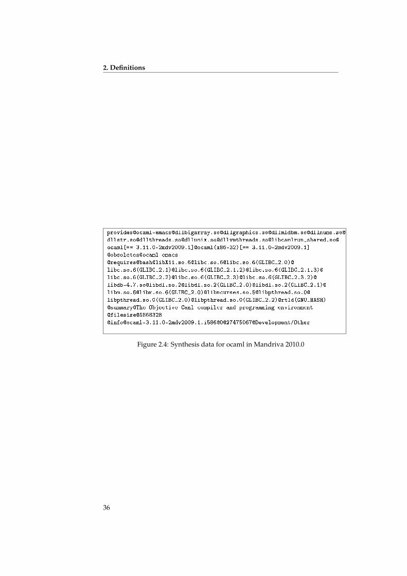
Mandriva’s urpmimeta-installer uses a textual format, called synthesis hdlist,which fulfils the same purpose as a ‘normal’ hdlist. However, it does not con-tain all tags from the RPM header and therefore it is far smaller (for Mandriva2010.0, the hdlist is 149 Mb in size, whereas the synthesis hdlist is 3.8 Mb).
An example of the data in the synthesis hdlist for the ocaml package is inFigure 2.4.
Package metadata
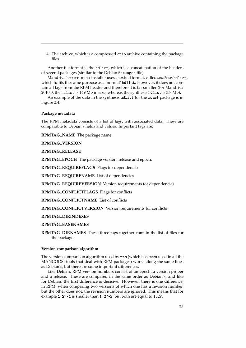
The RPM metadata consists of a list of tags, with associated data. These arecomparable to Debian’s fields and values. Important tags are:
RPMTAG NAME The package name.
RPMTAG VERSION
RPMTAG RELEASE
RPMTAG EPOCH The package version, release and epoch.
RPMTAG REQUIREFLAGS Flags for dependencies
RPMTAG REQUIRENAME List of dependencies
RPMTAG REQUIREVERSION Version requirements for dependencies
RPMTAG CONFLICTFLAGS Flags for conflicts
RPMTAG CONFLICTNAME List of conflicts
RPMTAG CONFLICTVERSION Version requirements for conflicts
RPMTAG DIRINDEXES
RPMTAG BASENAMES
RPMTAG DIRNAMES These three tags together contain the list of files forthe package.
Version comparison algorithm
The version comparison algorithm used by rpm (which has been used in all theMANCOOSI tools that deal with RPM packages) works along the same linesas Debian’s, but there are some important differences.
Like Debian, RPM version numbers consist of an epoch, a version properand a release. These are compared in the same order as Debian’s, and likefor Debian, the first difference is decisive. However, there is one difference:in RPM, when comparing two versions of which one has a revision number,but the other does not, the revision numbers are ignored. This means that forexample 1.27-1 is smaller than 1.27-2, but both are equal to 1.27.
25
2. Definitions
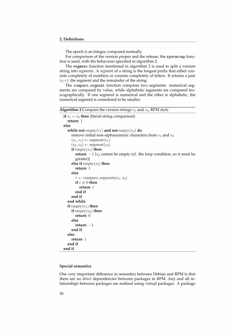
The epoch is an integer, compared normally.For comparison of the version proper and the release, the rpmvercmp func-
tion is used, with the behaviour specified in algorithm 2.The segment function mentioned in algorithm 2 is used to split a version
string into segments. A segment of a string is the longest prefix that either con-sists completely of numbers or consists completely of letters. It returns a pair(s, r): the segment and the remainder of the string.
The compare segment function compares two segments: numerical seg-ments are compared by value, while alphabetic segments are compared lex-icographically. If one segment is numerical and the other is alphabetic, thenumerical segment is considered to be smaller.
Algorithm 2 Compare the version strings v1 and v2, RPM style
if v1 = v2 then {literal string comparison}return 1
elsewhile not empty(v1) and not empty(v2) do
remove initial non-alphanumeric characters from v1 and v2(s1, v1)← segment(v1)(s2, v2)← segment(v2)if empty(s1) then
return −1 {s2 cannot be empty (cf. the loop condition, so it must begreater)}
else if empty(s2) thenreturn 1
elser ← compare segments(s1, s2)if r 6= 0 then
return rend if
end ifend whileif empty(v1) then
if empty(v2) thenreturn 0
elsereturn −1
end ifelse
return 1end if
end if
Special semantics
One very important difference in semantics between Debian and RPM is thatthere are no direct dependencies between packages in RPM. Any and all re-lationships between packages are realised using virtual packages. A package
26
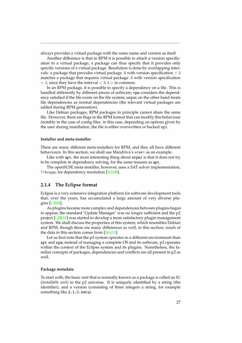
always provides a virtual package with the same name and version as itself.Another difference is that in RPM it is possible to attach a version specific-
ation to a virtual package; a package can thus specify that it provides onlyspecific versions of a virtual package. Resolution is done by overlapping inter-vals: a package that provides virtual package A with version specification > 3matches a package that requires virtual package A with version specification< 4, since they have the interval < 3, 4 > in common.
In an RPM package, it is possible to specify a dependency on a file. This ishandled differently by different pieces of software; rpm considers the depend-ency satisfied if the file exists on the file system; urpmi on the other hand treatsfile dependencies as normal dependencies (the relevant virtual packages areadded during RPM generation).
Like Debian packages, RPM packages in principle cannot share the samefile. However, there are flags in the RPM format that can modify this behaviour(notably in the case of config files: in this case, depending on options given bythe user during installation, the file is either overwritten or backed up).
Installer and meta-installer
There are many different meta-installers for RPM, and they all have differentbehaviours. In this section, we shall use Mandriva’s urpmi as an example.
Like with apt, the most interesting thing about urpmi is that it does not tryto be complete in dependency solving, for the same reasons as apt.
The openSUSE meta-installer, however, uses a SAT solver implementation,libzypp, for dependency resolution [Sch08].
2.1.4 The Eclipse format
Eclipse is a very extensive integration platform for software development toolsthat, over the years, has accumulated a large amount of very diverse plu-gins [CR08].
As plugins became more complex and dependencies between plugins beganto appear, the standard ‘Update Manager’ was no longer sufficient and the p2project [LBR10] was started to develop a more satisfactory plugin managementsystem. We shall discuss the properties of this system, which resembles Debianand RPM, though there are many differences as well, in this section; much ofthe data in this section comes from [Boz10].
Let us first note that the p2 system operates in a different environment thanapt and rpm; instead of managing a complete OS and its software, p2 operateswithin the context of the Eclipse system and its plugins. Nonetheless, the fa-miliar concepts of packages, dependencies and conflicts are all present in p2 aswell.
Package metadata
To start with, the basic unit that is normally known as a package is called an IU(installable unit) in the p2 universe. It is uniquely identified by a string (theidentifier), and a version (consisting of three integers a string, for examplesomething like 2.1.0.beta).
27
2. Definitions
Dependencies between IUs are created by requirements and capabilities: aswith RPM, an IU A depends on another IU B if A has a requirement thatmatches a capability of B.
Furthermore, every IU has an enablement filter, with which it can specifyconditions it needs to be installed, for example a particular OS or architecture.
IUs also have the possibility to set a singleton flag to specify that the systemshould not contain another IU with the same identifier (this is somewhat likethe combination of Provides and Conflicts fields in Debian).
And finally, an IU has an update specification, in which it identifies the IUsthat are considered predecessors to this IU.
Capabilities and requirements, as mentioned before, are used to create de-pendencies between packages. A capability consists of a namespace, a name(both strings), and a version; a requirement consists of a namespace, a nameand a version range. A requirement matches a capability if the namespace andname match, and the version of the capability is included in the version rangeof the requirement.
In addition to this, a requirement has a filter which can result in its beingdisabled under certain conditions (see the enablement filter for IUs mentionedabove).
Finally, requirements have two additional properties: they can be optionaland greedy. An optional requirement, as the name indicates, is a requirementthat does not have to be satisfied for the IU to be installed; the ‘greed’ propertyindicates whether an IU satisfying the requirement must be actively sought(greedy) or whether it must just be verified that the requirement has been met(non-greedy).
In fact, a requirement that is optional and non-greedy need not be installedat all; it is therefore akin to the Suggests field in the Debian format. If an IUsatisfying the requirement is found, it will be added to the dependencies of theIU to be installed, but if no such IU is found, the requirement will simply beconsidered satisfied and no further action will be taken.
Version comparison algorithm
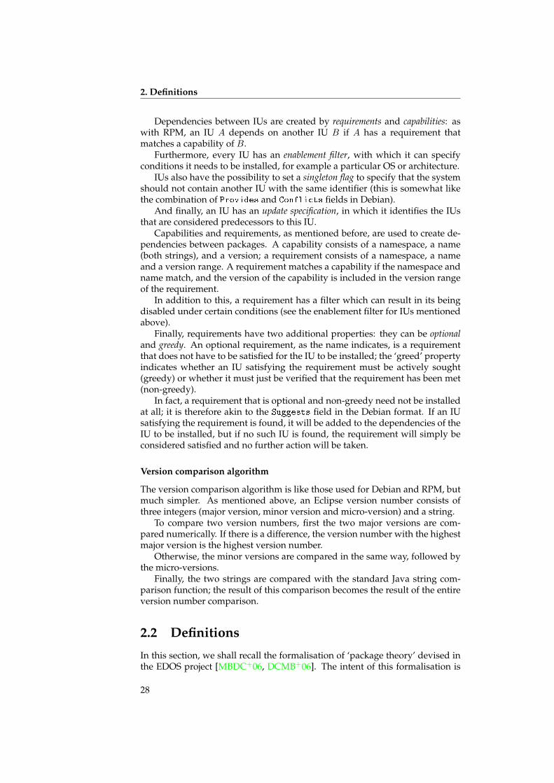
The version comparison algorithm is like those used for Debian and RPM, butmuch simpler. As mentioned above, an Eclipse version number consists ofthree integers (major version, minor version and micro-version) and a string.
To compare two version numbers, first the two major versions are com-pared numerically. If there is a difference, the version number with the highestmajor version is the highest version number.
Otherwise, the minor versions are compared in the same way, followed bythe micro-versions.
Finally, the two strings are compared with the standard Java string com-parison function; the result of this comparison becomes the result of the entireversion number comparison.
2.2 Definitions
In this section, we shall recall the formalisation of ‘package theory’ devised inthe EDOS project [MBDC+06, DCMB+06]. The intent of this formalisation is
28
to reflect the features of both standards presented above, especially those usedto determine package installability. We shall also present several lemmas thatfollow easily from these definitions, and that will come in useful when definingmore complicated properties later on.
The atomic entity in this thesis is the package; we shall abstract away fromnames and version numbers, since there are no theorems in this thesis thatmake use of these properties.
Definition 2.1 (Repository)A repository (R,D,C) is a triple consisting of a set of packages P , a conflictrelation C (C ⊆ R×R), and a dependency function D : R −→ ℘(℘(R)).
Axiom 2.2For any package p ∈ R, there does not exist a d ∈ D(p) such that p ∈ d.
In other words, a package never depends directly upon itself. This is ex-plicitly stated in the Debian specification, though not in the RPM specification.But even so, such a dependency would be trivially fulfilled (in order to installa package, the package itself is always installed); thus, it is safe to forbid suchdependencies.
Axiom 2.3The conflict relation is symmetrical and irreflexive.
Thus, a package can never conflict with itself. The Debian method of spe-cifying a conflict with a virtual package will be treated later on.
As for the dependency function, it associates a set of alternatives with a pack-age. These alternatives (which are themselves sets of packages) represent dis-junctive dependencies.
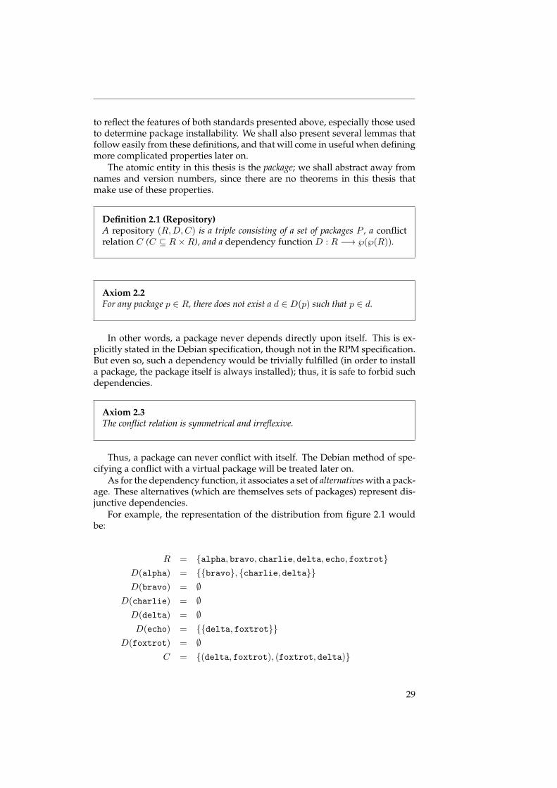
For example, the representation of the distribution from figure 2.1 wouldbe:
R = {alpha, bravo, charlie, delta, echo, foxtrot}D(alpha) = {{bravo}, {charlie, delta}}D(bravo) = ∅
D(charlie) = ∅D(delta) = ∅D(echo) = {{delta, foxtrot}}
D(foxtrot) = ∅C = {(delta, foxtrot), (foxtrot, delta)}
29
2. Definitions
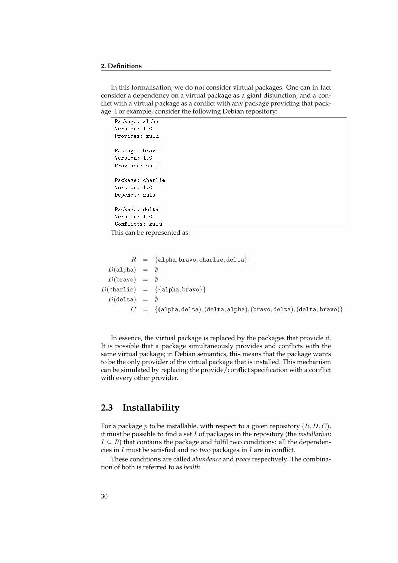
In this formalisation, we do not consider virtual packages. One can in factconsider a dependency on a virtual package as a giant disjunction, and a con-flict with a virtual package as a conflict with any package providing that pack-age. For example, consider the following Debian repository:
Package: alpha
Version: 1.0
Provides: zulu
Package: bravo
Version: 1.0
Provides: zulu
Package: charlie
Version: 1.0
Depends: zulu
Package: delta
Version: 1.0
Conflicts: zulu
This can be represented as:
R = {alpha, bravo, charlie, delta}D(alpha) = ∅D(bravo) = ∅
D(charlie) = {{alpha, bravo}}D(delta) = ∅
C = {(alpha, delta), (delta, alpha), (bravo, delta), (delta, bravo)}
In essence, the virtual package is replaced by the packages that provide it.It is possible that a package simultaneously provides and conflicts with thesame virtual package; in Debian semantics, this means that the package wantsto be the only provider of the virtual package that is installed. This mechanismcan be simulated by replacing the provide/conflict specification with a conflictwith every other provider.
2.3 Installability
For a package p to be installable, with respect to a given repository (R,D,C),it must be possible to find a set I of packages in the repository (the installation;I ⊆ R) that contains the package and fulfil two conditions: all the dependen-cies in I must be satisfied and no two packages in I are in conflict.
These conditions are called abundance and peace respectively. The combina-tion of both is referred to as health.
30
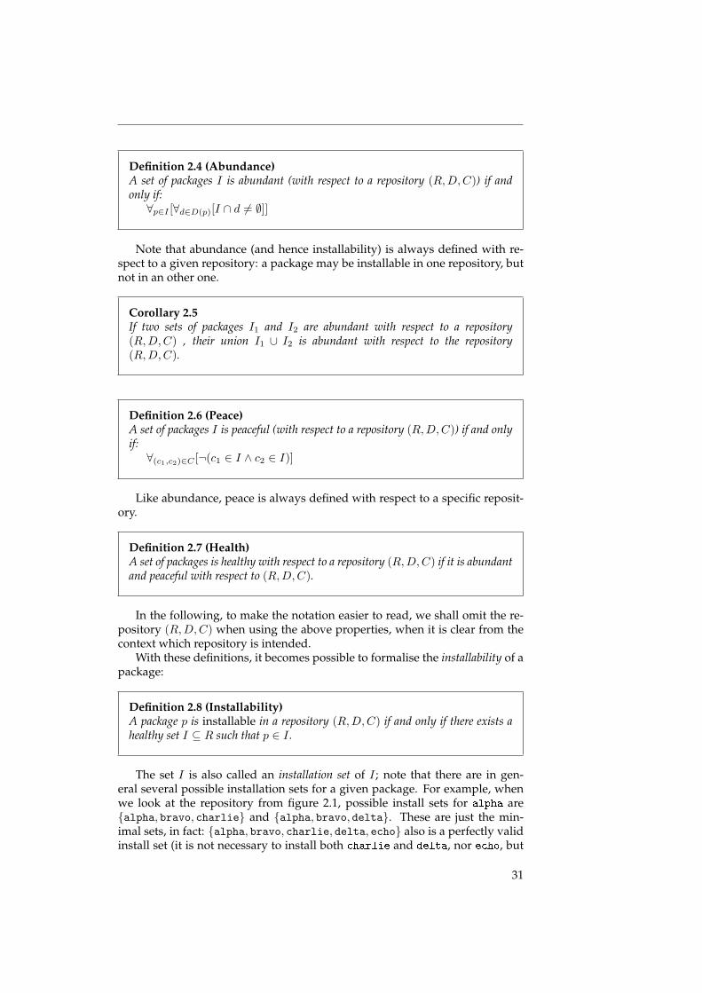
Definition 2.4 (Abundance)A set of packages I is abundant (with respect to a repository (R,D,C)) if andonly if:∀p∈I [∀d∈D(p)[I ∩ d 6= ∅]]
Note that abundance (and hence installability) is always defined with re-spect to a given repository: a package may be installable in one repository, butnot in an other one.
Corollary 2.5If two sets of packages I1 and I2 are abundant with respect to a repository(R,D,C) , their union I1 ∪ I2 is abundant with respect to the repository(R,D,C).
Definition 2.6 (Peace)A set of packages I is peaceful (with respect to a repository (R,D,C)) if and onlyif:∀(c1,c2)∈C [¬(c1 ∈ I ∧ c2 ∈ I)]
Like abundance, peace is always defined with respect to a specific reposit-ory.
Definition 2.7 (Health)A set of packages is healthy with respect to a repository (R,D,C) if it is abundantand peaceful with respect to (R,D,C).
In the following, to make the notation easier to read, we shall omit the re-pository (R,D,C) when using the above properties, when it is clear from thecontext which repository is intended.
With these definitions, it becomes possible to formalise the installability of apackage:
Definition 2.8 (Installability)A package p is installable in a repository (R,D,C) if and only if there exists ahealthy set I ⊆ R such that p ∈ I .
The set I is also called an installation set of I ; note that there are in gen-eral several possible installation sets for a given package. For example, whenwe look at the repository from figure 2.1, possible install sets for alpha are{alpha, bravo, charlie} and {alpha, bravo, delta}. These are just the min-imal sets, in fact: {alpha, bravo, charlie, delta, echo} also is a perfectly validinstall set (it is not necessary to install both charlie and delta, nor echo, but
31
2. Definitions
neither is it forbidden to install extra packages) However, since an install sethas to be peaceful, it is not possible to include both delta and foxtrot in aninstall set, because of the conflict between them.
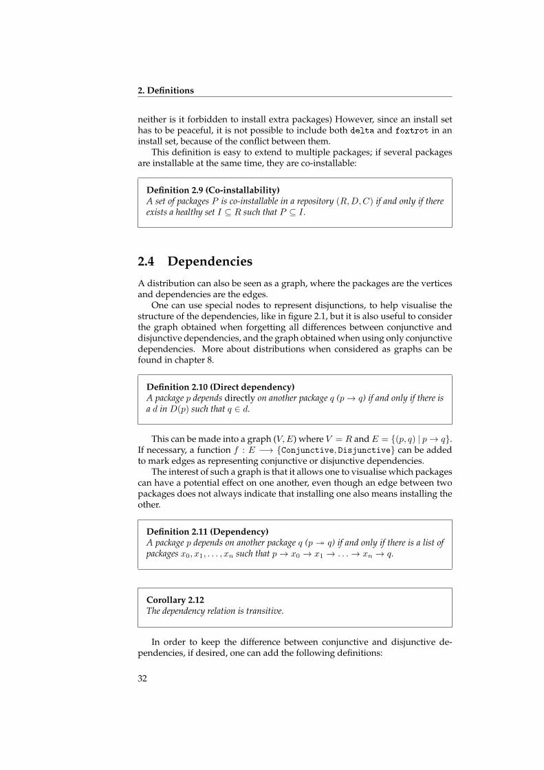
This definition is easy to extend to multiple packages; if several packagesare installable at the same time, they are co-installable:
Definition 2.9 (Co-installability)A set of packages P is co-installable in a repository (R,D,C) if and only if thereexists a healthy set I ⊆ R such that P ⊆ I .
2.4 Dependencies
A distribution can also be seen as a graph, where the packages are the verticesand dependencies are the edges.
One can use special nodes to represent disjunctions, to help visualise thestructure of the dependencies, like in figure 2.1, but it is also useful to considerthe graph obtained when forgetting all differences between conjunctive anddisjunctive dependencies, and the graph obtained when using only conjunctivedependencies. More about distributions when considered as graphs can befound in chapter 8.
Definition 2.10 (Direct dependency)A package p depends directly on another package q (p→ q) if and only if there isa d in D(p) such that q ∈ d.
This can be made into a graph (V,E) where V = R andE = {(p, q) | p→ q}.If necessary, a function f : E −→ {Conjunctive, Disjunctive} can be addedto mark edges as representing conjunctive or disjunctive dependencies.
The interest of such a graph is that it allows one to visualise which packagescan have a potential effect on one another, even though an edge between twopackages does not always indicate that installing one also means installing theother.
Definition 2.11 (Dependency)A package p depends on another package q (p � q) if and only if there is a list ofpackages x0, x1, . . . , xn such that p→ x0 → x1 → . . .→ xn → q.
Corollary 2.12The dependency relation is transitive.
In order to keep the difference between conjunctive and disjunctive de-pendencies, if desired, one can add the following definitions:
32
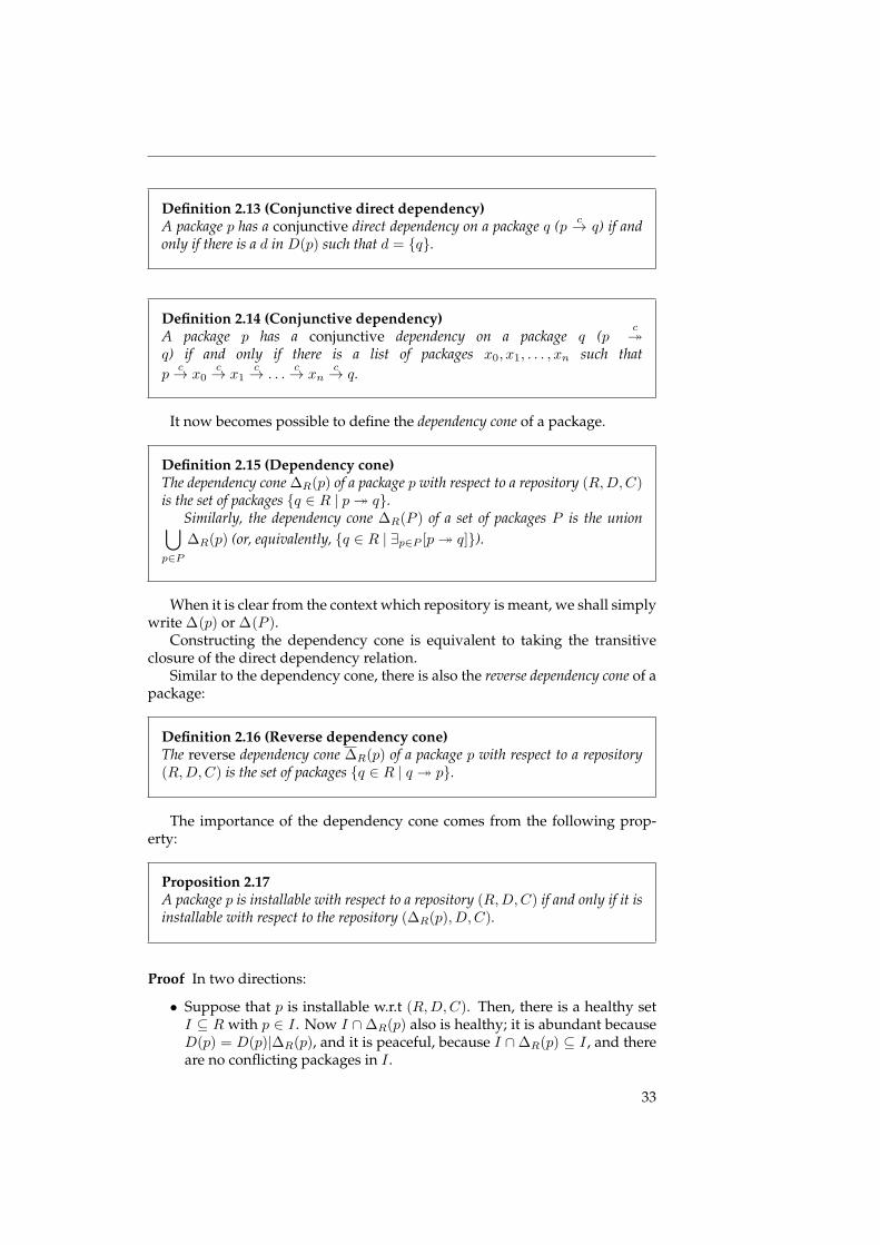
Definition 2.13 (Conjunctive direct dependency)A package p has a conjunctive direct dependency on a package q (p c→ q) if andonly if there is a d in D(p) such that d = {q}.
Definition 2.14 (Conjunctive dependency)A package p has a conjunctive dependency on a package q (p
c�
q) if and only if there is a list of packages x0, x1, . . . , xn such thatp
c→ x0c→ x1
c→ . . .c→ xn
c→ q.
It now becomes possible to define the dependency cone of a package.
Definition 2.15 (Dependency cone)The dependency cone ∆R(p) of a package p with respect to a repository (R,D,C)is the set of packages {q ∈ R | p� q}.
Similarly, the dependency cone ∆R(P ) of a set of packages P is the union⋃p∈P
∆R(p) (or, equivalently, {q ∈ R | ∃p∈P [p� q]}).
When it is clear from the context which repository is meant, we shall simplywrite ∆(p) or ∆(P ).
Constructing the dependency cone is equivalent to taking the transitiveclosure of the direct dependency relation.
Similar to the dependency cone, there is also the reverse dependency cone of apackage:
Definition 2.16 (Reverse dependency cone)The reverse dependency cone ∆R(p) of a package p with respect to a repository(R,D,C) is the set of packages {q ∈ R | q � p}.
The importance of the dependency cone comes from the following prop-erty:
Proposition 2.17A package p is installable with respect to a repository (R,D,C) if and only if it isinstallable with respect to the repository (∆R(p), D,C).
Proof In two directions:
• Suppose that p is installable w.r.t (R,D,C). Then, there is a healthy setI ⊆ R with p ∈ I . Now I ∩∆R(p) also is healthy; it is abundant becauseD(p) = D(p)|∆R(p), and it is peaceful, because I ∩∆R(p) ⊆ I , and thereare no conflicting packages in I .
33
2. Definitions
• Suppose that p is installable w.r.t. (∆R(p), D,C). Since R ⊇ ∆R(p), onecan re-use the same installation set for (R,D,C).
This means that, when determining the installability of a package (or setof packages) in a repository, one only has to consider packages that are in itsdependency cone. This is not surprising, as the installability of a package can-not depend on packages that it has no dependency relation with, but it is ofgreat importance when building efficient algorithms: many tools which arebeing used today to check installability are based on solvers that work on apropositional logic representation of a repository. The property proven in pro-position 2.17 shows that the dependency solver only needs the packages inthe dependency cone of the package it is investigating, which saves time andspace.
Another important property is stated in the following proposition: if apackage p has a conjunctive dependency on another, any installation set of pwill contain this package.
Proposition 2.18For two packages p, q such that p
c� q, any installation set of p includes q.
Proof Since pc� q, there is a list x0, x1, . . . xn such that p c→ x0
c→ x1c→ . . .
c→ xn →c q.Follows a proof by induction on k that given an installation set I of p, for
all xk, xk ∈ I :
• x0 ∈ I : p c→ x0, so that {x0} ∈ D(p). Since I is abundant, {x0} ∩ I 6= ∅,hence x0 ∈ I .
• xm ∈ I −→ xm+1 ∈ I : xmc→ xm+1, so that {xm+1} ∈ D(xm). Since I is
abundant, {xm+1} ∩ I 6= ∅, hence xm+1 ∈ I .
Thus, xn ∈ I . Given that xnc→ q, {q} ∈ D(xn) and thus q ∈ I .
Again, this property seems trivial, but we shall see in later chapters that itcan be used to optimise several algorithms.
34
Package: ocaml
Priority: optional
Section: devel
Installed-Size: 8368
Maintainer: Debian OCaml Maintainers <[email protected]>
Architecture: i386
Version: 3.10.2-3
Replaces: ocaml-nox (� 3.10.0-12)
Provides: ocaml-3.10.2
Depends: ocaml-base (= 3.10.2-3), ocaml-nox (= 3.10.2-3), libx11-dev
Suggests: tcl8.4-dev, tk8.4-dev
Filename: pool/main/o/ocaml/ocaml 3.10.2-3 i386.deb
Size: 2066194
MD5sum: cd876d71c86a2ed80f052f2994745dd7
SHA1: 0a65ca56fa0fc56c24ad44aa0b73b06e0d000bd1
SHA256: 7dcc3186984741313c663b638c68cf9f33028e71154ace3e4f35c4c46f4148bb
Description: ML language implementation with a class-based object system
Objective Caml (OCaml) is an implementation of the ML language, based on
the Caml Light dialect extended with a complete class-based object system
and a powerful module system in the style of Standard ML.
.
OCaml comprises two compilers. One generates bytecode
which is then interpreted by a C program. This compiler runs quickly,
generates compact code with moderate memory requirements, and is
portable to essentially any 32 or 64 bit Unix platform. Performance of
generated programs is quite good for a bytecoded implementation:
almost twice as fast as Caml Light 0.7. This compiler can be used
either as a standalone, batch-oriented compiler that produces
standalone programs, or as an interactive, toplevel-based system.
.
The other compiler generates high-performance native code for a number
of processors. Compilation takes longer and generates bigger code, but
the generated programs deliver excellent performance, while retaining
the moderate memory requirements of the bytecode compiler. It is not
available on all arches though.
.
This package contains everything needed to develop OCaml applications,
including the graphics libraries.
Homepage: http://caml.inria.fr/
Tag: devel::{compiler,interpreter,lang:ocaml}, implemented-in::ocaml,
role::meta
Figure 2.3: Metadata for the Debian ocaml package
35
2. Definitions
provides@[email protected]@[email protected]@dllnums.so@
[email protected]@[email protected]@libcamlrun shared.so@
ocaml[== 3.11.0-2mdv2009.1]@ocaml(x86-32)[== 3.11.0-2mdv2009.1]
@obsoletes@ocaml-emacs
@requires@[email protected]@[email protected](GLIBC 2.0)@
libc.so.6(GLIBC 2.1)@libc.so.6(GLIBC 2.1.2)@libc.so.6(GLIBC 2.1.3)@
libc.so.6(GLIBC 2.2)@libc.so.6(GLIBC 2.3)@libc.so.6(GLIBC 2.3.2)@
[email protected]@libdl.so.2(GLIBC 2.0)@libdl.so.2(GLIBC 2.1)@
[email protected](GLIBC 2.0)@[email protected]@
libpthread.so.0(GLIBC 2.0)@libpthread.so.0(GLIBC 2.2)@rtld(GNU HASH)
@summary@The Objective Caml compiler and programming environment
@filesize@5868328
@[email protected]@0@27475067@Development/Other
Figure 2.4: Synthesis data for ocaml in Mandriva 2010.0
36
Strong dependencies andconflicts 3ἁρμονίη αφανης φανερ ης κρείττων
— HERACLITUS OF EPHESUS
In F/OSS distributions, as well as many other component-based systems [Apa09,CR08], the language used to express inter-package relationships is expressiveenough to cover propositional logic. As a consequence, considering only ‘nor-mal’ dependencies, as expressed in the existing metadata, the existence of a de-pendency path between two packages does not guarantee that when installingthe first package, the second will always be installed. For example, if p is to beinstalled and there exists a dependency path from p to q, it is not true that q isalways needed for p, and in some cases q may even be incompatible with p.
In other terms, the syntactic connectivity notion—this being the existenceof a dependency path as specified in the package metadata—does not tell usmuch about the real structure of dependencies and conflicts: it is necessaryto go further and analyse the semantic connectivity—the essence of the de-pendency relationship: installing one package always implies installing an-other package as well—among software components induced by the explicitdependencies in the graph.
In this chapter, we shall explain these notions of semantic connectivity andpropose their basic properties, as well as theorems that can be used to effi-ciently compute them. The consequences of this notion when considering thedistribution graph will be treated in more detail in chapter 8.
3.1 Strong dependencies
When considering the dependencies of a package, it is interesting to restrictourselves to those dependencies that are always installed when the packageitself is installed; this gives us an under-representation of the actual packagesthat are going to be installed (there might still be other packages that are part ofa disjunctive dependency, for example), but it does give us the most importantdependencies: those that are absolutely essential.
In the MANCOOSI project, we have called this concept a strong dependency:in short, a package p depends strongly q if and only if it is impossible to installp without also installing q. The formal definition is as follows:
Definition 3.1 (Strong dependency)Given a repository % = (R,D,C), a package p strongly depends on a package q(denoted p ⇒% q) if and only if p is installable in %, and all installation sets of pin % contain q (If it is clear from the context which repository is meant, we shallsimply note p⇒ q to indicate a strong dependency).
37
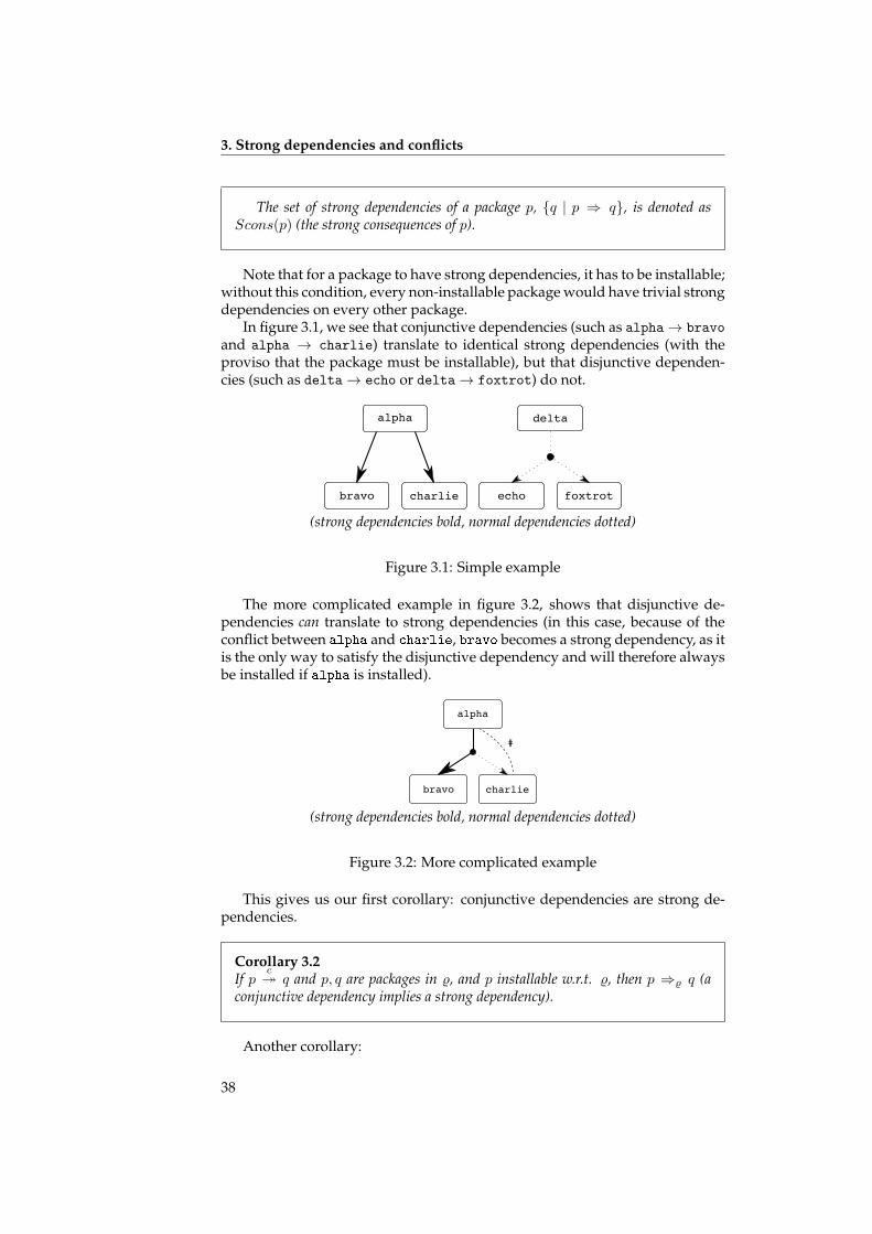
3. Strong dependencies and conflicts
The set of strong dependencies of a package p, {q | p ⇒ q}, is denoted asScons(p) (the strong consequences of p).
Note that for a package to have strong dependencies, it has to be installable;without this condition, every non-installable package would have trivial strongdependencies on every other package.
In figure 3.1, we see that conjunctive dependencies (such as alpha→ bravo
and alpha → charlie) translate to identical strong dependencies (with theproviso that the package must be installable), but that disjunctive dependen-cies (such as delta→ echo or delta→ foxtrot) do not.
alpha
bravo charlie
delta
echo foxtrot
(strong dependencies bold, normal dependencies dotted)
Figure 3.1: Simple example
The more complicated example in figure 3.2, shows that disjunctive de-pendencies can translate to strong dependencies (in this case, because of theconflict between alpha and charlie, bravo becomes a strong dependency, as itis the only way to satisfy the disjunctive dependency and will therefore alwaysbe installed if alpha is installed).
#
alpha
bravo charlie
(strong dependencies bold, normal dependencies dotted)
Figure 3.2: More complicated example
This gives us our first corollary: conjunctive dependencies are strong de-pendencies.
Corollary 3.2If p
c� q and p, q are packages in %, and p installable w.r.t. %, then p ⇒% q (a
conjunctive dependency implies a strong dependency).
Another corollary:
38
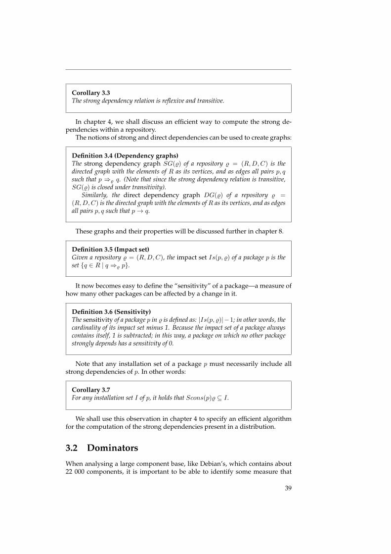
Corollary 3.3The strong dependency relation is reflexive and transitive.
In chapter 4, we shall discuss an efficient way to compute the strong de-pendencies within a repository.
The notions of strong and direct dependencies can be used to create graphs:
Definition 3.4 (Dependency graphs)The strong dependency graph SG(%) of a repository % = (R,D,C) is thedirected graph with the elements of R as its vertices, and as edges all pairs p, qsuch that p ⇒% q. (Note that since the strong dependency relation is transitive,SG(%) is closed under transitivity).
Similarly, the direct dependency graph DG(%) of a repository % =(R,D,C) is the directed graph with the elements of R as its vertices, and as edgesall pairs p, q such that p→ q.
These graphs and their properties will be discussed further in chapter 8.
Definition 3.5 (Impact set)Given a repository % = (R,D,C), the impact set Is(p, %) of a package p is theset {q ∈ R | q ⇒% p}.
It now becomes easy to define the “sensitivity” of a package—a measure ofhow many other packages can be affected by a change in it.
Definition 3.6 (Sensitivity)The sensitivity of a package p in % is defined as: |Is(p, %)|−1; in other words, thecardinality of its impact set minus 1. Because the impact set of a package alwayscontains itself, 1 is subtracted; in this way, a package on which no other packagestrongly depends has a sensitivity of 0.
Note that any installation set of a package p must necessarily include allstrong dependencies of p. In other words:
Corollary 3.7For any installation set I of p, it holds that Scons(p)% ⊆ I .
We shall use this observation in chapter 4 to specify an efficient algorithmfor the computation of the strong dependencies present in a distribution.
3.2 Dominators
When analysing a large component base, like Debian’s, which contains about22 000 components, it is important to be able to identify some measure that
39
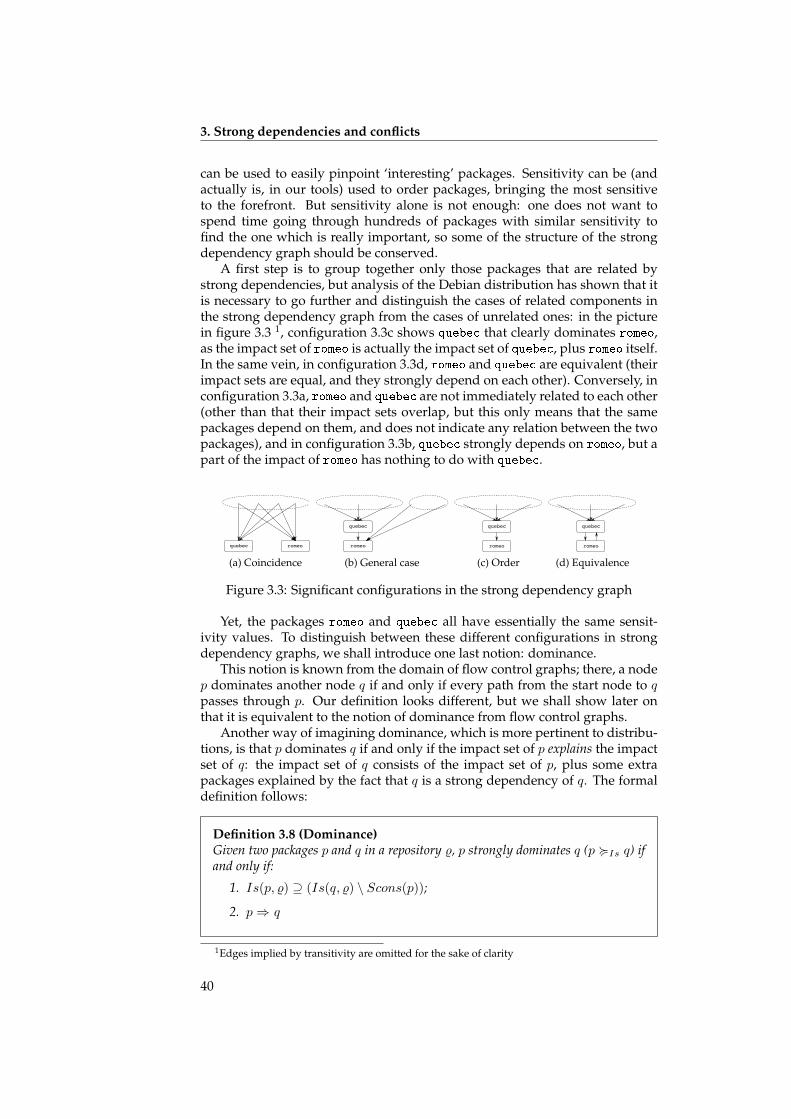
3. Strong dependencies and conflicts
can be used to easily pinpoint ‘interesting’ packages. Sensitivity can be (andactually is, in our tools) used to order packages, bringing the most sensitiveto the forefront. But sensitivity alone is not enough: one does not want tospend time going through hundreds of packages with similar sensitivity tofind the one which is really important, so some of the structure of the strongdependency graph should be conserved.
A first step is to group together only those packages that are related bystrong dependencies, but analysis of the Debian distribution has shown that itis necessary to go further and distinguish the cases of related components inthe strong dependency graph from the cases of unrelated ones: in the picturein figure 3.3 1, configuration 3.3c shows quebec that clearly dominates romeo,as the impact set of romeo is actually the impact set of quebec, plus romeo itself.In the same vein, in configuration 3.3d, romeo and quebec are equivalent (theirimpact sets are equal, and they strongly depend on each other). Conversely, inconfiguration 3.3a, romeo and quebec are not immediately related to each other(other than that their impact sets overlap, but this only means that the samepackages depend on them, and does not indicate any relation between the twopackages), and in configuration 3.3b, quebec strongly depends on romeo, but apart of the impact of romeo has nothing to do with quebec.
quebec romeo
(a) Coincidence
quebec
romeo
(b) General case
quebec
romeo
(c) Order
quebec
romeo
(d) Equivalence
Figure 3.3: Significant configurations in the strong dependency graph
Yet, the packages romeo and quebec all have essentially the same sensit-ivity values. To distinguish between these different configurations in strongdependency graphs, we shall introduce one last notion: dominance.
This notion is known from the domain of flow control graphs; there, a nodep dominates another node q if and only if every path from the start node to qpasses through p. Our definition looks different, but we shall show later onthat it is equivalent to the notion of dominance from flow control graphs.
Another way of imagining dominance, which is more pertinent to distribu-tions, is that p dominates q if and only if the impact set of p explains the impactset of q: the impact set of q consists of the impact set of p, plus some extrapackages explained by the fact that q is a strong dependency of q. The formaldefinition follows:
Definition 3.8 (Dominance)Given two packages p and q in a repository %, p strongly dominates q (p <Is q) ifand only if:
1. Is(p, %) ⊇ (Is(q, %) \ Scons(p));
2. p⇒ q
1Edges implied by transitivity are omitted for the sake of clarity
40
Using the transitivity of strong dependencies, it is possible to prove that thestrong domination relation is a partial pre-order:
Lemma 3.9The dominance relation is a partial pre-order.
Proof • Reflexivity: trivial to check.
• Transitivity: suppose that there are p, q, r such that p <Is q and q <Is r.Then, Is(p, %) ⊇ (Is(q, %) \ Scons(p)) and Is(q, %) ⊇ (Is(r, %) \ Scons(q)).By transitivity of strong dependencies, since p ⇒ q ⇒ r, it is also thecase that Scons(p) ⊇ Scons(q) ⊇ Scons(r). Then, (Is(r, %) \ Scons(q)) \Scons(p) = Is(r, %) \ Scons(p), and because Is(p,⊇)Is(r, %) \ Scons(q), itis the case that p <Is r.By transitivity of the strong dependency relation, it is also the case thatp⇒ r.
This pre-order is now able to distinguish among the cases of figure 3.3. Inconfiguration 3.3c, it is the case that quebec <Is romeo, but not the converse;in configuration 3.3d both quebec <Is romeo and romeo <Is quebec (in otherwords, romeo and quebec are equivalent with respect to dominance); in config-urations 3.3a and 3.3b, no dominance relationship can be established betweenromeo and quebec.
It is possible, and actually quite useful, to generalise the dominance relationto also cover the case from configuration 3.3b, where a part of the impact set ofthe package romeo is not covered by the impact set of quebec.
If the “uncovered” part is small in respect to the “covered” part, after all,there is still a strong correlation between the impact sets of both packages. Thisconcept of relative dominance is defined as follows:
Definition 3.10 (Relative dominance)Given two packages p and q in a repository %, p strongly dominates q up to z(p <z
Is q) if and only if:
• |(Is(q,%)\Scons(p))\Is(p,%)||Is(p,%)| ∗ 100 = z;
• p strongly depends on q.
It is easy to see that p <Is q is equivalent to p <0Is q, and one can compute
in a single pass on the repository the values z for each pair of packages suchthat p⇒ q, leaving for later the choice of a threshold value for z.
3.3 Dominators in strong dependency graphs andcontrol flow graphs
Dominance in a strong dependency graph can be formally put in correspond-ence with the traditional notion of dominators in control flow graphs [LT79].
41
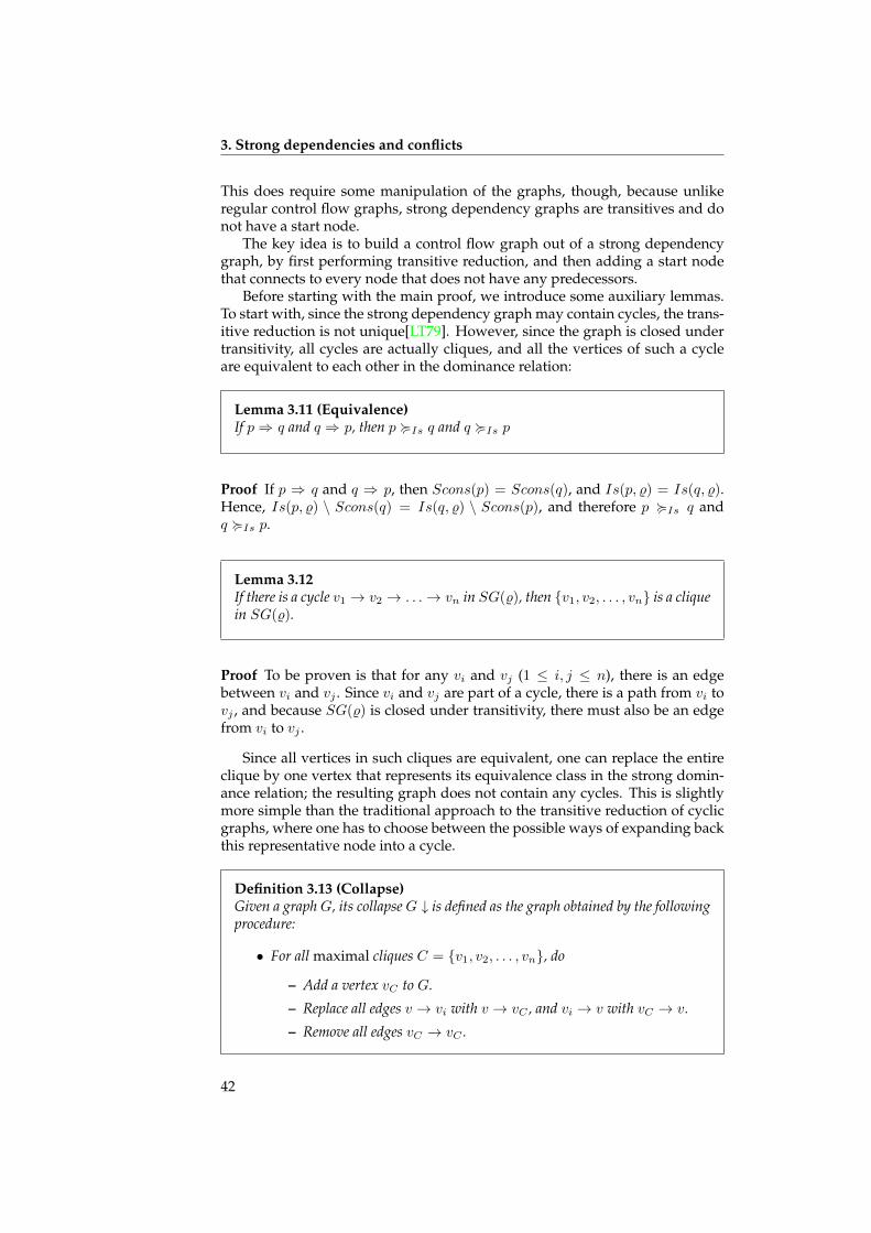
3. Strong dependencies and conflicts
This does require some manipulation of the graphs, though, because unlikeregular control flow graphs, strong dependency graphs are transitives and donot have a start node.
The key idea is to build a control flow graph out of a strong dependencygraph, by first performing transitive reduction, and then adding a start nodethat connects to every node that does not have any predecessors.
Before starting with the main proof, we introduce some auxiliary lemmas.To start with, since the strong dependency graph may contain cycles, the trans-itive reduction is not unique[LT79]. However, since the graph is closed undertransitivity, all cycles are actually cliques, and all the vertices of such a cycleare equivalent to each other in the dominance relation:
Lemma 3.11 (Equivalence)If p⇒ q and q ⇒ p, then p <Is q and q <Is p
Proof If p ⇒ q and q ⇒ p, then Scons(p) = Scons(q), and Is(p, %) = Is(q, %).Hence, Is(p, %) \ Scons(q) = Is(q, %) \ Scons(p), and therefore p <Is q andq <Is p.
Lemma 3.12If there is a cycle v1 → v2 → . . .→ vn in SG(%), then {v1, v2, . . . , vn} is a cliquein SG(%).
Proof To be proven is that for any vi and vj (1 ≤ i, j ≤ n), there is an edgebetween vi and vj . Since vi and vj are part of a cycle, there is a path from vi tovj , and because SG(%) is closed under transitivity, there must also be an edgefrom vi to vj .
Since all vertices in such cliques are equivalent, one can replace the entireclique by one vertex that represents its equivalence class in the strong domin-ance relation; the resulting graph does not contain any cycles. This is slightlymore simple than the traditional approach to the transitive reduction of cyclicgraphs, where one has to choose between the possible ways of expanding backthis representative node into a cycle.
Definition 3.13 (Collapse)Given a graph G, its collapseG ↓ is defined as the graph obtained by the followingprocedure:
• For all maximal cliques C = {v1, v2, . . . , vn}, do
– Add a vertex vC to G.
– Replace all edges v → vi with v → vC , and vi → v with vC → v.
– Remove all edges vC → vC .
42
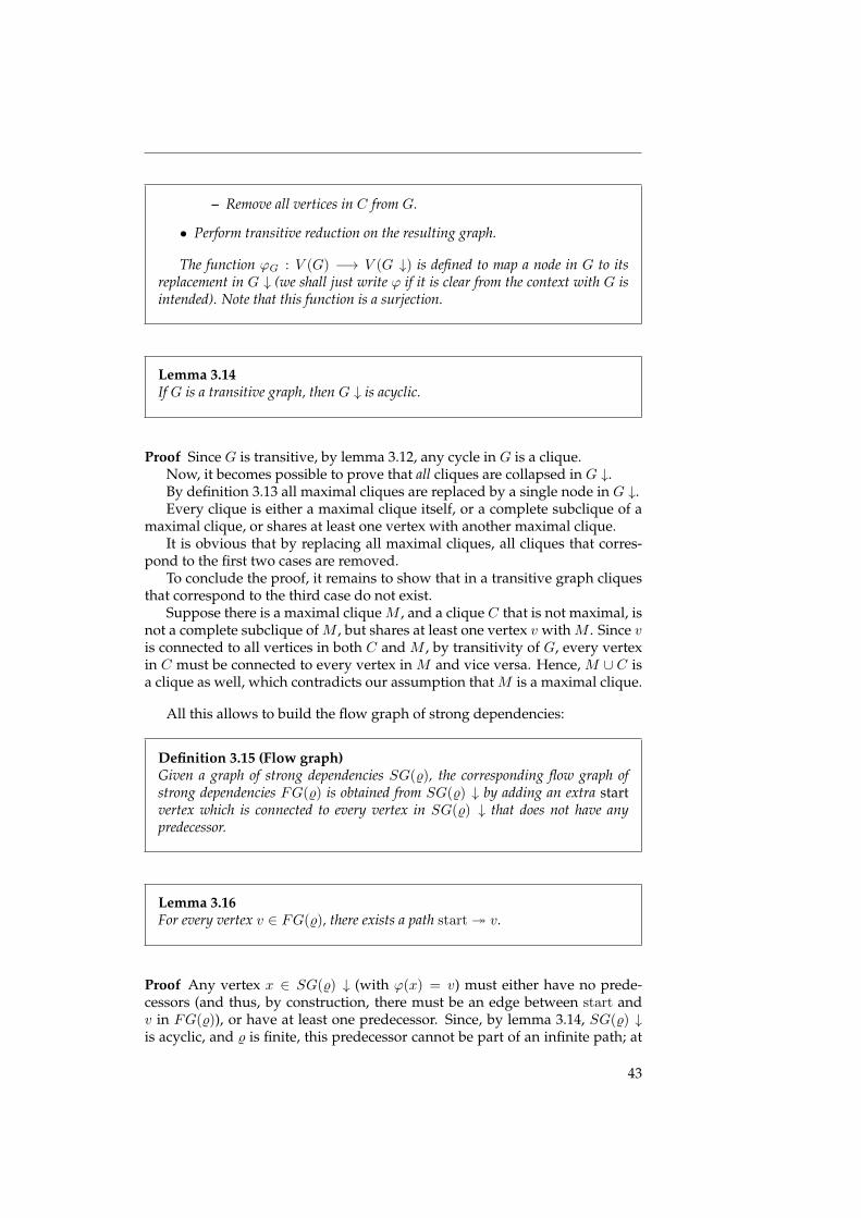
– Remove all vertices in C from G.
• Perform transitive reduction on the resulting graph.
The function ϕG : V (G) −→ V (G ↓) is defined to map a node in G to itsreplacement in G ↓ (we shall just write ϕ if it is clear from the context with G isintended). Note that this function is a surjection.
Lemma 3.14If G is a transitive graph, then G ↓ is acyclic.
Proof Since G is transitive, by lemma 3.12, any cycle in G is a clique.Now, it becomes possible to prove that all cliques are collapsed in G ↓.By definition 3.13 all maximal cliques are replaced by a single node in G ↓.Every clique is either a maximal clique itself, or a complete subclique of a
maximal clique, or shares at least one vertex with another maximal clique.It is obvious that by replacing all maximal cliques, all cliques that corres-
pond to the first two cases are removed.To conclude the proof, it remains to show that in a transitive graph cliques
that correspond to the third case do not exist.Suppose there is a maximal clique M , and a clique C that is not maximal, is
not a complete subclique of M , but shares at least one vertex v with M . Since vis connected to all vertices in both C and M , by transitivity of G, every vertexin C must be connected to every vertex in M and vice versa. Hence, M ∪ C isa clique as well, which contradicts our assumption that M is a maximal clique.
All this allows to build the flow graph of strong dependencies:
Definition 3.15 (Flow graph)Given a graph of strong dependencies SG(%), the corresponding flow graph ofstrong dependencies FG(%) is obtained from SG(%) ↓ by adding an extra startvertex which is connected to every vertex in SG(%) ↓ that does not have anypredecessor.
Lemma 3.16For every vertex v ∈ FG(%), there exists a path start� v.
Proof Any vertex x ∈ SG(%) ↓ (with ϕ(x) = v) must either have no prede-cessors (and thus, by construction, there must be an edge between start andv in FG(%)), or have at least one predecessor. Since, by lemma 3.14, SG(%) ↓is acyclic, and % is finite, this predecessor cannot be part of an infinite path; at
43
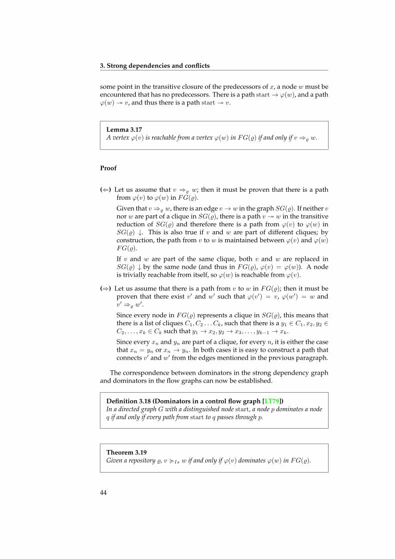
3. Strong dependencies and conflicts
some point in the transitive closure of the predecessors of x, a node w must beencountered that has no predecessors. There is a path start→ ϕ(w), and a pathϕ(w)� v, and thus there is a path start� v.
Lemma 3.17A vertex ϕ(v) is reachable from a vertex ϕ(w) in FG(%) if and only if v ⇒% w.
Proof
(⇐) Let us assume that v ⇒% w; then it must be proven that there is a pathfrom ϕ(v) to ϕ(w) in FG(%).
Given that v ⇒% w, there is an edge v → w in the graph SG(%). If neither vnor w are part of a clique in SG(%), there is a path v � w in the transitivereduction of SG(%) and therefore there is a path from ϕ(v) to ϕ(w) inSG(%) ↓. This is also true if v and w are part of different cliques; byconstruction, the path from v to w is maintained between ϕ(v) and ϕ(w)FG(%).
If v and w are part of the same clique, both v and w are replaced inSG(%) ↓ by the same node (and thus in FG(%), ϕ(v) = ϕ(w)). A nodeis trivially reachable from itself, so ϕ(w) is reachable from ϕ(v).
(⇒) Let us assume that there is a path from v to w in FG(%); then it must beproven that there exist v′ and w′ such that ϕ(v′) = v, ϕ(w′) = w andv′ ⇒% w
′.
Since every node in FG(%) represents a clique in SG(%), this means thatthere is a list of cliques C1, C2 . . . Ck, such that there is a y1 ∈ C1, x2, y2 ∈C2, . . . , xk ∈ Ck such that y1 → x2, y2 → x3, . . . , yk−1 → xk.
Since every xn and yn are part of a clique, for every n, it is either the casethat xn = yn or xn → yn. In both cases it is easy to construct a path thatconnects v′ and w′ from the edges mentioned in the previous paragraph.
The correspondence between dominators in the strong dependency graphand dominators in the flow graphs can now be established.
Definition 3.18 (Dominators in a control flow graph [LT79])In a directed graph G with a distinguished node start, a node p dominates a nodeq if and only if every path from start to q passes through p.
Theorem 3.19Given a repository %, v <Is w if and only if ϕ(v) dominates ϕ(w) in FG(%).
44
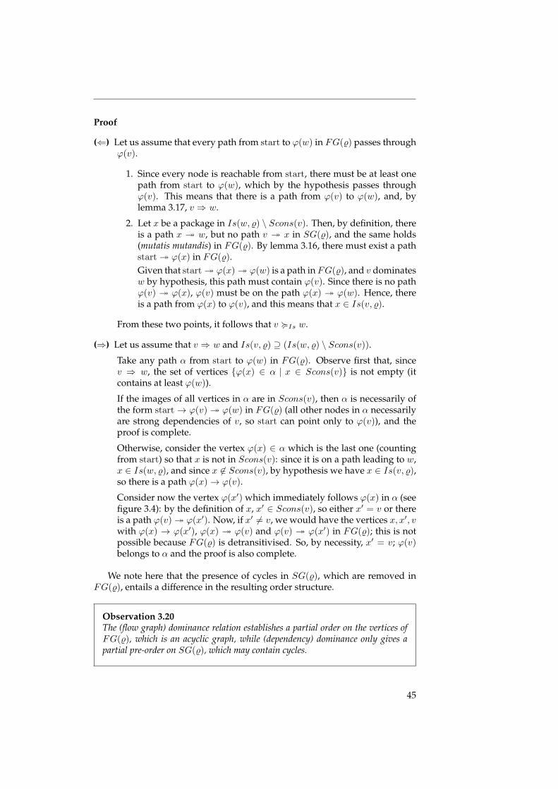
Proof
(⇐) Let us assume that every path from start to ϕ(w) in FG(%) passes throughϕ(v).
1. Since every node is reachable from start, there must be at least onepath from start to ϕ(w), which by the hypothesis passes throughϕ(v). This means that there is a path from ϕ(v) to ϕ(w), and, bylemma 3.17, v ⇒ w.
2. Let x be a package in Is(w, %) \ Scons(v). Then, by definition, thereis a path x � w, but no path v � x in SG(%), and the same holds(mutatis mutandis) in FG(%). By lemma 3.16, there must exist a pathstart� ϕ(x) in FG(%).Given that start� ϕ(x)� ϕ(w) is a path in FG(%), and v dominatesw by hypothesis, this path must contain ϕ(v). Since there is no pathϕ(v) � ϕ(x), ϕ(v) must be on the path ϕ(x) � ϕ(w). Hence, thereis a path from ϕ(x) to ϕ(v), and this means that x ∈ Is(v, %).
From these two points, it follows that v <Is w.
(⇒) Let us assume that v ⇒ w and Is(v, %) ⊇ (Is(w, %) \ Scons(v)).
Take any path α from start to ϕ(w) in FG(%). Observe first that, sincev ⇒ w, the set of vertices {ϕ(x) ∈ α | x ∈ Scons(v)} is not empty (itcontains at least ϕ(w)).
If the images of all vertices in α are in Scons(v), then α is necessarily ofthe form start→ ϕ(v)� ϕ(w) in FG(%) (all other nodes in α necessarilyare strong dependencies of v, so start can point only to ϕ(v)), and theproof is complete.
Otherwise, consider the vertex ϕ(x) ∈ α which is the last one (countingfrom start) so that x is not in Scons(v): since it is on a path leading to w,x ∈ Is(w, %), and since x 6∈ Scons(v), by hypothesis we have x ∈ Is(v, %),so there is a path ϕ(x)→ ϕ(v).
Consider now the vertex ϕ(x′) which immediately follows ϕ(x) in α (seefigure 3.4): by the definition of x, x′ ∈ Scons(v), so either x′ = v or thereis a path ϕ(v)� ϕ(x′). Now, if x′ 6= v, we would have the vertices x, x′, vwith ϕ(x) → ϕ(x′), ϕ(x) � ϕ(v) and ϕ(v) � ϕ(x′) in FG(%); this is notpossible because FG(%) is detransitivised. So, by necessity, x′ = v; ϕ(v)belongs to α and the proof is also complete.
We note here that the presence of cycles in SG(%), which are removed inFG(%), entails a difference in the resulting order structure.
Observation 3.20The (flow graph) dominance relation establishes a partial order on the vertices ofFG(%), which is an acyclic graph, while (dependency) dominance only gives apartial pre-order on SG(%), which may contain cycles.
45
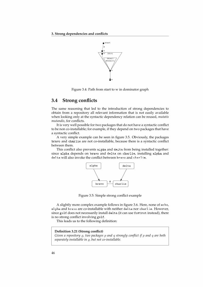
3. Strong dependencies and conflicts
v
w
IS(w)\
SCons(v)
IS(v)
start
x
x'
α
Figure 3.4: Path from start to w in dominator graph
3.4 Strong conflicts
The same reasoning that led to the introduction of strong dependencies toobtain from a repository all relevant information that is not easily availablewhen looking only at the syntactic dependency relation can be reused, mutatismutandis, for conflicts.
It is very well possible for two packages that do not have a syntactic conflictto be non co-installable; for example, if they depend on two packages that havea syntactic conflict.
A very simple example can be seen in figure 3.5. Obviously, the packagesbravo and charlie are not co-installable, because there is a syntactic conflictbetween them.
This conflict also prevents alpha and delta from being installed together:since alpha depends on bravo and delta on charlie, installing alpha anddelta will also invoke the conflict between bravo and charlie.
alpha
bravo charlie
delta
#
Figure 3.5: Simple strong conflict example
A slightly more complex example follows in figure 3.6. Here, none of echo,alpha and bravo are co-installable with neither delta nor charlie. However,since golf does not necessarily install delta (it can use foxtrot instead), thereis no strong conflict involving golf.
This leads us to the following definition:
Definition 3.21 (Strong conflict)Given a repository %, two packages p and q strongly conflict if p and q are bothseparately installable in %, but not co-installable.
46
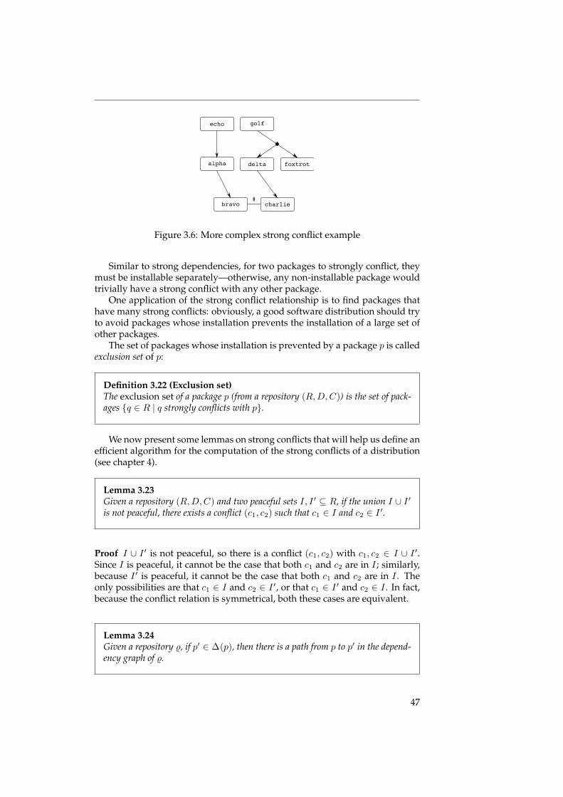
alphabravo charliedelta#echo foxtrotgolfFigure 3.6: More complex strong conflict example
Similar to strong dependencies, for two packages to strongly conflict, theymust be installable separately—otherwise, any non-installable package wouldtrivially have a strong conflict with any other package.
One application of the strong conflict relationship is to find packages thathave many strong conflicts: obviously, a good software distribution should tryto avoid packages whose installation prevents the installation of a large set ofother packages.
The set of packages whose installation is prevented by a package p is calledexclusion set of p:
Definition 3.22 (Exclusion set)The exclusion set of a package p (from a repository (R,D,C)) is the set of pack-ages {q ∈ R | q strongly conflicts with p}.
We now present some lemmas on strong conflicts that will help us define anefficient algorithm for the computation of the strong conflicts of a distribution(see chapter 4).
Lemma 3.23Given a repository (R,D,C) and two peaceful sets I, I ′ ⊆ R, if the union I ∪ I ′is not peaceful, there exists a conflict (c1, c2) such that c1 ∈ I and c2 ∈ I ′.
Proof I ∪ I ′ is not peaceful, so there is a conflict (c1, c2) with c1, c2 ∈ I ∪ I ′.Since I is peaceful, it cannot be the case that both c1 and c2 are in I ; similarly,because I ′ is peaceful, it cannot be the case that both c1 and c2 are in I . Theonly possibilities are that c1 ∈ I and c2 ∈ I ′, or that c1 ∈ I ′ and c2 ∈ I . In fact,because the conflict relation is symmetrical, both these cases are equivalent.
Lemma 3.24Given a repository %, if p′ ∈ ∆(p), then there is a path from p to p′ in the depend-ency graph of %.
47
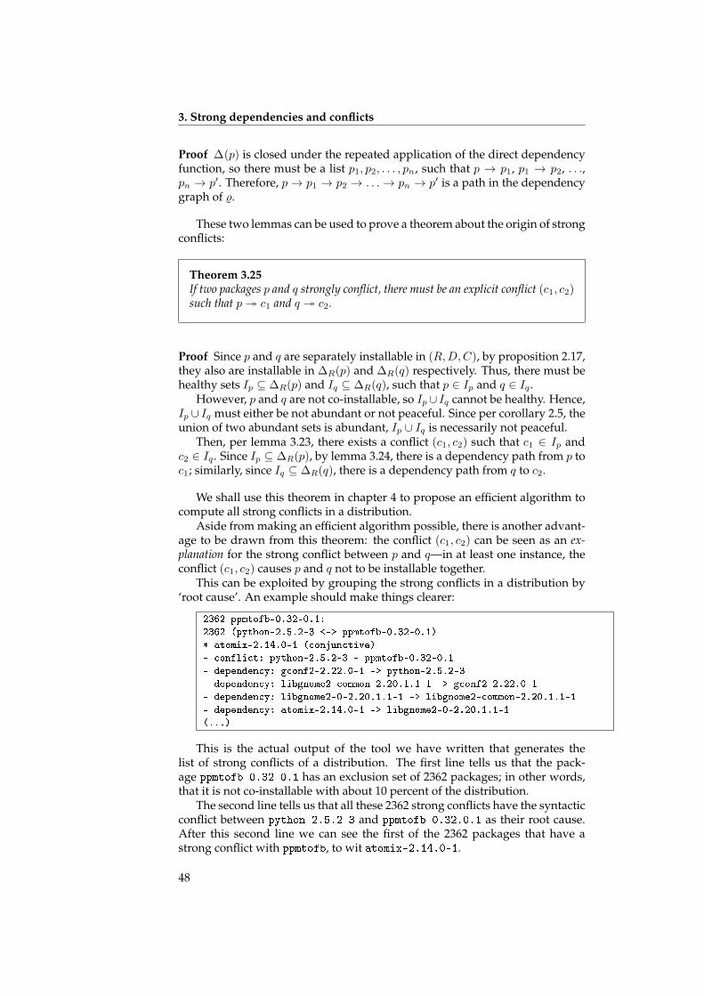
3. Strong dependencies and conflicts
Proof ∆(p) is closed under the repeated application of the direct dependencyfunction, so there must be a list p1, p2, . . . , pn, such that p → p1, p1 → p2, . . .,pn → p′. Therefore, p→ p1 → p2 → . . .→ pn → p′ is a path in the dependencygraph of %.
These two lemmas can be used to prove a theorem about the origin of strongconflicts:
Theorem 3.25If two packages p and q strongly conflict, there must be an explicit conflict (c1, c2)such that p� c1 and q � c2.
Proof Since p and q are separately installable in (R,D,C), by proposition 2.17,they also are installable in ∆R(p) and ∆R(q) respectively. Thus, there must behealthy sets Ip ⊆ ∆R(p) and Iq ⊆ ∆R(q), such that p ∈ Ip and q ∈ Iq .
However, p and q are not co-installable, so Ip ∪ Iq cannot be healthy. Hence,Ip ∪ Iq must either be not abundant or not peaceful. Since per corollary 2.5, theunion of two abundant sets is abundant, Ip ∪ Iq is necessarily not peaceful.
Then, per lemma 3.23, there exists a conflict (c1, c2) such that c1 ∈ Ip andc2 ∈ Iq . Since Ip ⊆ ∆R(p), by lemma 3.24, there is a dependency path from p toc1; similarly, since Iq ⊆ ∆R(q), there is a dependency path from q to c2.
We shall use this theorem in chapter 4 to propose an efficient algorithm tocompute all strong conflicts in a distribution.
Aside from making an efficient algorithm possible, there is another advant-age to be drawn from this theorem: the conflict (c1, c2) can be seen as an ex-planation for the strong conflict between p and q—in at least one instance, theconflict (c1, c2) causes p and q not to be installable together.
This can be exploited by grouping the strong conflicts in a distribution by‘root cause’. An example should make things clearer:
2362 ppmtofb-0.32-0.1:
2362 (python-2.5.2-3 <-> ppmtofb-0.32-0.1)
* atomix-2.14.0-1 (conjunctive)
- conflict: python-2.5.2-3 - ppmtofb-0.32-0.1
- dependency: gconf2-2.22.0-1 -> python-2.5.2-3
- dependency: libgnome2-common-2.20.1.1-1 -> gconf2-2.22.0-1
- dependency: libgnome2-0-2.20.1.1-1 -> libgnome2-common-2.20.1.1-1
- dependency: atomix-2.14.0-1 -> libgnome2-0-2.20.1.1-1
(...)
This is the actual output of the tool we have written that generates thelist of strong conflicts of a distribution. The first line tells us that the pack-age ppmtofb-0.32-0.1 has an exclusion set of 2362 packages; in other words,that it is not co-installable with about 10 percent of the distribution.
The second line tells us that all these 2362 strong conflicts have the syntacticconflict between python-2.5.2-3 and ppmtofb-0.32.0.1 as their root cause.After this second line we can see the first of the 2362 packages that have astrong conflict with ppmtofb, to wit atomix-2.14.0-1.
48
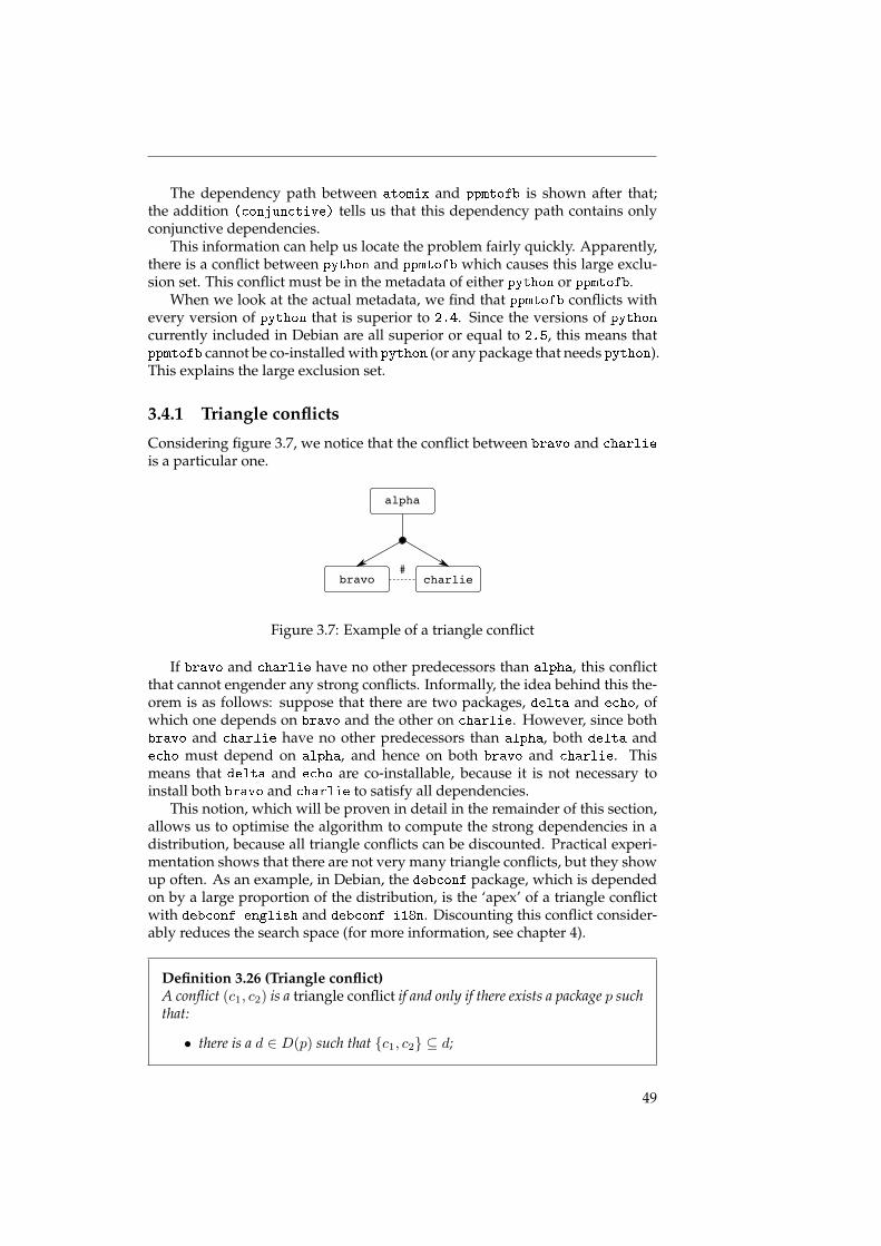
The dependency path between atomix and ppmtofb is shown after that;the addition (conjunctive) tells us that this dependency path contains onlyconjunctive dependencies.
This information can help us locate the problem fairly quickly. Apparently,there is a conflict between python and ppmtofb which causes this large exclu-sion set. This conflict must be in the metadata of either python or ppmtofb.
When we look at the actual metadata, we find that ppmtofb conflicts withevery version of python that is superior to 2.4. Since the versions of pythoncurrently included in Debian are all superior or equal to 2.5, this means thatppmtofb cannot be co-installed with python (or any package that needs python).This explains the large exclusion set.
3.4.1 Triangle conflicts
Considering figure 3.7, we notice that the conflict between bravo and charlie
is a particular one.
alpha
bravo charlie#
Figure 3.7: Example of a triangle conflict
If bravo and charlie have no other predecessors than alpha, this conflictthat cannot engender any strong conflicts. Informally, the idea behind this the-orem is as follows: suppose that there are two packages, delta and echo, ofwhich one depends on bravo and the other on charlie. However, since bothbravo and charlie have no other predecessors than alpha, both delta andecho must depend on alpha, and hence on both bravo and charlie. Thismeans that delta and echo are co-installable, because it is not necessary toinstall both bravo and charlie to satisfy all dependencies.
This notion, which will be proven in detail in the remainder of this section,allows us to optimise the algorithm to compute the strong dependencies in adistribution, because all triangle conflicts can be discounted. Practical experi-mentation shows that there are not very many triangle conflicts, but they showup often. As an example, in Debian, the debconf package, which is dependedon by a large proportion of the distribution, is the ‘apex’ of a triangle conflictwith debconf-english and debconf-i18n. Discounting this conflict consider-ably reduces the search space (for more information, see chapter 4).
Definition 3.26 (Triangle conflict)A conflict (c1, c2) is a triangle conflict if and only if there exists a package p suchthat:
• there is a d ∈ D(p) such that {c1, c2} ⊆ d;
49
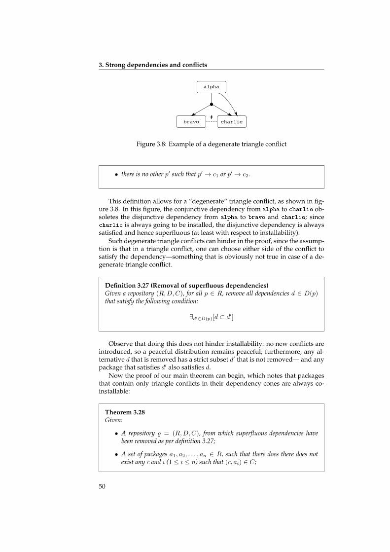
3. Strong dependencies and conflicts
alpha
bravo charlie#
Figure 3.8: Example of a degenerate triangle conflict
• there is no other p′ such that p′ → c1 or p′ → c2.
This definition allows for a “degenerate” triangle conflict, as shown in fig-ure 3.8. In this figure, the conjunctive dependency from alpha to charlie ob-soletes the disjunctive dependency from alpha to bravo and charlie; sincecharlie is always going to be installed, the disjunctive dependency is alwayssatisfied and hence superfluous (at least with respect to installability).
Such degenerate triangle conflicts can hinder in the proof, since the assump-tion is that in a triangle conflict, one can choose either side of the conflict tosatisfy the dependency—something that is obviously not true in case of a de-generate triangle conflict.
Definition 3.27 (Removal of superfluous dependencies)Given a repository (R,D,C), for all p ∈ R, remove all dependencies d ∈ D(p)that satisfy the following condition:
∃d′∈D(p)[d ⊂ d′]
Observe that doing this does not hinder installability: no new conflicts areintroduced, so a peaceful distribution remains peaceful; furthermore, any al-ternative d that is removed has a strict subset d′ that is not removed— and anypackage that satisfies d′ also satisfies d.
Now the proof of our main theorem can begin, which notes that packagesthat contain only triangle conflicts in their dependency cones are always co-installable:
Theorem 3.28Given:
• A repository % = (R,D,C), from which superfluous dependencies havebeen removed as per definition 3.27;
• A set of packages a1, a2, . . . , an ∈ R, such that there does there does notexist any c and i (1 ≤ i ≤ n) such that (c, ai) ∈ C;
50
• For every i such that 1 ≤ i ≤ n, a set Ai ⊆ R such that Ai is healthy andai ∈ Ai (in other words, ai is installable in R, using Ai as the installationset);
• For all packages c1, c2 ∈⋃n
i=1 ∆(ai) with (c1, c2) ∈ C, (c1, c2) is a tri-angle conflict.
Then a1, a2, . . . , an are co-installable with respect to %.
Proof Let us define a function K(A,B), where A and B are sets of packages,as a list of packages from A that are involved in a conflict spanning A and B;
K(A,B) = {p ∈ A | ∃q∈B [(p, q) ∈ C]}Furthermore, let us define a function αk such that:
• α1 = A1
• αk(1 < k ≤ n) = (αk−1 ∪Ak) \K(αk−1, Ak)
It is easy to see that since ai ∈ Ai, {a1, a2, . . . , an} ⊆ αn.Now, αn is abundant. Proof by induction:
• A1 is abundant, so α1 is abundant.
• Supposing that αk−1 is abundant, then by corollary 2.5, αk − 1 ∪ Ak isabundant. Therefore, for any package p ∈ αk−1 ∪ Ak and any d ∈ D(p),there must be an x ∈ d∩(αk−1∪Ak). Now, either x ∈ K(αk−1, Ak), or not.In the first case, there is a conflict (x, y), with both x and y in αk−1 ∪ Ak.Now, since x ∈ K(αk−1, Ak), it is not in αk, but d can still be satisfied byusing y (since p, x and y form a triangle conflict). Hence, αk is abundant.In the second case, trivially, x ∈ αk.
αn is also peaceful. Proof by induction:
• A1 is peaceful, so α1 is peaceful.
• Supposing that αk−1 is peaceful, then by lemma 3.23, αk−1 ∪Ak is peace-ful if there are no conflicts (c1, c2) with c1 ∈ αk−1 and c2 ∈ Ak. When welook at the construction of αk, we see that for any such conflict, one of itspackages from αk−1 ∪Ak is removed, so that αk is indeed peaceful.
51
3. Strong dependencies and conflicts
52
Algorithms 4Much better to sit quietly in a room and read the sheets, with nothing between yourself and themind of the composer but a scribble of ink. Having it played by sweaty fat men and people with
hair in their ears and spit dribbling out of the end of their oboe. . . well, the idea made himshudder.
— TERRY PRATCHETT, Soul Music
In the previous chapters, we have presented a model of F/OSS distributionsand their properties. Such a model is useful as a basis for reasoning about theproperties of distributions (as we have already done in chapter 3), but it canalso be used as a starting point for distribution analysis.
Given the scale of distributions, such analyses must necessarily be highlyautomated. Furthermore, their implementation must be efficient, since the ana-lyses will be run on large distributions, preferably on a daily basis in order tofollow the evolution of distributions over time.
Therefore, in this chapter, we shall explain the algorithms used to imple-ment the notions presented in chapters 2 and 3. Frequent reference will bemade to these chapters, as the theorems proposed there are used for optimisa-tion of the algorithms.
We shall also discuss the theoretical complexity of the algorithms.In chapter 7, we shall discuss the practical applicability of these algorithms
(for example in terms of running time), and talk in more detail about somemore interesting results found in their output.
4.1 Installability
As seen in definition 2.8, for a package to be installable, all its dependencies(and their dependencies, and the dependencies of those dependencies, etc.)must be satisfied (i.e. the install set must be abundant, cf. definition 2.4), andthere must not be any conflicts between the packages used to satisfy the de-pendencies (i.e. the install set must be peaceful, cf. definition 2.6).
An efficient way to check these conditions is by making use of a SAT solver;the installability problem translates easily into a SAT specification, as we shallshow now.
In order to translate a dependency D(p) = {{x11, x21, . . . , xn11 }, {x12, . . .}, . . .}
into SAT, the following clauses can be used:
¬p ∨ x11 ∨ x21 ∨ . . . ∨ xn11
¬p ∨ x12 ∨ x22 ∨ . . . ∨ xn22
...
A conflict (p, q) is specified as follows:
53
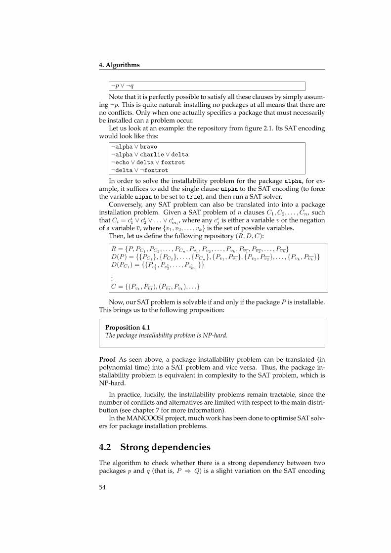
4. Algorithms
¬p ∨ ¬q
Note that it is perfectly possible to satisfy all these clauses by simply assum-ing ¬p. This is quite natural: installing no packages at all means that there areno conflicts. Only when one actually specifies a package that must necessarilybe installed can a problem occur.
Let us look at an example: the repository from figure 2.1. Its SAT encodingwould look like this:
¬alpha ∨ bravo¬alpha ∨ charlie ∨ delta¬echo ∨ delta ∨ foxtrot¬delta ∨ ¬foxtrot
In order to solve the installability problem for the package alpha, for ex-ample, it suffices to add the single clause alpha to the SAT encoding (to forcethe variable alpha to be set to true), and then run a SAT solver.
Conversely, any SAT problem can also be translated into into a packageinstallation problem. Given a SAT problem of n clauses C1, C2, . . . , Cn, suchthat Ci = ci1 ∨ ci2 ∨ . . . ∨ cimi
, where any cij is either a variable v or the negationof a variable v, where {v1, v2, . . . , vk} is the set of possible variables.
Then, let us define the following repository (R,D,C):
R = {P, PC1, PC2
, . . . , PCn, Pv1 , Pv2 , . . . , Pvk , Pv1 , Pv2 , . . . , Pvk}
D(P ) = {{PC1}, {PC2}, . . . , {PCn}, {Pv1 , Pv1}, {Pv2 , Pv2}, . . . , {Pvk , Pvk}}D(PC1) = {{Pc11
, Pc12, . . . , Pc1m1
}}...C = {(Pv1 , Pv1), (Pv1 , Pv1), . . .}
Now, our SAT problem is solvable if and only if the package P is installable.This brings us to the following proposition:
Proposition 4.1The package installability problem is NP-hard.
Proof As seen above, a package installability problem can be translated (inpolynomial time) into a SAT problem and vice versa. Thus, the package in-stallability problem is equivalent in complexity to the SAT problem, which isNP-hard.
In practice, luckily, the installability problems remain tractable, since thenumber of conflicts and alternatives are limited with respect to the main distri-bution (see chapter 7 for more information).
In the MANCOOSI project, much work has been done to optimise SAT solv-ers for package installation problems.
4.2 Strong dependencies
The algorithm to check whether there is a strong dependency between twopackages p and q (that is, P ⇒ Q) is a slight variation on the SAT encoding
54
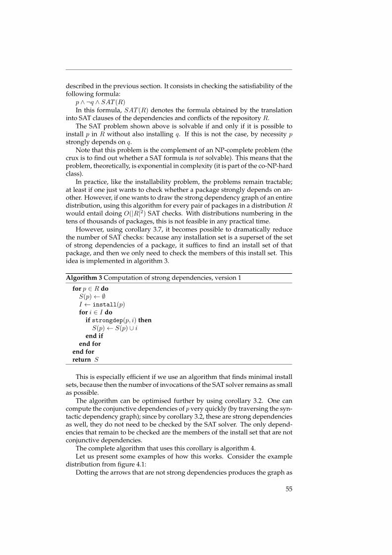
described in the previous section. It consists in checking the satisfiability of thefollowing formula:
p ∧ ¬q ∧ SAT (R)In this formula, SAT (R) denotes the formula obtained by the translation
into SAT clauses of the dependencies and conflicts of the repository R.The SAT problem shown above is solvable if and only if it is possible to
install p in R without also installing q. If this is not the case, by necessity pstrongly depends on q.
Note that this problem is the complement of an NP-complete problem (thecrux is to find out whether a SAT formula is not solvable). This means that theproblem, theoretically, is exponential in complexity (it is part of the co-NP-hardclass).
In practice, like the installability problem, the problems remain tractable;at least if one just wants to check whether a package strongly depends on an-other. However, if one wants to draw the strong dependency graph of an entiredistribution, using this algorithm for every pair of packages in a distributionRwould entail doing O(|R|2) SAT checks. With distributions numbering in thetens of thousands of packages, this is not feasible in any practical time.
However, using corollary 3.7, it becomes possible to dramatically reducethe number of SAT checks: because any installation set is a superset of the setof strong dependencies of a package, it suffices to find an install set of thatpackage, and then we only need to check the members of this install set. Thisidea is implemented in algorithm 3.
Algorithm 3 Computation of strong dependencies, version 1
for p ∈ R doS(p)← ∅I ← install(p)for i ∈ I do
if strongdep(p, i) thenS(p)← S(p) ∪ i
end ifend for
end forreturn S
This is especially efficient if we use an algorithm that finds minimal installsets, because then the number of invocations of the SAT solver remains as smallas possible.
The algorithm can be optimised further by using corollary 3.2. One cancompute the conjunctive dependencies of p very quickly (by traversing the syn-tactic dependency graph); since by corollary 3.2, these are strong dependenciesas well, they do not need to be checked by the SAT solver. The only depend-encies that remain to be checked are the members of the install set that are notconjunctive dependencies.
The complete algorithm that uses this corollary is algorithm 4.Let us present some examples of how this works. Consider the example
distribution from figure 4.1:Dotting the arrows that are not strong dependencies produces the graph as
55
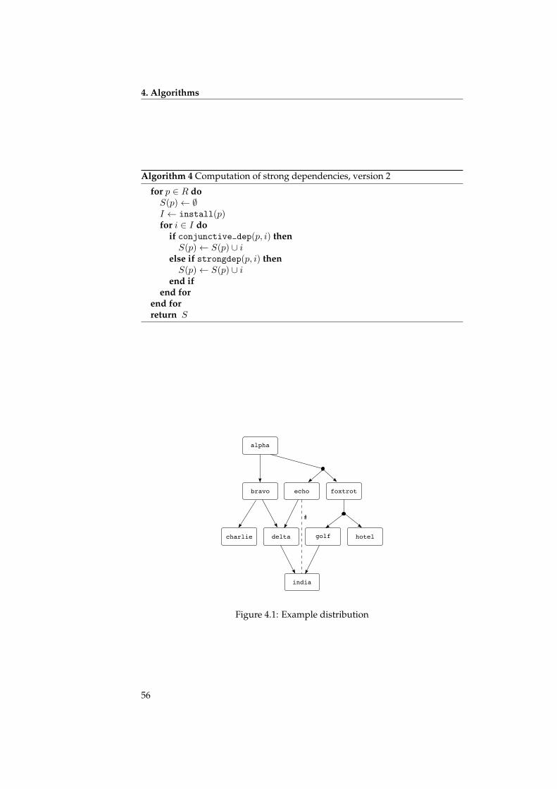
4. Algorithms
Algorithm 4 Computation of strong dependencies, version 2
for p ∈ R doS(p)← ∅I ← install(p)for i ∈ I do
if conjunctive dep(p, i) thenS(p)← S(p) ∪ i
else if strongdep(p, i) thenS(p)← S(p) ∪ i
end ifend for
end forreturn S alphacharlie echoindia hotelgolffoxtrot#bravo delta
Figure 4.1: Example distribution
56
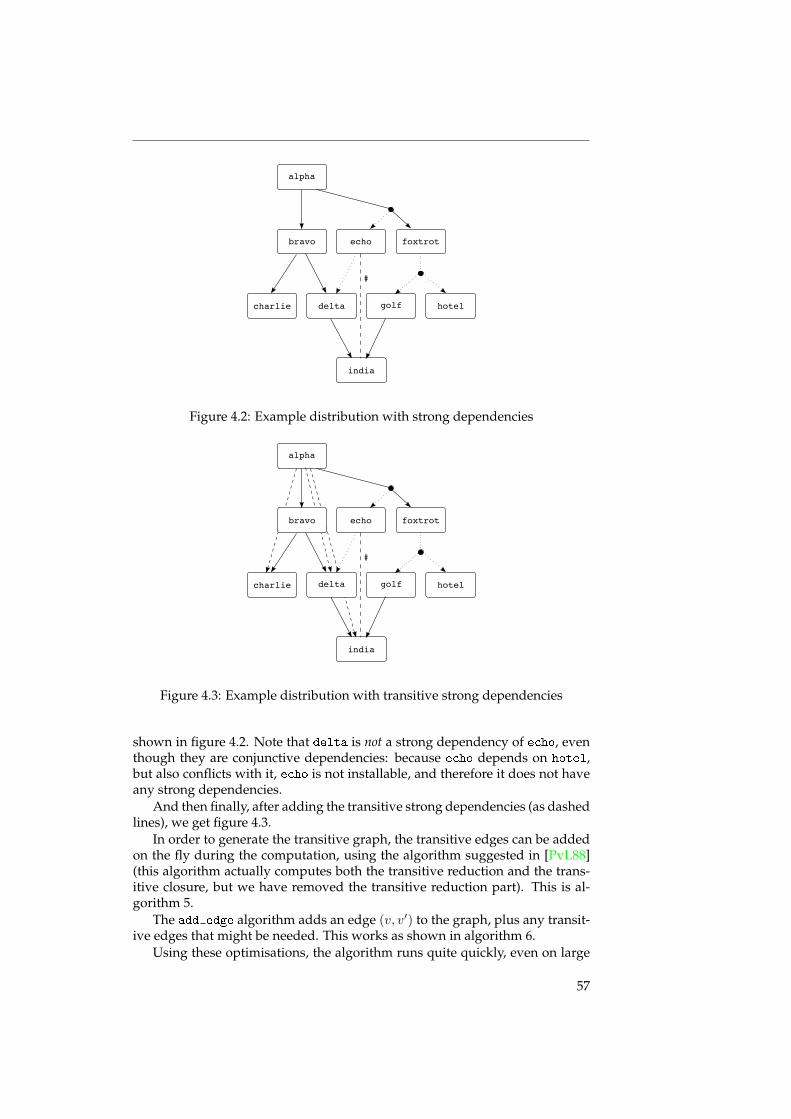
alphacharlie echoindia hotelgolffoxtrot#bravo deltaFigure 4.2: Example distribution with strong dependencies
alpha
charlie
echo
india
hotelgolf
foxtrot
#
bravo
delta
Figure 4.3: Example distribution with transitive strong dependencies
shown in figure 4.2. Note that delta is not a strong dependency of echo, eventhough they are conjunctive dependencies: because echo depends on hotel,but also conflicts with it, echo is not installable, and therefore it does not haveany strong dependencies.
And then finally, after adding the transitive strong dependencies (as dashedlines), we get figure 4.3.
In order to generate the transitive graph, the transitive edges can be addedon the fly during the computation, using the algorithm suggested in [PvL88](this algorithm actually computes both the transitive reduction and the trans-itive closure, but we have removed the transitive reduction part). This is al-gorithm 5.
The add edge algorithm adds an edge (v, v′) to the graph, plus any transit-ive edges that might be needed. This works as shown in algorithm 6.
Using these optimisations, the algorithm runs quite quickly, even on large
57
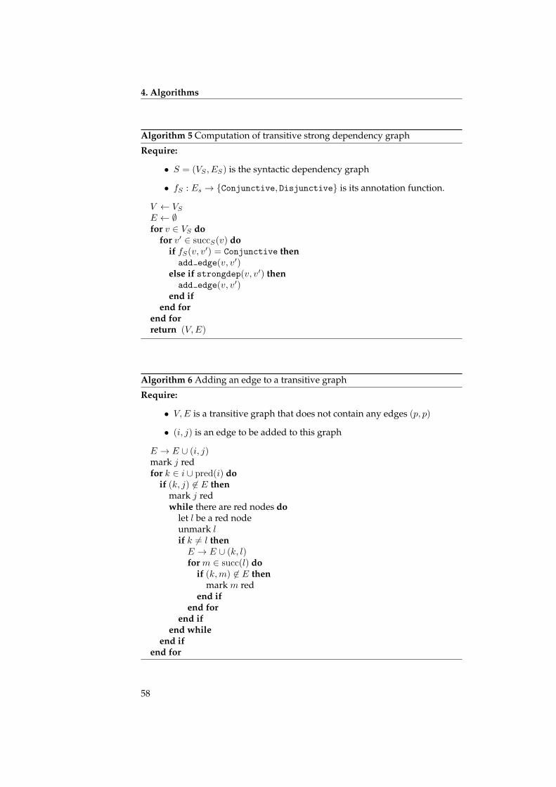
4. Algorithms
Algorithm 5 Computation of transitive strong dependency graph
Require:
• S = (VS , ES) is the syntactic dependency graph
• fS : Es → {Conjunctive, Disjunctive} is its annotation function.
V ← VSE ← ∅for v ∈ VS do
for v′ ∈ succS(v) doif fS(v, v′) = Conjunctive thenadd edge(v, v′)
else if strongdep(v, v′) thenadd edge(v, v′)
end ifend for
end forreturn (V,E)
Algorithm 6 Adding an edge to a transitive graph
Require:
• V,E is a transitive graph that does not contain any edges (p, p)
• (i, j) is an edge to be added to this graph
E → E ∪ (i, j)mark j redfor k ∈ i ∪ pred(i) do
if (k, j) 6∈ E thenmark j redwhile there are red nodes do
let l be a red nodeunmark lif k 6= l thenE → E ∪ (k, l)for m ∈ succ(l) do
if (k,m) 6∈ E thenmark m red
end ifend for
end ifend while
end ifend for
58
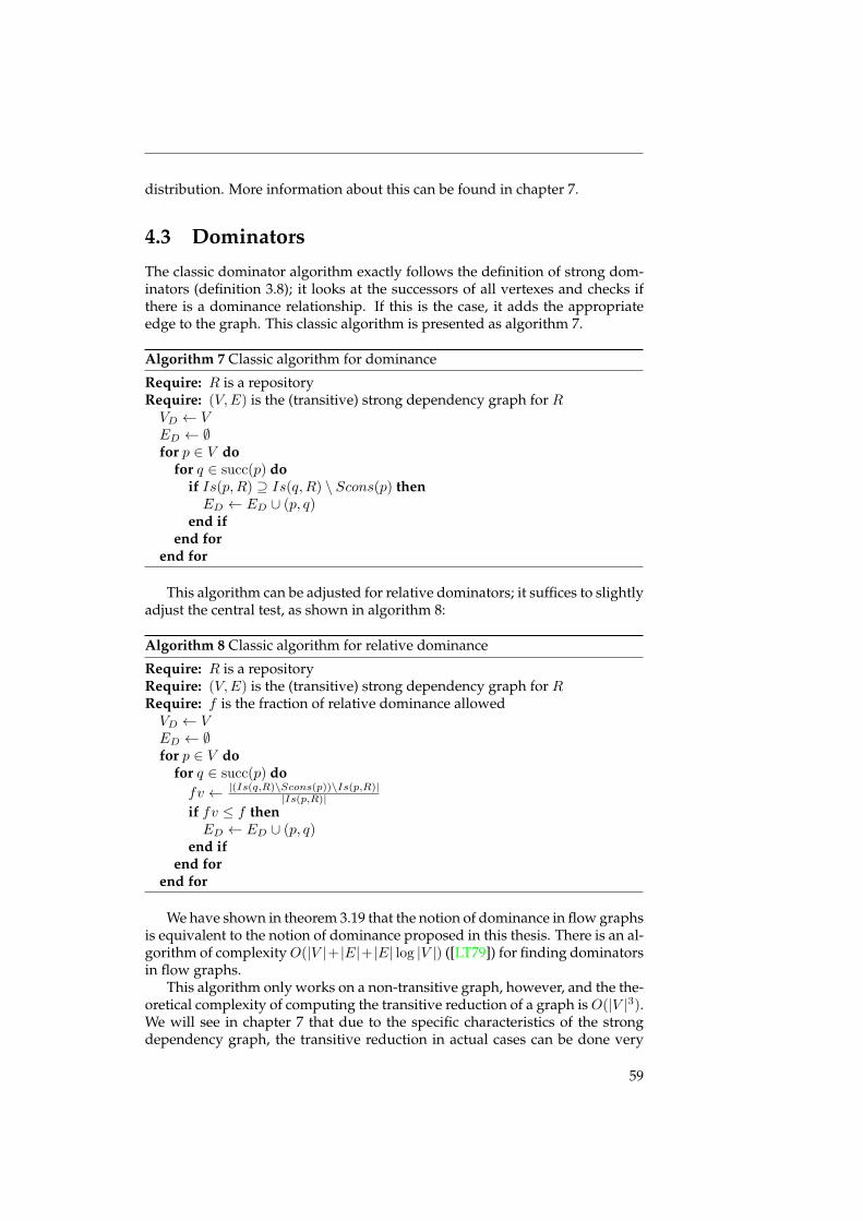
distribution. More information about this can be found in chapter 7.
4.3 Dominators
The classic dominator algorithm exactly follows the definition of strong dom-inators (definition 3.8); it looks at the successors of all vertexes and checks ifthere is a dominance relationship. If this is the case, it adds the appropriateedge to the graph. This classic algorithm is presented as algorithm 7.
Algorithm 7 Classic algorithm for dominance
Require: R is a repositoryRequire: (V,E) is the (transitive) strong dependency graph for RVD ← VED ← ∅for p ∈ V do
for q ∈ succ(p) doif Is(p,R) ⊇ Is(q,R) \ Scons(p) thenED ← ED ∪ (p, q)
end ifend for
end for
This algorithm can be adjusted for relative dominators; it suffices to slightlyadjust the central test, as shown in algorithm 8:
Algorithm 8 Classic algorithm for relative dominance
Require: R is a repositoryRequire: (V,E) is the (transitive) strong dependency graph for RRequire: f is the fraction of relative dominance allowedVD ← VED ← ∅for p ∈ V do
for q ∈ succ(p) dofv ← |(Is(q,R)\Scons(p))\Is(p,R)|
|Is(p,R)|if fv ≤ f thenED ← ED ∪ (p, q)
end ifend for
end for
We have shown in theorem 3.19 that the notion of dominance in flow graphsis equivalent to the notion of dominance proposed in this thesis. There is an al-gorithm of complexityO(|V |+ |E|+ |E| log |V |) ([LT79]) for finding dominatorsin flow graphs.
This algorithm only works on a non-transitive graph, however, and the the-oretical complexity of computing the transitive reduction of a graph isO(|V |3).We will see in chapter 7 that due to the specific characteristics of the strongdependency graph, the transitive reduction in actual cases can be done very
59
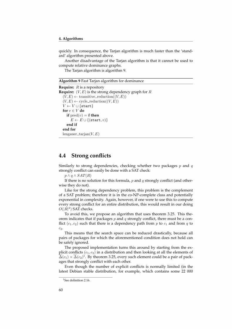
4. Algorithms
quickly. In consequence, the Tarjan algorithm is much faster than the ‘stand-ard’ algorithm presented above.
Another disadvantage of the Tarjan algorithm is that it cannot be used tocompute relative dominance graphs.
The Tarjan algorithm is algorithm 9.
Algorithm 9 Fast Tarjan algorithm for dominance
Require: R is a repositoryRequire: (V,E) is the strong dependency graph for R
(V,E)← transitive reduction((V,E))(V,E)← cycle reduction((V,E))V ← V ∪ {start}for v ∈ V do
if pred(v) = ∅ thenE ← E ∪ {(start, v)}
end ifend forlengauer tarjan(V,E)
4.4 Strong conflicts
Similarly to strong dependencies, checking whether two packages p and qstrongly conflict can easily be done with a SAT check:
p ∧ q ∧ SAT (R)
If there is no solution for this formula, p and q strongly conflict (and other-wise they do not).
Like for the strong dependency problem, this problem is the complementof a SAT problem; therefore it is in the co-NP-complete class and potentiallyexponential in complexity. Again, however, if one were to use this to computeevery strong conflict for an entire distribution, this would result in our doingO(|R|2) SAT checks.
To avoid this, we propose an algorithm that uses theorem 3.25. This the-orem indicates that if packages p and q strongly conflict, there must be a con-flict (c1, c2) such that there is a dependency path from p to c1 and from q toc2.
This means that the search space can be reduced drastically, because allpairs of packages for which the aforementioned condition does not hold canbe safely ignored.
The proposed implementation turns this around by starting from the ex-plicit conflicts (c1, c2) in a distribution and then looking at all the elements of∆(c1) ×∆(c2)1. By theorem 3.25, every such element could be a pair of pack-ages that strongly conflict with each other.
Even though the number of explicit conflicts is normally limited (in thelatest Debian stable distribution, for example, which contains some 22 000
1See definition 2.16.
60
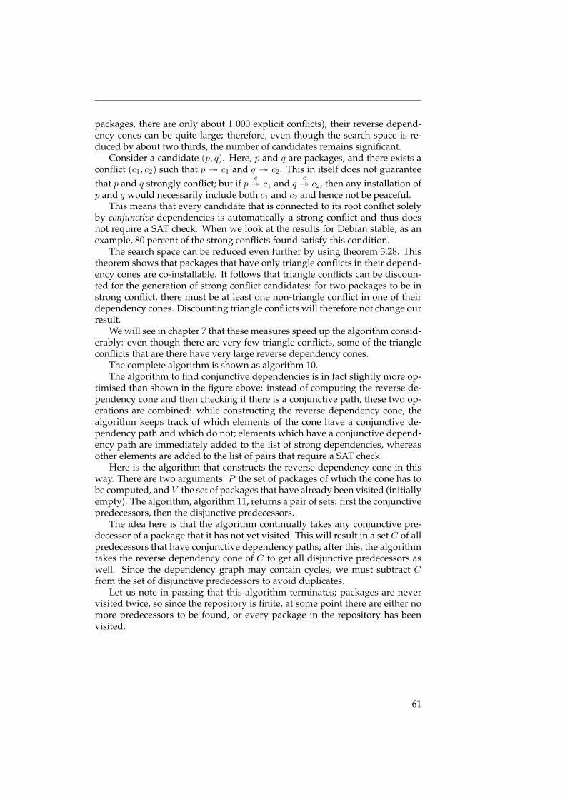
packages, there are only about 1 000 explicit conflicts), their reverse depend-ency cones can be quite large; therefore, even though the search space is re-duced by about two thirds, the number of candidates remains significant.
Consider a candidate (p, q). Here, p and q are packages, and there exists aconflict (c1, c2) such that p � c1 and q � c2. This in itself does not guaranteethat p and q strongly conflict; but if p
c� c1 and q
c� c2, then any installation of
p and q would necessarily include both c1 and c2 and hence not be peaceful.This means that every candidate that is connected to its root conflict solely
by conjunctive dependencies is automatically a strong conflict and thus doesnot require a SAT check. When we look at the results for Debian stable, as anexample, 80 percent of the strong conflicts found satisfy this condition.
The search space can be reduced even further by using theorem 3.28. Thistheorem shows that packages that have only triangle conflicts in their depend-ency cones are co-installable. It follows that triangle conflicts can be discoun-ted for the generation of strong conflict candidates: for two packages to be instrong conflict, there must be at least one non-triangle conflict in one of theirdependency cones. Discounting triangle conflicts will therefore not change ourresult.
We will see in chapter 7 that these measures speed up the algorithm consid-erably: even though there are very few triangle conflicts, some of the triangleconflicts that are there have very large reverse dependency cones.
The complete algorithm is shown as algorithm 10.The algorithm to find conjunctive dependencies is in fact slightly more op-
timised than shown in the figure above: instead of computing the reverse de-pendency cone and then checking if there is a conjunctive path, these two op-erations are combined: while constructing the reverse dependency cone, thealgorithm keeps track of which elements of the cone have a conjunctive de-pendency path and which do not; elements which have a conjunctive depend-ency path are immediately added to the list of strong dependencies, whereasother elements are added to the list of pairs that require a SAT check.
Here is the algorithm that constructs the reverse dependency cone in thisway. There are two arguments: P the set of packages of which the cone has tobe computed, and V the set of packages that have already been visited (initiallyempty). The algorithm, algorithm 11, returns a pair of sets: first the conjunctivepredecessors, then the disjunctive predecessors.
The idea here is that the algorithm continually takes any conjunctive pre-decessor of a package that it has not yet visited. This will result in a set C of allpredecessors that have conjunctive dependency paths; after this, the algorithmtakes the reverse dependency cone of C to get all disjunctive predecessors aswell. Since the dependency graph may contain cycles, we must subtract Cfrom the set of disjunctive predecessors to avoid duplicates.
Let us note in passing that this algorithm terminates; packages are nevervisited twice, so since the repository is finite, at some point there are either nomore predecessors to be found, or every package in the repository has beenvisited.
61
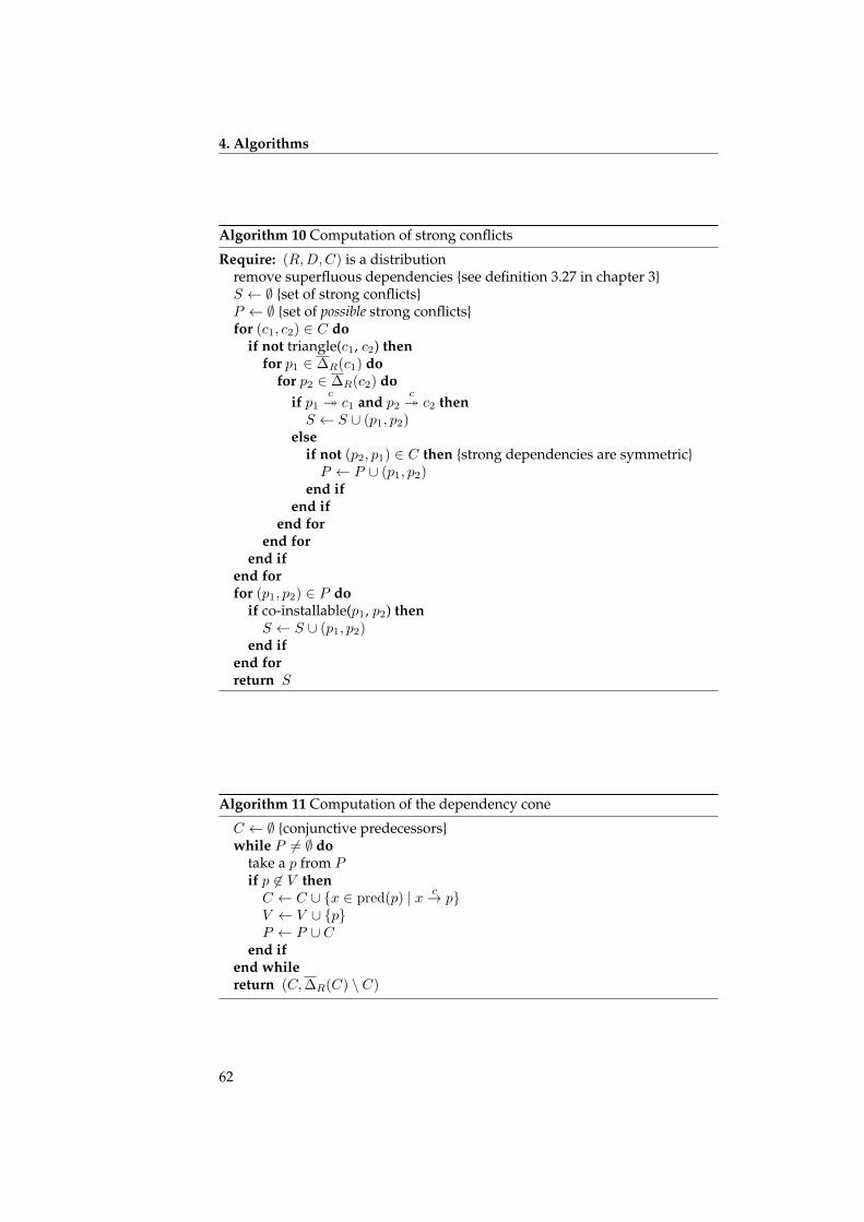
4. Algorithms
Algorithm 10 Computation of strong conflicts
Require: (R,D,C) is a distributionremove superfluous dependencies {see definition 3.27 in chapter 3}S ← ∅ {set of strong conflicts}P ← ∅ {set of possible strong conflicts}for (c1, c2) ∈ C do
if not triangle(c1, c2) thenfor p1 ∈ ∆R(c1) do
for p2 ∈ ∆R(c2) doif p1
c� c1 and p2
c� c2 then
S ← S ∪ (p1, p2)else
if not (p2, p1) ∈ C then {strong dependencies are symmetric}P ← P ∪ (p1, p2)
end ifend if
end forend for
end ifend forfor (p1, p2) ∈ P do
if co-installable(p1, p2) thenS ← S ∪ (p1, p2)
end ifend forreturn S
Algorithm 11 Computation of the dependency cone
C ← ∅ {conjunctive predecessors}while P 6= ∅ do
take a p from Pif p 6∈ V thenC ← C ∪ {x ∈ pred(p) | x c→ p}V ← V ∪ {p}P ← P ∪ C
end ifend whilereturn (C,∆R(C) \ C)
62
Tools 5For a list of all the ways technology has failed to improve the quality of life, please press three.
— ALICE KAHN
In this chapter, we shall give an overview of the different tools that havebeen developed over the course of the EDOS and MANCOOSI projects.
5.1 distcheck
This tool, developed by Jerôme Vouillon at the very start of the EDOS project,is used to check for non-installable packages in a distribution. The SAT solverat its heart (a re-implementation of Mini-SAT) is used for determining package(co-)installability in every tool mentioned hereafter.
Simply checking for non-installable packages is worthwhile in itself, butdistcheck does more: it also provides an explanation as to why a package is notinstallable. As we have seen in definition 2.8 from chapter 2, for a package tobe installable there has to be an abundant and peaceful subset of the repositorythat contains it. The possible reasons for a package not being installable arethus exactly two: there not being an abundant set (i.e. there is a dependencythat cannot be satisfied), or there not being a peaceful set (i.e. a package de-pends on two conflicting packages, and this conflict cannot be avoided). Forexample:
python-gnuradio (= 3.0.4-2): FAILED
The following constraints cannot be satisfied:
python-gnuradio (= 3.0.4-2) depends on python (� 2.5) {NOT AVAILABLE}
python-wxgtk2.4 (= 2.4.5.1.1+b1): FAILED
The following constraints cannot be satisfied:
python-wxgtk2.4 (= 2.4.5.1.1+b1) depends on python-wxversion
{python-wxversion (= 2.6.3.2.2-2)}
python-wxgtk2.4 (= 2.4.5.1.1+b1) conflicts with python-wxversion (=
2.6.3.2.2-2)
The first package, python-gnuradio, is an example of a package that cannotbe installed because of a non-satisfiable dependency; the second, python-wxgtk2.4cannot be installed because it simultaneously depends on and conflicts with thesame package.
5.2 dose
The dose library (Distribution Object Storage Engine) is the library used by allEDOS tools. It provides an API for storage, manipulation and reporting of all
63
5. Tools
types of package distribution algorithms.There have been two main versions of dose: version 2, written originally by
Berke Durak and extended fairly heavily by myself, and version 3, written byPietro Abate, in cooperation with myself.
The basic make-up of both versions is the same: a package store, with anAPI to manipulate packages and distributions, and to execute some of the al-gorithms. The implementation, however, is quite different.
5.2.1 dose2
The main goal in designing dose, version 2, was to have a library for storingmultiple snapshots of a distribution, from different dates, in such a way thatthey would take a minimum of space, and be quickly accessible. The reasonfor these requirements was that dose was intended as a back-end for the anlaweb interface (described below).
The obvious way of doing this is using an SQL database. This solutionwas not used, however, mainly because of performance issues (the state ofthe OCaml libraries for SQL databases was, at that time, not up to the task ofhandling databases with years’ worth of distributions).
Instead, a ‘dosebase’ consists of an index in dbm format; this index containsa record of every package, the distribution it is part of, and its lifetime, i.e. thedates on which it was present in the distribution. Furthermore, it containspointers to separate files that contain the actual package metadata.
In order to be able to quickly respond to queries, this ‘dosebase’ is only usedas a persistent storage; all package metadata is loaded into memory upon start-ing a dose2 application. This provides for great speed (once the initial loadingis done, responses to even the most complicated queries are instantaneous),but obviously takes up a large amount of memory.
In practice, though, it is possible to work with dose archives containingseveral years’ worth of distributions; memory usage in this case will be in theorder of 1 Gb.
In memory, the package metadata is stored in a simple table (the same struc-ture is used for all distribution formats; all packages in one instance of dose2must be of the same format), without translation, except for the version num-bers. In order to avoid having to call the complicated version comparison al-gorithm, every version number is translated into a pair of integers (one integerfor the epoch and version proper, and one integer for the release). In this way,instead of having to parse the entire version number, two integer comparisonssuffice.
It is not possible to use a single integer, since, as seen in chapter 2, the RPMversion order is not a complete order (for example, a version 1.27 is equal to1.27-1 and 1.27-2, but 1.27-1 is inferior to 1.27-2).
Dose2 supports the Debian, RPM and NetBSD pkgsrc package formats.On top of this index is a layer that deals with retrieving packages by name,
date or distribution.Furthermore, there are functions to deal with dependencies, dependency
cones, installability (the SAT solver from distcheck is integrated into dose2),strong dependencies and conflicts.
Figure 5.1 gives an overview of the structure of the dose2 library.
64
Taking the modules from top to bottom, the rapids module is the modulethat takes care of storage in memory, with indexes for rapid referral. The stor-age is filled using the waterway module, which uses napkin as a generic pack-age data structure, and ocamlrpm and ocamldeb as package-specific parsers.The algorithms are mostly in the packetology module; lifetime deals withdates and times. And finally, the satsolver module is used by packetology
to solve installability problems.
5.2.2 dose3
Dose3 is a complete rewrite of dose2. It has the same functionality, but there areseveral differences in implementation. When using dose2, it turned out thatthe functions for archiving distributions over time were used less frequentlythan the functions for considering just one universe of packages and runningalgorithms on those.
Furthermore, the CUDF format [TZ09] had been developed as a distribution-agnostic way of storing package metadata.
With this experience in mind, it was decided to reimplement dose2, usingCUDF as a universal data structure. This means that when merging a distribu-tion, it is first translated into CUDF, after which the different algorithms can beexecuted.
The dose2 data structures also have this property of universality with re-gard to the distribution format, but they are much more complicated.
For some algorithms, mostly the time-intensive ones such as the generationof the strong dependency or strong conflict graph, there is an extra transla-tion involved: every package is given an ID and dependencies and conflictsare translated into lists of (or lists of lists of) these IDs. This allows to reducememory usage and increase speed for these algorithms.
5.3 Ceve
Ceve (the name is supposed to have meant something, but exactly what hasbeen lost in the mists of time) was written by me, as a generalised packageformat parser and translator.
Its first function was to translate package repositories into SAT specifica-tions, in order to be able to compare different, external solvers, and to create adependency graph out of a repository using the EGraph format, a derivativeof the GraphML XML format.
Later on, the possibility to create databases out of repositories has been ad-ded: both SQL databases and the Dose2 format have been supported. Graphscan now also be output in the Dot format.
It is also possible to manipulate the data between parsing and output, forexample to output only the dependency cone of a certain package, or to elimin-ate virtual packages (by replacing them in dependencies with the list of pack-ages that provide them).
Ceve has now been rewritten using Dose3.
65
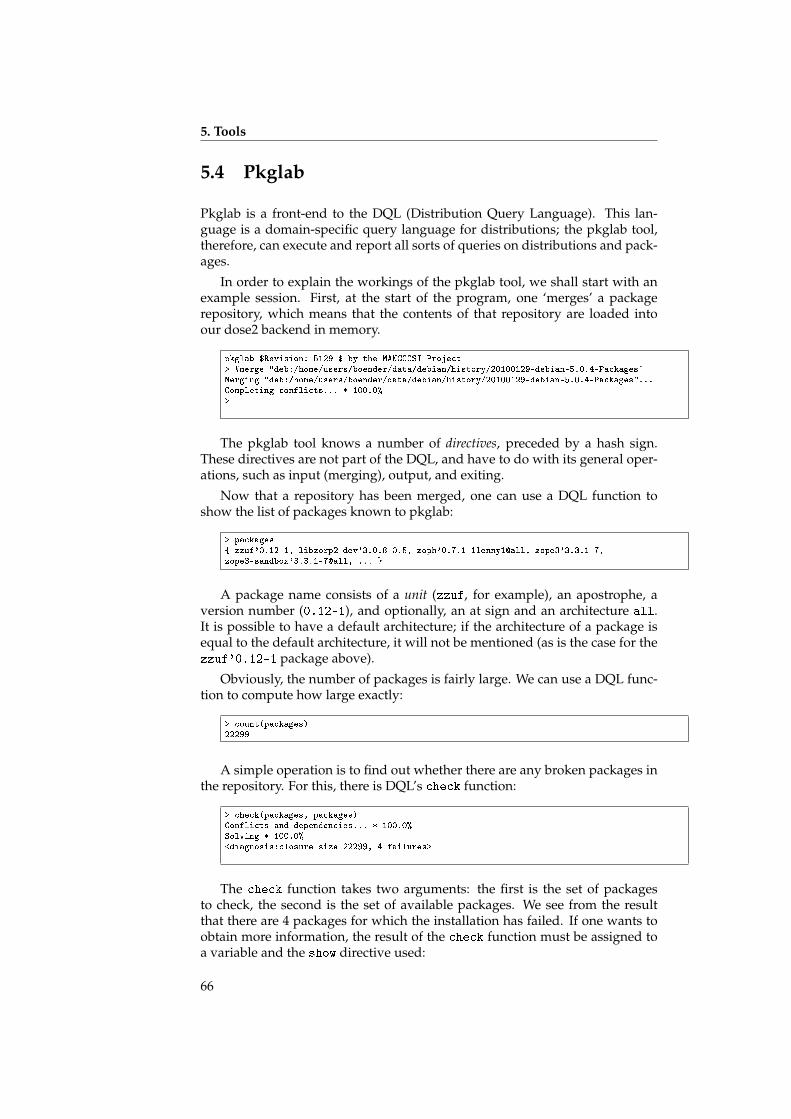
5. Tools
5.4 Pkglab
Pkglab is a front-end to the DQL (Distribution Query Language). This lan-guage is a domain-specific query language for distributions; the pkglab tool,therefore, can execute and report all sorts of queries on distributions and pack-ages.
In order to explain the workings of the pkglab tool, we shall start with anexample session. First, at the start of the program, one ‘merges’ a packagerepository, which means that the contents of that repository are loaded intoour dose2 backend in memory.
pkglab $Revision: 5129 $ by the MANCOOSI Project> #merge "deb:/home/users/boender/data/debian/history/20100129-debian-5.0.4-Packages"Merging "deb:/home/users/boender/data/debian/history/20100129-debian-5.0.4-Packages"...Completing conflicts... * 100.0%>
The pkglab tool knows a number of directives, preceded by a hash sign.These directives are not part of the DQL, and have to do with its general oper-ations, such as input (merging), output, and exiting.
Now that a repository has been merged, one can use a DQL function toshow the list of packages known to pkglab:
> packages{ zzuf'0.12-1, libzorp2-dev'3.0.8-0.5, zoph'0.7.1-1lenny1@all, zope3'3.3.1-7,zope3-sandbox'3.3.1-7@all, ... }
A package name consists of a unit (zzuf, for example), an apostrophe, aversion number (0.12-1), and optionally, an at sign and an architecture all.It is possible to have a default architecture; if the architecture of a package isequal to the default architecture, it will not be mentioned (as is the case for thezzuf'0.12-1 package above).
Obviously, the number of packages is fairly large. We can use a DQL func-tion to compute how large exactly:
> count(packages)22299
A simple operation is to find out whether there are any broken packages inthe repository. For this, there is DQL’s check function:
> check(packages, packages)Conflicts and dependencies... * 100.0%Solving * 100.0%<diagnosis:closure size 22299, 4 failures>
The check function takes two arguments: the first is the set of packagesto check, the second is the set of available packages. We see from the resultthat there are 4 packages for which the installation has failed. If one wants toobtain more information, the result of the check function must be assigned toa variable and the show directive used:
66
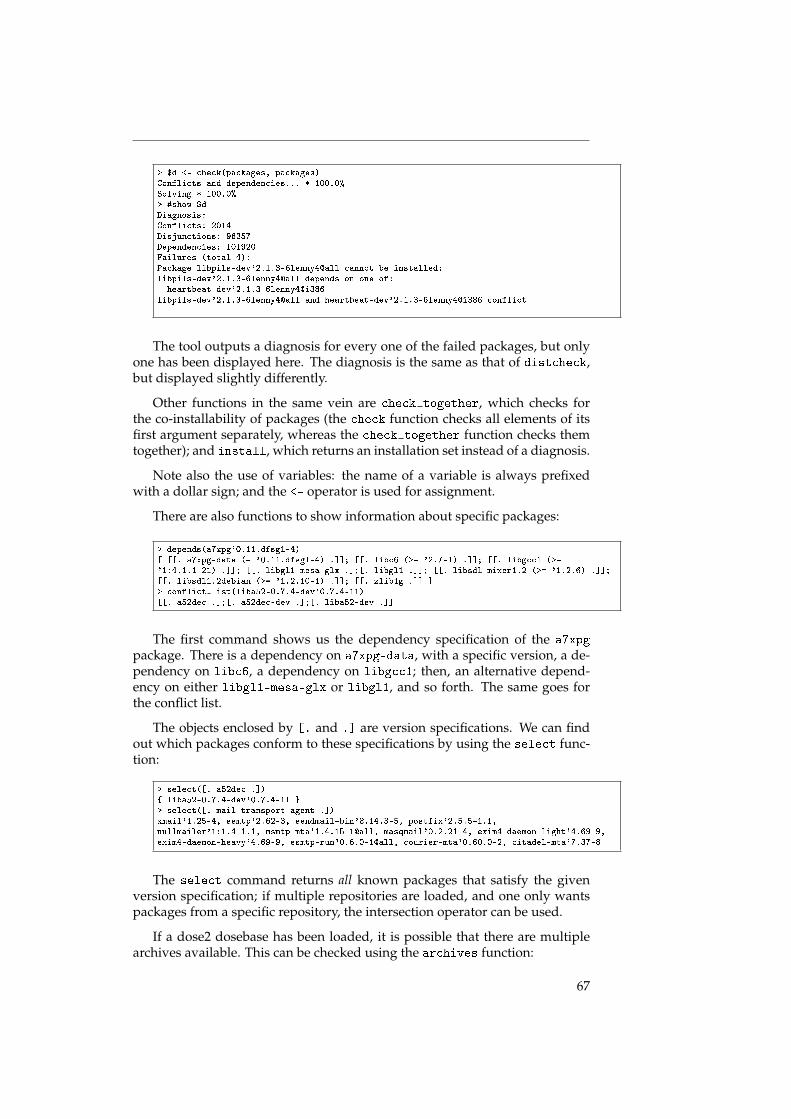
> $d <- check(packages, packages)Conflicts and dependencies... * 100.0%Solving * 100.0%> #show $dDiagnosis:Conflicts: 2014Disjunctions: 96357Dependencies: 101920Failures (total 4):Package libpils-dev'2.1.3-6lenny4@all cannot be installed:libpils-dev'2.1.3-6lenny4@all depends on one of:- heartbeat-dev'2.1.3-6lenny4@i386libpils-dev'2.1.3-6lenny4@all and heartbeat-dev'2.1.3-6lenny4@i386 conflict
The tool outputs a diagnosis for every one of the failed packages, but onlyone has been displayed here. The diagnosis is the same as that of distcheck,but displayed slightly differently.
Other functions in the same vein are check together, which checks forthe co-installability of packages (the check function checks all elements of itsfirst argument separately, whereas the check together function checks themtogether); and install, which returns an installation set instead of a diagnosis.
Note also the use of variables: the name of a variable is always prefixedwith a dollar sign; and the <- operator is used for assignment.
There are also functions to show information about specific packages:
> depends(a7xpg'0.11.dfsg1-4)[ [[. a7xpg-data (= '0.11.dfsg1-4) .]]; [[. libc6 (>= '2.7-1) .]]; [[. libgcc1 (>='1:4.1.1-21) .]]; [[. libgl1-mesa-glx .];[. libgl1 .]]; [[. libsdl-mixer1.2 (>= '1.2.6) .]];[[. libsdl1.2debian (>= '1.2.10-1) .]]; [[. zlib1g .]] ]> conflict list(liba52-0.7.4-dev'0.7.4-11)[[. a52dec .];[. a52dec-dev .];[. liba52-dev .]]
The first command shows us the dependency specification of the a7xpg
package. There is a dependency on a7xpg-data, with a specific version, a de-pendency on libc6, a dependency on libgcc1; then, an alternative depend-ency on either libgl1-mesa-glx or libgl1, and so forth. The same goes forthe conflict list.
The objects enclosed by [. and .] are version specifications. We can findout which packages conform to these specifications by using the select func-tion:
> select([. a52dec .]){ liba52-0.7.4-dev'0.7.4-11 }> select([. mail-transport-agent .])xmail'1.25-4, ssmtp'2.62-3, sendmail-bin'8.14.3-5, postfix'2.5.5-1.1,nullmailer'1:1.4-1.1, msmtp-mta'1.4.15-1@all, masqmail'0.2.21-4, exim4-daemon-light'4.69-9,exim4-daemon-heavy'4.69-9, esmtp-run'0.6.0-1@all, courier-mta'0.60.0-2, citadel-mta'7.37-8
The select command returns all known packages that satisfy the givenversion specification; if multiple repositories are loaded, and one only wantspackages from a specific repository, the intersection operator can be used.
If a dose2 dosebase has been loaded, it is possible that there are multiplearchives available. This can be checked using the archives function:
67
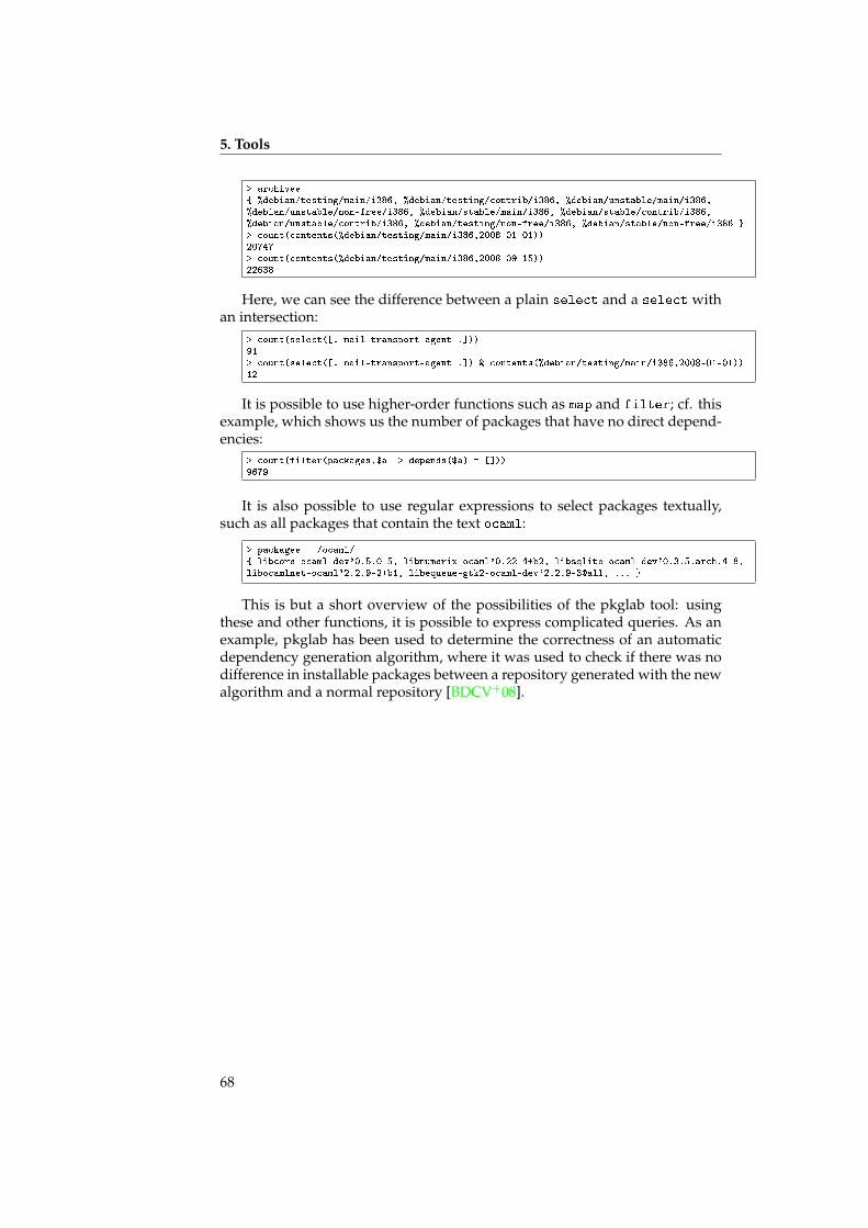
5. Tools
> archives{ %debian/testing/main/i386, %debian/testing/contrib/i386, %debian/unstable/main/i386,%debian/unstable/non-free/i386, %debian/stable/main/i386, %debian/stable/contrib/i386,%debian/unstable/contrib/i386, %debian/testing/non-free/i386, %debian/stable/non-free/i386 }> count(contents(%debian/testing/main/i386,2008-01-01))20747> count(contents(%debian/testing/main/i386,2008-09-15))22638
Here, we can see the difference between a plain select and a select withan intersection:
> count(select([. mail-transport-agent .]))91> count(select([. mail-transport-agent .]) & contents(%debian/testing/main/i386,2008-01-01))12
It is possible to use higher-order functions such as map and filter; cf. thisexample, which shows us the number of packages that have no direct depend-encies:
> count(filter(packages,$a -> depends($a) = []))9679
It is also possible to use regular expressions to select packages textually,such as all packages that contain the text ocaml:
> packages /ocaml/{ libcore-ocaml-dev'0.5.0-5, libnumerix-ocaml'0.22-4+b2, libsqlite-ocaml-dev'0.3.5.arch.4-8,libocamlnet-ocaml'2.2.9-2+b1, libequeue-gtk2-ocaml-dev'2.2.9-3@all, ... }
This is but a short overview of the possibilities of the pkglab tool: usingthese and other functions, it is possible to express complicated queries. As anexample, pkglab has been used to determine the correctness of an automaticdependency generation algorithm, where it was used to check if there was nodifference in installable packages between a repository generated with the newalgorithm and a normal repository [BDCV+08].
68
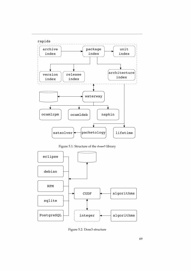
packageindex
versionindex
archiveindex
releaseindex
architectureindex
unitindex
rapids
waterway
ocamlrpm ocamldeb napkin
lifetimepacketologysatsolver
Figure 5.1: Structure of the dose2 library
CUDF
RPM
debian
sqlite
PostgreSQL integer algorithms
algorithms
eclipse
Figure 5.2: Dose3 structure
69
5. Tools
70
Formalisation 6
When one day an expedition was sent. . . they discovered only. . . a solitary old man who claimedrepeatedly that nothing was true, though he was later discovered to be lying.
— DOUGLAS ADAMS, The Hitchhiker’s Guide to the Galaxy
In this chapter, we shall introduce a formalisation of the theorems presentedin the previous chapters, together with their proofs. For this, we have used theCoq proof assistant.
Obviously, such a formalisation allows us to control the correctness of ourproofs, and even results in additions to the theory; as an example, the notionof a degenerate triangle conflict as shown in figure 3.6 in chapter 3 was coinedwhen formalising the proof of theorem 3.28.
The ultimate goal of this formalisation is to be able to verify the correctnessof the algorithms proposed in chapter 4. This is discussed in more detail in the‘Future work’ paragraph in the conclusion.
6.1 Repository
As seen in chapter 2, a repository is a tuple that contains a set of packages, a setof conflicts and a dependency function. For the purposes of the formalisation,we have separated these three parts, as not every definition needs all threeparts of the tuple.
Since repositories are always finite, we have used Coq’s FSet library, whichis a library for the representation of finite sets. There are other possibilities forsets, such as a representation of linked lists (ListSet), and a representationusing characteristic functions (Ensemble).
The advantages of the FSet library over these other implementations is thatit has a larger library of basic theorems, which saves quite a lot of time. Fur-thermore, the Ensemble library can also deal with infinite sets; this only com-plicates matters for our purposes, since repositories are always finite.
Let us start with defining a package type:
71
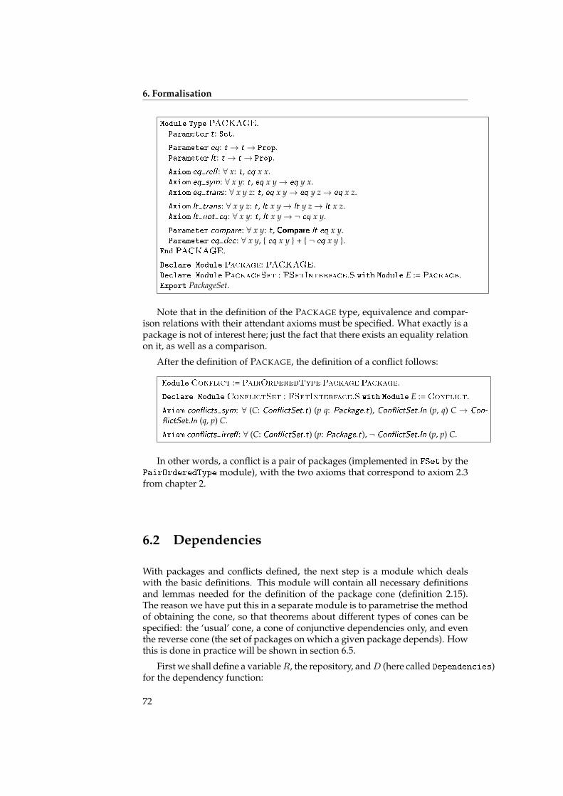
6. Formalisation
Module Type PACKAGE.Parameter t: Set.
Parameter eq: t → t → Prop.Parameter lt: t → t → Prop.
Axiom eq re� : ∀ x: t, eq x x.Axiom eq sym: ∀ x y: t, eq x y→ eq y x.Axiom eq trans : ∀ x y z: t, eq x y→ eq y z→ eq x z.
Axiom lt trans : ∀ x y z: t, lt x y→ lt y z→ lt x z.Axiom lt not eq: ∀ x y: t, lt x y→¬ eq x y.
Parameter compare: ∀ x y: t, Compare lt eq x y.Parameter eq dec : ∀ x y, { eq x y } + { ¬ eq x y }.
End PACKAGE.
Declare Module Package: PACKAGE.Declare Module PackageSet : FSetInterface.S with Module E := Package.Export PackageSet.
Note that in the definition of the PACKAGE type, equivalence and compar-ison relations with their attendant axioms must be specified. What exactly is apackage is not of interest here; just the fact that there exists an equality relationon it, as well as a comparison.
After the definition of PACKAGE, the definition of a conflict follows:
Module Conflict := PairOrderedType Package Package.
Declare Module ConflictSet : FSetInterface.S with Module E := Conflict.
Axiom con�icts sym: ∀ (C: Con�ictSet.t) (p q: Package.t), Con�ictSet.In (p, q) C→ Con-
�ictSet.In (q, p) C.
Axiom con�icts irre� : ∀ (C: Con�ictSet.t) (p: Package.t), ¬ Con�ictSet.In (p, p) C.
In other words, a conflict is a pair of packages (implemented in FSet by thePairOrderedType module), with the two axioms that correspond to axiom 2.3from chapter 2.
6.2 Dependencies
With packages and conflicts defined, the next step is a module which dealswith the basic definitions. This module will contain all necessary definitionsand lemmas needed for the definition of the package cone (definition 2.15).The reason we have put this in a separate module is to parametrise the methodof obtaining the cone, so that theorems about different types of cones can bespecified: the ‘usual’ cone, a cone of conjunctive dependencies only, and eventhe reverse cone (the set of packages on which a given package depends). Howthis is done in practice will be shown in section 6.5.
First we shall define a variableR, the repository, andD (here called Dependencies)for the dependency function:
72
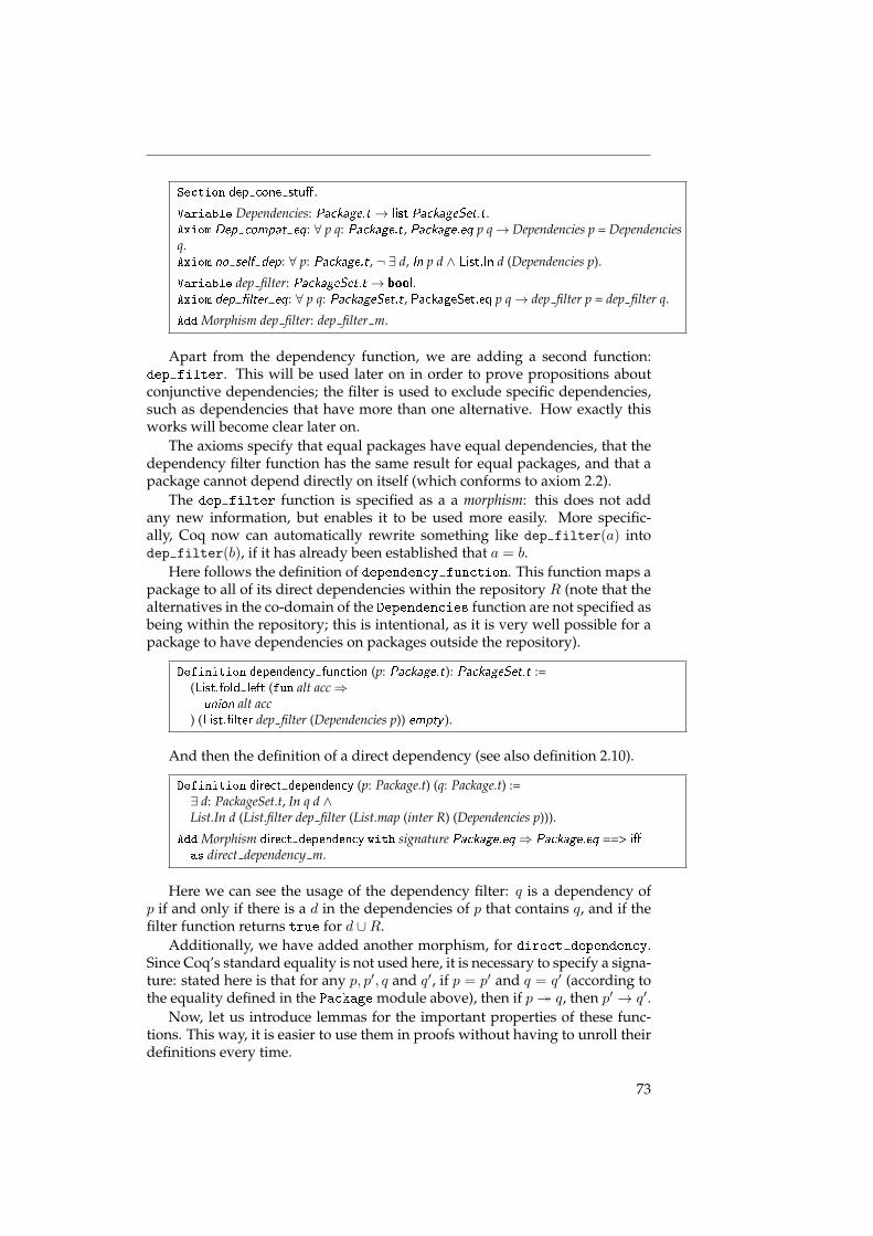
Section dep cone stu�.
Variable Dependencies: Package.t → list PackageSet.t.Axiom Dep compat eq: ∀ p q: Package.t, Package.eq p q→ Dependencies p = Dependenciesq.Axiom no self dep: ∀ p: Package.t, ¬ ∃ d, In p d ∧ List.In d (Dependencies p).
Variable dep filter: PackageSet.t → bool.Axiom dep �lter eq: ∀ p q: PackageSet.t, PackageSet.eq p q→ dep filter p = dep filter q.
Add Morphism dep filter: dep filter m.
Apart from the dependency function, we are adding a second function:dep filter. This will be used later on in order to prove propositions aboutconjunctive dependencies; the filter is used to exclude specific dependencies,such as dependencies that have more than one alternative. How exactly thisworks will become clear later on.
The axioms specify that equal packages have equal dependencies, that thedependency filter function has the same result for equal packages, and that apackage cannot depend directly on itself (which conforms to axiom 2.2).
The dep filter function is specified as a a morphism: this does not addany new information, but enables it to be used more easily. More specific-ally, Coq now can automatically rewrite something like dep filter(a) intodep filter(b), if it has already been established that a = b.
Here follows the definition of dependency function. This function maps apackage to all of its direct dependencies within the repository R (note that thealternatives in the co-domain of the Dependencies function are not specified asbeing within the repository; this is intentional, as it is very well possible for apackage to have dependencies on packages outside the repository).
Definition dependency function (p: Package.t): PackageSet.t :=(List.fold left (fun alt acc⇒
union alt acc) (List.�lter dep filter (Dependencies p)) empty ).
And then the definition of a direct dependency (see also definition 2.10).
Definition direct dependency (p: Package.t) (q: Package.t) :=∃ d: PackageSet.t, In q d ∧List.In d (List.filter dep filter (List.map (inter R) (Dependencies p))).
Add Morphism direct dependency with signature Package.eq⇒ Package.eq ==> i�
as direct dependency m.
Here we can see the usage of the dependency filter: q is a dependency ofp if and only if there is a d in the dependencies of p that contains q, and if thefilter function returns true for d ∪R.
Additionally, we have added another morphism, for direct dependency.Since Coq’s standard equality is not used here, it is necessary to specify a signa-ture: stated here is that for any p, p′, q and q′, if p = p′ and q = q′ (according tothe equality defined in the Package module above), then if p� q, then p′ → q′.
Now, let us introduce lemmas for the important properties of these func-tions. This way, it is easier to use them in proofs without having to unroll theirdefinitions every time.
73
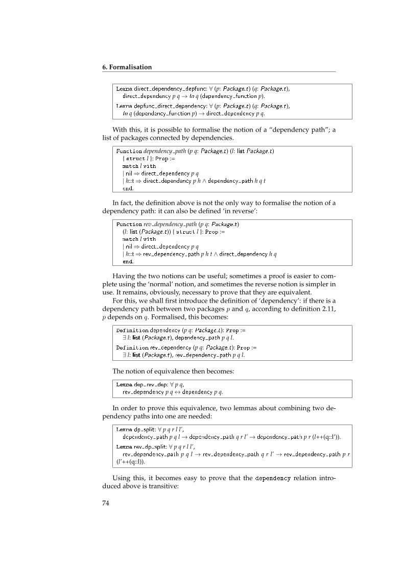
6. Formalisation
Lemma direct dependency depfunc: ∀ (p: Package.t) (q: Package.t),direct dependency p q→ In q (dependency function p).
Lemma depfunc direct dependency: ∀ (p: Package.t) (q: Package.t),In q (dependency function p)→ direct dependency p q.
With this, it is possible to formalise the notion of a “dependency path”; alist of packages connected by dependencies.
Function dependency path (p q: Package.t) (l: list Package.t){ struct l }: Prop :=match l with| nil⇒ direct dependency p q| h::t⇒ direct dependency p h ∧ dependency path h q tend.
In fact, the definition above is not the only way to formalise the notion of adependency path: it can also be defined ‘in reverse’:
Function rev dependency path (p q: Package.t)(l: list (Package.t)) { struct l }: Prop :=match l with| nil⇒ direct dependency p q| h::t⇒ rev dependency path p h t ∧ direct dependency h qend.
Having the two notions can be useful; sometimes a proof is easier to com-plete using the ‘normal’ notion, and sometimes the reverse notion is simpler inuse. It remains, obviously, necessary to prove that they are equivalent.
For this, we shall first introduce the definition of ‘dependency’: if there is adependency path between two packages p and q, according to definition 2.11,p depends on q. Formalised, this becomes:
Definition dependency (p q: Package.t): Prop :=∃ l: list (Package.t), dependency path p q l.
Definition rev dependency (p q: Package.t): Prop :=∃ l: list (Package.t), rev dependency path p q l.
The notion of equivalence then becomes:
Lemma dep rev dep: ∀ p q,rev dependency p q↔ dependency p q.
In order to prove this equivalence, two lemmas about combining two de-pendency paths into one are needed:
Lemma dp split: ∀ p q r l l’,dependency path p q l→ dependency path q r l’→ dependency path p r (l++(q::l’)).
Lemma rev dp split: ∀ p q r l l’,rev dependency path p q l → rev dependency path q r l’ → rev dependency path p r
(l’++(q::l)).
Using this, it becomes easy to prove that the dependency relation intro-duced above is transitive:
74
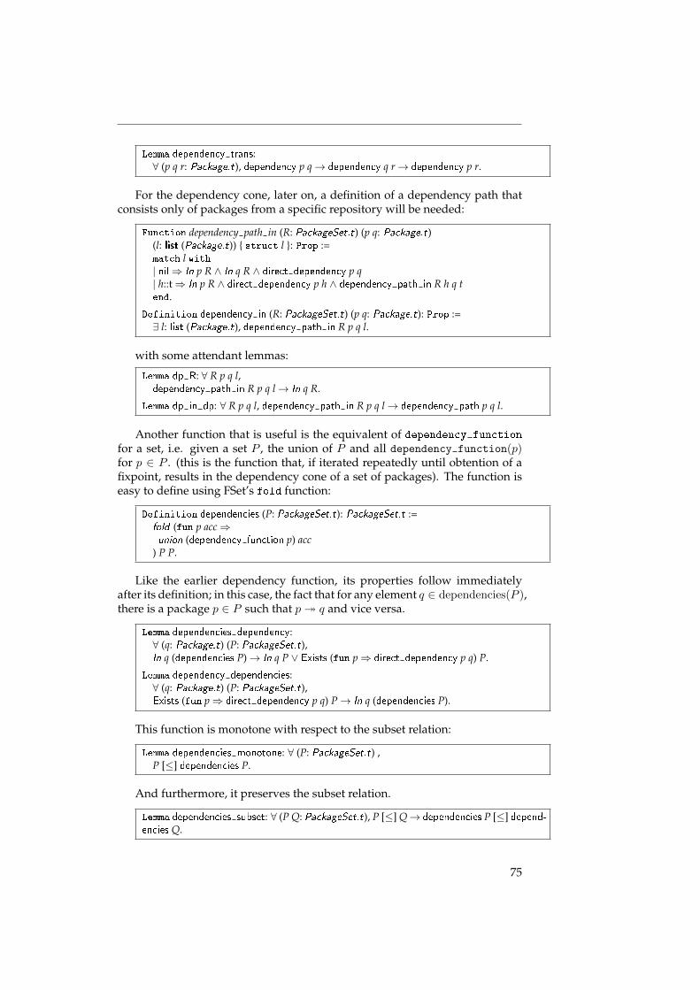
Lemma dependency trans:∀ (p q r: Package.t), dependency p q→ dependency q r→ dependency p r.
For the dependency cone, later on, a definition of a dependency path thatconsists only of packages from a specific repository will be needed:
Function dependency path in (R: PackageSet.t) (p q: Package.t)(l: list (Package.t)) { struct l }: Prop :=match l with| nil⇒ In p R ∧ In q R ∧ direct dependency p q| h::t⇒ In p R ∧ direct dependency p h ∧ dependency path in R h q tend.
Definition dependency in (R: PackageSet.t) (p q: Package.t): Prop :=∃ l: list (Package.t), dependency path in R p q l.
with some attendant lemmas:
Lemma dp R: ∀ R p q l,dependency path in R p q l→ In q R.
Lemma dp in dp: ∀ R p q l, dependency path in R p q l→ dependency path p q l.
Another function that is useful is the equivalent of dependency function
for a set, i.e. given a set P , the union of P and all dependency function(p)for p ∈ P . (this is the function that, if iterated repeatedly until obtention of afixpoint, results in the dependency cone of a set of packages). The function iseasy to define using FSet’s fold function:
Definition dependencies (P: PackageSet.t): PackageSet.t :=fold (fun p acc⇒union (dependency function p) acc
) P P.
Like the earlier dependency function, its properties follow immediatelyafter its definition; in this case, the fact that for any element q ∈ dependencies(P ),there is a package p ∈ P such that p� q and vice versa.
Lemma dependencies dependency:∀ (q: Package.t) (P: PackageSet.t),In q (dependencies P)→ In q P ∨ Exists (fun p⇒ direct dependency p q) P.
Lemma dependency dependencies:∀ (q: Package.t) (P: PackageSet.t),Exists (fun p⇒ direct dependency p q) P→ In q (dependencies P).
This function is monotone with respect to the subset relation:
Lemma dependencies monotone: ∀ (P: PackageSet.t) ,P [≤] dependencies P.
And furthermore, it preserves the subset relation.
Lemma dependencies subset: ∀ (P Q: PackageSet.t), P [≤] Q→ dependencies P [≤] depend-encies Q.
75
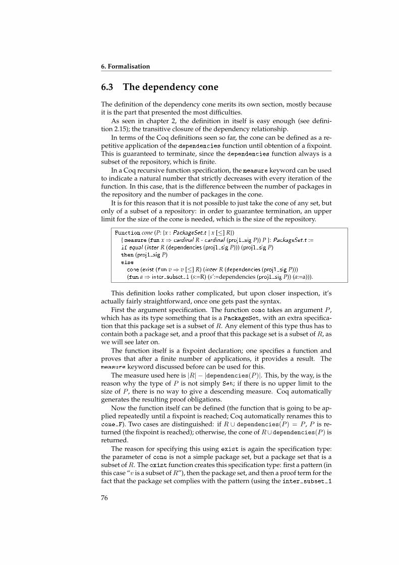
6. Formalisation
6.3 The dependency cone
The definition of the dependency cone merits its own section, mostly becauseit is the part that presented the most difficulties.
As seen in chapter 2, the definition in itself is easy enough (see defini-tion 2.15); the transitive closure of the dependency relationship.
In terms of the Coq definitions seen so far, the cone can be defined as a re-petitive application of the dependencies function until obtention of a fixpoint.This is guaranteed to terminate, since the dependencies function always is asubset of the repository, which is finite.
In a Coq recursive function specification, the measure keyword can be usedto indicate a natural number that strictly decreases with every iteration of thefunction. In this case, that is the difference between the number of packages inthe repository and the number of packages in the cone.
It is for this reason that it is not possible to just take the cone of any set, butonly of a subset of a repository: in order to guarantee termination, an upperlimit for the size of the cone is needed, which is the size of the repository.
Function cone (P: {x : PackageSet.t | x [≤] R}){ measure (fun x⇒ cardinal R - cardinal (proj1 sig P)) P }: PackageSet.t :=if equal (inter R (dependencies (proj1 sig P))) (proj1 sig P)then (proj1 sig P)else
cone (exist (fun v⇒ v [≤] R) (inter R (dependencies (proj1 sig P)))(fun a⇒ inter subset 1 (s:=R) (s’:=dependencies (proj1 sig P)) (a:=a))).
This definition looks rather complicated, but upon closer inspection, it’sactually fairly straightforward, once one gets past the syntax.
First the argument specification. The function cone takes an argument P ,which has as its type something that is a PackageSet, with an extra specifica-tion that this package set is a subset of R. Any element of this type thus has tocontain both a package set, and a proof that this package set is a subset of R, aswe will see later on.
The function itself is a fixpoint declaration; one specifies a function andproves that after a finite number of applications, it provides a result. Themeasure keyword discussed before can be used for this.
The measure used here is |R| − |dependencies(P )|. This, by the way, is thereason why the type of P is not simply Set; if there is no upper limit to thesize of P , there is no way to give a descending measure. Coq automaticallygenerates the resulting proof obligations.
Now the function itself can be defined (the function that is going to be ap-plied repeatedly until a fixpoint is reached; Coq automatically renames this tocone F). Two cases are distinguished: if R ∪ dependencies(P ) = P , P is re-turned (the fixpoint is reached); otherwise, the cone of R∪dependencies(P ) isreturned.
The reason for specifying this using exist is again the specification type:the parameter of cone is not a simple package set, but a package set that is asubset ofR. The exist function creates this specification type: first a pattern (inthis case “v is a subset ofR”), then the package set, and then a proof term for thefact that the package set complies with the pattern (using the inter subset 1
76
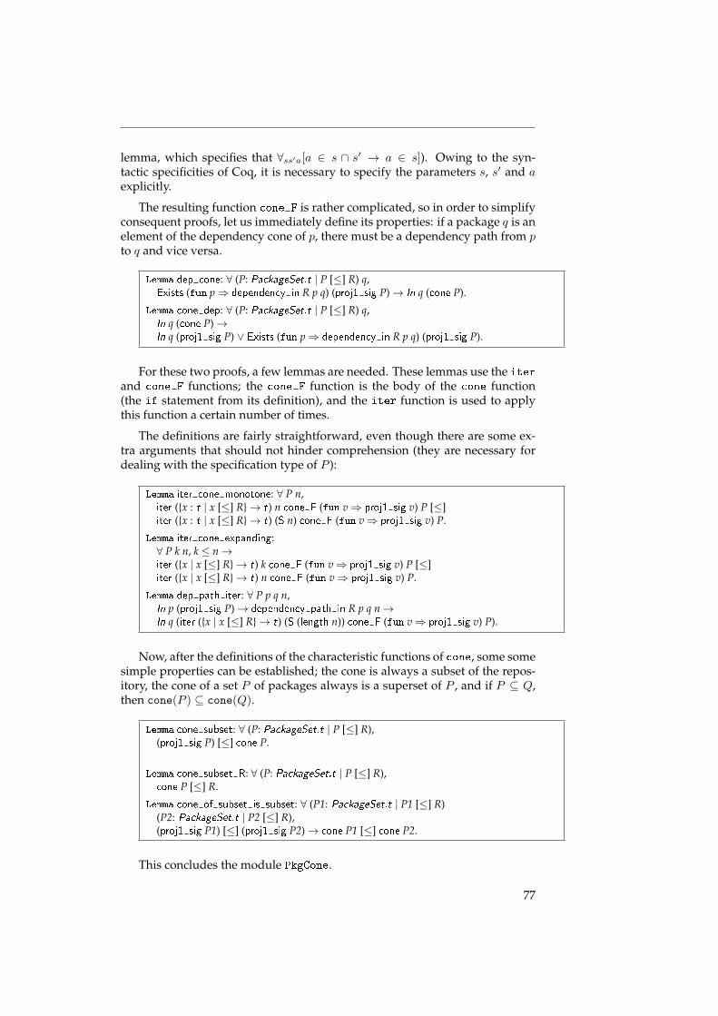
lemma, which specifies that ∀ss′a[a ∈ s ∩ s′ → a ∈ s]). Owing to the syn-tactic specificities of Coq, it is necessary to specify the parameters s, s′ and aexplicitly.
The resulting function cone F is rather complicated, so in order to simplifyconsequent proofs, let us immediately define its properties: if a package q is anelement of the dependency cone of p, there must be a dependency path from pto q and vice versa.
Lemma dep cone: ∀ (P: PackageSet.t | P [≤] R) q,Exists (fun p⇒ dependency in R p q) (proj1 sig P)→ In q (cone P).
Lemma cone dep: ∀ (P: PackageSet.t | P [≤] R) q,In q (cone P)→In q (proj1 sig P) ∨ Exists (fun p⇒ dependency in R p q) (proj1 sig P).
For these two proofs, a few lemmas are needed. These lemmas use the iterand cone F functions; the cone F function is the body of the cone function(the if statement from its definition), and the iter function is used to applythis function a certain number of times.
The definitions are fairly straightforward, even though there are some ex-tra arguments that should not hinder comprehension (they are necessary fordealing with the specification type of P ):
Lemma iter cone monotone: ∀ P n,iter ({x : t | x [≤] R}→ t) n cone F (fun v⇒ proj1 sig v) P [≤]iter ({x : t | x [≤] R}→ t) (S n) cone F (fun v⇒ proj1 sig v) P.
Lemma iter cone expanding:∀ P k n, k ≤ n→iter ({x | x [≤] R}→ t) k cone F (fun v⇒ proj1 sig v) P [≤]iter ({x | x [≤] R}→ t) n cone F (fun v⇒ proj1 sig v) P.
Lemma dep path iter: ∀ P p q n,In p (proj1 sig P)→ dependency path in R p q n→In q (iter ({x | x [≤] R}→ t) (S (length n)) cone F (fun v⇒ proj1 sig v) P).
Now, after the definitions of the characteristic functions of cone, some somesimple properties can be established; the cone is always a subset of the repos-itory, the cone of a set P of packages always is a superset of P , and if P ⊆ Q,then cone(P ) ⊆ cone(Q).
Lemma cone subset: ∀ (P: PackageSet.t | P [≤] R),(proj1 sig P) [≤] cone P.
Lemma cone subset R: ∀ (P: PackageSet.t | P [≤] R),cone P [≤] R.
Lemma cone of subset is subset: ∀ (P1: PackageSet.t | P1 [≤] R)(P2: PackageSet.t | P2 [≤] R),(proj1 sig P1) [≤] (proj1 sig P2)→ cone P1 [≤] cone P2.
This concludes the module PkgCone.
77
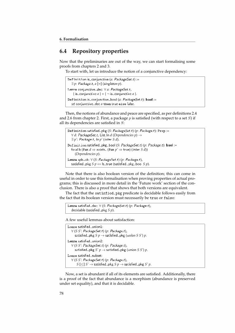
6. Formalisation
6.4 Repository properties
Now that the preliminaries are out of the way, we can start formalising someproofs from chapters 2 and 3.
To start with, let us introduce the notion of a conjunctive dependency:
Definition is conjunctive (a: PackageSet.t) :=∃ p: Package.t, a [=] (singleton p).
Lemma conjunctive dec: ∀ a: PackageSet.t,{ is conjunctive a } + { ¬ is conjunctive a }.
Definition is conjunctive bool (a: PackageSet.t): bool :=if conjunctive dec a then true else false.
Then, the notions of abundance and peace are specified, as per definitions 2.4and 2.6 from chapter 2. First, a package p is satisfied (with respect to a set S) ifall its dependencies are satisfied in S:
Definition satis�ed pkg (S: PackageSet.t) (p: Package.t): Prop :=∀ d: PackageSet.t, List.In d (Dependencies p)→∃ p’: Package.t, In p’ (inter S d).
Definition satis�ed pkg bool (S: PackageSet.t) (p: Package.t): bool :=forallb (fun d⇒ exists (fun p’⇒ true) (inter S d))
(Dependencies p).
Lemma spb ok: ∀ (S: PackageSet.t) (p: Package.t),satis�ed pkg S p↔ Is true (satis�ed pkg bool S p).
Note that there is also boolean version of the definition; this can come inuseful in order to use this formalisation when proving properties of actual pro-grams; this is discussed in more detail in the ‘Future work’ section of the con-clusion. There is also a proof that shows that both versions are equivalent.
The fact that the satisfied pkg predicate is decidable follows easily fromthe fact that its boolean version must necessarily be true or false:
Lemma satis�ed dec: ∀ (S: PackageSet.t) (p: Package.t),decidable (satis�ed pkg S p).
A few useful lemmas about satisfaction:
Lemma satis�ed union1:∀ (S S’: PackageSet.t) (p: Package.t),satis�ed pkg S p→ satis�ed pkg (union S S’) p.
Lemma satis�ed union2:∀ (S S’: PackageSet.t) (p: Package.t),satis�ed pkg S’ p→ satis�ed pkg (union S S’) p.
Lemma satis�ed subset:∀ (S S’: PackageSet.t) (p: Package.t),
S [≤] S’→ satis�ed pkg S p→ satis�ed pkg S’ p.
Now, a set is abundant if all of its elements are satisfied. Additionally, thereis a proof of the fact that abundance is a morphism (abundance is preservedunder set equality), and that it is decidable.
78
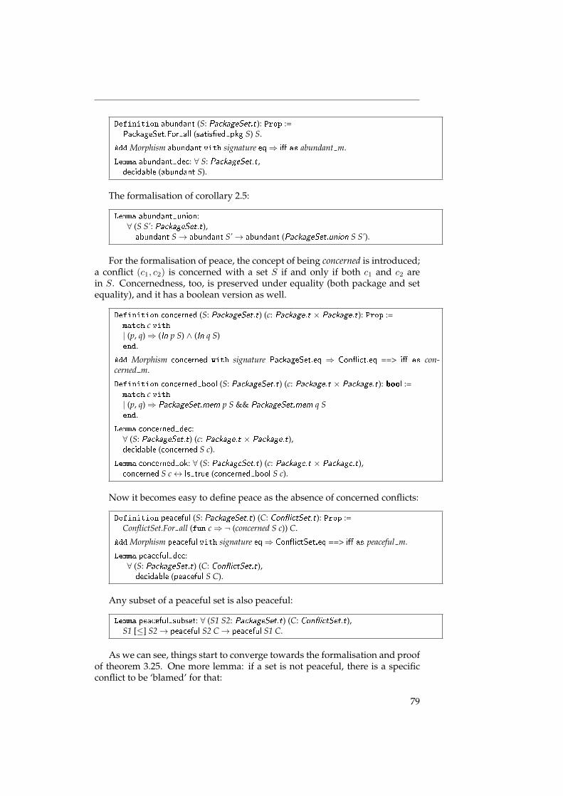
Definition abundant (S: PackageSet.t): Prop :=PackageSet.For all (satis�ed pkg S) S.
Add Morphism abundant with signature eq⇒ i� as abundant m.
Lemma abundant dec: ∀ S: PackageSet.t,decidable (abundant S).
The formalisation of corollary 2.5:
Lemma abundant union:∀ (S S’: PackageSet.t),abundant S→ abundant S’→ abundant (PackageSet.union S S’).
For the formalisation of peace, the concept of being concerned is introduced;a conflict (c1, c2) is concerned with a set S if and only if both c1 and c2 arein S. Concernedness, too, is preserved under equality (both package and setequality), and it has a boolean version as well.
Definition concerned (S: PackageSet.t) (c: Package.t × Package.t): Prop :=match c with| (p, q)⇒ (In p S) ∧ (In q S)end.
Add Morphism concerned with signature PackageSet.eq ⇒ Con�ict.eq ==> i� as con-cerned m.
Definition concerned bool (S: PackageSet.t) (c: Package.t × Package.t): bool :=match c with| (p, q)⇒ PackageSet.mem p S && PackageSet.mem q Send.
Lemma concerned dec:∀ (S: PackageSet.t) (c: Package.t × Package.t),decidable (concerned S c).
Lemma concerned ok: ∀ (S: PackageSet.t) (c: Package.t × Package.t),concerned S c↔ Is true (concerned bool S c).
Now it becomes easy to define peace as the absence of concerned conflicts:
Definition peaceful (S: PackageSet.t) (C: Con�ictSet.t): Prop :=ConflictSet.For all (fun c⇒¬ (concerned S c)) C.
Add Morphism peaceful with signature eq⇒ Con�ictSet.eq ==> i� as peaceful m.
Lemma peaceful dec:∀ (S: PackageSet.t) (C: Con�ictSet.t),decidable (peaceful S C).
Any subset of a peaceful set is also peaceful:
Lemma peaceful subset: ∀ (S1 S2: PackageSet.t) (C: Con�ictSet.t),S1 [≤] S2→ peaceful S2 C→ peaceful S1 C.
As we can see, things start to converge towards the formalisation and proofof theorem 3.25. One more lemma: if a set is not peaceful, there is a specificconflict to be ‘blamed’ for that:
79
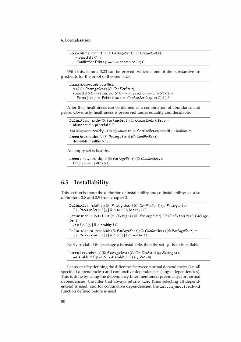
6. Formalisation
Lemma blame con�ict: ∀ (I: PackageSet.t) (C: Con�ictSet.t),¬ peaceful I C→Con�ictSet.Exists (fun c⇒ concerned I c) C.
With this, lemma 3.23 can be proved, which is one of the substantive in-gredients for the proof of theorem 3.25.
Lemma not peaceful con�ict:∀ (S S’: PackageSet.t) (C: Con�ictSet.t),(peaceful S C)→ (peaceful S’ C)→¬ (peaceful (union S S’) C)→Exists (fun p⇒ Exists (fun q⇒ Con�ictSet.In (p, q) C) S’) S.
After this, healthiness can be defined as a combination of abundance andpeace. Obviously, healthiness is preserved under equality and decidable.
Definition healthy (S: PackageSet.t) (C: Con�ictSet.t): Prop :=abundant S ∧ peaceful S C.
Add Morphism healthy with signature eq⇒ Con�ictSet.eq ==> i� as healthy m.
Lemma healthy dec: ∀ (S: PackageSet.t) (C: Con�ictSet.t),decidable (healthy S C).
An empty set is healthy.
Lemma empty healthy: ∀ (S: PackageSet.t) (C: Con�ictSet.t),Empty S→ healthy S C.
6.5 Installability
This section is about the definition of installability and co-installability; see alsodefinitions 2.8 and 2.9 from chapter 2.
Definition installable (R: PackageSet.t) (C: Con�ictSet.t) (p: Package.t) :=∃ I: PackageSet.t, I [≤] R ∧ In p I ∧ healthy I C.
Definition is install set (p: Package.t) (R: PackageSet.t) (C: Con�ictSet.t) (I: Package-Set.t) :=
In p I ∧ I [≤] R ∧ healthy I C.
Definition co installable (R: PackageSet.t) (C: Con�ictSet.t) (S: PackageSet.t) :=∃ I: PackageSet.t, I [≤] R ∧ S [≤] I ∧ healthy I C.
Fairly trivial: if the package p is installable, then the set {p} is co-installable.
Lemma inst coinst: ∀ (R: PackageSet.t) (C: Con�ictSet.t) (p: Package.t),installable R C p↔ co installable R C (singleton p).
Let us start by defining the difference between normal dependencies (i.e. allspecified dependencies) and conjunctive dependencies (single dependencies).This is done by using the dependency filter mentioned previously: for normaldependencies, the filter that always returns true (thus selecting all depend-encies) is used, and for conjunctive dependencies, the is conjunctive bool
function defined before is used.
80
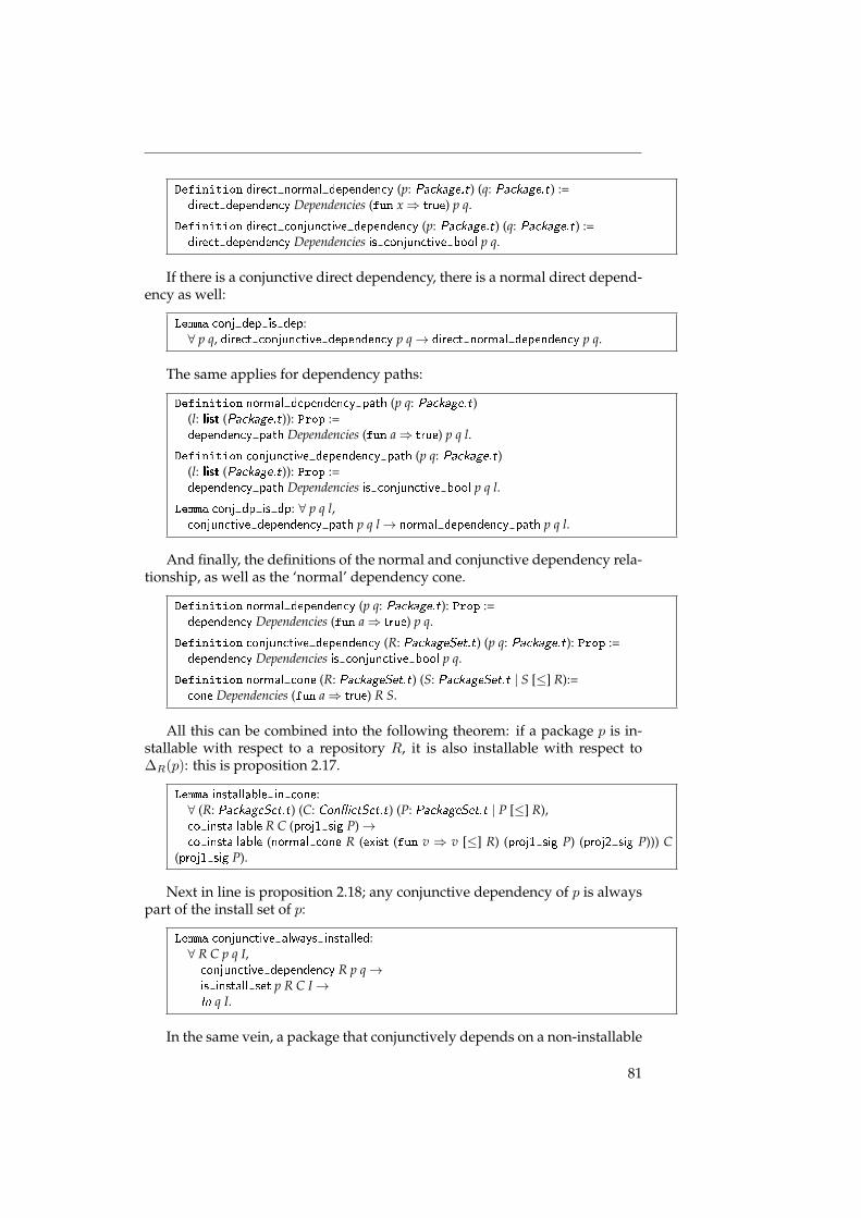
Definition direct normal dependency (p: Package.t) (q: Package.t) :=direct dependency Dependencies (fun x⇒ true) p q.
Definition direct conjunctive dependency (p: Package.t) (q: Package.t) :=direct dependency Dependencies is conjunctive bool p q.
If there is a conjunctive direct dependency, there is a normal direct depend-ency as well:
Lemma conj dep is dep:∀ p q, direct conjunctive dependency p q→ direct normal dependency p q.
The same applies for dependency paths:
Definition normal dependency path (p q: Package.t)(l: list (Package.t)): Prop :=dependency path Dependencies (fun a⇒ true) p q l.
Definition conjunctive dependency path (p q: Package.t)(l: list (Package.t)): Prop :=dependency path Dependencies is conjunctive bool p q l.
Lemma conj dp is dp: ∀ p q l,conjunctive dependency path p q l→ normal dependency path p q l.
And finally, the definitions of the normal and conjunctive dependency rela-tionship, as well as the ‘normal’ dependency cone.
Definition normal dependency (p q: Package.t): Prop :=dependency Dependencies (fun a⇒ true) p q.
Definition conjunctive dependency (R: PackageSet.t) (p q: Package.t): Prop :=dependency Dependencies is conjunctive bool p q.
Definition normal cone (R: PackageSet.t) (S: PackageSet.t | S [≤] R):=cone Dependencies (fun a⇒ true) R S.
All this can be combined into the following theorem: if a package p is in-stallable with respect to a repository R, it is also installable with respect to∆R(p): this is proposition 2.17.
Lemma installable in cone:∀ (R: PackageSet.t) (C: Con�ictSet.t) (P: PackageSet.t | P [≤] R),co installable R C (proj1 sig P)→co installable (normal cone R (exist (fun v ⇒ v [≤] R) (proj1 sig P) (proj2 sig P))) C
(proj1 sig P).
Next in line is proposition 2.18; any conjunctive dependency of p is alwayspart of the install set of p:
Lemma conjunctive always installed:∀ R C p q I,conjunctive dependency R p q→is install set p R C I→In q I.
In the same vein, a package that conjunctively depends on a non-installable
81
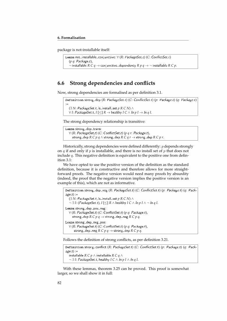
6. Formalisation
package is not-installable itself:
Lemma not installable conjunctive: ∀ (R: PackageSet.t) (C: Con�ictSet.t)(p q: Package.t),¬ installable R C q→ conjunctive dependency R p q→¬ installable R C p.
6.6 Strong dependencies and conflicts
Now, strong dependencies are formalised as per definition 3.1.
Definition strong dep (R: PackageSet.t) (C: Con�ictSet.t) (p: Package.t) (q: Package.t):=
(∃ N: PackageSet.t, is install set p R C N) ∧∀ I: PackageSet.t, I [≤] R→ healthy I C ∧ In p I→ In q I.
The strong dependency relationship is transitive:
Lemma strong dep trans:∀ (R: PackageSet.t) (C: Con�ictSet.t) (p q r: Package.t),strong dep R C p q ∧ strong dep R C q r→ strong dep R C p r.
Historically, strong dependencies were defined differently: p depends stronglyon q if and only if p is installable, and there is no install set of p that does notinclude q. This negative definition is equivalent to the positive one from defin-ition 3.1:
We have opted to use the positive version of the definition as the standarddefinition, because it is constructive and therefore allows for more straight-forward proofs. The negative version would need many proofs by absurdity(indeed, the proof that the negative version implies the positive version is anexample of this), which are not as informative.
Definition strong dep neg (R: PackageSet.t) (C: Con�ictSet.t) (p: Package.t) (q: Pack-age.t) :=
(∃ N: PackageSet.t, is install set p R C N) ∧¬ ∃ I: (PackageSet.t), I [≤] R ∧ healthy I C ∧ In p I ∧ ¬ In q I.
Lemma strong dep pos neg:∀ (R: PackageSet.t) (C: Con�ictSet.t) (p q: Package.t),strong dep R C p q→ strong dep neg R C p q.
Lemma strong dep neg pos:∀ (R: PackageSet.t) (C: Con�ictSet.t) (p q: Package.t),
strong dep neg R C p q→ strong dep R C p q.
Follows the definition of strong conflicts, as per definition 3.21.
Definition strong con�ict (R: PackageSet.t) (C: Con�ictSet.t) (p: Package.t) (q: Pack-
age.t) :=installable R C p ∧ installable R C q ∧¬ ∃ I: PackageSet.t, healthy I C ∧ In p I ∧ In q I.
With these lemmas, theorem 3.25 can be proved. This proof is somewhatlarger, so we shall show it in full:
82
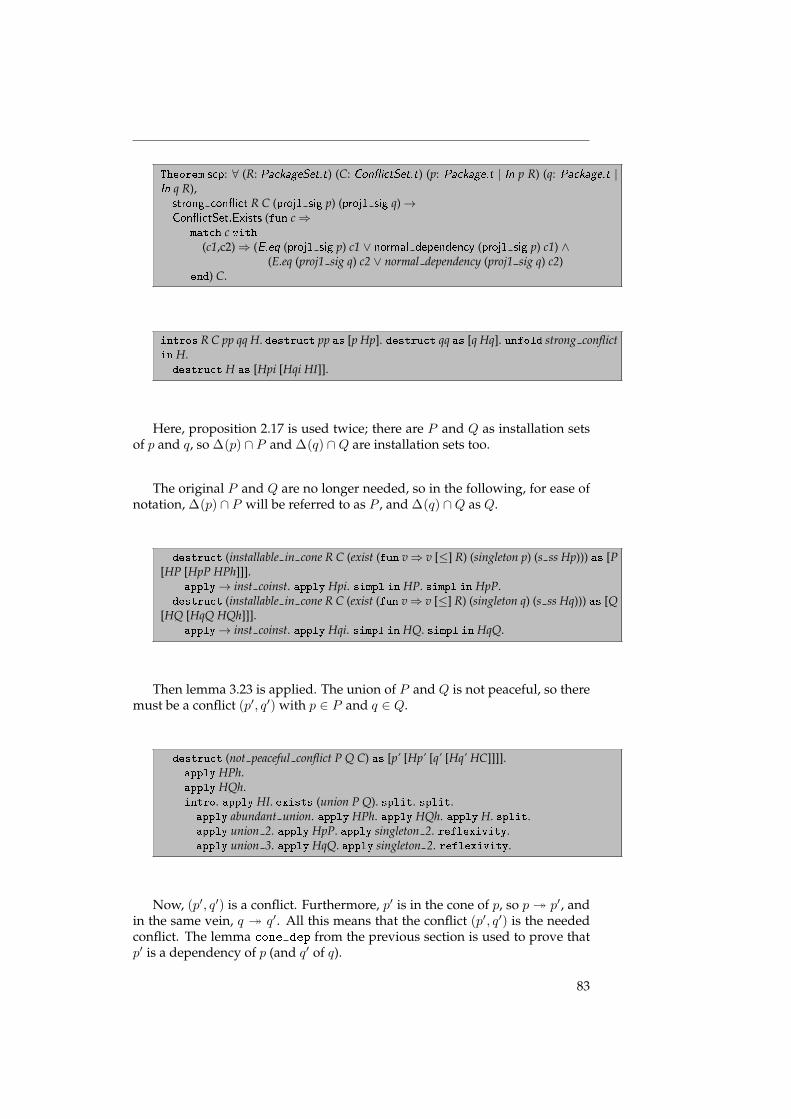
Theorem scp: ∀ (R: PackageSet.t) (C: Con�ictSet.t) (p: Package.t | In p R) (q: Package.t |In q R),strong con�ict R C (proj1 sig p) (proj1 sig q)→Con�ictSet.Exists (fun c⇒
match c with(c1,c2)⇒ (E.eq (proj1 sig p) c1 ∨ normal dependency (proj1 sig p) c1) ∧
(E.eq (proj1 sig q) c2 ∨ normal dependency (proj1 sig q) c2)end) C.
intros R C pp qq H. destruct pp as [p Hp]. destruct qq as [q Hq]. unfold strong conflictin H.destruct H as [Hpi [Hqi HI]].
Here, proposition 2.17 is used twice; there are P and Q as installation setsof p and q, so ∆(p) ∩ P and ∆(q) ∩Q are installation sets too.
The original P and Q are no longer needed, so in the following, for ease ofnotation, ∆(p) ∩ P will be referred to as P , and ∆(q) ∩Q as Q.
destruct (installable in cone R C (exist (fun v⇒ v [≤] R) (singleton p) (s ss Hp))) as [P[HP [HpP HPh]]].
apply→ inst coinst. apply Hpi. simpl in HP. simpl in HpP.destruct (installable in cone R C (exist (fun v⇒ v [≤] R) (singleton q) (s ss Hq))) as [Q
[HQ [HqQ HQh]]].apply→ inst coinst. apply Hqi. simpl in HQ. simpl in HqQ.
Then lemma 3.23 is applied. The union of P and Q is not peaceful, so theremust be a conflict (p′, q′) with p ∈ P and q ∈ Q.
destruct (not peaceful conflict P Q C) as [p’ [Hp’ [q’ [Hq’ HC]]]].apply HPh.apply HQh.intro. apply HI. exists (union P Q). split. split.apply abundant union. apply HPh. apply HQh. apply H. split.apply union 2. apply HpP. apply singleton 2. reflexivity.apply union 3. apply HqQ. apply singleton 2. reflexivity.
Now, (p′, q′) is a conflict. Furthermore, p′ is in the cone of p, so p � p′, andin the same vein, q � q′. All this means that the conflict (p′, q′) is the neededconflict. The lemma cone dep from the previous section is used to prove thatp′ is a dependency of p (and q′ of q).
83
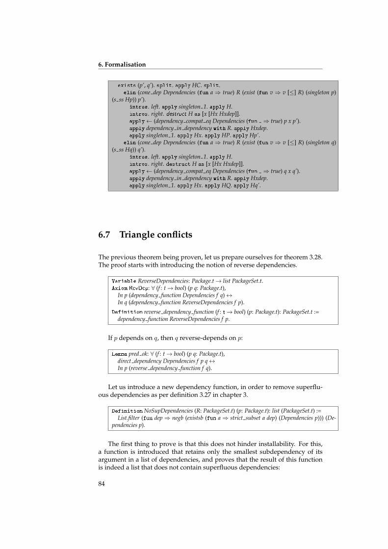
6. Formalisation
exists (p’, q’). split. apply HC. split.elim (cone dep Dependencies (fun a ⇒ true) R (exist (fun v ⇒ v [≤] R) (singleton p)
(s ss Hp)) p’).intros. left. apply singleton 1. apply H.intros. right. destruct H as [x [Hx Hxdep]].apply← (dependency compat eq Dependencies (fun ⇒ true) p x p’).apply dependency in dependency with R. apply Hxdep.apply singleton 1. apply Hx. apply HP. apply Hp’.
elim (cone dep Dependencies (fun a ⇒ true) R (exist (fun v ⇒ v [≤] R) (singleton q)(s ss Hq)) q’).
intros. left. apply singleton 1. apply H.intros. right. destruct H as [x [Hx Hxdep]].apply← (dependency compat eq Dependencies (fun ⇒ true) q x q’).apply dependency in dependency with R. apply Hxdep.apply singleton 1. apply Hx. apply HQ. apply Hq’.
6.7 Triangle conflicts
The previous theorem being proven, let us prepare ourselves for theorem 3.28.The proof starts with introducing the notion of reverse dependencies.
Variable ReverseDependencies: Package.t→ list PackageSet.t.Axiom RevDep: ∀ (f : t→ bool) (p q: Package.t),
In p (dependency function Dependencies f q)↔In q (dependency function ReverseDependencies f p).
Definition reverse dependency function (f : t→ bool) (p: Package.t): PackageSet.t :=dependency function ReverseDependencies f p.
If p depends on q, then q reverse-depends on p:
Lemma pred ok: ∀ (f : t→ bool) (p q: Package.t),direct dependency Dependencies f p q↔In p (reverse dependency function f q).
Let us introduce a new dependency function, in order to remove superflu-ous dependencies as per definition 3.27 in chapter 3.
Definition NoSupDependencies (R: PackageSet.t) (p: Package.t): list (PackageSet.t) :=List.filter (fun dep ⇒ negb (existsb (fun a ⇒ strict subset a dep) (Dependencies p))) (De-
pendencies p).
The first thing to prove is that this does not hinder installability. For this,a function is introduced that retains only the smallest subdependency of itsargument in a list of dependencies, and proves that the result of this functionis indeed a list that does not contain superfluous dependencies:
84
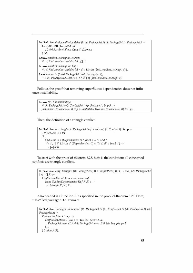
Definition find smallest subdep (l: list PackageSet.t) (d: PackageSet.t): PackageSet.t :=List.fold left (fun acc d’⇒if strict subset d’ acc then d’ else acc
) l d.
Lemma smallest subdep is subset:∀ l d, find smallest subdep l d [≤] d .
Lemma smallest subdep in list:∀ l d, find smallest subdep l d = d ∨ List.In (find smallest subdep l d) l.
Lemma ss ok: ∀ (l: list PackageSet.t) (d: PackageSet.t),¬ ∃ d’: PackageSet.t, List.In d’ l ∧ d’ [<] (find smallest subdep l d).
Follows the proof that removing superfluous dependencies does not influ-ence installability.
Lemma NSD installability:∀ (R: PackageSet.t) (C: ConflictSet.t) (p: Package.t), In p R→
(installable Dependencies R C p↔ installable (NoSupDependencies R) R C p).
Then, the definition of a triangle conflict.
Definition is triangle (R: PackageSet.t) (f : t→ bool) (c: Conflict.t): Prop :=let (c1, c2) := c in∃ t,
(∃ d, List.In d (Dependencies t) ∧ In c1 d ∧ In c2 d ∧(∀ d’, (∃ t’, List.In d' (Dependencies t’)) ∧ (In c1 d’ ∨ In c2 d’)→
d [=] d’)).
To start with the proof of theorem 3.28, here is the condition: all concernedconflicts are triangle conflicts.
Definition only triangles (R: PackageSet.t) (C: ConflictSet.t) (f : t→ bool) (A: PackageSet.t| A [≤] R) :=
ConflictSet.For all (fun c⇒ concerned(cone (NoSupDependencies R) f R A) c→is triangle R f c ) C.
Also needed is a function K as specified in the proof of theorem 3.28. Here,it is called packages to remove:
Definition packages to remove (R: PackageSet.t) (C: ConflictSet.t) (A: PackageSet.t) (B:PackageSet.t) :=
PackageSet.filter (fun p⇒ConflictSet.exists (fun c⇒ let (c1, c2) := c in
PackageSet.mem c1 A && PackageSet.mem c2 B && beq pkg p c1) C
) (union A B).
85
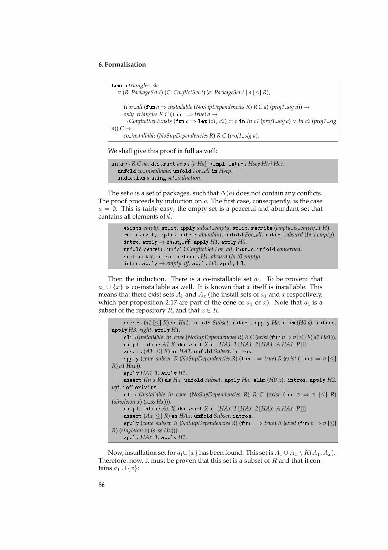
6. Formalisation
Lemma triangles ok:∀ (R: PackageSet.t) (C: ConflictSet.t) (a: PackageSet.t | a [≤] R),
(For all (fun a⇒ installable (NoSupDependencies R) R C a) (proj1 sig a))→only triangles R C (fun ⇒ true) a→¬ ConflictSet.Exists (fun c⇒ let (c1, c2) := c in In c1 (proj1 sig a) ∨ In c2 (proj1 sig
a)) C→co installable (NoSupDependencies R) R C (proj1 sig a).
We shall give this proof in full as well:
intros R C aa. destruct aa as [a Ha]. simpl. intros Hsep Htri Hcc.unfold co installable. unfold For all in Hsep.induction a using set induction.
The set a is a set of packages, such that ∆(a) does not contain any conflicts.The proof proceeds by induction on a. The first case, consequently, is the casea = ∅. This is fairly easy; the empty set is a peaceful and abundant set thatcontains all elements of ∅.
exists empty. split. apply subset empty. split. rewrite (empty is empty 1 H).reflexivity. split. unfold abundant. unfold For all. intros. absurd (In x empty).intro. apply→ empty i�. apply H1. apply H0.unfold peaceful. unfold ConflictSet.For all. intros. unfold concerned.destruct x. intro. destruct H1. absurd (In t0 empty).intro. apply→ empty iff. apply H3. apply H1.
Then the induction. There is a co-installable set a1. To be proven: thata1 ∪ {x} is co-installable as well. It is known that x itself is installable. Thismeans that there exist sets A1 and Ax (the install sets of a1 and x respectively,which per proposition 2.17 are part of the cone of a1 or x). Note that a1 is asubset of the repository R, and that x ∈ R.
assert (a1 [≤] R) as Ha1. unfold Subset. intros. apply Ha. elim (H0 a). intros.apply H3. right. apply H1.
elim (installable in cone (NoSupDependencies R) R C (exist (fun v⇒ v [≤] R) a1 Ha1)).simpl. intros A1 X. destruct X as [HA1 1 [HA1 2 [HA1 A HA1 P]]].assert (A1 [≤] R) as HA1. unfold Subset. intros.apply (cone subset R (NoSupDependencies R) (fun ⇒ true) R (exist (fun v⇒ v [≤]
R) a1 Ha1)).apply HA1 1. apply H1.assert (In x R) as Hx. unfold Subset. apply Ha. elim (H0 x). intros. apply H2.
left. reflexivity.elim (installable in cone (NoSupDependencies R) R C (exist (fun v ⇒ v [≤] R)
(singleton x) (s ss Hx))).simpl. intros Ax X. destruct X as [HAx 1 [HAx 2 [HAx A HAx P]]].assert (Ax [≤] R) as HAx. unfold Subset. intros.apply (cone subset R (NoSupDependencies R) (fun ⇒ true) R (exist (fun v⇒ v [≤]
R) (singleton x) (s ss Hx))).apply HAx 1. apply H1.
Now, installation set for a1∪{x} has been found. This set isA1 ∪Ax \K(A1, Ax).Therefore, now, it must be proven that this set is a subset of R and that it con-tains a1 ∪ {x}:
86
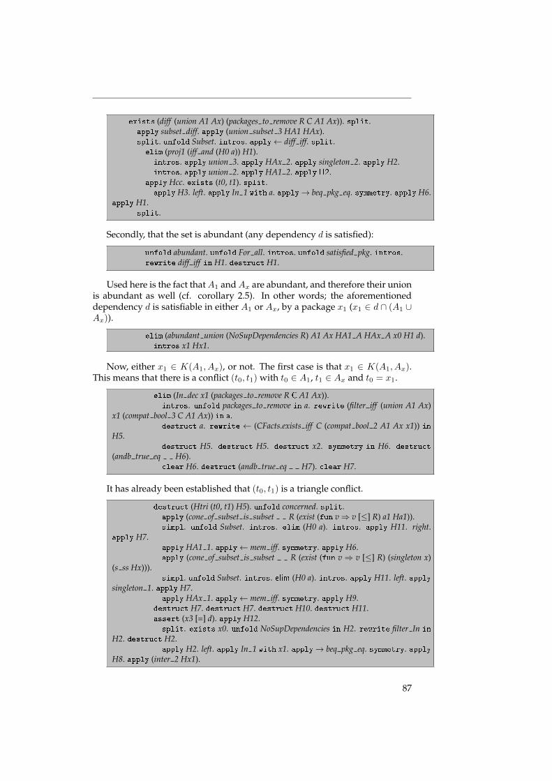
exists (diff (union A1 Ax) (packages to remove R C A1 Ax)). split.apply subset diff. apply (union subset 3 HA1 HAx).split. unfold Subset. intros. apply← diff iff. split.elim (proj1 (iff and (H0 a)) H1).intros. apply union 3. apply HAx 2. apply singleton 2. apply H2.intros. apply union 2. apply HA1 2. apply H2.
apply Hcc. exists (t0, t1). split.apply H3. left. apply In 1 with a. apply→ beq pkg eq. symmetry. apply H6.
apply H1.split.
Secondly, that the set is abundant (any dependency d is satisfied):
unfold abundant. unfold For all. intros. unfold satisfied pkg. intros.rewrite diff iff in H1. destruct H1.
Used here is the fact thatA1 andAx are abundant, and therefore their unionis abundant as well (cf. corollary 2.5). In other words; the aforementioneddependency d is satisfiable in either A1 or Ax, by a package x1 (x1 ∈ d ∩ (A1 ∪Ax)).
elim (abundant union (NoSupDependencies R) A1 Ax HA1 A HAx A x0 H1 d).intros x1 Hx1.
Now, either x1 ∈ K(A1, Ax), or not. The first case is that x1 ∈ K(A1, Ax).This means that there is a conflict (t0, t1) with t0 ∈ A1, t1 ∈ Ax and t0 = x1.
elim (In dec x1 (packages to remove R C A1 Ax)).intros. unfold packages to remove in a. rewrite (filter iff (union A1 Ax)
x1 (compat bool 3 C A1 Ax)) in a.destruct a. rewrite ← (CFacts.exists iff C (compat bool 2 A1 Ax x1)) in
H5.destruct H5. destruct H5. destruct x2. symmetry in H6. destruct
(andb true eq H6).clear H6. destruct (andb true eq H7). clear H7.
It has already been established that (t0, t1) is a triangle conflict.
destruct (Htri (t0, t1) H5). unfold concerned. split.apply (cone of subset is subset R (exist (fun v⇒ v [≤] R) a1 Ha1)).simpl. unfold Subset. intros. elim (H0 a). intros. apply H11. right.
apply H7.apply HA1 1. apply← mem iff. symmetry. apply H6.apply (cone of subset is subset R (exist (fun v⇒ v [≤] R) (singleton x)
(s ss Hx))).simpl. unfold Subset. intros. elim (H0 a). intros. apply H11. left. apply
singleton 1. apply H7.apply HAx 1. apply← mem iff. symmetry. apply H9.
destruct H7. destruct H7. destruct H10. destruct H11.assert (x3 [=] d). apply H12.split. exists x0. unfold NoSupDependencies in H2. rewrite filter In in
H2. destruct H2.apply H2. left. apply In 1 with x1. apply→ beq pkg eq. symmetry. apply
H8. apply (inter 2 Hx1).
87
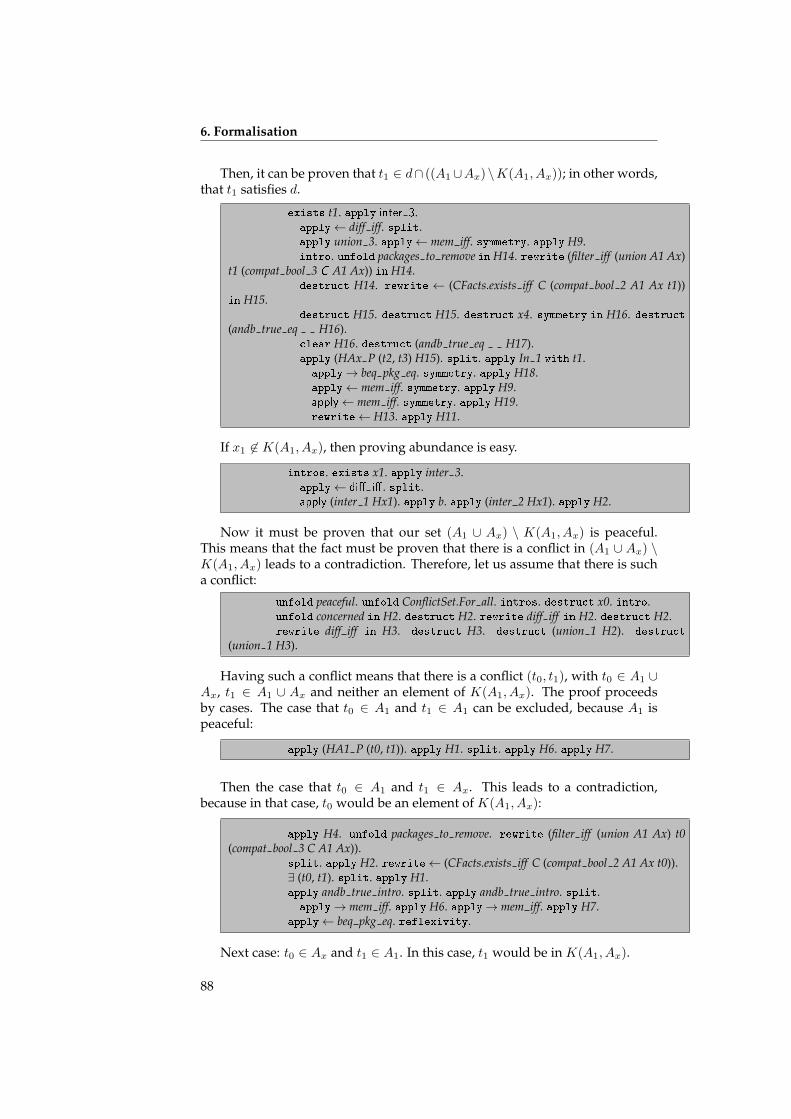
6. Formalisation
Then, it can be proven that t1 ∈ d∩ ((A1∪Ax)\K(A1, Ax)); in other words,that t1 satisfies d.
exists t1. apply inter 3.apply← diff iff. split.apply union 3. apply← mem iff. symmetry. apply H9.intro. unfold packages to remove in H14. rewrite (filter iff (union A1 Ax)
t1 (compat bool 3 C A1 Ax)) in H14.destruct H14. rewrite ← (CFacts.exists iff C (compat bool 2 A1 Ax t1))
in H15.destruct H15. destruct H15. destruct x4. symmetry in H16. destruct
(andb true eq H16).clear H16. destruct (andb true eq H17).apply (HAx P (t2, t3) H15). split. apply In 1 with t1.apply→ beq pkg eq. symmetry. apply H18.apply← mem iff. symmetry. apply H9.apply← mem iff. symmetry. apply H19.rewrite← H13. apply H11.
If x1 6∈ K(A1, Ax), then proving abundance is easy.
intros. exists x1. apply inter 3.apply← di� i�. split.apply (inter 1 Hx1). apply b. apply (inter 2 Hx1). apply H2.
Now it must be proven that our set (A1 ∪ Ax) \ K(A1, Ax) is peaceful.This means that the fact must be proven that there is a conflict in (A1 ∪ Ax) \K(A1, Ax) leads to a contradiction. Therefore, let us assume that there is sucha conflict:
unfold peaceful. unfold ConflictSet.For all. intros. destruct x0. intro.unfold concerned in H2. destruct H2. rewrite diff iff in H2. destruct H2.rewrite diff iff in H3. destruct H3. destruct (union 1 H2). destruct
(union 1 H3).
Having such a conflict means that there is a conflict (t0, t1), with t0 ∈ A1 ∪Ax, t1 ∈ A1 ∪ Ax and neither an element of K(A1, Ax). The proof proceedsby cases. The case that t0 ∈ A1 and t1 ∈ A1 can be excluded, because A1 ispeaceful:
apply (HA1 P (t0, t1)). apply H1. split. apply H6. apply H7.
Then the case that t0 ∈ A1 and t1 ∈ Ax. This leads to a contradiction,because in that case, t0 would be an element of K(A1, Ax):
apply H4. unfold packages to remove. rewrite (filter iff (union A1 Ax) t0(compat bool 3 C A1 Ax)).
split. apply H2. rewrite← (CFacts.exists iff C (compat bool 2 A1 Ax t0)).∃ (t0, t1). split. apply H1.apply andb true intro. split. apply andb true intro. split.apply→ mem iff. apply H6. apply→ mem iff. apply H7.
apply← beq pkg eq. reflexivity.
Next case: t0 ∈ Ax and t1 ∈ A1. In this case, t1 would be in K(A1, Ax).
88
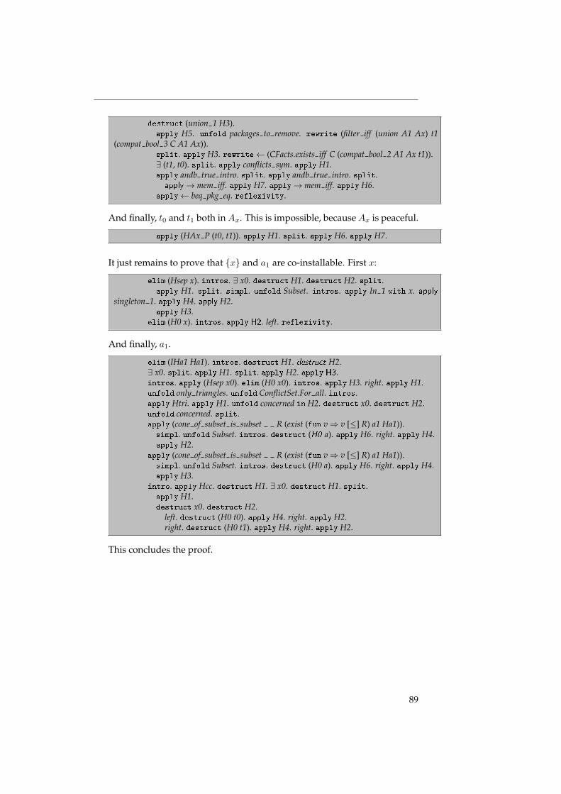
destruct (union 1 H3).apply H5. unfold packages to remove. rewrite (filter iff (union A1 Ax) t1
(compat bool 3 C A1 Ax)).split. apply H3. rewrite← (CFacts.exists iff C (compat bool 2 A1 Ax t1)).∃ (t1, t0). split. apply conflicts sym. apply H1.apply andb true intro. split. apply andb true intro. split.apply→ mem iff. apply H7. apply→ mem iff. apply H6.
apply← beq pkg eq. reflexivity.
And finally, t0 and t1 both in Ax. This is impossible, because Ax is peaceful.
apply (HAx P (t0, t1)). apply H1. split. apply H6. apply H7.
It just remains to prove that {x} and a1 are co-installable. First x:
elim (Hsep x). intros. ∃ x0. destruct H1. destruct H2. split.apply H1. split. simpl. unfold Subset. intros. apply In 1 with x. apply
singleton 1. apply H4. apply H2.apply H3.
elim (H0 x). intros. apply H2. left. reflexivity.
And finally, a1.
elim (IHa1 Ha1). intros. destruct H1. destruct H2.∃ x0. split. apply H1. split. apply H2. apply H3.intros. apply (Hsep x0). elim (H0 x0). intros. apply H3. right. apply H1.unfold only triangles. unfold ConflictSet.For all. intros.apply Htri. apply H1. unfold concerned in H2. destruct x0. destruct H2.unfold concerned. split.apply (cone of subset is subset R (exist (fun v⇒ v [≤] R) a1 Ha1)).simpl. unfold Subset. intros. destruct (H0 a). apply H6. right. apply H4.apply H2.
apply (cone of subset is subset R (exist (fun v⇒ v [≤] R) a1 Ha1)).simpl. unfold Subset. intros. destruct (H0 a). apply H6. right. apply H4.apply H3.
intro. apply Hcc. destruct H1. ∃ x0. destruct H1. split.apply H1.destruct x0. destruct H2.
left. destruct (H0 t0). apply H4. right. apply H2.right. destruct (H0 t1). apply H4. right. apply H2.
This concludes the proof.
89

6. Formalisation
90
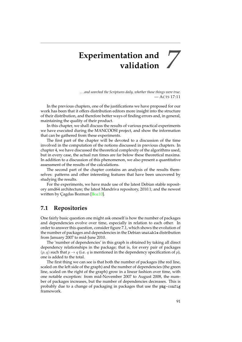
Experimentation andvalidation 7
. . . and searched the Scriptures daily, whether those things were true.— ACTS 17:11
In the previous chapters, one of the justifications we have proposed for ourwork has been that it offers distribution editors more insight into the structureof their distribution, and therefore better ways of finding errors and, in general,maintaining the quality of their product.
In this chapter, we shall discuss the results of various practical experimentswe have executed during the MANCOOSI project, and show the informationthat can be gathered from these experiments.
The first part of the chapter will be devoted to a discussion of the timeinvolved in the computation of the notions discussed in previous chapters. Inchapter 4, we have discussed the theoretical complexity of the algorithms used,but in every case, the actual run times are far below these theoretical maxima.In addition to a discussion of this phenomenon, we also present a quantitativeassessment of the results of the calculations.
The second part of the chapter contains an analysis of the results them-selves: patterns and other interesting features that have been uncovered bystudying the results.
For the experiments, we have made use of the latest Debian stable reposit-ory amd64 architecture; the latest Mandriva repository, 2010.1; and the newestwritten by Çagdas Bozman [Boz10].
7.1 Repositories
One fairly basic question one might ask oneself is how the number of packagesand dependencies evolve over time, especially in relation to each other. Inorder to answer this question, consider figure 7.1, which shows the evolution ofthe number of packages and dependencies in the Debian unstable distributionfrom January 2007 to mid-June 2010.
The ‘number of dependencies’ in this graph is obtained by taking all directdependency relationships in the package; that is, for every pair of packages(p, q) such that p→ q (i.e. q is mentioned in the dependency specification of p),one is added to the total.
The first thing we can see is that both the number of packages (the red line,scaled on the left side of the graph) and the number of dependencies (the greenline, scaled on the right of the graph) grow in a linear fashion over time, withone notable exception: from mid-November 2007 to August 2008, the num-ber of packages increases, but the number of dependencies decreases. This isprobably due to a change of packaging in packages that use the pkg-config
framework.
91
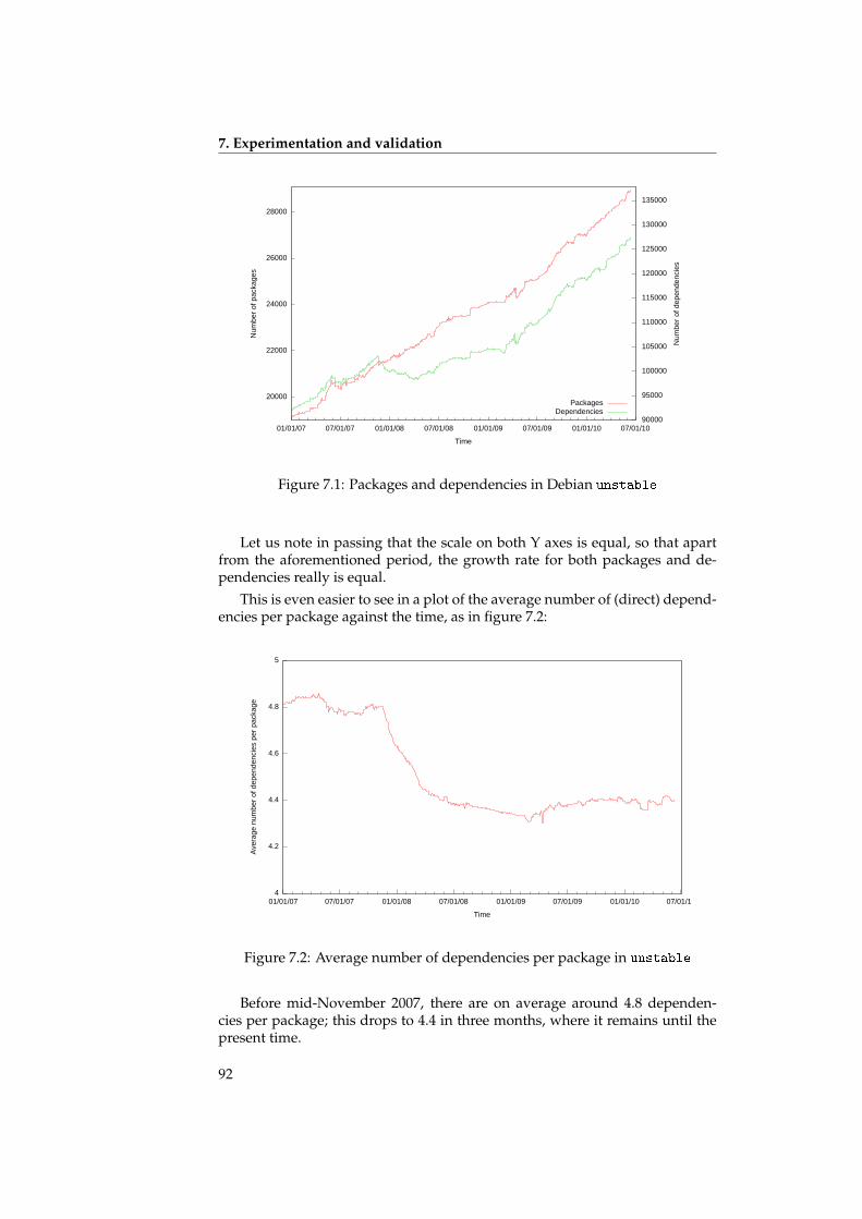
7. Experimentation and validation
20000
22000
24000
26000
28000
01/01/07 07/01/07 01/01/08 07/01/08 01/01/09 07/01/09 01/01/10 07/01/10 90000
95000
100000
105000
110000
115000
120000
125000
130000
135000
Num
ber o
f pac
kage
s
Num
ber o
f dep
ende
ncie
s
Time
PackagesDependencies
Figure 7.1: Packages and dependencies in Debian unstable
Let us note in passing that the scale on both Y axes is equal, so that apartfrom the aforementioned period, the growth rate for both packages and de-pendencies really is equal.
This is even easier to see in a plot of the average number of (direct) depend-encies per package against the time, as in figure 7.2:
4
4.2
4.4
4.6
4.8
5
01/01/07 07/01/07 01/01/08 07/01/08 01/01/09 07/01/09 01/01/10 07/01/10
Aver
age
num
ber o
f dep
ende
ncie
s pe
r pac
kage
Time
Figure 7.2: Average number of dependencies per package in unstable
Before mid-November 2007, there are on average around 4.8 dependen-cies per package; this drops to 4.4 in three months, where it remains until thepresent time.
92
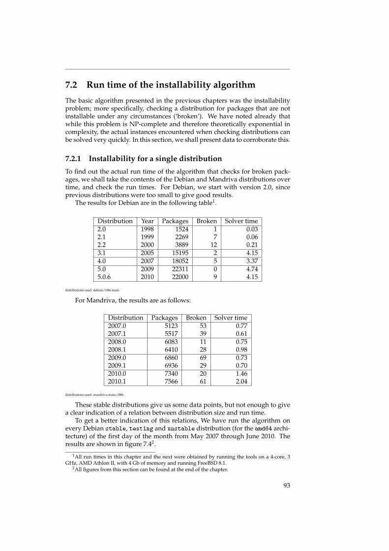
7.2 Run time of the installability algorithm
The basic algorithm presented in the previous chapters was the installabilityproblem; more specifically, checking a distribution for packages that are notinstallable under any circumstances (‘broken’). We have noted already thatwhile this problem is NP-complete and therefore theoretically exponential incomplexity, the actual instances encountered when checking distributions canbe solved very quickly. In this section, we shall present data to corroborate this.
7.2.1 Installability for a single distribution
To find out the actual run time of the algorithm that checks for broken pack-ages, we shall take the contents of the Debian and Mandriva distributions overtime, and check the run times. For Debian, we start with version 2.0, sinceprevious distributions were too small to give good results.
The results for Debian are in the following table1.
Distribution Year Packages Broken Solver time2.0 1998 1524 1 0.032.1 1999 2269 7 0.062.2 2000 3889 12 0.213.1 2005 15195 2 4.154.0 2007 18052 5 3.375.0 2009 22311 0 4.745.0.6 2010 22000 9 4.15
distributions used: debian/i386 main
For Mandriva, the results are as follows:
Distribution Packages Broken Solver time2007.0 5123 53 0.772007.1 5517 39 0.612008.0 6083 11 0.752008.1 6410 28 0.982009.0 6860 69 0.732009.1 6936 29 0.702010.0 7340 20 1.462010.1 7566 61 2.04
distributions used: mandriva main/i386
These stable distributions give us some data points, but not enough to givea clear indication of a relation between distribution size and run time.
To get a better indication of this relations, We have run the algorithm onevery Debian stable, testing and unstable distribution (for the amd64 archi-tecture) of the first day of the month from May 2007 through June 2010. Theresults are shown in figure 7.42.
1All run times in this chapter and the next were obtained by running the tools on a 4-core, 3GHz, AMD Athlon II, with 4 Gb of memory and running FreeBSD 8.1.
2All figures from this section can be found at the end of the chapter.
93
7. Experimentation and validation
The curve is mostly linear, though there are significant outliers. This is be-cause there can be great differences between two distributions that are similarin size: as an example, the unstable distribution for June 1st, 2008, has almostthe same size as the testing for December 1st, 2008, but the testing distri-bution takes 20% longer to solve. This can be attributed to the fact that thereare 5044 broken packages in the unstable distribution: many of these brokenpackages are broken because of the same reason, which greatly speeds up thework of the SAT solver.
7.2.2 Installability for multiple distributions
What happens if one takes two different distributions (stable and testing, ortesting and unstable) and check them for broken packages? Looking at fig-ure 7.5, we can see that the progression is still linear, but that the constantbecomes much higher.
To explain this, let us note first that if two distributions are added together,in many cases, this union contains two different versions of the same package.So, many dependencies that before had only one solution now have two solu-tions; and to add insult to injury, these two solutions are in conflict with eachother.
Let us give an example. In Debian 5.0.4, from January 2010, there is oneversion of the package libc6, to wit 2.7-18lenny1. Any dependency on libc6
will therefore have exactly one way to resolve it.However, in a Debian testing from May 2010, there is another version of
libc6: libc6-2.10.2-6. Since the dependency on libc6 is usually specifiedas libc6 (>= 2.7-1), this second version of libc6 also satisfies the depend-encies, of which there are some 10 000. This enormously complicates the taskof the SAT solver.
And when libc6 from the Debian unstable of the same date is added, thereis another version: libc6-2.10.2-7, which triples the problem.
Another interesting observation from figure 7.5 is that there are three dis-tinct lines to be seen. The first line corresponds to the distributions from May2007 up to and including February 2009. On February 14, 2009, Debian 5.0 wasreleased, so that the up-to-then testing became stable. This resulted in a de-crease in the number of packages (the combination stable and testing droppedfrom around 38 000 packages to less than 28 000). Given that on that date thestable distribution contained some 22 000 packages, there were a lot less pack-ages with multiple available versions (as explained in the previous paragraph),which explains the reduction in solver time.
The second line, therefore, represents the packages from March 2009 up toand including November 2009. There is a smaller drop here, which coincideswith an upgrade of the libc package (reducing the number of libc packagesavailable from two to one). We have already seen that this package is dependedon by a great many packages in the distribution, so this explains the effect(every package that depends on libc no longer has to make the choice betweentwo versions, but can simply install the single available version).
This becomes clearer in a 3d plot of the number of packages versus thesolver time versus the date, as in figure 7.6. The actual plot in this graph is thered line; the two other black lines are just projections of this line on the backand bottom plane, added for clarity.
94
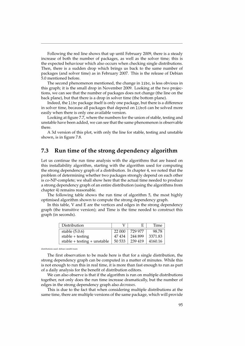
Following the red line shows that up until February 2009, there is a steadyincrease of both the number of packages, as well as the solver time; this isthe expected behaviour which also occurs when checking single distributions.Then, there is a sudden drop which brings us back to the same number ofpackages (and solver time) as in February 2007. This is the release of Debian5.0 mentioned before.
The second phenomenon mentioned, the change in libc, is less obvious inthis graph; it is the small drop in November 2009. Looking at the two projec-tions, we can see that the number of packages does not change (the line on theback plane), but that there is a drop in solver time (the bottom plane).
Indeed, the libc package itself is only one package, but there is a differencein solver time, because all packages that depend on libc6 can be solved moreeasily when there is only one available version.
Looking at figure 7.7, where the numbers for the union of stable, testing andunstable have been added, we can see that the same phenomenon is observablethere.
A 3d version of this plot, with only the line for stable, testing and unstableshown, is in figure 7.8.
7.3 Run time of the strong dependency algorithm
Let us continue the run time analysis with the algorithms that are based onthis installability algorithm, starting with the algorithm used for computingthe strong dependency graph of a distribution. In chapter 4, we noted that theproblem of determining whether two packages strongly depend on each otheris co-NP-complete; we shall show here that the actual time needed to producea strong dependency graph of an entire distribution (using the algorithms fromchapter 4) remains reasonable.
The following table shows the run time of algorithm 5, the most highlyoptimised algorithm shown to compute the strong dependency graph.
In this table, V and E are the vertices and edges in the strong dependencygraph (the transitive version); and Time is the time needed to construct thisgraph (in seconds).
Distribution V E Timestable (5.0.6) 22 000 729 977 98.78stable + testing 47 434 244 899 3371.83stable + testing + unstable 50 533 239 419 4160.16
distributions used: debian/amd64 main
The first observation to be made here is that for a single distribution, thestrong dependency graph can be computed in a matter of minutes. While thisis not enough to run this in real time, it is more than fast enough to run as partof a daily analysis for the benefit of distribution editors.
We can also observe is that if the algorithm is run on multiple distributionstogether, not only does the run time increase dramatically, but the number ofedges in the strong dependency graph also decreases.
This is due to the fact that when considering multiple distributions at thesame time, there are multiple versions of the same package, which will provide
95
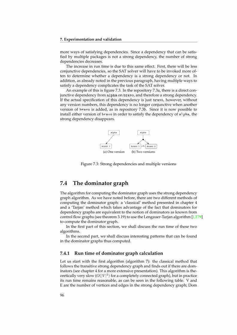
7. Experimentation and validation
more ways of satisfying dependencies. Since a dependency that can be satis-fied by multiple packages is not a strong dependency, the number of strongdependencies decreases.
The increase in run time is due to this same effect. First, there will be lessconjunctive dependencies, so the SAT solver will have to be invoked more of-ten to determine whether a dependency is a strong dependency or not. Inaddition, as already noted in the previous paragraph, having multiple ways tosatisfy a dependency complicates the task of the SAT solver.
An example of this is figure 7.3. In the repository 7.3a, there is a direct con-junctive dependency from alpha on bravo, and therefore a strong dependency.If the actual specification of this dependency is just bravo, however, withoutany version numbers, this dependency is no longer conjunctive when anotherversion of bravo is added, as in repository 7.3b. Since it is now possible toinstall either version of bravo in order to satisfy the dependency of alpha, thestrong dependency disappears.alphabravo 1
(a) One version
alphabravo 1 bravo 2#(b) Two versions
Figure 7.3: Strong dependencies and multiple versions
7.4 The dominator graph
The algorithm for computing the dominator graph uses the strong dependencygraph algorithm. As we have noted before, there are two different methods ofcomputing the dominator graph: a ‘classical’ method presented in chapter 4and a ‘Tarjan’ method which takes advantage of the fact that dominators fordependency graphs are equivalent to the notion of dominators as known fromcontrol flow graphs (see theorem 3.19) to use the Lengauer-Tarjan algorithm [LT79]to compute the dominator graph.
In the first part of this section, we shall discuss the run time of these twoalgorithms.
In the second part, we shall discuss interesting patterns that can be foundin the dominator graphs thus computed.
7.4.1 Run time of dominator graph calculation
Let us start with the first algorithm (algorithm 7): the classical method thatfollows the transitive strong dependency graph and finds out if there are dom-inators (see chapter 4 for a more extensive presentation). This algorithm is the-oretically very slow (O(|V |2) for a completely connected graph), but in practiceits run time remains reasonable, as can be seen in the following table. V andE are the number of vertices and edges in the strong dependency graph; Dom
96
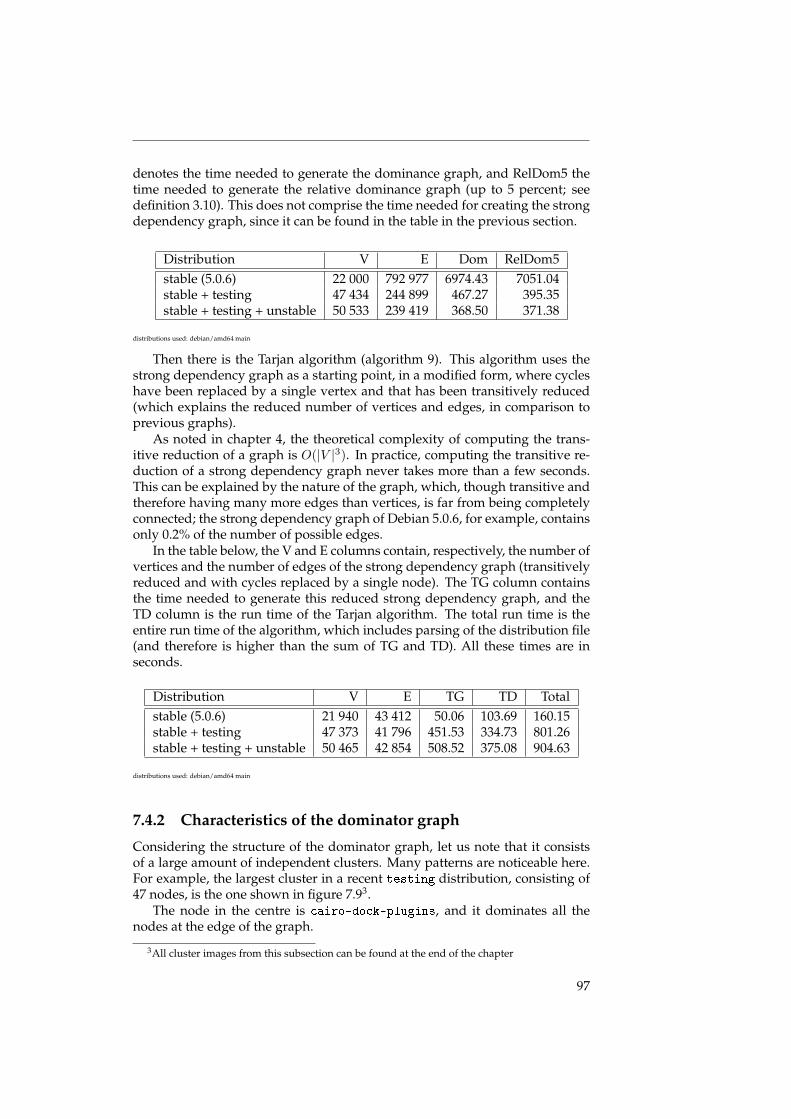
denotes the time needed to generate the dominance graph, and RelDom5 thetime needed to generate the relative dominance graph (up to 5 percent; seedefinition 3.10). This does not comprise the time needed for creating the strongdependency graph, since it can be found in the table in the previous section.
Distribution V E Dom RelDom5stable (5.0.6) 22 000 792 977 6974.43 7051.04stable + testing 47 434 244 899 467.27 395.35stable + testing + unstable 50 533 239 419 368.50 371.38
distributions used: debian/amd64 main
Then there is the Tarjan algorithm (algorithm 9). This algorithm uses thestrong dependency graph as a starting point, in a modified form, where cycleshave been replaced by a single vertex and that has been transitively reduced(which explains the reduced number of vertices and edges, in comparison toprevious graphs).
As noted in chapter 4, the theoretical complexity of computing the trans-itive reduction of a graph is O(|V |3). In practice, computing the transitive re-duction of a strong dependency graph never takes more than a few seconds.This can be explained by the nature of the graph, which, though transitive andtherefore having many more edges than vertices, is far from being completelyconnected; the strong dependency graph of Debian 5.0.6, for example, containsonly 0.2% of the number of possible edges.
In the table below, the V and E columns contain, respectively, the number ofvertices and the number of edges of the strong dependency graph (transitivelyreduced and with cycles replaced by a single node). The TG column containsthe time needed to generate this reduced strong dependency graph, and theTD column is the run time of the Tarjan algorithm. The total run time is theentire run time of the algorithm, which includes parsing of the distribution file(and therefore is higher than the sum of TG and TD). All these times are inseconds.
Distribution V E TG TD Totalstable (5.0.6) 21 940 43 412 50.06 103.69 160.15stable + testing 47 373 41 796 451.53 334.73 801.26stable + testing + unstable 50 465 42 854 508.52 375.08 904.63
distributions used: debian/amd64 main
7.4.2 Characteristics of the dominator graph
Considering the structure of the dominator graph, let us note that it consistsof a large amount of independent clusters. Many patterns are noticeable here.For example, the largest cluster in a recent testing distribution, consisting of47 nodes, is the one shown in figure 7.93.
The node in the centre is cairo-dock-plugins, and it dominates all thenodes at the edge of the graph.
3All cluster images from this subsection can be found at the end of the chapter
97
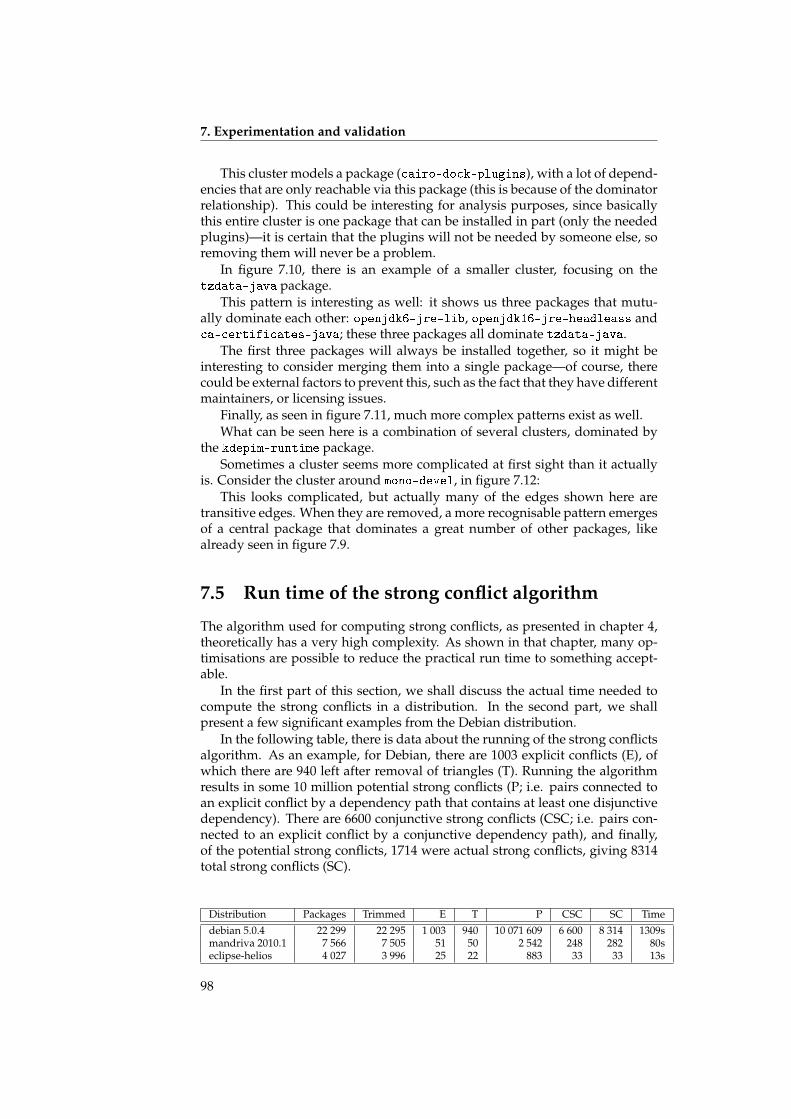
7. Experimentation and validation
This cluster models a package (cairo-dock-plugins), with a lot of depend-encies that are only reachable via this package (this is because of the dominatorrelationship). This could be interesting for analysis purposes, since basicallythis entire cluster is one package that can be installed in part (only the neededplugins)—it is certain that the plugins will not be needed by someone else, soremoving them will never be a problem.
In figure 7.10, there is an example of a smaller cluster, focusing on thetzdata-java package.
This pattern is interesting as well: it shows us three packages that mutu-ally dominate each other: openjdk6-jre-lib, openjdk16-jre-headleass andca-certificates-java; these three packages all dominate tzdata-java.
The first three packages will always be installed together, so it might beinteresting to consider merging them into a single package—of course, therecould be external factors to prevent this, such as the fact that they have differentmaintainers, or licensing issues.
Finally, as seen in figure 7.11, much more complex patterns exist as well.What can be seen here is a combination of several clusters, dominated by
the kdepim-runtime package.Sometimes a cluster seems more complicated at first sight than it actually
is. Consider the cluster around mono-devel, in figure 7.12:This looks complicated, but actually many of the edges shown here are
transitive edges. When they are removed, a more recognisable pattern emergesof a central package that dominates a great number of other packages, likealready seen in figure 7.9.
7.5 Run time of the strong conflict algorithm
The algorithm used for computing strong conflicts, as presented in chapter 4,theoretically has a very high complexity. As shown in that chapter, many op-timisations are possible to reduce the practical run time to something accept-able.
In the first part of this section, we shall discuss the actual time needed tocompute the strong conflicts in a distribution. In the second part, we shallpresent a few significant examples from the Debian distribution.
In the following table, there is data about the running of the strong conflictsalgorithm. As an example, for Debian, there are 1003 explicit conflicts (E), ofwhich there are 940 left after removal of triangles (T). Running the algorithmresults in some 10 million potential strong conflicts (P; i.e. pairs connected toan explicit conflict by a dependency path that contains at least one disjunctivedependency). There are 6600 conjunctive strong conflicts (CSC; i.e. pairs con-nected to an explicit conflict by a conjunctive dependency path), and finally,of the potential strong conflicts, 1714 were actual strong conflicts, giving 8314total strong conflicts (SC).
Distribution Packages Trimmed E T P CSC SC Time
debian 5.0.4 22 299 22 295 1 003 940 10 071 609 6 600 8 314 1309smandriva 2010.1 7 566 7 505 51 50 2 542 248 282 80seclipse-helios 4 027 3 996 25 22 883 33 33 13s
98
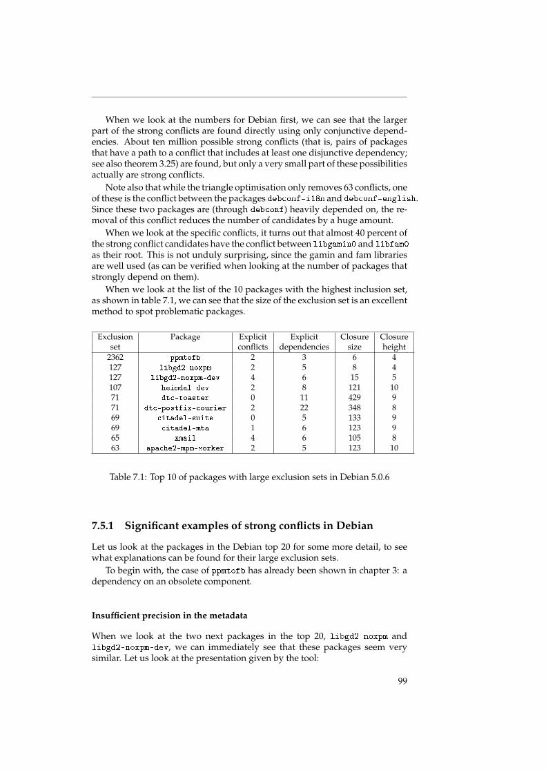
When we look at the numbers for Debian first, we can see that the largerpart of the strong conflicts are found directly using only conjunctive depend-encies. About ten million possible strong conflicts (that is, pairs of packagesthat have a path to a conflict that includes at least one disjunctive dependency;see also theorem 3.25) are found, but only a very small part of these possibilitiesactually are strong conflicts.
Note also that while the triangle optimisation only removes 63 conflicts, oneof these is the conflict between the packages debconf-i18n and debconf-english.Since these two packages are (through debconf) heavily depended on, the re-moval of this conflict reduces the number of candidates by a huge amount.
When we look at the specific conflicts, it turns out that almost 40 percent ofthe strong conflict candidates have the conflict between libgamin0 and libfam0
as their root. This is not unduly surprising, since the gamin and fam librariesare well used (as can be verified when looking at the number of packages thatstrongly depend on them).
When we look at the list of the 10 packages with the highest inclusion set,as shown in table 7.1, we can see that the size of the exclusion set is an excellentmethod to spot problematic packages.
Exclusion Package Explicit Explicit Closure Closureset conflicts dependencies size height
2362 ppmtofb 2 3 6 4127 libgd2-noxpm 2 5 8 4127 libgd2-noxpm-dev 4 6 15 5107 heimdal-dev 2 8 121 1071 dtc-toaster 0 11 429 971 dtc-postfix-courier 2 22 348 869 citadel-suite 0 5 133 969 citadel-mta 1 6 123 965 xmail 4 6 105 863 apache2-mpm-worker 2 5 123 10
Table 7.1: Top 10 of packages with large exclusion sets in Debian 5.0.6
7.5.1 Significant examples of strong conflicts in Debian
Let us look at the packages in the Debian top 20 for some more detail, to seewhat explanations can be found for their large exclusion sets.
To begin with, the case of ppmtofb has already been shown in chapter 3: adependency on an obsolete component.
Insufficient precision in the metadata
When we look at the two next packages in the top 20, libgd2-noxpm andlibgd2-noxpm-dev, we can immediately see that these packages seem verysimilar. Let us look at the presentation given by the tool:
99
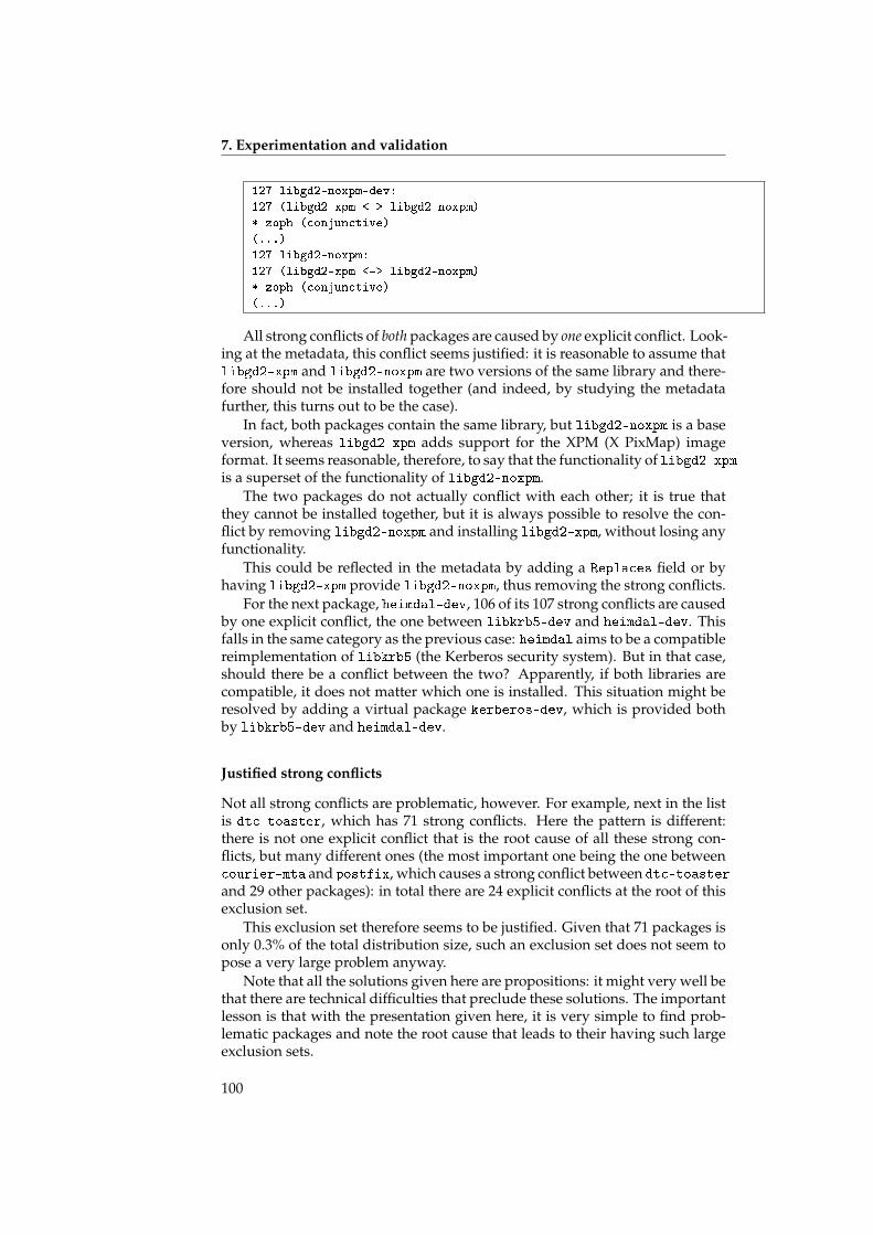
7. Experimentation and validation
127 libgd2-noxpm-dev:
127 (libgd2-xpm <-> libgd2-noxpm)
* zoph (conjunctive)
(...)
127 libgd2-noxpm:
127 (libgd2-xpm <-> libgd2-noxpm)
* zoph (conjunctive)
(...)
All strong conflicts of both packages are caused by one explicit conflict. Look-ing at the metadata, this conflict seems justified: it is reasonable to assume thatlibgd2-xpm and libgd2-noxpm are two versions of the same library and there-fore should not be installed together (and indeed, by studying the metadatafurther, this turns out to be the case).
In fact, both packages contain the same library, but libgd2-noxpm is a baseversion, whereas libgd2-xpm adds support for the XPM (X PixMap) imageformat. It seems reasonable, therefore, to say that the functionality of libgd2-xpmis a superset of the functionality of libgd2-noxpm.
The two packages do not actually conflict with each other; it is true thatthey cannot be installed together, but it is always possible to resolve the con-flict by removing libgd2-noxpm and installing libgd2-xpm, without losing anyfunctionality.
This could be reflected in the metadata by adding a Replaces field or byhaving libgd2-xpm provide libgd2-noxpm, thus removing the strong conflicts.
For the next package, heimdal-dev, 106 of its 107 strong conflicts are causedby one explicit conflict, the one between libkrb5-dev and heimdal-dev. Thisfalls in the same category as the previous case: heimdal aims to be a compatiblereimplementation of libkrb5 (the Kerberos security system). But in that case,should there be a conflict between the two? Apparently, if both libraries arecompatible, it does not matter which one is installed. This situation might beresolved by adding a virtual package kerberos-dev, which is provided bothby libkrb5-dev and heimdal-dev.
Justified strong conflicts
Not all strong conflicts are problematic, however. For example, next in the listis dtc-toaster, which has 71 strong conflicts. Here the pattern is different:there is not one explicit conflict that is the root cause of all these strong con-flicts, but many different ones (the most important one being the one betweencourier-mta and postfix, which causes a strong conflict between dtc-toaster
and 29 other packages): in total there are 24 explicit conflicts at the root of thisexclusion set.
This exclusion set therefore seems to be justified. Given that 71 packages isonly 0.3% of the total distribution size, such an exclusion set does not seem topose a very large problem anyway.
Note that all the solutions given here are propositions: it might very well bethat there are technical difficulties that preclude these solutions. The importantlesson is that with the presentation given here, it is very simple to find prob-lematic packages and note the root cause that leads to their having such largeexclusion sets.
100
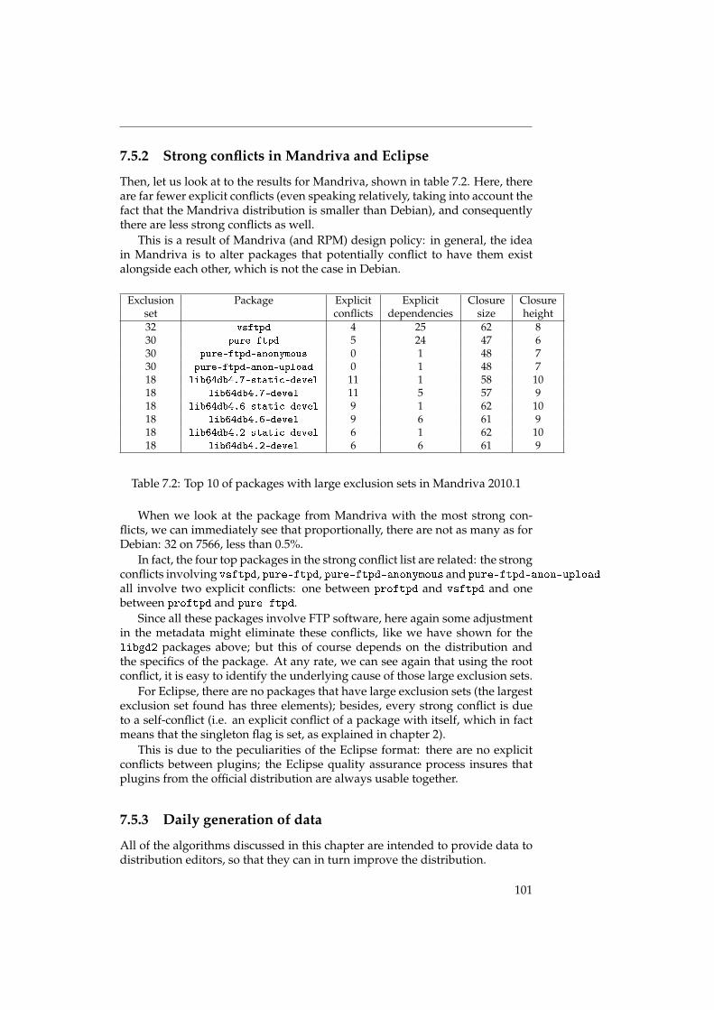
7.5.2 Strong conflicts in Mandriva and Eclipse
Then, let us look at to the results for Mandriva, shown in table 7.2. Here, thereare far fewer explicit conflicts (even speaking relatively, taking into account thefact that the Mandriva distribution is smaller than Debian), and consequentlythere are less strong conflicts as well.
This is a result of Mandriva (and RPM) design policy: in general, the ideain Mandriva is to alter packages that potentially conflict to have them existalongside each other, which is not the case in Debian.
Exclusion Package Explicit Explicit Closure Closureset conflicts dependencies size height32 vsftpd 4 25 62 830 pure-ftpd 5 24 47 630 pure-ftpd-anonymous 0 1 48 730 pure-ftpd-anon-upload 0 1 48 718 lib64db4.7-static-devel 11 1 58 1018 lib64db4.7-devel 11 5 57 918 lib64db4.6-static-devel 9 1 62 1018 lib64db4.6-devel 9 6 61 918 lib64db4.2-static-devel 6 1 62 1018 lib64db4.2-devel 6 6 61 9
Table 7.2: Top 10 of packages with large exclusion sets in Mandriva 2010.1
When we look at the package from Mandriva with the most strong con-flicts, we can immediately see that proportionally, there are not as many as forDebian: 32 on 7566, less than 0.5%.
In fact, the four top packages in the strong conflict list are related: the strongconflicts involving vsftpd, pure-ftpd, pure-ftpd-anonymous and pure-ftpd-anon-upload
all involve two explicit conflicts: one between proftpd and vsftpd and onebetween proftpd and pure-ftpd.
Since all these packages involve FTP software, here again some adjustmentin the metadata might eliminate these conflicts, like we have shown for thelibgd2 packages above; but this of course depends on the distribution andthe specifics of the package. At any rate, we can see again that using the rootconflict, it is easy to identify the underlying cause of those large exclusion sets.
For Eclipse, there are no packages that have large exclusion sets (the largestexclusion set found has three elements); besides, every strong conflict is dueto a self-conflict (i.e. an explicit conflict of a package with itself, which in factmeans that the singleton flag is set, as explained in chapter 2).
This is due to the peculiarities of the Eclipse format: there are no explicitconflicts between plugins; the Eclipse quality assurance process insures thatplugins from the official distribution are always usable together.
7.5.3 Daily generation of data
All of the algorithms discussed in this chapter are intended to provide data todistribution editors, so that they can in turn improve the distribution.
101
7. Experimentation and validation
In order to make this easy, on the MANCOOSI site, we have put a system inplace that generates the dominator graphs of Mandriva and Debian (testingand unstable; not stable, since it does not change every day) on a daily basis.
This daily generation also allows distribution editors to check the evolutionof their distribution over time; data is available from April 2009 onwards.
Since, as noted above, the dominators graph is highly clustered, there alsois a break-down of the graph into its component clusters. This can be usedto monitor changes in dependencies; for example, to check if packages movebetween clusters, if clusters merge or if they disappear. This might be indicat-ive of changes in the distribution.
102
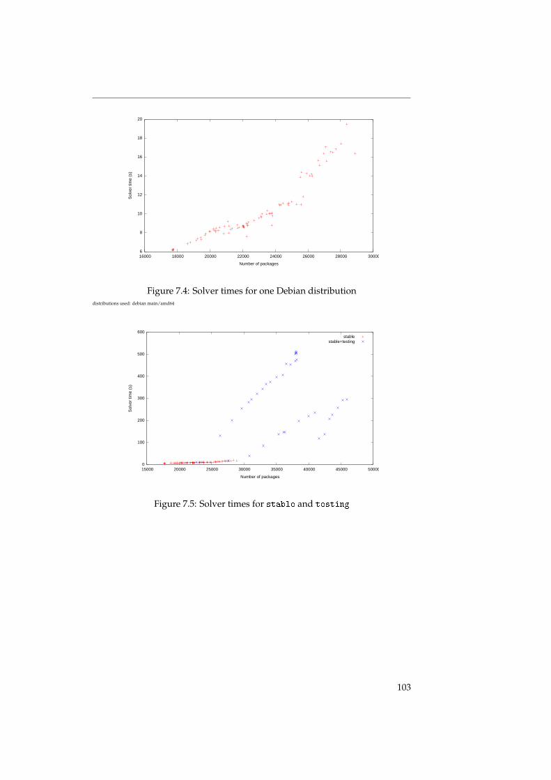
6
8
10
12
14
16
18
20
16000 18000 20000 22000 24000 26000 28000 30000
Solv
er ti
me
(s)
Number of packages
Figure 7.4: Solver times for one Debian distributiondistributions used: debian main/amd64
0
100
200
300
400
500
600
15000 20000 25000 30000 35000 40000 45000 50000
Solv
er ti
me
(s)
Number of packages
stablestable+testing
Figure 7.5: Solver times for stable and testing
103
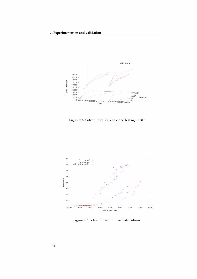
7. Experimentation and validation
01/01/07 01/07/07 01/01/08 01/07/08 01/01/09 01/07/09 01/01/10 01/07/10 0 100
200 300
400 500
600
0 5000
10000 15000 20000 25000 30000 35000 40000 45000 50000
Num
ber o
f pac
kage
s
stable+testing
Date
Solver time
Num
ber o
f pac
kage
s
Figure 7.6: Solver times for stable and testing, in 3D
0
100
200
300
400
500
600
700
800
15000 20000 25000 30000 35000 40000 45000 50000 55000
Solv
er ti
me
(s)
Number of packages
stablestable+testing
stable+testing+unstable
Figure 7.7: Solver times for three distributions
104
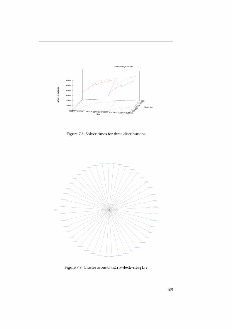
01/01/07 01/07/07 01/01/08 01/07/08 01/01/09 01/07/09 01/01/10 01/07/10 0 100
200 300
400 500
600 700
800
0
10000
20000
30000
40000
50000
60000
Num
ber o
f pac
kage
s
stable+testing+unstable
Date
Solver time
Num
ber o
f pac
kage
s
Figure 7.8: Solver times for three distributions
cairo-dock-alsamixer-plugin
cairo-dock-animated-icons-plugin
cairo-dock-cairo-penguin-plugin
cairo-dock-clipper-plugin
cairo-dock-clock-plugin
cairo-dock-compiz-icon-plugin
cairo-dock-dbus-plugin
cairo-dock-desklet-rendering-plugin
cairo-dock-dialog-rendering-plugin
cairo-dock-dnd2share-plugin
cairo-dock-drop-indicator-plugin
cairo-dock-dustbin-plugin cairo-dock-gmenu-plugin
cairo-dock-gnome-integration-plugin
cairo-dock-icon-effect-plugin
cairo-dock-illusion-plugin
cairo-dock-kde-integration-plugin
cairo-dock-keyboard-indicator-plugin
cairo-dock-logout-plugin
cairo-dock-mail-plugin
cairo-dock-motion-blur-plugin
cairo-dock-musicplayer-plugin
cairo-dock-netspeed-plugin
cairo-dock-network-monitor-plugin
cairo-dock-plugin-data
cairo-dock-plugins0.
0.
0.
0.
0.
0.
0.
0.
0.
0.
0.
0. 0.
0.
0.
0.
0.
0.
0.
0.
0.
0.
0.
0.
0.
cairo-dock-powermanager-plugin
0.
cairo-dock-quick-browser-plugin
0.
cairo-dock-rendering-plugin
0.
cairo-dock-rssreader-plugin
0.
cairo-dock-scooby-do-plugin
0.
cairo-dock-shortcuts-plugin
0.
cairo-dock-showdesktop-plugin
0.
cairo-dock-showmouse-plugin
0.
cairo-dock-slider-plugin
0.
cairo-dock-stack-plugin
0.
cairo-dock-switcher-plugin
0.
cairo-dock-system-monitor-plugin
0.
cairo-dock-systray-plugin
0.
cairo-dock-terminal-plugin
0.
cairo-dock-tomboy-plugin
0.
cairo-dock-toons-plugin
0.
cairo-dock-weather-plugin
0.
cairo-dock-weblets-plugin
0.
cairo-dock-wifi-plugin
0.
cairo-dock-xfce-integration-plugin
0.
cairo-dock-xgamma-plugin
0.
Figure 7.9: Cluster around cairo-dock-plugins
105
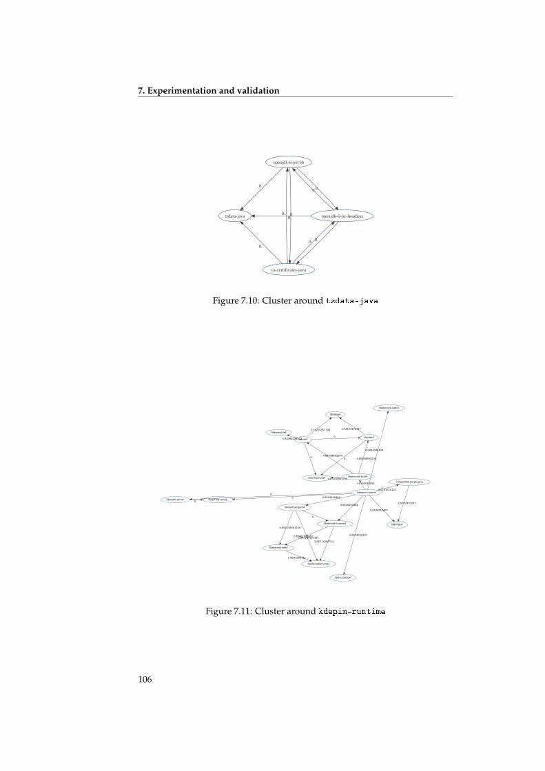
7. Experimentation and validation
ca-certificates-java
openjdk-6-jre-headless
0.
openjdk-6-jre-lib
0.tzdata-java
0.
0.
0.
0. 0.
0.0.
Figure 7.10: Cluster around tzdata-java
akonadi-server libqt4-sql-mysql0.
kdepim-runtime0.
0.
kdepimlibs-kio-plugins
1.0101010101
libakonadi-kabc4
4.0404040404
libakonadi-kcal4
3.0303030303
libakonadi-kmime4
4.0404040404
libkimap4
4.0404040404libmailtransport4
4.0404040404
libmicroblog4
4.0404040404
2.9702970297
libkabc4
4.85436893204
libkcal4
4.85436893204
libkresources4 4.85436893204
libakonadi-kde4
0.952380952381
libakonadiprivate1
2.85714285714
0.
0.961538461538
2.88461538462
0.
libkldap4
2.72727272727
0.
0.
2.75229357798libkpimutils4
1.83486238532
1.8691588785
Figure 7.11: Cluster around kdepim-runtime
106
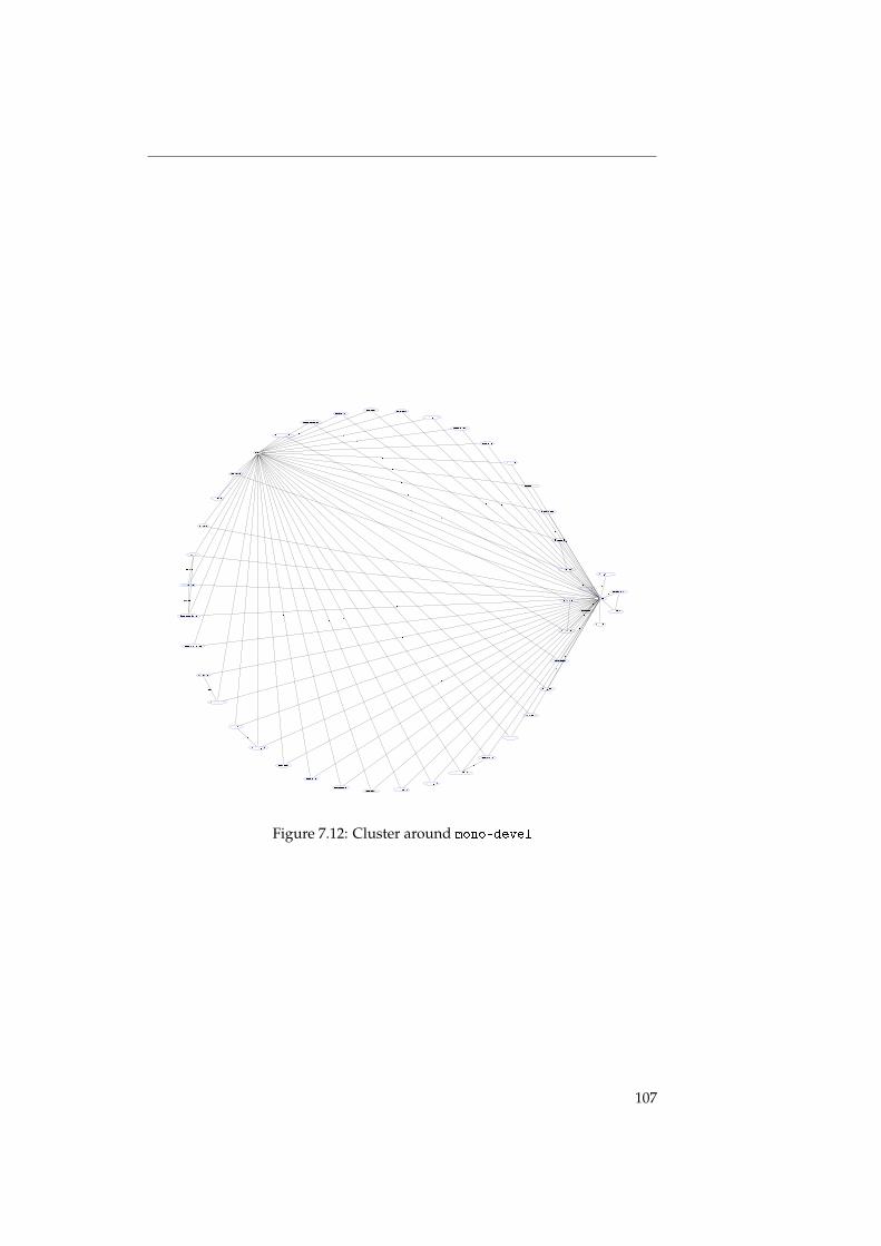
libmono-accessibility1.0-cil
libmono-bytefx0.7.6.1-cil
libmono-bytefx0.7.6.2-cil
libmono-c5-1.0-cil
libmono-cairo1.0-cil
libmono-cil-dev0.
0.
0.
0.
0.
libmono-cscompmgd7.0-cil
0.
libmono-cscompmgd8.0-cil
0.
libmono-data1.0-cil
0.
libmono-data2.0-cil
0.
libmono-db2-1.0-cil
0.
libmono-getoptions1.0-cil
5.
libmono-i18n-west1.0-cil
0.
libmono-i18n-west2.0-cil
5.
libmono-i18n1.0-cil
0.
libmono-i18n2.0-cil
5.
libmono-ldap1.0-cil
0.
libmono-ldap2.0-cil
5.
libmono-messaging-rabbitmq2.0-cil
0.
libmono-messaging2.0-cil
0.
libmono-microsoft7.0-cil
5.
libmono-microsoft8.0-cil
0.
libmono-npgsql1.0-cil
0.
libmono-oracle1.0-cil
0.
libmono-oracle2.0-cil
0.
libmono-peapi1.0-cil
5.
libmono-peapi2.0-cil
5.
libmono-rabbitmq2.0-cil
0.
libmono-relaxng1.0-cil
0.
libmono-relaxng2.0-cil
0.
libmono-sharpzip0.6-cil
0.
libmono-sharpzip2.6-cil
0.
libmono-simd2.0-cil
0.
libmono-sqlite1.0-cil
0.
libmono-system-ldap1.0-cil
0.
libmono-system-ldap2.0-cil
0.
libmono-system-messaging1.0-cil
0.
libmono-system-messaging2.0-cil
0.
libmono-system-runtime1.0-cil
0.
libmono-system-web-mvc1.0-cil
0.
libmono-wcf3.0-cil
0.
libmono-winforms1.0-cil
0.
libmono1.0-cil
5.
libnunit-cil-dev
0.
0.
0.
0.
0.
4.7619047619
4.54545454545
4.7619047619
0.
0.
mono-2.0-devel
5.
mono-devel
0.
0.
0.
0.
0.
0.
0.
0.
0.0.
0.
0.
0.
0.
0.
0.
0.
0.
0.
0.
0.
0.
0.
0.0.
0.
0.
0.
0.
0.
0.
0.
0.
0.
0.
0.
0.
0.
Figure 7.12: Cluster around mono-devel
107
7. Experimentation and validation
108
Graph properties ofdistributions 8
Qualsiasi dato diventa importante se è connesso a un altro. La connessione cambia laprospettiva.
— UMBERTO ECO, Il pendolo di Foucault
The relationships between components can be used to compute relevantquality measures, for example in order to identify particularly fragile compon-ents [DML+04, KAJH99, Liv05]. This chapter is devoted to a discussion of thisidea; more specifically, we shall discuss the properties of distributions whenseen as a graph.
It has been observed that in networks of objects generated by human activ-ity it is often the case that the number of hops needed to reach a vertex fromanother vertex is relatively small. This is called the small world property, firstdescribed by Stanley Milgram in [Mil67] (the famous concept of ‘six degrees ofseparation’), and can be found in the graph of the Internet [CMP00], the graphof the Web [BA99], and many other types of complex networks [AB02]. AsBarabasi says in his founding paper on small world properties, it seems thatthese large networks are ”governed by robust self-organizing phenomena thatgo beyond the particulars of the individual systems”.
It is quite natural to ask the question whether free software distributions,whose properties are being discussed in this thesis, also exhibit such scale-freebehaviour when considered as a graph. This is the question we are going toanswer in this chapter, after recalling the basic notions about the ‘small world’properties of a graph.
8.1 Small world properties
Formally, a network is deemed small-world if it satisfies two properties [WS98]:
1. The clustering coefficient (the chance that two neighbours of a vertex areconnected) is significantly higher than that of random networks.
2. On average, the path length between two vertices is low (on the sameorder as that of random networks);
Let us start with a more formal definition of these two concepts, the clus-tering coefficient and the path length. Assume that there is a directed graph G,with V the set of its vertices and E ⊆ V × V the set of its edges (if (p, q) ∈ E,then there is an edge from p to q).
109
8. Graph properties of distributions
Definition 8.1 (Clustering coefficent)Given a vertex v, the clustering coefficient cc(v) is defined as:
cc(v) =
0, if succ(v) = ∅1, if succ(v) = {p} for some p|{(p,p′)∈E|p,p′∈succ(v)∧p 6=p′}|
12∗|succ(v)|∗(|succ(v)|−1)
otherwise
The clustering coefficient cc(G) of a graph G is the average clustering coeffi-cient of all of its vertices.
Then the average path length. First, the path length P (v, v′) is defined asthe length of the shortest path between v and v′; if v and v′ are not connected,then P (v, v′) =∞.
Definition 8.2 (Average path length)The average path length apl(v) of a vertex v is defined as:
apl(v) =
{0, if succ(v) = ∅∑{P (v,v′)|P (v,v′)6=∞}|{P (v,v′)|P (v,v′)6=∞}| , otherwise
Again, the average path length apl(G) of a graph G is the average of the aver-age path lengths of all of its vertices.
In a small world network, these two properties result in a network thatconsists of many clusters (or near-clusters), whose central nodes are connected.This makes for the short average path lengths mentioned above.
These hubs can be recognised by looking at the degrees of the differentnodes in the graph. There are a few hubs—nodes that have many connections—and many nodes that have very few connections; thus, the degree distributionconforms to the well-known Pareto principle, also known as the 80/20-law.
When looking at a plot of the degrees of a Debian stable distribution graph,as presented in figure 8.1, this pattern can be recognised. In this graph, the de-gree is presented on the Y axis, and the number of nodes that has this particulardegree is presented on the X axis. We can see easily that there are many nodeswith a low degree, and few nodes with a high degree.
This particular structure makes such a graph very resistant to random at-tacks [AJB00]; if a random node is removed, the chance is very small that theaverage path length will increase: the only way the path length can be in-creased for many nodes is by removing a hub node, and as shown above, thereare few of these.
By the same argument, however, a small world graph is very vulnerableto directed attacks: by deleting only a few specific nodes (the hub nodes), theentire network can be paralysed.
110
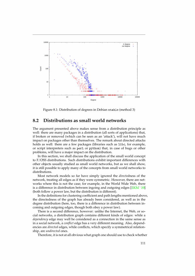
1
10
100
1000
10000
1 10 100 1000 10000 100000
Cou
nt
Degree
in degreeout degree
Figure 8.1: Distribution of degrees in Debian stable (method 3)
8.2 Distributions as small world networks
The argument presented above makes sense from a distribution principle aswell: there are many packages in a distribution (all sorts of applications) that,if broken or removed (which can be seen as an ‘attack’), will not have muchimpact on packages other than themselves. The remark about directed attacksholds as well: there are a few packages (libraries such as libc, for example,or script interpreters such as perl or python) that, in case of bugs or otherproblems, will have a major impact on the distribution.
In this section, we shall discuss the application of the small world conceptto F/OSS distributions. Such distributions exhibit important differences withother objects usually studied as small world networks, but as we shall show,it is still possible to apply many of the concepts from small world networks todistributions.
Most network models so far have simply ignored the directedness of thenetwork, treating all edges as if they were symmetric. However, there are net-works where this is not the case; for example, in the World Wide Web, thereis a difference in distribution between ingoing and outgoing edges [BKM+00](both follow a power law, but the distribution is different).
In the definitions for clustering coefficient and path lengths mentioned above,the directedness of the graph has already been considered, as well as in thedegree distribution (here, too, there is a difference in distribution between in-coming and outgoing edges, though both obey a power law).
There is a second difference, however: unlike the Internet, the Web, or so-cial networks, a distribution graph contains different kinds of edges: while adependency edge may well be considered as a connection in the same sense asin a social network, a conflict edge has a very different meaning. Also, depend-encies are directed edges, while conflicts, which specify a symmetrical relation-ship, are undirected ones.
Therefore, it is not at all obvious what graph one should use to check whether
111
8. Graph properties of distributions
the small world properties apply. At least three main possibilities for graphgeneration methods can be identified:
1. Treat all edges equally, irrespective of their significance (dependency, re-commendation, conflict, . . . ). More formally, there is an edge betweenpackages p and q if and only if q is mentioned in one of the relationshipsof p (notice that this notion totally misrepresents the semantics of a con-flict, which is symmetric)
2. Use the dependency closure; there is an edge between p and q if and onlyif q is a member of ∆(p). This creates an edge between p and all possibledependencies of p.
3. Use strong dependencies: there is an edge between p and q if and only ifp⇒ q1.
All these possibilities have different properties. If the idea is for an edgefrom p to q to represent the fact that q is needed to install p, then using thedependency closure will result in an over-estimation (not every package in thedependency closure is installed every time, but packages that are not in thedependency closure are guaranteed not to be needed), whereas using strongdependencies will result in an under-estimation—a strong dependency is guar-anteed to be installed, but usually other packages will be installed as well tosatisfy alternative dependencies.
There has been some prior research on the scale-free behaviour of Debiannetworks; in [LW04], it is claimed that Debian distributions show small-worldcharacteristics.
It is difficult, however, to attach conclusions to this claim, because the meth-odology used is not discussed in any detail. The numbers shown in the papersuggests that the authors have added an edge between two packages if therewas a dependency (conjunctive or disjunctive) between two packages, whichis akin to our method 1.
The problem with this approach is that such a relationship can mean verydifferent things. First, that a package depends on another does not necessarilymean that this other package is actually going to be installed; if the dependencyis disjunctive, another package might be chosen to satisfy the dependency. Andsecond, a package can be installed even if it is not linked by a direct depend-ency: see chapter 3 on strong dependencies for more information on this.
Another paper [NNR09], also claims to have found small-world character-istics in the different stable Debian distributions.
Again, it is not clear which methodology has been used, but the numberssuggest that for the dependency relationships, the same approach in graphgeneration has been used as in [LW04].
There are two differences in approach between the two papers, though:in [NNR09], a distinction is made between the graph of dependency relation-ships and the graph of conflict relationships; and the directedness of the graphis taken into account insofar as the in and out degrees are treated separately.
1This is the method used to create the degree distribution graphs presented in the previoussection.
112
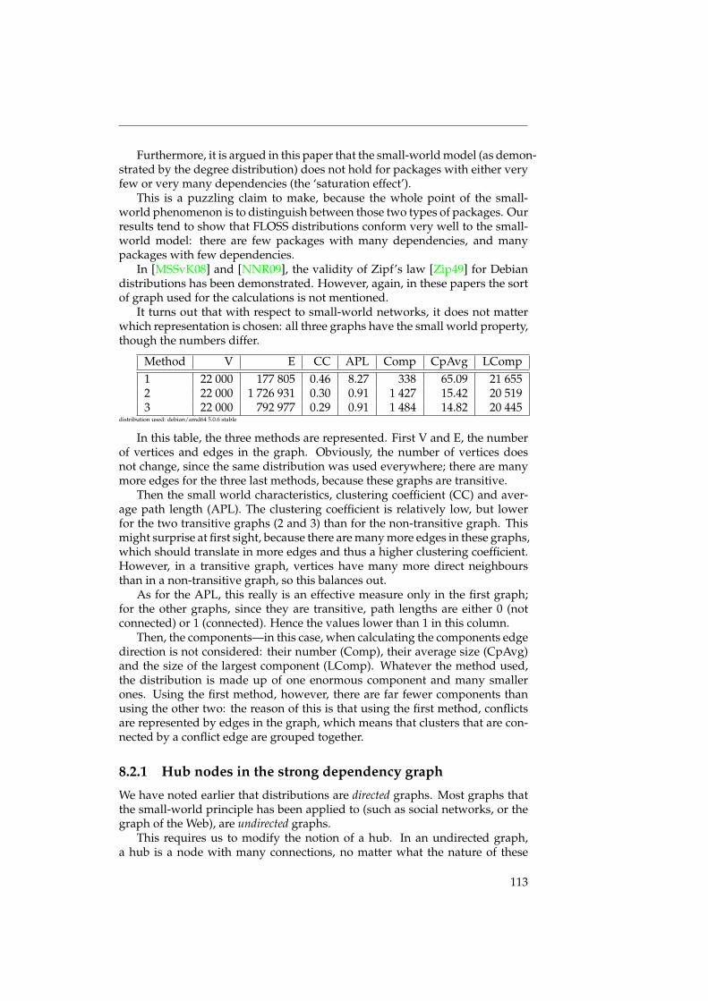
Furthermore, it is argued in this paper that the small-world model (as demon-strated by the degree distribution) does not hold for packages with either veryfew or very many dependencies (the ‘saturation effect’).
This is a puzzling claim to make, because the whole point of the small-world phenomenon is to distinguish between those two types of packages. Ourresults tend to show that FLOSS distributions conform very well to the small-world model: there are few packages with many dependencies, and manypackages with few dependencies.
In [MSSvK08] and [NNR09], the validity of Zipf’s law [Zip49] for Debiandistributions has been demonstrated. However, again, in these papers the sortof graph used for the calculations is not mentioned.
It turns out that with respect to small-world networks, it does not matterwhich representation is chosen: all three graphs have the small world property,though the numbers differ.
Method V E CC APL Comp CpAvg LComp1 22 000 177 805 0.46 8.27 338 65.09 21 6552 22 000 1 726 931 0.30 0.91 1 427 15.42 20 5193 22 000 792 977 0.29 0.91 1 484 14.82 20 445
distribution used: debian/amd64 5.0.6 stable
In this table, the three methods are represented. First V and E, the numberof vertices and edges in the graph. Obviously, the number of vertices doesnot change, since the same distribution was used everywhere; there are manymore edges for the three last methods, because these graphs are transitive.
Then the small world characteristics, clustering coefficient (CC) and aver-age path length (APL). The clustering coefficient is relatively low, but lowerfor the two transitive graphs (2 and 3) than for the non-transitive graph. Thismight surprise at first sight, because there are many more edges in these graphs,which should translate in more edges and thus a higher clustering coefficient.However, in a transitive graph, vertices have many more direct neighboursthan in a non-transitive graph, so this balances out.
As for the APL, this really is an effective measure only in the first graph;for the other graphs, since they are transitive, path lengths are either 0 (notconnected) or 1 (connected). Hence the values lower than 1 in this column.
Then, the components—in this case, when calculating the components edgedirection is not considered: their number (Comp), their average size (CpAvg)and the size of the largest component (LComp). Whatever the method used,the distribution is made up of one enormous component and many smallerones. Using the first method, however, there are far fewer components thanusing the other two: the reason of this is that using the first method, conflictsare represented by edges in the graph, which means that clusters that are con-nected by a conflict edge are grouped together.
8.2.1 Hub nodes in the strong dependency graph
We have noted earlier that distributions are directed graphs. Most graphs thatthe small-world principle has been applied to (such as social networks, or thegraph of the Web), are undirected graphs.
This requires us to modify the notion of a hub. In an undirected graph,a hub is a node with many connections, no matter what the nature of these
113
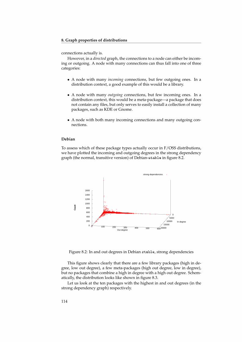
8. Graph properties of distributions
connections actually is.However, in a directed graph, the connections to a node can either be incom-
ing or outgoing. A node with many connections can thus fall into one of threecategories:
• A node with many incoming connections, but few outgoing ones. In adistribution context, a good example of this would be a library.
• A node with many outgoing connections, but few incoming ones. In adistribution context, this would be a meta-package—a package that doesnot contain any files, but only serves to easily install a collection of manypackages, such as KDE or Gnome.
• A node with both many incoming connections and many outgoing con-nections.
Debian
To assess which of these package types actually occur in F/OSS distributions,we have plotted the incoming and outgoing degrees in the strong dependencygraph (the normal, transitive version) of Debian-stable in figure 8.2.
0 100 200 300 400 500 600
0 5000
10000 15000
20000 0
200
400
600
800
1000
1200
1400
1600
Cou
nt
strong dependencies
Out degree
In degree
Cou
nt
Figure 8.2: In and out degrees in Debian stable, strong dependencies
This figure shows clearly that there are a few library packages (high in de-gree, low out degree), a few meta-packages (high out degree, low in degree),but no packages that combine a high in degree with a high out degree. Schem-atically, the distribution looks like shown in figure 8.3.
Let us look at the ten packages with the highest in and out degrees (in thestrong dependency graph) respectively.
114
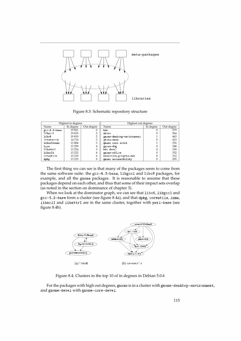
meta-packageslibrariesFigure 8.3: Schematic repository structure
Highest in degrees Highest out degreesName In degree Out degree Name In degree Out degreegcc-4.3-base 19 821 0 kde 0 579libgcc1 19 819 2 gnome 0 564libc6 19 819 2 gnome-desktop-environment 1 463libstdc++6 14 710 3 gnome-devel 0 415libselinux1 13 884 3 gnome-core-devel 1 376lzma 13 299 4 gnome-dbg 0 348libattr1 13 254 3 kde-devel 0 339libacl1 13 232 4 gnome-office 0 332coreutils 13 219 6 audacious-plugins-dev 0 312dpkg 13 215 9 gnome-accessibility 0 295
The first thing we can see is that many of the packages seem to come fromthe same software suite: the gcc-4.3-base, libgcc1 and libc6 packages, forexample, and all the gnome packages. It is reasonable to assume that thesepackages depend on each other, and thus that some of their impact sets overlap(as noted in the section on dominance of chapter 3).
When we look at the dominator graph, we can see that libc6, libgcc1 andgcc-4.3-base form a cluster (see figure 8.4a), and that dpkg, coreutils, lzma,libacl1 and libattr1 are in the same cluster, together with perl-base (seefigure 8.4b).
libc6 (= 2.7-18lenny4)
gcc-4.3-base (= 4.3.2-1.1)
libgcc1 (= 1:4.3.2-1.1)
(a) libc6
coreutils (= 6.10-6)
libacl1 (= 2.2.47-2)
libattr1 (= 1:2.4.43-2)
dpkg (= 1.14.29)
lzma (= 4.43-14)
perl-base (= 5.10.0-19lenny2)
(b) coreutils
Figure 8.4: Clusters in the top 10 of in degrees in Debian 5.0.6
For the packages with high out degrees, gnome is in a cluster with gnome-desktop-environment,and gnome-devel with gnome-core-devel.
115
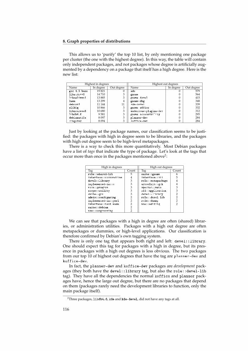
8. Graph properties of distributions
This allows us to ‘purify’ the top 10 list, by only mentioning one packageper cluster (the one with the highest degree). In this way, the table will containonly independent packages, and not packages whose degree is artificially aug-mented by a dependency on a package that itself has a high degree. Here is thenew list:
Highest in degrees Highest out degreesName In degree Out degree Name In degree Out degreegcc-4.3-base 19 821 0 kde 0 579libstdc++6 14 710 3 gnome 0 564libselinux1 13 885 3 gnome-devel 0 415lzma 13 299 4 gnome-dbg 0 348debconf 11 144 11 kde-devel 0 339zlib1g 10 866 3 gnome-office 0 332libncurses5 10 680 3 audacious-plugins-dev 0 312libdb4.6 9 581 3 gnome-accessibility 0 295debianutils 8 097 3 planner-dev 0 284libgdbm3 8 094 3 koffice-dev 0 284
Just by looking at the package names, our classification seems to be justi-fied: the packages with high in degree seem to be libraries, and the packageswith high out degree seem to be high-level metapackages.
There is a way to check this more quantitatively. Most Debian packageshave a list of tags that indicate the type of package. Let’s look at the tags thatoccur more than once in the packages mentioned above2:
High in degrees High out degreesTag Count Tag Countrole::shared-lib 5 suite::gnome 6interface::commandline 4 interface::x11 5devel::library 3 role::metapackage 4implemented-in::c 3 uitoolkit::gtk 4role::program 3 special::meta 3scope::utility 3 x11::application 3suite::gnu 3 devel::library 2admin::configuring 2 role::devel-lib 2implemented-in::perl 2 role::dummy 2interface::text-mode 2 use::editing 2suite::debian 2use::compressing 2
We can see that packages with a high in degree are often (shared) librar-ies, or administration utilities. Packages with a high out degree are oftenmetapackages or dummies, or high-level applications. Our classification istherefore confirmed by Debian’s own tagging system.
There is only one tag that appears both right and left: devel::library.One should expect this tag for packages with a high in degree, but its pres-ence in packages with a high out degrees is less obvious. The two packagesfrom our top 10 of highest out degrees that have the tag are planner-dev andkoffice-dev.
In fact, the planner-dev and koffice-dev packages are development pack-ages (they both have the devel::library tag, but also the role::devel-lib
tag). They have all the dependencies the normal koffice and planner pack-ages have, hence the large out degree, but there are no packages that dependon them (packages rarely need the development libraries to function, only themain package itself).
2Three packages, libdb4.6, kde and kde-devel, did not have any tags at all.
116
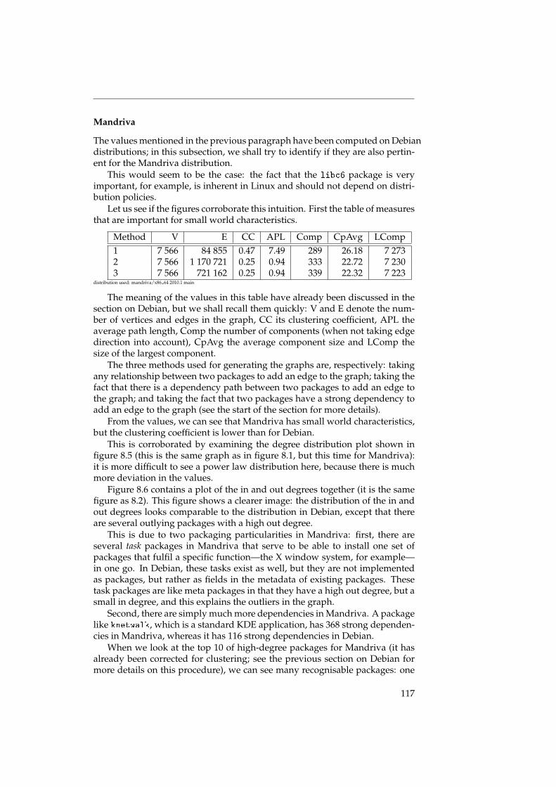
Mandriva
The values mentioned in the previous paragraph have been computed on Debiandistributions; in this subsection, we shall try to identify if they are also pertin-ent for the Mandriva distribution.
This would seem to be the case: the fact that the libc6 package is veryimportant, for example, is inherent in Linux and should not depend on distri-bution policies.
Let us see if the figures corroborate this intuition. First the table of measuresthat are important for small world characteristics.
Method V E CC APL Comp CpAvg LComp1 7 566 84 855 0.47 7.49 289 26.18 7 2732 7 566 1 170 721 0.25 0.94 333 22.72 7 2303 7 566 721 162 0.25 0.94 339 22.32 7 223
distribution used: mandriva/x86 64 2010.1 main
The meaning of the values in this table have already been discussed in thesection on Debian, but we shall recall them quickly: V and E denote the num-ber of vertices and edges in the graph, CC its clustering coefficient, APL theaverage path length, Comp the number of components (when not taking edgedirection into account), CpAvg the average component size and LComp thesize of the largest component.
The three methods used for generating the graphs are, respectively: takingany relationship between two packages to add an edge to the graph; taking thefact that there is a dependency path between two packages to add an edge tothe graph; and taking the fact that two packages have a strong dependency toadd an edge to the graph (see the start of the section for more details).
From the values, we can see that Mandriva has small world characteristics,but the clustering coefficient is lower than for Debian.
This is corroborated by examining the degree distribution plot shown infigure 8.5 (this is the same graph as in figure 8.1, but this time for Mandriva):it is more difficult to see a power law distribution here, because there is muchmore deviation in the values.
Figure 8.6 contains a plot of the in and out degrees together (it is the samefigure as 8.2). This figure shows a clearer image: the distribution of the in andout degrees looks comparable to the distribution in Debian, except that thereare several outlying packages with a high out degree.
This is due to two packaging particularities in Mandriva: first, there areseveral task packages in Mandriva that serve to be able to install one set ofpackages that fulfil a specific function—the X window system, for example—in one go. In Debian, these tasks exist as well, but they are not implementedas packages, but rather as fields in the metadata of existing packages. Thesetask packages are like meta packages in that they have a high out degree, but asmall in degree, and this explains the outliers in the graph.
Second, there are simply much more dependencies in Mandriva. A packagelike knetwalk, which is a standard KDE application, has 368 strong dependen-cies in Mandriva, whereas it has 116 strong dependencies in Debian.
When we look at the top 10 of high-degree packages for Mandriva (it hasalready been corrected for clustering; see the previous section on Debian formore details on this procedure), we can see many recognisable packages: one
117
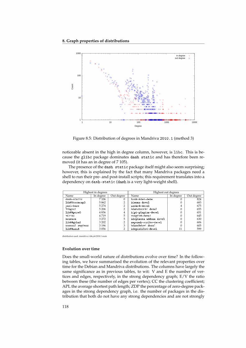
8. Graph properties of distributions
1
10
100
1000
1 10 100 1000 10000
Cou
nt
Degree
in degreeout degree
Figure 8.5: Distribution of degrees in Mandriva 2010.1 (method 3)
noticeable absent in the high in degree column, however, is libc. This is be-cause the glibc package dominates dash-static and has therefore been re-moved (it has an in degree of 7 105).
The presence of the dash-static package itself might also seem surprising;however, this is explained by the fact that many Mandriva packages need ashell to run their pre- and post-install scripts; this requirement translates into adependency on dash-static (dash is a very light-weight shell).
Highest in degrees Highest out degreesName In degree Out degree Name In degree Out degreedash-static 7 106 0 task-kde4-devel 0 824lib64termcap2 5 862 2 kimono-devel 0 683perl-base 5 274 2 smoke4-devel 4 675libgcc1 5 206 2 kdenetwork4-devel 0 655lib64pcre0 4 836 4 kipi-plugins-devel 0 651uClibc 4 719 5 kdepim4-devel 0 645ncurses 3 272 5 kdeplasma-addons-devel 0 630lib64gdbm3 3 202 2 nepomuk-scribo-devel 0 606openssl-engines 3 196 3 kdewebdev4-devel 0 605lib64xau6 3 056 2 kdepimlibs4-devel 11 599
distribution used: mandriva/x86 64 2010.1 main
Evolution over time
Does the small-world nature of distributions evolve over time? In the follow-ing tables, we have summarised the evolution of the relevant properties overtime for the Debian and Mandriva distributions. The columns have largely thesame significance as in previous tables, to wit: V and E the number of ver-tices and edges, respectively, in the strong dependency graph; E/V the ratiobetween these (the number of edges per vertex); CC the clustering coefficient;APL the average shortest path length; ZDP the percentage of zero-degree pack-ages in the strong dependency graph, i.e. the number of packages in the dis-tribution that both do not have any strong dependencies and are not strongly
118
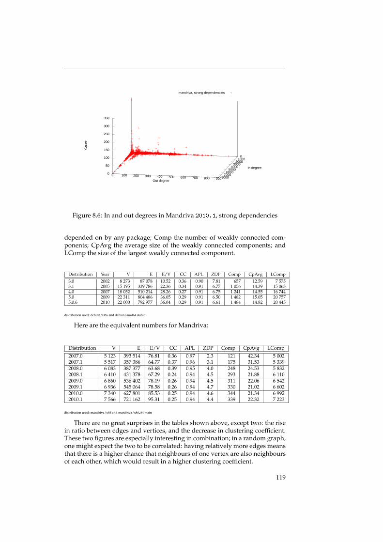
0 100 200 300 400 500 600 700 800 900
0 1000
2000 3000
4000 5000
6000 7000
8000 0
50
100
150
200
250
300
350
Cou
nt
mandriva, strong dependencies
Out degree
In degree
Cou
nt
Figure 8.6: In and out degrees in Mandriva 2010.1, strong dependencies
depended on by any package; Comp the number of weakly connected com-ponents; CpAvg the average size of the weakly connected components; andLComp the size of the largest weakly connected component.
Distribution Year V E E/V CC APL ZDP Comp CpAvg LComp
3.0 2002 8 273 87 078 10.52 0.36 0.90 7.81 657 12.59 7 5753.1 2005 15 195 339 786 22.36 0.34 0.91 6.77 1 056 14.39 15 0634.0 2007 18 052 510 214 28.26 0.27 0.91 6.75 1 241 14.55 16 7445.0 2009 22 311 804 486 36.05 0.29 0.91 6.50 1 482 15.05 20 7575.0.6 2010 22 000 792 977 36.04 0.29 0.91 6.61 1 484 14.82 20 445
distribution used: debian/i386 and debian/amd64 stable
Here are the equivalent numbers for Mandriva:
Distribution V E E/V CC APL ZDP Comp CpAvg LComp
2007.0 5 123 393 514 76.81 0.36 0.97 2.3 121 42.34 5 0022007.1 5 517 357 386 64.77 0.37 0.96 3.1 175 31.53 5 3392008.0 6 083 387 377 63.68 0.39 0.95 4.0 248 24.53 5 8322008.1 6 410 431 378 67.29 0.24 0.94 4.5 293 21.88 6 1102009.0 6 860 536 402 78.19 0.26 0.94 4.5 311 22.06 6 5422009.1 6 936 545 064 78.58 0.26 0.94 4.7 330 21.02 6 6022010.0 7 340 627 801 85.53 0.25 0.94 4.6 344 21.34 6 9922010.1 7 566 721 162 95.31 0.25 0.94 4.4 339 22.32 7 223
distribution used: mandriva/x86 and mandriva/x86 64 main
There are no great surprises in the tables shown above, except two: the risein ratio between edges and vertices, and the decrease in clustering coefficient.These two figures are especially interesting in combination; in a random graph,one might expect the two to be correlated: having relatively more edges meansthat there is a higher chance that neighbours of one vertex are also neighboursof each other, which would result in a higher clustering coefficient.
119
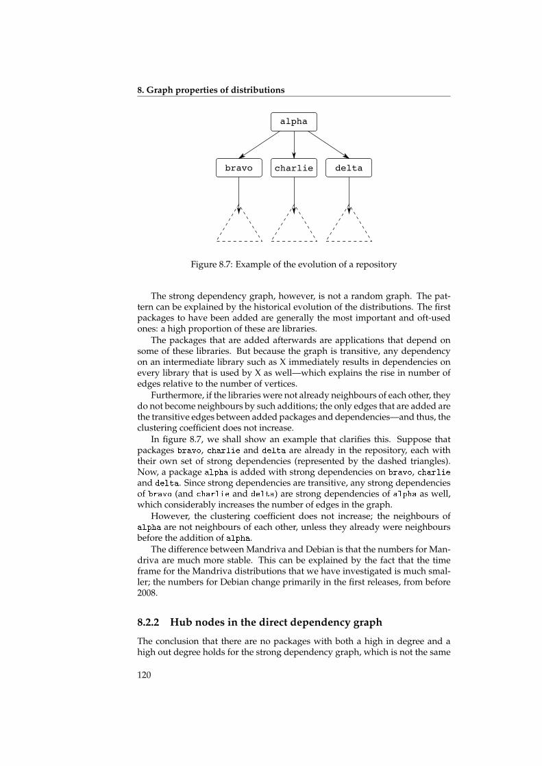
8. Graph properties of distributionsalphabravo charlie deltaFigure 8.7: Example of the evolution of a repository
The strong dependency graph, however, is not a random graph. The pat-tern can be explained by the historical evolution of the distributions. The firstpackages to have been added are generally the most important and oft-usedones: a high proportion of these are libraries.
The packages that are added afterwards are applications that depend onsome of these libraries. But because the graph is transitive, any dependencyon an intermediate library such as X immediately results in dependencies onevery library that is used by X as well—which explains the rise in number ofedges relative to the number of vertices.
Furthermore, if the libraries were not already neighbours of each other, theydo not become neighbours by such additions; the only edges that are added arethe transitive edges between added packages and dependencies—and thus, theclustering coefficient does not increase.
In figure 8.7, we shall show an example that clarifies this. Suppose thatpackages bravo, charlie and delta are already in the repository, each withtheir own set of strong dependencies (represented by the dashed triangles).Now, a package alpha is added with strong dependencies on bravo, charlieand delta. Since strong dependencies are transitive, any strong dependenciesof bravo (and charlie and delta) are strong dependencies of alpha as well,which considerably increases the number of edges in the graph.
However, the clustering coefficient does not increase; the neighbours ofalpha are not neighbours of each other, unless they already were neighboursbefore the addition of alpha.
The difference between Mandriva and Debian is that the numbers for Man-driva are much more stable. This can be explained by the fact that the timeframe for the Mandriva distributions that we have investigated is much smal-ler; the numbers for Debian change primarily in the first releases, from before2008.
8.2.2 Hub nodes in the direct dependency graph
The conclusion that there are no packages with both a high in degree and ahigh out degree holds for the strong dependency graph, which is not the same
120
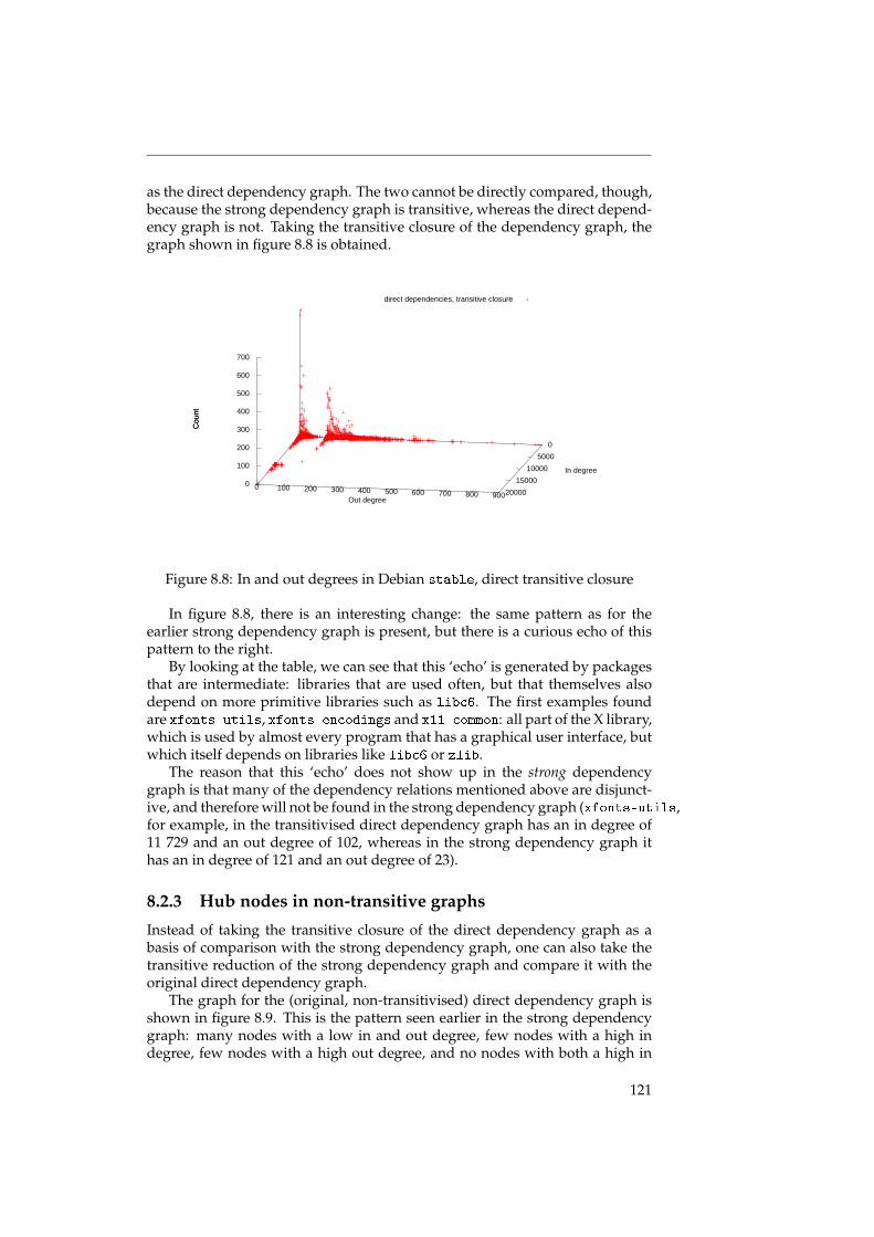
as the direct dependency graph. The two cannot be directly compared, though,because the strong dependency graph is transitive, whereas the direct depend-ency graph is not. Taking the transitive closure of the dependency graph, thegraph shown in figure 8.8 is obtained.
0 100 200 300 400 500 600 700 800 900
0 5000
10000 15000
20000 0
100
200
300
400
500
600
700
Cou
nt
direct dependencies, transitive closure
Out degree
In degree
Cou
nt
Figure 8.8: In and out degrees in Debian stable, direct transitive closure
In figure 8.8, there is an interesting change: the same pattern as for theearlier strong dependency graph is present, but there is a curious echo of thispattern to the right.
By looking at the table, we can see that this ‘echo’ is generated by packagesthat are intermediate: libraries that are used often, but that themselves alsodepend on more primitive libraries such as libc6. The first examples foundare xfonts-utils, xfonts-encodings and x11-common: all part of the X library,which is used by almost every program that has a graphical user interface, butwhich itself depends on libraries like libc6 or zlib.
The reason that this ‘echo’ does not show up in the strong dependencygraph is that many of the dependency relations mentioned above are disjunct-ive, and therefore will not be found in the strong dependency graph (xfonts-utils,for example, in the transitivised direct dependency graph has an in degree of11 729 and an out degree of 102, whereas in the strong dependency graph ithas an in degree of 121 and an out degree of 23).
8.2.3 Hub nodes in non-transitive graphs
Instead of taking the transitive closure of the direct dependency graph as abasis of comparison with the strong dependency graph, one can also take thetransitive reduction of the strong dependency graph and compare it with theoriginal direct dependency graph.
The graph for the (original, non-transitivised) direct dependency graph isshown in figure 8.9. This is the pattern seen earlier in the strong dependencygraph: many nodes with a low in and out degree, few nodes with a high indegree, few nodes with a high out degree, and no nodes with both a high in
121
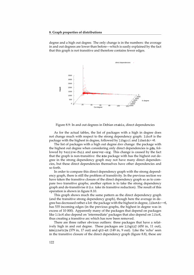
8. Graph properties of distributions
degree and a high out degree. The only change is in the numbers: the averagein and out degrees are lower than before—which is easily explained by the factthat this graph is not transitive and therefore contains fewer edges.
0 20 40 60 80 100 120
0 2000
4000 6000
8000 10000
12000 0
500
1000
1500
2000
2500
3000
3500
Cou
ntdirect dependencies
Out degree
In degree
Cou
nt
Figure 8.9: In and out degrees in Debian stable, direct dependencies
As for the actual tables, the list of packages with a high in degree doesnot change much with respect to the strong dependency graph: libc6 is thepackage with the highest in degree, followed by libgcc1 and libstdc++6.
The list of packages with a high out degree does change: the package withthe highest out degree when considering only direct dependencies is gdm, fol-lowed by texlive-full and xserver-org. This change is caused by the factthat the graph is non-transitive: the kde package with has the highest out de-gree in the strong dependency graph may not have many direct dependen-cies, but these direct dependencies themselves have other dependencies andso forth.
In order to compare this direct dependency graph with the strong depend-ency graph, there is still the problem of transitivity. In the previous section wehave taken the transitive closure of the direct dependency graph so as to com-pare two transitive graphs; another option is to take the strong dependencygraph and de-transitivise it (i.e. take its transitive reduction). The result of thisoperation is shown in figure 8.10.
This graph shows much the same pattern as the direct dependency graph(and the transitive strong dependency graph), though here the average in de-gree has decreased rather a lot: the package with the highest in degree, libstdc++6,has 535 incoming edges (in the previous graphs, the highest in degree was inexcess of 10 000). Apparently many of the packages that depend on packageslike libc6 also depend on ‘intermediate’ packages that also depend on libc6,thus creating a transitive arc which has now been removed.
There are three rather obvious outliers: three packages that have a relat-ively high in and out degree. These packages are libgtk2 (450 in, 11 out),kdelibs4c2a (379 in, 17 out) and qt3-mt (149 in, 9 out). Like the ‘echo’ seenin the transitive closure of the direct dependency graph (figure 8.8), these are
122
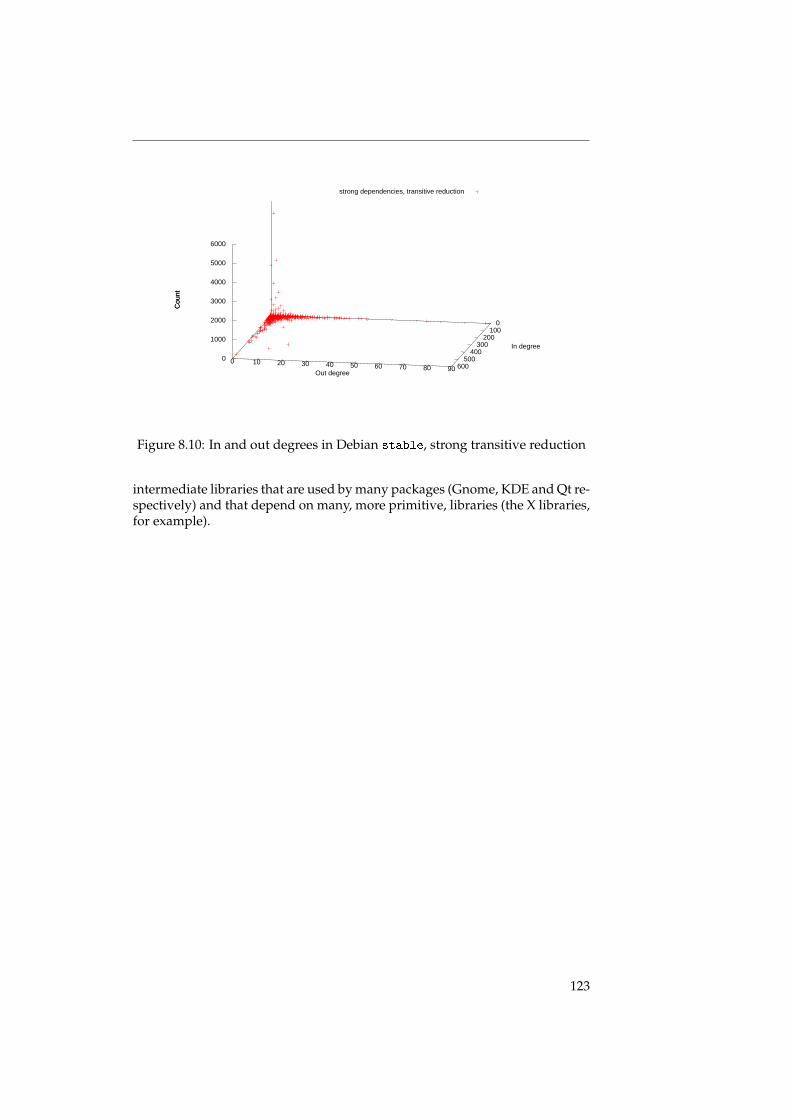
0 10 20 30 40 50 60 70 80 90
0 100
200 300
400 500
600 0
1000
2000
3000
4000
5000
6000
Cou
nt
strong dependencies, transitive reduction
Out degree
In degree
Cou
nt
Figure 8.10: In and out degrees in Debian stable, strong transitive reduction
intermediate libraries that are used by many packages (Gnome, KDE and Qt re-spectively) and that depend on many, more primitive, libraries (the X libraries,for example).
123
8. Graph properties of distributions
124
Conclusion 9Now this is not the end. It is not even the beginning of the end.
But it is, perhaps, the end of the beginning.— WINSTON CHURCHILL
In this chapter, I will start with a summary of the material presented in theprevious chapters, together with some thoughts about its practical usage. Thenfollows a discussion of related works, together with a discussion of possiblefuture research.
9.1 Summary
The technical matter in this thesis can be divided into four main parts:
1. The definitions of the theory of packages, and the new concepts that arederived from it such as strong dependencies and strong conflicts (chapters 2and 3);
2. Algorithms that use these definitions, and their implementation (chapters 4and 5);
3. A formalisation and verification of the definitions (chapter 6);
4. Observations about the general structure and evolution of distributionscollected during the application of our tools (chapters 7 and 8).
In the first part, the groundwork has been laid for the rest of this thesis; amathematical model that allows reasoning about distributions without havingto think about the messier details of packaging. Furthermore, the conceptsintroduced: strong dependencies, dominators and strong conflicts allow us tolook at the relations between packages at a higher, more semantic level, whichallows us to see errors that would otherwise have been hidden in the enormousamount of data that a distribution contains.
The second part, then, is the application of the first part: how to use the con-cepts presented to get concrete information about distributions? I have shownhow to use certain properties to obtain algorithms that are optimised enoughto be run in a few minutes, so that it becomes possible to run them every sooften on distributions that can change quickly.
In the third part, some material from the first part is formalised and verifiedusing the Coq proof assistant. The utility of this is fairly obvious: it gives moreassurance that the proofs presented are in fact correct.
Finally, the fourth part is more empirical: there is information about thepractical run time of the tools, showing that they can indeed be run in a usefultimeframe, as well as observations about the constitution of the average F/OSS
125
9. Conclusion
distribution. The bulk of these observations centre around the small-worldnature of F/OSS distributions: the various characteristics that are connectedwith this small-world nature, when analysed, provide interesting informationabout F/OSS distributions.
9.2 Practical usage
The material presented in this thesis is fairly practically oriented, the idea be-ing to adapt known theories in computing science to the specific problem ofdistribution management. In this section, I will suggest some practical uses forthe material presented here.
9.2.1 Theory of packages
In chapters 2 and 3, I have presented a precise, unambiguous specification ofthe ‘theory of packages’, developed during the EDOS and MANCOOSI pro-jects. This theory does not depend on any specific package format or distri-bution, and can therefore be used as a basis for any further works on packagemanagement.
Chapter 6 discusses a formalisation in Coq of this theory of packages. Thisformalisation is not complete (see also the section on future work, later in thischapter), but it could very well be used as a basis for extension efforts.
Another way to use the formalisation is as a basis for formal verificationefforts of existing or future package tools.
9.2.2 Tools
The most important practical results from this thesis are the algorithms presen-ted in chapter 4, as well as their implementations, presented in chapter 5.
In part, these tools are already in use with distributions: to name one ex-ample, the distcheck tool is in use with Debian to make sure that there are nobroken packages in its releases.
In section 7.5.3, I have shown another potential usage of the algorithms andtools: daily generation of reports. For the moment, these reports concern onlythe dominator graph (which primarily serves for analysis of patterns foundin the distribution structure), but the reports on strong conflicts could also beuseful in this regard: packages with a large exclusion set—which is potentiallyindicative of errors in the distribution—can thus be identified and eventualerrors removed.
9.2.3 Distribution analysis
In chapters 7 and 8, I have presented experimental results obtained by the ap-plication of our methods and tools to the Debian, Mandriva and Eclipse distri-butions.
126
9.3 Related works
The general field of research on component-based systems is quite extensive,and there is a great amount of literature on the usage of formal methods toimprove component interaction. In the following paragraphs, I will discusssome of the literature that explores thematics similar to the ones presented inthis thesis.
9.3.1 Predictable assembly
The problem of static analysis of F/OSS distributions is related to the problemof predictable assembly, as discussed in [CSSW02]. As defined there, a problem inpredictable assembly is a problem that can be reduced to the form: “Given a setof components C, predict property P of an assembly A of these components”.Taking C as a distribution, A as a set of packages, and P as the propertiesdescribed before (installability, strong dependency, etcetera), our problems canbe seen as instances of problems in predictable assembly.
In [HMSW01], the concept of latency has some connections to our concept ofabundance (definition 2.4); the latency of a component depends on the latencyof its dependency. Something similar applies in [LWNC02], where a concept ofconsistency is introduced that again resembles our definition of abundance.
9.3.2 Software product lines
A software product line is a family of related programs; the distinction betweenthe different members of a family lies in the features they support.
Features are similar to software packages in that there can be dependenciesand conflicts between them: an application might, for example, have supportfor two mutually exclusive methods of encryption that both depend on a gen-eric cryptographical module.
The standard method to reason about this is by using feature models [KCH+90],encoded in feature diagrams [SHT06]. These diagrams are a formal way of spe-cifying the relations between different features, and as such there is a decidedsimilarity between them and the problems discussed in this thesis.
As a matter of fact, it has been shown in [DCZ10] that a significant subset offree feature diagrams can be encoded as a package problem. This would openthe way to re-using the results from this thesis in the field of software productlines.
The configuration of a complex piece of software, for example the Linuxkernel, can also be seen as a software product line with features, where certainoptions imply others, or forbid them; this approach is presented in ??.
Another article that discusses product lines in conjunction with F/OSS dis-tributions is [HRCGB08]. This paper advocates the use of a product line ap-proach by noting that historically, the number of dependencies in Debian dis-tributions grows faster than the number of packages, which will eventuallylead to unmanageable distributions.
Though our data (see chapter 7) indicates that in recent distributions, thegrowth ratio between packages and dependencies has converged, the conclu-sion does stand that distributions, due to their size, need advanced manage-ment techniques.
127
9. Conclusion
9.3.3 F/OSS quality assurance
The field of quality assurance of F/OSS distributions has seen a fair amount ofgrowth these last few years.
I should start here by mentioning the EDOS project, and its successor, MAN-COOSI, as a part of which project this thesis has been written. The EDOS pro-ject (Environment for the development and Distribution of Open Source soft-ware), which ran from 2004 to 2007, has studied the problems associated withthe production, management and distribution of F/OSS packages. Some of themost important results from this project can be found in this thesis, as well asin [MBDC+06].
One of the results of the EDOS project is the EDOS weather site [pro10],where all current information about non-installable packages in the Debiandistribution is condensed into a “weather report”, which tells a user the stateof the current distribution. This then allows the user to determine whether torun an update, or to postpone it until the distribution is in a better state.
The successor project, MANCOOSI, has continued the work of EDOS, withthe results seen in this thesis. The project is larger than this subject alone, how-ever. An example is research done on a complete model for F/OSS packagesystems, as presented in [DRPPZ09].
Another area of research in the MANCOOSI project is the elaboration oftechniques for solvers; in this thesis, we have treated the SAT solver as a blackbox, but in [LBP08] and [TLO10], the specific problems of solving dependencyproblems (using SAT solvers and pseudo-boolean optimisation respectively)are treated in more detail.
There has also been work on transactional upgrading and rollback; in thiscase, if an upgrade goes wrong in some way or turns out not to have beensatisfactory, it is possible to go back to an earlier situation. This brings withit a large set of problems, the management of dependencies for example; onearticle that discusses this is ??.
Finally, in the project, there has also been some work on optimisation cri-teria, so that a user can specify in as much detail as possible how to selectthe packages to install (prefer the newest versions; change as little as possible;etcetera). More information on this can be found in [ALMS09].
The QUALOSS project, another project funded by the European Union, hasthe objective to create an objective method to assess the quality of open sourcesoftware. Although this thesis focuses on the quality of open source distribu-tions, the subject of QUALOSS complements it quite nicely: after all, the qualityof the software that is distributed has an enormous impact on the quality of thedistribution itself.
A fourth project funded by the European Union, QaliPSo, has as its motto“Trust and Quality in Open Source Systems”. In contrast with the MANCOOSIproject, it focuses more on the management side of things; its goal is to facilitatethe use of free and open source software by industries and government. Thisgoal is to be reached by defining and implementing the technologies, processesand policies that can be used by all the actors.
This mission has a certain overlap with this thesis, in that the results presen-ted here are technologies that, in providing improved methods for distributionquality assurance and therefore improving the quality of open source distribu-tions, make it easier to use free and open source software.
128
9.3.4 Distribution structure
As seen in chapter 8, the subject of small-world networks and its application toF/OSS distributions has already been treated in [LW04] and [MSSvK08].
The conclusions drawn in this thesis are similar to the ones drawn in thesepapers: F/OSS distributions present small-world characteristics.
However, since neither of the papers go into much detail about method-ology, it is difficult to draw many conclusions from them—and indeed, theauthors do not. They do indicate, however, especially in [LW04] that furtherstudy of the subject is necessary.
In [MSSvK08], a very detailed model is created that also takes into accountthe evolution of the repository.
Here also, no conclusions are drawn about what this actually means for thestructure of the repository and its management—the authors merely note thatthe fact that it is possible to create a model for F/OSS distributions can be usedas a first step in creating models for even more complex systems.
Within the broader topic of analysis of the structure of F/OSS distribu-tions, an extensive analysis of the evolution of Debian distribution is presentedin [GBRM+09]. In this paper, the authors note that whereas every release isdouble the size of its predecessor, the average size of packages does not changebetween distributions, which is consistent with our findings.
Furthermore, the authors present observations about the evolution of Debiandistribution, adding data about the usage of different programming languages,the persistence of packages between different releases and the evolution of thepackage population in terms of lines of code of the source packages.
9.3.5 Other component-based systems
F/OSS distributions are not the only component-based systems where depend-encies exist, even though they are amongst the most complex. For example, wehave already seen that software product lines also can be analysed using thedependency model.
The Eclipse software development environment been discussed in this thesis;it is similar to F/OSS distributions, though its different scope of application(plugins instead of independent applications) and the difference in quality as-surance processes (far less conflicts) make that the challenges are not entirelythe same. More detail about the Eclipse environment and its handling of plu-gins and their relations can be found in [LBR10] and [Boz10].
Another well-known component framework is the OSGi component model [All09],which is used for Java modules instead of software packages. Nevertheless, theideas are much the same and there is a relatively straightforward translation toSAT as well, as presented in [JDG10].
A different approach to the problem can be found in [VR02]. In this pa-per, the same general idea is used: a formal component description (in thiscase, using XML), followed by an automated phase in which dependencies areresolved (using partially ordered multisets). This approach is not oriented to-wards any specific component-based system, but can be used for any systemthat involves components and dependencies between them.
129
9. Conclusion
9.4 Future work
9.4.1 Tools
At the moment, the pkglab tool (see chapter 5) is implemented using dose2.An obvious improvement would be to re-implement it using dose3; this re-implementation effort would be a good time to implement some more import-ant changes as well.
First and foremost among these is a redesign of the DQL language, to in-tegrate it more with the underlying API. This would have the effect that if anew algorithm were implemented in dose3, it would be accessible in the DQLwithout much extra effort.
Another usage would be to revive the anla tool, to be an extensive Web-based synthesis of all the results that can be found using the algorithms andmethods presented in this thesis. Not only would it be possible to browsedistributions on-line, but also to follow their evolution through time.
9.4.2 Algorithm verification
In chapter 6, I have presented a formalisation using Coq of some of the theor-ems presented in this thesis. This formalisation is not complete; one notabletheorem that is still missing is theorem 3.19.
After the formalisation is complete, it can be used to formally verify thealgorithms presented in chapter 4, for example using Matthieu Sozeau’s PRO-GRAM extension to Coq.
A major obstacle for such a verification is the fact that one would need acertified SAT solver, which is not the easiest thing to implement.
One way around this using a methodology equivalent to that proposed byXavier Leroy in [Ler06]. For the certified compiler proposed there, some al-gorithms are not certified completely; only the results are verified by a certifiedchecker. The idea in our case would be not to provide a certified SAT solver,but only to verify the result of the SAT solver a posteriori.
This approach cannot be translated directly; it is true that a positive res-ult by the SAT solver can be verified quite easily, a negative result needs to beverified as well, which can only be done by a SAT check.
However, if our SAT solver gives a negative results, it also gives a reason forthis negative result (usually an unsatisfiable dependency or a conflict betweentwo necessary packages). It should be possible to use this reason to verify anegative result.
Another option is the usage of minimal unsatisfiable clauses. A SAT solverusing this technique can give a minimal subset of the problem that is unsatis-fiable. Since this subset is small, it should be possibly to verify this even witha basic (possibly brute-force) SAT solver, which can easily be certified.
130
Acknowledgements A‘Who did that?’
‘You owe a drink to Rogue Two, son.’‘Drink, hell, I’ll buy you a distillery!’
— AARON ALLSTON, Wraith Squadron
The six years of which this thesis is the culmination have been quite anadventure, and none of it would have been possible without the help of manypeople. I would like to take the time to thank some of them here.
First of all, my supervisor and the scientific leader of the MANCOOSI pro-ject, Roberto Di Cosmo, who even when (as he usually is) flooded with otherwork, still found time to help me along when I got stuck.
Thanks also to Peter Van Roy and Carsten Sinz, to whom I am very grate-ful for having accepted to review this thesis; and to Jesús González-Barahona,Diomidis Spinellis, Jean-Bernard Stefani and Ralf Treinen, whose presence inthe jury I appreciate greatly.
A big grazie to the Italians of the fifth floor, past and present: Fabio Man-cinelli, Pietro Abate and Stefano Zacchiroli.
This thesis has been written within the MANCOOSI project, which has beena great experience and a wonderful team. I would especially like to mentionYacine Boufkhad for correcting my French summary, and Sophie Cousin andAnne-Sophie Refloc’h for their administrative support.
During the work for this thesis, I have been a member of the PPS group,which is not at all a bad place to be. Thanks to all people at PPS for a greatatmosphere, good cheer and nice discussions during lunch.
And finally, on a more personal note, I would like to thank my parents,my brother, my family and my friends Andrew, Pieter-Paul and Annemiek forhaving supported me (in all possible senses of the word) during the writing ofthis thesis.
131

132
List of Figures F1 Dépôts d’exemple . . . . . . . . . . . . . . . . . . . . . . . . . . . . . 62.1 Example repository . . . . . . . . . . . . . . . . . . . . . . . . . . . . 182.2 Example repository . . . . . . . . . . . . . . . . . . . . . . . . . . . . 192.3 Metadata for the Debian ocaml package . . . . . . . . . . . . . . . . 352.4 Synthesis data for ocaml in Mandriva 2010.0 . . . . . . . . . . . . . 363.1 Simple example . . . . . . . . . . . . . . . . . . . . . . . . . . . . . . 383.2 More complicated example . . . . . . . . . . . . . . . . . . . . . . . 383.3 Significant configurations in the strong dependency graph . . . . . 403.4 Path from start to w in dominator graph . . . . . . . . . . . . . . . . 463.5 Simple strong conflict example . . . . . . . . . . . . . . . . . . . . . 463.6 More complex strong conflict example . . . . . . . . . . . . . . . . . 473.7 Example of a triangle conflict . . . . . . . . . . . . . . . . . . . . . . 493.8 Example of a degenerate triangle conflict . . . . . . . . . . . . . . . 504.1 Example distribution . . . . . . . . . . . . . . . . . . . . . . . . . . . 564.2 Example distribution with strong dependencies . . . . . . . . . . . 574.3 Example distribution with transitive strong dependencies . . . . . 575.1 Structure of the dose2 library . . . . . . . . . . . . . . . . . . . . . . 695.2 Dose3 structure . . . . . . . . . . . . . . . . . . . . . . . . . . . . . . 697.1 Packages and dependencies in Debian unstable . . . . . . . . . . . 927.2 Average number of dependencies per package in unstable . . . . . 927.3 Strong dependencies and multiple versions . . . . . . . . . . . . . . 967.4 Solver times for one Debian distribution . . . . . . . . . . . . . . . . 1037.5 Solver times for stable and testing . . . . . . . . . . . . . . . . . . 1037.6 Solver times for stable and testing, in 3D . . . . . . . . . . . . . . . . 1047.7 Solver times for three distributions . . . . . . . . . . . . . . . . . . . 1047.8 Solver times for three distributions . . . . . . . . . . . . . . . . . . . 1057.9 Cluster around cairo-dock-plugins . . . . . . . . . . . . . . . . . . 1057.10 Cluster around tzdata-java . . . . . . . . . . . . . . . . . . . . . . 1067.11 Cluster around kdepim-runtime . . . . . . . . . . . . . . . . . . . . 1067.12 Cluster around mono-devel . . . . . . . . . . . . . . . . . . . . . . . 1078.1 Distribution of degrees in Debian stable (method 3) . . . . . . . . 1118.2 In and out degrees in Debian stable, strong dependencies . . . . . 1148.3 Schematic repository structure . . . . . . . . . . . . . . . . . . . . . 1158.4 Clusters in the top 10 of in degrees in Debian 5.0.6 . . . . . . . . . . 1158.5 Distribution of degrees in Mandriva 2010.1 (method 3) . . . . . . . 1188.6 In and out degrees in Mandriva 2010.1, strong dependencies . . . 1198.7 Example of the evolution of a repository . . . . . . . . . . . . . . . . 1208.8 In and out degrees in Debian stable, direct transitive closure . . . 1218.9 In and out degrees in Debian stable, direct dependencies . . . . . 1228.10 In and out degrees in Debian stable, strong transitive reduction . . 123
133

LIST OF FIGURES
134
List of Algorithms A1 Compare the version strings v1 and v2, Debian style . . . . . . . . . 222 Compare the version strings v1 and v2, RPM style . . . . . . . . . . 263 Computation of strong dependencies, version 1 . . . . . . . . . . . . 554 Computation of strong dependencies, version 2 . . . . . . . . . . . . 565 Computation of transitive strong dependency graph . . . . . . . . . 586 Adding an edge to a transitive graph . . . . . . . . . . . . . . . . . . 587 Classic algorithm for dominance . . . . . . . . . . . . . . . . . . . . 598 Classic algorithm for relative dominance . . . . . . . . . . . . . . . 599 Fast Tarjan algorithm for dominance . . . . . . . . . . . . . . . . . . 6010 Computation of strong conflicts . . . . . . . . . . . . . . . . . . . . . 6211 Computation of the dependency cone . . . . . . . . . . . . . . . . . 62
135

136
Bibliography BDem, der studiert, um Einsicht zu erlangen, sind die Bücher und Studien bloß Sprossen der
Leiter, auf der er zum Gipfel der Erkenntnis steigt.— ARTHUR SCHOPENHAUER
[AB02] Réka Albert and Albert-László Barabási. Statistical mechanics ofcomplex networks. Rev. Mod. Phys., 74(1):47–97, Jan 2002.
[ADCBZ09] Pietro Abate, Roberto Di Cosmo, Jaap Boender, and Stefano Za-cchiroli. Strong dependencies between software components.In ESEM ’09: Proceedings of the 2009 3rd International Symposiumon Empirical Software Engineering and Measurement, pages 89–99,Washington, DC, USA, 2009. IEEE Computer Society.
[AJB00] Réka Albert, Hawoong Jeong, and Albert Barabási. Error andattack tolerance of complex networks. Nature, 406:378, 2000.
[All09] The OSGi Alliance. OSGi service platform core specification ver-sion 4.2, 2009.
[ALMS09] Josep Argelich, Inês Lynce, and Joao Marques-Silva. On solvingboolean multilevel optimization problems. In IJCAI, pages 393–398, 2009.
[Apa09] Apache Software Foundation. Maven project. http://maven.
apache.org/, 2009.
[BA99] Albert-László Barabási and Réka Albert. Emergence of Scaling inRandom Networks. Science, 286(5439):509–512, 1999.
[Bai97] Edward C. Bailey. Maximum RPM, taking the Red Hat packagemanager to the limit. http://rikers.org/rpmbook/, 1997.
[BDCV+08] J. Boender, R. Di Cosmo, J. Vouillon, B. Durak, and F. Mancinelli.Improving the quality of gnu/linux distributions. In ComputerSoftware and Applications, 2008. COMPSAC ’08. 32nd Annual IEEEInternational, pages 1240 –1246, jul. 2008.
[BKM+00] Andrei Broder, Ravi Kumar, Farzin Maghoul, PrabhakarRaghavan, Sridhar Rajagopalan, Raymie Stata, Andrew Tomkins,and Janet Wiener. Graph structure in the web. Computer Networks,33(1-6):309 – 320, 2000.
[Boz10] Çagdas Bozman. Converting Eclipse metadata into CUDF. Tech-nical Report TR5.3, MANCOOSI, September 2010.
[CMP00] G. Caldarelli, R. Marchetti, and L. Pietronero. The fractal proper-ties of internet. EPL (Europhysics Letters), 52(4):386, 2000.
137
[CR08] Eric Clayberg and Dan Rubel. Eclipse Plug-ins. Addison-WesleyProfessional, 3 edition, December 2008.
[CSSW02] Ivica Crnkovic, Heinz Schmidt, Judy Stafford, and Kurt Wallnau.Anatomy of a research project in predictable assembly. In Proceed-ings of the 5th ICSE Workshop on Component-Based Software Engin-eering, 2002. White paper.
[DCB10] Roberto Di Cosmo and Jaap Boender. Using strong conflicts todetect quality issues in component-based complex systems. InISEC ’10: Proceedings of the 3rd India software engineering conference,pages 163–172, New York, NY, USA, 2010. ACM.
[DCMB+06] Roberto Di Cosmo, Fabio Mancinelli, Jaap Boender, Jerome Vouil-lon, Berke Durak, Xavier Leroy, David Pinheiro, Paulo Trezentos,Mario Morgado, Tova Milo, Tal Zur, Rafael Suarez, Marc Lijour,and Ralf Treinen. Report on formal mangement of software de-pendencies. Technical report, EDOS, 2006.
[DCZ10] Roberto Di Cosmo and Stefano Zacchiroli. Feature diagrams aspackage dependencies. In Jan Bosch and Jaejoon Lee, editors,Software Product Lines: Going Beyond, volume 6287 of Lecture Notesin Computer Science, pages 476–480. Springer Berlin / Heidelberg,2010.
[DG98] Debian Group. Debian policy manual. http://www.debian.org/doc/debian-policy/, 1996–1998.
[DML+04] Scott Dick, Aleksandra Meeks, Mark Last, Horst Bunke, and Ab-raham Kandel. Data mining in software metrics databases. FuzzySets and Systems, 145(1):81–110, 2004.
[DP06] Debian Project. deb - Debian binary package format. deb(5)manual page, 2006.
[DRPPZ09] Davide Di Ruscio, Patrizio Pelliccione, Alfonso Pierantonio, andStefano Zacchiroli. Towards maintainer script modernization infoss distributions. In Proceedings of the 1st international workshop onOpen component ecosystems, IWOCE ’09, pages 11–20, New York,NY, USA, 2009. ACM.
[GBRM+09] Jesús M. González-Barahona, Gregorio Robles, Martin Michl-mayr, Juan José Amor, and Daniel M. Germán. Macro-level soft-ware evolution: a case study of a large software compilation. Em-pirical Software Engineering, 14(3):262–285, 2009.
[HMSW01] S. A. Hissam, G. A. Moreno, J. Stafford, and K. C. Wallnau. Pack-aging predictable assembly with prediction-enabled componenttechnology. Technical Report CMU/SEI-2001-TR-024 ESC-TR-2001-024, Carnegie Mellon University, Software Engineering In-stitute, 2001.
138
[HRCGB08] I. Herraiz, G. Robles, R. Capilla, and J.M. Gonzalez-Barahona.Managing libre software distributions under a product line ap-proach. In Computer Software and Applications, 2008. COMPSAC’08. 32nd Annual IEEE International, pages 1221 –1225, August2008.
[JDG10] Graham Jenson, Jens Dietrich, and Hans W. Guesgen. An empir-ical study of the component dependency resolution search space.In CBSE, volume 6092 of LNCS, pages 182–199. Springer, 2010.
[KAJH99] Taghi M. Khoshgoftaar, Edward B. Allen, Wendell D. Jones, andJohn P. Hudepohl. Data mining for predictors of software quality.International Journal of Software Engineering and Knowledge Engin-eering, 9(5):547–564, 1999.
[KCH+90] K. C. Kang, S. G. Cohen, J. A. Hess, W. E. Novak, and A. S.Peterson. Feature-oriented domain analysis (FODA) feasibilitystudy. Technical report, CMU, 1990.
[LBP08] Daniel Le Berre and Anne Parrain. On sat technologies for de-pendency management and beyond. In ASPL, pages 16–19, 2008.
[LBR10] Daniel Le Berre and Pascal Rapicault. Dependency managementfor the eclipse ecosystem: An update. In 3rd International Work-shop on Logic and Search(Lash2010), jul 2010.
[Ler06] Xavier Leroy. Formal certification of a compiler back-end or:programming a compiler with a proof assistant. SIGPLAN Not.,41(1):42–54, 2006.
[Liv05] Benjamin Livshits. Dynamine: Finding common error patterns bymining software revision histories. In In ESEC/FSE, pages 296–305. ACM Press, 2005.
[LT79] Thomas Lengauer and Robert Endre Tarjan. A fast algorithm forfinding dominators in a flowgraph. ACM Trans. Program. Lang.Syst., 1(1):121–141, 1979.
[LW04] Nathan LaBelle and Eugene Wallingford. Inter-package depend-ency networks in open-source software. CoRR, cs.SE/0411096,2004.
[LWNC02] Magnus Larsson, Anders Wall, Christer Norström, and IvicaCrnkovic. Using prediction-enabled technologies for embeddedproduct line a rchitectures. In Proceedings of CBSE5, 2002.
[MBDC+06] Fabio Mancinelli, Jaap Boender, Roberto Di Cosmo, Jerome Vouil-lon, Berke Durak, Xavier Leroy, and Ralf Treinen. Managing thecomplexity of large free and open source package-based softwaredistributions. In ASE, pages 199–208, 2006.
[Mil67] Stanley Milgram. The small world problem. Psychology Today,1(1):60–67, 1967.
139
[MSSvK08] T. Maillart, D. Sornette, S. Spaeth, and G. von Krogh. EmpiricalTests of Zipf’s Law Mechanism in Open Source Linux Distribu-tion. Phys. Rev. Lett., 101(21):218701, Nov 2008.
[NNR09] R. Nair, G. Nagarjuna, and A. K. Ray. Semantic structure andfinite-size saturation in scale-free dependency networks of freesoftware. ArXiv e-prints, January 2009.
[pro10] EDOS project. EDOS weather site. http://edos.debian.net,2006–2010.
[PvL88] J.A. La Poutré and J. van Leeuwen. Maintenance of transitiveclosures and transitive reductions of graphs. In WG ’87, volume314 of Lecture Notes in Computer Science, pages 106–120, 1988.
[Sch08] Michael Schröder. Using SAT for solving package dependencies.In FOSDEM 2008, 2008.
[SHT06] Pierre-Yves Schobbens, Patrick Heymans, and Jean-ChristopheTrigaux. Feature diagrams: A survey and a formal semantics.In RE’06, pages 136–145. IEEE, 2006.
[Syr99] Tommi Syrjänen. A rule-based formal model for software con-figuration. Research Report A55, Helsinki University of Techno-logy, Laboratory for Theoretical Computer Science, Espoo, Fin-land, December 1999.
[Szy02] Clemens Szyperski. Component Software: Beyond Object-OrientedProgramming, second edition. Addison Wesley Professional, 2002.
[TLO10] Paulo Trezentos, Inês Lynce, and Arlindo L. Oliveira. Apt-pbo:solving the software dependency problem using pseudo-booleanoptimization. In Proceedings of the IEEE/ACM international con-ference on Automated software engineering, ASE ’10, pages 427–436,New York, NY, USA, 2010. ACM.
[TZ09] Ralf Treinen and Stefano Zacchiroli. Common upgradeability de-scription format (cudf) 2.0. Technical Report TR003, Mancoosi,November 2009.
[VR02] Marlon Vieira and Debra Richardson. Analyzing dependencies inlarge component-based systems. Automated Software Engineering,International Conference on, 0:241, 2002.
[WS98] Duncan J. Watts and Steven H. Strogatz. Collective dynamics ofsmall-world networks. Nature, 393(6684):440–442, June 1998.
[Zip49] G. K. Zipf. Human Behavior and the Principle of Least Effort.Addison-Wesley Press, Cambrige, Mass., 1949.
140