equity volatility term structures and the cross-section of ... annual... · 1m), the volatility...

Equity Volatility Term Structures

and the Cross-Section of Option Returns

Aurelio Vasquez

ITAM School of Business�

First Draft: October 14, 2011This Draft: May 16, 2014

Abstract

The slope of the implied volatility term structure is positively related to future

option returns. We rank �rms based on the slope of the volatility term structure and

analyze the returns for straddle portfolios. Straddle portfolios with high slopes of the

volatility term structure outperform straddle portfolios with low slopes by an econom-

ically and statistically signi�cant amount. The results are robust to di¤erent empirical

setups and are not explained by traditional factors, higher-order option factors, or jump

risk. The most plausible explanation of our results is that the slope of the volatility

term structure is measuring volatility underreaction and overreaction.

JEL Classi�cation: C21, G12, G13, G14.

Keywords: Equity Options; Volatility Term Structure; Volatility Overreaction; Pre-

dictability; Cross-Section.

�This work is part of my dissertation at McGill University. I am grateful for helpful comments from DiegoAmaya, Hitesh Doshi, Redouane Elkamhi, Alex Horenstein, Lars Stentoft, Richard Roll, and especially frommy PhD supervisors Peter Christo¤ersen and Kris Jacobs. I also want to thank seminar participants at EFABoston, ITAM, FMA New York, IMEF Mexico, Laval University, McGill University, MFA New Orleans,NFA Vancouver, TEC of Monterrey, Texas A&M, and UQAM for helpful comments. I thank IFM2 andAsociación Mexicana de Cultura A.C for �nancial support. Correspondence to: Aurelio Vasquez, Facultyof Management, ITAM, Rio Hondo 1, Alvaro Obregon, Mexico DF; Tel: (52) 55 5628 4000 x.6518; E-mail:[email protected].

1

1 Introduction

We investigate if the shape of the term structure of implied volatility is related to the cross-

section of future one-month option returns. Every month, we sort stocks by the slope of

the volatility term structure, group them in deciles, and examine the average future straddle

returns.

We �nd a strong positive relation between the slope of the volatility term structure

and future straddle returns. The straddle, a trading strategy that bets on the direction of

volatility, has an average monthly return of �9:2% for the decile with the lowest slope of

the volatility term structure and a return of 7:3% for the decile with the highest slope. The

long-short strategy generates a monthly return of 16:5% with a t-statistic of 10:02.

These �ndings hold across di¤erent time periods, alternative horizons, moneyness levels,

weighting schemes, and alternative de�nitions of the slope of the volatility term structure.

Fama-MacBeth (1973) regressions of the type proposed by Brennan, Chordia, and Subrah-

manyam (1998), and double sorts on �rm characteristics further con�rm our �ndings. The

coe¢ cients of the slope of the volatility term structure and the long-short straddle returns

are positive and signi�cant when we control for �rm size, book-to-market, realized higher

moments, jump risk and option greeks.

We compute the alphas of the long-short straddle strategy using the Carhart model as

well as the coskewness and cokurtosis factor models proposed by Vanden (2006) that include

higher order moments of the market return and the market option return. The alphas from

the Carhart, coskewness and cokurtosis models are large and signi�cant, and are very close

to the raw returns.

We perform an extensive analysis on the relation between the slope of the volatility

term structure and several measures of volatility minus current implied volatility, IV1M .

These measures can be divided into three groups: measures of the volatility risk premium,

measures of volatility underreaction and overreaction, and option anomaly measures. Fol-

lowing Bollerslev, Tauchen, and Zhou (2009), we compute the volatility risk premium as the

2

di¤erence between realized volatility computed from �ve-minute returns and IV1M . Stein

(1989) and Poteshman (2001) report that investors overreact (underreact) to current volatil-

ity changes. The measures of volatility underreaction and overreaction are lagged one month,

three months, six months and average implied volatility minus IV1M . Finally, we include two

measures of volatility related to an existing option anomaly. Goyal and Saretto (2009) �nd

that straddle returns are positively related to the di¤erence between historical and implied

volatility, HV �IV1M . Cao and Han (2013) �nd that delta-hedged call returns are negatively

related to idiosyncratic volatility.

We study the behavior of these volatility measures across decile portfolios ranked by

the slope of the volatility term structure. All measures of volatility misreaction (minus

IV1M), the volatility risk premium, and the option anomaly measure monotonically increase

from portfolio 1 to portfolio 10. Moreover, all volatility measures report a negative value for

portfolio 1 (lowest slope of term structure) and a positive value for portfolio 10 (highest slope

of the volatility term structure). An examination of the correlation among these variables

shows that the slope of the volatility term structure is highly correlated with measures of

volatility overreaction ranging from 51% to 65%. The correlation with the volatility risk

premium is much lower, at only 15%. The slope of the volatility term structure reports a

correlation of 46% with HV � IV1M ; an option anomaly documented by Goyal and Saretto

(2009).

Next, we explore the relation between these volatility measures and future straddle re-

turns. The univariate Fama-MacBeth regressions reveal that each one of these measures can

individually predict straddle returns. There is a positive and signi�cant relation between

each volatility measure and future straddle returns. The volatility risk premium predicts fu-

ture straddle returns. Also, the average one month implied volatility over the last six months

(minus IV1M), and the lagged implied volatility for one, three and six month (minus IV1M)

predict future straddle returns. We perform a horserace among all these volatility measures

and the slope of the volatility term structure to see how they jointly predict straddle returns.

3

We �nd that only three variables report positive and signi�cant coe¢ cients: the slope of the

volatility term structure, lagged three month volatility minus current implied volatility, and

idiosyncratic volatility minus current implied volatility. The slope of the volatility term

structure reports the highest coe¢ cient of 0:201 with a Newey-West t-statistic of 2:80.

The large straddle returns potentially represent a compensation for jump risk. Several

measures of jump risk are proposed in the literature. Bakshi and Kapadia (2003) show

that risk-neutral skewness and risk-neutral kurtosis proxy for jump risk. Xing, Zhang and

Zhao (2010) proxy risk neutral skewness with the slope of the volatility smile. Yan (2011)

demonstrates that the spread between at-the-money put and call volatilities is a proxy of

jump risk. Bollerslev and Todorov (2011) propose two measures of risk-neutral jump, one for

the right tail and one for the left tail of the distribution. After controlling for jump risk, the

Fama-MacBeth coe¢ cients of the slope of the volatility term structure, and the long-short

straddle returns in the double sorts remain positive and signi�cant.

This paper contributes to the �nance literature in two ways. Our paper is one of the

�rst to document that the slope of the term structure of implied volatilities has a positive

relation with subsequent option returns in the cross-section.1 The shape of the volatility term

structure has previously been used to test the expectations hypothesis, and the overreaction

of long-term volatilities. Notable research in this area includes papers by Stein (1989),

Diz and Finucane (1993), Heynen, Kemna, and Vorst (1994), Campa and Chang (1995),

Poteshman (2001), Mixon (2007), and Bakshi, Panayotov, and Skoulakis (2011). However,

our paper is among the �rst to use the shape of the term structure to identify mispriced

options.

A second contribution relates to the forecasting of future realized volatility minus current

implied volatility. Since the slope of the volatility term structure is positively related with

option returns, we test if it forecasts future realized volatility minus current implied volatility.

Recent studies by Cao, Yu, and Zhong (2010) and Busch, Christensen, and Nielsen (2011)

1In contemporaneous work, Jones and Wang (2012) document a similar �nding.

4

show that short-term implied volatility, historical volatility and realized volatility are all good

predictors of future volatility.2 We document that the slope of the volatility term structure

also contributes to the prediction of future realized volatility minus current volatility.

Empirical option research has focused primarily on index options.3 This paper explores

the cross-section of equity options. In the literature on the cross-section of equity options,

Cao and Han (2013) �nd that delta-hedged option returns are negatively related to total

and idiosyncratic volatility. Jones and Shemesh (2010) document the options weekend e¤ect,

option returns are lower on weekends than on weekdays, and Choy (2011) reports a negative

relation between option returns and retail trading proportions. Bali and Murray (2012)

create skewness-assets using options and the underlying stock and �nd a negative relation

between the skewness-asset returns and their risk-neutral skewness. The most closely related

paper is Goyal and Saretto (2009), who show that option returns are positively related to the

di¤erence between individual historical realized volatility and at-the-money (ATM) implied

volatility.

The implied volatility term structure is used in the option pricing literature. Christof-

fersen, Jacobs, Ornthanalai, and Wang (2008) and Christo¤ersen, Heston, and Jacobs (2009)

show that an option pricing model that properly �ts the volatility term structure has a su-

perior out-of-sample performance compared to classical option pricing models such as the

Heston model. This result suggests that the volatility term structure contains crucial infor-

mation on future option prices. Our paper documents a positive relation between the slope

of the volatility term structure and future option returns.

The remainder of this paper is organized as follows. Section two describes the option

data. Section three describes the option trading strategies and the portfolio characteristics.

The straddle returns using di¤erent setups are presented in section four, and section �ve

2See Granger and Poon (2003) for a review on volatility forecasting.3Coval and Shumway (2001) study index option returns and �nd that zero cost at-the-money straddle

positions on the S&P 500 produce average losses of approximately 3% per week. Other studies of indexoption returns are Bakshi and Kapadia (2003), Jones (2006), Bondarenko (2003), Saretto and Santa-Clara(2009), Bollen and Whaley (2004), Shleifer and Vishny (1997), Jackwerth (2000), Buraschi and Jackwerth(2001), and Liu and Longsta¤ (2004).

5

contains a series of robustness checks. In Section six we discuss possible explanations for the

results. Section seven concludes the paper.

2 Data

In this section, we describe the data and explain the �lters that are applied.

We use the cross-section of options from the OptionMetrics Ivy database. The Option-

Metrics Ivy database is a comprehensive source of high quality historical price and volatility

data for the US equity and index options markets. We use data for all US equity options

and their underlying prices for the period starting on January 4, 1996 through January 30,

2012. Each observation contains information on the closing bid and ask quotes for Ameri-

can options, open interest, daily trading volume, implied volatilities, and Greeks. Implied

volatilities and Greeks are computed using the Cox, Ross, and Rubinstein (1979) binomial

model.

OptionMetrics also provides stock prices, dividends, and risk-free rates. A complete

history of splits is also available for each security. The risk-free rates are linearly interpolated

to match the maturity of the option. If the �rst risk-free rate maturity is greater than the

option maturity, no extrapolation is performed and the �rst available risk-free rate is used.

Next, we apply standard �lters for individual options as in Goyal and Saretto (2009). We

eliminate the prices that violate arbitrage bounds.4 That is, we eliminate call option prices

that fall outside of the interval (S�Ke��r�De��r; S), and put option prices that fall outside

of the interval (�S +Ke��r +De��r; S); where S is the price of the underlying stock, K is

the strike of the option, r is the risk-free rate, D is the dollar dividend, and � is the time to

expiration. An observation is eliminated if the ask is lower than the bid, the bid (ask) is equal

to zero, or the spread is lower than the minimum tick size. The minimum tick size is $0:05

for options trading below $3 and $0:10 for other options. Whenever the bid and ask prices

4Duarte and Jones (2007) point out that options that violate arbitrage bounds might still be valid options.The inclusion of options that violate arbitrage bounds does not change the conclusions.

6

are both equal to the previous day�s quotes, the observation is also eliminated. We �lter

one-month options with zero volume or zero open-interest to ensure that the one-month

option prices are valid. Options with underlying stock prices lower than $5 are removed

from the sample. Finally, the moneyness of the options must be between 0:95 and 1:05, and

volatilities should lie between 3% and 200%.5

Each month, we compute the slope of the volatility term structure for each stock. The

slope of the volatility term structure is de�ned as the di¤erence between the long-term and

the short-term volatility. The short-term volatility, IV1M ; is de�ned as the average of the one-

month ATM put and call implied volatilities. The long-term volatility, IVLT ; is the average

volatility of the ATM put and call options that have the longest time-to-maturity available

and the same strike as that of the short-term options. The longest time to expiration is

between 50 and 360 days. Hence, the maturity of the long-term options is di¤erent across

stocks and, for any given stock, can change across months.6

3 Portfolio Formation and Trading Strategies

In this section, we explain how portfolios are constructed and provide a summary of di¤erent

characteristics across portfolios. Then, we describe the return computation for straddles.

3.1 Portfolio Formation

Each month, we form ten portfolios based on the slope of the volatility term structure,

IVLT � IV1M .7 Decile portfolios contain the one-month ATM options that are available on

the second trading day (usually a Tuesday) after the expiration of the previous one-month

options, which occurs on the third Saturday of the month. We extract the ATM put and

5The conclusions hold when the volatility range is 3% to 100%.6Note that option returns are computed only for short-term options. Long-term options are only used to

extract long-term volatility to compute the slope of the volatility term structure.7Alternative de�nitions of the slope of the volatility term structure using variance, the square root of

volatility, volatility cubed, the cubed root of volatility, or the logarithm of volatility do not change theresults.

7

call options that are one-month away from maturity. The one-month option maturity ranges

from 26 to 33 days. The strike price is as close as possible to the closing price. For example,

if the stock price is 17, and the two closest strikes are 15 and 20, we select the options with

strike price 15. If the selected put or call options do not pass the �ltering process, we choose

the two options with a strike price of 20. If either of those two options is �ltered out, that

particular stock is excluded for that month because it has no valid options.

On the option expiry date, we compute the straddle returns. Then, we form decile

portfolios based on the slope of the volatility term structure. Since decile portfolios are

formed based on the options availability, stocks drop in and out of the sample from month

to month. On average, there are 515 stocks per month.

3.2 Characteristics of Portfolios Sorted by the Slope of the Volatil-

ity Term Structure

Panel A of Table 1 reports the time-series averages for di¤erent �rm characteristics for the ten

portfolios ranked by the slope of the volatility term structure. The characteristics included

are divided into three groups: variables related to the slope of the volatility term structure,

�rm and option characteristics, and higher moment measures.

[ Insert Table 1 here ]

The variables related to the slope of the volatility term structure are IV1M ; IVLT and the

slope of the term structure IVLT �IV1M . The �rm and option characteristics are the options

size (in $ thousands), de�ned as the open interest for calls and puts multiplied by their

price, the average maturity of IVLT , the average put-call spread of at-the-money implied

volatility, the bid-to-mid spread of at-the-money implied volatility, option Greeks, �rm size,

and book-to-market. Finally, the higher moment measures are the risk-neutral volatility,

skewness and kurtosis extracted from one-month options using the methodology proposed

by Bakshi, Kapadia, and Madan (2003), the risk-neutral jump as proposed by Yan (2011),

8

idiosyncratic volatility computed from the one month daily returns using the Fama-French

factors, and future volatility, FV , de�ned as the standard deviation of the underlying stock

return over the life of the option.

As reported in Panel A of Table 1, the slope of the volatility term structure increases

from �14:7% to 7:6% for portfolios 1 to 10. Portfolio 1 has the highest IV1M and the highest

IVLT . The average maturity of long-term options is approximately 221 days (7 months)

for all decile portfolios. Thus, the slope of the volatility term structure is computed using

volatilities that are on average six months apart. Extreme portfolios have the lowest vegas

of 7:1 and 7:3 compared with the vegas for portfolios 4 to 9 that are all over 9:1. According

to vega, extreme portfolios are the least sensitive to volatility movements. Additionally,

portfolios 1 and 10 (with portfolio 2) hold the �rms with the lowest value of $4:8 billion

and $9:7 billion, respectively. Firms in portfolios 5 and 6 have an average size of $16:6 and

$18:4 billion, respectively. Companies in extreme portfolios have a high risk-neutral jump.

No pattern is observed between the slope of the volatility term structure and risk-neutral

volatility, skewness and kurtosis, book to market, option size, and option delta.

Panel B of Table 1 reports the time series average of a battery of volatility measures

minus IV1M . These volatility measures are related to the volatility risk premium, investor

misreaction to volatility changes, and option anomalies. The volatility risk premium (V RP )

is de�ned as the RV1M�IV1M as proposed by Bollerslev, Tauchen, and Zhou (2009). Realized

volatility is computed with 5-minute returns over month (RV1M). We also include the 1-

day (RV1d), and 1-week (RV1w) realized volatility measures. We include a set of variables

that control for investor misreaction to volatility changes. Poteshman (2001) and Stein

(1989) document that investors can underreact or overreact to changes in volatility. Hence,

investors might be buying (selling) options that are overpriced (underpriced) and that will

generate negative (positive) future returns. To account for high volatility periods and investor

misreactions, we include measures of previous volatilities minus current implied volatility,

IV1M . The volatility measures are the one-month (IV t�11M ), 3-month (IV t�31M ), and 6-month

9

(IV t�61M ) lagged implied volatility as well as the maximum (IV max1M ) and the average implied

volatility (IV avg1M ) over the previous 6-months. Finally two variables account for option

anomalies: HV � IV1M ; and IdioV ol � IV1M . Goyal and Saretto (2009) �nd that straddle

and delta-hedged call returns have a positive relation with the di¤erence between historical

and implied volatility, HV �IV1M . Cao and Han (2013) report that delta-hedged call returns

decrease with the level of idiosyncratic volatility.

According to Panel B of Table 1, all volatility measures minus IV1M increase from portfo-

lio 1 to portfolio 10. For example, FV �IV1M increases from �6:8% to 1:3%, V RP increases

from �7:1% to 5:7%, IV t�61M � IV1M increases from �14:6% to 8:7%, and idioV ol � IV1M

increases from �70:3% to �45:7%. Panel C reports the correlations of the volatility vari-

ables minus IV1M . The correlation structure con�rms the results from Panel B: most of the

correlations are positive. In particular, the slope of the volatility term structure reports a

positive correlation with all the volatility measures (minus IV1M). There is a low correlation

between the slope of the volatility term structure and realized volatility measures minus

IV1M . The correlation between the slope of the volatility term structure and the volatility

risk premium (V RP ) is 15:0%. There is a high correlation between the slope of the volatility

term structure and measures of volatility overreaction ranging from 51:3% to 65:1%. For

example there is a positive correlation of 65:1% between the slope of the volatility term

structure and IV t�61M � IV1M . Finally, the slope of the volatility term structure has a positive

correlation of 46:3% and 29:2% with HV � IV1M and idioV ol � IV1M ; respectively.

In summary, Table 1 shows that the slope of the volatility term structure appears to be

related to past and future volatility (minus IV1M). We now attempt to establish a cross-

sectional relation between the slope of the volatility term structure and future option returns.

3.3 Trading Strategy and Option Returns

The analysis of option returns is not as straightforward as that of stock returns. Option

investors have several degrees of freedom when buying an option. Calls and puts with di¤er-

10

ent maturities and strike prices are available. Hence, many di¤erent trading strategies can

be implemented. Saretto and Santa-Clara (2009) analyze 23 di¤erent option trading strate-

gies for the S&P 500 index. Since liquidity is a major constraint when studying individual

stock options, we work with the most liquid options: at-the-money options that are close

to expiration. Given the positive relation between the slope of the volatility term structure

and several volatility measures, we study the returns of the option strategy that bets on the

future direction of volatility: straddle.

A straddle is an investment strategy that involves the simultaneous purchase (or sale) of

one call option and one put option. A long straddle return is de�ned as

rstraddlet;T =jST �Kjpt + ct

� rft;T (1)

where ct and pt are the average of the bid and ask prices of a call and a put option, on

trading day t, rft;T is the future value of one dollar from time t to T; K is the strike price,

and ST is the stock price at maturity T:

Given that the average bid to mid option spread for portfolios 1 and 10 is 6:2% and 8:1%;

and to avoid paying high transaction costs more than once, options are held until maturity.

By holding the options until maturity, the large transaction costs for the option are only

paid when opening the position and are avoided at expiration.

4 Slope of the Volatility Term Structure and the Cross-

Section of Option Returns

In this section, we �rst analyze the relation between the slope of the volatility term structure

and the one-month straddle returns. We report the raw straddle returns as well as the

Carhart, coskewness and cokurtosis risk adjusted alphas for the long-short straddle portfolio.

Second, we use the modi�ed two-stage Fama and MacBeth (1973) cross-sectional regressions

11

proposed by Brennan, Chordia, and Subrahmanyam (1998) to determine the signi�cance of

the slope of the volatility term structure and that of the other measures of volatility minus

IV1M . Third, we use double sorts to further understand the relation between the slope

of the volatility term structure, other volatility measures minus IV1M , and future straddle

returns. Then, we control for higher moments and jump risk. Finally, we assess the impact

of transaction costs on straddle returns.

4.1 Sorting Straddle Returns by the Slope of the Volatility Term

Structure


Each month, we rank stocks by the slope of their volatility term structure and form ten

option portfolios. Panel A on Table 2 reports equally weighted portfolio returns for straddles.

Straddle returns increase from portfolio 1 to portfolio 10. In particular, the straddle returns

are negative for portfolios 1 to 8 and are positive for portfolios 9 and 10. The long-short

straddle strategy (portfolio 10 minus portfolio 1) yields a 16:5% monthly average return with

a t-statistic of 10:02. Both portfolios contribute to the long-short portfolio return since the

straddle returns are �9:2% and 7:3% for portfolios 1 and 10, respectively.

[ Insert Figure 1 here ]

Figure 1 displays the time series of the long-short straddle returns. About 85% of the

monthly straddle returns are positive. The maximum long-short straddle return is 139% and

the minimum is �48%. Over the sample period, most of the positive returns are below 50%.

[ Insert Figure 2 here ]

Figure 2 displays the qq-plot of the long-short straddle returns. The distribution of

straddle returns has fatter tails than the normal distribution. Fat tails in the straddle return

12

distribution are con�rmed by the excess kurtosis of 5:4 reported in Panel A of Table 2.

Finally, the long-short straddle returns report a positive skewness of 1:2.

The long-short straddle returns are highly non-normal, con�rming the �ndings of Broadie,

Chernov, and Johannes (2009). Hence, the conventional t-statistic of 10:02 should be in-

terpreted with care. We include in Panel B of Table 2 the bootstrapped critical values for

the t-statistic of the long-short straddle returns. We compute the critical values for the

t-statistic by bootstrapping the long-short returns 50,000 times. The critical value at the 1%

level in a two-sided test is 2:165 which con�rms that the long-short straddle return of 16:5%

is signi�cant at the 1% level.

In conclusion, we �nd a clear positive and highly signi�cant relation between the slope of

the volatility term structure and the cross section of straddle returns. Bootstrapped critical

values con�rm this relation.

4.2 Alphas of Portfolios from Coskewness and Cokurtosis Pricing

Models

We now regress the long-short straddle returns, portfolio 10 minus portfolio 1, on various

linear pricing models. The linear pricing models are the Fama and French (1993) model,

the Carhart (1997) model, and the coskewness and cokurtosis models developed by Vanden

(2006). The coskewness model incorporates not only the market return and the square of the

market return but also the option return, the square of the option return, and the product

of the market and the option returns. Similarly, the cokurtosis model includes the cubes of

the market return and the option return, as well as the product between the market return

and the option return squared, and the product between the market return squared and the

option return.

13

The general version of the model is de�ned as

rP = �P + �1(Rm �Rf ) + �2SMB + �3HML+ �4UMD + (2)

�5(Ro �Rf ) + �6(R2m �Rf ) + �7(R2o �Rf ) + �8(RoRm �Rf ) (3)

�9(R3o �Rf ) + �10(R3m �Rf ) + �11(R2oRm �Rf ) + �12(RoR2m �Rf ) + "; (4)

where Rm is the market return, Ro is the market option return, Rf is the risk-free rate,

and SMB, HML and UMD are the Fama-French and momentum factors. This equation

embeds three factor models: the Fama-French-Carhart model (the �rst line of the equation),

the coskewness model (the market return on part of the �rst line, and the second line), and

the cokurtosis model (the market return on part of the �rst line, and the second and third

lines). For the market option return, we use the straddle return of the S&P 500.8

Panel C of Table 2 contains the results of the model regressions for the long-short straddle

returns. The �rst column presents the results of the Carhart model. The alpha is 17:4% with

a t-statistic of 10:18. The coe¢ cient of the market factor Rm is negative and signi�cant.

Hence, when the market goes down the long-short straddle return goes up.

The second and third columns present the results for the coskewness and cokurtosis

factors. The alpha for the long-short straddle return is positive and signi�cant for both

models. The alpha is 14:7% with a t-statistic of 7:8 for the coskewness model, and 13:0%

with a t-statistic of 3:75 for the cokurtosis model. The coe¢ cients of the S&P 500 straddle

return, Ro � Rf , and its square, R2o � Rf , are positive and signi�cant at the 10% level for

both models. The coe¢ cient of the RoRm�Rf factor is negative and signi�cant at the 10%

level for coskewness model.

The market factor has a negative and signi�cant coe¢ cient while the market straddle

factor has a positive and signi�cant coe¢ cient.

Given the strong factor structure in �rm volatility documented by Herskovic, Kelly,

8Using other option strategies for the S&P 500 option return such as naked call, naked put, delta-hedgedcall or delta-hedged put, does not change the results.

14

Lustig and Van Nieuwerburgh (2014), and that the returns of a straddle mainly depend on

volatility changes, the long-short straddle portfolio. This result con�rms the leverage e¤ect

documented in the option literature. When the stock market decreases, volatility increases.

, when the market goes down the long-short straddle portfolio reports positive returns.

In the fourth column we regress the long-short straddle returns against all factors. The

alpha is 13:5% with a signi�cant t-statistic of 3:85. The market factor is negative but not

signi�cant anymore. The factor with the highest t-statistic is the straddle return of the S&P

500 with a coe¢ cient of 0:08 and a t-statistic of 1:83.

We conclude that the Carhart, coskewness and cokurtosis factor models that include the

market return and the market option return do not explain the long-short straddle returns.

The alphas for all models are of the same magnitude as the raw returns of the long-short

straddle portfolio reported in Panel A of Table 2. The most important factors are the S&P

500 straddle return and its square that report a positive and signi�cant coe¢ cient in all

regressions.

4.3 Alternative Volatility Measures and the Slope of the Volatility

Term Structure

The results presented in Table 2 show that there is a strong positive relation between individ-

ual straddle returns and the slope of the volatility term structure. In Table 1, Panels B and

C, we report that the slope of the volatility term structure is positively related with other

measures of volatility minus IV1M . In this section we explore the predictability power of

each alternative measure of volatility (minus IV1M) and test how they jointly predict future

straddle returns.

To con�rm that the slope of the volatility term structure is positively related with option

returns in the cross section, we run the modi�ed two-stage Fama and MacBeth (1973) re-

gressions proposed by Brennan, Chordia, and Subrahmanyam (1998). An advantage of the

15

standard Fama and MacBeth (1973) regression is that it does not impose breakpoints for

portfolio formation but allows for an evaluation of the interaction among variables and the

slope of the volatility term structure. The modi�ed regression proposed by Brennan, Chor-

dia, and Subrahmanyam (1998) corrects for the error in variables problem and is de�ned

as

ri;t � b�iFt = 0;t + 00;tZi;t�1 + "i;twhere ri;t is the straddle return in excess of the risk free rate for each security i at time

t, Ft are the Fama-French-Carhart, coskewness and cokurtosis factors, and Zi;t�1 are the

characteristics for each stock i at time t� 1. The b�i are estimated in the �rst stage for eachstock i using the entire sample. In the second stage, for each month t, a regression is run

with the option return on the left hand side and the slope of the volatility term structure

along with other variables on the right hand side. From stage two, we obtain a time series of

t coe¢ cients that are averaged in the third stage to obtain an estimator for each coe¢ cient.

We evaluate the coe¢ cient�s signi�cance using the Newey-West t-statistic with 3 lags.9


Table 3 reports the regression results of the risk adjusted straddle returns on all volatil-

ity measures minus the one-month implied volatility and t-statistics for the modi�ed Fama-

MacBeth. As previously explained, these volatility measures (minus current implied volatil-

ity) account for the volatility risk premium, investor misreaction to volatility changes, and

option anomalies. The �rst eleven columns present the results of the univariate regressions,

and the last column reports the results of the multivariate regression. The �rst regression

con�rms the positive relation between the slope of the volatility term structure and straddle

returns. The coe¢ cient of the slope of the volatility term structure is 0:257 with a signi�cant

Newey-West t-statistic of 4:73. All the other volatility measures but one report a positive9Our results remain qualitatively the same when the number of lags in the Newey-West estimator takes

alternative values from 0 to 15.

16

coe¢ cient, and �ve out of ten have a signi�cant t-statistic greater than 3:27. Con�rming the

results by Goyal and Saretto (2009), HV � IV1M reports a positive coe¢ cient of 0:040 and a

t-statistic of 1:77. All volatility measures related with volatility overreaction (IV t�11M � IV1M ,

IV t�31M � IV1M , IV t�61M � IV1M , and IV avg1M � IV1M) report a positive and signi�cant coe¢ -

cient. For example, the coe¢ cient of IV t�31M � IV1M is 0:122 with a t-statistic of 4:74. The

volatility risk premium has a positive relation with future straddle returns with a coe¢ cient

of 0:045 and a t-statistic of 1:86. Only one variable, IV max1M � IV1M , reports a negative but

not signi�cant coe¢ cient.

The last column of Table 3 reports the multivariate regression with the eleven measures

of volatility minus IV1M . Only three variables report positive and signi�cant coe¢ cients:

the slope of the volatility term structure, IV t�31M � IV1M ; and IdioV ol � IV1M . The slope of

the volatility term structure reports the highest coe¢ cient (0:201) with a t-statistic of 2:80.

The coe¢ cients of IV t�31M � IV1M and IdioV ol� IV1M are 0:088 and 0:0730 with t-statistics

of 3:02 and 2:63 respectively. As opposed to the results in the univariate regressions, �ve

variables report negative coe¢ cients in the multivariate regression: HV � IV1M , RV1w �

IV1M , RV1M � IV1M , IV t�11M � IV1M , and IV max1M � IV1M . The most important �nding in the

multivariate regression is that the slope of the volatility term structure predicts risk-adjusted

straddle returns in the presence of ten volatility measures.


To ensure that the slope of the volatility term structure is related with straddle returns,

we use the double sorting methodology. In the �rst stage, we rank the stocks by the �rm

characteristic and form �ve portfolios. Portfolio 1 (5) has stocks with low (high) values of

the characteristic. In the second stage, we sort the stocks into �ve portfolios using the slope

of the volatility term structure within each �rm characteristic portfolio. Then, we compute

the average option return for each level of the slope of the volatility term structure and also

report the long-short option return. Table 4 reports quintile straddle returns, the long-short

option returns and the t-statistics for each volatility measure minus IV1M . All the long-short

17

straddle returns are positive and signi�cant. The long-short straddle returns are between

7:1% and 12:2%; while the t-statistics are between 6:43 and 9:70. The lowest long-short

return of 7:1% occurs when double sorting by the di¤erence between the lagged 3-month

implied volatility and implied volatility, IV t�31M � IV1M .

Using the modi�ed Fama-MacBeth regressions and double sorts, we conclude that the

slope of the volatility term structure predicts straddle returns over and above all volatility

measures. We now explore the source of this predictability.

4.4 Exploring the Source of Predictability

In the previous section we document that the slope of the volatility term structure is related

with future straddle returns. In addition, we �nd that other volatility measures (minus IV1M)

are also related with straddle returns. In this section we explore the source of predictability

of straddle returns.

The straddle is a trading strategy to buy or sell volatility. Positive (negative) straddle

returns are generated when the volatility over the life of the option (FV ), de�ned as the stan-

dard deviation of the underlying stock return, is greater (lower) than the implied volatility

(IV1M) of the straddle at the time of its purchase. We illustrate this point with an in-sample

exercise. We form ten straddle portfolios based on the di¤erence between future volatility

(FV ) and current volatility, FV �IV1M , and examine contemporaneous straddle returns. In

unreported results, sorting by FV � IV1M produces a long-short monthly straddle return of

90:0% with a t-statistic of 34:83. This result con�rms that straddle returns are largely driven

by the spread between future realized volatility and current implied volatility, FV � IV1M .

We now explore whether the slope of the volatility term structure and other volatility

measures can predict future realized volatility minus current implied volatility, FV � IV1M .

Following the analysis of Cao, Yu, and Zhong (2010), we perform time-series regressions of

the di¤erence between future realized volatility (FV ) minus implied volatility (IV1M) on

18

several volatility measures minus IV1M . Each month, we perform the following regression:

FVi;t� IV1Mi;t= B0;t+B1;t(IVLTi;t � IV1Mi;t

) +Bk;t(V olatility Measuresk;t� IV1Mi;t) + "i;t:

We run the two stage Fama and MacBeth (1973) regression. In the �rst stage, we run the

regression for every month. In the second stage, we obtain the average for each regressor.

To account for autocorrelation and heteroscedasticity, we evaluate the signi�cance of the

regressor with the Newey-West t-statistic with 3 lags.


Table 5 summarizes the results for seven regressions. We report the average coe¢ cients,

their t-statistics, and the percentage of times that the coe¢ cients are signi�cant. In the

�rst (univariate) regression the coe¢ cient of the slope of the volatility term structure is

0:347 with a Newey-West t-statistic of 10:73. In addition, 65% of the time the coe¢ cient is

statistically signi�cant. In the second univariate regression, the coe¢ cient of HV � IV1M

is 0:19 with a t-statistic of 10:13, and it is statistically signi�cant 64% of the time. Next,

we perform the regressions on the realized volatility measures minus IV1M . Corsi (2009)

and Busch, Christensen, and Nielsen (2011) document that the one-day, one-week and one-

month realized volatility measures are good predictors of future volatility. We include the

Heterogeneous Autoregressive model of realized volatility (HAR) proposed by Corsi (2009)

to forecast future volatility. Consistent with his results, the coe¢ cients of RV1d � IV1M

and RV1M� IV1M are positive and signi�cant, and are signi�cant 18% and 45% of the

time, respectively. Regressions 4 and 5 use lagged implied volatility measures (minus IV1M)

to account for volatility overreaction. The coe¢ cients of IV t�11M � IV1M , IV t�31M � IV1M ,

IV t�61M �IV1M and IV avg1M �IV1M are positive and signi�cant. IV max1M �IV1M reports a negative

and signi�cant coe¢ cient of �0:189 with a t-statistic of �6:44. Regression 6 reports the

regression on idiosyncratic volatility minus IV1M . The coe¢ cient is positive and signi�cant.

Finally, we perform a multivariate regression with all volatility measures. Six volatility

19

measures report a positive and signi�cant coe¢ cient: the slope of the volatility term structure

(IVLTi;t � IV1Mi;t), HV � IV1M , RV1d � IV1M , RV1w � IV1M , the volatility risk premium

(RV1M � IV1M), and IV avg1M � IV1M . These results con�rm that the HAR model is good at

forecasting future volatility. The highest coe¢ cients are those of the slope of the volatility

term structure (IVLTi;t � IV1Mi;t), HV � IV1M , the volatility risk premium (RV1M � IV1M),

and IV avg1M � IV1M that range between 0:100 and 0:183. Also, the percentage of times that

these coe¢ cients are positive is between 21% and 28%. On the other hand, the coe¢ cients

of IV t�11M � IV1M , IV t�61M � IV1M and IV max1M � IV1M are negative and signi�cant.

We conclude that the slope of the volatility term structure is related with future straddle

returns because of its ability to predict future volatility (minus IV1M). However, the slope

of the volatility term structure is not a perfect predictor of future volatility (minus IV1M).

Most of the other volatility measures, eight out of ten in the multivariate regression, are

needed to explain future realized volatility.

4.5 Controlling for Higher Moments and Jump Risk

Using the modi�ed Fama and MacBeth (1973) regressions proposed by Brennan, Chordia,

and Subrahmanyam (1998), we examine whether risk-adjusted straddle returns are explained

by the higher moments or jump risk. Higher risk-neutral moments, risk-neutral volatility

(RNV ol), skewness (RNSkew) and kurtosis (RNKurt), are computed with the model free

methodology proposed by Bakshi, Kapadia, and Madan (2003). To account for jump risk,

we include six proxy variables in the regressions. Bakshi and Kapadia (2003) show that risk-

neutral skewness and risk-neutral kurtosis proxy for jump risk. Another proxy for jump risk

is the slope of the volatility smile, OptionSkew, the di¤erence between out-of-the-money and

at-the-money volatilities proposed by Xing, Zhang and Zhao (2010). Yan (2011) proposes

a risk neutral jump measure, RNJump; computed as the spread between short-term at-

the-money put and call implied volatilities. Finally, we include the model-free measures

of left tail (RNJump Left) and right tail (RNJump Right) risk-neutral jump derived by

20

Bollerslev and Todorov (2011).


Table 6 reports the regressions of risk-adjusted option returns on the slope of the volatility

term structure, higher moments, and jump risk measures. The coe¢ cient of the slope of the

volatility term structure is positive and signi�cant for the two regressions. Comparing the

univariate and the multivariate regressions, we conclude that the strong positive relation

between the slope of the volatility term structure and straddle returns is not explained by

higher moments or by jump risk. The univariate regression shows that the coe¢ cient for the

slope of the volatility term structure is 0:298 with a t-statistic of 4:97. After including higher

moments and jump risk proxies, the coe¢ cient of the slope of the volatility term structure

increases to 0:303 and the t-statistic is now 3:42. Therefore, including higher moments and

jump risk exacerbates the e¤ect of the slope of the term structure instead of reducing it.


To further test that the abnormal straddle returns are not driven by higher moments or

jump risk, we perform the double sorting methodology between the slope of the volatility

term structure and each measure. Table 7 reports quintile straddle returns, the long-short

straddle returns and the t-statistics using two-way sorts for the higher moments and the

jump risk measures. The long-short straddle returns are positive and signi�cant across

all measures. The long-short straddle returns are between 10:6% and 11:7%; while the t-

statistics are between 8:11 and 10:10.

To summarize, we have shown that the positive relation between straddle returns and

the slope of the volatility term structure is not explained by higher risk neutral moments or

jump risk. The modi�ed Fama-MacBeth regressions and two-way sorts con�rm that there is a

positive relation between the straddle returns and the slope of the volatility term structure.

Moreover, controlling for jump risk and higher moments in the modi�ed Fama-MacBeth

regressions increases the e¤ect of the slope of the volatility term structure.

21

4.6 Transaction Costs

The results presented so far do not include trading frictions. We investigate the impact on

the long-short straddle returns of two types of trading frictions: bid-ask spreads and margin

requirements. In Panel A of Table 1 we report an average bid-to-mid percent spread for

option prices of 6:6% and 8:5% for portfolios 1 and 10. Hence, the bid-ask spreads will

reduce the large pro�ts of the straddle long-short strategy. To mitigate the e¤ect of the

bid-ask spreads, options are held until maturity. When expired, the payo¤ for the option is

based only on the stock price and the strike price. If the option expires in-the-money, the

stock incurs transaction costs.10

Financial research has reported that the e¤ective option spread can be lower than 50% of

the quoted spread (De Fontnouvelle, Fisher, and Harris (2003) and Mayhew (2002)), but in

some cases it can be as large as 1:0 (Battalio, Hatch, and Jennings (2004)). Recent work by

Muravyev and Pearson (2014) shows that average investors and algorithmic traders get an

e¤ective spread that is 50% and 12:5% lower than the bid-ask spread based on daily closing

quotes. Panel A of Table 8 reports the long-short straddle returns for e¤ective bid-ask spreads

of 25%, 50%, 75% and 100% across quartiles portfolios formed on bid-ask spread. Quartile 1

(Q1) contains straddles with the smallest quoted bid-ask spread and quartile 4 (Q4) contains

straddles with the highest quoted bid-ask spread. An e¤ective bid-ask spread ratio of 50%

(100%) is equivalent to paying half (full) the bid-ask quoted spread when executing the

option trading strategy.


Table 8, Panel A reports the long-short straddle return of quartile portfolios ranked by

their bid-ask spread across ratios of the e¤ective bid-ask spread. The �rst three quartile

portfolios (Q1, Q2 and Q3) report a positive and signi�cant return for all e¤ective spread

ratios (Q2 is not signi�cant when the ratio is 100%). For example, the portfolio with the

10For stocks, bid and ask quotes are obtained from the CRSP database.

22

lowest bid-ask spread (Q1) reports a long-short straddle return of 16:7% with a t-statistic of

4:88 when the e¤ective spread ratio is 25%. The combined portfolio of Q1 and Q2, or Q1, Q2

and Q3 also reports positive and signi�cant returns for all ratios. The long-short straddle

return for Q1, Q2 and Q3 is 6:8% with a t-statistic of 3:72 when the e¤ective option spread

is 100% of the quoted spread. The results are similar for the portfolio that trades Q1 and

Q2 simultaneously.

The portfolio with the highest bid-ask spreads, Q4, reports a signi�cant return of 8:7%

with a t-statistic of 2:98 when the transaction can be executed at an e¤ective bid-ask ratio

of 25%. However, for a ratio of 50% the long-short return is positive but not signi�cant,

and turns negative for ratios of 75% and 100%. Finally, the long-short straddle return for

the entire sample is positive and signi�cant when the e¤ective option bid-ask spread ratio is

lower or equal to 75%. When the ratio is 75%, the long-short straddle return is 6:5% with

a t-statistic of 3:91, compared with a return of 16:5% when trading at mid prices.

We now turn to the second type of trading friction: margin requirements. Saretto and

Santa-Clara (2009) document that margin requirements can be very high when shorting

options. Given that the long-short trading strategy involves a short position on straddles

for portfolio 1, an investor must open and maintain a margin account. The initial margin

requirement is the amount needed to open a position. Afterwards and until the position is

closed, a maintenance margin is computed on a daily basis to maintain the position open.

When the maintenance margin is greater than the initial margin requirement, the exchange

issues a margin call and the investor has to increase the margin or close out the position.

We compute the margin haircut ratio for Portfolio 1 as proposed by Saretto and Santa-

Clara (2009). The margin haircut ratio is the amount of required margin that exceeds the

price at which the straddle was written. The haircut ratio is equal to (Mt � V0)=V0, where

Mt is the margin at the end of each day t, and V0 is equal to the proceeds received at the

beginning of the trade for the straddle. To compute the margin requirements, we follow the

CBOE Margin Manual methodology. Speci�cally, for a straddle, the margin requirement at

23

time t is equal to the maximum of the call or put margin plus the option proceeds of the

other side. The call and put margins are de�ned as

Call Margin: Mt = max(ct + �St �max(K � St; 0); ct + �St) and

Put Margin: Mt = max(pt + �St �max(St �K; 0); pt + �K)

where ct and pt are the call and put option prices at time t, St is the underlying stock price

at time t, K is the strike price of the options, and � = 20% and � = 10% as speci�ed in the

CBOE Margin Manual.

Panel B of Table 8 reports descriptive statistics for the haircut ratio and the percentage

of wealth that must be used for margin requirements given the haircut ratio. On average,

an investor must deposit $1:54 in the margin account (in addition to the proceeds from

the straddle sale) for every dollar received from writing straddles. The maximum historical

haircut ratio for portfolio 1 is $4:41 and the minimum is 23 cents. The inverse of the haircut

ratio gives the percentage of wealth to be allocated to the margin account. An investor

must allocate on average 35% of his wealth, and up to a maximum of 77%; when shorting

portfolio 1. This analysis applies to individual investors since we used CBOE rules. Saretto

and Santa-Clara (2009) show the margin cost to write straddles is about three times lower

for institutional investors than for individual investor. Since large �rms can dedicate enough

cash for margin, the implementation of the long-short strategy should possible.

We conclude that in most cases the long-short straddle returns are positive and signi�cant

after transaction costs. To pro�t from the long-short straddle strategy, an investor should

trade the options in the lowest 75 percentile bid-ask spreads paying special attention to

execute the trades within the quoted bid-ask spread. Additionally, an individual investor

must allocate on average 35% of his wealth to maintain the margin account of the short side

of the portfolio.

24

5 Robustness Analysis

In this section, we check the robustness of the relation between the slope of the volatility term

structure and straddle returns. First, we check that the results are robust to di¤erent �rm

characteristics such as option illiquidity, size, book-to-market, historical higher moments, and

option greeks. Second, we investigate the robustness of the results for di¤erent subgroups

of the data, and for di¤erent de�nitions of the �lters and input variables. Third, we look at

straddle returns for di¤erent horizons.

5.1 Controlling for Stock Characteristics

Table 9 reports the results of the modi�ed Fama and MacBeth (1973) regressions proposed

by Brennan, Chordia, and Subrahmanyam (1998) of straddle returns on �rm characteristics

to further control that the slope of the volatility term structure predicts option returns. In

addition to the slope of the term structure, the regression includes the option volume (in

dollars and in contracts), option open interest, option bid-to-mid spread, size of the �rm,

historical volatility, book-to-market, skewness and kurtosis, and the option Greeks: delta,

gamma and vega.


Table 9 presents the results for three regressions. The coe¢ cient of the slope of the volatil-

ity term structure is positive and signi�cant for the three regressions. The �rst regression

includes the slope of the volatility term structure, and the option Greeks. The coe¢ cient of

the slope of the volatility term structure is 0:266 with a Newey-West t-statistic of 5:69. The

second regression includes the slope of the volatility term structure, option illiquidity mea-

sures and the option Greeks. The coe¢ cient of the slope of the volatility term structure is

0:253 with a Newey-West t-statistic of 5:60. The coe¢ cient of the bid-to-mid option spread

is 0:014 with a Newey-West t-statistic of 2:14, implying that options with higher bid-ask

25

spread report higher straddle returns. The dollar-volume coe¢ cient is negative and slightly

signi�cant. The other two liquidity measures, option contract volume and option open inter-

est, yield positive and not signi�cant coe¢ cients. As for the option greeks, the delta shows a

positive and signi�cant relation with the long-short straddle returns. The coe¢ cient is 0:111

with a Newey-West t-statistic of 4:36. We conclude that the relation between the slope of

the volatility term structure is not explained by option liquidity or option Greeks.

In the third regression, we regress risk-adjusted straddle returns on option greeks and

�ve �rm characteristics: size, book-to-market, historical volatility, skewness and kurtosis.

The coe¢ cient of the slope of the volatility term structure slightly increases to 0:303 with a

Newey-West t-statistic of 6:30. The coe¢ cients of size of the �rm, and historical volatility

are negative and signi�cant. The higher volatility is, the lower the straddle return. The

same negative relation applies for size: small �rms report a higher straddle return than

large �rms. Finally, delta displays a positive and signi�cant relation with straddle returns.

The other variables (book-to-market, skewness, kurtosis, gamma and vega) show no strong

relation with straddle returns.


Table 10 reports the long-short straddle returns and the t-statistics for each �rm char-

acteristic using the two-way sort methodology. As in the previous double sorting tables, all

of the long-short straddle returns are positive and signi�cant. In this case, the long-short

straddle returns range between 10:3% and 12:4%; while the t-statistics are between 7:89 and

13:99.

In conclusion, the slope of the volatility term structure is positively related to strad-

dle returns according to the modi�ed Fama-MacBeth regressions and the two-way sorting

methodology. We show that the slope of the volatility term structure is not a proxy for

option illiquidity or �rm characteristics such as size, book to market, historical moments or

option greeks.

26

5.2 Moneyness


In our study, the moneyness level for call and put options is between 0:95 and 1:05. Table

11 shows that when the moneyness bounds are changed to 0:975 and 1:025; the long-short

straddle return is 16:9% with a t-statistic of 9:94. In this case, the number of stocks per

month decreases from 516 to 328. If the moneyness is not bounded, the long-short straddle

return decreases to 15:4% with a t-statistic of 9:55, and the number of stocks per month

increases from 516 to 652. The magnitude of the straddle returns and the t-statistics remains

very similar to those reported in the primary analysis.

5.3 Sub-samples

We divide the sample into two sub-periods: 1996 to 2003 and 2004 to 2012. The long-short

straddle returns decrease from the �rst period to the second. For the 1996-2003 period, the

long-short straddle portfolio has an average monthly return of 19:0% with a t-statistic of

6:93, and the 2004-2012 period has a return of 14:0% with a t-statistic of 7:78. The decrease

in option returns from the �rst to the second sub-period is compensated by a decrease in

trading costs as reported by De Fontnouvelle, Fisher, and Harris (2003), Battalio, Hatch,

and Jennings (2004), and Hansch and Hatheway (2001).

Next, we ensure that the triple witching Friday is not driving the results. The triple

witching Friday refers to the third Friday of every March, June, September, and December

when three di¤erent types of securities expire on the same day: stock index futures, stock

index options and stock options. Since the market is particularly active in these months,

we divide the sample into two groups: options that expire on the triple witching-Friday and

options that expire in any other month. The two groups obtain similar straddle returns.

Table 11 shows that the triple-witching Friday group has a long-short straddle return of

16:6% with a t-statistic of 5:54 and the other group has a return of 16:5% with a t-statistic

27

of 8:34.

We also control for the January e¤ect that causes stock prices to increase during that

month. Option returns in the month of January are compared to those for the rest of the

year. As Table 11 reports, the January group has an average long-short straddle return of

20:4% with a t-statistic of 3:48 while the non-January group has a return of 16:2% with a

t-statistic of 9:42.

In conclusion, the relation between the slope of the volatility term structure and the

long-short straddle return holds for di¤erent sub-samples.

5.4 Filters, Implied Volatility, and Arbitrage Bounds

Options that violate arbitrage bounds are excluded from the analysis. Duarte and Jones

(2007) note that options that violate arbitrage bounds might be valid options that, at some

point in time, have their prices below intrinsic value making it impossible to solve for an

implied volatility. To account for this bias and to include as many options as possible, we

relax the �lters. First, all options with a positive volume are included even if they do not

have an implied volatility. Since some options do not have volatility, we now extract all of the

implied volatilities from the standardized OptionMetrics Volatility Surface database. IV1M

and IVLT are de�ned as the average implied volatility of the call and put options with 30

and 365 days to expiration, and an absolute delta of 0:5. When no volatility is available, we

look for a valid volatility on the 10 days before the transaction date and select the volatility

from the closest date to the transaction date. Third, all options have exactly 30 days to

expiration. When options with 30 days to maturity are not available, we extract all of the

at-the-money options with expirations between 20 and 40 days, and choose the pair with the

closest maturity to 30 days. When two pairs are available, say 28 and 32 days to expiration,

we select the one with the highest total volume. All the other �lters are applied: positive

bid-ask spread, volatility between 3% and 200%, moneyness between 0:95 and 1:05, and

underlying price above $5.

28

The results are robust to the inclusion of options that violate arbitrage bounds. As

reported in Table 11, the long-short straddle return is 15:9% with a t-statistic of 10:18.

The average number of stocks per month increases from 516 to 892. Options that violate

arbitrage bounds only account for 0:4% of the sample data. The increase in the number

of stocks comes from the usage of the OptionMetrics Volatility Surface to extract implied

volatilities.

In summary, straddle returns are robust to the inclusion of options that violate arbitrage

bounds.

5.5 Earnings Announcements

Dubinsky and Johannes (2005) report that earnings announcements enhance the uncertainty

of a company, de�ned as the implied volatility. Volatility increases before earnings are

announced and decreases after the announcement. To con�rm that the returns occur in

periods other than the earnings announcement periods, we exclude all �rms that have an

earnings announcement date that falls between the transaction day and the expiration day.

When �rms with earnings announcements are excluded, the magnitude of the long-short

straddle return increases to 19:0% with a signi�cant t-statistic of 9:61 as reported in Table

11. When �rms with earnings announcements are included, the long-short straddle return

is 15:1% with a t-statistic of 3:85. Therefore, the long-short straddle returns are robust to

earnings announcements.

5.6 Controlling for Weighting Schemes

In the primary analysis, the portfolios are equally weighted. We now explore the robustness

of the results for two di¤erent weighting schemes. First, we study value-weighted portfolios

which are based on the option dollar volume for each stock. Second, straddles portfolios are

weighted by the minimum dollar value of the volume or the open interest between the put

and the call. With the new weighting schemes, the long-short straddle returns are signi�cant

29

and of the same magnitude as the original returns. As shown in Table 11, the long-short

straddle returns for the value-weighted and the open-interest weighted portfolios are 12:2%

and 15:3%, respectively, and the t-statistics are above 3:11. Hence, the results are robust to

the weighting methodology.

5.7 Alternative De�nitions for the Slope of the Volatility Term

Structure

In the main analysis, the slope of the volatility term structure is de�ned as the di¤erence be-

tween the long-term implied volatility minus the one-month implied volatility. The maturity

of the long-term implied volatility can arbitrarily range from 2 to 12 months depending on

the availability of long-term options. We now study the robustness of the results to di¤erent

de�nitions of the slope of the volatility term structure where the long-term maturity is �xed

at 3-months, 6-months and 9-months. With the new de�nitions of the slope of the volatility

term structure, the long-short straddle returns are positive and signi�cant. As shown in

Table 11, the long-short straddle returns for the 3-month, 6-month and 9-month de�nitions

of the slope of the volatility term structure are 12:7%, 15:8% and 16:9% respectively, and

the t-statistics are above 7:65. The greater the maturity of the long-term implied volatility,

the higher the long-short straddle return. We conclude that the de�nition of the slope of the

volatility term structure does not change the results.

5.8 Alternative Forecast Horizons

Thus far the empirical analysis has been based on one-month straddle returns. In this section

we study two-week and three-week holding periods. The two-week returns are constructed

with options that are 2 weeks and 4 weeks away from maturity. We form straddle portfolios

based on the slope of the volatility term structure four weeks before options expiration and

hold these portfolios for two weeks. Then, we construct new straddle portfolios based on

30

the slope of the volatility term structure and hold the new portfolios until maturity. The

three-week straddle returns are constructed three weeks before the option�s maturity.


Table 12 contains the results for the two-week and three-week straddle returns. We

report the average straddle returns of decile portfolios, their t-statistic, standard deviation,

skewness and kurtosis. The two-week returns are 12:8% with a t-statistic of 7:68, and the

three week returns are 13:6% with a t-statistic of 6:16. The standard deviation is similar

for the 2-week and 3-week returns at 32:8% and 31:0%. The two-week straddle returns are

highly non-normal with a skewness of 3:3 and a kurtosis of 29:0. The three-week return is

closer to the normal distribution with a skewness of 0:2 and a kurtosis of 4:9.

The strong positive relation between the slope of the volatility term structure and straddle

returns in Table 2 is con�rmed for the two-week and three-week horizons.

6 Discussion

In this section we explore the possibility of a risk-based explanation for the documented

pattern in straddle returns. First, we study the risk of the portfolios with two measures of

portfolio risk, value-at-risk and expected shortfall. Second, we examine possible explanations

of our results.

6.1 Risk Based Explanations

In Panel C of Table 2, we conclude that factor models such as Carhart, coskewness, and

cokurtosis cannot explain the di¤erence in returns between portfolio 10 and portfolio 1. To

further explore the pattern of straddle returns across decile portfolios, we compute standard

risk measures for each portfolio. If straddle returns are explained by risk, higher levels of

risk should translate into higher returns.

31


Table 13 reports two risk measures: value-at-risk and expected shortfall at the 5 percent

level. Given that straddle returns are not normally distributed, we compute both measures

using historical monthly returns. An advantage of the historical method is that it does not

impose a particular distribution on returns. We �nd that portfolio 1, the one with the lowest

return, is riskier than portfolio 10, the one with the highest returns. The 5% value-at-risk

is 39:3% for portfolio 1 and 24:5% for portfolio 10. Similarly, the 5% expected shortfall is

46:0% and 34:7% for portfolios 1 and 10.

We conclude that standard risk measures such as value-at-risk and expected short fall do

not explain our results.

6.2 Discussion

We now explore other possible explanations of our empirical results such as volatility over-

reaction, volatility risk premium, idiosyncratic risk, and demand pressures.

Poteshman (2001) and Stein (1989) document that investors can underreact or overreact

to changes in short-term volatility. In Table 1 and Table 3 we include several measures

of volatility misreaction: IV t�11M � IV1M ; IV t�31M � IV1M , IV t�61M � IV1M , and IV avg1M � IV1M .

Given that volatility is mean reverting, a measure such as IV avg1M � IV1M captures deviations

of current implied volatility from its historical average. A positive (negative) value of IV avg1M �

IV1M means that current volatility has underreacted (overreacted) compared to its historical

average and such options are potentially underpriced (overpriced). According to Panel B

of Table 1, the magnitude of the slope of the volatility term structure and the measures of

volatility overreaction is very similar. For example, the slope of the volatility term structure

is �14:7%, �1:5%, and 7:6% for portfolios 1, 5 and 10, while IV t�61M � IV1M is �14:6%,

�0:2%, and 8:7% for the same portfolios. The correlation matrix on Panel C of Table 1

indicates a high correlation (ranging from 51:3% to 65:1%) between the slope of the volatility

32

term structure and the measures of volatility misreaction. The correlation among the four

measures of volatility overreaction is between 36:1% and 82:0%. In addition, the univariate

modi�ed Fama-MacBeth regressions in Table 3 report a positive and signi�cant relation

between the four measures of volatility overreaction and straddle returns. In the multivariate

regression, only the slope of the volatility term structure and IV t�31M � IV1M remain positive

and signi�cant. Given the large correlations and the results of the modi�ed Fama-MacBeth

regressions, it is possible that the slope of the volatility term structure is measuring volatility

underreaction and overreaction.

Investor underreaction and overreaction to current events is supported by models of in-

vestor sentiment such as the ones proposed by Barberis, Shleifer, and Vishny (1998) and

Daniel, Hirshleifer, and Subrahmanyam (1998). The logic from these models can be applied

to straddle returns and volatility misreaction as follows. In calm periods, when volatility is

low for a given �rm, investors underreact and underestimate volatility. This mistake is cor-

rected the following period (month) when straddles report positive returns. On the contrary,

in turbulent periods, investors overreact and overestimate volatility. This is corrected in the

following period when straddles report negative returns. These models support that the slope

of the volatility term structure could potentially capture underreaction and overreaction in

volatility.

Another possible explanation is that the slope of the volatility term structure is measuring

the volatility risk premium. We de�ne the volatility risk premium as FV � IV1M following

Carr and Wu (2008). On Table 5, we show that the slope of the volatility term structure

predicts FV � IV1M , a measure of the ex-post volatility risk premium. However, there are

�ve more measures of volatility that also predict FV � IV1M . Panel C of Table 1 shows that

the correlation between the slope of the volatility term structure and the (ex-post) volatility

risk premium is very low. The correlation between slope of the volatility term structure and

FV � IV1M is only 3:6%, and that with the volatility risk premium, RV1M � IV1M , is 15:0%.

In unreported results, we document that sorting by the ex-post volatility risk premium,

33

FV � IV1M , produces a long-short monthly straddle return of 90:0% with a t-statistic of

34:83. When we include FV � IV1M in Fama-MacBeth regressions similar to those on

Table 3, the coe¢ cient is 1:72 with a t-statistic of 19:68 in the univariate regression. In

the multivariate regressions the coe¢ cient remains virtually unchanged, and the coe¢ cient

of the slope of the volatility term structure remains positive and signi�cant. If the slope

of the volatility term structure were capturing cross-sectional volatility-risk premium its

coe¢ cient in the multivariate regression should not be signi�cant. Its explanatory power

would be subsumed by that of the ex-post volatility risk premium. Overall, we do not �nd

strong support that the slope of the volatility term structure is a proxy of the volatility risk

premium.

An alternative explanation of the large long-short straddle returns is idiosyncratic risk.

Ponti¤(2006) de�nes idiosyncratic risk as an arbitrage cost faced by arbitrageurs when trying

to pro�t from mispricing. The fact that the arbitrageur cannot hedge away idiosyncratic

risk might prevent the arbitrageur from entering the transaction. Even if the arbitrageur

holds a diversi�ed portfolio, the idiosyncratic risk of each individual straddle in the portfolio

prevents the arbitrageur from the transaction altogether. To pro�t from the long-short

straddle portfolio, the arbitrageur must sell portfolio1. According to Table 1, Panel A,

options in portfolio 1 have the largest average IV1M of 73:6%. When selling this portfolio, the

arbitrageur increases his vega (volatility) exposure considerably. The arbitrageur could hedge

the systematic volatility exposure of portfolio 1. However, the exposure of each individual

straddle might be impossible to hedge away given the large implied volatility and the large

number of stocks (52 on average). This idiosyncratic risk might move the arbitrageur away

from this pro�table strategy.

A �nal alternative explanation for the positive relation between the slope of the volatility

term structure and future straddle returns are demand pressures of the type studied by

Garleanu, Pedersen, and Poteshman (2009). On the one hand, when IV1M is too high

compared to IVLT , option investors demand more short-term options to hedge away further

34

volatility increments. This positive demand pressure makes these options more expensive.

On the other hand, when IV1M is too low compared to IVLT , there is no demand pressure

and options become cheap. Carr and Wu (2008) provide evidence of a similar phenomenon

for variance swaps, where variance swap buyers are willing to su¤er negative returns to

hedge away upward movements in the variance. Similar results are reported in Black and

Scholes (1972), who �nd that options of high variance stocks are overpriced and options of

low variance stocks are underpriced. Therefore, demand-pressure e¤ects might be causing

the mispricing in current option prices that leads to large future returns.

7 Conclusions

This paper documents a positive relation between the slope of the implied volatility term

structure and straddle returns in the cross section. The slope of the volatility term structure

is de�ned as the di¤erence between implied volatilities of long- and short-dated at-the-

money options. Every month, we rank stocks according to the slope of the volatility term

structure and study subsequent one month straddle returns. We �nd that as the slope of

the volatility term structure increases, so does the one-month future straddle return. The

straddle portfolio with the highest slope of the volatility term structure outperforms the

portfolio with the lowest slope by a signi�cant 16:5% per month.

The large abnormal returns hold for di¤erent time periods, alternative horizons, weighting

schemes, and for options that violate arbitrage bounds. Fama-MacBeth regressions of the

type proposed by Brennan, Chordia, and Subrahmanyam (1998) and double sorts con�rm

the predictive power of the slope of the volatility term structure. The abnormal straddle

returns are not explained by the Fama-French-Carhart factors, option factors, jump risk or

�rm characteristics. Transaction costs, namely bid-ask spreads, reduce the straddle monthly

pro�ts. However, positive and signi�cant returns can be generated when trading within the

bid-ask spread options in the lowest 75 percentile of the quoted bid-ask spread.

35

The most likely explanation underlying the large and signi�cant individual option returns

is underreaction and overreaction to volatility. Options are cheap (expensive) when investors

underreact (overreact) in their estimates of volatility. Once the misreaction is corrected,

straddle portfolios with cheap option generate positive returns and the ones with expensive

options generate negative returns. The evidence does not support a volatility risk premium

explanation for the slope of the volatility term structure e¤ect.

36

References

Bakshi, G., Kapadia, N., 2003. Delta-Hedged Gains and the Negative Market Volatility RiskPremium, Review of Financial Studies 16, 527-566.

Bakshi, G., Kapadia, N., Madan, D., 2003. Stock Return Characteristics, Skew Laws, andthe Di¤erential Pricing of Individual Equity Options, Review of Financial Studies 16,101-143.

Bakshi, G., Panayotov, G., Skoulakis, G., 2011. Improving the Predictability of Real Eco-nomic Activity and Asset Returns with Forward Variances Inferred from Option Portfo-lios, Journal of Financial Economics 100, 475-495.

Bali, T., Murray, S., 2012. Does Risk-Neutral Skewness Predict the Cross-Section of EquityOption Portfolio Returns?, Journal of Financial and Quantitative Analysis, forthcoming.

Barberis, N., Shleifer, A., Vishny, R., 1998. A Model of Investor Sentiment, Journal ofFinancial Economics 49, 307-343.

Battalio, R., Hatch, B., Jennings, R., 2004. Toward a National Market System for USExchange-Listed Equity Options, Journal of Finance 59, 933-962.

Black, F., Scholes, M., 1972. The Valuation of Option Contracts and a Test of MarketE¢ ciency, Journal of Finance 27, 399-417.

Bollen, N., Whaley, R. E., 2004. Does Net Buying Pressure A¤ect the Shape of ImpliedVolatility Functions?, Journal of Finance 59, 711-753.

Bollerslev, T., Tauchen, G., Zhou, H., 2009. Expected Stock Returns and Variance RiskPremia, Review of Financial Studies 22, 4463-4492.

Bollerslev, T., Todorov, V., 2011. Tails, Fears, and Risk Premia, Journal of Finance 66,2165�2211.

Bondarenko, O., 2003. Why are Put Options So Expensive?, Unpublished working paper.University of Illinois, Chicago.

Brennan, M., Chordia, T., Subrahmanyam, A., 1998. Alternative Factor Speci�cations, Se-curity Characteristics, and the Cross-Section of Expected Returns. Journal of FinancialEconomics 49, 345�373.

Broadie, M., Chernov, M., Johannes, M., 2009. Understanding Index Option Returns, Re-view of Financial Studies 22, 4493-4529.

Busch, T., Christensen, B.J., Nielsen, M., 2011. The Role of Implied Volatility in ForecastingFuture Realized Volatility and Jumps in Foreign Exchange, Stock, and Bond Markets,Journal of Econometrics 160, 48-57.

Buraschi, A., Jackwerth, J., 2001. The Price of a Smile: Hedging and Spanning in OptionMarkets, Review of Financial Studies 14, 495-527.

37

Campa, J. M., Chang, K., 1995. Testing the Expectations Hypothesis on the Term Structureof Volatilities in Foreign Exchange Options, Journal of Finance 50, 529-547.

Cao, C., Yu, F., Zhong, K., 2010. The Information Content of Option-Implied Volatility forCredit Default Swap Valuation, Journal of Financial Markets 13, 321-343.

Cao, J., Han, B., 2013. Cross-section of Stock Option Returns and Stock Volatility RiskPremium, Journal of Financial Economics 108, 231-249.

Carr, P., Wu, L., 2008. Variance Risk Premiums, Review of Financial Studies 22, 1311-41.

Carhart, M., 1997. On Persistence in Mutual Fund Performance, Journal of Finance 52,57-82.

Choy, S. K., 2011. Retail Clientele and Option Returns, Unpublished working paper. Uni-versity of Toronto, Canada.

Christo¤ersen, P., Heston, S., Jacobs, K., 2009. The Shape and Term Structure of the IndexOption Smirk: Why Multifactor Stochastic Volatility Models Work so Well, ManagementScience 55, 1914-1932.

Christo¤ersen, P., Jacobs, K., Ornthanalai, C., Wang, Y., 2008. Option Valuation withLong-Run and Short-Run Volatility Components, Journal of Financial Economics 90,272-297.

Corsi, F., 2009. A Simple Approximate Long-Memory Model of Realized Volatility, Journalof Financial Econometrics 7, 174-196.

Coval, J. D., Shumway, T., 2001. Expected Option Returns, Journal of Finance 56, 983�1009.

Cox, J., Ross, S., Rubinstein, M., 1979. Option Pricing: A Simpli�ed Approach, Journal ofFinancial Economics 7, 87�106.

Daniel, K., Hirshleifer, D., Subrahmanyam, A., 1998. Investor Psychology and SecurityMarket Under- and Overreactions. Journal of Finance 53, 1839�1885.

De Fontnouvelle, P., Fisher, R., Harris, J., 2003.The Behavior of Bid�Ask Spreads andVolume in Options Markets During the Competition for Listings in 1999. Journal ofFinance 58, 2437�2463.

Diz, F., Finucane, T. J., 1993. Do the Options Markets Really Overreact?, Journal of FuturesMarkets 13, 299-312.

Duarte, J., Jones, C.S., 2007. The Price of Market Volatility Risk, Unpublished workingpaper. Rice University and University of Southern California.

Dubinsky, A., Johannes, M., 2005. Earnings Announcements and Equity Options, Unpub-lished working paper. Columbia University, New York.

38

Fama, E., French, K., 1993. Common Risk Factors in the Returns on Stocks and Bonds,Journal of Financial Economics 33, 3-56.

Fama, E., MacBeth, J.D., 1973. Risk, Return, and Equilibrium: Empirical Tests, Journal ofPolitical Economy 81, 607-636.

Garleanu, N., Pedersen, L. H., Poteshman, A. M., 2009. Demand-Based Option Pricing,Review of Financial Studies 22, 4259-4299.

Goyal, A., Saretto, A., 2009. Cross-Section of Option Returns and Volatility, Journal ofFinancial Economics 94, 310-326.

Poon, S.H., Granger, C.W.J., 2003. Forecasting Volatility in Financial Markets: A Review,Journal of Economic Literature 41, 478�539.

Hansch, O., Hatheway, F., 2001. Measuring Execution Quality in the Listed Option Market,Unpublished working paper. University Park, Pennsylvania.

Herskovic, B., Kelly, B. T., Lustig, H., Van Nieuwerburgh, S., 2014. The Common Factor inIdiosyncratic Volatility: Quantitative Asset Pricing Implications, Unpublished workingpaper. National Bureau of Economic Research.

Heynen, R., Kemna, A., Vorst, T., 1994. Analysis of the Term Structure of Implied Volatil-ities, Journal of Financial and Quantitative Analysis 29, 31-56.

Jackwerth, J., 2000. Recovering Risk Aversion from Option Prices and Realized Returns,Review of Financial Studies 13, 433-451.

Jones, C., 2006. A Nonlinear Factor Analysis of S&P 500 Index Option Returns, Journal ofFinance 61, 2325�2363.

Jones, C., Shemesh, J., 2012. The Weekend E¤ect in Equity Option Returns, Unpublishedworking paper. University of Southern California.

Jones, C., Wang, T., 2012. The Term Structure of Equity Option Implied Volatility, Unpub-lished working paper. University of Southern California.

Liu, J., Longsta¤, F. A., 2004. Losing Money on Arbitrage: Optimal Dynamic PortfolioChoice in Markets with Arbitrage Opportunities, Review of Financial Studies 17, 611-641.

Mayhew, S., 2002. Competition, Market Structure, and Bid-Ask Spreads in Stock OptionMarkets. Journal of Finance 57, 931�958.

Muravyev, D., Pearson, N. D., 2014. Negative Externality of Algorithmic Trading: Evidencefrom the Option Market, Unpublished working paper. Boston College.

Mixon, S., 2007. The Implied Volatility Term Structure of Stock Index Options, Journal ofEmpirical Finance 14, 333-354.

39

Ponti¤, J., 2006. Costly Arbitrage and TheMyth of Idiosyncratic Risk, Journal of Accountingand Economics 42, 35-52.

Poteshman, A. M., 2001. Underreaction, Overreaction, and Increasing Misreaction to Infor-mation in the Options Market, Journal of Finance 56, 851-876.

Saretto, A, Santa-Clara, P., 2009. Option Strategies: Good Deals and Margin Calls, Journalof Financial Markets 12, 391-417.

Shleifer, A., Vishny, R.W., 1997. The Limits of Arbitrage, Journal of Finance 52, 35-55.

Stein, J., 1989. Overreactions in the Options Market, Journal of Finance 44, 1011-1023.

Vanden, J.M., 2006. Option Coskewness and Capital Asset Pricing, Review of FinancialStudies 19, 1279-1320.

Xing, Y., Zhang, X., Zhao, R., 2010, What Does Individual Option Volatility Smirks TellUs about Future Equity Returns?, Journal of Financial and Quantitative Analysis 45,641-662.

Yan, S., 2011. Jump Risk, Stock Returns, and Slope of Implied Volatility Smile, Journal ofFinancial Economics 99, 216-233.

40

Figure 1: Time Series of Straddle Returns

Straddle returns are generated as in Table 2. The �gures below display the option returns of thelong-short portfolios de�ned as the di¤erence between decile 10 (highest slope of volatility termstructure) and decile 1 (lowest slope of volatility term structure) straddle portfolios. The sampleperiod is January 1996 to January 2012.

1996 2000 2004 2008 201250

0

50

100

150

Time

Raw

Ret

urns

(% p

er m

onth

)

41

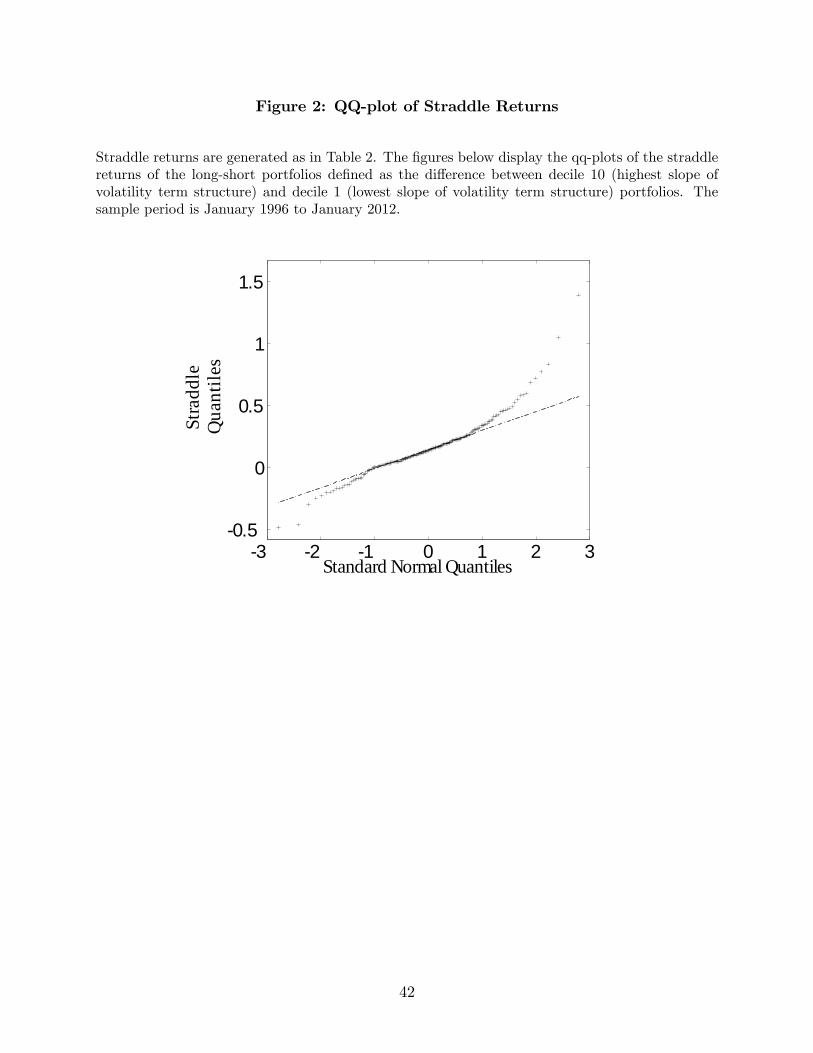
Figure 2: QQ-plot of Straddle Returns

Straddle returns are generated as in Table 2. The �gures below display the qq-plots of the straddlereturns of the long-short portfolios de�ned as the di¤erence between decile 10 (highest slope ofvolatility term structure) and decile 1 (lowest slope of volatility term structure) portfolios. Thesample period is January 1996 to January 2012.

3 2 1 0 1 2 30.5

0

0.5

1

1.5

Standard Normal Quantiles

Stra

ddle

Qua

ntile

s

42

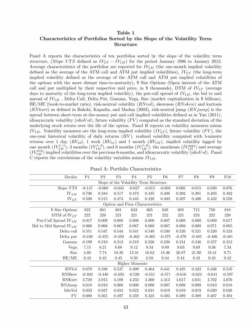
Table 1Characteristics of Portfolios Sorted by the Slope of the Volatility Term

Structure

Panel A reports the characteristics of ten portfolios sorted by the slope of the volatility termstructure, (Slope V TS de�ned as IVLT � IV1M ) for the period January 1996 to January 2012.Average characteristics of the portfolios are reported for IV1M (the one-month implied volatilityde�ned as the average of the ATM call and ATM put implied volatilities), IVLT (the long-termimplied volatility de�ned as the average of the ATM call and ATM put implied volatilities ofthe options with the more distant time-to-maturity), $ Size Options (Open interest of the ATMcall and put multiplied by their respective mid price, in $ thousands), DTM of IVLT (averagedays to maturity of the long-term implied volatility), the put-call spread of IV1M ; the bid to midspread of IV1M , Delta Call, Delta Put, Gamma, Vega, Size (market capitalization in $ billions),BE/ME (book-to-market ratio), risk-neutral volatility (RNvol), skewness (RNskew) and kurtosis(RNkurt) as de�ned in Bakshi, Kapadia, and Madan (2003), risk-neutral jump (RNjump) is thespread between short-term at-the-money put and call implied volatilities de�ned as in Yan (2011),idiosyncratic volatility (idioV ol), future volatility (FV ) computed as the standard deviation of theunderlying stock return over the life of the option. Panel B reports on volatility measures minusIV1M . Volatility measures are the long-term implied volatility (IVLT ), future volatility (FV ), theone-year historical volatility of daily returns (HV ), realized volatility computed with 5-minutereturns over 1 day (RV1d), 1 week (RV1w) and 1 month (RV1M ), implied volatility lagged byone month (IV t�11M ), 3 months (IV t�31M ), and 6 months (IV t�61M ), the maximum (IV max1M ) and average(IV avg1M ) implied volatilities over the previous 6-months, and idiosyncratic volatility (idioV ol). PanelC reports the correlations of the volatility variables minus IV1M .

Panel A: Portfolio Characteristics

Deciles P1 P2 P3 P4 P5 P6 P7 P8 P9 P10Slope of the Volatility Term Structure

Slope VTS -0.147 -0.068 -0.043 -0.027 -0.015 -0.005 0.005 0.015 0.030 0.076IV1M 0.736 0.584 0.517 0.473 0.435 0.408 0.392 0.391 0.403 0.482IVLT 0.590 0.515 0.474 0.445 0.420 0.403 0.397 0.406 0.432 0.558

Option and Firm Characteristics$ Size Options 822 661 681 643 665 638 685 712 750 618DTM of IVLT 222 220 221 221 221 222 221 223 222 220

Put-Call Spread IV1M 0.017 0.009 0.008 0.008 0.008 0.007 0.009 0.009 0.009 0.017Bid to Mid Spread IV1M 0.066 0.066 0.067 0.067 0.068 0.067 0.069 0.069 0.071 0.085

Delta call 0.551 0.547 0.544 0.541 0.540 0.530 0.526 0.521 0.520 0.523Delta put -0.449 -0.455 -0.459 -0.462 -0.465 -0.475 -0.479 -0.485 -0.486 -0.481Gamma 0.199 0.210 0.213 0.219 0.226 0.228 0.241 0.246 0.257 0.312Vega 7.15 8.21 8.68 9.12 9.34 9.89 9.63 9.69 9.36 7.34Size 4.80 7.74 10.39 13.31 16.62 18.36 20.87 21.00 19.41 9.71

BE/ME 0.43 0.45 0.45 0.50 0.58 0.44 0.44 0.42 0.45 0.42Higher Moments

RNVol 0.679 0.586 0.537 0.499 0.464 0.441 0.425 0.422 0.436 0.510RNSkew -0.402 -0.440 -0.493 -0.520 -0.551 -0.571 -0.616 -0.624 -0.641 -0.597RNKurt 3.739 3.915 4.109 4.232 4.360 4.413 4.617 4.641 4.702 4.676RNJump 0.018 0.010 0.008 0.009 0.008 0.007 0.009 0.009 0.010 0.018IdioVol 0.033 0.027 0.024 0.022 0.021 0.019 0.019 0.019 0.020 0.026

FV 0.668 0.561 0.497 0.459 0.425 0.403 0.389 0.388 0.407 0.494

43

Table 1 (Continued)

Panel B: Volatility Measures (minus IV1M)

Volatility Measures minus IV1M

Deciles P1 P2 P3 P4 P5 P6 P7 P8 P9 P10

Slope VTS -0.147 -0.068 -0.043 -0.027 -0.015 -0.005 0.005 0.015 0.030 0.076

FV-IV1M -0.068 -0.023 -0.020 -0.014 -0.010 -0.006 -0.003 -0.003 0.004 0.013

HV-IV1M -0.096 -0.018 -0.001 0.013 0.019 0.028 0.037 0.051 0.072 0.125

RV1d-IV1M -0.064 -0.030 -0.031 -0.024 -0.025 -0.022 -0.015 -0.012 -0.003 0.021

RV1w-IV1M -0.062 -0.030 -0.027 -0.021 -0.022 -0.019 -0.013 -0.010 -0.002 0.027

VRP (=RV1M -IV1M ) -0.071 -0.021 -0.018 -0.009 -0.010 -0.007 0.000 0.004 0.017 0.057

IVt�11M -IV1M -0.118 -0.042 -0.021 -0.008 0.003 0.011 0.021 0.032 0.048 0.091

IVt�31M -IV1M -0.134 -0.050 -0.026 -0.012 -0.001 0.010 0.018 0.028 0.044 0.087

IVt�61M -IV1M -0.146 -0.057 -0.033 -0.016 -0.002 0.009 0.017 0.031 0.046 0.087

IVavg1M -IV1M -0.077 -0.025 -0.012 -0.003 0.004 0.010 0.016 0.023 0.035 0.068

IVmax1M -IV1M 0.064 0.065 0.063 0.064 0.066 0.067 0.073 0.082 0.099 0.159

IdioVol-IV1M -0.703 -0.556 -0.493 -0.451 -0.415 -0.390 -0.374 -0.372 -0.383 -0.457

Panel C: Correlation Matrix

Slope VTS

FV-IV1M 3.6 FV-IV1M

HV-IV1M 46.3 2.1 HV�IV1MRV1d-IV1M 3.3 10.0 5.0 RV1d-IV1M

RV1w-IV1M 4.2 13.2 3.6 79.1 RV1w-IV1M

VRP (=RV1M -IV1M ) 15.0 11.5 13.8 55.3 71.5 VRP (=RV1M -IV1M )

IVt�11M -IV1M 57.9 -0.4 43.9 4.3 3.6 18.5 IVt�11M -IV1M

IVt�31M -IV1M 54.3 -2.8 60.2 1.1 -2.7 3.9 47.4 IVt�31M -IV1M

IVt�61M -IV1M 51.3 -1.9 68.8 0.6 -1.7 4.0 36.1 62.4 IVt�61M -IV1M

IVavg1M -IV1M 65.1 0.9 45.3 2.4 3.4 28.2 82.0 48.0 39.9 IVavg1M -IV1M

IVmax1M -IV1M 17.9 1.9 17.6 4.0 9.5 29.2 49.2 7.1 1.2 61.1 IVmax1M -IV1M

IdioVol-IV1M 29.2 2.5 24.5 18.2 23.1 36.2 28.1 17.4 18.3 33.2 22.5 IdioVol-IV1M

44

Table 2The Slope of the Volatility Term Structure and the Cross-Section of Straddle

Returns

Portfolios are constructed as in Table 1. Panel A reports the monthly equal-weighted straddlereturns of decile portfolios along with the t-statistics (t-stat), standard deviation (StDev), skewnessand kurtosis values. The last column displays the di¤erence between decile portfolio 10 (highestslope of volatility term structure) and decile 1 (lowest slope of volatility term structure). In PanelB, we sample the long-short (P10 � P1) straddle returns 50,000 times to generate the reported�nite sample critical value for the t-statistic. Panel C presents coe¢ cients and t-statistics from thefollowing regression:

rstraddle = �P + �1(Rm �Rf ) + �2SMB + �3HML+ �4UMD+�5(Ro �Rf ) + �6(R2m �Rf ) + �7(R2o �Rf ) + �8(RoRm �Rf )�9(R

3o �Rf ) + �10(R3m �Rf ) + �11(R2oRm �Rf ) + �12(RoR2m �Rf ) + "

where Rm is the return of the market, Ro is the straddle return of the S&P 500, Rf is the risk-free rate, and SMB, HML and UMD are the Fama-French and momentum factors, rstraddle is thestraddle return of the long-short portfolio. The �rst row gives the coe¢ cients of the regression andthe second row gives the t-statistics (in parentheses). Adjusted R2 is reported at the bottom of thetable. The sample period is January 1996 to January 2012.

Panel A: Straddle Returns

Deciles P1 P2 P3 P4 P5 P6 P7 P8 P9 P10 P10-P1Mean -0.092 -0.036 -0.044 -0.035 -0.028 -0.025 -0.033 -0.006 0.016 0.073 0.165t-stat (-5.96) (-2.02) (-2.58) (-1.85) (-1.44) (-1.31) (-1.64) (-0.30) (0.73) (3.50) (10.02)StDev 0.213 0.249 0.237 0.260 0.267 0.264 0.276 0.288 0.302 0.291 0.228Skewness 1.1 1.7 2.0 2.4 2.2 2.4 1.9 2.6 2.1 1.9 1.2Kurtosis 3.3 6.1 8.9 10.7 9.3 10.0 6.5 11.8 8.1 6.9 5.4

Panel B: Bootstrapped Critical Values for the t-statistic

Percentile (%) Bootstrapped t-statistic1 -2.5312.5 -2.1155 -1.75410 -1.35790 1.23495 1.56297.5 1.84299 2.165

45

Table 2 (Continued)

Panel C: Risk-Adjusted Returns

(1) (2) (3) (4)Alpha 0.174 0.147 0.130 0.135

(10.18) (7.38) (3.75) (3.85)Rm - Rf -0.801 -0.399 -0.197 -0.240

(-2.05) (-1.16) (-0.45) (-0.50)SMB -0.769 -0.493

(-1.56) (-1.04)HML -0.723 -0.361

(-1.39) (-0.72)UMD 0.110 -0.087

(0.35) (-0.28)Ro�Rf 0.057 0.079 0.080

(2.12) (1.81) (1.83)R2m�Rf -6.39 -7.18 -7.65

(-1.46) (-1.32) (-1.39)R2o�Rf 0.043 0.080 0.081

(1.80) (1.80) (1.80)RmRo�Rf -0.946 -0.823 -0.847

(-1.92) (-1.36) (-1.39)R3o�Rf -0.026 -0.027

(-1.01) (-1.03)R3m�Rf -1.64 -0.88

(-0.14) (-0.08)RmR

2o�Rf -0.346 -0.295

(-0.49) (-0.41)R2mRo�Rf -0.335 -0.094

(-0.05) (-0.01)Adj. R2 0.029 0.150 0.139 0.131

46

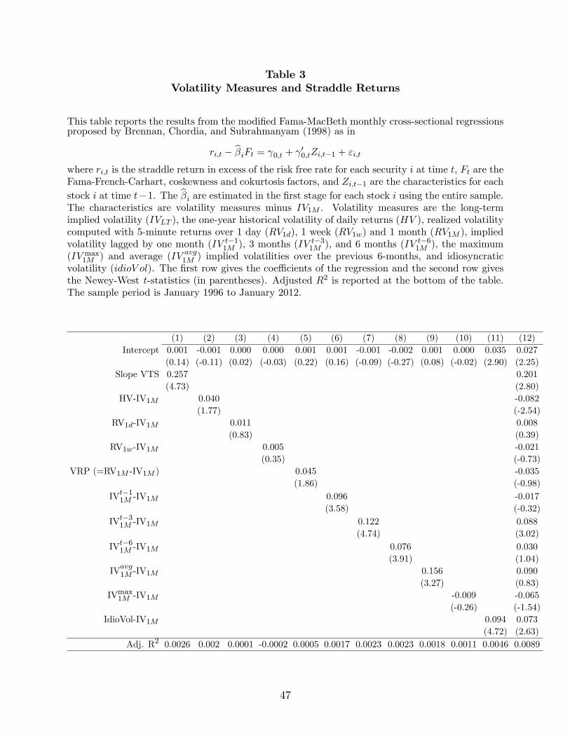
Table 3Volatility Measures and Straddle Returns

This table reports the results from the modi�ed Fama-MacBeth monthly cross-sectional regressionsproposed by Brennan, Chordia, and Subrahmanyam (1998) as in

ri;t � b�iFt = 0;t + 00;tZi;t�1 + "i;twhere ri;t is the straddle return in excess of the risk free rate for each security i at time t, Ft are theFama-French-Carhart, coskewness and cokurtosis factors, and Zi;t�1 are the characteristics for eachstock i at time t�1. The b�i are estimated in the �rst stage for each stock i using the entire sample.The characteristics are volatility measures minus IV1M . Volatility measures are the long-termimplied volatility (IVLT ), the one-year historical volatility of daily returns (HV ), realized volatilitycomputed with 5-minute returns over 1 day (RV1d), 1 week (RV1w) and 1 month (RV1M ), impliedvolatility lagged by one month (IV t�11M ), 3 months (IV t�31M ), and 6 months (IV t�61M ), the maximum(IV max1M ) and average (IV avg1M ) implied volatilities over the previous 6-months, and idiosyncraticvolatility (idioV ol). The �rst row gives the coe¢ cients of the regression and the second row givesthe Newey-West t-statistics (in parentheses). Adjusted R2 is reported at the bottom of the table.The sample period is January 1996 to January 2012.

(1) (2) (3) (4) (5) (6) (7) (8) (9) (10) (11) (12)Intercept 0.001 -0.001 0.000 0.000 0.001 0.001 -0.001 -0.002 0.001 0.000 0.035 0.027

(0.14) (-0.11) (0.02) (-0.03) (0.22) (0.16) (-0.09) (-0.27) (0.08) (-0.02) (2.90) (2.25)Slope VTS 0.257 0.201

(4.73) (2.80)HV-IV1M 0.040 -0.082

(1.77) (-2.54)RV1d-IV1M 0.011 0.008

(0.83) (0.39)RV1w-IV1M 0.005 -0.021

(0.35) (-0.73)VRP (=RV1M -IV1M ) 0.045 -0.035

(1.86) (-0.98)IVt�11M -IV1M 0.096 -0.017

(3.58) (-0.32)IVt�31M -IV1M 0.122 0.088

(4.74) (3.02)IVt�61M -IV1M 0.076 0.030

(3.91) (1.04)IVavg1M -IV1M 0.156 0.090

(3.27) (0.83)IVmax1M -IV1M -0.009 -0.065

(-0.26) (-1.54)IdioVol-IV1M 0.094 0.073

(4.72) (2.63)Adj. R2 0.0026 0.002 0.0001 -0.0002 0.0005 0.0017 0.0023 0.0023 0.0018 0.0011 0.0046 0.0089

47

Table 4The Slope of the Volatility Term Structure,Volatility Measures and Straddle Returns

Each month, �rms are �rst sorted into quintiles based on volatility measures (minus IV1M ), andthen, within each quintile, �rms are sorted by the slope of the volatility term structure, de�nedas IVLT � IV1M . The slope-of-the volatility term structure portfolios are averaged over each ofthe �ve characteristic portfolios. Volatility measures are the long-term implied volatility (IVLT ),the one-year historical volatility of daily returns (HV ), realized volatility computed with 5-minutereturns over 1 day (RV1d), 1 week (RV1w) and 1 month (RV1M ), implied volatility lagged by onemonth (IV t�11M ), 3 months (IV t�31M ), and 6 months (IV t�61M ), the maximum (IV max1M ) and average(IV avg1M ) implied volatilities over the previous 6-months, and idiosyncratic volatility (idioV ol). Thistable reports the average straddle return for quintiles 1 to 5, the di¤erence between quintile 5 andquintile 1, and the t-statistics (in parentheses). The sample period is January 1996 to January2012.

Control P1 P2 P3 P4 P5 P5-P1HV-IV1M -0.064 -0.039 -0.028 -0.022 0.047 0.110

(-4.15) (-2.32) (-1.52) (-1.14) (2.29) (8.07)

RV1d-IV1M -0.067 -0.036 -0.035 -0.018 0.049 0.115(-4.31) (-2.11) (-1.92) (-0.92) (2.41) (8.81)

RV1w-IV1M -0.072 -0.027 -0.037 -0.021 0.051 0.122(-4.68) (-1.56) (-2.09) (-1.09) (2.56) (9.65)

VRP (=RV1M -IV1M ) -0.064 -0.041 -0.030 -0.017 0.046 0.109(-4.01) (-2.50) (-1.65) (-0.88) (2.35) (9.22)

IVt�11M -IV1M -0.058 -0.038 -0.022 -0.018 0.030 0.088(-3.77) (-2.17) (-1.18) (-0.96) (1.56) (7.41)

IVt�31M -IV1M -0.045 -0.040 -0.033 -0.014 0.026 0.071(-2.82) (-2.25) (-1.89) (-0.74) (1.32) (6.43)

IVt�61M -IV1M -0.054 -0.044 -0.027 -0.016 0.035 0.089(-3.40) (-2.61) (-1.53) (-0.85) (1.77) (7.38)

IVavg1M -IV1M -0.053 -0.034 -0.024 -0.017 0.022 0.076(-3.39) (-1.94) (-1.32) (-0.89) (1.19) (6.83)

IVmax1M -IV1M -0.067 -0.037 -0.029 -0.003 0.030 0.097(-4.39) (-2.17) (-1.58) (-0.16) (1.53) (7.67)

IdioVol-IV1M -0.070 -0.044 -0.028 -0.008 0.043 0.113(-4.59) (-2.59) (-1.56) (-0.39) (2.25) (9.70)

48

Table 5Forecasting Realized Volatility

This tables reports the average coe¢ cients and Newey-West t-statistics from the two pass Fama-MacBeth(1973) regressions. Each month, future realized volatility minus IV1M is regressed on various volatilitymeasures minus IV1M as in FVi;t � IV1Mi;t

= B0;t + B1;t(IVLTi;t � IV1Mi;t) + Bk;t(V olatility Measures�

IV1Mi;t)+"i;t: In the second step, the estimator for each coe¢ cient is the average of the time series coe¢ cients.Future realized volatility (FVi;t) is the standard deviation of the underlying daily stock return over thelife of the option. Volatility measures are the long-term implied volatility (IVLT ), the one-year historicalvolatility of daily returns (HV ), realized volatility computed with 5-minute returns over 1 day (RV1d), 1week (RV1w) and 1 month (RV1M ), implied volatility lagged by one month (IV

t�11M ), 3 months (IV t�31M ),

and 6 months (IV t�61M ), the maximum (IV max1M ) and average (IV avg1M ) implied volatilities over the previous6-months, and idiosyncratic volatility (idioV ol). We report adjusted R2 and Newey-West t-statistics with 3lags in parentheses. Additionally, this table reports the percentage of regressors with t-statistics over 1:96for each estimator. The sample period is January 1996 to January 2012.

(1) (2) (3) (4) (5) (6) (7)Intercept -0.009 -0.014 -0.007 -0.016 -0.006 -0.006 -0.007

(-1.16) (-1.82) (-1.14) (-2.28) (-0.93) (-0.77) (-1.24)IVLT -IV1M 0.347 0.173

(10.73) (5.33)HV-IV1M 0.190 0.148

(10.13) (6.27)RV1d-IV1M 0.031 0.024

(3.59) (2.98)RV1w-IV1M 0.013 0.024

(0.97) (2.05)VRP (=RV1M -IV1M ) 0.166 0.100

(8.34) (4.86)IVt�11M -IV1M 0.076 -0.035

(5.67) (-1.92)IVt�31M -IV1M 0.078 0.002

(5.13) (0.14)IVt�61M -IV1M 0.057 -0.035

(3.50) (-2.74)IVavg1M -IV1M 0.475 0.183

(12.34) (3.94)IVmax1M -IV1M -0.189 -0.141

(-6.44) (-6.23)IdioVol-IV1M 0.056 -0.011

(5.78) (-1.22)Adj. R2 4% 3% 4% 4% 4% 1% 10%

Percentage of t>1.96 (IVLT -IV1M ) 65% 26%Percentage of t>1.96 (HV-IV1M ) 64% 28%

Percentage of t>1.96 (RV1d-IV1M ) 18% 15%Percentage of t>1.96 (RV1w-IV1M ) 13% 11%Percentage of t>1.96 (RV1M -IV1M ) 45% 28%Percentage of t>1.96 (IVt�11M -IV1M ) 26% 9%Percentage of t>1.96 (IVt�31M -IV1M ) 30% 13%Percentage of t>1.96 (IVt�61M -IV1M ) 28% 6%Percentage of t>1.96 (IVavg1M -IV1M ) 65% 21%Percentage of t>1.96 (IVmax1M -IV1M ) 8% 7%Percentage of t>1.96 (IdioVol-IV1M ) 35% 7%

49

Table 6Controlling for Higher Moments and Jump Risk


ri;t � b�iFt = 0;t + 00;tZi;t�1 + "i;twhere ri;t is the straddle return in excess of the risk free rate for each security i at time t, Ft arethe Fama-French-Carhart, coskewness and cokurtosis factors, and Zi;t�1 are the characteristics foreach stock i at time t� 1. The b�i are estimated in the �rst stage for each stock i using the entiresample. The characteristics are higher moments and jump risk variables. The variables includedare the slope of the volatility term structure, risk-neutral volatility, skewness and kurtosis (Bakshi,Kapadia, and Madan (2003)), option skew (Xing, Zhang and Zhao (2010)), risk-neutral jump (Yan(2011)), and the right-tail and left-tail risk neutral jumps (Bollerslev and Todorov (2011)). The�rst row gives the coe¢ cients of the regression and the second row gives the Newey-West t-statistics(in parentheses). Adjusted R2 is reported at the bottom of the table. The sample period is January1996 to January 2012.

(1) (2)Intercept -0.001 0.038

(-0.20) (1.08)Slope of VTS 0.298 0.303

(4.97) (3.42)RNVol -0.058

(-1.06)RNSkew -0.004

(-0.32)RNKurt -0.008

(-0.81)OptionSkew 0.172

(2.54)RNJump -0.245

(-2.88)RNJump Right -0.002

(-0.03)RNJump Left 0.004

(0.04)Adj. R2 0.003 0.009

50

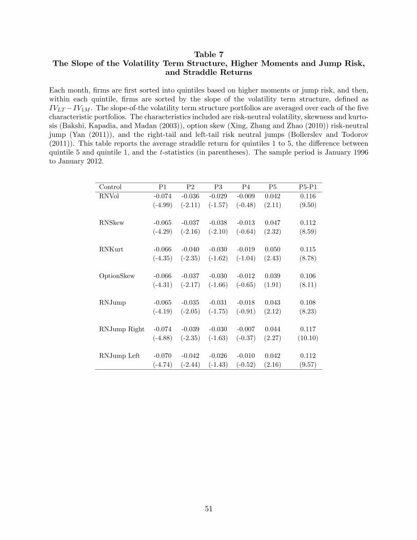
Table 7The Slope of the Volatility Term Structure, Higher Moments and Jump Risk,

and Straddle Returns

Each month, �rms are �rst sorted into quintiles based on higher moments or jump risk, and then,within each quintile, �rms are sorted by the slope of the volatility term structure, de�ned asIVLT �IV1M . The slope-of-the volatility term structure portfolios are averaged over each of the �vecharacteristic portfolios. The characteristics included are risk-neutral volatility, skewness and kurto-sis (Bakshi, Kapadia, and Madan (2003)), option skew (Xing, Zhang and Zhao (2010)) risk-neutraljump (Yan (2011)), and the right-tail and left-tail risk neutral jumps (Bollerslev and Todorov(2011)). This table reports the average straddle return for quintiles 1 to 5, the di¤erence betweenquintile 5 and quintile 1, and the t-statistics (in parentheses). The sample period is January 1996to January 2012.

Control P1 P2 P3 P4 P5 P5-P1RNVol -0.074 -0.036 -0.029 -0.009 0.042 0.116

(-4.99) (-2.11) (-1.57) (-0.48) (2.11) (9.50)

RNSkew -0.065 -0.037 -0.038 -0.013 0.047 0.112(-4.29) (-2.16) (-2.10) (-0.64) (2.32) (8.59)

RNKurt -0.066 -0.040 -0.030 -0.019 0.050 0.115(-4.35) (-2.35) (-1.62) (-1.04) (2.43) (8.78)

OptionSkew -0.066 -0.037 -0.030 -0.012 0.039 0.106(-4.31) (-2.17) (-1.66) (-0.65) (1.91) (8.11)

RNJump -0.065 -0.035 -0.031 -0.018 0.043 0.108(-4.19) (-2.05) (-1.75) (-0.91) (2.12) (8.23)

RNJump Right -0.074 -0.039 -0.030 -0.007 0.044 0.117(-4.88) (-2.35) (-1.63) (-0.37) (2.27) (10.10)

RNJump Left -0.070 -0.042 -0.026 -0.010 0.042 0.112(-4.74) (-2.44) (-1.43) (-0.52) (2.16) (9.57)

51

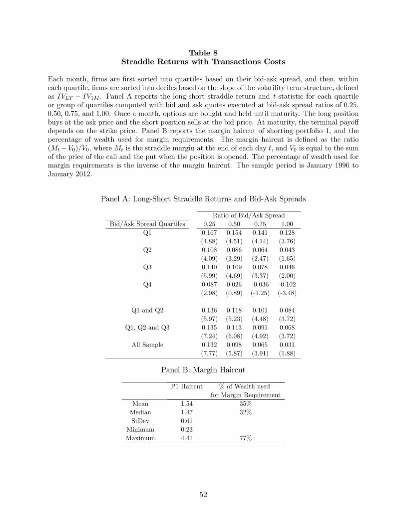
Table 8Straddle Returns with Transactions Costs

Each month, �rms are �rst sorted into quartiles based on their bid-ask spread, and then, withineach quartile, �rms are sorted into deciles based on the slope of the volatility term structure, de�nedas IVLT � IV1M . Panel A reports the long-short straddle return and t-statistic for each quartileor group of quartiles computed with bid and ask quotes executed at bid-ask spread ratios of 0:25,0:50, 0:75, and 1:00. Once a month, options are bought and held until maturity. The long positionbuys at the ask price and the short position sells at the bid price. At maturity, the terminal payo¤depends on the strike price. Panel B reports the margin haircut of shorting portfolio 1, and thepercentage of wealth used for margin requirements. The margin haircut is de�ned as the ratio(Mt�V0)=V0, where Mt is the straddle margin at the end of each day t, and V0 is equal to the sumof the price of the call and the put when the position is opened. The percentage of wealth used formargin requirements is the inverse of the margin haircut. The sample period is January 1996 toJanuary 2012.

Panel A: Long-Short Straddle Returns and Bid-Ask Spreads

Ratio of Bid/Ask SpreadBid/Ask Spread Quartiles 0.25 0.50 0.75 1.00

Q1 0.167 0.154 0.141 0.128(4.88) (4.51) (4.14) (3.76)

Q2 0.108 0.086 0.064 0.043(4.09) (3.29) (2.47) (1.65)

Q3 0.140 0.109 0.078 0.046(5.99) (4.69) (3.37) (2.00)

Q4 0.087 0.026 -0.036 -0.102(2.98) (0.89) (-1.25) (-3.48)

Q1 and Q2 0.136 0.118 0.101 0.084(5.97) (5.23) (4.48) (3.72)

Q1, Q2 and Q3 0.135 0.113 0.091 0.068(7.24) (6.08) (4.92) (3.72)

All Sample 0.132 0.098 0.065 0.031(7.77) (5.87) (3.91) (1.88)

Panel B: Margin Haircut

P1 Haircut % of Wealth usedfor Margin Requirement

Mean 1.54 35%Median 1.47 32%StDev 0.61

Minimum 0.23Maximum 4.41 77%

52

Table 9Controlling for Stock Characteristics


ri;t �12Xk=1

b�i;kFk;t = 0;t + 00;tZi;t�1 + "i;twhere ri;t is the straddle return in excess of the risk free rate for each security i at time t, Ft are theFama-French-Carhart, coskewness and cokurtosis factors, and Zi;t�1 are the characteristics for eachstock i at time t�1. The b�i are estimated in the �rst stage for each stock i using the entire sample.Characteristics included in the regressions are the slope of the volatility term structure, optiondollar volume ($V ol), option volume contracts (V ol), option open interest (OI), bid-to-mid optionspread (BM), size (market capitalization in $ billions), BE/ME (book-to-market ratio), historicalvolatility (HV ), skewness (HSkew) and kurtosis (HKurt), delta, gamma, and vega. The �rst rowgives the coe¢ cients of the regression and the second row gives the t-statistics (in parentheses).Adjusted R2 is reported at the bottom of the table. The sample period is January 1996 to January2012.

(1) (2) (3)Intercept -0.016 0.028 0.112

(-1.09) (1.20) (2.67)Slope VTS 0.266 0.253 0.303

(5.69) (5.60) (6.30)Ln($Vol) -0.004

(-1.88)Ln(Vol) 0.001

(0.34)Ln(OI) 0.002

(0.79)Ln(BM) 0.014

(2.18)Ln(size) -0.005

(-2.07)BE/ME -0.008

(-1.18)HV -0.080

(-3.49)HSkew 0.002

(0.70)HKurt -0.0001

(-1.24)Delta 0.115 0.111 0.113

(4.49) (4.36) (4.40)Gamma 0.019 -0.026 0.002

(0.62) (-0.83) (0.08)Vega 0.000 0.001 -0.001

(0.42) (1.02) (-0.68)Adj. R2 0.020 0.025 0.028

53

Table 10The Slope of the Volatility Term Structure,Stock Characteristics and Straddle Returns

Each month, �rms are �rst sorted into quintiles based on �rm characteristics, and then, withineach quintile, �rms are sorted by the slope of the volatility term structure, de�ned as IVLT �IV1M .The slope-of-the volatility term structure portfolios are averaged over each of the �ve characteristicportfolios. Characteristics include option dollar volume ($V ol), option volume contracts (V ol),option open interest (OI), bid-to-mid option spread (Bid-to-Mid), size (market capitalization in$ billions), BE/ME (book-to-market ratio), historical volatility (HV ), skewness (HSkew) andkurtosis (HKurt), realized volatility (RV ) from intraday �ve-minute returns, delta, gamma, andvega. This table reports the average straddle return for quintiles 1 to 5, the di¤erence betweenquintile 5 and quintile 1, and the t-statistics (in parentheses). The sample period is January 1996to January 2012.

StraddleControl P1 P2 P3 P4 P5 P5-P1$Vol -0.067 -0.037 -0.027 -0.022 0.047 0.114

(-4.50) (-2.20) (-1.42) (-1.18) (2.29) (8.45)Vol -0.064 -0.040 -0.028 -0.016 0.043 0.107

(-4.20) (-2.35) (-1.54) (-0.83) (2.12) (7.89)OI -0.066 -0.037 -0.026 -0.022 0.045 0.111

(-4.27) (-2.20) (-1.44) (-1.14) (2.25) (8.35)Bid-To-Mid -0.063 -0.038 -0.032 -0.014 0.040 0.103

(-4.18) (-2.27) (-1.78) (-0.68) (1.99) (8.02)Size -0.077 -0.032 -0.031 -0.008 0.042 0.119

(-4.91) (-1.91) (-1.73) (-0.43) (2.05) (9.17)BE/ME -0.070 -0.035 -0.030 -0.026 0.055 0.124

(-4.62) (-2.14) (-1.62) (-1.35) (2.63) (9.28)HV -0.064 -0.039 -0.028 -0.022 0.047 0.110

(-4.15) (-2.32) (-1.52) (-1.14) (2.29) (8.07)HSkew -0.064 -0.039 -0.028 -0.022 0.047 0.110

(-4.15) (-2.32) (-1.52) (-1.14) (2.29) (11.42)HKurt -0.064 -0.039 -0.028 -0.022 0.047 0.110

(-4.15) (-2.32) (-1.52) (-1.14) (2.29) (13.99)RV -0.072 -0.040 -0.020 -0.019 0.045 0.117

(-4.83) (-2.36) (-1.11) (-0.99) (2.26) (10.68)Delta -0.072 -0.043 -0.025 -0.011 0.046 0.119

(-4.96) (-2.54) (-1.37) (-0.57) (2.32) (9.59)Gamma -0.066 -0.036 -0.037 -0.009 0.041 0.106

(-4.32) (-2.15) (-2.06) (-0.44) (2.03) (8.20)Vega -0.072 -0.037 -0.022 -0.020 0.043 0.115

(-4.73) (-2.15) (-1.15) (-1.04) (2.15) (8.84)

54

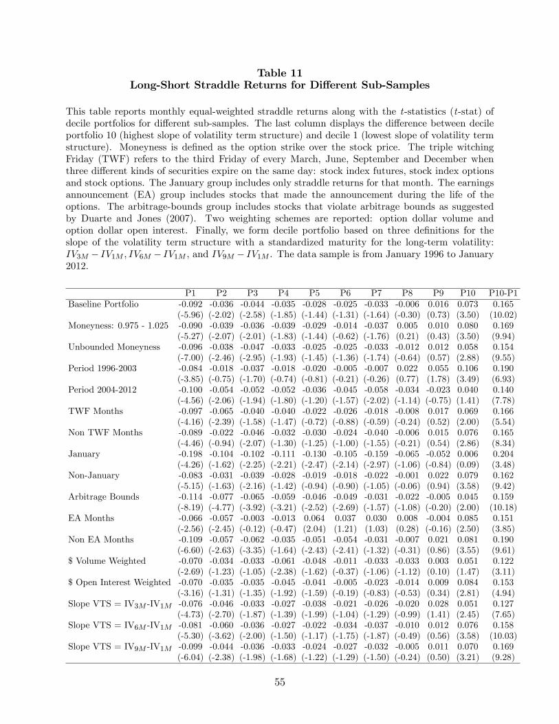
Table 11Long-Short Straddle Returns for Di¤erent Sub-Samples

This table reports monthly equal-weighted straddle returns along with the t-statistics (t-stat) ofdecile portfolios for di¤erent sub-samples. The last column displays the di¤erence between decileportfolio 10 (highest slope of volatility term structure) and decile 1 (lowest slope of volatility termstructure). Moneyness is de�ned as the option strike over the stock price. The triple witchingFriday (TWF) refers to the third Friday of every March, June, September and December whenthree di¤erent kinds of securities expire on the same day: stock index futures, stock index optionsand stock options. The January group includes only straddle returns for that month. The earningsannouncement (EA) group includes stocks that made the announcement during the life of theoptions. The arbitrage-bounds group includes stocks that violate arbitrage bounds as suggestedby Duarte and Jones (2007). Two weighting schemes are reported: option dollar volume andoption dollar open interest. Finally, we form decile portfolio based on three de�nitions for theslope of the volatility term structure with a standardized maturity for the long-term volatility:IV3M � IV1M , IV6M � IV1M , and IV9M � IV1M . The data sample is from January 1996 to January2012.

P1 P2 P3 P4 P5 P6 P7 P8 P9 P10 P10-P1Baseline Portfolio -0.092 -0.036 -0.044 -0.035 -0.028 -0.025 -0.033 -0.006 0.016 0.073 0.165

(-5.96) (-2.02) (-2.58) (-1.85) (-1.44) (-1.31) (-1.64) (-0.30) (0.73) (3.50) (10.02)Moneyness: 0.975 - 1.025 -0.090 -0.039 -0.036 -0.039 -0.029 -0.014 -0.037 0.005 0.010 0.080 0.169

(-5.27) (-2.07) (-2.01) (-1.83) (-1.44) (-0.62) (-1.76) (0.21) (0.43) (3.50) (9.94)Unbounded Moneyness -0.096 -0.038 -0.047 -0.033 -0.025 -0.025 -0.033 -0.012 0.012 0.058 0.154

(-7.00) (-2.46) (-2.95) (-1.93) (-1.45) (-1.36) (-1.74) (-0.64) (0.57) (2.88) (9.55)Period 1996-2003 -0.084 -0.018 -0.037 -0.018 -0.020 -0.005 -0.007 0.022 0.055 0.106 0.190

(-3.85) (-0.75) (-1.70) (-0.74) (-0.81) (-0.21) (-0.26) (0.77) (1.78) (3.49) (6.93)Period 2004-2012 -0.100 -0.054 -0.052 -0.052 -0.036 -0.045 -0.058 -0.034 -0.023 0.040 0.140

(-4.56) (-2.06) (-1.94) (-1.80) (-1.20) (-1.57) (-2.02) (-1.14) (-0.75) (1.41) (7.78)TWF Months -0.097 -0.065 -0.040 -0.040 -0.022 -0.026 -0.018 -0.008 0.017 0.069 0.166

(-4.16) (-2.39) (-1.58) (-1.47) (-0.72) (-0.88) (-0.59) (-0.24) (0.52) (2.00) (5.54)Non TWF Months -0.089 -0.022 -0.046 -0.032 -0.030 -0.024 -0.040 -0.006 0.015 0.076 0.165

(-4.46) (-0.94) (-2.07) (-1.30) (-1.25) (-1.00) (-1.55) (-0.21) (0.54) (2.86) (8.34)January -0.198 -0.104 -0.102 -0.111 -0.130 -0.105 -0.159 -0.065 -0.052 0.006 0.204

(-4.26) (-1.62) (-2.25) (-2.21) (-2.47) (-2.14) (-2.97) (-1.06) (-0.84) (0.09) (3.48)Non-January -0.083 -0.031 -0.039 -0.028 -0.019 -0.018 -0.022 -0.001 0.022 0.079 0.162

(-5.15) (-1.63) (-2.16) (-1.42) (-0.94) (-0.90) (-1.05) (-0.06) (0.94) (3.58) (9.42)Arbitrage Bounds -0.114 -0.077 -0.065 -0.059 -0.046 -0.049 -0.031 -0.022 -0.005 0.045 0.159

(-8.19) (-4.77) (-3.92) (-3.21) (-2.52) (-2.69) (-1.57) (-1.08) (-0.20) (2.00) (10.18)EA Months -0.066 -0.057 -0.003 -0.013 0.064 0.037 0.030 0.008 -0.004 0.085 0.151

(-2.56) (-2.45) (-0.12) (-0.47) (2.04) (1.21) (1.03) (0.28) (-0.16) (2.50) (3.85)Non EA Months -0.109 -0.057 -0.062 -0.035 -0.051 -0.054 -0.031 -0.007 0.021 0.081 0.190

(-6.60) (-2.63) (-3.35) (-1.64) (-2.43) (-2.41) (-1.32) (-0.31) (0.86) (3.55) (9.61)$ Volume Weighted -0.070 -0.034 -0.033 -0.061 -0.048 -0.011 -0.033 -0.033 0.003 0.051 0.122

(-2.69) (-1.23) (-1.05) (-2.38) (-1.62) (-0.37) (-1.06) (-1.12) (0.10) (1.47) (3.11)$ Open Interest Weighted -0.070 -0.035 -0.035 -0.045 -0.041 -0.005 -0.023 -0.014 0.009 0.084 0.153

(-3.16) (-1.31) (-1.35) (-1.92) (-1.59) (-0.19) (-0.83) (-0.53) (0.34) (2.81) (4.94)Slope VTS = IV3M -IV1M -0.076 -0.046 -0.033 -0.027 -0.038 -0.021 -0.026 -0.020 0.028 0.051 0.127

(-4.73) (-2.70) (-1.87) (-1.39) (-1.99) (-1.04) (-1.29) (-0.99) (1.41) (2.45) (7.65)Slope VTS = IV6M -IV1M -0.081 -0.060 -0.036 -0.027 -0.022 -0.034 -0.037 -0.010 0.012 0.076 0.158

(-5.30) (-3.62) (-2.00) (-1.50) (-1.17) (-1.75) (-1.87) (-0.49) (0.56) (3.58) (10.03)Slope VTS = IV9M -IV1M -0.099 -0.044 -0.036 -0.033 -0.024 -0.027 -0.032 -0.005 0.011 0.070 0.169

(-6.04) (-2.38) (-1.98) (-1.68) (-1.22) (-1.29) (-1.50) (-0.24) (0.50) (3.21) (9.28)

55

Table 12Straddle Returns for Di¤erent Horizons

Portfolios are constructed as in Table 1. This table reports equal-weighted straddle returns fordi¤erent horizons. We study 2-week and 3-week holding periods. We report t-statistics (t-stat),standard deviation (StDev), skewness and kurtosis values of the decile portfolio returns. Long-shortreturns are computed as the di¤erence between decile portfolio 10 (highest slope of volatility termstructure) and decile 1 (lowest slope of volatility term structure). The sample period is January1996 to January 2012.

Panel A: Two-Week Horizon

Deciles P1 P2 P3 P4 P5 P6 P7 P8 P9 P10 P10-P1Mean -0.035 -0.004 0.019 0.011 0.015 0.011 0.041 0.046 0.052 0.093 0.128t-stat (-3.18) (-0.32) (1.22) (0.76) (1.13) (0.86) (2.45) (2.75) (3.48) (5.53) (7.68)StDev 0.218 0.258 0.303 0.273 0.264 0.261 0.325 0.330 0.295 0.330 0.328Skewness 0.9 1.3 3.3 1.5 1.5 1.8 3.7 3.9 2.0 4.3 3.3Kurtosis 5.9 5.5 26.3 6.3 6.6 10.6 27.8 31.5 9.1 36.5 29.0

Panel B: Three-Week Horizon

Deciles P1 P2 P3 P4 P5 P6 P7 P8 P9 P10 P10-P1Mean -0.046 -0.013 -0.024 -0.013 -0.033 -0.014 -0.007 0.009 0.048 0.090 0.136t-stat (-2.76) (-0.62) (-1.30) (-0.67) (-1.80) (-0.74) (-0.33) (0.42) (2.09) (3.66) (6.16)StDev 0.234 0.286 0.259 0.268 0.257 0.274 0.288 0.294 0.320 0.344 0.310Skewness 2.5 2.1 1.9 1.6 1.8 2.2 2.4 2.0 2.0 1.7 0.2Kurtosis 13.1 7.6 6.1 3.9 5.8 9.0 9.5 5.7 6.0 4.5 4.9

56

Table 13Portfolio Risk Measures

This table reports two risk measures, the 5% value-at-risk and the 5% expected shortfall for eachdecile portfolio. The sample period is January 1996 to January 2012.

PortfolioRisk Measures 1 2 3 4 5 6 7 8 9 10

Value at Risk - 5% 0.393 0.349 0.338 0.350 0.361 0.328 0.399 0.345 0.344 0.245Expected Shortfall - 5% 0.460 0.412 0.405 0.385 0.419 0.398 0.456 0.383 0.406 0.347

57

equity volatility term structures and the cross-section of ... annual... · 1m), the volatility...

Documents