enabling technologies for distribution of broadband radio ... · la radio sur fibre (rof) a été...

UNIVERSITÉ DE MONTRÉAL

ENABLING TECHNOLOGIES FOR DISTRIBUTION OF BROADBAND

RADIO OVER FIBER

BOUCHAIB HRAIMEL

DÉPARTEMENT DE GÉNIE ÉLECTRIQUE

ÉCOLE POLYTECHNIQUE DE MONTRÉAL

THÈSE PRESENTÉE EN VUE DE L’OBTENTION

DU DIPLÔME DE PHILOSOPHIAE DOCTOR (Ph.D.)

(GÉNIE ÉLECTRIQUE)

AOÛT 2010

© Bouchaib Hraimel, 2010.

UNIVERSITÉ DE MONTRÉAL

ÉCOLE POLYTECHNIQUE DE MONTRÉAL

Cette thèse intitulée:

ENABLING TECHNOLOGIES FOR DISTRIBUTION OF BROADBAND RADIO OVER

FIBER

présentée par : M. HRAIMEL Bouchaib

en vue de l’obtention du diplôme de : Philosophiae Doctor

a été dûment acceptée par le jury d’examen constitué de :

M. AKYEL Cedvet, D.Sc.A., président

M. WU Ke, Ph.D., membre et directeur de recherche

M. KASHYAP Raman, Ph.D., membre

M. CHEN Lawrence R., Ph.D., membre

iii

DEDICATED TO

My wife

Karla Ortega Dolovitz

My loving kids: Jacob and Isaac

For their continuous love and support

iv

ACKNOWLEDGMENTS

I would like to express my sincere gratitude to my supervisor Dr. Ke Wu for his

guidance, discussions and long hours devoted to guiding my research and writings.

My thanks goes also to Dr. Xiupu Zhang for his insightful discussions and giving me the

opportunity to work at the Advanced Photonics System Lab at Concordia University, Montréal,

Canada that allowed me to fulfill all experimental work in my thesis.

I thank Dr. Mohmoud Mohamed for his help and discussions.

I would also like to extend my gratitude to my wife Karla for her encouragement and

support throughout my studies.

Last but not least, I am very grateful to my parents and family for their support,

encouragement and understanding.

v

ABSTRACT

Bouchaib Hraimel, Ph. D.

École Polytechnique de Montréal, 2010

Radio over fiber (RoF) has been considered as a very promising technology that will

indisputably compete as a viable solution for the distribution of current and future broadband

wireless communication systems such as IEEE 802.15.3a WPAN using Multiband-Orthogonal

Frequency Division Multiplexing Ultra-Wideband (MB-OFDM UWB) signal. The RoF

technology makes use of subcarrier modulation (SCM) to modulate an RF signal on light, which

in turn will be transmitted by optical fiber. Unfortunately, the transmission of RF signal over

fiber is subject to a number of impairments. These impairments include: low optical to electrical

conversion efficiency, fiber chromatic dispersion, and nonlinearity of the optical front end, etc..

The objective of this thesis is to develop enabling technologies for broadband RoF systems.

The proposed design platforms and techniques should address nonlinear distortion induced by

the optical transmitter; combat optical power fading issue induced by the chromatic dispersion;

and improve modulation efficiency of the optical small-signal modulation without significantly

adding excessive expense and complexity to the RoF system.

First of all, the performance of MB-OFDM UWB wireless over fiber transmission system is

investigated considering optical modulation and demodulation aspects. Theoretical analysis of

the effects of fiber chromatic dispersion, relative intensity noise (RIN), optical transmitter and

optical receiver response on system performance is carried out considering amplitude and phase

distortion. Experiments are conducted, which have verified our theoretical analysis and a good

agreement is obtained. It is found that low RF modulation index (4%) for optical transmitter with

Mach-Zehnder modulator (MZM), and optical receiver with Chebyshev-II response is the best

for MB-OFDM UWB over fiber. The wireless transmission performance is limited by the UWB

receiver sensitivity. Moreover, a high received optical power is required for transmission of MB-

OFDM UWB signal over fiber. It is also found that the parameters like laser output power, laser

linewidth and fiber dispersion that control RIN, will critically affect the overall performance of a

UWB over fiber system.

vi

Then, the performance of MB-OFDM UWB over fiber transmission system is also studied

considering the effect of in-band jammers such as WiMAX, WLAN MIMO, WLAN and marine

radar. Experiments were performed to show the effect of fiber transmission under various

interferer power levels. It is found that in-band interferers can cause a severe degradation in

system performance if certain interferer to UWB peak power ratio is not maintained.

Second, a novel technique for the suppression of intermodulation distortion (IMD) using a

mixed-polarization MZM is proposed. A comprehensive investigation was conducted in theory,

simulation and experiment. It is found that the suppression of third order IMD (3IMD) using the

mixed-polarization MZM is independent of modulation index. The power fading of the RF

carrier and crosstalk due to IMD via fiber chromatic dispersion is significantly suppressed

compared to using the conventional OSSB MZM. It was shown that an improvement of ~12.5

dB in spurious free dynamic range (SFDR) using discrete optical components was achieved and

a good agreement with theory and simulation is obtained. The experimental demonstration of the

proposed technique for MB-OFDM UWB signal shows an improvement of the error vector

magnitude (EVM) by 2 dB when transmitted over 20km of single mode fiber.

Because an EAM is polarization independent it is usually preferred to be used at the RoF

base station. However, mixed polarization technique cannot be applied to an EAM. Then a pre-

distortion circuit for the linearization of EAM using reflective diode pair has been designed for

the MB-OFDM UWB system at bandgoup-1. It is found that the designed predistortion circuit

leads to 11 dB improvements in the SFDR at the center frequency of bandgroup-1, and more

than 7 dB improvements in the suppression of 3IMD over the whole bandgroup-1. By evaluating

the predistortion circuit with the MB-OFDM UWB signal, a 1 dB EVM improvement is obtained

for MB-OFDM UWB over 20 km fiber. This suggests that the proposed predistortion circuit is a

cost effective broadband linearization technique for MB-OFDM UWB over fiber.

Third, a novel modulation technique is also proposed to overcome the fiber chromatic

dispersion that can cause power fading when ODSB modulation is used. This modulation

technique also improves the RF power by up to 3 dB compared to OSSB modulation. The main

advantage of the proposed technique is its simplicity and implementation in the electrical domain

with phase shifting. Theoretical analysis was made to obtain the optimum conditions for best

performance, such as optimum phase shift and impact of MZM extinction ratio. Then simulation

vii

was used to further analyze the proposed modulation and compared to the theory. Moreover, we

present an experimental proof to validate our concept for single RF tone and an MB-OFDM

UWB signal.

Fourth, we proposed and investigated for the first time a technique that improves the

modulation efficiency in RoF system. We have shown that a dual parallel MZM (dMZM) can be

used for obtaining not only OSSB modulation but also a wide dynamic range of optical carrier

suppression ratio (OCSR) tunability can be obtained by varying the bias voltage applied to the

inner MZMs. It is found that the optimum OCSR to obtain maximum RF output power depends

on the modulation index and extinction ratio of the dMZM. To achieve an OCSR of 0 dB there is

a minimum required extinction ratio that decreases with the increase of the modulation index.

Moreover, the impact of OCSR on the performance of MB-OFDM UWB signal is also

investigated. It is found that the maximum received RF power is obtained at 0 dB OCSR while

minimum EVM of the received MB-OFDM UWB constellation is achieved at 5.4dB OCSR.

Finally, the performance of millimetre-wave (MMW) MB-OFDM UWB signal generation

and transmission over fiber using an MZM and EAM for optical frequency up and down-

conversion technique for down and up-link, respectively, is investigated. For MMW up-

conversion, it is found that the MZM modulation index of 60% (theoretically) and 70%

(experimentally) is needed to achieve the minimum required EVM of -16 dB after 20 km of fiber

transmission. It is also found that a typical extinction ratio does not have significant impact on

the EVM, while MZM bias drift of 20% degrades the EVM by less than 1 dB. For MMW down-

conversion, four-wave-mixing (FWM) in an EAM is used. FWM efficiency has been

experimentally investigated versus reverse bias voltage and input pump power to the EAM. It is

found that maximum FWM efficiency is obtained at 2.3 V reverse bias and increases by a slope

of 2 in dB scale with respect to the input pump power. At 2.3 V reverse bias voltage, it is found

that ~7.5% is the best RF modulation index for the EAM driven by the MMW MB-OFDM

UWB, and the down-conversion is almost insensitive to the received optical power. This

investigation shows a potential possibility for the proposed techniques to be used for MMW

up/down conversion of MB-OFDM UWB signal over fiber.

viii

RÉSUMÉ

La radio sur fibre (RoF) a été considérée comme une technologie prometteuse qui concurrencera

de manière indisputable comme solution viable pour la distribution des systèmes de

communication sans fil à bande large actuels et futurs. La technologie RoF emploie la

modulation d'onde sous-porteuse (SCM) pour moduler la lumière par un signal RF, qui à son

tour sera transmise par la fibre. Malheureusement, la transmission du signal RF sur la fibre est

sujette à un certain nombre de défauts. Ces défauts incluent le faible rendement de la conversion

optique en électrique, à la dispersion chromatique de la fibre, et à la non-linéarité de l’émetteur

optique.

L'objectif de cette thèse est de développer des technologies habilitantes pour la radio sur fibre

à large bande. Les conceptions proposées devraient adresser la déformation non linéaire induite

par l'émetteur optique, combattre le problème de l’affaiblissement de la puissance RF induit par

la dispersion chromatique de la fibre, et améliorer l'efficacité de modulation optique au petit

signal sans augmenter de manière significative le cout et la complexité du système RoF. Pour le

signal RF à large bande, nous considérons le signal à bande ultra large utilisant le multiplexage

par répartition orthogonale de la fréquence (ULB MB-MROF), qui a été proposé comme solution

pour le réseau de secteur personnel sans fil d’IEEE 802.15.3a (WPAN).

D'abord, la performance de la transmission de l'ULB MB-MROF par la fibre est étudiée en

considérant l'impact de modulation et démodulation optique. L'analyse théorique de l'effet de la

dispersion de la fibre, de la réponse de l'émetteur optique et du récepteur optique sur la

performance du système est effectuée en considérant la distorsion de la phase et de l'amplitude.

Des expériences sont réalisées pour vérifier notre analyse théorique et une bonne concordance

est obtenue. Il est constaté que l'index de modulation RF de ~4% est optimum pour l'émetteur

optique avec le modulateur de Mach-Zehnder (MZM), et le récepteur optique avec la réponse de

Tchebychev-II est le meilleur pour l'ULB MB-MROF sur fibre. Aussi, la performance de la

transmission sans fil est limitée par la sensibilité du récepteur ULB MB-MROF. Il est aussi

trouvé qu’une haute puissance optique reçue est exigée pour la transmission du signal de l'ULB

MB-MROF sur fibre.

ix

L'analyse théorique de l'effet sur la performance du système est effectuée pour la dispersion

chromatique de la fibre qui convertit le bruit de phase du laser en bruit d'intensité ou bruit

d'intensité relative (RIN). Des expériences sont entreprises pour vérifier notre analyse théorique.

La simulation est aussi effectuée pour montrer la relation entre le RIN et la fréquence centrale

des bandes de l'ULB. Il est constaté que la performance globale du système ULB sur fibre est

clairement affectée par les paramètres comme la puissance de sortie du laser, largeur spectrale du

laser et la dispersion de la fibre qui contrôlent le RIN.

Il est aussi étudié la performance de la transmission de l'ULB MB-MROF par la fibre en

considérant l'effet des brouilleurs dans la bande tels que WiMAX, WLAN MIMO, WLAN et

radar de marine. Des expériences ont été effectuées pour montrer l'effet de la transmission par

fibre sous différents niveaux de puissance du brouilleur. Il est constaté que les brouilleurs dans la

bande peuvent causer une dégradation sérieuse dans la performance du système si un certain

rapport de la puissance du brouilleur sur la puissance crête de l'ULB n'est pas maintenu.

Pour supprimer de la distorsion d'intermodulation on propose une technique originale

utilisant un mélange de polarisation du MZM. Une étude détaillée a été effectuée par théorie,

simulation et expérimentation. On a constaté que la suppression de la distorsion

d'intermodulation du troisième ordre (IMD3), utilisant le mélange de polarisation du MZM, est

indépendante de l'index de modulation. L'évanouissement du signal RF et de la diaphonie due à

l'intermodulation par l'intermédiaire de la dispersion chromatique de la fibre est

considérablement supprimé comparé à l’usage du modulateur MZM à band latérale unique

optique (OSSB) conventionnel. Ensuite, nous avons expérimentalement vérifié la technique de

modulation par mélange de polarisation. On a montré qu'une amélioration de ~12.5dB de la

gamme dynamique libre de parasites (SFDR) a été réalisée en utilisant des composantes optiques

distinctes, et une bonne concordance avec les résultats de la théorie et la simulation est obtenue.

L'application expérimentale de la technique proposée au signal ULB MB-MROF montre une

amélioration de l'EVM de 2 dB après la transmission sur 20km de fibre optique monomode.

Puisqu'un modulateur par électroabsorption (EAM) est indépendant de la polarisation, il est

préférable d’être employé à la station de base de la RoF. Cependant, la technique de polarisation

mixte ne peut pas être appliquée à un EAM. Alors, un circuit de pré-distorsion pour la

linéarisation de l’EAM, utilisant une paire de diodes réfléchissantes, a été conçu pour le système

x

de l’ULB MB-MROF à la bande de groupe 1 (3.1~ 4.8 GHz). On a constaté que le circuit conçu

de pré-distorsion mène à 11dB d’amélioration du SFDR à la fréquence centrale de la bande de

groupe 1, et plus de 7 dB d’amélioration dans la suppression de IMD3 sur toute la bande de

groupe 1. En évaluant le circuit de pré-distorsion avec un signal ULB MB-MROF, on a amélioré

l’EVM de 1dB pour les trois premières bandes ULB MROF sur 20 km de fibre. Ceci suggère que

le circuit proposé de pré-distorsion soit une technique de linéarisation à large bande rentable pour

l’ULB MB-MROF sur fibre.

On propose aussi une technique originale de modulation pour surmonter l’évanouissement du

signal causé par la dispersion chromatique de la fibre quand la modulation optique à double

bande latérale (ODSB) est employée. Cette technique de modulation améliore aussi la puissance

RF par 3dB comparé à la modulation OSSB. Le principal avantage de la technique proposée est

sa simplicité et son application dans le domaine électrique avec un déphaseur. L'analyse

théorique a été faite pour obtenir les conditions optimales pour la performance optimale, telle

que le déphasage optimal et l'impact du rapport d'extinction de MZM. La simulation a été faite

pour une analyse supplémentaire de la modulation proposée et ensuite pour la comparer à la

théorie. En outre, nous présentons une preuve expérimentale pour valider notre concept pour un

signal RF d’une seule porteuse et un signal ULB MB-MROF. En utilisant notre technique de

modulation proposée, une amélioration de puissance RF de 3dB, comparée à OSSB, a été

réalisée expérimentalement sans dégradation de la qualité du signal.

Après, nous avons proposé une technique de modulation qui améliore l'efficacité de

modulation dans la transmission du signal radio sur fibre. Nous avons montré qu'un modulateur

de deux MZMs en parallèle (dMZM) peut être employé pour obtenir non seulement la

modulation OSSB mais aussi un rapport variable de la porteuse optique sur la bande latérale

(OCSR). Le dMZM est intégré dans une puce de Niobate de Lithium, tranchée

perpendiculairement à l’axe électrique, et se compose d'un MZM externe avec un MZM interne

inséré dans chaque bras. La fonction d’ajustement du OCSR utilisant ce modulateur est proposée

et étudiée pour la première fois à notre connaissance. On a montré qu'une large plage dynamique

d’ajustement de l’OCSR peut être obtenue en variant la tension de polarisation appliquée aux

MZMs internes. On a constaté que un OCSR optimale pour obtenir le maximum de puissance de

sortie RF dépend de l'index de modulation et du rapport d'extinction du dMZM. Pour réaliser un

xi

OCSR de 0 dB il y a un rapport d'extinction minimal exigé qui diminue avec l'augmentation de

l'index de modulation. En outre, nous avons étudié l'impact du OCSR sur la performance du

signal ULB MB-MROF. On a constaté que le maximum de puissance RF reçue est obtenu à un

OCSR de 0 dB, tandis que le minimum d’EVM de la constellation du ULB MB-MROF reçue est

obtenu à un OCSR de 5.4dB.

On a expérimentalement démontrée la performance de la génération et de la transmission de

signaux à l'onde millimétrique ULB MB-MROF par fibre utilisant une technique optique comme

changeur élévateur de fréquence. On a constaté que ~4% est l'indice optimal de modulation RF

du MZM commandé par le ULB MB-MROF, et un indice de modulation LO de 60%

(théoriquement) et 70% (expérimentalement) est nécessaire pour obtenir un EVM maximum de -

16dB requis après 20 km de transmission par fibre. On a aussi constaté qu’un rapport

d'extinction typique n'a pas d'impact significatif sur l'EVM, tandis que l’instabilité de la

différence de potentiel de 20% peut dégrader l'EVM par au plus 1 dB.

Finalement, nous avons expérimentalement étudié et démontré une nouvelle technique

utilisant mélange à quatre ondes (FWM) dans un modulateur à électro-absorption (EAM) pour

convertir l'onde millimétrique (MMW) en fréquence intermédiaire pour des liaisons montantes

de l'onde millimétrique sur fibre. L'efficacité de FWM a été étudiée en fonction de la tension de

polarisation inverse et de la puissance de pompe à l'entrée de l'EAM. On a constaté que

l'efficacité maximum de FWM est obtenue à de la tension de polarisation inverse de 2.3 V et

augmente par une pente de 2 à l’échelle décibels par rapport à la puissance de pompe d'entrée.

Nous avons également étudié la performance de la transposition par abaissement de fréquence

de signal MMW ULB MB-MROF par FWM dans un EAM. On a trouvé que ~7.5% est l'indice

de modulation RF optimal de l’EAM commandé par le ULB MB-MROF, et la transposition par

abaissement de fréquence est presque insensible à la puissance optique reçue. Cette recherche

montre une potentielle possibilité pour que les technique photoniques, de la transposition par

élévation ou abaissement de fréquence, proposées soient employées pour le signal MMW ULB

MB-MROF sur fibre.

xii

CONDENSÉ EN FRANÇAIS

Dans les systèmes de distribution de Radio sur Fibre (RoF), la modulation optique d'onde sous-

porteuse (SCM) est adoptée pour produire en général deux bandes latérales autour de la porteuse

optique, c.-à-d., la double bande latérale SCM. Il a été constaté que modulation optique à double

bande latérale (ODSB) d'onde sous-porteuse présentera un affaiblissement de la puissance RF

dans les systèmes de la RoF à cause de la dispersion chromatique de la fibre [10]. Cet

affaiblissement de puissance peut causer une pénalité de puissance RF dans la performance du

système [11] et par la suite le système RoF ne fonctionnera pas à certaines longueurs de la fibre.

Ainsi, la modulation optique à bande latérale unique (OSSB) d'onde sous-porteuse a été proposée

et a été utilisée pour supprimer cet affaiblissement de puissance [12]. Cependant, comparé à

l’ODSB, lorsque l’OSSB est employée la moitié de la puissance RF est perdue à cause de la

suppression de l'une des deux bandes latérales. Plusieurs approches ont été proposées pour

contrer l’affaiblissement de la puissance, induite par la dispersion chromatique de la fibre, dans

la transmission photonique analogue utilisant ODSB conventionnelle, y compris un récepteur en

diversité de modulation [13], réseaux non linéaire chirp [14] et la conjugaison optique de phase

mi-chemin [15]. Ces techniques augmentent la complexité du récepteur et limitent la largeur de

bande [13]. En plus, elles doivent être activement accordées, ou introduisent une dispersion

différentielle causant un évanouissement du signal RF [14], ou sont limitées par le changement

asymétrique de puissance [15-16].

En outre, la performance de RoF est sensible aux distorsions non linéaires induites par les

non-linéarités dans les lignes de transmission et la réponse du modulateur optique. Par exemple,

le modulateur externe tel que le modulateur de Mach-Zehnder (MZM) ou le modulateur à

électro-absorption (EAM) exhibe une réponse non-linéaire dans sa fonction de transfert. Les

non-linéarités produisent des distorsions harmoniques (HD) et d'intermodulations (IMD)

optiques, que s’elles ne sont pas supprimées, dégraderont sévèrement la transmission RoF. Parmi

les distorsions non-linéaires, les produits IMD peuvent nuire à la transmission de la RoF, parce

qu’ils sont plus probables de coexister dans la même bande que la porteuse RF et sont difficiles à

filtrer.

xiii

La modulation optique en petit signal est la façon la plus simple pour réduire au minimum les

harmoniques optiques d'ordre supérieur. Ceci est particulièrement important pour des systèmes

non linéaires sensibles aux harmoniques d'ordre élevé, tels que les liens incorporant le

multiplexage par répartition en longueur d'onde dense (DWDM), le SCM, ou le multiplexage par

répartition orthogonale de la fréquence (MROF). Dans la modulation optique du petit signal, le

rapport optique de la porteuse sur la bande latérale (OCSR) peut excéder 20 dB, c.-à-d., comparé

à la porteuse optique, la puissance optique de la bande latérale modulée est très faible. Donc, la

majorité de la puissance optique reçue par photo-détection est convertie en courant continu (C.C)

tandis qu'une petite fraction est convertie en signal RF. Ceci mène à une très faible efficacité de

transmission du signal RF. En outre, puisque l'information est portée par les bandes latérales

optiques, dans le lien de la RoF avec la modulation optique du petit signal, une puissance optique

du récepteur relativement élevée est nécessaire pour obtenir le rapport signal sur bruit (SNR)

nécessaire. Par conséquent, un C.C relativement élevé, qui est principalement produit par la

porteuse optique, peut endommager le photo-détecteur. En plus, une grande puissance optique du

récepteur résulte en un plus faible bilan de puissance et une distance de transmission plus courte

de la liaison par fibre. Aussi, les problèmes de non-linéarité liés à la fibre optique soumise à une

puissance optique élevée, comme le mélange à quatre ondes (FWM) dans les systèmes de

DWDM, peuvent surgir et mener à une détérioration additionnelle des performances.

Une méthode efficace pour améliorer l'efficacité de modulation des liens RoF, avec la

modulation optique de petit signal, est de réduire le rapport de puissance de la porteuse optique

sur celle de la bande latérale. En supprimant la porteuse optique, une grande portion de la

puissance optique est convertie en signal RF et ainsi le gain intrinsèque du lien RoF est

augmenté. Un certain nombre de méthodes pour supprimer la porteuse optique ont été proposées

et démontrées [17-21]. En général, la plupart des méthodes démontrées sont basées sur le filtrage

optique avec: filtre coupe-bande [17-18]; filtre optique de blocage hyperfin [19]; filtrage par

diffusion de Brillouin non linéaire [20]; ou basées sur la tension de polarisation du MZM [21].

Cependant, ces techniques ont besoin d’accorder la porteuse optique [17-18], souffrent d’une

grande perte par insertion et une pénalité de puissance [19], tolèrent une déformation de signal et

une instabilité de la puissance transmise [20, 22]; ou expérimentent une dispersion chromatique

induisant un affaiblissement de puissance [21].

xiv

D’autre part, pour fournir des services sans fil à large bande et de haute capacité dans des

architectures pico-cellulaire ou micro-cellulaire, il faut opérer à des fréquences d'onde

millimétriques (MMW). Transférer la fréquence d'opération radio dans la région d'onde

millimétrique surmonte la congestion spectrale dans la région inférieure de micro-onde. En outre,

les principaux avantages de l'utilisation de l'onde millimétrique (57-64 GHz, par exemple) sont 7

GHz de disponibilité de largeur de bande aussi bien que la perspective des réseaux de multi-

gigabit au térabit. Pour réaliser des réseaux d’accès de haute capacité, les normes IEEE

802.15.3a [5] et IEEE 8.2.15.3 c [23] ont été proposées pour le réseau d'accès local personnel à

large bande (WPLAN). Dans IEEE 802.15.3a, 14 canaux RF ultra-large-bande (ULB) à

multiplexage par répartition orthogonale de la fréquence (MROF), utilisant la bande de 3.1-10.6

GHz, ont été suggérés et chaque canal peut supporter des données à un débit jusqu'à 480 Mb/s.

Dans IEEE 802.15.3c, 4 canaux d'onde millimétrique de MROF ont été proposés, utilisant la

bande de 56-67 GHz et chaque canal peut fournir des données à un débit jusqu'à 3 Gb/s. Ainsi,

l'onde millimétrique sans fil, dans IEEE 802.15.3c, peut transmettre des signaux de plus haut

débit binaire comparé à IEEE 802.15.3a. Cependant, l'onde millimétrique peut être sévèrement

atténué lorsqu’elle est transmise par air, selon la bande de fréquence, telle que ~15 dB/km à 60

GHz. Alors, la transmission de l’ULB à la bande d'onde millimétrique sans fil est limitée à

quelques mètres et beaucoup de stations de base doivent être déployées pour assurer la

couverture d’un grand secteur. Il est certes que la fibre optique ait une énorme largeur de bande,

mais elle ne supporte pas la mobilité des utilisateurs et la reconfiguration flexible du système.

Par conséquent, si l’on combine, dans les réseaux d'accès, la communication sans fil d'onde

millimétrique et la communication par fibre optique, il serait possible de réaliser simultanément

des réseaux locaux d'accès de haute capacité avec des avantages de: grande portée, mobilité et

faible coût; et plus particulièrement la complexité du système et les dispositifs coûteux

pourraient être déplacés à la station centrale (SC). Cependant, en plus des perturbations

précédemment cités, la transmission d'onde millimétrique sur de la fibre optique peut devenir

impraticable à cause de l'indisponibilité et du défi de conception des composants électriques à

large bande et à haute fréquence tels que: les mélangeurs, les amplificateurs de puissance, les

oscillateurs locaux, les récepteurs et les émetteurs optiques, etc. Dans une liaison RoF montante,

le signal sans fil à onde millimétrique, qui est converti par conversion optique-électrique (O/E),

est toujours en bande de fréquence millimétrique, ce qui nécessite l’usage d’un récepteur optique

xv

plus cher. De façon similaire, une liaison RoF descendante exigera un émetteur et un récepteur

optique à large bande. Par conséquent, des techniques simples et rentables seront exigées pour

produire et distribuer des signaux sans fil d'onde millimétrique de capacité élevée pour les deux

liaisons : montante et descendante.

L'objectif de ces travaux de recherche est de développer de nouvelles technologies

habilitantes pour surmonter l'affaiblissement de puissance du signal RF dû à la dispersion

chromatique de la fibre, les non-linéarités dans les modulateurs optiques, pour améliorer

l'efficacité de la modulation optique et pour transmettre l'onde millimétrique sur la fibre. Les

technologies proposées apporteront des améliorations par rapport à celles existantes, afin de

rendre les systèmes de RoF une alternative économique aux réseaux sans fil, réseaux optiques à

large bande et passifs (PONs) existants. Basé sur ces travaux de recherche, nous avons:

Proposé, développé et étudié en détail par théorie, simulation et expérience, des

technologies et conceptions originales pour :

Linéariser des modulateurs optoélectroniques à large bande,

Compenser l'affaiblissement de la puissance du signal RF dû à la dispersion

chromatique de la fibre,

Améliorer l'efficacité de la modulation optique,

Élever/Abaisser la fréquence à l’onde millimétrique pour la liaison RoF

descendante/montante.

Vérifié et évalué expérimentalement la performance de la transmission du signal ULB MB-

MROF par fibre en appliquant nos techniques proposées.

Dans ce travail de thèse, nous avons étudié tout d'abord, en termes d'erreur de magnitude du

vecteur (EVM), la dégradation de la performance de transmission du signal ULB MB-MROF

sur fibre causée par divers perturbations comprenant les non-linéarités du MZM, la dispersion de

la fibre, la puissance optique reçue et la réponse du récepteur. En outre, la performance de l’ULB

MB-MROF sans fil a été expérimentalement étudiée, en termes de taux d'erreur par paquets

(PER), une fois transmise plus de 20 kilomètres de fibre monomode (SMF). PER a été mesuré à

différents débits binaires pour évaluer la sensibilité du récepteur, la puissance de l’ULB

xvi

transmise minimale requise, effet de la distance sans fil, index de modulation du MZM, et la

puissance optique reçue etc. En plus, la performance de l’ULB MB-MROF transmise par fibre a

été étudiée sous l'influence du bruit relatif d'intensité (RIN) en considérant les paramètres du

système tels que: la puissance de sortie du laser, la largeur spectrale et la longueur de

transmission par fibre. La performance de transmission de l’ULB MB-MROF par fibre a été

également évaluée considérant l'effet des brouilleurs dans la bande tels que: WiMAX, WLAN

MIMO, WLAN et radar de marine.

Basé sur ces travaux de recherche on a trouvé :

Pour un MZM modulé à OSSB, l’index de modulation RF de ~4% est optimum pour

obtenir la meilleure performance en EVM de transmettre l’ULB MB-MROF par fibre,

Un récepteur optique avec la réponse de Tchebychev-II de cinquième ordre et de la

largeur de bande de 3 GHz est le meilleur pour la meilleure performance en EVM de

transmettre l’ULB MB-MROF par fibre considéré dans notre travail,

La sensibilité du récepteur optique dans la transmission de l’ULB par fibre est

raisonnablement faible et la performance se dégrade presque linéairement avec la

diminution de la puissance optique du récepteur,

La transmission par fibre optique est encore limitée par le bruit de phase du laser, qui

est converti en RIN, et par la distorsion de phase induits par la dispersion chromatique

de la fibre,

Le système devrait être opéré à une haute puissance de sortie du laser pour éviter la

dégradation du RIN,

Un laser d’une largeur spectrale étroite avec un faible RIN améliorera de manière

significative la performance du système,

La portée de transmission sans fil de l’ULB MB-MROF est limitée par la sensibilité

de récepteur,

La performance de transmission de l’ULB MB-MROF est sévèrement affectée par

différents signaux brouilleurs dans la bande si certain rapport de puissance du signal

brouilleur sur la puissance crête de l’ULB n'est pas maintenu : Pour répondre à

xvii

l'exigence de -16 dB EVM, qui est le seuil de l’EVM spécifié par l'essai de conformité

selon la norme récente de WiMedia pour l’ULB, ce rapport est de ~14, ~15, ~17.5 et

~20 dB pour les signaux WiMAX, radar, WLAN MIMO et WLAN, respectivement,

pour la distribution sur 20 kilomètres de fibre monomode.

Nos résultats permettront aux futurs chercheurs, dans le domaine de la transmission de l’ULB

MB-MROF par fibres optiques, d'optimiser la performance de la transmission de l’ULB par

fibres optiques en fonction des paramètres du système et sous la présence de tous les signaux

brouilleurs coexistant sur la même bande de fréquence.

Dans ce travail, nous avons proposé, développé et étudié en détail par théorie, simulation et

expérimentation, des nouvelles technologies et techniques de conception habilitante pour la

linéarisation à large bande, compensation de l’évanouissement du signal RF dû à la dispersion

chromatique, amélioration de l'efficacité de la modulation optique, et la transposition par

élévation/abaissement de fréquence d’onde millimétrique pour la liaison descendante/montante

de la RoF. Nous avons également vérifié et évalué expérimentalement la performance de la

transmission par fibre optique du signal ULB MB-MROF en utilisant nos techniques proposées.

Pour la linéarisation à large bande, nous avons proposé la technique de mélange de

polarisation pour un MZM et de distorsion préalable analogique pour un EAM. On a trouvé que

le troisième ordre d’intermodulation (3IMD) est supprimé indépendamment de l'index de

modulation. Le coefficient électro-optique du MZM dépend fortement de la polarisation de la

lumière incidente et par suite différente quantité de 3IMD peut être générée à différente

polarisation. Si les deux polarisations orthogonales du MZM sont mélangées dans une certaine

proportion, le 3IMD total peut être compensé. Dans la technique de mélange de polarisation,

l'évanouissement du signal RF et la diaphonie due à l'intermodulation par l'intermédiaire de la

dispersion chromatique de la fibre sont considérablement supprimés en comparaison avec

l’usage du modulateur MZM à OSSB conventionnel. La gamme dynamique libre de parasites

(SFDR) est améliorée de ~12.5 dB expérimentalement et nous avons obtenu une bonne

concordance avec les résultats prévus par la théorie et la simulation. En outre, la technique

proposée montre une amélioration de 2dB en EVM une fois appliquée au système de

transmission de l’ULB MB-MROF par fibre. Un circuit de distorsion préalable pour la

linéarisation du EAM, utilisant une paire de diodes réfléchissantes, a été conçu pour le système

xviii

de l’ULB MB-MROF dans la bande du groupe 1 (3.1~ 4.8 GHz). Une paire de diodes Schottky

balancées a été utilisée pour générés seulement la fondamentale et le 3IMD qui seront injectés

dans le EAM. Le 3IMD généré par la fondamentale injectée dans le EAM sera compensé par le

3IMD injecté dans le EAM. On a constaté que le circuit conçu de distorsion préalable mène à 11

dB d’amélioration du SFDR à la fréquence centrale de la bande de groupe 1, et plus de 7 dB

d’amélioration dans la suppression de 3IMD sur toute la bande de groupe 1. En évaluant le

circuit de distorsion préalable avec le signal ULB MB-MROF, une amélioration de 1-dB en

EVM est obtenue pour les trois premières bandes de l’ULB MROF transmises sur 20 km de

fibre. Ceci suggère que les conceptions proposées soient des techniques de linéarisation à large

bande rentable pour l’ULB MB-MROF sur fibre.

Pour surmonter l’évanouissement du signal causé par la dispersion chromatique de la fibre

quand la modulation ODSB est utilisée, nous avons proposé une technique originale de

modulation. Un modulateur MZM, à deux électrodes polarisé en quadrature, est configuré en

tandem OSSB avec un déphasage entre les deux OSSB qui peut être contrôlé par un déphaseur

électrique et ainsi compenser la dispersion chromatique de la fibre. Cette technique de

modulation améliore aussi la puissance RF de 3dB comparé à la modulation OSSB. Le principal

avantage de la technique proposée est sa simplicité et son application dans le domaine électrique

avec un déphaseur. L'analyse théorique a été faite pour obtenir les conditions optimales pour la

performance optimale, telle que le déphasage optimal et l'impact du rapport d'extinction de

MZM. La simulation a été faite pour une analyse supplémentaire de la modulation proposée et

ensuite pour la comparer à la théorie. En outre, nous présentons une preuve expérimentale pour

valider notre concept pour un signal RF d’une seule porteuse et un signal ULB MB-MROF. En

utilisant notre technique de modulation proposée, une amélioration de puissance RF de 3dB,

comparée à OSSB, a été obtenue expérimentalement sans dégradation de la qualité du signal.

Après, nous avons proposé une technique de modulation qui améliore l'efficacité de

modulation dans la transmission du signal radio sur fibre. Nous avons montré qu'un modulateur

de deux MZMs en parallèle (dMZM) peut être employé pour obtenir non seulement la

modulation OSSB mais aussi un OCSR variable. Pour obtenir OSSB modulation la tension de

polarisation du modulateur MZM principal est accordée afin de mettre les deux MZMs intégrées

en quadrature de phase optique. La fonction d’ajustement de l’OCSR utilisant ce modulateur est

xix

proposée et étudiée pour la première fois à notre connaissance. On a montré qu'une large plage

dynamique d’ajustement de l’OCSR peut être obtenue en variant la tension de polarisation

appliquée aux MZMs internes. On a constaté que un OCSR optimale pour obtenir le maximum

de puissance de sortie RF dépend de l'index de modulation et du rapport d'extinction du dMZM.

Pour réaliser un OCSR de 0 dB il y a un rapport d'extinction minimal exigé qui diminue avec

l'augmentation de l'index de modulation. En outre, nous avons étudié l'impact de l’OCSR sur la

performance du signal ULB MB-MROF. On a constaté que le maximum de puissance RF reçue

est obtenu à un OCSR de 0 dB, tandis que le minimum d’EVM de la constellation du ULB MB-

MROF reçue est obtenu à un OCSR de 5.4dB.

Ensuite, on a expérimentalement démontrée la performance de la génération et de la

transmission de signaux ULB MB-MROF à l'onde millimétrique par fibre utilisant une technique

optique basée sur un MZM à deux électrodes comme changeur élévateur de fréquence. Le MZM

a été polarisé et configuré pour le maximum de transmission afin de produire principalement des

harmoniques optiques d’ordre paire et ainsi générer une onde millimétrique de fréquence égale à

quatre fois la fréquence de l’oscillateur local qui commande le MZM. On a constaté que ~4% est

l'indice optimal de modulation RF du MZM commandé par le ULB MB-MROF, et un indice de

modulation LO de 60% (théoriquement) et 70% (expérimentalement) est nécessaire pour obtenir

un EVM maximum de -16dB requis après 20 km de transmission par fibre. On a aussi constaté

qu’un rapport d'extinction typique n'a pas d'impact significatif sur l'EVM, tandis que l’instabilité

de la différence de potentiel de 20% dégrade l'EVM de moins de 1 dB.

Finalement, nous avons expérimentalement étudié et démontré une nouvelle technique

utilisant le FWM dans un EAM pour convertir l'onde millimétrique (MMW) en fréquence

intermédiaire pour des liaisons montantes de l'onde millimétrique sur fibre. En injectant deux

lumières pompes, avec une fréquence de séparation de l’ordre de l’onde millimétrique fLO, dans

un EAM modulée par une onde millimétrique fmm, une lumière FWM (comme porteuse optique)

et une bande latérale (comme sous-porteuse modulée) séparées de |fLO – fmm| sont générées à la

sortie de l’EAM. Après filtrage et photo-détection, un signal RF est généré à une fréquence

intermédiaire |fLO – fmm|. On a constaté que l'efficacité de FWM peut être maximisée on accordant

la tension de polarisation inverse (2.3 V) et augmente par une pente de 2 à l’échelle décibels par

rapport à la puissance de pompe d'entrée. Nous avons également étudié la performance de la

xx

transposition par abaissement de fréquence de signal MMW ULB MB-MROF par FWM dans un

EAM. On a trouvé qu’il existe est l'indice de modulation RF optimal (~7.5%) de l’EAM

commandé par le ULB MB-MROF, et la transposition par abaissement de fréquence est presque

insensible à la puissance d’entrée LO et RF. Cette recherche montre le potentiel d’application

des techniques photoniques proposées dans la transposition par élévation/abaissement de

fréquence millimétrique d’un signal MMW ULB MB-MROF transmis par une liaison

montante/descendante sur fibre.

Puisque ces travaux de recherche sont concernés par une multitude d'aspects de la RoF et

plusieurs sujets sont traités et étudiés en détail, le tableau suivant récapitule les contributions

principales décrites dans cette thèse avec des commentaires sur chaque technique proposée.

xxi

Tableau. Contributions Majeures et Commentaires.

Contributions Avantages Inconvénients

Mélange de polarisation du MZM

suppression du 3ème d'ordre

Indépendant de l’index de modulation

SFDR améliorée

Transmission à band latérale unique optique

large bande, faible coût et moins de complexité

10 dB de pénalité en puissance RF

Appliqué seulement aux modules dépendant de la polarisation

Circuit analogique de distorsion préalable utilisant une paire de diodes réfléchissantes

suppression du 3ème d'ordre

Indépendant de l’index de modulation

SFDR améliorée

Appliqué à tous composants non linéaires


3 dB de pénalité en puissance RF

Compensation électrique de l’évanouissement de puissance due à la dispersion chromatique de fibre dans l’ODSB

3 dB amélioration de puissance RF comparée à l’OSSB

Mise en application simple dans le domaine électrique

Exige un déphaseur électrique accordable

OSSB & OCSR accordable utilisant un dMZM

Large dynamique d’accordabilité de l'OCSR

Efficacité de modulation améliorée

transmission à band latérale unique optique bande latérale


Dépend de la polarisation en courant continue.

Abaisseur de fréquence millimétrique utilisant FWM dans un EAM

Réduit la fréquence LO requise de quatre fois

Transmission à band latérale unique optique


faible rendement

xxii

Les contributions de recherches présentées dans cette thèse peuvent être étendues de plusieurs

façons.

D'abord, ULB MB-MROF sur fibre est une technologie émergente. Cependant, beaucoup de

domaines ULB MB-MROF sur fibre doivent encore être explorés:

ULB MB-MROF sur fibre avec multiplexage par répartition en longueur d'onde

optique (WDM) ouvre de nouveaux horizons et défis dans la recherche.

La transmission bidirectionnelle sur la fibre en est un autre sujet important qui doit

être abordé. L’ULB MB-MROF bidirectionnel a de grandes perspectives pour des

applications des réseaux d'accès futurs. Si la même longueur d'onde optique est

utilisée, l'étude de la rétrodiffusion de Rayleigh (RBS) et de la diffusion Brillouin

stimulée (SBS) sera un domaine de recherche intéressant.

Étudier la performance de la transmission optique utilisant des modulateurs optiques à

faible coût tel que l’EAM ou EAM avec un laser à rétroaction répartie (DFB) intégré

(EML).

En outre, l'effet de l'interférence croisée des brouilleurs à bande étroite n'est pas étudié

dans cette thèse. Pratiquement deux brouilleurs peuvent exister simultanément dans la

bande par exemple IEEE 802.11b/g à 2.4 GHz et 802.11a à 5.8 GHz peut se mélanger

pour créer des harmoniques à 3.4 GHz qui interféreront avec la sous-bande 1 de la

bande de groupe 1.

La technologie de l’ULB MB-MROF sur fibre profitera des études sur les couches de

protocole MAC pour optimiser la performance de la transmission.

En second lieu, il serait intéressant d'étudier s'il y a une façon d'améliorer d’avantage la

technique de linéarisation par un mélange de polarisation du MZM en réduisant ou en

supprimant les ~10 dB de pénalité en puissance de la porteuse RF. En outre, puisque le mélange

de polarisation du MZM a été réalisé avec des composantes optiques discrètes, la prochaine

expérience pratique importante serait d'incorporer le MZM avec le mélange de polarisation sur

un seul substrat ou module pour étudier d’avantage ses performances.

xxiii

Troisièmement, des améliorations supplémentaires dans la conception du circuit de distorsion

préalable peuvent être étudiées :

Réduire la taille du circuit distorsion préalable. Dans cette thèse, l'adaptation

d'impédance à large bande (de 3.1-4.8 GHz) a été réalisée en utilisant un

transformateur d'impédance quart d’onde de trois sections. Toutefois, la taille du

circuit peut être réduite en utilisant un substrat dur ou d'autres techniques d'adaptation

d'impédance, par exemple en utilisant un mélange d’ éléments localisés et des ligne de

transmission dans le circuit d'adaptation; ou en augmentant la résistance interne de la

diode en insérant une résistance; ou en cascadant plusieurs diodes en série. De cette

façon, non seulement la taille sera réduite mais aussi la largeur de bande sera élargie.

Après avoir rendu sa taille plus petite, le circuit de distorsion préalable peut être

fabriqué par la méthode du circuit intégré hybride micro-onde (HMIC), et être intégré

dans un boitier de circuit intégré micro-onde prêt à être commercialisé.

Le circuit de distorsion préalable peut aussi être modifié pour linéariser les lasers DFB

ou le MZM. Le circuit de distorsion préalable et le laser DFB ou le MZM peuvent être

montés sur la même carte de circuit imprimé, et après avoir été intégré, le laser DFB

ou le MZM linéarisé pourrait être commercialisé.

Au lieu d’utiliser la diode, des transistors peuvent également être utilisés dans la

polarisation symétrique pour produire le signal préalablement distordu. De cette façon,

le circuit de distorsion préalable peut non seulement fonctionner comme linéariseur

mais également comme amplificateur à faible bruit.

Quatrièmement, la modulation en fréquence d'une sous-porteuse (SCM) ODSB pré-

compensée, immunisée contre l'évanouissement du signal causé par la dispersion chromatique de

la fibre, peut être très attrayante si un déphaseur électrique à large bande accordable est

disponible. Ceci est possible en utilisant des techniques photoniques de micro-onde.

Cinquièmement, pour réduire le coût du convertisseur photonique élévateur de fréquence

millimétrique proposée, un MZM balancé avec une seule électrode peut être utilisé au lieu d'un

MZM à double électrodes.

xxiv

Sixièmement, afin de réduire le coût de l’abaisseur photonique de fréquence millimétrique

proposée, il est intéressant d'étudier la possibilité de substituer l'amplificateur à fibre dopée à

l'erbium, utilisé avant le modulateur EAM, par un amplificateur optique semiconducteur.

Enfin et notamment, étudier la possibilité d'intégrer toutes les techniques proposées dans un

seul système avec l'utilisation du WDM.

xxv

TABLE OF CONTENTS

DEDICATED TO ..........................................................................................................................III

ACKNOWLEDGMENTS ............................................................................................................ IV

ABSTRACT .......................................................................................................................... V

RÉSUMÉ ........................................................................................................................ VIII

CONDENSÉ EN FRANÇAIS ..................................................................................................... XII

TABLE OF CONTENTS .......................................................................................................... XXV

LIST OF TABLES .................................................................................................................... XXX

LIST OF FIGURES .................................................................................................................XXXI

LIST OF ACRONYMS .............................................................................................................XLII

LIST OF SYMBOLS ............................................................................................................... XLVI

CHAPTER 1 INTRODUCTION ...............................................................................................1

1.1 Introduction ..................................................................................................................... 1

1.1.1 Advantages of RoF Systems ....................................................................................... 2

1.1.2 Applications of RoF Systems...................................................................................... 3

1.1.3 Ultra-wideband Technology ....................................................................................... 4

1.2 Multiband OFDM Ultra-wideband ................................................................................. 6

1.2.1 UWB over Fiber Technologies ................................................................................... 7

1.3 Impairments of MB-OFDM UWB in RoF...................................................................... 8

1.4 VPI Transmission Maker Simulation Tool ..................................................................... 9

1.5 Motivation ....................................................................................................................... 9

1.6 Research Objectives ...................................................................................................... 12

1.7 Thesis Outline ............................................................................................................... 13

xxvi

CHAPTER 2 TRANSMISSION PERFORMANCE OF MB-OFDM UWB WIRELESS

SYSTEMS OVER FIBER .............................................................................................................15

2.1 Introduction ................................................................................................................... 15

2.2 Theoretical Analysis ..................................................................................................... 16

2.2.1 Calculation of EVM for Transmission through Optical Fiber using DE-MZM ....... 16

2.2.2 Wireless Transmission of UWB ............................................................................... 20

2.3 Experimental System Configuration ............................................................................. 21

2.4 Simulation Setup ........................................................................................................... 25

2.5 Single Channel UWB over Fiber System ..................................................................... 26

2.5.1 Impact of Optical Modulation and Fiber Transmission ............................................ 27

2.5.2 Impact of Optical Demodulation .............................................................................. 33

2.5.3 Effect of Receiver Noise and Received Optical Power ............................................ 38

2.6 Single Channel Wireless UWB over Fiber System ...................................................... 40

2.6.1 Transmitted UWB signal power and Receiver Sensitivity ....................................... 40

2.6.2 Effect of Wireless Link ............................................................................................. 41

2.6.3 Impact of Optical Received Power and Receiver Response ..................................... 42

2.7 Impact of Relative Intensity Noise ............................................................................... 43

2.7.1 Laser Intrinsic RIN, Resonant Frequency and Laser Output Power ......................... 43

2.7.2 Laser Linewidth, Fiber Dispersion and RF frequency .............................................. 46

2.8 Performance of Multi-band OFDM Ultra-Wideband over Fiber Transmission under the

Presence of In Band Interferers ................................................................................................. 49

2.8.1 UWB over Single Mode Fiber Stand Alone Operation ............................................ 51

2.8.2 Performance of Band Group 1 of MB OFDM UWB under the presence of WiMAX

with Fiber Distribution .......................................................................................................... 52

xxvii

2.8.3 Performance of Band Group 2 of MB OFDM UWB under the presence of WLAN

MIMO and WLAN with Fiber Distribution .......................................................................... 54

2.8.4 Performance of Band Group 4 of MB OFDM UWB under the presence of Marine

Radar with Fiber Distribution ............................................................................................... 57

2.9 Chapter Summary ......................................................................................................... 59

CHAPTER 3 PROPOSED LINEARIZATION TECHNIQUE FOR MZM ............................62

3.1 Introduction ................................................................................................................... 62

3.2 Proposed Mixed-Polarization OSSB Mach-Zehnder Modulator .................................. 63

3.3 SFDR and Sensitivity Analysis ..................................................................................... 67

3.4 Simulation Results and Analysis .................................................................................. 70

3.5 Experimental Results with Two RF Tones ................................................................... 74

3.6 Experimental Results with MB-OFDM UWB Signal .................................................. 77

3.7 Chapter Summary ......................................................................................................... 78

CHAPTER 4 PROPOSED PREDISTORTION CIRCUIT FOR EAM ...................................79

4.1 Introduction ................................................................................................................... 79

4.2 Principle and Theory ..................................................................................................... 80

4.3 Proposed Predistortion Circuit ...................................................................................... 82

4.4 Performance Evaluation in Back to Back RoF System with Two RF Tone Test ......... 85

4.5 Performance Evaluation in MB-OFDM over Fiber System ......................................... 89

4.6 Chapter Summary ......................................................................................................... 91

CHAPTER 5 PRE-COMPENSATED OPTICAL DOUBLE-SIDEBAND SUBCARRIER

MODULATION IMMUNE TO FIBER CHROMATIC DISPERSION INDUCED RF POWER

FADING ...........................................................................................................................92

5.1 Introduction ................................................................................................................... 92

5.2 Theoretical Analysis ..................................................................................................... 93

xxviii

5.2.1 Optimum Phase Shift ................................................................................................ 93

5.2.2 Power Efficiency Improvement ................................................................................ 94

5.3 Verification and Analysis by Simulation ...................................................................... 95

5.4 Experimental Verification using One RF Tone ............................................................ 99

5.5 Experimental Verification using MB-OFDM UWB Signal ....................................... 101

5.6 Chapter Summary ....................................................................................................... 106

CHAPTER 6 TUNABLE OPTICAL CARRIER SUPPRESSION SINGLE SIDEBAND

TECHNIQUE FOR IMPROVED OPTICAL MODULATION EFFICIENCY OF RF AND MB-

OFDM UWB SIGNAL OVER FIBER ........................................................................................107

6.1 Introduction ................................................................................................................. 107

6.2 Principle and Theory of Tunable Optical Carrier Suppression Single Sideband

Modulation Technique ............................................................................................................ 108

6.2.1 Theoretical Analysis for Single RF Tone ............................................................... 109

6.2.2 Theoretical Analysis for Two RF Tones ................................................................. 118

6.3 Simulation using Commercial Software and Comparison to Theory ......................... 128

6.4 Experimental Results and Discussion using Commercial dMZM .............................. 131

6.4.1 Experimental Setup ................................................................................................. 131

6.4.2 Distortion Effects using Two RF Tone Test ........................................................... 132

6.4.3 Performance of MB-OFDM UWB using the Proposed Technique ........................ 134

6.5 Chapter Conclusion ..................................................................................................... 137

CHAPTER 7 PHOTONIC UP/DOWN CONVERSION AND DISTRIBUTION OF

MILLIMETER WAVE MB-OFDM UWB WIRELESS SIGNAL OVER FIBER SYSTEMS ..138

7.1 Introduction ................................................................................................................. 138

7.2 Photonic UP-Conversion of MMW MB-OFDM UWB Signal Using MZM ............. 139

7.2.1 Proposed Technique ................................................................................................ 139

xxix

7.2.2 Simulation Results and Discussion ......................................................................... 140

7.2.3 Experimental Results and Discussion ..................................................................... 144

7.3 Photonic Down-Conversion of MMW MB-OFDM UWB Signal using FWM in an

EAM .................................................................................................................................... 148

7.3.1 Proposed Technique ................................................................................................ 148

7.3.2 Experimental Setup ................................................................................................. 150

7.3.3 Characterization of Four Wave Mixing in EAM .................................................... 153

7.3.4 Application to MMW MB-OFDM UWB ............................................................... 155

7.4 Chapter Summary ....................................................................................................... 157

CHAPTER 8 CONCLUSION ................................................................................................159

8.1 Concluding Remarks ................................................................................................... 159

8.2 Future Work ................................................................................................................ 163

8.3 List of Publications ..................................................................................................... 165

REFERENCES .........................................................................................................................168

APPENDIX A .........................................................................................................................173

APPENDIX B ANALYSIS OF OPTICAL RECEIVER NOISE ................................................180

APPENDIX C .........................................................................................................................183

APPENDIX D SIMULATED MAGNITUDE AND DELAY RESPONSE OF CHEBYSHEV-II

FILTER .........................................................................................................................185

APPENDIX E EXTRACTION OF NONLINEAR TRANSFER FUNCTION OF THE

PREDISTORTION CIRCUIT .....................................................................................................186

APPENDIX F DERIVATION OF OPTIMAL PHASE SHIFT AND IMPROVED POWER

EFFICIENCY .........................................................................................................................194

xxx

LIST OF TABLES

Table 1.1 Comparison between SMF and coaxial cable ................................................................. 2

Table 2.1 Generated UWB sub-bands and corresponding interferers. ......................................... 50

Table 2.2 Generated UWB sub-bands, interferers and their corresponding PSD. ....................... 50

Table 2.3 Measured EVM Performance for Stand Alone UWB Transmission. ........................... 51

Table 3.1 Physical experimental parameters ................................................................................ 75

Table 8. 1 Main Contributions and Comments. .......................................................................... 162

Table A. 1 Timing Related Parameters of MB OFDM [5]. ........................................................ 176

Table A. 2 Band Group allocation for MB OFDM UWB [7]. ................................................... 177

Table A. 3 Time frequency codes for Group-1 MB OFDM system [7]. ................................... 177

Table A. 4 Data rate dependent parameters MB OFDM system [7]. ......................................... 178

Table A. 5 Sensitivity of UWB receiver [7]. .............................................................................. 178

Table A. 6 Permissible Relative Constellation Error (EVM). .................................................... 179

Table F. 1 Variation of function η versus φ. .............................................................................. 199

xxxi

LIST OF FIGURES

Figure 1.1 Basic RoF system. ......................................................................................................... 2

Figure 1.2 FCC UWB emission spectrum [4]. ................................................................................ 6

Figure 1.3 Optical impairments in point to point radio-over fiber link. ......................................... 8

Figure 1.4 Radio-over fiber link mentioning the parts to which the thesis work will be related. 13

Figure 2.1 Experimental setup for externally modulated MB-OFDM UWB over fiber system

(BW: bandwidth, G: gain, NF: noise figure, R: responsivity) .............................................. 22

Figure 2.2 Simulation setup for MB OFDM UWB. ..................................................................... 25

Figure 2.3 First three bands of MB-OFDM UWB wireless in (a) Optical spectrum, (b) spectral

mask test according to FCC, (c) frequency domain, (d) frequency-time domain and (e)

received constellation. ........................................................................................................... 27

Figure 2.4 Measured EVM with RF modulation index with a parameter of fiber length for bit rate

of (a) 53.3Mb/s and (b) 200Mb/s. ......................................................................................... 28

Figure 2.5 Relative amplitude of subcarriers in second band versus RF modulation index for

back-to-back UWB over fiber. .............................................................................................. 30

Figure 2.6 Calculated relative amplitude of subcarriers at 1, 32, 64, 96 and 128 in band 2 versus

RF modulation index for UWB over fiber at (a) 20 and (b) 40 km of fiber. ........................ 30

Figure 2.7 Calculated phase distortion of subcarriers (1, 32, 64, 96 and 128) in band-two versus

RF modulation index at (a) 20 and (b) 40 km of fiber transmission. .................................... 31

Figure 2.8 Calculated EVM degradation versus fiber length with respect to back to back and 0

dBm received optical power. Black square: experimental results for 20, 40 and 52 km. ..... 32

Figure 2.9 (a) Measured magnitude |S21| and (b) measured phase response of the experimental

filter measured with a HP 8720 vector network analyzer. .................................................... 34

Figure 2.10 Measured (symbol) and simulated (line) EVM using two receivers. Black square:

experimental results using optical Rx with Chebyshev-I response, Black circle:

experimental results using the “ideal” optical Rx. ................................................................ 34

xxxii

Figure 2.11 Simulated EVM using optical receiver with different responses. The used filters are

fifth order centered at frequency fc = 4GHz with a 3dB bandwidth of 3GHz. ..................... 35

Figure 2.12 Simulated EVM with Chebyshev-II filter order and bandwidth for 200 Mb/s UWB

signal transmitted over 20 km of fiber. ................................................................................. 37

Figure 2.13 Measured EVM versus received optical power at photodetector. ............................. 39

Figure 2.14 Calculated EVM degradation versus received optical power for back-to-back

transmission with respect to 0 dBm received optical power. ................................................ 39

Figure 2.15 PER versus UWB power and data rate for 20 km optical link and 1 m wireless link.

............................................................................................................................................... 41

Figure 2.16 PER versus wireless range and data rate for 20 km of optical link. .......................... 42

Figure 2.17 Effect of receiver response and received optical power on PER for 200 Mb/s with

modified optical response (dashed) and with ideal receiver response (solid) after 20km of

fiber and 1m wireless transmission. ...................................................................................... 43

Figure 2.18 Measured spectral density of RIN as a function of frequency for back to back

transmission. ......................................................................................................................... 44

Figure 2.19 Measured RIN peak frequency and corresponding spectral density of RIN for back to

back transmission. ................................................................................................................. 45

Figure 2.20 Measured EVM with laser output power for back to back transmission at bit rate of

200Mb/s. ............................................................................................................................... 45

Figure 2.21 Calculated RIN versus frequency for 20, 40 and 60 km (Solid: linewidth of 30 MHz.

Dotted: linewidth of 1 GHz). ................................................................................................ 47

Figure 2.22 Calculated EVM degradation versus fiber length with respect to back-to-back.

Square: experimental results for 20, 40 and 52 km. ............................................................. 47

Figure 2.23 Simulated (line) EVM versus bands in an MB UWB over fiber system. Square:

experimental results for 0, 20 and 40 km centered at 3.432, 3.96 and 4.488 GHz band. ..... 48

Figure 2.24 Spectrum of UWB signal with narrow band interferers. ........................................... 49

xxxiii

Figure 2.25 RF spectrum of UWB band group 1 and WiMAX (a) transmitted at point B (b)

received at point D in Figure 2.1 for bit rate of 200 Mb/s with 20 km fiber transmission

(Interferer to UWB peak power ratio is 20 dB). ................................................................... 53

Figure 2.26 EVM performance of UWB over fiber transmission under the presence of WiMAX

as a function of WiMAX to UWB peak power ratio (Solid lines: best fitted curves, dotted

lines: without interference). .................................................................................................. 53

Figure 2.27 RF spectrum of UWB band group 2 and WLAN MIMO (a) transmitted at point B (b)



Figure 2.28 EVM performance of UWB over fiber transmission under the presence of WLAN

MIMO as a function of WLAN MIMO to UWB peak power ratio (Solid lines: best fitted

curves, dotted lines: without interference). ........................................................................... 55

Figure 2.29 RF spectrum of UWB band group 2 and WLAN (a) transmitted at point B (b)



Figure 2.30 EVM performance of UWB over fiber transmission under the presence of WLAN as

a function of WLAN to UWB peak power ratio (Solid lines: best fitted curves, dotted lines:

without interference). ............................................................................................................ 56

Figure 2.31 RF spectrum of UWB band group 4 and marine radar (a) transmitted at point B (b)





without interference). ............................................................................................................ 58

Figure 2.33 Received time domain waveform for band group 4 after 20 Km of fiber transmission

with bit rate of 200Mb/s without any signal interferer. ........................................................ 58

xxxiv


with bit rate of 200Mb/s with radar signal as interferer (Interferer to UWB peak power ratio

is 20 dB). ............................................................................................................................... 59

Figure 3.1 The mixed polarization OSSB MZM considered. ....................................................... 64

Figure 3.2 (a) Theoretical SFDR versus angular detuning Δφ with electro-optic coefficient ratio

of γ = 1/3 and (b) theoretical SFDR versus electro-optic coefficient ratio γ with Δφ = 0 for

the mixed-polarization OSSB MZM. .................................................................................... 69

Figure 3.3 Simulated optical spectra at the input of the photodetector, for a RoF system through

20 km of SMF using (a) conventional OSSB MZM and (b) mixed polarization OSSB MZM

with polarizer angles optimally set to ±790. .......................................................................... 71

Figure 3.4 Simulated RF spectra corresponding to Figure 3.3 . ................................................... 72

Figure 3.5 Simulated RF carrier and 3IMD power versus fiber length for a RoF system using the

conventional and mixed polarization OSSB MZM, respectively, with compensated fiber

loss. ....................................................................................................................................... 72

Figure 3.6 Simulated spurious free dynamic range for a RoF system using the mixed polarization

and conventional OSSB MZM in (a) back-to-back and (b) through 20 km of single mode

fiber. ...................................................................................................................................... 73

Figure 3.7 Experimental setup for a RoF system using the mixed polarization OSSB MZM. SSG:

Synthesized Sweep Generator, PC: Polarization controller. ................................................. 75

Figure 3.8 Experimentally measured optical spectrum for the conventional and mixed

polarization OSSB MZM. ..................................................................................................... 76

Figure 3.9 Measured SFDR in a normalized 1 Hz noise bandwidth for (a) back-to-back and (b)

20 km RoF system using the conventional and mixed polarization OSSB MZM. ............... 76

Figure 3.10 Measured waveform, constellation and EVM of received MB-OFDM UWB signal

after 20 km of fibre transmission when using conventional MZM (a) and (c), and mixed

polarization MZM (b) and (d), respectively. The RF modulation index is 6.54%. .............. 77

Figure 4.1 Traditional predistortion circuit ................................................................................... 80

xxxv

Figure 4.2 Normalized transfer function of EAM and the power of IMD3 and fundamental

carrier versus EAM bias. Input power is 3 dBm per RF tone. .............................................. 81

Figure 4.3 Block diagram of predistortion circuit and EAM. ....................................................... 82

Figure 4.4 Schematic of predistortion circuit ............................................................................... 83

Figure 4.5 Measured, simulated and calculated RF power of (a) fundamental carrier and (b)

IMD3. The input power is -5 dBm per RF tone. ................................................................... 84

Figure 4.6 Experimental setup for a RoF system using predistortion circuit. Two tone test A

connected to B, and MB-OFDM UWB test C connected to B. ............................................ 85

Figure 4.7 Fabricated predistortion circuit .................................................................................... 86

Figure 4.8 Measured spectra at the output of the EAM, (a) without and (b) with predistortion

circuit. Input power is 3.5 dBm per RF tone and EAM reverse bias is 0.5 V. ..................... 87

Figure 4.9 Simulated (a) and measured (b) spurious free dynamic range. EAM reverse bias is 0.5

V. ........................................................................................................................................... 88

Figure 4.10 Measured frequency response of the EAM with and without predistortion circuit.

Input power is 3.5 dBm per RF tone and EAM reverse bias is 0.5 V. .................................. 89

Figure 4.11 Measured EVM versus UWB input power for (a) back to back and (b) after 20 km of

fiber transmission with and without predistortion circuit. .................................................... 90

Figure 5.1 RoF link setup where the proposed modulator is used. ............................................... 93

Figure 5.2 Calculated optimum electrical phase shift versus dispersion induced phase shift θ2 for

different MZM extinction ratios (ER): 15, 20 and 30 dB. A laser emitting at 1550 nm and

fiber dispersion of 16 ps/(nm.km) are used. ........................................................................ 94

Figure 5.3 Calculated RF power efficiency improvement versus dispersion induced phase shift θ2

for different MZM extinction ratios (ER): 15, 20 and 30 dB, and when using optimum

electrical phase shift φ. A laser emitting at 1550 nm and fiber dispersion of 16 ps/(nm.km)

are used. ................................................................................................................................ 95

xxxvi

Figure 5.4 Simulated RF power versus electrical phase shift at different fiber length. A laser

emitting at 1550 nm, fRF=12 GHz, fiber dispersion of 16 ps/(nm.km), MZM extinction ratio

of 30 dB and RF modulation index of 2 10are used. ........................................................ 96

Figure 5.5 RF power improvement versus MZM extinction ratio at different fiber length obtained

by using simulation (lines) and theory (marks). ................................................................... 97

Figure 5.6 Q factor for OSSB and proposed ODSB versus received optical power for 12 GHz

RF signal carrying NRZ data at 625Mb/s bit rate. ................................................................ 98

Figure 5.7 Eye diagram for OSSB: (i) back to back (B-T-B), (ii) 52 km, and for proposed ODSB:

(iii) B-T-B, (iv) 52 km. The received optical power is -15.9 dBm and -17.4 dBm for OSSB

and proposed ODSB, respectively. ....................................................................................... 98

Figure 5.8 Experimental set up for proof of concept. ................................................................... 99

Figure 5.9 Measured optical spectrum using OSSB (solid line), conventional ODSB (dashed line)

and our proposed ODSB (mark) modulation. ..................................................................... 100

Figure 5.10 Measured electrical spectrum for (a) back-to-back and (b) after 52 km of fiber

transmission. ....................................................................................................................... 101

Figure 5.11 Measured EVM versus UWB input power for OSSB, conventional and proposed

ODSB for (a) back to back and (b) 20 km of fiber transmission. ....................................... 102

Figure 5.12 Measured constellation with minimum EVM at optimum input UWB power to MZM

at back to back (B-T-B) for (i) OSSB, (ii) proposed ODSB and (iii) conventional ODSB,

and after 20 km for (iv) OSSB, (v) proposed ODSB and (vi) conventional ODSB. .......... 104

Figure 5.13 Measured optical spectrum using OSSB modulation (dashed line), and the

conventional ODSB (solid line) and our proposed ODSB (mark) modulation. ................. 104

Figure 5.14 RF spectrum of the (a) transmitted and (b) received UWB signal for OSSB,

conventional and proposed ODSB for back-to-back transmission. .................................... 105

Figure 5.15 Received power versus transmitted power of the UWB MB-OFDM signal for OSSB

and proposed ODSB at back to back transmission. ............................................................ 106

xxxvii

Figure 6.1 Dual parallel MZM used for OSSB modulation with tunability of optical carrier

suppression .......................................................................................................................... 108

Figure 6.2 Optical power ratio of second harmonic to the carrier 2P2ω/P0 and third harmonic to

the fundamental P3ω/Pω. ...................................................................................................... 111

Figure 6.3 Optical spectrum at the output of the dMZM showing the generation of the RF signal

from the contribution of different optical components. ...................................................... 111

Figure 6.4 Distortion power level relative to the RF output carrier versus modulation index. . 112

Figure 6.5 Relative RF power versus OCSR for constant received optical power. ................... 113

Figure 6.6 Optimum OCSR and corresponding phase shift versus modulation index for different

extinction ratio (ER): 15, 20, 28.5 and 35 dB. .................................................................... 115

Figure 6.7 Approximated phase shift versus modulation index for high extinction ratio. ........ 116

Figure 6.8 Optimum OCSR versus extinction ratio (ER) for different modulation index: 1, 5, 10,

19, 20 and 50%. .................................................................................................................. 117

Figure 6.9 Minimum required ER to achieve an OCSR=1 versus modulation index. ............... 117

Figure 6.10 Optimum phase shift versus extinction ratio (ER) for different modulation index: 1,

5, 10, 19, 30, 40 and 50%. .................................................................................................. 118

Figure 6.11 Optical spectrum showing the generation of the RF component at ω1 and 3IMD at

2ω1-ω2 after beating at the photodetector. .......................................................................... 119

Figure 6.12 Optical power ratio of optical components at second harmonics and 2nd IMDs

frequencies to the optical carrier ( ( )1 2 12 04 P P Pω ω ω−+ ), and the optical components at 3rd

IMD to the optical subcarriers at fundamental frequencies (1 2 12P Pω ω ω− ) versus modulation

index. ................................................................................................................................... 120

Figure 6.13 Power level of in-band distortion relative to the RF output power in the carrier

versus modulation index. .................................................................................................... 122

Figure 6.14 Relative RF power versus OCSR for constant received optical power. .................. 123

xxxviii

Figure 6.15 Optimum OCSR and corresponding phase shift versus modulation index for different

extinction ratio (ER): 15, 20, 28.5 and 35 dB. .................................................................... 125

Figure 6.16 Approximated phase shift versus modulation index for high extinction ratio in two

tone case. ............................................................................................................................. 125

Figure 6.17 Optimum OCSR versus extinction ratio (ER) for different modulation index: 1, 2, 5,

8, 10, 14, 15 and 31%. ........................................................................................................ 126

Figure 6.18 Minimum required ER to achieve an OCSR=2 versus modulation index. .............. 127


2, 5, 8, 10, 14, 15 and 31%. ................................................................................................ 127

Figure 6.20 Optical and RF spectrum for one RF tone (3.96 GHz) at OCSR (a-d) -20 dB, (b-e) 0

dB and (c-f) 20 dB. The extinction ratio is 28.5dB and the modulation index is 28.28 %. 128

Figure 6.21 Optical and RF spectrum for two RF tones (3.96 and 4.46GHz) at OCSR of (a-d) -20

dB, (b-e) 3 dB and (c-f) 23 dB, respectively. The extinction ratio is 28.5dB and the

modulation index is 28.28 %. ............................................................................................. 129

Figure 6.22 Optimum OCSR and RF power versus modulation index for 28.5dB extinction ratio.

Simulation (mark) and theory (line). (a) One RF tone and (b) two RF tones. .................... 130

Figure 6.23. Compared theory (lines) and simulation (marks) of OCSR and RF power versus

phase shift at different modulation index: 14.14, 22.63 and 28.28%. (a) One RF tone and

(b) two RF tones. an extinction ratio of 28.5dB are used. The extinction ratio is 28.5 dB. 130

Figure 6.24 Compared theory (lines) and simulation (marks) of RF power versus OCSR for (a)

one and (b) two RF tones and at different modulation indices: 14.14, 22.63 and 28.28%.

The extinction ratio is 28.5dB. ............................................................................................ 131

Figure 6.25 Experimental setup for the proposed OSSB with tunable OCSR using dual-parallel

MZM modulator. PC: Polarization controller. .................................................................... 132

Figure 6.26 RF power and power ratio of 3rd order intermodualtion distortion to carrier

(3IMD/C) versus OCSR for two tones. Two RF tones at 3.96 and 3.964GHz with 12 dBm

RF power per RF tone are used. .......................................................................................... 133

xxxix

Figure 6.27 RF and optical spectrum at different OCSR (a) OCSR = 1 dB, (b) OCSR = -20 dB

and (c) OCSR = 21.4 dB. An RF input power of 12 dBm per RF tone is used. ................. 134

Figure 6.28 First three bands of MB-OFDM UWB wireless in (a) frequency domain and (b)

received constellation. ......................................................................................................... 135

Figure 6.29 Measured EVM and RF output power versus OCSR for (a) back to back and (b) after

20 km of fiber transmission. The UWB input power to the dMZM is -6.14 dBm. ............ 135

Figure 6.30 Optical spectrum, constellation and waveform for 20 km at different OCSR: 18.8,

5.4 and -7.4 dB. ................................................................................................................... 136

Figure 7.1 Schematic of the proposed MMW MB-OFDM RoF link. ........................................ 140

Figure 7.2 Simulated EVM versus RF modulation index of second MZM. LO modulation index

of 67.5 % is used. ................................................................................................................ 141

Figure 7.3 Simulated EVM versus LO modulation index of first DE-MZM for MMW generation.

RF modulation index of 4% is used. ................................................................................... 141

Figure 7.4 Calculated relative power of the generated MMW MB-OFDM UWB signal vs. LO

modulation index for proposed technique........................................................................... 142

Figure 7.5 EVM vs. bias drift of the DE-MZM used in the proposed technique for MMW

generation after transmission over 20 km of SMF. RF and LO modulation index of 4% and

70% is used, respectively. ................................................................................................... 143

Figure 7.6 Simulated EVM versus extinction ratio of the MZM used in the proposed technique

for MMW generation after transmission over 20 km of SMF. RF and LO modulation index

of 4% and 70% is used, respectively. ................................................................................. 143

Figure 7.7 Experimental setup for the MMW MB-OFDM UWB over fiber system using

proposed MMW generation (dashed box). ......................................................................... 144

Figure 7.8 Measured optical spectrum after transmission over 20-km of fiber. ......................... 145

Figure 7.9 Measured electrical spectrum of MB-OFDM UWB wireless system. (a) before and (b)

after electrical frequency down-conversion. ....................................................................... 145

xl

Figure 7.10 Measured EVM versus RF modulation index for back-to-back, and after 20-km of

fiber transmission. LO modulation index of 83.5% is used. ............................................... 146

Figure 7.11 Measured constellation of QPSK MMW MB-OFDM for (a) back-to-back and (b)

after 20-km of fiber transmission. RF and LO modulation index of 4% and 83.5% is used,

respectively. ........................................................................................................................ 147

Figure 7.12 EVM vs. LO modulation index of first MZM for MMW generation after

transmission over 20 km of SMF. Marks: measured EVM. Dashed line: simulated EVM. RF

modulation index of 4% is used. ......................................................................................... 147

Figure 7.13 Schematic of MMW over fiber uplink using an EAM for frequency down-

conversion. .......................................................................................................................... 149

Figure 7.14 Experimental setup for photonic MMW down-conversion using FWM in an EAM.

OC: optical circulator. ......................................................................................................... 150

Figure 7.15 (a), (b), (c) and (d) represents the measured optical spectrum at point A, C, D and

E, and (e) and (f) shows the RF spectrum of the transmitted MMW and received IF MB-

OFDM UWB signal at point B and F, respectively in Figure 7.14. ................................... 152

Figure 7.16 Measured relative transmission of the EAM at optical wavelength of 1548.823 nm

and calculated relative third intermodulation distortion (3rd IMD). .................................... 153

Figure 7.17 Measured FWM efficiency at the output of the EAM as a function of the reverse

bias voltage. Pump and Probe input optical power is 6.5 dBm. ......................................... 154

Figure 7.18 Measured FWM efficiency and output pump power at the output of the EAM as a

function of the input pump power. Reverse bias voltage of the EAM is 2.3 V. ................. 154

Figure 7.19 EVM versus RF modulation index of the EAM. Received optical power is 0 dBm

and the LO power to the DE-MZM is 16.5 dBm. ............................................................... 155

Figure 7.20 EVM performance versus received optical power. RF modulation index is 7.5 % and

LO signal power to the DE-MZM is 16.5 dBm (mlo = 42%). ............................................. 156

Figure 7.21 EVM versus LO modulation index. RF modulation index of the EAM is 7.5%.

Received optical power is 0 dBm. ...................................................................................... 157

xli

Figure A. 1 UWB transmitter and receiver [5]. .......................................................................... 175

Figure A. 2 QPSK constellation [5]. ........................................................................................... 175

Figure A. 3 Band Group allocation for MB OFDM UWB [7]. ................................................. 176

Figure B. 1 Noise power level at the receiver versus received optical power for back-to-back

transmission. ....................................................................................................................... 181

Figure B. 2 Calculated total RIN versus fiber length. ................................................................ 182

Figure C. 1 Measured optical signal (a) OSSB and (b) ODSB. .................................................. 183

Figure C. 2 Measured EVM using OSSB and ODSB. ................................................................ 184

Figure C. 3 QPSK OFDM constellation in a) two dimension b) three dimension received at the

real time oscilloscope for band group 1 after 20 Km of fiber transmission with bit rate of

200Mb/s (Colors indicate intensity of power concentration in the received symbol). ....... 184

Figure D. 1 Simulated (a) magnitude and (b) delay response of Chebyshev-II filter. ................ 185

Figure E. 1 Equivalent circuit of the diode, where G(v) indicates the nonlinear conductor of the

diode. ................................................................................................................................... 186

Figure E. 2 Equivalent circuit of the nonlinear diode connected with a voltage source and load.

............................................................................................................................................. 187

xlii

LIST OF ACRONYMS

ACPR Adjacent Channel Power

ADS Advanced Design System

ASE Amplified Spontaneous Emission

AM/AM Amplitude/ Amplitude

PM/AM Phase/ Amplitude

BER Bit error rate

BPF Bandpass filter

BPSK Binary Phase Shift Keying

BS Base Station

CATV Cable antenna television

CS Central Station

CTB Composite triple beat distortion

CW Continuous Wave

DE Dual Electrode

dB Decibel

dBm The measured power referenced to one milliwatt

DC Direct Current

DCM Dual Carrier Modulation

DFB Distributed feedback

dMZM dual parallel MZM

DSB Double sideband

DWDM Dense wavelength division multiplexing

EAM Electro-absorption modulator

EBF Electrical Bandpass Filter

xliii

ECMA European Computer Manufacturers' Association

EDFA Erbium Doped Fiber Amplifier

EIRP Effective Isotropic Radiated Power

EML EAM integrated distributed feedback laser

EVM Error Vector Magnitude

FBG Fiber Bragg grating

FCC Federal Communications Commission

FFT Fast Fourier Transform

FWM Four wave mixing

Gb/s Gigabit per second = 109 bits per second

GHz Gigahertz

GVD Group Velocity Dispersion

HEC Hybrid electrical coupler

HD Harmonic distortion

HP Hewlett Packard

Hz Hertz

km Kilometer = 103 meters

IEEE Institute of Electrical and Electronic Engineers

IF Intermediate frequency

IFFT Inverse Fast Fourier Transform

IMD Intermodulation distortion

IMD3 (3IMD) Third Order Intermodulation Distortion

IP Internet protocol

LiNbO3 Lithium niobate oxide

LNA Low noise amplifier

xliv

LO Local oscillator

MAC Media Access Control

MATB Maximum transmission bias

MB Multi-Band

MB-OFDM UWB Multiband Orthogonal Frequency Division Multiplexing

Ultra-Wideband

MIMO Multiple input, Multiple output

MZM Mach-Zehnder Modulator

OC Optical Circulator

ODSB Optical Double Side Band

O/E Optical-to-Electrical

OFDM Orthogonal Frequency Division Multiplexing

OSSB Optical Single Side Band

OSA Optical Spectrum Analyzer

PAPR Peak-to-Average Power Ratio

PC Polarization controller

PCB Printed Circuit Board

PD Photodiode

PER Packet Error Rate

PHY Physical Layer

PLL Phase-locked-loop

PON Passive optical network

PRBS Pseudo-random bit sequence

QAM Qudrature Amplitude Modulation

QPSK Quadrature Phase Shift keying

RBS Rayleigh Back Scattering

RF Radio Frequency

xlv

RIN Relative Intensity Noise

RMS Root Mean Square

RoF Radio over Fiber

RSA RF Spectrum Analyzer

SMF Single Mode Fiber

SNR Signal to Noise Ratio

SBS Stimulated Brillouin Scattering

SCM Subcarrier Modulation

SFDR Spurious Free Dynamic Range

SSB Single Sideband

TE Transverse Electric

TFC Time Frequency Code

TM Transverse Magnetic

TSSB Tandem Single Sideband

UWB Ultra Wideband

WLAN Wireless Local Area Network

WPAN Wireless Personal Area Network

WIMAX Worldwide Interoperability for Microwave Access

VA Variable Attenuator

VPI Virtual photonics Inc. (simulation software manufacturer)

xlvi

LIST OF SYMBOLS

ASE Amplified spontaneous emission

Be Bandwidth of electrical filter

Bo Bandwidth of optical filter

Rb Bit rate

A Ampere

F Amplifier noise figure

LOω Angular frequency of the LO signal

RFω Angular frequency of the RF signal

LoV Voltage of the LO driven sinusoid

RFV Voltage of the RF driven sinusoid

RFm RF modulation index

Lom LO modulation index

K Boltzman’s constant

h Plank’s constant

LR Receiver resistance load

Vπ Half wave switching voltage

( )nJ ⋅ The nth order Bessel function of the first kind

thN Thermal noise

2sσ Received UWB signal power

2nσ Receiver noise power

cf RF carrier frequency

xlvii

STN Number of subcarriers

s Dispersion slope ( )/( 2 kmnmps ⋅ )

CPT Cyclic prefix (ns)

GIT Guard interval

fΔ Subcarrier frequency spacing (MHz)

λ Wavelength (nm)

α Fiber loss ( kmdB / )

vg group velocity

c Speed of light

D Chromatic dispersion parameter

L Fiber length

2β GVD coefficient ( kmps /2 )

m Modulation index

ℜ Responsivity

q Electron charge

ik Coefficient of the nonlinear transfer function of EAM

ia Coefficient of the nonlinear transfer function of predistortion circuit

ig Coefficient of the nonlinear conductance of the diode

K Boltzmann’s constant, 1.37·10-23 J/K

T Absolute temperature

VT Threshold Voltage of Diode

Cj0 Zero Bias Capacitance

Z0 Characteristic Impedance of the Transmission Line

xlviii

Zs Impedance of the RF Power Source

Zload Impedance of the Load

Vin Output Voltage from the RF Power Source

i(t) Current in time domain

( )V t Voltage in time domain

Γ Reflection Coefficient

Is Diode Saturation Current

mA Milli Ampere

eB Electrical noise bandwidth or channel bandwidth

oB Optical filter bandwidth

GA RF Amplifier gain

G EDFA gain

spn Population inversion parameter

fft MZM insertion loss

ER MZM extinction ratio

outP Output power

inP Input optical power

mV Modulating signal voltage

inE Input optical field

outE Output optical field

φΔ Angular detuning from ideal

τΔ Propagation delay

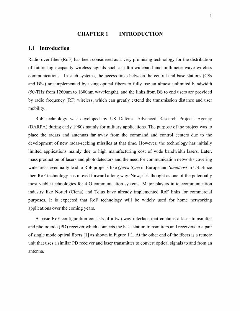
1

CHAPTER 1 INTRODUCTION

1.1 Introduction

Radio over fiber (RoF) has been considered as a very promising technology for the distribution

of future high capacity wireless signals such as ultra-wideband and millimeter-wave wireless

communications. In such systems, the access links between the central and base stations (CSs

and BSs) are implemented by using optical fibers to fully use an almost unlimited bandwidth

(50-THz from 1260nm to 1600nm wavelength), and the links from BS to end users are provided

by radio frequency (RF) wireless, which can greatly extend the transmission distance and user

mobility.

RoF technology was developed by US Defense Advanced Research Projects Agency

(DARPA) during early 1980s mainly for military applications. The purpose of the project was to

place the radars and antennas far away from the command and control centers due to the

development of new radar-seeking missiles at that time. However, the technology has initially

limited applications mainly due to high manufacturing cost of wide bandwidth lasers. Later,

mass production of lasers and photodetectors and the need for communication networks covering

wide areas eventually lead to RoF projects like Quasi-Sync in Europe and Simulcast in US. Since

then RoF technology has moved forward a long way. Now, it is thought as one of the potentially

most viable technologies for 4-G communication systems. Major players in telecommunication

industry like Nortel (Ciena) and Telus have already implemented RoF links for commercial

purposes. It is expected that RoF technology will be widely used for home networking

applications over the coming years.

A basic RoF configuration consists of a two-way interface that contains a laser transmitter

and photodiode (PD) receiver which connects the base station transmitters and receivers to a pair

of single mode optical fibers [1] as shown in Figure 1.1. At the other end of the fibers is a remote

unit that uses a similar PD receiver and laser transmitter to convert optical signals to and from an

antenna.

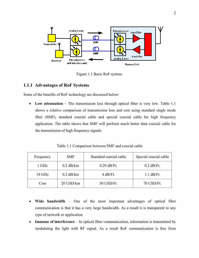
2

Figure 1.1 Basic RoF system.

1.1.1 Advantages of RoF Systems

Some of the benefits of RoF technology are discussed below:

• Low attenuation – The transmission loss through optical fiber is very low. Table 1.1

shows a relative comparison of transmission loss and cost using standard single mode

fiber (SMF), standard coaxial cable and special coaxial cable for high frequency

application. The table shows that SMF will perform much better than coaxial cable for

the transmission of high frequency signals.

Table 1.1 Comparison between SMF and coaxial cable

Frequency SMF Standard coaxial cable Special coaxial cable

1 GHz 0.2 dB/km 0.29 dB/Ft. 0.2 dB/Ft.

18 GHz 0.2 dB/km 4 dB/Ft. 1.1 dB/Ft.

Cost 20 USD/km 50 USD/Ft. 70 USD/Ft.

• Wide bandwidth – One of the most important advantages of optical fiber

communication is that it has a very large bandwidth. As a result it is transparent to any

type of network or application.

• Immune of interference – In optical fiber communication, information is transmitted by

modulating the light with RF signal. As a result RoF communication is free from

3

electromagnetic interference. Also, RoF does not suffer from multipath interference

which is a common problem in normal wireless communication.

• Low RF power – Low RF power antennas are required if fiber is used for distribution;

this has many advantages. For instance, reducing the RF power radiated by antennas

reduces interference. Reducing emitted power is also environmentally friendly.

• Economical solution – Optical fiber is very cheap (Table 1.1). If low cost lasers and

photodetectors are used RoF can provide a very economic solution for broadband access

networks. Also optical fiber communication is more reliable and costs less for

maintenance.

• Easier cell planning – In conventional wireless communication, cell planning is a

complicated task. Designers have to be careful that interference from the edge of one cell

does not affect the other. Also RoF reduces the number of handovers.

1.1.2 Applications of RoF Systems

Some of the applications of RoF technology are discussed below:

• CATV distribution systems – RoF technology has been widely used to provide video

distribution services in 40 GHz band over the last decade. Fiber to home networks

(FTTH) are used for multi-point video distribution service (MVDS) and transmission of

IEEE 802.16 broadband services.

• Local access networks – Recently there has been growing interest in transmitting

wireless signals over fiber networks for local access network (LAN) applications. Fiber

can provide a low cost communication under office environments. Over the last few

years, many work has been done on transmission of 2.4 GHz IEEE 802.11b over fiber [2-

3] and it is found that fiber has superb potential for this application. In December 2008,

Nortel (Ciena) inaugurated their solution for Ethernet over fiber in USA for LAN

applications.

• Cellular networks – Under densely populated areas, RoF fiber can become very handy

for transmission of mobile signals. In fact, during 2000 Sydney Olympics, Allen Telecom

installed BriteCell, a fiber optic-based mobile communications system. According to

press releases on the opening day of the Olympics, over 500,000 wireless calls were

4

made from Olympic Park venues. RoF systems are an effective solution under situations

like this where the number of subscriber increases suddenly in an area at a particular

time. In Canada, Telus has established their network for transmission of mobile signals

through optical fiber.

• Vehicular Technology – RoF is also used for toll collection data transfer, intelligent

transport and road to vehicle communication systems. Also a wireless sensor network with

fiber distribution is used for traffic control and traffic data collection.

1.1.3 Ultra-wideband Technology

The basic concept of ultra wideband (UWB) is to use ultra short pulse (<2 ns) in time domain to

spread the frequency energy over wide bandwidth (>500MHz) to a low level, in order to share

the spectrum with existing narrowband transmission without causing unwanted interference. The

US Federal Communications Commission (FCC) was the first to open radio spectrum of 3.1-10.6

GHz for UWB use [4]. The wireless personal area network (WPAN) working group of IEEE

responded by the draft 802.15.3a standard, which divides the whole spectrum into 14 bands with

bandwidth of 528 MHz for each band [7]. The 14 channels are organized in five groups. Each

group has three channels except group five which has only two channels. A variable throughput

from 53.3 to 480 Mb/s in each channel is suggested. To enable the operation of multiple UWB

systems at the same time, the carrier hops around in frequency. The carrier can hop to one of

fourteen channels (2904 + 528n MHz, n = 1, 2 . . . 14). Other countries quickly followed the

FCC and IEEE initiative. Though in Japan, Korea, China and European Union countries,

transmission in band group two (4.752-6.336 GHz) is not permitted to avoid interference with

existing IEEE 802.11a (wireless local area network) WLAN. The greatest advantage with UWB

radio is that it is software configurable. Therefore, any of the frequency bands can be turned off

to meet specific spectral requirements.

However, the WiMedia alliance was the first to take major initiative towards the

implementation by selecting multi-band (MB) orthogonal frequency division multiplexing

(OFDM) for high speed UWB wireless [6]. In December 2007, European Computer

Manufacturers' Association (ECMA) adopted the WiMedia approach and ratified ECMA-368

standard [7] which gave a huge boost for the industry and academia. Various prototypes of

5

WiMedia UWB devices are already in the market. Low cost UWB devices are expected to hit the

mass market by early 2012.

UWB technology shows a lot of potential. It has many important applications. These include

the following:

• Broad Band Wireless Access Networks – The most important use of UWB is in the field

of broadband WLANs. UWB devices can support bit rates of up to 480 Mb/s compared to

54 Mb/s in IEEE 802.11 WLAN and 3 Mb/s in Bluetooth, respectively. IEEE 802.11

requires high power so it cannot be used in portable handheld devices. Using Bluetooth, it

takes about 45 minutes to transfer data from a 1 Gb memory card; whereas it takes about

only 3 minutes to transfer the same data if UWB is used. Sony and Hitachi already

included UWB interfaces with their new DVD cameras. It is thought that small UWB

device will soon replace USB pen drives, garage door openers, etc.

• Stealth – In order to satisfy the effective isotropic radiated power (EIRP) requirement

defined by FCC, UWB signals are designed to have noise-like properties and the energy

of the high frequency signal is spread over a very large bandwidth. As a result, the signal

appears to be very low level background noise to an unintended narrowband receiver.

• Sensor Application – UWB can transfer data over a high bit rate without causing

interference to other narrowband systems. In the field of medical sensors, UWB can

replace wires connected to a patient’s body and improve comfort.

• Position Location – UWB systems are capable of determining the 3D location of any of

its transponders to within a few centimeters.

• Radar Imaging – UWB systems can be used as an open-air through-wall or ground-

penetrating radar imager. In several airports of Denmark and Netherlands UWB radar

imaging systems are used for searching guns and explosives. Also UWB’s ability to

penetrate through walls makes it perfect for use in cubicles under office environments.

• Vehicular Radar Systems – UWB also has applications in vehicular radar systems for use

in collision avoidance and parking aids.

Despite all its promises, UWB has a serious limitation in terms of transmission coverage.

Due to very low transmitted power, it is impossible to distribute UWB signals over air for more

than tens of meter. On the other hand, due to the wide bandwidth of 7.5 GHz it is very hard and

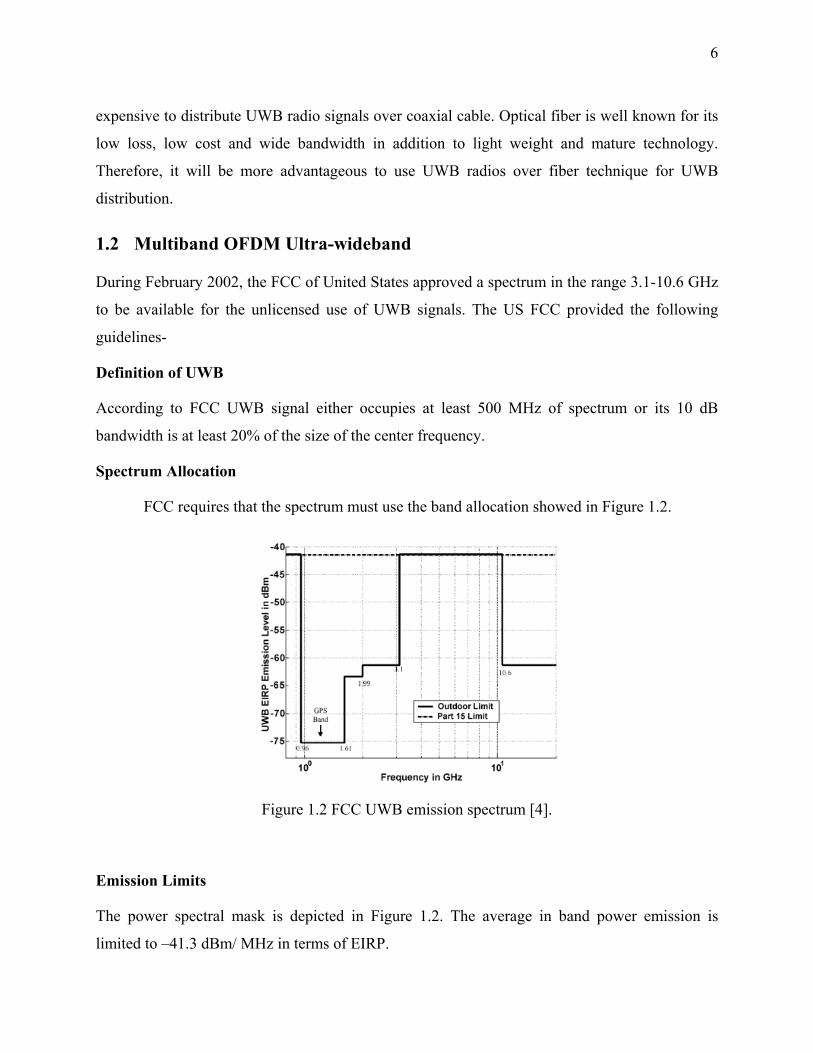
6

expensive to distribute UWB radio signals over coaxial cable. Optical fiber is well known for its

low loss, low cost and wide bandwidth in addition to light weight and mature technology.

Therefore, it will be more advantageous to use UWB radios over fiber technique for UWB

distribution.

1.2 Multiband OFDM Ultra-wideband

During February 2002, the FCC of United States approved a spectrum in the range 3.1-10.6 GHz

to be available for the unlicensed use of UWB signals. The US FCC provided the following

guidelines-

Definition of UWB

According to FCC UWB signal either occupies at least 500 MHz of spectrum or its 10 dB

bandwidth is at least 20% of the size of the center frequency.

Spectrum Allocation

FCC requires that the spectrum must use the band allocation showed in Figure 1.2.

Figure 1.2 FCC UWB emission spectrum [4].

Emission Limits

The power spectral mask is depicted in Figure 1.2. The average in band power emission is

limited to –41.3 dBm/ MHz in terms of EIRP.

7

FCC only provides a guideline for UWB rather than giving details about the PHY layer

implementation. So, several UWB transmission techniques have been proposed. These

techniques can be categorized in two major groups: single band and MB UWB. The single band

approach is implemented by direct modulation of information into a sequence of impulse like

waveforms which occupy the available bandwidth of 7.5 GHz [8]. Multiple users are supported

by using a complex time hopping sequence. But building devices to handle ultra short pulse

signal is quite challenging. Also this approach requires a very complex receiver structure. In

multi-band approach the information is processed over a small bandwidth of at least 500 MHz

[5]. This reduces design complexity and provides flexible worldwide compliance.

An MB OFDM signal consists of 128 subcarriers using quadrature phase shift keying

(QPSK) for lower bit rates. However, advanced dual carrier modulation technique is used for bit

rate of higher than 200 Mb/s.

In Appendix A the physical layer (PHY) of MB OFDM system is described as proposed in the

IEEE 802.15.3a [5] and ECMA-368 standard [7].

1.2.1 UWB over Fiber Technologies

FCC imposed a strict spectral mask for the UWB to avoid interference with existing narrow band

wireless systems. It is required that allowed EIRP is -41.3 dBm/MHz, and the total transmitted

power from a UWB antenna is limited to 0.5 mW only. In order to satisfy the EIRP requirement

defined by FCC, UWB signals are designed to have noise-like properties and the energy of the

high frequency signal is spread over a very large bandwidth. This is why the distribution of

UWB over coaxial cable is exceedingly expensive. Optical fiber provides an excellent alternative

for the distribution of UWB signals due to its low loss, low cost and wide bandwidth

characteristics.

First the UWB signal is generated from an UWB transmitter and directly drives a laser or an

optical modulator as shown in Figure 1.1, and then MB OFDM UWB signal becomes optical

subcarriers. After fiber distribution PD directly converts optical UWB subcarrier to UWB radio

signal, which will be emitted by a UWB antenna at user’s location. All the features of UWB over

fiber will be discussed in details in Chapter 2.

8

1.3 Impairments of MB-OFDM UWB in RoF

Figure 1.3 shows a point-to-point radio-over-fiber link connecting a remote antenna base station

and a central office. The MB-OFDM UWB wireless signal undergoes different signal

impairments as they propagate in the hybrid link. When the MB-OFDM UWB wireless signal is

received at the remote antenna base station, the signal is first amplified and converted to optical

signals. The electro-optical modulation can be carried out either by direct modulation using an

optical source or by external modulation combining an external modulator with an optical

carrier.

Figure 1.3 Optical impairments in point to point radio-over fiber link.

The MB-OFDM UWB signal modulated onto the optical carrier is typically very weak as a

result of low modulation efficiency at RF frequencies. The conversion efficiency in this context

refers to optical-electrical-optical conversion. In addition, the nonlinear characteristics of the

optical intensity modulator limit the amplitude of electrical modulation to a very narrow window

for linear operation. Once the MB-OFDM UWB signals are modulated onto the optical carrier,

the optical signal will be transported over the optical fiber link to the central office. The optical

distribution of the MB-OFDM UWB signals is subject to the effects of fiber chromatic

dispersion that will severely limit the overall transmission distance [1]. In addition, in a long-

reach environment, the optical signal may experience fiber nonlinearities if the optical signal

power is required to be amplified in order to overcome the link losses while the amplified optical

power is also sufficiently large to trigger the nonlinear fiber effects. Upon reception at the

receiver, the optical signal undergoes an optical-to-electrical conversion using a PD. The PD is

9

also a nonlinear device and is governed by the square-law process. Thus, the detection process

will further introduce distortions into the system. Therefore it is of great importance that these

impairments be mitigated to improve the signal quality and performance of hybrid fiber–wireless

links.

1.4 VPI Transmission Maker Simulation Tool

VPI Transmission maker is a sampling based optical simulation tool developed by VPI Photonics

Inc. The simulation tool is composed of components, e.g. laser, optical modulator, fiber,

wavelength multiplexers/demultiplexers and photodetectors that are placed on a worksheet in the

desired configuration and independently configured with parameters to model true-off-the-shelf

components including components being tested before fabrication. Some of the adjustable

parameters include thermal noise, shot noise, dispersion, etc. The samples may be processed by

each component in the design by independent samples or blocks of samples. The sample window

may be adjusted accordingly to allow for a greater resolution at the expense of extra processing

time. Included in the simulation package are visualizers, such as universal bit error rate (BER)

analyzer, optical spectrum analyzer (OSA), RF spectrum analyzer (RSA), oscilloscopes etc.

Design parameters may be swept dynamically to study the performance and stability of a design

platform. The simulation tool has the ability to track transit time and custom variables. The

package has the ability to run co-simulations with such 3rd party packages as © Matlab and ©

Python [9].

1.5 Motivation

In RoF distribution systems, optical subcarrier modulation (SCM) is used to generate typically

two sidebands around the optical carrier, i.e., double sideband SCM. It was found that optical

double sideband (ODSB) subcarrier modulation will introduce RF power fading in RoF systems

due to fiber chromatic dispersion [10]. This power fading can cause power penalty in system’s

10

performance [11] and eventually the RoF system does not work at some fiber lengths. Thus,

optical single sideband (OSSB) subcarrier modulation was proposed and has been used to

remove this power fading [12]. However when OSSB is used 3 dB RF power is lost due to the

suppression of one of the two sidebands compared to ODSB. Several approaches were proposed

to compensate for the dispersion-induced power fading in conventional ODSB analog photonic

transmission, including a modulation diversity receiver [13], nonlinearly chirped gratings [14]

and midway optical phase conjugation [15]. These techniques have increased complexity of the

receiver and limited bandwidth [13]. Also they either must be actively tuned, or introduce

differential dispersion-causing RF fading [14], or are limited by the asymmetric power change

[15-16].

Moreover RoF performance is susceptible to nonlinear distortions that can be induced by

nonlinearities in the transmission lines and optical modulator response. For example, the external

modulator such as Mach-Zehnder modulator (MZM) or Electro-absorption modulator (EAM)

exhibits a nonlinear transfer function response. The nonlinearities generate optical harmonic

distortion (HD) and intermodulation distortion (IMD), which if not suppressed will severely

degrade RoF transmission. Among the nonlinear distortions, IMD components may be the most

detrimental to the RoF transmission, because it is a high probability for them to lie very close to

and/or overlapped with the RF carriers. These undesirable components are difficult to filter out.

Optical small-signal modulation is a straightforward way to minimize optical high-order

harmonics. This is particularly important for systems sensitive to nonlinear high-order

harmonics, such as links incorporating dense-wavelength division multiplexing (DWDM), SCM,

or OFDM. In optical small-signal modulation, the optical carrier to- sideband ratio (OCSR) can

be more than 20 dB, i.e., compared to optical carrier, the generated modulated optical

sideband(s) is (are) very weak. Then in photodetection most of the received optical power is

converted to direct current (DC) while a small portion is converted to RF signals. This leads to a

very low transmission efficiency of RF signals. Moreover, since information is carried by optical

sideband(s), in RoF link with optical small-signal modulation, a relatively strong optical receiver

power is required to achieve the required signal-to-noise ratio (SNR). The consequent relatively

strong DC, which is mainly generated from the optical carrier, may damage the photodetector. In

addition, higher optical receiver power results in smaller link budget and shorter fiber link

11

distance. Also, nonlinearity problems associated with optical fiber under high optical power, like

four-wave mixing in DWDM systems, may arise and lead to additional performance

deterioration.

An effective method to improve the modulation efficiency of RoF links with small-signal

optical modulation is to reduce the optical carrier-to-sideband ratio. By suppressing the optical

carrier, more portion of optical power is converted to RF signal thus the intrinsic gain of the RoF

link is increased. A number of schemes suppressing optical carrier have been proposed and

demonstrated [17-21]. In summary, most of the demonstrated schemes are based on optical

filtering with: optical notch filter [17-18]; optical hyperfine blocking filter [19]; nonlinear

Brillouin scattering/filtering [20]; or MZM bias voltage [21]. However, these techniques need

optical carrier tuning [17-18], suffer from high insertion loss and power penalty [19], endure

signal distortion and instabilities in the transmitted power [20, 22] ; or experience chromatic

dispersion induced power fading [21].

Millimeter wave (MMW) frequency operation can provide high-capacity broadband wireless

services in picocellular or microcellular architecture. Moving the radio operating frequency into

the MMW region overcomes the spectral congestion in the lower microwave region. In addition,

the main advantages in the use of MMW band (57-64 GHz, for example) are 7 GHz bandwidth

availability as well as the prospect of multi-gigabit to terabit networks. To achieve high capacity

access networks, IEEE 802.15.3a [5] and IEEE 8.2.15.3c [23] were proposed for wideband

personal local access networks (WPLAN). In IEEE 802.15.3a 14-channel OFDM UWB wireless

using RF of 3.1-10.6 GHz band was suggested, and each channel can carry data of up to 480

Mb/s. In IEEE 802.15.3c, 4-channel OFDM millimeter-wave wireless using RF of 56-67 GHz

band was proposed and each channel can deliver data of up to 3 Gb/s. Therefore, MMW

wireless, IEEE 802.15.3c, can transmit higher data rate signals compared to IEEE 802.15.3a.

However, MMW may have a very high attenuation for transmission over air, depending on

frequency ranges, such as ~15 dB/km at 60 GHz. Therefore, the transmission of ultra-wideband

(UWB) at MMW band wirelessly is limited to a few meters and many base stations have to be

deployed for large coverage area. It is well known that optical fiber has tremendous bandwidth,

but it does not support users’ mobility and flexible system reconfiguration. Therefore, if

combining MMW wireless and optical fiber communications for access networks, it would be

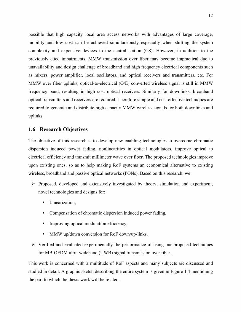
12

possible that high capacity local area access networks with advantages of large coverage,

mobility and low cost can be achieved simultaneously especially when shifting the system

complexity and expensive devices to the central station (CS). However, in addition to the

previously cited impairments, MMW transmission over fiber may become impractical due to

unavailability and design challenge of broadband and high frequency electrical components such

as mixers, power amplifier, local oscillators, and optical receivers and transmitters, etc. For

MMW over fiber uplinks, optical-to-electrical (O/E) converted wireless signal is still in MMW

frequency band, resulting in high cost optical receivers. Similarly for downlinks, broadband

optical transmitters and receivers are required. Therefore simple and cost effective techniques are

required to generate and distribute high capacity MMW wireless signals for both downlinks and

uplinks.

1.6 Research Objectives

The objective of this research is to develop new enabling technologies to overcome chromatic

dispersion induced power fading, nonlinearities in optical modulators, improve optical to

electrical efficiency and transmit millimeter wave over fiber. The proposed technologies improve

upon existing ones, so as to help making RoF systems an economical alternative to existing

wireless, broadband and passive optical networks (PONs). Based on this research, we

Proposed, developed and extensively investigated by theory, simulation and experiment,

novel technologies and designs for:

Linearization,

Compensation of chromatic dispersion induced power fading,

Improving optical modulation efficiency,

MMW up/down conversion for RoF down/up-links.

Verified and evaluated experimentally the performance of using our proposed techniques

for MB-OFDM ultra-wideband (UWB) signal transmission over fiber.

This work is concerned with a multitude of RoF aspects and many subjects are discussed and

studied in detail. A graphic sketch describing the entire system is given in Figure 1.4 mentioning

the part to which the thesis work will be related.

13

Figure 1.4 Radio-over fiber link mentioning the parts to which the thesis work will be related.

1.7 Thesis Outline

This thesis is organized as follows.

Chapter 2 will investigate in terms of error vector magnitude (EVM) the performance

degradation of MB-OFDM UWB transmission over fiber caused by various impairments

including MZM nonlinearities, fiber dispersion, receiver optical power and optical receiver

response. Also, the performance of MB-OFDM wireless UWB in terms of packet error rate

(PER) when transmitted over 20 km of SMF is experimentally investigated. PER was measured

at different bit rates to evaluate the receiver sensitivity, required minimum transmitted UWB

power, effect of wireless distance, MZM modulation index, and received optical power etc. The

performance of MB-OFDM UWB was investigated when transmitted over fiber under the effect

of relative intensity noise (RIN) considering system’s parameters such as laser output power,

linewidth and fiber transmission length. The performance of MB-OFDM UWB over fiber

transmission system is also studied considering the effect of in-band jammers such as WiMAX,

WLAN MIMO, WLAN and marine radar.

Chapters 3 and 4 propose two linearization techniques using an optical mixed polarization

for MZM and electrical pre-distortion circuit for EAM, respectively. The performance of the

14

proposed techniques will be evaluated by theory, simulation and experiment. Moreover the

proposed designs will experimentally be demonstrated for MB-OFDM UWB signal transmission

over fiber to show the potential and cost effectiveness of these techniques to be applied in current

and future broadband wireless over fiber systems.

Chapter 5 will introduce the proposed electrical compensation for chromatic dispersion

induced power fading and provide mathematical formulations behind its principle. Simulation

and experiment are also conducted for single RF tone and MB-OFDM UWB signal. The results

show the potential and cost effectiveness of the proposed technique for broadband wireless over

fiber transmission system.

Chapter 6 will present a tunable optical carrier suppression-based single sideband technique

to improve the optical modulation efficiency and receiver sensitivity in subcarrier multiplexing

RoF system. The proposed technique will be investigated by theory, simulation and experiment.

The performance improvement of the proposed technique will also be demonstrated for MB-

OFDM UWB signal to show the potential and cost effectiveness of this technique for broadband

wireless over fiber system.

Chapter 7 will describe two proposed techniques for photonic up- and down conversions of

millimeter-wave, respectively, in radio over fiber system. The millimeter-wave up conversion is

accomplished by using dual electrode MZM (DE-MZM) for frequency quadrupling. The

millimeter-wave down-conversion is achieved by using four-wave mixing in EAM. Both

techniques are comprehensively investigated and applied to MB-OFDM UWB signal showing

their potential use in broadband wireless millimeter-wave over fiber system.

Chapter 8 will conclude the thesis with summarizing the amount of progress that was

accomplished and potential implication to knowledge, theory and practice. Also discussed is the

future work that remains and over all insights.

15

CHAPTER 2 TRANSMISSION PERFORMANCE OF MB-OFDM UWB

WIRELESS SYSTEMS OVER FIBER

2.1 Introduction

MB-OFDM UWB wireless, which provides high data rate access, is required to be distributed by

using optical fiber. In this chapter, we, for the first time to our knowledge, investigate the

combined effect of fiber dispersion, and nonlinearities of optical transmitter’s and optical

receiver’s response on the OFDM subcarriers for MB OFDM UWB over fiber system through a

detailed theoretical and experimental analysis. Theoretical analysis of the effect of fiber

dispersion, optical transmitter and optical receiver response on system performance is carried out

considering amplitude and phase distortion. Theoretical analysis of the effect of fiber chromatic

dispersion induced laser phase to intensity noise or RIN on system performance is carried out.

Simulation is also made to show the relationship between RIN and center frequency of UWB

bands. Experiments are also conducted to verify our simulation and theoretical analysis and a

good agreement is obtained. The performance of MB-OFDM UWB over fiber transmission

system is also studied considering the effect of in-band jammers such as WiMAX, WLAN

MIMO, WLAN and marine radar. Experiments are performed to show the effect of fiber

transmission under various interferer power levels.

The chapter is organized into nine sections. Theoretical analyses for OSSB modulation are

given in Section 2.2 considering amplitude and phase distortion experienced by each of the

OFDM subcarriers within one symbol after transmission over fiber. In Sections 2.3 and 2.4, the

experimental and simulation setups are described, respectively. In Section 2.5, the performance

of UWB over fiber system is clarified with focus on the ECMA-368 standard using MB OFDM.

Optical transmitter’s nonlinearities and fiber dispersion effect on system performance are studied

experimentally and compared to the theoretical analysis. Also, simulations and experiments are

performed to assess the effect of optical receiver’s response and received optical power on UWB

performance. The transmission performance of wireless MB-OFDM signals over 20 km of SMF

is also investigated in Section 2.6 by measuring packet error rate (PER) at different bit rates,

transmitted and received UWB power level, RF modulation index of the MZM, wireless

transmission range, received optical power and optical receiver response. Next, the impact of

16

various physical parameters that control laser RIN and fiber transmission with focus of MB

UWB technology is discussed in Section 2.7. Thereafter, error vector magnitude (EVM)

performance of MB UWB over fiber under different in band interference scenarios is analyzed in

Section 2.8. Finally, our conclusions are drawn in Section 2.9.

2.2 Theoretical Analysis

In this section we theoretically analyze MB-OFDM UWB wireless over fiber transmission with

OSSB modulation. The common way to generate OSSB is to use a DE-MZM modulator.

However, an MZM modulator is known to be inherently nonlinear in response and may

introduce high nonlinear distortion to which OFDM signals are exposed. On the other hand, at

the receiver side a narrowband electrical bandpass filter (EBF) is usually used to filter out the

data modulated RF carrier, and the filter determines the optical receiver’s response. This filter

may have a great impact on the performance of the received data because of its response that

may introduce phase and amplitude distortion to which MB UWB OFDM signal is vulnerable.

Therefore the theoretical analysis should include the effect of DE-MZM response nonlinearities,

fiber dispersion and optical receiver’s response. Finally EVM due to fiber dispersion and RF

carrier phase noise induced phase distortion is given.

On the other hand, the radiation from a UWB system can cover 2 to 7 GHz of bandwidth. This

wide bandwidth operation makes the UWB wireless channel distinct from narrow band channels.

The wireless path loss will be expressed and the received UWB power will be calculated.

2.2.1 Calculation of EVM for Transmission through Optical Fiber using DE-

MZM

The MB OFDM RF signal (yRF(t)) is related to the complex baseband signal (xk(t)) of kth OFDM

symbol as [5]

( ) ( )( )( )1

0( ) Re exp 2

N

RF k SYM RF ck

y t x t kT V j f t tπ ϕ−

=

⎧ ⎫= − +⎨ ⎬

⎩ ⎭∑ (2.1)

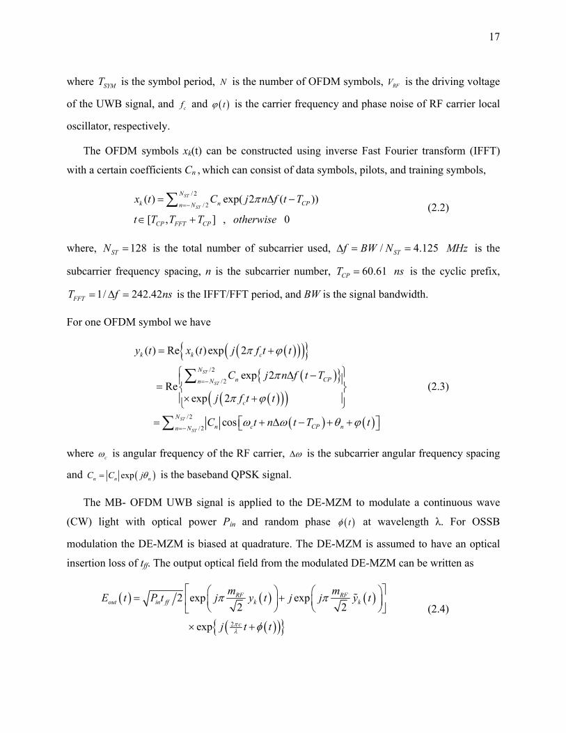
17

where SYMT is the symbol period, N is the number of OFDM symbols, RFV is the driving voltage

of the UWB signal, and cf and ( )tϕ is the carrier frequency and phase noise of RF carrier local

oscillator, respectively.

The OFDM symbols xk(t) can be constructed using inverse Fast Fourier transform (IFFT)

with a certain coefficients Cn , which can consist of data symbols, pilots, and training symbols,

/ 2

/ 2( ) exp( 2 ( ))

[ , ] , 0

ST

ST

Nk n CPn N

CP FFT CP

x t C j n f t T

t T T T otherwise

π=−

= Δ −

∈ +

∑ (2.2)

where, 128STN = is the total number of subcarrier used, / 4.125STf BW N MHzΔ = = is the

subcarrier frequency spacing, n is the subcarrier number, 60.61CPT ns= is the cyclic prefix,

1/ 242.42FFTT f ns= Δ = is the IFFT/FFT period, and BW is the signal bandwidth.

For one OFDM symbol we have

( )( )( ) ( )

( )( )( )( ) ( )

/2

/2

/2

/2

( ) Re ( )exp 2

exp 2 Re

exp 2

cos

ST

ST

ST

ST

k k c

Nn CPn N

c

Nn c CP nn N

y t x t j f t t

C j n f t T

j f t t

C t n t T t

π ϕ

π

π ϕ

ω ω θ ϕ

=−

=−

= +

⎧ ⎫Δ −⎪ ⎪= ⎨ ⎬× +⎪ ⎪⎩ ⎭

= + Δ − + +⎡ ⎤⎣ ⎦

∑

∑

(2.3)

where cω is angular frequency of the RF carrier, ωΔ is the subcarrier angular frequency spacing

and ( )expn n nC C jθ= is the baseband QPSK signal.

The MB- OFDM UWB signal is applied to the DE-MZM to modulate a continuous wave

(CW) light with optical power Pin and random phase ( )tφ at wavelength λ. For OSSB

modulation the DE-MZM is biased at quadrature. The DE-MZM is assumed to have an optical

insertion loss of tff. The output optical field from the modulated DE-MZM can be written as

( ) ( ) ( )

( )( ) 2

2 exp exp2 2

exp

RF RFout in ff k k

c

m mE t P t j y t j j y t

j t tπλ

π π

φ

⎡ ⎤⎛ ⎞ ⎛ ⎞= +⎢ ⎥⎜ ⎟ ⎜ ⎟⎝ ⎠ ⎝ ⎠⎣ ⎦

× +

(2.4)

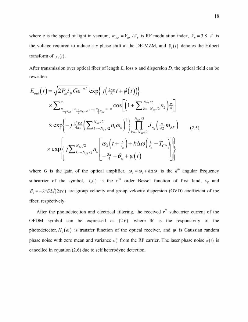
18

where c is the speed of light in vacuum, /RF RFm V Vπ= is RF modulation index, 3.8V Vπ = is

the voltage required to induce a π phase shift at the DE-MZM, and ( )ky t denotes the Hilbert

transform of ( )ky t .

After transmission over optical fiber of length L, loss α and dispersion D, the optical field can be

rewritten

( ) ( )( ) ( )

( ) ( )

( )

1 1 112 2 2

2

2

/24, , ..., /2

/22/24 2/2

/2

2 exp

cos 1

exp

exp

ST

STN N NST ST ST

STST

kSTST

g

L cout in ff

Nkn n n k N

NNDL

k k n RFc k Nk N

Lk v

k

E t P t Ge j t t

n

j n J m

t kj n

α πλ

π

λ ππ

φ

ω

ω ω

− − +

−

∞

=−∞ =−

=−=−

= +

⎡ ⎤× +⎢ ⎥⎣ ⎦

× −

+ + Δ×

∑ ∑

∑ ∏

( )( )

2

2 34

ST g

ST

LN CPv

k Nk

T

tπ θ ϕ=−

⎧ ⎫⎡ ⎤−⎪ ⎪⎢ ⎥⎨ ⎬⎢ ⎥+ + +⎪ ⎪⎣ ⎦⎩ ⎭

∑

(2.5)

where G is the gain of the optical amplifier, k c kω ω ω= + Δ is the kth angular frequency

subcarrier of the symbol, ( )nJ ⋅ is the nth order Bessel function of first kind, vg and

( )22 2DL cβ λ π= − are group velocity and group velocity dispersion (GVD) coefficient of the

fiber, respectively.

After the photodetection and electrical filtering, the received rth subcarrier current of the

OFDM symbol can be expressed as (2.6), where ℜ is the responsivity of the

photodetector, ( )eH ω is transfer function of the optical receiver, and φr is Gaussian random

phase noise with zero mean and variance 2ϕσ from the RF carrier. The laser phase noise ( )tφ is

cancelled in equation (2.6) due to self heterodyne detection.

19

( ) ( ) ( ) ( ) ( )( ) ( )( )

( )( ) ( )( )

12 4

221 1

1 2 0 22 22,

221 1

1 2 0 22 4 2 42,

211 22

exp

2 2 sin 2 sin

2 sin 2 sin

2 cos

g

ST

ST

ST

ST

L Lr in ff r e r r CP r rv

N

RF r RF r kk N r

N

RF r RF r kk N r

RF r

i t P t Ge H j t r T

J m L J m L

jJ m L J m L

jJ m L

α π

π π

ω ω ω ω θ ϕ

π β ω π β ω ω

π β ω π β ω ω

π β ω

−

=− ≠

=− ≠

⎡ ⎤= − ℜ + − Δ + + +⎢ ⎥⎣ ⎦

× + + +

+

∏

∏

( )( ) ( )( )2

10 24 2 4

2,

2 cosST

ST

N

RF r kk N r

J m Lπ ππ β ω ω=− ≠

⎧ ⎫⎪ ⎪⎪ ⎪⎪ ⎪⎪ ⎪⎨ ⎬⎪ ⎪⎪ ⎪⎪ ⎪+ +⎪ ⎪⎩ ⎭

∏

(2.6)

Equation (2.6) shows that each subcarrier will be distorted in amplitude and phase. This

distortion results from intrinsic nonlinearities of the DE-MZM response, fiber dispersion and

frequency response of the optical receiver.

Considering a low RF modulation index of 1RFm and the ideal optical receiver, we can

simplify equation (2.6) into

( )

( )

12 2

23 124 2 exp

g

L RFr in ff

Lr r CP r r rv

Vi t P t GeV

C j t r T L

α

π

π

π

ω ω β ω θ ϕ

−= −

⎡ ⎤× + − Δ + − + +⎣ ⎦

(2.7)

Using the approximation of 2 2 2r c crω ω ω ω+ Δ∼ , the received OFDM symbol can be written as

( ) ( )

( ) 2

2

2

2ˆ exp

ST

ST

ST

gST

Nk rr N

N Lr CPvr N

y t i t

Y jr t Tω

=−

=−

∞

∞ Δ + −

∑∑

(2.8)

where ( ) 2ˆ expr r c rY X j r Lβ ω ω ϕ= − Δ + is the normalized received symbol corresponding to the

transmitted symbol ( )expr r rX C jθ= of the rth subcarrier. Assuming that constant delay will be

compensated by cyclic prefix, the EVM can be approximated using [24]

( )( )

2220 2

2 222

1 ˆ

2 1 cos

ST

ST

ST

ST

Nk kk N

ST

Nk c kk N

ST

EVM Y XN

X k LN

β ω ω ϕ

=−

=−

= −

= − Δ +

∑

∑ (2.9)

Using the following identities

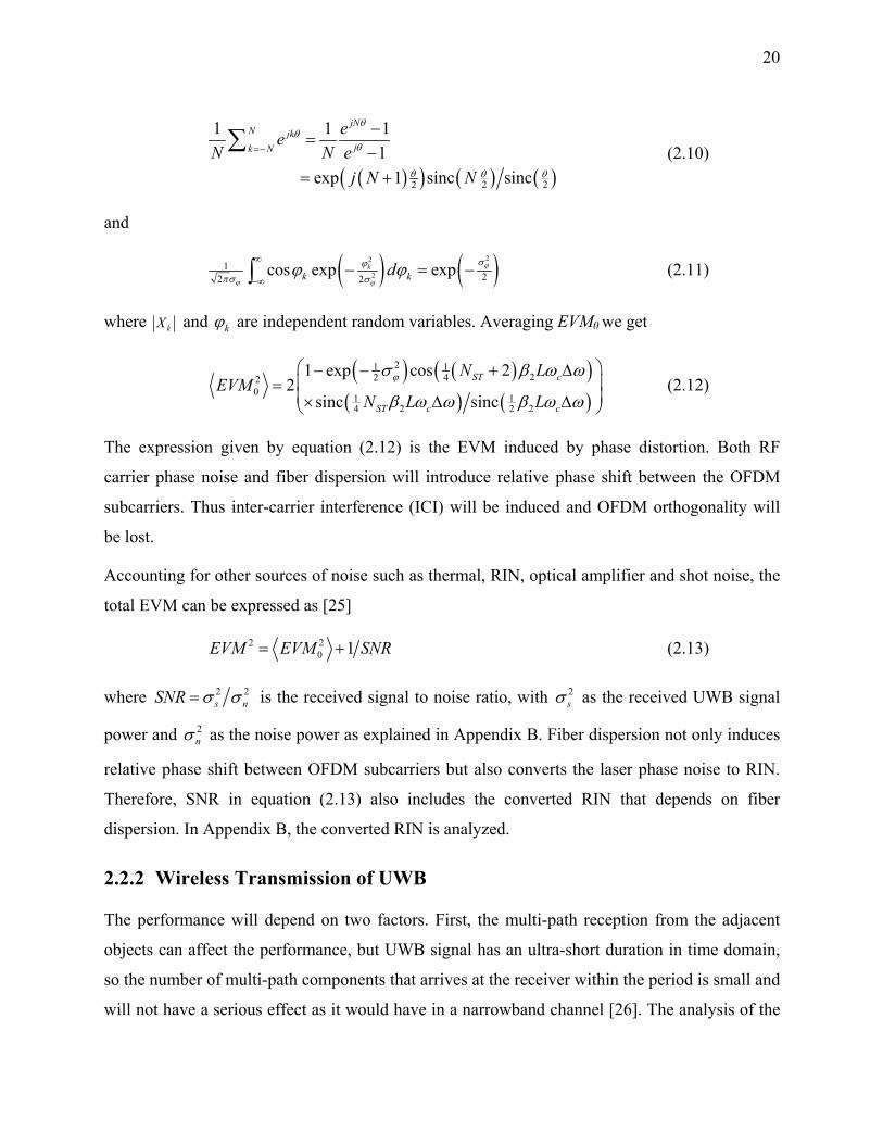
20

( )( ) ( ) ( )2 22

1 1 11

exp 1 sinc sinc

jNN jk

jk N

eeN N e

j N N

θθ

θ

θ θ θ

=−

−=

−= +

∑ (2.10)

and

( ) ( )22

21

22 2cos exp expk

k kd ϕ

ϕ ϕ

σϕπσ σ

ϕ ϕ∞

−∞− = −∫ (2.11)

where kX and kϕ are independent random variables. Averaging EVM0 we get

( ) ( )( )

( ) ( )

21 122 42

01 1

2 24 2

1 exp cos 22

sinc sincST c

ST c c

N LEVM

N L Lϕσ β ω ω

β ω ω β ω ω

⎛ ⎞− − + Δ⎜ ⎟=⎜ ⎟× Δ Δ⎝ ⎠

(2.12)

The expression given by equation (2.12) is the EVM induced by phase distortion. Both RF

carrier phase noise and fiber dispersion will introduce relative phase shift between the OFDM

subcarriers. Thus inter-carrier interference (ICI) will be induced and OFDM orthogonality will

be lost.

Accounting for other sources of noise such as thermal, RIN, optical amplifier and shot noise, the

total EVM can be expressed as [25]

2 20 1EVM EVM SNR= + (2.13)

where 2 2s nSNR σ σ= is the received signal to noise ratio, with 2

sσ as the received UWB signal

power and 2nσ as the noise power as explained in Appendix B. Fiber dispersion not only induces

relative phase shift between OFDM subcarriers but also converts the laser phase noise to RIN.

Therefore, SNR in equation (2.13) also includes the converted RIN that depends on fiber

dispersion. In Appendix B, the converted RIN is analyzed.

2.2.2 Wireless Transmission of UWB

The performance will depend on two factors. First, the multi-path reception from the adjacent

objects can affect the performance, but UWB signal has an ultra-short duration in time domain,

so the number of multi-path components that arrives at the receiver within the period is small and

will not have a serious effect as it would have in a narrowband channel [26]. The analysis of the

21

effect of multi-path is rather complex and highly dependent on the environment. As a rule of

thumb, the loss increases due to multi-path when the distance between the transmitting and

receiving antennas is increased. Secondly, the path loss is of an important issue, which at a

distance d is given by [27]

( ) ( ) ( )0 10 010 log /L LP d P d d S dγ= + +⎡ ⎤⎣ ⎦ (2.14)

here 1020 log (4 / ) 44 dBLO cP f d cπ= ≈ is the path loss for d0 = 1 m, min max 3.88 GHzcf f f= = where

fmin = 3.168 GHz and fmax = 4.752 GHz being the lower and upper -10 dB cutoff frequencies of

the power spectrum of band group 1 for MB-OFDM UWB system, 10 010 log ( / )d dγ is the mean

path-loss referenced to 1 m, 2γ ≈ is the path-loss exponent and S(d) represents the lognormal

shadowing [26-27] and can be approximated from transmitted and received RF power

measurement to 1.85 dB with a standard deviation of 0.3. All the values stated are empirical

values for a line of sight (LOS) model with omnidirectional transmit and receive antennas and

can vary from location to location. Then the RF power at the receiver (Prec) in terms of

transmitted UWB power (Puwb), transmit antenna gain (GT) and receive antenna gain (GR) can be

expressed by

( )rec uwb T R LP P G G P d= + + − (2.15)

In the experiment, we used pair of In4Tel antennas with gain 2 dBiT RG G= = . Therefore, from the

above equation it is seen that the received power will depend mainly on the mean path-loss

referenced to 1 m.

2.3 Experimental System Configuration

The considered system setup for the performance evaluation of UWB over fiber is shown in

Figure 2.1. A commercially available evaluation board, DV 9110M TX (point A in Figure 2.1),

from WisAir, providing MB-OFDM compliant modulation with three WiMedia sub-bands

allocated at center frequency of 3.432, 3.96 and 4.488 GHz, is used for MB-UWB generation.

For the performance evaluation of UWB wireless systems with fiber distribution, the UWB

signal after 20km of fiber transmission is launched to air by an antenna and received by a

receiver module DV 9110M RX (point E in Figure 2.1) . A laptop is used to run the built-in

22

WisMan software provided with the DV 9110M modules to configure and control the transmitter

and receiver modules. Number of transmitted packets is fixed at 106 and each packet has 1024

octets. The PER is evaluated from number of the transmitted and received packets.

An arbitrary waveform generator, AWG 7122B (point B in Figure 2.1), from Tektronix with

9.6 GHz effective RF bandwidth is used for UWB signal generation. First the MB-OFDM UWB

signals compliant with WiMedia standard [5] and the narrow band interferers are generated using

MATLAB. For the MB-OFDM UWB signal each generated sub-band has an RF bandwidth of

528 MHz with 128 OFDM subcarriers and bit rate of 200 Mb/s with QPSK modulation. Among

the subcarriers, 100 subcarriers carry data and the rest are null, pilot and guard tones. The

separation between subcarriers is 4.125 MHz. The signal also has a cyclic prefix and guard

interval of 60.61 and 9.47 ns, respectively. The generated WiMedia sub-band follows a simple

hopping sequence as f1, f2, and f3 according to Time Frequency Code (TFC) 1, defined in

WiMedia standard [5], so that only one channel exists at any particular time.

Figure 2.1 Experimental setup for externally modulated MB-OFDM UWB over fiber system

(BW: bandwidth, G: gain, NF: noise figure, R: responsivity)

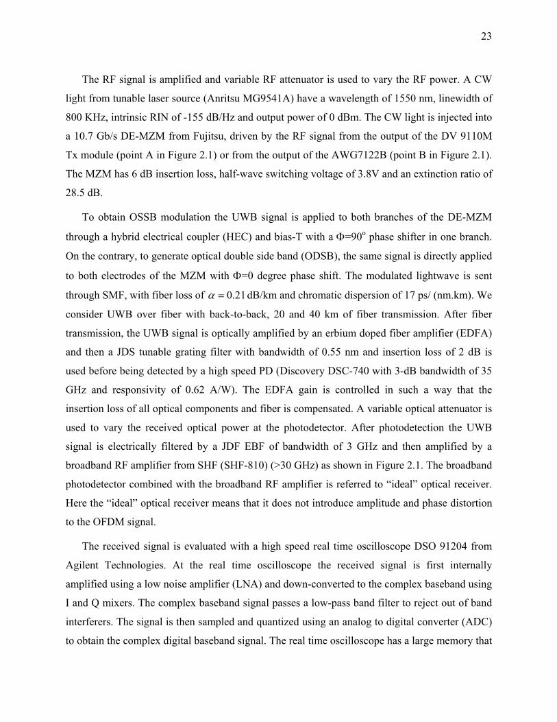
23

The RF signal is amplified and variable RF attenuator is used to vary the RF power. A CW

light from tunable laser source (Anritsu MG9541A) have a wavelength of 1550 nm, linewidth of

800 KHz, intrinsic RIN of -155 dB/Hz and output power of 0 dBm. The CW light is injected into

a 10.7 Gb/s DE-MZM from Fujitsu, driven by the RF signal from the output of the DV 9110M

Tx module (point A in Figure 2.1) or from the output of the AWG7122B (point B in Figure 2.1).

The MZM has 6 dB insertion loss, half-wave switching voltage of 3.8V and an extinction ratio of

28.5 dB.

To obtain OSSB modulation the UWB signal is applied to both branches of the DE-MZM

through a hybrid electrical coupler (HEC) and bias-T with a Φ=90o phase shifter in one branch.

On the contrary, to generate optical double side band (ODSB), the same signal is directly applied

to both electrodes of the MZM with Φ=0 degree phase shift. The modulated lightwave is sent

through SMF, with fiber loss of 0.21α = dB/km and chromatic dispersion of 17 ps/ (nm.km). We

consider UWB over fiber with back-to-back, 20 and 40 km of fiber transmission. After fiber

transmission, the UWB signal is optically amplified by an erbium doped fiber amplifier (EDFA)

and then a JDS tunable grating filter with bandwidth of 0.55 nm and insertion loss of 2 dB is

used before being detected by a high speed PD (Discovery DSC-740 with 3-dB bandwidth of 35

GHz and responsivity of 0.62 A/W). The EDFA gain is controlled in such a way that the

insertion loss of all optical components and fiber is compensated. A variable optical attenuator is

used to vary the received optical power at the photodetector. After photodetection the UWB

signal is electrically filtered by a JDF EBF of bandwidth of 3 GHz and then amplified by a

broadband RF amplifier from SHF (SHF-810) (>30 GHz) as shown in Figure 2.1. The broadband

photodetector combined with the broadband RF amplifier is referred to “ideal” optical receiver.

Here the “ideal” optical receiver means that it does not introduce amplitude and phase distortion

to the OFDM signal.

The received signal is evaluated with a high speed real time oscilloscope DSO 91204 from

Agilent Technologies. At the real time oscilloscope the received signal is first internally

amplified using a low noise amplifier (LNA) and down-converted to the complex baseband using

I and Q mixers. The complex baseband signal passes a low-pass band filter to reject out of band

interferers. The signal is then sampled and quantized using an analog to digital converter (ADC)

to obtain the complex digital baseband signal. The real time oscilloscope has a large memory that

24

stores about 5 million samples of the signal for processing. Baseband processing begins with the

packet detection followed by Fast Fourier transform (FFT) operation. The output signal from the

FFT is equalized using a frequency domain equalizer. A phase correction is applied to the output

of the equalizer to undo the effect of carrier and timing mismatch between transmitter and

receiver according to ECMA-368 standard [7]. The pilot tones in each OFDM symbol are used to

drive the digital phase-locked-loop (PLL). The output of the equalizer is de-mapped and de-

interleaved before passing to a Viterbi decoder. The error corrected bit sequence is descrambled

and passed on to the media access control (MAC) layer for further processing.

EVM or relative constellation root mean square (RMS) error is the PHY performance and it

contains information about both phase and amplitude errors that are more useful for assessing

microwave properties of the signal like the random noise, phase noise, Amplitude/Amplitude

(AM/AM) distortion, Amplitude/Phase (AM/PM) distortion, delay distortion and interference

effects. Average EVM in WiMedia PHY 1.2 standard [7] is computed as follows

2 2

, , , ,1 1

1 1 0

[ ] [ ] [ ] [ ]1

( )

D P

f packet

sync hdr

N N

N N D n D n P n P nk k

i n N Nf D P frame

R k C k R k C kEVM

N N N N P= =

= = + +

⎡ ⎤− + −⎢ ⎥

⎢ ⎥=+⎢ ⎥

⎢ ⎥⎣ ⎦

∑ ∑∑ ∑ (2.16)

where Nf is the number of packets under test, Npacket is the number of symbols in the packet, Nsync

is the number of symbols in the preamble, Nhdr is the number of symbols in the header, Nframe =

Npacket − Nsync − Nhdr is the number of symbols in the frame, ND is the number of data subcarriers,

NP is the number of pilot subcarriers, P0 is the average power over all payload symbols of the

data and pilot constellations, CD,n[k] and CP,n[k] are the transmitted kth data subcarrier and kth

pilot subcarrier for the nth OFDM symbol, respectively, and RD,n[k] and RP,n[k] are the observed

kth data subcarrier and kth pilot subcarrier for the nth OFDM symbol, respectively.

The EVM required at the transmitter for bit rates of up to 200 Mb/s is -17dB and above 200

Mb/s it is -19.5 dB respectively with no transmitter attenuation [7]. For conformance testing -16

dB is the EVM limit for 200 Mb/s. The EVM is analyzed on the payload portion of the packet

only, over a minimum of 100 packets generated from random data. The payload of each packet

has to be at least 30 symbols in length. In our experiment each packet consists of 60 symbols.

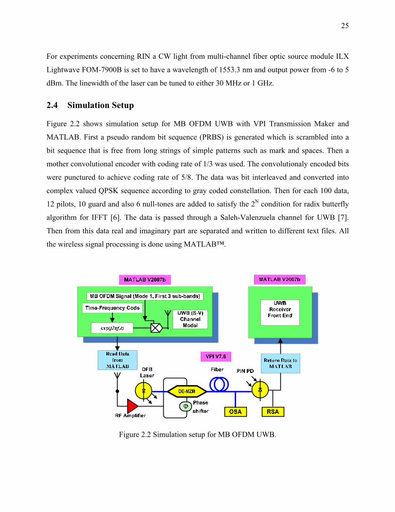
25

For experiments concerning RIN a CW light from multi-channel fiber optic source module ILX

Lightwave FOM-7900B is set to have a wavelength of 1553.3 nm and output power from -6 to 5

dBm. The linewidth of the laser can be tuned to either 30 MHz or 1 GHz.

2.4 Simulation Setup

Figure 2.2 shows simulation setup for MB OFDM UWB with VPI Transmission Maker and

MATLAB. First a pseudo random bit sequence (PRBS) is generated which is scrambled into a

bit sequence that is free from long strings of simple patterns such as mark and spaces. Then a

mother convolutional encoder with coding rate of 1/3 was used. The convolutionaly encoded bits

were punctured to achieve coding rate of 5/8. The data was bit interleaved and converted into

complex valued QPSK sequence according to gray coded constellation. Then for each 100 data,

12 pilots, 10 guard and also 6 null-tones are added to satisfy the 2N condition for radix butterfly

algorithm for IFFT [6]. The data is passed through a Saleh-Valenzuela channel for UWB [7].

Then from this data real and imaginary part are separated and written to different text files. All

the wireless signal processing is done using MATLAB™.

Figure 2.2 Simulation setup for MB OFDM UWB.

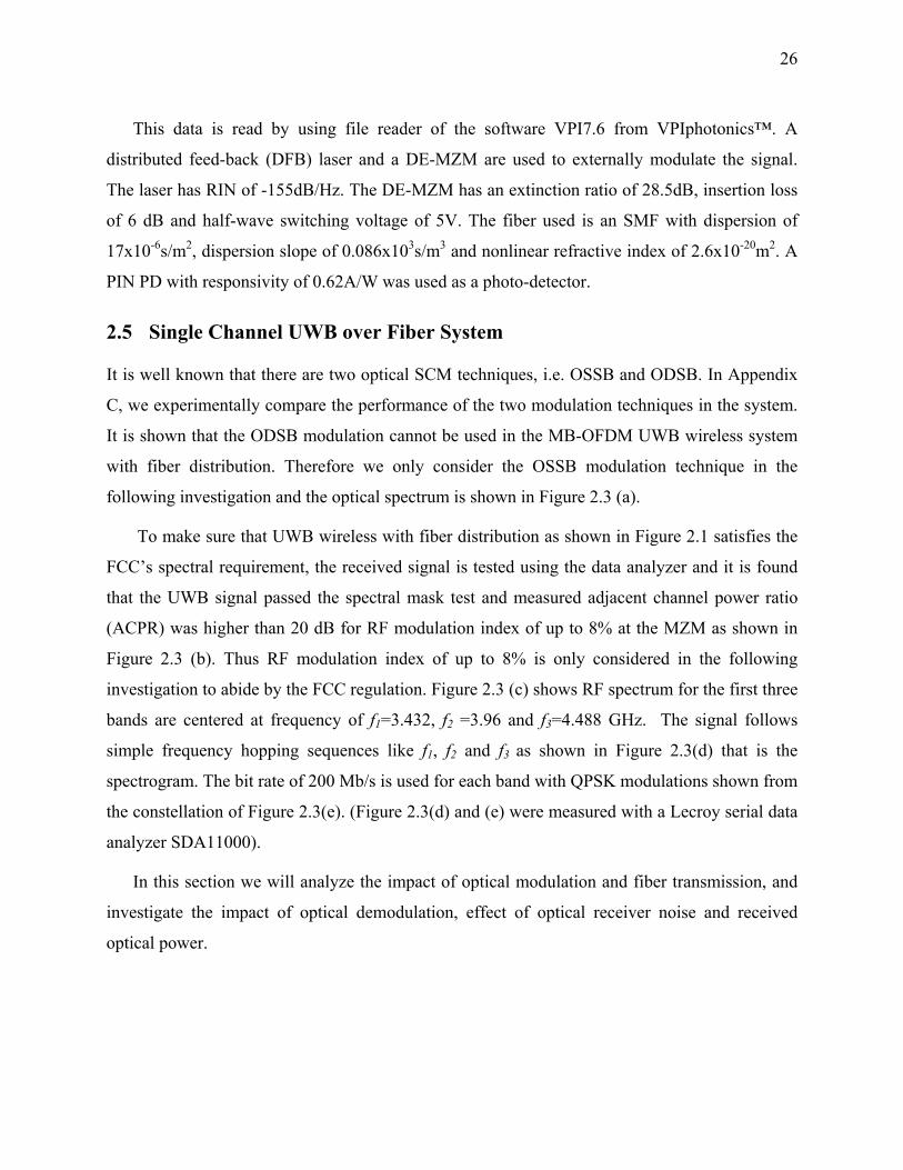
26

This data is read by using file reader of the software VPI7.6 from VPIphotonics™. A

distributed feed-back (DFB) laser and a DE-MZM are used to externally modulate the signal.

The laser has RIN of -155dB/Hz. The DE-MZM has an extinction ratio of 28.5dB, insertion loss

of 6 dB and half-wave switching voltage of 5V. The fiber used is an SMF with dispersion of

17x10-6s/m2, dispersion slope of 0.086x103s/m3 and nonlinear refractive index of 2.6x10-20m2. A

PIN PD with responsivity of 0.62A/W was used as a photo-detector.

2.5 Single Channel UWB over Fiber System

It is well known that there are two optical SCM techniques, i.e. OSSB and ODSB. In Appendix

C, we experimentally compare the performance of the two modulation techniques in the system.

It is shown that the ODSB modulation cannot be used in the MB-OFDM UWB wireless system

with fiber distribution. Therefore we only consider the OSSB modulation technique in the

following investigation and the optical spectrum is shown in Figure 2.3 (a).

To make sure that UWB wireless with fiber distribution as shown in Figure 2.1 satisfies the

FCC’s spectral requirement, the received signal is tested using the data analyzer and it is found

that the UWB signal passed the spectral mask test and measured adjacent channel power ratio

(ACPR) was higher than 20 dB for RF modulation index of up to 8% at the MZM as shown in

Figure 2.3 (b). Thus RF modulation index of up to 8% is only considered in the following

investigation to abide by the FCC regulation. Figure 2.3 (c) shows RF spectrum for the first three

bands are centered at frequency of f1=3.432, f2 =3.96 and f3=4.488 GHz. The signal follows

simple frequency hopping sequences like f1, f2 and f3 as shown in Figure 2.3(d) that is the

spectrogram. The bit rate of 200 Mb/s is used for each band with QPSK modulations shown from

the constellation of Figure 2.3(e). (Figure 2.3(d) and (e) were measured with a Lecroy serial data

analyzer SDA11000).

In this section we will analyze the impact of optical modulation and fiber transmission, and

investigate the impact of optical demodulation, effect of optical receiver noise and received

optical power.

27

-50

-40

-30

-20

-10

0

-0.1 -0.05 0 0.05 0.1

Pow

er (d

Bm

)

Wavelength (nm) relative to 1549.892 nm (a) (b)

f 3Freq

uenc

y f 2

f 1

Qua

drat

ure

10dB

/div

(c) (d) (e)

Figure 2.3 First three bands of MB-OFDM UWB wireless in (a) Optical spectrum, (b) spectral

mask test according to FCC, (c) frequency domain, (d) frequency-time domain and (e) received

constellation.

2.5.1 Impact of Optical Modulation and Fiber Transmission

Using the setup as shown in Figure 2.1, we experimentally characterize the impact of optical

modulation and fiber transmission using measured EVM. For different fiber lengths, we adjust

the gain of the EDFA to fully compensate for all loss and keep the same input power to the PD.

The ideal optical receiver used has broadband response with flat magnitude and linear delay over

the considered signal bandwidth. Figure 2.4 shows measured EVM with RF modulation index

for UWB over fiber with fiber length of 0, 20 and 40 km, considering bit rate of 53.3 and 200

Mb/s. It is apparent that the minimum EVM is obtained at RF modulation index of 3~4 % for

both 53.3 and 200 Mb/s, almost independent of the bit rate, as shown in Figure 2.4 (a) and (b). At

the low RF power the EVM is high due to low SNR. On the other hand, at the high power level

the EVM increases due to DE-MZM nonlinearities and fiber dispersion induced nonlinear

distortion mainly.

28

-24

-23

-22

-21

-20

-19

-18

1 2 3 4 5 6 7 8

0 km 20 km 40 km

EVM

(dB

)

RF modulation index (%)

53.3 Mb/s

-24

-23

-22

-21

-20

-19

-18

1 2 3 4 5 6 7 8RF modulation index (%)

200 Mb/s

(a) (b)

Figure 2.4 Measured EVM with RF modulation index with a parameter of fiber length for bit rate

of (a) 53.3Mb/s and (b) 200Mb/s.

To fully understand the behaviors in Figure 2.4, it is required to have a full understanding of

nonlinear distortion. It is well known that the OFDM signal has a high peak to average power

ratio (PAPR). The measured PAPR for the UWB signal is about 14~17 dB from the DV9110

module. Nonlinear distortion for the UWB signal can be induced by RF amplifier due to large

PAPR, phase noise of the RF carrier local oscillator due to Phase/ Amplitude (PM/AM)

conversion and nonlinear response of the DE-MZM. However, RF amplifier can induce

nonlinear distortion only at higher RF power level. But for OFDM UWB, the RF amplifier is

operated in the linear region for most of the time owing to low power spectral density of the

UWB. The phase noise may induce nonlinear distortion due to PM/AM conversion and created

PM/AM modulation is imposed onto the complex waveform. Nonlinear distortion induced by the

nonlinearities of the DE-MZM due to AM/AM modulation and fiber dispersion due to PM/AM

conversion is the most important. Equation (2.6) reveals that the DE-MZM nonlinearities

combined with fiber dispersion will induce both AM/AM and PM/AM distortion within one

symbol.

To distinguish the impact of the DE-MZM response nonlinearities and fiber dispersion, we

first consider the back to back UWB over fiber, i.e. without fiber. If the response nonlinearities

of the DE-MZM are only considered, equation (2.6) is reduced to

29

( ) ( ) ( )

11 0

4 exp

STNLr in ff RF RF

r CP r

i t P t Ge J m J m

j t r T

α

π

π π

ω ω θ

−−= ⎡ ⎤⎣ ⎦

× − Δ − +⎡ ⎤⎣ ⎦ (2.17)

where the ideal optical receiver response is assumed.

It can be noted from equation (2.17), that the received constellation is rotated by 45o. It is also

shown that there is a pure AM/AM conversion induced distortion due to the term of

( ) ( ) 11 0

STNRF RFJ m J mπ π

−⎡ ⎤⎣ ⎦ , which depends only on the total transmitted RF power level at the

DE-MZM. Figure 2.5 shows the relative amplitude (i.e. ( ) ( ) 11 02 STN

RF RFJ m J mπ π−

⎡ ⎤⎣ ⎦ ) of the 128

subcarriers versus RF modulation index for the second band. It is obvious that the amplitude of

all the 128 subcarriers is the same for any modulation index, and almost linearly increases with

modulation index at RF modulation index of up to 4%. However, RF modulation index of higher

than 4% will decrease the amplitude, i.e. AM/AM compression. Consequently RF modulation

index of 4% is found optimum theoretically. This optimum modulation index of 4% is almost in

good agreement with the above experimental results as shown in Figure 2.4. However, there is a

small discrepancy between the optimum modulation indexes found from Figure 2.4 and Figure

2.5. This small discrepancy is mainly due to our simplified approach used in theory where it is

assumed that all subcarriers are carrying data, DE-MZM extinction ratio is infinite, and there is

no dependence of transmitted power level on bit rate.

In order to investigate the combined effect of fiber dispersion and DE-MZM response

nonlinearities on each of the 128 subcarriers, relative amplitude of the subcarriers at 1, 32, 64,

96, and 128 in the second band (centered at 3.96 GHz) after fiber transmission of 20 and 40 km

is shown in Figure 2.6, calculated by equation (2.6). It is shown that all the subcarriers have

identical relative amplitude that increases almost linearly with the RF modulation index of up to

~4%. However, the subcarriers may not have the same amplitude if modulation index is more

than 4%. For example, at the modulation index of 10%, the subcarriers have different amplitudes

as shown in Figure 2.6(a) and (b). This is contrary to the back-to-back transmission as shown in

Figure 2.5. Any amplitude mismatch between subcarriers will distort the received constellation

and degrade the EVM. For the back-to-back UWB over fiber system, the relative phase of the

128 subcarriers is constant and -450 for any modulation index. Because fiber dispersion will

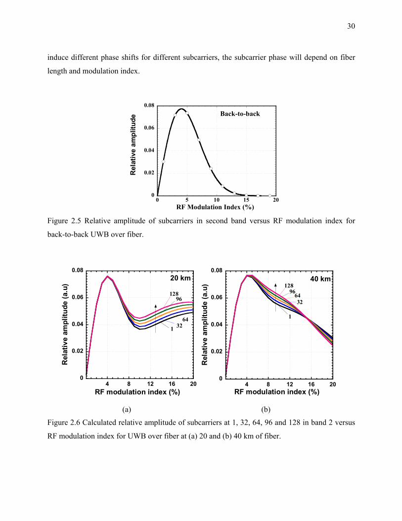
30

induce different phase shifts for different subcarriers, the subcarrier phase will depend on fiber

length and modulation index.

0

0.02

0.04

0.06

0.08

0 5 10 15 20RF Modulation Index (%)

Rel

ativ

e am

plitu

de Back-to-back

Figure 2.5 Relative amplitude of subcarriers in second band versus RF modulation index for

back-to-back UWB over fiber.

0

0.02

0.04

0.06

0.08

4 8 12 16 20

Rel

ativ

e am

plitu

de (a

.u)


12896

64321

20 km

0

0.02

0.04

0.06

0.08

4 8 12 16 20

Rel

ativ

e am

plitu

de (a

.u)


12896

6432

1

40 km

(a) (b)

Figure 2.6 Calculated relative amplitude of subcarriers at 1, 32, 64, 96 and 128 in band 2 versus

RF modulation index for UWB over fiber at (a) 20 and (b) 40 km of fiber.

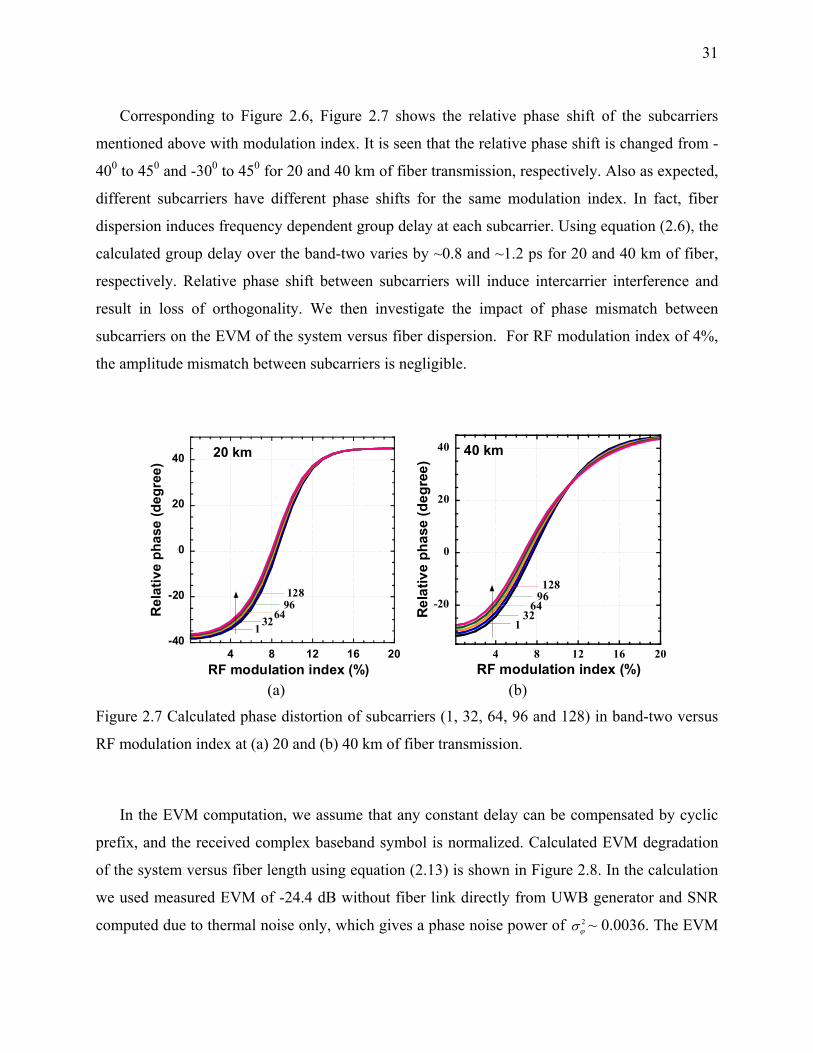
31

Corresponding to Figure 2.6, Figure 2.7 shows the relative phase shift of the subcarriers

mentioned above with modulation index. It is seen that the relative phase shift is changed from -

400 to 450 and -300 to 450 for 20 and 40 km of fiber transmission, respectively. Also as expected,

different subcarriers have different phase shifts for the same modulation index. In fact, fiber

dispersion induces frequency dependent group delay at each subcarrier. Using equation (2.6), the

calculated group delay over the band-two varies by ~0.8 and ~1.2 ps for 20 and 40 km of fiber,

respectively. Relative phase shift between subcarriers will induce intercarrier interference and

result in loss of orthogonality. We then investigate the impact of phase mismatch between

subcarriers on the EVM of the system versus fiber dispersion. For RF modulation index of 4%,

the amplitude mismatch between subcarriers is negligible.

-40

-20

0

20

40

4 8 12 16 20

Rel

ativ

e ph

ase

(deg

ree)


12896

64321

20 km

-20

0

20

40

4 8 12 16 20

Rel

ativ

e ph

ase

(deg

ree)


12896

6432

1

40 km

(a) (b)

Figure 2.7 Calculated phase distortion of subcarriers (1, 32, 64, 96 and 128) in band-two versus

RF modulation index at (a) 20 and (b) 40 km of fiber transmission.

In the EVM computation, we assume that any constant delay can be compensated by cyclic

prefix, and the received complex baseband symbol is normalized. Calculated EVM degradation

of the system versus fiber length using equation (2.13) is shown in Figure 2.8. In the calculation

we used measured EVM of -24.4 dB without fiber link directly from UWB generator and SNR

computed due to thermal noise only, which gives a phase noise power of 2ϕσ ~ 0.0036. The EVM

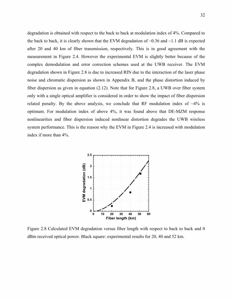
32

degradation is obtained with respect to the back to back at modulation index of 4%. Compared to

the back to back, it is clearly shown that the EVM degradation of ~0.36 and ~1.1 dB is expected

after 20 and 40 km of fiber transmission, respectively. This is in good agreement with the

measurement in Figure 2.4. However the experimental EVM is slightly better because of the

complex demodulation and error correction schemes used at the UWB receiver. The EVM

degradation shown in Figure 2.8 is due to increased RIN due to the interaction of the laser phase

noise and chromatic dispersion as shown in Appendix B, and the phase distortion induced by

fiber dispersion as given in equation (2.12). Note that for Figure 2.8, a UWB over fiber system

only with a single optical amplifier is considered in order to show the impact of fiber dispersion

related penalty. By the above analysis, we conclude that RF modulation index of ~4% is

optimum. For modulation index of above 4%, it was found above that DE-MZM response

nonlinearities and fiber dispersion induced nonlinear distortion degrades the UWB wireless

system performance. This is the reason why the EVM in Figure 2.4 is increased with modulation

index if more than 4%.

0

0.5

1

1.5

2

2.5

0 10 20 30 40 50 60

EVM

deg

rada

tion

(dB

)

Fiber length (km)

Figure 2.8 Calculated EVM degradation versus fiber length with respect to back to back and 0

dBm received optical power. Black square: experimental results for 20, 40 and 52 km.

33

2.5.2 Impact of Optical Demodulation

In this subsection, we will analyze the impact of optical demodulation. We consider two cases:

one is the “ideal” optical receiver and the other is bandwidth-limited and has variation of

magnitude and time delay over the OFDM signal bandwidth. The bandwidth-limited optical

receiver is obtained by inserting a bandwidth-limited electrical filter in the “ideal” optical

receiver. Equation (2.6) shows that the band limited optical receiver response will have great

impact on overall performance.

We used a Chebyshev-I bandpass filter (BPF) centered at frequency, 4cf = GHz with a 3 dB

bandwidth of 3 GHz. The magnitude and phase response measured are shown in Figure 2.9. It is

clearly seen from Figure 2.9(a) that the magnitude response of filter has a ripple of ±0.5 dB over

the passband. It is expected that the magnitude ripple will induce distortion for the subcarriers of

the OFDM signal. We measured EVM for the system with fiber transmission of 20 km, where

the two receivers are used. Figure 2.10 shows measured EVM with RF modulation index. We

also simulate the UWB over fiber system using VPI-Transmission Maker™ and MATLAB as

described in Section 2.4. The simulated EVM is also shown in Figure 2.10. It is seen that a good

agreement between the simulated and measured is obtained for using the two optical receivers.

However, with ideal receiver response there is a discrepancy in EVM performance at higher

modulation index due to nonlinearity of the RF amplifier and harmonic distortion effects arising

from the A/D converters of the real time oscilloscope. It is found that the EVM is degraded by

more than 2 dB at modulation index of 4% because of using the optical receiver with Chebyshev-

I response. Due to the in-band ripples of the Chebyshev-I response, some of the sub-carriers of

the OFDM signal are distorted in amplitude. Also, the filter’s phase or group delay response may

cause a slow varying decay trail and can smear the signal at the edges [28]. Smearing will

increase the delay spread resulting in inter symbol interference.

34

-25

-20

-15

-10

-5

0

2 3 4 5 6

S21

(dB

)

RF frequency (MHZ)

-150

-100

-50

0

50

100

150

2 3 4 5 6

Phas

e (D

egre

e)

RF frequency (MHZ)

(a) (b)

Figure 2.9 (a) Measured magnitude |S21| and (b) measured phase response of the experimental

filter measured with a HP 8720 vector network analyzer.

-24

-22

-20

-18

-16

1 2 3 4 5 6 7 8

EVM

(dB

)


Optical Rx response

Chebyshev-I

Ideal Optical Rx

Figure 2.10 Measured (symbol) and simulated (line) EVM using two receivers. Black square:

experimental results using optical Rx with Chebyshev-I response, Black circle: experimental

results using the “ideal” optical Rx.

35

-24

-22

-20

-18

-16

1 2 3 4 5 6 7 8

EVM

(dB

)


Butterworth

ChebyshevIIBessel

Gaussian

Optical Rx response

Figure 2.11 Simulated EVM using optical receiver with different responses. The used filters are

fifth order centered at frequency fc = 4GHz with a 3dB bandwidth of 3GHz.

To further understand the impact of optical receiver response, we consider optical receiver

with fifth order Butterworth, Bessel, Chebyshev-II, and Gaussian responses, respectively.

Simulated EVM using the above optical receivers is shown in Figure 2.11. The bandwidth is 3

GHz for all the optical receivers. It is seen that the optical receiver with Gaussian response leads

to the best performance. A Gaussian filter with fifth order has flat magnitude and zero delay

response in the passband. So, the performance using the optical receiver with Gaussian response

will be similar to the ideal receiver. But a Gaussian response is not physically realizable. In

Figure 2.11, the EVM using Butterworth response is -21.2 dB compared to -20.7 dB using

Chebyshev-I in Figure 2.10 at modulation index of 4% and it is evident that Butterworth

response performs slightly better than Chebyshev-I response of the same order because

Butterworth has a flat magnitude response and better delay characteristics than Chebyshev-I

filter. To achieve a sharp cutoff, a higher order Butterworth filter is required. But, higher order

Butterworth filter will have high overshoot and instability in response compared to Bessel and

Chebyshev-II filter [29] and lower order Butterworth filter does not fulfill filtering requirements

due to its wide passband. Bessel filter’s performance is in between Butterworth and Chebyshev-

II response since Bessel filter has a linear phase response and excellent impulse response with

minimal overshoot within its passband. For a given order, its magnitude response is not as flat as

Butterworth and other filters. Also, a Bessel filter requires more complex design and is difficult

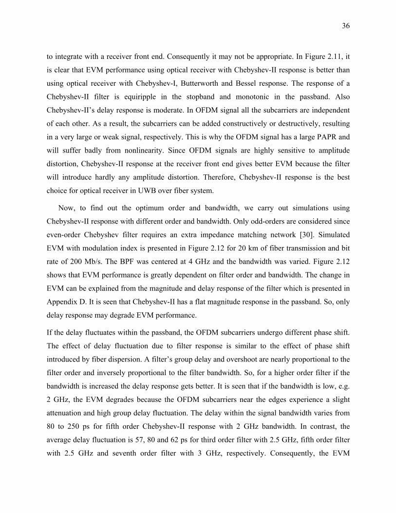
36

to integrate with a receiver front end. Consequently it may not be appropriate. In Figure 2.11, it

is clear that EVM performance using optical receiver with Chebyshev-II response is better than

using optical receiver with Chebyshev-I, Butterworth and Bessel response. The response of a

Chebyshev-II filter is equiripple in the stopband and monotonic in the passband. Also

Chebyshev-II’s delay response is moderate. In OFDM signal all the subcarriers are independent

of each other. As a result, the subcarriers can be added constructively or destructively, resulting

in a very large or weak signal, respectively. This is why the OFDM signal has a large PAPR and

will suffer badly from nonlinearity. Since OFDM signals are highly sensitive to amplitude

distortion, Chebyshev-II response at the receiver front end gives better EVM because the filter

will introduce hardly any amplitude distortion. Therefore, Chebyshev-II response is the best

choice for optical receiver in UWB over fiber system.

Now, to find out the optimum order and bandwidth, we carry out simulations using

Chebyshev-II response with different order and bandwidth. Only odd-orders are considered since

even-order Chebyshev filter requires an extra impedance matching network [30]. Simulated

EVM with modulation index is presented in Figure 2.12 for 20 km of fiber transmission and bit

rate of 200 Mb/s. The BPF was centered at 4 GHz and the bandwidth was varied. Figure 2.12

shows that EVM performance is greatly dependent on filter order and bandwidth. The change in

EVM can be explained from the magnitude and delay response of the filter which is presented in

Appendix D. It is seen that Chebyshev-II has a flat magnitude response in the passband. So, only

delay response may degrade EVM performance.

If the delay fluctuates within the passband, the OFDM subcarriers undergo different phase shift.

The effect of delay fluctuation due to filter response is similar to the effect of phase shift

introduced by fiber dispersion. A filter’s group delay and overshoot are nearly proportional to the

filter order and inversely proportional to the filter bandwidth. So, for a higher order filter if the

bandwidth is increased the delay response gets better. It is seen that if the bandwidth is low, e.g.

2 GHz, the EVM degrades because the OFDM subcarriers near the edges experience a slight

attenuation and high group delay fluctuation. The delay within the signal bandwidth varies from

80 to 250 ps for fifth order Chebyshev-II response with 2 GHz bandwidth. In contrast, the

average delay fluctuation is 57, 80 and 62 ps for third order filter with 2.5 GHz, fifth order filter

with 2.5 GHz and seventh order filter with 3 GHz, respectively. Consequently, the EVM

37

performance using seventh order filter with 3 GHz is in between fifth order filter with 2.5 GHz

and third order filter with 2.5 GHz. For the 3 GHz bandwidth a seventh order filter has a very

sharp cutoff but its delay response is not as good as third and fifth order filter. Also microwave

filter with higher than fifth order is complex to be implemented and is expensive.

-24

-22

-20

-18

-16

5 10 15

5th, 2 GHz

5th, 2.5 GHz

7th, 3 GHz

5th, 3 GHz

3rd, 3 GHz

5th, 3.5 GHz

3rd, 2.5 GHz

EVM

(dB

)


Chebyshev-II response

Figure 2.12 Simulated EVM with Chebyshev-II filter order and bandwidth for 200 Mb/s UWB

signal transmitted over 20 km of fiber.

Figure 2.12 shows the EVM performance using third order 3 GHz, fifth order 3 and 3.5 GHz

filter’s response is alike since their average delay fluctuation is close (42, 47 and 40 ps

respectively). On the other hand, the best filter order and bandwidth of the optical receiver in

uplink UWB over fiber system may also depend on environment, because an UWB antenna may

be placed close to some narrow band interferers like GSM at 0.8~0.9 GHz and microwave ovens

at 1.5~2 GHz. So, for uplink when the data is received by a base station from a user with an

antenna under the presence of such narrow band interferers, optical receiver with third order

filter response can perform poorly due to its slowly decaying stopband and the large magnitude

of out of band ripples. From magnitude response in Appendix D it is seen third order 3 GHz

filter will not satisfy the required 20 dB suppression of the sidebands. So, optical receiver with

fifth order filter response is a better choice than third order filter response for filtering of MB

OFDM UWB signals.

38

As stated before, increasing the filter bandwidth for a given order improves its delay

response, and therefore reduces the EVM. But, the receiver noise increases if the electrical

bandwidth of optical receiver is increased which is explained in Appendix B. Consequently, an

optical receiver with bandwidth as narrow as possible should be selected without introducing

amplitude and delay distortion. It is also seen from Figure 2.12 that the EVM performance using

the fifth order filter response was improved by only 0.29 dB at RF modulation index of 4% when

the bandwidth is increased from 3 GHz to 3.5 GHz. Therefore, 3 GHz is considered the optimum

bandwidth, which is roughly two times of the bandwidth (3.168 GHz=2×3×528 MHz) of the

band.

2.5.3 Effect of Receiver Noise and Received Optical Power

Until now, we have assumed all the losses due to fiber and optical components are compensated

using an EDFA. To see the effect of the received optical power, we first operate the system for

the best EVM at data rate of 200 Mb/s by setting the RF modulation index to 4% and received

optical power to 0 dBm at the photodetector. Then we insert a precision variable optical

attenuator Agilent 8156A before the photodetector to vary the received optical power.

Figure 2.13 shows measured EVM at 200 Mb/s considering back-to-back and after 20 km of

fiber. The EVM performance is degraded as the received optical power decreases. To understand

the behavior in Figure 2.13, we study the impairment of noise. In Appendix B, each contribution

of thermal noise, shot noise, RIN, signal-ASE beat and ASE-ASE beat noise is studied. It is

found that signal-ASE beat noise is dominant in additive noise. Therefore, EVM decrease with

the increase of the received optical power is due to the fact that UWB RF power is increased

with the increase of received optical power. The total EVM dependency on the optical power

(given by equation (2.13) is of the form 20optA P EVM+ , A-constant, and EVM0 does not depend

on optical power. It is clear that EVM degradation is inversely proportional to received optical

power. Another important finding from Figure 2.13 is that the required optical power at optical

receiver in UWB over fiber is reasonably higher than that in radio over fiber with other

modulation schemes which can work with optical power of as low as -40 dBm [1]. The higher

optical power requirement is due to the low RF modulation index and the low power spectral

density (-41.3 dBm/MHz) of the UWB RF signal.

39

-24

-22

-20

-18

-16

-14

-12

-10 -8 -6 -4 -2 0

EV

M (d

B)

Received optical power (dBm)

20 km

back-to-back

Figure 2.13 Measured EVM versus received optical power at photodetector.

0

2

4

6

8

-10 -8 -6 -4 -2 0

EV

M d

egra

datio

n (d

B)


Figure 2.14 Calculated EVM degradation versus received optical power for back-to-back

transmission with respect to 0 dBm received optical power.

We calculate the EVM degradation versus received optical power as shown in Figure 2.14. It

is evident by Figure 2.14 that the EVM degrades almost linearly with the received optical power.

Experimental results in Figure 2.13 are in good agreement with calculated EVM from 0 up to -9

dBm. However there is a small discrepancy at low optical power and it is due to the limited

sensitivity of the real time oscilloscope that has difficulty in triggering at low RF power level. As

40

shown in Figure 2.13, there is a difference in EVM performance between back-to-back and 20

km of fiber, which is explained in Figure 2.8.

2.6 Single Channel Wireless UWB over Fiber System

In this Section, using the setup described above in Section 2.3, here also, our system passed the

spectral mask requirement set by US Federal Communications Commission (FFC) and measured

ACPR was higher than 20 dB for maximum transmitted UWB power.

2.6.1 Transmitted UWB signal power and Receiver Sensitivity

The PER depends on the received SNR and receiver sensitivity. As the power level of the input

UWB signal to the DE-MZM increases the transmitted output power increases up to a certain

value corresponding to a modulation index mRF = 4% then starts decreasing due to AM/AM

compression of the DE-MZM as found in Section 2.5.1. If the SNR increases the packet error

rate will decrease. We vary the transmitted UWB power level from -46.5 dBm up to -11.13 dBm

by changing the UWB input power to the DE-MZM from -32.5 to 3.17 dBm and measure

transmitted, received RF power and the corresponding PER at the receiver after 1 m distance of

wireless link, shown in Figure 2.15.

From Figure 2.15 we find out that for maximum allowable PER of 8% and for 53.3, 200 and 480

Mb/s the receiver sensitivity is -82, -76.7 and -72.3 dBm, respectively, which meet the required

receiver sensitivity of -80.8, -74.5 and -70.4 dBm specified by WiMedia physical (PHY) layer

[7] as shown in

Table A. 5 (Appendix A). Because the measured UWB receiver sensitivity determines the

minimum transmitted power before the transmitting antenna, the required minimum power as

shown in Figure 6.16 is -30.7, -35 and -40.5 dBm for 480, 200 and 53.3 Mb/s, respectively. In

addition, it is clear that the receiver sensitivity is worst for the 480 Mb/s. This will limit the

dynamic range and wireless transmission range for high bit rates. This is why for 480 Mb/s the

PER performance is poor at low transmitted power levels.

41

0

20

40

60

80

100

-45 -40 -35 -30 -25 -20 -15

-85 -80 -75 -70 -65 -60 -55

480 Mbps200 Mbps53.3 Mbps

PER

(%)

Transmitted RF power (dBm)

Received RF power (dBm)

Figure 2.15 PER versus UWB power and data rate for 20 km optical link and 1 m wireless link.

2.6.2 Effect of Wireless Link

It is seen from equation (2.15) that the received power will depend mainly on the mean path-loss

referenced to 1 m. To show the performance under a wireless channel, we vary the distance

between two UWB antennas in Figure 2.1 from 1 to 4 m and observe the corresponding PER at

the UWB receiver as shown in Figure 2.16. From equation (2.14) mean path-loss referenced to 1

m is 6, 9.6 and 12 dB for 2, 3 and 4 m, respectively. As the distance between two antennas

increases the packet error rate will aggravate, and this is because the losses are increased and the

received signal is attenuated.

From Figure 2.16 it is found that PER is almost zero for up to 2 m wireless at bit rates of up to

480 Mb/s and input power level of more than -12.5 dBm (mRF = 2%) at the DE-MZM which

corresponds to average transmitted power before the antenna of Puwb= -26 dBm. It is also found

that the highest bit rate 480 Mb/s is the most degraded one by the wireless link length. This is

primarily due to the fact that the receiver sensitivity is the worst for this bit rate. After 4 m

wireless transmission and for typical average transmitted power of -20 and -26 dBm

(corresponding to RF modulation index of 4% and 2%, respectively) the received RF power

using equation (2.15) is -73.85 and -79.85 dBm, respectively, which is below the receiver

sensitivity at 480 and 200 Mb/s, respectively. The corresponding PER can be easily deduced

from Figure 2.15, for example for received RF power of -73.85 dBm (mRF = 4%) the PER is ~

45% and ~ 0% for 480 and 200 Mb/s, respectively, while for received RF power of -79.85 dBm

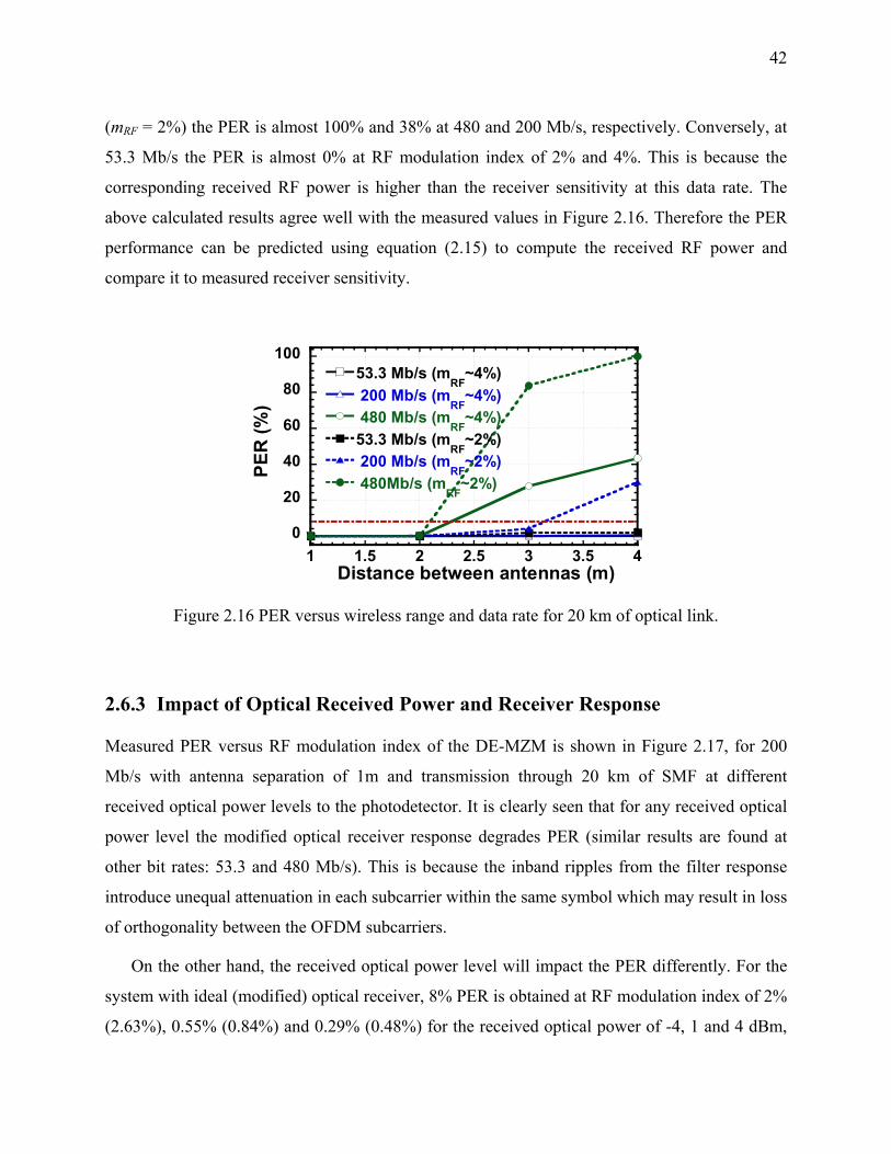
42

(mRF = 2%) the PER is almost 100% and 38% at 480 and 200 Mb/s, respectively. Conversely, at

53.3 Mb/s the PER is almost 0% at RF modulation index of 2% and 4%. This is because the

corresponding received RF power is higher than the receiver sensitivity at this data rate. The

above calculated results agree well with the measured values in Figure 2.16. Therefore the PER

performance can be predicted using equation (2.15) to compute the received RF power and

compare it to measured receiver sensitivity.

0

20

40

60

80

100

1 1.5 2 2.5 3 3.5 4

53.3 Mb/s (mRF

~4%) 200 Mb/s (m

RF~4%)

480 Mb/s (mRF

~4%)53.3 Mb/s (m

RF~2%)

200 Mb/s (mRF

~2%) 480Mb/s (m

RF~2%)

PER

(%)

Distance between antennas (m)

Figure 2.16 PER versus wireless range and data rate for 20 km of optical link.

2.6.3 Impact of Optical Received Power and Receiver Response

Measured PER versus RF modulation index of the DE-MZM is shown in Figure 2.17, for 200

Mb/s with antenna separation of 1m and transmission through 20 km of SMF at different

received optical power levels to the photodetector. It is clearly seen that for any received optical

power level the modified optical receiver response degrades PER (similar results are found at

other bit rates: 53.3 and 480 Mb/s). This is because the inband ripples from the filter response

introduce unequal attenuation in each subcarrier within the same symbol which may result in loss

of orthogonality between the OFDM subcarriers.

On the other hand, the received optical power level will impact the PER differently. For the

system with ideal (modified) optical receiver, 8% PER is obtained at RF modulation index of 2%

(2.63%), 0.55% (0.84%) and 0.29% (0.48%) for the received optical power of -4, 1 and 4 dBm,

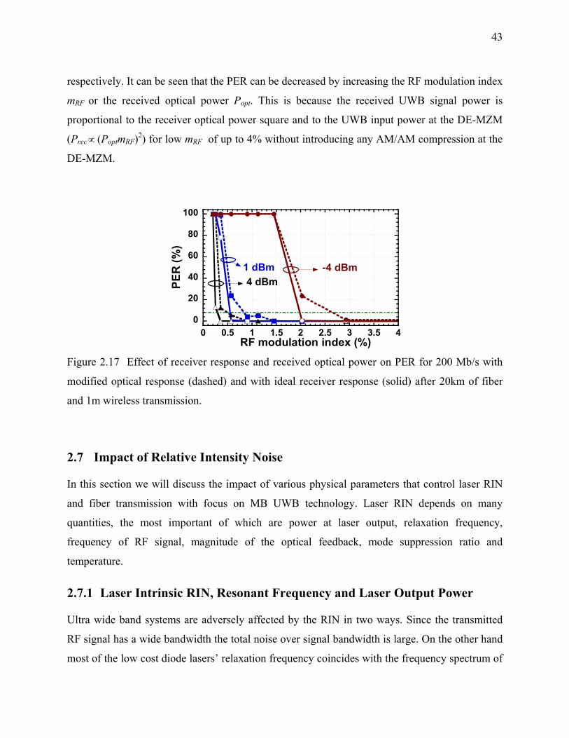
43

respectively. It can be seen that the PER can be decreased by increasing the RF modulation index

mRF or the received optical power Popt. This is because the received UWB signal power is

proportional to the receiver optical power square and to the UWB input power at the DE-MZM

(Prec ∝ (PoptmRF)2) for low mRF of up to 4% without introducing any AM/AM compression at the

DE-MZM.

0

20

40

60

80

100

0 0.5 1 1.5 2 2.5 3 3.5 4

PER

(%)


-4 dBm1 dBm4 dBm

Figure 2.17 Effect of receiver response and received optical power on PER for 200 Mb/s with

modified optical response (dashed) and with ideal receiver response (solid) after 20km of fiber

and 1m wireless transmission.

2.7 Impact of Relative Intensity Noise

In this section we will discuss the impact of various physical parameters that control laser RIN

and fiber transmission with focus on MB UWB technology. Laser RIN depends on many

quantities, the most important of which are power at laser output, relaxation frequency,

frequency of RF signal, magnitude of the optical feedback, mode suppression ratio and

temperature.

2.7.1 Laser Intrinsic RIN, Resonant Frequency and Laser Output Power

Ultra wide band systems are adversely affected by the RIN in two ways. Since the transmitted

RF signal has a wide bandwidth the total noise over signal bandwidth is large. On the other hand

most of the low cost diode lasers’ relaxation frequency coincides with the frequency spectrum of

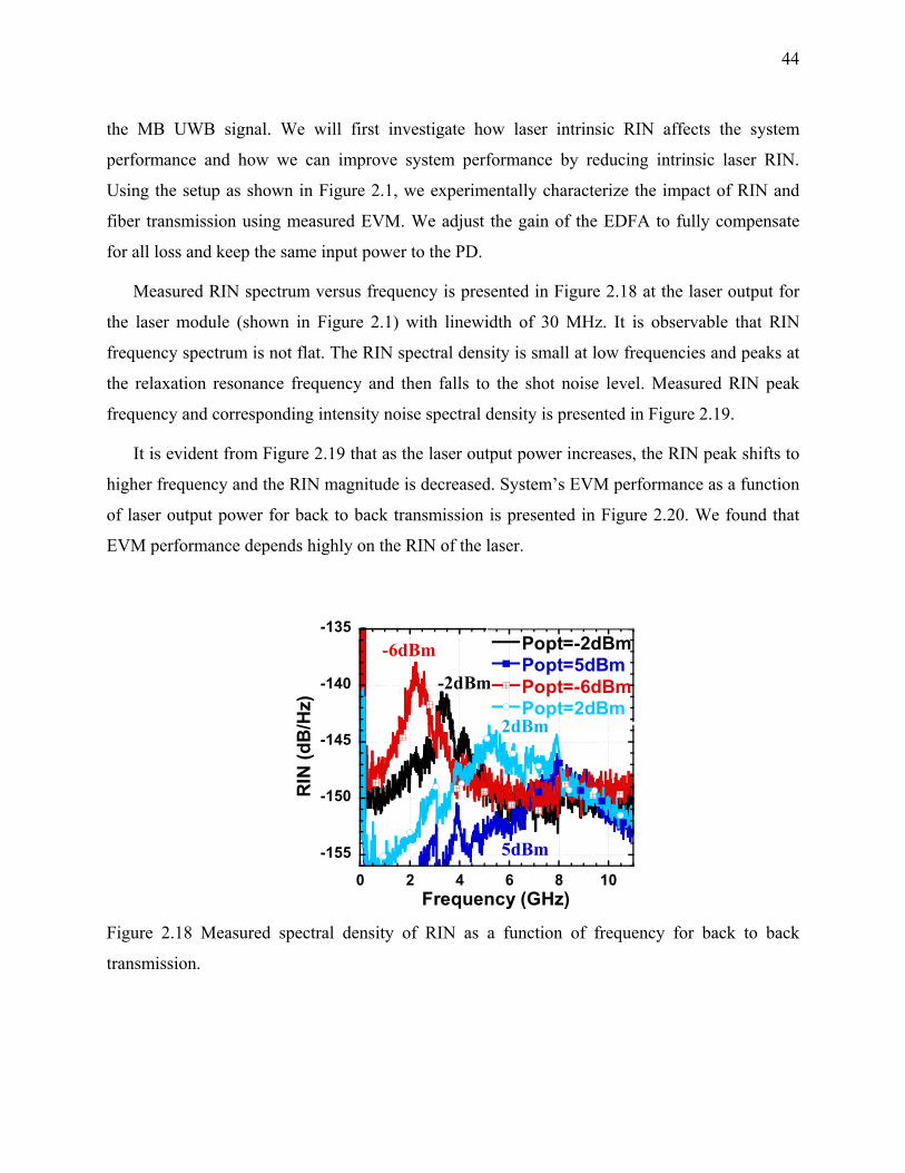
44

the MB UWB signal. We will first investigate how laser intrinsic RIN affects the system

performance and how we can improve system performance by reducing intrinsic laser RIN.

Using the setup as shown in Figure 2.1, we experimentally characterize the impact of RIN and

fiber transmission using measured EVM. We adjust the gain of the EDFA to fully compensate

for all loss and keep the same input power to the PD.

Measured RIN spectrum versus frequency is presented in Figure 2.18 at the laser output for

the laser module (shown in Figure 2.1) with linewidth of 30 MHz. It is observable that RIN

frequency spectrum is not flat. The RIN spectral density is small at low frequencies and peaks at

the relaxation resonance frequency and then falls to the shot noise level. Measured RIN peak

frequency and corresponding intensity noise spectral density is presented in Figure 2.19.

It is evident from Figure 2.19 that as the laser output power increases, the RIN peak shifts to

higher frequency and the RIN magnitude is decreased. System’s EVM performance as a function

of laser output power for back to back transmission is presented in Figure 2.20. We found that

EVM performance depends highly on the RIN of the laser.

-155

-150

-145

-140

-135

0 2 4 6 8 10

Popt=-2dBmPopt=5dBmPopt=-6dBmPopt=2dBm

RIN

(dB

/Hz)

Frequency (GHz)

-2dBm

-6dBm

2dBm

5dBm

Figure 2.18 Measured spectral density of RIN as a function of frequency for back to back

transmission.

45

-146

-144

-142

-140

-138

0

2

4

6

8

10

-6 -4 -2 0 2 4

RIN

(dB

/ Hz)

RIN

peak (GH

z)

Laser ouput power (dBm) Figure 2.19 Measured RIN peak frequency and corresponding spectral density of RIN for back to

back transmission.

-20.5

-20

-19.5

-19

-18.5

-18

-17.5

-6 -4 -2 0 2 4

f1= 3.432 GHz

f2= 3.96 GHz

f3= 4.488 GHz

EVM

(dB

)

Laser ouput power (dBm) Figure 2.20 Measured EVM with laser output power for back to back transmission at bit rate of

200Mb/s.

At low power levels, i.e. from -6 to -2 dBm, EVM performance of all three bands is poor due

to high RIN of the laser. Also at low power the RIN peak resides at low frequencies. That is why

the first band (3.432 GHz) of MB UWB suffers most at low power and has poor EVM

performance. We see that EVM peaks at around -3 dBm which makes perfect sense since at

around -3 dBm the RIN peak exactly coincides with the first band. As the laser output power

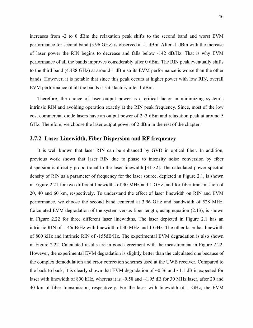
46

increases from -2 to 0 dBm the relaxation peak shifts to the second band and worst EVM

performance for second band (3.96 GHz) is observed at -1 dBm. After -1 dBm with the increase

of laser power the RIN begins to decrease and falls below -142 dB/Hz. That is why EVM

performance of all the bands improves considerably after 0 dBm. The RIN peak eventually shifts

to the third band (4.488 GHz) at around 1 dBm so its EVM performance is worse than the other

bands. However, it is notable that since this peak occurs at higher power with low RIN, overall

EVM performance of all the bands is satisfactory after 1 dBm.

Therefore, the choice of laser output power is a critical factor in minimizing system’s

intrinsic RIN and avoiding operation exactly at the RIN peak frequency. Since, most of the low

cost commercial diode lasers have an output power of 2~3 dBm and relaxation peak at around 5

GHz. Therefore, we choose the laser output power of 2 dBm in the rest of the chapter.

2.7.2 Laser Linewidth, Fiber Dispersion and RF frequency

It is well known that laser RIN can be enhanced by GVD in optical fiber. In addition,

previous work shows that laser RIN due to phase to intensity noise conversion by fiber

dispersion is directly proportional to the laser linewidth [31-32]. The calculated power spectral

density of RIN as a parameter of frequency for the laser source, depicted in Figure 2.1, is shown

in Figure 2.21 for two different linewidths of 30 MHz and 1 GHz, and for fiber transmission of

20, 40 and 60 km, respectively. To understand the effect of laser linewidth on RIN and EVM

performance, we choose the second band centered at 3.96 GHz and bandwidth of 528 MHz.

Calculated EVM degradation of the system versus fiber length, using equation (2.13), is shown

in Figure 2.22 for three different laser linewidths. The laser depicted in Figure 2.1 has an

intrinsic RIN of -145dB/Hz with linewidth of 30 MHz and 1 GHz. The other laser has linewidth

of 800 kHz and intrinsic RIN of -155dB/Hz. The experimental EVM degradation is also shown

in Figure 2.22. Calculated results are in good agreement with the measurement in Figure 2.22.

However, the experimental EVM degradation is slightly better than the calculated one because of

the complex demodulation and error correction schemes used at the UWB receiver. Compared to

the back to back, it is clearly shown that EVM degradation of ~0.36 and ~1.1 dB is expected for

laser with linewidth of 800 kHz, whereas it is ~0.58 and ~1.95 dB for 30 MHz laser, after 20 and

40 km of fiber transmission, respectively. For the laser with linewidth of 1 GHz, the EVM

47

degradation is ~1 and ~3 dB for the two fiber lengths. The EVM degradation shown in Figure

2.22 is due to increased RIN due to the interaction of the laser phase noise and chromatic

dispersion as shown in Figure 2.21.

-132

-128

-124

-120

-116

-112

-108

2 4 6 8 10 12

RIN

(dB

/Hz)

Frequency (GHz)

20 km

60 km40 km

20 km

60 km

40 km

Figure 2.21 Calculated RIN versus frequency for 20, 40 and 60 km (Solid: linewidth of 30 MHz.

Dotted: linewidth of 1 GHz).

0

1

2

3

4

5

0 10 20 30 40 50 60

EVM

deg

rada

tion

(dB

)

Fiber length (km)

800 kHz

1 GHz

30 MHz

Figure 2.22 Calculated EVM degradation versus fiber length with respect to back-to-back.

Square: experimental results for 20, 40 and 52 km.

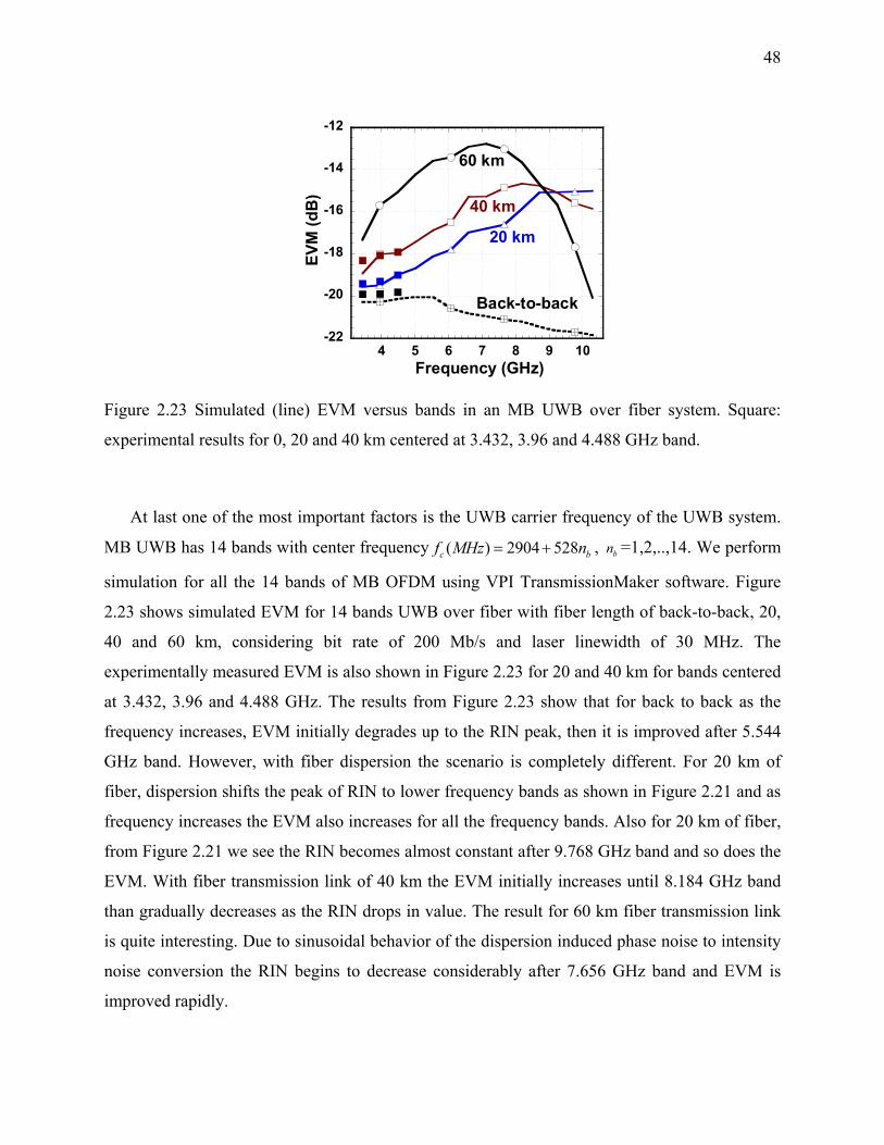
48

-22

-20

-18

-16

-14

-12

4 5 6 7 8 9 10

EVM

(dB

)

Frequency (GHz)

Back-to-back

20 km

60 km

40 km

Figure 2.23 Simulated (line) EVM versus bands in an MB UWB over fiber system. Square:

experimental results for 0, 20 and 40 km centered at 3.432, 3.96 and 4.488 GHz band.

At last one of the most important factors is the UWB carrier frequency of the UWB system.

MB UWB has 14 bands with center frequency ( ) 2904 528c bf MHz n= + , bn =1,2,..,14. We perform

simulation for all the 14 bands of MB OFDM using VPI TransmissionMaker software. Figure

2.23 shows simulated EVM for 14 bands UWB over fiber with fiber length of back-to-back, 20,

40 and 60 km, considering bit rate of 200 Mb/s and laser linewidth of 30 MHz. The

experimentally measured EVM is also shown in Figure 2.23 for 20 and 40 km for bands centered

at 3.432, 3.96 and 4.488 GHz. The results from Figure 2.23 show that for back to back as the

frequency increases, EVM initially degrades up to the RIN peak, then it is improved after 5.544

GHz band. However, with fiber dispersion the scenario is completely different. For 20 km of

fiber, dispersion shifts the peak of RIN to lower frequency bands as shown in Figure 2.21 and as

frequency increases the EVM also increases for all the frequency bands. Also for 20 km of fiber,

from Figure 2.21 we see the RIN becomes almost constant after 9.768 GHz band and so does the

EVM. With fiber transmission link of 40 km the EVM initially increases until 8.184 GHz band

than gradually decreases as the RIN drops in value. The result for 60 km fiber transmission link

is quite interesting. Due to sinusoidal behavior of the dispersion induced phase noise to intensity

noise conversion the RIN begins to decrease considerably after 7.656 GHz band and EVM is

improved rapidly.

49

2.8 Performance of Multi-band OFDM Ultra-Wideband over Fiber

Transmission under the Presence of In Band Interferers

For real world applications UWB receivers face jamming scenarios from multiple in-band and

out of band interferers. Some of the typical interferers at the input of a MB OFDM receiver are

shown in Figure 2.24. IEEE 802.11b/g, Bluetooth and microwave ovens act as out of band

interferers. WiMAX at 3.5 GHz interferes with band group 1, IEEE 802.11a/n interferes with

band group 2 and radar signal interferes with band group 4, respectively.

We used the experimental setup of Figure 2.1. The MB-OFDM UWB signal with 200Mb/s is

generated by the AWG 7122B. The generated WiMedia sub-bands are presented in Table 2.1.

The sub-bands follow a simple hopping sequence as f1, f2, f3 according to TFC 1, defined in

WiMedia standard so that only one channel exists at any particular time.

Figure 2.24 Spectrum of UWB signal with narrow band interferers.

The generated UWB signal has a low power spectral density (PSD) and small footprint. As a

result, the UWB signal appears to be very low level background noise to an unintended

narrowband receiver. The PSD of the generated signal and interferers (for interferer to UWB

peak power ratio of 20 dB) at point B in Figure 2.1 is given in

Table 2.2 that shows the PSD level difference between UWB and interferer is roughly 20 dB.

This difference gives a rough estimation of signal to noise ratio at the narrowband receiver.

The received power at the photodetector is fixed at 4 dBm in all cases. After the photodetection

the UWB signal is amplified by a broadband RF amplifier from MiniCircuits (ZVA-213) with

gain of 26 dB as shown in Figure 2.1. The received signal (at point D) is evaluated with a high

speed real time oscilloscope DPO 72004B from Tektronix.

50

Table 2.1 Generated UWB sub-bands and corresponding interferers.

Band Group Corresponding in band interferer

Band group 1, 3 sub-bands centered at f1= 3.432, f2= 3.96 and f3= 4.488 GHz

IEEE 802.16-2004, WiMAX at 3.5 GHz

Band group 2, 3 sub-bands centered at f1= 5.016, f2= 5.544 and f3= 6.072 GHz

IEEE 802.11n, MIMO at 5 GHz and IEEE 802.11a, WLAN at 5.8 GHz

Band group 4, 3 sub-bands centered at f1= 8.184, f2= 8.712 and f3= 9.240 GHz Marine radar at 8 GHz

Table 2.2 Generated UWB sub-bands, interferers and their corresponding PSD.

Band Group UWB PSD (dBm/Hz)

Interferer PSD (dBm/Hz)

Band group 1 -111.48 -91.53

Band group 2 -112.35 -92.19/ -92.29

Band group 4 -118.19 -98.07

In this section we will analyze EVM performance of MB UWB over fiber under different in-

band interference scenarios. We first investigate the system performance without any in-band

interference and use the information to compare degradation under interference conditions. To

emulate 1 m transmission over air under real antenna scenarios we added two multipath version

of our generated signal with delay of 1 symbol and 2 symbols, relative amplitude of -35 dB and -

40 dB and phase of 5 and 10 degree, respectively from the arbitrary waveform generator before

transmission through the fiber. We tried to make our results independent of the amplification at

the receiver front end so we present the results as a parameter of interferer to UWB peak power

ratio rather than the power of interferer. For example free space path loss for 1 m can be

emulated by inserting a 40 dB attenuator between points B and C in Figure 2.1. In that case,

extra RF amplification has to be provided to keep the RF modulation index at the electro optic

modulator constant. It should be noted that EVM is the ratio of the distortion in the received

constellation with respect to transmitted constellation. So, theoretically fixed gain or attenuation

51

at the front end is a common multiplication factor both for the numerator and denominator and

does not have any impact on EVM performance.

2.8.1 UWB over Single Mode Fiber Stand Alone Operation

We turn off the interferers from arbitrary waveform generator and transmit only MB UWB signal

of band group 1, band group 2 and band group 4 according to WiMedia specification as

described in Table 2.1 through the fiber one by one and measure the EVM at point D in Figure

2.1. We also measure the intrinsic EVM of the generator, where the output of generator at point

B is directly connected to point D in Figure 2.1 using a coaxial cable. Results from our

measurement are enlisted in Table 2.3. The results show that EVM degradation due to electrical

to optical conversion is usually 2~3 dB. EVM performance for back-to-back (B-B), i.e. no actual

fiber transmission is around -24 dB for all the band groups. This value increases by 1.4~2 dB for

20 km fiber transmission. At high frequencies there is a higher degradation in EVM performance

for 20 km fiber transmission compared to back-to-back due to fiber chromatic dispersion induced

laser phase to intensity noise conversion or RIN [31]. The results obtained are still much better

than the WiMedia defined -16 dB limit of EVM [7] and for lower band groups and the fiber link

can be easily extended up to 60~80 km of single mode fiber depending on the quality of the

devices used for electrical to optical and optical to electrical conversion.

Table 2.3 Measured EVM Performance for Stand Alone UWB Transmission.

Band Group Intrinsic B-B 20 km of SMF

Band group 1 -27.32 dB -24.50 dB -23.12 dB



52

2.8.2 Performance of Band Group 1 of MB OFDM UWB under the presence

of WiMAX with Fiber Distribution

Recently (21/5/2008) European Commission has opened the radio spectrum 3.4~3.8 GHz for

WiMAX applications [33]. This notion raised many concerns among the UWB communities

because WiMAX will interfere with band group 1. Band goup 1 of UWB was thought to have the

most potential because of mature CMOS technology in this frequency range and absence of other

interferers. Subsequently, how WiMAX will affect UWB over fiber transmission has become a

cause of apprehension among researchers. We study the performance of UWB over fiber

transmission under the presence of WiMAX. We generate a 20 MHz wide WiMAX signal

centered at 3.5 GHz with 64 Quadrature Amplitude Modulation (QAM) and a bit rate of 54 Mb/s

based on IEEE 802.16-2004 technology [33]. The signal has 256 OFDM subcarriers among

which 56 are null and guard tones, 8 are pilots and the rest 192 are data tones. Transmitted RF

spectrum of UWB and WiMAX at point B and received spectrum after 20 km at point D in

Figure 2.1 is showed in Figure 2.25 (a) and (b), respectively.

The results from EVM measurement presented in Figure 2.26 show that EVM performance

of UWB over fiber transmission is severely degraded under presence of WiMAX. If the WiMAX

to UWB peak power ratio is more than ~14 dB the transmission performance quickly falls below

WiMedia defined limit of -16 dB. The performance degradation is mainly due to large number of

subcarriers present in WiMAX within a small bandwidth so the sub-carriers interact with each

other and the OFDM subcarriers in MB OFDM UWB signal resulting in a high carrier leakage

and inter carrier interference.

53

Figure 2.25 RF spectrum of UWB band group 1 and WiMAX (a) transmitted at point B (b)


(Interferer to UWB peak power ratio is 20 dB).

-24

-20

-16

-12

-8

-10 -5 0 5 10 15 20

B-B20 km

B-B20 km

EVM

(dB

)

WiMAX to UWB peak power ratio (dB)

Figure 2.26 EVM performance of UWB over fiber transmission under the presence of WiMAX

as a function of WiMAX to UWB peak power ratio (Solid lines: best fitted curves, dotted lines:

without interference).

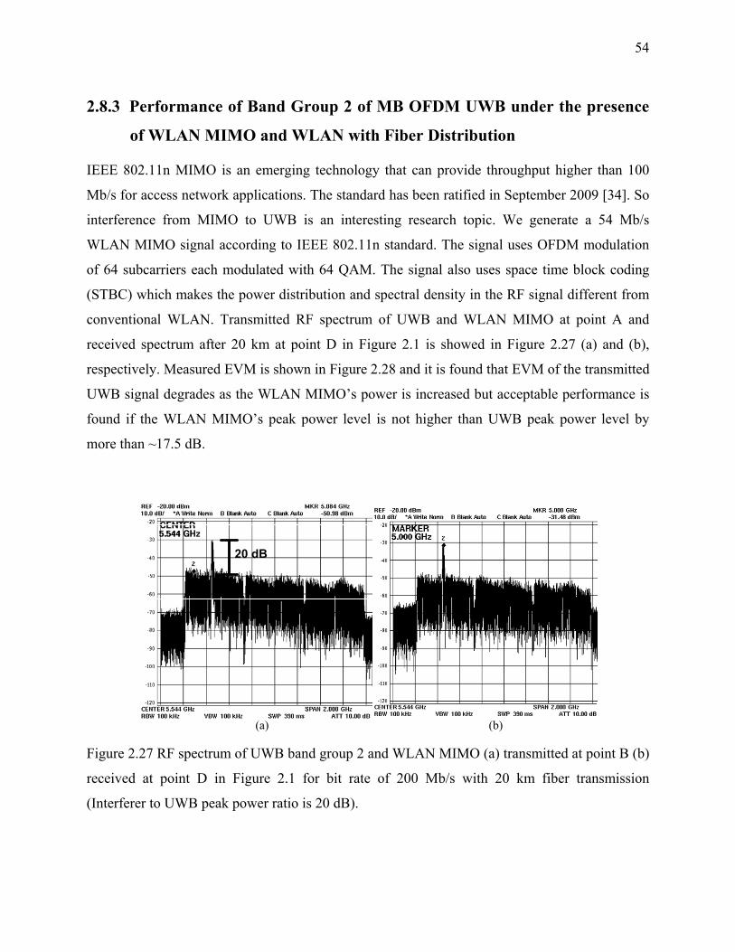
54


of WLAN MIMO and WLAN with Fiber Distribution

IEEE 802.11n MIMO is an emerging technology that can provide throughput higher than 100

Mb/s for access network applications. The standard has been ratified in September 2009 [34]. So

interference from MIMO to UWB is an interesting research topic. We generate a 54 Mb/s

WLAN MIMO signal according to IEEE 802.11n standard. The signal uses OFDM modulation

of 64 subcarriers each modulated with 64 QAM. The signal also uses space time block coding

(STBC) which makes the power distribution and spectral density in the RF signal different from

conventional WLAN. Transmitted RF spectrum of UWB and WLAN MIMO at point A and

received spectrum after 20 km at point D in Figure 2.1 is showed in Figure 2.27 (a) and (b),

respectively. Measured EVM is shown in Figure 2.28 and it is found that EVM of the transmitted

UWB signal degrades as the WLAN MIMO’s power is increased but acceptable performance is

found if the WLAN MIMO’s peak power level is not higher than UWB peak power level by

more than ~17.5 dB.

(a) (b)

20 dB

Figure 2.27 RF spectrum of UWB band group 2 and WLAN MIMO (a) transmitted at point B (b)



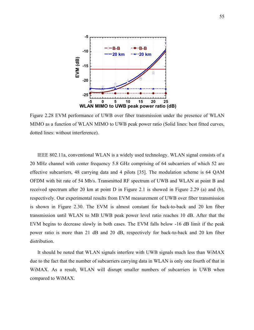
55

-25

-20

-15

-10

-5

-5 0 5 10 15 20 25

B-B20 km

B-B20 km

EVM

(dB

)

WLAN MIMO to UWB peak power ratio (dB) Figure 2.28 EVM performance of UWB over fiber transmission under the presence of WLAN

MIMO as a function of WLAN MIMO to UWB peak power ratio (Solid lines: best fitted curves,

dotted lines: without interference).

IEEE 802.11a, conventional WLAN is a widely used technology. WLAN signal consists of a

20 MHz channel with center frequency 5.8 GHz comprising of 64 subcarriers of which 52 are

effective subcarriers, 48 carrying data and 4 pilots [35]. The modulation scheme is 64 QAM

OFDM with bit rate of 54 Mb/s. Transmitted RF spectrum of UWB and WLAN at point B and

received spectrum after 20 km at point D in Figure 2.1 is showed in Figure 2.29 (a) and (b),

respectively. Our experimental results from EVM measurement of UWB over fiber transmission

is shown in Figure 2.30. The EVM is almost constant for back-to-back and 20 km fiber

transmission until WLAN to MB UWB peak power level ratio reaches 10 dB. After that the

EVM begins to decrease slowly in both cases. The EVM falls below -16 dB limit if the peak

power ratio is more than 21 dB and 20 dB, respectively for back-to-back and 20 km fiber

distribution.

It should be noted that WLAN signals interfere with UWB signals much less than WiMAX

due to the fact that the number of subcarriers carrying data in WLAN is only one fourth of that in

WiMAX. As a result, WLAN will disrupt smaller numbers of subcarriers in UWB when

compared to WiMAX.

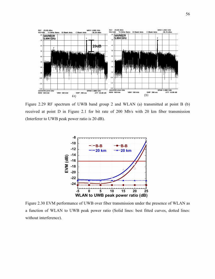
56

Figure 2.29 RF spectrum of UWB band group 2 and WLAN (a) transmitted at point B (b)



-24-22-20-18-16-14-12-10-8

-5 0 5 10 15 20 25

B-B20 km

B-B20 km

EVM

(dB

)

WLAN to UWB peak power ratio (dB) Figure 2.30 EVM performance of UWB over fiber transmission under the presence of WLAN as



57


of Marine Radar with Fiber Distribution

Radar signals at high frequency can also interfere with MB UWB signals. We used a linear

frequency modulated pulse (LFM) centered at 8 GHz with pulse width of 5 µs and frequency

sweep of 20 MHz as a radar source and combined with band group 4 of UWB signal.

Transmitted RF spectrum of UWB and marine radar and received spectrum after 20 km is

showed in Figure 2.31(a) and (b), respectively. The EVM performance of UWB as a parameter

of radar peak power to UWB peak power is shown in Figure 2.32. The EVM degrades quickly if

the radar peak power is increased for both back-to-back and 20 km fiber transmission. Referring

to Figure 2.32, EVM value of -16 dB is found for radar to UWB peak power ratio of 17 dB and

15 dB for back-to-back and 20 km fiber transmission, respectively. Large difference between

back-to-back and 20 km fiber distribution is due to laser RIN as explained in Section 2.7.

Experiments with C band military radar in the frequency range of 5.250~5.925 GHz and band

group 2 (4.752~6.336 GHz) give similar results.

Figure 2.31 RF spectrum of UWB band group 4 and marine radar (a) transmitted at point B (b)



58

-25

-20

-15

-10

-10 -5 0 5 10 15 20

B-B20 km

B-B20 km

EVM

(dB

)

Marine radar to UWB peak power ratio (dB)




Low duty cycle pulses from radar signal interact and disrupt the subcarriers in UWB signal.

Time domain waveforms after 20 km of fiber transmission without and with radar signal as

interferer are presented in Figure 2.33 and Figure 2.34, respectively. It is clearly visible that

radar signal distorts the waveform at the edges. It should be noted that in UWB receivers most

of the signal processing is performed in time domain. Therefore, any short pulse like radar in

time domain jams the UWB signal at UWB receiver input and causes the degradation of EVM.


with bit rate of 200Mb/s without any signal interferer.

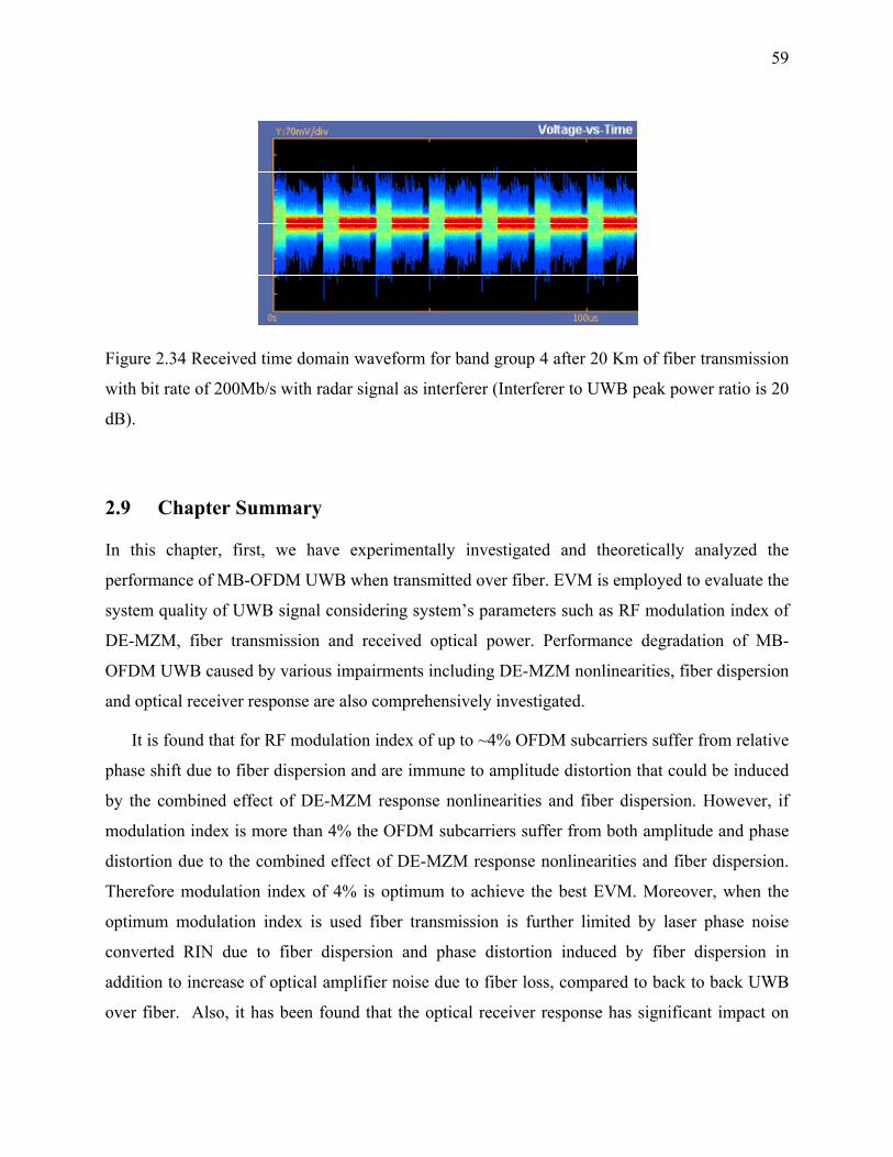
59


with bit rate of 200Mb/s with radar signal as interferer (Interferer to UWB peak power ratio is 20

dB).

2.9 Chapter Summary

In this chapter, first, we have experimentally investigated and theoretically analyzed the

performance of MB-OFDM UWB when transmitted over fiber. EVM is employed to evaluate the

system quality of UWB signal considering system’s parameters such as RF modulation index of

DE-MZM, fiber transmission and received optical power. Performance degradation of MB-

OFDM UWB caused by various impairments including DE-MZM nonlinearities, fiber dispersion

and optical receiver response are also comprehensively investigated.

It is found that for RF modulation index of up to ~4% OFDM subcarriers suffer from relative

phase shift due to fiber dispersion and are immune to amplitude distortion that could be induced

by the combined effect of DE-MZM response nonlinearities and fiber dispersion. However, if

modulation index is more than 4% the OFDM subcarriers suffer from both amplitude and phase

distortion due to the combined effect of DE-MZM response nonlinearities and fiber dispersion.

Therefore modulation index of 4% is optimum to achieve the best EVM. Moreover, when the

optimum modulation index is used fiber transmission is further limited by laser phase noise

converted RIN due to fiber dispersion and phase distortion induced by fiber dispersion in

addition to increase of optical amplifier noise due to fiber loss, compared to back to back UWB

over fiber. Also, it has been found that the optical receiver response has significant impact on

60

EVM performance. It is found that Chebyshev-II response with 3 GHz bandwidth and fifth order

is the best for MB OFDM UWB over fiber. This is due to low amplitude and phase distortion

within the passband. Since the UWB over fiber is operated at a low RF modulation index and

multiband UWB has a low power spectral density, it is found that required optical power at

optical receiver in UWB over fiber is reasonably higher than that in radio over fiber with other

modulation schemes. Furthermore, we have found that EVM in UWB over fiber is degraded

almost linearly with the decrease of receiver optical power.

Next, we have investigated experimentally the performance of MB-OFDM wireless UWB in

terms of PER when transmitted over 20 km of SMF. PER was measured at different bit rates to

evaluate the receiver sensitivity, required minimum transmitted UWB power, effect of wireless

distance, DE-MZM modulation index, received optical power and optical receiver response. It is

found that for 20 km of fiber and 1 m wireless range transmission, the minimum transmitted

UWB power to achieve the allowable 8% PER is -40.5, -35 and -30.7dBm at 53.3, 200 and 480

Mb/s, respectively, and is limited by the measured receiver sensitivity of -82, -76.7 and -72.3

dBm, respectively, which is better than the required sensitivity specified by the Wimedia PHY

layer. In addition, we found that increasing the received optical power will improve PER and

increase RF dynamic range suggesting that an optical amplification is better than RF counterpart.

Also an optical receiver with flat magnitude response in the passband performs better with a

MB-OFDM UWB over fiber. The results show that radio over fiber is very promising technology

for increasing the coverage distance for the emerging and future ultra wideband systems

operating at higher bit rates.

The performance of MB OFDM UWB was investigated when transmitted over fiber under

the effect of RIN considering system’s parameters such as laser output power, linewidth and

fiber transmission length. It is found that the system should be operated at a high laser output

power to avoid RIN degradation. It is shown using a narrow linewidth laser with low RIN will

significantly improve system performance. Also simulations were performed for all the 14 bands

of MB UWB to show performance dependence of RF carrier frequency. The results show that

bands higher than 7.656 GHz are critically affected depending on fiber dispersion induced phase

to intensity noise conversion.

61

It is found that different in-band interferers can affect the performance of MB-OFDM UWB

severely if certain interferer to UWB peak power ratio is not maintained. For WiMax/ marine

radar and UWB devices that are co-located this ratio is only ~14 and ~15 dB, respectively, for

WiMAX and radar signals if distributed over 20 km of single mode fiber. MB UWB over fiber is

more resistant to interference from WLAN MIMO and conventional WLAN. The interferer to

MB UWB peak power ratio is ~17.5 and ~20 dB for 20 km fiber transmission for WLAN MIMO

and conventional WLAN, respectively for satisfying the EVM requirement of -16 dB, which is

the EVM threshold specified for conformance testing according to the recent WiMedia standard

for UWB. Our results will allow the future researchers in the field of MB UWB over fiber

transmission to optimize performance UWB over fiber transmission under the presence of all

possible in-band interferers.

62

CHAPTER 3 PROPOSED LINEARIZATION TECHNIQUE FOR MZM

3.1 Introduction

Many techniques for reducing nonlinear distortion have been described in literature, such as

analog predistortion techniques [36-45], the adaptive pre-distortion method [46], the feed

forward linearization technique [47], dual-parallel modulation techniques [48], serially cascaded

modulation techniques [49], and balanced detection [50-51]. Each devised with its advantages

and disadvantages. A linearization technique called the dual parallel linearized modulator, which

consists of two MZMs placed in parallel, was also proposed. The upper MZM is biased at

positive quadrature with modulation index set high and the lower is biased at negative quadrature

with modulation index set low, where the two resulting inverted optical powers are combined to

cancel IMD along with some RF carrier power [52-53]. This linearization technique may become

impractical, because of the optical combining of two independent MZM transfer responses and

the required accuracy in the relative phase shift between the two MZMs, which need to be within

a few degrees for satisfactory IMD cancellation.

Recently, a simple technique that suppresses IMD was proposed, which consists of two linear

polarizers placed before and after an optical phase modulator [54]. Because this technique

transmits phase modulated light, it uses an acousto-optic frequency shifter for coherent

heterodyne detection, which limits the RF bandwidth of the system and increases the cost and

complexity. A linear optical phase demodulation has also been proposed in coherent receivers

[55]. It is based on optical phase-locked loop and additional components, which will add cost to

the receiver.

The objective in this chapter is to design a linearized modulator whose performance does not

depend on modulation index, RF bandwidth limitation is removed and complexity is reduced, so

that it may be incorporated into one silicon substrate or module for practical purposes. A

linearized MZM that consists of two linear polarizers and a DE-MZM is proposed in this chapter.

Using this modulator, OSSB modulation can be realized with the cancellation of third-order IMD

(3IMD). This modulator utilizes both TE and TM polarization states. Therefore, this modulator is

referred to as the mixed polarization OSSB MZM. However, when multiple RF tones are applied

to the modulator and particularly with high modulation index, many harmonics and

63

intermodulation products are generated due to optical modulation and may lead to dispersion

induced power fading and crosstalk even for OSSB modulation. This is because higher order

distortion components beat with one another and generated component products that may overlap

with or land very close to RF carriers. The proposed mixed-polarization OSSB MZM will be

compared to the conventional MZM in terms of spurious free dynamic range (SFDR), 3IMD

suppression and overall reduction of nonlinear distortion components.

This chapter is organized as follows; Section 3.2 will describe the proposed mixed-

polarization OSSB MZM, Section 3.3 will provide the equation development for the SFDR and

report on the sensitivity analysis due to polarization angle and electro-optic coefficient ratio

errors, Section 3.4 will provide simulated third order suppression results, SFDR results and a

comparison analysis to the conventional MZM, Section 3.5 will explore experimental SFDR and

a comparison analysis to the conventional MZM. Section 3.6 will demonstrate the application of

the proposed modulator to a MB-OFDM UWB signal and Section 3.7 will finally provide

concluding remarks.

3.2 Proposed Mixed-Polarization OSSB Mach-Zehnder Modulator

Figure 3.1 shows the proposed mixed-polarization OSSB MZM, which consists of a linear

polarizer adjusted to an angle of α , a z-cut Lithium Niobate Oxide (LiNbO3) DE-MZM and a

second linear polarizer adjusted to an angle of β . It is well known that the z-cut LiNbO3 MZM

exhibits an electro-optic coefficient r31 along the x-(TE) axis, which is approximately 1/3 of r33

coefficient of the z- (TM) axis [56]. The anisotropy will allow different amounts of modulation

depth in the two polarized states. The optical signal entering the modulator passes through a

linear polarizer set to an angle α with respect to the z-axis, this will excite a superposition of TE

and TM modes that will be modulated to different modulation depths. This will have the effect of

allowing the z-(TM) axis carry more IMD, while the x-(TE) axis will carry less IMD. The optical

signal is then passed through a second linear polarizer that is angled to β with respect to the z-

axis. The two angles are related to one another, but a unique solution does not exist, so they will

be selected in such a fashion as to maximize the RF carriers and minimize IMD. By carefully

selecting α and β of the two linear polarizers, the combined IMD from the two arms of the DE-

MZM can be suppressed.

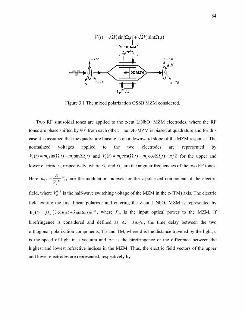
64

x TE−

z TM−

β

α x TE−

z TM−

1 1 2 2( ) 2 sin( ) 2 sin( )V t V t V t= Ω + Ω

Figure 3.1 The mixed polarization OSSB MZM considered.

Two RF sinusoidal tones are applied to the z-cut LiNbO3 MZM electrodes, where the RF

tones are phase shifted by 900 from each other. The DE-MZM is biased at quadrature and for this

case it is assumed that the quadrature biasing is on a downward slope of the MZM response. The

normalized voltages applied to the two electrodes are represented by

1 1 2 2( ) sin( ) sin( )uV t m t m t= Ω + Ω and 1 1 2 2( ) cos( ) cos( ) 2lV t m t m t π= Ω + Ω − for the upper and

lower electrodes, respectively, where 1Ω and 2Ω are the angular frequencies of the two RF tones.

Here 1,2 1,2( )zm VVπ

π= are the modulation indexes for the z-polarized component of the electric

field, where ( )zVπ is the half-wave switching voltage of the MZM in the z-(TM) axis. The electric

field exiting the first linear polarizer and entering the z-cut LiNbO3 MZM is represented by

( ) j tin int P z x e ωα α= + ˆˆE ( ) cos( ) sin( ) , where Pin is the input optical power to the MZM. If

birefringence is considered and defined as d n cτΔ = Δ , the time delay between the two

orthogonal polarization components, TE and TM, where d is the distance traveled by the light, c

is the speed of light in a vacuum and nΔ is the birefringence or the difference between the

highest and lowest refractive indices in the MZM. Thus, the electric field vectors of the upper

and lower electrodes are represented, respectively by

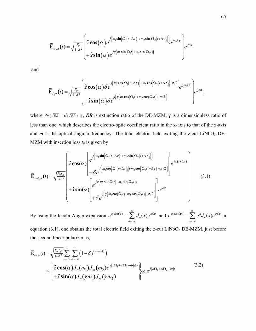
65

( ) ( ) ( )

( ) ( ) ( )( )

1 1 2 2

21 1 2 2

1in

j m t m t jP j t

uj m t m t

z e et e

x e

τ τ ω τω

α δ γ

α

α

⎛ ⎞⎡ ⎤ ⎡ ⎤⎜ ⎟⎢ ⎥ ⎢ ⎥⎣ ⎦ ⎣ ⎦⎝ ⎠

Ω +Δ + Ω +Δ Δ

+ Ω + Ω

⎛ ⎞⎜ ⎟⎜ ⎟⎜ ⎟⎜ ⎟⎝ ⎠

=+

sin sin

,sin sin

ˆ cosE ( )

ˆ sin

and

( ) ( ) ( )

( ) ( ) ( )( )

1 1 2 2

21 1 2 2

2

1 2

in

j m t m t jP j t

lj m t m t

z e et e

x e

τ τ π ω τω

α δ γ π

α δ

α δ

⎛ ⎞⎡ ⎤ ⎡ ⎤⎜ ⎟⎢ ⎥ ⎢ ⎥⎣ ⎦ ⎣ ⎦⎝ ⎠

⎛ ⎞⎜ ⎟⎝ ⎠

Ω +Δ + Ω +Δ − Δ

+ Ω + Ω −

⎛ ⎞⎜ ⎟⎜ ⎟⎜ ⎟⎜ ⎟⎝ ⎠

=

+

cos cos

,cos cos

ˆ cosE ( )

ˆ sin,

where = ( 1) ( 1)ER ERδ − + , ER is extinction ratio of the DE-MZM, γ is a dimensionless ratio of

less than one, which describes the electro-optic coefficient ratio in the x-axis to that of the z-axis

and ω is the optical angular frequency. The total electric field exiting the z-cut LiNbO3 DE-

MZM with insertion loss tff is given by

( ) ( )

( ) ( )( )

( ) ( )( )

( ) ( )( )

2

1 1 2 2

1 1 2 2

1 1 2 2

1 1 2 2

1

2

2

in ff

j t

P tout

j m t m t

j m t m t

j m t m t

j m t m t

z e

t

x

e

e

e

e

ω τ

α δ

τ τ

τ τ π

γ

γ π

α

α

δ

δ

⎛ ⎞⎡ ⎤ ⎡ ⎤⎜ ⎟⎢ ⎥ ⎢ ⎥⎣ ⎦ ⎣ ⎦⎝ ⎠

⎛ ⎞⎡ ⎤ ⎡ ⎤⎜ ⎟⎢ ⎥ ⎢ ⎥⎣ ⎦ ⎣ ⎦⎝ ⎠

⎛ ⎞⎜ ⎟⎝ ⎠

+Δ

+

Ω +Δ + Ω +Δ

Ω +Δ + Ω +Δ −

Ω + Ω

Ω + Ω −

⎡ ⎤⎢ ⎥⎢ ⎥⎢ ⎥⎣ ⎦

⎡⎢⎢

⎣

=

+

+

+

,

sin sin

cos cos

sin sin

cos cos

ˆ cos( )

E ( )

ˆ sin( ) j te ω

⎛ ⎞⎜ ⎟⎜ ⎟⎜ ⎟⎜ ⎟⎜ ⎟

⎤⎜ ⎟⎥⎜ ⎟⎥⎜ ⎟

⎢ ⎥⎜ ⎟⎦⎝ ⎠

(3.1)

By using the Jacobi-Auger expansion sin( ) ( )jx t jn tn

ne J x e

∞Ω Ω

=−∞

= ∑ and cos( ) ( )jx t n jn tn

ne j J x e

∞Ω Ω

=−∞

= ∑ in

equation (3.1), one obtains the total electric field exiting the z-cut LiNbO3 DE-MZM, just before

the second linear polarizer as,

( )( )( )

( )

12

1 21 2

1

1 2

1 2

1

out

n m

n m

in ffP t

j n mj n m tn m

n m

t j

z J m J m e ex J m J m

α δ

ω τω

δ

αα γ γ

∞ ∞+ +

=−∞ =−∞+

Ω + Ω + ΔΩ + Ω +

= −

⎧ ⎫⎪ ⎪⎨ ⎬⎪ ⎪⎩ ⎭

× ×+

∑ ∑,E ( )

ˆ cos( ) ( ) ( )ˆ sin( ) ( ) ( )

(3.2)

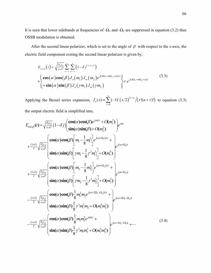
66

It is seen that lower sidebands at frequencies of -Ω1 and -Ω2 are suppressed in equation (3.2) thus

OSSB modulation is obtained.

After the second linear polarizer, which is set to the angle of β with respect to the z-axis, the

electric field component exiting the second linear polarizer is given by,

( ) ( )( )

( ) ( ) ( ) ( ) ( )

( ) ( ) ( ) ( )( )

12

1 2

1 2

1

1 2

1 2

1 n min ff

outn m

P t

j n mn m j n m t

n m

E t j

J m J m ee

J m J m

β δ

ω τω

δ

α β

α β γ γ

∞ ∞+ +

=−∞ =−∞+

Ω + Ω + ΔΩ + Ω +

= −

⎧ ⎫⎪ ⎪× ×⎨ ⎬+⎪ ⎪⎩ ⎭

∑ ∑,

cos cos

sin sin

(3.3)

Applying the Bessel series expansion, ( ) ( )2

0( ) ( 1) 2 !( )!r nr

nr

J x x r n r∞

+

=

≡ − +∑ to equation (3.3)

the output electric field is simplified into,

( )

( )

( )

( )

( )

2

1

12

21

1 22

31 1

12 1

3 3 51 1 1

12 1

1

18

18

in ff

in ff

in ff

jP t j t

out

j

P t j t

P t

e O mE t j e

O m

m m ee

m m O m

ω τω

β δ

ω τ

δ ωδ

δ

α βδ

α β

α β

α β γ γ

Δ

+

+Ω Δ

+ +Ω+

+

⎛ ⎞⎜ ⎟⎜ ⎟⎝ ⎠

⎛ ⎞⎡ ⎤⎜ ⎟⎢ ⎥

⎣ ⎦⎜ ⎟⎜ ⎟⎡ ⎤⎜ ⎟⎢ ⎥⎜ ⎟⎣ ⎦⎝ ⎠

+= −

+

− ++

− +

+

,cos( )cos( ) ( )

( )sin( )sin( ) ( )

cos( )cos( )

sin( )sin( ) ( )

( )

( )

( )( )

( )

2

22

1 2

1 22

32 2

3 3 52 2 2

221 21 2

2 13 2 4 3

1 2 1 2

1

1818

18 18

in ff

j t

j

j

P t j t

em m e

m m O m

m m ee

m m O m m

ω τ

ωδ

ω τ

δ ωδ

α β

α β γ γ

α β

α β γ

+Ω Δ

+Ω+

+ Ω −Ω Δ

+ + Ω −Ω+

⎛ ⎞⎡ ⎤⎜ ⎟⎢ ⎥

⎣ ⎦⎜ ⎟⎜ ⎟⎡ ⎤⎜ ⎟⎢ ⎥⎜ ⎟⎣ ⎦⎝ ⎠⎛ ⎞⎜ ⎟⎜ ⎟⎜ ⎟⎜ ⎟⎝ ⎠

− +

− +

+−

+

−

cos( )cos( )

sin( )sin( ) ( )

cos( )cos( )

sin( )sin( ) ( )

( ) 2 12

2

21 2

2 13 2 3 4

1 2 1 2

1818

in ff j t

j

P t em m e

m m O m m

ω

ω τ

δδ

α β

α β γ

+ Ω

Δ

+ −Ω+

⎛ ⎞⎜ ⎟⎜ ⎟⎜ ⎟⎜ ⎟⎝ ⎠

++⋅⋅⋅

+

( )cos( )cos( )

sin( )sin( ) ( )

(3.4)

67

From equation (3.4) it can be seen that ( ) 1, 2,ije iω τ+Ω Δ = is the differential phase delay between

the two orthogonal polarization components for a given RF subcarrier. Third order IMD cannot

be completely suppressed if this differential phase delay is not negligible. However, if it is

negligible, i.e. ( ) ( )( )21 2i

ije ω τ τω+Ω Δ

− Ω Δ+≈ , for 1τωΔ << , which is usually the case as stated

in [54] the differential phase delay is small for the MZM, ~1 % and the condition for the

complete suppression of third order IMD will depend on the differential group delay, as given in

equation (3.5). It is seen from equation (3.4) that the IMD due to the characteristic of the MZM

can be removed by eliminating the IMD components or the terms proportional to 31,2m in electric

field, if the following condition of

( )231

2cos( )cos( ) sin( )sin( ) 0,

ω τα β γ α β

⎡ ⎤⎢ ⎥⎢ ⎥⎢ ⎥⎣ ⎦

Δ− + = (3.5)

is satisfied, where the assumption of 1τωΔ << was used. We may see that equation (3.5) does not

have a unique solution, so it would be ideal to choose a solution that maximizes the RF carriers

that are proportional to 1,2m in electric field. This yields ( )( )3 21 2 1 2tan ω τα β γ−−

− Δ= − = ± . Due

to linearization, a decrease in optical RF signal subcarrier power is induced by a factor of

( )( ) ( )( )2

22

3

(1 )

1 21 2

ω τ

γ γω τ

γ−

− Δ +− Δ , for 1τωΔ << . If birefringence is neglected, i.e. 0τωΔ = and

1 3γ = for a typical z-cut LiNbO3 MZM, this leads to 079α β ±= − = and the above factor yields

an 11 dB loss, which is the same as [54]. It is also noted from equation (3.5) that the suppression

of 3IMD is not dependent on individual modulation depths, so a costly DC bias controller is not

required for this proposed design.

3.3 SFDR and Sensitivity Analysis

A development for the expression of SFDR for a RoF system, where the considered mixed-

polarization OSSB MZM is used. The IMD output power includes residual IMD and its higher

orders components. Assuming equal modulation index, i.e. 1 2m m m= = , using equation (3.4) to

obtain the photo-current 12 out outopt optG L E t E t

β βℜ *

, ,( ) ( ) , where ℜ is the responsivity of the

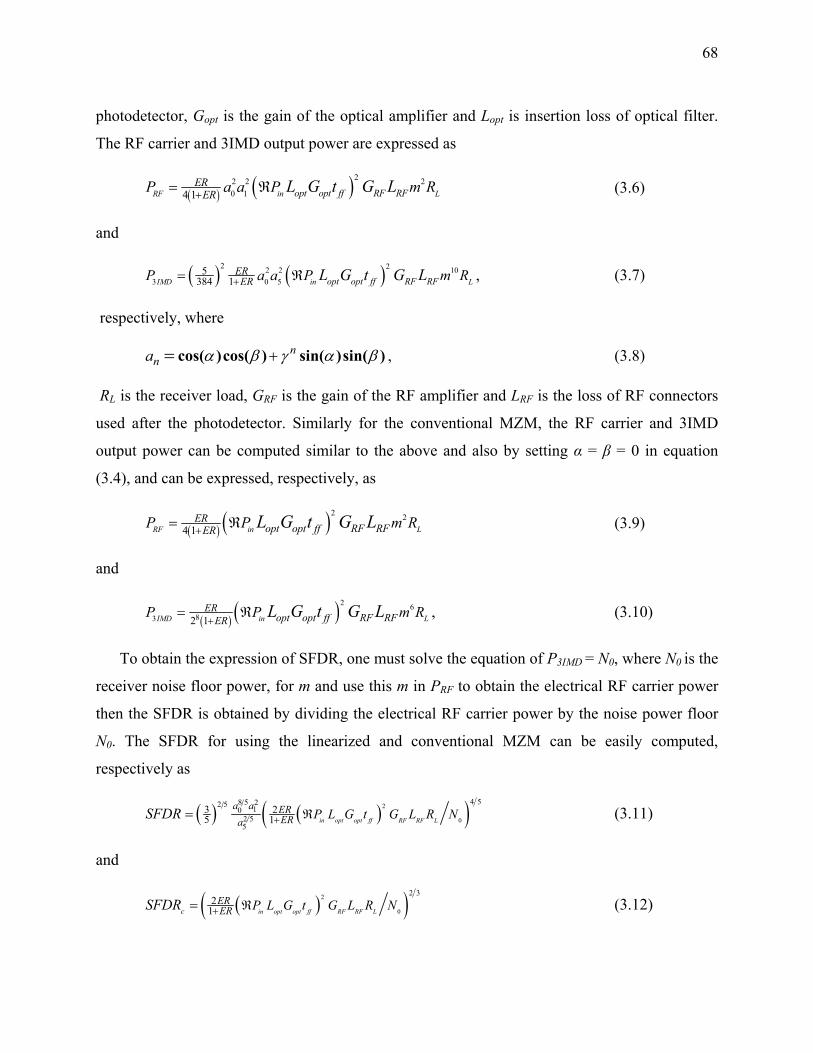
68

photodetector, Gopt is the gain of the optical amplifier and Lopt is insertion loss of optical filter.

The RF carrier and 3IMD output power are expressed as

( ) ( )22 2 20 14 1RF in Lopt opt ff RF RF

ERERP a a P m RL G t G L+= ℜ (3.6)

and

( ) ( )2 22 2 103 0 5

5384 1IMD in Lopt opt ff RF RF

ERERP a a P m RL G t G L+= ℜ , (3.7)

respectively, where

nna α β γ α β+= cos( )cos( ) sin( )sin( ) , (3.8)

RL is the receiver load, GRF is the gain of the RF amplifier and LRF is the loss of RF connectors

used after the photodetector. Similarly for the conventional MZM, the RF carrier and 3IMD

output power can be computed similar to the above and also by setting α = β = 0 in equation

(3.4), and can be expressed, respectively, as

( ) ( )2 2

4 1RF in LER

opt opt RF RFffERP P m RL G t G L+= ℜ (3.9)

and

( ) ( )2 683 2 1IMD in L

ERopt opt RF RFffER

P P m RL G t G L+

= ℜ , (3.10)

To obtain the expression of SFDR, one must solve the equation of P3IMD = N0, where N0 is the

receiver noise floor power, for m and use this m in PRF to obtain the electrical RF carrier power

then the SFDR is obtained by dividing the electrical RF carrier power by the noise power floor

N0. The SFDR for using the linearized and conventional MZM can be easily computed,

respectively as

( ) ( )( )2

0

4 58 5 22 5 102 55

3 25 1 in opt opt ff RF RF L

a a ERERa

P L G t G L R NSFDR + ℜ= (3.11)

and

( )( )2

0

2 32

1 in opt opt ff RF RF LcERER P L G t G L R NSFDR + ℜ= (3.12)

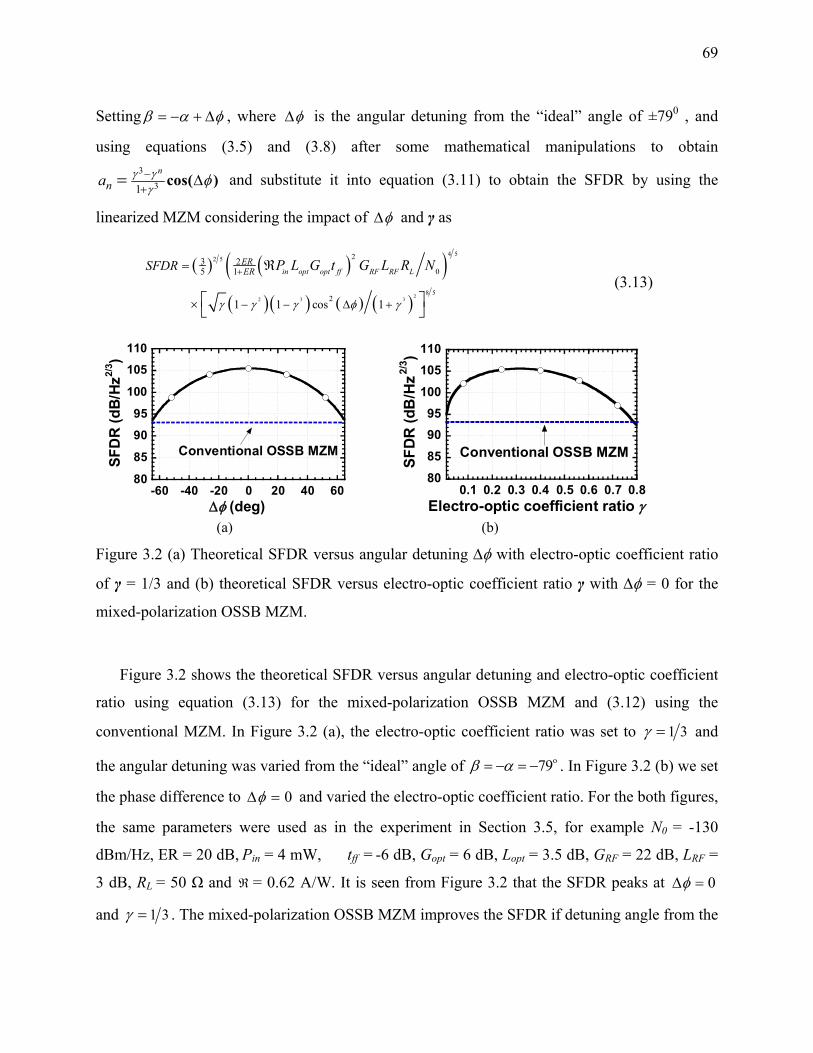
69

Setting β α φ= − + Δ , where φΔ is the angular detuning from the “ideal” angle of ±790 , and

using equations (3.5) and (3.8) after some mathematical manipulations to obtain 3

31

n

na γ γγ

φ−+

Δ= cos( ) and substitute it into equation (3.11) to obtain the SFDR by using the

linearized MZM considering the impact of φΔ and γ as

( ) ( )( )

( )( ) ( ) ( )22 3 3

4 52 5

8 5

2

0

2

3 25 1

1 1 cos 1

in opt opt ff RF RF LERERSFDR P L G t G L R N

γ γ γ φ γ

+

− − Δ +

=

×

ℜ

⎡ ⎤⎣ ⎦

(3.13)

80

85

90

95

100

105

110

-60 -40 -20 0 20 40 60

SFD

R (d

B/H

z2/3 )

Δφ (deg)

Conventional OSSB MZM

80859095

100105110

0.1 0.2 0.3 0.4 0.5 0.6 0.7 0.8Electro-optic coefficient ratio γ

SFD

R (d

B/H

z2/3 )

Conventional OSSB MZM

(a) (b)

Figure 3.2 (a) Theoretical SFDR versus angular detuning Δφ with electro-optic coefficient ratio

of γ = 1/3 and (b) theoretical SFDR versus electro-optic coefficient ratio γ with Δφ = 0 for the

mixed-polarization OSSB MZM.

Figure 3.2 shows the theoretical SFDR versus angular detuning and electro-optic coefficient

ratio using equation (3.13) for the mixed-polarization OSSB MZM and (3.12) using the

conventional MZM. In Figure 3.2 (a), the electro-optic coefficient ratio was set to 1 3γ = and

the angular detuning was varied from the “ideal” angle of o79β α= − = − . In Figure 3.2 (b) we set

the phase difference to 0φΔ = and varied the electro-optic coefficient ratio. For the both figures,

the same parameters were used as in the experiment in Section 3.5, for example N0 = -130

dBm/Hz, ER = 20 dB, Pin = 4 mW, tff = -6 dB, Gopt = 6 dB, Lopt = 3.5 dB, GRF = 22 dB, LRF =

3 dB, RL = 50 Ω and ℜ = 0.62 A/W. It is seen from Figure 3.2 that the SFDR peaks at 0φΔ =

and 1 3γ = . The mixed-polarization OSSB MZM improves the SFDR if detuning angle from the

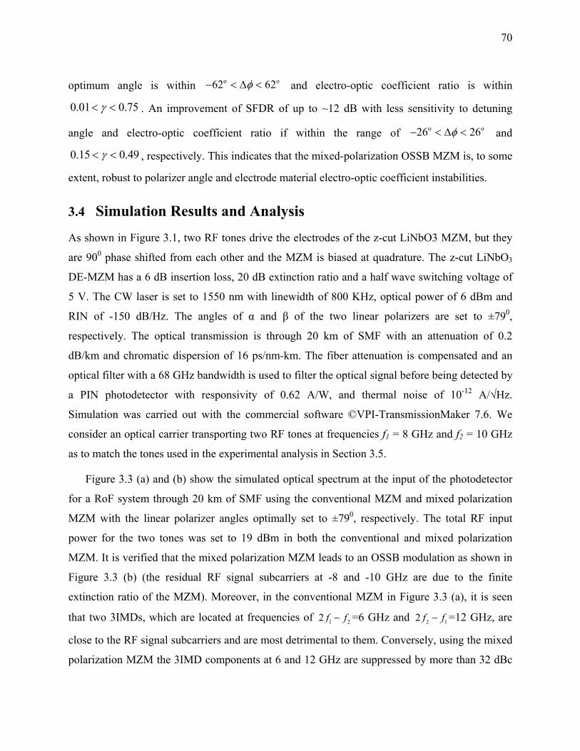
70

optimum angle is within o o62 62φ− < Δ < and electro-optic coefficient ratio is within

0.01 0.75γ< < . An improvement of SFDR of up to ~12 dB with less sensitivity to detuning

angle and electro-optic coefficient ratio if within the range of o o26 26φ− < Δ < and

0.15 0.49γ< < , respectively. This indicates that the mixed-polarization OSSB MZM is, to some

extent, robust to polarizer angle and electrode material electro-optic coefficient instabilities.

3.4 Simulation Results and Analysis

As shown in Figure 3.1, two RF tones drive the electrodes of the z-cut LiNbO3 MZM, but they

are 900 phase shifted from each other and the MZM is biased at quadrature. The z-cut LiNbO3

DE-MZM has a 6 dB insertion loss, 20 dB extinction ratio and a half wave switching voltage of

5 V. The CW laser is set to 1550 nm with linewidth of 800 KHz, optical power of 6 dBm and

RIN of -150 dB/Hz. The angles of α and β of the two linear polarizers are set to ±790,

respectively. The optical transmission is through 20 km of SMF with an attenuation of 0.2

dB/km and chromatic dispersion of 16 ps/nm-km. The fiber attenuation is compensated and an

optical filter with a 68 GHz bandwidth is used to filter the optical signal before being detected by

a PIN photodetector with responsivity of 0.62 A/W, and thermal noise of 10-12 A/√Hz.

Simulation was carried out with the commercial software ©VPI-TransmissionMaker 7.6. We

consider an optical carrier transporting two RF tones at frequencies f1 = 8 GHz and f2 = 10 GHz

as to match the tones used in the experimental analysis in Section 3.5.

Figure 3.3 (a) and (b) show the simulated optical spectrum at the input of the photodetector

for a RoF system through 20 km of SMF using the conventional MZM and mixed polarization

MZM with the linear polarizer angles optimally set to ±790, respectively. The total RF input

power for the two tones was set to 19 dBm in both the conventional and mixed polarization

MZM. It is verified that the mixed polarization MZM leads to an OSSB modulation as shown in

Figure 3.3 (b) (the residual RF signal subcarriers at -8 and -10 GHz are due to the finite

extinction ratio of the MZM). Moreover, in the conventional MZM in Figure 3.3 (a), it is seen

that two 3IMDs, which are located at frequencies of 1 22 f f− =6 GHz and 2 12 f f− =12 GHz, are

close to the RF signal subcarriers and are most detrimental to them. Conversely, using the mixed

polarization MZM the 3IMD components at 6 and 12 GHz are suppressed by more than 32 dBc

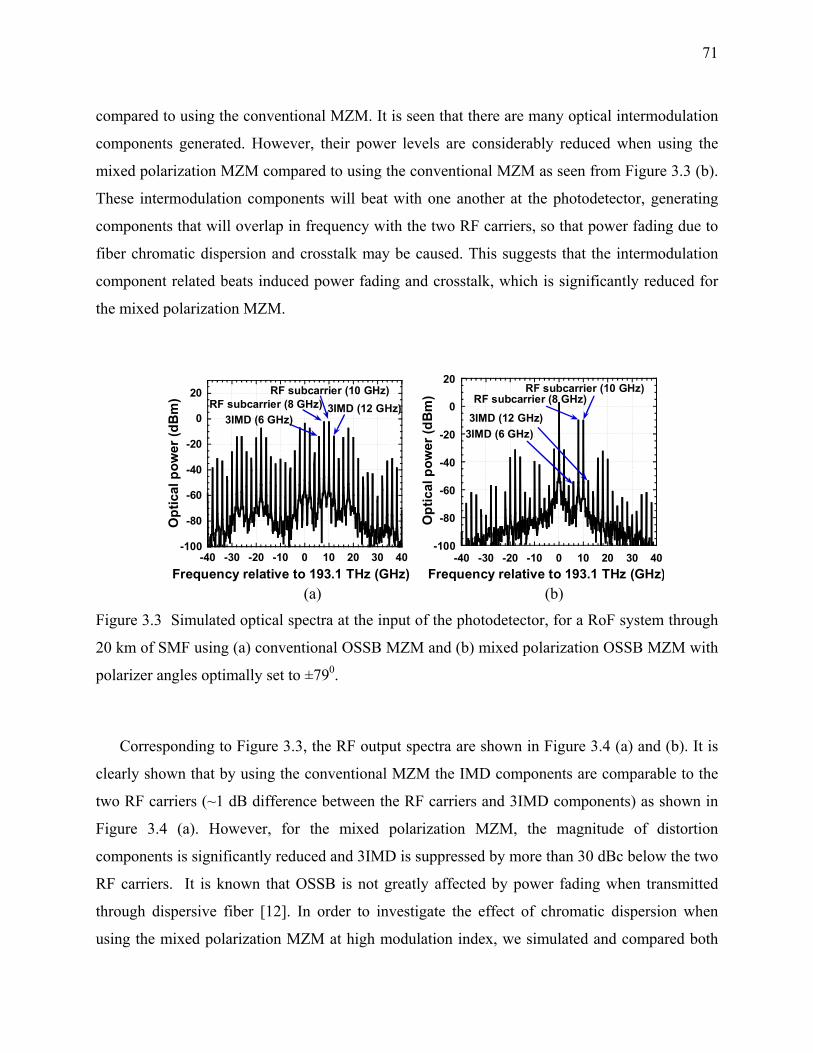
71

compared to using the conventional MZM. It is seen that there are many optical intermodulation

components generated. However, their power levels are considerably reduced when using the

mixed polarization MZM compared to using the conventional MZM as seen from Figure 3.3 (b).

These intermodulation components will beat with one another at the photodetector, generating

components that will overlap in frequency with the two RF carriers, so that power fading due to

fiber chromatic dispersion and crosstalk may be caused. This suggests that the intermodulation

component related beats induced power fading and crosstalk, which is significantly reduced for

the mixed polarization MZM.

-100

-80

-60

-40

-20

0

20

-40 -30 -20 -10 0 10 20 30 40

Opt

ical

pow

er (d

Bm

)

Frequency relative to 193.1 THz (GHz)

RF subcarrier (10 GHz)

3IMD (6 GHz)3IMD (12 GHz)RF subcarrier (8 GHz)

RF subcarrier (10 GHz)

-100

-80

-60

-40

-20

0

20

-40 -30 -20 -10 0 10 20 30 40Frequency relative to 193.1 THz (GHz)

Opt

ical

pow

er (d

Bm

)3IMD (6 GHz)3IMD (12 GHz)RF subcarrier (8 GHz)

(a) (b)

Figure 3.3 Simulated optical spectra at the input of the photodetector, for a RoF system through

20 km of SMF using (a) conventional OSSB MZM and (b) mixed polarization OSSB MZM with

polarizer angles optimally set to ±790.

Corresponding to Figure 3.3, the RF output spectra are shown in Figure 3.4 (a) and (b). It is

clearly shown that by using the conventional MZM the IMD components are comparable to the

two RF carriers (~1 dB difference between the RF carriers and 3IMD components) as shown in

Figure 3.4 (a). However, for the mixed polarization MZM, the magnitude of distortion

components is significantly reduced and 3IMD is suppressed by more than 30 dBc below the two

RF carriers. It is known that OSSB is not greatly affected by power fading when transmitted

through dispersive fiber [12]. In order to investigate the effect of chromatic dispersion when

using the mixed polarization MZM at high modulation index, we simulated and compared both

72

conventional and mixed polarization MZM with RF tones of 8 and 10 GHz, where the input RF

power level was set to 19 dBm for both the conventional and mixed polarization MZM.

-120

-100

-80

-60

-40

-20

0

0 5 10 15 20 25 30 35 40

Frequency (GHz)

Det

ecte

d R

F po

wer

(dB

m)

RF carrier (8 GHz)RF carrier (10 GHz)

3IMD (12 GHz)

3IMD (6 GHz)

-140

-120

-100

-80

-60

-40

-20

0 5 10 15 20 25 30 35 40

Det

ecte

d R

F po

wer

(dB

m)

Frequency (GHz)

RF carrier (8 GHz)RF carrier (10 GHz)3IMD (12 GHz)

3IMD (6 GHz)

(a) (b)

Figure 3.4 Simulated RF spectra corresponding to Figure 3.3 .

-60

-50

-40

-30

-20

-10

0

10

0 20 40 60 80 100

RF carrier, conventional

3IMD, conventional

RF carrier, mixed polarization

3IMD, mixed polarizationDet

ecte

d R

F po

wer

(dB

m)

Fiber Length (km) Figure 3.5 Simulated RF carrier and 3IMD power versus fiber length for a RoF system using the

conventional and mixed polarization OSSB MZM, respectively, with compensated fiber loss.

Figure 3.5 compares the RF carrier and 3IMD powers for the conventional and mixed

polarization MZM. Fiber loss is compensated in order to emphasize the effects of chromatic

dispersion on the RF signal. We can see that the RF carrier power does not vary with changing

73

fiber length and thus there is no intermodulation component induced power fading and crosstalk,

when using the mixed polarization MZM, while the RF carrier power fluctuates with changing

fiber length and thus intermodulation component induced power fading and crosstalk must exist

when using the conventional MZM. This is due to constructive and destructive interactions

between many harmonic and intermodulation components for the conventional MZM as shown

in Figure 3.4 (a). Thus the beats between distortion components are overlapped in frequency with

the RF carriers, and then these beats interplay with the RF carriers. It is clearly shown that the

mixed polarization MZM is immune to power fading and crosstalk caused by these interactions

of intermodulation components and chromatic dispersion. It is shown that 3IMD is suppressed by

more than 30 dBc as shown in Figure 3.4 (b). Therefore, not only is the mixed polarization

OSSB transmission immune to power fading and crosstalk, but it also provides a greater

suppression of 3IMD, which leads to an improvement in SFDR.

-140

-120

-100

-80

-60

-40

-20

0

20

-40 -20 0 20 40

Conventional Mixed polarization

Det

ecte

d R

F po

wer

(dB

m)

Input RF power (dBm)

SFD

R =

97.

5 dB

/Hz2/

3

SFD

R =

110

.5 d

B/H

z4/5

Noise floor @ -130 dBm/Hz

3IMD

RF carrier

-140

-120

-100

-80

-60

-40

-20

0

20

-40 -20 0 20 40

Det

ecte

d R

F po

wer

(dB

m)

Input RF power (dBm)

SFD

R =

97.

5 dB

/Hz2/

3

SFD

R =

110

.5 d

B/H

z4/5


3IMD

RF carrier

(a) (b)

Figure 3.6 Simulated spurious free dynamic range for a RoF system using the mixed polarization

and conventional OSSB MZM in (a) back-to-back and (b) through 20 km of single mode fiber.

In order to show the suppression of 3IMD by using the mixed polarization MZM over the

conventional MZM, we compared the SFDR for a RoF system using a mixed polarization and

conventional OSSB MZM as shown in Figure 3.6 (a) and (b) for back-to-back and through 20

km of SMF, respectively. From Figure 3.6 (a) and (b) it is shown that nonlinear distortion is 5th

order limited (see the slope of 3IMD power) for the RoF system using the mixed polarization

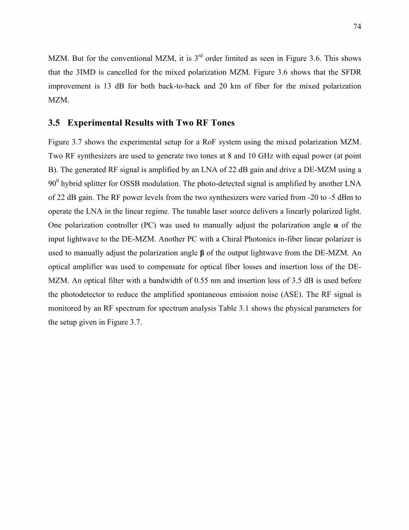
74

MZM. But for the conventional MZM, it is 3rd order limited as seen in Figure 3.6. This shows

that the 3IMD is cancelled for the mixed polarization MZM. Figure 3.6 shows that the SFDR

improvement is 13 dB for both back-to-back and 20 km of fiber for the mixed polarization

MZM.

3.5 Experimental Results with Two RF Tones

Figure 3.7 shows the experimental setup for a RoF system using the mixed polarization MZM.

Two RF synthesizers are used to generate two tones at 8 and 10 GHz with equal power (at point

B). The generated RF signal is amplified by an LNA of 22 dB gain and drive a DE-MZM using a

900 hybrid splitter for OSSB modulation. The photo-detected signal is amplified by another LNA

of 22 dB gain. The RF power levels from the two synthesizers were varied from -20 to -5 dBm to

operate the LNA in the linear regime. The tunable laser source delivers a linearly polarized light.

One polarization controller (PC) was used to manually adjust the polarization angle α of the

input lightwave to the DE-MZM. Another PC with a Chiral Photonics in-fiber linear polarizer is

used to manually adjust the polarization angle β of the output lightwave from the DE-MZM. An

optical amplifier was used to compensate for optical fiber losses and insertion loss of the DE-

MZM. An optical filter with a bandwidth of 0.55 nm and insertion loss of 3.5 dB is used before

the photodetector to reduce the amplified spontaneous emission noise (ASE). The RF signal is

monitored by an RF spectrum for spectrum analysis Table 3.1 shows the physical parameters for

the setup given in Figure 3.7.

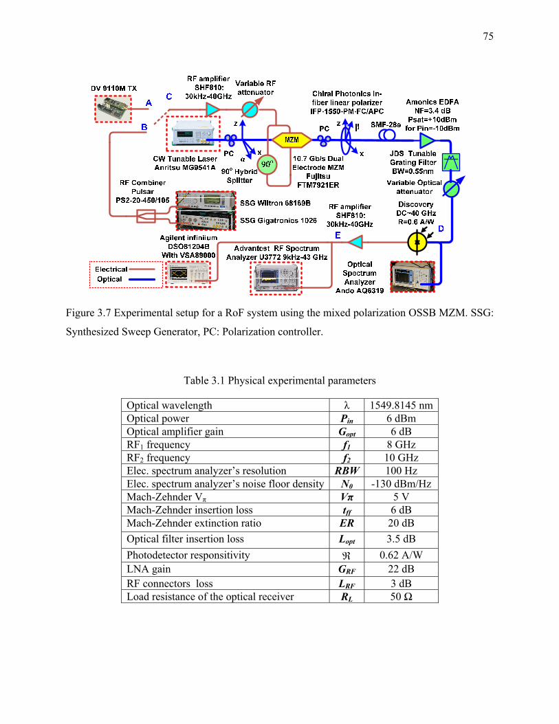
75

Figure 3.7 Experimental setup for a RoF system using the mixed polarization OSSB MZM. SSG:

Synthesized Sweep Generator, PC: Polarization controller.

Table 3.1 Physical experimental parameters

Optical wavelength λ 1549.8145 nm Optical power Pin 6 dBm Optical amplifier gain Gopt 6 dB RF1 frequency f1 8 GHz RF2 frequency f2 10 GHz Elec. spectrum analyzer’s resolution RBW 100 Hz Elec. spectrum analyzer’s noise floor density N0 -130 dBm/Hz Mach-Zehnder Vπ Vπ 5 V Mach-Zehnder insertion loss tff 6 dB Mach-Zehnder extinction ratio ER 20 dB Optical filter insertion loss Lopt 3.5 dB Photodetector responsitivity ℜ 0.62 A/W LNA gain GRF 22 dB RF connectors loss LRF 3 dB Load resistance of the optical receiver RL 50 Ω

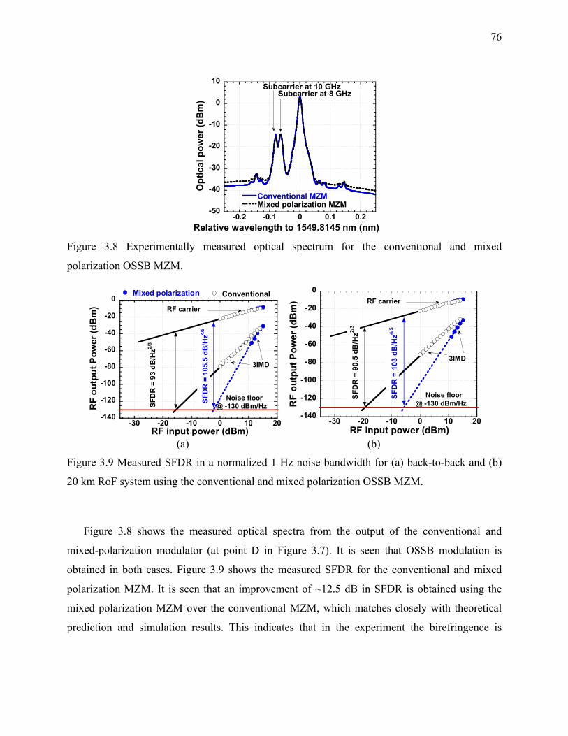
76

-50

-40

-30

-20

-10

0

10

-0.2 -0.1 0 0.1 0.2

Conventional MZMMixed polarization MZM

Opt

ical

pow

er (d

Bm

)

Relative wavelength to 1549.8145 nm (nm)

Subcarrier at 10 GHzSubcarrier at 8 GHz

Figure 3.8 Experimentally measured optical spectrum for the conventional and mixed

polarization OSSB MZM.

-140

-120

-100

-80

-60

-40

-20

0

-30 -20 -10 0 10 20

Mixed polarization Conventional

RF

outp

ut P

ower

(dB

m)

RF input power (dBm)

SFD

R =

93

dB/H

z2/3

SFD

R =

105

.5 d

B/H

z4/5


3IMD

RF carrier

-140

-120

-100

-80

-60

-40

-20

0

-30 -20 -10 0 10 20

RF

outp

ut P

ower

(dB

m)

RF input power (dBm)

SFD

R =

90.

5 dB

/Hz2/

3

SFD

R =

103

dB

/Hz4/

5 Noise floor @ -130 dBm/Hz

3IMD

RF carrier

(a) (b)

Figure 3.9 Measured SFDR in a normalized 1 Hz noise bandwidth for (a) back-to-back and (b)

20 km RoF system using the conventional and mixed polarization OSSB MZM.

Figure 3.8 shows the measured optical spectra from the output of the conventional and

mixed-polarization modulator (at point D in Figure 3.7). It is seen that OSSB modulation is

obtained in both cases. Figure 3.9 shows the measured SFDR for the conventional and mixed

polarization MZM. It is seen that an improvement of ~12.5 dB in SFDR is obtained using the

mixed polarization MZM over the conventional MZM, which matches closely with theoretical

prediction and simulation results. This indicates that in the experiment the birefringence is

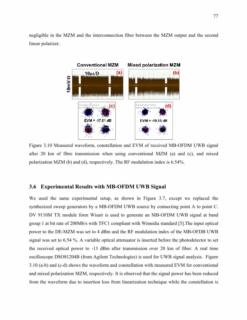
77

negligible in the MZM and the interconnection fiber between the MZM output and the second

linear polarizer.

Figure 3.10 Measured waveform, constellation and EVM of received MB-OFDM UWB signal

after 20 km of fibre transmission when using conventional MZM (a) and (c), and mixed

polarization MZM (b) and (d), respectively. The RF modulation index is 6.54%.

3.6 Experimental Results with MB-OFDM UWB Signal

We used the same experimental setup, as shown in Figure 3.7, except we replaced the

synthesized sweep generators by a MB-OFDM UWB source by connecting point A to point C.

DV 9110M TX module form Wisair is used to generate an MB-OFDM UWB signal at band

group 1 at bit rate of 200Mb/s with TFC1 compliant with Wimedia standard [5].The input optical

power to the DE-MZM was set to 4 dBm and the RF modulation index of the MB-OFDB UWB

signal was set to 6.54 %. A variable optical attenuator is inserted before the photodetector to set

the received optical power to -13 dBm after transmission over 20 km of fiber. A real time

oscilloscope DSO81204B (from Agilent Technologies) is used for UWB signal analysis. Figure

3.10 (a-b) and (c-d) shows the waveform and constellation with measured EVM for conventional

and mixed polarization MZM, respectively. It is observed that the signal power has been reduced

from the waveform due to insertion loss from linearization technique while the constellation is

78

less distorted and the EVM is improved by more than 2 dB when using the mixed polarization

MZM.

3.7 Chapter Summary

This chapter presented the mixed-polarization OSSB MZM, which alleviated most of the

limitations incurred by the previous proposed linearization techniques. A comprehensive

investigation was conducted for the mixed-polarization MZM in the suppression of IMD in

theory, simulation and experiment. The suppression of third order IMD using the mixed-

polarization MZM is independent of modulation index. Both theory and simulation predict a 13

dB improvement of SFDR for back-to-back and 20 km fiber RoF system using the mixed-

polarization modulator. Moreover, power fading of the RF carrier and crosstalk due to

intermodulation via fiber chromatic dispersion is significantly suppressed compared to using the

conventional OSSB MZM. We experimentally verified the mixed-polarization modulation

technique. It was shown that an improvement of ~12.5 dB in SFDR using discrete optical

components was achieved and good agreement with theory and simulation is obtained. Also, an

improvement of 2 dB in EVM is achieved when applying our proposed mixed polarization

technique to MB-OFDM UWB signal after transmission over 20 km of fiber. Due to the

linearization process an RF carrier power penalty is incurred, which will need to be compensated

for with optical amplifiers or increasing the input optical power. It will remain as a future

research to find a way to improve upon this technique by reducing the power penalty.

79

CHAPTER 4 PROPOSED PREDISTORTION CIRCUIT FOR EAM

4.1 Introduction

The mixed polarization technique proposed in Chapter 3 cannot be applied to the EAMs because

they are designed and fabricated to be polarization independent. In [47], a feed-forward

linearization technique of EAM was proposed. The basic idea of feed-forward linearization is as

follows. Part of the output light from EAM is converted back to RF signal, and by subtracting

this RF signal from the original RF signal, only the distortion generated by the EAM is left, then

this distorted RF signal is applied to modulate a DFB-laser to cancel the distortion induced by

the EAM. However, this method has a very rigorous requirement on the wavelength of the two

lasers. If the wavelengths of the two lasers are not exactly the same, then, the linearization would

not happen. Also, the feed-forward linearization method requires an extra laser and PD, which

will increase the cost and the complexity of the whole system. In [48-49], two EAMs are used

either in parallel or in series, and the reverse biases of the EAMs are adjusted to have third order

intermodualtion (IMD3) cancelled. These two methods gave a good suppression of IMD3, but

using two EAMs will also increase cost.

In [40, 44], the analog predistortion circuits were used in narrowband system to linearize RF

power amplifiers. In [36-37], it was successfully introduced the wildly used predistortion circuit

architecture in radio-over-fiber system with radio of below 1 GHz like CATV, GSM, and so on.

In the traditional predistortion circuit, as shown in Figure 4.1, the input RF signal is first split

into two paths, one path goes through the nonlinearity generation circuit, the other path goes

through the time delay, and then these two paths are combined together by a power combiner. A

phase shifter and an amplifier are used in the nonlinear path to adjust the phase and the

magnitude of IMD3 of the pre-distorted signal, so that good cancellation of IMD3 can be

achieved. In [36] the composite triple beat distortion (CTB) is reduced by 10 dB over 400-960

MHz, and in [37] the CTB is reduced by 22.6 dB over 55.25-535.25 MHz for CATV over fiber

system. However, the drawback of the traditional predistortion circuit is the use of extra RF

components, including phase shifter and amplifier, which may introduce new IMD that would be

mixed with the original pre-distorted signal generated by the predistortion circuit, besides that

the phase shifter is a narrow band RF component and cannot be used in UWB system. Another

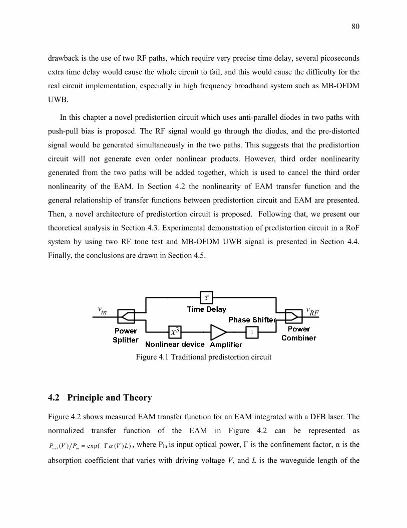
80

drawback is the use of two RF paths, which require very precise time delay, several picoseconds

extra time delay would cause the whole circuit to fail, and this would cause the difficulty for the

real circuit implementation, especially in high frequency broadband system such as MB-OFDM

UWB.

In this chapter a novel predistortion circuit which uses anti-parallel diodes in two paths with

push-pull bias is proposed. The RF signal would go through the diodes, and the pre-distorted

signal would be generated simultaneously in the two paths. This suggests that the predistortion

circuit will not generate even order nonlinear products. However, third order nonlinearity

generated from the two paths will be added together, which is used to cancel the third order

nonlinearity of the EAM. In Section 4.2 the nonlinearity of EAM transfer function and the

general relationship of transfer functions between predistortion circuit and EAM are presented.

Then, a novel architecture of predistortion circuit is proposed. Following that, we present our

theoretical analysis in Section 4.3. Experimental demonstration of predistortion circuit in a RoF

system by using two RF tone test and MB-OFDM UWB signal is presented in Section 4.4.

Finally, the conclusions are drawn in Section 4.5.

τ

3x

inv RFv

Figure 4.1 Traditional predistortion circuit

4.2 Principle and Theory

Figure 4.2 shows measured EAM transfer function for an EAM integrated with a DFB laser. The

normalized transfer function of the EAM in Figure 4.2 can be represented as

( ) exp( ( ) )out inP V P V Lα= −Γ , where Pin is input optical power, Γ is the confinement factor, α is the

absorption coefficient that varies with driving voltage V, and L is the waveguide length of the

81

EAM. The driving voltage is given by b RFV V v= + , where bV is the bias voltage of the EAM, and

RFv is voltage of the RF signal. For the small signal approximation, i.e. RFv << bV , we can expand

the normalized transfer function at a given bias into Taylor series

2 31 2 3

( )outout RF RF RF

in

P Vp k v k v k vP

= = + + +⋅⋅⋅ (4.1)

where ik (i=1, 2, 3, …) are the coefficients related to the EAM transfer function and bias.

Figure 4.2 also shows measured power of IMD3 and fundamental RF carrier at different DC

bias voltage when the input power of RF tones at 3.96 and 3.964 GHz is 3 dBm per RF tone. It is

seen that power of fundamental carrier is the highest when the reversed bias is near 0 V, and the

IMD3 is also the highest at 0 V bias due to the signal clipping but not to the transfer function

nonlinearity of the EAM. While the reversed bias increases, the power of the fundamental carrier

starts decreasing. For RoF system, it is desired to have higher power of the fundamental carrier.

So in this work, we bias the EAM at 0.5 V to avoid clipping and also have higher power of the

fundamental carrier.

0

0.2

0.4

0.6

0.8

1

1.2

-140

-120

-100

-80

-60

-40

-20

0

0 0.5 1 1.5 2 2.5 3 3.5

Nor

mal

ized

Tra

nsm

issi

onD

etected RF Pow

er (dBm

)

Reversed Vbias

(V)

IMD3

Carrier

Figure 4.2 Normalized transfer function of EAM and the power of IMD3 and fundamental

carrier versus EAM bias. Input power is 3 dBm per RF tone.

The block diagram of the predistortion circuit followed with an EAM is depicted in Figure 4.3.

With the small signal assumption, we can only consider up to third order nonlinearity.

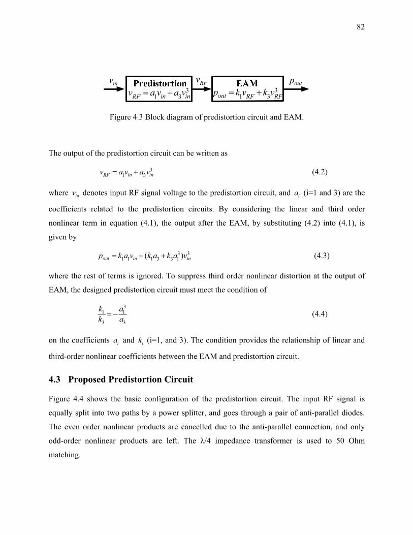
82

inv RFv outp3

1 3in inRFv a v a v= + 31 3out RF RFp k v k v= +

Figure 4.3 Block diagram of predistortion circuit and EAM.

The output of the predistortion circuit can be written as

31 3in inRFv a v a v= + (4.2)

where inv denotes input RF signal voltage to the predistortion circuit, and ia (i=1 and 3) are the

coefficients related to the predistortion circuits. By considering the linear and third order

nonlinear term in equation (4.1), the output after the EAM, by substituting (4.2) into (4.1), is

given by

3 31 1 1 3 3 1( )out in inp k a v k a k a v= + + (4.3)

where the rest of terms is ignored. To suppress third order nonlinear distortion at the output of

EAM, the designed predistortion circuit must meet the condition of

3

1 1

3 3

k ak a= − (4.4)

on the coefficients ia and ik (i=1, and 3). The condition provides the relationship of linear and

third-order nonlinear coefficients between the EAM and predistortion circuit.

4.3 Proposed Predistortion Circuit

Figure 4.4 shows the basic configuration of the predistortion circuit. The input RF signal is

equally split into two paths by a power splitter, and goes through a pair of anti-parallel diodes.

The even order nonlinear products are cancelled due to the anti-parallel connection, and only

odd-order nonlinear products are left. The λ/4 impedance transformer is used to 50 Ohm

matching.

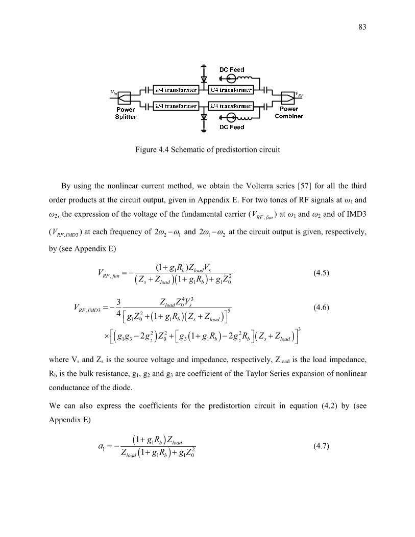
83

RFvinv

Figure 4.4 Schematic of predistortion circuit

By using the nonlinear current method, we obtain the Volterra series [57] for all the third

order products at the circuit output, given in Appendix E. For two tones of RF signals at ω1 and

ω2, the expression of the voltage of the fundamental carrier ( ,RF funV ) at ω1 and ω2 and of IMD3

( , 3RF IMDV ) at each frequency of 2 12ω ω− and 1 22ω ω− at the circuit output is given, respectively,

by (see Appendix E)

( )( )1

, 21 1 0

(1 )1

sb loadRF fun

s load b

g R Z VVZ Z g R g Z

+= −

+ + + (4.5)

( )( )

( ) ( ) ( )2 2

4 30

, 3 521 0 1

32 2 2

1 3 0 3 1

34 1

2 1 2

sloadRF IMD

sb load

sb b load

Z Z VVg Z g R Z Z

g g g Z g g R g R Z Z

⎡ ⎤⎣ ⎦

⎡ ⎤⎡ ⎤⎣ ⎦⎣ ⎦

= −+ + +

× − + + − +

(4.6)

where Vs and Zs is the source voltage and impedance, respectively, Zload is the load impedance,

Rb is the bulk resistance, g1, g2 and g3 are coefficient of the Taylor Series expansion of nonlinear

conductance of the diode.

We can also express the coefficients for the predistortion circuit in equation (4.2) by (see

Appendix E)

( )

( )1

21 1 0

11

1b load

load b

g R ZZ g R g Z

a+

−+ +

= (4.7)

84

( )( )

( ) ( ) ( )( )

2 2

40

221 0 1

2 2 21 3 0 3 1

321 1 0

31

2 1 2

1

load

b s load

b b s load

load b

Z Z

g Z g R Z Z


Z g R g Z

a −⎡ ⎤+ + +⎣ ⎦

⎡ ⎤− + + − +⎣ ⎦×⎡ ⎤+ +⎣ ⎦

= (4.8)

Equations (4.5) and (4.6) are used to calculate the fundamental carrier and IMD3 voltage at the

circuit output, respectively. We carried out Harmonic Balance simulation in Advanced Design

System (ADS) from Agilent Technologies for the diode with 50 Ohm load. Here we used two

tones of input signal at 3960 and 3964.125MHz with equal power of -5 dBm. In Figure 4.5 (a)-

(b), we compare calculated, simulated and measured RF power of fundamental carrier and

IMD3, respectively, at different DC bias current from 0 to 9 mA. Figure 4.5 (a) shows very good

agreement in RF carrier power between simulation and measurement for up to 6 mA, while the

calculated results show a discrepancy of less than 0.5 dB. This is mainly due to the third order

limited approximation used in the theory. At high bias current of the diode, higher order

nonlinearity must be considered for the diode in theory. In Figure 4.5 (b) both simulation and

calculation present some discrepancy in IMD3 power from the measured but follow similar trend

as the measured IMD3. This discrepancy is mainly due to some residual IMD3 generated by the

RF source and the RSA. However, a good prediction can be obtained from either simulation or

calculation, and fine tuning of the bias current can set the right IMD3 magnitude and phase.

-9

-8

-7

-6

-5

0 2 4 6 8

MeasuredCalculatedSimulated

Fund

amen

tal C

arrie

r (dB

m)

Ibias

(mA)

-90

-80

-70

-60

-50

-40

-30

0 2 4 6 8

MeasuredCalculatedSimulated

IMD

3 (d

Bm

)

Ibias

(mA)

(a) (b)

Figure 4.5 Measured, simulated and calculated RF power of (a) fundamental carrier and (b)

IMD3. The input power is -5 dBm per RF tone.

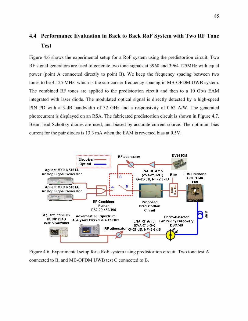
85

4.4 Performance Evaluation in Back to Back RoF System with Two RF Tone

Test

Figure 4.6 shows the experimental setup for a RoF system using the predistortion circuit. Two

RF signal generators are used to generate two tone signals at 3960 and 3964.125MHz with equal

power (point A connected directly to point B). We keep the frequency spacing between two

tones to be 4.125 MHz, which is the sub-carrier frequency spacing in MB-OFDM UWB system.

The combined RF tones are applied to the predistortion circuit and then to a 10 Gb/s EAM

integrated with laser diode. The modulated optical signal is directly detected by a high-speed

PIN PD with a 3-dB bandwidth of 32 GHz and a responsivity of 0.62 A/W. The generated

photocurrent is displayed on an RSA. The fabricated predistortion circuit is shown in Figure 4.7.

Beam lead Schottky diodes are used, and biased by accurate current source. The optimum bias

current for the pair diodes is 13.3 mA when the EAM is reversed bias at 0.5V.

Figure 4.6 Experimental setup for a RoF system using predistortion circuit. Two tone test A

connected to B, and MB-OFDM UWB test C connected to B.

86

Figure 4.7 Fabricated predistortion circuit

Figure 4.8(a)-(b) shows measured RF spectra at the output of the photodetector, without and

with the predistortion circuit, for 3.5 dBm input power of per RF tone and 0.5 V reverse bias of

the EAM. After using the predistortion circuit, the IMD3 is suppressed by more than 18.5 dB

while the fundamental carrier is reduced by 3 dB compared to without predistortion circuit. Thus

the predistortion circuit introduces 3 dB insertion loss, and 3 dB back off in the input power

would reduce the IMD3 by 9 dB. Thus the predistortion circuit gives an effective improvement

of 9.5 dB in suppression of IMD3.

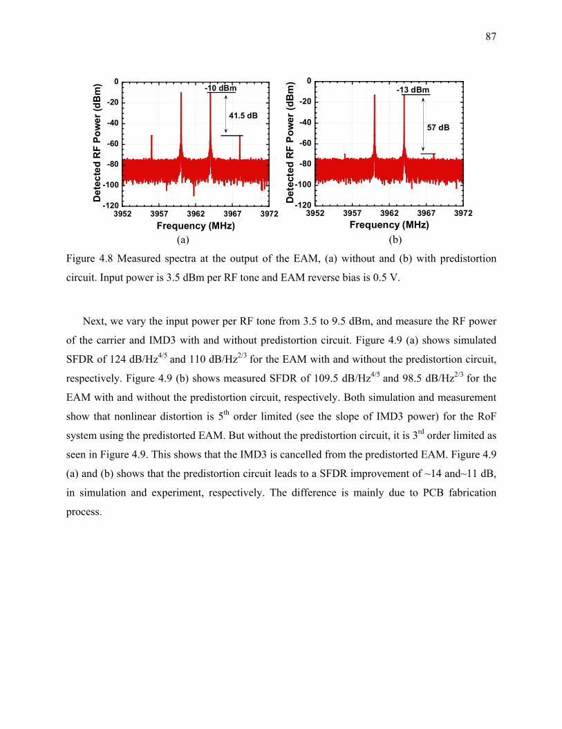
87

-120

-100

-80

-60

-40

-20

0

3952 3957 3962 3967 3972

Det

ecte

d R

F Po

wer

(dB

m)

Frequency (MHz)

41.5 dB

-10 dBm

-120

-100

-80

-60

-40

-20

0

3952 3957 3962 3967 3972

Det

ecte

d R

F Po

wer

(dB

m)

Frequency (MHz)

57 dB

-13 dBm

(a) (b)

Figure 4.8 Measured spectra at the output of the EAM, (a) without and (b) with predistortion

circuit. Input power is 3.5 dBm per RF tone and EAM reverse bias is 0.5 V.

Next, we vary the input power per RF tone from 3.5 to 9.5 dBm, and measure the RF power

of the carrier and IMD3 with and without predistortion circuit. Figure 4.9 (a) shows simulated

SFDR of 124 dB/Hz4/5 and 110 dB/Hz2/3 for the EAM with and without the predistortion circuit,

respectively. Figure 4.9 (b) shows measured SFDR of 109.5 dB/Hz4/5 and 98.5 dB/Hz2/3 for the

EAM with and without the predistortion circuit, respectively. Both simulation and measurement

show that nonlinear distortion is 5th order limited (see the slope of IMD3 power) for the RoF

system using the predistorted EAM. But without the predistortion circuit, it is 3rd order limited as

seen in Figure 4.9. This shows that the IMD3 is cancelled from the predistorted EAM. Figure 4.9

(a) and (b) shows that the predistortion circuit leads to a SFDR improvement of ~14 and~11 dB,

in simulation and experiment, respectively. The difference is mainly due to PCB fabrication

process.

88

-160

-140

-120

-100

-80

-60

-40

-20

0

20

-25 -20 -15 -10 -5 0 5 10

Det

ecte

d R

F Po

wer

(dB

m)

Input RF Power (dBm)

Noise floor @-135 dBm/Hz

without predistortionwith predistortion

SFDR=124 dB/Hz4/5

SFDR=110dB/Hz2/3

RF Carrier

IMD3

15

13

(a)

-140

-120

-100

-80

-60

-40

-20

0

20

-25 -20 -15 -10 -5 0 5 10 15

without predistortion with predistortion

Det

ecte

d R

F Po

wer

(dB

m)

Input RF Power (dBm)

Extrapolated noise floor@ -135 dBm/Hz

SFDR=98.5

dB/Hz2/3

SFDR = 109.5

dB/Hz4/5

noise floor=-95dBm Measured 10 kHz RBW

3 511

(b)

Figure 4.9 Simulated (a) and measured (b) spurious free dynamic range. EAM reverse bias is 0.5

V.

We also investigated the performance of the predistortion circuit for broadband operation. For

this, we vary the frequency of the two RF tones over band group 1 of MB-OFDM UWB and

measure the power level of the RF carrier and IMD3. The input power was set to 3.5 dBm per

RF tone. We swept frequency from 3.168 to 4.752 GHz to cover all frequency of bandgroup 1 in

89

MB-OFDM UWB and kept the two tones with 4.125MHz spacing. For fair comparison, we

attenuate the RF input power to the EAM by 3 dB in order to keep the same RF output power of

the carrier with and without predistotion circuit at the center frequency 3.96 GHz of band group

1. Figure 4.10 shows the frequency response with and without the predistortion circuit. It is

observed that the improvement in IMD3 suppression reduces at lower frequencies. This is

because at lower frequencies the insertion loss is lower and the input RF power is higher, then

the nonlinearities are more pronounced in the EAM. However, the frequency response of the

predistorted EAM is almost constant for up to 3.96 GHz and then decreases by almost 2 dB in

the upper frequency band. The predistortion circuit achieves a suppression of IMD3 by more

than 7 dB over the whole band group 1 of MB-OFDM UWB.

-20

-15

-10

-5

0

-85

-75

-65

-55

-45

3168 3432 3696 3960 4224 4488 4752

With predistortionWithout predistortion

RF

Fund

amen

tal C

arrie

r (dB

m)

IMD

3/C (dB

c)

Frequency (MHz)

Figure 4.10 Measured frequency response of the EAM with and without predistortion circuit.

Input power is 3.5 dBm per RF tone and EAM reverse bias is 0.5 V.

4.5 Performance Evaluation in MB-OFDM over Fiber System

We used the same experimental setup shown in Figure 4.6 for performance evaluation of UWB

over fiber using our predistortion circuit (point C is connected to point B). To generate MB-

OFDM UWB, we used a commercially available evaluation board, DV 9110M from WisAir,

90

which provides MB-OFDM compliant modulation with the first three WiMedia sub-bands of 528

MHz bandwidth allocated at center frequency of f1=3.432, f2=3.96 and f3=4.488 GHz. The signal

follows simple frequency hopping sequences like f1, f2 and f3. The bit rate of 200 Mb/s is used for

each band with QPSK modulations. The MB-OFDM UWB signal generated from DV 9110M

module is applied to predistortion circuit and then to an EAM. The modulated optical signal was

transmitted through an SMF. The EVM of the photodetected signal was measured by a 12 GHz

high speed real time oscilloscope DSO81204B from Agilent Technologies. The optimum bias

current for the pair diodes is 13.3 mA when the EAM was reversely biased at 0.5 V.

To show the improved performance of the transmitted MB-OFDM-UWB signal over fiber

using our predistortion circuit, we have measured and compared EVM using EAM with and

without predistortion circuit in back-to-back and after 20 km of fiber transmission, respectively.

The transmitted power level from the DVM9110M is ~-14 dBm, the loss from RF connections

and Bias Tee is 4 dB, and the maximum losses from the RF attenuator are 16dB. By using a low-

noise amplifier of 26 dB gain and attenuator, we are able to vary the input power to the

predistortion circuit from ~-8 to ~8 dBm. Because the predistortion circuit has 3- dB insertion

loss, we insert 3-dB attenuator before the EAM for without predistortion circuit to make fair

comparison between EAM with and without predistortion. Figure 4.11 (a)-(b) shows the

measured EVM for back to back and after 20 km of fiber transmission for EAM with and

without predistortion circuit.

-22

-20

-18

-16

-8 -6 -4 -2 0 2 4 6 8


EVM

(dB

)

UWB input power (dBm)

-22

-20

-18

-16

-8 -6 -4 -2 0 2 4 6 8


EVM

(dB

)

UWB input power (dBm) (a) (b)

Figure 4.11 Measured EVM versus UWB input power for (a) back to back and (b) after 20 km of

fiber transmission with and without predistortion circuit.

91

It is observed that the predistortion circuit leads to improvement of EVM at high input power

levels, where the nonlinearity is the main limiting factor to the signal to noise ratio. However, at

low power level of less than ~0 dBm, there is no improvement in the EVM by adding the

predistortion circuit. This is because the RoF system is not limited by nonlinearity at these power

levels. For back to back and after 20 km of fiber transmission, the EVM can be improved by up

to 1 dB by using the predistortion circuit.

4.6 Chapter Summary

In this chapter, a predistortion circuit for linearization of EAM using reflective diodes pair has

been designed for MB-OFDM UWB system at bandgoup 1 (3.1~ 4.8 GHz). It is found that the

designed predistortion circuit leads to 11-dB improvement in the SFDR at the center frequency

of bandgroup 1, and more than 7-dB improvement in suppression of IMD3 over the whole

bandgroup 1. By evaluating the predistortion circuit with the MB-OFDM UWB signal, a 1-dB

EVM improvement is obtained for first three band OFDM UWB over 20 km fiber. This suggests

the proposed predistortion circuit is a cost effective broadband linearization technique for MB-

OFDM UWB over fiber.

92

CHAPTER 5 PRE-COMPENSATED OPTICAL DOUBLE-SIDEBAND

SUBCARRIER MODULATION IMMUNE TO FIBER CHROMATIC

DISPERSION INDUCED RF POWER FADING

5.1 Introduction

We propose and demonstrate a new optical double-sideband modulation technique that is

immune to fiber chromatic dispersion and thus free of dispersion induced RF power fading. The

proposed modulation technique also provides a 3-dB improvement of RF power compared to

OSSB modulation. The proposed modulation technique is analyzed in theory and simulation. It is

shown that for a given fiber length an optimum electrical phase shift exists to completely cancel

the dispersion induced RF power fading. We verify this proposed modulation technique

experimentally for single tone RF signal and for a MB OFDM UWB signal.

In this chapter we will present a very simple and new modulation technique to overcome

dispersion-induced power fading and increase the power efficiency by 3 dB. A DE-MZM which

has been used for optical SCM [58-62] will be the key component in our proposed technique.

The dispersion-induced phase difference between upper and lower sidebands is compensated by

splitting the RF signal into two phase shifted RF signals. The resulting RF signals will drive a

DE-MZM in a tandem single sideband (TSSB) modulation, i.e., each signal will generate

different OSSB. The electrical phase difference between the two RF drives will be tuned to

compensate for the dispersion-induced power fading. Simulation and theoretical analysis are

carried out with experimental proof of concept to validate the potential of the proposed technique

to overcome both power fading caused by chromatic dispersion in ODSB and 3 dB power loss

experienced in OSSB modulation. This chapter is organized as follows; Section 5.2 will provide

theoretical analysis and give a closed form expression of the electrical tuning phase shift between

the two electrical drives, and of the power efficiency improvement as functions of system

parameters namely DE-MZM extinction ratio, fiber transmission length and chromatic

dispersion. Simulation analysis and verification of our theory is given in Section 5.3. In Section

5.4, the proposed technique is experimentally demonstrated for 12 GHz RF tone at back to back

and 52 km fiber transmission. In Section 5.5, the proposed technique is also applied to MB-

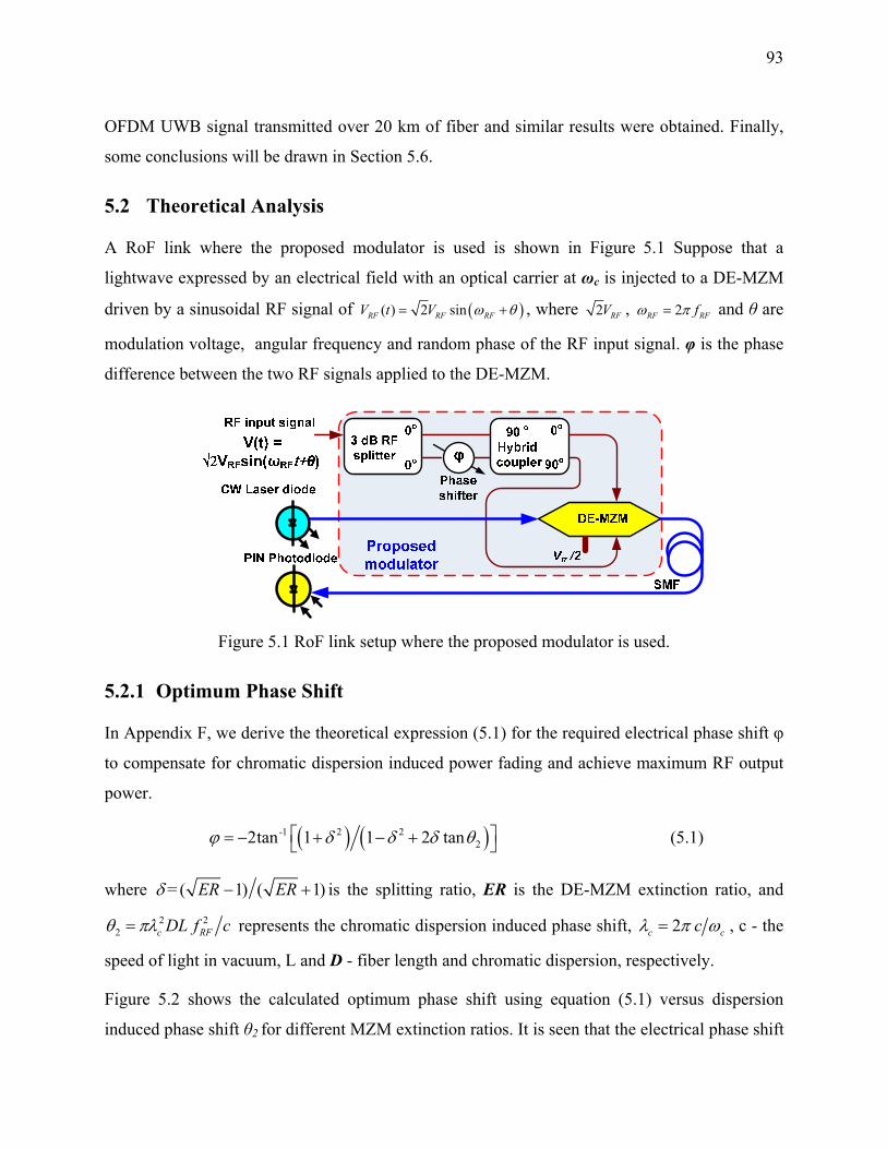
93

OFDM UWB signal transmitted over 20 km of fiber and similar results were obtained. Finally,

some conclusions will be drawn in Section 5.6.

5.2 Theoretical Analysis

A RoF link where the proposed modulator is used is shown in Figure 5.1 Suppose that a

lightwave expressed by an electrical field with an optical carrier at ωc is injected to a DE-MZM

driven by a sinusoidal RF signal of ( )( ) 2 sinRF RF RFV t V ω θ= + , where 2 RFV , 2RF RFfω π= and θ are

modulation voltage, angular frequency and random phase of the RF input signal. φ is the phase

difference between the two RF signals applied to the DE-MZM.

Figure 5.1 RoF link setup where the proposed modulator is used.

5.2.1 Optimum Phase Shift

In Appendix F, we derive the theoretical expression (5.1) for the required electrical phase shift φ

to compensate for chromatic dispersion induced power fading and achieve maximum RF output

power.

( ) ( )-1 2 222tan 1 1 2 tanϕ δ δ δ θ⎡ ⎤= − + − +⎣ ⎦ (5.1)

where = ( 1) ( 1)ER ERδ − + is the splitting ratio, ER is the DE-MZM extinction ratio, and 2 2

2 c RFDL f cθ πλ= represents the chromatic dispersion induced phase shift, 2c ccλ π ω= , c - the

speed of light in vacuum, L and D - fiber length and chromatic dispersion, respectively.

Figure 5.2 shows the calculated optimum phase shift using equation (5.1) versus dispersion

induced phase shift θ2 for different MZM extinction ratios. It is seen that the electrical phase shift

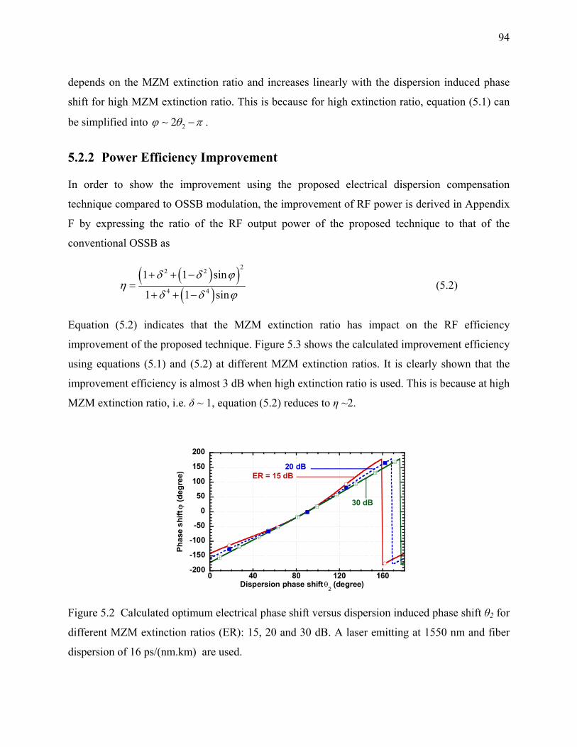
94

depends on the MZM extinction ratio and increases linearly with the dispersion induced phase

shift for high MZM extinction ratio. This is because for high extinction ratio, equation (5.1) can

be simplified into 22ϕ θ π−∼ .

5.2.2 Power Efficiency Improvement

In order to show the improvement using the proposed electrical dispersion compensation

technique compared to OSSB modulation, the improvement of RF power is derived in Appendix

F by expressing the ratio of the RF output power of the proposed technique to that of the

conventional OSSB as

( )( )( )

22 2

4 4

1 1 sin

1 1 sin

δ δ ϕη

δ δ ϕ

+ + −=

+ + − (5.2)

Equation (5.2) indicates that the MZM extinction ratio has impact on the RF efficiency

improvement of the proposed technique. Figure 5.3 shows the calculated improvement efficiency

using equations (5.1) and (5.2) at different MZM extinction ratios. It is clearly shown that the

improvement efficiency is almost 3 dB when high extinction ratio is used. This is because at high

MZM extinction ratio, i.e. δ ~ 1, equation (5.2) reduces to η ~2.

-200

-150

-100

-50

0

50

100

150

200

0 40 80 120 160

Phas

e sh

ift ϕ

(deg

ree)

Dispersion phase shift θ2 (degree)

ER = 15 dB20 dB

30 dB

Figure 5.2 Calculated optimum electrical phase shift versus dispersion induced phase shift θ2 for

different MZM extinction ratios (ER): 15, 20 and 30 dB. A laser emitting at 1550 nm and fiber

dispersion of 16 ps/(nm.km) are used.

95

2.4

2.5

2.6

2.7

2.8

2.9

3

3.1

0 40 80 120 160

impr

ovem

ent o

f RF

pow

er (d

B)

Dispersion phase shift θ2 (degree)

ER = 15 dB

20 dB

30 dB

Figure 5.3 Calculated RF power efficiency improvement versus dispersion induced phase shift θ2

for different MZM extinction ratios (ER): 15, 20 and 30 dB, and when using optimum electrical

phase shift φ. A laser emitting at 1550 nm and fiber dispersion of 16 ps/(nm.km) are used.

5.3 Verification and Analysis by Simulation

In order to validate the theoretical analysis of dispersion compensation using our technique

presented in Section 5.2, we simulated the system setup shown in Figure 5.1. Simulation was

carried out with the commercial software VPItransmissionMaker 7.6. A continuous wave light

from a laser source is assumed to have a wavelength of 1550 nm, output power of 0 dBm, and

RIN of -155 dB/Hz. The CW light is injected into a DE-MZM, driven by an RF signal. The RF

signal is split equally into two RF signals and one of them is phase shifted by a tunable phase

shifter. The resulting two RF signals are applied to both electrodes of the DE-MZM through a

double arrow 90° HEC. Low total RF modulation index 2RF RFm V Vπ= is used, Vπ- the

halfwave switching voltage of the DE-MZM. The output signal from the DE-MZM is injected

into an SMF of length L, loss of α = 0.2 dB/km and chromatic dispersion of D = 16 ps/(nm.km) .

The optical signal is detected by a high-speed PIN PD with a 3 dB bandwidth of 32 GHz and a

responsivity of 0.62 A/W. In the simulation insertion loss from the DE-MZM and fiber are

compensated using an EDFA that maintain a 0 dBm optical power at the photodetector.

We assume that the DE-MZM has an extinction ratio of 30 dB and is driven by an RF signal

with an RF modulation index of 2 10RFm = . We used an RF signal at 12 GHz and 3.96 GHz

transmitted over 52 km and 20 km of fiber, as for the experimental analysis in Section 5.4 and

96

5.5, respectively. We sweep the electrical phase shift and measure the RF output power. Figure

5.4 shows the RF output power versus electrical phase shift at different fiber lengths and RF

frequencies. For back to back transmission the maximum RF power is obtained at electrical

phase shift of -173°. The maximum RF power is obtained at electrical phase shift of -158.5° and

174° after transmission of the RF signal at 3.96 GHz and 12 GHz over 20 km and 52 km of fiber,

respectively. For back-to-back there is no dispersion induced phase shift, while after

transmission of the RF signal at 12 GHz and 3.96 GHz over 52 km and 20 km of fiber, the

dispersion induced phase shift is 173.5° and 7.5°, respectively. The corresponding optimum

electrical phase shift displayed in Figure 5.2 using equation (5.1) agrees very well with the

simulated values obtained at the maximum RF power shown in Figure 5.4.

-70

-65

-60

-55

-50

-45

-40

-150 -100 -50 0 50 100 150

Back-to-back

20km & fRF

= 3.96GHz

52 km & f

RF = 12GHz

RF

outp

ut p

ower

(dB

m)

Electrical phase shift ϕ (degree)

Figure 5.4 Simulated RF power versus electrical phase shift at different fiber length. A laser

emitting at 1550 nm, fRF=12 GHz, fiber dispersion of 16 ps/(nm.km), MZM extinction ratio of 30

dB and RF modulation index of 2 10are used.

Then we simulated the improvement of RF power compared to OSSB versus MZM

extinction ratio using the optimum electrical phase shift calculated by equation (5.1). Figure 5.5

depicts the simulated (lines) and calculated (marks) RF power efficiency improvement for back-

to-back and after transmission of the RF signal at 12 GHz and 3.96 GHz over 52 km and 20 km

of fiber, respectively. For the calculation we used equations (5.1) and (5.2). It is clearly shown

97

that the simulated and calculated improvements agree well. This verifies that our theory

developed in Section 5.2 is accurate. Moreover, it is seen that almost 3 dB improvement in RF

power is obtained if the MZM has an extinction ratio of more than 20 dB. The dependency on

low extinction ratio is clear from equation (5.2) and the maximum and minimum improvement in

RF power is 2 and ( ) ( )( )22 1 1ER ER− + , respectively.

1

1.5

2

2.5

3

12 16 20 24 28 32 36 40

Back-to-back

3.96GHz @ 20km 12GHz @ 52km Back-to-back

3.96GHz @ 20km 12GHz @ 52km

RF

pow

er im

prov

emen

t (dB

c)

Extinction Ratio (dB)

Simulation Theory

Figure 5.5 RF power improvement versus MZM extinction ratio at different fiber length obtained

by using simulation (lines) and theory (marks).

The improvement in RF power may not clearly display the influence of fiber chromatic

dispersion on the signal pulse when the RF signal is carrying data. For this case we investigated

the performance of 12 GHz RF signal carrying non return to zero (NRZ) data at bit rate of 625

Mb/s. We used an optimum electrical phase shift of -173° and 174° for back to back and after 52

km of fiber transmission, respectively, and measured the Q factor versus received optical power

and compare our proposed ODSB to OSSB. Simulation results in Figure 5.6 show no power

penalty at Q = 9 for either OSSB or proposed ODSB after 52 km of fiber transmission. However,

there is 1.5 dB improvement of optical receiver sensitivity in our proposed ODSB compared to

OSSB. Figure 5.6 shows that Q = 9 can be achieved at -15.9 dBm of received optical power for

OSSB whereas only -17.4 dBm is required for our proposed ODSB. The corresponding eye

diagrams in Figure 5.7 show a good quality of the transmitted signal and suggest that at least

98

similar performance of OSSB could be achieved by using our proposed ODSB with 3 dB RF

power improvement.

2

4

68

10

-24 -22 -20 -18 -16 -14 -12

back-to-back52 km

Q fa

ctor

Received power (dBm)

1.5dB

Proposed ODSB

OSSB

Figure 5.6 Q factor for OSSB and proposed ODSB versus received optical power for 12 GHz

RF signal carrying NRZ data at 625Mb/s bit rate.

(i) (ii) (iii) (iv)

Figure 5.7 Eye diagram for OSSB: (i) back to back (B-T-B), (ii) 52 km, and for proposed ODSB:

(iii) B-T-B, (iv) 52 km. The received optical power is -15.9 dBm and -17.4 dBm for OSSB and

proposed ODSB, respectively.

Next, we will verify experimentally the performance of two different RF signals: one is a

single RF tone without data modulation, and the other is MB-OFDM UWB transmitted over

fiber using our proposed ODSB modulation technique.

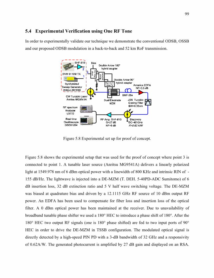
99

5.4 Experimental Verification using One RF Tone

In order to experimentally validate our technique we demonstrate the conventional ODSB, OSSB

and our proposed ODSB modulation in a back-to-back and 52 km RoF transmission.

Figure 5.8 Experimental set up for proof of concept.

Figure 5.8 shows the experimental setup that was used for the proof of concept where point 3 is

connected to point 1. A tunable laser source (Anritsu MG9541A) delivers a linearly polarized

light at 1549.978 nm of 6 dBm optical power with a linewidth of 800 KHz and intrinsic RIN of -

155 dB/Hz. The lightwave is injected into a DE-MZM (T. DEH. 5-40PD-ADC Sumitomo) of 6

dB insertion loss, 32 dB extinction ratio and 5 V half wave switching voltage. The DE-MZM

was biased at quadrature bias and driven by a 12.1115 GHz RF source of 10 dBm output RF

power. An EDFA has been used to compensate for fiber loss and insertion loss of the optical

filter. A 0 dBm optical power has been maintained at the receiver. Due to unavailability of

broadband tunable phase shifter we used a 180° HEC to introduce a phase shift of 180°. After the

180° HEC two output RF signals (one is 180° phase shifted) are fed to two input ports of 90°

HEC in order to drive the DE-MZM in TSSB configuration. The modulated optical signal is

directly detected by a high-speed PIN PD with a 3-dB bandwidth of 32 GHz and a responsivity

of 0.62A/W. The generated photocurrent is amplified by 27 dB gain and displayed on an RSA.

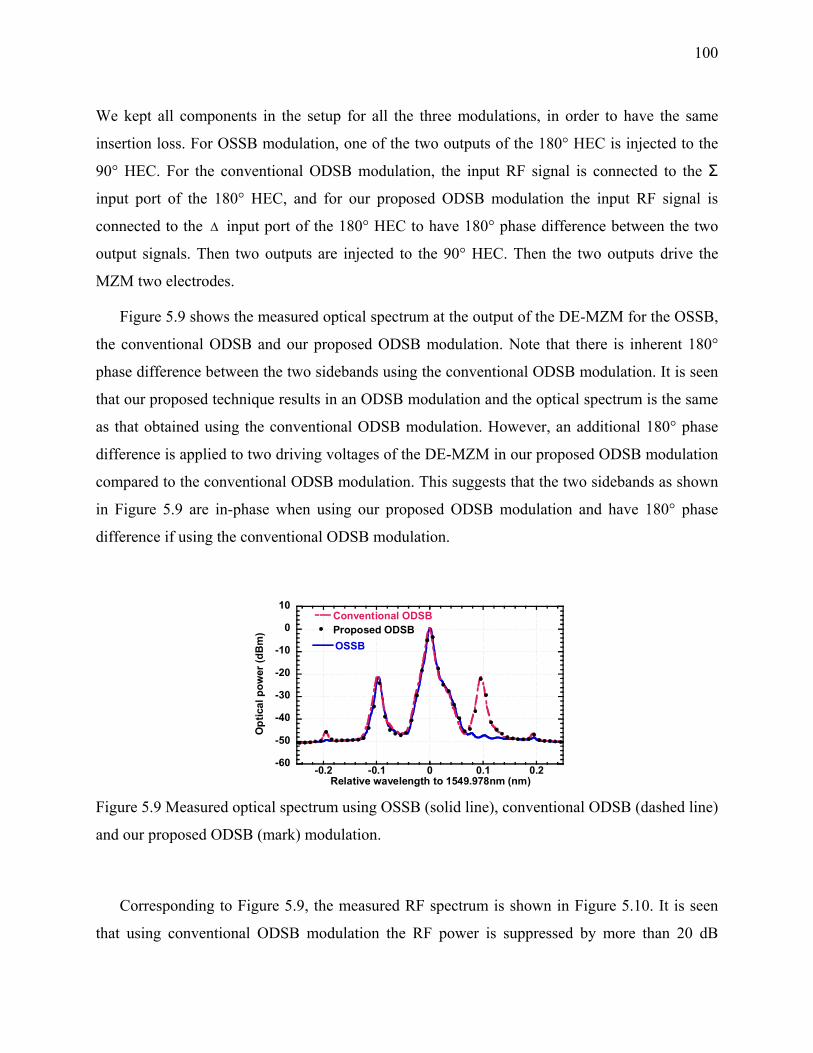
100

We kept all components in the setup for all the three modulations, in order to have the same

insertion loss. For OSSB modulation, one of the two outputs of the 180° HEC is injected to the

90° HEC. For the conventional ODSB modulation, the input RF signal is connected to the Σ

input port of the 180° HEC, and for our proposed ODSB modulation the input RF signal is

connected to the Δ input port of the 180° HEC to have 180° phase difference between the two

output signals. Then two outputs are injected to the 90° HEC. Then the two outputs drive the

MZM two electrodes.

Figure 5.9 shows the measured optical spectrum at the output of the DE-MZM for the OSSB,

the conventional ODSB and our proposed ODSB modulation. Note that there is inherent 180°

phase difference between the two sidebands using the conventional ODSB modulation. It is seen

that our proposed technique results in an ODSB modulation and the optical spectrum is the same

as that obtained using the conventional ODSB modulation. However, an additional 180° phase

difference is applied to two driving voltages of the DE-MZM in our proposed ODSB modulation

compared to the conventional ODSB modulation. This suggests that the two sidebands as shown

in Figure 5.9 are in-phase when using our proposed ODSB modulation and have 180° phase

difference if using the conventional ODSB modulation.

-60

-50

-40

-30

-20

-10

0

10

-0.2 -0.1 0 0.1 0.2

OSSB

Conventional ODSBProposed ODSB

Opt

ical

pow

er (d

Bm

)

Relative wavelength to 1549.978nm (nm) Figure 5.9 Measured optical spectrum using OSSB (solid line), conventional ODSB (dashed line)

and our proposed ODSB (mark) modulation.

Corresponding to Figure 5.9, the measured RF spectrum is shown in Figure 5.10. It is seen

that using conventional ODSB modulation the RF power is suppressed by more than 20 dB

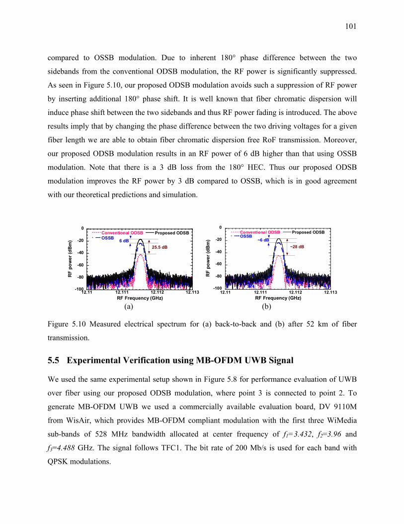
101

compared to OSSB modulation. Due to inherent 180° phase difference between the two

sidebands from the conventional ODSB modulation, the RF power is significantly suppressed.

As seen in Figure 5.10, our proposed ODSB modulation avoids such a suppression of RF power

by inserting additional 180° phase shift. It is well known that fiber chromatic dispersion will

induce phase shift between the two sidebands and thus RF power fading is introduced. The above

results imply that by changing the phase difference between the two driving voltages for a given

fiber length we are able to obtain fiber chromatic dispersion free RoF transmission. Moreover,

our proposed ODSB modulation results in an RF power of 6 dB higher than that using OSSB

modulation. Note that there is a 3 dB loss from the 180° HEC. Thus our proposed ODSB

modulation improves the RF power by 3 dB compared to OSSB, which is in good agreement

with our theoretical predictions and simulation.

-100

-80

-60

-40

-20

0

12.11 12.111 12.112 12.113

Conventional ODSBOSSB

Proposed ODSB

RF

pow

er (d

Bm

)

RF Frequency (GHz)

6 dB25.5 dB

-100

-80

-60

-40

-20

0

12.11 12.111 12.112 12.113

Conventional ODSB OSSB

Proposed ODSB

RF

pow

er (d

Bm

)

RF Frequency (GHz)

~6 dB~28 dB

(a) (b)

Figure 5.10 Measured electrical spectrum for (a) back-to-back and (b) after 52 km of fiber

transmission.

5.5 Experimental Verification using MB-OFDM UWB Signal

We used the same experimental setup shown in Figure 5.8 for performance evaluation of UWB

over fiber using our proposed ODSB modulation, where point 3 is connected to point 2. To

generate MB-OFDM UWB we used a commercially available evaluation board, DV 9110M

from WisAir, which provides MB-OFDM compliant modulation with the first three WiMedia

sub-bands of 528 MHz bandwidth allocated at center frequency of f1=3.432, f2=3.96 and

f3=4.488 GHz. The signal follows TFC1. The bit rate of 200 Mb/s is used for each band with

QPSK modulations.

102

The tunable laser source is set to wavelength of 1550 nm, and output power of 0 dBm. The

CW light is injected into a 10.7 Gb/s DE-MZM from Fujitsu, driven by the UWB signal from the

output of the DV 9110M Tx module. The MZM has 6 dB insertion loss, RF half wave switching

voltage of 3.8 V and an extinction ratio of 28.5 dB. The modulated optical signal was transmitted

through an SMF fiber. The EDFA compensates for all optical losses and maintains 0 dBm optical

power at the receiver. The EVM of the photodetected signal was measured by a 12 GHz high

speed real time oscilloscope DSO91204 from Agilent Technologies. The RF spectrum is also

measured with 43 GHz RSA. For OSSB modulation, the 180° HEC is removed and the amplified

UWB signal is directly injected to the 90° HEC.

To show the improved performance of the transmitted MB-OFDM-UWB signal over fiber

using our proposed technique, we have measured and compared the EVM using OSSB, ODSB

and our proposed ODSB modulation in back-to-back and after 20 km of fiber transmission,

respectively. The total RF input power at the MZM was varied by changing the attenuation level

of the transmitted power from 0 to 15 dB using the built-in WisMan software provided with the

DV 9110M module. The maximum transmitted power level from the DV 9110M is ~-18 dBm

and the amplification of the LNA is ~27 dB with~1.5 dB loss from RF connections and Bias Tee.

This gives a transmitted power level range from ~-6 to ~7.5 dBm.

-25

-20

-15

-10

-5

-6-4-202468

OSSBProposed ODSBConventional ODSB

EVM

(dB

)

UWB input power to MZM (dBm)

3 dB

-25

-20

-15

-10

-5

-6-4-202468

OSSBProposed ODSB Conventional ODSB

UWB input power to MZM (dBm)

3 dB

EVM

(dB

)

(a) (b)

Figure 5.11 Measured EVM versus UWB input power for OSSB, conventional and proposed

ODSB for (a) back to back and (b) 20 km of fiber transmission.

103

Figure 5.11 shows the EVM versus the total input power to the MZM modulator for OSSB,

conventional and proposed ODSB in (a) back-to-back and (b) after 20 km of fiber transmission.

It is clearly shown that conventional ODSB presents the worst EVM performance due to power

fading caused chromatic dispersion effect. The EVM using ODSB is slightly improved with 20

km fiber length because the optical sidebands are not completely out of phase due to fiber

dispersion. It can be also seen that our proposed ODSB technique compared to OSSB presents

better EVM at low transmitted power level of less than ~0 dBm. For back-to-back a minimum

EVM of -22.4, -23.1 and -17.8 dB is achieved at 0.16, -2.92 and 7.48 dBm for OSSB, proposed

and conventional ODSB, respectively, and the corresponding constellations are shown in inset

(i), (ii) and (iii) of Figure 5.12, respectively. While after 20 km of fiber transmission a minimum

EVM of -21.4, -21.8 and -19.6 dB is obtained at 0.16, -2.92 and 5.21 dBm, and the

corresponding constellations are shown in inset (iv), (v) and (vi) of Figure 5.12, respectively. It

can be noticed that our proposed ODSB has ~3 dB improvement in power efficiency for

optimum input power with slightly better EVM compared to OSSB.

Now, we set the power of transmitted UWB to 0.16 dBm and -2.92 dBm at the input to the

MZM for OSSB and conventional/proposed ODSB, respectively, and measure the optical and RF

spectrum before and after the photodetection, respectively, for back to back transmission. Figure

5.13 shows no difference in the optical spectrum of the conventional- and proposed- ODSB

modulation.

104

(i) 0.16 dBm (ii) -2.92 dBm (iii) 7.48 dBm

(iv) 0.16 dBm (v) -2.92 dBm (vi) 5.21 dBm

Figure 5.12 Measured constellation with minimum EVM at optimum input UWB power to MZM

at back to back (B-T-B) for (i) OSSB, (ii) proposed ODSB and (iii) conventional ODSB, and

after 20 km for (iv) OSSB, (v) proposed ODSB and (vi) conventional ODSB.

-60

-50

-40

-30

-20

-10

0

10

-0.15-0.1-0.0500.050.10.15

OSSB

Conventional ODSBProposed ODSB

Opt

ical

pow

er (d

Bm

)

Offset wavelength to 1550 (nm)

Figure 5.13 Measured optical spectrum using OSSB modulation (dashed line), and the

conventional ODSB (solid line) and our proposed ODSB (mark) modulation.

105

-70

-60

-50

-40

-30

-20

-10

3 3.5 4 4.5

OSSBProposed and conventional ODSB

RF

pow

er (d

Bm

)

RF frequency (GHz)

~3 dB

-70

-60

-50

-40

-30

3 3.5 4 4.5

OSSB Proposed DSB Conventional ODSB

RF frequency (GHz)

RF

pow

er (d

Bm

)

(a) (b)

Figure 5.14 RF spectrum of the (a) transmitted and (b) received UWB signal for OSSB,

conventional and proposed ODSB for back-to-back transmission.

Figure 5.14 shows measured electrical spectrum of transmitted and received three band UWB

signals using the three modulation techniques. The effect of dispersion is apparent only after the

photodetection as shown in Figure 5.14(b). Actually an 180° phase difference exists in back-to-

back between the two optical subcarrier sidebands with respect to the optical carrier, resulting in

maximum fading of the UWB signal after the photodetection in conventional ODSB modulation.

However, in our proposed ODSB modulation an additional 180° phase difference is applied to

two driving voltages of the DE-MZM to make the two sidebands in-phase, resulting in fully

recovered UWB signal. The above results imply that by changing the phase difference between

the two driving voltages for a given fiber length we are able to mitigate the fiber chromatic

dispersion caused power fading in RoF transmission. Practically by tuning the electrical phase

shift, the phase difference due to the chromatic dispersion between the upper and lower

sidebands can be removed, resulting in fully recovered RF carrier. Figure 5.14 (a) and (b) also

show power efficiency improvement of 3 dB in our proposed ODSB compared to OSSB.

Power efficiency improvement has been also measured for different input power levels as

shown in Figure 5.15. It is clearly seen that almost the same received power level in OSSB can

be obtained by reducing the transmitted power by 3 dB for using our proposed ODSB. Because

EVM is inversely proportional to the square root of the received signal to noise ratio [25], this

implies at least the same EVM performance as OSSB can be achieved using our proposed ODSB

with 3 dB saving in the transmitted power, which is in good agreement with our theoretical

prediction.

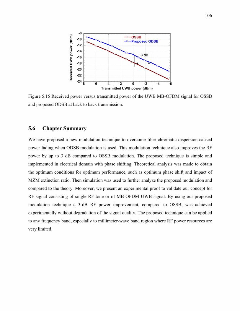
106

-24-22-20-18-16-14-12-10-8

-6-4-202468

OSSB Proposed ODSB

Rec

eive

d U

WB

pow

er (d

Bm

)

Transmitted UWB power (dBm)

~3 dB

Figure 5.15 Received power versus transmitted power of the UWB MB-OFDM signal for OSSB

and proposed ODSB at back to back transmission.

5.6 Chapter Summary

We have proposed a new modulation technique to overcome fiber chromatic dispersion caused

power fading when ODSB modulation is used. This modulation technique also improves the RF

power by up to 3 dB compared to OSSB modulation. The proposed technique is simple and

implemented in electrical domain with phase shifting. Theoretical analysis was made to obtain

the optimum conditions for optimum performance, such as optimum phase shift and impact of

MZM extinction ratio. Then simulation was used to further analyze the proposed modulation and

compared to the theory. Moreover, we present an experimental proof to validate our concept for

RF signal consisting of single RF tone or of MB-OFDM UWB signal. By using our proposed

modulation technique a 3-dB RF power improvement, compared to OSSB, was achieved

experimentally without degradation of the signal quality. The proposed technique can be applied

to any frequency band, especially to millimeter-wave band region where RF power resources are

very limited.

107

CHAPTER 6 TUNABLE OPTICAL CARRIER SUPPRESSION SINGLE

SIDEBAND TECHNIQUE FOR IMPROVED OPTICAL MODULATION

EFFICIENCY OF RF AND MB-OFDM UWB SIGNAL OVER FIBER

6.1 Introduction

For an optical carrier used for distributing an optical subcarrier or sideband signal, it was found

experimentally that the optimum optical power ratio of the optical carrier to sideband is 0 dB

[18, 63]. One approach to alter the power ratio is to use an optical notch filter for reducing

optical carrier power [18]. However carrier filtering needs tuning when the laser or carrier drifts

(chirping effect). An optical carrier-suppressed single sideband modulation using a hyperfine

blocking filter based on a virtually imaged phased-array has been reported in [19]. In this scheme

the blocking filter can be tuned for simultaneous single sideband and strong carrier suppression

up to 30 dB below the unsuppressed single sideband. However, this technique suffers from high

insertion loss of more than 13 dB and power penalty caused by the blocking filtering effects such

as sideband shaping and residual chromatic dispersion. Another technique [20] intentionally used

stimulated Brillouin scattering as a carrier filter. An injected power above the SBS threshold into

a length of optical fiber is used to reject the carrier while allowing the modulated sidebands to

pass with low loss. However the system suffers from signal distortion and instabilities in the

transmitted power attributed to the noise in the spontaneous scattering process that initiates SBS

[22]. Later, a technique was proposed that a MZM is used and the power ratio can be tuned with

the help of bias voltage [21]. However, this technique only enables to obtain ODSB modulation

and OSSB modulation cannot be obtained without optical filtering.

In [64] an x-cut Lithium Niobate dual parallel Mach-Zhender modulator (dMZM) has been

designed for OSSB modulation with carrier-suppression ratio over 25dB. The dMZM comprises

a main MZM with an MZM inserted in each arm. Several applications are possible with this

device: generation of optical mm-wave signals using frequency doubling [65], quadrupling [66]

and octupling [67], and optical carrier suppressed-optical differential quadrature and phase-shift

keying signals in radio over fiber systems [68].

Using the same modulator as in [64-68], this chapter will show that not only OSSB modulation

but also tunability of the power ratio of optical carrier to sideband (OCSR) can be obtained

108

simultaneously. By changing bias voltage, the power ratio of optical carrier to sideband can be

tuned continuously. The chapter is organized into five sections. In Section 6.2, the principle and

theory of the proposed modulation technique are presented for both single and two RF tones

signal. Simulations using commercial software are carried out and compared to theory in Section

6.3 considering tunability of OCSR, RF power and impact of extinction ratio and RF modulation

index of the two integrated MZMs. In Section 6.4, the distortion effects are experimentally

investigated and the performance improvement of using our proposed modulation technique is

demonstrated for MB-OFDM UWB signal transmission over 20 km of single mode fiber.

Finally, our conclusions are drawn in Section 6.5.

6.2 Principle and Theory of Tunable Optical Carrier Suppression Single

Sideband Modulation Technique

Figure 6.1 Dual parallel MZM used for OSSB modulation with tunability of optical carrier

suppression

Figure 6.1 shows the schematic of the dMZM modulator. The dMZM is similar to the one used

in [64-68]. As shown in Figure 6.1, the injected light is split into two branches i.e. I and II by a

3-dB optical splitter. In each branch there is a single-electrode MZM, i.e. MZMa in branch I and

MZMb in branch II. The two MZMs are integrated in another principal MZMc. Because of the x-

cut design, the three MZMs are configured for push pull operation, and each has independent DC

bias. It is assumed that the two parallel MZMs are identical.

109

To obtain OSSB modulation, it is required that the optical phase difference between path-I

and path-II be / 2π , and the two RF signals driving MZMa and MZMb must have same amplitude

but in quadrature phase. Thus MZMa and MZMb must have identical bias voltage (φ1 = φ2 = φ),

and the applied bias voltage to MZMc port must be / 4Vπ± (φ3 = / 4π± ), where Vπ is the π-shift

voltage assumed to be the same for the three MZMs without loss of generality. The applied bias

voltage φ to MZMa and MZMb will be controlled to tune the suppression of the optical carrier.

6.2.1 Theoretical Analysis for Single RF Tone

The theory of the mechanics of the modulator is given as follows. Considering one RF signal

with ( )cosmV tω θ+ , at a frequency of 2πω , phase θ and an amplitude of mV , driving the

modulator, we obtain the output electric field in branch I and II, at the output of MZMa and

MZMb, respectively,

( ) ( ) 1 12 2( ) 2 exp cos exp cosj jinI ffE t t E ae j m t re j m tϕ ϕπ πω θ ω θ−⎡ ⎤ ⎡ ⎤

⎣ ⎦ ⎣ ⎦= + + − + (6.1)

( ) ( ) 2 22 2( ) 2 exp sin exp sinj jinII ffE t t E ae j m t re j m tϕ ϕπ πω θ ω θ−⎡ ⎤ ⎡ ⎤

⎣ ⎦ ⎣ ⎦= + + − + (6.2)

where fft represents insertion loss of each parallel MZM, 0.5a ε= + , 21r a= − with

( )1ER ERε = + represents the difference in the power split ratio of their Y-junctions and ER is

the MZM extinction ratio. inE is amplitude of input electric field. The power splitting and

coupling ratios of the Y-junctions of MZMc are assumed to be 3-dB. The parameter mm V Vπ=

defined modulation index (MI), ( )2k kDC VV πϕ π= and kDCV are the applied bias voltage at

each port to each of the MZMs as shown in Figure 6.1.

The output electric field from the dMZM at III is

( ) ( )

( ) ( )

3 3

2

( ) 1 2

1 exp2

j jIII I II

n ninffn

E t E t e E t e

t E a J m jn t

ϕ ϕ

π ω θ

−

∞

=−∞

⎡ ⎤⎣ ⎦

⎡ ⎤⎣ ⎦

= +

= +∑ (6.3)

where

( ) ( )3 31 1 2 21 1n nj jj j j jnna j ae re e ae re eϕ ϕϕ ϕ ϕ ϕ −− −⎡ ⎤ ⎡ ⎤= + − + + −⎣ ⎦ ⎣ ⎦ (6.4)

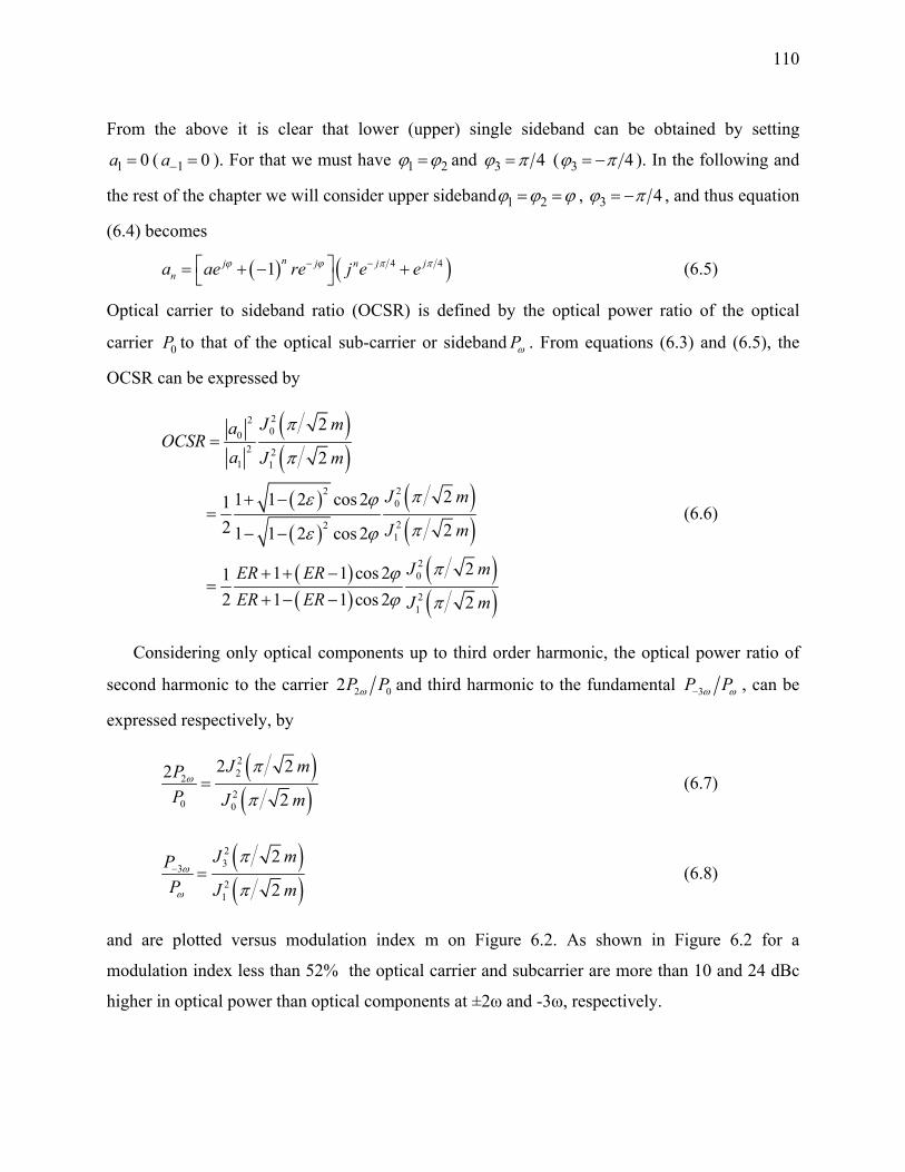
110

From the above it is clear that lower (upper) single sideband can be obtained by setting

1 0a = ( 1 0a− = ). For that we must have 1 2ϕ ϕ= and 3 4ϕ π= ( 3 4ϕ π= − ). In the following and

the rest of the chapter we will consider upper sideband 1 2ϕ ϕ ϕ= = , 3 4ϕ π= − , and thus equation

(6.4) becomes

( ) ( )4 41 nj j n j jna ae re j e eϕ ϕ π π− −⎡ ⎤= + − +⎣ ⎦ (6.5)

Optical carrier to sideband ratio (OCSR) is defined by the optical power ratio of the optical

carrier 0P to that of the optical sub-carrier or sideband Pω . From equations (6.3) and (6.5), the

OCSR can be expressed by

( )( )

( )( )

( )( )

( )( )

( )( )

2200

2 21 1

220

221

20

21

2

2

21 1 2 cos 21 2 21 1 2 cos 2

21 1 cos 21 2 1 1 cos 2 2

J maOCSR

a J m

J m

J m

J mER ERER ER J m

π

π

πε ϕ

πε ϕ

πϕϕ π

=

+ −=

− −

+ + −=

+ − −

(6.6)

Considering only optical components up to third order harmonic, the optical power ratio of

second harmonic to the carrier 2 02P Pω and third harmonic to the fundamental 3P Pω ω− , can be

expressed respectively, by

( )

( )222

20 0

2 222

J mPP J m

ωπ

π= (6.7)

( )( )

2332

1

2

2

J mPP J m

ω

ω

π

π− = (6.8)

and are plotted versus modulation index m on Figure 6.2. As shown in Figure 6.2 for a

modulation index less than 52% the optical carrier and subcarrier are more than 10 and 24 dBc

higher in optical power than optical components at ±2ω and -3ω, respectively.

111

-100

-50

0

50

0 20 40 60 80 100

2P2ω

/P0

P3ω

/Pω

Rel

ativ

e op

tical

pow

er (d

Bc)

Modulation index (%) Figure 6.2 Optical power ratio of second harmonic to the carrier 2P2ω/P0 and third harmonic to

the fundamental P3ω/Pω.

Optical carrier 0

2ω-3ω

-2ω

ω

ω

Generation of ω

Figure 6.3 Optical spectrum at the output of the dMZM showing the generation of the RF signal

from the contribution of different optical components.

Because of the beating of these optical components at the photodetector, there will be some

distortion induced into the RF output signal at ω. For example the optical component at 2ω and -

2ω will beat with that at ω and -3ω, respectively, to generate an RF component at ω as shown in

Figure 6.3. The RF power ratio of the resulting distortion term to that of the RF output signal can

be expressed by

112

( ) ( ) ( ) ( )

( ) ( )( )( )

( )( )

2

2 2 32

0

2

2 1 2 1 2 3 2 3

2

1 0 1 0

222 3

20 1

2 2 2 2

2 2

2 2 1

2 2

dis

RF

E E E EPP E E

a a J m J m a a J m J m

a a J m J m

J m J m

J m J m

ω ω ω ω

ω

π π π π

π π

π π

π π

∗ ∗− −

∗

∗ ∗− −

∗

+=

−=

⎡ ⎤⎢ ⎥= −⎢ ⎥⎣ ⎦

(6.9)

Figure 6.4 shows that distortion power level relative to the RF carrier versus modulation index. It

is clear that the in-band distortion level is suppressed by more than 14 dB if the modulation

index is kept below 52%.

-100

-80

-60

-40

-20

0

20

40

0 20 40 60 80 100

Rel

ativ

e di

stor

tion

pow

er (d

Bc)

Modulation index (%) Figure 6.4 Distortion power level relative to the RF output carrier versus modulation index.

In the following we assume the modulation index is less than 52% then we can ignore the optical

power from all high-order harmonics and IMD. The total output optical power from the

modulator can be written 0outP P Pω= + , and then ( )1outP OCSR Pω= + . When the light with al

field given by equation (6.3) is injected to a photodetector with responsivity of ℜ , the detected

RF power at ω can be given by

113

( )

1

220

20

2 22

12

2

21

RF

out

P E E

P POCSRP

OCSR

ω

ω

= ℜ

= ℜ

= ℜ+

(6.10)

Figure 6.5 shows the relative RF power versus OCSR and that maximum RF power can be

obtained when the OCSR=1.

-50

-40

-30

-20

-10

0

-40 -20 0 20 40

Rel

ativ

e R

F po

wer

(dB

c)

OCSR (dB) Figure 6.5 Relative RF power versus OCSR for constant received optical power.

It is clear from equation (6.6) that by tuning the phase shift φ the OCSR will swing between

maximum and minimum values given, respectively, by

( ) ( )2 21max 0 12 2 2OCSR ER J m J mπ π= (6.11)

( ) ( )1 2 21min 0 12 2 2OCSR ER J m J mπ π−= (6.12)

Then tunability range of OCSR is ER2 (= max minOCSR OCSR ) and the maximum achievable PRF

will depend on the extinction ratio and modulation index, and three cases can arise.

114

Case 1: if min max1OCSR OCSR≤ ≤ , i.e

( ) ( )2 20 11 2 2 2ER J m J m ERπ π⎡ ⎤≤ ≤⎣ ⎦ (6.13)

then maximum PRF is obtained at OCSR = 1 by tuning the phase shift to an optimum value

directly expressed from (6.6) by

( ) ( )( ) ( )

2 210 12

2 210 12

1 2 21 1arccos2 11 2 2

J m J mERER J m J m

π πϕ

π π

⎡ ⎤−+⎢ ⎥= ±⎢ ⎥− +⎣ ⎦

(6.14)

and the RF power is expressed by

2 212RF outP P= ℜ (6.15)

Case 2: if min 1OCSR > , i.e

( ) ( )2 20 12 2 2ER J m J mπ π⎡ ⎤< ⎣ ⎦ (6.16)

then maximum PRF is obtained at OCSR = OCSRmin by tuning the phase shift to ±π/2, and the RF

power is expressed by

( )

( ) ( )( ) ( )

2 2 min2

min

2 20 12 2

22 20 1

21

2 2 2

2 2 2

RF out

out

OCSRP POCSR

J m J mP ER

J m ERJ m

π π

π π

= ℜ+

= ℜ⎡ ⎤+⎣ ⎦

(6.17)

Case 3: if max 1OCSR < , i.e

( ) ( )2 20 12 2 2 1J m J m ERπ π⎡ ⎤ <⎣ ⎦ (6.18)

then maximum PRF is obtained at OCSR = OCSRmax by tuning the phase shift to 0, and the RF


115

( )

( ) ( )( ) ( )

2 2 max2

max

2 20 12 2

22 2

1 0

21

2 2 4

2 2 2

RF out

out

OCSRP POCSR

J m J mP ER

J m ERJ m

π π

π π

= ℜ+

= ℜ⎡ ⎤+⎣ ⎦

(6.19)

Figure 6.6 shows optimum OCSR and corresponding phase shift versus modulation index for

different extinction ratio (ER): 15, 20, 28.5 and 35 dB. It is clear that higher extinction ratio

allows to achieve an OCSR=1 for maximum RF power at lower modulation index. For example

OCSR =1 is achieved at modulation index of 11, 7, 3 and 2% for an ER of 15, 20, 28.5 and 35

dB, respectively. Also for high extinction ratios of greater than 20 dB the required optimum

phase bias is almost independent on ER and varies linearly with the modulation index. This is

because at high extinction ratio 1ER the optimal phase shift expressed by equation (6.14)

reduces to

( ) ( )1 0~ 2 arc tan 2 2 2J m J mϕ π π π⎡ ⎤− ⎣ ⎦ (6.20)

and is almost linear with the modulation index as shown from the plot of Figure 6.7.

-10

-5

0

5

10

15

20

25

0.2

0.25

0.3

0.35

0.4

0.45

0.5

0.55

0 10 20 30 40 50

ER =15dBER = 20dBER = 28.5dBER = 35dB

Opt

imum

OC

SR (d

B)

Optim

um phase ϕ

/π (radian)

Modulation index m (%) Figure 6.6 Optimum OCSR and corresponding phase shift versus modulation index for different

extinction ratio (ER): 15, 20, 28.5 and 35 dB.

116

0

0.1

0.2

0.3

0.4

0.5

0 20 40 60 80 100

Opt

imum

pha

se ϕ

/π (

radi

an)

Modulation index m (%) Figure 6.7 Approximated phase shift versus modulation index for high extinction ratio.

Figure 6.8 shows the impact of extinction ratio on the optimum OCSR at different modulation

index. It can be seen that by increasing the modulation index or extinction ratio the optimum

OCSR decreases up to an OCSR = 1. To achieve an optimum OCSR = 1 the minimum required

ER is 37, 23, 17, 11 and 10 for modulation index of 1, 5, 10, 19 and 20%, respectively. For

modulation index less than 52%, the minimum required extinction ratio to achieve an OCSR = 1,

is given by (see equation (6.13))

( ) ( )2 2min 0 12 2 2ER J m J mπ π⎡ ⎤= ⎣ ⎦ (6.21)

and it decreases with the increase of the modulation index as shown in Figure 6.9.

Optimum phase shift versus extinction ratio is depicted in Figure 6.10 for different modulation

index. It is shown that the optimum phase shift is almost independent on extinction ratios of

greater than 20 dB. For modulation index of 1, 5, 10, 19, 30, 40 and 50%, the optimum phase

shift φ is ~0.5π, 0.48π, 0.45π, 0.4π, 0.35π, 0.3π and 0.26π, respectively. This is also confirmed

by equation (6.21) and Figure 6.7. It is then advantageous to have very high extinction ratio to

improve both the efficiency and linearity of the modulator.

117

-5

0

5

10

15

20

25

30

10 15 20 25 30 35 40

m = 1%m = 5% m = 10% m = 19%m = 20% m 50%

Opt

imum

OC

SR (d

B)

Extinction ratio ER (dB) Figure 6.8 Optimum OCSR versus extinction ratio (ER) for different modulation index: 1, 5, 10,

19, 20 and 50%.

-10

0

10

20

30

40

50

0 10 20 30 40 50

Min

imum

requ

ired

ER (d

B)

Modulation index m (%) Figure 6.9 Minimum required ER to achieve an OCSR=1 versus modulation index.

118

0.2

0.25

0.3

0.35

0.4

0.45

0.5

0.55

10 15 20 25 30 35 40

Opt

imum

pha

se ϕ

/π (r

adia

n)

Extinction ratio ER (dB)

m = 1%

19%

30%

40%

50%

5%10%


5, 10, 19, 30, 40 and 50%.

6.2.2 Theoretical Analysis for Two RF Tones

In this section, we investigate the situation in which one optical carrier carries two sub-carriers.

Considering two RF signals: ( )1 1cosmV tω θ+ and ( )2 2cosmV tω θ+ with frequencies of ω1/2π

and ω2/2π, arbitrary phase θ1 and θ2, and amplitude of mV driving the modulator, after

mathematical manipulations, we obtain the output electric field from the dMZM modulator at III

in Figure 6.1,

( ) ( ) ( )( )

1 2 1 21 2,

1 1 2 2 1 1 2 2

1 2 22

exp

III ff in n n n nn n

E t t E a J m J m

j n n t n n

π π

ω ω θ θ

∞

+=−∞

= ∑

× + + +⎡ ⎤⎣ ⎦

(6.22)

where na is given by equation (6.5) and other parameters are defined above. Here also the OCSR

can be expressed by equation (6.6).

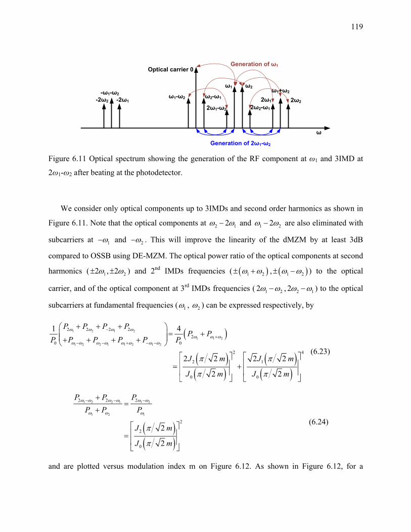
119

ω1-ω2 ω2-ω1

Optical carrier 0

ω1+ω2

2ω1

-ω1-ω2-2ω2 -2ω1

Generation of 2ω1-ω2

ω

2ω1-ω2 2ω2-ω1

2ω2

ω2ω1

Generation of ω1

Figure 6.11 Optical spectrum showing the generation of the RF component at ω1 and 3IMD at

2ω1-ω2 after beating at the photodetector.

We consider only optical components up to 3IMDs and second order harmonics as shown in

Figure 6.11. Note that the optical components at 2 12ω ω− and 1 22ω ω− are also eliminated with

subcarriers at 1ω− and 2ω− . This will improve the linearity of the dMZM by at least 3dB

compared to OSSB using DE-MZM. The optical power ratio of the optical components at second

harmonics ( 12ω± , 22ω± ) and 2nd IMDs frequencies ( ( )1 2ω ω± + , ( )1 2ω ω± − ) to the optical

carrier, and of the optical component at 3rd IMDs frequencies ( 1 22ω ω− , 2 12ω ω− ) to the optical

subcarriers at fundamental frequencies ( 1ω , 2ω ) can be expressed respectively, by

( )

( )( )

( )( )

1 2 1 2

1 1 2

1 2 2 1 1 2 1 2

2 2 2 22

0 0

2 4

2 1

0 0

1 4

2 2 2 2

2 2

P P P PP P

P P P PP P

J m J m

J m J m

ω ω ω ωω ω ω

ω ω ω ω ω ω ω ω

π π

π π

−

+− − + − −

+ + +⎛ ⎞= +⎜ ⎟⎜ ⎟+ + + +⎝ ⎠

⎡ ⎤ ⎡ ⎤⎢ ⎥ ⎢ ⎥= +⎢ ⎥ ⎢ ⎥⎣ ⎦ ⎣ ⎦

(6.23)

( )( )

1 2 2 1 1 2

1 2 1

2 2 2

2

2

0

2

2

P P PP P P

J m

J m

ω ω ω ω ω ω

ω ω ω

π

π

− − −+=

+

⎡ ⎤⎢ ⎥=⎢ ⎥⎣ ⎦

(6.24)

and are plotted versus modulation index m on Figure 6.12. As shown in Figure 6.12, for a

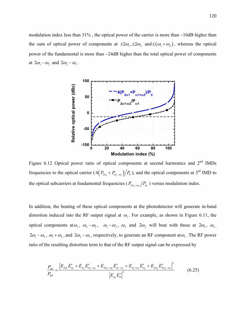
120

modulation index less than 31% , the optical power of the carrier is more than ~10dB higher than

the sum of optical power of components at 12ω± , 22ω± and ( )1 2ω ω± + , whereas the optical

power of the fundamental is more than ~24dB higher than the total optical power of components

at 1 22ω ω− and 2 12ω ω− .

-100

-50

0

50

100

0 20 40 60 80 100

4(P2ω1

+Pω1+ω2

)/P0

P2ω1-ω2

/Pω1

Rel

ativ

e op

tical

pow

er (d

Bc)

Modulation index (%) Figure 6.12 Optical power ratio of optical components at second harmonics and 2nd IMDs

frequencies to the optical carrier ( ( )1 2 12 04 P P Pω ω ω−+ ), and the optical components at 3rd IMD to

the optical subcarriers at fundamental frequencies (1 2 12P Pω ω ω− ) versus modulation index.

In addition, the beating of these optical components at the photodetector will generate in-band

distortion induced into the RF output signal at 1ω . For example, as shown in Figure 6.11, the

optical components at 1ω , 2 1ω ω− , 1 2ω ω− , 2ω and 22ω will beat with those at 12ω , 2ω ,

1 22ω ω− , 1 2ω ω+ , and 2 12ω ω− , respectively, to generate an RF component at 1ω . The RF power

ratio of the resulting distortion term to that of the RF output signal can be expressed by

1 1 2 2 1 1 2 1 2 1 2 2 2 2 1

1

2

2 2 2 22

0

dis

RF

E E E E E E E E E EPP E E

ω ω ω ω ω ω ω ω ω ω ω ω ω ω ω

ω

∗ ∗ ∗ ∗ ∗− − − + −

∗

+ + + += (6.25)

121

( )( )

( )( )

( )( )

( )( )

( )( )

22 2

1 2 22 1

1 0 0 0 0

2

1 2

0 0

2 2 2

2 2 2

2 21

2 2

J m J m J ma aa a J m J m J m

J m J m

J m J m

π π π

π π π

π π

π π

∗

∗

⎡ ⎤⎛ ⎞ ⎛ ⎞⎢ ⎥⎜ ⎟ ⎜ ⎟− +⎢ ⎥⎜ ⎟ ⎜ ⎟⎢ ⎥⎝ ⎠ ⎝ ⎠⎣ ⎦=

⎛ ⎞ ⎡ ⎤⎜ ⎟ ⎢ ⎥− −⎜ ⎟ ⎢ ⎥⎝ ⎠ ⎣ ⎦

( )( )

( )( )

( )( )

( )( )

( )( )

( )( )

22

1

0

2

2 2

0 0

2

1 2

0 0

2

22 1 sin 22 1 sin 2 2 2

2 2

2 21

2 2

J m

J mER j ERER j ER J m J m

J m J m

J m J m

J m J m

π

πϕϕ π π

π π

π π

π π

⎡ ⎤⎛ ⎞⎢ ⎥⎜ ⎟⎢ ⎥⎜ ⎟

− − ⎢ ⎥⎝ ⎠⎢ ⎥+ − ⎛ ⎞⎢ ⎥

⎜ ⎟= ⎢ ⎥− +⎜ ⎟⎢ ⎥⎝ ⎠⎣ ⎦

⎛ ⎞ ⎡ ⎤⎜ ⎟ ⎢ ⎥− −⎜ ⎟ ⎢ ⎥⎝ ⎠ ⎣ ⎦

The above expression will vary between upper and lower limits as

( )( )

( )( )

( )( )

( )( )

( )( )

( )( )

( )( )

( )( )

( )( )

( )( )

2 2

1 2 2

0 0 0

2

1 2

0 0

22 2

1 2 2

0 0 0

2

1 2

0 0

2 2 2

2 2 2

2 21

2 2

2 2 2

2 2 2

2 21

2 2

dis

RF

J m J m J m

J m J m J m PP

J m J m

J m J m

J m J m J m

J m J m J m

J m J m

J m J m

π π π

π π π

π π

π π

π π π

π π π

π π

π π

⎛ ⎞ ⎛ ⎞⎜ ⎟ ⎜ ⎟− +⎜ ⎟ ⎜ ⎟⎝ ⎠ ⎝ ⎠

≤⎛ ⎞⎜ ⎟− −⎜ ⎟⎝ ⎠

⎛ ⎞ ⎛ ⎞⎜ ⎟ ⎜ ⎟− +⎜ ⎟ ⎜ ⎟⎝ ⎠ ⎝ ⎠

≤⎛ ⎞⎜ ⎟+ −⎜ ⎟⎝ ⎠

(6.26)

122

Figure 6.13 shows the lower and upper bound of Pdis/PRF using equation (6.26) versus

modulation index. It is clear that for modulation index less than 31%, the power of the

fundamental RF is at least 10 dB greater than that of the in band distortion.

-100

-50

0

50

100

150

0 20 40 60 80 100

min Pdis/PRF

max Pdis/PRF

Rel

ativ

e di

stor

tion

pow

er (d

Bc)

Modulation index (%) Figure 6.13 Power level of in-band distortion relative to the RF output power in the carrier

versus modulation index.

In the following, we assume that the modulation index is less than 31%, therefore we can

neglect the optical power from all optical components at high-order harmonic and IMD

frequencies compared to the optical carrier and optical subcarriers at fundamental frequencies,

respectively. The total output optical power from the modulator can be written10 2outP P Pω= + ,

and then ( )1

2outP OCSR Pω= + . When the light with optical filed expressed by equation (6.22)

is injected to a photodetector with responsivity of ℜ , the detected RF power at ω1 can be given

by

( )

1

1

220

20

2 22

12

2

22

RF

out

P E E

P P

OCSRPOCSR

ω

ω

= ℜ

= ℜ

= ℜ+

(6.27)

123

Figure 6.14 shows the relative RF power versus OCSR and that maximum RF power can be

obtained when the OCSR=2.

-50

-40

-30

-20

-10

0

-40 -20 0 20 40

Rel

ativ

e R

F po

wer

(dB

c)

OCSR (dB) Figure 6.14 Relative RF power versus OCSR for constant received optical power.

As stated before by tuning the phase shift φ the OCSR will swing between maximum and

minimum values given, respectively, by equation (6.11) and (6.12). Thus here also the maximum

achievable PRF will depend on the extinction ratio and modulation index, and three cases arise.

Case 1: if min max2OCSR OCSR≤ ≤ , i.e

( ) ( )2 20 11 2 4 2ER J m J m ERπ π⎡ ⎤≤ ≤⎣ ⎦ (6.28)

then maximum PRF is obtained at OCSR = 2 by tuning the phase shift to an optimum value

directly expressed from equation (6.6) by

( ) ( )( ) ( )

2 210 14

2 210 14

1 2 21 1arccos2 11 2 2

J m J mERER J m J m

π πϕ

π π

⎡ ⎤−+⎢ ⎥= ±⎢ ⎥− +⎣ ⎦

(6.29)


2 214RF outP P= ℜ (6.30)

124

Case 2: if min 2OCSR > , i.e

( ) ( )2 20 12 4 2ER J m J mπ π⎡ ⎤< ⎣ ⎦ (6.31)

then maximum PRF is obtained at OCSR = OCSRmin by tuning the phase shift to ±π/2, and the RF


( )

( ) ( )( ) ( )

2 2 min2

min

2 20 12 2

22 20 1

22

2 2 4

2 4 2

RF out

out

OCSRP POCSR

J m J mP ER

J m ERJ m

π π

π π

= ℜ+

= ℜ⎡ ⎤+⎣ ⎦

(6.32)

Case 3: if max 2OCSR < , i.e

( ) ( )2 20 12 4 2 1J m J m ERπ π⎡ ⎤ <⎣ ⎦ (6.33)

then maximum PRF is obtained at OCSR = OCSRmax by tuning the phase shift to 0,


( )

( ) ( )( ) ( )

2 2 max2

max

2 20 12 2

22 2

1 0

22

2 2 4

4 2 2

RF out

out

OCSRP POCSR

J m J mP ER

J m ERJ m

π π

π π

= ℜ+

= ℜ⎡ ⎤+⎣ ⎦

(6.34)

Figure 6.15 shows optimum OCSR and corresponding phase shift versus modulation index for

different extinction ratio (ER): 15, 20, 28.5 and 35 dB. It is clear that higher extinction ratio

allows to achieve an OCSR=2 for maximum RF power at lower modulation index. For example

OCSR =2 is achieved at modulation index of 8, 5, 2 and 1% for an ER of 15, 20, 28.5 and 35 dB,

respectively. Also for high extinction ratios of greater than 20 dB the required optimum phase

bias is almost independent on ER and varies linearly with the modulation index. This is because

125

at high extinction ratio 1ER the optimal phase shift given by equation (6.29) reduces to

( ) ( )1 0~ 2 arc tan 2 2 2J m J mϕ π π π⎡ ⎤− ⎣ ⎦ (6.35)

and is almost linear with the modulation index as shown from the plot of Figure 6.16.

-10

-5

0

5

10

15

20

25

0.2

0.25

0.3

0.35

0.4

0.45

0.5

0.55

0 5 10 15 20 25 30

ER = 15dBER = 20dBER = 28.5dBER = 35dB

Opt

imum

OC

SR (d

B)

Optim

um phase ϕ/π (radian)

Modulation index m (%) Figure 6.15 Optimum OCSR and corresponding phase shift versus modulation index for different

extinction ratio (ER): 15, 20, 28.5 and 35 dB.

0

0.1

0.2

0.3

0.4

0.5

0 20 40 60 80 100

Opt

imum

pha

se ϕ

/π (

radi

an)

Modulation index m (%) Figure 6.16 Approximated phase shift versus modulation index for high extinction ratio in two

tone case.

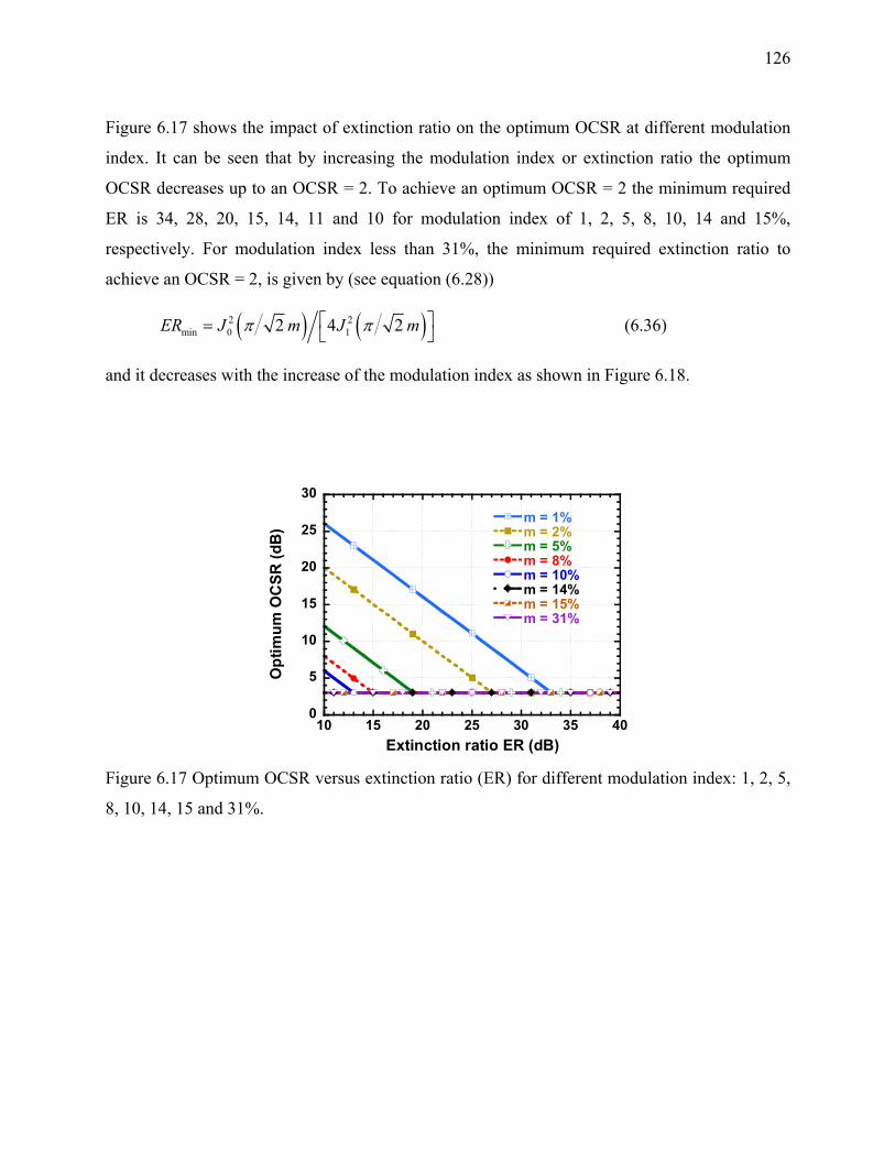
126

Figure 6.17 shows the impact of extinction ratio on the optimum OCSR at different modulation

index. It can be seen that by increasing the modulation index or extinction ratio the optimum

OCSR decreases up to an OCSR = 2. To achieve an optimum OCSR = 2 the minimum required

ER is 34, 28, 20, 15, 14, 11 and 10 for modulation index of 1, 2, 5, 8, 10, 14 and 15%,

respectively. For modulation index less than 31%, the minimum required extinction ratio to

achieve an OCSR = 2, is given by (see equation (6.28))

( ) ( )2 2min 0 12 4 2ER J m J mπ π⎡ ⎤= ⎣ ⎦ (6.36)

and it decreases with the increase of the modulation index as shown in Figure 6.18.

0

5

10

15

20

25

30

10 15 20 25 30 35 40

m = 1% m = 2% m = 5% m = 8% m = 10% m = 14% m = 15% m = 31%

Opt

imum

OC

SR (d

B)

Extinction ratio ER (dB) Figure 6.17 Optimum OCSR versus extinction ratio (ER) for different modulation index: 1, 2, 5,

8, 10, 14, 15 and 31%.

127

-10

0

10

20

30

40

50

0 5 10 15 20 25 30

Min

imum

requ

ired

ER (d

B)

Modulation index m (%) Figure 6.18 Minimum required ER to achieve an OCSR=2 versus modulation index.

Optimum phase shift versus extinction ratio is depicted in Figure 6.19 for different

modulation index. It is shown that the optimum phase shift is almost independent on extinction

ratios of greater than 23 dB. For modulation index of 1, 2, 5, 8, 10, 14, 15 and 31%, the

optimum phase shift φ is ~0.5π, 0.5π, 0.46π, 0.45π, 0.43π, 0.4π, 0.4π and 0.3π, respectively. This

is also confirmed by equation (6.35) and Figure 6.16.

0.25

0.3

0.35

0.4

0.45

0.5

0.55

10 15 20 25 30 35 40

Opt

imum

pha

se ϕ

/π (r

adia

n)

Extinction ratio ER (dB)

m = 1%

8%10%14%

15%

2%5%

31%


2, 5, 8, 10, 14, 15 and 31%.

128

6.3 Simulation using Commercial Software and Comparison to Theory

To verify that not only OSSB modulation but also tunability of OCSR can be obtained

simultaneously using dMZM modulator, we simulate this modulator using VPI-

TransmissionMaker. In the simulation, it is assumed that a laser has a wavelength of 1550.57nm,

linewidth of 800 KHz and power of 6 dBm. Each inner MZM modulator has π-phase shifted

voltage of 6.5 V, insertion loss of 5.5 dB and Y-junction has extinction ratio of 28.5 dB.

First the modulation index was set to 28.28% and the case of single and two RF tones are

studied. Figure 6.20 shows the optical and RF spectrum for single RF tone at 3.96 GHz and for

different OCSR: (a-d) -20 dB, (b-e) 0 dB and (c-f) 20 dB. Figure 6.21 shows the optical and RF

spectrum for two RF tones at 3.96 and 4.46 GHz and for different OCSR: (a-d) -20 dB, (b-e) 0

dB and (c-f) 23 dB. It is clear that OSSB is obtained with tunable OCSR for both single and two

RF tones.

20 dB2GHz/Div

Optical carrier 0

ω2ω-2ω

-3ω

(a) (b) (c)

(d) (e) (f)

Figure 6.20 Optical and RF spectrum for one RF tone (3.96 GHz) at OCSR (a-d) -20 dB, (b-e) 0

dB and (c-f) 20 dB. The extinction ratio is 28.5dB and the modulation index is 28.28 %.

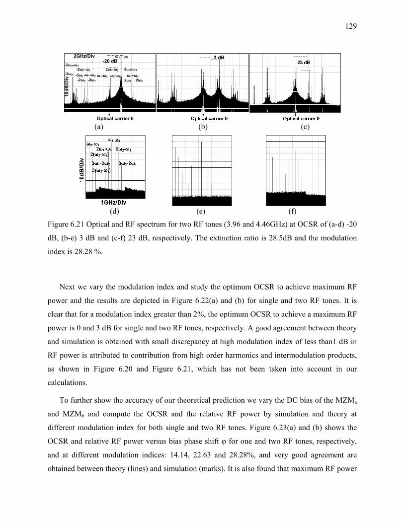
129

-20 dB

10dB

/Div

2GHz/Div

Optical carrier 0

ω1

-2ω1-2ω2

ω2

2ω2-ω12ω1-ω2

ω1-ω2 ω2-ω1-ω1-ω2 ω1+ω22ω22ω1

-2ω1-ω2

-2ω2-ω1

-3ω2 -3ω1

(a) (b) (c)

(d) (e) (f)

Figure 6.21 Optical and RF spectrum for two RF tones (3.96 and 4.46GHz) at OCSR of (a-d) -20

dB, (b-e) 3 dB and (c-f) 23 dB, respectively. The extinction ratio is 28.5dB and the modulation

index is 28.28 %.

Next we vary the modulation index and study the optimum OCSR to achieve maximum RF

power and the results are depicted in Figure 6.22(a) and (b) for single and two RF tones. It is

clear that for a modulation index greater than 2%, the optimum OCSR to achieve a maximum RF

power is 0 and 3 dB for single and two RF tones, respectively. A good agreement between theory

and simulation is obtained with small discrepancy at high modulation index of less than1 dB in

RF power is attributed to contribution from high order harmonics and intermodulation products,

as shown in Figure 6.20 and Figure 6.21, which has not been taken into account in our

calculations.

To further show the accuracy of our theoretical prediction we vary the DC bias of the MZMa

and MZMb and compute the OCSR and the relative RF power by simulation and theory at

different modulation index for both single and two RF tones. Figure 6.23(a) and (b) shows the

OCSR and relative RF power versus bias phase shift φ for one and two RF tones, respectively,

and at different modulation indices: 14.14, 22.63 and 28.28%, and very good agreement are

obtained between theory (lines) and simulation (marks). It is also found that maximum RF power

130

is achieved at an OCSR of 0 and 3 dB for single and two RF tones independently on the RF

modulation index of less than 31% as depicted from Figure 6.24(a) and (b), respectively.

-1

0

1

2

3

4

5

-42

-41

-40

-39

-38

-37

-36

0 5 10 15 20 25 30

SimulationTheory

Opt

imum

OC

SR (d

B)

RF pow

er (dBm

)Modulation index (%)

2.5

3

3.5

4

4.5

5

-44

-43

-42

-41

-40

-39

0 5 10 15 20 25 30

SimulationTheory

Modulation index (%) (a) (b)

Figure 6.22 Optimum OCSR and RF power versus modulation index for 28.5dB extinction ratio.

Simulation (mark) and theory (line). (a) One RF tone and (b) two RF tones.

-30

-20

-10

0

10

20

30

40

50

-35

-30

-25

-20

-15

-10

-5

0

5

-0.5 -0.4 -0.3 -0.2 -0.1 0

m=14.14%m=22.63%m=28.28%

OC

SR (d

B)

Relative R

F POW

ER (dB

m)

Phase shift (π-radian)

OCSR = 0dB

-30

-20

-10

0

10

20

30

40

-30

-25

-20

-15

-10

-5

0

5

-0.5 -0.4 -0.3 -0.2 -0.1 0

m=14.14%m=22.63%m=28.28%

Phase shift (π−radian)

OCSR = 3dB

(a) (b)

Figure 6.23. Compared theory (lines) and simulation (marks) of OCSR and RF power versus

phase shift at different modulation index: 14.14, 22.63 and 28.28%. (a) One RF tone and (b)

two RF tones. an extinction ratio of 28.5dB are used. The extinction ratio is 28.5 dB.

131

-35

-30

-25

-20

-15

-10

-5

0

5

-30 -20 -10 0 10 20 30 40 50

m=14.14%m=22.63%m=28.28%

Rel

ativ

e R

F Po

wer

(dB

)

OCSR (dB)

OCSR = 0dB

-25

-20

-15

-10

-5

0

5

-30 -20 -10 0 10 20 30 40 50

m=14.14%m=22.63%m=28.28%

OCSR (dB)

OCSR = 3dB

(a) (b)

Figure 6.24 Compared theory (lines) and simulation (marks) of RF power versus OCSR for (a)

one and (b) two RF tones and at different modulation indices: 14.14, 22.63 and 28.28%. The

extinction ratio is 28.5dB.

6.4 Experimental Results and Discussion using Commercial dMZM

6.4.1 Experimental Setup

Figure 6.25 shows the experimental setup for the measurement of the performance of the

proposed OSSB with tunable OCSR using a dMZM from Covega (Mach-10TM060). The used

dMZM is integrated on a single x-cut lithium niobate chip, has insertion loss of 5.5 dB,

extinction ratio of more than 20 dB, RF and DC half-wave switching voltage of 6.5 V and 4.5 V,

respectively. A tunable laser source (Anritsu MG9541A) delivers a linearly polarized light at

1550.57nm of 6 dBm optical power with a linewidth of 800 KHz and intrinsic RIN of -155

dB/Hz. The lightwave source is injected into the dMZM driven by an RF source. The bias

voltages V1 and V2 are tuned to change the OCSR while Vc is tuned to achieve OSSB

modulation. The externally modulated signal passed through a single mode fiber, amplified with

an EDFA and filtered by a tunable optical filter with 0.55nm bandwidth. A variable optical

attenuator is used to control and set the received optical power to 0 dBm at the photodetector.

An optical splitter is used to monitor the received optical signal by an OSA of 0.01nm resolution.

After photo-detection the received RF signal is amplified with an LNA of 26dB gain and 2.6dB

noise figure. The received signal is analyzed in the frequency domain by a 43 GHz RSA. A 12

132

GHz reel time oscilloscope (Agilent infiniium DSO81204B) with a sampling rate of 40 GSa/s is

used to analyze the received RF signal in time domain.

Figure 6.25 Experimental setup for the proposed OSSB with tunable OCSR using dual-parallel

MZM modulator. PC: Polarization controller.

6.4.2 Distortion Effects using Two RF Tone Test

In order to assess the distortion effects of the RF signal for the proposed OSSB with tunable

OCSR technique, we measure the IMD using two RF tones test with respect to OCSR. Two

analog signal generators (Agilent MXG N5181A) were used to provide two RF tones at 3.96GHz

and 3.964GHz with fixed power level at 12 dBm. We connected point 3 to point 1 in the

experimental setup shown in Figure 6.25.

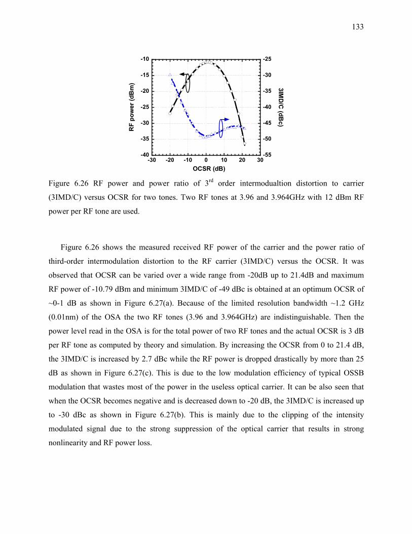
133

-40

-35

-30

-25

-20

-15

-10

-55

-50

-45

-40

-35

-30

-25

-30 -20 -10 0 10 20 30

RF

pow

er (d

Bm

) 3IMD

/C (dB

c)

OCSR (dB) Figure 6.26 RF power and power ratio of 3rd order intermodualtion distortion to carrier

(3IMD/C) versus OCSR for two tones. Two RF tones at 3.96 and 3.964GHz with 12 dBm RF

power per RF tone are used.

Figure 6.26 shows the measured received RF power of the carrier and the power ratio of

third-order intermodulation distortion to the RF carrier (3IMD/C) versus the OCSR. It was

observed that OCSR can be varied over a wide range from -20dB up to 21.4dB and maximum

RF power of -10.79 dBm and minimum 3IMD/C of -49 dBc is obtained at an optimum OCSR of

~0-1 dB as shown in Figure 6.27(a). Because of the limited resolution bandwidth ~1.2 GHz

(0.01nm) of the OSA the two RF tones (3.96 and 3.964GHz) are indistinguishable. Then the

power level read in the OSA is for the total power of two RF tones and the actual OCSR is 3 dB

per RF tone as computed by theory and simulation. By increasing the OCSR from 0 to 21.4 dB,

the 3IMD/C is increased by 2.7 dBc while the RF power is dropped drastically by more than 25

dB as shown in Figure 6.27(c). This is due to the low modulation efficiency of typical OSSB

modulation that wastes most of the power in the useless optical carrier. It can be also seen that

when the OCSR becomes negative and is decreased down to -20 dB, the 3IMD/C is increased up

to -30 dBc as shown in Figure 6.27(b). This is mainly due to the clipping of the intensity

modulated signal due to the strong suppression of the optical carrier that results in strong

nonlinearity and RF power loss.

134

10dB

/div

(a) OCSR ~ 1 dB

(b) OCSR = -20 dB

(c) OCSR = 21.4 dB

Figure 6.27 RF and optical spectrum at different OCSR (a) OCSR = 1 dB, (b) OCSR = -20 dB and (c) OCSR = 21.4 dB. An RF input power of 12 dBm per RF tone is used.

6.4.3 Performance of MB-OFDM UWB using the Proposed Technique

Next we used the same experimental setup shown in Figure 6.25 for performance evaluation

of UWB over fiber using our proposed OSSB modulation with tunable OCSR, where point 3 is

connected to point 2. To generate MB-OFDM UWB we used a commercially available

evaluation board, DV 9110M from WisAir, which provides MB-OFDM compliant modulation

with the first three WiMedia sub-bands of 528 MHz bandwidth allocated at center frequency of

f1=3.432, f2=3.96 and f3=4.488 GHz, as shown in Figure 6.28(a). The signal follows simple

frequency hopping sequences like f1, f2 and f3. The bit rate of 200 Mb/s is used for each band

with QPSK modulations shown from the constellation of Figure 6.28(b). The UWB power input

to the dMZM is set to -6.14dBm and the bias voltage applied to MZMc was set to obtain OSSB

135

modulation. The OCSR was tuned by changing the applied bias voltages to MZMa and MZMb

and the received optical power at the photo-detector was maintained to be 0 dBm. We used the

real time oscilloscope DSO81204B to measure the EVM and received UWB power versus

OCSR for back to back and after 20km of fiber transmission and the results are shown in Figure

6.29(a) and (b), respectively. It can be seen that maximum RF power is obtained at 0 dB OCSR,

while minimum EVM of -21.8 dB is obtained around 5.4 dB OCSR. This is due to the high

PAPR which is inherent to OFDM signal. The measured PAPR of the transmitted signal was

around 11 dB, then by setting the OCSR to 5.4 dB, optical intensity clipping is avoided and

better EVM performance is obtained. It is also seen that the system is compliant with the

maximum required EVM of -17dB [7] when the OCSR is ranging between ~-8dB and 20dB.

f1 f2 f3

180MHz/div (a) (b)

Figure 6.28 First three bands of MB-OFDM UWB wireless in (a) frequency domain and (b)

received constellation.

-22

-20

-18

-16

-14

-12

-45

-40

-35

-30

-25

-20

-15 -10 -5 0 5 10 15 20 25

EVM

(dB

)

RF pow

er (dBm

)

OCSR (dB)

-17 dB

-22

-20

-18

-16

-14

-12

-45

-40

-35

-30

-25

-20

-15 -10 -5 0 5 10 15 20 25OCSR (dB)

-17 dB

(a) Back to back (b) 20 km

Figure 6.29 Measured EVM and RF output power versus OCSR for (a) back to back and (b) after

20 km of fiber transmission. The UWB input power to the dMZM is -6.14 dBm.

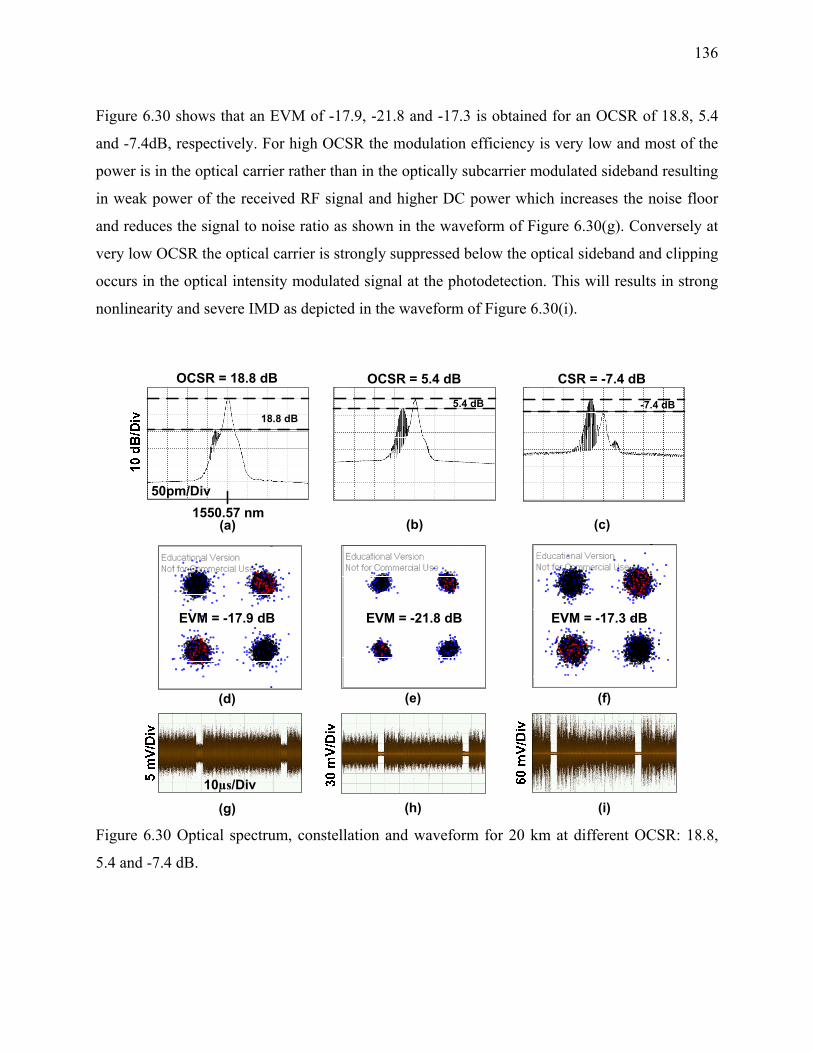
136

Figure 6.30 shows that an EVM of -17.9, -21.8 and -17.3 is obtained for an OCSR of 18.8, 5.4

and -7.4dB, respectively. For high OCSR the modulation efficiency is very low and most of the

power is in the optical carrier rather than in the optically subcarrier modulated sideband resulting

in weak power of the received RF signal and higher DC power which increases the noise floor

and reduces the signal to noise ratio as shown in the waveform of Figure 6.30(g). Conversely at

very low OCSR the optical carrier is strongly suppressed below the optical sideband and clipping

occurs in the optical intensity modulated signal at the photodetection. This will results in strong

nonlinearity and severe IMD as depicted in the waveform of Figure 6.30(i).

18.8 dB

50pm/Div

(a) 1550.57 nm

5.4 dB

(b)

-7.4 dB

(c)

EVM = -21.8 dB

OCSR = 18.8 dB OCSR = 5.4 dB CSR = -7.4 dB

EVM = -17.3 dBEVM = -17.9 dB

(d) (e) (f)

10µs/Div

(g) (h) (i) Figure 6.30 Optical spectrum, constellation and waveform for 20 km at different OCSR: 18.8,

5.4 and -7.4 dB.

137

6.5 Chapter Conclusion

We have shown that a dual parallel MZM modulator can be used for obtaining not only OSSB

modulation but also tunability of OCSR. The dMZM is integrated in a single x-cut Lithium

Niobate chip and consists of an outer MZM with an inner MZM inserted in each arm. To the best

of our knowledge the function of OCSR tunability using this modulator is proposed and

investigated for the first time. It is shown that a wide dynamic range of OCSR tunability can be

obtained by varying the bias voltage applied to the inner MZMs. It is found that the optimum

OCSR to obtain maximum RF output power depends on the modulation index and the extinction

ratio of the dMZM. To achieve an OCSR of 0 dB there is a minimum required extinction ratio at

a given modulation index. Moreover, we have investigated the impact of OCSR on the

performance of MB-OFDM UWB signal. It is found that maximum received RF power is

obtained at 0 dB OCSR while minimum EVM of the received MB-OFDM UWB constellation is

achieved at 5.4dB OCSR. The proposed technique has been proven to be effective solution to

improve the modulation efficiency of OSSB modulation.

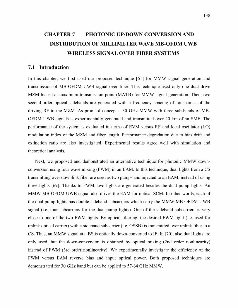
138

CHAPTER 7 PHOTONIC UP/DOWN CONVERSION AND

DISTRIBUTION OF MILLIMETER WAVE MB-OFDM UWB

WIRELESS SIGNAL OVER FIBER SYSTEMS

7.1 Introduction

In this chapter, we first used our proposed technique [61] for MMW signal generation and

transmission of MB-OFDM UWB signal over fiber. This technique used only one dual drive

MZM biased at maximum transmission point (MATB) for MMW signal generation. Then, two

second-order optical sidebands are generated with a frequency spacing of four times of the

driving RF to the MZM. As proof of concept a 30 GHz MMW with three sub-bands of MB-

OFDM UWB signals is experimentally generated and transmitted over 20 km of an SMF. The

performance of the system is evaluated in terms of EVM versus RF and local oscillator (LO)

modulation index of the MZM and fiber length. Performance degradation due to bias drift and

extinction ratio are also investigated. Experimental results agree well with simulation and

theoretical analysis.

Next, we proposed and demonstrated an alternative technique for photonic MMW down-

conversion using four wave mixing (FWM) in an EAM. In this technique, dual lights from a CS

transmitting over downlink fiber are used as two pumps and injected to an EAM, instead of using

three lights [69]. Thanks to FWM, two lights are generated besides the dual pump lights. An

MMW MB OFDM UWB signal also drives the EAM for optical SCM. In other words, each of

the dual pump lights has double sideband subcarriers which carry the MMW MB OFDM UWB

signal (i.e. four subcarriers for the dual pump lights). One of the sideband subcarriers is very

close to one of the two FWM lights. By optical filtering, the desired FWM light (i.e. used for

uplink optical carrier) with a sideband subcarrier (i.e. OSSB) is transmitted over uplink fiber to a

CS. Thus, an MMW signal at a BS is optically down-converted to IF. In [70], also dual lights are

only used, but the down-conversion is obtained by optical mixing (2nd order nonlinearity)

instead of FWM (3rd order nonlinearity). We experimentally investigate the efficiency of the

FWM versus EAM reverse bias and input optical power. Both proposed techniques are

demonstrated for 30 GHz band but can be applied to 57-64 GHz MMW.

139

The chapter is organized into three sections. Section 7.2 presents the principle of photonic

MMW up-conversion using DE-MZM. The performance of the generated MMW MB-OFDM

UWB signal is also numerically and experimentally evaluated in terms of EVM versus RF and

LO modulation index for back to back and after 20km of fiber transmission. Section 7.3 explains

the principle and gives the experimental characterization of photonic MMW down-conversion

using FWM in an EAM. FWM efficiency is studied versus input optical power and applied

reverse bias to the EAM. Also, the performance of the down-converted MMW MB-OFDM

UWB signal is experimentally evaluated in terms of EVM versus EAM, LO modulation index

and received optical power after 20km of fiber. Finally summary is drawn in Section 7.4.

7.2 Photonic UP-Conversion of MMW MB-OFDM UWB Signal Using MZM

7.2.1 Proposed Technique

The proposed modulation technique for MMW MB-OFDM UWB signal is shown schematically

in Figure 7.1. A CW laser is assumed to have a wavelength of λ=1548.5 nm, an output optical

power of P=7.5 dBm, a linewidth of 800 KHz, and RIN of -150 dB/Hz. A sinusoidal LO signal

has a frequency of fLO=6.51 GHz and voltage of ( ) sin( )LO LO LO LOV t V tω φ= + , where ωLO=2πfLO ,

φLO- random phase noise of the LO. The total LO modulation index for the MMW generation is

defined by mLO=VLO/Vπ, where Vπ is the modulator’s switching voltage. The CW light is injected

to the first DE-MZM, biased at maximum transmission. This DE-MZM has a switching voltage

of 3.8 V, an extinction ratio of 28.5 dB and insertion loss of 6 dB. The dual electrodes are driven

by the same LO sinusoid with 180 degree phase shift. Thus, only even-order optical harmonics

are generated whereas all odd-order optical harmonics are suppressed ideally. Following the

optical MMW generation, a second DE-MZM is driven by an MB-OFDM UWB signal and

generates OSSB modulation. This DE-MZM has an extinction ratio of 32 dB, half wave

switching voltage of 5 V, and insertion loss of 7 dB. The bit rate of 200 Mbps is used for each

band of the MB-OFDM UWB signal with QPSK modulation.

Following the second DE-MZM an EDFA with a noise figure (NF) of 5 dB is used to

compensate for optical losses. To reduce optical amplifier noise, an optical BPF is used after the

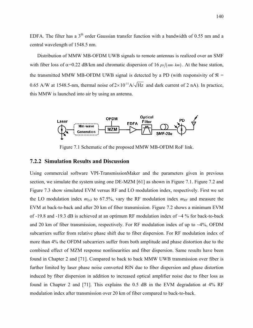
140

EDFA. The filter has a 3th order Gaussian transfer function with a bandwidth of 0.55 nm and a

central wavelength of 1548.5 nm.

Distribution of MMW MB-OFDM UWB signals to remote antennas is realized over an SMF

with fiber loss of α=0.22 dB/km and chromatic dispersion of 16 ( )ps nm km⋅ . At the base station,

the transmitted MMW MB-OFDM UWB signal is detected by a PD (with responsivity of ℜ =

0.65 A/W at 1548.5-nm, thermal noise of -112 10 A/ Hz× and dark current of 2 nA). In practice,

this MMW is launched into air by using an antenna.

Figure 7.1 Schematic of the proposed MMW MB-OFDM RoF link.

7.2.2 Simulation Results and Discussion

Using commercial software VPI-TransmissionMaker and the parameters given in previous

section, we simulate the system using one DE-MZM [61] as shown in Figure 7.1. Figure 7.2 and

Figure 7.3 show simulated EVM versus RF and LO modulation index, respectively. First we set

the LO modulation index mLO to 67.5%, vary the RF modulation index mRF and measure the

EVM at back-to-back and after 20 km of fiber transmission. Figure 7.2 shows a minimum EVM

of -19.8 and -19.3 dB is achieved at an optimum RF modulation index of ~4 % for back-to-back

and 20 km of fiber transmission, respectively. For RF modulation index of up to ~4%, OFDM

subcarriers suffer from relative phase shift due to fiber dispersion. For RF modulation index of

more than 4% the OFDM subcarriers suffer from both amplitude and phase distortion due to the

combined effect of MZM response nonlinearities and fiber dispersion. Same results have been

found in Chapter 2 and [71]. Compared to back to back MMW UWB transmission over fiber is

further limited by laser phase noise converted RIN due to fiber dispersion and phase distortion

induced by fiber dispersion in addition to increased optical amplifier noise due to fiber loss as

found in Chapter 2 and [71]. This explains the 0.5 dB in the EVM degradation at 4% RF

modulation index after transmission over 20 km of fiber compared to back-to-back.

141

-20

-19

-18

-17

-16

0 2 4 6 8 10

back-to-back

20 km

EVM

(dB

)

RF Modulation Index (%)

Figure 7.2 Simulated EVM versus RF modulation index of second MZM. LO modulation index

of 67.5 % is used.

-30

-25

-20

-15

-10

-5

0

5

20 30 40 50 60 70 80 90 100

back to back

20 km

EVM

(dB

)

LO Modulation Index (%)

- 16 dB

Figure 7.3 Simulated EVM versus LO modulation index of first DE-MZM for MMW generation.

RF modulation index of 4% is used.

Next, we fixed the RF modulation index at optimum ~4 % and investigate the impact of the

LO modulation index. We vary the LO modulation index from 20% to 100% and measure the

EVM for back to back and after transmission over 20 km of fiber. Figure 7.3 shows that by

increasing the LO modulation index from 20 to ~100% the EVM decreases from -0.5 dB to -25

dB after 20 km of fiber transmission. It is also seen that for 20 km of fiber transmission an LO

modulation index of more than 60% is necessary to achieve the minimum required EVM of -16

dB [7]. Compared to back-to-back transmission, the EVM is degraded by 0.5 dB after

transmission through 20 km of fiber. The EVM is inversely proportional to the signal to noise

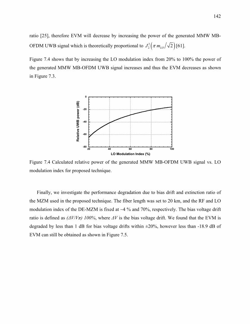
142

ratio [25], therefore EVM will decrease by increasing the power of the generated MMW MB-

OFDM UWB signal which is theoretically proportional to ( )22 2LOJ mπ [61].

Figure 7.4 shows that by increasing the LO modulation index from 20% to 100% the power of

the generated MMW MB-OFDM UWB signal increases and thus the EVM decreases as shown

in Figure 7.3.

-80

-60

-40

-20

0

20 40 60 80 100

Rel

ativ

e U

WB

pow

er (d

B)


Figure 7.4 Calculated relative power of the generated MMW MB-OFDM UWB signal vs. LO

modulation index for proposed technique.

Finally, we investigate the performance degradation due to bias drift and extinction ratio of

the MZM used in the proposed technique. The fiber length was set to 20 km, and the RF and LO

modulation index of the DE-MZM is fixed at ~4 % and 70%, respectively. The bias voltage drift

ratio is defined as (ΔV/Vπ) 100%, where ΔV is the bias voltage drift. We found that the EVM is

degraded by less than 1 dB for bias voltage drifts within ±20%, however less than -18.9 dB of

EVM can still be obtained as shown in Figure 7.5.

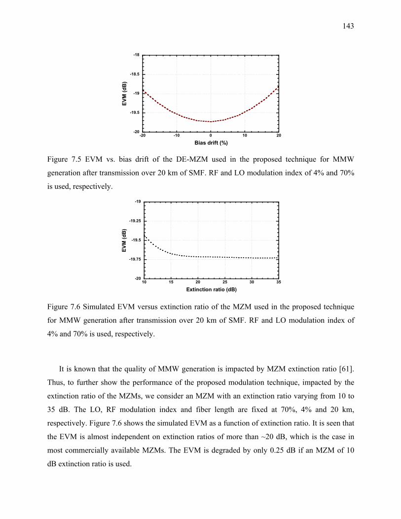
143

-20

-19.5

-19

-18.5

-18

-20 -10 0 10 20

EVM

(dB

)

Bias drift (%)

Figure 7.5 EVM vs. bias drift of the DE-MZM used in the proposed technique for MMW

generation after transmission over 20 km of SMF. RF and LO modulation index of 4% and 70%

is used, respectively.

-20

-19.75

-19.5

-19.25

-19

10 15 20 25 30 35

EVM

(dB

)

Extinction ratio (dB)

Figure 7.6 Simulated EVM versus extinction ratio of the MZM used in the proposed technique

for MMW generation after transmission over 20 km of SMF. RF and LO modulation index of

4% and 70% is used, respectively.

It is known that the quality of MMW generation is impacted by MZM extinction ratio [61].

Thus, to further show the performance of the proposed modulation technique, impacted by the

extinction ratio of the MZMs, we consider an MZM with an extinction ratio varying from 10 to

35 dB. The LO, RF modulation index and fiber length are fixed at 70%, 4% and 20 km,

respectively. Figure 7.6 shows the simulated EVM as a function of extinction ratio. It is seen that

the EVM is almost independent on extinction ratios of more than ~20 dB, which is the case in

most commercially available MZMs. The EVM is degraded by only 0.25 dB if an MZM of 10

dB extinction ratio is used.

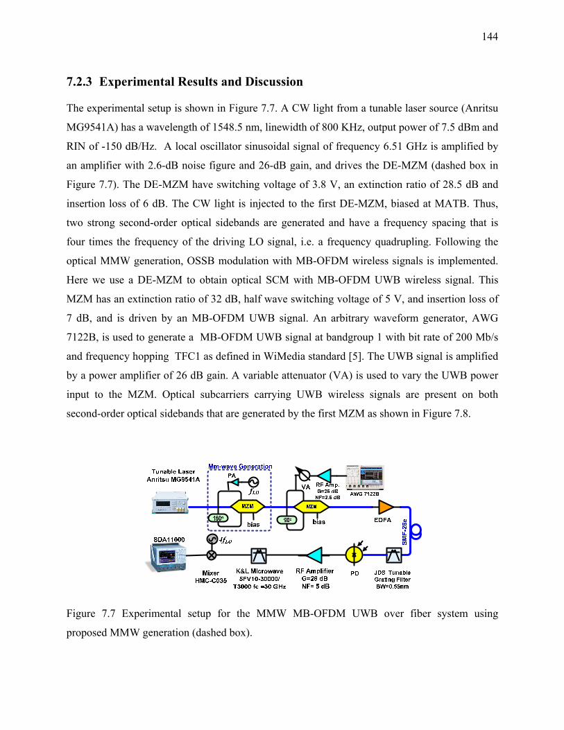
144

7.2.3 Experimental Results and Discussion

The experimental setup is shown in Figure 7.7. A CW light from a tunable laser source (Anritsu

MG9541A) has a wavelength of 1548.5 nm, linewidth of 800 KHz, output power of 7.5 dBm and

RIN of -150 dB/Hz. A local oscillator sinusoidal signal of frequency 6.51 GHz is amplified by

an amplifier with 2.6-dB noise figure and 26-dB gain, and drives the DE-MZM (dashed box in

Figure 7.7). The DE-MZM have switching voltage of 3.8 V, an extinction ratio of 28.5 dB and

insertion loss of 6 dB. The CW light is injected to the first DE-MZM, biased at MATB. Thus,

two strong second-order optical sidebands are generated and have a frequency spacing that is

four times the frequency of the driving LO signal, i.e. a frequency quadrupling. Following the

optical MMW generation, OSSB modulation with MB-OFDM wireless signals is implemented.

Here we use a DE-MZM to obtain optical SCM with MB-OFDM UWB wireless signal. This

MZM has an extinction ratio of 32 dB, half wave switching voltage of 5 V, and insertion loss of

7 dB, and is driven by an MB-OFDM UWB signal. An arbitrary waveform generator, AWG

7122B, is used to generate a MB-OFDM UWB signal at bandgroup 1 with bit rate of 200 Mb/s

and frequency hopping TFC1 as defined in WiMedia standard [5]. The UWB signal is amplified

by a power amplifier of 26 dB gain. A variable attenuator (VA) is used to vary the UWB power

input to the MZM. Optical subcarriers carrying UWB wireless signals are present on both

second-order optical sidebands that are generated by the first MZM as shown in Figure 7.8.

Figure 7.7 Experimental setup for the MMW MB-OFDM UWB over fiber system using

proposed MMW generation (dashed box).

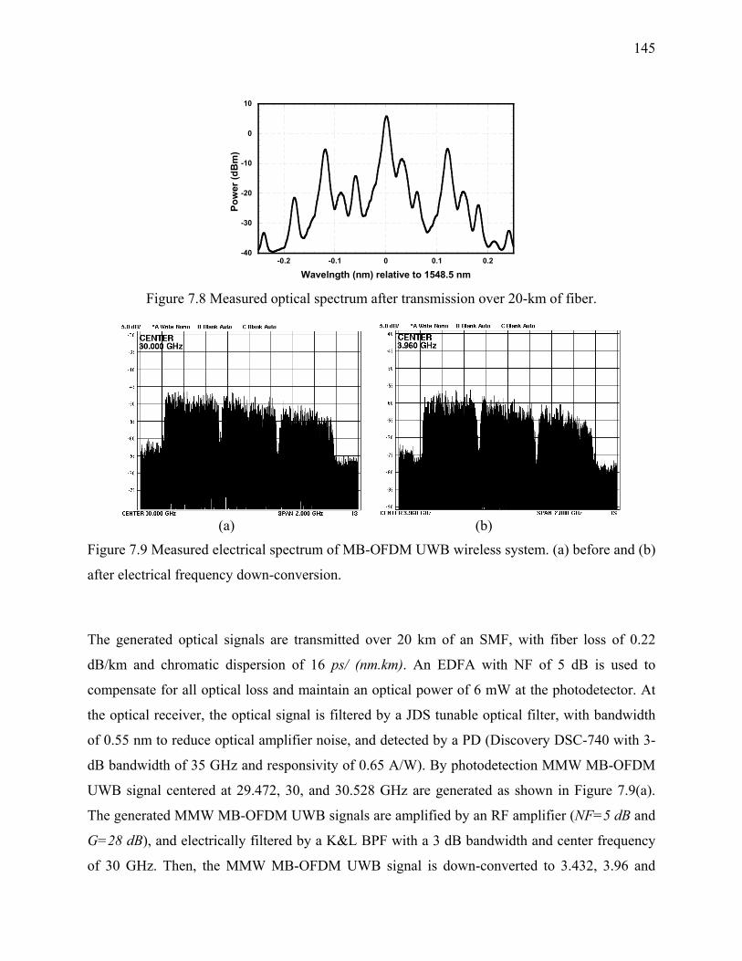
145

-40

-30

-20

-10

0

10

-0.2 -0.1 0 0.1 0.2

Pow

er (d

Bm

)

Wavelngth (nm) relative to 1548.5 nm Figure 7.8 Measured optical spectrum after transmission over 20-km of fiber.

(a) (b)

Figure 7.9 Measured electrical spectrum of MB-OFDM UWB wireless system. (a) before and (b)

after electrical frequency down-conversion.

The generated optical signals are transmitted over 20 km of an SMF, with fiber loss of 0.22

dB/km and chromatic dispersion of 16 ps/ (nm.km). An EDFA with NF of 5 dB is used to

compensate for all optical loss and maintain an optical power of 6 mW at the photodetector. At

the optical receiver, the optical signal is filtered by a JDS tunable optical filter, with bandwidth

of 0.55 nm to reduce optical amplifier noise, and detected by a PD (Discovery DSC-740 with 3-

dB bandwidth of 35 GHz and responsivity of 0.65 A/W). By photodetection MMW MB-OFDM

UWB signal centered at 29.472, 30, and 30.528 GHz are generated as shown in Figure 7.9(a).

The generated MMW MB-OFDM UWB signals are amplified by an RF amplifier (NF=5 dB and

G=28 dB), and electrically filtered by a K&L BPF with a 3 dB bandwidth and center frequency

of 30 GHz. Then, the MMW MB-OFDM UWB signal is down-converted to 3.432, 3.96 and

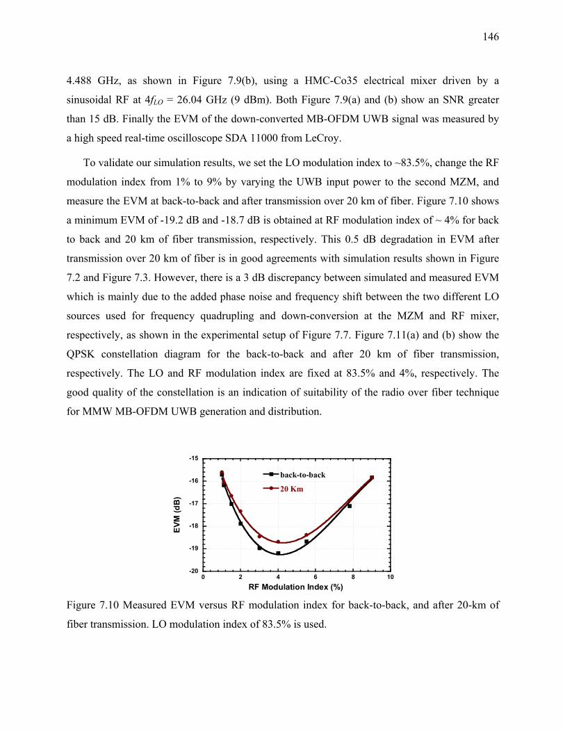
146

4.488 GHz, as shown in Figure 7.9(b), using a HMC-Co35 electrical mixer driven by a

sinusoidal RF at 4fLO = 26.04 GHz (9 dBm). Both Figure 7.9(a) and (b) show an SNR greater

than 15 dB. Finally the EVM of the down-converted MB-OFDM UWB signal was measured by

a high speed real-time oscilloscope SDA 11000 from LeCroy.

To validate our simulation results, we set the LO modulation index to ~83.5%, change the RF

modulation index from 1% to 9% by varying the UWB input power to the second MZM, and

measure the EVM at back-to-back and after transmission over 20 km of fiber. Figure 7.10 shows

a minimum EVM of -19.2 dB and -18.7 dB is obtained at RF modulation index of ~ 4% for back

to back and 20 km of fiber transmission, respectively. This 0.5 dB degradation in EVM after

transmission over 20 km of fiber is in good agreements with simulation results shown in Figure

7.2 and Figure 7.3. However, there is a 3 dB discrepancy between simulated and measured EVM

which is mainly due to the added phase noise and frequency shift between the two different LO

sources used for frequency quadrupling and down-conversion at the MZM and RF mixer,

respectively, as shown in the experimental setup of Figure 7.7. Figure 7.11(a) and (b) show the

QPSK constellation diagram for the back-to-back and after 20 km of fiber transmission,

respectively. The LO and RF modulation index are fixed at 83.5% and 4%, respectively. The

good quality of the constellation is an indication of suitability of the radio over fiber technique

for MMW MB-OFDM UWB generation and distribution.

-20

-19

-18

-17

-16

-15

0 2 4 6 8 10

back-to-back

20 Km

EVM

(dB

)

RF Modulation Index (%)

Figure 7.10 Measured EVM versus RF modulation index for back-to-back, and after 20-km of

fiber transmission. LO modulation index of 83.5% is used.

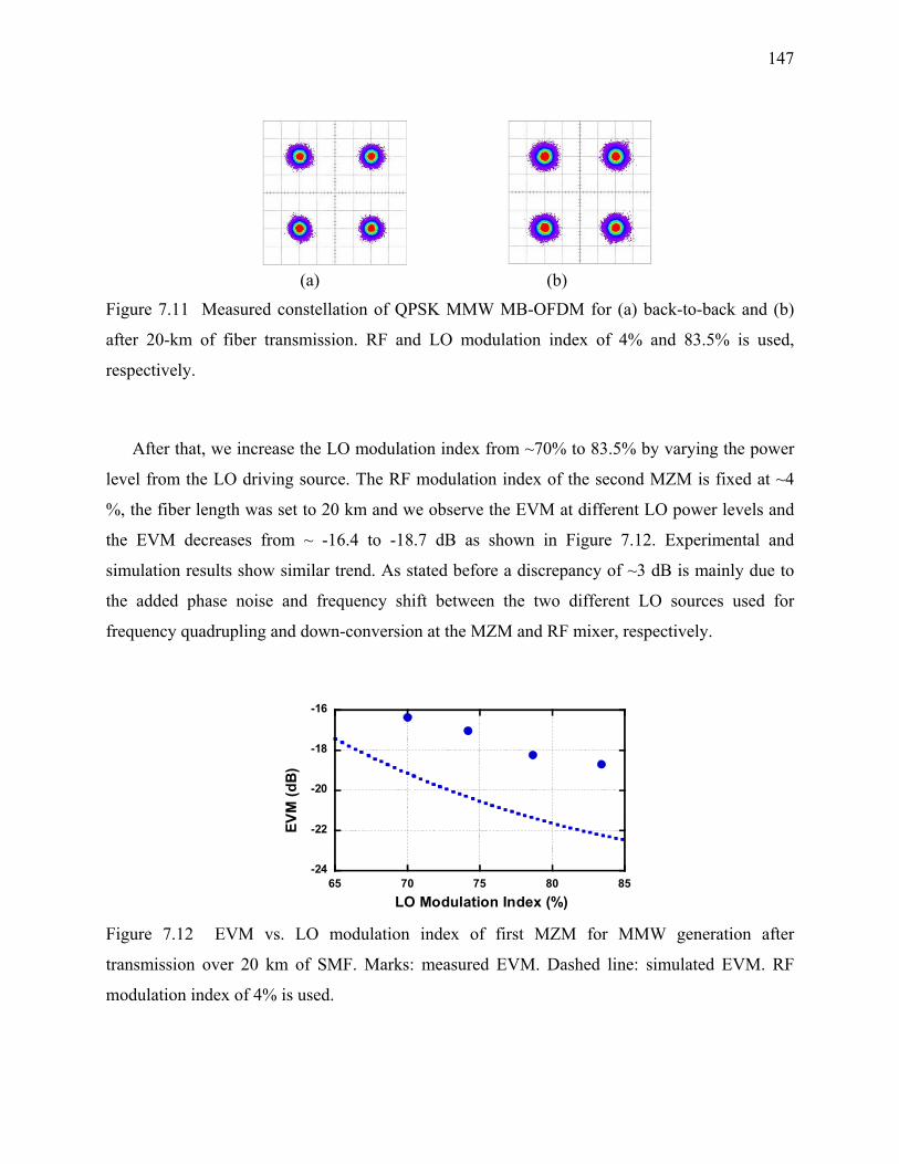
147

(a) (b)

Figure 7.11 Measured constellation of QPSK MMW MB-OFDM for (a) back-to-back and (b)

after 20-km of fiber transmission. RF and LO modulation index of 4% and 83.5% is used,

respectively.

After that, we increase the LO modulation index from ~70% to 83.5% by varying the power

level from the LO driving source. The RF modulation index of the second MZM is fixed at ~4

%, the fiber length was set to 20 km and we observe the EVM at different LO power levels and

the EVM decreases from ~ -16.4 to -18.7 dB as shown in Figure 7.12. Experimental and

simulation results show similar trend. As stated before a discrepancy of ~3 dB is mainly due to

the added phase noise and frequency shift between the two different LO sources used for

frequency quadrupling and down-conversion at the MZM and RF mixer, respectively.

-24

-22

-20

-18

-16

65 70 75 80 85

EVM

(dB

)


Figure 7.12 EVM vs. LO modulation index of first MZM for MMW generation after

transmission over 20 km of SMF. Marks: measured EVM. Dashed line: simulated EVM. RF

modulation index of 4% is used.

148

7.3 Photonic Down-Conversion of MMW MB-OFDM UWB Signal using

FWM in an EAM

For downlinks, we have already investigated cost-effective techniques for the generation and

distribution of MMW signals using optical frequency up-conversion [61-62], including MMW

MB-OFDM UWB signal generation and transmission over fiber as presented in Section 7.2. For

uplinks, it is preferable to use an EAM because it presents a low power consumption, compact

size, polarization insensitivity, easy integration with other devices, and higher speed operation in

photodetection, mixing and optical modulation due to the EAM inherent characteristics. It was

demonstrated that an EAM can be used for frequency down-conversion from an MMW to an

intermediate frequency (IF) signal [72-73] using cross-absorption modulation in an EAM for

uplinks. Instead of using both a CW light for uplink and dual pump lights for down-conversion

[72], a simpler technique [73] was proposed for MMW down-conversion in an EAM, in which

only the dual lights are used for both uplink transmission and down-conversion.

7.3.1 Proposed Technique

The proposed technique is illustrated in Figure 7.13 using an EAM for frequency down-

conversion, and optical modulation. In a CS, the downlink lightwave at frequency fc is modulated

in a MZM driven by an RF signal at a frequency flo/2 with optical carrier suppression. Thus the

two optical subcarriers are generated with a frequency separation of flo, and the two optical

subcarriers are referred to dual pump lights. This is one way to obtain dual pump lights with a

given spacing. These dual pump lights are transmitted over downlink fiber to a BS. At a BS, the

dual pump lights are injected into an EAM that is also driven by an MMW radio signal at fmm.

Due to FWM process in the EAM [74-75], two FWM lights separated by 3flo are generated

besides the dual-pump lights. In the same time, an MMW signal is applied to the EAM which

leads to ODSB SCM, and thus two optical subcarriers are generated for each pump light. The

optical sidebands carry the modulation data, and the FWM lights can serve as uplink optical

carriers. Then with proper optical filtering as shown in Figure 7.13, an OSSB together with the

optical carrier (one FWM light) can be extracted for further transmission. After the

photodetection, an IF signal will be generated at fmm - flo.

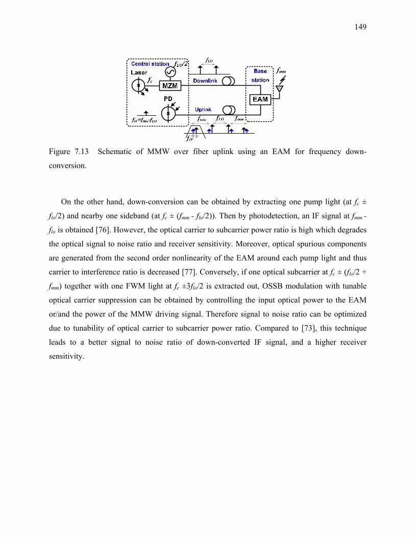
149

Figure 7.13 Schematic of MMW over fiber uplink using an EAM for frequency down-

conversion.

On the other hand, down-conversion can be obtained by extracting one pump light (at fc ±

flo/2) and nearby one sideband (at fc ± (fmm - flo/2)). Then by photodetection, an IF signal at fmm -

flo is obtained [76]. However, the optical carrier to subcarrier power ratio is high which degrades

the optical signal to noise ratio and receiver sensitivity. Moreover, optical spurious components

are generated from the second order nonlinearity of the EAM around each pump light and thus

carrier to interference ratio is decreased [77]. Conversely, if one optical subcarrier at fc ± (flo/2 +

fmm) together with one FWM light at fc ±3flo/2 is extracted out, OSSB modulation with tunable

optical carrier suppression can be obtained by controlling the input optical power to the EAM

or/and the power of the MMW driving signal. Therefore signal to noise ratio can be optimized

due to tunability of optical carrier to subcarrier power ratio. Compared to [73], this technique

leads to a better signal to noise ratio of down-converted IF signal, and a higher receiver

sensitivity.

150

7.3.2 Experimental Setup

The considered system setup shown in Figure 7.14 is used to investigate the FWM efficiency in

an EAM and to evaluate the performance of the down-converted MMW MB-OFDM UWB in

MMW over fiber uplink. A tunable laser source delivers a light at 1548.823 nm of 0 dBm optical

power with a linewidth of 800 KHz and intrinsic RIN of -155 dB/Hz. The light is injected into a

dual-electrode MZM (DE-MZM) of 6 dB insertion loss, 32 dB extinction ratio and 5 V half wave

switching voltage. The DE-MZM is biased at minimum transmission point and driven by a flo/2 =

13.02 GHz sinusoidal LO source. An 1800 HEC is used to insert 1800 phase shift between the

two electrodes of the DE-MZM. ODSB with carrier suppression is obtained at the output of the

DE-MZM. Thus, two optical sidebands, separated by 0.208 nm (flo=26.04 GHz), are generated

and referred to dual pump lights as shown in Figure 7.15(a), together with some high-order

nonlinear distortion products. The lights are launched into 20 km of standard SMF and amplified

by an EDFA before being injected into an EAM. We use a commercial EAM from OKI with a 3

dB bandwidth of 32 GHz. The measured characteristic transmission of the EAM at 1548.823 nm

and the calculated relative third intermodulation distortion are shown in Figure 7.16.

Figure 7.14 Experimental setup for photonic MMW down-conversion using FWM in an EAM.

OC: optical circulator.

151

The AWG 7122B provides MB-OFDM compliant modulation with three WiMedia bands

allocated at the center frequency of 3.432, 3.96 and 4.488 GHz. This MB OFDM UWB signal is

mixed with an LO signal at 26.04 GHz, amplified and passes an EBF of 3 GHz bandwidth

centered at 30 GHz. An MMW MB OFDM UWB signal hopping at 29.472, 30, and 30.528 GHz

is generated as shown in Figure 7.15(e) and drives the EAM. The optical spectrum at the output

of the EAM is shown in Figure 7.15(b). It is seen that there are two sidebands which both carry

the MB OFDM UWB MMW signal, and they are close to the FWM lights (the other two

sidebands are overlapped with the two pump lights and invisible). We use a reflective fiber

Bragg grating (FBG) of 7.5 GHz 3-dB bandwidth with a circulator to extract the optical upper

sideband for uplink transmission. The optical spectrum at point D in Figure 7.14 is shown in

Figure 7.15(c). The extracted upper sideband consists of the FWM light (at -39.06 GHz) and MB

OFDM UWB subcarrier (with signal hopping at -42.492, -43.02, and -43.548 GHz), together

with some residual optical spectral components. After transmission over SMF of 20 km,

amplification and optical filtering (for reducing ASE noise), the optical spectrum at the

photodetector is shown in Figure 7.15(d). A variable optical attenuator is used to control the

received optical power at the photodetector. After photodetection, the UWB signal is amplified

by a broadband RF amplifier with gain of 26 dB and noise figure of 2.6 dB, and passes an EBF

centered at 4 GHz with a 3 GHz bandwidth as shown in Figure 7.14. The received MB-OFDM

UWB signal is shown in Figure 7.15(f) and evaluated with a high speed real-time oscilloscope

DPO 70804 from Tektronix.

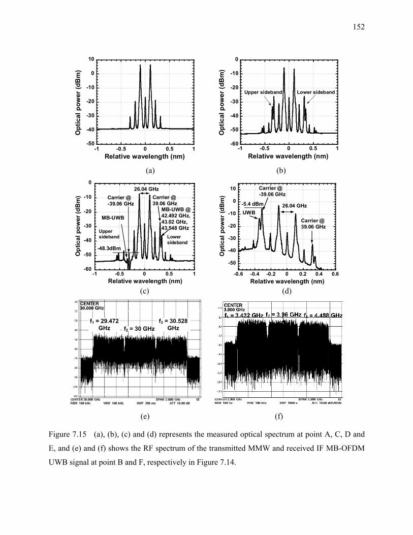
152

-50

-40

-30

-20

-10

0

10

-1 -0.5 0 0.5 1

Opt

ical

pow

er (d

Bm

)

Relative wavelength (nm)

-60

-50

-40

-30

-20

-10

0

-1 -0.5 0 0.5 1

Opt

ical

pow

er (d

Bm

)


Upper sideband Lower sideband

(a) (b)

-60

-50

-40

-30

-20

-10

0

-1 -0.5 0 0.5 1

Opt

ical

pow

er (d

Bm

)


-48.3dBm

MB-UWB

Carrier @-39.06 GHz

26.04 GHz

MB-UWB @ 42.492 GHz, 43.02 GHz, 43.548 GHz

Carrier @39.06 GHz

Upper sideband Lower

sideband

-50

-40

-30

-20

-10

0

10

-0.6 -0.4 -0.2 0 0.2 0.4 0.6

Opt

ical

pow

er (d

Bm

)


-5.4 dBm

Carrier @ -39.06 GHz

26.04 GHzUWB

Carrier @39.06 GHz

(c) (d)

f1 = 29.472 GHz f2 = 30 GHz

f3 = 30.528 GHz

(e) (f)

Figure 7.15 (a), (b), (c) and (d) represents the measured optical spectrum at point A, C, D and

E, and (e) and (f) shows the RF spectrum of the transmitted MMW and received IF MB-OFDM

UWB signal at point B and F, respectively in Figure 7.14.

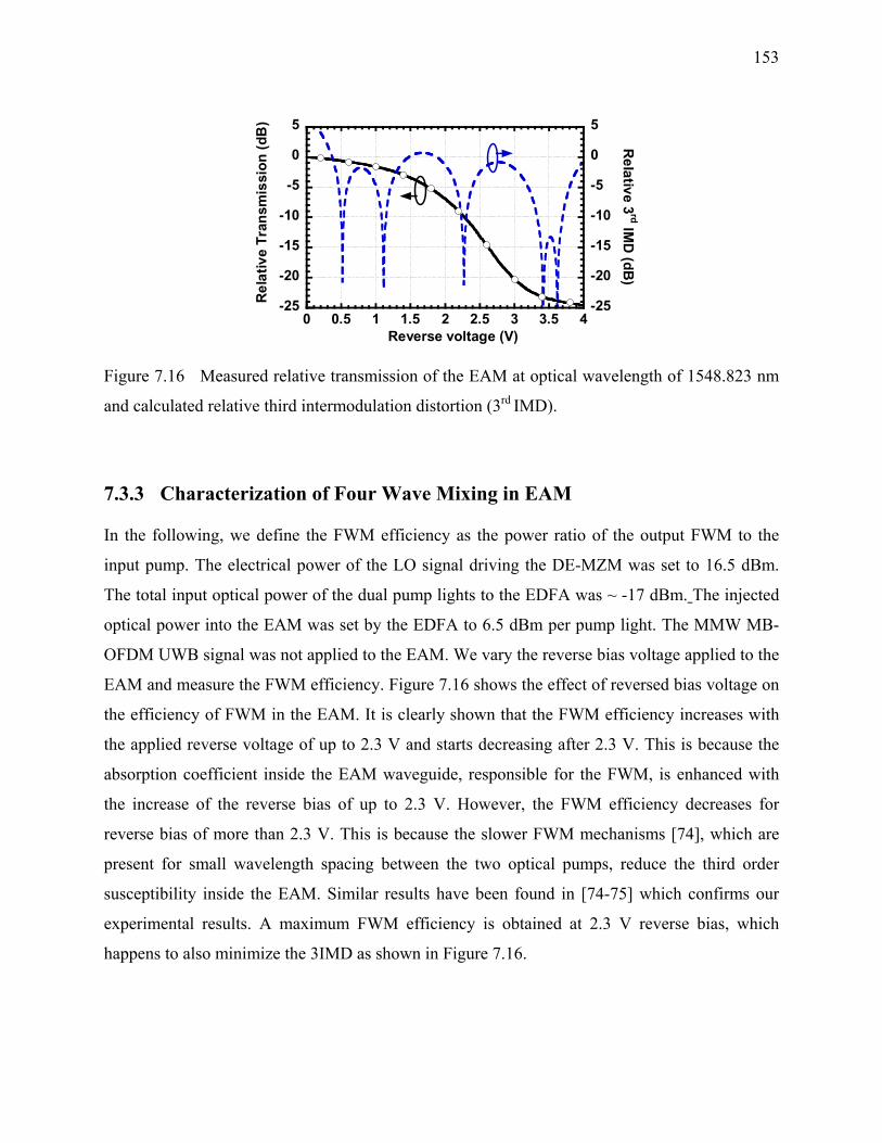
153

-25

-20

-15

-10

-5

0

5

-25

-20

-15

-10

-5

0

5

0 0.5 1 1.5 2 2.5 3 3.5 4

Rel

ativ

e Tr

ansm

issi

on (d

B)

Relative 3

rd IMD

(dB)

Reverse voltage (V)

Figure 7.16 Measured relative transmission of the EAM at optical wavelength of 1548.823 nm

and calculated relative third intermodulation distortion (3rd IMD).

7.3.3 Characterization of Four Wave Mixing in EAM

In the following, we define the FWM efficiency as the power ratio of the output FWM to the

input pump. The electrical power of the LO signal driving the DE-MZM was set to 16.5 dBm.

The total input optical power of the dual pump lights to the EDFA was ~ -17 dBm. The injected

optical power into the EAM was set by the EDFA to 6.5 dBm per pump light. The MMW MB-

OFDM UWB signal was not applied to the EAM. We vary the reverse bias voltage applied to the

EAM and measure the FWM efficiency. Figure 7.16 shows the effect of reversed bias voltage on

the efficiency of FWM in the EAM. It is clearly shown that the FWM efficiency increases with

the applied reverse voltage of up to 2.3 V and starts decreasing after 2.3 V. This is because the

absorption coefficient inside the EAM waveguide, responsible for the FWM, is enhanced with

the increase of the reverse bias of up to 2.3 V. However, the FWM efficiency decreases for

reverse bias of more than 2.3 V. This is because the slower FWM mechanisms [74], which are

present for small wavelength spacing between the two optical pumps, reduce the third order

susceptibility inside the EAM. Similar results have been found in [74-75] which confirms our

experimental results. A maximum FWM efficiency is obtained at 2.3 V reverse bias, which

happens to also minimize the 3IMD as shown in Figure 7.16.

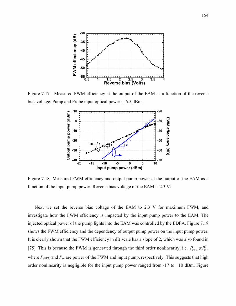
154

-55

-50

-45

-40

-35

-30

0.5 1 1.5 2 2.5 3 3.5 4FW

M e

ffeci

ency

(dB

)

Reverse bias (Volts)

Figure 7.17 Measured FWM efficiency at the output of the EAM as a function of the reverse

bias voltage. Pump and Probe input optical power is 6.5 dBm.

-40

-30

-20

-10

0

10

-70

-60

-50

-40

-30

-20

-20 -15 -10 -5 0 5 10

Out

put p

ump

pow

er (d

Bm

)FW

M effeciency (dB

)

Input pump power (dBm)

11

12

Figure 7.18 Measured FWM efficiency and output pump power at the output of the EAM as a

function of the input pump power. Reverse bias voltage of the EAM is 2.3 V.

Next we set the reverse bias voltage of the EAM to 2.3 V for maximum FWM, and

investigate how the FWM efficiency is impacted by the input pump power to the EAM. The

injected optical power of the pump lights into the EAM was controlled by the EDFA. Figure 7.18

shows the FWM efficiency and the dependency of output pump power on the input pump power.

It is clearly shown that the FWM efficiency in dB scale has a slope of 2, which was also found in

[75]. This is because the FWM is generated through the third order nonlinearity, i.e. 3FWM inP Pα ,

where PFWM and Pin are power of the FWM and input pump, respectively. This suggests that high

order nonlinearity is negligible for the input pump power ranged from -17 to +10 dBm. Figure

155

7.18 also shows that the output power of the pump varies linearly with the input pump power,

showing no saturation within this input power range.

7.3.4 Application to MMW MB-OFDM UWB

The MMW MB OFDM UWB signals centered at 29.472, 30, and 30.528 GHz are applied to the

EAM. The reverse bias voltage is set to 2.3 V for maximum FWM efficiency and the input pump

power to the EAM is set to 6.5 dBm. Here we will investigate the performance of the down-

converted MMW MB OFDM UWB signal in terms of RF modulation index of EAM, received

optical power and LO modulation index of the MZM. The RF modulation index of the EAM is

defined by mRF = Veff/Vb, where Veff is the root mean square of the average applied RF power

and Vb is the applied reverse bias voltage. The LO modulation index of the MZM is defined by

mlo = Vlo/Vπ, where Vπ is the half-wave switching voltage of the MZM.

First we set the received optical power at the photodetector to 0 dBm by the EDFA. We vary

the RF modulation index of the EAM by changing the peak to peak voltage of the generated

UWB signal from the AWG7122B. The measured EVM versus modulation index is shown in

Figure 7.19. It is clear that the EVM degrades at low and high modulation index where noise at

the low index and nonlinear distortion at the high index become dominant. Therefore, there is an

optimum RF modulation index of around 7.5% to achieve the maximum SNR and minimum

EVM. The good quality of the down-converted MMW MB-OFDM UWB signal is seen from the

measured constellation (Figure 7.19 inset (a) and (b)).

-22

-21

-20

-19

-18

-17

-16

4 5 6 7 8 9

EVM

(dB

)

EAM modulation index (%) Figure 7.19 EVM versus RF modulation index of the EAM. Received optical power is 0 dBm

and the LO power to the DE-MZM is 16.5 dBm.

156

-23

-22

-21

-20

-19

-18

-2 -1.5 -1 -0.5 0 0.5 1 1.5EV

M (d

B)


Figure 7.20 EVM performance versus received optical power. RF modulation index is 7.5 % and

LO signal power to the DE-MZM is 16.5 dBm (mlo = 42%).

Next, we set the RF modulation index to 7.5 % and vary the received optical power at the

photodetector. The EAM is operated in the linear region (minimum 3rd IMD) as shown in Figure

7.16. Measured EVM versus received optical power is shown in Figure 7.20. It is clearly seen

that the EVM decreases slowly and linearly with the increase of the received optical power. This

indicates that this down-conversion technique is less sensitive to the received optical power, to

some extent. In the absence of other imperfections such as gain and phase imbalance of the

transmitter’s IQ modulator and phase noise from the MMW and/or RF sources, the minimum

EVM can be expressed as [25] min 1EVM SNR= , in which the shot noise and signal-ASE beat

noise are assumed dominant. Therefore, Figure 7.20 can be understood by the fact that optical

receiver is limited by signal-ASE beat noise.

We also investigate the EVM performance versus LO modulation index, as shown in Figure

7.21. To obtain this, we fix the peak to peak voltage of the generated UWB signal to 0.85 V,

which corresponds to the optimum RF modulation index of the EAM of 7.5%, and vary the

power of the LO signal to the MZM from 16.5 to 23.5 dBm. The received optical power at the

photodetector is set to 0 dBm. It is clearly seen from Figure 7.21 that the EVM is almost

unchanged with the change of LO signal power. The best EVM is obtained at the LO modulation

index of mlo =~84%. In fact the FWM light is proportional to ( )61 2loJ mπ in optical power,

where ( )1J ⋅ is the first order Bessel function of the first kind, and the MMW MB-OFDM UWB

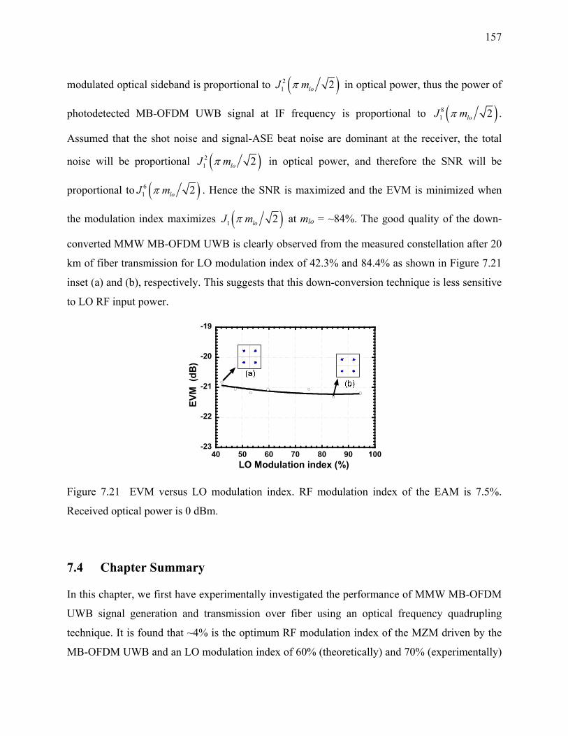
157

modulated optical sideband is proportional to ( )21 2loJ mπ in optical power, thus the power of

photodetected MB-OFDM UWB signal at IF frequency is proportional to ( )81 2loJ mπ .

Assumed that the shot noise and signal-ASE beat noise are dominant at the receiver, the total

noise will be proportional ( )21 2loJ mπ in optical power, and therefore the SNR will be

proportional to ( )61 2loJ mπ . Hence the SNR is maximized and the EVM is minimized when

the modulation index maximizes ( )1 2loJ mπ at mlo = ~84%. The good quality of the down-

converted MMW MB-OFDM UWB is clearly observed from the measured constellation after 20

km of fiber transmission for LO modulation index of 42.3% and 84.4% as shown in Figure 7.21

inset (a) and (b), respectively. This suggests that this down-conversion technique is less sensitive

to LO RF input power.

-23

-22

-21

-20

-19

40 50 60 70 80 90 100

EVM

(dB

)

LO Modulation index (%)

Figure 7.21 EVM versus LO modulation index. RF modulation index of the EAM is 7.5%.

Received optical power is 0 dBm.

7.4 Chapter Summary

In this chapter, we first have experimentally investigated the performance of MMW MB-OFDM

UWB signal generation and transmission over fiber using an optical frequency quadrupling

technique. It is found that ~4% is the optimum RF modulation index of the MZM driven by the

MB-OFDM UWB and an LO modulation index of 60% (theoretically) and 70% (experimentally)

158

is needed to achieve the minimum required EVM of -16 dB after 20 km of fiber transmission. It

is also found that typical extinction ratio does not have significant impact on the EVM, whereas

bias drift of 20% may degrade the EVM by up to 1 dB. Simulations, theoretical analysis and

experiment have been carried out to evaluate the performance of the proposed system and

obtained results are in good agreements.

Then, we have experimentally investigated and demonstrated a new technique using FWM in

an EAM to down-convert the MMW to IF for MMW over fiber uplinks. FWM efficiency has

been studied versus reverse bias voltage and input pump power to the EAM. It is found that

maximum FWM efficiency is obtained at 2.3 V reverse bias and increases by a slope of 2 in dB

scale with respect to the input pump power. We also have investigated the performance of an

MMW MB-OFDM UWB signal down-conversion in an EAM with FWM. It is found that the

optimum RF modulation index to the EAM driven by the MB-OFDM UWB, is ~7.5%, and the

down-conversion is almost insensitive to LO RF input power. It is found that signal to noise ratio

can be optimized due to tunability of optical carrier to subcarrier power ratio. Compared to [73],

this technique leads to a better signal to noise ratio of down-converted IF signal, and a higher

receiver sensitivity. Furthermore, an experimental investigation was conducted with 30 GHz

MMW MB-OFDM signal over fiber as an example, considering RF modulation index to EAM,

the dual-light power, and receiver sensitivity.

This investigation shows a potential possibility for the proposed photonic up/down-

conversion technique to be used for MMW MB-OFDM UWB signal over fiber down/uplinks. In

addition, this proposed technique can be applied to 57-64 GHz MMW band.

159

CHAPTER 8 CONCLUSION

8.1 Concluding Remarks

In this thesis work, we have investigated first of all, in terms of error vector magnitude (EVM),

the performance degradation of MB-OFDM UWB transmission over fiber caused by various

impairments including MZM nonlinearities, fiber dispersion, receiver optical power and optical

receiver response. Also, the performance of MB-OFDM wireless UWB has been experimentally

investigated in terms of packet error rate (PER) when transmitted over 20 km of SMF. PER was

measured at different bit rates to evaluate the receiver sensitivity, required minimum transmitted

UWB power, effect of wireless distance, MZM modulation index, and received optical power

etc. In addition, the performance of MB-OFDM UWB has been studied when transmitted over

fiber under the influence of relative intensity noise (RIN) considering system parameters such as

laser output power, linewidth and fiber transmission length. The performance of MB-OFDM

UWB over fiber transmission system has been also assessed considering the effect of in-band

jammers such as WiMAX, WLAN MIMO, WLAN and marine radar.

Based on this research it is found that:

For OSSB modulated MZM, RF modulation index of ~4% is optimum to obtain the

best possible EVM performance of MB-OFDM UWB over fiber.

The optical receiver with fifth order Chebyshev-II response and 3 GHz bandwidth is

the best for MB OFDM UWB over fiber in our work.

Optical receiver sensitivity in UWB over fiber is reasonably low and the performance

degrades almost linearly with the decrease of receiver optical power.

Fiber transmission is further limited by laser phase noise converted RIN due to fiber

dispersion and phase distortion induced by fiber dispersion.

The system should be operated at a high laser output power to avoid RIN degradation.

A narrow linewidth laser with low RIN will significantly improve system

performance.

Wireless range transmission of MB-OFDM UWB is limited by the receiver sensitivity.

160

The performance of MB-OFDM UWB is severely affected by different in-band

interferers if certain interferer to UWB peak power ratio is not maintained:

For satisfying the EVM requirement of -16 dB, which is the EVM threshold specified

for conformance testing according to the recent WiMedia standard for UWB, this ratio

is ~14, ~15, ~17.5 and ~20 dB for WiMAX, Radar, WLAN MIMO and WLAN

signals, respectively, for distribution over 20 km of single mode fiber.

Our results will allow future researchers in the field of MB UWB over fiber transmission to

optimize performance of UWB over fiber transmission versus systems parameters and under the

presence of all possible in-band interferers.

In this work, we have proposed, developed and extensively investigated by theory,

simulation and experiment, novel enabling technologies and design techniques for broadband

linearization, compensation of chromatic dispersion induced power fading, improving optical

modulation efficiency, and MMW up/down conversion for RoF down/up-links. We have also

verified and evaluated experimentally the performance of using our proposed techniques for MB-

OFDM ultra-wideband (UWB) signal transmission over fiber.

For broadband linearization, we have proposed a mixed polarization for MZM and analog

predistortion for EAM. It is found that the 3IMD is suppressed independent of the modulation

index. In the mixed polarization technique, the power fading of the RF carrier and crosstalk due

to intermodulation via fiber chromatic dispersion are significantly suppressed compared to the

case of using the conventional OSSB MZM. SFDR is improved by ~12.5 dB in experiment with

good agreement with theory and simulation. Moreover, the proposed technique shows an

improvement of 2dB in EVM when applied to MB-OFDM UWB system. A predistortion circuit

for linearization of EAM using reflective diode pair has been designed for MB-OFDM UWB

system at bandgoup 1 (3.1~ 4.8 GHz). It is found that the designed predistortion circuit leads to

11 dB improvements in the SFDR at the center frequency of bandgroup 1, and more than 7 dB

improvements in suppression of IMD3 over the whole bandgroup 1. By evaluating the

predistortion circuit with the MB-OFDM UWB signal, a 1-dB EVM improvement is obtained for

the first three bands OFDM UWB over 20 km fiber. This suggests that the proposed designs are

cost effective broadband linearization technique for MB-OFDM UWB over fiber.

161

To overcome the fiber chromatic dispersion that causes power fading when ODSB

modulation is used, a novel modulation technique has been proposed. This modulation technique

also improves the RF power by up to 3 dB compared to OSSB modulation. The main advantage

of the proposed technique is simple and implemented in electrical domain with phase shifting.

Theoretical analysis was made to obtain the optimum conditions for optimum performance, such

as optimum phase shift and impact of MZM extinction ratio. Then simulation was used to further

analyze the proposed modulation and compared to the theory. Moreover, we have presented an

experimental proof to validate our concept for RF signal consisting of single RF tone or of MB-

OFDM UWB signal. By using our proposed modulation technique, a 3-dB RF power

improvement, compared to OSSB, was achieved experimentally without degradation of the

signal quality.

We have proposed a modulation technique to improve the modulation efficiency in radio

over fiber transmission. We have shown that a dMZM modulator can be used for obtaining not

only OSSB modulation but also tunability of OCSR. To our knowledge, the function of OCSR

tunability using this modulator was proposed and investigated for the first time. It has been

shown that a wide dynamic range of OCSR tunability can be obtained by varying the bias

voltage applied to the inner MZMs. It was found that the optimum OCSR to obtain maximum RF

output power depends on the modulation index and the extinction ratio of the dMZM. To achieve

an OCSR of 0 dB there is a minimum required extinction ratio that decreases with the increase of

the modulation index. Moreover, we have investigated the impact of OCSR on the performance

of MB-OFDM UWB signal. It was found that maximum received RF power is obtained at 0 dB

OCSR while minimum EVM of the received MB-OFDM UWB constellation is achieved at

5.4dB OCSR.

The performance of MMW MB-OFDM UWB signal generation and transmission over fiber

using an optical frequency up-conversion technique was experimentally demonstrated. It was

found that ~4% is the optimum RF modulation index of the MZM driven by the MB-OFDM

UWB and an LO modulation index of 60% (theoretically) and 70% (experimentally) is needed to

achieve the minimum required EVM of -16 dB after 20 km of fiber transmission. It was also

found that typical extinction ratio does not have significant impact on the EVM, whereas bias

drift of 20% may degrade the EVM by up to 1 dB.

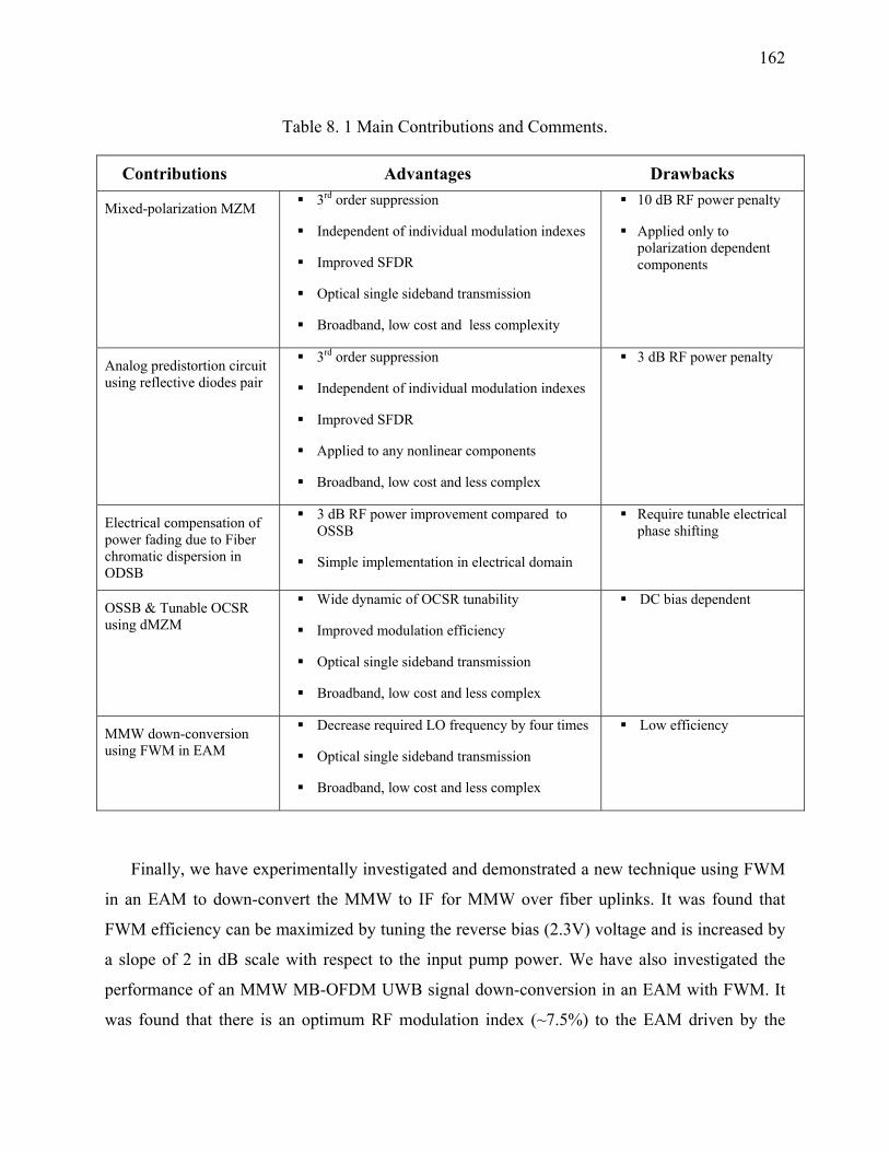
162

Table 8. 1 Main Contributions and Comments.

Contributions Advantages Drawbacks

Mixed-polarization MZM 3rd order suppression

Independent of individual modulation indexes

Improved SFDR

Optical single sideband transmission

Broadband, low cost and less complexity

10 dB RF power penalty

Applied only to polarization dependent components

Analog predistortion circuit using reflective diodes pair

3rd order suppression

Independent of individual modulation indexes

Improved SFDR

Applied to any nonlinear components

Broadband, low cost and less complex

3 dB RF power penalty

Electrical compensation of power fading due to Fiber chromatic dispersion in ODSB

3 dB RF power improvement compared to OSSB

Simple implementation in electrical domain

Require tunable electrical phase shifting

OSSB & Tunable OCSR using dMZM

Wide dynamic of OCSR tunability

Improved modulation efficiency



DC bias dependent

MMW down-conversion using FWM in EAM

Decrease required LO frequency by four times



Low efficiency

Finally, we have experimentally investigated and demonstrated a new technique using FWM

in an EAM to down-convert the MMW to IF for MMW over fiber uplinks. It was found that

FWM efficiency can be maximized by tuning the reverse bias (2.3V) voltage and is increased by

a slope of 2 in dB scale with respect to the input pump power. We have also investigated the

performance of an MMW MB-OFDM UWB signal down-conversion in an EAM with FWM. It

was found that there is an optimum RF modulation index (~7.5%) to the EAM driven by the

163

MB-OFDM UWB, and the down-conversion is almost insensitive to LO RF input power. This

investigation shows a potential for the proposed photonic up/down-conversion technique to be

used for MMW MB-OFDM UWB signal over fiber up/downlinks.

Since this work is concerned with a multitude of RoF aspects and many subjects are

discussed and studied in detail, Table 8. 1 summarizes the main contributions described in this

thesis along with comments on each proposed technique.

8.2 Future Work

The research contributions presented in this thesis may be extended in several ways.

First, MB-OFDM UWB over fiber is a fast emerging technology. However, many areas of

UWB over fiber are yet to be explored.

MB-OFDM UWB over optical wavelength division multiplexing (WDM) WDM is an

open research challenge.

Bi-directional transmission over fiber is another important issue that needs to be

addressed. Bi-directional MB-OFDM UWB has great prospect for future access

network applications. If the same optical wavelength is used, the study of Rayleigh

back scattering (RBS) and stimulated Brillouin scattering (SBS) will be an interesting

research topic.

Investigation of performance of optical transmission by using a low cost EAM or

EAM integrated distributed feedback laser (EML) can be done.

Also, the effect of cross interference from narrowband jammers is not studied in this

thesis. Practically two in-band jammers can exist simultaneously i.e. IEEE 802.11b/g

at 2.4 GHz and 802.11a at 5.8 GHz can beat together to create harmonics at 3.4 GHz

which will interfere with sub-band 1 Band Group 1.

Besides, MB-OFDM UWB over fiber technology will benefit from studies on MAC

layer protocols for optimum transmission performance.

Second, there is a need to investigate if there is a way to further improve the mixed-

polarization OSSB MZM by reducing or removing the RF carrier power penalty of ~10 dB.

164

Also, since the mixed-polarization OSSB MZM was realized with discrete optical components,

the next important practical experiment required would be to incorporate the mixed-polarization

OSSB MZM on one silicon substrate or module to further investigate its performance.

Third, a further improvement of the predistortion circuit design can be investigated:

Reduce the size of the predistortion circuit. In this thesis, the broadband impedance

matching (from 3.1-4.8 GHz) was achieved by using the three section quarter-wave

impedance transformer. However the size of circuit can be reduced by using hard

substrate or other impedance matching techniques, for example using hybrid lumped

elements and transmission line in the matching circuit or increasing the internal

resistor of the diode by inserting a resistor or cascading many diodes in series. In this

way, not only the size will be reduced but also the bandwidth will be broadened. After

making its size smaller, the predistortion circuit can be fabricated by the Hybrid

Microwave Integrated Circuit (HMIC) method, and wrapped into a commercialized

microwave IC package.

The predistortion circuit can also be modified to linearize DFB lasers or MZM. The

predistortion circuit and the DFB laser or MZM can be soldered on the same printed

circuit board (PCB), and after being packaged, the linearized DFB laser or MZM

could be commercialized.

Instead of using the diode, the transistors could also be used in the push-pull bias to

generate the predistortion signal. In this way, the predistortion circuit can not only

work as linearizer but also as a low noise amplifier.

Fourth, the pre-compensated ODSB SCM immune to fiber chromatic dispersion induced RF

power fading can be very attractive if a broadband and tunable electrical phase shifter is

available. This can be made possible by using photonic microwave techniques.

Fifth, in the proposed photonic MMW up-conversion, a balanced MZM with a single drive

could be used instead of a DE-MZM to reduce cost.

Sixth, in the proposed photonic MMW down-conversion, it is interesting to investigate the

possibility of substituting the EDFA used prior to the EAM, by a semiconductor optical amplifier

in order to reduce cost.

165

Last but not the least, the possibility of integrating all proposed technique in one system with the

use of WDM can be investigated.

8.3 List of Publications

1. B. Hraimel, X. Zhang, and K. Wu, “Optical Single-Sideband Modulation with Tunable Optical Carrier to Sideband Ratio in Radio over Fiber Systems,” Journal of Lightwave Technology, submitted.

2. C. Sui, B. Hraimel, X. Zhang, L. Wu, Y. Shen, K. Wu, T. Liu, T. Xu and Q. Nie, “Impact of Electro-Absorption Modulator Integrated Laser on MB-OFDM Ultra-Wideband Signals over Fiber Systems,” Journal of Lightwave Technology, under review.

3. Y. Pei, Xiupu Zhang , K. Xu, X. Sun, B. Hraimel, J. Wu and J. Lin, “Power Control for Radio-over-Fiber Downlinks in Frequency Division Multiplexing Cellular Communication Systems,” IEEE/OSA J. Optical Communications and Networking, accepted 2010.

4. M. N. Sakib, B. Hraimel, X. Zhang, K. Wu, T. Liu, T. Xu, and Q. Nie, “Impact of Laser Relative Intensity Noise on Multiband OFDM Ultra Wideband Wireless Signal over Fiber System,” OSA/IEEE J. Optical Communications and Networking, vol. 2, no. 10 , 2010.

5. B. Hraimel, W. Jiang, X. Zhang, K. Wu, T. Liu, T. Xu, Q. Nie, and K. Xu, “Experimental Demonstration of a Mixed-Polarization to Linearize Electro-Absorption Modulators in Radio-over-Fiber Links,” Photonics Technology Letters, submitted.

6. L. Wu, B. Hraimel , X. Zhang, K. Wu, M. Mohamed, and C. Sui, “Photonic Generation of Millimeter-Waves Using Two Cascaded Electro-Absorption Modulators in Radio-over-Fiber Systems,” 2010 International Topical Meeting Microwave Photonics, 5-9 Oct. 2010, accepted.

7. Y. Pei, B. Hraimel, Y. Shen, Kun Xu, X. Zhang, X. Sun, J. Wu, and J. Lin, “Performance Characterization and Limitation of Coherence Multiplexing Technique in Radio over Fiber Systems,” 2010 International Topical Meeting Microwave Photonics, 5-9 Oct. 2010, accepted.

8. C. Sui, B. Hraimel, X. Zhang, and K. Wu, “Performance Evaluation of MB-OFDM Ultra-Wideband Over Fiber Transmission Using a Low Cost Electro-Absorption Modulator Integrated Laser,” 2010 International Topical Meeting Microwave Photonics, 5-9 Oct. 2010, accepted.

9. Y. Shen, B. Hraimel, X. Zhang, G. Cowan, K. Wu, and T. Liu, “A Novel Analog Broadband RF Predistortion Circuit to Linearize Electroabsorption Modulator in Multiband OFDM Ultra-Wideband Radio over Fiber System,” IEEE Transaction on Microwave Theory and Technique, special issue on Microwave Photonics, accepted 2010.

10. B. Hraimel, X. Zhang, and K. Wu, “Photonic Down-Conversion of Millimeter Wave Multiband Orthogonal Frequency Division Multiplexing Ultra-Wideband Using Four

166

Wave Mixing in an Electro-Absorption Modulator,” IEEE/OSA Journal of Lightwave Technology, vol. 28, no. 13, pp. 1987-1993, July 2010.

11. M. Mohamed, B. Hraimel, and X. Zhang, “Optical Generation of Millimeter Wave Multiband OFDM UWB Wireless Signal and Distribution over Fiber,” Photonics Technology Letters, vol. 22, no. 15, pp. 1180-1182, Aug. 2010.

12. B. Hraimel, X. Zhang, M. Mohamed, and K. Wu, “Precompensated Optical Double-Sideband Subcarrier Modulation Immune to Fiber Chromatic Dispersion Induced RF Power Fading,” OSA/IEEE J. Optical Communications and Networking, vol. 1, no. 4, pp. 331–342, 2009.

13. B. Hraimel, X. Zhang, M. Mohamed, M. Sakib, and K. Wu “Performance Improvement of Multiband OFDM Ultra-Wideband over Fiber Link using a Novel Optical Double Sideband Subcarrier Modulation Scheme,” International Microwave Symposium, paper TUPF-2, Boston, USA, June 2009.

14. B. Hraimel, X. Zhang, M. Mohamed, and K. Wu, “Electrical Compensation of Fiber Chromatic Dispersion Induced RF Power Fading in Optical Double-Sideband Subcarrier Modulation,” OFC/NFOEC, paper JWA55, USA, Mar. 2009

15. B. Hraimel, M. Mohamed, X. Zhang, and K. Wu, “Transmission performance of multiband orthogonal frequency division multiplexing ultra-wideband wireless systems with fiber distribution,” Asia-Pacific Microwave Photonics Conference 2009 (APMP), paper C06, Beijing, April 2009.

16. B. Masella, B. Hraimel, and X. Zhang, "Mixed-polarization to improve dynamic range of optical single sideband in a Mach-Zehnder modulator," in 2009 Conference on Optical Fiber Communication - OFC 2009, 22-26 March 2009, Piscataway, NJ, USA, 2009, pp. 1-3.

17. M. Mohamed, B. Hraimel, X. Zhang, M. N. Sakib, and K. Wu, “Performance of millimeter wave MB-OFDM ultra wideband signal generation using optical frequency up-conversion and transmission over fiber,” Asia-Pacific Microwave Photonics Conference 2009.

18. M. Sakib, B. Hraimel, X. Zhang, M. Mohamed, and K. Wu, “Effect of Relative Intensity Noise Induced Distortion on Multiband OFDM Ultra-Wideband over Fiber System,” APMP, paper J03, Beijing, April 2009.

19. B. Masella, B. Hraimel, and X. Zhang , "Enhanced Spurious-Free Dynamic Range Using Mixed Polarization in Optical Single Sideband Mach–Zehnder Modulator," Journal of Lightwave Technology, vol. 27, pp. 3034-3041, 2009.

20. X. Zhang, M. Sakib, B. Hraimel, K. Wu, M. Mohamed, and Dongya Shen, “Multiband OFDM Ultra-Wideband wireless communication systems with Fiber distribution,” IEEE Communications Magazine, December 2009.

21. M. N. Sakib, B. Hraimel, X. Zhang, and K. Wu, “Investigation of the performance of multiband orthogonal frequency division multiplexing ultrawideband over fiber transmission under the presence of in-band interferers,” IEEE/OSA Journal of Optical Communications and Networking, vol. 1, pp. 235-44, 2009.

167

22. M. Mohamed, B. Hraimel, X. Zhang, and M. Sakib, “Optical Generation of Millimeter Wave Multiband OFDM Ultra-Wideband Wireless Signal and Transmission over Fiber,” International Conference on Advanced Infocomm Technology, Xi'an, China, July 2009.

23. M. Sakib, B. Hraimel, X. Zhang, M. Mohamed, W. Jiang, K. Wu, and Dongya Shen “Impact of Optical Transmission on Multiband OFDM Ultra-Wideband Wireless System with Fiber Distribution,” IEEE/OSA Journal of Lightwave Technology, vol. 27, pp. 4112-4123, 2009.

24. M. Mohamed, B. Hraimel, X. Zhang, M. N. Sakib, and Ke, Wu, “Frequency quadrupler for millimeter-wave multiband OFDM ultrawideband wireless signals and distribution over fiber systems,” IEEE/OSA Journal of Optical Communications and Networking, vol. 1, pp. 428-38, 2009.

25. M. Mohamed, B. Hraimel, X. Zhang, and M. Sakib, “Performance of Optical Frequency Multiplication for Millimeter Wave MB-OFDM Ultrawideband Signal Generation and Distribution in RoF Systems,” IEEE International Conference on Broadband Network and Multimedia Technology, China, October 2009.

26. M. Mohamed, B. Hraimel, X. Zhang, and K. Wu, "Efficient photonic generation of millimeter-waves using optical frequency multiplication in radio-over-fiber systems," in 2007 International Topical Meeting Microwave Photonics, 3-5 Oct. 2007, Piscataway, NJ, USA, 2007, pp. 179-82.

27. M. Mohamed, B. Hraimel, X. Zhang, and K. Wu, “Frequency sixupler for millimeter-wave signal generation and transmission in radio-over-fiber systems,” Proceeding of ICAIT, paper conf189a16, Da Meisha, China, July 2008.

28. M. Mohamed, B. Hraimel, X. Zhang, and K. Wu, "Frequency sixupler for millimeter-wave over fiber systems," Optics Express, vol. 16, pp. 10141-51, 2008.

29. M. Mohamed, B. Hraimel, X. Zhang, and K. Wu, "Analysis of frequency quadrupling using a single Mach-Zehnder modulator for millimeter-wave generation and distribution over fiber systems," Optics Express, vol. 16, pp. 10786-10802, 2008.

30. B. Hraimel, R. Kashyap, X. Zhang, J. Yao, and K. Wu, "Large signal analysis of fiber dispersion effect on photonic up-conversion in radio over fiber link using dual electrode Mach-Zehnder external modulator," in Photonics North 2006, 5-8 June 2006, USA, 2006, pp. 63432-1.

31. B. Hraimel, M. O. Twati, and K. Wu, "Closed-form dynamic range expression of dual-electrode Mach-Zehnder modulator in radio-over-fiber WDM system," Journal of Lightwave Technology, vol. 24, pp. 2380-7, 2006.

168

REFERENCES

[1] H. Al-Raweshidy and S. Komaki, Radio over fiber technologies for mobile communications networks, 1st ed. ed.: Artech House Boston, MA, 2002.

[2] B. Dang and I. Niemegeers, "Analysis of IEEE 802.11 in radio over fiber home networks," 2005, pp. 744-747.

[3] P. Tang, et al., "PER and EVM measurements of a radio-over-fiber network for cellular and WLAN system applications," Lightwave Technology, Journal of, vol. 22, pp. 2370-2376, 2004.

[4] http://www.naic.edu/~astro/RXstatus/Lnarrow/fcc_UWB.pdf [Online].

[5] http://www.ieee802.org/15/pub/2003/Jul03/03268r2P802-15_TG3a-Multi-band-CFP-Document.pdf [Online].

[6] G. Heidari, WiMedia UWB: technology of choice for wireless USB and Bluetooth: Wiley Publishing, 2008.

[7] http://www.ecma-international.org/publications/files/ECMA-ST/ECMA-368.pdf [Online].

[8] M. Welborn, "System considerations for ultra-wideband wireless networks," 2001.

[9] http://www.vpiphotonics.com/ [Online].

[10] U. Gliese, et al., "Chromatic dispersion in fiber-optic microwave and millimeter-wave links," Microwave Theory and Techniques, IEEE Transactions on, vol. 44, pp. 1716-1724, 1996.

[11] J. Yu, et al., "Centralized lightwave WDM-PON employing 16-QAM intensity modulated OFDM downstream and OOK modulated upstream signals," IEEE Photonics Technology Letters, vol. 20, pp. 1545-1547, 2008.

[12] G. Smith, et al., "Technique for optical SSB generation to overcome dispersion penalties in fibre-radio systems," Electronics Letters, vol. 33, p. 74, 1997.

[13] V. Urick and F. Bucholtz, "Compensation of arbitrary chromatic dispersion in analog links using a modulation-diversity receiver," IEEE Photonics Technology Letters, vol. 17, pp. 893-895, 2005.

[14] H. Sun, et al., "Tunable RF-power-fading compensation of multiple-channeldouble-sideband SCM transmission using a nonlinearly chirped FBG," IEEE Photonics Technology Letters, vol. 12, pp. 546-548, 2000.

[15] H. Sotobayashi and K. Kitayama, "Cancellation of the signal fading for 60 GHz subcarrier multiplexed optical DSB signal transmission in nondispersion shifted fiber using midway optical phase conjugation," Journal of Lightwave Technology, vol. 17, p. 2488, 1999.

[16] H. Sotobayashi and K. Kitayama, "Effects of asymmetric power change on BER performance using midwayoptical phase conjugation for fading cancellation in 60 GHz

169

millimetre-wave optical DSB signal transmission over 100 kmnon-dispersion-shifted fibre," Electronics Letters, vol. 35, pp. 992-993, 1999.

[17] M. Attygalle, et al., "Extending optical transmission distance in fiber wireless links using passive filtering in conjunction with optimized modulation," Journal of Lightwave Technology, vol. 24, p. 1703, 2006.

[18] M. Attygalle, et al., "Transmission improvement in fiber wireless links using fiber Bragg gratings," IEEE Photonics Technology Letters, vol. 17, pp. 190-192, 2005.

[19] S. Xiao and A. Weiner, "Optical carrier-suppressed single sideband (O-CS-SSB) modulation using a hyperfine blocking filter based on a virtually imaged phased-array (VIPA)," IEEE Photonics Technology Letters, vol. 17, pp. 1522-1524, 2005.

[20] K. Williams and R. Esman, "Stimulated Brillouin scattering for improvement of microwave fibre-optic link efficiency," Electronics Letters, vol. 30, p. 1965, 1994.

[21] W. Hu, et al., "High SNR 50 GHz radio-over-fibre uplink system by use of low biased Mach-Zehnder modulator technique," Electronics Letters, vol. 42, pp. 550-552, 2006.

[22] A. Gaeta and R. Boyd, "Stochastic dynamics of stimulated Brillouin scattering in an optical fiber," Physical Review A, vol. 44, pp. 3205-3209, 1991.

[23] K. Mandke, et al., "The evolution of ultra wide band radio for wireless personal area networks," Spectrum, vol. 3, p. 10.6, 2003.

[24] C. Zhao and R. Baxley, "Error vector magnitude analysis for OFDM systems," 2006, pp. 1830-1834.

[25] A. Georgiadis, "Gain, phase imbalance, and phase noise effects on error vector magnitude," IEEE Transactions on Vehicular Technology, vol. 53, pp. 443-449, 2004.

[26] W. Siriwongpairat and K. Liu, Ultra-wideband communications systems: multiband OFDM approach: Wiley-IEEE Press, 2007.

[27] S. Ghassemzadeh and V. Tarokh, "UWB path loss characterization in residential environments," 2003, pp. 501-504.

[28] X. Li and L. Cimini Jr, "Effects of clipping and filtering on the performance of OFDM," 1997.

[29] L. Paarmann, Design and analysis of analog filters: Kluwer Academic Publishers, 2001.

[30] D. Pozar, "Microwave Engineering, 3rd," ed: John Wiley & Sons, Hoboken, NJ, USA, 2007, pp. 77-78.

[31] W. Marshall, et al., "Laser phase noise to intensity noise conversion by lowest-order group-velocity dispersion in optical fiber: exact theory," Optics Letters, vol. 25, pp. 165-167, 2000.

[32] P. Laurencio and M. Medeiros, "Relative Intensity Noise in Optical Single Side Band Systems with Multiple In-Line Amplifiers: Analysis and Validation," Fiber and Integrated Optics, vol. 27, pp. 78-88, 2008.

[33] http://eurlex.europa.eu/LexUriServ/LexUriServ.do?uri=OJ:L:2008:144:0077:008

170

1:EN:PDF, "European Commission’s decision of 21:5:2008 on the harmonization of 3400~3800 MHz frequency band for terrestrial system capable of providing electronic communication services in the community."

[34] http://standards.ieee.org/announcements/ieee802.11n_2009amendment_ratified.ht

ml, 2009.

[35] http://easy.intranet.gr/IEEE80211a.pdf [Online].

[36] L. Roselli, et al., "Analog laser predistortion for multiservice radio-over-fiber systems," Journal of Lightwave Technology, vol. 21, p. 1211, 2003.

[37] G. Wilson, et al., "Predistortion of electroabsorption modulators for analog CATVsystems at 1.55 m," Lightwave Technology, Journal of, vol. 15, pp. 1654-1662, 1997.

[38] H. Lu, et al., "Intermodulation distortion suppression in a full-duplex radio-on-fiber ring network," IEEE Photonics Technology Letters, vol. 16, pp. 602-604, 2004.

[39] V. Urick, et al., "Wide-band predistortion linearization for externally modulated long-haul analog fiber-optic links," IEEE Transactions on Microwave Theory and Techniques, vol. 54, pp. 1458-1463, 2006.

[40] N. Imai, et al., "Novel linearizer using balanced circulators and its application tomultilevel digital radio systems," IEEE Transactions on Microwave Theory and Techniques, vol. 37, pp. 1237-1243, 1989.

[41] S. C. Bera, et al., "Diode-based predistortion lineariser for power amplifiers," Electronics Letters, vol. 44, pp. 125-127, 2008.

[42] H. Jeong, et al., "A design of K-band predistortion linearizer using reflective Schottky diode for satellite TWTAs," 2005, pp. 597-600.

[43] L. Roselli, et al., "An active cuber circuit for power amplifier analog predistortion," 2003.

[44] H. Park, et al., "Analysis and design of compact third-order intermodulation generation circuits," Microwave and Optical Technology Letters, vol. 51, 2009.

[45] L. Roselli, et al., "Predistortion circuit design for II and III order simultaneous linearization in multiservice telecommunications apparatuses," in Microwave Symposium Digest, 2002 IEEE MTT-S International, 2002, pp. 1711-1714.

[46] S. P. Stapleton, "Amplifier linearization using adaptive digital predistortion," Applied Microwave & Wireless, vol. 13, pp. 72-74, 2001.

[47] T. Iwai, et al., "Signal distortion and noise in AM-SCM transmission systemsemploying the feedforward linearized MQW-EA external modulator," Lightwave Technology, Journal of, vol. 13, pp. 1606-1612, 1995.

[48] W. Choi, "Nonlinearity suppression of electroabsorption modulator through dual-parallel modulation," Microwave and Optical Technology Letters, vol. 29, p. 2, 2001.

[49] S. Sohn and S. Han, "Linear optical modulation in a serially cascaded electroabsorption modulator," Microwave and Optical Technology Letters, vol. 27, pp. 447-450, 2000.

171

[50] S. Mathai, et al., "Experimental demonstration of a balanced electroabsorption modulated microwave photonic link," IEEE Transactions on Microwave Theory and Techniques, vol. 49, pp. 1956-61, 2001.

[51] Y. Wu, "Optical heterodyned radio over fiber link design using electro-absorption and electro-optic modulators," PHD, University of California, San Diego, Chapter 6, 2004.

[52] J. Brooks, et al., "Implementation and evaluation of a dual parallel linearizationsystem for AM-SCM video transmission," Journal of Lightwave Technology, vol. 11, pp. 34-41, 1993.

[53] T. Cho and K. Kim, "Effect of third-order intermodulation on radio-over-fiber systems by a dual-electrode Mach-Zehnder modulator with ODSB and OSSB signals," Journal of Lightwave Technology, vol. 24, p. 2052, 2006.

[54] B. M. Haas and T. E. Murphy, "A simple, linearized, phase-modulated analog optical transmission system," IEEE Photonics Technology Letters, vol. 19, pp. 729-31, 2007.

[55] A. Ramaswamy, et al., "Coherent receiver based on a broadband optical phase-lock loop," 2007.

[56] L. Johnson and H. Roussell, "Reduction intermodulation distortion in interferometric optical modulators," Optics Letters, vol. 13, pp. 928-930, 1988.

[57] S. Maas, Nonlinear microwave and RF circuits, 2nd Edition ed.: Artech House Publishers, 2003.

[58] B. Hraimel, et al., "Closed-form dynamic range expression of dual-electrode Mach-Zehnder modulator in radio-over-fiber WDM system," Journal of Lightwave Technology, vol. 24, pp. 2380-2387, 2006.

[59] B. Hraimel, et al., "Large signal analysis of fiber dispersion effect on photonic up-conversion in radio over fiber link using dual electrode Mach-Zehnder external modulator," 2006, p. 63432L.

[60] M. Mohamed, et al., "Efficient photonic generation of millimeter-waves using optical frequency multiplication in radio-over-fiber systems," 2007, pp. 179-182.

[61] M. Mohamed, et al., "Analysis of frequency quadrupling using a single Mach-Zehnder modulator for millimeter-wave generation and distribution over fiber systems," Opt. Express, vol. 16, pp. 10786-10802, 2008.

[62] M. Mohamed, et al., "Frequency sixupler for millimeter-wave over fiber systems," Opt. Express, vol. 16, pp. 10141-10151, 2008.

[63] C. Lim, et al., "Analysis of optical carrier-to-sideband ratio for improving transmission performance in fiber-radio links," IEEE Transactions on Microwave Theory and Techniques, vol. 54, pp. 2181-2187, 2006.

[64] K. Higuma, et al., "X-cut lithium niobate optical single-sideband modulator," Electronics Letters, vol. 37, pp. 515-16, 2001.

[65] P.-T. Shih, et al., "Hybrid access network integrated with wireless multilevel vector and wired baseband signals using frequency doubling and no optical filtering," IEEE Photonics Technology Letters, vol. 21, pp. 857-859, 2009.

172

[66] C. Lin, et al., "Generation of Carrier Suppressed Optical mm-wave Signals using Frequency Quadrupling and no Optical Filtering," 2008.

[67] J. Ma, et al., "64GHz optical millimeter-wave generation by octupling 8GHz local oscillator via a nested LiNbO3 modulator," Optics and Laser Technology, 2009.

[68] Q. Chang, et al., "Generation and Transmission of Optical Carrier Suppressed-Optical Differential (Quadrature) Phase-Shift Keying (OCS-OD (Q) PSK) Signals in Radio Over Fiber Systems," Journal of Lightwave Technology, vol. 26, pp. 2611-2618, 2008.

[69] H. Chi and J. Yao, "Frequency quadrupling and upconversion in a radio over fiber link," Lightwave Technology, Journal of, vol. 26, pp. 2706-2711, 2008.

[70] J. Yu, et al., "Optical millimeter-wave generation or up-conversion using external modulators," IEEE Photonics Technology Letters, vol. 18, pp. 265-267, 2006.

[71] M. Sakib, et al., "Impact of optical transmission on multiband OFDM ultra-wideband wireless system with fiber distribution," J. Lightwave Technol, vol. 27, pp. 4112-4123, 2009.

[72] J. Seo, et al., "Remote optoelectronic frequency down-conversion using 60-GHz optical heterodyne signals and an electroabsorption modulator," IEEE Photonics Technology Letters, vol. 17, pp. 1073-1075, 2005.

[73] Z. Xu, et al., "Electroabsorption Modulator Frequency Down-Conversion for Uplink Radio-Over-Fiber," IEEE Photonics Technology Letters, vol. 20, pp. 1875-1877, 2008.

[74] E. Awad, et al., "Simultaneous four-wave mixing and cross-absorption modulation inside a single EAM for high-speed optical demultiplexing and clock recovery," IEEE Photonics Technology Letters, vol. 17, pp. 1534-1536, 2005.

[75] T. Mori and H. Kawaguchi, "Characteristics of nondegenerate four-wave mixing in electroabsorption modulator," Applied Physics Letters, vol. 85, p. 869, 2004.

[76] X. Zhang, et al., "A novel millimeter-wave-band radio-over-fiber system with dense wavelength-division multiplexing bus architecture," IEEE Transactions on Microwave Theory and Techniques, vol. 54, p. 929, 2006.

[77] C. Lim, et al., "Investigation of Intermodulation Distortion Reduction Technique for Multi-Channel Fiber-Radio Transmission in Heterogeneous Access Networks," 2006, pp. 264-265.

173

APPENDIX A

UWB Standardization

IEEE is one of the pioneers in standardizing the UWB. In December 2002, IEEE 802.15.3a was

formed to address high data rate UWB. The task groups eventually choose two technologies for

UWB: MB-OFDM or Direct sequence (DS) CDMA. MB OFDM approach has more supporters

but it failed to achieve super majority (70%). The battle between two sides became more political

and the draft standard came to a standstill.

WiMedia

The supporters for MB OFDM approach bypassed IEEE and started their own standardization

effort. The group was led by Intel, Texas Instruments, Nokia, HP, Samsung, and Sony and was

followed by many others. They formed WiMedia Alliance which is a nonprofit organization that

promotes MB OFDM UWB.

ECMA

ECMA International is a standardization body which aims to facilitate the standardization of

technologies in information and communication technology. WiMedia submitted its specification

to ECMA in 2005. In the same year ECMA approved the publication of the first combined PHY

layer and MAC sub layer specification in single document called ECMA-368. ECMA-368 has

been widely accepted by most UWB PHY developers. In December 2007 the ECMA-368

underwent another revision. ECMA-368 has also been published by International Organization

for Standardization (ISO) and European Telecommunication Standards Institute (ETSI) named

ISO/IEC 26907 and ETSI IS 102455 respectively.

Current Worldwide Regulations

US FCC is the pioneer in standardizing the UWB. Other countries quickly followed FCC

initiative. After FCC Japan’s Ministry of Internal affairs and Communications (MIC) made its

rulings in September 2005. MIC introduced some new concepts in their rulings. One of them is

the introduction of Detection-And-Avoidance (DAA) scheme. In DAA scheme UWB

transceiver first send a beacon signal to detect any other narrowband transmitters in its close

proximity and if an interferer is present UWB devices switch to next available frequency sub-

174

band. On February 21, 2007 European Commission (EC) released a policy document in favor of

allocating spectrum for UWB. The policy requires a DAA scheme for Band Group 1. Ministry of

Information and Communications (MIC) in Korea adopted a UWB spectrum similar to Japan and

EC. Chinese Ministry of information and Industry (MII) has not yet finalized its policy on UWB.

MII’s draft resolution requires DAA scheme for sub-band 3 of Band group 1.

MB UWB Wireless Transmitter and Receiver

The structure of an MB OFDM transmitter and receiver is shown in Figure A. 1. At the

transmitter the input data stream is first scrambled. The purpose of the data scrambler is to

convert a data bit sequence into pseudorandom sequence that is free from long strings of simple

patterns such as ones and zeroes. Then the data is conventionally encoded which improves the

SNR due to addition of patterns of redundancy. The basic coding rate is usually called mother

encoding rate. To obtain other coding rates the coded sequence again punctured. Puncturing is a

procedure for omitting some encoded bits at the transmitter and inserting dummy zero into the

sequence received at the receiver in place of the bits omitted. The third block in the UWB

transmitter is the bit interleaver. Bit interlaever provides robustness against burst errors, which

consists of a symbol interleaving followed by tone interleaving. Then the bit interleaved

sequence is mapped into a sequence of QPSK symbols according to gray coded constellation as

shown in Figure A. 2. The complex valued sequence from constellation mapper is then OFDM

modulated. The sequence is first converted in to parallel sequence. After adding pilot, guard and

null tones the IFFT is performed. The OFDM signal is up-converted to a specific sub band. Each

OFDM symbol contains 128 subcarriers with symbol duration of TS =242.42 ns as presented.

After digital to analog conversion, each band or channel will be imposed on a RF carrier.

The operation of the receiver is similar to the transmitter. The high frequency signal is passed

through a preselect filter, amplified with an RF amplifier and down converted into baseband.

After performing synchronization FFT is done to demodulate QPSK symbols from the received

OFDM signal. From the QPSK symbols an estimated bit sequence is reconstructed and de-

interleaved. The QPSK sequence is then channel decoded using Viterbi algorithm [5]. Finally the

decoder output is descrambled to desired bit sequence.

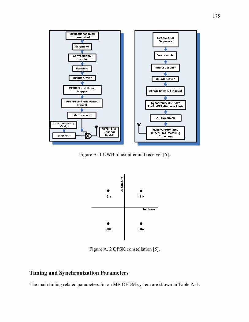
175

Figure A. 1 UWB transmitter and receiver [5].

Figure A. 2 QPSK constellation [5].

Timing and Synchronization Parameters

The main timing related parameters for an MB OFDM system are shown in Table A. 1.

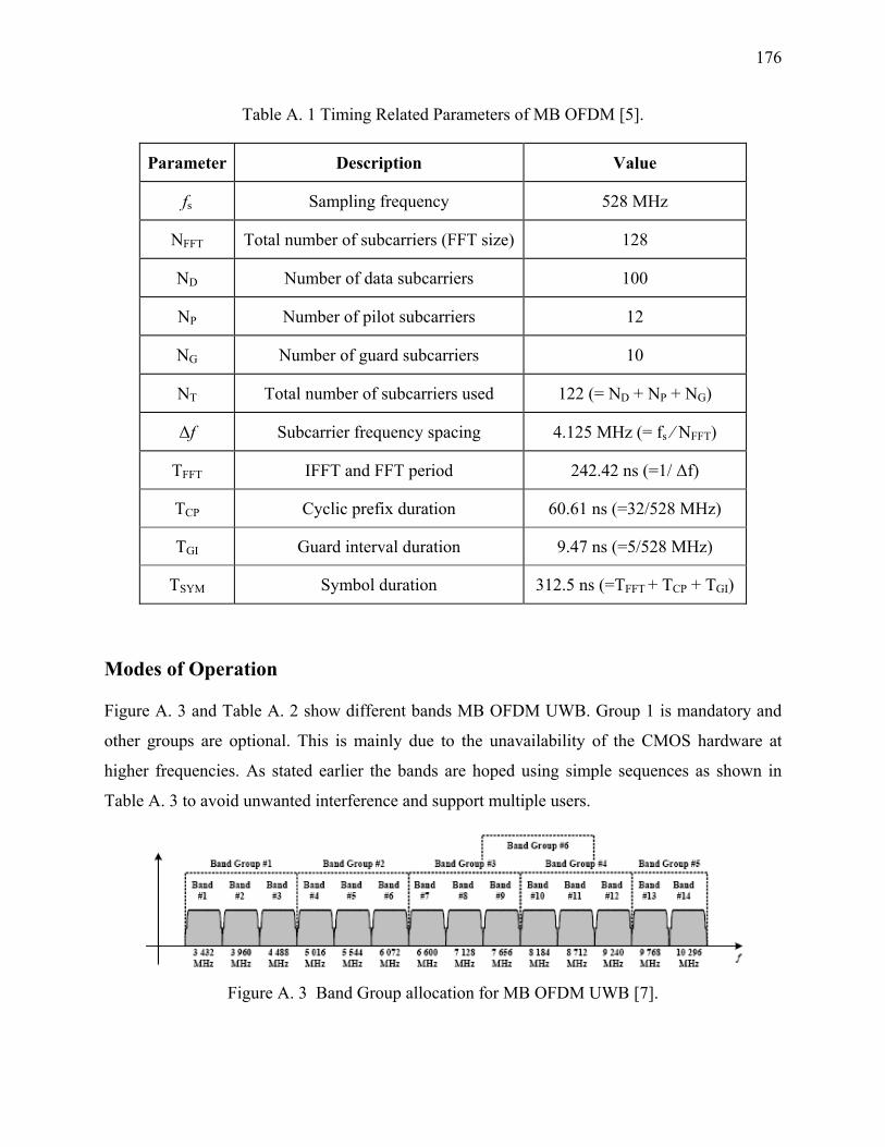
176

Table A. 1 Timing Related Parameters of MB OFDM [5].

Parameter Description Value

fs Sampling frequency 528 MHz

NFFT Total number of subcarriers (FFT size) 128

ND Number of data subcarriers 100

NP Number of pilot subcarriers 12

NG Number of guard subcarriers 10

NT Total number of subcarriers used 122 (= ND + NP + NG)

Δf Subcarrier frequency spacing 4.125 MHz (= fs ⁄ NFFT)

TFFT IFFT and FFT period 242.42 ns (=1/ Δf)

TCP Cyclic prefix duration 60.61 ns (=32/528 MHz)

TGI Guard interval duration 9.47 ns (=5/528 MHz)

TSYM Symbol duration 312.5 ns (=TFFT + TCP + TGI)

Modes of Operation

Figure A. 3 and Table A. 2 show different bands MB OFDM UWB. Group 1 is mandatory and

other groups are optional. This is mainly due to the unavailability of the CMOS hardware at

higher frequencies. As stated earlier the bands are hoped using simple sequences as shown in

Table A. 3 to avoid unwanted interference and support multiple users.

Figure A. 3 Band Group allocation for MB OFDM UWB [7].

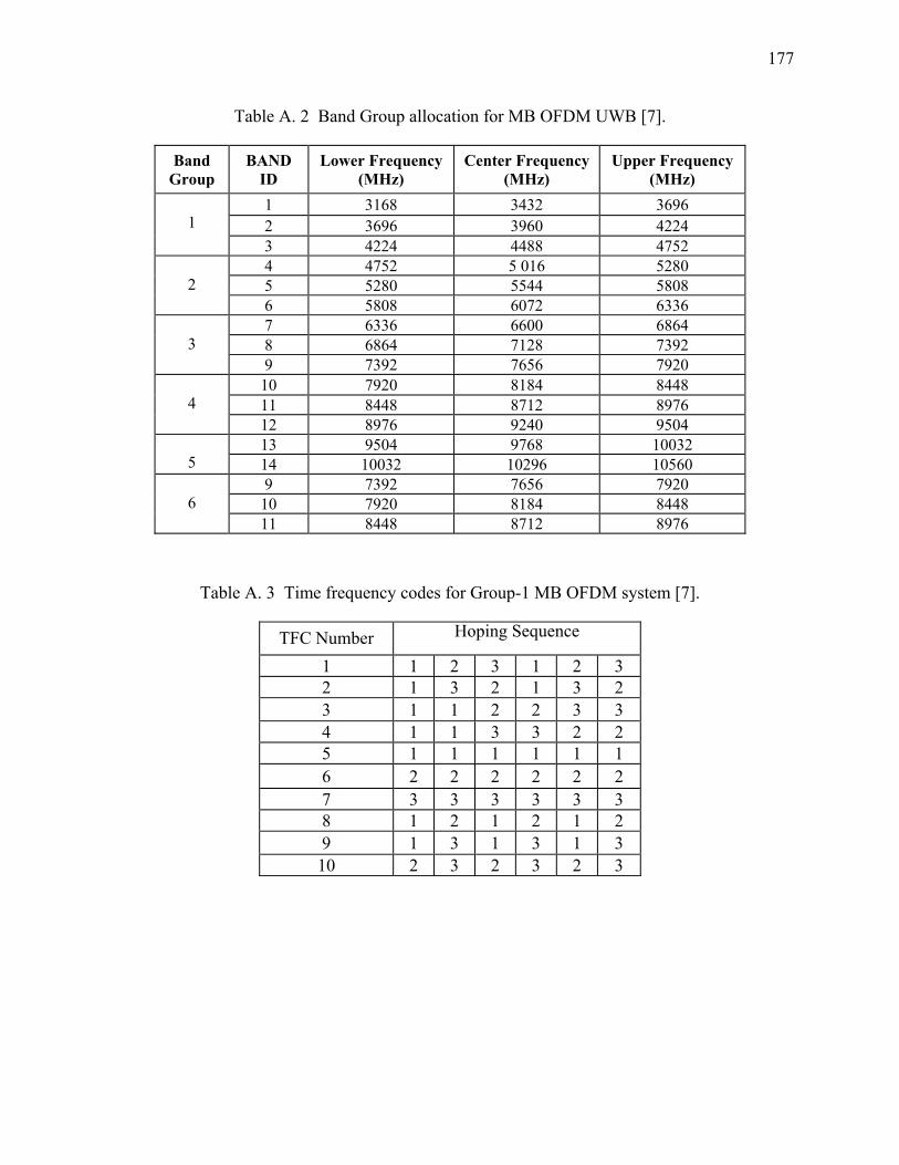
177

Table A. 2 Band Group allocation for MB OFDM UWB [7].

Band Group

BAND ID

Lower Frequency (MHz)

Center Frequency (MHz)

Upper Frequency (MHz)

1

1 3168 3432 3696 2 3696 3960 4224 3 4224 4488 4752

2

4 4752 5 016 5280 5 5280 5544 5808 6 5808 6072 6336

3

7 6336 6600 6864 8 6864 7128 7392 9 7392 7656 7920

4

10 7920 8184 8448 11 8448 8712 8976 12 8976 9240 9504

5 13 9504 9768 10032 14 10032 10296 10560

6

9 7392 7656 7920 10 7920 8184 8448 11 8448 8712 8976

Table A. 3 Time frequency codes for Group-1 MB OFDM system [7].

TFC Number Hoping Sequence

1 1 2 3 1 2 3 2 1 3 2 1 3 2 3 1 1 2 2 3 3 4 1 1 3 3 2 2 5 1 1 1 1 1 1 6 2 2 2 2 2 2 7 3 3 3 3 3 3 8 1 2 1 2 1 2 9 1 3 1 3 1 3 10 2 3 2 3 2 3

178

Data Rate Dependent Parameters

Table A. 4 and Table A. 5 lists data rate dependent parameters and receiver sensitivity for an MB

OFDM UWB system, respectively. For bit rates lower than 200Mb/s MB-OFDM UWB uses

QPSK while for higher bit rate advanced dual carrier modulation technique (DCM) is used.

Maximum permissible relative constellation error or root mean square EVM is depicted in Table

A. 6.

Table A. 4 Data rate dependent parameters MB OFDM system [7].

Data Rate

(Mb/s) Modulation

Coding Rate (R)

Frequency Spreading

Time Spreading

Coded Bits / 6 OFDM

Symbol

Info Bits / 6 OFDM Symbol

53.3 QPSK 1/3 YES YES 300 100 80 QPSK 1/2 YES YES 300 150

106.7 QPSK 1/3 NO YES 600 200

160 QPSK 1/2 NO YES 600 300

200 QPSK 5/8 NO YES 600 375

320 DCM 1/2 NO NO 1200 600

400 DCM 5/8 NO NO 1200 750 480 DCM 3/4 NO NO 1200 900

Table A. 5 Sensitivity of UWB receiver [7].

Data Rate (Mb/s) Minimum Receiver Sensitivity (dBm) 53.3 −80.8 80 −78.9

106.7 −77.8

160 −75.9

200 −74.5

320 −72.8

400 −71.5 480 −70.4

179

Table A. 6 Permissible Relative Constellation Error (EVM).

Relative Constellation RMS Error

Data Rate No TX Attenuation

TX Attenuation of 2, 4, 6 dB (All TFCs)

TX Attenuation of 8, 10, 12 dB (All TFCs)

53.3 Mb/s, 80 Mb/s, 106.7 Mb/s, 160 Mb/s,

200 Mb/s −17.0 dB −15.5 dB −14.5 dB

320 Mb/s, 400 Mb/s, 480 Mb/s −19.5 dB −18.0 dB −17.0 dB

180

APPENDIX B ANALYSIS OF OPTICAL RECEIVER NOISE

Let us assume the optical and electrical filter are rectangular with equivalent bandwidth 21

2 ( )o FB H dπ ω ω∞

−∞= ∫ and 21

2 ( )e eB H dπ ω ω∞

−∞= ∫ , where ( )FH ω and ( )eH ω are the transfer

function of the optical and electrical filter respectively. Because the optical bandwidth is

considerably larger than the signal bandwidth, the optical filter won’t affect the UWB signal but

only the ASE noise. Variance of the ASE-ASE beat noise, 2 ( )ASE ASEI tσ

−, signal-ASE beat noise,

2 ( )Signal ASEI tσ

−, and electrical noise, 2

elecσ , at the receiver can be expressed as [61]

( ) ( )

( )

2 2 22 2 2 12

2 2 2

( ) 2 ( ) ( )

2 2

ASE ASEI A o e F F

A o o e e

t G N H H H d

G N B B B

πσ ω ω ω ω−

∞

−∞

= ℜ ⊗

= ℜ −

∫ (B.1)

222 2 1

2

2

( ) 2 ( ) ( ) ( )

2

signal ASE

j tI A o F e

A o opt e

t G N H S t e h t d

G N P B

ωπσ ω ω

−

∞∗

−∞

= ℜ × ⊗

= ℜ

∫ (B.2)

and

( )

222 1

22

2 2

RIN ( )

2

RIN 2

A opt o o delec e

A opt o o d th

A opt o o d A opt o o d th e

G P N B It H d

G q P N B I N

G P N B I G q P N B I N B

∞

−∞

⎧ ⎫⎡ ⎤ℜ + ℜ +⎪ ⎪⎣ ⎦= ⎨ ⎬⎡ ⎤+ ℜ + ℜ + +⎪ ⎪⎣ ⎦⎩ ⎭

⎡ ⎤ ⎡ ⎤= ℜ + ℜ + + ℜ + ℜ + +⎣ ⎦ ⎣ ⎦

∫πσ ω ω (B.3)

which consists of contribution of RIN, 2RIN A opt o o d eG P N B I B⎡ ⎤ℜ + ℜ +⎣ ⎦ , shot noise,

2 A opt o o d eG q P N B I B⎡ ⎤ℜ + ℜ +⎣ ⎦ , and thermal noise, 2th eN B , where ( )S t∗ is the complex conjugate of

the received optical signal at the photodetector, = 26 dBAG is the RF amplifier gain at the

optical receiver, Popt is the received optical power, and oN represents the single sided ASE noise

density for a single polarization expressed by ( 1) /(2 )oN Fhc G λ= − , h - the Plank’s constant, λ

- the wavelength of the laser source, c - speed of light in vacuum, and noise figure of F = 4 dB

and gain of G = 8 dB of the EDFA. The symbol ⊗ denotes the convolution. 2elecσ is the noise

contribution from both optical transmitter and receiver electronic noise, and this is called “back-

181

to-back” system noise (shot noise, thermal noise, and RIN). q is the electron charge, and

= 100 nAdI is the dark current. The variance of thermal noise is given as 2 4 /th B n e LN k TF B R= ,

where -23=1.38×10Bk J/K is the Boltzman constant, and = 5 dBnF is noise figure of the RF

amplifier at the receiver, T is the room temperature in degree Kelvin, and =50 LR Ω is the load

resistance. Now, the total noise power will be given as [61]

( ) ( ) ( ) ( )2 2 2 22ASE ASE Signal ASEn I I elect t t tσ σ σ σ

− −= + + (B.4)

All calculated receiver noise contributions are presented in Figure B. 1 for the back to back.

It is shown that ASE-ASE beat noise is negligible because of the low noise figure of the EDFA

and narrow bandwidth of the optical filter used. The output from the RF amplifier at the optical

receiver in Figure 2.1 is directly connected to the data analyzer. The scope captures the signal in

time domain and performs FFT on it. It analyzes the data within 1.6 GHz bandwidth. The

thermal noise within this bandwidth is around -71.2 dBm which is small compared to other noise

contributions. It is seen that shot noise, RIN and signal-ASE beat noise are the major sources of

noise at the receiver for higher optical power.

-80

-70

-60

-50

-40

-10 -8 -6 -4 -2 0

Noi

se p

ower

(dB

m)


ASE-ASE

Signal-ASE

RINShot noise

Thermal noise

Total noise

Figure B. 1 Noise power level at the receiver versus received optical power for back-to-back

transmission.

182

-155

-150

-145

-140

-135

0 20 40 60 80 100

RIN

(dB

/Hz)

Fiber length (km)

Figure B. 2 Calculated total RIN versus fiber length.

Fiber dispersion changes the laser RIN due phase noise to intensity noise conversion [31-32].

Figure B. 2 shows total RIN due to fiber dispersion for a laser with linewidth of

/(2 )= 800 KHzω πΔ at 1550 nm by using [31]

( ) ( )22 281 1

22( ) 0 sinu

u l l

RIN L RIN L dω βΩ

ΔΩ −Ω ΩΩ

+ Ω Ω∫ (B.5)

where ( ) 2u l BWπΩ − Ω = is the signal occupied bandwidth, L is the fiber length and

(0) 155 dB/HzRIN = − is the laser intrinsic RIN.

For the frequency band of 3.176 to 4.744 GHz, the dispersion increases the RIN by 6.7 and

11.8 dB for 20 and 40 km, respectively, compared to the back to back. This is one of the reasons

why the EVM degrades with fiber length.

183

APPENDIX C

We compare the OSSB and ODSB, as commonly used optical external modulation techniques.

Figure C. 1(a) and (b) shows measured optical spectrum using OSSB and ODSB, respectively. It

is well known that OSSB is used to overcome chromatic dispersion caused power fading by

suppression of one of the optical sidebands [1]. However, there is a 3 dB power loss if compared

to ODSB. Conversely, ODSB does suffer from power fading specially for back to back because

optical sidebands are out of phase and will beat with the optical carrier and add destructively to

produce a single RF signal. Figure C. 2 shows comparison of EVM using OSSB and ODSB for

back to back and after 20 km of fiber transmission. Figure C. 2 shows that the EVM is -3 dB or

71% at data rate of 200 Mb/s for the back to back with ODSB. At 20 km the EVM is

significantly improved compared to the back-to-back because chromatic dispersion of fiber

causes each optical sideband to have different phase shift depending on the fiber length,

frequency of RF signal and fiber dispersion and thus the power of the detected RF signal

changes.

-50

-40

-30

-20

-10

0

-0.1 -0.05 0 0.05 0.1

Pow

er (d

Bm

)

Wavelength (nm) relative to 1549.892 nm

-50

-40

-30

-20

-10

0

-0.1 -0.05 0 0.05 0.1

Pow

er (d

Bm

)

Wavelength (nm) relative to 1549.892 nm (a) (b)

Figure C. 1 Measured optical signal (a) OSSB and (b) ODSB.

In opposition, the OSSB is almost independent of fiber dispersion. As shown in Figure C. 2,

the EVM is very close and less than -20 dB for both back-to back and after 20 km of fiber

transmission. The power fading in ODSB repeats at periodic fiber lengths and can be

compensated using different compensation techniques at the expense of increased complexity

184

and cost [1]. It is clearly seen from Figure C. 2 that OSSB outperforms ODSB at any power level

and fiber length. Therefore only OSSB modulation was considered in Chapter 2.

-25

-20

-15

-10

-5

0 1 2 3 4 5 6 7 8

0 km (OSSB) 20 km (OSSB) 0 km (ODSB) 20 km (ODSB)

EVM

(dB

)


OSSB

ODSB

ODSB

Figure C. 2 Measured EVM using OSSB and ODSB.

With OSSB modulation, the QPSK constellation for data and BPSK constellation for pilots

after 20 km at 200 Mb/s is presented in Figure C. 3 (measured with a Lecroy serial data analyzer

SDA 11000). The good quality of the constellation is an indication of suitability of the RoF

systems for UWB applications.

Qua

drat

ure

Qua

drat

ure

Figure C. 3 QPSK OFDM constellation in a) two dimension b) three dimension received at the

real time oscilloscope for band group 1 after 20 Km of fiber transmission with bit rate of

200Mb/s (Colors indicate intensity of power concentration in the received symbol).

185

APPENDIX D SIMULATED MAGNITUDE AND DELAY RESPONSE OF

CHEBYSHEV-II FILTER

Simulated magnitude and delay response of Chebyshev-II filter is presented in Figure D. 1 for

third, fifth and seventh order filters with different bandwidths. From Figure D. 1(a) we see

Chebyshev-II filter has a flat magnitude response in the passband. Though, out of band ripples

increase with filter order, which is not of importance if the side-lobe suppression is higher than

the required 20 dB ACPR for WiMedia standard. Figure D. 1(b) shows that the delay increases if

the filter order is increased and decreases if the filter bandwidth is increased. Also higher order

filters have high delay overshoot at the edges.

-40

-35

-30

-25

-20

-15

-10

-5

0

1 2 3 4 5 6 7 8

3rd , 3 GHz5th , 2 GHz5th , 3 GHz7th , 3 GHz

S21

(dB

)

Frequency (GHz)

0

100

200

300

400

500

600

700

800

2.5 3 3.5 4 4.5 5 5.5

3rd, 3 GHz5th, 2 GHz5th, 3 GHz5th, 3.5 GHz7th, 3 GHz5th, 2.5GHz

3rd, 2.5 GHz

Del

ay (p

s)

Frequency (GHz) (a) (b)

Figure D. 1 Simulated (a) magnitude and (b) delay response of Chebyshev-II filter.

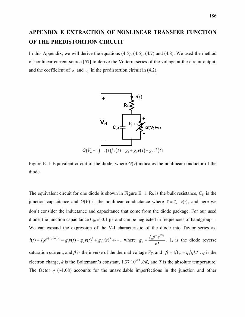
186

APPENDIX E EXTRACTION OF NONLINEAR TRANSFER FUNCTION

OF THE PREDISTORTION CIRCUIT

In this Appendix, we will derive the equations (4.5), (4.6), (4.7) and (4.8). We used the method

of nonlinear current source [57] to derive the Volterra series of the voltage at the circuit output,

and the coefficient of 1a and 3a in the predistortion circuit in (4.2).

( ) ( ) ( ) ( ) ( )21 2 3bG V v i t v t g g v t g v t+ = = + +

( )i t

bV v+

Figure E. 1 Equivalent circuit of the diode, where G(v) indicates the nonlinear conductor of the

diode.

The equivalent circuit for one diode is shown in Figure E. 1. Rb is the bulk resistance, Cjo is the

junction capacitance and G(V) is the nonlinear conductance where ( )bV V v t= + , and here we

don’t consider the inductance and capacitance that come from the diode package. For our used

diode, the junction capacitance Cjo is 0.1 pF and can be neglected in frequencies of bandgroup 1.

We can expand the expression of the V-I characteristic of the diode into Taylor series as,

( )( ) 2 31 2 3( ) ( ) ( ) ( )bV v t

si t I e g v t g v t g v tβ += = + + + ⋅⋅⋅ , where !

bVns

nI eg

n

ββ= , Is is the diode reverse

saturation current, and β is the inverse of the thermal voltage VT, and 1 TV q kTβ η= = . q is the

electron charge, k is the Boltzmann’s constant, 1.37·10-23 J/K, and T is the absolute temperature.

The factor η (~1.08) accounts for the unavoidable imperfections in the junction and other

187

secondary phenomena. For small signal application, we only consider up to third order, and the

nonlinear conductance is then given by ( ) 21 2 3( ) ( )bG V v g g v t g v t+ = + +

0Z , 90lβ =

0

inVl−Γ lΓ

0Z , 90lβ =

( )1 tv1g

( )2 ti ( )3 ti

( )212 tg v ( ) ( )

( )31

2 1 2

3

2 t tt

g v vg v+

0ΓRFV,diode funV

( )s tv

-l l

Figure E. 2 Equivalent circuit of the nonlinear diode connected with a voltage source and load.

The Volterra series can be found by using the nonlinear current method [57]. In this method,

the nonlinear conductor component is replaced by one linear conductor and several current

sources, and the current components are calculated from voltage components of lower order. By

substituting the nonlinear conductor G with a conductor 1g and nonlinear current source 2 ( )i t

and 3( )i t in the predistortion circuit, we can have the equivalent circuit shown in Figure E. 2. In

Figure E. 2, a voltage source and load are connected to the nonlinear diode. V1 is the voltage

applied to the conductance g1, Zeq=Rb+1/g1 is the equivalent impedance of the diode, Zload,0 is the

load impedance at the position of the diode, and Zs,0 is the source impedance at the position of

the diode. Zeq,total is the total impedance at the position of the diode, and Zeq,total equals Zeq in

parallel with Zload,0. The reflection coefficient at the diode is Γ0, the reflection coefficient at the

source is Γ-l, and the reflection coefficient at the load is Γl. Vin is the total voltage coming out

from the RF source.

Now we compute Zin.. The / 4l λ= transmission line is used for impedance matching between

the load and the diode, then 2,0 0load loadZ Z Z= .

188

The total impedance at the position of the diode ,0totalZ equals the equivalent impedance of the

diode 11/eq bZ R g= + in parallel with ,0loadZ , then

( )( )

2,0 1 0

,0 2,0 1 1 0

11

load eq btotal

load eq b load

Z Z g R ZZ

Z Z g R Z g Z+

= =+ + +

(E.1)

another / 4l λ= transmission line is used for impedance matching between the source and the diode, then using (E.1) the input impedance is

2 20 1 0

,0 11in loadtotal b

Z g ZZ ZZ g R

= = ++

(E.2)

and the voltage applied at the input of the circuit is

( )

( )( )

21 1 0

21 1 0

1( ) 1

load binin s s

in s s load b

Z g R g ZZV V VZ Z Z Z g R g Z

+ += =

+ + + + (E.3)

To find the voltage of the fundamental carrier and IMD3 at the circuit output, we first need to

find the voltage Vdiode,fun of the fundamental carrier applied to the diode.

Using the transmission line theory [30] with , ,0diode funV + and , ,0diode funV − representing the incident

and reflected voltage at the position of the diode, the input voltage can be expressed as

[ ]2 2, ,0 , ,0 , ,0 01

j j

in diode fun diode fun diode funV V e V e jVπ π

−+ − += + = − Γ (E.4)

where ,0 00

,0 0

total

total

Z ZZ Z

−Γ =

+

On the other hand, the incident and reflected voltages at the position of the diode can be

expressed, respectively, as

, ,001

indiode fun

VV j+ = −− Γ

(E.5)

0, ,0

01in

diode funVV j− Γ

= −− Γ

(E.6)

then the voltage applied to the diode ,diode funV is expressed by

189

, , ,0 , ,0

0

0

,0

0

0

1 1

diode fun diode fun diode fun

in

totalin

inin

V V V

j V

Zj V

ZZj VZ

+ −= +

+ Γ= −

− Γ

= −

= −

(E.7)

Using equations (E.2) and (E.3) in equation (E.7) the applied voltage to the diode becomes

( )( )( )

1 0, 2

1 1 0

1

1b s

diode funs load b

g R Z VV j

Z Z g R g Z+

= −+ + +

(E.8)

In similar way using the transmission line theory [30] with ,RF funV + and ,RF funV − representing the

incident and reflected voltage at the position of the load, ,RF funV can be calculated. The applied

voltage to the diode can be rewritten

[ ]2 2, , , , 1

j j

diode fun RF fun RF fun RF fun lV V e V e jVπ π

−+ − += + = − Γ (E.9)

where 0

0

loadl

load

Z ZZ Z

−Γ =

+

then the incident and reflected voltage at the position of the load can be expressed, respectively, as

,, 1

diode funRF fun

l

VV j+ = −

− Γ (E.10)

and ,, 1

l diode funRF fun

l

VV j− Γ

= −− Γ

(E.11)

then the voltage applied to the load ,RF funV is simply expressed by

( )( )

, , ,

,

,0

12

1 1 0

1 1

(1 )1

RF fun RF fun RF fun

ldiode fun

l

loaddiode fun

b load s

s load b

V V V

j V

Zj VZ

g R Z VZ Z g R g Z

+ −= +

+ Γ= −

− Γ

= −

+= −

+ + +

(E.12)

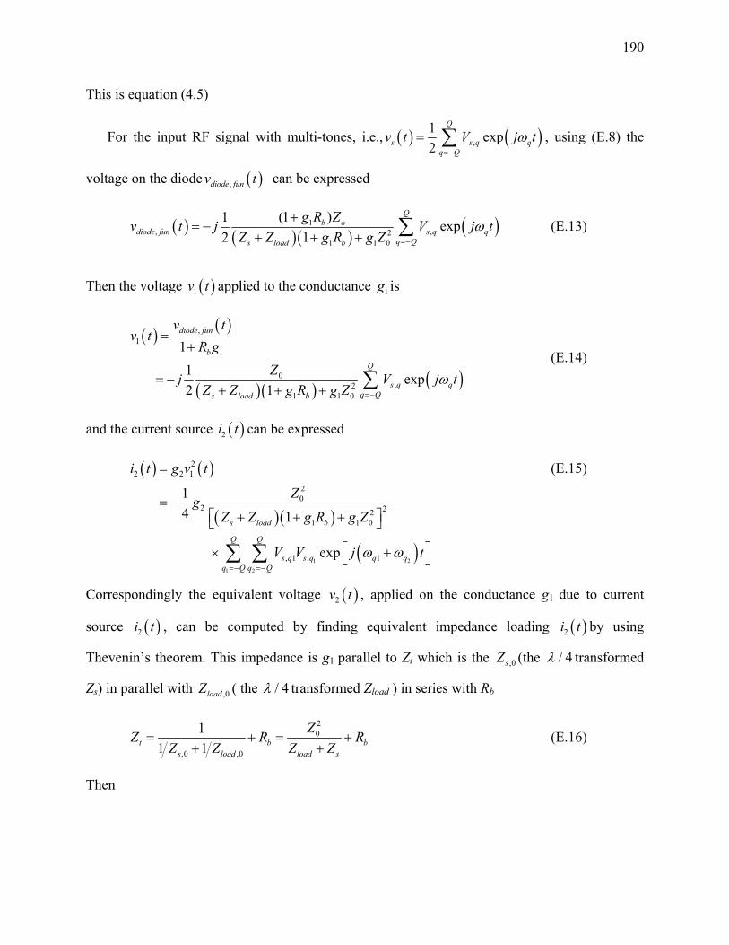
190

This is equation (4.5)

For the input RF signal with multi-tones, i.e., ( ) ( ),1 exp2

Q

s s q qq Q

v t V j tω=−

= ∑ , using (E.8) the

voltage on the diode ( ),diode funv t can be expressed

( ) ( )( ) ( )1, ,2

1 1 0

(1 )1 exp2 1

Qb o

diode fun s q qq Qs load b

g R Zv t j V j tZ Z g R g Z

ω=−

+= −

+ + + ∑ (E.13)

Then the voltage ( )1v t applied to the conductance 1g is

( ) ( )

( )( ) ( )

,1

1

0,2

1 1 0

11 exp2 1

diode fun

b

Q

s q qq Qs load b

v tv t

R gZj V j t

Z Z g R g Zω

=−

=+

= −+ + + ∑

(E.14)

and the current source ( )2i t can be expressed

( ) ( )

( )( )

( )1 2

1 2

22 2 1

20

2 221 1 0

, 1 , 1

14 1

exp

s load b

Q Q

s q s q q qq Q q Q

i t g v t

ZgZ Z g R g Z

V V j tω ω=− =−

=

= −⎡ ⎤+ + +⎣ ⎦

⎡ ⎤× +⎣ ⎦∑ ∑

(E.15)

Correspondingly the equivalent voltage ( )2v t , applied on the conductance g1 due to current

source ( )2i t , can be computed by finding equivalent impedance loading ( )2i t by using

Thevenin’s theorem. This impedance is g1 parallel to Zt which is the ,0sZ (the / 4λ transformed

Zs) in parallel with ,0loadZ ( the / 4λ transformed Zload ) in series with Rb

20

,0 ,0

11 1t b b

s load load s

ZZ R RZ Z Z Z

= + = ++ +

(E.16)

Then

191

( ) ( )

( )( )( )

( )1 2

1 2

2 21

2 20 0

2 , 1 , 1321 1 0

1

1 exp4 1

t

t

Q Qb s load

s q s q q qq Q q Qs load b

Zv t i tZ g

Z Z R Z Zg V V j t

Z Z g R g Zω ω

=− =−

−=

+

⎡ ⎤+ +⎣ ⎦ ⎡ ⎤= +⎣ ⎦⎡ ⎤+ + +⎣ ⎦∑ ∑

(E.17)

Now we have the voltages ( )1v t and ( )2v t , we can compute the current ( )3i t

( ) ( ) ( ) ( )

( )( )

( ) ( ) ( )

( )2 2

1 2 3 2 3

1 2 3

33 2 1 2 3 1

30

421 0 1

2 2 21 3 0 3 1

, , , 1

2

8 1

2 1 2

exp

b s load

b b s load

Q Q Q

s q s q s q q q qq Q q Q q Q

i t g v t v t g v t

Zj

g Z g R Z Z


V V V j tω ω ω=− =− =−

= +

=⎡ ⎤+ + +⎣ ⎦

⎡ ⎤⎡ ⎤× − + + − +⎣ ⎦⎣ ⎦

⎡ ⎤× + +⎣ ⎦∑ ∑ ∑

(E.18)

By using circuit theory the third order nonlinear product voltage generated by ( )3i t at the diode

can be expressed

( ) ( )

( )( )

( ) ( ) ( )

( )2 2

1 2 3 2 3

1 2 3

,3 3,0 ,0 1

50

521 0 1

2 2 21 3 0 3 1

, , , 1

11 1 1

8 1

2 1 2

exp

t tdiode

s load t

b s load

b b s load

Q Q Q


Z Zv t i tZ Z Z g

Zj

g Z g R Z Z


V V V j tω ω ω=− =− =−

=+ +

=⎡ ⎤+ + +⎣ ⎦

⎡ ⎤⎡ ⎤× − + + − +⎣ ⎦⎣ ⎦

⎡ ⎤× + +⎣ ⎦∑ ∑ ∑

(E.19)

Then after the / 4l λ= transmission line, using the same microwave transmission line theory

[30] used to get equation (E.7) and (E.12), the third order nonlinear distortion voltage at the

circuit output can be expressed in Voltera Series as

192

( ) ( )

( )( )

( ) ( ) ( )

( )2 2

1 2 3 2 3

1 2 3

,3 ,30

40

521 0 1

2 2 21 3 0 3 1

, , , 1

18 1

2 1 2

exp

loadRF diode

load

b s load

b b s load

Q Q Q


Zv t j v tZ

Z Z

g Z g R Z Z


V V V j tω ω ω=− =− =−

=

= −⎡ ⎤+ + +⎣ ⎦

⎡ ⎤⎡ ⎤× − + + − +⎣ ⎦⎣ ⎦

⎡ ⎤× + +⎣ ⎦∑ ∑ ∑

(E.20)

The voltage in (E.20) includes all third-order nonlinear products. But we are only concerned in a

special case where the RF signal consists of two tones at 1ω and 2ω with equal magnitude. We

may not be concerned in all the third order nonlinear products. The most important third-order

nonlinear products are IMD3 at frequency of 2 12ω ω− and 1 22ω ω− . Suppose that these two

third order nonlinear products are equal in voltage with , 3diode IMDV . Using (E.20) we can find the

voltage of IMD3 at the load,

( )( )

( ) ( ) ( )2 2

4 30

, 3 521 0 1

2 2 21 3 0 3 1

34 1

2 1 2

load sRF IMD

b s load

b b s load

Z Z VVg Z g R Z Z


= −⎡ ⎤+ + +⎣ ⎦

⎡ ⎤⎡ ⎤× − + + − +⎣ ⎦⎣ ⎦

(E.21)

This is equation (4.6).

Using (E.2) we can rewrite (E.12) and (E.21) in terms of inV , respectively, as

( )( )

1, 2

1 1 0

11

b load inRF fun

load b

g R Z VV

Z g R g Z+

= −+ +

(E.22)

( )( )

( ) ( ) ( )( )

2 2

4 30

, 3 221 0 1

2 2 21 3 0 3 1

321 1 0

34 1

2 1 2

1

load inRF IMD

b s load

b b s load

load b

Z Z VVg Z g R Z Z


Z g R g Z

= −⎡ ⎤+ + +⎣ ⎦

⎡ ⎤⎡ ⎤− + + − +⎣ ⎦⎣ ⎦×⎡ ⎤+ +⎣ ⎦

(E.23)

193

For an RF input signal to the predistortion circuit with two tones at 1ω and 2ω with equal

magnitude Vin, the coefficient in (4.2) are ,1

RF fun

in

Va

V= and , 3

3 3

43

RF IMD

in

Va

V= using (E. 22) and

(E.23) we get

( )( )

11 2

1 1 0

11

b load

load b

g R Za

Z g R g Z+

= −+ +

(E.24)

( )( )

( ) ( ) ( )( )

2 2

40

3 221 0 1

2 2 21 3 0 3 1

321 1 0

1

2 1 2

1

load

b s load

b b s load

load b

Z Zag Z g R Z Z


Z g R g Z

= −⎡ ⎤+ + +⎣ ⎦

⎡ ⎤⎡ ⎤− + + − +⎣ ⎦⎣ ⎦×⎡ ⎤+ +⎣ ⎦

(E.25)

These are equations (4.7) and (4.8), respectively.

194

APPENDIX F DERIVATION OF OPTIMAL PHASE SHIFT AND

IMPROVED POWER EFFICIENCY

In this Appendix we show the derivation details of how to obtain equation (5.1). Let

2RFm mπ= , where 2RF RFm V Vπ= is the modulation index, and Vπ- the halfwave switching

voltage of the DE-MZM. The total RF signal applied to upper and lower electrodes of the DE-

MZM can be expressed, respectively, as

( ) ( )

( ) ( )sin 2 sin

2 sin 2 4 sin 2 4RF RF

RF

m t m t

m t

ω θ π ω θ ϕ

ω θ ϕ π ϕ π

+ + + + +

= + + + + (F.1)

and

( ) ( )

( ) ( )sin sin 2

2 sin 2 4 cos 2 4RF RF

RF

m t m t

m t

ω θ ω θ ϕ π

ω θ ϕ π ϕ π

+ + + + +

= + + + + (F.2)

Then the output optical field from the DE-MZM can be written as

( ) ( ) ( ) ( ) ( ) ( ) 21

exp 2 sin 2 4 sin 2 4

exp 2 sin 2 4 cos 2 4ff in c c

RFj tout

RF

t P j m tE t e

j j m tω φ

δ

ω θ ϕ π ϕ π

δ ω θ ϕ π ϕ π+

+

⎡ ⎤+ + + +⎢ ⎥=⎢ ⎥+ + + + +⎣ ⎦

(F.3)

where = ( 1) ( 1)ER ERδ − + , ER is the DE-MZM extinction ratio, Pin is the input optical

power to the DE-MZM, tff is the optical insertion loss of the DE-MZM. The output signal of the

DE-MZM is transmitted through an SMF. By applying the Jacobi-Anger expansion

( )( ) expexp sin( ) nn

J xjx t jn t∞

=−∞

=Ω Ω∑ (F.4)

to (F.3), where Jn(·) is the nth order Bessel function of first kind, the output optical field from the

DE-MZM becomes

( ) ( )

( ) ( )( )( )( )

( )

21

sin 2 4

cos 2 4

exp 2 4

ff in c c n

n

out nn

j t

n

RF

t P J m

j J m

E t E t

e

jn t

ω φ

δ

ϕ π

δ ϕ π

ω θ ϕ π

∞

=−∞

∞+

=−∞+

+

+ +

=

⎧ ⎫⎪ ⎪= ⎨ ⎬⎪ ⎪⎩ ⎭

× + + +

∑

∑ (F.5)

195

By only considering the optical carrier and the two first sidebands, the complex amplitude of the

photo-detected current at the RF frequency ωRF is expressed as

( )( ) ( ) ( )

( ) ( ) ( )

( ) ( ) ( )( )

( ) ( ) ( )( )

210 1 2 12

211 0 2 12

12

12

exp12 exp

1 exp 2 4 exp2 1

Im exp 2 3 4 exp1

RF

RF RF

RF RF

Lin ff

RF

Lin ff

RF

E t E t j L LI t

E t E t j L L

P t eZ Z j j t L

P t eZ j j t L

ω

α

α

β ω β ω

β ω β ω

ϕ π ω β θδ

ϕ π ω β θδ

∗

∗−

−∗

−

⎡ ⎤− +⎢ ⎥= ℜ⎢ ⎥+ −⎣ ⎦

= ℜ − + − ++

= ℜ + − ++

(F.6)

where ℜ is responsivity of the photodetector, α is the fiber loss, 1/β1 is the fiber group delay,

( )22 2c D cβ λ π= − , λc is the optical wavelength, c - the speed of light in vacuum, L and D - fiber

length and chromatic dispersion, respectively, Z* stands for complex conjugate of Z and

( )( ) ( )( )( )( ) ( )( ) ( )

( )

0 0

1 1 2

2 22

2 sin 2 4 2 cos 2 4

2 sin 2 4 2 cos 2 4 exp

exp

Z J m j J m

J m j J m j

A B j

ϕ π δ ϕ π

ϕ π δ ϕ π θ

θ ψ

⎡ ⎤= + − +⎣ ⎦⎡ ⎤× + + +⎣ ⎦

= + +

(F.7)

212 22 RFLθ β ω= − (F.8)

( )( ) ( )( )

( )( ) ( )( )0 1

20 1

2 sin 2 4 2 sin 2 4

2 cos 2 4 2 cos 2 4

J m J mA

J m J m

ϕ π ϕ π

δ ϕ π ϕ π

⎡ ⎤+ +⎢ ⎥=+ + +⎢ ⎥⎣ ⎦

(F.9)

( )( ) ( )( )

( )( ) ( )( )0 1

0 1

2 sin 2 4 2 cos 2 4

2 cos 2 4 2 sin 2 4

J m J mB

J m J m

ϕ π ϕ πδ

ϕ π ϕ π

⎡ ⎤+ +⎢ ⎥=− + +⎢ ⎥⎣ ⎦

(F.10)

and

( )-1tan B Aψ = (F.11)

Then the photocurrent can be rewritten as

( ) ( )

( )( )

2 222

1

sin1

exp 2 3 4

RF

Lin ff

RF

P t eI t A B

j t L

α

ω ψ θδ

ω β θ ϕ π

−

= ℜ + ++

× − + + + (F.12)

196

Thus maximum photocurrent amplitude can be reached if and only if ( )2sin 1ψ θ+ = , which

implies

( )2cos 0ψ θ+ = (F.13)

This leads to the following expression

2tan 1 tanB Aψ θ= = (F.14)

By using the small signal condition i.e. 2 1m , we can write ( ) ( )2 !nnJ z z n∼ and applying to

(F.9) and (F.10) the equation (F.14) can be simplified to

( ) ( ) ( )

( )

2 2

2

1 1 tan 2tan

2 tan 2

δ δ ϕθ

δ ϕ

⎡ ⎤+ + −⎣ ⎦ =−

(F.15)

which can be solved for φ as

( ) ( )-1 2 222tan 1 1 2 tanϕ δ δ δ θ⎡ ⎤= − + − +⎣ ⎦ (F.16)

This is expression (5.1) of the required electrical phase shift to maximize the output RF power

and compensate for chromatic dispersion induced power fading.

Next, we show the derivation details of how to obtain equation (5.2). First we compute the

RF output power when using the proposed ODSB. Using (F.14) and (F.10) we can write

( )

( )( )

2 2 2 22

2 2 2 22

1 tan

2 sin 2 1 tan

A B B

m

θ

δ ϕ θ

+ = +

= + (F.17)

Using (F.15) the above can be rewritten

( )( ) ( )( ) ( ) ( )

( )

( )

22 2 4

2 2 2 22

222 22

1 1 tan 2 2 1 tan 21 sin 22 tan 2

1 1 1 1 sin2 1

A B m

m

δ ϕ δ ϕϕ

ϕ

δδ ϕδ

⎡ ⎤+ + + −⎢ ⎥⎣ ⎦+ =

⎡ ⎤−= + +⎢ ⎥+⎣ ⎦

(F.18)

Hence using (F.18) in (F.12), the photocurrent can be expressed as

197

( ) ( )1 exp2RF in ffI P t L m Fω α ϕ= ℜ − (F.19)

where

( )2

2

11 sin1

F δϕ ϕδ

−= +

+ (F.20)

and the corresponding RF output power is expressed as

( )( ) ( )

2

2

2

1 exp4

RF RF L

in ff RF L

P I R

P t L m F R

ω ω

α π ϕ

=

= ℜ − (F.21)

where RL is the resistance load of the receiver.

Next we compute the RF output power when using OSSB modulation. For OSSB modulation the

optical field after the MZM can be expressed, by using Jacobi-Anger expansion (F.4), as

( ) ( )( )

( )( ) ( ) ( ) ( ) ( )

2

12

exp 2 sin

1 exp 2 sin 2 2

1 2 exp1

c c

c c

RFj tin ff

out

RF

j tin ff nn RF

n

j m tP tE t e

j m t

P te j J m jn t

ω φ

ω φ

ω θ

δ δ ω θ π π

δ ω θδ

+

∞+ +

=−∞

⎡ ⎤+⎢ ⎥= ⎢ ⎥+ + + + +⎢ ⎥⎣ ⎦

= + ++ ∑

(F.22)

The optical field at the photodetector can be expressed as

( ) ( ) ( ) ( )( ) 212 12exp 2 explink n RF RF

nE t L E t j L n Lnα β ω β ω

∞

=−∞

= − − +∑ (F.23)

where

( ) ( ) ( ) ( ) ( )12 1 2 exp

1c cj tin ff n

n n RF

P tE t j J m jn t e ω φδ ω θ

δ++= + +

+ (F.24)

By only considering the optical carrier and the two first sidebands, the complex amplitude of the

photo-detected current at the RF frequency ωRF is expressed as

198

( ) ( )( ) ( ) ( )

( ) ( ) ( )( )

( ) ( ) ( ) ( )( ) ( )( )( ) ( )

( )( )

0 1 2

1 0 2

20 12

2

1

exp1 exp2 exp

1 1 expexp 2 2

1 1 exp2 1

exp

RF

in ff

RF

E t E t jI t L

E t E t j

j jP t LJ m J m

j j

j t L

ω

θα

θ

δ δ θαδ δ θδ

ω β θ

∗−

∗

⎡ ⎤−= ℜ − ⎢ ⎥

+⎢ ⎥⎣ ⎦− −⎡ ⎤ℜ −

= ⎢ ⎥− + + −+ ⎢ ⎥⎣ ⎦

× − +

(F.25)

Under the small signal assumption the amplitude of the photocurrent can be approximated by

( )2

exp1 2 2RF

in ffP t L mI Cω

αδ

ℜ −=

+ (F.26)

where

( ) ( ) ( ) ( ) ( )22 2 22 22 1 2 1 1 cos 2 2 sin 2C δ δ δ θ δ θ⎡ ⎤= + − − − +⎣ ⎦ (F.27)

Applying the following identities to (F.27)

( )2

2

1 tancos 21 tan

θθθ

−=

+ (F.28)

( ) 2

2 tansin 21 tan

θθθ

=+

(F.29)

And using (F.15), (F.27) can be rewritten, after some calculations and rearrangements, as

( ) ( ) ( ) ( )( ) ( ) ( )

( ) ( )( ) ( ) ( )

( ) ( ) ( ) ( )( ) ( )

2 2 222 2

22 2 4

2 222 2

22 4

1 1 tan 2 2 1 tan 22 1 2 1

1 1 tan 2 2 1 tan 2

1 1 sin 2 1 2 1

1 1 sin

Cδ ϕ δ ϕ

δ δδ ϕ δ ϕ

δ δ ϕδ δ

δ δ ϕ

⎡ ⎤− + + +⎣ ⎦= + + − ×+ + + −

⎡ ⎤− + +⎣ ⎦= + + −+ + −

(F.30)

Replacing (F.30) into (F.26) the amplitude of the photocurrent can be rewritten as

( )( ) ( )

( )2 2

2 2

2

2

21 11 1

11

1 2 sin1 exp2 1 sinRF in ffI P t L m

δ δδ δ

ω δδ

ϕα

ϕ

− −+ +

−+

+ += ℜ −

+ (F.31)

and the RF output power is expressed as

( )( ) ( )21 exp4RF

SSBin ff RF LP P t L G m G Rω α π ϕ= ℜ − (F.32)

199

where ϕ is the electrical phase shift given by (E.16) and

( )( ) ( )

( )2 2

2 2

2

2

21 11 1

11

1 2 sin12 1 sin

Gδ δδ δ

δδ

ϕϕ

ϕ

− −+ +

−+

⎛ ⎞+ +⎜ ⎟=⎜ ⎟+⎝ ⎠

(F.33)

Then the ratio of the RF output power of the proposed ODSB (F.21) to that of the conventional

OSSB (F.32) is

( )( )

( )( )( )

22 2

4 4

1 1 sin

1 1 sinRF

RF

SSB

P FP G

ω

ω

δ δ ϕϕη

ϕ δ δ ϕ

+ + −= = =

+ + − (F.34)

This is the improvement of the RF power given in equation (5.2).

The variation of function η versus φ is summarized in Table F. 1.

As can be seen from Table F. 1 the function η reaches maximum of 2 and minimum of

8δ2/(1+δ2)2 = 2((ER-1)/(ER+1))2 at sin-1(( δ2-1)/(1+δ2)) and ±π/2, respectively. For high

extinction ratios we have δ ~ 1 and η(φ)~2.

Table F. 1 Variation of function η versus φ.

ϕ -π - 2π ( )2

21 1

1sin δ

δ− −

+0 2π π

( )ddη ϕ

ϕ + 0 - 0 + + 0 -

( )η ϕ ( )( )

22

4

1

1

δ

δ

+

+

2 ( )

222

81

δδ+

( )( )

22

4

1

1

δ

δ

+

+

2 ( )( )

22

4

1

1

δ

δ

+

+

enabling technologies for distribution of broadband radio ... · la radio sur fibre (rof) a été...

Documents