ecole de technologie supÉrieure …espace.etsmtl.ca/110/4/miranda_dos_santos_eulanda-web.pdf ·...
TRANSCRIPT

ECOLE DE TECHNOLOGIE SUPÉRIEURE UNIVERSITÉ DU QUÉBEC
THESES PRESENTED 10 ÉCOLE DE TECHNOLOGIE SUPÉRIEURE
IN PARTIAL FULFILLMENT OE THE REQUIREMENTS FOR THE DEGREE OF DOCTOR OE PHILOSOPHY
Ph.D.
BY MIRANDA DOS SANTOS, Eulanda
STAl'IC AND DYNAMIC OVERPRODUCTION AND SELIX^TION OE CLASSIEIER ENSEMBLES WITH GENETIC ALGORITHMS
MONTREAL, EEBRUARY 27, 2008
© Copyright 2008 reserved by Eulanda Miranda Dos Santos


ECOLE DE TECHNOLOGIE SUPERIEURE UNIVERSITÉ DU QUÉBEC
THESIS PRESENTED TO ÉCOLE DE TECHNOLOGIE SUPÉRIEURE
IN PAR'llAL FULl ILLMENT OF l'HE REQUIREMENTS FOR THE DEGREE OE DOCTOR OE PHILOSOPHY
Ph.D.
BY MIRANDA DOS SANTOS, Eulanda
STATIC AND DYNAMIC OVERPRODUCTION AND SELECTION OE CLASSIEIER ENSEMBLES WITH GENETIC ALGORITHMS
MONTREAL, EEBRUARY 27, 2008
© Copyright 2008 reserved by Eulanda Miranda Dos Santos

Tins l'HESIS H AS BEllN EVALUATED
BY THE FOLLOWING BOARD OE EXAMINERS
Mr. Robert Sabourin, thesis director Département de génie de la production automatisée at École de technologie supérieure
Mr. Patrick Maupin, thesis co-director
Recherche et développement pour la défense Canada (Valcartier), groupe de monotoring et analyse de la situafion
Mr. Pierre Dumouchel, committee président Département de génie logiciel et des technologies de l'information at École de technologie supérieure
Mr. Jean Meunier, extemal examiner Département d'Informatique et Recherche Opérationnelle at Université de Montréal
Mr. Éric Granger, examiner Département de génie de la producfion automatisée at École de technologie supérieure
THIS FHESIS WAS PRESENTED AND DEFENDED
BEFORE A BOARD OE EXAMINERS AND PUBLIC
ON EEBRUARY 22, 2008
AT ÉCOLE DE TECHNOLOGIE SUPÉRIEURE

ACKNOWLEDGMENTS
I would like to acknowledgc the support and hclp of many pcoplc who encouraged me
throughout thèse years of Ph.D. It is not possible to cnumeratc ail of thcm but 1 would like
to express my grafitude to some people in particular,
Eirst, 1 would like to thank my supervisor, Dr. Robert Sabourin who has been source of
encouragement, guidance and patience. His support and supervision were fundamental for
the development of this work.
Thanks also to Patrick Maupin from Defence Research and Development Canada, DRDC-
Valcartier. His involvement along the course of this research helped make the thesis more
complète.
1 would like to thank the members of my examining committee: Dr. Éric Granger, Dr.
Jean Meunier and Dr. Pierre Dumouchel, who has made valuablc suggesfions to the final
version of this thesis.
Thanks to the members of LFVIA (Laboratoire d'imagerie, de vision et d'intelligence
artificielle) who contributed to a friendly and open research environment. Spécial thanks
to Albert Ko, Carlos Cadena, Clément Chion, Dominique Rivard, Eduardo Vellasques,
Éric Thibodeau, Guillaume 'fremblay, Jonathan Milgram, Luana Bafista, Luis Da Costa,
Marcelo Kapp, Malhias Adankon, Paulo Cavalin, Paulo Radtke and Vincent Doré.

11
This research has been fundcd by the CAPES (Coordenaçâo de Apcrfeiçoamento de Pes-
soal de Ni'vel Supenor), Brazilian Government, and Defence Research and Development
Canada under the contract W7701-2-4425. Spécial thanks to people from CAPES and
Defence Research and Development Canada, DRDC-Valcartier, who hâve had the vision
to support this project.
I am indebted to Marie-Adelaide Vaz who has been my family and best friend in Montréal.
Words cannot express how grateful 1 am for everything you hâve donc for me. I also would
like to thank Cinthia and Marcelo Kapp, who besides friends, hâve been very spécial trip
partners. I am also indebted to my family for their love, support, guidance and prayers,
not only throughout the years of my PhD, but, throughout my life. To them is ail my love
and prayers.
Finally, ail thanks and praise are due to God for giving me the strength and knowledge to
complète this work, "for from him and through him and to him are ail things. To him be
the glory forever!"

STATIC AND DYNAMI C OVERPRODUCTION AN D SELECTION O F CLASSIEIER ENSEMBLE S WIT H GENETI C ALGORITHM S
MIRANDA DOS SANTOS, Eulanda
ABSTRACT
The overproduce-and-choose sttategy is a static classifier ensemble sélection approach, which is divided into overproduction and sélection phases. This thesis focuses on the sélection phase, which is the challenge in overproduce-and-choose strategy. When this phase is implemented as an opttmization process, the search criterion and the search algorithm are the two major topics involved. In this thesis, we concenttate in optimization processes conducted using genetic algorithms guided by both single- and multi-objective functions. We first focus on finding the best search criterion. Various search criteria are investigated, such as diversity, the error rate and ensemble size. Error rate and diversity measures are directly compared in the single-objective optimization approach. Diversity measures are combined with the error rate and with ensemble size, in pairs of objective functions, to guide the multi-optimization approach. Expérimental results are presented and discussed.
Thereafter, we show that besides focusing on the characteristics of the décision profiles of ensemble members, the conlrol of overfitting at the sélection phase of overproduce-and-choose strategy must also be taken into account. We show how overfitfing can be detected at the sélection phase and présent three stratégies to control overfitting. Thèse stratégies are tailored for the classifier ensemble sélection problcm and compared. This comparison allows us to show that a global validation strategy should be applied to control overfitting in optimization processes involving a classifier ensembles sélection task. Furthermore, this study has helped us establish that this global validation strategy can be used as a tool to measure the relationship between diversity and classification performance when diversity measures are employed as single-objective functions.
Finally, the main contribution of this thesis is a proposed dynamic overproduce-and-choose strategy. While the static overproduce-and-choose sélection strategy has tradi-tionally focused on finding the most accuratc subsel of classifiers during the sélection phase, and using it to predict the class of ail the test samples, our dynamic overproduce-and-choose strategy allows the .sélection of the most confident subset of classifiers to label each test sample individually. Our method combines optimization and dynamic sélection in a two-level sélection phase. The optimization level is intended to générale a population of highly accurate classifier ensembles, while the dynamic sélection level applies measures of confidence in order to sélect the ensemble with the highest degree of confidence in the current décision. Three différent confidence measures are presented and compared. Our method outperforms classical static and dynamic sélection stratégies.

SURPRODUCTION E T SELECTION STATIQU E ET DYNAMIQUE DE S ENSEMBLES D E CLASSIFICATEURS AVE C ALGORITHMES GÉNÉTIQUE S
MIRANDA DOS SANTOS, liulanda
RÉSUMÉ
La stratégie de "surproduction et choix" est une approche de sélecfion stafique des ensembles de classificateurs, et elle est divisée en deux étapes: une phase de surproduction et une phase de sélecfion. Cette thèse porte principalement sur l'étude de la phase de sélection, qui constitue le défi le plus important dans la stratégie de surproduction et choix. La phase de sélection est considérée ici comme un problème d'optimisation mono ou multi-critère. Conséquemment, le choix de la fonction objectif et de l'algorithme de recherche font l'objet d'une attention particulière dans cette thèse. Les critères étudiés incluent les mesures de diversité, le taux d'erreur et la cardinalité de l'ensemble. L'optimisafion monocritère permet la comparaison objective des mesures de diversité par rapport à la performance globale des ensembles. De plus, les mesures de diversité sont combinées avec le taux d'erreur ou la cardinalité de l'ensemble lors de l'optimisation multicritère. Des résultats expérimentaux sont présentés et discutés.
Ensuite, on montre expérimentalement que le surapprentissage est potentiellement présent lors la phase de sélection du meilleur ensemble de classificateurs. Nous proposons une nouvelle méthode pour délecter la présence de surapprentissage durant le processus d'optimisation (phase de sélection). Trois stratégies sont ensuite analysées pour tenter de contrôler le surapprentissage. L'analyse des résultats révèle qu'une stratégie de validation globale doit être considérée pour contrôler le surapprentissage pendant le processus d'optimisation des ensembles de classificateurs. Cette étude a également permis de vérifier que la stratégie globale de validation peut être ufilisée comme outil pour mesurer empiriquement la relation possible entre la diversité et la performance globale des ensembles de classificateurs.
Finalement, la plus importante contribufion de cette thèse est la mise en oeuvre d'une nouvelle stratégie pour la sélecfion dynamique des ensembles de classificateurs. Les approches traditionnelles pour la sélecfion des ensembles de classificateurs sont essentiellement stafiques, c'est-à-dire que le choix du meilleur ensemble est définitif et celui-ci servira pour classer tous les exemples futurs. La stratégie de surproduction et choix dynamique proposée dans cette thèse permet la sélection, pour chaque exemple à classer, du sous-ensemble de classificateurs le plus confiant pour décider de la classe d'appartenance. Notre méthode conciHc l'opfimisafion et la sélection dynamique dans une phase de sélection à deux niveaux. L'objectif du premier niveau est de produire une population d'ensembles de classificateurs candidats qui montrent une grande capacité de généralisa-

111
fion, alors que le deuxième niveau se charge de sélecfionner dynamiquement l'ensemble qui présente le degré de cerfitude le plus élevé pour décider de la classe d'appartenance de l'objet à classer. La méthode de sélection dynamique proposée domine les approches conventionnelles (approches statiques) sur les problèmes de reconnaissance de formes étudiés dans le cadre de cette thèse.

SURPRODUCTION E T SELECTION STATIQU E ET DYNAMIQUE DE S ENSEMBLES D E CLASSIFICATEURS AVE C ALGORITHMES GÉNÉTIQUE S
MIRANDA DOS SANTOS, Eulanda
SYNTHÈSE
Le choix du meilleur classificaleur est toujours dépendant de la connaissance a priori définie par la base de données utilisée pour l'apprentissage. Généralement la capacité de généraliser sur des nouvelles données n'est pas safisfaisante étant donné que le problème de reconnaissance est mal défini. Afin de palier à ce problème, les ensembles de classificateurs permettent en général une augmentation de la capacité de généraliser sur de nouvelles données.
Les méthodes proposées pour la sélection des ensembles de classificateurs sont réparties en deux catégories : la sélection statique et la sélection dynamique. Dans le premier cas, le sous-ensemble des classificateurs le plus performant, trouvé pendant la phase d'entraînement, est utilisé pour classer tous les échanttllons de la base de test. Dans le second cas, le choix est fait dynamiquement durant la phase de test, en tenant compte des propriétés de l'échantillon à classer. La stratégie de "surproduction et choix" est une approche statique pour la sélection de classificateurs. Cette stratégie repose sur l'hypothèse que plusieurs classificateurs candidats sont redondants et n'apportent pas de contribution supplémentaire lors de la fusion des décisions individuelles.
La stratégie de "surproduction et choix" est divisée en deux étapes de ttaitement : la phase de surproduction et la phase de sélection. La phase de surproduction est responsable de générer un large groupe initial de classificateurs candidats, alors que la phase de sélection cherche à tester les différents sous-ensembles de classificateurs afin de choisir le sous-ensemble le plus performant. La phase de surproduction peut être mise en oeuvre en ufilisant n'importe quelle méthode de génération des ensembles de classificateurs, et ce indépendamment du choix des classificateurs de base. Cependant, la phase de sélection est l'aspect fondamental de la stratégie de surproduction et choix. Ceci reste un problème non résolu dans la littérature.
La phase de sélecfion est formalisée comme un problème d'optimisation mono ou multicritère. Conséquemment, le choix de la fonction objectif et de l'algorithme de recherche sont les aspects les plus importants à considérer. Il n'y a pas de consensus actuellement dans la littérature concernant le choix de la fonction objectif lin termes d'algorithmes de recherche, plusieurs algorithmes ont été proposées pour la réalisation du processus de sélecfion. Les algorithmes génétiques sont intéressants parce qu'ils génèrent les N meilleures solutions à la fin du processus d'optimisafion. En effet, plusieurs solufions sont dispo-

11
nibles à la fin du processus ce qui permet éventuellement la conception d'une phase de post-traitement dans les systèmes réels.
L'objectif principal de cette thèse est de proposer une alternative à l'approche classique de type surproduction et choix (approche statique). Cette nouvelle stratégie de surproduction et choix dynamique, permet la sélection du sous-ensemble des classificateurs le plus compétent pour décider la classe d'appartenance de chaque échantillon de test à classer.
Le premier chapitre présente l'état de l'art dans les domaines des ensembles des classificateurs. Premièrement, les méthodes classiques proposées pour la combinaison d'ensemble de classificateurs sont présentées et analysées. Ensuite, une typologie des méthodes publiées pour la sélection dynamique de classificateurs est présentée et la stratégie de surproduction et choix est introduite.
Les critères de recherche pour guider le processus d'optimisafion de la phase de sélection sont évalués au chapitre deux. Les algorithmes génétiques monocritère et mulficritère sont utilisés pour la mise en oeuvre du processus d'optimisation. Nous avons analysé quatorze fonctions objectives qui sont proposées dans la littérature pour la sélection des ensembles de classificateurs : le taux d'erreur, douze mesures de diversité et la cardinalité. Le taux d'erreur et les mesures de diversité ont été directement comparés en utifisant une approche d'optimisation monocritère. Cette comparaison permet de vérifier la possibilité de remplacer le taux d'erreur par la diversité pour trouver le sous-ensemble des classificateurs le plus performant. De plus, les mesures de diversité ont été ufihsées conjointement avec le taux d'erreur pour l'étude des approches d'optimisation multicritère. Ces expériences permettent de vérifier si l'ufilisafion conjointe de la diversité et du taux d'erreur permet la sélection des ensembles classificateurs plus performants. Ensuite, nous avons montré l'analogie qui existe entre la sélecfion de caractéristiques et la sélection des ensembles des classificateurs en tenant compte conjointement des mesures de cardinalité des ensembles avec le taux d'erreur (ou une mesure de diversité). Les résultats expérimentaux ont a été obtenus sur un problème de reconnaissance de chiffres manuscrits.
Le chapitre trois constitue une contribution importante de cette thèse. Nous montrons dans quelle mesure le processus de sélection des en.sembles de classificateurs souffre du problème de surapprenfissage. Etant donné que les algorithmes génétiques monocritère et multicritère sont utilisés dans cette thèse, trois stratégies basées sur un mécanisme d'archivage des meilleures solutions sont présentées et comparées. Ces stratégies sont : la validation parfielle, oîi le mécanisme d'archivage est mis à jour seulement à la fin du processus d'optimisation ; "backwarding", oii le mécanisme d'archivage est mis à jour à chaque génération sur la base de la meilleure solution identifiée pour chaque populafion durant l'évolution ; et la vaUdation globale, qui permet la mise à jour de l'archive avec la meilleure solution identifiée dans la base de données de validation à chaque génération. Finalement, la stratégie de validafion globale est présentée comme un outil pour mesurer

111
le lien entre la diversité d'opinion évaluée entte les membres de l'ensemble et la performance globale. Nous avons montré expérimentalement que plusieurs mesures de diversité ne sont pas reliées avec la performance globale des ensembles, ce qui confirme plusieurs études publiées récemment sur ce sujet.
Finalement, la contribution la plus importante de cette thèse, soit la mise en oeuvre d'une nouvelle stratégie pour la sélection dynamique des ensembles de classificateurs, fait l'objet du chapitre quatre. Les approches tradifionnelles pour la sélection des ensembles de classificateurs sont essentiellement statiques, c'est-à-dire que le choix du meilleur ensemble est définitif et celui-ci servira pour classer tous les exemples futurs. La stratégie de surproduction et choix dynamique proposée dans cette thèse permet la sélection, pour chaque exemple à classer, du sous-ensemble de classificateurs le plus confiant pour décider de la classe d'appartenance. Notre méthode concilie l'optimisation et la sélection dynamique dans une phase de sélection à deux niveaux. L'objectif du premier niveau est de produire une population d'ensembles de classificateurs candidats qui montrent une grande capacité de généralisation, alors que le deuxième niveau se charge de sélecfionner dynamiquement l'ensemble qui présente le degré de certitude le plus élevé pour décider de la classe d'appartenance de l'objet à classer. La méthode de sélection dynamique proposée domine les approches conventionnelles (approches statiques) sur les problèmes de reconnaissance de formes étudiés dans le cadre de cette thèse.

TABLE O F CONTENT S
Page
ACKNOWLEDGMENTS i
ABSTRACT n
RÉSUMÉ iii
SYNTHÈSE vi
TABLE OF CONTENT v
LIST OF TABLES vu
LIST OF FIGURES xi
LIST OF ABBREVIATIONS xvii
LIST OF SYMBOLS xix
INTRODUCTION 1
CHAPTER 1 LITERATURE REVIEW 09
1.1 Construction of classifier ensembles 12 1.1.1 Stratégies for generating classifier ensembles 12 1.1.2 Combination Function 16
1.2 Classifier Sélection 20 1.2.1 Dynamic Classifier Sélection 20 1.2.2 Overproduce-and-Choose Strategy 25 1.2.3 Overfitting in Overproduce-and-Choose Strategy 30 1.2.4 Discussion 32
CHAPTER 2 STATIC OVERPRODUCE-AND-CHOOSE STRATEGY 33 2.1 Overproduction Phase 36 2.2 Sélection Phase 36
2.2.1 Search Criteria 36 2.2.2 Search Algorithms: Single- and Mulfi-Objecfive GAs 42
2.3 Experiments 46 2.3.1 Parameter Setfings on Experiments 46 2.3.2 Performance Analysis 48 2.3.3 Ensemble Size Analysis 53
2.4 Discussion 56
V
CHAPTER 3 OVERFITTING-CAUTIONS SELECTION OF CLASSIFER ENSEMBLES 59
3.1 Overfitting in Selecting Classifier Ensembles 60 3.1.1 Overfitting in single-objective GA 61 3.1.2 Overfitting in MOGA 64
3.2 Overfitfing Control Methods 64 3.2.1 Partial Validation (PV) 66 3.2.2 Backwarding (BV) 67 3.2.3 Global Validation (GV) 69
3.3 Experiments 71 3.3.1 Parameter Settings on Experiments 71 3.3.2 Expérimental Protocol 74 3.3.3 Holdout validation results 75 3.3.4 Cross-validation results 77 3.3.5 Relationship between performance and diversity 79
3.4 Discussion 84
CHAPTER 4 DYNAMIC OVERPRODUCE-AND-CHOOSE STRATEGY 86 4.1 The Proposed Dynamic Overproduce-and-Choose Strategy 89
4.1.1 Overproduction Phase 90 4.2 Optimization Level 91 4.3 Dynamic Sélection Level 93
4.3.1 Ambiguity-Guided Dynamic Sélecfion (ADS) 95 4.3.2 Margin-based Dynamic Sélection (MDS) 97 4.3.3 Class Strength-based Dynamic Sélection (CSDS) 99 4.3.4 Dynamic Ensemble Sélection with Local Accuracy (DCS-LA) 99
4.4 Experiments 103 4.4.1 Comparison of Dynamic Sélection Stratégies 105 4.4.2 Comparison between DOCS and Several Methods 109 4.4.3 Comparison of DOCS and SOCS results 112
4.5 Dicussion 114
CONCLUSION 118
APPENDIX 1 COMPARISON OF MULTl-OBJECTlVE GENETIC ALGORITHMS 122
APPENDIX 2 OVERFITTING ANALYSIS FOR NIST-DIGITS 126
APPENDIX 3 PARETO ANALYSIS 131
APPENDIX 4 ILLUSTRATION OF OVERFITTING IN SINGLE- AND MULTI-OBJECTIVE GA 141

VI
APPENDIX 5 COMPARISON BETWEEN PARTICLE SWARM OPTIMIZATON AND GENETIC ALGORITHM TAKING EMTO ACCOUNT OVERFITTING 146
BIBLIOGRAPHY 153

LIST OF TABLES
Page
Table I
Table II
Table 111
Table IV
Table V
Table VI
Table VII
Compilation of some of the results reported in the DCS literature highlighfing the type of base classifiers, the strategy employed for generafing régions of compétence, and the phase in which they are gcnerated, the criteria used to perform the sélection and whether or not fusion is also used (Het: heterogeneous classifiers) 24
Compilation of some of the results reported in the OCS literature (ESS: Feature Subset Sélecfion, and RSS: Random Subspace 29
List of search criteria used in the optimization process of the SOCS conducted in this chapter. The type spécifies whether the search criterion must be minimized (similarity) or maximized (dissimilarity) 42
Experiments parameters relatcd to the classifiers, ensemble génération method and database 47
Genetic Algorithms parameters 48
Spécifications of the large datasets used in the experiments in section 3.3.3 72
Specificafions of the small datasets used in the experiments in secfion 3.3.4 72
Table VIII Mean and standard déviation values of the error rates obtained on 30 replications comparing sélection procédures on large datasets using GA and NSGA-II. Values in bold indicate that a validation method decreased the error rates significantly, and underlined values indicate that a validation strategy is significanfiy beUer than the others ,76
Table IX Mean and standard déviation values of the error rates obtained on 30 replications comparing sélection procédures on small datasets using GA and NSGA-II. Values in bold indicate that a validation method decreased the error

vin
Table X
Table XI
Table XI1
Table XIII
Table XIV
Table XV
rates significantly, and underlined values indicate when a validation strategy is significantly better than the others ,78
Mean and standard déviation values of the error rates obtained on measuring the uncontrolled overfitting. The relationship between diversity and performance is sttonger as 0 decreases. 'Hie best resuit for each case is shown in bold.
Case study: the results obtained by GA and NSGA-II when performing SOCS are compared with the resuit achicved by combining ail classifier members of the pool C
83
94
Summary of the four stratégies employed at the dynamic sélection level. The arrows specify whether or not the certainty of the décision is greater if the strategy is lower (i) or greater (î) 101
Case study: comparison among the results achieved by combining ail classifiers in the inittal pool C and by performing classifier ensemble sélection employing both SOCS and DOCS
Specificafions of the small datasets used in the experiments.
101
105
Mean and standard déviation values obtained on 30 replications of the sélection phase of our method. The overproduction phase was performed using an initial pool of kNN classifiers generated by RSS. The best resuit for each dataset is shown in bold 106
Table XVI Mean and standard déviation values obtained on 30 replications of the sélection phase of our method. The overproduction phase was performed using an initial pool of DT classifiers generated by RSS. Ihe best resuit for each dataset is shown in bold 107
Table XVII Mean and standard déviation values obtained on 30 replications of the sélection phase of our method. The overproduction phase was performed using an initial pool of DT classifiers generated by Bagging. The best resuit for each dataset is shown in bold 108
IX
Table XVII I
Table XIX
Table XX
Error rates attained by several methods. NSGA-II (X), GA (Y), I (DCS-LA), II (ADS), II I (MDS), IV (CSDS). Values in bold and underlined indicate the best resuit in each dataset for each overproduction method and the best overall resuit for each dataset respectively
The error rates obtained, the data partition and the sélection method employed in works which used the databases investigated in this chapter (FSS: feature subset sélection)....
110
112
Mean and standard déviation values of the error rates obtained on 30 replications comparing DOCS and SOCS with no rejection. Values in bold indicate the lowest error rate and underhned when a method is significantly better than the others 113
Table XXI Mean and standard déviation values of the error rates obtained on 30 replications comparing DOCS and SOCS with rejection. Values in bold indicate the lowest error rate attained and underlined when a method is significantly better than the others 115
Table XXII
Table XXIIl
Table XXIV
Mean and standard déviation values of the error rates obtained on 30 replications comparing DOCS and SOCS with rejection. Values in bold indicate the lowest error rate attained and underlined when a method is significantly better than the others
Case study: comparing oracle results
116
117
Comparing overfitting control methods on data-test 1. Values are shown in bold when GV decreased the error rates significantly, and are shown underlined when it increased the error rates 127
Table XXV
Table XXVI
Comparing overfitting control methods on data-test2. Values are shown in bold when GV decreased the error rates significantly, and are shown underlined when it increased the error rates 128
Worst and best points, minima and maxima points, the A"* objecfive Pareto spread values and overall Pareto spread values for each Pareto front 137

Table XXVII
Table XXVIII
Table XXIX
The average k"^ objective Pareto spread values and the average overall Pareto spread values for each pair of objective function 138
Comparing GA and PSO in terms of overfitfing control on NIST-digits dataset. Values are shown in bold when GV decreased the error rates significantly. The results were calculated using data-test 1 and data-test2 149
Comparing GA and PSO in terms of overfitfing control on NIST-lelter dataset 150

LIST OF FIGURE S
Page
Figure 1 'ITie stafistical, compulational and representational reasons for combining classifiers [16] 10
Figure 2 Overview of the création process of classifier ensembles 16
Figure 3 The classical DCS process: DCS is divided into three levels focusing on training individual classifiers, generafing régions of compétence and selecting the most compétent classifier for each région... 21
Figure 4 Overview of the OCS process. OCS is divided into the overproduction and Ihe sélection phases. The overproduction phase créâtes a large pool of classifiers, while the sélecfion phase focus on finding the most performing subset of classifiers 26
Figure 5 l"he overproducfion and sélecfion phases of SOCS. The sélecfion phase is formulated as an optimization process, which générâtes différent candidate ensembles. This optimizafion process uses a validation strategy to avoid overfitting. The best candidate ensemble is then selected to classify the test samples 34
Figure 6 (3pttmization using GA with the error rate e as the objective funcfion in Figure 6(a). Optimizafion using NSGA-II and the pair of objective functions: e and ensemble size C in Figure 6(b). The complète search space, the Pareto front (circles) and the best solution C*' (diamonds) are projected onto the validation dataset. 'Fhe best performing solutions are highlighted by arrows 43
Figure 7 Results of 30 replicafions using GA and 13 différent objective functions. 'Hie performances were calculated on the data-test 1 (Figure 7(a)) and on the data-tesl2 (Figure 7(b)) 49
Figure 8 Results of 30 replications using NSGA-II and 13 différent pairs of objective funcfions. The performances were calculated on data-test 1 (Figure 8(a)) and data-test2 (Figure 8(b)). The first value corresponds to GA with the error rate e as the objective function while the second value corresponds to NSGA-II guided by e with ensemble size ( 51

xu
Figure 9 Size of the classifier ensembles found using 13 différent measures combined with ensemble size ( in pairs of objective funcfions used by NSGA-II 53
Figure 10 Performance of the classifier ensembles found using NSGA-II with pairs of objective functions made up of ensemble size ( and the 13 différent measures. Performances were calculated on data-test 1 (Figure 10(a)) and on data-test2 (Figure 10(b)) 54
Figure 11 Ensemble size of the classifier ensembles found using GA (Figure 11 (a)) and NSGA-II (Figure ll(b)). Each optimizafion process was performed 30 fimes 55
Figure 12 Overview of the process of sélection of classifier ensembles and the points of entry of the four datasets used 62
Figure 13 Opfimization using GA guided by e. Hère, we follow the évolution of C'*(.g) (diamonds) from ^ = 1 to max{g) (Figures 13(a), 13(c) and 13(e)) on the optimizafion dataset O, as well as on the validation dataset V (Figures 13(b), 13(d) and 13(f)). The overfitting is measured as the différence in error between C*' (circles) and C* (13(0)- There is a 0.30% overfit in this example, where the minimal error is reached sfightly after y = 52 on V, and overfitting is measured by comparing it to the minimal error reached on O. Solutions not yet evaluated are in grey and the best performing solufions are highlighted by arrows 63
Figure 14 Opfimization using NSGA-II and the pair of objecfive functions: difficulty measure and e. We follow the évolution of Ck{g) (diamonds) from g — l to ma.x{g) (Figures 14(a), 14(c) and 14(e)) on the optimizafion dataset O, as well as on the validation dataset V (Figures 14(b), 14(d) and 14(0). The overfitfing is measured as the différence in error between the most accurate solution in C; ' (circles) and in C . (14(f)). There is a 0.20% overfit in this example, where the minimal error is reached slighfiy after g = 15 on l/', and overfitfing is measured by comparing it to the minimal error reached on O. Solutions not yet evaluated are in grey 65
Figure 15 Opfimizafion using GA with the 0 as the objective function. ail Cj evaluated during the optimizafion process (points), C* (diamonds), C*' (circles) and C'j (stars) in O. Arrows highlight C'^ 80

XUl
Figure 16 Opfimization using G A with the 9 as the objective funcfion. Ail Cj evaluated during the optimization process (points), C* (diamonds), ( '*' (circles) and C'j (stars) in V. Controlled and uncontrolled overfitting using GV 81
Figure 17 Overview of the proposed DOCS. The method divides the sélecfion phase into optimization level, which yields a population of ensembles, and dynamic sélection level, which chooses the most compétent ensemble for classifying each test sample. In SOCS, only one ensemble is selected to classify the whole test dataset. ... 89
Figure 18 1 ensembles generated using single-objective GA guided by e in Figure 18(a) and NSGA-II guided by 9 and e in Figure 18(b). The output of the optimization level obtained as the n best solufions by GA in Figure 18(c) and the Pareto front by NSGA-II in Figure 18(d). 'Hiese results were calculated for samples contained in \^. 'Hie black circles indicate the solutions with lowest c, which are selected when performing SOCS 93
Figure 19 Ambiguity-guided dynamic sélection using a Pareto front as input. The classifier ensemble with least ambiguity among its members is selected to classify each test sample 98
Figure 20 Case study: histogram of the frequency of sélecfion of candidate ensembles performed by each dynamic sélection strategy. The populafion C* is the n best solution generated by GA (see Figure 18(c)).103
Figure 21 Case study: histogram of the frequency of sélecfion of candidate ensembles performed by each dynamic sélection method. The populafion C*' is the Pareto front generated by NSGA-II (see Figure 18(d)) 104
Figure 22 Case Sttidy: Error-reject curves for GA (22(a)) and NSGA-II (22(b)). . .114
Figure 23 Results of 30 replications using NSGA, NSGA-II and controlled elitist NSGA. The search was guided using ambiguity and the error rate 124
Figure 24 Results of 30 replicafions using NSGA, NSGA-II and controlled elitist NSGA. 'Hie search was guided using ensemble size and the error rate 125

xiv
Figure 25 Uncontrolled overfitting 0 based on 30 replicafions using GA with diversity measures as the objective function. The performances were calculated on the data-test 1. l'he relationship between diversity and error rate becomes stronger as 0 decreases 129
Figure 26 Uncontrolled overfitting 0 based on 30 replicafions using GA with diversity measures as the objective function. The performances were calculated on the data-test2. 'ITie relationship between diversity and error rate becomes stronger as 0 decreases 130
Figure 27 Pareto front after 1000 générations found using NSGA-II and the pairs of objective functions: jointly minimize the error rate and the difficulty measure (a), jointly minimize the error rate and ensemble size (b), jointly minimize ensemble size and the difficulty measure (c) and jointly minimize ensemble size and the interrater agreement (d) 134
Figure 28 Scaled objecfive space of a two-objecfive problem used to calculate the overall Pareto spread and the A-"* objecfive Pareto spread 135
Figure 29 Pareto front after 1000 générations found using NSGA-II and the pairs of objective functions: minimize ensemble size and maximizc ambiguity (a) and minimize ensemble size and maximize Kohavi-Wolpert (b) 140
Figure 30 Opfimization using GA guided by e. Hère, we follow the évolution of C'*{g) (diamonds) for ^ = 1 (Figure 30(a)) on the optimization dataset O, as well as on the validafion dataset V (Figure 30(b)). Solutions not yet evaluated are in grey and the best performing solutions are highlighted by arrows 142
Figure 31 Optimization using GA guided by e. Hère, we follow the évolution of C'*{g) (diamonds) for ^ = 52 (Figure 31 (a)) on the optimization dataset O, as well as on the validation dataset V (Figure 31(b)). The minimal error is reached slighUy after g — 52 on V, and overfitting is measured by comparing it to the minimal error reached on O. Solutions not yet evaluated are in grey and the best performing solutions are highlighted by arrows 143
Figure 32 Optimizafion using G A guided by e. Hère, we follow the évolution of Cj{g) (diamonds) for rna.vfg) (Figure 32(a)) on the optimizafion dataset O, as well as on the validafion dataset V

XV
Figure 33
Figure 34
Figure 35
Figure 36
Figure 37
Figure 38
Figure 39
(Figure 32(b)). The overfitting is measured as the différence in error between C*' (circles) and C* (Figure 32(b)). There is a 0.30% overfit in this example. Solutions not yet evaluated are in grey and the best performing solutions are highlighted by arrows.
Optimization using NSGA-II and the pair of objective functions: difficulty measure and e. We follow the évolution of CA;(^)
(diamonds) ior g = 1 (Figure 33(a)) on the optimization dataset O, as well as on the validation dataset V (Figure 33(b)). Solutions not yet evaluated are in grey
143
144
Optimization using NSGA-II and the pair of objective functions: difficulty measure and t. We follow the évolution of Ck{g) (diamonds) for 5 = 1 5 (Figure 34(a)) on the optimization dataset O, as well as on the validation dataset V (Figure 34(b)). The minimal error is reached slightly after g — 15 on V, and overfitting is measured by comparing it to the minimal error reached on O. Solutions not yet evaluated are in grey 144
Optimization using NSGA-II and the pair of objective functions: difficulty measure and e. We follow the évolution of Ck{g) (diamonds) for ma.r{g) (Figure 35(a)) on the optimization dataset O, as well as on the validation dataset \^ (Figure 35(b)). The overfitting is measured as the différence in error between the most accurate solution in C^' (circles) and in C . (Figure 35(b)). There is a 0.20% overfit in this example. Solutions not yet evaluated are in grey 145
NIST-digits: the convergence points of GA and PSO. The génération when the best solution was found on optimization (36(a)) and on validation (36(b)) 149
NIST-letters: the convergence points of G A and PSO. The génération when the best solution was found on optimization (37(a)) and on validation (37(b)) 150
NlSl-digits: error rates of the solutions found on 30 replications using GA and PSO. The performances were calculated on the data-testl (38(a)) and on the data-test2 (38(b)) 151
NIST-letters: error rates of the solutions found on 30 replications using GA and PSO (39(a)). Size of the ensembles found using both GA and PSO search algorithms (39(b)) 151

XVI
Figure 40 NIST-digits: Size of the ensembles found using both GA and PSO search algorithms 152

LIST OF ABBREVIATION S
ADS
BAG
BKS
BS
BV
CSDS
DCS-LA
DCS
DOCS
DT
FS
FSS
GA
GANSEN
GP
GV
HC
Het
Ambiguity-guided dynamic sélection
Bag o i n o
Behavior-Knowledge Space
Backward search
Backwarding validation
Class sttength-based dynamic sélection
Dynamic classifier sélection with local accuracy
Dynamic classifier sélection
Dynamic overproduce-and-choose strategy
Décision tree
Forward search
Feature subset sélection
Genetic algorithm
GA-based Sélective Ensemble
Genetic Programming
Global Validation
Hill-climbing search
Heterogeneous classifiers

XVlll
IPS k^'' Objective Pareto Spread
kNN K Nearest Neighbors
KNORA K nearest-oracles
MDS Margin-based dynamic sélection
MLP Multilayer perceptron
MOGA Multi-objective genetic algorithm
MOOP Multi-objective optimization problems
NlSl' National Institute of Standards and Technology
NSGA-II F'ast ehtist non-dominated sorting genetic algorithm
NSGA Non-dominated Sorting Genetic Algorithm
OCS Overproduce-and-choose strategy
OPS Overall Pareto spread
PBIL Population-based incrémental leaming
PSO Particle Swarm Optimization
PV Partial Validation
RBE Radial Basis l'unction
RSS Random subspace method
SOCS Static overproduce-and-choose strategy
SVM Support Vector Machines
TS Tabu search

LIST O F S Y M B O L S
Oi Ambigui ty of the i-th classifier
A Auxil iary archive
cvcj Local candidate ensemble ' s class accuracy
C Initial pool of classifiers
C* Population of candidate ensembles found using the vaHdation dataset at
the optimization level
C* Population of candidate ensembles found using the optimization dataset
at the optimization level
0^(5) Offspring population
C^{g) Elitism population
C{g) Population of ensembles found at each génération g
c* Winning individual classifier
Ci Individual classifier
CJ' The best performing subset of classifiers obtained in the validation
dataset
C* 'l"he best performing subset of classifiers obtained in the opfimization
dataset
CJ Individual candidate ensemble
c' Candidate ensemble with lowest e

XX
Ck{g) Pareto front found in O at generafion g
Cl Final Pareto fronts found in O
Cl Final Pareto fronts found in V
cav Coverage function
6 Double-fault
e The error rate objective function
F Number of classifiers in Cj that correctly classify a pattem x
f{x) Unknown function
0 Uncontrolled overfitfing
G Test dataset
g Each generafion step
7 Ambiguity
7 Local ambiguity calculated for the test sample X; g
h Approximafion function
H Hypothcsis space
imp Pareto improvement measure
7] Disagreement
K Interrater agreement
/ Number of classifiers in candidate ensemble Cj
A Fault majority

XXI
inax Maximum mie
max{g) Maximum number of générations
min Minimum rule
m.v Majority voting combination function
m(:r,) Number of classifiers making error on observation x^
p Measure of margin
N°^ Number of examples classified in A', a,b may assume the value of 1
when the classifier is correct and 0, otherwise.
n Size of initial pool of candidate classifiers
nb Naive Bayes
O Opfimization dataset
V{C) PowersetofC
p{i) Probability that /' classifier(s) fail when classifying a sample a:
pr Product rule
p Average individual accuracy
<P Q-statistic
9 Difficulty measure
0 Strength relative to the closest class
R* Winning région of compétence
Rj Régions of compétence

XXll
/"(:!') Number of classifiers that correctly classify sample x
p Corrélation coefficient
sr Sum rule
a Coïncident failure diversity
T Training dataset
T GeneraUzed diversity
n = {uji , 0 2 • • • ^ i c} ^^^ of class labels
u!k Class labels
V Validation dataset
y(u-'/,) Number of votes for class tOk
w Size of the population of candidate ensembles
^ Entropy
x,,g Test sample
x,_o Opfimization sample
yi,t Training sample
x,, , Validation sample
yj Class label output of the i-th classifier
Y Proportion of classifiers that do not correcUy classify a randomly chosen
sample x
•il) Kohavi-Wolpert
C Ensemble size

INTRODUCTION
The ensemble of classifiers method has become a dominant approach in several différent
fields of application such as Machine Leaming and Pattern Récognition. Such interest is
motivated by the theoretical [16] and expérimental [31; 96] studies, which show that clas
sifier ensembles may improve traditional single classifiers. Among the various ensemble
génération metiiods available, the most popular are bagging [5], boosting [21] and the ran
dom subspace method [32]. Two main approaches for the design of classifier ensembles
are clearly defined in the literature: (1) classifier fusion; and (2) classifier sélection.
The most common and most gênerai opération is the combination of ail classifiers mem
bers' décisions. Majority voting, sum, product, maximum, minimum [35], Bayesian rule
[86] and Dempster-Shafer [68] are examples of functions used to combine ensemble mem
bers' décisions. Classifier fusion relies on the assumption that ail ensemble members
make independent errors. Thus, pooling the décisions of the ensemble members may lead
to increasing the overall performance of the System. However, it is difficult to impose
independence among ensemble's component members, especially since the component
classifiers are redundant [78], i.e. they provide responses to the same problem [30]. As
a conséquence, there is no guarantee that a particular ensemble combination method will
achieve error independence. When the condition of independence is not verified, it cannot
be guaranteed that the combination of classifier members' décision will improve the final
classification performance.
Classifier sélection is traditionally defined as a sttategy which assumes that each ensemble
membcr is an expert in some local régions of the feature space [107]. The most locally
accurate classifier is selected to esfimate the class of each particular test pattern. Two caté
gories of classifier sélection techniques exist: static and dynamic. In the first case, régions
of compétence are defined during the training phase, while in the second case, they are
defined during the classification phase taking into account the characteristics of the sam-

pie to be classified. However, there may be a drawback to both sélection stratégies: when
the local expert does not classify the test pattern correcfiy, there is no way to avoid the
misclassification [80]. Moreover, thèse approaches, for instance Dynamic Classifier Sé-
lection with Local Accuracy (DCS-LA) [101], often involve high Computing complexity,
as a resuit of cstimating régions of compétence, and may be critically affected by parame
ters such as the number of neighbors considered (k value) for régions defined by k nearest
neighbors and distance functions.
Another définition of static classifier sélection can be found in the Neural Network liter
ature. It is called either the overproduce-and-choose strategy [58] or the test-and-select
methodology [78]. From this différent perspective, the overproduction phase involves the
génération of an initial large pool of candidate classifiers, while the sélection phase is in
tended to test différent subsets in order to sélect the best performing subset of classifiers,
which is then used to classify the whole test set. The assumption behind overproduce-and-
choose strategy is that candidate classifiers are redundant as an analogy with the feature
subset sélection problem. Thus, finding the most relevant subset of classifiers is better
than combining ail the available classifiers.
Problem Statemen t
In this thesis, the focus is on the overproduce-and-choose sttategy, which is traditionally
divided into two phases: (1) overproducfion; and (2) sélection. The former is devoted to
constructing an initial large pool of classifiers. The latter tests différent combinations of
thèse classifiers in order to identify the optimal candidate ensemble. Clearly, the over
production phase may be undertaken using any ensemble génération method and base
classifier model. The sélection phase, however, is the fundamental issue in overproduce-
and-choose strategy, since it focuses on finding the subset of classifiers with optimal accu
racy. This remains an open problem in the literature. Although the search for the optimal
subset of classifiers can be exhaustive [78], search algorithms might be used when a large

initial pool of candidate classifiers C is involved due to the exponential complexity of an
exhaustive search, since the size of •p(C) is 2", n being the number of classifiers in C and
V{C) the powerset of C defining the population of ail possible candidate ensembles.
When dealing with the sélection phase using a non-exhaustive search, two important as
pects should be analyzed: (1) the search criterion; and (2) the search algorithm. The
first aspect has received a great deal of attenfion in the récent literature, without much
consensus. Ensemble combination performance, ensemble size and diversity measures
are the most fréquent search criteria employed in the Uterature. Performance is the most
obvions of thèse, since it allows the main objective of pattem récognition, i.e. finding
predictors with a high récognition rate, to be achieved. Ensemble size is interesting due
to the possibility of increasing performance while minimizing the number of classifiers in
order to accomplish requirements of high performance and low ensemble size [62]. Fi
nally, there is agreement on the important rôle played by diversity since ensembles can be
more accurate than individual classifiers only when classifier members présent diversity
among themselves. Nonetheless, the relationship between diversity measures and accu
racy is unclear [44]. The combination of performance and diversity as search criteria in a
multi-objective optimization approach offers a better way to overcome such an apparent
dilemma by allowing the simultaneous use of both measures.
In terms of search algorithms, several algorithms hâve been applied in the literature for
the sélection phase, ranging from ranking the n best classifiers [58] to genetic algorithms
(GAs) [70]. GAs are attractive since they allow the fairly easy implementation of en
semble classifier sélection tasks as optimization processes [82] using both single- and
multi-objective functions. Moreover, population-based GAs are good for classifier sélec
tion problems because of the possibility of dealing with a population of solufions rather
than only one, which can be important in performing a post-processing phase. However it
has been shown that such stochastic search algorithms when used in conjunction to Ma
chine Leaming techniques are prone to overfitting in différent application problems like

the distribution estimation algorithms [102], the design of evolutionary multi-objective
leaming System [46], multi-objective pattem classification [3], multi-objective optimiza
tion of Support Vector Machines [87] and wrapper-based feature subset sélection [47; 22].
Even though différent aspects hâve been addressed in works that investigate overfitting
in the context of ensemble of classifiers, for instance regularization terms [63] and meth
ods for tuning classifiers members [59], very few work has been devoted to the control of
overfitting at the sélection phase.
Besides search criterion and search algorithm, other difficulties are concemed when per
forming sélection of classifier ensembles. Classical overproduce-and-choose strategy is
subject to two main problems. Eirst, a fixed subset of classifiers defined using a train-
ing/optimization dataset may not be well adapted for the whole test set. This problem is
similar to searching for a universal best individual classifier, i.e. due to différences among
samples, there is no individual classifier that is perfecUy adapted for every test sample.
Moreover, as stated by the "No Free Lunch" theorem [10], no algorithm may be assumed
to be better than any other algorithm when averaged over ail possible classes of problems.
The second problem occurs when Pareto-based algorithms are used at the sélection phase.
Thèse algorithms are efficient tools for overproduce-and-choose strategy due to their ca-
pacity to solve multi-objective optimization problems (MOOPs) such as the simultaneous
use of diversity and classification performance as the objective functions. They use Pareto
dominance to solve MOOPs. Since a Pareto front is a set of nondominated solutions rep-
resenting différent tradeoffs with respect to the multiple objective functions, the task of
selecting the best subset of classifiers is more complex. This is a persistent problem in
MOOPs applications. Often, only one objective function is taken into account to perform
the choice. In [89], for example, the solution with the highest classification performance
was picked up to classify the test samples, even though the solutions were optimized re-
garding both diversity and classificafion performance measures.

Goals of the Research and Contribution s
The first goal of this thesis is to détermine the best objective funcfion for finding high-
performance classifier ensembles at the sélecfion phase, when this sélection is formulated
as an optimization problem performed by both single- and muUi-objecfive GAs. Sev
eral issues were addressed in order to deal with this problem: (1) the error rate and di
versity measures were directly compared using a single-objective optimization approach
performed by GA. This direct comparison allowed us to verify the possibility of using di
versity instead of performance to find high-performance subset of classifiers. (2) diversity
measures were applied in combination with the error rate in pairs of objecfive funcfions in
a multi-optimization approach performed by multi-objective GA (MOGA) in order to in
vestigate whether including both performance and diversity as objecfive functions leads to
sélection of high-performance classifier ensembles. Finally, (3) we invesfigated the possi
bility of establishing an analogy between feature subset sélection and ensemble classifier
sélection by combining ensemble size with the error rate, as well as with the diversity
measures in pairs of objective funcfions in the muhi-opfimization approach. Part of this
analysis was presented in [72].
The second goal is to show experimentally that an overfitting control strategy must be
conducted during the optimization process, which is performed at the sélection phase. In
this study, we used the bagging and random subspace algorithms for ensemble génération
at the overproduction phase. The classification error rate and a set of diversity measures
were applied as search criteria. Since both GA and MOGA search algorithms were exam-
ined, we invesfigated in this thesis the use of an auxiliary archive to store the best subset
of classifiers (or Pareto front in the MOGA case) obtained in a validation process using
a validation dataset to control overfitting. Three différent stratégies to update the aux
iliary archive hâve been compared and adapted in this thesis to the context of single and
multi-objective sélection of classifier ensembles: (\) partial validation where the auxiliary
archive is updated only in the last génération of the optimization process; (2) backward-

ing [67] which relies on monitoring the optimization process by updating the auxiliary
archive with the best solution from each génération and (3) global validation [62] up
dating the archive by storing in it the Pareto front (or the best solution in the GA case)
identified on the validation dataset at each génération step.
The global validation strategy is presented as a tool to show the relafionship between
diversity and performance, specifically when diversity measures are used to guide GA.
The assumpfion is that if a strong relationship between diversity and performance exists,
the solufion obtained by performing global validation solely guided by diversity should be
close or equal to the solution with the highest performance among ail solutions evaluated.
This offers a new possibility to analyze the relationship between diversity and performance
which has received a great deal of attention in the literature. In [75], we présent this
overfitting analysis.
Finally, the last goal is to propose a dynamic overproduce-and-choose strategy which com
bines optimization and dynamic sélection in a two-level sélection phase to allow sélecfion
of the most confident subset of classifiers to label each test sample individually. Sélecfion
at the opfimization level is intended to générale a population of highly accurate candidate
classifier ensembles, while at the dynamic sélection level measures of confidence are used
to reveal the candidate ensemble with highest degree of confidence in the current décision.
Three différent confidence measures are investigated.
Our objective is to overcome the three drawbacks mentioned above: Rather than select
ing only one candidate ensemble found during the optimization level, as is done in static
overproduce-and-choose strategy, the sélection of the best candidate ensemble is based
directly on the test pattems. Our assumption is that the generalization performance will
increase, since a population of potential high accuracy candidate ensembles are considered
to sélect the most compétent solution for each test sample. 'Fhis first point is parficularly
important in problems involving Pareto-based algorithms, because our method allows ail

equafiy compétent solutions over the Pareto front to be tested; (2) Instead of using only
one local expert to classify each test sample, as is done in traditional classifier sélec
tion stratégies (both static and dynamic), the sélection of a subset of classifiers may de-
crease misclassification; and, finally, (3) Our dynamic sélection avoids estimating régions
of compétence and distance measures in selecting the best candidate ensemble for each
test sample, since it relies on calculating confidence measures rather than on performance.
Moreover, we prove both theoretically and experimentally that the sélection of the solution
with the highest level of confidence among its members permits an increase in the "degree
of certainty" of the classification, increasing the generalization performance as a consé
quence. Thèse interesting results motivated us to investigate three confidence measures in
this thesis which measure the extent of consensus of candidate ensembles: (l) Ambiguity
measures the number of classifiers in disagreement with the majority voting; (2) Margin,
inspired by the definifion of margin, measures the différence between the number of votes
assigned to the two classes with the highest number of votes, indicating the candidate en
semble's level of certainty about the majority voting class; and (3) Strength relative to the
closest class [8] also measures the différence between the number of votes received by
the majority voting class and the class with the second highest number of votes; however,
this différence is divided by the performance achieved by each candidate ensemble when
assigning the majority voting class for samples contained in a validation dataset. ITiis ad-
ditional information indicates how often each candidate ensemble made the right décision
in assigning the selected class.
As marginal contributions, we also point out the best method for the overproduction phase
on comparing bagging and the random subspace method. In [73], we first introduced the
idea that choosing the candidate ensemble with the largest consensus, measured using
ambiguity, to predict the test pattern class leads to selecting the solution with greatest
certainty in the current décision. In [74], we présent the complète dynamic overproduce-
and-choose strategy.

Organization o f the Thesi s
This thesis is organized as follows. In Chapter 1, we présent a brief overview of the liter
ature related to ensemble of classifiers in order to be able to introduce ail définitions and
research work related to the overproduce-and-choose strategy. Firstly, the combination of
classifier ensemble is presented. Then, the ttaditional définition of dynamic classifier sé
lecfion is summarized. Finally, the overproduce-and-choose strategy is explained. In this
chapter we emphasize that the overproduce-and-choose strategy is based on combining
classifier sélection and fusion. In addition, it is shown that the overproduce-and-choose
stratégies reported in the literature are static sélection approaches.
In Chapter 2, we investigate the search algorithm and search criteria at the sélection phase,
when this sélection is performed as an optimization process. Single- and multi-objective
GAs are used to conduct the optimization process, while fourteen objective functions are
used to guide this optimization. Thus, the experiments and the results are presented and
analyzed.
The overfitting aspect is addressed in Chapter 3. We demonstrate the circumstances under
which the process of classifier ensemble sélection results in overfitting. ITien, three straté
gies used to control overfitting are introduced. Finally, expérimental results are presented.
In Chapter 4 we présent our proposed dynamic overproduce-and-choose strategy. We
describe the opfimization and the dynamic sélection levels performed in the two-level
sélection phase by population-based GAs and confidence-based measures respectively.
Then, the experiments and the results obtained are presented. Finally, our conclusions and
suggestions for future work are discussed.

CHAPTER 1
LITERATURE REVIE W
Leaming algorithms are used to solve tasks for which the design of software using tta
ditional programming techniques is difficult. Machine failures predicfion, filter for elec-
tronic mail messages and handwritten digits récognition are examples of thèse tasks. Sev
eral différent learning algorithms hâve been proposed in the literature such as Décision
Trees, Neural Networks, k Nearest Neighbors (kNN), Support Vector Machines (SVM),
etc. (Jiven sample x and its class label u.\. with an unknown function uj^ = f{x), ail thèse
learning algorithms focus on finding in the hypothesis space / / the best approximation
function //, which is a classifier, to the funcfion /(;r). Hence, the goal of thèse learning
algorithms is the design of a robust well-suited single classifier to the problem concemed.
Classifier ensembles attempt to overcome the complex task of designing a robust, well-
suited individual classifier by combining the décisions of relatively simpler classifiers. It
has been shown that significant performance improvements can be obtained by creating
classifier ensembles and combining their classifier members' outputs instead of using sin
gle classifiers. Altinçay [2] and Tremblay et al. [89] showed that ensemble of kNN is
superior to single kNN; Zhang [105] and Valentini [93] concluded that ensemble of SVM
outperforms single SVM and Ruta and Gabrys [71] demonstrated performance improve
ments by combining ensemble of Neural Networks, instead of using a single Neural Net
work. Moreover, the wide applicability of ensemble-of-classifier techniques is important,
since most of the leaming techniques available in the literature may be used for generat
ing classifier ensembles. Besides, ensembles are effective tools to solve difficulty Pattern
Récognition problems such as remote sensing, person récognition, intrusion détection,
médical applications and others [54].

10
According to Dietterich [16] there are three main reasons for the improved performance
verified using classifier ensembles: (1) statistical; (2) compulational; and (3) representa-
tional. Figure 1 illustrâtes thèse reasons. The first aspect is related to the problem that
arises when a learning algorithm finds différent hypothèses h^, which appear equally ac
curate during the training phase, but chooses the less compétent hypothesis, when tested
in unknown data. This problem may be avoided by combining ail classifiers. The compu
lational reason refers to the situation when learning algorithms get stuck in local optima,
since the combination of différent local minima may lead to better solutions. The last
reason refers to the situation when the hypothesis space H does not contain good approx
imations to the function f{x). In this case, classifier ensembles allow to expand the space
of functions evaluated, leading to a better approximation of f{x).
Staristicn C'ompiiT.itionn
Representational
Figure 1 The statistical, compulational and representational reasons for combining classifiers [16].

11
However, the literature has shown that diversity is the key issue for employing classifier
ensembles successfully [44]. Il is intuitively accepted that ensemble members must be dif
férent from each other, exhibiting especially diverse errors [7]. However, highly accurate
and reliable classificafion is required in practical machine learning and pattem récognition
applications. Thus, ideally, ensemble classifier members must be accurate and différent
from each other to ensure performance improvement. 'Fherefore, the key challenge for
classifier ensemble research is to understand and measure diversity in order to establish
the perfect trade-off between diversity and accuracy [23].
Although the concept of diversity is still considered an ill-defined concept [7], there are
several différent measures of diversity reported in the literature from différent fields of re
search. Moreover, the most widely used ensemble création techniques, bagging, boosting
and the random subspace method are focused on incorporating the concept of diversity
into the construction of effecfive ensembles. Bagging and the random subspace method
impliciUy try to create diverse ensemble members by using random samples or random
features respectively, to train each classifier, while boosting try to explicitly ensure diver
sity among classifiers. The overproduce-and-choose strategy is another way to explicitly
enforce a measure of diversity during the génération of ensembles. This strategy allows
the sélection of accurate and diverse classifier members [69].
This chapter is organized as follows. In section 1.1, it is presented a survey of construction
of classifier ensembles. Ensemble création methods are described in section 1.1.1, while
the combination functions are discussed in section 1.1.2. In section 1.2 it is presented an
overview of classifier sélection. The classical dynamic classifier sélection is discussed in
section 1.2.1; the overproduce-and-choose strategy is presented in section 1.2.2; and the
problem of overfitfing in overproduce-and-choose strategy is analysed in section 1.2.3.
Finally, section 1.3 présents the dicussion.

12
1.1 Constructio n o f classifier ensemble s
The constmction of classifier ensembles may be performed by adopting différent straté
gies. One possibility is to manipulate the classifier models involved, such as using différent
classifier types [70], différent classifier architectures [71] and différent leaming parame
ters initialization [2]. Another option is varying the data, for instance using différent data
sources, différent pre-processing methods, différent sampling methods, distortion, etc. It
is important to mention that the génération of an ensemble of classifiers involves the de
sign of the classifiers members and the choice of the fusion function to combine their
décisions. Thèse two aspects are analyzed in this section.
1.1.1 Stratégie s for generating classifie r ensemble s
Some authors [77; 7] hâve proposed to divide the ensemble création methods into différent
catégories. Sharkey [77] hâve shown that the following four aspects can be manipulated
to yield ensembles of Neural Networks: initial conditions, training data, topology of the
networks and the training algorithm. More recently, Brown et. al. [7] proposed that
ensemble création methods may be divided into three groups according to the aspects
that are manipulated. (1) Star'ting point in hypothesis space involves varying the start
points of the classifiers, such as the initial random weights of Neural Networks. (2) Set of
accessible hypothesis is related to varying the topology of the classifiers or the data, used
for training ensemble's component members. Finally, (3) traversai of hypothesis space is
focused on enlarging the search space in order to evaluate a large amount of hypothesis
using genetic algorithms and penalty methods, for example. We présent in this section the
main ensemble creafion methods divided into five groups. This categorization takes into
account whether or not one of the following aspects are manipulated: training examples,
input features, output targets, ensemble members and injecting randomness.

13
Manipulating th e Training Example s
This first group contains methods, which constmct classifier ensembles by varying the
training samples in order to generate différent datasets for training the ensemble members.
The following ensemble constmcfion methods are examples of this kind of approach.
• Bagging - It is a bootstrap technique proposed by Breiman [5]. Bagging is an
acronym for fiootstrap A^^regation Veaming, which builds n replicate training
datasets by randomly sampling, with replacement, from the original ttaining dataset.
Thus, each replicated dataset is used to train one classifier member. The classifiers
outputs are then combined via an appropriate fusion function. It is expected that
63,2% of the original training samples will be included in each replicate [5].
• Boosting - Several variants of boosting hâve been proposed. We describe hère the
Adaboost (short for A<i(3ptive Boosting) algorithm proposed by Freund and Schapire
[21], which appears to be the most popular boosting variant [54J. This ensemble
création method is similar to bagging, since it also manipulâtes the training exam
ples to generate multiple hypothèses. However, boosting is an itérative algorithm,
which assigns weights to each example contained in the training dataset and génér
âtes classifiers sequentially. At each itération, the algorithm adjusts the weights of
the misclassified training samples by previous classifiers. Thus, the samples consid
ered by previous classifiers as difficult for classification, will hâve higher chances
to be put together to form the training set for future classifiers. fhe final ensem
ble composed of ail classifiers generated at each itération is usually combined by
majority voting or weighted voting.
• Ensemble Clustering - It is a method used in unsupervised classification that is moti
vated for the success of classifier ensembles in the supervised classification context.
The idea is to use a partition génération process to produce différent clusters. Af-
terwards, thèse partitions are combined in order to produce an improved solution.

14
Diversity among clusters is also important for the success of this ensemble création
method and several stratégies to provide diversity in cluster algorithms hâve been
investigated [26].
It is important to take into account the distinction between unstable or stable classifiers
[42]. 'Hie first group is strongly dépendent on the training samples, while the second group
is less sensitive to changes on the ttaining dataset. The literature has shown that unstable
classifiers, such as Décision Trees and Neural Networks, présent high variance, which is a
component of the bias-variance décomposition of the error framework [19]. Consequently,
stable classifiers like kNN and Fischer linear discriminant présent low variance. Indeed,
one of the advantages of combining individual classifiers to compose one ensemble is
to reducc the variance component of the error [59]. Thus, due to the fact that boosting
is assumed to reduce both bias and variance [19], this ensemble génération method is
efficient using both stable and unstable classifiers. On the other hand, bagging is mostiy
effective with unstable classifiers, since bagging is assumed to reduce variance [94].
Manipulating th e Input Feature s
Thèse methods construct classifier ensembles manipulating the original set of features
available for training. The objecfive is to provide a partial view of the training dataset to
each ensemble member, leading them to be différent from each other. In addition, thèse
methods try to reduce the number of features to fight the effects of the so-called curse of
dimensionality problem [90].
• Feature Subset Sélection - The objective of ensemble feature sélection is to build sets
of classifiers using small subsets of features whilst keeping high accurate classifiers,
as was done in [51]. An interesting overview about several techniques used to create
ensemble feature sélection is presented in [90].

15
• The Random Subspace Method - 'Fhis method introduced by Ho in [32] is considered
to be a feature subset sélection approach. Il works by randomly choosing n différent
subspaces from the original feature space. Each random subspace is used to train
one individual classifier. The n classifiers are usually combined by the majority
voting rule. Although the random subspace method is supposed to reduce variance
[94], it is assumed be an efficient method for building ensembles using both stable
and unstable classifiers.
Manipulating th e Output Target s
This group contains methods, which are based on manipulating the labels of the samples
contained in the training dataset. In the error-correcting output coding technique used
by Dietterich and Bakiri [18], a multi-class problem is transformed into a set of binary
problems. At each itération a new binary division of the training dataset is used to train a
new classifier. Another example is the method proposed by Breiman [6], which introduces
noise to change some class labels of the ttaining samples.
Manipulating th e Ensemble Members (Heterogeneous Ensembles )
Thèse methods work by using différent classifier types [70], différent classifier architec
tures [69] or différent initializations of the leaming parameters [107], whilst maintaining
the same training dataset. For instance, Valentini and Dietterich [95] used an ensemble
of SVM with kernel RBE (radial basis functions) in which the classifier members were
trained using différent parameters a. Ruta and Gabrys [70] employed 15 différent leam
ing algorithms, including Quadratic discriminant. Radial Basis Network, k-NN, Décision
Tree, and others, in order to compose an ensemble of 15 heterogeneous classifiers.

16
Injecting randomnes s
This group contains methods, which inject randomness into the classifier members to pro
duce différent classifiers in order to build ensembles. The random initial weights of Neural
Networks [78] and the random choice of the feature that décides the split at the internai
nodes of Décision Tree [17], are examples of randomness injected into classifier members.
1.1.2 Combinatio n Functio n
The application of one of the above mentioned ensemble création methods générâtes an
initial set of classifiers C, where C = {ci,C2,... ,c„}. Figure 2 shows that the ensem
ble generafion method is employed using samples x,, contained in the training dataset
T . Given such a pool of classifiers, the most common operafion is the fusion of ail n
classifiers. Thus, an effective way of combining the classifier members' outputs must
be found. Even though some classification techniques, such as Neural Networks [97] and
Polynomial classifiers [20], hâve been used to combine classifier members, there are many
différent classifier fusion funcfions proposed. In this section we présent a brief description
of some of the most widely used fusion functions.
T
X,,(
Ensemble Génération
Method -C = {c i ,C2 , . . . ,C„}
Figure 2 Overview of the creafion process of classifier ensembles.

17
Majority Votin g
It is the simplest and most popular method to combine classifiers. The definifion presented
in Equafion 1.1 is also called Plurality vote [40]. Considering the set oïn classifiers, yi as
the class label output of the /-th classifier, and a classification problem with the following
set of class labels Q. = [uj] , 12 • • •, ^c]i majority voting for sample :r is calculated as:
n
m.v[.v) = max^.^j ^ y,^^ (1-1) i=\
When there is a tie for the number of votes, it may be broken randomly or a rejection strat
egy must be performed. There are other versions of vote, such as unanimous consensus,
weighted voting, etc [40].
Product Rul e
It is a simple combination function that is calculated taking into account outputs of classi
fiers Ci provided as class probabilities P[iOk\yi{x)), denoting that the class label of sample
X is uJk if classifier Q assigns the class label output yi. The product mie is computed as:
n
pr{x)=^rr^axU,\{PMy^{x)) (1.2)
Sum Rul e
This funcfion also opérâtes using the class probabilities provided by classifier members c,.
The décision is obtained as follows:
n
sr{x) = maxLi X^/'C^^cly.^r)) (1.3) ( - 1

18
Maximum Rul e
It is possible to approximate the combination functions product (Equation 1.2) and sum
(Equation 1.3) by its upper or lower bounds. If the sum is approximated by the maximum
of the class probabilities, max rule is obtained as:
ma.r{.v) = max^,^imax"^jP(a;fc|i/,(aO) (1-4)
Minimum Rul e
This function is obtained through approximating the product mie of class probabilities by
the minimum:
min{x) ^ maXfc^imin"^iP(cjfc|f/i(x)) (1.5)
Naive Baye s
This method, also called Bayesian combination mie [86], assumes that classifier members
are mutually independent and opérâtes on the confusion matrix of each classifier member
c,. The objecfive is to take into account the performance of each classifier c,, for each
class involved in the classification problem, over samples contained in dataset T. Let
P{tOt\yi{x) — ujk) be an estimated of the probability that the tme class label of sample x
is uJt if classifier c, assigns as output the class label u^k- The probability P{iJt\y,{x) = uj^)
is computed as the ratio between the number of training samples assigned by classifier
Cj to class uJk, whose tme class label is cot, and the total number of ttaining samples as
signed by c, to class iv^. Thus, Naive Bayes classifies new samples using thèse estimated
probabihties as follows:
n
nbk{x) = Yl Pi^tlVi(x) = LJk) (1 .6)

19
Naive Bayes décision mie sélects the class with the highest probability computed by the
estimated probabilities in Equation 1.6.
Dempster-Shafer
This combination method is based on belief funcfions. Given the set of class labels
Q, = {uji.^h • • • ^^v}, the set Q has subsets which are known as proposifions. The set
of propositions is denoted as P. Letting A and B dénote two arbitrary class sets where
A & P and B e P, a basic probability assignment (bpa) is assigned to each proposition,
for instance bpa.{A) represents the output of the classifier on A. Thus, the basic proba
bihties assigned to ail subsets of A are added in order to calculate a numeric value in the
range [0,1] that indicates the belief in proposition, as follows:
bel{A) = ^ 6 p a ( / l ) (1.7) BÇ.A
Given the sets A and B with two différent basic probabilities, bpai{A) for one classifier
and bpa2{B) for the other classifier, C indicates the basic probability of their conjunction
C = An B, which is proportional to bpai{A) x bpa2{B). Finally, the classifiers are then
combined by using the Dempster-Shafer rule as:
The fusion functions described in this section are few examples of the variety of classifier
combinafion mies reported in the literature. Other approaches to combine ensemble clas
sifier members include Behavior-Knowledge Space (BKS) [33], Décision Templates [41]
and Wemecke's method [98].
Classifier fusion assumes error independence among ensemble's component members.
This means that the classifier members are supposed to misclassify différent pattems [43].

20
In this way, fiie combinafion of classifier members' décision will improve the final classi
fication performance. However, when the condition of independence is no verified, there
is no guarantee that the combination of classifiers will outperf'orm single classifiers [83].
On the one hand, it is difficult to impose independence among ensemble's component
members. On the other, the sélection of classifiers has focused on finding either the most
efficient individual classifier or the best subset of classifiers, rather than combining ail
available n classifiers. Therefore, classifier sélecfion techniques avoid the assumption of
independence. Classifier sélection is described in the next section.
1.2 Classifie r Sélectio n
It was mentioned in the introduction that classifier sélection is traditionally defined as a
strategy that assumes each ensemble member as an expert in some régions of compétence
[55; 107]. The sélection is called dynamic or static whether the régions of compétence
are defined during the test or the training phase respectively. However, several methods
reported in the literature as dynamic classifier sélection methods define régions of com
pétence during the training phase [107; 81; 79]. Thèse stratégies are discussed in section
1.2.1. 'ITie overproduce-and-choose strategy, which is the classifier ensemble sélection
technique studied in this thesis, is classically assumed to be a static classifier sélection
method [69]. In section 1.2.2 we présent an overview of the overproduce-and-choose
strategy.
1.2.1 Dynami c Classifier Sélectio n
Classical dynamic classifier sélection (DCS) methods are divided into three levels, as illus-
trated in Figure 3. The first level, called classifier génération employs one of the ensemble
création methods presented in section 1.1.1, using the samples x,,g contained in the train
ing dataset T, to obtain classifiers to compose the initial pool of classifiers C. However,
rather than combining ail available n classifiers using one of the fusion functions men
tioned in section 1.1.2, the second level called région of compétence génération, uses T

21
or an independent validafion dataset V to produce régions of compétence Rj. Finally, Dy-
namic Sélection chooses a winning partition R* and the winning classifier c*, over samples
contained in R*, to assign the label lOk to the sample x,,^ from the test dataset G-
Theoretically, level 2 and level 3 are performed during the test phase in DCS methods, i.e.
based on samples x, g. Due to the high Computing complexity of esfimating régions of
compétence dynamically [40], several DCS methods preestimate régions of compétence
during the training phase [107; 81; 79], and perform only the third level during the test
phase. Thus, the term DCS will hereafter be used to refer to approaches, which assign
label uJk taking into account the test samples, whatever the phase in which the régions of
compétence are generated.
r
Classifier Génération
C = {ci ,C2,- • ,Cn}
2 Région o f Compétence Génération
- « 1 -
-R2- Dynamic Sélection - • - / ? ;
x,,<
Figure 3 'Fhe classical DCS process: DCS is divided into three levels focusing on training individual classifiers, generating régions of compétence and selecting the most compétent classifier for each région.
The main différence between the various DCS methods is the partition génération strategy
employed. K nearest neighbors [101], clustering [38] and various training datasets [81]
are examples of techniques used. In DCS-LA {Dynamic Classifier Sélection with Local
Accuracy), proposed by Woods [101], the first level générâtes a population of five het-

22
erogeneous classifiers through feature subset sélection. The algorithm defines the local
région R* as the sel of k nearest neighbors from T surrounding x,_y. 'ITius, at the third
level, the local accuracy of each classifier c, is estimated, and the most locally accurate
classifier c* is then selected to estimate the true class of x, g. Giacinto and RoH [24] pro
posed an approach very similar to Woods' method. The différence is that the local région
used to estimate the individual performances of each c, is defined as the nearest neighbors
from V that hâve a similarity with x,,^ that is higher than a threshold. Such a similarity
is measured by comparing the vector of class labels assigned by each c, to x,_g and to its
neighbors.
In the clustering and sélection method proposed by Kuncheva [38], multilayerperceptrons
(MLPs) with différent number of nodes in the hidden layer compose C. Thus, at the second
level, the feature space is partitioned into clusters using K means, and cluster centroids are
computed. At the third level, the région with a cluster center nearest to x,,g is picked up
as R* and the c, with the highest classification accuracy is nominated to label x g. In the
DCS method employed by Sohn and Shin [85], T is first divided into n clusters, cluster
centroids are computed and each cluster is used to train one classifier. The base algorithm
was a logistic model. The second level and the third level are conducted as in Kuncheva's
method [38]. Liu et al. [45] presented a clustering and selecfion-based method that first
générâtes three heterogeneous classifiers to compose C. At the second level, T is divided
into two groups for each Q: (1) correctly classified training samples; and (2) misclassified
training samples. Thèse two groups are further partitioned using a clustering algorithm to
compose régions of compétence, i.e. each c, has its own. At the dynamic sélection level,
the cluster closest to x, g from each of c,'s régions of compétence is pointed out and the
most accurate classifier is chosen to assign x,,g's label.
Singh and Singh [81] described a DCS method for image région labeling in which the first
level générâtes C by ttaining each c, (kNN classifiers) with n différent training datasets
which are obtained through applying n différent texture analysis methods. The régions of

23
compétence are defined at the second level as the class centroids of each training dataset.
The sélection level measures the distance between Xi,g and ail the class centroids. Then,
the c, responsible by the closest région is selected to classify x;,g. In [107], a DCS method
for data stream mining applications is proposed. For the first level, T is divided into
n chunks which are further used to train the n DT classifiers that compose C. Vocal
régions are generated with statistical information on the attribute values of samples from
V. Finally, at the third level, the most accurate classifier in the région sharing the same
statistical information on attribute values with x, g is selected to label it.
It is important to mention that ail thèse methods pick up only one candidate classifier
to make the décision. This may lead to a classifier with a low level of confidence in its
décision, or even one with a wrong décision, being chosen. A combination of sélection
and fusion has been investigated in the literature as a strategy for avoiding this drawback.
Kuncheva [39] proposed to use statistical tests to switch between sélection and fusion.
The classifier c*, selected using clustering and sélection [38], is employed to label Xi,g
only when it is significantly better than the remaining classifiers. Otherwise, ail classifiers
in C are combined through décision templates. Gunes et al. [28] applied a fuzzy clustering
algoridim in combination with ambiguity rejection in order make it possible to deal with
overlapping régions of compétence. 'Hiey switch between classifying x, g using either c* or
the combination of the best adapted classifiers whether x,_g falls into a single cluster or into
an ambiguous cluster, respectively. The k-nearest-oracles (KNORA) method proposed
by Ko et al. [36] explores the properfies of the oracle concept [15] to sélect the most
suitable classifier ensemble for each test sample. KNORA first finds the set of k nearest
neighbors from V surrounding x,,g. Then the algorithm sélects each classifier c,, which
correctly classifies this set of neighbors, to compose a classifier ensemble. This selected
classifier ensemble is then used for classifying Xi,g. In the method used by Tsymbal et
al. [92], called Dynamic Voting with Sélection (DVS), a weight is determined for each
classifier c, according to its local accuracy measured using the set of k nearest neighbors

24
from V surrounding x, g. 'Fhen, the classifiers with the lowest accuracy are rcmoved,
while the remaining classifiers are combined through weighted voting to assign the class
of x,,g. Finally, Soares et al. [84] hâve tailored Kuncheva's method [39] to sélect candidate
classifiers based on accuracy and diversity.
Table 1 summarizes the DCS methods reported in ihe literature and mentioned in this
section. It is interesting to note that heterogeneous classifiers at the first level, clustering
at the second level and accuracy as a sélection criterion at the third level are most often
applied. An alternative to DCS is the overproduce-and-choose strategy, which allows the
sélection of classifier ensembles instead of only one classifier. Hence, this strategy is also
based on combining sélection and fusion, as it is explained in the next section.
Table I
Compilation of some of the results reported in the DCS literature highlighting the type of base classifiers, the strategy employed for generating régions of compétence, and the
phase in which they are generated, the criteria used to perform the sélection and whether or not fusion is also used (Het: heterogeneous classifiers).
Référence Number 1107] 124J 1101] 1811 138] 185] 145] [39] 128] 136] 192] 184]
Classilier Members D'Y Het Het kNN MLP Logistic Het MLP/Het Bayesian kNN Het Het
Régions of Compétence Blocks of samples kNN rule kNN rule Différent features Clustering Clustering Clustering Clustering Clustering kNN rule kNN rule Clustering
Partition Phase Training Lest Test Lraining Training Lraining Lraining Lraining Lraining Lest Lest Lraining
Sélection Criteria Accuracy Accuracy Accuracy Distance measure Distance & accuracy Distance & accuracy Distance & accuracy Distance & accuracy Distance measure Oracle Accuracy Accuracy & diversity
Sélection /fusion Sélection Sélection Sélection Sélection Sélection Sélection Sélection Sélection or fusion Sélection or fusion Sélection & fusion Sélection & fusion Sélection & fusion

25
1.2.2 Overproduce-and-Choos e Strateg y
Given the pool of classifiers C ~ {ci, C2,. . . , c,,} generated using any ensemble création
method, classifier fusion combines the n classifiers assuming that they are ail important
and independent. By contrast, classifier sélection, especially DCS, sélects one individual
classifier c* to assign the label of each sample contained in the test dataset Ç. A combina
tion of both approaches is the overproduce-and-choose strategy (OCS). The objective of
OCS is to find the most relevant subset of classifiers, based on the assumption that clas
sifiers in C are redundant [106]. Once the best subset of classifiers has been selected, the
output of its classifier members must be combined.
Methods based on OCS are divided into two phases: (l) overproduction; and (2) sélection.
The first phase is related to the first level of DCS, hère however, the overproducfion phase
must constmct an initial large pool of candidate classifiers C, using the training dataset T.
The second phase is devoted to identify the best performing subset of classifiers in V{C).
As mentioned in the introduction, V{C) is the powerset of C defining the population of ail
possible candidate ensembles Cf The selected ensemble C* is then combined to estimate
the class labels of the samples contained in the test dataset Ç. Figure 4 illustrâtes the OCS
phases.
OCS based in heuristic techniques has been proposed in the literature. Margineantu and
Dietterich [48] proposed an OCS to reduce the compulational costs of boosting. The
pool C was composed of homogeneous DT generated by boosting. Then, pmning algo
rithms were applied to sélect each classifier c, used to form C*. 'Fhe authors pointed
out a diversity-based pmning algorithm, which used Kappa diversity, as the best pmning
method. Partridge and Yates [58] generated the pool C using two types of Neural Net
works, MLP and Radial Basis Function (RBF). The Neural Networks were trained using
différent number of hidden units and weight initialization. They proposed the use of two
heuristics during the sélection phase. The first heurisfic relies on ranking the candidate

26
T
X,,i
Ensemble Génération
Method
Pool of classifiers C
C2-=X ' v
J V.
Population 'P{C of ensembles
OVERPRODUCTION PHAS E SELECTION PlUS E
Figure 4 Overview of the OCS process. OCS is divided into the overproduction and the sélection phases. The overproduction phase créâtes a large pool of classifiers, while the sélection phase focus on finding the most performing subset of classifiers.
classifiers by its performance and selecting the k best to compose C*, where k < n. The
second heuristic, picks the classifier with the highest performance, from each type of clas
sifier, to compose C*. In the same light, Canuto et al. [9] generated C using heterogeneous
classifiers such as MLP, RBF, SVM, kNN, and others, and tested différent fixed sizes of
classifier ensembles. 'ITieir sélection phase took into account both performance and diver
sity of each candidate ensemble generated. Aksela and Laaksonen [1] also generated a
pool C of heterogeneous classifiers at the overproducfion phase. Neural Networks, SVM,
etc, are examples of classifiers u.sed. The authors successfully applied an OCS for se
lecting classifiers focusing on the diversity of errors. The candidate ensembles were also
generated using fixed ensembles' size.
Although thèse heurisfic-based approaches lead to reduce the complexity of the sélection
phase, there is no guarantee that the optimal solution will be found. An alternative to
heuristic-based OCS is to use search algorithms. When performing OCS using search

27
algorithms, it is important to choose the best search criterion and the best search algo
rithm for the classifier ensemble sélection problem. Sharkey and Sharkey [78] proposed
an exhaustive search algorithm to find C* from an initial pool C composed of MLPs. The
classifiers were trained using différent number of hidden units and différent random initial
conditions. 'Fhus, candidate ensembles' performances were used to guide the sélection
phase. Based on the same idea, Zhou et al. [107] developed équations, which were used
to identify the classifiers that should be eliminated from C in order to keep the combina
tion with optimal accuracy. Their pool C was composed of différent Neural Networks.
Nonetheless, non-exhaustive search algorithms might be used when a large C is available
due to the high Computing complexity of an exhaustive search, since the size of V{C) is
2".
Several non-exhaustive search algorithms hâve been applied in the literature for the sélec
tion of classifier ensembles. Zhou et al. [107] proposed GANSEN (GA-based Sélective
Ensemble), which employs GAs to assign random weight to each Neural Network and
evolves thèse weights by assessing the performance of the combination obtained when
each Neural Network is included in the ensemble. Then, each Neural Network whose
weight is higher than a fixed threshold is used to compose C*. Roli et al. [69] compared
forward (ES), backward (BS) and tabu (TS) search algorithms, guided by accuracy and
the following three diversity measures: generalized diversity (r), Q-statistic [44] ($) and
double-fault (6), called by the authors compound diversity. Their initial pool C was com
posed of heterogeneous classifiers such as MLP, kNN and RBF. They concluded that the
search criteria and the search algorithms investigated presented équivalent results. Follow
ing the idea of identifying the best search criteria and search algorithm, Ruta and Gabrys
[70], used the candidate ensembles' error rate and 12 diversity measures, including the
same measures investigated by Roli et al. [69], to guide the following 5 single-objective
search algorithms: ES, BS, GA, stochastic hill-climbing (HC) search and population-based
incrémental leaming (PBIL). They concluded that diversity was not a better measure for

28
finding ensembles that perform well than the candidate ensembles' error rate. Their ini
tial pool of candidate classifiers was composed of 15 heterogeneous classifiers, including
MLR kNN, RBE, Quadratic Bayes, and others.
The combination of the error rate and diversity as search criteria allows the simultaneous
use of both measures in OCS. It is not surprising that this idea has already been inves
tigated in the literature. Opitz and Shavlik [53] applied a GA using a single-objective
function combining both the error rate and ambiguity diversity measure (as defined in
[53]) to search for C* in a population C of Neural Networks. They showed that this OCS
outperformed the combination of ail classifiers in C. Zenobi and Cunningham [104] cre-
ated at the overproduction phase a pool C of kNN classifiers by applying a feature subset
sélection approach. At the sélection phase, ambiguity (as defined in [104]) and the error
rate were used to guide a hill-climbing search method. They showed that their combined
approach outperformed the ensembles selected using the error rate as the only objective
function. Tremblay et al. [89] used a MOGA (a modified version of Non-dominated Sort
ing G A - NSGA [11]) guided by pairs of objective functions compose of the error rate
with the following four diversity measures: ambiguity [104] (7), fault majority [70] (A),
entropy (^ and Q-statistic ($) [44]. They generated a pool C of kNN classifiers gener
ated by the random subspace method at the overproduction phase. ' They concluded that
MOGA did not find better ensembles than single-objective GA using only the error rate
as the objective function. Finally, in the OCS proposed by Oliveira et al. [51], a feature
subset sélection process was applied to generate a population of Neural Networks at the
overproduction phase. The sélection phase was also guided by 7 and the error rate as the
objective functions.
It is important to mention that, thèse previous works on OCS hâve one characteristic in
common: the solution C* assumed to be the best candidate ensemble, found and analyzed
during the sélection phase, is used to classify ail samples contained in Ç. Due to this char
acteristic, we call this method static (SOCS). However, as mentioned in the introduction.

29
there is no guarantee that the C* chosen is indeed the solution most likely to be the correct
one for classifying each test sample x,,g individually. In Chapter 4, we propose a dynamic
OCS to avoid this drawback.
Table II présents some of the results reported in the literature dealing with OCS. Il is im
portant to see that heterogeneous classifiers at the overproduction phase and GA guided
by the error rate at the choice phase, are most often appfied. Moreover, the error rate is
the search criterion most frequently pointed out as the best évaluation function for select
ing C*. Thèse results show that the définition of the best search algorithm and the best
search criterion for the sélection phase of OCS is still an open issue. Moreover, much less
work has been devoted to combining différent search criteria in a multi-objective sélection
phase. Thèse issues are addressed in Chapter 2 of this thesis. In addition, as shown in Table
11, most of the search algorithms employed in OCS are stochastic search algorithms, such
as G A, HC and PBIL. However, taking into account that the problem of selecting classi
fier ensembles can be assumed as a leaming task, the literature has shown that stochasfic
search algorithms are prone to overfitting when used in conjunction with Machine L^eam-
ing techniques. In next section, the problem of overfitting in OCS is described.
'Fable II
Compilation of some of the results reported in the OCS fiterature (FSS: Feature Subset Sélection, and RSS: Random Subspace.
Référence number 1107J [58] [78] [70] [9] [69] 148]
[Il [51] [89]
Classifier Members NN NN NN Hel Het Het DT Het .NN kNN
Ensemble Method NNHet NNHet NNHel Het Het Het Boosting Hel FSS RSS
Search criterion Error rate Error rate Error rate Error rate and diversily(I2) 6 and Ç Error rate, r , Ç and â Error rate. Kappa Diversity (11) A and Error rate Error rate. 7, A. ô and Ç
Search algorithm GA N best Exhaustive GA, FS. BS. HC and PBIL N best FS. BS and TS Pruning N best NSGA NSGA
Best Searc h criteria ---Error rate No best -Kappa
--Error rate

30
1.2.3 Overfittin g i n Overproduce-and-Choose Strateg y
It has been shown in the last section that the research in classifier sélection has focused
on the characteristics of the décision profiles of ensemble members in order to optimize
performance, lliese characteristics are particularly important in the sélection of ensemble
members performed in OCS. However, the control of overfitting is a challenge in Machine
Learning, and it is difficult to monitor this when creating classifier ensembles.
Overfitting is a key problem in supervised classification tasks. Il is the phenomenon de
tected when a learning algorithm fits the training set so well that noise and the peculiarities
of the training data are memorized. As a resuit of this, the leaming algorithm's perfor
mance drops when it is tested in an unknown dataset. The amount of data used for the
leaming process is fundamental in this context. Small datasets are more prone to overfit
ting than large datasets [37], although, due to the complexity of some learning problems,
even large datasets can be affected by overfitting. In an attempt to tackle this issue, sev
eral Machine Leaming studies hâve proposed solutions, such as: regularization methods,
adding noise to the training set, cross-validation and early stopping [64]. Early stopping
is the most common solution for overfitting.
Moreover, overfitting in pattern récognition has attracted considérable attention in opti
mization applications. Llorà et al. [46] suggested the use of optimization constraints to
remove the overfitted solutions over the Pareto front in an evolutionary multi-objective
leaming System. Wiegand et al. [100] [62] proposed global validation stratégies for the
evolutionary optimization of Neural Network parameters. Loughrey and C!unningham [47]
presented an early-stopping criterion to control overfitting in wrapper-based feature subset
sélection using stochastic search algorithms such as GA and Simulated Annealing. Finally,
Robilliard and Fonlupt [67] proposed "backwarding", a method for preventing overfitting
in Genetic Programming.

31
Overfitting control methods applied to pattern récognition problems may be divided into
three catégories. The first contains problem-dependent methods, which, as the name sug-
gests, cannot be widely reused [46; 91]. The second contains the early stopping-based
methods [47], which can be directly used in single-objective optimizafion problems. The
method proposed in [47], for example, relies on determining a stopping génération number
by averaging the best solution from each génération over a set of 10-fold cross-validation
trials. However, defining an early-stopping criterion is more difficult when a Pareto front
(i.e. a set of non-dominated solutions) is involved due to the fact that comparing sets of
equal importance is a very complex task. Finally, the third contains the archive-based
methods [62; 100; 67], which hâve been shown to be efficient tools for tackling overfitting
[100; 67] and may be widely reused in ail optimization problems [62].
We show in the next Chapter that the sélection phase of OCS may be formulated as an
optimization problem. Hence, since it has been shown that the optimization process can
generate overfitted solufions [47; 65] and considering that the création of classifier en
sembles with a high level of generalization performance is the main objective in leaming
problems [53], it is important to take the necessary précautions to avoid overfitting in
OCS. Even though, very few work has been devoted to the control of overfitting in clas
sifier ensemble sélection tasks. Tsymbal et al. [91] suggested that using individual mem
ber accuracy (instead of ensemble accuracy) together with diversity in a genetic search
can overcome overfitfing. Radtke et al. [62] proposed a global validation method for
multi-objective evolutionary optimization including ensemble sélection. In Chapter 3 we
show how overfitting can be detected at the sélection phase of OCS and investigate three
différent archive-based overfitting control method. 'Fhey are analyzed in the context of
population-based evolutionary algorithms with single- and multi-objective functions.

32
1.3 Discussio n
In this chapter we hâve presented a literature review of classifier ensembles related to
our research. It has been observed that classifier fusion and classifier sélection are the
two approaches available to designing classifier ensembles. In the context of classifier fu
sion, différent methods for generating classifier ensembles and fusion functions hâve been
briefiy described. In terms of classifier sélection, the two main methods for selecting clas
sifiers hâve been presented and discussed. 'ITiese methods arc dynamic classilier sélection
and overproduce-and-choose strategy.
It has been observed that the overproduce-and-choose strategy is the main topic of this
thesis. We hâve seen that, even though several important contributions hâve been made in
this topic, the définition of the best search criterion for finding the best subset of classifiers
is still an open quesfion. Moreover, the control of overfitting in the overproduce-and-
choose strategy is often neglected. Finally, we hâve observed that the previous works on
overproduce-and-choose strategy define a single classifier ensemble to label ail samples
contained in the test dataset. This leads to a drawback since the selected ensemble is not
assured to be the most likely to be correct for classifying each test sample individually.
We hâve called this strategy as static overproduce-and-choose strategy. In the next chapter
we will analyze several search criteria and single- and multi-objective GA as the search
algorithms in the context of static overproduce-and-choose strategy.

CHAPTER 2
STATIC OVERPRODUCE-AND-CHOOS E STRATEG Y
In the previous chapter we mentioned that the search for the best subset of classifiers
in SOCS is frequentiy conducted using search algorithms, when an initial large pool of
classifiers C is involved. Even though there is no guarantee that a particular non-exhaustive
search algorithm will find the optimal subset of classifiers, since the complète powerset
'P{C) is not evaluated, search algorithms are employed in order to avoid both problems,
the high complexity of generating the powerset 7^(C) using an exhaustive enumeration and
the low number of candidate ensembles generated using heuristic-based approaches [69].
It is interesting to note that, when dealing with a non-exhaustive search, the sélection
phase required by SOCS can be easily formulated as an optimization problem in which
the search algorithm opérâtes by minimizing/maximizing one objective function or a set
of objective functions.
In Figure 5 it is shown how the sélection phase may be implemented as an optimization
process. In the overproduction phase, T is used by any ensemble création method to
generate C. Then, the sélection phase performs an optimization process conducted by the
search algorithm, which calculâtes the objective function using samples x,,„ contained in
an optimization dataset O. The objective of the optimization process is to generate and test
différent combinations of the initial classifiers Q in order to identify the best performing
candidate ensemble.
We may categorize two gênerai stratégies for selecting classifier ensembles by performing
an optimization process: (1) sélection without validation; and (2) sélection with validation.
The first and simplest procédure relies on selecting the best candidate ensemble on the
same dataset as used during the search process. There is no independent validation dataset
hère, but rather the optimization process is performed using a dataset for a fixed number

34
X,,( ;;
Ensemble _ Génération 11^ = {ci.c^
Method ,c„}
OVERPRODUCTION PHASE SELECTION PHASE
Figure 5 The overproduction and sélection phases of SOCS. The sélection phase is formulated as an optimization process, which générâtes différent candidate ensembles. This optimization process uses a validafion strategy to avoid overfitting. The best candidate ensemble is then selected to classify the test samples.
of générations. A populafion of solufions is generated and analyzed. Then, the same
optimization dataset is used to identify the best performing candidate ensemble C*. This
procédure was applied in [90] for ensemble feature sélection. Flowever, it is well accepted
in the Uterature that an independent data set must be used to vaUdate sélection methods in
order to reduce overfitting and increase the generalization ability [78; 65].
Following this idea, in the second sélection strategy when the optimization process is
finished, the best solution Cf obtained on a validafion dataset V is picked up to classify
the test samples in G- Tremblay et al. [89] hâve applied the second procédure in a classifier
ensemble sélection problem. As is illustrated in Figure 5, the second strategy is employed
in this thesis. In the next chapter we describe how the validation procédure is conducted.

35
In this chapter, our focus is on the two important aspects that must be analyzed when deal
ing with the optimization process using a non-exhaustive search: (1) the search algorithm;
and (2) the search criterion [70]. Evolutionary algorithms appear to fit well with the sé
lection phase of SOCS in the context of optimization processes [82]. Moreover, Ruta and
Gabrys [70] observe that population-based evolutionary algorithms allow the possibility of
dealing witii a population of classifier ensembles rather than one individual best candidate
ensemble. This important property enabled us to propose our dynamic SOCS in chapter 5.
The problem of choosing the most appropriate search criterion is the challenge in the
literature. Although it is widely accepted that diversity is an important criterion, the re
lationship between diversity and performance is unclear. As mentioned in the previous
chapter, the combination of the classification error rate and diversity as search criteria in
a multi-objective optimization approach, offers the possibility of enforcing both search
criteria at the sélection phase of SOCS. Finally, it can be observed that, since SOCS re
lies on the idea that component classifiers are redundant, an analogy can be established
between feature subset sélection and SOCS. Feature subset sélection (FSS) approaches
work by selecting the most discriminant features in order to reduce the number of features
and to increase the récognition rate. Following this analogy, the sélection phase of SOCS
could focus on discarding redundant classifiers in order to increase performance and re
duce complexity. Based on thèse standpoints, our objective in this chapter is to conduct
an expérimental study to answer the foUowing questions:
1. Which measure is the best objective function for finding high-performance classifier
ensembles?
2. Can we find better performing ensembles by including both performance and diver
sity as objective functions in a multi-optimization process?
3. Is il possible to establish an analogy between FSS and SOCS, i.e. can we reduce the
number of classifiers while at the same time increasing performance?

36
In sections 2.1 and 2.2 wc describe the détails of both the overproduction and the sélec
tion phases. Then, a description of the parameter settings on experiments is presented in
section 2.3.1. Finally, the experiments and the results obtained are presented in section
2.3.
2.1 Overproductio n Phas e
Random Subspace-based ensembles of kNN are used to perform the overproduction phase
of the experiments carried out in this chapter. The Random Subspace (RSS) method is one
of the most popular ensemble construction methods apart from Bagging and Boosting. As
described in section 1.1.1, each randomly chosen subspace is used to train one individual
classifier. In this way, a small number of features are used, reducing the training-time
process and the so-called curse of dimensionality. Since the RSS method has the advantage
of being capable of dealing with huge feature spaces, kNN appears to be a good candidate
as a learner in a RSS-based ensemble. Indeed, Ho [31] maintains that, by using RSS to
generate ensembles of kNN, we may achieve high generalization rates and avoid the high
dimensionality problem, which is the main problem with kNN classifiers. We use in this
chapter an ensemble of 100 kNN classifiers, which was generated using the RSS method.
We présent in section 2.3.1 détails related to the set up of the parameters.
2.2 Sélectio n Phase
We discuss in this section the search criteria and the search algorithm, which are the two
main factors analyzed when dealing with the optimization process at the sélection phase.
2.2.1 Searc h Criteri a
The previous works on classifier ensemble sélection summarized in Table II hâve one
characteristic in common: performance of solutions was the only criterion used to déter
mine whether or not one sélecfion criterion was better than the others. Although Ruta

37
and Gabrys [70] mentioned the necessity of dealing with performance, complexity and
overfitfing in selecfing classifier ensembles, they did not analyze ail three aspects simulta-
neously. According to the authors, using the ensemble performance as the search criterion
meets the requirement for high performance, while using a search algorithm addresses the
complexity aspect and using a post-processing approach, such as the sélecfion and fusion
approach that they propose, may reduce overfitting. However, as mentioned before, com
plexity in terms of number of classifiers should also be addressed. Moreover, as it will be
detailed in the next chapter, an improvement in generalized performance can be obtained
by controlling overfitting during the optimization process without the need for a sélection
fusion method.
Hence, ensemble error rate, ensemble size and diversity measures are the most fréquent
search criteria employed in the literature (70). The first, is the most obvions search cri
terion. By applying a search on minimizing the error rate (e), we may accomplish the
main objective in pattern récognition, which is to find high-performance predictors. In
terms of ensemble size, the minimization of the number of classifiers, which is inspired
by FSS methods through which it is possible to increase recognifion rates while reducing
the number of features, appears to be a good objective function. The hope is to increase
the récognition rate while minimizing the number of classifiers in order to meet both the
performance and complexity requirements. Finally, the important rôle played by diversity
is clearly defined in the literature. liven though, Kuncheva and Whitaker [44] hâve shown
that diversity and accuracy do not hâve a strong relationship and concluded that accuracy
estimation cannot be substituted for diversity. Thèse results were confirmed by Ruta and
Gabrys [70] in the context of classifier subset sélection. They used diversity measures to
guide the sélecfion of classifier ensembles in order to reduce the generalization error. ITiey
concluded that diversity is not a better measure for finding ensembles that perform well
than e. By contrast, Aksela and Laaksonen [1] successfully applied a method for selecting
classifiers focusing on the diversity of errors. Moreover, diversity measures appear to be

38
an altemative to perform the optimization process without assuming a given combination
function [69]. Therefore, there is no consensus about how and where to measure diversity
nor which proposed diversity measure is the best one.
Various approaches defining diversity hâve been proposed. In this section, we describe
the diversity measures used in the optimization process conducted in the experiments pre
sented in this chapter. In order to simplify the description of the measures, we use the
following notation. Let Cj be the candidate ensemble of classifiers, X the dataset, and l
and /( their respective cardinalities. X°^ dénotes the number of examples classified in X,
where a, b may assume the value of 1 when the classifier is correct and 0 otherwise. r{x)
dénotes the number of classifiers that correctly classify sample x. It is worth noting that
dissimilarity measures must be maximized, while similarity measures must be minimized
when used as objective functions during the optimization process. The pairwise measures
are calculated for each pair of classifiers ci and c^, while the non-pairwise measures are
calculated on the whole ensemble Cj.
Ambiguity - The classificafion ambiguity (dissimilarity) measure proposed by Zenobi and
Cunningham [104] is defined as:
0 i f V i = '^k ai{x)={ (2.1)
1 otherwise
where a, is the ambiguity and y, is the output of the /"' classifier on the observation x, and
^\. is the candidate ensemble output. The ambiguity of the ensemble is:

39
Corrélation Coefficient [44] - A pairwise similarity measure calculated as:
/Vn/yoo _ /yoiA^io Pik = , (2.3)
^(yviiyvio) + (yvoiyvoo) ^ (A^nyvoo) y (A ioyyoo)
Difficulty Measur e [44] - Given F calculated from { y , y , . . . , l } , which represents the
number of classifiers in Cj that correctly classify a pattem x, this similarity measure may
be calculated as:
9 = Va.r{F) (2.4)
Disagreement [44] - A pairwise dissimilarity measure measured as:
Double-fault [44] - A pairwise similarity measure defined as:
yVOO
Entropy [44] - A dissimilarity measure which can be calculated as follows:
1 " 1
Fault Majorit y - A pairwise dissimilarity measure proposed by Ruta and Gabrys [70]
which sélects those classifiers with the highest probability of contribufing to the majority

40
voting error of the classifier combination:
j = \l/2\i' = l
, E . " - i - | l - y a M . r , ) - 0 ] / n if j=0 x,*j = < ; (2.9 )
l- J2l: 1 -U - yi.k\m{xk) = 0]/nj otherwise
where in{x,) is the number of classifiers making error on observation x,, m{xi) = / —
J2j=i Vij' ^^^ where Vi,j is 1 if correct and 0 otherwise, by classifier j and example /.
Generalized Diversit y [44] - A measure also based on the distribution Y defined for the
coïncident failure diversity. Letting p{i), p{l), p{2) be the probability that /, 1 and 2
classifier(s) respectively, fail when classifying a sample x, we calculate:
P(l) = E l P ' (2.10) 1^1
The dissimilarity generalized diversity is calculated as:
- ' - ^ (2.12 )
Coïncident Failur e Diversit y [44] - The resuit of a modification to Generalized Diver
sity (Equation 2.12), which is based on the same distribution proposed for the difficulty

41
measure. Hère, however, Y -- j dénotes the proportion of classifiers that do not cor
rectly classify a randomly chosen sample :r. Therefore, Y = l — F (F from the difficulty
measure). It is also a dissimilarity measure, which is defined as follows:
0 PO = 1.0
-po) l^q=\ l (/ -ôiyEUffciyP. Po<o (2.13)
Interrater Agreemen t [44] - A similarity measure written as:
n{l- l ) p ( l - p )
where p is the average individual accuracy:
p - = i - ^ r ( x O (2.15) 1=1
Kohavi-Wolpert [44] - A dissimilarity measure calculated as:
' / '=^;r^è^(^^')(^-^(^')) (2-16)
1=1
Q-Statics [44] - A pairwise measure calculated as:
yyllyyOO _ fsfOl jsj 10 ^hk = j^njsfoo j^ yvoiyyio (2.17)
Summarizing, fourteen search criteria are used to guide the optimization process of the
sélection phase presented in this chapter. As shown in Table III, thèse search criteria com
prise twelve diversity measures, plus the ensemble's combined error rate and ensemble
size.

42
Table 111
List of search criteria used in the optimization process of the SOCS conducted in this chapter. The type spécifies whether the search criterion must be minimized (similarity) or
maximized (dissimilarity)
Nanie Krror rate Ensemble size Ambiguity Coïncident failure diversity Corrélation coefficient Difficulty measure Disagreement Double-fault Entropy Fault majority Generalized diversity Interrater agreement Kohavi-Wolpert Q-statistic
Label (
C 7(104] a [44] p[44] 0[44] r/[44] 5 144] ^ 4 4 ] A (70] r | 4 4 ] K[44] )/-144[ <P [44]
Type Similarity Similarity Dissimilarity 13issimilarity Similarity Similarity Dissimilarity Similarity Dissimilarity Dissimilarity Dissimilarity Similarity Dissimilarity Similarity
2.2.2 Searc h Algorithms: Single - and Multi-Objective GAs
Single- and multi-objective GA (MOGA) are the two stratégies available when dealing
with GAs. Traditionally, when the opfimization process is conducted as a single-objective
problem, GA is guided by an objective function during a fixed maximum number of gén
érations (user defined inax{g)). The sélection of classifier ensembles is applied in the
context of GA based on binary vectors. Each individual, called chromosome, is repre-
sented by a binary vector with a size n, since the initial pool of classifiers is composed
of n members. Inifially, a population with a fixed number of chromosomes is randomly
created, i.e. a random population of candidate classifier ensembles. ITius, at each généra
tion step g, the algorithm calculâtes fitness of each candidate ensemble in the population
C{g), which is the population of ensembles found at each génération g. The population is
evolved through the operators of crossover and mutation.

43
Figure 6(a) depicts an example of the évolution of the optimization process for max{g) =
1,000 using GA as the search algorithm and the minimization of the error rate e as the
objective function. Even though we employed e as objective function, we show in Figure
6(a) plots of e versus number of classifiers Ç, to better illustrate the problem. Each point on
the plot corresponds to a candidate ensemble Cj taken from 'P(C) and evaluated during the
optimization process. Indeed, thèse points represent the complète search space explored
for max{g) = 1,000. The number of individuals at any C{g) is 128. It is important to
mention that thèse candidate ensembles are projected onto the validation dataset in Figure
6(a), since our sélection phase is conducted with validation. In SOCS, the solution with
lowest e is selected as the best solution C*', which is further used to classify the test
samples, as shown in Figure 5. Diamond represents C*' in Figure 6(a).
Ensembles evaluate d C
0 Bes l solution c '
i:iU|l|l||^iP luiiliiiiiiiiiiiliiïii»"- '-oH- i
Ensembles evaluate d C
O Paret o fron t
Q Bes l solutio n c '
llIlUPHifu.
10 2 0 3 0 4 0 5 0 6 0 7 0 Ensemble siz e
(a) GA guided by p
10 2 0 3 0 4 0 5 0 6 0 7 0 8 0 9 0 10 0 Ensemble siz e
(b) NSGA-n guided by e and C
Figure 6 Optimization using GA with the error rate e as the objective function in Figure 6(a). Optimization using NSGA-II and the pair of objective functions: e and ensemble size ( in Figure 6(b). The complète search space, the Pareto front (circles) and the best solution C*' (diamonds) are projected onto the validation dataset. The best performing solutions are highlighted by arrows.
MOGAs often constitute solutions to optimization processes guided by multi-objective
functions. Since the combination of e and diversity measures as search criteria has been in
vestigated in the literature as a strategy to sélect accurate and diverse candidate ensembles

44
[89; 104], MOGAs allow the simultaneous use of both measures to guide the optimization
process of SOCS. Thèse algorithms use Pareto dominance to reproduce the individuals.
A Pareto front is a set of nondominated solutions representing différent tradeoffs between
the multi-objective functions. In our classifier ensemble sélection applicafion, a candi
date ensemble solution C, is said to dominate solution Cj, denoted C, :< Cj, if C, is no
worse than ( j on ail the objective functions and C, is better than Cj in at least one objec
tive function. Based on this non-domination criterion, solutions over the Pareto front are
considered to be equally important.
Among several Pareto-based evolutionary algorithms proposed in the literature, NSGA-II
(elitist non-dominated sorting genetic algorithm) [11] appears to be interesting because
it has two important characteristics: a full elite-preservation strategy and a diversity-
preserving mechanism using the crowding distance as the distance measure. The crowding
distance does not need any parameter to be set [11]. Elitism is used to provide the means to
keep good solutions among générations, and the diversity-preserving mechanism is used
to allow a better spread among the solutions over the Pareto front. In addition, in appendix
1 we investigated three différent MOGAs: (1) NSGA [11]; (2) NSGA-II [13]; and (3)
controlled elitist NSGA [14]. Our results indicated that the three MOGAs investigated
presented équivalent performances when guiding the optimization process.
NSGA-II [11] works as follows. At each génération step g, a parent population Ci{g) of
size w evolves and an offspring population C''(^), also of size w, is created. Thèse two
populations are combined to create a third population C{g) of size 2w. The population
Q^{g) is sorted according to the nondominance criteria, and différent nondominated fronts
are obtained. Then, the new population C(.g + 1) is filled by the fronts according to the
Pareto ranking. In this way, the worst fronts are discarded, since the size of C((7 + 1) is
w. When the last front allowed to be included in C{g -|- 1) has more solutions than the
C>{g f 1) available free space, the crowding distance is measured in order to sélect the

45
most isolated solutions in the objective space in order to increase diversity. Algorithm 1
sununarizes NSGA-II.
The optimization process performed by NSGA-II for inax{g) =- 1,000 is illustrated in
Figure 6(b). NSGA-II was employed, using the pair of objective functions: jointly mini
mize the error rate e and the ensemble size (. Circles on the plot represent the Pareto front.
Due to the fact that ail solutions over the Pareto front are equally important, the sélection
of the best candidate ensemble C*' is more complex. Several works reported in the liter
ature take into account only one objective function to perform the sélection. In [89], [51]
and [62], the candidate ensemble with lowest e was chosen as the best solution C*', even
though the optimization process was guided regarding multi-objective functions. We also
sélect the solution with lowest e as C* , to classify the test samples in order to perform
SOCS in this chapter. Diamond indicates the solution C* in Figure 6(b). In chapter 5 we
propose a dynamics SOCS to sélect the best candidate ensemble dynamically.
Algorithm 1 NSGA-H
1 2 3 4 5
6 7 8 9
10 11 12 13 14
Créâtes initial population C( l ) of w chromosomes while g < max{g) do
créâtes C'(p) setC^{g) = C{g)UCHg) perform a nondominated sorting to C''{g) and identify différent fronts Ck, k -1,2,...,etc while |C(^ -f- 1)1 + \Ck\ <wdo
s e t C ( y + l ) : = C ( p + l ) U C , set k:=k -\- 1
end whil e perform crowding distance sort to Ck set C{g + l)-C{g + 1) U € , [ 1 : {'w - \C{g + 1)|)J créâtes C^ig + 1) from C{g + 1) set g:=g + 1
end whil e

46
2.3 Experiment s
A séries of experiments has been carried out to investigate the search criteria and the search
algorithm we proposed to deal with at the beginning of this chapter. Our experiments are
broken down into three main séries. In the first séries, 13 différent objecfive functions,
including the 12 diversity measures, are appfied individually as single-objective functions.
In the second séries, the diversity measures are used in pairs of objective functions com
bined with the error rate in a multi-objective approach. Finally, the third séries is per
formed by applying pairs of objective functions combining either the diversity measures
or the error rate with ensemble size. We begin our analysis taking into account perfor
mance (section 2.3.2), foUowed by a ensemble size analysis (section 2.3.3). It is important
to mention that ail the experiments were replicated 30 times and the results were tested
on multiple comparisons using the Kruskal-Wallis nonparametric statistical test by testing
the equality between mean values. 'Fhe confidence level was 95% (a = 0.05), and the
Dunn-Sidak correction was applied to the critical values. First, we présent a description
of the parameters settings on experiments.
2.3.1 Paramete r Settings on Experiment s
The détails of the parameters used in our experiments are described hère. 'Hiese détails
are related to the database, the ensemble constmction method and the search algorithms.
Database
The experiments were carried out using the NIST Spécial Database 19 (NIST SD19)
which is a popular database used to investigate digit récognition algorithms. It is com
posed of 10 digit classes extracted from eight handwritten sample form (hsf) séries, hsf-
(0,1,2,3,4,6,7,8). It was originally divided into 3 sets: hsf-{0123}, hsf-7 and hsf-4. The
last two sets are referred hère as data-testl (60,089 samples) and data-test2 (58,646 sam
ples). Data-test2 is well known to be more difficult to use for classification than data-testl

47
[25]. On the basis of the results available in the literature, the représentation proposed by
Oliveira et al. [52] appears to be well defined and well suited to the NlS'f SD19 database.
The features are a combinafion of the concavity, contour and surface of characters. 'Fhe
final feature vector is composed of 132 components: 78 for concavity, 48 for contour and
6 for surface.
Ensemble Construction Metho d
As mentioned in section 2.1, RSS is used during the overproduction phase to générale an
initial pool of 100 kNN classifiers. Majority vofing was used as the combination func
tion. 'fhis combination function is shown in Equafion 1.1, chapter 1. In [89], rigorous
expérimental tests were conducted to set up parameters such as: k value and the number
of prototypes (to kNN classifiers), the number of subspace dimensions and the number of
classifier members to RSS, the size of the optimization and the size of the validation data
sets. The best parameters defined in [89] are used in this chapter. Table IV summarizes
the parameter sets used.
Table IV
Experiments parameters related to the classifiers, ensemble génération method and database.
Number of nearest neighbors (k) Random subspace (number of features) Training data set (hsf-j0123}) Optimization data set size (hsf-{0123)) Validation data set (hsf-(01231) Data-testl Oisf-7) Data-test2 (hsf-4)
1 32 5,000 10,000 10,000 60.089 58,646
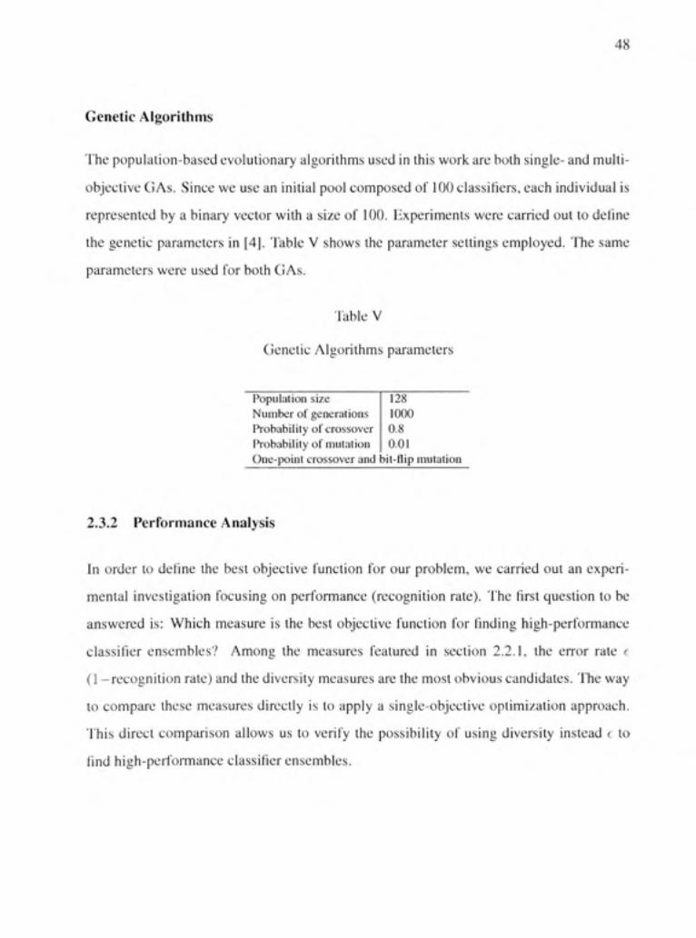
48
Genetic Algorithm s
The population-based evolutionary algorithms used in this work are both single- and multi-
objective GAs. Since we use an initial pool composed of 100 classifiers, each individual is
represented by a binary vector with a size of 100. Experiments were carried out to define
the genefic parameters in [4]. Table V shows the parameter settings employed. The same
parameters were used for both GAs.
Table V
Genetic Algorithms parameters
Population size Number of générations Probability of crossover F*robability of mutation
128 1000 0.8 0.01
One-point crossover and bit-flip mutation
2.3.2 Performanc e Analysi s
In order to define the best objective function for our problem, we carried out an expéri
mental invesfigation focusing on performance (récognition rate). The first question to be
answered is: Which measure is the best objective function for finding high-performance
classifier ensembles? Among the measures featured in section 2.2.1, the error rate e
(1 —récognition rate) and the diversity measures are the most obvions candidates. ITie way
to compare thèse measures directly is to apply a single-objective optimization approach.
This direct comparison allows us to verify the possibility of using diversity instead e to
find high-performance classifier ensembles.
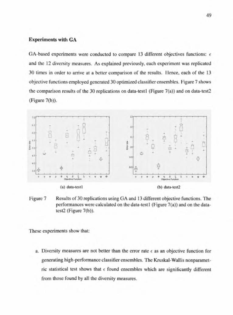
49
Experiments with G A
GA-based experiments were conducted to compare 13 différent objecfives functions: e
and the 12 diversity measures. As explained previously, each experiment was replicated
30 times in order to arrive at a better comparison of the results. Hence, each of the 13
objective functions employed generated 30 optimized classifier ensembles. Figure 7 shows
the comparison results of the 30 replications on data-testl (Figure 7(a)) and on data-test2
(Figure 7(b)).
70
6.5
6.0
55
50
45
4.0
35
—I 1 1 1 1 —
X
Ê? p è ^ ^ l - L
Otijeclive Functio n E y a p Q r \ 6 ^ X x K \ \ i < i >
Ob|ective Functio n
(a) data-testl (b) data-test2
Figure 7 Results of 30 replicafions using GA and 13 différent objective functions. The performances were calculated on the data-testl (Figure 7(a)) and on the data-test2 (Figure 7(b)).
Thèse experiments show that:
a. Diversity measures are not better than the error rate e as an objective function for
generating high-performance classifier ensembles. The Kmskal-Wallis nonparamet
ric statistical test shows that e found ensembles which are significantly différent
from those found by ail the diversity measures.

50
b. The most successful diversity measure was the difficulty measure 9. However, the
performance of the classifier ensembles found using this measure was, on average,
0.12% (data-testl) and 0.31% (data-test2) worse than that of the ensembles found
using e direcUy.
c. Fault majority A was the worst objective function. 'Fhis is a différent resuit from
those presented by Ruta and Gabrys [70]. l'hey observed that measures with better
corrélation with majority voting error, i.e. fault majority and double-fault Ô, are bet
ter objective functions for generating high-performance ensembles than the others.
We found that 5 was the third best diversity measure and A was the worst objective
function, even though there is no significant différence, according to the Kmskal-
Wallis statistical test, between A, coïncident failure, disagreement and enU opy on
data-testl, and among the three first measures on data-test2.
The results achieved using GA were expected, apart from those for A and 8. In fact, we
confirmed the results of previous work, e.g. [70] and [44], that diversity alone cannot
substitute for e as an objective function for finding the highest performing classifier en
sembles. Since diversity alone is no better than c, can we find better performing ensembles
by including both objective functions in the optimization process? We try to answer this
question using a multi-objective optimization approach in the next section.
Experiments with NSGA-I I
We continue our expérimental study using NSGA-II as the search algorithm. Fhe pre-
liminary study with GA suggested that diversity alone is not better than t for generating
the best performing classifier ensemble. This observation led us to use both t and diver
sity jointly to guide the optimization process with NSGA-II, since we hâve the option of
combining différent objective functions. The hope is that greater diversity between base
classifiers leads to the sélection of high-performance classifier ensembles.

51
3.85
3 80
3 75
370
365
3.60
3 55
3 5 0
3 45
340
T 1 1—
nmm s 4. 4 -
Obfedive Funclio n
(a) data-testl
>. T K \|; <P
Objeclive Funclio n X K f <I >
(b) data-test2
Figure 8 Results of 30 replications using NSGA-II and 13 différent pairs of objective functions. The performances were calculated on data-testl (Figure 8(a)) and data-test2 (Figure 8(b)). The first value corresponds to GA with the error rate e as the objective function while the second value corresponds to NSGA-II guided by e with ensemble size (.
Each diversity measure menfioned in section 2.2.1 was combined with e to make up pairs
of objective functions to guide the optimization process. Again, the optimization process
using each pair of objective functions was replicated 30 times. Figure 8 shows the results
of 30 repUcafions on data-testl (Figure 8(a)) and data-test2 (Figure 8(b)). It is important
to mention that the first value corresponds to the results using GA as the search algorithm
and e as the objective function. This means that we can compare the single- and multi-
objective results. The second value corresponds to the results using NSGA-II guided by
ensemble size (, with e as the objective functions (discussed in the next section).
Some observations can be made from thèse results:
a. By including both diversity and e in a multi-objective optimization process, we may
find more high-performance classifier ensembles than by using diversity alone; how
ever, the performance of thèse ensembles is still worse than the performance of the
ensembles found using ( in the single-objective optimization process.

52
b. The best diversity measures are difficulty 9, interrater agreement K., corrélation co
efficient p and double-fault à on data-testl. The Kmskal-Wallis test shows that the
first three measures found classifier ensembles with no significantly différent mean
ranks from those found using GA with c as the objective function on data-testl. On
data-test2, almost ail the diversity measure results were similar. According to the
Kxuskal-WalUs statistical test, except for coïncident failure a and 9, ail the diversity
measures found classifier ensembles with no significanfiy différent mean ranks on
data-test2. It is important to note that the différence between ensembles found using
diversity (multi-objective optimization) and ensembles found using only e (single-
objective optimization) was dramatically less. The classifier ensembles found using
the three best diversity measures were, on average, 0.05% worse than those found
using only e on data-testl and 0.13% worse on data-test2,
c. It is interesting to note that 9 found high-performance classifier ensembles on data-
testl, but, on data-test2, 9 yielded one of the worst performances. Such behavior
shows that thèse two data sets are actually very différent.
d. The two measures pointed oui by Ruta and Gabrys [70] as the best diversity mea
sures (6 and A) found better classifier ensembles on multi-objective than on single-
objective optimization, as was the case for ail the measures. However, especially
on data-testl, A was the worst measure, and, once again, was significantly différent
from the other measures, as shown by the Kxuskal-Wallis test.
As indicated in the beginning of this chapter, besides performance, we hâve to take into
account ensemble size when selecting classifier ensembles. In the following section, this
aspect is analyzed.

53
2.3.3 Ensembl e Siz e Analysis
Our ensemble size analysis relies on the analogy between feature subset sélecfion and
SOCS. In this sensé, discarding redundant classifiers could improve performance. Hence,
the minimization of the ensemble size ( is the most obvions objective funcfion to use to
achieve such a réduction in the number of classifiers. However, ( cannot be used in a
single-objective optimization process, because it might be combined with other measures
in order to increase performance while reducing the number of classifiers. In fine with
this idea, we combine ( with e and the 12 diversity measures described in section 2.2.1
to make up pairs of objecfive functions to guide the opfimization process using NSGA-
II. Figure 9 présents a graph containing the size of the classifier ensembles found in 30
replications generated by each pair of objective functions, while the performances are
shown in Figure 10 (10(a), data-testl and 10(b), data-test2). The first value corresponds
to the results obtained using GA as the search algorithm and e as the objective function in
order to arrive at a better comparison.
Figure 9 Size of the classifier ensembles found using 13 différent measures combined with ensemble size ( in paks of objective funcfions used by NSGA-II.

54
We also show the ensemble si/e of the classifier ensembles found in the first two séries
of experiments, i.e., single objective functions and diversity combined with e. This allows
us to better analyze the ensemble size issue. Figure 11 shows the ensemble size of the
classifier ensembles found with G A (Figure 11 (a)) and with NSGA-II combining e with
diversity (Figure 1 l(b)). Based on ail thèse results, we observe that:
65
6.0
5.5 15
^ 5 0 UJ
4.5
4.0
35 X
è + ^
[ J
;
r
) \ V
-+
= :
1
^
•»••
•+•
. 5 F :
•
[] X
•
•
.
•
95
g 8 5 •
—1 1 1 — +
+ -r
ù é J. +
±
* à U
-*- 4 -
è
Obiedive Funclio n e Ç Y O p ( t T | ô ^ X X i ç i j ( < ï »
Ob)ec1ive Funclion
(a) data-test l (b) data-test2
Figure 10 Performance of the classifier ensembles found using NSGA-II with pairs of objective functions made up of ensemble size ( and the 13 différent measures. Performances were calculated on data-testl (Figure 10(a)) and on data-test2 (Figure 10(b)).
a. Diversity combined with ( in pairs of objective funcfions does not find high-
performance classifier ensembles. Taking into account ail the results obtained in ail
the séries of experiments, the performances of the ensembles found using thèse pairs
of objective functions made up of ( and diversity showed the worst performances.
In contrast, those ensembles were the smallest. It is interesfing to note that, using
this combination of objecfive functions, NSGA-II converges to the same solution
at each replication, with the exception of the difficulty measure 9. The minimum
number of classifiers allowed by the search algorithms was 5. Fhis fixed minimum
ensemble size was defined to avoid generating too small classifier ensembles.

55
60
50
Ense
mbl
e siz
e
20
10
0
" 7
,8 •
. , E Y
_ ^
T ; ; ; i : ; ;
^
3 P
1. ; : :
^ " ^ à _ ,
: •
:
, 3 X] 6 t, k T K \ i ; < I > Objectve Functio n
(a) GA
50-
g 30
20
(b) NSGA-II
Figure 11 Ensemble size of the classifier ensembles found using GA (Figure 1 l(a)) and NSGA-II (Figure 1 l(b)). Each optimization process was performed 30 times.
b. The most successful diversity measure in terms of performance was 9. However, the
performance of the ensembles obtained using ( and e are better. According to the
Kmskal-Wallis statistical test, the performances are significantly différent.
c. The analogy between ESS and SOCS may be established. The performance of our
baseline System, i.e. the pool of 100 kNN (96.28% on data-testl), is 0.07% worse
than the average resuit using ( and e as the objective functions (average of 96.35%
on data-testl (Figure 10), while the averaged ensemble size is 27 classifiers (Figure
40). However, better performing classifier ensembles can be found using G A and
e. The Kxuskal-Wallis statistical test showed that the performances are significantly
différent. Moreover, the combination of ( and e as the objective funcfion did not
establish the best trade-off between thèse two measures. Interrater agreement K
combined with e generated smaller (24 classifiers on average) and better performing
classifier ensembles (96.41% and 92.16%, on average, on data-testl and on datâ
tes t2 respectively. Figure 8).

56
d. Ambiguity 7 combined with e, and Kohavi-Wolpert (/' combined with e, found the
largest classifier ensembles (45 classifiers on average). What is more interesting is
that, although we found the best performing classifier ensemble using GA as the
search algorithm and e as the objective function, such single-objective function did
not find the largest solutions.
2.4 Discussion
This chapter presented the expérimental results of a study using the single- and multi-
objective optimization processes to perform the sélection phase of SOCS. An ensemble
of 100 kNN classifiers generated using the Random Subspace method was used as the
initial pool of classifiers. Fourteen différent objective functions were applied: 12 diversity
measures, error rate and ensemble size. The experiments were divided into three séries. In
the first, the error rate and the 12 diversity measures were directly compared in a single-
optimization approach. In the second, the 12 diversity measures were combined with the
error rate to make up pairs of objective funcfions in a mulfi-optimization approach. Finally,
in the third, the error rate and the 12 diversity measures were combined with ensemble size
in pairs of objective functions, again in a mulfi-optimization approach.
'Fhe first séries of experiments was conducted in order to answer the first quesfion (1)
posed in the beginning of this chapter. Our results confirm the observafion made in pre
vious work that diversity alone cannot be better than the error rate at finding the most
accurate classifier ensembles. The difficulty measure was the best diversity measure when
the diversity measures are compared. In our attempt to answer question (2) when both the
error rate and diversity are combined in a mulfi-objective approach (second séries of ex
periments), we found that the performance of the solufions using diversity is much higher
than the performance of the solufions using diversity in a single-objecfive opfimization
approach. However, the performance of the classifier ensembles found using diversity
measures combined with the error rate to guide the sélecfion were still worse than the per-

57
formance of the ensembles found using only the error rate, although the différence was
reduced.
We are now able to establish an analogy between feature subset sélection and SOCS, in
response to question (3). By combining ensemble size and the error rate in a pair of ob
jective functions, we increased the initial pool of classifier performances and decreased
the number of classifiers to 27, instead of 100, from the initial pool. In contrast, diversity
measures achieved the worst performance in the third séries of experiments. Moreover,
the combined minimization of ensemble size and error rate was not the best pair of objec
tive funcfions to accomplish the trade-off between complexity and performance. In fact,
interrater agreement combined with the error rate established the best trade-off between
performance and ensemble size. We conclude, therefore, that it is not necessary to include
ensemble size in the optimizafion process. The réduction in the number of classifiers is a
conséquence of the sélection of classifiers, whatever the objective function used to guide
the search. Some objective functions generate smaller classifier ensembles, while others
generate bigger ones.
It is also important to observe that our experiments showed that ensemble size and di
versity are not confiicting objective functions (see Figure 9). We observe that we cannot
decrease the generalization error rate by combining this pair of objective functions. In
appendix 3, we présent further évidence to show why diversity and ensemble size are not
confiicting objective functions. Moreover, we can see in Table XXIV and Table XXV in
appendix 2, that the results obtained using diversity measures in a single-objective opti
mization approach are quite similar to the results obtained using diversity combined with
ensemble size in pairs of objective functions in a multi-objective optimization approach.
Hence, the minimum number of classifiers is achieved when using most of the diversity
measures in single-objective opfimization (see Figure 1 l(a)). 'Fhus, the results related to
the first séries of our experiments may be différent if the minimum number of classifiers
is fixed and larger than we hâve defined in this chapter, i.e. 5 classifiers.

58
Moreover, in this chapter, we conducted the optimization processes using, besides the
traditional optimization dataset, a validation dataset in order to avoid overfiUing during
the sélection phase of SOCS. Despite such apparent overfiUing conlrol, we observed that
this strategy fails to address the overfitting phenomenon since, although an independent
dataset was used to validate the solufions, the overfitfing phenomenon may sfiU be présent.
In the next chapter we show that overfitting can be detected at the sélection phase of SOCS
and présent stratégies to control overfitting.

CHAPTER 3
OVERFITTING-CAUTIOUS SELECTION O F CLASSIFIER ENSEMBLE S
We show in this chapter that overfitting can be detected during the sélection phase of
SOCS, this sélection phase being formulated as an opfimization problem. We attempt to
prove experimentally that an overfitting control strategy must be conducted during the
optimization process. In order to pursue our analysis on population-based evolufionary
algorithms, we keep using both single- and multi-objective GA. Taking into account this,
we investigate the use of an auxiliary archive A to store the best performing candidate
ensembles (or Pareto fronts in the MOGA case) obtained in a validation process using the
validation partition V to control overfitting. Three différent stratégies for update A hâve
been compared and adapted in this chapter to the context of the single- and multi-objective
sélection of classifier ensembles: (l) partial validation where A is updated only in the last
génération of the optimization process; (2) bach\>arding [67] which relies on monitoring
the optimizafion process by updating A with the best solufion from each génération; and
(3) global validation [62] updating A by storing in it the Pareto front (or the best solution
in the GA case) identified on V at each génération step.
Besides the ensemble of kNN created at the overproduction phase using the RSS method
in the previous chapter, two additional initial pool of classifiers are investigated in this
chapter: (1) a pool of DT created using bagging; and (2) a pool of DT created using the
RSS method. In addition, considering the results related to the analysis of search criteria
obtained previously, we use only four diversity measures (described in section 2.2.1) and e
to guide the optimization process presented in this chapter. Diversity measures are applied
by NSGA-II in combination with e in pairs of objective functions. Moreover, e, as well
as the diversity measures, are employed as single-objective functions by GA. To avoid
the problem of reaching a too small ensemble size, we defined a large fixed minimum
ensemble size for ail diversity measures in our experiments. It is important to mention

60
that in appendix 2, we carried out an overfitting analysis using both GA and NSGA-II,
guided by ail the objective funcfions and combinations of objective functions discussed
previously.
In this chapter, the global validation strategy is presented as a tool to show the relationship
between diversity and performance, specifically when diversity measures are used to guide
GA. The assumption is that, if a strong relationship exists between diversity and perfor
mance, the solution obtained by performing global validafion solely guided by diversity
should be close, or equal, to the solution with the highest performance among ail solutions
evaluated. This offers a new possibility for analyzing the relationship between diversity
and perf'ormance, which has received a great deal of attention in the literature [44; 17; 70].
Our objective in this chapter is to answer the following questions:
1. Which is the best sù^ategy employing an archive A for reducing overfitting at the
sélection phase of SOCS when this sélection is formulated as an optimization prob
lem?
2. Are classifier ensembles generated by bagging and RSS equally affected by overfit
ting in the sélection of classifier ensembles?
The following section demonstrates the circumstances under which the process of classi
fier ensemble sélecfion results in overfitfing. In section 3.2, three stratégies used to control
overfitting are introduced. The parameters employed for the experiments are described
in section 3.3, where the validation stratégies are applied using holdout and A--fold cross-
validation schemes. Finally, expérimental results are presented in section 3.3.
3.1 Overfittin g i n Selecting Classifier Ensemble s
The problem of selecfing classifier ensembles, using an optimization dataset O can be for
mulated as a leaming task, since the search algorithm opérâtes by minimizing/maximizing

61
the objective function, such as maximizing the classification perf'ormance or maximizing
the diversity of the members of a given ensemble Cf Indeed, Radtke et al. [62] showed
that multi-objecfive evolutionary optimization, such as the sélection of classifier ensem
bles, is prone to overfitting. We may define overfitting in the context of ensemble sélection
inspired by the définition provided by Milchell [49] in the following way. Let C* and C*'
be the besl performing candidate ensembles found through calculating the error rate e for
each élément of P(C) over samples contained in O and V respectively. Consider the clas
sification error e of thèse two candidate ensembles measured using samples from V. We
will dénote this classification error by e{V, C*) and e{V, C*'). In this setfing, C* is said
to overfit on O if an altemative candidate ensemble C*' G P(C) can be found such that
e ( V . C ; ) > e ( V , q ' ) .
The sélection process for classifier ensembles in SOCS is illustrated in Figure 12. An en
semble création method is employed using T to generate the initial pool of classifiers C.
'Fhus, the search algorithm calculâtes fitness on O by testing différent candidate ensem
bles. The best candidate ensemble C*' is identified in V to prevent overfitting. Finally, the
generalization performance of C*' is measured using the test dataset (G)- Hence, SOCS
requires at least thèse four datasets. It is important to mention that V is différent from
the validation dataset typically used to adjust base classifier parameters, such as weights
in MLP, the number of neighbors considered (k value) in kNN classifiers, etc. When
such parameter adjustment is necessary, a fifth dataset must be used, as was done in [62],
to avoid overly oplimistic performance as.sessment. The following sections describe how
overfitting can be detected in single- and multi-objective optimization problems performed
by GAs.
3.1.1 Overfittin g i n single-objective G A
In Figure 13, e is employed as Ihe objective function to guide G A using the NIST-digits
database as the problem and RSS as the method to generate C as a pool of 100 kNN clas-

'[
Ensemble Génération
Method C = {ci.c^,-. i C ^
x,,„
Optimization | Process
OVERPRODUCTION PHASE SELECTION PHASE
t
62
Figure 12 Overview of the process of sélection of classifier ensembles and the points of entry of the four datasets used.
sifiers. Thèse same parameters were investigated in last chapter, section 2.3.1. Although
GA was only guided by e, we show plots of e versus the ensemble's size to better illustrate
the process.
We dénote C(^) as the population of candidate classifier ensembles found at each généra
tion g and the best candidate ensemble found by evaluating ail individuals from C{g) on
O by Cj{g). Each point on the plot corresponds to a candidate ensemble Cj taken from
V{C) and evaluated during the opfimization process. Indeed, thèse points represent the
complète search space explored for max{g) = 1,000. The number of individuals at any
C(^) is 128.
Actually, the overfitting phenomenon measured when selecting classifier ensembles
présents a behavior very similar to what is seen in a typical Machine Learning process,
i.e. the chance that the search algorithm will overfit on samples taken from O increases
with the number of générations. This phenomenon can be observed in Figure 13(e), which
shows the évolution of e{0, C* ) in the search space. On the one hand, it is clear that the
optimization process could be stopped before overfitting starts to occur in this problem

63
m» c (Qvaluatod )
0 CJI I
ii!M^:/!iiji':'H'- :
20 3 0 4 0 5 0 6 0 7 0 8 0 9 0 10 0 Ensemble sue
(a) O dataset and g = l
ÊÊÊÊÊ-:
c. (evajualad)
0 Cj(l )
;!. :i '•'•/• :••-:... .
20 3 0 4 0 5 0 6 0 7 0 6 0 9 0 10 0 EnsemUa si; »
(b) V dataset and g = l
c (evaJualed )
0 C'(52 )
• • l ' . i . - . i - i ' ; , . • ! , - l ' i . , *-. .1 I , ' . , • *. •
^. . : : . : i i ; j l i i i i !! ' ; î : •"'•:••• : •••• •
-'iiiiP''' i|lii;'-!''i:i!î''i;
20 3 0 4 0 5 0 6 0 7 0 8 0 3 0 10 0 EnsembJo su e
(c) O dataset and g = 52
" ^ ^ ^
c (evaJualad )
0 C|(62 |
I..'>'••'.'•:.•',•':•.
20 3 0 4 0 5 0 6 0 7 0 8 0 3 0 10 0 Ensamble Si^ e
(d) V dataset and g = 52
;'i!::iii^fi
: - 1 >
ijiiil'!';. m i.li:'î;:''i- ••• ;: iMîiiii;.; •
• S 0 c ; •
o 0 | •
* • • : • .
•
20 30 40 50 60 70 80 90 100
(e) O dataset and max (g)
48
46
44
4 2
40
38
36
34
32
: | j jli|il|iii!!l ^
- C
0 o ; •
o c ' •
overiilting
•
20 3 0 4 0 5 0 e O 7 0 8 0 9 0 10 0
(0 V dataset and max{g)
Figure 13 Optimization using GA guided by e. Hère, we follow the évolution of C'j{g) (diamonds) from ^ = 1 to max{g) (Figures 13(a), 13(c) and 13(e)) on the optimization dataset O, as well as on the validation dataset V (Figures 13(b), 13(d) and 13(0)- The overfitfing is measured as the différence in error between C*' (circles) andC* (13(0)- There is a 0.30% overfit in this example, where the minimal error is reached slightly after g - r/i on V, and overfitting is measured by comparing it to the minimal error reached on O. Solutions not yet evaluated are in grey and the best performing solutions are highlighted by arrows.

64
using GA. On the other, it is difficult to define a stopping criterion to control overfitting in
a multi-objective optimization process, as explained in section 3.1.2.
3.1.2 Overfittin g i n MOGA
Figure 14 (left) illustrâtes the optimization process performed for max{g) — 1,000 using
NSGA-n guided by the following pair of objective functions: jointly minimize e and dif
ficulty measure (section 2.2.1) in the same problem investigated with GA in last section.
The Pareto front from population C{g) found in O is denoted by Ck{g). Thus, C^ (dia
monds) and C .' (circles) represent the final Pareto fronts found in O and V respectively.
Especially noteworthy in Figure 14(0 is that, besides the fact that the solutions over C^'
are différent from solutions over C ,, which was expected considering that V and O are dif
férent datasets, the nondominated solufions over C^' are discarded during the opfimization
process (Figure 14(e)). Hence, the définition of a stopping criterion for multi-objective op
timization problems is difficult for the following reasons: (1) solutions over Ck{g) found
during the optimization process may not be nondominated solutions over V and (2) since
the évolution of Ck{g) must be monitored on V, comparing sets of equally important so
lutions is a complex task. We show in the next section that the use of an auxiliary archive
A makes it possible to control overfitting taking into account thèse aspects.
3.2 Overfittin g Contro l Method s
The focus of this chapter is to evaluate stratégies that rely on using V to create an archive
A to control overfitting, since thèse memory-based stratégies may be appfied in any op
timization problem. The idea is to use the error rate measured on V as an estimation
of the generalization error. In order to accomplish the objectives of this chapter, we hâve
adapted two overfitting control stratégies to the context of classifier ensemble sélection for
both single- and multi-objective optimization problems: (1) backwarding originally pro
posed in [67] to prevent overfitting in GP; and (2) global validation proposed in [62] and

65
0 035 0 03 6 0 03 7 0 03 6 0 039 0 04 0 041 0 042 0 043 CSIticuliy Uaesur e
(a) O dataset and g = 1
. U (avalualad)
0 =.(' 1
:...• m..0' : -•»iw?'-'
0 035 0 036 0 037 0 038 0 039 0 04 0 041 0 042 0 043 Ortt'OJlty Measur e
(b) V dataset and 9 = 1
b 40
c (eveiuaied}
0 C,(15 ) , ^ * « - -
0 035 0 036 0 037 038 0 039 0 04 0 041 0 042 0 04 3 OillicuttY Meaaur a
(c) O dataset and g = 15
s 4 0
&
C (avalualad)
0 0,(15 |
^-<' ".... ^TjH
•
îySfi^- '
•
0 035 0 036 0 037 0 038 0 03 9 0 0 4 0 04 1 0 042 0 043 Dtllicuily Ueasur g
(d) V dataset and g = 15
48
46 0 ^K
0 035 0 03 6 0 03 7 0 03 8 0 039 0 04 0 04 t 0 04 2 0 043 ÛHioutiy Msasur e
(e) O dataset and max{g)
• c
0 = ;
iË^É 0'^ • T cvarliUin g
0 035 0 036 0 037 0 038 0 039 0 04 0 041 0 042 0 043 Drtliculty Meaaur q
(0 V dataset and max{g)
Figure 14 Optimization using NSGA-II and the pair of objective functions: difficulty measure and e. We follow the évolution of Ck{g) (diamonds) from g = l to max (g) (Figures 14(a), 14(c) and 14(e)) on the optimization dataset O, as well as on the validation dataset V (Figures 14(b), 14(d) and 14(f)). The overfitting is measured as the différence in error between the most accurate solution in C*^ (circles) and in C^ (14(f)). There is a 0.20% overfit in this example, where the minimal error is reached slighfiy after g = 15 on V, and overfitting is measured by comparing it to the minimal error reached on O. Solufions not yet evaluated are in grey.

66
[67] to control overfitting in multi-objective evolutionary optimization problems. Partial
validation, a control strategy iradilionafiy used to avoid overfitting in classifier ensemble
sélection problems [89] is also investigated. This is the strategy used in previous chapter.
It is interesting to note that thèse stratégies can be ordered with respect to the cardinality
of the solution set used for overfitting control: partial validation uses only the last popu
lation of solutions (or C . in the MOGA case) and backwarding validâtes the best solution
(or Cl{g)) at each g, while global validation uses ail solutions at each g.
It is important to note that the global validation strategy is employed in [62] in a complex
two-level System which includes feature extraction, feature sélection and classifier ensem
ble sélection, ail performed by MOGA. In this thesis, we adapt their strategy to single-
objective GA. As mentioned earlier, we use ensembles generated by bagging (BAG) and
RSS.
3.2.1 Partia l Validatio n (PV )
The first and simplest procédure relies on selecting C'*' at the end of the opfimization
process by validating the last population C{7nax{g)) (for GA) or C . (respectively for
MOGA). Consequently, in PV, it is assumed that, Cf G C{m.ax{g)) and C*' G 0;^.
Hence, there is only one update on A, more precisely for 'max{g). PV is summarized in
Algorithm 2.
Algorithm 2 Partial Validation
1: Créâtes initial population C(l ) of u; chromosomes 2: ^ - 0 3: fo r each génération g G { 1 , . . . ,max{g)} d o 4: perform ail genetic operators and generate new population C{g + 1). 5: en d fo r 6: validate ail solutions from C{rnax{g)) (for GA) or C; (for MOGA) 7: choose as C* the solution with highest récognition rate
8: update A by storing C*' 9: retur n C*' stored in A

67
3.2.2 Backwardin g (BV )
Overfitting remains uncontrolled even when PV is used, because C{tnax{g)) (for G A)
or C' for MOGA are composed of overfitted solutions, as explained in section 3.1. An
alternative to PV is to validate not only C{rnax{g)) (or C; .), but the C*{g) (or Ci,.{g))
found at each génération. ITie BV method [67] proposed for GP problems is based on this
idea. The authors advocate that GP is prone to overfitfing especially on later générations
as in Machine Leaming tasks. Motivated by this observation, they proposed BV to control
overfitting by monitoring the optimization process on V to détermine the point where GP
starts to overfit O. This approach uses A to store the best solution found before overfitting
starts to occur. Even though e is not the only objective function used to guide GA in this
chapter, we use e to represent the objective function in Algorithm 3, which shows how
BV is employed with GA. However, other objective functions can be used without loss of
gcnerality.
Where multi-objective optimization is concemed, Pareto fronts must be stored in A instead
of individual solutions. 'Faking into account that BV relies on comparing each new solution
found on O to the solution stored on A, this fact leads to the following question: How can
Pareto fronts be compared so as to identify whether or not one Pareto front is better than the
others. Because of the various tradeoffs over the Pareto front, the définition of a quality
measure is much more complex in multi-objective than in single-objective optimization
problems. Some quality measures such as the Pareto front spread, the objective functions
spread [103], the epsilon indicator and the coverage function [108] hâve been proposed. In
order to détermine whether or not the Ck{g) found at each génération is better than the C^'
stored in A, we propose to use the Pareto quality measure called the coverage function,
introduced by Zitzler et al. [108]. This measure was used in [61] to define a stopping
criterion for MOGAs.

68
Algorithm 3 Backwarding for GA
1: Créâtes inifial population C( l ) of u; chromosomes 2: A = ib 3: Find q ( l ) and set C*' : C*{1) 4: Store C]' in A 5: fo r each génération y G { 1 , . . . , max{g)] d o 6: perform ail genetic operators 7: generate new population C(y + 1) and find C*{g + 1) as usual
8: i f e ( V , q ) ( ( 7 + l ) < e ( V , C 7 ' ) t h e n
9: s e t C ; ' : = C 7 ( ( 7 + l ) 10: update A by storing in it the new C*' 11: en d if 12: en d fo r 13: retur n C*'stored on ^
The coverage function, measured on V, is based on the weak dominance criteria and indi
cates the number of candidate ensembles in Ck{g) that are weakly dominated by at least
one solution in C|.'. Given two solutions C, G C^' and Cj G Ck{g), we may say that Ci
covers Cj if C, is not worse than Cj in ail objective functions. The idea is to verify the
Pareto improvement among générations on A. Coverage can be denoted as:
cov{Ct,Ck{g)) (3.1)
In this way, the average number of solutions in C .' covering the solutions on Ck{g) is
calculated. 'Fhus, cov{Cl^,Ck{g)) < 1 or cou{C*f^,Ck{g)) = 1, whether C .' covers the
entire Pareto Ck{g) or not. The Pareto improvement at each génération is then measured
as:
im.p{Ck{g). C*') =r. 1 - coviCi;,Ck{g)) (3.2)
Improvement reaches its maximum (imp 1) when there is no solution on Ck{g) cov-
ered by solutions on Cl and its lowest possible value {imp ~~ 0), when ail solutions on

69
Ck{g) are covered by those on Cj^'. Consequently, the update of A is dépendent on the
improvement obtained between thèse two Pareto fronts. When imp > 0, ^ is updated;
otherwise, there is no update. The BV for MOGA is summarized in Algorithm 4.
Algorithm 4 Backwarding for MOGA
2 3: 4 5 6 7 8 9
10 11 12 13
Créâtes initial population C( l ) of u; chromosomes A^iè Find Cfc(l) and sel C^ ' :=CA.(1)
Store C .' in A for each génération ^, ^ G {1 max{g)} do
peri'orm ail genetic operators; generate C{g + 1) and find Ck{g + 1) as usual i{imp{Ck{g + 1), C^/) > 0 then
setC^':=Cfc(p + l) update A by storing in it the new C .'
end if end for return C ,' stored on A to pick up C*'.
3.2.3 Globa l Validatio n (GV)
There is a problem with BV because, since, at each génération, GA (or MOGA) créâtes
a population of solutions, C*{g) (or Ck{g) for MOGA) found on O may not be the best
solution (or Pareto front) on V. An approach avoiding such a limitation is global validation
GV [62; 100], which relies on using A to validate the entire populafion C{g) from each
génération.
GV works as follows in the context of multi-objective optimization (Algorithm 5): at each
g step, ail solutions are validated, and thus the set of non-dominated solutions found on V
is stored in A. When the optimization process is completed, two sets of non-dominated
solutions are available: (1) the traditional Cl found on O; and (2) C^', the set of non
dominated solutions found on V. In Figure 14(f), the solutions composing C' ' stored in A
are represented by circles. As can be observed in this figure, the solutions stored in A are
différent from the solutions over C^.

70
Algorithm 5 Global Validation for MOGA
1 2 3: 4 5 6 7: 8: 9
10
Créâtes initial population C( l ) of w chromosomes ^ - = 0 for each génération g G { 1 , . . . , 7nax{g)} d o
pert'orm ail genetic operators generate C(.g -(- 1) validate ail solutions in C{g + 1) over samples contained in V perform a nondominated sorting to C((/ + 1) U ^ to find C ,' update A by storing in it C .'
end fo r return Cj ,' stored in A
We propose to change Radtke et al.'s method [62] slightly to adapt it to single-objective
optimization problems. Since no Pareto front is involved when using GA, we are interested
in the best solution C*'. In this case, it is sufficient to validate ail solutions at each new
génération, find the best solution C*' (g) and compare it to C*', which is stored in A. In
this way, we keep the solution C*' found on V stored in A. Ixtting e represent the objective
function, the complète GV algorithm for GA is described in Algorithm 6.
Algorithm 6 Global Validation for GA
1 2 3 4 5 6 7
9 10 11 12 13 14 15
Créâtes initial population C( l ) of w chromosomes A = ^ Validate ail solutions in C( l ) over samples contained in V Find C';'(l) from C(l ) setr';':-r;'(i) for each génération ^ G { 1 , . . . , iriax{g)} d o
perform ail genetic opérations and generate C{g + 1) validate ail solutions m C{g + \) i\ndCfig+ 1) i f e ( V , C ; ' ) ( ^ + l ) < e ( V , C 7 ' ) t h e n
se tC ' ; ' :=C7' (5 + l) update A by storing in il the new C*'
end if end fo r return C*' stored in A
An example of the GV strategy for single-objecfive GA is illustrated in Figure 13(0- This
figure shows overfitfing when comparing e(V, C*') and e{V, C*). The ensemble Cf prob-

71
ably has higher generalization performance than C* obtained in O. In section 3.3, we
analyze such an assumption experimentally.
3.3 Experiment s
The parameters and the expérimental protocol employed are described in sections 3.3.1
and 3.3.2 respectively.
3.3.1 Paramete r Setting s on Experiment s
The databases, ensemble constmction methods, search algorithms and objective functions
used to conduct the experiments are defined in this section.
Databases
It is important to note that the databases must be large enough to be partitioned into the four
above-mentioned datasets: T, O, V and G, to perform experiments using the holdout val
idation strategy, as was done in the previous chapter. However, very few large databases
containing real classification problems are available in the literature. SOCS is gênerai
enough to be conducted using small datasets by applying /:-fold cross-vafidation. Ac-
cordingly, we performed experiments using both the holdout and 10-fold cross-validation
stratégies. Another important aspect taken into account in selecting the databases for our
experiments is that relatively high-dimensional feature spaces are necessary for the RSS
method.
Two databases were used in the holdout validation experiments: (1) NIST Spécial
Database 19 containing digits (NIST SD19), used in the previous chapter, which we call
NIST-digits hère; and (2) NIST SD19 containing handwritten uppercase letters, which we
caU NIST-letters hère. We use the représentation proposed by Oliveira et al. [52] for
both databases. Table VI lists important information about thèse two databases and the
partitions used to compose the four separate datasets. Thèse same partitions were used

72
in [89] for NIST-digits and in [61] for NIST-letters. We used the two test datasets from
NIST-digits, as was done in the previous chapter.
Table VI I describcs the three databases used in the 10-fold cross-validation experiments:
dna, texture and satimage. The Dna and satimage datasets are provided by Project Statlog
on www.niaad.liacc.up.pt/old/staUog; and textur e is available within the UCI machine
Learning Repository.
Table VI
Spécifications of the large datasets used in the experiments in section 3.3.3.
Dataset # uf Trainin g Optimizatio n Validatio n features Se t (T) Se t (C) Se t (V)
NIST-digits 132 5,000 10,000 10,000
NIST-letters 132 43,160 3.980 7,960
fable VII
Spécifications of the small datasets used in the experiments in section 3.3.4.
Dataset # of samples # of features Features RSS Pool C size m 45 m 40 20 100 36 8 100
Ensemble Construction Method s and Base Classifier s
We chose kNN and DT as the base classifiers in our experiments. The C4.5 algorithm [60]
(Release 8) was used to constmct the trees with pruning. In addition, we used A- = 1 for
kNN classifiers in ail databases without fine-tuning this parameter in order to avoid addi
tional experiments. BAG and RSS were applied to generate the initial pools of classifiers
in our experiments. 'IFiree initial pools of 100 classifiers were created: (1) 100 DT and (2)
Test Set (G)
testl 60,089 test2 58,646
12,092
Features RSS 32
32
PooIC size 100
100
dna texture satimage
3186 5500 6435

73
100 kNN, which were generated using RSS, and (3) 100 DT, which was generated using
BAG (BAG is mostiy effective with unstable classifiers, such as D'F). The size of the sub
sets of features used by RSS is shown in Table VI for large datasets and in Table VII for
small datasets. The same subspaces are used for both kNN and DT classifiers. Majority
voting was used as the combination function.
Objective Function s
In order to reduce redundancy in our experiments, we chose to employ only four diversity
measures: (1) difficulty measure (9), which was pointed out as the best diversity measure
when the diversity measures were compared in single-objective optimization problems; (2)
double-fault (6), which was one of the best diversity measure used in combination with the
error rate to guide NSGA-II, (3) coïncident failure diversity (a), which was chosen due to
the conclusions presented by Kuncheva and Whitaker [44] indicating that this measure is
less correlated to the other measures; (4) ambiguity (7) as defined in [104], which was not
investigated in [44]. Kuncheva and Whitaker [44] studied ten diversity measures. 'ITiey
conclude that thèse diversity measures may be divided into three différent groups, taking
into account the corrélation among measures: the double-fault alone; coïncident failure
diversity (also alone); and the remaining eight diversity measures.
In terms of ensemble size, we hâve shown in the previous chapter that the réduction in
the number of classifiers is a conséquence of the optimizafion task, whatever the objective
function used to guide the search. Hence, there is no need to explicitly include ensemble
size in the optimization process.
Genetic Algorithm s
The same parameters used in the previous chapter is also employed in our experiments in
this chapter.

74
3.3.2 Expérimenta l Protoco l
Our experiments were broken down into three main séries. In the first and second séries,
the holdout and 10-fold cross-validation stratégies were implemented to verify the impact
of overfitting in large and small databases respectively. The validation control methods
PV, BV and GV were also compared in order to détermine the best method for controlling
overfitting. Diversity measures were employed in pairs of objective functions combined
with e by NSGA-11, and only c was used to guide GA in both séries of experiments.
Finally, in the third séries, diversity measures were applied individually as single-objective
functions. As a resuit of this last séries of experiments, we show that the relationship
between diversity and performance may be measured using the GV strategy.
The sélection phase perf'ormed for large datasets was also replicated 30 times, as was
done in the previous chapter, owing to the use of stochastic search algorithms. To conduct
the 10-fold cross-validation experiments, the original whole datasets were divided into 10
folds. Each time, one of the 10 folds was used as G, another fold as V, a third as O and the
other 7 were put together to form T. Thus, T, O and V were used at the overproduction
phase to generate the initial pools of classifiers, to perform the optimization process and
to perform the three validation stratégies respectively. This process was repeated 10 times,
i.e. the optimization process was repeated for 10 trials. Il is also important to mention that
the sélection phase was replicated 30 times for each trial. Thus, the mean of the error rates
over 30 replications for each trial were computed and the error rates reported in ail tables
of results were obtained as the mean of the error rates across ail 10 trials.
Then, in both stratégies, the best solution for each mn was picked up according to the
overfitting control strategy employed. The solutions were tested on multiple comparisons
using the Kmskal-Wallis nonparametric statistical test by testing the equality between
mean values. The confidence level was 95% (a ^ 0.05), and the Dunn-Sidak correcfion
was applied to the critical values.

75
3.3.3 Holdou t validatio n result s
Table VIII shows the mean error rates obtained using both GA and NSGA-II search al
gorithms in NIST-digit s data-test l and data-test2 , and in NIST-letters . ITie error rates
obtained by combining the initial pool of 100 classifiers are also included in this table as
well as the results with no overfitting control, denoted NV.
Thèse experiments showed the following:
a. Fhe results from the fiterature [37], which conclude that complex leaming problems
are more affected by overfitting, are confirmed. There are more problems presenting
overfitting in NIST-digits data-test2 than in data-testl. As we mentioned in section
2.3.1, NIST-digits data-test2 is more difficult to use for classification.
b. NSGA-II is more prone to overfitting than GA. Even though, in the majority of the
experiments using GA, at least one of the validation methods slightly decreased the
error rates when compared with NV, the différences are not significant. In contrast,
thèse différences are more likely to be significant in experiments with NSGA-II. Of
36 cases using NSGA-II, an overfitting control decreased the error rates in 30. In 17
of thèse experiments, the différences were significant.
c. When overfitting was detected, GV outperformed both PV and BV. Fhe Kmskal-
WaUis test shows that, among 19 cases where overfitting control decreased the error
rates significanfiy, GV was the best strategy in 18 problems.
d. In terms of ensemble création methods, our results indicate an order relation be
tween the methods investigated for the NIST-digits database. BAG was more prone
to overfitting than RSS. In addition, ensembles of DT were less prone to overfitting
than ensembles of kNN, both generated using RSS. For the NIST-letters database,
the results were équivalent.

76
Table VIII
Mean and standard déviation values of the error rates obtained on 30 replications comparing sélection procédures on large datasets using GA and NSGA-II. Values in bold
indicate that a validation method decreased the error rates significanfiy, and underlined values indicate that a vafidation strategy is significantly better than the others.
NIST-digits - testl (lOOkNN = 3.72; lOODT-RSS = 2.92; lOODT-BAG = 5.65)
Metliod Va l NV PV
kNN-RSS 3 ^
GV NV PV
DT-RSS 3 ^
GV NV PV
DT-BAG g ^
GV
GA error (e)
3.60(0.06) 3.60 (0.06) 3.57 (0.07) 3.55 (0.06) 2.82 (0.05) 2.80 (0.05) 2.83 (0.05) 2.84 (0.06) 5.20 (0.07) 5.18(0.07) 5.18(0.05) 5.18(0.06)
NSGA-II ambiguity (7) coïncident (a) difficulty (0) double-fault (6)
3.66(0.06) 3.67(0.03) 3.64(0.05) 3.63(0.07) 3.70(0.07) 3.68(0.04) 3.63(0.05) 3.64(0.07) 3.70(0.07) 3.65(0.03) 3.63(0.07) 3.64(0.07) 3.63(0.06) 3.62(0.06) 3.60(0.08) 3.60(0.09) 2.96(0.10) 2.92(0.07) 2.81(0.03) 2.81(0.04) 2.97(0.10) 2.97(0.11) 2.83(0.02) 2.82(0.05) 2.97(0.10) 2.97(0.11) 2.83(0.02) 2.82(0.06) 2.94(0.08) 2.94(0.09) 2.82(0.06) 2.84(0.07) 5.73(0.07) 5.87(0.12) 5.67(0.06) 5.73(0.08) 5.71(0.08) 5.86(0.10) 5.68(0.05) 5.73(0.08) 5.71(0.08) 5.85(0.10) 5.69(0.05) 5.72(0.09) 5.54(0.06) 5.56(0.11) 5.55(0.09) 5.57(0.07)
NIST-digits - test2 (lOOkNN = 8.10; lOODT-RSS = 6.67; lOODT-BAG = 10.99) NV PV
kNN-RSS nV GV NV PV
DT-RSS 3 ^
GV NV PV
DT-BAG 3 ^
GV
7.91 (0.14) 7.89(0.12) 7.85(0.17) 7.80(0.13) 6.53 (0.08) 6.50 (0.09) 6.53 (0.09) 6.53(0.09) 10.16(0.15) 10.11 (0.15) 10.11(0.13) 10.09(0.13)
7.90(0.14) 8.09(0.16) 8.12(0.09) 8.12(0.09) 7.97(0.15) 8.11(0.18) 8.11(0.11) 8.14(0.12) 7.97(0.15) 8.10(0.18) 8.11(0.10) 8.14(0.14) 7.87(0.13) 7.94(0.15) 7.93(0.10) 7.93(0.13) 6.76(0.17) 6.77(0.14) 6.59(0.11) 6.60(0.10) 6.79(0.18) 6.88(0.21) 6.69(0.06) 6.65(0.11) 6.79(0.18) 6.88(0.21) 6.69(0.06) 6.65(0.12) 6.73(0.13) 6.76(0.12) 6.59(0.09) 6.63(0.13) 10.99(0.17) 11.28(0.28) 11.05(0.08) 11.13(0.08) 10.96(0.17) 11.25(0.23) 11.06(0.11) 11.12(0.21) 10.94(0.17) 11.24(0.24) 11.06(0.10) 11.10(0.14) 10.68(0.11) 10.76(0.22) 10.76(0.15) 10.83(0.07)
NIST-le«cr (lOOkNN = 6.60; lOODI-RSS = 6.06; lOODT-BAG = 7.63) NV PV
kNN-RSS 3 ^
GV NV PV
DT-RSS 3 ^
GV NV PV
DT-BAG 3 ^
GV
6.49(0.11) 6.50 (0.09) 6.47(0.12) 6.49 (0.09) 6.03 (0.07) 6.03 (0.07) 6.05 (0.09) 6.01 (0.09) 7.71 (0.10) 7.69 (0.08) 7.71 (0.10) 7.70 (0.08)
6.58(0.10) 6.73(0.25) 6.41(0.09) 6.55(0.13) 6.58(0.11) 6.71(0.26) 6.43(0.11) 6.60(0.12) 6.58(0.12) 6.71(0.26) 6.43(0.11) 6.58(0.12) 6.54(0.14) 6.50(0.13) 6.33(0.16) 6.45(0.12) 6.24(0.11) 6.34(0.19) 5.93(0.08) 6.10(0.12) 6.25(0.11) 6.34(0.19) 5.92(0.06) 6.11(0.12) 6.24(0.11) 6.34(0.19) 5.92(0.07) 6.03(0.13) 6.08(0.09) 6.12(0.14) 5.89(0.07) 6.02(0.10) 7.68(0.09) 8.00(0.14) 7.56(0.08) 7.78(0.12) 7.64(0.07) 8.08(0.18) 7.51(0.05) 7.78(0.13) 7.64(0.07) 8.03(0.16) 7.51(0.05) 7.76(0.12) 7.64(0.07) 7.87(0.14) 7.54(0.08) 7.64(0.12)

77
e. Although this thesis does not focus on comparing ensemble création methods in
terms of performance, our results indicate that ensembles generated with BAG per
formed worse than ensembles generated by RSS. Also, DT ensembles performed
better than kNN.
f. 'Fhe sélection of ensembles of classifiers was a better option than combining the
initial pools of classifiers. For NIST-digits , GA using e as the objective function,
and for NIST-letters , NSGA-II using 9 and e as the pair of objective functions,
found solutions better than the baseline composed of 100 classifiers in aU three
problems.
3.3.4 Cross-validatio n result s
Table IX summarizes the mean values and the standard déviation values achieved on the
three small datasets presented in 'Fable VIL We also report the error rates obtained on
combining the initial pools of classifiers by majority voting.
Based on thèse results, it may be observed that:
a. F'or small databases, NSGA-II was also more prone to overfitting than GA. The
overfitting control stratégies significantly decreased the error raies of the solutions
found by GA only in one case (dn a wilh kNN-based ensembles) out of nine, while
they significanfiy reduced the error rates of the solutions found by NSGA-II in 16
of 36 cases.
b. In 15 cases in which overfiUing was detected, the différence between the overfit
ting control methods was significant. GV was also the best strategy for controUing
overfitting in this séries of experiments.
c. Textur e is a highly stable database: it has the same class distribution and il can be
easily classified, since the error rates can be lower than 1% (see results obtained

78
Table IX
Mean and standard déviation values of the error rates obtained on 30 replications comparing sélection procédures on small datasets using GA and NSGA-II. Values in bold
indicate that a validation method decreased the error rates significanfiy, and underfincd values indicate when a validation strategy is significanfiy better than the others.
Texture (lOOkNN
Metliod
kNN-RSS
DT-RSS
DT-BAG
Val NV PV BV GV NV PV BV GV NV PV BV GV
GA error (e)
1.09(0.03) 1.09(0.04) 1.08(0.04) 1.11 (0.03) 2,54 (0.07) 2.52 (0.09) 2,55 (0.08) 2,51 (0,09) 3,58(0,10) 3,53 (0,08) 3.60 (0,08) 3,58 (0,08)
= 1,11; lOODT-RSS = 2,56; lOODT-BAG = 3,60) NSGA-II
ambiguity (7) 1,28(0.03) 1,40(0.06) 1,41 (0,06) 1.26(0,06)
2,94(0,11) 3,03(0,14) 3,04(0,15) 2.93(0.15) 3,60(0,09) 3,63(0,13) 3.62(0.11) 3.63(0,10)
coincident (a) 1.19(0.06) 1.21 (0.07) 1.21 (0.08) 1,18(0.08) 3,16(0,15) 3,41 (0,19) 3,42(0,15) 3,20(0,21) 4,09(0,15) 4.18(0,20) 4,17(0.18) 4.01 (0.15)
difficulty (61) 0,87 (0,03) 0.84 (0.03) 0.88 (0,04) 0.95 (0.05) 2.40 (0,05) 2,41 (0,06) 2,44 (0,06) 2,41 (0,09) 3,49 (0,09) 3,55 (0.08) 3.46(0.12) 3,43(0.11)
double-fault (ô) 0,90 (0.05) 0.94 (0,06) 0.89 (0.06) 0.98 (0,09) 3.00(0.14) 3,09(0,11) 3,10(0,10) 2,91 (0.18) 4,02(0,14) 4,14(0,19) 4.14(0.20) 4.04 (0,22)
kNN-RSS
DT-RSS
DT-BAG
DNAdOOkNN: NV PV BV GV NV PV BV GV NV PV BV GV
8.01 (0.27) 8,02 (0,2)
7.64 (0.24) 7.69 (0,23) 5.10(0,24) 4.99(0.18) 4.98 (0.25) 4.97(0,16) 5,00(0,10) 4,99(0,11) 4,98(0.15) 4,99 (0,08)
= 6,87; lOODT-RSS = 5,05; lOODT-BAG = 5.02) 9,61 (0,36) 9,85 (0,35) 9,82 (0.37) 8.60 (0.37) 6,44 (0,25) 6,76(0,31) 6.76 (0.30) 5.93 (0.29) 5,35 (0,14) 5,50(0.12) 5.51 (0.11 ) 5.36 (0.20)
10,60(0,51 10,85 (0,55) 10,76(0.52) 8.75 (0,45) 7,05 (0,43) 7,30 (0,46) 7.30 (0,47) 6.36 (0,42) 5,51 (0,22) 5.69 (0.20) 5,69 (0,20) 5,41 (0,21)
8,86 (0,22 8,93 (0,20) 8.85(0.21) 8.01 (0,33) 5,15(0,18) 4,96(0,12) 4,93(0.14) 4.77(0.17) 5,13(0,14) 5.08(0.12) 4,99(0.12) 4,93(0.13)
9.21 (0.35) 9,38 (0,39) 9,37(0,41) 8.36 (0.30) 6,20 (0,27) 6,31 (0,30) 6.30 (0.30) 5.67 (0,33) 5,55 (0,23) 5.35(0,14) 5,38(0,15) 5,54 (0,22)
Satimage (lOOkNN = 8.59; lOODT-RSS = 8,64; lOODT-BAG = 9.59)
kNN-RSS
DT-RSS
DT-BAG
NV PV BV GV NV PV BV GV NV PV BV GV
8.64 (0.09) 8,62 (0,07) 8,57(0,10) 8.58(0,11) 8,83(0,11) 8.80 (0,09) 8.81 (0,09) 8.82(0,12) 9,63 (0,09) 9,61 (0,07) 9,65(0,10) 9.63 (0.09)
8.76(0.12) 8,76 (0.09) 8,75 (0.09) 8.69(0.10) 8,92(0.11) 9.00(0.12) 9.00(0.10) 8.77(0.11) 9.81 (0,10) 9,81 (0.12) 9,82(0,12) 9.65(0,14)
9,12(0,16) 9.25(0.17) 9.23(0.18) 9,05(0.17) 9.44(0.20) 9,63 (0,22) 9,61 (0,23) 9.19(0,18) 10.40(0,19) 10.55(0.18) 10,53(0,17) 10,25 (0,22)
8,81 (0,23) 8,88 (0,25) 8,88 (0,26) 8.84(0.18 8,88(0.10) 8.93(0.12) 8,94(0.11) 8.75(0.13) 9.91 (0.13) 9,89 (0,09) 9,91 (0.09) 9.71(0,13)
9,15(0,14) 9,28(0,13) 9,33(0,14) 9,15(0,17) 9,25(0,19) 9,38(0,18) 9,39(0,17) 9.03(0,17) 10.14(0,18) 10.34(0,17) 10,35(0.16) 10,10(0,16)

79
using 9 and e to guide NSGA-II). Hence, it is not surprising that our results do not
show overfitting in this database.
d. For dna , overfitting was detected in the two problems involving ensembles gen
erated using RSS. For satimage , D'F-based ensembles generated using RSS were
more prone to overfitting than the other two methods. 'Fhus, unlike the NIST-digit s
results, BAG was less prone to overfitting than RSS for thèse two databases.
e. RSS-based ensembles presented lower error rates than BAG-based ensembles in ail
three databases.
f. The solutions found by NSGA-II guided by 9 and e were better than the baseline
combination for textur e and dna , except for ensembles of kNN for dna . However,
for satimage , sélection did not outperform combination.
3.3.5 Relationshi p between performanc e an d diversity
When GA was guided by diversity measures as single-objective functions, we observed
that a relationship between diversity measures and performance could be measured using
the GV strategy, as illustrated in Figure 15. The same optimization problem investigated
in section 3.1 is shown hère. GA was guided by the minimization of 9 as the objective
function. It is important to mention that the optimization was only guided by 9. The
reason for showing plots of e versus 9 in this figure is to demonstrate the relationship
between this diversity measure and performance.
Figure 15 shows aU Cj evaluated during the opfimization process (points) and C* (in
terms of 9 values) found on O. Il is interesfing to note that Figure 16 confirms that the
overfitting problem is also detected when 9 is the objective function used to guide GA,
since e(V,C'*) > e{V,C*'). Thus, in this example, there is an overfitting measured by
e(V, C*')-t{V, Cf) - 0.23. The use of GV allows us to keep {C*') stored in A. However,
Figure 16 also shows that C* is not the solution with the smallest t among ail candidate

80
5,0
4 8
4,6
4.4
4,2 B
5 4, 0 LU
3,8
3 6
34
3,2
-
-
-
3,0 0.035
Jt .'
0.036
^^^K**** • • j ^
0037
1 1 1 1
JET»
\
1 1 1 i
0,038 0.03 9 0 04 0.04 1 Difficulty Measur e
. C
0 ^i " o c " •
^ c . .
1
0.042 0.04 3
Figure 15 Optinfization using GA with fiie 9 as the objective function. ail Cj evaluated during the optimization process (points), C* (diamonds), ('*' (circles) and C'j (stars) in O. Arrows highlight C'j.
ensembles evaluated. In fact, the solufion denoted C'j is the candidate ensemble with
lowest e.
Thèse observations lead us to propose the use of GV as a tool to measure the relationship
between diversity and performance. ITie assumption is that there is a relationship between
thèse two measures when the generafization performance is increased by keeping the so
lution Cj' stored in A (based on diversity values). In addition, the relationship may range
from weak to strong, based on the différence (overfitting) between e(V, C*') and e{V,(''j).
For instance, since e{VX''j)- ({V,('*') = 0.05 in Figure 16, a 0.23'X' overfitting was con
trolled using GV and a 0.05% overfitting remains uncontrolled. Because this différence is
close to 0, 9 is strongly related to performance in this problem.
Taking into account that the relationship between diversity and performance has been mea
sured in the literature, using correlafion measures [44| and kappa-error diagrams [17] for
example, the use of GV offers a différent strategy for analyzing such a key aspect in the

81
. c 0 c ; o c '
overfitting
uncônt^llgdjçiyirfiîting "
3.0 0.035 0.036 0.037 0.038 0.039 0.04 0.041 0.042 0.043
Difficulty Measur e
Figure 16 Optimizafion using G A with the 9 as the objective function. Ail Cj evaluated during the optimization process (points), C* (diamonds), C* (circles) and Cj (stars) in V. Controlled and uncontrolled overfitfing using GV.
ensembles of classifiers fiterature. However, taking into account the results obtained previ
ously, there may be a drawback to this strategy: diversity measures are not independent of
ensemble size, i.e. when diversity measures are employed as single-objective functions, a
minimization of the number of classifiers may resuit. It is expected that ensembles which
are too small will perform considerably less well than other approaches [1; 50], such as
combining the initial pools of classifiers or selecting the best subset of classifiers using
GA only guided by e or MOGA guided by e combined with diversity.
To avoid the problem of reaching a too small ensemble size, we defined a large fixed mini
mum ensemble size for ail diversity measures in this séries of experiments. TTie minimum
ensemble size was fixed based on the médian size of the ensembles obtained using e as
a single-objective function calculated on the three small datasets described in Table VII.
Taking into account thèse results, we set the minimum ensemble size to 49 classifiers.

82
The four diversity measures investigated in this chapter were used in this séries of experi
ments. 'Fhe objective of the experiments was to verify which measure is the most closely
related to performance. The relationship between the four diversity measures and perfor
mance is measured by calculating the uncontrolled overfiUing 0 •^- ({y,C'f) - tiy, C'*').
The lower 0, the stronger the relationship.
Table X summarizes the results obtained. We hâve also included the results achieved using
GA guided only by e, so that the solutions found by ail five single-objective functions
investigated in this chapter can be compared. 'Fhese results are the same as those shown
in Fable IX.
Our results indicate that the différences among the results obtained with diversity measures
are smafi, except for dn a in RSS-based ensembles. In fact, we confirmed the results of
previous work, e.g. [70] and [44], that diversity measures are highly correlated. However,
our experiments reveal important information about the relationship between performance
and diversity. 'Faking into account the assumption that the doser to zéro the uncontrolled
overfitting, the stronger the relationship between the two measures, we can observe the
following results:
a. The diversity measure b was more closely related to performance. The uncontrolled
overfitting 0 was either zéro or as close as possible to zéro in 5 cases out of a total
of9 cases.
b. The diversity measure 7 was less closely related to performance. Fhe results ob
tained using 7 presented the highest 0 in 6 cases.
c. 9 was highly related to performance and appears to be better than t for guiding the
sélection of Ihe ensembles of classifiers. In 8 cases, 9 found solufions better than
those found using e as a single-objective funcfion. In addifion, the ensembles found

83
Table X
Mean and standard déviation values of the error rates obtained on measuring the uncontrolled overfitting. The relationship between diversity and performance is stronger
as 0 decreases. ' Fhe best resuit for each case is shown in bold.
Method
kNN-RSS
G A e = 1,11
DT-RSS
GAe = 2.51
DT-BAG
G A e = 3,58
Stratej^y
e(v,r;) Kv,r;)
<yxf) <ViC'^)
<V.Cf) e{y,c]) <t>
ambiguity (7)
1,20(0,04) 1,12(0,03) 0,08 (0,03) 2,80(0,04) 2,63 (0,08) 0,18(0,06)
3,59 (0,09) 3.61 (0,09) -0,02(0,09)
Texture coincident (a)
1.12(0,03) 1,09(0,04) 0.03 (0,04)
2,50 (0,08) 2,50 (0,07) 0,00 (0,07)
3,56(0,07) 3,61 (0,08) -0,05 (0,08)
difficulty (0) 1.01 (0.03) 1,09(0,04)
-0.08 (0.04)
2.40 (0,06) 2,43 (0,09) -0.03 (0,07)
3.48 (0,06) 3,.54 (0,06) -0,06 (0,06)
double-fault (6) 1,01 (0.02) 1,09(0,05)
-0.08 (0,03) 2,46 (0,07) 2,46 (0,09) 0.00 (0,08)
3,49 (0,06) 3,57 (0,08) -0.08 (0,07)
Dna
kNN-RSS
GAe = 7,69
DT-RSS GA e = 4.97
DT-BAG
GA e = 4,99
<vxf) <VX']) <p e(v,r;')
e(v,c;') e(v,c;)
10.6(0.00) 9.05 (0,00) 1.56 (0.00)
7,40(0,16) 5,17(0,18) 2,23(0,17)
5.02(0,11) 5,00(0,10) 0,03(0,10)
8.33(0,21) 8,00(0,33) 0,33 (0,27)
5.01(0,18) 5,09 (0,20) -0,07(0,19) 5,16(0,10) 5.08(0,10) 0,08(0.10)
7.50 (0,25) 8,44 (0,30) -0.94 (0,30)
4.50(0,16) 5.24 (0.22) -0,73(0,19) 4.93 (0,09) 5.05(0,12) -0,12(0,10)
7.89(0.16) 7,75 (0.29) 0,14(0,20)
4,67(0,10) 4,91 (0.19) -0,24(0,14) 4,94 (0,07) 5.01 (0,09) -0,07 (0,08)
Satimage
kNN-RSS
GA t = 8,58
DT-RSS
GAe = 8,82
DT-BAG
GA e = 9,63
<V,C*') <v,(-)
<vxf)
0 <vxf) <vx)) 4>
8,60 (0,09) 8.55 (0,07) 0.05 (0,08)
8.22(0,12) 8,11 (0,12) 0,11 (0,12)
9,61 (0,09) 9,66(0,15) -0,05(0,12)
8.58(0.11) 8.60(0,08) -0.02 (0.09)
8.77(0,11) 8.72(0,11) 0,05(0,11)
9.64(0,13) 9,65(0,13) -0,01 (0,13)
8,64 (0,08) 8,66(0,12) -0.02(0.10)
8.34 (0,03) 8,47(0,14) -0.10(0,08)
9.61 (0,09) 9,66(0,12) -0,05(0,10)
8.62(0,10) 8.62 (0,09) 0.00 (0.09)
8.67(0,11) 8,71 (0,11) -0,04(0,10) 9,71 (0,11) 9,70(0.10) 0,01(0,10)
using 9 presented the highest négative 0. What this means, in effect, is that guiding
GV using 9 is better than doing so using e.

84
d. Our results indicate that diversity measures can be effective objective functions for
selecting high-pert'ormance ensembles of classifiers. 'Fhis is a différent resuit from
those presented in the previous chapter. 'Fhe main problem is that diversity measures
are critically affected by ensemble size. Since we hâve fixed quite a large ensemble
size, i.e. 49 classifiers, diversity measure performances exceeded those of e.
3.4 Discussion
This chapter presented the expérimental results of a study comparing three overfitting
control stratégies adapted to the sélection phase of SOCS, which is performed as an op
timization problem using single- and multi-objecfive GAs. We showed that the task of
selecting classifier ensembles may be prone to overfitting, we pointed out Ihe best strat
egy for controlling overfitting and we presented a global validation strategy GV as a tool
to measure the relationship between diversity and performance. The following overfitting
control methods were investigated: (1) Parfial Validation, in which only the last population
of solutions is validated; (2) Backwarding, which relies on validafing each best solution
at each génération; and (3) GV, in which ail solutions at each generafion are validated.
Three initial pools of 100 classifiers were generated: 100 kNN and 100 D'F using RSS,
and a third pool of 100 DT using BAG. Five différent objecfive functions were applied: 4
diversity measures and e.
The experiments were divided into three séries. The three overfitfing control methods were
compared in two large databases (first séries of experiments) and in three small datasets
(second séries). The combination error rate e was employed as a single-objective function
by GA and the four diversity measures were combined with c to make up pairs of objective
functions to guide NSGA-II. iMnafiy, in the third séries of experiments, the four diversity
measures were directly applied by GA, and the GV strategy was performed to conlrol
overfitting. The objective in this third séries of experiments was to show that GV can be a
tool for idenfifying the diversity measure more closely related to performance.
85
The results show that overfitting can be detected at the sélecfion phase of SOCS, espe
cially when NSGA-II is employed as the search algorithm. In response to question (1)
posed in the beginning of this chapter, GV may be deemed to be the best strategy for con
troUing overfitting. In ail problems where overfitting was detected, in both large and small
databases, GV outperformed the other overfitting control methods. In response to ques
tion (2), our results indicate that RSS-based ensembles are more prone to overfitting than
BAG-based ones, even though the same behavior was not observed in ail databases inves
tigated. In terms of ensembles generated by RSS, our results globally showed that kNN
ensembles and DT ensembles are equaUy affected by overfitting. This aspect is totafiy
problem-dependent.
Finally, our results outlined a relationship between performance and diversity. Double-
fault 6 and ambiguity 7 were the diversity measures more and less closely related to per
formance respectively. Moreover, wc show that the difficulty measure 9 can be better than
e as a single-objective function for selecting high-performance ensembles of classifiers. Il
is important, however, to realize that quite a large minimum ensemble size (49) was fixed
for ail diversity measures. Such a size was defined based on the size of the ensembles
found by G A guided by e.
Although we were able to increase the generalizafion performance of the baseline initial
pools of classifiers by employing SOCS in chapter 2 and SOCS with overfitting control in
this chapter, the sélection of only one candidate ensemble to classify the whole test dataset,
does not guarantee that the candidate ensemble most likely to be correct for classifying
each test sample individually is selected. In the next chapter of this thesis we propose
a dynamic OCS in order to investigate whether or not the gain in performance can be
increased still further.

CHAPTER 4
DYNAMIC OVERPRODUCE-AND-CHOOS E STRATEG Y
In chapter 2 and chapter 3, we bave considered static overproduce-and-choose strategy
(SOCS). We bave investigated search criteria and search algorithms to guide the opfimiza
tion process and how this may be affected by the overfitting problem. We also presented
methods to control overfitting. The objective was to finding the most accurate subset of
classifiers during the sélecfion phase, and using it to predict the class of ail the samples in
the test dataset. In this chapter, wc propose a dynamic overproduce-and-choose strategy,
which relies on combining optimizafion and dynamic sélection to compose a two-level
sélection phase. The optimization process is conducted to generate candidate classifier
ensembles and the dynamic sélection is performed by calculafing a measure of confidence
to allow the sélection of the most confident subset of classifiers to label each test sample
individually.
In our approach, an ensemble création method, such as bagging or the random subspace
method, is applied to obtain the initial pool of candidate classifiers C at the overproduction
phase. 'IFius, the optimization process described in chapter 2 is assumed to be the first
level of the sélecfion phase. At this first level, a populafion-based search algorithm is
employed to generate a population C*' -^ {C'i,C'2,..., Cj,} of highly accurate candidate
ensembles Cj. This population is denoted C* to indicate that it was obtained by using the
validation process described in chapter 3. Assuming C* as the population found using the
optimization dataset, C* is the altemative population found using the validation dataset
to avoid overfitfing. At the second level proposed in this chapter, the candidate ensembles
in C*' are considered for dynamic sélecfion in order to identify, for each test sample x^g,
the solution C*' most likely to be correct for classifying it.

87
In fiie introduction of this thesis we mentioned that our objective by proposing a dynamic
overproduce-and-choose strategy is to overcome the following three drawbacks: Rather
than selecting only one candidate ensemble found during the optimizafion level, as is done
in SOCS, the sélection of C*' is based directly on the test patterns. Our assumpfion is that
the generalization performance will increase, since ail potential high accuracy candidate
ensembles from the populafion C*' are considered to sélect the most compétent solution
for each test sample. 'Fhis first point is parficularly important in problems involving Pareto-
based algorithms, because our method allows ail equally compétent solutions over the
Pareto front to be tested; (2) Instead of using only one local expert to classify each test
sample, as is done in traditional classifier sélection stratégies (both static and dynamic),
the sélection of a subset of classifiers may decrease misclassification; and, finally, (3)
Our dynamic sélection avoids esfimating régions of compétence and distance measures in
selecting ('*' for each test sample, since it relies on calculating confidence measures rather
than on performance.
Therefore, in this chapter, we présent a new method for dynamic sélection of classifier
ensembles. The proposed method relies on choosing dynamically from the population
C*' of highly accurate candidate ensembles generated at the opfimization level, the candi
date ensemble with the largest consensus to predict the test pattern class. We prove both
theoretically and experimentaUy that this sélecfion permits an increase in the "degree of
certainty" of the classification [29], increasing the generalization performance as a consé
quence. We propose in this thesis the use of three différent confidence measures, which
measure the extent of consensus of candidate ensembles to guide the dynamic sélection
level of our method. Thèse measures are: (1) Ambiguity; (2) Margin; and (3) Strength
relative to the closest class.
The first measure is based on Ihe definifion of ambiguity shown in Equafion 2.2, which in
dicates that the solufion with least ambiguity among its members présents high confidence
level of classification. 'Hie second measure, which is inspired by the définition of margin.

88
measures the différence between the number of votes assigned to the two classes with the
highest number of voles, indicating the candidate ensemble's level of certainty about the
majority voting class. Finally, the third measure also measures the différence between the
number of votes received by the majority voting class and the class with the second highest
number of votes; however, this différence is divided by the performance achieved by each
candidate ensemble when assigning the majority vofing class for samples contained in a
validation dataset. This additional information indicates how often each candidate ensem
ble made the right décision in assigning the selected class. Différent candidate ensembles
may hâve différent levels of confidence for the same class [8].
Besides thèse three new confidence measures, DCS-LA is also investigated. DCS-LA is
classical dynamic classifier sélection method [101]. It has been summarized in chapter
1, more precisely in section 1.2.1. We bave tailored DCS-LA to the sélection of classi
fier ensembles to be compared to the three confidence-based dynamic sélection methods.
Following the same expérimental protocol employed in chapter 3, in this chapter, bagging
and ihe random subspace method are used to generate ensemble members, while DT and
kNN classifiers are used for the création of homogeneous ensembles at the overproduction
phase, showing that the validity of our approach does not dépend on the particulars of the
ensemble génération method. Single- and multi-objective GAs are used to perform the
optimization of our DOCS, employing the same five objective functions for assessing the
effectiveness of candidate ensembles.
This chapter is organized as follows. Our proposed DOCS is introduced in section 4.1.
Then, sections 4.2 and 4.3 describe the optimization and dynamic sélecfion performed in
the two-level sélecfion phase by population-based GAs and confidence-based measures
respecfively. Finally, the parameters employed in the experiments and the results obtained
are presented in section 4.4. Conclusions are discussed in secfion 4.5.

89
4.1 Th e Proposed Dynamic Overproduce-and-Choose Strategy
The method proposed in this chapter does not follow the classical définition of DCS (see
section 1.2.1 in chapter 1), however, and so a partifion génération procédure is not needed
and the sélection level is not based on accuracy. Instead, our approach is based on the
définition of OCS, 'fraditionaUy, OCS is divided into two phases: (1) overproduction; and
(2) sélection. Fhe former is devoted to constructing C. The latter tests différent combi
nations of thèse classifiers in order to identify the opfimal solution, C*'. Figure 17 shows
that, in SOCS, C*' is picked up from the population of candidate ensembles, C*, found
and analyzed during the sélection phase, and is used to classify ail samples contained in
G- However, as mentioned in the introduction, there is no guarantee that the C* chosen is
indeed the solution most likely to be the correct one for classifying each Xjg individually.
^t
)
Ensemble _ Génération • Pool of classifiers
Method l e = {c,,C2,.. .,c„}
.First level - Optimizaliun Second level - Dynamic Selectioi^
OVERPRODUCTION PHASE SELECTION PHASE
Figure 17 Overview of the proposed DOCS. The method divides the sélection phase into optimization level, which yields a population of ensembles, and dynamic sélection level, which chooses the most compétent ensemble for classifying each test sample. In SOCS, only one ensemble is selected to classify the whole test dataset.
We propose a dynamic OCS in this chapter, as summarized in Figure 17 and Algorithm
7. The overproduction phase is performed, as defined in previous chapters, to generate

90
the initial pool of classifiers C. Thus, the sélection phase is divided into two levels: (1)
optimization; and (2) dynamic sélection. 'Fhe opfimization is performed by GAs guided
by both single- and multi-objective functions as was done in ail the experiments presented
throughout this thesis. According to the global validafion strategy defined in chapter 3 to
avoid overfitting at this level, the optimization dataset (O) is used by the search algorithm
to calculate fitness, and the validation V is used to keep stored, in the auxiliary archive A,
the population of /? best solutions for the GA or the Parelo front for NSGA-II found before
overfitting starts to occur. As explained below, in the single-objective GA case, hère we
keep stored in A ihe population of n best solutions rather than only one solution, as was
done in chapter 3. The population of solutions C* , is further used at the dynamic sélection
level, which allows the dynamic choice of C* to classify x,_g, based on the certainty of
the candidate ensemble's décision. Finally, C*' is combined by majority voting.
4.1.1 Overproductio n Phas e
In the overproduction phase, any ensemble génération technique may be used, such as
varying the classifier type [70], the classifier architecture [78], the leaming parameter ini
tialization [107], boosting [48], the random subspace method [72], etc. In this chapter, we
employ bagging (BAG) and the random subspace (RSS) method to generate C. RSS [32]
works by randomly choosing n différent subspaces from the original feature space. Each
random subspace is used to train one individual classifier c,. BAG is a bootstrap technique
[5] which builds rz replicate training data sets by randomly sampling, with replacement,
from T. Thus, each replicated dataset is used to train one c,.
In the following sections we describe the two levels of the sélection phase of our DOCS.
Since we hâve considered and described the optimization level in previous chapters, this
level is briefiy presented. We concentrate hère in our proposed dynamic sélection level.

91
Algorithm 7 Dynamic Overproduce-and-Choose Sfi-ategy (DOCS) 1 : Design a pool of classifiers C. 2: Perform the optimization level using a search algorithm to generate a population of
candidate ensembles C*'. 3: fo r each test sample x,_g do 4: i f ail candidate ensembles agrée on the label the n 5: classify x, ^ assigning it the consensus label. 6: els e 7: perform the dynamic sélecfion level calculafing the confidence of solutions in
8 9
10 11
13 14 15
if a winner candidate ensemble is identified the n sélect the most compétent candidate ensemble C*' to classify x,_g
else if a majority voting class among ail candidate ensembles with equal compétence is identified the n
12: assign the majority voting class to X; g else
sélect the second highest compétent candidate ensemble if a majority vofing class among ail candidate ensembles with the first and the second highest compétence is idenfified the n
16: assign the majority voting class to x,_g 17: els e 18: randomly sélect a candidate ensemble to classify x, g 19: en d i f 20: en d i f 21: en d i f 22: en d if 23: en d fo r
4.2 Optimizatio n Leve l
In order to clarify the proposed DOCS, we will use a case study obtained in one replication
using the NIST-letters database (section 3.3.1) throughout this chapter. The inifial pool of
DT classifiers was generated using RSS. The maximum number of générations is fixed at
max{g)^ 1,000.
Figure 18(a) depicts the optimization level conducted as a single-objective problem. Al
though GA was guided by the minimization of the error rate f as the objeclive function.

92
we show plots of e versus the difficulty measure 9 lo better illustrate the process. Again,
each point on the plot corresponds to a candidate ensemble, i.e. they represent ail solutions
evaluated for inax{g). 'fhe population C*' (circles) is composed of the n best solufions.
We fixed n — 21 (see secfion 4.4). In Figure 18(c), only the 21 best solutions are shown.
In SOCS, C*' is assumed to be the solufion with the lowest e (black circle in Figure 18(c)),
without knowing whether the C*' chosen is indeed the best solution for correctly classify
ing each x,,g. Hence, the additional dynamic sélection level proposed in this chapter is a
post-processing strategy which takes advantage of the possibility of dealing with a set of
high-performance solutions rather than only one. In this way, the whole population C*'
is picked up at the dynamic sélection level of our method. 'Hie parameter n should be
defined experimentally.
Figure 18(b) shows ail the classifier ensembles evaluated using NSGA-II guided by the
following pair of objective functions: joinUy minimize 9 and e. Hère, the Pareto front is
assumed to be C*' (circles in Figures 18(b) and 18(d)). Although the solutions over the
Pareto front are equally important, the candidate ensemble with the lowest e (black circle
in Figure 18(d)) is usuafiy chosen to be C*' in classical SOCS, as was done in [72] and
[89].
Considering this case study. Table XI shows the results calculated using samples from G
comparing SOCS and the combination of the initial pool of classifiers C. The sélecfion
of a subsel of classifiers using SOCS outperformed the combination ofC. Il is interesting
to observe that NSGA-11 was slightly superior to GA, and that the sizes of the candidate
ensembles in C* found using both GAs were smaller than the initial pool size. In addition,
NSGA-II found a C*' even smaller than the solution found by GA. Fhe assumption of
proposing an additional dynamic sélection level is that performance may still be increased
when selecfing C*' dynamically for each Xi,g.

93
Ensembles evaluale d C
O Populatio n o f the n besl ensembles C
0.058 0.058 5 0.05 9 0 0595 0 06 0 0605 0.06 1 0.061 5 0.06 2 0.062 5 Difficully Measur e
(a) GA - Evalualed solutions
Ensembles evalualed C
O Parol e frorfl c '
0 058 0 0585 0 059 0 0595 0 06 0 0605 0 061 0 0616 0 062 0 062 5 Difficully Measur e
(b) NSGA-II - Evaluated solutions
7.55
750
745
7 40 n 'X_ HJirrM? ^^^^'^
0 0584 0 0586 0 0588 0 059 0 0592 0 0594 0.059 6 0 0598 0.0 6 Difficully Measur e
(c) GA - nbest solutions
0 0584 0 0586 0 0588 0 059 0 0592 0 0594 0 0596 0 0598 0.0 6 Difficulty Measure s
(d) NSGA-11 - Pareto front
Figure 18 Ensembles generated using single-objective GA guided by e in Figure 18(a) and NSGA-II guided by 9 and r in Figure 18(b). 'Fhe output of the optimizafion level obtained as the n best solufions by GA in Figure 18(c) and the Pareto front by NSGA-II in Figure 18(d). Thèse results were calculated for samples contained in V. TTie black circles indicate the solutions with lowest e, which are selected when performing SOCS.
4.3 Dynami c Sélectio n Leve l
The sélection process in classical DCS approaches is based on the certainty of the classi
fiers décision for each parficular x^^. Consequently, thèse methods explore the domain of
expertise of each classifier to measure the degree of certainty of its décision, as described

94
Table XI
Case study: the results obtained by GA and NSGA-II when performing SOCS are compared with the resull achieved by combining ail classifier members of the pool C.
Optimization Erro r C* Averag e size Level rat e siz e o f Cj e C* Combination NSGA-11 (f & 0) GA (f)
6.06 5.86 5.90
100 45 55
-50 (2.50) 55 (3.89)
in secfion 1.2.1, chapter 1. The dynamic sélection level proposed in this chapter is also
based on décision certainty. However, instead calculating the confidence of each individual
classifier, our method calculâtes the confidence of each candidate ensemble that composes
C*', when assigning a label for Xjg. We show below that it is possible to calculate the
certainty of a candidate ensemble décision by measuring the extent of the consensus asso-
ciated with it. Fhe standpoint is that the higher the consensus among classifier members,
the higher the level of confidence in ihe décision.
Considering a classification problem with the following set of class labels fi =
{uj\,ijj2..., cJc}, the confidence level is related to theposteriorprobabilits' P(a;/t|xj_g) that
X, g comes from class io^- Hansen et al. [29] hâve observed that P(a'fc|x, g) may be calcu
lated in the context of an ensemble of classifiers by measuring the extent of the consensus
of ensembles, as given below:
Given the candidate ensemble Cj ^ {ci,C2 , 0} and the output of the v-th classifier
yj(x,,g), without loss of generalily, we can assume that each classifier produces a class
label as output. The number of votes v{u!k\^,g) for class LO^ given x,g is obtained as
follows:
•y(c^yt|X,,g) - \{C, : y,{X^,g) =~ UJk}\ (4.1 )

95
Assuming majority voting as the combination function, the consensus décision is:
i'iv{x,_g) = arg . 1 max f (Lc;/,.|x,,g) (4.2)
Thus, the extent of consensus on sample x,,g is:
P(...,x,„) = "''""'^fl"-'' (4.3 ) \Cj\
The extent of consensus measures the number of classifiers in agreement with the ma
jority voting. Consequenfiy, by maximizing the extent of consensus of an ensemble, the
degree of certainty that it will make a correct classificafion is increased. Another important
point to mention is that no information on the correctness of the output is needed. ITiese
observations allow us to présent three confidence measures that calculate the extent of
consensus of each candidate ensemble from the populafion C*', to be used at the dynamic
sélection level of our DOCS: (1) ambiguity, (2) margin, and (3) strength relafive to the
closest class. The first two measures are directly related to the évaluation of the extent of
consensus. The third measure also considers the candidate ensembles' performance mea
sured for each class involved in the classification problem. 'Fhis additional informafion is
calculated over samples contained in V. In addition, DCS-LA is adapted to the context of
DOCS to be compared to thèse three confidence-based stratégies.
4.3.1 Ambiguity-Guide d Dynami c Sélection (ADS )
The classification ambiguity proposed by Zenobi and Cunningham [104] attempts to esti
mate the diversity of opinions among classifier members. lliis diversity measure, which is
defined in Equation 2.2, chapter 2, appears to be well suited for the dynamic sélecfion level
we are proposing, since it does not need knowledge on the correctness of the décision.

96
It is important to note in Equation 2.2 that, if we calculate the ambiguity 7 for a particular
test sample x,,g instead of calculating it for the whole dataset, 7 becomes the complément
of the extent of consensus in Equation 4.3. Denoting 7 calculated for the given X;g as 7,
we may assume 7 + P(c<;fc|x, g) = 1. Thus, Equation 2.2 simplifies to:
7 = ^ E a , ( x , , g ) (4.4 )
Since such a local ambiguity measures the number of classifiers in disagreement with
the majority voting, the nfinimizalion of 7 leads lo the maximization of the extent of
consensus. Consequenfiy, the certainty of correct classificafion is increased. In addition,
although 7 does not take into account the label of the given sample, the minimization
of 7 also leads to the maximization of the margin in the case of a correct classification.
The so-called margin is a measure of confidence of classification. 'Hiere are two gênerai
définitions of margin reported in the literature [27]. The first définition is presented below
and the second is presented in section 4.3.2.
The classification margin for sample Xi,g is the following:
//(x,,g) = v{uJt\x,^g) - ^î;(u;fc|x,,g) (4.5)
where ^, is the true class label of x,,g. Hence, the margin measures the différence between
the number of votes assigned for the true class label and the number of voles given for
any other class. Consequently, the certainty of the classification is increased by trying to
maximize the margin. Based on the standpoints presented in this section, our dynamic
level guided by 7, denoted ADS, will pick up C*' as the candidate ensemble with lowest
7. The assumption is that the candidate ensemble with the lowest 7 présents the lowest
possibifity of making a mistake when classifying x,_g,

97
However, it is important to take into account the différence between 7 (Equation 2.2) and
7 (Equation 4.4). Fhe former, called global ambiguity in this chapter, is used to guide the
optimization level, and it is calculated for the whole dataset (O or V). Fhe latter, called
local ambiguity, is used in the dynamic sélection level calculated for each x, g individually.
Since the global ambiguity is a dissimilarity measure (see II I in chapter 2), it must be
maximized at the optimization level.
ADS is summarized in Figure 19. In this example, the output of the optimization level is
the Pareto front found by MOGA. 7 is calculated for each solution over the Pareto front.
Thus, the solution ('*' with the lowest 7 is selected and combined to assign the majority
voting class niv to the test sample Xj g.
4.3.2 Margin-base d Dynami c Sélection (MDS)
The second measure proposed for use in guiding dynamic sélection in our approach has
been inspired by the second définition of the margin. Following this définition, the margin
of sample x, g is computed as follows:
//(x,,g) :^ y(^;|x,,g) - max ky^tuM^i,g) (4.6)
This équation calculâtes the différence between the number of votes given to the correct
class v{LOt\:>c,^g) and the number of votes given to the incorrect class label with the highest
number of votes. In our approach, however, f (a;^|x,,g) is unknown, since the dynamic
sélection is performed for test samples. In order to employ this measure to guide the dy
namic sélection of our DOCS, we bave tailored the margin measure defined in Equation
4.6 to our problem. Considering y(m(;|x,_g) as the number of votes assigned to the major
ity vofing class, we propose to replace î;(u;/|x,,g) by v{mv\yii^g). In this way, the margin

98
Optimization Level
X;,,,
7c,(x,,s)-
ïcMi.g'r
ïcMi.g)-7C„(Xi,9h
argj^i min7c,(x, , j )
C]
Dynamic Sélection Level
Figure 19 Ambiguity-guided dynamic sélection using a Pareto front as input. The classifier ensemble with least ambiguity among its members is selected to classify each test sample.
of sample x,,g for each Cj from the population C*' may be calculated as follows:
/^(X«,g) j{mv\yii^g) - max k^rnvv{(^k\y^i,g) (4.7)
Hence, our définition of margin measures the différence between the number of votes as
signed to the majority vofing class and the number of votes assigned to the class with
second highest resuit. Fhen, the margin value represents the confidence of the classifi-
cafions, since the higher the margin from Equation 4.7, the higher the confidence of the
ensemble consensus décision. Thus, the dynamic sélection level guided by the margin,
denoted MDS, will choose as ('*' the candidate ensemble with the highest margin. For
instance, when //(Xjg) = 1 the majority vofing matches well to just one class, indicating
the highest level of certainty of correct classification.

99
4.3.3 Clas s Strength-based Dynami c Sélection (CSDS )
The définition of margin in Equation 4.6 also inspired this third confidence measure. Hère,
however, besides calculating Equation 4.7, we also consider the candidate ensemble's con
fidence with respect to the identity of the majority voting class measured in V. This is ad
ditional knowledge related to the performance achieved by each candidate ensemble when
assigning the chosen class. Our objective is to investigate whether or not performance may
help a confidence measure, which does not take into account the correctness of the output,
to increase the candidate ensemble's level of certainty of classification.
Strength relative to the closest class is presented in [8] as a method for defining weights in
DCS-LA. It is calculated for each individual classifier c, to verify whether or not the input
pattern is closely similar to more than one class. We bave adapted this measure to enable
us to calculate it for candidate ensembles Cj in the dynamic sélecfion of our DOCS.
Assuming Pj{mv) as the performance of Cj measured over samples contained in V for the
majority vofing class, strength relative to the closest class may be calculated for x,,g as
follows:
Q. , (t;(mt;|x,,g) - max k^^.,v{uk\y^,J)/\Cj\ '' Pjimv)
A low value of 0(xj,g) means a low level of certainty of correct classification. In contrast,
higher 0(x,,g) values lead to an increase in the level of confidence of classification. TTius,
the dynamic sélection level guided by 0 , called CSDS, will choose as C*' the candidate
ensemble with the highest 0(x,,g) to provide a label for x,,g.
4.3.4 Dynami c Ensembl e Sélection with Local Accurac y (DCS-LA )
As explained in secfion 1.2.1, DCS-LA dynamically sélects the most accurate individual
classifier from the population C to predict the label of the test sample x,,g. Local accuracy

100
is measured in the région of compétence composed as the set of k nearest neighbors from T
surrounding Xjg. Woods et al. [101] compared two stratégies to measure local accuracy:
(1) overall local accuracy; and (2) local class accuracy. 'Hie overall local accuracy is
computed as the number of neighbors correctly classitied by each classifier c,. However,
in this chapter, we use the second strategy, since Woods et al. bave concluded thaï this is
the strategy that achieves the better results.
Given the pool C and the class assigned by the 7-th classifier, tOy, to the test sample x,,g,
we dénote A ^ as the number of neighbors of x, g for which classifier c, has correctly
assigned class u)y, and Y2i=i ^'^ i ^e total number of neighbors labeled for c, as class iVy.
According to the définition provided in [101], local class accuracy estimation is computed
as follows:
!\jy cvc,(x, ,g)= (4.9)
Eli '
Taking into account that DCS-LA was originally proposed to deal with populations of
classifiers, as summarized in Equafion 4.9, it cannot be directly employed in problems in
volving populations of classifier ensembles. Thus, we propose lo change the DCS-LA with
local class accuracy estimation sfightly in order to allow it to be used to guide dynamic
sélection in our proposed approach. Given a population C* of candidate ensembles, we
assume ujy as the class assigned by the candidate ensemble Cj (composed of / classifiers)
to the test pattem x,g. We define as région of compétence the set of k nearest neighbors
from V surrounding x,,g. Clearly, DCS-LA can be criticaUy affected by the choice of the
k parameter. The local candidate ensemble's class accuracy is then estimated as follows:
acji^i.g) - TTH (4.10)

101
To summarize, in this chapter, ac- for pattem x,,g is calculated as the sum of the local class
accuracy (a^) of each classifier composing Cj, divided by the size ofCj. The higher ac^,
the greater the certainty of the décision. 'Fable XII shows a summary of the four différent
stratégies proposed for use at the dynamic sélection level of our DOCS.
fable XII
Summary of the four stratégies employed at the dynamic sélection level. The arrows specify whether or not the certainty of the décision is greater if the strategy is lower (J.) or
greater {]).
Name Ambiguity-Guided Dynamic Sélection Margin-based Dynamic Sélection Class Strength-based Dynamic Sélection Dynamic Ensemble Sélection with Local Accuracy
Label ADS MDS CSDS
DCS-LA
î / i (1) (î) (T) (T)
Using the case study menfioned in section 4.2, we compare, in Table Xni, the results
obtained in G using the combination of Ihe inifial pool C, SOCS and our DOCS employ
ing the four dynamic stratégies presented in this section. Thèse preliminary results show
that, except for CSDS, our dynamic method guided by confidence measures outperformed
SOCS performed by NSGA-II. In terms of the single-objecfive GA, static and dynamic
sélection methods presented similar results, except for CSDS and DCS-LA.
Fable XIII
Case study: comparison among the results achieved by combining ail classifiers in the inifial pool C and by performing classifier ensemble sélecfion employing both SOCS and
DOCS.
^Optimization Combinatio n SOC S AD S MD S CSD S DCS-L A NSGA-U(c&6») 6.06 5.86 5.74 5.7 1 6.01 5.74 GA(£) 6.06 5.90 5.90 5.88 6.13 5.98

102
Figures 20 and 21 show histograms of the frequency of sélecfion of each candidate en
semble performed using each dynamic sélection strategy presented in this section. 'Fhe
histograms in Figure 20 were obtained for the population C*' compo.sed of n best candi
date ensembles generated by GA shown in Figure 18(c), while the histograms in Figure
21 were obtained considering the Pareto front determined by II shown in Figure 18(d).
Especially noteworthy is the fact that the test set G used for the case study is composed
of 12,092 samples (Table VI), even though the dynamic sélection level was conducted
over only 325 and 436 of test samples for MOGA and GA respectively. Ail candidate
ensembles in C* agreed on the label for the remaining test samples.
Il is also important to observe in Figure 21 that ADS, MDS and DCS-LA more often
selected as C* the same candidate ensemble selected statically (C'i in Figure 18(d)). In
contrast, the opposite behavior is shown in Figure 20. TTiese results indicate why DOCS
did not outperform SOCS for the GA's population of candidate ensembles (see Table XIII).
In addition, two of the confidence-based dynamic stratégies, namely ADS and MDS,
more frequently selected the same candidate ensembles as selected by DCS-LA, which
is an accuracy-oriented strategy. Thèse results support our assumption that selecting the
candidate ensemble with the largest consensus improves the performance of fiie System.
Moreover, considering the results obtained by CSDS, we can conclude that measures of
confidence that do not take into account the correctness of the output provide enough in
formation about a candidate ensemble's level of certainty of classification. 'Fhe additional
information calculated by CSDS through measuring the performance of each candidate
ensemble over samples in V did not help in finding better performing ensembles. In next
section, we présent expérimental results lo verify whether or not thèse preliminary results
are gênerai, considering other databases and ensemble generafion methods.
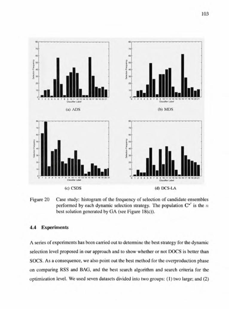
103
^ 3 0
0 1 2 3 4 5 9 1 0 1 1 1 2 1 3 1 4 1 5 1 6 1 7 1 6 1 9 20 2 1 Oassifier Labe l
(a) ADS
3 4 5 6 7 8 9 1 0 111 2 1 3 1 4 1 5 1 6 1 7 1 8 1 9 2 0 2 1 Classifier Labe l
(b) MDS
H 5 0
Lhdi 0 1 2 3 4 5 6 7 B 9 1 0 1 1 1 2 1 3 1 4 1 5 1 6 1 7 1 8 1 9 2 0 2 1
Classrlier Labe l
(c) CSDS
•î 3 0
0 1 2 3 4 5 7 8 9 1 0 1 1 1 2 1 3 1 4 1 5 1 6 1 7 1 Cfassifier Labe l
(d) DCS-LA
Figure 20 Case study: histogram of the frequency of sélection of candidate ensembles performed by each dynamic sélection strategy. The population C*' is the n best solution generated by GA (see Figure 18(c)).
4.4 Experiment s
A séries of experiments has been carried out to détermine the best strategy for the dynamic
sélecfion level proposed in our approach and to show whether or not DOCS is better than
SOCS. As a conséquence, we also point out the best method for the overproduction phase
on comparing RSS and BAG, and the best search algorithm and search criteria for the
opfimization level. We used seven datasets divided into two groups: (1) two large; and (2)

104
1 2 3 4 5 6 7 8 9 1 0 1 1 1 2 Classifier Labe l
(a) ADS
1 2 3 4 5 6 7 a 9 1 0 1 1 1 2 Classrlier Labe l
(b) MDS
—1 1 1 r — 100
90
r T I I
1 2 3 4 5 6 7 8 9 1 0 1 1 1 2 Classrfier Labe l
(c) (\SDS
1 2 3 4 5 9 1 0 1 1 1 2 Classrfier Labe l
(d) DCS-LA
Figure 21 Case study: histogram of the frequency of sélection of candidate ensembles performed by each dynamic sélection method. The population C*' is the Pareto front generated by NSGA-11 (.see Figure 18(d)).
five smaU, Tables VI and XIV respectively. TTie datasets from group 1 are the same large
datasets used in chapter 3. Therefore, they are large enough to be partitioned into the four
independent datasets, illustrated in Figure 17: T, O, V and G using the classical holdout
validation strategy for the evaluafion of performance. By contrast, 10-fold cross-validafion
is applied for the évaluation of performance using small datasets due to the small number
of samples available for évaluation.
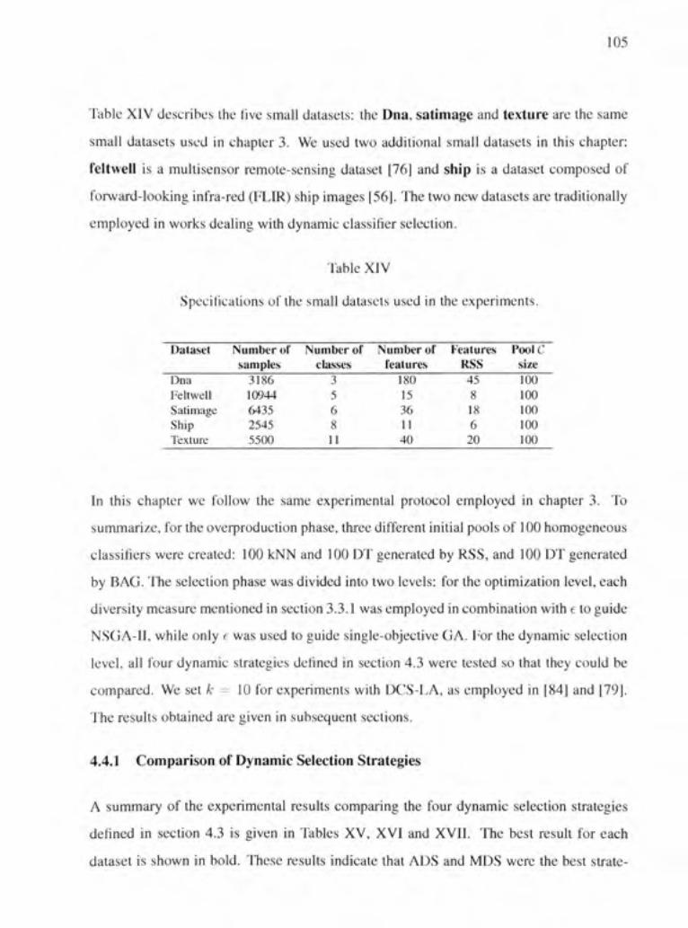
105
Table XIV describes the five small datasets: the Dna, satimage and texture are the same
small datasets used in chapter 3. We used two addifional small datasets in this chapter:
feltwell is a multisensor remote-sensing dataset [76] and shi p is a dataset composed of
forward-looking infra-red (FLIR) ship images [56]. The two new datasets are traditionally
employed in works dealing with dynamic classifier sélection.
Table XIV
Specificafions of the small datasets used in the experiments.
Dataset
Dna Feltwell Satimage Ship Texture
Number of samples
3186 10944 6435 2545 5500
Number of classes
3 5 6 8 11
Number of features
180 15 36 11 40
Features RSS 45 8 18 6 20
PooIC size 100 100 100 100 100
In this chapter we follow the same expérimental protocol employed in chapter 3. To
summarize, for the overproducfion phase, three différent inifial pools of 100 homogeneous
classifiers were created: 100 kNN and 100 DT generated by RSS, and 100 DT generated
by BAG. The sélection phase was divided into two levels: for the optimization level, each
diversity measure mentioned in section 3.3.1 was employed in combination with e to guide
NSGA-11, while only e was used to guide single-objecfive GA. For the dynamic sélection
level, ail four dynamic stratégies delined in section 4.3 were tested so that they could be
compared. We set k ~ 10 for experiments wilh DCS-LA, as employed in [84] and [79].
The results obtained are given in subséquent sections.
4.4.1 Compariso n o f Dynamic Sélection Stratégies
A summary of the expérimental results comparing fiie four dynamic sélection stratégies
defined in section 4.3 is given in Tables XV, XVI and XVII. The best resuit for each
dataset is shown in bold. ITiese results indicate that ADS and MDS were the best strate-

106
Table XV
Mean and standard déviation values obtained on 30 replications of the sélection phase of our method. The overproduction phase was performed using an initial pool of kNN
classifiers generated by RSS. The best resuit for each dataset is shown in bold.
Dataset
DNA
Nist-digits Testl
Nist-digits Test2
Nist-letters
Satimage
Ship
Texture
Method
DCS-LA ADS MDS CSDS DCS-LA ADS MDS CSDS DCS-LA ADS MDS CSDS DCS-LA ADS MDS CSDS DCS-LA ADS MDS CSDS DCS-LA ADS MDS CSDS DCS-LA ADS MDS CSDS DCS-LA ADS MDS CSDS
ambiguity (1)
9.33 (0.27) 10.31 (0.28) 10.34 (0.30) 10.56(0.30) 11.17(0.21) 10.51 (0.11) 10.51 (0.11) 10.57(0.10) 4.12(0.07) 3.80 (0.04) 3.80(0.04) 5.21 (0.09) 8.57(0.14) 8.11 (0.06) 8.12(0.07) 9.95(0.11) 7.63 (0.43) 7.23(0.17) 7.16(0.16) 10.15(0.45) 8.75 (0.08) 8.67 (0.08) 8.68 (0.09) 8.96(0.13) 14.24 (0.32) 13.25(0.24) 13.37(0.26) 14.06(0.25) 1.51 (0.06) 1.37(0.05) 1.37(0.05) 1.37(0.07)
NSGA-II coincident
(a) 9.84 (0.28) 9.72 (0.47) 9.57(0.41) 9.89(0.19) 10.46 (0.25) 10.34 (0.25) 10.34 (0.26) 10.40 (0.25) 4.59(0.17) 3.95 (0.05) 3.94 (0.05) 7.25 (0.26) 9.34 (0.28) 8.55 (0.08) 8.53 (0.09) 9.89 (0.33) 8.22 (0.69) 8.22(0.12) 7.07(0.11) 14.53 (0.63) 9.60(0.15) 9.05(0.17) 9.04(0.18) 10.13(0.24) 10.31 (0.29) 9.60 (0.33) 9.66(0.31) 10.17(0.34) 1.64 (0.08) 1.23(0.09) 1.22(0.09) 1.28(0.10)
difficulty (0)
7.48 (0.24) 7.51 (0.22) 7.47(0.21) 7.48(0.19) 9.70(0.14) 9.82(0.16) 9.82(0.14) 9.84(0.14) 3.72 (0.05) 3.58 (0.03) 3.58 (0.02) 3.80 (0.04) 8.18(0.11) 7.97 (0.05) 7.97 (0.05) 8.21 (0.08) 6.48(0.15) 6.48 (0.07) 6.27 (0.07) 6.47 (0.14) 8.73(0.13) 8.64(0.13) 8.65(0.14) 8.80(0.16) 9.34 (0.24) 9.25 (0.20) 9.24 (0.20) 9.39(0.21) 0.97 (0.05) 0.94 (0.05) 0.94 (0.05) 0.94 (0.06)
double-fault (ô)
9.36(0.30) 9.30 (0.23) 9.16(0.28) 8.36(0.30) 10..59(0.31) 10.62(0.28) 10.59(0.29) 10.66 (0.32) 4.43 (0.26) 7.49 (2.29) 7.46 (2.32) 6.67 (0.22) 9.48 (0.43) 8.40 (0.48) 8.36 (0.55) 9.42 (0.45) 7.20(0.33) 6.95(0.12) 6.88(0.12) 9.35(0.41) 9.40(0.13) 9.16(0.16) 9.16(0.18) 9.78(0.19) 9.24 (0.23) 9.13(0.21) 9.15(0.22) 9.31 (0.29) 1.02(0.07) 0.98 (0.07) 0.98 (0.07) 0.98 (0.09)
GA error
(0 7.47(0.15) 7.24(0.21) 7.24(0.15) 7.25(0.17) 9.87(0.13) 9.95(0.17) 9.95(0.16) 9.97(0.17) 3.60 (0.06) 3.53 (0.05) 3.53 (0.05) 3.80 (0.06) 7.91 (0.10) 7.78(0.10) 7.78(0.10) 8.09(0.10) 6.55(0.16) 6.43 (0.06) 6.41 (0.08) 6.70 (0.09) 8.63 (0.07) 8.61 (0.09) 8.61 (0.09) 8.67(0.11) 10.40(0.20) 9.81 (0.16) 9.83(0.13) 10.23(0.18) 1.18(0.03) 1.11 (0.01) 1.11 (0.02) 1.11 (0.03)
gies for performing the dynamic sélecfion level of our approach, considering ail three
ensemble creafion methods investigated, i.e. (I) ensemble of kNN; (2) ensemble of DT
generated through RSS (Tables XV and XVI); and (3) ensembles of DT generated by BAG

107
Table XVI
Mean and standard deviafion values obtained on 30 replications of the sélection phase of our method. The overproducfion phase was performed using an initial pool of DT
classifiers generated by RSS. llie best resuh for each dataset is shown in bold.
Dataset
D N A
Nist-digits Testl
Nist-digits Test2
Nist-le tiers
Satimage
Ship
Texture
Method
DCS-LA ADS MDS CSDS DCS-LA ADS MDS CSDS DCS-LA ADS MDS CSDS DCS-LA ADS MDS CSDS DCS-LA ADS MDS CSDS DCS-LA ADS MDS CSDS DCS-LA ADS MDS CSDS DCS-LA ADS MDS CSDS
ambiguity (7)
7.05(0.21) 7.94 (0.23) 7.92 (0.23) 8.01 (0.24) 12.68(0.19) 11.60(0.15) 11.59(0.14) 11.66(0.15) 3.82(0.12) 3.35 (0.04) 3.35 (0.04) 5,63 (0.09) 8.18(0.18) 7.38 (0.07) 7.34 (0.06) 9.05(0.14) 7.57 (0.30) 7.13(0.09) 7.12(0.09) 10.65(0.11) 9.30 (0.09) 8.73(0.10) 8.73(0.10) 9.13(0.13) 10.65 (0.30) 8.86(0.25) 8.94 (0.26) 9.97 (0.24) 3.42(0.17) 2.98 (0.08) 3.00 (0.08) 3.01 (0.08)
NSGA-II coincident
(o) 7.54 (0.28) 6.50 (0.29) 6.54 (0.30) 6.59 (0.28) 13.27(0.47) 12.71 (0.40) 12.74(0.42) 12.80(0.43) 5.37 (0.29) 4.11 (0.20) 3.83(0.13) 5.53(0.12) 10.06(0.50) 9.16(0.32) 8.61 (0.20) 8.77 (0.54) 6.12(0.50) 9.31 (0.29) 7.69(0.19) 15.92(0.14) 10.66(0.19) 9.22(0.19) 9.22(0.19) 11.23(0.24) 9.16(0.30) 8.26 (0.34) 8.26(0.32) 9.15(0.41) 3.85(0.14) 3.02(0.14) 3.04(0.14) 3.06(0.15)
difficulty iO)
4.63(0.15) 4.59(0.17) 4.63(0.17) 4.62(0.17) 11.65(0.32) 11.65(0.33) 11.65(0.32) 11.65(0.32) 2.91 (0.04) 2.77 (0.03) 2.77 (0.02) 2.98 (0.06) 6.79 (0.09) 6.45 (0.05) 6.50 (0.05) 6.50 (0.09) 6.03 (0.14) 5.84 (0.06) 5.84 (0.06) 5.98 (0.08) 8.97 (0.09) 8.64(0.10) 8.63 (0.09) 8.94(0.12) 7.53(0.18) 7.17(0.15) 7.18(0.15) 7.18(0.17) 2.47 (0.07) 2.35 (0.06) 2.35 (0.05) 2.35 (0.05)
double-fault (6)
7.23 (0.23) 6.27 (0.23) 6.27(0.19) 6.34 (0.22) 12.79(0.51) 12.51 (0.51) 12.49(0.48) 12.51 (0.50) 3.68 (0.20) 3.59 (0.23) 3.40(0.12) 4.47 (0.78) 8.07 (0.37) 8.11 (0.40) 7.80 (0.20) 8.69 (0.50) 7.20 (0.39) 7.12(0.14) 6.93(0.10) 10.95 (0.46) 10.12(0.15) 9.17(0.15) 9.16(0.15) 10.64 (0.26) 7.93 (0.29) 7.72 (0.28) 7.75 (0.29) 8.03 (0.27) 3.51 (0.16) 2.97(0.14) 2.65(0.16) 2.96(0.16)
GA error
(0 5.14(0.14) 4.95(0.18) 4.92(0.19) 4.93(0.19) 11.59(0.14) 11.50(0.17) 11.53(0.16) 11.51 (0.16) 2.89 (0.04) 2.77 (0.09) 2.77 (0.04) 3.12(0.06) 6.66 (0.08) 6.45 (0.05) 6.45 (0.05) 6.98(0.10) 6.17(0.14) 5.96 (0.06) 5.95 (0.06) 6.29 (0.09) 8.96(0.09) 8.78(0.12) 8.77(0.13) 8.86(0.12) 7.24(0.14) 6.98(0.14) 6.95(0.13) 7.35(0.12) 2.84 (0.09) 2.44) (0.05 2.44 (0.05) 2.44 (0.06)
(Table XVII). Thèse two dynamic stratégies presented équivalent performances, which
confirms the prefiminary results in our ca.se-study problem (see Table XIII). CSDS was
the worst dynamic sélection strategy for 1 and 3, while DCS-LA was most likely to be the
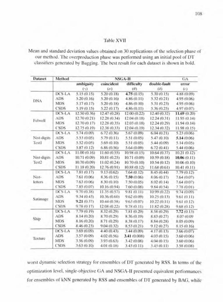
108
Table XVII
Mean and standard deviafion values obtained on 30 replications of the sélecfion phase of our method. The overproducfion phase was performed using an initial pool of DT classifiers generated by Bagging. 'Fhe best resuit for each dataset is shown in bold.
Dataset
DNA
Nist-digits Testl
Nist-digits Test2
Nist-letters
Satimage
Ship
Texture
Method
DCS-LA ADS MDS CSDS DCS-LA ADS MDS CSDS DCS-LA ADS MDS CSDS DCS-LA ADS MDS CSDS DCS-LA ADS MDS CSDS DCS-LA ADS MDS CSDS DCS-LA ADS MDS CSDS DCS-LA ADS MDS CSDS
ambiguity (7)
5.15(0.15) 5.20(0.16) 5.17(0.17) 5.19(0.15) 12.50(0.36) 12.70(0.21) 12.70(0.17) 12.75(0.19) 5.74 (0.09) 5.53 (0.05) 5.52 (0.05) 5.87(0.12) 11.00(0.16) 10.71 (0.09) 10.70 (0.09) 11.18(0.20) 7.81 (0.17) 7.61 (0.06) 7.63 (0.06) 7.85 (0.07) 9.70 (0.38) 9.34 (0.43) 9.21 (0.37) 9.78(0.17) 7.79(0.19) 8.14(0.20) 8.16(0.20) 8.46 (0.23) 3.69 (0.09) 3.57 (0.09) 3.56 (0.09) 3.63(0.10)
NSGA-II coincident
(a) 5.20(0.18) 5.20(0.16) 5.20(0.18) 5.22(0.17) 12.47(0.28) 12.28(0.34) 12.28(0.35) 12.38(0.33) 6.72 (0.36) 5.79(0.11) 5.69(0.10) 6.86 (0.56) 11.60(0.55) 10.81 (0.25) 11.02(0.24) 12.76(0.91) 9.13(0.62) 8.36(0.15) 8.30(0.10) 10.16(0.94) 11.35(0.57) 10.36(0.60) 10.44(0.58) 12.08(0.22) 8.32 (0.29) 8.70 (0.29) 8.71 (0.29) 9.04 (0.32) 4.40 (0.43) 4.02 (0.56) 3.93 (0.63) 4.01 (0.18)
difficulty (0)
4.75(0.15) 4.86(0.11) 4.86(0.10) 4.86(0.11) 12.00(0.22) 12.04(0.18) 12.03(0.18) 12.04(0.19) 5.67 (0.09) 5.51 (0.05) 5.51 (0.05) 5.64 (0.09) 10.98(0.15) 10.71 (0.09) 10.70(0.10) 10.88(0.12) 7.64(0.12) 7.50 (0.06) 7.50 (0.05) 7.60 (0.08) 9.81 (0.11) 9.62 (0.09) 9.63 (0.07) 9.78(0.11) 7.81 (0.29) 8.36(0.19) 8.38(0.17) 8.53(0.21) 3.44 (0.09)
3.41 (0.008) 3.42 (0.08) 3.43(0.11)
double-fault (S)
5.30(0.15) 5.32(0.21) 5.31 (0.23) 5.36 (0.25) 12.40(0.32) 12.24(0.31) 12.24(0.29) 12.34(0.32) 6.04(0.21) 5.47(0.10) 5.44 (0.09) 6.72(0.41) 10.64(0.37) 10.59(0.18) 10.54(0.12) 11.68(0.61) 8.45 (0.44) 8.06(0.17) 8.02(0.14) 9.84 (0.54) 10.99(0.22) 10.25(0.13) 10.22(0.11) 11.82(0.28) 8.58 (0.29) 8.83 (0.27) 8.84 (0.28) 9.12(0.27) 4.17(0.13) 4.03(0.15) 4.04(0.15) 3.43(0.11)
GA error
(e) 4.88 (0.09) 4.95 (0.06) 4.95 (0.06) 4.97 (0.07) 11.69(0.20) 11.95(0.14) 11.94(0.14) 11.98(0.15) 5.23 (0.06) 5.14 (0.06) 5.14(0.05) 5.44 (0.06) 10.21 (0.12) 10.06(0.11) 10.06(0.10) 10.41 (0.11) 7.79(0.12) 7.64 (0.07) 7.64 (0.07) 7.78(0.01) 9.74 (0.09) 9.61 (0.11) 9.61 (0.12) 9.68(0.12) 7.72(0.13) 8.07 (0.09 8.05 (0.09) 8.15(0.16) 3.66(0.07) 3.60(0.06) 3.60(0.06) 3.58 (0.08)
worst dynamic sélection strategy for ensembles of DT generated by RSS. In terms of the
optimization level, single-objective GA and NSGA-II presented équivalent performances
for ensembles of kNN generated by RSS and ensembles of DT generated by BAG, while

109
NSGA-II found the best results for populations of ensembles of DT generated by RSS. 9
was clearly the besl diversity measure for composing, with e, a pair of objective functions
to guide NSGA-11, while 7 and o were the worst diversity mea.sures.
Il is important to noie that DCS-LA was better than the oUier dynamic sélection stratégies
in 3 of the 8 datasets in problems involving DT generated by BAG. The reason for this
behavior is thaï BAG provides the complète représentation of the problem to each classifier
member, whereas RSS provides only a partial representafion. TTius, DCS-LA calculâtes
the local accuracy of each classifier more accurately when BAG is used as the ensemble
création method. Also important is the fact that CSDS was less effecfive in problems
involving a large number of classes, such as NIST-letters , because it takes into account
the performance of the candidate ensembles for each class involved in the classification
problem, in addition to the extent of consensus of the ensembles. Moreover, for the same
reason, CSDS is much more crifically affected by the quality of the population of candidate
ensembles found at the opfimization level. For instance, since 7 and o were the worst
objective functions when guiding the optimization level, CSDS was much worse than
the other three stratégies when used to perform the dynamic sélection on populations of
candidate ensembles found by Ihese two diversity measures.
4.4.2 Compariso n betwee n DOC S and Several Method s
In this section, we summarize the best results obtained by our DOCS for each dataset, in
order lo show that the proposed approach outperforms other related methods. Table XVIII
reports the results attained by the following methods:
• Fusion of the initial pool of classifiers C by majority voting;
• Sélection of the best individual classifier from the initial pool C;
• Individual kNNs and DTs trained using ail available features;
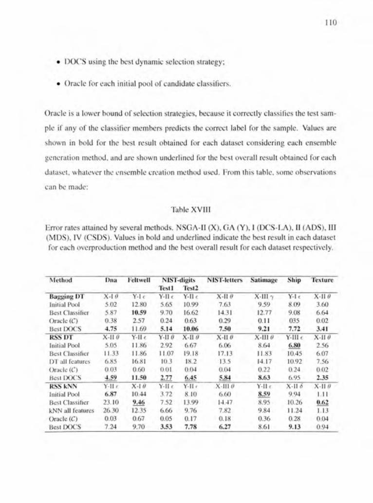
110
• DOCS using the best dynamic sélecfion strategy;
• Oracle for each initial pool of candidate classifiers.
Oracle is a lower bound of sélection stratégies, because it correctly classifies the test sam
ple if any of the classifier members predicts the correct label for the sample. Values are
shown in bold for the best resuit obtained for each dataset considering each ensemble
génération method, and are shown underlined for the best overall resuit obtained for each
dataset, whatever the ensemble création method used. From this table, some observations
can be made:
Table XVIII
Error rates attained by several methods. NSGA-II (X), GA (Y), I (DCS-LA), II (ADS), III (MDS), IV (CSDS). Values in bold and underlined indicate the best resuit in each dataset for each overproduction method and the best overall resuit for each dataset respectively.
Method
Bagging D T Initial Pool Besl Classifier Oracle (C) Best DOCS RSSDT Initial Pool Best Classifier DT ail features Oracle (C) Best DOCS RSS kN N Initial Pool Best Classifier kNN ail features Oracle (C) Best DOCS
Dna
X-10 5.02 5.87 0.38 4.75
x-ne 5.05 11.33 6.85 0.03 4.59 Y-llf 6.87 23.10 26.30 0.03 7.24
Feltwell
Y-l€ 12.80 10.59 2.57 11.69 Y-IIe 11.86 11.86 16.81 0.60 11.50 X-10 10.44 9.46 12.35 0.67 9.70
NIST Testl Y-lIe 5.65 9.70 0.24 5.14
Y-II^ 2.92 11.07 10.3 0.01 2.77 Y-lle 3.72 7.52 6.66 0.05 3.53
•digits Tesl2 Y-lIe 10.99 16.62 0.63 10.06 x-n0 6.67 19.18 18.2 0.04 6.45 Y-IW 8.10 13.99 9.76 0.17 7.78
NIST-letters
X-IIé» 7.63 14.31 0.29 7.50
X-n0 6.06 17.13 13.5 0.04 5.84
X-111 6» 6.60 14.47 7.82 0.18 6.27
Satimage
X-111 7 9.59 12.77 0.11 9.21
X-III 0 8.64 11.83 14.17 0.22 8.63 Y-Ilf 8.59 8.95 9.84 0.36 8.61
Ship
Y-le 8.09 9.08 035 7.72
Y-III e 6.80 10.45 10.92 0.24 6.95
X-11 S 9.94 10.26 11.24 0.28 9.13
Texture
X-U0 3.60 6.64 0.02 3.41
X-Hé» 2.56 6.07 7.56 0.02 2.35
X-U0 1.11 0.62 1.13 0.04 0.94

111
• Analyzing the results obtained for ensembles of DT generated using BAG, our
DOCS outperformed the other methods, except for feltwell . Fhe same scénario
was observed for ensembles of DT generated using RSS, but the excepfion was the
ship dataset. For ensembles of kNN generated using RSS, however, the proposed
method outperformed the other methods in only 4 of the 8 cases. For the remaining
4 datasets, our DOCS was the second best method. 'Fhe combinafion of the initial
pool C was the best method for dna and satimage while the individual best classifier
from C was the best method for feltwel l and texture .
• Confidence-based dynamic stratégies were better than DCS-LA for performing the
dynamic sélection of the sélection phase. Even though ADS and MDS presented
similar behavior, we show in Table XVlll values obtained using ADS to perform
Ihe comparison in next section.
• The search algorithms presented équivalent performances. The best results found
using DOCS were obtained in populations of candidate ensembles optimized by
NSGA-II in 13 cases and by single-objective GA in 11 cases out of a total of 24
cases investigated.
• 9 was the best diversity measure for combining with e to guide NSGA-II.
• RSS was better than BAG for use during the overproduction phase. Results obtained
using ensembles generated by RSS were both better than those obtained using en
sembles generated by BAG.
• DT was the best classifier model to be used as a base classifier during the overpro
duction phase. Five of the best overall results were obtained with ensembles of DT,
whereas in the remaining three datasets they were obtained with ensembles of kNN.
Both ensembles were generated by RSS.

112
Table XIX présents some of the results reported in the literature dealing with the sélection
of classifiers, except for références [32] and [66], on the databases used in this chapter. In
this way, it is possible to gain an overview of the results obtained in the literature, even
though the method of partition of the data used in some of thèse works was nol the same
as that used in this chapter.
Table XIX
The error rates obtained, the data partifion and Ihe sélection method employed in works which used the databases investigated in this chapter (FSS: feature subset sélection).
Database
Dna Feltwell NIST-digits Testl NIST-letters Satimage Ship Texture
Référence Number
[32] [15] [89] [61] [15] [66] [101]
Ensemble Création
RSS Het RSS FSS Het Het DT
Classifiers Members
DT Het
kNN MLP Het Het Het
Partition Strategy Holdout Cross-validation Holdout Holdout Cross-validation Holdout Holdout
Sélection Type
Fusion DCS-LA
SOCS SOCS
DCS-LA Fusion
DCS-LA
Error (%) 9.19 13.62 3.65 4.02 10.82 5.68 0.75
To verify whether or not our DOCS is better that the classical SOCS, in the next section,
we concentrate our analysis on the methods that attained the best results in this section,
i.e. DT ensembles generated by RSS, ADS as dynamic strategy; MOGA guided by 9 in
combination with e; and GA guided by e.
4.4.3 Compariso n o f DOCS and SOCS Result s
The static sélection results were obtained by picking up the candidate ensemble presenting
the lowest e value of ail the solutions composing the n best solution (for single-objective
G A) or the Pareto front (for NSGA-11). Thèse ensembles are represented in Figures 18(c)
and 18(d) by black circles. It is important to mention that the results were tested on mul
tiple comparisons using the Kruskal-Wallis nonparametric statistical and the confidence
level was 95% (Q = 0.05), as was done in previous chapters.
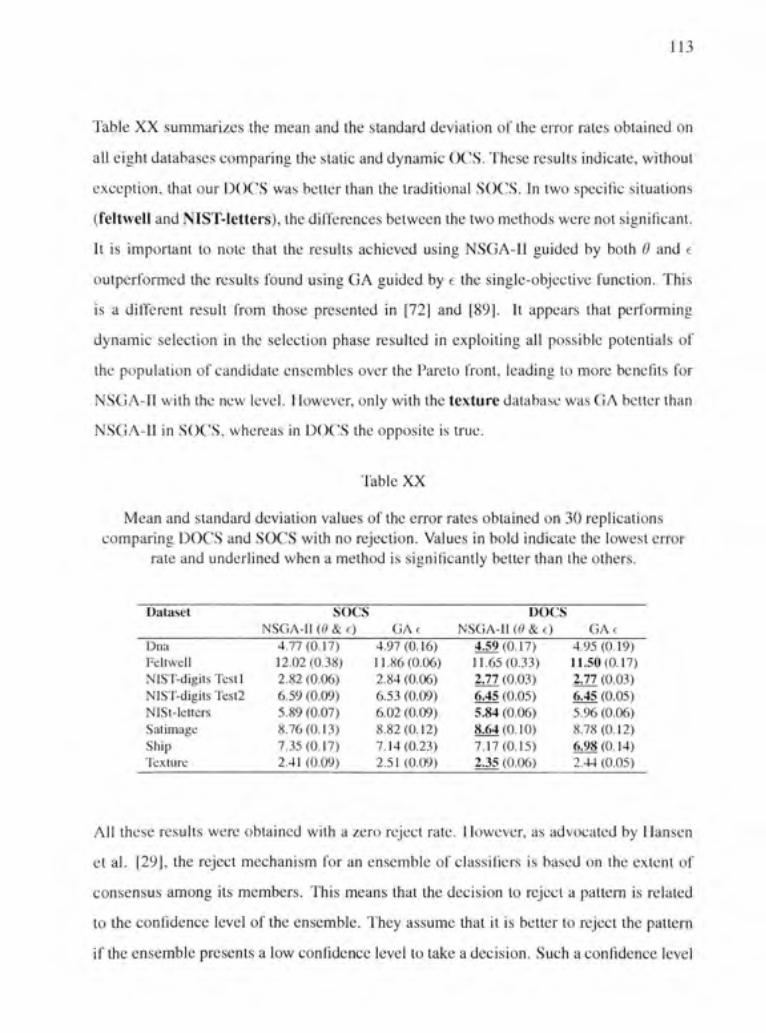
113
Table XX summarizes the mean and the standard déviation of the error rates obtained on
aU eight databases comparing the stafic and dynamic OCS. 'Fhese results indicate, without
exception, that our DOCS was better ihan the traditional SOCS. In two spécifie situations
(feltwell and NIST-letters), the différences between the two methods were not significant.
It is important to note that the results achieved using NSGA-II guided by both 9 and e
outperformed the results found using GA guided by e the single-objective function. This
is a différent resuit from those presented in [72] and [89]. It appears that performing
dynamic sélection in the sélection phase resulted in exploiting ail possible potenfials of
the population of candidate ensembles over the Pareto front, leading lo more benefits for
NSGA-II with Uie new level. However, only with the texture database was GA better Ihan
NSGA-II in SOCS, whereas in DOCS the opposite is true.
Table XX
Mean and standard déviation values of the error rates obtained on 30 replications comparing DOCS and SOCS with no rejection. Values in bold indicate the lowest error
rate and underlined when a method is significantly better than Ihe others.
Dataset
Dna Feltwell NIST-digits Testl NIST-digits Test2 NlSt-letters Satimage Ship Texture
SOCS NSGA-11 (0 & f)
4.77(0.17) 12.02(0.38) 2.82 (0.06) 6.59 (0.09) 5.89 (0.07) 8.76(0.13) 7.35(0.17) 2.41 (0.09)
GAe 4.97(0.16) 11.86 (0.06) 2.84 (0.06) 6.53 (0.09) 6.02 (0.09) 8.82(0.12) 7.14(0.23) 2.51 (0.09)
DOCS N.SGA-11 (0 & e)
4.59(0.17) 11.65(0.33) 2.77 (0.03) 6.45 (0.05) 5.84 (0.06) 8.64(0.10) 7.17(0.15) 2.35 (0.06)
GAe 4.95(0.19) 11.50(0.17) 2.77 (0.03) 6.45 (0.05) 5.96 (0.06) 8.78(0.12) 6.98 (0.14) 2.44 (0.05)
Ail thèse results were obtained wilh a zéro reject rate. However, as advocated by Hansen
et al. [29], the reject mechanism for an ensemble of classifiers is based on the extent of
consensus among its members. This means that the décision to reject a pattem is related
to the confidence level of the ensemble, l'hey assume that it is better to reject the pattem
if the ensemble présents a low confidence level to take a décision. Such a confidence level

114
is clearly related to 7 (Equation 4.4), which is used to guide ADS. Thus, since 7 is the
criterion used to perform the reject mechanism, we might assume that the différence be
tween SOCS and DOCS will increase as the rejection rate increases. We analyze such an
assumption in Figure 22 taking into account the case study problem investigated through
out this chapter. 'This prefiminary resuit does not confirm this assumpfion. Both the stafic
and the dynamic OCS presented similar error-reject curves for ensembles generated by
GA 22(a) and NSGA-11 22(b).
? 3 -
- SOC S [xx :s • socs
DOCS
Reied 20% 25 % 30 % 35 % 40 % 45 % 50 %
Reject
(a) GA (b) MOGA
Figure 22 Case Sfiidy: En-or-reject curves for GA (22(a)) and NSGA-11 (22(b)).
In order to show more gênerai results about the error-reject tradeoff, we fixed four différent
reject rates: 0.5% and 1.0% (Table XXI), 5.0% and 10.0% (Table XXII), to investigate ail
the problems dealt with in this chapter. Fhese results confirm that we should not assume
that DOCS is more effective than SOCS when increasing the rejection rate.
4.5 Discussio n
We propose a dynamic overproduce-and-choose strategy which is composed of the tradi
tional overproduction and sélection phases. The novelty is to divide the sélection phase
into two levels: optimizafion and dynamic sélection, conducting the second level using

115
Table XXI
Mean and standard déviation values of the error rates obtained on 30 replications comparing DOCS and SOCS with rejection. Values in bold indicate the lowest error rate
attained and underlined when a method is significantly better than the others.
Dataset SOCS NSGA-11 (0 & e) GAe
DOCS NSGA-II (0 & c) GAe
Dna Feltwell NIST-digits Testl NIST-digits Test2 NIST-letters Satimage Ship Texture
4.50(0.18) 11.79(0.38) 2.55 (0.06) 6.32(0.10) 5.60(0.09) 8.52(0.13) 7.06(0.17) 2.22(0.10)
0.5%-rejection 4.72(0.18) 11.62(0.24) 2.55 (0.06) 6.26 (0.08) 5.71 (0.11) 8.58(0.13) 6.89 (0.24) 2.26 (0,09)
4.38(0.19) 11.42(0.33) 2.52 (0.04) 6.25 (0.05) 5.53 (0.07) 8.44 (0.09) 6.88(0.18) 2.17 (0.06)
4.78(0.18) 11.29(0.17) 2.53 (0.03) 6.20 (0.06) 5.67 (0.06) 8.54(0.12) 6.87(0.16) 2.25 (0.06)
Dna Feltwell NIST-digits Testl NIST-digits Test2 NIST-letters Satimage Ship Texture
4.29(0.17) 11.53(0.37) 2.30 (0.06) 6.04(0.10) 5.27 (0.08) 8.31 (0.13) 6.74(0.18) 2.04 (0.09)
1.0%-rejection 4.54 (0.20) 11.38(0.23) 2.34 (0.06) 5.99(0.11) 5.41(0.11) 8.38(0.14) 6.59(0.21) 2.07 (0.09)
4.22(0.18) 11.14(0.33) 2.31 (0.04) 6.09 (0.07) 5.24 (0.06) 8.24(0.11) 6.57(0.18) 2.01 (0.06)
4.63(0.19) 11.08(0.17) 2.34 (0.03) 5.97 (0.06) 5.41 (0.07) 8.34(0.12) 6.52(0.17) 2.06 (0.05)
confidence measures based on the extent of consensus of ensembles. TTie two classical
ensemble creafion methods, the random subspace method and bagging, were used for the
overproduction phase, while single- and multi-objective GAs were used at the optimization
level. The ensemble error rates and diversity measures guided the optimization. Finally,
three confidence measures were applied at the dynamic sélection level: (1) ambiguity; (2)
margin; and (3) strength relative to the closest class. In addition, DCS-LA was compared
to the confidence-based stratégies.
Experiments conducted using eight datasets demonstrated that the proposed approach out
performs both static sélecfion and the fusion of the initial pool of classifiers. Ambiguity
and margin were the best measures to use at the dynamic sélection level, presenting equiva-

116
Table XXU
Mean and standard déviation values of the error rates obtained on 30 replications comparing DOCS and SOCS with rejection. Values in bold indicate Ihe lowest error rate
attained and underlined when a method is significantly better than the others.
Dataset SOCS NSGA-11 (0 & c) GAe
DOCS N.SGA-11 (0 & c) GAe
Dna Feltwell NIST-digits Testl NIST-digits test2 NIST-letters Satimage Ship Texture
5.0%-rejection 3.13(0.15) 3.37(0.14) 9.70 (0.-35) 1.21 (0.05) 4.38(0.14) 3.64(0.11) 6.72(0.13) 5.05(0.21) 1.01 (0.05)
9.46 (0.22) 1.22(0.04) 4.34(0.10) 3.79(0.10) 6.71 (0.12) 4.99(0.17) 1.03(0.05)
3.18(0.17) 9.48 (0.36) 1.24(0.05) 4.41 (0.10) 3.64 (0.09) 6.68(0.12) 5.05(0.16) 0.98 (0.07)
3.54(0.16) 9.26 (0.20) 1.29(0.02) 4.44 (0.08) 3.83 (0.06) 6.71(0.11) 5.16(0.17) 1.04(0.04)
Dna Feltwell NIST-digits Testl NIST-digits Test2 NIST-letters Satimage Ship Texture
10.0%-rejection 2.06(0.18) 2.14(0.18) 7.45 (0.40) 0.54 (0.03) 2.83(0.10) 2.27 (0.07) 5.05(0.10) 3.59(0.13) 0.39 (0.05)
7.50 (0.20) 0.56 (0.04) 2.83(0.10) 2.30 (0.08) 5.02 (0.09) 3.62(0.11) 0.37 (0.03)
2.05(0.19) 7.51 (0.29) 0.54 (0.03) 2.89 (0.09) 2.31 (0.08) 5.02(0.10) 3.64(0.14) 0.37 (0.05)
2.36(0.13) 7.39 (0.22) 0.58 (0.03) 2.93 (0.09) 2.42 (0.05) 4.98 (0.09) 3.79(0.12) 0.36 (0.04)
lent performances. It was shown that NSGA-II guided by the difficulty measure combined
with the error rate found better ensembles than single-objective GA guided only by the er
ror rate. In addifion, although not as clearly as one might bave hoped, our results indicate
that our method is especially valuable for tasks using NSGA-II, since différences between
the results found using NSGA-II and GA are greater in the dynamic than in the static
overproduce-and-choose strategy. Ideally, wc should exploit ail the potential of the pop
ulation of candidate ensembles over a Pareto front using the proposed dynamic sélection
level.
However, the quality of the population of candidate ensembles found al the optimization
level critically affects the performance of our approach. We can confirm this observation

117
taking into account the concept of oracle. As mentioned before, the so-called oracle is a
lower bound of sélection stratégies. 'Fable XXIIl shows resuhs attained by the fusion of the
initial pool of classifiers C and its oracle for the same case study investigated throughout
this chapter. Only NSGA-II guided by 9 combined with t is considered in this example.
Table XXIII
Case study: comparing oracle results.
Fusion of Oracle of initial pool C initial pool C
SOCS DOCS Oracle of population of ensembles C*
6.06 0.04 5.86 5.71 4.81
It is important to mention that, instead of C, the Pareto front (population of ensembles C* )
is the input to our dynamic sélection level. Hence, we should consider the oracle of the
population C* as the lower bound for our DOCS. Thus, it is assumed thaï oracle correctly
classifies the test sample if any of candidate ensembles in C* predicts the correct label for
the sample. In Table XXIII, it is shown that our DOCS may not achieve an error rate lower
than 4.81. 'Fhe large différence between the results of the C and C*' oracles leads us to
conclude that there is a major loss of oracle power at the optimizafion level. Populations
of candidate ensembles with oracle error rates doser to those obtained using C wUl bring
about an effective improvement in the performances attained by our method.

CONCLUSION
The focus of this thesis was the sélection of classifier ensembles. Our efforts were concen-
trated towards the overproduction-and-choose strategy. We hâve seen fiiat this strategy is
classically composed of the overproduction and sélection phases. While the overproduc
tion phase may be pert'ormed using any ensemble construction strategy and base classifier
model, the sélecfion phase is the main challenge in the overproduction-and-choose strat
egy, since it focuses on finding the best performing subset of classifiers. We bave called
this approach static overproduction-and-choose strategy due to the fact that the candidate
ensemble selected as the best performing subset of classifiers is used to classify the whole
test dataset.
In our first investigation we analyzed the search criterion, which is one of the two main as
pects that should be analyzed when the sélecfion phase performs an opfimization process
conducted by non-exhaustive search algorithms. Single- and mulfi-objective opfimiza
tion processes were conducted using GAs. NSGA-II was the multi-objective GA used (in
appendix 1 we show expérimental results which support our choice). Fourteen différent
objective functions were applied: 12 diversity measures, the error rate and ensemble size,
while an ensemble of 100 kNN classifiers generated using the random subspace method
was used as the initial pool of classifiers created at the overproduction phase. The re
sults of our experiments bave shown that diversity alone cannot be better than Ihe error
rate al finding the most accurate classifier ensembles. However, when both the error rate
and diversity are combined in a multi-objective approach, wc observed that the perfor
mance of the solutions found using diversity is much higher than the performance of the
solufions found using diversity in a single-objective optimizafion approach. Finafiy, we
showed that it can be established an analogy between feature subset sélection and static
overproduction-and-choose strategy by combining ensemble size and the error rate in a
pair of objective functions. However, we observed that the réduction in the number of
classifiers is a conséquence of the sélecfion process, then, it is not necessary to include

119
explicitly ensemble size in the optimization process. Moreover, our experiments showed
that ensemble size and diversity are not conflicfing objecfive funcfions, and should not
be used combined to guide the optimization process in a multi-objective approach. 'Fhis
observation, which is also confirmed in appendix 3, leads to the conclusion that the results
obtained using single-objective GA in our experiments may be différent if the minimum
number of classifiers is fixed and larger than we bave defined in chapter 2.
We then proceeded to investigate the problem of overfitting detected at the opfimization
process of the sélection phase. We presented three overfitting control methods: (1) partial
validation; (2) backwarding; and (3) global vafidation. 'Fhree initial pools of 100 classifiers
were generated: 100 kNN and 100 Décision Trees using the random subspace method, and
a third pool of 100 Décision Trees using bagging. Five différent objective functions were
applied: four diversity measures and the error rate were used to guide both single- and
multi-objective GAs. We confirmed that overfitting can be detected at the sélection phase,
especially when NSGA-11 is employed as the search algorithm. Global validation out
performed the other overfitting control methods, while random subspace-based ensembles
were more prone to overfitting than bagging-based ones. We also proposed to use global
validation as a tool for identifying Ihe diversity measure most closely related to perfor
mance. Our results indicated that double-fault was the diversity measure more closely
related to performance. In addition, we showed that the difficulty measure can be better
than the error rate as a single-objective function for selecting high-performance ensem
bles of classifiers. However, taking into account our previous expérimental results, which
show that the minimum number of classifiers is achieved when using most of the diversity
measures in single-objective optimization, quile a large minimum ensemble size was fixed
in our experiments. Therefore, thèse results are still dépendent of the minimum ensemble
size defined.
Lastly, we bave proposed a dynamic overproduce-and-choose strategy which combines
optimization and dynamic sélection in a two-level sélection phase to allow the sélection of

120
the most confident subsel of classifiers to label each test sample individually. In this way,
instead of choosing only one solution to classify the whole test dataset, afi potential high
accuracy candidate ensembles from the population generated by the search algorithms,
are considered to sélect the most compétent solution for each test sample. Moreover, we
proposed lo conduct our dynamic sélection level using confidence measures based on the
extent of consensus of candidate ensembles. Thèse measures lead to the sélection of the
solution with the highest level of confidence among its members, allowing an increase
in the "degree of certainty" of the classification. The same three initial pools of classi
fiers, generated by the random subspace method and bagging, were used as output of the
overproduction phase. Single- and multi-objecfive GAs guided by the same five objective
functions, i.e. four diversity measures and the error rate, were used at the opfimization
level. Finally, three différent confidence measures were proposed lo be used at the dy
namic sélection level.
Our experiments, which were carried oui on eight real classification problems in
cluding handwritten digits and letters, texture, mulfisensor remote-sensing images and
forward-looking infra-red ship images, demonstrated that our method outperforms static
overproduce-and-choose strategy, a classical dynamic classifier sélection method and the
combination of the décisions of the classifiers in the initial pools. In despile of thèse per
formance improvements, we observed fiiat the quality of the population of candidate en
sembles found at the optimization level critically affects the performance of our approach.
Still more interesting is the observed major loss of oracle power at the optimization level.
Taking into account that oracle is Ihe lower bound of sélection stratégies, the optimiza
tion level of our method increases the lower bound, consequently avoiding the dynamic
sélection level to attain more effective improvement in the performances.

121
Future Work s
Even though this thesis successfully investigated the static overproduce-and-choose strat
egy and proposed a dynamic overproduce-and-choose strategy, some issues were not ad
dressed owing to time. The following future directions are possible and worthy of investi
gation:
• Détermine stratégies to improve Ihe quality of the population of ensembles. We
believe that the opfimization level can be improved in order lo decrease the lower
bound oracle for our dynamic overproduce-and-choose strategy.
• Invesfigate différent stratégies for the génération of the population of classifier en
sembles, which is the input of the dynamic sélecfion level of our method.
• Develop new confidence measures focusing on increasing the confidence of the dé
cisions.
• Invesfigate the impact of our dynamic overproduce-and-choose strategy in problems
involving missing features.

APPENDIX 1
Comparison of IVlulti-Objective Genetic Algorithms

123
Genefic Algorithms are the population-based search algorithms investigated in this thesis.
In chapter 2 we mentioned thaï single- and multi-objective GAs are two possible options
when dealing with GAs. 'ITiree MOGAs were investigated in order to allow us to define
the best option to be used in ail the experiments conducted in this thesis. The following
three MOGAs were investigated: (I) Non-dominated sorting G A (NSGA) [11]; (2) Fast
efitist non-dominated sorting GA (NSGA-II) [13]; and (3) controlled efifist NSGA [14].
The gênerai G A parameters presented in Table V, chapter 2, are used for ail three MOGAs.
However, NSGA and controlled elitist NSGA need some parameters to be set. In the first
case, a niche distance parameter must be defined. This parameter, which indicates the
maximum distance allowed between any two solutions to participate into a niche, is used
to control the number of solutions allowed to be concentrated over small régions (niches)
over the Pareto front. In the case of controUed elifist NSGA, Ihe portion of the population
thaï is allowed to keep the besl non-dominated solutions must be set, which controls the
extent of elifism.
The same initial pool of candidate classifiers generated at the overproduction phase in
chapter 2 is used hère. 'Fhis is a pool of 100 kNN classifiers (k=l) created using the ran
dom subspace method. Moreover, the same NIST SD19 database is invesfigated. How
ever, only data-testl is concemed hère. In Table IV, ail thèse parameters are summarized.
The three main search criteria, i.e. combination performance, ensemble size and diversity
measures are employed in the experiments shown in this appendix. However, only ambi
guity (as defined in Equafion 2.1) is used as the diversity measure. 'Fhus, the following
two pairs of objective functions are used to guide the three MOGAs: the maximization
of ambiguity combined with the minimization of the error rate; and the minimization of
ensemble size combined with the minimizafion of the error rate.
The level of elifism defined is equal to 50% for conlrofied elitist NSGA. In terms of
NSGA's parameters, we set the besl niche distance values defined by Tremblay in [88].
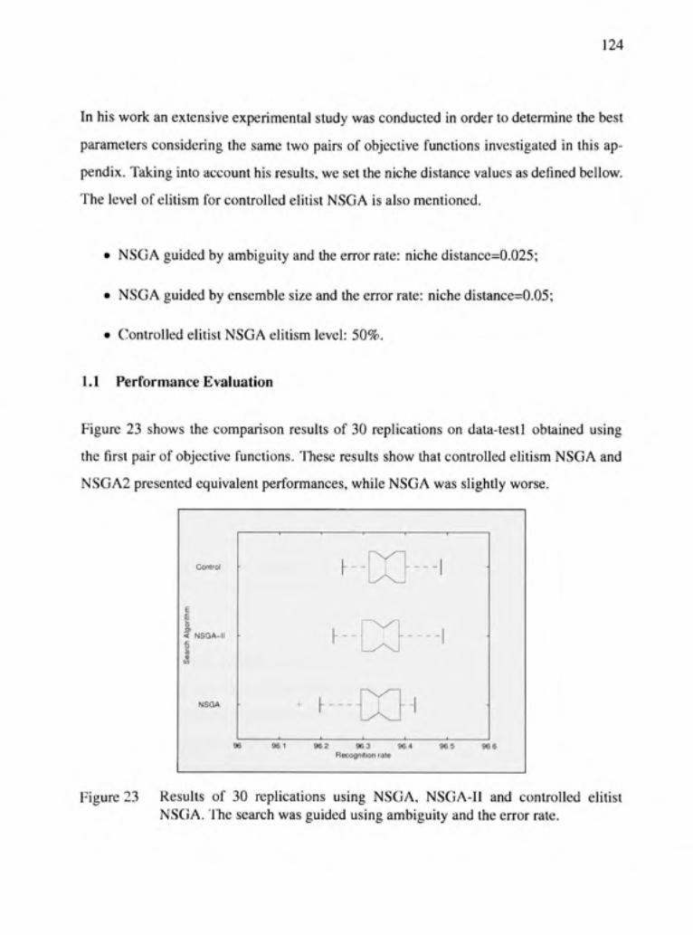
124
In his work an extensive expérimental study was conducted in order to détermine the best
parameters considering the same two pairs of objective funcfions investigated in this ap
pendix. Taking into account his results, we set the niche distance values as defined bellow.
The level of elifism for controlled elifist NSGA is also mentioned.
• NSGA guided by ambiguity and the error rate: niche distance=0.025;
• NSGA guided by ensemble size and the error rate: niche distance=0.05;
• Controlled elitist NSGA elifism level: 50%.
1.1 Performanc e Evaluation
Figure 23 shows the comparison results of 30 replications on data-testl obtained using
the first pair of objective funcfions. Thèse results show that conlrofied efifism NSGA and
NSGA2 presented équivalent performances, while NSGA was slighfiy worse.
NSGA
96
^ h - - - - " i
- - - - - 1
96 2 9 6 3 9 6 4 Récognition rate
96 5
Figure 23 Results of 30 replications using NSGA, NSGA-II and controlled elifist NSGA. The search was guided using ambiguity and the error rate.

125
The results obtained by combining ensemble size and the error rate in a pair of objective
functions to guide the three MOGAs are shown in Figure 24. Using this second pair of
objective functions we observe that controlled elifism NSGA and NSGA presented équiv
alent performances. Thus, unlike the previous pair of objective results, NSGA2 was the
worst search algorithm. However, it is important to note that the variance of the récogni
tion rates achieved by each algorithm is small (from 96.1% to 96,6%).
Figure 24
< NSGA-I I
NSGA
96 1 96 3 9 6 4 Récognition rate
Results of 30 replications using NSGA, NSGA-II and controlled elitist NSGA. The search was guided using ensemble size and the error rate.
Therefore, our results globally showed that the three MOGAs investigated in this appendix
are equally compétent to guide the opfimization process involved at the sélection phase of
SOCS. Since no search algorithm can be claimed to be the best, NSGA-11 is the MOGA
applied in the experiments presented throughout this thesis. This choice is specially due
lo the fact that NSGA-II does not need any parameter to be sel.

APPENDIX 2
Overfitting Analysis for NIST-digits

127
In this appendix we carried oui a comparative study using only two overfitting control
stratégies described in chapter 3: (1) partial validation PV; and (2) global validation GV.
The objeclive is to verify whether or not overfitting is detected in opfimizafion process
using both GA and NSGA-11, guided by ail the objeclive functions and combinations of
objective functions discussed in chapter 2. Hence, we show hère the overfiUing analysis
for the three séries of experiments carried oui in chapter 2: single-objective functions,
diversity measures combined wilh the error rate e and diversity measures combined wilh
ensemble size (^. 'Fhe minimum number of classifiers allowed by the search algorithms
was 5 and the pool of 100 kNN classifiers generated with the random subspace method
was used in this experiments.
Table XXIV summarizes the average results on data-testl, and Table XXV summarizes the
results on dala-lesl2. The results are shown in bold when GV decreased the generalization
error rate significantly, according to the Kruskal-WaUis stafisfical lest. The results are
shown underlined when GV increased the generalizafion error rate. The results wilh no
overfitting control NV are also included in thèse tables.
Table XXIV
Comparing overfitting conlrol methods on data-testl. Values are shown in bold when GV decreased the error rates significantly, and are shown underlined when it increased the
error rates.
Vletliod NV PV GV
NV PV GV
NV PV GV
GA - Single objective function s e
3.60 3.60 3.SS
7 4.70 4.70 4.63
a 6.36 6.35 5.92
P 5.34 5.61 5.15
0 3.76 3.76 3.67
1 6.32 6.32 5.81
S 4.80 480 4.53
Ç 6.11 6.12 5.86
A 6.00 6.00 6.32
T
4.76 4.84 4.72
K
5.17 5.16 4.96
«/' 4.28 4.28 4.25
* 5.73 5.73 5.43
NSGA-U - Pairs of objective function wit h the error rate (
-3.66 3.70 3.63
3.67 3.68 3.62
3.60 3.59 3.59
3.64 3.63 3.60
3.66 3.69 3.64
3.63 3.64 3.60
3.66 3.67 3.63
3.69 3.70 3.65
3.65 3.63 3.61
3.62 3.60 3.59
3.67 3.67 3.63
3.65 3.63 3.60
NSGA-II - Pairs of objective function wit h ensemble size C 3.66 3.67 3.65
4.70 4.70 5.20
6.28 6.28 6.27
5.50 5.50 5.72
3.76 3.83 3.71
6.39 6.39 6.47
4.80 4,80 4.85
6.35 6.35 6.45
6.34 6.34 6.63
4.85 4.85 4.97
5.18 5.18 5.33
4.31 4.31 4.49
5.84 5.84 6.08

128
Table XXV
Comparing overfitting control methods on dala-tesl2. Values are shown in bold when GV decreased the error rates significantly, and are shown underlined when it increased the
error rates.
Method NV PV GV
NV PV GV
NV PV GV
GA - Single objective function s e
7.89 7.91 7.80
7 9.42 9.42 9.31
a 11.79 11,79 11.02
P 10.42 10.64 10.01
e 8.43 8.44 8.11
f;
11.70 11.70 10.92
<5 10.45 10.45 9.85
i. 11.30 11.33 10.82
A 11.39 11.39 11.92
T
10.29 9.98 9.64
K
10.24 10.21 10.01
i> 8.89 8.89 8.81
* 10.97 10.97 10.37
NSGA-II - Pairs of objective function v it h the error rat e t 7.90 7.97 7.87
8.09 8.11 7.94
7,91 7,90 7,84
8.12 8.11 7.93
7.99 8,01 7.88
8.12 8.14 7.93
7.96 7.98 7.87
8.02 8.01 7.90
8.08 8,00 7.92
7.96 7,92 7.84
7.96 7.97 7.89
7.98 7.94 7.84
NSGA-II - Pairs of objective function wit h ensemble siz e (," 8.08 8.08 7.98
9.42 9.42 10.27
11.61 11.61 11.58
10.63 10.63 10.76
8.44 8.49 8.25
11.83 11.83 11.80
10.45 10.45 10.42
11.77 11.77 11.79
12.11 12.11 12.54
10.00 10.00 10.06
10.22 10.22 10.37
8.91 8.91 9.20
11.08 11.08 11.21
Thèse experiments show that:
a. The overfitting phenomenon was detected and controlled in afi the multi-objective
optimization results when diversity measures were combined wilh c. The GV pro
cédure allowed us lo find classifier ensembles with a higher power of generalization,
whatever pair of objective functions was used lo guide the NSGA-II search.
b. Except for fault majority A, the GV procédure helped to find classifier ensembles
with higher récognition rates in afi the single-objective optimization problems stud
ied in this paper. ITius, overfitting was detected even when diversity was used as the
objective funclion.
c. The overfiUing phenomenon was nol detected on multi-objective opfimization when
diversity measures were combined with C,. 'Fhus, other than when C is combined
with e, the difficulty measure 9 or coincident failure a, GV leads to a decrease in the
generalization performances. We can explain this apparent discrepancy by the fact
that the combination of C and diversity is not related lo performance.

129
The relationship between diversity and error rate is illustrated in Figures 25 and 26. For
each diversity measure employed in the single-objective optimization experiments de
scribed in section 2.2.1, we bave measured the uncontrolled overfitfing (j) — ^Ç^X']) —
e(y, C* ) . TTiese figures show 0 based on 30 replications on data-testl (Figure 25) and on
dala-test2 (Figure 26) for each diversity measure. According lo thèse results, 9 was the
diversity measure that was more closely related lo the error rate, while A was the diver
sity measure that was less closely related to the error rate, since a stronger relationship
between diversity and error rate leads to a lower 0.
3.0
2.5
2.0 O) c i 1.5 > D
1.0
0.5
0
-1 1 1 1 1 1 1 1 1 1 1 r
1
I J.
X i .
L
T) 6 ^ X Objective Functio n
4-
K \| / <I >
Figure 25 Uncontrolled overfitting 0 based on 30 replicafions using GA with diversity measures as the objecfive function. The performances were calculated on the data-testl. Fhe relationship between diversity and error rate becomes stronger as 0 decreases.
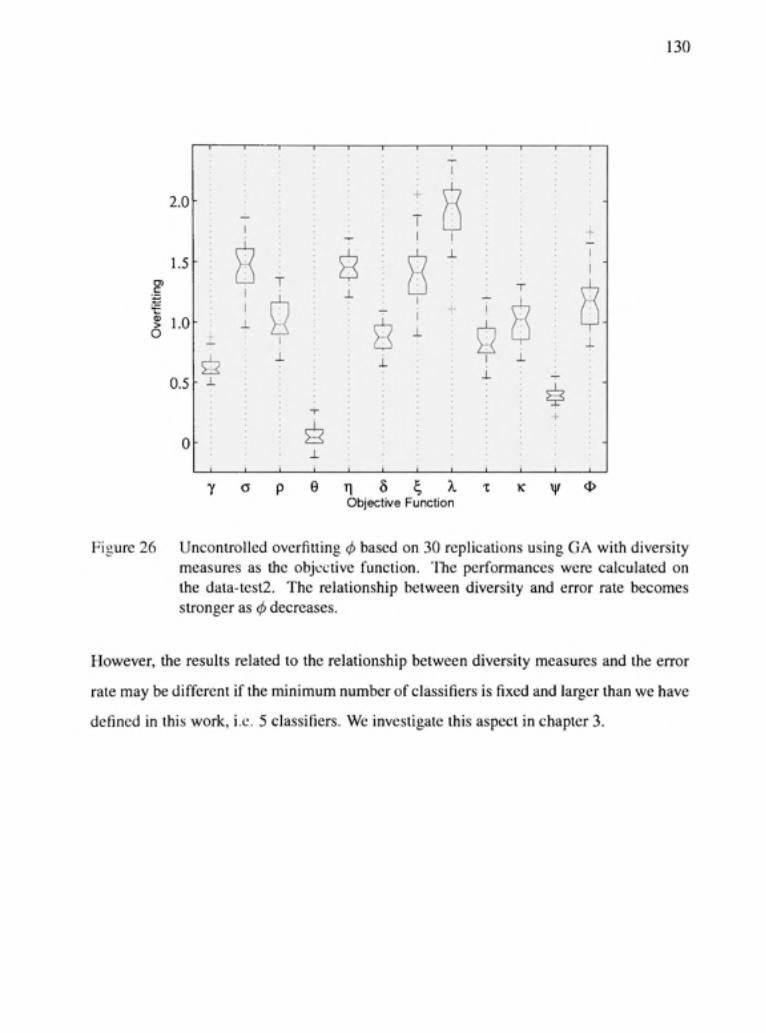
130
2.0
1.5
c
S 1.0 o
0.5
I r~
- X
J.
T
J-
±
±
X
I i
1
n Ô ^ À Objective Functio n
K \\f O
Figure 26 Uncontrolled overfiUing 0 based on 30 replicafions using GA wilh diversity measures as the objecfive function. 'ITie performances were calculated on the data-lesl2. The relationship between diversity and error rate becomes stronger as 0 decreases.
However, the results related to the relationship between diversity measures and the error
rate may be différent if the minimum number of classifiers is fixed and larger than we bave
defined in this work, i.e. 5 classifiers. We investigate this aspect in chapter 3.

APPENDIX 3
Pareto Analysis

132
3.1 Introductio n
Based on Uie results obtained in appendix 2 we observed fiiat fiie performance of fiie so
lutions found in both single- and multi-objecfive optimization processes was increased by
applying the global validation GV method to reduce overfitting. However, when ensemble
size C and diversity were combined lo make up pairs of objective functions lo guide the
optimization and the validation processes, the results were very différent. GV increased
the generalization error rates. We explained ihis behavior in appendix 2 by the fofiowing
assumption: the combination of C and diversity is not related lo the performance. First,
in despite of the fact that good results were obtained using GV guided by diversity in the
single-objective optimization approach, our experiments outlined thaï, although reduced,
overfitting was nol lolally controlled. Second, even if we can establish an analogy between
feature subsel sélection and SOCS, we cannot increase performance by selecting classifier
ensembles wilh the minimum (, specially because we need lo deal wilh a large initial pool
of classifiers. Tlierefore, we cannot decrease the generalization error rate by combining
this pair of objecfive functions.
In this appendix, we présent further évidence on Pareto front analysis to show why diver
sity and C are nol strongly related to the performance
3.2 Paret o Analysi s
Objective functions in multi-objecfive optimization problems are often confiicting. Since
différent tradeoffs are established over the Pareto front, when one solution is better ac
cording lo one objeclive, il is often worse according to Ihe remaining objective functions.
Indeed, Deb [12] points oui that, for instance in a two confiicting objecfive problem, if
a ranking of nondominated solutions is carried out in an ascending order according lo
one objective function, a ranking in a descending order is obtained according to the other
objective funclion.

133
Thèse observations are illustrated in Figure 27. NSGA-U was employed as the search
algorithm. In Figure 27(a) the search was guided by the nfinimizalion of the error rate e
and the difficully measure 9. The Pareto front solutions are shown in an ascending order of
e, consequently, in a descending order of Ihe 9. Figure 27(b) shows the Parelo front found
using the following pair of objeclive functions: jointly nfinimize e and Q. Once again, the
solutions were ordered according to e, and in a descending order of C- In Figure 27(c)
the pair of objeclive functions employed was the minimization of Ç and 9. The Pareto
solutions are shown in an ascending order of 9 (descending order of Q. However, the
same behavior cannot be detected in Figure 27(d) where it is shown an example of the
évolution of the optimization process after 1,000 générations which was generated using
the following pair of objective functions: jointly minimize C and the interrater agreement
K. Il can be seen that only one solution was found over the Parelo front.
The first two figures show that either 9 or Ç combined with e are confiicting objectives. In
Figure 27(c) il is shown that 9 and C are also confiicting objectives. In contrast, K and C, are
not confiicting objectives. In order to show whether or nol the pairs of objective functions
applied in chapter 2 are confiicting objecfive funcfions we apply hère two quality melrics
based on calculating the overall Parelo spread and k*^ objective Pareto spread introduced
by Wu and Azarm [103]. Given a multi-objective problem with m objective functions
fi, f2i • • •, fm^ we show how to calculate the two measures of spread taking into account,
without loss of generalily, ail objective funcfions lo be minimized and equally important.
Given s ,, be the possible worst solufion and Sb be the possible besl solufion, the objective
space should be scaled by the following équation:
hM = % r i^ (3-' ) 1} 1J

134
0 0359 0 036 0 036 0 0361 0 0361 0 0362 0 0362 0 0363 Oitticulty
10 1 2 Ensemble siz e
(a) (b)
(c)
8 1 0 1 2 1 4 1 6 1 8 2 0 2 2 Ensemble siz e
Complète searc h spac e
O Non-dominate d solution s
.:;iii!!iilliii!ii!iiilli'^^''' lilH:'^
20 3 0 4 0 Ensemble siz e
50 6 0
(d)
Figure 27 Pareto front after 1000 générations found using NSGA-II and the pairs of objeclive functions: jointly minimize the error rate and the difficulty measure (a), jointly minimize the error rate and ensemble size (b), jointly minimize ensemble size and the difficully measure (c) and jointly minimize ensemble size and the interrater agreement (d).
In a two-objeclive problem, the scaled objeclive space is a hyper-rectangle, as shown in
Figure 28 defined by the scaled worst (1,1) and best (0,0) solufions. The overall Pareto
spread is defined as:

135
f.
( f f linin ' 2max )
®
• - - • s
. @ ^ Imax Ziiun ' '
Figure 28 Scaled objective space of a two-objeclive problem used lo calculate the overall Parelo spread and the /c"" objeclive Pareto spread.
OPS - UT=i np
maxX iiPk)i min np l{Pk)i\
U.T=l\iPw)^- {Pb)i\ (3.2)
or
OPS n inu.i np i\M-'-k)] iniii np \f,M] (3.3)
where np is the total number of Pareto solutions. When we are dealing wilh no confiicting
objective functions OPS is equal to 0. Hence, a wider spread leads to more diversity over
the Pareto front which is a desired Pareto property. However, OPS does nol measure the
individual objective spread. For example, if instead of having 7 solutions over the Pareto
front as shown in Figure 28, we had only two solutions, for instance (fimin-hmax) and
ifimax, f2min), thc samc OPS valuc would be obtained but the diversity over a Parelo with
only two solutions is much smaller than the diversity over a Parelo with 7 solutions. In
order to overcome this problem, the k*^^ Objective Pareto Spread (IPS), also proposed by
Wu and Azarm[103], is appfied. The IPSk is calculated as:

136
rpo \maxXl{{p^)k) - minX^{{p,)k)\ I^^k ~ r, —^; } —r-, (3.4)
\{Pw)k - {Pb)k\
or
IPSk |ma.r;'f,(/,(:r,)) - in>n:',{f,{x,))\ (3.5)
In the two-objeclive problem shown in Figure 28, the k'^ objective Parelo Spread and the
overaU Parelo spread are respectively:
IPSfj^ — \flmax — flminl (3.6)
-^• '5/2 ^ l/2mQX ~ /2min I (3.7)
OPS^ IPSfJPSf, (3.8)
The k^^ objeclive Parelo Spread is important lo measure the diversity over the Pareto
front and lo show whether or not spread is wider for one objeclive funclion than for the
others. We try to identify if there is more variation in one objective function or if the
objective functions are equally diverse. Table XXVI présents the A"' objecfive Pareto
Spread and the overall Pareto spread calculated for each Parelo front shown in Figure 27.

137
The difficulty measure 9 and the error rate e are confiicting objeclive functions but there
is much more variation among e values than among 9 values. Ensemble size ( and c are
confiicting objeclive functions and there is more variation in ( values than in e values. In
addition, 9 and (" are confiicting objective functions but once again, there is less variation
among 9 values. Il is important note that there is more variation among 9 values when
this diversity measure is combined with ( than when it is combined wilh e. Finafiy, the
interrater agreement K and ( are not confiicting objective functions.
Table XXVI
Worst and best points, minima and maxima points, the k*^ objective Parelo spread values and overall Parelo spread values for each Parelo front.
Objective Functions
Difficulty (?( / i ) Error rate e (/2) Ensemble size C ( / i ) Error rate t (/2) Ensemble size C ( / l ) Difficulty 0 ( / 2 ) Ensemble size c; (f\) Interrater K ( / O )
Original value s Sw
1 100 100 100 100
1 100
1
« 6
0 0 0 0 0 0 0 0
min 0.0359 3.2800
5 3.2900
21 0.0415
5 0.2752
max 0.0362 3.5600
17 4.7000
5 0.0356
5 0.2752
Scaled value s Su,. •56
0 0 0 0 0 0 0 0
min 0.0359 0.0328 0.0500 0.0329 0.0500 0.0356 0.0500 0.2752
max 0.0362 0.0356 0.1700 0.0470 0.2100 0.0415 0.0500 0.2752
IPS 0.0003 0.0028 0.1200 0.0141 0.1600 0.0059 0.0000 0.0000
OPS
0.1 X 10-^
0.17 X 10⁻²
0.9 X 10⁻³
0.0000
We bave calculated both quality measures in order to show which measures are confiicting
or nol. The same pairs of objeclive functions investigated in appendix 2 were used hère:
diversity measures combined wilh e; diversity measures combined wilh ( and e combined
with C- Table XXVII shows the average results from 30 replications for each pair of
objeclive functions. 'Fhis table shows the values of the A"' objective Parelo spread and the
overall Parelo spread, as well as the différence between the A"* objeclive Pareto spreads.
This différence indicates the variation among objective functions values.
Thèse results show that afi diversity measures are confiicting objective functions when
combined with e. Except Kohavi-Wolpert ip, 9 and ambiguity 7, there is more variation
among diversity values than among e values. Ensemble size Ç and e are also confiicting

138
objeclive functions and there is more variation among ( values. However, there are only
three diversity measures which are confiicting objeclive functions when combined with
ensemble size, the same 0, 9 and 7.
The literature has shown that the pairwise diversity measures and ( are not confiicting
objective functions. Aksela and Eaaksonen [1] observe that pairwise diversity measures
always try lo find the two most diverse classifiers which leads to the minimizafion of the
number of classifiers during the optimization process. Our resulls confirm this observation
since ail pairwise measures (see Chapter 2, section 2.2.1 employed in our experiments are
not confiicting objective functions when combined with Q. However, our results show
that some of the nonpairwise measures lead also lo the minimizafion of C,. TTiree of the
nonpairwise measures employed: 7, 9 and 0, do nol minimize C,.
Table XXVII
The average A-"' objective Parelo spread values and the average overall Parelo spread values for each pair of objeclive function.
Diversity
7 a P 0 n ô ç A T
K
4> *
Error rate IPS, 0.0187 0.0134 0.0213 0.0025 0.0330 0.0159 0.0249 0.0192 0.0150 0.0159 0.0119 0.0265
IPSd.,. 0.0254 0.0368 0.0442 0.0006 0.0428 0.0068 0.0659 0.0460 0.0357 0.0447 0.0113 0.0927
IPS, 0.0119
IPS,i,,. -IPS, 0.0067 0.0234 0.0229 -0.0019 0.0098 -0.0091 0.0410 0.0268 0.0207 0.0288 -0.0006 0.0662
OPS 0.5x10-^ 0 .5x10-3 0.9 X 10⁻³ 0 . 2 x 1 0 - ^
0.14 X 10⁻² 0.1 X 10⁻³
0.17 X 10⁻² 0,9 X 10⁻³ 0 5 X 10⁻³ 0.7 X 10⁻³ 0.1 X 10⁻³
0.25 X 10⁻² Ensemble size ( a n
IPSc^ 0.2163
Ensemble size IPSc^ 0.0503 0.0000 0.0000 0.1733 0.0000 0.0000 0.0000 0.0000 0.0000 0.0000 0.1000 0.0000
d Error rs IPSç
^ ^ • 5 d n i
0.0030 0.0000 0.0000 0.0058 0.0000 0.0000 0.0000 0.0000 0.0000 0.0000 0.0079 0.0000
itC E
- IPS, 0.2045
IPS^ - IPSdtv -0.0474 0.0000 0.0000 -0.1675 0.0000 0.0000 0.0000 0.0000 0.0000 0.0000 -0.0921 0.0000
OPS 0,0001 0.0000 0.0000 0.0010 0.0000 0.0000 0.0000 0.0000 0.0000 0.0000 0.0008 0.0000
OPS 0.0025
According to Whitaker and Kuncheva [99] nonpairwise measures are calculated by using
either entropy or corrélation between individual outputs and Ihe ensemble's output or dis
tribution of "difficully" of the data samples. Among the three diversity measures, which

139
are confiicting objeclive functions when combined with (, Iwo measures are based on
Ihe variance over Ihe dataset (9 and </') and 7 is based on the variance among ensemble's
members. Thus, our observation is that, besides ihe pairwise diversity measures pointed
out by Aksela and Laaksonen [1], ail non-pairwise diversity measures based on entropy or
corrélation between individual outputs are also nol able to find the best ensemble's size,
i.e. they minimize ( during the optimizafion process.
Moreover, there is no guarantee of finding the besl ensemble's size using one of the three
diversity measures based on variance, specially ambiguity, which générâtes the less diverse
Pareto front (Table XXVll and Figure 29(a)) and the smallest classifier ensembles (Figure
29(a)). Flowever, thèse three measures bave such a property that makes them able lo
générale larger classifier ensembles, which is useful in OCS methods since we deal wilh
a large initial pool of classifiers. TTie two diversity measures based on the variance over
the dataset found more diverse Pareto front and larger classifier ensembles than ambiguity
(based on the variance of the classifiers' output). The difficully measure 9 was better than
Kohavi-Wolpert if' in thèse two aspects, as il can seen in Figure 29(b) for 4' and in Figure
27(c) for 9, as well as in 'fable XXVII.

140
0146
0145
0144
>. 0 143
1 •* 0 14 2
0141
014
0139
'
6 7 e 9 1 0 1 ErïsamWe S'IB
0 146
0145
' 0 144
ç 0 143
i i
0 14 2
1 ^ 0 14 1
014
0 13 9
0 138
0137 1
'
^ - ^ - ^ • ^ ^ e N
x^ ^ ;
. /
• ^
6 8 1 0 1 2 1 4 1 6 1 Eneembls SIZB
e
(a) (b)
Figure 29 Pareto front after 1000 générations found using NSGA-11 and the pairs of objective funcfions: minimize ensemble size and maximize ambiguity (a) and minimize ensemble size and maximize Kohavi-Wolpert (b).

APPENDIX 4
Illustration of overfitting in single- and mulfi-objective GA

142
In this appendix we show the Figures 13 and 14, which ifiustrated the overfitfing problem
in single- and mulfi-objective GA in chapter 3, in larger versions.
5 0
4 8 -
4 6
4 4 -
4 2
4 0
3 3
3 5
3 4
3 2
3 0
C (evaluated )
0 c'n )
(a) o dataset and g = 1
50 6 0 7 0 8 0 9 0 10 0 Ensemble siz e
50
4,B
4,6
4.4
42
40
38
3.6
3.4
3 2
C (evaluated )
0 C'(1 )
illiillli:;:''
50 6 0 7 0 Ensemble siz e
(b) V dataset and g — 1
Figure 30 Optimizafion using GA guided by e. Hère, we follow the evolufion of Cj{g) (diamonds) for ^ = 1 (Figure 30(a)) on the opfimization dataset O, as well as on the validation dataset V (Figure 30(b)). Solutions nol yet evalualed are in grey and the best performing solutions are highlighted by arrows.

143
5 0 -
4 8 •
4 6 -
4 4 -
42 -S s 4 0 -
UJ
3 8 -
3 6 -
3 4 -
3 2 -
3 0 •
C (evaluated )
0 C'(52 )
:i: •:!"l'iiiii - " i l '"! : "
• • " !!k:.!;;;i.!ii.i:
. • ; . ! ; . • ; • ' . : . : . : • : : •
50 6 0 7 0 Ensemble siz e
(a) C dataset and g = 52
5.0
4.8
46
44
42
40
3 8
3.6 •
3.4 •
3 2 •
3 0 20
iiijl|;iiii':iiiii:!i!;:-i>-i i!l|!!;!li!;!i!J!:!!i':i"::.-
C (evaluated )
0 C'(52 )
50 6 0 7 0 Ensemble siz e
(b) V dataset and g = 52
Figure 31 Optimization using GA guided by e. Hère, we follow the évolution of Cj{g) (diamonds) for g — 52 (Figure 31 (a)) on the opfimization dataset O, as well as on the validation dataset V (Figure 31(b)). TTie minimal error is reached slightly after g = 52 on V, and overfitting is measured by comparing it to the minimal error reached on O. Solutions nol yet evaluated are in grey and the best performing solutions are highlighted by arrows.
5 0 -
4 8 •
4 6 -
4 4 -
4 2 •
4 0 •
3 8 -
3 6 -
3 4 -
3 2 -
. : •^i':»;'.i-i'!i , •; . •!•( . •.•• • ; - i ! i . : , . ' ! ' i i , i | ; ; ' : i
•::c.:i,:ii!il!liî!:: j!;; : V-:::iii:i!ii!i!'!i!:Jî:i:^î::"=
50 6 0 7 0 EnsemUe siz e
(a) o dataset and max(g)
. c 0 c ; o c '
• : . : ' ' . i ' . : • ' . : . ' ••••: i l . , / . • ; • . : ' • • •
5 0
4 8
4,6
4.4
4 2 (D
(5 5 " O t UJ
33
36
3.4
3.2
. C
0 ^', O c'
ii:!ii!iiil !ii!i:>:<-:ii
overfitting
50 5 0 7 0 Ensemble siz e
(b) V dataset and inax(g)
Figure 32 Opfimization using GA guided by f. Hère, we follow the évolution of Cj{g) (diamonds) for max{g) (Figure 32(a)) on the optimization dataset O, as well as on the validafion dataset V (Figure 32(b)). ITie overfiUing is measured as the différence in error between C'*' (circles) and C* (Figure 32(b)). 'Fhere is a 0.30% overfit in this example. Solutions not yet evaluated are in grey and the best performing solutions are highlighted by arrows.

144
5 0
4 8
4,6
4 4
4 2 Q
te fe 4 0 t LU
38
36
3 4
32
30
0
-•
c (evaluated )
C,(1)
.^âÉî^
T W P ^
M f<^*V".l
w **>
•
.•6^:^x.
y • .
•
0 035 0 036 0 037 0 033 0 039 0 04 0 041 0 042 0 04 3 Dilfiojlty Measur e
5 0
4 8
4 6
4.4
i &
3 8
3,6
3.4
3 2
C (evaluated )
0 '^kl' l
M"JX4^^X
i.\?^f?^
0 03 5 0 036 0 037 0 033 0 039 0 04 0 041 0 042 0 04 3 Ditflcuity Measur e
(a) O dataset and g = 1 (b) V dataset and g ~ 1
Figure 33 Optimizafion using NSGA-II and the pair of objective functions: difficulty measure and e. We follow the evolufion of Ck{g) (diamonds) for = 1 (Figure 33(a)) on the optimization dataset O, as well as on the validation dataset V (Figure 33(b)). Solutions not yet evaluated are in grey.
5 0
4 3
4 6
4 4
4 2 S
g 4 0
UJ
3 8
3 6
3 4 -
3 2 •
C (evaluated )
0 <=k<15 t
3 0 0 035 0 036 0 037 0 038 0 039 0 04 0 041 0 042 0 043
Ditficuity Measur e
(a) O dataset and g = 15
c (evaluated )
0 CJ15 )
•
.
•
'JÙA t'^gt
.*¥j
•
•
•
.
•
0 03 5 0 036 0 037 0 038 0 039 0 04 0 041 0 042 0 04 3 Ditflcuity Measur e
(b) V dataset and g - 15
Figure 34 Opfimizafion using NSGA-11 and the pair of objeclive functions: difficully measure and e. We follow the evolufion of Ck{g) (diamonds) for ^ = 15 (Figure 34(a)) on the optimization dataset O, as well as on the validation dataset V (Figure 34(b)). The minimal error is reached slightly after ^ = 15 on V, and overfitting is measured by comparing it to the minimal error reached on O. Solutions not yet evaluated are in grey.

145
0.035 0 036 0 037 0 033 0 039 0 04 0 041 0 042 0 043 Dittiajily Measure
(a) O dataset and jnax(g)
46
44
42
40
38
36
3.4
3.2
. c
0 \ o c ^
•
•
d ^ H H ^ * " • overfittin g
0.035 0 036 0 037 0 038 0 039 0 04 0 041 0 042 0 043 Difficulty Measure
(b) V dataset and max{g)
Figure 35 Opfimizafion using NSGA-II and the pair of objective funcfions: difficulty measure and e. We follow the évolution of Ck{g) (diamonds) for max{g) (Figure 35(a)) on the optimization dataset O, as well as on the validation dataset V (Figure 35(b)). The overfitting is measured as the différence in error between the most accurate solution in C^' (circles) and in Cl (Figure 35(b)). There is a 0.20% overfit in this example. Solutions not yet evaluated are in grey.

APPENDIX 5
Comparison between Particle Swarm Optimization and Genetic Algorithm taking
into account overfitting

147
The objective of this appendix is to présent the results of a short comparative study be
tween Particle Swarm Optimization (PSO) [34] and GA in order lo show which algorithm
is more prone lo overfitfing. 'Fhese experiments were conducted using only the error rate
e as the objecfive function. 'Fhe comparative study is focused on detecting and controlling
overfitting in both GA and PSO search algorithms at the optimization process, by applying
the global vafidation strategy GV.
5.1 Particl e Swarm Optimizatio n
PSO simulâtes the behaviors of bird fiocking or Osh schooling. Each individual of the pop
ulation is called particles. Ail particles bave fitness values which are evaluated during the
optimization process of the sélection phase of SOCS. Algorithm 8 summarizes the variant
of the PSO algorithm used in this appendix. ITiis variant is called global neighborhood
[57] in the literature.
Al 1 2 3 4 5 6 7 8 9
10 11 12 13 14 15 16
gorithm 8 PSO for each particle d o
Inilialize particle end fo r while maximum itérations or stop criteria are not attained d o
for each particle d o Compute fitness value if fitness value is better than the best fitness (pBesl) in hislory the n
Sel current value as the new pBest end if
end fo r Choose the particle wilh the best fitness as the gBest for each particle d o
Compute its velocity Update its position
end fo r end whil e

148
The solution gBest dénotes the best particle in Ihe whole population. In PSO the popu
lation is called swarm. LeUing C{g) dénote the swarm in itération g and e represent the
objective funclion, the complète GV algorithm for PSO is described in Algorithm 9.
Algorithm 9 Global Validation for PSO 1 2
3 4
5 6 7 8 9
10 11 12 13 14 15
Créâtes initial swarm
Validate ail solutions in C(l ) over samples contained in V Find ( ' / ( l ) from C(l )
S e i r ; ' : = c ; ' ( i ) for each itération g ^ { 1 , . . . , max{g)} d o
run PSO and generate C{g + 1) validate ail solutions in C(^ -|- 1) findC;'(^+l)
i f c ( V , C ; ' ) ( 5 + l ) < e ( V , 6 ' ; ' ) t h e n
setc;':=c;'(^+i) update A by storing in il the new C*'
end if end fo r return ( '*' stored in A
5.2 Experiment s
In order lo develop our experiments we use the two large datasets described in chapter
3, Table VI: NlS'l'-digils and NlS'F-lelters. The same initial pool of 100 kNN classifiers
generated by applying the Random Subspace method is investigated hère.
Table XXVIII shows the average results from 30 replications obtained using NlS'F-digits
dataset. Values are shown in bold when GV decreased the generalization error signif
icantly, according lo the Kruskal-Wallis stafistical test, llie results with no overfiUing
conlrol NV are also included in this table. Thèse initial results show that although both
search algorithms are prone lo overfitting, GA appears lo be more affected. Il is important
to note that this behavior confirms Reunamen's work [65]. Ile pointed oui that the degree
of overfitting increases as the intensily of search increases. Figure 36(a) shows that GA

149
needs more générations to find the besl solufion during the optimization process than PSO.
On fiie other hand, the best solution C*' stored in A is found much earlier using G A than
PSO (Figure 36(b)). This resuit can be explained by the fact that, since during the opfi
mization process PSO keeps searching by solutions even worse than gBest, it is possible
lo generate solutions that are beUer in generalization after finding gBest.
Table XXVni
Comparing GA and PSO in terms of overfitting conlrol on NIST-digits dataset. Values are shown in bold when GV decreased the error rates significantly. The results were
calculated using data-testl and data-lesl2.
Validation Metlio d
NV GV
GA data-testl
3.60 3.55
data-test2 7.91 7.80
PSO data-testl
3.62 3.61
data-test2 8.02 7.88
Search Algonthm
(a) (b)
Figure 36 NIS'F-digils: the convergence points of GA and PSO. The generafion when the besl solution was found on oplinfizafion (36(a)) and on vafidafion (36(b)).
However, the experiments with NIST-letters did not confirm our first observations. The
average resulls from 30 replicafions obtained using NIST-letters dataset are reported in
Table XXFX. Thèse results show that GV only slighfiy decreased the generalization error

150
rate for NlS'f-letters. In despile of this, the results obtained using NIST-letters dataset
afiow us to confirm that GA performs a more intense search process. Figure 37(a) shows
that GA needs more générations to find the best solufion during the optimization process
than PSO also on NIS'F-lellers dataset. Again, GA finds C*' much eariier than PSO (Figure
37(b)). Moreover, the performance of the solutions found by GA were slighfiy better
using both NIST-digits (Figure 38) and NIST-letters (Figure 39(a)) datasets. However,
the classifier ensembles found employing GA were larger than those found using PSO, as
illustrated in Figure 40 for NIST-digits and in Figure 39(b) for NIST-letters.
Table XXIX
Comparing GA and PSO in terms of overfitting control on NIS'F-letter dataset.
Data set
NIST-letters
No validation GA 6.49
PSO 6,54
Global validation GA 6.44
PSO 6,49
900
800
t Sol
utio
n
i g
; 500
Gen
erat
on
i 1
200
100
( ! 1
U ' s •
1000
900
800 o S 700
5 MO m
1 400
£ 300
200
too 0
GA PS O Search Algonih m Search Algonih m
(a) (b)
Figure 37 NIST-letters: the convergence points of GA and PSO. The génération when the besl solution was found on optimization (37(a)) and on validafion (37(b)).

151
I
! j
1
Search Algorrthm
(a)
b
Search Algonth m
(b)
Figure 38 NIST-digits: error rates of the solufions found on 30 replications using G A and PSO. The performances were calculated on the data-testl (38(a)) and on the data-test2 (38(b)).
Figure 39
71
7
6 9
6 6
fer t 6 6
6 5
63
•
1
• U GA
Search Algonih m
' •
1 1
>^-< :
1
PSO
(a)
30
BO
70
60
90
40
30
- p -1 1 1
1
M - ^
•
•
1
^ •
1
Serirch Algonihm
(b)
NIST-letters: error rates of the solufions found on 30 replications using G A and PSO (39(a)). Size of the ensembles found using both GA and PSO search algorithms (39(b)).

152
Figure 40 NIST-digits: Size of the ensembles found using both GA and PSO search algorithms.

BIBLIOGRAPHY
[1] M. Aksela and J. Eaaksonen. Using diversity of errors for selecfing members of a committee classifier. Pattern Récognition, 39(4):608-623, 2006.
[2] FI. Altinçay. Ensembling evidenfial k-nearest neighbor classifiers through multi-modal pertubation. Applied Soft Computing, 7(3): 1072-1083, 2007.
[3] S. Bandyopadhyay, S.K. Pal, and B. Aruna. Multiobjective gas, quantitative indices, and pattern classificafion. IEEE Transactions on System, Man, and Cybernetics -PartB, 34(5):2088-2099, 2004.
[4] N. Benahmed. Optimisafion de réseaux de neurones pour la reconnaissance de chiffres manuscrits isolés: Sélection et pondération des primifives par algorithmes génétiques. Masler's thesis. École de technologie supérieure, 2002.
[5] E. Breiman. Bagging predictors. Machine Learning, 24{2):123-14Q, 1996.
[6] L. Breiman. Randomizing outputs to increase prédiction accuracy. Machine Learning, 40(3):229-242, 2000.
[7] G. Brown, J. WyaU, R. Harris, and X. Yao. Diversity création methods: a survey and catégorisation. Information Fusion, 6(l):5-20, 2005.
[8] A. Canuto, G. Howells, and M. Fairhurst. ITie use of confidence measures lo enhance combination stratégies in mulli-nelwork neuro-fuzzy Systems. Connection Science, 12(3/4):315-331, 2000.
[9] A. Canuto, M.C.C.Abreu, L.M. Oliveira, J.C. Xavier Jr., and A. M. Santos. Invesligating the influence of the choice of the ensemble members in accuracy and diversity of selection-based and fusion-based methods for ensembles. Pattern Récognition Letters, 28:472-486, 2007.
[10] D. Corne and J. Knowles. No free lunch and free leftovers theorems for multiobjective optimization problems. In Proceedings of Evolutionary Multi-Criterion Optimization, pages 327-341, Faro, Portugal, 2003.
[11] K. Deb. Multi-Objective Optimization using Evolutionary Algorithms. John Wiley & Sons, LTD, 2001.
[12] K. Deb. Unveiling ûinovalive design principles by means of muUiple confiicting objecfives. Engineering Optimization, 35(5):445^70, 2003.

154
[13] K. Deb, S. Agrawal, A. Pratab, and T. Meyarivan. A fast elifist non-dominated sorfing genetic algorithm for mulfi-objective optimization: Nsga-u. In Proceedings ofthe Parallel Problem Solvingfrom Nature VI Conférence, pages 849-858, Paris, France, 2000.
[14] K. Deb and T. Goel. Controlled elifist non-donrfinaled sorfing genetic algorithms for better convergence. In Proceedings of First Evolutionary Multi-Criterion Optimization, pages 67-81, 2001.
[15] E. Didaci, G. Giacinto, F'. Roli, and G.E. Marcialis. A study on the performances of the dynamic classifier sélecfion based on local accuracy estimation. Pattern Récognition, 28:2188-2191, 2005.
[16] T. G. Dietterich. Ensemble methods in machine leaming. In Proceedings of I International Workshop on Multiple Classifier System, pages 1-15, Cagliari, Italy, 2000.
[17] T.G. Dietterich. An expérimental comparison of three methods for constructing ensembles of décision trees: Bagging, boosting, and randomization. Machine Learning, 40(2): 139-158, 2000.
[18] T.G. Dietterich and G. Bakiri. Solving multiclass leaming problems via error-corteling output codes. Journal of Artificial Intteligence Research, 2:263-286, 1995.
[19] P. Domingos. A unified bias-variance décomposition and its applicafions. In Proc. 17th International Conf. on Machine Learning, pages 231-238. Morgan Kaufmann, San Francisco, CA, 2000.
[20] J. Franke and M. Oberlander. Writing style détection by statistical combination of classifiers in form reader applications. In Proceedings of II International Conférence on Document Analysis and Récognition, pages 581-584, 1993.
[21] Y. Freund and R. Schapire. Experiments wilh a new boosting algorithm. In Proceedings of XIII International Conférence on Machine Learning, pages 148-156, 1996.
[22] FI. Frohlich and O. Champelle. Feature sélecfion for support vector machines by means of genetic algorithms. In Proceedings oflEEE International Conférence on Tools with AI, pages 142-148, 2003.
[23] B. Gabrys and D. Ruta. Genetic algorithms in classifier fusion. Applied Soft Computing, 6(4):337-347, 2006.

155
[24] G. Cîiacinto and E Roli. Dynamic classifier sélection based on multiple classifier behaviour. Pattern Récognition, 33:1879-1881, 2001.
[25] PJ. Gother. NIST Spécial Database 19 - Handprited forms and characters database. National Inslitule of Standard and Technology - NIST : database CD documentation, 1995.
[26] D. Greene, A. Tsymbal, N. Bolshakova, and P. Cunningham. Ensemble clustering in médical diagnostics. In Proceedings ofthe IEEE Symposium on Coniputer-Based Médical Systems, pages 570-575, Belhesda, USA, 2004.
[27] A.J. Grove and D. Schuurmans. Boosting in the limit: Maximizing the margin of leamed ensembles. In Proceedings of I5th National Conférence on Artificial Intelligence, pages 692-699, 1998.
[28] V. Gunes, M. Menard, and P. Loonis. A multiple classifier System using ambiguity rejection for cluslering-classification cooperafion. International Journal of Uncertainty, Fuzziness and Knowledge-Based Systems, 8(6):747-762, 2000.
[29] L.K. Hansen, C. Liisberg, and P. Salomon. 'The error-reject tradeoff. Open Systems & Information Dynamics, 4(2): 159-184, 1997.
[30] T. K. Ho. Multiple classifier combinafion: Fessons and next steps. In A. Kandel and H. Bunke, editors, Hybrid Methods in Pattern Récognition, pages 171-198. World Scienfific, 2002.
[31] T.K. Ho. Nearest neighbors in random subspaces. In Proceedings of the Second International Workshop on Statistical Techniques in Pattern Récognition, pages 640-648, Sydney, Auslralia, 1998.
[32] T.K. Ho. The random subspace method for constructing décision forests. IEEE Transactions on Pattern Analysis and Machine Intelligence, 20(8):832-844, 1998.
[33] YS. Huang and C. Suen. Combination of multiple experts for the recognifion of unconslrained handwritten numerals. IEEE Transactions on Pattern Analysis and Machine Intelligence, 17(l):90-94, 1995.
[34] J. Kennedy and R.C. Eberhart. Particle swarm intelligence. In Proceedings of International Conférence on Neural Network, pages 1942-1948, 1995.
[35] J. Kitller, M. Hatef, RPW. Duin, and J. Matas. On combining classifiers. IEEE Transactions on Pattern Analysis and Machine Intelligence, 20(3):226-238, 1998.

156
[36] A. Ko, R. Sabourin, and A. BriUo Jr. A new dynamic ensemble sélection method for numéral récognition. In Proceedings ofthe 7"" International Workshop on Multiple Classifier Systerm, pages 302-311, Prague-Czech Republic, 2007.
[37] R. Kohavi and D. Sommerfield. Feature subset sélection using the wrapper model: Overfitting and dynamic search space topology. In Proceedings of The First International Conférence on Knowledge Discoverv and Data Mining, pages 192-197,1995.
[38] L.l. Kuncheva. Clusler-and-selection model for classitier combination. In Proceedings of International Conférence on Knowledge Based Intelligent Engineering Systems and Allied Technologies, pages 185-188, 2000.
[39] L.l. Kuncheva. Swilching between sélection and fusion in combining classifiers: An experiment. IEEE Transactions on Systems, Man, and Cybernetics, 32(2): 146-156, 2002.
[40] L.l. Kuncheva. Combining Pattern Classifiers: Methods and Algorithms. Jhon Wiley & Sons, LTD, USA, 2004.
[41] L.l. Kuncheva, J. Bezdek, and R. Duin. Décision templates for multiple classifier fusion: an expérimental comparison. Pattern Récognition, 34(2):299-314, 2001.
[42] L.l. Kuncheva, M.Skurichina, and R.P.W. Duin. An expérimental study on diversity for bagging and boosting with linear classifiers. Information Fusion, 3(4):245-258, 2002.
[43] L.l. Kuncheva and J. Rodriguez, Classifier ensembles wilh a random linear oracle. IEEE Transactions on Knowledge and Data Engineering, 19(4):500-508, 2007.
[44] L.l. Kuncheva and CJ. Whitaker. Measures of diversity in classifier ensembles an their relafionship wilh the ensemble accuracy. Machine Learning, 51:181-207, 2002.
[45] R. Liu and B. Yuan. Mulfiple classifiers combination by clustering and sélecfion. Information Fusion, 2(4): 163-168, 2001.
[46] X. Llorà, D.E. Goldberg, I. Traus, and i:. Bernadô i Mansilla. Accuracy, parsimony, and generalily in evolutionary leaming Systems via multiobjective sélection. In International Workshop in Learning Classifier Systems, pages 118-142, 2002.
[47] J. Loughrey and P. ('unningham. Overfitting in wrapper-based feature subset sélection: The barder you try the worse it gels. In Proceedings of International Conférence on Innovative Techniques and Applications ofAI, pages 33-43, 2004.

157
[48] D.D. Margineantu and T.G. Dietterich. Pruning adapfive boosting. In Proceedings ofthe International Conférence on Machine Learning, pages 358-366, 1997.
[49] 'F M. Milchell. Machine Learning. McGraw-Hill, USA, 1997.
[50] N. Narasimhamurthy. Evaluafion of diversity measures for binary classifier ensembles. In Proceedings ofMCS, pages 267-277, Seaside, USA, 2005.
[51] L.S. Oliveira, M. Morila, R. Sabourin, and F. Bortolozi. Multi-objective genetic algorithms to create ensemble of classifiers. In Proceedings of the International Conférence on Evolutionary Multi-Criterion Optimization, pages 592-606, 2005.
[52] L.S. Ofiveira, R. Sabourin, F. Bortolozzi, and C.Y Suen. Automatic récognition of handwritten numerical slrings: A recognifion and verificafion strategy. IEEE Transactions on Pattern Analysis and Machine Intelligence, 24(11): 1438-1454, 2002.
[53] D. W. Opitz and J. W. Shavlik. Aclively searching for an effective neural-network ensemble. Connection Science, ^{31 A):?)!)!-351), 1996.
[54] N.C. Oza and K. Tumer. Classifier ensembles: sélect real-world applicafions. Information Fusion, 9(l):4-20, 2008.
[55] D. Parikh and R. Polikar. An ensemble-based incrémental leaming approach lo data fusion. IEEE Transactions on Systems, Man, and Cybernetics-PartB, 37(2):500-508, 2007.
[56] Y. Park and J. Sklansky. Aulomated design of linear tree classifiers. Pattern Récognition, 23(12):1393-1412, 1990.
[57] K.E. Parsopoulos and M.N. Vrahatis. Récent approaches lo global opfimization problems through particle swarm optimization. Natural Computing, l(2):235-306, 2002.
[58] D. Partridge and W.B. Yales. Engineering multiversion neural-net Systems. Neural Computation, 8(4):869-893, 1996.
[59] M. Prior and T. Windeall. Over-fitting in ensembles of neural networks classifiers within ecoc frameworks. In Proceedings of International Workshop on Multiple Classifier System, pages 286-295, Seaside, USA, 2005.
[60] J.R. Quinlan. Programs for Machine Learning. Morgan Kaufmann, 1993.

158
[61] P.V.W. Radtke. Classification Systems Optimization with Multi-Objective Evolutionary Algorithms. PhD thesis. Ecole de 'Fechnologie Supérieure - Université du Québec, 2006.
[62] P.V.W. Radtke, R. Sabourin, and 'F. Wong. Impact of solufion over-fil on evolutionary multi-objective optimization for classification Systems. In Proceedings oflJCNN, Vancouver, Canada - accepted, 2006.
[63] G. Ratsch, F Onoda, and K-R. Muller. An improvement of adaboost to avoid overfitting. In Proceedings of The Fifth International Conférence on Neural Information Processing, pages 506-509, Kitakyushu, Japan, 1998.
[64] R. Rééd. Pmning algorithms - a survey. IEEE Transactions on Neural Nen\'orks, 4(5):740-747, 1993.
[65] J. Reunanen. Overfitting in making comparisons between variable sélecfion methods. Journal of Machine Learning Research, 3:1371-1382, 2003.
[66] F. Rheaume, A-L. Jousselme, D. Grenier, E. Bosse, and P. ValinThomas. New initial basic probabifily assignmenls for multiple classifiers. In Proceedings ofXI Signal Processing, Sensor Fusion, and Target Récognition, pages 319-328, 2002.
[67] D. RobiUiard and C. Fonlupt. Backwarding: An overfitting control for genetic programming in a remole sensing applicafion. In Proceedings ofthe 5th European Conférence on Artificial Evolution, pages 245-254, 2000.
[68] G. Rogova. Combining the results of several neural network classifiers. Neural Networks, 1(5):111-1SI, 1994.
[69] F. Roli, G. Giacinto, and G. Vemazza. Methods for designing multiple classifier Systems. In Proceedings of the International Workshop on Multiple Classifier System, pages lS-^1, 2001.
[70] D. Ruta and B. Gabrys. Classifier sélection for majority voting. Information Fusion, 6(1):163-168,2005.
[71] D. Ruta and B. Gabrys. Neural network ensembles for fime séries predicfion. In Proceedings ofthe IEEE International Joint Conférence on Neural NetA'ork, pages 1204-1209, Oriando, USA, 2007.
[72] E.M. Dos Santos, R. Sabourin, and P. Maupin. Single and multi-objective genetic algorithms for the sélection of ensemble of classifiers. In Proceedings of International Joint Conférence on Neural Networks, pages 5377-5384, 2006.

159
[73] E.M. Dos Santos, R. Sabourin, and P. Maupin. Ambiguity-guided dynamic sélection of ensemble of classifiers. In Proceedings of International Conférence on Information Fusion, Québec, CA, 2007.
[74] E.M. Dos Santos, R. Sabourin, and P. Maupin. A dynamic overproduce-and-choose strategy for the sélection of classifier ensembles. Submitted to Pattern Récognition, 2007.
[75] E.M. Dos Santos, R. Sabourin, and P. Maupin. Overfitfing cautions sélection of classifier ensembles with genetic algorithm. Submitted to Information Fusion, 2007.
[76] S.B. Serpico, L. Bruzzone, and F. Roli. An expérimental comparison of neural and statistical non-paramelric algorithms for supervised classification of remote-sensing images. Pattern Récognition Letters, 17(13):1331-1341, 1996.
[77] A.J.C. Sharkey. Multi-net Systems. In Combining Artificial Neural Nets: Ensemble and Modular Multi-Net Systems, pages 1-27. Spring-Verlag, 1999.
[78] A.J.C. Sharkey and N.E Sharkey. The "test and sélect" approach to ensemble combination. In J. Kiltler and E. Roli, editors. Multiple Classifier System, pages 30-44. Spring-Veriag, 2000.
[79] H.W. Shin and S.Y. Sohn. Combining both ensemble and dynamic classifier sélection schemes for prédiction of mobile internet subscribers. Expert Systems with Applications, 25:63-68, 2003.
[80] H.W. Shin and S.Y. Sohn. Selected tree classifier combinafion based on both accuracy and error diversity. Pattern Récognition, 38(2): 191-197, 2005.
[81] S. Singh and M. Singh. A dynamic classifier sélection and combination approach to image région labelling. Signal Processing: Image Communication, 20:219-231, 2005.
[82] K. Sirianlzis, M.C. Fairhurst, and R.M. Guesl. An evolutionary algorithm for classifier and combination rule sélection in multiple classifier System. In Proceedings ofICPR, pages 771-774, 2002.
[83] P. C. Smits. Multiple classifier Systems for supervised remote sensing image classification based on dynamic classifier sélection. IEEE Transactions on Geoscience and Remote Sensing, 40(4):801-813, 2002.
[84] R.G.F. Soares, A. Santana, A.M.P. Canuto, and M.C.P. de Souto. Using accuracy and diversity lo sélect classifiers lo build ensembles. In Proceedings of International Joint Conférence on Neural Networks, pages 2289-2295, 2006.

160
[85] S.Y. Sohn and H.W. Shin. Expérimental study for the comparison of classifier combination methods. Pattern Récognition, 40(1):33^0, 2007.
[86] C.Y. Suen and Louisa Lam. Multiple classilier combination méthodologies for différent output levels. In First International Workshop on Multiple Classifier Systems, pages 52-66, London, UK, 2000.
[87] 'F. Sullorp and C. Igel. Multi-objective optimization of support vector machines. Studies in Computational Intelligence - Multi-objective Machine Learning, 16:199-220, 2006.
[88] G. Tremblay. Optimisation d'ensembles de classifieurs non paramétriques avec aprentissage par représentation parliefie de l'information. Masler's thesis. École de technologie supérieure, 2004.
[89] G. Tremblay, R. Sabourin, and P. Maupin. Optimizing nearest neighbour in random subspaces using a multi-objective genetic algorithm. In Prvceedings of International Conférence Pattern Recogndion, pages 208-211, Cambridge, UK, 2004.
[90] A. Tsymbal, M. Pechenizkiy, and P. Cunningham. Diversity in search stratégies for ensemble feature sélection. Information Fusion, 6(l):83-98, 2005.
[91] A. Tsymbal, M. Pechenizkiy, and P. Cunningham. Sequential genetic search for ensemble feature sélecfion. In Proceedings of International Joint Conférence on Artificial Intelligence, pages 877-882, 2005.
[92] A. Tsymbal, M. Pechenizkiy, P. Cunningham, and S. Puuronen. Dynamic intégration of classifiers for handling concept drifl. Information Fusion, 9(1):56-68, 2008.
[93] G. Valentini. Ensemble methods based on bias-variance analysis. PhD thesis, Genova University, 2003.
[94] G. Valentini and T. Dietterich. Low bias bagged support vector machines. In Proc. International Conf. on Machine Learning, pages 776-783, 2003.
[95] G. Valentini and 'F. G. Dietterich. Bias-variance analysis and ensembles of svm. In F. Roli and J. KiUler, editors. Multiple Classifier System, pages 222-231. Spring-Veriag, 2002.
[96] X. Wang and H. Wang. Classificafion by evolutionary ensembles. Pattern Récognition, 39(4):595-607, 2006.

161
[97] ( \ Wenzel, S. Baumann, and T. Jager. Advances in document classification by voting of competifive approaches. In J.J. IIull and S. Lebowilz, editors. Document Analysis Systems II, pages 385-405. Worid Scientific, 1998.
[98] K-D. Wernccke. A coupling procédure for the discrimination of mixed data. Biométries, 48(2):497-506, 1992.
[99] CJ . Whitaker and L.l. Kuncheva. Examining the relationship between majority vole accuracy and diversity in bagging and boosfing. Technical report, School of Informalics, Unversily of Wales, 2003.
[100] S. Wiegand, C. Igel, and U. Handmann. Evolutionary multi-objective optimization of neural networks for face détection. International Journal of Computational Intelligence and Applications, 4(3):237-253, 2004.
[101] K. Woods. Combination ofmulliple classifiers using local accuracy esfimates. IEEE Transactions on Pattern Analysis and Machine Intelligence, 19(4):405—410, 1997.
[102] 11. Wu and J.L. Shapiro. Does overfitfing affecl performance in esfimalion of distribution algorithms. In Proceedings of the Genetic and Evolutionary Computation Conférence, pages 433-434, Seattle, USA, 2006.
[103] J. Wu and S. Azarm. Melrics for quality assessment of a multiobjective design optimization solution set. Transactions ASME, Jour-nal of Mechanical Design, 123:18-25,2001.
[104] G. Zenobi and P. Cunningham. Using diversity in preparing ensembles of classifiers based on différente feature subsets lo minimize generalization error. In Proceedings of XII European Conférence on Machine Learning, pages 576-587, Ereiburg, Germany, 2001.
[105] Z. Zhang. Mining relational data from texl: From strictly supervised to weakly supervised learning. Information Systems, In Press, 2008.
[106] / -H . Zhou, J. Wu, and W. 'Fang. Ensembling neural networks: Many could be better than ail. Artificial Intelligence, 137(l-2):239-263, 2002.
[107] X. Zhu, X. Wu, and Y. Yang. Dynamic sélection for effective mining from noisy data streams. In Proceedings of Fourth IEEE International Conférence on Data Mining, pages 305-312, 2004.
[108] E. Zitzler, L. l'hiele, M. Laumanns, CM. Fonseca, and VG. F'onseca. Performance assessment of multiobjective oplimizers: An analysis and review. IEEE Transactions on Evolutionary Computation, 7(2): 117-132, 2003.