Dremel: Interactive Analysis of Web-Scale Datasets

Sergey Melnik, Andrey Gubarev, Jing Jing Long, Geoffrey Romer,Shiva Shivakumar, Matt Tolton, Theo Vassilakis

Google, Inc.

{melnik,andrey,jlong,gromer,shiva,mtolton,theov}@google.com

ABSTRACTDremel is a scalable, interactive ad-hoc query system for analy-sis of read-only nested data. By combining multi-level executiontrees and columnar data layout, it is capable of running aggrega-tion queries over trillion-row tables in seconds. The system scalesto thousands of CPUs and petabytes of data, and has thousandsof users at Google. In this paper, we describe the architectureand implementation of Dremel, and explain how it complementsMapReduce-based computing. We present a novel columnar stor-age representation for nested records and discuss experiments onfew-thousand node instances of the system.

1. INTRODUCTIONLarge-scale analytical data processing has become widespread inweb companies and across industries, not least due to low-coststorage that enabled collecting vast amounts of business-criticaldata. Putting this data at the fingertips of analysts and engineershas grown increasingly important; interactive response times of-ten make a qualitative difference in data exploration, monitor-ing, online customer support, rapid prototyping, debugging of datapipelines, and other tasks.

Performing interactive data analysis at scale demands a high de-gree of parallelism. For example, reading one terabyte of com-pressed data in one second using today’s commodity disks wouldrequire tens of thousands of disks. Similarly, CPU-intensivequeries may need to run on thousands of cores to complete withinseconds. At Google, massively parallel computing is done usingshared clusters of commodity machines [5]. A cluster typicallyhosts a multitude of distributed applications that share resources,have widely varying workloads, and run on machines with differenthardware parameters. An individual worker in a distributed appli-cation may take much longer to execute a given task than others,or may never complete due to failures or preemption by the clustermanagement system. Hence, dealing with stragglers and failures isessential for achieving fast execution and fault tolerance [10].

The data used in web and scientific computing is often non-relational. Hence, a flexible data model is essential in these do-mains. Data structures used in programming languages, messages

Permission to make digital or hard copies of all or part of this work forpersonal or classroom use is granted without fee provided that copies arenot made or distributed for profit or commercial advantage and that copiesbear this notice and the full citation on the first page. To copy otherwise, torepublish, to post on servers or to redistribute to lists, requires prior specificpermission and/or a fee. Articles from this volume were presented at The36th International Conference on Very Large Data Bases, September 13-17,2010, Singapore.Proceedings of the VLDB Endowment, Vol. 3, No. 1Copyright 2010 VLDB Endowment 2150-8097/10/09... $ 10.00.

exchanged by distributed systems, structured documents, etc. lendthemselves naturally to a nested representation. Normalizing andrecombining such data at web scale is usually prohibitive. A nesteddata model underlies most of structured data processing at Google[21] and reportedly at other major web companies.

This paper describes a system called Dremel1 that supports inter-active analysis of very large datasets over shared clusters of com-modity machines. Unlike traditional databases, it is capable of op-erating on in situ nested data. In situ refers to the ability to accessdata ‘in place’, e.g., in a distributed file system (like GFS [14]) oranother storage layer (e.g., Bigtable [8]). Dremel can execute manyqueries over such data that would ordinarily require a sequence ofMapReduce (MR [12]) jobs, but at a fraction of the execution time.Dremel is not intended as a replacement for MR and is often usedin conjunction with it to analyze outputs of MR pipelines or rapidlyprototype larger computations.

Dremel has been in production since 2006 and has thousands ofusers within Google. Multiple instances of Dremel are deployed inthe company, ranging from tens to thousands of nodes. Examplesof using the system include:

• Analysis of crawled web documents.• Tracking install data for applications on Android Market.• Crash reporting for Google products.• OCR results from Google Books.• Spam analysis.• Debugging of map tiles on Google Maps.• Tablet migrations in managed Bigtable instances.• Results of tests run on Google’s distributed build system.• Disk I/O statistics for hundreds of thousands of disks.• Resource monitoring for jobs run in Google’s data centers.• Symbols and dependencies in Google’s codebase.

Dremel builds on ideas from web search and parallel DBMSs.First, its architecture borrows the concept of a serving tree used indistributed search engines [11]. Just like a web search request, aquery gets pushed down the tree and is rewritten at each step. Theresult of the query is assembled by aggregating the replies receivedfrom lower levels of the tree. Second, Dremel provides a high-level,SQL-like language to express ad hoc queries. In contrast to layerssuch as Pig [18] and Hive [16], it executes queries natively withouttranslating them into MR jobs.

Lastly, and importantly, Dremel uses a column-striped storagerepresentation, which enables it to read less data from secondary

1Dremel is a brand of power tools that primarily rely on their speedas opposed to torque. We use this name for an internal project only.

storage and reduce CPU cost due to cheaper compression. Columnstores have been adopted for analyzing relational data [1] but to thebest of our knowledge have not been extended to nested data mod-els. The columnar storage format that we present is supported bymany data processing tools at Google, including MR, Sawzall [20],and FlumeJava [7].

In this paper we make the following contributions:

• We describe a novel columnar storage format for nesteddata. We present algorithms for dissecting nested recordsinto columns and reassembling them (Section 4).• We outline Dremel’s query language and execution. Both are

designed to operate efficiently on column-striped nested dataand do not require restructuring of nested records (Section 5).• We show how execution trees used in web search systems can

be applied to database processing, and explain their benefitsfor answering aggregation queries efficiently (Section 6).• We present experiments on trillion-record, multi-terabyte

datasets, conducted on system instances running on 1000-4000 nodes (Section 7).

This paper is structured as follows. In Section 2, we explain howDremel is used for data analysis in combination with other datamanagement tools. Its data model is presented in Section 3. Themain contributions listed above are covered in Sections 4-8. Re-lated work is discussed in Section 9. Section 10 is the conclusion.

2. BACKGROUNDWe start by walking through a scenario that illustrates how interac-tive query processing fits into a broader data management ecosys-tem. Suppose that Alice, an engineer at Google, comes up with anovel idea for extracting new kinds of signals from web pages. Sheruns an MR job that cranks through the input data and produces adataset containing the new signals, stored in billions of records inthe distributed file system. To analyze the results of her experiment,she launches Dremel and executes several interactive commands:

DEFINE TABLE t AS /path/to/data/*SELECT TOP(signal1, 100), COUNT(*) FROM t

Her commands execute in seconds. She runs a few other queriesto convince herself that her algorithm works. She finds an irregular-ity in signal1 and digs deeper by writing a FlumeJava [7] programthat performs a more complex analytical computation over her out-put dataset. Once the issue is fixed, she sets up a pipeline whichprocesses the incoming input data continuously. She formulates afew canned SQL queries that aggregate the results of her pipelineacross various dimensions, and adds them to an interactive dash-board. Finally, she registers her new dataset in a catalog so otherengineers can locate and query it quickly.

The above scenario requires interoperation between the queryprocessor and other data management tools. The first ingredient forthat is a common storage layer. The Google File System (GFS [14])is one such distributed storage layer widely used in the company.GFS uses replication to preserve the data despite faulty hardwareand achieve fast response times in presence of stragglers. A high-performance storage layer is critical for in situ data management. Itallows accessing the data without a time-consuming loading phase,which is a major impedance to database usage in analytical dataprocessing [13], where it is often possible to run dozens of MRanalyses before a DBMS is able to load the data and execute a sin-gle query. As an added benefit, data in a file system can be con-veniently manipulated using standard tools, e.g., to transfer to an-other cluster, change access privileges, or identify a subset of datafor analysis based on file names.

A

B C D

E *

*

*

. . .

record- oriented

. . . r1

r2 r1 r2

r1

r2

r1

r2

column- oriented

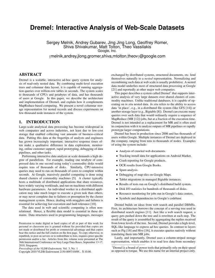
Figure 1: Record-wise vs. columnar representation of nested data

The second ingredient for building interoperable data manage-ment components is a shared storage format. Columnar storageproved successful for flat relational data but making it work forGoogle required adapting it to a nested data model. Figure 1 illus-trates the main idea: all values of a nested field such as A.B.C arestored contiguously. Hence, A.B.C can be retrieved without read-ing A.E, A.B.D, etc. The challenge that we address is how to pre-serve all structural information and be able to reconstruct recordsfrom an arbitrary subset of fields. Next we discuss our data model,and then turn to algorithms and query processing.

3. DATA MODELIn this section we present Dremel’s data model and introduce someterminology used later. The data model originated in the contextof distributed systems (which explains its name, ‘Protocol Buffers’[21]), is used widely at Google, and is available as an open sourceimplementation. The data model is based on strongly-typed nestedrecords. Its abstract syntax is given by:

τ = dom | 〈A1 : τ [∗|?], . . . , An : τ [∗|?]〉

where τ is an atomic type or a record type. Atomic types in domcomprise integers, floating-point numbers, strings, etc. Recordsconsist of one or multiple fields. Field i in a record has a name Ai

and an optional multiplicity label. Repeated fields (∗) may occurmultiple times in a record. They are interpreted as lists of values,i.e., the order of field occurences in a record is significant. Optionalfields (?) may be missing from the record. Otherwise, a field isrequired, i.e., must appear exactly once.

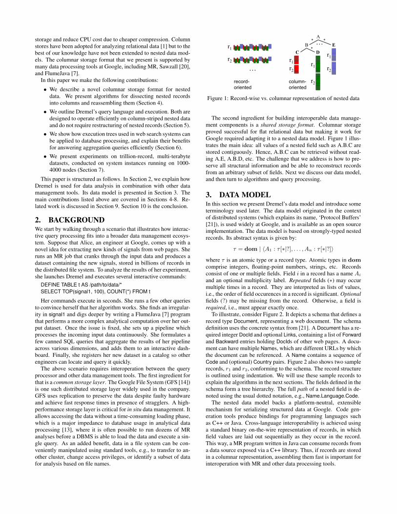
To illustrate, consider Figure 2. It depicts a schema that defines arecord type Document, representing a web document. The schemadefinition uses the concrete syntax from [21]. A Document has a re-quired integer DocId and optional Links, containing a list of Forwardand Backward entries holding DocIds of other web pages. A docu-ment can have multiple Names, which are different URLs by whichthe document can be referenced. A Name contains a sequence ofCode and (optional) Country pairs. Figure 2 also shows two samplerecords, r1 and r2, conforming to the schema. The record structureis outlined using indentation. We will use these sample records toexplain the algorithms in the next sections. The fields defined in theschema form a tree hierarchy. The full path of a nested field is de-noted using the usual dotted notation, e.g., Name.Language.Code.

The nested data model backs a platform-neutral, extensiblemechanism for serializing structured data at Google. Code gen-eration tools produce bindings for programming languages suchas C++ or Java. Cross-language interoperability is achieved usinga standard binary on-the-wire representation of records, in whichfield values are laid out sequentially as they occur in the record.This way, a MR program written in Java can consume records froma data source exposed via a C++ library. Thus, if records are storedin a columnar representation, assembling them fast is important forinteroperation with MR and other data processing tools.

DocId: 10 Links Forward: 20 Forward: 40 Forward: 60 Name Language Code: 'en-us' Country: 'us' Language Code: 'en' Url: 'http://A' Name Url: 'http://B' Name Language Code: 'en-gb' Country: 'gb'

r1 message Document { required int64 DocId; optional group Links { repeated int64 Backward; repeated int64 Forward; } repeated group Name { repeated group Language { required string Code; optional string Country; } optional string Url; }}

DocId: 20 Links Backward: 10 Backward: 30 Forward: 80 Name Url: 'http://C'

r2

Figure 2: Two sample nested records and their schema

4. NESTED COLUMNAR STORAGEAs illustrated in Figure 1, our goal is to store all values of a givenfield consecutively to improve retrieval efficiency. In this section,we address the following challenges: lossless representation ofrecord structure in a columnar format (Section 4.1), fast encoding(Section 4.2), and efficient record assembly (Section 4.3).

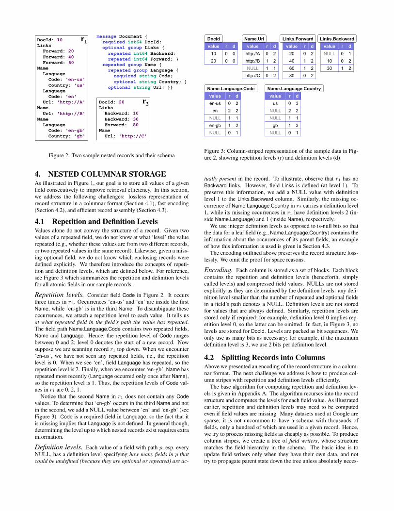
4.1 Repetition and Definition LevelsValues alone do not convey the structure of a record. Given twovalues of a repeated field, we do not know at what ‘level’ the valuerepeated (e.g., whether these values are from two different records,or two repeated values in the same record). Likewise, given a miss-ing optional field, we do not know which enclosing records weredefined explicitly. We therefore introduce the concepts of repeti-tion and definition levels, which are defined below. For reference,see Figure 3 which summarizes the repetition and definition levelsfor all atomic fields in our sample records.

Repetition levels. Consider field Code in Figure 2. It occursthree times in r1. Occurrences ‘en-us’ and ‘en’ are inside the firstName, while ’en-gb’ is in the third Name. To disambiguate theseoccurrences, we attach a repetition level to each value. It tells usat what repeated field in the field’s path the value has repeated.The field path Name.Language.Code contains two repeated fields,Name and Language. Hence, the repetition level of Code rangesbetween 0 and 2; level 0 denotes the start of a new record. Nowsuppose we are scanning record r1 top down. When we encounter‘en-us’, we have not seen any repeated fields, i.e., the repetitionlevel is 0. When we see ‘en’, field Language has repeated, so therepetition level is 2. Finally, when we encounter ‘en-gb’, Name hasrepeated most recently (Language occurred only once after Name),so the repetition level is 1. Thus, the repetition levels of Code val-ues in r1 are 0, 2, 1.

Notice that the second Name in r1 does not contain any Codevalues. To determine that ‘en-gb’ occurs in the third Name and notin the second, we add a NULL value between ‘en’ and ‘en-gb’ (seeFigure 3). Code is a required field in Language, so the fact that itis missing implies that Language is not defined. In general though,determining the level up to which nested records exist requires extrainformation.

Definition levels. Each value of a field with path p, esp. everyNULL, has a definition level specifying how many fields in p thatcould be undefined (because they are optional or repeated) are ac-

value r d 10 0 0 20 0 0

DocId value r d

http://A 0 2 http://B 1 2 NULL 1 1

http://C 0 2

Name.Url

value r d en-us 0 2

en 2 2 NULL 1 1 en-gb 1 2 NULL 0 1

Name.Language.Code Name.Language.Country

Links.Backward Links.Forward

value r d us 0 3

NULL 2 2 NULL 1 1

gb 1 3 NULL 0 1

value r d 20 0 2 40 1 2 60 1 2 80 0 2

value r d NULL 0 1

10 0 2 30 1 2

Figure 3: Column-striped representation of the sample data in Fig-ure 2, showing repetition levels (r) and definition levels (d)

tually present in the record. To illustrate, observe that r1 has noBackward links. However, field Links is defined (at level 1). Topreserve this information, we add a NULL value with definitionlevel 1 to the Links.Backward column. Similarly, the missing oc-currence of Name.Language.Country in r2 carries a definition level1, while its missing occurrences in r1 have definition levels 2 (in-side Name.Language) and 1 (inside Name), respectively.

We use integer definition levels as opposed to is-null bits so thatthe data for a leaf field (e.g., Name.Language.Country) contains theinformation about the occurrences of its parent fields; an exampleof how this information is used is given in Section 4.3.

The encoding outlined above preserves the record structure loss-lessly. We omit the proof for space reasons.

Encoding. Each column is stored as a set of blocks. Each blockcontains the repetition and definition levels (henceforth, simplycalled levels) and compressed field values. NULLs are not storedexplicitly as they are determined by the definition levels: any defi-nition level smaller than the number of repeated and optional fieldsin a field’s path denotes a NULL. Definition levels are not storedfor values that are always defined. Similarly, repetition levels arestored only if required; for example, definition level 0 implies rep-etition level 0, so the latter can be omitted. In fact, in Figure 3, nolevels are stored for DocId. Levels are packed as bit sequences. Weonly use as many bits as necessary; for example, if the maximumdefinition level is 3, we use 2 bits per definition level.

4.2 Splitting Records into ColumnsAbove we presented an encoding of the record structure in a colum-nar format. The next challenge we address is how to produce col-umn stripes with repetition and definition levels efficiently.

The base algorithm for computing repetition and definition lev-els is given in Appendix A. The algorithm recurses into the recordstructure and computes the levels for each field value. As illustratedearlier, repetition and definition levels may need to be computedeven if field values are missing. Many datasets used at Google aresparse; it is not uncommon to have a schema with thousands offields, only a hundred of which are used in a given record. Hence,we try to process missing fields as cheaply as possible. To producecolumn stripes, we create a tree of field writers, whose structurematches the field hierarchy in the schema. The basic idea is toupdate field writers only when they have their own data, and nottry to propagate parent state down the tree unless absolutely neces-

Name.Language.Country Name.Language.Code

Links.Backward Links.Forward

Name.Url

DocId

1 0

1 0

0,1,2 2

0,1 1 0

0

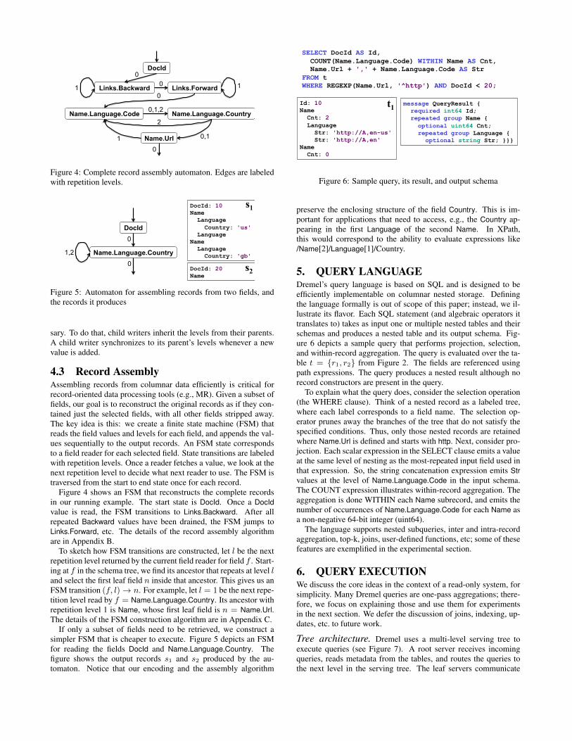
Figure 4: Complete record assembly automaton. Edges are labeledwith repetition levels.

DocId

Name.Language.Country 1,2 0

0

DocId: 10 Name Language Country: 'us' Language Name Language Country: 'gb'

DocId: 20 Name

s1

s2

Figure 5: Automaton for assembling records from two fields, andthe records it produces

sary. To do that, child writers inherit the levels from their parents.A child writer synchronizes to its parent’s levels whenever a newvalue is added.

4.3 Record AssemblyAssembling records from columnar data efficiently is critical forrecord-oriented data processing tools (e.g., MR). Given a subset offields, our goal is to reconstruct the original records as if they con-tained just the selected fields, with all other fields stripped away.The key idea is this: we create a finite state machine (FSM) thatreads the field values and levels for each field, and appends the val-ues sequentially to the output records. An FSM state correspondsto a field reader for each selected field. State transitions are labeledwith repetition levels. Once a reader fetches a value, we look at thenext repetition level to decide what next reader to use. The FSM istraversed from the start to end state once for each record.

Figure 4 shows an FSM that reconstructs the complete recordsin our running example. The start state is DocId. Once a DocIdvalue is read, the FSM transitions to Links.Backward. After allrepeated Backward values have been drained, the FSM jumps toLinks.Forward, etc. The details of the record assembly algorithmare in Appendix B.

To sketch how FSM transitions are constructed, let l be the nextrepetition level returned by the current field reader for field f . Start-ing at f in the schema tree, we find its ancestor that repeats at level land select the first leaf field n inside that ancestor. This gives us anFSM transition (f, l)→ n. For example, let l = 1 be the next repe-tition level read by f = Name.Language.Country. Its ancestor withrepetition level 1 is Name, whose first leaf field is n = Name.Url.The details of the FSM construction algorithm are in Appendix C.

If only a subset of fields need to be retrieved, we construct asimpler FSM that is cheaper to execute. Figure 5 depicts an FSMfor reading the fields DocId and Name.Language.Country. Thefigure shows the output records s1 and s2 produced by the au-tomaton. Notice that our encoding and the assembly algorithm

Id: 10 Name Cnt: 2 Language Str: 'http://A,en-us' Str: 'http://A,en' Name Cnt: 0

t1

SELECT DocId AS Id, COUNT(Name.Language.Code) WITHIN Name AS Cnt, Name.Url + ',' + Name.Language.Code AS Str FROM t WHERE REGEXP(Name.Url, '^http') AND DocId < 20;

message QueryResult { required int64 Id; repeated group Name { optional uint64 Cnt; repeated group Language { optional string Str; }}}

Figure 6: Sample query, its result, and output schema

preserve the enclosing structure of the field Country. This is im-portant for applications that need to access, e.g., the Country ap-pearing in the first Language of the second Name. In XPath,this would correspond to the ability to evaluate expressions like/Name[2]/Language[1]/Country.

5. QUERY LANGUAGEDremel’s query language is based on SQL and is designed to beefficiently implementable on columnar nested storage. Definingthe language formally is out of scope of this paper; instead, we il-lustrate its flavor. Each SQL statement (and algebraic operators ittranslates to) takes as input one or multiple nested tables and theirschemas and produces a nested table and its output schema. Fig-ure 6 depicts a sample query that performs projection, selection,and within-record aggregation. The query is evaluated over the ta-ble t = {r1, r2} from Figure 2. The fields are referenced usingpath expressions. The query produces a nested result although norecord constructors are present in the query.

To explain what the query does, consider the selection operation(the WHERE clause). Think of a nested record as a labeled tree,where each label corresponds to a field name. The selection op-erator prunes away the branches of the tree that do not satisfy thespecified conditions. Thus, only those nested records are retainedwhere Name.Url is defined and starts with http. Next, consider pro-jection. Each scalar expression in the SELECT clause emits a valueat the same level of nesting as the most-repeated input field used inthat expression. So, the string concatenation expression emits Strvalues at the level of Name.Language.Code in the input schema.The COUNT expression illustrates within-record aggregation. Theaggregation is done WITHIN each Name subrecord, and emits thenumber of occurrences of Name.Language.Code for each Name asa non-negative 64-bit integer (uint64).

The language supports nested subqueries, inter and intra-recordaggregation, top-k, joins, user-defined functions, etc; some of thesefeatures are exemplified in the experimental section.

6. QUERY EXECUTIONWe discuss the core ideas in the context of a read-only system, forsimplicity. Many Dremel queries are one-pass aggregations; there-fore, we focus on explaining those and use them for experimentsin the next section. We defer the discussion of joins, indexing, up-dates, etc. to future work.

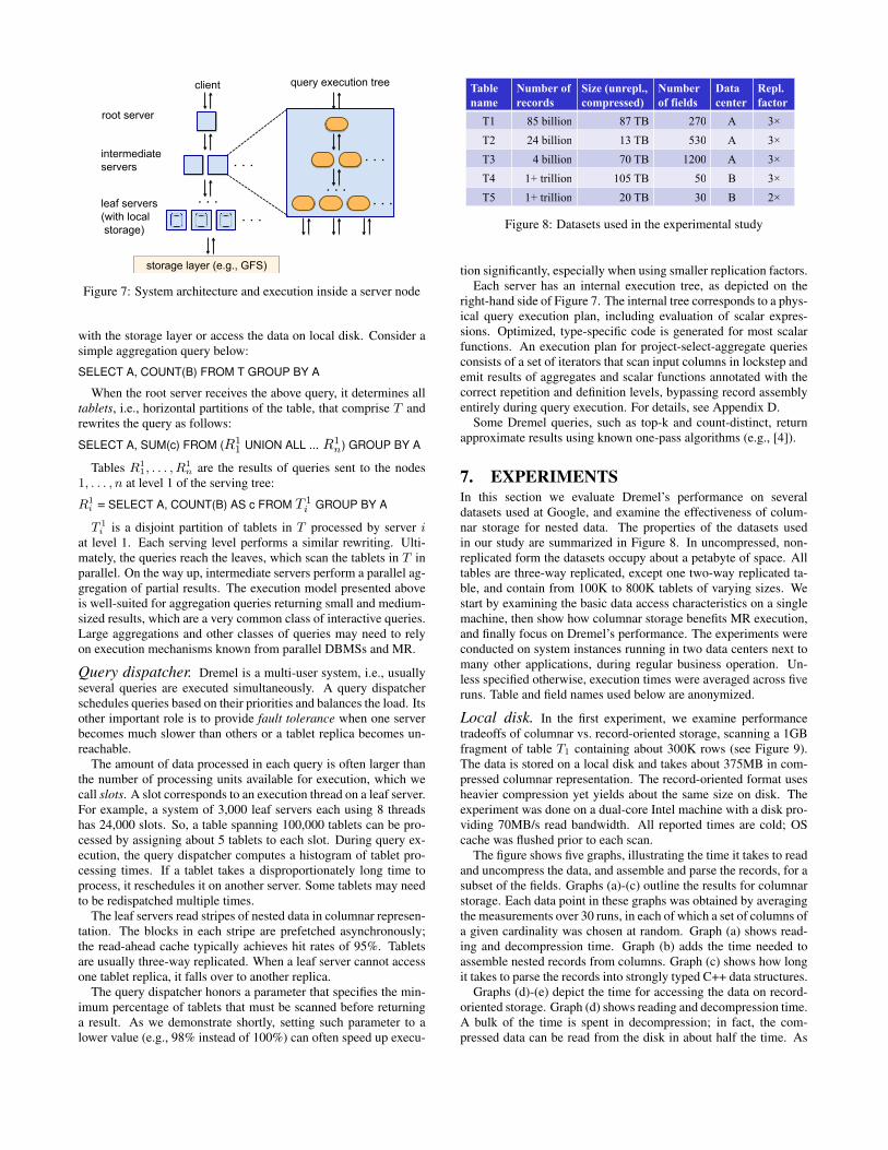
Tree architecture. Dremel uses a multi-level serving tree toexecute queries (see Figure 7). A root server receives incomingqueries, reads metadata from the tables, and routes the queries tothe next level in the serving tree. The leaf servers communicate

query execution tree

. . .

. . . . . .

storage layer (e.g., GFS)

. . .

. . . . . . leaf servers

(with local storage)

intermediate servers

root server

client

Figure 7: System architecture and execution inside a server node

with the storage layer or access the data on local disk. Consider asimple aggregation query below:

SELECT A, COUNT(B) FROM T GROUP BY A

When the root server receives the above query, it determines alltablets, i.e., horizontal partitions of the table, that comprise T andrewrites the query as follows:

SELECT A, SUM(c) FROM (R11 UNION ALL ... R1

n) GROUP BY A

Tables R11, . . . , R

1n are the results of queries sent to the nodes

1, . . . , n at level 1 of the serving tree:

R1i = SELECT A, COUNT(B) AS c FROM T 1

i GROUP BY A

T 1i is a disjoint partition of tablets in T processed by server i

at level 1. Each serving level performs a similar rewriting. Ulti-mately, the queries reach the leaves, which scan the tablets in T inparallel. On the way up, intermediate servers perform a parallel ag-gregation of partial results. The execution model presented aboveis well-suited for aggregation queries returning small and medium-sized results, which are a very common class of interactive queries.Large aggregations and other classes of queries may need to relyon execution mechanisms known from parallel DBMSs and MR.

Query dispatcher. Dremel is a multi-user system, i.e., usuallyseveral queries are executed simultaneously. A query dispatcherschedules queries based on their priorities and balances the load. Itsother important role is to provide fault tolerance when one serverbecomes much slower than others or a tablet replica becomes un-reachable.

The amount of data processed in each query is often larger thanthe number of processing units available for execution, which wecall slots. A slot corresponds to an execution thread on a leaf server.For example, a system of 3,000 leaf servers each using 8 threadshas 24,000 slots. So, a table spanning 100,000 tablets can be pro-cessed by assigning about 5 tablets to each slot. During query ex-ecution, the query dispatcher computes a histogram of tablet pro-cessing times. If a tablet takes a disproportionately long time toprocess, it reschedules it on another server. Some tablets may needto be redispatched multiple times.

The leaf servers read stripes of nested data in columnar represen-tation. The blocks in each stripe are prefetched asynchronously;the read-ahead cache typically achieves hit rates of 95%. Tabletsare usually three-way replicated. When a leaf server cannot accessone tablet replica, it falls over to another replica.

The query dispatcher honors a parameter that specifies the min-imum percentage of tablets that must be scanned before returninga result. As we demonstrate shortly, setting such parameter to alower value (e.g., 98% instead of 100%) can often speed up execu-

Table name

Number of records

Size (unrepl., compressed)

Number of fields

Data center

Repl. factor

T1 85 billion 87 TB 270 A 3× T2 24 billion 13 TB 530 A 3× T3 4 billion 70 TB 1200 A 3× T4 1+ trillion 105 TB 50 B 3× T5 1+ trillion 20 TB 30 B 2×

Figure 8: Datasets used in the experimental study

tion significantly, especially when using smaller replication factors.Each server has an internal execution tree, as depicted on the

right-hand side of Figure 7. The internal tree corresponds to a phys-ical query execution plan, including evaluation of scalar expres-sions. Optimized, type-specific code is generated for most scalarfunctions. An execution plan for project-select-aggregate queriesconsists of a set of iterators that scan input columns in lockstep andemit results of aggregates and scalar functions annotated with thecorrect repetition and definition levels, bypassing record assemblyentirely during query execution. For details, see Appendix D.

Some Dremel queries, such as top-k and count-distinct, returnapproximate results using known one-pass algorithms (e.g., [4]).

7. EXPERIMENTSIn this section we evaluate Dremel’s performance on severaldatasets used at Google, and examine the effectiveness of colum-nar storage for nested data. The properties of the datasets usedin our study are summarized in Figure 8. In uncompressed, non-replicated form the datasets occupy about a petabyte of space. Alltables are three-way replicated, except one two-way replicated ta-ble, and contain from 100K to 800K tablets of varying sizes. Westart by examining the basic data access characteristics on a singlemachine, then show how columnar storage benefits MR execution,and finally focus on Dremel’s performance. The experiments wereconducted on system instances running in two data centers next tomany other applications, during regular business operation. Un-less specified otherwise, execution times were averaged across fiveruns. Table and field names used below are anonymized.

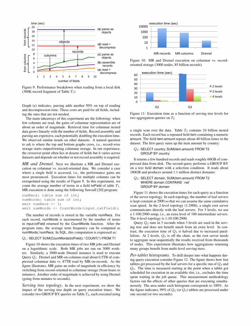
Local disk. In the first experiment, we examine performancetradeoffs of columnar vs. record-oriented storage, scanning a 1GBfragment of table T1 containing about 300K rows (see Figure 9).The data is stored on a local disk and takes about 375MB in com-pressed columnar representation. The record-oriented format usesheavier compression yet yields about the same size on disk. Theexperiment was done on a dual-core Intel machine with a disk pro-viding 70MB/s read bandwidth. All reported times are cold; OScache was flushed prior to each scan.

The figure shows five graphs, illustrating the time it takes to readand uncompress the data, and assemble and parse the records, for asubset of the fields. Graphs (a)-(c) outline the results for columnarstorage. Each data point in these graphs was obtained by averagingthe measurements over 30 runs, in each of which a set of columns ofa given cardinality was chosen at random. Graph (a) shows read-ing and decompression time. Graph (b) adds the time needed toassemble nested records from columns. Graph (c) shows how longit takes to parse the records into strongly typed C++ data structures.

Graphs (d)-(e) depict the time for accessing the data on record-oriented storage. Graph (d) shows reading and decompression time.A bulk of the time is spent in decompression; in fact, the com-pressed data can be read from the disk in about half the time. As

!"

#"

$"

%"

&"

'!"

'#"

'$"

'%"

'&"

#!"

'" #" (" $" )" %" *" &" +" '!"

columns records

objects

from

reco

rds

from

col

umns

(a) read + decompress

(b) assemble records

(c) parse as objects

(d) read + decompress

(e) parse as objects

time (sec)

number of fields

Figure 9: Performance breakdown when reading from a local disk(300K-record fragment of Table T1)

Graph (e) indicates, parsing adds another 50% on top of readingand decompression time. These costs are paid for all fields, includ-ing the ones that are not needed.

The main takeaways of this experiment are the following: whenfew columns are read, the gains of columnar representation are ofabout an order of magnitude. Retrieval time for columnar nesteddata grows linearly with the number of fields. Record assembly andparsing are expensive, each potentially doubling the execution time.We observed similar trends on other datasets. A natural questionto ask is where the top and bottom graphs cross, i.e., record-wisestorage starts outperforming columnar storage. In our experience,the crossover point often lies at dozens of fields but it varies acrossdatasets and depends on whether or not record assembly is required.

MR and Dremel. Next we illustrate a MR and Dremel exe-cution on columnar vs. record-oriented data. We consider a casewhere a single field is accessed, i.e., the performance gains aremost pronounced. Execution times for multiple columns can beextrapolated using the results of Figure 9. In this experiment, wecount the average number of terms in a field txtField of table T1.MR execution is done using the following Sawzall [20] program:numRecs: table sum of int;numWords: table sum of int;emit numRecs <- 1;emit numWords <- CountWords(input.txtField);

The number of records is stored in the variable numRecs. Foreach record, numWords is incremented by the number of termsin input.txtField returned by the CountWords function. After theprogram runs, the average term frequency can be computed asnumWords/numRecs. In SQL, this computation is expressed as:

Q1: SELECT SUM(CountWords(txtField)) / COUNT(*) FROM T1

Figure 10 shows the execution times of two MR jobs and Dremelon a logarithmic scale. Both MR jobs are run on 3000 work-ers. Similarly, a 3000-node Dremel instance is used to executeQuery Q1. Dremel and MR-on-columns read about 0.5TB of com-pressed columnar data vs. 87TB read by MR-on-records. As thefigure illustrates, MR gains an order of magnitude in efficiency byswitching from record-oriented to columnar storage (from hours tominutes). Another order of magnitude is achieved by using Dremel(going from minutes to seconds).

Serving tree topology. In the next experiment, we show theimpact of the serving tree depth on query execution times. Weconsider two GROUP BY queries on Table T2, each executed using

!"

!#"

!##"

!###"

!####"

$%&'()*'+," $%&)*-./0," 1'(/(-"

execution time (sec)

Figure 10: MR and Dremel execution on columnar vs. record-oriented storage (3000 nodes, 85 billion records)

!"

#!"

$!"

%!"

&!"

'!"

(!"

)$" )%"

$"*+,+*-"

%"*+,+*-"

&"*+,+*-"

execution time (sec)

Figure 11: Execution time as a function of serving tree levels fortwo aggregation queries on T2

a single scan over the data. Table T2 contains 24 billion nestedrecords. Each record has a repeated field item containing a numericamount. The field item.amount repeats about 40 billion times in thedataset. The first query sums up the item amount by country:

Q2: SELECT country, SUM(item.amount) FROM T2GROUP BY country

It returns a few hundred records and reads roughly 60GB of com-pressed data from disk. The second query performs a GROUP BYon a text field domain with a selection condition. It reads about180GB and produces around 1.1 million distinct domains:

Q3: SELECT domain, SUM(item.amount) FROM T2WHERE domain CONTAINS ’.net’GROUP BY domain

Figure 11 shows the execution times for each query as a functionof the server topology. In each topology, the number of leaf serversis kept constant at 2900 so that we can assume the same cumulativescan speed. In the 2-level topology (1:2900), a single root servercommunicates directly with the leaf servers. For 3 levels, we usea 1:100:2900 setup, i.e., an extra level of 100 intermediate servers.The 4-level topology is 1:10:100:2900.

Query Q2 runs in 3 seconds when 3 levels are used in the serv-ing tree and does not benefit much from an extra level. In con-trast, the execution time of Q3 is halved due to increased paral-lelism. At 2 levels, Q3 is off the chart, as the root server needsto aggregate near-sequentially the results received from thousandsof nodes. This experiment illustrates how aggregations returningmany groups benefit from multi-level serving trees.

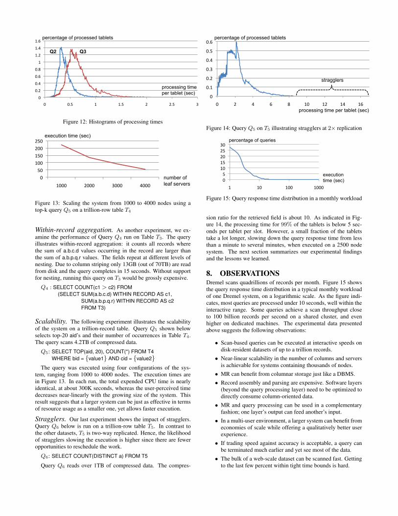
Per-tablet histograms. To drill deeper into what happens dur-ing query execution consider Figure 12. The figure shows how fasttablets get processed by the leaf servers for a specific run ofQ2 andQ3. The time is measured starting at the point when a tablet gotscheduled for execution in an available slot, i.e., excludes the timespent waiting in the job queue. This measurement methodologyfactors out the effects of other queries that are executing simulta-neously. The area under each histogram corresponds to 100%. Asthe figure indicates, 99% of Q2 (or Q3) tablets are processed underone second (or two seconds).

!"

!#$"

!#%"

!#&"

!#'"

("

(#$"

(#%"

(#&"

!" !#)" (" (#)" $" $#)" *"

percentage of processed tablets

processing time per tablet (sec)

Q3 Q2

Figure 12: Histograms of processing times

!"

#!"

$!!"

$#!"

%!!"

%#!"

$!!!" %!!!" &!!!" '!!!"

execution time (sec)

number of leaf servers

Figure 13: Scaling the system from 1000 to 4000 nodes using atop-k query Q5 on a trillion-row table T4

Within-record aggregation. As another experiment, we ex-amine the performance of Query Q4 run on Table T3. The queryillustrates within-record aggregation: it counts all records wherethe sum of a.b.c.d values occurring in the record are larger thanthe sum of a.b.p.q.r values. The fields repeat at different levels ofnesting. Due to column striping only 13GB (out of 70TB) are readfrom disk and the query completes in 15 seconds. Without supportfor nesting, running this query on T3 would be grossly expensive.

Q4 : SELECT COUNT(c1 > c2) FROM(SELECT SUM(a.b.c.d) WITHIN RECORD AS c1,

SUM(a.b.p.q.r) WITHIN RECORD AS c2FROM T3)

Scalability. The following experiment illustrates the scalabilityof the system on a trillion-record table. Query Q5 shown belowselects top-20 aid’s and their number of occurrences in Table T4.The query scans 4.2TB of compressed data.

Q5: SELECT TOP(aid, 20), COUNT(*) FROM T4WHERE bid = {value1} AND cid = {value2}

The query was executed using four configurations of the sys-tem, ranging from 1000 to 4000 nodes. The execution times arein Figure 13. In each run, the total expended CPU time is nearlyidentical, at about 300K seconds, whereas the user-perceived timedecreases near-linearly with the growing size of the system. Thisresult suggests that a larger system can be just as effective in termsof resource usage as a smaller one, yet allows faster execution.

Stragglers. Our last experiment shows the impact of stragglers.Query Q6 below is run on a trillion-row table T5. In contrast tothe other datasets, T5 is two-way replicated. Hence, the likelihoodof stragglers slowing the execution is higher since there are feweropportunities to reschedule the work.

Q6: SELECT COUNT(DISTINCT a) FROM T5

Query Q6 reads over 1TB of compressed data. The compres-

!"

!#$"

!#%"

!#&"

!#'"

!#("

!#)"

!" %" '" )" *" $!" $%" $'" $)"

percentage of processed tablets

processing time per tablet (sec)

stragglers

Figure 14: Query Q5 on T5 illustrating stragglers at 2× replication

!"

#"

$!"

$#"

%!"

%#"

&!"

$" $!" $!!" $!!!"

execution time (sec)

percentage of queries

Figure 15: Query response time distribution in a monthly workload

sion ratio for the retrieved field is about 10. As indicated in Fig-ure 14, the processing time for 99% of the tablets is below 5 sec-onds per tablet per slot. However, a small fraction of the tabletstake a lot longer, slowing down the query response time from lessthan a minute to several minutes, when executed on a 2500 nodesystem. The next section summarizes our experimental findingsand the lessons we learned.

8. OBSERVATIONSDremel scans quadrillions of records per month. Figure 15 showsthe query response time distribution in a typical monthly workloadof one Dremel system, on a logarithmic scale. As the figure indi-cates, most queries are processed under 10 seconds, well within theinteractive range. Some queries achieve a scan throughput closeto 100 billion records per second on a shared cluster, and evenhigher on dedicated machines. The experimental data presentedabove suggests the following observations:

• Scan-based queries can be executed at interactive speeds ondisk-resident datasets of up to a trillion records.• Near-linear scalability in the number of columns and servers

is achievable for systems containing thousands of nodes.• MR can benefit from columnar storage just like a DBMS.• Record assembly and parsing are expensive. Software layers

(beyond the query processing layer) need to be optimized todirectly consume column-oriented data.• MR and query processing can be used in a complementary

fashion; one layer’s output can feed another’s input.• In a multi-user environment, a larger system can benefit from

economies of scale while offering a qualitatively better userexperience.• If trading speed against accuracy is acceptable, a query can

be terminated much earlier and yet see most of the data.• The bulk of a web-scale dataset can be scanned fast. Getting

to the last few percent within tight time bounds is hard.

Dremel’s codebase is dense; it comprises less than 100K lines ofC++, Java, and Python code.

9. RELATED WORKThe MapReduce (MR) [12] framework was designed to address thechallenges of large-scale computing in the context of long-runningbatch jobs. Like MR, Dremel provides fault tolerant execution, aflexible data model, and in situ data processing capabilities. Thesuccess of MR led to a wide range of third-party implementations(notably open-source Hadoop [15]), and a number of hybrid sys-tems that combine parallel DBMSs with MR, offered by vendorslike Aster, Cloudera, Greenplum, and Vertica. HadoopDB [3] isa research system in this hybrid category. Recent articles [13, 22]contrast MR and parallel DBMSs. Our work emphasizes the com-plementary nature of both paradigms.

Dremel is designed to operate at scale. Although it is conceivablethat parallel DBMSs can be made to scale to thousands of nodes,we are not aware of any published work or industry reports that at-tempted that. Neither are we familiar with prior literature studyingMR on columnar storage.

Our columnar representation of nested data builds on ideas thatdate back several decades: separation of structure from contentand transposed representation. A recent review of work on col-umn stores, incl. compression and query processing, can be foundin [1]. Many commercial DBMSs support storage of nested datausing XML (e.g., [19]). XML storage schemes attempt to separatethe structure from the content but face more challenges due to theflexibility of the XML data model. One system that uses columnarXML representation is XMill [17]. XMill is a compression tool.It stores the structure for all fields combined and is not geared forselective retrieval of columns.

The data model used in Dremel is a variation of the com-plex value models and nested relational models discussed in [2].Dremel’s query language builds on the ideas from [9], which intro-duced a language that avoids restructuring when accessing nesteddata. In contrast, restructuring is usually required in XQuery andobject-oriented query languages, e.g., using nested for-loops andconstructors. We are not aware of practical implementations of [9].A recent SQL-like language operating on nested data is Pig [18].Other systems for parallel data processing include Scope [6] andDryadLINQ [23], and are discussed in more detail in [7].

10. CONCLUSIONSWe presented Dremel, a distributed system for interactive analy-sis of large datasets. Dremel is a custom, scalable data manage-ment solution built from simpler components. It complements theMR paradigm. We discussed its performance on trillion-record,multi-terabyte datasets of real data. We outlined the key aspectsof Dremel, including its storage format, query language, and exe-cution. In the future, we plan to cover in more depth such areas asformal algebraic specification, joins, extensibility mechanisms, etc.

11. ACKNOWLEDGEMENTSDremel has benefited greatly from the input of many engineers andinterns at Google, in particular Craig Chambers, Ori Gershoni, Ra-jeev Byrisetti, Leon Wong, Erik Hendriks, Erika Rice Scherpelz,Charlie Garrett, Idan Avraham, Rajesh Rao, Andy Kreling, Li Yin,Madhusudan Hosaagrahara, Dan Belov, Brian Bershad, LawrenceYou, Rongrong Zhong, Meelap Shah, and Nathan Bales.

12. REFERENCES

[1] D. J. Abadi, P. A. Boncz, and S. Harizopoulos.Column-Oriented Database Systems. VLDB, 2(2), 2009.

[2] S. Abiteboul, R. Hull, and V. Vianu. Foundations ofDatabases. Addison Wesley, 1995.

[3] A. Abouzeid, K. Bajda-Pawlikowski, D. J. Abadi, A. Rasin,and A. Silberschatz. HadoopDB: An Architectural Hybrid ofMapReduce and DBMS Technologies for AnalyticalWorkloads. VLDB, 2(1), 2009.

[4] Z. Bar-Yossef, T. S. Jayram, R. Kumar, D. Sivakumar, andL. Trevisan. Counting Distinct Elements in a Data Stream. InRANDOM, pages 1–10, 2002.

[5] L. A. Barroso and U. Holzle. The Datacenter as a Computer:An Introduction to the Design of Warehouse-Scale Machines.Morgan & Claypool Publishers, 2009.

[6] R. Chaiken, B. Jenkins, P.-A. Larson, B. Ramsey, D. Shakib,S. Weaver, and J. Zhou. SCOPE: Easy and Efficient ParallelProcessing of Massive Data Sets. VLDB, 1(2), 2008.

[7] C. Chambers, A. Raniwala, F. Perry, S. Adams, R. Henry,R. Bradshaw, and N. Weizenbaum. FlumeJava: Easy,Efficient Data-Parallel Pipelines. In PLDI, 2010.

[8] F. Chang, J. Dean, S. Ghemawat, W. C. Hsieh, D. A.Wallach, M. Burrows, T. Chandra, A. Fikes, and R. Gruber.Bigtable: A Distributed Storage System for Structured Data.In OSDI, 2006.

[9] L. S. Colby. A Recursive Algebra and Query Optimizationfor Nested Relations. SIGMOD Rec., 18(2), 1989.

[10] G. Czajkowski. Sorting 1PB with MapReduce. OfficialGoogle Blog, Nov. 2008. At http://googleblog.blogspot.com/2008/11/sorting-1pb-with-mapreduce.html.

[11] J. Dean. Challenges in Building Large-Scale InformationRetrieval Systems: Invited Talk. In WSDM, 2009.

[12] J. Dean and S. Ghemawat. MapReduce: Simplified DataProcessing on Large Clusters. In OSDI, 2004.

[13] J. Dean and S. Ghemawat. MapReduce: a Flexible DataProcessing Tool. Commun. ACM, 53(1), 2010.

[14] S. Ghemawat, H. Gobioff, and S.-T. Leung. The Google FileSystem. In SOSP, 2003.

[15] Hadoop Apache Project. http://hadoop.apache.org.[16] Hive. http://wiki.apache.org/hadoop/Hive, 2009.[17] H. Liefke and D. Suciu. XMill: An Efficient Compressor for

XML Data. In SIGMOD, 2000.[18] C. Olston, B. Reed, U. Srivastava, R. Kumar, and

A. Tomkins. Pig Latin: a Not-so-Foreign Language for DataProcessing. In SIGMOD, 2008.

[19] P. E. O’Neil, E. J. O’Neil, S. Pal, I. Cseri, G. Schaller, andN. Westbury. ORDPATHs: Insert-Friendly XML NodeLabels. In SIGMOD, 2004.

[20] R. Pike, S. Dorward, R. Griesemer, and S. Quinlan.Interpreting the Data: Parallel Analysis with Sawzall.Scientific Programming, 13(4), 2005.

[21] Protocol Buffers: Developer Guide. Available athttp://code.google.com/apis/protocolbuffers/docs/overview.html.

[22] M. Stonebraker, D. Abadi, D. J. DeWitt, S. Madden,E. Paulson, A. Pavlo, and A. Rasin. MapReduce and ParallelDBMSs: Friends or Foes? Commun. ACM, 53(1), 2010.

[23] Y. Yu, M. Isard, D. Fetterly, M. Budiu, U. Erlingsson, P. K.Gunda, and J. Currey. DryadLINQ: A System forGeneral-Purpose Distributed Data-Parallel Computing Usinga High-Level Language. In OSDI, 2008.

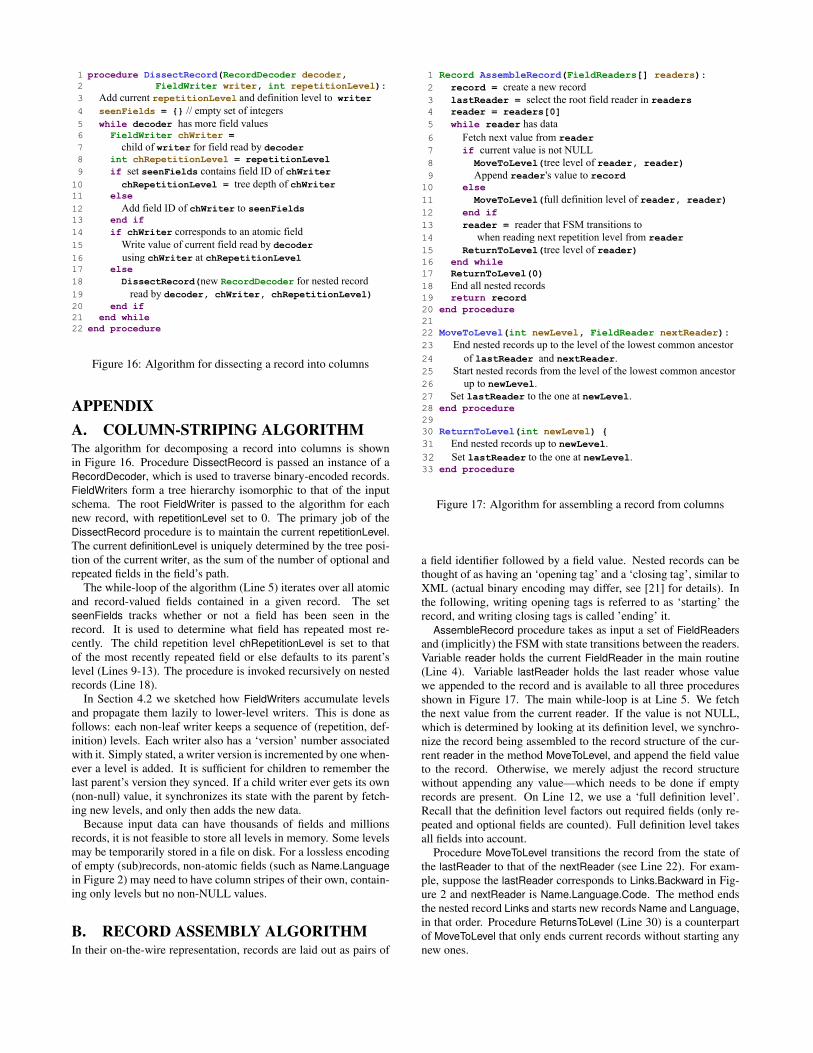
1 procedure DissectRecord(RecordDecoder decoder, 2 FieldWriter writer, int repetitionLevel): 3 Add current repetitionLevel and definition level to writer 4 seenFields = {} // empty set of integers 5 while decoder has more field values 6 FieldWriter chWriter = 7 child of writer for field read by decoder 8 int chRepetitionLevel = repetitionLevel 9 if set seenFields contains field ID of chWriter 10 chRepetitionLevel = tree depth of chWriter 11 else 12 Add field ID of chWriter to seenFields 13 end if 14 if chWriter corresponds to an atomic field 15 Write value of current field read by decoder 16 using chWriter at chRepetitionLevel 17 else 18 DissectRecord(new RecordDecoder for nested record 19 read by decoder, chWriter, chRepetitionLevel) 20 end if 21 end while 22 end procedure

Figure 16: Algorithm for dissecting a record into columns

APPENDIXA. COLUMN-STRIPING ALGORITHMThe algorithm for decomposing a record into columns is shownin Figure 16. Procedure DissectRecord is passed an instance of aRecordDecoder, which is used to traverse binary-encoded records.FieldWriters form a tree hierarchy isomorphic to that of the inputschema. The root FieldWriter is passed to the algorithm for eachnew record, with repetitionLevel set to 0. The primary job of theDissectRecord procedure is to maintain the current repetitionLevel.The current definitionLevel is uniquely determined by the tree posi-tion of the current writer, as the sum of the number of optional andrepeated fields in the field’s path.

The while-loop of the algorithm (Line 5) iterates over all atomicand record-valued fields contained in a given record. The setseenFields tracks whether or not a field has been seen in therecord. It is used to determine what field has repeated most re-cently. The child repetition level chRepetitionLevel is set to thatof the most recently repeated field or else defaults to its parent’slevel (Lines 9-13). The procedure is invoked recursively on nestedrecords (Line 18).

In Section 4.2 we sketched how FieldWriters accumulate levelsand propagate them lazily to lower-level writers. This is done asfollows: each non-leaf writer keeps a sequence of (repetition, def-inition) levels. Each writer also has a ‘version’ number associatedwith it. Simply stated, a writer version is incremented by one when-ever a level is added. It is sufficient for children to remember thelast parent’s version they synced. If a child writer ever gets its own(non-null) value, it synchronizes its state with the parent by fetch-ing new levels, and only then adds the new data.

Because input data can have thousands of fields and millionsrecords, it is not feasible to store all levels in memory. Some levelsmay be temporarily stored in a file on disk. For a lossless encodingof empty (sub)records, non-atomic fields (such as Name.Languagein Figure 2) may need to have column stripes of their own, contain-ing only levels but no non-NULL values.

B. RECORD ASSEMBLY ALGORITHMIn their on-the-wire representation, records are laid out as pairs of

1 Record AssembleRecord(FieldReaders[] readers): 2 record = create a new record 3 lastReader = select the root field reader in readers 4 reader = readers[0] 5 while reader has data 6 Fetch next value from reader 7 if current value is not NULL 8 MoveToLevel(tree level of reader, reader) 9 Append reader's value to record 10 else 11 MoveToLevel(full definition level of reader, reader) 12 end if 13 reader = reader that FSM transitions to 14 when reading next repetition level from reader 15 ReturnToLevel(tree level of reader) 16 end while 17 ReturnToLevel(0) 18 End all nested records 19 return record 20 end procedure 21 22 MoveToLevel(int newLevel, FieldReader nextReader): 23 End nested records up to the level of the lowest common ancestor 24 of lastReader and nextReader. 25 Start nested records from the level of the lowest common ancestor 26 up to newLevel. 27 Set lastReader to the one at newLevel. 28 end procedure 29 30 ReturnToLevel(int newLevel) { 31 End nested records up to newLevel. 32 Set lastReader to the one at newLevel. 33 end procedure

Figure 17: Algorithm for assembling a record from columns

a field identifier followed by a field value. Nested records can bethought of as having an ‘opening tag’ and a ‘closing tag’, similar toXML (actual binary encoding may differ, see [21] for details). Inthe following, writing opening tags is referred to as ‘starting’ therecord, and writing closing tags is called ’ending’ it.

AssembleRecord procedure takes as input a set of FieldReadersand (implicitly) the FSM with state transitions between the readers.Variable reader holds the current FieldReader in the main routine(Line 4). Variable lastReader holds the last reader whose valuewe appended to the record and is available to all three proceduresshown in Figure 17. The main while-loop is at Line 5. We fetchthe next value from the current reader. If the value is not NULL,which is determined by looking at its definition level, we synchro-nize the record being assembled to the record structure of the cur-rent reader in the method MoveToLevel, and append the field valueto the record. Otherwise, we merely adjust the record structurewithout appending any value—which needs to be done if emptyrecords are present. On Line 12, we use a ‘full definition level’.Recall that the definition level factors out required fields (only re-peated and optional fields are counted). Full definition level takesall fields into account.

Procedure MoveToLevel transitions the record from the state ofthe lastReader to that of the nextReader (see Line 22). For exam-ple, suppose the lastReader corresponds to Links.Backward in Fig-ure 2 and nextReader is Name.Language.Code. The method endsthe nested record Links and starts new records Name and Language,in that order. Procedure ReturnsToLevel (Line 30) is a counterpartof MoveToLevel that only ends current records without starting anynew ones.

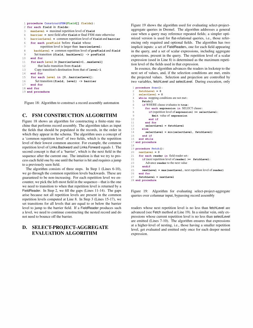
1 procedure ConstructFSM(Field[] fields): 2 for each field in fields: 3 maxLevel = maximal repetition level of field 4 barrier = next field after field or final FSM state otherwise 5 barrierLevel = common repetition level of field and barrier 6 for each preField before field whose 7 repetition level is larger than barrierLevel: 8 backLevel = common repetition level of preField and field 9 Set transition (field, backLevel) -> preField 10 end for 11 for each level in [barrierLevel+1..maxLevel] 12 that lacks transition from field: 13 Copy transition's destination from that of level-1 14 end for 15 for each level in [0..barrierLevel]: 16 Set transition (field, level) -> barrier 17 end for 18 end for 19 end procedure

Figure 18: Algorithm to construct a record assembly automaton

C. FSM CONSTRUCTION ALGORITHMFigure 18 shows an algorithm for constructing a finite-state ma-chine that performs record assembly. The algorithm takes as inputthe fields that should be populated in the records, in the order inwhich they appear in the schema. The algorithm uses a concept ofa ‘common repetition level’ of two fields, which is the repetitionlevel of their lowest common ancestor. For example, the commonrepetition level of Links.Backward and Links.Forward equals 1. Thesecond concept is that of a ‘barrier’, which is the next field in thesequence after the current one. The intuition is that we try to pro-cess each field one by one until the barrier is hit and requires a jumpto a previously seen field.

The algorithm consists of three steps. In Step 1 (Lines 6-10),we go through the common repetition levels backwards. These areguaranteed to be non-increasing. For each repetition level we en-counter, we pick the left-most field in the sequence—that is the onewe need to transition to when that repetition level is returned by aFieldReader. In Step 2, we fill the gaps (Lines 11-14). The gapsarise because not all repetition levels are present in the commonrepetition levels computed at Line 8. In Step 3 (Lines 15-17), weset transitions for all levels that are equal to or below the barrierlevel to jump to the barrier field. If a FieldReader produces sucha level, we need to continue constructing the nested record and donot need to bounce off the barrier.

D. SELECT-PROJECT-AGGREGATEEVALUATION ALGORITHM

Figure 19 shows the algorithm used for evaluating select-project-aggregate queries in Dremel. The algorithm addresses a generalcase when a query may reference repeated fields; a simpler opti-mized version is used for flat-relational queries, i.e., those refer-encing only required and optional fields. The algorithm has twoimplicit inputs: a set of FieldReaders, one for each field appearingin the query, and a set of scalar expressions, including aggregateexpressions, present in the query. The repetition level of a scalarexpression (used in Line 8) is determined as the maximum repeti-tion level of the fields used in that expression.

In essence, the algorithm advances the readers in lockstep to thenext set of values, and, if the selection conditions are met, emitsthe projected values. Selection and projection are controlled bytwo variables, fetchLevel and selectLevel. During execution, only

1 procedure Scan(): 2 fetchLevel = 0 3 selectLevel = 0 4 while stopping conditions are not met: 5 Fetch() 6 if WHERE clause evaluates to true: 7 for each expression in SELECT clause: 8 if (repetition level of expression) >= selectLevel: 9 Emit value of expression 10 end if 11 end for 12 selectLevel = fetchLevel 13 else 14 selectLevel = min(selectLevel, fetchLevel) 15 end if 16 end while 17 end procedure 18 19 procedure Fetch(): 20 nextLevel = 0 21 for each reader in field reader set: 22 if (next repetition level of reader) >= fetchLevel: 23 Advance reader to the next value 24 endif 25 nextLevel = max(nextLevel, next repetition level of reader) 26 end for 27 fetchLevel = nextLevel 28 end procedure

Figure 19: Algorithm for evaluating select-project-aggregatequeries over columnar input, bypassing record assembly

readers whose next repetition level is no less than fetchLevel areadvanced (see Fetch method at Line 19). In a similar vein, only ex-pressions whose current repetition level is no less than selectLevelare emitted (Lines 7-10). The algorithm ensures that expressionsat a higher-level of nesting, i.e., those having a smaller repetitionlevel, get evaluated and emitted only once for each deeper nestedexpression.