THÈSE d’HABILITATION à DIRIGER des RECHERCHES
Spécialité : Informatique
présentée par
Albert COHEN
pour obtenir l’HABILITATION à DIRIGER des RECHERCHES de l’UNIVERSITÉ PARIS-SUD 11
Sujet :
Contributions à la conception de systèmes à hautes performances,programmables et sûrs :
principes, interfaces, algorithmes et outils
Contributions to the Design of Reliable and ProgrammableHigh-Performance Systems:
Principles, Interfaces, Algorithms and Tools
Soutenue le 23 mars 2007 devant le jury composé de :
Nicolas HALBWACHS RapporteurFrançois IRIGOIN RapporteurLawrence RAUCHWERGER RapporteurAlain DARTE ExaminateurMarc DURANTON ExaminateurOlivier TEMAM ExaminateurPaul FEAUTRIER Membre Invité
Thèse d’Habilitation préparée au sein de l’équipe ALCHEMY
INRIA Futurs et LRI, UMR 8623 CNRS et Université Paris-Sud 11

Remerciements
À Isabelle, Mathilde et Loïc,si proches et si souvent inaccessibles.
Je remercie les membres de mon jury pour avoir accepté de rapporter sur mon travail. Leurapport critique est précieux : il répond à une rare occasion de rassembler un ensemble significatifde résultats, et de tracer ainsi des pistes d’approfondissement ou d’exploration prioritaires. Je leuren suis d’autant plus reconnaissant, que leur rôle n’est pasplus confortable que celui du candidatdans l’exercice mandarinal de l’habilitation à diriger desrecherches. Loin de moi l’idée de contesterle principe originel de l’exercice, étape importante incitant tout chercheur à réaliser et publier unesynthèse de ses travaux. Mais dans sa forme hexagonale contemporaine, l’exercice est dénaturé aupoint de ne refléter que des motivations mandarinales et jacobines beaucoup moins louables. Jem’efforcerai donc un jour de consacrer les mois nécessairesà l’écriture d’un livre de référence. Pasaujourd’hui, c’est bien trop tôt.
Je salue chaleureusement tous mes camarades de remue-méninges et de labeur développatoireou TEXnique, d’hier et d’aujourd’hui, de toujours et d’un jour... sans qui peu de choses auraient étépossibles. Ils se reconnaîtront, qu’ils fussent étudiantséclairés ou déprimés, ingénieurs virtuoses oufatigués, chercheurs en herbe ou académiciens : leur travail et leur stimulation constantes sont lemoteur essentiel de toute mon activité passée et future.
Je saisis l’opportunité de saluer l’un de ces premiers camarades, Jean-François Collard, mo-teur de la compilation par instances, mentor aux préceptes éclairés, héritier des grands sages fon-dateurs (et néanmoins collègues) Paul Feautrier et Luc Bougé que je salue également. Je remercieégalement Christine Eisenbeis pour m’avoir ouvert les portes de l’INRIA, et surtout, pour m’avoirconstamment encouragé à dépasser les frontières du cloisonnement de la connaissance académique.Enfin, je ne trouve pas les mots pour saluer l’influence déterminante d’Olivier Temam, dont la vision,l’enthousiasme, le recul et la générosité m’ont accompagnédans la construction d’une stratégie derecherche que je crois cohérente et pertinente.
Je tiens également à tirer mon chapeau aux instituts de recherche et d’enseignement supérieurfrançais et étrangers qui ont soutenu ce travail, et à travers eux, à tous mes collègues “accompagna-teurs et accompagnatrices de la recherche”. Je suis particulièrement débiteur de l’INRIA, établisse-ment permettant l’expression de projets scientifiques et technologiques ambitieux dans un environ-nement de liberté, de souplesse et de confort qu’il se doit deprotéger, alors que de nombreux instru-ments de recherche et d’enseignement supérieur, en France et en Europe, sombrent dans l’incapacité,l’incompréhension et l’abandon.
3

Dedicated to a Brave GNU World
http://www.gnu.org
Copyright c© Albert Cohen 2006.
Verbatim copying and distribution of this document is permitted in any medium, provided this notice is preserved.
La copie et la distribution de copies exactes de ce document sont autorisées, mais aucune modification n’est permise.
Contents
List of Figures 6
1 Introduction 91.1 Optimization Problems for Real Processor Architectures . . . . . . . . . . . . . . . . . . . . . . . . . . . . . 111.2 Going Instancewise . . . . . . . . . . . . . . . . . . . . . . . . . . . . . . .. . . . . . . . . . . . . . . . . . 131.3 Navigating the Optimization Oceans . . . . . . . . . . . . . . . . .. . . . . . . . . . . . . . . . . . . . . . . 141.4 Harnessing Massive On-Chip Parallelism . . . . . . . . . . . . .. . . . . . . . . . . . . . . . . . . . . . . . 18
2 Instancewise Program Analysis 202.1 Control Structures and Execution Traces . . . . . . . . . . . . .. . . . . . . . . . . . . . . . . . . . . . . . . 21
2.1.1 Control Structures in the MOGUL Language . . . . . . . . . . . . . . . . . . . . . . . . . . . . . . . 212.1.2 Interprocedural Control Flow Graph . . . . . . . . . . . . . . .. . . . . . . . . . . . . . . . . . . . . 222.1.3 The Pushdown Trace Automaton . . . . . . . . . . . . . . . . . . . . .. . . . . . . . . . . . . . . . . 232.1.4 The Trace Grammar . . . . . . . . . . . . . . . . . . . . . . . . . . . . . . .. . . . . . . . . . . . . 24
2.2 The Instancewise Model . . . . . . . . . . . . . . . . . . . . . . . . . . . .. . . . . . . . . . . . . . . . . . 262.2.1 From the Pushdown Trace Automaton to Control Words . . .. . . . . . . . . . . . . . . . . . . . . . 262.2.2 From Traces to Control Words . . . . . . . . . . . . . . . . . . . . . .. . . . . . . . . . . . . . . . . 262.2.3 From the Trace Grammar to Control Words . . . . . . . . . . . . .. . . . . . . . . . . . . . . . . . . 272.2.4 Control Words and Program Termination . . . . . . . . . . . . .. . . . . . . . . . . . . . . . . . . . 272.2.5 The Control Automaton . . . . . . . . . . . . . . . . . . . . . . . . . . .. . . . . . . . . . . . . . . 292.2.6 Instances and Control Words . . . . . . . . . . . . . . . . . . . . . .. . . . . . . . . . . . . . . . . . 29
2.3 Data Structure Model and Induction Variables . . . . . . . . .. . . . . . . . . . . . . . . . . . . . . . . . . . 302.3.1 Data Model . . . . . . . . . . . . . . . . . . . . . . . . . . . . . . . . . . . . .. . . . . . . . . . . . 312.3.2 Induction Variables . . . . . . . . . . . . . . . . . . . . . . . . . . . .. . . . . . . . . . . . . . . . . 31
2.4 Binding Functions . . . . . . . . . . . . . . . . . . . . . . . . . . . . . . . .. . . . . . . . . . . . . . . . . . 322.4.1 From Instances to Memory Locations . . . . . . . . . . . . . . . .. . . . . . . . . . . . . . . . . . . 322.4.2 Bilabels . . . . . . . . . . . . . . . . . . . . . . . . . . . . . . . . . . . . . .. . . . . . . . . . . . . 332.4.3 Building Recurrence Equations . . . . . . . . . . . . . . . . . . .. . . . . . . . . . . . . . . . . . . 33
2.5 Computing Binding Functions . . . . . . . . . . . . . . . . . . . . . . .. . . . . . . . . . . . . . . . . . . . 352.5.1 Binding Matrix . . . . . . . . . . . . . . . . . . . . . . . . . . . . . . . . .. . . . . . . . . . . . . . 362.5.2 Binding Transducer . . . . . . . . . . . . . . . . . . . . . . . . . . . . .. . . . . . . . . . . . . . . . 38
2.6 Experiments . . . . . . . . . . . . . . . . . . . . . . . . . . . . . . . . . . . . .. . . . . . . . . . . . . . . . 392.7 Applications of Instancewise Analysis . . . . . . . . . . . . . .. . . . . . . . . . . . . . . . . . . . . . . . . 41
2.7.1 Instancewise Dead-Code Elimination . . . . . . . . . . . . . .. . . . . . . . . . . . . . . . . . . . . 412.7.2 State of the Art . . . . . . . . . . . . . . . . . . . . . . . . . . . . . . . . .. . . . . . . . . . . . . . 42
2.8 Conclusion . . . . . . . . . . . . . . . . . . . . . . . . . . . . . . . . . . . . . .. . . . . . . . . . . . . . . 42
3 Polyhedral Program Manipulation 443.1 A New Polyhedral Program Representation . . . . . . . . . . . . .. . . . . . . . . . . . . . . . . . . . . . . 44
3.1.1 Limitations of Syntactic Transformations . . . . . . . . .. . . . . . . . . . . . . . . . . . . . . . . . 443.1.2 Introduction to the Polyhedral Model . . . . . . . . . . . . . .. . . . . . . . . . . . . . . . . . . . . 493.1.3 Isolating Transformations Effects . . . . . . . . . . . . . . .. . . . . . . . . . . . . . . . . . . . . . 503.1.4 Putting it All Together . . . . . . . . . . . . . . . . . . . . . . . . . .. . . . . . . . . . . . . . . . . 543.1.5 Normalization Rules . . . . . . . . . . . . . . . . . . . . . . . . . . . .. . . . . . . . . . . . . . . . 56
3.2 Revisiting Classical Transformations . . . . . . . . . . . . . .. . . . . . . . . . . . . . . . . . . . . . . . . . 573.2.1 Transformation Primitives . . . . . . . . . . . . . . . . . . . . . .. . . . . . . . . . . . . . . . . . . 573.2.2 Implementing Loop Unrolling . . . . . . . . . . . . . . . . . . . . .. . . . . . . . . . . . . . . . . . 593.2.3 Parallelizing Transformations . . . . . . . . . . . . . . . . . .. . . . . . . . . . . . . . . . . . . . . 613.2.4 Facilitating the Search for Compositions . . . . . . . . . .. . . . . . . . . . . . . . . . . . . . . . . . 61
5
6 CONTENTS
3.3 Higher Performance Requires Composition . . . . . . . . . . . .. . . . . . . . . . . . . . . . . . . . . . . . 623.3.1 Manual Optimization Results . . . . . . . . . . . . . . . . . . . . .. . . . . . . . . . . . . . . . . . 623.3.2 Polyhedral vs. Syntactic Representations . . . . . . . . .. . . . . . . . . . . . . . . . . . . . . . . . 64
3.4 Implementation . . . . . . . . . . . . . . . . . . . . . . . . . . . . . . . . . .. . . . . . . . . . . . . . . . . 653.4.1 WRaP-IT: WHIRL Represented as Polyhedra — Interface Tool . . . . . . . . . . . . . . . . . . . . . 653.4.2 URUK: Unified Representation Universal Kernel . . . . . .. . . . . . . . . . . . . . . . . . . . . . . 673.4.3 URDeps: URUK Dependence Analysis . . . . . . . . . . . . . . . . .. . . . . . . . . . . . . . . . . 673.4.4 URGenT: URUK Generation Tool . . . . . . . . . . . . . . . . . . . . .. . . . . . . . . . . . . . . . 69
3.5 Semi-Automatic Optimization . . . . . . . . . . . . . . . . . . . . . .. . . . . . . . . . . . . . . . . . . . . 693.6 Automatic Correction of Loop Transformations . . . . . . . .. . . . . . . . . . . . . . . . . . . . . . . . . . 71
3.6.1 Related Work and Applications . . . . . . . . . . . . . . . . . . . .. . . . . . . . . . . . . . . . . . 723.6.2 Dependence Analysis . . . . . . . . . . . . . . . . . . . . . . . . . . . .. . . . . . . . . . . . . . . . 733.6.3 Characterization of Violated Dependences . . . . . . . . .. . . . . . . . . . . . . . . . . . . . . . . . 743.6.4 Correction by Shifting . . . . . . . . . . . . . . . . . . . . . . . . . .. . . . . . . . . . . . . . . . . 753.6.5 Correction by Index-Set Splitting . . . . . . . . . . . . . . . .. . . . . . . . . . . . . . . . . . . . . 803.6.6 Experimental Results . . . . . . . . . . . . . . . . . . . . . . . . . . .. . . . . . . . . . . . . . . . . 83
3.7 Related Work . . . . . . . . . . . . . . . . . . . . . . . . . . . . . . . . . . . . .. . . . . . . . . . . . . . . 843.8 Future Work . . . . . . . . . . . . . . . . . . . . . . . . . . . . . . . . . . . . . .. . . . . . . . . . . . . . . 853.9 Conclusion . . . . . . . . . . . . . . . . . . . . . . . . . . . . . . . . . . . . . .. . . . . . . . . . . . . . . 85
4 Quality High Performance Systems 864.1 Motivation . . . . . . . . . . . . . . . . . . . . . . . . . . . . . . . . . . . . . .. . . . . . . . . . . . . . . . 86
4.1.1 The Need to Capture Periodic Execution . . . . . . . . . . . . .. . . . . . . . . . . . . . . . . . . . . 874.1.2 The Need for a Relaxed Approach . . . . . . . . . . . . . . . . . . . .. . . . . . . . . . . . . . . . . 88
4.2 Ultimately Periodic Clocks . . . . . . . . . . . . . . . . . . . . . . . .. . . . . . . . . . . . . . . . . . . . . 894.2.1 Definitions and Notations . . . . . . . . . . . . . . . . . . . . . . . .. . . . . . . . . . . . . . . . . 894.2.2 Clock Sampling and Periodic Clocks . . . . . . . . . . . . . . . .. . . . . . . . . . . . . . . . . . . 904.2.3 Synchronizability . . . . . . . . . . . . . . . . . . . . . . . . . . . . .. . . . . . . . . . . . . . . . . 91
4.3 The Programming Language . . . . . . . . . . . . . . . . . . . . . . . . . .. . . . . . . . . . . . . . . . . . 914.3.1 A Synchronous Data-Flow Kernel . . . . . . . . . . . . . . . . . . .. . . . . . . . . . . . . . . . . . 914.3.2 Synchronous Semantics . . . . . . . . . . . . . . . . . . . . . . . . . .. . . . . . . . . . . . . . . . 924.3.3 Relaxed Synchronous Semantics . . . . . . . . . . . . . . . . . . .. . . . . . . . . . . . . . . . . . . 97
4.4 Translation Procedure . . . . . . . . . . . . . . . . . . . . . . . . . . . .. . . . . . . . . . . . . . . . . . . . 1054.4.1 Translation Semantics . . . . . . . . . . . . . . . . . . . . . . . . . .. . . . . . . . . . . . . . . . . 1054.4.2 Practical Buffer Implementation . . . . . . . . . . . . . . . . .. . . . . . . . . . . . . . . . . . . . . 1054.4.3 Correctness . . . . . . . . . . . . . . . . . . . . . . . . . . . . . . . . . . .. . . . . . . . . . . . . . 106
4.5 Synchrony and Asynchrony . . . . . . . . . . . . . . . . . . . . . . . . . .. . . . . . . . . . . . . . . . . . . 1074.6 Conclusion . . . . . . . . . . . . . . . . . . . . . . . . . . . . . . . . . . . . . .. . . . . . . . . . . . . . . 107
5 Perspectives 1085.1 Compilers and Programming Languages . . . . . . . . . . . . . . . .. . . . . . . . . . . . . . . . . . . . . . 108
5.1.1 First step: Sparsely Irregular Applications . . . . . . .. . . . . . . . . . . . . . . . . . . . . . . . . . 1085.1.2 Second step: General-Purpose Parallel Clocked Programming . . . . . . . . . . . . . . . . . . . . . . 110
5.2 Compilers and Program Generators . . . . . . . . . . . . . . . . . . .. . . . . . . . . . . . . . . . . . . . . . 1105.3 Compilers and Architectures . . . . . . . . . . . . . . . . . . . . . . .. . . . . . . . . . . . . . . . . . . . . 111
5.3.1 Decoupled Control, Address and Data Flow . . . . . . . . . . .. . . . . . . . . . . . . . . . . . . . . 1115.3.2 Fine-Grain Scheduling and Mapping . . . . . . . . . . . . . . . .. . . . . . . . . . . . . . . . . . . . 111
5.4 Compilers and Runtime Systems . . . . . . . . . . . . . . . . . . . . . .. . . . . . . . . . . . . . . . . . . . 1125.4.1 Staged Compilation and Learning . . . . . . . . . . . . . . . . . .. . . . . . . . . . . . . . . . . . . 1125.4.2 Dynamically Extracted Parallelism . . . . . . . . . . . . . . .. . . . . . . . . . . . . . . . . . . . . . 113
5.5 Tools . . . . . . . . . . . . . . . . . . . . . . . . . . . . . . . . . . . . . . . . . . .. . . . . . . . . . . . . . 113
Bibliography 117
List of Figures
1.1 Speedup for 12 SPEC CPU2000 fp benchmarks . . . . . . . . . . . . .. . . . . . . . . . . . . . . . . . . . . 121.2 Bounded backward slice . . . . . . . . . . . . . . . . . . . . . . . . . . . .. . . . . . . . . . . . . . . . . . 121.3 Simple instancewise dead-code elimination . . . . . . . . . .. . . . . . . . . . . . . . . . . . . . . . . . . . 141.4 More complex example . . . . . . . . . . . . . . . . . . . . . . . . . . . . . .. . . . . . . . . . . . . . . . . 141.5 Influence of parameter selection . . . . . . . . . . . . . . . . . . . .. . . . . . . . . . . . . . . . . . . . . . 17
2.1 ProgramToy in C . . . . . . . . . . . . . . . . . . . . . . . . . . . . . . . . . . . . . . . . . . . . . . . .. . 222.2 ProgramToy in MOGUL . . . . . . . . . . . . . . . . . . . . . . . . . . . . . . . . . . . . . . . . . . . . . . 222.3 Simplified MOGUL syntax (control structures) . . . . . . . . . . . . . . . . . . . . . . . . .. . . . . . . . . 222.4 Interprocedural Control Flow Graph . . . . . . . . . . . . . . . . .. . . . . . . . . . . . . . . . . . . . . . . 232.5 Simplified Pushdown Trace Automaton . . . . . . . . . . . . . . . . .. . . . . . . . . . . . . . . . . . . . . 232.6 Pushdown Trace Automaton . . . . . . . . . . . . . . . . . . . . . . . . . .. . . . . . . . . . . . . . . . . . 242.7 Activation tree . . . . . . . . . . . . . . . . . . . . . . . . . . . . . . . . . .. . . . . . . . . . . . . . . . . . 252.8 Example Control Automaton . . . . . . . . . . . . . . . . . . . . . . . . .. . . . . . . . . . . . . . . . . . . 292.9 Construction of the Control Automaton . . . . . . . . . . . . . . .. . . . . . . . . . . . . . . . . . . . . . . 292.10 Computation of a matrix star . . . . . . . . . . . . . . . . . . . . . . .. . . . . . . . . . . . . . . . . . . . . 362.11 Example of matrix automaton . . . . . . . . . . . . . . . . . . . . . . .. . . . . . . . . . . . . . . . . . . . 382.12 Binding Transducer forToy . . . . . . . . . . . . . . . . . . . . . . . . . . . . . . . . . . . . . . . . . . . . . 392.13 ProgramPascaline . . . . . . . . . . . . . . . . . . . . . . . . . . . . . . . . . . . . . . . . . . . . . . . . 392.14 Binding transducer forPascaline . . . . . . . . . . . . . . . . . . . . . . . . . . . . . . . . . . . . . . . . . 392.15 ProgramMerge_sort_tree . . . . . . . . . . . . . . . . . . . . . . . . . . . . . . . . . . . . . . . . . . . . 402.16 Binding transducer forMerge_sort_tree . . . . . . . . . . . . . . . . . . . . . . . . . . . . . . . . . . . . . 402.17 Sample recursive programs applicable to binding function analysis . . . . . . . . . . . . . . . . . . . . . . . . 41
3.1 Introductory example . . . . . . . . . . . . . . . . . . . . . . . . . . . . .. . . . . . . . . . . . . . . . . . . 453.2 Code size versus representation size . . . . . . . . . . . . . . . .. . . . . . . . . . . . . . . . . . . . . . . . 453.3 Execution time . . . . . . . . . . . . . . . . . . . . . . . . . . . . . . . . . . .. . . . . . . . . . . . . . . . 453.4 Versioning after outer loop fusion . . . . . . . . . . . . . . . . . .. . . . . . . . . . . . . . . . . . . . . . . 453.5 Original program and graphical view of its polyhedral representation . . . . . . . . . . . . . . . . . . . . . . . 473.6 Target optimized program and graphical view . . . . . . . . . .. . . . . . . . . . . . . . . . . . . . . . . . . 473.7 Fusion of the three loops . . . . . . . . . . . . . . . . . . . . . . . . . . .. . . . . . . . . . . . . . . . . . . 483.8 Peeling prevents fusion . . . . . . . . . . . . . . . . . . . . . . . . . . .. . . . . . . . . . . . . . . . . . . . 483.9 Dead code before fusion . . . . . . . . . . . . . . . . . . . . . . . . . . . .. . . . . . . . . . . . . . . . . . 483.10 Fusion before dead code . . . . . . . . . . . . . . . . . . . . . . . . . . .. . . . . . . . . . . . . . . . . . . 483.11 Advanced example . . . . . . . . . . . . . . . . . . . . . . . . . . . . . . . .. . . . . . . . . . . . . . . . . 483.12 Fusion of the three loops . . . . . . . . . . . . . . . . . . . . . . . . . .. . . . . . . . . . . . . . . . . . . . 483.13 Spurious dependences . . . . . . . . . . . . . . . . . . . . . . . . . . . .. . . . . . . . . . . . . . . . . . . . 483.14 A polynomial multiplication kernel and its polyhedraldomains . . . . . . . . . . . . . . . . . . . . . . . . . . 493.15 Transformation template and its application . . . . . . . .. . . . . . . . . . . . . . . . . . . . . . . . . . . . 503.16 Target code generation . . . . . . . . . . . . . . . . . . . . . . . . . . .. . . . . . . . . . . . . . . . . . . . 513.17 Schedule matrix examples . . . . . . . . . . . . . . . . . . . . . . . . .. . . . . . . . . . . . . . . . . . . . 533.18 Some classical transformation primitives . . . . . . . . . .. . . . . . . . . . . . . . . . . . . . . . . . . . . . 583.19 Composition of transformation primitives . . . . . . . . . .. . . . . . . . . . . . . . . . . . . . . . . . . . . 593.20 Generic strip-mined loop after code generation . . . . . .. . . . . . . . . . . . . . . . . . . . . . . . . . . . 603.21 Strip-mining and unrolling transformation . . . . . . . . .. . . . . . . . . . . . . . . . . . . . . . . . . . . . 603.22 Optimizingapsi (base 378s) . . . . . . . . . . . . . . . . . . . . . . . . . . . . . . . . . . . . . . . . .. . . 633.23 Optimizingapplu (base 214s) . . . . . . . . . . . . . . . . . . . . . . . . . . . . . . . . . . . . . . . . .. . . 633.24 Optimizingwupwise (base 236s) . . . . . . . . . . . . . . . . . . . . . . . . . . . . . . . . . . . . . . . . .. 63
7
8 LIST OF FIGURES
3.25 Optimizinggalgel (base 171s) . . . . . . . . . . . . . . . . . . . . . . . . . . . . . . . . . . . . . . . . .. . 643.26 Optimisation process . . . . . . . . . . . . . . . . . . . . . . . . . . . .. . . . . . . . . . . . . . . . . . . . 653.27 SCoP size (instructions) . . . . . . . . . . . . . . . . . . . . . . . . .. . . . . . . . . . . . . . . . . . . . . . 663.28 SCoP depth . . . . . . . . . . . . . . . . . . . . . . . . . . . . . . . . . . . . . .. . . . . . . . . . . . . . . 663.29 Static and dynamic SCoP coverage . . . . . . . . . . . . . . . . . . .. . . . . . . . . . . . . . . . . . . . . . 673.30 Move constructor . . . . . . . . . . . . . . . . . . . . . . . . . . . . . . . . . . . . . . . .. . . . . . . . . . 683.31 FISSIONprimitive . . . . . . . . . . . . . . . . . . . . . . . . . . . . . . . . . . . . . . . . . .. . . . . . . . 683.32 TILE primitive . . . . . . . . . . . . . . . . . . . . . . . . . . . . . . . . . . . . . . . . . .. . . . . . . . . . 683.33 URUK script to optimizeswim . . . . . . . . . . . . . . . . . . . . . . . . . . . . . . . . . . . . . . . . . . . 703.34 Violated dependence at depthp > 0 . . . . . . . . . . . . . . . . . . . . . . . . . . . . . . . . . . . . . . . . 743.35 Violated dependence candidates at depthp≤ 0 . . . . . . . . . . . . . . . . . . . . . . . . . . . . . . . . . . 743.36 Conditional separation . . . . . . . . . . . . . . . . . . . . . . . . . .. . . . . . . . . . . . . . . . . . . . . 763.37 Shifting a node for correction . . . . . . . . . . . . . . . . . . . . .. . . . . . . . . . . . . . . . . . . . . . . 773.38 Correcting a VDG . . . . . . . . . . . . . . . . . . . . . . . . . . . . . . . . .. . . . . . . . . . . . . . . . . 773.39 Correction algorithm . . . . . . . . . . . . . . . . . . . . . . . . . . . .. . . . . . . . . . . . . . . . . . . . 783.40 Original code . . . . . . . . . . . . . . . . . . . . . . . . . . . . . . . . . . .. . . . . . . . . . . . . . . . . 793.41 Illegal schedule . . . . . . . . . . . . . . . . . . . . . . . . . . . . . . . .. . . . . . . . . . . . . . . . . . . 793.42 After correctingp = 0 . . . . . . . . . . . . . . . . . . . . . . . . . . . . . . . . . . . . . . . . . . . . . . . 793.43 Outline of the correction forp = 0 . . . . . . . . . . . . . . . . . . . . . . . . . . . . . . . . . . . . . . . . . 793.44 Correcting + versioningS2 . . . . . . . . . . . . . . . . . . . . . . . . . . . . . . . . . . . . . . . . . . . . . 793.45 Correcting + versioningS3 . . . . . . . . . . . . . . . . . . . . . . . . . . . . . . . . . . . . . . . . . . . . . 793.46 Outline of the correction forp = 1 . . . . . . . . . . . . . . . . . . . . . . . . . . . . . . . . . . . . . . . . . 793.47 CaseN≤ 4 . . . . . . . . . . . . . . . . . . . . . . . . . . . . . . . . . . . . . . . . . . . . . . . . . .. . . 803.48 CaseN≥ 5 . . . . . . . . . . . . . . . . . . . . . . . . . . . . . . . . . . . . . . . . . . . . . . . . . .. . . 803.49 Originalmgrid-like code . . . . . . . . . . . . . . . . . . . . . . . . . . . . . . . . . . . . . . . . . .. . . . 813.50 Optimized code . . . . . . . . . . . . . . . . . . . . . . . . . . . . . . . . . .. . . . . . . . . . . . . . . . . 813.51 Originalswim-like code . . . . . . . . . . . . . . . . . . . . . . . . . . . . . . . . . . . . . . . . . .. . . . . 813.52 Optimized code . . . . . . . . . . . . . . . . . . . . . . . . . . . . . . . . . .. . . . . . . . . . . . . . . . . 813.53 Original and parallelized Code . . . . . . . . . . . . . . . . . . . .. . . . . . . . . . . . . . . . . . . . . . . 823.54 Correction Experiments . . . . . . . . . . . . . . . . . . . . . . . . . .. . . . . . . . . . . . . . . . . . . . . 83
4.1 The downscaler . . . . . . . . . . . . . . . . . . . . . . . . . . . . . . . . . . .. . . . . . . . . . . . . . . . 864.2 Synchronous implementation ofhf . . . . . . . . . . . . . . . . . . . . . . . . . . . . . . . . . . . . . . . . . 874.3 Synchronous code using periodic clock . . . . . . . . . . . . . . .. . . . . . . . . . . . . . . . . . . . . . . 924.4 The core clock calculus . . . . . . . . . . . . . . . . . . . . . . . . . . . .. . . . . . . . . . . . . . . . . . . 944.5 Semantics for the core primitives . . . . . . . . . . . . . . . . . . .. . . . . . . . . . . . . . . . . . . . . . . 964.6 Data-flow semantics over clocked sequences . . . . . . . . . . .. . . . . . . . . . . . . . . . . . . . . . . . . 964.7 The relaxed clock calculus . . . . . . . . . . . . . . . . . . . . . . . . .. . . . . . . . . . . . . . . . . . . . 1004.8 Clock constraints resolution . . . . . . . . . . . . . . . . . . . . . .. . . . . . . . . . . . . . . . . . . . . . 1024.9 A synchronous buffer . . . . . . . . . . . . . . . . . . . . . . . . . . . . . .. . . . . . . . . . . . . . . . . . 1064.10 Synchronous buffer implementation . . . . . . . . . . . . . . . .. . . . . . . . . . . . . . . . . . . . . . . . 106
5.1 Overview of GRAPHITE . . . . . . . . . . . . . . . . . . . . . . . . . . . . . .. . . . . . . . . . . . . . . . 115
Chapter 1
Introduction
It is an exciting time for high-performance and embedded computing research. The exponential growth of com-puting resources enters dangerous waters: the physics of silicon-based semiconductors is progressively puttingMoore’s law to an end. The close demise of this empirical law threatens the domination of 40-years old incre-mental research in the compilation of imperative languagesand (super-)scalar von Neumann architectures. Thisrepresents an unprecedented challenge for the whole computer research and industry. As a positive side effect, thespectrum and depth of applied research broadens to new horizons, allowing to revisit scientific and technical areasonce doomed too disruptive. This is a great opportunity for conducting fundamental research while maximizingthe potential impact on actual computing systems.
In more immediate terms, these challenges are associated with the crackling of the von Neumann computingparadigm. The all-time dominant trend has been to push scalar architectures towards higher operating frequencies,showing secondary interest for power consuption, and hiding spatial concerns behind ever-increasing complexity.Ten years algo, this trend started to crackle in power- and area-efficient embedded systems; its collapse is completewith the now ubiquitous on-chip multi-processor architectures. Nevertheless, despite decades of academic andcommercial attention, parallel computing is nowhere closeto the maturity and accessibility of single-threadedprogramming and software engineering practices.
• The design of concurrent hardware (on-chip or multi-chip) did make tremendous progress: only the emer-gence of post-semiconductor technologies will, in a forseable future, disrupt the state of the art.
• Operating systems for shared and distributed memory architectures also made a giant leap (both the kerneland application-support libraries): just consider the scalability and portability of GNU/Linux, from 1024Itanium 2 NUMA (SGI Altix) to heterogeneous system-on-chiparchitectures based on a variety of ISAs(ARM 7–11, SH 4, ST 231, etc.) and interconnection networks;yet the situation seems far from ideal interms of efficiency (especially, dealing with fine grain, tightly coupled threads) and reliability (although thekernel may be closely looked upon by concurrency experts).
• The picture is much bleaker for the programming languages and compilers. Just ask yourself the question:what parallel programming language/model would you recommend and teach to mainstream applicationdeveloppers? It is vain to answer there is no such thing as a universal parallel computing theory. Evenrestricting to a specific domain, and even recognizing the need for programmers to adopt a different state ofmind when designing parallel software, it is hard to pick-upa satisfactory answer from the state-of-the-art.
Position of our contributions. Unlike most researchers in applied high-performance computing, we do notbelieve the main problem comes from concurrency itself. Despite the lack of a unifying model, parallel computingdoes not lack well understood semantics, syntaxes and and concurrency-aware compilation schemes. Emergingfrom the data-flow computing model [Kah74], from the reactive control theory [Cas01] and from synchronousprogramming languages [BCE+03], we believe thedata-flow synchronousmodel [CP96, CGHP04, CDE+06] hasthe highest potential for high-performance, general-purpose and embedded computing:
• it expresses regular and irregular concurrency in acompositional(some say modular) anddeterministicfashion;
• it may serve as anintermediate languagefor computation, control and data-centric parallel computing, syn-thesis, to generate multi and single-threaded scalar code as well as synchronous and asynchronous circuits;
9
10 CHAPTER 1. INTRODUCTION
• on demand, it may enforcenon-functional properties(liveness, boundedness of memory, real-time) of thegenerated software/hardwareby construction;
• our ongoing research encourages us to believe it isoverhead-free, meaning that a portable synchronous data-flow program can be transformed into a target-specific one expliciting all the spatial and dynamic aspects ofthe underlying hardware/software layers, not relying on any hidden runtime support of inspection.
If concurrency is not, per se, the main challenge, then why isparallel computing not mainstream? Our answercomes from the in-depth analysis of two apparently simpler problems:
• architecture-aware optimization of single-threaded imperative programs,
• and maximizing the compute-density of explicitely parallel streaming applications.
We addressed these two problems for 6 years, studying both principled and applied viewpoints, and following atheoretical thesis on automatic parallelization [Coh99] (focusing on the extraction of static forms of parallelism inboth regular and irregular programs). One important lessonis that resource management is by far the most complexand combinatorial task for the compiler, and the most misunderstood, hard to generalize and low-productivityactivity for the system designer.
This lesson strongly influenced our ongoing research and long-term strategy.
1. We acknowledge the spatial distribution of the hardware,the combined complexity of underlying hard-ware/software layers, and the dominance of the resource mapping problem in current and future high-performance systems. This leads to the design of mapping-aware concurrent intermediate representations— the long term goal beyond our proposedn-synchronous Kahn networks — and this also motivates ourempirical, iterative and adaptive optimization work.
2. We ought to learn, understand, synthesize and teach the rationale behind relevant research in computerarchitecture, runtime/operating systems, backend and high-level compilation, software engineering, andprogramming languages.
3. We aim to contribute to the design of computing systems that are simultaneouslyscalable, productive,efficient andreliable; in the following, these four goals will be instanciated in language design, compileralgorithms and compiler internals.
We do not expect these four goals will be simultaneously satisfied anytime soon, even with a larger and morediverse community recently addressing them. Indeed, parallel computing pionneers were facing somewhat simplerproblems (mostly because of the elitist environment of engineers interested in parallel computers), and althoughsome of the most brilliant computer scientists and engineers contributed to this fertile research area, the currentstate of the art is quite disappointing.
Nobody will argue against the importance of the first two goals. Yet it is unfortunate that many researchers donot consider efficiency (in power and space) and reliability(either by construction or through tolerant detectionand replay mechanisms) as critical elements of a computing system. We do, because embedded systems — high-performance ones in particular — will likely become the dominant drive for computing research and engineeringin the future, and because it is dangerous to ignore that complex concurrent systems are plagued with the nastiestbugs.
When studying scalability and efficiency, we consider the specific angle of architecture-aware code generationand optimization, targetting language designs that are both portable (the productivity goal) and overhead-free. Wedo not ignore the importance of higher-level programming models and the associated challenges with abstraction-penalty removal, but do not specifically address them.
When studying productivity, we only deal with the primitiveconstructs of intermediate languages and compilerinternals, although we do check that all options are left open for more abstract language designs and softwareengineering to take advantage of them.
When studying relyability, we focus on the design and on the concurrency-induced problems. We also rec-ognize the importance of fault detection and tolerance studies (putting speculative and transactionnal approachesinto this body of work), but abstract them away, assuming therelevant mechanisms are present when needed.
Let us synthesize our interests and dedication. We work on the design and compilation ofintermediatelanguagelayers, aiming for the satisfaction of the four abovementioned goalsby construction,1, operating at thefinest possible level of the program semantics, the so-called instancewiselevel. Needless to tell this strategy maynot bring the fastests results; we hope, however, it may contribute some of the most impactful in the long term.
1Rather than “passing the hot potato” to the next layer, whichleads to diminishing returns.
1.1. OPTIMIZATION PROBLEMS FOR REAL PROCESSOR ARCHITECTURES 11
Structure of this manuscript. This introductory chapter summarizes the state of the problem and the stateof the art. It also surveys our research approach toscalbility, productivity, efficiencyand reliability issues inprogramming and compiling for high-performance systems.
The three following chapters match the three technical areas where our contributions are well identified, anddevelop introductory and foundational material.
The last chapter discusses research perspectives that arise naturally from recent research partially covered inthis manuscript.
The spinal column of this work is calledinstancewise compilationand will be described momentarily. It drivesour contributions into four complementary aspects of the design ofreliable and programmable, high-performancesystems: theprinciples, thealgorithms, the interfacesand thetools. We try to view these four aspects as equallyimportant, justifying our empirical work and infrastructure developments (mostly in GCC and in polyhedral com-pilation technology) through contributions to the understanding of the deeper scientific problems, computing prin-ciples and algorithms.
1.1 Optimization Problems for Real Processor Architectures
Because processor architectures are increasingly complex, it has become practically impossible to embed accuratemachine models within compilers. As a result, compiler efficiency tends to decrease with every improvement ofprocessorsustainedperformance. To address this challenge, several research work on iterative, feedback-directedoptimization [OKF00, FOK02, CST02] have proven the potential of iterative optimization. The goal of our re-search (and the resulting optimization process) is to address some of thepractical issues that hinder the effectiveapplication of iterative optimization. Feedback-directed techniques [KKOW00, FOK02, OKF00, CST02] are cur-rently limited to finding appropriate program transformation parameters, such as tile size, unroll factor, paddingsize, rather than the program transformation themselves, let alone compositions of program transformations; how-ever, several recent work have outlined that complex and variable compositions of program transformations canbe necessary to reach high performance [YLR+03, PTV02, PTCV04, CGP+05], beyond the rigid sequence ofprogram transformations embedded in static compilers. Howcan we find a proper composition of program trans-formations within such a huge search space? Currently, searching is restricted to a few optimizations, and eventhen, it usually requires several hundreds of runs using genetic algorithms or other operations research heuristics[KKOW00, CST02, SAMO03].
To better understand the potential and limitations of iterative optimization, Parello et al. adopted a bottom-up approach to the architecture complexity issue. We recognize this work as a milestone on the road towardsa new generation of optimization methodologies and optimizing compilers compatible with the complexity andvariability of the hardware. Therefore, although we playeda late and minor role in this work [PTCV04], itconsitutes an important baseline for our research. Parello’s bottom-up approach is the following: assuming weknow everything about the behavior of the program on the target processor (extensive dynamic analysis), whatcan we do to improve its performance? An extensive analysis of programs behaviors on a complex processorarchitecture led to the design of a systematic and iterativeoptimization methodology.
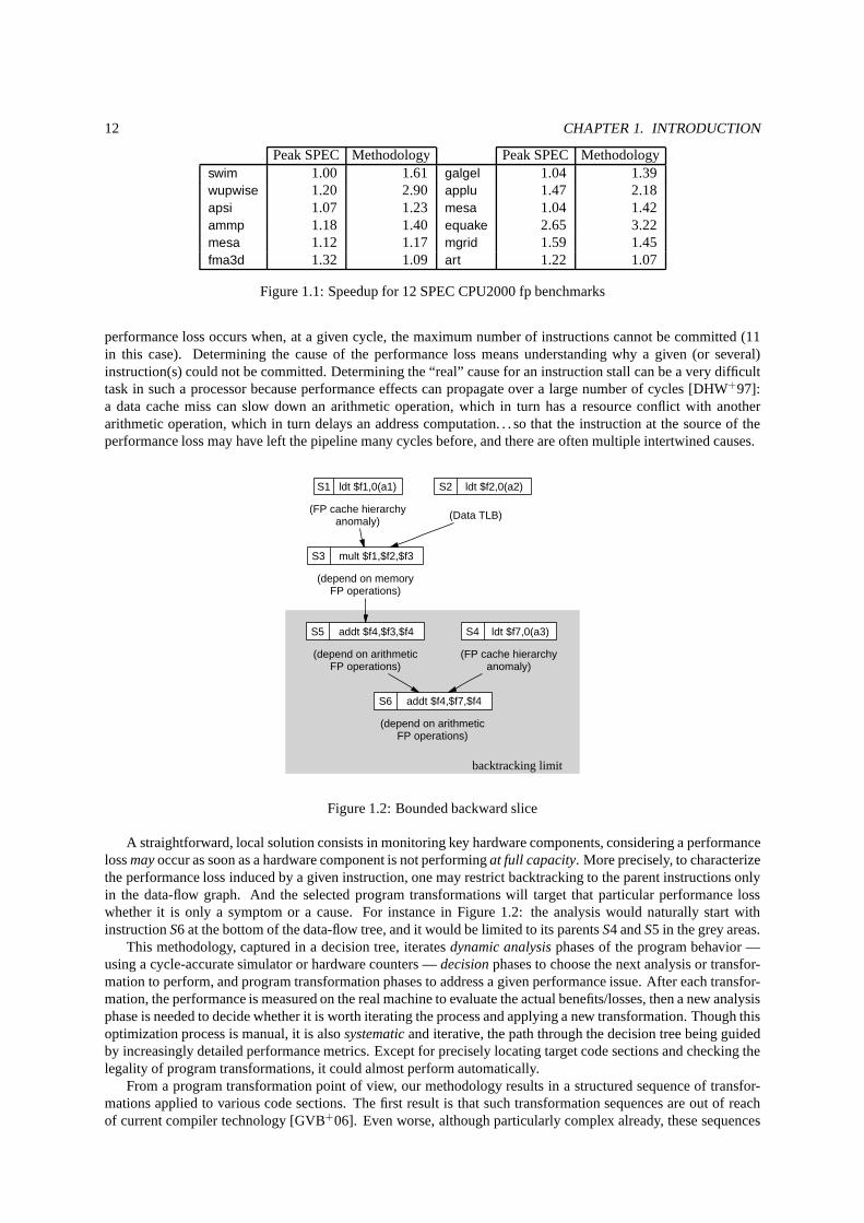
The approach takes the form of a decision tree which guides the optimization process. Each branch of thetree is a sequence of analysis/decision steps based on run-time metrics (dynamic analysis), calledperformanceanomalies, and a branch leaf is one or a few localized program transformation suggestions. An iteration of theoptimization process is equivalent to walking down one branch. After the corresponding optimization has beenapplied, the program is run again, new statistics are gathered, the process starts again at the tree top and a newbranch is followed. Progressively, the process builds a sequence (composition) of program transformations. Theprocess repeats until further transformations do not bringany significant additional improvement. Of course, theprocess is just one of the many possible “walks” within a hugesearch space, but this walk is systematic; to alimited extent it provides an approach for whole-program optimization and it has been experimentally proved toyield significant performance improvement on SPEC benchmarks for the Alpha 21264 processor, beyond peakSPEC (best optimization flags for each benchmark [Spe], using HP’s latest compiler), see Figure 1.1.
The process relies on the observation of tenths of differentperformanceanomalies; some of these anomaliescorrespond to traditional statistics, e.g., data TLB misses, available from program counters, and others are slightlymore elaborate performance indicators. They aim at enumerating and separating the different possible causes ofperformance loss. Why do we need such “performance anomalies” and what are they exactly?
The initial motivation was tofind the exact cause of any performance lossduring a program execution, in orderto apply the appropriate program optimization. In an out-of-order superscalar processor like the Alpha 21264, a
12 CHAPTER 1. INTRODUCTION
Peak SPEC Methodology Peak SPEC Methodologyswim 1.00 1.61 galgel 1.04 1.39wupwise 1.20 2.90 applu 1.47 2.18apsi 1.07 1.23 mesa 1.04 1.42ammp 1.18 1.40 equake 2.65 3.22mesa 1.12 1.17 mgrid 1.59 1.45fma3d 1.32 1.09 art 1.22 1.07
Figure 1.1: Speedup for 12 SPEC CPU2000 fp benchmarks
performance loss occurs when, at a given cycle, the maximum number of instructions cannot be committed (11in this case). Determining the cause of the performance lossmeans understanding why a given (or several)instruction(s) could not be committed. Determining the “real” cause for an instruction stall can be a very difficulttask in such a processor because performance effects can propagate over a large number of cycles [DHW+97]:a data cache miss can slow down an arithmetic operation, which in turn has a resource conflict with anotherarithmetic operation, which in turn delays an address computation. . . so that the instruction at the source of theperformance loss may have left the pipeline many cycles before, and there are often multiple intertwined causes.
backtracking limit
S1 ldt $f1,0(a1)
(FP cache hierarchyanomaly)
S3 mult $f1,$f2,$f3
S2 ldt $f2,0(a2)
(Data TLB)
(depend on memoryFP operations)
S5 addt $f4,$f3,$f4
(depend on arithmeticFP operations)
S4 ldt $f7,0(a3)
(FP cache hierarchyanomaly)
S6 addt $f4,$f7,$f4
(depend on arithmeticFP operations)
Figure 1.2: Bounded backward slice
A straightforward, local solution consists in monitoring key hardware components, considering a performancelossmayoccur as soon as a hardware component is not performingat full capacity. More precisely, to characterizethe performance loss induced by a given instruction, one mayrestrict backtracking to the parent instructions onlyin the data-flow graph. And the selected program transformations will target that particular performance losswhether it is only a symptom or a cause. For instance in Figure1.2: the analysis would naturally start withinstructionS6 at the bottom of the data-flow tree, and it would be limited toits parentsS4 andS5 in the grey areas.
This methodology, captured in a decision tree, iteratesdynamic analysisphases of the program behavior —using a cycle-accurate simulator or hardware counters —decisionphases to choose the next analysis or transfor-mation to perform, and program transformation phases to address a given performance issue. After each transfor-mation, the performance is measured on the real machine to evaluate the actual benefits/losses, then a new analysisphase is needed to decide whether it is worth iterating the process and applying a new transformation. Though thisoptimization process is manual, it is alsosystematicand iterative, the path through the decision tree being guidedby increasingly detailed performance metrics. Except for precisely locating target code sections and checking thelegality of program transformations, it could almost perform automatically.
From a program transformation point of view, our methodology results in a structured sequence of transfor-mations applied to various code sections. The first result isthat such transformation sequences are out of reachof current compiler technology [GVB+06]. Even worse, although particularly complex already, these sequences
1.2. GOING INSTANCEWISE 13
are only the premises of the real optimizations that will be needed on future architectures with multiple levels ofparallelism, heterogeneous computing resources, explicit management of the communication network topology,and non-deterministic run-time adaptation systems. Beyond complexity and unpredictability, this example alsoshows how important are extensibility (provisions for implementing new transformations) and debugging support(static and/or dynamic).
Essentially, the research results surveyed in the following sections are as many coordinated attempts to avoidthe diminishing returns associated with incremental improvements to current compilation and programming ap-proaches.
1.2 Going Instancewise
Most programming languages closely reflect the inductive nature of the main Church-equivalent computing mod-els and bringabstraction as a feature for programmer’s comfort. We are interested in compilers that operate onsemantically richer program abstractions, with statically tractable algebraic properties (i.e., closed mathematicalforms, representations in Presburger arithmetic or decidable automata-theoretic classes).
Whether denotational, operational or axiomatic, program semantics assigns “meaning” to afinite set of syn-tactic elements— statements or variables — using inductive definitions. When designing a static analysis ortransformation framework to reason about programs, it is very natural to attach static properties to this finite set ofsyntactic elements. Indeed, in many situations, semantical program manipulations operate locally on the inductivedefinitions associated with each program expression.
For the more sophisticated analyses and transformations, being so closely related to the inductive definitionsof the semantics may not be practical. Another approach, sometimes referred to asconstraint-basedin the staticanalysis context [NNH99], consists in operating on an abstraction more or less decoupled from the natural induc-tive semantics; typically, a system ofconstraintsthat characterize the static property or the program behavior ofinterest.
For example, constant propagation [ASU86] amounts to computing a property of a variablev at a statements,asking whetherv has some valuev beforesexecutes. It is quite natural to formalize constant propagation as a typesystem, in a data-flow setting or in abstract interpretation. But let us now consider another static analysis problemthat may be seen as an extension of constant propagation:induction variable recognition[GSW95] captures thevalue of some variablev at a statements as a functionfv of the number of timess has been executed. In otherwords, it capturesv as afunction of the execution pathitself. Of course, the value of a variable at any stage ofthe execution is a function of the initial contents of memoryand of the execution path leading to this stage. Forcomplexity reasons, the execution path may not be recoverable from memory. In the case of induction variables,we may assume the number of executions ofs is recorded as a genuine loop counter. From such a functionfv fors, we can discover the other induction variables using analyses of linear constraints [CH78], but such syntacticallybound approaches will not easily cope with the calculation of function fv itself.
In the following, we will qualify asinstancewise any compilation method operating on finitely presentedfunctions of the infinite set of runtime control points.
Historically, the instancewise approach derived from loop-restructuring compiler frameworks [Wol96] aimingat a large spectrum of optimizations: vectorization, instruction-level, thread-level or data parallelism, schedulingand mapping for automatic parallelization, locality optimization, and many others [PD96, AK02]. The associatedloop-nest analyses and representations share a common principle: they characterize static properties asfunctions ofrun-time control points (infinite or unbounded)andnot asfunctions of syntactic program elements (finite). Loop-restructuring compilers effectively operate at a higher level of understanding of the program behavior, decouplingprogram reasoning from the natural inductive semantics of most programming languages.
At this point, we are forced to reexamine the principles of traditional compilation methods in a wider worldof abstract domains without fix-point calculations where loops and recursive functions may often be manipulatedwith maximal accuracy. For example, abstract interpretation [CC77] is certainly not the only way to use formal ab-straction and concretization principles (as Galois connections or insertions) in compilation: the need to effectivelyresort to a form of staticinterpretationis only the translation of the inductive, fix-point based program semantics.When operating in a constraint-based representation of theprogram and its properties, this interpretation may beiteration-less [Muc97, WCPH01, PCS05] (no need to compute afix point, as in many SSA-based analyses) or evenresort to operation research algorithms thoroughly alien to program interpretation, including linear programming,constraint solving, and all sorts of empirical methods [Bar98, Fea92]. The work of Creusillet [Cre96] is one of therare instancewise analyses to resort to abstract interpretation, the reason lying in its interprocedural nature.
14 CHAPTER 1. INTRODUCTION
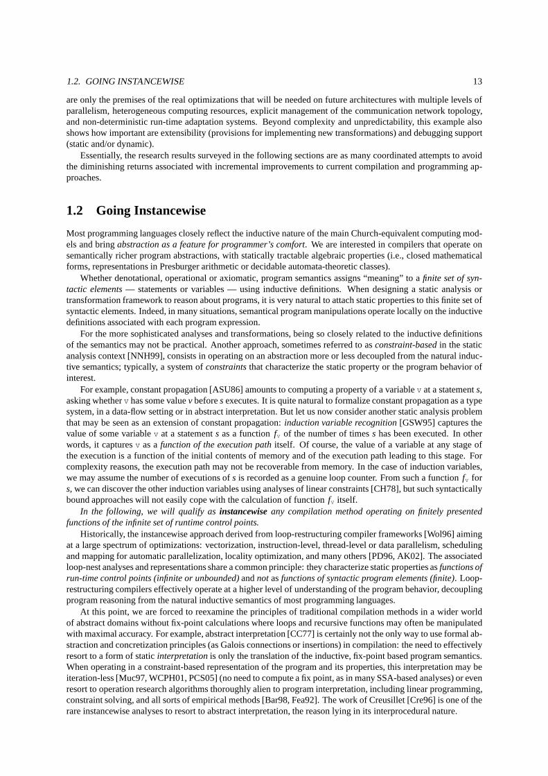
Back to instancewise compilation, Figure 1.3 shows a synthetic example where an arrayA is initialized in aloop nest and read in a recursive procedure. The footprint ofreads toA in procedureline is a “chess-board”: onlyelementsA[i][j] such thati + j is an even number are read in the procedure. This observationleads to a simpleoptimization: half of the dynamic assignments toA in the loop nest are useless, they can be avoided through asimple transformation of the bounds and strides. We call this optimizationinstancewise dead-code elimination.
A typical static analysis technique to solve this kind of problems is calledarray-region analysis[CH78, Cre96].However, because the “chess-board” footprint is not a convex polyhedron, all the array-region analyses we areaware of will fail on this example. In theory, recovering such precise information seems possible by abstractinterpretation, provided the widening operator forZ-polyhedra (also called lattice polyhedra) can handle somelevel of non-convexity [Sch86, LW97], which is not the case in the current state of the art [BRZ03]. In addition,such precision may only be achieved by acontext-sensitiveanalysis.
int A[10][10];
void line (int i, int j) {... = A[i][j];if (j<10) line (i, j+2)
}
int main () {for (i=0; i<10; i++)for (j=0; j<10; j++)
A[i][j] = ...;for (i=0; i<10; i+=2) {line(i, j);line(i+1, j+1);
}
Figure 1.3: Simple instancewise dead-code elimination
int A[10][10];
void line (int i, int j, int k, int l) {... = A[i][j];if (j<10) line (k, l, i, j+2)
}
int main () {for (i=0; i<10; i++)for (j=0; j<10; j++)A[i][j] = ...;
for (i=0; i<10; i+=2) {line(i, j, i+1, j+1);
}
Figure 1.4: More complex example
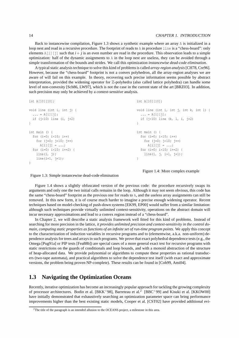
Figure 1.4 shows a slightly obfuscated version of the previous code: the procedure recursively swaps itsarguments and only one the two initial calls remains in the loop. Although it may not seem obvious, this code hasthe same “chess-board” footprint as the previous one for reads toA, and the useless array assignments can still beremoved. In this new form, it is of course much harder to imagine a precise enough widening operator. Recenttechniques based on model-checking of push-down systems [EK99, EP00] would suffer from a similar limitation:although such techniques provide virtually unlimited context-sensitivity, operations on the abstract domain willincur necessary approximations and lead to a convex region instead of a “chess-board”.
In Chapter 2, we will describe a static analysis framework well fitted for this kind of problems. Instead ofsearching for more precision in the lattice,it provides unlimited precision and context-sensitivity in the control do-main, computing static properties as functions of an infinite set of run-time program points. We apply this conceptto the characterization of induction variables in recursive programs and to (elementwise, a.k.a. non-uniform) de-pendence analysis for trees and arrays in such programs. We prove that exact polyhedral dependence tests (e.g., theOmega [Pug91a] or PIP tests [Fea88b]) are special cases of a more general exact test for recursive programs withstatic restrictions on the guards of conditionals and loop bounds, and with a monoid abstraction of the structureof heap-allocated data. We provide polynomial or algorithms to compute these properties as rational transduc-ers (two-tape automata), and practical algorithms to solvethe dependence test itself (with exact and approximateversions, the problem being proven NP-complete). These results can be found in [Coh99, Ami04].
1.3 Navigating the Optimization Oceans
Recently, iterative optimization has become an increasingly popular approach for tackling the growing complexityof processor architectures. Bodin et al. [BKK+98], Barreteau et al.2 [BBC+99] and Kisuki et al. [KKOW00]have initially demonstrated that exhaustively searching an optimization parameter space can bring performanceimprovements higher than the best existing static models, Cooper et al. [CST02] have provided additional evi-
2The title of the paragraph is an intended allusion to the OCEANS project, a milestone in this area.
1.3. NAVIGATING THE OPTIMIZATION OCEANS 15
dence for finding best sequences of various compiler transformations. Since then, recent studies [TVA05, FOK02,BFF05] demonstrate the potential of iterative optimization for a large range of optimization techniques.
Some studies show how iterative optimization can be usedin practice, for instance, for tuning optimization pa-rameters in libraries [WPD00, BACD97] or for building static models for compiler optimization parameters. Suchmodels derive from the automatic discovery of the mapping function between key program characteristics andcompiler optimization parameters; e.g., Stephenson et al.[SA05] successfully applied this approach to unrolling.
However, most other articles on iterative optimization take the same approach: several benchmarks are re-peatedly executed with the same data set, a new optimizationparameter (e.g., tile size, unrolling factor, inliningdecision,. . . ) being tested at each execution. So, while these studies demonstrate thepotentialfor iterative opti-mization, few provide apractical approach for effectively applying iterative optimization. The issue at stake is:what do we need to do to make iterative optimization a reality? There are three main caveats to iterative opti-mization: quickly scanning a large search space, optimizing based on and across multiple data sets, and extendingiterative optimization to complex composed optimizationsbeyond simple optimization parameter tuning.
We aim at the general goal of making iterative optimization ausable technique and especially focus on the firstissue, i.e., how to speed up the scanning of a large optimization space. As iterative optimization moves beyondsimple parameter tuning to composition of multiple transformations [FOK02, PTCV04, LF05, CGP+05] (the thirdissue mentioned above), this search space can become potentially huge, calling for faster evaluation techniques.There are at least four possible ways to speeding up the search space scanning:
1. search more smartly by exploring points with the highest potential using genetic algorithms and machinelearning techniques [CSS99, CST02, VAGL03, SAMO03, ACG+04, MBQ02, HBKM03, SA05],
2. enhance the structure of the search space so that faster operation research algorithms with better understoodmathematical properties can be applied [O’B98, CGP+05],
3. or use the programmer’s expertise to directly or indirectly drive the optimization heuristic [CHH+93,LGP04, PTCV04, DBR+05, CDG+06],
4. evaluating multiple optimizations at runtime or reducing the duration of profile runs, effectively scanningmore points within the same amount of time [FCOT05].
Speeding up the search has mostly focused on the first approach, while we have so far focused on the three otherones.
Enhancing the search-space structure. Optimizing compilers have traditionally been limited to systematicand tedious tasks that are either not accessible to the programmer (e.g., instruction selection, register allocation)or that the programmer in a high level language does not want to deal with (e.g., constant propagation, partialredundancy elimination, dead-code elimination, control-flow optimizations). Generating efficient code for deepparallelism and deep memory hierarchies with complex and dynamic hardware components is a completely dif-ferent story: the compiler (and run-time system) now has to take the burden of much smarter tasks, that onlyexpert programmers would be able to carry. In a sense, it is not clear that these new optimization and paral-lelization tasks should be called “compilation” anymore. Iterative optimization and machine learning compilation[KKOW00, CST02, LO04] are part of the answer to these challenges, building on artificial intelligence and oper-ation research know-how to assist compiler heuristic. Iterative optimization generalizes profile-directed approachto integrate precise feedback from the runtime behavior of the program into optimization algorithms, while ma-chine learning approaches provide an automated framework to build new optimizers from empirical optimizationdata. However, considering the ability to perform complex transformations, or complex sequences of transforma-tions [PTV02, PTCV04], iterative optimization and machinelearning compilation will fare no better than existingcompilers on top of which they are currently implemented. Inaddition, any operation research algorithm willbe highly sensitive to the structure of the search space it istraversing. E.g., genetic algorithms are known tocope with unstructured spaces but at a higher cost and lower scalability towards larger problems, as opposed tomathematical programming (e.g., semi-definite or linear programming) which benefit from strong regularity andalgebraic properties of the optimization search space. Unfortunately, current compilers offer a very unstructuredoptimization search space. First of all, by imposing phase ordering constraints [Wol96], they lack the ability toperform long sequences of transformations. In addition, compilers embed a large collection of ad-hoc programtransformations, but they aresyntactictransformations, i.e., control structures are regenerated after each programtransformation, sometimes making it harder to apply the next transformations, especially when the application ofprogram transformations relies on pattern-matching techniques.
16 CHAPTER 1. INTRODUCTION
Clearly, there is a need for a compiler infrastructure that can apply complex and possibly long compositionsof optimizing or parallelizing transformations, in a rich,structured search space.
We claim that existing compilers are ill-equipped to address these challenges, because of improper programrepresentations and inappropriate conditioning of the search space structure.
In Chapter 3, we try to remedy to the lack of an algebraic structure in traditional loop-nest optimizers, asa small step towards bridging the gap between peak and sustained performance in future and emerging on-chipmultiprocessors. Our framework facilitates the search forcompositionsof program transformations, relying ona unified representation of loops and statements [CGP+05]. This framework improves on classical polyhedralrepresentations [Fea92, Wol92, Kel96, LL97, AMP00, LLL01]to support a large array of useful and efficient pro-gram transformations (loop fusion, tiling, array forward substitution, statement reordering, software pipelining,array padding, etc.), as well ascompositions(also in a mathematical sense) of these transformations. Comparedto the attempts at expressing a large array of program transformations as matrix operations within the polyhedralmodel [Wol92, Pug91c, Kel96], the distinctive asset of our representation lies in the simplicity of the formalismto compose non-unimodular transformations across long, flexible sequences. Existing formalisms have been de-signed for black-box optimization [Fea92, LL97, AMP00], and applying a classical loop transformation withinthem — as proposed in [Wol92, Kel96, LO04] — requires a syntactic form of the program to anchor the transfor-mation to existing statements. Up to now, the easy composition of transformations was restricted to unimodulartransformations [Wol96], with some extensions to singulartransformations [LP94].
The key to our approach is to clearly separate the four different types of actions performed by program trans-formations: modification of the iteration domain (loop bounds and strides), modification of the schedule of eachindividual statement, modification of the access functions(array subscripts), and modification of the data layout(array declarations). This separation makes it possible toprovide a matrix representation for each kind of action,enabling the easy and independent composition of the different “actions” induced by program transformations, andas a result, enabling the composition of transformations themselves. Current representations of program transfor-mations do not clearly separate these four types of actions;as a result, the implementation of certain compositionsof program transformations can be complicated or even impossible. For instance, current implementations ofloop fusion must include loop bounds and array subscript modifications even though they are only byproductsof a schedule-oriented program transformation; after applying loop fusion, target loops are often peeled, increas-ing code size and making further optimizations more complex. Within our representation, loop fusion is onlyexpressed as a schedule transformation, and the modifications of the iteration domain and access functions areimplicitly handled, so that the code complexity is exactly the same before and after fusion. Similarly, an iterationdomain-oriented transformation like unrolling should have no impact on the schedule or data layout representa-tions; or a data layout-oriented transformation like padding should have no impact on the schedule or iterationdomain representations. Eventually, since all program transformations correspond to a set of matrix operationswithin our representation, searching for compositions of transformations is often (though not always) equivalentto testing different values of the matrices parameters, further facilitating the search for compositions. Besides,with this framework, it should also be possible to find and evaluate new sequences of transformations for whichno static model has yet been developed (e.g., array forward substitution versus loop fusion as a temporal localityoptimization).
Using the programmer’s expertise. Beyond a potential strategy for driving iterative optimization, the method-ological work on bottom-up optimization outlined at the beginning of this section [PTCV04] has several imme-diate benefits. (1) It provides a manual optimization process that can be used by engineers; because this processis systematic, less expertise is required on the part of the engineer to optimize a program. (2) The decision treeformalizes the empirical expertise of engineers, and it is away to pass this expertise, traditionally hard to teach,to new engineers or researchers. (3) Each branch actually defines a mapping between a given architecture perfor-mance issue and appropriate program transformations; thismapping is based on empirical expertise. (4) Beyondthe optimization process, this empirical work also had the benefit of filtering which, among the many existingprogram transformations, bring the best benefits in practice.
Indeed, programmers of computationally intensive applications complain about the lack of efficiency of theirmachines — the ratio of sustained to peak performance — and the poor performance of optimizing compilers[WPD00]. Of course, they do not wait for research prototypesto become production-quality optimizers beforeattempting to improve the productivity of their manual, application-specific optimizations. In addition, no black-box compiler has ever compiled a matrix-matrix product codewritten in Fortran or C on a modern multi-coresuperscalar processor and reached performance levels close to hand-tuned mathematical libraries. There are fun-damental reasons for such a disastrous situation:
1.3. NAVIGATING THE OPTIMIZATION OCEANS 17
• domain-specific knowledge unavailable to the compiler can be required to prove optimizations’ legality orprofitability [BGGT02, LBCO03];
• hard-to-drive transformations are not available in compilers, including transformations whose profitability isdifficult to assess or whose risk of degrading performance ishigh, e.g., speculative optimizations [ACM+98,RP99];
• complex loop transformations do not compose well, due to syntactic constraints and code size increase[CGT04];
• some optimizations are in fact algorithm replacements, where the selection of the most appropriate codemay depend on the architecture and input data [LGP04].
50 100 150 200 250NB
200
400
600
800
1000
1200
MFLOPS
Figure 1.5: Influence of parameter selection
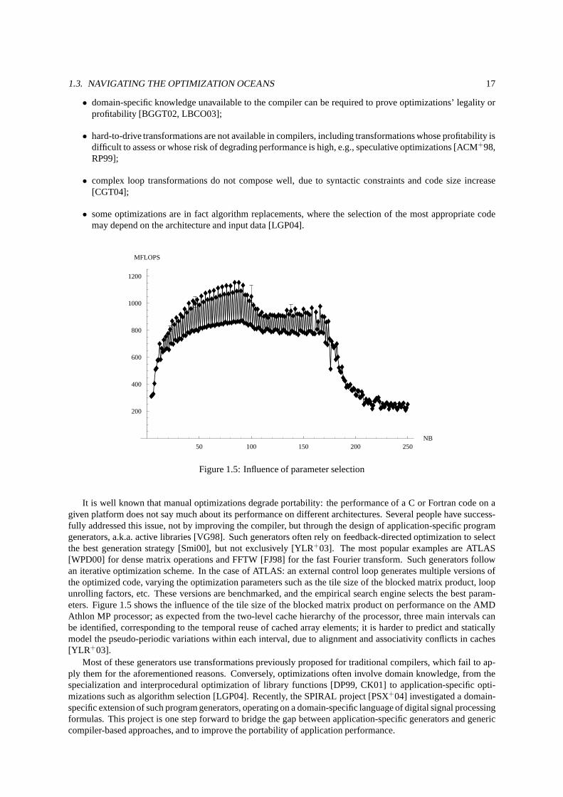
It is well known that manual optimizations degrade portability: the performance of a C or Fortran code on agiven platform does not say much about its performance on different architectures. Several people have success-fully addressed this issue, not by improving the compiler, but through the design of application-specific programgenerators, a.k.a. active libraries [VG98]. Such generators often rely on feedback-directed optimization to selectthe best generation strategy [Smi00], but not exclusively [YLR+03]. The most popular examples are ATLAS[WPD00] for dense matrix operations and FFTW [FJ98] for the fast Fourier transform. Such generators followan iterative optimization scheme. In the case of ATLAS: an external control loop generates multiple versions ofthe optimized code, varying the optimization parameters such as the tile size of the blocked matrix product, loopunrolling factors, etc. These versions are benchmarked, and the empirical search engine selects the best param-eters. Figure 1.5 shows the influence of the tile size of the blocked matrix product on performance on the AMDAthlon MP processor; as expected from the two-level cache hierarchy of the processor, three main intervals canbe identified, corresponding to the temporal reuse of cachedarray elements; it is harder to predict and staticallymodel the pseudo-periodic variations within each interval, due to alignment and associativity conflicts in caches[YLR+03].
Most of these generators use transformations previously proposed for traditional compilers, which fail to ap-ply them for the aforementioned reasons. Conversely, optimizations often involve domain knowledge, from thespecialization and interprocedural optimization of library functions [DP99, CK01] to application-specific opti-mizations such as algorithm selection [LGP04]. Recently, the SPIRAL project [PSX+04] investigated a domain-specific extension of such program generators, operating ona domain-specific language of digital signal processingformulas. This project is one step forward to bridge the gap between application-specific generators and genericcompiler-based approaches, and to improve the portabilityof application performance.
18 CHAPTER 1. INTRODUCTION
We advocate for the use of generative programming languagesand techniques, to support the design of suchgeneric adaptive libraries by high-performance computingexperts [CDG+06]. We show that complex optimiza-tions can be implemented in a type-safe, purely generative framework. We also show that peak performance isachievable through the careful combination of a high-level, multi-stage language — MetaOCaml [CTHL03] —with low-level code generation techniques.
We also show that combining generative techniques withsemantics-preserving transformationsis an evenbetter solution, and may further improve the productivity of high-performance library developers [DBR+05].This approach can be opposed to introspective and reflectiveapproaches in more expressive meta-programmingframeworks: it provides the right abstractions and primitives for architecture-aware optimization while preservingthe most important safety properties. We are planning further research in this area, in particular through an attemptto combine the rich algebraic structure of the polyhedral model with generative programming.
Scanning more points within the same amount of time. The principle of our approach is to improve theefficiency of iterative optimization by taking advantage ofprogramperformance stabilityat run-time. There isample evidence that many programs exhibit phases [SPHC02, LSC05], i.e., program trace intervals of severalmillions instructions where performance is similar. What is the point of waiting for the end of the execution inorder to evaluate an optimization decision (e.g., evaluating a tiling or unrolling factor, or a given compositionof transformations) if the program performance is stable within phases or the whole execution? One could takeadvantage of phase intervals with the same performance to evaluate a different optimization option at each interval.As in standard iterative optimization, many options are evaluated, except that multiple options are evaluated withinthe same run.
Note that there are alternative ways to gather feedback datain a shorter time. Statistical simulation techniques[SPHC02] could potentially be adapted to compilation purposes, provided an optimization-agnostic checkpointingof a process state can be performed [GMCT03]. Alternatively, one may also use machine learning techniques toconstruct cost models automatically, and apply these cost models instead of performing a full profile run. Theseideas are left for future work.
The main assets of our approach over previous techniques aresimplicity and practicality. We show that alow-overhead performance stability/phase detection scheme is sufficient for optimization space pruning for loop-based floating point benchmarks. We also show that it is possible to search (even complex) optimizations atruntime without resorting to sophisticated dynamic optimization/recompilation frameworks. Beyond iterativeoptimization, our approach also enables one to quickly design self-tuned applications, significantly easier thanmanually tuned libraries.
Phase detection and optimization evaluation are respectively implemented using code instrumentation andversioning within the EKOPath compiler. Considering 5 self-tuned SPEC CPU2000 fp benchmarks, our spacepruning approach speeds up iterative search by a factor of 32to 962, with a 99.4% accurate phase prediction anda 2.6% performance overhead on average; we achieve speedups ranging from 1.10 to 1.72 [FCOT05].
1.4 Harnessing Massive On-Chip Parallelism
Future and emerging processor designs will integrate massive amounts of parallelism. This is a fact of the physics,essentially due to communication delays (currently, wire delays), and marginally (or temporarily) to power dissi-pation and architecture design issues.
With such architectures, performance scalability is the most immediate challenge. While these processorsstart invading all domains of computing, they will also put an end to the low expectations in terms ofefficiency,programmer productivityandreliability — thinking of the functional correctness and fault tolerance — that areunfortunately common in parallel computing. Who wants to program cheap massively-parallel chips with method-ologies and systems for worldwide grids? Beyond pure performance, it is well known that this evolution stressesproductivity issues in the design of parallel systems, as emphasized by the DARPA HPCS program and the Fortresslanguage initiative by Sun Microsystems [ACL+06].
In addition, the rapid evolution of embedded system technology — favored by Moore’s law and standards— is increasingly blurring the barriers between the design of safety-critical, real-time and high-performance sys-tems. A good example is the domain of high-end video applications, where tera-operations per second (on pixelcomponents) in hard real-time will soon be common in low-power devices. Parallel embedded computing makethe parallel programming productivity issue even more challenging: no current framework is able to bring com-positionality to explicit time and resource management while generating efficient parallel code from high-level
1.4. HARNESSING MASSIVE ON-CHIP PARALLELISM 19
distributed computing models.Unfortunately, general-purpose architectures and compilers are not suitable for the design of real-timeand
high-performance (massively parallel)and low-powerand programmablesystem-on-chip [CDC+03]. Achievinga high compute density and still preserving programmability is a challenge for the choice of an appropriate ar-chitecture, programming language and compiler. Typically, thousands of operations per cycle must be sustainedon chip, exploiting multiple levels of parallelism in the compute kernel, with tightly coupled operations, whileenforcing strong real-time properties.
To address these challenges, we studied the synchronous model of computation [BCE+03] which allows forthe generation of custom, parallel hardware and software systems withcorrect-by-construction structural proper-ties, including real-time and resource constraints. This modelmet industrial success for safety-critical, reactivesystems, through languages like SIGNAL [BLJ91], LUSTRE(SCADE) [HCRP91] and ESTEREL [Ber00].
To enforce real-time and resources properties, synchronous languages assume a common clock for all registers,and an overall predictable execution layer where communications and computations can be proven to take less thana (physical or logical) clock cycle. Due to wire delays, a massively parallel system-on-chip has to be divided intomultiple, asynchronous clock domains: the so calledGlobally Asynchronous Locally Synchronous(GALS) model[Cha84]. This has a strong impact on the formalization of synchronous execution itself and on the associatedcompilation strategies [LTL03].
Due to the complexity of high-performance applications andto the intrinsic combinatorics of synchronousexecution,multiple clock domainshave to be consideredat the application level as well[CDE+05]. This is thecase for modular designs with separate compilation phases,and for a single system with multiple input/outputassociated with different real-time clocks (e.g., video streaming). It is thus necessary to compose independentlyscheduled processes.Kahn Process Networks(KPN) [Kah74] can accommodate for such a composition, com-pensating for the local asynchrony through unbounded blocking FIFO buffers. But allowing a global synchronousexecution imposes additional constraints on the composition. We introduce the concept ofn-synchronousclocksto formalize these concepts and constraints. This concept describes naturally the semantics of KPN with bounded,statically computable buffer sizes. This extension allowsthe modular composition of independently scheduledcomponents with multiple periodic clocks satisfying a flow preservation equation, through the automatic infer-ence of bounded delays and FIFO buffers. Our first results aredetailed in Chapter 4.
Chapter 2
Instancewise Program Analysis
This chapter studies the extension of instancewise compilation techniques to imperative, first-order, well structuredrecursive programs. It focuses on static analysis and on thecharacterization of induction variables as closed formexpressions over non-tail-recursive definitions.
Statementwise analysis. We use the termstatementwiseto refer to the classical type systems, data-flow analysisand abstract interpretation frameworks, that define and compute program properties at each program statement.A typical example is static analysis by abstract interpretation [CC77, Cou81, Cou96]: it relies on thecollectingsemanticsto operate on a lattice of abstract properties. This restricts the attachment of properties to afiniteset of control points. Little research addressed the attachment of static properties at a finer grain than syntacticprogram elements. Refinement of this coarse grain abstraction involves a previouspartitioning [Cou81] of thecontrol points: e.g.,polyvariantanalysis distinguishes the context of function calls, andloop unfoldingvirtuallyunrolls a loop several times.Dynamic partitioning[Bou92] integrates partitioning into the analysis itself.Controlpoints can be extended withcall strings (abstract call stacks) andtimestamps, but ultimately rely onk-limiting[SP81, Har89] orsummarizationheuristics [RHS95] to achieve convergence. Although unbounded lattices havelong been used to capture abstract properties [CH78, Deu94]), there was little interest in the computation of data-flow facts attached to anunbounded set of control points, following the seminal paper by Esparza and Knoop[EK99]. This approach is the closest to our work and a detailed comparison is provided in Section 2.7; it builds onmodel-checking of push-down systems to extend precision and context sensitivity, without sacrifying efficiency[EP00], but it ultimately results in the computation of data-flow properties attached to afinite number of controlpoints.
Instancewise analysis. On the other hand, ad-hoc, constraint-based approaches to static analysis are able tocompute program properties asfunctions defined on an infinite (or unbounded) number of run-time control points.The so-calledpolytope modelencompasses most work on analysis and transformation of the(Turing-incomplete)class ofstatic-control programs[Fea88a, PD96], roughly defined as nested loops with affine loop bounds andarray accesses. Aniteration vectorabstracts the runtime control point corresponding to a given iteration of astatement. Program properties are expressed and computed for each vector of values of the surrounding loopcounters. In general, the result of the analysis is a mappingfrom the infinite set of iteration vectors (the run-time control points) to an arbitrary (analysis-specific) vector space (e.g., dependence vector). Instead of iterativelymerging data-flow properties, most analyses in the polytopemodel use algebraic solvers for the direct computationof symbolic relations: e.g., array dependence analysis uses integer linear programming [Fea88a]. Iteration vectorsare quite different from time-stamps in control point partitioning techniques [Bou92]: they are multidimensional,lexicographically ordered,unbounded, and constrained by Presburger formula [Pug92].
First contribution. We introduce a general static analysis framework that uncompasses most ad-hoc formalismsfor the fine grain analysis of loop nests and arrays in sequential procedural languages. Within this framework,one maydefine, abstract and computeprogram properties at aninfinite number ofruntime control points. Ourframework is calledinstancewiseand runtime points are further referenced asinstances. We will formally defineinstances astrace abstractions, understood as iteration vectors extended to arbitrary recursive programs. Themathematical foundation for instancewise analysis isformal language theory: rational languages finitely representinfinite set of instances, and instancewise properties may be captured by rational relations [Ber79]. This paper
20
2.1. CONTROL STRUCTURES AND EXECUTION TRACES 21
goes far beyond our previous attempts to extend iteration vectors to recursive programs, for the analysis of arrays[CCG96, CC98, Coh99, Col02, ACF03] or recursive data structures [Fea98, Col02, Coh99].
Second contribution. Building on the instancewise framework, we extend the concept of induction variablesto arbitrary recursive programs. This extension demonstrates the ability to characterize properties of programsas functions from an infinite set of run-time control points,beyond the restricted domain of Fortran loop nests.Technically, the valuation of induction variables is analog to parameter passing in a purely functional language:each statement is considered as a function, binding and initializing one or more induction variables. Our inductionvariable characterization does not take the outcome of loopand test predicates into account.1 Thus, we willconsider a superset of the valid traces for the evaluation ofinduction variables. We propose two alternativealgorithms for this evaluation. The result of both algorithms for each induction variable is abinding functionmapping instances to the abstract memory locations they access. It is arational functionon the Cartesian productof two monoids and can be efficiently represented as arational transducer[Ber79]. This binding function willgive anexactresult for valid traces.
Structure of the chapter. To focus on the core concepts and contributions, we introduce MOGUL, a domain-specific language with high-level constructs for traversing data structures addressed by induction variables in afinitely presented monoid. In a general-purpose (imperative or functional) language, our technique would requireadditional information about the shape of data structures,using dedicated annotations [HHN92, KS93, FM97]or shape analyses [GH96, SRW99]. Despite the generality of the control structures in MOGUL, as said before,binding functions giveexactvalues for valid traces. This may be used to derivealiasanddependenceinformationof recursive programs with an unprecedented precision [Coh99, Col02, ACF03]. We will survey the currentapplications of instancewise analysis for recursive programs; the reader interested in more details (for loop nestsor more general recursive programs) may refer to [Col02] fora pedagogical and synthetic presentation.
Section 2.1 describes the control structures and trace semantics of MOGUL. Section 2.2 defines the abstrac-tion of runtime control points into instances. Section 2.3 extends induction variables to recursive control and datastructures. Section 2.4 states the existence of rational binding functions from individual instances to individualdata structure elements. Section 2.5 addresses the computation and representation of binding functions as ratio-nal transducers. We consider practical examples in Section2.6. Section 2.7 gives two simple applications ofinstancewise analysis to program optimization and surveysthe current state of the art.
2.1 Control Structures and Execution Traces
We consider a simplified notion ofexecution tracewith emphasis on the identification of runtime control points.For our purpose, atrace is a sequence of symbols calledlabelsthat denotes acompleteexecution of a program.Each label registers either thebeginningof a statement execution or itscompletion. A trace prefixis the trace of apartial execution, given by a prefix of a complete trace. In the remainder, we will consider trace prefixes insteadof the intuitive notion of runtime control point.
Figure 2.1 presents our running example. It features a recursive call to theToy function, nested in the body ofa for loop, operating on an arrayA. Thus, there is no simple way to remove the recursion. In thispaper,we willconstruct a finite-state representation for the infinite setof trace prefixes ofToy, then compute an exact finite-statecharacterization of the elements ofA accessed by a given trace prefix.
2.1.1 Control Structures in theMOGUL Language
Figure 2.2 gives the MOGUL version ofToy. It abstracts the shape of arrayA through a monoid typeMonoid_int.Induction variablesi andk are bound to values in this monoid. Traversals ofA are expressed throughi, k andthe monoid operation·. Further explanations about MOGUL data structures and induction variables are deferredto Section 2.3. We present in Figure 2.3 a simplified version of the MOGUL syntax, focusing on the controlstructures.
This is aC-like syntax with some specific concepts. Italic non-terminals are defined elsewhere in the syn-tax: infinite binary wordelementary_statement covers the usual atomic statements, including assignments, in-put/output statements, void statements, etc.; infinite binary wordpredicate is a boolean expression; infinite binary
1This limitation can be overcome thanks to approximations and higher complexity algorithms. We will present our solutions in anotherpaper.
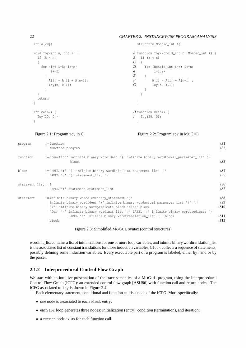
22 CHAPTER 2. INSTANCEWISE PROGRAM ANALYSIS
int A[20];
void Toy(int n, int k) {if (k < n){
for (int i=k; i<=n;i+=2)
{A[i] = A[i] + A[n-i];Toy(n, k+1);
}}return
}
int main() {Toy(20, 0);
}
Figure 2.1: ProgramToy in C
structure Monoid_int A;
A function Toy(Monoid_int n, Monoid_int k) {B if (k < n)C {D for (Monoid_int i=k; i<=n;d i=i.2)E {F A[i] = A[i] + A[n-i] ;G Toy(n, k.1);
}}
}
H function main() {I Toy(20, 0);}
Figure 2.2: ProgramToy in MOGUL
program ::=function (S1)|function program (S2)
function ::=’function’ infinite binary wordident ’(’ infinite binary wordformal_parameter_list ’)’block (S3)
block ::=LABEL ’:’ ’{’ infinite binary wordinit_list statement_list ’}’ (S4)|LABEL ’:’ ’{’ statement_list ’}’ (S5)
statement_list::=ε (S6)|LABEL ’:’ statement statement_list (S7)
statement ::=infinite binary wordelementary_statement ’;’ (S8)|infinite binary wordident ’(’ infinite binary wordactual_parameter_list ’)’ ’;’ (S9)|’if’ infinite binary wordpredicate block ’else’ block (S10)|’for’ ’(’ infinite binary wordinit_list ’;’ LABEL ’:’ infinite binary wordpredicate ’;’
LABEL ’:’ infinite binary wordtranslation_list ’)’ block (S11)|block (S12)
Figure 2.3: Simplified MOGUL syntax (control structures)
wordinit_list contains a list of initializations for one ormore loop variables, and infinite binary wordtranslation_listis the associated list of constant translations for those induction variables;block collects a sequence of statements,possibly defining some induction variables. Every executable part of a program is labeled, either by hand or bythe parser.
2.1.2 Interprocedural Control Flow Graph
We start with an intuitive presentation of the trace semantics of a MOGUL program, using the InterproceduralControl Flow Graph (ICFG): an extended control flow graph [ASU86] with function call and return nodes. TheICFG associated toToy is shown in Figure 2.4.
Each elementary statement, conditional and function call is a node of the ICFG. More specifically:
• one node is associated to eachblock entry;
• eachfor loop generates three nodes: initialization (entry), condition (termination), and iteration;
• areturn node exists for each function call.
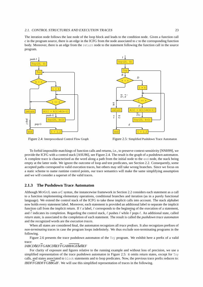
2.1. CONTROL STRUCTURES AND EXECUTION TRACES 23
The iteration node follows the last node of the loop block andleads to the condition node. Given a function callc in the program source, there is an edge in the ICFG from the node associated toc to the corresponding functionbody. Moreover, there is an edge from thereturn node to the statement following the function call in the sourceprogram.
Toy(20, 0)
Toy
k < n
i = k
b
b i <= n
return A[i] = A[i]+A[n-i]
Toy(20, k+1)
end i = i.2
pushI
popG
popI
pushG
Figure 2.4:Interprocedural Control Flow Graph
Toy(20, 0)
Toy
k < n
i = k
b
b i <= n
return A[i] = A[i]+A[n-i]
Toy(20, k+1)
end i = i.2
I
BD
d
I G
F
D ; d∗
B
FG
Figure 2.5:Simplified Pushdown Trace Automaton
To forbid impossible matchings of function calls and returns, i.e., to preserve context-sensitivity [NNH99], weprovide the ICFG with a control stack [ASU86], see Figure 2.4. The result is the graph of a pushdown automaton.A complete trace is characterized as the word along a path from the initial node to theend node, the stack beingempty at the latter node. We ignore the outcome of loop and test predicates, see Section 2.2. Consequently, someaccepted paths correspond to valid execution traces, but others may still take wrong branches. Since we focus ona static scheme to name runtime control points, our trace semantics will make the same simplifying assumptionand we will consider a superset of the valid traces.
2.1.3 The Pushdown Trace Automaton
Although MOGUL uses aC syntax, the instancewise framework in Section 2.2 considers each statement as a callto a function implementing elementary operations, conditional branches and iteration (as in a purely functionallanguage). We extend the control stack of the ICFG to take these implicit calls into account. The stack alphabetnow holds every statement label. Moreover, each statement is provided an additional label to separate the implicitfunction call from the implicit return. Ifℓ a label,ℓ corresponds to the beginning of the execution of a statement,andℓ indicates its completion. Regarding the control stack,ℓ pushesℓ while ℓ popsℓ. An additional state, calledreturn state, is associated to the completion of each statement. The result is called thepushdown trace automatonand the recognized words are theexecution traces.
When all states are considered final, the automaton recognizes alltrace prefixes. It also recognizes prefixes ofnon-terminatingtraces in case the program loops indefinitely. We thus exclude non-terminating programs in thefollowing.
Figure 2.6 presents the trace pushdown automaton of theToy program. We exhibit here a prefix of a validtrace:IABCDδEFFGABCDδEFFGABBAGEδdδEF
For clarity of exposure and figures relative to the running example and without loss of precision, we use asimplified representation of the trace pushdown automaton in Figure 2.5: it omits return states, except forToycalls, and states associated toblock statements and to loop predicates. Now, the previous trace prefix reduces to:IBDFFGBDFFGBBGdF. We will use this simplified representation of traces in the following.
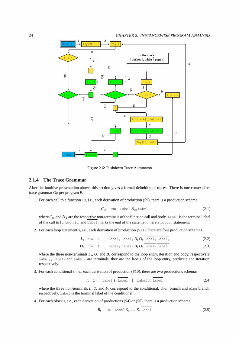
24 CHAPTER 2. INSTANCEWISE PROGRAM ANALYSIS
Main { Toy(20, 0) Toy {
k < n
{
i = k i = i.2 i = k
k < n } i <= n i <= n i = i.2
{
A[i] = A[i]+A[n-i]
} Toy A[i] = A[i]+A[n-i]
Toy(20, k+1)
} Main return }
In the stack:ℓ pushesℓ, while ℓ popsℓ.
I A
B
C
D
δ
E
δ
F
D d
δ
C
B
A
I
G
E
F
B
Gd
δ
A
Figure 2.6: Pushdown Trace Automaton
2.1.4 The Trace Grammar
After the intuitive presentation above, this section givesa formal definition of traces. There is one context-freetrace grammarGP per programP.
1. For each call to a functionid, i.e., each derivation of production (S9), there is a production schema
Cid ::= Label Bid Label (2.1)
whereCid andBid are the respective non-terminals of the function call and body. Label is the terminal labelof the call to functionid, andLabel marks the end of the statement, here areturn statement.
2. For each loop statements, i.e., each derivation of production (S11), there are four production schemas
Ls ::= ε | Labele Labelp Bs Os Labelp Labele (2.2)
Os ::= ε | Labeli Labelp Bs Os Labelp Labeli (2.3)
where the three non-terminalsLs, Os andBs correspond to the loop entry, iteration and body, respectively.Labele, Labelp andLabeli are terminals, they are the labels of the loop entry, predicate and iteration,respectively.
3. For each conditionals, i.e., each derivation of production (S10), there are two productions schemas
Is ::= Label Ts Label | Label Fs Label (2.4)
where the three non-terminalsIs, Ts andFs correspond to the conditional,then branch andelse branch,respectively.Label is the terminal label of the conditional.
4. For each blocks, i.e., each derivation of productions (S4) or (S5), there is a production schema
Bs ::= Label S1 . . . Sn Label (2.5)
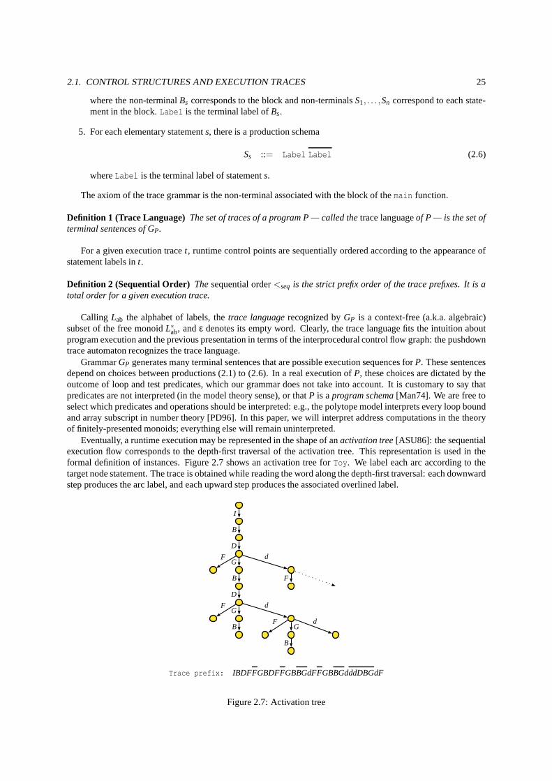
2.1. CONTROL STRUCTURES AND EXECUTION TRACES 25
where the non-terminalBs corresponds to the block and non-terminalsS1, . . . ,Sn correspond to each state-ment in the block.Label is the terminal label ofBs.
5. For each elementary statements, there is a production schema
Ss ::= Label Label (2.6)
whereLabel is the terminal label of statements.
The axiom of the trace grammar is the non-terminal associated with the block of themain function.
Definition 1 (Trace Language) The set of traces of a program P — called thetrace languageof P — is the set ofterminal sentences of GP.
For a given execution tracet, runtime control points are sequentially ordered according to the appearance ofstatement labels int.
Definition 2 (Sequential Order) Thesequential order<seq is the strict prefix order of the trace prefixes. It is atotal order for a given execution trace.
Calling Lab the alphabet of labels, thetrace languagerecognized byGP is a context-free (a.k.a. algebraic)subset of the free monoidL∗ab, andε denotes its empty word. Clearly, the trace language fits the intuition aboutprogram execution and the previous presentation in terms ofthe interprocedural control flow graph: the pushdowntrace automaton recognizes the trace language.
GrammarGP generates many terminal sentences that are possible execution sequences forP. These sentencesdepend on choices between productions (2.1) to (2.6). In a real execution ofP, these choices are dictated by theoutcome of loop and test predicates, which our grammar does not take into account. It is customary to say thatpredicates are not interpreted (in the model theory sense),or thatP is aprogram schema[Man74]. We are free toselect which predicates and operations should be interpreted: e.g., the polytope model interprets every loop boundand array subscript in number theory [PD96]. In this paper, we will interpret address computations in the theoryof finitely-presented monoids; everything else will remainuninterpreted.
Eventually, a runtime execution may be represented in the shape of anactivation tree[ASU86]: the sequentialexecution flow corresponds to the depth-first traversal of the activation tree. This representation is used in theformal definition of instances. Figure 2.7 shows an activation tree forToy. We label each arc according to thetarget node statement. The trace is obtained while reading the word along the depth-first traversal: each downwardstep produces the arc label, and each upward step produces the associated overlined label.
I
B
D
FG
B
D
FG
d
F dG
d
F
B
B
Trace prefix: IBDFFGBDFFGBBGdFFGBBGdddDBGdF
Figure 2.7: Activation tree
26 CHAPTER 2. INSTANCEWISE PROGRAM ANALYSIS
2.2 The Instancewise Model
This section is dedicated to the first part of our framework: the abstraction oftrace prefixesinto control words,the formal representation ofinstances. The control word abstraction characterizes an infinite setof trace prefixesin a tractable, finite-state representation. We present theproperties of control words from several points of view:pushdown trace automata, trace prefixes, activation trees,and MOGUL grammar. This last insight introduces acontrol words grammar that generates a superset of control words. We then investigate the conditions realizing theequivalence of the language generated by the control words grammar and the set of control words. This sectionends with the description of the control word language in theform of a finite-state automaton, a counterpart of thepushdown trace automaton. Finally, we expose one of the mainresults of this work, justifying the introduction ofcontrol words as the basis for instancewise analysis.
2.2.1 From the Pushdown Trace Automaton to Control Words
The pushdown trace automaton will help us prove an importantproperty of control words.
Definition 3 (Stack Word Language) The stack word language of a pushdown automatonA is the set of stackwords u such that there exists a state q inA for which the configuration(q,u) is both accessible and co-accessible— there is an accepting path traversing q with stack word u.
Definition 4 (Control Word) The stack word language of the pushdown trace automaton is called thecontrolword language. A control wordis the sequence of labels of all statements that have begun their execution but notyet completed it. Any trace prefix has a corresponding control word.
Since the stack word language of a pushdown automaton is rational [RS97a], we have:
Theorem 1 The language of control words is rational.
The activation tree is a convenient representation of control words. When the label of noden is at the top of thecontrol stack, the control word is the sequence of labels along thebranchof n in the activation tree, i.e., the pathfrom the root to noden [ASU86]. Conversely, a word labeling a branch of the activation tree is a control word.For example,IBDdF is the control word of trace prefixIBDFFGBDFFGBBGdFFGBBGdddDBGdFin Figure 2.7.
2.2.2 From Traces to Control Words
The trace language is a Dyck language [Ber79], i.e., a hierarchical parenthesis language. The restricted Dyckcongruence overL∗ab is the congruence generated byℓℓ≡ ε, for all ℓ ∈ Lab.2 This definition induces a rewritingrule overL∗ab, obviously confluent. This rule is the direct transpositionof the control stack behavior. Applying itto any trace prefixp we can associate a minimal wordw.
Lemma 1 The control word w associated to the trace prefix p is the shortest element in the class of p modulo therestricted Dyck congruence.
Definition 5 (Slimming Function) Theslimming functionmaps each trace prefix to its associated control word.
Theorem 2 The set of control words is the quotient set of trace prefixes modulo the restricted Dyck congruence,and the slimming function is the canonical projection of trace prefixes over control words.
From now on, the restricted Dyck congruence will be called the slimming congruence. The following tableillustrates the effect of the slimming function on a few trace prefixes.
Trace prefix IBDFFGBDFControl word IBD GBDF
Trace prefix IBDFFGBDFFGBBGdFFGControl word IBD GBD d G
Trace prefix IBDFFGBDFFGBBGdFFGBBGdddDBGdFControl word IBD dF
The slimming function extends Harrison’s NET function, and control words are very similar to hisprocedurestrings[Har89]. Harrison introduced these concepts for a statementwise analysis with dynamic partitioning.
2Therestrictedqualifier means that onlyℓℓ couples are considered,ℓℓ being a nonsensical sub-word for the trace grammar.
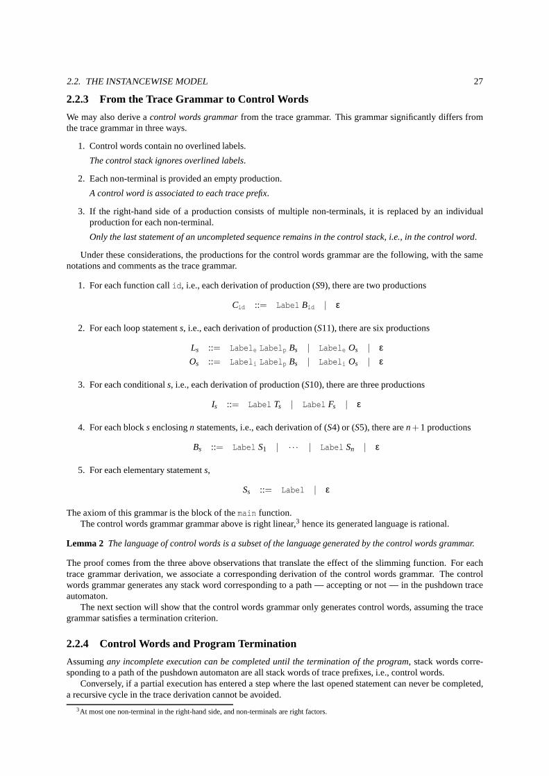
2.2. THE INSTANCEWISE MODEL 27
2.2.3 From the Trace Grammar to Control Words
We may also derive acontrol words grammarfrom the trace grammar. This grammar significantly differs fromthe trace grammar in three ways.
1. Control words contain no overlined labels.
The control stack ignores overlined labels.
2. Each non-terminal is provided an empty production.
A control word is associated to each trace prefix.
3. If the right-hand side of a production consists of multiple non-terminals, it is replaced by an individualproduction for each non-terminal.
Only the last statement of an uncompleted sequence remains in the control stack, i.e., in the control word.
Under these considerations, the productions for the control words grammar are the following, with the samenotations and comments as the trace grammar.
1. For each function callid, i.e., each derivation of production (S9), there are two productions
Cid ::= Label Bid | ε
2. For each loop statements, i.e., each derivation of production (S11), there are six productions
Ls ::= Labele Labelp Bs | Labele Os | εOs ::= Labeli Labelp Bs | Labeli Os | ε
3. For each conditionals, i.e., each derivation of production (S10), there are three productions
Is ::= Label Ts | Label Fs | ε
4. For each blocks enclosingn statements, i.e., each derivation of (S4) or (S5), there aren+1 productions
Bs ::= Label S1 | · · · | Label Sn | ε
5. For each elementary statements,
Ss ::= Label | ε
The axiom of this grammar is the block of themain function.The control words grammar grammar above is right linear,3 hence its generated language is rational.
Lemma 2 The language of control words is a subset of the language generated by the control words grammar.
The proof comes from the three above observations that translate the effect of the slimming function. For eachtrace grammar derivation, we associate a corresponding derivation of the control words grammar. The controlwords grammar generates any stack word corresponding to a path — accepting or not — in the pushdown traceautomaton.
The next section will show that the control words grammar only generates control words, assuming the tracegrammar satisfies a termination criterion.
2.2.4 Control Words and Program Termination
Assumingany incomplete execution can be completed until the termination of the program, stack words corre-sponding to a path of the pushdown automaton are all stack words of trace prefixes, i.e., control words.
Conversely, if a partial execution has entered a step where the last opened statement can never be completed,a recursive cycle in the trace derivation cannot be avoided.
3At most one non-terminal in the right-hand side, and non-terminals are right factors.
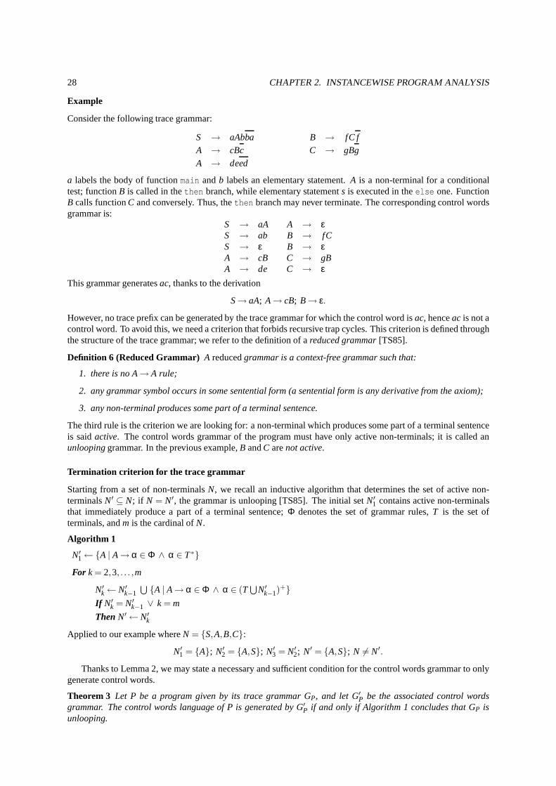
28 CHAPTER 2. INSTANCEWISE PROGRAM ANALYSIS
Example
Consider the following trace grammar:
S → aAbba B → fCf
A → cBc C → gBg
A → deed
a labels the body of functionmain andb labels an elementary statement.A is a non-terminal for a conditionaltest; functionB is called in thethen branch, while elementary statements is executed in theelse one. FunctionB calls functionC and conversely. Thus, thethen branch may never terminate. The corresponding control wordsgrammar is:
S → aA A → εS → ab B → fCS → ε B → εA → cB C → gBA → de C → ε
This grammar generatesac, thanks to the derivation
S→ aA; A→ cB; B→ ε.
However, no trace prefix can be generated by the trace grammarfor which the control word isac, henceac is not acontrol word. To avoid this, we need a criterion that forbidsrecursive trap cycles. This criterion is defined throughthe structure of the trace grammar; we refer to the definitionof a reduced grammar[TS85].
Definition 6 (Reduced Grammar) A reducedgrammar is a context-free grammar such that:
1. there is no A→ A rule;
2. any grammar symbol occurs in some sentential form (a sentential form is any derivative from the axiom);
3. any non-terminal produces some part of a terminal sentence.
The third rule is the criterion we are looking for: a non-terminal which produces some part of a terminal sentenceis saidactive. The control words grammar of the program must have only active non-terminals; it is called anunloopinggrammar. In the previous example,B andC arenot active.
Termination criterion for the trace grammar
Starting from a set of non-terminalsN, we recall an inductive algorithm that determines the set ofactive non-terminalsN′ ⊆ N; if N = N′, the grammar is unlooping [TS85]. The initial setN′1 contains active non-terminalsthat immediately produce a part of a terminal sentence;Φ denotes the set of grammar rules,T is the set ofterminals, andm is the cardinal ofN.
Algorithm 1
N′1← {A | A→ α ∈Φ ∧ α ∈ T∗}
For k = 2,3, . . . ,m
N′k← N′k−1S
{A | A→ α ∈Φ ∧ α ∈ (TS
N′k−1)+}
If N′k = N′k−1 ∨ k = m
Then N′←N′k
Applied to our example whereN = {S,A,B,C}:
N′1 = {A}; N′2 = {A,S}; N′3 = N′2; N′ = {A,S}; N 6= N′.
Thanks to Lemma 2, we may state a necessary and sufficient condition for the control words grammar to onlygenerate control words.
Theorem 3 Let P be a program given by its trace grammar GP, and let G′P be the associated control wordsgrammar. The control words language of P is generated by G′
P if and only if Algorithm 1 concludes that GP isunlooping.
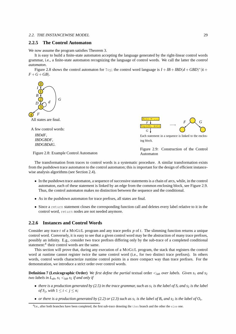
2.2. THE INSTANCEWISE MODEL 29
2.2.5 The Control Automaton
We now assume the program satisfies Theorem 3.It is easy to build a finite-state automaton accepting the language generated by the right-linear control words
grammar, i.e., a finite-state automaton recognizing the language of control words. We call the latter thecontrolautomaton.
Figure 2.8 shows the control automaton forToy; the control word language isI + IB+ IBD(d+ GBD)∗(ε +F +G+GB).
0
1
2
3
4
I
B
D
F
dG
All states are final.
A few control words:
IBDdF,IBDGBDF,IBDGBDdG.
Figure 2.8: Example Control Automaton
A[i] = ...
Toy(20, k+1)F
G
−→F G
Each statement in a sequence is linked to the enclos-
ing block.
Figure 2.9: Construction of the ControlAutomaton
The transformation from traces to control words is a systematic procedure. A similar transformation existsfrom the pushdown trace automaton to the control automaton;this is important for the design of efficient instance-wise analysis algorithms (see Section 2.4).
• In the pushdown trace automaton, a sequence of successive statements is a chain of arcs, while, in the controlautomaton, each of these statement is linked by an edge from the common enclosing block, see Figure 2.9.Thus, the control automaton makes no distinction between the sequence and the conditional.
• As in the pushdown automaton for trace prefixes, all states are final.
• Since areturn statement closes the corresponding function call and deletes every label relative to it in thecontrol word,return nodes are not needed anymore.
2.2.6 Instances and Control Words
Consider any tracet of a MOGUL program and any trace prefixp of t. The slimming function returns a uniquecontrol word. Conversely, it is easy to see that a given control word may be the abstraction of many trace prefixes,possibly an infinity. E.g., consider two trace prefixes differing only by the sub-trace of a completed conditionalstatement:4 their control words are the same.
This section will prove that, during any execution of a MOGUL program, the stack that registers the controlword at runtime cannot register twice the same control word (i.e., for two distinct trace prefixes). In otherswords, control words characterize runtime control points in a more compact way than trace prefixes. For thedemonstration, we introduce a strict order over control words.
Definition 7 (Lexicographic Order) We first define the partialtextual order<lab over labels. Given s1 and s2two labels in Lab, s1 <lab s2 if and only if
• there is a production generated by (2.5) in the trace grammar, such as s1 is the label of Si and s2 is the labelof Sj , with 1≤ i < j ≤ n;
• or there is a production generated by (2.2) or (2.3) such as s1 is the label of Bs and s2 is the label of Os.
4I.e., after both branches have been completed, the first sub-trace denoting thethen branch and the other theelse one.
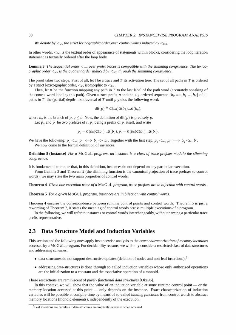
30 CHAPTER 2. INSTANCEWISE PROGRAM ANALYSIS
We denote by<lex the strict lexicographic order over control words induced by <lab.
In other words,<lab is the textual order of appearance of statements within blocks, considering the loop iterationstatement as textually ordered after the loop body.
Lemma 3 The sequential order<seqover prefix traces is compatible with the slimming congruence. The lexico-graphic order<lex is the quotient order induced by<seq through the slimming congruence.
The proof takes two steps. First of all, lett be a trace andT its activation tree. The set of all paths inT is orderedby a strict lexicographic order,<T , isomorphic to<lex.
Then, letα be the function mapping any path inT to the last label of the path word (accurately speaking ofthe control word labeling this path). Given a trace prefixp and the<T ordered sequence{b0 = ε,b1, ...,bn} of allpaths inT, the (partial) depth-first traversal ofT until p yields the following word:
dft(p), α(b0)α(b1)...α(bq),
wherebq is the branch ofp, q≤ n. Now, the definition of dft(p) is preciselyp.Let pq andpr be two prefixes oft, pq being a prefix ofpr itself, and write
pq = α(b0)α(b1)...α(bq), pr = α(b0)α(b1)...α(br).
We have the following:pq <seq pr ⇐⇒ bq <T br . Together with the first step,pq <seq pr ⇐⇒ bq <lex br .We now come to the formal definition of instances.
Definition 8 (Instance) For a MOGUL program, aninstanceis a class of trace prefixes modulo the slimmingcongruence.
It is fundamental to notice that, in this definition, instances do not depend on any particular execution.From Lemma 3 and Theorem 2 (the slimming function is the canonical projection of trace prefixes to control
words), we may state the two main properties of control words.
Theorem 4 Given one execution trace of aMOGUL program, trace prefixes are in bijection with control words.
Theorem 5 For a givenMOGUL program, instances are in bijection with control words.
Theorem 4 ensures the correspondence between runtime control points and control words. Theorem 5 is just arewording of Theorem 2, it states the meaning of control words across multiple executions of a program.
In the following, we will refer to instances or control wordsinterchangeably, without naming a particular traceprefix representative.
2.3 Data Structure Model and Induction Variables
This section and the following ones apply instancewise analysis to theexact characterization of memory locationsaccessed by a MOGUL program. For decidability reasons, we will only consider arestricted class of data structuresand addressing schemes:
• data structures do not support destructive updates (deletion of nodes and non-leaf insertions);5
• addressing data-structures is done through so called induction variables whose only authorized operationsare the initialization to a constant and the associative operation of a monoid.
These restrictions are reminiscent ofpurely functional data structures[Oka96].In this context, we will show that the value of an induction variable at some runtime control point — or the
memory location accessed at this point — only depends on the instance. Exact characterization of inductionvariables will be possible at compile-time by means of so-called binding functionsfrom control words to abstractmemory locations (monoid elements), independently of the execution.
5Leaf insertions are harmless if data-structures are implicitly expanded when accessed.
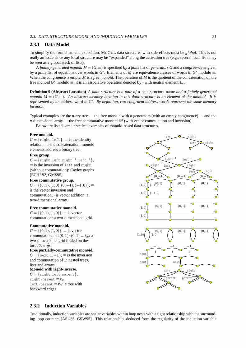
2.3. DATA STRUCTURE MODEL AND INDUCTION VARIABLES 31
2.3.1 Data Model
To simplify the formalism and exposition, MOGUL data structures with side-effects must beglobal. This is notreally an issue since any local structure may be “expanded” along the activation tree (e.g., several local lists maybe seen as a global stack of lists).
A finitely-generated monoid M= (G,≡) is specified by afinite list of generators Gand acongruence≡ givenby afinite list of equations over words inG∗. Elements ofM are equivalence classes of words inG∗ modulo≡.When the congruence is empty,M is afree monoid. The operation ofM is the quotient of the concatenation on thefree monoidG∗ modulo≡; it is an associative operation denoted by· with neutral elementεm.
Definition 9 (Abstract Location) A data structure is a pair of adata structure nameand a finitely-generatedmonoid M= (G,≡). An abstract memory location in this data structure is an element of the monoid. It isrepresented by anaddress wordin G∗. By definition, two congruent address words represent the same memorylocation.
Typical examples are then-ary tree — the free monoid withn generators (with an empty congruence) — and then-dimensional array — the free commutative monoidZn (with vector commutation and inversion).
Below are listed some practical examples of monoid-based data structures.
Free monoid.G = {right,left},≡ is the identityrelation,· is the concatenation: monoidelements address a binary tree.
left right
left right
Free group.G = {right,left,right−1,left−1},≡ is the inversion ofleft andright(without commutation): Cayley graphs[ECH+92, GMS95].
right−1left−1
left rightright−1
left right
Free commutative group.G = {(0,1),(1,0),(0,−1),(−1,0)},≡is the vector inversion andcommutation,· is vector addition: atwo-dimensional array.
(0,1) (0,1) (0,1)(1,0)
(1,0)
(0,−1) (0,−1) (0,−1)
(−1,0)
(−1,0)
Free commutative monoid.G = {(0,1),(1,0)},≡ is vectorcommutation: a two-dimensional grid.
(0,1) (0,1) (0,1)(1,0)
(1,0)
Commutative monoid.G = {(0,1),(1,0)},≡ is vectorcommutation and(0,1) · (0,1)≡ εm: atwo-dimensional grid folded on thetorusZ× Z
2Z.
(0,1) (0,1) (0,1)(1,0) (1,0)
Free partially-commutative monoid.G = {next,1,−1},≡ is the inversionand commutation of 1: nested trees,lists and arrays.
1 1 1next
next next
−1 −1 −1
Monoid with right-inverse.G = {right,left,parent},right ·parent ≡ εm,left ·parent ≡ εm: a tree withbackward edges.
left right
parent parent
2.3.2 Induction Variables
Traditionally, induction variables are scalar variables within loop nests with a tight relationship with the surround-ing loop counters [ASU86, GSW95]. This relationship, deduced from the regularity of the induction variable
32 CHAPTER 2. INSTANCEWISE PROGRAM ANALYSIS
updates, is a critical information for many analyses (dependence, array region, array bound checking) and opti-mizations (strength-reduction, loop transformations, hoisting).
A basic linear induction variablex is assigned (once or more) in a loop, each assignment being inthe formx = c or x = x + c, wherec is a constant known at compile-time. More generally, a variablex is called alinearinduction variableif on every iteration of the surrounding loop,x is added a constant value. This is the case whenassignments tox in the cycle are in the basic form or in the formx = y + c, y being another induction variable.The value ofx may then be computed as an affine function of the surrounding loop counters.
MOGUL extensions are twofold:
• induction variables are not restricted to arrays but handleall monoid-based data structures;
• both loops and recursive function calls are considered.
As a consequence, induction variables represent abstract addresses in data structures, and the basic operation overinduction variables becomes the monoid operation.
Definition 10 (Induction Variable) A variablex is an induction variable if and only if the three following con-ditions are satisfied:
a. x is defined at ablock entry, afor loop initialization, orx is a formal parameter;
b. x is constant in theblock, thefor loop or the function where it has been defined;
c. the definition ofx (according toa) is in one of the forms:
1. x = c, and c is a constant known at compile-time,
2. x = y · c, andy is an induction variable, possibly equal tox.
A M OGUL induction variable can be used in different address expressions which referencedistinctdata struc-tures, provided these structures are defined over the same monoid. This separation between data structure andshape follows the approach of the declarative language 81/2 [GMS95]. It is a convenient way to expose moresemantics to the static analyzer, compared with C pointers or variables of product types in ML.
Eventually, the MOGUL syntax is designed such thatevery variable of a monoid type is an induction variable,other variables being ignored. The only valid definitions and operations on MOGUL variables are those satisfyingDefinition 10. For any monoid shape, data structure accessesfollow the C array syntax:D[a] denotes elementwith addressa of structureD, wherea is in the formx or x · c, x an induction variable andc a constant.
If A is an array (i.e.,A is addressed in a free commutative group), the affine subscript A[i+2j-1] is not a validMOGUL syntax. This is not a real limitation, however, since affinesubscripts may be replaced by new inductionvariables defined when necessary whilei or j are defined. As an illustration, letk be the induction variable equalto i+2j-1, the subscript in the reference above. We have to build, through a backward motion, static chains ofinduction variables from the program start point to the considered reference. Suppose the last modification of thesubscript before the considered program point is given by the statementj= h denoted bys, whereh is anotherinduction variable. We have to define a new induction variable g = i+2h-1, living before this statement, and toconsider thats initializesk through an additional assignmentk= g. This work has to be done recursively for allpaths in the control flow graph until reaching the start point.
2.4 Binding Functions
In MOGUL, the computations on two induction variables in two distinct monoids are completely separate. Thus,without loss of generality, we suppose that all induction variables belong to a single monoidMloc, with operation· and neutral elementεm, called thedata structure monoid.
2.4.1 From Instances to Memory Locations
In a purely functional language, function application is the only way to define a variable. In MOGUL, everystatement is handled that way; the scope of a variable is restricted to the statement at the beginning of which it hasbeen declared, and an induction variable is constant in its scope.
2.4. BINDING FUNCTIONS 33
Since overloading of variable names occurs at the beginningof each statement, the value of an inductionvariable depends on the runtime control point of interest. Letx be an induction variable, we define thebinding forx as the pair (p, vp), wherep is a trace prefix andvp the value ofx after executingp.
Consider two trace prefixesp1 andp2 representative of the same instance. The previous rules guarantee thatall induction variables living right afterp1 (resp.p2) have been defined in statements not closed yet. Now, therespective sequences of non-closed statements forp1 andp2 are identical and equal to the control word ofp1 andp2. Thus the bindings ofx for p1 andp2 are equal. In others words, the function that binds the traceprefix to thevalue ofx is compatible with the slimming congruence.
Theorem 6 Given an induction variablex in a MOGUL program, the function mapping a trace prefix p to thevalue ofx only depends on the instance associated to p, i.e., on the control word.
In other words, given an execution trace, the bindings at anytrace prefix are identified by the control word (i.e.,the instance).
Definition 11 (Binding Function) A binding forx is a couple(w,v), where w is a control word and v the valueof x at the instance w.
Λx denotes thebinding function forx, mapping control words to the corresponding value ofx.
2.4.2 Bilabels
We now describe the mathematical framework to compute binding functions.
Definition 12 (Bilabel) A bilabel is a pair in the set L∗ab×Mloc. The first part of the pair is called theinput label,the second one is called theoutput label.
B = L∗ab×Mloc denotes the set of bilabels. From thedirect productof the control word free monoidL∗ab and thedata monoidMloc, B is provided with a monoid structure: its operation• is defined componentwise onL∗ab andMloc,
(α|a)• (β|b)de f= (αβ|a ·b). (2.7)
A binding for an induction variable is a bilabel. Every statement updates the binding of induction variablesaccording to their definitions and scope rules, the corresponding equations will be studied in Section 2.4.3.
Definition 13 The set ofrational subsetsof a monoid M is the least set that contains the finite subsets of M, closedby union, product and the star operation [Ber79].
A rational relationover two monoids M and M′ is a rational subset of the monoid M×M′.
We focus on the familyBrat of rational subsets ofB.
Definition 14 A semiring is a monoid for two binary operations, the “addition” +, which is commutative, andthe “product” ×, distributive over+; the neutral element for+ is the zero for×.
The powerset of a monoidM is a semiring for union and the operation ofM [Ber79]. The set of rationalsubsets ofM is a sub-semiring of the latter [Ber79]; it can be expressed through the set of rational expressions inM. ThusBrat is a semiring.
We overload• to denote the product operation inBrat; /0 is the zero element (the empty set of bilabels); and theneutral element for• is E = {(ε,εm)}. From now on, we identifyBrat with the set of rational expressions inM,and we also identify a singleton with the bilabel inside it: {(s|c)} may be written (s|c).
2.4.3 Building Recurrence Equations
To compute a finite representation of the binding function for each induction variable, we show that the bindingscan be expressed as a finite number of rational sets. First of all, bindings can be grouped according to the lastexecuted statement, i.e., the last label of the control word. Next, we build a system of equations in which unknownsare sets of bindings for induction variablex at staten of the control automaton. GivenAn the control automatonmodified so thatn is the unique final state, letLn be the language recognized byAn. Thebinding function forx atstate n, Λn
x, is the binding function forx restricted toLn. We also introduce a new induction variablez, constantand equal toεm.
The system of equations is a direct translation of the semantics of induction variable definitions; it follows thesyntax of a MOGUL programP; we illustrate each rule on the running example.
34 CHAPTER 2. INSTANCEWISE PROGRAM ANALYSIS
1. At the initial state 0 and for any induction variablex,
Λ0x = E (2.8)
E.g., theToy program involves three induction variables, the loop counteri and the formal parametersk andn. We willnot considern since it does not subscript any data structure. The output monoid isZ, its neutral elementεm is 0.
Λ0k = Λ0
i = (ε|0).
2. Λnz denotes the set defined by
Λnz =
[
w∈Ln
(w|εm). (2.9)
Λnz is the binding function for the new induction variablez restricted toLn; it is constant and equal toεm.
For each statements defining an induction variablex to csx (casec.1 of Definition 10), and callingd andathe respective departure and arrival states ofs in the control automaton,
Λax ⊇ Λd
z • (s|csx). (2.10)
SinceΛdz • (s|csx) =
S
w∈Ld(ws|csx), (2.10) means: ifw∈ Ld is a control word,wsis also a control word and
its binding forx is (ws|csx).
The control automaton automaton ofToy has 5 states. For the casec.1 of Definition 10,
statementI : k = 0, (2.11)
and (2.10) yields
Λ1k ⊇ Λ0
z • (I |0).
3. For each statements defining an induction variablex to y · c (casec.2 of Definition 10), andd anda therespective departure and arrival states ofs,
Λax ⊇ Λd
x • (s|csx). (2.12)
To complete the system, we add for every induction variablex unchanged bysa set of equations in the form(2.12), wherecsx = εm.
E.g., for casec.2 of Definition 10,
statementG : k = k · 1 (2.13)
statementd : i = i · 2 (2.14)
statementD : i = k (2.15)
and (2.12) yields
Λ1i ⊇ Λ3
i • (G|0)
Λ1k ⊇ Λ3
k • (G|1)
Λ2i ⊇ Λ1
i • (B|0)
Λ2k ⊇ Λ1
k • (B|0)
Λ3i ⊇ Λ2
k • (D|0)
Λ3i ⊇ Λ3
i • (d|2)
Λ3k ⊇ Λ2
k • (D|0)
Λ3k ⊇ Λ2
k • (d|0)
Λ4i ⊇ Λ3
i • (F |0)
Λ4k ⊇ Λ3
k • (F |0)
Λ1z ⊇ Λ0
z • (I |0)
Λ1z ⊇ Λ3
z • (G|0)
Λ2z ⊇ Λ1
z • (B|0)
Λ3z ⊇ Λ2
z • (D|0)
Λ3z ⊇ Λ2
z • (d|0)
Λ4z ⊇ Λ3
z • (F |0)
Gathering all equations generated from (2.8), (2.10) and (2.12) yields a system(S) of nv×ns equations withnv×ns unknowns, wherenv is the number of induction variables, includingz, andns the number of statements inthe program.6
Toy yields the system
6Some unknown sets correspond to variables that are not boundat the node of interest, they are useless.
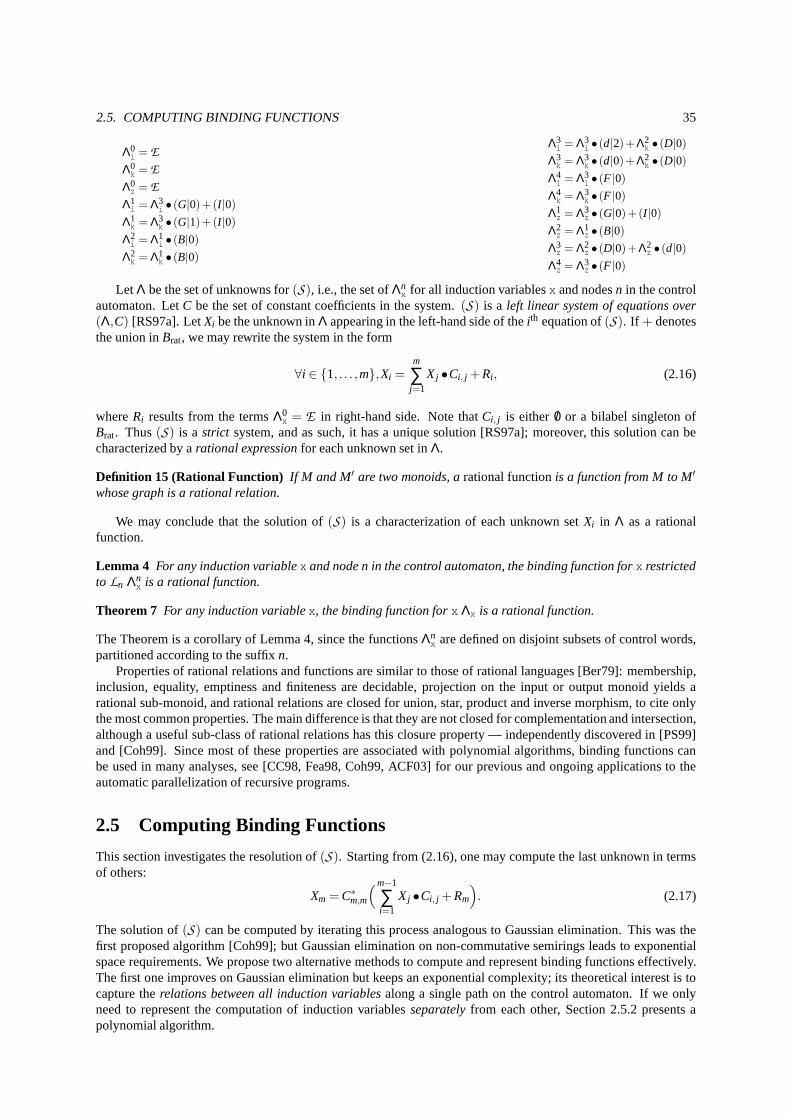
2.5. COMPUTING BINDING FUNCTIONS 35
Λ0i = E
Λ0k = E
Λ0z = E
Λ1i = Λ3
i • (G|0)+(I |0)
Λ1k = Λ3
k • (G|1)+(I |0)
Λ2i = Λ1
i • (B|0)
Λ2k = Λ1
k • (B|0)
Λ3i = Λ3
i • (d|2)+Λ2k • (D|0)
Λ3k = Λ3
k • (d|0)+Λ2k • (D|0)
Λ4i = Λ3
i • (F |0)
Λ4k = Λ3
k • (F |0)
Λ1z = Λ3
z • (G|0)+(I |0)
Λ2z = Λ1
z • (B|0)
Λ3z = Λ2
z • (D|0)+Λ2z • (d|0)
Λ4z = Λ3
z • (F |0)
Let Λ be the set of unknowns for(S), i.e., the set ofΛnx for all induction variablesx and nodesn in the control
automaton. LetC be the set of constant coefficients in the system.(S) is a left linear system of equations over(Λ,C) [RS97a]. LetXi be the unknown inΛ appearing in the left-hand side of theith equation of(S). If + denotesthe union inBrat, we may rewrite the system in the form
∀i ∈ {1, . . . ,m},Xi =m
∑j=1
Xj •Ci, j +Ri, (2.16)
whereRi results from the termsΛ0x = E in right-hand side. Note thatCi, j is either /0 or a bilabel singleton of
Brat. Thus(S) is a strict system, and as such, it has a unique solution [RS97a]; moreover, this solution can becharacterized by arational expressionfor each unknown set inΛ.
Definition 15 (Rational Function) If M and M′ are two monoids, arational functionis a function from M to M′
whose graph is a rational relation.
We may conclude that the solution of(S) is a characterization of each unknown setXi in Λ as a rationalfunction.
Lemma 4 For any induction variablex and node n in the control automaton, the binding function forx restrictedto Ln Λn
x is a rational function.
Theorem 7 For any induction variablex, the binding function forx Λx is a rational function.
The Theorem is a corollary of Lemma 4, since the functionsΛnx are defined on disjoint subsets of control words,
partitioned according to the suffixn.Properties of rational relations and functions are similarto those of rational languages [Ber79]: membership,
inclusion, equality, emptiness and finiteness are decidable, projection on the input or output monoid yields arational sub-monoid, and rational relations are closed forunion, star, product and inverse morphism, to cite onlythe most common properties. The main difference is that theyare not closed for complementation and intersection,although a useful sub-class of rational relations has this closure property — independently discovered in [PS99]and [Coh99]. Since most of these properties are associated with polynomial algorithms, binding functions canbe used in many analyses, see [CC98, Fea98, Coh99, ACF03] forour previous and ongoing applications to theautomatic parallelization of recursive programs.
2.5 Computing Binding Functions
This section investigates the resolution of(S). Starting from (2.16), one may compute the last unknown in termsof others:
Xm = C∗m,m
(m−1
∑i=1
Xj •Ci, j +Rm
)
. (2.17)
The solution of(S) can be computed by iterating this process analogous to Gaussian elimination. This was thefirst proposed algorithm [Coh99]; but Gaussian eliminationon non-commutative semirings leads to exponentialspace requirements. We propose two alternative methods to compute and represent binding functions effectively.The first one improves on Gaussian elimination but keeps an exponential complexity; its theoretical interest is tocapture therelations between all induction variablesalong a single path on the control automaton. If we onlyneed to represent the computation of induction variablesseparatelyfrom each other, Section 2.5.2 presents apolynomial algorithm.
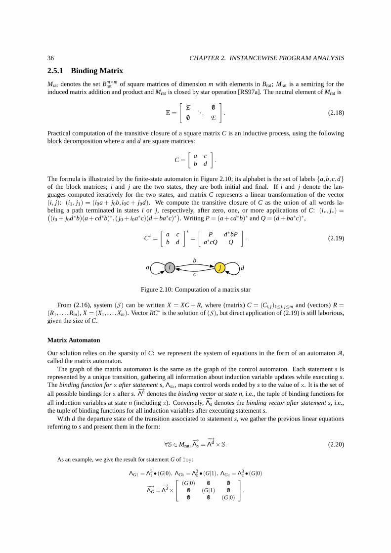
36 CHAPTER 2. INSTANCEWISE PROGRAM ANALYSIS
2.5.1 Binding Matrix
Mrat denotes the setBm×mrat of square matrices of dimensionm with elements inBrat; Mrat is a semiring for the
induced matrix addition and product andMrat is closed by star operation [RS97a]. The neutral element ofMrat is
E =
[
E /0. . ./0 E
]
. (2.18)
Practical computation of the transitive closure of a squarematrixC is an inductive process, using the followingblock decomposition wherea andd are square matrices:
C =
[
a cb d
]
.
The formula is illustrated by the finite-state automaton in Figure 2.10; its alphabet is the set of labels{a,b,c,d}of the block matrices;i and j are the two states, they are both initial and final. Ifi and j denote the lan-guages computed iteratively for the two states, and matrixC represents a linear transformation of the vector(i, j): (i1, j1) = (i0a+ j0b, i0c+ j0d). We compute the transitive closure ofC as the union of all words la-beling a path terminated in statesi or j, respectively, after zero, one, or more applications ofC: (i∗, j∗) =(
(i0 + j0d∗b)(a+cd∗b)∗,( j0 + i0a∗c)(d+ba∗c)∗)
. Writing P = (a+cd∗b)∗ andQ = (d+ba∗c)∗,
C∗ =
[
a cb d
]∗
=
[
P d∗bPa∗cQ Q
]
. (2.19)
i jab
cd
Figure 2.10: Computation of a matrix star
From (2.16), system(S) can be writtenX = XC+ R, where (matrix)C = (Ci, j )1≤i, j≤m and (vectors)R =(R1, . . . ,Rm), X = (X1, . . . ,Xm). VectorRC∗ is the solution of(S), but direct application of (2.19) is still laborious,given the size ofC.
Matrix Automaton
Our solution relies on the sparsity ofC: we represent the system of equations in the form of an automaton A ,called the matrix automaton.
The graph of the matrix automaton is the same as the graph of the control automaton. Each statements isrepresented by a unique transition, gathering all information about induction variable updates while executings.Thebinding function forx after statement s, Λsx, maps control words ended bys to the value ofx. It is the set ofall possible bindings forx afters.
−→Λn denotes thebinding vector at state n, i.e., the tuple of binding functions for
all induction variables at staten (includingz). Conversely,−→Λs denotes thebinding vector after statement s, i.e.,
the tuple of binding functions for all induction variables after executing statements.With d the departure state of the transition associated to statement s, we gather the previous linear equations
referring tosand present them in the form:
∀S ∈Mrat,−→Λs =
−→Λd×S. (2.20)
As an example, we give the result for statementG of Toy:
ΛGi = Λ3i • (G|0), ΛGk = Λ3
k • (G|1), ΛGz = Λ3z • (G|0)
−→ΛG =
−→Λ3×
(G|0) /0 /0/0 (G|1) /0/0 /0 (G|0)
.
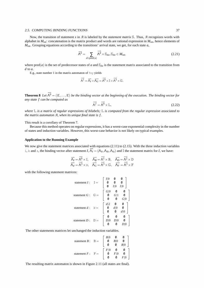
2.5. COMPUTING BINDING FUNCTIONS 37
Now, the transition of statements in A is labeled by thestatement matrixS. Thus,A recognizes words withalphabet inMrat: concatenation is the matrix product and words are rationalexpression inMrat, hence elements ofMrat. Grouping equations according to the transitions’ arrivalstate, we get, for each statea,
−→Λa = ∑
d∈pred(a)
−→Λd×Sda,Sda∈Mrat, (2.21)
where pred(a) is the set of predecessor states ofa andSda is the statement matrix associated to the transition fromd to a.
E.g., state number 1 in the matrix automaton ofToy yields
−→Λ1 =
−→ΛI +
−→ΛG =
−→Λ0× I+
−→Λ3×G.
Theorem 8 Let−→Λ0 = (E , . . . ,E) be the binding vector at the beginning of the execution. The binding vector for
any state f can be computed as−→Λ f =
−→Λ0×L, (2.22)
whereL is a matrix of regular expressions of bilabels;L is computed from the regular expression associated tothe matrix automatonA , when its unique final state is f .
This result is a corollary of Theorem 7.Because this method operates on regular expressions, it hasa worst-case exponential complexity in the number
of states and induction variables. However, this worst-case behavior is not likely on typical examples.
Application to the Running Example
We now give the statement matrices associated with equations (2.11) to (2.15). With the three induction variablesi, k andz, the binding vector after statementI ,
−→ΛI = (ΛIi ,ΛIk,ΛIz) andI the statement matrix forI , we have:
−→ΛI =
−→Λ0× I,
−→ΛB =
−→Λ1×B,
−→ΛD =
−→Λ2×D
−→Λd =
−→Λ3×D,
−→ΛG =
−→Λ3×G,
−→ΛF =
−→Λ3×F
with the following statement matrices:
statementI : I =
I |0 /0 /0/0 /0 /0/0 I |0 I |0
statementG : G =
G|0 /0 /0/0 G|1 /0/0 /0 G|0
statementd : D =
d|2 /0 /0/0 d|0 /0/0 /0 d|0
statementD : D =
/0 /0 /0D|0 D|0 /0
/0 /0 D|0
The other statements matrices let unchanged the induction variables.
statementB : B =
B|0 /0 /0/0 B|0 /0/0 /0 B|0
statementF : F =
F |0 /0 /0/0 F |0 /0/0 /0 F |0
The resulting matrix automaton is shown in Figure 2.11 (all states are final).
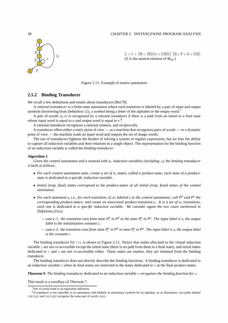
38 CHAPTER 2. INSTANCEWISE PROGRAM ANALYSIS
0
1
2
3
4
I
B
D
F
DG
L = I + IB+ IBD(
D+GBD)∗(
E+F+G+GB)
(E is the neutral element ofMrat.)
Figure 2.11: Example of matrix automaton
2.5.2 Binding Transducer
We recall a few definitions and results about transducers [Ber79].A rational transduceris a finite-state automaton where each transition is labeledby a pair ofinput andoutput
symbols (borrowing from Definition 12), a symbol being a letter of the alphabet or the empty word.7
A pair of words(u,v) is recognizedby a rational transducer if there is a path from an initial to afinal statewhose input word is equal tou and output word is equal tov.8
A rational transducer recognizes a rational relation, and reciprocally.A transducer offers either a static point of view — as a machine that recognizes pairs of words — or a dynamic
point of view — the machine reads an input word and outputs theset of image words.The use of transducers lightens the burden of solving a system of regular expressions, but we lose the ability
to capture all induction variables and their relations in a single object. The representation for the binding functionof an induction variable is called thebinding transducer.
Algorithm 2Given the control automaton and a monoid with nv induction variables (includingz), the binding transducer
is built as follows:
• For each control automaton state, create a set of nv states, called aproduct-state; each state of a product-state is dedicated to a specific induction variable.
• Initial (resp. final) states correspond to the product-states of all initial (resp. final) states of the controlautomaton.
• For each statement s, i.e., for each transition(d,a) labeled s in the control automaton; call Pd and Pa thecorresponding product-states; and create an associatedproduct-transitionts. It is a set of nv transitions,each one is dedicated to a specific induction variable. We consider again the two cases mentioned inDefinition (10.c).
– casec.1: the transition runs from state Pdz in Pd to the state Pax in Pa. The input label is s, the outputlabel is the initialization constant c;
– casec.2: the transition runs from state Pdy in Pd to state Pax in Pa. The input label is s, the output labelis the constant c.
The binding transducer forToy is shown in Figure 2.12. Notice that nodes allocated to the virtual inductionvariablez are not co-accessible except the initial state (there is no path from them to a final state), and initial statesdedicated toi andk are not co-accessible either. These states are useless, they are trimmed from the bindingtransducer.
The binding transducer does not directly describe the binding functions. A binding transducer isdedicatedtoan induction variablex when its final states are restricted to the states dedicated to x in the final product-states.
Theorem 9 The binding transducer dedicated to an induction variablex recognizes the binding function forx.
This result is a corollary of Theorem 7.
7Pair of words leads to an equivalent definition.8A transducer is not reducible to an automaton with bilabels as elementary symbols for its alphabet; as an illustration, two paths labeled
(x|ε)(y|z) and(x|z)(y|ε) recognize the same pair of words(xy|z).
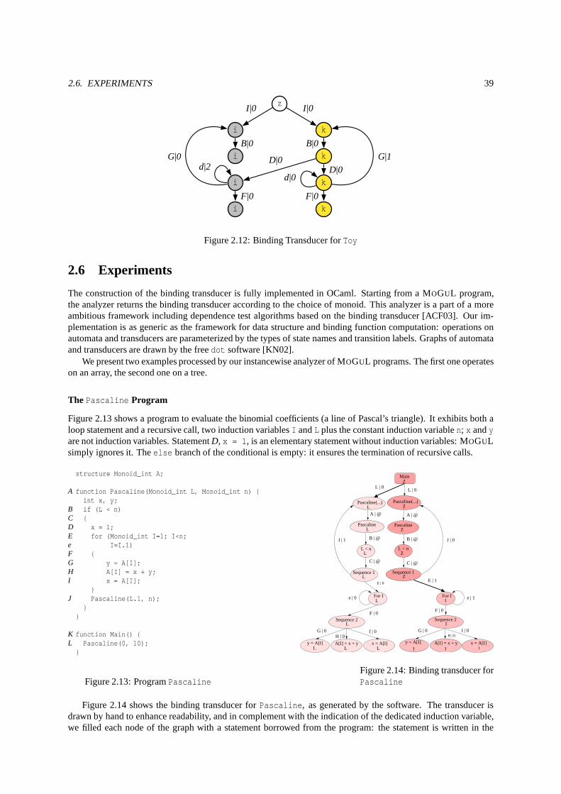
2.6. EXPERIMENTS 39
z
i k
i k
i k
i k
I |0 I |0
B|0 B|0
D|0D|0
F|0 F|0
d|2d|0
G|0 G|1
Figure 2.12: Binding Transducer forToy
2.6 Experiments
The construction of the binding transducer is fully implemented in OCaml. Starting from a MOGUL program,the analyzer returns the binding transducer according to the choice of monoid. This analyzer is a part of a moreambitious framework including dependence test algorithmsbased on the binding transducer [ACF03]. Our im-plementation is as generic as the framework for data structure and binding function computation: operations onautomata and transducers are parameterized by the types of state names and transition labels. Graphs of automataand transducers are drawn by the freedot software [KN02].
We present two examples processed by our instancewise analyzer of MOGUL programs. The first one operateson an array, the second one on a tree.
The Pascaline Program
Figure 2.13 shows a program to evaluate the binomial coefficients (a line of Pascal’s triangle). It exhibits both aloop statement and a recursive call, two induction variablesI andL plus the constant induction variablen; x andyare not induction variables. StatementD, x = 1, is an elementary statement without induction variables: MOGULsimply ignores it. Theelse branch of the conditional is empty: it ensures the termination of recursive calls.
structure Monoid_int A;
A function Pascaline(Monoid_int L, Monoid_int n) {int x, y;
B if (L < n)C {D x = 1;E for (Monoid_int I=1; I<n;e I=I.1)F {G y = A[I];H A[I] = x + y;I x = A[I];
}J Pascaline(L.1, n);
}}
K function Main() {L Pascaline(0, 10);
}
Figure 2.13: ProgramPascaline
E | 0
I
H | 0
Pascaline(...) Pascaline(...)
e | 1
A | @ A | @
L | 0L | 0
Main
y = A[I] A[I] = x + y x = A[I]L
y = A[I] A[I] = x + y I
x = A[I] ILL
LSequence 2
ISequence 2
L For I
G | 0 I | 0
For I I
E | 1
Sequence 1 L
Sequence 1 Z
L < n L
L < n Z
ZPascalinePascaline
L
B | @
C | @
B | @
C | @
J | 1 J | 0
F | 0
I | 0H | 0
G | 0
F | 0
e | 0
Z
L Z
Figure 2.14: Binding transducer forPascaline
Figure 2.14 shows the binding transducer forPascaline, as generated by the software. The transducer isdrawn by hand to enhance readability, and in complement withthe indication of the dedicated induction variable,we filled each node of the graph with a statement borrowed fromthe program: the statement is written in the
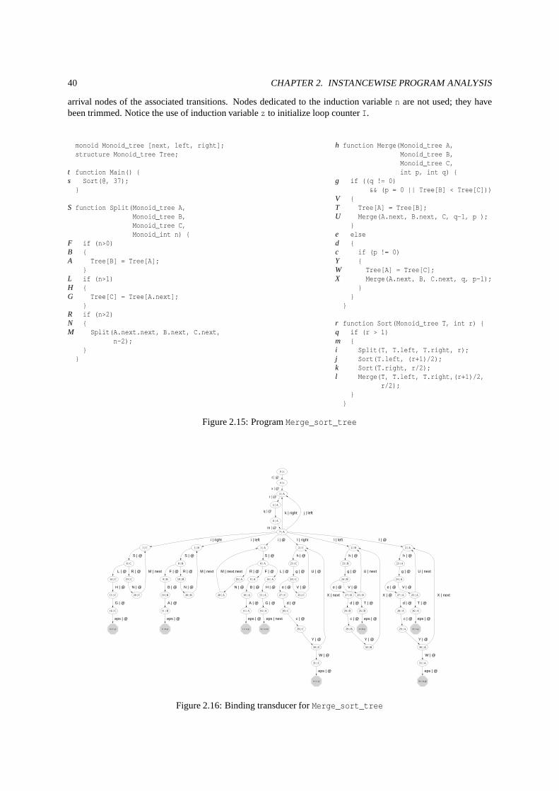
40 CHAPTER 2. INSTANCEWISE PROGRAM ANALYSIS
arrival nodes of the associated transitions. Nodes dedicated to the induction variablen are not used; they havebeen trimmed. Notice the use of induction variablez to initialize loop counterI.
monoid Monoid_tree [next, left, right];structure Monoid_tree Tree;
t function Main() {s Sort(@, 37);
}
S function Split(Monoid_tree A,Monoid_tree B,Monoid_tree C,Monoid_int n) {
F if (n>0)B {A Tree[B] = Tree[A];
}L if (n>1)H {G Tree[C] = Tree[A.next];
}R if (n>2)N {M Split(A.next.next, B.next, C.next,
n-2);}
}
h function Merge(Monoid_tree A,Monoid_tree B,Monoid_tree C,int p, int q) {
g if ((q != 0)&& (p = 0 || Tree[B] < Tree[C]))
V {T Tree[A] = Tree[B];U Merge(A.next, B.next, C, q-1, p );
}e elsed {c if (p != 0)Y {W Tree[A] = Tree[C];X Merge(A.next, B, C.next, q, p-1);
}}
}
r function Sort(Monoid_tree T, int r) {q if (r > 1)m {i Split(T, T.left, T.right, r);j Sort(T.left, (r+1)/2);k Sort(T.right, r/2);l Merge(T, T.left, T.right,(r+1)/2,
r/2);}
}
Figure 2.15: ProgramMerge_sort_tree
0 | z
4 | z
t | @
3 | A
s | @
11 | B.@ 11 | A.@16 | C.@ 16 | A.next 26 | B.@ 26 | A.@
31 | C.@ 31 | A.@
1 | C
8 | C
S | @
19 | C
R | @
14 | C
L | @
1 | B
8 | B
S | @
19 | B
R | @
9 | B
F | @
1 | A
8 | A
S | @
19 | A
R | @
14 | A
L | @
9 | A
F | @
2 | C
23 | C
h | @
24 | C
g | @
2 | B
23 | B
h | @
24 | B
g | @
2 | A
23 | A
h | @
24 | A
g | @
5 | A
r | @
6 | A
q | @
7 | A
m | @
i | right i | left i | @ l | right l | left l | @
k | right j | left
20 | C
N | @
15 | C
H | @
20 | B
N | @
10 | B
B | @
20 | A
N | @
15 | A
H | @
10 | A
B | @
11 | B
A | @
11 | A
A | @
eps | @ eps | @
16 | C
G | @
16 | A
G | @
eps | @ eps | next
M | next M | next M | next.next
27 | C
e | @
25 | C
V | @
27 | B
e | @
25 | B
V | @
27 | A
e | @
25 | A
V | @
28 | C
d | @
28 | B
d | @
28 | A
d | @
U | @ U | next
26 | B
T | @
U | next
26 | A
T | @
eps | @ eps | @
29 | C
c | @
29 | B
c | @
29 | A
c | @
30 | C
Y | @
30 | B
Y | @
30 | A
Y | @
X | next
31 | C
W | @
X | @ X | next
31 | A
W | @
eps | @ eps | @
Figure 2.16: Binding transducer forMerge_sort_tree
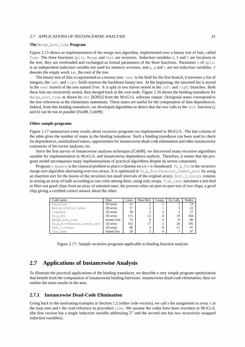
2.7. APPLICATIONS OF INSTANCEWISE ANALYSIS 41
The Merge_sort_tree Program
Figure 2.15 shows an implementation of the merge sort algorithm, implemented over a binary tree of lists, calledTree. The three functionsSplit, Merge andSort are recursive. Induction variablesA, B andC are locations inthe tree; they are overloaded and exchanged as formal parameters of the three functions. Parametern of Splitis an independent induction variable not used for memory accesses, andp, q andr are not induction variables.@denotes the empty word, i.e., the root of the tree.
The binary tree of lists is represented as a ternary tree:next is the field for the first branch, it traverses a list ofintegers, theleft andright fields traverse the backbone binary tree. At the beginning, the unsorted list is storedin thenext branch of the tree namedTree. It is split in two halves stored in theleft andright branches. Boththese lists are recursively sorted, then merged back in the root node. Figure 2.16 shows the binding transducer forMerge_sort_tree as drawn bydot [KN02] from the MOGUL software output. Octogonal states correspond tothe tree references at the elementary statements. These states are useful for the computation of data dependences.Indeed, from this binding transducer, we developed algorithms to detect that the two calls to theSort function (jandk) can be run in parallel [Fea98, Coh99].
Other sample programs
Figure 2.17 summarizes some results about recursive programs we implemented in MOGUL. The last column ofthe table gives the number of states in the binding transducer. Such a binding transducer can been used to checkfor dependences, uninitialized values, opportunities forinstancewise dead-code elimination and other instancewiseextensions of bit-vector analyses, etc.
Since the first survey of instancewise analyses techniques [Coh99], we discovered many recursive algorithmssuitable for implementation in MOGUL and instancewise dependence analysis. Therefore, it seems that the pro-gram model encompasses many implementations of practical algorithms despite its severe constraints.
Programn-Queens is the classical problem to placen Queens on an×n chessboard.To_&_fro is the recursivemerge-sort algorithm alternating over two arrays. It is optimized inTo_&_fro+Terminal_insert_sort by usingan insertion sort for the leaves of the recursion (on small intervals of the original array).Sort_3_colors consistsin sorting an array of balls according to one color among three, using only swaps.Vlsi_test simulates a test-bedto filter-out good chips from an array of untested ones; the process relies on peer-to-peer test of two chips, a goodchip giving a certified correct answer about the other.
Code name Data Lines Data Refs Loops Fn Calls NodesPascaline 1D array 21 2 1 2 13Multiplication table 2D array 17 5 1 3 22n-Queens 1D array 39 2 2 2 27To_&_fro 1D array 115 12 0 19 164Merge_sort_tree ternary tree 75 8 0 8 80To_&_fro+Terminal_insert_sort 1D array 162 17 2 26 195Sort_3_colors 1D array 80 4 0 11 97Vlsi_test linked lists 58 2 0 7 97
Figure 2.17: Sample recursive programs applicable to binding function analysis
2.7 Applications of Instancewise Analysis
To illustrate the practical applications of the binding transducer, we describe a very simple program optimizationthat benefit from the computation of instancewise binding functions:instancewise dead-code elimination, then weoutline the main results in the area.
2.7.1 Instancewise Dead-Code Elimination
Going back to the motivating examples in Section 1.2 (eithercode version), we calls the assignment to arrayA inthe loop nest andt the read reference in procedureline. We assume the codes have been rewritten in MOGUL(the first version has a single induction variable addressing Z2 and the second one has two recursively swappedinduction variables).
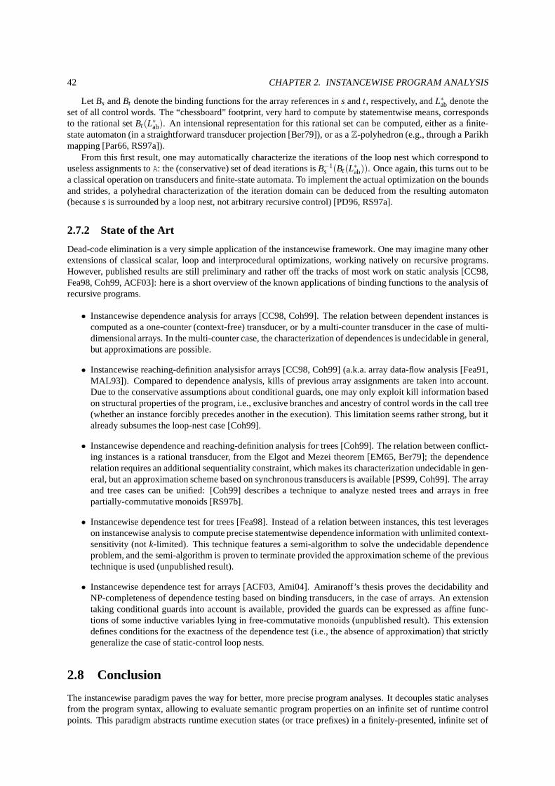
42 CHAPTER 2. INSTANCEWISE PROGRAM ANALYSIS
Let Bs andBt denote the binding functions for the array references insandt, respectively, andL∗ab denote theset of all control words. The “chessboard” footprint, very hard to compute by statementwise means, correspondsto the rational setBt(L∗ab). An intensional representation for this rational set can becomputed, either as a finite-state automaton (in a straightforward transducer projection [Ber79]), or as aZ-polyhedron (e.g., through a Parikhmapping [Par66, RS97a]).
From this first result, one may automatically characterize the iterations of the loop nest which correspond touseless assignments toA: the (conservative) set of dead iterations isB−1
s (Bt(L∗ab)). Once again, this turns out to bea classical operation on transducers and finite-state automata. To implement the actual optimization on the boundsand strides, a polyhedral characterization of the iteration domain can be deduced from the resulting automaton(becauses is surrounded by a loop nest, not arbitrary recursive control) [PD96, RS97a].
2.7.2 State of the Art
Dead-code elimination is a very simple application of the instancewise framework. One may imagine many otherextensions of classical scalar, loop and interprocedural optimizations, working natively on recursive programs.However, published results are still preliminary and rather off the tracks of most work on static analysis [CC98,Fea98, Coh99, ACF03]: here is a short overview of the known applications of binding functions to the analysis ofrecursive programs.
• Instancewise dependence analysis for arrays [CC98, Coh99]. The relation between dependent instances iscomputed as a one-counter (context-free) transducer, or bya multi-counter transducer in the case of multi-dimensional arrays. In the multi-counter case, the characterization of dependences is undecidable in general,but approximations are possible.
• Instancewise reaching-definition analysisfor arrays [CC98, Coh99] (a.k.a. array data-flow analysis [Fea91,MAL93]). Compared to dependence analysis, kills of previous array assignments are taken into account.Due to the conservative assumptions about conditional guards, one may only exploit kill information basedon structural properties of the program, i.e., exclusive branches and ancestry of control words in the call tree(whether an instance forcibly precedes another in the execution). This limitation seems rather strong, but italready subsumes the loop-nest case [Coh99].
• Instancewise dependence and reaching-definition analysisfor trees [Coh99]. The relation between conflict-ing instances is a rational transducer, from the Elgot and Mezei theorem [EM65, Ber79]; the dependencerelation requires an additional sequentiality constraint, which makes its characterization undecidable in gen-eral, but an approximation scheme based on synchronous transducers is available [PS99, Coh99]. The arrayand tree cases can be unified: [Coh99] describes a technique to analyze nested trees and arrays in freepartially-commutative monoids [RS97b].
• Instancewise dependence test for trees [Fea98]. Instead ofa relation between instances, this test leverageson instancewise analysis to compute precise statementwisedependence information with unlimited context-sensitivity (notk-limited). This technique features a semi-algorithm to solve the undecidable dependenceproblem, and the semi-algorithm is proven to terminate provided the approximation scheme of the previoustechnique is used (unpublished result).
• Instancewise dependence test for arrays [ACF03, Ami04]. Amiranoff’s thesis proves the decidability andNP-completeness of dependence testing based on binding transducers, in the case of arrays. An extensiontaking conditional guards into account is available, provided the guards can be expressed as affine func-tions of some inductive variables lying in free-commutative monoids (unpublished result). This extensiondefines conditions for the exactness of the dependence test (i.e., the absence of approximation) that strictlygeneralize the case of static-control loop nests.
2.8 Conclusion
The instancewise paradigm paves the way for better, more precise program analyses. It decouples static analysesfrom the program syntax, allowing to evaluate semantic program properties on an infinite set of runtime controlpoints. This paradigm abstracts runtime execution states (or trace prefixes) in a finitely-presented, infinite set of

2.8. CONCLUSION 43
control words. Instancewise analysis is also an extension of the domain-specific iteration-vector approach (theso-called polytope model) to general recursive programs.
As an application of the instancewise framework, we extend the concept of induction variables to recursiveprograms. For a restricted class of data structures (including arrays and recursive structures), induction variablescapture the exact memory location accessed at every step of the execution. This compile-time characterization,called the binding function, is a rational function mappingcontrol words to abstract memory locations. We give apolynomial algorithm for the computation of binding functions.
Our current work focuses on instancewise alias and dependence analysis, for the automatic parallelization andoptimization of recursive programs [Ami04]. We also look after new benchmark applications and data-structuresto assess the applicability of binding functions; multi-grid and sparse codes are interesting candidates. We wouldalso like to release a few constraints on the data structuresand induction variables, aiming for the computation ofapproximate binding functions through abstract interpretation.
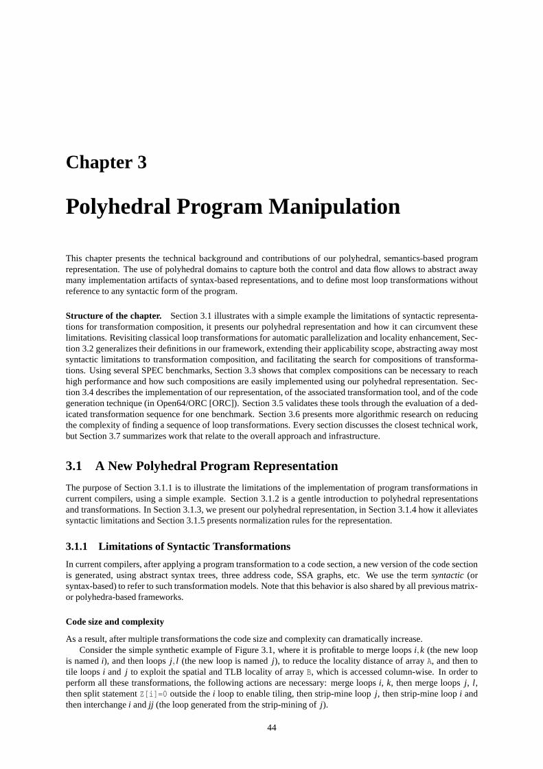
Chapter 3
Polyhedral Program Manipulation
This chapter presents the technical background and contributions of our polyhedral, semantics-based programrepresentation. The use of polyhedral domains to capture both the control and data flow allows to abstract awaymany implementation artifacts of syntax-based representations, and to define most loop transformations withoutreference to any syntactic form of the program.
Structure of the chapter. Section 3.1 illustrates with a simple example the limitations of syntactic representa-tions for transformation composition, it presents our polyhedral representation and how it can circumvent theselimitations. Revisiting classical loop transformations for automatic parallelization and locality enhancement, Sec-tion 3.2 generalizes their definitions in our framework, extending their applicability scope, abstracting away mostsyntactic limitations to transformation composition, andfacilitating the search for compositions of transforma-tions. Using several SPEC benchmarks, Section 3.3 shows that complex compositions can be necessary to reachhigh performance and how such compositions are easily implemented using our polyhedral representation. Sec-tion 3.4 describes the implementation of our representation, of the associated transformation tool, and of the codegeneration technique (in Open64/ORC [ORC]). Section 3.5 validates these tools through the evaluation of a ded-icated transformation sequence for one benchmark. Section3.6 presents more algorithmic research on reducingthe complexity of finding a sequence of loop transformations. Every section discusses the closest technical work,but Section 3.7 summarizes work that relate to the overall approach and infrastructure.
3.1 A New Polyhedral Program Representation
The purpose of Section 3.1.1 is to illustrate the limitations of the implementation of program transformations incurrent compilers, using a simple example. Section 3.1.2 isa gentle introduction to polyhedral representationsand transformations. In Section 3.1.3, we present our polyhedral representation, in Section 3.1.4 how it alleviatessyntactic limitations and Section 3.1.5 presents normalization rules for the representation.
3.1.1 Limitations of Syntactic Transformations
In current compilers, after applying a program transformation to a code section, a new version of the code sectionis generated, using abstract syntax trees, three address code, SSA graphs, etc. We use the termsyntactic(orsyntax-based) to refer to such transformation models. Notethat this behavior is also shared by all previous matrix-or polyhedra-based frameworks.
Code size and complexity
As a result, after multiple transformations the code size and complexity can dramatically increase.Consider the simple synthetic example of Figure 3.1, where it is profitable to merge loopsi,k (the new loop
is namedi), and then loopsj, l (the new loop is namedj), to reduce the locality distance of arrayA, and then totile loops i and j to exploit the spatial and TLB locality of arrayB, which is accessed column-wise. In order toperform all these transformations, the following actions are necessary: merge loopsi, k, then merge loopsj, l ,then split statementZ[i]=0 outside thei loop to enable tiling, then strip-mine loopj, then strip-mine loopi andthen interchangei andjj (the loop generated from the strip-mining ofj).
44
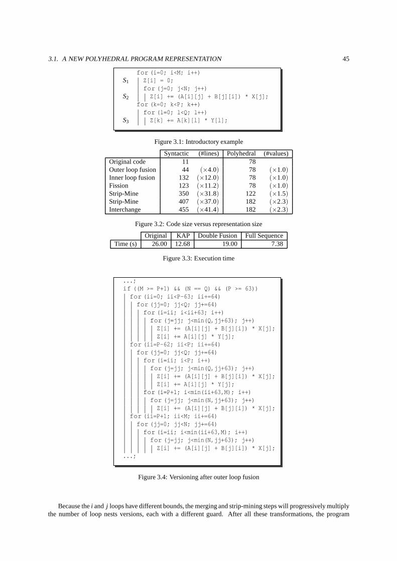
3.1. A NEW POLYHEDRAL PROGRAM REPRESENTATION 45
for (i=0; i<M; i++)S1 Z[i] = 0;
for (j=0; j<N; j++)S2 Z[i] += (A[i][j] + B[j][i]) * X[j];
for (k=0; k<P; k++)for (l=0; l<Q; l++)
S3 Z[k] += A[k][l] * Y[l];
Figure 3.1: Introductory example
Syntactic (#lines) Polyhedral (#values)Original code 11 78Outer loop fusion 44 (×4.0) 78 (×1.0)Inner loop fusion 132 (×12.0) 78 (×1.0)Fission 123 (×11.2) 78 (×1.0)Strip-Mine 350 (×31.8) 122 (×1.5)Strip-Mine 407 (×37.0) 182 (×2.3)Interchange 455 (×41.4) 182 (×2.3)
Figure 3.2: Code size versus representation size
Original KAP Double Fusion Full SequenceTime (s) 26.00 12.68 19.00 7.38
Figure 3.3: Execution time
...;if ((M >= P+1) && (N == Q) && (P >= 63))for (ii=0; ii<P-63; ii+=64)for (jj=0; jj<Q; jj+=64)for (i=ii; i<ii+63; i++)for (j=jj; j<min(Q,jj+63); j++)
Z[i] += (A[i][j] + B[j][i]) * X[j];Z[i] += A[i][j] * Y[j];
for (ii=P-62; ii<P; ii+=64)for (jj=0; jj<Q; jj+=64)for (i=ii; i<P; i++)for (j=jj; j<min(Q,jj+63); j++)
Z[i] += (A[i][j] + B[j][i]) * X[j];Z[i] += A[i][j] * Y[j];
for (i=P+1; i<min(ii+63,M); i++)for (j=jj; j<min(N,jj+63); j++)
Z[i] += (A[i][j] + B[j][i]) * X[j];for (ii=P+1; ii<M; ii+=64)for (jj=0; jj<N; jj+=64)for (i=ii; i<min(ii+63,M); i++)for (j=jj; j<min(N,jj+63); j++)
Z[i] += (A[i][j] + B[j][i]) * X[j];...;
Figure 3.4: Versioning after outer loop fusion
Because thei and j loops have different bounds, the merging and strip-mining steps will progressively multiplythe number of loop nests versions, each with a different guard. After all these transformations, the program
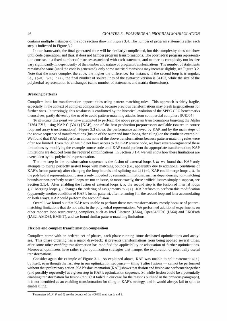
46 CHAPTER 3. POLYHEDRAL PROGRAM MANIPULATION
contains multiple instances of the code section shown in Figure 3.4. The number of program statements after eachstep is indicated in Figure 3.2.
In our framework, the final generated code will be similarly complicated, but this complexity does not showuntil code generation, and thus, it does not hamper program transformations. The polyhedral program representa-tion consists in a fixed number of matrices associated with each statement, and neither its complexity nor its sizevary significantly, independently of the number and nature of program transformations. The number of statementsremains the same (until the code is generated), only some matrix dimensions may increase slightly, see Figure 3.2.Note that the more complex the code, the higher the difference: for instance, if the second loop is triangular,i.e., (j=0; j<i; j++), the final number of source lines of the syntactic version is 34153, while the size of thepolyhedral representation is unchanged (same number of statements and matrix dimensions).
Breaking patterns
Compilers look for transformation opportunities using pattern-matching rules. This approach is fairly fragile,especially in the context of complex compositions, becauseprevious transformations may break target patterns forfurther ones. Interestingly, this weakness is confirmed by the historical evolution of the SPEC CPU benchmarksthemselves, partly driven by the need to avoid pattern-matching attacks from commercial compilers [PJEJ04].
To illustrate this point we have attempted to perform the above program transformations targeting the Alpha21364 EV7, using KAP C (V4.1) [KAP], one of the best production preprocessors available (source to sourceloop and array transformations). Figure 3.3 shows the performance achieved by KAP and by the main steps ofthe above sequence of transformations (fusion of the outer and inner loops, then tiling) on the synthetic example.1
We found that KAP could perform almost none of the above transformations because pattern-matching rules wereoften too limited. Even though we did not have access to the KAP source code, we have reverse-engineered theselimitations by modifying the example source code until KAP could perform the appropriate transformation; KAPlimitations are deduced from the required simplifications.In Section 3.1.4, we will show how these limitations areoverridden by the polyhedral representation.
The first step in the transformation sequence is the fusion ofexternal loopsi, k: we found that KAP onlyattempts to merge perfectly nested loops with matching bounds (i.e., apparently due to additional conditions ofKAP’s fusion pattern); after changing the loop bounds and splitting out Z[i]=0, KAP could merge loopsi, k. Inthe polyhedral representation, fusion is only impeded by semantic limitations, such as dependences; non-matchingbounds or non-perfectly nested loops are not an issue, or more exactly, these artificial issues simply disappear, seeSection 3.1.4. After enabling the fusion of external loopsi, k, the second step is the fusion of internal loopsj, l . Merging loopsj, l changes the ordering of assignments toZ[i]. KAP refuses to perform this modification(apparently another condition of KAP’s fusion pattern); after renamingZ in the second loop and later accumulatingon both arrays, KAP could perform the second fusion.
Overall, we found out that KAP was unable to perform these twotransformations, mostly because of pattern-matching limitations that do not exist in the polyhedral representation. We performed additional experiments onother modern loop restructuring compilers, such as Intel Electron (IA64), Open64/ORC (IA64) and EKOPath(IA32, AMD64, EM64T), and we found similar pattern-matching limitations.
Flexible and complex transformation composition
Compilers come with an ordered set of phases, each phase running some dedicated optimizations and analy-ses. This phase ordering has a major drawback: it prevents transformations from being applied several times,after some otherenablingtransformation has modified the applicability or adequation of further optimizations.Moreover, optimizers have rather rigid optimization strategies that hamper the exploration of potentially usefultransformations.
Consider again the example of Figure 3.1. As explained above, KAP was unable to split statementZ[i]by itself, even though the last step in our optimization sequence — tiling j after fusions — cannot be performedwithout that preliminary action. KAP’s documentation [KAP] shows that fission and fusion are performed together(and possibly repeatedly) at a given step in KAP’s optimization sequence. So while fission could be a potentiallyenabling transformation for fusion (though it failed in ourcase for the reasons outlined in the previous paragraph),it is not identified as an enabling transformation for tilingin KAP’s strategy, and it would always fail to split toenable tiling.
1ParametersM, N, P andQ are the bounds of the 400MB matricesA andB.
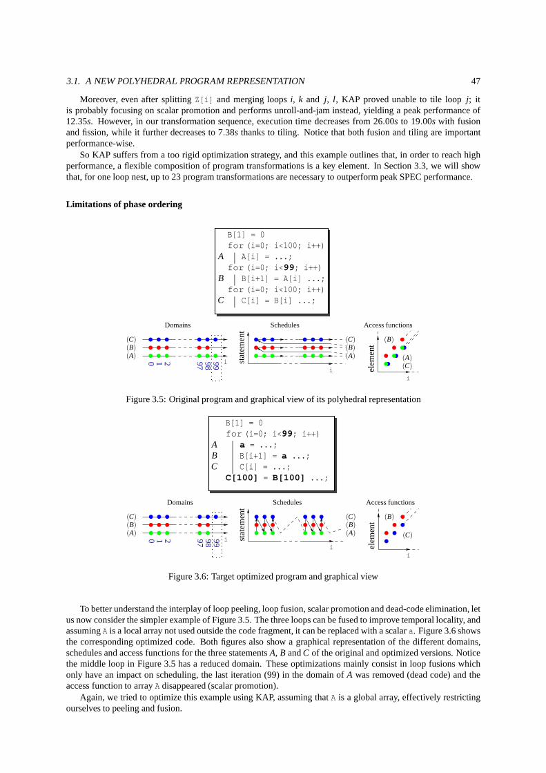
3.1. A NEW POLYHEDRAL PROGRAM REPRESENTATION 47
Moreover, even after splittingZ[i] and merging loopsi, k and j, l , KAP proved unable to tile loopj; itis probably focusing on scalar promotion and performs unroll-and-jam instead, yielding a peak performance of12.35s. However, in our transformation sequence, execution time decreases from 26.00s to 19.00s with fusionand fission, while it further decreases to 7.38s thanks to tiling. Notice that both fusion and tiling are importantperformance-wise.
So KAP suffers from a too rigid optimization strategy, and this example outlines that, in order to reach highperformance, a flexible composition of program transformations is a key element. In Section 3.3, we will showthat, for one loop nest, up to 23 program transformations arenecessary to outperform peak SPEC performance.
Limitations of phase ordering
B[1] = 0for (i=0; i<100; i++)
A A[i] = ...;for (i=0; i<99; i++)
B B[i+1] = A[i] ...;for (i=0; i<100; i++)
C C[i] = B[i] ...;
999897210 stat
emen
t
elem
ent
Domains
i
(C)(B)(A)
Schedules
i(C)(A)
(B)
Access functions
i
(C)(B)(A)
Figure 3.5: Original program and graphical view of its polyhedral representation
B[1] = 0for (i=0; i<99; i++)
A a = ...;B B[i+1] = a ...;C C[i] = ...;
C[100] = B[100] ...;
999897210 stat
emen
t
elem
ent(C)
(B)(A)
Domains
i
(C)
(A)(B)
Schedules
i
(B)
(C)
Access functions
i
Figure 3.6: Target optimized program and graphical view
To better understand the interplay of loop peeling, loop fusion, scalar promotion and dead-code elimination, letus now consider the simpler example of Figure 3.5. The three loops can be fused to improve temporal locality, andassumingA is a local array not used outside the code fragment, it can be replaced with a scalara. Figure 3.6 showsthe corresponding optimized code. Both figures also show a graphical representation of the different domains,schedules and access functions for the three statementsA, B andC of the original and optimized versions. Noticethe middle loop in Figure 3.5 has a reduced domain. These optimizations mainly consist in loop fusions whichonly have an impact on scheduling, the last iteration (99) inthe domain ofA was removed (dead code) and theaccess function to arrayA disappeared (scalar promotion).
Again, we tried to optimize this example using KAP, assumingthatA is a global array, effectively restrictingourselves to peeling and fusion.
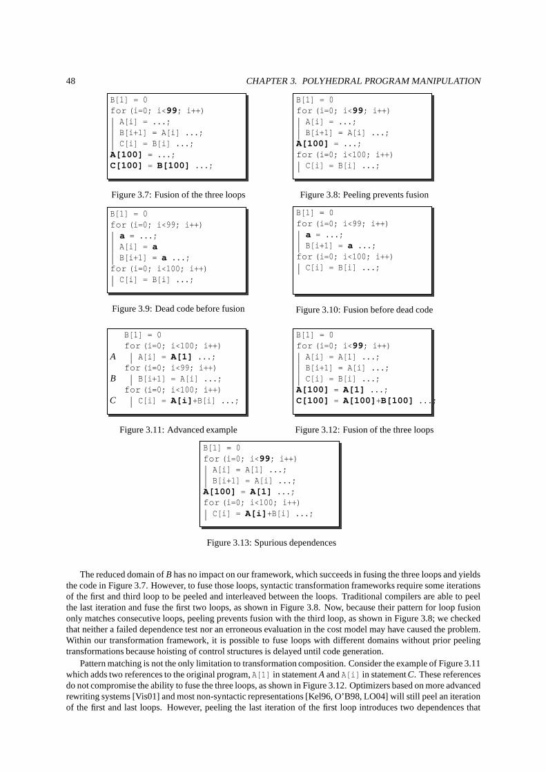
48 CHAPTER 3. POLYHEDRAL PROGRAM MANIPULATION
B[1] = 0for (i=0; i<99; i++)
A[i] = ...;B[i+1] = A[i] ...;C[i] = B[i] ...;
A[100] = ...;C[100] = B[100] ...;
Figure 3.7: Fusion of the three loops
B[1] = 0for (i=0; i<99; i++)
A[i] = ...;B[i+1] = A[i] ...;
A[100] = ...;for (i=0; i<100; i++)
C[i] = B[i] ...;
Figure 3.8: Peeling prevents fusion
B[1] = 0for (i=0; i<99; i++)a = ...;A[i] = aB[i+1] = a ...;
for (i=0; i<100; i++)C[i] = B[i] ...;
Figure 3.9: Dead code before fusion
B[1] = 0for (i=0; i<99; i++)a = ...;B[i+1] = a ...;
for (i=0; i<100; i++)C[i] = B[i] ...;
Figure 3.10: Fusion before dead code
B[1] = 0for (i=0; i<100; i++)
A A[i] = A[1] ...;for (i=0; i<99; i++)
B B[i+1] = A[i] ...;for (i=0; i<100; i++)
C C[i] = A[i]+B[i] ...;
Figure 3.11: Advanced example
B[1] = 0for (i=0; i<99; i++)
A[i] = A[1] ...;B[i+1] = A[i] ...;C[i] = B[i] ...;
A[100] = A[1] ...;C[100] = A[100]+B[100] ...;
Figure 3.12: Fusion of the three loops
B[1] = 0for (i=0; i<99; i++)
A[i] = A[1] ...;B[i+1] = A[i] ...;
A[100] = A[1] ...;for (i=0; i<100; i++)
C[i] = A[i]+B[i] ...;
Figure 3.13: Spurious dependences
The reduced domain ofB has no impact on our framework, which succeeds in fusing the three loops and yieldsthe code in Figure 3.7. However, to fuse those loops, syntactic transformation frameworks require some iterationsof the first and third loop to be peeled and interleaved between the loops. Traditional compilers are able to peelthe last iteration and fuse the first two loops, as shown in Figure 3.8. Now, because their pattern for loop fusiononly matches consecutive loops, peeling prevents fusion with the third loop, as shown in Figure 3.8; we checkedthat neither a failed dependence test nor an erroneous evaluation in the cost model may have caused the problem.Within our transformation framework, it is possible to fuseloops with different domains without prior peelingtransformations because hoisting of control structures isdelayed until code generation.
Pattern matching is not the only limitation to transformation composition. Consider the example of Figure 3.11which adds two references to the original program,A[1] in statementA andA[i] in statementC. These referencesdo not compromise the ability to fuse the three loops, as shown in Figure 3.12. Optimizers based on more advancedrewriting systems [Vis01] and most non-syntactic representations [Kel96, O’B98, LO04] will still peel an iterationof the first and last loops. However, peeling the last iteration of the first loop introduces two dependences that
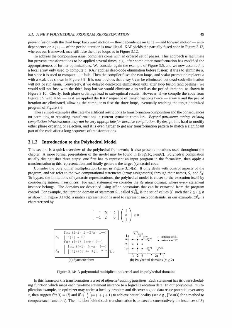
3.1. A NEW POLYHEDRAL PROGRAM REPRESENTATION 49
prevent fusion with the third loop: backward motion — flow dependence onA[1] — and forward motion — anti-dependence onA[i] — of the peeled iteration is now illegal. KAP yields the partially fused code in Figure 3.13,whereas our framework may still fuse the three loops as in Figure 3.12.
To address the composition issue, compilers come with an ordered set of phases. This approach is legitimatebut prevents transformations to be applied several times, e.g., after some other transformation has modified theappropriateness of further optimizations. We consider again the example of Figure 3.5, and we now assumeA isa local array only used to computeB. KAP applies dead-code elimination before fusion: it triesto eliminateA,but since it is used to computeB, it fails. Then the compiler fuses the two loops, and scalar promotion replacesAwith a scalar, as shown in Figure 3.9. It is now obvious that arrayA can be eliminated but dead-code eliminationwill not be run again. Conversely, if we delayed dead-code elimination until after loop fusion (and peeling), wewould still not fuse with the third loop but we would eliminate A as well as the peeled iteration, as shown inFigure 3.10. Clearly, both phase orderings lead to sub-optimal results. However, if we compile the code fromFigure 3.9 with KAP — as if we applied the KAP sequence of transformations twice — arrayA and the peelediteration are eliminated, allowing the compiler to fuse thethree loops, eventually reaching the target optimizedprogram of Figure 3.6.
These simple examples illustrate the artificial restrictions to transformation composition and the consequenceson permuting or repeating transformations in current syntactic compilers. Beyond parameter tuning, existingcompilation infrastructures may not be very appropriate for iterative compilation. By design, it is hard to modifyeither phase ordering or selection, and it is even harder to get any transformation pattern to match a significantpart of the code after a long sequence of transformations.
3.1.2 Introduction to the Polyhedral Model
This section is a quick overview of the polyhedral framework; it also presents notations used throughout thechapter. A more formal presentation of the model may be foundin [Pug91c, Fea92]. Polyhedral compilationusually distinguishes three steps: one first has to represent an input program in the formalism, then apply atransformation to this representation, and finally generate the target (syntactic) code.
Consider the polynomial multiplication kernel in Figure 3.14(a). It only deals with control aspects of theprogram, and we refer to the two computational statements (array assignments) through their names,S1 andS2.To bypass the limitations of syntactic representations, the polyhedral model is closer to the execution itself byconsideringstatement instances. For each statement we consider theiteration domain, where every statementinstance belongs. The domains are described using affine constraints that can be extracted from the programcontrol. For example, the iteration domain of statementS1, calledD
S1om, is the set of values(i) such that 2≤ i ≤ n
as shown in Figure 3.14(b); a matrix representation is used to represent such constraints: in our example,DS1om is
characterized by
[
1 0 −2−1 2 0
]
in1
≥ 0.
for (i=2; i<=2*n; i++)S1 Z[i] = 0;
for (i=1; i<=n; i++)for (j=1; j<=n; j++)
S2 Z[i+j] += X[i] * Y[j];1
2
nj
1 2 i
i>=1i>=2
i<=nj<=n
j>=1 i<=2n
S2S1
S2S2
S2 S1
n
instance of S1
2n
instance of S2
(a) Syntactic form (b) Polyhedral domains (n≥ 2)
Figure 3.14: A polynomial multiplication kernel and its polyhedral domains
In this framework, a transformation is a set ofaffine scheduling functions. Each statement has its own schedul-ing function which maps each run-time statement instance toa logical execution date. In our polynomial multi-plication example, an optimizer may notice a locality problem and discover a good data reuse potential over arrayZ, then suggestθS1(i) = (i) andθS2
(
ij
)
= (i + j +1) to achieve better locality (see e.g., [Bas03] for a method to
compute such functions). The intuition behind such transformation is to execute consecutively the instances ofS2
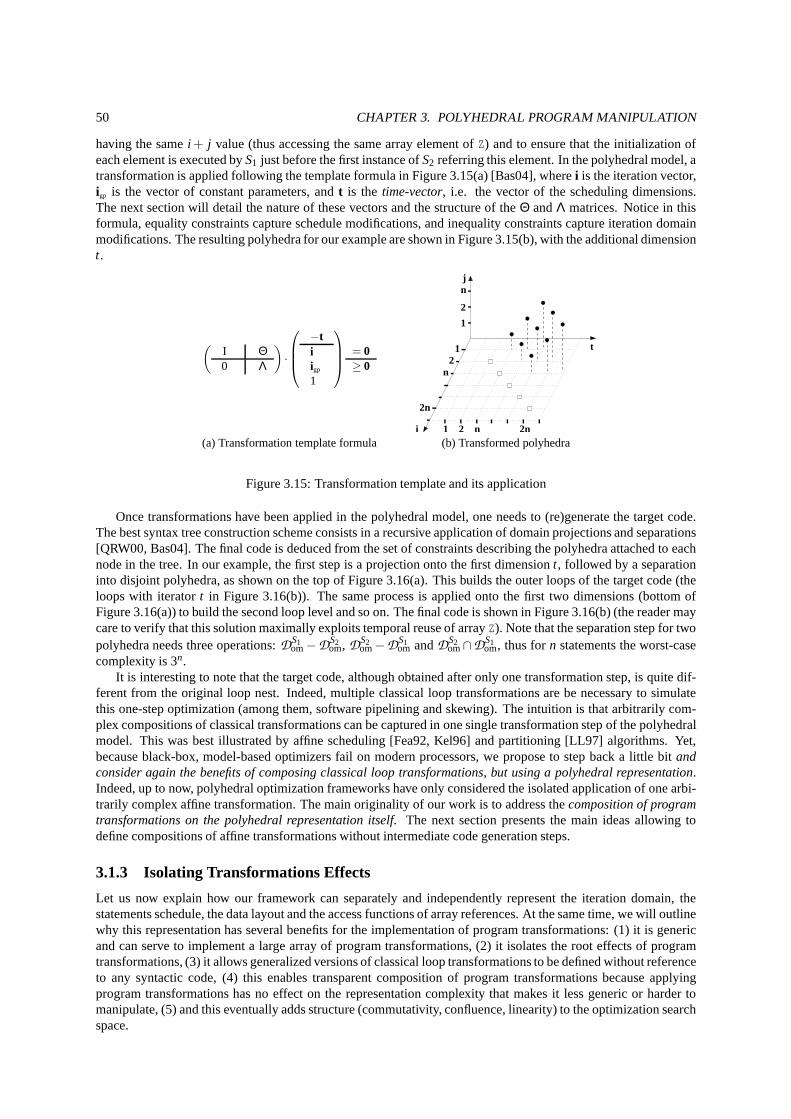
50 CHAPTER 3. POLYHEDRAL PROGRAM MANIPULATION
having the samei + j value (thus accessing the same array element ofZ) and to ensure that the initialization ofeach element is executed byS1 just before the first instance ofS2 referring this element. In the polyhedral model, atransformation is applied following the template formula in Figure 3.15(a) [Bas04], wherei is the iteration vector,igp is the vector of constant parameters, andt is the time-vector, i.e. the vector of the scheduling dimensions.The next section will detail the nature of these vectors and the structure of theΘ andΛ matrices. Notice in thisformula, equality constraints capture schedule modifications, and inequality constraints capture iteration domainmodifications. The resulting polyhedra for our example are shown in Figure 3.15(b), with the additional dimensiont.
(
I Θ0 Λ
)
·
−tiigp
1
= 0≥ 0
1
2
21
n
2n
1 2 n 2n
n
i
j
t
(a) Transformation template formula (b) Transformed polyhedra
Figure 3.15: Transformation template and its application
Once transformations have been applied in the polyhedral model, one needs to (re)generate the target code.The best syntax tree construction scheme consists in a recursive application of domain projections and separations[QRW00, Bas04]. The final code is deduced from the set of constraints describing the polyhedra attached to eachnode in the tree. In our example, the first step is a projectiononto the first dimensiont, followed by a separationinto disjoint polyhedra, as shown on the top of Figure 3.16(a). This builds the outer loops of the target code (theloops with iteratort in Figure 3.16(b)). The same process is applied onto the firsttwo dimensions (bottom ofFigure 3.16(a)) to build the second loop level and so on. The final code is shown in Figure 3.16(b) (the reader maycare to verify that this solution maximally exploits temporal reuse of arrayZ). Note that the separation step for twopolyhedra needs three operations:D
S1om−D
S2om, D
S2om−D
S1om andD
S2om∩D
S1om, thus forn statements the worst-case
complexity is 3n.It is interesting to note that the target code, although obtained after only one transformation step, is quite dif-
ferent from the original loop nest. Indeed, multiple classical loop transformations are be necessary to simulatethis one-step optimization (among them, software pipelining and skewing). The intuition is that arbitrarily com-plex compositions of classical transformations can be captured in one single transformation step of the polyhedralmodel. This was best illustrated by affine scheduling [Fea92, Kel96] and partitioning [LL97] algorithms. Yet,because black-box, model-based optimizers fail on modern processors, we propose to step back a little bitandconsider again the benefits of composing classical loop transformations, but using a polyhedral representation.Indeed, up to now, polyhedral optimization frameworks haveonly considered the isolated application of one arbi-trarily complex affine transformation. The main originality of our work is to address thecomposition of programtransformations on the polyhedral representation itself. The next section presents the main ideas allowing todefine compositions of affine transformations without intermediate code generation steps.
3.1.3 Isolating Transformations Effects
Let us now explain how our framework can separately and independently represent the iteration domain, thestatements schedule, the data layout and the access functions of array references. At the same time, we will outlinewhy this representation has several benefits for the implementation of program transformations: (1) it is genericand can serve to implement a large array of program transformations, (2) it isolates the root effects of programtransformations, (3) it allows generalized versions of classical loop transformations to be defined without referenceto any syntactic code, (4) this enables transparent composition of program transformations because applyingprogram transformations has no effect on the representation complexity that makes it less generic or harder tomanipulate, (5) and this eventually adds structure (commutativity, confluence, linearity) to the optimization searchspace.
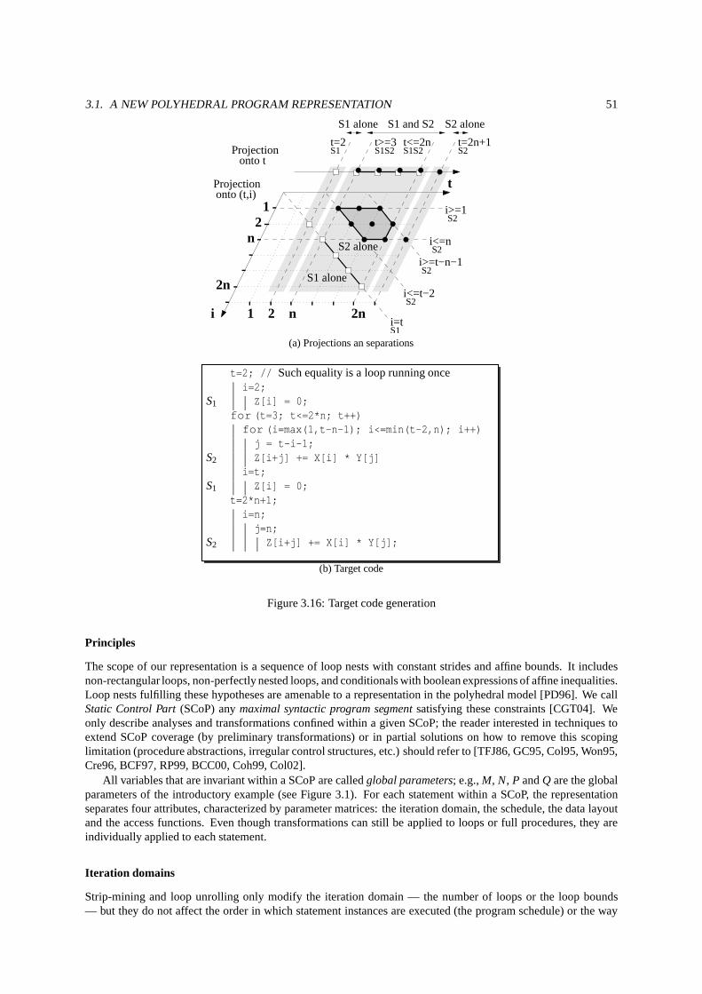
3.1. A NEW POLYHEDRAL PROGRAM REPRESENTATION 51
21
n
2n
1 2 ni
t
i<=n
i>=1
i<=t−2
i>=t−n−1
S1i=t
2n
S1 alone
S2 alone
Projection
Projectiononto t
onto (t,i)
S2
S2
S2
S2
t=2S1
t>=3S1S2
t<=2nS1S2 S2
S1 alone S1 and S2 S2 alone
t=2n+1
(a) Projections an separations
t=2; // Such equality is a loop running oncei=2;
S1 Z[i] = 0;for (t=3; t<=2*n; t++)for (i=max(1,t-n-1); i<=min(t-2,n); i++)j = t-i-1;
S2 Z[i+j] += X[i] * Y[j]i=t;
S1 Z[i] = 0;t=2*n+1;
i=n;j=n;
S2 Z[i+j] += X[i] * Y[j];
(b) Target code
Figure 3.16: Target code generation
Principles
The scope of our representation is a sequence of loop nests with constant strides and affine bounds. It includesnon-rectangular loops, non-perfectly nested loops, and conditionals with boolean expressions of affine inequalities.Loop nests fulfilling these hypotheses are amenable to a representation in the polyhedral model [PD96]. We callStatic Control Part(SCoP) anymaximal syntactic program segmentsatisfying these constraints [CGT04]. Weonly describe analyses and transformations confined withina given SCoP; the reader interested in techniques toextend SCoP coverage (by preliminary transformations) or in partial solutions on how to remove this scopinglimitation (procedure abstractions, irregular control structures, etc.) should refer to [TFJ86, GC95, Col95, Won95,Cre96, BCF97, RP99, BCC00, Coh99, Col02].
All variables that are invariant within a SCoP are calledglobal parameters; e.g.,M, N, P andQ are the globalparameters of the introductory example (see Figure 3.1). For each statement within a SCoP, the representationseparates four attributes, characterized by parameter matrices: the iteration domain, the schedule, the data layoutand the access functions. Even though transformations can still be applied to loops or full procedures, they areindividually applied to each statement.
Iteration domains
Strip-mining and loop unrolling only modify the iteration domain — the number of loops or the loop bounds— but they do not affect the order in which statement instances are executed (the program schedule) or the way
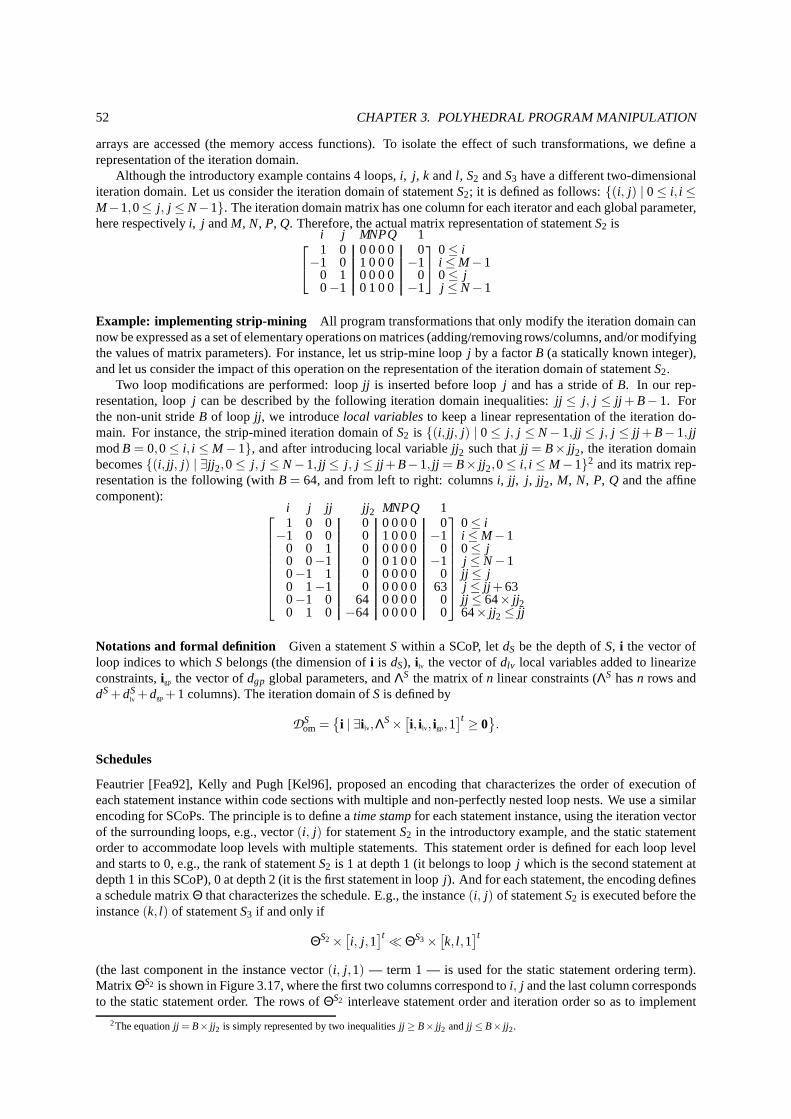
52 CHAPTER 3. POLYHEDRAL PROGRAM MANIPULATION
arrays are accessed (the memory access functions). To isolate the effect of such transformations, we define arepresentation of the iteration domain.
Although the introductory example contains 4 loops,i, j, k andl , S2 andS3 have a different two-dimensionaliteration domain. Let us consider the iteration domain of statementS2; it is defined as follows:{(i, j) | 0≤ i, i ≤M−1,0≤ j, j ≤N−1}. The iteration domain matrix has one column for each iterator and each global parameter,here respectivelyi, j andM, N, P, Q. Therefore, the actual matrix representation of statementS2 is
i1
j0
M0
N0
P0
Q0
10
−1 0 1 0 0 0 −10 1 0 0 0 0 00−1 0 1 0 0 −1
0≤ ii ≤M−10≤ jj ≤ N−1
Example: implementing strip-mining All program transformations that only modify the iterationdomain cannow be expressed as a set of elementary operations on matrices (adding/removing rows/columns, and/or modifyingthe values of matrix parameters). For instance, let us strip-mine loop j by a factorB (a statically known integer),and let us consider the impact of this operation on the representation of the iteration domain of statementS2.
Two loop modifications are performed: loopjj is inserted before loopj and has a stride ofB. In our rep-resentation, loopj can be described by the following iteration domain inequalities: jj ≤ j, j ≤ jj + B− 1. Forthe non-unit strideB of loop jj , we introducelocal variablesto keep a linear representation of the iteration do-main. For instance, the strip-mined iteration domain ofS2 is {(i, jj , j) | 0≤ j, j ≤ N−1, jj ≤ j, j ≤ jj + B−1, jjmodB = 0,0≤ i, i ≤M−1}, and after introducing local variablejj2 such thatjj = B× jj2, the iteration domainbecomes{(i, jj , j) | ∃jj2,0≤ j, j ≤ N−1, jj ≤ j, j ≤ jj +B−1, jj = B× jj2,0≤ i, i ≤M−1}2 and its matrix rep-resentation is the following (withB = 64, and from left to right: columnsi, jj , j, jj2, M, N, P, Q and the affinecomponent):
i1
j0
jj0
jj20
M0
N0
P0
Q0
10
−1 0 0 0 1 0 0 0 −10 0 1 0 0 0 0 0 00 0−1 0 0 1 0 0 −10−1 1 0 0 0 0 0 00 1−1 0 0 0 0 0 630−1 0 64 0 0 0 0 00 1 0 −64 0 0 0 0 0
0≤ ii ≤M−10≤ jj ≤ N−1jj ≤ jj ≤ jj +63jj ≤ 64× jj264× jj2≤ jj
Notations and formal definition Given a statementS within a SCoP, letdS be the depth ofS, i the vector ofloop indices to whichS belongs (the dimension ofi is dS), i lv the vector ofdlv local variables added to linearizeconstraints,igp the vector ofdgp global parameters, andΛS the matrix ofn linear constraints (ΛS hasn rows anddS+dS
lv +dgp+1 columns). The iteration domain ofS is defined by
DSom =
{
i | ∃i lv,ΛS×[
i, i lv, igp,1]t≥ 0
}
.
Schedules
Feautrier [Fea92], Kelly and Pugh [Kel96], proposed an encoding that characterizes the order of execution ofeach statement instance within code sections with multipleand non-perfectly nested loop nests. We use a similarencoding for SCoPs. The principle is to define atime stampfor each statement instance, using the iteration vectorof the surrounding loops, e.g., vector(i, j) for statementS2 in the introductory example, and the static statementorder to accommodate loop levels with multiple statements.This statement order is defined for each loop leveland starts to 0, e.g., the rank of statementS2 is 1 at depth 1 (it belongs to loopj which is the second statement atdepth 1 in this SCoP), 0 at depth 2 (it is the first statement in loop j). And for each statement, the encoding definesa schedule matrixΘ that characterizes the schedule. E.g., the instance(i, j) of statementS2 is executed before theinstance(k, l) of statementS3 if and only if
ΘS2×[
i, j,1]t≪ ΘS3×
[
k, l ,1]t
(the last component in the instance vector(i, j,1) — term 1 — is used for the static statement ordering term).Matrix ΘS2 is shown in Figure 3.17, where the first two columns correspond to i, j and the last column correspondsto the static statement order. The rows ofΘS2 interleave statement order and iteration order so as to implement
2The equationjj = B× jj2 is simply represented by two inequalitiesjj ≥ B× jj2 andjj ≤ B× jj2.
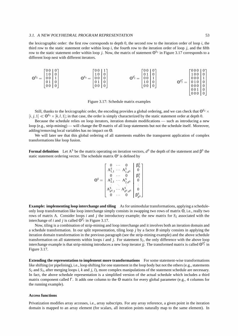
3.1. A NEW POLYHEDRAL PROGRAM REPRESENTATION 53
the lexicographic order: the first row corresponds to depth 0, the second row to the iteration order of loopi, thethird row to the static statement order within loopi, the fourth row to the iteration order of loopj, and the fifthrow to the static statement order within loopj. Now, the matrix of statementΘS3 in Figure 3.17 corresponds to adifferent loop nest with different iterators.
ΘS2 =
0 0 01 0 00 0 10 1 00 0 0
ΘS3 =
0 0 11 0 00 0 00 1 00 0 0
ΘS′2 =
0 0 00 1 00 0 11 0 00 0 0
ΘS′′2 =
0 0 0 01 0 0 00 0 0 10 1 0 00 0 0 00 0 1 00 0 0 0
Figure 3.17: Schedule matrix examples
Still, thanks to the lexicographic order, the encoding provides a global ordering, and we can check thatΘS2×[i, j,1]≪ ΘS3× [k, l ,1]; in that case, the order is simply characterized by the static statement order at depth 0.
Because the schedule relies on loop iterators, iteration domain modifications — such as introducing a newloop (e.g., strip-mining) — will change theΘ matrix of all loop statements but not the schedule itself. Moreover,adding/removing local variables has no impact onΘ.
We will later see that this global ordering of all statementsenables the transparent application of complextransformations like loop fusion.
Formal definition Let AS be the matrix operating on iteration vectors,dS the depth of the statement andβS thestatic statement ordering vector. The schedule matrixΘs is defined by
ΘS =
0 · · · 0 βS0
AS1,1 · · · AS
1,dS 0
0 · · · 0 βS1
AS2,1 · · · AS
2,dS 0...
. . ....
...
ASdS,1· · · AS
dS,dS 0
0 · · · 0 βSdS
Example: implementing loop interchange and tiling As for unimodular transformations, applying a schedule-only loop transformation like loop interchange simply consists in swapping two rows of matrixΘ, i.e., really tworows of matrix A. Consider loopsi and j the introductory example; the new matrix forS2 associated with theinterchange ofi and j is calledΘS′2 in Figure 3.17.
Now, tiling is a combination of strip-mining and loop interchange and it involves both an iteration domain anda schedule transformation. In our split representation, tiling loop j by a factorB simply consists in applying theiteration domain transformation in the previous paragraph(see the strip-mining example) and the above scheduletransformation on all statements within loopsi and j. For statementS2, the only difference with the above loopinterchange example is that strip-mining introduces a new loop iteratorjj . The transformed matrix is calledΘS′′2 inFigure 3.17.
Extending the representation to implement more transformations For some statement-wise transformationslike shifting (or pipelining), i.e., loop shifting for one statement in the loop body but not the others (e.g., statementsS2 andS3, after merging loopsi, k and j, l ), more complex manipulations of the statement schedule arenecessary.In fact, the above schedule representation is a simplified version of the actual schedule which includes a thirdmatrix component calledΓ. It adds one column to theΘ matrix for every global parameter (e.g., 4 columns forthe running example).
Access functions
Privatization modifies array accesses, i.e., array subscripts. For any array reference, a given point in the iterationdomain is mapped to an array element (for scalars, all iteration points naturally map to the same element). In
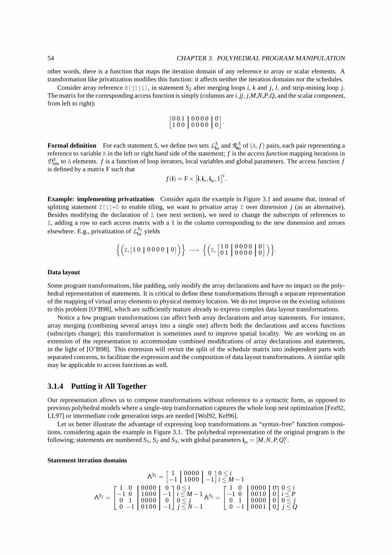
54 CHAPTER 3. POLYHEDRAL PROGRAM MANIPULATION
other words, there is a function that maps the iteration domain of any reference to array or scalar elements. Atransformation like privatization modifies this function:it affects neither the iteration domains nor the schedules.
Consider array referenceB[j][i], in statementS2 after merging loopsi, k and j, l , and strip-mining loopj.The matrix for the corresponding access function is simply (columns arei, jj , j,M,N,P,Q, and the scalar component,from left to right):
[
0 0 1 0 0 0 0 01 0 0 0 0 0 0 0
]
.
Formal definition For each statementS, we define two setsLShs andR S
hs of (A, f ) pairs, each pair representing areference to variableA in the left or right hand side of the statement;f is theaccess functionmapping iterations inDS
om to A elements.f is a function of loop iterators, local variables and global parameters. The access functionfis defined by a matrix F such that
f (i) = F×[
i, i lv, igp,1]t
.
Example: implementing privatization Consider again the example in Figure 3.1 and assume that, instead ofsplitting statementZ[i]=0 to enable tiling, we want to privatize arrayZ over dimensionj (as an alternative).Besides modifying the declaration ofZ (see next section), we need to change the subscripts of references toZ, adding a row to each access matrix with a 1 in the column corresponding to the new dimension and zeroeselsewhere. E.g., privatization ofL
S2hs yields
{(
Z, [1 0 0 0 0 0 0])}
−→{(
Z,[
1 0 0 0 0 0 00 1 0 0 0 0 0
])}
.
Data layout
Some program transformations, like padding, only modify the array declarations and have no impact on the poly-hedral representation of statements. It is critical to define these transformations through a separate representationof the mapping of virtual array elements to physical memory location. We do not improve on the existing solutionsto this problem [O’B98], which are sufficiently mature already to express complex data layout transformations.
Notice a few program transformations can affect both array declarations and array statements. For instance,array merging (combining several arrays into a single one) affects both the declarations and access functions(subscripts change); this transformation is sometimes used to improve spatial locality. We are working on anextension of the representation to accommodate combined modifications of array declarations and statements,in the light of [O’B98]. This extension will revisit the split of the schedule matrix into independent parts withseparated concerns, to facilitate the expression and the composition of data layout transformations. A similar splitmay be applicable to access functions as well.
3.1.4 Putting it All Together
Our representation allows us to compose transformations without reference to a syntactic form, as opposed toprevious polyhedral models where a single-step transformation captures the whole loop nest optimization [Fea92,LL97] or intermediate code generation steps are needed [Wol92, Kel96].
Let us better illustrate the advantage of expressing loop transformations as “syntax-free” function composi-tions, considering again the example in Figure 3.1. The polyhedral representation of the original program is thefollowing; statements are numberedS1, S2 andS3, with global parametersigp = [M,N,P,Q]t .
Statement iteration domains
ΛS1 =[
1 0000 0−1 1000 −1
]
0≤ ii ≤M−1
ΛS2 =
1 0 0000 0−1 0 1000 −10 1 0000 00 −1 0100 −1
0≤ ii ≤M−10≤ jj ≤ N−1
ΛS3 =
1 0 0000 0−1 0 0010 00 1 0000 00 −1 0001 0
0≤ ii ≤ P0≤ jj ≤Q
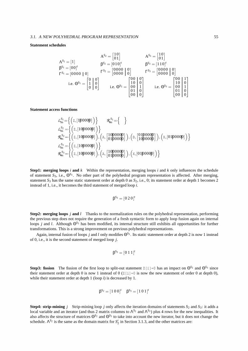
3.1. A NEW POLYHEDRAL PROGRAM REPRESENTATION 55
Statement schedules
AS1 = [1]
βS1 = [00]t
ΓS1 = [0000 0]
i.e. ΘS1 =
[
0 01 00 0
]
AS2 =[
1001
]
βS2 = [010]t
ΓS2 =[
0000 00000 0
]
i.e. ΘS2 =
00 010 000 101 000 0
AS3 =[
1001
]
βS3 = [110]t
ΓS3 =[
0000 00000 0
]
i.e. ΘS3 =
00 110 000 101 000 0
Statement access functions
LS1hs=
{(
Z, [100000])}
RS1
hs ={ }
LS2hs =
{(
Z, [1000000])}
RS2
hs ={(
Z, [1000000])
,(
A,[
10000000100000
])
,(
B,[
01000001000000
])
,(
X, [0100000])}
LS3hs =
{(
Z, [1000000])}
RS3
hs ={(
Z, [1000000])
,(
A,[
10000000100000
])
,(
X, [0100000])}
Step1: merging loopsi and k Within the representation, merging loopsi andk only influences the scheduleof statementS3, i.e., ΘS3. No other part of the polyhedral program representation is affected. After merging,statementS3 has the same static statement order at depth 0 asS2, i.e., 0; its statement order at depth 1 becomes 2instead of 1, i.e., it becomes the third statement of merged loopi.
βS3 = [0 2 0]t
Step2: merging loopsj and l Thanks to the normalization rules on the polyhedral representation, performingthe previous step does not require the generation of a fresh syntactic form to apply loop fusion again on internalloops j and l . AlthoughΘS3 has been modified, its internal structure still exhibits allopportunities for furthertransformations. This is a strong improvement on previous polyhedral representations.
Again, internal fusion of loopsj andl only modifiesΘS3. Its static statement order at depth 2 is now 1 insteadof 0, i.e., it is the second statement of merged loopj.
βS3 = [0 1 1]t
Step3: fission The fission of the first loop to split-out statementZ[i]=0 has an impact onΘS2 andΘS3 sincetheir statement order at depth 0 is now 1 instead of 0 (Z[i]=0 is now the new statement of order 0 at depth 0),while their statement order at depth 1 (loopi) is decreased by 1.
βS2 = [1 0 0]t βS3 = [1 0 1]t
Step4: strip-mining j Strip-mining loopj only affects the iteration domains of statementsS2 andS3: it adds alocal variable and an iterator (and thus 2 matrix columns toΛS2 andΛS3) plus 4 rows for the new inequalities. Italso affects the structure of matricesΘS2 andΘS3 to take into account the new iterator, but it does not change theschedule.ΛS2 is the same as the domain matrix forS′2 in Section 3.1.3, and the other matrices are:
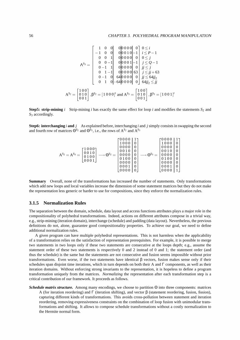
56 CHAPTER 3. POLYHEDRAL PROGRAM MANIPULATION
ΛS3 =
1 0 0 0 0 0 0 0 0−1 0 0 0 0 0 1 0−1
0 0 1 0 0 0 0 0 00 0−1 0 0 0 0 1−10−1 1 0 0 0 0 0 00 1−1 0 0 0 0 0 630−1 0 640 0 0 0 00 1 0−640 0 0 0 0
0≤ ii ≤ P−10≤ jj ≤Q−1jj ≤ jj ≤ jj +63jj ≤ 64jj264jj2 ≤ jj
AS2 =
[
1 0 00 1 00 0 1
]
,βS2 = [1 0 0 0]t and AS3 =
[
1 0 00 1 00 0 1
]
,βS3 = [1 0 0 1]t
Step5: strip-mining i Strip-miningi has exactly the same effect for loopi and modifies the statementsS2 andS3 accordingly.
Step6: interchangingi and j As explained before, interchangingi and j simply consists in swapping the secondand fourth row of matricesΘS2 andΘS3, i.e., the rows of AS2 and AS3
AS2 = AS3 =
1 0 0 00 0 1 00 1 0 00 0 0 1
−→ΘS2 =
0 0 0 0 11 0 0 0 00 0 0 0 00 0 1 0 00 0 0 0 00 1 0 0 00 0 0 0 00 0 0 1 00 0 0 0 0
−→ΘS3 =
0 0 0 0 11 0 0 0 00 0 0 0 00 0 1 0 00 0 0 0 00 1 0 0 00 0 0 0 00 0 0 1 00 0 0 0 1
Summary Overall, none of the transformations has increased the number of statements. Only transformationswhich add new loops and local variables increase the dimension of some statement matrices but they do not makethe representation less generic or harder to use for compositions, since they enforce the normalization rules.
3.1.5 Normalization Rules
The separation between the domain, schedule, data layout and access functions attributes plays a major role in thecompositionality of polyhedral transformations. Indeed,actions on different attributes compose in a trivial way,e.g., strip-mining (iteration domain), interchange (schedule) and padding (data layout). Nevertheless, the previousdefinitions do not, alone, guarantee good compositionalityproperties. To achieve our goal, we need to defineadditional normalization rules.
A given program can have multiple polyhedral representations. This is not harmless when the applicabilityof a transformation relies on the satisfaction of representation prerequisites. For example, it is possible to mergetwo statements in two loops only if these two statements are consecutive at the loops depth; e.g., assume thestatement order of these two statements is respectively 0 and 2 instead of 0 and 1; the statement order (andthus the schedule) is the same but the statements are not consecutive and fusion seems impossible without priortransformations. Even worse, if the two statements have identical β vectors, fusion makes sense only if theirschedules span disjoint time iterations, which in turn depends on both their A andΓ components, as well as theiriteration domains. Without enforcing strong invariants tothe representation, it is hopeless to define a programtransformation uniquely from the matrices.Normalizingthe representation after each transformation step is acritical contribution of our framework. It proceeds as follows.
Schedule matrix structure. Among many encodings, we choose to partitionΘ into three components: matricesA (for iteration reordering) andΓ (iteration shifting), and vectorβ (statement reordering, fusion, fission),capturing different kinds of transformations. This avoidscross-pollution between statement and iterationreordering, removing expressiveness constraints on the combination of loop fusion with unimodular trans-formations and shifting. It allows to compose schedule transformations without a costly normalization tothe Hermite normal form.
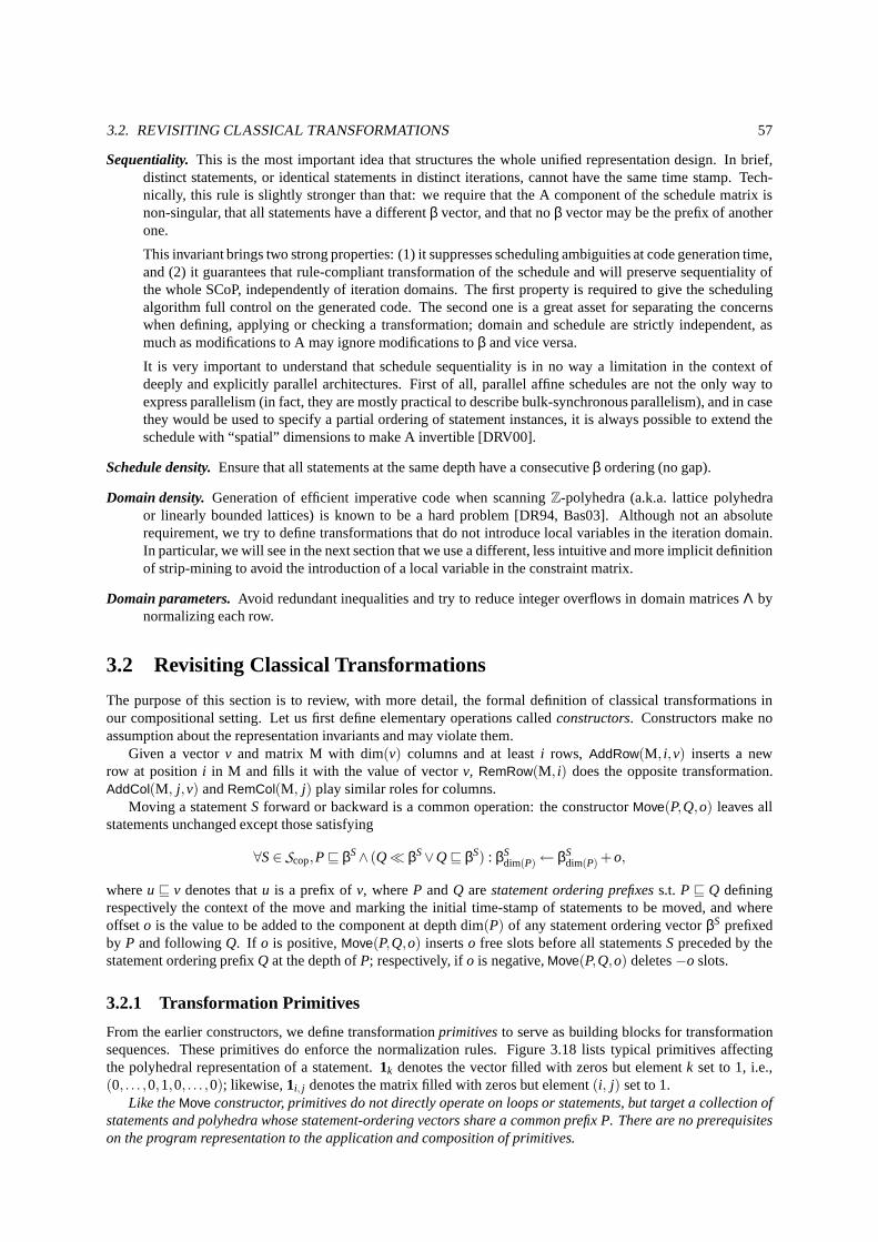
3.2. REVISITING CLASSICAL TRANSFORMATIONS 57
Sequentiality. This is the most important idea that structures the whole unified representation design. In brief,distinct statements, or identical statements in distinct iterations, cannot have the same time stamp. Tech-nically, this rule is slightly stronger than that: we require that the A component of the schedule matrix isnon-singular, that all statements have a differentβ vector, and that noβ vector may be the prefix of anotherone.
This invariant brings two strong properties: (1) it suppresses scheduling ambiguities at code generation time,and (2) it guarantees that rule-compliant transformation of the schedule and will preserve sequentiality ofthe whole SCoP, independently of iteration domains. The first property is required to give the schedulingalgorithm full control on the generated code. The second oneis a great asset for separating the concernswhen defining, applying or checking a transformation; domain and schedule are strictly independent, asmuch as modifications to A may ignore modifications toβ and vice versa.
It is very important to understand that schedule sequentiality is in no way a limitation in the context ofdeeply and explicitly parallel architectures. First of all, parallel affine schedules are not the only way toexpress parallelism (in fact, they are mostly practical to describe bulk-synchronous parallelism), and in casethey would be used to specify a partial ordering of statementinstances, it is always possible to extend theschedule with “spatial” dimensions to make A invertible [DRV00].
Schedule density. Ensure that all statements at the same depth have a consecutiveβ ordering (no gap).
Domain density. Generation of efficient imperative code when scanningZ-polyhedra (a.k.a. lattice polyhedraor linearly bounded lattices) is known to be a hard problem [DR94, Bas03]. Although not an absoluterequirement, we try to define transformations that do not introduce local variables in the iteration domain.In particular, we will see in the next section that we use a different, less intuitive and more implicit definitionof strip-mining to avoid the introduction of a local variable in the constraint matrix.
Domain parameters. Avoid redundant inequalities and try to reduce integer overflows in domain matricesΛ bynormalizing each row.
3.2 Revisiting Classical Transformations
The purpose of this section is to review, with more detail, the formal definition of classical transformations inour compositional setting. Let us first define elementary operations calledconstructors. Constructors make noassumption about the representation invariants and may violate them.
Given a vectorv and matrix M with dim(v) columns and at leasti rows, AddRow(M, i,v) inserts a newrow at positioni in M and fills it with the value of vectorv, RemRow(M, i) does the opposite transformation.AddCol(M, j,v) andRemCol(M, j) play similar roles for columns.
Moving a statementS forward or backward is a common operation: the constructorMove(P,Q,o) leaves allstatements unchanged except those satisfying
∀S∈ Scop,P⊑ βS∧ (Q≪ βS∨Q⊑ βS) : βSdim(P)← βS
dim(P) +o,
whereu⊑ v denotes thatu is a prefix ofv, whereP andQ arestatement ordering prefixess.t. P⊑ Q definingrespectively the context of the move and marking the initialtime-stamp of statements to be moved, and whereoffseto is the value to be added to the component at depth dim(P) of any statement ordering vectorβS prefixedby P and followingQ. If o is positive,Move(P,Q,o) insertso free slots before all statementsS preceded by thestatement ordering prefixQ at the depth ofP; respectively, ifo is negative,Move(P,Q,o) deletes−o slots.
3.2.1 Transformation Primitives
From the earlier constructors, we define transformationprimitivesto serve as building blocks for transformationsequences. These primitives do enforce the normalization rules. Figure 3.18 lists typical primitives affectingthe polyhedral representation of a statement.1k denotes the vector filled with zeros but elementk set to 1, i.e.,(0, . . . ,0,1,0, . . . ,0); likewise,1i, j denotes the matrix filled with zeros but element(i, j) set to 1.
Like theMove constructor, primitives do not directly operate on loops orstatements, but target a collection ofstatements and polyhedra whose statement-ordering vectors share a common prefix P. There are no prerequisiteson the program representation to the application and composition of primitives.
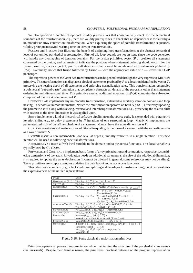
58 CHAPTER 3. POLYHEDRAL PROGRAM MANIPULATION
We also specified a number of optionalvalidity prerequisitesthat conservatively check for the semanticalsoundness of the transformation, e.g., there are validity prerequisites to check that no dependence is violated by aunimodular or array contraction transformation. When exploring the space of possible transformation sequences,validity prerequisites avoid wasting time on corrupt transformations.
FUSION and FISSION best illustrate the benefit of designing loop transformations at the abstract semanticallevel of our unified polyhedral representation. First of all, loop bounds are not an issue since the code generatorwill handle any overlapping of iteration domains. For the fission primitive, vector(P,o) prefixes all statementsconcerned by the fission; and parameterb indicates the position where statement delaying should occur. For thefusion primitive, vector(P,o+ 1) prefixes all statements that should be interleaved with statements prefixed by(P,o). Eventually, notice that fusion followed by fission — with the appropriate value ofb — leaves the SCoPunchanged.
The expressive power of the latter two transformations can be generalized through the very expressive MOTION
primitive. This transformation can displace a block of statements prefixed byP to a location identified by vectorT,preserving the nesting depth of all statements and enforcing normalization rules. This transformation ressemblesa polyhedral “cut-and-paste” operation that completely abstracts all details of the programs other than statementordering in multidimensional time. This primitive uses an additional notation: pfx(V,d) computes the sub-vectorcomposed of the firstd components ofV.
UNIMODULAR implements any unimodular transformation, extended to arbitrary iteration domains and loopnesting. U denotes a unimodular matrix. Notice the multiplication operates on both AandΓ, effectively updatingthe parametric shift along with skewing, reversal and interchange transformations, i.e., preserving the relative shiftwith respect to the time dimensions it was applied upon.
SHIFT implements a kind of hierarchical software pipelining on the source code. It is extended with parametriciteration shifts, e.g., to delay a statement byN iterations of one surrounding loop. Matrix M implements theparameterized shift of the affine schedule of a statement. M must have the same dimension asΓ.
CUTDOM constrains a domain with an additional inequality, in the form of a vectorc with the same dimensionas a row of matrixΛ.
EXTEND inserts a new intermediate loop level at depthℓ, initially restricted to a single iteration. This newiterator will be used in following code transformations.
ADDLOCALVAR insert a fresh local variable to the domain and to the access functions. This local variable istypically used by CUTDOM.
PRIVATIZE and CONTRACT implement basic forms of array privatization and contraction, respectively, consid-ering dimensionℓ of the array. Privatization needs an additional parameters, the size of the additional dimension;s is required to update the array declaration (it cannot be inferred in general, some references may not be affine).These primitives are simple examples updating the data layout and array access functions.
This table is not complete (e.g., it lacks index-set splitting and data-layout transformations), but it demonstratesthe expressiveness of the unified representation.
Syntax Effect
UNIMODULAR (P,U) ∀S∈ Scop | P⊑ βS,AS← U.AS; ΓS← U.ΓS
SHIFT(P,M) ∀S∈ Scop | P⊑ βS,ΓS← ΓS+MCUTDOM(P,c) ∀S∈ Scop | P⊑ βS,ΛS← AddRow
(
ΛS,0,c/gcd(c1, . . . ,cdS+dSlv +dgp+1)
)
EXTEND(P,ℓ,c) ∀S∈ Scop | P⊑ βS,
dS← dS+1; ΛS← AddCol(ΛS,c,0);βS← AddRow(βS,ℓ,0);AS← AddRow(AddCol(AS,c,0),ℓ,1ℓ);ΓS← AddRow(ΓS,ℓ,0);∀(A,F) ∈ LS
hs∪R Shs,F← AddRow(F,ℓ,0)
ADDLOCALVAR (P) ∀S∈ Scop | P⊑ βS,dSlv ← dS
lv +1; ΛS← AddCol(ΛS,dS+1,0);∀(A,F) ∈ LS
hs∪R Shs,F← AddCol(F,dS+1,0)
PRIVATIZE (A,ℓ) ∀S∈ Scop,∀(A,F) ∈ LShs∪R S
hs,F← AddRow(F,ℓ,1ℓ)CONTRACT(A,ℓ) ∀S∈ Scop,∀(A,F) ∈ LS
hs∪R Shs,F← RemRow(F,ℓ)
FUSION(P,o) b = max{βSdim(P)+1 | (P,o)⊑ βS}+1
Move((P,o+1),(P,o+1),b); Move(P,(P,o+1),−1)FISSION(P,o,b) Move(P,(P,o,b),1); Move((P,o+1),(P,o+1),−b)MOTION(P,T) if dim(P)+1= dim(T) thenb = max{βS
dim(P) | P⊑ βS}+1 elseb = 1Move(pfx(T,dim(T)−1),T,b)∀S∈ Scop | P⊑ βS,βS← βS+T−pfx(P,dim(T))Move(P,P,−1)
Figure 3.18: Some classical transformation primitives
Primitives operate on program representation while maintaining the structure of the polyhedral components(the invariants). Despite their familiar names, the primitives’ practical outcome on the program representation
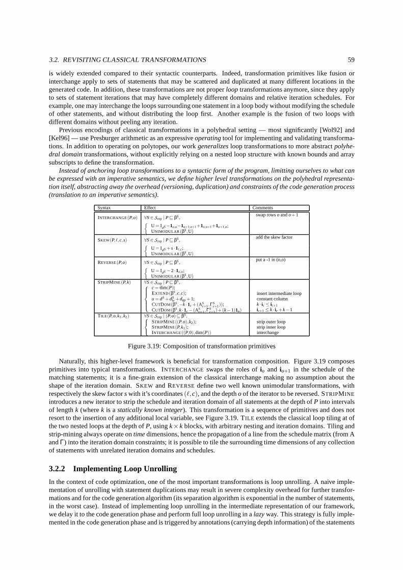
3.2. REVISITING CLASSICAL TRANSFORMATIONS 59
is widely extended compared to their syntactic counterparts. Indeed, transformation primitives like fusion orinterchange apply to sets of statements that may be scattered and duplicated at many different locations in thegenerated code. In addition, these transformations are notproperloop transformations anymore, since they applyto sets of statement iterations that may have completely different domains and relative iteration schedules. Forexample, one may interchange the loops surrounding one statement in a loop body without modifying the scheduleof other statements, and without distributing the loop first. Another example is the fusion of two loops withdifferent domains without peeling any iteration.
Previous encodings of classical transformations in a polyhedral setting — most significantly [Wol92] and[Kel96] — use Presburger arithmetic as an expressiveoperatingtool for implementing and validating transforma-tions. In addition to operating on polytopes, our workgeneralizesloop transformations to more abstractpolyhe-dral domaintransformations, without explicitly relying on a nested loop structure with known bounds and arraysubscripts to define the transformation.
Instead of anchoring loop transformations to a syntactic form of the program, limitting ourselves to what canbe expressed with an imperative semantics, we define higher level transformations on the polyhedral representa-tion itself, abstracting away the overhead (versioning, duplication) and constraints of the code generation process(translation to an imperative semantics).
Syntax Effect Comments
INTERCHANGE(P,o) ∀S∈ Scop | P⊑ βS,swap rowso ando+1
{
U = IdS−1o,o−1o+1,o+1+1o,o+1+1o+1,o;UNIMODULAR (βS,U)
SKEW(P,ℓ,c,s) ∀S∈ Scop | P⊑ βS,add the skew factor
{
U = IdS +s·1ℓ,c;UNIMODULAR (βS,U)
REVERSE(P,o) ∀S∈ Scop | P⊑ βS,put a -1 in (o,o)
{
U = IdS−2·1o,o;UNIMODULAR (βS,U)
STRIPM INE (P,k) ∀S∈ Scop | P⊑ βS,
c = dim(P);EXTEND(βS,c,c);u = dS+dS
lv +dgp+1;CUTDOM(βS,−k ·1c +(AS
c+1,ΓSc+1));
CUTDOM(βS,k ·1c− (ASc+1,Γ
Sc+1)+(k−1)1u)
insert intermediate loopconstant columnk · ic ≤ ic+1ic+1 ≤ k · ic +k−1
TILE (P,o,k1,k2) ∀S∈ Scop | (P,o)⊑ βS,
STRIPM INE((P,o),k2);STRIPM INE(P,k1);INTERCHANGE((P,0),dim(P))
strip outer loopstrip inner loopinterchange
Figure 3.19: Composition of transformation primitives
Naturally, this higher-level framework is beneficial for transformation composition. Figure 3.19 composesprimitives into typical transformations. INTERCHANGE swaps the roles ofio and io+1 in the schedule of thematching statements; it is a fine-grain extension of the classical interchange making no assumption about theshape of the iteration domain. SKEW and REVERSE define two well known unimodular transformations, withrespectively the skew factorswith it’s coordinates(ℓ,c), and the deptho of the iterator to be reversed. STRIPM INE
introduces a new iterator to strip the schedule and iteration domain of all statements at the depth ofP into intervalsof lengthk (wherek is astatically known integer). This transformation is a sequence of primitives and does notresort to the insertion of any additional local variable, see Figure 3.19. TILE extends the classical loop tiling at ofthe two nested loops at the depth ofP, usingk×k blocks, with arbitrary nesting and iteration domains. Tiling andstrip-mining always operate ontimedimensions, hence the propagation of a line from the schedule matrix (from AandΓ) into the iteration domain constraints; it is possible to tile the surrounding time dimensions of any collectionof statements with unrelated iteration domains and schedules.
3.2.2 Implementing Loop Unrolling
In the context of code optimization, one of the most important transformations is loop unrolling. A naive imple-mentation of unrolling with statement duplications may result in severe complexity overhead for further transfor-mations and for the code generation algorithm (its separation algorithm is exponential in the number of statements,in the worst case). Instead of implementing loop unrolling in the intermediate representation of our framework,we delay it to the code generation phase and perform full loopunrolling in alazyway. This strategy is fully imple-mented in the code generation phase and is triggered by annotations (carrying depth information) of the statements
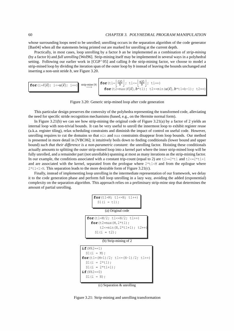
60 CHAPTER 3. POLYHEDRAL PROGRAM MANIPULATION
whose surrounding loops need to be unrolled; unrolling occurs in the separation algorithm of the code generator[Bas04] when all the statements being printed out are markedfor unrolling at the current depth.
Practically, in most cases, loop unrolling by a factorb an be implemented as a combination ofstrip-mining(by a factorb) andfull unrolling [Wol96]. Strip-mining itself may be implemented in severalways in a polyhedralsetting. Following our earlier work in [CGP+05] and callingb the strip-mining factor, we choose to model astrip-mined loop by dividing the iteration span of the outerloop byb instead of leaving the bounds unchanged andinserting a non-unit strideb, see Figure 3.20.
for(i=ℓ(~x); i<=u(~x); i++) strip-mine(b)−→
for(t1=⌊
ℓ(~x)b
⌋
; t1<=⌊
u(~x)b
⌋
; t1++)
for(t2=max(ℓ(~x),b*t1); t2<=min(u(~x),b*t1+b-1); t2++)
Figure 3.20: Generic strip-mined loop after code generation
This particular design preserves the convexity of the polyhedra representing the transformed code, alleviatingthe need for specific stride recognition mechanisms (based,e.g., on the Hermite normal form).
In Figure 3.21(b) we can see how strip-mining the original code of Figure 3.21(a) by a factor of 2 yields aninternal loop with non-trivial bounds. It can be very usefulto unroll the innermost loop to exhibit register reuse(a.k.a. register tiling), relax scheduling constraints and diminish the impact of control on useful code. However,unrolling requires to cut the domains so thatmin andmax constraints disappear from loop bounds. Our methodis presented in more detail in [VBC06]; it intuitively boilsdown to finding conditionals (lower bound and upperbound)such that their difference is a non-parametric constant: the unrolling factor. Hoisting these conditionalsactually amounts to splitting the outer strip-mined loop into a kernel part where the inner strip-mined loop will befully unrolled, and a remainder part (not unrollable) spanning at most as many iterations as the strip-mining factor.In our example, the conditions associated with a constant trip-count (equal to 2) aret2>=2*t1 andt2<=2*t1+1and are associated with the kernel, separated from the prologue where2*t1<M and from the epilogue where2*t1+1>N. This separation leads to the more desirable form of Figure 3.21(c).
Finally, instead of implementing loop unrolling in the intermediate representation of our framework, we delayit to the code generation phase and perform full loop unrolling in a lazy way, avoiding the added (exponential)complexity on the separation algorithm. This approach relies on a preliminary strip-mine step that determines theamount of partial unrolling.
for(t1=M; t1<=N; t1++)S1(i = t1);
(a) Original code
for(t1=M/2; t1<=N/2; t1++)for(t2=max(M,2*t1);
t2<=min(N,2*t1+1); t2++)S1(i = t2);
(b) Strip-mining of 2
if(M%2==1)S1(i = M);
for(t1=(M+1)/2; t1<=(N-1)/2; t1++)S1(i = 2*t1);S1(i = 2*t1+1);
if(N%2==0)S1(i = N);
(c) Separation & unrolling
Figure 3.21: Strip-mining and unrolling transformation
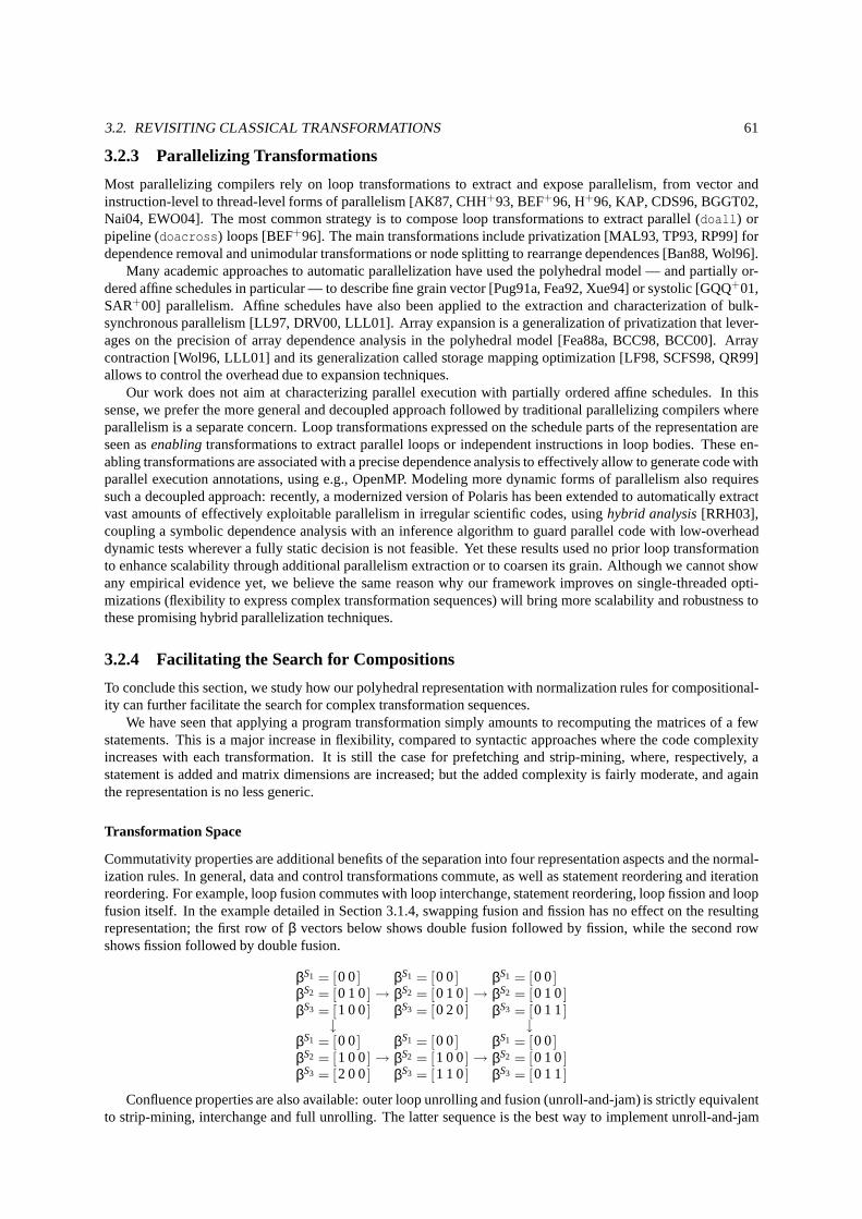
3.2. REVISITING CLASSICAL TRANSFORMATIONS 61
3.2.3 Parallelizing Transformations
Most parallelizing compilers rely on loop transformationsto extract and expose parallelism, from vector andinstruction-level to thread-level forms of parallelism [AK87, CHH+93, BEF+96, H+96, KAP, CDS96, BGGT02,Nai04, EWO04]. The most common strategy is to compose loop transformations to extract parallel (doall) orpipeline (doacross) loops [BEF+96]. The main transformations include privatization [MAL93, TP93, RP99] fordependence removal and unimodular transformations or nodesplitting to rearrange dependences [Ban88, Wol96].
Many academic approaches to automatic parallelization have used the polyhedral model — and partially or-dered affine schedules in particular — to describe fine grain vector [Pug91a, Fea92, Xue94] or systolic [GQQ+01,SAR+00] parallelism. Affine schedules have also been applied to the extraction and characterization of bulk-synchronous parallelism [LL97, DRV00, LLL01]. Array expansion is a generalization of privatization that lever-ages on the precision of array dependence analysis in the polyhedral model [Fea88a, BCC98, BCC00]. Arraycontraction [Wol96, LLL01] and its generalization called storage mapping optimization [LF98, SCFS98, QR99]allows to control the overhead due to expansion techniques.
Our work does not aim at characterizing parallel execution with partially ordered affine schedules. In thissense, we prefer the more general and decoupled approach followed by traditional parallelizing compilers whereparallelism is a separate concern. Loop transformations expressed on the schedule parts of the representation areseen asenablingtransformations to extract parallel loops or independent instructions in loop bodies. These en-abling transformations are associated with a precise dependence analysis to effectively allow to generate code withparallel execution annotations, using e.g., OpenMP. Modeling more dynamic forms of parallelism also requiressuch a decoupled approach: recently, a modernized version of Polaris has been extended to automatically extractvast amounts of effectively exploitable parallelism in irregular scientific codes, usinghybrid analysis[RRH03],coupling a symbolic dependence analysis with an inference algorithm to guard parallel code with low-overheaddynamic tests wherever a fully static decision is not feasible. Yet these results used no prior loop transformationto enhance scalability through additional parallelism extraction or to coarsen its grain. Although we cannot showany empirical evidence yet, we believe the same reason why our framework improves on single-threaded opti-mizations (flexibility to express complex transformation sequences) will bring more scalability and robustness tothese promising hybrid parallelization techniques.
3.2.4 Facilitating the Search for Compositions
To conclude this section, we study how our polyhedral representation with normalization rules for compositional-ity can further facilitate the search for complex transformation sequences.
We have seen that applying a program transformation simply amounts to recomputing the matrices of a fewstatements. This is a major increase in flexibility, compared to syntactic approaches where the code complexityincreases with each transformation. It is still the case forprefetching and strip-mining, where, respectively, astatement is added and matrix dimensions are increased; butthe added complexity is fairly moderate, and againthe representation is no less generic.
Transformation Space
Commutativity properties are additional benefits of the separation into four representation aspects and the normal-ization rules. In general, data and control transformations commute, as well as statement reordering and iterationreordering. For example, loop fusion commutes with loop interchange, statement reordering, loop fission and loopfusion itself. In the example detailed in Section 3.1.4, swapping fusion and fission has no effect on the resultingrepresentation; the first row ofβ vectors below shows double fusion followed by fission, whilethe second rowshows fission followed by double fusion.
βS1 = [0 0]βS2 = [0 1 0]βS3 = [1 0 0]
→βS1 = [0 0]βS2 = [0 1 0]βS3 = [0 2 0]
→βS1 = [0 0]βS2 = [0 1 0]βS3 = [0 1 1]
↓ ↓βS1 = [0 0]βS2 = [1 0 0]βS3 = [2 0 0]
→βS1 = [0 0]βS2 = [1 0 0]βS3 = [1 1 0]
→βS1 = [0 0]βS2 = [0 1 0]βS3 = [0 1 1]
Confluence properties are also available: outer loop unrolling and fusion (unroll-and-jam) is strictly equivalentto strip-mining, interchange and full unrolling. The latter sequence is the best way to implement unroll-and-jam
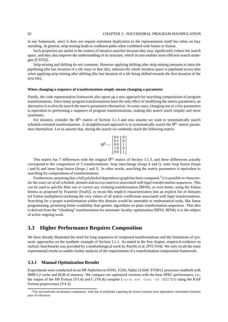
62 CHAPTER 3. POLYHEDRAL PROGRAM MANIPULATION
in our framework, since it does not require statement duplication in the representation itself but relies on lazyunrolling. In general, strip-mining leads to confluent paths when combined with fusion or fission.
Such properties are useful in the context of iterative searches because they may significantly reduce the searchspace, and they also improve the understanding of its structure, which in turn enables more efficient search strate-gies [CST02].
Strip-mining and shifting donot commute. However applying shifting after strip-mining amounts to intra-tilepipelining (the last iteration of a tile stays in that tile),whereas the whole iteration space is pipelined across tileswhen applying strip-mining after shifting (the last iteration of a tile being shifted towards the first iteration of thenext tile).
When changing a sequence of transformations simply means changing a parameter
Finally, the code representation framework also opens up a new approach for searching compositions of programtransformations. Since many program transformations havethe only effect of modifying the matrix parameters, analternative is todirectly search the matrix parameters themselves. In some cases, changing one or a few parametersis equivalent to performing a sequence of program transformations, making this search much simpler and moresystematic.
For instance, consider theΘS3 matrix of Section 3.1.3 and now assume we want to systematically searchschedule-oriented transformations. A straightforward approach is to systematically search theΘS3 matrix param-eters themselves. Let us assume that, during the search we randomly reach the following matrix:
ΘS′3 =
0 0 00 1 00 0 11 0 00 0 1
This matrix has 7 differences with the originalΘS3 matrix of Section 3.1.3, and these differences actuallycorrespond to the composition of 3 transformations: loop interchange (loopsk and l ), outer loop fusion (loopsi andk) and inner loop fusion (loopsj and l ). In other words, searching the matrix parameters is equivalent tosearching for compositions of transformations.
Furthermore, assuming that a full polyhedral dependence graph has been computed,3 it is possible to character-ize theexact set of all schedule, domain and access matrices associated with legal transformation sequences. Thiscan be used to quickly filter out or correct any violating transformation [BF04], or even better, using the Farkaslemma as proposed by Feautrier [Fea92], to recast this implicit characterization into an explicit list of domains(of Farkas multipliers) enclosing the very values of all matrix coefficients associated with legal transformations.Searching for a proper transformation within this domain would be amenable to mathematical tools, like linearprogramming, promising better scalability than genetic algorithms on plain transformation sequences. This ideais derived from the “chunking” transformation for automatic locality optimization [BF03, BF04]; it is the subjectof active ongoing work.
3.3 Higher Performance Requires Composition
We have already illustrated the need for long sequences of composed transformations and the limitations of syn-tactic approaches on the synthetic example of Section 3.1.1. As stated in the first chapter, empirical evidence onrealistic benchmarks was provided by a methodological workby Parello et al. [PTCV04]. We only recall the mainexperimental results to enable further analysis of the requirements of a transformation composition framework.
3.3.1 Manual Optimization Results
Experiments were conducted on an HP AlphaServer ES45, 1GHz Alpha 21264C EV68 (1 processor enabled) with8MB L2 cache and 8GB of memory. We compare our optimized versions with thebaseSPEC performance, i.e.,the output of the HP Fortran (V5.4) and C (V6.4) compiler (-arch ev6 -fast -O5 ONESTEP) using the KAPFortran preprocessor (V4.3).
3Our tool performs on-demand computation, with lists of polyhedra capturing the (exact) instance-wise dependence information betweenpairs of references.
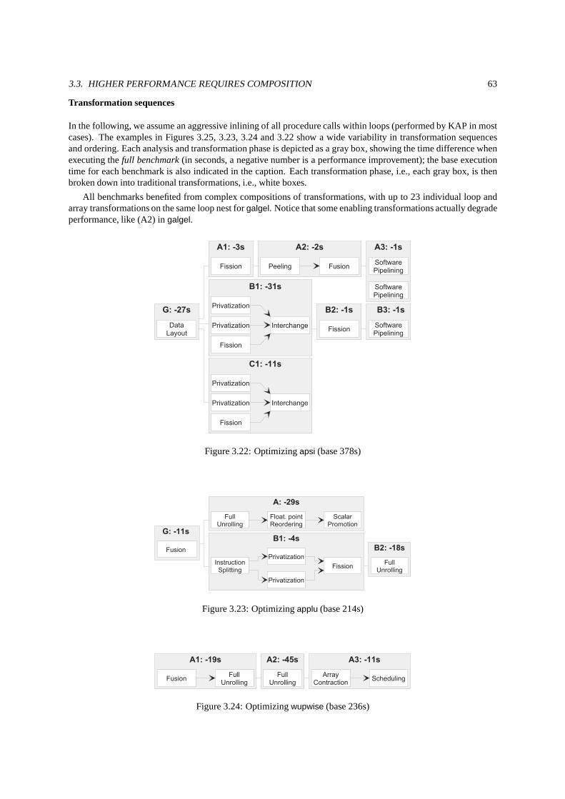
3.3. HIGHER PERFORMANCE REQUIRES COMPOSITION 63
Transformation sequences
In the following, we assume an aggressive inlining of all procedure calls within loops (performed by KAP in mostcases). The examples in Figures 3.25, 3.23, 3.24 and 3.22 show a wide variability in transformation sequencesand ordering. Each analysis and transformation phase is depicted as a gray box, showing the time difference whenexecuting thefull benchmark(in seconds, a negative number is a performance improvement); the base executiontime for each benchmark is also indicated in the caption. Each transformation phase, i.e., each gray box, is thenbroken down into traditional transformations, i.e., whiteboxes.
All benchmarks benefited from complex compositions of transformations, with up to 23 individual loop andarray transformations on the same loop nest forgalgel. Notice that some enabling transformations actually degradeperformance, like (A2) ingalgel.
B 1 : - 3 1 s
B 2 : - 1 s B 3 : - 1 s
C 1 : - 1 1 s
A 1 : - 3 s A 2 : - 2 s A 3 : - 1 s
G : - 2 7 s P r i v a t i z a t i o n
P r i v a t i z a t i o n
F i s s i o n
I n t e r c h a n g e S o f t w a r eP i p e l i n i n gF i s s i o n
P r i v a t i z a t i o n
P r i v a t i z a t i o n
F i s s i o n
I n t e r c h a n g e
F i s s i o n F u s i o nP e e l i n g
S o f t w a r eP i p e l i n i n g
S o f t w a r eP i p e l i n i n g
D a t aL a y o u t
Figure 3.22: Optimizingapsi (base 378s)
G : - 1 1 s
A : - 2 9 s
B 1 : - 4 sB 2 : - 1 8 s
F u l lU n r o l l i n g
S c a l a rP r o m o t i o n
F l o a t . p o i n tR e o r d e r i n g
I n s t r u c t i o nS p l i t t i n g F i s s i o n
P r i v a t i z a t i o nF u s i o n
F u l lU n r o l l i n g
P r i v a t i z a t i o n
Figure 3.23: Optimizingapplu (base 214s)
A 1 : - 1 9 s A 3 : - 1 1 sA 2 : - 4 5 sF u l l
U n r o l l i n gF u l l
U n r o l l i n gF u s i o n S c h e d u l i n gA r r a yC o n t r a c t i o n
Figure 3.24: Optimizingwupwise (base 236s)
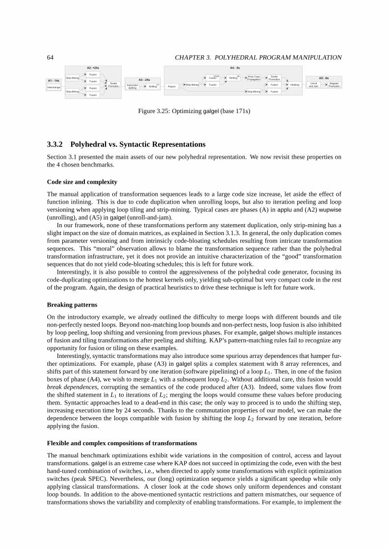
64 CHAPTER 3. POLYHEDRAL PROGRAM MANIPULATION
A 2 : + 2 4 s
A 1 : - 1 4 sA 5 : - 6 s
A 4 : - 5 s
A 3 : - 2 4 sF u s i o n
S c a l a rP r o m o t i o nI n t e r c h a n g e
S t r i p - M i n i n g
S t r i p - M i n i n gS h i f t i n gI n s t r u c t i o n
S p l i t i n g F i s s i o n S t r i p - M i n i n g
F i s s i o nF i s s i o nF u s i o n
F u s i o n
S h i f t i n g A r r a y C o p yP r o p a g a t i o n
S c a l a rP r o m o t i o nF u s i o n
F u s i o nS t r i p - M i n i n g
H o i s t i n g R e g i s t e rP r o m o t i o n
U n r o l la n d J a m
F u s i o n
F u s i o n
F u s i o n
L 1
L 1 - L 2 L 2
Figure 3.25: Optimizinggalgel (base 171s)
3.3.2 Polyhedral vs. Syntactic Representations
Section 3.1 presented the main assets of our new polyhedral representation. We now revisit these properties onthe 4 chosen benchmarks.
Code size and complexity
The manual application of transformation sequences leads to a large code size increase, let aside the effect offunction inlining. This is due to code duplication when unrolling loops, but also to iteration peeling and loopversioning when applying loop tiling and strip-mining. Typical cases are phases (A) inapplu and (A2)wupwise(unrolling), and (A5) ingalgel (unroll-and-jam).
In our framework, none of these transformations perform anystatement duplication, only strip-mining has aslight impact on the size of domain matrices, as explained inSection 3.1.3. In general, the only duplication comesfrom parameter versioning and from intrinsicly code-bloating schedules resulting from intricate transformationsequences. This “moral” observation allows to blame the transformation sequence rather than the polyhedraltransformation infrastructure, yet it does not provide an intuitive characterization of the “good” transformationsequences that do not yield code-bloating schedules; this is left for future work.
Interestingly, it is also possible to control the aggressiveness of the polyhedral code generator, focusing itscode-duplicating optimizations to the hottest kernels only, yielding sub-optimal but very compact code in the restof the program. Again, the design of practical heuristics todrive these technique is left for future work.
Breaking patterns
On the introductory example, we already outlined the difficulty to merge loops with different bounds and tilenon-perfectly nested loops. Beyond non-matching loop bounds and non-perfect nests, loop fusion is also inhibitedby loop peeling, loop shifting and versioning from previousphases. For example,galgel shows multiple instancesof fusion and tiling transformations after peeling and shifting. KAP’s pattern-matching rules fail to recognize anyopportunity for fusion or tiling on these examples.
Interestingly, syntactic transformations may also introduce some spurious array dependences that hamper fur-ther optimizations. For example, phase (A3) ingalgel splits a complex statement with 8 array references, andshifts part of this statement forward by one iteration (software pipelining) of a loopL1. Then, in one of the fusionboxes of phase (A4), we wish to mergeL1 with a subsequent loopL2. Without additional care, this fusion wouldbreak dependences, corrupting the semantics of the code produced after (A3). Indeed, some values flow fromthe shifted statement inL1 to iterations ofL2; merging the loops would consume these values before producingthem. Syntactic approaches lead to a dead-end in this case; the only way to proceed is to undo the shifting step,increasing execution time by 24 seconds. Thanks to the commutation properties of our model, we can make thedependence between the loops compatible with fusion by shifting the loopL2 forward by one iteration, beforeapplying the fusion.
Flexible and complex compositions of transformations
The manual benchmark optimizations exhibit wide variations in the composition of control, access and layouttransformations.galgel is an extreme case where KAP does not succeed in optimizing the code, even with the besthand-tuned combination of switches, i.e., when directed toapply some transformations with explicit optimizationswitches (peak SPEC). Nevertheless, our (long) optimization sequence yields a significant speedup while onlyapplying classical transformations. A closer look at the code shows only uniform dependences and constantloop bounds. In addition to the above-mentioned syntactic restrictions and pattern mismatches, our sequence oftransformations shows the variability and complexity of enabling transformations. For example, to implement the
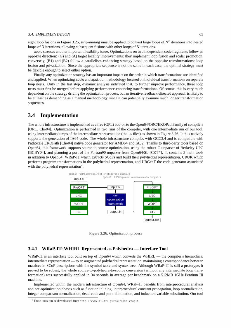
3.4. IMPLEMENTATION 65
eight loop fusions in Figure 3.25, strip-mining must be applied to convert large loops ofN2 iterations into nestedloops ofN iterations, allowing subsequent fusions with other loops of N iterations.
applu stresses another important flexibility issue. Optimizations on two independent code fragments follow anopposite direction: (G) and (A) target locality improvements: they implement loop fusion and scalar promotion;conversely, (B1) and (B2) follow a parallelism-enhancing strategy based on the opposite transformations: loopfission and privatization. Since the appropriate sequence is not the same in each case, the optimal strategy mustbe flexible enough to select either option.
Finally, any optimization strategy has an important impacton the order in which transformations are identifiedand applied. When optimizingapplu andapsi, our methodology focused on individual transformations onseparateloop nests. Only in the last step, dynamic analysis indicated that, to further improve performance, these loopnests must first be merged before applying performance-enhancing transformations. Of course, this is very muchdependent on the strategy driving the optimization process, but an iterative feedback-directed approach is likely tobe at least as demanding as a manual methodology, since it canpotentially examine much longer transformationsequences.
3.4 Implementation
The whole infrastructure is implemented as a free (GPL) add-on to the Open64/ORC/EKOPath family of compilers[ORC, Cho04]. Optimization is performed in two runs of the compiler, with one intermediate run of our tool,using intermediate dumps of the intermediate representation (the.N files) as shown in Figure 3.26. It thus nativelysupports the generation of IA64 code. The whole infrastructure compiles with GCC3.4 and is compatible withPathScale EKOPath [Cho04] native code generator for AMD64 and IA32. Thanks to third-party tools based onOpen64, this framework supports source-to-source optimization, using the robust C unparser of Berkeley UPC[BCBY04], and planning a port of the Fortran90 unparser fromOpen64/SL [CZT+]. It contains 3 main toolsin addition to Open64: WRaP-IT which extracts SCoPs and build their polyhedral representation, URUK whichperforms program transformations in the polyhedral representation, and URGenT the code generator associatedwith the polyhedral representation4.
input.c
PreOPT
LNO
WOPT
CG
PreOPT
LNO
WOPT
CG
output.bin
input.N
output.N
ouroptimisationframework
open64 -PHASE:p=on:l=off:w=off:c=off input.copen64 -PHASE:p=on:l=on:w=on:c=on output.N
Figure 3.26: Optimisation process
3.4.1 WRaP-IT: WHIRL Represented as Polyhedra — Interface Tool
WRaP-IT is an interface tool built on top of Open64 which converts the WHIRL — the compiler’s hierarchicalintermediate representation — to an augmented polyhedral representation, maintaining a correspondence betweenmatrices in SCoP descriptions with the symbol table and syntax tree. Although WRaP-IT is still a prototype, itproved to be robust; the whole source-to-polyhedra-to-source conversion (without any intermediate loop trans-formation) was successfully applied in 34 seconds in average per benchmark on a 512MB 1GHz Pentium IIImachine.
Implemented within the modern infrastructure of Open64, WRaP-IT benefits from interprocedural analysisand pre-optimization phases such as function inlining, interprocedural constant propagation, loop normalization,integer comparison normalization, dead-code andgoto elimination, and induction variable substitution. Our tool
4These tools can be downloaded fromhttp://www.lri.fr/~girbal/site_wrapit.
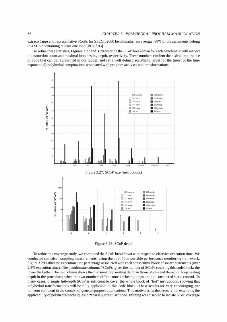
66 CHAPTER 3. POLYHEDRAL PROGRAM MANIPULATION
extracts large and representative SCoPs for SPECfp2000 benchmarks: on average, 88% of the statements belongto a SCoP containing at least one loop [BCG+03].
To refine these statistics, Figures 3.27 and 3.28 describe the SCoP breakdown for each benchmark with respectto instruction count and maximal loop nesting depth, respectively. These numbers confirm the lexical importanceof code that can be represented in our model, and set a well defined scalability target for the (most of the timeexponential) polyhedral computations associated with program analyses and transformations.
10
20
30
40
50
60
70
80
90
100
110
Num
ber
ofS
CoP
s
0-2 3-4 5-8 9-16 17-32 33-64 65-128 129-256 257+
168.wupwise
171.swim
172.mgrid
173.applu
177.mesa
179.art
183.equake
187.facerec
188.ammp
191.fma3d
200.sixtrack
301.apsi
Figure 3.27: SCoP size (instructions)
1
10
100
1000
Num
ber
ofS
CoP
s
1 2 3 4 5 6
168.wupwise
171.swim
172.mgrid
173.applu
177.mesa
179.art
183.equake
187.facerec
188.ammp
191.fma3d
200.sixtrack
301.apsi
Figure 3.28: SCoP depth
To refine this coverage study, we computed the SCoP breakdownwith respect to effective execution time. Weconducted statistical sampling measurements, using theoprofile portable performance monitoring framework.Figure 3.29 gather the execution time percentage associated with each consecutive block of source statements (over2.5% execution time). The penultimate column, #SCoPs, gives the number of SCoPs covering this code block: thelower the better. The last column shows the maximal loop nesting depth in those SCoPs and the actual loop nestingdepth in the procedure; when the two numbers differ, some enclosing loops are not considered static control. Inmany cases,a single full-depthSCoP is sufficient to cover the whole block of “hot” instructions, showing thatpolyhedral transformations will be fully applicable to this code block. These results are very encouraging, yetfar from sufficient in the context of general-purpose applications. This motivates further research in extending theapplicability of polyhedral techniques to “sparsely irregular” code. Inlining was disabled to isolate SCoP coverage
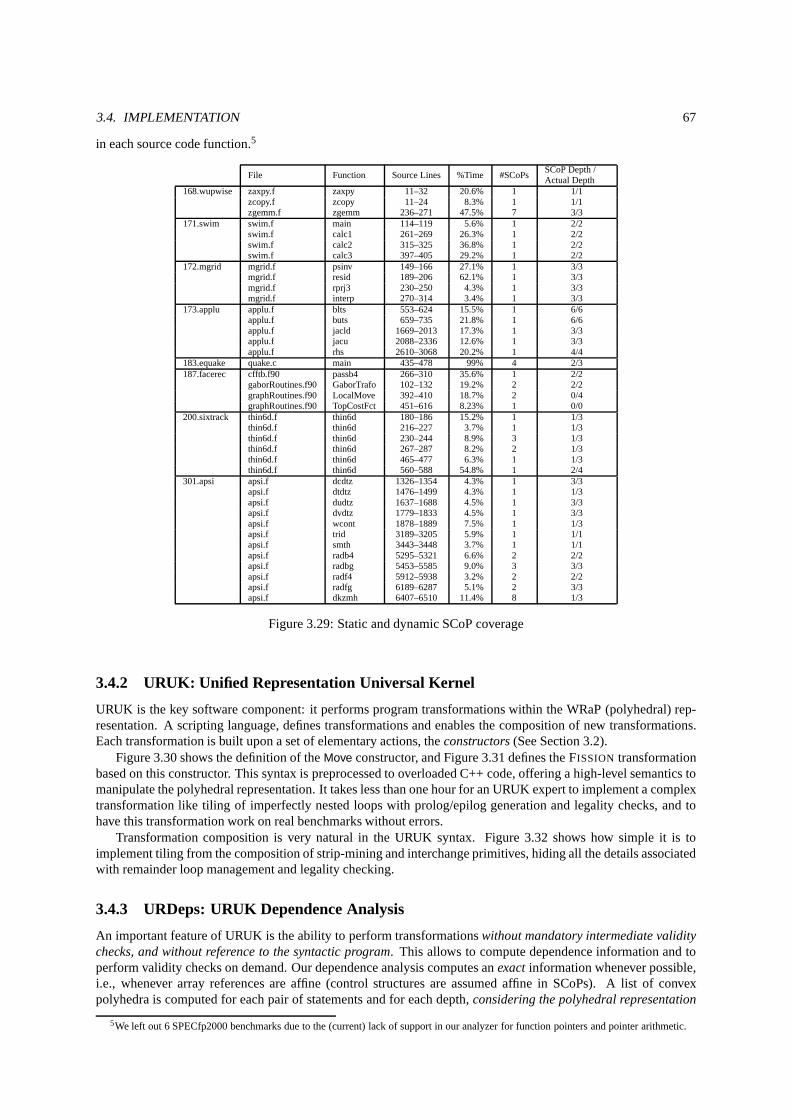
3.4. IMPLEMENTATION 67
in each source code function.5
File Function Source Lines %Time #SCoPsSCoP Depth /Actual Depth
168.wupwise zaxpy.f zaxpy 11–32 20.6% 1 1/1zcopy.f zcopy 11–24 8.3% 1 1/1zgemm.f zgemm 236–271 47.5% 7 3/3
171.swim swim.f main 114–119 5.6% 1 2/2swim.f calc1 261–269 26.3% 1 2/2swim.f calc2 315–325 36.8% 1 2/2swim.f calc3 397–405 29.2% 1 2/2
172.mgrid mgrid.f psinv 149–166 27.1% 1 3/3mgrid.f resid 189–206 62.1% 1 3/3mgrid.f rprj3 230–250 4.3% 1 3/3mgrid.f interp 270–314 3.4% 1 3/3
173.applu applu.f blts 553–624 15.5% 1 6/6applu.f buts 659–735 21.8% 1 6/6applu.f jacld 1669–2013 17.3% 1 3/3applu.f jacu 2088–2336 12.6% 1 3/3applu.f rhs 2610–3068 20.2% 1 4/4
183.equake quake.c main 435–478 99% 4 2/3187.facerec cfftb.f90 passb4 266–310 35.6% 1 2/2
gaborRoutines.f90 GaborTrafo 102–132 19.2% 2 2/2graphRoutines.f90 LocalMove 392–410 18.7% 2 0/4graphRoutines.f90 TopCostFct 451–616 8.23% 1 0/0
200.sixtrack thin6d.f thin6d 180–186 15.2% 1 1/3thin6d.f thin6d 216–227 3.7% 1 1/3thin6d.f thin6d 230–244 8.9% 3 1/3thin6d.f thin6d 267–287 8.2% 2 1/3thin6d.f thin6d 465–477 6.3% 1 1/3thin6d.f thin6d 560–588 54.8% 1 2/4
301.apsi apsi.f dcdtz 1326–1354 4.3% 1 3/3apsi.f dtdtz 1476–1499 4.3% 1 1/3apsi.f dudtz 1637–1688 4.5% 1 3/3apsi.f dvdtz 1779–1833 4.5% 1 3/3apsi.f wcont 1878–1889 7.5% 1 1/3apsi.f trid 3189–3205 5.9% 1 1/1apsi.f smth 3443–3448 3.7% 1 1/1apsi.f radb4 5295–5321 6.6% 2 2/2apsi.f radbg 5453–5585 9.0% 3 3/3apsi.f radf4 5912–5938 3.2% 2 2/2apsi.f radfg 6189–6287 5.1% 2 3/3apsi.f dkzmh 6407–6510 11.4% 8 1/3
Figure 3.29: Static and dynamic SCoP coverage
3.4.2 URUK: Unified Representation Universal Kernel
URUK is the key software component: it performs program transformations within the WRaP (polyhedral) rep-resentation. A scripting language, defines transformations and enables the composition of new transformations.Each transformation is built upon a set of elementary actions, theconstructors(See Section 3.2).
Figure 3.30 shows the definition of theMove constructor, and Figure 3.31 defines the FISSION transformationbased on this constructor. This syntax is preprocessed to overloaded C++ code, offering a high-level semantics tomanipulate the polyhedral representation. It takes less than one hour for an URUK expert to implement a complextransformation like tiling of imperfectly nested loops with prolog/epilog generation and legality checks, and tohave this transformation work on real benchmarks without errors.
Transformation composition is very natural in the URUK syntax. Figure 3.32 shows how simple it is toimplement tiling from the composition of strip-mining and interchange primitives, hiding all the details associatedwith remainder loop management and legality checking.
3.4.3 URDeps: URUK Dependence Analysis
An important feature of URUK is the ability to perform transformationswithout mandatory intermediate validitychecks, and without reference to the syntactic program. This allows to compute dependence information and toperform validity checks on demand. Our dependence analysiscomputes anexactinformation whenever possible,i.e., whenever array references are affine (control structures are assumed affine in SCoPs). A list of convexpolyhedra is computed for each pair of statements and for each depth,considering the polyhedral representation
5We left out 6 SPECfp2000 benchmarks due to the (current) lackof support in our analyzer for function pointers and pointerarithmetic.
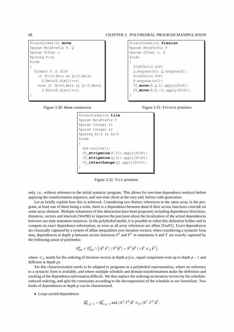
68 CHAPTER 3. POLYHEDRAL PROGRAM MANIPULATION
%transformation move%param BetaPrefix P, Q%param Offset o%prereq P<=Q%code{foreach S in SCoP
if (P<=S.Beta && Q<=S.Beta)S.Beta(P.dim())+=o;
else if (P<=S.Beta && Q<<S.Beta)S.Beta(P.dim())+=o;
}
Figure 3.30:Move constructor
%transformation fission%param BetaPrefix P%param Offset o, b%code{UrukVector Q=P;Q.enqueue(o); Q.enqueue(b);UrukVector R=P;R.enqueue(o+1);UT_move(P,Q,1).apply(SCoP);UT_move(R,R,-1).apply(SCoP);
}
Figure 3.31: FISSION primitive
%transformation tile%param BetaPrefix P%param Integer k1%param Integer k2%prereq k1>0 && k2>0%code{Q=P.enclose();UT_stripmine(P,k2).apply(SCoP);UT_stripmine(Q,k1).apply(SCoP);UT_interchange(Q).apply(SCoP);
}
Figure 3.32: TILE primitive
only, i.e., without reference to the initial syntactic program.This allows forone-time dependence analysisbeforeapplying the transformation sequence, andone-time checkat the very end, before code generation.
Let us briefly explain how this is achieved. Considering two distinct references to the same array in the pro-gram, at least one of them being a write, there is a dependencebetween them if their access functions coincide onsome array element. Multiple refinement of this abstractionhave been proposed, including dependence directions,distances, vectors and intervals [Wol96] to improve the precision about the localization of the actual dependencesbetween run-time statement instances. In the polyhedral model, it is possible to refine this definition further and tocompute anexactdependence information, as soon as all array references areaffine [Fea91]. Exact dependencesare classically captured by a system of affine inequalities over iteration vectors; when considering a syntactic loopnest, dependences at depthp between access functions FS and FT in statementsS andT are exactly captured bythe following union of polyhedra:
DSom×DT
om∩{
(iS, iT) | FS(iS) = FT(iT)∧ iS≪p iT}
,
where≪p stands for the ordering of iteration vectors at depthp (i.e., equal component-wise up to depthp−1 anddifferent at depthp).
Yet this characterization needs to be adapted to programs ina polyhedral representation, where no referenceto a syntactic form is available, and where multiple schedule and domain transformations make the definition andtracking of the dependence information difficult. We thus replace the ordering on iteration vectors by the schedule-induced ordering, and split the constraints according to the decomposition of the schedule in our formalism. Twokinds of dependences at depthp can be characterized.
• Loop-carried dependence:
βS0..p−1 = βT
0..p−1 and(AS,ΓS)iS≪p (AT ,ΓT)iT .
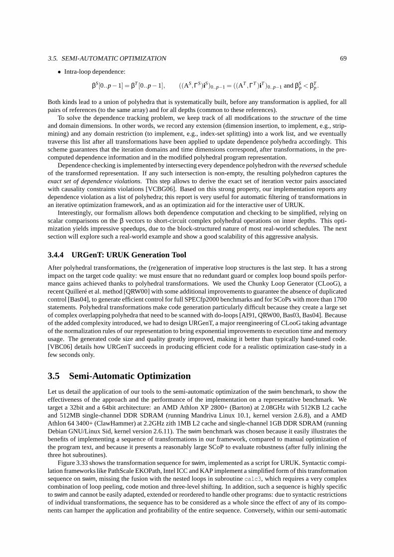
3.5. SEMI-AUTOMATIC OPTIMIZATION 69
• Intra-loop dependence:
βS[0..p−1] = βT [0..p−1], ((AS,ΓS)iS)0..p−1 = ((AT ,ΓT)iT)0..p−1 andβSp < βT
p.
Both kinds lead to a union of polyhedra that is systematically built, before any transformation is applied, for allpairs of references (to the same array) and for all depths (common to these references).
To solve the dependence tracking problem, we keep track of all modifications to thestructureof the timeand domain dimensions. In other words, we record any extension (dimension insertion, to implement, e.g., strip-mining) and any domain restriction (to implement, e.g., index-set splitting) into a work list, and we eventuallytraverse this list after all transformations have been applied to update dependence polyhedra accordingly. Thisscheme guarantees that the iteration domains and time dimensions correspond, after transformations, in the pre-computed dependence information and in the modified polyhedral program representation.
Dependence checking is implemented by intersecting every dependence polyhedron with thereversedscheduleof the transformed representation. If any such intersection is non-empty, the resulting polyhedron captures theexact set of dependence violations. This step allows to derive the exact set of iteration vectorpairs associatedwith causality constraints violations [VCBG06]. Based on this strong property, our implementation reports anydependence violation as a list of polyhedra; this report is very useful for automatic filtering of transformations inan iterative optimization framework, and as an optimization aid for the interactive user of URUK.
Interestingly, our formalism allows both dependence computation and checking to be simplified, relying onscalar comparisons on theβ vectors to short-circuit complex polyhedral operations oninner depths. This opti-mization yields impressive speedups, due to the block-structured nature of most real-world schedules. The nextsection will explore such a real-world example and show a good scalability of this aggressive analysis.
3.4.4 URGenT: URUK Generation Tool
After polyhedral transformations, the (re)generation of imperative loop structures is the last step. It has a strongimpact on the target code quality: we must ensure that no redundant guard or complex loop bound spoils perfor-mance gains achieved thanks to polyhedral transformations. We used the Chunky Loop Generator (CLooG), arecent Quilleré et al. method [QRW00] with some additional improvements to guarantee the absence of duplicatedcontrol [Bas04], to generate efficient control for full SPECfp2000 benchmarks and for SCoPs with more than 1700statements. Polyhedral transformations make code generation particularly difficult because they create a large setof complex overlapping polyhedra that need to be scanned with do-loops [AI91, QRW00, Bas03, Bas04]. Becauseof the added complexity introduced, we had to design URGenT,a major reengineering of CLooG taking advantageof the normalization rules of our representation to bring exponential improvements to execution time and memoryusage. The generated code size and quality greatly improved, making it better than typically hand-tuned code.[VBC06] details how URGenT succeeds in producing efficient code for a realistic optimization case-study in afew seconds only.
3.5 Semi-Automatic Optimization
Let us detail the application of our tools to the semi-automatic optimization of theswim benchmark, to show theeffectiveness of the approach and the performance of the implementation on a representative benchmark. Wetarget a 32bit and a 64bit architecture: an AMD Athlon XP 2800+ (Barton) at 2.08GHz with 512KB L2 cacheand 512MB single-channel DDR SDRAM (running Mandriva Linux10.1, kernel version 2.6.8), and a AMDAthlon 64 3400+ (ClawHammer) at 2.2GHz zith 1MB L2 cache and single-channel 1GB DDR SDRAM (runningDebian GNU/Linux Sid, kernel version 2.6.11). Theswim benchmark was chosen because it easily illustrates thebenefits of implementing a sequence of transformations in our framework, compared to manual optimization ofthe program text, and because it presents a reasonably largeSCoP to evaluate robustness (after fully inlining thethree hot subroutines).
Figure 3.33 shows the transformation sequence forswim, implemented as a script for URUK. Syntactic compi-lation frameworks like PathScale EKOPath, Intel ICC and KAPimplement a simplified form of this transformationsequence onswim, missing the fusion with the nested loops in subroutinecalc3, which requires a very complexcombination of loop peeling, code motion and three-level shifting. In addition, such a sequence is highly specificto swim and cannot be easily adapted, extended or reordered to handle other programs: due to syntactic restrictionsof individual transformations, the sequence has to be considered as a whole since the effect of any of its compo-nents can hamper the application and profitability of the entire sequence. Conversely, within our semi-automatic
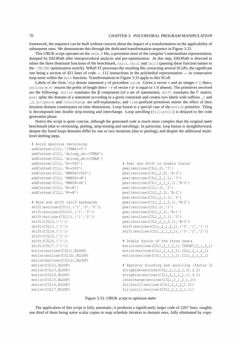
70 CHAPTER 3. POLYHEDRAL PROGRAM MANIPULATION
framework, the sequence can be built without concern about the impact of a transformation on the applicability ofsubsequent ones. We demonstrate this through the dedicatedtransformation sequence in Figure 3.33.
This URUK script operates on theswim.N file, a persistent store of the compiler’s intermediate representation,dumped by EKOPath after interprocedural analysis and pre-optimization. At this step, EKOPath is directed toinline the three dominant functions of the benchmark,calc1, calc2 andcalc3 (passing these function names tothe-INLINE optimization switch). WRaP-IT processes the resulting file, extracting several SCoPs, the significantone being a section of 421 lines of code — 112 instructions in the polyhedral representation — in consecutiveloop nests within themain function. Transformations in Figure 3.33 apply to this SCoP.
Labels of the formCxLy denote statementy of procedurecalcx. Given a vectorv and an integerr ≤ dimv,enclose(v,r) returns the prefix of length dimv− r of vectorv (r is equal to 1 if absent). The primitives involvedare the following:motion translates theβ component (of a set of statements),shift translates theΓ matrix;peel splits the domain of a statement according to a given constraint and creates two labels with suffixes_1 and_2; stripmine andinterchange are self-explanatory; andtime-prefixed primitives mimic the effect of theiriteration domain counterparts on time dimensions. Loop fusion is a special case of themotion primitive. Tilingis decomposed into double strip-mining and interchange. Loop unrolling (fullunroll) is delayed to the codegeneration phase.
Notice the script is quite concise, although the generated code is much more complex than the originalswimbenchmark (due to versioning, peeling, strip-mining and unrolling). In particular, loop fusion is straightforward,despite the fused loops domains differ by one or two iterations (due to peeling), and despite the additional multi-level shifting steps.
# Avoid spurious versioningaddContext(C1L1,’ITMAX>=9’)addContext(C1L1,’doloop_ub>=ITMAX’)addContext(C1L1,’doloop_ub<=ITMAX’)addContext(C1L1,’N>=500’)addContext(C1L1,’M>=500’)addContext(C1L1,’MNMIN>=500’)addContext(C1L1,’MNMIN<=M’)addContext(C1L1,’MNMIN<=N’)addContext(C1L1,’M<=N’)addContext(C1L1,’M>=N’)
# Move and shift calc3 backwardsshift(enclose(C3L1),{’1’,’0’,’0’})shift(enclose(C3L10),{’1’,’0’})shift(enclose(C3L11),{’1’,’0’})shift(C3L12,{’1’})shift(C3L13,{’1’})shift(C3L14,{’1’})shift(C3L15,{’1’})shift(C3L16,{’1’})shift(C3L17,{’1’})motion(enclose(C3L1),BLOOP)motion(enclose(C3L10),BLOOP)motion(enclose(C3L11),BLOOP)motion(C3L12,BLOOP)motion(C3L13,BLOOP)motion(C3L14,BLOOP)motion(C3L15,BLOOP)motion(C3L16,BLOOP)motion(C3L17,BLOOP)
# Peel and shift to enable fusionpeel(enclose(C3L1,2),’3’)peel(enclose(C3L1_2,2),’N-3’)peel(enclose(C3L1_2_1,1),’3’)peel(enclose(C3L1_2_1_2,1),’M-3’)peel(enclose(C1L1,2),’2’)peel(enclose(C1L1_2,2),’N-2’)peel(enclose(C1L1_2_1,1),’2’)peel(enclose(C1L1_2_1_2,1),’M-2’)peel(enclose(C2L1,2),’1’)peel(enclose(C2L1_2,2),’N-1’)peel(enclose(C2L1_2_1,1),’3’)peel(enclose(C2L1_2_1_2,1),’M-3’)shift(enclose(C1L1_2_1_2_1),{’0’,’1’,’1’})shift(enclose(C2L1_2_1_2_1),{’0’,’2’,’2’})
# Double fusion of the three nestsmotion(enclose(C2L1_2_1_2_1),TARGET_2_1_2_1)motion(enclose(C1L1_2_1_2_1),C2L1_2_1_2_1)motion(enclose(C3L1_2_1_2_1),C1L1_2_1_2_1)
# Register blocking and unrolling (factor 2)stripmine(enclose(C3L1_2_1_2_1,2),2,2)stripmine(enclose(C3L1_2_1_2_1,1),4,2)interchange(enclose(C3L1_2_1_2_1,2))fullunroll(enclose(C3L1_2_1_2_1,2))fullunroll(enclose(C3L1_2_1_2_1,1))
Figure 3.33: URUK script to optimizeswim
The application of this script is fully automatic; it produces a significantly larger code of 2267 lines, roughlyone third of them being naive scalar copies to map schedule iterators to domain ones, fully eliminated by copy-
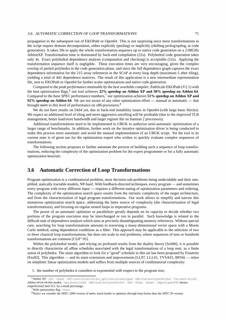
3.6. AUTOMATIC CORRECTION OF LOOP TRANSFORMATIONS 71
propagation in the subsequent run of EKOPath or Open64. Thisis not surprising since most transformations inthe script require domain decomposition, either explicitly (peeling) or implicitly (shifting prolog/epilog, at codegeneration). It takes 39s to apply the whole transformationsequence up to native code generation on a 2.08GHzAthlonXP. Transformation time is dominated by back-end compilation (22s). Polyhedral code generation takesonly 4s. Exact polyhedral dependence analysis (computation and checking) is acceptable (12s). Applying thetransformation sequence itself is negligible. These execution times are very encouraging, given the complexoverlap of peeled polyhedra in the code generation phase, and since the full dependence graph captures the exactdependence information for the 215 array references in the SCoP at every loop depth (maximum 5 after tiling),yielding a total of 441 dependence matrices. The result of this application is a new intermediate representationfile, sent to EKOPath or Open64 for further scalar optimizations and native code generation.
Compared to thepeak performance attainable by the best available compiler, PathScale EKOPath (V2.1) withthe best optimization flags,6 our tool achieves32% speedup on Athlon XP and 38% speedup on Athlon 64.Compared to thebase SPECperformance numbers,7 our optimization achieves51% speedup on Athlon XP and92% speedup on Athlon 64. We are not aware of any other optimization effort — manual orautomatic — thatbroughtswim to this level of performance on x86 processors.8
We do not have results on IA64 yet, due to back-end instability issues in Open64 (with large basic blocks).We expect an additional level of tiling and more aggressive unrolling will be profitable (due to the improved TLBmanagement, better load/store bandwitdh and larger register file on Itanium 2 processors).
Additional transformations need to be implemented in URUK to authorize semi-automatic optimization of alarger range of benchmarks. In addition, further work on theiterative optimization driver is being conducted tomake this process more automatic and avoid the manual implementation of an URUK script. Yet the tool in itscurrent state is of great use for the optimization expert whowishes to quickly evaluate complex sequences oftransformations.
The following section proposes to further automate the process of building such a sequence of loop transfor-mations, reducing the complexity of the optimization problem for the expert programmer or for a fully automaticoptimization heuristic.
3.6 Automatic Correction of Loop Transformations
Program optimization is a combinatorial problem, most decision sub-problems being undecidable and their sim-plified, statically tractable models, NP-hard. With feedback-directed techniques, every program — and sometimesevery program with every different input — requires a different tuning of optimization parameters and ordering.The complexity of the optimization search space results from the intrinsic complexity of the target architecture,and from the characterization of legal program transformations. Our work allows to simplify and narrow thismonstrous optimization search space, addressing the latter source of complexity (the characterization of legaltransformations), and focusing on regular nested loops in imperative programs.
The power of an automatic optimizer or parallelizer greatlydepends on its capacity to decide whether twoportions of the program execution may be interchanged or runin parallel. Such knowledge is related to thedifficult task ofdependence analysiswhich aims at precisely disambiguating memory references.Without specialcare, searching for loop transformations amounts to traversing a many-dimensional vector space with a MonteCarlo method, using dependence conditions as a filter. This approach may be applicable to the selection of twoor three classical loop transformations, but does not scaleto real problems, where sequences of tens or hundredstransformations are common [CGP+05].
Within the polyhedral model, and relying on profound results from the duality theory [Sch86], it is possibleto directly characterize all affine schedules associated with the legal transformations of a loop nest, as a finiteunion of polyhedra. The main algorithm to look for a “good” schedule in this set has been proposed by Feautrier[Fea92]. This algorithm — and its main extensions and improvements [LL97, LLL01, TVSA01, BF04] — relieson simplistic linear optimization models and suffers from multiple sources of combinatorial complexity:
1. the number of polyhedra it considers is exponential with respect to the program size;
6Athlon XP:-m32 -Ofast -OPT:ro=2:Olimit=0:div_split=on:alias=typed -LNO:fusion=2:prefetch=2 -fno-math-errno;Athlon 64 (in 64 bits mode):-march=athlon64 -LNO:fusion=2:prefetch=2 -m64 -Ofast -msse2 -lmpath; pathf90 alwaysoutperformed Intel ICC by a small percentage.
7With optimization flag-Ofast.8Notice we consider the SPEC 2000 version ofswim, much harder to optimize through loop fusion than the SPEC 95version.
72 CHAPTER 3. POLYHEDRAL PROGRAM MANIPULATION
2. the dimensionality of polyhedra is proportional to the program size, which incurs an exponential complexityin the integer linear programs the algorithm relies on.
Radical improvements are needed to scale these algorithms to real-size loop nests (a few hundred statements ormore), and to complement linear programming with more pragmatic empirical operation research heuristics. Weare working along these lines [PBCV07], but it is unreasonable to expect this approach will scale alone to full-sizeprograms.
We thus develop a complementary approach to reduce the complexity and size of the transformation space. Itconsists in narrowing the set of variables of this combinatorial problem. Intuitively, operation research heuristicsare focused on the “hard to find”and “most performance impacting” ones, relying on a simple model to optimizeacross other dimensions of the search space.
Our main technical contribution is an algorithm to exploitdependence violations: by identifying exactly theviolated dependences, we derivean automatic correction scheme to fix an illegal transformation sequencewith“minimal changes”. This correction scheme amounts to decomposing the iteration domain and translating (a.k.a.shifting) the schedule on each part (by a minimal amount) so that dependences are satisfied. Our algorithm hastwo important qualities:
1. it is sound andcomplete: any multidimensional affine schedule will be corrected as long as dependenceviolations can be corrected by translation;
2. it applies apolynomialnumber of operations on dependence polyhedra (each one may be exponential, butdoes not depend on the program size).
We will demonstrate the effectiveness and scalability of our automatic correction scheme through the opti-mization of two of these benchmarks:swim andmgrid.
3.6.1 Related Work and Applications
The concept ofenablingtransformation is central to design of loop optimizers [AK02]. Very often, a localityor parallelism enhancing transformation violates the data-flow semantics of the program, although a simple pre-conditioning step on the operational semantics — typicallythe program schedule or its storage management —suffices to enable it. Loop shifting or pipelining [DH00], and loop skewing [Ban92] are such enabling transforma-tions of the schedule, while loop peeling isolates violations on boundary conditions [Muc97, FGL99] and variablerenaming or privatization removes dependences [CFR+91, MAL93, KS98]. Unfortunately, except in special cases(e.g., the unimodular transformation framework, or acyclic dependence graphs), one faces the decision problemof choosing an enabling transformation with no guarantee that it will do any good.
The induced combinatorics of these decision problems drivethe search for a more compositional approach,where transformation legality is guaranteed by construction, using the Farkas lemma on affine schedules. Asstated in the introduction, this is our main motivation, buttaking all legality constraints into account makes thealgorithms not scalable, and suggest staging the selectionof a loop nest transformation into an “approximatelycorrect” combinatorial step — addressing the main performance concerns — and a secondcorrectionstep. Theidea of applying “after-thought” corrections on affine schedules was first proposed by Bastoul [BF05]. However,it still relies on a projection of the schedule on the subspace of legal Farkas coefficients and does not scale withprogram size.
We follow the idea of correcting illegal schedules, but focus on a particular kind of correction that general-izes loopshifting, fusionanddistribution [AK02]. These three classical (operational) program transformationsboil down to the same algebraic translation in multidimensional affine scheduling. These are some of the mostimportant enabling transformations in the context of automatic loop parallelization [AK02, DH00]. They induceless code complexity than, e.g., loop skewing (which may degrade performance due to the complexity of loopbound expressions), and can cope with a variety of cyclic dependence graphs. Yet the problem, seen as a decisionone, has been proved NP-complete by Darte [DH00]. This is dueto the inability to characterize data-parallelismin loops in a linear fashion (many data-parallel programs cannot be expressed with multi-dimensional schedules[LL97]). Although we use the same tools as Darte to correct schedules, we avoid this pitfall stating our problemas a linear optimization (using the Bellman-Ford algorithm[CLR89]).
Decoupling research on the linear and constant parts of the schedule has been proposed earlier [DSV97, DH00,VBJC03]. These techniques all use simplified representation of dependences (i.e., dependence vectors) and relyon finding enabling transformations for their specific purpose, driven by optimization heuristics. Our approach ismore general as it applies to any potentially illegal affine schedule.
3.6. AUTOMATIC CORRECTION OF LOOP TRANSFORMATIONS 73
Alternatively, Crop and Wilde [CW99] and Feautrier [Fea06]attempt to reduce the complexity of affinescheduling with a modular or structural decomposition. These algorithms are very effective, but still resort tosolving large, non-scalable integer-linear programs. They are complementary to our correction scheme.
To sum-up, our approach has two main complexity advantages.
1. The number of dimensions of the optimization search spaceis reduced. Depending on the optimizationstrategy and the program, it may eliminate from one third to almost all of the unknowns in the optimizationproblem. We also show that remaining dimensions have a lowercontribution to the size of the search spaceand a higher impact on performance than the ones that can be eliminated.
2. Index-set splitting is the state-of-the-art technique to decompose iteration domains, allowing more expres-sive piecewise affine schedules to be built. Its current formulation is a complex decision problem [FGL99]which requires interaction with a non scalable scheduling algorithm. Our approach replaces it by a simpleheuristic, combined with the automatic correction procedure. This is extremely helpful, considering thateach decision problem has a combinatorial impact on the phase ordering, selection and parameterizationproblem associated with the feedback-directed optimization of each application.
Finally, our results also facilitate the design of domain-specific program generators [WPD00, FJ98, PSX+04,DBR+05, GVB+06, CDG+06], a very pragmatic solution to the design of portable optimized libraries. Indeed,although human-written code is concise (code factoring in loops and functions), optimizing it for modern ar-chitectures incurs several code size expansion steps, including function inlining, specialization, loop versioningand unrolling. Domain-specific program generators (also known as active libraries [LBCO03]) rely on feedback-directed optimization and iterative search to generate nearly optimal library or application code. Our approachreduces the number of transformation steps, focusing the optimization problem to the core execution anomalies.Since most steps are enabling transformations that enable key optimizations [PTCV04], it is quite beneficial to theproductivity and comfort of designers of such program generators.
3.6.2 Dependence Analysis
Array dependence analysis is the starting point for any polyhedral optimization. It computes non transitively-redundant, iteration vector to iteration vector, directeddependences [Fea88a, VCBG06]. In order to correct depen-dence violations, it is first needed tocompute the exact dependence information between every pair of instances,i.e., every pair of statement iterations. Considering a pair of statementsSandT accessing memory locations whereat least one of them is a write, there is a dependence from an instance〈S, iS〉 of S to an instance〈T, iT〉 of T (or〈T, iT〉 depends on〈S, iS〉) if and only if the followinginstancewiseconditions are met:
Execution condition: both instances belong to the corresponding statement iteration domain: DSi · i
S≥ 0 andDT
i · iT ≥ 0,
Conflict condition: both instances refer the same memory location:(
AccSi | AccS
igp
)
· iS =(
AccTi | AccT
igp
)
· iT ,
and
Causality condition: the instance〈S, iS〉 is executed before〈T, iT〉 in the original execution:ΘS· iS≪ΘT · iT ,
where≪ denotes the lexicographic order on vectors.The schedule (the multidimensional time-stamp) at which aninstance is executed is determined, for statement
S, by the 2dS+ 1 vector given byΘS · iS. Relative order between instances is given by the relative lexicographicorder of their schedule vectors.
Consider the original polyhedral representation of a program, before any transformation has been applied. Fora given statementS, matrix AS is the identity,ΓS is 0 and vectorβS captures the syntactic position ofS in theoriginal code. In this configuration, the three aforementioned conditions correspond to the classical definition ofpolyhedral dependences [Fea88a, Pug91b].
A dependence is said to be loop independent of depthp≤ 0 if the causality conditionΘS · iS≪ ΘT · iT isresolved sequentially on theβ|p| component of the schedule. A dependence is said to be loop carried at loop depthp > 0 if the causality condition is resolved by the(A | Γ) component of the schedule at depthp.Loop-carried dependence at depthp > 0:
(
(AS | ΓS) · iS)
0..p−1 =(
(AT | ΓT) · iT)
0..p−1,
βS0..p−1 = βT
0..p−1 and(
(AS | ΓS) · iS)
p <(
(AT | ΓT) · iT)
p
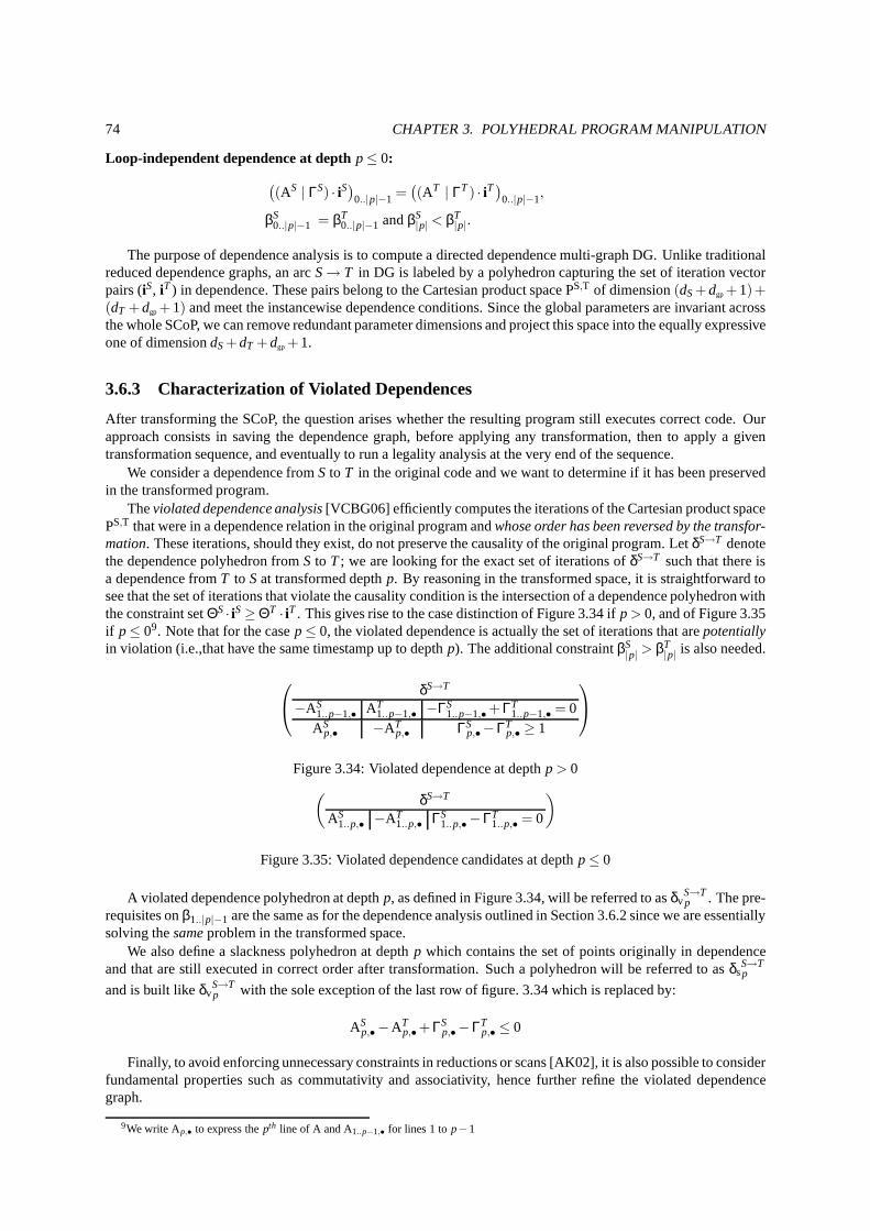
74 CHAPTER 3. POLYHEDRAL PROGRAM MANIPULATION
Loop-independent dependence at depthp≤ 0:
(
(AS | ΓS) · iS)
0..|p|−1 =(
(AT | ΓT) · iT)
0..|p|−1,
βS0..|p|−1 = βT
0..|p|−1 andβS|p| < βT
|p|.
The purpose of dependence analysis is to compute a directed dependence multi-graph DG. Unlike traditionalreduced dependence graphs, an arcS→ T in DG is labeled by a polyhedron capturing the set of iteration vectorpairs (iS, iT ) in dependence. These pairs belong to the Cartesian productspace PS,T of dimension(dS+dgp+1)+(dT +dgp+1) and meet the instancewise dependence conditions. Since theglobal parameters are invariant acrossthe whole SCoP, we can remove redundant parameter dimensions and project this space into the equally expressiveone of dimensiondS+dT +dgp+1.
3.6.3 Characterization of Violated Dependences
After transforming the SCoP, the question arises whether the resulting program still executes correct code. Ourapproach consists in saving the dependence graph, before applying any transformation, then to apply a giventransformation sequence, and eventually to run a legality analysis at the very end of the sequence.
We consider a dependence fromS to T in the original code and we want to determine if it has been preservedin the transformed program.
Theviolated dependence analysis[VCBG06] efficiently computes the iterations of the Cartesian product spacePS,T that were in a dependence relation in the original program and whose order has been reversed by the transfor-mation. These iterations, should they exist, do not preserve the causality of the original program. LetδS→T denotethe dependence polyhedron fromS to T; we are looking for the exact set of iterations ofδS→T such that there isa dependence fromT to Sat transformed depthp. By reasoning in the transformed space, it is straightforward tosee that the set of iterations that violate the causality condition is the intersection of a dependence polyhedron withthe constraint setΘS· iS≥ΘT · iT . This gives rise to the case distinction of Figure 3.34 ifp> 0, and of Figure 3.35if p≤ 09. Note that for the casep≤ 0, the violated dependence is actually the set of iterationsthat arepotentiallyin violation (i.e.,that have the same timestamp up to depthp). The additional constraintβS
|p| > βT|p| is also needed.
δS→T
−AS1..p−1,• AT
1..p−1,• −ΓS1..p−1,•+ ΓT
1..p−1,• = 0AS
p,• −ATp,• ΓS
p,•−ΓTp,• ≥ 1
Figure 3.34: Violated dependence at depthp > 0
(
δS→T
AS1..p,• −AT
1..p,• ΓS1..p,•−ΓT
1..p,• = 0
)
Figure 3.35: Violated dependence candidates at depthp≤ 0
A violated dependence polyhedron at depthp, as defined in Figure 3.34, will be referred to asδvS→Tp . The pre-
requisites onβ1..|p|−1 are the same as for the dependence analysis outlined in Section 3.6.2 since we are essentiallysolving thesameproblem in the transformed space.
We also define a slackness polyhedron at depthp which contains the set of points originally in dependenceand that are still executed in correct order after transformation. Such a polyhedron will be referred to asδs
S→Tp
and is built likeδvS→Tp with the sole exception of the last row of figure. 3.34 which isreplaced by:
ASp,•−AT
p,•+ ΓSp,•−ΓT
p,• ≤ 0
Finally, to avoid enforcing unnecessary constraints in reductions or scans [AK02], it is also possible to considerfundamental properties such as commutativity and associativity, hence further refine the violated dependencegraph.
9We write Ap,• to express thepth line of A and A1..p−1,• for lines 1 top−1
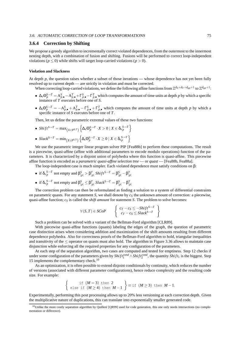
3.6. AUTOMATIC CORRECTION OF LOOP TRANSFORMATIONS 75
3.6.4 Correction by Shifting
We propose a greedy algorithm to incrementally correct violated dependences, from the outermost to the innermostnesting depth, with a combination of fusion and shifting. Fusions will be performed to correct loop-independentviolations (p≤ 0) while shifts will target loop-carried violations (p > 0).
Violation and Slackness
At depthp, the question raises whether a subset of those iterations — whose dependence has not yet been fullyresolved up to current depth — are strictly in violation and must be corrected.
When correcting loop-carried violations, we define the following affine functions fromZdS+dT+dgp+1 toZdgp+1:
• ∆vΘS→Tp = AS
p,•−ATp,•+ΓS
p,•−ΓTp,• which computes the amount of time units at depthp by which a specific
instance ofT executes before one ofS.
• ∆sΘS→Tp = −AS
p,•+ ATp,•− ΓS
p,•+ ΓTp,• which computes the amount of time units at depthp by which a
specific instance ofSexecutes before one ofT.
Then, let us define the parametric extremal values of these two functions:
• Shi f tS→T = max(X∈PS,T)
{
∆vΘS→Tp ·X > 0 | X ∈ δv
S→Tp
}
• SlackS→T = min(X∈PS,T)
{
∆sΘS→Tp ·X ≥ 0 | X ∈ δs
S→Tp
}
We use the parametric integer linear program solver PIP [Fea88b] to perform these computations. The resultis a piecewise, quasi-affine (affine with additional parameters to encode modulo operations) function of the pa-rameters. It is characterized by a disjoint union of polyhedra where this function is quasi-affine. This piecewiseaffine function is encoded as aparametric quasi-affine selection tree— or quast— [Fea88b, Fea88a].
The loop-independent case is much simpler. Each violated dependence must satisfy conditions onβ:
• if δvS→Tp not empty andβS
|p| > βT|p| Shi f tS→T = βS
|p|−βT|p|
• if δvS→Tp not empty andβS
|p| ≤ βT|p| SlackS→T = βS
|p|−βT|p|
The correction problem can then be reformulated as finding a solution to a system of differential constraintson parametric quasts. For any statementS, we shall denote bycS the unknown amount of correction: a piecewise,quasi-affine function;cS is called theshift amountfor statementS. The problem to solve becomes:
∀(S,T) ∈ SCoP
{
cT −cS≤−Shi f tS→T
cT −cS≤ SlackS→T
}
Such a problem can be solved with a variant of the Bellman-Ford algorithm [CLR89].With piecewise quasi-affine functions (quasts) labeling the edges of the graph, the question of parametric
case distinction arises when considering addition and maximization of the shift amounts resulting from differentdependence polyhedra. Also for correctness proofs of the Bellman-Ford algorithm to hold, triangular inequalitiesand transitivity of the≤ operator on quasts must also hold. The algorithm in Figure 3.36 allows to maintain casedisjunction while enforcing all the required properties for any configuration of the parameters.
At each step of the separation algorithm, two cases are computed and tested for emptiness. Step 12 checks ifunder some configuration of the parameters given byShi f tcond
1 ∧Shi f tcond2 , the quantityShi f t1 is the biggest. Step
15 implements the complementary check.10
As an optimization, it is often possible to extend disjoint conditionals by continuity, which reduces the numberof versions (associated with different parameter configurations), hence reduce complexity and the resulting codesize. For example:
{
if (M = 3) then 2else if (M ≥ 4) then M−1
}
≡ if (M ≥ 3) then M−1.
Experimentally, performing this post processing allows upto 20% less versioning at each correction depth. Giventhe multiplicative nature of duplications, this can translate into exponentially smaller generated code.
10Unlike the more costly separation algorithm by Quilleré [QR99] used for code generation, this one only needs intersections (no comple-mentation or difference).
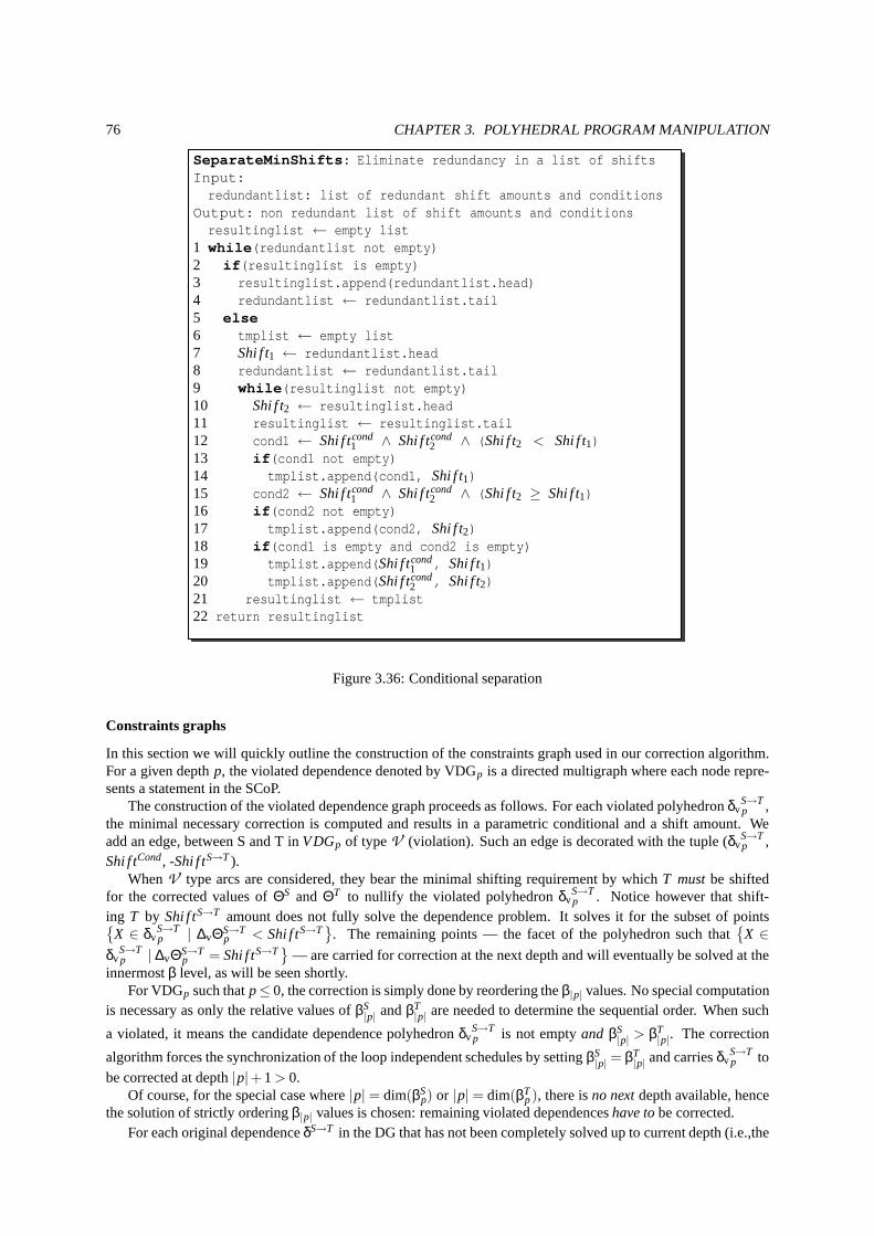
76 CHAPTER 3. POLYHEDRAL PROGRAM MANIPULATION
SeparateMinShifts: Eliminate redundancy in a list of shiftsInput:redundantlist: list of redundant shift amounts and conditions
Output: non redundant list of shift amounts and conditionsresultinglist ← empty list
1 while(redundantlist not empty)2 if(resultinglist is empty)3 resultinglist.append(redundantlist.head)4 redundantlist ← redundantlist.tail5 else6 tmplist ← empty list7 Shi f t1 ← redundantlist.head8 redundantlist ← redundantlist.tail9 while(resultinglist not empty)10 Shi f t2 ← resultinglist.head11 resultinglist ← resultinglist.tail12 cond1 ← Shi f tcond
1 ∧ Shi f tcond2 ∧ (Shi f t2 < Shi f t1)
13 if(cond1 not empty)14 tmplist.append(cond1, Shi f t1)15 cond2 ← Shi f tcond
1 ∧ Shi f tcond2 ∧ (Shi f t2 ≥ Shi f t1)
16 if(cond2 not empty)17 tmplist.append(cond2, Shi f t2)18 if(cond1 is empty and cond2 is empty)19 tmplist.append(Shi f tcond
1 , Shi f t1)20 tmplist.append(Shi f tcond
2 , Shi f t2)21 resultinglist ← tmplist22 return resultinglist
Figure 3.36: Conditional separation
Constraints graphs
In this section we will quickly outline the construction of the constraints graph used in our correction algorithm.For a given depthp, the violated dependence denoted by VDGp is a directed multigraph where each node repre-sents a statement in the SCoP.
The construction of the violated dependence graph proceedsas follows. For each violated polyhedronδvS→Tp ,
the minimal necessary correction is computed and results ina parametric conditional and a shift amount. Weadd an edge, between S and T inVDGp of typeV (violation). Such an edge is decorated with the tuple (δv
S→Tp ,
Shi f tCond, -Shi f tS→T ).WhenV type arcs are considered, they bear the minimal shifting requirement by whichT mustbe shifted
for the corrected values ofΘS and ΘT to nullify the violated polyhedronδvS→Tp . Notice however that shift-
ing T by Shi f tS→T amount does not fully solve the dependence problem. It solves it for the subset of points{
X ∈ δvS→Tp | ∆vΘS→T
p < Shi f tS→T}
. The remaining points — the facet of the polyhedron such that{
X ∈
δvS→Tp | ∆vΘS→T
p = Shi f tS→T}
— are carried for correction at the next depth and will eventually be solved at theinnermostβ level, as will be seen shortly.
For VDGp such thatp≤ 0, the correction is simply done by reordering theβ|p| values. No special computationis necessary as only the relative values ofβS
|p| andβT|p| are needed to determine the sequential order. When such
a violated, it means the candidate dependence polyhedronδvS→Tp is not emptyand βS
|p| > βT|p|. The correction
algorithm forces the synchronization of the loop independent schedules by settingβS|p| = βT
|p| and carriesδvS→Tp to
be corrected at depth|p|+1> 0.Of course, for the special case where|p|= dim(βS
p) or |p|= dim(βTp), there isno nextdepth available, hence
the solution of strictly orderingβ|p| values is chosen: remaining violated dependenceshave tobe corrected.For each original dependenceδS→T in the DG that has not been completely solved up to current depth (i.e.,the
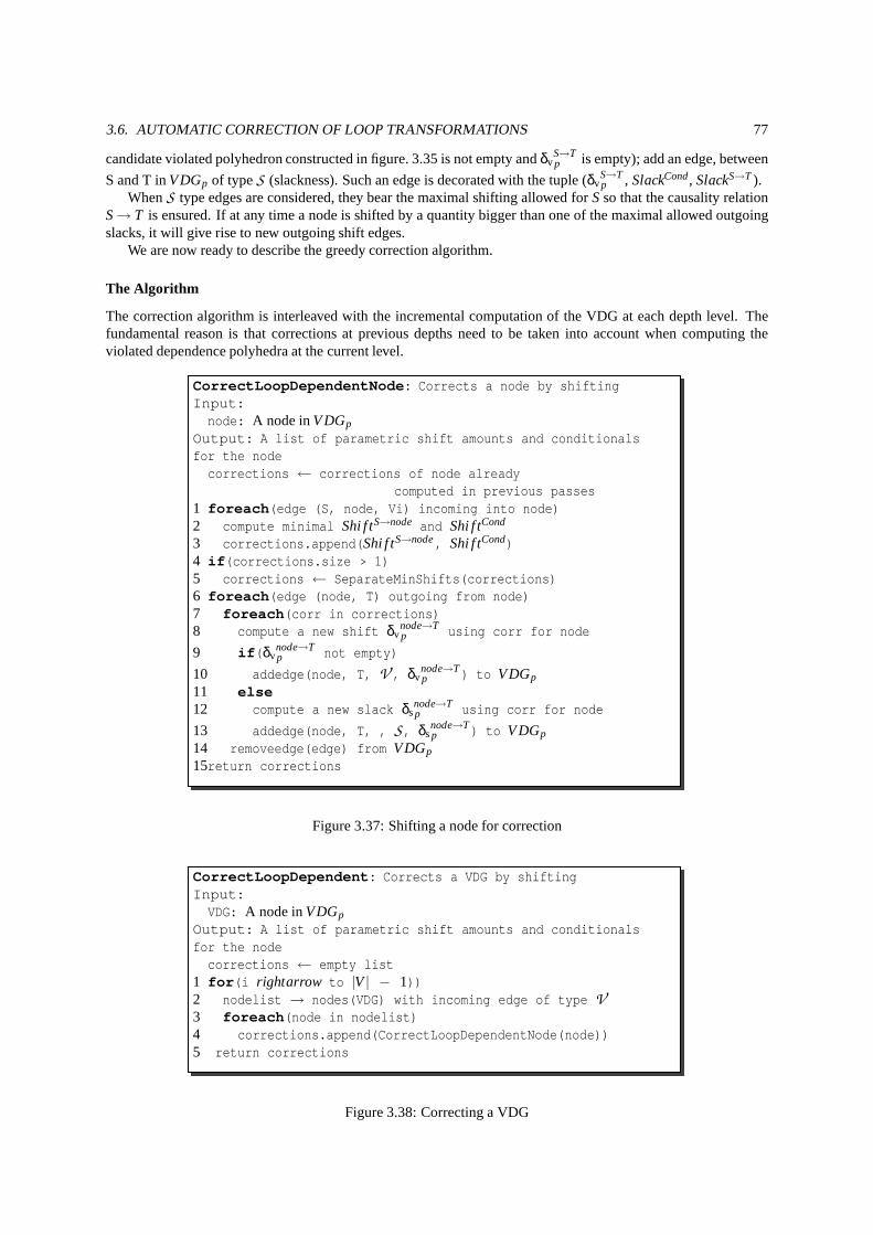
3.6. AUTOMATIC CORRECTION OF LOOP TRANSFORMATIONS 77
candidate violated polyhedron constructed in figure. 3.35 is not empty andδvS→Tp is empty); add an edge, between
S and T inVDGp of typeS (slackness). Such an edge is decorated with the tuple (δvS→Tp , SlackCond, SlackS→T ).
WhenS type edges are considered, they bear the maximal shifting allowed forSso that the causality relationS→ T is ensured. If at any time a node is shifted by a quantity bigger than one of the maximal allowed outgoingslacks, it will give rise to new outgoing shift edges.
We are now ready to describe the greedy correction algorithm.
The Algorithm
The correction algorithm is interleaved with the incremental computation of the VDG at each depth level. Thefundamental reason is that corrections at previous depths need to be taken into account when computing theviolated dependence polyhedra at the current level.
CorrectLoopDependentNode: Corrects a node by shiftingInput:node: A node inVDGp
Output: A list of parametric shift amounts and conditionalsfor the nodecorrections ← corrections of node already
computed in previous passes1 foreach(edge (S, node, Vi) incoming into node)2 compute minimal Shi f tS→node and Shi f tCond
3 corrections.append(Shi f tS→node, Shi f tCond)4 if(corrections.size > 1)5 corrections ← SeparateMinShifts(corrections)6 foreach(edge (node, T) outgoing from node)7 foreach(corr in corrections)8 compute a new shift δv
node→Tp using corr for node
9 if(δvnode→Tp not empty)
10 addedge(node, T, V , δvnode→Tp ) to VDGp
11 else12 compute a new slack δs
node→Tp using corr for node
13 addedge(node, T, , S, δsnode→Tp ) to VDGp
14 removeedge(edge) from VDGp
15return corrections
Figure 3.37: Shifting a node for correction
CorrectLoopDependent: Corrects a VDG by shiftingInput:VDG: A node inVDGp
Output: A list of parametric shift amounts and conditionalsfor the nodecorrections ← empty list
1 for(i rightarrow to |V| − 1))2 nodelist → nodes(VDG) with incoming edge of type V
3 foreach(node in nodelist)4 corrections.append(CorrectLoopDependentNode(node))5 return corrections
Figure 3.38: Correcting a VDG
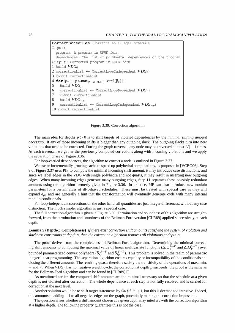
78 CHAPTER 3. POLYHEDRAL PROGRAM MANIPULATION
CorrectSchedules: Corrects an illegal scheduleInput:program: A program in URUK formdependences: The list of polyhedral dependences of the program
Output: Corrected program in URUK form1 Build VDG0
2 correctionList ← CorrectLoopIndependent(V DG0)3 commit correctionList4 for(p=1; p<=max(S in SCoP) {rank(βS)})5 Build VDGp
6 correctionList ← CorrectLoopDependent(V DGp)7 commit correctionList8 Build VDG−p
9 correctionList ← CorrectLoopIndependent(V DG−p)10 commit correctionList
Figure 3.39: Correction algorithm
The main idea for depthsp > 0 is to shift targets of violated dependences by theminimal shifting amountnecessary. If any of those incoming shifts is bigger than any outgoing slack. The outgoing slacks turn into newviolations that need to be corrected. During the graph traversal, any node may be traversed at most|V|−1 times.At each traversal, we gather the previously computed corrections along with incoming violations and we applythe separation phase of Figure 3.36.
For loop-carried dependences, the algorithm to correct a node is outlined in Figure 3.37.We use an incrementally growing cache to speed up polyhedralcomputations, as proposed in [VCBG06]. Step
8 of Figure 3.37 uses PIP to compute the minimal incoming shift amount; it may introduce case distinctions, andsince we label edges in the VDG with single polyhedra and not quasts, it may result in inserting new outgoingedges. When many incoming edges generate many outgoing edges, Step 11 separates these possibly redundantamounts using the algorithm formerly given in Figure 3.36. In practice, PIP can also introduce new moduloparameters for a certain class of ill-behaved schedules. These must be treated with special care as they willexpanddgp and are generally a hint that the transformation will eventually generate code with many internalmodulo conditionals.
For loop-independent corrections on the other hand, all quantities are just integer differences, without any casedistinction. The much simpler algorithm is just a special case.
The full correction algorithm is given in Figure 3.39. Termination and soundness of this algorithm are straight-forward, from the termination and soundness of the Bellman-Ford version [CLR89] applied successively at eachdepth.
Lemma 5 (Depth-p Completeness)If there exist correction shift amounts satisfying the system of violation andslackness constraints at depth p, then the correction algorithm removes all violations at depth p.
The proof derives from the completeness of Bellman-Ford’s algorithm. Determining the minimal correct-ing shift amounts to computing the maximal value of linear multivariate functions (∆vΘS→T
p and∆sΘS→Tp ) over
bounded parameterized convex polyhedra (δvS→Tp andδs
S→Tp ). This problem is solved in the realm of parametric
integer linear programming. The separation algorithm ensures equality or incompatibility of the conditionals en-closing the different amounts. The resulting quasts therefore satisfy the transitivity of the operations of max, min,+ and≤. WhenVDGp has no negative weight cycle, the correction at depthp succeeds; the proof is the same asfor the Bellman-Ford algorithm and can be found in [CLR89].�
As mentioned earlier, the computed shift amounts are the minimal necessary so that the schedule at a givendepth is not violated after correction. The whole dependence at each step is not fully resolved and is carried forcorrection at the next level.
Another solution would be to shift target statements byShi f tS→T +1, but this is deemed too intrusive. Indeed,this amounts to adding−1 to all negative edges on the graph, potentially making the correction impossible.
The question arises whether a shift amount chosen at a given depth may interfere with the correction algorithmat a higher depth. The following property guarantees this isnot the case.
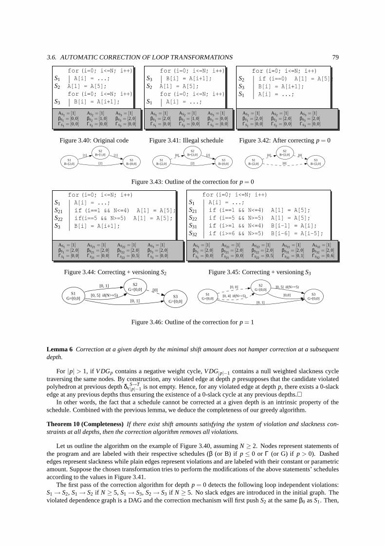
3.6. AUTOMATIC CORRECTION OF LOOP TRANSFORMATIONS 79
for (i=0; i<=N; i++)S1 A[i] = ...;S2 A[1] = A[5];
for (i=0; i<=N; i++)S3 B[i] = A[i+1];
AS1 = [1] AS2 = [1] AS3 = [1]βS1 = [0,0] βS2 = [1,0] βS3 = [2,0]ΓS1 = [0,0] ΓS2 = [0,0] ΓS3 = [0,0]
Figure 3.40: Original code
for (i=0; i<=N; i++)S3 B[i] = A[i+1];S2 A[1] = A[5];
for (i=0; i<=N; i++)S1 A[i] = ...;
AS1 = [1] AS2 = [1] AS3 = [1]βS1 = [2,0] βS2 = [1,0] βS3 = [0,0]ΓS1 = [0,0] ΓS2 = [0,0] ΓS3 = [0,0]
Figure 3.41: Illegal schedule
for (i=0; i<=N; i++)S2 if (i==0) A[1] = A[5];S3 B[i] = A[i+1];S1 A[i] = ...;
AS1 = [1] AS2 = [1] AS3 = [1]βS1 = [2,0] βS2 = [2,0] βS3 = [2,0]ΓS1 = [0,0] ΓS2 = [0,0] ΓS3 = [0,0]
Figure 3.42: After correctingp = 0
S1B=[2,0]
S2B=[1,0][1]
S3B=[0,0][2]
[1]
S1B=[2,0]
S2B=[2,0][0]
S3B=[0,0][2]
[2]
S1B=[2,0]
S2B=[2,0][0]
S3B=[2,0][0]
[0]
Figure 3.43: Outline of the correction forp = 0
for (i=0; i<=N; i++)S1 A[i] = ...;S21 if (i==1 && N<=4) A[1] = A[5];S22 if(i==5 && N>=5) A[1] = A[5];S3 B[i] = A[i+1];
AS1 = [1] AS21 = [1] AS22 = [1] AS3 = [1]βS1 = [2,0] βS21 = [2,0] βS22 = [2,0] βS3 = [2,0]ΓS1 = [0,0] ΓS21 = [0,0] ΓS22 = [0,5] ΓS3 = [0,0]
Figure 3.44: Correcting + versioningS2
for (i=0; i<=N; i++)S1 A[i] = ...;S21 if (i==1 && N<=4) A[1] = A[5];S22 if (i==5 && N>=5) A[1] = A[5];S31 if (i>=1 && N<=4) B[i-1] = A[i];S32 if (i>=6 && N>=5) B[i-6] = A[i-5];
AS1 = [1] AS21 = [1] AS22 = [1] AS31 = [1] AS32 = [1]βS1 = [2,0] βS21 = [2,0] βS22 = [2,0] βS31 = [2,0] βS32 = [2,0]ΓS1 = [0,0] ΓS21 = [0,0] ΓS22 = [0,5] ΓS31 = [0,1] ΓS32 = [0,6]
Figure 3.45: Correcting + versioningS3
S1G=[0,0]
S2G=[0,0]
[0, 1]
[0, 5] if(N>=5) S3G=[0,0][0, 1]
[0]S1
G=[0,0]
S2G=[0,0]
[0, 0]
[0, 4] if(N>=5) S3G=[0,0]
[0, 1]
[0, 5] if(N>=5)
[0,0]
Figure 3.46: Outline of the correction forp = 1
Lemma 6 Correction at a given depth by the minimal shift amount does not hamper correction at a subsequentdepth.
For |p| > 1, if VDGp contains a negative weight cycle,VDG|p|−1 contains a null weighted slackness cycletraversing the same nodes. By construction, any violated edge at depthp presupposes that the candidate violatedpolyhedron at previous depthδv
S→T|p|−1 is not empty. Hence, for any violated edge at depthp, there exists a 0-slack
edge at any previous depths thus ensuring the existence of a 0-slack cycle at any previous depths.�In other words, the fact that a schedule cannot be corrected at a given depth is an intrinsic property of the
schedule. Combined with the previous lemma, we deduce the completeness of our greedy algorithm.
Theorem 10 (Completeness)If there exist shift amounts satisfying the system of violation and slackness con-straints at all depths, then the correction algorithm removes all violations.
Let us outline the algorithm on the example of Figure 3.40, assumingN ≥ 2. Nodes represent statements ofthe program and are labeled with their respective schedules(β (or B) if p≤ 0 or Γ (or G) if p > 0). Dashededges represent slackness while plain edges represent violations and are labeled with their constant or parametricamount. Suppose the chosen transformation tries to performthe modifications of the above statements’ schedulesaccording to the values in Figure 3.41.
The first pass of the correction algorithm for depthp = 0 detects the following loop independent violations:S1→ S2, S1→ S2 if N ≥ 5, S1→ S3, S2→ S3 if N ≥ 5. No slack edges are introduced in the initial graph. Theviolated dependence graph is a DAG and the correction mechanism will first pushS2 at the sameβ0 asS1. Then,
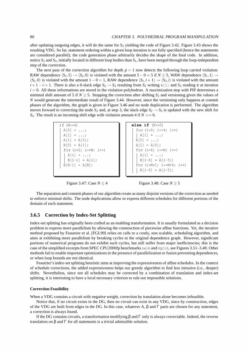
80 CHAPTER 3. POLYHEDRAL PROGRAM MANIPULATION
after updating outgoing edges, it will do the same forS3 yielding the code of Figure 3.42. Figure 3.43 shows theresulting VDG. So far, statement ordering within a given loop iteration is not fully specified (hence the statementsare considered parallel); the code generation phase arbitrarily decides the shape of the final code. In addition,noticeS2 andS3, initially located in different loop bodies thanS1, have been merged through the loop-independentstep of the correction.
The next pass of the correction algorithm for depthp = 1 now detects the following loop carried violation:RAW dependence〈S1,5〉 → 〈S2,0〉 is violated with the amount 5−0 = 5 if N ≥ 5, WAW dependence〈S1,1〉 →〈S2,0〉 is violated with the amount 1−0 = 1, RAW dependence〈S1, i + 1〉 → 〈S3, i〉 is violated with the amounti + 1− i = 1. There is also a 0-slack edgeS2→ S3 resulting fromS2 writing A[1] andS3 reading it at iterationi = 0. All these informations are stored in the violation polyhedron. A maximization step with PIP determines aminimal shift amount of 5 ifN ≥ 5. Stopping the correction after shiftingS2 and versioning given the values ofN would generate the intermediate result of Figure 3.44. However, since the versioning only happens at commitphases of the algorithm, the graph is given in Figure 3.46 andno node duplication is performed. The algorithmmoves forward to correcting the nodeS3 and, at step 3, the slack edgeS2→ S3 is updated with the new shift forS2. The result is an incoming shift edge with violation amount 4if N >= 6.
if (N<=4)A[0] = ...;A[1] = ...;A[1] = A[5];B[0] = A[1];for (i=2; i<=N; i++)A[i] = ...;B[i-1] = A[i];
B[N-1] = A[N];
Figure 3.47: CaseN≤ 4
else if (N>=5)for (i=0; i<=4; i++)A[i] = ...;
A[5] = ...;A[1] = A[5];for (i=6; i<=N; i++)A[i] = ...;B[i-6] = A[i-5];
for (i=N+1; i<=N+6; i++)B[i-6] = A[i-5];
Figure 3.48: CaseN≥ 5
The separation and commit phases of our algorithm create as many disjoint versions of the correction as neededto enforce minimal shifts. The node duplications allow to express different schedules for different portions of thedomain of each statement.
3.6.5 Correction by Index-Set Splitting
Index-set splitting has originally been crafted as an enabling transformation. It is usually formulated as a decisionproblem to express more parallelism by allowing the construction of piecewise affine functions. Yet, the iterativemethod proposed by Feautrier et al. [FGL99] relies on calls to a costly, non scalable, scheduling algorithm, andaims at exhibiting more parallelism by breaking cycles in the original dependence graph. However, significantportions of numerical programs do not exhibit such cycles, but still suffer from major inefficiencies; this is thecase of the simplified excerpts from SPEC CPU2000fp benchmarksswim andmgrid, see Figures 3.51–3.49. Othermethods fail to enable important optimizations in the presence of parallelization or fusion preventing dependences,or when loop bounds are not identical.
Feautrier’s index-set splitting heuristic aims at improving the expressiveness of affine schedules. In the contextof schedule corrections, the added expressiveness helps our greedy algorithm to find less intrusive (i.e., deeper)shifts. Nevertheless, since not all schedules may be corrected by a combination of translation and index-setsplitting, it is interesting to have a local necessary criterion to rule out impossible solutions.
Correction Feasibility
When a VDG contains a circuit with negative weight, correction by translation alone becomes infeasible.Notice that, if no circuit exists in the DG, then no circuit can exist in any VDG, since by construction, edges
of the VDG are built from edges in the DG. In this case, whatever A, β andΓ parts are chosen for any statement,a correction is always found.
If the DG contains circuits, a transformation modifyingβ andΓ only is always correctable. Indeed, the reversetranslation onβ andΓ for all statements is a trivial admissible solution.
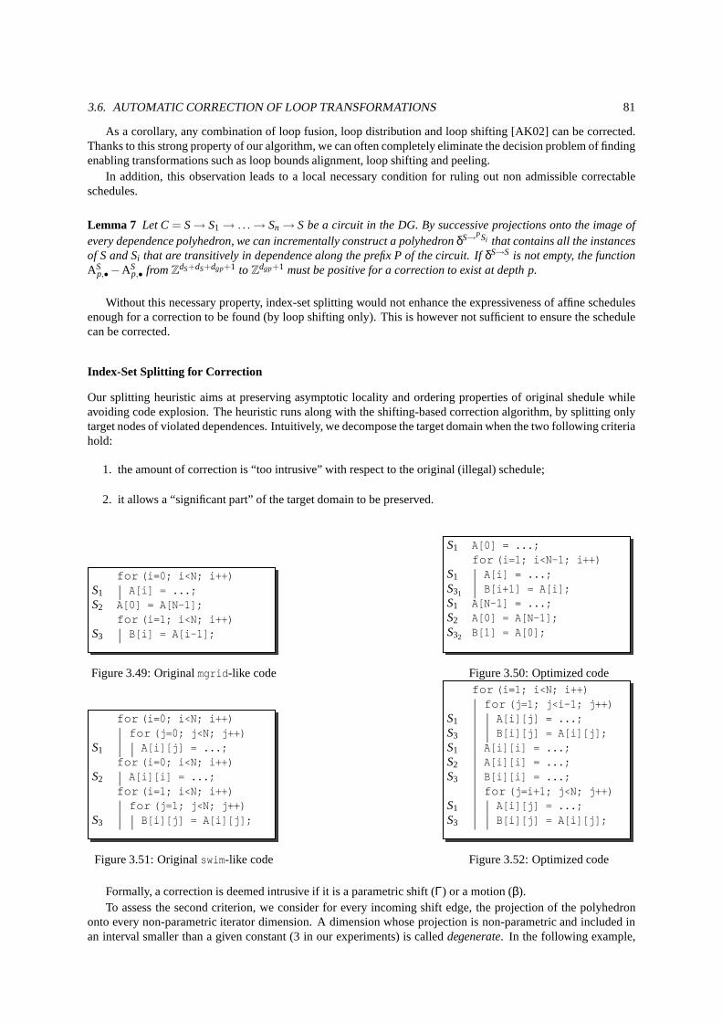
3.6. AUTOMATIC CORRECTION OF LOOP TRANSFORMATIONS 81
As a corollary, any combination of loop fusion, loop distribution and loop shifting [AK02] can be corrected.Thanks to this strong property of our algorithm, we can oftencompletely eliminate the decision problem of findingenabling transformations such as loop bounds alignment, loop shifting and peeling.
In addition, this observation leads to a local necessary condition for ruling out non admissible correctableschedules.
Lemma 7 Let C= S→ S1→ . . .→ Sn→ S be a circuit in the DG. By successive projections onto the image ofevery dependence polyhedron, we can incrementally construct a polyhedronδS→PSi that contains all the instancesof S and Si that are transitively in dependence along the prefix P of the circuit. If δS→S is not empty, the functionAS
p,•−ASp,• fromZdS+dS+dgp+1 to Zdgp+1 must be positive for a correction to exist at depth p.
Without this necessary property, index-set splitting would not enhance the expressiveness of affine schedulesenough for a correction to be found (by loop shifting only). This is however not sufficient to ensure the schedulecan be corrected.
Index-Set Splitting for Correction
Our splitting heuristic aims at preserving asymptotic locality and ordering properties of original shedule whileavoiding code explosion. The heuristic runs along with the shifting-based correction algorithm, by splitting onlytarget nodes of violated dependences. Intuitively, we decompose the target domain when the two following criteriahold:
1. the amount of correction is “too intrusive” with respect to the original (illegal) schedule;
2. it allows a “significant part” of the target domain to be preserved.
for (i=0; i<N; i++)S1 A[i] = ...;S2 A[0] = A[N-1];
for (i=1; i<N; i++)S3 B[i] = A[i-1];
Figure 3.49: Originalmgrid-like code
S1 A[0] = ...;for (i=1; i<N-1; i++)
S1 A[i] = ...;S31 B[i+1] = A[i];S1 A[N-1] = ...;S2 A[0] = A[N-1];S32 B[1] = A[0];
Figure 3.50: Optimized code
for (i=0; i<N; i++)for (j=0; j<N; j++)
S1 A[i][j] = ...;for (i=0; i<N; i++)
S2 A[i][i] = ...;for (i=1; i<N; i++)for (j=1; j<N; j++)
S3 B[i][j] = A[i][j];
Figure 3.51: Originalswim-like code
for (i=1; i<N; i++)for (j=1; j<i-1; j++)
S1 A[i][j] = ...;S3 B[i][j] = A[i][j];S1 A[i][i] = ...;S2 A[i][i] = ...;S3 B[i][i] = ...;
for (j=i+1; j<N; j++)S1 A[i][j] = ...;S3 B[i][j] = A[i][j];
Figure 3.52: Optimized code
Formally, a correction is deemed intrusive if it is a parametric shift (Γ) or a motion (β).To assess the second criterion, we consider for every incoming shift edge, the projection of the polyhedron
onto every non-parametric iterator dimension. A dimensionwhose projection is non-parametric and included inan interval smaller than a given constant (3 in our experiments) is calleddegenerate. In the following example,

82 CHAPTER 3. POLYHEDRAL PROGRAM MANIPULATION
dimensionj is degenerate:
−2i + 3 j + 4M + 5 ≥ 0i + j − M + 2 ≥ 0i − 3 j + 2M − 9 ≥ 0−i + M ≥ 0i ≥ 0
which simplifies into 2i +2≥ 6 j ≥ 2i−5.To determine if a domain split should be performed, we incrementally remove violated parts of the target
domain corresponding to intrusive corrections until either: we run out of incoming violations, or the remainingpart of the domain is degenerate.
The intuition is to keep a non-degenerate core of the domain free of any parametric correction, to preservelocality properties of the original schedule. In the end, ifthe remaining portion of the domain still has the samedimension as the original one, a split is performed that separates the statement into the core that is not in violationand the rest of the domain.
Index set splitting is thus plugged into our correction algorithm as a preconditioning phase before step 4 ofFigure 3.38.
Notice that a statement is only splitted a finite number of times, since each incoming shift edge is split at mostonce at each depth.
To limit the number of duplications, we allow only the core ofa domain to be split among successive correc-tions. If a statement has already been decomposed at a given depth, only its core still exhibits the same localityproperties as the original schedule. It is then unnecessary, and even harmful as far as code size is concerned, tofurther split the out-of-core part of the domain.
Figure 3.49 is a simplified version of one of the problems to solve when optimizingmgrid. The fusion of thefirst and third nests is clearly illegal since it would reverse the dependence from〈S1,N− 1〉 to 〈S2〉, as well asevery dependence from〈S1, i〉 to 〈S3, i + 1〉. To enable this fusion, it is sufficient to shift the scheduleof S2 byN−1 iterations and to shift the schedule ofS3 by 1 iteration. Fortunately, only iterationi = 0 of S3 (after shiftingby 1) is concerned by the violated dependence fromS2: peeling this iteration ofS3 gives rise toS31 andS32. Inturn,S31 is not concerned by the violation fromS2 while S32 must still be shifted byN−1 and eventually pops outof the loop. In the resulting code in Figure 3.50, the locality benefits of the fusion are preserved and the legality isensured.
A simplified version of theswim benchmark exhibits the need for a more complex split. The code in Fig-ure 3.51 features two doubly nested loops separated by an intermediate diagonal assignment loop, with poortemporal locality on arrayA. While allowing to maintain the order of the original schedule for a non-degenerate,triangular portion ofS1 andS3 instances (i.e.,{(i, j) ∈ [1,N] | j 6= i}); the code in Figure 3.52 also exhibits muchmore reuse opportunities and yields better performance.
While originally targeted at preserving locality properties of given schedules during correction, our methodalso succeeds at breaking cycles in a violated dependence graph. Consider the following example from Feautrieret al. [FGL99] given in Figure 3.53, AS1 is set to[0]. Since source and target parts of the domain are disjoint, anytransformation satisfies the previously defined feasibility criterion.
A self violation is detected provided iteratori statisfiesi ≥ 0 and−2i−2N≥ 0. This domain is not degeneratew.r.t. the original one, hence a split will occur for{i ≤ N}, which breaks the self violated dependence and allowsa correction at depth−1, yielding the alternate parallelized code.
for (i=0; i<N; i++)S1 A[2*N - i] = A[i];
AS1 = [1]βS1 = [0,0]ΓS1 = [0,0]
DOALL(i ∈ [0, N])S11 A[2*N - i] = A[i];
DOALL(i ∈ [N+1, 2∗N])S12 A[2*N - i] = A[i];
AS11 = [0] AS12 = [0]βS11 = [0,0] βS12 = [0,1]ΓS11 = [0,0] ΓS12 = [0,0]
Figure 3.53: Original and parallelized Code
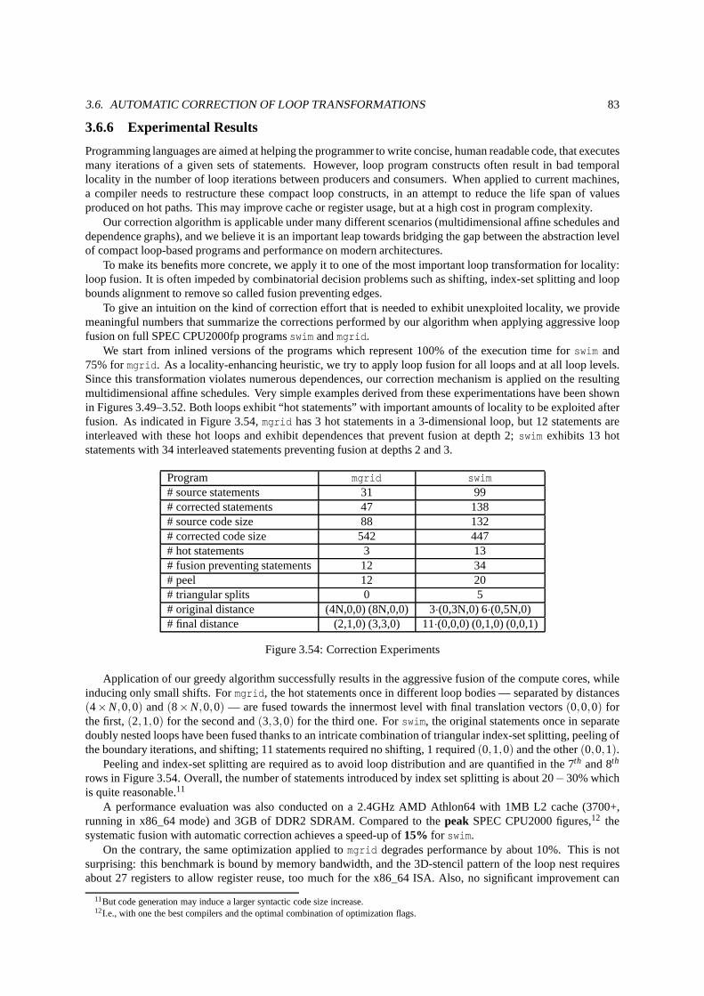
3.6. AUTOMATIC CORRECTION OF LOOP TRANSFORMATIONS 83
3.6.6 Experimental Results
Programming languages are aimed at helping the programmer to write concise, human readable code, that executesmany iterations of a given sets of statements. However, loopprogram constructs often result in bad temporallocality in the number of loop iterations between producersand consumers. When applied to current machines,a compiler needs to restructure these compact loop constructs, in an attempt to reduce the life span of valuesproduced on hot paths. This may improve cache or register usage, but at a high cost in program complexity.
Our correction algorithm is applicable under many different scenarios (multidimensional affine schedules anddependence graphs), and we believe it is an important leap towards bridging the gap between the abstraction levelof compact loop-based programs and performance on modern architectures.
To make its benefits more concrete, we apply it to one of the most important loop transformation for locality:loop fusion. It is often impeded by combinatorial decision problems such as shifting, index-set splitting and loopbounds alignment to remove so called fusion preventing edges.
To give an intuition on the kind of correction effort that is needed to exhibit unexploited locality, we providemeaningful numbers that summarize the corrections performed by our algorithm when applying aggressive loopfusion on full SPEC CPU2000fp programsswim andmgrid.
We start from inlined versions of the programs which represent 100% of the execution time forswim and75% formgrid. As a locality-enhancing heuristic, we try to apply loop fusion for all loops and at all loop levels.Since this transformation violates numerous dependences,our correction mechanism is applied on the resultingmultidimensional affine schedules. Very simple examples derived from these experimentations have been shownin Figures 3.49–3.52. Both loops exhibit “hot statements” with important amounts of locality to be exploited afterfusion. As indicated in Figure 3.54,mgrid has 3 hot statements in a 3-dimensional loop, but 12 statements areinterleaved with these hot loops and exhibit dependences that prevent fusion at depth 2;swim exhibits 13 hotstatements with 34 interleaved statements preventing fusion at depths 2 and 3.
Program mgrid swim# source statements 31 99# corrected statements 47 138# source code size 88 132# corrected code size 542 447# hot statements 3 13# fusion preventing statements 12 34# peel 12 20# triangular splits 0 5# original distance (4N,0,0) (8N,0,0) 3·(0,3N,0) 6·(0,5N,0)# final distance (2,1,0) (3,3,0) 11·(0,0,0) (0,1,0) (0,0,1)
Figure 3.54: Correction Experiments
Application of our greedy algorithm successfully results in the aggressive fusion of the compute cores, whileinducing only small shifts. Formgrid, the hot statements once in different loop bodies — separated by distances(4×N,0,0) and(8×N,0,0) — are fused towards the innermost level with final translation vectors(0,0,0) forthe first,(2,1,0) for the second and(3,3,0) for the third one. Forswim, the original statements once in separatedoubly nested loops have been fused thanks to an intricate combination of triangular index-set splitting, peeling ofthe boundary iterations, and shifting; 11 statements required no shifting, 1 required(0,1,0) and the other(0,0,1).
Peeling and index-set splitting are required as to avoid loop distribution and are quantified in the 7th and 8th
rows in Figure 3.54. Overall, the number of statements introduced by index set splitting is about 20−30% whichis quite reasonable.11
A performance evaluation was also conducted on a 2.4GHz AMD Athlon64 with 1MB L2 cache (3700+,running in x86_64 mode) and 3GB of DDR2 SDRAM. Compared to thepeak SPEC CPU2000 figures,12 thesystematic fusion with automatic correction achieves a speed-up of15% for swim.
On the contrary, the same optimization applied tomgrid degrades performance by about 10%. This is notsurprising: this benchmark is bound by memory bandwidth, and the 3D-stencil pattern of the loop nest requiresabout 27 registers to allow register reuse, too much for the x86_64 ISA. Also, no significant improvement can
11But code generation may induce a larger syntactic code size increase.12I.e., with one the best compilers and the optimal combination of optimization flags.
84 CHAPTER 3. POLYHEDRAL PROGRAM MANIPULATION
be expected regarding L2-cache locality (on top of the back-end compiler’s optimizations). The performancedegradation results from the complexity of the nest after loop peeling and shifting. We were not able to optimizemgrid for the Intel Itanium 2 processor due to unstabilities in theOpen64 compiler, but we expect strong speed-upson this platform.13
No existing optimizing compiler is capable (up to our knowledge) of discovering the opportunity and applyingsuch aggressive fusions. In addition, existing compilers deal with combinatorial decision problems associatedwith the selection of enabling transformations. All these decision problems disappear naturally with our correctionscheme, in favor of more powerful heuristics that aim at limiting the amount of duplication in the resulting codewhile enforcing the compute intensive part of the program benefits from locality or parallelization improvements.
We are exploring the application of this correction algorithm to the compression of optimization search spaces,combining empirical heuristics (e.g., Monte-Carlo searches and machine-learning) with linear programming tools[PBCV07]. We are also using these results in the design of a meta-programming environment for loop transfor-mations, where automatic correction allows to raise the level of abstraction for the expert programmer involved inthe semi-automatic optimization of a program.
3.7 Related Work
The closest technical work has already been discussed in theprevious sections. This section surveys the formerefforts in designing an advanced loop nest transformation infrastructure and representation framework.
Most loop restructuring compilers introduced syntax-based models and intermediate representations. ParaS-cope [CHH+93] and Polaris [BEF+96] are dependence based, source-to-source parallelizersfor Fortran. KAP[KAP] is closely related to these academic tools.
SUIF [H+96] is a platform for implementing advanced compiler prototypes. SUIF was the vehicle for impor-tant advances in polyhedral compilation [LL97, LLL01], butthe resulting prototypes had little impact due to aweak code generation method and the lack of scalability of the core algorithms. PIPS [IJT91] is one of the mostcomplete loop restructuring compiler, implementing interprocedural polyhedral analyses and transformations (in-cluding an advanced array region analysis, automatic parallelization at the function and loop level, and a limitedform of affine scheduling); it uses a syntax tree extended with polyhedral annotations, but not a unified polyhedralrepresentation.
Closer to our motivations, the MARS compiler [O’B98] has been applied to iterative optimization [KKGO01];this compiler’s goal is to unify classical dependence-based loop transformations with data storage optimizations.However, the MARS intermediate representation only captures part of the loop-specific information (domains andaccess functions): it lacks the characterization of iteration orderings through multidimensional affine schedules.Recently, a similar unified representation has been appliedto the optimization of compute-intensive Java pro-grams, combining machine learning and iterative optimization [LO04]; again, despite the unification of multipletransformations, the lack of multidimensional affine schedules hampers the ability to perform long sequences oftransformations and complicates the characterization andtraversal of the search space, ultimately limiting perfor-mance improvements.
To date, the most thorough application of the polyhedral representation was the Petit dependence analyzerand loop restructuring tool [Kel96], based on the Omega library [KPR95]. It provides space-time mappings foriteration reordering, and it shares our emphasis on per-statement transformations, but it is intended as a researchtool for small kernels only. Our representation — whose foundations were presented in [CGT04] — improves onthe polyhedral representation proposed by [Kel96], and this explains how and why it is the first one that enablesthe composition of polyhedral generalizations of classical loop transformations, decoupled from any syntacticform of the program. We show how classical transformations like loop fusion or tiling can be composed in anyorder and generalized to imperfectly-nested loops with complex domains, without intermediate translation to asyntactic form (which leads to code size explosion). Eventually, we use a code generation technique suitable to apolyhedral representation that is again significantly morerobust than the code generation proposed in the Omegalibrary [Bas04, VBC06].
13We try to fix these issues before the camera-ready version.
3.8. FUTURE WORK 85
3.8 Future Work
To avoid diminishing returns in tuning sequences of programtransformations, we advocate for the collapse ofmultiple optimization phases into a single, unconventional, iterative search algorithm. This said, it does not bringany concrete hope of any simplification of the problem... except if, by construction, the search space we exploreis much simpler than the cross-product of the search spaces of a sequence of optimisation phases.
We are still far from a general multi-purpose iterative optimization phase — if it exists — but we already madeone step in that direction: we built a search space suitable for iterative traversal that encompassesall legal programtransformations in a particular class. Technically, we considered the whole class of loop nest transformations thatcan be modeled asone-dimensional schedules[Fea92], a significant leap in model and search space complexitycompared to state-of-the-art applications of iterative optimization [PBCV07]. This is only a preliminary step, butit will shape our future work in the area. Up to now, we made thefollowing contributions:
• we statically construct the optimization space of all, arbitrarily complex, arbitrarily long sequences of looptransformations that can be expressed as one-dimensional affine schedules (using a polyhedral abstraction);
• this search space is built free of illegal and redundant transformation sequences, avoiding them altogetherat the very source of the exploration;
• we demonstrate multiple orders of magnitude reduction in the size of the search space, compared to filtering-based approaches on loop transformation sequences or state-of-the-art affine schedule enumeration tech-niques;
• these smaller search spaces are amenable to fast-converging, mathematically founded operation researchalgorithms, allowing to compute the exact size of the space and to traverse it exhaustively;
• our approach is compatible with acceleration techniques for feedback-directed optimization, in particularon machine-learning techniques which focus the search to a narrow set of most promising transformations;
• our source-to-source transformation tool yields significant performance gains on top of a heavily tuned,aggressive optimizing compiler.
We are extending this approach to multi-dimensional schedules, using empirical and statistical sampling tech-niques to learn how good schedules distribute dependences across multiple time dimensions. Also we can onlyapply such radical techniques to small codes, we will make all efforts to scale those to real-size benchmarks,building on modular affine scheduling approaches, algorithmic and mathematical formulation improvements, andempirical decoupling of the constraints.
3.9 Conclusion
The ability to perform numerous compositions of program transformations is driven by the development of iter-ative optimization environments, and motivated through the manual optimization of standard numerical bench-marks. From these experiments, we show that current compilers are challenged by the complexity of aggressiveloop optimization sequences. We believe that little improvements can be expected without redesigning the com-pilation infrastructure for compositionality and richer search space structure.
We presented a polyhedral framework that enables the composition of long sequences of program transforma-tions. Coupled with a robust code generator, our method avoids the typical restrictions and code bloat of long com-positions of program transformations. These techniques have been implemented in the Open64/ORC/EKOPathcompiler and applied to theswim benchmark automatically. We have also shown that our framework opens upnew directions for searching for complex transformation sequences for automatic or semi-automatic optimizationor parallelization.
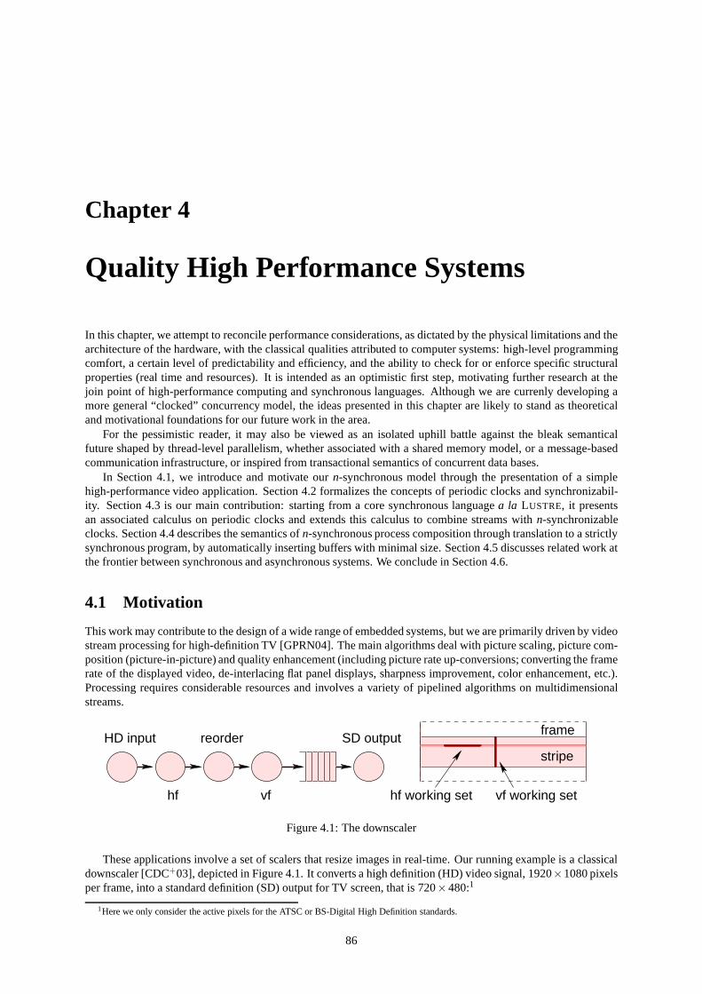
Chapter 4
Quality High Performance Systems
In this chapter, we attempt to reconcile performance considerations, as dictated by the physical limitations and thearchitecture of the hardware, with the classical qualitiesattributed to computer systems: high-level programmingcomfort, a certain level of predictability and efficiency, and the ability to check for or enforce specific structuralproperties (real time and resources). It is intended as an optimistic first step, motivating further research at thejoin point of high-performance computing and synchronous languages. Although we are currenly developing amore general “clocked” concurrency model, the ideas presented in this chapter are likely to stand as theoreticaland motivational foundations for our future work in the area.
For the pessimistic reader, it may also be viewed as an isolated uphill battle against the bleak semanticalfuture shaped by thread-level parallelism, whether associated with a shared memory model, or a message-basedcommunication infrastructure, or inspired from transactional semantics of concurrent data bases.
In Section 4.1, we introduce and motivate ourn-synchronous model through the presentation of a simplehigh-performance video application. Section 4.2 formalizes the concepts of periodic clocks and synchronizabil-ity. Section 4.3 is our main contribution: starting from a core synchronous languagea la LUSTRE, it presentsan associated calculus on periodic clocks and extends this calculus to combine streams withn-synchronizableclocks. Section 4.4 describes the semantics ofn-synchronous process composition through translation to astrictlysynchronous program, by automatically inserting buffers with minimal size. Section 4.5 discusses related work atthe frontier between synchronous and asynchronous systems. We conclude in Section 4.6.
4.1 Motivation
This work may contribute to the design of a wide range of embedded systems, but we are primarily driven by videostream processing for high-definition TV [GPRN04]. The mainalgorithms deal with picture scaling, picture com-position (picture-in-picture) and quality enhancement (including picture rate up-conversions; converting the framerate of the displayed video, de-interlacing flat panel displays, sharpness improvement, color enhancement, etc.).Processing requires considerable resources and involves avariety of pipelined algorithms on multidimensionalstreams.
stripe
frame
hf
HD input
vf
SD output
vf working sethf working set
reorder
Figure 4.1: The downscaler
These applications involve a set of scalers that resize images in real-time. Our running example is a classicaldownscaler [CDC+03], depicted in Figure 4.1. It converts a high definition (HD) video signal, 1920×1080 pixelsper frame, into a standard definition (SD) output for TV screen, that is 720×480:1
1Here we only consider the active pixels for the ATSC or BS-Digital High Definition standards.
86
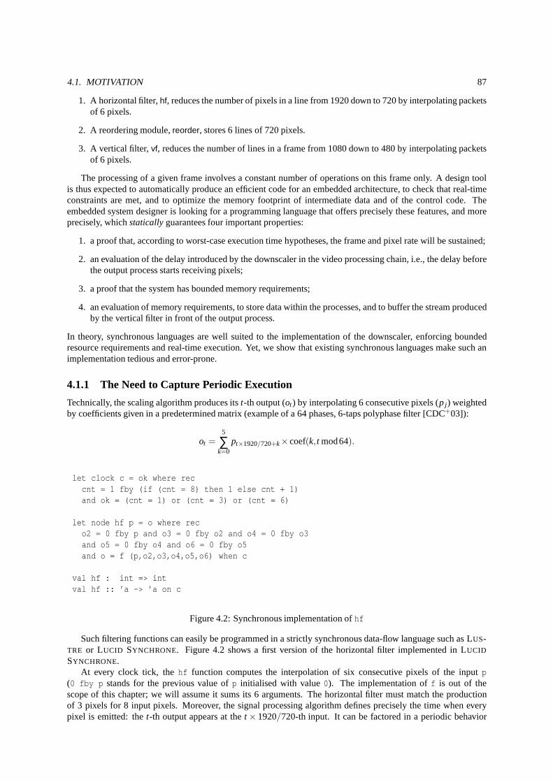
4.1. MOTIVATION 87
1. A horizontal filter,hf, reduces the number of pixels in a line from 1920 down to 720 byinterpolating packetsof 6 pixels.
2. A reordering module,reorder, stores 6 lines of 720 pixels.
3. A vertical filter,vf, reduces the number of lines in a frame from 1080 down to 480 byinterpolating packetsof 6 pixels.
The processing of a given frame involves a constant number ofoperations on this frame only. A design toolis thus expected to automatically produce an efficient code for an embedded architecture, to check that real-timeconstraints are met, and to optimize the memory footprint ofintermediate data and of the control code. Theembedded system designer is looking for a programming language that offers precisely these features, and moreprecisely, whichstaticallyguarantees four important properties:
1. a proof that, according to worst-case execution time hypotheses, the frame and pixel rate will be sustained;
2. an evaluation of the delay introduced by the downscaler inthe video processing chain, i.e., the delay beforethe output process starts receiving pixels;
3. a proof that the system has bounded memory requirements;
4. an evaluation of memory requirements, to store data within the processes, and to buffer the stream producedby the vertical filter in front of the output process.
In theory, synchronous languages are well suited to the implementation of the downscaler, enforcing boundedresource requirements and real-time execution. Yet, we show that existing synchronous languages make such animplementation tedious and error-prone.
4.1.1 The Need to Capture Periodic Execution
Technically, the scaling algorithm produces itst-th output (ot) by interpolating 6 consecutive pixels (p j ) weightedby coefficients given in a predetermined matrix (example of a64 phases, 6-taps polyphase filter [CDC+03]):
ot =5
∑k=0
pt×1920/720+k×coef(k,t mod64).
let clock c = ok where reccnt = 1 fby (if (cnt = 8) then 1 else cnt + 1)and ok = (cnt = 1) or (cnt = 3) or (cnt = 6)
let node hf p = o where reco2 = 0 fby p and o3 = 0 fby o2 and o4 = 0 fby o3and o5 = 0 fby o4 and o6 = 0 fby o5and o = f (p,o2,o3,o4,o5,o6) when c
val hf : int => intval hf :: ’a -> ’a on c
Figure 4.2: Synchronous implementation ofhf
Such filtering functions can easily be programmed in a strictly synchronous data-flow language such as LUS-TRE or LUCID SYNCHRONE. Figure 4.2 shows a first version of the horizontal filter implemented in LUCID
SYNCHRONE.At every clock tick, thehf function computes the interpolation of six consecutive pixels of the inputp
(0 fby p stands for the previous value ofp initialised with value0). The implementation off is out of thescope of this chapter; we will assume it sums its 6 arguments.The horizontal filter must match the productionof 3 pixels for 8 input pixels. Moreover, the signal processing algorithm defines precisely the time when everypixel is emitted: thet-th output appears at thet × 1920/720-th input. It can be factored in a periodic behavior
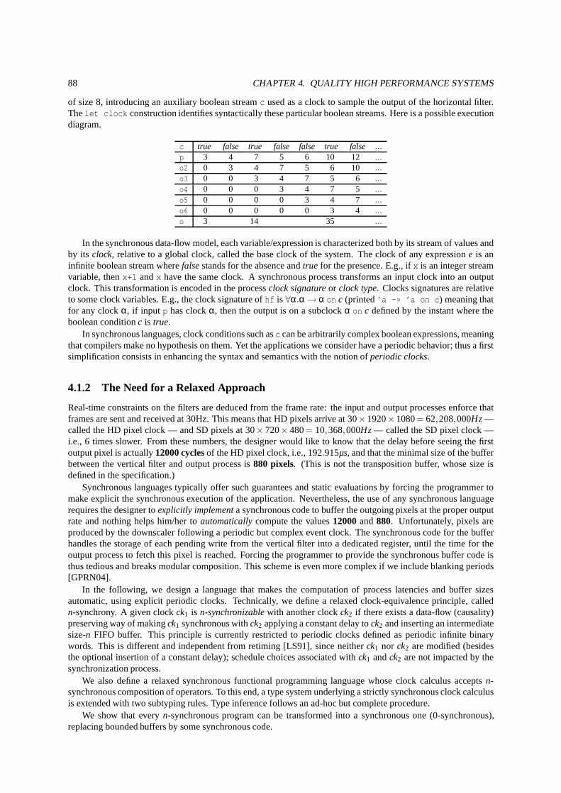
88 CHAPTER 4. QUALITY HIGH PERFORMANCE SYSTEMS
of size 8, introducing an auxiliary boolean streamc used as a clock to sample the output of the horizontal filter.Thelet clock construction identifies syntactically these particular boolean streams. Here is a possible executiondiagram.
c true false true false false true false...p 3 4 7 5 6 10 12 ...
o2 0 3 4 7 5 6 10 ...
o3 0 0 3 4 7 5 6 ...
o4 0 0 0 3 4 7 5 ...
o5 0 0 0 0 3 4 7 ...
o6 0 0 0 0 0 3 4 ...
o 3 14 35 ...
In the synchronous data-flow model, each variable/expression is characterized both by its stream of values andby its clock, relative to a global clock, called the base clock of the system. The clock of any expressione is aninfinite boolean stream wherefalsestands for the absence andtrue for the presence. E.g., ifx is an integer streamvariable, thenx+1 andx have the same clock. A synchronous process transforms an input clock into an outputclock. This transformation is encoded in the processclock signatureor clock type. Clocks signatures are relativeto some clock variables. E.g., the clock signature ofhf is ∀α.α→ α on c (printed’a -> ’a on c) meaning thatfor any clockα, if input p has clockα, then the output is on a subclockα on c defined by the instant where theboolean conditionc is true.
In synchronous languages, clock conditions such asc can be arbitrarily complex boolean expressions, meaningthat compilers make no hypothesis on them. Yet the applications we consider have a periodic behavior; thus a firstsimplification consists in enhancing the syntax and semantics with the notion ofperiodic clocks.
4.1.2 The Need for a Relaxed Approach
Real-time constraints on the filters are deduced from the frame rate: the input and output processes enforce thatframes are sent and received at 30Hz. This means that HD pixels arrive at 30×1920×1080= 62,208,000Hz—called the HD pixel clock — and SD pixels at 30×720×480= 10,368,000Hz— called the SD pixel clock —i.e., 6 times slower. From these numbers, the designer wouldlike to know that the delay before seeing the firstoutput pixel is actually12000 cyclesof the HD pixel clock, i.e., 192.915µs, and that the minimal size of the bufferbetween the vertical filter and output process is880 pixels. (This is not the transposition buffer, whose size isdefined in the specification.)
Synchronous languages typically offer such guarantees andstatic evaluations by forcing the programmer tomake explicit the synchronous execution of the application. Nevertheless, the use of any synchronous languagerequires the designer toexplicitly implementa synchronous code to buffer the outgoing pixels at the proper outputrate and nothing helps him/her toautomaticallycompute the values12000and880. Unfortunately, pixels areproduced by the downscaler following a periodic but complexevent clock. The synchronous code for the bufferhandles the storage of each pending write from the vertical filter into a dedicated register, until the time for theoutput process to fetch this pixel is reached. Forcing the programmer to provide the synchronous buffer code isthus tedious and breaks modular composition. This scheme iseven more complex if we include blanking periods[GPRN04].
In the following, we design a language that makes the computation of process latencies and buffer sizesautomatic, using explicit periodic clocks. Technically, we define a relaxed clock-equivalence principle, calledn-synchrony. A given clockck1 is n-synchronizablewith another clockck2 if there exists a data-flow (causality)preserving way of makingck1 synchronous withck2 applying a constant delay tock2 and inserting an intermediatesize-n FIFO buffer. This principle is currently restricted to periodic clocks defined as periodic infinite binarywords. This is different and independent from retiming [LS91], since neitherck1 nor ck2 are modified (besidesthe optional insertion of a constant delay); schedule choices associated withck1 andck2 are not impacted by thesynchronization process.
We also define a relaxed synchronous functional programminglanguage whose clock calculus acceptsn-synchronous composition of operators. To this end, a type system underlying a strictly synchronous clock calculusis extended with two subtyping rules. Type inference follows an ad-hoc but complete procedure.
We show that everyn-synchronous program can be transformed into a synchronousone (0-synchronous),replacing bounded buffers by some synchronous code.
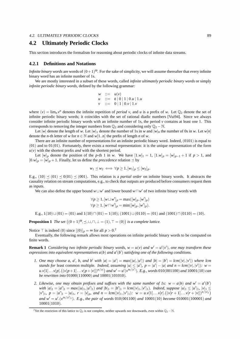
4.2. ULTIMATELY PERIODIC CLOCKS 89
4.2 Ultimately Periodic Clocks
This section introduces the formalism for reasoning about periodic clocks of infinite data streams.
4.2.1 Definitions and Notations
Infinite binary wordsare words of(0+1)ω. For the sake of simplicity, we will assume thereafter that every infinitebinary word has an infinite number of 1s.
We are mostly interested in a subset of these words, calledinfinite ultimately periodic binary wordsor simplyinfinite periodic binary words,defined by the following grammar:
w ::= u(v)u ::= ε | 0 | 1 | 0.u | 1.uv ::= 0 | 1 | 0.v | 1.v
where(v) = limnvn denotes the infinite repetition ofperiod v, andu is a prefix ofw. Let Q2 denote the set ofinfinite periodic binary words; it coincides with the set of rational diadic numbers [Vui94]. Since we alwaysconsider infinite periodic binary words with an infinite number of 1s, the periodv contains at least one 1. Thiscorresponds to removing the integer numbers fromQ2 and considering onlyQ2−N.
Let |w| denote the length ofw. Let |w|1 denote the number of 1s inw and|w|0 the number of 0s inw. Let w[n]denote then-th letter ofw for n∈N andw[1..n] the prefix of lengthn of w.
There are an infinite number of representations for an infinite periodic binary word. Indeed,(0101) is equal to(01) and to 01(01). Fortunately, there exists a normal representation: it is the unique representation of the formu(v) with the shortest prefixandwith the shortest period.
Let [w]p denote the position of thep-th 1 in w. We have[1.w]1 = 1, [1.w]p = [w]p−1 + 1 if p > 1, and[0.w]p = [w]p +1. Finally, let us define theprecedencerelation� by
w1 � w2 ⇐⇒ ∀p≥ 1, [w1]p≤ [w2]p.
E.g., (10) � (01) � 0(01) � (001). This relation is apartial order on infinite binary words. It abstracts thecausality relation on stream computations, e.g., to check that outputs are produced before consumers request themas inputs.
We can also define the upper boundw⊔w′ and lower boundw⊓w′ of two infinite binary words with
∀p≥ 1, [w⊔w′]p = max([w]p, [w′]p)
∀p≥ 1, [w⊓w′]p = min([w]p, [w′]p).
E.g., 1(10)⊔ (01) = (01) and 1(10)⊓ (01) = 1(10); (1001)⊔ (0110)= (01) and(1001)⊓ (0110) = (10).
Proposition 1 The set(
(0+1)ω,�,⊔,⊓,⊥ = (1),⊤= (0))
is a complete lattice.
Notice⊤ is indeed(0) since[(0)]p = ∞ for all p > 0.2
Eventually, the following remark allows most operations oninfinite periodic binary words to be computed onfinite words.
Remark 1 Considering two infinite periodic binary words, w= u(v) and w′ = u′(v′), one may transform theseexpressions into equivalent representatives a(b) and a′(b′) satisfying one of the following conditions.
1. One may choose a, a′, b, and b′ with |a| = |a′| = max(|u|, |u′|) and |b| = |b′| = lcm(|v|, |v′|) where lcmstands forleast common multiple. Indeed, assuming|u| ≤ |u′|, p = |u′| − |u| and n= lcm(|v|, |v′|): w =
u.v[1] . . .v[p].(
(v[p+1] . . .v[p+ |v|])n/|v|)
and w′ = u′(v′n/|v′|). E.g., words010(001100) and10001(10) canbe rewritten into01000(110000) and10001(101010).
2. Likewise, one may obtain prefixes and suffixes with the samenumber of 1s: w= a(b) and w′ = a′(b′)with |a|1 = |a′|1 = max(|u|1, |u′|1) and |b|1 = |b′|1 = lcm(|v|1, |v′|1). Indeed, suppose|u|1 ≤ |u′|1, |v|1 ≤|v′|1, p = |u′|1− |u|1, r = [v]p, and n= lcm(|v|1, |v′|1): w = u.v[1] . . .v[r].
(
(v[r + 1] . . .v[r + |v|])n/|v|1)
and w′ = u′.(v′n/|v′|1). E.g., the pair of words010(001100) and10001(10) become010001(100001) and10001(1010).
2Yet the restriction of this lattice toQ2 is not complete, neither upwards nor downwards, even withinQ2−N.
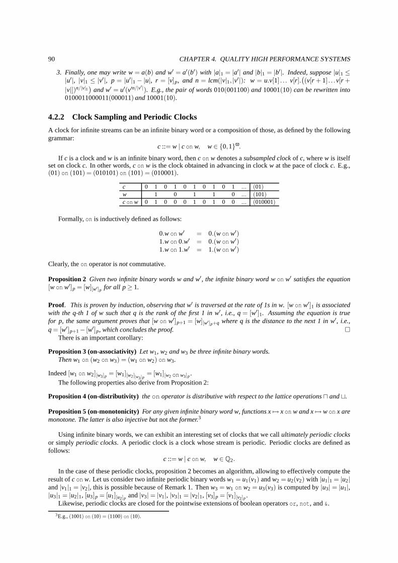
90 CHAPTER 4. QUALITY HIGH PERFORMANCE SYSTEMS
3. Finally, one may write w= a(b) and w′ = a′(b′) with |a|1 = |a′| and |b|1 = |b′|. Indeed, suppose|u|1 ≤|u′|, |v|1 ≤ |v′|, p = |u′|1− |u|, r = [v]p, and n= lcm(|v|1, |v′|): w = u.v[1] . . . v[r].
(
(v[r + 1] . . .v[r +
|v|])n/|v|1)
and w′ = u′(v′n/|v′|). E.g., the pair of words010(001100) and10001(10) can be rewritten into0100011000011(000011) and10001(10).
4.2.2 Clock Sampling and Periodic Clocks
A clock for infinite streams can be an infinite binary word or a composition of those, as defined by the followinggrammar:
c ::= w | c on w, w∈ {0,1}ω.
If c is a clock andw is an infinite binary word, thenc on w denotes asubsampled clockof c, wherew is itselfset on clockc. In other words,c on w is the clock obtained in advancing in clockw at the pace of clockc. E.g.,(01) on (101) = (010101) on (101) = (010001).
c 0 1 0 1 0 1 0 1 0 1 ... (01)w 1 0 1 1 0 ... (101)c on w 0 1 0 0 0 1 0 1 0 0 ... (010001)
Formally,on is inductively defined as follows:
0.w on w′ = 0.(w on w′)1.w on 0.w′ = 0.(w on w′)1.w on 1.w′ = 1.(w on w′)
Clearly, theon operator isnot commutative.
Proposition 2 Given two infinite binary words w and w′, the infinite binary word won w′ satisfies the equation[w on w′]p = [w][w′]p for all p≥ 1.
Proof. This is proven by induction, observing that w′ is traversed at the rate of 1s in w.[w on w′]1 is associatedwith the q-th 1 of w such that q is the rank of the first 1 in w′, i.e., q= [w′]1. Assuming the equation is truefor p, the same argument proves that[w on w′]p+1 = [w][w′]p+q where q is the distance to the next 1 in w′, i.e.,q = [w′]p+1− [w′]p, which concludes the proof. �
There is an important corollary:
Proposition 3 (on-associativity)Let w1, w2 and w3 be three infinite binary words.Then w1 on (w2 on w3) = (w1 on w2) on w3.
Indeed[w1 on w2][w3]p = [w1][w2][w3]p= [w1][w2 on w3]p.
The following properties also derive from Proposition 2:
Proposition 4 (on-distributivity) theon operator is distributive with respect to the lattice operations⊓ and⊔.
Proposition 5 (on-monotonicity) For any given infinite binary word w, functions x7→ xon w and x7→won x aremonotone. The latter is also injective butnot the former.3
Using infinite binary words, we can exhibit an interesting set of clocks that we callultimately periodic clocksor simply periodic clocks. A periodic clock is a clock whose stream is periodic. Periodic clocks are defined asfollows:
c ::= w | c on w, w∈Q2.
In the case of these periodic clocks, proposition 2 becomes an algorithm, allowing to effectively compute theresult ofc on w. Let us consider two infinite periodic binary wordsw1 = u1(v1) andw2 = u2(v2) with |u1|1 = |u2|and|v1|1 = |v2|, this is possible because of Remark 1. Thenw3 = w1 on w2 = u3(v3) is computed by|u3| = |u1|,|u3|1 = |u2|1, [u3]p = [u1][u2]p and|v3|= |v1|, |v3|1 = |v2|1, [v3]p = [v1][v2]p.
Likewise, periodic clocks are closed for the pointwise extensions of boolean operatorsor, not, and&.
3E.g.,(1001) on (10) = (1100) on (10).
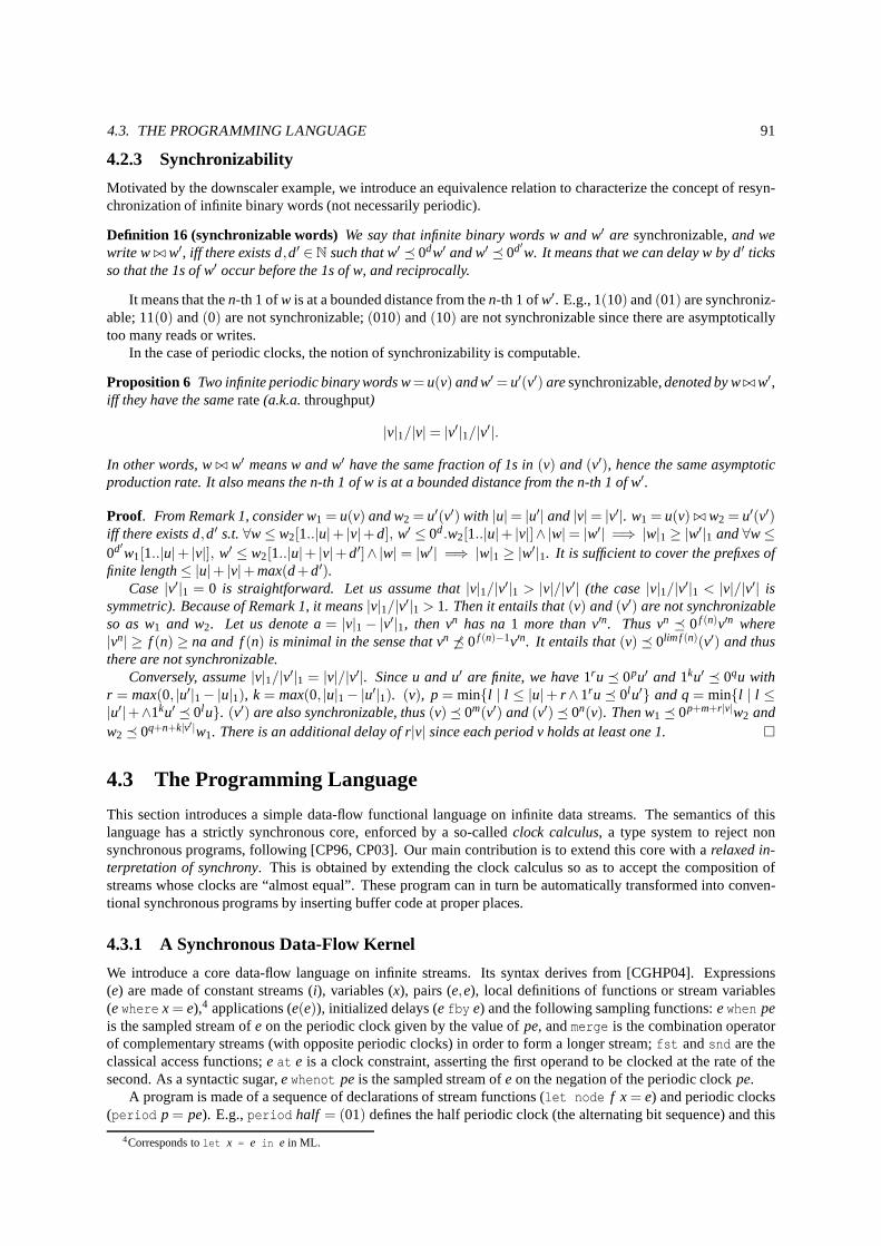
4.3. THE PROGRAMMING LANGUAGE 91
4.2.3 Synchronizability
Motivated by the downscaler example, we introduce an equivalence relation to characterize the concept of resyn-chronization of infinite binary words (not necessarily periodic).
Definition 16 (synchronizable words) We say that infinite binary words w and w′ are synchronizable, and wewrite w⊲⊳ w′, iff there exists d,d′ ∈N such that w′ � 0dw′ and w′ � 0d′w. It means that we can delay w by d′ ticksso that the 1s of w′ occur before the 1s of w, and reciprocally.
It means that then-th 1 ofw is at a bounded distance from then-th 1 ofw′. E.g., 1(10) and(01) are synchroniz-able; 11(0) and(0) are not synchronizable;(010) and(10) are not synchronizable since there are asymptoticallytoo many reads or writes.
In the case of periodic clocks, the notion of synchronizability is computable.
Proposition 6 Two infinite periodic binary words w= u(v) and w′= u′(v′) aresynchronizable, denoted by w⊲⊳ w′,iff they have the samerate(a.k.a.throughput)
|v|1/|v|= |v′|1/|v
′|.
In other words, w⊲⊳ w′ means w and w′ have the same fraction of 1s in(v) and(v′), hence the same asymptoticproduction rate. It also means the n-th 1 of w is at a bounded distance from the n-th 1 of w′.
Proof. From Remark 1, consider w1 = u(v) and w2 = u′(v′) with |u|= |u′| and|v|= |v′|. w1 = u(v) ⊲⊳ w2 = u′(v′)iff there exists d,d′ s.t.∀w≤ w2[1..|u|+ |v|+d], w′ ≤ 0d.w2[1..|u|+ |v|]∧|w|= |w′| =⇒ |w|1 ≥ |w′|1 and∀w≤0d′w1[1..|u|+ |v|], w′ ≤ w2[1..|u|+ |v|+d′]∧|w| = |w′| =⇒ |w|1 ≥ |w′|1. It is sufficient to cover the prefixes offinite length≤ |u|+ |v|+max(d+d′).
Case|v′|1 = 0 is straightforward. Let us assume that|v|1/|v′|1 > |v|/|v′| (the case|v|1/|v′|1 < |v|/|v′| issymmetric). Because of Remark 1, it means|v|1/|v′|1 > 1. Then it entails that(v) and(v′) are not synchronizableso as w1 and w2. Let us denote a= |v|1− |v′|1, then vn has na1 more than v′n. Thus vn � 0f (n)v′n where|vn| ≥ f (n) ≥ na and f(n) is minimal in the sense that vn 6� 0f (n)−1v′n. It entails that(v) � 0lim f (n)(v′) and thusthere are not synchronizable.
Conversely, assume|v|1/|v′|1 = |v|/|v′|. Since u and u′ are finite, we have1ru� 0pu′ and 1ku′ � 0qu withr = max(0, |u′|1− |u|1), k = max(0, |u|1− |u′|1). (v), p = min{l | l ≤ |u|+ r ∧1ru� 0l u′} and q= min{l | l ≤|u′|+∧1ku′ � 0l u}. (v′) are also synchronizable, thus(v)� 0m(v′) and(v′)� 0n(v). Then w1 � 0p+m+r|v|w2 andw2 � 0q+n+k|v′|w1. There is an additional delay of r|v| since each period v holds at least one 1. �
4.3 The Programming Language
This section introduces a simple data-flow functional language on infinite data streams. The semantics of thislanguage has a strictly synchronous core, enforced by a so-called clock calculus, a type system to reject nonsynchronous programs, following [CP96, CP03]. Our main contribution is to extend this core with arelaxed in-terpretation of synchrony. This is obtained by extending the clock calculus so as to accept the composition ofstreams whose clocks are “almost equal”. These program can in turn be automatically transformed into conven-tional synchronous programs by inserting buffer code at proper places.
4.3.1 A Synchronous Data-Flow Kernel
We introduce a core data-flow language on infinite streams. Its syntax derives from [CGHP04]. Expressions(e) are made of constant streams (i), variables (x), pairs (e,e), local definitions of functions or stream variables(ewhere x = e),4 applications (e(e)), initialized delays (efby e) and the following sampling functions:ewhen peis the sampled stream ofe on the periodic clock given by the value ofpe, andmerge is the combination operatorof complementary streams (with opposite periodic clocks) in order to form a longer stream;fst andsnd are theclassical access functions;eat e is a clock constraint, asserting the first operand to be clocked at the rate of thesecond. As a syntactic sugar,ewhenot pe is the sampled stream ofe on the negation of the periodic clockpe.
A program is made of a sequence of declarations of stream functions (let node f x = e) and periodic clocks(period p = pe). E.g.,period half = (01) defines the half periodic clock (the alternating bit sequence) and this
4Corresponds tolet x = e in e in ML.
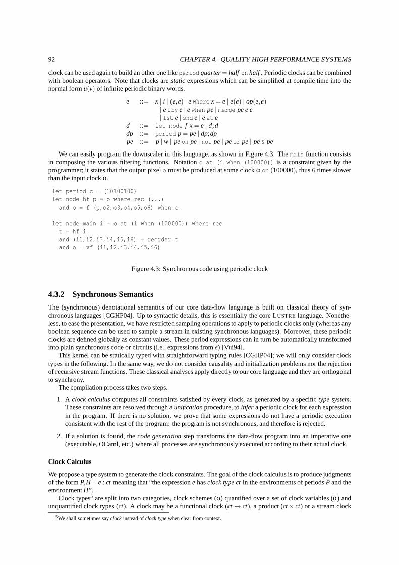
92 CHAPTER 4. QUALITY HIGH PERFORMANCE SYSTEMS
clock can be used again to build an other one likeperiod quarter= half on half. Periodic clocks can be combinedwith boolean operators. Note that clocks arestaticexpressions which can be simplified at compile time into thenormal formu(v) of infinite periodic binary words.
e ::= x | i | (e,e) | ewhere x = e | e(e) | op(e,e)| efby e | ewhen pe| merge pe e e| fst e | snd e | eat e
d ::= let node f x = e | d;ddp ::= period p = pe| dp;dppe ::= p |w | peon pe| not pe| peor pe| pe& pe
We can easily program the downscaler in this language, as shown in Figure 4.3. Themain function consistsin composing the various filtering functions. Notationo at (i when (100000)) is a constraint given by theprogrammer; it states that the output pixelo must be produced at some clockα on (100000), thus 6 times slowerthan the input clockα.
let period c = (10100100)let node hf p = o where rec (...)
and o = f (p,o2,o3,o4,o5,o6) when c
let node main i = o at (i when (100000)) where rect = hf iand (i1,i2,i3,i4,i5,i6) = reorder tand o = vf (i1,i2,i3,i4,i5,i6)
Figure 4.3: Synchronous code using periodic clock
4.3.2 Synchronous Semantics
The (synchronous) denotational semantics of our core data-flow language is built on classical theory of syn-chronous languages [CGHP04]. Up to syntactic details, thisis essentially the core LUSTRE language. Nonethe-less, to ease the presentation, we have restricted samplingoperations to apply to periodic clocks only (whereas anyboolean sequence can be used to sample a stream in existing synchronous languages). Moreover, these periodicclocks are defined globally as constant values. These periodexpressions can in turn be automatically transformedinto plain synchronous code or circuits (i.e., expressionsfrom e) [Vui94].
This kernel can be statically typed with straightforward typing rules [CGHP04]; we will only consider clocktypes in the following. In the same way, we do not consider causality and initialization problems nor the rejectionof recursive stream functions. These classical analyses apply directly to our core language and they are orthogonalto synchrony.
The compilation process takes two steps.
1. A clock calculuscomputes all constraints satisfied by every clock, as generated by a specifictype system.These constraints are resolved through aunificationprocedure, toinfer a periodic clock for each expressionin the program. If there is no solution, we prove that some expressions do not have a periodic executionconsistent with the rest of the program: the program is not synchronous, and therefore is rejected.
2. If a solution is found, thecode generationstep transforms the data-flow program into an imperative one(executable, OCaml, etc.) where all processes are synchronously executed according to their actual clock.
Clock Calculus
We propose a type system to generate the clock constraints. The goal of the clock calculus is to produce judgmentsof the formP,H ⊢ e : ct meaning that “the expressione hasclock type ctin the environments of periodsP and theenvironmentH”.
Clock types5 are split into two categories, clock schemes (σ) quantified over a set of clock variables (α) andunquantified clock types (ct). A clock may be a functional clock (ct→ ct), a product (ct× ct) or a stream clock
5We shall sometimes sayclock instead ofclock typewhen clear from context.
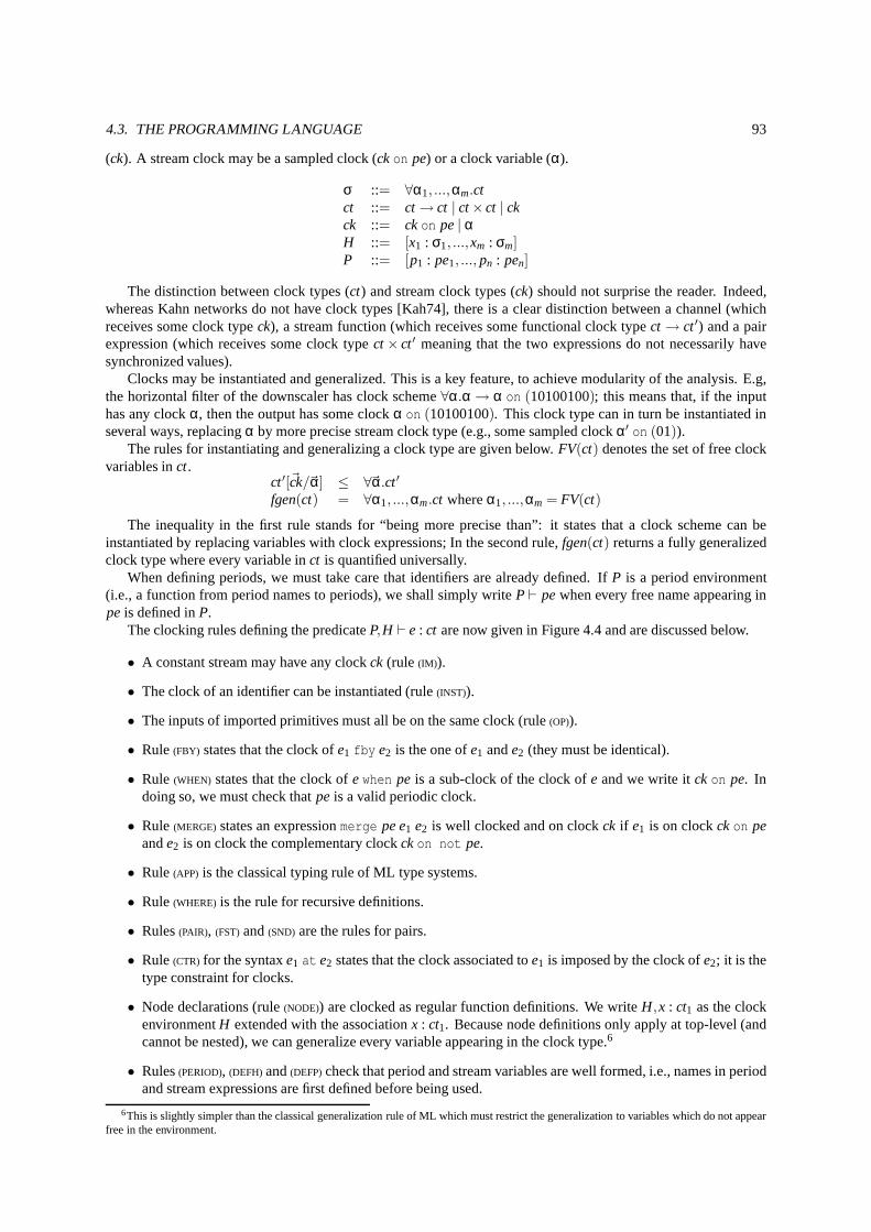
4.3. THE PROGRAMMING LANGUAGE 93
(ck). A stream clock may be a sampled clock (ckon pe) or a clock variable (α).
σ ::= ∀α1, ...,αm.ctct ::= ct→ ct | ct×ct | ckck ::= ckon pe| αH ::= [x1 : σ1, ...,xm : σm]P ::= [p1 : pe1, ..., pn : pen]
The distinction between clock types (ct) and stream clock types (ck) should not surprise the reader. Indeed,whereas Kahn networks do not have clock types [Kah74], thereis a clear distinction between a channel (whichreceives some clock typeck), a stream function (which receives some functional clock typect→ ct′) and a pairexpression (which receives some clock typect× ct′ meaning that the two expressions do not necessarily havesynchronized values).
Clocks may be instantiated and generalized. This is a key feature, to achieve modularity of the analysis. E.g,the horizontal filter of the downscaler has clock scheme∀α.α→ α on (10100100); this means that, if the inputhas any clockα, then the output has some clockα on (10100100). This clock type can in turn be instantiated inseveral ways, replacingα by more precise stream clock type (e.g., some sampled clockα′ on (01)).
The rules for instantiating and generalizing a clock type are given below.FV(ct) denotes the set of free clockvariables inct.
ct′[~ck/~α] ≤ ∀~α.ct′
fgen(ct) = ∀α1, ...,αm.ct whereα1, ...,αm = FV(ct)
The inequality in the first rule stands for “being more precise than”: it states that a clock scheme can beinstantiated by replacing variables with clock expressions; In the second rule,fgen(ct) returns a fully generalizedclock type where every variable inct is quantified universally.
When defining periods, we must take care that identifiers are already defined. IfP is a period environment(i.e., a function from period names to periods), we shall simply write P⊢ pewhen every free name appearing inpe is defined inP.
The clocking rules defining the predicateP,H ⊢ e : ct are now given in Figure 4.4 and are discussed below.
• A constant stream may have any clockck (rule (IM)).
• The clock of an identifier can be instantiated (rule(INST)).
• The inputs of imported primitives must all be on the same clock (rule (OP)).
• Rule (FBY) states that the clock ofe1 fby e2 is the one ofe1 ande2 (they must be identical).
• Rule (WHEN) states that the clock ofewhen pe is a sub-clock of the clock ofe and we write itck on pe. Indoing so, we must check thatpe is a valid periodic clock.
• Rule (MERGE) states an expressionmerge pe e1 e2 is well clocked and on clockck if e1 is on clockckon peande2 is on clock the complementary clockckon not pe.
• Rule (APP) is the classical typing rule of ML type systems.
• Rule (WHERE) is the rule for recursive definitions.
• Rules(PAIR), (FST) and(SND) are the rules for pairs.
• Rule(CTR) for the syntaxe1 at e2 states that the clock associated toe1 is imposed by the clock ofe2; it is thetype constraint for clocks.
• Node declarations (rule(NODE)) are clocked as regular function definitions. We writeH,x : ct1 as the clockenvironmentH extended with the associationx : ct1. Because node definitions only apply at top-level (andcannot be nested), we can generalize every variable appearing in the clock type.6
• Rules(PERIOD), (DEFH) and(DEFP)check that period and stream variables are well formed, i.e., names in periodand stream expressions are first defined before being used.
6This is slightly simpler than the classical generalizationrule of ML which must restrict the generalization to variables which do not appearfree in the environment.
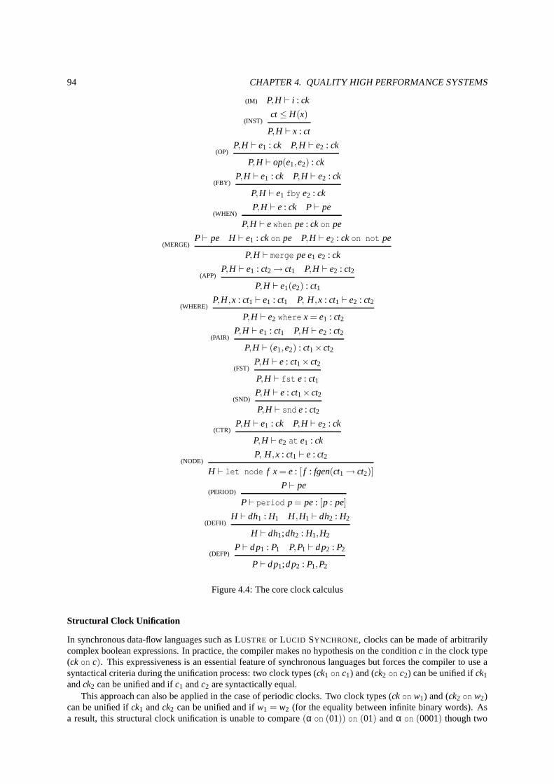
94 CHAPTER 4. QUALITY HIGH PERFORMANCE SYSTEMS
(IM) P,H ⊢ i : ck
ct≤ H(x)(INST)
P,H ⊢ x : ct
P,H ⊢ e1 : ck P,H ⊢ e2 : ck(OP)
P,H ⊢ op(e1,e2) : ck
P,H ⊢ e1 : ck P,H ⊢ e2 : ck(FBY)
P,H ⊢ e1 fby e2 : ck
P,H ⊢ e : ck P⊢ pe(WHEN)
P,H ⊢ ewhen pe: ckon pe
P⊢ pe H⊢ e1 : ckon pe P,H ⊢ e2 : ckon not pe(MERGE)
P,H ⊢ merge pe e1 e2 : ck
P,H ⊢ e1 : ct2→ ct1 P,H ⊢ e2 : ct2(APP)
P,H ⊢ e1(e2) : ct1P,H,x : ct1 ⊢ e1 : ct1 P, H,x : ct1 ⊢ e2 : ct2
(WHERE)
P,H ⊢ e2 where x = e1 : ct2P,H ⊢ e1 : ct1 P,H ⊢ e2 : ct2
(PAIR)
P,H ⊢ (e1,e2) : ct1×ct2P,H ⊢ e : ct1×ct2
(FST)
P,H ⊢ fst e : ct1P,H ⊢ e : ct1×ct2
(SND)
P,H ⊢ snd e : ct2P,H ⊢ e1 : ck P,H ⊢ e2 : ck
(CTR)
P,H ⊢ e2 at e1 : ck
P, H,x : ct1 ⊢ e : ct2(NODE)
H ⊢ let node f x = e : [ f : fgen(ct1→ ct2)]
P⊢ pe(PERIOD)
P⊢ period p = pe: [p : pe]
H ⊢ dh1 : H1 H,H1 ⊢ dh2 : H2(DEFH)
H ⊢ dh1;dh2 : H1,H2
P⊢ dp1 : P1 P,P1 ⊢ dp2 : P2(DEFP)
P⊢ dp1;dp2 : P1,P2
Figure 4.4: The core clock calculus
Structural Clock Unification
In synchronous data-flow languages such as LUSTRE or LUCID SYNCHRONE, clocks can be made of arbitrarilycomplex boolean expressions. In practice, the compiler makes no hypothesis on the conditionc in the clock type(ck on c). This expressiveness is an essential feature of synchronous languages but forces the compiler to use asyntactical criteria during the unification process: two clock types (ck1 on c1) and (ck2 on c2) can be unified ifck1
andck2 can be unified and ifc1 andc2 are syntactically equal.This approach can also be applied in the case of periodic clocks. Two clock types (ckon w1) and (ck2 on w2)
can be unified ifck1 andck2 can be unified and ifw1 = w2 (for the equality between infinite binary words). Asa result, this structural clock unification is unable to compare(α on (01)) on (01) andα on (0001) though two

4.3. THE PROGRAMMING LANGUAGE 95
stream on these clocks are present and absent at the very sameinstants. A more clever unification mechanism willbe the purpose of section 4.3.3.
Semantics over Clocked Streams
We provide our language with a data-flow semantics over finiteand infinite sequences following Kahn formulation[Kah74]. Nonetheless, we restrict the Kahn semantics by making the absence of a value explicit. The set ofinstantaneous values is enriched with a special value⊥ representing the absence of a value.
We need a few preliminary notations. IfT is a set,T∞ denotes the set of finite or infinite sequences of elementsover the setT (T∞ = T∗+Tω). The empty sequence is notedε andx.s denotes the sequence whose head isx andtail is s. Let≤ be the prefix order over sequences, i.e.,x≤ y if x is a prefix ofy. The ordered setD = (T∞,≤) isa complete partial order (CPO). IfD1 andD2 are CPOs, thenD1×D2 is a CPO with the coordinate-wise order.[D1→ D2] as the set of continuous functions fromD1 to D2 is also a CPO by taking the pointwise order. Iff isa continuous mapping fromD1 to D2, we shall writefix( f ) = limn→∞ f n(ε) for the smallest fix point off (Kleenetheorem). We define the setClockedStream(T) of clocked sequencesas the set of finite and infinite sequences ofelements over the setT⊥ = T ∪{⊥}.
T⊥ = T ∪{⊥}ClockedStream(T) = (T⊥)∞
A clocked sequence is made of present or absent values. We define the clock of a sequences as a booleansequence (without absent values) indicating when a value ispresent. For this purpose, we define the functionclockfrom clocked sequences to boolean sequences:
clock(ε) = εclock(⊥.s) = 0.clock(s)clock(x.s) = 1.clock(s)
We shall use the letterv for present values. Thus,v.s denotes a stream whose first element is present andwhose rest iss whereas⊥.sdenotes a stream whose first element is absent. The interpretation of basic primitivesof the core language over clocked sequences is given in figure4.5. We use the mark # to distinguish the syntacticconstruct (e.g.,fby) from its interpretation as a stream transformer.
• Theconst primitive produces a constant stream from an immediate value. This primitive is polymorphicsince it may produce a value (or not) according to the environment. For this reason, we add an extra argu-ment giving its clock. Thus,const# i c denotes a constant stream with stream clockc (clock(const# i c) =c).
• For a binary operator, the two operands must be synchronous (together present or together absent) and thepurpose of the clock calculus is to ensure it statically (otherwise, some buffering is necessary).
• fby is the unitary delay: it “conses” the head of its first argument to its second one. The arguments andresult offby must be on the same clock.fby corresponds to a two-state machine: while both arguments areabsent, it emits nothing and stays in its initial state (fby#). When both are present, it emits its first argumentand enters the new state (fby1#) storing the previous value of its second argument. In this state, it emits avalue every time its two arguments are present.
• The sampling operator expects two arguments on the same clock. The clock of the result depends on theboolean condition (c).
• The definition ofmerge states that one branch must be present when the other is absent.
• Note thatnot# andon# operate on boolean sequences only. The other boolean operations on clocks, e.g.orand&, follow the same principle.
It is easy to check that all these functions are continuous onclocked sequences.Semantics is given to expressions which have passed the clock calculus (⊢ judgments). We define the inter-
pretation of clock types as the following:
[[ct1→ ct2]]P = [[[ct1]]P→ [[ct2]]P][[ct1×ct2]]P = [[ct1]]P× [[ct2]]Ps∈ [[∀α1, ...,αn.ct]]P = ∀ck1, ...,ckn,s∈ [[ct[ck1/α1, ...,ckn/αn]]]Ps∈ [[ck]]P = clock(s)≤ P(ck)
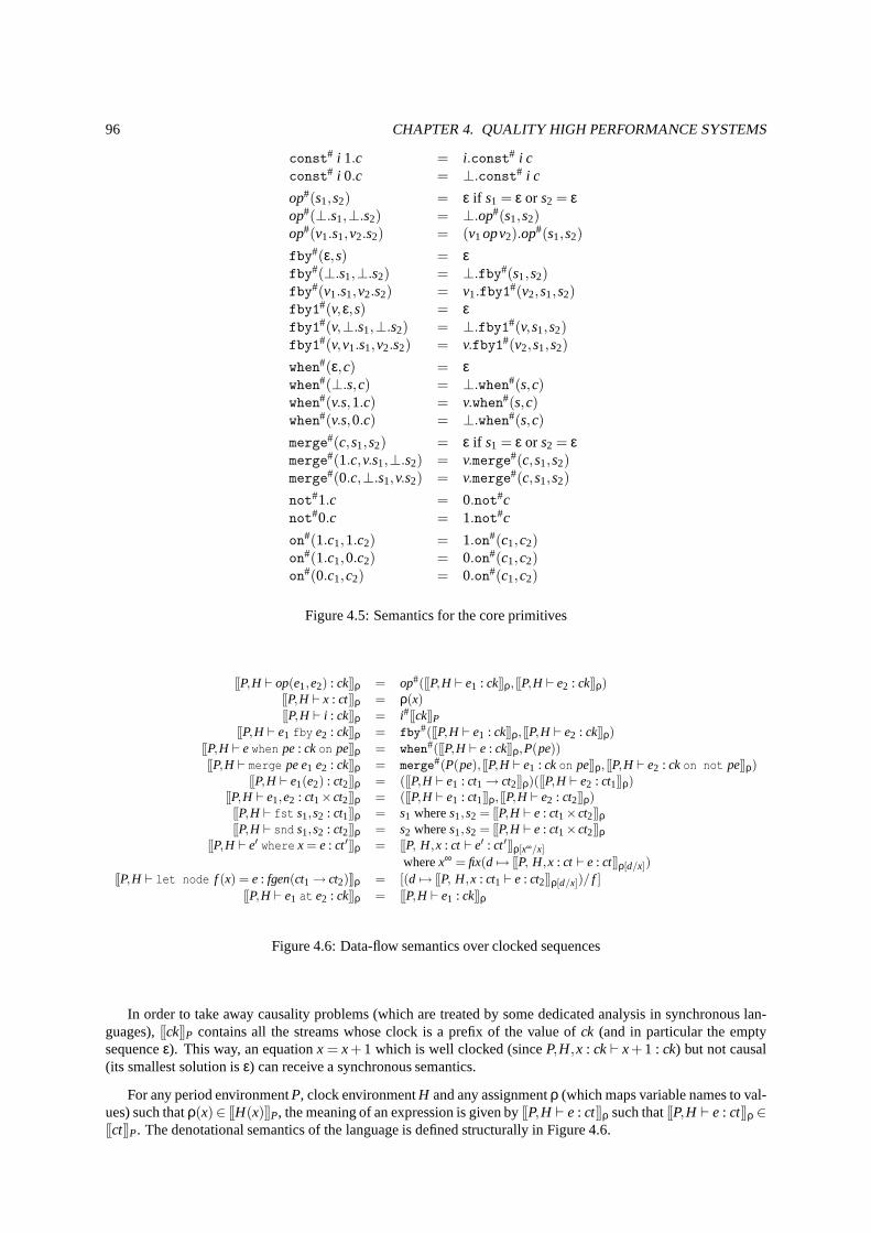
96 CHAPTER 4. QUALITY HIGH PERFORMANCE SYSTEMS
const# i 1.c = i.const# i cconst# i 0.c = ⊥.const# i c
op#(s1,s2) = ε if s1 = ε or s2 = εop#(⊥.s1,⊥.s2) = ⊥.op#(s1,s2)op#(v1.s1,v2.s2) = (v1opv2).op#(s1,s2)
fby#(ε,s) = εfby#(⊥.s1,⊥.s2) = ⊥.fby#(s1,s2)fby#(v1.s1,v2.s2) = v1.fby1
#(v2,s1,s2)fby1#(v,ε,s) = εfby1#(v,⊥.s1,⊥.s2) = ⊥.fby1#(v,s1,s2)fby1#(v,v1.s1,v2.s2) = v.fby1#(v2,s1,s2)
when#(ε,c) = εwhen#(⊥.s,c) = ⊥.when#(s,c)when#(v.s,1.c) = v.when#(s,c)when#(v.s,0.c) = ⊥.when#(s,c)
merge#(c,s1,s2) = ε if s1 = ε or s2 = εmerge#(1.c,v.s1,⊥.s2) = v.merge#(c,s1,s2)merge#(0.c,⊥.s1,v.s2) = v.merge#(c,s1,s2)
not#1.c = 0.not#cnot#0.c = 1.not#c
on#(1.c1,1.c2) = 1.on#(c1,c2)on#(1.c1,0.c2) = 0.on#(c1,c2)on#(0.c1,c2) = 0.on#(c1,c2)
Figure 4.5: Semantics for the core primitives
[[P,H ⊢ op(e1,e2) : ck]]ρ = op#([[P,H ⊢ e1 : ck]]ρ, [[P,H ⊢ e2 : ck]]ρ)[[P,H ⊢ x : ct]]ρ = ρ(x)[[P,H ⊢ i : ck]]ρ = i#[[ck]]P
[[P,H ⊢ e1 fby e2 : ck]]ρ = fby#([[P,H ⊢ e1 : ck]]ρ, [[P,H ⊢ e2 : ck]]ρ)
[[P,H ⊢ ewhen pe: ckon pe]]ρ = when#([[P,H ⊢ e : ck]]ρ,P(pe))[[P,H ⊢ merge pe e1 e2 : ck]]ρ = merge#(P(pe), [[P,H ⊢ e1 : ckon pe]]ρ, [[P,H ⊢ e2 : ckon not pe]]ρ)
[[P,H ⊢ e1(e2) : ct2]]ρ = ([[P,H ⊢ e1 : ct1→ ct2]]ρ)([[P,H ⊢ e2 : ct1]]ρ)[[P,H ⊢ e1,e2 : ct1×ct2]]ρ = ([[P,H ⊢ e1 : ct1]]ρ, [[P,H ⊢ e2 : ct2]]ρ)[[P,H ⊢ fst s1,s2 : ct1]]ρ = s1 wheres1,s2 = [[P,H ⊢ e : ct1×ct2]]ρ[[P,H ⊢ snd s1,s2 : ct2]]ρ = s2 wheres1,s2 = [[P,H ⊢ e : ct1×ct2]]ρ
[[P,H ⊢ e′ where x = e : ct′]]ρ = [[P, H,x : ct ⊢ e′ : ct′]]ρ[x∞/x]wherex∞ = fix(d 7→ [[P, H,x : ct ⊢ e : ct]]ρ[d/x])
JP,H ⊢ let node f (x) = e : fgen(ct1→ ct2)Kρ = [(d 7→ [[P, H,x : ct1 ⊢ e : ct2]]ρ[d/x])/ f ][[P,H ⊢ e1 at e2 : ck]]ρ = [[P,H ⊢ e1 : ck]]ρ
Figure 4.6: Data-flow semantics over clocked sequences
In order to take away causality problems (which are treated by some dedicated analysis in synchronous lan-guages),[[ck]]P contains all the streams whose clock is a prefix of the value ofck (and in particular the emptysequenceε). This way, an equationx = x+1 which is well clocked (sinceP,H,x : ck⊢ x+1 : ck) but not causal(its smallest solution isε) can receive a synchronous semantics.
For any period environmentP, clock environmentH and any assignmentρ (which maps variable names to val-ues) such thatρ(x)∈ [[H(x)]]P, the meaning of an expression is given by[[P,H ⊢ e : ct]]ρ such that[[P,H ⊢ e : ct]]ρ ∈[[ct]]P. The denotational semantics of the language is defined structurally in Figure 4.6.
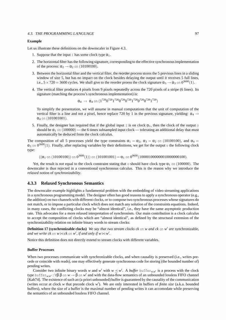
4.3. THE PROGRAMMING LANGUAGE 97
Example
Let us illustrate these definitions on the downscaler in Figure 4.3.
1. Suppose that the inputi has some clock typeα1.
2. The horizontal filter has the following signature, corresponding to the effective synchronous implementationof the process:α2→ α2 on (10100100).
3. Between the horizontal filter and the vertical filter, thereorder process stores the 5 previous lines in a slidingwindow of size 5, but has no impact on the clock besides delaying the output until it receives 5 full lines,i.e., 5×720= 3600 cycles. We shall give to the reorder proess the clock signatureα3→ α3 on 03600(1).
4. The vertical filter produces 4 pixels from 9 pixels repeatedly across the 720 pixels of a stripe (6 lines). Itssignature (matching the process’s synchronous implementation) is:
α4 → α4 on (172007201720072007201720072007201720)
To simplify the presentation, we will assume in manual computations that the unit of computation of thevertical filter is a line and not a pixel, hence replace 720 by 1in the previous signature, yielding:α4→α4 on (101001001).
5. Finally, the designer has required that if the global input i is on clockα1, then the clock of the outputoshould beα1 on (100000) — the 6 times subsampled input clock — tolerating an additional delay that mustautomatically be deduced from the clock calculus.
The composition of all 5 processes yield the type constraints α1 = α2, α3 = α2 on (10100100), and α4 =α3 on 03600(1). Finally, after replacing variables by their definitions, we get for the outputo the following clocktype:
((α1 on (10100100)) on 03600(1)) on (101001001)= α1 on 09600(100001000000010000000100).
Yet, the result isnot equal to the clock constraint stating thato should have clock typeα1 on (100000). Thedownscaler is thus rejected in a conventional synchronous calculus. This is the reason why we introduce therelaxednotion ofsynchronizability.
4.3.3 Relaxed Synchronous Semantics
The downscaler example highlights a fundamental problem with the embedding of video streaming applicationsin a synchronous programming model. The designer often has good reasons to apply a synchronous operator (e.g.,the addition) on two channels with different clocks, or to compose two synchronous processes whose signatures donot match, or to impose a particular clock which does not match any solution of the constraints equations. Indeed,in many cases, the conflicting clocks may be “almost identical”, i.e., they have the same asymptotic productionrate. This advocates for a more relaxed interpretation of synchronism. Our main contribution is a clock calculusto accept the composition of clocks which are “almost identical”, as defined by the structural extension of thesynchronizability relation on infinite binary words to stream clocks:
Definition 17 (synchronizable clocks)We say that two stream clocks ckon w and ckon w′ are synchronizable,and we write ckon w ⊲⊳ ckon w′, if and only if w⊲⊳ w′.
Notice this definition does not directly extend to stream clocks with different variables.
Buffer Processes
When two processes communicate with synchronizable clocks, and when causality is preserved (i.e., writes pre-cede or coincide with reads), one may effectively generate synchronous code for storing (the bounded number of)pending writes.
Consider two infinite binary wordsw andw′ with w� w′. A buffer bufferw,w′ is a process with the clocktypebufferw,w′ : ∀β.β on w→ β on w′ and with the data-flow semantics of an unbounded lossless FIFO channel[Kah74]. The existence of such an (a priori unbounded) buffer is guaranteed by the causality of the communication(writes occur at clockw that precede clockw′). We are only interested in buffers offinite size(a.k.a. boundedbuffers), where the size of a buffer is the maximal number of pending writes it can accomodate while preservingthe semantics of an unbounded lossless FIFO channel.
98 CHAPTER 4. QUALITY HIGH PERFORMANCE SYSTEMS
Proposition 7 Consider two processes f: ck→ α on w and f′ : α on w′ → ck′, with w⊲⊳ w′ and w� w′. Thereexists a bufferbufferw,w′ : ∀β.β on w→ β on w′ such that f′ ◦bufferw,w′ ◦ f is a (0−)synchronous composition(with the unificationα = β).
Proof. A buffer of size n can be implemented with n data registers xi and2n+1 clocks(wi)1≤i≤n and(r i)0≤i≤n.Pending writes are stored in data registers: wi [ j] = 1 means that there is a pending write stored in xi at cycle j.Clocks ri determine the instants when the process associated with w′ reads the data in xi : r i [ j] = 1 means that thedata in register xi is read at cycle j. For a sequence of pushes and pops imposed byclocks w and w′, the followingcase distinction simulates a FIFO on the xi registersstaticallycontrolled through clocks wi and ri :
NOP: w[ j] = 0 and w′[ j] = 0. No operation affects the buffer, i.e., ri [ j] = 0, wi [ j] = wi [ j −1]; registers xi are leftunchanged.
PUSH: w[ j] = 1 and w′[ j] = 0. Some data is written into the buffer and stored in register x1, all the data in thebuffer being pushed from xi into xi+1. Thus xi = xi−1 and x1 = input,∀i > 2,wi [ j] = wi−1[ j −1], w1[ j] = 1and ri [ j] = 0.
POP: w[ j] = 0 and w′[ j] = 1. Let p= max({0}∪{1≤ i ≤ n|wi [ j−1] = 1}). If p is zero, then no register storesany data at cycle j: input data must be bypassed directly to the output, crossing the wire clocked by r0,setting ri [ j] = 0 for i > 0 and r0[ j] = 1, wi [ j] = wi [ j−1]. Conversely, if p> 0, ∀i 6= p, r i [ j] = 0, rp[ j] = 1,∀i 6= p,wi [ j] = wi [ j−1] and wp[ j] = 0. Registers xi are left unchanged (notice this is not symmetric to thePUSH operation).
POP; PUSH: w[ j] = 1 and w′[ j] = 1. This case boils down to the implementation of aPOP followed by aPUSH,as defined in the two previous cases.
�
Assumingw andw′ are periodic and have been writtenw= u(v) andw′ = u′(v′) under the lines of Remark 1, itis sufficient to conduct the previous simulation for|u|+ |v| cycles to compute periodic clockswi andr i . This leadsto an implementation in a plain(0−)synchronous language; yet this implementation is impractical because eachclock wi or r i has a worst case quadratic size in the maximum of the periods of w andw′ (from the application ofremark 1), yielding cubic control space, memory usage and code size. This motivates the search for an alternativebuffer implementation decoupling the memory management for the FIFO from the combinatorial control space;such an implementation is proposed in Section 4.4.2.
Relaxed Clock Calculus
Let us now modify the clock calculus in two ways:
1. a subtyping [Pie02] rule(SUB) is added to the clock calculus to permit the automatic insertion of a finitebuffer in order to synchronize clocks;
2. rule(CTR) is modified into a subtyping rule to allow automatic insertion (and calculation) of a bounded delay.
The Subtyping Rule
Definition 18 The relation<: is defined by
w <: w′⇐⇒ w ⊲⊳ w′∧w� w′.
This is a partial order, and its restriction to equivalence classes for the synchronizability relation (⊲⊳) forms acomplete lattice.
We structurally extend this definition to stream clocks ckon w and ckon w′ where w<: w′.7
Relation<: defines a subtyping rule(SUB) on stream clocks types:
P,H ⊢ e : ckon w w<: w′(SUB)
P,H ⊢ e : ckon w′
7Yet this definition does not directly extends to stream clocks with different variables.
4.3. THE PROGRAMMING LANGUAGE 99
This is a standard subsumption rule, and all classical results on subtyping apply [Pie02].The clock calculus defined in the previous section rejects expressions such asx+y when the clocks ofx andy
cannot be unified. With rule(SUB), we can relax this calculus to allow an expressionewith clockck to be used “asif it had” clock ck′ as soon asck andck′ aresynchronizableand causality is preserved.
E.g., the following program is rejected in the(0−)synchronous calculus since, assumingx has some clockα,α on (01) cannot be unified withα on 1(10).
let node f (x) = y wherey = (x when (01))+ (xwhen 1(10))
Let e1 denote expression (x when (01)) ande2 denote expression (x when 1(10)), and let us generate the typeconstraints for each construct in the program:
1. (NODE): suppose that the signature off is of form f : α→ α′;
2. (+): the addition expects two arguments with the same clocks;
3. (WHEN): we getck1 = α on (01) for the clock ofe1 andck2 = α on 1(10) for the clock ofe2;
4. (SUB): because(01) and 1(10) are synchronizable, the two clocksck1 = α on (01) andck2 = α on 1(10) canbe resynchronized intoα on (01), since(01) <: (01) and 1(10) <: (01).
The final signature isf : ∀α.α→ α on (01).Considering the downscaler example, this subtyping rule (alone) does not solve the clock conflict: the imposed
clock first needs to be delayed to avoid starvation of the output process. This is the purpose of the following rule.
The Clock Constraint Rule The designer may impose the clock of certain expressions. Rule (CTR) is relaxedinto the following subtyping rule:
P,H ⊢ e1 : ckon w1 P,H ⊢ e2 : ckon w2 w1 <: 0dw2(CTR)
P,H ⊢ e1 at e2 : ckon 0dw2
Consider the previous example with the additional constraint that the output must have clock(1001).
let node f (x) = y at (x when (1001)) wherey = (x when (01))+ (x when 1(10))
We previously computed that(x when (01))+ (x when 1(10)) has signatureα → α on (01), and(01) does notunify with (1001). Rule(CTR) yields
P,H ⊢ y : a on (01),x when (1001) : a on (1001) (01) <: 0(1001)
P,H ⊢ y at (x when (1001)) : a on 0(1001)
Finally, f : ∀α.α→ α on 0(1001). Indeed, one cycle delay is the minimum to allow synchronization with theimposed output clock.
Relaxed Clock Calculus Rules The predicateP,H ⊢s e : ct states that an expressionehas clockct in the periodenvironmentP and the clock environmentH, under the use of some synchronization mechanism. Its definitionextends the one ofP,H ⊢ e : ct with the new rules in Figure 4.7. The axiom and all other rulesare identical to theones in Figure 4.4, using⊢s judgments instead of⊢.
Thus, starting from a standard clock calculus whose purposeis to reject non-synchronous program, we extendit with subtypingrules expressing that a stream produced on some clockck1 can be read on the clockck2 as soonasck1 can be synchronized intock2, using some buffering mechanism. By presenting the system in two steps, theadditional expressiveness with respect to classical synchrony is made more precise.
100 CHAPTER 4. QUALITY HIGH PERFORMANCE SYSTEMS
P,H ⊢s e : ckon w1 w1 <: w2(SUB)
P,H ⊢s e : ckon w2
P,H ⊢s e1 : ckon w1 P,H ⊢s e2 : ckon w2 w1 <: 0dw2(CTR)
P,H ⊢s e1 at e2 : ckon 0dw2
Figure 4.7: The relaxed clock calculus
Relaxed Synchrony and thefby Operator Notice fby is considered a length preserving function in data-flow networks, hence its clock scheme∀α.α×α→ α in the 0-synchronous case, and despite it only needs itsfirst argument at the very first instant. In the relaxed case, we could have chosen one of the following clocksignatures:∀α.α on 1(0)e×α→ α, ∀α.α on 1(0)×α on 0(1)→ α, or ∀α.α×α on 0(1)→ α. The first twosignatures require the first argument to be present at the very first instant only, which is overly restrictive inpractice. The third signature is fully acceptable, with theobservation that the original length-preserving signaturecan be reconstructed by applying the subtyping ruleα on (1) <: α on 0(1). This highlights the fact that thefbyoperator is a one-place buffer.
Construction of the System of Clock Constraints
The system of clock constraints is build from the systematicapplication of the core rules in Figure 4.4 and therelaxed calculus rules in Figure 4.7. All rules are syntax directed except(SUB) whose application is implicit at each(function or operator) composition.
Rule (CTR) is a special case: the clock constraint is built by computinga possible value for the delayd. Thiscomputation is syntax directed, and we always choose to minimize delay insertion: delay(w,w′) = min{l | w�0l w′}. Whenw� w′, no delay is necessary. Note that in general, delay(w,w′) 6= delay(w′,w).
Proposition 8 The delay to synchronize an infinite periodic binary word w with an imposed infinite periodicbinary word w′ can be automatically computed by the formula
delay(w,w′) = max(maxp
([w]p− [w′]p),0).
On periodic words, this delay is effectively computable thanks to Remark 1.
Proof. Indeed, let d= max(maxp([w]p− [w′]p),0) and v= 0dw′ we have w� v since for all p,[v]p = d+[w′]p.Moreover, d is minimal: suppose there exists p such that d−1 < [w]p− [w′]p, then v′ = 0d−1w′ satisfies[v]p =d−1+[w′]p < [w]p. Thus, w6� v′. �
For the simplified downscaler, the minimal delay to resynchronize the vertical filter with the output process is09603, since 9603 (clock cycles) is the minimal value ofd such that09600(100001000000010000000100)� 0d(100000). For the real downscaler (with fully developed vertical filtersignature), we automatically computed that the minimal delay was12000to permit communication with the SDoutput.
Unification
We need a better unification procedure on clock types than thestructural one (see Section 4.3.2), types to obtainan effective resolution algorithm for this system of constraints. In our case, a syntactic unification would unnec-essarily reject many synchronous programs with periodic clocks. We propose a semi-interpreted unification thattakes into account the semantics of periodic clocks. More precisely, the unification of two clock typesct andct′
can be purely structural on functional and pair types, whereno simplification on periodic clocks can be applied,but it has to be aware of the properties of the sampling operator (on) when unifying stream clock types of the formckon w andck′ on w′. Two cases must be considered.
First of all, unifyingα on w andα on w′ returns true if and only ifw = w′.In the most general case, assumeα andα′ are clock variables (clocks can be normalised, thanks to theasso-
ciativity of on). Equationα on w = α′ on w′ always has an infinite number of solutions; these solutions generatean infinite number of different infinite binary words. Intuitively, a periodic sampling ofw consists of the insertion
4.3. THE PROGRAMMING LANGUAGE 101
of 0s inw, in a periodic manner. Ifw� w′, it is always possible to delay thep-th 1 in w (resp.w′) until the p-th 1in w′ (resp.w) through the insertion of 0s inα (resp. inα′). Let us define the subsampling relation≤SS, such that
a≤SSa′ ⇐⇒ ∃α,a = α on a′.
Note that ifa≤SSa′ thena′ � a, but the converse is not true:(01)� (0011) and there is no solutionα such that(0011) = α on (01).
Proposition 9 Relation≤SSis a partial order.
Proof. ≤SS is trivially reflexive and transitive. Antisymmetry holds because� is a partial order, and a≤SSa′
implies a′ � a. �
In a typical unification scheme, one would like to replace theabove type equation by “the most general clocktype satisfying the equation”. We will see that there is indeed a most general wordm such that all commonsubsamples ofw andw′ are subsamples ofm (≤SS is an upper semi-lattice), yet the expression ofm= v on w =v′ on w′ does not lead to a unique choice form and for the maximal unifiersv andv′. In fact, there can be aninfinite set of such words.
In a strictly synchronous setting, we need to fall back to an incomplete unification scheme (some synchronousprograms with periodic clocks will be rejected), choosing one of these solutions. If(v,v′) is the chosen solution,the unification ofa on w anda′ on w′ yields a unique clock typeα on von w = α on v′ on w′, and every occurenceof a (resp.a′) is replaced byα on v (resp.α on v′).
Yet in our relaxed synchronous setting, the most general unifier has an interesting property:
Proposition 10 (synchronizable unifiers)Consider w, v1, v2 such that v1 on w = v2 on w; we have v1 ⊲⊳ v2.
This directly derives from Proposition 2.We may thus make an arbitrary choice for(v,v′) among maximal unifiers, and select one that is easy to
compute. Formally, we define theearliestsubstitutionsV andV ′ through the following recurrent equations:
V (0d1.w,0d0d′1.w′) = 1d0d′1.V (w,w′)V (0d0d′1.w,0d1.w′) = 1d1d′1.V (w,w′)V ′(0d1.w,0d0d′1.w′) = 1d1d′1.V ′(w,w′)V ′(0d0d′1.w,0d1.w′) = 1d0d′1.V ′(w,w′)
Let M (w,w′) denote the unifier
M (w,w′) = V (w,w′) on w = V ′(w,w′) on w′.
The computation ofV andV ′ terminates on periodic words because there are a finite number of configurations(bounded by the product of the period lenghts ofw andw′).
E.g.,a on (1000) = a′ on 0(101):
w 1 0 0 0 1 0 0 0 1 0 0 0 1. . . (1000)w′ 0 1 0 1 1 0 1 1 0 1 1 0 1. . . 0(101)V (w,w′) 0 1 1 1 1 1 1 1 1 1 1 1 1. . . 0(1)
V ′(w,w′) 1 1 1 0 0 1 0 0 0 1 1 0 0. . . 1(11001000)M (w,w′) 0 1 0 0 0 1 0 0 0 1 0 0 0. . . 0(1000)
Proposition 11 For all w,w′, p,
[M (w,w′)]p+1 = [M (w,w′)]p +max([w]p+1− [w]p, [w′]p+1− [w′]p).
Proof. An inductive proof derives naturally from the previous algorithm. In particular, observe that betweentwo consecutive 1s inM (w,w′), the associated subword of either v or v′ is a sequence of 1s; hence either[M (w,w′)]p+1− [M (w,w′)]p = [w]p+1− [w]p or [M (w,w′)]p+1− [M (w,w′)]p = [w′]p+1− [w′]p. �
In addition,M (w,w′) is the maximumcommon subsample ofw andw′ and has several interesting properties:
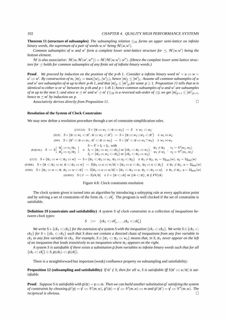
102 CHAPTER 4. QUALITY HIGH PERFORMANCE SYSTEMS
Theorem 11 (structure of subsamples)The subsampling relation≤SS forms an upper semi-lattice on infinitebinary words, the supremum of a pair of words w,w′ beingM (w,w′).
Common subsamples of w and w′ form a complete lower semi-lattice structure for�, M (w,w′) being thebottom element.
M is also associative:M (w,M (w′,w′′)) = M (M (w,w′),w′′). (Hence the complete lower semi-lattice struc-ture for� holds for common subsamples of any finite set of infinite binary words.)
Proof. We proceed by induction on the position of the p-th 1. Consider a infinite binary word m′ = u on w =u′ on w′. By construction of m,[m]1 = max([w]1, [w′]1), hence[m]1≤ [m′]1. Assume all common subsamples of wand w′ are subsamples of m up to their p-th 1, and that[m]p≤ [m′]p for some p≥ 1. Proposition 11 tells that m isidentical to either w or w′ between its p-th and p+1-th 1; hence common subsamples of w and w′ are subsamplesof m up to the next 1; and since w�m′ and w′ �m′ (≤SSis a reversed sub-order of�), we get[m]p+1≤ [m′]p+1,hence m�m′ by induction on p.
Associativity derives directly from Proposition 11. �
Resolution of the System of Clock Constraints
We may now define a resolution procedure through a set of constraint-simplification rules.
(CYCLE) S+{α on w1 <: α on w2} S if w1 <: w2
(SUP) S+{α on w1 <: α′, α on w2 <: α′} S+{α on w1⊔w2 <: α′} if w1 ⊲⊳ w2
(INF) S+{α′ <: α on w1, α′ <: α on w2} S+{α′ <: α on w1⊓w2} if w1 ⊲⊳ w2
(EQUAL) S S[ α′1 on v1/α1
α′2 on v2/α2
]
if
S= S′+ I1 + I2, withI1 = {α1 on w1 <: ck1} or {ck1 <: α1 on w1}I2 = {α2 on w2 <: ck2} or {ck2 <: α2 on w2}
,α1 6= α2w1 6= w2
,v1 = V (w1,w2)v2 = V ′(w1,w2)
(CUT) S+{α1 on w <: α2 on w} S+{α1 <: α3 on u1, α3 on u2 <: α2} if α1 6= α2, u1 = Umax(w), u2 = Umin(w)
(FORK) S+{α <: α1 on w, α <: α2 on w} S[α3 on u on w/α]+{α3 on u <: α1, α3 on u <: α2} if α1 6= α2, u = Umin(w)
(JOIN) S+{α1 on w <: α, α2 on w <: α} S[α3 on u on w/α]+{α1 <: α3 on u, α2 <: α3 on u} if α1 6= α2, u = Umax(w)
(SUBST) S⊕ I S[ck/α] if I = {α <: ck} or {ck<: α}, α /∈ FV(ck)
Figure 4.8: Clock constraints resolution
The clock system given is turned into an algorithm by introducing a subtyping rule at every application pointand by solving a set of constraints of the formcki <: ck′i . The program is well clocked if the set of constraints issatisfiable.
Definition 19 (constraints and satisfiability) A system S of clock constraints is a collection of inequations be-tween clock types:
S ::= {ck1 <: ck′1, . . . ,ckn <: ck′n}
We write S+{ck1 <: ck2} for the extension of a system S with the inequation{ck1 <: ck2}. We write S⊕{ck1 <:ck2} for S+ {ck1 <: ck2} such that S does not contain adirected chainof inequations from any free variable inck1 to any free variable in ck2. For example, S⊕{α1 <: α2 on w2} means that, in S,α1 never appear on the leftof an inequation that leads transitively to an inequation whereα2 appears on the right.
A system S is satisfiable if there exists a substitutionρ from variables to infinite binary words such that for all{cki <: ck′i} ∈ S,ρ(cki) <: ρ(ck′i).
There is a straightforward but important (weak) confluence property on subsampling and satisfiability:
Proposition 12 (subsampling and satisfiability) If α′ /∈ S, then for all w, S is satisfiable iff S[α′ on w/α] is sat-isfiable.
Proof. Suppose S is satisfiable withρ(α) = γ onm. Then we can build another substitutionρ′ satisfying the systemof constraints by choosingρ′(γ) = γ′ on V (m,w), ρ′(α) = γ′ on V (m,w) on m andρ′(α′) = γ′ on V ′(m,w). Thereciprocal is obvious. �
4.3. THE PROGRAMMING LANGUAGE 103
Let us eventually define three functions useful to bound the set of subsamples of a given word:Umin, Umax
and∆ are defined recursively as follows:
Umin(0a1b.w) = 1a0a0b1b.Umin(w)Umax(0a1b.w) = 0a0b1a1b.Umax(w)∆(u1.u2.u,0a1b.w) = 1a0c11a1b.u2.∆(u,w)
with |u1|1 = 2a+b, |u2|1 = b, |u1|0 = c1, |u2|0 = c2
Notice∆ — from pairs of infinite binary words to infinite binary words—is of technical interest for the proofsonly.
Proposition 13 For all w, Umin(w) ⊲⊳ Umax(w), Umin(w) <: Umax(w), andUmin(w) on w = Umax(w) on w.For all u, w, ∆(u,w) is an infinite periodic binary word and is synchronizable with u.
Proof. The first part of the proposition is proven inductively on theposition of 1s in the subsampling.
The second part derives from|1a0c11a1b.u2|1|1a0c11a1b.u2|
= 2a+2b2a+2b+c1+c2
= |u1.u2|1|u1.u2|
, where u1.u2 satisfies the constraints in
the inductive definition of∆. �
Proposition 14 For all u, v, w,
∆(u,w) on Umin(w) on w = u on Umin(w) on w =
u on Umax(w) on w = ∆(u,w) on Umax(w) on w
Proof. SinceUmin(w) on w = Umax(w) on w, we haveu on Umin(w) on w = u on Umax(w) on w and∆(u,w) on Umin(w) on w = ∆(u,w) on Umax(w) on w In addition,Umin(0a1b.w) on 0a1b.w = 0a0b0a1b, hence∆(u1.u2.u,0a1b.w) on Umin(0a1b.w) on 0a1b.w =0a0c10b0a.u2.∆(u,w) on Umin(w) on w (since|u2|1 = b). Finally, u1.u2.u on Umin(0a1b.w) on 0a1b.w =02a+b+c1.u2.u on Umin(w) on w. �
Proposition 15 ∆(u,w) on Umin(w) is the minimum (for�) of all v′ such that
v′ on w = ∆(u,w) on Umin(w) on w.
∆(u,w) on Umax(w) is the maximum (for�) of all v′ such that
v′ on w = ∆(u,w) on Umax(w) on w.
Proof. The result is proven by induction, observing that the p-th 1 in v′ is enclosed between the p-th 1 in∆(u,w) on Umin(w) and in∆(u,w) on Umax(w). Indeed, we have∆(u1.u2.u,0a1b.w) on Umin(0a1b.w) =1a0c10a0b.u2.∆(u,w) on Umin(w), and∆(u1.u2.u,0a1b.w) on Umax(0a1b.w) = 0a0c10b1a.u2.∆(u,w) on Umax(w).
�
The set of subsamples of a given word is characterized by the following technical proposition:
Proposition 16 For all u, v, w,
u on Umin(w) on w <: v on w =⇒ ∆(u,w) on Umin(w) <: v
andv on w <: u on Umax(w) on w =⇒ v <: ∆(u,w) on Umax(w).
Proof. Observe that uon Umin(w) on w <: v on w. From Proposition 14, we have∆(u,w) on Umin(w) on w <:v on w. And from Proposition 15, we get∆(u,w) on Umin(w) <: v. The second part of the proof is symmetrical.�
Let us finally define the simplification relation between clock constraints. Its definition is given in Fig-ure 4.8. Any new variable appearing in right-hand side of thesimplification relation is assumed to be fresh.
Theorem 12 (preservation of satisfiability) If S is satisfiable and S S′ then S′ is satisfiable.
104 CHAPTER 4. QUALITY HIGH PERFORMANCE SYSTEMS
Proof. Proposition 12 authorizes to sample (to slow down) the system and will be used throughout the proof.Let us consider every relation in Figure 4.8.
(SUP), (INF) and(CYCLE). Presevation of satisfiability is a direct application of Propositions 2 and 5.
(EQUAL). This rule preserves satisfiability: it just subsamples a pair of variables.
(CUT). By definition ofUmin andUmax, the right-hand side of the relation is a sufficient condition of satisfiability.
Conversely, consider a solutionα1 = α on v1 and α2 = α on v2. Let V1 = V (v1,Umin(w)) and V′1 =V ′(v1,Umin(w)), and replaceα by α′ on V1. We haveα1 = α′ on V ′1 on Umin(w). Let us chooseα3 =α′ on ∆(V ′1,w); From Proposition 16, we haveα1 <: α′ onV ′1 on Umax(w) <: α3 on Umax(w).
We also have V′1 on Umin(w) on w <: V1 on v2 on w, hence Proposition 16 yields∆(V ′1,w) on Umin(w) <:V1 on v2. Sinceα2 = α′ on V1 on v2, we haveα3 on Umin(w) <: α2. The right-hand side of the relation isthus satisfiable.
(FORK) and(JOIN). The proof is very similar: choosing the sameα3 satisfies both inequalities onα1 andα2 simul-taneously.
(SUBST). Consider the form of the inequality I onα. The right-hand side of the relation is of course a sufficientcondition of satisfiability. It is also clear that it is necessary when the inequality does not belong to a circuit.Assuming it belongs to a circuit, simplify the system through the systematic application of all other rules,enforcing that no inequality belongs to multiple simple circuits. A retiming argument [LS91] shows that, ifthe system is satisfiable, then there is a solution such that all inequalities in a given circuit but (at most) oneare converted to equalities: considering a solution with atleast two strict inequalities, split the circuit byrenaming the common clock variable, choosing one name for the path from one inequality to the other andanother one on the other path, unify any one of the broken inequalities to effectively remove this inequalityfrom the solution.
The proof is symmetical for the second form of I.
�
Rule (EQUAL) is only provided to factor the unification step out of the(CUT), (FORK) and (JOIN) rules. As aconsequence, in the following resolution algorithm, we assume rule(EQUAL) is an enabling simplification, appliedonce before each rule(CUT), (FORK) and(JOIN).
Theorem 13 (resolution algorithm) The set of rules in Figure 4.8 defines a non-deterministic, but always termi-nating resolution algorithm:
1. the tree of simplifications S S′ is finite;
2. if S is satisfiable, there is a sequence of rule applications leading to the empty set.
Proof. The proof is based on the graph structure induced by S.(SUP) and (INF) strictly reduces the number of acyclic paths.(EQUAL) is only used once for each application
of (CUT), (FORK) and (JOIN). The w1 6= w2 condition guarantees it can only be applied a finite number oftimes.A systematic application of(SUP), (INF), (CUT), (FORK) and (JOIN) leads to a system where no inequality belongs tomultiple simple circuits. This enables(SUBST), which strictly reduces the length of any circuit or multi-path sub-graphs.(CYCLE)reduces short-circuits on a single variable.
Any ordering in the application of these rules terminates, and yields the empty set when S is satisfiable.�As a corollary:
Theorem 14 (completeness)For any expression e, and for any period and clock environments P and H, if e hasan admissible clock type in P,H for the relaxed clock calculus, then the type inference algorithm computes a clockct verifying P,H ⊢s e : ct.
Intuitively, if the type constraints imposed by the clock calculus are satisfiable, then our resolution algorithmdiscovers one solution. This strong result guarantees the clock calculus’s ability to accept all programs withperiodic clocks that can be translated to a strictly(0−)synchronous framework.
Completeness would be easier to derive from principality, i.e., from the existence of a most general type forevery expression [Pie02, AW93]. Yet the unification of clockstream types is not purely structural (it exploits the
4.4. TRANSLATION PROCEDURE 105
properties of theon operator), and there are many ways to solve an equation on clock types. There is not muchhope either that the system of clock constraints can be solved by a set of confluent rules, since multiple solutionsare often equivalent up to retiming [LS91].
Finally, although Theorem 13 proves completeness, our resolution algorithm does not guarantee anythingabout the quality of the result (total buffer size, period length, rate of the common clock).
4.4 Translation Procedure
When a network is associated with a system of clock inequalities where not all of them are simplified into equal-ities, its execution is undefined with respect to the semantics of 0-synchronous programs. Buffer processes areneeded to synchronize producers with consumers.
4.4.1 Translation Semantics
Consider the input clockckon w and the output periodckon w′, with w�w′. To fully synchronize the communi-cation, we insert a new buffer nodebufferw,w′ with clock∀β.β on w → β on w′; w (resp.w′) states when apush(resp.pop) occurs.
Proposition 17 (buffer size) Consider two synchronizable infinite binary words w and w′ such that w� w′. Theminimal buffer to allow communication from w to w′ is of size
size(w,w′) = max(maxp,q
({q− p | [w′]p≥ [w]q}),0).
Communication from w to w′ is called size(w,w′)-synchronous.On periodic words, this size is effectively computable thanks to Remark 1.
Proof. This is the maximal number of pending writes appearing before their matching reads, hence a lowerbound on the minimal size. It is also the minimal size, since it is possible to implement a size n buffer with nregisters. �
For the simplified downscaler, buffer size is equal to 1, since clock 09600(1000010000000 10000000100) maytake at most one advance tick with respect to clock 09603(100000). For the real downscaler, we automatically com-puted the size880. (This is not the transposition buffer in the reorder node: its size is defined in the specificationand not inferred from the clocks.)
Let us now define atranslation semanticsfor programs accepted with the relaxed clock calculus. Thiswillenable us to state the cornerstone result of this work, namely that programs accepted with the relaxed clockcalculus can be turned into synchronous programs which are accepted by the original clock calculus. This isobtained through a program transformation which inserts a buffer every time a strict inequality on stream clocktypes remains after resolution. Because a buffer is itself asynchronous program, the resulting translated programcan be clocked with the initial system and can thus be synchronously evaluated. This translation is obtained byasserting judgmentP,H ⊢s e : ct⇒ e′, meaning that in the period environmentP and the clock environmentH, theexpressionewith clockct is translated intoe′. The insertion rule is:
P,H ⊢s e : ckon w⇒ e′ w <: w′(TRANSLATION)
P,H ⊢s e : ckon w′⇒ bufferw,w′(e′)
Other rules are simple morphisms.8
4.4.2 Practical Buffer Implementation
From the definition in Section 4.3.3, one may define a custom buffer process with the exact clock type to resynchro-nize a communication. Yet this definition suffers from the intrinsic combinatorics of(0−)synchronous commu-nication between periodic clocks (with statically known periodic clocks). We propose an alternative constructionwhere the presence or absence of data is captured by dynamically computed clocks. The memory and code size
8Notice the(CTR) rule shifts a clock constraint imposed by the programmer; this rule will often lead to the insertion of a synchronizationbuffer, triggering the(TRANSLATION) rule indirectly.
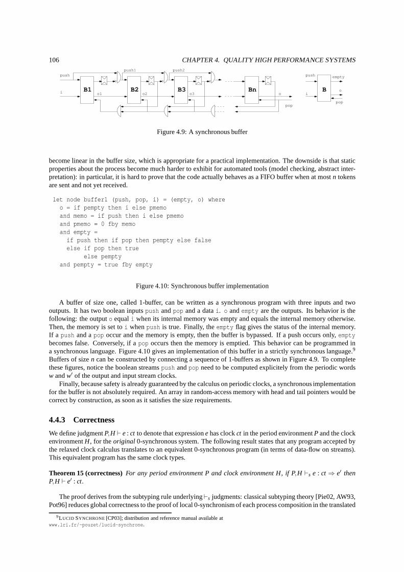
106 CHAPTER 4. QUALITY HIGH PERFORMANCE SYSTEMS
Bn
push
i
pop
push1 push2
o3o2o1 o
push empty
io
pop
BB1 B2 B3
Figure 4.9: A synchronous buffer
become linear in the buffer size, which is appropriate for a practical implementation. The downside is that staticproperties about the process become much harder to exhibit for automated tools (model checking, abstract inter-pretation): in particular, it is hard to prove that the code actually behaves as a FIFO buffer when at mostn tokensare sent and not yet received.
let node buffer1 (push, pop, i) = (empty, o) whereo = if pempty then i else pmemoand memo = if push then i else pmemoand pmemo = 0 fby memoand empty =
if push then if pop then pempty else falseelse if pop then true
else pemptyand pempty = true fby empty
Figure 4.10: Synchronous buffer implementation
A buffer of size one, called 1-buffer, can be written as a synchronous program with three inputs and twooutputs. It has two boolean inputspush andpop and a datai. o andempty are the outputs. Its behavior is thefollowing: the outputo equali when its internal memory was empty and equals the internal memory otherwise.Then, the memory is set toi whenpush is true. Finally, theempty flag gives the status of the internal memory.If a push and apop occur and the memory is empty, then the buffer is bypassed. Ifa push occurs only,emptybecomes false. Conversely, if apop occurs then the memory is emptied. This behavior can be programmed ina synchronous language. Figure 4.10 gives an implementation of this buffer in a strictly synchronous language.9
Buffers of sizen can be constructed by connecting a sequence of 1-buffers as shown in Figure 4.9. To completethese figures, notice the boolean streamspush andpop need to be computed explicitely from the periodic wordsw andw′ of the output and input stream clocks.
Finally, because safety is already guaranteed by the calculus on periodic clocks, a synchronous implementationfor the buffer is not absolutely required. An array in random-access memory with head and tail pointers would becorrect by construction, as soon as it satisfies the size requirements.
4.4.3 Correctness
We define judgmentP,H ⊢ e: ct to denote that expressionehas clockct in the period environmentP and the clockenvironmentH, for theoriginal 0-synchronous system. The following result states that anyprogram accepted bythe relaxed clock calculus translates to an equivalent 0-synchronous program (in terms of data-flow on streams).This equivalent program has the same clock types.
Theorem 15 (correctness)For any period environment P and clock environment H, if P,H ⊢s e : ct⇒ e′ thenP,H ⊢ e′ : ct.
The proof derives from the subtyping rule underlying⊢s judgments: classical subtyping theory [Pie02, AW93,Pot96] reduces global correctness to the proof of local 0-synchronism of each process composition in the translated
9LUCID SYNCHRONE [CP03]; distribution and reference manual available atwww.lri.fr/~pouzet/lucid-synchrone.
4.5. SYNCHRONY AND ASYNCHRONY 107
program (includingat clock constraints). This is guaranteed by the previous buffer insertion scheme, since eachbuffer’s signature is tailored to the resynchronization ofa pair of different but synchronizable clocks. This ensuresthe translated program is synchronous.
4.5 Synchrony and Asynchrony
A system that does not have a single synchronous clock is not necessarily asynchronous: numerous studies havetackled with relaxed or multi-clocked synchrony at the hardware or software levels. We only discuss the mostclosely related sudies, a wide and historical perspective can be found in [Cas01].
There are a number of approaches to the specification and design of hybrid hardware/software systems. Mostof them are graphical tools based on process networks. Kahn process networks (KPN) [Kah74] is a fundamentalone, but it models only functional properties, as opposed tostructural properties. KPN are used in a number oftools such as YAPI [dKES+00] or the COSY project [BKK+00]; such tools still require expertise from differentdomains and there is no universal language that combines functional and structural features in a single framework.
Steps towards the synchronous control of asynchronous systems are also conducted in the domain of syn-chronous programming languages, such as the work of Le Guernic et al. [LTL03] on Polychrony. This worktargets the automatic and correct by construction refinement of programs, in the same spirit as our clock com-position, but it does not consider quantitative propertiesof clocks. StreamIt [TKA02] is a language for highperformance streaming computations that tackles mainly stream-level and algebraic optimization issues.
Ptolemy [BHLM94] is a rich platform with simulation and analysis tools for the design of embedded streamingsystems: it is based on the synchronous data-flow (SDF) modelof computation [EAL87]. Unlike synchronouslanguages, SDF graphs cannot express (bounded or not) recursion and arbitrary aperiodic execution. They are notexplicitly clocked either: synchrony is a consequence of local balance equations on periodic execution schemes.The SDF model allows static scheduling and is convenient forthe automatic derivation of timing properties[MBvM04], but the lack of clocks weakens its amenability forformal reasoning and correct-by-constructiongeneration of synchronous code, with respect to synchronous languages [HCRP91, BCE+03]. Interestingly,n-synchronizable clocks seem to fill this hole, leading to the definition of a formal semantics for SDF while exposingthe precise static schedule to the programmer (for increased control on buffer management and code generation).Further analyses of the correspondence between the two models are left for future work.
4.6 Conclusion
We proposed a synchronous programming language to implement correct-by-construction, high-performancestreaming applications. Our model addresses the automaticsynthesis of communications between processes thatare not strictly synchronous. In this model, we show that latencies and buffer requirements can be inferred auto-matically. We extend a core data-flow language with a notion of periodic clocks and with a relaxed clock calculusto compose synchronous processes. This relaxed synchronous model defines a formal semantics for synchronousdata-flow graphs, building a long awaited bridge with synchronous languages. The clock calculus and the transla-tion procedure from relaxed synchronous to strictly synchronous programs are proven correct, and the associatedtype inference is proven complete. An implementation in thesynchronous language LUCID SYNCHRONE is underway and was applied to a classical video downscaler example.We believe this work widens the scope of syn-chronous programming beyond safety-critical reactive systems and circuit synthesis, promising increased safetyand productivity in the design and optimization of a large spectrum of applications.
Chapter 5
Perspectives
To conclude this manuscript, we build on our results and understanding to propose a structured analysis of theimmediate and longer-term perspectives.
Our work-plan intensionally extends the recent results presented in this thesis. Although this may look likea rather closed point of view (w.r.t. the global research area), this plan contributes to a tighter integration of theresearch conducted so far. The aim is to prioritize the achievement of key contributions involving the deepest levelof specialization, while maximizing the impact on applied domains. The proposed work is also wide enough tocover several challenges identified by the research community, and to drive the activity of multiple research groups.As a matter of fact, most of these perspectives are supportedby research projects involving the ALCHEMY group(from European and French funding agencies) and collaborations with the best research group from academia andindustry, in Europe and abroad.
We hope this manuscript will help other research groups share, criticize and confront our analysis, and thuscontribute to the achievement of significant advances in high-performance computing.
This chapter addresses the interplay of compiler foundations and technology with
1. programming languages,
2. program generators,
3. processor architectures,
4. runtime systems,
5. and the associated tool (infrastructure) development efforts.
5.1 Compilers and Programming Languages
We believe the future of scalable and efficient computing systems lies in parallel programming languages withstrong semantical guarantees, allowing to maximize productivity, robustness and portability of performance. Thissection is a first attempt at shaping an “ideal” parallel programming model. The goal is to let the programmerexpressmostof the parallelism, in adeterministic, compositional(or modular) andcompiler-friendly(or overhead-free) semantics.
5.1.1 First step: Sparsely Irregular Applications
Starting from the experience of the data-flow language StreamIt, we believe we can dramatically improve expres-siveness, parallelism extraction, optimization and mapping opportunities on specific hardware. This work willfirst be targeted towards regular data and computationally intensive applications, with sparsely irregular control(mostly mode transitions).
Most of the parallelism. Most parallel languages ask the programmer to make sensiblechoices in the expositionof coarse grain parallelism. Yet to allow multi-level parallelism to be efficiently exploited on a variety of targets, itis absolutely necessary to expose the fine-grain data-flow structure of the computation. To simplify the compilationand runtime, we first assume a restricted form of control-flow, operating at a sparse, higher “reconfiguration” level.
108
5.1. COMPILERS AND PROGRAMMING LANGUAGES 109
In a data-flow execution model, there is no need for an explicit distinction between data and control paral-lelism. Processes are functions with private memory/state; they can be composed and replicated. Communicationand control is explicit, and can be provided with an additional interface for comfortable data parallel programmingand for the flexible expression of functional pipelines. This interface may take the form of semantically rich com-munication and partially-parallel computation skeletons, built on top of the abovementioned data-flow primitives,like reductions/scans, collective communications. This interface should also provide a clean atomic execution andsynchronization semantics at the higher level of control.
Deterministic. To preserve the Kahn principle [Kah74] (determinism and absence of schedule or resource-induced dead-locks), there must be no information flow between processes without explicit communications,assuming non-blocking writes and blocking reads on FIFO channels. Non-FIFO communications can be seenas “peek/poke” operations into implicitly unbounded single-assignment buffers (but practically bounded throughstatic analysis), which can in turn be translated into FIFO operations [TKA02], but compiled much more efficientlywith circular buffers, address generators or rotating register files. Communications can be hierarchically structuredto reflect the organization of data or computation itself: one write/read operation in a high-level process may befurther detailed into a deterministic sequence of finer-grain communications in nested processes. The mapping ofthese semantically abstract communications onto target-specific primitives is completely hidden.
Compositional. Determinism offers composition (or modularity) for free, as long as liveness and equity prop-erties are satisfied (prerequisites of the Kahn principle).Equity depends on the compilation flow, for the largerpart, in a statically controlled architecture. Liveness must be proven at compilation time by static analysis (e.g.,checking for delays in circuits of the data-flow graph).
Preserving compositionality of resource, placement and schedule properties is much more difficult, but syn-chronous Kahn networks [CP96, CGHP04] are a great progress in this direction, as discussed in the next paragraph.
Compiler-friendly. To ensure early satisfaction of the resource and real-time constraints in the compilationflow, the data-flow semantics must be complemented with implicit and local scheduling information to reasonglobally about the application-architecture mapping. This is the contribution of the synchronous execution modelto high-performance parallel programming; constraining all computations to take place at well defined instants ina global, totally ordered, logical time (hence the term “synchronous”) allows for much more advanced compilationstrategies and optimizations. The lack of such semantical information is a major reason for StreamIt’s inability toharness multi-level, heterogeneous and fine-grain parallelism.
A synchronous distributed system does not have any hidden communication buffer: all communications are“logical wires” and do not need any particular storage beyond the duration of the “instantaneous clock tick”. Inpractice, depending on the compilation strategy, registers, memory or communication elements may be required.We advocate for a pragmatic implementation of this principle, to go much beyond the limitations of StreamIt[TKA02] which are those of the SDF [EAL87]. We propose to use two levels of clocks:
• asymptotically periodic, or piecewise affine ones to model the start-up and steady state of the regular data-flow level of the computation;
• arbitrary boolean clocks (which depend on external signal or internal reactions) to model the reconfigura-tions and trigger transient executions of the application,effectively modeled by an bounded aperiodic butstatically known behavior of the application.
The periodic/affine level of clocks yields a statically manageable hierarchy of computations that may be con-verted into compact, efficient loop nests, amenable to further optimizations and fine-grain parallelization. Theseclocks also allow to relax the synchronous hypothesis by allowing to compose “almost synchronous” processes andinfer the intermediate buffers automatically to statically allocate memory/communication resources [CDE+06].Finally, these logical clocks are needed to generate efficient code and manage resources statically, but they can beoverridden in the optimization flow, through multi-dimensional retiming techniques.
The higher level of more expressive but semantically poorerclocks requires dynamic control in the generatedcode (nestedif conditionals), and resembles the compilation of most synchronous languages [BCE+03].
Sparsely irregular. The abovementioned two-level clocks allow to model irregular reconfigurations or “modetransitions”. Typically, all modes and all transitions would be statically defined in the application, letting the
110 CHAPTER 5. PERSPECTIVES
compiler best optimize the schedule and resource mapping for each transient and steady state. Early feedbackon the satisfaction of the resource and real-time constraints can be gathered, facilitating the adaptation of thepartitioning in a manual or automatic design-space exploration of the application-architecture mapping.
On the data and communication side, the non-FIFO communications can be translated into bounded arrays.Specific treatment of affine subscripts is very important, but allowing indirect subscripts is important for somerendering algorithms and for mesh computations.
5.1.2 Second step: General-Purpose Parallel Clocked Programming
To broaden the acceptation of data-flow concurrency in parallel computing (beyond streaming applications andsystems), we revisit the basic principles of synchronous data-flow computing with a more compiler-centric point ofview. For example, instead of emphasizing on the synchrony of the “rendez-vous” between independent threadsand the instantaneity of the local computations, we prefer to develop the ability of the concurrency model tocompute directly on clocks as first-class citizens. This point of view does not match all flavors of synchrony, inparticular it radically departs from the Esterel point of view where clocks should not exist in the program semanticsitself. There are numerous reasons why clocks — and the associated semantical restrictions and clock-directedcompilation strategies — are necessary to enable “efficient-by-design” compilation methods (e.g., generatingsequential code with nested loops and no conditional control-flow from multiple processes with different clocks).
The extension to more general, less regular computations, is also a longer term challenge. Our current ap-proach is to investigate how dynamic parallelization and adaptation techniques can be combined with the data-flowprogramming model, to allow for limited non-deterministic, speculative or data-dependent computations to be ef-ficiently compiled on a parallel architecture. The section on runtime systems below provides more insights aboutthis, and we advocate for a tight cooperation between deterministic and non-deterministic forms of parallelism —atomic transactions, with inspector-executor instrumentation or speculation — with a core data-flow concurrencymodel.
5.2 Compilers and Program Generators
The quality of compiler-optimized code for high-performance applications is far behind what optimization anddomain experts can achieve by hand. Although it may seem surprising at first glance, the performance gap hasbeen widening over time, due to the tremendous complexity increase in microprocessor and memory architectures,and to the rising level of abstraction of popular programming languages and styles. We wish to further explore in-between solutions, neither fully automatic nor fully manual ways to adapt a computationally intensive applicationto the target architecture. As hinted to in the introduction, much progress was achieved, not by improving thecompiler, but through the design of application-specific program generators, a.k.a. active libraries [VG98]. Themost advanced project in this area is SPIRAL [PSX+04].
We are interested in improving language support for domain experts to implement such active libraries. Thismotivation is apparently shared by language designs in Fortress [ACL+06]. Our early work is based on multi-stage languages. In particular, we used MetaOCaml to experiment with off-line and online generation of high-performance programs [CDG+06]. The main advantages of this approach are the ability to generate code thatdoes not trigger future-stage compilation errors (syntax,structure, type), and the seamless integration of valuesproduced in various execution stages (for online optimization and specialization).
Yet our results have been mitigated by the constraints on code introspection (opening code expressions) as-sociated with the simultaneous enforcement of type safety for all stages. The ability to implement generic andreusable program generator components is also restricted by the need to express some transformations on a higherlevel, non-syntactic representation, using unconventional domain-specific denotations, polyhedral encodings of it-erative computations, etc. Some progresses can be expectedfrom extended type systems to manage the recaptureof variable names exposed through the opening of code expressions.
Another interesting perspective is the extension of safetyguarantees to abstract properties like memory depen-dences. This would allow semantics-preserving transformations to take place on well-formed code expressionsor denotations. Our first proposal, theX-language, goes in this direction. It combines multi-stageprogrammingwith programmable semantics-preserving loop transformation primitives and search-space traversal capabilities[DBR+05].
Eventually, in collaboration with Denis Barthou, we are investigating the complementation of program gener-ators with a resolution-based search engine. Using Prolog or Stratego [Vis01] rules, it is quite natural to design
5.3. COMPILERS AND ARCHITECTURES 111
an iterative optimization system based on term-rewriting,guided by profile feedback and performance models.This allows direct search techniques (optimizations basedon direct performance measurements) to be acceleratedand focused in a narrower space thanks to the knowledge of a domain expert. This knowledge is implemented asoptimizationgoalsof the rewriting system. Therefore, we call this approachgoal-driven iterative optimization.A major challenge consists in inverting the performance models to infer optimization sub-goals from partial goalfulfillments and partial transformation sequences.
5.3 Compilers and Architectures
The biggest challenge for the design of future architectures is to achieve scalability of performance. Yet, scalabilityis not so useful if efficiently and programmability are neglected. It is well known from VLIW processor designthat the main improvements in efficiency come with progresses in compiler technology. To make an architectureresource-efficient, the balance may vary between functional units, memory and communication; however, theinvariant goal is to minimize the size of control structuresin favor of smarter software support (at runtime andcompile-time).
We believe that future processors will necessarily follow adistributed memory model and feature a heteroge-neous, coarse-grain reconfigurable mesh of resources. Unlike FPGAs and fine-grain reconfigurable devices (whichwaste too many transistors in hardware lookup tables), coarser grain reconfigurable processors with heterogeneousand distributed resources offer the best tradeoff in terms of scalability and efficiency. The RAW machine was apionneer in this direction, but major challenges remain to adapt the computing paradigm to the capabilities of codegenerators and optimization techniques, or alternatively, to involve the programmer in the mapping process whilepreserving productivity.
5.3.1 Decoupled Control, Address and Data Flow
Our approach to the efficiency challenge takes two consecutive steps.The first step focuses on embedded streaming applications and processors, with regular computation and com-
munication patterns. Inspired by the early DSP designs (Harvard architecture), it makes sense to strictly decouplethe architecture into control, address generation and data-flow streams. Our previous work in the SANDRA project[CDC+03], in collaboration with Philips Research, was a first attempt to design a compiler for such a decoupledarchitecture for stream-processing. Improvements in polyhedral code generation and automatic distribution willbe very valuable for regular applications. Yet more generaland irregular processing will benefit from a explic-itly parallel data-flow programs with synchronous clocks, to guide the mapping and scheduling on a distributeddecoupled architecture. In this direction, we are working on explicitly modeling hardware resources and the map-ping of operations and communications in the application tothose resources, as the composition of synchronousprocesses. The design of a common synchronous language interface between the programmer and a suite of op-timization tools would be a fundamental progress. It would also be of immediate use throughout the design of amassively parallel real-time embedded system, as an exchange representation between signal-processing experts,application programmers, optimization and architecture experts.
The second step will also be language-centric, and will address general-purpose computing. Building on theclock abstraction of the synchronous data-flow paradigm, weknow it is possible to design a concurrent program-ming language and to extend compilation techniques designed in the first step, to target more general clock andprocess semantics, possibly with a graceful degradation inperformance as irregularity grows. Neither decoupledarchitectures nor synchronous languages are intrinsicly domain-specific: we believe the current state-of-the-art,inertia and misuse of vocabulary1 make them appear so.
5.3.2 Fine-Grain Scheduling and Mapping
Modulo scheduling is the dominant family of heuristics for software pipelining. Its success lies in its scalabilityand its ability to produce compact code with near-optimal initiation intervals. This success comes with a heavy biastowards asymptotic performance for high trip-count loops,leaving considerations about single-iteration make-spanand register usage as second-class optimization criteria.Empirical results also indicate that modulo-schedulingheuristics achieve low complexity at the expense of chaoticperformance results (on realistic resource models).Eventually, modulo scheduling lacks an integrated way to reason about code size (unrolling factor) and to model
1Synchronous languages do not require synchronous execution and can model arbitrary non-reactive semantics [CP96, CGHP04].
112 CHAPTER 5. PERSPECTIVES
resource constraints that are not transparent to the data dependence graph (register spill and reload, clusteredregister files, instruction selection). The combination ofthis overall success and intrinsic limitations has drivennumerous theoretical and practical studies, but with a relatively low impact on actual compiler designs at the endof the road.
We are working on a new cyclic scheduling algorithm, called Pursuit Scheduling. It is a bi-criteria heuristicfor software pipelining, based on a Petri net representation of dependence and resource constraints. The aim is tosimulate modulo scheduling, but extend it into a bi-criteria optimization problem, to improve both the initiationinterval and make-span. We attempt to preserve the best of modulo scheduling heuristics, while improving perfor-mance stability and allowing for a variety of optimization goals and resource constraints. Unlike existing Petri netscheduling approaches, our algorithm does not iterate until a fix point to ultimately recognize a periodic executionkernel. Instead, it complements the traditional Petri net semantics with an original transition-firing rule that pre-serves the distinctive code-size control of modulo scheduling. Our current results are encouraging: when directingthe optimization towards asymptotic performance, our experimental results match or outperform state-of-the-artmodulo scheduling heuristics. Our results also show benefits when optimizing loops with low trip-counts, whichare common in multimedia routines and hierarchically tiledhigh-performance libraries.
Given the flexibility of the model, it is very attractive to extend this heuristic to multidimensional softwarepipelining. Indeed, when scheduling quasi-periodic data-flow processes on a massively parallel chip multi-processor, the optimization problem becomes intrinsicly multi-criteria. The problem consists in optimizing codesize, buffer size, computation throughput and computationlatency, but none of these dimensions can be neglected,since the figures in each dimension may vary by multiple orders of magnitude (unlike traditional software pipelin-ing problems). We believe that programmer intervention will be necessary to drive the optimization towards rea-sonable sub-spaces of this daunting problem. We are currently studying, as a preliminary example, the schedulingof Synchronous Data-Flow graphs (SDF) [EAL87] on the Cell processor. When stepping from regular quasi-periodic applications to general-purpose ones, our previous work on Deep Jam — a generalization of nestedunroll-and-jam for irregular codes — will be quite valuable[CCJ05].
5.4 Compilers and Runtime Systems
Embedded systems and large-scale parallel architectures both require dynamic adaptation to make most effectiveuse of computing resources. These research perspectives would not be complete without considering stagedcompilation, as well as dynamic parallelization and optimization techniques.
5.4.1 Staged Compilation and Learning
In a just-in-time (JIT) compilation environment, optimizations are staged, i.e., split into off-line and runtimeprogram manipulations. The success of this compilation model suggests additional improvements could arise froma tighter coupling between program analyses and transformations at different stages of the compilation/execution.We are particularly interested in progresses in three areas.
1. Enabling new, more aggressive optimizations to take place in JIT or runtime compilers, using annotationsof the intermediate language (bytecode) to pass static properties or predigested results of operation researchalgorithms. For example, software pipelining and global scheduling algorithms are usually too expensivebeyond classical static compiler environments. This couldchange provided a sparse and accurate encodingof memory dependences and/or partial schedule hints can be passed to a JIT compiler.
2. Intermediate language annotations can convey messages for future-stage code generation, including codespecialization, loop unrolling and procedure inlining. This may have a strong impact on code size andbenefit to embedded systems research.
3. We believe in the combination machine learning and phase/context adaptation, passing features throughthe compilation stages to postpone the key optimization andparallelization decisions to the “right exe-cution/compilation stage”. This approach builds on our previous work on runtime iterative optimization[FCOT05].
5.5. TOOLS 113
5.4.2 Dynamically Extracted Parallelism
A variety of computational problems benefit from the dynamicextraction of parallelism. For example, it doesnot make much sense to extract fully-static parallelism from sparse matrix computations, or from finite elementmethods on irregular meshes, in general. In some cases, speculation can further improve scalability in extractingparallelism at a coarser grain or in reducing load imbalance.
The most promising work in this area are those of Lawrence Rauchwerger, related work by Josep Torrellas,and the recent hype on transactional memory in computer architecture.
• Hybrid analysis performs a symbolic static analysis to synthesize the minimal dynamic (in)dependence testto parallelize a loop [RRH03]. Extending this to more general control and data structures may bring signif-icant improvements in irregular, computationally intensive applications, with very little overhead. This ap-proach is compatible with most embedded system constraints. Similarly, STAPL proposes a library-centric,container-centric parallel programming model based on theC++ STL [AJR+01]. Besides its C++ speci-ficities, this model combines dynamic and static information to exploit vast amounts of parallelism on dis-tributed architectures. Combining both approaches, allowing the compiler to reason about (in)dependencein general-purpose computations, seems the most promisingapproach. Once again, this research area needslibrary, program generators and compilers to be tightly integrated.
• Speculative parallelization can be done on software or hardware [OHL99, RP99, CMT00, LTC+06]. It hasan interesting potential in speeding up sequential and parallel applications. Yet its intrinsic overheads (mem-ory management, communications, squash and commit, useless computations) limits its practical applica-bility. Transactional memory models (hardware or softwarebased) [MCC+06, HMJH05] and programminglanguages [ACL+06] are an interesting progress over lock-based multi-threaded programs and over thefully automated extraction of speculative threads. We are interested in minimizing the impact on hardwareresources (using speculation when strictly necessary, andreducing on-chip storage for atomic transactionstate), and in the combination of transactional semantics with deterministic, synchronous data-flow seman-tics.
Regarding the potential of transactional memory semantics, let us quote Tim Harris, Simon Marlow, SimonPeyton Jones, and Maurice Herlihy [HMJH05] (Section 2, page2) describing a software transactional memorysystem built on Concurrent Haskell:
Perhaps the most fundamental objection [...] is that lock-based programs do not compose: correctfragments may fail when combined. For example, consider a hash table with thread-safe insert anddelete operations. Now suppose that we want to delete one item A from tablet1, and insert it intotablet2; but the intermediate state (in which neither table contains the item) must not be visible toother threads. Unless the implementor of the hash table anticipates this need, there is simply no wayto satisfy this requirement. [...] In short, operations that are individually correct (insert, delete) cannotbe composed into larger correct operations.
The ability to compose parallel programs into correct larger ones is nothing new. The already mentioned Kahnproperty of data-flow systems already offers this benefit, ina distributed but more constrained — deterministic— concurrency model. We encourage further comparisons in terms of scalability, efficiency and expressiveness,aiming for the integration of the two models.
Eventually, given the complexity and intrication of decisions associated with deferring analyses to runtimeor with speculation, it is obvious that this research will benefit from advances in machine learning compilation[ABC+06].
5.5 Tools
This chapter closes with a discussion of tool and development issues. Perspectives in this area are not secondary.Compilation research has long suffered from the lack of interoperability between research prototypes, productioncompilers and academic language front-ends. Given the highcomplexity of any modern compiler and program-ming language, we defend the idea that academic research will suffer from ever-increasing inefficiencies if notembracing a widespread production compilation framework.
Practically, this means choosing GCC, since all other platforms are either very narrow in terms of retargetabil-ity and language support, or not robust and maintainable enough in the long term. We are not encouragingall
114 CHAPTER 5. PERSPECTIVES
developments to take place in GCC, only those which have the ambition to survive the research projectthatinitially motivated them.
The GCC is a multi-language, multi-target, and multi-OS cross-compiler with about 2.5 million lines of(mostly C) code. The development started in 1984 as part of the GNU project of the Free Software Foundation(FSF). In 2005, GCC 4.0 was released thanks to the efforts of many developers. It introduces a new, innovativemiddle-end based on a state-of-the-art SSA-form intermediate representation. This was the result of many yearsof commitment by major hardware, software and service companies, including Red Hat (Cygnus), Novell (SuSE),IBM, Apple, Intel, AMD, HP, Sony, Code Sourcery, among others.
Although GCC has always been a reference in terms of robustness and conformance to standards, the per-formance of the compiled code was lagging behind target-specific compilers developed by hardware vendors.The rise of GCC 4.0 eventually allowed to implement modern (static and dynamic) analyses and optimizations,quickly bridging the gap with the best compilers on the market. These improvements also affect embedded andspecial-purpose processors: e.g., GCC recently achieved the top of the ranking published by the EEMBC telecombenchmark on the PowerPC 970FX processor, with 2.8× speed-up over the previous compiler.
GCC 4.2 features more than 170 compilation passes, two thirds of them playing a direct role in programoptimization. These passes are selected, scheduled, and parameterized through a versatile pass manager. Themain families of passes can be classified as:
• interprocedural analyses and optimizations;
• profile-directed optimization (interprocedural and intraprocedural);
• induction variable analysis, canonicalization and strength-reduction;
• loop optimizations;
• automatic vectorization;
• data layout optimization.
More advanced developments are in progress. We identified three major ones with a direct impact on high-performance embedded systems research:
• link-time optimization (towards just-in-time and dynamiccompilation), with emphasis on scalability towhole-program optimization and compatibility with production usage;
• automatic parallelization, featuring full OpenMP 2.5 support and evolving towards automatic extraction ofloop and functional parallelism, with ongoing research on speculative forms of parallelism.
Outside of GCC, the two traditional alternatives would be:
1. The source-to-source model, by far the most popular in research environments, during the last two decades.It is much less attractive now, for two reasons. Experienceswith the new infrastructure of GCC showcomparable development time and no significant increase in complexity of the intermediate representationor programmer interface: in practice, the design freedom benefits do not offset the development overheads,except on limited toy prototypes. Second, the lack of an integrated compilation flow, broken by one ore moreconversions to a programming language, is a source of runtime overheads (not speaking about compile-timeoverheads of course), semantical mismatches and design bugs, usage restrictions.2
We believe the only and most significant advantage of source-to-source compilation is portability, not ease ofdevelopment. Given the openness of GCC (license-wise, language-wise and target-wise), this advantage isnot very significant. Of course, some research fields still require the use of proprietary back-ends, includinghardware synthesis, and generating code for awkward, but more and more attractive (performance-wise)fine-grained controlled architectures. In the latter case,we encourage researchers to mutualize efforts tobypass these tools and obsolete them through combined applied research and software engineering withindustrial third parties.
2Notice many compilers use persistent (sometimes semantically well defined) intermediate languages. This is quite different from source-to-source compilation, since arbitrarily rich semantics (including the result of static and dynamic analysis) can be embedded in such interme-diate languages.
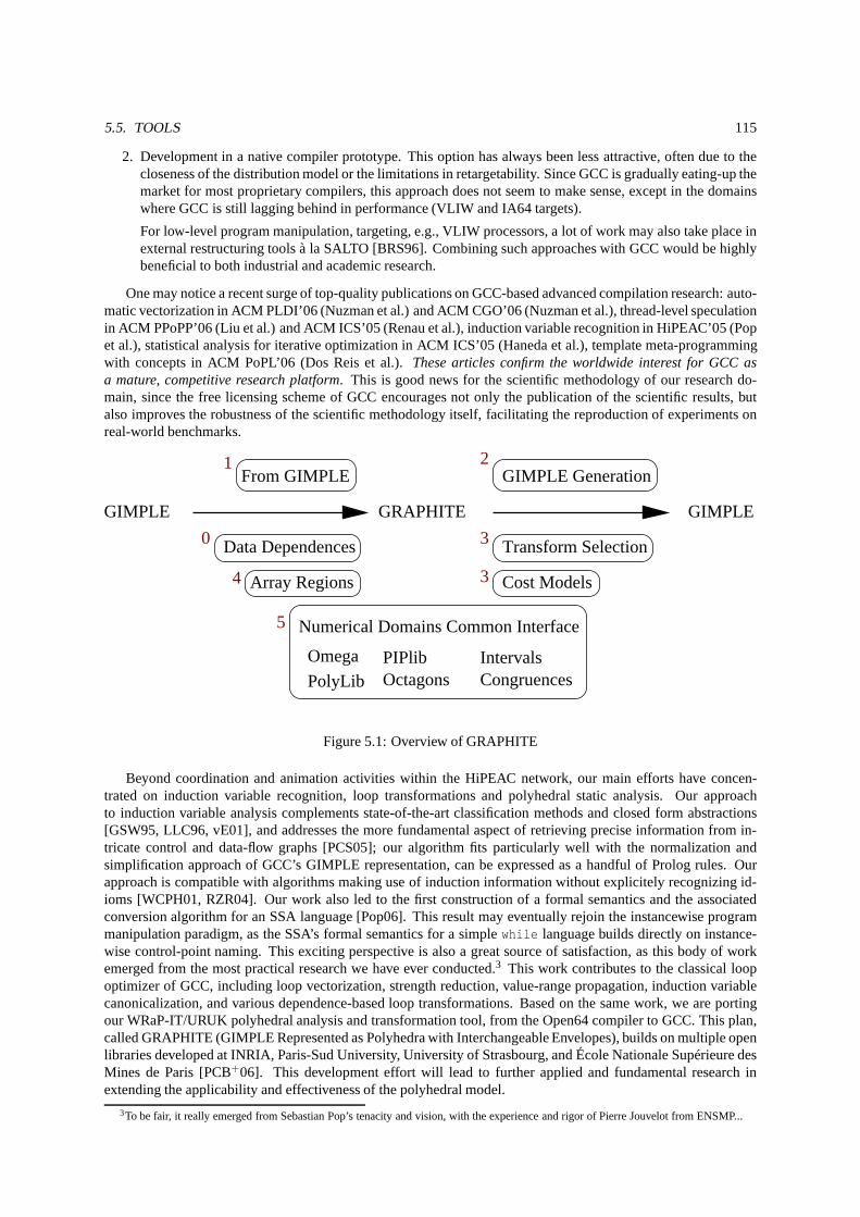
5.5. TOOLS 115
2. Development in a native compiler prototype. This option has always been less attractive, often due to thecloseness of the distribution model or the limitations in retargetability. Since GCC is gradually eating-up themarket for most proprietary compilers, this approach does not seem to make sense, except in the domainswhere GCC is still lagging behind in performance (VLIW and IA64 targets).
For low-level program manipulation, targeting, e.g., VLIWprocessors, a lot of work may also take place inexternal restructuring tools à la SALTO [BRS96]. Combiningsuch approaches with GCC would be highlybeneficial to both industrial and academic research.
One may notice a recent surge of top-quality publications onGCC-based advanced compilation research: auto-matic vectorization in ACM PLDI’06 (Nuzman et al.) and ACM CGO’06 (Nuzman et al.), thread-level speculationin ACM PPoPP’06 (Liu et al.) and ACM ICS’05 (Renau et al.), induction variable recognition in HiPEAC’05 (Popet al.), statistical analysis for iterative optimization in ACM ICS’05 (Haneda et al.), template meta-programmingwith concepts in ACM PoPL’06 (Dos Reis et al.).These articles confirm the worldwide interest for GCC asa mature, competitive research platform. This is good news for the scientific methodology of our research do-main, since the free licensing scheme of GCC encourages not only the publication of the scientific results, butalso improves the robustness of the scientific methodology itself, facilitating the reproduction of experiments onreal-world benchmarks.
1 2
0
4
5
3
3
PolyLib
Omega PIPlib
Numerical Domains Common Interface
Cost Models
Transform Selection
GIMPLE
GIMPLE GenerationFrom GIMPLE
Data Dependences
Array Regions
GIMPLE GRAPHITE
IntervalsCongruencesOctagons
Figure 5.1: Overview of GRAPHITE
Beyond coordination and animation activities within the HiPEAC network, our main efforts have concen-trated on induction variable recognition, loop transformations and polyhedral static analysis. Our approachto induction variable analysis complements state-of-the-art classification methods and closed form abstractions[GSW95, LLC96, vE01], and addresses the more fundamental aspect of retrieving precise information from in-tricate control and data-flow graphs [PCS05]; our algorithmfits particularly well with the normalization andsimplification approach of GCC’s GIMPLE representation, can be expressed as a handful of Prolog rules. Ourapproach is compatible with algorithms making use of induction information without explicitely recognizing id-ioms [WCPH01, RZR04]. Our work also led to the first construction of a formal semantics and the associatedconversion algorithm for an SSA language [Pop06]. This result may eventually rejoin the instancewise programmanipulation paradigm, as the SSA’s formal semantics for a simple while language builds directly on instance-wise control-point naming. This exciting perspective is also a great source of satisfaction, as this body of workemerged from the most practical research we have ever conducted.3 This work contributes to the classical loopoptimizer of GCC, including loop vectorization, strength reduction, value-range propagation, induction variablecanonicalization, and various dependence-based loop transformations. Based on the same work, we are portingour WRaP-IT/URUK polyhedral analysis and transformation tool, from the Open64 compiler to GCC. This plan,called GRAPHITE (GIMPLE Represented as Polyhedra with Interchangeable Envelopes), builds on multiple openlibraries developed at INRIA, Paris-Sud University, University of Strasbourg, and École Nationale Supérieure desMines de Paris [PCB+06]. This development effort will lead to further applied and fundamental research inextending the applicability and effectiveness of the polyhedral model.
3To be fair, it really emerged from Sebastian Pop’s tenacity and vision, with the experience and rigor of Pierre Jouvelot from ENSMP...
116 CHAPTER 5. PERSPECTIVES
The main components of GRAPHITE, the development priorities, and the important dependences betweencomponents are depicted in Figure 5.1. Our development plancontains five stages, numbered on the figure:first the translation from GIMPLE to the polyhedral representation, then the translation back to GIMPLE, thedevelopment of cost models and the selection of the transform schedule. The interprocedural refinement of thedata dependence information based on the array regions is optional, but it is necessary for gathering more preciseinformations that potentially could enable more transformations, or more precise transform decisions. Finally, theleast critical component is the integration of the numerical domains common interface, based on which it will bepossible to change the complexity of the algorithms used in the polyhedral analyses.
We plan to progressively integrate within GCC most of the implementation efforts associated with our researchprojects. Particularly important is the the development ofa convincing, widely applicable and distributed imple-mentation of the parallel programming language designs proposed at the beginning of this chapter. This work isintended to be implemented on top of the existing OpenMP, interprocedural optimization and loop transformationframeworks in GCC, with additional support for managing communications, the optimization of these, and theextended type systems associated with logical clocks for mapping and schedule annotations.
This implementation work will not contribute to the compiler mainline before most of the effective research hasbeen completed. The long-term management of GCC branches with highly sophisticated compilation techniquesis a problem. We do not hope that GCC will be a magical solutionto the dilemma of academic prototypes: nobodywants to maintain them when it would be most useful in terms ofdissemination and transfer. However, we willmake constant efforts to involve other members of the GCC community in our research, hence maximize thechances of a successful transfer.
Bibliography
[ABC+06] F. Agakov, E. Bonilla, J. Cavazos, B. Franke, G. Fursin, M.F.P. O’Boyle, J. Thomson, M. Tous-saint, and C.K.I. Williams. Using machine learning to focusiterative optimization. In4th AnnualInternational Symposium on Code Generation and Optimization (CGO), March 2006.
[ACF03] P. Amiranoff, A. Cohen, and P. Feautrier. Instancewise array dependence test for recursive programs.In Proc. of the 10th Workshop on Compilers for Parallel Computers (CPC’03), Amsterdam, NL,January 2003. University of Leiden.
[ACG+04] L. Almagor, K. D. Cooper, A. Grosul, T.J. Harvey, S.W. Reeves, D. Subramanian, L. Torczon, andT. Waterman. Finding effective compilation sequences. InProc. Languages, Compilers, and Toolsfor Embedded Systems (LCTES), pages 231–239, 2004.
[ACL+06] E. Allen, D. Chase, V. Luchangco, C. Flood, J.-W. Maessen, S. Ryu, S. Tobin-Hochstadt, and G. L.Steele. The fortress language specification 0.866. Technical report, Sun Microsystems, 2006.
[ACM+98] D. I. August, D. A. Connors, S. A. Mahlke, J. W. Sias, K. M. Crozier, B.-C. Cheng, P. R. Eaton,Q. B. Olaniran, and W.-M. Hwu. Integrated predicated and speculative execution in the IMPACTEPIC architecture. InProceedings of the 25th Intl. Symp. on Computer Architecture, July 1998.
[AI91] C. Ancourt and F. Irigoin. Scanning polyhedra with DOloop. In ACM Symp. on Principles andPractice of Parallel Programming (PPoPP’91), pages 39–50, June 1991.
[AJR+01] P. An, A. Jula, S. Rus, S. Saunders, T. Smith, G. Tanase, N.Thomas, N. M. Amato, and L. Rauch-werger. Stapl: An adaptive, generic parallel c++ library. In Languages and Compilers for ParallelComputing (LCPC’01), pages 193–208, 2001.
[AK87] J. Allen and K. Kennedy. Automatic translation of Fortran programs to vector form.ACM Trans. onProgramming Languages and Systems, 9(4):491–542, October 1987.
[AK02] R. Allen and K. Kennedy.Optimizing Compilers for Modern Architectures. Morgan and Kaufman,2002.
[Ami04] P. Amiranoff. An Automata-Theoretic Modelization of Instancewise Program Analysis: Transducersas mappings from Instances to Memory Locations. PhD thesis, CNAM, Paris, December 2004.
[AMP00] N. Ahmed, N. Mateev, and K. Pingali. Synthesizing transformations for locality enhancement ofimperfectly-nested loop nests. InACM Supercomputing’00, May 2000.
[ASU86] A. Aho, R. Sethi, and J. Ullman.Compilers: Principles, Techniques and Tools. Addison-Wesley,1986.
[AW93] A. Aiken and E. L. Wimmers. Type inclusion constraints and type inference. InFunctional Pro-gramming Languages and Computer Architecture, pages 31–41, 1993.
[BACD97] J. Bilmes, K. Asanovic, C.W. Chin, and J. Demmel. Optimizing matrix multiply using PHiPAC: Aportable, high-performance, ANSI C coding methodology. InACM Intl. Conf. on Supercomputing(ICS’97), pages 340–347, 1997.
[Ban88] U. Banerjee.Dependence Analysis for Supercomputing. Kluwer Academic Publishers, Boston, 1988.
117
118 BIBLIOGRAPHY
[Ban92] U. Banerjee.Loop Transformations for Restructuring Compilers: The Foundations. Kluwer Aca-demic Publishers, Boston, 1992.
[Bar98] D. Barthou.Array Dataflow Analysis in Presence of Non-affine Constraints. PhD thesis, Universitéde Versailles, France, February 1998.http://www.prism.uvsq.fr/~bad/these.html.
[Bas03] C. Bastoul. Efficient code generation for automaticparallelization and optimization. InISPDC’2IEEE International Symposium on Parallel and Distributed Computing, Ljubjana, Slovenia, October2003.
[Bas04] C. Bastoul. Code generation in the polyhedral modelis easier than you think. InParallel Architec-tures and Compilation Techniques (PACT’04), Antibes, France, September 2004.
[BBC+99] M. Barreteau, François Bodin, Zbigniew Chamski, Henri-Pierre Charles, Christine Eisenbeis, John R.Gurd, Jan Hoogerbrugge, Ping Hu, William Jalby, Toru Kisuki, Peter M. W. Knijnenburg, Paulvan der Mark, Andy Nisbet, Michael F. P. O’Boyle, Erven Rohou, André Seznec, Elena Stöhr, MennoTreffers, and Harry A. G. Wijshoff. Oceans - optimising compilers for embedded applications. InEuro-Par’99, pages 1171–1775, August 1999.
[BCBY04] Christian Bell, Wei-Yu Chen, Dan Bonachea, and Katherine Yelick. Evaluating support for globaladdress space languages on the cray X1. InACM Intl. Conf. on Supercomputing (ICS’04), St-Malo,France, June 2004.
[BCC98] D. Barthou, A. Cohen, and J.-F. Collard. Maximal static expansion. In25th ACM Symp. on Principlesof Programming Languages (PoPL’98), pages 98–106, San Diego, California, January 1998.
[BCC00] D. Barthou, A. Cohen, and J.-F. Collard. Maximal static expansion.Intl. J. of Parallel Programming,28(3):213–243, June 2000.
[BCE+03] A. Benveniste, P. Caspi, S. A. Edwards, N. Halbwachs, P. Le Guernic, and R. de Simone. Thesynchronous languages 12 years later.Proceedings of the IEEE, 91(1), January 2003.
[BCF97] D. Barthou, J.-F. Collard, and P. Feautrier. Fuzzy array dataflow analysis.J. of Parallel and Dis-tributed Computing, 40:210–226, 1997.
[BCG+03] C. Bastoul, A. Cohen, S. Girbal, S. Sharma, and O. Temam. Putting polyhedral loop transformationsto work. In Languages and Compilers for Parallel Computing (LCPC’03), LNCS, pages 23–30,College Station, Texas, October 2003. Springer-Verlag.
[BEF+96] W. Blume, R. Eigenmann, K. Faigin, J. Grout, J. Hoeflinger, D. Padua, P. Petersen, W. Pottenger,L. Rauchwerger, P. Tu, and S. Weatherford. Parallel programming with Polaris. IEEE Computer,29(12):78–82, December 1996.
[Ber79] J. Berstel.Transductions and Context-Free Languages. Teubner, Stuttgart, Germany, 1979.
[Ber00] G. Berry.The Foundations of Esterel. MIT Press, 2000.
[BF03] C. Bastoul and P. Feautrier. Improving data localityby chunking. InCC Intl. Conf. on CompilerConstruction, number 2622 in LNCS, pages 320–335, Warsaw, Poland, april 2003.
[BF04] C. Bastoul and P. Feautrier. More legal transformations for locality. InEuro-Par’10, number 3149 inLNCS, pages 272–283, Pisa, August 2004.
[BF05] Cédric Bastoul and Paul Feautrier. Adjusting a program transformation for legality.Parallel process-ing letters, 15(1):3–17, March 2005.
[BFF05] J. Thomson B. Franke, M. O’Boyle and G. Fursin. Probabilistic source-level optimisation of embed-ded systems software. InACM SIGPLAN/SIGBED Conference on Languages, Compilers, and Toolsfor Embedded Systems (LCTES’05), 2005.
[BGGT02] A. J. C. Bik, M. Girkar, P. M. Grey, and X. Tian. Automatic intra-register vectorization for the intelarchitecture.Intl. J. of Parallel Programming, 30(2):65–98, 2002.
BIBLIOGRAPHY 119
[BHLM94] J. Buck, S. Ha, E. A. Lee, and D. G. Messerschmitt. Ptolemy: A framework for simulating andprototyping heterogenous systems.Int. J. in Computer Simulation, 4(2):155–182, 1994.
[BKK +98] F. Bodin, T. Kisuki, P.M.W. Knijnenburg, M.F.P. O’Boyle, and E. Rohou. Iterative compilation ina non-linear optimisation space. InProc. Workshop on Profile and Feedback Directed Compilation,1998.
[BKK +00] J.-Y. Brunel, W. M. Kruijtzer, H. J. H. N. Kenter, F. Pétrot, L. Pasquier, E. A. de Kock, and W. J. M.Smits. COSY communication IP’s. In37thDesign Automation Conference (DAC’00), pages 406–409,Los Angeles, California, June 2000.
[BLJ91] A. Benveniste, P. Le Guernic, and C. Jacquemot. Synchronous programming with events and rela-tions: the signal language and its semantics.Science of Computer Programming, 16(2):103–149,1991.
[Bou92] F. Bourdoncle. Abstract interpretation by dynamicpartitioning. J. of Functional Programming,2(4):407–423, 1992.
[BRS96] F. Bodin, E. Rohou, and A. Seznec. Salto: System for assembly-language transformation and opti-mization. InWorkshop on Compilers for Parallel Computers (CPC’96), December 1996.
[BRZ03] R. Bagnara, E. Ricci, and E. Zaffanella. Precise widening operators for convex polyhedra. InInt.Symp. on Static Analysis (SAS’03), LNCS, San Diego, CA, June 2003. Springer-Verlag.
[Cas01] P. Caspi. Embedded control: From asynchrony to synchrony and back. InEMSOFT’01, volume 2211of LNCS, Lake Tahoe, October 2001. Springer-Verlag.
[CC77] P. Cousot and R. Cousot. Abstract interpretation: a unified lattice model for static analysis of pro-grams by construction of approximation of fixpoints. In4thACM Symp. on Principles of ProgrammingLanguages, pages 238–252, Los Angeles, CA, January 1977.
[CC98] A. Cohen and J.-F. Collard. Instancewise reaching definition analysis for recursive programs usingcontext-free transductions. InParallel Architectures and Compilation Techniques (PACT’98), pages332–340, Paris, France, October 1998. IEEE Computer Society.
[CCG96] A. Cohen, J.-F. Collard, and M. Griebl. Data-flow analysis of recursive structures. InProc. of the6th Workshop on Compilers for Parallel Computers (CPC’96), pages 181–192, Aachen, Germany,December 1996.
[CCJ05] P. Carribault, A. Cohen, and W. Jalby. Deep Jam: Conversion of coarse-grain parallelism toinstruction-level and vector parallelism for irregular applications. InParallel Architectures and Com-pilation Techniques (PACT’05), pages 291–300, St-Louis, Missouri, September 2005. IEEE Com-puter Society.
[CDC+03] Z. Chamski, M. Duranton, A. Cohen, C. Eisenbeis, P. Feautrier, and D. Genius.Ambient Intelli-gence: Impact on Embedded-System Design, chapter Application Domain-Driven System Design forPervasive Video Processing, pages 251–270. Kluwer Academic Press, 2003.
[CDE+05] A. Cohen, M. Duranton, C. Eisenbeis, C. Pagetti, F. Plateau, and M. Pouzet. Synchronization ofperiodic clocks. InACM Conf. on Embedded Software (EMSOFT’05), pages 339–342 (short paper),Jersey City, New York, September 2005.
[CDE+06] A. Cohen, M. Duranton, C. Eisenbeis, C. Pagetti, F. Plateau, and M. Pouzet. N-sychronous Kahnnetworks. In33th ACM Symp. on Principles of Programming Languages (PoPL’06), pages 180–193,Charleston, South Carolina, January 2006.
[CDG+06] A. Cohen, S. Donadio, M.-J. Garzaran, C. Herrmann, O. Kiselyov, and D. Padua. In search of aprogram generator to implement generic transformations for high-performance computing.Scienceof Computer Programming, 62(1):25–46, September 2006. Special issue on the First MetaOCamlWorkshop 2004.
120 BIBLIOGRAPHY
[CDS96] S. Carr, C. Ding, and P. Sweany. Improving software pipelining with unroll-and-jam. InProceedingsof the 29th Hawaii Intl. Conf. on System Sciences (HICSS’96)Volume 1: Software Technology andArchitecture. IEEE Computer Society, 1996.
[CFR+91] R. Cytron, J. Ferrante, B. K. Rosen, M. N. Wegman, and F. K.Zadeck. Efficiently computing staticsingle assignment form and the control dependence graph.ACM Trans. on Programming Languagesand Systems, 13(4):451–490, October 1991.
[CGHP04] J.-L. Colaço, A. Girault, G. Hamon, and M. Pouzet. Towards a Higher-order Synchronous Data-flowLanguage. InEMSOFT’04, Pisa, Italy, September 2004.
[CGP+05] A. Cohen, S. Girbal, D. Parello, M. Sigler, O. Temam, and N. Vasilache. Facilitating the search forcompositions of program transformations. InACM Intl. Conf. on Supercomputing (ICS’05), pages151–160, Boston, Massachusetts, June 2005.
[CGT04] A. Cohen, S. Girbal, and O. Temam. A polyhedral approach to ease the composition of programtransformations. InEuro-Par’04, number 3149 in LNCS, pages 292–303, Pisa, Italy, August 2004.Springer-Verlag.
[CH78] P. Cousot and N. Halbwachs. Automatic discovery of linear restraints among variables of a program.In 5thACM Symp. on Principles of Programming Languages, pages 84–96, January 1978.
[Cha84] D. M. Chapiro.Globally-Asynchronous Locally-Synchronous Systems. PhD thesis, Stanford Univer-sity, October 1984.
[CHH+93] K. D. Cooper, M. W. Hall, R. T. Hood, K. Kennedy, K. S. McKinley, J. M. Mellor-Crummey, L. Torc-zon, and S. K. Warren. The ParaScope parallel programming environment.Proceedings of the IEEE,81(2):244–263, 1993.
[Cho04] F. Chow. Maximizing application performance through interprocedural optimization with the path-scale eko compiler suite.http://www.pathscale.com/whitepapers.html, August 2004.
[CK01] A. Chauhan and K. Kennedy. Optimizing strategies fortelescoping languages: procedure strengthreduction and procedure vectorization. InACM Intl. Conf. on Supercomputing (ICS’04), pages 92–101, June 2001.
[CLR89] T. H. Cormen, C. E. Leiserson, and R. L. Rivest.Introduction to Algorithms. MIT Press, 1989.
[CMT00] M. H. Cintra, J. F. Martínez, and J. Torrellas. Architectural support for scalable speculative paral-lelization in shared-memory multiprocessors. InACM/IEEE Intl. Symp. on Computer Architecture(ISCA’00), pages 13–24, 2000.
[Coh99] A. Cohen.Program Analysis and Transformation: from the Polytope Model to Formal Languages.PhD thesis, Université de Versailles, France, December 1999.
[Col95] J.-F. Collard. Automatic parallelization of while-loops using speculative execution.Intl. J. of ParallelProgramming, 23(2):191–219, April 1995.
[Col02] J.-F. Collard.Reasoning About Program Transformations. Springer-Verlag, 2002.
[Cou81] P. Cousot.Semantic foundations of programs analysis. Prentice-Hall, 1981.
[Cou96] P. Cousot. Program analysis: The abstract interpretation perspective.ACM Computing Surveys,28A(4es), December 1996.
[CP96] P. Caspi and M. Pouzet. Synchronous Kahn networks. InICFP ’96: Proceedings of the 1stACMSIGPLAN Intl. Conf. on Functional programming, pages 226–238. ACM Press, 1996.
[CP03] J.-L. Colaço and M. Pouzet. Clocks as first class abstract types. InEMSOFT’03, pages 134–155,Grenoble, France, 2003.
[Cre96] B. Creusillet.Array Region Analyses and Applications. PhD thesis, École Nationale Supérieure desMines de Paris (ENSMP), France, December 1996.
BIBLIOGRAPHY 121
[CSS99] K. D. Cooper, P.J. Schielke, and D. Subramanian. Optimizing for reduced code space using geneticalgorithms. InProc. Languages, Compilers, and Tools for Embedded Systems(LCTES), pages 1–9,1999.
[CST02] K. D. Cooper, D. Subramanian, and L. Torczon. Adaptive optimizing compilers for the 21st century.J. of Supercomputing, 2002.
[CTHL03] C. Calcagno, W. Taha, L. Huang, and X. Leroy. Implementing multi-stage languages using asts,gensym, and reflection. InACM SIGPLAN/SIGSOFT Intl. Conf. Generative Programming and Com-ponent Engineering (GPCE’03), pages 57–76, 2003.
[CW99] J. B. Crop and D. K. Wilde. Scheduling structured systems. InEuroPar’99, LNCS, pages 409–412,Toulouse, France, September 1999. Springer-Verlag.
[CZT+] C. Coarfa, F. Zhao, N. Tallent, J. Mellor-Crummey, and Y. Dotsenko. Open-source compiler tech-nology for source-to-source optimization.http://www.cs.rice.edu/~johnmc/research.html(project page).
[DBR+05] S. Donadio, J. Brodman, T. Roeder, K. Yotov, D. Barthou, A. Cohen, M. Garzaran, D. Padua, andK. Pingali. A language for the compact representation of multiple program versions. InLanguagesand Compilers for Parallel Computing (LCPC’05), LNCS, Hawthorne, New York, October 2005.Springer-Verlag. 15 pages.
[Deu94] A. Deutsch. Interprocedural may-alias analysis for pointers: beyondk-limiting. In ACM Symp. onProgramming Language Design and Implementation (PLDI’94), pages 230–241, Orlando, Florida,June 1994.
[DH00] A. Darte and G. Huard. Loop shifting for loop parallelization. Intl. J. of Parallel Programming,28(5):499–534, 2000.
[DHW+97] J. Dean, J. E. Hicks, C. A. Waldspurger, W. E. Weihl, and G.Z. Chrysos. ProfileMe: Hard-ware support for instruction level profiling on out-of-order processors. InIn Proceedings of the30thInternational Symposium on Microarchitecture, NC, December 1997.
[dKES+00] E. A. de Kock, G. Essink, W. J. M. Smits, P. van der Wolf, J.-Y. Brunel, W. M. Kruijtzer, P. Lieverse,and K. A. Vissers. Yapi: Application modeling for signal processing systems. In37th DesignAutomation Conference, Los Angeles, California, June 2000. ACM Press.
[DP99] L. De Rose and D. Padua. Techniques for the translation of matlab programs into fortran 90.ACMTrans. on Programming Languages and Systems, 21(2):286–323, 1999.
[DR94] A. Darte and Y. Robert. Mapping uniform loop nests onto distributed memory architectures.ParallelComputing, 20(5):679–710, 1994.
[DRV00] A. Darte, Y. Robert, and F. Vivien.Scheduling and Automatic Parallelization. Birkhaüser, Boston,2000.
[DSV97] Alain Darte, Georges-Andre Silber, and Frederic Vivien. Combining retiming and scheduling tech-niques for loop parallelization and loop tiling.Parallel Processing Letters, 7(4):379–392, 1997.
[EAL87] D. G. Messerschmitt E. A. Lee. Static scheduling of synchronous data flow programs for digitalsignal processing.IEEE Trans. Computers, 36(1):24–25, 1987.
[ECH+92] D. B. A. Epstein, J. W. Cannon, D. F. Holt, S. V. F. Levy, M.S. Paterson, and W.P. Thurston.WordProcessing in Groups. Jones and Bartlett Publishers, Boston, 1992.
[EK99] J. Esparza and J. Knoop. An automata-theoretic approach to interprocedural data-flow analysis. InFOSSACS’99, 1999.
[EM65] C. C. Elgot and J. E. Mezei. On relations defined by generalized finite automata.IBM J. of Researchand Development, pages 45–68, 1965.
122 BIBLIOGRAPHY
[EP00] J. Esparza and A. Podelski. Efficient algorithms for pre* and post* on interprocedural parallel flowgraphs. InACM Symp. on Principles of Programming Languages (PoPL’00), pages 1–11, 2000.
[EWO04] A. E. Eichenberger, P. Wu, and K. O’Brien. Vectorization for simd architectures with alignmentconstraints. InACM Symp. on Programming Language Design and Implementation (PLDI ’04),pages 82–93, 2004.
[FCOT05] G. Fursin, A. Cohen, M. O’Boyle, and O. Temam. A practical method for quickly evaluating pro-gram optimizations. InIntl. Conf. on High Performance Embedded Architectures andCompilers(HiPEAC’05), number 3793 in LNCS, pages 29–46, Barcelona, Spain, November 2005. Springer-Verlag.
[Fea88a] P. Feautrier. Array expansion. InACM Intl. Conf. on Supercomputing, pages 429–441, St. Malo,France, July 1988.
[Fea88b] P. Feautrier. Parametric integer programming.RAIRO Recherche Opérationnelle, 22:243–268,September 1988.
[Fea91] P. Feautrier. Dataflow analysis of scalar and array references. Intl. J. of Parallel Programming,20(1):23–53, February 1991.
[Fea92] P. Feautrier. Some efficient solutions to the affine scheduling problem, part II, multidimensional time.Intl. J. of Parallel Programming, 21(6):389–420, December 1992. See also Part I, one dimensionaltime, 21(5):315–348.
[Fea98] P. Feautrier. A parallelization framework for recursive tree programs. InEuroPar’98, LNCS,Southampton, UK, September 1998. Springer-Verlag.
[Fea06] P. Feautrier. Scalable and structured scheduling.To appear at Intl. J. of Parallel Programming, 28,2006.
[FGL99] P. Feautrier, M. Griebl, and C. Lengauer. On index set splitting. In Parallel Architectures andCompilation Techniques (PACT’99), Newport Beach, CA, October 1999. IEEE Computer Society.
[FJ98] M. Frigo and S. G. Johnson. FFTW: An adaptive softwarearchitecture for the FFT. InProc. of theICASSP Conf., volume 3, pages 1381–1384, 1998.
[FM97] P. Fradet and D. Le Metayer. Shape types. InACM Symp. on Principles of Programming Languages(PoPL’97), pages 27–39, Paris, France, January 1997.
[FOK02] G. Fursin, M. O’Boyle, and P. Knijnenburg. Evaluating iterative compilation. In11thLanguages andCompilers for Parallel Computing, LNCS, Washington DC, July 2002. Springer-Verlag.
[GC95] M. Griebl and J.-F. Collard. Generation of synchronous code for automatic parallelization ofwhileloops. In S. Haridi, K. Ali, and P. Magnusson, editors,EuroPar’95, volume 966 ofLNCS, pages315–326. Springer-Verlag, 1995.
[GH96] R. Ghiya and L. J. Hendren. Is it a tree, a DAG, or a cyclic graph? A shape analysis for heap-directedpointers in C. InACM Symp. on Principles of Programming Languages (PoPL’96), pages 1–15, St.Petersburg Beach, Florida, January 1996.
[GMCT03] S. Girbal, G. Mouchard, A. Cohen, and O. Temam. DiST: A simple, reliable and scalable methodto significantly reduce processor architecture simulationtime. In Intl. Conf. on Measurement andModeling of Computer Systems, ACM SIGMETRICS’03, San Diego, California, June 2003.
[GMS95] J.-L. Giavitto, O. Michel, and J.-P. Sansonnet. Group-based fields. InProc. of the Parallel SymbolicLanguages and Systems, October 1995. See also “Design and Implementation of 81/2, a DeclarativeData-Parallel Language, RR 1012, Laboratoire de Rechercheen Informatique, Université Paris Sud11, France, 1995”.
BIBLIOGRAPHY 123
[GPRN04] K. Goossens, G. Prakash, J. Röver, and A. P. Niranjan. Interconnect and memory organization inSOCs for advanced set-top boxes and TV — evolution, analysis, and trends. In Jari Nurmi, HannuTenhunen, Jouni Isoaho, and Axel Jantsch, editors,Interconnect-Centric Design for Advanced SoCand NoC, chapter 15, pages 399–423. Kluwer Academic Press, April 2004.
[GQQ+01] A.-C. Guillou, F. Quilleré, P. Quinton, S. Rajopadhye, and T. Risset. Hardware design methodologywith the Alpha language. InFDL’01, Lyon, France, September 2001.
[GSW95] M. P. Gerlek, E. Stoltz, and M. J. Wolfe. Beyond induction variables: detecting and classifyingsequences using a demand-driven ssa form.ACM Trans. on Programming Languages and Systems,17(1):85–122, January 1995.
[GVB+06] S. Girbal, N. Vasilache, C. Bastoul, A. Cohen, D. Parello, M. Sigler, and O. Temam. Semi-automaticcomposition of loop transformations for deep parallelism and memory hierarchies.Intl. J. of ParallelProgramming, 34(3), 2006. Special issue on Microgrids. 57 pages.
[H+96] M. Hall et al. Maximizing multiprocessor performance with the SUIF compiler.IEEE Computer,29(12):84–89, December 1996.
[Har89] W. L. Harrison. The interprocedural analysis and automatic parallelisation of Scheme programs.Lispand Symbolic Computation, 2(3):176–396, October 1989.
[HBKM03] K. Heydeman, F. Bodin, P.M.W. Knijnenburg, and L. Morin. UFC: a global trade-off strategy forloop unrolling for VLIW architectures. InProc. Compilers for Parallel Computers (CPC), pages59–70, 2003.
[HCRP91] N. Halbwachs, P. Caspi, P. Raymond, and D. Pilaud. The synchronous dataflow programming lan-guage lustre.Proceedings of the IEEE, 79(9):1305–1320, September 1991.
[HHN92] L. J. Hendren, J. Hummel, and A. Nicolau. Abstractions for recursive pointer data structures: im-proving the analysis and transformation of imperative programs. InACM Symp. on ProgrammingLanguage Design and Implementation (PLDI’92), pages 249–260, San Francisco, Calfifornia, June1992.
[HMJH05] T. Harris, S. Marlow, S. Peyton Jones, and M. Herlihy. Composable memory transactions. InACMSymp. on Principles and Practice of Parallel Programming (PPoPP’05), Chicago, Illinois, 2005.
[IJT91] F. Irigoin, P. Jouvelot, and R. Triolet. Semanticalinterprocedural parallelization: An overview of thepips project. InACM Intl. Conf. on Supercomputing (ICS’91), Cologne, Germany, June 1991.
[Kah74] G. Kahn. The semantics of a simple language for parallel programming. In J. L. Rosenfeld, editor,Information processing, pages 471–475, Stockholm, Sweden, August 1974. North Holland, Amster-dam.
[KAP] KAP C/OpenMP for Tru64 UNIX and KAP DEC Fortran for Digital UNIX. http://www.hp.com/techsevers/software/kap.html.
[Kel96] W. Kelly. Optimization within a unified transformation framework. Technical Report CS-TR-3725,University of Maryland, 1996.
[KKGO01] T. Kisuki, P. Knijnenburg, K. Gallivan, and M. O’Boyle. The effect of cache models on iterativecompilation for combined tiling and unrolling. InParallel Architectures and Compilation Techniques(PACT’00). IEEE Computer Society, October 2001.
[KKOW00] T. Kisuki, P. Knijnenburg, M. O’Boyle, and H. Wijshoff. Iterative compilation in program optimiza-tion. In Proc. CPC’10 (Compilers for Parallel Computers), pages 35–44, 2000.
[KN02] E. Koutsofios and S. North.Drawing Graphs Withdot, February 2002.http://www.research.att.com/sw/tools/graphviz/dotguide.pdf.
[KPR95] W. Kelly, W. Pugh, and E. Rosser. Code generation formultiple mappings. InFrontiers’95 Symp. onthe frontiers of massively parallel computation, McLean, 1995.
124 BIBLIOGRAPHY
[KS93] N. Klarlund and M. I. Schwartzbach. Graph types. InACM Symp. on Principles of ProgrammingLanguages (PoPL’93), pages 196–205, Charleston, South Carolina, January 1993.
[KS98] K. Knobe and V. Sarkar. Array SSA form and its use in parallelization. In25thACM Symp. onPrinciples of Programming Languages, pages 107–120, San Diego, CA, January 1998.
[LBCO03] C. Lengauer, D. Batory, C. Consel, and M. Odersky, editors. Domain-Specific Program Generation.Number 3016 in LNCS. Springer-Verlag, 2003.
[LF98] V. Lefebvre and P. Feautrier. Automatic storage management for parallel programs.Parallel Com-puting, 24(3):649–671, 1998.
[LF05] S. Long and G. Fursin. A heuristic search algorithm based on unified transformation framework. In7th Intl. Workshop on High Performance Scientific and Engineering Computing (HPSEC-05), 2005.
[LGP04] X. Li, M.-J. Garzaran, and D. Padua. A dynamically tuned sorting library. InACM Conf. on CodeGeneration and Optimization (CGO’04), San Jose, CA, March 2004.
[LL97] A. W. Lim and M. S. Lam. Communication-free parallelization via affine transformations. In24thACM Symp. on Principles of Programming Languages, pages 201–214, Paris, France, jan 1997.
[LLC96] S.-M. Liu, R. Lo, and F. Chow. Loop induction variable canonicalization in parallelizing compilers.In Proceedings of the 1996 Conference on Parallel Architectures and Compilation Techniques (PACT’96), page 228. IEEE Computer Society, 1996.
[LLL01] A. W. Lim, S.-W. Liao, and M. S. Lam. Blocking and array contraction across arbitrarily nestedloops using affine partitioning. InACM Symp. on Principles and Practice of Parallel Programming(PPoPP’01), pages 102–112, 2001.
[LO04] S. Long and M. O’Boyle. Adaptive java optimisation using instance-based learning. InACM Intl.Conf. on Supercomputing (ICS’04), pages 237–246, St-Malo, France, June 2004.
[LP94] W. Li and K. Pingali. A singular loop transformation framework based on non-singular matrices.Intl. J. of Parallel Programming, 22(2):183–205, April 1994.
[LS91] C. E. Leiserson and J. B. Saxe. Retiming synchronous circuitry. Algorithmica, 6(1), 1991.
[LSC05] J. Lau, S. Schoenmackers, and B. Calder. Transitionphase classification and prediction. InInterna-tional Symposium on High Performance Computer Architecture, 2005.
[LTC+06] W. Liu, J. Tuck, L. Ceze, W. Ahn, K. Strauss, J. Renau, and J. Torrellas. Posh: a tls compiler thatexploits program structure. InACM Symp. on Principles and Practice of Parallel Programming(PPoPP’06), pages 158–167, New York, New York, 2006.
[LTL03] P. Le Guernic, J.-P. Talpin, and J.-C. Le Lann. Polychrony for system design.Journal for Circuits,Systems and Computers, Special Issue on Application Specific Hardware Design, April 2003.
[LW97] V. Loechner and D. Wilde. Parameterized polyhedra and their vertices.Intl. J. of Parallel Program-ming, 25(6), December 1997.http://icps.u-strasbg.fr/PolyLib.
[MAL93] D. E. Maydan, S. P. Amarasinghe, and M. S. Lam. Array dataflow analysis and its use in arrayprivatization. In20thACM Symp. on Principles of Programming Languages, pages 2–15, Charleston,South Carolina, January 1993.
[Man74] Z. Manna.Mathematical Theory of Computation. McGraw-Hill, 1974.
[MBQ02] A. Monsifrot, F. Bodin, and R. Quiniou. A machine learning approach to automatic production ofcompiler heuristics. InProc. AIMSA, number 2443 in LNCS, pages 41–50, 2002.
[MBvM04] A.J.M. Moonen, M. Bekooij, and J. van Meerbergen. Timing analysis model for network basedmultiprocessor systems. InProc. of ProRISC, 15th annual Workshop of Circuits, System and SignalProcessing, pages pages 91–99, Veldhoven, The Netherlands, November 2004.
BIBLIOGRAPHY 125
[MCC+06] A. McDonald, J. Chung, B. Carlstrom, C. Minh, H. Chafi, C. Kozyrakis, and K. Olukotun. Ar-chitectural semantics for practical transactional memory. In ACM/IEEE Intl. Symp. on ComputerArchitecture (ISCA’06), 2006.
[Muc97] S. S. Muchnick.Advanced Compiler Design & Implementation. Morgan Kaufmann, 1997.
[Nai04] D. Naishlos. Autovectorization in GCC. InProceedings of the 2004 GCC Developers Summit, pages105–118, 2004.http://www.gccsummit.org/2004.
[NNH99] F. Nielson, H. Nielson, and C. Hankin.Principles of Program Analysis. Springer-Verlag, 1999.
[O’B98] M. O’Boyle. MARS: a distributed memory approach to shared memory compilation. InProc. Lan-guage, Compilers and Runtime Systems for Scalable Computing, Pittsburgh, May 1998. Springer-Verlag.
[OHL99] J. T. Oplinger, D. L. Heine, and M. S. Lam. In search ofspeculative thread-level parallelism. InParallel Architectures and Compilation Techniques (PACT’99), Newport Beach, California, October1999.
[Oka96] C. Okasaki. Functional data structures.Advanced Functional Programming, pages 131–158, 1996.
[OKF00] M. O’Boyle, P. Knijnenburg, and G. Fursin. Feedbackassisted iterative compiplation. InProc. LCR,2000.
[ORC] Open research compiler.http://ipf-orc.sourceforge.net.
[Par66] R. J. Parikh. On context-free languages.J. of the ACM, 13(4):570–581, 1966.
[PBCV07] L.-N. Pouchet, C. Bastoul, A. Cohen, and N. Vasilache. Iterative optimization in the polyhedralmodel: Part i, one-dimensional time. InACM Conf. on Code Generation and Optimization (CGO’07),San Jose, California, March 2007. To appear.
[PCB+06] S. Pop, A. Cohen, C. Bastoul, S. Girbal, G.-A. Silber, andN. Vasilache. Graphite: Loop optimizationsbased on the polyhedral model for GCC. InProc. of the 4th GCC Developper’s Summit, Ottawa,Canada, June 2006.
[PCS05] S. Pop, A. Cohen, and G.-A. Silber. Induction variable analysis with delayed abstractions. InIntl.Conf. on High Performance Embedded Architectures and Compilers (HiPEAC’05), number 3793 inLNCS, pages 218–232, Barcelona, Spain, November 2005. Springer-Verlag.
[PD96] G.-R. Perrin and A. Darte, editors.The Data Parallel Programming Model. Number 1132 in LNCS.Springer-Verlag, 1996.
[Pie02] B. C. Pierce.Types and Programming Languages. MIT Press, 2002.
[PJEJ04] A. Phansalkar, A. Joshi, L. Eeckhout, and L. John. Four generations of SPEC CPU benchmarks:what has changed and what has not. Technical Report TR-041026-01-1, University of Texas Austin,2004.
[Pop06] S. Pop.The SSA Representation Framework: Semantics, Analyses andGCC Implementation. PhDthesis, École Nationale Supérieure des Mines de Paris, dec 2006.
[Pot96] F. Pottier. Simplifying subtyping constraints. InACM Intl. Conf. on Functional Programming(ICFP’96), volume 31(6), pages 122–133, 1996.
[PS99] M. Pelletier and J. Sakarovitch. On the representation of finite deterministic 2-tape automata.Theo-retical Computer Science, 225(1-2):1–63, 1999.
[PSX+04] M. Püschel, B. Singer, J. Xiong, J. Moura, J. Johnson, D. Padua, M. Veloso, and R. W. Johnson.SPIRAL: A generator for platform-adapted libraries of signal processing algorithms.Journal ofHigh Performance Computing and Applications, special issue on Automatic Performance Tuning,18(1):21–45, 2004.
126 BIBLIOGRAPHY
[PTCV04] D. Parello, O. Temam, A. Cohen, and J.-M. Verdun. Towards a systematic, pragmatic andarchitecture-aware program optimization process for complex processors. InACM Supercomput-ing’04, Pittsburgh, Pennsylvania, November 2004. 15 pages.
[PTV02] D. Parello, O. Temam, and J.-M. Verdun. On increasing architecture awareness in program opti-mizations to bridge the gap between peak and sustained processor performance? matrix-multiplyrevisited. InSuperComputing’02, Baltimore, Maryland, November 2002.
[Pug91a] W. Pugh. The omega test: a fast and practical integer programming algorithm for dependence analy-sis. InACM/IEEE Conf. on Supercomputing, pages 4–13, Albuquerque, August 1991.
[Pug91b] W. Pugh. The omega test: a fast and practical integer programming algorithm for dependence analy-sis. InProceedings of the third ACM/IEEE conference on Supercomputing, pages 4–13, Albuquerque,August 1991.
[Pug91c] W. Pugh. Uniform techniques for loop optimization. In ACM Intl. Conf. on Supercomputing (ICS’91),pages 341–352, Cologne, Germany, June 1991.
[Pug92] W. Pugh. A practical algorithm for exact array dependence analysis.Communications of the ACM,35(8):27–47, August 1992.
[QR99] F. Quilleré and S. Rajopadhye. Optimizing memory usage in the polyhedral model. Technical Report1228, Institut de Recherche en Informatique et Systèmes Aléatoires, Université de Rennes, France,January 1999.
[QRW00] F. Quilleré, S. Rajopadhye, and D. Wilde. Generation of efficient nested loops from polyhedra.Intl.J. of Parallel Programming, 28(5):469–498, October 2000.
[RHS95] T. Reps, S. Horwitz, and M. Sagiv. Precise interprocedural dataflow analysis via graph reachability.In ACM Symp. on Principles of Programming Languages (PoPL’95), San Francisco, CA, January1995.
[RP99] L. Rauchwerger and D. Padua. The LRPD test: Speculative run–time parallelization of loops withprivatization and reduction parallelization.IEEE Transactions on Parallel and Distributed Systems,Special Issue on Compilers and Languages for Parallel and Distributed Computers, 10(2):160–180,1999.
[RRH03] S. Rus, L. Rauchwerger, and J. Hoeflinger. Hybrid analysis: static & dynamic memory referenceanalysis.Intl. J. of Parallel Programming, 31(4):251–283, 2003.
[RS97a] G. Rozenberg and A. Salomaa, editors.Handbook of Formal Languages, volume 1: Word LanguageGrammar. Springer-Verlag, 1997.
[RS97b] G. Rozenberg and A. Salomaa, editors.Handbook of Formal Languages, volume 3: Beyond Words.Springer-Verlag, 1997.
[RZR04] S. Rus, D. Zhang, and L. Rauchwerger. The value evolution graph and its use in memory referenceanalysis. InParallel Architectures and Compilation Techniques (PACT’04), Antibes, France, 2004.IEEE Computer Society.
[SA05] M. Stephenson and S. Amarasinghe. Predicting unrollfactors using supervised classification. InIEEE / ACM International Symposium on Code Generation and Optimization (CGO 2005). IEEEComputer Society, 2005.
[SAMO03] M. Stephenson, S. P. Amarasinghe, M. C. Martin, andU.-M. O’Reilly. Meta optimization: improvingcompiler heuristics with machine learning. InACM Symp. on Programming Language Design andImplementation (PLDI’03), pages 77–90, San Diego, California, 2003.
[SAR+00] R. Schreiber, S. Aditya, B. Rau, V. Kathail, S. Mahlke, S.Abraham, and G. Snider. High-levelsynthesis of nonprogrammable hardware accelerators. Technical Report HPL-2000-31, Hewlett-Packard, May 2000.
BIBLIOGRAPHY 127
[SCFS98] M. M. Strout, L. Carter, J. Ferrante, and B. Simon. Schedule-independant storage mapping forloops. InACM Symp. on Architectural Support for Programming Languages and Operating Systems(ASPLOS’98), 8, 1998.
[Sch86] A. Schrijver.Theory of Linear and Integer Programming. John Wiley and Sons, Chichester, UK,1986.
[Smi00] M. D. Smith. Overcoming the challenges to feedback-directed optimization. InACM SIGPLANWorkshop on Dynamic and Adaptive Compilation and Optimization, pages 1–11, 2000. (KeynoteTalk).
[SP81] M. Sharir and A. Pnueli.Program Flow Analysis: Theory and Applications, chapter Two Approachesto Interprocedural Data Flow Analysis. Prenticce Hall, 1981.
[Spe] Standard performance evaluation corp.http://www.spec.org.
[SPHC02] T. Sherwood, E. Perelman, G. Hamerly, and B. Calder. Automatically characterizing large scaleprogram behavior. In10th International Conference on Architectural Support for ProgrammingLanguages and Operating Systems, 2002.
[SRW99] S. Sagiv, T. W. Reps, and R. Wilhelm. Parametric shape analysis via 3-valued logic. InACM Symp.on Principles of Programming Languages (PoPL’99), pages 105–118, San Antonio, Texas, January1999.
[TFJ86] R. Triolet, P. Feautrier, and P. Jouvelot. Automatic parallelization of fortran programs in the presenceof procedure calls. InProc. of the 1stEuropean Symp. on Programming (ESOP’86), number 213 inLNCS, pages 210–222. Springer-Verlag, March 1986.
[TKA02] W. Thies, M. Karczmarek, and S. Amarasinghe. StreamIt: A language for streaming applications. InIntl. Conf. on Compiler Construction, Grenoble, France, April 2002.
[TP93] P. Tu and D. Padua. Automatic array privatization. In6thLanguages and Compilers for ParallelComputing, number 768 in LNCS, pages 500–521, Portland, Oregon, August 1993.
[TS85] J.-P. Tremblay and P.-G. Sorenson.The theory and practice of compiler writing. McGraw-Hill, 1985.
[TVA05] S. Triantafyllis, M. Vachharajani, and D. I. August. Compiler optimization-space exploration. InJournal of Instruction-level Parallelism, 2005.
[TVSA01] W. Thies, F. Vivien, J. Sheldon, and S. Amarasinghe. A unified framework for schedule and storageoptimization. InACM Symp. on Programming Language Design and Implementation (PLDI’01),pages 232–242, 2001.
[VAGL03] X. Vera, J. Abella, A. González, and J. Llosa. Optimizing program locality through CMEs and GAs.In Proc. PACT, pages 68–78, 2003.
[VBC06] N. Vasilache, C. Bastoul, and A. Cohen. Polyhedral code generation in the real world. InProceedingsof the International Conference on Compiler Construction (ETAPS CC’06), LNCS, pages 185–201,Vienna, Austria, March 2006. Springer-Verlag.
[VBJC03] Sven Verdoolaege, Maurice Bruynooghe, Gerda Janssens, and Francky Catthoor. Multi-dimentsionalincremetal loops fusion for data locality. InASAP, pages 17–27, 2003.
[VCBG06] N. Vasilache, A. Cohen, C. Bastoul, and S. Girbal. Violated dependence analysis. InACM Intl. Conf.on Supercomputing (ICS’06), Cairns, Australia, June 2006.
[vE01] R. A. van Engelen. Efficient symbolic analysis for optimizing compilers. InProceedings of theInternational Conference on Compiler Construction (ETAPSCC’01), pages 118–132, 2001.
[VG98] T. Veldhuizen and D. Gannon. Active libraries: Rethinking the roles of compilers and libraries. InSIAM Workshop on Object Oriented Methods for Inter-operable Scientific and Engineering Comput-ing, October 1998.
128 BIBLIOGRAPHY
[Vis01] E. Visser. Stratego: A language for program transformation based on rewriting strategies. System de-scription of Stratego 0.5. In A. Middeldorp, editor,Rewriting Techniques and Applications (RTA’01),volume 2051 ofLecture Notes in Computer Science, pages 357–361. Springer-Verlag, May 2001.
[Vui94] J. E. Vuillemin. On circuits and numbers.IEEE Trans. on Computers, 43(8):868–879, 1994.
[WCPH01] P. Wu, A. Cohen, D. Padua, and J. Hoeflinger. Monotonic evolution: an alternative to induction vari-able substitution for dependence analysis. InACM Intl. Conf. on Supercomputing (ICS’01), Sorrento,Italy, June 2001.
[Wol92] M. E. Wolf. Improving Locality and Parallelism in Nested Loops. PhD thesis, Stanford University,August 1992. Published as CSL-TR-92-538.
[Wol96] M. J. Wolfe. High Performance Compilers for Parallel Computing. Addison-Wesley, 1996.
[Won95] D. G. Wonnacott.Constraint-Based Array Dependence Analysis. PhD thesis, University of Maryland,1995.
[WPD00] R. C. Whaley, A. Petitet, and J. J. Dongarra. Automated empirical optimizations of software and theatlas project.Parallel Computing, 2000.
[Xue94] J. Xue. Automating non-unimodular loop transformations for massive parallelism.Parallel Comput-ing, 20(5):711–728, 1994.
[YLR+03] K. Yotov, X. Li, G. Ren, M. Cibulskis, G. DeJong, M. Garzaran, D. Padua, K. Pingali, P. Stodghill,and P. Wu. A comparison of empirical and model-driven optimization. InACM Symp. on Program-ming Language Design and Implementation (PLDI’03), San Diego, CA, June 2003.

BIBLIOGRAPHY 129
Résumé
La loi de Moore sur semi-conducteurs approche de sa fin. L’evolution de l’architecture de von Neu-mann à travers les 40 ans d’histoire du microprocesseur a conduit à des circuits d’une insoutenablecomplexité, à un très faible rendement de calcul par transistor, et une forte consommation énerge-tique. D’autre-part, le monde du calcul parallèle ne supporte pas la comparaison avec les niveauxde portabilité, d’accessibilité, de productivité et de fiabilité de l’ingénérie du logiciel séquentiel. Cedangereux fossé se traduit par des défis passionnants pour larecherche en compilation et en langagesde programmation pour le calcul à hautes performances, généraliste ou embarqué. Cette thèse mo-tive notre piste pour relever ces défis, introduit nos principales directions de travail, et établit desperspectives de recherche.
Abstract
Moore’s law on semiconductors is coming to an end. Scaling the von Neumann architecture over the40 years of the microprocessor has led to unsustainable circuit complexity, very low compute-density,and high power consumption. On the other hand, parallel computing practices are nowhere closeto the portability, accessibility, productivity and reliability levels of single-threaded software engi-neering. This dangerous gap translates into exciting challenges for compilation and programminglanguage research in high-performance, general purpose and embedded computing. This thesis moti-vates our approach to these challenges, introduces our maindirections and results, and draws researchperspectives.


