
THEORIE DE LA DETECTION DU SIGNAL
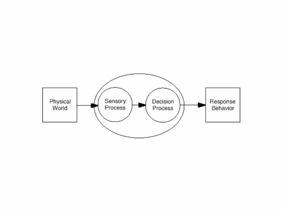
La Théorie de la Détection du Signal (TDS) est à la fois un instrument de
mesure de la performance* et un cadre théorique dans lequel cette
performance est interprétée du point de vue des mécanismes sous-jacents.
En tant que telle, la TDS peut être regardée comme étant à la base de la
psychophysique moderne. Le cours développera les bases de la TDS,
discutera sa relation avec les concepts de seuil sensoriel et de décision et
exemplifiera son application dans des situations expérimentales allant
depuis le sensoriel jusqu'au cognitif.
*Signal Detection Theory is a computational framework that describes how to extract a signal from noise, while
accounting for biases and other factors that can influence the extraction process. It has been used
effectively to describe how the brain overcomes noise from both the environment and its own internal processes to
perceive sensory signals (from Gold &Watanabe (2010). Perceptual learning. Current Biol., 20(2) R46-R48.

SIGNAL DETECTION THEORY AND PSYCHOPHYSICS
David M. Green & John A. Swets
1st published in 1966 by Wiley & Sons, Inc., New York
Reprint with corrections in 1974
Copyright © 1966 by Wiley & Sons, Inc.
Revision Copyright © 1988 by D.M. Green & J. A. Swets
1988 reprint edition published by Peninsula Publishing, Los Altos, CA 94023, USA
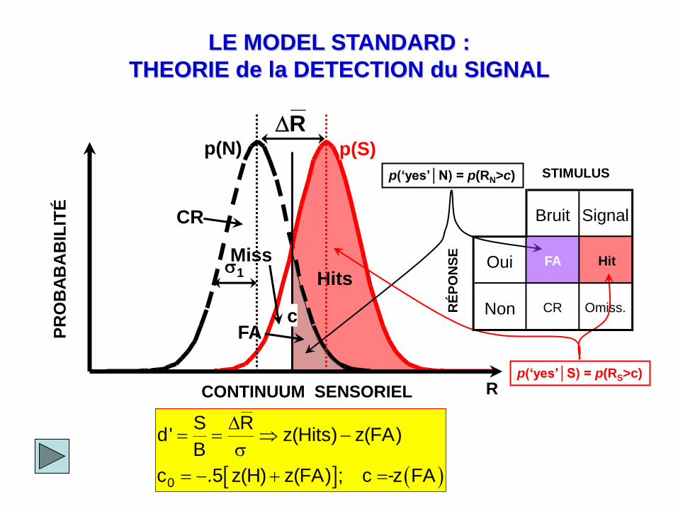
CONTINUUM SENSORIEL
PR
OB
AB
AB
ILIT
É
s1
R
FA
Hits
p(‘yes’│N) = p(RN>c)
p(‘yes’│S) = p(RS>c)
p(N) p(S)
STIMULUS
RÉ
PO
NS
E
Bruit Signal
Oui FA Hit
Non CR Omiss. c
R
LE MODEL STANDARD :
THEORIE de la DETECTION du SIGNAL
CR
Miss
0
S Rd' z(Hits) z(FA)
B
c .5 z(H) z(FA) ; c z FA
s
-
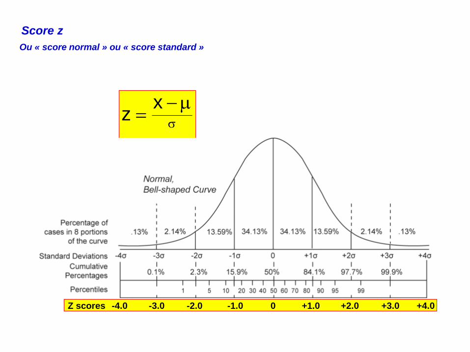
xz
s
Score z
Ou « score normal » ou « score standard »
-4.0 -3.0 -2.0 -1.0 0 +1.0 +2.0 +3.0 +4.0 Z scores

LE MODEL STANDARD :
THEORIE de la DETECTION du SIGNAL
CONTINUUM SENSORIEL
f R:
PR
OB
AB
AB
ILIT
É
FA
Hits
The likelihood ratio
Le rapport de vraisemblance
c R
cf
cf
NcRp
ScRp)X(L
N
S
R
R

-4 -3 -2 -1 0 1 2 3 4 5 6
Sensory Continuum (z)
0
0,1
0,2
0,3
0,4
0,5
P(z
)
N S
d’=1
cA = c + d’/2 = 1.60 = cA
c = 1.10 c
LE MODEL STANDARD :
THEORIE de la DETECTION du SIGNAL
p(S) = .25
c
3p
p
czp
czp
S
N
N
S
pN(z
=c
)
pS (z
=c
)
-zFA
c0
= 1
p(S) = . 50
c = 0

CONTINUUM SENSORIEL
PR
OB
AB
AB
ILIT
Y
p(N)
R
c ' z FA
c’
THE STANDARD MODEL: SIGNAL DETECTION THEORY Criterion: the border between seen and not-seen
FA
s
c’ in s units!
s

Criterion setting
Observers set a criterion that attempts to minimize the total error
rate (pMiss + pFA).
For equally probable Signal and Noise, choose S and not N when
p(x|S) > p(x|N)
i.e. when the likelihood ratio
= p(x|S) / p(x|N) > 1
For unequal probabilities of S and N, p(S) and p(N), optimal
p(N) / p(S)
x

Sensory Continuum
Pro
bab
ilit
y
THE STANDARD MODEL: SIGNAL DETECTION THEORY Criterion: the border between seen and not-seen
c’
d’
opt c’ = .5d’
c’
d’
c’
d’
c’
d’ d’
c’
d’
c’

Green & Swets (1966)
Measured vs. Optimal criterion ()
Observers are close to
optimal for p(S) = p(N) but
become more and more
suboptimal with the
increasing difference
between p(S) & p(N)
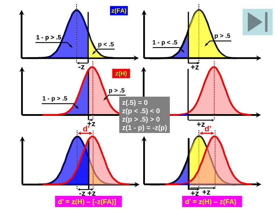
z(FA)
-z
1 - p > .5 p < .5
1 - p > .5
+z
p > .5 1 - p < .5
p > .5
1 - p > .5
+z +z
z(H)
-z +z d’ = z(H) – [-z(FA)]
+z +z
d’ = z(H) – z(FA)
d’ d’
z(.5) = 0
z(p < .5) < 0
z(p > .5) > 0
z(1 - p) = -z(p)
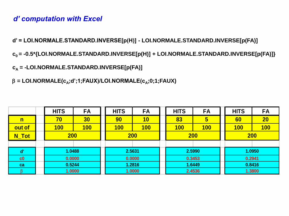
d’ computation with Excel
d’ = LOI.NORMALE.STANDARD.INVERSE[p(H)] - LOI.NORMALE.STANDARD.INVERSE[p(FA)]
c0 = -0.5*{LOI.NORMALE.STANDARD.INVERSE[p(H)] + LOI.NORMALE.STANDARD.INVERSE[p(FA)]}
cA = -LOI.NORMALE.STANDARD.INVERSE[p(FA)]
= LOI.NORMALE(cA;d’;1;FAUX)/LOI.NORMALE(cA;0;1;FAUX)
HITS FA HITS FA HITS FA HITS FA
n 70 30 90 10 83 5 60 20
out of 100 100 100 100 100 100 100 100
N_Tot
d'
c0
ca
1.0000
0.3453 0.2941
0.5244 1.2816 1.6449 0.8416
200 200 200 200
1.0000 2.4536 1.3800
1.09502.59902.56311.0488
0.0000 0.0000

Receiving Operating Characteristics (ROC)
0
0.2
0.4
-8 -4 0 4 8
Sensory Continuum (z)
P(z
d' = 0
0
0.2
0.4
0.6
0.8
1
0.0 0.2 0.4 0.6 0.8 1.0
pFA
pH
d' = 0
0
0.2
0.4
-8 -4 0 4 8
Sensory Continuum (z)
P(z
d' = 0
0
0.2
0.4
0.6
0.8
1
0.0 0.2 0.4 0.6 0.8 1.0
pFA
pH
d' = 0
0
0.2
0.4
-8 -4 0 4 8
Sensory Continuum (z)
P(z
d' = 0
0
0.2
0.4
0.6
0.8
1
0.0 0.2 0.4 0.6 0.8 1.0
pFA
pH
d' = 0
0
0.2
0.4
-8 -4 0 4 8
Sensory Continuum (z)
P(z
d' = 0
0
0.2
0.4
0.6
0.8
1
0.0 0.2 0.4 0.6 0.8 1.0
pFA
pH
d' = 0
0
0.2
0.4
-8 -4 0 4 8
Sensory Continuum (z)
P(z
d' = 0
0
0.2
0.4
0.6
0.8
1
0.0 0.2 0.4 0.6 0.8 1.0
pFA
pH
d' = 0
0
0.2
0.4
-8 -4 0 4 8
Sensory Continuum (z)
P(z
d' = 1
0
0.2
0.4
0.6
0.8
1
0.0 0.2 0.4 0.6 0.8 1.0
pFA
pH
d' = 1
0
0.2
0.4
-8 -4 0 4 8
Sensory Continuum (z)
P(z
d' = 1
0
0.2
0.4
0.6
0.8
1
0.0 0.2 0.4 0.6 0.8 1.0
pFA
pH
d' = 1
0
0.2
0.4
-8 -4 0 4 8
Sensory Continuum (z)
P(z
d' = 1
0
0.2
0.4
0.6
0.8
1
0.0 0.2 0.4 0.6 0.8 1.0
pFA
pH
d' = 1
0
0.2
0.4
-8 -4 0 4 8
Sensory Continuum (z)
P(z
d' = 1
0
0.2
0.4
0.6
0.8
1
0.0 0.2 0.4 0.6 0.8 1.0
pFA
pH
d' = 1
0
0.2
0.4
-8 -4 0 4 8
Sensory Continuum (z)
P(z
d' = 1
0
0.2
0.4
0.6
0.8
1
0.0 0.2 0.4 0.6 0.8 1.0
pFA
pH
d' = 1
0
0.2
0.4
-8 -4 0 4 8
Sensory Continuum (z)
P(z
d' = 1
0
0.2
0.4
0.6
0.8
1
0.0 0.2 0.4 0.6 0.8 1.0
pFA
pH
d' = 1
0
0.2
0.4
-8 -4 0 4 8
Sensory Continuum (z)
P(z
d' = 1
0
0.2
0.4
0.6
0.8
1
0.0 0.2 0.4 0.6 0.8 1.0
pFA
pH
d' = 1
0
0.2
0.4
-8 -4 0 4 8
Sensory Continuum (z)
P(z
d'= 2
0
0.2
0.4
0.6
0.8
1
0.0 0.2 0.4 0.6 0.8 1.0
pFA
pH
d' = 2
0
0.2
0.4
-8 -4 0 4 8
Sensory Continuum (z)
P(z
d'= 2
0
0.2
0.4
0.6
0.8
1
0.0 0.2 0.4 0.6 0.8 1.0
pFA
pH
d' = 2
0
0.2
0.4
-8 -4 0 4 8
Sensory Continuum (z)
P(z
d'= 2
0
0.2
0.4
0.6
0.8
1
0.0 0.2 0.4 0.6 0.8 1.0
pFA
pH
d' = 2
0
0.2
0.4
-8 -4 0 4 8
Sensory Continuum (z)
P(z
d'= 2
0
0.2
0.4
0.6
0.8
1
0.0 0.2 0.4 0.6 0.8 1.0
pFA
pH
d' = 2
0
0.2
0.4
-8 -4 0 4 8
Sensory Continuum (z)
P(z
d'= 2
0
0.2
0.4
0.6
0.8
1
0.0 0.2 0.4 0.6 0.8 1.0
pFA
pH
d' = 2
0
0.2
0.4
-8 -4 0 4 8
Sensory Continuum (z)
P(z
d'= 2
0
0.2
0.4
0.6
0.8
1
0.0 0.2 0.4 0.6 0.8 1.0
pFA
pH
d' = 2
0
0.2
0.4
-8 -4 0 4 8
Sensory Continuum (z)
P(z
d'= 2
0
0.2
0.4
0.6
0.8
1
0.0 0.2 0.4 0.6 0.8 1.0
pFA
pH
d' = 2
0
0.2
0.4
-8 -4 0 4 8
Sensory Continuum (z)
P(z
d'= 3
0
0.2
0.4
0.6
0.8
1
0.0 0.2 0.4 0.6 0.8 1.0
pFA
pH
d' = 3
0
0.2
0.4
-8 -4 0 4 8
Sensory Continuum (z)
P(z
d'= 3
0
0.2
0.4
0.6
0.8
1
0.0 0.2 0.4 0.6 0.8 1.0
pFA
pH
d' = 3
0
0.2
0.4
-8 -4 0 4 8
Sensory Continuum (z)
P(z
d'= 3
0
0.2
0.4
0.6
0.8
1
0.0 0.2 0.4 0.6 0.8 1.0
pFA
pH
d' = 3
0
0.2
0.4
-8 -4 0 4 8
Sensory Continuum (z)
P(z
d'= 3
0
0.2
0.4
0.6
0.8
1
0.0 0.2 0.4 0.6 0.8 1.0
pFA
pH
d' = 3
0
0.2
0.4
-8 -4 0 4 8
Sensory Continuum (z)
P(z
d'= 3
0
0.2
0.4
0.6
0.8
1
0.0 0.2 0.4 0.6 0.8 1.0
pFA
pH
d' = 3
0
0.2
0.4
-8 -4 0 4 8
Sensory Continuum (z)
P(z
d'= 3
0
0.2
0.4
0.6
0.8
1
0.0 0.2 0.4 0.6 0.8 1.0
pFA
pH
d' = 3
0
0.2
0.4
-8 -4 0 4 8
Sensory Continuum (z)
P(z
d'= 3
0
0.2
0.4
0.6
0.8
1
0.0 0.2 0.4 0.6 0.8 1.0
pFA
pH
d' = 3
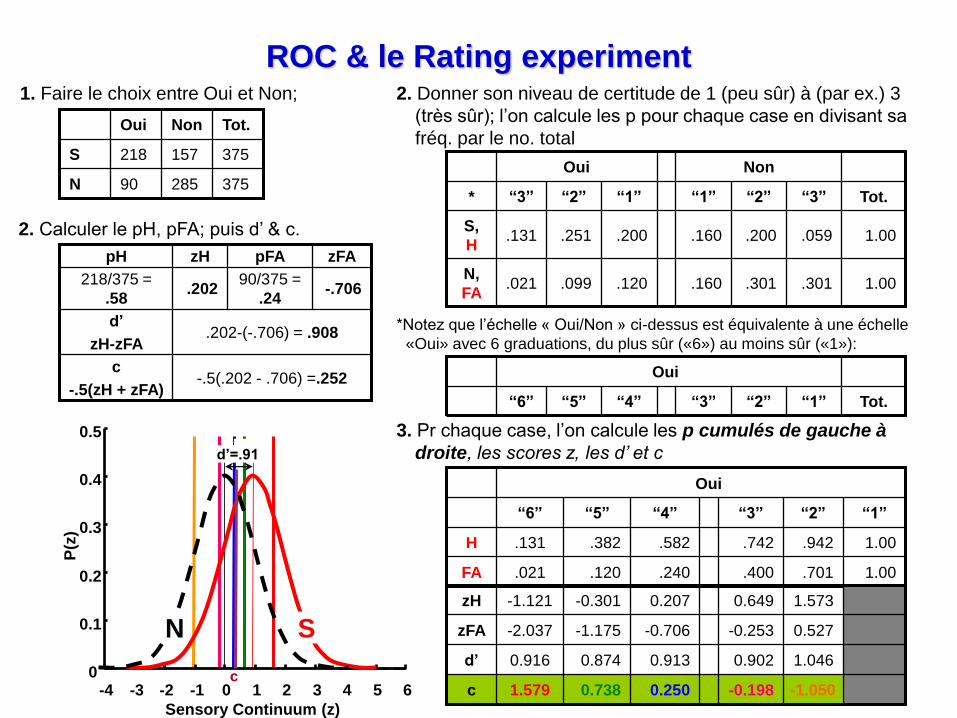
ROC & le Rating experiment 1. Faire le choix entre Oui et Non;
375
375
Tot.
285 90 N
157 218 S
Non Oui
2. Donner son niveau de certitude de 1 (peu sûr) à (par ex.) 3
(très sûr); l’on calcule les p pour chaque case en divisant sa
fréq. par le no. total
1.00
1.00
Tot.
N,
FA
S,
H
*
.301
.059
“3”
.301
.200
“2”
.160
.160
“1”
Non
.200 .251 .131
.120 .099 .021
“1” “2” “3”
Oui
3. Pr chaque case, l’on calcule les p cumulés de gauche à
droite, les scores z, les d’ et c
FA
H
1.00
1.00
“1”
.701
.942
“2”
.400
.742
“3”
.582 .382 .131
.240 .120 .021
“4” “5” “6”
Oui
-1.050 -0.198 0.250 0.738 1.579 c
1.046 0.902 0.913 0.874 0.916 d’
zFA
zH
0.527
1.573
-0.253
0.649 0.207 -0.301 -1.121
-0.706 -1.175 -2.037
-4 -3 -2 -1 0 1 2 3 4 5 6
Sensory Continuum (z)
0
0.1
0.2
0.3
0.4
0.5
P(z
)
N S
d’=.91
c
.202-(-.706) = .908 d’
zH-zFA
-.706
zFA
-.5(.202 - .706) =.252 c
-.5(zH + zFA)
90/375 =
.24 .202
218/375 =
.58
pFA zH pH
2. Calculer le pH, pFA; puis d’ & c.
*Notez que l’échelle « Oui/Non » ci-dessus est équivalente à une échelle
«Oui» avec 6 graduations, du plus sûr («6») au moins sûr («1»):
Tot. “1” “2” “3” “4” “5” “6”
Oui

ROC & le Rating experiment
-4 -3 -2 -1 0 1 2 3 4 5 6
Sensory Continuum (z)
0
0.1
0.2
0.3
0.4
0,5
P(z
)
N S
d’=.91
p z p z p z p z p z p z
H 0.131 -1.122 0.382 -0.300 0.582 0.207 0.742 0.650 0.942 1.572 1.000 ######
FA 0.021 -2.034 0.120 -1.175 0.240 -0.706 0.400 -0.253 0.701 0.527 1.000 ######
d'
c0
OUI NON
#NOMBRE!1.0450.9030.9130.8750.912
"2""3"
#NOMBRE!-1.050-0.1980.2500.7381.578
"3""2""1""1"
Note that a symmetrical ROC indicates that d’ is independent of c0
0
0.2
0.4
0.6
0.8
1
0 0.2 0.4 0.6 0.8 1
pFA
pH
The slope of the ROC curve at any point is equal to
the likelihood ratio criterion that generated that point.

ROC & le Rating experiment
p z p z p z p z p z p z
H 0.131 -1.122 0.382 -0.300 0.582 0.207 0.742 0.650 0.942 1.572 1.000 ######
FA 0.021 -2.034 0.120 -1.175 0.240 -0.706 0.400 -0.253 0.701 0.527 1.000 ######
d'
c0
OUI NON
#NOMBRE!1.0450.9030.9130.8750.912
"2""3"
#NOMBRE!-1.050-0.1980.2500.7381.578
"3""2""1""1"
ROC in z units
-2.5
-1.5
-0.5
0.5
1.5
-2.5 -0.5 1.5
z(FA)
z(H
)
0
0.2
0.4
0.6
0.8
1
0 0.2 0.4 0.6 0.8 1
pFA
pH

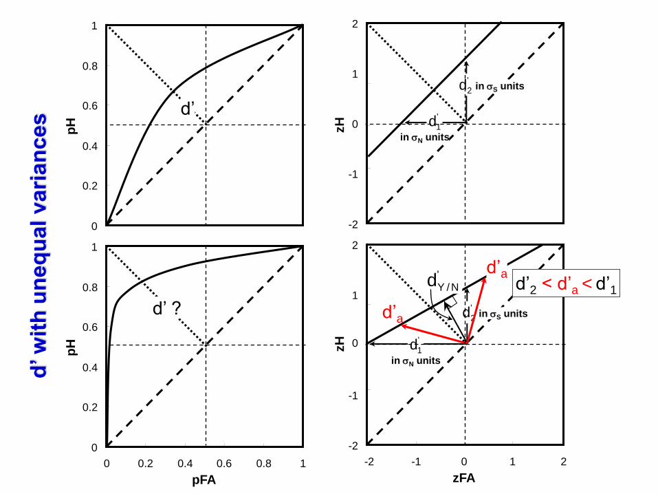
d’ with unequal variances
CONTINUUM SENSORIEL
PR
OB
AB
AB
ILIT
É
FA
Hits
c
?'d
s1
s2
0
0.2
0.4
0.6
0.8
1
0 0.2 0.4 0.6 0.8 1
pFA
pH
d’ ?
0
0.2
0.4
0.6
0.8
1
pH
d’
-2
-1
0
1
2
-2 -1 0 1 2
zFA
zH
in sN units
'
1d
'
2d in sS units
'
N/Ydd’a
d’a
-2
-1
0
1
2
zH
'
2d
in sN units
in sS units
'
1d
d’2 < d’a < d’1
d’ w
ith
un
eq
ual vari
an
ces

The index da has the properties we want.
1. It is intermediate in size between d1 and d‘2.
2. It is equivalent to d' when the ROC slope is 1,
for then the perpendicular line of length DY/N
coincides with the minor diagonal, and the two
lines of length da coincide with the d'1, and d'2
segments.
3. It turns out to be equivalent to the difference
between the means in units of the root-mean-
square (rms) standard deviation, a kind of
average equal to the square root of the mean of
the squares of the standard deviations of S1
and S2.
2
2
2
1
'
N/Y
'
a /Rd2d ss
To find da from an ROC that is linear in z coordinates, it is
easiest to first estimate d’1, d’2 and the slope s = d’1/d’2.
Because the standard deviation of the S1 distribution is s
times as large as that of S2, we can set the standard
deviation of S1 to s and that of S2 to 1.
To find da directly from one point on the ROC once s is known:
-2
-1
0
1
2
-2 -1 0 1 2
zFA
zH
in sN units
'
1d
'
2d in sS units
'
N/Ydd’a
d’a
d’ w
ith
un
eq
ual vari
an
ces
5.
'
25.
'
2'
a²s1
2d
²s15.
dd
5.
'
a²s1
2FszHzd
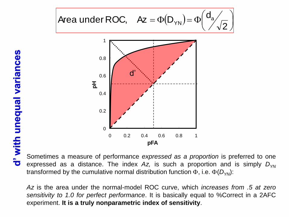
Sometimes a measure of performance expressed as a proportion is preferred to one
expressed as a distance. The index Az, is such a proportion and is simply DYN
transformed by the cumulative normal distribution function , i.e. (DYN):
Az is the area under the normal-model ROC curve, which increases from .5 at zero
sensitivity to 1.0 for perfect performance. It is basically equal to %Correct in a 2AFC
experiment. It is a truly nonparametric index of sensitivity.
d’ w
ith
un
eq
ual vari
an
ces
0
0.2
0.4
0.6
0.8
1
0 0.2 0.4 0.6 0.8 1
pFA
pH
d’
2
dDAz,ROCunderArea a
YN

High-Threshold
Sum Absolute Difference (SAD)
Max Absolute Difference (MAD)
Schematic of a single trial used for the set size and the
target number experiments. In the orientation and
spatial frequency experiments, the colored squares
were replaced with Gabor patches.
Wilken, P. & Ma, W.J (2004). A detection theory account of change detection. J. Vision 4, 1120-1135.
ROCs obtenus avec une méthode de « rating » sur une échelle de 1 à 4. Different symbols represent performance at different set sizes: set-size 2 for color,
orientation and SF – red stars; set-size 4 for color and SF, set-size 3 for orientation – green triangles; set-size 6 for color and SF, set-size 4 for orientation –
blue circles; set-size 8 for color and SF, set-size 5 for orientation – purple squares.
Hits & FA
HT
SAD
MAD
H
FA
H
FA
H
FA
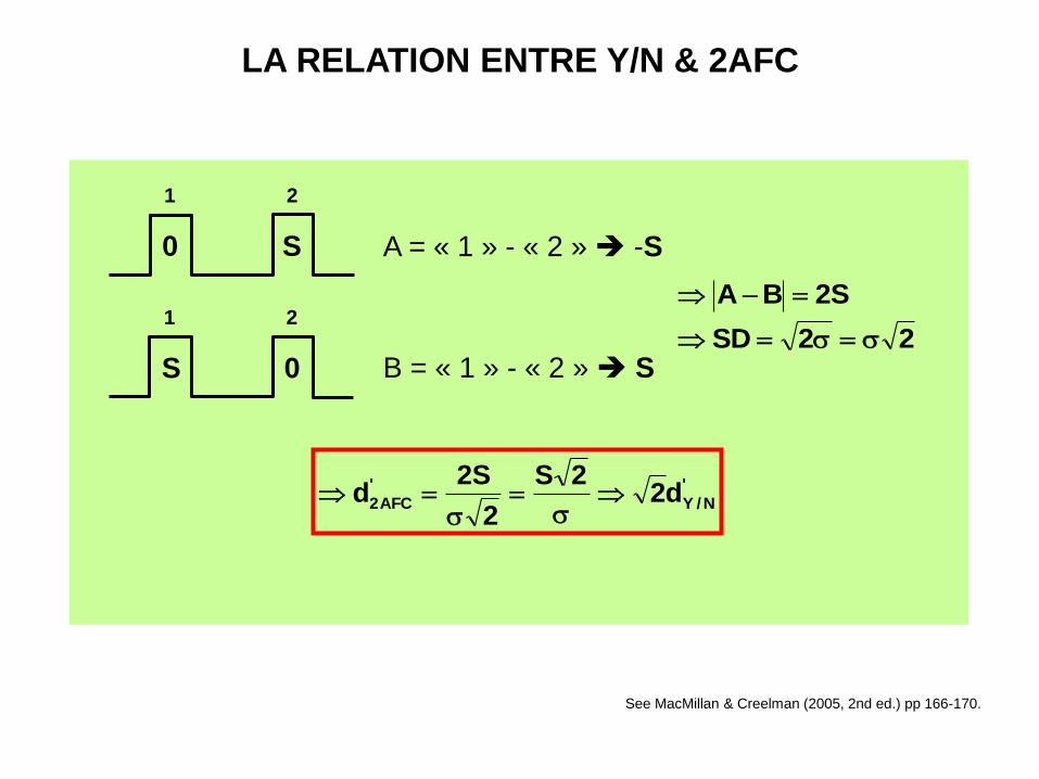
LA RELATION ENTRE Y/N & 2AFC
See MacMillan & Creelman (2005, 2nd ed.) pp 166-170.
0 S
1 2
S 0
1 2
A = « 1 » - « 2 » -S
B = « 1 » - « 2 » S 22SD ss
S2BA
'
N/Y
'
AFC2 d22S
2
S2d
s
s
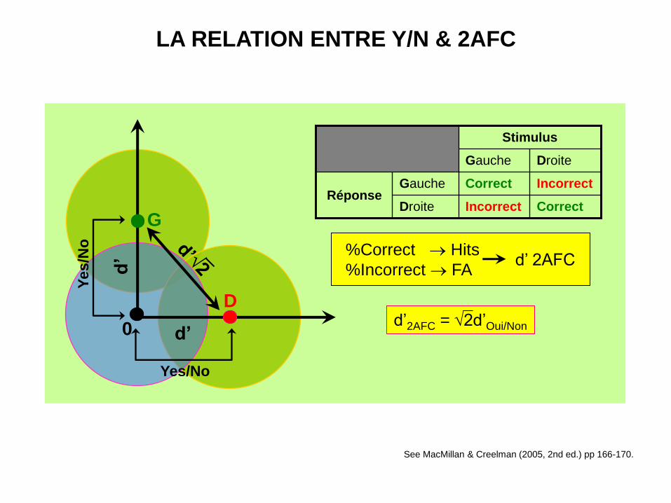
LA RELATION ENTRE Y/N & 2AFC
d’
d’
Réponse Correct Incorrect Droite
Incorrect Correct Gauche
Droite Gauche
Stimulus
%Correct Hits
%Incorrect FA d’ 2AFC
d’2AFC = 2d’Oui/Non
D
0
G
Yes/No
Yes/N
o
See MacMillan & Creelman (2005, 2nd ed.) pp 166-170.
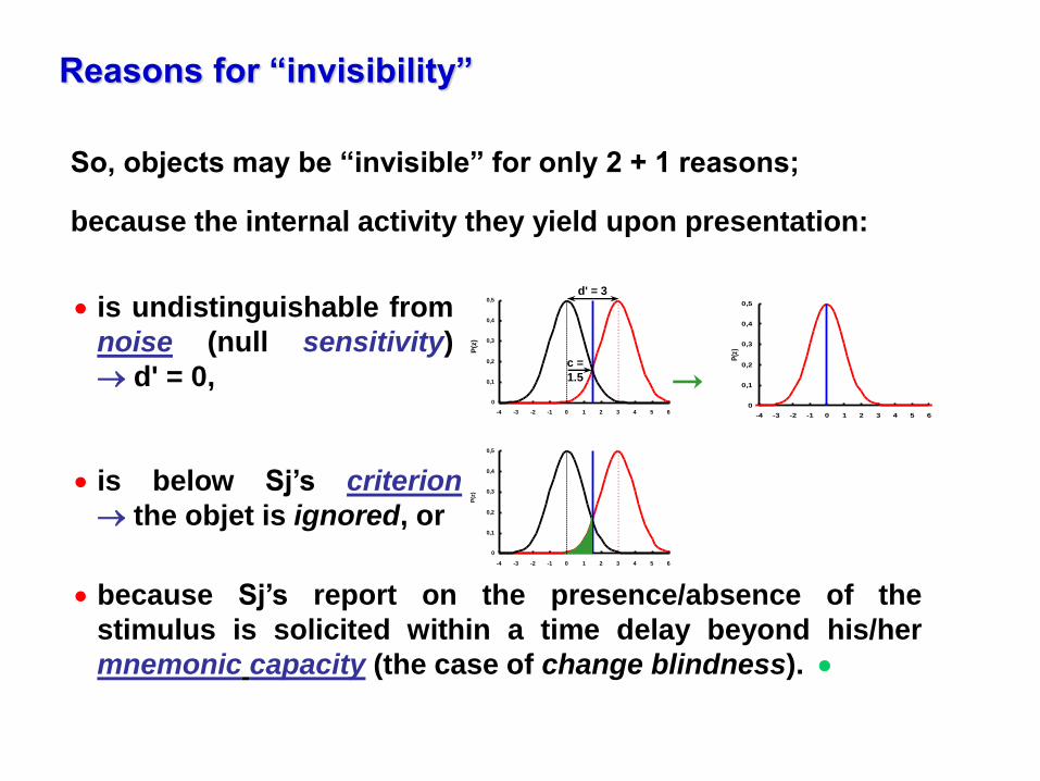
So, objects may be “invisible” for only 2 + 1 reasons;
because the internal activity they yield upon presentation:
because Sj’s report on the presence/absence of the
stimulus is solicited within a time delay beyond his/her
mnemonic capacity (the case of change blindness).
is below Sj’s criterion
the objet is ignored, or 0
0,1
0,2
0,3
0,4
0,5
-4 -3 -2 -1 0 1 2 3 4 5 6
P(z
)
is undistinguishable from
noise (null sensitivity)
d' = 0, 0
0,1
0,2
0,3
0,4
0,5
-4 -3 -2 -1 0 1 2 3 4 5 6
P(z
)
0
0,1
0,2
0,3
0,4
0,5
-4 -3 -2 -1 0 1 2 3 4 5 6
P(z
)
d' = 3
c =
1.5
Reasons for “invisibility”
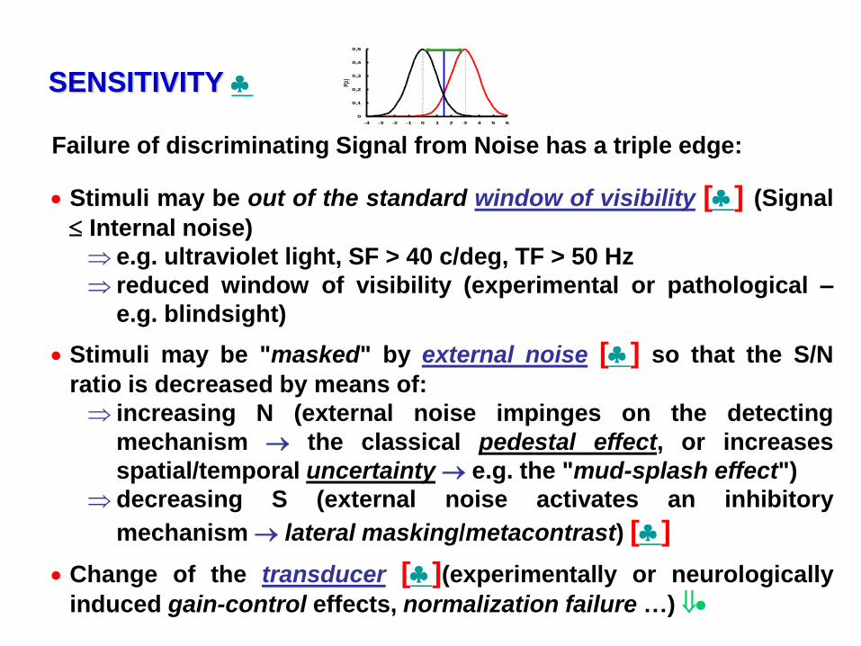
Failure of discriminating Signal from Noise has a triple edge:
Stimuli may be out of the standard window of visibility [] (Signal
Internal noise)
e.g. ultraviolet light, SF > 40 c/deg, TF > 50 Hz
reduced window of visibility (experimental or pathological –
e.g. blindsight)
Stimuli may be "masked" by external noise [] so that the S/N
ratio is decreased by means of:
increasing N (external noise impinges on the detecting
mechanism the classical pedestal effect, or increases
spatial/temporal uncertainty e.g. the "mud-splash effect")
decreasing S (external noise activates an inhibitory
mechanism lateral masking/metacontrast) []
Change of the transducer [](experimentally or neurologically
induced gain-control effects, normalization failure …)
SENSITIVITY 0
0,1
0,2
0,3
0,4
0,5
-4 -3 -2 -1 0 1 2 3 4 5 6
P(z)
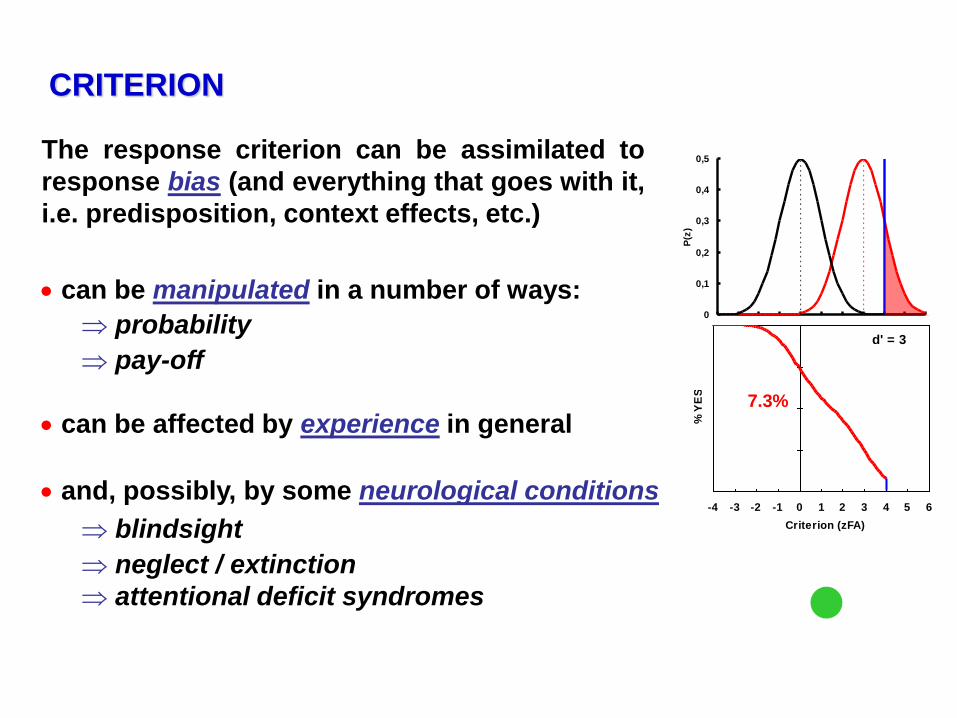
can be manipulated in a number of ways:
probability
pay-off
can be affected by experience in general
and, possibly, by some neurological conditions
blindsight
neglect / extinction
attentional deficit syndromes
CRITERION
0
0,1
0,2
0,3
0,4
0,5
-4 -3 -2 -1 0 1 2 3 4 5 6
P(z
)
-4 -3 -2 -1 0 1 2 3 4 5 6
Criterion (zFA)
% Y
ES
d' = 3
49.4%50%
0
0,1
0,2
0,3
0,4
0,5
-4 -3 -2 -1 0 1 2 3 4 5 6
P(z
)
-4 -3 -2 -1 0 1 2 3 4 5 6
Criterion (zFA)
% Y
ES
d' = 3
98.7%
0
0,1
0,2
0,3
0,4
0,5
-4 -3 -2 -1 0 1 2 3 4 5 6
P(z
)
-4 -3 -2 -1 0 1 2 3 4 5 6
Criterion (zFA)
% Y
ES
d' = 3
91.5%
0
0,1
0,2
0,3
0,4
0,5
-4 -3 -2 -1 0 1 2 3 4 5 6
P(z
)
-4 -3 -2 -1 0 1 2 3 4 5 6
Criterion (zFA)
% Y
ES
d' = 3
73.9%
0
0,1
0,2
0,3
0,4
0,5
-4 -3 -2 -1 0 1 2 3 4 5 6
P(z
)
-4 -3 -2 -1 0 1 2 3 4 5 6
Criterion (zFA)
% Y
ES
d' = 3
56.1%
0
0,1
0,2
0,3
0,4
0,5
-4 -3 -2 -1 0 1 2 3 4 5 6
P(z
)
-4 -3 -2 -1 0 1 2 3 4 5 6
Criterion (zFA)
% Y
ES
d' = 3
49.4%50%
0
0,1
0,2
0,3
0,4
0,5
-4 -3 -2 -1 0 1 2 3 4 5 6
P(z
)
-4 -3 -2 -1 0 1 2 3 4 5 6
Criterion (zFA)
% Y
ES
d' = 3
42.5%
0
0,1
0,2
0,3
0,4
0,5
-4 -3 -2 -1 0 1 2 3 4 5 6
P(z
)
-4 -3 -2 -1 0 1 2 3 4 5 6
Criterion (zFA)
% Y
ES
d' = 3
24.1%
0
0,1
0,2
0,3
0,4
0,5
-4 -3 -2 -1 0 1 2 3 4 5 6
P(z
)
-4 -3 -2 -1 0 1 2 3 4 5 6
Criterion (zFA)
% Y
ES
d' = 3
7.3%
The response criterion can be assimilated to
response bias (and everything that goes with it,
i.e. predisposition, context effects, etc.)

CANAUX, BRUIT
et
THÉORIE DE LA DÉTECTION DU SIGNAL

« Qualité » (l) Intensité ou « qualité » du Stimulus Rép
on
se
d’u
n f
iltr
e (
s/s
ou
au
tre
) Le principe de l’UNIVARIANCE
Un Canal,
Filtre.
Chp Récep.
R V
Snn
n
max RI
IRR
s
I = stimulus intensity
R = response
Rmax = max resp.
N = max slope
S = semi-saturation cst.
Rs = spontaneous R
Un autre R
ép
on
se
d’u
n f
iltr
e

Normalization works (here) by
dividing each output
by the sum of all outputs.
Heeger, D.J. (1992). Normalization of cell responses in cat striate cortex. Visual Neuroscience, 9, 181-197.
RESPONSE NORMALIZATION
Divisive
inhibition

R V
RÉPONSE
CANAUX & PROBABILITÉ DE RÉPONSE
Intensity Discrimination
p(s/s)
RE
PO
NS
E (
e.g
. s
/s)
pmin
pMax
pmin
pMax
p(s/s)

R V
RÉPONSE
CANAUX & PROBABILITÉ DE RÉPONSE
Within & Across Channels Discrimination
p(s/s)
p(s/s)
RE
PO
NS
E (
e.g
. s
/s)
pmin
pMax
pmin
pMax
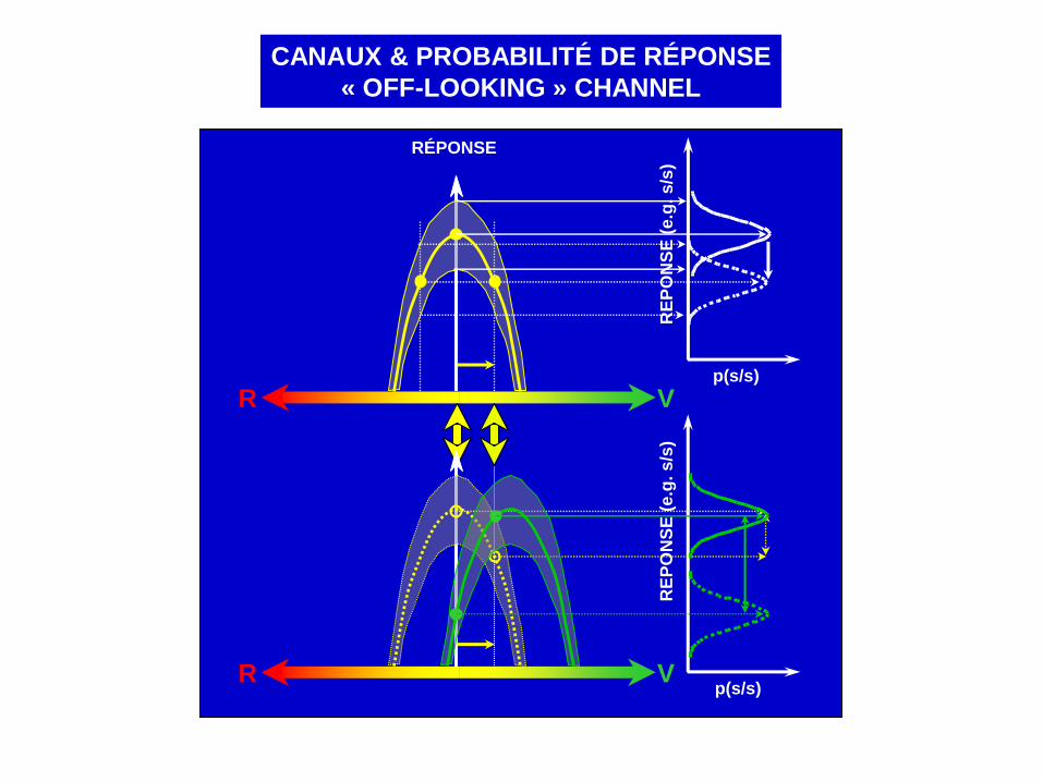
CANAUX & PROBABILITÉ DE RÉPONSE
« OFF-LOOKING » CHANNEL
RÉPONSE
R V p(s/s)
RE
PO
NS
E (
e.g
. s
/s)
p(s/s)
RE
PO
NS
E (
e.g
. s
/s)
R V

I0 I1
kIR
s = cst.
kI
.)cstiff;at(kR
IR
IR
s
log (I) lo
g (
I
)
NO Weber ’s Law
I = k
k
Input
R =
kI
p(R)
II1
R
II0
R
TRANSDUCTION
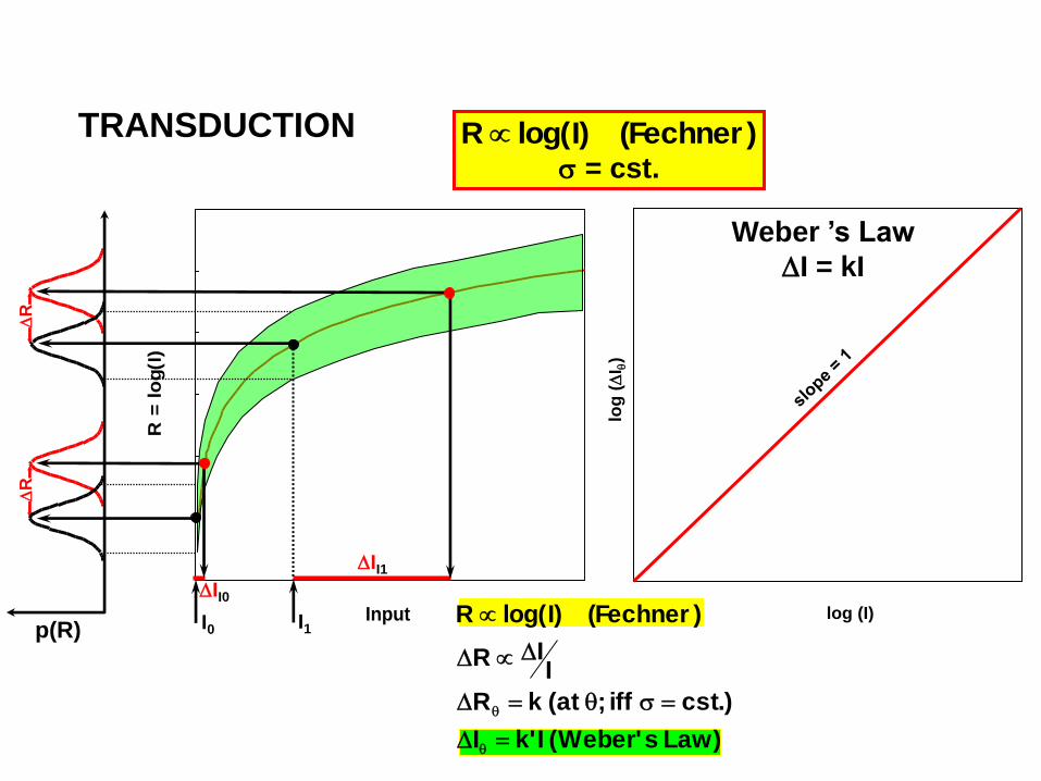
Input
R =
lo
g(I
)
I0 I1
II1
R
II0
R
)Fechner()Ilog(R
s = cst.
p(R) log (I)
log
(
I )
Weber ’s Law
I = kI
)Laws'Weber(I'kI
.)cstiff;at(kR
IIR
)Fechner()Ilog(R
s
TRANSDUCTION
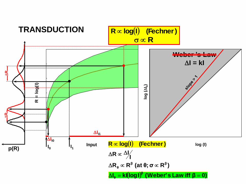
Input
R =
lo
g(I
)
I0 I1
)0βiffLaws'Weber(IlogkII
)Rσ;θat(RR
IIR
)Fechner(IlogR
β
θ
ββ
θ
II0
R
p(R)
R
II1
log (I) lo
g (
I
)
Weber ’s Law
I = kI
)Fechner(IlogR
Rs
TRANSDUCTION

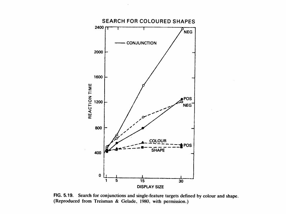
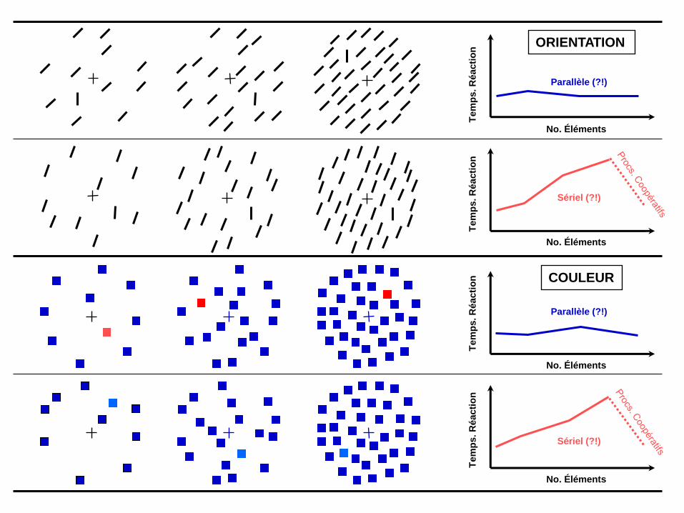
VISUAL SEARCH
and
SIGNAL DETECTION THEORY


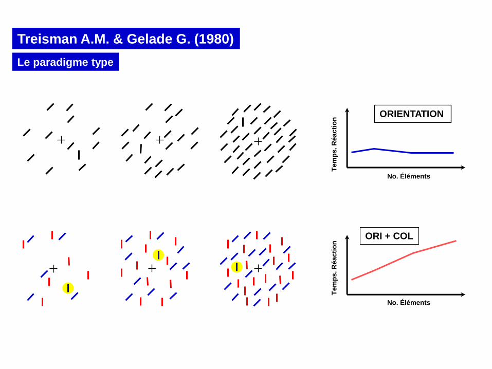
Tem
ps. R
éacti
on
No. Éléments
ORIENTATION
Parallèle (?!)
Tem
ps. R
éacti
on
No. Éléments
Sériel (?!)
ORI + COL
Le paradigme type
Treisman A.M. & Gelade G. (1980)

LE MODÉLE STANDARD : LA THÉORIE DE LA DÉTECTION DU SIGNAL
« COULEUR »
L
R V
RE
SP
ON
SE
l
RE
SP
ON
SE
l
CONTINUUM SENSORIEL (R-V)
PR
OB
AB
.
s
R
d’ n’est pas mesurable
« COULEUR »
L
R V
RE
SP
ON
SE
l
CONTINUUM SENSORIEL (R-V)
PR
OB
AB
.
s
R
R s d’=
Tem
ps. R
éacti
on
No. Éléments
ORIENTATION
Parallèle (?!)
Tem
ps. R
éacti
on
No. Éléments
Sériel (?!)
Tem
ps. R
éacti
on
No. Éléments
COULEUR
Parallèle (?!)
Tem
ps. R
éacti
on
No. Éléments
Sériel (?!)


