Download - FZID Discussion Papers - uni-hohenheim.de
FZID Discussion Papers
Universität hohenheim | Forschungszentrum Innovation und Dienstleistung www.fzid.uni-hohenheim.de
CC Economics
Discussion Paper 10-2010
Kyoto anD thE Carbon ContEnt oF traDE
rahel aichele and Gabriel Felbermayr
Universität hohenheim | Forschungszentrum Innovation und Dienstleistung
www.fzid.uni-hohenheim.de
Discussion Paper 10-2010
KYOTO AND THE CARBON CONTENT OF TRADE
Rahel Aichele and Gabriel Felbermayr
Download this Discussion Paper from our homepage:
https://fzid.uni-hohenheim.de/71978.html
ISSN 1867-934X (Printausgabe) ISSN 1868-0720 (Internetausgabe)
Die FZID Discussion Papers dienen der schnellen Verbreitung von Forschungsarbeiten des FZID. Die Beiträge liegen in alleiniger Verantwortung
der Autoren und stellen nicht notwendigerweise die Meinung des FZID dar.
FZID Discussion Papers are intended to make results of FZID research available to the public in order to encourage scientific discussion and suggestions for revisions. The authors are solely
responsible for the contents which do not necessarily represent the opinion of the FZID.
Kyoto and the carbon content of trade∗
Rahel Aichele, and Gabriel Felbermayr‡
Hohenheim University
January 2010
Abstract
A unilateral tax on CO2 emissions may drive up indirect carbon imports from
non-committed countries, leading to carbon leakage. Using a gravity model of car-
bon trade, we analyze the effect of the Kyoto Protocol on the carbon content of
bilateral trade. We construct a novel data set of CO2 emissions embodied in bi-
lateral trade flows. Its panel structure allows dealing with endogenous selection of
countries into the Protocol. We find strong statistical evidence for Kyoto commit-
ments to affect carbon trade. On average, the Kyoto protocol led to substantial
carbon leakage but its total effect on carbon trade was only minor.
JEL Classification: F18, Q54, Q56
Keywords: carbon leakage, gravity model, international trade, climate change, em-
bodied emission, input-output analysis.
∗We are grateful to seminar participants at the Universities of Kiel, Aarhus and Tubingen (GLAMOUR
seminar) for comments. Special thanks to Benjamin Jung, Wilhelm Kohler, Sonja Peterson, Philipp J.H.
Schroder, Marcel Smolka, M. Scott Taylor, and Andreas Zahn for helpful suggestions.‡Corresponding author: Gabriel Felbermayr, Department of Economics, Box 520E, Universitat Ho-
henheim. E-mail: [email protected].
1 Introduction
Global warming caused by anthropogenic CO2 emissions has become a major policy con-
cern. Because countries’ greenhouse gas emissions have global effects, decentralized na-
tional regulation is inefficient. Therefore, starting 1992 in Rio de Janeiro, a series of
international summits has taken place to coordinate action against climate warming; so
far, with mixed results.
In the Kyoto Protocol of 1997, 37 industrialized countries and the European Com-
munity have committed to legally binding emission targets. In 2012, emissions in those
countries should be down on average by 5.2% relative to the base year of 1990. The Proto-
col says little about how countries are to achieve this objective and it has not introduced a
generalized scheme for international trade of emission permits. More importantly, guided
by the principle of common but differentiated responsibilities, emerging and developing
countries including major polluters like China or India do not face any binding emission
limits. The U.S. did not ratify the protocol after a non-binding Senate Resolution (Byrd-
Hagel resolution) urged the Clinton administration to not accept any treaty that did not
include the “meaningful” participation of all developing as well as industrialized countries,
arguing that to do so would unfairly put the U.S. at a competitive disadvantage.
International economists have long pointed out that unilateral climate policy may
generate carbon leakage: production of CO2 intensive goods may move to unregulated
countries from where regulated countries would import those goods. Those imports would
embody foreign countries’ CO2 emissions so that one can speak about the carbon content
of trade. A recent study by Wang and Watson (2007) argues that about a quarter of
China’s CO2 emissions result from production for exports, mainly to Europe and the
USA. Findings of a study of the World Bank (2008) also indicate that energy-intensive
industries relocate to developing countries. Indeed, Grether and Mathys (2009) argue
that the global center of gravity of CO2 emissions has shifted faster eastwards than the
center of economic activity, a finding that is in line with the carbon leakage hypothesis.
Carbon leakage can even lead to a global increase in emissions if non-committed countries
operate out-dated carbon-intensive technologies or a carbon-intensive energy mix. Kyoto’s
1
Clean Development Mechanism was designed as a way of funding the required technology
transfer to mitigate this problem but measured sectoral CO2 intensities of production
still vary strongly across countries and converge only very slowly (see e.g. Baumert et al.,
2005, p. 26).
In the U.S. and Europe, the issue of carbon leakage has triggered a debate about
border adjustment measures against countries that do not take actions to prevent climate
change. The American Clear Energy and Security (ACES) Act (the so called Waxman-
Markey Bill) contains such a provision and the French president Nicolas Sarkozy has made
similar proposals for the EU. The possibility of carbon leakage has prompted researchers
to argue in favor of consumption-based rather than production-based regulation, see e.g.
Eder and Narodoslawsky (1999).
In theory, trade in carbon need not imply an inefficiency. When all countries have
binding (but potentially different) emission targets, and there is national and international
trade of pollution permits, trade in carbon would just reflect the pattern of comparative
advantage.1 More generally, under the assumption that the global supply of pollution per-
mits is fixed, trade would be efficient and environmentally neutral. The central problem,
of course, is that only a minority of countries has binding emission caps. Moreover, only
a few of them allocate pollution permits through the market mechanism,2 technologies
are different across countries,3 and trade costs are important.
In this study, we address the positive side of carbon trade rather than the normative
one. We are interested in understanding, whether and by what extent commitments made
1Note that trade in goods can suffice to equalize the price of pollution permits across countries
(Copeland and Taylor, 2005). This happens when the standard assumptions of the factor price equaliza-
tion theorem hold, i.e., that there are no trade costs, technologies are identical across countries, every
country has a cap-and-trade system for CO2 emissions, and emission targets relative to endowments of
production factors are not too different across countries.2Even the emission trading system in Europe (ETS) only covers about 40% of total CO2 emissions
(EC, 2009).3In particular, the carbon intensity of production varies greatly across countries, even within narrowly
defined industries (see e.g. the detailed estimates of Nakano et al., 2009, p. 30 f.).
2
under the Kyoto Protocol affect bilateral trade in carbon embodied in goods. To that
purpose, we develop a multi-input multi-sector multi-country partial equilibrium model
of trade in carbon as embodied in goods. The model allows for international trade in
final output goods and in intermediate inputs; it also provides a guideline for computing
the carbon content of international trade flows. We derive a gravity equation for bilat-
eral trade in CO2 emissions and discuss a number of comparative statics results. Most
importantly, we show that a unilateral carbon tax in some country leads to increased net
imports of carbon from countries without such taxes. This is driven by two mutually
reinforcing channels: (i) a technique effect, by which producers shift toward less-carbon
intensive modes of production, and (ii) a scale effect due to an increase in overall produc-
tion costs. We also discuss subsidies and find that, within the framework of our model,
the scale effect may have the opposite sign than the technique effect.
In the empirical part of this paper, we present evidence that committed countries
have more incentives and subsidy programs targeted toward emission reductions and that
they reserve a more important role for environment-related taxes in their governments’
budgets. We argue that the comprehensive use of country × year effects in our gravity
equation effectively accounts for all reasons why a country may commit at a certain point
in time to pollution targets under the Kyoto Protocol. Our within estimations imply that
carbon imports of a committed country from an uncommitted exporter are about 10%
higher than if the country had no commitments. This effect is mainly driven by a change
in trade structure and trade flows, and not by technological change. In contrast, the
reduced carbon exports of a committed country are mainly due to technological change
and the implied reduction in CO2 intensity. These result are confirmed in regressions of
net imports of carbon. We run the Wooldridge regression-based test of strict exogeneity of
the Kyoto commitment variable and find that our estimates can be interpreted as causal
effects. We also present evidence on the sectoral level and find robust evidence for carbon
leakage for seven out of twelve sectors. The affected sectors include such likely candidates
as chemicals and petrochemicals or pulp and paper. Evidence is weaker for sectors such
as agriculture, food, or textiles. Also in terms of economic significance, carbon leakage
is important: On average, about 40% of carbon savings due to the Protocol have been
3
offset by increased emissions in non-Kyoto countries.
Related literature. In theoretical models such as Copeland and Taylor (2005), uni-
lateral climate policy necessarily has implications for the location of production of dirty
goods. Production of emission-intensive goods would concentrate in “pollution havens”,
i.e., countries with weak environmental regulation (Copeland and Taylor, 2004) and the
ensuing gap between countries’ pollution content of consumption and that of production
would be filled by international trade. The carbon leakage phenomenon is only a special
case of this.4
According to Copeland and Taylor (see e.g. Copeland and Taylor, 2004, p. 9), a pollu-
tion haven effect occurs when stricter environmental regulation leads to changes in trade
flows and plant location. The pollution haven hypothesis, in contrast, states that trade lib-
eralization leads to relocation of pollution-intensive industries into countries with weaker
environmental regulation. An empirical body of literature has been in search of pollu-
tion havens for twenty years. The early literature (see Jaffe et al., 1995 for a summary)
only finds small, insignificant or non-robust effects of environmental regulation on trade
or FDI flows in a cross section. By employing panel methods to control for unobserved
heterogeneity and instrumenting for environmental regulation, newer studies find signifi-
cant pollution haven effects for trade flows (see e.g. Ederington et al., 2005; Levinson and
Taylor, 2008) as well as FDI flows (see e.g. Keller and Levinson, 2002; List et al., 2003;
Dean et al., 2009). Frankel and Rose (2005) use a cross section of countries to test the
pollution haven hypothesis; they find little evidence that trade openness leads poor (i.e.,
unregulated) countries to become pollution havens.
Related to CO2 emissions, most authors have used CGE modeling to quantify the
extent of carbon leakage;5 see Mattoo et al. (2009) for a recent example. The general
4However, carbon leakage might be lowered by induced technological effects (see e.g. Di Maria and
van der Werf, 2008; Acemoglu et al., 2009).5Results of CGE models typically depend on parameterization and modeling assumptions. Studies
with an Armington specification for energy intensive goods such as Felder and Rutherford (1993) or
Burniaux and Martins (2000) find only limited evidence of carbon leakage, whereas Babiker (2005) finds
a carbon leakage effect of up to 130% when assuming that energy intensive goods are homogeneous.
4
conclusion there is that unilateral emission cuts have minimal carbon leakage effects. The
only study that uses regression techniques, is World Bank (2008) who finds that carbon
taxes do affect the value of bilateral trade in goods, but do not find evidence for carbon
leakage. In contrast, our econometric analysis yields statistically strong and unambiguous
evidence of the carbon leakage hypothesis. The reasons for this performance are that (i)
our analysis studies bilateral rather than multilateral trade (which dramatically increases
the number of observations), (ii) it looks at the carbon content of trade and not on the
value of trade, (iii) it controls for unobserved heterogeneity and self-selection of countries
into climate control policies by exploiting the panel structure of the data.
Calculations of the carbon content of trade flows are strongly influenced by the “fac-
tor content of trade” literature. Its analytical methods carry over easily to environmen-
tal services, see Leontief (1970). A growing body of literature has since analyzed the
pollution embodiment of trade using input-output (I/O) techniques empirically, most re-
cently Levinson (2009). Studies estimating the carbon content of trade in a multi-country
framework are, however, scarce and focused on cross-sectional data, see e.g. Ahmad and
Wyckoff (2003), Peters and Hertwich (2008) and Nakano et al. (2009).
Finally, our work is related to the empirical gravity literature that studies the effect
of trade policy on bilateral trade volume. See, e.g., Rose (2004) or Baier and Bergstrand
(2007). Similar to us, in the absence of good data about actual policies, these authors use
institutional dummies in their gravity models: the former study looks at membership in
the WTO, the latter at free trade agreements.
To our knowledge, so far no paper has tried to directly test for carbon leakage resulting
from unilateral climate policy empirically. This paper intends to fill the gap and to assess
the role played by the Kyoto Protocol in shaping the sectoral, cross-country, and time
patterns of trade in CO2 as embodied in goods.
Plan of the paper. The second chapter develops our theoretical framework and
derives a number of comparative statics results. The second chapter discusses our data.
It also provides a first descriptive shot at the effect of Kyoto membership on bilateral
trade in carbon. The fourth part of this study turns to the econometric analysis. The
5
Appendix contains all proofs and a battery of robustness checks.
2 Gravity for CO2
This section develops a model for indirect bilateral trade in CO2 emissions. The model
allows for international trade not only in final but also in intermediate goods and shows
how input-output accounting can be integrated into the gravity context to compute the
carbon content of bilateral trade. Focusing on the scale, technique and composition
effects6, the model provides a partial equilibrium treatment which leaves the international
energy and capital markets outside of the analysis.
2.1 A simple multi-sector multi-input gravity model
There is a final non-traded output good Yi in each country i = 1, ..., K, which is assembled
under conditions of perfect competition and constant returns to scale using home-made
or imported intermediary inputs from H + 1 sectors. One of these sectors acts as a
numeraire sector, whose output q0 is freely tradable and which uses only labor in a linear
production function. The use of fossil energy in all other intermediary sectors causes
carbon dioxide emissions and consequently a global externality. There are K countries,
which are structurally similar, but may differ with respect to size.
The utility function of the representative household in country i is additively separable
in the externality and linear in consumption of Yi. That same good can be used as input
for the production of intermediate goods as well. The aggregate production function is
modeled as a two-tier function, where the upper tier is a Cobb-Douglas of sectoral output
indices. Those are aggregated using a constant elasticity of substitution (CES) production
function over varieties produced by a mass of monopolistically competitive identical firms.
Yi = qµ0
0
H∏h=1
(Y hi
)µh , Y hi =
K∑j=1
Nhj
(xhij)σh−1
σh withH∑h=1
µh + µ0 = 1, σh > 1. (1)
6Those terms where introduced by Grossman and Krueger (1993) in their study on the environmental
effects of NAFTA.
6
Quantities of varieties are denoted xhij, where j denotes the country of production, and
Nhj is the number of producers in country j. The index h denotes a sector, µh is the cost
share of sector-h varieties and σh is the elasticity of substitution.
The price index dual to Yi is denoted by
Pi =H∏h=1
(P hi
)µh , where P hi =
[K∑j=1
Nhj
(phij)1−σh] 1
1−σh
. (2)
Prices of sector-h varieties delivered from country j to i have the c.i.f. price phij = τhijphj ,
where τhij ≥ 1 is the usual iceberg trade cost factor and phj is the mill (ex-factory) price of
a generic variety in country j.
In each sector a large number of input producers operate under conditions of increas-
ing returns to scale and monopolistic competition. Firms combine primary factors, the
final output good, and energy to produce other intermediary inputs. The minimum cost
function of a firm that produces a generic variety is
Chi = chi (·)
(yhi + fh
), (3)
where chi (·) = Pαhi εβhi w
1−αh−βh is a minimum unit cost function with the usual properties.
yhi is the output level of a generic firm; fh denotes a fixed input requirement at the firm
level; Pi is the price index of the aggregate good; w is the wage rate which is equalized
across all countries due to our modeling of the numeraire sector; and εi is the cost of
energy.
The energy mix comprises climate-friendly and dirty energies, namely wind power
and fossil fuels, which are assumed to be imperfect substitutes. Wind energy is produced
with capital and wind and energy from fossil fuels is generated combining capital and
fuel according to a Leontief production function. Capital and fossil fuel are each supplied
by the world market at exogenous prices.7 The cost of energy is εi = (qfueli )νi(qwindi )1−νi ,
where qwindi and qfueli are the prices of wind and fossil energy, respectively, and νi is the cost
share of dirty energy. Both prices carry a country index because of country-specific taxes
or subsidies. More precisely, we posit the price of dirty energy to be qfueli = r+qfuel (1 + ti)
7Note that this assumption rules out “supply-side leakage” as discussed by Sinn (2008).
7
where ti is an ad-valorem tax rate, r denotes the capital rental rate and qfuel gives the
world price of fossil fuel. Also the use of clean energy (as a carbon-free input) could be
subsidized at rate si, which leads to a price of wind energy of qwindi = r (1− si).
Profits of a generic input producer in country j are phj yhj − chj (·)
(yhj + fh
). Optimal
behavior implies markup pricing of the form phj = chjσh/(σh − 1). Due to free entry,
profits are zero in equilibrium, and the size of the firm is pinned down by technological
parameters: yhj = (σh − 1) fh.
Maximizing (1) subject to the appropriate budget constraint yields country i consumer
demand for varieties of sector h produced in country j
dhij = Nhj
µhGi
P hi
(phijP hi
)−σh, (4)
where Gi is GDP of country i, µhGi/Phi denotes real expenditure allocated to sector h
and phij/Phi is the relative price of sector-h varieties from country j relative to the average
of all consumed varieties.
Besides demand for consumption dhij, differentiated goods are also used as intermediate
inputs with αh their cost share. This gives rise to the following Proposition.
Proposition 1. Total imports of country i from j of sector-h varieties (in physical units)
for consumption and intermediate usage are given by
Mhij = (1 + αh)d
hij,
where
dhij = ZhNhj Gi
(P hi
)σh−1 (τhij)−σh [chj (·)
]−σh (5)
is a reformulation of (4) and Zh ≡ µh(σh−1σh
)σh is a constant.
Proof see Appendix.
2.2 Calculating the carbon content of bilateral trade
Mhij denotes the physical flow of goods in sector h from country j to i. The production of
those goods mandates demand for labor, the final output good, and energy in country j.
8
However, while labor is immobile geographically, the final output good is itself a composite
of domestic and imported goods from all sectors. Hence, the carbon content of Mhij
depends also on the carbon content of intermediate inputs used for assembling sector-h
output.
In a first step, we limit attention to indirect emissions caused by intermediate inter-
dependence in country j only. We label this the simple method of CO2 accounting of
trade.
Proposition 2. The CO2 emission content of h−imports of i from j for the simple method
is given by
Ehij = ηhjM
hij,
where ηhj ≡ ejAhj is the scalar product between the vector of sectoral emission coefficients
ej and the vector of input requirements Ahj . The latter is given by the hth column of
(I −Bj)−1, where, by Shepard’s lemma,
Bj =
∂c1j∂p1j· · · ∂chj
∂p1j· · · ∂cHj
∂p1j
.... . .
...∂c1j∂phj
· · · ∂chj∂phj
· · · ∂cHj∂phj
... · · · ...
,
is the input-output matrix of country j, and I is the identity matrix.
Proof see Appendix.
Substituting for Mhij, sector-h embodied carbon imports of country i from country j
are given by
Ehij = ηhj (1 + αh)Z
hGiNhj (P h
i )σh−1(τhij)−σh[chj (·)
]−σh . (6)
It is understood that ηhj , Nhj , P
hi and chj (·) depend on climate policy. The aggregate
(bilateral) embodied carbon emission imports then result as the sum over all sectoral
carbon imports of i from j, i.e. Eij =∑
hEhij.
If the upstream emissions in all countries are taken into account, one requires a multi-
region input-output model (MRIO). The calculation of the emission factor ηhj gets more
involved (see Appendix B.3 for a detailed explanation), but a gravity equation for carbon
similar to (6) results.
9
2.3 Unilateral climate policy and the CO2 content of bilateral
trade
Next, we want to investigate the effect of unilateral climate policy in the trade partners i
and j on bilateral trade flows. Climate policy can take the form of increasing the national
carbon tax or subsidizing clean energies. Therefore we are interested in the reaction of
emission imports to the exporter’s and the importer’s climate policies.
The effect of a stricter carbon tax in the exporting country j on emission imports of
country i of sector-h varieties is decomposed as follows
∂Ehij
∂tj=∂ηhj∂tj
Mhij + ηhj
∂Mhij
∂tj. (7)
The increased costs for fossil fuel energy will induce substitution toward cleaner energy in
every sector, greening the technology in country j. But the cost increase also implies a loss
in competitiveness for all sectors in country j. Therefore two channels act to reduce the
carbon content of imports on the sectoral level. This carries over to more climate-friendly
imports in the aggregate, i.e. on the bilateral level. Proposition 3 summarizes.
Proposition 3. A stricter carbon tax in the exporting country j causes a technique and
a scale effect for sectoral carbon imports and a composition effect of aggregate (bilateral)
imports of carbon of country i.
(i) The technique effect reduces the sectoral carbon content of imports:∂ηhj∂tjMh
ij < 0.
(ii) The carbon tax affects the extensive margin Nhl for all countries l, and not the
intensive margin (i.e. the quantity of an h−variety import).
(iii) The scale effect reduces the sectoral carbon content of imports: ηhj∂Mh
ij
∂tj< 0.
(iv) The composition effect shifts the bilateral (aggregate) imports toward less carbon-
intensive sectors.
(v) The carbon intensity of sectoral and bilateral imports falls.
Proof see Appendix.
10
What will the effect on Ehij be, if instead the importing country i imposes a stricter
climate policy? Domestic varieties lose competitiveness and hence the number of sector-h
varieties imported from the trade partner j, Nhj , increases:
∂Ehij
∂ti= ηhj
∂Mhij
∂ti= ηhj
Mhij
Nhj
∂Nhj
∂ti> 0.
In other words, there is again a scale or pollution haven effect at work which increases
imports for a country with a more stringent environmental policy. This raises embodied
carbon imports from trade partners j. Again this effect is strongest for dirty sectors
because their costs increase most. Therefore, on the bilateral level, there is a composition
effect toward dirtier imports. This leads to a rising carbon intensity of bilateral imports.
In conclusion, if a country imposes a carbon tax its embodied emission imports rise and
its embodied emission exports fall.
Next, we investigate the effect of an increase in the carbon tax of j on the demand for
fuel in countries i and j. Demand for fuel in a country is given by sectoral emissions per
unit of output times overall output
Dfuelj =
H∑h=1
ehj (·)(yhj + fh
)Nhj . (8)
The effect of a stricter climate policy in country j on its own fuel demand and hence
its carbon dioxide emissions is negative, since emission intensity falls and the number of
varieties produced shrinks in all sectors:
∂Dfuelj
∂tj=
H∑h=1
∂ehj∂tj
(yhj + fh
)Nhj +
H∑h=1
ehj (·)(yhj + fh
) ∂Nhj
∂tj< 0, (9)
The effect of this climate policy change on carbon dioxide emissions in a trade partner i
is∂Dfuel
i
∂tj=
H∑h=1
ehi (·)(yhi + fh
) ∂Nhi
∂tj> 0. (10)
Therefore, the emission reductions in a country due to a stricter climate policy,∂Dfuelj
∂tj<
0 lead to an increase in emissions in another country∂Dfueli
∂tj> 0 through the shift in
production of varieties, which is exactly how the IPCC (2007, p. 811) defines carbon
leakage. Therefore, the scale effect acts as carbon leakage. Note that the technique
11
should not be mistaken for carbon leakage since it has no effect on the emissions of the
country that does not change its climate policy.
The decomposition of the effects of a subsidy to alternative energies in an exporting
and an importing country is similar to the one above but leads to different conclusions.
Proposition 4 summarizes the effects.
Proposition 4. Subsidization of clean energy.
(i) A subsidy to clean energies in exporting country j causes a negative technique effect
but a positive scale effect. The sign of∂Eij∂sj
is unclear.
(ii) A subsidy to alternative energies in importing country i unambiguously reduces the
carbon content of its imports,∂Eij∂si
< 0.
(iii) The subsidization of clean energies does not lead to carbon leakage.
Proof see Appendix.
Summarizing, the simple multi-sector multi-input gravity model for carbon trade pre-
dicts that the unilateral use of carbon taxes leads to carbon leakage. In contrast, sub-
sidization of clean energy does not lead to carbon leakage since lower emissions in the
committed countries are generally not offset by higher emissions in non-committed coun-
tries. Hence, how Kyoto membership affects bilateral trade in emissions depends on details
of countries’ climate policies. This ambiguity calls for an empirical treatment.
Note that our simple model is subject to a number of caveats. First, we have not
imposed balance of the government budget. If subsidies are financed by carbon taxes,
they would also lead to carbon leakage. Second, we have left the price of fuel exogenous.
In our empirical exercise we use year effects to control for any feedback of demand changes
on the price of fuel. Third, the technique effect reflects a substitution effect but no genuine
technological change. Fourth, we abstract from classical factor endowment motives for
international trade. These limitations of the model contribute to its tractability and have
no major bearing on our empirical exercise.
12
3 Data presentation
3.1 Data sources
In this section, we construct a novel dataset of CO2 emissions embodied in bilateral trade
flows for the period 1995 to 2005. The computations apply the input-output methodol-
ogy suggested by our theoretical model. Three types of data are required: sectoral CO2
emission coefficients, input-output tables, and bilateral trade data. Input-output tables
are provided by the OECD (2009), bilateral trade data is obtained from the UN COM-
TRADE database and data on sectoral carbon dioxide emissions (in million tons, mt) are
taken from the International Energy Agency (IEA, 2008)8. The latter were translated into
sectoral CO2 emission coefficients using sectoral output data from various sources. A de-
tailed description of the data and the necessary adjustments is given in Appendix D. After
matching all data, we end up with a dataset spanning the years 1995 to 2005 comprising
15 sectors9 and 38 countries. 27 out of the investigated countries face binding emissions
restrictions at some point in the period 1995-2005 due to the Kyoto Protocol and ten are
non-OECD member countries (Argentina, Brazil, China, Estonia, India, Indonesia, Israel,
Russia, Slovenia and South Africa). The sampled countries are responsible for about 70
to 80% of worldwide carbon dioxide emissions in the sample years.
3.2 A first exploration of the data
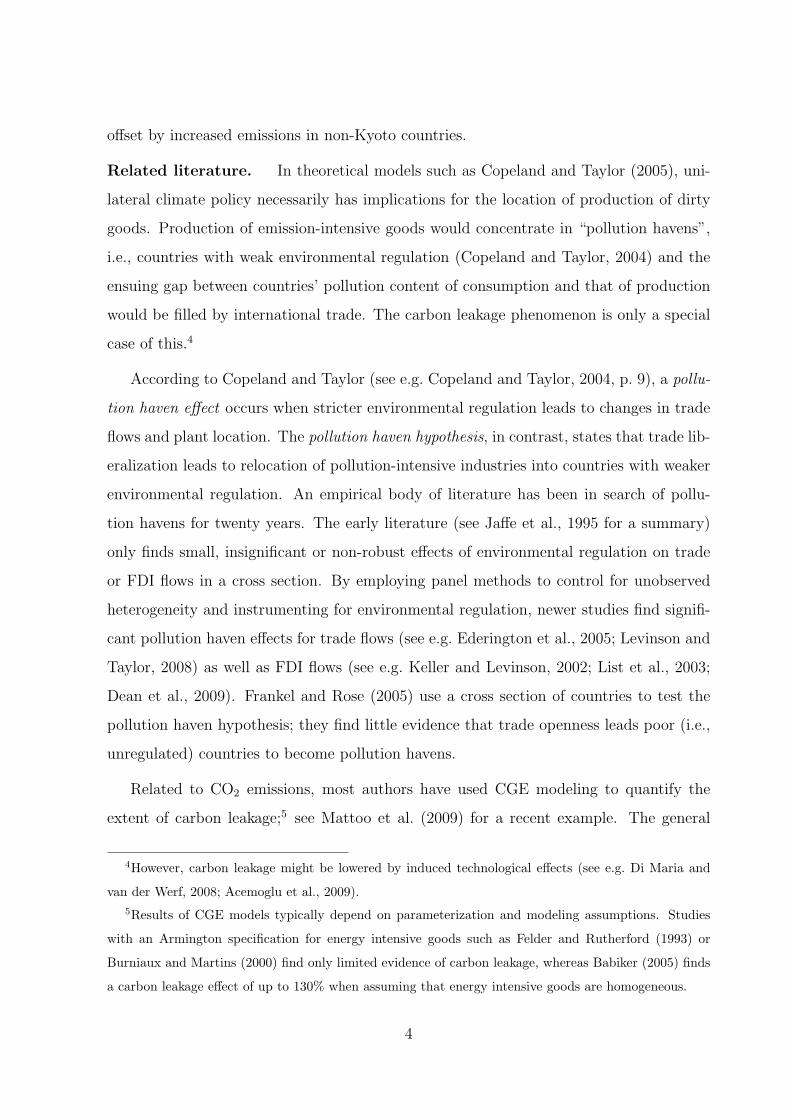
In this subsection, we take a descriptive look at the data. Figure 1 plots the percentage
share of carbon imports from uncommitted countries over total carbon imports for the
time period 1995 to 2005, thereby updating similar statistics found in Peters and Hertwich
(2008). The solid curve shows that, on average, Kyoto countries (those that have binding
commitments under the Kyoto Protocol) have carbon imports from non-Kyoto countries
amounting to about 40% of their total carbon imports. That measure exhibits an increas-
8Note that those emissions stem from fuel combustion only and emissions from international trans-
portation are exempt due to data limitations.912 out of 15 sectors comprise internationally tradable goods.
13
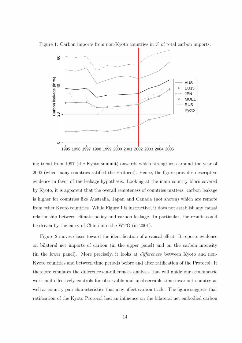
Figure 1: Carbon imports from non-Kyoto countries in % of total carbon imports.
020
4060
Car
bon
leak
age
(in %
)
1995 1996 1997 1998 1999 2000 2001 2002 2003 2004 2005
AUSEU15JPNMOELRUSKyoto
ing trend from 1997 (the Kyoto summit) onwards which strengthens around the year of
2002 (when many countries ratified the Protocol). Hence, the figure provides descriptive
evidence in favor of the leakage hypothesis. Looking at the main country blocs covered
by Kyoto, it is apparent that the overall remoteness of countries matters: carbon leakage
is higher for countries like Australia, Japan and Canada (not shown) which are remote
from other Kyoto countries. While Figure 1 is instructive, it does not establish any causal
relationship between climate policy and carbon leakage. In particular, the results could
be driven by the entry of China into the WTO (in 2001).
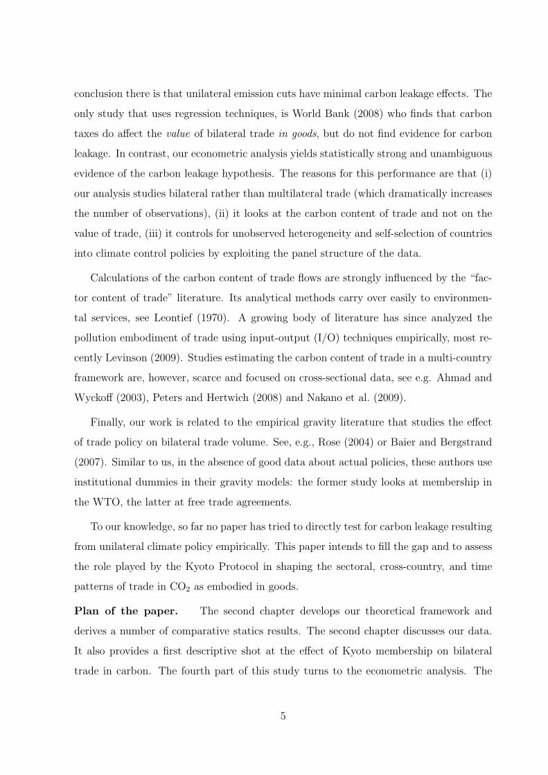
Figure 2 moves closer toward the identification of a causal effect. It reports evidence
on bilateral net imports of carbon (in the upper panel) and on the carbon intensity
(in the lower panel). More precisely, it looks at differences between Kyoto and non-
Kyoto countries and between time periods before and after ratification of the Protocol. It
therefore emulates the differences-in-differences analysis that will guide our econometric
work and effectively controls for observable and unobservable time-invariant country as
well as country-pair characteristics that may affect carbon trade. The figure suggests that
ratification of the Kyoto Protocol had an influence on the bilateral net embodied carbon
14
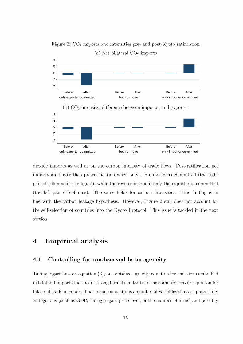
Figure 2: CO2 imports and intensities pre- and post-Kyoto ratification
(a) Net bilateral CO2 imports-1
-.5
0.5
1
only exporter committed both or none only importer committed
Before After Before After Before After
Net bilateral CO2 imports-1
-.5
0.5
1
only exporter committed both or none only importer committed
Before After Before After Before After
CO2 intensity, difference between importer and exporter
Source: Calculation by authors; see text.
(b) CO2 intensity, difference between importer and exporter
-1-.
50
.51
only exporter committed both or none only importer committed
Before After Before After Before After
Net bilateral CO2 imports
-1-.
50
.51
only exporter committed both or none only importer committed
Before After Before After Before After
CO2 intensity, difference between importer and exporter
Source: Calculation by authors; see text.
dioxide imports as well as on the carbon intensity of trade flows. Post-ratification net
imports are larger then pre-ratification when only the importer is committed (the right
pair of columns in the figure), while the reverse is true if only the exporter is committed
(the left pair of columns). The same holds for carbon intensities. This finding is in
line with the carbon leakage hypothesis. However, Figure 2 still does not account for
the self-selection of countries into the Kyoto Protocol. This issue is tackled in the next
section.
4 Empirical analysis
4.1 Controlling for unobserved heterogeneity
Taking logarithms on equation (6), one obtains a gravity equation for emissions embodied
in bilateral imports that bears strong formal similarity to the standard gravity equation for
bilateral trade in goods. That equation contains a number of variables that are potentially
endogenous (such as GDP, the aggregate price level, or the number of firms) and possibly
15
hard to observe directly. Following Feenstra (2004), we deal with this problem by adding
a full host of interaction terms between country dummies and year dummies and estimate
our gravity equation by OLS.
This strategy has the additional advantage that it deals with the potentially endoge-
nous selection of countries into the Kyoto protocol. This is a serious issue: countries with
lower carbon intensities of production, lower costs of reducing emissions, or ex-communist
countries in the process of updating out-dated technologies with modern, carbon-saving
ones, could be more willing to commit to climate policy targets as the costs of meet-
ing those targets would be lower. Kyoto membership is then endogenous and a possible
correlation between emissions embodied in trade and Kyoto status could be spurious.
Including country × year interaction terms controls for all reasons why a country may
join the agreement at some point in time.10 Failing to account for selection into the Pro-
tocol would introduce correlation between the Kyoto commitment variable and the error
term and therefore lead to endogeneity bias. The drawback of including those interaction
terms is that only variables with a country-pair dimension can be identified. Moreover,
only the average effect of Kyoto membership on bilateral carbon trade can be estimated
with potential country-heterogeneity remaining undisclosed.
Another challenge in gravity modeling is how to deal with country-pair specific unob-
served heterogeneity, due, for instance, to imperfect observability of trade costs. Usually,
time-invariant variables such as geographical distance, contiguity, the existence of a com-
mon language, and so forth, are used as proxies. The bilateral stance of trade policy is
proxied by two countries’ joint membership in free trade areas (FTA), the world trade
organization (WTO), a currency zone, and the like. However, trade costs depend on the
availability of infrastructure and are only partly influenced by geography. Moreover, joint
membership in FTAs may be endogenous. For this reason, Baier and Bergstrand (2007)
propose to use fixed-effects estimation (i.e., include country-pair effects into the regres-
sion) or to time-differentiate equation (6), which has the advantage of controlling for all
10In other words, the country× year effects make the inclusion of odds-ratios for selection into treatment
redundant.
16
historical and geographical determinants that may have lead to self-selection of countries
into FTAs or into international climate-policy agreements. The fixed-effects model uses
only the within-country-pair variance to identify the effect of policy variables on emis-
sions trade. The strategy therefore accounts for country characteristics that are strictly
time-invariant. However, it fails to control for unobserved changes in those characteristics
(e.g., if a change in consumer preferences leads at the same time to less carbon imports
and to stricter climate control policies).11
4.2 Measuring the Kyoto effect
The OECD has started to collect data on climate-related taxes;12 however, there still
is no harmonized data base that could be exploited in econometric analysis. Moreover,
data typically refers to tax revenue which is clearly endogenous to the carbon leakage
phenomenon. Similarly, the International Energy Agency collects information on national
legislation pertaining to subsidy and incentive programs.13 These data suggest that Kyoto
member states do have stricter policies: they have higher environmental taxes as a percent
of total tax income, or in terms of GDP per capita. A simple count of subsidy and
incentives programs shows that committed countries have about 3 times more of them
than non-committed countries and that most of the difference has emerged since the
ratification of the Kyoto Protocol. While suggestive, these statistics are only partially
informative about the general stance of climate control policies.14
We will therefore assume that there is a link between Kyoto commitment and actual
climate policies and then use Kyoto commitment as our key independent variable of
11Alternatively, we could work with first differences. If T = 2, this strategy gives exactly the same
results as the within estimator. If T = 3, results can differ if the error term exhibits serial correlation.
We provide robustness checks based on first differences in the Appendix.12http://www2.oecd.org/ecoinst/queries/index.htm
13http://www.iea.org/textbase/pm/
14See also the discussion in Levinson and Taylor (2008, p. 230) who also use a summary measure of
environmental regulation in their empirical analysis.
17
interest.15 In most of our regressions we use
Kyotoit =
1 if country i has a binding emission cap and t ≥ year of ratification
0 else.
(11)
For instance, Kyotoit = 0 for a country i that has not ratified the Protocol yet or has no
binding emission targets under the Protocol. This variable has variance across countries
and time: we have 38 countries in our sample, 12 have no commitments over the entire
period 1995-2005. The ratification of the Protocol by national parliaments started in 2000
(Mexico). Some countries have ratified the Protocol in 2004 (India, Israel, Russia), and
most have ratified in the years 2001, 2002, 2003.
Alternatively, we may summarize the stance of climate-saving policies in country i by
Kyotoit =
−1 if i has no commitments at time t
0 if EMit ≤ CAPi and t ≥ year of ratification
1 if EMit > CAPi and t ≥ year of ratification
, (12)
where EMit is the level of recorded CO2 emissions at time t and CAPi is the level of
emissions promised for the year of 2012. While the definition in (11) measures whether
a country is committed to keep carbon emissions below some target level, the definition
in (12) also takes into account the restrictiveness of that target. We prefer the former,
simpler measure, because the assumed linearity in (12) may be problematic. However, we
present robustness checks that use (12).16
These considerations lead us to write (6) in estimable form as
lnEhijt = κh (Kyotoit −Kyotojt) + γhPOLijt + νi × νt + νj × νt + νij + υijt (13)
where Ehijt is the amount of CO2 emissions embodied in country i′s imports from country j
at time t. POLijt is a vector of trade policy variables in dummy form (common WTO
15This strategy is commonly used in empirical modeling of trade policy when researchers, for instance,
proxy the stance of trade policy by a WTO membership dummy (Rose, 2004).16We have also experimented with setting Kyotoit = 1 if EMit ≥ CAPi and t ≥ year of ratification
and 0 else and have obtained almost identical results as compared to (11).
18
membership, common FTA membership, Euro-zone), νij is the country-pair specific inter-
cept, and the vectors νi, νj, νt collect country i, country j, and year dummies. The error
term υijt is assumed to have the usual properties. We run (13) separately for each of our
12 sectors. Note that we cannot separately estimate the effects of the importer and the
exporter being committed as long as we maintain the term νi × νt + νj × νt. Hence, we
have bilateralized the Kyoto variable. To make the effect of importer commitment relative
to exporter commitment visible, we drop the country × year effects in some regressions
but give warning about the interpretation of the coefficients obtained. We will also work
with regressions on aggregate bilateral data, which correspond to (13) with the h−index
dropped.
A more demanding alternative specification uses the bilateral net balance of carbon
imports as the dependent variable:
lnEhijt − lnEh
jit = 2κh (Kyotoit −Kyotojt) + νi × νt + νj × νt + νij + υijt, (14)
which follows from (13) and where POLijt drops out due to its assumed symmetric effect
on importers and exporters. The country × year interaction terms remain in the equation
since nothing ensures that the terms (13) are symmetric across importers and exporters.
Again, in some regressions, to make the separate effects of importer or exporter country
commitments visible, we drop the country × year effects.
4.3 Does carbon trade obey the law of gravity?
As a first step in our empirical analysis we run a standard gravity model of bilateral
trade in embodied carbon emissions. We work with the pure cross-section of aggregate
bilateral trade for the year of 2004. The analysis covers 33 out of our 38 countries (we
lack recent sectoral output data for 5 countries). One would expect that indirect bilateral
trade in carbon emissions should be affected very similarly by economic, political, and
geographical determinants of trade in goods since the former is derived from the latter.
Table 1 reports results. Most regressions are ‘naive’ (i.e., they omit importer and
exporter effects) so that the separate effect of Kyoto commitments by the exporter and
19
the importer can be estimated. As proposed by Baier and Bergstrand (2009), we compute
a multilateral resistance term and include it into the regression to account for third
country effects as well. We add an array of country-specific geographical controls which are
also meant to capture country-specific unobserved heterogeneity.17 While our theoretical
model does not explicitly ask for it, we also include GDP per capita of the exporter and
the importer. The reason is the well-known environmental Kuznets curve: richer countries
have smaller emissions per unit of GDP than poorer ones. Column (1) reports a standard
gravity equation with the value of bilateral trade as the dependent variable. Results are
as expected: the elasticity of bilateral trade with respect to either the importer’s or the
exporter’s GDP is very close to unity, and the elasticity with respect to geographical
distance is virtually identical to minus one. In column (2), this changes little when the
dependent variable is the log of carbon emissions as embodied in bilateral trade instead
as the log of the (deflated by importer CPI) trade values.
However, column (2) contains a surprise: while GDP per capita of both the exporter
and the importer increase the value of trade in goods (as in the empirical literature
on the Linder hypothesis), richer countries appear to import more carbon than poorer
ones, holding market size constant. However, those imports are lower when the export
partner has higher GDP per capita. This finding suggests that climate policies (and
hence emissions) may be endogenous to country characteristics, with richer countries
having greener policies than poorer ones.18
Columns (3) and (4) add the Kyoto commitment dummies as given in (11) to the
regression. Kyoto commitment of both the importer and the exporter appears to reduce
the value of bilateral trade and the amount of emissions embodied in that trade flow. In
both equations, commitment of the exporter has a stronger trade-defeating effect than
commitment of the importer. Again, we find the change in sign across columns (3) and
(4) of the coefficient of GDP per capita of the exporter. Columns (3) and (4) may fail to
17The inclusion of those variables is of little importance for parameter estimates.18Including the exporter’s squared GDP per capita results in a positive sign for the linear term and a
negative for the squared one, both statistically significant. This is further evidence in favor of a Kuznets-
curve effect.
20
control for countries’ multilateral resistance and for their endogenous selection into the
climate policy agreement. Column (5) therefore includes a comprehensive set of importer
and exporter fixed effects. Country-specific effects can no longer be identified and drop
out. Controls with bilateral dimension (such as distance) remain and do not change much
relative to the ‘naive’ regressions. However, the difference in Kyoto commitment between
the importer and the exporter now appears strongly significant and with the expected
sign: on average, a committed importer imports about 56% more carbon emissions from
a non-committed exporter; or, equivalently, a committed exporter exports about 56% less
carbon emissions to a non-committed country.
Columns (6) to (8) repeat the above exercise, but use the Kyoto restrictiveness mea-
sure as defined in (12) instead of the commitment dummies. Results from (8) are
qualitatively and quantitatively comparable to those from (5), with the additional in-
sight that the strength of commitments matters: imports of a strongly committed im-
porter (Kyotoit = 1) from a totally uncommitted exporter (Kyotojt = −1) are again
about 56% higher than in a situation where both countries have the same commitment
(0.279 ∗ 2 = 0.558).
4.4 CO2 accounting and carbon imports in the panel
Next, we extend the analysis to a panel setup using yearly data from 1995-2005. Ta-
ble 2 looks at aggregate trade and varies the exact definition of the dependent variable.
This allows to control for country-pair specific unobserved heterogeneity using a within-
transformation of the data. The strategy accounts for all time-invariant determinants of
trade in emissions, i.e., also exporter- and importer-specific factors as long as they do
not change over time. This may cover endowment structures, preferences, and so on. All
regressions in Table 2 include a full set of year dummies to control for changes in the price
of fuel, or the global business cycle. Even numbered regressions use country-specific year
dummies (i.e., interaction terms between country dummies and year dummies), which, of
course, precludes the estimation of country-specific influences on carbon trade.
The dependent variable in columns (1) and (2) in Table 2 is based on the “simple”
21
method of carbon accounting. It draws only on the domestic CO2 emissions that are
required to produce the exports of some country and disregards CO2 emissions that are
embodied in imported inputs. Columns (3) and (4) use a broader definition (MRIO),
where the carbon content of a country’s exports is based on all CO2 emissions, regardless
of the place where they occur.19 That is, the carbon content of imported inputs that are
required for a country’s exports is booked in the exporter’s carbon account. Columns (5)
and (6) compute the carbon content of trade based on the simple method and ruling
out the technique effect. That is, the input-output table and the sectoral CO2 emission
coefficients are held constant at the 1995 level. Then, variation in the dependent vari-
able can only derive from changes in the structure of bilateral trade flows and not from
emission-saving technical change. Thus, the importance of the technique and scale ef-
fect are singled out, as motivated by the decomposition exercise in equation (7). Finally,
columns (7) and (8) use the carbon intensity of imports as the dependent variable. It uses
the (log of) carbon content of trade (simple method) divided by the (log of the) value of
bilateral imports (deflated by the base-2000 GDP deflator of the exporter).20 The loss in
competitiveness should be strongest for the most carbon-intensive sectors. Therefore, we
expect a higher carbon intensity of imports for Kyoto countries on the aggregate level.
The most important insight from Table 2 is that carbon imports of a committed
country are by about 14% larger than those of a non-committed country, and carbon
imports from a committed exporter are by about 15% smaller than those from a non-
committed exporter. This is shown, for the simple method, in column (1). When including
a full set of country × year interaction terms (column (2)), only the effect of differential
19Note that in a MRIO model there are many feedback effects due to vertical integration which makes
it hard to disentangle effects in the investigated country from effects in other countries. Hence, in the
MRIO approach, a Kyoto country’s exports could embody more carbon because of carbon leakage. For
example consider a case where a carbon-intensive intermediate which is used to produce those exports
is imported from a carbon-intensively producing non-Kyoto country after ratification due to the Kyoto
commitments. Therefore, in our context, we prefer the simple specification over the MRIO model for the
empirical tests of the carbon leakage hypothesis, but always report results for the MRIO model as well.20Defining the carbon intensity measure as the ratio of carbon imports over the deflated value of imports
(i.e., not taking logs) leads to very similar results.
22
Kyoto commitment can be estimated. The estimated coefficient of 0.125 implies that
carbon imports are about 12.5% higher if the importer is committed and the exporter
not, and 12.5% lower if the exporter is committed and the importer is not. Comparing
this estimate with the one obtained in Table 1 for the cross-section of 2004, one notes
that controlling for country-pair specific unobserved heterogeneity strongly reduces the
estimate. This may be due to unobserved details of differential comparative advantage:
if the importer has a comparative advantage in non-carbon-intensive products and the
exporter in carbon-intensive products, then self-selection into the Kyoto Protocol is more
likely for the importer. This leads to spurious regression as the importer has both higher
carbon emissions embodied in imports and commitments under Kyoto.
When turning to the MRIO definition of carbon imports, the picture barely changes.
There are two important observations. Measured carbon leakage is somewhat smaller in
column (4) as compared to column (2). This is as expected, since the MRIO definition
blurs the link between the effect of domestic carbon emissions and the carbon content of
domestically assembled goods (final or intermediate). Moreover, carbon leakage seems to
be driven primarily by an increase in carbon imports and not so much by a decrease in
carbon exports. This is also not surprising: carbon emissions of foreign input producers
are factored into a country’s exports, but have a much weaker influence on imports.
Columns (5) and (6) fix the technology used in producing final and intermediate goods.
Imports of committed countries do not differ much as parameter estimates are similar
between columns (1) and (5). The coefficient for committed exporters, in contrast, turns
insignificant. Committed exporters seem to reduce the overall carbon content of their
exports primarily by adopting greener (i.e., less carbon-intensive) technologies and not by
altering the structure of production and, hence, of trade. The effect of differential Kyoto
commitments (column (6)) is now only half of the one estimated in column (2). But
relocation of production (the aggregate scale effect) still leads to about 7% more carbon
imports of Kyoto countries from non-Kyoto countries. Keeping in mind that the scale
effect is interpreted as the carbon leakage channel, we again find evidence in favor of the
carbon leakage hypothesis.
Finally, we turn to the carbon intensity of imports. Results suggest that differen-
23
tial Kyoto commitment leads to carbon leakage in the sense that the carbon intensity
of imports grows and that of exports falls if the importer is committed. This result is
complementary to the one shown in columns (5) and (6): The carbon intensity of a com-
mitted country’s exports falls precisely because of technological change and not because of
a change in trade volumes or trade structure. In contrast, the carbon intensity of imports
barely changes as increased carbon imports are matched with increased trade volumes.
To better assess the economic significance of our results, one needs to have answers to
the following two questions: By how much would an average non-Kyoto country’s carbon
imports increase if it had ratified the Protocol in 2002 (the average date of ratification)?
And by how much would domestic emission fall? Using sample averages for the year of
2002 and the coefficient of 0.125 found in column (2) of Table 2, the answer to the first
question is 3.07 mt. The second question is much harder to answer. In our data, average
yearly growth rates of emissions are 0.33% lower in committed relative to uncommitted
countries.21 Hence, from year of ratification to 2005, accumulated savings would have been
about 1.327%. Again, evaluating at the sample mean of 2002, this results in emissions
savings of 6.92 mt: approximately 44.4% of all savings would leak. This result is robust
over columns (2), (4) and (6). Hence, historically, the Kyoto Protocol has led to a
fairly strong leakage effect. This does, however, not allow predicting the effects of more
ambitious (and more successful) carbon saving initiatives. Also note that the portion of
total world imports (in our sample) per year caused by Kyoto is only about 5%.22
21In our data, from ratification onwards, Kyoto countries have average emission growth rates of 0.38%
p.a. while non-Kyoto countries have 0.71%.22In our sample, total carbon imports in 2005 amount to 2,191 mt, thereof 755 mt of Kyoto coun-
tries from non-Kyoto countries and 236 mt of the non-Kyoto countries from Kyoto members. Hence,
additional carbon imports from non-Kyoto countries caused by Kyoto are approximately 83.9 mt
(= 755 × 0.125/ [1 + 0.125]) while imports from Kyoto countries fall by approximately -33.7 mt (=
236 × [−0.125] / [1− 0.125]). Relative to observed carbon imports, Kyoto is responsible for about 5.1%
(= [83.9− 33.7] / [755 + 236]).
24
4.5 Net carbon imports and the Kyoto effect
Still using aggregate data, Table 3 proposes the most demanding test of the carbon leakage
hypothesis. Rather than using carbon imports as the dependent variable, it uses net
imports, as defined in (14). The hypothesis is that a committed importer should increase
its net imports of carbon from a non-committed exporter. Clearly, when looking at net
imports, the number of independent observations is half than when looking at imports.
Deviating from the specification in (14) by adding policy variables and the log product
of GDPs (without consequences for results), we provide results for Kyoto commitment
(according to definition (11)) and Kyoto restrictiveness (according to definition (12)). All
models use the within estimator and include a full set of exporter × year and importer ×year dummies. Robustness checks using the first-differenced model are in the Appendix.
The results are generally in line with the leakage hypothesis. Across all models, differ-
ential Kyoto commitment (i.e., the importer committed while the exporter is not) leads
to increased net imports of carbon. Because we are looking at the bilateral trade balance,
the effect of Kyoto commitment is expected to be larger than when focusing on imports.
Again, the phenomenon of carbon leakage is economically relevant: when the exporter
displays maximum restrictiveness and the exporter minimum restrictiveness, the net im-
ports of carbon can increase by as much as 185% (0.927 ∗ 2 = 1.854; simple method of
CO2 accounting). Also the carbon intensity of net imports reacts positively to differential
Kyoto commitment, signaling that Kyoto influences both, technologies and the structure
and volume of bilateral trade.
Table 3 also presents the p-values associated to the regression-based test of strict
exogeneity proposed by Wooldridge (2002, p. 285).23 In all cases, the test is easily passed.
Hence, our variable of interest can be considered as strictly exogenous in the context of
the specific model analyzed and its effect of the bilateral balance of carbon trade can be
understood as a causal effect.
23The idea of the test is that including the lead of the independent variable should yield an insignificant
coefficient if the contemporaneous level is strictly exogenous. Similarly, the level of the independent
variable should not be significant in a first-differenced model.
25
4.6 CO2 imports and carbon leakage across sectors
Finally, we look at sectoral bilateral imports and the sectoral bilateral trade balance
(net imports) of carbon. Hallak (forthcoming) has shown that estimation of the gravity
equation using aggregate data can suffer from aggregation bias. While his paper is about
the Linder hypothesis, a similar problem may arise in the present context if patterns of
comparative advantage correlate with adopted climate control policies. Hence, looking
at sectors separately may lead to more consistent results than studying aggregate trade
flows.
Table 4 presents the most important results from estimating sectoral gravity equations.
The carbon content of trade is computed using the ‘simple’ method. The econometric
model is again a within panel estimator with country × year interaction terms (where
applicable). The table only reports the key parameters; the remaining details of the
regressions and additional results can be found in the Appendix.
The overall picture again strongly confirms the carbon leakage hypothesis. Estimated
coefficients of differential Kyoto commitment have the correct sign (with the only ex-
ception being the wood industry). The sign pattern of the separate estimates for the
importer’s and the exporter’s commitment are also in line with expectations (except in
the agricultural and the textiles sector). The size of the effects is similar in magnitude to
the ones found in Table 2 for aggregate trade. The aggregate effects turn out to be close
to the average of the sectoral effects.
The effect of Kyoto commitment is larger in more carbon-intensive sectors such as
basic metals, chemicals and petrochemicals, non-metallic mineral products, transport
equipment, machinery or paper and pulp. Evidence is much weaker in low-carbon sectors
such as agriculture, forestry, and fishing, food, wood, or textiles. There is no evidence
for carbon leakage in the electricity sector, probably because formal and informal trade
costs are very high in this sector. Electricity being a major input in all other sectors
may, however, play an important indirect role, since the carbon intensity of domestically
produced inputs importantly affects the carbon content of exports. Finally, since we have
no direct information about countries’ policies (carbon taxes versus subsidies), failure to
26
detect evidence for carbon leakage in a specific industry may signal the importance of
subsidies as compared to taxes.
5 Conclusions
We have developed a multi-sector multi-input multi-country gravity model of trade in
CO2 emissions as embodied in goods. We have shown strong structural similarity to
the standard gravity equation, from which our equation is derived by applying appropri-
ately computed emission coefficients. Consequently, the emissions embodied in trade also
depend on standard gravity variables such as tariffs and country size and their implied
emissions per unit of trade. If a country unilaterally adopts a tax on CO2 emissions,
the carbon intensity of its production and of its exports falls. The tax also lowers price
competitiveness so that indirect carbon imports from non-committed countries rise. The
result is carbon leakage. In the case of a subsidy to alternative energy no such clear
pattern arises.
We calculate the CO2 emissions embodied in bilateral trade flows for a large sample of
countries over the period 1995 to 2005. With the resulting panel dataset we try to detect
the effect of the Kyoto Protocol on the carbon content of trade. The descriptive evidence
reveals that carbon imports of Kyoto countries from non-Kyoto countries rose since the
ratification process of the Kyoto Protocol started. This indicates potential carbon leakage
as result of the non-global deal to curb greenhouse gas emissions.
While suggestive, the descriptive evidence cannot clarify whether the Kyoto Protocol
has any causal effect on measured trade in carbon. To investigate this issue, we have used
panel econometrics. Using a complete array of time-varying country-specific effects in
theory-based gravity regressions, we can control for all potential reasons that may explain
why some country has ratified the Protocol or not. We also account for country-pair and
year specific determinants of carbon trade.
Our main result is that carbon imports of a committed country from a non-Kyoto
exporter are about 10% higher than if the country had no commitments. This carbon
27
leakage effect is strongest in the most carbon-intensive sectors. Hence, asymmetric com-
mitment to policies geared toward the reduction of carbon emissions may have measurable
consequences on bilateral trade patterns. The reduced emissions caused by domestic pro-
duction are then offset by increased emissions in foreign countries; the total effect of the
Kyoto Protocol on global emissions is therefore unclear. On average, we find a carbon
leakage effect of about 44%. However, the volume of trade in carbon caused by Kyoto is
rather small.
Our results suggest that the issue of carbon leakage is a serious challenge to interna-
tional climate saving programs. Since a multilateral agreement that commits all countries
to binding emission targets does not exist and looks increasingly unlikely, the first-best
policy to combat climate change, namely a world-wide cap on emissions, is not feasible.
Policy-makers in the European Union and the U.S. have called for carbon tariffs to tackle
the problem. Establishing the existence of carbon leakage as a result of unilateral climate
policy, our analysis justifies the importance that policy-makers accord to international
trade. However, rather than advocating carbon tariffs the use of which can have impor-
tant negative side-effects on world trade, we propose that willing countries commit to
binding restrictions not of their emission levels but of the amount of carbon embodied in
consumption. These could be achieved by domestic consumption taxes and/or subsidies.
However, such taxes pose important informational problems.
Importantly, our results also imply that simulations by climatologists (such as the one
by Sawin et al., 2009), which disregard the possibility of carbon leakage, may overesti-
mate the effect of unilateral emission control policies on the carbon concentration in the
atmosphere.
Before closing, we want to stress that our empirical strategy was geared toward iden-
tifying the average causal effect of unilateral climate policy. Our empirical results cannot
straightforwardly be used for the simulation of global CO2 emissions as a response to
climate policy scenarios, e.g., the potential commitment to an emission cap by the U.S.,
or the counterfactual situation of no global climate policy at all. To that end, one would
need to use the estimated elasticities in a structural general equilibrium model.
28
References
Acemoglu, Daron, Philippe Aghion, Leonardo Bursztyn, and David Hemous,
“The Environment and Directed Technical Change,” NBER Working Paper Series,
October 2009, No. 15451.
Ahmad, Nadim and Andrew Wyckoff, “Carbon Dioxide Emissions Embodied in In-
ternational Trade of Goods,” OECD, Directorate for Science, Technology and Industry
Working Papers, November 2003, No. 2003/15.
Babiker, Mustafa H., “Climate change policy, market structure, and carbon leakage,”
Journal of International Economics, March 2005, 65 (2), 421–445.
Baier, Scott L. and Jeffrey H. Bergstrand, “Do free trade agreements actually
increase members’ international trade?,” Journal of International Economics, March
2007, 71 (1), 72–95.
and , “Bonus vetus OLS: A simple method for approximating international trade-
cost effects using the gravity equation,” Journal of International Economics, February
2009, 77 (1), 77–85.
Baumert, Kevin A., Timothy Herzog, and Jonathan Pershing, Navigating the
Numbers: Greenhouse Gas Data and International Climate Policy, Washington: World
Resources Institute, 2005.
Burniaux, Jean-Marc and Joaquim Oliveira Martins, “Carbon Emission Leakages
– A general equilibrium view,” OECD Economics Department Working Paper, 2000,
No. 242.
Copeland, Brian R. and M. Scott Taylor, “Trade, Growth, and the Environment,”
Journal of Economic Literature, March 2004, 42 (1), 7–71.
and , “Free trade and global warming: a trade theory view of the Kyoto protocol,”
Journal of Environmental Economics and Management, March 2005, 49 (2), 205–234.
29
Dean, Judith M., Mary E. Lovely, and Hua Wang, “Are foreign investors attracted
to weak environmental regulations? Evaluating the evidence from China,” Journal of
Development Economics, September 2009, 90 (1), 1–13.
EC, “Progress towards achieving the Kyoto objectives,” Report from the Commission to
the European Parliament and the Council, 2009, SEC(2009)1581, Commission of the
European Communities.
Eder, Peter and Michael Narodoslawsky, “What environmental pressures are a
region’s industries responsible for? A method of analysis with descriptive indices and
input-output models,” Ecological Economics, June 1999, 29 (3), 359–374.
Ederington, Josh, Arik Levinson, and Jenny Minier, “Footloose and Pollution-
Free,” Review of Economics and Statistics, February 2005, 87 (1), 92–99.
Feenstra, Robert C., Advanced International Trade: Theory and Evidence, Princeton:
Princeton University Press, 2004.
Felder, Stefan and Thomas F. Rutherford, “Unilateral CO2 Reductions and Carbon
Leakage: The Consequences of International Trade in Oil and Basic Materials,” Journal
of Environmental Economics and Management, September 1993, 25 (2), 162–176.
Frankel, Jeffrey A. and Andrew K. Rose, “Is Trade Good or Bad for the Environ-
ment? Sorting Out the Causality,” Review of Economics and Statistics, February 2005,
87 (1), 85–91.
Grether, Jean-Marie and Nicola A. Mathys, “How fast are CO2 emissions moving
to Asia?,” http://www.voxeu.org/index.php?q=node/4243, 2009.
Grossman, Gene M. and Alan B. Krueger, “Environmental Impacts of a North
American Free Trade Agreement,” in Peter M. Garber, ed., The Mexico-U.S. Free
Trade Agreement, Chicago: MIT Press, 1993, pp. 13–56.
Hallak, Juan Carlos, “A product quality view of the Linder hypothesis,” Review of
Economics and Statistics, forthcoming.
30
IEA, “CO2 Emissions from Fuel Combustion (detailed estimates),” 2008, Vol. 2008 release
01, Paris.
IPCC, “Revised 1996 IPCC Guidelines for National Greenhouse Gas Inventories,”
http://www.ipcc-nggip.iges.or.jp/public/gl/invs1.html, 1996.
, Climate Change 2007: Mitigation of Climate Change Contribution of Working Group
III to the Fourth Assessment Report of the Intergovernmental Panel on Climate Change,
Cambridge, United Kingdom and New York, NY, USA: Cambridge University Press,
2007.
Jaffe, Adam B., Steven R. Peterson, Paul R. Portney, and Robert N. Stavins,
“Environmental Regulation and the Competitiveness of U.S. Manufacturing: What
Does the Evidence Tell Us?,” Journal of Economic Literature, March 1995, 33 (1),
132–163.
Keller, Wolfgang and Arik Levinson, “Pollution Abatement Costs and Foreign Direct
Investment Inflows to U.S. States,” Review of Economics and Statistics, November 2002,
84 (4), 691–703.
Leontief, Wassily, “Environmental Repercussions and the Economic Structure: An
Input-Output Approach,” The Review of Economics and Statistics, August 1970, 52
(3), 262–271.
Levinson, Arik, “Technology, International Trade, and Pollution from US Manufactur-
ing,” American Economic Review, December 2009, 99 (5), 2177–2192.
and M. Scott Taylor, “Unmasking The Pollution Haven Effect,” International Eco-
nomic Review, February 2008, 49 (1), 223–254.
List, John A., Daniel L. Millimet, Per G. Fredriksson, and W. Warren
McHone, “Effects of Environmental Regulations on Manufacturing Plant Births: Ev-
idence from a Propensity Score Matching Estimator,” The Review of Economics and
Statistics, November 2003, 85 (4), 944–952.
31
Maria, Corrado Di and Edwin van der Werf, “Carbon leakage revisited: unilateral
climate policy with directed technical change,” Environmental and Resource Economics,
February 2008, 39 (2), 55–74.
Mattoo, Aaditya, Arvind Subramanian, Dominique van der Mensbrugghe, and
Jianwu He, “Reconciling Climate Change and Trade Policy,” Peterson Institute for
International Economics Working Paper Series, 2009, No. 09-15.
Nakano, Satoshi, Asako Okamura, Norihisa Sakurai, Masayuki Suzuki, Yoshi-
aki Tojo, and Norihiko Yamano, “The Measurement of CO2 Embodiments in In-
ternational Trade: Evidence from the Harmonised Input-Output and Bilateral Trade
Database,” OECD Science, Technology and Industry Working Papers, 2009, No.
2009/3.
OECD, “Input-Output Tables (2009),” 2009, Paris.
Peters, Glen P. and Edgar G. Hertwich, “CO2 Embodied in International Trade
with Implications for Global Climate Policy,” Environmental Science & Technology,
March 2008, 42 (5), 1401–1407.
Rose, Andrew K., “Do We Really Know That the WTO Increases Trade?,” American
Economic Review, March 2004, 94 (1), 98–114.
Sawin, Elizabeth R., Andrew P. Jones, Tom Fiddaman, Lori S. Siegel, Diana
Wright, Travis Franck, Andreas Barkman, Tom Cummings, Felicitas von
Peter, Jacqueline McGlade, Robert W. Correll, and John Sterman, “Current
emissions reductions proposals in the lead-up to COP-15 are likely to be insufficient
to stabilize atmospheric CO2 levels: Using C-ROADS – A simple computer simulation
of climate change – to support long-term climate policy development,” 2009, Paper
presented at the Climate Change – Global Risks, Challenges, and Decisions Conference,
Copenhagen, Denmark.
Sinn, Hans-Werner, “Public policies against global warming: a supply side approach,”
International Tax and Public Finance, August 2008, 15 (4), 360–394.
32
Trefler, Daniel and Susan Chun Zhu, “The Structure of Factor Content Predictions,”
NBER Working Paper, March 2005, No. 11221.
UNFCCC, “National greenhouse gas inventory data for the period 1990–2006,”
http://unfccc.int/resource/docs/2008/sbi/eng/12.pdf, 2008.
Unido, “Industrial Statistics Database at the 4-digit Level of ISIC (Revision 2 and 3),”
CD-Rom, 2009, Vienna.
Wang, T. and J. Watson, “Who Owns China’s Carbon Emissions?,” Tyndall Centre
Briefing Note, 2007, No. 23.
Wooldridge, Jeffrey, Econometric Analysis of Cross Section and Panel Data, Chicago:
MIT Press, 2002.
World Bank, International Trade and Climate Change - Economic, Legal, and Institu-
tional Perspectives, Washington: IBRD/The World Bank, 2008.
33
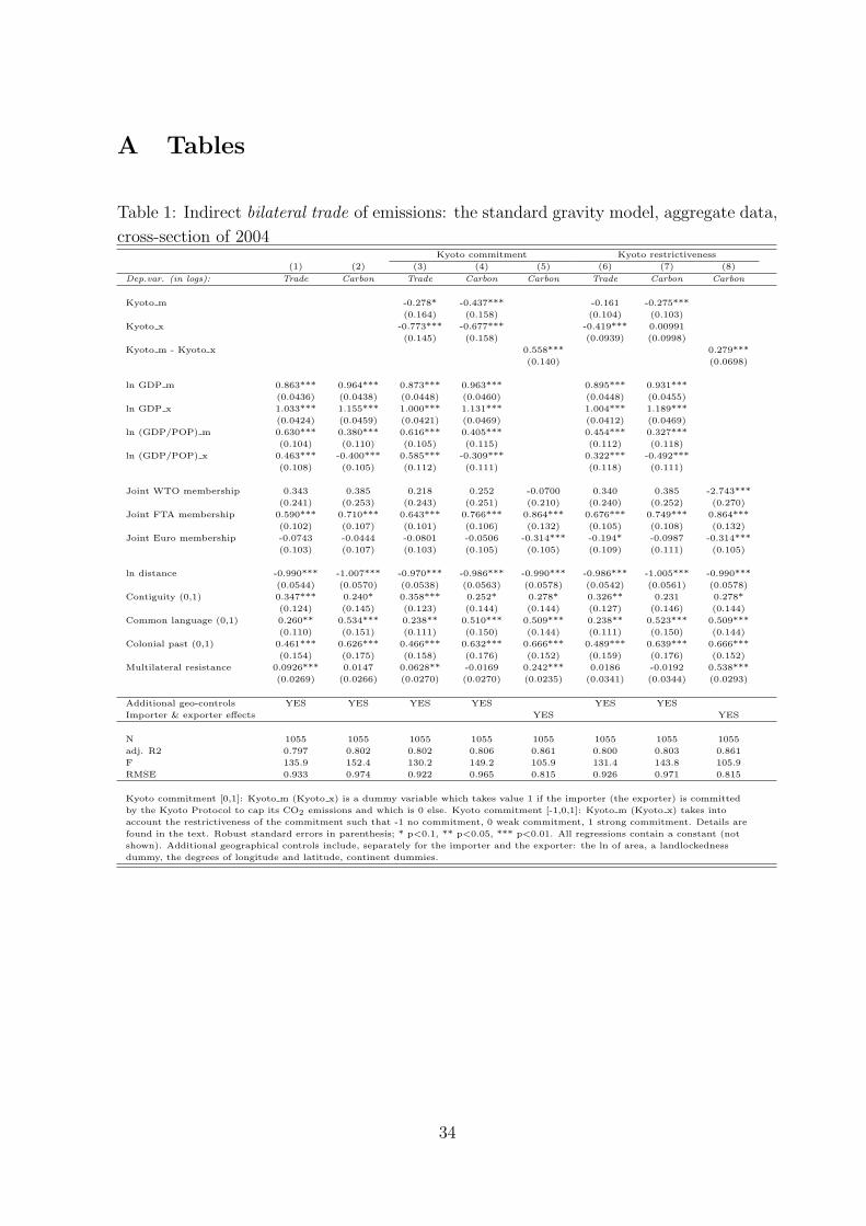
A Tables
Table 1: Indirect bilateral trade of emissions: the standard gravity model, aggregate data,
cross-section of 2004Kyoto commitment Kyoto restrictiveness
(1) (2) (3) (4) (5) (6) (7) (8)
Dep.var. (in logs): Trade Carbon Trade Carbon Carbon Trade Carbon Carbon
Kyoto m -0.278* -0.437*** -0.161 -0.275***
(0.164) (0.158) (0.104) (0.103)
Kyoto x -0.773*** -0.677*** -0.419*** 0.00991
(0.145) (0.158) (0.0939) (0.0998)
Kyoto m - Kyoto x 0.558*** 0.279***
(0.140) (0.0698)
ln GDP m 0.863*** 0.964*** 0.873*** 0.963*** 0.895*** 0.931***
(0.0436) (0.0438) (0.0448) (0.0460) (0.0448) (0.0455)
ln GDP x 1.033*** 1.155*** 1.000*** 1.131*** 1.004*** 1.189***
(0.0424) (0.0459) (0.0421) (0.0469) (0.0412) (0.0469)
ln (GDP/POP) m 0.630*** 0.380*** 0.616*** 0.405*** 0.454*** 0.327***
(0.104) (0.110) (0.105) (0.115) (0.112) (0.118)
ln (GDP/POP) x 0.463*** -0.400*** 0.585*** -0.309*** 0.322*** -0.492***
(0.108) (0.105) (0.112) (0.111) (0.118) (0.111)
Joint WTO membership 0.343 0.385 0.218 0.252 -0.0700 0.340 0.385 -2.743***
(0.241) (0.253) (0.243) (0.251) (0.210) (0.240) (0.252) (0.270)
Joint FTA membership 0.590*** 0.710*** 0.643*** 0.766*** 0.864*** 0.676*** 0.749*** 0.864***
(0.102) (0.107) (0.101) (0.106) (0.132) (0.105) (0.108) (0.132)
Joint Euro membership -0.0743 -0.0444 -0.0801 -0.0506 -0.314*** -0.194* -0.0987 -0.314***
(0.103) (0.107) (0.103) (0.105) (0.105) (0.109) (0.111) (0.105)
ln distance -0.990*** -1.007*** -0.970*** -0.986*** -0.990*** -0.986*** -1.005*** -0.990***
(0.0544) (0.0570) (0.0538) (0.0563) (0.0578) (0.0542) (0.0561) (0.0578)
Contiguity (0,1) 0.347*** 0.240* 0.358*** 0.252* 0.278* 0.326** 0.231 0.278*
(0.124) (0.145) (0.123) (0.144) (0.144) (0.127) (0.146) (0.144)
Common language (0,1) 0.260** 0.534*** 0.238** 0.510*** 0.509*** 0.238** 0.523*** 0.509***
(0.110) (0.151) (0.111) (0.150) (0.144) (0.111) (0.150) (0.144)
Colonial past (0,1) 0.461*** 0.626*** 0.466*** 0.632*** 0.666*** 0.489*** 0.639*** 0.666***
(0.154) (0.175) (0.158) (0.176) (0.152) (0.159) (0.176) (0.152)
Multilateral resistance 0.0926*** 0.0147 0.0628** -0.0169 0.242*** 0.0186 -0.0192 0.538***
(0.0269) (0.0266) (0.0270) (0.0270) (0.0235) (0.0341) (0.0344) (0.0293)
Additional geo-controls YES YES YES YES YES YES
Importer & exporter effects YES YES
N 1055 1055 1055 1055 1055 1055 1055 1055
adj. R2 0.797 0.802 0.802 0.806 0.861 0.800 0.803 0.861
F 135.9 152.4 130.2 149.2 105.9 131.4 143.8 105.9
RMSE 0.933 0.974 0.922 0.965 0.815 0.926 0.971 0.815
Kyoto commitment [0,1]: Kyoto m (Kyoto x) is a dummy variable which takes value 1 if the importer (the exporter) is committed
by the Kyoto Protocol to cap its CO2 emissions and which is 0 else. Kyoto commitment [-1,0,1]: Kyoto m (Kyoto x) takes into
account the restrictiveness of the commitment such that -1 no commitment, 0 weak commitment, 1 strong commitment. Details are
found in the text. Robust standard errors in parenthesis; * p<0.1, ** p<0.05, *** p<0.01. All regressions contain a constant (not
shown). Additional geographical controls include, separately for the importer and the exporter: the ln of area, a landlockedness
dummy, the degrees of longitude and latitude, continent dummies.
0
34
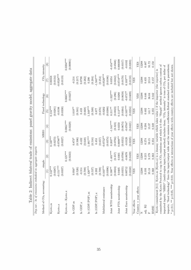
Tab
le2:
Indir
ect
bila
tera
ltr
ade
ofem
issi
ons:
pan
elgr
avit
ym
odel
,ag
greg
ate
dat
a
Dep
.var.
:ln
ofem
issi
ons
embo
die
din
agg
rega
teim
port
s
Met
hod
of
CO
2acc
ounti
ng:
sim
ple
MR
IOF
ixed
tech
nolo
gy
CO
2in
tensi
ty
(1)
(2)
(3)
(4)
(5)
(6)
(7)
(8)
Kyoto
m0.1
42***
0.1
40***
0.1
34***
0.0
0358
(0.0
287)
(0.0
273)
(0.0
281)
(0.0
134)
Kyoto
x-0
.151***
-0.0
788**
-0.0
198
-0.0
528***
(0.0
337)
(0.0
327)
(0.0
330)
(0.0
119)
Kyoto
m-
Kyoto
x0.1
25***
0.0
861***
0.0
665***
0.0
394***
(0.0
243)
(0.0
229)
(0.0
227)
(0.0
0901)
lnG
DP
m0.9
56*
0.8
73*
1.0
19**
-0.2
14
(0.5
26)
(0.5
06)
(0.5
01)
(0.2
17)
lnG
DP
x-0
.314
-0.4
32
0.4
33
0.0
798
(0.7
09)
(0.6
48)
(0.6
68)
(0.2
62)
ln(G
DP
/P
OP
)m
1.4
20***
1.4
81***
1.3
49***
0.2
90
(0.5
37)
(0.5
16)
(0.5
09)
(0.2
04)
ln(G
DP
/P
OP
)x
0.2
02
0.4
53
0.8
77
-1.5
83***
(0.7
09)
(0.6
57)
(0.6
76)
(0.2
54)
Mult
ilate
ral
resi
stance
-0.1
03***
-0.0
752**
-0.0
202
-0.0
529***
(0.0
396)
(0.0
374)
(0.0
388)
(0.0
186)
Join
tW
TO
mem
ber
ship
0.1
90**
-1.4
01***
0.2
03**
-1.3
41***
0.2
11**
-1.3
22***
0.0
354
-0.4
54***
(0.0
824)
(0.3
57)
(0.0
794)
(0.3
23)
(0.0
823)
(0.2
96)
(0.0
242)
(0.0
568)
Join
tF
TA
mem
ber
ship
0.0
405
0.0
301
0.0
698**
0.0
250
0.1
13***
0.0
280
-0.0
719***
0.0
00398
(0.0
355)
(0.0
700)
(0.0
352)
(0.0
674)
(0.0
364)
(0.0
659)
(0.0
170)
(0.0
317)
Join
tE
uro
mem
ber
ship
0.0
0712
-0.0
676
-0.0
120
-0.0
764*
-0.1
05***
-0.0
717*
0.1
03***
-0.0
102
(0.0
240)
(0.0
439)
(0.0
235)
(0.0
421)
(0.0
234)
(0.0
409)
(0.0
110)
(0.0
203)
Yea
reff
ects
YE
SY
ES
YE
SY
ES
Countr
y×
yea
reff
ects
YE
SY
ES
YE
SY
ES
N12288
12288
12288
12288
12288
12288
12288
12288
adj.
R2
0.1
93
0.2
15
0.2
74
0.2
94
0.4
02
0.4
46
0.4
35
0.4
87
F35.1
89.1
79
59.1
513.3
7141.7
36.0
4215.0
91.7
2
RM
SE
0.3
68
0.3
63
0.3
54
0.3
49
0.3
55
0.3
42
0.1
57
0.1
50
Kyoto
com
mit
men
t[0
,1]:
Kyoto
m(K
yoto
x)
isa
dum
my
vari
able
whic
hta
kes
valu
e1
ifth
eim
port
er(t
he
exp
ort
er)
is
com
mit
ted
by
the
Kyoto
Pro
toco
lto
cap
its
CO
2em
issi
ons
and
whic
his
0el
se.
“Sim
ple
”m
ethod
ignore
sca
rbon
conte
nt
of
imp
ort
edin
puts
;“M
RIO
”(m
ult
i-re
gio
nin
put/
outp
ut
met
hod)
incl
udes
them
;“C
O2
inte
nsi
ty”
isto
ns
of
CO
2p
erdollar
of
imp
ort
s;“fixed
tech
nolo
gy”
fixes
the
input/
outp
ut
table
and
the
emis
sion
coeffi
cien
ts.R
obust
standard
erro
rsin
pare
nth
esis
;
*p<
0.1
,**
p<
0.0
5,
***
p<
0.0
1.
Yea
reff
ects
or
inte
ract
ions
of
yea
reff
ects
wit
hco
untr
yeff
ects
are
incl
uded
but
not
show
n.
0
35
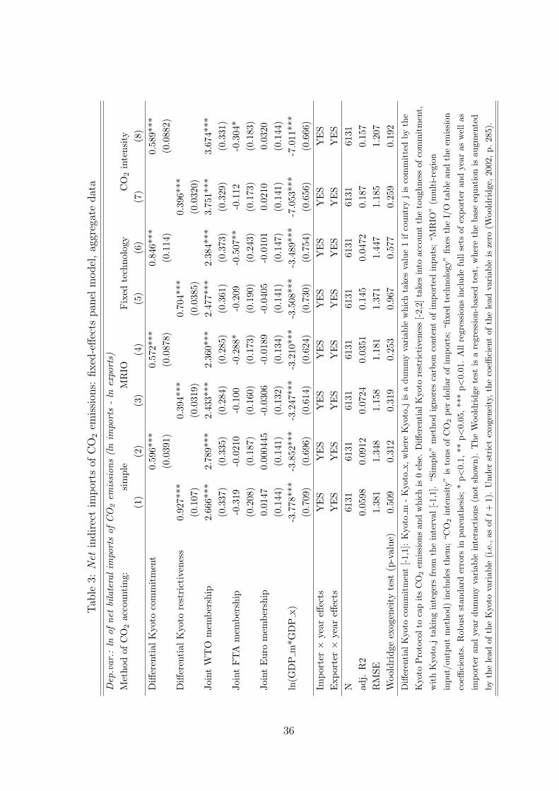
Tab
le3:
Net
indir
ect
imp
orts
ofC
O2
emis
sion
s:fixed
-eff
ects
pan
elm
odel
,ag
greg
ate
dat
a
Dep
.var
.:ln
ofne
tbi
late
ralim
port
sof
CO
2em
issi
ons
(ln
impo
rts
-ln
expo
rts)
Met
hod
ofC
O2
acco
unti
ng:
sim
ple
MR
IOF
ixed
tech
nolo
gyC
O2
inte
nsit
y(1
)(2
)(3
)(4
)(5
)(6
)(7
)(8
)D
iffer
enti
alK
yoto
com
mit
men
t0.
596*
**0.
572*
**0.
846*
**0.
589*
**(0
.039
1)(0
.087
8)(0
.114
)(0
.088
2)D
iffer
enti
alK
yoto
rest
rict
iven
ess
0.92
7***
0.39
4***
0.70
4***
0.39
6***
(0.1
07)
(0.0
319)
(0.0
385)
(0.0
320)
Join
tW
TO
mem
bers
hip
2.66
6***
2.78
9***
2.43
3***
2.36
0***
2.47
7***
2.38
4***
3.75
1***
3.67
4***
(0.3
37)
(0.3
35)
(0.2
84)
(0.2
85)
(0.3
61)
(0.3
73)
(0.3
29)
(0.3
31)
Join
tF
TA
mem
bers
hip
-0.3
19-0
.021
0-0
.100
-0.2
88*
-0.2
09-0
.507
**-0
.112
-0.3
04*
(0.2
08)
(0.1
87)
(0.1
60)
(0.1
73)
(0.1
90)
(0.2
43)
(0.1
73)
(0.1
83)
Join
tE
uro
mem
bers
hip
0.01
470.
0004
45-0
.030
6-0
.018
9-0
.040
5-0
.010
10.
0210
0.03
20(0
.144
)(0
.141
)(0
.132
)(0
.134
)(0
.141
)(0
.147
)(0
.141
)(0
.144
)ln
(GD
Pm
*GD
Px)
-3.7
78**
*-3
.852
***
-3.2
47**
*-3
.210
***
-3.5
08**
*-3
.489
***
-7.0
53**
*-7
.011
***
(0.7
09)
(0.6
96)
(0.6
14)
(0.6
24)
(0.7
30)
(0.7
54)
(0.6
56)
(0.6
66)
Impo
rter×
year
effec
tsY
ES
YE
SY
ES
YE
SY
ES
YE
SY
ES
YE
SE
xpor
ter×
year
effec
tsY
ES
YE
SY
ES
YE
SY
ES
YE
SY
ES
YE
SN
6131
6131
6131
6131
6131
6131
6131
6131
adj.
R2
0.05
980.
0912
0.07
240.
0351
0.14
50.
0472
0.18
70.
157
RM
SE1.
381
1.34
81.
158
1.18
11.
371
1.44
71.
185
1.20
7W
oold
ridg
eex
ogen
eity
test
(p-v
alue
)0.
509
0.31
20.
319
0.25
30.
967
0.57
70.
259
0.19
2D
iffer
enti
alK
yoto
com
mit
men
t[-
1,1]
:K
yoto
m-
Kyo
tox,
whe
reK
yoto
jis
adu
mm
yva
riab
lew
hich
take
sva
lue
1if
coun
try
jis
com
mit
ted
byth
e
Kyo
toP
roto
colt
oca
pit
sC
O2
emis
sion
san
dw
hich
is0
else
.D
iffer
enti
alK
yoto
rest
rict
iven
ess
[-2,
2]ta
kes
into
acco
unt
the
toug
hnes
sof
com
mit
men
t,
wit
hK
yoto
jta
king
inte
gers
from
the
inte
rval
[-1,
1].
“Sim
ple”
met
hod
igno
res
carb
onco
nten
tof
impo
rted
inpu
ts;
“MR
IO”
(mul
ti-r
egio
n
inpu
t/ou
tput
met
hod)
incl
udes
them
;“C
O2
inte
nsit
y”is
tons
ofC
O2
per
dolla
rof
impo
rts;
“fixe
dte
chno
logy
”fix
esth
eI/
Ota
ble
and
the
emis
sion
coeffi
cien
ts.
Rob
ust
stan
dard
erro
rsin
pare
nthe
sis;
*p<
0.1,
**p<
0.05
,**
*p<
0.01
.A
llre
gres
sion
sin
clud
efu
llse
tsof
expo
rter
and
year
asw
ell
as
impo
rter
and
year
dum
my
vari
able
inte
ract
ions
(not
show
n).
The
Woo
ldri
dge
test
isa
regr
essi
on-b
ased
test
,w
here
the
base
equa
tion
isau
gmen
ted
byth
ele
adof
the
Kyo
tova
riab
le(i
.e.,
asof
t+
1).
Und
erst
rict
exog
enei
ty,
the
coeffi
cien
tof
the
lead
vari
able
isze
ro(W
oold
ridg
e,20
02,
p.28
5).
036
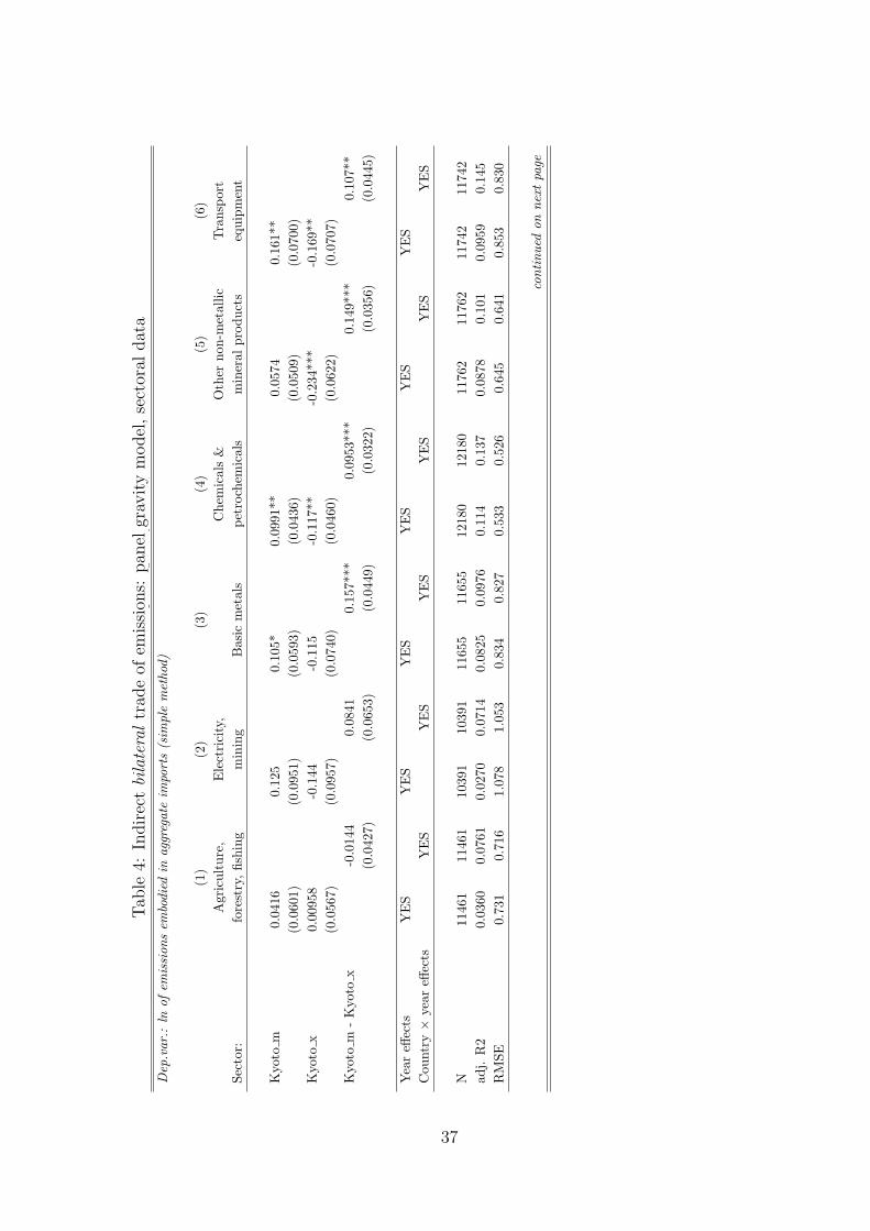
Tab
le4:
Indir
ect
bila
tera
ltr
ade
ofem
issi
ons:
pan
elgr
avit
ym
odel
,se
ctor
aldat
aT
able
1:In
dire
ctbi
late
ral
trad
eof
emis
sion
s:pa
nel
grav
ity
mod
el,
sect
oral
data
Dep
.var
.:ln
ofem
issi
ons
embo
died
inag
greg
ate
impo
rts
(sim
ple
met
hod)
(1)
(2)
(3)
(4)
(5)
(6)
Agr
icul
ture
,E
lect
rici
ty,
Che
mic
als
&O
ther
non-
met
allic
Tra
nspo
rtSe
ctor
:fo
rest
ry,
fishi
ngm
inin
gB
asic
met
als
petr
oche
mic
als
min
eral
prod
ucts
equi
pmen
t
Kyo
tom
0.04
160.
125
0.10
5*0.
0991
**0.
0574
0.16
1**
(0.0
601)
(0.0
951)
(0.0
593)
(0.0
436)
(0.0
509)
(0.0
700)
Kyo
tox
0.00
958
-0.1
44-0
.115
-0.1
17**
-0.2
34**
*-0
.169
**(0
.056
7)(0
.095
7)(0
.074
0)(0
.046
0)(0
.062
2)(0
.070
7)K
yoto
m-
Kyo
tox
-0.0
144
0.08
410.
157*
**0.
0953
***
0.14
9***
0.10
7**
(0.0
427)
(0.0
653)
(0.0
449)
(0.0
322)
(0.0
356)
(0.0
445)
Yea
reff
ects
YE
SY
ES
YE
SY
ES
YE
SY
ES
Cou
ntry×
year
effec
tsY
ES
YE
SY
ES
YE
SY
ES
YE
S
N11
461
1146
110
391
1039
111
655
1165
512
180
1218
011
762
1176
211
742
1174
2ad
j.R
20.
0360
0.07
610.
0270
0.07
140.
0825
0.09
760.
114
0.13
70.
0878
0.10
10.
0959
0.14
5R
MSE
0.73
10.
716
1.07
81.
053
0.83
40.
827
0.53
30.
526
0.64
50.
641
0.85
30.
830
cont
inue
don
next
page
137
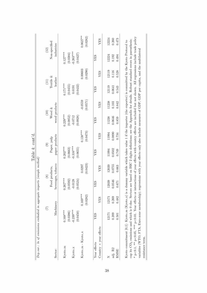
Tab
le4:
cont’
d.
Dep
.var
.:ln
ofem
issi
ons
embo
died
inag
greg
ate
impo
rts
(sim
ple
met
hod)
(7)
(8)
(9)
(10)
(11)
(12)
Food
prod
ucts
,P
aper
,pu
lpW
ood
&T
exti
le&
Non
-spe
cifie
dSe
ctor
:M
achi
nery
beve
rage
s,to
bacc
opa
per
prod
ucts
woo
dpr
oduc
tsle
athe
rin
dust
ries
Kyo
tom
0.16
8***
0.26
7***
0.20
2***
0.22
9***
0.17
1***
0.12
7***
(0.0
386)
(0.0
592)
(0.0
663)
(0.0
852)
(0.0
455)
(0.0
384)
Kyo
tox
-0.2
39**
*-0
.012
8-0
.316
***
-0.0
712
0.01
91-0
.263
***
(0.0
450)
(0.0
524)
(0.0
655)
(0.0
928)
(0.0
432)
(0.0
427)
Kyo
tom
-K
yoto
x0.
169*
**0.
0297
0.13
8***
-0.0
559
0.00
603
0.06
27**
(0.0
282)
(0.0
423)
(0.0
473)
(0.0
571)
(0.0
290)
(0.0
282)
Yea
reff
ects
YE
SY
ES
YE
SY
ES
YE
SY
ES
Cou
ntry×
year
effec
tsY
ES
YE
SY
ES
YE
SY
ES
YE
S
N12
171
1217
112
039
1203
911
994
1199
411
238
1123
812
119
1211
912
224
1222
4ad
j.R
20.
209
0.26
90.
0546
0.07
550.
0502
0.08
900.
0646
0.10
30.
0641
0.11
60.
192
0.26
0R
MSE
0.50
10.
482
0.67
10.
663
0.74
90.
734
0.85
90.
842
0.54
30.
528
0.49
40.
473
Kyo
toco
mm
itm
ent
[0,1
]:K
yoto
m(K
yoto
x)is
adu
mm
yva
riab
lew
hich
take
sva
lue
1if
the
impo
rter
(the
expo
rter
)is
com
mit
ted
byth
eK
yoto
Pro
toco
lto
cap
its
CO
2em
issi
ons
and
whi
chis
0el
se.
Sect
ors
are
base
don
ISIC
2di
gits
defin
itio
ns;
see
the
App
endi
xfo
rde
tails
.R
obus
tst
anda
rder
rors
inpa
rent
hesi
s;*
p<0.
1,**
p<0.
05,*
**p<
0.01
.Y
ear
effec
tsor
inte
ract
ions
ofye
areff
ects
wit
hco
untr
yeff
ects
are
incl
uded
but
not
show
n.A
llre
gres
sion
sin
clud
etr
ade
polic
yva
riab
les
(WT
O,
FT
A,
Eur
o-zo
nem
embe
rshi
p);
regr
essi
ons
wit
hye
areff
ects
only
also
incl
ude
mea
sure
sof
GD
P,G
DP
per
capi
ta,
and
the
mul
tila
tera
lre
sist
ance
term
.
138
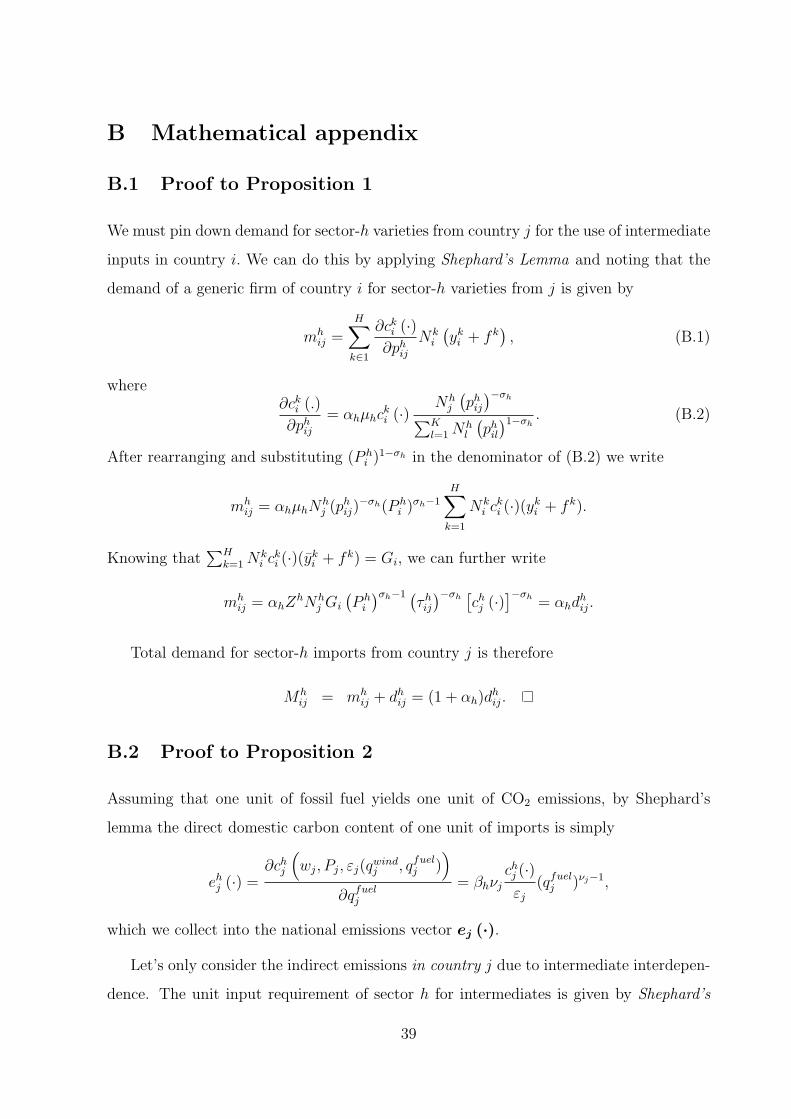
B Mathematical appendix
B.1 Proof to Proposition 1
We must pin down demand for sector-h varieties from country j for the use of intermediate
inputs in country i. We can do this by applying Shephard’s Lemma and noting that the
demand of a generic firm of country i for sector-h varieties from j is given by
mhij =
H∑k∈1
∂cki (·)∂phij
Nki
(yki + fk
), (B.1)
where∂cki (.)
∂phij= αhµhc
ki (·) Nh
j
(phij)−σh∑K
l=1Nhl
(phil)1−σh . (B.2)
After rearranging and substituting (P hi )1−σh in the denominator of (B.2) we write
mhij = αhµhN
hj (phij)
−σh(P hi )σh−1
H∑k=1
Nki c
ki (·)(yki + fk).
Knowing that∑H
k=1Nki c
ki (·)(yki + fk) = Gi, we can further write
mhij = αhZ
hNhj Gi
(P hi
)σh−1 (τhij)−σh [chj (·)
]−σh = αhdhij.
Total demand for sector-h imports from country j is therefore
Mhij = mh
ij + dhij = (1 + αh)dhij.
B.2 Proof to Proposition 2
Assuming that one unit of fossil fuel yields one unit of CO2 emissions, by Shephard’s
lemma the direct domestic carbon content of one unit of imports is simply
ehj (·) =∂chj
(wj, Pj, εj(q
windj , qfuelj )
)∂qfuelj
= βhνjchj (·)εj
(qfuelj )νj−1,
which we collect into the national emissions vector ej (·).
Let’s only consider the indirect emissions in country j due to intermediate interdepen-
dence. The unit input requirement of sector h for intermediates is given by Shephard’s
39
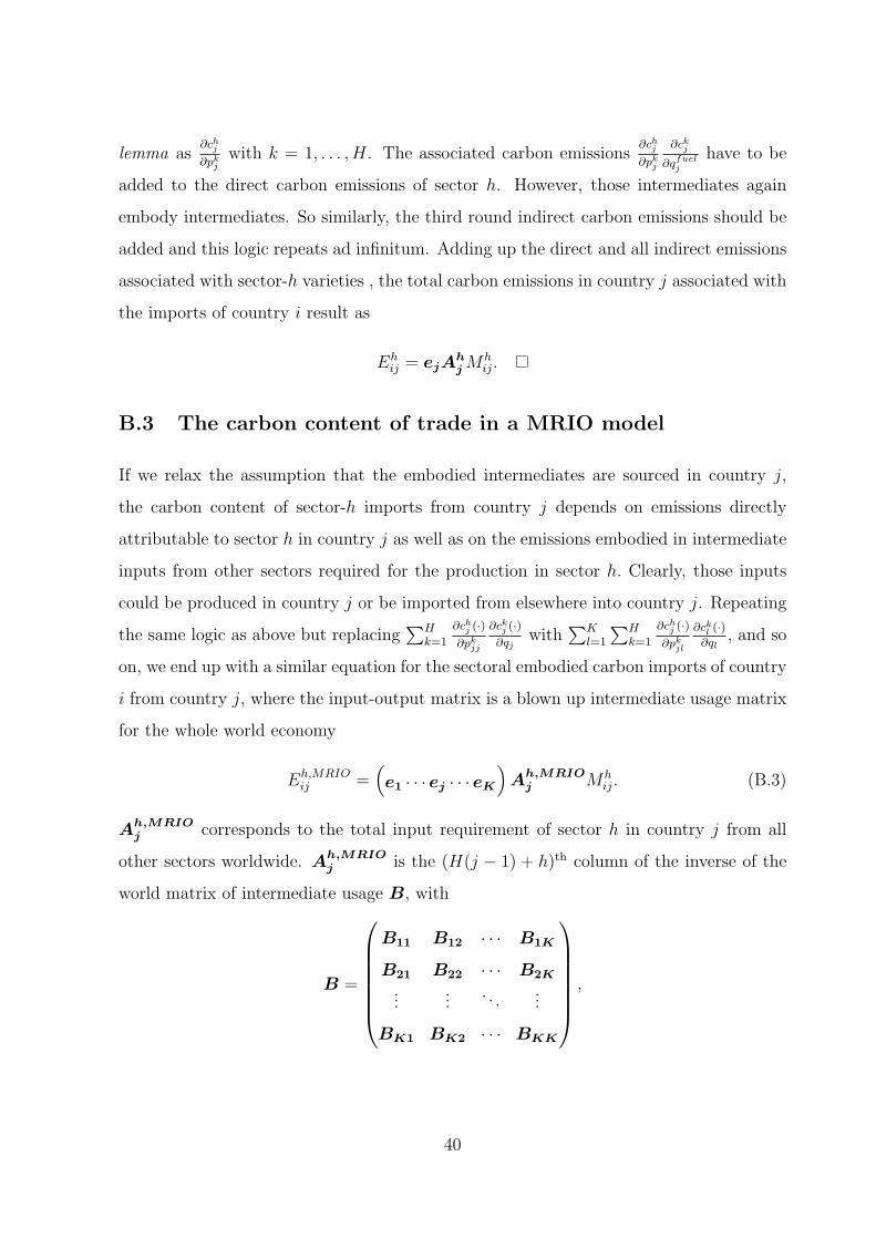
lemma as∂chj∂pkj
with k = 1, . . . , H. The associated carbon emissions∂chj∂pkj
∂ckj
∂qfuelj
have to be
added to the direct carbon emissions of sector h. However, those intermediates again
embody intermediates. So similarly, the third round indirect carbon emissions should be
added and this logic repeats ad infinitum. Adding up the direct and all indirect emissions
associated with sector-h varieties , the total carbon emissions in country j associated with
the imports of country i result as
Ehij = ejA
hjM
hij.
B.3 The carbon content of trade in a MRIO model
If we relax the assumption that the embodied intermediates are sourced in country j,
the carbon content of sector-h imports from country j depends on emissions directly
attributable to sector h in country j as well as on the emissions embodied in intermediate
inputs from other sectors required for the production in sector h. Clearly, those inputs
could be produced in country j or be imported from elsewhere into country j. Repeating
the same logic as above but replacing∑H
k=1
∂chj (·)∂pkjj
∂ckj (·)∂qj
with∑K
l=1
∑Hk=1
∂chj (·)∂pkjl
∂ckl (·)∂ql
, and so
on, we end up with a similar equation for the sectoral embodied carbon imports of country
i from country j, where the input-output matrix is a blown up intermediate usage matrix
for the whole world economy
Eh,MRIOij =
(e1 · · · ej · · · eK
)Ah,MRIO
j Mhij. (B.3)
Ah,MRIOj corresponds to the total input requirement of sector h in country j from all
other sectors worldwide. Ah,MRIOj is the (H(j − 1) + h)th column of the inverse of the
world matrix of intermediate usage B, with
B =
B11 B12 · · · B1K
B21 B22 · · · B2K
......
. . ....
BK1 BK2 · · · BKK
,
40
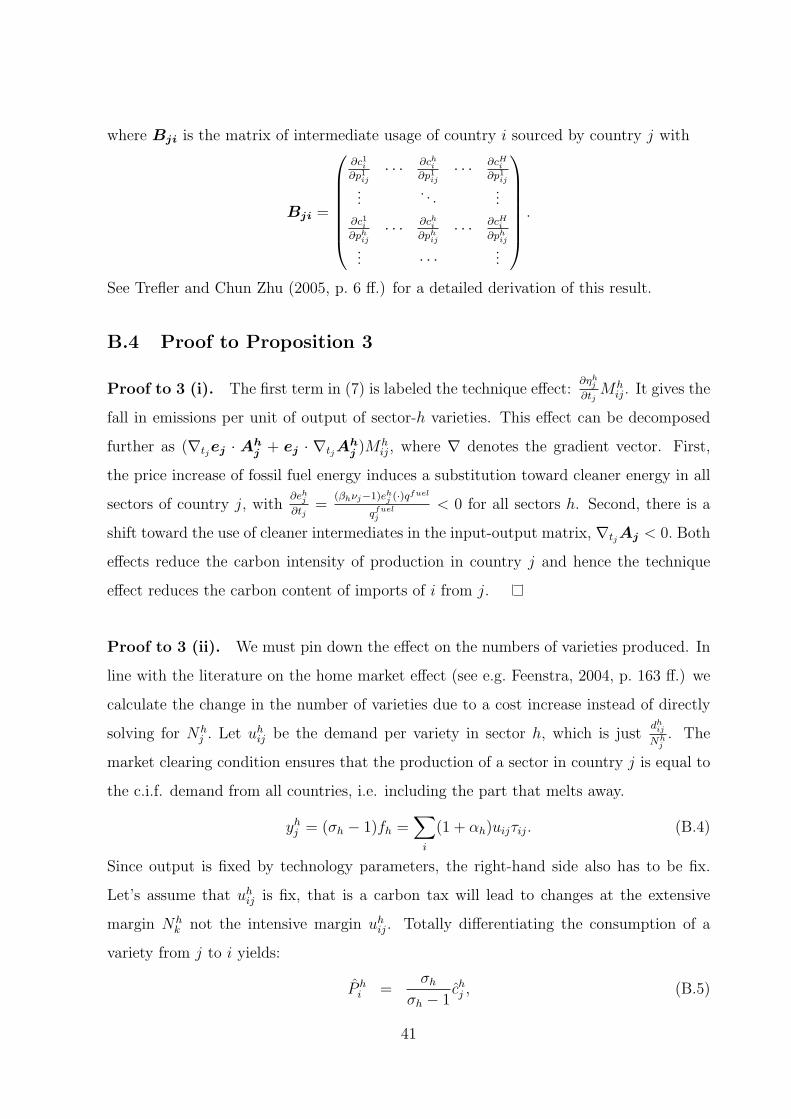
where Bji is the matrix of intermediate usage of country i sourced by country j with
Bji =
∂c1i∂p1ij· · · ∂chi
∂p1ij· · · ∂cHi
∂p1ij
.... . .
...
∂c1i∂phij
· · · ∂chi∂phij
· · · ∂cHi∂phij
... · · · ...
.
See Trefler and Chun Zhu (2005, p. 6 ff.) for a detailed derivation of this result.
B.4 Proof to Proposition 3
Proof to 3 (i). The first term in (7) is labeled the technique effect:∂ηhj∂tjMh
ij. It gives the
fall in emissions per unit of output of sector-h varieties. This effect can be decomposed
further as (∇tjej · Ahj + ej · ∇tjA
hj )Mh
ij, where ∇ denotes the gradient vector. First,
the price increase of fossil fuel energy induces a substitution toward cleaner energy in all
sectors of country j, with∂ehj∂tj
=(βhνj−1)ehj (·)qfuel
qfuelj
< 0 for all sectors h. Second, there is a
shift toward the use of cleaner intermediates in the input-output matrix, ∇tjAj < 0. Both
effects reduce the carbon intensity of production in country j and hence the technique
effect reduces the carbon content of imports of i from j.
Proof to 3 (ii). We must pin down the effect on the numbers of varieties produced. In
line with the literature on the home market effect (see e.g. Feenstra, 2004, p. 163 ff.) we
calculate the change in the number of varieties due to a cost increase instead of directly
solving for Nhj . Let uhij be the demand per variety in sector h, which is just
dhijNhj
. The
market clearing condition ensures that the production of a sector in country j is equal to
the c.i.f. demand from all countries, i.e. including the part that melts away.
yhj = (σh − 1)fh =∑i
(1 + αh)uijτij. (B.4)
Since output is fixed by technology parameters, the right-hand side also has to be fix.
Let’s assume that uhij is fix, that is a carbon tax will lead to changes at the extensive
margin Nhk not the intensive margin uhij. Totally differentiating the consumption of a
variety from j to i yields:
P hi =
σhσh − 1
chj , (B.5)
41
where z = dzz
denotes the growth rate of a variable z. The change in the price index is
proportional to the increase in costs in a country if the assumption of fixed consumption
per variety holds.
Next we check whether there is a change in the number of varieties produced that is
consistent with this change in the price index. Totally differentiate the price index to
obtain
P hi =
1
1− σh∑k
φhikNhk +
∑k
φhikchj , (B.6)
where φhik = (phikPhi
)1−σhNhk denotes the share of country k products in sector h of country i
and these shares add up to one. Plug in (B.5) into (B.6) to obtain∑k
φhikNhk = (σh − 1)
∑k
φhikchj − σhchj . (B.7)
This gives a system of K equations that can be expressed in matrix notation as
Φh
Nh1
...
Nhj
...
NhK
= (σh − 1)Φh
ch1...
chj...
chK
− σh
0...
chj...
0
(B.8)
where Φh is a K × K matrix that collects all φhik. Φh is for example invertible when
φhii > φhik for i 6= k, i.e. a country devotes more of its budget to own varieties (Feenstra,
2004, p. 164). Then
Nh1
...
Nhj
...
NhK
= (σh − 1)
ch1...
chj...
chK
− σh Φh−1
0...
chj...
0
(B.9)
constitutes a solution to the equation system. Put differently an increase in costs indeed
induces changes at the extensive not the intensive margin. A cost increase (for example
due to a higher carbon tax) will lead to a relocation of firms.
42
Proof to 3 (iii). The second term in (7) is the scale or pollution haven effect: ηhj∂Mh
ij
∂tj.
It shows how the h-sector exports of country j react to a stricter climate policy. More
specifically∂Mh
ij
∂tj= −σh
∂chj (·)∂tj
Mhij
chj (·)+Mh
ij
Nhj
∂Nhj
∂tj,+(σh − 1)
Mhij
P hi
∂P hi
∂tj. (B.10)
This can be simplified further. We can express (B.5) alternatively with partial derivatives
with respect to tj as
∂P hi
∂tj=
σhσh − 1
P hi
chj
∂chj∂tj
(B.11)
Thus, the change in the price index and the costs in (B.10) cancel each other out. This
leaves∂Mh
ij
∂tj=Mh
ij
Nhj
∂Nhj
∂tj.
Only the change in the location of firms – the extensive margin – matters for the carbon
content of trade. Next, we have to determine the sign of∂Nh
j
∂tj.
Let φhik−1
denote the entries of the inverse of Φh. This gives the total weight of
country-k varieties in consumption of country i after considering all input-output relations.
Then we can write (B.9) as
Nhj = (σh − 1− σh φhjj
−1)chj , (B.12)
Nhi = (σh − 1)chi − σh φhij
−1chj ∀ i 6= j. (B.13)
A carbon tax leads to a cost increase in country j, chj > 0. If φhjj−1
> σh−1σh
, this
implies a decrease in the number of varieties country j produces, i.e. Nhj < 0. Country j
loses competitiveness in sector h. Put differently there is a pollution haven effect, because
stricter environmental regulation in a country causes its exports to fall. The change in
the numbers of varieties Nhi other countries i produce will be positive if the cost-weighted
fraction of country-j varieties in consumptionchjchiφhij−1< σh−1
σh.
The intuition of this finding is straightforward. The unilateral climate policy puts
country j to a comparative disadvantage in the energy-intensive differentiated goods sector
compared to the labor-intensive numeraire sector. Thus other countries will produce
more of the differentiated goods and export them while country j produces more of the
43
homogeneous numeraire good. This sectoral scale effect feeds through to less carbon
imports in country i from country j in all sectors h.
Proof to 3 (iv). The dislocation of firms is governed by cost increases, which are given
by∂chj (.)
∂tj= ehj q
fuel = βhνjchj (·)εj
(qfuelj )νj−1qfuel. (B.14)
The cost increase will be highest for dirty sectors, i.e. sectors with a high βh. In other
words, the loss in competitiveness is highest for carbon-intensive sectors. This means there
is a negative correlation between sectoral emission intensity and the change in sectoral
imports due to a carbon tax increase. That said, on the aggregate bilateral level, there
will be a change in the composition of Mij toward cleaner sectors beside the fall in trade
volume when the exporter j imposes a stricter climate policy.
Proof to 3 (v). The carbon intensity of country i’s sectoral imports from j is given byEhijMhij
= ηhj . As shown in the proof to proposition 3 (i) the sectoral emission coefficient falls
with a rising carbon tax in the very country.
The carbon intensity of country i’s bilateral imports is given by ηj =EijMij
=∑h E
hij∑
hMhij.
∂(EijMij
)
∂tj=
Mij
∑h(
∂ηhj∂tjMh
ij + ηhj∂Mh
ij
∂tj)− Eij
∑h
∂Mhij
∂tj
(Mij)2
=
∑h TE
hj +
∑h(η
hj − ηj)
∂Mhij
∂tj
Mij
=
∑h TE
hj +
∑h(η
hj − ηj)(
∂Mhij
∂tj− ¯∂Mij
∂tj) +
¯∂Mij
∂tj
∑h(η
hj − ηj)
Mij
=
∑h TE
hj +
∑h(η
hj − ηj)(
∂Mhij
∂tj− ¯∂Mij
∂tj)
Mij
< 0 (B.15)
where TEhj =
∂ηhj∂tjMh
ij is the sectoral technique effect in country j,¯∂Mhij
∂tjis the average
change of sectoral imports due to the tax increase and∑
h(ηhj − ηj) =
∑h η
hj − hηj = 0.
The technique effect is negative for every sector which implies that the aggregate technique
effect, the first term in the denominator of (B.15), is also negative. The composition effect
states that the sectoral emission coefficient and the change in the sectoral imports due to a
44
carbon tax are negatively correlated. Therefore also the second term in the denominator
of (B.15) is negative. Taken together, a tax increase reduces the carbon intensity of
bilateral imports.
B.5 Proof to Proposition 4
The proofs are analogous to the one of Proposition 3.
Proof to 4 (i). The effect of a subsidy of alternative energies in exporting country j
can be decomposed as in (7).
∂Ehij
∂sj=∂ηhj∂sj
Mhij + ηhj
∂Mhij
∂sj. (B.16)
The subsidy has similar effects on the emission of one unit of sector-h variety as a carbon
tax due to a substitution toward wind energy:∂ehj∂sj
< 0 in all sectors h. Put differently,
the subsidy causes a negative technique effect:∂ηhj∂sjMh
ij < 0.
However, it lowers the costs of sectors h in country j
∂chj (·)∂sj
= −βh(1− νj)rchj (·)
εj(qwindj )vj< 0. (B.17)
Hence, the subsidy leads to an increase in the number of varieties country j exports to
i (see the proof to Proposition 3). This constitutes a positive scale effect: ηhj∂Mh
ij
∂sj> 0,
where we use the finding of Proposition 3 (ii). The composition changes in favor of dirty
industries because they profit most from a decrease in overall energy costs governed by
βh. Taken together the sign of∂Eij∂sj
is unclear.
Proof to 4 (ii). The effect of a subsidy of alternative energies in the importing country
i is∂Eh
ij
∂si= ηhj
∂Mhij
∂si= ηhj
Mhij
Nhj
∂Nhj
∂si< 0, (B.18)
where we use the fact that the subsidy only induces changes at the extensive margin (see
proof to Proposition 3). The subsidy in the importing country i will reduce the number of
varieties imported from its trade partners due to the gains in competitiveness in country
45
i (see the proof to Proposition 3). Since the benefits are highest in the most energy-
intensive domestic sectors the composition of bilateral carbon imports from country j
will become cleaner. Summing up, when a country grants a subsidy to clean energies its
bilateral carbon imports decline unambiguously.
Proof to 4 (iii). The effect of a subsidy to alternative energy in country j on its own
fuel demand and hence its carbon dioxide emissions is unclear, since emission intensity
falls but the number of varieties produced increases in all sectors:
∂Dfuelj
∂sj=
H∑h=1
<0︷︸︸︷∂ehj∂sj
(yhj + fh
)Nhj +
H∑h=1
ehj (·)(yhj + fh
) >0︷ ︸︸ ︷∂Nh
j
∂sj=?. (B.19)
The effect of this climate policy change on carbon dioxide emissions in a trade partner i
is unambiguously negative:
∂Dfueli
∂sj=
H∑h=1
ehi (·)(yhi + fh
) ∂Nhi
∂sj< 0. (B.20)
Hence, the promotion of alternative energies does not lead to a pattern of carbon leakage:
the emissions of the subsidizing country might rise or fall depending on which channel
outweighs while the emissions in other countries fall unambiguously.
46
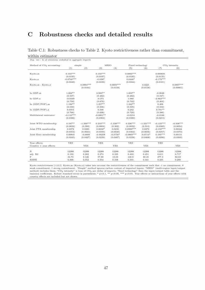
C Robustness checks and detailed results
Table C.1: Robustness checks to Table 2. Kyoto restrictiveness rather than commitment,
within estimatorDep. var.: ln of emissions embodied in aggregate imports
Method of CO2 accounting: simple MRIO Fixed technology CO2 intensity
(1) (2) (3) (4) (5) (6) (7) (8)
Kyoto m 0.103*** 0.102*** 0.0895*** 0.000691
(0.0195) (0.0187) (0.0185) (0.0135)
Kyoto x -0.0740*** -0.0367 0.0446* -0.178***
(0.0249) (0.0239) (0.0244) (0.0161)
Kyoto m - Kyoto x 0.0884*** 0.0693*** 0.0221 0.0897***
(0.0164) (0.0158) (0.0158) (0.00861)
ln GDP m 1.062** 0.983** 1.003** -0.0646
(0.507) (0.482) (0.482) (0.347)
ln GDP x -0.0349 -0.271 1.080 -2.862***
(0.750) (0.676) (0.702) (0.404)
ln (GDP/POP) m 1.196** 1.257** 1.242** 0.406
(0.530) (0.506) (0.505) (0.332)
ln (GDP/POP) x 0.0354 0.348 0.242 0.781**
(0.766) (0.698) (0.720) (0.386)
Multilateral resistance -0.110*** -0.0801** -0.0314 -0.0166
(0.0386) (0.0364) (0.0380) (0.0215)
Joint WTO membership 0.197** -1.399*** 0.210*** -1.338*** 0.226*** -1.321*** -0.122*** -0.508***
(0.0834) (0.393) (0.0804) (0.362) (0.0832) (0.314) (0.0360) (0.0634)
Joint FTA membership 0.0372 0.0285 0.0630* 0.0235 0.0989*** 0.0272 -0.150*** 0.00344
(0.0354) (0.0663) (0.0350) (0.0640) (0.0362) (0.0656) (0.0257) (0.0373)
Joint Euro membership 0.00845 -0.0668 -0.00258 -0.0756* -0.0869*** -0.0714* 0.195*** 0.00151
(0.0245) (0.0427) (0.0239) (0.0407) (0.0238) (0.0408) (0.0206) (0.0303)
Year effects YES YES YES YES
Country × year effects YES YES YES YES
N 12288 12288 12288 12288 12288 12288 12288 12288
adj. R2 0.192 0.262 0.274 0.335 0.402 0.451 0.611 0.717
F 34.73 9.126 57.89 13.03 140.8 30.45 277.3 82.63
RMSE 0.368 0.352 0.354 0.338 0.355 0.341 0.235 0.200
Kyoto restrictiveness [-1,0,1]: Kyoto m (Kyoto x) takes into account the restrictiveness of the commitment such that -1 no commitment, 0
weak commitment, 1 strong commitment. “Simple” method ignores carbon content of imported inputs; “MRIO” (multi-region input/output
method) includes them; “CO2 intensity” is tons of CO2 per dollar of imports; “fixed technology” fixes the input/output table and the
emission coefficients. Robust standard errors in parenthesis; * p<0.1, ** p<0.05, *** p<0.01. Year effects or interactions of year effects with
country effects are included but not shown.
47
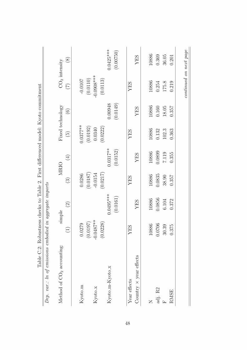
Tab
leC
.2:
Rob
ust
nes
sch
ecks
toT
able
2.F
irst
diff
eren
ced
model
:K
yoto
com
mit
men
t
Dep
.va
r.:
lnof
emis
sion
sem
bodi
edin
aggr
egat
eim
port
s
Met
hod
ofC
O2
acco
unti
ng:
sim
ple
MR
IOF
ixed
tech
nol
ogy
CO
2in
tensi
ty
(1)
(2)
(3)
(4)
(5)
(6)
(7)
(8)
Kyo
tom
0.02
790.
0286
0.03
77**
-0.0
107
(0.0
197)
(0.0
187)
(0.0
192)
(0.0
110)
Kyo
tox
-0.0
487*
*-0
.015
40.
0340
-0.0
908*
**
(0.0
228)
(0.0
217)
(0.0
222)
(0.0
113)
Kyo
tom
-Kyo
tox
0.04
95**
*0.
0317
**0.
0094
80.
0425
***
(0.0
161)
(0.0
152)
(0.0
149)
(0.0
0750
)
Yea
reff
ects
YE
SY
ES
YE
SY
ES
Cou
ntr
y×
year
effec
tsY
ES
YE
SY
ES
YE
S
N10
886
1088
610
886
1088
610
886
1088
610
886
1088
6
adj.
R2
0.07
060.
0856
0.08
350.
0899
0.13
20.
160
0.25
40.
369
F30
.39
6.10
438
.90
7.11
910
2.3
18.0
517
5.8
36.0
5
RM
SE
0.37
50.
372
0.35
70.
355
0.36
30.
357
0.21
90.
201
con
tin
ued
onn
ext
page
48
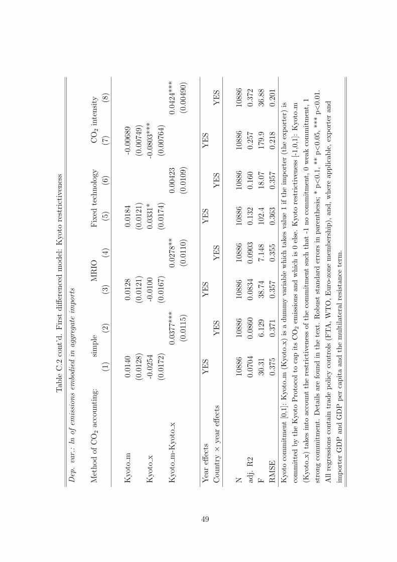
Tab
leC
.2co
nt’
d.
Fir
stdiff
eren
ced
model
:K
yoto
rest
rict
iven
ess
Dep
.va
r.:
lnof
emis
sion
sem
bodi
edin
aggr
egat
eim
port
s
Met
hod
ofC
O2
acco
unti
ng:
sim
ple
MR
IOF
ixed
tech
nol
ogy
CO
2in
tensi
ty
(1)
(2)
(3)
(4)
(5)
(6)
(7)
(8)
Kyo
tom
0.01
400.
0128
0.01
84-0
.006
89
(0.0
128)
(0.0
121)
(0.0
121)
(0.0
0749
)
Kyo
tox
-0.0
254
-0.0
100
0.03
31*
-0.0
803*
**
(0.0
172)
(0.0
167)
(0.0
174)
(0.0
0764
)
Kyo
tom
-Kyo
tox
0.03
77**
*0.
0278
**0.
0042
30.
0424
***
(0.0
115)
(0.0
110)
(0.0
109)
(0.0
0490
)
Yea
reff
ects
YE
SY
ES
YE
SY
ES
Cou
ntr
y×
year
effec
tsY
ES
YE
SY
ES
YE
S
N10
886
1088
610
886
1088
610
886
1088
610
886
1088
6
adj.
R2
0.07
040.
0860
0.08
340.
0903
0.13
20.
160
0.25
70.
372
F30
.31
6.12
938
.74
7.14
810
2.4
18.0
717
9.9
36.8
8
RM
SE
0.37
50.
371
0.35
70.
355
0.36
30.
357
0.21
80.
201
Kyo
toco
mm
itm
ent
[0,1
]:K
yoto
m(K
yoto
x)is
adu
mm
yva
riab
lew
hich
take
sva
lue
1if
the
impo
rter
(the
expo
rter
)is
com
mit
ted
byth
eK
yoto
Pro
toco
lto
cap
its
CO
2em
issi
ons
and
whi
chis
0el
se.
Kyo
tore
stri
ctiv
enes
s[-
1,0,
1]:
Kyo
tom
(Kyo
tox)
take
sin
toac
coun
tth
ere
stri
ctiv
enes
sof
the
com
mit
men
tsu
chth
at-1
noco
mm
itm
ent,
0w
eak
com
mit
men
t,1
stro
ngco
mm
itm
ent.
Det
ails
are
foun
din
the
text
.R
obus
tst
anda
rder
rors
inpa
rent
hesi
s;*
p<0.
1,**
p<0.
05,
***
p<0.
01.
All
regr
essi
ons
cont
ain
trad
epo
licy
cont
rols
(FT
A,
WT
O,
Eur
o-zo
nem
embe
rshi
p),
and,
whe
reap
plic
able
,ex
port
eran
dim
port
erG
DP
and
GD
Ppe
rca
pita
and
the
mul
tila
tera
lre
sist
ance
term
.
49
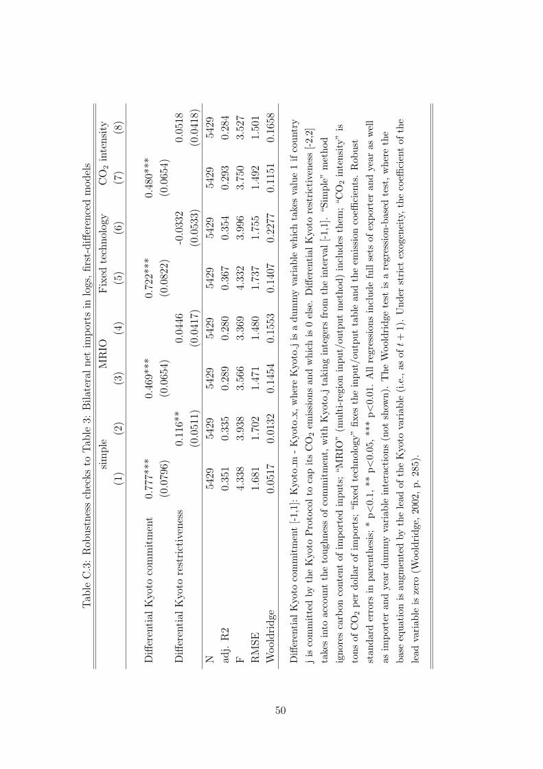
Tab
leC
.3:
Rob
ust
nes
sch
ecks
toT
able
3:B
ilat
eral
net
imp
orts
inlo
gs,
firs
t-diff
eren
ced
model
s
sim
ple
MR
IOF
ixed
tech
nol
ogy
CO
2in
tensi
ty
(1)
(2)
(3)
(4)
(5)
(6)
(7)
(8)
Diff
eren
tial
Kyo
toco
mm
itm
ent
0.77
7***
0.46
9***
0.72
2***
0.48
0***
(0.0
796)
(0.0
654)
(0.0
822)
(0.0
654)
Diff
eren
tial
Kyo
tore
stri
ctiv
enes
s0.
116*
*0.
0446
-0.0
332
0.05
18
(0.0
511)
(0.0
417)
(0.0
533)
(0.0
418)
N54
2954
2954
2954
2954
2954
2954
2954
29
adj.
R2
0.35
10.
335
0.28
90.
280
0.36
70.
354
0.29
30.
284
F4.
338
3.93
83.
566
3.36
94.
332
3.99
63.
750
3.52
7
RM
SE
1.68
11.
702
1.47
11.
480
1.73
71.
755
1.49
21.
501
Wool
dri
dge
0.05
170.
0132
0.14
540.
1553
0.14
070.
2277
0.11
510.
1658
Diff
eren
tial
Kyo
toco
mm
itm
ent
[-1,
1]:
Kyo
tom
-K
yoto
x,w
here
Kyo
toj
isa
dum
my
vari
able
whi
chta
kes
valu
e1
ifco
untr
yj
isco
mm
itte
dby
the
Kyo
toP
roto
col
toca
pit
sC
O2
emis
sion
san
dw
hich
is0
else
.D
iffer
enti
alK
yoto
rest
rict
iven
ess
[-2,
2]ta
kes
into
acco
unt
the
toug
hnes
sof
com
mit
men
t,w
ith
Kyo
toj
taki
ngin
tege
rsfr
omth
ein
terv
al[-
1,1]
.“S
impl
e”m
etho
dig
nore
sca
rbon
cont
ent
ofim
port
edin
puts
;“M
RIO
”(m
ulti
-reg
ion
inpu
t/ou
tput
met
hod)
incl
udes
them
;“C
O2
inte
nsit
y”is
tons
ofC
O2
per
dolla
rof
impo
rts;
“fixe
dte
chno
logy
”fix
esth
ein
put/
outp
utta
ble
and
the
emis
sion
coeffi
cien
ts.
Rob
ust
stan
dard
erro
rsin
pare
nthe
sis;
*p<
0.1,
**p<
0.05
,**
*p<
0.01
.A
llre
gres
sion
sin
clud
efu
llse
tsof
expo
rter
and
year
asw
ell
asim
port
eran
dye
ardu
mm
yva
riab
lein
tera
ctio
ns(n
otsh
own)
.T
heW
oold
ridg
ete
stis
are
gres
sion
-bas
edte
st,
whe
reth
eba
seeq
uati
onis
augm
ente
dby
the
lead
ofth
eK
yoto
vari
able
(i.e
.,as
oft
+1)
.U
nder
stri
ctex
ogen
eity
,the
coeffi
cien
tof
the
lead
vari
able
isze
ro(W
oold
ridg
e,20
02,
p.28
5).
50
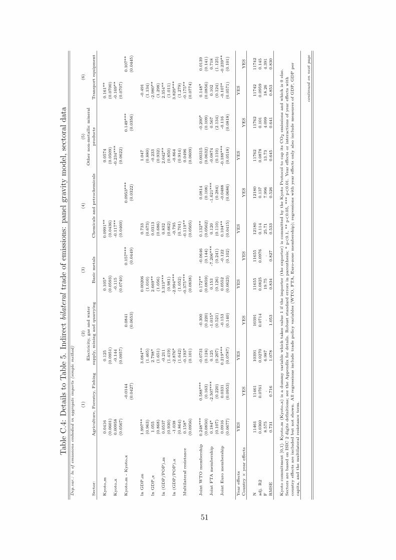
Tab
leC
.4:
Det
ails
toT
able
5.In
dir
ect
bila
tera
ltr
ade
ofem
issi
ons:
pan
elgr
avit
ym
odel
,se
ctor
aldat
aD
ep.v
ar.:
lnofem
issi
ons
em
bodie
din
aggre
gate
imports
(sim
ple
meth
od)
(1)
(2)
(3)
(4)
(5)
(6)
Ele
ctr
icit
y,
gas
and
wate
rO
ther
non-m
eta
llic
min
era
l
Secto
r:A
gri
cult
ure
,Fore
stry
,F
ishin
gsu
pply
,m
inin
gand
quarr
yin
gB
asi
cm
eta
lsC
hem
icals
and
petr
ochem
icals
pro
ducts
Tra
nsp
ort
equip
ment
Kyoto
m0.0
416
0.1
25
0.1
05*
0.0
991**
0.0
574
0.1
61**
(0.0
601)
(0.0
951)
(0.0
593)
(0.0
436)
(0.0
509)
(0.0
700)
Kyoto
x0.0
0958
-0.1
44
-0.1
15
-0.1
17**
-0.2
34***
-0.1
69**
(0.0
567)
(0.0
957)
(0.0
740)
(0.0
460)
(0.0
622)
(0.0
707)
Kyoto
m-
Kyoto
x-0
.0144
0.0
841
0.1
57***
0.0
953***
0.1
49***
0.1
07**
(0.0
427)
(0.0
653)
(0.0
449)
(0.0
322)
(0.0
356)
(0.0
445)
lnG
DP
m1.9
97**
3.0
84**
0.0
0206
0.7
33
1.0
47
-0.4
91
(0.9
63)
(1.4
65)
(1.0
10)
(0.6
73)
(0.8
80)
(1.1
34)
lnG
DP
x1.0
55
2.7
98*
2.6
69**
0.0
313
-0.2
33
-2.9
80**
(0.8
68)
(1.6
51)
(1.0
56)
(0.6
86)
(0.9
32)
(1.2
98)
ln(G
DP
/P
OP
)m
0.0
537
-0.2
11
3.3
13***
0.8
32
2.0
42**
2.3
54**
(0.9
30)
(1.4
19)
(0.9
81)
(0.6
62)
(0.8
50)
(1.0
11)
ln(G
DP
/P
OP
)x
-1.0
38
-2.8
76*
-2.9
94***
-0.7
95
-0.8
64
3.8
29***
(0.8
64)
(1.6
42)
(1.0
52)
(0.7
01)
(0.9
14)
(1.2
79)
Mult
ilate
ral
resi
stance
0.1
58*
-0.1
93*
-0.3
75***
-0.1
19**
0.0
496
-0.1
75**
(0.0
956)
(0.1
01)
(0.0
838)
(0.0
505)
(0.0
609)
(0.0
774)
Join
tW
TO
mem
bers
hip
0.2
48***
0.5
88***
-0.0
731
-0.3
00
0.1
72**
-0.0
646
0.1
32**
0.0
814
0.0
0315
-0.2
00*
0.1
48*
0.0
139
(0.0
850)
(0.1
63)
(0.1
24)
(0.2
20)
(0.0
859)
(0.1
44)
(0.0
562)
(0.1
08)
(0.0
632)
(0.1
09)
(0.0
856)
(0.1
41)
Join
tF
TA
mem
bers
hip
0.1
84*
-2.5
07***
0.1
25
-1.0
15*
0.1
53
-7.2
06***
0.1
20
-1.6
21***
-0.0
874
0.5
67
0.1
02
0.7
18
(0.1
07)
(0.2
20)
(0.2
07)
(0.5
21)
(0.1
26)
(0.2
41)
(0.1
10)
(0.2
84)
(0.1
10)
(2.1
34)
(0.1
24)
(1.1
25)
Join
tE
uro
mem
bers
hip
0.0
916
0.0
331
0.2
19***
-0.1
53
0.0
552
-0.1
22
0.1
04**
-0.0
488
-0.1
88***
-0.1
16
-0.1
07*
-0.2
39**
(0.0
677)
(0.0
953)
(0.0
787)
(0.1
40)
(0.0
623)
(0.1
02)
(0.0
415)
(0.0
686)
(0.0
518)
(0.0
818)
(0.0
571)
(0.1
01)
Year
eff
ects
YE
SY
ES
YE
SY
ES
YE
SY
ES
Countr
y×
year
eff
ects
YE
SY
ES
YE
SY
ES
YE
SY
ES
N11461
11461
10391
10391
11655
11655
12180
12180
11762
11762
11742
11742
adj.
R2
0.0
360
0.0
761
0.0
270
0.0
714
0.0
825
0.0
976
0.1
14
0.1
37
0.0
878
0.1
01
0.0
959
0.1
45
F8.5
75
.6.9
87
.19.7
5.
25.7
17.9
96
13.7
34.0
99
18.2
64.3
91
RM
SE
0.7
31
0.7
16
1.0
78
1.0
53
0.8
34
0.8
27
0.5
33
0.5
26
0.6
45
0.6
41
0.8
53
0.8
30
Kyoto
com
mit
ment
[0,1
]:K
yoto
m(K
yoto
x)
isa
dum
my
vari
able
whic
hta
kes
valu
e1
ifth
eim
port
er
(the
exp
ort
er)
iscom
mit
ted
by
the
Kyoto
Pro
tocol
tocap
its
CO
2em
issi
ons
and
whic
his
0els
e.
Secto
rsare
base
don
ISIC
2dig
its
defi
nit
ions;
see
the
App
endix
for
deta
ils.
Robust
standard
err
ors
inpare
nth
esi
s;*
p<
0.1
,**
p<
0.0
5,
***
p<
0.0
1.
Year
eff
ects
or
inte
racti
ons
of
year
eff
ects
wit
h
countr
yeff
ects
are
inclu
ded
but
not
show
n.
All
regre
ssio
ns
inclu
de
trade
poli
cy
vari
able
s(W
TO
,F
TA
,E
uro
-zone
mem
bers
hip
);re
gre
ssio
ns
wit
hyear
eff
ects
only
als
oin
clu
de
measu
res
of
GD
P,
GD
Pp
er
capit
a,
and
the
mult
ilate
ral
resi
stance
term
.
continued
on
nextpage
51
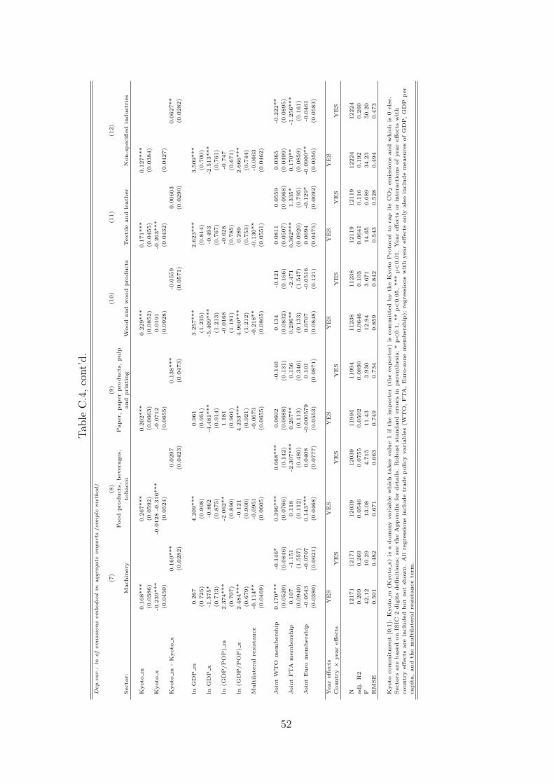
Tab
leC
.4,
cont’
d.
Dep.v
ar.:
lnofem
issi
ons
em
bodie
din
aggre
gate
imports
(sim
ple
meth
od)
(7)
(8)
(9)
(10)
(11)
(12)
Food
pro
ducts
,b
evera
ges,
Pap
er,
pap
er
pro
ducts
,pulp
Secto
r:M
achin
ery
tobacco
and
pri
nti
ng
Wood
and
wood
pro
ducts
Texti
leand
leath
er
Non-s
pecifi
ed
indust
ries
Kyoto
m0.1
68***
0.2
67***
0.2
02***
0.2
29***
0.1
71***
0.1
27***
(0.0
386)
(0.0
592)
(0.0
663)
(0.0
852)
(0.0
455)
(0.0
384)
Kyoto
x-0
.239***
-0.0
128
-0.3
16***
-0.0
712
0.0
191
-0.2
63***
(0.0
450)
(0.0
524)
(0.0
655)
(0.0
928)
(0.0
432)
(0.0
427)
Kyoto
m-
Kyoto
x0.1
69***
0.0
297
0.1
38***
-0.0
559
0.0
0603
0.0
627**
(0.0
282)
(0.0
423)
(0.0
473)
(0.0
571)
(0.0
290)
(0.0
282)
lnG
DP
m0.2
67
4.2
09***
0.9
61
3.2
57***
2.6
23***
3.5
09***
(0.7
25)
(0.9
08)
(0.9
51)
(1.2
35)
(0.8
14)
(0.7
00)
lnG
DP
x-1
.375*
-0.8
62
-4.4
81***
-5.4
09***
-0.4
93
-2.5
13***
(0.7
13)
(0.8
75)
(0.9
14)
(1.2
13)
(0.7
67)
(0.7
61)
ln(G
DP
/P
OP
)m
2.3
74***
-2.0
62**
1.1
81
-0.0
168
-0.6
28
-0.7
47
(0.7
07)
(0.8
90)
(0.9
01)
(1.1
81)
(0.7
85)
(0.6
71)
ln(G
DP
/P
OP
)x
2.4
84***
-0.1
21
4.2
33***
4.9
60***
0.2
89
2.6
66***
(0.6
79)
(0.9
00)
(0.9
21)
(1.2
12)
(0.7
53)
(0.7
44)
Mult
ilate
ral
resi
stance
-0.1
14**
-0.0
951
-0.0
673
-0.2
18**
-0.1
30**
-0.0
663
(0.0
469)
(0.0
605)
(0.0
655)
(0.0
865)
(0.0
551)
(0.0
462)
Join
tW
TO
mem
bers
hip
0.1
70***
-0.1
46*
0.3
96***
0.6
68***
0.0
602
-0.1
40
0.1
34
-0.1
21
0.0
811
0.0
559
0.0
365
-0.2
22**
(0.0
520)
(0.0
846)
(0.0
766)
(0.1
42)
(0.0
688)
(0.1
31)
(0.0
832)
(0.1
66)
(0.0
507)
(0.0
968)
(0.0
499)
(0.0
895)
Join
tF
TA
mem
bers
hip
0.1
07
-1.1
51
0.1
18
-2.3
07***
0.2
67**
0.1
56
0.2
96**
-2.4
71
0.3
62***
1.3
35*
0.1
70**
-1.2
56***
(0.0
940)
(1.5
57)
(0.1
12)
(0.4
80)
(0.1
13)
(0.3
46)
(0.1
33)
(1.5
47)
(0.0
920)
(0.7
95)
(0.0
859)
(0.1
61)
Join
tE
uro
mem
bers
hip
-0.0
543
-0.0
707
0.1
43***
0.0
408
-0.0
00579
0.1
01
0.0
707
-0.0
516
0.0
694
-0.1
29*
-0.0
900**
-0.0
461
(0.0
380)
(0.0
621)
(0.0
468)
(0.0
777)
(0.0
553)
(0.0
871)
(0.0
848)
(0.1
21)
(0.0
475)
(0.0
692)
(0.0
356)
(0.0
583)
Year
eff
ects
YE
SY
ES
YE
SY
ES
YE
SY
ES
Countr
y×
year
eff
ects
YE
SY
ES
YE
SY
ES
YE
SY
ES
N12171
12171
12039
12039
11994
11994
11238
11238
12119
12119
12224
12224
adj.
R2
0.2
09
0.2
69
0.0
546
0.0
755
0.0
502
0.0
890
0.0
646
0.1
03
0.0
641
0.1
16
0.1
92
0.2
60
F42.1
210.2
913.0
84.7
15
11.4
33.9
30
12.9
43.6
71
14.6
56.6
89
34.2
350.2
0
RM
SE
0.5
01
0.4
82
0.6
71
0.6
63
0.7
49
0.7
34
0.8
59
0.8
42
0.5
43
0.5
28
0.4
94
0.4
73
Kyoto
com
mit
ment
[0,1
]:K
yoto
m(K
yoto
x)
isa
dum
my
vari
able
whic
hta
kes
valu
e1
ifth
eim
port
er
(the
exp
ort
er)
iscom
mit
ted
by
the
Kyoto
Pro
tocol
tocap
its
CO
2em
issi
ons
and
whic
his
0els
e.
Secto
rsare
base
don
ISIC
2dig
its
defi
nit
ions;
see
the
App
endix
for
deta
ils.
Robust
standard
err
ors
inpare
nth
esi
s;*
p<
0.1
,**
p<
0.0
5,
***
p<
0.0
1.
Year
eff
ects
or
inte
racti
ons
of
year
eff
ects
wit
h
countr
yeff
ects
are
inclu
ded
but
not
show
n.
All
regre
ssio
ns
inclu
de
trade
poli
cy
vari
able
s(W
TO
,F
TA
,E
uro
-zone
mem
bers
hip
);re
gre
ssio
ns
wit
hyear
eff
ects
only
als
oin
clu
de
measu
res
of
GD
P,
GD
Pp
er
capit
a,
and
the
mult
ilate
ral
resi
stance
term
.
52
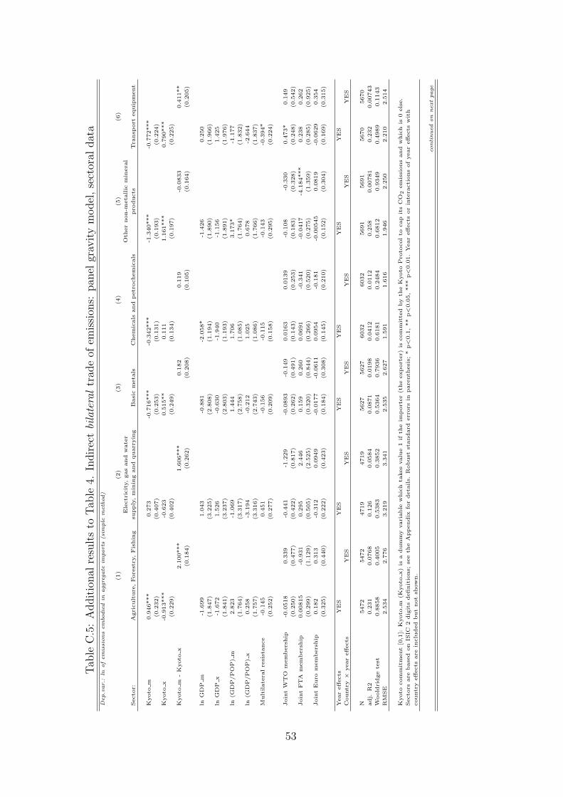
Tab
leC
.5:
Addit
ional
resu
lts
toT
able
4.In
dir
ect
bila
tera
ltr
ade
ofem
issi
ons:
pan
elgr
avit
ym
odel
,se
ctor
aldat
aD
ep.v
ar.:
lnofem
issi
ons
em
bodie
din
aggre
gate
imports
(sim
ple
meth
od)
(1)
(2)
(3)
(4)
(5)
(6)
Ele
ctr
icit
y,
gas
and
wate
rO
ther
non-m
eta
llic
min
era
l
Secto
r:A
gri
cult
ure
,Fore
stry
,F
ishin
gsu
pply
,m
inin
gand
quarr
yin
gB
asi
cm
eta
lsC
hem
icals
and
petr
ochem
icals
pro
ducts
Tra
nsp
ort
equip
ment
Kyoto
m0.9
46***
0.2
73
-0.7
16***
-0.3
42***
-1.3
40***
-0.7
72***
(0.2
32)
(0.4
07)
(0.2
53)
(0.1
31)
(0.1
93)
(0.2
24)
Kyoto
x-0
.913***
-0.6
23
0.5
15**
0.1
11
1.1
61***
0.7
90***
(0.2
29)
(0.4
02)
(0.2
49)
(0.1
34)
(0.1
97)
(0.2
25)
Kyoto
m-
Kyoto
x2.1
00***
1.6
06***
0.1
82
0.1
19
-0.0
833
0.4
11**
(0.1
84)
(0.2
62)
(0.2
08)
(0.1
05)
(0.1
64)
(0.2
05)
lnG
DP
m-1
.699
1.0
43
-0.8
81
-2.0
58*
-1.4
26
0.2
50
(1.8
47)
(3.2
25)
(2.8
08)
(1.1
94)
(1.8
90)
(1.9
66)
lnG
DP
x-1
.672
1.5
26
-0.6
30
-1.9
40
-1.1
56
1.4
25
(1.8
41)
(3.2
37)
(2.8
03)
(1.1
93)
(1.8
91)
(1.9
76)
ln(G
DP
/P
OP
)m
2.8
23
-1.0
69
1.4
44
1.7
06
3.1
73*
-1.1
77
(1.7
64)
(3.3
17)
(2.7
58)
(1.0
85)
(1.7
64)
(1.8
32)
ln(G
DP
/P
OP
)x
0.2
58
-3.1
94
-0.2
12
1.0
25
0.6
78
-2.6
44
(1.7
57)
(3.3
16)
(2.7
43)
(1.0
86)
(1.7
66)
(1.8
37)
Mult
ilate
ral
resi
stance
-0.1
45
0.4
51
-0.1
56
-0.1
15
-0.1
43
-0.3
94*
(0.2
52)
(0.2
77)
(0.2
09)
(0.1
58)
(0.2
95)
(0.2
24)
Join
tW
TO
mem
bers
hip
-0.0
518
0.3
39
-0.4
41
-1.2
29
-0.0
893
-0.1
49
0.0
163
0.0
139
-0.1
08
-0.3
30
0.4
73*
0.1
49
(0.2
50)
(0.4
77)
(0.4
22)
(0.8
17)
(0.2
62)
(0.4
91)
(0.1
43)
(0.2
53)
(0.1
83)
(0.3
28)
(0.2
48)
(0.5
42)
Join
tF
TA
mem
bers
hip
0.0
0815
-0.9
31
0.2
95
2.4
46
0.1
59
0.2
60
0.0
691
-0.3
41
-0.0
417
-4.1
84***
0.2
38
0.2
62
(0.2
99)
(1.1
29)
(0.5
05)
(2.5
25)
(0.3
20)
(0.8
44)
(0.2
66)
(0.5
20)
(0.2
75)
(1.3
59)
(0.2
85)
(0.9
25)
Join
tE
uro
mem
bers
hip
0.1
82
0.3
13
-0.3
12
0.0
949
-0.0
177
-0.0
611
0.0
954
-0.1
81
-0.0
0545
0.0
819
-0.0
629
0.3
54
(0.3
25)
(0.4
40)
(0.2
22)
(0.4
23)
(0.1
84)
(0.3
08)
(0.1
45)
(0.2
10)
(0.1
52)
(0.3
04)
(0.1
69)
(0.3
15)
Year
eff
ects
YE
SY
ES
YE
SY
ES
YE
SY
ES
Countr
y×
year
eff
ects
YE
SY
ES
YE
SY
ES
YE
SY
ES
N5472
5472
4719
4719
5627
5627
6032
6032
5691
5691
5670
5670
adj.
R2
0.2
31
0.0
768
0.1
26
0.0
584
0.0
871
0.0
198
0.0
412
0.0
112
0.2
58
0.0
0781
0.2
32
0.0
0743
Woold
ridge
test
0.8
858
0.4
005
0.5
383
0.3
852
0.5
364
0.7
936
0.6
181
0.2
484
0.6
812
0.9
349
0.4
989
0.1
143
RM
SE
2.5
34
2.7
76
3.2
19
3.3
41
2.5
35
2.6
27
1.5
91
1.6
16
1.9
46
2.2
50
2.2
10
2.5
14
Kyoto
com
mit
ment
[0,1
]:K
yoto
m(K
yoto
x)
isa
dum
my
vari
able
whic
hta
kes
valu
e1
ifth
eim
port
er
(the
exp
ort
er)
iscom
mit
ted
by
the
Kyoto
Pro
tocol
tocap
its
CO
2em
issi
ons
and
whic
his
0els
e.
Secto
rsare
base
don
ISIC
2dig
its
defi
nit
ions;
see
the
App
endix
for
deta
ils.
Robust
standard
err
ors
inpare
nth
esi
s;*
p<
0.1
,**
p<
0.0
5,
***
p<
0.0
1.
Year
eff
ects
or
inte
racti
ons
of
year
eff
ects
wit
h
countr
yeff
ects
are
inclu
ded
but
not
show
n.
continued
on
nextpage
53
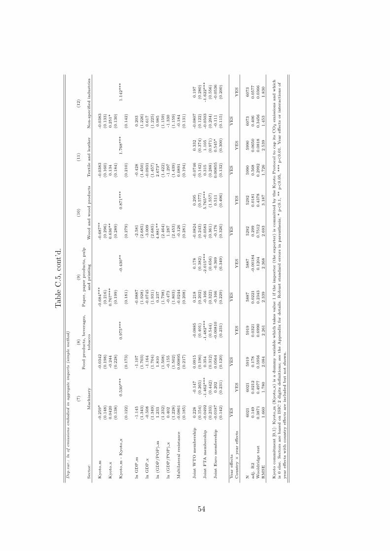
Tab
leC
.5,
cont’
d.
Dep.v
ar.:
lnofem
issi
ons
em
bodie
din
aggre
gate
imports
(sim
ple
meth
od)
(7)
(8)
(9)
(10)
(11)
(12)
Food
pro
ducts
,b
evera
ges,
Pap
er,
pap
er
pro
ducts
,pulp
Secto
r:M
achin
ery
tobacco
and
pri
nti
ng
Wood
and
wood
pro
ducts
Texti
leand
leath
er
Non-s
pecifi
ed
indust
ries
Kyoto
m-0
.259*
-0.0
342
-0.6
84***
-0.6
87**
-0.0
383
-0.0
383
(0.1
48)
(0.1
98)
(0.2
16)
(0.2
96)
(0.1
60)
(0.1
33)
Kyoto
x0.0
420
-0.2
44
0.7
67***
0.6
36**
0.1
34
0.2
51*
(0.1
38)
(0.2
28)
(0.1
99)
(0.2
89)
(0.1
84)
(0.1
30)
Kyoto
m-
Kyoto
x0.5
30***
0.9
75***
-0.4
30**
0.8
71***
1.7
68***
1.1
42***
(0.1
22)
(0.1
73)
(0.1
81)
(0.2
79)
(0.2
10)
(0.1
42)
lnG
DP
m-1
.145
-1.1
07
-0.0
887
-2.5
81
-0.4
28
0.2
03
(1.3
43)
(1.7
03)
(1.9
28)
(2.6
85)
(1.4
50)
(1.2
26)
lnG
DP
x-0
.508
-1.1
64
-0.0
745
-3.0
09
-0.0
931
0.6
17
(1.3
49)
(1.7
04)
(1.9
31)
(2.6
85)
(1.4
57)
(1.2
25)
ln(G
DP
/P
OP
)m
1.2
33
1.8
10
0.2
37
4.8
81**
2.6
73*
0.9
85
(1.2
32)
(1.5
08)
(1.7
98)
(2.4
64)
(1.4
22)
(1.1
59)
ln(G
DP
/P
OP
)x
0.4
02
-0.1
55
-0.4
73
1.2
87
-1.2
97
-1.3
30
(1.2
28)
(1.5
02)
(1.8
03)
(2.4
53)
(1.4
39)
(1.1
59)
Mult
ilate
ral
resi
stance
-0.0
861
0.0
0895
-0.0
244
-0.1
26
0.0
891
-0.1
84
(0.1
85)
(0.2
17)
(0.2
08)
(0.2
81)
(0.1
94)
(0.1
31)
Join
tW
TO
mem
bers
hip
0.2
28
-0.1
47
0.0
915
-0.0
885
0.2
18
0.1
78
-0.0
824
0.2
95
-0.0
746
0.3
32
-0.0
807
0.1
97
(0.1
54)
(0.2
65)
(0.1
96)
(0.4
01)
(0.2
02)
(0.3
82)
(0.2
43)
(0.5
77)
(0.1
42)
(0.3
74)
(0.1
22)
(0.2
80)
Join
tF
TA
mem
bers
hip
-0.0
492
-1.4
62***
0.3
54
-1.4
82***
-0.1
66
-2.0
15***
-0.0
581
5.7
65***
0.3
15
1.1
05
-0.0
503
-1.6
22***
(0.2
33)
(0.4
42)
(0.3
12)
(0.5
44)
(0.3
22)
(0.6
56)
(0.3
61)
(1.5
57)
(0.2
88)
(0.9
71)
(0.2
04)
(0.5
56)
Join
tE
uro
mem
bers
hip
-0.0
187
0.2
02
0.0
564
-0.0
0810
-0.1
66
-0.3
69
-0.1
76
0.5
11
0.0
0855
0.5
45*
-0.1
11
-0.0
536
(0.1
42)
(0.2
31)
(0.1
20)
(0.2
31)
(0.2
29)
(0.3
49)
(0.3
26)
(0.4
96)
(0.1
32)
(0.3
00)
(0.1
15)
(0.2
00)
Year
eff
ects
YE
SY
ES
YE
SY
ES
YE
SY
ES
Countr
y×
year
eff
ects
YE
SY
ES
YE
SY
ES
YE
SY
ES
N6021
6021
5919
5919
5887
5887
5292
5292
5990
5990
6073
6073
adj.
R2
0.1
49
0.0
212
0.1
78
0.0
321
0.0
221
-0.0
0184
0.2
99
0.0
181
0.5
68
0.0
650
0.4
06
0.0
577
Woold
ridge
test
0.3
871
0.4
977
0.5
956
0.6
990
0.2
343
0.1
204
0.7
512
0.4
378
0.2
992
0.0
818
0.3
456
0.0
366
RM
SE
1.6
60
1.7
80
2.0
84
2.2
61
2.3
39
2.3
68
2.6
93
3.1
87
1.7
26
2.5
39
1.4
53
1.8
30
Kyoto
com
mit
ment
[0,1
]:K
yoto
m(K
yoto
x)
isa
dum
my
vari
able
whic
hta
kes
valu
e1
ifth
eim
port
er
(the
exp
ort
er)
iscom
mit
ted
by
the
Kyoto
Pro
tocol
tocap
its
CO
2em
issi
ons
and
whic
h
is0
els
e.
Secto
rsare
base
don
ISIC
2dig
its
defi
nit
ions;
see
the
App
endix
for
deta
ils.
Robust
standard
err
ors
inpare
nth
esi
s;*
p<
0.1
,**
p<
0.0
5,
***
p<
0.0
1.
Year
eff
ects
or
inte
racti
ons
of
year
eff
ects
wit
hcountr
yeff
ects
are
inclu
ded
but
not
show
n.
54
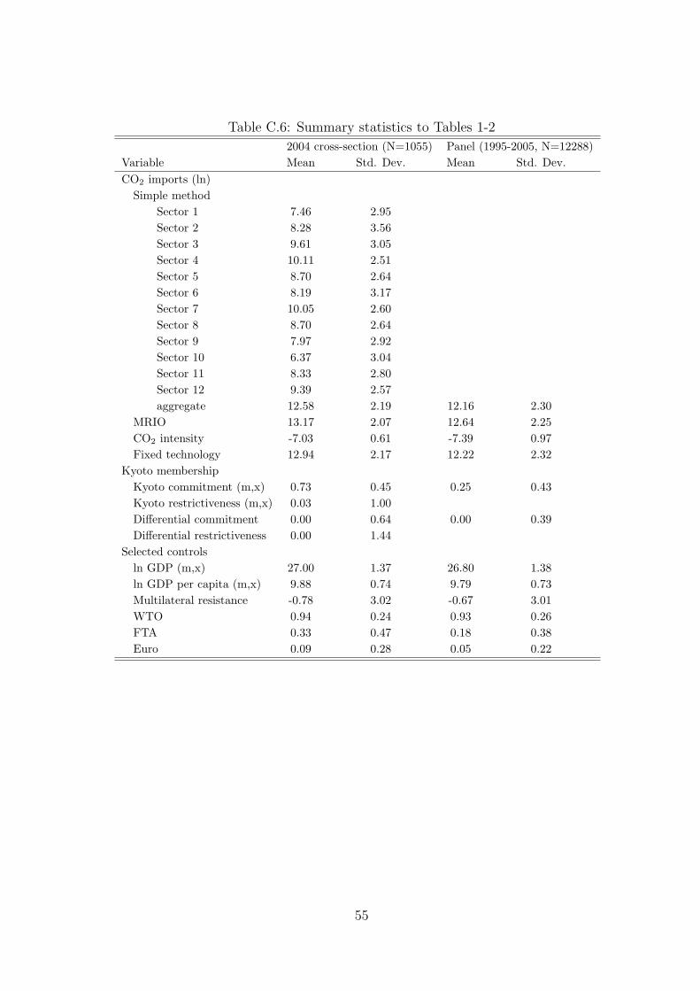
Table C.6: Summary statistics to Tables 1-2
2004 cross-section (N=1055) Panel (1995-2005, N=12288)Variable Mean Std. Dev. Mean Std. Dev.CO2 imports (ln)
Simple methodSector 1 7.46 2.95Sector 2 8.28 3.56Sector 3 9.61 3.05Sector 4 10.11 2.51Sector 5 8.70 2.64Sector 6 8.19 3.17Sector 7 10.05 2.60Sector 8 8.70 2.64Sector 9 7.97 2.92Sector 10 6.37 3.04Sector 11 8.33 2.80Sector 12 9.39 2.57aggregate 12.58 2.19 12.16 2.30
MRIO 13.17 2.07 12.64 2.25CO2 intensity -7.03 0.61 -7.39 0.97Fixed technology 12.94 2.17 12.22 2.32
Kyoto membershipKyoto commitment (m,x) 0.73 0.45 0.25 0.43Kyoto restrictiveness (m,x) 0.03 1.00Differential commitment 0.00 0.64 0.00 0.39Differential restrictiveness 0.00 1.44
Selected controlsln GDP (m,x) 27.00 1.37 26.80 1.38ln GDP per capita (m,x) 9.88 0.74 9.79 0.73Multilateral resistance -0.78 3.02 -0.67 3.01WTO 0.94 0.24 0.93 0.26FTA 0.33 0.47 0.18 0.38Euro 0.09 0.28 0.05 0.22
55
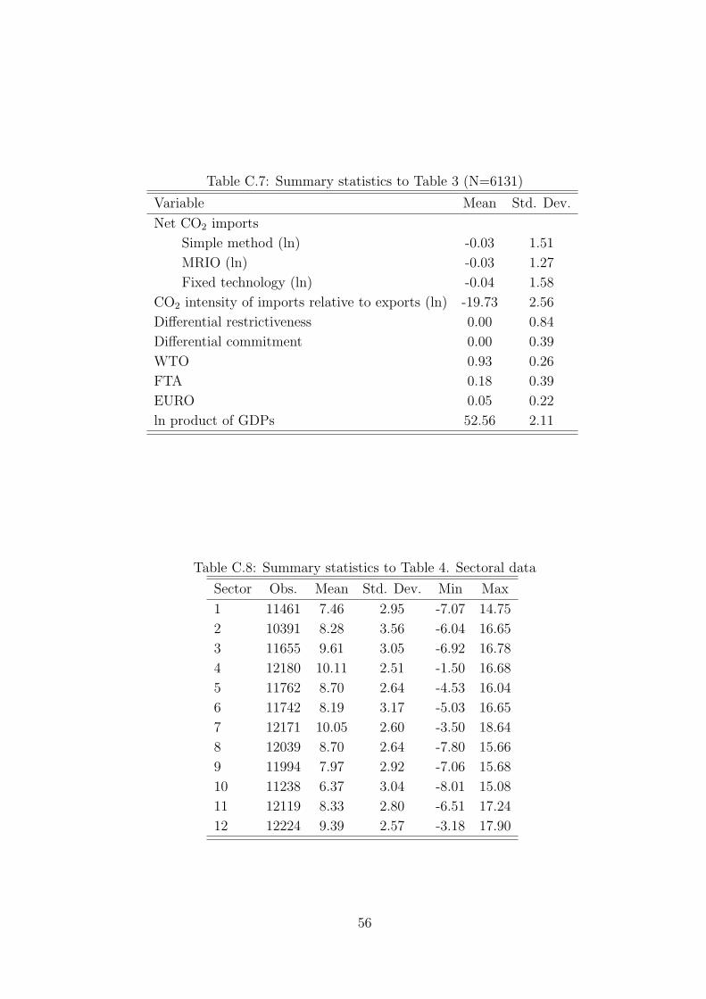
Table C.7: Summary statistics to Table 3 (N=6131)
Variable Mean Std. Dev.
Net CO2 imports
Simple method (ln) -0.03 1.51
MRIO (ln) -0.03 1.27
Fixed technology (ln) -0.04 1.58
CO2 intensity of imports relative to exports (ln) -19.73 2.56
Differential restrictiveness 0.00 0.84
Differential commitment 0.00 0.39
WTO 0.93 0.26
FTA 0.18 0.39
EURO 0.05 0.22
ln product of GDPs 52.56 2.11
Table C.8: Summary statistics to Table 4. Sectoral data
Sector Obs. Mean Std. Dev. Min Max
1 11461 7.46 2.95 -7.07 14.75
2 10391 8.28 3.56 -6.04 16.65
3 11655 9.61 3.05 -6.92 16.78
4 12180 10.11 2.51 -1.50 16.68
5 11762 8.70 2.64 -4.53 16.04
6 11742 8.19 3.17 -5.03 16.65
7 12171 10.05 2.60 -3.50 18.64
8 12039 8.70 2.64 -7.80 15.66
9 11994 7.97 2.92 -7.06 15.68
10 11238 6.37 3.04 -8.01 15.08
11 12119 8.33 2.80 -6.51 17.24
12 12224 9.39 2.57 -3.18 17.90
56
D Data description
Input-output tables Input-output tables describe the economic structure of an econ-
omy for a given point in time. They allow to track the intermediate and factor usage
along the production chain. The OECD collects input-output tables for its members and
various other countries. Table D.2 gives an overview of the availability of those IO tables.
In the case where no input-output table was available for the years under investigation
we chose the input-output table of the nearest year possible. Thereby we assume that the
economic structure (and the relative prices) has not changed between these two points
in time. The OECD input-output tables contain 48 industries, mostly on the 2 digit
ISIC level. We aggregated these IO industries to 15 industries to match the emission
data of the IEA (see Table D.1). Since we apply a highly aggregated sectoral analysis
the problem of an aggregation bias arises. That is, we assume that all products within
a sector are produced with the same CO2 intensity which might lead to an error in the
estimation of the carbon content of trade the higher the sectoral aggregation. A more
disaggregated sectoral detail would be highly desirable, but was impeded in this study by
data availability issues.
Another issue arising when calculating the carbon content of trade with a MRIO model
empirically is that bilateral input-output tables are not available.24 Hence, the amount of
an intermediate good from country j used to produce a good in country i is constructed
with a proportionality assumption. Basically we assume that in country i the intermediate
usage produced by country j in a sector h is proportional to the overall fraction of imports
of this intermediate from country j. That is, when Germany imports 20% of its steel from
China and a sector uses steel as intermediate input, then it is assumed that 20% of the
utilized steel was sourced in China. Therefore we construct the bilateral input-output
tables as follows. Let θhij denote country i’s share of domestic absorption of intermediate
24Note that this information is not needed in the simplified model.
57
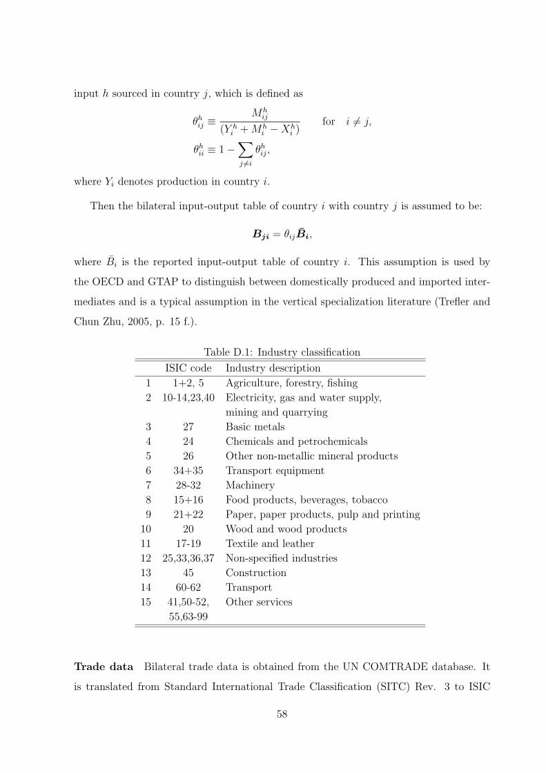
input h sourced in country j, which is defined as
θhij ≡Mh
ij
(Y hi +Mh
i −Xhi )
for i 6= j,
θhii ≡ 1−∑j 6=i
θhij,
where Yi denotes production in country i.
Then the bilateral input-output table of country i with country j is assumed to be:
Bji = θijBi,
where Bi is the reported input-output table of country i. This assumption is used by
the OECD and GTAP to distinguish between domestically produced and imported inter-
mediates and is a typical assumption in the vertical specialization literature (Trefler and
Chun Zhu, 2005, p. 15 f.).
Table D.1: Industry classification
ISIC code Industry description
1 1+2, 5 Agriculture, forestry, fishing
2 10-14,23,40 Electricity, gas and water supply,
mining and quarrying
3 27 Basic metals
4 24 Chemicals and petrochemicals
5 26 Other non-metallic mineral products
6 34+35 Transport equipment
7 28-32 Machinery
8 15+16 Food products, beverages, tobacco
9 21+22 Paper, paper products, pulp and printing
10 20 Wood and wood products
11 17-19 Textile and leather
12 25,33,36,37 Non-specified industries
13 45 Construction
14 60-62 Transport
15 41,50-52, Other services
55,63-99
Trade data Bilateral trade data is obtained from the UN COMTRADE database. It
is translated from Standard International Trade Classification (SITC) Rev. 3 to ISIC
58
Rev. 3 with an industry concordance table provided by Eurostat25. Imports are valued
with CIF prices, exports with FOB prices for most countries. In order to have the same
valuation for imports and exports, we use the FOB export price of the partner country
as FOB price of imports. That is, the trade matrix T becomes
T =
X1 −X12 · · · −X1N
−X21 X2 · · · −X2N
......
. . ....
−XN1 −XN2 · · · XN
where the ith column refers to the trade vector of country i. The results presented in
the main text are in this FOB FOB valuation. Thereby we ignore the carbon dioxide
emissions caused by international transportation. The main results do not change but in
the latter case the emissions embodied in trade do not add up to zero across all countries.
For Russia, bilateral trade data is not available in the year 1995. Hence, we assume
the trade relations in 1995 to be as in 1996 and use trade data of 1996 for the Russian
Federation. Prior to 1999 bilateral trade data for Belgium and Luxembourg is reported
jointly. Therefore trade, output and emissions data of both countries is aggregated. It
is assumed that both countries produce with Belgian technology and therefore we apply
the Belgian IO table to the region Belgium-Luxembourg. Furthermore, service trade is
assumed to be zero. Therefore the bilateral trade vectors contain zero entries for all
service industries.
Sectoral CO2 emissions Sectoral CO2 emissions are taken from the IEA, which esti-
mates the CO2 emissions from fossil fuel combustion with the default method and emission
factors suggested by the Intergovernmental Panel on Climate Change (IPCC, 1996) guide-
lines. We only consider CO2 emissions, but they contribute to around 80% to greenhouse
gas emissions. These are only the emissions due to fossil fuel combustion. Other sources
of carbon dioxide emissions such as fugitive emissions, industrial processes or waste are
disregarded. However, CO2 emissions from fuel combustion make up 80% of total CO2
25http://ec.europa.eu/eurostat/ramon
59
emissions.26
Output data Sectoral output data is not obtained by a single source. Output data come
from the Structural Analysis Database (STAN) of the OECD27, the Industrial Statistics
Database of the Unido (2009) or the System of National Accounts of the UN28. For some
countries and years however, sectoral output data is missing altogether (see below for
details). Therefore we created an unbalanced sample in which countries were melted into
the rest of world aggregate in the respective year when their observation was missing and
could not be interpolated. This unbalanced sample is used for econometric analysis. In
the balanced sample we imputed the missing data by applying growth rates of output or
where those were not available growth rates of real GDP of the respective country and
year. The balanced sample is used for descriptive statistics.
For most OECD countries (i.e. for Austria, Belgium, Luxembourg, Canada, Switzer-
land, Czech Republic, Germany, Denmark, Spain, Finland, France, United Kingdom,
Greece, Hungary, Italy, Japan, Korea, Netherlands, Norway, Poland, Portugal, Slovakia,
Sweden and the United States) sectoral output data comes from STAN. Agricultural out-
put is missing for Spain in 2002, 2003 and 2005. We interpolated the agricultural output
for 2002 and 2003 and applied the growth rate of the output of the total economy to obtain
the agricultural output in 2005, where this growth rate comes from Table 2.3 of the UN
SNA. For Switzerland manufacturing output (category 3-12) is missing in 1995 and 1996
and is therefore calculated by the growth rate of manufacturing output obtained from
STAN. In 1995 and 1996 the transportation sector output is also missing in Switzerland
and is calculated by applying the growth rate of the output of the total economy, where
this growth rate comes from the STAN database. The STAN output data is only available
in current national currency and was converted to current U.S. dollars with the period
average exchange rates from the IFS database. Except for the United States (market
prices) and Japan (producer’s prices) STAN output data is given at basic prices.
26Own calculation, see UNFCCC (2008, p. 12).27http://www.oecd.org/document/62/0,3343,en 2649 34445 40696318 1 1 1 1,00.html28http://data.un.org/Data.aspx?d=SNA&f=group code%3a203
60
For countries not covered by STAN, sectoral output for the manufacturing industries
was taken from the INDSTAT4 2009 (ISIC Rev. 3) and complemented by UN SNA
data for non-manufacturing output (industry categories 1, 2, 13-15). These countries are
Argentina, Brazil, Estonia, India, Israel, Mexico, Russia, Slovenia and South Africa. In
the UN SNA transport (ISIC 60-62) and storage (ISIC 63) are reported jointly, therefore
our industry category 14 contains part of category 15 in those countries. Manufacturing
output is interpolated for the years 1995 and 1997 for South Africa. Manufacturing output
is not available for Argentina from 2002-2005, Brazil in the year 1995, India between 1995
and 1998 and in 2005, Mexico from 2001-2005 and Russia from 1995-2001. For Argentina,
Brazil, India and Mexico the unavailable data were calculated with the growth rate of
manufacturing output from the UN SNA. For Russia, missing non-manufacturing output
data for the years 1995-2001 and missing manufacturing output data for the years 1995-
1999 were constructed with the growth rate of the output of the total economy from the
UN SNA. Data for Mexico in 2005 is neither available in the INDSTAT4 2009 nor in
the UN SNA. For the balanced sample, sectoral output for Mexico in 2005 is therefore
constructed with the growth rate of real GDP from the OECD29 because no information
on output growth was available. Manufacturing output data are available in producer’s
prices for Argentina, India and Russia, while the Brazilian manufacturing output is given
in factor values. For the rest of the countries the valuation in the INDSTAT4 2009 is not
defined. In the UN SNA output is valued in basic prices except for Argentina, where data
is given in producer’s prices. For Argentina, Brazil, Israel, Mexico, Russia and Slovenia we
only used one series of the UN SNA (series 100, 300, 100, 100, 300 and 200 respectively)
whereas for Estonia we had to prolong the series 300 with the series 400 in the year 2005,
for South Africa we had to extend the series 100 with the series 200 in the year 2005 and
for India we used the series 100 from 1999-2004 and had to complement the output data
with series 30 of the SNA68 prior to 1999.
For Australia, China, Indonesia, Ireland, New Zealand and Turkey sectoral output
was not available in either the INDSTAT4 2009 or the UN SNA. Therefore we construct
29OECD Economic Outlook, 2008, No. 84.
61
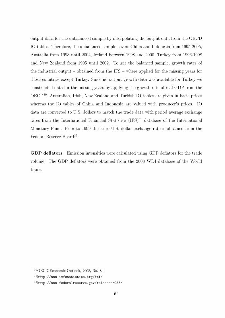
output data for the unbalanced sample by interpolating the output data from the OECD
IO tables. Therefore, the unbalanced sample covers China and Indonesia from 1995-2005,
Australia from 1998 until 2004, Ireland between 1998 and 2000, Turkey from 1996-1998
and New Zealand from 1995 until 2002. To get the balanced sample, growth rates of
the industrial output – obtained from the IFS – where applied for the missing years for
those countries except Turkey. Since no output growth data was available for Turkey we
constructed data for the missing years by applying the growth rate of real GDP from the
OECD30. Australian, Irish, New Zealand and Turkish IO tables are given in basic prices
whereas the IO tables of China and Indonesia are valued with producer’s prices. IO
data are converted to U.S. dollars to match the trade data with period average exchange
rates from the International Financial Statistics (IFS)31 database of the International
Monetary Fund. Prior to 1999 the Euro-U.S. dollar exchange rate is obtained from the
Federal Reserve Board32.
GDP deflators Emission intensities were calculated using GDP deflators for the trade
volume. The GDP deflators were obtained from the 2008 WDI database of the World
Bank.
30OECD Economic Outlook, 2008, No. 84.31http://www.imfstatistics.org/imf/32http://www.federalreserve.gov/releases/G5A/
62
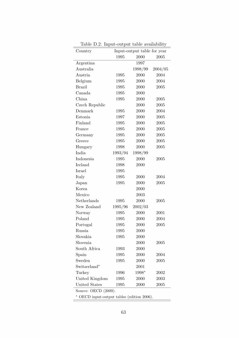
Table D.2: Input-output table availability
Country Input-output table for year1995 2000 2005
Argentina 1997Australia 1998/99 2004/05Austria 1995 2000 2004Belgium 1995 2000 2004Brazil 1995 2000 2005Canada 1995 2000China 1995 2000 2005Czech Republic 2000 2005Denmark 1995 2000 2004Estonia 1997 2000 2005Finland 1995 2000 2005France 1995 2000 2005Germany 1995 2000 2005Greece 1995 2000 2005Hungary 1998 2000 2005India 1993/94 1998/99Indonesia 1995 2000 2005Ireland 1998 2000Israel 1995Italy 1995 2000 2004Japan 1995 2000 2005Korea 2000Mexico 2003Netherlands 1995 2000 2005New Zealand 1995/96 2002/03Norway 1995 2000 2001Poland 1995 2000 2004Portugal 1995 2000 2005Russia 1995 2000Slovakia 1995 2000Slovenia 2000 2005South Africa 1993 2000Spain 1995 2000 2004Sweden 1995 2000 2005Switzerland∗ 2001Turkey 1996 1998∗ 2002United Kingdom 1995 2000 2003United States 1995 2000 2005Source: OECD (2009).∗ OECD input-output tables (edition 2006).
63

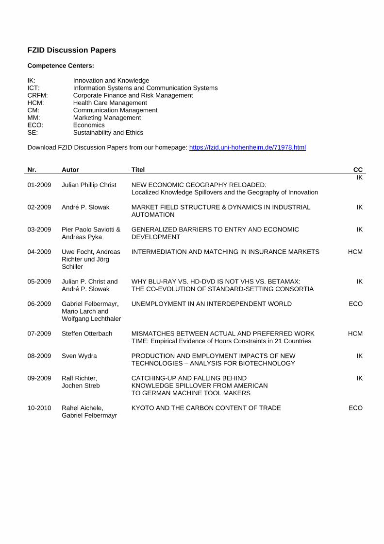
FZID Discussion Papers Competence Centers: IK: Innovation and Knowledge ICT: Information Systems and Communication Systems CRFM: Corporate Finance and Risk Management HCM: Health Care Management CM: Communication Management MM: Marketing Management ECO: Economics SE: Sustainability and Ethics Download FZID Discussion Papers from our homepage: https://fzid.uni-hohenheim.de/71978.html
Nr. Autor Titel CC 01-2009
Julian Phillip Christ
NEW ECONOMIC GEOGRAPHY RELOADED: Localized Knowledge Spillovers and the Geography of Innovation
IK
02-2009 André P. Slowak MARKET FIELD STRUCTURE & DYNAMICS IN INDUSTRIAL AUTOMATION
IK
03-2009 Pier Paolo Saviotti & Andreas Pyka
GENERALIZED BARRIERS TO ENTRY AND ECONOMIC DEVELOPMENT
IK
04-2009 Uwe Focht, Andreas Richter und Jörg Schiller
INTERMEDIATION AND MATCHING IN INSURANCE MARKETS HCM
05-2009 Julian P. Christ and André P. Slowak
WHY BLU-RAY VS. HD-DVD IS NOT VHS VS. BETAMAX: THE CO-EVOLUTION OF STANDARD-SETTING CONSORTIA
IK
06-2009 Gabriel Felbermayr, Mario Larch and Wolfgang Lechthaler
UNEMPLOYMENT IN AN INTERDEPENDENT WORLD ECO
07-2009 Steffen Otterbach MISMATCHES BETWEEN ACTUAL AND PREFERRED WORK TIME: Empirical Evidence of Hours Constraints in 21 Countries
HCM
08-2009 Sven Wydra PRODUCTION AND EMPLOYMENT IMPACTS OF NEW TECHNOLOGIES – ANALYSIS FOR BIOTECHNOLOGY
IK
09-2009 Ralf Richter, Jochen Streb
CATCHING-UP AND FALLING BEHIND KNOWLEDGE SPILLOVER FROM AMERICAN TO GERMAN MACHINE TOOL MAKERS
IK
10-2010 Rahel Aichele,
Gabriel Felbermayr
KYOTO AND THE CARBON CONTENT OF TRADE ECO

U n i v e r s i t ä t H o h e n h e i m
F o r s c h u n g s z e n t r u m
Innovation und Dienstleistung
Fruwirthstr. 12
D-70593 Stuttgart
Phone +49 (0)711 / 459-22476
Fax +49 (0)711 / 459-23360
Internet www.fzid.uni-hohenheim.de


