doctorat paristech t h e s e telecom paristech · doctorat paristech t h e s e ... timédia...
TRANSCRIPT
2012-ENST-056
EDITE - ED 130
Doctorat ParisTech
T H E S E
pour obtenir le grade de docteur délivré par
TELECOM ParisTech
Spécialité « Signal et Images »
présentée et soutenue publiquement par
Manel ABID
le 5 Octobre 2012
Codage/décodage source-canal conjoint
des contenus multimédia
Directeur de thèse : Béatrice PESQUET-POPESCU
Co-direction de la thèse : Maria TROCAN
Jury
M. Fabrice LABEAU Rapporteur
M. Peter SCHELKENS Rapporteur
Mme Anissa MOKRAOUI Examinateur
M. François-Xavier COUDOUX Examinateur
M. Michel KIEFFER Examinateur
TELECOM ParisTech
école de l’Institut Télécom - membre de ParisTech
Contents
Remerciements 1
Abstract 3
Résumé de la Thèse 5
1. Introduction 351.1. Motivation . . . . . . . . . . . . . . . . . . . . . . . . . . . . . . . . . 351.2. Outline of the Thesis . . . . . . . . . . . . . . . . . . . . . . . . . . . 361.3. Summary of the Contributions . . . . . . . . . . . . . . . . . . . . . . 37
2. Joint Source-Channel Coding and Decoding 392.1. Introduction . . . . . . . . . . . . . . . . . . . . . . . . . . . . . . . . 392.2. Tandem Coding Techniques . . . . . . . . . . . . . . . . . . . . . . . 40
2.2.1. Channel Coding . . . . . . . . . . . . . . . . . . . . . . . . . . 412.2.2. Limitations of Tandem Systems . . . . . . . . . . . . . . . . . 41
2.3. Joint Source-Channel Coding and Decoding Techniques . . . . . . . . 422.3.1. JSCC for Rate Allocation . . . . . . . . . . . . . . . . . . . . 442.3.2. Unequal Error Protection . . . . . . . . . . . . . . . . . . . . 45
2.4. Multiple Description Coding . . . . . . . . . . . . . . . . . . . . . . . 472.4.1. Theoretical Performance of MD Coding Schemes . . . . . . . . 482.4.2. Practical MD Coding Schemes . . . . . . . . . . . . . . . . . . 502.4.3. MD for Video Coding and Transmission . . . . . . . . . . . . 55
2.5. JSCD Techniques . . . . . . . . . . . . . . . . . . . . . . . . . . . . 562.5.1. Soft Decoding of Variable Length Codes . . . . . . . . . . . . 572.5.2. Use of Artificial Redundancy . . . . . . . . . . . . . . . . . . 58
2.6. Error Concealment . . . . . . . . . . . . . . . . . . . . . . . . . . . . 592.7. Conclusion . . . . . . . . . . . . . . . . . . . . . . . . . . . . . . . . . 59
3. JSC Decoding of t + 2D Video Streams 613.1. Conceptual JSC Video Decoder . . . . . . . . . . . . . . . . . . . . . 61
3.1.1. Channel Model . . . . . . . . . . . . . . . . . . . . . . . . . . 623.1.2. Optimal Estimation Schemes . . . . . . . . . . . . . . . . . . 63
3.2. Overview of Vidwav Video Coder . . . . . . . . . . . . . . . . . . . . 653.2.1. Entropy Coding . . . . . . . . . . . . . . . . . . . . . . . . . . 67
i
Contents Contents
3.3. JSCD of Single Layer Bit Streams . . . . . . . . . . . . . . . . . . . . 693.3.1. Syntax Compliance Tests . . . . . . . . . . . . . . . . . . . . 713.3.2. Sequential Estimation . . . . . . . . . . . . . . . . . . . . . . 733.3.3. Simulation Results . . . . . . . . . . . . . . . . . . . . . . . . 74
3.4. JSCD of Multiple Layers Bit Streams . . . . . . . . . . . . . . . . . . 823.4.1. Layered Bit Stream Generation . . . . . . . . . . . . . . . . . 823.4.2. JSCD Scheme . . . . . . . . . . . . . . . . . . . . . . . . . . . 843.4.3. Simulation Results . . . . . . . . . . . . . . . . . . . . . . . . 86
3.5. Conclusion . . . . . . . . . . . . . . . . . . . . . . . . . . . . . . . . . 88
4. JSC Decoding of Multiple Description Encoded Video 89
4.1. Problem Formulation . . . . . . . . . . . . . . . . . . . . . . . . . . . 894.1.1. Optimal MAP Estimation . . . . . . . . . . . . . . . . . . . . 91
4.2. MD Coding Scheme . . . . . . . . . . . . . . . . . . . . . . . . . . . . 924.3. JSCD of the Descriptions . . . . . . . . . . . . . . . . . . . . . . . . . 94
4.3.1. When ρ(i)k > 1 . . . . . . . . . . . . . . . . . . . . . . . . . . . 95
4.3.2. When ρ(i)k = 0 . . . . . . . . . . . . . . . . . . . . . . . . . . . 96
4.4. Reconstruction . . . . . . . . . . . . . . . . . . . . . . . . . . . . . . 964.5. Simulation Results . . . . . . . . . . . . . . . . . . . . . . . . . . . . 97
4.5.1. Bit Stream Organization . . . . . . . . . . . . . . . . . . . . . 974.5.2. Performance of the JSCD Scheme . . . . . . . . . . . . . . . 994.5.3. Comparison to an SD Scheme Combined with a FEC . . . . . 102
4.6. Conclusion . . . . . . . . . . . . . . . . . . . . . . . . . . . . . . . . . 106
5. Robust Estimation from Noisy Overcomplete Signal Representation 107
5.1. Introduction . . . . . . . . . . . . . . . . . . . . . . . . . . . . . . . . 1075.2. Problem Formulation . . . . . . . . . . . . . . . . . . . . . . . . . . . 108
5.2.1. Optimal MAP Estimator . . . . . . . . . . . . . . . . . . . . . 1095.2.2. Running Example . . . . . . . . . . . . . . . . . . . . . . . . . 110
5.3. Consistent Estimation of x . . . . . . . . . . . . . . . . . . . . . . . . 1125.3.1. Negligible Channel Noise . . . . . . . . . . . . . . . . . . . . . 1125.3.2. General Case . . . . . . . . . . . . . . . . . . . . . . . . . . . 1145.3.3. Practical Implementation . . . . . . . . . . . . . . . . . . . . . 119
5.4. Estimation by Belief Propagation . . . . . . . . . . . . . . . . . . . . 1205.4.1. BP algorithm . . . . . . . . . . . . . . . . . . . . . . . . . . . 1205.4.2. Running Example . . . . . . . . . . . . . . . . . . . . . . . . . 123
5.5. Comparison between the two Estimation Schemes . . . . . . . . . . . 1235.6. Application to Oversampled Filter Banks . . . . . . . . . . . . . . . 126
5.6.1. Brief Presentation of OFBs . . . . . . . . . . . . . . . . . . . 1265.6.2. Signal Expansion using OFBs . . . . . . . . . . . . . . . . . . 1275.6.3. Iterative Implementation of the Consistent MAP Estimator . . 129
5.7. Conclusion . . . . . . . . . . . . . . . . . . . . . . . . . . . . . . . . . 134
ii
Contents
6. Conclusions and Perspectives 1376.1. Synthesis of the Contributions . . . . . . . . . . . . . . . . . . . . . . 1376.2. Perspectives . . . . . . . . . . . . . . . . . . . . . . . . . . . . . . . . 138
A. Sum-Product Algorithm 141A.1. Problem Formulation . . . . . . . . . . . . . . . . . . . . . . . . . . . 141
A.1.1. Simple Example . . . . . . . . . . . . . . . . . . . . . . . . . . 142A.2. Computation of the Marginals . . . . . . . . . . . . . . . . . . . . . 142
A.2.1. Detailed Example . . . . . . . . . . . . . . . . . . . . . . . . . 144A.3. Sum-Product Algorithm for Factor Graphs with Cycles . . . . . . . . 145A.4. Belief Propagation . . . . . . . . . . . . . . . . . . . . . . . . . . . . 145
B. Oversampled Filter Banks 149B.1. Introduction to Oversampled Filter Banks . . . . . . . . . . . . . . . 149
B.1.1. Time Domain Analysis . . . . . . . . . . . . . . . . . . . . . . 149B.1.2. Polyphase Domain Analysis . . . . . . . . . . . . . . . . . . . 152B.1.3. Perfect Reconstruction . . . . . . . . . . . . . . . . . . . . . . 153
B.2. OFBs as Error Correcting Codes . . . . . . . . . . . . . . . . . . . . 154B.2.1. Time Domain . . . . . . . . . . . . . . . . . . . . . . . . . . . 154B.2.2. Polyphase Domain . . . . . . . . . . . . . . . . . . . . . . . . 156
C. Image Denoising by Adaptive Lifting Schemes 159C.1. Introduction . . . . . . . . . . . . . . . . . . . . . . . . . . . . . . . . 159C.2. Adaptive Lifting Schemes . . . . . . . . . . . . . . . . . . . . . . . . 160
C.2.1. Classical Lifting Schemes . . . . . . . . . . . . . . . . . . . . . 160C.3. Adaptive Prediction Lifting Scheme . . . . . . . . . . . . . . . . . . . 161C.4. Distortion Estimation in the Transform Domain . . . . . . . . . . . . 162C.5. Application to Image Denoising . . . . . . . . . . . . . . . . . . . . . 163C.6. Simulation Results . . . . . . . . . . . . . . . . . . . . . . . . . . . . 164
C.6.1. Noise Standard Deviation Estimation . . . . . . . . . . . . . . 164C.6.2. Denoising by Soft Thresholding . . . . . . . . . . . . . . . . . 165
C.7. Conclusion . . . . . . . . . . . . . . . . . . . . . . . . . . . . . . . . . 166
List of Acronyms 169
List of Publications 171
Bibliography 173
iii

Remerciements
Je remercie tout d’abord mes directrices de thèse, Béatrice Pesquet-Popescu et MariaTrocan, pour m’avoir fait confiance et pour m’avoir guidée, encouragée, conseilléetout au long de ces trois années. Je tiens de plus à remercier Michel Kieffer pour saprécieuse collaboration au cours de ma thèse.
J’adresse également mes remerciements à tous le membres de mon jury : François-Xavier Coudoux qui m’a fait l’honneur de présider ce jury, Peter Schelkens et FabriceLabeau qui ont bien voulu accepter la charge de rapporteur et Anissa Mokraoui quia bien voulu juger ce travail.
Je souhaite de plus remercier toutes les personnes que j’ai pu côtoyer et aveclesquelles j’ai pu collaborer durant mes trois années de thèse au département TSIde Télécom Paris Tech, et plus spécifiquement, tous les membres de l’équipe multi-média.
Enfin, je remercie du fond du coeur mes chers parents qui n’ont jamais cessé decroire en moi pendant toutes mes années d’études et qui m’ont toujours encouragéeà aller de l’avant. Je leur dédie cette thèse.
1

Abstract
The development of multimedia broadcasting and on-demand services for mobiledevices such as tablets or smartphones involves the transmission of contents overheterogeneous networks, consisting of mixed wired and wireless channels. For suchbest-effort networks, the quality of service (packet loss rate, delay and reconstructedsignal quality) is not always satisfactory due to time-varying characteristics of thechannels. Compressed data packets may be lost due to congestion in the networkor corrupted by channel impairments. Moreover, due to the limited bandwidth, themultimedia content has to be highly compressed, which makes the transmitted bitstreams extremely sensitive to transmission impairments. Therefore, the demandfor efficient compression algorithms, as well as reliable coding techniques, is veryimportant in multimedia transmission systems.
This thesis aims at proposing and implementing efficient joint source-channel codingand decoding schemes in order to enhance the robustness of multimedia contentstransmitted over unreliable networks.
In a first time, we propose to identify and exploit the residual redundancy left bywavelet video coders in the compressed bit streams. An efficient joint-source channeldecoding scheme is proposed to detect and correct some of the transmission errorsoccurring during a noisy transmission. This technique is further applied to multipledescription video streams transmitted over a mixed architecture consisting of a wiredlossy part and a wireless noisy part.
In a second time, we propose to use the structured redundancy deliberately intro-duced by multirate coding systems, such as oversampled filter banks, in order toperform a robust estimation of the input signals transmitted over noisy channels.Two efficient estimation approaches are proposed and compared. The first one ex-ploits the linear dependencies between the output variables, jointly to the boundedquantization noise, in order to perform a consistent estimation of the source out-come. The second approach uses the belief propagation algorithm to estimate theinput signal via a message passing procedure along the graph representing the lineardependencies between the variables. These schemes are then applied to estimate theinput of an oversampled filter bank and their performance are compared.
3

Résumé de la Thèse
Contexte et motivations
Le développement croissant d’applications multimédia, de services à la demandeet de terminaux mobiles (tablettes et smartphones) a conduit à un usage intensifd’architectures mixtes, comprenant canaux radio-mobiles et réseaux à pertes depaquets comme Internet. Pour de tels supports de communication, la qualité deservice n’est pas toujours garantie à cause des variations des caractéristiques dela source et des conditions du canal. Les paquets de données peuvent être perdusau cours de leur acheminement, suite à des congestions survenant sur la partieInternet du canal de transmission, ou/et corrompus par des erreurs causées pardes perturbations sur la partie radio-mobile. Garantir une transmission fiable descontenus multimédia devient alors d’une grande necessité, d’autant plus que lesapplications conversationnelles ou de type diffusion, largement utilisées de nos jours,ne permettent pas la retransmisssion de l’information perdue ou erronée.
Pour augmenter la robustesse des contenus transmis, les recherches se sont pendantlongtemps axées sur l’optimisation séparée du codeur source et du codeur canal,appliquant ainsi le théorème de Shannon [141] qui établit qu’une telle séparationpermet au système de communication d’atteindre les performances optimales et degarantir ainsi une transmission fiable avec une probabilité d’erreur aussi petite quel’on veut. Cependant, cette optimisation séparée, suppose que les caractéristiques dela source et du canal sont parfaitement connues, ce qui n’est généralement pas le casen pratique. De plus, elle fait l’hypothèse que les codeurs source et canal travaillentsur des blocs de données de tailles infiniment longues, ce qui conduit à une complexitéélevée des deux codeurs, prohibitive pour les situations de communication pratiques,telles que les applications en temps réel. Dans de telles situations, le codeur canala une complexité limitée, ce qui ne permet pas de corriger toutes les erreurs detransmission. Par ailleurs, la théorie de Shannon ne fournit pas de méthode deconstruction de codes source optimaux, capables de corriger les erreurs résiduelleslaissées après décodage canal. Ces erreurs peuvent alors fortement dégrader le signalreconstruit par le décodeur source.
Ainsi, les dernières décennies ont connu le développement de solutions alternativesreposant sur des techniques de codage/décodage source-canal conjoint [44, 49]. Cestechniques ont pour objectif de répondre aux contraintes de délai et de complexitéimposées en pratique, et d’assurer une transmission robuste vis-à-vis des perturba-tions inconnues et variables du canal de communnication.
5
Résumé de la Thèse
Cette thèse s’inscrit dans ce contexte et a pour but de proposer des schémas decodage/décodage source-canal conjoint, augmentant la robustesse des contenus mul-timédia transmis sur des canaux radio-mobiles ou mixtes Internet et radio-mobiles,qui sont peu fiables.
Codage/décodage source-canal conjoint
Ces techniques se répartissent essentiellement en deux catégories
1. Codage source-canal conjoint : dans cette catégorie, les codeur source et canalsont construits de manière conjointe. Le codeur canal peut être informé des de-grés de sensibilité des données compressées qui lui sont délivrées par le codeursource, et ainsi adapter son niveau de protection. On parle alors de schémasde protection inégale vis-à-vis des erreurs [20, 24, 26, 12]. A l’inverse, le codeursource peut être construit pour un canal de transmission donné. Tel est le casdes schémas de codage par descriptions multiples, conçus pour les canaux àpertes de paquets et pour les applications ayant des exigences de délais trèsréduits [165, 115, 43, 52, 157]. Dans ces schémas, le codeur source génère plu-sieurs descriptions, qui peuvent être décodées indépendemment les unes desautres, ou ensemble, permettant ainsi une meilleure reconstruction. D’autresschémas de codage source-canal conjoint sont basés sur des transformationsredondantes de la source à coder, ce qui revient en quelque sorte à réaliser uncodage canal avant le codage source [56, 116, 79]. Les erreurs résiduelles lais-sées par un décodeur canal classique peuvent alors être détectées et corrigéesgrâce à cette redondance structurée introduite au niveau de la source. On peutciter l’exemple des bancs de filtres suréchantillonnés [151] qui fournissent unereprésentation redondante du signal placé en entrée, pouvant être exploitée audécodeur pour détecter et corriger les erreurs de transmission et/ou compenserles effacements [56, 131, 54, 79, 86, 130, 2].
2. Décodage source-canal conjoint : les techniques appartenant à cette catégorie sebasent sur le fait que tous les codeurs source pratiques produisent des trains bi-naires contenant une certaine redondance [137]. Cette redondance peut prove-nir de la syntaxe du codeur source [138, 168], de la corrélation résiduelles entreles coefficients après transformation, ou encore de la paquétisation des données[11, 91, 136]. Les techniques de décodage source-canal conjoint cherchent alorsà exploiter au mieux cette redondance pour améliorer le décodage [62, 22, 42].Un exemple de telles méthodes, est le décodage souple des codes à longueursvariables (CLVs) de type Huffman et arithmétiques [76, 122]. Le décodagesouple des CLVs se base sur l’estimation statistique de la séquence émise parla source, à partir d’un ensemble d’observations bruitées. Généralement, uncritère de vraisemblance ou de probabilité a posteriori est considéré pour opti-miser l’estimateur. La recherche de la solution s’effectue alors dans l’ensembledes séquences vérifiant un certain nombre de contraintes, déduites à partir de
6
la redondance résiduelle présente dans les CLVs. Des algorithmes de décodagetels que l’algorithme de Viterbi [114], sont souvent utilisés pour effectuer cetterecherche et éliminer les séquences non valides.
Les schémas proposés dans cette thèse appartiennent aux deux catégories citéesci-dessus. Nous nous sommes intéressés dans un premier temps aux techniques dedécodage source-canal conjoint des trains binaires délivrés par des codeurs vidéopar ondelettes. La redondance résiduelle laissée par de tels codeurs est identifiée,puis exploitée pour détecter et corriger les erreurs de transmission survenant lors dela transmission sur un canal radio-mobile. Ce schéma est ensuite appliqué dans lecadre d’une diffusion des contenus vidéo à travers un canal hétérogène, où les pertesde paquets sont compensées à l’aide du codage par descriptions multiples.
Nous nous sommes ensuite intéressés aux techniques de codage source-canal conjointbasées sur une transformation redondante. Un schéma d’estimation cohérente de lasource, exploitant de manière efficace la redondance introduite, est proposé. Des ou-tils de programmation linéaire et de calculs par intervalles sont mis en oeuvre pourdétecter les erreurs de trasmission et estimer la source. Un autre schéma d’estima-tion, basé sur l’algorithme de propagation de croyances est également introduit. Cesdeux schémas sont alors appliqués pour estimer l’entrée de bancs de filtres suréchan-tillonnés, et leurs performances sont comparées.
Décodage source-canal conjoint des sources vidéo
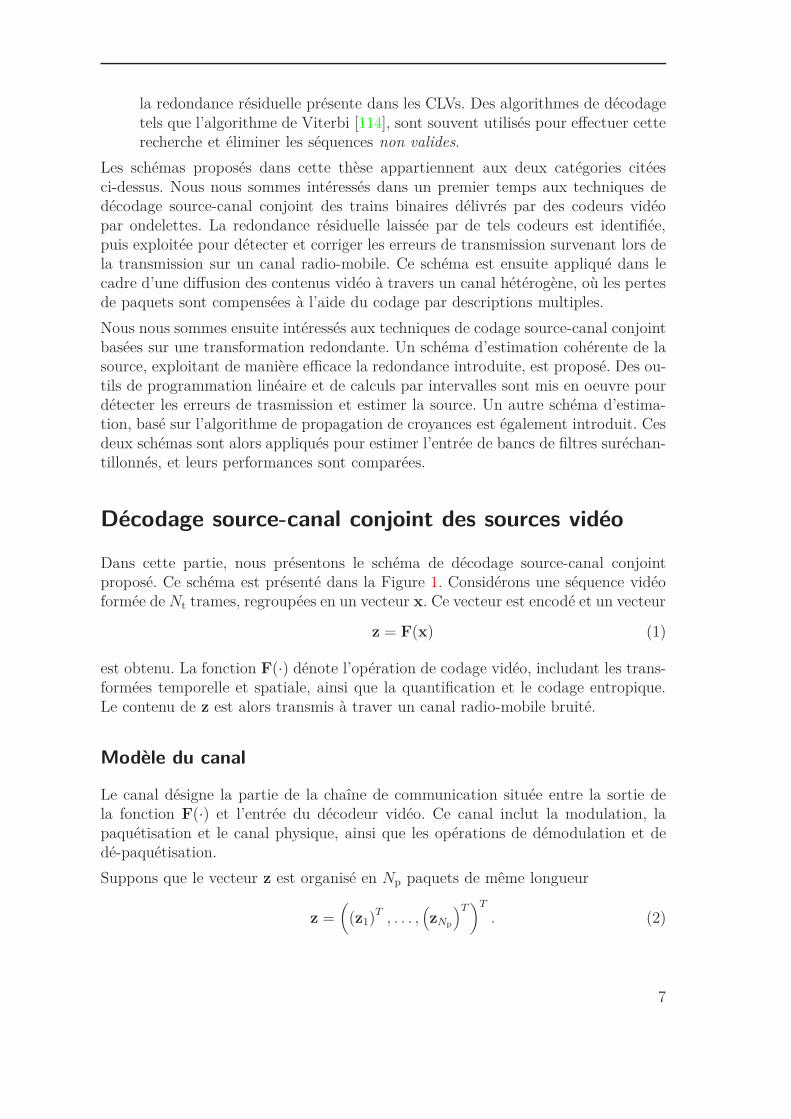
Dans cette partie, nous présentons le schéma de décodage source-canal conjointproposé. Ce schéma est présenté dans la Figure 1. Considérons une séquence vidéoformée de Nt trames, regroupées en un vecteur x. Ce vecteur est encodé et un vecteur
z = F(x) (1)
est obtenu. La fonction F(·) dénote l’opération de codage vidéo, includant les trans-formées temporelle et spatiale, ainsi que la quantification et le codage entropique.Le contenu de z est alors transmis à traver un canal radio-mobile bruité.
Modèle du canal
Le canal désigne la partie de la chaîne de communication située entre la sortie dela fonction F(·) et l’entrée du décodeur vidéo. Ce canal inclut la modulation, lapaquétisation et le canal physique, ainsi que les opérations de démodulation et dedé-paquétisation.
Suppons que le vecteur z est organisé en Np paquets de même longueur
z =(
(z1)T , . . . ,
(zNp
)T)T
. (2)
7
Résumé de la Thèse
Les mécanismes classiques de détection d’erreurs, mis en place au niveau des couchesprotocolaires basses, ne permettent pas aux paquets corrompus d’atteindre la coucheapplicative. L’implémentation de schémas de décodage source-canal conjoint au ni-veau de la couche applicative, nécessite alors la présence de mécanismes dits trans-couches (cross-layer) pour permettre aux différentes couches protocolaires de com-munniquer entre elles et d’assurer ainsi la remontée d’informations, telles que cellesdes paquets contenant des erreurs, et les informations souples du canal, des couchesbasses vers les couches hautes de la pile protocolaire [117, 42].
Tout au long de ce travail, nous supposons qu’un tel schéma trans-couches est implé-menté, ainsi que des mécanismes de décodage robuste des entêtes des paquets reçus,pour permettre l’extraction des informations provenant des couches protocolairesbasses [100, 101].
A la sortie de ce canal, deux types d’information sont obtenus. D’une part les infor-mations souples sur les paquets transmis zk, modélisées par le vecteur
r =(
(r1)T , . . . ,(rNp
)T)T
. (3)
Les information souples contenues dans le vecteur rk consistent par exemple, en desprobabilités à posteriori ou des vraisemblances sur les données transmises dans lepaquet zk. Ces informations sont fournies par le décodeur canal, au niveau de lacouche physique, du côté du récepteur.
D’autre part, les informations sur l’état du canal sont également disponibles et sontmodélisées par le vecteur
ρ =(ρ1, . . . , ρNp
)T, (4)
dont les composantes indiquent si le paquet zk, a été perdu (ρk = 0) ou reçu (ρk > 1).Le fait que ρk = 0 peut être déduit par exemple du contenu des entêtes de paquets.Les valeurs de ρk > 1 sont supposées être connues au récepteur. Elle indiquent parexemple, le niveau du bruit introduit dans le paquet zk.
x
x r
ρ
z
F(.)
Canal
Codeur vidéo
Estimateur
redondance
Décodeur vidéo
Figure 1.: Schéma de décodage source-canal conjoint.
8
Schémas d’estimation optimale
Cette section présente deux schémas d’estimation optimale, qui sont indépendantsdu codeur vidéo considéré. Nous commençons par formuler l’estimée optimale de x,qui est difficile à mettre en oeuvre en pratique. Ensuite, nous décrivons une estiméecontrainte de z qui est plus pratique et pour laquelle les informations souples ensortie du canal ainsi que la redondance de la source, sont plus faciles à exploiter.
Estimation optimale de x
Le critère d’estimation que nous considérons est celui du maximum à posteriori(MAP). L’estimée xMAP de x connaissant ρ et r est
xMAP = arg maxx
p (x|ρ, r) . (5)
Cette estimée peut être écrite de la manière suivante
xMAP = arg maxx
p (ρ, r|F (x)) p (x) , (6)
en faisant la somme sur tous les z possibles, puis en utilisant la règle de Bayes. Seulz = F (x) est alors gardé dans cette somme. L’évaluation de xMAP est difficile àmettre en place en pratique. En effet, elle requiert la maximisation d’une fonctiondiscontinue, à cause de la quantification présente dans F(·), sur un nombre trèsgrand de variables qui sont tous les pixels des Nt trames de x.
Estimation contrainte de z
De manière alternative, nous proposons d’estimer d’abord le vecteur z, en utilisant lefait que ce train binaire a été généré à partir d’une séquence vidéo x. Nous obtenonsalors une estimation contrainte de z connaissant ρ et r
zMAP = arg maxz∈S
p (z|ρ, r) , (7)
où
S = {z | ∃x, z = F(x)} (8)
est l’ensemble de tous les trains binaires pouvant être générés à partir des vecteursx.
En effectuant l’estimation de z parmi les éléments de l’ensemble S, nous prenonsimplicitement en compte la redondance laissée par le codeur vidéo. En effet, puisquela séquence zMAP aurait pu être générée par le codeur vidéo, elle est nécessairementcohérente avec les contraintes imposées par la redondance résiduelle.
9
Résumé de la Thèse
En utilisant la règle de Bayes et en supposant que les conditions du canal de trans-mission sont indépendantes pour chaque paquet zk, nous obtenons
zMAP = arg maxz∈S
p (z)Np∏
k=1
p (rk|ρk, zk) p (ρk|zk) . (9)
Dans cette thèse, nous avons considéré le codeur vidéo par ondelettes Vidwav [126].Dans la section suivante, nous présentons brièvement ce codeur et la structure dutrain binaire qu’il génère. Cela nous aidera à identifier une partie de la redondancerésiduelle et nous permettra de construire l’ensemble S. Nous soulignons ici le fait,que le schéma de décodage proposé peut être étendu à d’autres codeurs vidéo parondelettes, dès que la rédondance résiduelle de ces codeurs est identifiée.
Présentation de Vidwav
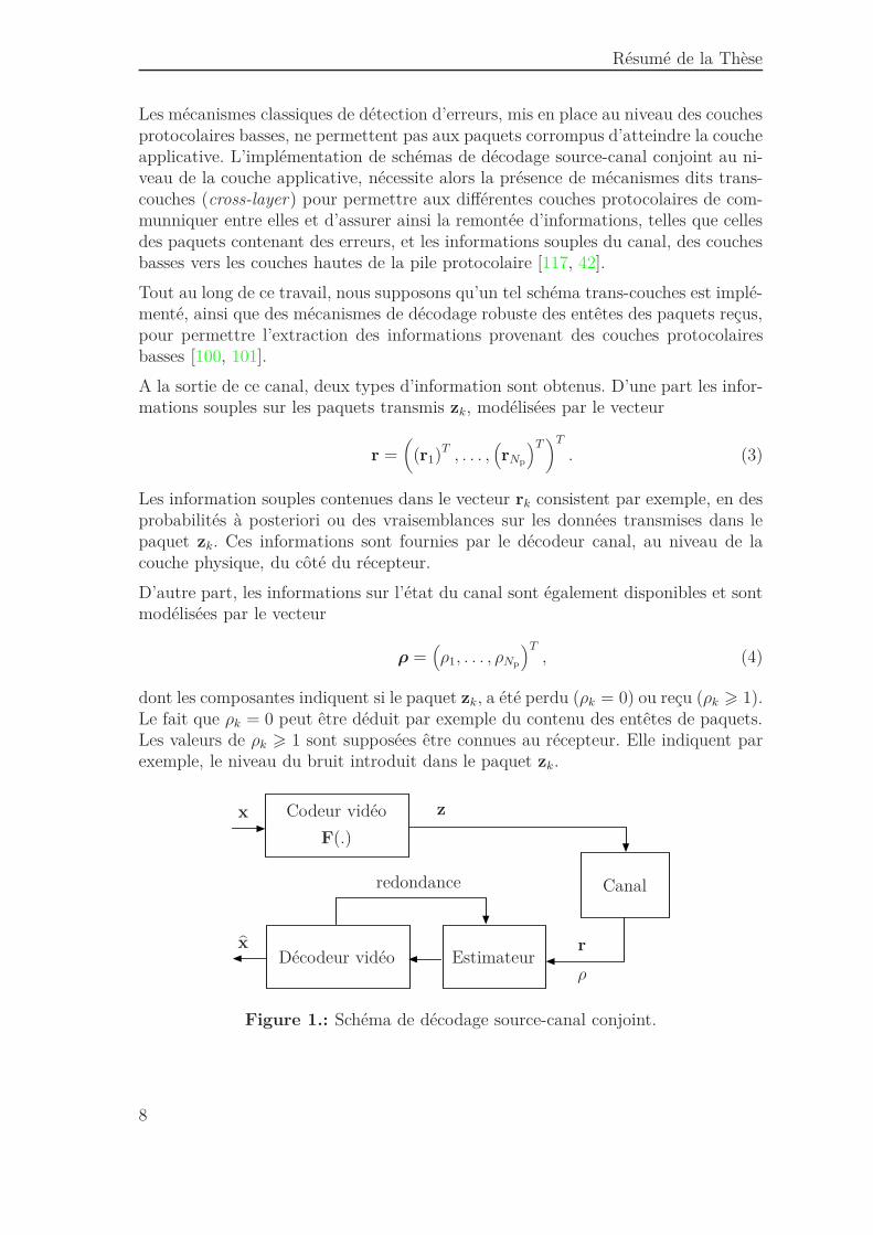
Vidwav est un codeur scalable par ondelettes 3D utilisant un filtrage temporel com-pensé en mouvement (FTCM) [126]. Dans ce travail, le schéma t + 2D, illustré parla Figure 2 est considéré. Le FTCM est d’abord opéré sur les trames de la séquencevidéo x, placée en entrée. Ensuite, la transformation spatiale par ondelettes est ef-fectuée sur les sous-bandes temporelles générées. Les sous-bandes spatio-temporellesobtenues sont alors divisées en Nb blocs 3D bk, k = 1, . . . , Nb qui sont ensuite codés,indépendamment les uns des autres, à l’aide du codeur entropique 3D-ESCOT [71].
Transformée
Information adjaçante
spatialePaquets
Séquence vidéo
Codage
entropique PaquétisationFTCM
Estimation de
mouvement
Vecteurs de mouvement
Figure 2.: Schéma en blocs de Viwav.
Codage entropique
Pour chaque bloc 3D bk, l’algorithme 3D-ESCOT opère un codage arithmétiquepar plan de bits, avec adaptation de contexte. Un train binaire emboîté pk est alorsgénéré. Il est formé par différents segments, résultant chacun d’une passe de codagepar plan de bits [71]. De plus, des informations relatives à pk sont obtenues, tellesque le nombre de passes de codage nk considérées dans bk, la longueur en octects
10
de pk, etc. Ces informations sont enregistrées dans l’entête hk, associée au trainbinaire pk. Cette entête contient également d’autres informations, nécessaires pourle décodage du bloc bk, telles que l’indexe de la sous-bande spatio-temporelle ouencore les vecteurs de mouvement associés à bk.
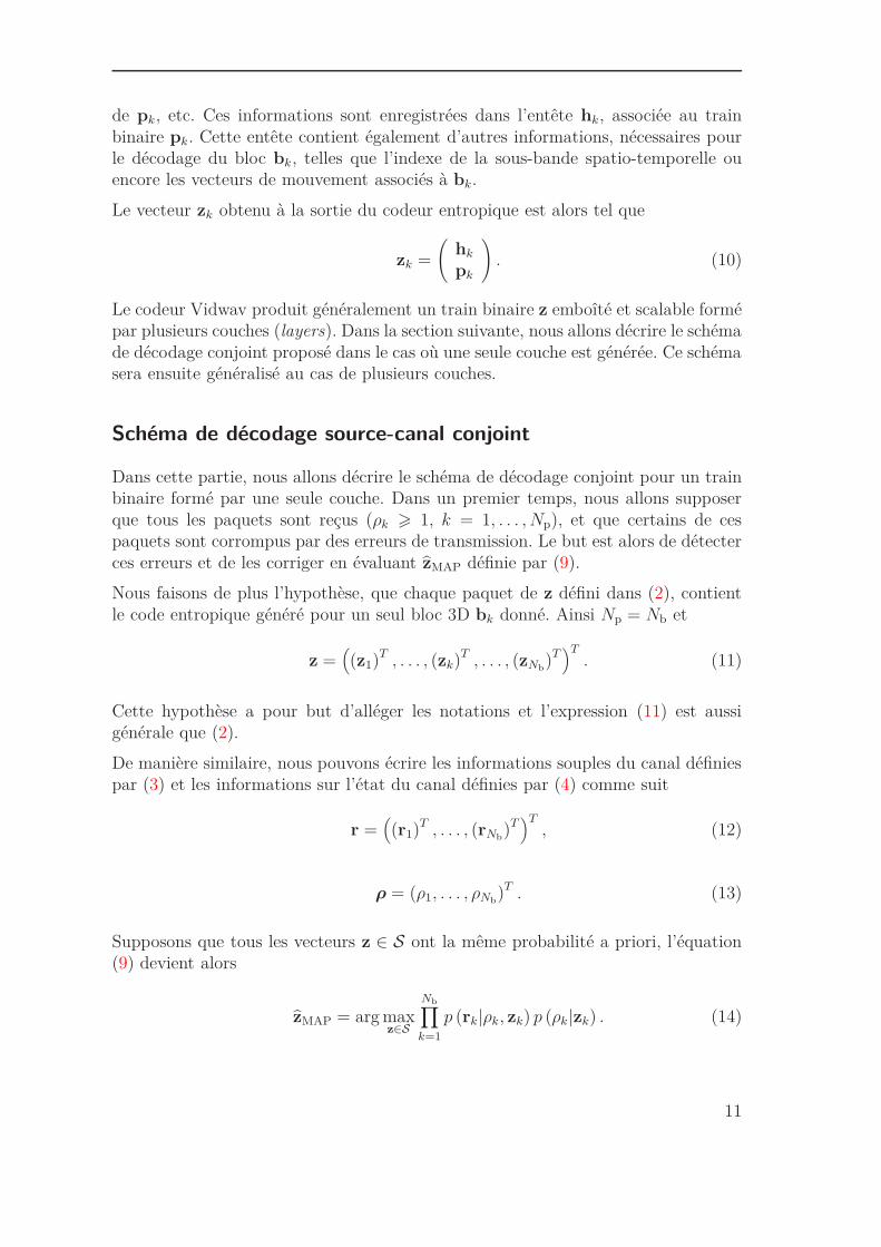
Le vecteur zk obtenu à la sortie du codeur entropique est alors tel que
zk =
(hk
pk
). (10)
Le codeur Vidwav produit généralement un train binaire z emboîté et scalable formépar plusieurs couches (layers). Dans la section suivante, nous allons décrire le schémade décodage conjoint proposé dans le cas où une seule couche est générée. Ce schémasera ensuite généralisé au cas de plusieurs couches.
Schéma de décodage source-canal conjoint
Dans cette partie, nous allons décrire le schéma de décodage conjoint pour un trainbinaire formé par une seule couche. Dans un premier temps, nous allons supposerque tous les paquets sont reçus (ρk > 1, k = 1, . . . , Np), et que certains de cespaquets sont corrompus par des erreurs de transmission. Le but est alors de détecterces erreurs et de les corriger en évaluant zMAP définie par (9).
Nous faisons de plus l’hypothèse, que chaque paquet de z défini dans (2), contientle code entropique généré pour un seul bloc 3D bk donné. Ainsi Np = Nb et
z =((z1)T , . . . , (zk)T , . . . , (zNb
)T)T
. (11)
Cette hypothèse a pour but d’alléger les notations et l’expression (11) est aussigénérale que (2).
De manière similaire, nous pouvons écrire les informations souples du canal définiespar (3) et les informations sur l’état du canal définies par (4) comme suit
r =((r1)
T , . . . , (rNb)T)T
, (12)
ρ = (ρ1, . . . , ρNb)T . (13)
Supposons que tous les vecteurs z ∈ S ont la même probabilité a priori, l’équation(9) devient alors
zMAP = arg maxz∈S
Nb∏
k=1
p (rk|ρk, zk) p (ρk|zk) . (14)
11
Résumé de la Thèse
Cette hypothèse est valide tant qu’aucun a priori sur x n’est disponible au décodeur.
Considérons les ensembles
Sk =
zk | ∃x, ∃ (z1, . . . , zk−1, zk+1, . . . , zNb
) ,
tq((z1)
T , . . . , (zk−1)T , (zk)T , (zk+1)
T , . . . , (zNb)T)T
= F (x)
, (15)
définis pour chaque k = 1, . . . , Nb. L’ensemble Sk contient tous les trains binaireszk pouvant résulter du codage entropique d’un bloc bk qui peut être obtenu à partird’une certaine séquence vidéo x à Nt trames. Nous avons alors
S ⊂ S1 × · · · × SNb. (16)
En utilisant (14) et (16), nous dérivons une estimée sous-optimale pour chaque trainbinaire zk
zk = arg maxzk∈Sk
p (rk|ρk, zk) p (ρk|zk) . (17)
L’estimée((z1)
T , . . . , (zNb)T)T
est alors une solution sous-optimale de (14) puisque
((zk)T , . . . , (zNb
)T)T
n’est pas forcément dans S, d’après (16).
Tests de syntaxe
Dans cette partie, nous allons décrire deux tests de syntaxe permettant de tenircompte de la redondance résiduelle laissée par Vidwav.
Comme nous l’avons mentionné précédemment, chaque zk est formé d’une entête hk
et d’un train binaire pk. Après la transmission de zk, le vecteur reçu
rk =((rk,h)T , (rk,p)T
)T
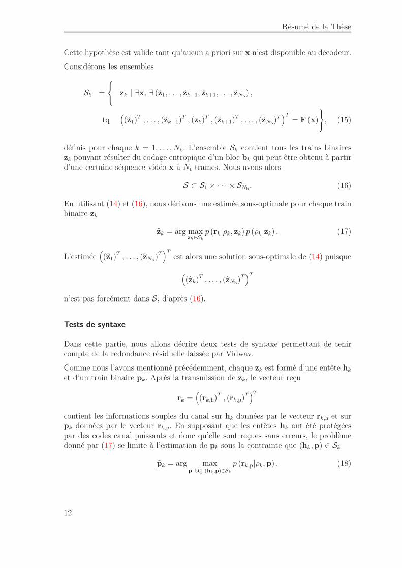
contient les informations souples du canal sur hk données par le vecteur rk,h et surpk données par le vecteur rk,p. En supposant que les entêtes hk ont été protégéespar des codes canal puissants et donc qu’elle sont reçues sans erreurs, le problèmedonné par (17) se limite à l’estimation de pk sous la contrainte que (hk, p) ∈ Sk
pk = arg maxp tq (hk,p)∈Sk
p (rk,p|ρk, p) . (18)
12
La valeur de ρk contient des informations sur les caractéristiques du canal commepar exemple son rapport signal à bruit (SNR), et permet d’évaluer la vraisemblancep(rk,p|ρk, p). L’espace de recherche de pk est l’ensemble de toutes les séquences p
pouvant être générées à partir d’une séquence vidéo x, et qui sont en même tempscohérentes avec les informations contenues dans hk.
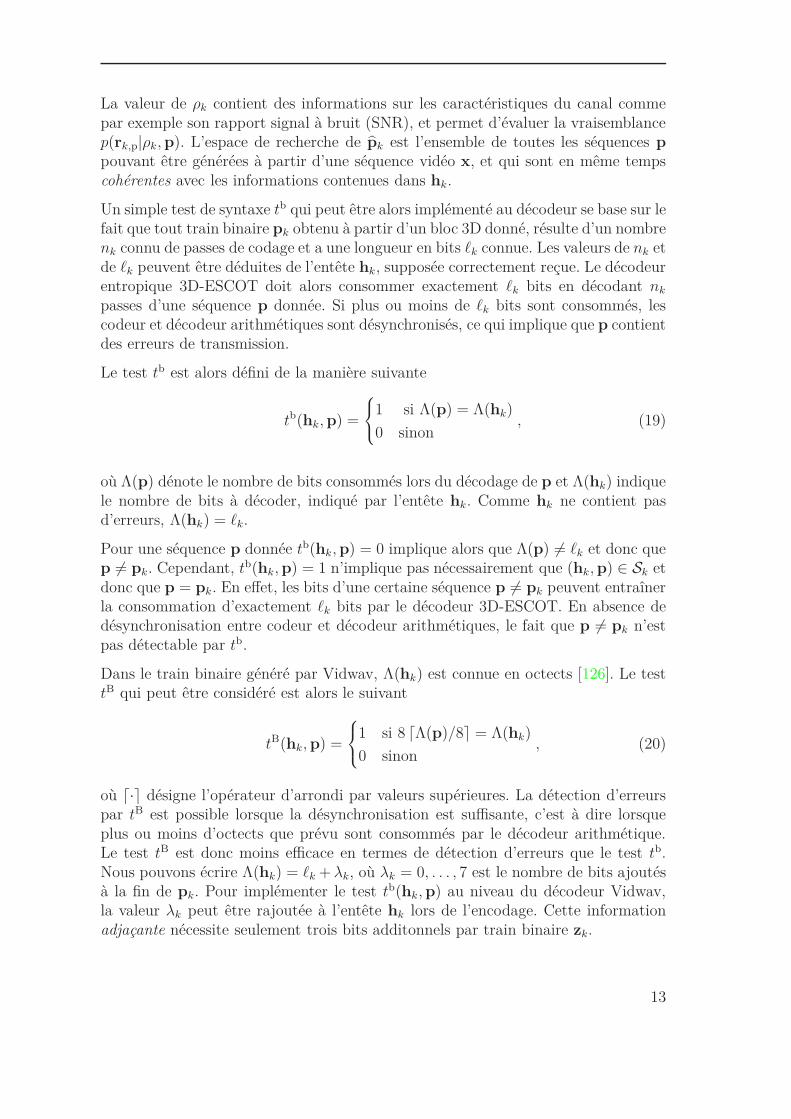
Un simple test de syntaxe tb qui peut être alors implémenté au décodeur se base sur lefait que tout train binaire pk obtenu à partir d’un bloc 3D donné, résulte d’un nombrenk connu de passes de codage et a une longueur en bits ℓk connue. Les valeurs de nk etde ℓk peuvent être déduites de l’entête hk, supposée correctement reçue. Le décodeurentropique 3D-ESCOT doit alors consommer exactement ℓk bits en décodant nk
passes d’une séquence p donnée. Si plus ou moins de ℓk bits sont consommés, lescodeur et décodeur arithmétiques sont désynchronisés, ce qui implique que p contientdes erreurs de transmission.
Le test tb est alors défini de la manière suivante
tb(hk, p) =
1 si Λ(p) = Λ(hk)
0 sinon, (19)
où Λ(p) dénote le nombre de bits consommés lors du décodage de p et Λ(hk) indiquele nombre de bits à décoder, indiqué par l’entête hk. Comme hk ne contient pasd’erreurs, Λ(hk) = ℓk.
Pour une séquence p donnée tb(hk, p) = 0 implique alors que Λ(p) 6= ℓk et donc quep 6= pk. Cependant, tb(hk, p) = 1 n’implique pas nécessairement que (hk, p) ∈ Sk etdonc que p = pk. En effet, les bits d’une certaine séquence p 6= pk peuvent entraînerla consommation d’exactement ℓk bits par le décodeur 3D-ESCOT. En absence dedésynchronisation entre codeur et décodeur arithmétiques, le fait que p 6= pk n’estpas détectable par tb.
Dans le train binaire généré par Vidwav, Λ(hk) est connue en octects [126]. Le testtB qui peut être considéré est alors le suivant
tB(hk, p) =
1 si 8 ⌈Λ(p)/8⌉ = Λ(hk)
0 sinon, (20)
où ⌈·⌉ désigne l’opérateur d’arrondi par valeurs supérieures. La détection d’erreurspar tB est possible lorsque la désynchronisation est suffisante, c’est à dire lorsqueplus ou moins d’octects que prévu sont consommés par le décodeur arithmétique.Le test tB est donc moins efficace en termes de détection d’erreurs que le test tb.Nous pouvons écrire Λ(hk) = ℓk + λk, où λk = 0, . . . , 7 est le nombre de bits ajoutésà la fin de pk. Pour implémenter le test tb(hk, p) au niveau du décodeur Vidwav,la valeur λk peut être rajoutée à l’entête hk lors de l’encodage. Cette informationadjaçante nécessite seulement trois bits additonnels par train binaire zk.
13
Résumé de la Thèse
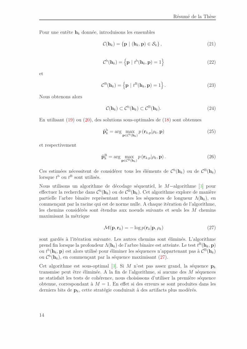
Pour une entête hk donnée, introduisons les ensembles
C(hk) = {p | (hk, p) ∈ Sk} , (21)
Cb(hk) ={
p | tb(hk, p) = 1}
(22)
et
CB(hk) ={
p | tB(hk, p) = 1}
. (23)
Nous obtenons alors
C(hk) ⊂ Cb(hk) ⊂ CB(hk). (24)
En utilisant (19) ou (20), des solutions sous-optimales de (18) sont obtenues
pbk = arg max
p∈Cb(hk)p (rk,p|ρk, p) (25)
et respectivement
pBk = arg max
p∈CB(hk)p (rk,p|ρk, p) . (26)
Ces estimées nécessitent de considérer tous les éléments de Cb(hk) ou de CB(hk)lorsque tb ou tB sont utilisés.
Nous utilisons un algorithme de décodage séquentiel, le M−algorithme [3] poureffectuer la recherche dans Cb(hk) ou de CB(hk). Cet algorithme explore de manièrepartielle l’arbre binaire représentant toutes les séquences de longueur Λ(hk), encommençant par la racine qui est de norme nulle. A chaque itération de l’algorithme,les chemins considérés sont étendus aux noeuds suivants et seuls les M cheminsmaximisant la métrique
M(p, rk) = − log p(rk|p, ρk) (27)
sont gardés à l’itération suivante. Les autres chemins sont éliminés. L’algorithmeprend fin lorsque la profondeur Λ(hk) de l’arbre binaire est atteinte. Le test tB(hk, p)ou tb(hk, p) est alors utilisé pour éliminer les séquences n’appartenant pas à CB(hk)ou Cb(hk), en commençant par la séquence maximisant (27).
Cet algorithme est sous-optimal [3]. Si M n’est pas assez grand, la séquence pk
transmise peut être éliminée. A la fin de l’algorithme, si aucune des M séquencesne statisfait les tests de cohérence, nous choisissons d’utiliser la première séquenceobtenue, correspondant à M = 1. En effet si des erreurs se sont produites dans lesderniers bits de pk, cette stratégie conduirait à des artifacts plus modérés.
14
Résultats expérimentaux
9 9.5 10 10.5 11 11.5 1210
15
20
25
30
35
40
Channel SNR (dB)
Y−
PS
NR
(dB
)
Reference PSNR
JSC−NoSI, M=32
JSC−NoSI, M=8
JSC−NoSI, M=2
M=1, Non−robust decoder
9 9.5 10 10.5 11 11.5 1210
15
20
25
30
35
40
Channel SNR (dB)
Y−
PS
NR
(dB
)
Referece PSNR
JSC−SI, M=32
JSC−SI, M=8
JSC−SI, M=2
M=1, Non−robust decoder
(a) foreman.qcif, JSC-NoSI (b) foreman.qcif, JSC-SI
9 9.5 10 10.5 11 11.5 1212
15
18
21
24
27
30
Channel SNR (dB)
Y−
PS
NR
(dB
)
Reference PSNR
JSC−NoSI, M=64
JSC−NoSI, M=32
JSC−NoSI, M=8
JSC−NoSI, M=2
M=1, Non−robust decoder
9 9.5 10 10.5 11 11.5 1212
15
18
21
24
27
30
Channel SNR (dB)
Y−
PS
NR
(dB
)
Reference PSNR
JSC−SI, M=64
JSC−SI, M=32
JSC−SI, M=8
JSC−SI, M=2
M=1, Non−robust decoder
(c) mobile.cif, JSC-NoSI (d) mobile.cif, JSC-SI
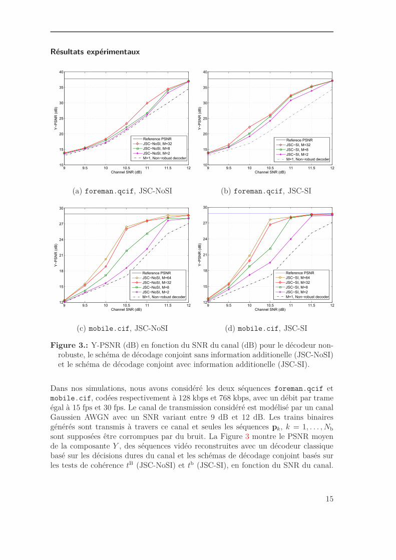
Figure 3.: Y-PSNR (dB) en fonction du SNR du canal (dB) pour le décodeur non-robuste, le schéma de décodage conjoint sans information additionelle (JSC-NoSI)et le schéma de décodage conjoint avec information additionelle (JSC-SI).
Dans nos simulations, nous avons considéré les deux séquences foreman.qcif etmobile.cif, codées respectivement à 128 kbps et 768 kbps, avec un débit par trameégal à 15 fps et 30 fps. Le canal de transmission considéré est modélisé par un canalGaussien AWGN avec un SNR variant entre 9 dB et 12 dB. Les trains binairesgénérés sont transmis à travers ce canal et seules les séquences pk, k = 1, . . . , Nb
sont supposées être corrompues par du bruit. La Figure 3 montre le PSNR moyende la composante Y , des séquences vidéo reconstruites avec un décodeur classiquebasé sur les décisions dures du canal et les schémas de décodage conjoint basés surles tests de cohérence tB (JSC-NoSI) et tb (JSC-SI), en fonction du SNR du canal.
15
Résumé de la Thèse
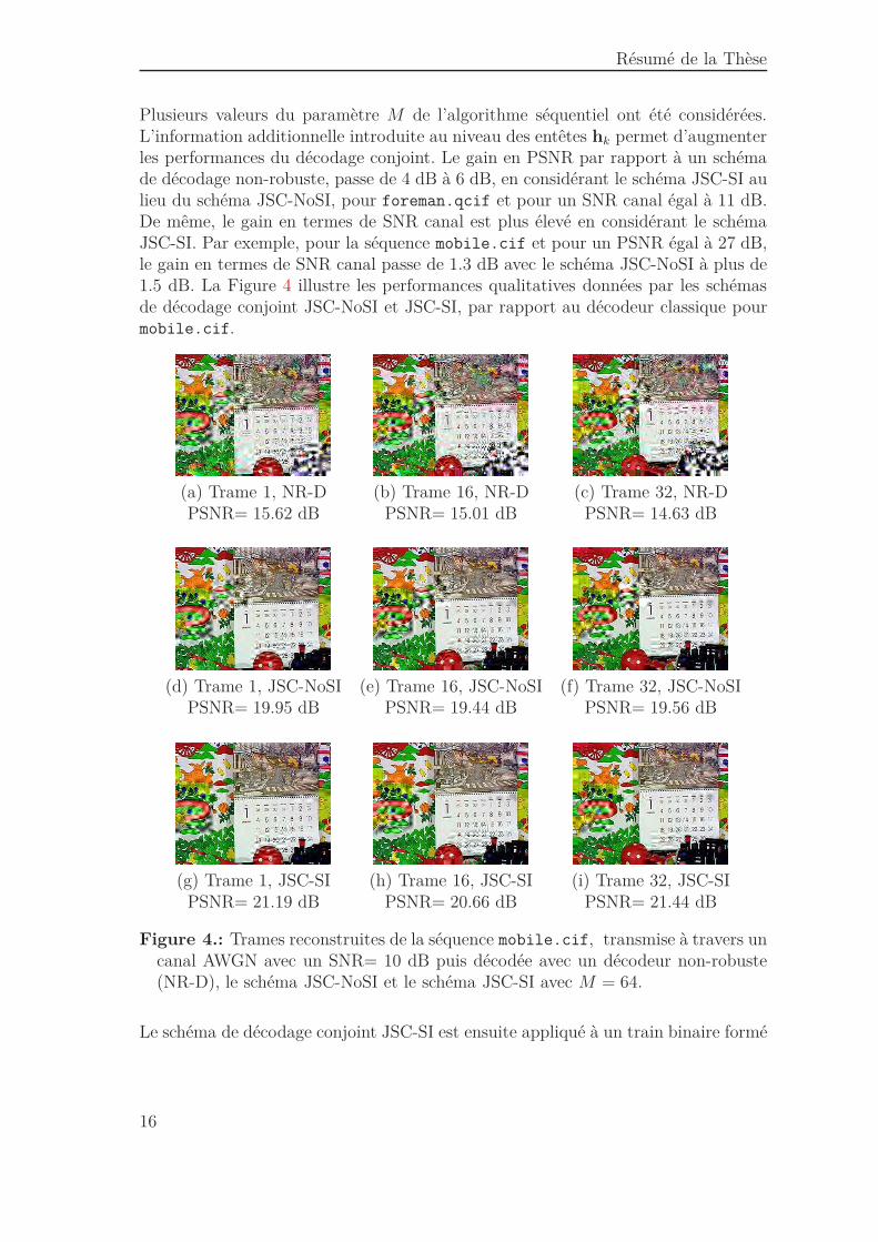
Plusieurs valeurs du paramètre M de l’algorithme séquentiel ont été considérées.L’information additionnelle introduite au niveau des entêtes hk permet d’augmenterles performances du décodage conjoint. Le gain en PSNR par rapport à un schémade décodage non-robuste, passe de 4 dB à 6 dB, en considérant le schéma JSC-SI aulieu du schéma JSC-NoSI, pour foreman.qcif et pour un SNR canal égal à 11 dB.De même, le gain en termes de SNR canal est plus élevé en considérant le schémaJSC-SI. Par exemple, pour la séquence mobile.cif et pour un PSNR égal à 27 dB,le gain en termes de SNR canal passe de 1.3 dB avec le schéma JSC-NoSI à plus de1.5 dB. La Figure 4 illustre les performances qualitatives données par les schémasde décodage conjoint JSC-NoSI et JSC-SI, par rapport au décodeur classique pourmobile.cif.
(a) Trame 1, NR-D (b) Trame 16, NR-D (c) Trame 32, NR-DPSNR= 15.62 dB PSNR= 15.01 dB PSNR= 14.63 dB
(d) Trame 1, JSC-NoSI (e) Trame 16, JSC-NoSI (f) Trame 32, JSC-NoSIPSNR= 19.95 dB PSNR= 19.44 dB PSNR= 19.56 dB
(g) Trame 1, JSC-SI (h) Trame 16, JSC-SI (i) Trame 32, JSC-SIPSNR= 21.19 dB PSNR= 20.66 dB PSNR= 21.44 dB
Figure 4.: Trames reconstruites de la séquence mobile.cif, transmise à travers uncanal AWGN avec un SNR= 10 dB puis décodée avec un décodeur non-robuste(NR-D), le schéma JSC-NoSI et le schéma JSC-SI avec M = 64.
Le schéma de décodage conjoint JSC-SI est ensuite appliqué à un train binaire formé
16
par plusieurs couches. Dans ce cas, chaque séquence pk, k = 1, . . . , Nb est forméepar plusieurs segments comme suit
pk =((
p(1)k
)T, . . . ,
(p
(NL)k
)T)T
, (28)
où NL est le nombre de couches et p(m)k est le segment de pk inclu dans la couche
m = 1, . . . , NL. Une entête h(m)k est alors associée à ce segment. Cette entête contient
le nombre de passes de codage n(m)k dont résulte p
(m)k , ainsi que sa longueur ℓ
(m)k
en octects. Pour implémenter le test tb, nous ajoutons 3 bits supplémentaires àh
(m)k pour connaitre ℓ
(m)k au bit près. Le test tb est alors appliqué pour estimer
chaque segment p(m)k , en commençant par la première couche. Pour chaque couche
m = 1, . . . , NL, nous vérifions si∑m
i=1 ℓ(i)k bits ont été consommés par le décodeur
arithmétique. Si pour une couche donnée m = 2, . . . , NL, le M−algorithme, nedélivre aucune séquence candidate validant le test tb, les séquences p
(i)k , i > m
courante et suivantes sont considérées comme perdues et la reconstruction du blocbk s’effectue en décodant jusqu’à la couche m − 1.
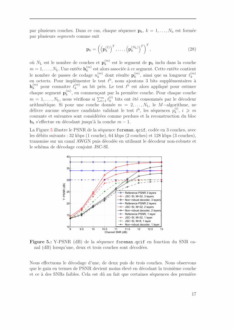
La Figure 5 illustre le PSNR de la séquence foreman.qcif, codée en 3 couches, avecles débits suivants : 32 kbps (1 couche), 64 kbps (2 couches) et 128 kbps (3 couches),transmise sur un canal AWGN puis décodée en utilisant le décodeur non-robuste etle schéma de décodage conjoint JSC-SI.
9 9.5 10 10.5 11 11.5 12 12.5 1310
15
20
25
30
35
40
Channel SNR (dB)
Y−
PS
NR
(dB
)
Reference PSNR 3 layers
JSC−SI, M=32, 3 layers
Non−robust decoder, 3 layers
Reference PSNR 2 layers
JSC−SI, M=32, 2 layers
Non−robust decoder, 2 layers
Reference PSNR, 1 layer
JSC−SI, M=32, 1 layer
JSC−SI, M=8, 1 layer
Non−robust decoder, 1 layer
Figure 5.: Y-PSNR (dB) de la séquence foreman.qcif en fonction du SNR ca-nal (dB) lorsqu’une, deux et trois couches sont décodées.
Nous effectuons le décodage d’une, de deux puis de trois couches. Nous observonsque le gain en termes de PSNR devient moins élevé en décodant la troisième coucheet ce à des SNRs faibles. Cela est dû au fait que certaines séquences des première
17
Résumé de la Thèse
et deuxième couches sont corrompues et ne sont pas détectées avec le test tb, ou nesont pas correctement estimées. Certaines séquences de la troisième couche, reçuessans erreurs, peuvent alors être détectées comme corrompues. Le schéma JSC-SIest alors moins efficace pour les couches hautes, dont l’impact est néanmoins plusfaible sur le décodage que les chouches plus basses. Notons toutefois, qu’à un mêmedébit de codage égal à 128 kbps, le schéma JSC-SI est plus efficace en considérantun train binaire à 3 couches au lieu d’un train binaire à une couche. Par exemple,pour M = 32 et pour un SNR canal égal à 10.5 dB, le gain en PSNR obtenu enconsidérant un train binaire à 3 couches est d’envrion 10 dB et de 5 dB avec untrain binaire à une seule couche.
Application au codage par descriptions multiples
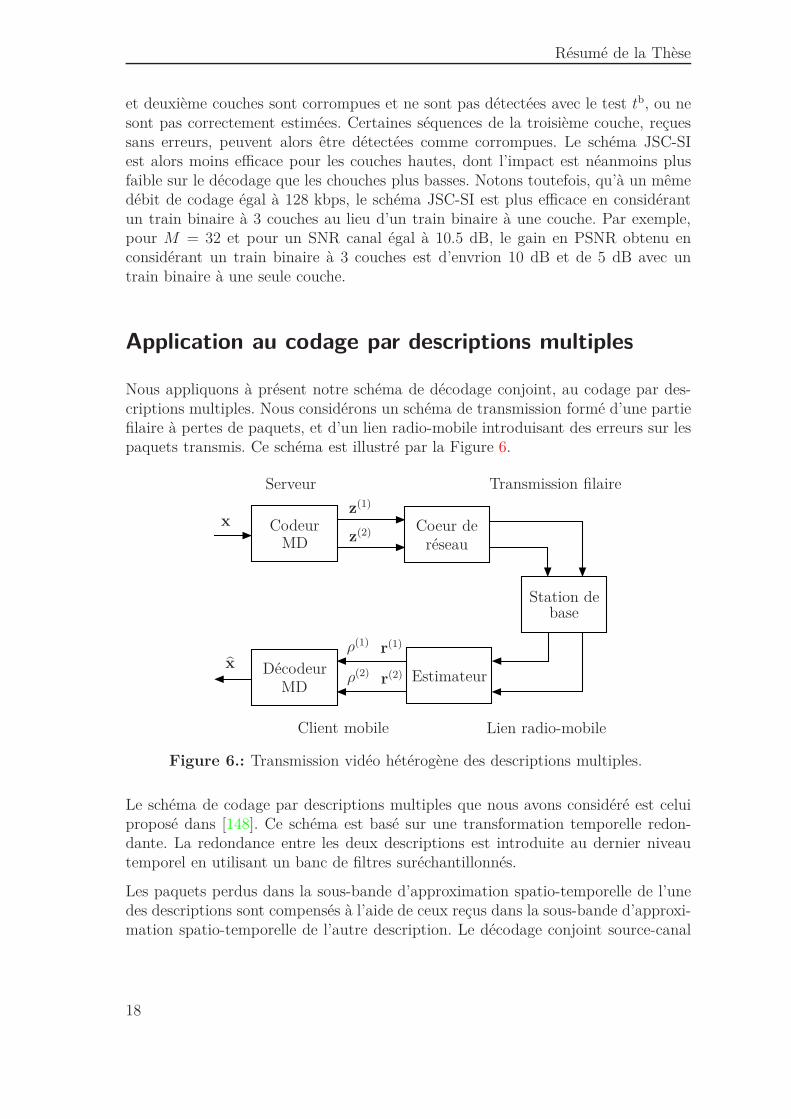
Nous appliquons à présent notre schéma de décodage conjoint, au codage par des-criptions multiples. Nous considérons un schéma de transmission formé d’une partiefilaire à pertes de paquets, et d’un lien radio-mobile introduisant des erreurs sur lespaquets transmis. Ce schéma est illustré par la Figure 6.
xz(1)
z(2)
r(1)
r(2)
ρ(1)
ρ(2)x
CodeurMD
Décodeur
Coeur deréseau
Station debase
MDEstimateur
Lien radio-mobile
Transmission filaire
Client mobile
Serveur
Figure 6.: Transmission vidéo hétérogène des descriptions multiples.
Le schéma de codage par descriptions multiples que nous avons considéré est celuiproposé dans [148]. Ce schéma est basé sur une transformation temporelle redon-dante. La redondance entre les deux descriptions est introduite au dernier niveautemporel en utilisant un banc de filtres suréchantillonnés.
Les paquets perdus dans la sous-bande d’approximation spatio-temporelle de l’unedes descriptions sont compensés à l’aide de ceux reçus dans la sous-bande d’approxi-mation spatio-temporelle de l’autre description. Le décodage conjoint source-canal
18
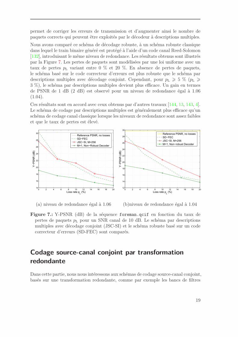
permet de corriger les erreurs de transmission et d’augmenter ainsi le nombre depaquets corrects qui peuvent être exploités par le décodeur à descriptions multiples.
Nous avons comparé ce schéma de décodage robuste, à un schéma robuste classiquedans lequel le train binaire généré est protégé à l’aide d’un code canal Reed-Solomon[132], introduisant le même niveau de redondance. Les résultats obtenus sont illustréspar la Figure 7. Les pertes de paquets sont modélisées par une loi uniforme avec untaux de pertes pL variant entre 0 % et 20 %. En absence de pertes de paquets,le schéma basé sur le code correcteur d’erreurs est plus robuste que le schéma pardescriptions multiples avec décodage conjoint. Cependant, pour pL > 5 % (pL >
3 %), le schéma par descriptions multiples devient plus efficace. Un gain en termesde PSNR de 1 dB (2 dB) est observé pour un niveau de redondance égal à 1.06(1.04).
Ces résultats sont en accord avec ceux obtenus par d’autres travaux [144, 13, 143, 4].Le schéma de codage par descriptions multiples est généralement plus efficace qu’unschéma de codage canal classique lorsque les niveaux de redondance sont assez faibleset que le taux de pertes est élevé.
0 2 4 6 8 10 12 14 16 18 2014
16
18
20
22
24
26
28
30
Loss rate pL
(%)
Y−
PS
NR
(dB
)
Reference PSNR, no losses
SD−FEC
JSC−SI, M=256
M=1, Non−Robust Decoder
0 2 4 6 8 10 12 14 16 18 2012
14
16
18
20
22
24
26
28
30
Loss rate pL
(%)
Y−
PS
NR
(dB
)
Reference PSNR, no losses
SD−FEC
JSC−SI, M=256
M=1, Non−robust Decoder
(a) niveau de redondance égal à 1.06 (b)niveau de redondance égal à 1.04
Figure 7.: Y-PSNR (dB) de la séquence foreman.qcif en fonction du taux depertes de paquets pL pour un SNR canal de 10 dB. Le schéma par descriptionsmultiples avec décodage conjoint (JSC-SI) et le schéma robuste basé sur un codecorrecteur d’erreurs (SD-FEC) sont comparés.
Codage source-canal conjoint par transformation
redondante
Dans cette partie, nous nous intéressons aux schémas de codage source-canal conjoint,basés sur une transformation redondante, comme par exemple les bancs de filtres
19
Résumé de la Thèse
suréchantillonnés [151]. Le but est alors d’exploiter la redondance structurée intro-duite, pour estimer de manière robuste la source, à partir des sorties bruitées ducanal de transmission.
Schéma de transmission
x y
r
H
x
z
y
Q
Q−1Estimation
Canal
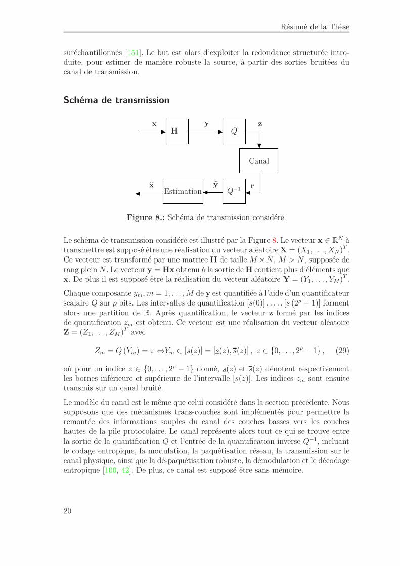
Figure 8.: Schéma de transmission considéré.
Le schéma de transmission considéré est illustré par la Figure 8. Le vecteur x ∈ RN àtransmettre est supposé être une réalisation du vecteur aléatoire X = (X1, . . . , XN)T .Ce vecteur est transformé par une matrice H de taille M × N , M > N , supposée derang plein N . Le vecteur y = Hx obtenu à la sortie de H contient plus d’éléments quex. De plus il est supposé être la réalisation du vecteur aléatoire Y = (Y1, . . . , YM)T .
Chaque composante ym, m = 1, . . . , M de y est quantifiée à l’aide d’un quantificateurscalaire Q sur ρ bits. Les intervalles de quantification [s(0)] , . . . , [s (2ρ − 1)] formentalors une partition de R. Après quantification, le vecteur z formé par les indicesde quantification zm est obtenu. Ce vecteur est une réalisation du vecteur aléatoireZ = (Z1, . . . , ZM)T avec
Zm = Q (Ym) = z ⇔Ym ∈ [s(z)] = [s(z), s(z)] , z ∈ {0, . . . , 2ρ − 1} , (29)
où pour un indice z ∈ {0, . . . , 2ρ − 1} donné, s(z) et s(z) dénotent respectivementles bornes inférieure et supérieure de l’intervalle [s(z)]. Les indices zm sont ensuitetransmis sur un canal bruité.
Le modèle du canal est le même que celui considéré dans la section précédente. Noussupposons que des mécanismes trans-couches sont implémentés pour permettre laremontée des informations souples du canal des couches basses vers les coucheshautes de la pile protocolaire. Le canal représente alors tout ce qui se trouve entrela sortie de la quantification Q et l’entrée de la quantification inverse Q−1, incluantle codage entropique, la modulation, la paquétisation réseau, la transmission sur lecanal physique, ainsi que la dé-paquétisation robuste, la démodulation et le décodageentropique [100, 42]. De plus, ce canal est supposé être sans mémoire.
20
A la sortie du canal, les informations souples r =((r1)
T , . . . , (rM)T)T
sur les bitstransmis sont obtenues. Le vecteur rm ∈ Rρ (or Cρ) est la sortie du canal associée àzm. L’effet du canal de transmission est alors décrit par la probabilité de transitionpR|Z (r|z) .
Le problème que nous considérons est celui d’estimer l’entrée x, à partir de r
xMAP = arg maxx∈RN
pX|R (x|r1:M) , (30)
où r1:M =((r1)
T , . . . , (rM)T)T
.
En utilisant la règle de Bayes, le fait que les intervalles de quantifications formentune parition de R et le fait que le canal considéré est sans mémoire, nous pouvonsmontrer que (30) peut être écrite de la manière suivante
xMAP = arg maxx∈RN
pX (x)M∏
m=1
pR|Z(rm|Q
(hT
mx))
. (31)
Pour une observation r1:M donnée, la fonction
f (x, r1:M) = pX (x)M∏
m=1
pR|Z(rm|Q
(hT
mx))
(32)
est continue par morceaux, dû à la quantification. La maximisation de f (x, r1:M)sur toutes les valeurs possibles de x ∈ RN n’est pas facile, surtout pour des valeursélevées de N .
Nous proposons dans ce qui suit deux méthodes d’estimation sous-optimales de (31),mais qui sont moins complexes.
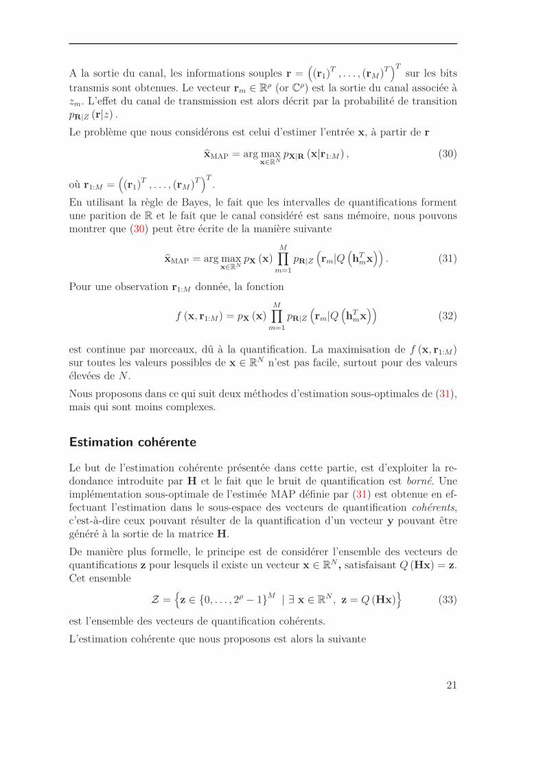
Estimation cohérente
Le but de l’estimation cohérente présentée dans cette partie, est d’exploiter la re-dondance introduite par H et le fait que le bruit de quantification est borné. Uneimplémentation sous-optimale de l’estimée MAP définie par (31) est obtenue en ef-fectuant l’estimation dans le sous-espace des vecteurs de quantification cohérents,c’est-à-dire ceux pouvant résulter de la quantification d’un vecteur y pouvant êtregénéré à la sortie de la matrice H.
De manière plus formelle, le principe est de considérer l’ensemble des vecteurs dequantifications z pour lesquels il existe un vecteur x ∈ RN , satisfaisant Q (Hx) = z.Cet ensemble
Z ={z ∈ {0, . . . , 2ρ − 1}M | ∃ x ∈ R
N , z = Q (Hx)}
(33)
est l’ensemble des vecteurs de quantification cohérents.
L’estimation cohérente que nous proposons est alors la suivante
21
Résumé de la Thèse
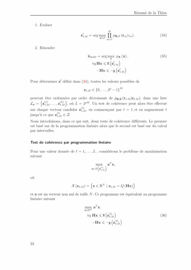
1. Evaluer
zf1:M = arg max
z∈Z
M∏
m=1
pR|Z (rm|zm) . (34)
2. Résoudre
xMAP = arg maxx
pX (x) . (35)
tq Hx 6 s(zf
1:M
)
−Hx 6 −s(zf
1:M
)
Pour déterminer zf défini dans (34), toutes les valeurs possibles de
z1:M ∈ {0, . . . , 2ρ − 1}M
peuvent être ordonnées par ordre décroissant de pR|Z (r1:M |z1:M), dans une liste
Lz ={z
(1)1:M , . . . , z
(L)1:M
}, où L = 2ρM . Un test de cohérence peut alors être effectué
sur chaque vecteur candidat z(ℓ)1:M , en commençant par ℓ = 1 et en augmentant ℓ
jusqu’à ce que z(ℓ)1:M ∈ Z.
Nous introduisons, dans ce qui suit, deux tests de cohérence différents. Le premierest basé sur de la programmation linéaire alors que le second est basé sur du calculpar intervalles.
Test de cohérence par programmation linéaire
Pour une valeur donnée de ℓ = 1, . . . , L , considérons le problème de maximisationsuivant
maxx∈X
(z
(ℓ)1:M
) aT x,
où
X (z1:M) ={x ∈ R
N | z1:M = Q (Hx)}
et a est un vecteur non nul de taille N . Ce programme est équivalent au programmelinéaire suivant
maxx∈RN
aT x.
tq Hx 6 s(z
(ℓ)1:M
)(36)
−Hx 6 −s(z
(ℓ)1:M
)
22
Si une solution x est trouvée pour (36), alors X (z1:M) 6= ∅ et z(ℓ) est cohérent.
Ainsi, pour déterminer zf, nous pouvons résoudre (36) pour différents z(ℓ)1:M , en com-
mençant par ℓ = 1 et en augmentant ℓ jusqu’à ce qu’une solution existe pour uncertain ℓf. Le vecteur zf est alors égal à z(ℓf).
Notons que nous aurions pu résoudre directement (35) avec z(ℓ)1:M , en commençant par
ℓ = 1 et en augmentant ℓ jusqu’à ce qu’une solution existe. Il est cependant moinscomplexe de résoudre (36) pour trouver zf. Le problème (35) est ensuite résolu aveczf.
Test de cohérence par calcul par intervalles
Une autre approche pour déterminer si un vecteur de quantification z appartient àZ, utilise la matrice à détection de parité P, associée à H. En effet, comme H estsupposée de rang plein N , il existe un matrice P de taille (M − N) × M et de rangplein (M − N) telle que
PHx = 0, ∀x ∈ RN . (37)
Nous avons alors
Py = 0 ⇐⇒ ∃ x ∈ RN tq y = Hx. (38)
En utilisant la définition (33) de l’ensemble Z et l’équivalance (38)
Py 6= 0 ⇐⇒ z = Q(y) /∈ Z (39)
Appliquons à présent l’équivalence (29) à toutes les composantess zm, m = 1, . . . , Md’un vecteur z donné
z = Q(y) ⇐⇒ y ∈ [s(z)] , (40)
où [s (z1:M)] =([
s(z
(ℓ)1
)], . . . ,
[s(z
(ℓ)M
)])Test une boîte, c’est-à-dire un vecteur d’in-
tervalles.
Le vecteur d’intervalles P [s (z1:M)] pouvant être évalué avec de simples opérationsd’additions et de multiplications sur des intervalles [73], est tel que
{Py, y ∈ [s (z1:M)]} ⊂ P [s (z1:M)] . (41)
En utilisant (39) et (41), nous pouvons alors écrire
0 /∈ P [s (z)] ⇒ z /∈ Z. (42)
23
Résumé de la Thèse
Le test (42) permet de prouver qu’un vecteur de quantification z n’est pas cohérent,mais il ne permet de prouver qu’un vecteur z est cohérent, puisque l’inclusion (41)est stricte.
Ce test est donc moins efficace que le test basé sur la programmation linéaire intro-duit par (36). Il a cependant une complexité entre O (M) et O (M (M − N)), ce quiest généralement moins complexe que de résoudre directement (36). Ce test permetd’éliminer rapidement les vecteurs de quantification z(ℓ), ℓ = 1, . . . , L qui ne sontpas cohérents. Les séquences jugées cohérentes par ce test peuvent alors être testéesà l’aide du programme linéaire (36).
Nous introduisons dans ce qui suit un petit exemple pour mettre en oeuvre les testsde cohérence introduits précédemment, et montrer l’intérêt d’utiliser le test basé surla matrice de parité avant celui qui est basé sur la programmation linéaire.
Exemple
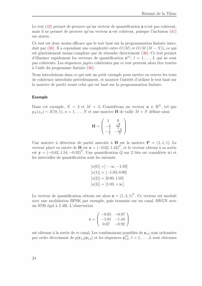
Dans cet exemple, N = 2 et M = 3. Considérons un vecteur x ∈ RN , tel quepX(xn) ∼ N (0, 1), n = 1, . . . , N et une matrice H de taille M × N définie ainsi
H =
1 0
−12
√3
2
−12
−√
32
Une matrice à détection de parité associée à H est la matrice P = (1, 1, 1). Levecteur placé en entrée de H est x = (−0.62, 1.42)T , et le vecteur obtenu à sa sortieest y = (−0.62, 1.54, −0.92)T . Une quantification Q sur 2 bits est considérée ici etles intervalles de quantification sont les suivants
[s(0)] =] − ∞, −1.03]
[s(1)] = [−1.03, 0.00]
[s(2)] = [0.00, 1.03]
[s(3)] = [1.03, +∞[.
Le vecteur de quantification obtenu est alors z = (1, 3, 1)T . Ce vecteur est moduléavec une modulation BPSK par exemple, puis transmis sur un canal AWGN avecun SNR égal à 2 dB. L’observation
r =
−0.65 −0.97−1.01 −1.440.07 −0.92
est obtenue à la sortie de ce canal. Les combinaisons possibles de z1:3 sont ordonnéespar ordre décroissant de p(r1:3|z1:3) et les séquences z
(ℓ)1:3, ℓ = 1, . . . , L sont obtenues
24
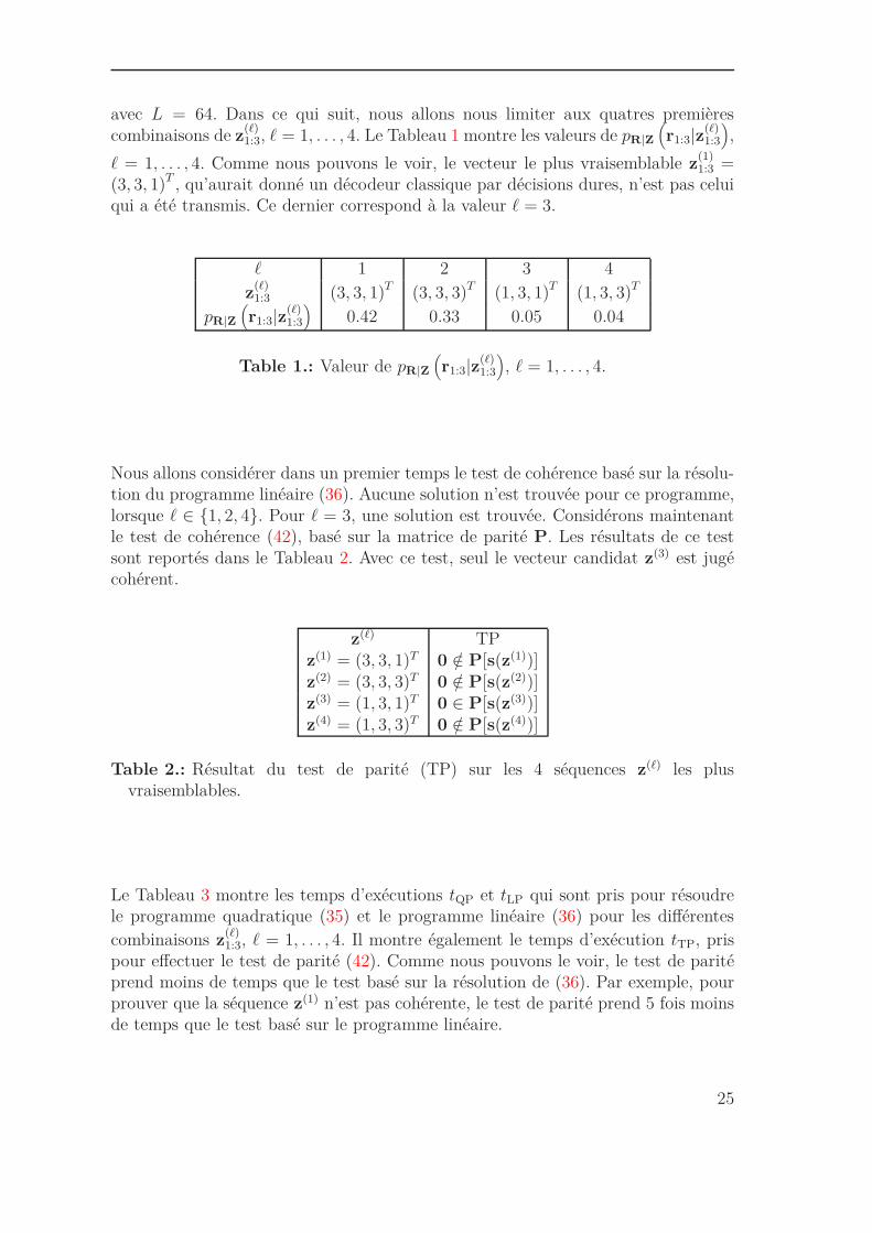
avec L = 64. Dans ce qui suit, nous allons nous limiter aux quatres premièrescombinaisons de z
(ℓ)1:3, ℓ = 1, . . . , 4. Le Tableau 1 montre les valeurs de pR|Z
(r1:3|z(ℓ)
1:3
),
ℓ = 1, . . . , 4. Comme nous pouvons le voir, le vecteur le plus vraisemblable z(1)1:3 =
(3, 3, 1)T , qu’aurait donné un décodeur classique par décisions dures, n’est pas celuiqui a été transmis. Ce dernier correspond à la valeur ℓ = 3.
ℓ 1 2 3 4
z(ℓ)1:3 (3, 3, 1)T (3, 3, 3)T (1, 3, 1)T (1, 3, 3)T
pR|Z(r1:3|z(ℓ)
1:3
)0.42 0.33 0.05 0.04
Table 1.: Valeur de pR|Z(r1:3|z(ℓ)
1:3
), ℓ = 1, . . . , 4.
Nous allons considérer dans un premier temps le test de cohérence basé sur la résolu-tion du programme linéaire (36). Aucune solution n’est trouvée pour ce programme,lorsque ℓ ∈ {1, 2, 4}. Pour ℓ = 3, une solution est trouvée. Considérons maintenantle test de cohérence (42), basé sur la matrice de parité P. Les résultats de ce testsont reportés dans le Tableau 2. Avec ce test, seul le vecteur candidat z(3) est jugécohérent.
z(ℓ) TPz(1) = (3, 3, 1)T 0 /∈ P[s(z(1))]z(2) = (3, 3, 3)T 0 /∈ P[s(z(2))]z(3) = (1, 3, 1)T 0 ∈ P[s(z(3))]z(4) = (1, 3, 3)T 0 /∈ P[s(z(4))]
Table 2.: Résultat du test de parité (TP) sur les 4 séquences z(ℓ) les plusvraisemblables.
Le Tableau 3 montre les temps d’exécutions tQP et tLP qui sont pris pour résoudrele programme quadratique (35) et le programme linéaire (36) pour les différentes
combinaisons z(ℓ)1:3, ℓ = 1, . . . , 4. Il montre également le temps d’exécution tTP, pris
pour effectuer le test de parité (42). Comme nous pouvons le voir, le test de paritéprend moins de temps que le test basé sur la résolution de (36). Par exemple, pourprouver que la séquence z(1) n’est pas cohérente, le test de parité prend 5 fois moinsde temps que le test basé sur le programme linéaire.
25
Résumé de la Thèse
ℓ 1 2 3 4
z(ℓ)1:3 (3, 3, 1)T (3, 3, 3)T (1, 3, 1)T (1, 3, 3)T
tQP(secondes) 0.0058 0.0066 0.0072 0.0164tLP(secondes) 0.0024 0.0030 0.0014 0.0022tTP(secondes) 0.00048 0.00048 0.00047 0.00047
Table 3.: Temps d’exécution tQP, tLP et tTP pris respectivement par (35), (36) et(42), pour z(ℓ), ℓ = 1, . . . , 4.
En sélectionnant zf = z(3) = (1, 3, 1)T pour résoudre (35), l’estimée xMAP = (−0.51, 0.89)T
est obtenue.
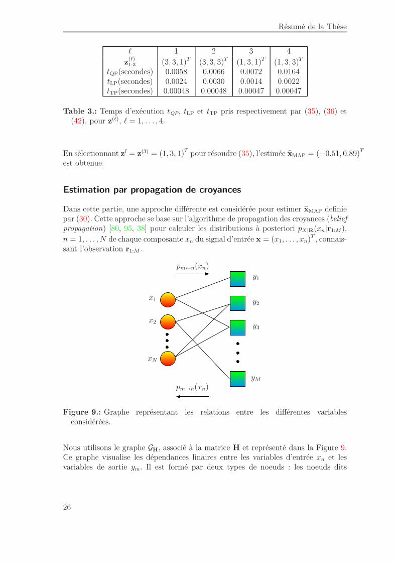
Estimation par propagation de croyances
Dans cette partie, une approche différente est considérée pour estimer xMAP definiepar (30). Cette approche se base sur l’algorithme de propagation des croyances (beliefpropagation) [80, 95, 38] pour calculer les distributions à posteriori pX|R(xn|r1:M),
n = 1, . . . , N de chaque composante xn du signal d’entrée x = (x1, . . . , xn)T , connais-sant l’observation r1:M .
x1
x2
xN
y1
y2
y3
yM
pm←n(xn)
pm→n(xn)
Figure 9.: Graphe représentant les relations entre les différentes variablesconsidérées.
Nous utilisons le graphe GH, associé à la matrice H et représenté dans la Figure 9.Ce graphe visualise les dépendances linaires entre les variables d’entrée xn et lesvariables de sortie ym. Il est formé par deux types de noeuds : les noeuds dits
26
variables n = 1, . . . , N et les noeuds dits facteurs m = 0, . . . , M . Ces différentsnoeuds s’échangent des messages (ou beliefs) le long des arêtes
EH {(n, m) ∈ {1, . . . , N} × {1, . . . , M} | H(m, n) 6= 0}du graphe GH.
Soit N (n) l’ensemble des noeuds facteurs connectés à un noeud variable n. Demanière similaire, soit N (m) l’ensemble des noeuds variables connectés à un noeudfacteur m.
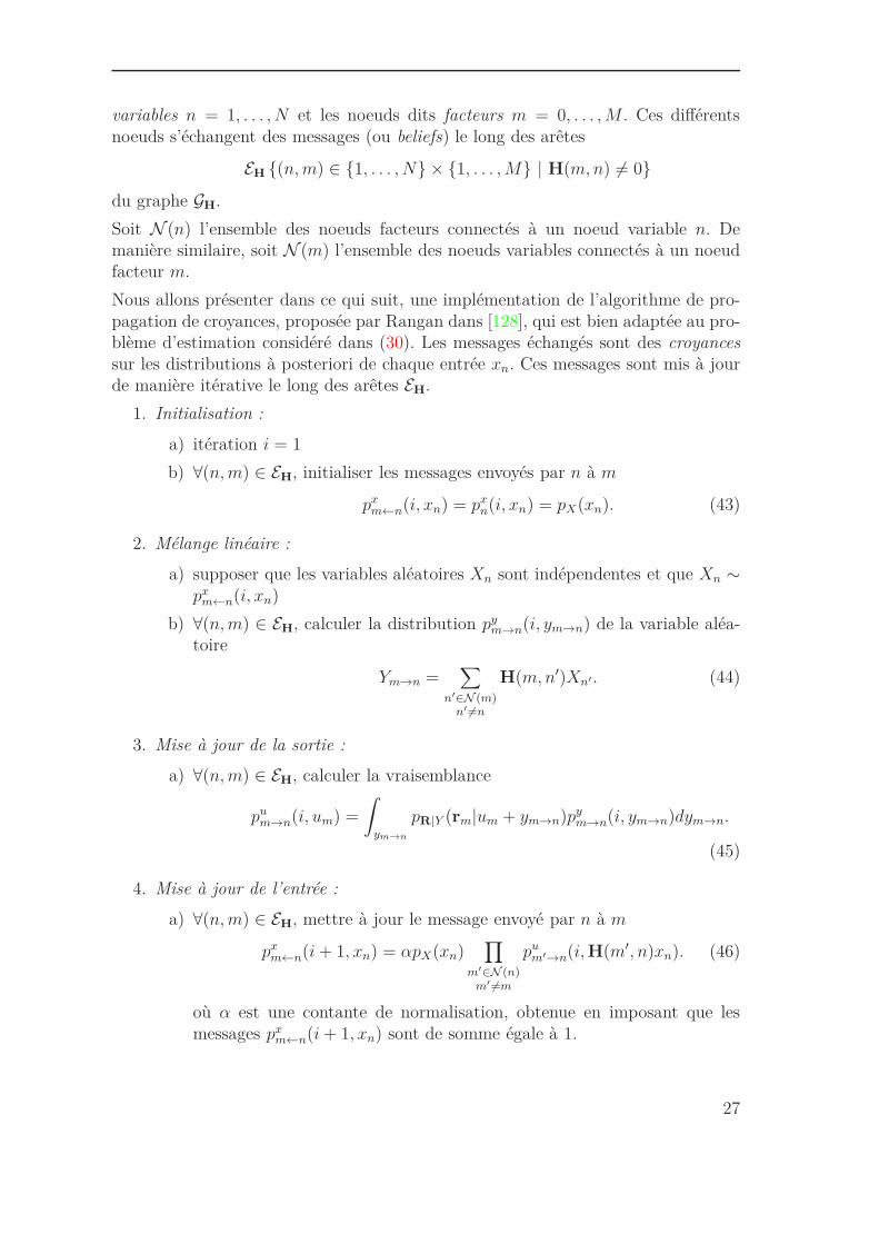
Nous allons présenter dans ce qui suit, une implémentation de l’algorithme de pro-pagation de croyances, proposée par Rangan dans [128], qui est bien adaptée au pro-blème d’estimation considéré dans (30). Les messages échangés sont des croyancessur les distributions à posteriori de chaque entrée xn. Ces messages sont mis à jourde manière itérative le long des arêtes EH.
1. Initialisation :
a) itération i = 1
b) ∀(n, m) ∈ EH, initialiser les messages envoyés par n à m
pxm←n(i, xn) = px
n(i, xn) = pX(xn). (43)
2. Mélange linéaire :
a) supposer que les variables aléatoires Xn sont indépendentes et que Xn ∼px
m←n(i, xn)
b) ∀(n, m) ∈ EH, calculer la distribution pym→n(i, ym→n) de la variable aléa-
toire
Ym→n =∑
n′∈N (m)n′ 6=n
H(m, n′)Xn′. (44)
3. Mise à jour de la sortie :
a) ∀(n, m) ∈ EH, calculer la vraisemblance
pum→n(i, um) =
ˆ
ym→n
pR|Y (rm|um + ym→n)pym→n(i, ym→n)dym→n.
(45)
4. Mise à jour de l’entrée :
a) ∀(n, m) ∈ EH, mettre à jour le message envoyé par n à m
pxm←n(i + 1, xn) = αpX(xn)
∏
m′∈N (n)m′ 6=m
pum′→n(i, H(m′, n)xn). (46)
où α est une contante de normalisation, obtenue en imposant que lesmessages px
m←n(i + 1, xn) sont de somme égale à 1.
27
Résumé de la Thèse
b) ∀n = 1, . . . , .N , mettre à jour les distributions
pxn(i + 1, xn) = βpX(xn)
∏
m∈N(n)
pum→n(i, H(m, n)xn). (47)
où β est une constante de normalisation, obtenue en imposant que lesmessages px
n(i + 1, xn) sont de somme égale à 1.
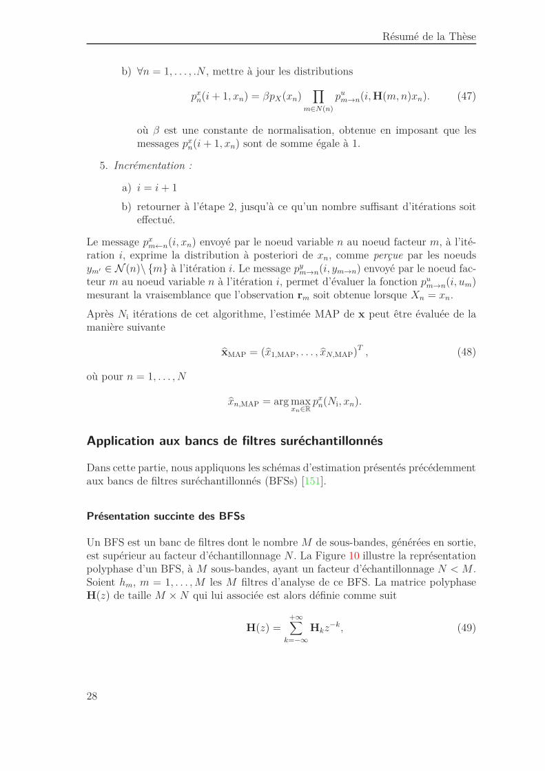
5. Incrémentation :
a) i = i + 1
b) retourner à l’étape 2, jusqu’à ce qu’un nombre suffisant d’itérations soiteffectué.
Le message pxm←n(i, xn) envoyé par le noeud variable n au noeud facteur m, à l’ité-
ration i, exprime la distribution à posteriori de xn, comme perçue par les noeudsym′ ∈ N (n)\ {m} à l’itération i. Le message py
m→n(i, ym→n) envoyé par le noeud fac-teur m au noeud variable n à l’itération i, permet d’évaluer la fonction pu
m→n(i, um)mesurant la vraisemblance que l’observation rm soit obtenue lorsque Xn = xn.
Après Ni itérations de cet algorithme, l’estimée MAP de x peut être évaluée de lamanière suivante
xMAP = (x1,MAP, . . . , xN,MAP)T , (48)
où pour n = 1, . . . , N
xn,MAP = arg maxxn∈R
pxn(Ni, xn).
Application aux bancs de filtres suréchantillonnés
Dans cette partie, nous appliquons les schémas d’estimation présentés précédemmentaux bancs de filtres suréchantillonnés (BFSs) [151].
Présentation succinte des BFSs
Un BFS est un banc de filtres dont le nombre M de sous-bandes, générées en sortie,est supérieur au facteur d’échantillonnage N . La Figure 10 illustre la représentationpolyphase d’un BFS, à M sous-bandes, ayant un facteur d’échantillonnage N < M .Soient hm, m = 1, . . . , M les M filtres d’analyse de ce BFS. La matrice polyphaseH(z) de taille M × N qui lui associée est alors définie comme suit
H(z) =+∞∑
k=−∞Hkz−k, (49)
28
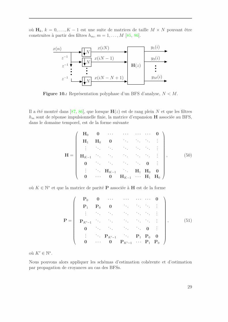
où Hk, k = 0, . . . , K − 1 est une suite de matrices de taille M × N pouvant êtreconstruites à partir des filtres hm, m = 1, . . . , M [85, 86].
g
x(n) x(iN)
x(iN − 1)
x(iN − N + 1)
N
N
N
H(z)
y1(i)
y2(i)
yM(i)
z−1
z−1
z−1
Figure 10.: Représentation polyphase d’un BFS d’analyse, N < M .
Il a été montré dans [87, 86], que lorsque H(z) est de rang plein N et que les filtreshm sont de réponse impulsionnelle finie, la matrice d’expansion H associée au BFS,dans le domaine temporel, est de la forme suivante
H =
H0 0 · · · · · · · · · · · · 0
H1 H0 0. . . . . . . . .
......
. . . . . . . . . . . . . . ....
HK−1. . . . . . . . . . . . . . .
...
0. . . . . . . . . . . . 0
......
. . . HK−1. . . H1 H0 0
0 · · · 0 HK−1 · · · H1 H0
, (50)
où K ∈ N∗ et que la matrice de parité P associée à H est de la forme
P =
P0 0 · · · · · · · · · · · · 0
P1 P0 0. . . . . . . . .
......
. . . . . . . . . . . . . . ....
PK ′−1. . . . . . . . . . . . . . .
...
0. . . . . . . . . . . . 0
......
. . . PK ′−1. . . P1 P0 0
0 · · · 0 PK ′−1 · · · P1 P0
, (51)
où K ′ ∈ N∗.
Nous pouvons alors appliquer les schémas d’estimation cohérente et d’estimationpar propagation de croyances au cas des BFSs.
29
Résumé de la Thèse
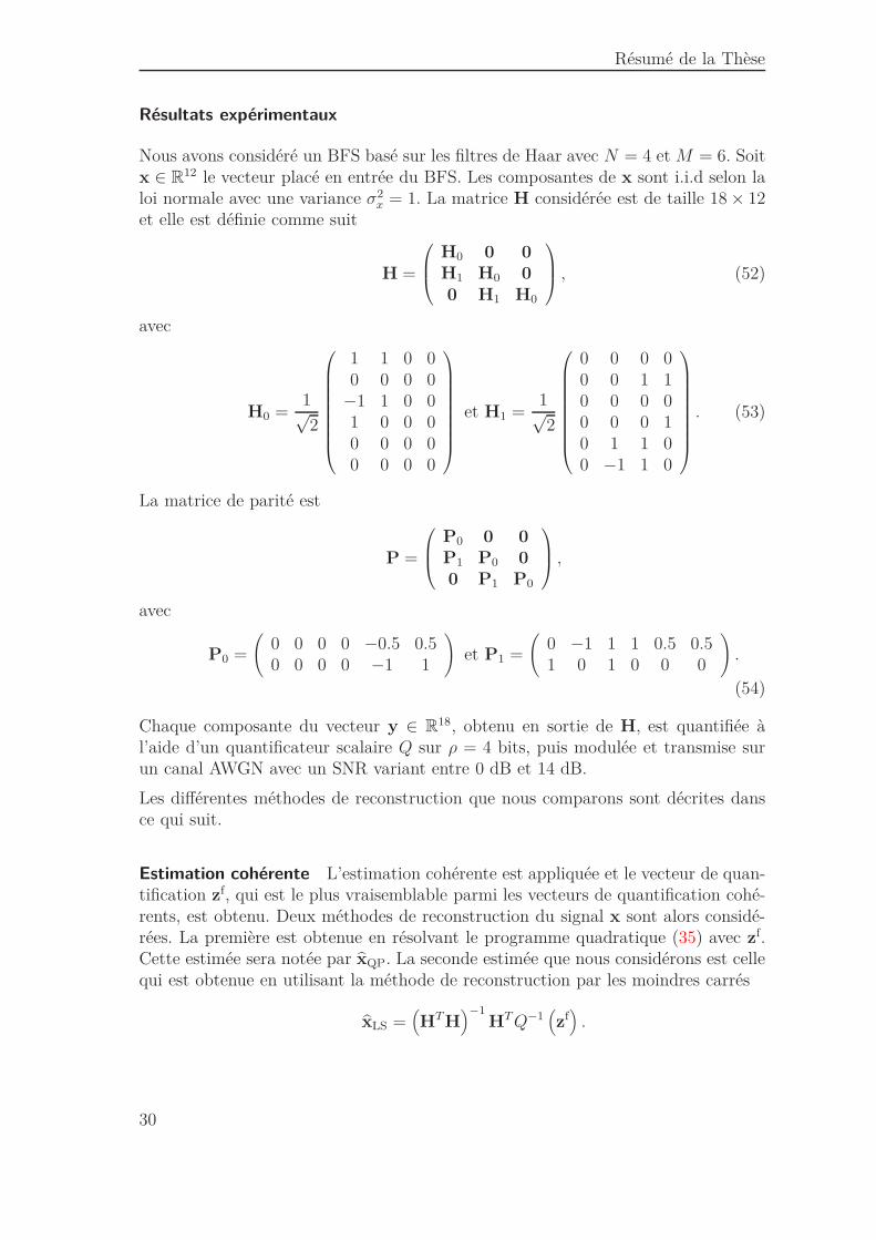
Résultats expérimentaux
Nous avons considéré un BFS basé sur les filtres de Haar avec N = 4 et M = 6. Soitx ∈ R
12 le vecteur placé en entrée du BFS. Les composantes de x sont i.i.d selon laloi normale avec une variance σ2
x = 1. La matrice H considérée est de taille 18 × 12et elle est définie comme suit
H =
H0 0 0
H1 H0 0
0 H1 H0
, (52)
avec
H0 =1√2
1 1 0 00 0 0 0
−1 1 0 01 0 0 00 0 0 00 0 0 0
et H1 =1√2
0 0 0 00 0 1 10 0 0 00 0 0 10 1 1 00 −1 1 0
. (53)
La matrice de parité est
P =
P0 0 0
P1 P0 0
0 P1 P0
,
avec
P0 =
(0 0 0 0 −0.5 0.50 0 0 0 −1 1
)et P1 =
(0 −1 1 1 0.5 0.51 0 1 0 0 0
).
(54)
Chaque composante du vecteur y ∈ R18, obtenu en sortie de H, est quantifiée àl’aide d’un quantificateur scalaire Q sur ρ = 4 bits, puis modulée et transmise surun canal AWGN avec un SNR variant entre 0 dB et 14 dB.
Les différentes méthodes de reconstruction que nous comparons sont décrites dansce qui suit.
Estimation cohérente L’estimation cohérente est appliquée et le vecteur de quan-tification zf, qui est le plus vraisemblable parmi les vecteurs de quantification cohé-rents, est obtenu. Deux méthodes de reconstruction du signal x sont alors considé-rées. La première est obtenue en résolvant le programme quadratique (35) avec zf.Cette estimée sera notée par xQP. La seconde estimée que nous considérons est cellequi est obtenue en utilisant la méthode de reconstruction par les moindres carrés
xLS =(HT H
)−1HT Q−1
(zf)
.
30
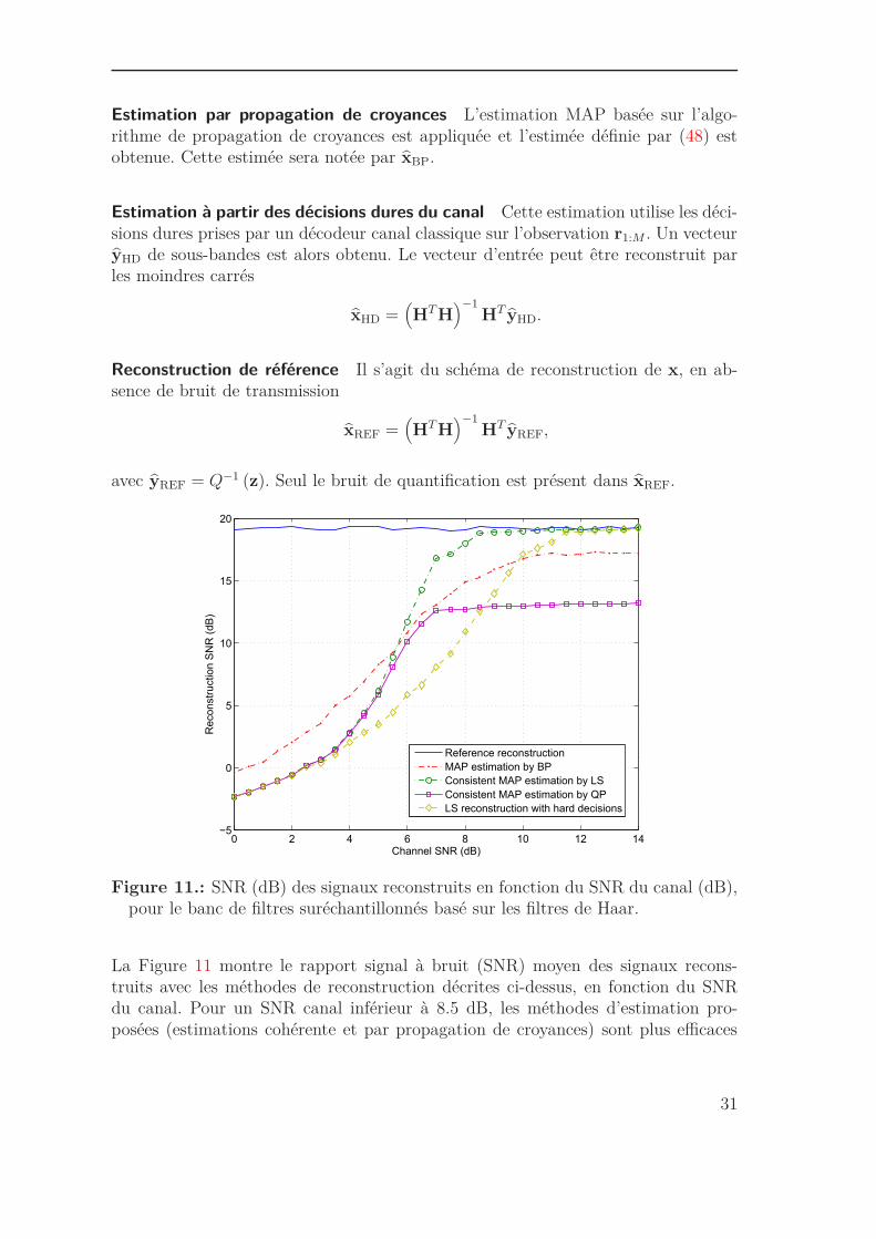
Estimation par propagation de croyances L’estimation MAP basée sur l’algo-rithme de propagation de croyances est appliquée et l’estimée définie par (48) estobtenue. Cette estimée sera notée par xBP.
Estimation à partir des décisions dures du canal Cette estimation utilise les déci-sions dures prises par un décodeur canal classique sur l’observation r1:M . Un vecteuryHD de sous-bandes est alors obtenu. Le vecteur d’entrée peut être reconstruit parles moindres carrés
xHD =(HT H
)−1HT yHD.
Reconstruction de référence Il s’agit du schéma de reconstruction de x, en ab-sence de bruit de transmission
xREF =(HT H
)−1HT yREF,
avec yREF = Q−1 (z). Seul le bruit de quantification est présent dans xREF.
0 2 4 6 8 10 12 14−5
0
5
10
15
20
Channel SNR (dB)
Reconstr
uction S
NR
(dB
)
Reference reconstruction
MAP estimation by BP
Consistent MAP estimation by LS
Consistent MAP estimation by QP
LS reconstruction with hard decisions
Figure 11.: SNR (dB) des signaux reconstruits en fonction du SNR du canal (dB),pour le banc de filtres suréchantillonnés basé sur les filtres de Haar.
La Figure 11 montre le rapport signal à bruit (SNR) moyen des signaux recons-truits avec les méthodes de reconstruction décrites ci-dessus, en fonction du SNRdu canal. Pour un SNR canal inférieur à 8.5 dB, les méthodes d’estimation pro-posées (estimations cohérente et par propagation de croyances) sont plus efficaces
31
Résumé de la Thèse
que l’approche de reconstruction classique basée sur les décisions dures du canal.Par exemple, pour un SNR canal de 4 dB, le gain obtenu en termes de SNR dereconstruction est d’environ 2 dB pour xQP ou xLS. Pour le même niveau de SNR,le gain en SNR de reconstruction est plus important en considérant l’estimation parpropagation de croyances et il est environ égal à 4 dB.
Pour un SNR canal inférieur à 4 dB, les reconstructions xQP et xLS, obtenues parestimation cohérente donnent les mêmes performances. Par contre, pour un niveaude SNR canal plus élevé, xLS devient plus efficaces que xQP et l’écart en SNR dereconstruction entre ces deux estimées se creuse lorsque le SNR du canal devient plusélevé, pour enfin se stabiliser à environ 6 dB. Ce comportenment est expliqué par lefait que pour des bruits de transmission très faibles, le vecteur de quantification leplus vraisemblable z∗ est celui qui a été transmis. La reconstruction par les moindrescarrés minimise dans ce cas le bruit de quantification, ce qui est généralement plusefficace que maximiser l’a priori pX(x) sur l’ensemble X (z∗).
L’estimation par propagation de croyances est plus efficace que l’estimation cohé-rente pour des niveaux faibles de SNR canal. Pour un SNR canal supérieur à 5.5 dB,xLS devient plus efficace que xBP et pour un SNR canal supérieur à 9.5 dB, xHD
est également plus efficace que xBP. Cela pourrait être expliqué par le fait que l’ob-tention de xBP se base sur des distributions de probabilités marginales au lieu dela distribution de probabilité jointe de x. De plus, l’algorithme de propagation decroyances peut ne pas converger en présence de cycles dans le graphe GH. Ces deuxeffets n’appraissent pas lorsque l’effet du bruit est très important.
Conclusions et perspectives
Dans cette thèse, nous nous sommes intéressés aux schémas de codage et de déco-dage conjoint source-canal des contenus multimédia. Nous avons montré commentla redondance laissée par le codeur vidéo pouvait être exploitée pour réaliser undécodage robuste des séquences transmises sur un lien radio-mobile bruité. Grâceau schéma de décodage conjoint proposé, le nombre de paquets corrompus est si-gnificativement réduit au prix d’une très légère augmentation du débit. Nous avonsappliqué ce schéma de décodage robuste à la transmission par descriptions mul-tiples sur une architecture mixte Internet et radio-mobile. Le décodage source-canalconjoint des paquets reçus permet de corriger les erreurs de transmission et d’aug-menter ainsi le nombre de paquets utilisés par le décodeur à descriptions multiplespour compenser les paquets perdus. L’efficacité de ce schéma a été démontrée parrapport à un schéma classique basé sur les décisions dures du canal et sur un codecorrecteur d’erreurs introduisant le même niveau de redondance.
Une deuxième partie de la thèse a été consacrée à l’étude de schémas de codagesource-canal conjoint basés sur une transformation redondante. Deux schémas d’es-timation ont été proposés. Dans le premier schéma, nous avons exploité la redon-dance structurée introduite et le caractère borné du bruit de quantification pour
32
construire un estimateur cohérent corrigeant les erreurs de transmission. Dans ledeuxième schéma d’estimation, nous avons appliqué l’algorithme de propagation decroyances pour évaluer les distributions a posteriori des composantes du signal d’en-trée, à partir des sorties bruitées du canal. Nous avons appliqué ces deux schémasaux bancs de filtres suréchantillonnés et constaté leur supériorité par rapport à unschéma de décodage classique basé sur les décisions dures du canal.
A l’issue de cette thèse, plusieurs pistes de recherche peuvent être envisagées. Pourconclure ce résumé, nous proposons d’en décrire quelques unes.
Le schéma de décodage robuste proposé pourrait être amélioré. Comme nous l’avonsmentionné, certaines erreurs de transmission sont indétectables par les tests de syn-taxe introduits. Afin d’augmenter les taux de détection et de correction d’erreurs,il est possible d’insérer des informations supplémentaires sur les paquets transmis,dans les enêtes correspondantes, comme par exemple le nombre de coefficients nonnuls dans une sous-bande spatio-temporelle, le CRC d’un bloc ou d’un ensemble deblocs, etc. Par ailleurs, ces informations supplémentaires pourraient être choisies etadaptées selon le degré d’importance des blocs à protéger. De manière similaire, uneoptimisation de la complexité du décodage en fonction de la sensitbilité des don-nées décodées, pourrait être envisagée. Le paramètre M de l’algorithme séquentielpeut être adapté à la couche décodée et à la sous-bande spatio-temporelle du bloccourant.
Le schéma de décodage robuste appliqué aux descriptions multiples a montré sonefficacité pour de faibles niveaux de redondance. En effet, les schémas classiquesde décodage basés sur des codes canal sont généralement plus robustes pour desniveaux de redondance élevés, et lorsque les conditions de transmission sont bienconnues. En se plaçant à des niveaux de redondance plus importants, les schémasclassiques combinent généralement des codes correcteurs d’erreurs et des codes canalà pertes de paquets, ce qui augmente nettement leurs performances. Il serait alorsintéressant de comparer de tels schémas à un schéma de codage par descriptionsmultiples plus redondant que celui que nous avons considéré, et dans lequel la re-dondance est introduite par exemple en duplicant la sous-bande d’approximationspatio-temporelle.
Pour faire le lien entre les schémas étudiés pendant cette thèse, une perspectiveà envisager est d’appliquer notre technique d’estimation cohérente au schéma dedécodage robuste par descriptions multiples. En effet, les deux descriptions sontgénérées à l’aide d’un banc de filtres suréchantillonné. Il est alors possible d’exploiterla redondance structurée introduite par ce banc de filtres et la redondance résiduellepour améliorer le décodage conjoint des deux descriptions. Certaines erreurs nondétectées par les tests de syntaxe utilisés, peuvent alors être détectées et corrigéesgrâce aux tests de cohérence introduits.
De manière plus générale, il reste un gros travail à faire pour optimiser les algo-rithmes d’estimation proposés afin de les appliquer à des bancs de filtres à matriced’analyse plus dense et à un facteur de suréchantillonnage plus faible. En particu-
33

Résumé de la Thèse
lier, l’algorithme d’estimation par propagation de croyances pourrait être amélioréen incluant les contraintes de parité dans le graphe représentant les dépendanceslinéaires entre les variables. De plus, afin de pouvoir appliquer ces deux schémasd’estimation au codage d’images et de vidéo, il semble nécessaire d’étudier leurscomportement et performances sur des bancs de filtres suréchantillonnés ayant unfort gain de codage.
34
1. Introduction
1.1. Motivation
The development of multimedia broadcasting and on-demand services for mobiledevices, such as tablets or smartphones, involves the transmission of contents overheterogeneous networks, consisting of mixed wired and wireless channels. To trans-mit multimedia contents over such best-effort networks, two main problems have tobe solved. First, due to bandwidth scarcity, data generated by multimedia sourceshave to be efficiently compressed. Second, the compressed bit streams have to bemade robust to the unavoidable transmission impairments. Current image and videocoders achieve high compression ratio. They are however very sensitive to transmis-sion errors and to packet lossses. Indeed, a single bit error or packet loss, affectingthe compressed bit stream, may have a detrimental effect on the reconstructed con-tent.
Conventional communication systems based on Shannon’s separation principle han-dle these issues by optimizing separately the source and the channel coders. Suchan optimization assumes that the source and the channel characteristics are per-fectly known and that the processed blocks are of infinite lengths. However, thesehypotheses cannot be met in practical situations, due to delivery delay, complexityconstraints and to unknown and time-varying transmission conditions. As a con-sequence, alternative coding schemes, namely the joint source-channel coding anddecoding techniques have been developed to address these issues. In these schemes,the source and the channel coders are jointly designed to enable the optimization ofthe communication system resources when there are stringent delay and complexityconstraints, and to increase the robustness of multimedia contents transmitted overunreliable networks.
The work conducted during this thesis fits into this category and aims at providingefficient joint-source channel coding and decoding techniques to ensure a robustmultimedia transmission. The targeted applications are the real-time and mobileapplications, in which the retransmission of damaged or lost data is not allowed.
We start by showing how the residual redundancy left by video coders, and wastedby classical separate source-channel decoders, can be exploited to design a joint
35
Chapter 1 Introduction
source-channel decoder able to detect and correct the transmission errors. Corruptedpackets, which would be dropped in conventional communication schemes, are thencorrected. This decoding approach is further applied to multiple description videostreams transmitted over a mixed architecture consisting of a wired lossy part and awireless noisy part. The errors introduced by the wireless transmission are correctedby the joint-source channel decoder whereas the losses occurring during the wiredcommunication are compensated thanks to multiple description coding.
Another direction investigated in this thesis concerns the joint source-channel cod-ing schemes based on a redundant transform, such as oversampled filter banks. Suchschemes introduce some structured redundancy in the transmitted bit stream. Inthe presence of transmission errors, we show how this redundancy may be used toimprove the decoding performance by proposing two efficient estimation approaches.The first one exploits the linear dependencies between the output variables, jointlyto the bounded quantization noise, to perform a consistent estimation of the sourceoutcome. The second approach uses the belief propagation algorithm to estimatethe input signal via a message passing procedure along the graph representing thelinear dependencies between the variables. These two schemes are further appliedto estimate the input of an oversampled filter bank and their performance are com-pared.
1.2. Outline of the Thesis
This manuscript is organized as follows. In Chapter 2, we start by motivating theresort to joint source-channel coding and decoding approaches. We overview somerelevant existing methods and particularly focus on the approaches close to the oneswe propose, such as joint source-channel decoding, multiple description coding andsource coding schemes based on redundant transforms.
Our joint-source channel decoding scheme is described in Chapter 3. We start byformulating the estimation problem of a video bit stream transmitted over somenoisy channel. Then, we consider a particular wavelet video coder and identify apart of the residual redundancy it leaves. This allows us to build an efficient testdetecting the damaged parts of the bit stream as the ones which are not compliantwith the redundancy. Combined with a sequential decoding algorithm, we showhow this test is able to correct most of the transmission errors, with a manageablecomplexity.
An application of our joint source-channel decoder to multiple description codingschemes is described in Chapter 4, where we consider a general transmission chainconsisting of a packet-loss network followed by a noisy wireless channel. The ideabehind the use of multiple description coding is to mitigate the effects of packetlosses, while avoiding retransmission and reducing delays. We show how joint source-channel decoding significantly improves the performance of the multiple descriptiondecoder, by increasing the number of received error-free packets.
36
1.3 Summary of the Contributions
In Chapter 5, we focus on joint source-channel coding schemes based on a redun-dant linear transform. We address the problem of estimating a signal placed atthe input of such a transform, when its output is corrupted by some transmissionnoise. Then, we describe the consistent estimation scheme we propose and the es-timation approach based on belief propagation. We show how these two schemesfind an application in oversampled filter banks and in particular, how the consistentestimation technique may be iteratively implemented in this case.
Finally, conclusions and perspectives are drawn in Chapter 6.
The remainder of the manuscript provides a succinct presentation of the sum-product algorithm, from which the belief propagation algorithm we used is derived,in Appendix A. The oversampled filter banks are then briefly introduced in Ap-pendix B. An image denoising technique, based on adaptive lifting schemes andproposed during this thesis, is presented in Appendix C, as it is not directly relatedto the main topic of this work.
1.3. Summary of the Contributions
This thesis contains several original contributions, which are summarized in thesequel
• An efficient joint source-channel decoding scheme increasing the robustness ofvideo contents transmitted over noisy channels and presenting a manageablecomplexity.
• An improvement of an existent multiple description coding scheme, thanks tojoint source-channel decoding.
• A consistent estimation technique for joint source-channel coding schemes,based on a redundant linear transform and its iterative implementation adaptedto oversampled filter banks.
• An application of the belief propagation algorithm for estimating the input ofan oversampled filter bank from its noisy subbands.
37

2. Joint Source-Channel Coding andDecoding
2.1. Introduction
In video communication systems, the usage of heterogeneous and best effort networkshas become widespread. In such networks, the quality of service (bandwidth, lossesand errors rates, delay, etc.) required by video communication applications such ason-demand video streaming, is not always guaranteed. Data packets may be lostdue to traffic congestion or corrupted by impairments in physical channels.
The issues associated to video transmission are then twofold:
• Data delivered by the video encoders has to be efficiently compressed due tobandwidth scarcity.
• Compressed video bit streams have to be made robust to the unavoidabletransmission impairments.
Increasing the robustness of video content is a challenging problem and it raisesseveral issues.
The high compression efficiency reached by many encoders such as H.264/AVC [70]and Vidwav [126], makes the compressed video streams extremely sensitive to errorsoccurring during transmission. For example, due to spatial and temporal predic-tions, errors can rapidly propagate in time and space leading to the so called drifteffect. In a similar way, when using an entropy coder such as CAVLC [70] andCABAC [103], a single bit error is likely to cause a desynchronization between theencoder and the decoder making the following bits useless, even if they were correctlyreceived. This leads to an uncontrolled degradation of the whole video quality.
On the other hand, the characteristics of the transmission channel are generallyunknown and time-varying. This makes it difficult to tune efficiently a robust trans-mission scheme for a given video signal. Furthermore, a reliable transmission schemeover heterogeneous channels has to take into account the hierarchical nature of thedelivered video bit streams: scalability and robustness should be jointly consideredin order to design an efficient source and channel coding system that allows the
39
Chapter 2 Joint Source-Channel Coding and Decoding
video content to be transmitted and used at different resolutions and/or qualitylevels with respect to specific terminals and users preferences.
Finally, stringent delay and complexity constraints are often imposed by real-timevideo applications and have to be taken into account in the design of a communica-tion system.
A number of approaches have been proposed to ensure a robust video transmission:
1. A first group includes the approaches wherein the source and the channelcoders work separately, or in tandem, in order to make the delivered bit streamsmore robust to transmission losses and errors. These methods are referred toas the tandem-coding techniques.
2. A second group gathers the methods in which the source and the channelcoders are jointly designed to overcome transmission impairments. These areknown as the joint source channel coding and decoding techniques.
3. A last group contains the methods which act at the decoder side to concealthe impacts of unrecoverable and/or corrupted data, on the reconstructedsignals. These methods are known as error concealment techniques and theycan be jointly employed with the approaches in the first two groups in orderto increase the decoding quality.
Section 2.2 presents the first group of approaches, namely the tandem coding schemesand points out to its limitations. Then, Section 2.3 describes the principle of jointsource channel coding techniques. Two main approaches of this group are reviewedin Sections 2.4 and 2.5 since the contributions of this thesis fit into this category.Finally, some error concealment schemes are presented in Section 2.6.
2.2. Tandem Coding Techniques
The tandem coding techniques rely on Shannon’s separation theorem [141] statingthat source coder and channel coder can be optimized separately without introduc-ing any performance sacrifice for the overall communication system. In Shannon’stheory, the source and channel are assumed to be stationary with known character-istics. Moreover, the blocks are assumed to be of infinite lengths, which makes thedelay and the complexity grow to infinity. Under these hypothesis, the source codercan approach the optimal rate-distortion behavior and the channel can transmit thebit stream with a probability of error arbitrary small provided that its coding rateis below its capacity.
Usually in tandem coding techniques, the channel coder is first optimized with re-spect to the channel capacity to ensure a reliable transmission, then the source coderis optimally designed with the available source coding rate.
In the next section, a brief overview of the channel coding techniques is presented.
40
2.2 Tandem Coding Techniques
2.2.1. Channel Coding
Classical approaches for combating channel/network impairments consist in addingstructured redundancy to the compressed bit stream at the transmitter side. Thisredundancy may be introduced at the physical layer of the protocol stack usedto transmit the packetized content, by using bit-level Forward Error Correctioncodes (FEC) [93, 133], to combat transmission errors. Packet erasure codes, suchas Reed-Solomon codes [132], Fountain codes [19], or Raptor codes [142] may beintroduced at intermediate layers of the protocol stack to recover lost packets, asis the case, e.g., in Multimedia Broadcast/Multicast Services [74, 107]. In bothcases, the redundancy introduced results into an increased final bit rate. At thereceiver side, error detection mechanisms, such as Cyclic Redundancy Check (CRC)or checksums are employed to verify the efficiency of the channel decoding at physicallayer. If enough error-free packets are received, packet erasure codes may recoverthe missing packets, otherwise retransmission is requested using Automatic RepeatRequest (ARQ) [94] mechanisms, when the application is delay-tolerant.
2.2.2. Limitations of Tandem Systems
As previously mentioned, the separation principle inspired the development of tan-dem systems. It is assumed that an optimal source encoder removing all the sourceredundancy is followed by an optimal channel coder that corrects all the errors pro-vided that the coding rate is below the channel capacity. These assumptions canonly be met for idealized conditions, e.g., codes of infinite length, infinite delay andcomplexity, and do not hold in practical situations. For example, channel codesprocess blocks of finite lengths, for which the probability of error is not equal tozero. The separation principle does not provide any optimal algorithm to designsuch channel codes, and it does not address either the problem of designing optimalsource coders and decoders when the error probability is non-zero.
In practical communication situations, the characteristics of the transmission chan-nels are time-varying and the transmitted packets have different protection needs.Therefore, classical error correcting codes and packet erasure codes may be eitheroversized, leading to a waste of the available bandwidth, or not strong enough,resulting in residual transmission errors. Adaptation of these codes to the sourceand the channel conditions may be considered [67], which implies a communicationsystem in which the source and the channel coders are jointly designed. Moreover,the bit streams delivered by the source coder may still contain a certain amount ofredundancy and it appears as common sense to use this redundancy as a form ofchannel coding, at the receiver side. One may even consider to intentionally intro-duce some redundancy during source coding, to enhance the bit stream robustnessto transmission impairments, which may lead to removing or reducing the protectionintroduced by channel coder.
41
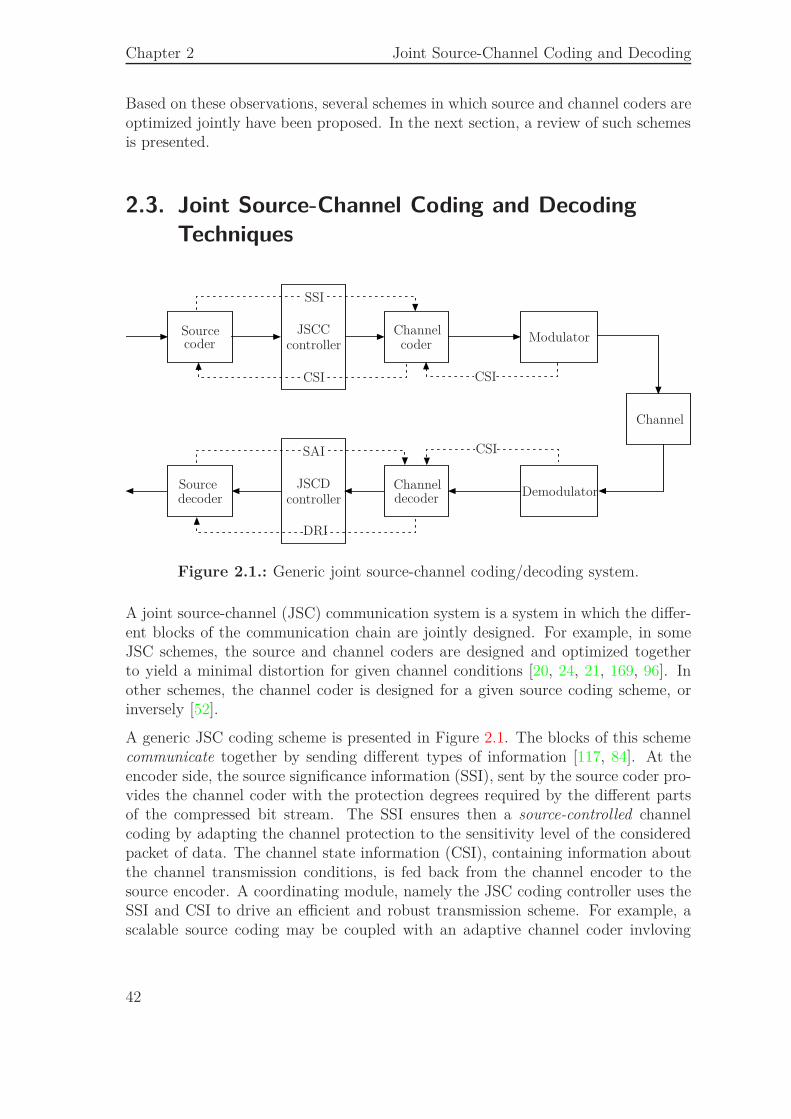
Chapter 2 Joint Source-Channel Coding and Decoding
Based on these observations, several schemes in which source and channel coders areoptimized jointly have been proposed. In the next section, a review of such schemesis presented.
2.3. Joint Source-Channel Coding and Decoding
Techniques
DRI
Source
Source
Channel
Channel
Channel
coder coder
decoder decoder
Modulator
Demodulator
JSCC
JSCD
controller
controller
SSI
CSICSI
CSISAI
Figure 2.1.: Generic joint source-channel coding/decoding system.
A joint source-channel (JSC) communication system is a system in which the differ-ent blocks of the communication chain are jointly designed. For example, in someJSC schemes, the source and channel coders are designed and optimized togetherto yield a minimal distortion for given channel conditions [20, 24, 21, 169, 96]. Inother schemes, the channel coder is designed for a given source coding scheme, orinversely [52].
A generic JSC coding scheme is presented in Figure 2.1. The blocks of this schemecommunicate together by sending different types of information [117, 84]. At theencoder side, the source significance information (SSI), sent by the source coder pro-vides the channel coder with the protection degrees required by the different partsof the compressed bit stream. The SSI ensures then a source-controlled channelcoding by adapting the channel protection to the sensitivity level of the consideredpacket of data. The channel state information (CSI), containing information aboutthe channel transmission conditions, is fed back from the channel encoder to thesource encoder. A coordinating module, namely the JSC coding controller uses theSSI and CSI to drive an efficient and robust transmission scheme. For example, ascalable source coding may be coupled with an adaptive channel coder invloving
42
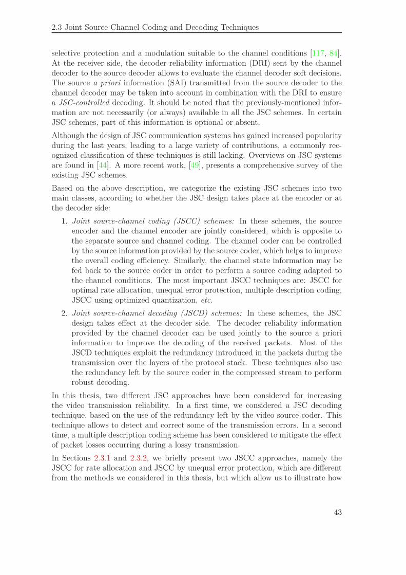
2.3 Joint Source-Channel Coding and Decoding Techniques
selective protection and a modulation suitable to the channel conditions [117, 84].At the receiver side, the decoder reliability information (DRI) sent by the channeldecoder to the source decoder allows to evaluate the channel decoder soft decisions.The source a priori information (SAI) transmitted from the source decoder to thechannel decoder may be taken into account in combination with the DRI to ensurea JSC-controlled decoding. It should be noted that the previously-mentioned infor-mation are not necessarily (or always) available in all the JSC schemes. In certainJSC schemes, part of this information is optional or absent.
Although the design of JSC communication systems has gained increased popularityduring the last years, leading to a large variety of contributions, a commonly rec-ognized classification of these techniques is still lacking. Overviews on JSC systemsare found in [44]. A more recent work, [49], presents a comprehensive survey of theexisting JSC schemes.
Based on the above description, we categorize the existing JSC schemes into twomain classes, according to whether the JSC design takes place at the encoder or atthe decoder side:
1. Joint source-channel coding (JSCC) schemes: In these schemes, the sourceencoder and the channel encoder are jointly considered, which is opposite tothe separate source and channel coding. The channel coder can be controlledby the source information provided by the source coder, which helps to improvethe overall coding efficiency. Similarly, the channel state information may befed back to the source coder in order to perform a source coding adapted tothe channel conditions. The most important JSCC techniques are: JSCC foroptimal rate allocation, unequal error protection, multiple description coding,JSCC using optimized quantization, etc.
2. Joint source-channel decoding (JSCD) schemes: In these schemes, the JSCdesign takes effect at the decoder side. The decoder reliability informationprovided by the channel decoder can be used jointly to the source a prioriinformation to improve the decoding of the received packets. Most of theJSCD techniques exploit the redundancy introduced in the packets during thetransmission over the layers of the protocol stack. These techniques also usethe redundancy left by the source coder in the compressed stream to performrobust decoding.
In this thesis, two different JSC approaches have been considered for increasingthe video transmission reliability. In a first time, we considered a JSC decodingtechnique, based on the use of the redundancy left by the video source coder. Thistechnique allows to detect and correct some of the transmission errors. In a secondtime, a multiple description coding scheme has been considered to mitigate the effectof packet losses occurring during a lossy transmission.
In Sections 2.3.1 and 2.3.2, we briefly present two JSCC approaches, namely theJSCC for rate allocation and JSCC by unequal error protection, which are differentfrom the methods we considered in this thesis, but which allow us to illustrate how
43

Chapter 2 Joint Source-Channel Coding and Decoding
the source and the channel coders may cooperate to yield a robust transmissionscheme. The two next sections, Sections 2.4 and 2.5 will be devoted to review themultiple description coding and JSCD techniques.
2.3.1. JSCC for Rate Allocation
The principal motivation of JSCC is to derive practical communication schemessuitable for realistic transmission situations which are usually subject to some con-straints, such as complexity and/or coding rate. The aim of this section is to presentthe JSCC schemes responding to the second type of constraints, namely the codingrate constraint, which we will refer to as the JSCC for rate allocation between thesource and the channel coders.
Unlike the tandem communication systems, in which the redundancy is removed bythe source coder and then re-introduced at the channel coder side, the JSCC-RAconsiders the source and the channel coders as a single coding block consuming acertain bit rate Rs + Rc, where Rs and Rc are the rates consumed by the sourceand the channel coders respectively. A high source coding rate Rs results in a lowsource distortion Ds, whereas a high channel coding rate Rc implies a strong errorprotection and correction capabilities and thus a weak channel distortion Dc.
The aim of JSCC for rate allocation is to determine, for a fixed transmission rate bud-get Rb, the optimal rate distribution (R∗s , R∗c) between the source and the channel,which minimizes the overall average end-to-end transmission distortion D = Ds+Dc.The basic idea behind this optimization problem is illustrated in Figure 2.2.
D
Rs
D∗0
D∗1
D∗2
R∗0R∗1R∗2
S0
S1
S2
Figure 2.2.: Illustration of a joint source-channel rate allocation problem.
Three different channel states S0, S1 and S2 are considered. Each channel state
44
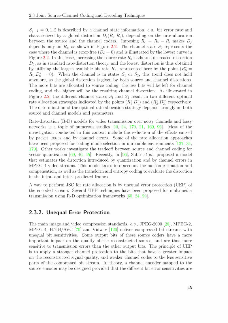
2.3 Joint Source-Channel Coding and Decoding Techniques
Sj, j = 0, 1, 2 is described by a channel state information, e.g. bit error rate andcharacterized by a global distortion Dj(Rs, Rc), depending on the rate allocationbetween the source and the channel coders. Imposing Rc = Rb − Rs makes Dj
depends only on Rs, as shown in Figure 2.2. The channel state S0 represents thecase where the channel is error-free (Dc = 0) and is illustrated by the lowest curve inFigure 2.2. In this case, increasing the source rate Rs leads to a decreased distortionD0, as in standard rate-distortion theory, and the lowest distortion is thus obtainedby utilizing the largest available bit rate Rb, represented here by the point (R∗0 =Rb,D∗0 = 0). When the channel is in states S1 or S2, this trend does not holdanymore, as the global distortion is given by both source and channel distortions.The more bits are allocated to source coding, the less bits will be left for channelcoding, and the higher will be the resulting channel distortion. As illustrated inFigure 2.2, the different channel states S1 and S2 result in two different optimalrate allocation strategies indicated by the points (R∗1,D∗1) and (R∗2,D∗2) respectively.The determination of the optimal rate allocation strategy depends strongly on bothsource and channel models and parameters.
Rate-distortion (R-D) models for video transmission over noisy channels and lossynetworks is a topic of numerous studies [20, 24, 170, 21, 169, 96]. Most of theinvestigation conducted in this context include the reduction of the effects causedby packet losses and by channel errors. Some of the rate allocation approacheshave been proposed for coding mode selection in unreliable environments [127, 34,170]. Other works investigate the tradeoff between source and channel coding forvector quantization [69, 46, 45]. Recently, in [96], Sabir et al. proposed a modelthat estimates the distortion introduced by quantization and by channel errors inMPEG-4 video streams. This model takes into account the motion estimation andcompensation, as well as the transform and entropy coding to evaluate the distortionin the intra- and inter- predicted frames.
A way to perform JSC for rate allocation is by unequal error protection (UEP) ofthe encoded stream. Several UEP techniques have been proposed for multimediatransmission using R-D optimization frameworks [65, 24, 20].
2.3.2. Unequal Error Protection
The main image and video compression standards, e.g., JPEG-2000 [28], MPEG-2,MPEG-4, H.264/AVC [70] and Vidwav [126] deliver compressed bit streams withunequal bit sensitivities. Some output bits of these source coders have a moreimportant impact on the quality of the reconstructed source, and are thus moresensitive to transmission errors than the other output bits. The principle of UEPis to apply a stronger channel protection to the bits that have a greater impacton the reconstructed signal quality, and weaker channel codes to the less sensitiveparts of the compressed bit stream. In theory, a channel encoder mapped to thesource encoder may be designed provided that the different bit error sensitivities are
45
Chapter 2 Joint Source-Channel Coding and Decoding
known for each bit position. However the channel coding adaptation to such a finegranularity is complex in practice.
Usually the implementation of practical UEP schemes involves the hierarchical bitstream representation which is achieved through scalability and data partitioning:
• Scalability is the capacity of a compressed bit stream to adapt itself to thetransmission conditions as well as to the terminals characteristics. An appro-priate partial decoding of the scalable bit stream allows to generate a ver-sion of the original signal, with a lower quality and/or a reduced resolution(spatial/temporal) level. For example, recent hybrid video codecs such asH.264/SVC [139] support scalability and generate hierarchical bit streams or-ganized into one base layer, which has the highest protection demand, and sev-eral refinement layers with different temporal/spatial resolutions and qualitylevels, which results in various error sensitivities. Wavelet-based video coders,such as Vidwav [126], offer an inherent spatio-temporal scalability thanks tothe multiresolution paradigm.
• Data partitioning consists in a hierarchical representation which separates themore critical parts of the bit stream (such as headers, motion vectors, lowfrequency DCT and wavelet coefficients, etc.) from the less important parts(such as higher frequency DCT and wavelet coefficients, etc.).
The channel encoder uses the knowledge of the source bit error sensitivities to per-form UEP. Particular error correction codes supporting rate compatibility have beenproposed to provide different protections according to the sensitivity level of thecontent to be transmitted. For example, rate compatible convolutional codes [67]and rate compatible Turbo codes [33] can easily obtain different channel code ratesthrough puncturing the same low-rate mother code. In [171], authors proposed anUEP technique for the 3D-SPIHT video coder. The 3D-SPIHT bit stream is firstdivided into blocks of the same length. Each block is supplemented with a CRCand then encoded using the a rate compatible convolutional code prior to its trans-mission through the channel. At the decoder side, a treillis decoder chooses thepath with the best metric satisfying the checksum equations. An automatic repeatrequest (ARQ) strategy is used when the decoder fails to find a satisfying solutionin a reasonable time. Another UEP approach has been proposed in [26] for theMPEG-4 video bit streams transmitted over error-prone wireless networks, whererate compatible convolutional coding is performed with rates chosen according tothe perceived importance of bits. In [12], authors introduced a semi-analytical modelthat estimates the distortion introduced in H.264/AVC bit streams. They studiedthe effects of error propagation in the next frames of the video sequence, caused byinter prediction as well as the distortion in intra-predicted frames. The proposedmodel is then used to evaluate the different protection levels in order to implementUEP to the coded video bit stream.
As mentioned in Section 2.3.1, JSCC for rate allocation and unequal error protec-tion may be considered together to jointly derive optimal source and channel coding
46
2.4 Multiple Description Coding
rates. In [20], Bystrom and Modestino considered a video transmission scheme inwhich the bit stream data is first classified according to its priority, then protectedby rate compatible convolutional codes before being transmitted over an additivewhite Gaussian noise (AWGN) channel. They proposed a method which optimallyallocates source and channel coding bits under a fixed constraint on the transmis-sion bandwidth. For a given video sequence, rate-distortion curves are constructedand used to determine the optimal rate and distortion values. Despite of its highaccuracy, this approach requires a significant amount of computations to constructthe rate-distortion curves for each video sequence which makes it infeasible for real-time video applications. Few years later, Bystrom and Stockhammer introducedin [21] a generic method for optimal source and channel rate allocation. To limitthe complexity of this problem, they used polynomial models to approximate therate-distortion surfaces for different video frames. These surfaces are then used withmodels of the channel bit error rates in order to allocate the source and the chan-nel coding rates between the different frames of a video sequence, with the goal ofminimizing the overall distortion under a constraint of the total rate. This schemewas successfully applied to a video sequence compressed with H.263 and channelcoded using rate-compatible systematic recursive convolutional codes. In [24], theauthors proposed an efficient method for allocating source and channel bits betweenthe subbands of the scalable video coder proposed in [146], such that the overalldistortion is minimized given the channel conditions and a total bit rate budget.The spatio-temporal subbands obtained by 3D subband coding are successively re-fined via layered quantization techniques and coded using a context-based arithmeticcoder. An UEP is then applied on the source bits using the rate compatible codes.
As discussed in this section, UEP techniques exploit the hierarchical manner inwhich the bit streams are usually organized in order to perform channel coding. Inparticular, when scalable or layered bit streams are considered, the highest level ofprotection is accorded to the more important base layer. Although this technique isrelatively simple and has proven to be efficient, it has the main drawback of beingadvantageous only if the base layer is received, otherwise the enhancement layersare undecodable even if correctly received. Usually, in such situations, the baselayer is retransmitted. However in applications which do not tolerate delay, such aretransmission is not possible.
An important family of JSCC techniques, namely the multiple description codingtechniques, has been proposed to overcome such situations, by creating several ver-sions of the signal, each of which being independently decodable. This is the topicof the next section.
2.4. Multiple Description Coding
Multiple description (MD) coding is a JSCC technique which enhances the robust-ness of a video delivery system. The principle of MD coding consists in represent-
47
Chapter 2 Joint Source-Channel Coding and Decoding
ing the original input signal by M correlated, but independently decodable signalscalled descriptions. These descriptions are assumed to be independently transmit-ted through different channels. Each transmission channel has a probability of notdelivering its description. The receiver is then formed by 2M − 1 decoders corre-sponding to all the decoding situations resulting from the reception of a subset ofthe transmitted descriptions. When the transmission of some of the descriptionsfails, the corresponding side decoder should be able to reconstruct the original sig-nal from the available descriptions with an acceptable quality. The reception of alldescriptions should allow signal reconstruction with the highest quality by using thecentral decoder. When descriptions are packetized, the robustness of MD codingschemes comes then from the fact that it is unlikely that the same packet of theencoded signal is affected in all descriptions.
The amount of redundancy introduced between the descriptions with respect to asingle description (SD) coding scheme is an important issue in MD coding, sincethere is a trade-off between this redundancy and the resulting distortion; the morethe descriptions are correlated the better will be the side decoding of a subset ofreceived descriptions but the worse will be the R-D performance of the centraldecoding when all the descriptions are available. Therefore, a great effort has beenspent on analyzing the performance achievable with MD coding schemes the early1980’s [165, 115, 43] and till more recently [157].
2.4.1. Theoretical Performance of MD Coding Schemes
The idea of MD coding was first investigated by the information theory commu-nity [165, 115, 43] as a source coding technique. Later, in the second half of the1990’s, with the emergence of best-effort packet-switched networks, e.g., Internet,MD coding has gained more popularity as an effective (source) coding strategy whichovercomes channel impairments and has been classified as a JSCC technique. Sincethen, a large variety of MD coders have been designed for speech, image and videocontents. A comprehensive review on MD coding theory is provided by Goyal et al.in [52].
Figure 2.3 illustrates an MD coding system with M = 2 descriptions and 3 decoders.The source, represented by a random vector X = (X1, . . . , XN)T is first encodedusing an MD encoder which generates two descriptions X(1) = F(1)(X) and X(2) =F(2)(X). These descriptions are further transmitted through two distinct channels.Let Ri, i = 1, 2 be the channel rate used to transmit X(i). The MD decoder handles2 different situations:
1. One of the channels fails to deliver its description. The side decoder associatedto the other channel is then used to decode the received description. Let
X(i) =(X
(i)1 , . . . , X
(i)N
)T, i = 1, 2 denote the reconstruction at the i-th side
decoder and Di the obtained distortion.
48
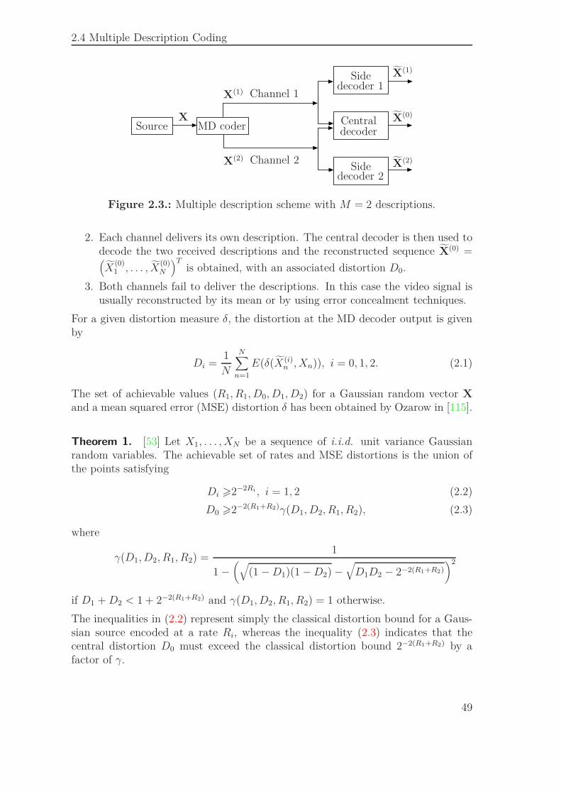
2.4 Multiple Description Coding
X
X(1)
X(2)
X(0)
X(1)
X(2)
Source
decoder 2Side
Sidedecoder 1
decoderCentralMD coder
Channel 1
Channel 2
Figure 2.3.: Multiple description scheme with M = 2 descriptions.
2. Each channel delivers its own description. The central decoder is then used todecode the two received descriptions and the reconstructed sequence X(0) =(X
(0)1 , . . . , X
(0)N
)Tis obtained, with an associated distortion D0.
3. Both channels fail to deliver the descriptions. In this case the video signal isusually reconstructed by its mean or by using error concealment techniques.
For a given distortion measure δ, the distortion at the MD decoder output is givenby
Di =1
N
N∑
n=1
E(δ(X(i)n , Xn)), i = 0, 1, 2. (2.1)
The set of achievable values (R1, R1, D0, D1, D2) for a Gaussian random vector X
and a mean squared error (MSE) distortion δ has been obtained by Ozarow in [115].
Theorem 1. [53] Let X1, . . . , XN be a sequence of i.i.d. unit variance Gaussianrandom variables. The achievable set of rates and MSE distortions is the union ofthe points satisfying
Di >2−2Ri , i = 1, 2 (2.2)
D0 >2−2(R1+R2)γ(D1, D2, R1, R2), (2.3)
where
γ(D1, D2, R1, R2) =1
1 −(√
(1 − D1)(1 − D2) −√
D1D2 − 2−2(R1+R2)
)2
if D1 + D2 < 1 + 2−2(R1+R2) and γ(D1, D2, R1, R2) = 1 otherwise.
The inequalities in (2.2) represent simply the classical distortion bound for a Gaus-sian source encoded at a rate Ri, whereas the inequality (2.3) indicates that thecentral distortion D0 must exceed the classical distortion bound 2−2(R1+R2) by afactor of γ.
49
Chapter 2 Joint Source-Channel Coding and Decoding
When the two descriptions are individually good, i.e., Di = 2−2Ri , i = 1, 2 thenD1 + D2 < 1 + 2−2(R1+R2) and (2.3) becomes
D0 > D1D21
1 − (1 − D1)(1 − D2). (2.4)
Since
D1D21
1 − (1 − D1)(1 − D2)=
11
D1+ 1
D2− 1
>min(D1, D2)
2,
the central distortion is only slightly lower than the lowest of the two side distortions,which means that relatively to the side decoding, the performance of the centraldecoding is poor. Inversely, assume that the central distortion is as low as possible,i.e., D0 = 2−2(R1+R2). Then γ = 1 and D1 + D2 6 1 + 2−2(R1+R2), which implies thatunless the rates Ri, i = 1, 2 are very low, the reconstruction of at least one of theside decoders is very poor. Therefore, one can not have at the same time optimalcentral and side distortions.
Usually the transmission channels are assumed to have the same rates and lossesprobabilities. Therefore, practical MD schemes generally consider the balanced case,where D1 ≈ D2 and R1 ≈ R2, to design the two descriptions.
2.4.2. Practical MD Coding Schemes
In practical MD coding systems, the main issue is how to create descriptions suchthat the resulting rates, distortions and complexity satisfy some conditions pre-scribed by the transmission constraints.
Two main directions have been investigated by the researchers to design MD systems.In the first direction pioneered by Vaishampayan [152], the redundancy is introducedafter the signal has been decorrelated, by diversifying the quantization to generatethe descriptions, e.g., MD by scalar quantization. The second direction that hasbeen studied is to introduce the redundancy during the signal transformation. Aredundant transform is used to generate two correlated descriptions. In this category,two main strategies are found in the literature depending on whether the introducedredundancy is statistical, e.g., MD by correlating transforms or deterministic, e.g.,MD by frame expansion. Each of these approaches is reviewed in the sequel.
2.4.2.1. MD by Scalar Quantization
Vaishampayan was the first to provide a practical MD coding framework in which thedescriptions are generated by scalar quantization followed by an index assignment
50
2.4 Multiple Description Coding
[152]. This technique, known as multiple description scalar quantization (MDSQ),consists in encoding a memoryless stationary zero-mean source X = {Xn}n∈Z usingdifferent scalar quantizers Qi, i = 1, 2 to generate the quantized descriptions X(i).
Each scalar quantizer is defined by a dictionary A(i) ={
a(i)k
}Ki
k=1and a partition
P(i) ={P
(i)k
}Ki
k=1of R
Qi : R → {1, . . . , Ki}x →Qi(x) = k if x ∈ P
(i)k . (2.5)
At the decoder side, three inverse quantizers Q−11 , Q−1
2 and Q−10 are considered, de-
pending on whether only X(1) or X(2) or both X(1) and X(2) are received. Theinverse quantizer Q−1
i : {1, . . . , Ki} → A(i), i = 1, 2 associates to each quan-tization index k ∈ {1, . . . , Ki} the corresponding element of the dictionary A(i):
Q−1i (k) = a
(i)k . Let I(0) be the subset of {1, . . . , K1} × {1, . . . , K2} containing all the
pairs of quantization indexes that may be generated at the output of Q1 and Q2.Then, the inverse quantizer Q−1
0 : I(0) → D(0) associates to each pair of receivedquantization indexes (k1, k2) ∈ I(0) the corresponding element of the dictionary
A(0) ={
a(0)k1k2
, (k1, k2) ∈ I(0)}
associated to Q−10 and constructed from the central
partition
P(0) ={P
(0)k1k2
, (k1, k2) ∈ I(0)}
, (2.6)
where P(0)k1k2
= P(1)k1
∩ P(2)k2
, (k1, k2) ∈ I(0). If a received pair (k1, k2) /∈ I(0), oneknows that a transmission error has occurred. In [152], the MDSQ is designedby minimizing the central distortion D0 subject to maximal admissible distortionsDi. Further developments of MDSQ include design of entropy-constrained MDSQ[154, 153] and extensions to vector quantization [140, 47, 155].
2.4.2.2. MD by Correlating Transforms
In classical source coding techniques, the transform step aims at decorrelating theinput signal. Usually, an orthogonal transform is used, e.g. the discrete cosinustransform (DCT) or the wavelet transform, to generate a sparse representation ofthe original signal. The problems associated to these representations are their highsensitivity to errors and erasures; since the symbols are decorrelated, the knowledgeof the correctly received symbols does not bring any information allowing to estimatethe lost or corrupted ones.
In Section 2.4.2.1, we have presented an MD approach which uses a scalar quantiza-tion producing two quantized symbols instead of one. The MD approach presentedin this section is totally different; the descriptions are obtained by the mean of acorrelating transform, which introduces some statistical redundancy between theindependent random variables. This MD approach is referred to as MD with corre-lating transform (MDCT).
51
Chapter 2 Joint Source-Channel Coding and Decoding
The statistical dependencies between the descriptions are used, at the decoder side,to improve the estimation of the missing coefficients within a description, from theones received in the other description. MDCT was firstly introduced by Wang,Orchard and Reibman for two variables [162, 164], then generalized by Goyal et al.to the multiple variable case [53]. This technique consists in transforming a blockof N centered, independent Gaussian random variables into a block of N correlatedvariables.
Consider the case where N = 2 and let X1 and X2 be two independent zero-meanGaussian random variables with variances σ2
1 and σ22 respectively. These two vari-
ables are linearly transformed to get two correlated variables X(1) and X(2)
(X(1)
X(2)
)= T
(X1
X2
), (2.7)
where T is a linear continuous-valued transform. It was shown in [53] that perform-ing the quantization after T leads to a higher distortion than when quantizationand transform are performed in the reverse order. This is due to the fact that T ,which intentionally introduces some redundancy between X(1) and X(2), is usuallya non-orthogonal transform, and thus the quantization cells obtained after apply-ing T are not square, which is suboptimal. The idea is then to perform first thequantization then apply a discrete-valued transform T to the obtained quantizationindexes. The discrete-valued transform T is constructed from the linear transformT which is assumed to be invertible of determinant 1. First, T is factorized intoa product of triangular matrices then T is computed by intermediate rounding ofthese triangular matrix factors. It is then shown that T is invertible. When both
X(1) and X(2) are received, the decoder uses the inverse of T to obtain(X1, X2
)T.
The distortion D0 is then equal to the quantization error. When only one of thedescriptions is received, for example X(1), the original vector (X1, X2)
T is estimated
using the least square estimator:(X1, X2
)T= E
[(X1, X2)T |X(1)
]. Neglecting the
quantization, a linear estimator of (X1, X2)T is obtained as
(X1
X2
)= T−1
(X(1)
X(2)
), (2.8)
where X(2) = E[X(2)|X(1)
].
For an equal probability of failure on the two channels and assuming that σ1 > σ2,Goyal has shown in [53] that the optimal continuous-valued transform T has theform
T =
(α (2α)−1
−α (2α)−1
), (2.9)
where α varies between√
12
σ2
σ1and +∞. The transforms defined in (2.9) lead to equal
rates and distortions R1 = R2 and D1 = D2. The parameter α allows to control the
52
2.4 Multiple Description Coding
amount of redundancy
ρ =1
2log
σ21α2 + σ2
2/(4α2)
σ1σ2(2.10)
introduced between X(1) and X(2), which in turn controls the side distortions Di,i = 1, 2.
2.4.2.3. MD through Frame Expansion
The MDCT exposed in Section 2.4.2.2 introduces a statistical correlation betweenthe descriptions which allows to estimate the missing transform coefficients from thereceived ones. A similar approach which introduces a deterministic correlation intothe transmitted signal was also proposed by Goyal et al. [55, 56, 79]. In this case,the input signal X is expanded via a frame decomposition
Y = FX, (2.11)
where F is called a frame operator. The theory of frames was first introduced byDuffin and Schaeffer [41] in 1952 in the context of non-harmonic Fourier series. Inthe sequel a brief recall on frames is given since the multiple description frameworkconsidered in this thesis is built on this type of redundant decompositions. A carefulmathematical review of frames is found in [98].
Frames Consider a Hilbert space H endowed with the inner product 〈·, ·〉 and thenorm
∥∥∥·∥∥∥. Given a countable index set Γ, a family of vectors fk ∈ H, k ∈ Γ is a
frame of H if there are two constants 0 < A < B such that for all f ∈ H
A∥∥∥f∥∥∥
26∑
k∈Γ
|〈f, fk〉|2 6 B∥∥∥f∥∥∥
2. (2.12)
The constants A and B are called the frame bounds. If A = B, the frame is calledtight. Given a frame fk, k ∈ Γ of H, the frame operator F mapping the Hilbertspace H into the space ℓ2(Z)
(Ff)k = 〈f, fk〉 , (2.13)
admits a pseudo inverse defined as
F# = (F∗F)−1 F∗, (2.14)
where F∗ is the adjoint operator of F . The vector f can then be recovered in astable manner from the projections 〈f, fk〉, k ∈ Γ as follows
f =∑
k∈Γ
〈f, fk〉 f#k , (2.15)
53
Chapter 2 Joint Source-Channel Coding and Decoding
where the family of vectors f#k defined as
f#k f =
(F#F
)−1fk (2.16)
represents the dual frame verifying
1
B
∥∥∥f∥∥∥
26∑
k∈Γ
∣∣∣⟨f, f#
k
⟩∣∣∣26
1
A
∥∥∥f∥∥∥
2. (2.17)
MD via Frame Expansion Multiple descriptions by frame expansion consists inprojecting the source on a redundant frame. Each of the resulting coefficient setsforms a description, which is further quantized [56]. The frame approach is similarto error-correcting codes in the sense that both techniques transform a group ofN symbols into a group of N ′ > N symbols by introducing a certain amount ofstructured redundancy, which increases the robustness to channel impairments [54].The difference between these two schemes is that the redundancy is introducedprior to quantization for the frame approach, whereas in the case of channel codingthe redundancy introduction occurs after quantization. The main advantage of theframe approach is the potential quantization noise reduction [57]. In [56] a numericalcomparison between the frame approach and traditional channel coding is providedfor a Gaussian source. When there are no packet losses, the redundancy introducedby the channel code is useless, whereas the one introduced by the frame approachallows to reduce the quantization noise.
MD by Filter Banks An example of frames of ℓ2(Z) are filter banks. Alreadypopular for audio and image coding applications, filter banks have received a lot ofinterest since their link to wavelet transforms has been highlighted.
Filter banks frame expansions have been studied to achieve resilience to erasures in[166, 56, 116, 79]. The first application of filter banks to MD was proposed by Yangand Ramchandran in [166], where the descriptions are generated using orthonormalanalysis filters. The filtered signals obtained at the analysis stage are decimated by afactor of two, quantized and entropy coded, then transmitted over separate channels.At the reconstruction, the associated synthesis filters are used. The lost symbolswithin a description are estimated from the received ones by using a linear prediction.The problem of designing optimal filter banks for MD has also been addressed byDragotti et al. in [40]. The difference between the two approaches is given by theplace of the quantizer in the transmission chain. The advantage of the approachin [40] is that the quantization cells do not change shape and the quantizationerror is not increased by the use of non-orthogonal transforms. In [56, 79], thecorrespondence between oversampled filter banks and frames is shown. For example,oversampled block transforms, like the Discrete Fourier Transforms (DFT) [104]codes, are actually a special class of frames, as shown in [130]. These codes areregarded as JSC block codes which enhance robustness to erasures [79, 130, 102]and may be used for MD coding.
54
2.4 Multiple Description Coding
2.4.3. MD for Video Coding and Transmission
The main motivation behind the use of MD video coding in packet-loss networkscomes from its ability to provide a minimal quality for video reconstruction withoutrequiring the retransmission of lost packets. Indeed, unlike layered video coding,the descriptions are of an equivalent importance and each received description pro-vides a primary reconstruction quality, even if all the other descriptions are lost.This property makes MD coding particularly interesting for real-time and broad-cast applications, where the retransmission of lost data is usually not possible. Onemay distinguish the MD video coding schemes designed for hybrid video coders,as MPEG and H.264/AVC, from the ones proposed for t + 2D wavelet coders. Athorough survey on MD coding for hybrid video coders can be found in [163] anda more recent overview on the MD techniques for wavelet based video coders is in[48].
In [148] a two-description coding scheme is proposed for scalable video coders. Thecorrelation between the descriptions is introduced in the temporal domain by themean of an oversampled motion-compensated temporal filter. Each description ispacketized prior to transmission over a packet-loss channel. Separate packets arecreated for the motion vectors and for the spatio-temporal subbands. If packets con-taining motion vectors are lost, or if the packets containing the spatial approximationsubband of the temporal approximation subband are lost in one of the descriptions,the entire video sequence is considered as lost and the side decoder associated to theother description is used to reconstruct the input frames. Simulations have shownthat, in presence of packet losses, this scheme outperforms both the non-redundantsingle description (SD) one and the MD-based on temporal splitting of the videosequence into odd and even frames.
Recent works have focused on comparing MD coding schemes to single descriptioncoding schemes followed by channel codes, for video transmission over packet-lossnetworks [144, 13, 143, 4]. In [144], a comparative analysis based on theoreticalR-D performance of both techniques is presented. This analysis explicitly takes intoaccount the loss probability introduced by the network as well as the redundancyintroduced by the MD coder. In matched channel conditions, the use of an opti-mized single description scheme combined with a channel code always outperformsMD coding, as predicted by Shannon’s separation principle [141]. In [13], a com-parison between MD and single descriptions video coding schemes is performed forH.264/AVC coded bit streams. Descriptions are generated via temporal splittingof odd and even frames within the video sequence. The lossy network is describedby a two-state Markov model. For similar amount of redundancy and equivalentreconstruction PSNR in the loss-free case, MD coding, which is robust to long burstof erasures, performs better than single description protected with a channel code.In [143], an MDSQ coding scheme is compared to a single description scheme fora scalable wavelet video coder. Unlike channel codes, the redundancy level intro-duced by the MD coding scheme does not impact a lot the decoding performance. In
55
Chapter 2 Joint Source-Channel Coding and Decoding
[13, 143], it is shown that MD coding performs better at high losses rates. Moreover,hypothetical schemes able to adapt the redundancy level to the receiver channel con-ditions have been considered. Adaptive channel coding of single description turnedout to outperform the adaptive MD, as recently shown in [144].
In this thesis, the considered MD coding scheme is based on the redundant temporalwavelet decomposition proposed in [148]. The obtained temporal descriptions aretransmitted over an heterogeneous network formed by a packet-loss wired part,followed by a noisy wireless channel. Most of the above-mentioned works assumethat packets are either dropped or arrive error-free at the MD decoder. In this work,joint protocol-channel decoding mechanisms [100] are assumed to be implementedto allow erroneous packets to reach the application layer. At the MD decoder side,JSC decoding is used to recover, if possible, the corrupted packets. This approachhas already been considered for theoretical MD coding schemes in [64, 89] and in[1] for a t + 2D video coder, where MD is performed by duplicating the waveletcoefficients to form the two descriptions, which are then quantized with differentquantizers designed to ensure balanced descriptions [121]. The number of errorsdue to transmission impairments is significantly reduced thanks to JSC decoding,which is based on the use of the redundancy left by the source encoder. Such JSCDtechniques are presented in the next section.
2.5. JSCD Techniques
The JSCD techniques usually rely on the observation that all practical source codersproduce a (packetized) bit stream containing some redundancy [137]. The sourceresidual redundancy is interpreted as the rate excess left by practical source encodersinside the compressed data. This redundancy can result e.g., from the residual corre-lation left between the samples after temporal and spatial decorrelation transforms,from the non-uniform distributions of the entropy-coded source symbols or from thestructural properties of the bit stream imposed by the coding standard. In addi-tion to this natural residual redundancy, one may deliberately insert some artificialredundancy into the compressed bit stream, via error resilient source coding toolssuch as reversible variable length codes, which enhances robustness while keeping ef-ficient compression rates. The JSC decoding techniques based on source redundancy(either natural or artificial) exploit this rate excess using robust channel decodingtechniques [156].
The large majority of image and video coding standards adopt variable-length codes(VLCs) as entropy codes due to their high compression ratio and reduced complexity.As a consequence, JSCD techniques based on source residual redundancy have beenproposed for VLC codes. A comprehensive survey of these techniques is proposedin [62, 22]. One may distinguish the JSCD techniques exploiting the natural resid-ual redundancy present in VLCs [76, 122] from the ones exploiting some artificialredundancy inserted into the coded bit stream.
56
2.5 JSCD Techniques
2.5.1. Soft Decoding of Variable Length Codes
The soft decoding of VLCs is based on estimating the transmitted sequence at thesource coder from its noisy measurements. The residual redundancy present in thebit stream is used to reduce the search space. The estimation is then achieved bylimiting the search to the sequences satisfying some constraints deduced from thisredundancy. In [22, 42] are identified three main categories for residual redundancyto be exploited while decoding VLCs:
1. Redundancy due to the VLC syntax: This type of redundancy may be usedwhen the considered VLC is incomplete, i.e., the Kraft inequality is strict[138, 168]. In this case, some sequences can not be generated from the entropycoder and are not examined during the estimation process. In [138], authorsused a first-order Markov model for the source and incorporated the residualredundancy into the decoding process by considering a symbol-constraineddirected graph with the list Viterbi algorithm [5] to decode the VLCs.
2. Redundancy due to the source coder semantics: This redundancy comes fromthe constraints on the bit stream imposed by the source coder when coding thetexture information [149, 136, 111, 109, 113]. In [109], Nguyen and Duhameldemonstrated that a significant residual source redundancy is available in theVLC data and may be exploited if appropriate information on the structureand the properties of the compressed image and video streams are taken intoaccount. They proposed a tool to quantify this redundancy as an equivalent ofthe redundancy introduced by channel coding. Later, in [111], they presenteda method to decode the DCT coefficients by taking into account the sourceconstraints, e.g. the maximum number of DCT coefficients in a block - therun constraint - and the fact that only the last VLC codeword within a blockshould be labeled as last - the last constraint.
3. Redundancy due to the packetization of VLC data: Prior to transmission overa packet-switched network, the compressed data is packetized. Several in-formation may be deduced and exploited in each received packet to detectand correct transmission errors [11, 91, 136]. For the H.264 video coder, thepacketization process is indicated by the standard and each bit stream is ef-ficiently organized into a set of independently decodable network abstractionlayer units (NALUs). Robust decoding of each NALU may be performed byusing the information extracted from its header, see [136]. In [91], a robustdecoding algorithm is considered to process the packets delivered by a H.263+coder. Firstly the texture blocks, which correspond to variable length-codedDCT coefficients, are localized within each packet. Then, each localized blockis decoded by exploiting the constraints imposed by the H.263 coder, e.g. thenumber of DCT coefficients within a block.
These various redundancies may be combined altogether to significantly improvethe decoding performance [112, 91, 109, 111, 136]. Recently, in [112], the authors
57
Chapter 2 Joint Source-Channel Coding and Decoding
proposed a new VLC decoder exploiting jointly the VLC syntax and the sourcesemantic constraints, and delivering both maximum likelihood (ML) optimum hard-output and soft-output solutions. Furthermore, the residual redundancy of VLCsmay be used jointly to the redundancy introduced by channel codes at physical layersto perform iterative decoding as in [147, 7, 110, 99, 112] which improves the decodingperformance. In [99], the authors presented a sequential decoding algorithm whichmakes a simultaneous usage of the redundancy provided by the CRC at the mediaacess control (MAC) layer and the inherent source redundancy (syntax and semanticconstraints) to achieve robust video decoding in downlink situations.
In this thesis, the redundancy which we exploit comes from the information providedduring the packetization of the video bit stream. This information, is necessary todecode the received packets. We will show how this information can also be exploitedto detect and correct some of the transmission errors.
2.5.2. Use of Artificial Redundancy
The JSCD techniques presented in Section 2.5.1 rely on the use of the inherentsource redundancy. They present the advantage of increasing the robustness ofthe transmitted data without any modification of the standard and without anyincrease in the total bit rate. In addition to this inherent source redundancy, someartificial redundancy may be introduced at the source coder to further enhancethe error resiliency and increase the decoding performance. For example, manyworks have proposed to design arithmetic coders with error detection and correctioncapabilities [60, 27, 59, 123, 63]. These approaches are based on the insertion of aforbidden symbol [27] or synchronization markers [63] to enable error detection at thereceiver. The correction of the detected errors is then based on sequential decoding[3, 58, 61] using maximum a posteriori (MAP) or ML estimation or ARQ techniques[27, 59, 123]. In [27], a robust JSCD scheme using jointly forbidden symbol and ARQis proposed. This scheme allows continuous error detection and correction unlikeclassical ARQ-based techniques which require the reception of the whole packet toenable error detection and the retransmission of its whole content. In [123], Pettijohnet al. used both depth-first and breadth-first sequential decoding algorithms, todetect transmission errors. Binary signaling with null-zone soft decoding is employedby testing the presence of an FS in the decoded bit stream.
All the error-resilient coding techniques presented so far require a total or partialmodification of the source or/and channel coders and/or decoders. The techniquesthat will be presented in the next section do not modify the blocks of the com-munication systems, but conceal the effects of the transmission impairments byappropriately exploiting the received data.
58
2.6 Error Concealment
2.6. Error Concealment
Error concealment (EC) is used as a last resort after an error or packet loss has beendetected at the decoder side. The effects of lost or corrupted data are concealed tolimit the signal quality degradation. Good surveys on EC techniques is proposed in[164, 174].
Video error concealment techniques can be devided into two main categories: tem-poral error concealment and spatial error concealment.
Temporal error concealment (TEC) exploits the inter-frame correlation in video se-quences in order to replace the damaged macroblock of the current frame by thespatially corresponding macroblock in the previously decoded frame. Motion com-pensation is usually integrated into the TEC process to fit the dynamic characterof the video sequence and to limit the visual artifacts, especially in the presenceof high motion. When the motion vectors are corrupted or lost, they are usuallyestimated from the motion vectors of adjacent macroblocks [173, 88]. Spatial errorconcealment (SEC) is performed in the spatial domain by interpolating the pixelsof the damaged part of the video frame from the neighboring pixels [172, 78, 51].Adaptive SEC approaches are further considered to choose for each damaged mac-roblock the suitable SEC method to be used, which allows to exploit the advantagesof the different SEC techniques [160, 161, 135, 9]. Further, hybrid error concealmentschemes combining TEC and SEC techniques have been considered [82, 66].
2.7. Conclusion
In this chapter we presented several approaches proposed in the literature for in-creasing the robustness of video bit streams transmitted over unreliable networks.In particular, we have focused on the class of joint source-channel coding and decod-ing techniques since the contributions of this thesis fit into this category. We brieflypresented the existing approaches in this area and distinguished the ones acting atthe coder side, namely the joint source-channel coding techniques, from those im-plemented at the decoder side, the joint source-channel decoding techniques. Thispresentation is not exhaustive, our first goal being to give a general panorama ofthe communication systems designed in a joint-source channel perspective and tohighlight the motivation behind the use of such systems in practical situations.
In the next chapters, we will present some of our contributions in this domain,namely a joint source-channel decoding scheme developed to enhance the robustnessof bit streams obtained by subband video coders.
59

3. JSC Decoding of t + 2D VideoStreams
In practical situations with stringent delay and complexity constraints, communica-tion systems based on JSC coding and decoding are an efficient alternative to theclassical communication schemes, which are only optimal under idealized conditions.In particular, the JSC decoding (JSCD) techniques are attractive since they rely onthe use of the redundancy left by the source encoder and do not introduce any in-crease in the total bit rate (in the case when no artificial redundancy is inserted).Moreover, these schemes are implemented at the decoder side and usually introducea manageable complexity.
Current video compression coders and, more particularly, the wavelet-based onesare very efficient, leaving a very small amount of redundancy and making thusthe compressed bit streams extremely sensitive to transmission errors, fact thatmotivates even more the use of the residual redundancy in order to detect andcorrect the transmission errors.
This chapter presents an efficient JSCD scheme suited for subband video codersand is organized as follows: first, the conceptual JSC decoding scheme is presentedin Section 3.1. Then, the considered wavelet video coder is briefly presented inSection 3.2. The aim is to describe the bit streams delivered by this coder andto identify the redundancy that may be exploited at the decoder side in order toperform JSCD. The proposed JSC decoding scheme is described in the case of a bitstream formed by one layer in Section 3.3, then it is extended to the multi-layer casein Section 3.4.
3.1. Conceptual JSC Video Decoder
The considered JSC video decoding scheme is presented in Figure 3.1. Assume thatthe input video sequence is formed by Nf frames. These frames are gathered intoone vector x, which is assumed to be the realization of some random vector X. Theinput vector x is encoded and a vector
z = F(x) (3.1)
61
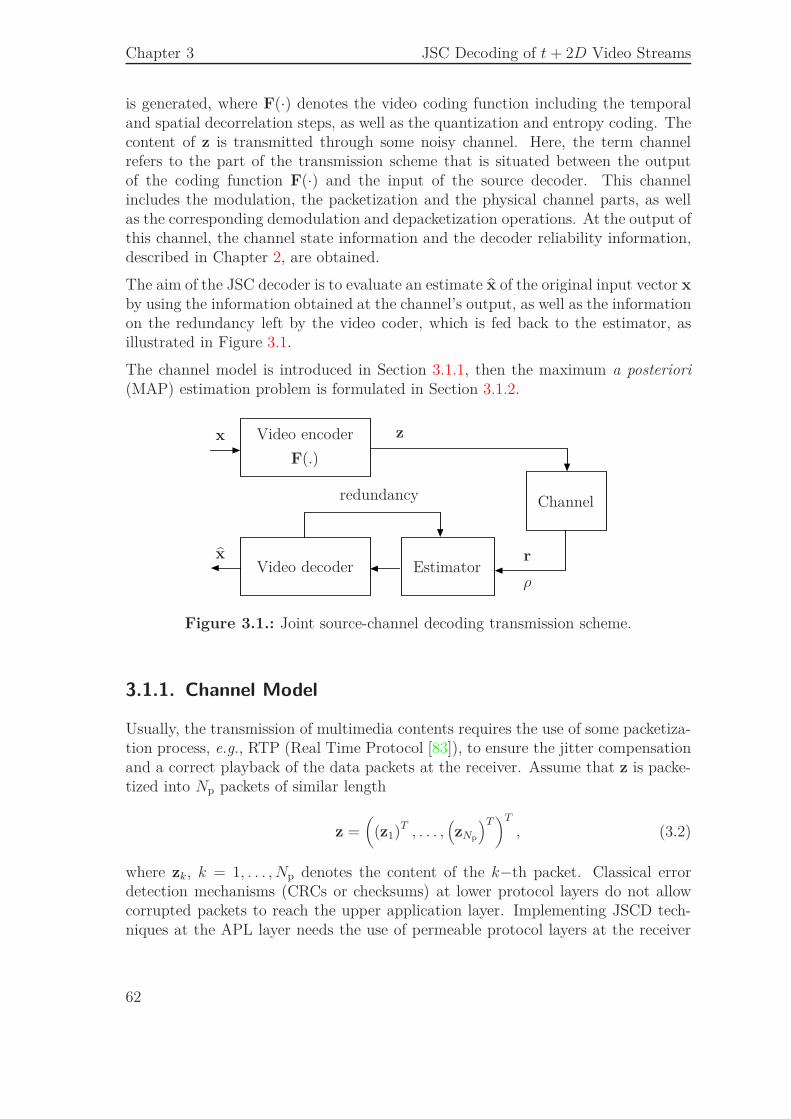
Chapter 3 JSC Decoding of t + 2D Video Streams
is generated, where F(·) denotes the video coding function including the temporaland spatial decorrelation steps, as well as the quantization and entropy coding. Thecontent of z is transmitted through some noisy channel. Here, the term channelrefers to the part of the transmission scheme that is situated between the outputof the coding function F(·) and the input of the source decoder. This channelincludes the modulation, the packetization and the physical channel parts, as wellas the corresponding demodulation and depacketization operations. At the output ofthis channel, the channel state information and the decoder reliability information,described in Chapter 2, are obtained.
The aim of the JSC decoder is to evaluate an estimate x of the original input vector x
by using the information obtained at the channel’s output, as well as the informationon the redundancy left by the video coder, which is fed back to the estimator, asillustrated in Figure 3.1.
The channel model is introduced in Section 3.1.1, then the maximum a posteriori(MAP) estimation problem is formulated in Section 3.1.2.
x
x r
ρ
z
F(.)
Channel
Video encoder
EstimatorVideo decoder
redundancy
Figure 3.1.: Joint source-channel decoding transmission scheme.
3.1.1. Channel Model
Usually, the transmission of multimedia contents requires the use of some packetiza-tion process, e.g., RTP (Real Time Protocol [83]), to ensure the jitter compensationand a correct playback of the data packets at the receiver. Assume that z is packe-tized into Np packets of similar length
z =(
(z1)T , . . . ,(zNp
)T)T
, (3.2)
where zk, k = 1, . . . , Np denotes the content of the k−th packet. Classical errordetection mechanisms (CRCs or checksums) at lower protocol layers do not allowcorrupted packets to reach the upper application layer. Implementing JSCD tech-niques at the APL layer needs the use of permeable protocol layers at the receiver
62
3.1 Conceptual JSC Video Decoder
side [75, 42, 101]. Such mechanisms require robust header decoding techniques [101]and transmission of the bit soft information or reliability measures (coming fromthe channel decoders at physical layer) to the upper protocol layers, as detailed in[117]. Reliable recovery of the various headers involved in the protocol stack maybe ensured by employing joint protocol-channel decoding techniques at the receiverside [101, 42]. Provided that such mechanisms are implemented, the whole networkpacketization process, the physical channel, the robust depacketization, as well asthe channel decoding operation, are modeled by a channel representing everythingbetween the source coder and the source decoder. The channel state informationand the decoder reliability information may then be obtained at the output of thischannel.
Let the reliability information be modeled by the vector
r =(
(r1)T , . . . ,
(rNp
)T)T
, (3.3)
where the vector rk, k = 1, . . . , Np contains soft information on the transmittedpacket zk. This soft information consists, e.g., in likelihood ratios, or a posterioriprobabilities on the transmitted data. They are provided by the channel decodersat the physical layer on receiver side. Moreover, let the channel state informationbe modeled by the vector
ρ =(ρ1 . . . , ρNp
)T, (3.4)
whose components indicate whether a packet zk, k = 1, . . . , Np has been received(ρk > 1) or not (ρk = 0). The value ρk = 0 may be deduced, e.g., from the contentof successive RTP packet headers. The values of ρk > 1 indicate the noise/fade leveland are assumed to be known by the receiver.
Along this chapter, all the packets are assumed to be received (ρk > 1, k =1, . . . , Np), but some of them may be corrupted by the transmission noise.
3.1.2. Optimal Estimation Schemes
This section presents two optimal estimation schemes, which are more or less in-dependent of the considered video coder. First, the estimation of x is formulatedin Section 3.1.2.1. Then, a constrained estimation of z, which is more practical tohandle, and for which it is easier to exploit the channel information and the sourceresidual redundancy, is described in Section 3.1.2.2.
3.1.2.1. MAP Estimation of x
The MAP estimate xMAP of x knowing ρ and r is
xMAP = arg maxx
p (x|ρ, r) . (3.5)
63
Chapter 3 JSC Decoding of t + 2D Video Streams
Marginalizing (3.5) with respect to z, one gets
xMAP = arg maxx
∑
z
p (x, z|ρ, r)
= arg maxx
∑
z
p (ρ, r|x, z) p (z|x) p (x) . (3.6)
Since z is deduced from x, in (3.6) one has
p (z|x) =
1 if z=F (x)
0 otherwise.
Consequently, (3.6) becomes
xMAP = arg maxx
p (ρ, r|F (x)) p (x) , (3.7)
where the fact that the knowledge of x does not bring any additional informationon ρ and r once F (x) is known has been taken into account.
Even if p (ρ, r|F (x)) in (3.7) is quite easy to evaluate for a given x, the evaluation ofxMAP requires the maximization of a discontinuous function (due to the quantizationpresent in F(·)), over a prohibitively large number of variables (i.e., the componentsof x, which are all the pixels within the considered video sequence frames).
3.1.2.2. Constrained Estimation of the Entropy Coded Bit Stream z
Alternatively, one may try to estimate z in a first time, accounting for the factthat this bit stream has been generated from a video sequence x. The resultingconstrained MAP estimator of z, knowing ρ and r, is
zMAP = arg maxz∈S
p (z|ρ, r) , (3.8)
where
S = {z st ∃x, z = F (x)} (3.9)
is the set of all the bit streams that can be generated from all the vectors x. We pointout here that performing the estimation among the elements of S takes into accountthe information fed back from the source coder to the estimator, and implies thatzMAP is a valid sequence, since it could have been generated by the source encoder.
Using Bayes’ rule, (3.8) becomes
zMAP = arg maxz∈S
p (ρ, r|z) p (z) . (3.10)
In (3.10) one has
p (ρ, r|z) = p (r|ρ, z) p (ρ|z) . (3.11)
64
3.2 Overview of Vidwav Video Coder
Assuming that the congestion conditions for each packet of z are independent, onegets
p (ρ|z) =Np∏
k=1
p (ρk|zk) . (3.12)
Usually p (ρk|zk), k = 1, . . . , Np only depends on the length of the packet zk andnot on its content. Assuming now that each packet zk of z encounters independenttransmission channel realizations, one gets
p (r|ρ, z) =Np∏
k=1
p (rk|ρk, zk) . (3.13)
Since we assumed that ρk > 1, the evaluation of p (rk|ρk, zk) depends on the valuesof zk, ρk and on the channel model. Combining (3.10)–(3.13) one gets
zMAP = arg maxz∈S
p (z)Np∏
k=1
p (rk|ρk, zk) p (ρk|zk) . (3.14)
In (3.14), determining whether z ∈ S depends on the function F(.) used to performthe video encoding.
In this work, the subband video coder Vidwav [126] has been considered. In the nextsection, a brief overview of this coder is presented, as well as a description of thebit stream it delivers. This will help to identify a part of the residual redundancywhich will be used to build the set S.
3.2. Overview of Vidwav Video Coder
Vidwav is a 3D scalable wavelet-based video coder using motion-compensated tem-poral filtering (MCTF) based on the Barbell filter [126]. It allows both spatial andin-band MCTF (t + 2D or 2D + t + 2D). In this work we consider only the t + 2Dscheme, illustrated in Figure 3.2. First, the MCTF is performed on the frames of theinput video sequence x, then the spatial wavelet transform is applied on the result-ing temporal subbands. The obtained spatio-temporal subbands are then dividedinto 3D blocks which are entropy encoded in an independent manner.
Consider an input video sequence x of Nf frames X1, . . . , XNf, represented by the
vectors xn, n = 1, . . . , Nf of size NrNc, where Nr and Nc denote the number of rowsand columns in each frame Xn. Then
x =((x1)T , . . . (xn)T , . . . , (xNf
)T)T
. (3.15)
65
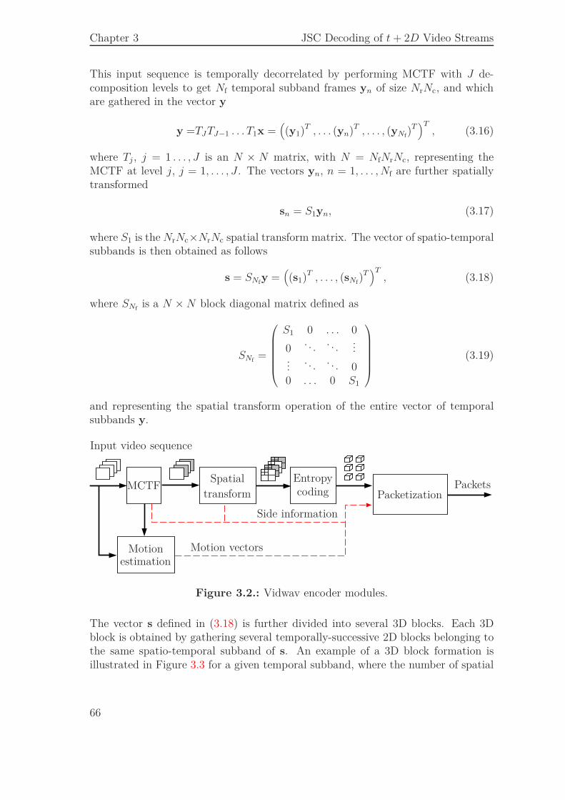
Chapter 3 JSC Decoding of t + 2D Video Streams
This input sequence is temporally decorrelated by performing MCTF with J de-composition levels to get Nf temporal subband frames yn of size NrNc, and whichare gathered in the vector y
y =TJTJ−1 . . . T1x =((y1)
T , . . . (yn)T , . . . , (yNf)T)T
, (3.16)
where Tj , j = 1 . . . , J is an N × N matrix, with N = NfNrNc, representing theMCTF at level j, j = 1, . . . , J . The vectors yn, n = 1, . . . , Nf are further spatiallytransformed
sn = S1yn, (3.17)
where S1 is the NrNc×NrNc spatial transform matrix. The vector of spatio-temporalsubbands is then obtained as follows
s = SNfy =
((s1)T , . . . , (sNf
)T)T
, (3.18)
where SNfis a N × N block diagonal matrix defined as
SNf=
S1 0 . . . 0
0. . . . . .
......
. . . . . . 00 . . . 0 S1
(3.19)
and representing the spatial transform operation of the entire vector of temporalsubbands y.
Spatial
Side information
transformPackets
Input video sequence
Entropycoding Packetization
MCTF
Motionestimation
Motion vectors
Figure 3.2.: Vidwav encoder modules.
The vector s defined in (3.18) is further divided into several 3D blocks. Each 3Dblock is obtained by gathering several temporally-successive 2D blocks belonging tothe same spatio-temporal subband of s. An example of a 3D block formation isillustrated in Figure 3.3 for a given temporal subband, where the number of spatial
66
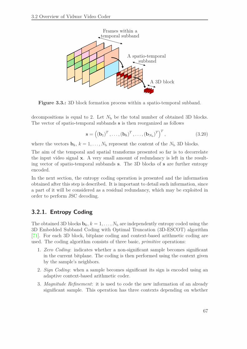
3.2 Overview of Vidwav Video Coder
Frames within atemporal subband
A spatio-temporal
A 3D block
subband
Figure 3.3.: 3D block formation process within a spatio-temporal subband.
decompositions is equal to 2. Let Nb be the total number of obtained 3D blocks.The vector of spatio-temporal subbands s is then reorganized as follows
s =((b1)T , . . . , (bk)T , . . . , (bNb
)T)T
, (3.20)
where the vectors bk, k = 1, . . . , Nb represent the content of the Nb 3D blocks.
The aim of the temporal and spatial transforms presented so far is to decorrelatethe input video signal x. A very small amount of redundancy is left in the result-ing vector of spatio-temporal subbands s. The 3D blocks of s are further entropyencoded.
In the next section, the entropy coding operation is presented and the informationobtained after this step is described. It is important to detail such information, sincea part of it will be considered as a residual redundancy, which may be exploited inorder to perform JSC decoding.
3.2.1. Entropy Coding
The obtained 3D blocks bk, k = 1, . . . , Nb are independently entropy coded using the3D Embedded Subband Coding with Optimal Truncation (3D-ESCOT) algorithm[71]. For each 3D block, bitplane coding and context-based arithmetic coding areused. The coding algorithm consists of three basic, primitive operations:
1. Zero Coding: indicates whether a non-significant sample becomes significantin the current bitplane. The coding is then performed using the context givenby the sample’s neighbors.
2. Sign Coding: when a sample becomes significant its sign is encoded using anadaptive context-based arithmetic coder.
3. Magnitude Refinement: it is used to code the new information of an alreadysignificant sample. This operation has three contexts depending on whether
67
Chapter 3 JSC Decoding of t + 2D Video Streams
the magnitude refinement has been used or not for the current sample and onthe significance state of its neighbors.
For each bitplane, the 3D-ESCOT algorithm uses, in turn, three distinct codingpasses:
1. Significance propagation pass: this pass encodes the neighbors of samples al-ready found significant (either at the current bitplane or at previously codedbitplanes). For each processed sample, the zero coding primitive is applied.Moreover, if the sample becomes significant at the current bitplane, then thesign coding primitive is used to code its sign.
2. Magnitude refinement pass: in this pass, only the significant samples are con-sidered and the symbols of these samples in the current bitplane are codedusing the magnitude refinement primitive.
3. Cleanup pass: in this pass, the samples that are not yet coded in the previoustwo passes are coded using the zero coding primitive.
Finally, rate distortion (R-D) optimization is used to decide how many bytes areallocated for each coding block. After all these operations, the following informationis obtained for each 3D block bk:
1. the number of bitplanes dk within bk and the number of coding passes1 nk =3dk − 2.
2. the coded bit stream pk of bk, which is an embedded bit stream formed by nk
segments, each one corresponding to the output bit stream of one coding pass.
3. the length in bytes of each bit stream segment and its spatio-temporal subband.
4. the R-D slope information at the end of each coding pass.
Let E(.) denotes the 3D-ESCOT entropy coding function. The bit stream
zk = E(bk), k = 1, . . . , Nb (3.21)
is the output associated to the 3D block bk. This bit stream is formed by theembedded payload pk corresponding the entropy-coded spatio-temporal wavelet co-efficients of the block bk, and by a header hk containing the motion informationassociated to bk and other metadata necessary for decoding, e.g., the number ofcoding passes used to code the block, its length in bytes, its spatio-temporal index,its R-D slope information, etc. Then
zk =
(hk
pk
), (3.22)
and the vector
z =((z1)
T , . . . , (zk)T , . . . , (zNb)T)T
(3.23)
1For the first bitplane, the significance propagation pass is not performed.
68
3.3 JSCD of Single Layer Bit Streams
represents the compressed bit stream delivered by the Vidwav encoder for the inputvideo sequence x. Finally, the video coding function F(·) defined in (3.1) can bewritten as follows
F(x) = E(SNfTJ . . . T1x). (3.24)
The Vidwav encoder generally produces a fully embedded and scalable output bygenerating bit streams formed by several layers, each layer corresponding to a scal-abiliy degree (i.e., temporal, spatial and/or SNR or quality scalability).
In Section 3.3, the proposed joint source-channel decoding scheme is described forsingle layer bit streams and the obtained simulation results are presented. Thisdecoding scheme is further extended to multiple layers bit streams in Section 3.4.
3.3. JSCD of Single Layer Bit Streams
In this section, the entropy-coded bit stream z is assumed to be formed by onelayer. The aim is to provide an implementable counterpart of the optimal estimationschemes presented is Section 3.1.2, which is adapted to the Vidwav coder presentedin Section 3.2 and to the structure of the bit stream it delivers. The estimationschemes presented here are based on JSCD by exploiting the redundancy left by theVidwav encoder.
To simplify the notations, and without loss of generality, each packet of z defined in(3.2) is assumed to contain one entropy-coded bit stream zk of some 3D block bk.Therefore, Np = Nb and
z =((z1)
T , . . . , (zNb)T)T
. (3.25)
The decoder soft information r and the channel state information ρ, defined in (3.3)and (3.4) are then rewritten as follows
r =((r1)
T , . . . , (rNb)T)T
, (3.26)
ρ = (ρ1, . . . , ρNb)T . (3.27)
Assume now that all the vectors z ∈ S are a priori equally probable, so that (3.14)becomes
zMAP = arg maxz∈S
Nb∏
k=1
p (rk|ρk, zk) p (ρk|zk) . (3.28)
This assumption is reasonable as long as no informative a priori probabilities onx are available, where x represents the uncoded video sequence. If such a priori
69
Chapter 3 JSC Decoding of t + 2D Video Streams
knowledge was available, deducing p (z) would be far from being trivial and (3.28)would be suboptimal compared to (3.14).
Consider the sets
Sk =
zk | ∃x, ∃ (z1, . . . , zk−1, zk+1, . . . , zNb
) ,
st((z1)T , . . . , (zk−1)
T , (zk)T , (zk+1)T , . . . , (zNb
)T)T
= E(SNf
TJ . . . T1x),
(3.29)
defined for each k = 1, . . . , Nb. The set Sk contains all the possible bit streams thatcan result from the entropy coding of a 3D block bk obtained for a video sequencex of Nf frames.
Remark 1. Consider the set S introduced in (3.9) which contains all the possibleentropy-coded sequences z that can be generated from all the video sequences x.One has
S ⊂ S1 × · · · × SNb. (3.30)
In general, S 6= S1 × · · · × SNb. Consider (z1, . . . , zNb
) ∈ S1 × · · · × SNband let
Xk (zk) be the set of the vectors x such as the k−th entropy-coded sequence ofE(SNf
TJ . . . T1x)
is equal to zk. One knows that Xk (zk) 6= ∅, since zk ∈ Sk. If⋂Nb
k=1 Xk (zk) 6= ∅ then (z1, . . . , zNb) ∈ S. Now assume that for all (z1, . . . , zNb
) ∈S1 × · · · × SNb
,⋂Nb
k=1 Xk (zk) 6= ∅, this means that the sequences z1, . . . , zNbare
uncorrelated, which is not usually the case since these sequences are obtained fromthe entropy coding of the same video sequence, and thus present some correlation.
Using (3.28)–(3.30), one may derive a suboptimal estimator for each zk as follows
zk = arg maxzk∈Sk
p (rk|ρk, zk) p (ρk|zk) . (3.31)
The estimator((z1)
T , . . . , (zNb)T)T
is a suboptimal solution of (3.28) since
((zk)T , . . . , (zNb
)T)T
is not necessarily in S, see (3.30).
As described in Section 3.2.1, each entropy-coded bit stream zk is formed by a headerhk and a payload pk. After the transmission of zk, the received vector
rk =((rk,h)T , (rk,p)T
)T
contains soft information on hk given by rk,h, and on pk given by rk,p.
70
3.3 JSCD of Single Layer Bit Streams
Assuming that the headers hk have been received without errors, the estimationproblem in (3.31) is reduced to the constrained estimation of pk from rk, hk and ρk
pk = arg maxp st (hk,p)∈Sk
p (rk,p|ρk, p) . (3.32)
In (3.32), the term p (ρk|zk) of (3.31) is removed. As mentionned in Section 3.1.2.2,p (ρk|zk) usually depends on the length of zk, which is stored in hk. Since hk isassumed to be error-free, p (ρk|zk) is known and does not depend on zk.
The value of ρk gives information on the channel characteristics, e.g., signal to noiseratio (SNR), bit error probability, level of fading and allows to evaluate the likelihoodp(rk,p|ρk, p) in (3.32).
The search space for pk is the set of all the payloads p that may be generated fromsome video sequence x and which are compliant with the information stored in hk.
In the next section, two tests are introduced to determine whether a given payload p
is syntax-compliant i.e., whether (hk, p) ∈ Sk. These tests are then used to performJSCD using the M−algorithm [3] to obtain approximate versions of (3.32).
3.3.1. Syntax Compliance Tests
Recall that the payload pk represents the output of the 3D-ESCOT coder for a given3D block bk. It results from a known number of coding passes nk and has a knownlength ℓk in bits. As mentioned in Section 3.2.1, nk and ℓk are stored in the headerhk at the encoder side. The 3D-ESCOT decoder has then to process exactly ℓk
bits when decoding nk passes for a given stream p. If more or less than ℓk bits areprocessed, the arithmetic encoder and the arithmetic decoder are desynchronized,which implies that p contains transmission errors.
More formally, let Λ(p) be the number of bits processed when decoding nk passesfor a given payload p and let Λ(hk) be the number of bits that should be processedin p. The value of Λ(hk) is extracted from hk. Consider the following compliancetest
tb(hk, p) =
1 if Λ(p) = Λ(hk)
0 otherwise.(3.33)
Assuming that the headers hk are error-free, Λ(hk) = ℓk and nk are known at thedecoder. Therefore, for a given sequence p, tb(hk, p) = 0 implies that p 6= pk.
For a given header bit stream hk, consider the sets
Cb(hk) ={
p st tb(hk, p) = 1}
(3.34)
and
C(hk) = {p st (hk, p) ∈ Sk} . (3.35)
71
Chapter 3 JSC Decoding of t + 2D Video Streams
Each element p ∈ C(hk) is compliant with hk, i.e., the pair (hk, p) can be obtainedfrom some x, which implies that Λ(p) = Λ(hk) and thus p ∈ Cb(hk). Therefore
C(hk) ⊂ Cb(hk) (3.36)
and tb(hk, p) = 0 implies that p /∈ C(hk). The test tb(hk, p) allows thus to provethat a payload p is not compliant with a given header hk, but it is unable to provethat some p is compliant with a given header hk. The bits contained in some p 6= pk
may lead to the processing of exactly ℓk bits by the 3D-ESCOT decoder. In absenceof desynchronisation between the encoder and decoder, the fact that p 6= pk is notdetectable by tb.
In the bit stream generated by the Vidwav coder, as specified in [126], the data isbyte-aligned and Λ(hk) is only known in bytes. Without any modification of theVidwav specifications, (3.33) becomes
tB(hk, p) =
1 if 8 ⌈Λ(p)/8⌉ = Λ(hk)
0 otherwise.(3.37)
where ⌈·⌉ means the upward rounding. Error detection with tB is then only possiblewhen the desynchronization is sufficient. For a given header hk consider the set
CB(hk) ={p st tB(hk, p) = 1
}. (3.38)
One has
C(hk) ⊂ Cb(hk) ⊂ CB(hk) (3.39)
and tB is thus less efficient2 in terms of error detection than tb.
One may write Λ(hk) = ℓk+λk, where λk = 0, . . . , 7 is the number of bits used to padpk. In order to implement tb(hk, p) at the Vidwav decoder, one has to supplementhk with the content of λk at the encoder side. This side information requires onlythree additional bits per entropy-coded 3D block zk.
Using (3.33) or (3.37), one gets the approximate versions of (3.32)
pbk = arg max
p∈Cb(hk)p (rk,p|ρk, p) (3.40)
and respectively
pBk = arg max
p∈CB(hk)p (rk,p|ρk, p) , (3.41)
which require to consider all the sequences in Cb(hk) or in CB(hk), when tb or tB
are used. These two sets are not well-structured, i.e., their content cannot be easily
2Note however that in this case, the packet length information, stored in the header, is shorter.
72
3.3 JSCD of Single Layer Bit Streams
generated by a finite-state automaton with a reasonable number of states as is thecase for Huffman-based variable-length codes [42]. Thus, efficient decoders derivedfrom the BCJR algorithm [6] may not be employed in this case.
Approximate versions of (3.40) and (3.41), with manageable complexity, may be ob-tained using sequential decoding algorithms, such as the M-algorithm [3] describedin the next section.
3.3.2. Sequential Estimation
All the vectors p of ℓ bits may be represented by a binary tree T of 2ℓ leaves.A given node at depth d in T represents a subsequence p1:d of d bits, which isrepresented by the path of length d, starting from the root of T and leading tothe considered node. For a given hk, only a subset of leaves in T corresponds tosequences belonging to CB(hk) or Cb(hk). The aim of the M−algorithm is to partlyexplore T . At iteration d, the M sequences of length d maximizing the metric
M(p1:d, rk) = − log p(rk|p1:d, ρk) (3.42)
are kept in a list L to be used at iteration d+1. When d = Λ(hk), the test tB(hk, p)or tb(hk, p) is used to eliminate the sequences in L which do not belong to CB(hk)or Cb(hk), starting from the sequence maximizing (3.42).
The steps of the M− algorithm are:
1. Initialization: L = ∅, corresponding to the root of T to which the null metricis assigned.
2. Extend all paths in L to the following nodes in T .
3. Among the extended paths, keep at most M paths with the largest metricaccording to (3.42).
4. Go to Step 2 until all the paths in L reach the depth Λ(hk).
5. Select the path p in L with the largest metric satisfying tB(hk, p) = 1 ortb(hk, p) = 1.
This algorithm is suboptimal [3]: if M is not large enough, the transmitted vectorpk may be discarded at Step 3.
At Step 5, if no vector in L satisfies one of the compliance tests, pk could be consid-ered as dropped and error concealment methods may be used to alleviate the missingblocks effect at the spatial and temporal inverse transform levels. Alternatively, onemay use the first element in the list L, corresponding to M = 1, even if it does notsatisfy tB(hk, p) = 1 or tb(hk, p) = 1; this translates into considering that errorshave occurred only at the end of pk, leading thus to moderate decoding artifacts.In this work this latter strategy is adopted.
In the next section, the simulation results obtained by using the syntax compliancetests tb and tB are presented.
73
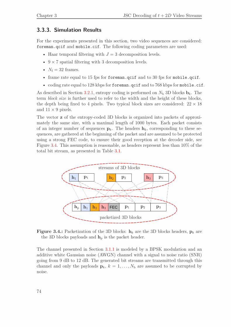
Chapter 3 JSC Decoding of t + 2D Video Streams
3.3.3. Simulation Results
For the experiments presented in this section, two video sequences are considered:foreman.qcif and mobile.cif. The following coding parameters are used:
• Haar temporal filtering with J = 3 decomposition levels.
• 9 × 7 spatial filtering with 3 decomposition levels.
• Nf = 32 frames.
• frame rate equal to 15 fps for foreman.qcif and to 30 fps for mobile.qcif.
• coding rate equal to 128 kbps for foreman.qcif and to 768 kbps for mobile.cif.
As described in Section 3.2.1, entropy coding is performed on Nb 3D blocks bk. Theterm block size is further used to refer to the width and the height of these blocks,the depth being fixed to 4 pixels. Two typical block sizes are considered: 22 × 18and 11 × 9 pixels.
The vector z of the entropy-coded 3D blocks is organized into packets of approxi-mately the same size, with a maximal length of 1000 bytes. Each packet consistsof an integer number of sequences pk. The headers hk, corresponding to these se-quences, are gathered at the beginning of the packet and are assumed to be protectedusing a strong FEC code, to ensure their good reception at the decoder side, seeFigure 3.4. This assumption is reasonable, as headers represent less than 10% of thetotal bit stream, as presented in Table 3.1.
FECh1
h1 h2
h2 h3
h3
p1
p1 p2
p2 p3
p3
hp
streams of 3D blocks
packetized 3D blocks
Figure 3.4.: Packetization of the 3D blocks: hk are the 3D blocks headers, pk arethe 3D blocks payloads and hp is the packet header.
The channel presented in Section 3.1.1 is modeled by a BPSK modulation and anadditive white Gaussian noise (AWGN) channel with a signal to noise ratio (SNR)going from 9 dB to 12 dB. The generated bit streams are transmitted through thischannel and only the payloads pk, k = 1, . . . , Nb are assumed to be corrupted bynoise.
74
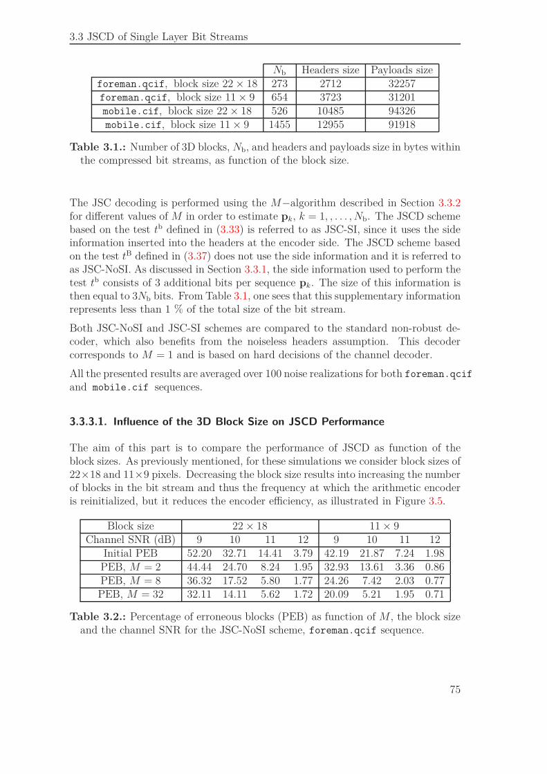
3.3 JSCD of Single Layer Bit Streams
Nb Headers size Payloads sizeforeman.qcif, block size 22 × 18 273 2712 32257foreman.qcif, block size 11 × 9 654 3723 31201mobile.cif, block size 22 × 18 526 10485 94326mobile.cif, block size 11 × 9 1455 12955 91918
Table 3.1.: Number of 3D blocks, Nb, and headers and payloads size in bytes withinthe compressed bit streams, as function of the block size.
The JSC decoding is performed using the M−algorithm described in Section 3.3.2for different values of M in order to estimate pk, k = 1, , . . . , Nb. The JSCD schemebased on the test tb defined in (3.33) is referred to as JSC-SI, since it uses the sideinformation inserted into the headers at the encoder side. The JSCD scheme basedon the test tB defined in (3.37) does not use the side information and it is referred toas JSC-NoSI. As discussed in Section 3.3.1, the side information used to perform thetest tb consists of 3 additional bits per sequence pk. The size of this information isthen equal to 3Nb bits. From Table 3.1, one sees that this supplementary informationrepresents less than 1 % of the total size of the bit stream.
Both JSC-NoSI and JSC-SI schemes are compared to the standard non-robust de-coder, which also benefits from the noiseless headers assumption. This decodercorresponds to M = 1 and is based on hard decisions of the channel decoder.
All the presented results are averaged over 100 noise realizations for both foreman.qcif
and mobile.cif sequences.
3.3.3.1. Influence of the 3D Block Size on JSCD Performance
The aim of this part is to compare the performance of JSCD as function of theblock sizes. As previously mentioned, for these simulations we consider block sizes of22×18 and 11×9 pixels. Decreasing the block size results into increasing the numberof blocks in the bit stream and thus the frequency at which the arithmetic encoderis reinitialized, but it reduces the encoder efficiency, as illustrated in Figure 3.5.
Block size 22 × 18 11 × 9Channel SNR (dB) 9 10 11 12 9 10 11 12
Initial PEB 52.20 32.71 14.41 3.79 42.19 21.87 7.24 1.98PEB, M = 2 44.44 24.70 8.24 1.95 32.93 13.61 3.36 0.86PEB, M = 8 36.32 17.52 5.80 1.77 24.26 7.42 2.03 0.77PEB, M = 32 32.11 14.11 5.62 1.72 20.09 5.21 1.95 0.71
Table 3.2.: Percentage of erroneous blocks (PEB) as function of M , the block sizeand the channel SNR for the JSC-NoSI scheme, foreman.qcif sequence.
75
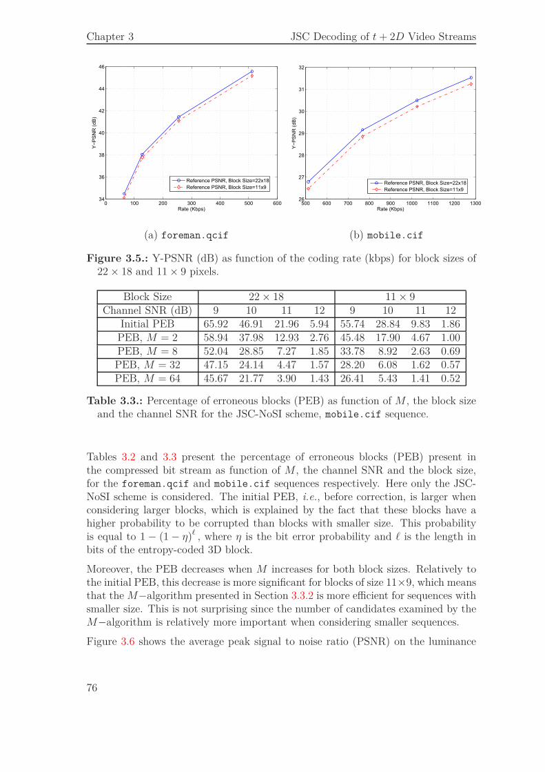
Chapter 3 JSC Decoding of t + 2D Video Streams
0 100 200 300 400 500 60034
36
38
40
42
44
46
Rate (Kbps)
Y−
PS
NR
(dB
)
Reference PSNR, Block Size=22x18
Reference PSNR, Block Size=11x9
500 600 700 800 900 1000 1100 1200 130026
27
28
29
30
31
32
Rate (Kbps)
Y−
PS
NR
(dB
)
Reference PSNR, Block Size=22x18
Reference PSNR, Block Size=11x9
(a) foreman.qcif (b) mobile.cif
Figure 3.5.: Y-PSNR (dB) as function of the coding rate (kbps) for block sizes of22 × 18 and 11 × 9 pixels.
Block Size 22 × 18 11 × 9Channel SNR (dB) 9 10 11 12 9 10 11 12
Initial PEB 65.92 46.91 21.96 5.94 55.74 28.84 9.83 1.86PEB, M = 2 58.94 37.98 12.93 2.76 45.48 17.90 4.67 1.00PEB, M = 8 52.04 28.85 7.27 1.85 33.78 8.92 2.63 0.69PEB, M = 32 47.15 24.14 4.47 1.57 28.20 6.08 1.62 0.57PEB, M = 64 45.67 21.77 3.90 1.43 26.41 5.43 1.41 0.52
Table 3.3.: Percentage of erroneous blocks (PEB) as function of M , the block sizeand the channel SNR for the JSC-NoSI scheme, mobile.cif sequence.
Tables 3.2 and 3.3 present the percentage of erroneous blocks (PEB) present inthe compressed bit stream as function of M , the channel SNR and the block size,for the foreman.qcif and mobile.cif sequences respectively. Here only the JSC-NoSI scheme is considered. The initial PEB, i.e., before correction, is larger whenconsidering larger blocks, which is explained by the fact that these blocks have ahigher probability to be corrupted than blocks with smaller size. This probabilityis equal to 1 − (1 − η)ℓ , where η is the bit error probability and ℓ is the length inbits of the entropy-coded 3D block.
Moreover, the PEB decreases when M increases for both block sizes. Relatively tothe initial PEB, this decrease is more significant for blocks of size 11×9, which meansthat the M−algorithm presented in Section 3.3.2 is more efficient for sequences withsmaller size. This is not surprising since the number of candidates examined by theM−algorithm is relatively more important when considering smaller sequences.
Figure 3.6 shows the average peak signal to noise ratio (PSNR) on the luminance
76
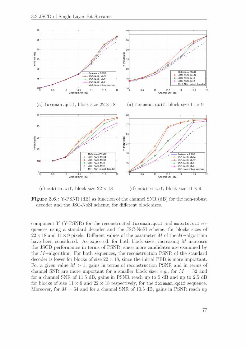
3.3 JSCD of Single Layer Bit Streams
9 9.5 10 10.5 11 11.5 1210
15
20
25
30
35
40
Channel SNR (dB)
Y−
PS
NR
(dB
)
Reference PSNR
JSC−NoSI, M=32
JSC−NoSI, M=8
JSC−NoSI, M=2
M=1, Non−robust decoder
9 9.5 10 10.5 11 11.5 1210
15
20
25
30
35
40
Channel SNR (dB)
Y−
PS
NR
(dB
)
Reference PSNR
JSC−NoSI, M=32
JSC−NoSI, M=8
JSC−NoSI, M=2
M=1, Non−robust decoder
(a) foreman.qcif, block size 22 × 18 (a) foreman.qcif, block size 11 × 9
9 9.5 10 10.5 11 11.5 125
10
15
20
25
30
Channel SNR (dB)
Y−
PS
NR
(dB
)
Reference PSNR
JSC−NoSI, M=64
JSC−NoSI, M=32
JSC−NoSI, M=8
JSC−NoSI, M=2
M=1, Non−robust decoder
9 9.5 10 10.5 11 11.5 1212
15
18
21
24
27
30
Channel SNR (dB)
Y−
PS
NR
(dB
)
Reference PSNR
JSC−NoSI, M=64
JSC−NoSI, M=32
JSC−NoSI, M=8
JSC−NoSI, M=2
M=1, Non−robust decoder
(c) mobile.cif, block size 22 × 18 (d) mobile.cif, block size 11 × 9
Figure 3.6.: Y-PSNR (dB) as function of the channel SNR (dB) for the non-robustdecoder and the JSC-NoSI scheme, for different block sizes.
component Y (Y-PSNR) for the reconstructed foreman.qcif and mobile.cif se-quences using a standard decoder and the JSC-NoSI scheme, for blocks sizes of22 × 18 and 11 × 9 pixels. Different values of the parameter M of the M−algorithmhave been considered. As expected, for both block sizes, increasing M increasesthe JSCD performance in terms of PSNR, since more candidates are examined bythe M−algorithm. For both sequences, the reconstruction PSNR of the standarddecoder is lower for blocks of size 22 × 18, since the initial PEB is more important.For a given value M > 1, gains in terms of reconstruction PSNR and in terms ofchannel SNR are more important for a smaller block size, e.g., for M = 32 andfor a channel SNR of 11.5 dB, gains in PSNR reach up to 5 dB and up to 2.5 dBfor blocks of size 11 × 9 and 22 × 18 respectively, for the foreman.qcif sequence.Moreover, for M = 64 and for a channel SNR of 10.5 dB, gains in PSNR reach up
77
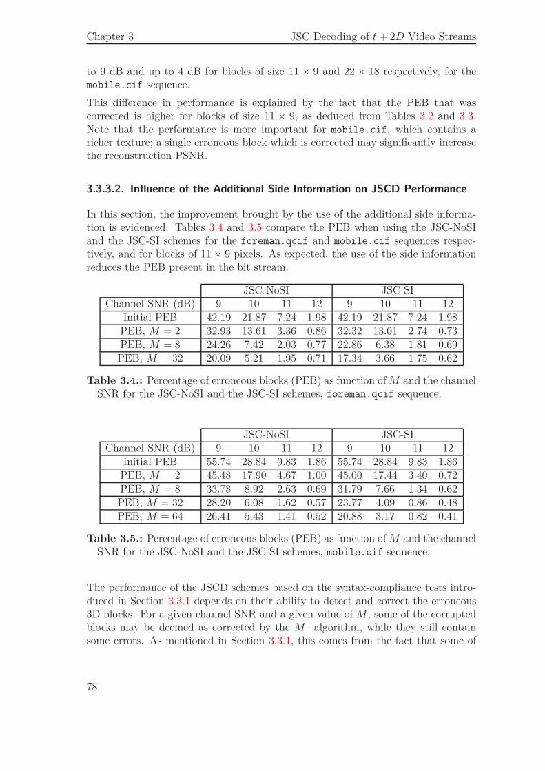
Chapter 3 JSC Decoding of t + 2D Video Streams
to 9 dB and up to 4 dB for blocks of size 11 × 9 and 22 × 18 respectively, for themobile.cif sequence.
This difference in performance is explained by the fact that the PEB that wascorrected is higher for blocks of size 11 × 9, as deduced from Tables 3.2 and 3.3.Note that the performance is more important for mobile.cif, which contains aricher texture; a single erroneous block which is corrected may significantly increasethe reconstruction PSNR.
3.3.3.2. Influence of the Additional Side Information on JSCD Performance
In this section, the improvement brought by the use of the additional side informa-tion is evidenced. Tables 3.4 and 3.5 compare the PEB when using the JSC-NoSIand the JSC-SI schemes for the foreman.qcif and mobile.cif sequences respec-tively, and for blocks of 11 × 9 pixels. As expected, the use of the side informationreduces the PEB present in the bit stream.
JSC-NoSI JSC-SIChannel SNR (dB) 9 10 11 12 9 10 11 12
Initial PEB 42.19 21.87 7.24 1.98 42.19 21.87 7.24 1.98PEB, M = 2 32.93 13.61 3.36 0.86 32.32 13.01 2.74 0.73PEB, M = 8 24.26 7.42 2.03 0.77 22.86 6.38 1.81 0.69PEB, M = 32 20.09 5.21 1.95 0.71 17.34 3.66 1.75 0.62
Table 3.4.: Percentage of erroneous blocks (PEB) as function of M and the channelSNR for the JSC-NoSI and the JSC-SI schemes, foreman.qcif sequence.
JSC-NoSI JSC-SIChannel SNR (dB) 9 10 11 12 9 10 11 12
Initial PEB 55.74 28.84 9.83 1.86 55.74 28.84 9.83 1.86PEB, M = 2 45.48 17.90 4.67 1.00 45.00 17.44 3.40 0.72PEB, M = 8 33.78 8.92 2.63 0.69 31.79 7.66 1.34 0.62PEB, M = 32 28.20 6.08 1.62 0.57 23.77 4.09 0.86 0.48PEB, M = 64 26.41 5.43 1.41 0.52 20.88 3.17 0.82 0.41
Table 3.5.: Percentage of erroneous blocks (PEB) as function of M and the channelSNR for the JSC-NoSI and the JSC-SI schemes, mobile.cif sequence.
The performance of the JSCD schemes based on the syntax-compliance tests intro-duced in Section 3.3.1 depends on their ability to detect and correct the erroneous3D blocks. For a given channel SNR and a given value of M , some of the corruptedblocks may be deemed as corrected by the M−algorithm, while they still containsome errors. As mentioned in Section 3.3.1, this comes from the fact that some of
78
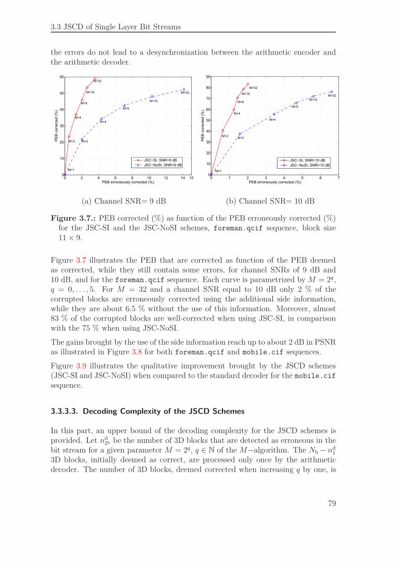
3.3 JSCD of Single Layer Bit Streams
the errors do not lead to a desynchronization between the arithmetic encoder andthe arithmetic decoder.
0 2 4 6 8 10 12 14 150
10
20
30
40
50
60
PEB erroneously corrected (%)
PE
B c
orr
ecte
d (
%)
JSC−SI, SNR=9 dB
JSC−NoSI, SNR=9 dB
M=1
M=2M=2
M=4
M=4
M=16
M=16
M=32
M=8
M=8
M=32
0 1 2 3 4 5 6 70
10
20
30
40
50
60
70
80
90
PEB erroneously corrected (%)
PE
B c
orr
ecte
d (
%)
JSC−SI, SNR=10 dB
JSC−NoSI, SNR=10 dB
M=2
M=32
M=8
M=4
M=1
M=16
M=8
M=4
M=2
M=16
M=32
(a) Channel SNR= 9 dB (b) Channel SNR= 10 dB
Figure 3.7.: PEB corrected (%) as function of the PEB erroneously corrected (%)for the JSC-SI and the JSC-NoSI schemes, foreman.qcif sequence, block size11 × 9.
Figure 3.7 illustrates the PEB that are corrected as function of the PEB deemedas corrected, while they still contain some errors, for channel SNRs of 9 dB and10 dB, and for the foreman.qcif sequence. Each curve is parametrized by M = 2q,q = 0, . . . , 5. For M = 32 and a channel SNR equal to 10 dB only 2 % of thecorrupted blocks are erroneously corrected using the additional side information,while they are about 6.5 % without the use of this information. Moreover, almost83 % of the corrupted blocks are well-corrected when using JSC-SI, in comparisonwith the 75 % when using JSC-NoSI.
The gains brought by the use of the side information reach up to about 2 dB in PSNRas illustrated in Figure 3.8 for both foreman.qcif and mobile.cif sequences.
Figure 3.9 illustrates the qualitative improvement brought by the JSCD schemes(JSC-SI and JSC-NoSI) when compared to the standard decoder for the mobile.cif
sequence.
3.3.3.3. Decoding Complexity of the JSCD Schemes
In this part, an upper bound of the decoding complexity for the JSCD schemes isprovided. Let nd
2q be the number of 3D blocks that are detected as erroneous in thebit stream for a given parameter M = 2q, q ∈ N of the M−algorithm. The Nb − nd
1
3D blocks, initially deemed as correct, are processed only once by the arithmeticdecoder. The number of 3D blocks, deemed corrected when increasing q by one, is
79
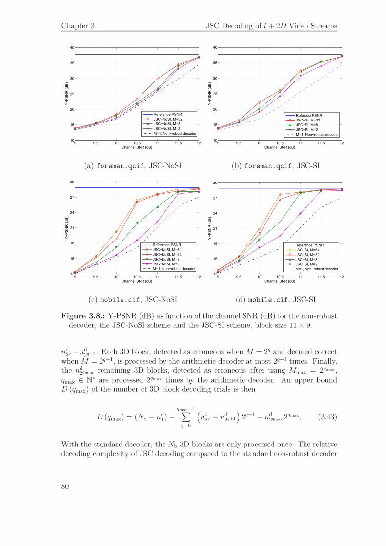
Chapter 3 JSC Decoding of t + 2D Video Streams
9 9.5 10 10.5 11 11.5 1210
15
20
25
30
35
40
Channel SNR (dB)
Y−
PS
NR
(dB
)
Reference PSNR
JSC−NoSI, M=32
JSC−NoSI, M=8
JSC−NoSI, M=2
M=1, Non−robust decoder
9 9.5 10 10.5 11 11.5 1210
15
20
25
30
35
40
Channel SNR (dB)
Y−
PS
NR
(dB
)
Referece PSNR
JSC−SI, M=32
JSC−SI, M=8
JSC−SI, M=2
M=1, Non−robust decoder
(a) foreman.qcif, JSC-NoSI (b) foreman.qcif, JSC-SI
9 9.5 10 10.5 11 11.5 1212
15
18
21
24
27
30
Channel SNR (dB)
Y−
PS
NR
(dB
)
Reference PSNR
JSC−NoSI, M=64
JSC−NoSI, M=32
JSC−NoSI, M=8
JSC−NoSI, M=2
M=1, Non−robust decoder
9 9.5 10 10.5 11 11.5 1212
15
18
21
24
27
30
Channel SNR (dB)
Y−
PS
NR
(dB
)
Reference PSNR
JSC−SI, M=64
JSC−SI, M=32
JSC−SI, M=8
JSC−SI, M=2
M=1, Non−robust decoder
(c) mobile.cif, JSC-NoSI (d) mobile.cif, JSC-SI
Figure 3.8.: Y-PSNR (dB) as function of the channel SNR (dB) for the non-robustdecoder, the JSC-NoSI scheme and the JSC-SI scheme, block size 11 × 9.
nd2q −nd
2q+1 . Each 3D block, detected as erroneous when M = 2q and deemed correctwhen M = 2q+1, is processed by the arithmetic decoder at most 2q+1 times. Finally,the nd
2qmax remaining 3D blocks, detected as erroneous after using Mmax = 2qmax,qmax ∈ N∗ are processed 2qmax times by the arithmetic decoder. An upper boundD (qmax) of the number of 3D block decoding trials is then
D (qmax) = (Nb − nd1) +
qmax−1∑
q=0
(nd
2q − nd2q+1
)2q+1 + nd
2qmax 2qmax. (3.43)
With the standard decoder, the Nb 3D blocks are only processed once. The relativedecoding complexity of JSC decoding compared to the standard non-robust decoder
80
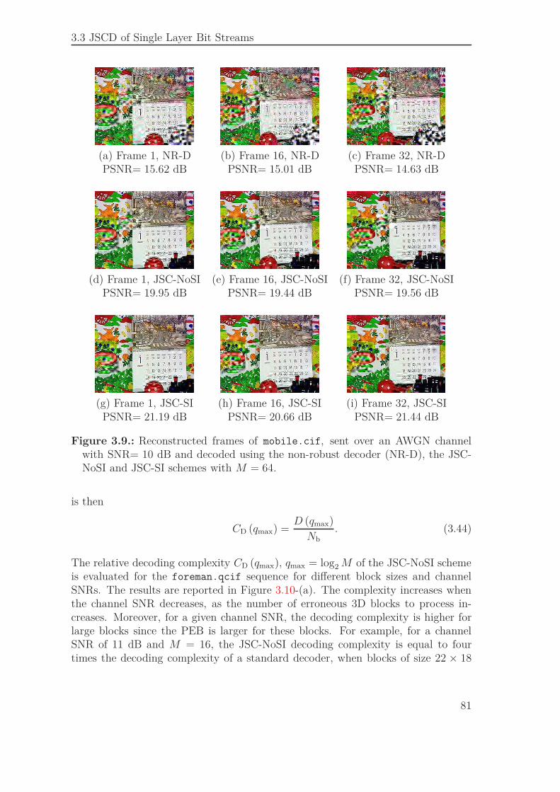
3.3 JSCD of Single Layer Bit Streams
(a) Frame 1, NR-D (b) Frame 16, NR-D (c) Frame 32, NR-DPSNR= 15.62 dB PSNR= 15.01 dB PSNR= 14.63 dB
(d) Frame 1, JSC-NoSI (e) Frame 16, JSC-NoSI (f) Frame 32, JSC-NoSIPSNR= 19.95 dB PSNR= 19.44 dB PSNR= 19.56 dB
(g) Frame 1, JSC-SI (h) Frame 16, JSC-SI (i) Frame 32, JSC-SIPSNR= 21.19 dB PSNR= 20.66 dB PSNR= 21.44 dB
Figure 3.9.: Reconstructed frames of mobile.cif, sent over an AWGN channelwith SNR= 10 dB and decoded using the non-robust decoder (NR-D), the JSC-NoSI and JSC-SI schemes with M = 64.
is then
CD (qmax) =D (qmax)
Nb. (3.44)
The relative decoding complexity CD (qmax), qmax = log2 M of the JSC-NoSI schemeis evaluated for the foreman.qcif sequence for different block sizes and channelSNRs. The results are reported in Figure 3.10-(a). The complexity increases whenthe channel SNR decreases, as the number of erroneous 3D blocks to process in-creases. Moreover, for a given channel SNR, the decoding complexity is higher forlarge blocks since the PEB is larger for these blocks. For example, for a channelSNR of 11 dB and M = 16, the JSC-NoSI decoding complexity is equal to fourtimes the decoding complexity of a standard decoder, when blocks of size 22 × 18
81
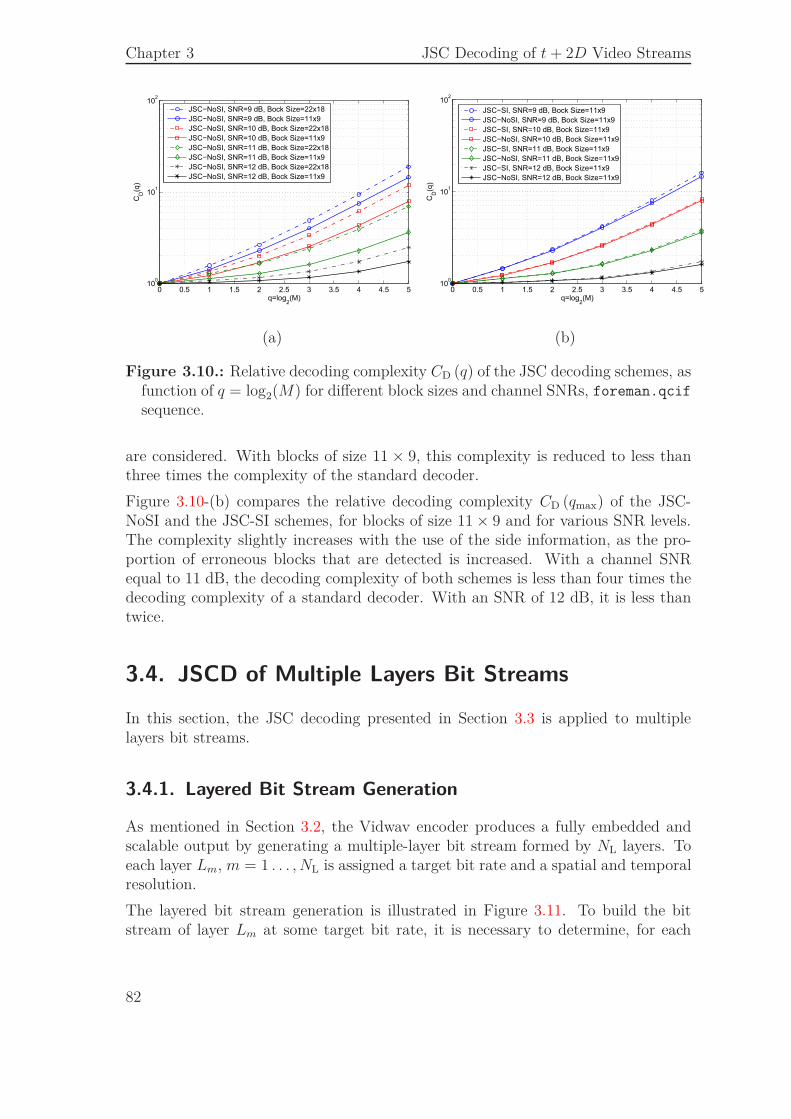
Chapter 3 JSC Decoding of t + 2D Video Streams
0 0.5 1 1.5 2 2.5 3 3.5 4 4.5 510
0
101
102
q=log2(M)
CD(q
)
JSC−NoSI, SNR=9 dB, Bock Size=22x18
JSC−NoSI, SNR=9 dB, Bock Size=11x9
JSC−NoSI, SNR=10 dB, Bock Size=22x18
JSC−NoSI, SNR=10 dB, Bock Size=11x9
JSC−NoSI, SNR=11 dB, Bock Size=22x18
JSC−NoSI, SNR=11 dB, Bock Size=11x9
JSC−NoSI, SNR=12 dB, Bock Size=22x18
JSC−NoSI, SNR=12 dB, Bock Size=11x9
0 0.5 1 1.5 2 2.5 3 3.5 4 4.5 510
0
101
102
q=log2(M)
CD(q
)
JSC−SI, SNR=9 dB, Bock Size=11x9
JSC−NoSI, SNR=9 dB, Bock Size=11x9
JSC−SI, SNR=10 dB, Bock Size=11x9
JSC−NoSI, SNR=10 dB, Bock Size=11x9
JSC−SI, SNR=11 dB, Bock Size=11x9
JSC−NoSI, SNR=11 dB, Bock Size=11x9
JSC−SI, SNR=12 dB, Bock Size=11x9
JSC−NoSI, SNR=12 dB, Bock Size=11x9
(a) (b)
Figure 3.10.: Relative decoding complexity CD (q) of the JSC decoding schemes, asfunction of q = log2(M) for different block sizes and channel SNRs, foreman.qcif
sequence.
are considered. With blocks of size 11 × 9, this complexity is reduced to less thanthree times the complexity of the standard decoder.
Figure 3.10-(b) compares the relative decoding complexity CD (qmax) of the JSC-NoSI and the JSC-SI schemes, for blocks of size 11 × 9 and for various SNR levels.The complexity slightly increases with the use of the side information, as the pro-portion of erroneous blocks that are detected is increased. With a channel SNRequal to 11 dB, the decoding complexity of both schemes is less than four times thedecoding complexity of a standard decoder. With an SNR of 12 dB, it is less thantwice.
3.4. JSCD of Multiple Layers Bit Streams
In this section, the JSC decoding presented in Section 3.3 is applied to multiplelayers bit streams.
3.4.1. Layered Bit Stream Generation
As mentioned in Section 3.2, the Vidwav encoder produces a fully embedded andscalable output by generating a multiple-layer bit stream formed by NL layers. Toeach layer Lm, m = 1 . . . , NL is assigned a target bit rate and a spatial and temporalresolution.
The layered bit stream generation is illustrated in Figure 3.11. To build the bitstream of layer Lm at some target bit rate, it is necessary to determine, for each
82
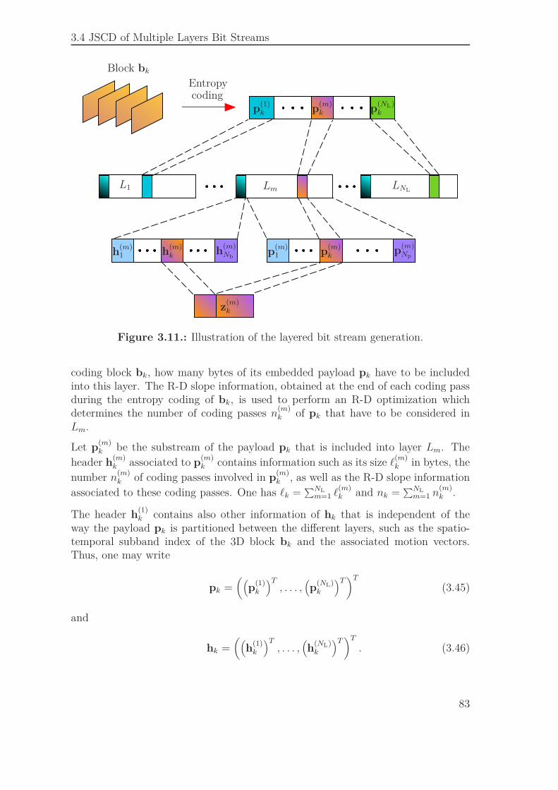
3.4 JSCD of Multiple Layers Bit Streams
p(1)k p
(NL)k
L1 Lm LNL
h(m)1 h
(m)k h
(m)Nb
p(m)1 p
(m)k
p(m)k
p(m)Np
z(m)k
Block bk
Entropycoding
Figure 3.11.: Illustration of the layered bit stream generation.
coding block bk, how many bytes of its embedded payload pk have to be includedinto this layer. The R-D slope information, obtained at the end of each coding passduring the entropy coding of bk, is used to perform an R-D optimization whichdetermines the number of coding passes n
(m)k of pk that have to be considered in
Lm.
Let p(m)k be the substream of the payload pk that is included into layer Lm. The
header h(m)k associated to p
(m)k contains information such as its size ℓ
(m)k in bytes, the
number n(m)k of coding passes involved in p
(m)k , as well as the R-D slope information
associated to these coding passes. One has ℓk =∑NL
m=1 ℓ(m)k and nk =
∑NLm=1 n
(m)k .
The header h(1)k contains also other information of hk that is independent of the
way the payload pk is partitioned between the different layers, such as the spatio-temporal subband index of the 3D block bk and the associated motion vectors.Thus, one may write
pk =((
p(1)k
)T, . . . ,
(p
(NL)k
)T)T
(3.45)
and
hk =((
h(1)k
)T, . . . ,
(h
(NL)k
)T)T
. (3.46)
83
Chapter 3 JSC Decoding of t + 2D Video Streams
The layers Lm, m = 1, . . . , NL are then formed as follows
Lm =((
h(m)1
)T, . . . ,
(h
(m)Nb
)T,(p
(m)1
)T, . . . ,
(p
(m)Nb
)T)T
. (3.47)
Finally, the vector z to be transmitted is reorganized in layers
z =((L1)
T , . . . , (LNL)T)T
. (3.48)
3.4.2. JSCD Scheme
The JSCD scheme presented in this section relies on the same compliance testsintroduced in Section 3.3.1, which are applied here to each substream p
(m)k , k =
1, . . . , Nb of each layer Lm, m = 1, . . . , NL.
As defined in Section 3.3.1, let Λ(p
(m)k
)be the number of bits processed when
decoding n(m)k passes of a given payload p
(m)k . The number of bits Λ
(h
(m)k
)that
should be processed in p(m)k is deduced from the header h
(m)k . As the header hk
defined in (3.46) is assumed to be reliably transmitted, then Λ(h
(m)k
)= ℓ
(m)k .
For a given layer m = 1, . . . , NL, if for some estimate
p(1:m)k =
((p
(1)k
)T, . . . ,
(p
(m)k
)T)T
,
the decoding of∑m
i=1 n(i)k passes requires strictly more or strictly less than
∑mi=1 Λ
(h
(i)k
)
bits, then p(1:m)k 6= p
(1:m)k .
As mentioned in Section 3.3.1, the lengths Λ(h
(m)k
)are known in bytes at the
decoder side. The syntax compliance test tB defined in (3.37) may then be usedwithout introducing any additional information. In this case, error detection ispossible when the desynchronization between the arithmetic encoder and decoderis sufficient, i.e., when more or less bytes than expected are consumed. The mostreliable compliance test tb defined in (3.33) may be considered, provided that eachheader h
(m)k is supplemented with three bits indicating the number of bits used to
pad the last byte of p(m)k . Erros leading to a single bit desynchronization may then
be detected using tb for each substream p(m)k .
The tests tb and tB may be performed to estimate each substream p(m)k of each layer
Lm, m = 1, . . . , NL as follows:
1. for m = 1, p(1)k is estimated as in Section 3.3 and p
(1)k is obtained by (3.40) or
by (3.41).
2. for m = 2, . . . , NL, assume that estimates p(i)k , i = 1, . . . , m − 1 of p
(i)k have
been obtained:
84
3.4 JSCD of Multiple Layers Bit Streams
a) as in Section 3.3.2, the M−algorithm is used to get the M most likely
candidates p (1) , . . . , p (M) to estimate p(m)k
b) k = 1
c) do
i. if
Λ(p
(1:m−1)k , p (k)
)=
m∑
i=1
Λ(h
(i)k
), (3.49)
return p(m)k = p (k)
ii. else k = k + 1
d) while k 6 M .
If no vector p (k), k = 1, . . . , M satisfying (3.49) is found, the vectors p(m)k , . . . , p
(NL)k
are dropped and the recovery of the content of the 3D block bk is obtained by entropydecoding the sequence p
(1:m−1)k .
3.4.2.1. Efficiency of the Compliance Tests in the Multi-Layer Case
As discussed in the single-layer case, the compliance tests tb and tB allow only toprove that some payload p is not syntax-compliant.
Generalizing to the multi-layer case, the bits contained in some corrupted sequence
((p
(1)k
)T, . . . ,
(p
(m)k
)T)T
, m = 1, . . . , NL
may lead to the processing of exactly∑m
i=1 ℓ(i)k bits. Therefore, for m = 2, . . . , NL
the fact that
Λ(p
(1:m)k
)=
m∑
i=1
Λ(h
(i)k
)
does not imply that p(m)k = p
(m)k , for each m = 2, . . . , NL.
As a consequence, for m = 2, . . . , NL and for a given sequence of estimates p(1)k , . . . , p
(m−1)k
verifying
Λ(p
(1:m′)k
)=
m′∑
i=1
Λ(h
(i)k
), m′ = 1, . . . , m − 1,
the fact that
Λ(p
(1:m−1)k , p
(m)k
)6=
m∑
i=1
Λ(h
(i)k
)
85
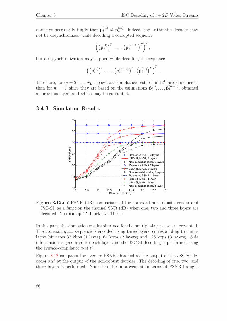
Chapter 3 JSC Decoding of t + 2D Video Streams
does not necessarily imply that p(m)k 6= p
(m)k . Indeed, the arithmetic decoder may
not be desynchronized while decoding a corrupted sequence
((p
(1)k
)T, . . . ,
(p
(m−1)k
)T)T
,
but a desynchronization may happen while decoding the sequence
((p
(1)k
)T, . . . ,
(p
(m−1)k
)T,(p
(m)k
)T)T
.
Therefore, for m = 2, . . . , NL the syntax-compliance tests tb and tB are less efficientthan for m = 1, since they are based on the estimations p
(1)k , . . . , p
(m−1)k , obtained
at previous layers and which may be corrupted.
3.4.3. Simulation Results
9 9.5 10 10.5 11 11.5 12 12.5 1310
15
20
25
30
35
40
Channel SNR (dB)
Y−
PS
NR
(dB
)
Reference PSNR 3 layers
JSC−SI, M=32, 3 layers
Non−robust decoder, 3 layers
Reference PSNR 2 layers
JSC−SI, M=32, 2 layers
Non−robust decoder, 2 layers
Reference PSNR, 1 layer
JSC−SI, M=32, 1 layer
JSC−SI, M=8, 1 layer
Non−robust decoder, 1 layer
Figure 3.12.: Y-PSNR (dB) comparison of the standard non-robust decoder andJSC-SI, as a function the channel SNR (dB) when one, two and three layers aredecoded, foreman.qcif, block size 11 × 9.
In this part, the simulation results obtained for the multiple-layer case are presented.The foreman.qcif sequence is encoded using three layers, corresponding to cumu-lative bit rates 32 kbps (1 layer), 64 kbps (2 layers) and 128 kbps (3 layers). Sideinformation is generated for each layer and the JSC-SI decoding is performed usingthe syntax-compliance test tb.
Figure 3.12 compares the average PSNR obtained at the output of the JSC-SI de-coder and at the output of the non-robust decoder. The decoding of one, two, andthree layers is performed. Note that the improvement in terms of PSNR brought
86
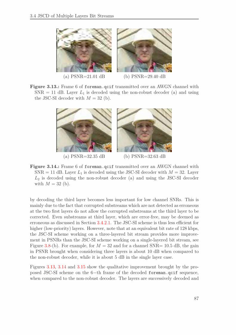
3.4 JSCD of Multiple Layers Bit Streams
(a) PSNR=21.01 dB (b) PSNR=29.40 dB
Figure 3.13.: Frame 6 of foreman.qcif transmitted over an AWGN channel withSNR = 11 dB. Layer L1 is decoded using the non-robust decoder (a) and usingthe JSC-SI decoder with M = 32 (b).
(a) PSNR=32.35 dB (b) PSNR=32.63 dB
Figure 3.14.: Frame 6 of foreman.qcif transmitted over an AWGN channel withSNR = 11 dB. Layer L1 is decoded using the JSC-SI decoder with M = 32. LayerL2 is decoded using the non-robust decoder (a) and using the JSC-SI decoderwith M = 32 (b).
by decoding the third layer becomes less important for low channel SNRs. This ismainly due to the fact that corrupted substreams which are not detected as erroneousat the two first layers do not allow the corrupted substreams at the third layer to becorrected. Even substreams at third layer, which are error-free, may be deemed aserroneous as discussed in Section 3.4.2.1. The JSC-SI scheme is thus less efficient forhigher (low-priority) layers. However, note that at an equivalent bit rate of 128 kbps,the JSC-SI scheme working on a three-layered bit stream provides more improve-ment in PSNRs than the JSC-SI scheme working on a single-layered bit stream, seeFigure 3.8-(b). For example, for M = 32 and for a channel SNR= 10.5 dB, the gainin PSNR brought when considering three layers is about 10 dB when compared tothe non-robust decoder, while it is about 5 dB in the single layer case.
Figures 3.13, 3.14 and 3.15 show the qualitative improvement brought by the pro-posed JSC-SI scheme on the 6−th frame of the decoded foreman.qcif sequence,when compared to the non-robust decoder. The layers are successively decoded and
87
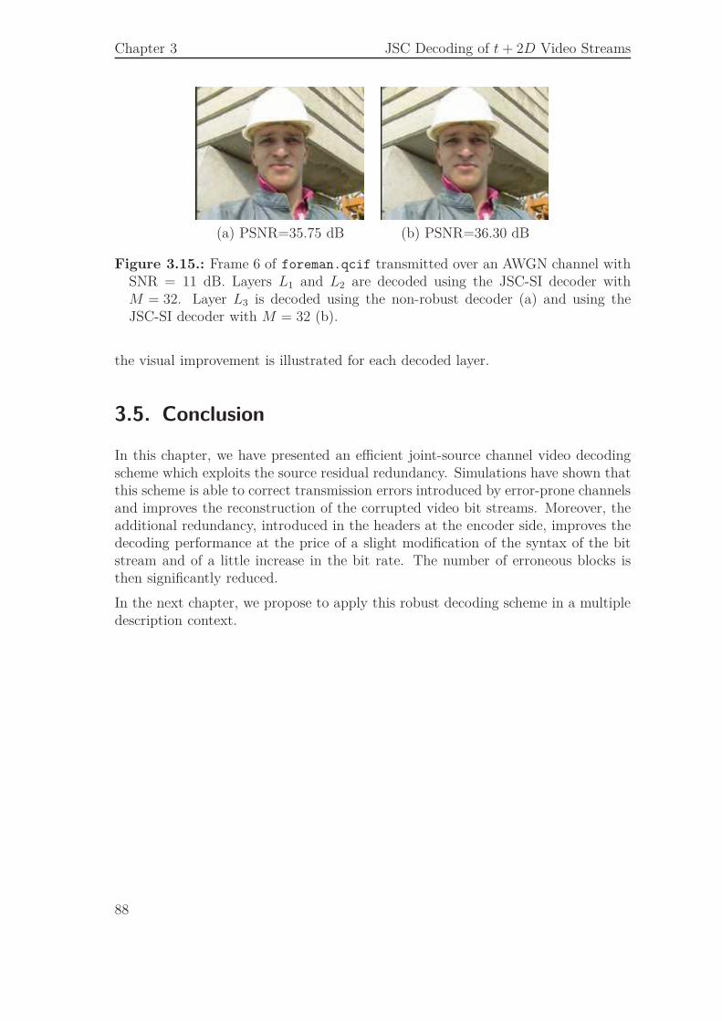
Chapter 3 JSC Decoding of t + 2D Video Streams
(a) PSNR=35.75 dB (b) PSNR=36.30 dB
Figure 3.15.: Frame 6 of foreman.qcif transmitted over an AWGN channel withSNR = 11 dB. Layers L1 and L2 are decoded using the JSC-SI decoder withM = 32. Layer L3 is decoded using the non-robust decoder (a) and using theJSC-SI decoder with M = 32 (b).
the visual improvement is illustrated for each decoded layer.
3.5. Conclusion
In this chapter, we have presented an efficient joint-source channel video decodingscheme which exploits the source residual redundancy. Simulations have shown thatthis scheme is able to correct transmission errors introduced by error-prone channelsand improves the reconstruction of the corrupted video bit streams. Moreover, theadditional redundancy, introduced in the headers at the encoder side, improves thedecoding performance at the price of a slight modification of the syntax of the bitstream and of a little increase in the bit rate. The number of erroneous blocks isthen significantly reduced.
In the next chapter, we propose to apply this robust decoding scheme in a multipledescription context.
88
4. JSC Decoding of MultipleDescription Encoded Video
In Chapter 3, we have proposed a joint-source channel decoding technique whichcombats errors occurring during a noisy transmission.
In this chapter, we consider a more general transmission scheme consisting of amixed network, formed by a packet-loss wired part followed by a noisy wirelesschannel. The effect of packet losses occurring on the wired part is mitigated bymultiple description coding, which avoids packet retransmission and reduces trans-mission delays. The aim of the joint source channel decoding approach described inChapter 3, is to correct transmission errors introduced by the wireless part of thenetwork and remaining after channel decoding. This allows to increase the numberof error-free packets which are processed by the multiple description decoder. Theredundancy introduced between the descriptions is then used to exploit the receivedand corrected packets and reconstruct the video sequence.
4.1. Problem Formulation
Assume that some video sequence has to be encoded and transmitted from a serverto a client via a heterogeneous network. A typical application context, illustratedin Figure 4.1, is video streaming to a mobile client connected to some 3G/4G basestation or WiFi access point. The network consists of a wired part introducing somelosses e.g., packet-switched network such as Internet, and a wireless part introducingsome noise in the transmitted bit stream.
As in Chapter 3, the frames of the video sequence are assumed to be represented bya vector x. In Chapter 3, we have assumed that the transmission were losses-free. Inthis chapter, the wired part of the network is not reliable. To mitigate packet lossesoccurring in this part e.g., due to congestion or router failure, a multiple description(MD) encoder is employed to produce two correlated descriptions x(1) and x(2) of x
x(i) = F(i) (x) , i = 1, 2, (4.1)
where F(i) (·) is the coding function for the i-th description. Prior to transmission,the descriptions are quantized and entropy coded to get
z(i) = E(x(i)
), (4.2)
89
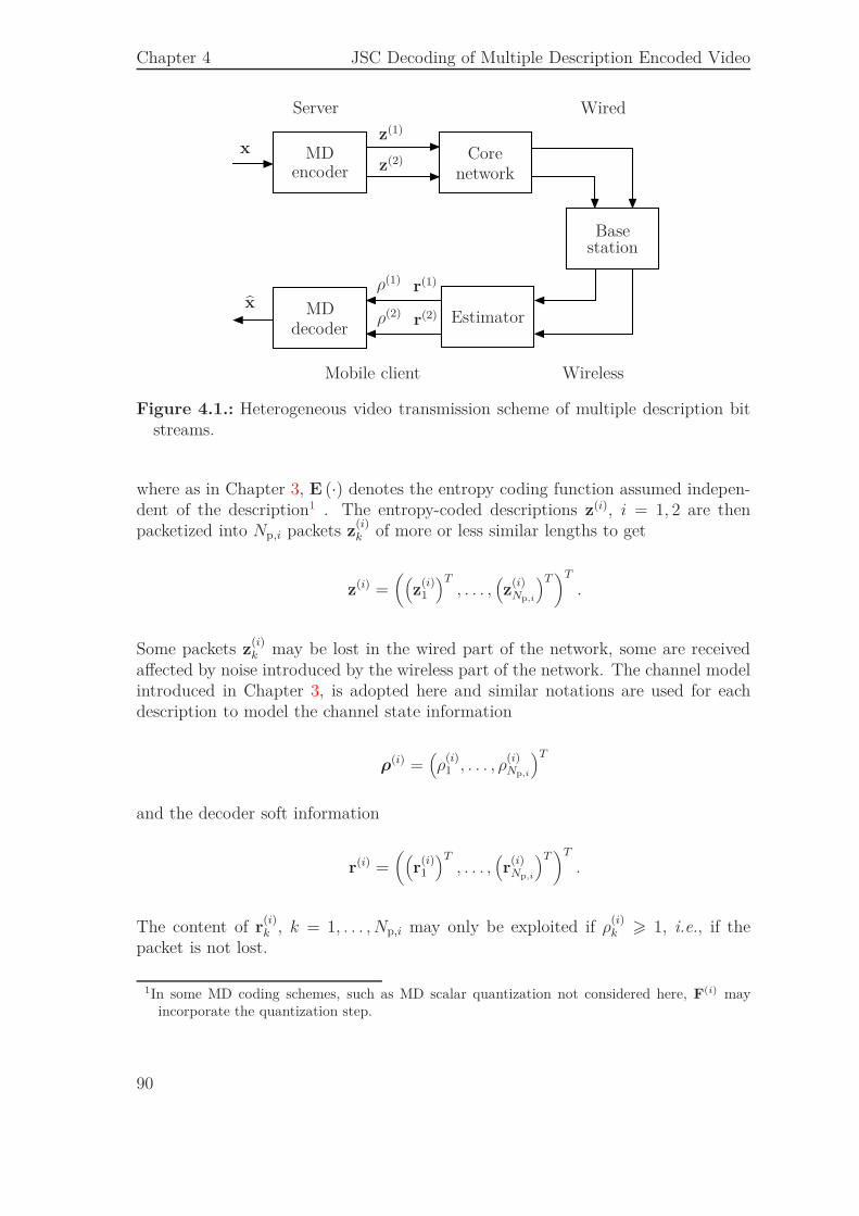
Chapter 4 JSC Decoding of Multiple Description Encoded Video
xz(1)
z(2)
r(1)
r(2)
ρ(1)
ρ(2)x MD
encoderMD Core
network
Basestation
decoderEstimator
Wireless
Wired
Mobile client
Server
Figure 4.1.: Heterogeneous video transmission scheme of multiple description bitstreams.
where as in Chapter 3, E (·) denotes the entropy coding function assumed indepen-dent of the description1 . The entropy-coded descriptions z(i), i = 1, 2 are thenpacketized into Np,i packets z
(i)k of more or less similar lengths to get
z(i) =((
z(i)1
)T, . . . ,
(z
(i)Np,i
)T)T
.
Some packets z(i)k may be lost in the wired part of the network, some are received
affected by noise introduced by the wireless part of the network. The channel modelintroduced in Chapter 3, is adopted here and similar notations are used for eachdescription to model the channel state information
ρ(i) =
(ρ
(i)1 , . . . , ρ
(i)Np,i
)T
and the decoder soft information
r(i) =((
r(i)1
)T, . . . ,
(r
(i)Np,i
)T)T
.
The content of r(i)k , k = 1, . . . , Np,i may only be exploited if ρ
(i)k > 1, i.e., if the
packet is not lost.
1In some MD coding schemes, such as MD scalar quantization not considered here, F(i) may
incorporate the quantization step.
90
4.1 Problem Formulation
4.1.1. Optimal MAP Estimation
The aim here is to evaluate the MAP estimate xMAP of x knowing ρ(i) and r(i),
i = 1, 2
xMAP = arg maxx
p(x|ρ(1), ρ
(2), r(1), r(2))
. (4.3)
Marginalizing (4.3) with respect to z(1) and z(2), one gets
xMAP = arg maxx
∑
z(1),z(2)
p(x, z(1), z(2)|ρ(1), ρ
(2), r(1), r(2))
, (4.4)
where
p(x, z(1), z(2)|ρ(1), ρ
(2), r(1), r(2))
=p (x) p
(ρ
(1), ρ(2), r(1), r(2)|x, z(1), z(2)
)p(z(1), z(2)|x
)
p (ρ(1), ρ(2), r(1), r(2)).
(4.5)
Since z(1) and z(2) are deduced from x, in (4.5) one has
p(z(1), z(2)|x
)=
1 if z(i)=E(F(i) (x)
), i = 1, 2
0 otherwise.
Using the fact that x does not provide more information than E(F(i) (x)
), i = 1, 2
on ρ(i) and r(i) , from (4.5) one gets
xMAP = arg maxx
p (x) p(ρ
(1), ρ(2), r(1), r(2)|E
(F(1) (x)
), E
(F(2) (x)
)). (4.6)
Again, the estimator in (4.6) is not easily obtained. This estimator has been em-ployed, e.g., in [1], where MD is performed by duplicating spatial subbands ade-quately quantized to minimize redundancy. However, (4.6) is unpractical for theMD scheme we have considered.
As in Section 3.1.2.2 of Chapter 3, one may proceed by estimating first z(1) and z(2),accounting for the fact that these entropy-coded descriptions have been generatedfrom the same video signal x, before deducing an estimate for x. The resultingconstrained MAP estimator of z(1) and z(2) knowing ρ
(i) and r(i), i = 1, 2, is(z(1), z(2)
)= arg max
(z(1),z(2))∈Sp(z(1), z(2)|ρ(1), ρ
(2), r(1), r(2))
, (4.7)
where
S ={(
z(1), z(2))
st ∃x | z(1)=E(F(1) (x)
)and z(2) = E
(F(2) (x)
)}(4.8)
91
Chapter 4 JSC Decoding of Multiple Description Encoded Video
is the set of all pairs of entropy-coded descriptions that may be generated from allthe possible x.
Using Bayes’ rule, (4.7) becomes(z(1), z(2)
)= arg max
(z(1),z(2))∈Sp(ρ
(1), ρ(2), r(1), r(2)|z(1), z(2)
)p(z(1), z(2)
). (4.9)
In (4.9), one has
p(ρ
(1), ρ(2), r(1), r(2)|z(1), z(2)
)= p
(r(1), r(2)|ρ(1), ρ
(2), z(1), z(2))p(ρ
(1), ρ(2)|z(1), z(2)
).
(4.10)
Assuming that the transmission of each description follows its own route, with in-dependent transmission conditions, in the wired part of the network, one has
p(ρ
(1), ρ(2)|z(1), z(2)
)=
2∏
i=1
p(ρ
(i)|z(i))
. (4.11)
Furthermore, assuming that the realizations of the wireless part of the network areindependent for each description, one gets
p(r(1), r(2)|ρ(1), ρ
(2), z(1), z(2))
=2∏
i=1
p(r(i)|ρ(i), z(i)
). (4.12)
The assumptions made in Section 3.1.2.2 of Chapter 3 for a single description bitstream and which concern the independence of the congestion conditions and of thewireless channel realizations, for each transmitted packet, may be considered herefor each description z(i). One finally obtains
(z(1), z(2)
)= arg max
(z(1),z(2))∈S
p(z(1), z(2)
) 2∏
i=1
Np,i∏
k=1
p(r
(i)k |ρ(i)
k , z(i)k
)p(ρ
(i)k |z(i)
k
).
(4.13)
Note that in (4.13), when ρ(i)k = 0, the packet has been lost before reaching the
wireless part of the network. In this case, p(r
(i)k |ρ(i)
k , z(i)k
)is independent of z
(i)k .
When ρ(i)k > 1, the evaluation of p
(r
(i)k |ρ(i)
k , z(i)k
)depends on the values of z
(i)k and
ρ(i)k and on the channel model. Moreover, in (4.13), determining whether a pair
(z(1), z(2)) belongs to the set S, depends on the MD coding scheme used to generatethe two descriptions. This scheme is described in the next section.
4.2. MD Coding Scheme
As in Chapter 3, the number of frames considered in x is denoted by Nf, andN = NfNrNc is the total number of entries of x, where Nr and Nc denote thenumber of rows and columns in each frame respectively.
92
4.2 MD Coding Scheme
The considered MD coding scheme relies on a redundant motion-compensated waveletdecomposition with J levels in the temporal domain based on the Haar filter bank[148]. We have implemented the MD scheme of [148], on the Vidwav coder presentedin Section 3.2, which is originally designed for single description coding. This MDscheme belongs to the family of frame expansion, presented in Section 2.4.2.3 ofChapter 2.
The redundancy between the descriptions is introduced by an oversampled decom-position at the last temporal level J , leading to a redundancy factor in terms of
number of frames equal to 1 +(
12
)J. The J-th temporal decomposition is repre-
sented by an N(1 + (12)J) × N redundant transform matrix T r
J . The redundantvector of temporal subbands yr of size N(1 + (1
2)J), is obtained as follows
yr =T rJTJ−1 . . . T1x =
((yr
1)T , . . . ,
(yr
Nrf
)T)T
, (4.14)
where N rf = Nf(1 + (1
2)J) and yr
n, n = 1, . . . , N rf is of size NrNc. The temporal
subbands yr are spatially transformed to get
sr = Sryr =(
(sr1)
T , . . . ,(sr
Nrf
)T)T
, (4.15)
where Sr is the N r × N r block diagonal matrix, with N r = N rfNrNc, of the same
structure as the matrix S defined in (3.18).
The vector of redundant spatio-temporal coefficients sr is further partitioned into twodescriptions. Let N (1) and N (2) be a partition of {1, . . . , N r
f }. Then the descriptionx(i) contains all sr
n with n ∈ N (i). This partitioning can be represented by x(i) =P (i)sr, i = 1, 2, where P (i) is a Nr
2×N r binary matrix defining the partition of frames
in the spatio-temporal subbands within each description. As in [148], a balancedpartitioning scheme is considered, to allow an independent reconstruction of eachdescription with similar quality. The MD encoding functions F(i) introduced in (4.1)are then
F(i) = P (i)SrT rJTJ−1 . . . T1, i = 1, 2. (4.16)
As in the case of single description coding, each x(i) is organized into Nb,i 3D blocksbk, k = 1, . . . , Nb,i. These blocks are further independently entropy-coded using the
3D-ESCOT algorithm to get z(i)k , leading to the bit streams
z(i) =((
z(i)1
)T, . . . ,
(z
(i)Nb,i
)T)T
= E(x(i)), i = 1, 2.
In this chapter, one layered bit streams are considered for each description. Notehowever that multiple layer bit streams may be generated for each description,leading to a scalable MD coding scheme. Along this chapter, the notation (·)(i),i = 1, 2 is used to refer to which description a given sequence belongs.
93
Chapter 4 JSC Decoding of Multiple Description Encoded Video
4.3. JSCD of the Descriptions
The aim of this section is to provide a practical implementation of (4.13), which isadapted to the MD coding scheme presented in Section 4.2.
As in Chapter 3, we assume for simplicity sake that each packet z(i)k introduced in
Section 4.1 contains a single 3D block. In this case, Np,i = Nb,i, i = 1, 2. Moreover,
all the pairs(z(1), z(2)
)∈ S are assumed to be equally probable a priori, so that
(4.13) becomes
(z(1), z(2)
)= arg max(
z(1)1:Nb,1
,z(2)1:Nb,2
)∈S
2∏
i=1
Ni∏
j=1
p(r
(i)j |ρ(i)
j , z(i)j
)p(ρ
(i)j |z(i)
j
), (4.17)
where
z(i)1:Nb,i
=((
z(i)1
)T, . . . ,
(z
(i)Nb,i
)T)T
.
Now let us consider the sets
S(i) ={
z(i) st ∃x | z(i)=E(F(i) (x)
)}(4.18)
and
S(i)k =
z
(i)k st ∃x | ∃
(z
(i)1 , . . . , z
(i)k−1, z
(i)k+1, . . . , z
(i)Nb,i
),
((z
(i)1
)T, . . . ,
(z
(i)k−1
)T,(z
(i)k
)T,(z
(i)k+1
)T, . . . ,
(z
(i)Nb,i
)T)T
=E(F(i) (x)
).
(4.19)
The sets S(i) and S(i)k contain respectively all the entropy-coded descriptions and all
the entropy-coded 3D blocks z(i)k , k = 1, . . . , Nb,i one may obtain considering all the
possible values of x.
Remark 2. One has
S ⊂ S(1) × S(2) ⊆
Nb,1⊗
k=1
S(1)k
×
Nb,2⊗
k=1
S(2)k
. (4.20)
Consider(z(1), z(2)
)∈ S. From (4.8), there exists some sequence x such that z(i) =
E(F(i)(x)), i = 1, 2, which implies z(i) ∈ S(i) and(z(1), z(2)
)∈ S(1) × S(2). Consider
now(z(1), z(2)
)∈ S(1) × S(2). For i = 1, 2
∃xi st z(i) =((
z(i)1
)T, . . . ,
(z
(i)Nb,i
)T)T
= E(F(i)(xi)), (4.21)
94
4.3 JSCD of the Descriptions
and thus z(i)k ∈ S(i)
k , k = 1, . . . , Nb,i, leading to z(i) ∈(⊗Nb,i
k=1 S(i)k
)and (z(1), z(2)) ∈(⊗Nb,1
k=1 S(1)k
)×(⊗Nb,2
k=1 S(2)k
).
In general, S 6= S(1) × S(2). Consider(z(1), z(2)
)∈ S(1) × S(2) and let X
(z(i)
)={
x st z(i) = E(F(i)(x))}. If X
(z(1)
)∩ X
(z(2)
)66= ∅ then
(z(1), z(2)
)∈ S. Assume
now that for all(z(1), z(2)
)∈ S(1) × S(2), one has X
(z(1)
)∩ X
(z(2)
)66= ∅. This
means that z(1) and z(2) are independent, which is not the case in a general MDcoding scheme, as soon as it introduces some redundancy. Similarly, to show thatS(1) × S(2) =
(⊗Nb,1
k=1 S(1)k
)×(⊗Nb,2
k=1 S(2)k
), it suffices to show that
(⊗Nb,i
k=1 S(i)k
)⊂
S(i), i = 1, 2. For that purpose, one has to show that⋂Nb,i
k=1 X(z
(i)k
)6= ∅ for all
z(i)1:Nb,i
∈(⊗Nb,i
k=1 S(i)k
). Necessary conditions for this is that the quantization and
entropy-coding operations of each z(i)k are performed independently and that each
individual F(i) does not introduce any redundancy.
Similarly to the single description coding case, on may derive a suboptimal estimatorfor each component z
(i)k , k = 1, . . . , Nb,i of z(i), i = 1, 2, using (4.17) and (4.20)
z(i)k = arg max
z(i)k∈S(i)
k
p(r
(i)k |ρ(i)
k , z(i)k
)p(ρ
(i)k |z(i)
k
). (4.22)
This estimator may be used only when ρ(i)j > 1. The estimator
(z
(1)1:Nb,1
, z(2)1:Nb,2
)is a
suboptimal solution of (4.17) since(z
(1)1:Nb,1
, z(2)1:Nb,2
)is not necessarily in S, see (4.20).
In what follows the estimation process of z(i)k is described when ρ
(i)k > 1, then when
ρ(i)k = 0.
4.3.1. When ρ(i)k > 1
As in Chapter 3, each transmitted packet z(i)k , k = 1, . . . , Nb,i consists of a header
h(i)k and a payload p
(i)k
z(i)k =
((h
(i)k
)T,(p
(i)k
)T)T
.
The received vector
r(i)k =
((r
(i)k,h
)T,(r
(i)k,p
)T)T
contains soft information on h(i)k given by r
(i)k,h and on p
(i)k given by r
(i)k,p.
Moreover, the header h(i)k is assumed to be received without errors. As mentioned
earlier, the term p(ρ
(i)k |z(i)
k
)in (4.22) does not depend on the content of z
(i)k but on
95
Chapter 4 JSC Decoding of Multiple Description Encoded Video
its length which is stored in h(i)k . Thus, the estimation problem in (4.22) reduces to
evaluate
p(i)k = arg max
p(i)k
st(
h(i)k
,p(i)k
)∈S(i)
k
p(r
(i)k,p|ρ(i)
k , p(i)k
). (4.23)
The estimation in (4.23) is performed as in the case of single description bit streams,presented in Section 3.3 of Chapter 3 by using a JSC decoder which exploits theresidual redundancy left in each description. The syntax compliance tests tb andtB introduced in Section 3.3.1 are considered for each p
(i)k to eliminate the elements
which are not syntax-compliant by using the M−algorithm as described in Sec-tion 3.3.2.
4.3.2. When ρ(i)k = 0
When ρ(i)j = 0, the estimator in (4.22) cannot be used since neither r
(i)k,h nor r
(i)k,p
are available. All vectors z(i)k are equally likely. The most reasonable estimate for
z(i)k is to take the all zero vector and to replace the coefficients in the corresponding
spatio-temporal subband by zeros, or to ignore these coefficients when performingreconstruction, as will be presented in the next section.
4.4. Reconstruction
In this section, we propose to reconstruct the video stream x from(z
(1)1:Nb,1
, z(2)1:Nb,2
)
obtained as described in the previous section. Consider the vector
x(i) =((
x(i)1
)T, . . . ,
(x
(i)Nb,i
)T)T
,
with x(i)k = E−1(z(i)
k ) if ρ(i)k > 1 and x
(i)k = 0 otherwise, where E−1 represents
the entropy decoding function associated to E. By combining x(1) and x(2), andassuming that all the corrupted blocks have been efficiently corrected, one gets thevector sr which is a version of the transmitted vector of spatio-temporal subbandssr, affected by quantization noise and block losses. The aim is to recover x from sr.
In a first time, we consider the case where there are no lost blocks, i.e., ρ(i)k > 1,
k = 1, . . . , Nb,i, i = 1, 2. Then sr is only affected by the quantization noise and thereconstruction of x corresponds to central decoding. After inverse spatial transformof sr, one obtains the vector of temporal subbbands w = (Sr)−1
sr.
As mentioned in Section 4.2, the redundancy between the two descriptions is intro-duced at the last temporal level J by the means of oversampled motion-compensatedtemporal filtering. In [148], the central decoding is performed on w to recover the
96
4.5 Simulation Results
frames of the temporal approximation subband at level J − 1 (the detail frames ofthe temporal levels 1, .., J − 1 do not contain any redundancy). The reconstructionfor a temporal approximation frame at level J − 1 is performed by the central de-coder either by taking into account only one reconstructed description, given by oneof the side decoders, or by computing the mean of the reconstructions provided bythe two side decoders, as proposed in [148]. We point out that this central decod-ing corresponds to multiplying w by the pseudo-inverse of the redundant temporaltransform T r when no motion estimation/compensation is considered.
Let us now consider the case where blocks have been lost. The spatio-temporalapproximation subband contains the most important part of the bit stream. Ablock lost in this subband can seriously damage the whole reconstruction of thevideo sequence. To limit the damage propagation when losses occur within thissubband, we identify the frames of the temporal approximation subband at levelJ − 1 that would be affected by these losses. Once these frames are identified, theyare reconstructed by taking into account only the description wherein these blockshave been correctly received; otherwise, if the same blocks have been corrupted inboth descriptions, the central decoding is performed as in [148]. For the temporaldetail subbands, the lost blocks are simply replaced with zero coefficients, losingthus the details of the inverse motion-compensation.
In this reconstruction approach, neither spatial nor temporal concealment has beenconsidered. Only the temporal correlation between the descriptions has been ex-ploited to reconstruct the temporal approximation frames at level J − 1.
4.5. Simulation Results
For the experimental part, the foreman.qcif sequence has been encoded at a framerate Rf = 15 frames per second (fps) using the temporal MD coding scheme pre-sented in Section 4.2, with J = 3 temporal decomposition levels and 3 spatialdecomposition levels. The 3D blocks are of size 11 × 9, as in the Chapter 3, theproposed JSC decoding scheme has proven to be more efficient for this block sizethan for a block size of 22 × 18. The number of frames considered in x is Nf = 32.
In the next section, we provide some statistics about the proportion of headers anddata generated by the MD coder and the amount of redundancy introduced by theadditional side information (SI) to allow the use of the syntax-compliance test tb.
4.5.1. Bit Stream Organization
For both single description (SD) and MD coding schemes, the generated bit streamis put into packets of approximately the same size, with a length limit of Lmax =1000 bytes. Each packet contains an integer number of encoded 3D blocks. The
97
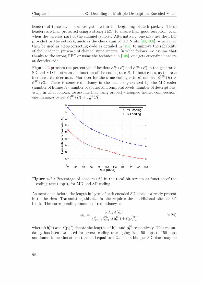
Chapter 4 JSC Decoding of Multiple Description Encoded Video
headers of these 3D blocks are gathered in the beginning of each packet. Theseheaders are then protected using a strong FEC, to ensure their good reception, evenwhen the wireless part of the channel is noisy. Alternatively, one may use the FECprovided by the network, such as the check sum of UDP-Lite [90, 108], which maythen be used as error-correcting code as detailed in [108] to improve the reliabilityof the header in presence of channel impairments. In what follows, we assume thatthanks to the strong FEC or using the technique in [108], one gets error-free headersat decoder side.
Figure 4.2 presents the percentage of headers φSDH (R) and φMD
H (R) in the generatedSD and MD bit streams as function of the coding rate R. In both cases, as the rateincreases, φH decreases. Moreover for the same coding rate R, one has φMD
H (R) >φSD
H (R). There is some redundancy in the headers generated by the MD coder(number of frames Nf, number of spatial and temporal levels, number of descriptions,etc.). In what follows, we assume that using properly-designed header compression,one manages to get φMD
H (R) ≃ φSDH (R).
50 60 70 80 90 100 110 120 130 140 1508
10
12
14
16
18
20
22
24
26
Rate (Kbps)
Perc
enta
ge o
f headers
(%
)
MD coding
SD coding
Figure 4.2.: Percentage of headers (%) in the total bit stream as function of thecoding rate (kbps), for MD and SD coding.
As mentioned before, the length in bytes of each encoded 3D block is already presentin the headers. Transmitting this size in bits requires three additional bits per 3Dblock. The corresponding amount of redundancy is
φSI =
∑2i=1 3Nb,i
∑2i=1
∑Nb,i
k=1 ℓ(h(i)k ) + ℓ(p(i)
k ), (4.24)
where ℓ(h(i)k ) and ℓ(p(i)
k ) denote the lengths of h(i)k and p
(i)k respectively. This redun-
dancy has been evaluated for several coding rates going from 50 kbps to 150 kbpsand found to be almost constant and equal to 1 %. The 3 bits per 3D block may be
98
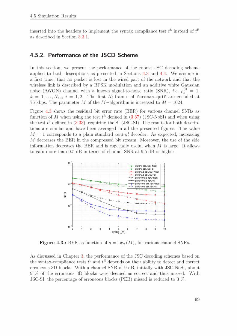
4.5 Simulation Results
inserted into the headers to implement the syntax compliance test tb instead of tB
as described in Section 3.3.1.
4.5.2. Performance of the JSCD Scheme
In this section, we present the performance of the robust JSC decoding schemeapplied to both descriptions as presented in Sections 4.3 and 4.4. We assume ina first time, that no packet is lost in the wired part of the network and that thewireless link is described by a BPSK modulation and an additive white Gaussiannoise (AWGN) channel with a known signal-to-noise ratio (SNR), i.e, ρ
(i)k = 1,
k = 1, . . . , Nb,i, i = 1, 2. The first Nf frames of foreman.qcif are encoded at75 kbps. The parameter M of the M−algorithm is increased to M = 1024.
Figure 4.3 shows the residual bit error rate (BER) for various channel SNRs asfunction of M when using the test tB defined in (3.37) (JSC-NoSI) and when usingthe test tb defined in (3.33), requiring the SI (JSC-SI). The results for both descrip-tions are similar and have been averaged in all the presented figures. The valueM = 1 corresponds to a plain standard central decoder. As expected, increasingM decreases the BER in the compressed bit stream. Moreover, the use of the sideinformation decreases the BER and is especially useful when M is large. It allowsto gain more than 0.5 dB in terms of channel SNR at 9.5 dB or higher.
0 1 2 3 4 5 6 7 8 9 1010
−4
10−3
10−2
10−1
q=log2(M)
BE
R
SNR=9 dB JSC−NoSI
SNR=9 dB JSC−SI
SNR=9.5 dB JSC−NoSI
SNR=9.5 dB JSC−SI
SNR=10 dB JSC−NoSI
SNR=10 dB JSC−SI
SNR=10.5 dB JSC−NoSI
SNR=10.5 dB JSC−SI
Figure 4.3.: BER as function of q = log2 (M), for various channel SNRs.
As discussed in Chapter 3, the performance of the JSC decoding schemes based onthe syntax-compliance tests tb and tB depends on their ability to detect and correcterroneous 3D blocks. With a channel SNR of 9 dB, initially with JSC-NoSI, about9 % of the erroneous 3D blocks were deemed as correct and thus missed. WithJSC-SI, the percentage of erroneous blocks (PEB) missed is reduced to 3 %.
99
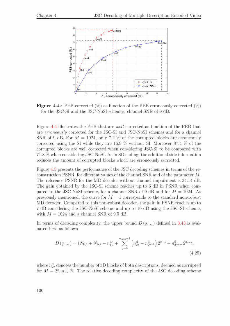
Chapter 4 JSC Decoding of Multiple Description Encoded Video
0 2 4 6 8 10 12 14 16 180
10
20
30
40
50
60
70
80
90
PEB erroneously corrected (%)
PE
B c
orr
ecte
d (
%)
JSC−SI
JSC−NoSIM=1
M=32
M=8
M=4
M=2M=2
M=8
M=1024
M=1024
M=4
M=32
Figure 4.4.: PEB corrected (%) as function of the PEB erroneously corrected (%)for the JSC-SI and the JSC-NoSI schemes, channel SNR of 9 dB.
Figure 4.4 illustrates the PEB that are well corrected as function of the PEB thatare erroneously corrected for the JSC-SI and JSC-NoSI schemes and for a channelSNR of 9 dB. For M = 1024, only 7.2 % of the corrupted blocks are erroneouslycorrected using the SI while they are 16.9 % without SI. Moreover 87.4 % of thecorrupted blocks are well corrected when considering JSC-SI to be compared with71.8 % when considering JSC-NoSI. As in SD coding, the additional side informationreduces the amount of corrupted blocks which are erroneously corrected.
Figure 4.5 presents the performance of the JSC decoding schemes in terms of the re-construction PSNR, for different values of the channel SNR and of the parameter M .The reference PSNR for the MD decoder without channel impairment is 34.14 dB.The gain obtained by the JSC-SI scheme reaches up to 6 dB in PSNR when com-pared to the JSC-NoSI scheme, for a channel SNR of 9 dB and for M = 1024. Aspreviously mentioned, the curve for M = 1 corresponds to the standard non-robustMD decoder. Compared to this non-robust decoder, the gain in PSNR reaches up to7 dB considering the JSC-NoSI scheme and up to 10 dB using the JSC-SI scheme,with M = 1024 and a channel SNR of 9.5 dB.
In terms of decoding complexity, the upper bound D (qmax) defined in 3.43 is eval-uated here as follows
D (qmax) = (Nb,1 + Nb,2 − nd1) +
qmax−1∑
q=0
(nd
2q − nd2q+1
)2q+1 + nd
2qmax 2qmax,
(4.25)
where nd2q denotes the number of 3D blocks of both descriptions, deemed as corrupted
for M = 2q, q ∈ N. The relative decoding complexity of the JSC decoding scheme
100
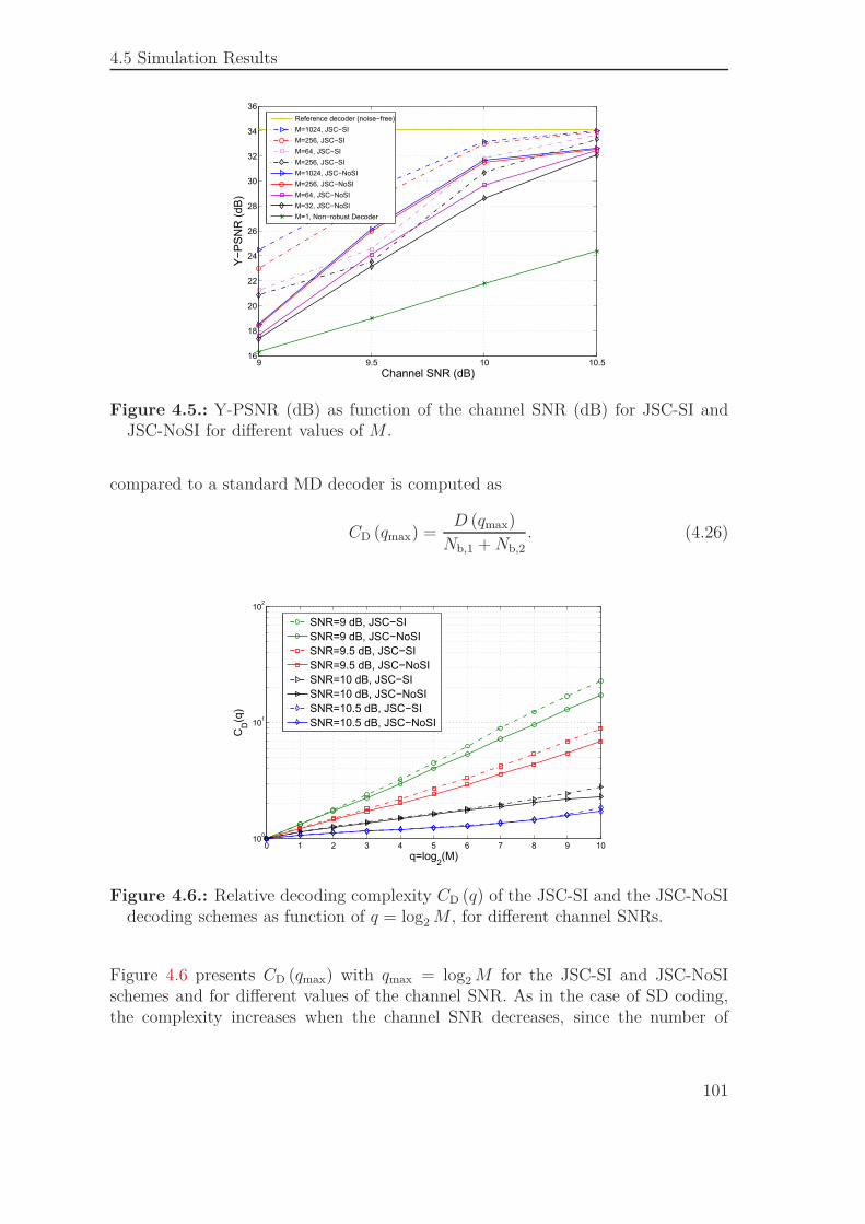
4.5 Simulation Results
9 9.5 10 10.516
18
20
22
24
26
28
30
32
34
36
Channel SNR (dB)
Y−
PS
NR
(dB
)
Reference decoder (noise−free)
M=1024, JSC−SI
M=256, JSC−SI
M=64, JSC−SI
M=256, JSC−SI
M=1024, JSC−NoSI
M=256, JSC−NoSI
M=64, JSC−NoSI
M=32, JSC−NoSI
M=1, Non−robust Decoder
Figure 4.5.: Y-PSNR (dB) as function of the channel SNR (dB) for JSC-SI andJSC-NoSI for different values of M .
compared to a standard MD decoder is computed as
CD (qmax) =D (qmax)
Nb,1 + Nb,2. (4.26)
0 1 2 3 4 5 6 7 8 9 1010
0
101
102
q=log2(M)
CD(q
)
SNR=9 dB, JSC−SI
SNR=9 dB, JSC−NoSI
SNR=9.5 dB, JSC−SI
SNR=9.5 dB, JSC−NoSI
SNR=10 dB, JSC−SI
SNR=10 dB, JSC−NoSI
SNR=10.5 dB, JSC−SI
SNR=10.5 dB, JSC−NoSI
Figure 4.6.: Relative decoding complexity CD (q) of the JSC-SI and the JSC-NoSIdecoding schemes as function of q = log2 M , for different channel SNRs.
Figure 4.6 presents CD (qmax) with qmax = log2 M for the JSC-SI and JSC-NoSIschemes and for different values of the channel SNR. As in the case of SD coding,the complexity increases when the channel SNR decreases, since the number of
101
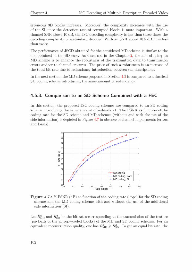
Chapter 4 JSC Decoding of Multiple Description Encoded Video
erroneous 3D blocks increases. Moreover, the complexity increases with the useof the SI since the detection rate of corrupted blocks is more important. With achannel SNR above 10 dB, the JSC decoding complexity is less than three times thedecoding complexity of a standard decoder. With an SNR above 10.5 dB, it is lessthan twice.
The performance of JSCD obtained for the considered MD scheme is similar to theone obtained in the SD case. As discussed in the Chapter 2, the aim of using anMD scheme is to enhance the robustness of the transmitted data to transmissionerrors and/or to channel erasures. The price of such a robustness is an increase ofthe total bit rate due to redundancy introduction between the descriptions.
In the next section, the MD scheme proposed in Section 4.3 is compared to a classicalSD coding scheme introducing the same amount of redundancy.
4.5.3. Comparison to an SD Scheme Combined with a FEC
In this section, the proposed JSC coding schemes are compared to an SD codingscheme introducing the same amount of redundanct. The PSNR as function of thecoding rate for the SD scheme and MD schemes (without and with the use of theside information) is depicted in Figure 4.7 in absence of channel impairments (errorsand losses).
20 40 60 80 100 120 140 160 18029
30
31
32
33
34
35
36
37
38
39
Rate (Kbps)
Y−
PS
NR
(dB
)
SD coding
MD coding, NoSI
MD coding, SI
Figure 4.7.: Y-PSNR (dB) as function of the coding rate (kbps) for the SD codingscheme and the MD coding scheme with and without the use of the additionalside information (SI).
Let RdMD and Rd
SD be the bit rates corresponding to the transmission of the texture(payloads of the entropy-coded blocks) of the MD and SD coding schemes. For anequivalent reconstruction quality, one has Rd
MD > RdSD. To get an equal bit rate, the
102
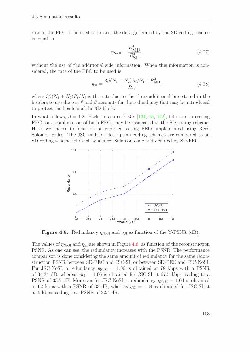
4.5 Simulation Results
rate of the FEC to be used to protect the data generated by the SD coding schemeis equal to
ηNoSI =Rd
MDRd
SD, (4.27)
without the use of the additional side information. When this information is con-sidered, the rate of the FEC to be used is
ηSI =3β(N1 + N2)Rf/Nf + Rd
MD
RdSD
, (4.28)
where 3β(N1 + N2)Rf/Nf is the rate due to the three additional bits stored in theheaders to use the test tband β accounts for the redundancy that may be introducedto protect the headers of the 3D block.
In what follows, β = 1.2. Packet-erasures FECs [134, 15, 142], bit-error correctingFECs or a combination of both FECs may be associated to the SD coding scheme.Here, we choose to focus on bit-error correcting FECs implemented using ReedSolomon codes. The JSC multiple description coding schemes are compared to anSD coding scheme followed by a Reed Solomon code and denoted by SD-FEC.
32 32.5 33 33.5 34 34.5 35 35.5 361
1.05
1.1
1.15
Y−PSNR (dB)
Redundancy
JSC−SI
JSC−NoSI
Figure 4.8.: Redundancy ηNoSI and ηSI as function of the Y-PSNR (dB).
The values of ηNoSI and ηSI are shown in Figure 4.8, as function of the reconstructionPSNR. As one can see, the redundancy increases with the PSNR. The performancecomparison is done considering the same amount of redundancy for the same recon-struction PSNR between SD-FEC and JSC-SI, or between SD-FEC and JSC-NoSI.For JSC-NoSI, a redundancy ηNoSI = 1.06 is obtained at 78 kbps with a PSNRof 34.34 dB, whereas ηSI = 1.06 is obtained for JSC-SI at 67.5 kbps leading to aPSNR of 33.5 dB. Moreover for JSC-NoSI, a redundancy ηNoSI = 1.04 is obtainedat 62 kbps with a PSNR of 33 dB, whereas ηSI = 1.04 is obtained for JSC-SI at55.5 kbps leading to a PSNR of 32.4 dB.
103
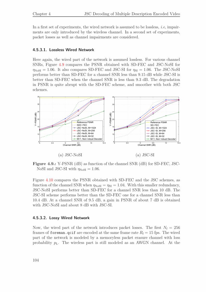
Chapter 4 JSC Decoding of Multiple Description Encoded Video
In a first set of experiments, the wired network is assumed to be lossless, i.e, impair-ments are only introduced by the wireless channel. In a second set of experiments,packet losses as well as channel impairments are considered.
4.5.3.1. Lossless Wired Network
Here again, the wired part of the network is assumed lossless. For various channelSNRs, Figure 4.9 compares the PSNR obtained with SD-FEC and JSC-NoSI forηNoSI = 1.06. It also compares SD-FEC and JSC-SI for ηSI = 1.06. The JSC-NoSIperforms better than SD-FEC for a channel SNR less than 9.15 dB while JSC-SI isbetter than SD-FEC when the channel SNR is less than 9.3 dB. The degradationin PSNR is quite abrupt with the SD-FEC scheme, and smoother with both JSCschemes.
8 8.5 9 9.5 10 10.55
10
15
20
25
30
35
Channel SNR (dB)
Y−
PS
NR
(dB
)
Reference PSNR
SDC−FEC
JSC−NoSI, M=1024
JSC−NoSI, M=256
JSC−NoSI, M=64
JSC−NoSI, M=32
M=1, Non−robust Decoder
8 8.5 9 9.5 10 10.55
10
15
20
25
30
35
Channel SNR (dB)
Y−
PS
NR
(dB
)
Reference PSNR
SD−FEC
JSC−SI, M=1024
JSC−SI, M=256
JSC−SI, M=64
JSC−SI, M=32
M=1, Non−robust Decoder
(a) JSC-NoSI (a) JSC-SI
Figure 4.9.: Y-PSNR (dB) as function of the channel SNR (dB) for SD-FEC, JSC-NoSI and JSC-SI with ηNoSI = 1.06.
Figure 4.10 compares the PSNR obtained with SD-FEC and the JSC schemes, asfunction of the channel SNR when ηNoSI = ηSI = 1.04. With this smaller redundancy,JSC-NoSI performs better than SD-FEC for a channel SNR less than 10 dB. TheJSC-SI scheme performs better than the SD-FEC one for a channel SNR less than10.4 dB. At a channel SNR of 9.5 dB, a gain in PSNR of about 7 dB is obtainedwith JSC-NoSI and about 8 dB with JSC-SI.
4.5.3.2. Lossy Wired Network
Now, the wired part of the network introduces packet losses. The first Nf = 256frames of foreman.qcif are encoded at the same frame rate Rf = 15 fps. The wiredpart of the network is modeled by a memoryless packet erasure channel with lossprobability pL. The wireless part is still modeled as an AWGN channel. At the
104
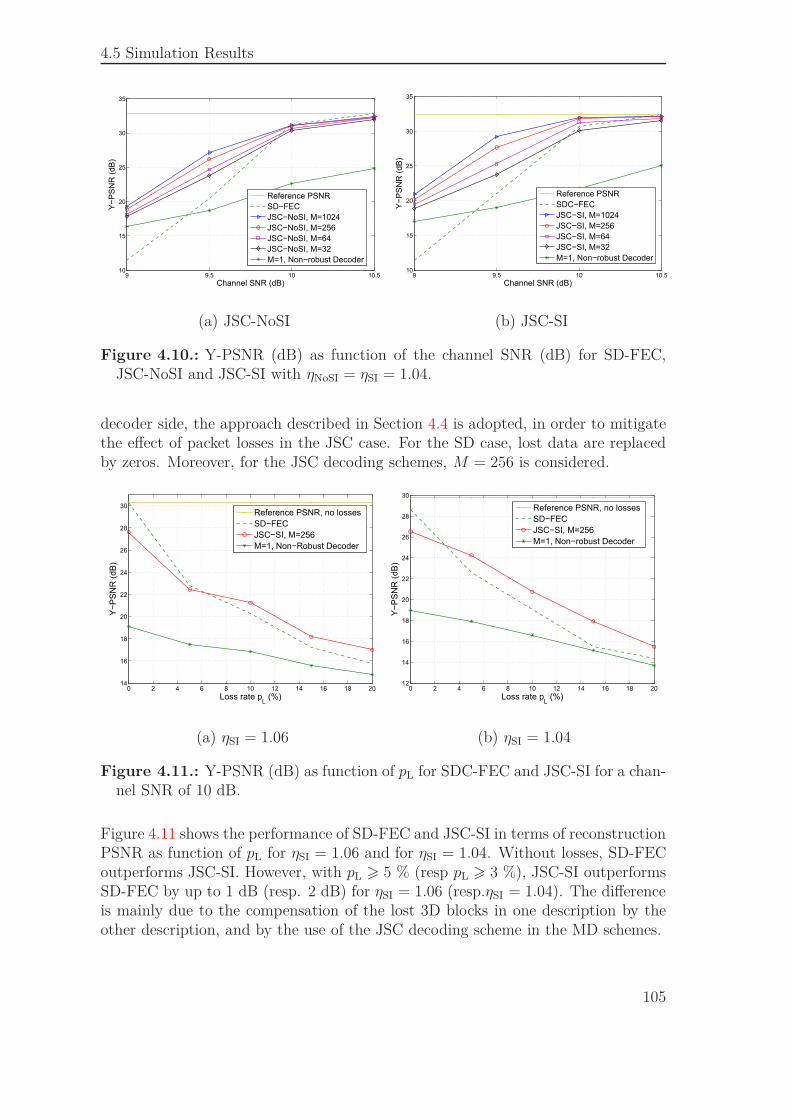
4.5 Simulation Results
9 9.5 10 10.510
15
20
25
30
35
Channel SNR (dB)
Y−
PS
NR
(dB
)
Reference PSNR
SD−FEC
JSC−NoSI, M=1024
JSC−NoSI, M=256
JSC−NoSI, M=64
JSC−NoSI, M=32
M=1, Non−robust Decoder
9 9.5 10 10.510
15
20
25
30
35
Channel SNR (dB)
Y−
PS
NR
(dB
)
Reference PSNR
SDC−FEC
JSC−SI, M=1024
JSC−SI, M=256
JSC−SI, M=64
JSC−SI, M=32
M=1, Non−robust Decoder
(a) JSC-NoSI (b) JSC-SI
Figure 4.10.: Y-PSNR (dB) as function of the channel SNR (dB) for SD-FEC,JSC-NoSI and JSC-SI with ηNoSI = ηSI = 1.04.
decoder side, the approach described in Section 4.4 is adopted, in order to mitigatethe effect of packet losses in the JSC case. For the SD case, lost data are replacedby zeros. Moreover, for the JSC decoding schemes, M = 256 is considered.
0 2 4 6 8 10 12 14 16 18 2014
16
18
20
22
24
26
28
30
Loss rate pL
(%)
Y−
PS
NR
(dB
)
Reference PSNR, no losses
SD−FEC
JSC−SI, M=256
M=1, Non−Robust Decoder
0 2 4 6 8 10 12 14 16 18 2012
14
16
18
20
22
24
26
28
30
Loss rate pL
(%)
Y−
PS
NR
(dB
)
Reference PSNR, no losses
SD−FEC
JSC−SI, M=256
M=1, Non−robust Decoder
(a) ηSI = 1.06 (b) ηSI = 1.04
Figure 4.11.: Y-PSNR (dB) as function of pL for SDC-FEC and JSC-SI for a chan-nel SNR of 10 dB.
Figure 4.11 shows the performance of SD-FEC and JSC-SI in terms of reconstructionPSNR as function of pL for ηSI = 1.06 and for ηSI = 1.04. Without losses, SD-FECoutperforms JSC-SI. However, with pL > 5 % (resp pL > 3 %), JSC-SI outperformsSD-FEC by up to 1 dB (resp. 2 dB) for ηSI = 1.06 (resp.ηSI = 1.04). The differenceis mainly due to the compensation of the lost 3D blocks in one description by theother description, and by the use of the JSC decoding scheme in the MD schemes.
105
Chapter 4 JSC Decoding of Multiple Description Encoded Video
4.6. Conclusion
In this chapter, we have applied joint source channel decoding exploiting the sourceresidual redundancy in a multiple description coding context. The aim was topresent a typical application of such a scheme, e.g., video broadcasting over mixedarchitectures, in which retransmission of the lost data is not allowed. The redun-dancy introduced between the descriptions is exploited to compensate packet losses,whereas the joint decoding allows to increase the number of error-free packets reach-ing the multiple description decoder, and thus to improve its performance.
In the considered multiple description scheme, the redundancy is introduced by usingan overcomplete temporal decomposition which operates an expansion of the inputvideo signal to generate the two descriptions. The linear relations between the entriesof the descriptions may be exploited to detect and correct some of the transmissionerrors. However, this redundancy is only exploitable after entropy decoding andinverse spatial transform. This makes it difficult to use this redundancy directly fromthe channel soft outputs. Moreover due to motion estimation and compensation,a single entry in one of the descriptions may be involved in several linear relationsmaking the error detection and correction particularly difficult.
In the next chapter, we study, in a more theoretical context, schemes operatingsuch a signal expansion. The aim is to explore the way the introduced redundancycould be exploited to detect and correct transmission errors in a joint source channelcoding framework.
106
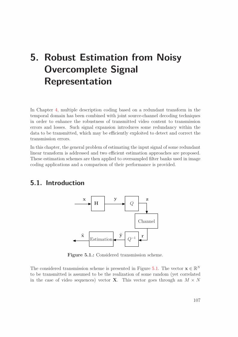
5. Robust Estimation from NoisyOvercomplete SignalRepresentation
In Chapter 4, multiple description coding based on a redundant transform in thetemporal domain has been combined with joint source-channel decoding techniquesin order to enhance the robustness of transmitted video content to transmissionerrors and losses. Such signal expansion introduces some redundancy within thedata to be transmitted, which may be efficiently exploited to detect and correct thetransmission errors.
In this chapter, the general problem of estimating the input signal of some redundantlinear transform is addressed and two efficient estimation approaches are proposed.These estimation schemes are then applied to oversampled filter banks used in imagecoding applications and a comparison of their performance is provided.
5.1. Introduction
x y
r
H
x
z
y
Q
Q−1Estimation
Channel
Figure 5.1.: Considered transmission scheme.
The considered transmission scheme is presented in Figure 5.1. The vector x ∈ RN
to be transmitted is assumed to be the realization of some random (yet correlatedin the case of video sequences) vector X. This vector goes through an M × N
107
Chapter 5 Robust Estimation from Noisy Overcomplete Signal Representation
transform matrix H. The resulting vector y = Hx is first quantized to get thevector of quantization indexes z, then transmitted through some noisy channel.
The problem one is faced with is to estimate the input vector x. Classical approacheshandle this problem by using the hard decisions of the channel decoder, then byperforming a reconstruction which minimizes a given metric, e.g., the mean squarederror. In the particular expansion case (M > N), these approaches are not efficient,since they do not fully exploit the redundancy introduced in the output vector y,i.e., the linear dependencies between the entries of y are not taken into accountduring the estimation of x, in order to detect, e.g., the transmission errors.
As discussed in the previous chapters, the redundancy present in y may efficientlybe exploited at the receiver side to perform joint source-channel decoding (JSCD).To implement JSCD at the application layer, we assume as in Chapters 3 and 4 thatpermeable protocol layers [75, 42] and robust header recovery mechanisms [101] areimplemented, so that the soft information coming from the channel decoders atphysical layer reaches the application layer. The channel represents then all what isbetween the quantization output and the inverse quantization input, including theentropy coding, the network packetization and the physical channel, as well as thecorresponding robust depacketization and entropy decoding modules [42]. At theoutput of this channel, the soft information r on the transmitted bits is obtained.
In this chapter, data redundancy is introduced by the mean of a redundant lineartransform. A first direction to exploit such a structured redundancy between thesamples of y is to perform a consistent estimation of the input x, i.e., an estimationin the subspace of the vectors that could have been obtained from the expansionmatrix H. A second proposed direction to estimate x considers the estimationproblem illustrated in Figure 5.1 as a linear mixing problem, which may be handledusing belief propagation [120] in order to evaluate the marginal posterior probabilitydistribution of each entry of x knowing r [128, 129].
In the sequel, we present the linear mixing problem in Section 5.2. Then the optimalestimator is derived in Section 5.2.1. The proposed reconstruction approaches, basedon consistent estimation and belief propagation are described in Sections 5.3 and5.4. Finally, the application to oversampled filter banks is presented in Section 5.6.
5.2. Problem Formulation
Let pX (x) be the probability density function (PDF) of the random vector X =(X1, . . . , XM)T . The vector y obtained at the output of H is a realization of therandom vector Y = (Y1, . . . , YM)T . Along this chapter, the study is limited to thecase of an expansion (M > N), i.e., the output vector
y = Hx, (5.1)
108
5.2 Problem Formulation
contains more samples than the input vector x and the M ×N matrix H is thus a tallmatrix. Moreover, this matrix is assumed to be of full rank N . Each component ym,m = 1, . . . , M of y is quantized with a scalar quantizer Q of rate ρ. The quantizationintervals [s(0)] , . . . , [s (2ρ − 1)] form a partition of R.
After quantization, one gets a vector z of quantization indexes, which is a realizationof the random vector Z = (Z1, . . . , ZM)T with
Zm = Q (Ym) = z ⇔Ym ∈ [s(z)] = [s(z), s(z)] , z ∈ {0, . . . , 2ρ − 1} , (5.2)
where for a given quantization index z ∈ {0, . . . , 2ρ − 1}, s(z) and s(z) denote thelower and upper bounds of the interval [s(z)] respectively.
The quantization indexes zm are then transmitted through some noisy channel, asdescribed in Section 5.1. This channel is assumed to be memoryless, property whichmay be ensured by employing proper interleavers prior to channel coding. Thechannel output related to zm is assumed to be described by the vector rm ∈ Rρ (orCρ) , m = 1, . . . , M . The effect of the transmission channel is then described by thechannel transition probability pR|Z (r|z) .
The considered problem consists in the evaluation of the MAP estimate of x
xMAP = arg maxx∈RN
pX|R (x|r1:M) . (5.3)
In the sequel, for a set of k vectors a1, . . . , ak, the following notation is used a1:k =(aT
1 , . . . , aTk
)T.
5.2.1. Optimal MAP Estimator
In this part, we propose to derive the optimal estimator for (5.3). Using Bayes’ rule,one may rewrite (5.3) as
xMAP = arg maxx∈RN
pR|X (r1:M |x) pX (x) , (5.4)
where
pR|X (r1:M |x) =∑
z1:M
pR,Z|X (r1:M , z1:M |x)
=∑
z1:M
pR|Z,X (r1:M |z1:M , x) pZ|X (z1:M |x) . (5.5)
In (5.5), once z1, . . . , zM are known, x does not bring additional knowledge onr1, . . . , rM , and since the channel is memoryless, one gets
pR|Z,X (r1:M |z1:M , x) =M∏
m=1
pR|Z (rm|zm) . (5.6)
109
Chapter 5 Robust Estimation from Noisy Overcomplete Signal Representation
Moreover, since a scalar quantization is considered, one has
pZ|X (z1:M |x) = pZ|Y (z1:M |Hx) =M∏
m=1
pZ|Y(zm|hT
mx)
, (5.7)
where hTm is the m-th row of H. According to (5.2), one has
pZ|Y(zm|hT
mx)
= I[s(zm)]
(hT
mx)
, (5.8)
where the indicator function is
I[s] (x) =
1 if x ∈ [s] ,
0 otherwise.(5.9)
Finally, combining (5.5)–(5.9) in (5.4), one obtains
xMAP = arg maxx∈RN
pX (x)∑
z1:M
M∏
m=1
pR|Z (rm|zm) I[s(zm)]
(hT
mx)
. (5.10)
For a given x ∈ RN , by definition of the indicator function and due to the fact that
the quantization intervals form a partition of R, the sum over z1:M consists of asingle non-zero term when zm = Q
(hT
mx), m = 1, . . . , M . Thus (5.10) becomes
xMAP = arg maxx∈RN
pX (x)M∏
m=1
pR|Z(rm|Q
(hT
mx))
. (5.11)
Obtaining xMAP requires the maximization of the function
f (x, r1:M) = pX (x)M∏
m=1
pR|Z(rm|Q
(hT
mx))
(5.12)
over all possible x ∈ RN . The evaluation of f (x, r1:M) is easy, however, due to the
quantization, this function is only piecewise-continuous, which makes its maximiza-tion difficult, especially when N is large.
5.2.2. Running Example
In this example, M = 3 and N = 2. Consider a vector x ∈ RN such as pX(xn) ∼N (0, 1), n = 1, . . . , N and an M × N transform matrix H defined as follows
x =
(−0.621.42
), H =
1 0
−12
√3
2
−12
−√
32
.
110
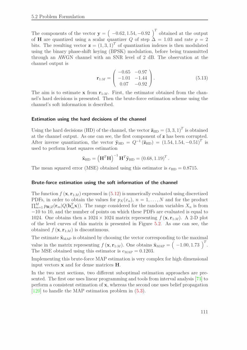
5.2 Problem Formulation
The components of the vector y =(
−0.62, 1.54, −0.92)T
obtained at the outputof H are quantized using a scalar quantizer Q of step ∆ = 1.03 and rate ρ = 2bits. The resulting vector z = (1, 3, 1)T of quantization indexes is then modulatedusing the binary phase-shift keying (BPSK) modulation, before being transmittedthrough an AWGN channel with an SNR level of 2 dB. The observation at thechannel output is
r1:M =
−0.65 −0.97−1.01 −1.440.07 −0.92
. (5.13)
The aim is to estimate x from r1:M . First, the estimator obtained from the chan-nel’s hard decisions is presented. Then the brute-force estimation scheme using thechannel’s soft information is described.
Estimation using the hard decisions of the channel
Using the hard decisions (HD) of the channel, the vector zHD = (3, 3, 1)T is obtainedat the channel output. As one can see, the first component of z has been corrupted.After inverse quantization, the vector yHD = Q−1 (zHD) = (1.54, 1.54, −0.51)T isused to perform least squares estimation
xHD =(HT H
)−1HT yHD = (0.68, 1.19)T .
The mean squared error (MSE) obtained using this estimator is eHD = 0.8715.
Brute-force estimation using the soft information of the channel
The function f (x, r1:M) expressed in (5.12) is numerically evaluated using discretizedPDFs, in order to obtain the values for pX(xn), n = 1, . . . , N and for the product∏M
m=1 pR|Z(rm|Q(hTmx)). The range considered for the random variables Xn is from
−10 to 10, and the number of points on which these PDFs are evaluated is equal to1024. One obtains then a 1024 × 1024 matrix representing f (x, r1:M). A 2-D plotof the level curves of this matrix is presented in Figure 5.2. As one can see, theobtained f (x, r1:M) is discontinuous.
The estimate xMAP is obtained by choosing the vector corresponding to the maximal
value in the matrix representing f (x, r1:M). One obtains xMAP =(
−1.00, 1.73)T
.The MSE obtained using this estimator is eMAP = 0.1203.
Implementing this brute-force MAP estimation is very complex for high dimensionalinput vectors x and for dense matrices H.
In the two next sections, two different suboptimal estimation approaches are pre-sented. The first one uses linear programming and tools from interval analysis [73] toperform a consistent estimation of x, whereas the second one uses belief propagation[120] to handle the MAP estimation problem in (5.3).
111
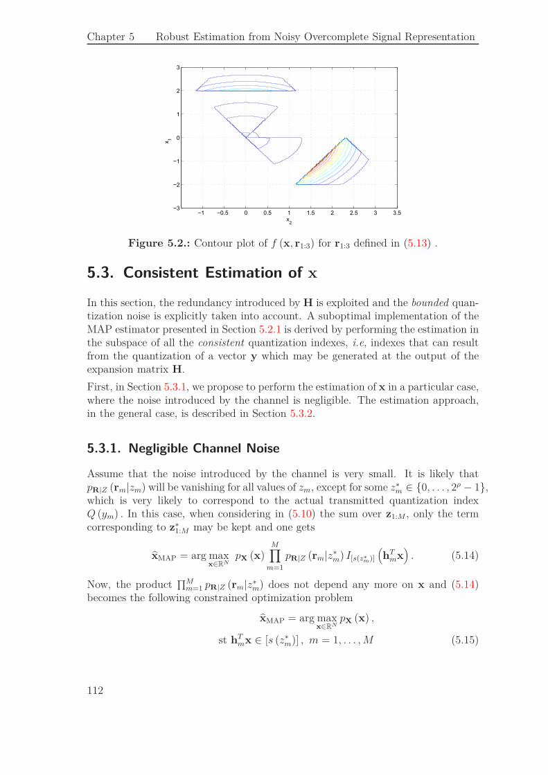
Chapter 5 Robust Estimation from Noisy Overcomplete Signal Representation
x2
x1
−1 −0.5 0 0.5 1 1.5 2 2.5 3 3.5−3
−2
−1
0
1
2
3
Figure 5.2.: Contour plot of f (x, r1:3) for r1:3 defined in (5.13) .
5.3. Consistent Estimation of x
In this section, the redundancy introduced by H is exploited and the bounded quan-tization noise is explicitly taken into account. A suboptimal implementation of theMAP estimator presented in Section 5.2.1 is derived by performing the estimation inthe subspace of all the consistent quantization indexes, i.e, indexes that can resultfrom the quantization of a vector y which may be generated at the output of theexpansion matrix H.
First, in Section 5.3.1, we propose to perform the estimation of x in a particular case,where the noise introduced by the channel is negligible. The estimation approach,in the general case, is described in Section 5.3.2.
5.3.1. Negligible Channel Noise
Assume that the noise introduced by the channel is very small. It is likely thatpR|Z (rm|zm) will be vanishing for all values of zm, except for some z∗m ∈ {0, . . . , 2ρ − 1},which is very likely to correspond to the actual transmitted quantization indexQ (ym) . In this case, when considering in (5.10) the sum over z1:M , only the termcorresponding to z∗1:M may be kept and one gets
xMAP = arg maxx∈RN
pX (x)M∏
m=1
pR|Z (rm|z∗m) I[s(z∗m)]
(hT
mx)
. (5.14)
Now, the product∏M
m=1 pR|Z (rm|z∗m) does not depend any more on x and (5.14)becomes the following constrained optimization problem
xMAP = arg maxx∈RN
pX (x) ,
st hTmx ∈ [s (z∗m)] , m = 1, . . . , M (5.15)
112
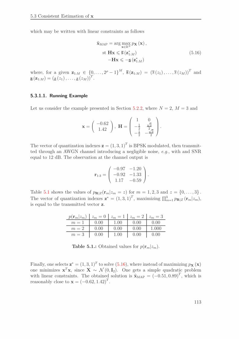
5.3 Consistent Estimation of x
which may be written with linear constraints as follows
xMAP = arg maxx∈RN
pX (x) ,
st Hx 6 s (z∗1:M) (5.16)
−Hx 6 −s (z∗1:M)
where, for a given z1:M ∈ {0, . . . , 2ρ − 1}M , s (z1:M) = (s (z1) , . . . , s (zM ))T ands (z1:M) = (s (z1) , . . . , s (zM ))T .
5.3.1.1. Running Example
Let us consider the example presented in Section 5.2.2, where N = 2, M = 3 and
x =
(−0.621.42
), H =
1 0
−12
√3
2
−12
−√
32
.
The vector of quantization indexes z = (1, 3, 1)T is BPSK modulated, then transmit-ted through an AWGN channel introducing a negligible noise, e.g., with and SNRequal to 12 dB. The observation at the channel output is
r1:3 =
−0.97 −1.20−0.92 −1.331.17 −0.59
.
Table 5.1 shows the values of pR|Z(rm|zm = z) for m = 1, 2, 3 and z = {0, . . . , 3} .
The vector of quantization indexes z∗ = (1, 3, 1)T , maximizing∏3
m=1 pR|Z (rm|zm),is equal to the transmitted vector z.
p(rm|zm) zm = 0 zm = 1 zm = 2 zm = 3m = 1 0.00 1.00 0.00 0.00m = 2 0.00 0.00 0.00 1.000m = 3 0.00 1.00 0.00 0.00
Table 5.1.: Obtained values for p(rm|zm).
Finally, one selects z∗ = (1, 3, 1)T to solve (5.16), where instead of maximizing pX (x)one minimizes xT x, since X ∼ N (0, I2). One gets a simple quadratic problemwith linear constraints. The obtained solution is xMAP = (−0.51, 0.89)T , which isreasonably close to x = (−0.62, 1.42)T .
113
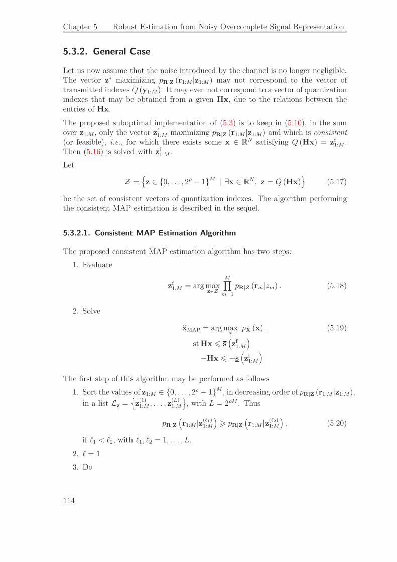
Chapter 5 Robust Estimation from Noisy Overcomplete Signal Representation
5.3.2. General Case
Let us now assume that the noise introduced by the channel is no longer negligible.The vector z∗ maximizing pR|Z (r1:M |z1:M) may not correspond to the vector oftransmitted indexes Q (y1:M). It may even not correspond to a vector of quantizationindexes that may be obtained from a given Hx, due to the relations between theentries of Hx.
The proposed suboptimal implementation of (5.3) is to keep in (5.10), in the sumover z1:M , only the vector zf
1:M maximizing pR|Z (r1:M |z1:M) and which is consistent(or feasible), i.e., for which there exists some x ∈ R
N satisfying Q (Hx) = zf1:M .
Then (5.16) is solved with zf1:M .
Let
Z ={z ∈ {0, . . . , 2ρ − 1}M | ∃x ∈ R
N , z = Q (Hx)}
(5.17)
be the set of consistent vectors of quantization indexes. The algorithm performingthe consistent MAP estimation is described in the sequel.
5.3.2.1. Consistent MAP Estimation Algorithm
The proposed consistent MAP estimation algorithm has two steps:
1. Evaluate
zf1:M = arg max
z∈Z
M∏
m=1
pR|Z (rm|zm) . (5.18)
2. Solve
xMAP = arg maxx
pX (x) . (5.19)
st Hx 6 s(zf
1:M
)
−Hx 6 −s(zf
1:M
)
The first step of this algorithm may be performed as follows
1. Sort the values of z1:M ∈ {0, . . . , 2ρ − 1}M , in decreasing order of pR|Z (r1:M |z1:M),
in a list Lz ={z
(1)1:M , . . . , z
(L)1:M
}, with L = 2ρM . Thus
pR|Z(r1:M |z(ℓ1)
1:M
)> pR|Z
(r1:M |z(ℓ2)
1:M
), (5.20)
if ℓ1 < ℓ2, with ℓ1, ℓ2 = 1, . . . , L.
2. ℓ = 1
3. Do
114
5.3 Consistent Estimation of x
a) If z(ℓ) ∈ Zb) zf = z(ℓ); End;
c) Else ℓ = ℓ + 1;
4. While ℓ 6 L.
Our aim now is to describe how Step 3 (a) may be performed. Consider the set
X (z) ={x ∈ R
N | z = Q(Hx)}
(5.21)
containing all the vectors x from which the quantization vector z may be obtained.Alternatively, this set may be defined as follows
X (z) =M⋂
m=1
Xm (zm) , (5.22)
where, for a given z ∈ {0, . . . , 2ρ − 1}, Xm (z) ={x ∈ RN | z = Q
(hT
mx)}
.
By definitions (5.17) and (5.22), one has
X (z) 6= ∅ ⇐⇒ z ∈ Z. (5.23)
For a given ℓ = 1, . . . , L, in order to determine whether z(ℓ) ∈ Z, or equivalently,whether X
(z(ℓ)
)6= ∅, one may use, e.g., linear programming [8] or interval analysis
tools [73].
5.3.2.2. Consistency Test using Linear Programming
For a given ℓ = 1, . . . , L, consider the maximization problem
maxx∈X
(z
(ℓ)1:M
) aT x,
a being any non-zero vector of size N . This is equivalent to the following linearproblem
maxx∈RN
aT x.
st Hx 6 s(z
(ℓ)1:M
)(5.24)
−Hx 6 −s(z
(ℓ)1:M
)
If a solution x is found for (5.24), then X(z(ℓ)
)6= ∅ and z(ℓ) is consistent.
Note that one could try to directly solve (5.16) with z(ℓ)1:M , starting from ℓ = 1 and
increasing ℓ until a solution exists. Nevertheless, solving first (5.24) for various z(ℓ)1:M
with increasing ℓ is much less complex than solving (5.16), especially if pX (x) is ageneral PDF.
115
Chapter 5 Robust Estimation from Noisy Overcomplete Signal Representation
5.3.2.3. Consistency Test using Interval Analysis
Another approach to determine whether a quantization vector z belongs to Z in-volves the parity-check matrix P associated to H. Since H is of rank N , there existsan (M − N) × M matrix P of rank (M − N) such that
PHx = 0, ∀x ∈ RN . (5.25)
One has
Py = 0 ⇐⇒ ∃x ∈ RN st y = Hx. (5.26)
From (5.26), one deduces
∃y st Py = 0 and z = Q(y) ⇐⇒ ∃x st z = Q (Hx) . (5.27)
Using the definition of Z in (5.17) and (5.27), one obtains
z ∈ Z ⇐⇒ ∃y ∈ RM , z = Q(y) and Py = 0. (5.28)
Now let us apply the equivalence (5.2) to all the components zm, m = 1, . . . , M ofa given vector z
z = Q(y) ⇐⇒ y ∈ [s(z)] , (5.29)
where [s (z1:M)] =([
s(z
(ℓ)1
)], . . . ,
[s(z
(ℓ)M
)])Tis a box, i.e., a vector of intervals.
The box P [s (z1:M)], which can be evaluated using basic interval additions andmultiplications [73], is such that
{Py with y ∈ [s (z1:M)]} ⊂ P [s (z1:M)] . (5.30)
Using (5.29) and (5.30)
z = Q(y) and Py = 0 ⇒ 0 ∈ P [s (z)] . (5.31)
Finally, from (5.28) and (5.31) one gets
z ∈ Z ⇒ 0 ∈ P [s (z)]. (5.32)
One may rewrite (5.32) as
0 /∈ P [s (z)] ⇒ z /∈ Z. (5.33)
The test (5.33) allows to prove that a vector of quantization indexes z is not con-sistent, but it is unable to prove that some z is consistent, as the inclusion (5.30) isstrict. This test allows to eliminate some of the inconsistent vectors z(ℓ), ℓ = 1, . . . , Land has a complexity between O (M) and O (M (M − N)), which is in general lowerthan solving directly (5.24).
116
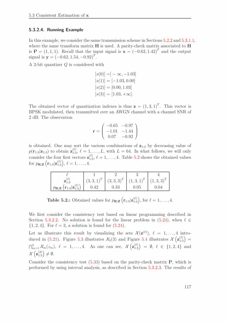
5.3 Consistent Estimation of x
5.3.2.4. Running Example
In this example, we consider the same transmission scheme in Sections 5.2.2 and 5.3.1.1,where the same transform matrix H is used. A parity-check matrix associated to H
is P = (1, 1, 1). Recall that the input signal is x = (−0.62, 1.42)T and the outputsignal is y = (−0.62, 1.54, −0.92)T .
A 2-bit quantizer Q is considered with
[s(0)] =] − ∞, −1.03]
[s(1)] = [−1.03, 0.00]
[s(2)] = [0.00, 1.03]
[s(3)] = [1.03, +∞[.
The obtained vector of quantization indexes is thus z = (1, 3, 1)T . This vector isBPSK modulated, then transmitted over an AWGN channel with a channel SNR of2 dB. The observation
r =
−0.65 −0.97−1.01 −1.440.07 −0.92
is obtained. One may sort the various combinations of z1:3 by decreasing value ofp(r1:3|z1:3) to obtain z
(ℓ)1:3, ℓ = 1, . . . , L, with L = 64. In what follows, we will only
consider the four first vectors z(ℓ)1:3, ℓ = 1, . . . , 4. Table 5.2 shows the obtained values
for pR|Z(r1:3|z(ℓ)
1:3
), ℓ = 1, . . . , 4.
ℓ 1 2 3 4
z(ℓ)1:3 (3, 3, 1)T (3, 3, 3)T (1, 3, 1)T (1, 3, 3)T
pR|Z(r1:3|z(ℓ)
1:3
)0.42 0.33 0.05 0.04
Table 5.2.: Obtained values for pR|Z(r1:3|z(ℓ)
1:3
), for ℓ = 1, . . . , 4.
We first consider the consistency test based on linear programming described inSection 5.3.2.2. No solution is found for the linear problem in (5.24), when ℓ ∈{1, 2, 4}. For ℓ = 3, a solution is found for (5.24).
Let us illustrate this result by visualizing the sets X (z(ℓ)), ℓ = 1, . . . , 4 intro-
duced in (5.21). Figure 5.3 illustrates X3(3) and Figure 5.4 illustrates X(z
(ℓ)1:3
)=
⋂3m=1 Xm(zm), ℓ = 1, . . . , 4. As one can see, X
(z
(ℓ)1:3
)= ∅, ℓ ∈ {1, 2, 4} and
X(z
(3)1:3
)6= ∅.
Consider the consistency test (5.33) based on the parity-check matrix P, which isperformed by using interval analysis, as described in Section 5.3.2.3. The results of
117
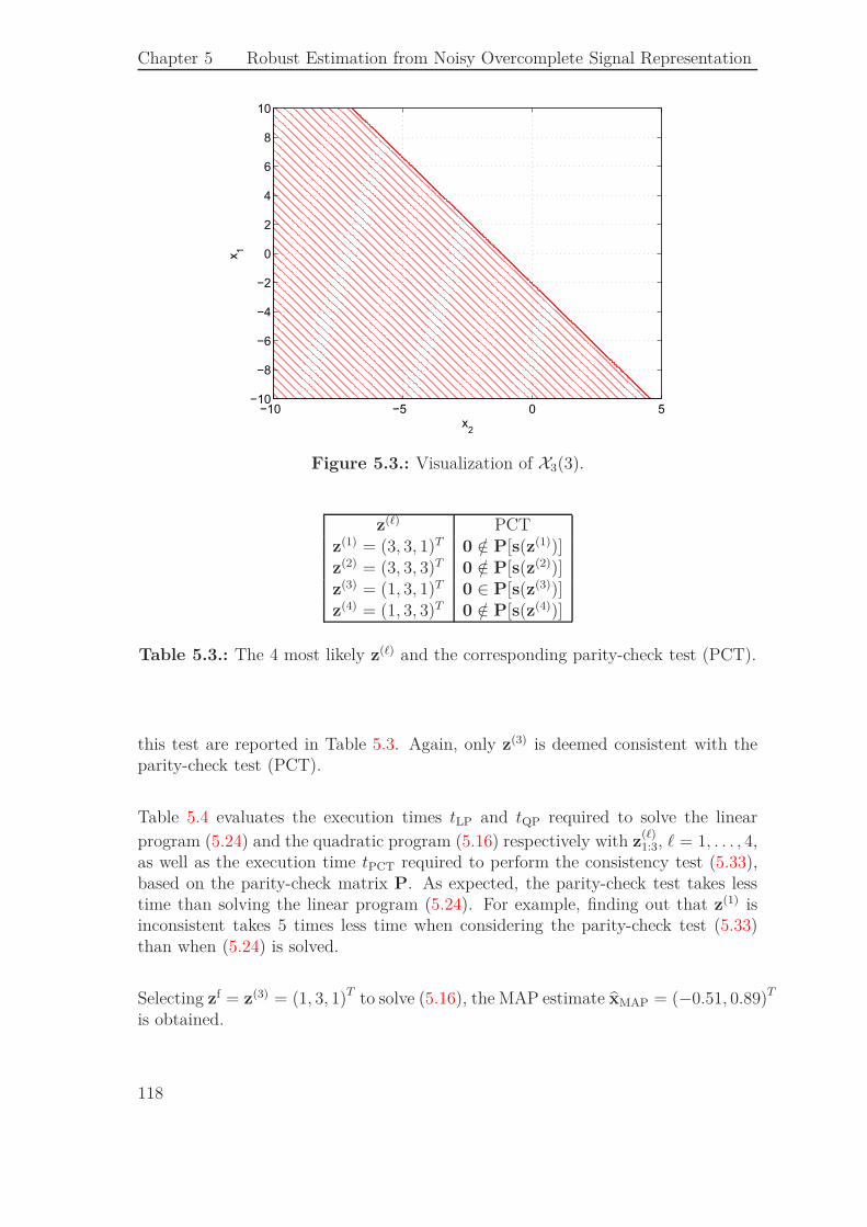
Chapter 5 Robust Estimation from Noisy Overcomplete Signal Representation
x2
x1
−10 −5 0 5−10
−8
−6
−4
−2
0
2
4
6
8
10
Figure 5.3.: Visualization of X3(3).
z(ℓ) PCTz(1) = (3, 3, 1)T 0 /∈ P[s(z(1))]z(2) = (3, 3, 3)T 0 /∈ P[s(z(2))]z(3) = (1, 3, 1)T 0 ∈ P[s(z(3))]z(4) = (1, 3, 3)T 0 /∈ P[s(z(4))]
Table 5.3.: The 4 most likely z(ℓ) and the corresponding parity-check test (PCT).
this test are reported in Table 5.3. Again, only z(3) is deemed consistent with theparity-check test (PCT).
Table 5.4 evaluates the execution times tLP and tQP required to solve the linear
program (5.24) and the quadratic program (5.16) respectively with z(ℓ)1:3, ℓ = 1, . . . , 4,
as well as the execution time tPCT required to perform the consistency test (5.33),based on the parity-check matrix P. As expected, the parity-check test takes lesstime than solving the linear program (5.24). For example, finding out that z(1) isinconsistent takes 5 times less time when considering the parity-check test (5.33)than when (5.24) is solved.
Selecting zf = z(3) = (1, 3, 1)T to solve (5.16), the MAP estimate xMAP = (−0.51, 0.89)T
is obtained.
118
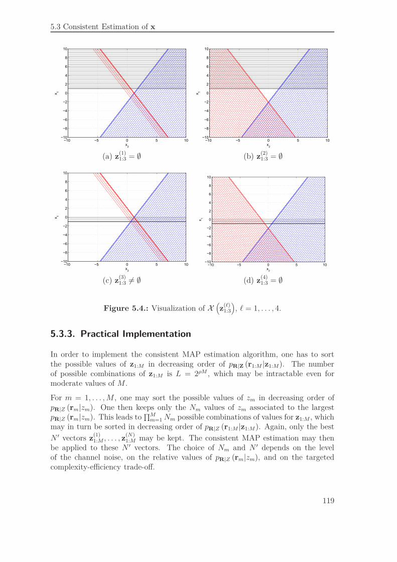
5.3 Consistent Estimation of x
x2
x1
−10 −5 0 5 10−10
−8
−6
−4
−2
0
2
4
6
8
10
x2
x1
−10 −5 0 5 10−10
−8
−6
−4
−2
0
2
4
6
8
10
(a) z(1)1:3 = ∅ (b) z
(2)1:3 = ∅
x2
x1
−10 −5 0 5 10−10
−8
−6
−4
−2
0
2
4
6
8
10
x2
x1
−10 −5 0 5 10−10
−8
−6
−4
−2
0
2
4
6
8
10
(c) z(3)1:3 6= ∅ (d) z
(4)1:3 = ∅
Figure 5.4.: Visualization of X(z
(ℓ)1:3
), ℓ = 1, . . . , 4.
5.3.3. Practical Implementation
In order to implement the consistent MAP estimation algorithm, one has to sortthe possible values of z1:M in decreasing order of pR|Z (r1:M |z1:M). The numberof possible combinations of z1:M is L = 2ρM , which may be intractable even formoderate values of M .
For m = 1, . . . , M , one may sort the possible values of zm in decreasing order ofpR|Z (rm|zm). One then keeps only the Nm values of zm associated to the largestpR|Z (rm|zm). This leads to
∏Mm=1 Nm possible combinations of values for z1:M , which
may in turn be sorted in decreasing order of pR|Z (r1:M |z1:M). Again, only the best
N ′ vectors z(1)1:M , . . . , z
(N)1:M may be kept. The consistent MAP estimation may then
be applied to these N ′ vectors. The choice of Nm and N ′ depends on the levelof the channel noise, on the relative values of pR|Z (rm|zm), and on the targetedcomplexity-efficiency trade-off.
119
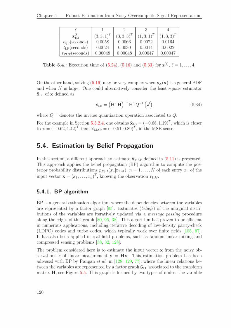
Chapter 5 Robust Estimation from Noisy Overcomplete Signal Representation
ℓ 1 2 3 4
z(ℓ)1:3 (3, 3, 1)T (3, 3, 3)T (1, 3, 1)T (1, 3, 3)T
tQP(seconds) 0.0058 0.0066 0.0072 0.0164tLP(seconds) 0.0024 0.0030 0.0014 0.0022
tPCT(seconds) 0.00048 0.00048 0.00047 0.00047
Table 5.4.: Execution time of (5.24), (5.16) and (5.33) for z(ℓ), ℓ = 1, . . . , 4.
On the other hand, solving (5.16) may be very complex when pX(x) is a general PDFand when N is large. One could alternatively consider the least square estimatorxLS of x defined as
xLS =(HT H
)−1HT Q−1
(zf)
, (5.34)
where Q−1 denotes the inverse quantization operation associated to Q.
For the example in Section 5.3.2.4, one obtains xLS = (−0.68, 1.19)T , which is closerto x = (−0.62, 1.42)T than xMAP = (−0.51, 0.89)T , in the MSE sense.
5.4. Estimation by Belief Propagation
In this section, a different approach to estimate xMAP defined in (5.11) is presented.This approach applies the belief propagation (BP) algorithm to compute the pos-terior probability distributions pX|R(xn|r1:M), n = 1, . . . , N of each entry xn of the
input vector x = (x1, . . . , xn)T , knowing the observation r1:M .
5.4.1. BP algorithm
BP is a general estimation algorithm where the dependencies between the variablesare represented by a factor graph [95]. Estimates (beliefs) of the marginal distri-butions of the variables are iteratively updated via a message passing procedurealong the edges of this graph [80, 95, 38]. This algorithm has proven to be efficientin numerous applications, including iterative decoding of low-density parity-check(LDPC) codes and turbo codes, which typically work over finite fields [105, 97].It has also been applied in real field problems, such as random linear mixing andcompressed sensing problems [38, 32, 128].
The problem considered here is to estimate the input vector x from the noisy ob-servations r of linear measurement y = Hx. This estimation problem has beenadressed with BP by Rangan et al. in [128, 129, 77], where the linear relations be-tween the variables are represented by a factor graph GH, associated to the transformmatrix H, see Figure 5.5. This graph is formed by two types of nodes: the variable
120
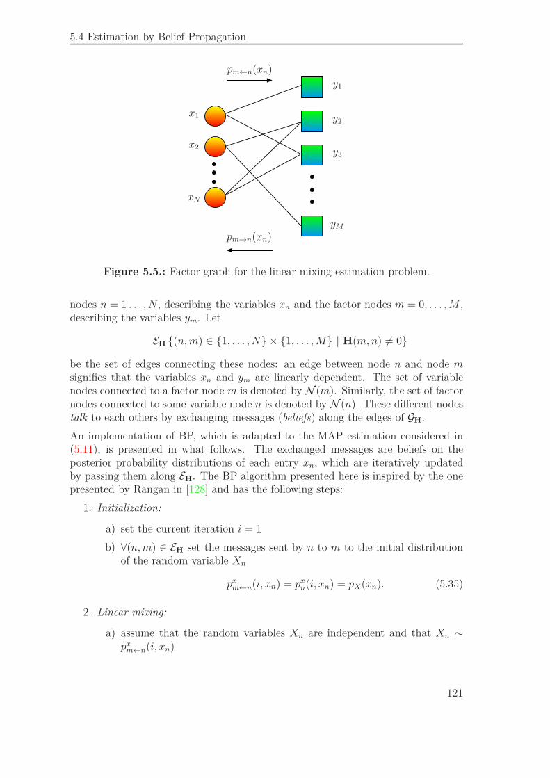
5.4 Estimation by Belief Propagation
x1
x2
xN
y1
y2
y3
yM
pm←n(xn)
pm→n(xn)
Figure 5.5.: Factor graph for the linear mixing estimation problem.
nodes n = 1 . . . , N , describing the variables xn and the factor nodes m = 0, . . . , M ,describing the variables ym. Let
EH {(n, m) ∈ {1, . . . , N} × {1, . . . , M} | H(m, n) 6= 0}
be the set of edges connecting these nodes: an edge between node n and node msignifies that the variables xn and ym are linearly dependent. The set of variablenodes connected to a factor node m is denoted by N (m). Similarly, the set of factornodes connected to some variable node n is denoted by N (n). These different nodestalk to each others by exchanging messages (beliefs) along the edges of GH.
An implementation of BP, which is adapted to the MAP estimation considered in(5.11), is presented in what follows. The exchanged messages are beliefs on theposterior probability distributions of each entry xn, which are iteratively updatedby passing them along EH. The BP algorithm presented here is inspired by the onepresented by Rangan in [128] and has the following steps:
1. Initialization:
a) set the current iteration i = 1
b) ∀(n, m) ∈ EH set the messages sent by n to m to the initial distributionof the random variable Xn
pxm←n(i, xn) = px
n(i, xn) = pX(xn). (5.35)
2. Linear mixing:
a) assume that the random variables Xn are independent and that Xn ∼px
m←n(i, xn)
121
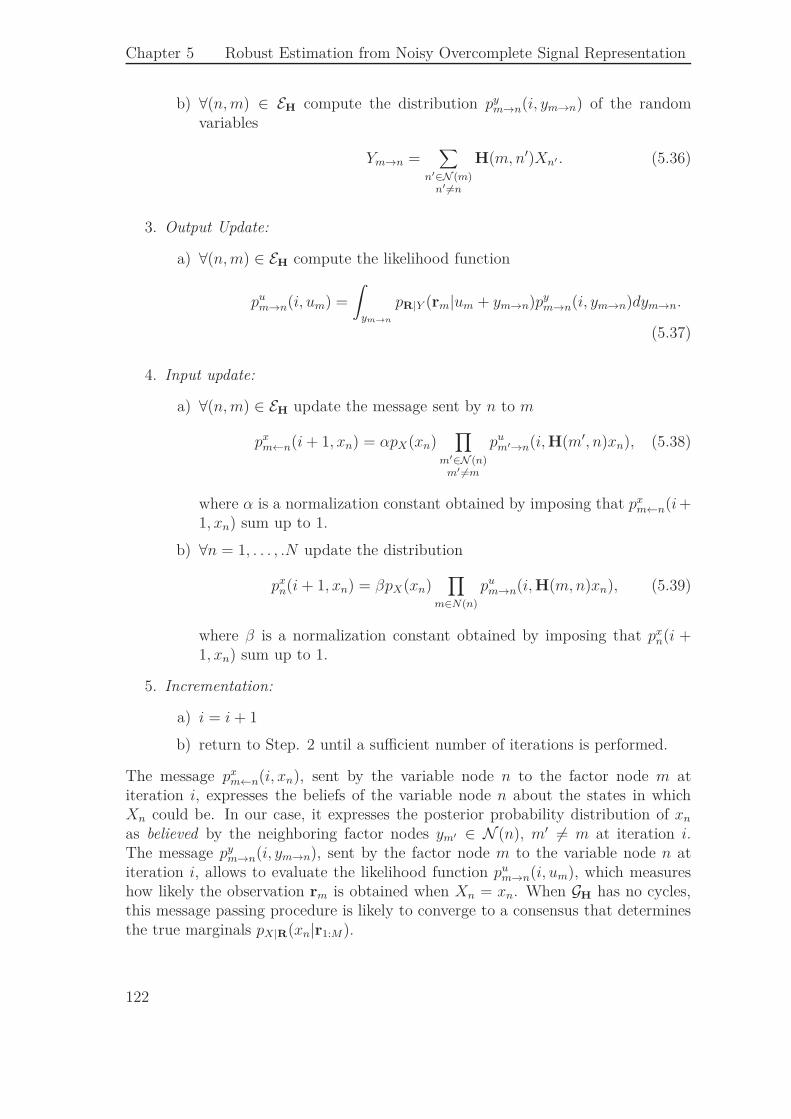
Chapter 5 Robust Estimation from Noisy Overcomplete Signal Representation
b) ∀(n, m) ∈ EH compute the distribution pym→n(i, ym→n) of the random
variables
Ym→n =∑
n′∈N (m)n′ 6=n
H(m, n′)Xn′ . (5.36)
3. Output Update:
a) ∀(n, m) ∈ EH compute the likelihood function
pum→n(i, um) =
ˆ
ym→n
pR|Y (rm|um + ym→n)pym→n(i, ym→n)dym→n.
(5.37)
4. Input update:
a) ∀(n, m) ∈ EH update the message sent by n to m
pxm←n(i + 1, xn) = αpX(xn)
∏
m′∈N (n)m′ 6=m
pum′→n(i, H(m′, n)xn), (5.38)
where α is a normalization constant obtained by imposing that pxm←n(i +
1, xn) sum up to 1.
b) ∀n = 1, . . . , .N update the distribution
pxn(i + 1, xn) = βpX(xn)
∏
m∈N(n)
pum→n(i, H(m, n)xn), (5.39)
where β is a normalization constant obtained by imposing that pxn(i +
1, xn) sum up to 1.
5. Incrementation:
a) i = i + 1
b) return to Step. 2 until a sufficient number of iterations is performed.
The message pxm←n(i, xn), sent by the variable node n to the factor node m at
iteration i, expresses the beliefs of the variable node n about the states in whichXn could be. In our case, it expresses the posterior probability distribution of xn
as believed by the neighboring factor nodes ym′ ∈ N (n), m′ 6= m at iteration i.The message py
m→n(i, ym→n), sent by the factor node m to the variable node n atiteration i, allows to evaluate the likelihood function pu
m→n(i, um), which measureshow likely the observation rm is obtained when Xn = xn. When GH has no cycles,this message passing procedure is likely to converge to a consensus that determinesthe true marginals pX|R(xn|r1:M).
122
5.5 Comparison between the two Estimation Schemes
After Ni iterations of the BP algorithm, the MAP estimate of x defined in (5.3) isobtained as follows
xMAP = (x1,MAP, . . . , xN,MAP)T , (5.40)
where, for n = 1, . . . , N
xn,MAP = arg maxxn∈R
pxn(Ni, xn).
The steps of the BP presented here are derived from the sum-product algorithm,which is a generic representation of the message-passing algorithms operating in afactor graph [81, 95]. A presentation of the sum-product algorithm is provided inAppendix C.1, where it is shown how the BP algorithm presented in this sectioncan be viewed as a particular instance of this generic algorithm.
5.4.2. Running Example
In this section the example of Section 5.3.2.4 is considered. The input signal isx = (−0.62, 1.42)T and the output signal is y = (−0.62, 1.54, −0.92)T . Moreover,the same 2-bit quantizer Q is used.
The MAP estimation based on the BP algorithm described in Section 5.4.1 is im-plemented by considering probability mass functions approximating the continuousdistributions. The range considered for the input variables xn, n = 1, 2 is from −10to 10 and the number of points on which the probability distribution functions areevaluated is set to 1024. The considered resolution is then of 20/1024. The totalnumber of iterations of the BP algorithm is equal to 10. At each iteration, the mes-sages px
m←n(i, xn) and pum→n(i, um) are vectors of 1024 entries, where the probability
distribution is evaluated. The MAP estimate described in (5.40) is then obtained:xMAP = (−1.33, 2.20)T .
5.5. Comparison between the two Estimation
Schemes
In this section, the two estimation schemes presented in Sections 5.3 and 5.4 arecompared. The same running example introduced previously is considered: N = 2,M = 3, X ∼ N (0, I2) and
H =
1 0
−12
√3
2
−12
−√
32
.
123
Chapter 5 Robust Estimation from Noisy Overcomplete Signal Representation
A 4−bit quantizer Q is used here for each entry of y = Hx. The components ofz = Q(y) are BPSK modulated, then transmitted over an AWGN channel, with anSNR varying between 0 dB and 14 dB. The number of noise realizations is set to3000 for each value of the channel SNR.
In the sequel, we describe the different reconstruction approaches and compare them.
Consistent estimation scheme
The consistent MAP estimation scheme presented in Section 5.3 is performed, andthe most likely feasible vector of quantization indexes zf defined in (5.18) is obtained.
Two MAP estimates of the input x are considered. The first one is obtained bysolving the quadratic program (QP) in (5.19) with zf. This estimate is reffered toas xQP.
The second estimate we consider is the one obtained using least squares (LS) recon-struction, as follows
xLS =(HT H
)−1HT Q−1
(zf)
.
Estimation using BP
The MAP estimation based on the BP algorithm and presented in Section 5.4.1 isperformed as described in the example of Section 5.4.2. The MAP estimate definedin (5.40) is then obtained. In this section, this estimate is reffered to as xBP.
Estimation scheme using the hard decisions of the channel
This estimation scheme uses the hard decisions taken by a classical non-robust de-coder on the received vector r1:M . As described in Section 5.2.2, after demodulationand inverse quantization, the received vector yHD is obtained, and the input vectormay be reconstructed using LS estimation as:
xHD =(HT H
)−1HT yHD.
Reference reconstruction scheme
The scheme serving as a reference considers the noise-free signal xREF, reconstructedafter inverse quantization of z. Let yREF = Q−1 (z). Then
xREF =(HT H
)−1HT yREF.
124
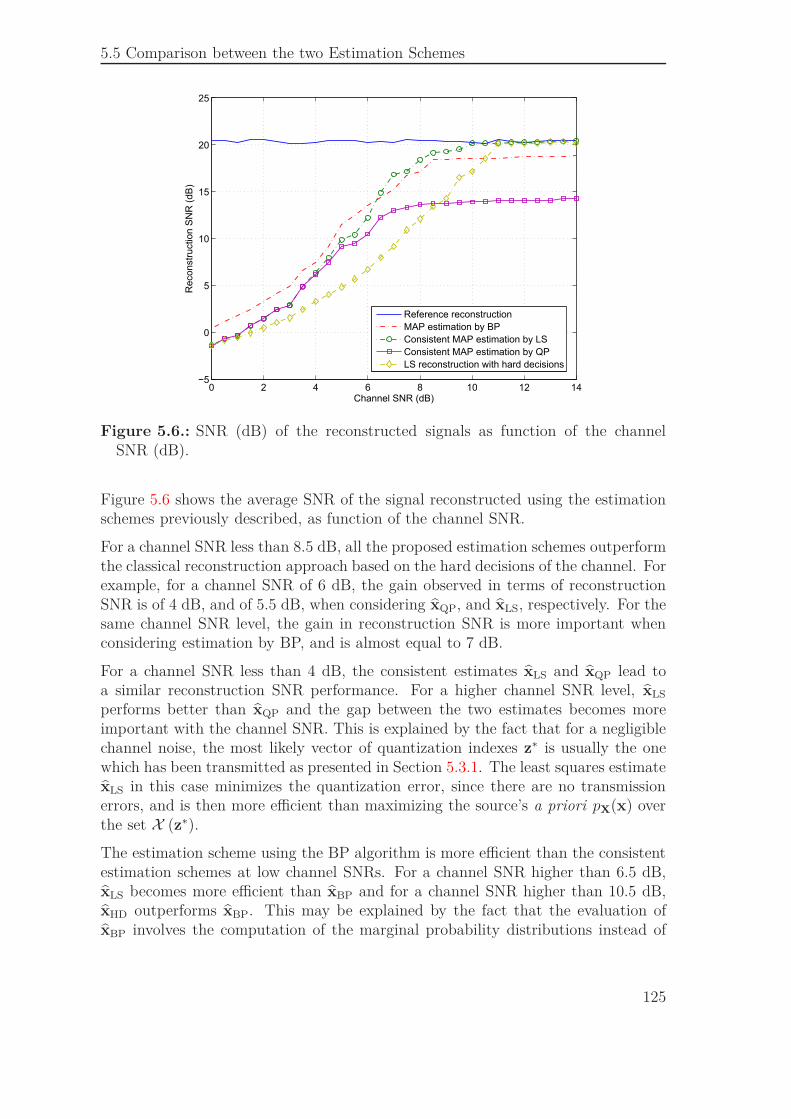
5.5 Comparison between the two Estimation Schemes
0 2 4 6 8 10 12 14−5
0
5
10
15
20
25
Channel SNR (dB)
Reconstr
uction S
NR
(dB
)
Reference reconstruction
MAP estimation by BP
Consistent MAP estimation by LS
Consistent MAP estimation by QP
LS reconstruction with hard decisions
Figure 5.6.: SNR (dB) of the reconstructed signals as function of the channelSNR (dB).
Figure 5.6 shows the average SNR of the signal reconstructed using the estimationschemes previously described, as function of the channel SNR.
For a channel SNR less than 8.5 dB, all the proposed estimation schemes outperformthe classical reconstruction approach based on the hard decisions of the channel. Forexample, for a channel SNR of 6 dB, the gain observed in terms of reconstructionSNR is of 4 dB, and of 5.5 dB, when considering xQP, and xLS, respectively. For thesame channel SNR level, the gain in reconstruction SNR is more important whenconsidering estimation by BP, and is almost equal to 7 dB.
For a channel SNR less than 4 dB, the consistent estimates xLS and xQP lead toa similar reconstruction SNR performance. For a higher channel SNR level, xLS
performs better than xQP and the gap between the two estimates becomes moreimportant with the channel SNR. This is explained by the fact that for a negligiblechannel noise, the most likely vector of quantization indexes z∗ is usually the onewhich has been transmitted as presented in Section 5.3.1. The least squares estimatexLS in this case minimizes the quantization error, since there are no transmissionerrors, and is then more efficient than maximizing the source’s a priori pX(x) overthe set X (z∗).
The estimation scheme using the BP algorithm is more efficient than the consistentestimation schemes at low channel SNRs. For a channel SNR higher than 6.5 dB,xLS becomes more efficient than xBP and for a channel SNR higher than 10.5 dB,xHD outperforms xBP. This may be explained by the fact that the evaluation ofxBP involves the computation of the marginal probability distributions instead of
125
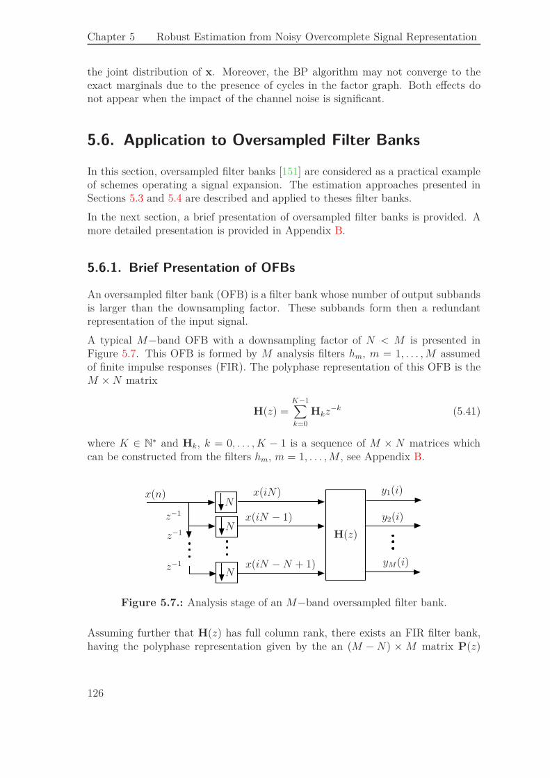
Chapter 5 Robust Estimation from Noisy Overcomplete Signal Representation
the joint distribution of x. Moreover, the BP algorithm may not converge to theexact marginals due to the presence of cycles in the factor graph. Both effects donot appear when the impact of the channel noise is significant.
5.6. Application to Oversampled Filter Banks
In this section, oversampled filter banks [151] are considered as a practical exampleof schemes operating a signal expansion. The estimation approaches presented inSections 5.3 and 5.4 are described and applied to theses filter banks.
In the next section, a brief presentation of oversampled filter banks is provided. Amore detailed presentation is provided in Appendix B.
5.6.1. Brief Presentation of OFBs
An oversampled filter bank (OFB) is a filter bank whose number of output subbandsis larger than the downsampling factor. These subbands form then a redundantrepresentation of the input signal.
A typical M−band OFB with a downsampling factor of N < M is presented inFigure 5.7. This OFB is formed by M analysis filters hm, m = 1, . . . , M assumedof finite impulse responses (FIR). The polyphase representation of this OFB is theM × N matrix
H(z) =K−1∑
k=0
Hkz−k (5.41)
where K ∈ N∗ and Hk, k = 0, . . . , K − 1 is a sequence of M × N matrices whichcan be constructed from the filters hm, m = 1, . . . , M , see Appendix B.
x(n) x(iN)
x(iN − 1)
x(iN − N + 1)
N
N
N
H(z)
y1(i)
y2(i)
yM(i)
z−1
z−1
z−1
Figure 5.7.: Analysis stage of an M−band oversampled filter bank.
Assuming further that H(z) has full column rank, there exists an FIR filter bank,having the polyphase representation given by the an (M − N) × M matrix P(z)
126
5.6 Application to Oversampled Filter Banks
which verifies
P(z)H(z) = 0, ∀z ∈ C (5.42)
and
P(z) =K ′−1∑
k=0
Pkz−k,
where K ′ ∈ N∗ and Pk, k = 0, . . . , K ′ − 1 is a sequence of (M − N) × M matrices,see Appendix B. The matrix P(z) is the parity-check matrix associated to H(z).
5.6.2. Signal Expansion using OFBs
Let x ∈ RV N and y ∈ RV M be the input and output vectors of an OFB, where V issome positive integer . One may write
x =((
x1)T
, . . . ,(xV)T)T
and
y =((
y1)T
, . . . ,(yV)T)T
,
where
xi = (x (iN − N + 1) , . . . , x (iN))T
and
yi = (y (iM − M + 1) , . . . , y (iM))T
are the input and the output of the OFB at time instant i = 1, . . . , V .
It is shown in Appendix B that
yi =K−1∑
k=0
Hkxi−k, (5.43)
with xi = 0, if i 6 0.
Let HK−1:0 = (HK−1, . . . , H0) be the M ×KN matrix constructed from the matricesHk and let
xi−K+1:i =((
xi−K+1)T
, . . . ,(xi)T)T
127
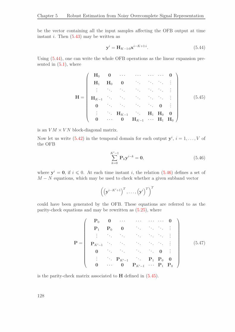
Chapter 5 Robust Estimation from Noisy Overcomplete Signal Representation
be the vector containing all the input samples affecting the OFB output at timeinstant i. Then (5.43) may be written as
yi = HK−1:0xi−K+1:i. (5.44)
Using (5.44), one can write the whole OFB operations as the linear expansion pre-sented in (5.1), where
H =
H0 0 · · · · · · · · · · · · 0
H1 H0 0. . . . . . . . .
......
. . . . . . . . . . . . . . ....
HK−1. . . . . . . . . . . . . . .
...
0. . . . . . . . . . . . 0
......
. . . HK−1. . . H1 H0 0
0 · · · 0 HK−1 · · · H1 H0
(5.45)
is an V M × V N block-diagonal matrix.
Now let us write (5.42) in the temporal domain for each output yi, i = 1, . . . , V ofthe OFB
K ′−1∑
k=0
Pkyi−k = 0, (5.46)
where yi = 0, if i 6 0. At each time instant i, the relation (5.46) defines a set ofM − N equations, which may be used to check whether a given subband vector
((yi−K ′+1
)T, . . . ,
(yi)T)T
could have been generated by the OFB. These equations are referred to as theparity-check equations and may be rewritten as (5.25), where
P =
P0 0 · · · · · · · · · · · · 0
P1 P0 0. . . . . . . . .
......
. . . . . . . . . . . . . . ....
PK ′−1. . . . . . . . . . . . . . .
...
0. . . . . . . . . . . . 0
......
. . . PK ′−1. . . P1 P0 0
0 · · · 0 PK ′−1 · · · P1 P0
(5.47)
is the parity-check matrix associated to H defined in (5.45).
128
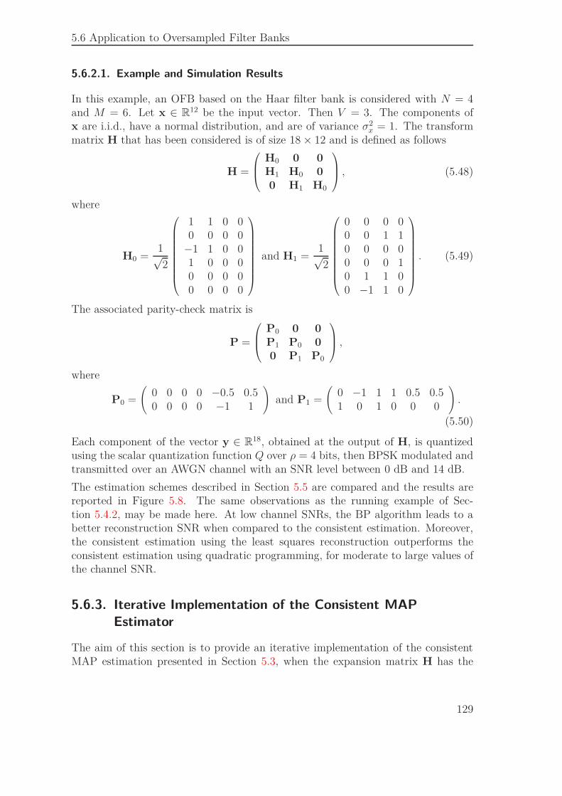
5.6 Application to Oversampled Filter Banks
5.6.2.1. Example and Simulation Results
In this example, an OFB based on the Haar filter bank is considered with N = 4and M = 6. Let x ∈ R12 be the input vector. Then V = 3. The components ofx are i.i.d., have a normal distribution, and are of variance σ2
x = 1. The transformmatrix H that has been considered is of size 18 × 12 and is defined as follows
H =
H0 0 0
H1 H0 0
0 H1 H0
, (5.48)
where
H0 =1√2
1 1 0 00 0 0 0
−1 1 0 01 0 0 00 0 0 00 0 0 0
and H1 =1√2
0 0 0 00 0 1 10 0 0 00 0 0 10 1 1 00 −1 1 0
. (5.49)
The associated parity-check matrix is
P =
P0 0 0
P1 P0 0
0 P1 P0
,
where
P0 =
(0 0 0 0 −0.5 0.50 0 0 0 −1 1
)and P1 =
(0 −1 1 1 0.5 0.51 0 1 0 0 0
).
(5.50)
Each component of the vector y ∈ R18, obtained at the output of H, is quantizedusing the scalar quantization function Q over ρ = 4 bits, then BPSK modulated andtransmitted over an AWGN channel with an SNR level between 0 dB and 14 dB.
The estimation schemes described in Section 5.5 are compared and the results arereported in Figure 5.8. The same observations as the running example of Sec-tion 5.4.2, may be made here. At low channel SNRs, the BP algorithm leads to abetter reconstruction SNR when compared to the consistent estimation. Moreover,the consistent estimation using the least squares reconstruction outperforms theconsistent estimation using quadratic programming, for moderate to large values ofthe channel SNR.
5.6.3. Iterative Implementation of the Consistent MAP
Estimator
The aim of this section is to provide an iterative implementation of the consistentMAP estimation presented in Section 5.3, when the expansion matrix H has the
129
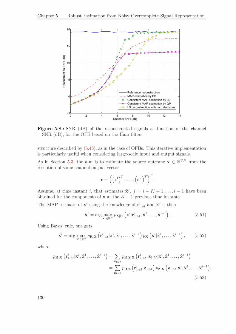
Chapter 5 Robust Estimation from Noisy Overcomplete Signal Representation
0 2 4 6 8 10 12 14−5
0
5
10
15
20
Channel SNR (dB)
Reconstr
uction S
NR
(dB
)
Reference reconstruction
MAP estimation by BP
Consistent MAP estimation by LS
Consistent MAP estimation by QP
LS reconstruction with hard decisions
Figure 5.8.: SNR (dB) of the reconstructed signals as function of the channelSNR (dB), for the OFB based on the Haar filters.
structure described by (5.45), as in the case of OFBs. This iterative implementationis particularly useful when considering large-scale input and output signals.
As in Section 5.3, the aim is to estimate the source outcome x ∈ RV N from thereception of some channel output vector
r =((
r1)T
, . . . ,(rV)T)T
.
Assume, at time instant i, that estimates xj , j = i − K + 1, . . . , i − 1 have beenobtained for the components of x at the K − 1 previous time instants.
The MAP estimate of xi using the knowledge of ri1:M and xj is then
xi = arg maxxi∈RN
pX|R(xi|ri
1:M , x1, . . . , xi−1)
. (5.51)
Using Bayes’ rule, one gets
xi = arg maxxi∈RN
pR|X(ri
1:M |xi, x1, . . . , xi−1)
pX
(xi|x1, . . . , xi−1
), (5.52)
where
pR|X(ri
1:M |xi, x1, . . . , xi−1)
=∑
z1:M
pR,Z|X(ri
1:M , z1:M |xi, x1, . . . , xi−1)
=∑
z1:M
pR|Z(ri
1:M |z1:M
)pZ|X
(z1:M |xi, x1, . . . , xi−1
).
(5.53)
130
5.6 Application to Oversampled Filter Banks
The second term of the sum (5.53) may be written as
pZ|X(z1:M |xi, x1, . . . , xi−1
)= pZ|Y
(z1:M |H0x
i + HK−1:1xi−K+1:i−1
). (5.54)
Now using (5.2), one obtains
pZ|X
(z1:M |H0x
i +K−1∑
u=1
Huxi−u
)= I[s(z1:M )]
(H0x
i + HK−1:1xi−K+1:i−1
),
= I[s(z1:M )]−HK−1:1xi−K+1:i−1
(H0x
i)
. (5.55)
Finally, one gets
xi = arg maxxi∈RN
pX
(xi|x1, . . . , xi−1
) ∑
z1:M
pR|Z(ri
1:M |z1:M
)I[s(z1:M )]−HK−1:1xi−K+1:i−1
(H0x
i)
.
(5.56)
Consider the set
Z i ={
z1:M ∈ {0, . . . , 2ρ − 1}M | ∃xi ∈ RN st H0x
i ∈ [z1:M ] − HK−1:1xi−K+1:i−1
}
(5.57)
of feasible quantization indexes, defined at each time instant i.
As in Section 5.3.2, in the sum (5.56) over all the vectors z1:M , one keeps only
zf = arg maxz1:M∈Zi
pR|Z(ri
1:M |z1:M
). (5.58)
Finally, the following linearly-constrained optimization problem derived from (5.56)is obtained
xi = arg maxxi∈RN
pX
(xi|x1, . . . , xi−1
). (5.59)
st H0xi6 s
(zf)
− HK−1:1xi−K+1−i−1
− H0xi6 −s
(zf)
+ HK−1:1xi−K+1−i−1
In what follows, we will present a practical implementation of this estimator, usinginterval analysis.
5.6.3.1. Practical Implementation
Assume that the estimation process at the previous instants j = i − K + 1, . . . , i −1 has been able to provide boxes [xj ], such that xj ∈ [xj ]. The set of feasiblequantization indexes at time instant i, defined in (5.57), becomes
Z i ={
z1:M ∈ {0, . . . , 2ρ − 1}M |∃xi ∈ RN and ∃xi−K+1:i−1 ∈
[xi−K+1:i−1
]
st H0xi ∈ [z1:M ] − HK−1:1x
i−K+1:i−1}
.
(5.60)
131
Chapter 5 Robust Estimation from Noisy Overcomplete Signal Representation
Assume further that the estimation process in the previous instants j′ = i − K ′ +1, . . . , i − 1 has been able to provide boxes
[yj′], such that yj′ ∈
[yj′].
Using (5.27)–(5.30), (5.46) and the definition in (5.60)
0 /∈ P0 [s (z)] + Pi−K ′+1:i−1
[yi−K ′+1:i−1
]⇒ z /∈ Z i.
Now consider the set
X (i) (z) ={xi|∃xi−K+1:i−1 ∈
[xi−K+1:i−1
]st H0x
i ∈ [s (z)] − HK−1:1xi−K+1:i−1
},
(5.61)
defined for a given z ∈ {0, , 2ρ − 1}M at time instant i. Therefore
X (i) (z) 6= ∅ ⇔ z ∈ Z i.
The set X (i) (z) is called a polytope [159]. An outer approximation1[X (i) (z)
]of
this polytope may be obtained using basic operations on the intervals [xj ] , j =i − K + 1, . . . , i − 1 and [s (z)] [73]. Since
X (i) (z) ⊂[X (i) (z)
], (5.62)
one has
[X (i) (z)
]= ∅ ⇒ X (i) (z) = ∅. (5.63)
Therefore, for a given vector of quantization indexes z ∈ {0, . . . , 2ρ − 1}M , if anempty box
[X (i) (z)
]is obtained as an outer approximation of X (i) (z), then z /∈ Z i.
Estimation at i = 1, input: r(1), output [x1], [y1], y1
The estimation of zf at initialization is performed as described in Section 5.3.2.1,using only r1, with H = H0 and P = P0
1. Evaluate zf;
2. Evaluate[X (1)
(zf)]
;
3. Return [x1] =[X (1)
(zf)]
, y1 =[s(zf)]
and y1 = Q−1(zf).
1An outer approximation of X (i) (z) is a box enclosing X (i) (z).
132
5.6 Application to Oversampled Filter Banks
Estimation at i > 2, input: ri,[xi−K+1:i−1
],[yi−K ′+1:i−1
], output: [xi], [yi], yi
1. Sort the vectors of quantization indexes z ∈ {0, . . . , 2ρ − 1}M in decreasingorder of pR|Z (ri|z) in a list Li =
{z(1), . . . , z(L)
}, with L = 2ρM .
2. Do
a) If 0 ∈ P0
[s(z(ℓ)
)]+ Pi−K ′+1:i−1
[yi−K ′+1:i−1
]
i. If[X (i)
(z(ℓ)
)]6= ∅
A. Return [xi] =[X (i)
(z(ℓ)
)], [yi] =
[s(z(ℓ)
)]and yi = Q−1
(z(ℓ)
);
End;
ii. Else
A. ℓ = ℓ + 1;
b) Else
i. ℓ = ℓ + 1;
3. While ℓ 6 L.
5.6.3.2. Simulation Results
In this section, the OFB described in the example of Section 5.6.2.1 is considered.Recall that the polyphase representations of this OFB and the associated parity-check filter are
H(z) =1∑
k=0
Hkz−k
and
P(z) =1∑
k=0
Pkz−k,
where the matrices Hk and Pk, k = 0, 1 are defined in (5.49) and (5.50) respectively.
Two types of signals are considered: a discrete-valued signal formed by 4 lines of theimage Lena.pgm and a continuous-valued signal corresponding to the realizations ofa zero-mean unit variance correlated Gaussian signal, with a correlation coefficientc = 0.9. The first NV = 2000 samples are kept for each signal, with V = 500. Theoutput vector y is then of length MV = 3000. The components of the vector yi,i = 1, . . . , V are quantized with a rate ρ = 4. A BPSK modulation of the result-ing quantized indexes is then performed before their transmission over an AWGNchannel with an SNR level between 6 dB and 11 dB.
133
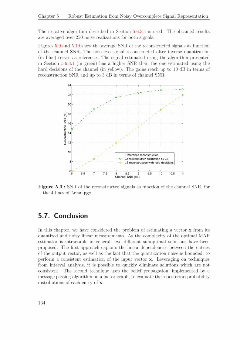
Chapter 5 Robust Estimation from Noisy Overcomplete Signal Representation
The iterative algorithm described in Section 5.6.3.1 is used. The obtained resultsare averaged over 250 noise realizations for both signals.
Figures 5.9 and 5.10 show the average SNR of the reconstructed signals as functionof the channel SNR. The noiseless signal reconstructed after inverse quantization(in blue) serves as reference. The signal estimated using the algorithm presentedin Section 5.6.3.1 (in green) has a higher SNR than the one estimated using thehard decisions of the channel (in yellow). The gains reach up to 10 dB in terms ofreconstruction SNR and up to 3 dB in terms of channel SNR.
6 6.5 7 7.5 8 8.5 9 9.5 10 10.5 116
8
10
12
14
16
18
20
22
24
Channel SNR (dB)
Reconstr
uction S
NR
(dB
)
Reference reconstruction
Consistent MAP estimation by LS
LS reconstruction with hard decisions
Figure 5.9.: SNR of the reconstructed signals as function of the channel SNR, forthe 4 lines of Lena.pgm.
5.7. Conclusion
In this chapter, we have considered the problem of estimating a vector x from itsquantized and noisy linear measurements. As the complexity of the optimal MAPestimator is intractable in general, two different suboptimal solutions have beenproposed. The first approach exploits the linear dependencies between the entriesof the output vector, as well as the fact that the quantization noise is bounded, toperform a consistent estimation of the input vector x. Leveraging on techniquesfrom interval analysis, it is possible to quickly eliminate solutions which are notconsistent. The second technique uses the belief propagation, implemented by amessage passing algorithm on a factor graph, to evaluate the a posteriori probabilitydistributions of each entry of x.
134
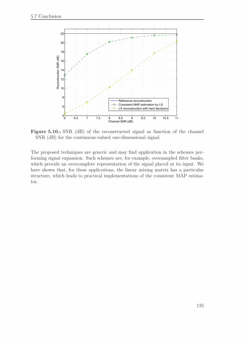
5.7 Conclusion
6 6.5 7 7.5 8 8.5 9 9.5 10 10.5 114
6
8
10
12
14
16
18
20
22
Channel SNR (dB)
Reconstr
uction S
NR
(dB
)
Reference reconstruction
Consistent MAP estimation by LS
LS reconstruction with hard decisions
Figure 5.10.: SNR (dB) of the reconstructed signal as function of the channelSNR (dB) for the continuous-valued one-dimensional signal.
The proposed techniques are generic and may find application in the schemes per-forming signal expansion. Such schemes are, for example, oversampled filter banks,which provide an overcomplete representation of the signal placed at its input. Wehave shown that, for these applications, the linear mixing matrix has a particularstructure, which leads to practical implementations of the consistent MAP estima-tor.
135

6. Conclusions and Perspectives
The extensive usage of heterogeneous best-effort networks puts the transmissionreliability and the processing complexity at the core of any communication system.During the few past years, increasing efforts have been dedicated to the developmentof practical joint source-channel coding and decoding schemes responding to theseissues.
In this thesis, we investigated some of these schemes and mainly focused on propos-ing techniques to increase the robustness of multimedia contents transmitted overunreliable networks, with limited transmission delay and complexity.
To conclude this dissertation, we provide in this chapter a synthesis of our contri-butions, before opening up some perspectives to the pursuit of this work.
6.1. Synthesis of the Contributions
Joint Source-Channel Decoding
We have proposed an efficient joint source-channel decoder for an error-resilient videotransmission. The proposed joint decoder employs the residual redundancy left inthe bit stream by the video coder, combined with bit reliability information providedby the channel, in order to detect and correct transmission errors. We have shownthat this technique leads to a manageable complexity, while significantly improvingthe decoding performance.
Application to Multiple Description Coding
We applied the joint source-channel decoder to multiple description video streamstransmitted over a mixed architecture, consisting of a wired lossy network and awireless noisy channel. The joint decoding increases the number of error-free packetsreceived by the multiple description decoder. As a consequence, the lost packets arebetter compensated and the decoder performance is improved.
137
Chapter 6 Conclusions and Perspectives
Robust Estimation Techniques
Also, we focused on studying joint source-channel coding schemes relying on a re-dundant transform.
We proposed a consistent estimation technique exploiting the structured redundancyintroduced by such schemes and accounting for the bounded nature of the quanti-zation noise. More precisely, we have shown how the estimation problem can beformulated as a constrained optimization problem, to which suboptimal solutionsmay be delivered by solving several linear programs or by using tools from intervalanalysis. In the presence of transmission errors, we illustrated how this estimationscheme improves the decoding performance when compared to a classical approachbased on the hard decisions of the channel.
Further, we applied this consistent estimation to recover the input of an oversampledfilter bank from its noisy subbands. We proposed an iterative implementation ofthis estimation scheme, particularly adapted to oversampled filter banks.
Alternatively, we proposed to apply the belief propagation algorithm, widely usedin inference problems, to estimate the signals placed at the input of an oversampledfilter bank. More precisely, we used belief propagation to compute the probabilitydistribution of each entry of the input vector, knowing the noisy subbands. We haveshown that this approach is particularly efficient when the noise introduced by thechannel is significant.
6.2. Perspectives
At the end of this thesis, several directions may be investigated to pursue this workand open up some new perspectives for future development.
First of all, the joint source-channel decoding scheme may be improved by exploitingother sources of redundancy. One may even consider to add some supplementaryredundancy on the transmitted packets in the corresponding headers, such as thenumber of non-zero coefficients within a spatio-temporal subband, the check-sumof some video frame or a part of it, etc. The amount of this information maybe chosen according to the importance of the transmitted packets. Moreover, anoptimization of the decoding complexity as a function of the packets sensitivity mayalso be considered. More precisely, the number of candidates examined by the jointdecoder may be adapted to the current layer and to the spatio-temporal subband ofthe processed block.
The application of the proposed joint source-channel decoder to multiple descriptioncoding has proven to be efficient for small redundancy levels. Indeed, combining botherror correcting and packet erasure codes should increase the performance of classicalsingle description schemes, at higher redundancy levels. The multiple description
138
6.2 Perspectives
scheme could further benefit from this redundancy increase, by duplicating, forexample, some spatio-temporal subbands in both descriptions, to better compensatethe effect of packet losses.
To connect our work on redundant joint source channel coding schemes and on jointsource-channel decoding, a direction to further investigate is how to use the proposedconsistent estimation technique and the belief propagation algorithm to improvethe multiple description decoding. Indeed, the two descriptions are generated byan oversampled filter bank in the temporal domain. It is thus possible to exploitthe structured redundancy introduced by this filter bank jointly with the residualredundancy, in order to improve the joint decoding of the descriptions.
More generally, a great deal of effort still needs to be made to optimize the proposedestimation algorithms in the case of oversampled filter banks with a dense analysismatrix and a reduced oversampling ratio. In particular, the estimation algorithmbased on belief propagation may be improved by including the parity-check con-straints in the factor graph. Finally, in order to apply these estimation approachesto image and video coding applications, it seems necessary to study its performancewhen oversampled filter banks with high coding gains are considered.
139

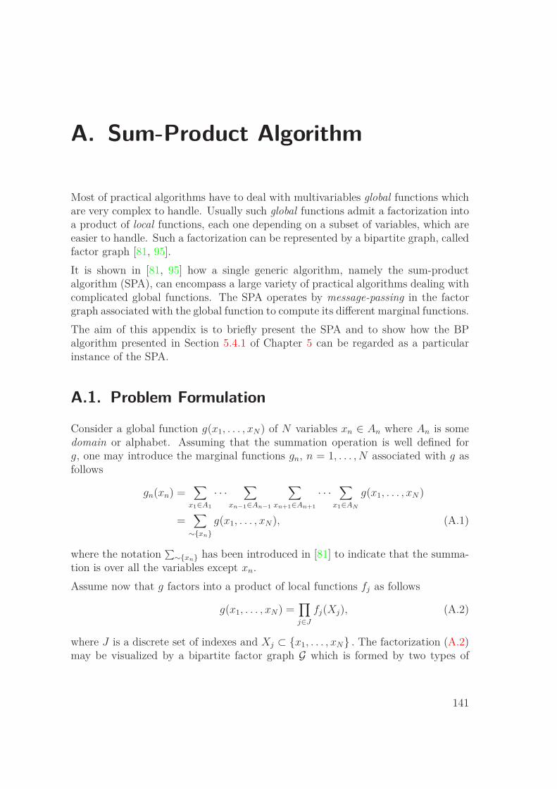
A. Sum-Product Algorithm
Most of practical algorithms have to deal with multivariables global functions whichare very complex to handle. Usually such global functions admit a factorization intoa product of local functions, each one depending on a subset of variables, which areeasier to handle. Such a factorization can be represented by a bipartite graph, calledfactor graph [81, 95].
It is shown in [81, 95] how a single generic algorithm, namely the sum-productalgorithm (SPA), can encompass a large variety of practical algorithms dealing withcomplicated global functions. The SPA operates by message-passing in the factorgraph associated with the global function to compute its different marginal functions.
The aim of this appendix is to briefly present the SPA and to show how the BPalgorithm presented in Section 5.4.1 of Chapter 5 can be regarded as a particularinstance of the SPA.
A.1. Problem Formulation
Consider a global function g(x1, . . . , xN) of N variables xn ∈ An where An is somedomain or alphabet. Assuming that the summation operation is well defined forg, one may introduce the marginal functions gn, n = 1, . . . , N associated with g asfollows
gn(xn) =∑
x1∈A1
· · ·∑
xn−1∈An−1
∑
xn+1∈An+1
· · ·∑
x1∈AN
g(x1, . . . , xN )
=∑
∼{xn}g(x1, . . . , xN), (A.1)
where the notation∑∼{xn} has been introduced in [81] to indicate that the summa-
tion is over all the variables except xn.
Assume now that g factors into a product of local functions fj as follows
g(x1, . . . , xN) =∏
j∈J
fj(Xj), (A.2)
where J is a discrete set of indexes and Xj ⊂ {x1, . . . , xN} . The factorization (A.2)may be visualized by a bipartite factor graph G which is formed by two types of
141
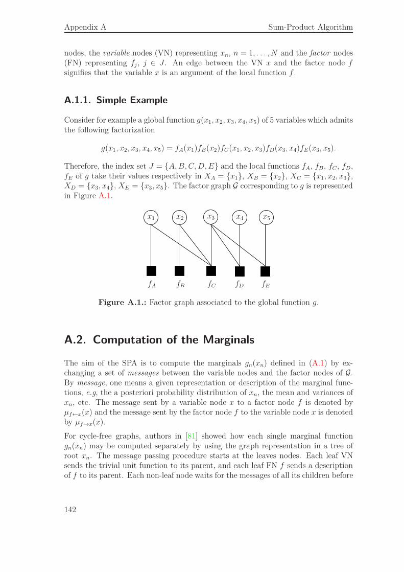
Appendix A Sum-Product Algorithm
nodes, the variable nodes (VN) representing xn, n = 1, . . . , N and the factor nodes(FN) representing fj , j ∈ J . An edge between the VN x and the factor node fsignifies that the variable x is an argument of the local function f .
A.1.1. Simple Example
Consider for example a global function g(x1, x2, x3, x4, x5) of 5 variables which admitsthe following factorization
g(x1, x2, x3, x4, x5) = fA(x1)fB(x2)fC(x1, x2, x3)fD(x3, x4)fE(x3, x5).
Therefore, the index set J = {A, B, C, D, E} and the local functions fA, fB, fC , fD,fE of g take their values respectively in XA = {x1}, XB = {x2}, XC = {x1, x2, x3},XD = {x3, x4}, XE = {x3, x5}. The factor graph G corresponding to g is representedin Figure A.1.
x1 x2 x3 x4 x5
fA fB fC fD fE
Figure A.1.: Factor graph associated to the global function g.
A.2. Computation of the Marginals
The aim of the SPA is to compute the marginals gn(xn) defined in (A.1) by ex-changing a set of messages between the variable nodes and the factor nodes of G.By message, one means a given representation or description of the marginal func-tions, e.g, the a posteriori probability distribution of xn, the mean and variances ofxn, etc. The message sent by a variable node x to a factor node f is denoted byµf←x(x) and the message sent by the factor node f to the variable node x is denotedby µf→x(x).
For cycle-free graphs, authors in [81] showed how each single marginal functiongn(xn) may be computed separately by using the graph representation in a tree ofroot xn. The message passing procedure starts at the leaves nodes. Each leaf VNsends the trivial unit function to its parent, and each leaf FN f sends a descriptionof f to its parent. Each non-leaf node waits for the messages of all its children before
142
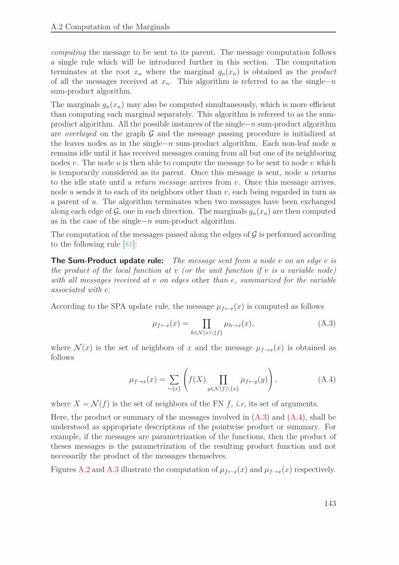
A.2 Computation of the Marginals
computing the message to be sent to its parent. The message computation followsa single rule which will be introduced further in this section. The computationterminates at the root xn where the marginal gn(xn) is obtained as the productof all the messages received at xn. This algorithm is referred to as the single−nsum-product algorithm.
The marginals gn(xn) may also be computed simultaneously, which is more efficientthan computing each marginal separately. This algorithm is refereed to as the sum-product algorithm. All the possible instances of the single−n sum-product algorithmare overlayed on the graph G and the message passing procedure is initialized atthe leaves nodes as in the single−n sum-product algorithm. Each non-leaf node uremains idle until it has received messages coming from all but one of its neighboringnodes v. The node u is then able to compute the message to be sent to node v whichis temporarily considered as its parent. Once this message is sent, node u returnsto the idle state until a return message arrives from v. Once this message arrives,node u sends it to each of its neighbors other than v, each being regarded in turn asa parent of u. The algorithm terminates when two messages have been exchangedalong each edge of G, one in each direction. The marginals gn(xn) are then computedas in the case of the single−n sum-product algorithm.
The computation of the messages passed along the edges of G is performed accordingto the following rule [81]:
The Sum-Product update rule: The message sent from a node v on an edge e isthe product of the local function at v (or the unit function if v is a variable node)with all messages received at v on edges other than e, summarized for the variableassociated with e.
According to the SPA update rule, the message µf←x(x) is computed as follows
µf←x(x) =∏
h∈N (x)\{f}µh→x(x), (A.3)
where N (x) is the set of neighbors of x and the message µf→x(x) is obtained asfollows
µf→x(x) =∑
∼{x}
f(X)
∏
y∈N (f)\{x}µf←y(y)
, (A.4)
where X = N (f) is the set of neighbors of the FN f, i.e, its set of arguments.
Here, the product or summary of the messages involved in (A.3) and (A.4), shall beunderstood as appropriate descriptions of the pointwise product or summary. Forexample, if the messages are parametrization of the functions, then the product oftheses messages is the parametrization of the resulting product function and notnecessarily the product of the messages themselves.
Figures A.2 and A.3 illustrate the computation of µf←x(x) and µf→x(x) respectively.
143
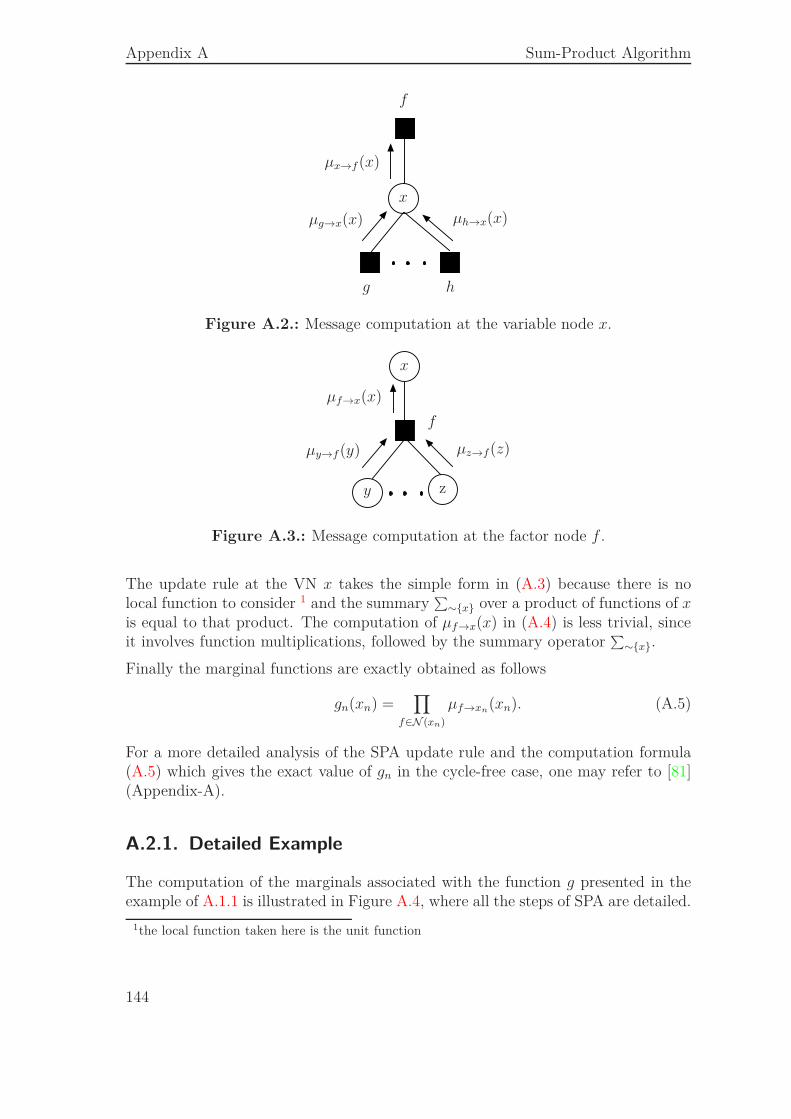
Appendix A Sum-Product Algorithm
x
f
g h
µx→f(x)
µg→x(x) µh→x(x)
Figure A.2.: Message computation at the variable node x.
x
y z
f
µy→f(y) µz→f(z)
µf→x(x)
Figure A.3.: Message computation at the factor node f .
The update rule at the VN x takes the simple form in (A.3) because there is nolocal function to consider 1 and the summary
∑∼{x} over a product of functions of x
is equal to that product. The computation of µf→x(x) in (A.4) is less trivial, sinceit involves function multiplications, followed by the summary operator
∑∼{x}.
Finally the marginal functions are exactly obtained as follows
gn(xn) =∏
f∈N (xn)
µf→xn(xn). (A.5)
For a more detailed analysis of the SPA update rule and the computation formula(A.5) which gives the exact value of gn in the cycle-free case, one may refer to [81](Appendix-A).
A.2.1. Detailed Example
The computation of the marginals associated with the function g presented in theexample of A.1.1 is illustrated in Figure A.4, where all the steps of SPA are detailed.
1the local function taken here is the unit function
144
A.3 Sum-Product Algorithm for Factor Graphs with Cycles
A.3. Sum-Product Algorithm for Factor Graphs with
Cycles
The SPA presented so far considered cycle-free factor graphs. In the case of factorgraphs with cycles, the computations introduced in the cycle-free case may be ap-plied by following the same update SPA rule, since all the updates are local. Howeverdue to the presence of cycles, the SPA has no natural termination and the messagesmay be passed infinitely along the same edge. The exact summary in (A.4) usuallyincludes an infinite number of terms.
The number of iterations of the SPA is usually decided according to whether thealgorithm has converged or not. The convergence occurs when identical messagesare obtained between two successive iterations. Nonetheless, the major problemof graphs with cycles is that the convergence is usually not perfect, messages mayoscillate between a set of values or states, or the convergence may be obtained for awrong fixed point. Therefore, unlike the cycle-free case, the results obtained whenoperating the SPA on graphs with cycles are not considered as exact.
In some applications, e.g, Markov chains, the associated factor graphs are naturallycycle-free. In other applications, e.g, decoding of LDPC and Turbo codes, theunderlying graphs contain cycles but the algorithm performances can still achievevery good performance as shown in [14, 97].
It is shown in [81] how equivalent cycle-free representations may be obtained from afactor graph with cycles, e.g for Bayesian networks. Such representations are usuallyachieved by operating a number of graph transformations. Note however that thecycles elimination comes at the expense of an increase of the complexity. In [167], twomodified versions of belief-propagation decoding, referred to as normalized belief-propagation and offset belief-propagation are proposed to improve the performanceof BP in graphs with cycles.
A.4. Belief Propagation
The SPA described in Section A.1 can encompass a wide number of practical algo-rithms such as the forward/backward algorithm, the Viterbi algorithm, the beliefpropagation (BP) algorithm, etc [81].
In this section its is shown how BP presented in Section 5.4.1 of Chapter 5, may bederived as a particular instance of the SPA to compute the a posteriori probabilitydistributions (APPDs) p(xn|r1:M).
The function to maximize in the MAP estimation problem of Chapter 5, is recalled
g(x1, . . . , xN ) = p(x1, . . . , xN |r1:M)
= p(x1, . . . , xN )p(r1:M |x1, . . . , xN )
145
Appendix A Sum-Product Algorithm
Assuming that the variables xn are independent with prior pXn(xn), the joint APPD
g admits the following factorization
g(x1, . . . , xN ) =N∏
n=1
pXn(xn)
M∏
m=1
p
(rm|
N∑
n=1
H(m, n)xn
). (A.6)
The graph GH associated to the factorization (A.2) has N variables nodes xn, M fac-tor nodes fm, each of which represents the likelihood function p
(rm|∑N
n=1 H(m, n)xn
)
and N (leaf) factor nodes hn which represent the a priori distribution of the vari-ables xn. Note, that these N factor nodes have not been mentioned in Section 5.4.1of Chapter 5, for simplicity sake. However they are implicitly taken into account inthe initialization step of the presented BP algorithm.
In deed, the SPA starts at these FN since they are the (only) leaves of GH . Eachnode hn sends the message pXn
(xn) to xn. At this level, there is no computation tobe made, these messages are simply transferred from each VN xn to its neighboringFN fm as described in (5.35) .
From now on, the nodes xn and fm are refereed to as n and m respectively. More-over, the messages µfm←xn
(xn) and µfm→xn(xn) exchanged at iteration i of the BP
algorithm are denoted by pxm←n(i, xn) and pu
m→n(i, um = um) respectively (withum = H(m, n)xn), as introduced in Section 5.4.1, to refer to the fact that thesemessages represent PDFs.
At the level of each FN m, the messages product∏
n∈N (m) pxm←n(i, xn) is defined here
as the distribution pm→n(i, ym→n) of the random variable ym→n defined in (5.36).
The function fm(X), X = N (fm) defined in (A.4) is the likelihood p(rm|∑N
n=1 H(m, n)xn
)
which takes the elements of N (m) as argument, rm being a fixed parameter of thisfunction.
The message computation in (A.4) is performed as described by (5.38), where thesummary operator
∑∼{xn} is defined as the integration over the (continuous) random
variable ym→n.
At the level of each VN node n, the message computation in (A.3) is performedas described by (5.38), where the actual product of the messages is performed2.The same observation is made for the computation (A.5) of the marginals gn(xn) =p(xn|r1:M) which performed in (5.39).
2It is the product of likelihoods sent by the FN nodes m′ ∈ N (n)\ {m}
146
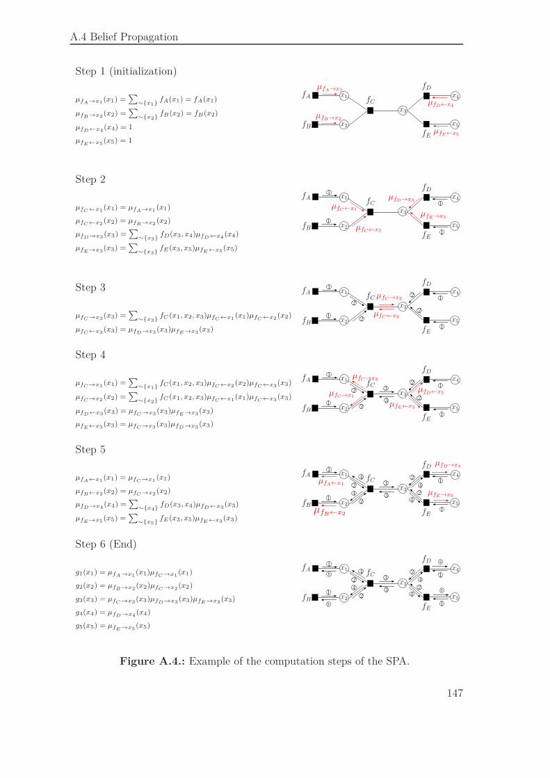
A.4 Belief Propagation
Step 1 (initialization)
x1
x2
x3
x4
x5
fA fC
fE
fD
fB
µfD←x4
µfE←x5
µfA→x1
µfB→x2
µfA→x1(x1) =
∑∼{x1}
fA(x1) = fA(x1)
µfB→x2(x2) =
∑∼{x2}
fB(x2) = fB(x2)
µfD←x4(x4) = 1
µfE←x5(x5) = 1
x1
x2
x3
x4
x5
fA fC
fE
fD
fB
µfD→x3
µfE→x3
µfC←x1
µfC←x2
1
1
1
1
Step 2
µfC←x1(x1) = µfA→x1
(x1)
µfC←x2(x2) = µfB→x2
(x2)
µfD→x3(x3) =
∑∼{x3}
fD(x3, x4)µfD←x4(x4)
µfE→x3(x3) =
∑∼{x3}
fE(x3, x5)µfE←x5(x5)
x1
x2
x3
x4
x5
fA fC
fE
fD
fB
µfC→x3
µfC←x31
1
1
12
22
2
Step 3
µfC→x3(x3) =
∑∼{x3}
fC(x1, x2, x3)µfC←x1(x1)µfC←x2
(x2)
µfC←x3(x3) = µfD→x3
(x3)µfE→x3(x3)
Step 4
x1
x2
x3
x4
x5
fA fC
fE
fD
fB
µfC→x1
µfC→x2
µfD←x3
µfE←x31
1
1
12
22
2
3
3
µfC→x1(x1) =
∑∼{x1}
fC(x1, x2, x3)µfC←x2(x2)µfC←x3
(x3)
µfC→x2(x2) =
∑∼{x2}
fC(x1, x2, x3)µfC←x1(x1)µfC←x3
(x3)
µfD←x3(x3) = µfC→x3
(x3)µfE→x3(x3)
µfE←x3(x3) = µfC→x3
(x3)µfD→x3(x3)
Step 5
x1
x2
x3
x4
x5
fA fC
fE
fD
fB
µfA←x1
µfB←x2
µfD→x4
µfE→x51
1
1
12
22
2
3
34
44
4
µfA←x1(x1) = µfC→x1
(x1)
µfB←x2(x2) = µfC→x2
(x2)
µfD→x4(x4) =
∑∼{x4}
fD(x3, x4)µfD←x3(x3)
µfE→x5(x5) =
∑∼{x5}
fE(x3, x5)µfE←x3(x3)
Step 6 (End)
5
5
5
5
x1
x2
x3
x4
x5
fA fC
fE
fD
fB1
1
1
12
22
2
3
34
44
4
g1(x1) = µfA→x1(x1)µfC→x1
(x1)
g2(x2) = µfB→x2(x2)µfC→x2
(x2)
g3(x3) = µfC→x3(x3)µfD→x3
(x3)µfE→x3(x3)
g4(x4) = µfD→x4(x4)
g5(x5) = µfE→x5(x5)
Figure A.4.: Example of the computation steps of the SPA.
147

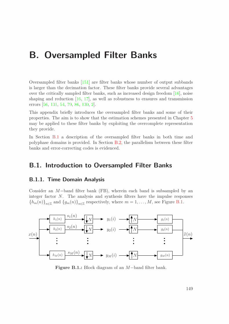
B. Oversampled Filter Banks
Oversampled filter banks [151] are filter banks whose number of output subbandsis larger than the decimation factor. These filter banks provide several advantagesover the critically sampled filter banks, such as increased design freedom [16], noiseshaping and reduction [16, 17], as well as robustness to erasures and transmissionerrors [56, 131, 54, 79, 86, 130, 2].
This appendix briefly introduces the oversampled filter banks and some of theirproperties. The aim is to show that the estimation schemes presented in Chapter 5may be applied to these filter banks by exploiting the overcomplete representationthey provide.
In Section B.1 a description of the oversampled filter banks in both time andpolyphase domains is provided. In Section B.2, the parallelism between these filterbanks and error-correcting codes is evidenced.
B.1. Introduction to Oversampled Filter Banks
B.1.1. Time Domain Analysis
Consider an M−band filter bank (FB), wherein each band is subsampled by aninteger factor N . The analysis and synthesis filters have the impulse responses{hm(n)}n∈Z and {gm(n)}n∈Z respectively, where m = 1, . . . , M , see Figure B.1.
x(n) x(n)
h1(n) g1(n)
h2(n) g2(n)
hM(n) gM(n)
s1(n)
s2(n)
sM(n)
N
N
N
N
N
N
y1(i)
y2(i)
yM(i)
Figure B.1.: Block diagram of an M−band filter bank.
149
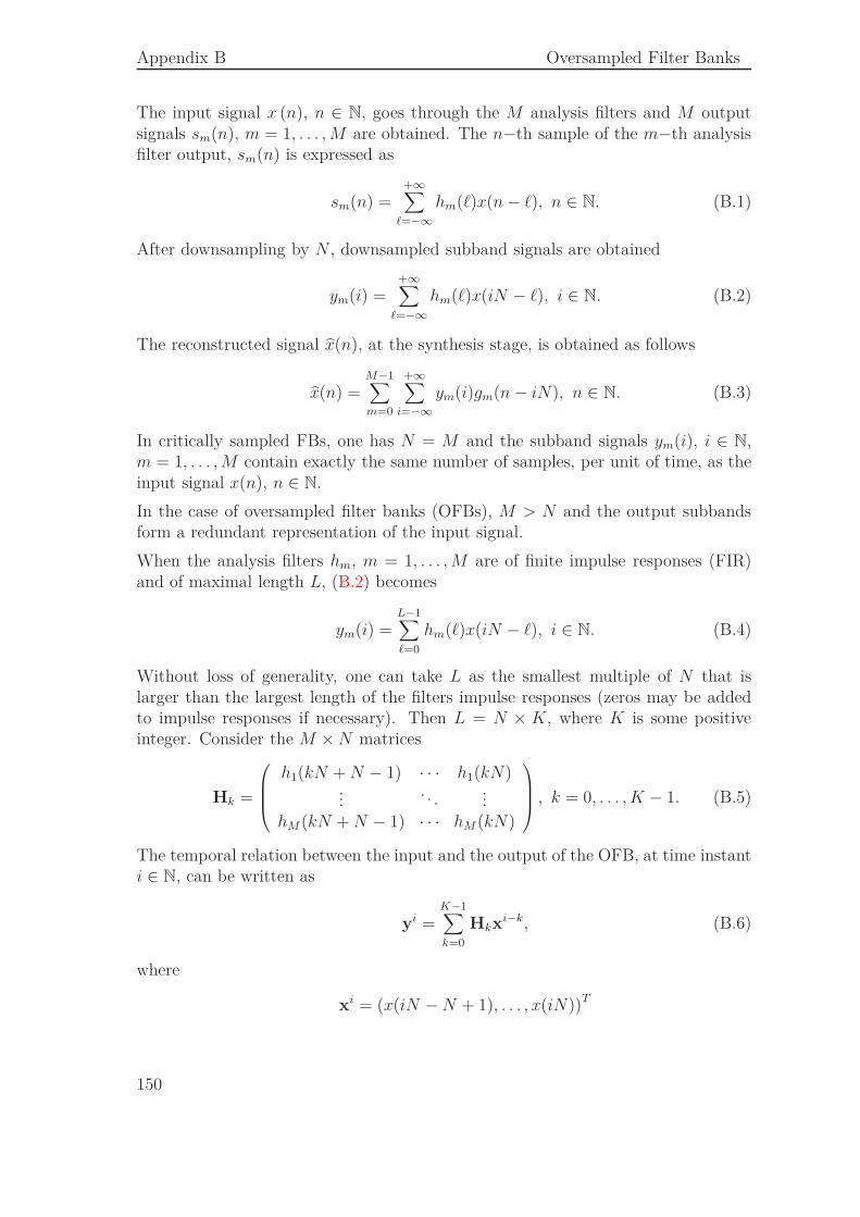
Appendix B Oversampled Filter Banks
The input signal x (n), n ∈ N, goes through the M analysis filters and M outputsignals sm(n), m = 1, . . . , M are obtained. The n−th sample of the m−th analysisfilter output, sm(n) is expressed as
sm(n) =+∞∑
ℓ=−∞hm(ℓ)x(n − ℓ), n ∈ N. (B.1)
After downsampling by N , downsampled subband signals are obtained
ym(i) =+∞∑
ℓ=−∞hm(ℓ)x(iN − ℓ), i ∈ N. (B.2)
The reconstructed signal x(n), at the synthesis stage, is obtained as follows
x(n) =M−1∑
m=0
+∞∑
i=−∞ym(i)gm(n − iN), n ∈ N. (B.3)
In critically sampled FBs, one has N = M and the subband signals ym(i), i ∈ N,m = 1, . . . , M contain exactly the same number of samples, per unit of time, as theinput signal x(n), n ∈ N.
In the case of oversampled filter banks (OFBs), M > N and the output subbandsform a redundant representation of the input signal.
When the analysis filters hm, m = 1, . . . , M are of finite impulse responses (FIR)and of maximal length L, (B.2) becomes
ym(i) =L−1∑
ℓ=0
hm(ℓ)x(iN − ℓ), i ∈ N. (B.4)
Without loss of generality, one can take L as the smallest multiple of N that islarger than the largest length of the filters impulse responses (zeros may be addedto impulse responses if necessary). Then L = N × K, where K is some positiveinteger. Consider the M × N matrices
Hk =
h1(kN + N − 1) · · · h1(kN)...
. . ....
hM (kN + N − 1) · · · hM (kN)
, k = 0, . . . , K − 1. (B.5)
The temporal relation between the input and the output of the OFB, at time instanti ∈ N, can be written as
yi =K−1∑
k=0
Hkxi−k, (B.6)
where
xi = (x(iN − N + 1), . . . , x(iN))T
150
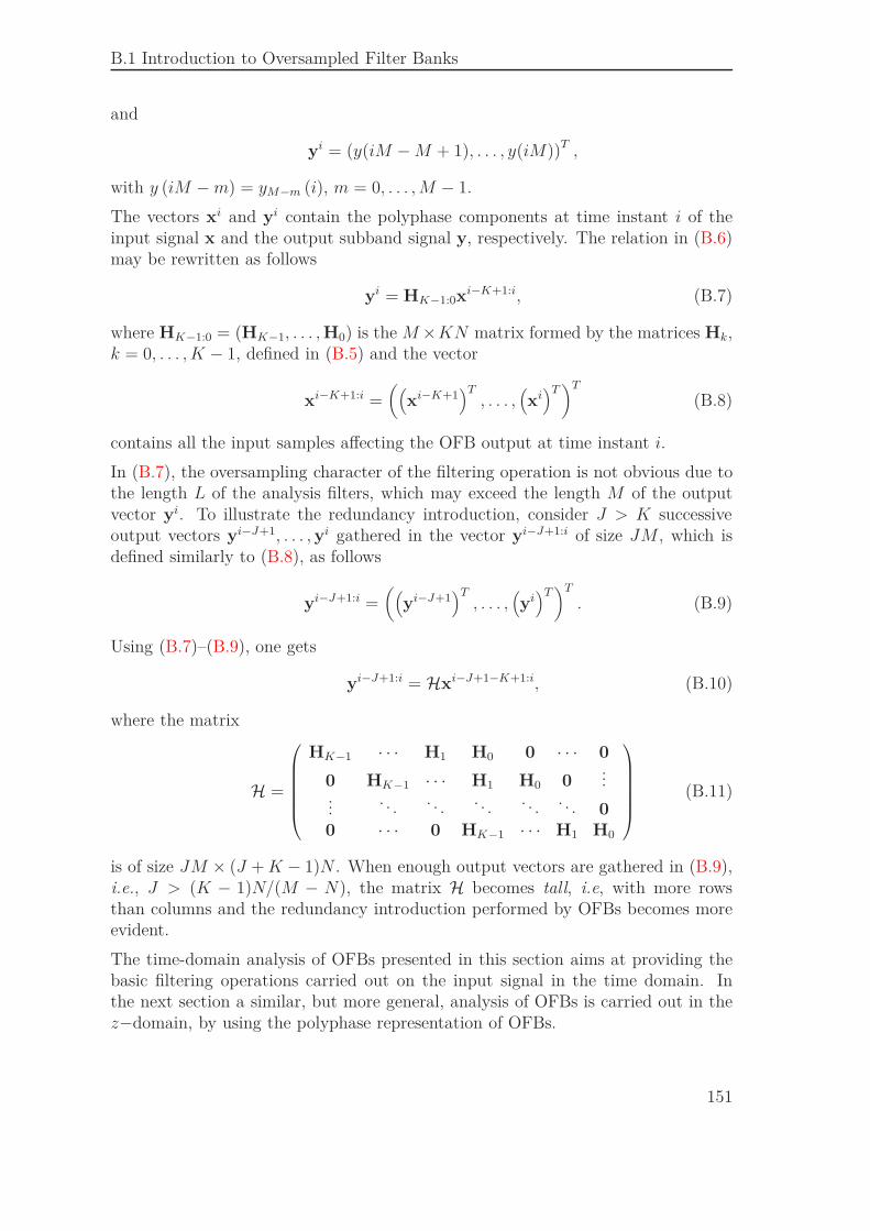
B.1 Introduction to Oversampled Filter Banks
and
yi = (y(iM − M + 1), . . . , y(iM))T ,
with y (iM − m) = yM−m (i), m = 0, . . . , M − 1.
The vectors xi and yi contain the polyphase components at time instant i of theinput signal x and the output subband signal y, respectively. The relation in (B.6)may be rewritten as follows
yi = HK−1:0xi−K+1:i, (B.7)
where HK−1:0 = (HK−1, . . . , H0) is the M ×KN matrix formed by the matrices Hk,k = 0, . . . , K − 1, defined in (B.5) and the vector
xi−K+1:i =((
xi−K+1)T
, . . . ,(xi)T)T
(B.8)
contains all the input samples affecting the OFB output at time instant i.
In (B.7), the oversampling character of the filtering operation is not obvious due tothe length L of the analysis filters, which may exceed the length M of the outputvector yi. To illustrate the redundancy introduction, consider J > K successiveoutput vectors yi−J+1, . . . , yi gathered in the vector yi−J+1:i of size JM , which isdefined similarly to (B.8), as follows
yi−J+1:i =((
yi−J+1)T
, . . . ,(yi)T)T
. (B.9)
Using (B.7)–(B.9), one gets
yi−J+1:i = Hxi−J+1−K+1:i, (B.10)
where the matrix
H =
HK−1 · · · H1 H0 0 · · · 0
0 HK−1 · · · H1 H0 0...
.... . . . . . . . . . . . . . . 0
0 · · · 0 HK−1 · · · H1 H0
(B.11)
is of size JM × (J + K − 1)N . When enough output vectors are gathered in (B.9),i.e., J > (K − 1)N/(M − N), the matrix H becomes tall, i.e, with more rowsthan columns and the redundancy introduction performed by OFBs becomes moreevident.
The time-domain analysis of OFBs presented in this section aims at providing thebasic filtering operations carried out on the input signal in the time domain. Inthe next section a similar, but more general, analysis of OFBs is carried out in thez−domain, by using the polyphase representation of OFBs.
151
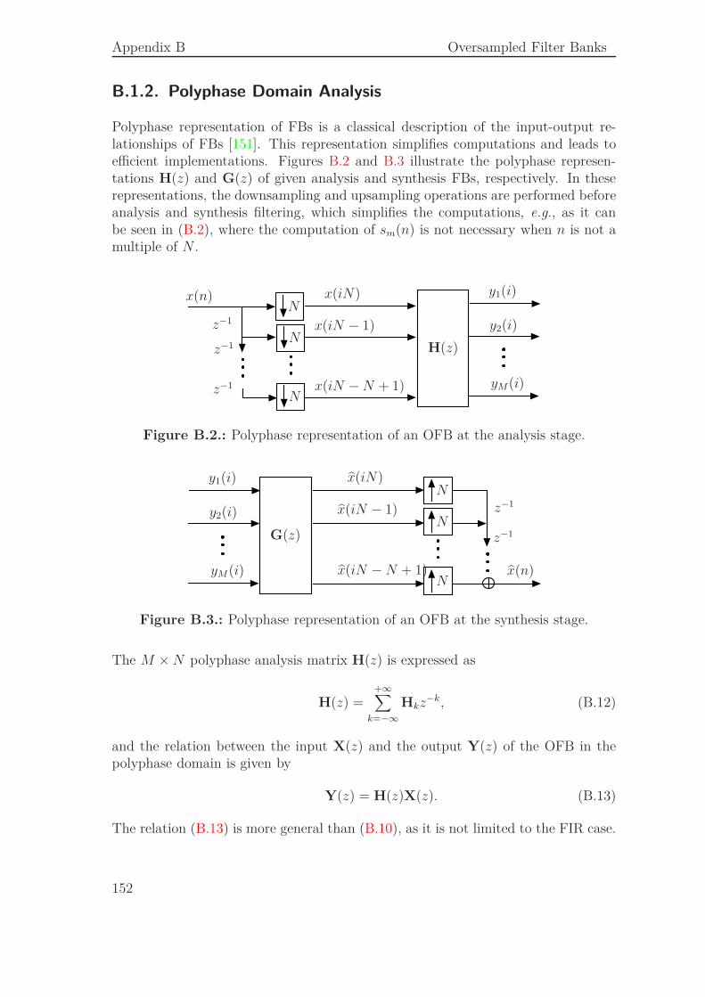
Appendix B Oversampled Filter Banks
B.1.2. Polyphase Domain Analysis
Polyphase representation of FBs is a classical description of the input-output re-lationships of FBs [151]. This representation simplifies computations and leads toefficient implementations. Figures B.2 and B.3 illustrate the polyphase represen-tations H(z) and G(z) of given analysis and synthesis FBs, respectively. In theserepresentations, the downsampling and upsampling operations are performed beforeanalysis and synthesis filtering, which simplifies the computations, e.g., as it canbe seen in (B.2), where the computation of sm(n) is not necessary when n is not amultiple of N .
x(n) x(iN)
x(iN − 1)
x(iN − N + 1)
N
N
N
H(z)
y1(i)
y2(i)
yM(i)
z−1
z−1
z−1
Figure B.2.: Polyphase representation of an OFB at the analysis stage.
x(n)
x(iN)
x(iN − 1)
x(iN − N + 1)
N
N
N
G(z)
y1(i)
y2(i)
yM(i)
z−1
z−1
Figure B.3.: Polyphase representation of an OFB at the synthesis stage.
The M × N polyphase analysis matrix H(z) is expressed as
H(z) =+∞∑
k=−∞Hkz−k, (B.12)
and the relation between the input X(z) and the output Y(z) of the OFB in thepolyphase domain is given by
Y(z) = H(z)X(z). (B.13)
The relation (B.13) is more general than (B.10), as it is not limited to the FIR case.
152
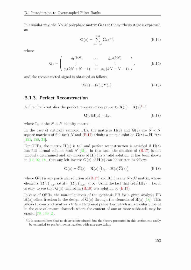
B.1 Introduction to Oversampled Filter Banks
In a similar way, the N×M polyphase matrix G(z) at the synthesis stage is expressedas
G(z) =+∞∑
k=−∞Gkz−k, (B.14)
where
Gk =
g1(kN) · · · gM(kN)...
. . ....
g1(kN + N − 1) · · · gM(kN + N − 1)
, (B.15)
and the reconstructed signal is obtained as follows
X(z) = G(z)Y(z). (B.16)
B.1.3. Perfect Reconstruction
A filter bank satisfies the perfect reconstruction property X(z) = X(z)1 if
G(z)H(z) = IN , (B.17)
where IN is the N × N identity matrix.
In the case of critically sampled FBs, the matrices H(z) and G(z) are N × Nsquare matrices of full rank N and (B.17) admits a unique solution G(z) = H−1(z)[151, 158, 31].
For OFBs, the matrix H(z) is tall and perfect reconstruction is satisfied if H(z)has full normal column rank N [31]. In this case, the solution of (B.17) is notuniquely determined and any inverse of H(z) is a valid solution. It has been shownin [10, 92, 18], that any left inverse G(z) of H(z) can be written as follows
G(z) = G(z) + R(z)(IM − H(z)G(z)
), (B.18)
where G(z) is any particular solution of (B.17) and R(z) is any N×M matrix, whoseelements (R(z))n,m satisfy
∣∣∣(R(z))n,m
∣∣∣ < ∞. Using the fact that G(z)H(z) = IN , itis easy to see that G(z) defined in (B.18) is a solution of (B.17).
In case of OFBs, the non-uniqueness of the synthesis FB for a given analysis FBH(z) offers freedom in the design of G(z) through the elements of R(z) [18]. Thisallows to construct synthesis FBs with desired properties, which is particularly usefulin the case of erasure channels where the content of one or more subbands may beerased [79, 130, 2].
1It is assumed here that no delay is introduced, but the theory presented in this section can easilybe extended to perfect reconstruction with non-zero delay.
153
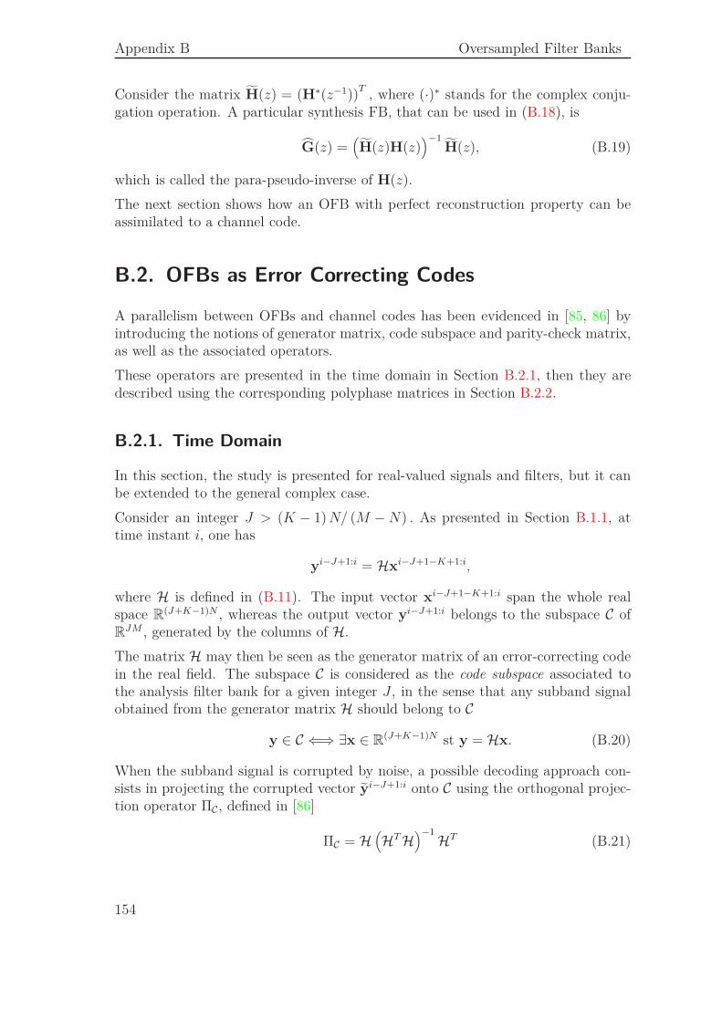
Appendix B Oversampled Filter Banks
Consider the matrix H(z) = (H∗(z−1))T, where (·)∗ stands for the complex conju-
gation operation. A particular synthesis FB, that can be used in (B.18), is
G(z) =(H(z)H(z)
)−1H(z), (B.19)
which is called the para-pseudo-inverse of H(z).
The next section shows how an OFB with perfect reconstruction property can beassimilated to a channel code.
B.2. OFBs as Error Correcting Codes
A parallelism between OFBs and channel codes has been evidenced in [85, 86] byintroducing the notions of generator matrix, code subspace and parity-check matrix,as well as the associated operators.
These operators are presented in the time domain in Section B.2.1, then they aredescribed using the corresponding polyphase matrices in Section B.2.2.
B.2.1. Time Domain
In this section, the study is presented for real-valued signals and filters, but it canbe extended to the general complex case.
Consider an integer J > (K − 1) N/ (M − N) . As presented in Section B.1.1, attime instant i, one has
yi−J+1:i = Hxi−J+1−K+1:i,
where H is defined in (B.11). The input vector xi−J+1−K+1:i span the whole realspace R(J+K−1)N , whereas the output vector yi−J+1:i belongs to the subspace C ofRJM , generated by the columns of H.
The matrix H may then be seen as the generator matrix of an error-correcting codein the real field. The subspace C is considered as the code subspace associated tothe analysis filter bank for a given integer J , in the sense that any subband signalobtained from the generator matrix H should belong to C
y ∈ C ⇐⇒ ∃x ∈ R(J+K−1)N st y = Hx. (B.20)
When the subband signal is corrupted by noise, a possible decoding approach con-sists in projecting the corrupted vector yi−J+1:i onto C using the orthogonal projec-tion operator ΠC, defined in [86]
ΠC = H(HT H
)−1 HT (B.21)
154
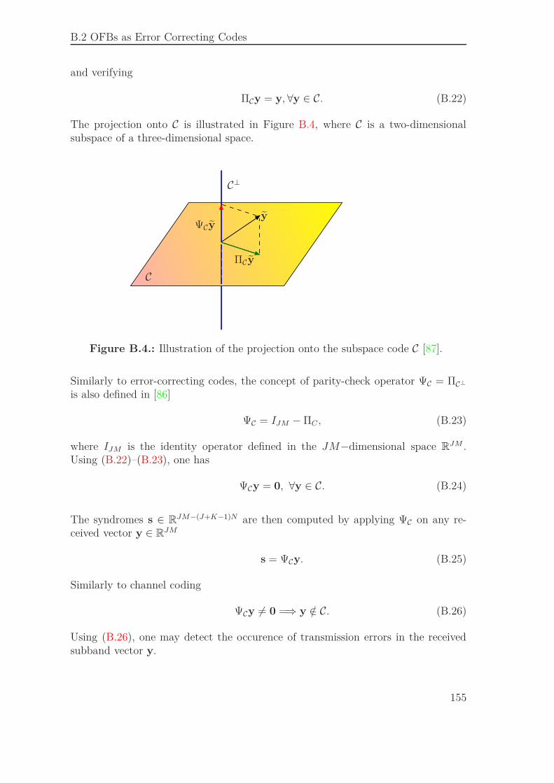
B.2 OFBs as Error Correcting Codes
and verifying
ΠCy = y, ∀y ∈ C. (B.22)
The projection onto C is illustrated in Figure B.4, where C is a two-dimensionalsubspace of a three-dimensional space.
C
C⊥
yΨCy
ΠCy
Figure B.4.: Illustration of the projection onto the subspace code C [87].
Similarly to error-correcting codes, the concept of parity-check operator ΨC = ΠC⊥is also defined in [86]
ΨC = IJM − ΠC , (B.23)
where IJM is the identity operator defined in the JM−dimensional space RJM .Using (B.22)–(B.23), one has
ΨCy = 0, ∀y ∈ C. (B.24)
The syndromes s ∈ RJM−(J+K−1)N are then computed by applying ΨC on any re-ceived vector y ∈ RJM
s = ΨCy. (B.25)
Similarly to channel coding
ΨCy 6= 0 =⇒ y /∈ C. (B.26)
Using (B.26), one may detect the occurence of transmission errors in the receivedsubband vector y.
155
Appendix B Oversampled Filter Banks
B.2.2. Polyphase Domain
In Section B.2.1, the subspace interpretation of OFBs as error-correcting codes isillustrated by stacking up J successive subband vectors, which is somewhat restric-tive.
In this section, the parallelism between OFBs and error-correction codes is drawnin the more general polyphase domain framework.
B.2.2.1. Smith-McMillan Decomposition
As mentioned in Section B.1.3, in the case of OFBs, the perfect reconstructionproperty is satisfied if H(z) has full column rank N . In this case, H(z) admits aSmith-McMillan decomposition [151] of the form
H(z) = U(z)
(Λ(z)
0
)W(z), (B.27)
where U(z) and W(z) are unimodular2 matrices of sizes M ×M and N ×N respec-tively, and Λ(z) is an N × N diagonal matrix, see Figure B.5.
X(z) X0(z)
X1(z))
XN−1(z)
N
N
N
U(z)
Y1(z)
Y2(z)
YM(z)
z−1
z−1
z−1
Λ(z)W(z)
0
Figure B.5.: Illustration of the Smith-McMillan decomposition [85].
The decomposition (B.27) allows a more clear understanding of the different op-erations performed at the analysis stage of an OFB. First an N × N multipleinput multiple output (MIMO) filter Λ(z)W(z) transforms an N -input sequenceX(z) = (X1(z), . . . , XN(z))T into a sequence of N subbands. These subbandsare padded with M − N null subbands. The M resulting subbands enter thenan M × M MIMO filter U(z). At the output of U(z), an M-subband vectorY(z) = (Y1(z), . . . , YM(z))T is obtained.
A mapping as the one illustrated by Figure B.5 cannot span the entire output space.The output subband vector Y(z) only spans a subspace C of RM of dimension N .
2Unimodular matrices are polynomial matrices with polynomial inverse [151].
156
B.2 OFBs as Error Correcting Codes
This code space C is spanned by the columns of H, or equivalently, by the first Ncolumns of U(z) [87, 85, 86].
The analogy between H and the generator matrix of an error-correcting channelcode becomes more clear through the Smith-McMillan form, and OFBs may then beconsidered as real-valued error-correcting codes [104, 25]. The orthogonal projectiononto the code subspace ΠC defined in (B.21) is implemented by using the para-pseudo-inverse G(z) defined in (B.19), at the synthesis stage [17]. It is shown in[85, 87] how the parity-check matrix and the syndrome associated to H(z) may becomputed using (B.27). This is the topic of next part.
B.2.2.2. Parity-Check Matrix and Syndrome Computation
Since the matrix U(z) is unimodular, it is invertible and its inverse may be writtenas follows
U−1(z) =
(V(z)P(z)
), (B.28)
where V(z) and P(z) are matrices of sizes N × M and (M − N) × N , respectively.From (B.27)–(B.28), one gets
(V(z)P(z)
)H(z) =
(Λ(z)W(z)
0
), (B.29)
and thus
P(z)H(z) = 0. (B.30)
Consider a subband signal Y(z) obtained at the output of the OFB from some inputsignal X(z). Then, using (B.30), one obtains
P(z)Y(z) = P(z)H(z)X(z)
= 0. (B.31)
Now assume that Y(z) is corrupted by some error signal of polyphase representationE(z). The corrupted subband signal Y(z) = Y(z) + E(z) verifies
P(z)Y(z) = P(z)E(z). (B.32)
Therefore P(z) is considered as the parity-check matrix associated to H(z) and
S(z) = P(z)Y(z)
is the syndrome associated to Y(z), which has to be equal to zero in the error-freecase, and may be different from zero if some transmission errors are encountered3.
3As in error-correcting codes, some transmission errors lead to a null syndrome and are thusundetectable.
157

Appendix B Oversampled Filter Banks
The parity-check matrix P(z) may be written as follows
P(z) =+∞∑
k=−∞Pkz−k, (B.33)
where Pk, k ∈ Z are (M − N) × M matrices.
In the case of FIR analysis filters, the parity-check filter P(z) is also FIR [87] and(B.33) becomes
P(z) =K ′−1∑
k=0
Pkz−k, (B.34)
where K ′ ∈ N∗.
158
C. Image Denoising by AdaptiveLifting Schemes
This appendix addresses the problem of image denoising by using adaptive liftingschemes. Such methods can adapt themselves to the analyzed signal, allowing tokeep useful information for denoising applications. However, these schemes result innon-isometric transforms, impacting thus the denoising approaches performing thenoise energy estimation in the subband domain. In [118, 119], the authors proposeda model to evaluate the subband energies of an uncorrelated signal when using suchadaptive lifting schemes. Based on this work, an estimation of the noise energies inthe wavelet transform domain is proposed in the sequel for image denoising.
C.1. Introduction
During its acquisition or transmission, an image is often corrupted by noise. Theaim of denoising techniques is to remove this noise while keeping as much as possiblethe important features of the image. A particular interest has been dedicated todenoising by wavelet thresholding [35, 39, 36]. The principal motivation relies onthe energy compaction property inherent to wavelet transforms: the small detailcoefficients are more likely due to noise whereas the large ones are due to impor-tant signal features [72]. These small coefficients can be then thresholded withoutaffecting the significant features of the image.
The lifting scheme (LS), introduced by Sweldenes [145] is a practical way for con-structing wavelets, which leads to the so called second generation wavelet trans-forms. It is popular because it has the capability of adjusting the wavelet transformto complex geometries and offers a simple, yet efficient, implementation of the firstgeneration wavelet transforms. However, an important limitation of the LS is that itdoes not cope well with the sudden changes in the input signal, that hide importantinformation in many applications, such as denoising. It becomes desirable to have alifting scheme that is able to adapt itself to the data. The adaptive lifting schemes(ALS) have been designed for this particular purpose [124, 29, 68, 125, 106].
The idea behind the ALS application in the particular case of denoising via thresh-olding, is that these schemes allow to perfectly preserve the original characteristics
159
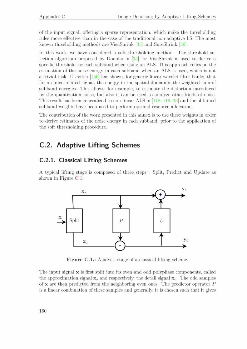
Appendix C Image Denoising by Adaptive Lifting Schemes
of the input signal, offering a sparse representation, which make the thresholdingrules more effective than in the case of the traditional non-adaptive LS. The mostknown thresholding methods are VisuShrink [35] and SureShrink [36].
In this work, we have considered a soft thresholding method. The threshold se-lection algorithm proposed by Donoho in [35] for VisuShrink is used to derive aspecific threshold for each subband when using an ALS. This approach relies on theestimation of the noise energy in each subband when an ALS is used, which is nota trivial task. Usevitch [150] has shown, for generic linear wavelet filter banks, thatfor an uncorrelated signal, the energy in the spatial domain is the weighted sum ofsubband energies. This allows, for example, to estimate the distortion introducedby the quantization noise, but also it can be used to analyze other kinds of noise.This result has been generalized to non-linear ALS in [118, 119, 23] and the obtainedsubband weights have been used to perform optimal resource allocation.
The contribution of the work presented in this annex is to use these weights in orderto derive estimates of the noise energy in each subband, prior to the application ofthe soft thresholding procedure.
C.2. Adaptive Lifting Schemes
C.2.1. Classical Lifting Schemes
A typical lifting stage is composed of three steps : Split, Predict and Update asshown in Figure C.1.
+
-
x
xa
xd
ya
yd
UPSplit
Figure C.1.: Analysis stage of a classical lifting scheme.
The input signal x is first split into its even and odd polyphase components, calledthe approximation signal xa and respectively, the detail signal xd. The odd samplesof x are then predicted from the neighboring even ones. The predictor operator Pis a linear combination of these samples and generally, it is chosen such that it gives
160
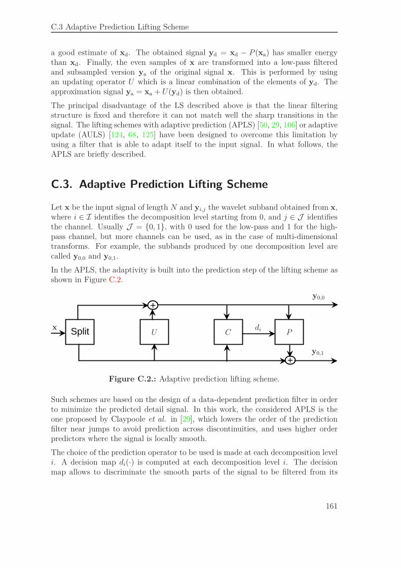
C.3 Adaptive Prediction Lifting Scheme
a good estimate of xd. The obtained signal yd = xd − P (xa) has smaller energythan xd. Finally, the even samples of x are transformed into a low-pass filteredand subsampled version ya of the original signal x. This is performed by usingan updating operator U which is a linear combination of the elements of yd. Theapproximation signal ya = xa + U(yd) is then obtained.
The principal disadvantage of the LS described above is that the linear filteringstructure is fixed and therefore it can not match well the sharp transitions in thesignal. The lifting schemes with adaptive prediction (APLS) [50, 29, 106] or adaptiveupdate (AULS) [124, 68, 125] have been designed to overcome this limitation byusing a filter that is able to adapt itself to the input signal. In what follows, theAPLS are briefly described.
C.3. Adaptive Prediction Lifting Scheme
Let x be the input signal of length N and yi,j the wavelet subband obtained from x,where i ∈ I identifies the decomposition level starting from 0, and j ∈ J identifiesthe channel. Usually J = {0, 1}, with 0 used for the low-pass and 1 for the high-pass channel, but more channels can be used, as in the case of multi-dimensionaltransforms. For example, the subbands produced by one decomposition level arecalled y0,0 and y0,1.
In the APLS, the adaptivity is built into the prediction step of the lifting scheme asshown in Figure C.2.
Split
+
+
x
y0,0
y0,1
diU PC
Figure C.2.: Adaptive prediction lifting scheme.
Such schemes are based on the design of a data-dependent prediction filter in orderto minimize the predicted detail signal. In this work, the considered APLS is theone proposed by Claypoole et al. in [29], which lowers the order of the predictionfilter near jumps to avoid prediction across discontinuities, and uses higher orderpredictors where the signal is locally smooth.
The choice of the prediction operator to be used is made at each decomposition leveli. A decision map di(·) is computed at each decomposition level i. The decisionmap allows to discriminate the smooth parts of the signal to be filtered from its
161
Appendix C Image Denoising by Adaptive Lifting Schemes
textured parts. Usually, the decision map takes its value in a discrete index set{1, . . . , Nf}, each value h of this set being associated to a given prediction filter{γh(n), n ∈ Z}. The position k, e.g. di(k) = h, h = 1, . . . , Nf, indicates that theh−th prediction filter γh has to be used. Once the decision maps are calculated, thefollowing equations are used for the analysis stage at level i
yi,0(k) = yi−1,0(2k) +∑
n∈Zβ(n)yi−1,0(2k + 1 − 2n)
yi,1(k) = yi−1,0(2k + 1) −∑
n∈Zγdi(k)(n)yi,0(k)(k − n),
where yi−1,0 = x, if i = 0, and {β(n), n ∈ Z} represents the non-adaptive updatefilter. The synthesis stage at level i is described by
yi−1,0(2k + 1) = yi,1(k) +∑
n∈Zγd(k)(n)yi,0(k − n)
yi−1,0(2k) = yi,0(k) −∑
n∈Zβ(n)yi−1,0(2k + 1 − 2n)
where yi−1,0, if i = 0, is the reconstructed input signal x.
As one can notice, this system is non-linear since the prediction operator dependson the decision map which, at its turn, depends on the input signal.
C.4. Distortion Estimation in the Transform Domain
For generic linear wavelet filter banks, Usevitch showed [150] that the energy σ2
(in the spatial domain) of an uncorrelated one-dimensional signal is related to theenergies σ2
i,j of the wavelet subbands yi,j by the following linear relation
σ2 =∑
i,j
1
2i+1wi,jσ
2i,j . (C.1)
The weights wi,j are computed as the norm of the synthesis polyphase matrix Gi,j
used to reconstruct the subband yi,j of size Ni,j [150]
wi,j =2
N
∑
n,m
Gi,j(m, n)2. (C.2)
This approach has been extended in [118, 119] to the case of the inherently non-linear ALS, for which no polyphase representation exists. The basic idea was tolook at the overall ALS as a linear time-varying system, which is possible once thedecision maps di(·) are given. In fact, the authors have shown that the non-linearityof the system depends only on the decision maps and not on the whole input signal.Therefore, the weights depend only on the values of di(·), and more precisely on thechoice of the prediction filters.
162
C.5 Application to Image Denoising
Consider the polyphase synthesis matrix G(h)i,j corresponding to the value h of the
decision map di(·). This matrix can be considered as the polyphase synthesis matrixused in the non-adaptive lifting case, where the h−th prediction filter γh is alwaysused. Let N
(h)i,j be the number of times the h−th filter is used in the subband yi,j.
In [118, 119] is shown that
wi,j =Nf∑
h=1
2N(h)i,j
Nw
(h)i,j =
Nf∑
h=1
ρ(h)w(h)i,j , (C.3)
where w(h)i,j is obtained from (C.2) and ρ(h) =
2N(h)i,j
Nmeasures the relative frequency
of using filter h for the current subband yi,j.
C.5. Application to Image Denoising
In the APLS approach, the prediction operator adapts itself to the input signal sothat the characteristics of the original signal are very well preserved. This propertyhas been successfully exploited to perform optimal resources allocation [118, 119],by estimating the distortion, introduced by quantization, in the transform domain.
In this work, the APLS properties are exploited for the purpose of image denoising.Let the image input signal be x(k, ℓ), k, ℓ = 1, . . . , N . Assume that this signalis corrupted by an additive noise ǫ of energy σ2 assumed independent of x. Thecorrupted image z is then obtained as
z(k, ℓ) = x(k, ℓ) + ǫ(k, ℓ). (C.4)
The goal is to denoise z(k, ℓ) and to obtain an estimate x(k, ℓ) of x(k, ℓ).
Let I denotes the coarsest scale of the APLS decomposition. As introduced inSection C.3, the same notation yi,j is kept for the subbands obtained from x, wherei ∈ I, j ∈ J , I = {0, . . . , I − 1} and J = {0, . . . , 3}, the only difference being thatthe two-dimensional case is considered here. The noisy subbands obtained from z
are denoted by yi,j. In the case of an orthogonal wavelet transform, the coefficientsin each noisy subband yi,j are i.i.d, as N (0, σ2). In the case of an APLS, this resultdoes not hold anymore since the considered transform is neither isometric nor linear.The standard deviation σi,j of the noise within the subband yi,j is not equal to thestandard deviation σ of the noise introduced the spatial domain.
In what follows, wavelet thresholding is used for removing the noise. It consists inthresholding only the wavelet coefficients of the detail subbands (i.e., yi,1, yi,2 andyi,3), while keeping the low resolution coefficients unchanged. The soft thresholdingmethod in [37] is considered here as it gives the best performances when coupledwith an undecimated discrete wavelet transform [30]. For an one-dimensional signalof length M , Donoho and Johnstone [35] proposed the universal threshold, TU =
σ√
2 log(M), which results in an asymptotic optimal estimate in the minimax sense.
163
Appendix C Image Denoising by Adaptive Lifting Schemes
In the case of APLS, the soft thresholding is applied to each noisy detail subband yi,j ,
i ∈ I, j = 1, 2, 3, with a specific threshold Ti,j = σi,j
√2 log(N2
i ), where N2i = N2
4i+1 isthe number of coefficients in the subband yi,j and σi,j is the noise standard deviationof the corrupted detail subband yi,j . The problem is thus to obtain a good estimationσi,j of σi,j within each subband. The relation in C.1 is only valid when σi,j representsthe energy of an uncorrelated signal, which might not be the case when using APLSon a noisy signal.
Consider the equation C.1 for the two-dimensional APLS, wherein the energy ofthe noise introduced in the spatial domain is σ2 =
∑i,j
14i+1 wi,jσ
2i,j. As explained in
[150], the use of a non-orthogonal transform results in weighting the energy in eachsubband. The weights can be seen as a measure of the closeness of the biorthogonalfilters to the class of orthogonal filters. The introduction of these weights allows thusto approach the behavior of the orthogonal transform in the sense that the equalitybetween the energies in the subbands, which is verified by an orthogonal transform,is changed into an equality between the weighted energies when a non-orthogonaltransform is used. This relation may be written as
wi,jσ2i,j ≈ wi′,j′σ
2i′,j′, (C.5)
where i 6= i′ and j 6= j′.
At the first decomposition level, the noise energy of the diagonal details subband
y0,3 may be estimated [35, 39] as: σ20,3 =
(m
0.6745
)2, where m is the median absolute
deviation of the wavelet diagonal details at the finest decomposition level. From(C.5), an estimation of σi,j can be derived
σi,j =
√√√√(
w0,3
wi,j
)σ0,3. (C.6)
One should point out that the equation (C.5), from which (C.6) is derived, relieson the assumption of equality between the weighted subband energies. In the nextsection, the energies expressions in (C.6) are used to achieve soft thresholding.
C.6. Simulation Results
C.6.1. Noise Standard Deviation Estimation
In this subsection, the aim is to evaluate the correctness of the noise standard devia-tion estimation provided by equation (C.6). A white Gaussian noise with a standarddeviation σ is introduced in the original image, which is further transformed usingan APLS with five decomposition levels, as described in Section C.3. The equation(C.6) is then used to calculate the estimations σi,j of the noise standard deviation
164
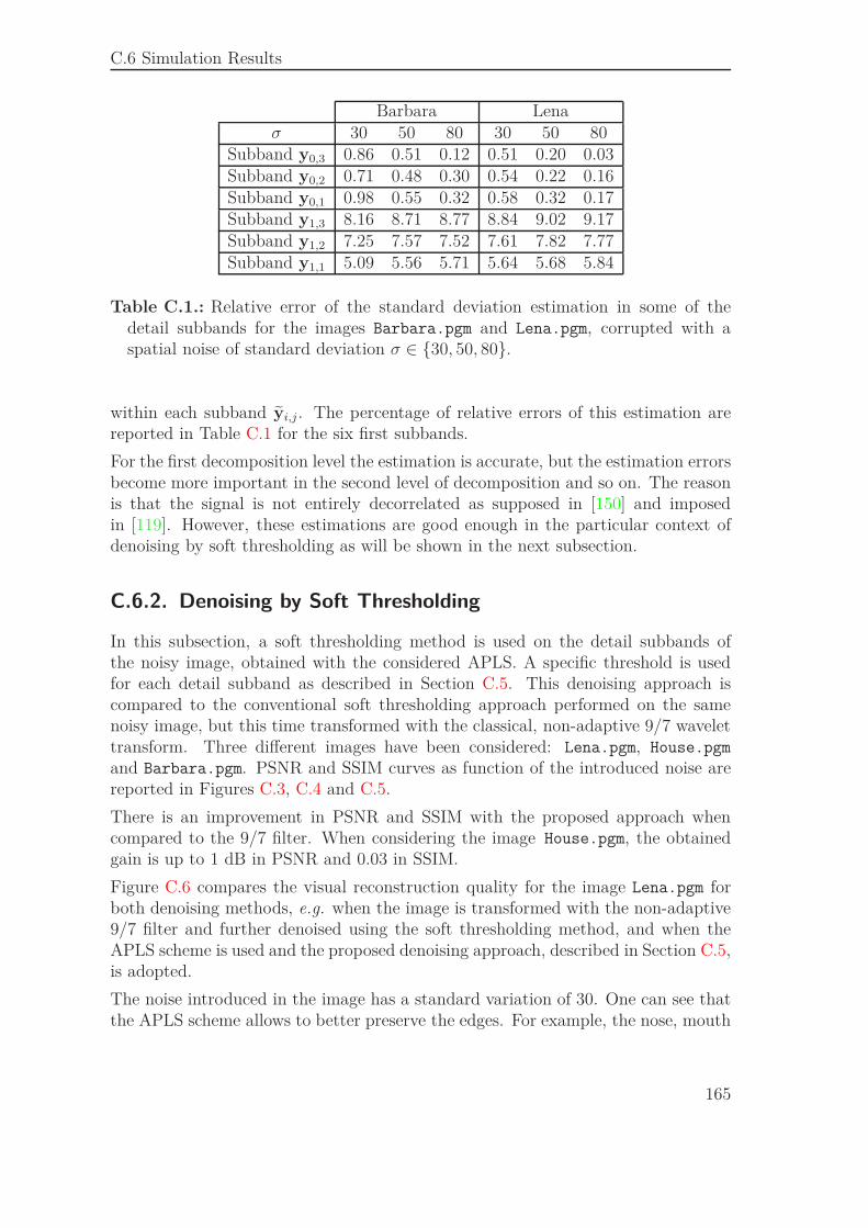
C.6 Simulation Results
Barbara Lenaσ 30 50 80 30 50 80
Subband y0,3 0.86 0.51 0.12 0.51 0.20 0.03Subband y0,2 0.71 0.48 0.30 0.54 0.22 0.16Subband y0,1 0.98 0.55 0.32 0.58 0.32 0.17Subband y1,3 8.16 8.71 8.77 8.84 9.02 9.17Subband y1,2 7.25 7.57 7.52 7.61 7.82 7.77Subband y1,1 5.09 5.56 5.71 5.64 5.68 5.84
Table C.1.: Relative error of the standard deviation estimation in some of thedetail subbands for the images Barbara.pgm and Lena.pgm, corrupted with aspatial noise of standard deviation σ ∈ {30, 50, 80}.
within each subband yi,j . The percentage of relative errors of this estimation arereported in Table C.1 for the six first subbands.
For the first decomposition level the estimation is accurate, but the estimation errorsbecome more important in the second level of decomposition and so on. The reasonis that the signal is not entirely decorrelated as supposed in [150] and imposedin [119]. However, these estimations are good enough in the particular context ofdenoising by soft thresholding as will be shown in the next subsection.
C.6.2. Denoising by Soft Thresholding
In this subsection, a soft thresholding method is used on the detail subbands ofthe noisy image, obtained with the considered APLS. A specific threshold is usedfor each detail subband as described in Section C.5. This denoising approach iscompared to the conventional soft thresholding approach performed on the samenoisy image, but this time transformed with the classical, non-adaptive 9/7 wavelettransform. Three different images have been considered: Lena.pgm, House.pgm
and Barbara.pgm. PSNR and SSIM curves as function of the introduced noise arereported in Figures C.3, C.4 and C.5.
There is an improvement in PSNR and SSIM with the proposed approach whencompared to the 9/7 filter. When considering the image House.pgm, the obtainedgain is up to 1 dB in PSNR and 0.03 in SSIM.
Figure C.6 compares the visual reconstruction quality for the image Lena.pgm forboth denoising methods, e.g. when the image is transformed with the non-adaptive9/7 filter and further denoised using the soft thresholding method, and when theAPLS scheme is used and the proposed denoising approach, described in Section C.5,is adopted.
The noise introduced in the image has a standard variation of 30. One can see thatthe APLS scheme allows to better preserve the edges. For example, the nose, mouth
165
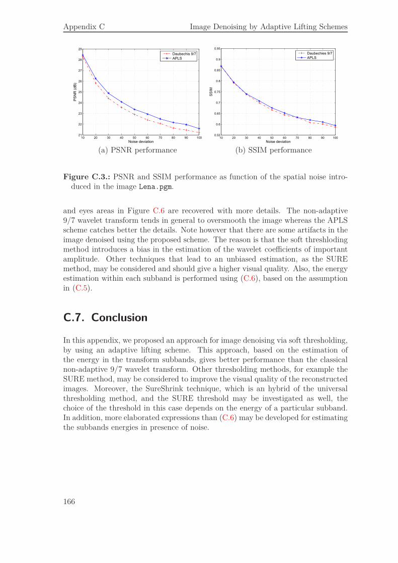
Appendix C Image Denoising by Adaptive Lifting Schemes
10 20 30 40 50 60 70 80 90 10021
22
23
24
25
26
27
28
29
Noise deviation
PS
NR
(dB
)
Daubechis 9/7
APLS
10 20 30 40 50 60 70 80 90 1000.55
0.6
0.65
0.7
0.75
0.8
0.85
0.9
0.95
Noise deviation
SS
IM
Daubechies 9/7
APLS
(a) PSNR performance (b) SSIM performance
Figure C.3.: PSNR and SSIM performance as function of the spatial noise intro-duced in the image Lena.pgm.
and eyes areas in Figure C.6 are recovered with more details. The non-adaptive9/7 wavelet transform tends in general to oversmooth the image whereas the APLSscheme catches better the details. Note however that there are some artifacts in theimage denoised using the proposed scheme. The reason is that the soft threshlodingmethod introduces a bias in the estimation of the wavelet coefficients of importantamplitude. Other techniques that lead to an unbiased estimation, as the SUREmethod, may be considered and should give a higher visual quality. Also, the energyestimation within each subband is performed using (C.6), based on the assumptionin (C.5).
C.7. Conclusion
In this appendix, we proposed an approach for image denoising via soft thresholding,by using an adaptive lifting scheme. This approach, based on the estimation ofthe energy in the transform subbands, gives better performance than the classicalnon-adaptive 9/7 wavelet transform. Other thresholding methods, for example theSURE method, may be considered to improve the visual quality of the reconstructedimages. Moreover, the SureShrink technique, which is an hybrid of the universalthresholding method, and the SURE threshold may be investigated as well, thechoice of the threshold in this case depends on the energy of a particular subband.In addition, more elaborated expressions than (C.6) may be developed for estimatingthe subbands energies in presence of noise.
166
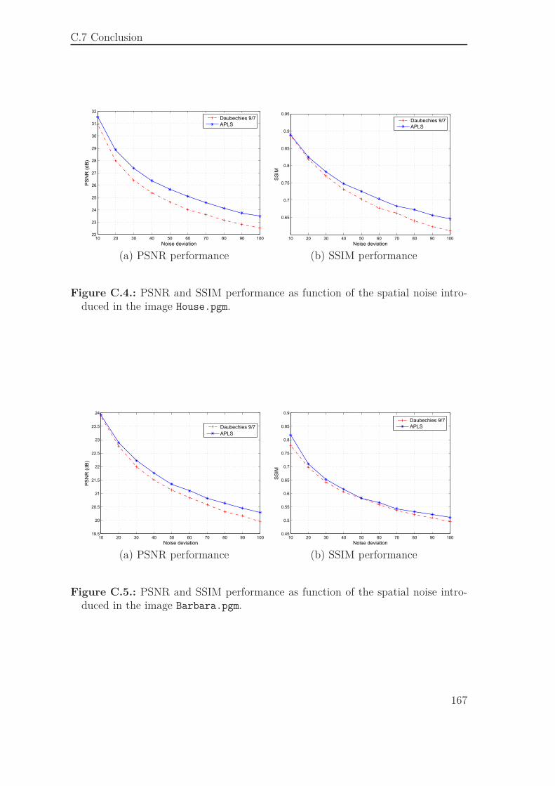
C.7 Conclusion
10 20 30 40 50 60 70 80 90 10022
23
24
25
26
27
28
29
30
31
32
Noise deviation
PS
NR
(dB
)
Daubechies 9/7
APLS
10 20 30 40 50 60 70 80 90 100
0.65
0.7
0.75
0.8
0.85
0.9
0.95
Noise deviation
SS
IM
Daubechies 9/7
APLS
(a) PSNR performance (b) SSIM performance
Figure C.4.: PSNR and SSIM performance as function of the spatial noise intro-duced in the image House.pgm.
10 20 30 40 50 60 70 80 90 10019.5
20
20.5
21
21.5
22
22.5
23
23.5
24
Noise deviation
PS
NR
(dB
)
Daubechies 9/7
APLS
10 20 30 40 50 60 70 80 90 1000.45
0.5
0.55
0.6
0.65
0.7
0.75
0.8
0.85
0.9
Noise deviation
SS
IM
Daubechies 9/7
APLS
(a) PSNR performance (b) SSIM performance
Figure C.5.: PSNR and SSIM performance as function of the spatial noise intro-duced in the image Barbara.pgm.
167
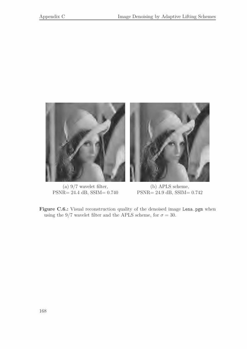
Appendix C Image Denoising by Adaptive Lifting Schemes
(a) 9/7 wavelet filter, (b) APLS scheme,PSNR= 24.4 dB, SSIM= 0.740 PSNR= 24.9 dB, SSIM= 0.742
Figure C.6.: Visual reconstruction quality of the denoised image Lena.pgm whenusing the 9/7 wavelet filter and the APLS scheme, for σ = 30.
168

List of Acronyms
ARQ Automatic Repeat Request
AVC Advanced Video Coding
AWGN Additive White Gaussian Noise
BER Bit Error Rate
BP Belief Propagation
BPSK Binary Phase-Shift Keying
CRC Cyclic Redundancy Check
DCT Discrete Cosine Transform
FB Filter Bank
FEC Forward Error Correction
FIR Finite Impulse Response
HD Hard Decisions
JSC Joint Source-Channel
JSC-NoSI JSC with No Side Information
JSC-SI JSC with Side Information
JSCC Joint Source-Channel Coding
JSCD Joint Source-Channel Decoding
LDPC Low-Density Parity-Check
LS Least Squares
MAC Media Access Control
MAP Maximum a Posteriori
169
MCTF Motion-Compensated Temporal Filtering
MD Multiple Description
MDCT Multiple Descriptions with Correlating Transform
MDSQ Multiple Description Scalar Quantization
ML Maximum Likelihood
MSE Mean Squared Error
NALU Network Abstraction Layer Unit
NR-D Non Robust Decoder
OFB Oversampled Filter Banks
PCT Parity-Check Test
PDF Probability Density Function
PEB Percentage of Erroneous Blocks
PSNR Peak Signal to Noise Ratio
R-D Rate-Distorsion
RTP Real Time Protocol
SD Single Description
SNR Signal to Noise Ratio
UEP Unequal Error Protection
VLC Variable Length Code
Y-PSNR PSNR on the luminance component Y
170
List of Publications
1. M. Abid, M. Trocan, M. Kieffer and B. Pesquet-Popescu, “Joint source-channeldecoding of multiple-description encoded video transmitted over heteregeneousnetworks”, in Signal Processing: Image Communication, 2012, submitted.
2. M. Abid, M. Kieffer and B. Pesquet-Popescu, “Maximum a posteriori con-sistent estimation using interval analysis”, in the 16th IFAC Symposium onSystem Identification (SYSID), Belgium, July 11-13, 2012.
3. Q. Wang, M. Abid, M. Kieffer and B. Pesquet-Popescu, “MAP estimation ofthe input of an oversampled filter bank from noisy subbands by belief prop-agation”, in Proceedings of the IEEE International Conference on Acoustics,Speech, and Signal Processing (ICASSP), Kyoto, March 25-30, 2012.
4. M. Abid, M. Kieffer and B. Pesquet-Popescu, “Reconstruction cohérente del’entrée d’un banc de filtres suréchantillonnés à partir de sa sortie bruitée”, inProceedings of GRETSI, Bordeaux, September 5-8, 2011.
5. M. Abid, M. Kieffer and B. Pesquet-Popescu, “Consistent reconstruction ofthe input of an oversampled filter bank from noisy subbands”, in Proceedingsof the European Signal Processing Conference (EUSIPCO), Barcelona, August29 - September 2, 2011.
6. M. Abid, M. Kieffer and B. Pesquet-Popescu, “Joint source-channel coding/decodingof 3D-ESCOT bitstreams, in Proceedings of the IEEE International Workshopon Multimedia Signal Processing (MMSP), Saint-Malo, October 4-6, 2010.
7. M. Abid, M. Kieffer, M. Cagnazzo and B. Pesquet-Popescu, “Robust decodingof a 3D-ESCOT bitstream transmitted over noisy channels”, in Proceedings ofthe IEEE International Conference on Image Processing, (ICIP), Hong Kong,September 26-29, 2010.
8. M. Abid, M. Cagnazzo and B. Pesquet-Popescu, “Image denoising by adaptivelifting schemes”, in Proceedings of the European Workshop on Visual Informa-tion Processing (EUVIP)”, Paris, July 5-7, 2010.
171

Bibliography
[1] M. A. Agostini, M. Kieffer, and M. Antonini. MAP estimation of multipledescription encoded video transmitted over noisy channels. In Proceedingsof IEEE International Conference on Image Processing, ICIP, Cairo, Egypt,November 7-10 2009. 56, 91
[2] M. Akbari and F. Labeau. Recovering the output of an OFB in the case ofinstantaneous erasures in sub-band domain. In Proc. MMSP, St Malo, France,2010, pp. 274-279. 6, 149, 153
[3] J. B. Anderson and S. Mohan. Source and Channel Coding: An AlgorithmicApproach. Kluwer, 1991. 14, 58, 71, 73
[4] E. Baccaglini, T. Tillo, and G. Olmo. Image and video transmission: a com-parison study of using unequal loss protection and multiple description coding.Multimedia Tools and Applications, 55(2):247–259, 2011. 19, 55
[5] S. Badri-Hoeher and P. Hoeher. Use of the list viterbi algorithm to computethe distance spectrum of trellis codes and isi channels. In Information Theory,2000. Proceedings. IEEE International Symposium on, page 101, 25-30 June2000. 57
[6] L. R. Bahl, J. Cocke, F. Jelinek, and J. Raviv. Optimal decoding of linearcodes for minimizing symbol error rate. IEEE Transactions on InformationTheory, 20:284–287, 1974. 73
[7] R. Bauer and J. Hagenauer. On variable length codes for iterativesource/channel decoding. In Proc. IEEE Data Compression Conference, pages272–282, Snowbird, UT, 1998. 58
[8] Olivier Beaumont and Bernard Philippe. Linear interval tolerance problemand linear programming techniques. Reliable Computing, 7(6):433–447, 2001.115
[9] N. El Beheiry, M. El Sharkawy, M. Lotfy, and S. Elnoubi. An adaptive fastand efficient spatial error concealment technique for block-based video codingsystems. IEEE International Midwest Symposium on Circuits and Systems,pages pp. 663–668, August 2009. 59
[10] A. Ben-Israel and T. N. E. Greville. Generalized Inverses: Theory and Appli-cations. Wiley-Interscience, 1974. 153
173
[11] C. Bergeron and C. Lamy-Bergot. Soft-input decoding of variable-length codesapplied to the H.264 standard. In Proc. IEEE Workshop on Multimedia SignalProcessing, pages 87–90, 29 Sept.-1 Oct. 2004. 6, 57
[12] C. Bergeron and C. Lamy-Bergot. Modelling h.264/avc sensitivity for errorprotection in wireless transmissions. In Multimedia Signal Processing, 2006IEEE 8th Workshop on, pages 302–305, Oct. 2006. 6, 46
[13] R. Bernardini, M. Durigon, R. Rinaldo, and A. Vitali. Comparison betweenmultiple description and single description video coding with forward errorcorrection. In Proceedings of IEEE International Workshop on MultimediaSignal Processing, MMSP, Shangai, China, October 30-November 2 2005. 19,55, 56
[14] C. Berrou, A. Glavieux, and P. Thitimajhima. Near shannon limit error cor-recting coding and decoding : Turbo-codes. Proc. Of ICC, Geneva, pages1064–1070, 1993. 145
[15] R. E. Blahut. Algebraic Codes for Data Transmission. Cambridge UniversityPress, February 2003. 103
[16] H. Bölcskei and F. Hlawatsch. Oversampled filterbanks: Optimal noise shap-ing, design freedom and noise analysis. In Proc. IEEE Conference on Acous-tics, Speech and Signal Processing, volume 3, pages 2453–2456, Munich, Ger-many, 1997. 149
[17] H. Bölcskei and F. Hlawatsch. Noise reduction in oversampled filter banksusing predictive quantization. IEEE Transactions on Information Theory,47(1):155–172, January 2001. 149, 157
[18] H. Bölcskei, F. Hlawatsch, and H. G. Feichtinger. Frame-theoretic analysis ofoversampled filter banks. IEEE Trans. Signal Processing, 46(12):3256–3268,1998. 153
[19] J.W. Byers, M. Luby, and M. Mitzenmacher. A digital fountain approach toasynchronous reliable multicast. IEEE Journal on Selected Areas in Commu-nications, 20(8):1528–1540, 2002. 41
[20] M. Bystrom and J. W. Modestino. Combined source-channel coding schemesfor video transmission over an additive white gaussian noise channel. IEEEJournal on Selected Areas in Communications, 18:880–890, 2000. 6, 42, 45, 47
[21] M. Bystrom and T. Stockhammer. Dependent source and channel rate alloca-tion for video transmission. IEEE Transactions on Wireless Communications,3(1):258– 268, 2004. 42, 45, 47
[22] T. André C. Lamy-Bergot, A. Mokraoui-Zergainoh and B. Pesquet-Popescu.Panorama des techniques de codage/décodage conjoint et techniques de di-versité adaptées à la transmission de flux vidéo et html sur lien ip sans filpoint/multipoint. Revue Traitement du Signal, 25, no.5 (in French), Octobre2008. 6, 56, 57
174
Bibliography
[23] M. Cagnazzo and B. Pesquet-Popescu. Perceptual impact of transform coef-ficients quantization for adaptive lifting schemes. In International Workshopon Video Processing and Quality Metrics for Consumer Electronics, 2010. 160
[24] G. Cheung and A. Zakhor. "bit allocation for joint source/channel coding ofscalable video",. IEEE Transactions on Image Processing, 9:340–356, 2000. 6,42, 45, 47
[25] J.C. Chiang, M. Kieffer, and P. Duhamel. Robust image transmission usingoversampled filterbank. In Proceedings of EUSIPCO, pages 1325–1328, 2004.157
[26] M. Chiani and M.G. Martini. Proportional unequal error protection for mpeg–4 video transmission. In Proceedings (ICC 2001), Helsinki (Finland), 2001. 6,46
[27] J. Chou and K. Ramchandran. Arithmetic coding-based continuous errordetection for efficient arq-based image transmission. Selected Areas in Com-munications, IEEE Journal on, 18(6):861–867, June 2000. 58
[28] C. Christopoulos, A. Skodras, and T. Ebrahimi. The jpeg-2000 still imagecoding system: An overview. IEEE Trans. Consumer Electron., 46:1103–1127,2000. 45
[29] R. L. Claypoole, G. M. Davis, W. Sweldens, and R. G. Baraniuk. Nonlinearwavelet transforms for image coding via lifting. IEEE Transactions on ImageProcessing,, 12, no. 12(12):1449–1459, December 2003. 159, 161
[30] R. R. Coifman and D. L. Donoho. Translation invariant de-noising. In Waveletsand Statistics, A. Antoniadis and G. Oppenheim, Eds. New York: Springer-Verlag,, 1995, pp. 125–150. 163
[31] Z. Cvetković and M. Vetterli. Oversampled filter banks. IEEE Transactionson Signal Processing, 46(5):1245–1255, 1998. 153
[32] S. Sarvotham D. Baron and R. G. Baraniuk. Bayesian compressive sensing viabelief propagation. IEEE Transactions on Signal Processing, 58(1):269–280,January 2010. 120
[33] L. B. Milstein D. N. Rowitch. Rate Compatible Punctured Turbo (RCPT)Codes in a hybrid FEC/ARQ system. Proceedings of the IEEE Global Com-munication Conference, 4:55–59, Phoenix, AZ, USA, 1997. 46
[34] B. Li W. Zhu Y. Q. Zhang D. Wu, Y. T. Hou and H. J. Chao. An end-to-endapproach for optimal mode selection in internet video communication: theoryand application. IEEE Journal on Selected Areas in Communications, 18, no.6:977–995, 2000. 45
[35] D. L. Donoho and I. M. Johnstone. Ideal spatial adaptation via wavelet shrink-age. In Biometrika, 1994, vol. 81, pp. 425-455. 159, 160, 163, 164
175
[36] D. L. Donoho and I. M. Johnstone. Adapting to unknown smoothness viawavelet shrinkage. In Journal of the American Statistical Association, vol-ume 90, pages 1200–1224, 1995. 159, 160
[37] D.L. Donoho. De-noising by soft-thresholding. In IEEE Transactions onInformation Theory, volume 41, 1995. 163
[38] D.L. Donoho, A.Maleki, and A. Montanari. Message Passing Algorithm forCompressed Sensing. Proceedings of the National Academy of Sciences, 106no. 45:18914–18919, 2009. 26, 120
[39] D.L. Donoho and I.M Johnstone. Threshold selection for wavelet shrinkage ofnoisy data. In Proceedings of the IEEE Conference on Engineering in Medicineand Biology Society, Maryland, USA, pages 24–25, 1994. 159, 164
[40] P. L. Dragotti, S. D. Servetto, and M. Vetterli. Optimal filter banks formultiple description coding: Analysis and synthesis. IEEE Transactions onInformation Theory, 48(7):2036–2052, July 2002. 54
[41] R.J. Duffin and A. C. Schaeffer. A class of nonharmonic Fourier series. Trans.Amer. Math. Soc., 72:341–366, 1952. 53
[42] P. Duhamel and M. Kieffer. Joint source-channel decoding: A cross-layerperspective with applications in video broadcasting. Academic Press, 2009. 6,8, 20, 57, 63, 73, 108
[43] A. A. El Gamal and T. M. Cover. Achievable rate for multiple description.IEEE Transactions on Information Theory, 28(6):851–857, 1982. 6, 48
[44] A. K. Katsaggelos F. Zhai, Y. Eisenberg. Handbook of Image and Video Pro-cessing, chapter Joint source-channel coding for video communications. June2005. 5, 43
[45] F. Farvardin. A study of vector quantization for noisy channels. IEEE Trans-actions on Information Theory, 36:799–809, 1990. 45
[46] N. Farvardin and V. Vaishampayan. Optimal quantizer design for noisy chan-nels: An approach to combined source-channel coding. IEEE Transactions onInformation Theory, 33(6):827–837, 1991. 45
[47] M. Fleming and M. Effros. Generalized multiple description vector quantiza-tion. In Proceedings of the IEEE Data Compression Conference, pages 3–12,1999. 51
[48] J. E. Fowler and B. Pesquet-Popescu. An overview on wavelets in sourcecoding, communications, and networks. EURASIP Journal on Image andVideo Processing, pages 1–28, 2007. 55
[49] C. Zhang S. S. Gao G. F. Tu, J. J. Liu and S. D. Li. Studies and advances onjoint source-channel encoding/decoding techniques in flow media communica-tions. Science China Information Sciences, 53, no. 1:1–17, 2010. 5, 43
176
Bibliography
[50] Ö. N. Gerek and A. E. Çetin. Adaptive polyphase subband decompositionstructures for image compression. IEEE Transactions on Image Processing,9(10):1649–1659, October 2000. 161
[51] H. Gharavi and S. I. Gao. Spatial interpolation algorithm for error concealmentapril 2008, pp. 1153-1156. In Proceedings of the IEEE International Conferenceon Acoustics, Speech and Signal Processing, ICASSP, pages 1153–1156, April2008. 59
[52] V. K. Goyal. Multiple description coding: compression meets the network.IEEE Signal Processing Magazine, 18(5):74–93, September 2001. 6, 42, 48
[53] V. K. Goyal and J. Kovacević. Generalized multiple description coding withcorrelating transforms. IEEE Trans. Information Theory, 47(6):2199–2224,2001. 49, 52
[54] V. K Goyal, J. Kovacevic, and J.A. Kelner. Quantized frame expansions witherasures. Journal of Appl. and Comput. Harmonic Analysis, 10(3):203–233,2001. 6, 54, 149
[55] V. K. Goyal, J. Kovacević, and M. Vetterli. Multiple description transformcoding : Robustness to erasures using tight frame expansion. In Proc. IEEEInt. Symp. On Inform. Th., page 408, Boston, MA, August 1998. 53
[56] V. K. Goyal, Jelena Kovacevic, and Martin Vetterli. Quantized frame expan-sions as source-channel codes for erasure channels. In Proceedings of DataCompression Conference, pages 326–335, 1999. 6, 53, 54, 149
[57] V. K. Goyal, M. Vetterli, and N. T. Thao. Quantized overcomplete expansionsin Rn : Analysis, synthesis, and algorithms. IEEE Transactions on Informa-tion Theory, 44(1):16–31, 1998. 54
[58] M. Grangetto and P. Cosman. Map decoding of arithmetic codes with aforbidden symbol. Proc. of ACIVS 2002, Ghent, Belgium, 2002. 58
[59] M. Grangetto, P. Cosman, and G. Olmo. Joint source/channel coding andmap decoding of arithmetic codes. IEEE Trans. on Comm., 53(6):1007–1016,2005. 58
[60] M. Grangetto, E. Magli, and G. Olmo. Robust video transmission over error-prone channels via error correcting arithmetic codes. IEEE Comm. Letters,pages 596–598, 2003. 58
[61] M. Grangetto, E. Magli, and G. Olmo. Joint source-channel iterative decodingof arithmetic codes. Proc. of ICC, Paris, pages 20–24, 2004. 58
[62] C. Guillemot and P. Siohan. Joint source-channel decoding with soft informa-tion: A survey. Elsevier Journal on Applied Signal Processing, special issueon the turbo principle, 6:906–927, 2005. 6, 56
[63] T. Guionnet and C. Guillemot. Soft decoding and synchronization of arith-metic codes: Application to image transmission over noisy channels. IEEETrans. on Image Processing, 12(12):1599–1609, 2003. 58
177
[64] T. Guionnet, C. Guillemot, and E. Fabre. Soft decoding of multiple descrip-tions. In Proceedings of IEEE International Conference on Multimedia andExpo, ICME, volume 2, pages 601–604, August 26-29 2002. 56
[65] C. Yim H. Ha and Y. Y. Kim. Packet loss resilience using unequal forward errorcorrection assignment for video transmission over communication networks.Computer Communications, 30, no. 12:3676–3689, 2007. 45
[66] O. Hadar, M. Huber, R. Huber, and S. Greenberg. New hybrid error conceal-ment for digital compressed video. EURASIP Journal on Advances in SignalProcessing, pages vol. 12, pp.1821–1833, July 2005. 59
[67] J. Hagenauer. Rate-compatible punctured convolutional codes (RCPC codes)and their applications. IEEE Transactions on Communications, 36(4):389–400, 1988. 41, 46
[68] Henk J. A. M. Heijmans, Béatrice Pesquet-Popescu, and Gemma Piella. Build-ing nonredundant adaptive wavelets by update lifting. Applied ComputationalHarmonic Analysis, (18):252–281, May 2005, no. 18. 159, 161
[69] B. Hochwald and K. Zeger. Tradeoff between source and channel coding. IEEETransactions on Information Theory, 43:1412–1424, 1997. 45
[70] ITU-T and ISO/IEC JTC 1. Advanced video coding for generic audiovisualservices. Technical report, ITU-T Rec. H.264, and ISO/IEC 14496-10 AVC,nov. 2003. 39, 45
[71] S. Li J. Xu, Z.Xioong and Y. Zhang. Three-dimensional embedded subbandcoding with optimal truncation (3D ESCOT). Applied and ComputationalHarmonic Analysis, May 2001, vol. 10, pp. 290-315. 10, 67
[72] Maarten Jansen. Noise reduction by wavelet thresholding. In Springer Verlag,Lecture notes in Statistics, vol. 161,, 2001. 159
[73] L. Jaulin, M. Kieffer, O. Didrit, and E. Walter. Applied Interval Analysis.Springer-Verlag, London, 2001. 23, 111, 115, 116, 132
[74] H. Jenkac, G. Liebl, T. Stockhammer, and X. Wen. Flexible outer Reed-Solomon coding on RLC layer for MBMS over GERAN. In IEEE VehicularTechnology Conference, volume 5, pages 2777–2781, May 17-19 2004. 41
[75] H. Jenkac, T. Stockhammer, and W. Xu. Permeable-layer receiver for reliablemulticast transmission in wireless systems. In Proc. IEEE Wireless Communi-cations and Networking Conference, volume 3, pages 1805–1811, 13-17 March2005. 63, 108
[76] S. Kaiser and M. Bystrom. Soft decoding of variable-length codes. In Proc.IEEE ICC, volume 3, pages 1203–1207, New Orleans, 2000. 6, 56
[77] U. Kamilov, V.K Goyal, and S. Rangan. Message-passing estimation fromquantized samples. arXiv:1105.6368v1 [cs.IT], 31 May 2011. 120
178
Bibliography
[78] M. Kim, H. Lee, and S. Sull. Spatial error concealment for H.264 using sequen-tial directional interpolation. IEEE Transactions on Consumer Electronics,pages vol. 54, no. 4, pp. 1811–1818, November 2008. 59
[79] J. Kovacević, P. L. Dragotti, and V. K Goyal. Filter bank frame expansionswith erasures. IEEE Transactions on Information Theory, 48(6):1439–1450,2002. 6, 53, 54, 149, 153
[80] F. R. Kschischang, B. J. Frey, and H. A. Loeliger. Factor Graphs and the Sum-Product Algorithm. IEEE Transactions on Information Theory, 47(2):pp.498–519, February 2001. 26, 120
[81] F.R. Kschischang, B.J. Frey, and H.A. Loeliger. Factor graphs and the sum-product algorithm. IEEE Transactions on Information Theory, 47:498–519,2001. 123, 141, 142, 143, 144, 145
[82] W.-Y. KUNG, C.-S. KIM, and C.-C. J. KUO. Spatial and temporal errorconcealment techniques for video transmission over noisy channels. IEEEtransactions on circuits and systems for video technology, 16:789–802, 2006.59
[83] J. F. Kurose and K. W. Ross. Computer Networking: A Top-Down ApproachFeaturing the Internet. Addison Wesley, Boston, third edition, 2005. 62
[84] L. Meilhac S. Olivieri P. Verdi L. Camiciotti, C. Lamy. Joint Source-ChannelCoding for 4G Multimedia Streaming. 2nd WWRF Meeting, WG3, Helsinki,Finland, 2001. 42, 43
[85] F. Labeau. Strategies for exploiting residual redundancy in joint source-channelcoding. PhD thesis, Université Catholique de Louvain, Louvain-la-Neuve, 2000.29, 154, 156, 157
[86] F. Labeau, J.C. Chiang, M. Kieffer, P. Duhamel, L. Vandendorpe, andB. Mack. Oversampled filter banks as error correcting codes: theory andimpulse correction. IEEE Transactions on Signal Processing, 53(12):4619 –4630, 2005. 6, 29, 149, 154, 155, 157
[87] F. Labeau, L. Vandendorpe, and B. Macq. Oversampled filter banks as errorcorrecting codes. In International Symposium on Wireless Personal Multime-dia Communications, volume 3, pages 1265–1269, October 27-30 2002. 29,155, 157, 158
[88] W. M. Lam, A. R. Reibman, and B. Liu. Recovery of lost or erroneouslyreceived motion vectors. In Proceedings ICASSP, volume 5, pages 417–420,1993. 59
[89] M. H. Larsen, C. Weidmann, and M. Kieffer. Iterative decoding of entropy–constrained multiple description trellis–coded quantization. In Proceedings ofIEEE Global Telecommunications Conference, GLOBECOM, San Francisco,United States, November 27-December 1 2006. 56
179
[90] L. A. Larzon, M. Degermark, L. E. Jonsson, and G. Fairhurst. The lightweightuser datagram protocol (UDP-Lite). Technical Report RFC 3828, The InternetSociety, 2004. 98
[91] C.M. Lee, M. Kieffer, and P. Duhamel. Soft decoding of VLC encoded datafor robust transmission of packetized video. In Proceedings of ICASSP, pages737–740, 2005. 6, 57
[92] S. Li and D. M. Healy, Jr. A parametric class of discrete Gabor expansions.IEEE Transactions on Signal Processing, 44(2):201–211, 1996. 153
[93] S. Lin and D. J. Costello. Error Control Coding: Fundamentals and applica-tions. Prentice-Hall, Englewood Cliffs, 1983. 41
[94] S. Lin, D. J. Costello, Jr., and M. J. Miller. Automatic repeat request error-control schemes. IEEE Communications Magazine, 22:5–16, 1984. 41
[95] H.A. Loeliger. An Introduction to Factor Graph. IEEE Signal ProcessingMagazine, 04:28–41, 2004. 26, 120, 123, 141
[96] R. W. Heath Jr. M. F. Sabir and A. C. Bovik. Joint source-channel distortionmodeling for mpeg-4 video. IEEE Transactions on Image Processing, 18, no11:90–105, 2009. 42, 45
[97] D. J. C. MacKay. Good error-correcting codes based on very sparse matrices.IEEE Transactions on Information Theory, 45(3):399–431, 1999. 120, 145
[98] S. Mallat. A Wavelet Tour of Signal Processing. Academic, Boston, MA, 1998.53
[99] C. Marin, K. Bouchireb, M. Kieffer, and P. Duhamel. Joint exploitation ofresidual source information and mac layer crc redundancy for robust videodecoding. IEEE Transactions on Wireless Communications, pages vol. 9, no.7, pp. 2165–2175, July 2010. 58
[100] C. Marin, Y. Leprovost, M. Kieffer, and P. Duhamel. Robust header recov-ery based enhanced permeable protocol layer mechanism. In Proceedings ofIEEE Workshop in Signal Processing Advances in Wireless Communications,SPAWC, pages 91–95, 2008. 8, 20, 56
[101] C. Marin, Y. Leprovost, M. Kieffer, and P. Duhamel. Robust MAC-Lite andsoft header recovery for packetized multimedia transmission. IEEE Transac-tions on Communications, March 2010, vol. 58, no. 3, pp. 775-784. 8, 63,108
[102] S. Marinkovic and C. Guillemot. Joint source-channel coding by means ofoversampled filter banks codes. Eurasip journal on applied signal processing,(4):510–524, 2005. 54
[103] D. Marpe, H. Schwarz, G. Blattermann, and T Weigand. Final cabac cleanup.JVT of ISO/IEC JTC1/SC29/WG11 & ITU-T SG16/Q.6 Doc. JVT-F039, Awaji, Japan, 2002. 39
180
Bibliography
[104] T. G. Marshall. Coding of real-number sequences for error correction: A digitalsignal processing problem. IEEE Journal on Selected Areas in Communica-tions, 2(2):381–392, 1984. 54, 157
[105] R. J. McEliece, D. J. C. MacKay, and J. F. Cheng. Turbo decoding as aninstance of Pearl’ s ‘Belief Propagation’ Algorithm. IEEE Journal on SelectedAreas in Communications, 16(2):140–152, February 1998. 120
[106] Nagita Mehrseresht and David Taubman. Spatially continuous orientationadaptive discrete packet wavelet decomposition for image compression. pages1593–1596, Atlanta, GA (USA), October 2006. 159, 161
[107] T. Mladenov, S. Nooshabadi, and K. Kiseon. MBMS Raptor codes designtrade-offs for IPTV. IEEE Transactions on Consumer Electronics, 56(3):1264–1269, August 2010. 41
[108] F. Mériaux and M. Kieffer. Robust IP and UDP-lite header recovery for pack-etized multimedia transmission. In Proceedings of IEEE International Con-ference on Acoustics, Speech and Signal Processing, ICASSP, Dallas, UnitedStates, March 14-19 2010. 98
[109] H. Nguyen and P. Duhamel. Estimation of redundancy in compressed imageand video data for joint source–channel decoding. In Proc. GLOBECOM,2003. 57
[110] H. Nguyen and P. Duhamel. Iterative joint source–channel decoding of variablelength encoded video sequences exploiting source semantics. In Proceedings ofICIP, 2004. 58
[111] H. Nguyen and P. Duhamel. Robust source decoding of variable-length en-coded video data taking into accounts source constraints. IEEE Transactionson Communications, 53, no.7:pp. 1077–1084, July 2005. 57
[112] H. Nguyen and P. Duhamel. Iterative joint source-channel decoding of vlcexploiting source semantics over realistic radio-mobile channels. IEEE Trans-actions on Communications, 57, no. 6:1701–1711, June 2009. 57, 58
[113] H. Nguyen, P. Duhamel, J. Brouet, and D. Rouffet. Robust vlc sequence de-coding exploiting additional video stream properties with reduced complexity.In Proc. IEEE International Conference on Multimedia and Expo (ICME),pages 375–378, June 2004. Taipei, Taiwan. 57
[114] J. K. Omura. On the Viterbi decoding algorithm. IEEE trans. InformationTheory, 15(1):177–179, 1969. 7
[115] L. Ozarow. On a source-coding problem with two channels and three receivers.Bell Syst. Techn. J., 59(10):1909–1921, 1980. 6, 48, 49
[116] J. Kovacevic P. L. Dragotti and V. Goyal. Quantized oversampled filter bankswith erasures. In Proceedings of the IEEE Data Compression Conference,,pages 173–182, Snowbird, UT, March 2001. 6, 54
181
[117] G. Panza, E. Balatti, G. Vavassori, C. Lamy-Bergot, and F. Sidoti. Support-ing network transparency in 4G networks. In Proceedings of IST Mobile andWireless Communication Summit, June 19-23, 2005, Dresne, Germany. 8, 42,43, 63
[118] S. Parrilli, M. Cagnazzo, and B. Pesquet-Popescu. Distortion evaluation intransform domain for adaptive lifting schemes. In IEEE Workshop on Multi-media Signal Processing, Cairns, Australia, 2008. 159, 160, 162, 163
[119] S. Parrilli, M. Cagnazzo, and B. Pesquet-Popescu. Estimation of quantizationnoise for adaptive-prediction lifting schemes. In IEEE Workshop on Multime-dia Signal Processing, 2009. 159, 160, 162, 163, 165
[120] J. Pearl. Probabilistic Reasoning in Intelligent Systems: Networks of PlausibleInference. Morgan Kaufmann, San Mateo, CA, 1988. 108, 111
[121] M. Pereira, M. Antonini, and M. Barlaud. Multiple description image andvideo coding for wireless channels. EURASIP Special Issue on Recent Ad-vances in Wireless Video, 18(10):925–945, November 2003. 56
[122] L. Perros-Meilhac and C. Lamy. Huffman tree based metric derivation fora low-complexity soft VLC decoding. In Proc. IEEE ICC, volume 2, pages783–787, 2002. 6, 56
[123] B. D. Pettijohn, W. Hoffman, and K Sayood. Joint source/channel codingusing arithmetic codes. IEEE Trans. on Comm., 49(5):826–836, 2001. 58
[124] G. Piella, B. Pesquet-Popescu, and H. J. A. M. Heijmans. Adaptive updatelifting with a decision rule based on derivative filters. 9:329–332, October 2002.159, 161
[125] Gemma Piella, Béatrice Pesquet-Popescu, and Henk J. A. M. Heijmans.Gradient-driven update lifting for adaptive wavelets. Signal Processing: ImageCommunication, 20(9-10):813–831, Oct.-Nov. 2005. 159, 161
[126] D. Zhang J. Xu G. Pau M. Trocan S. Brangoulo R. Xiong, X. Ji and V. Bot-treau. Vidwav Wavelet Video Coding Specifications. Technical report, MPEGdocument, Poznan, July 2005. 10, 13, 39, 45, 46, 65, 72
[127] S. L. Regunathan R. Zhang and K.Roth. Video coding with optimalinter/intra-mode switching for packet loss resilience. IEEE Journal on Se-lected Areas in Communications, 18, no. 6:966–976, 2000. 45
[128] S. Rangan. Estimation with Random Linear Mixing, Belief Propagation andCompressed Sensing. arXiv:1001.2228v2 [cs.IT], 18 May 2010. 27, 108, 120,121
[129] S. Rangan. Generalized Approximate Message Passing for Estimation withrandom Linear Mixing. arXiv:1010.5141v1 [cs.IT], 25 Oct 2010. 108, 120
[130] G. Rath and C. Guillemot. Frame-theoretic analysis of DFT codes with era-sures. IEEE Transactions on Signal Processing, 52(2):447–460, 2004. 6, 54,149, 153
182
Bibliography
[131] G. R. Redinbo. Decoding real block codes: Activity detection, wiener esti-mation. IEEE Transactions on Information Theory, 46(2):609–623, 2000. 6,149
[132] I.S. Reed and G. Solomon. Polynomial codes over certain finite fields. SIAMJournal of Applied Mathematics, 8:300–304, 1960. 19, 41
[133] T. Richardson and U. Urbanke. Modern Coding Theory. Cambridge UniversityPress, 2008. 41
[134] L. Rizzo. Effective erasure codes for reliable computer communication proto-cols. ACM Computer Communication Review, 27(2):24–36, April 1997. 103
[135] Z. Rongfu. Content-adaptive spatial error concealment for video communica-tion. IEEE Transactions on Consumer Electronics, pages vol. 50, no. 1, pp.335–341, February 2004. 59
[136] G. Sabeva, S. Ben Jamaa, M. Kieffer, and P. Duhamel. Robust decoding ofh.264 encoded video transmitted over wireless channels. In Multimedia SignalProcessing, 2006 IEEE 8th Workshop on, October 2006. 6, 57
[137] K. Sayood and J. C. Borkenhagen. Use of residual redundancy in the designof joint source/channel coders. IEEE trans. Communication, 39(6):838–846,1991. 6, 56
[138] K. Sayood, H. H. Otu, and N. Demir. Joint source/channel coding for variablelength codes. IEEE Trans. Commun., 48(5):787–794, may 2000. 6, 57
[139] H. Schwarz, D. Marpe, and T. Wiegand. Overview of the scalable video codingextension of the H.264/AVC standard. IEEE Transactions on Circuits andSystems for Video Technology, 17(9):1103–1120, 2007. 46
[140] S. D. Servetto, V. A. Vaishampayan, and N. J. A. Sloane. Multiple descriptionlattice vector quantization. In Proceedings of the IEEE Data CompressionConference, pages 13–22, March 1999. 51
[141] C. E. Shannon. A mathematical theory of communication. Bell System Tech-nical Journal, 27:379–423, October 1948. 5, 40, 55
[142] A. Shokrollahi. Raptor codes. IEEE Transactions on Information Theory,52(6):2551–2567, June 2006. 41, 103
[143] C. Soldani, G. Leduc, F. Verdicchio, and A. Munteanu. Multiple descriptioncoding versus transport layer FEC for resilient video transmission. In Inter-national Conference on Digital Telecommunications, ICDT, page 20, August29-31 2006. 19, 55, 56
[144] M. R. Stoufs, A. Munteanu, J. Barbarien, J. Cornelis, and P. Schelkens. Errorprotection of scalable soures: A comparative analysis of forward error correc-tion and multiple description coding. In Proceedings of IEEE InternationalConference on Digital Signal Processing, pages 1–6, July 5-7 2009. 19, 55, 56
183
[145] W. Sweldens. The lifting scheme: A custom-design construction of biorthog-onal wavelets. Appl. Comput. Harmon. Anal., 3(2):186–200, 1996. 159
[146] D. Taubman and A. Zakhor. Multirate 3-d subband coding of video. IEEETrans. Image Processing, 3(5):572–588, 1994. 47
[147] R. Thobaben and J. Kliewer. On iterative source-channel decoding forvariable-length encoded markov sources using a bit-level trellis. In Proc. IVIEEE Signal Processing Workshop on Signal Processing Advances in WirelessCommunications (SPAWC’03), Rome, 2003. 58
[148] C. Tillier, T. Petrisor, and B. Pesquet-Popescu. A motion-compensated over-complete temporal decomposition for multiple description scalable video cod-ing. EURASIP Journal on Image and Video Processing, March 2007. 18, 55,56, 93, 96, 97
[149] T. Tillo, M. Grangetto, and G. Olmo. A flexible error resilient scheme for jpeg2000. In Multimedia Signal Processing, 2004 IEEE 6th Workshop on, pages295–298, 29 Sept.-1 Oct. 2004. 57
[150] B. Usevitch. Optimal bit allocation for biorthogonal wavelet coding. pages387–395, Snowbird, USA, March 1996. 160, 162, 164, 165
[151] P. P. Vaidyanathan. Multirate Systems and Filterbanks. Prentice-Hall,Englewood-Cliffs, NJ, 1993. 6, 20, 28, 126, 149, 152, 153, 156
[152] V. A. Vaishampayan. Design of multiple description scalar quantizers. IEEETransactions on Information Theory, 39(3):821–834, May 1993. 50, 51
[153] V. A. Vaishampayan and J.-C. Batllo. Asymptotic analysis of multiple descrip-tion quantizers. IEEE Transactions on Information Theory, 44(1):278–284,1998. 51
[154] V. A. Vaishampayan and J. Domaszewicz. Design of entropy-constrainedmultiple-description scalar quantizers. IEEE Transactions on InformationTheory, 40(1):245–250, January 1994. 51
[155] V. A. Vaishampayan, N. J. A. Sloane, and S. D. Servetto. Multiple descrip-tion vector quantization with lattice codebooks: Design and analysis. IEEETransactions on Information Theory, 47(5):1718–1734, July 2001. 51
[156] R. E. Van Dyck and D. J. Miller. Transport of wireless video using separate,concatenated and joint source-channel coding. Proc. IEEE, 87(10):1734–1750,1999. 56
[157] R. Venkataramani, G. Kramer, and V. K. Goyal. Multiple description codingwith many channels. IEEE Transactions on Information Theory, 49(9):2106–2114, September 2003. 6, 48
[158] M. Vetterli and J. Kovaˇ cević. Wavelets and Subband Coding. Prentice Hall,Englewood Cliffs, 1995. 153
184
Bibliography
[159] E. Walter and L. Pronzato. Identification of Parametric Models from Experi-mental Data. Springer-Verlag, London, 1997. 132
[160] J. Wang, L. Wang, T. Ikenaga, and S. Goto. Standard deviation and intra pre-diction mode based adaptive spatial error concealment (SEC) in H.264/AVC.EICE Transactions on Fundamentals of Electronics, Communications andComputer Sciences, pages vol. E.91–A, no. 10, pp. 2954–2962, October 2008.59
[161] L. Wang, T. Ikenaga, and S. Goto. An adaptive spatial error concealment(SEC) with more accurate MB type decision in H.264/AVC. 5th InternationalConference on Visual Information Engineering, pages pp. 759–764, 2008. 59
[162] T. Wang, M. T. Orchard, and A. R. Reibman. Multiple description imagecoding for noisy channels by pairing transform coefficients. In Proceedings ofIEEE International Workshop on Multimedia Signal Processing, MMSP, pages419–424, June 23-25 1997. 52
[163] Y. Wang, A. R. Reibman, and S.Lin. Multiple description coding for videodelivery. In Proceedings of the IEEE, volume 93, pages 57–70, January 2005.55
[164] Y. Wang and Q. Zhu. Error control and concealment for video communication:A review. Proceedings of the IEEE, 86:974–997, 1998. 52, 59
[165] J. K. Wolf, A. D. Wyner, and J. Ziv. Source coding for multiple description.Bell System Technical Journal., 59(8):1417–1426, October 1980. 6, 48
[166] X. Yang and K. Ramchandran. Optimal multiple description subband coding.In Proceedings of the IEEE International Conference on Image Processing,ICIP, volume 1, pages 684–658, Chicago, October 1998. 54
[167] M. R. Yazdani, S. Hemati, and A. H. Banihashemi. Improving belief prop-agation on graphs with cycles. IEEE Communications Letters, 8(1):57–59,January 2004. 145
[168] R. W. Yeung. A First Course in Information Theory. Springer, New-York,2002. 6, 57
[169] Y.Lu Q.Huang Y.Zhang, W.Gao and D.Zhao. Joint source-channel rate-distortion optimization for h.264 video coding over error-prone networks. IEEETransactions on Multimedia, 9, no. 3:445–454, 2007. 42, 45
[170] J.Cai Z. He and C.W.Chen. Joint source-channel rate-distortion analysis foradaptive mode selection and rate control in wireless video coding. IEEE Trans-actions on Circuits and Systems for Video Technology, 12, no. 6:511–523, 2002.45
[171] B. J. Kim Z. Xiong and W. A. Pearlman. "progressive video coding for noisychannels",. IEEE International Conference on Image Processing, 1:334–337,1998. 46
185
[172] Y. Zhao and D. Tian. Spatial error concealment based on directional decisionand intra prediction. IEEE International Symposium on Circuits and Systems,3:2899–2902, May 2005. 59
[173] J. Zheng and L.-P. Chau. A motion vector recovery algorithm for digital videousing lagrange interpolation. IEEE Transactions on Broadcasting, 49(4):383– 389, 2003. 59
[174] Q.-F. Zhu and Y. Wang. Error concealment in visual communications. A. R.Reibman and M. T. Sun, eds. Compressed Video over Networks, pp. 217-250.Marcel Dekker, Inc., 2000. 59
186