Distribution Distillation Loss: Generic Approach for Improving FaceRecognition from Hard Samples

Yuge Huang†∗ Pengcheng Shen†∗ Ying Tai†] Shaoxin Li†] Xiaoming Liu ‡

Jilin Li † Feiyue Huang† Rongrong Ji§†Youtu Lab, Tencent ‡Michigan State University §Xiamen University

†{yugehuang, quantshen, yingtai, darwinli, jerolinli, garyhuang}@tencent.com‡liuxm@cse.msu.edu, §rrji@xmu.edu.cn

Abstract

Large facial variations are the main challenge in facerecognition. To this end, previous variation-specific meth-ods make full use of task-related prior to design special net-work losses, which are typically not general among differenttasks and scenarios. In contrast, the existing generic meth-ods focus on improving the feature discriminability to min-imize the intra-class distance while maximizing the inter-class distance, which perform well on easy samples but failon hard samples. To improve the performance on thosehard samples for general tasks, we propose a novel Dis-tribution Distillation Loss to narrow the performance gapbetween easy and hard samples, which is a simple, effectiveand generic for various types of facial variations. Specifi-cally, we first adopt state-of-the-art classifiers such as Arc-Face to construct two similarity distributions: teacher dis-tribution from easy samples and student distribution fromhard samples. Then, we propose a novel distribution-drivenloss to constrain the student distribution to approximate theteacher distribution, which thus leads to smaller overlap be-tween the positive and negative pairs in the student distri-bution. We have conducted extensive experiments on bothgeneric large-scale face benchmarks and benchmarks withdiverse variations on race, resolution and pose. The quan-titative results demonstrate the superiority of our methodover strong baselines, e.g., Arcface and Cosface.

1. IntroductionA primary challenge of large-scale face recognition on

unconstrained imagery is to handle the diverse variationson pose, resolution, race, age and illumination, etc. Whilesome variations are easy to address, many others are rela-tively difficult. As shown in Fig. 1, images with small varia-

∗ indicates equal contributions. ] denotes Ying Tai and Shaoxin Li arecorresponding authors. Code will be publicly available upon publication.

Arcface

DDL (Ours)

0.52

0.56

0.31

0.49

Easy samples

Hard samples

Teacher

Student

Samples from Distance3

Samples from Distance1

Teacher

Student

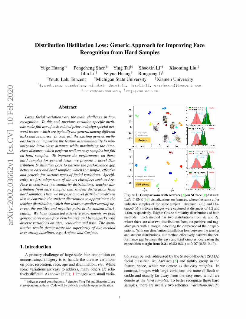
Figure 1: Comparisons with Arcface [5] on SCface [9] dataset.Left: T-SNE [19] visualizations on features, where the same colorindicates samples of the same subject. Distance1 (d1) and Dis-tance3 (d3) indicate images were captured at distances of 4.2 and1.0m, respectively. Right: Cosine similarity distributions of bothmethods. Each method has two distributions from d3 and d1,where there are also two distributions from the positive and neg-ative pairs with a margin indicating the difference of their expec-tations. With our distribution distillation loss between the teacherand student distributions, our method effectively narrows the per-formance gap between the easy and hard samples, decreasing theexpectation margin from 0.21 (0.52-0.31) to 0.07 (0.56-0.49).

tions can be well addressed by the State-of-the-Art (SOTA)facial classifier like ArcFace [5] and tightly group in thefeature space, which we denote as the easy samples. Incontrast, images with large variations are more difficult totackle and usually far away from the easy ones, which wedenote as the hard samples. To better recognize these hardsamples, there are usually two schemes: variation-specific

1

arX

iv:2

002.

0366

2v1

[cs

.CV

] 1

0 Fe

b 20

20

methods and generic methods.Variation-specific methods are usually designed for a

specific task. For instance, to achieve pose-invariant facerecognition, either handcrafted or learned features are ex-tracted, which are able to enhance robustness against posewhile remaining discriminative to the identities [32]. Re-cently, joint face frontalization and disentangled identitypreservation are incorporated to facilitate the pose-invariantfeature learning [34, 51]. To address resolution-invariantface recognition, a unified feature space is learned in [14,26] for mapping Low-Resolution (LR) and High-Resolution(HR) images. The works [3,53] first apply super-resolutionon the LR images and then perform recognition on thesuper-resolved images. However, the above methods arespecifically designed for the respective variations, thereforetheir ability to generalize from one variation to another islimited. Yet, it is highly desirable to handle multiple varia-tions in real world recognition systems.

Different from variation-specific methods, generic meth-ods focus on improving the discriminate power of facial fea-tures, for small intra-class and large inter-class distances.Basically, the prior works fall into two categories, i.e., soft-max loss-based and triplet loss-based methods. Softmaxloss-based methods regard each identity as a unique classto train the classification networks. Since the traditionalsoftmax loss is insufficient to acquire the discriminate fea-tures, several variants [5,16,38,42] are proposed to enhancethe discriminability. In contrast, triplet loss-based meth-ods [21,24] directly learn an Euclidean space embedding foreach face, in which faces from the same person are closer,forming separated cluster to faces of other persons. Withlarge-scale training data and well-designed network struc-tures, both types of methods can obtain promising results.

However, the performance of these methods degradesdramatically on hard samples, such as very large-pose andlow-resolution faces. As illustrated in Fig. 1, the featuresextracted from HR images (i.e., d3) by the strong face clas-sifier of Arcface [5] are well separated, but the featuresextracted from LR images (i.e., d1) cannot be well distin-guished. From the perspective of the angle distributions ofpositive and negative pairs, we can easily observe that Arc-face generates more confusion regions on LR face images.It is thereby a natural consequence that such generic meth-ods perform worse on hard samples.

To narrow the performance gap between the easy andhard samples, we propose a novel Distribution DistillationLoss (DDL). By leveraging the best of both the variation-specific and generic methods, our method is generic and canbe applied to diverse variations to improve face recognitionin hard samples. Specifically, we first adopt current SOTAface classifiers as the baseline (e.g., Arcface) to constructthe initial similarity distributions between teacher (e.g., easysamples from d3 in Fig. 1) and student (e.g., hard samples

from d1 in Fig. 1) according to the difficulties of samples,respectively. Compared to finetuning the baseline modelswith domain data, our method firstly does not require extradata or inference time (i.e., simple); secondly makes full useof hard sample mining and directly optimizes the similaritydistributions to improve the performance on hard samples(i.e., effective); and finally can be easily applied to addressdifferent kinds of large variations (i.e., general).

To sum up, the contributions of this work are three-folds:• Our method narrows the performance gap between

easy and hard samples on diverse facial variations,which is simple, effective and general.• To our best knowledge, it is the first work that adopts

similarity distribution distillation loss for face recogni-tion, which provides a new perspective to obtain morediscriminative features to better address hard samples.• Significant gains compared to the SOTA Arcface clas-

sifier are reported, e.g., 97.0% over 92.7% on SC-face [9], 93.4% over 92.1% on CPLFW [58], 90.7%over 89.9% (@FAR=1e−4) on IJB-B [43] and 93.1%over 92.1% (@FAR=1e−4) on IJB-C [20].

2. Related WorkLoss Function in FR. Loss function design is pivotal forlarge-scale face recognition. Softmax is commonly used forface recognition [29, 33, 37], which encourages the separa-bility of features but the learned features are not guaranteedto be discriminative. To address this issue, contrastive [28]and triplet [21, 24] losses are proposed to increase the mar-gin in the Euclidean space. However, both contrastive andtriplet losses occasionally encounter training instability dueto the selection of effective training samples. As a simplealternative, center loss and its variants [6, 42, 55] are pro-posed to compress the intra-class variance. More recently,angular margin-based losses [5, 16, 17, 36] facilitate featurediscrimination, and thus lead to larger angular/cosine sepa-rability between learned features. The above loss functionsare designed to apply constraints either between samples, orbetween sample and center of the corresponding subject.

In contrast, our proposed loss is distribution driven.While being similar to the histogram loss [35] that con-strains the overlap between the distributions of positive andnegative pairs across the training set, our loss differs in thatwe first separate the training set to a teacher distribution(easy samples) and student distribution (hard samples), andthen constrain the student distribution to approximate theteacher distribution via our novel loss, which narrows theperformance gap between easy and hard samples.

Variation-Specific FR. Apart from those generic solu-tions [29,33] for face recognition, there are also many meth-ods designed to handle specific facial variations, such as res-olutions, poses, illuminations, expressions and occlusions.

Training set

𝒙~𝑷𝓔

𝒙~𝑷𝓗

…

…

Positive Pairs (𝑥1, 𝑥2)~𝑃ℰ

Different IDs 𝑥~𝑃ℰ

Positive Pairs (𝑥1, 𝑥2)~𝑃ℋ

Different IDs 𝑥~𝑃ℋ

One mini-batch (batch size=6b)

Embedded batch

Teacher

Student

Similarity Distribution

𝓛𝑫𝑫𝑳ConvNet

{(𝒔𝓔𝒊+ , 𝒔𝓔𝒊

− )}

{(𝒔𝓗𝒊

+ , 𝒔𝓗𝒊

− )}

Figure 2: Illustration of our DDL. We sample b positive pairs (i.e., 2b samples) and b samples with different identities, for both ofteacher PE and student PH distributions, to form one mini-batch. {(s+Ei , s

−Ei)|i = 1, ..., b} indicates we construct b positive and negative

pairs from PE via Eqs. 1 and 2 respectively to estimate the teacher distribution. And {(s+Hi, s−Hi

)|i = 1, ..., b} also indicates we constructb positive and negative pairs from PH via Eqs. 1 and 2 respectively to estimate the student distribution.

For example, cross-pose FR [32, 34, 50, 57] is very chal-lenging, and previous methods mainly focus on either facefrontalization or pose invariant representations. Low resolu-tion FR is also a difficult task, especially in the surveillancescenario. One common approach is to learn a unified fea-ture space for LR and HR images [10,18,59]. And the otherway is to perform super resolution [3,30,31,53] to enhancethe facial identity information. Differing from the abovemethods that mainly deal with one specific variation, ournovel loss is a generic approach to improve FR from hardsamples, which is applicable to a wide variety of variations.Knowledge Distillation. Knowledge Distillation (KD) isan emerging topic. Its basic idea is to distill knowledgefrom a large teacher model into a small one by learning theclass distributions provided by the teacher via softened soft-max [11]. Typically, Kullback Leibler (KL) divergence [11,56] and Maximum Mean Discrepancy (MMD) [13] canbe adopted to minimize the posterior probabilities betweenteacher and student models. More recently, Generative Ad-versarial Networks [8] are introduced as an alternative wayto learn the true data distribution [41, 47]. Our distillationloss differs from the above conventional KD methods in twoaspects: 1) The conventional KD methods adopt differentteacher (i.e., high-capacity) and student models, while oursuse the same model to construct different teacher (i.e., easysamples) and student (i.e., hard samples) distributions. 2)The objective of many KD methods is for model compres-sion, while ours is generic to improve the recognition per-formance from hard samples.

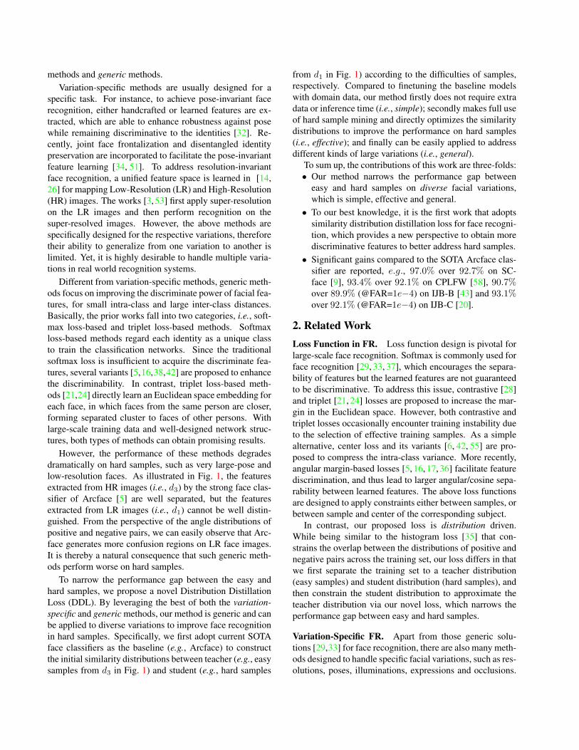
3. The Proposed MethodFig. 2 illustrates the framework of the proposed method.

We separate the training set into two parts, i.e., E for easysamples andH for hard samples to form the teacher and stu-

dent distributions, respectively. In general, for each mini-batch during training, we sample from both parts. To ensurea good teacher distribution, we use the SOTA FR model [5]as our initialization. The extracted features are used toconstruct the positive and negative pairs (Sec. 3.1), whichare further utilized to estimate the similarity distributions(Sec. 3.2). Finally, based on the similarity distributions, theproposed DDL is kicked in to train the classifier (Sec. 3.3).3.1. Sampling Strategy from PE and PH

First, we introduce the details on how we construct thepositive and negative pairs in one mini-batch during train-ing. Given two types of input data from both PE and PH,each mini-batch consists of four parts, two kinds of posi-tive pairs (i.e., (x1, x2) ∼ PE and (x1, x2) ∼ PH), and twokinds of samples with different identities (i.e., x ∼ PE andx ∼ PH). To be specific, we on one hand construct b posi-tive pairs (i.e., 2b samples), and on the other hand b sampleswith different identities from PE and PH, respectively. Asthe result, there are 6b = (2b+ b) ∗ 2 samples in each mini-batch (see Fig. 2 for more details).Positive Pairs. The positive pairs are constructed offlinein advance, and each pair consist of two samples with thesame identity. As shown in Fig. 2, samples of each posi-tive pair are arranged in order. After emebdding data intoa high-dimensional feature space by a deep network F , thesimilarity of a positive pair s+ can be obtained as follows:

s+i =< F(xposi1),F(xposi2) >, i = 1, ..., b (1)

where xposi1 , xposi2 are the samples of one positive pair.Note that positive pairs with similarity less than 0 are usu-ally outliers, which are deleted as a practical setting sinceour main goal is not to specifically handle noise.Negative Pairs. Different from the positive pair, we con-struct negative pairs online from the samples with different

identities via hard negative mining, which selects negativepairs with the largest similarities. To be specific, the simi-larity of a negative pair s− is defined as:

s−i = maxj

({s−ij =< F(xnegi),F(xnegj ) > |j = 1, ..., b}

),

(2)where xnegi , xnegj are from different subjects. Once thesimilarities of positive and negative pairs are constructed,the corresponding distributions can be estimated, which isdescried in the next subsection.3.2. Similarity Distribution Estimation

The process of similarity distribution estimation is sim-ilar to [35], which is performed in a simple and piece-wisedifferentiable manner using 1D histograms with soft assign-ment. Specifically, two samples xi, xj from the same per-son form a positive pair, and the corresponding label is de-noted as mij = +1. In contrast, two samples from dif-ferent persons form a negative pair, and the label is de-noted as mij = −1. Then, we obtain two sample setsS+ = {s+ = 〈F(xi),F(xj)〉|mij = +1} and S− ={s− = 〈F(xi),F(xj)〉|mij = −1} corresponding to thesimilarities of positive and negative pairs, respectively.

Let p+ and p− denote the two probability distributionsof S+ and S−, respectively. Supposing cosine distance-based methods [5] are used as our baseline, the similar-ity of each pair is bounded to [−1 : 1], which is demon-strated to simplify the task [35]. Motivated by the histogramloss, we estimate this type of one-dimensional distributionby fitting simple histograms with uniformly spaced bins.We adopt R-dimensional histograms H+and H−, with thenodes t1 = −1, t2, · · ·, tR = 1 uniformly filling [−1 : 1]with the step4 = 2

R−1 . Then, we estimate the value h+r ofthe histogram H+ at each bin as:

h+r =1

|S+|∑

(i,j):mij=+1

δi,j,r, (3)

where (i, j) spans all the positive pairs. Different from [35],the weights δi,j,r are chosen by an exponential function as:

δi,j,r = exp(−γ(sij − tr)2), (4)

where γ denotes the spread parameter of Gaussian kernelfunction, and tr denotes the rth node of histograms. Weadopt the Gaussian kernel function because it is the mostcommonly used kernel function for density estimation androbust to the small sample size. The estimation of H− pro-ceeds analogously.3.3. Distribution Distillation Loss

We make use of SOTA face recognition engines like [5],to obtain the similarity distributions from two kinds of sam-ples: easy and hard samples. Here, easy samples indicatethat the FR engine performs well, in which the similarity

𝑜ℰ

𝑜ℋ

𝑜ℋℰ

𝑜ℰℋ

Teacher

Student

𝑜ℰ = 𝔼 𝒮𝑝+ − 𝔼 𝒮𝑝

−

𝑜ℰℋ = 𝔼 𝒮𝑝+ − 𝔼 𝒮𝑞

−

𝑜ℋ = 𝔼 𝒮𝑞+ − 𝔼 𝒮𝑞

−

𝑜ℋℰ = 𝔼 𝒮𝑞+ − 𝔼 𝒮𝑝

−

Only KL loss: 𝑜ℰ , 𝑜ℰℋ

KL + order loss:𝑜ℋ ,𝑜ℋℰ

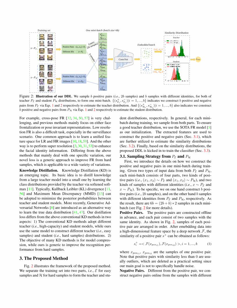
Figure 3: Illustration on the effects of our order loss. Left:Similarity distributions constructed by Arcface [5] on dataset SC-face, in which we have 4 kinds of order distances formed fromboth of the teacher and student distributions according to Eq. 6.

distributions of positive and negative pairs are clearly sepa-rated (see the teacher distribution in Fig. 3), while hard sam-ples indicate that the FR engine performs poorly, in whichthe similarity distributions may be highly overlapped (seethe student distribution in Fig. 3).KL Divergence Loss. To narrow the performance gapbetween the easy and hard samples, we constrain the simi-larity distribution of hard samples (i.e., student distribution)to approximate the similarity distribution of easy samples(i.e., teacher distribution). The teacher distribution consistsof two similarity distributions of both positive and negativepairs, denoted as P+ and P−, respectively. Similarly, thestudent distribution also consists of two similarity distribu-tions, denoted as Q+ and Q−. Motivated by the previousKD methods [11, 56], we adopt the KL divergence to con-strain the similarity between the student and teacher distri-butions, which is defined as follows:

LKL = λ1DKL(P+||Q+) + λ2DKL(P

−||Q−)

= λ1

∑s

P+(s) logP+(s)

Q+(s)︸ ︷︷ ︸KL loss on pos. pairs

+λ2

∑s

P−(s) logP−(s)

Q−(s)︸ ︷︷ ︸KL loss onneg. pairs

, (5)

where λ1, λ2 are the weight parameters.Order Loss. However, only performing KL loss does notguarantee satisfying performance. In fact, the teacher dis-tribution may choose to approach the student distributionand lead to more confusion regions between the distribu-tions of positive and negative pairs, which is opposite to ourobjective (See Fig. 3). To address this problem, we designa simple yet effective term named order loss, which mini-mizes the distances between the expectations of similaritydistributions from the negative and positive pairs to controlthe overlap. Our order loss can be formulated as follows:

Lorder = −λ3∑

(i,j)∈(p,q)

(E[S+i ]− E[S−j ]), (6)

ℰ

ℋ

ℰ

ℋ1

ℋ2

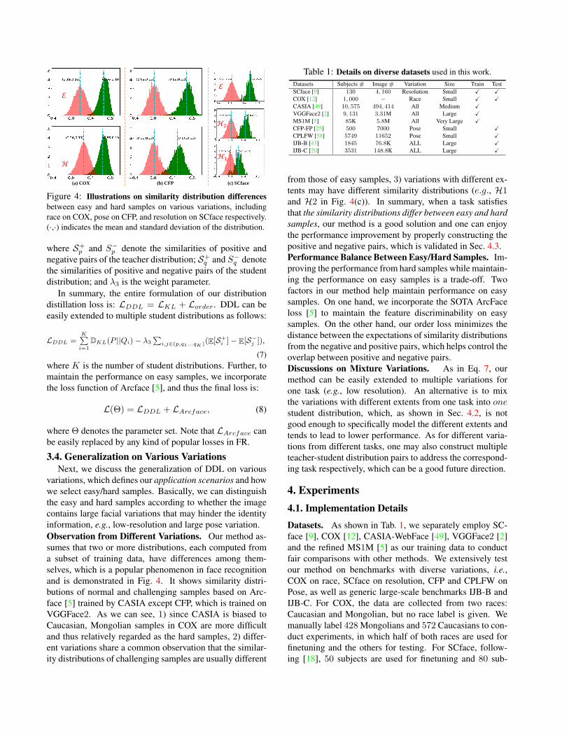
(a) COX (b) CFP (c) SCface

Figure 4: Illustrations on similarity distribution differencesbetween easy and hard samples on various variations, includingrace on COX, pose on CFP, and resolution on SCface respectively.(·,·) indicates the mean and standard deviation of the distribution.

where S+p and S−p denote the similarities of positive andnegative pairs of the teacher distribution; S+q and S−q denotethe similarities of positive and negative pairs of the studentdistribution; and λ3 is the weight parameter.

In summary, the entire formulation of our distributiondistillation loss is: LDDL = LKL + Lorder. DDL can beeasily extended to multiple student distributions as follows:

LDDL =K∑i=1

DKL(P ||Qi)− λ3

∑i,j∈(p,q1...qK)(E[S

+i ]− E[S−j ]),

(7)where K is the number of student distributions. Further, tomaintain the performance on easy samples, we incorporatethe loss function of Arcface [5], and thus the final loss is:

L(Θ) = LDDL + LArcface, (8)

where Θ denotes the parameter set. Note that LArcface canbe easily replaced by any kind of popular losses in FR.

3.4. Generalization on Various VariationsNext, we discuss the generalization of DDL on various

variations, which defines our application scenarios and howwe select easy/hard samples. Basically, we can distinguishthe easy and hard samples according to whether the imagecontains large facial variations that may hinder the identityinformation, e.g., low-resolution and large pose variation.Observation from Different Variations. Our method as-sumes that two or more distributions, each computed froma subset of training data, have differences among them-selves, which is a popular phenomenon in face recognitionand is demonstrated in Fig. 4. It shows similarity distri-butions of normal and challenging samples based on Arc-face [5] trained by CASIA except CFP, which is trained onVGGFace2. As we can see, 1) since CASIA is biased toCaucasian, Mongolian samples in COX are more difficultand thus relatively regarded as the hard samples, 2) differ-ent variations share a common observation that the similar-ity distributions of challenging samples are usually different

Table 1: Details on diverse datasets used in this work.Datasets Subjects # Image # Variation Size Train TestSCface [9] 130 4, 160 Resolution Small X XCOX [12] 1, 000 − Race Small X XCASIA [49] 10, 575 494, 414 All Medium XVGGFace2 [2] 9, 131 3.31M All Large XMS1M [5] 85K 5.8M All Very Large XCFP-FP [25] 500 7000 Pose Small XCPLFW [58] 5749 11652 Pose Small XIJB-B [43] 1845 76.8K ALL Large XIJB-C [20] 3531 148.8K ALL Large X

from those of easy samples, 3) variations with different ex-tents may have different similarity distributions (e.g., H1and H2 in Fig. 4(c)). In summary, when a task satisfiesthat the similarity distributions differ between easy and hardsamples, our method is a good solution and one can enjoythe performance improvement by properly constructing thepositive and negative pairs, which is validated in Sec. 4.3.Performance Balance Between Easy/Hard Samples. Im-proving the performance from hard samples while maintain-ing the performance on easy samples is a trade-off. Twofactors in our method help maintain performance on easysamples. On one hand, we incorporate the SOTA ArcFaceloss [5] to maintain the feature discriminability on easysamples. On the other hand, our order loss minimizes thedistance between the expectations of similarity distributionsfrom the negative and positive pairs, which helps control theoverlap between positive and negative pairs.Discussions on Mixture Variations. As in Eq. 7, ourmethod can be easily extended to multiple variations forone task (e.g., low resolution). An alternative is to mixthe variations with different extents from one task into onestudent distribution, which, as shown in Sec. 4.2, is notgood enough to specifically model the different extents andtends to lead to lower performance. As for different varia-tions from different tasks, one may also construct multipleteacher-student distribution pairs to address the correspond-ing task respectively, which can be a good future direction.

4. Experiments4.1. Implementation Details

Datasets. As shown in Tab. 1, we separately employ SC-face [9], COX [12], CASIA-WebFace [49], VGGFace2 [2]and the refined MS1M [5] as our training data to conductfair comparisons with other methods. We extensively testour method on benchmarks with diverse variations, i.e.,COX on race, SCface on resolution, CFP and CPLFW onPose, as well as generic large-scale benchmarks IJB-B andIJB-C. For COX, the data are collected from two races:Caucasian and Mongolian, but no race label is given. Wemanually label 428 Mongolians and 572 Caucasians to con-duct experiments, in which half of both races are used forfinetuning and the others for testing. For SCface, follow-ing [18], 50 subjects are used for finetuning and 80 sub-

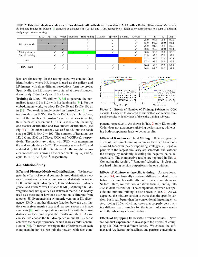
Table 2: Extensive ablation studies on SCface dataset. All methods are trained on CASIA with a ResNet50 backbone. d1, d2 andd3 indicate images in SCface [9] captured at distances of 4.2, 2.6 and 1.0m, respectively. Each color corresponds to a type of ablationstudy experimental setting.

EMD JS KL Order Random Hard Mining Mixture Specific Softmax ArcFace d1 d2 d3 Avg.

Distance metric

X X X X X 78.0 97.8 96.8 90.5X X X X X 83.0 98.3 99.0 93.4

X X X X 76.0 94.3 98.5 89.6X X X X 80.8 97.5 99.0 92.4

Mining strategy X X X X X 80.3 96.3 95.3 90.6

Specific training X X X X X 81.5 97.0 97.8 92.1

LossX 77.3 97.5 97.8 90.8

X 67.3 93.5 98.0 86.3

DDL (ours)X X X X X 90.0 98.0 97.5 95.2X X X X X 86.8 98.3 98.3 94.4

jects are for testing. In the testing stage, we conduct faceidentification, where HR image is used as the gallery andLR images with three different resolutions form the probe.Specifically, the LR images are captured at three distances:4.2m for d1, 2.6m for d2 and 1.0m for d3.Training Setting. We follow [5, 38] to generate the nor-malised faces (112×112) with five landmarks [54]. For theembedding network, we adopt ResNet50 and ResNet100 asin [5]. Our work is implemented in Tensorflow [7]. Wetrain models on 8 NVIDIA Tesla P40 GPUs. On SCface,we set the number of positive/negative pairs as b = 16,thus the batch size on one GPU is 3b × 3 = 96, includingone teacher distribution and two student distributions (seeFig. 4(c)). On other datasets, we set b to 32, thus the batchsize per GPU is 3b×2 = 192. The numbers of iterations are1K, 2K and 20K on SCface, COX and VGGFace2, respec-tively. The models are trained with SGD, with momentum0.9 and weight decay 5e−4. The learning rate is 1e−3, andis divided by 10 at half of iterations. All the weight param-eter are consistent across all the experiments. λ1, λ2 and λ3equal to 1e−1, 2e−2, 5e−1, respectively.

4.2. Ablation Study

Effects of Distance Metric on Distributions. We investi-gate the effects of several commonly used distribution met-rics to constrain the teacher and student distributions in ourDDL, including KL divergence, Jensen-Shannon (JS) diver-gence, and Earth Mover Distance (EMD). Although KL di-vergence does not qualify as a statistical metric, it is widelyused as a measure of how one distribution is different fromanother. JS divergence is a symmetric version of KL diver-gence. EMD is another distance function between distribu-tions on a given metric space and has seen success in imagesynthesis [8]. We incorporate our order loss with the abovedistance metrics, and report the results in Tab. 2. As wecan see, we choose the KL divergence in our DDL since itachieves the best performance, which shares similar conclu-sion in [56]. To further investigate the effectiveness of eachcomponent in our loss, we train the network with each com-

Figure 5: Effects of Number of Training Subjects on COXdatasets. Compared to Arcface-FT, our method can achieve com-parable results with only half of the entire training subjects.

ponent, respectively. As shown in Tab. 2, only KL or onlyOrder does not guarantee satisfying performance, while us-ing both components leads to better results.

Effects of Random vs. Hard Mining. To investigate theeffect of hard sample mining in our method, we train mod-els on SCface with the corresponding strategy (i.e., negativepairs with the largest similarity are selected), and withoutthe strategy by randomly selecting the negative pairs, re-spectively. The comparative results are reported in Tab. 2.Comparing the results of “Random” selecting, it is clear thatour hard mining version outperforms the one without.

Effects of Mixture vs. Specific training. As mentionedin Sec. 3.4, we basically construct different student distri-butions for samples with different extents of variations onSCface. Here, we mix two variations from d1 and d2 intoone student distribution. The comparison between our spe-cific and mixture training is also shown in Tab. 2. As weexpected, the mixture version is worse than the specific ver-sion, but is still better than the conventional finetuning (i.e.,Avg. being 86.3), which indicates that properly construct-ing different hard samples for the target tasks may maxi-mize the advantages of our method.

Effects of Equipping DDL with Different Losses. Next,we conduct experiment to investigate the effects of equip-ping our DDL with different losses. We choose the soft-max and Arcface as our baselines, and perform conventional

0.37

0.163

0.36 Triplet-FT

0.097

0.36 OHEM-FT

0.136

Ours0.49

0.091

0.23

0.283

0.35

0.153

Histogram-FT 0.52

0.024

Student Teacher0.31

0.202

ArcFace-FTFocal-FT

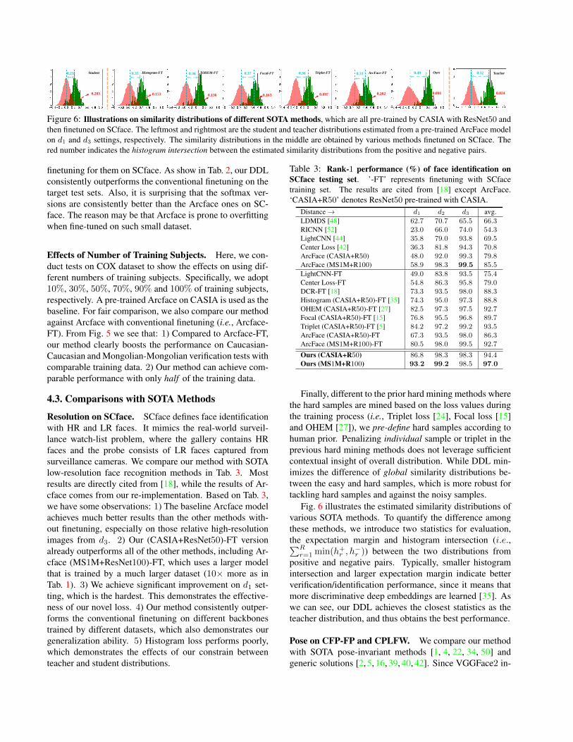
Figure 6: Illustrations on similarity distributions of different SOTA methods, which are all pre-trained by CASIA with ResNet50 andthen finetuned on SCface. The leftmost and rightmost are the student and teacher distributions estimated from a pre-trained ArcFace modelon d1 and d3 settings, respectively. The similarity distributions in the middle are obtained by various methods finetuned on SCface. Thered number indicates the histogram intersection between the estimated similarity distributions from the positive and negative pairs.

finetuning for them on SCface. As show in Tab. 2, our DDLconsistently outperforms the conventional finetuning on thetarget test sets. Also, it is surprising that the softmax ver-sions are consistently better than the Arcface ones on SC-face. The reason may be that Arcface is prone to overfittingwhen fine-tuned on such small dataset.

Effects of Number of Training Subjects. Here, we con-duct tests on COX dataset to show the effects on using dif-ferent numbers of training subjects. Specifically, we adopt10%, 30%, 50%, 70%, 90% and 100% of training subjects,respectively. A pre-trained Arcface on CASIA is used as thebaseline. For fair comparison, we also compare our methodagainst Arcface with conventional finetuning (i.e., Arcface-FT). From Fig. 5 we see that: 1) Compared to Arcface-FT,our method clearly boosts the performance on Caucasian-Caucasian and Mongolian-Mongolian verification tests withcomparable training data. 2) Our method can achieve com-parable performance with only half of the training data.

4.3. Comparisons with SOTA Methods

Resolution on SCface. SCface defines face identificationwith HR and LR faces. It mimics the real-world surveil-lance watch-list problem, where the gallery contains HRfaces and the probe consists of LR faces captured fromsurveillance cameras. We compare our method with SOTAlow-resolution face recognition methods in Tab. 3. Mostresults are directly cited from [18], while the results of Ar-cface comes from our re-implementation. Based on Tab. 3,we have some observations: 1) The baseline Arcface modelachieves much better results than the other methods with-out finetuning, especially on those relative high-resolutionimages from d3. 2) Our (CASIA+ResNet50)-FT versionalready outperforms all of the other methods, including Ar-cface (MS1M+ResNet100)-FT, which uses a larger modelthat is trained by a much larger dataset (10× more as inTab. 1). 3) We achieve significant improvement on d1 set-ting, which is the hardest. This demonstrates the effective-ness of our novel loss. 4) Our method consistently outper-forms the conventional finetuning on different backbonestrained by different datasets, which also demonstrates ourgeneralization ability. 5) Histogram loss performs poorly,which demonstrates the effects of our constrain betweenteacher and student distributions.

Table 3: Rank-1 performance (%) of face identification onSCface testing set. ’-FT’ represents finetuning with SCfacetraining set. The results are cited from [18] except ArcFace.‘CASIA+R50’ denotes ResNet50 pre-trained with CASIA.

Distance→ d1 d2 d3 avg.LDMDS [48] 62.7 70.7 65.5 66.3RICNN [52] 23.0 66.0 74.0 54.3LightCNN [44] 35.8 79.0 93.8 69.5Center Loss [42] 36.3 81.8 94.3 70.8ArcFace (CASIA+R50) 48.0 92.0 99.3 79.8ArcFace (MS1M+R100) 58.9 98.3 99.5 85.5

LightCNN-FT 49.0 83.8 93.5 75.4Center Loss-FT 54.8 86.3 95.8 79.0DCR-FT [18] 73.3 93.5 98.0 88.3Histogram (CASIA+R50)-FT [35] 74.3 95.0 97.3 88.8OHEM (CASIA+R50)-FT [27] 82.5 97.3 97.5 92.7Focal (CASIA+R50)-FT [15] 76.8 95.5 96.8 89.7Triplet (CASIA+R50)-FT [5] 84.2 97.2 99.2 93.5ArcFace (CASIA+R50)-FT 67.3 93.5 98.0 86.3ArcFace (MS1M+R100)-FT 80.5 98.0 99.5 92.7

Ours (CASIA+R50) 86.8 98.3 98.3 94.4Ours (MS1M+R100) 93.2 99.2 98.5 97.0

Finally, different to the prior hard mining methods wherethe hard samples are mined based on the loss values duringthe training process (i.e., Triplet loss [24], Focal loss [15]and OHEM [27]), we pre-define hard samples according tohuman prior. Penalizing individual sample or triplet in theprevious hard mining methods does not leverage sufficientcontextual insight of overall distribution. While DDL min-imizes the difference of global similarity distributions be-tween the easy and hard samples, which is more robust fortackling hard samples and against the noisy samples.

Fig. 6 illustrates the estimated similarity distributions ofvarious SOTA methods. To quantify the difference amongthese methods, we introduce two statistics for evaluation,the expectation margin and histogram intersection (i.e.,∑R

r=1 min(h+r , h−r )) between the two distributions from

positive and negative pairs. Typically, smaller histogramintersection and larger expectation margin indicate betterverification/identification performance, since it means thatmore discriminative deep embeddings are learned [35]. Aswe can see, our DDL achieves the closest statistics as theteacher distribution, and thus obtains the best performance.

Pose on CFP-FP and CPLFW. We compare our methodwith SOTA pose-invariant methods [1, 4, 22, 34, 50] andgeneric solutions [2, 5, 16, 39, 40, 42]. Since VGGFace2 in-

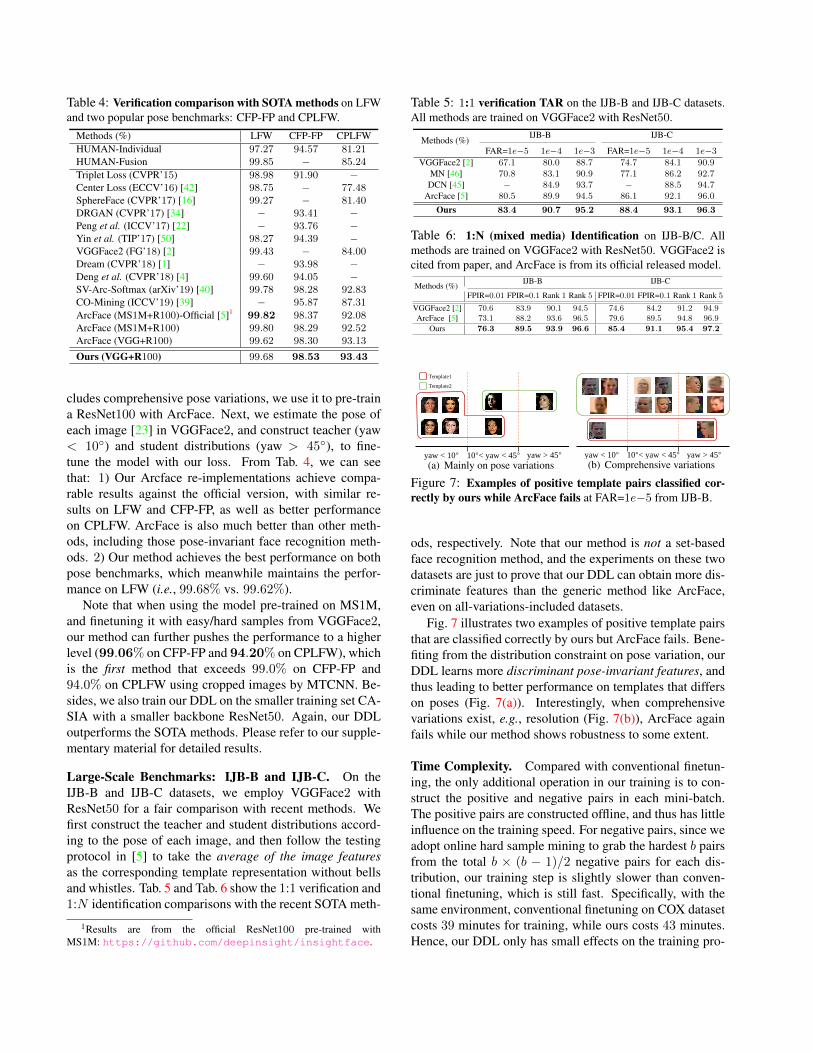
Table 4: Verification comparison with SOTA methods on LFWand two popular pose benchmarks: CFP-FP and CPLFW.

Methods (%) LFW CFP-FP CPLFWHUMAN-Individual 97.27 94.57 81.21HUMAN-Fusion 99.85 − 85.24

Triplet Loss (CVPR’15) 98.98 91.90 −Center Loss (ECCV’16) [42] 98.75 − 77.48SphereFace (CVPR’17) [16] 99.27 − 81.40DRGAN (CVPR’17) [34] − 93.41 −Peng et al. (ICCV’17) [22] − 93.76 −Yin et al. (TIP’17) [50] 98.27 94.39 −VGGFace2 (FG’18) [2] 99.43 − 84.00Dream (CVPR’18) [1] − 93.98 −Deng et al. (CVPR’18) [4] 99.60 94.05 −SV-Arc-Softmax (arXiv’19) [40] 99.78 98.28 92.83CO-Mining (ICCV’19) [39] − 95.87 87.31ArcFace (MS1M+R100)-Official [5]1 99.82 98.37 92.08ArcFace (MS1M+R100) 99.80 98.29 92.52ArcFace (VGG+R100) 99.62 98.30 93.13

Ours (VGG+R100) 99.68 98.53 93.43

cludes comprehensive pose variations, we use it to pre-traina ResNet100 with ArcFace. Next, we estimate the pose ofeach image [23] in VGGFace2, and construct teacher (yaw< 10◦) and student distributions (yaw > 45◦), to fine-tune the model with our loss. From Tab. 4, we can seethat: 1) Our Arcface re-implementations achieve compa-rable results against the official version, with similar re-sults on LFW and CFP-FP, as well as better performanceon CPLFW. ArcFace is also much better than other meth-ods, including those pose-invariant face recognition meth-ods. 2) Our method achieves the best performance on bothpose benchmarks, which meanwhile maintains the perfor-mance on LFW (i.e., 99.68% vs. 99.62%).

Note that when using the model pre-trained on MS1M,and finetuning it with easy/hard samples from VGGFace2,our method can further pushes the performance to a higherlevel (99.06% on CFP-FP and 94.20% on CPLFW), whichis the first method that exceeds 99.0% on CFP-FP and94.0% on CPLFW using cropped images by MTCNN. Be-sides, we also train our DDL on the smaller training set CA-SIA with a smaller backbone ResNet50. Again, our DDLoutperforms the SOTA methods. Please refer to our supple-mentary material for detailed results.

Large-Scale Benchmarks: IJB-B and IJB-C. On theIJB-B and IJB-C datasets, we employ VGGFace2 withResNet50 for a fair comparison with recent methods. Wefirst construct the teacher and student distributions accord-ing to the pose of each image, and then follow the testingprotocol in [5] to take the average of the image featuresas the corresponding template representation without bellsand whistles. Tab. 5 and Tab. 6 show the 1:1 verification and1:N identification comparisons with the recent SOTA meth-

1Results are from the official ResNet100 pre-trained withMS1M: https://github.com/deepinsight/insightface.

Table 5: 1:1 verification TAR on the IJB-B and IJB-C datasets.All methods are trained on VGGFace2 with ResNet50.

Methods (%)IJB-B IJB-C

FAR=1e−5 1e−4 1e−3 FAR=1e−5 1e−4 1e−3VGGFace2 [2] 67.1 80.0 88.7 74.7 84.1 90.9

MN [46] 70.8 83.1 90.9 77.1 86.2 92.7DCN [45] − 84.9 93.7 − 88.5 94.7

ArcFace [5] 80.5 89.9 94.5 86.1 92.1 96.0

Ours 83.4 90.7 95.2 88.4 93.1 96.3

Table 6: 1:N (mixed media) Identification on IJB-B/C. Allmethods are trained on VGGFace2 with ResNet50. VGGFace2 iscited from paper, and ArcFace is from its official released model.

Methods (%)IJB-B IJB-C

FPIR=0.01 FPIR=0.1 Rank 1 Rank 5 FPIR=0.01 FPIR=0.1 Rank 1 Rank 5

VGGFace2 [2] 70.6 83.9 90.1 94.5 74.6 84.2 91.2 94.9ArcFace [5] 73.1 88.2 93.6 96.5 79.6 89.5 94.8 96.9

Ours 76.3 89.5 93.9 96.6 85.4 91.1 95.4 97.2

yaw < 10° 10°< yaw < 45° yaw > 45°

Template1

Template2

(a) Mainly on pose variationsyaw < 10° 10°< yaw < 45° yaw > 45°(b) Comprehensive variations

Figure 7: Examples of positive template pairs classified cor-rectly by ours while ArcFace fails at FAR=1e−5 from IJB-B.

ods, respectively. Note that our method is not a set-basedface recognition method, and the experiments on these twodatasets are just to prove that our DDL can obtain more dis-criminate features than the generic method like ArcFace,even on all-variations-included datasets.

Fig. 7 illustrates two examples of positive template pairsthat are classified correctly by ours but ArcFace fails. Bene-fiting from the distribution constraint on pose variation, ourDDL learns more discriminant pose-invariant features, andthus leading to better performance on templates that differson poses (Fig. 7(a)). Interestingly, when comprehensivevariations exist, e.g., resolution (Fig. 7(b)), ArcFace againfails while our method shows robustness to some extent.

Time Complexity. Compared with conventional finetun-ing, the only additional operation in our training is to con-struct the positive and negative pairs in each mini-batch.The positive pairs are constructed offline, and thus has littleinfluence on the training speed. For negative pairs, since weadopt online hard sample mining to grab the hardest b pairsfrom the total b × (b − 1)/2 negative pairs for each dis-tribution, our training step is slightly slower than conven-tional finetuning, which is still fast. Specifically, with thesame environment, conventional finetuning on COX datasetcosts 39 minutes for training, while ours costs 43 minutes.Hence, our DDL only has small effects on the training pro-

cess, which totally has NO influence for inference.

5. Conclusion

In this paper, we propose a novel general framework,named Distribution Distillation Loss (DDL), aiming to im-prove various variation-specific tasks, which comes fromthe observations that state-of-the-art methods (e.g., Arc-face) witness significant performance gap between easy andhard samples. The key idea of our method is to construct ateacher and a student distribution from easy and hard sam-ples, respectively. Then, the proposed loss drives the stu-dent distribution to approximate the teacher distribution toreduce the overlap between the positive and negative pairs.Extensive experiments demonstrate the effectiveness of ourDDL on a wide range of recognition tasks compared to thestate-of-the-art face recognition methods.

References[1] Kaidi Cao, Yu Rong, Cheng Li, Xiaoou Tang, and Chen

Change Loy. Pose-robust face recognition via deep resid-ual equivariant mapping. In CVPR, pages 5187–5196, 2018.7, 8

[2] Qiong Cao, Li Shen, Weidi Xie, Omkar M Parkhi, and An-drew Zisserman. Vggface2: A dataset for recognising facesacross pose and age. In FG, pages 67–74. IEEE, 2018. 5, 7,8

[3] Yu Chen, Ying Tai, Xiaoming Liu, Chunhua Shen, and JianYang. Fsrnet: End-to-end learning face super-resolution withfacial priors. In CVPR, pages 2492–2501, 2018. 2, 3

[4] Jiankang Deng, Shiyang Cheng, Niannan Xue, YuxiangZhou, and Stefanos Zafeiriou. Uv-gan: Adversarial facialuv map completion for pose-invariant face recognition. InCVPR, pages 7093–7102, 2018. 7, 8

[5] Jiankang Deng, Jia Guo, Niannan Xue, and StefanosZafeiriou. Arcface: Additive angular margin loss for deepface recognition. In CVPR, pages 4690–4699, 2019. 1, 2, 3,4, 5, 6, 7, 8

[6] Jiankang Deng, Yuxiang Zhou, and Stefanos Zafeiriou.Marginal loss for deep face recognition. In CVPR Work-shops, pages 60–68, 2017. 2

[7] Martın Abadi et al. TensorFlow: Large-scale machine learn-ing on heterogeneous systems, 2015. Software availablefrom tensorflow.org. 6

[8] Ian Goodfellow, Jean Pouget-Abadie, Mehdi Mirza, BingXu, David Warde-Farley, Sherjil Ozair, Aaron Courville, andYoshua Bengio. Generative adversarial nets. In NIPS, pages2672–2680, 2014. 3, 6

[9] Mislav Grgic, Kresimir Delac, and Sonja Grgic. Scface–surveillance cameras face database. Multimedia Tools andApplications, 51(3):863–879, 2011. 1, 2, 5, 6

[10] Pablo H Hennings-Yeomans, Simon Baker, and BVK VijayaKumar. Simultaneous super-resolution and feature extractionfor recognition of low-resolution faces. In CVPR, pages 1–8.IEEE, 2008. 3

[11] Geoffrey Hinton, Oriol Vinyals, and Jeff Dean. Distilling theknowledge in a neural network. In NIPS Workshop, 2014. 3,4

[12] Zhiwu Huang, Shiguang Shan, Ruiping Wang, HaihongZhang, Shihong Lao, Alifu Kuerban, and Xilin Chen.A benchmark and comparative study of video-based facerecognition on cox face database. IEEE Transactions on Im-age Processing, 24(12):5967–5981, 2015. 5

[13] Zehao Huang and Naiyan Wang. Like what youlike: Knowledge distill via neuron selectivity transfer.arXiv:1707.01219v2, 2017. 3

[14] Zhen Lei, Timo Ahonen, Matti Pietikainen, and Stan Z Li.Local frequency descriptor for low-resolution face recogni-tion. In FG, pages 161–166. IEEE, 2011. 2

[15] Tsung-Yi Lin, Priya Goyal, Ross Girshick, Kaiming He, andPiotr Dollar. Focal loss for dense object detection. In ICCV,pages 2980–2988, 2017. 7

[16] Weiyang Liu, Yandong Wen, Zhiding Yu, Ming Li, BhikshaRaj, and Le Song. Sphereface: Deep hypersphere embeddingfor face recognition. In CVPR, pages 212–220, 2017. 2, 7, 8

[17] Weiyang Liu, Yandong Wen, Zhiding Yu, and Meng Yang.Large-margin softmax loss for convolutional neural net-works. In ICML, volume 2, page 7, 2016. 2

[18] Ze Lu, Xudong Jiang, and Alex Kot. Deep coupled resnetfor low-resolution face recognition. IEEE Signal ProcessingLetters, 25(4):526–530, 2018. 3, 5, 7

[19] Laurens van der Maaten and Geoffrey Hinton. Visualizingdata using t-sne. Journal of Machine Learning Research,9(Nov):2579–2605, 2008. 1

[20] Brianna Maze, Jocelyn Adams, James A Duncan, NathanKalka, Tim Miller, Charles Otto, Anil K Jain, W TylerNiggel, Janet Anderson, Jordan Cheney, et al. Iarpa janusbenchmark-c: Face dataset and protocol. In ICB, pages 158–165. IEEE, 2018. 2, 5

[21] Omkar M Parkhi, Andrea Vedaldi, Andrew Zisserman, et al.Deep face recognition. In BMVC, volume 1, page 6, 2015. 2

[22] Xi Peng, Xiang Yu, Kihyuk Sohn, Dimitris N Metaxas, andManmohan Chandraker. Reconstruction-based disentangle-ment for pose-invariant face recognition. In ICCV, pages1623–1632, 2017. 7, 8

[23] Nataniel Ruiz, Eunji Chong, and James M Rehg. Fine-grained head pose estimation without keypoints. In CVPRWorkshops, pages 2074–2083, 2018. 8

[24] Florian Schroff, Dmitry Kalenichenko, and James Philbin.Facenet: A unified embedding for face recognition and clus-tering. In CVPR, pages 815–823, 2015. 2, 7

[25] Soumyadip Sengupta, Jun-Cheng Chen, Carlos Castillo,Vishal M Patel, Rama Chellappa, and David W Jacobs.Frontal to profile face verification in the wild. In WACV,pages 1–9. IEEE, 2016. 5

[26] Sumit Shekhar, Vishal M Patel, and Rama Chellappa.Synthesis-based recognition of low resolution faces. In IJCB,pages 1–6. IEEE, 2011. 2

[27] Abhinav Shrivastava, Abhinav Gupta, and Ross Girshick.Training region-based object detectors with online hard ex-ample mining. In CVPR, pages 761–769, 2016. 7

[28] Yi Sun, Yuheng Chen, Xiaogang Wang, and Xiaoou Tang.Deep learning face representation by joint identification-verification. In NIPS, pages 1988–1996, 2014. 2

[29] Yi Sun, Xiaogang Wang, and Xiaoou Tang. Deep learningface representation from predicting 10,000 classes. In CVPR,pages 1891–1898, 2014. 2

[30] Ying Tai, Jian Yang, and Xiaoming Liu. Image super-resolution via deep recursive residual network. In CVPR,pages 3147–3155, 2017. 3

[31] Ying Tai, Jian Yang, Xiaoming Liu, and Chunyan Xu. Mem-net: A persistent memory network for image restoration. InICCV, pages 4539–4547, 2017. 3

[32] Ying Tai, Jian Yang, Yigong Zhang, Lei Luo, Jianjun Qian,and Yu Chen. Face recognition with pose variations and mis-alignment via orthogonal procrustes regression. IEEE Trans-actions on Image Processing, 25(6):2673–2683, 2016. 2, 3

[33] Yaniv Taigman, Ming Yang, Marc’Aurelio Ranzato, and LiorWolf. Deepface: Closing the gap to human-level perfor-mance in face verification. In CVPR, pages 1701–1708,2014. 2

[34] Luan Tran, Xi Yin, and Xiaoming Liu. Disentangled repre-sentation learning gan for pose-invariant face recognition. InCVPR, pages 1415–1424, 2017. 2, 3, 7, 8

[35] Evgeniya Ustinova and Victor Lempitsky. Learning deepembeddings with histogram loss. In NIPS, pages 4170–4178,2016. 2, 4, 7

[36] Feng Wang, Jian Cheng, Weiyang Liu, and Haijun Liu. Ad-ditive margin softmax for face verification. IEEE Signal Pro-cessing Letters, 25(7):926–930, 2018. 2

[37] Feng Wang, Xiang Xiang, Jian Cheng, and Alan LoddonYuille. Normface: l 2 hypersphere embedding for face veri-fication. In ACMMM, pages 1041–1049. ACM, 2017. 2

[38] Hao Wang, Yitong Wang, Zheng Zhou, Xing Ji, DihongGong, Jingchao Zhou, Zhifeng Li, and Wei Liu. Cosface:Large margin cosine loss for deep face recognition. In CVPR,pages 5265–5274, 2018. 2, 6

[39] Xiaobo Wang, Shuo Wang, Jun Wang, Hailin Shi, and TaoMei. Co-mining: Deep face recognition with noisy labels.In ICCV, pages 9358–9367, 2019. 7, 8

[40] Xiaobo Wang, Shuo Wang, Shifeng Zhang, Tianyu Fu,Hailin Shi, and Tao Mei. Support vector guided softmax lossfor face recognition. arXiv:1812.11317, 2018. 7, 8

[41] Xiaojie Wang, Rui Zhang, Yu Sun, and Jianzhong Qi.Kdgan: knowledge distillation with generative adversarialnetworks. In NIPS, pages 775–786, 2018. 3

[42] Yandong Wen, Kaipeng Zhang, Zhifeng Li, and Yu Qiao. Adiscriminative feature learning approach for deep face recog-nition. In ECCV, pages 499–515. Springer, 2016. 2, 7, 8

[43] Cameron Whitelam, Emma Taborsky, Austin Blanton, Bri-anna Maze, Jocelyn Adams, Tim Miller, Nathan Kalka,Anil K Jain, James A Duncan, Kristen Allen, et al. Iarpajanus benchmark-b face dataset. In CVPR Workshops, pages90–98, 2017. 2, 5

[44] Xiang Wu, Ran He, Zhenan Sun, and Tieniu Tan. A light cnnfor deep face representation with noisy labels. IEEE Trans-actions on Information Forensics and Security, 13(11):2884–2896, 2018. 7

[45] Weidi Xie, Li Shen, and Andrew Zisserman. Comparatornetworks. In ECCV, pages 782–797, 2018. 8

[46] Weidi Xie and Andrew Zisserman. Multicolumn networksfor face recognition. In BMVC, 2018. 8

[47] Zheng Xu, Yen-Chang Hsu, and Jiawei Huang. Train-ing shallow and thin networks for acceleration via knowl-edge distillation with conditional adversarial networks.arXiv:1709.00513v2, 2018. 3

[48] Fuwei Yang, Wenming Yang, Riqiang Gao, and QingminLiao. Discriminative multidimensional scaling for low-resolution face recognition. IEEE Signal Processing Letters,25(3):388–392, 2017. 7

[49] Dong Yi, Zhen Lei, Shengcai Liao, and Stan Z Li. Learningface representation from scratch. arXiv:1411.7923, 2014. 5

[50] Xi Yin and Xiaoming Liu. Multi-task convolutional neuralnetwork for pose-invariant face recognition. IEEE Transac-tions on Image Processing, 27(2):964–975, 2017. 3, 7, 8

[51] Xi Yin, Xiang Yu, Kihyuk Sohn, Xiaoming Liu, and Man-mohan Chandraker. Towards large-pose face frontalizationin the wild. In ICCV, pages 3990–3999, 2017. 2

[52] Dan Zeng, Hu Chen, and Qijun Zhao. Towards resolutioninvariant face recognition in uncontrolled scenarios. In ICB,pages 1–8. IEEE, 2016. 7

[53] Kaipeng Zhang, Zhanpeng Zhang, Chia-Wen Cheng, Win-ston H Hsu, Yu Qiao, Wei Liu, and Tong Zhang. Super-identity convolutional neural network for face hallucination.In ECCV, pages 183–198, 2018. 2, 3

[54] Kaipeng Zhang, Zhanpeng Zhang, Zhifeng Li, and Yu Qiao.Joint face detection and alignment using multitask cascadedconvolutional networks. IEEE Signal Processing Letters,23(10):1499–1503, 2016. 6

[55] Xiao Zhang, Zhiyuan Fang, Yandong Wen, Zhifeng Li, andYu Qiao. Range loss for deep face recognition with long-tailed training data. In ICCV, pages 5409–5418, 2017. 2

[56] Ying Zhang, Tao Xiang, Timothy M Hospedales, andHuchuan Lu. Deep mutual learning. In CVPR, pages 4320–4328, 2018. 3, 4, 6

[57] Jian Zhao, Lin Xiong, Yu Cheng, Yi Cheng, Jianshu Li, LiZhou, Yan Xu, Jayashree Karlekar, Sugiri Pranata, ShengmeiShen, et al. 3d-aided deep pose-invariant face recognition. InIJCAI, volume 2, page 11, 2018. 3

[58] Tianyue Zheng and Weihong Deng. Cross-pose lfw: Adatabase for studying crosspose face recognition in uncon-strained environments. Beijing University of Posts andTelecommunications, Tech. Rep, pages 18–01, 2018. 2, 5

[59] Wilman WW Zou and Pong C Yuen. Very low resolutionface recognition problem. IEEE Transactions on Image Pro-cessing, 21(1):327–340, 2011. 3