discrete event simulation of wireless cellular networks
TRANSCRIPT
Discrete event simulation of wireless cellular networks 1
Discrete event simulation of wireless cellular networks
Enrica Zola, Israel Martín-Escalona and Francisco Barceló-Arroyo
X
Discrete event simulation of wireless cellular networks
Enrica Zola, Israel Martín-Escalona and Francisco Barceló-Arroyo
Universitat Politècnica de Catalunya (UPC) Spain
1. Introduction
The design of telecommunication networks usually comprises three major phases. First, mathematical analysis is carried out and numerical results obtained. During this phase, simple models are used to facilitate calculations. These simple models involve hypotheses that are not realistic, leading to rough performance figures that are valid only as a first approach to the feasibility of the proposed network. Simulation is the second step in the design process before performance can be monitored and measured in the true network. In contrast to the simple models necessary for the mathematical analysis, models used in simulations permit the relaxation of strict adherence to most of the hypotheses assumed in those models. The results obtained by simulation are much closer to the true world than those obtained by analysis. The simulation of wireless cellular networks raises a set of specific problems that are not encountered in the simulation of other networks. The aim of this chapter is to state those issues and to present several ways to cope with them. Two types of simulation, Montecarlo and discrete event, are most commonly used in cellular networks to cope with two different problems. Montecarlo simulation has been shown to be appropriate for determining the coverage of base stations (BSs), the radiation patterns of antennas and other related problems. The main goal after these simulations is to fit the BSs at their possible emplacements using a geographic information system (GIS). Given the parameters of the equipment at the BS and receiving devices and the probabilistic models employed for propagation in the specific environment, the probability of a certain device at a certain point being covered can be determined. This is computed by averaging snapshots of the coverage in the desired area. On the other hand, most researchers and network designers make use of discrete event simulation for addressing issues related to the cellular features, mobility, handovers between neighbouring cells and traffic. The simulation of traffic-related issues in cellular networks is based on the arrival of traffic events (e.g., voice or data calls, packets, messages, etc.) to the network. The goal is to compute the probability of traffic being carried by the network given a certain network capacity (e.g., number of BSs, channels, bandwidth, etc.). A key issue is the intuitive fact that increasing the mobility leads to lower performance: i.e., when devices move faster, they need more handovers of their session between different BSs, increasing the probability of
1
www.intechopen.com
interruption. In fact, mobility not only depends on speed, but also smaller cells lead to more handovers for the same speed; even the cell shape has an impact on the handover rate. These layout and mobility issues are dealt with in Section 2. Propagation issues are presented in Section 3. The models presented are common to the Montecarlo simulation of radio coverage, but they are used in a different manner when applied to the discrete event simulation of traffic and mobility. Section 4 deals with other issues, such as the cell wrapping needed to improve the efficiency of the simulation to achieve statistically reliable results, the features of different traffic classes and the various methods used to obtain statistical results.
2. Layout and Mobility
When simulating a cellular network, a layout for the BSs to which the mobile devices are connected must be assumed. There are several well established patterns, including hexagonal (typical for suburban areas), Manhattan (urban) and linear (highways). The possibility of having several connection layers must also be considered, e.g., microcells as the first choice and macrocells as umbrellas for overflowing traffic. In real cellular networks, the designer can plan BSs at any point, and therefore, the simulation should allow any position for the BSs. The problem of the cell borders is related to the layout. For simplicity, it is possible to simulate a network in which devices are covered by the BS closest to them. This kind of simulation is simple and allows direct conclusions from the results; however, it is not realistic. When the radiation patterns and random nature of the radio channel are taken into account (see Section 3), the borders are not regular shapes and may change with time. This increases the complexity of the simulation significantly; however, it offers realistic results, although they are more difficult to interpret. Section 2.1 addresses the above-mentioned issues, showing how each kind of layout must be programmed and the way in which results must be interpreted. The mobile behaviour of devices within the cellular network can be characterised and simulated in a variety of ways, with each of them corresponding to a different scenario and environment. Experimental research has been conducted during the last two decades to determine the statistical properties of each representative user class, e.g., public networks, local area networks (LANs), indoors, outdoors, cars, pedestrians, etc. According to the network technology, geographical area and type of user, it is possible to feed the simulation with certain parameters such that the resulting movement will be similar to the real one. The Random Waypoint and Gauss-Markov models are the most relevant, but other useful models are also available. Section 2.2 addresses the way in which every model must be programmed and the different properties found with every movement. It also shows the simulation results acquired by the authors about the residence time in cells belonging to a wireless LAN (WLAN) when different models are applied.
2.1 Layout The first issue is to select the area of the network that should be simulated. Depending on the environment (e.g., suburban, dense urban, indoors, etc.) and on the technology under study (e.g., GSM, UMTS, WiMax, WiFi, Bluetooth, etc.), the simulation area may encompass square kilometres (e.g., big city) or square meters (e.g., a single building). This area may be
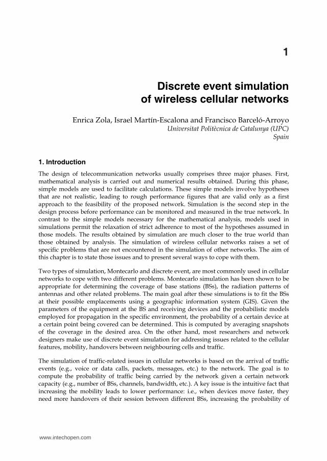
covered by a single high transmission power antenna or by many low power transmitters, with each providing coverage to a small portion of the whole simulation area. The second solution is the basis for cellular systems; the area covered by a single antenna (i.e., one BS) corresponds to the cell area. Different layouts can be obtained by positioning BSs according to different patterns. The selection of the best pattern to use can be driven by simple observations of the geometry of the area under study. As an example, linear patterns can be used to provide coverage on highways; BSs will be positioned along the path at regular distances. A regular pattern can also be applied when modelling symmetrical layouts in large suburban areas. The common technique used to position antennas to obtain a network of non-overlapping cells is by following the hexagonal pattern displayed in Fig. 1. Each cell is allocated a subset of the total radio channels assigned to the system. The cells are grouped into clusters, wherein the available channels are not allowed to be reused, to prevent interference among users of different cells. The number of cells per cluster represents the cluster size (N). According to (Rappaport, 1996), N can only have values that satisfy the following equation
N = i2 + i· j + j2 , (1)
where i and j are non-negative integers. N is equal to 7 in Fig. 1.
Fig. 1. Hexagonal layout with a cluster size of 7 (in red). In dense urban environments with regular patterns, the Manhattan model is preferred because it follows the geometry of the streets, thus providing coverage both outside and inside the buildings. It considers a regular pattern of buildings, which are represented by regular squares, and a regular network of horizontal and vertical streets between the blocks. Antennas should be placed at every street crossing, and the cell size is assumed to be half a
www.intechopen.com
Discrete event simulation of wireless cellular networks 3
interruption. In fact, mobility not only depends on speed, but also smaller cells lead to more handovers for the same speed; even the cell shape has an impact on the handover rate. These layout and mobility issues are dealt with in Section 2. Propagation issues are presented in Section 3. The models presented are common to the Montecarlo simulation of radio coverage, but they are used in a different manner when applied to the discrete event simulation of traffic and mobility. Section 4 deals with other issues, such as the cell wrapping needed to improve the efficiency of the simulation to achieve statistically reliable results, the features of different traffic classes and the various methods used to obtain statistical results.
2. Layout and Mobility
When simulating a cellular network, a layout for the BSs to which the mobile devices are connected must be assumed. There are several well established patterns, including hexagonal (typical for suburban areas), Manhattan (urban) and linear (highways). The possibility of having several connection layers must also be considered, e.g., microcells as the first choice and macrocells as umbrellas for overflowing traffic. In real cellular networks, the designer can plan BSs at any point, and therefore, the simulation should allow any position for the BSs. The problem of the cell borders is related to the layout. For simplicity, it is possible to simulate a network in which devices are covered by the BS closest to them. This kind of simulation is simple and allows direct conclusions from the results; however, it is not realistic. When the radiation patterns and random nature of the radio channel are taken into account (see Section 3), the borders are not regular shapes and may change with time. This increases the complexity of the simulation significantly; however, it offers realistic results, although they are more difficult to interpret. Section 2.1 addresses the above-mentioned issues, showing how each kind of layout must be programmed and the way in which results must be interpreted. The mobile behaviour of devices within the cellular network can be characterised and simulated in a variety of ways, with each of them corresponding to a different scenario and environment. Experimental research has been conducted during the last two decades to determine the statistical properties of each representative user class, e.g., public networks, local area networks (LANs), indoors, outdoors, cars, pedestrians, etc. According to the network technology, geographical area and type of user, it is possible to feed the simulation with certain parameters such that the resulting movement will be similar to the real one. The Random Waypoint and Gauss-Markov models are the most relevant, but other useful models are also available. Section 2.2 addresses the way in which every model must be programmed and the different properties found with every movement. It also shows the simulation results acquired by the authors about the residence time in cells belonging to a wireless LAN (WLAN) when different models are applied.
2.1 Layout The first issue is to select the area of the network that should be simulated. Depending on the environment (e.g., suburban, dense urban, indoors, etc.) and on the technology under study (e.g., GSM, UMTS, WiMax, WiFi, Bluetooth, etc.), the simulation area may encompass square kilometres (e.g., big city) or square meters (e.g., a single building). This area may be
covered by a single high transmission power antenna or by many low power transmitters, with each providing coverage to a small portion of the whole simulation area. The second solution is the basis for cellular systems; the area covered by a single antenna (i.e., one BS) corresponds to the cell area. Different layouts can be obtained by positioning BSs according to different patterns. The selection of the best pattern to use can be driven by simple observations of the geometry of the area under study. As an example, linear patterns can be used to provide coverage on highways; BSs will be positioned along the path at regular distances. A regular pattern can also be applied when modelling symmetrical layouts in large suburban areas. The common technique used to position antennas to obtain a network of non-overlapping cells is by following the hexagonal pattern displayed in Fig. 1. Each cell is allocated a subset of the total radio channels assigned to the system. The cells are grouped into clusters, wherein the available channels are not allowed to be reused, to prevent interference among users of different cells. The number of cells per cluster represents the cluster size (N). According to (Rappaport, 1996), N can only have values that satisfy the following equation
N = i2 + i· j + j2 , (1)
where i and j are non-negative integers. N is equal to 7 in Fig. 1.
Fig. 1. Hexagonal layout with a cluster size of 7 (in red). In dense urban environments with regular patterns, the Manhattan model is preferred because it follows the geometry of the streets, thus providing coverage both outside and inside the buildings. It considers a regular pattern of buildings, which are represented by regular squares, and a regular network of horizontal and vertical streets between the blocks. Antennas should be placed at every street crossing, and the cell size is assumed to be half a
www.intechopen.com
block in all directions. The cluster size for this layout can be computed using the equation from (Rappaport, 1996)
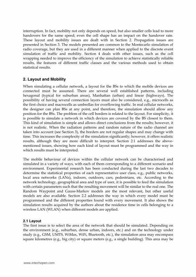
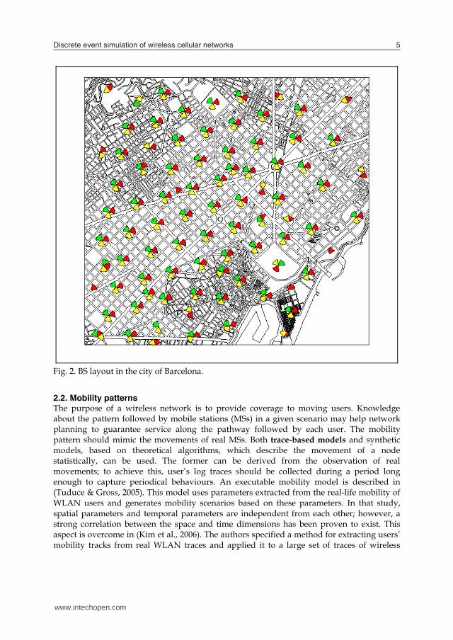
N = i2 + j2 , (2) where i and j are non-negative integers. Multi-layer layouts may be needed for capacity constraints (i.e., hotspots). A regular macrocell pattern (e.g., hexagonal or Manhattan) representing the first layer of coverage, which provides continuity in the service, is superimposed, like an umbrella, onto a microcell pattern, which guarantees service for the overcrowded areas. Of course, different radio channels should be assigned to the two layers. Once the layout has been selected, the following problem is to find the number of BSs needed to cover the whole simulation area. For this purpose, the area covered by a single cell must be known. The cell boundaries can be evaluated according to the antennas’ parameters (e.g., transmission power, the radiation diagram, the antenna gain, the antenna height, etc.) and the radiation pattern of the environment under study. In a first approximation, the cell boundaries can be estimated according to the free space model, for which the transmission power decays with the power of distance. Different radiation patterns can be selected to represent a more realistic scenario in which the cell boundaries are not regular shapes and may change over time (see Section 3.2). The theoretical boundaries may be verified with specific simulation tools. Besides the BSs needed for coverage constraints, the number of antennas may also be tuned to meet the specific capacity requirements. The number of channels that a single BS may support limits the number of simultaneous users that can be connected to that BS. In dense urban areas, where a higher concentration of users is forecasted, it is better to position more BSs than the minimum number specified by coverage constraints. An example of tuning the cell boundaries can be found in (Zola & Barceló, 2006). Their work relies on an analytical study, known as link budget, from which it is possible to estimate the coverage range of a single-cell in different environments for a given system capacity. Many issues affect the system performance (i.e., propagation conditions, traffic density, user profiles, interference conditions, cell breathing, etc.), making the network designer's task quite complex. Software planning tools can assist greatly in managing complex situations. Starting from simulation analysis in a single-cell environment in which analytical results have been tested, a first layout of the BSs in the city of Barcelona is provided in (Zola & Barceló, 2006). In this multiple-cell asset, the intercell interference, the cell breathing, and the capacity requirements due to soft-handover generate new problems that do not appear in the single-cell scenario (i.e., noise rise, BS power limits, etc.). With the final purpose of providing good coverage, the authors investigate how to improve this first layout by changing the configuration of any BSs (e.g., tilt and height) and, eventually, changing their locations (see Fig. 2). Optimal planning requires a long process of trial and error, from which one has to adjust the parameters to finally achieve a good provision of service.
Fig. 2. BS layout in the city of Barcelona.
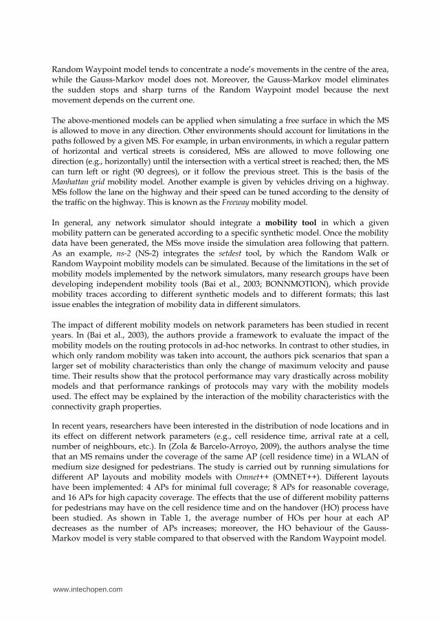
2.2. Mobility patterns The purpose of a wireless network is to provide coverage to moving users. Knowledge about the pattern followed by mobile stations (MSs) in a given scenario may help network planning to guarantee service along the pathway followed by each user. The mobility pattern should mimic the movements of real MSs. Both trace-based models and synthetic models, based on theoretical algorithms, which describe the movement of a node statistically, can be used. The former can be derived from the observation of real movements; to achieve this, user’s log traces should be collected during a period long enough to capture periodical behaviours. An executable mobility model is described in (Tuduce & Gross, 2005). This model uses parameters extracted from the real-life mobility of WLAN users and generates mobility scenarios based on these parameters. In that study, spatial parameters and temporal parameters are independent from each other; however, a strong correlation between the space and time dimensions has been proven to exist. This aspect is overcome in (Kim et al., 2006). The authors specified a method for extracting users’ mobility tracks from real WLAN traces and applied it to a large set of traces of wireless
www.intechopen.com
Discrete event simulation of wireless cellular networks 5
block in all directions. The cluster size for this layout can be computed using the equation from (Rappaport, 1996)
N = i2 + j2 , (2) where i and j are non-negative integers. Multi-layer layouts may be needed for capacity constraints (i.e., hotspots). A regular macrocell pattern (e.g., hexagonal or Manhattan) representing the first layer of coverage, which provides continuity in the service, is superimposed, like an umbrella, onto a microcell pattern, which guarantees service for the overcrowded areas. Of course, different radio channels should be assigned to the two layers. Once the layout has been selected, the following problem is to find the number of BSs needed to cover the whole simulation area. For this purpose, the area covered by a single cell must be known. The cell boundaries can be evaluated according to the antennas’ parameters (e.g., transmission power, the radiation diagram, the antenna gain, the antenna height, etc.) and the radiation pattern of the environment under study. In a first approximation, the cell boundaries can be estimated according to the free space model, for which the transmission power decays with the power of distance. Different radiation patterns can be selected to represent a more realistic scenario in which the cell boundaries are not regular shapes and may change over time (see Section 3.2). The theoretical boundaries may be verified with specific simulation tools. Besides the BSs needed for coverage constraints, the number of antennas may also be tuned to meet the specific capacity requirements. The number of channels that a single BS may support limits the number of simultaneous users that can be connected to that BS. In dense urban areas, where a higher concentration of users is forecasted, it is better to position more BSs than the minimum number specified by coverage constraints. An example of tuning the cell boundaries can be found in (Zola & Barceló, 2006). Their work relies on an analytical study, known as link budget, from which it is possible to estimate the coverage range of a single-cell in different environments for a given system capacity. Many issues affect the system performance (i.e., propagation conditions, traffic density, user profiles, interference conditions, cell breathing, etc.), making the network designer's task quite complex. Software planning tools can assist greatly in managing complex situations. Starting from simulation analysis in a single-cell environment in which analytical results have been tested, a first layout of the BSs in the city of Barcelona is provided in (Zola & Barceló, 2006). In this multiple-cell asset, the intercell interference, the cell breathing, and the capacity requirements due to soft-handover generate new problems that do not appear in the single-cell scenario (i.e., noise rise, BS power limits, etc.). With the final purpose of providing good coverage, the authors investigate how to improve this first layout by changing the configuration of any BSs (e.g., tilt and height) and, eventually, changing their locations (see Fig. 2). Optimal planning requires a long process of trial and error, from which one has to adjust the parameters to finally achieve a good provision of service.
Fig. 2. BS layout in the city of Barcelona.
2.2. Mobility patterns The purpose of a wireless network is to provide coverage to moving users. Knowledge about the pattern followed by mobile stations (MSs) in a given scenario may help network planning to guarantee service along the pathway followed by each user. The mobility pattern should mimic the movements of real MSs. Both trace-based models and synthetic models, based on theoretical algorithms, which describe the movement of a node statistically, can be used. The former can be derived from the observation of real movements; to achieve this, user’s log traces should be collected during a period long enough to capture periodical behaviours. An executable mobility model is described in (Tuduce & Gross, 2005). This model uses parameters extracted from the real-life mobility of WLAN users and generates mobility scenarios based on these parameters. In that study, spatial parameters and temporal parameters are independent from each other; however, a strong correlation between the space and time dimensions has been proven to exist. This aspect is overcome in (Kim et al., 2006). The authors specified a method for extracting users’ mobility tracks from real WLAN traces and applied it to a large set of traces of wireless
www.intechopen.com
users from Dartmouth College. Despite the ability of trace-based models to reflect real movements, they may be too specific for the environment from which they have been extracted.
(a)
(b)
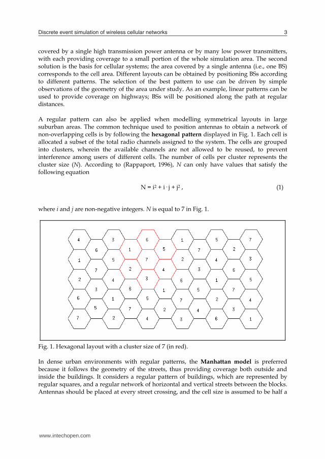
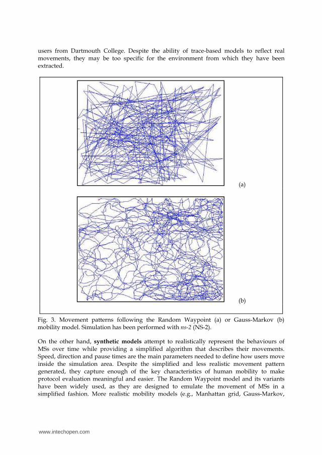
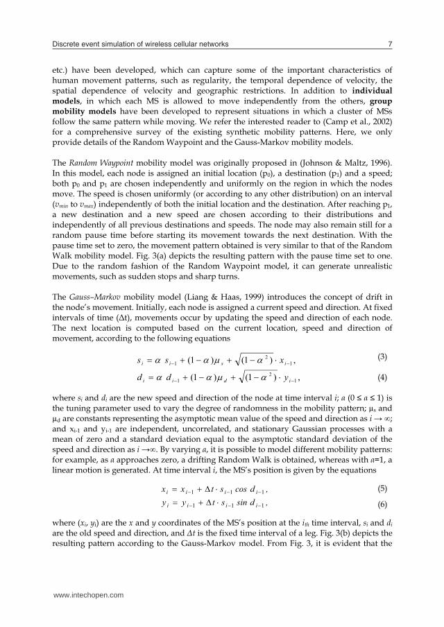
Fig. 3. Movement patterns following the Random Waypoint (a) or Gauss-Markov (b) mobility model. Simulation has been performed with ns-2 (NS-2).
On the other hand, synthetic models attempt to realistically represent the behaviours of MSs over time while providing a simplified algorithm that describes their movements. Speed, direction and pause times are the main parameters needed to define how users move inside the simulation area. Despite the simplified and less realistic movement pattern generated, they capture enough of the key characteristics of human mobility to make protocol evaluation meaningful and easier. The Random Waypoint model and its variants have been widely used, as they are designed to emulate the movement of MSs in a simplified fashion. More realistic mobility models (e.g., Manhattan grid, Gauss-Markov,
etc.) have been developed, which can capture some of the important characteristics of human movement patterns, such as regularity, the temporal dependence of velocity, the spatial dependence of velocity and geographic restrictions. In addition to individual models, in which each MS is allowed to move independently from the others, group mobility models have been developed to represent situations in which a cluster of MSs follow the same pattern while moving. We refer the interested reader to (Camp et al., 2002) for a comprehensive survey of the existing synthetic mobility patterns. Here, we only provide details of the Random Waypoint and the Gauss-Markov mobility models. The Random Waypoint mobility model was originally proposed in (Johnson & Maltz, 1996). In this model, each node is assigned an initial location (p0), a destination (p1) and a speed; both p0 and p1 are chosen independently and uniformly on the region in which the nodes move. The speed is chosen uniformly (or according to any other distribution) on an interval (vmin to vmax) independently of both the initial location and the destination. After reaching p1, a new destination and a new speed are chosen according to their distributions and independently of all previous destinations and speeds. The node may also remain still for a random pause time before starting its movement towards the next destination. With the pause time set to zero, the movement pattern obtained is very similar to that of the Random Walk mobility model. Fig. 3(a) depicts the resulting pattern with the pause time set to one. Due to the random fashion of the Random Waypoint model, it can generate unrealistic movements, such as sudden stops and sharp turns. The Gauss–Markov mobility model (Liang & Haas, 1999) introduces the concept of drift in the node’s movement. Initially, each node is assigned a current speed and direction. At fixed intervals of time (Δt), movements occur by updating the speed and direction of each node. The next location is computed based on the current location, speed and direction of movement, according to the following equations
,)1()1(
,)1()1(
12
1
12
1
idii
isii
ydd
xss
(3)
(4) where si and di are the new speed and direction of the node at time interval i; α (0 ≤ α ≤ 1) is the tuning parameter used to vary the degree of randomness in the mobility pattern; µs and µd are constants representing the asymptotic mean value of the speed and direction as i → ∞; and xi-1 and yi-1 are independent, uncorrelated, and stationary Gaussian processes with a mean of zero and a standard deviation equal to the asymptotic standard deviation of the speed and direction as i →∞. By varying α, it is possible to model different mobility patterns: for example, as α approaches zero, a drifting Random Walk is obtained, whereas with α=1, a linear motion is generated. At time interval i, the MS’s position is given by the equations
,dsinstyy,dcosstxx
iiii
iiii
111
111
(5)
(6) where (xi, yi) are the x and y coordinates of the MS’s position at the ith time interval, si and di are the old speed and direction, and Δt is the fixed time interval of a leg. Fig. 3(b) depicts the resulting pattern according to the Gauss-Markov model. From Fig. 3, it is evident that the
www.intechopen.com
Discrete event simulation of wireless cellular networks 7
users from Dartmouth College. Despite the ability of trace-based models to reflect real movements, they may be too specific for the environment from which they have been extracted.
(a)
(b)
Fig. 3. Movement patterns following the Random Waypoint (a) or Gauss-Markov (b) mobility model. Simulation has been performed with ns-2 (NS-2).
On the other hand, synthetic models attempt to realistically represent the behaviours of MSs over time while providing a simplified algorithm that describes their movements. Speed, direction and pause times are the main parameters needed to define how users move inside the simulation area. Despite the simplified and less realistic movement pattern generated, they capture enough of the key characteristics of human mobility to make protocol evaluation meaningful and easier. The Random Waypoint model and its variants have been widely used, as they are designed to emulate the movement of MSs in a simplified fashion. More realistic mobility models (e.g., Manhattan grid, Gauss-Markov,
etc.) have been developed, which can capture some of the important characteristics of human movement patterns, such as regularity, the temporal dependence of velocity, the spatial dependence of velocity and geographic restrictions. In addition to individual models, in which each MS is allowed to move independently from the others, group mobility models have been developed to represent situations in which a cluster of MSs follow the same pattern while moving. We refer the interested reader to (Camp et al., 2002) for a comprehensive survey of the existing synthetic mobility patterns. Here, we only provide details of the Random Waypoint and the Gauss-Markov mobility models. The Random Waypoint mobility model was originally proposed in (Johnson & Maltz, 1996). In this model, each node is assigned an initial location (p0), a destination (p1) and a speed; both p0 and p1 are chosen independently and uniformly on the region in which the nodes move. The speed is chosen uniformly (or according to any other distribution) on an interval (vmin to vmax) independently of both the initial location and the destination. After reaching p1, a new destination and a new speed are chosen according to their distributions and independently of all previous destinations and speeds. The node may also remain still for a random pause time before starting its movement towards the next destination. With the pause time set to zero, the movement pattern obtained is very similar to that of the Random Walk mobility model. Fig. 3(a) depicts the resulting pattern with the pause time set to one. Due to the random fashion of the Random Waypoint model, it can generate unrealistic movements, such as sudden stops and sharp turns. The Gauss–Markov mobility model (Liang & Haas, 1999) introduces the concept of drift in the node’s movement. Initially, each node is assigned a current speed and direction. At fixed intervals of time (Δt), movements occur by updating the speed and direction of each node. The next location is computed based on the current location, speed and direction of movement, according to the following equations
,)1()1(
,)1()1(
12
1
12
1
idii
isii
ydd
xss
(3)
(4) where si and di are the new speed and direction of the node at time interval i; α (0 ≤ α ≤ 1) is the tuning parameter used to vary the degree of randomness in the mobility pattern; µs and µd are constants representing the asymptotic mean value of the speed and direction as i → ∞; and xi-1 and yi-1 are independent, uncorrelated, and stationary Gaussian processes with a mean of zero and a standard deviation equal to the asymptotic standard deviation of the speed and direction as i →∞. By varying α, it is possible to model different mobility patterns: for example, as α approaches zero, a drifting Random Walk is obtained, whereas with α=1, a linear motion is generated. At time interval i, the MS’s position is given by the equations
,dsinstyy,dcosstxx
iiii
iiii
111
111
(5)
(6) where (xi, yi) are the x and y coordinates of the MS’s position at the ith time interval, si and di are the old speed and direction, and Δt is the fixed time interval of a leg. Fig. 3(b) depicts the resulting pattern according to the Gauss-Markov model. From Fig. 3, it is evident that the
www.intechopen.com
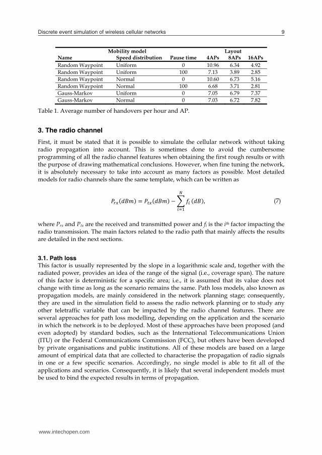
Random Waypoint model tends to concentrate a node’s movements in the centre of the area, while the Gauss-Markov model does not. Moreover, the Gauss-Markov model eliminates the sudden stops and sharp turns of the Random Waypoint model because the next movement depends on the current one. The above-mentioned models can be applied when simulating a free surface in which the MS is allowed to move in any direction. Other environments should account for limitations in the paths followed by a given MS. For example, in urban environments, in which a regular pattern of horizontal and vertical streets is considered, MSs are allowed to move following one direction (e.g., horizontally) until the intersection with a vertical street is reached; then, the MS can turn left or right (90 degrees), or it follow the previous street. This is the basis of the Manhattan grid mobility model. Another example is given by vehicles driving on a highway. MSs follow the lane on the highway and their speed can be tuned according to the density of the traffic on the highway. This is known as the Freeway mobility model. In general, any network simulator should integrate a mobility tool in which a given mobility pattern can be generated according to a specific synthetic model. Once the mobility data have been generated, the MSs move inside the simulation area following that pattern. As an example, ns-2 (NS-2) integrates the setdest tool, by which the Random Walk or Random Waypoint mobility models can be simulated. Because of the limitations in the set of mobility models implemented by the network simulators, many research groups have been developing independent mobility tools (Bai et al., 2003; BONNMOTION), which provide mobility traces according to different synthetic models and to different formats; this last issue enables the integration of mobility data in different simulators. The impact of different mobility models on network parameters has been studied in recent years. In (Bai et al., 2003), the authors provide a framework to evaluate the impact of the mobility models on the routing protocols in ad-hoc networks. In contrast to other studies, in which only random mobility was taken into account, the authors pick scenarios that span a larger set of mobility characteristics than only the change of maximum velocity and pause time. Their results show that the protocol performance may vary drastically across mobility models and that performance rankings of protocols may vary with the mobility models used. The effect may be explained by the interaction of the mobility characteristics with the connectivity graph properties. In recent years, researchers have been interested in the distribution of node locations and in its effect on different network parameters (e.g., cell residence time, arrival rate at a cell, number of neighbours, etc.). In (Zola & Barcelo-Arroyo, 2009), the authors analyse the time that an MS remains under the coverage of the same AP (cell residence time) in a WLAN of medium size designed for pedestrians. The study is carried out by running simulations for different AP layouts and mobility models with Omnet++ (OMNET++). Different layouts have been implemented: 4 APs for minimal full coverage; 8 APs for reasonable coverage, and 16 APs for high capacity coverage. The effects that the use of different mobility patterns for pedestrians may have on the cell residence time and on the handover (HO) process have been studied. As shown in Table 1, the average number of HOs per hour at each AP decreases as the number of APs increases; moreover, the HO behaviour of the Gauss-Markov model is very stable compared to that observed with the Random Waypoint model.
Mobility model Layout Name Speed distribution Pause time 4APs 8APs 16APs Random Waypoint Uniform 0 10.96 6.34 4.92 Random Waypoint Uniform 100 7.13 3.89 2.85 Random Waypoint Normal 0 10.60 6.73 5.16 Random Waypoint Normal 100 6.68 3.71 2.81 Gauss-Markov Uniform 0 7.05 6.79 7.37 Gauss-Markov Normal 0 7.03 6.72 7.82
Table 1. Average number of handovers per hour and AP.
3. The radio channel
First, it must be stated that it is possible to simulate the cellular network without taking radio propagation into account. This is sometimes done to avoid the cumbersome programming of all the radio channel features when obtaining the first rough results or with the purpose of drawing mathematical conclusions. However, when fine tuning the network, it is absolutely necessary to take into account as many factors as possible. Most detailed models for radio channels share the same template, which can be written as �������� � �������� �����
��� ����, (7)
where Prx and Ptx are the received and transmitted power and fi is the ith factor impacting the radio transmission. The main factors related to the radio path that mainly affects the results are detailed in the next sections.
3.1. Path loss This factor is usually represented by the slope in a logarithmic scale and, together with the radiated power, provides an idea of the range of the signal (i.e., coverage span). The nature of this factor is deterministic for a specific area; i.e., it is assumed that its value does not change with time as long as the scenario remains the same. Path loss models, also known as propagation models, are mainly considered in the network planning stage; consequently, they are used in the simulation field to assess the radio network planning or to study any other teletraffic variable that can be impacted by the radio channel features. There are several approaches for path loss modelling, depending on the application and the scenario in which the network is to be deployed. Most of these approaches have been proposed (and even adopted) by standard bodies, such as the International Telecommunications Union (ITU) or the Federal Communications Commission (FCC), but others have been developed by private organisations and public institutions. All of these models are based on a large amount of empirical data that are collected to characterise the propagation of radio signals in one or a few specific scenarios. Accordingly, no single model is able to fit all of the applications and scenarios. Consequently, it is likely that several independent models must be used to bind the expected results in terms of propagation.
www.intechopen.com
Discrete event simulation of wireless cellular networks 9
Random Waypoint model tends to concentrate a node’s movements in the centre of the area, while the Gauss-Markov model does not. Moreover, the Gauss-Markov model eliminates the sudden stops and sharp turns of the Random Waypoint model because the next movement depends on the current one. The above-mentioned models can be applied when simulating a free surface in which the MS is allowed to move in any direction. Other environments should account for limitations in the paths followed by a given MS. For example, in urban environments, in which a regular pattern of horizontal and vertical streets is considered, MSs are allowed to move following one direction (e.g., horizontally) until the intersection with a vertical street is reached; then, the MS can turn left or right (90 degrees), or it follow the previous street. This is the basis of the Manhattan grid mobility model. Another example is given by vehicles driving on a highway. MSs follow the lane on the highway and their speed can be tuned according to the density of the traffic on the highway. This is known as the Freeway mobility model. In general, any network simulator should integrate a mobility tool in which a given mobility pattern can be generated according to a specific synthetic model. Once the mobility data have been generated, the MSs move inside the simulation area following that pattern. As an example, ns-2 (NS-2) integrates the setdest tool, by which the Random Walk or Random Waypoint mobility models can be simulated. Because of the limitations in the set of mobility models implemented by the network simulators, many research groups have been developing independent mobility tools (Bai et al., 2003; BONNMOTION), which provide mobility traces according to different synthetic models and to different formats; this last issue enables the integration of mobility data in different simulators. The impact of different mobility models on network parameters has been studied in recent years. In (Bai et al., 2003), the authors provide a framework to evaluate the impact of the mobility models on the routing protocols in ad-hoc networks. In contrast to other studies, in which only random mobility was taken into account, the authors pick scenarios that span a larger set of mobility characteristics than only the change of maximum velocity and pause time. Their results show that the protocol performance may vary drastically across mobility models and that performance rankings of protocols may vary with the mobility models used. The effect may be explained by the interaction of the mobility characteristics with the connectivity graph properties. In recent years, researchers have been interested in the distribution of node locations and in its effect on different network parameters (e.g., cell residence time, arrival rate at a cell, number of neighbours, etc.). In (Zola & Barcelo-Arroyo, 2009), the authors analyse the time that an MS remains under the coverage of the same AP (cell residence time) in a WLAN of medium size designed for pedestrians. The study is carried out by running simulations for different AP layouts and mobility models with Omnet++ (OMNET++). Different layouts have been implemented: 4 APs for minimal full coverage; 8 APs for reasonable coverage, and 16 APs for high capacity coverage. The effects that the use of different mobility patterns for pedestrians may have on the cell residence time and on the handover (HO) process have been studied. As shown in Table 1, the average number of HOs per hour at each AP decreases as the number of APs increases; moreover, the HO behaviour of the Gauss-Markov model is very stable compared to that observed with the Random Waypoint model.
Mobility model Layout Name Speed distribution Pause time 4APs 8APs 16APs Random Waypoint Uniform 0 10.96 6.34 4.92 Random Waypoint Uniform 100 7.13 3.89 2.85 Random Waypoint Normal 0 10.60 6.73 5.16 Random Waypoint Normal 100 6.68 3.71 2.81 Gauss-Markov Uniform 0 7.05 6.79 7.37 Gauss-Markov Normal 0 7.03 6.72 7.82
Table 1. Average number of handovers per hour and AP.
3. The radio channel
First, it must be stated that it is possible to simulate the cellular network without taking radio propagation into account. This is sometimes done to avoid the cumbersome programming of all the radio channel features when obtaining the first rough results or with the purpose of drawing mathematical conclusions. However, when fine tuning the network, it is absolutely necessary to take into account as many factors as possible. Most detailed models for radio channels share the same template, which can be written as �������� � �������� �����
��� ����, (7)
where Prx and Ptx are the received and transmitted power and fi is the ith factor impacting the radio transmission. The main factors related to the radio path that mainly affects the results are detailed in the next sections.
3.1. Path loss This factor is usually represented by the slope in a logarithmic scale and, together with the radiated power, provides an idea of the range of the signal (i.e., coverage span). The nature of this factor is deterministic for a specific area; i.e., it is assumed that its value does not change with time as long as the scenario remains the same. Path loss models, also known as propagation models, are mainly considered in the network planning stage; consequently, they are used in the simulation field to assess the radio network planning or to study any other teletraffic variable that can be impacted by the radio channel features. There are several approaches for path loss modelling, depending on the application and the scenario in which the network is to be deployed. Most of these approaches have been proposed (and even adopted) by standard bodies, such as the International Telecommunications Union (ITU) or the Federal Communications Commission (FCC), but others have been developed by private organisations and public institutions. All of these models are based on a large amount of empirical data that are collected to characterise the propagation of radio signals in one or a few specific scenarios. Accordingly, no single model is able to fit all of the applications and scenarios. Consequently, it is likely that several independent models must be used to bind the expected results in terms of propagation.
www.intechopen.com
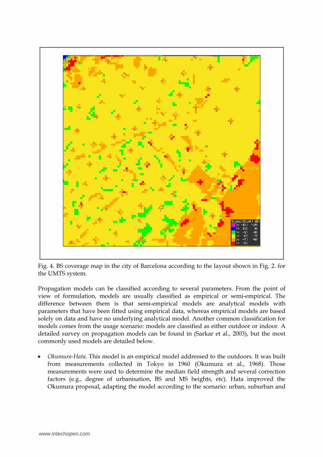
Fig. 4. BS coverage map in the city of Barcelona according to the layout shown in Fig. 2. for the UMTS system. Propagation models can be classified according to several parameters. From the point of view of formulation, models are usually classified as empirical or semi-empirical. The difference between them is that semi-empirical models are analytical models with parameters that have been fitted using empirical data, whereas empirical models are based solely on data and have no underlying analytical model. Another common classification for models comes from the usage scenario: models are classified as either outdoor or indoor. A detailed survey on propagation models can be found in (Sarkar et al., 2003), but the most commonly used models are detailed below. Okumura-Hata. This model is an empirical model addressed to the outdoors. It was built
from measurements collected in Tokyo in 1960 (Okumura et al., 1968). Those measurements were used to determine the median field strength and several correction factors (e.g., degree of urbanisation, BS and MS heights, etc). Hata improved the Okumura proposal, adapting the model according to the scenario: urban, suburban and
open areas. The Okumura-Hata model is especially applicable in networks operating in the band under 1500 MHz and in medium to large urban areas.
COST-231. The Cost Action 231 (COST 231) proposed two models for signal propagation
in urban areas in the band from 900 to 1800 MHz: the Hata model and the Walfisch-Ikegami model. The former is a semi-empirical model addressed to the urban outdoors. The Walfisch-Ikegami model is based on the theoretical Walfisch-Bertoni model. The Walfisch-Ikegami and Okumura-Hata models are commonly used for path-loss modelling in wireless networks simulations (e.g., GSM, UMTS, etc.).
Young. This model was built on the data collected in New York City in 1952 (Seybold, 2005). It is a simpler model compared with those mentioned above and, hence, is less used but still suitable for first approaches. It is addressed to applications from 150 MHz to 3.7 GHz, and it has been used for radio modelling in technologies such as IEEE 802.11.
Dual-Slope Model. This model is based on a two-ray model (Feuerstein et al., 1994), accounting for the reflection of signals from the ground in addition to the direct path. It is mainly addressed to line-of-sight propagation (e.g., WiMax links).
Most of the radio channel models presented above can be computed as proposed in (Martin-Escalona & Barceló, 2004) 畦牒� ���� � 畦� ���� � など #坦.æ̌���, (8) where A1 is the power lost at one-meter, As stands for the path-loss slope and d is the distance between network nodes (usually a base station and a mobile station).
Table 2 shows the parameters proposed for featuring the propagation in UMTS (e.g., public land mobile networks (PLMNs)) and in IEEE 802.11 networks (e.g., WLAN) according to (Holma & Toskala, 2000) and (Martin-Escalona & Barcelo-Arroyo, 2008), respectively. Furthermore, (ETSI TR 101 112) provides figures for these parameters in several environments typically used for radio-channel planning in PLMN. It has been observed that completely different radio channels can be characterised by the same propagation model as long as the parameters can be suited to the technology studied.
Parameter UMTS WLAN A1 23 dB 40 dB AS 4 3.5
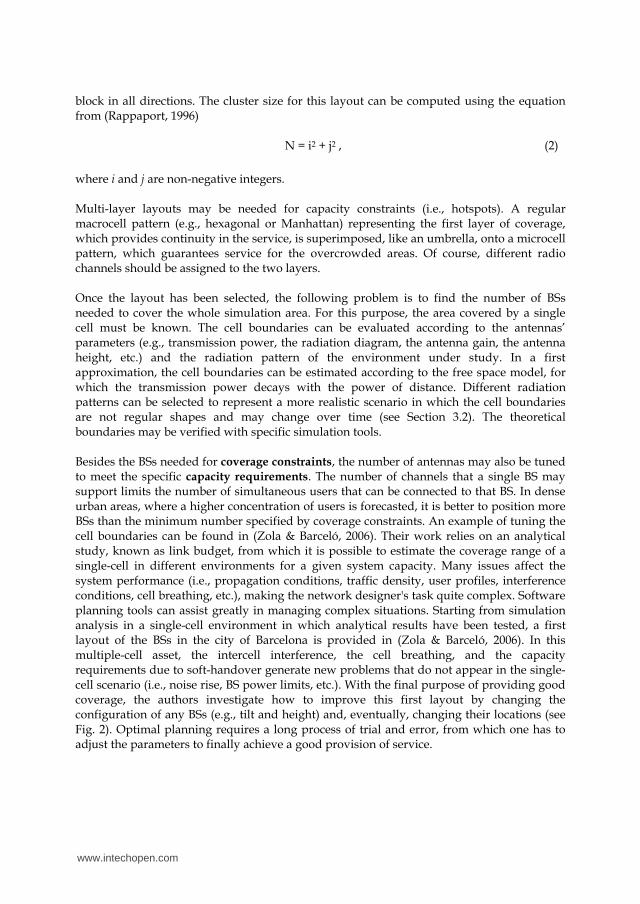
Table 2. Parameters of Equation (8) according to two network technologies. An example of a coverage study for the UMTS system is described in (Zola & Barceló, 2006). The Okumura-Hata propagation model is used, in which the propagation losses in urban scenario can be computed as 畦牒� � なぬぬ┻ばは � ぬね┻ばひ.æ̌���, (9) where d is the distance in kilometres. The coverage map for the BS layout in Barcelona shown in Fig. 2 is displayed in Fig. 4. Colours from red to yellow represent good coverage. The green
www.intechopen.com
Discrete event simulation of wireless cellular networks 11
Fig. 4. BS coverage map in the city of Barcelona according to the layout shown in Fig. 2. for the UMTS system. Propagation models can be classified according to several parameters. From the point of view of formulation, models are usually classified as empirical or semi-empirical. The difference between them is that semi-empirical models are analytical models with parameters that have been fitted using empirical data, whereas empirical models are based solely on data and have no underlying analytical model. Another common classification for models comes from the usage scenario: models are classified as either outdoor or indoor. A detailed survey on propagation models can be found in (Sarkar et al., 2003), but the most commonly used models are detailed below. Okumura-Hata. This model is an empirical model addressed to the outdoors. It was built
from measurements collected in Tokyo in 1960 (Okumura et al., 1968). Those measurements were used to determine the median field strength and several correction factors (e.g., degree of urbanisation, BS and MS heights, etc). Hata improved the Okumura proposal, adapting the model according to the scenario: urban, suburban and
open areas. The Okumura-Hata model is especially applicable in networks operating in the band under 1500 MHz and in medium to large urban areas.
COST-231. The Cost Action 231 (COST 231) proposed two models for signal propagation
in urban areas in the band from 900 to 1800 MHz: the Hata model and the Walfisch-Ikegami model. The former is a semi-empirical model addressed to the urban outdoors. The Walfisch-Ikegami model is based on the theoretical Walfisch-Bertoni model. The Walfisch-Ikegami and Okumura-Hata models are commonly used for path-loss modelling in wireless networks simulations (e.g., GSM, UMTS, etc.).
Young. This model was built on the data collected in New York City in 1952 (Seybold, 2005). It is a simpler model compared with those mentioned above and, hence, is less used but still suitable for first approaches. It is addressed to applications from 150 MHz to 3.7 GHz, and it has been used for radio modelling in technologies such as IEEE 802.11.
Dual-Slope Model. This model is based on a two-ray model (Feuerstein et al., 1994), accounting for the reflection of signals from the ground in addition to the direct path. It is mainly addressed to line-of-sight propagation (e.g., WiMax links).
Most of the radio channel models presented above can be computed as proposed in (Martin-Escalona & Barceló, 2004) 畦牒� ���� � 畦� ���� � など #坦.æ̌���, (8) where A1 is the power lost at one-meter, As stands for the path-loss slope and d is the distance between network nodes (usually a base station and a mobile station).
Table 2 shows the parameters proposed for featuring the propagation in UMTS (e.g., public land mobile networks (PLMNs)) and in IEEE 802.11 networks (e.g., WLAN) according to (Holma & Toskala, 2000) and (Martin-Escalona & Barcelo-Arroyo, 2008), respectively. Furthermore, (ETSI TR 101 112) provides figures for these parameters in several environments typically used for radio-channel planning in PLMN. It has been observed that completely different radio channels can be characterised by the same propagation model as long as the parameters can be suited to the technology studied.
Parameter UMTS WLAN A1 23 dB 40 dB AS 4 3.5
Table 2. Parameters of Equation (8) according to two network technologies. An example of a coverage study for the UMTS system is described in (Zola & Barceló, 2006). The Okumura-Hata propagation model is used, in which the propagation losses in urban scenario can be computed as 畦牒� � なぬぬ┻ばは � ぬね┻ばひ.æ̌���, (9) where d is the distance in kilometres. The coverage map for the BS layout in Barcelona shown in Fig. 2 is displayed in Fig. 4. Colours from red to yellow represent good coverage. The green
www.intechopen.com
areas represent weaker signal strength, and in those areas, users may not be allowed to connect to the system (or the service may be interrupted) due to coverage constraints.
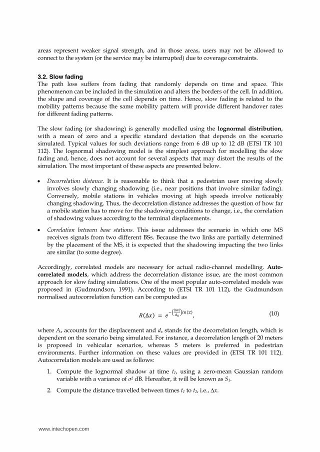
3.2. Slow fading The path loss suffers from fading that randomly depends on time and space. This phenomenon can be included in the simulation and alters the borders of the cell. In addition, the shape and coverage of the cell depends on time. Hence, slow fading is related to the mobility patterns because the same mobility pattern will provide different handover rates for different fading patterns. The slow fading (or shadowing) is generally modelled using the lognormal distribution, with a mean of zero and a specific standard deviation that depends on the scenario simulated. Typical values for such deviations range from 6 dB up to 12 dB (ETSI TR 101 112). The lognormal shadowing model is the simplest approach for modelling the slow fading and, hence, does not account for several aspects that may distort the results of the simulation. The most important of these aspects are presented below. Decorrelation distance. It is reasonable to think that a pedestrian user moving slowly
involves slowly changing shadowing (i.e., near positions that involve similar fading). Conversely, mobile stations in vehicles moving at high speeds involve noticeably changing shadowing. Thus, the decorrelation distance addresses the question of how far a mobile station has to move for the shadowing conditions to change, i.e., the correlation of shadowing values according to the terminal displacements.
Correlation between base stations. This issue addresses the scenario in which one MS receives signals from two different BSs. Because the two links are partially determined by the placement of the MS, it is expected that the shadowing impacting the two links are similar (to some degree).
Accordingly, correlated models are necessary for actual radio-channel modelling. Auto-correlated models, which address the decorrelation distance issue, are the most common approach for slow fading simulations. One of the most popular auto-correlated models was proposed in (Gudmundson, 1991). According to (ETSI TR 101 112), the Gudmundson normalised autocorrelation function can be computed as ����� � � ���|��|�� ������, (10) where Ax accounts for the displacement and dx stands for the decorrelation length, which is dependent on the scenario being simulated. For instance, a decorrelation length of 20 meters is proposed in vehicular scenarios, whereas 5 meters is preferred in pedestrian environments. Further information on these values are provided in (ETSI TR 101 112). Autocorrelation models are used as follows:
1. Compute the lognormal shadow at time t1, using a zero-mean Gaussian random variable with a variance of σ2 dB. Hereafter, it will be known as S1.
2. Compute the distance travelled between times t1 to t2, i.e., ∆x.
3. Evaluate the normalised autocorrelation function at ∆x, i.e., R(∆x).
4. The lognormal shadow at t2 (i.e., S2) is computed as a Gaussian random variable (in dB) with an average of R(∆x)· S1 and a variance of (1-R(∆x))· σ2.
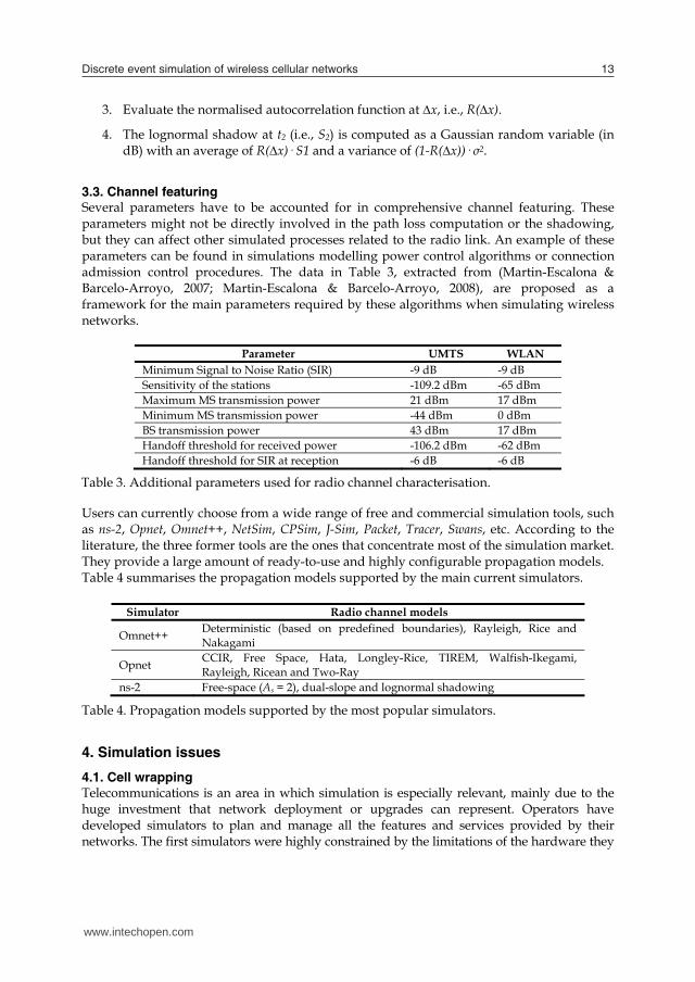
3.3. Channel featuring Several parameters have to be accounted for in comprehensive channel featuring. These parameters might not be directly involved in the path loss computation or the shadowing, but they can affect other simulated processes related to the radio link. An example of these parameters can be found in simulations modelling power control algorithms or connection admission control procedures. The data in Table 3, extracted from (Martin-Escalona & Barcelo-Arroyo, 2007; Martin-Escalona & Barcelo-Arroyo, 2008), are proposed as a framework for the main parameters required by these algorithms when simulating wireless networks.
Parameter UMTS WLAN Minimum Signal to Noise Ratio (SIR) -9 dB -9 dB Sensitivity of the stations -109.2 dBm -65 dBm Maximum MS transmission power 21 dBm 17 dBm Minimum MS transmission power -44 dBm 0 dBm BS transmission power 43 dBm 17 dBm Handoff threshold for received power -106.2 dBm -62 dBm Handoff threshold for SIR at reception -6 dB -6 dB
Table 3. Additional parameters used for radio channel characterisation.
Users can currently choose from a wide range of free and commercial simulation tools, such as ns-2, Opnet, Omnet++, NetSim, CPSim, J-Sim, Packet, Tracer, Swans, etc. According to the literature, the three former tools are the ones that concentrate most of the simulation market. They provide a large amount of ready-to-use and highly configurable propagation models.
Table 4 summarises the propagation models supported by the main current simulators.
Simulator Radio channel models
Omnet++ Deterministic (based on predefined boundaries), Rayleigh, Rice and Nakagami
Opnet CCIR, Free Space, Hata, Longley-Rice, TIREM, Walfish-Ikegami, Rayleigh, Ricean and Two-Ray
ns-2 Free-space (As = 2), dual-slope and lognormal shadowing
Table 4. Propagation models supported by the most popular simulators.
4. Simulation issues
4.1. Cell wrapping Telecommunications is an area in which simulation is especially relevant, mainly due to the huge investment that network deployment or upgrades can represent. Operators have developed simulators to plan and manage all the features and services provided by their networks. The first simulators were highly constrained by the limitations of the hardware they
www.intechopen.com
Discrete event simulation of wireless cellular networks 13
areas represent weaker signal strength, and in those areas, users may not be allowed to connect to the system (or the service may be interrupted) due to coverage constraints.
3.2. Slow fading The path loss suffers from fading that randomly depends on time and space. This phenomenon can be included in the simulation and alters the borders of the cell. In addition, the shape and coverage of the cell depends on time. Hence, slow fading is related to the mobility patterns because the same mobility pattern will provide different handover rates for different fading patterns. The slow fading (or shadowing) is generally modelled using the lognormal distribution, with a mean of zero and a specific standard deviation that depends on the scenario simulated. Typical values for such deviations range from 6 dB up to 12 dB (ETSI TR 101 112). The lognormal shadowing model is the simplest approach for modelling the slow fading and, hence, does not account for several aspects that may distort the results of the simulation. The most important of these aspects are presented below. Decorrelation distance. It is reasonable to think that a pedestrian user moving slowly
involves slowly changing shadowing (i.e., near positions that involve similar fading). Conversely, mobile stations in vehicles moving at high speeds involve noticeably changing shadowing. Thus, the decorrelation distance addresses the question of how far a mobile station has to move for the shadowing conditions to change, i.e., the correlation of shadowing values according to the terminal displacements.
Correlation between base stations. This issue addresses the scenario in which one MS receives signals from two different BSs. Because the two links are partially determined by the placement of the MS, it is expected that the shadowing impacting the two links are similar (to some degree).
Accordingly, correlated models are necessary for actual radio-channel modelling. Auto-correlated models, which address the decorrelation distance issue, are the most common approach for slow fading simulations. One of the most popular auto-correlated models was proposed in (Gudmundson, 1991). According to (ETSI TR 101 112), the Gudmundson normalised autocorrelation function can be computed as ����� � � ���|��|�� ������, (10) where Ax accounts for the displacement and dx stands for the decorrelation length, which is dependent on the scenario being simulated. For instance, a decorrelation length of 20 meters is proposed in vehicular scenarios, whereas 5 meters is preferred in pedestrian environments. Further information on these values are provided in (ETSI TR 101 112). Autocorrelation models are used as follows:
1. Compute the lognormal shadow at time t1, using a zero-mean Gaussian random variable with a variance of σ2 dB. Hereafter, it will be known as S1.
2. Compute the distance travelled between times t1 to t2, i.e., ∆x.
3. Evaluate the normalised autocorrelation function at ∆x, i.e., R(∆x).
4. The lognormal shadow at t2 (i.e., S2) is computed as a Gaussian random variable (in dB) with an average of R(∆x)· S1 and a variance of (1-R(∆x))· σ2.
3.3. Channel featuring Several parameters have to be accounted for in comprehensive channel featuring. These parameters might not be directly involved in the path loss computation or the shadowing, but they can affect other simulated processes related to the radio link. An example of these parameters can be found in simulations modelling power control algorithms or connection admission control procedures. The data in Table 3, extracted from (Martin-Escalona & Barcelo-Arroyo, 2007; Martin-Escalona & Barcelo-Arroyo, 2008), are proposed as a framework for the main parameters required by these algorithms when simulating wireless networks.
Parameter UMTS WLAN Minimum Signal to Noise Ratio (SIR) -9 dB -9 dB Sensitivity of the stations -109.2 dBm -65 dBm Maximum MS transmission power 21 dBm 17 dBm Minimum MS transmission power -44 dBm 0 dBm BS transmission power 43 dBm 17 dBm Handoff threshold for received power -106.2 dBm -62 dBm Handoff threshold for SIR at reception -6 dB -6 dB
Table 3. Additional parameters used for radio channel characterisation.
Users can currently choose from a wide range of free and commercial simulation tools, such as ns-2, Opnet, Omnet++, NetSim, CPSim, J-Sim, Packet, Tracer, Swans, etc. According to the literature, the three former tools are the ones that concentrate most of the simulation market. They provide a large amount of ready-to-use and highly configurable propagation models.
Table 4 summarises the propagation models supported by the main current simulators.
Simulator Radio channel models
Omnet++ Deterministic (based on predefined boundaries), Rayleigh, Rice and Nakagami
Opnet CCIR, Free Space, Hata, Longley-Rice, TIREM, Walfish-Ikegami, Rayleigh, Ricean and Two-Ray
ns-2 Free-space (As = 2), dual-slope and lognormal shadowing
Table 4. Propagation models supported by the most popular simulators.
4. Simulation issues
4.1. Cell wrapping Telecommunications is an area in which simulation is especially relevant, mainly due to the huge investment that network deployment or upgrades can represent. Operators have developed simulators to plan and manage all the features and services provided by their networks. The first simulators were highly constrained by the limitations of the hardware they
www.intechopen.com
used, which led to simulations that were very time-consuming. Technology has evolved to the point that relatively complex models can be handled in acceptable execution times. However, cellular networks raise new issues that must be dealt with by simulation tools. Cellular networks divide coverage area into cells. Though planners are often interested in obtaining performance metrics for an area that is ideal, continuous and unlimited, an infinite area is impossible to simulate. If the simulated area is finite, there is a major difference between core cells (i.e., in the middle of the simulated layout) and boundary cells (i.e., at the edge of the layout). Core cells receive more traffic and interference than boundary cells. Because core cells are surrounded by other cells, performance metrics obtained in them are less impacted by the edge effect, and they can be considered to be representative of the ideal infinite layout. This fact raises an issue: because metrics and statistics are only obtained from centre cells, the simulation will consume much more time than is strictly necessary to obtain results. In addition, simulators have to set specific procedures to deal with users reaching the boundaries of the simulation area. These issues are collectively known as the edge or boundary effect (Zander & Kim, 2001).
Several proposals address mitigating the edge effect in cellular network simulators. Overcoming the edge effect involves addressing two issues: mobility and the propagation model. Mobility wrapping aims to stop the mobile station from determining the limits of the simulated area. On the other hand, propagation wrapping assures that all of the cells show the same propagation features without accounting for their position inside the simulated area. Several proposals are explained below.
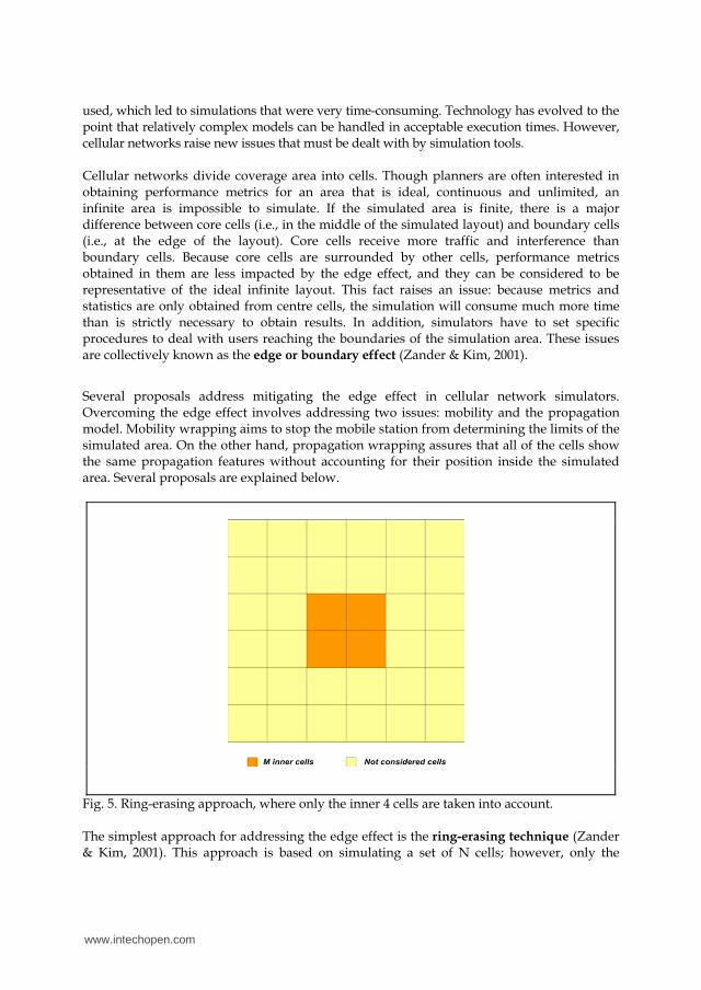
Fig. 5. Ring-erasing approach, where only the inner 4 cells are taken into account. The simplest approach for addressing the edge effect is the ring-erasing technique (Zander & Kim, 2001). This approach is based on simulating a set of N cells; however, only the
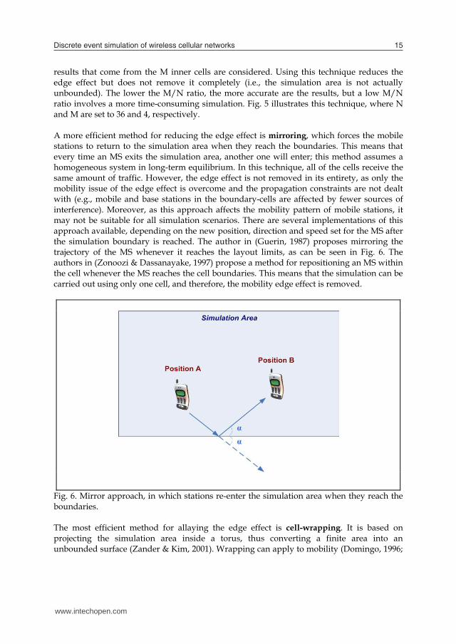
results that come from the M inner cells are considered. Using this technique reduces the edge effect but does not remove it completely (i.e., the simulation area is not actually unbounded). The lower the M/N ratio, the more accurate are the results, but a low M/N ratio involves a more time-consuming simulation. Fig. 5 illustrates this technique, where N and M are set to 36 and 4, respectively. A more efficient method for reducing the edge effect is mirroring, which forces the mobile stations to return to the simulation area when they reach the boundaries. This means that every time an MS exits the simulation area, another one will enter; this method assumes a homogeneous system in long-term equilibrium. In this technique, all of the cells receive the same amount of traffic. However, the edge effect is not removed in its entirety, as only the mobility issue of the edge effect is overcome and the propagation constraints are not dealt with (e.g., mobile and base stations in the boundary-cells are affected by fewer sources of interference). Moreover, as this approach affects the mobility pattern of mobile stations, it may not be suitable for all simulation scenarios. There are several implementations of this approach available, depending on the new position, direction and speed set for the MS after the simulation boundary is reached. The author in (Guerin, 1987) proposes mirroring the trajectory of the MS whenever it reaches the layout limits, as can be seen in Fig. 6. The authors in (Zonoozi & Dassanayake, 1997) propose a method for repositioning an MS within the cell whenever the MS reaches the cell boundaries. This means that the simulation can be carried out using only one cell, and therefore, the mobility edge effect is removed.
Fig. 6. Mirror approach, in which stations re-enter the simulation area when they reach the boundaries. The most efficient method for allaying the edge effect is cell-wrapping. It is based on projecting the simulation area inside a torus, thus converting a finite area into an unbounded surface (Zander & Kim, 2001). Wrapping can apply to mobility (Domingo, 1996;
www.intechopen.com
Discrete event simulation of wireless cellular networks 15
used, which led to simulations that were very time-consuming. Technology has evolved to the point that relatively complex models can be handled in acceptable execution times. However, cellular networks raise new issues that must be dealt with by simulation tools. Cellular networks divide coverage area into cells. Though planners are often interested in obtaining performance metrics for an area that is ideal, continuous and unlimited, an infinite area is impossible to simulate. If the simulated area is finite, there is a major difference between core cells (i.e., in the middle of the simulated layout) and boundary cells (i.e., at the edge of the layout). Core cells receive more traffic and interference than boundary cells. Because core cells are surrounded by other cells, performance metrics obtained in them are less impacted by the edge effect, and they can be considered to be representative of the ideal infinite layout. This fact raises an issue: because metrics and statistics are only obtained from centre cells, the simulation will consume much more time than is strictly necessary to obtain results. In addition, simulators have to set specific procedures to deal with users reaching the boundaries of the simulation area. These issues are collectively known as the edge or boundary effect (Zander & Kim, 2001).
Several proposals address mitigating the edge effect in cellular network simulators. Overcoming the edge effect involves addressing two issues: mobility and the propagation model. Mobility wrapping aims to stop the mobile station from determining the limits of the simulated area. On the other hand, propagation wrapping assures that all of the cells show the same propagation features without accounting for their position inside the simulated area. Several proposals are explained below.
Fig. 5. Ring-erasing approach, where only the inner 4 cells are taken into account. The simplest approach for addressing the edge effect is the ring-erasing technique (Zander & Kim, 2001). This approach is based on simulating a set of N cells; however, only the
results that come from the M inner cells are considered. Using this technique reduces the edge effect but does not remove it completely (i.e., the simulation area is not actually unbounded). The lower the M/N ratio, the more accurate are the results, but a low M/N ratio involves a more time-consuming simulation. Fig. 5 illustrates this technique, where N and M are set to 36 and 4, respectively. A more efficient method for reducing the edge effect is mirroring, which forces the mobile stations to return to the simulation area when they reach the boundaries. This means that every time an MS exits the simulation area, another one will enter; this method assumes a homogeneous system in long-term equilibrium. In this technique, all of the cells receive the same amount of traffic. However, the edge effect is not removed in its entirety, as only the mobility issue of the edge effect is overcome and the propagation constraints are not dealt with (e.g., mobile and base stations in the boundary-cells are affected by fewer sources of interference). Moreover, as this approach affects the mobility pattern of mobile stations, it may not be suitable for all simulation scenarios. There are several implementations of this approach available, depending on the new position, direction and speed set for the MS after the simulation boundary is reached. The author in (Guerin, 1987) proposes mirroring the trajectory of the MS whenever it reaches the layout limits, as can be seen in Fig. 6. The authors in (Zonoozi & Dassanayake, 1997) propose a method for repositioning an MS within the cell whenever the MS reaches the cell boundaries. This means that the simulation can be carried out using only one cell, and therefore, the mobility edge effect is removed.
Fig. 6. Mirror approach, in which stations re-enter the simulation area when they reach the boundaries. The most efficient method for allaying the edge effect is cell-wrapping. It is based on projecting the simulation area inside a torus, thus converting a finite area into an unbounded surface (Zander & Kim, 2001). Wrapping can apply to mobility (Domingo, 1996;
www.intechopen.com
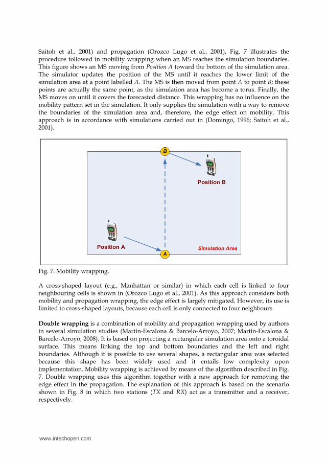
Saitoh et al., 2001) and propagation (Orozco Lugo et al., 2001). Fig. 7 illustrates the procedure followed in mobility wrapping when an MS reaches the simulation boundaries. This figure shows an MS moving from Position A toward the bottom of the simulation area. The simulator updates the position of the MS until it reaches the lower limit of the simulation area at a point labelled A. The MS is then moved from point A to point B; these points are actually the same point, as the simulation area has become a torus. Finally, the MS moves on until it covers the forecasted distance. This wrapping has no influence on the mobility pattern set in the simulation. It only supplies the simulation with a way to remove the boundaries of the simulation area and, therefore, the edge effect on mobility. This approach is in accordance with simulations carried out in (Domingo, 1996; Saitoh et al., 2001).
Fig. 7. Mobility wrapping.
A cross-shaped layout (e.g., Manhattan or similar) in which each cell is linked to four neighbouring cells is shown in (Orozco Lugo et al., 2001). As this approach considers both mobility and propagation wrapping, the edge effect is largely mitigated. However, its use is limited to cross-shaped layouts, because each cell is only connected to four neighbours. Double wrapping is a combination of mobility and propagation wrapping used by authors in several simulation studies (Martin-Escalona & Barcelo-Arroyo, 2007; Martin-Escalona & Barcelo-Arroyo, 2008). It is based on projecting a rectangular simulation area onto a toroidal surface. This means linking the top and bottom boundaries and the left and right boundaries. Although it is possible to use several shapes, a rectangular area was selected because this shape has been widely used and it entails low complexity upon implementation. Mobility wrapping is achieved by means of the algorithm described in Fig. 7. Double wrapping uses this algorithm together with a new approach for removing the edge effect in the propagation. The explanation of this approach is based on the scenario shown in Fig. 8 in which two stations (TX and RX) act as a transmitter and a receiver, respectively.
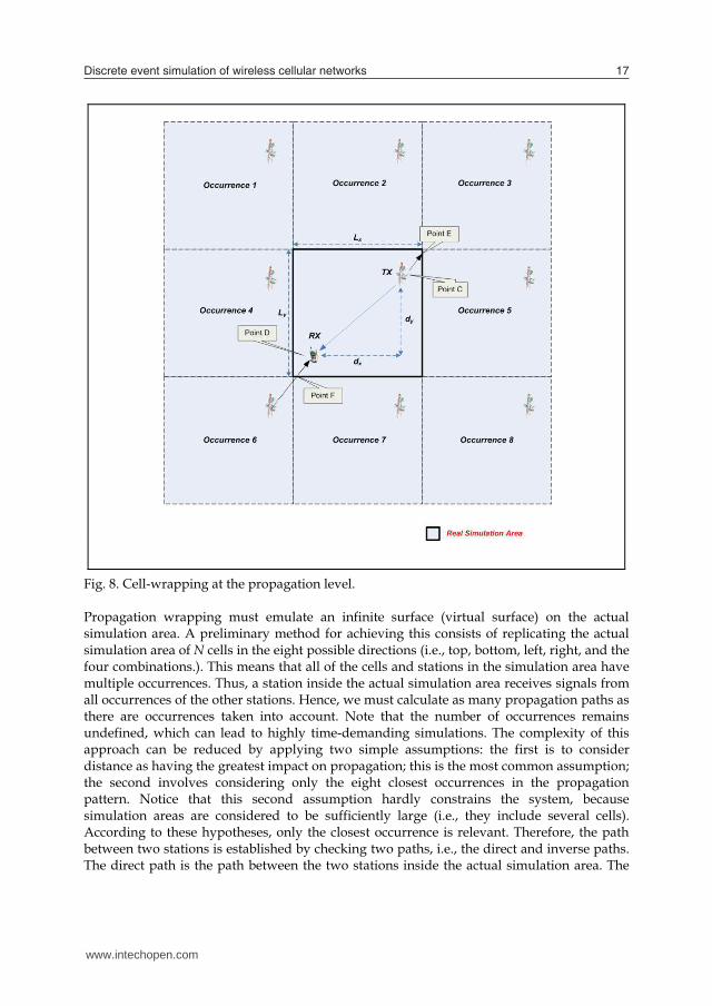
Fig. 8. Cell-wrapping at the propagation level. Propagation wrapping must emulate an infinite surface (virtual surface) on the actual simulation area. A preliminary method for achieving this consists of replicating the actual simulation area of N cells in the eight possible directions (i.e., top, bottom, left, right, and the four combinations.). This means that all of the cells and stations in the simulation area have multiple occurrences. Thus, a station inside the actual simulation area receives signals from all occurrences of the other stations. Hence, we must calculate as many propagation paths as there are occurrences taken into account. Note that the number of occurrences remains undefined, which can lead to highly time-demanding simulations. The complexity of this approach can be reduced by applying two simple assumptions: the first is to consider distance as having the greatest impact on propagation; this is the most common assumption; the second involves considering only the eight closest occurrences in the propagation pattern. Notice that this second assumption hardly constrains the system, because simulation areas are considered to be sufficiently large (i.e., they include several cells). According to these hypotheses, only the closest occurrence is relevant. Therefore, the path between two stations is established by checking two paths, i.e., the direct and inverse paths. The direct path is the path between the two stations inside the actual simulation area. The
www.intechopen.com
Discrete event simulation of wireless cellular networks 17
Saitoh et al., 2001) and propagation (Orozco Lugo et al., 2001). Fig. 7 illustrates the procedure followed in mobility wrapping when an MS reaches the simulation boundaries. This figure shows an MS moving from Position A toward the bottom of the simulation area. The simulator updates the position of the MS until it reaches the lower limit of the simulation area at a point labelled A. The MS is then moved from point A to point B; these points are actually the same point, as the simulation area has become a torus. Finally, the MS moves on until it covers the forecasted distance. This wrapping has no influence on the mobility pattern set in the simulation. It only supplies the simulation with a way to remove the boundaries of the simulation area and, therefore, the edge effect on mobility. This approach is in accordance with simulations carried out in (Domingo, 1996; Saitoh et al., 2001).
Fig. 7. Mobility wrapping.
A cross-shaped layout (e.g., Manhattan or similar) in which each cell is linked to four neighbouring cells is shown in (Orozco Lugo et al., 2001). As this approach considers both mobility and propagation wrapping, the edge effect is largely mitigated. However, its use is limited to cross-shaped layouts, because each cell is only connected to four neighbours. Double wrapping is a combination of mobility and propagation wrapping used by authors in several simulation studies (Martin-Escalona & Barcelo-Arroyo, 2007; Martin-Escalona & Barcelo-Arroyo, 2008). It is based on projecting a rectangular simulation area onto a toroidal surface. This means linking the top and bottom boundaries and the left and right boundaries. Although it is possible to use several shapes, a rectangular area was selected because this shape has been widely used and it entails low complexity upon implementation. Mobility wrapping is achieved by means of the algorithm described in Fig. 7. Double wrapping uses this algorithm together with a new approach for removing the edge effect in the propagation. The explanation of this approach is based on the scenario shown in Fig. 8 in which two stations (TX and RX) act as a transmitter and a receiver, respectively.
Fig. 8. Cell-wrapping at the propagation level. Propagation wrapping must emulate an infinite surface (virtual surface) on the actual simulation area. A preliminary method for achieving this consists of replicating the actual simulation area of N cells in the eight possible directions (i.e., top, bottom, left, right, and the four combinations.). This means that all of the cells and stations in the simulation area have multiple occurrences. Thus, a station inside the actual simulation area receives signals from all occurrences of the other stations. Hence, we must calculate as many propagation paths as there are occurrences taken into account. Note that the number of occurrences remains undefined, which can lead to highly time-demanding simulations. The complexity of this approach can be reduced by applying two simple assumptions: the first is to consider distance as having the greatest impact on propagation; this is the most common assumption; the second involves considering only the eight closest occurrences in the propagation pattern. Notice that this second assumption hardly constrains the system, because simulation areas are considered to be sufficiently large (i.e., they include several cells). According to these hypotheses, only the closest occurrence is relevant. Therefore, the path between two stations is established by checking two paths, i.e., the direct and inverse paths. The direct path is the path between the two stations inside the actual simulation area. The
www.intechopen.com
inverse path accounts for wrapping and is defined as the shortest path between any occurrence of the transmitter station outside the real simulation area and the receiver station. For example, in Fig. 8, the direct path goes from point C to D, but the inverse path involves Occurrence 6 (the closest one). This means that the inverse path goes from point C to E and then from point F to D. The path selected for propagation purposes is the shortest path between the direct and inverse paths. The distance associated with this path can be computed as ��� � ����� � ���� � ������|��|, |�� � ��|��� � ���������, ��� � ������, (11)
where dsx and dsy indicate the distance of the shortest path in the x and y axes, respectively. Additionally, the path direction can be easily obtained using the following expression ��� � ����� ��������������������������������, (12) where αsp is the angle of the path if the position of the transmitter is considered as the origin of the coordinate system. Accordingly, the propagation path is completely defined by Equations (11) and (12). Note that this approach can be used together with any propagation model because it only removes the edge effect and does not interfere with the application propagation model.
4.2. Traffic issues Each kind of traffic is characterised and modelled with different features that must be accounted for in the simulation. This includes the bandwidth required, time use, mobility, etc. In this way, it is unlikely that a worker using a laptop in a WLAN moves at a high speed, whereas voice traffic can be provided to devices in cars on a highway. On the other hand, the arrival of connections to the network and the time connected must be simulated in a different way depending on the service. Whereas a Poisson arrival process, which is easy to implement in the simulation, is suitable for voice, video or data connections must be simulated by other distributions that introduce further complexity. In the case of voice and low bit-rate data services, call duration is often modelled as a lognormal variable instead of the classic (and less complex) exponential assumption. This latter fact tends to favour lower service durations, whilst the lognormal assumption provides more realistic durations. The impact of the service duration model in certain teletraffic variables is studied in (Spedalieri et al., 2005). Specifically, channel holding time (i.e., the time that a channel of a cell remains busy due to the call), the time between handoff arrivals (i.e., the handoff traffic) and the handoff duration in UMTS networks are studied. In the case of the channel holding time, the exponential assumption involves lower average values compared with those of the lognormal case. Furthermore, the exponential call duration involves channel holding times that are not particularly sensitive to the load (in average), whilst the lognormal assumption produces more realistic figures, i.e., the higher the load, the lower is the mean channel holding time.
Table 5 shows the average value under both assumptions and different network loads. The results show that even though shape and scale factors are different, the channel holding time is fit by the same candidate functions independently of whether the service duration is exponential or lognormal.
Load Average(Log) Average(EXP) 50 % 8.36 s 8.60 s 70 % 8.32 s 8.39 s 90 % 7.83 s 8.68 s
Table 5. Channel holding time according to service duration: lognormal (log) and exponential (exp).
The time between two consecutive handoffs to the same cell (i.e., sector in a BS) is studied in (Spedalieri et al., 2005) from a twofold point of view: including and neglecting simultaneous handoffs requests. It must be noted that the higher the user mobility, the more likely are simultaneous handoffs. Thus, in vehicle simulation, simultaneous handoffs occur frequently. The probability density function is then expected to show a peak at the origin due to the presence of the simultaneous handoffs. Table 6 shows the results achieved in (Spedalieri et al., 2005), where P0 provides the probability that the time between consecutive handoffs is zero. As in the case of the channel holding time, results under the lognormal assumption are more sensitive to the load, especially when the load is very high. The results obtained for exponential service durations also depend on the system load, but the evolution is smoother. In both cases, simulations without accounting for the simultaneous handoffs do not seem to be sensitive to the load (on average). Furthermore, the model for the service duration also impacts the handoff traffic model, which is best fit by means of different random variables according to the approach followed to characterise the service duration.
Load P0 (%) With all handoffs Without simultaneous handoffs
Log Exp Average (Log)
Average (Exp)
Average (Log)
Average (Exp)
50 % 62.73 64.20 0.43 s 0.41 s 1.18 s 1.16 s 70 % 69.43 69.50 0.34 s 0.33 s 1.10 s 1.09 s 90 % 81.97 72.23 0.18 s 0.29 s 1.16 s 1.06 s
Table 6. Results for the time between consecutive handoff requests.
4.3. Gathering simulation results Collecting data is one of the main tasks of the simulation tools. The procedure followed to gather the information resulting from simulation has to be set up when modelling the system, because it can constrain the whole simulation process. Simulation tools usually allow three types of sampling: deterministic, event-driven and probabilistic. The former sets a deterministic rate and collects samples accordingly. This approach is the simplest and is generally followed in continuous simulations (e.g., electrical models). The main difficulty in this approach is setting the sampling frequency. High sampling frequencies involve more precise data but also entails a longer runtime (i.e., time spent until the simulation finishes). Conversely, low sampling frequencies provide faster simulations but less precise data. Setting a suitable sampling frequency can be hard work, and it is often based on experience,
www.intechopen.com

Discrete event simulation of wireless cellular networks 19
inverse path accounts for wrapping and is defined as the shortest path between any occurrence of the transmitter station outside the real simulation area and the receiver station. For example, in Fig. 8, the direct path goes from point C to D, but the inverse path involves Occurrence 6 (the closest one). This means that the inverse path goes from point C to E and then from point F to D. The path selected for propagation purposes is the shortest path between the direct and inverse paths. The distance associated with this path can be computed as ��� � ����� � ���� � ������|��|, |�� � ��|��� � ���������, ��� � ������, (11)
where dsx and dsy indicate the distance of the shortest path in the x and y axes, respectively. Additionally, the path direction can be easily obtained using the following expression ��� � ����� ��������������������������������, (12) where αsp is the angle of the path if the position of the transmitter is considered as the origin of the coordinate system. Accordingly, the propagation path is completely defined by Equations (11) and (12). Note that this approach can be used together with any propagation model because it only removes the edge effect and does not interfere with the application propagation model.
4.2. Traffic issues Each kind of traffic is characterised and modelled with different features that must be accounted for in the simulation. This includes the bandwidth required, time use, mobility, etc. In this way, it is unlikely that a worker using a laptop in a WLAN moves at a high speed, whereas voice traffic can be provided to devices in cars on a highway. On the other hand, the arrival of connections to the network and the time connected must be simulated in a different way depending on the service. Whereas a Poisson arrival process, which is easy to implement in the simulation, is suitable for voice, video or data connections must be simulated by other distributions that introduce further complexity. In the case of voice and low bit-rate data services, call duration is often modelled as a lognormal variable instead of the classic (and less complex) exponential assumption. This latter fact tends to favour lower service durations, whilst the lognormal assumption provides more realistic durations. The impact of the service duration model in certain teletraffic variables is studied in (Spedalieri et al., 2005). Specifically, channel holding time (i.e., the time that a channel of a cell remains busy due to the call), the time between handoff arrivals (i.e., the handoff traffic) and the handoff duration in UMTS networks are studied. In the case of the channel holding time, the exponential assumption involves lower average values compared with those of the lognormal case. Furthermore, the exponential call duration involves channel holding times that are not particularly sensitive to the load (in average), whilst the lognormal assumption produces more realistic figures, i.e., the higher the load, the lower is the mean channel holding time.
Table 5 shows the average value under both assumptions and different network loads. The results show that even though shape and scale factors are different, the channel holding time is fit by the same candidate functions independently of whether the service duration is exponential or lognormal.
Load Average(Log) Average(EXP) 50 % 8.36 s 8.60 s 70 % 8.32 s 8.39 s 90 % 7.83 s 8.68 s
Table 5. Channel holding time according to service duration: lognormal (log) and exponential (exp).
The time between two consecutive handoffs to the same cell (i.e., sector in a BS) is studied in (Spedalieri et al., 2005) from a twofold point of view: including and neglecting simultaneous handoffs requests. It must be noted that the higher the user mobility, the more likely are simultaneous handoffs. Thus, in vehicle simulation, simultaneous handoffs occur frequently. The probability density function is then expected to show a peak at the origin due to the presence of the simultaneous handoffs. Table 6 shows the results achieved in (Spedalieri et al., 2005), where P0 provides the probability that the time between consecutive handoffs is zero. As in the case of the channel holding time, results under the lognormal assumption are more sensitive to the load, especially when the load is very high. The results obtained for exponential service durations also depend on the system load, but the evolution is smoother. In both cases, simulations without accounting for the simultaneous handoffs do not seem to be sensitive to the load (on average). Furthermore, the model for the service duration also impacts the handoff traffic model, which is best fit by means of different random variables according to the approach followed to characterise the service duration.
Load P0 (%) With all handoffs Without simultaneous handoffs
Log Exp Average (Log)
Average (Exp)
Average (Log)
Average (Exp)
50 % 62.73 64.20 0.43 s 0.41 s 1.18 s 1.16 s 70 % 69.43 69.50 0.34 s 0.33 s 1.10 s 1.09 s 90 % 81.97 72.23 0.18 s 0.29 s 1.16 s 1.06 s
Table 6. Results for the time between consecutive handoff requests.
4.3. Gathering simulation results Collecting data is one of the main tasks of the simulation tools. The procedure followed to gather the information resulting from simulation has to be set up when modelling the system, because it can constrain the whole simulation process. Simulation tools usually allow three types of sampling: deterministic, event-driven and probabilistic. The former sets a deterministic rate and collects samples accordingly. This approach is the simplest and is generally followed in continuous simulations (e.g., electrical models). The main difficulty in this approach is setting the sampling frequency. High sampling frequencies involve more precise data but also entails a longer runtime (i.e., time spent until the simulation finishes). Conversely, low sampling frequencies provide faster simulations but less precise data. Setting a suitable sampling frequency can be hard work, and it is often based on experience,
www.intechopen.com
which usually involves running the simulation several times. Event-driven sampling is proposed to overcome the drawbacks of deterministic sampling. It is used in discrete event simulations, which is the common case in the network field. Event-driven sampling consists of collecting one sample per event in the system. Hence, it is a comprehensive approach, as is deterministic sampling, but it only obtains a sample when something in the system happens. Although it requires lighter constraints in terms of computer resources, event-driven sampling can represent a noticeable part of the simulation in complex systems where events are very frequent. The achievement of results can sometimes be simplified if the characteristics of the processes involved are considered. This is the main purpose of probabilistic sampling, which aims to reduce the complexity and improve the scalability of the sampling procedure. In this way, because of the PASTA property (Poisson arrivals see time averages), if the traffic is Poisson, the time statistics will be the same as the per connection statistics, and therefore, only one of them is needed. For other simple distributions, it is possible to obtain time results from connections, or vice versa, by simple calculations, simplifying the simulation needs.
5. Concluding remarks
This chapter offers an overview of discrete event simulation applied to wireless cellular networks. The layout and mobility patterns selected in the simulation are more realistic than are those assumed in the mathematical calculation. However, the specific model for a given network must be selected with care because the differences in the results obtained with different models are not negligible. The propagation models applied are common to Montecarlo simulations of radio coverage, but due to the different simulation principles, they are applied in a different manner. In addition, different simulated propagation models have an impact on the obtained traffic performance. The number of operations to be carried out in the discrete event simulation of wireless networks is high, raising the need for other techniques, such as cell wrapping. This technique performs best when applied to both the mobility and the propagation.
6. References
Bai, F.; Sadagopan, N.; Helmy, A. (2003). The IMPORTANT framework for analyzing the Impact of Mobility on Performance Of RouTing protocols for Adhoc NeTworks, Ad Hoc Networks, Vol. 1, No. 4, (November 2003) 383-403, ISSN 1570-8705.
BONNMOTION. http://net.cs.uni-bonn.de/wg/cs/applications/bonnmotion/. Last access: April 2010.
Camp, T.; Boleng, J.; Davies, V. (2002). A survey of mobility models for ad hoc network research, Wireless Communication and Mobile Computing: Special Issue on Mobile Ad Hoc Networking, Vol. 2, No. 5, (August 2002) 483-502.
COST 231 TD (90). (1991). Urban transmission loss models for mobile radio in the 900 and 1800 MHz bands (rev. 2), 119, Rev. 2, Den Haag, 1991.
Domingo, L.R. (1996). Influence of the Handoff Process on the Channel Holding Time Distribution for Cellular Systems, Proceedings of IEEE International Conference on Personal Wireless Communications, pp. 149-152, ISBN 0-7803-3177-X, New Delhi (India), February 1996.
ETSI Technical Report TR 101 112. Universal Mobile Telecommunications System (UMTS); Selection procedures for the choice of radio transmission technologies of the UMTS, UMTS 30.03, version. 3.2.0.
Feuerstein, M. J.; Blackard, K. L.; Rappaport, T. S.; Seidel, S. Y.; Xia, H. H. (1994). Path Loss, Delay Spread, and Outage Models as Functions of Antenna Height for Macrocellular System Design, IEEE Transactions on Vehicular Technology, vol. VT-43, No. 3, (August 1994) 487-498, ISSN 0018-9545.
Gudmundson, M. (1991). Correlation Model for Shadow Fading in Mobile Radio Systems, Electronics Letters, vol. 27, No 23, (November 1991) 2145-2146, ISSN 0013-5194.
Guerin, R.A. (1987). Channel occupancy time distribution in a cellular radio system, IEEE Transactions on Vehicular Technology, Vol. 35, No. 3, (August 1987) 89-99, ISSN 0018-954.
Holma, H.; Toskala, A. (2000). WCDMA for UMTS, John Wiley & Sons, ISBN 0471720518. Johnson, D. B.; Maltz, D. A. (1996). Dynamic Source Routing in Ad Hoc Wireless Networks,
Mobile Computing, Vol. 353, (1996) 153-181. Kim, M.; Kotz, D.; Kim, S. (2006). Extracting a mobility model from real user traces,
Proceedings of the 25th Annual Joint Conference of the IEEE Computer and Communications Societies (INFOCOM), pp. 1-13, ISBN 1-4244-0221-2, Barcelona (Spain), April 2006.
Liang, B.; Haas, Z. (1999). Predictive distance-based mobility management for PCS networks, Proceedings of Joint Conference of the IEEE Computer and Communications Societies (INFOCOM), pp. 1377-1384 vol.3, New York (NY, USA), March 1999.
Martin-Escalona, I.; Barceló, F. (2004). Characterization of teletraffic and QoS variables in urban FCA cellular networks: A simulation approach, Proceedings of International Conference on Next Generation Teletraffic and Wired/Wireless Advanced Networking (New2an’04), pp. 260-265, St. Petersburg, Russia, February 2004.
Martin-Escalona, I.; Barcelo-Arroyo, F. (2007). Performance evaluation of middleware for provisioning LBS in cellular networks, Proceedings of IEEE International Conference on Communications (ICC), pp. 5537-5544, ISBN 1-4244-0353-7, Glasgow (UK), June 2007.
Martin-Escalona, I.; Barcelo-Arroyo, F. (2008). An approach to increase the scalability of location systems in WLAN networks, Proceedings of the 1st international conference on MOBILe Wireless MiddleWARE, Operating Systems, and Applications (MOBILWARE), pp. 1-6, Vol. 278, ISBN 978-1-59593-984-5, Innsbruck (Austria), 2008.
NS-2. http://isi.edu/nsnam/ns//. Last access: April 2010. Okumura, Y.; Ohmori, E.; Kawano, T.; Fukuda, K. (1968). Field Strength and Its Variability
in VHF and UHF Land-Mobile Radio Service, Review of the Electrical Communication Laboratory, Vol. 16, No. 9-10, (September 1968) 825-873.
OMNET++. http://www.omnetpp.org/. Last access: April 2010. Orozco Lugo, A.G.; Cruz Prez, F.A.; Hernandez Valdez, G. (2001). Investigating the
Boundary Effect of a Multimedia TDMA Personal Mobile Communication Network Simulation, Proceedings of Vehicular Technology Conference (IEEE VTC 2001 Fall), pp. 2740-2744, Vol. 4, ISBN 0-7803-7005-8, Atlantic City (NJ, USA), October 2001.
Prabhakaran, P.; Sankar, R. (2006). Impact of Realistic Mobility Models on Wireless Networks Performance, Proceedings of IEEE International Conference on Wireless and Mobile Computing, Networking and Communications (WiMob'2006), pp. 329-334, ISBN 1-4244-0494-0, Montreal (Canada), June 2006.
www.intechopen.com
Discrete event simulation of wireless cellular networks 21
which usually involves running the simulation several times. Event-driven sampling is proposed to overcome the drawbacks of deterministic sampling. It is used in discrete event simulations, which is the common case in the network field. Event-driven sampling consists of collecting one sample per event in the system. Hence, it is a comprehensive approach, as is deterministic sampling, but it only obtains a sample when something in the system happens. Although it requires lighter constraints in terms of computer resources, event-driven sampling can represent a noticeable part of the simulation in complex systems where events are very frequent. The achievement of results can sometimes be simplified if the characteristics of the processes involved are considered. This is the main purpose of probabilistic sampling, which aims to reduce the complexity and improve the scalability of the sampling procedure. In this way, because of the PASTA property (Poisson arrivals see time averages), if the traffic is Poisson, the time statistics will be the same as the per connection statistics, and therefore, only one of them is needed. For other simple distributions, it is possible to obtain time results from connections, or vice versa, by simple calculations, simplifying the simulation needs.
5. Concluding remarks
This chapter offers an overview of discrete event simulation applied to wireless cellular networks. The layout and mobility patterns selected in the simulation are more realistic than are those assumed in the mathematical calculation. However, the specific model for a given network must be selected with care because the differences in the results obtained with different models are not negligible. The propagation models applied are common to Montecarlo simulations of radio coverage, but due to the different simulation principles, they are applied in a different manner. In addition, different simulated propagation models have an impact on the obtained traffic performance. The number of operations to be carried out in the discrete event simulation of wireless networks is high, raising the need for other techniques, such as cell wrapping. This technique performs best when applied to both the mobility and the propagation.
6. References
Bai, F.; Sadagopan, N.; Helmy, A. (2003). The IMPORTANT framework for analyzing the Impact of Mobility on Performance Of RouTing protocols for Adhoc NeTworks, Ad Hoc Networks, Vol. 1, No. 4, (November 2003) 383-403, ISSN 1570-8705.
BONNMOTION. http://net.cs.uni-bonn.de/wg/cs/applications/bonnmotion/. Last access: April 2010.
Camp, T.; Boleng, J.; Davies, V. (2002). A survey of mobility models for ad hoc network research, Wireless Communication and Mobile Computing: Special Issue on Mobile Ad Hoc Networking, Vol. 2, No. 5, (August 2002) 483-502.
COST 231 TD (90). (1991). Urban transmission loss models for mobile radio in the 900 and 1800 MHz bands (rev. 2), 119, Rev. 2, Den Haag, 1991.
Domingo, L.R. (1996). Influence of the Handoff Process on the Channel Holding Time Distribution for Cellular Systems, Proceedings of IEEE International Conference on Personal Wireless Communications, pp. 149-152, ISBN 0-7803-3177-X, New Delhi (India), February 1996.
ETSI Technical Report TR 101 112. Universal Mobile Telecommunications System (UMTS); Selection procedures for the choice of radio transmission technologies of the UMTS, UMTS 30.03, version. 3.2.0.
Feuerstein, M. J.; Blackard, K. L.; Rappaport, T. S.; Seidel, S. Y.; Xia, H. H. (1994). Path Loss, Delay Spread, and Outage Models as Functions of Antenna Height for Macrocellular System Design, IEEE Transactions on Vehicular Technology, vol. VT-43, No. 3, (August 1994) 487-498, ISSN 0018-9545.
Gudmundson, M. (1991). Correlation Model for Shadow Fading in Mobile Radio Systems, Electronics Letters, vol. 27, No 23, (November 1991) 2145-2146, ISSN 0013-5194.
Guerin, R.A. (1987). Channel occupancy time distribution in a cellular radio system, IEEE Transactions on Vehicular Technology, Vol. 35, No. 3, (August 1987) 89-99, ISSN 0018-954.
Holma, H.; Toskala, A. (2000). WCDMA for UMTS, John Wiley & Sons, ISBN 0471720518. Johnson, D. B.; Maltz, D. A. (1996). Dynamic Source Routing in Ad Hoc Wireless Networks,
Mobile Computing, Vol. 353, (1996) 153-181. Kim, M.; Kotz, D.; Kim, S. (2006). Extracting a mobility model from real user traces,
Proceedings of the 25th Annual Joint Conference of the IEEE Computer and Communications Societies (INFOCOM), pp. 1-13, ISBN 1-4244-0221-2, Barcelona (Spain), April 2006.
Liang, B.; Haas, Z. (1999). Predictive distance-based mobility management for PCS networks, Proceedings of Joint Conference of the IEEE Computer and Communications Societies (INFOCOM), pp. 1377-1384 vol.3, New York (NY, USA), March 1999.
Martin-Escalona, I.; Barceló, F. (2004). Characterization of teletraffic and QoS variables in urban FCA cellular networks: A simulation approach, Proceedings of International Conference on Next Generation Teletraffic and Wired/Wireless Advanced Networking (New2an’04), pp. 260-265, St. Petersburg, Russia, February 2004.
Martin-Escalona, I.; Barcelo-Arroyo, F. (2007). Performance evaluation of middleware for provisioning LBS in cellular networks, Proceedings of IEEE International Conference on Communications (ICC), pp. 5537-5544, ISBN 1-4244-0353-7, Glasgow (UK), June 2007.
Martin-Escalona, I.; Barcelo-Arroyo, F. (2008). An approach to increase the scalability of location systems in WLAN networks, Proceedings of the 1st international conference on MOBILe Wireless MiddleWARE, Operating Systems, and Applications (MOBILWARE), pp. 1-6, Vol. 278, ISBN 978-1-59593-984-5, Innsbruck (Austria), 2008.
NS-2. http://isi.edu/nsnam/ns//. Last access: April 2010. Okumura, Y.; Ohmori, E.; Kawano, T.; Fukuda, K. (1968). Field Strength and Its Variability
in VHF and UHF Land-Mobile Radio Service, Review of the Electrical Communication Laboratory, Vol. 16, No. 9-10, (September 1968) 825-873.
OMNET++. http://www.omnetpp.org/. Last access: April 2010. Orozco Lugo, A.G.; Cruz Prez, F.A.; Hernandez Valdez, G. (2001). Investigating the
Boundary Effect of a Multimedia TDMA Personal Mobile Communication Network Simulation, Proceedings of Vehicular Technology Conference (IEEE VTC 2001 Fall), pp. 2740-2744, Vol. 4, ISBN 0-7803-7005-8, Atlantic City (NJ, USA), October 2001.
Prabhakaran, P.; Sankar, R. (2006). Impact of Realistic Mobility Models on Wireless Networks Performance, Proceedings of IEEE International Conference on Wireless and Mobile Computing, Networking and Communications (WiMob'2006), pp. 329-334, ISBN 1-4244-0494-0, Montreal (Canada), June 2006.
www.intechopen.com
Rappaport, T. S. (1996). Wireless Communications. Principles and Practice, Prentice Hall PTR, ISBN 0-13-375536-3, Upper Saddle River, New Jersey 07458.
Saitoh, K.; Hidaka H.; Shinagawa N.; Kobayashi T. (2001). Vehicle motion in large and small cities and teletraffic characterization in cellular communication systems, IEICE Transactions on Communication, Vol. E84-B, No. 4, (April 2001) 805-813, ISSN 0916-8516.
Sarkar, T. K.; Zhong, J.; Kyungjung, K.; Medouri, A.; Salazar-Palma, M. (2003). A survey of various propagation models for mobile communication, IEEE Antennas and Propagation Magazine, Vol. 45, No. 3, (January 2003) 51-82, ISSN 1045-9243.
Seybold, J. S. (2005). Introduction to RF Propagation, John Wiley & Sons, ISBN 978-0-471-65596-1, New Jersey.
Spedalieri, A.; Martin-Escalona, I.; Barcelo, F. (2005). Simulation of Teletraffic Variables in UMTS Networks: Impact of Lognormal Distributed Call Duration, Proceedings of IEEE Wireless Communications and Networking Conference (WCNC05), pp. 2381–2386, Vol. 4, ISBN 0-7803-8966-2, New Orleans (USA), March 2005.
Tuduce, C.; Gross, T. (2005). A Mobility Model Based on WLAN Traces and its Validation, Proceedings of the 24th Annual Joint Conference of the IEEE Computer and Communications Societies (INFOCOM 2005), pp. 664-674, Vol. 1, ISBN 0780389689, Miami (Florida, USA), March 2005.
Zander, J.; Kim, S.L. (2001). Radio Resource Management for Wireless Networks, Artech House, ISBN 1580531466, Norwood (MA, USA).
Zola, E.; Barcelo-Arroyo, F. (2009). Impact of Mobility Models on the Cell Residence Time in WLAN Networks, Proceedings of IEEE Sarnoff Symposium, pp. 1-5, ISBN 978-1-4244-3381-0, Princeton (NJ, USA), March 2009.
Zola, E.; Barceló, F. (2006). About the location of Base Stations for a UMTS System: analytical study and simulations. Journal of Communications and Networks, Vol. 8, No. 1, (March 2006), pp. 49-58, ISSN 1229-2370.
Zonoozi, M.M.; Dassanayake, P. (1997). User Mobility Modeling and Characterization of Mobility patterns, IEEE Journal on Selected Areas in Communications, Vol. 15, No. 7, (September 1997) 1239-1232, ISSN 0733-8716.
Acronyms BS Base Station FCC Federal Communications Commission GIS Geographic Information System GSM Global System for Mobile communications HO Handover ITU International Telecommunications Union LAN Local Area Network MS Mobile Station PLMN Public Land Mobile Network UMTS Universal Mobile Telecommunications System WiFi Wireless Fidelity WiMax Worldwide Interoperability for Microwave Access WLAN Wireless LAN
www.intechopen.com
Discrete Event SimulationsEdited by Aitor Goti
ISBN 978-953-307-115-2Hard cover, 330 pagesPublisher SciyoPublished online 18, August, 2010Published in print edition August, 2010
InTech EuropeUniversity Campus STeP Ri Slavka Krautzeka 83/A 51000 Rijeka, Croatia Phone: +385 (51) 770 447 Fax: +385 (51) 686 166www.intechopen.com
InTech ChinaUnit 405, Office Block, Hotel Equatorial Shanghai No.65, Yan An Road (West), Shanghai, 200040, China
Phone: +86-21-62489820 Fax: +86-21-62489821
Considered by many authors as a technique for modelling stochastic, dynamic and discretely evolvingsystems, this technique has gained widespread acceptance among the practitioners who want to representand improve complex systems. Since DES is a technique applied in incredibly different areas, this book reflectsmany different points of view about DES, thus, all authors describe how it is understood and applied withintheir context of work, providing an extensive understanding of what DES is. It can be said that the name of thebook itself reflects the plurality that these points of view represent. The book embraces a number of topicscovering theory, methods and applications to a wide range of sectors and problem areas that have beencategorised into five groups. As well as the previously explained variety of points of view concerning DES,there is one additional thing to remark about this book: its richness when talking about actual data or actualdata based analysis. When most academic areas are lacking application cases, roughly the half part of thechapters included in this book deal with actual problems or at least are based on actual data. Thus, the editorfirmly believes that this book will be interesting for both beginners and practitioners in the area of DES.
How to referenceIn order to correctly reference this scholarly work, feel free to copy and paste the following:
Enrica Zola, Israel Martin-Escalona and Francisco Barcelo-Arroyo (2010). Discrete Event Simulation ofWireless Cellular Networks, Discrete Event Simulations, Aitor Goti (Ed.), ISBN: 978-953-307-115-2, InTech,Available from: http://www.intechopen.com/books/discrete-event-simulations/discrete-event-simulation-of-wireless-cellular-networks

© 2010 The Author(s). Licensee IntechOpen. This chapter is distributedunder the terms of the Creative Commons Attribution-NonCommercial-ShareAlike-3.0 License, which permits use, distribution and reproduction fornon-commercial purposes, provided the original is properly cited andderivative works building on this content are distributed under the samelicense.