Debt, Policy Uncertainty and Expectations Stabilization�

Stefano Eusepiy Bruce Prestonz

January 23, 2011

Abstract

This paper develops a model of policy regime uncertainty and its consequences forstabilizing expectations. Because of learning dynamics, uncertainty about monetary and�scal policy is shown to restrict, relative to a rational expectations analysis, the set ofpolicies consistent with macroeconomic stability. Anchoring expectations by communicat-ing about monetary and �scal policy enlarges the set of policies consistent with stability.However, absent anchored �scal expectations, the advantages from anchoring monetaryexpectations are smaller the larger is the average level of indebtedness. Finally, even whenexpectations are stabilized in the long run, the higher are average debt levels the morepersistent will be the e¤ects of disturbances out of rational expectations equilibrium.

JEL Classi�cations: E52, D83, D84

Keywords: Fiscal and Monetary Policy, Expectations, Learning, Ricardian equivalence

�This paper was formerly circulated as �Stabilizing Expectations under Monetary and Fiscal Policy Co-ordination�. The authors thank seminar participants at the Bank of Japan, IGIER Universita Bocconi, theCAMA and Lowey Institute conference on �Fiscal Policy Frameworks�, The Central Bank of Chile, ColumbiaUniversity, CREI-Universitat Pompeu Fabra, the European Central Bank conference on �Learning, Asset Pricesand Monetary Policy�, Federal Reserve Bank of New York, Federal Reserve Bank of St Louis �Learning Week�,Indiana University, NCER Working Group in Macroeconometics, The University of Melbourne, UNSW, TheReserve Bank of New Zealand and Yale University. Fabio Canova, Jordi Gali, Mike Woodford and particularlyEric Leeper, an anonymous referee and our discussants Timothy Kam, Donald Kohn and Frank Smets arethanked for useful conversations and detailed comments. The usual caveat applies. The views expressed in thepaper are those of the authors and are not necessarily re�ective of views at the Federal Reserve Bank of NewYork or the Federal Reserve System. Preston thanks the Federal Reserve Bank of New York for its hospitalityand resources while completing some of this work.

yMacroeconomic and Monetary Studies Function, Federal Reserve Bank of New York. E-mail: ste-fano.eusepi@ny.frb.org.

zDepartment of Economics, Columbia University and Center for Applied Macroeconomic Analysis, Aus-tralian National University. E-mail: bp2121@columbia.edu.

1

1 Introduction

Following Taylor (1993) a large literature has developed arguing that a simple linear relation-

ship between nominal interest rates, in�ation and some measure of real activity, can account

for the behavior of the Federal Reserve and central banks in a number of developed countries.

Subsequent theoretical and applied work on monetary policy has introduced such rules as

behavioral equations for policy makers in general equilibrium models. Simple rules have the

desirable property of stabilizing expectations when policy is su¢ ciently active in response to

developments in the macroeconomy. This property is often referred to as the Taylor principle.

It assumes that �scal policy is �passive�and the resulting equilibrium Ricardian, implying that

in�ation and real activity are independent of �scal variables, and that agents have complete

knowledge of the economic environment; in particular, the monetary and �scal regime.1

The appropriateness of this view rests on policy being of a particular kind and on the

absence of regime change. Yet the recent U.S. �nancial crisis and recession demonstrates

episodes of unconventional policy occasionally punctuate conventional policy. And in such

times there exists profound uncertainty about the scale, scope and duration of the stance of

stabilization policy � witness the extensive discussions of �exit strategies�for monetary and

�scal policy. More generally, there are clearly historical episodes indicating on-going shifts in

the con�guration of monetary and �scal policy in the U.S. post-war era. They suggest that

policy might better be described by evolving combinations of active and passive policy rules,

for which monetary policy may or may not satisfy the Taylor principle, and equilibrium may

1The term �passive� follows the language of Leeper (1991). The descriptor �Ricardian� follows Woodford

(1996): for all sequences of prices, the �scal accounts of the government are intertemporally solvent. Conversely,

passive monetary and active �scal policy lead to non-Ricardian equilibribria described later.

1

or may not be Ricardian.2 Given these observations, it seems reasonable both to consider

con�gurations of policy that di¤er to the standard account and to assume that in the initial

phase of a given policy regime market participants lack full information about policy and its

e¤ects on the macroeconomy.

This paper evaluates the consequences of uncertainty about the prevailing policy regime

for the e¢ cacy of stabilization policy. We consider a model of near-rational expectations where

market participants and policy makers have incomplete knowledge about the structure of the

economy. Private agents are optimizing, have a completely speci�ed belief system, but do not

know the equilibrium mapping between observed state variables and market clearing prices.

By extrapolating from historical patterns in observed data they approximate this mapping

to forecast exogenous variables relevant to their decision problems, such as prices and policy

variables. Unless the monetary and �scal authorities credibly announce the policy regime in

place, agents are assumed to lack knowledge of the policy rules. Because agents must learn

from historical data, beliefs need not be consistent with the objective probabilities implied by

the economic model. Expectations need not be consistent with implemented monetary and

�scal policy � in contrast to a rational expectations analysis of the model.3 This permits a

meaningful notion of �anchored expectations�.

A policy regime is characterized by a monetary policy rule that speci�es nominal interest

2The bond price support regime in the U.S. in the late 1940s discussed by Woodford (2001), and recent

empirical evidence of shifting policy rules by Davig and Leeper (2006), are two examples.

3A further implication of imperfect knowledge is agents respond with a delay to changes in policy. Given

a change in policy regime, agents have few initial data points to infer the nature of the new regime and its

implications for equilibrium outcomes. This accords with Friedman (1968), which emphasizes the existence of

lags in monetary policy.

2

rates as a function of expected in�ation and a tax rule that describes how the structural surplus

is adjusted in response to outstanding public debt. The central bank has imperfect knowledge

about the current state: it has to forecast the current in�ation rate to implement policy. It,

like households and �rms, must learn from historical data. The central bank therefore reacts

with a delay to changing economic conditions: argued to be characteristic of actual policy-

making � see McCallum (1999). Stabilization policy is harder because it is more di¢ cult to

predict business cycle �uctuations.

Policy regime changes are not explicitly modelled. Instead, a stationary model environment

is studied: policy rules are constant for all time. In contrast to rational expectations, we

assume that initial expectations are not consistent with the policy regime in place. The

environment constitutes a best-case scenario. If agents are unable to learn the policy reaction

functions describing monetary and �scal policy in a stationary environment, then learning

such objects when there are changes in policy regime can only occur under more stringent

conditions. As such, the analysis likely understates the severity of inference problems that

agents face.

The analysis commences by identifying a class of policies that ensures determinacy of ra-

tional expectations equilibrium in our model. The requirements for determinacy are called

the Leeper conditions � after Leeper (1991) � which de�ne the set of policies under con-

sideration. Within this class, policy rules are considered desirable if they have the additional

property of stabilizing expectations under imperfect information, in the sense that expecta-

tions under learning dynamics converge to the rational expectations equilibrium associated

with a given policy regime. This is adjudged by the property of expectational stability devel-

oped by Marcet and Sargent (1989) and Evans and Honkapohja (2001). Good policy should

3

be robust to both central bank and private agents�imperfect knowledge.

This robustness property is assessed in three scenarios which successively resolve uncer-

tainty about the policy regime: i) agents have no knowledge of the monetary and �scal policy

regime; ii) agents understand the monetary policy strategy of the central bank. This implies

all details of the central bank�s monetary policy rule are correctly understood so that agents

make policy-consistent forecasts. Monetary expectations are said to be anchored; and iii)

agents further understand that �scal policy is conducted to ensure the intertemporal solvency

of the government budget. In which case, �scal expectations are consistent with long-run pol-

icy and said to be anchored. Within each scenario two regimes are considered: one with active

monetary and passive �scal policy and one with passive monetary and active �scal policy.

Four results are of note. First, under regime uncertainty, stabilization policy with simple

rules is demonstrated to be more di¢ cult than in a rational expectations analysis of the model:

the menu of policies consistent with expectations stabilization is narrowed considerably relative

to the Leeper conditions. Instability arises due to a failure of traditional aggregate demand

management. It is shown that when both monetary and �scal policy are not well understood,

uncertainty about monetary policy is the main source of instability. As real interest rates are

not accurately projected, anticipated future changes in monetary policy are less e¤ective in

managing current aggregate demand.

Second, resolving uncertainty about monetary policy and thereby anchoring monetary ex-

pectations improves the stabilization properties of simple rules, in the sense that a larger set

of policies are consistent with stabilizing expectations. Independently of the policy regime in

place, the improvement in macroeconomic stability stems from e¤ective demand management,

as the evolution of real interest rates becomes more predictable. However, the extent of advan-

4

tage a¤orded by anchored monetary expectations depends on the economy�s debt-to-output

ratio. The more heavily indebted an economy, the smaller the menu of policies consistent

with stability. Only in a zero debt economy are the full set of policies given by the Leeper

conditions consistent with expectational stability. That average indebtedness mitigates the

e¢ cacy of stabilization policy stems from departures from Ricardian equivalence under learn-

ing � compare Barro (1974). These wealth e¤ects on aggregate demand have magnitude

proportional to the average debt-to-output ratio of the economy and can be destabilizing:

tighter monetary policy to restrain in�ation expectations can lead to positive valuation ef-

fects on holdings of the public debt, which stimulates demand. These �ndings resonate with

practical policy-making, which frequently cites concern about the size of the public debt for

stabilization policy.

Third, in addition to anchoring monetary expectations, anchoring �scal expectations by

communicating details of the long-run conduct of �scal policy restores the full menu of policies

described by the Leeper conditions. An economy with anchored �scal expectations is shown to

be isomorphic to a zero debt economy. This suggests that communication about �scal policy

may be as important as communication about monetary policy in high debt economies. The

constraints imposed on monetary policy by indebtedness only matter to the extent that agents

are unsure about the long-term consequences of �scal policy. Fiscal uncertainty compromises

monetary policy in economies with non-trivial public debt.

Fourth, because of departures from Ricardian equivalence, if agents are uncertain about

the intertemporal solvency of the government accounts, the stock of debt can be a source

of macroeconomic instability even when expectational stability is guaranteed. We analyze

the dynamic response of the economy to a small shock to in�ation expectations (equivalent

5

to a change in the perceived in�ation target) in a zero-debt and high-debt economy. Rela-

tive to zero-debt economies, a shock to in�ation expectations in high-debt economies leads

to persistent �uctuations in in�ation and output before convergence to rational expectations

equilibrium. Indebtedness fundamentally changes an economy�s response to shocks and un-

dermines the e¢ cacy of simple rules for stabilization policy.

Related Literature: The analysis owes much to Leeper (1991) and the subsequent

literature on the �scal theory of the price level � see, in particular, Sims (1994), Woodford

(1996) and Cochrane (1998). It also contributes to a growing literature on policy design under

learning dynamics � see, inter alia, Howitt (1992), Bullard and Mitra (2002, 2006), Bullard

and Eusepi (2008), Eusepi (2007), Evans and Honkapohja (2003, 2005, 2006), Preston (2005,

2006, 2008) � but is most directly related to Evans and Honkapohja (2007) and Eusepi and

Preston (2010). Evans and Honkapohja (2007) considers the interaction of monetary and

�scal policy in the context of Leeper�s model under learning dynamics rather than rational

expectations. The analysis here advances their �ndings by considering a model in which

agents are optimizing conditional on their beliefs. Eusepi and Preston (2010) analyzes the role

of communication in stabilizing expectations. The presence or absence of knowledge about

the policy regime is adapted from the notions of full communication and no communication

developed in that paper. The results here di¤er in non-trivial ways as a broader class of

�scal policy is considered. Rather than assuming a zero-debt passive �scal policy, which

is understood by households, the analysis here considers a class of passive and active �scal

policies determined by the dual speci�cation of a tax rule, which is unknown to agents, and

choice of debt-to-output ratio. This engenders signi�cantly richer model predictions regarding

policy interactions and expectations stabilization, because agents must forecast future taxes

6

to make current spending decisions and because holdings of the public debt are treated as

net wealth. Wherefore this more general framework permits evaluating the advantages of

communication about �scal policy, an under studied topic.

2 A Simple Model

The following section details a model similar in spirit to Clarida, Gali, and Gertler (1999)

and Woodford (2003). The major di¤erence is the incorporation of near-rational beliefs de-

livering an anticipated utility model as described by Kreps (1998) and Sargent (1999). The

analysis follows Marcet and Sargent (1989a) and Preston (2005), solving for optimal decisions

conditional on current beliefs.

2.1 Microfoundations

Households: The economy is populated by a continuum of households which seeks to maxi-

mize future expected discounted utility

Eit

1XT=t

�T�t�ln�CiT + g

�� hiT

�(1)

where utility depends on a consumption index, CiT , the amount of labor supplied for the

production of each good j, hiT , and the quantity of government expenditures g > 0.4 The

consumption index, Cit , is the Dixit-Stiglitz constant-elasticity-of-substitution aggregator of

the economy�s available goods and has associated price index written, respectively, as

Cit �

24 1Z0

cit(j)��1� dj

35�

��1

and Pt �

24 1Z0

pt(j)1��dj

351

1��

(2)

4The adopted functional form facilitates analytical results.

7

where � > 1 is the elasticity of substitution between any two goods and cit(j) and pt(j) denote

household i�s consumption and the price of good j. The discount factor is assumed to satisfy

0 < � < 1.

Eit denotes the beliefs at time t held by each household i; which satisfy standard probabil-

ity laws. Section 3 describes the precise form of these beliefs and the information set available

to agents when forming expectations. Households and �rms observe only their own objec-

tives, constraints and realizations of aggregate variables that are exogenous to their decision

problems and beyond their control. They have no knowledge of the beliefs, constraints and

objectives of other agents in the economy: in consequence agents are heterogeneous in their

information sets in the sense that even though their decision problems are identical, they do

not know this to be true.

Asset markets are assumed to be incomplete. The only asset in non-zero net supply is

government debt to be discussed below. The household�s �ow budget constraint is

Bit+1 � Rt�Bit +Wth

it + Pt�t � Tt � PtCit

�(3)

where Bit is household �{�s holdings of the public debt, Rt the gross nominal interest rate, Wt

the nominal wage and Tt lump-sum taxes. �t denotes pro�ts from holding shares in an equal

part of each �rm and Pt is the aggregate price level de�ned below. Period nominal income is

determined as

PtYit =Wth

it +

1Z0

�t (j) dj

for each household i. Finally, there is a No-Ponzi constraint

limT!1

EitRt;TBiT � 0

8

where Rt;T =T�1Ys=t

R�1s for T � 1 and Rt;t = 1.5

A log-linear approximation to the �rst-order conditions of the household problem provides

the Euler equation

Cit = EitC

it+1 �

�{t � Eit �t+1

�and intertemporal budget constraint

sCEit

1XT=t

�T�tCiT =�b�Ybit + Et

1XT=t

�T�t�Y iT �

���Y�T +

�b�Y(�{T � �T )

�(4)

where

Yt � ln(Yt= �Y ); Cit � ln(Cit= �C); {t � ln(Rt= �R); �t = ln (Pt=Pt�1) ;

� t � ln(� t=��); � t = Tt=Pt; bit = ln�~Bit=

�B�and ~Bit = B

it=Pt�1

and �z denotes the steady-state value of any variable zt.

Solving the Euler equation recursively backwards, taking expectations at time t and sub-

stituting into the intertemporal budget constraint gives

Cit = s�1C ��bit � �t

�+

s�1C Eit

1XT=t

�T�th(1� �)

�YT � �sT

�� (1� �)� ({T � �T+1)

iwhere

st = �� � t=�s; sC = �C= �Y and � = �s= �Y = (1� �)�b= �Y5 In general, No Ponzi does not ensure satisfaction of the intertemporal budget constraint under incomplete

markets. Given the assumption of identical preferences and beliefs and aggregate shocks, a symmetric equi-

librium will have the property that all households have non-negative wealth. A natural debt limit of the kind

introduced by Aiyagari (1994) would never bind.

9

are the structural surplus (de�ned below), the steady-state consumption-to-income ratio and

the steady-state structural surplus-to-income ratio.6 Optimal consumption decisions depend

on current wealth and on the expected future path of after-tax income and the real interest

rate.7 The optimal allocation rule is analogous to permanent income theory, with di¤erences

emerging from allowing variations in the real rate of interest, which can occur due to variations

in either the nominal interest rate or in�ation. As households become more patient, current

consumption demand is more sensitive to expectations about future macroeconomic conditions.

The steady-state structural surplus-to-income ratio, �, a¤ects consumption decisions in

three ways: i) it determines after-tax income; ii) it reduces the elasticity of consumption

spending with respect to real interest rates; and iii) it indexes wealth e¤ects on consumption

spending that result from variations in the real value of government debt holdings. To interpret

these e¤ects further it is useful to consider aggregate consumption demand. Aggregating over

the continuum and rearranging provides

Ct = s�1C �

�bt � �t

�� Et

1XT=t

�T�t [(1� �) sT � � ({T � �T+1)]!

+s�1C Et

1XT=t

�T�th(1� �) YT � � ({T � �T+1)

i(5)

where1Z0

Citdi = Ct;

1Z0

bitdi = bt; and

1Z0

Eitdi = Et

6Calculations are in an on-line appendix.

7Using the fact that total household income is the sum of dividend and wage income, combined with the

�rst-order conditions for labor supply and consumption, delivers a decision rule for consumption that depends

only on forecasts of prices: that is, goods prices, nominal interest rates, wages and dividends. However, we

make the simplifying assumption that households forecast total income, the sum of dividend payments and

wages received.

10

give aggregate consumption demand; total outstanding public debt; and average expectations.

The second line gives the usual terms that arise from permanent income theory. The term pre-

multiplied by s�1C � in the �rst line is the intertemporal budget constraint of the government.

In a rational expectations analysis of the model, this is an equilibrium restriction known to be

equal to zero. However, agents might face uncertainty about the current �scal regime.8 And

under arbitrary subjective expectations, households will in general incorrectly forecast future

tax obligations and real interest rates, leading to holdings of the public debt being perceived

as net wealth: Ricardian equivalence need not hold out of rational expectations equilibrium.

The failure of Ricardian equivalence leads to wealth e¤ects on consumption demand, and the

magnitude of these e¤ects is indexed by the structural surplus-to-output ratio, or equivalently

the debt-to-output ratio as these steady-state quantities are proportional.9 On average, the

more indebted an economy the larger are the e¤ects on demand. This is shown to be important

in the design of stabilization policy.

Finally, note that if either the debt-to-output ratio is zero or the intertemporal budget

constraint is for some reason known to hold by households, then consumption demand is

determined by the second term only, delivering the model analyzed by Preston (2005, 2006).10

8The tax rule is such that each household faces the same tax pro�le. However, agents are not aware of this:

in forecasting future tax obligations they consider the possibility that their individual tax pro�le might have

changed.

9Leith and von Thadden (2006) in Blanchard-Yaari model with rational expectations show that holdings

of the public debt are treated as net wealth which has implications for determinacy of rational expectations

equilibrium. However, the model structures are quite di¤erent. In their case, the probability of death gets built

into the overall discount factor which in turn permits deviations from Ricardian equivalence. This is distinct

to the structure inherent in (5).

10 In general, assuming knowledge of the intertemporal budget constraint is questionable as it is just one of

11

Those papers consider the case of a zero-debt �scal policy, understood to hold in all future

periods so that households need not forecast taxes. This paper extends that analysis to a

considerably broader class of �scal policies that agents must learn about � with non-trivial

consequence.

Firms. There is a continuum of monopolistically competitive �rms. Each di¤erentiated

consumption good is produced according to the linear production function yt(j) = Atht(j)

where At > 0 denotes an aggregate technology shock. Each �rm faces a demand curve Yt (j) =

(Pt (j) =Pt)�� Yt, where Yt denotes aggregate output, and solves a Calvo-style price-setting

problem where prices can be optimally chosen in any period with probability 0 < 1� � < 1.

A price p is chosen to maximize the expected discounted value of pro�ts

Ejt

1XT=t

�T�tQt;T�jT (p) and �

jT (p) = p

1��P �TYT � p��P �TYTWT =AT

denotes period T pro�ts. Given the incomplete markets assumption it is assumed that �rms

value future pro�ts according to the marginal rate of substitution evaluated at aggregate

income Qt;T = �T�tPtYT =(PTYt) for T � t.11

Denote the optimal price p�t . Since all �rms changing prices in period t face identical

decision problems, the aggregate price index evolves according to

Pt =h�P 1��t�1 + (1� �) p

�1��t

i 11��

:

Log-linearizing the �rst-order condition for the optimal price gives

pt = Eit

1XT=t

(��)T�t [(1� ��) �T + ���T+1]

the many equilibrium restrictions that households are attempting to learn.

11The precise details of this assumption are not important to the ensuing analysis so long as in the log-linear

approximation future pro�ts are discounted at the rate �T�t.

12

where pt = log (p�t =Pt) and �t � ln (�t=��) is average marginal costs de�ned below. Each �rm�s

current price depends on the expected future path of real marginal costs and in�ation. The

higher the degree of nominal rigidity, the greater the weight on future in�ation in determining

current prices. The average real marginal cost function is �t =Wt= (PtAt) = Yt=At, where the

second equality comes from the household�s labor supply decision. Log-linearizing provides

�t = Yt � at, where at = ln (At) so that current prices depend on expected future demand,

in�ation and technology.

2.2 Monetary and Fiscal Authorities

Monetary Policy: The central bank is assumed to implement monetary policy according to

a one-parameter family of interest-rate rules Rt = �R�Ecbt�1�t

��� where Ecbt�1�t is a measure ofcurrent in�ation and �� � 0. The central bank does not observe in�ation in real time and,

like private agents, has an incomplete model of the economy. For simplicity, it is assumed

the central bank has the same forecasting model for in�ation as private agents. This is easily

generalized. The nominal interest-rate rule satis�es the approximation

{t = ��Ecbt�1�t: (6)

This class of rule has had considerable popularity in the recent literature on monetary

policy. It ensures determinacy of rational expectations equilibrium if the Taylor principle is

satis�ed. More importantly, the central bank is here appropriately modelled as an agent that

must learn. Central banks face uncertainty about the current state, and particularly in�ation.

For example, in the U.S., in any given quarter only an estimate of the current CPI in�ation

rate is available from the BLS. Furthermore, even if uncertainty about a given in�ation mea-

sure is small, there remains considerable uncertainty about to which measure of in�ationary

13

pressure ought the central bank respond. Aside from measurement issues, the informational

assumption is congruous with identi�cation strategies adopted in vector autoregression stud-

ies on the e¤ects of monetary policy shocks � see, for example, Christiano, Eichenbaum,

and Evans (1999). It also resonates with evidence adduced by Rotemberg and Woodford

(1997) on the response of spending and pricing decisions to monetary policy shocks. While

the present study assumes households and �rms make decisions based on time t information,

rather than time t � 1 information, Eusepi and Preston (2010) makes clear that such timing

would tend to exacerbate instability from learning since agents possess less information about

the determination of prices.

Similar results would obtain in a model in which monetary policy is conditioned on expec-

tations of next-period in�ation given time t information. Preference is given to (6) because

of the above mentioned measurement issues and because it implies identical determinacy con-

ditions to a policy in which the central bank perfectly observes current in�ation. Regardless,

what is to be emphasized is the central bank is realistically described as learning about the

current state.

Fiscal Policy: The �scal authority �nances government purchases of g per period by

issuing public debt and levying lump-sum taxes. Denoting Bt as the outstanding government

debt at the beginning of any period t, and assuming for simplicity that the public debt is

comprised entirely of one-period riskless nominal Treasury bills, government liabilities evolve

according to

Bt+1 = (1 + it) [Bt + gPt � Tt] :

It is convenient to rewrite this constraint as

bt+1 = (1 + it)�bt�

�1t � st

�14

where st = Tt=Pt�g denotes the primary surplus and bt = Bt=Pt�1 a measure of the real value

of the public debt. Observe that bt is a predetermined variable sinceWt is determined a period

in advance.12 The government�s �ow budget constraint satis�es the log-linear approximation

bt+1 = ��1�bt � �t � (1� �) st

�+ {t: (7)

The model is closed with an assumption on the path of primary surpluses fstg.13 Analogous

to the monetary authority, it is assumed that the �scal authority adjusts the primary surplus

according to the one-parameter family of rules

st = �s

�bt�b

���where �s;�b > 0 are constants coinciding with the steady-state level of the primary surplus and

the public debt respectively. �� � 0 is a policy parameter. The �scal authority faces no

uncertainty about outstanding liabilities as they are determined a period in advance. The tax

rule satis�es the log-linear approximation

st = �� bt: (8)

2.3 Market clearing and aggregate dynamics

General equilibrium requires goods market clearing,

1Z0

Citdi+ g = Ct + g = Yt: (9)

This relation satis�es the log-linear approximation

sC

1Z0

Citdi = sCCt = Yt:

12See Eusepi and Preston (2007) for a more general analysis with multiple-maturity debt.

13This is without loss of generality. It would be straightforward to specify separate policies for the revenues

and expenditures of the government accounts without altering the substantive implications of the model.

15

It is useful to characterize the natural rate of output � the level of output that would prevail

absent nominal rigidities under rational expectations. Under these assumptions, optimal price

setting implies the log-linear approximation Y nt = at. Movements in the natural rate of output

are determined by variations in aggregate technology shocks. Using this de�nition, aggregate

dynamics of the economy can be characterized in terms of deviations from the �exible price

equilibrium. Finally, asset market clearing requires

1Z0

Bitdi = Bt and

1Z0

bitdi = bt;

implying the sum of individual holdings of the public debt equals the supply of one-period

bonds.

Aggregating household and �rm decisions provides

xt = ���1�bt � �t

�� ��1�st +

Et

1XT=t

�T�t [(1� �) (xT+1 � �sT+1)� (1� �) ({T � �T+1) + rnT ] (10)

assuming for analytical convenience, and without loss of generality, g = 0; so that sC = 1, and

�t = �xt + Et

1XT=t

(��)T�t [���xT+1 + (1� �)��T+1] (11)

where

1Z0

Eitdi = Et gives average expectations; xt = Yt�Y nt denotes the log-deviation of output

from its natural rate; rnt = Ynt+1 � Y nt the corresponding natural rate of interest � assumed

to be an identically independently distributed process; and � = (1� �) (1� ��)��1 > 0.

The average expectations operator does not satisfy the law of iterated expectations due to

the assumption of completely imperfect common knowledge on the part of all households and

�rms. Because agents do not know the beliefs, objectives and constraints of other households

and �rms in the economy, they cannot infer aggregate probability laws. This is the property

of the irreducibility of long-horizon forecasts noted by Preston (2005).

16

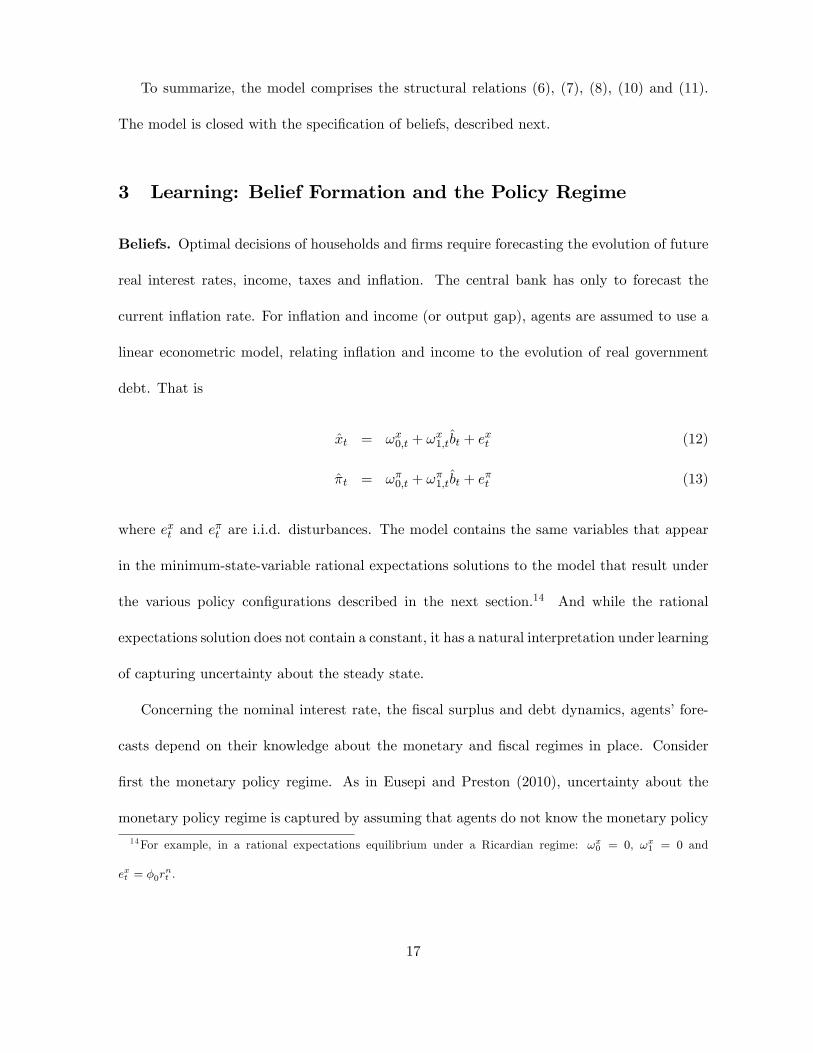
To summarize, the model comprises the structural relations (6), (7), (8), (10) and (11).

The model is closed with the speci�cation of beliefs, described next.

3 Learning: Belief Formation and the Policy Regime

Beliefs. Optimal decisions of households and �rms require forecasting the evolution of future

real interest rates, income, taxes and in�ation. The central bank has only to forecast the

current in�ation rate. For in�ation and income (or output gap), agents are assumed to use a

linear econometric model, relating in�ation and income to the evolution of real government

debt. That is

xt = !x0;t + !x1;tbt + e

xt (12)

�t = !�0;t + !�1;tbt + e

�t (13)

where ext and e�t are i.i.d. disturbances. The model contains the same variables that appear

in the minimum-state-variable rational expectations solutions to the model that result under

the various policy con�gurations described in the next section.14 And while the rational

expectations solution does not contain a constant, it has a natural interpretation under learning

of capturing uncertainty about the steady state.

Concerning the nominal interest rate, the �scal surplus and debt dynamics, agents�fore-

casts depend on their knowledge about the monetary and �scal regimes in place. Consider

�rst the monetary policy regime. As in Eusepi and Preston (2010), uncertainty about the

monetary policy regime is captured by assuming that agents do not know the monetary policy

14For example, in a rational expectations equilibrium under a Ricardian regime: !x0 = 0, !x1 = 0 and

ext = �0rnt .

17

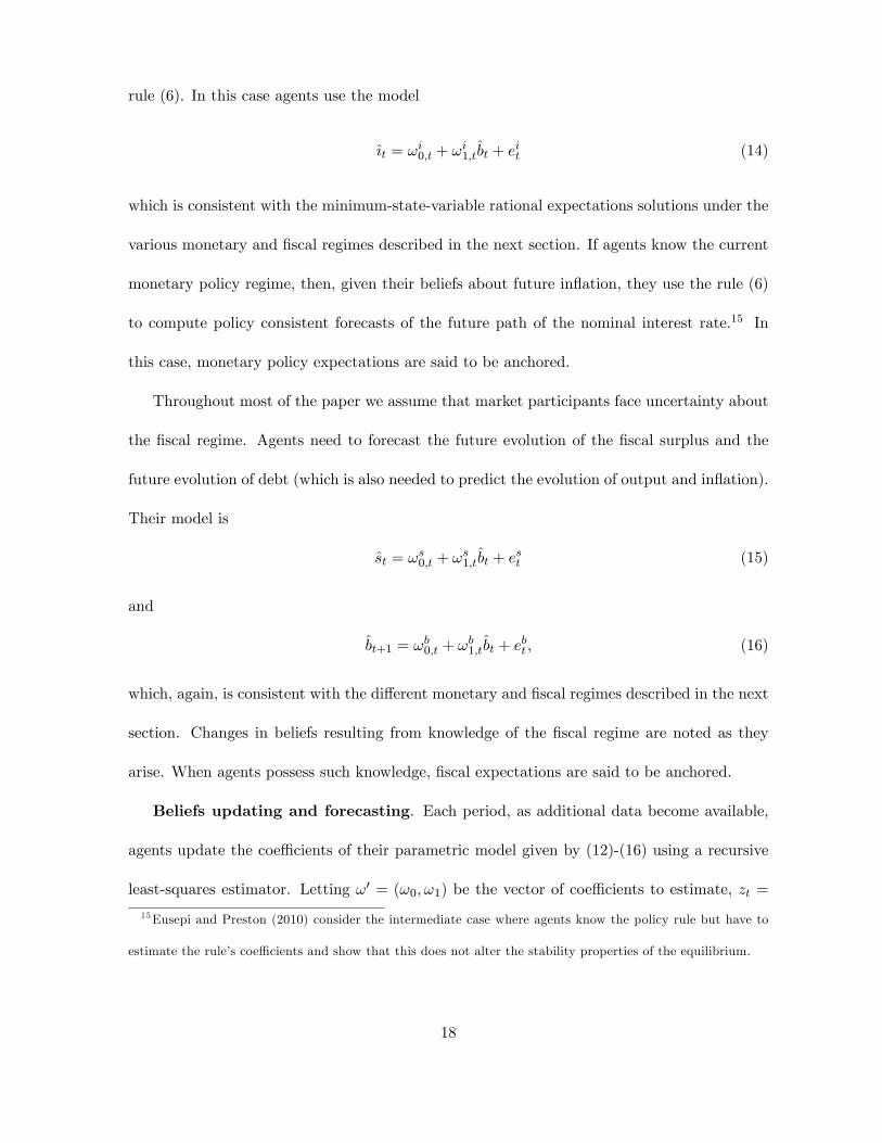
rule (6). In this case agents use the model

{t = !i0;t + !

i1;tbt + e

it (14)

which is consistent with the minimum-state-variable rational expectations solutions under the

various monetary and �scal regimes described in the next section. If agents know the current

monetary policy regime, then, given their beliefs about future in�ation, they use the rule (6)

to compute policy consistent forecasts of the future path of the nominal interest rate.15 In

this case, monetary policy expectations are said to be anchored.

Throughout most of the paper we assume that market participants face uncertainty about

the �scal regime. Agents need to forecast the future evolution of the �scal surplus and the

future evolution of debt (which is also needed to predict the evolution of output and in�ation).

Their model is

st = !s0;t + !

s1;tbt + e

st (15)

and

bt+1 = !b0;t + !

b1;tbt + e

bt ; (16)

which, again, is consistent with the di¤erent monetary and �scal regimes described in the next

section. Changes in beliefs resulting from knowledge of the �scal regime are noted as they

arise. When agents possess such knowledge, �scal expectations are said to be anchored.

Beliefs updating and forecasting. Each period, as additional data become available,

agents update the coe¢ cients of their parametric model given by (12)-(16) using a recursive

least-squares estimator. Letting !0 = (!0; !1) be the vector of coe¢ cients to estimate, zt =

15Eusepi and Preston (2010) consider the intermediate case where agents know the policy rule but have to

estimate the rule�s coe¢ cients and show that this does not alter the stability properties of the equilibrium.

18

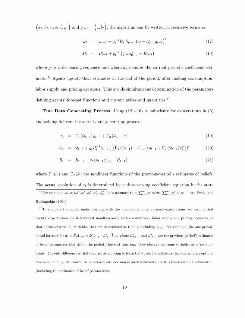
�xt; �t; {t; st; bt+1

�and qt�1 =

�1; bt

�, the algorithm can be written in recursive terms as

!t = !t�1 + g�1t R

�1t qt�1

�zt � !0t�1qt�1

�0 (17)

Rt = Rt�1 + g�1t

�qt�1q

0t�1 �Rt�1

�(18)

where gt is a decreasing sequence and where !t denotes the current-period�s coe¢ cient esti-

mate.16 Agents update their estimates at the end of the period, after making consumption,

labor supply and pricing decisions. This avoids simultaneous determination of the parameters

de�ning agents�forecast functions and current prices and quantities.17

True Data Generating Process. Using (12)-(16) to substitute for expectations in (5)

and solving delivers the actual data generating process

zt = �1 (!t�1) qt�1 + �2 (!t�1) rnt (19)

!t = !t�1 + gtR�1t qt�1

����1 (!t�1)� !0t�1

�qt�1 + �2 (!t�1) r

nt

��0 (20)

Rt = Rt�1 + gt�qt�1q

0t�1 �Rt�1

�(21)

where �1 (!) and �2 (!) are nonlinear functions of the previous-period�s estimates of beliefs.

The actual evolution of zt is determined by a time-varying coe¢ cient equation in the state16For example, !0 = (!x0 ; !

�0 ; !

i0; !

s0; !

b0). It is assumed that

P1t=1 gt = 1,

P1t=1 g

2t < 1 � see Evans and

Honkapohja (2001).

17To compare the model under learning with the predictions under rational expectations, we assume that

agents�expectations are determined simultaneously with consumption, labor supply and pricing decisions, so

that agents observe all variables that are determined at time t, including bt+1. For example, the one-period-

ahead forecast for �t is Et�t+1 = !�0;t�1+ !�1t�1bt+1 where !

�0;t�1 and !

�1t�1 are the previous-period�s estimates

of belief parameters that de�ne the period-t forecast function. They observe the same variables as a �rational�

agent. The only di¤erence is that they are attempting to learn the �correct�coe¢ cients that characterize optimal

forecasts. Finally, the central bank interest rate decision is predetermined since it is based on t� 1 information

(including the estimates of belief parameters).

19

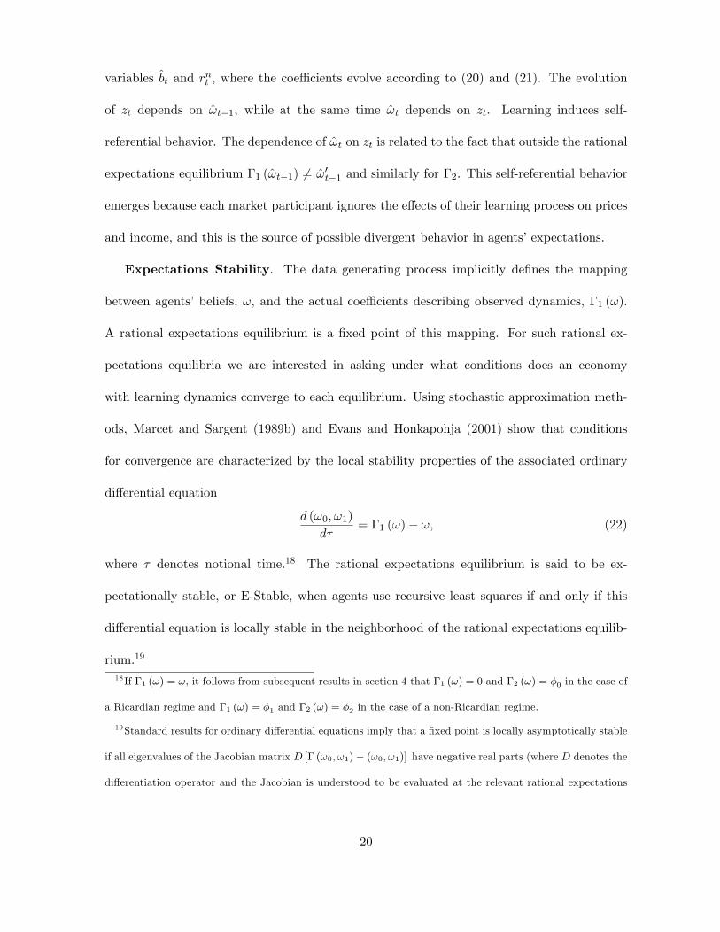
variables bt and rnt , where the coe¢ cients evolve according to (20) and (21). The evolution

of zt depends on !t�1, while at the same time !t depends on zt. Learning induces self-

referential behavior. The dependence of !t on zt is related to the fact that outside the rational

expectations equilibrium �1 (!t�1) 6= !0t�1 and similarly for �2. This self-referential behavior

emerges because each market participant ignores the e¤ects of their learning process on prices

and income, and this is the source of possible divergent behavior in agents�expectations.

Expectations Stability. The data generating process implicitly de�nes the mapping

between agents�beliefs, !, and the actual coe¢ cients describing observed dynamics, �1 (!).

A rational expectations equilibrium is a �xed point of this mapping. For such rational ex-

pectations equilibria we are interested in asking under what conditions does an economy

with learning dynamics converge to each equilibrium. Using stochastic approximation meth-

ods, Marcet and Sargent (1989b) and Evans and Honkapohja (2001) show that conditions

for convergence are characterized by the local stability properties of the associated ordinary

di¤erential equation

d (!0; !1)

d�= �1 (!)� !; (22)

where � denotes notional time.18 The rational expectations equilibrium is said to be ex-

pectationally stable, or E-Stable, when agents use recursive least squares if and only if this

di¤erential equation is locally stable in the neighborhood of the rational expectations equilib-

rium.19

18 If �1 (!) = !, it follows from subsequent results in section 4 that �1 (!) = 0 and �2 (!) = �0 in the case of

a Ricardian regime and �1 (!) = �1 and �2 (!) = �2 in the case of a non-Ricardian regime.

19Standard results for ordinary di¤erential equations imply that a �xed point is locally asymptotically stable

if all eigenvalues of the Jacobian matrix D [� (!0; !1)� (!0; !1)] have negative real parts (where D denotes the

di¤erentiation operator and the Jacobian is understood to be evaluated at the relevant rational expectations

20

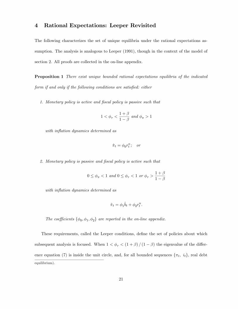
4 Rational Expectations: Leeper Revisited

The following characterizes the set of unique equilibria under the rational expectations as-

sumption. The analysis is analogous to Leeper (1991), though in the context of the model of

section 2. All proofs are collected in the on-line appendix.

Proposition 1 There exist unique bounded rational expectations equilibria of the indicated

form if and only if the following conditions are satis�ed: either

1. Monetary policy is active and �scal policy is passive such that

1 < �� <1 + �

1� � and �� > 1

with in�ation dynamics determined as

�t = �0rnt ; or

2. Monetary policy is passive and �scal policy is active such that

0 � �� < 1 and 0 � �� < 1 or �� >1 + �

1� �

with in�ation dynamics determined as

�t = �1bt + �2rnt :

The coe¢ cients f�0; �1; �2g are reported in the on-line appendix.

These requirements, called the Leeper conditions, de�ne the set of policies about which

subsequent analysis is focused. When 1 < �� < (1 + �) = (1� �) the eigenvalue of the di¤er-

ence equation (7) is inside the unit circle, and, for all bounded sequences f�t; itg; real debt

equilibrium).

21

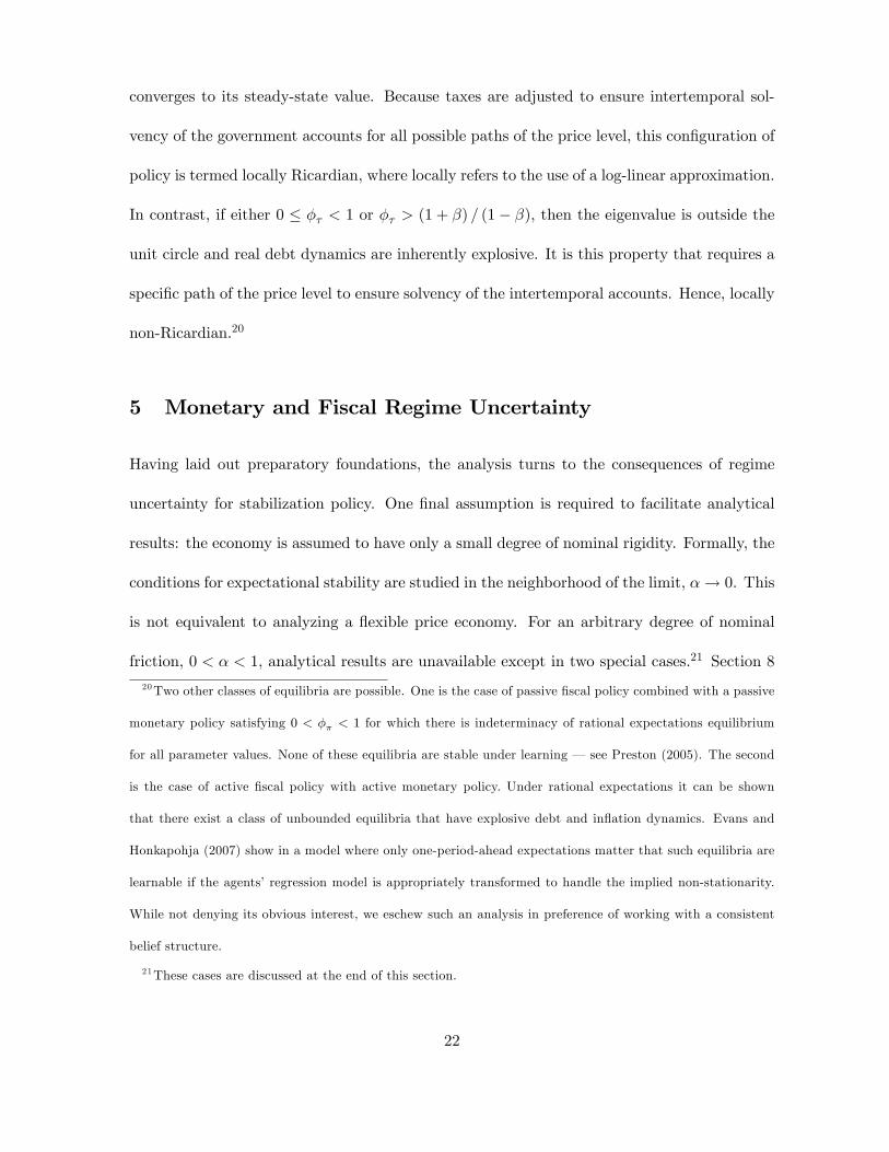
converges to its steady-state value. Because taxes are adjusted to ensure intertemporal sol-

vency of the government accounts for all possible paths of the price level, this con�guration of

policy is termed locally Ricardian, where locally refers to the use of a log-linear approximation.

In contrast, if either 0 � �� < 1 or �� > (1 + �) = (1� �), then the eigenvalue is outside the

unit circle and real debt dynamics are inherently explosive. It is this property that requires a

speci�c path of the price level to ensure solvency of the intertemporal accounts. Hence, locally

non-Ricardian.20

5 Monetary and Fiscal Regime Uncertainty

Having laid out preparatory foundations, the analysis turns to the consequences of regime

uncertainty for stabilization policy. One �nal assumption is required to facilitate analytical

results: the economy is assumed to have only a small degree of nominal rigidity. Formally, the

conditions for expectational stability are studied in the neighborhood of the limit, �! 0. This

is not equivalent to analyzing a �exible price economy. For an arbitrary degree of nominal

friction, 0 < � < 1, analytical results are unavailable except in two special cases.21 Section 8

20Two other classes of equilibria are possible. One is the case of passive �scal policy combined with a passive

monetary policy satisfying 0 < �� < 1 for which there is indeterminacy of rational expectations equilibrium

for all parameter values. None of these equilibria are stable under learning � see Preston (2005). The second

is the case of active �scal policy with active monetary policy. Under rational expectations it can be shown

that there exist a class of unbounded equilibria that have explosive debt and in�ation dynamics. Evans and

Honkapohja (2007) show in a model where only one-period-ahead expectations matter that such equilibria are

learnable if the agents�regression model is appropriately transformed to handle the implied non-stationarity.

While not denying its obvious interest, we eschew such an analysis in preference of working with a consistent

belief structure.

21These cases are discussed at the end of this section.

22

provides some more general numerical examples.

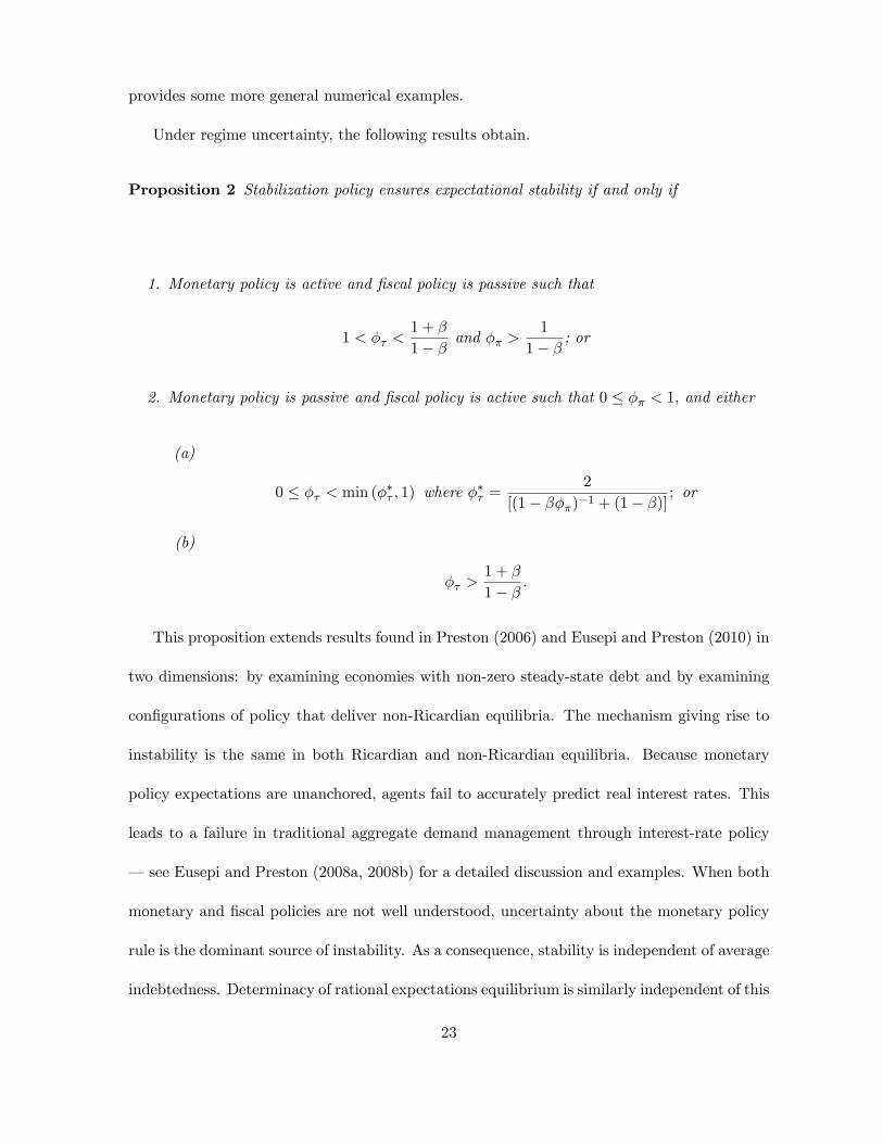
Under regime uncertainty, the following results obtain.

Proposition 2 Stabilization policy ensures expectational stability if and only if

1. Monetary policy is active and �scal policy is passive such that

1 < �� <1 + �

1� � and �� >1

1� � ; or

2. Monetary policy is passive and �scal policy is active such that 0 � �� < 1; and either

(a)

0 � �� < min (��� ; 1) where ��� =2

[(1� ���)�1 + (1� �)]; or

(b)

�� >1 + �

1� � :

This proposition extends results found in Preston (2006) and Eusepi and Preston (2010) in

two dimensions: by examining economies with non-zero steady-state debt and by examining

con�gurations of policy that deliver non-Ricardian equilibria. The mechanism giving rise to

instability is the same in both Ricardian and non-Ricardian equilibria. Because monetary

policy expectations are unanchored, agents fail to accurately predict real interest rates. This

leads to a failure in traditional aggregate demand management through interest-rate policy

� see Eusepi and Preston (2008a, 2008b) for a detailed discussion and examples. When both

monetary and �scal policies are not well understood, uncertainty about the monetary policy

rule is the dominant source of instability. As a consequence, stability is independent of average

indebtedness. Determinacy of rational expectations equilibrium is similarly independent of this

23

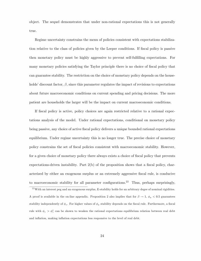
object. The sequel demonstrates that under non-rational expectations this is not generally

true.

Regime uncertainty constrains the menu of policies consistent with expectations stabiliza-

tion relative to the class of policies given by the Leeper conditions. If �scal policy is passive

then monetary policy must be highly aggressive to prevent self-ful�lling expectations. For

many monetary policies satisfying the Taylor principle there is no choice of �scal policy that

can guarantee stability. The restriction on the choice of monetary policy depends on the house-

holds�discount factor, �, since this parameter regulates the impact of revisions to expectations

about future macroeconomic conditions on current spending and pricing decisions. The more

patient are households the larger will be the impact on current macroeconomic conditions.

If �scal policy is active, policy choices are again restricted relative to a rational expec-

tations analysis of the model. Under rational expectations, conditional on monetary policy

being passive, any choice of active �scal policy delivers a unique bounded rational expectations

equilibrium. Under regime uncertainty this is no longer true. The precise choice of monetary

policy constrains the set of �scal policies consistent with macroeconomic stability. However,

for a given choice of monetary policy there always exists a choice of �scal policy that prevents

expectations-driven instability. Part 2(b) of the proposition shows that a �scal policy, char-

acterized by either an exogenous surplus or an extremely aggressive �scal rule, is conducive

to macroeconomic stability for all parameter con�gurations.22 Thus, perhaps surprisingly,

22With an interest peg and an exogenous surplus, E-stability holds for an arbitrary degee of nominal rigidities.

A proof is available in the on-line appendix. Proposition 2 also implies that for � ! 1, �� < 0:5 guarantees

stability independently of �� . For higher values of �� stability depends on the �scal rule. Furthermore, a �scal

rule with �� > ��� can be shown to weaken the rational expectations equilibrium relation between real debt

and in�ation, making in�ation expectations less responsive to the level of real debt.

24

non-Ricardian regimes appear to be more robust to learning dynamics.

The learning behavior of both private agents and the central bank engenders the insta-

bility result. If the central bank could perfectly observe current in�ation, then the stability

conditions under learning are the Leeper conditions: the same restrictions implied by local

determinacy.23 This result is special to the model at hand. Permitting multiple-maturity debt

is su¢ cient to undermine stability even when in�ation is accurately observed � see Eusepi

and Preston (2007). This is because bond prices themselves depend on expectations about

future policy, which tends to make the equilibria more susceptible to instability.

6 Resolving Uncertainty about Monetary Policy

To isolate the role of uncertainty about the �scal regime, follow Eusepi and Preston (2010),

and consider the bene�ts of credibly communicating the monetary policy rule to �rms and

households. The precise details of the monetary policy rule are announced, including the

policy coe¢ cients and conditioning variables. Knowledge of this rule serves to simplify �rms�

and households�forecasting problems. Agents need only forecast in�ation: policy-consistent

forecasts of future nominal interest rates can then be determined directly from the announced

policy rule. It follows that credible announcements have the property that expectations about

future macroeconomic conditions are consistent with the policy strategy of the monetary

authority. In this sense, monetary policy expectations are anchored.

23A proof for arbitrary degree of nominal rigidity is available in the on-line appendix.

25

Under communication of the policy regime the aggregate demand equation becomes

xt = ���1�bt � �t

�� ��1�st � (1� �)��Et�1�t

+Et

1XT=t

�T�t [(1� �) (xT+1 � �sT+1)� (1� �) (��� � 1) �T+1 + rnT ] (23)

determined by direct substitution of the monetary policy rule into equation (10). The re-

maining model equations are unchanged with the exception of beliefs. As nominal interest

rates need not be forecast, an agent�s vector autoregression model is estimated on the re-

stricted state vector zt =�xt; �t; st; bt+1

�: Knowledge of the monetary policy regime does not

eliminate uncertainty about the statistical laws determining state variables, as future output,

in�ation, taxes and real debt must still be forecasted to make spending and pricing decisions.

And, in particular, the details of the �scal policy regime remain uncertain.

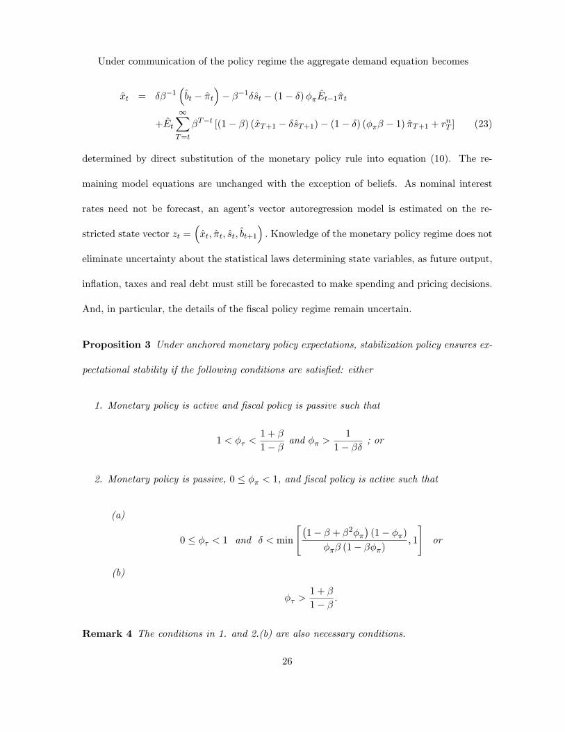
Proposition 3 Under anchored monetary policy expectations, stabilization policy ensures ex-

pectational stability if the following conditions are satis�ed: either

1. Monetary policy is active and �scal policy is passive such that

1 < �� <1 + �

1� � and �� >1

1� �� ; or

2. Monetary policy is passive, 0 � �� < 1, and �scal policy is active such that

(a)

0 � �� < 1 and � < min

"�1� � + �2��

�(1� ��)

��� (1� ���); 1

#or

(b)

�� >1 + �

1� � :

Remark 4 The conditions in 1. and 2.(b) are also necessary conditions.

26

Regardless of the regime, guarding against expectations-driven instability for a given choice

of tax rule, �� , requires a choice of monetary policy rule that depends on two model parameters:

the household�s discount factor, �, and the steady-state ratio of the primary surplus to output,

� (or equivalently the steady-state debt-to-output ratio since �s = (1� �)�b). The choice of

�scal regime, re�ected in the implied average debt-to-output ratio, imposes constraints on

stabilization policy. Less �scally responsible governments have access to a smaller set of

monetary policies to ensure learnability of rational expectations equilibrium. In the case of

passive �scal policies, the higher is the average debt-to-output ratio, the more aggressive must

monetary policy be to protect the economy from self-ful�lling expectations.

Similarly, under active �scal policies, the choice of monetary policy is again constrained

by the average level of indebtedness of the economy. The higher are average debt levels the

more passive must be the adopted monetary policy rule. Regardless of the policy regime,

for 0 < � < 1, the menu of policies consistent with stabilizing expectations is larger than

when agents are uncertain about monetary policy strategy � compare proposition 2. This

discussion is summarized in the following proposition which presents two special cases of the

above results.

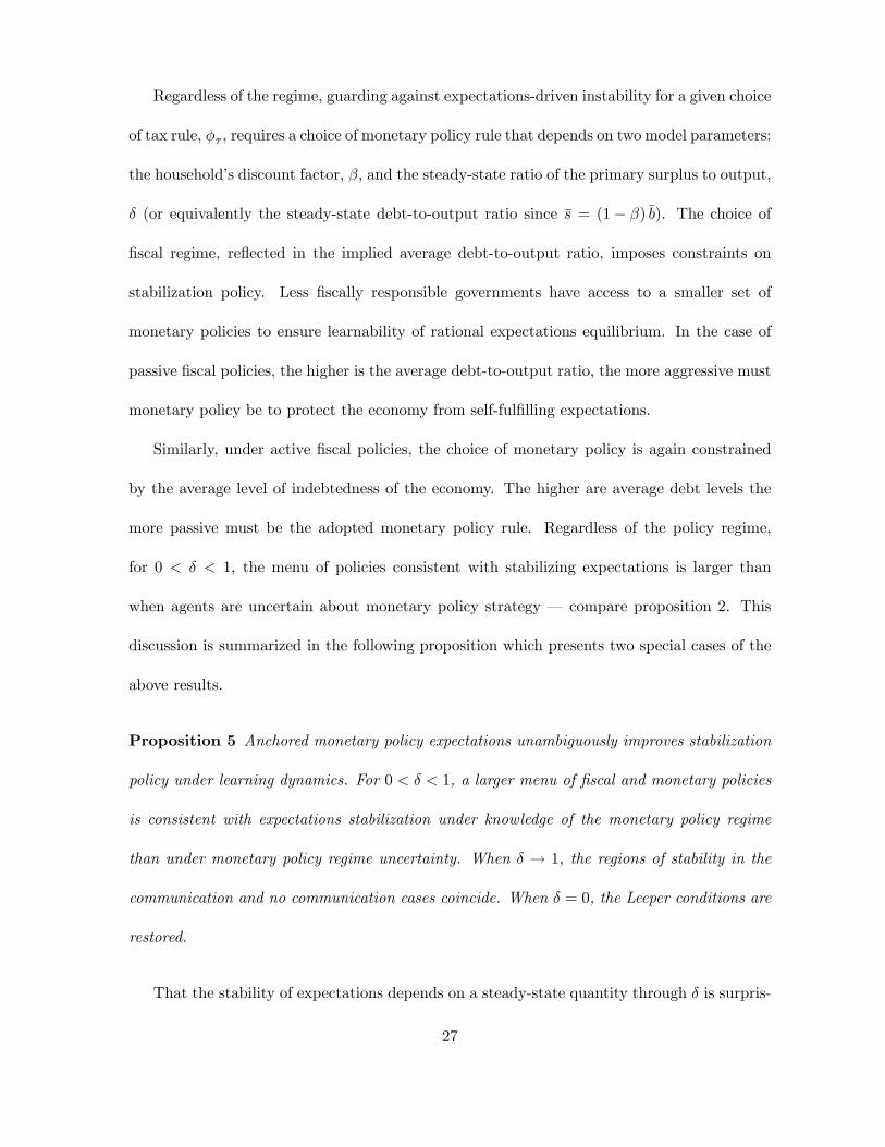
Proposition 5 Anchored monetary policy expectations unambiguously improves stabilization

policy under learning dynamics. For 0 < � < 1, a larger menu of �scal and monetary policies

is consistent with expectations stabilization under knowledge of the monetary policy regime

than under monetary policy regime uncertainty. When � ! 1, the regions of stability in the

communication and no communication cases coincide. When � = 0, the Leeper conditions are

restored.

That the stability of expectations depends on a steady-state quantity through � is surpris-

27

ing when compared to a rational expectations analysis: determinacy conditions are indepen-

dent of this quantity. What then is the source of this dependence?

Proposition 3 makes clear that the choice of monetary policy, ��, and the steady-state

structural surplus-to-output ratio, �, play a crucial role in determining stability, in both Ri-

cardian and non-Ricardian policy equilibria. The main source of instability is a class of wealth

e¤ects arising from violations of Ricardian equivalence: agents perceive real bonds to be net

wealth out of rational expectations equilibrium.

Active Monetary Policy and Passive Fiscal Policy. To provide intuition, consider

a regime with active monetary policy and passive �scal policy. Suppose that in�ation ex-

pectations increase. Because of communication agents correctly predict a steeper path of the

nominal interest rate (as forecasts satisfy the Taylor principle), which restrains aggregate de-

mand, leading to lower actual in�ation. In an economy with zero net debt, expectations of

future in�ation decline, driving the economy back to equilibrium. But with holdings of the

public debt treated as net wealth, lower in�ation generates a positive wealth e¤ect, stimulating

aggregate demand and increasing in�ationary pressures. The increase in real debt is larger if

the monetary authority does not observe current prices because the nominal interest rate does

not immediately decrease with in�ation. On the one hand, active policy restrains demand as

agents expect higher future real interest rates. On the other hand, larger real debt and higher

expected nominal interest rates generate wealth e¤ects with in�ationary consequences. If the

monetary policy rule is not su¢ ciently active and the stock of government debt is large the

latter prevail, leading to instability.

Further insight into this result can be obtained by considering a more general form of

utility function with constant consumption intertemporal elasticity of substitution, � > 0.

28

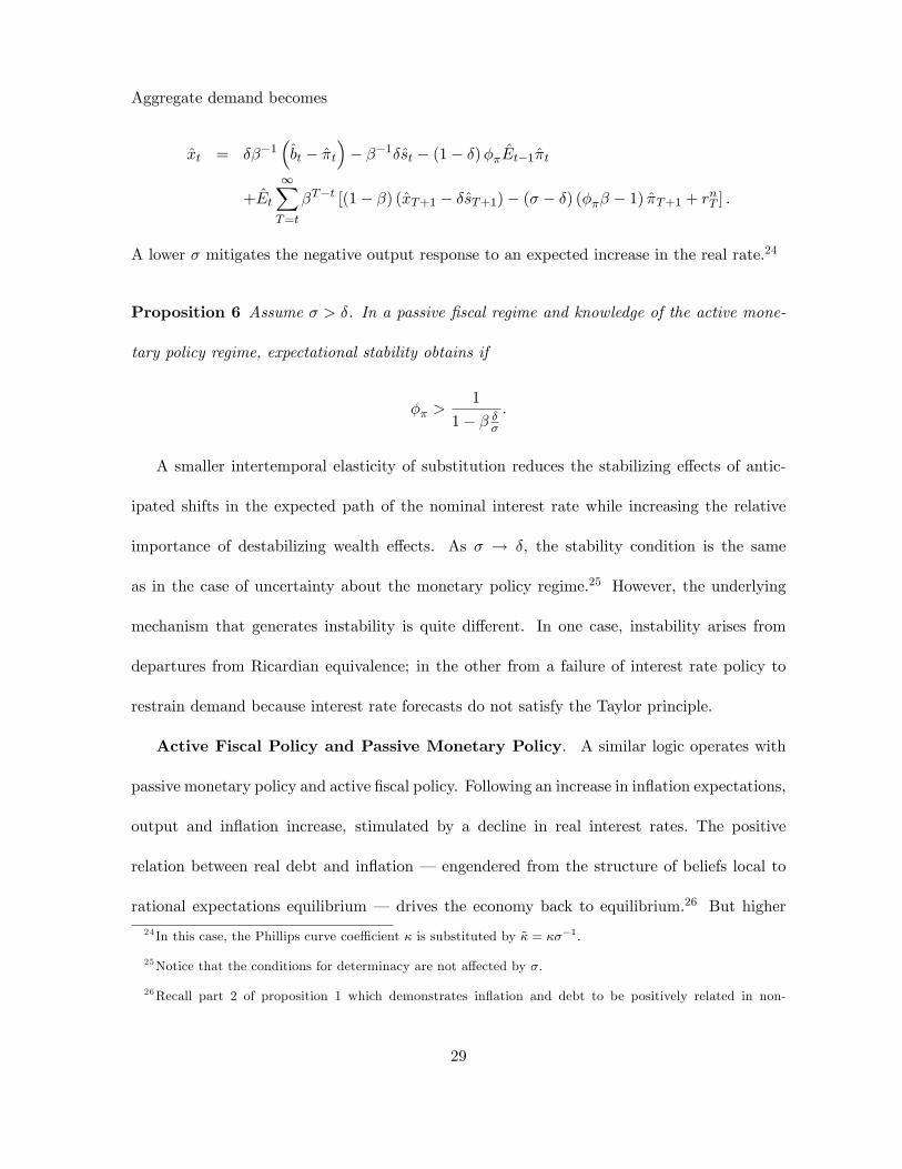
Aggregate demand becomes

xt = ���1�bt � �t

�� ��1�st � (1� �)��Et�1�t

+Et

1XT=t

�T�t [(1� �) (xT+1 � �sT+1)� (� � �) (��� � 1) �T+1 + rnT ] :

A lower � mitigates the negative output response to an expected increase in the real rate.24

Proposition 6 Assume � > �. In a passive �scal regime and knowledge of the active mone-

tary policy regime, expectational stability obtains if

�� >1

1� � ��:

A smaller intertemporal elasticity of substitution reduces the stabilizing e¤ects of antic-

ipated shifts in the expected path of the nominal interest rate while increasing the relative

importance of destabilizing wealth e¤ects. As � ! �, the stability condition is the same

as in the case of uncertainty about the monetary policy regime.25 However, the underlying

mechanism that generates instability is quite di¤erent. In one case, instability arises from

departures from Ricardian equivalence; in the other from a failure of interest rate policy to

restrain demand because interest rate forecasts do not satisfy the Taylor principle.

Active Fiscal Policy and Passive Monetary Policy. A similar logic operates with

passive monetary policy and active �scal policy. Following an increase in in�ation expectations,

output and in�ation increase, stimulated by a decline in real interest rates. The positive

relation between real debt and in�ation � engendered from the structure of beliefs local to

rational expectations equilibrium � drives the economy back to equilibrium.26 But higher

24 In this case, the Phillips curve coe¢ cient � is substituted by ~� = ���1.

25Notice that the conditions for determinacy are not a¤ected by �.

26Recall part 2 of proposition 1 which demonstrates in�ation and debt to be positively related in non-

29

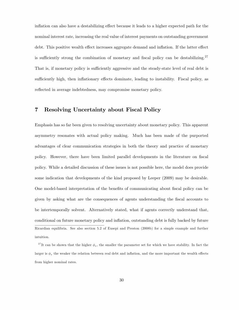
in�ation can also have a destabilizing e¤ect because it leads to a higher expected path for the

nominal interest rate, increasing the real value of interest payments on outstanding government

debt. This positive wealth e¤ect increases aggregate demand and in�ation. If the latter e¤ect

is su¢ ciently strong the combination of monetary and �scal policy can be destabilizing.27

That is, if monetary policy is su¢ ciently aggressive and the steady-state level of real debt is

su¢ ciently high, then in�ationary e¤ects dominate, leading to instability. Fiscal policy, as

re�ected in average indebtedness, may compromise monetary policy.

7 Resolving Uncertainty about Fiscal Policy

Emphasis has so far been given to resolving uncertainty about monetary policy. This apparent

asymmetry resonates with actual policy making. Much has been made of the purported

advantages of clear communication strategies in both the theory and practice of monetary

policy. However, there have been limited parallel developments in the literature on �scal

policy. While a detailed discussion of these issues is not possible here, the model does provide

some indication that developments of the kind proposed by Leeper (2009) may be desirable.

One model-based interpretation of the bene�ts of communicating about �scal policy can be

given by asking what are the consequences of agents understanding the �scal accounts to

be intertemporally solvent. Alternatively stated, what if agents correctly understand that,

conditional on future monetary policy and in�ation, outstanding debt is fully backed by future

Ricardian equilibria. See also section 5.2 of Eusepi and Preston (2008b) for a simple example and further

intuition.

27 It can be shown that the higher �� , the smaller the parameter set for which we have stability. In fact the

larger is �� the weaker the relation between real debt and in�ation, and the more important the wealth e¤ects

from higher nominal rates.

30

taxation � in which case we say agents��scal expectations are anchored. Aside from this

implied restriction, agents�beliefs are speci�ed as in section 6.

Proposition 7 Suppose agents have anchored �scal expectations, so that households and �rms

understand that the restriction�bt � �t

�= Et

1XT=t

�T�t [(1� �) sT � � ({T � �T+1)] (24)

holds at all times. Anchored �scal expectations restore the Leeper conditions as necessary and

su¢ cient for stability.

Proposition 7 suggests that communication about �scal policy may be as important to

stabilization objectives as communication about monetary policy. If both monetary and �scal

expectations are anchored in the sense that i) forecasts of in�ation and nominal interest rates

satisfy the monetary policy rule (6); and ii) forecasts of in�ation, debt, nominal interest rates

and taxes satisfy the intertemporal solvency condition (24), then the Leeper conditions are

necessary and su¢ cient for stabilizing expectations. Contrasting propositions 3 and 7 reveals

a deeper insight: absent anchored �scal expectations, anchoring monetary policy expectations

yields fewer stabilization bene�ts � a smaller set of monetary policies are consistent with

stability � the larger is the debt-to-output ratio. In the limit � ! 1, failure to communicate

about �scal policy completely undermines any stabilization bene�ts from anchoring monetary

policy expectations. This raises serious questions about the e¢ cacy of monetary policy in

situations of considerable macroeconomic uncertainty in which there are dramatic expansions

in the scale and scope of �scal activities, as witnessed in many economies in response to the

�nancial crisis of 2008.

The special case � = 0 is isomorphic in terms of stability of expectations to the more

general case of anchored �scal expectations. This underscores the importance of debt dynamics

31

to expectations stabilization: from an expectational stability viewpoint, indebtedness only

matters to the extent agents are uncertain about the long-run consequences of �scal policy.

Absent anchored monetary expectations, anchored �scal expectations provide no advantages

from an expectational stability perspective � the conditions of proposition 3 are operative.

Implications for the sequencing of institutional reform suggests themselves.

Finally, note that for the question of expectational stability, no speci�c assumption need

be made about how the government actually intends to achieve intertemporal solvency. All

that is required is agents believe government promises that the �scal regime is consistent with

�scal solvency at any point in time. Given observed current debt and in�ation, and forecasts

of future interest rates and in�ation, agents can infer the expected present discounted value

of taxes that satis�es (24). This does not mean �scal variables are irrelevant � the projected

evolution of debt is still used in forecasts. And the precise details of how taxes are actually

adjusted will matter for dynamics out-of-rational-expectations equilibrium.

8 The Public Debt and Macroeconomic Dynamics

The preceding analytical results have focused on the implications of regime uncertainty on

the ability of monetary and �scal policy makers to stabilize expectations in the long run. A

no less interesting and pressing question in the light of the Global Financial Crisis concerns

the consequences of policy uncertainty for macroeconomic dynamics, even when expectational

stability is guaranteed asymptotically. Speci�cally, do anchored �scal expectations improve

stabilization policy out of rational expectations equilibrium? And do high debt levels impair

macroeconomic control by monetary and �scal policy makers? The following examines model-

implied impulse response functions to an in�ation shock to answer these questions.

32

8.1 Generating Impulse Response Functions

The impulse response functions to a shock to in�ation expectations are generated as follows.

The model is simulated 5000 times assuming shocks to the natural rate, monetary policy and

tax policy have standard deviations: �r = 1, �i = 0:1 and �� = 0:1.28 A quarterly model is

assumed giving a discount factor � = 0:99. In contrast to the analytical results, more general

assumptions are made about the degree of nominal rigidities and the elasticity of intertemporal

substitution. The Calvo parameter is �xed at � = 0:6, consistent with Blinder, Canetti,

Lebow, and Rudd (1998) and Bils and Klenow (2004). A utility function with intertemporal

elasticity of substitution of consumption equal to 0:3 is considered, consistent with broad

�ndings in the macroeconomics literature. Monetary policy is speci�ed as �� = 1:5 and tax

policy as �� = 4. Monetary expectations are anchored; �scal expectations are not.

Two levels of average indebtedness are considered: a low debt economy, which has a debt-

to-output ratio of zero on average, � = 0; and a high debt economy with a debt-to-output ratio

of 4�b= �Y = 2:3 (in annual terms). While the latter is arguably large, it is chosen to emphasize

the dynamics that operate in a high debt economy. It is also the only asset that can be held

in this economy � there is no capital. Note also that these two economies are su¢ cient to

answer the two questions posed above. High average indebtedness is only relevant to dynamics

when �scal expectations are not anchored � recall section 7.

The impulse response functions are computed by perturbing each simulated path by an

expectational shock. The di¤erence between these perturbed paths and the original paths pro-

vides the impulse response functions. They are non-linear because of the learning dynamics

28Shocks to the policy rules are added to prevent agents from learning the policy coe¢ cients after few data

points. However, their inclusion does not a¤ect the stability results.

33

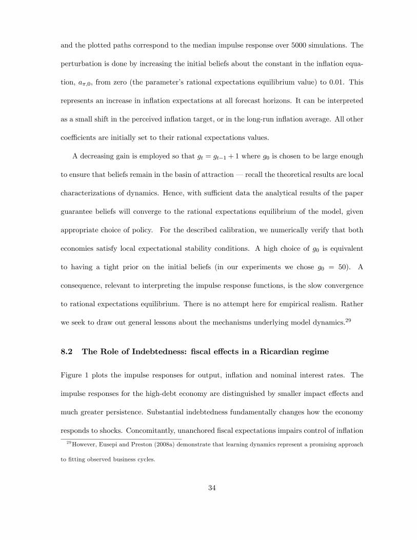
and the plotted paths correspond to the median impulse response over 5000 simulations. The

perturbation is done by increasing the initial beliefs about the constant in the in�ation equa-

tion, a�;0, from zero (the parameter�s rational expectations equilibrium value) to 0:01. This

represents an increase in in�ation expectations at all forecast horizons. It can be interpreted

as a small shift in the perceived in�ation target, or in the long-run in�ation average. All other

coe¢ cients are initially set to their rational expectations values.

A decreasing gain is employed so that gt = gt�1 + 1 where g0 is chosen to be large enough

to ensure that beliefs remain in the basin of attraction � recall the theoretical results are local

characterizations of dynamics. Hence, with su¢ cient data the analytical results of the paper

guarantee beliefs will converge to the rational expectations equilibrium of the model, given

appropriate choice of policy. For the described calibration, we numerically verify that both

economies satisfy local expectational stability conditions. A high choice of g0 is equivalent

to having a tight prior on the initial beliefs (in our experiments we chose g0 = 50). A

consequence, relevant to interpreting the impulse response functions, is the slow convergence

to rational expectations equilibrium. There is no attempt here for empirical realism. Rather

we seek to draw out general lessons about the mechanisms underlying model dynamics.29

8.2 The Role of Indebtedness: �scal e¤ects in a Ricardian regime

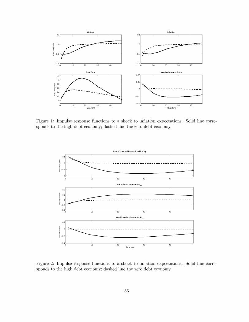
Figure 1 plots the impulse responses for output, in�ation and nominal interest rates. The

impulse responses for the high-debt economy are distinguished by smaller impact e¤ects and

much greater persistence. Substantial indebtedness fundamentally changes how the economy

responds to shocks. Concomitantly, unanchored �scal expectations impairs control of in�ation

29However, Eusepi and Preston (2008a) demonstrate that learning dynamics represent a promising approach

to �tting observed business cycles.

34

and output.

To understand the nature of these di¤erences it is useful to decompose aggregate demand

into the following terms

xt = �

��1

�bt � �t

�� ��1st + Et

1XT=t

�T�t [({T � �T+1)� (1� �) sT+1]!

+Et

1XT=t

�T�t [(1� �) xT+1 � � ({T � �T+1) + rnT ]

= �;t +R;t (25)

where

�;t = �

��1

�bt � �t

�� ��1st + Et

1XT=t

�T�t [({T � �T+1)� (1� �) sT+1]!

and R;t captures remaining terms. The variable R;t isolates terms that would obtain in

a zero-debt economy, or equivalently, one in which �scal expectations are anchored. �;t

captures departures from this benchmark, representing deviations from Ricardian equivalence

because holdings of the public debt are treated as net wealth. It is the real value of holdings

of the public debt once future tax and interest obligations are accounted for.

Figure 2 plots these two terms. It is immediate that �;t generates destabilizing demand

e¤ects in a high-debt economy. In a regime with zero steady-state debt, active monetary

policy increases the expected future path of real rates reducing demand, and, in turn, curbing

in�ation until the economy returns to rational expectations equilibrium � see Figure 2 which

also plots the real long rate de�ned as

�t = Et

1XT=t

�T�t ({T � �T+1) :

In an economy with high steady-state debt this channel is still present. However, deviations

from Ricardian equivalence drive aggregate demand in the opposite direction. The term �;t

35

0 10 20 30 40­0.2

­0.1

0

0.1Output

%de

v. s

tead

y st

ate

0 10 20 30 40­0.2

­0.1

0

0.1Inflation

0 10 20 30 40

0

0.2

0.4

0.6

0.8

1

1.2

Real Debt

Quarters

%de

v. s

tead

y st

ate

0 10 20 30 40­0.04

­0.02

0

0.02

0.04Nominal Interest Rate

Quarters

Figure 1: Impulse response functions to a shock to in�ation expectations. Solid line corre-sponds to the high debt economy; dashed line the zero debt economy.

0 10 20 30 40­1

­0.5

0

0.5

D isc. Expected Future R eal R ate s:ρt

%de

v. s

tead

y st

ate

0 10 20 30 40­0.4

­0.2

0

0.2

0 .4

R icardian C omponent:ΨR,t

%de

v. s

tead

y st

ate

0 10 20 30 40­0.4

­0.2

0

0.2

N onR icardian C omponent :Ψδ,t

Quarte rs

%de

v. s

tead

y st

ate

Figure 2: Impulse response functions to a shock to in�ation expectations. Solid line corre-sponds to the high debt economy; dashed line the zero debt economy.

36

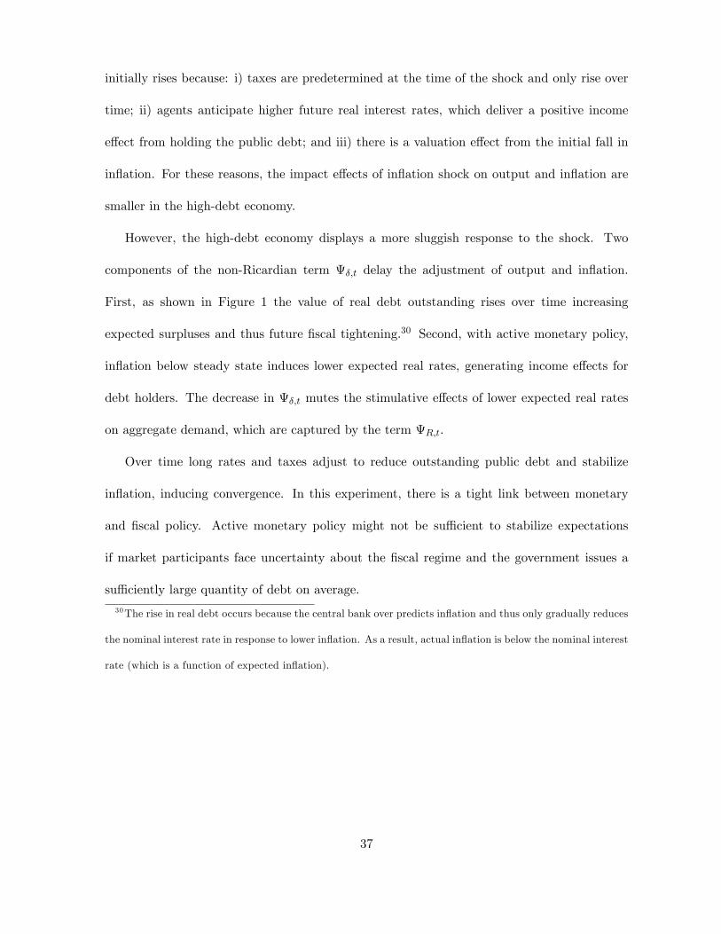
initially rises because: i) taxes are predetermined at the time of the shock and only rise over

time; ii) agents anticipate higher future real interest rates, which deliver a positive income

e¤ect from holding the public debt; and iii) there is a valuation e¤ect from the initial fall in

in�ation. For these reasons, the impact e¤ects of in�ation shock on output and in�ation are

smaller in the high-debt economy.

However, the high-debt economy displays a more sluggish response to the shock. Two

components of the non-Ricardian term �;t delay the adjustment of output and in�ation.

First, as shown in Figure 1 the value of real debt outstanding rises over time increasing

expected surpluses and thus future �scal tightening.30 Second, with active monetary policy,

in�ation below steady state induces lower expected real rates, generating income e¤ects for

debt holders. The decrease in �;t mutes the stimulative e¤ects of lower expected real rates

on aggregate demand, which are captured by the term R;t.

Over time long rates and taxes adjust to reduce outstanding public debt and stabilize

in�ation, inducing convergence. In this experiment, there is a tight link between monetary

and �scal policy. Active monetary policy might not be su¢ cient to stabilize expectations

if market participants face uncertainty about the �scal regime and the government issues a

su¢ ciently large quantity of debt on average.

30The rise in real debt occurs because the central bank over predicts in�ation and thus only gradually reduces

the nominal interest rate in response to lower in�ation. As a result, actual in�ation is below the nominal interest

rate (which is a function of expected in�ation).

37

9 Conclusions

This paper develops a model of policy regime uncertainty and its consequences for stabilizing

expectations. Uncertainty about monetary and �scal policy is shown to restrict, relative to

a rational expectations analysis, the set of policies consistent with macroeconomic stability.

Anchoring expectations about monetary and �scal policy enlarges the set of policies consistent

with stability. However, absent anchored �scal expectations, the advantages from anchoring

monetary expectations are smaller the larger is the average level of indebtedness. Finally, even

when expectations are stabilized in the long run, the higher are average debt levels the more

persistent will be the e¤ects of disturbances out of rational expectations equilibrium.

References

Aiyagari, R. (1994): �Uninsured Idiosyncratic Risk and Aggregate Saving,�Quarterly Jour-

nal of Economics, 109, 659�684.

Bils, M., and P. Klenow (2004): �Some Evidence on the Importance of Sticky Prices,�

Journal of Political Economy, 112, 947�985.

Blinder, A. S., E. R. D. Canetti, D. E. Lebow, and J. B. Rudd (1998): Asking

about prices: A new approach to understanding Price Stickiness. New York: Russell Sage

Foundation.

Bullard, J., and S. Eusepi (2008): �When Does Determinacy Imply Learnability?,�Federal

Reserve Bank of St. Louis Working Paper (007A).

Bullard, J., and K. Mitra (2002): �Learning About Monetary Policy Rules,�Journal of

Monetary Economics, 49(6), 1105�1129.

38

(2007): �Determinacy, Learnability and Monetary Policy Inertia,�Journal of Money,

Credit and Banking, 39, 1177�1212.

Christiano, L. J., M. Eichenbaum, and C. Evans (1999): �Monetary Policy Shocks:

What Have We Learned and to What End?,�in Handbook of Macroeconomics, ed. by J. B.

Taylor, and M. Woodford, vol. 1, chap. 2, pp. 65�148. Elsevier.

Clarida, R., J. Gali, and M. Gertler (1999): �The Science of Monetary Policy: A New

Keynesian Perspective,�Journal of Economic Literature, 37, 1661�1707.

Cochrane, J. H. (1998): �A Frictionless View of U.S. In�ation,� University of Chicago

mimeo.

Davig, T., and E. Leeper (2006): �Fluctuating Macro Policies and the Fiscal Theory,� in

NBER Macroeconomics Annual, ed. by D. Acemoglu, K. Rogo¤, and M. Woodford.

Eusepi, S. (2007): �Learnability and Monetary Policy: A Global Perspective,� Journal of

Monetary Economics, Forthcoming.

Eusepi, S., and B. Preston (2007): �Stabilization Policy with Near-Ricardian Households,�

unpublished, Columbia University.

(2008a): �Expectations, Learning and Business Cycle Fluctuations,�American Eco-

nomic Review, forthcoming.

(2008b): �Expectations Stabilization under Monetary and Fiscal Policy Coordina-

tion,�NBER Working Paper 14391.

(2010): �Central Bank Communication and Macroeconomic Stabilization,�American

Economic Journal: Macroeconomics, 2, 235�271.

39

Evans, G. W., and S. Honkapohja (2001): Learning and Expectations in Economics.

Princeton, Princeton University Press.

(2003): �Expectations and the Stability Problem for Optimal Monetary Policies,�

Review of Economic Studies, 70(4), 807�824.

(2005): �Policy Interaction, Expectations and the Liquidity Trap,�Review of Eco-

nomic Dynamics, 8, 303�323.

(2006): �Monetary Policy, Expectations and Commitment,�Scandanavian Journal

of Economics, 108, 15�38.

(2007): �Policy Interaction, Learning and the Fiscal Theory of Prices,�Macroeco-

nomic Dynamics, 11, 665�690.

Friedman, M. (1968): �The Role of Monetary Policy,�American Economic Review, 58(1),

1�17.

Howitt, P. (1992): �Interest Rate Control and Nonconvergence to Rational Expectations,�

Journal of Political Economy, 100(4), 776�800.

Kreps, D. (1998): �Anticipated Utility and Dynamic Choice,� in Frontiers of Research in

Economic Theory, ed. by D. Jacobs, E. Kalai, and M. Kamien, pp. 242�274. Cambridge:

Cambridge University Press.

Leeper, E. (1991): �Equilibria Under �Active�and �Passive�Monetary and Fiscal Policies,�

Journal of Monetary Economics, 27, 129�147.

(2009): �Anchoring Fiscal Expectations,�Reserve Bank of New Zealand: Bulletin,

Vol. 72, No. 3.

40

Leith, C., and L. von Thadden (2006): �Monetary and Fiscal Policy Interactions ina

New Keynesian Model with Capital Accumulation and Non-Ricardian Consumers,� ECB

Working Paper No. 649.

Marcet, A., and T. J. Sargent (1989a): �Convergence of Least-Squares Learning in

Environments with Hidden State Variables and Private Information,� Journal of Political

Economy, pp. 1306�1322.

(1989b): �Convergence of Least Squares Learning Mechanisms in Self-Referential

Linear Stochastic Models,�Journal of Economic Theory, (48), 337�368.

McCallum, B. T. (1999): �Issues in the Design of Monetary Policy Rules,�in Handbook of

Macroeconomics, ed. by J. Taylor, and M. Woodford. North-Holland, Amsterdam.

Preston, B. (2005): �Learning About Monetary Policy Rules when Long-Horizon Expecta-

tions Matter,�International Journal of Central Banking, 1(2), 81�126.

(2006): �Adaptive Learning, Forecast-Based Instrument Rules and Monetary Policy,�

Journal of Monetary Economics, 53, 507�535.

(2008): �Adaptive Learning and the Use of Forecasts in Monetary Policy,�Journal

of Economic Dynamics and Control, 32(4), 2661�3681.

Sargent, T. J. (1999): The Conquest of American In�ation. Princeton University Press.

Sims, C. (1994): �A Simple Model for the Determination of the Price Level and the Interaction

of Monetary and Fiscal Policy,�Economic Theory, 4, 381�399.

Taylor, J. (1993): �Discretion Versus Policy Rules in Practice,�Carnegie-Rochester Con-

ference Series on Public Policy, 39, 195-214.

41

Woodford, M. (1996): �Control of the Public Debt: A Requirement for Price Stability,�

NBER Working Paper 5684.

(2001): �Fiscal Requirements of Price Stability,� Journal of Money, Credit and

Banking, 33, 669�728.

(2003): Interest and Prices: Foundations of a Theory of Monetary Policy. Princeton

University Press.

42