chamnet: towards efficient network design through platform...

ChamNet: Towards Efficient Network Design through Platform-Aware Model

Adaptation

Xiaoliang Dai1∗, Peizhao Zhang2, Bichen Wu3∗, Hongxu Yin1, Fei Sun2, Yanghan Wang2, Marat Dukhan2,

Yunqing Hu2, Yiming Wu2, Yangqing Jia2, Peter Vajda2, Matt Uyttendaele2, Niraj K. Jha1

1Princeton University, 2Facebook Inc., 3University of California, Berkeley

Abstract

This paper proposes an efficient neural network (NN)

architecture design methodology called Chameleon that

honors given resource constraints. Instead of developing

new building blocks or using computationally-intensive re-

inforcement learning algorithms, our approach leverages

existing efficient network building blocks and focuses on

exploiting hardware traits and adapting computation re-

sources to fit target latency and/or energy constraints. We

formulate platform-aware NN architecture search in an op-

timization framework and propose a novel algorithm to

search for optimal architectures aided by efficient accu-

racy and resource (latency and/or energy) predictors. At

the core of our algorithm lies an accuracy predictor built

atop Gaussian Process with Bayesian optimization for iter-

ative sampling. With a one-time building cost for the pre-

dictors, our algorithm produces state-of-the-art model ar-

chitectures on different platforms under given constraints

in just minutes. Our results show that adapting computa-

tion resources to building blocks is critical to model per-

formance. Without the addition of any special features, our

models achieve significant accuracy improvements relative

to state-of-the-art handcrafted and automatically designed

architectures. We achieve 73.8% and 75.3% top-1 accuracy

on ImageNet at 20ms latency on a mobile CPU and DSP. At

reduced latency, our models achieve up to 8.2% (4.8%) and

6.7% (9.3%) absolute top-1 accuracy improvements com-

pared to MobileNetV2 and MnasNet, respectively, on a mo-

bile CPU (DSP), and 2.7% (4.6%) and 5.6% (2.6%) accu-

racy gains over ResNet-101 and ResNet-152, respectively,

on an Nvidia GPU (Intel CPU).

1. Introduction

Neural networks (NNs) have led to state-of-the-art per-

formance in myriad areas, such as computer vision, speech

recognition, and machine translation. Due to the pres-

∗ This work was supported in part by a summer internship at Facebook

and in part by NSF under Grant No. CNS-1617640.

ence of millions of parameters and floating-point operations

(FLOPs), NNs are typically too computationally intensive

to be deployed on resource-constrained platforms. Many ef-

forts have been made to design compact NN architectures.

Examples include NNs presented in [24, 21], which have

significantly cut down the computation cost and achieved a

more favorable trade-off between accuracy and efficiency.

However, a compact model design still faces challenges

upon deployment in real-world applications [33]:

• Different platforms have diverging hardware charac-

teristics. It is hard for a single NN architecture to run

optimally on all the different platforms. For example, a

Hexagon v62 DSP prefers convolution operators with

a channel size that is a multiple of 32, as shown later,

whereas this may not be the case on another platform.

• Real-world applications may face very different con-

straints. For example, real-time video frame analysis

may have a strict latency constraint, whereas Internet-

of-Things (IoT) edge device designers may care more

about run-time energy for longer battery life. It is in-

feasible to have one NN that can meet all these con-

straints simultaneously. This makes it necessary to

adapt the NN architecture to the specific use scenarios.

There are two common practices for tackling these chal-

lenges. The first practice is to manually craft the archi-

tectures based on the characteristics of a given platform.

However, such a trial-and-error methodology might be too

time-consuming for large-scale cross-platform NN deploy-

ment and may not be able to effectively explore the design

space. Moreover, it also requires substantial knowledge of

the hardware details and driver libraries. The other practice

focuses on platform-aware neural architecture search (NAS)

and sequential model-based optimization (SMBO) [37].

Both NAS and SMBO require computationally-expensive

network training and measurement of network performance

metrics (e.g., latency and energy) throughout the entire

search and optimization process. For example, the latency-

driven mobile NAS (MNAS) architecture requires hundreds

11398

of GPU hours to develop [28], which becomes unafford-

able when targeting numerous platforms with various re-

source budgets. Moreover, it may be difficult to implement

the new cell-level structures discovered by NAS because of

their complexity [37].

In this paper, we propose an efficient, scalable, and au-

tomated NN architecture adaptation methodology. We refer

to this methodology as Chameleon. It does not rely on new

cell-level building blocks nor does it use computationally-

intensive reinforcement learning (RL) techniques. Instead,

it takes into account the traits of the hardware platform to

allocate computation resources accordingly when searching

the design space for the given NN architecture with exist-

ing building blocks. This adaptation reduces search time. It

employs predictive models (namely, accuracy, latency, and

energy predictors) to speed up the entire search process by

enabling immediate performance metric estimation. The ac-

curacy and energy predictors incorporate Gaussian process

(GP) regressors augmented with Bayesian optimization and

imbalanced quasi Monte-Carlo (QMC) sampling. It also

includes an operator latency look-up table (LUT) in the la-

tency predictor for fast, yet accurate, latency estimation. It

consistently delivers higher accuracy and less run-time la-

tency against state-of-the-art handcrafted and automatically

searched models across several hardware platforms (e.g.,

mobile CPU, DSP, Intel CPU, and Nvidia GPU) under dif-

ferent resource constraints.

Our contributions can be summarized as follows:

1. We show that computation distribution is critical to

model performance. By leveraging existing efficient

building blocks, we adapt models with significant im-

provements over state-of-the-art handcrafted and auto-

matically searched models under a wide spectrum of

devices and resource budgets.

2. We propose a novel algorithm that searches for optimal

architectures through efficient accuracy and resource

predictors. At the core of our algorithm lies an accu-

racy predictor built based on GP with Bayesian opti-

mization that enables a more effective search over a

similar space than RL-based NAS.

3. Our proposed algorithm is efficient and scalable.

With a one-time building cost, it only takes min-

utes to search for models under different plat-

forms/constraints, thus making them suitable for large-

scale heterogeneous deployment.

2. Related Work

Efficient NN design and deployment is a vibrant field.

We summarize the related work next.

Model simplication: An important direction for effi-

cient NN design is model simplification. Network prun-

ing [11, 29, 6, 34, 32, 7] has been a popular approach

for removing redundancy in NNs. For example, Ne-

tAdapt [33] utilizes a hardware-aware filter pruning algo-

rithm and achieves up to 1.2× speedup for MobileNetV2

on the ImageNet dataset [8]. AMC [13] employs RL for

automated model compression and achieves 1.53× speedup

for MobileNetV1 on a Titan XP GPU. Quantization [10, 17]

has also emerged as a powerful tool for significantly cutting

down computation cost with no or little accuracy loss. For

example, Zhu et al. [36] show that there is only a 2% top-5

accuracy loss for ResNet-18 when using a 3-bit representa-

tion for weights compared to its full-precision counterpart.

Compact architecture: Apart from simplifying existing

models, handcrafting more efficient building blocks and op-

erators for mobile-friendly architectures can also substan-

tially improve the accuracy-efficiency trade-offs [18, 30].

For example, at the same accuracy level, MobileNet [15]

and ShuffleNet [31] cut down the computation cost sub-

stantially compared to ResNet [12] by utilizing depth-

wise convolution and low-cost group convolution, respec-

tively. Their successors, MobileNetV2 [24] and Shuf-

fleNetV2 [21], further shrink the model size while main-

taining or even improving accuracy. In order to deploy these

models on different real-world platforms, Andrew et al. pro-

pose linear scaling in [15]. This is a simple but widely-used

method to accommodate various latency constraints. It re-

lies on thinning a network uniformly at each layer or reduc-

ing the input image resolution.

NAS and SMBO: Platform-aware NAS and SMBO have

emerged as a promising direction for automating the syn-

thesis flow of a model based on direct metrics, making it

more suitable for deployment [14, 22, 3, 19, 20, 4]. For ex-

ample, MnasNet [28] yields an absolute 2% top-1 accuracy

gain compared to MobileNetV2 1.0x with only a 1.3% la-

tency overhead on Google Pixel 1 using TensorFlow Lite.

As for SMBO, Stamoulis et al. use a Bayesian optimization

approach and reduce the energy consumed for VGG-19 [25]

on a mobile device by up to 6×. Unfortunately, it is difficult

to scale NAS and SMBO for large-scale platform deploy-

ment, since the entire search and optimization needs to be

conducted once per network per platform per use case.

3. Methodology

We first give a high-level overview of the Chameleon

framework, after which we zoom into predictive models.

3.1. Platformaware Model Adaptation

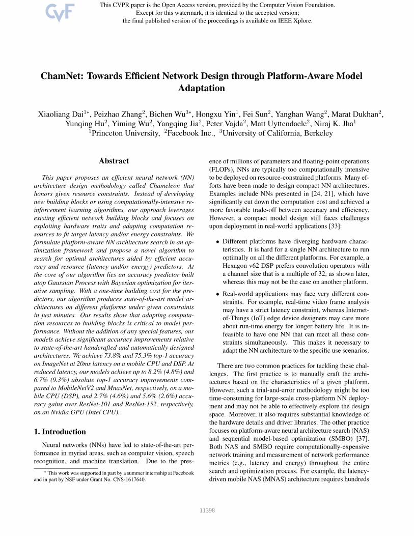
We illustrate the Chameleon approach in Fig. 1. The

adaptation step takes a default NN architecture and a spe-

cific use scenario (i.e., platform and resource budget) as

inputs and generates an adapted architecture as output.

Chameleon searches for a variant of the base NN architec-

ture that fits the use scenario through efficient evolutionary

search (EES). EES is based on an adaptive genetic algo-

11399

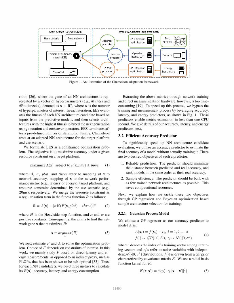
Figure 1. An illustration of the Chameleon adaptation framework

rithm [26], where the gene of an NN architecture is rep-

resented by a vector of hyperparameters (e.g., #Filters and

#Bottlenecks), denoted as x ∈ Rn, where n is the number

of hyperparameters of interest. In each iteration, EES evalu-

ates the fitness of each NN architecture candidate based on

inputs from the predictive models, and then selects archi-

tectures with the highest fitness to breed the next generation

using mutation and crossover operators. EES terminates af-

ter a pre-defined number of iterations. Finally, Chameleon

rests at an adapted NN architecture for the target platform

and use scenario.

We formulate EES as a constrained optimization prob-

lem. The objective is to maximize accuracy under a given

resource constraint on a target platform:

maximize A(x) subject to F(x, plat) ≤ thres (1)

where A, F , plat, and thres refer to mapping of x to

network accuracy, mapping of x to the network perfor-

mance metric (e.g., latency or energy), target platform, and

resource constraint determined by the use scenario (e.g.,

20ms), respectively. We merge the resource constraint as

a regularization term in the fitness function R as follows:

R = A(x)− [αH(F (x, plat)− thres)]w (2)

where H is the Heaviside step function, and α and w are

positive constants. Consequently, the aim is to find the net-

work gene x that maximizes R:

x = argmaxx

(R) (3)

We next estimate F and A to solve the optimization prob-

lem. Choice of F depends on constraints of interest. In this

work, we mainly study F based on direct latency and en-

ergy measurements, as opposed to an indirect proxy, such as

FLOPs, that has been shown to be sub-optimal [33]. Thus,

for each NN candidate x, we need three metrics to calculate

its R(x): accuracy, latency, and energy consumption.

Extracting the above metrics through network training

and direct measurements on hardware, however, is too time-

consuming [19]. To speed up this process, we bypass the

training and measurement process by leveraging accuracy,

latency, and energy predictors, as shown in Fig. 1. These

predictors enable metric estimation in less than one CPU

second. We give details of our accuracy, latency, and energy

predictors next.

3.2. Efficient Accuracy Predictor

To significantly speed up NN architecture candidate

evaluation, we utilize an accuracy predictor to estimate the

final accuracy of a model without actually training it. There

are two desired objectives of such a predictor:

1. Reliable prediction: The predictor should minimize

the distance between predicted and real accuracy, and

rank models in the same order as their real accuracy.

2. Sample efficiency: The predictor should be built with

as few trained network architectures as possible. This

saves computational resources.

Next, we explain how we tackle these two objectives

through GP regression and Bayesian optimization based

sample architecture selection for training.

3.2.1 Gaussian Process Model

We choose a GP regressor as our accuracy predictor to

model A as:

A(xi) = f(xi) + ǫi, i = 1, 2, ..., s

f(·) ∼ GP(·|0,K), ǫi ∼ N (·|0, σ2)(4)

where i denotes the index of a training vector among s train-

ing vectors and ǫi’s refer to noise variables with indepen-

dent N (·|0, σ2) distributions. f(·) is drawn from a GP prior

characterized by covariance matrix K. We use a radial basis

function kernel for K:

K(x, x′) = exp(−γ||x − x′||2) (5)

11400

50 60 70

50

60

70

Pred

ictio

n MSE=1.69Gaussian process

50 60 70

50

60

70 MSE=3.02MLP

50 60 70

50

60

70

Pred

ictio

n MSE=3.52Linear regression

50 60 70

50

60

70 MSE=13.92Decision tree regression

50 60 70Actual

50

60

70

Pred

ictio

n MSE=6.15Boosted decision tree

50 60 70Actual

50

60

70 MSE=3.52Bayesian Ridge

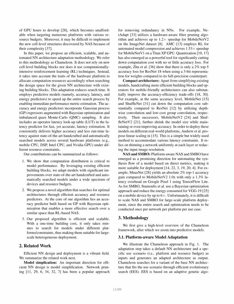
Figure 2. Performance comparison of different accuracy prediction

models, built with 240 pre-trained models under different config-

urations. MSE refers to leave-one-out mean squared error.

A GP regressor provides two benefits. First, it offers

reliable predictions when training data are scarce. As an

example, we compare several regression models for Mo-

bileNetV2 accuracy prediction in Fig. 2. The GP regressor

has the lowest mean squared error (MSE) among all six re-

gression models. Second, a GP regressor produces predic-

tions with uncertainty estimations, which offers additional

guidance for new sample architecture selection for training.

This helps boost the convergence speed and improves sam-

ple efficiency, as shown next.

3.2.2 Iterative Sample Selection

As mentioned earlier, our objective is to train the GP pre-

dictor with as few NN architecture samples as possible.

We summarize our efficient sample generation and predic-

tor training method in Algorithm 1. Since the number of

unique architectures in the adaptation search space can still

be quite large, we first sample representative architectures

from this search space to form an architecture pool. We

adopt the QMC sampling method [2], which is known to

provide similar accuracy to Monte Carlo sampling but with

orders of magnitude fewer samples. We then build the ac-

curacy predictor iteratively. In each iteration, we use the

current predictor as a guide for selecting additional sample

architectures to add to the training set. We train these sam-

ple architectures and then upgrade the predictor based on

new architecture-accuracy observations.

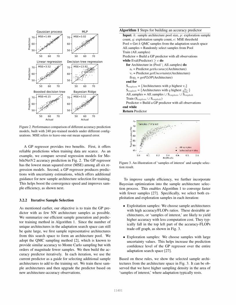
Algorithm 1 Steps for building an accuracy predictor

Input: k: sample architecture pool size, p: exploration sample

count, q: exploitation sample count, e: MSE threshold

Pool = Get k QMC samples from the adaptation search space

All samples = Randomly select samples from Pool

Train (All samples)

Predictor = Build a GP predictor with all observations

while Eval(Predictor) ≥ e do

for Architecture in (Pool \ All samples) do

ai = Predictor.getAccuracy(Architecture)

vi = Predictor.getUncertainty(Architecture)

flopi = getFLOP(Architecture)

end for

Sexplore = {Architectures with p highest vi}Sexploit = {Architectures with q highest

aiflopi

}All samples = All samples ∪ Sexplore ∪ Sexploit

Train (Sexplore ∪ Sexploit)

Predictor = Build a GP predictor with all observations

end while

Return Predictor

Figure 3. An illustration of ‘samples of interest’ and sample selec-

tion result.

To improve sample efficiency, we further incorporate

Bayesian optimization into the sample architecture selec-

tion process. This enables Algorithm 1 to converge faster

with fewer samples [27]. Specifically, we select both ex-

ploitation and exploration samples in each iteration:

• Exploitation samples: We choose sample architectures

with high accuracy/FLOPs ratios. These desirable ar-

chitectures, or ‘samples of interest,’ are likely to yield

higher accuracy with less computation cost. They typ-

ically fall in the top left part of the accuracy-FLOPs

trade-off graph, as shown in Fig. 3.

• Exploration samples: We choose samples with large

uncertainty values. This helps increase the prediction

confidence level of the GP regressor over the entire

adaptation search space [27].

Based on these rules, we show the selected sample archi-

tectures from the architecture space in Fig. 3. It can be ob-

served that we have higher sampling density in the area of

‘samples of interest,’ where adaptation typically rests.

11401

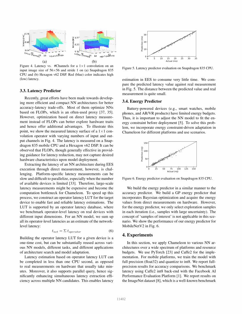
(a) (b)Figure 4. Latency vs. #Channels for a 1×1 convolution on an

input image size of 56×56 and stride 1 on (a) Snapdragon 835

CPU and (b) Hexagon v62 DSP. Red (blue) color indicates high

(low) latency.

3.3. Latency Predictor

Recently, great efforts have been made towards develop-

ing more efficient and compact NN architectures for better

accuracy-latency trade-offs. Most of them optimize NNs

based on FLOPs, which is an often-used proxy [37, 35].

However, optimization based on direct latency measure-

ment instead of FLOPs can better explore hardware traits

and hence offer additional advantages. To illustrate this

point, we show the measured latency surface of a 1×1 con-

volution operator with varying numbers of input and out-

put channels in Fig. 4. The latency is measured on a Snap-

dragon 835 mobile CPU and a Hexagon v62 DSP. It can be

observed that FLOPs, though generally effective in provid-

ing guidance for latency reduction, may not capture desired

hardware characteristics upon model deployment.

Extracting the latency of an NN architecture during EES

execution through direct measurement, however, is chal-

lenging. Platform-specific latency measurements can be

slow and difficult to parallelize, especially when the number

of available devices is limited [33]. Therefore, large-scale

latency measurements might be expensive and become the

computation bottleneck for Chameleon. To speed up this

process, we construct an operator latency LUT for the target

device to enable fast and reliable latency estimations. The

LUT is supported by an operator latency database, where

we benchmark operator-level latency on real devices with

different input dimensions. For an NN model, we sum up

all its operator-level latencies as an estimate of the network-

level latency:

tnet = Σ toperator (6)

Building the operator latency LUT for a given device is a

one-time cost, but can be substantially reused across vari-

ous NN models, different tasks, and different applications

of architecture search and model adaptation.

Latency estimation based on operator latency LUT can

be completed in less than one CPU second, as opposed

to real measurements on hardware that usually take min-

utes. Moreover, it also supports parallel query, hence sig-

nificantly enhancing simultaneous latency extraction effi-

ciency across multiple NN candidates. This enables latency

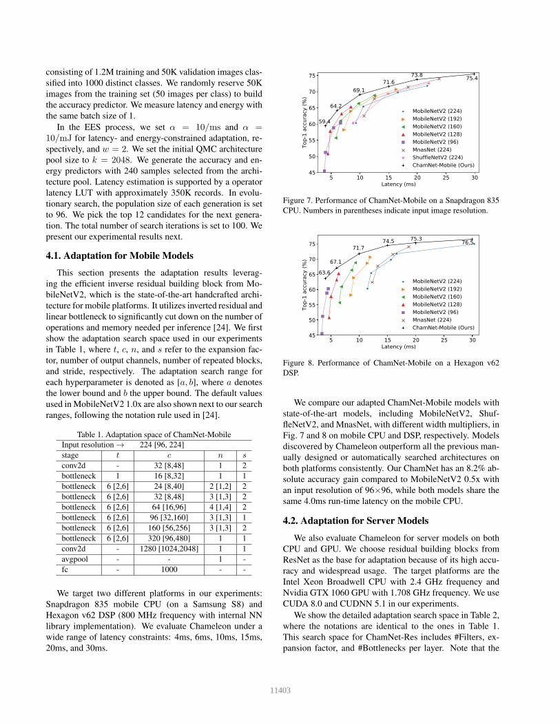
0 5 10 15 20 25 30 35Actual (ms)

0

10

20

30

Pred

ictio

n (m

s)

Figure 5. Latency predictor evaluation on Snapdragon 835 CPU.

estimation in EES to consume very little time. We com-

pare the predicted latency value against real measurement

in Fig. 5. The distance between the predicted value and real

measurement is quite small.

3.4. Energy Predictor

Battery-powered devices (e.g., smart watches, mobile

phones, and AR/VR products) have limited energy budgets.

Thus, it is important to adjust the NN model to fit the en-

ergy constraint before deployment [5]. To solve this prob-

lem, we incorporate energy constraint-driven adaptation in

Chameleon for different platforms and use scenarios.

0 25 50 75 100 125 150Actual (mJ)

0

50

100

150Pr

edict

ion

(mJ)

Figure 6. Energy predictor evaluation on Snapdragon 835 CPU.

We build the energy predictor in a similar manner to the

accuracy predictor. We build a GP energy predictor that

incorporates Bayesian optimization and acquire the energy

values from direct measurements on hardware. However,

for the energy predictor, we only select exploration samples

in each iteration (i.e., samples with large uncertainty). The

concept of ‘samples of interest’ is not applicable in this sce-

nario. We show the performance of our energy predictor for

MobileNetV2 in Fig. 6.

4. Experiments

In this section, we apply Chameleon to various NN ar-

chitectures over a wide spectrum of platforms and resource

budgets. We use PyTorch [23] and Caffe2 for the imple-

mentation. For mobile platforms, we train the model with

full precision (float32) and quantize to int8. We report full-

precision results for accuracy comparisons. We benchmark

latency using Caffe2 int8 back-end with the Facebook AI

Performance Evaluation Platform [1]. We report results on

the ImageNet dataset [8], which is a well-known benchmark

11402

consisting of 1.2M training and 50K validation images clas-

sified into 1000 distinct classes. We randomly reserve 50K

images from the training set (50 images per class) to build

the accuracy predictor. We measure latency and energy with

the same batch size of 1.

In the EES process, we set α = 10/ms and α =10/mJ for latency- and energy-constrained adaptation, re-

spectively, and w = 2. We set the initial QMC architecture

pool size to k = 2048. We generate the accuracy and en-

ergy predictors with 240 samples selected from the archi-

tecture pool. Latency estimation is supported by a operator

latency LUT with approximately 350K records. In evolu-

tionary search, the population size of each generation is set

to 96. We pick the top 12 candidates for the next genera-

tion. The total number of search iterations is set to 100. We

present our experimental results next.

4.1. Adaptation for Mobile Models

This section presents the adaptation results leverag-

ing the efficient inverse residual building block from Mo-

bileNetV2, which is the state-of-the-art handcrafted archi-

tecture for mobile platforms. It utilizes inverted residual and

linear bottleneck to significantly cut down on the number of

operations and memory needed per inference [24]. We first

show the adaptation search space used in our experiments

in Table 1, where t, c, n, and s refer to the expansion fac-

tor, number of output channels, number of repeated blocks,

and stride, respectively. The adaptation search range for

each hyperparameter is denoted as [a, b], where a denotes

the lower bound and b the upper bound. The default values

used in MobileNetV2 1.0x are also shown next to our search

ranges, following the notation rule used in [24].

Table 1. Adaptation space of ChamNet-Mobile

Input resolution → 224 [96, 224]

stage t c n s

conv2d - 32 [8,48] 1 2

bottleneck 1 16 [8,32] 1 1

bottleneck 6 [2,6] 24 [8,40] 2 [1,2] 2

bottleneck 6 [2,6] 32 [8,48] 3 [1,3] 2

bottleneck 6 [2,6] 64 [16,96] 4 [1,4] 2

bottleneck 6 [2,6] 96 [32,160] 3 [1,3] 1

bottleneck 6 [2,6] 160 [56,256] 3 [1,3] 2

bottleneck 6 [2,6] 320 [96,480] 1 1

conv2d - 1280 [1024,2048] 1 1

avgpool - - 1 -

fc - 1000 - -

We target two different platforms in our experiments:

Snapdragon 835 mobile CPU (on a Samsung S8) and

Hexagon v62 DSP (800 MHz frequency with internal NN

library implementation). We evaluate Chameleon under a

wide range of latency constraints: 4ms, 6ms, 10ms, 15ms,

20ms, and 30ms.

5 10 15 20 25 30Latency (ms)

45

50

55

60

65

70

75

Top-

1 ac

cura

cy (%

)

75.473.871.6

69.1

64.2

59.4MobileNetV2 (224)MobileNetV2 (192)MobileNetV2 (160)MobileNetV2 (128)MobileNetV2 (96)MnasNet (224)ShuffleNetV2 (224)ChamNet-Mobile (Ours)

Figure 7. Performance of ChamNet-Mobile on a Snapdragon 835

CPU. Numbers in parentheses indicate input image resolution.

5 10 15 20 25 30Latency (ms)

45

50

55

60

65

70

75

Top-

1 ac

cura

cy (%

)

76.575.374.571.7

67.163.6

MobileNetV2 (224)MobileNetV2 (192)MobileNetV2 (160)MobileNetV2 (128)MobileNetV2 (96)MnasNet (224)ChamNet-Mobile (Ours)

Figure 8. Performance of ChamNet-Mobile on a Hexagon v62

DSP.

We compare our adapted ChamNet-Mobile models with

state-of-the-art models, including MobileNetV2, Shuf-

fleNetV2, and MnasNet, with different width multipliers, in

Fig. 7 and 8 on mobile CPU and DSP, respectively. Models

discovered by Chameleon outperform all the previous man-

ually designed or automatically searched architectures on

both platforms consistently. Our ChamNet has an 8.2% ab-

solute accuracy gain compared to MobileNetV2 0.5x with

an input resolution of 96×96, while both models share the

same 4.0ms run-time latency on the mobile CPU.

4.2. Adaptation for Server Models

We also evaluate Chameleon for server models on both

CPU and GPU. We choose residual building blocks from

ResNet as the base for adaptation because of its high accu-

racy and widespread usage. The target platforms are the

Intel Xeon Broadwell CPU with 2.4 GHz frequency and

Nvidia GTX 1060 GPU with 1.708 GHz frequency. We use

CUDA 8.0 and CUDNN 5.1 in our experiments.

We show the detailed adaptation search space in Table 2,

where the notations are identical to the ones in Table 1.

This search space for ChamNet-Res includes #Filters, ex-

pansion factor, and #Bottlenecks per layer. Note that the

11403

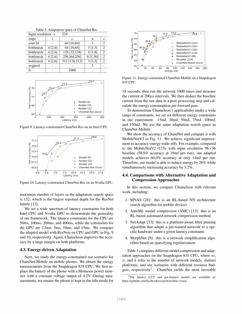
Table 2. Adaptation space of ChamNet-Res

Input resolution → 224

stage t c n s

conv2d - 64 [16,64] 1 2

bottleneck 4 [2,6] 64 [16,64] 3 [1,3] 2

bottleneck 4 [2,6] 128 [32,128] 4 [1,8] 2

bottleneck 4 [2,6] 256 [64,256] 6 [1,36] 2

bottleneck 4 [2,6] 512 [128,512] 3 [1,3] 2

avgpool - - 1 -

fc - 1000 - -

0 100 200 300 400 500Latency (ms)

64

68

72

76

Top-

1 ac

cura

cy (%

)

72.7

75.277.2

78.5

ResNet-50ResNet-101ResNet-152ChamNet-Res (Ours)

Figure 9. Latency-constrained ChamNet-Res on an Intel CPU.

0.0 2.5 5.0 7.5 10.0 12.5 15.0 17.5Latency (ms)

65.0

67.5

70.0

72.5

75.0

77.5

Top-

1 ac

cura

cy (%

)

70.8

75.777.7 78.6

ResNet-50ResNet-101ResNet-152ChamNet-Res (Ours)

Figure 10. Latency-constrained ChamNet-Res on an Nvidia GPU.

maximum number of layers in the adaptation search space

is 152, which is the largest reported depth for the ResNet

family [12].

We set a wide spectrum of latency constraints for both

Intel CPU and Nvidia GPU to demonstrate the generality

of our framework. The latency constraints for the CPU are

50ms, 100ms, 200ms, and 400ms, while the constraints for

the GPU are 2.5ms, 5ms, 10ms, and 15ms. We compare

the adapted model with ResNets on CPU and GPU in Fig. 9

and 10, respectively. Again, Chameleon improves the accu-

racy by a large margin on both platforms.

4.3. Energydriven Adaptation

Next, we study the energy-constrained use scenario for

ChamNet-Mobile on mobile phones. We obtain the energy

measurements from the Snapdragon 835 CPU. We first re-

place the battery of the phone with a Monsoon power mon-

itor with a constant voltage output of 4.2V. During mea-

surements, we ensure the phone is kept in the idle mode for

0 20 40 60 80 100 120 140 160 180Energy (mJ)

45

50

55

60

65

70

75

Top-

1 ac

cura

cy (%

)

75.674.072.670.2

65.8

60.0MobileNetV2 (224)MobileNetV2 (192)MobileNetV2 (160)MobileNetV2 (128)MobileNetV2 (96)MnasNet (224)ChamNet-Mobile (Ours)

Figure 11. Energy-constrained ChamNet-Mobile on a Snapdragon

835 CPU.

18 seconds, then run the network 1000 times and measure

the current at 200µs intervals. We then deduct the baseline

current from the raw data in a post-processing step and cal-

culate the energy consumption per forward pass.

To demonstrate Chameleon’s applicability under a wide

range of constraints, we set six different energy constraints

in our experiment: 15mJ, 30mJ, 50mJ, 75mJ, 100mJ,

and 150mJ. We use the same adaptation search space as

ChamNet-Mobile.

We show the accuracy of ChamNet and compare it with

MobileNetV2 in Fig. 11. We achieve significant improve-

ment in accuracy-energy trade-offs. For example, compared

to the MobileNetV2 0.75x with input resolution 96×96

baseline (58.8% accuracy at 19mJ per run), our adapted

models achieves 60.0% accuracy at only 14mJ per run.

Therefore, our model is able to reduce energy by 26% while

simultaneously increasing accuracy by 1.2%.

4.4. Comparisons with Alternative Adaptation andCompression Approaches

In this section, we compare Chameleon with relevant

work, including:

1. MNAS [28]: this is an RL-based NN architecture

search algorithm for mobile devices.

2. AutoML model compression (AMC) [13]: this is an

RL-based automated network compression method.

3. NetAdapt [33]: this is a platform-aware filter pruning

algorithm that adapts a pre-trained network to a spe-

cific hardware under a given latency constraint.

4. MorphNet [9]: this is a network simplification algo-

rithm based on sparsifying regularization.

Table 3 compares different model compression and adap-

tation approaches on the Snapdragon 835 CPU, where m,

n, and k refer to the number of network models, distinct

platforms, and use scenarios with different resource bud-

gets, respectively1 . ChamNet yields the most favorable

1The latency LUT and pre-trained models are available at:

https://github.com/facebookresearch/mobile-vision

11404

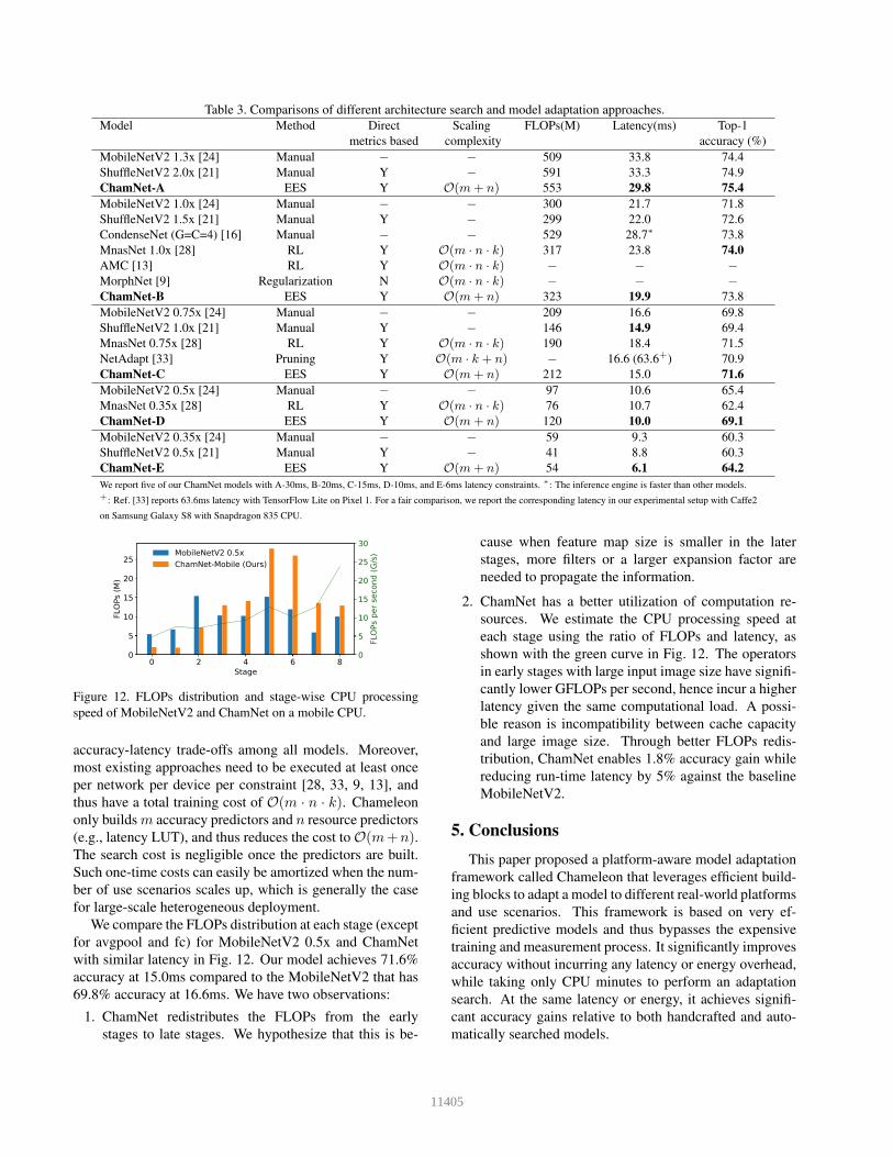
Table 3. Comparisons of different architecture search and model adaptation approaches.

Model Method Direct Scaling FLOPs(M) Latency(ms) Top-1

metrics based complexity accuracy (%)

MobileNetV2 1.3x [24] Manual − − 509 33.8 74.4

ShuffleNetV2 2.0x [21] Manual Y − 591 33.3 74.9

ChamNet-A EES Y O(m+ n) 553 29.8 75.4



CondenseNet (G=C=4) [16] Manual − − 529 28.7∗ 73.8

MnasNet 1.0x [28] RL Y O(m · n · k) 317 23.8 74.0

AMC [13] RL Y O(m · n · k) − − −MorphNet [9] Regularization N O(m · n · k) − − −ChamNet-B EES Y O(m+ n) 323 19.9 73.8




NetAdapt [33] Pruning Y O(m · k + n) − 16.6 (63.6+) 70.9

ChamNet-C EES Y O(m+ n) 212 15.0 71.6



ChamNet-D EES Y O(m+ n) 120 10.0 69.1



ChamNet-E EES Y O(m+ n) 54 6.1 64.2

We report five of our ChamNet models with A-30ms, B-20ms, C-15ms, D-10ms, and E-6ms latency constraints. ∗: The inference engine is faster than other models.

+: Ref. [33] reports 63.6ms latency with TensorFlow Lite on Pixel 1. For a fair comparison, we report the corresponding latency in our experimental setup with Caffe2

on Samsung Galaxy S8 with Snapdragon 835 CPU.

0 2 4 6 8Stage

0

5

10

15

20

25

FLOP

s (M

)

0

5

10

15

20

25

30

FLOP

s per

seco

nd (G

/s)MobileNetV2 0.5x

ChamNet-Mobile (Ours)

Figure 12. FLOPs distribution and stage-wise CPU processing

speed of MobileNetV2 and ChamNet on a mobile CPU.

accuracy-latency trade-offs among all models. Moreover,

most existing approaches need to be executed at least once

per network per device per constraint [28, 33, 9, 13], and

thus have a total training cost of O(m · n · k). Chameleon

only builds m accuracy predictors and n resource predictors

(e.g., latency LUT), and thus reduces the cost to O(m+n).The search cost is negligible once the predictors are built.

Such one-time costs can easily be amortized when the num-

ber of use scenarios scales up, which is generally the case

for large-scale heterogeneous deployment.

We compare the FLOPs distribution at each stage (except

for avgpool and fc) for MobileNetV2 0.5x and ChamNet

with similar latency in Fig. 12. Our model achieves 71.6%

accuracy at 15.0ms compared to the MobileNetV2 that has

69.8% accuracy at 16.6ms. We have two observations:

1. ChamNet redistributes the FLOPs from the early

stages to late stages. We hypothesize that this is be-

cause when feature map size is smaller in the later

stages, more filters or a larger expansion factor are

needed to propagate the information.

2. ChamNet has a better utilization of computation re-

sources. We estimate the CPU processing speed at

each stage using the ratio of FLOPs and latency, as

shown with the green curve in Fig. 12. The operators

in early stages with large input image size have signifi-

cantly lower GFLOPs per second, hence incur a higher

latency given the same computational load. A possi-

ble reason is incompatibility between cache capacity

and large image size. Through better FLOPs redis-

tribution, ChamNet enables 1.8% accuracy gain while

reducing run-time latency by 5% against the baseline

MobileNetV2.

5. Conclusions

This paper proposed a platform-aware model adaptation

framework called Chameleon that leverages efficient build-

ing blocks to adapt a model to different real-world platforms

and use scenarios. This framework is based on very ef-

ficient predictive models and thus bypasses the expensive

training and measurement process. It significantly improves

accuracy without incurring any latency or energy overhead,

while taking only CPU minutes to perform an adaptation

search. At the same latency or energy, it achieves signifi-

cant accuracy gains relative to both handcrafted and auto-

matically searched models.

11405

References

[1] Facebook AI performance evaluation platform. https://

github.com/facebook/FAI-PEP, 2018.

[2] Søren Asmussen and Peter W Glynn. Stochastic Simulation:

Algorithms and Analysis, volume 57. Springer Science &

Business Media, 2007.

[3] Bowen Baker, Otkrist Gupta, Ramesh Raskar, and Nikhil

Naik. Accelerating neural architecture search using perfor-

mance prediction. arXiv preprint arXiv:1705.10823, 2017.

[4] James S Bergstra, Remi Bardenet, Yoshua Bengio, and

Balazs Kegl. Algorithms for hyper-parameter optimization.

In Proc. Advances in Neural Information Processing Sys-

tems, pages 2546–2554, 2011.

[5] Ermao Cai, Da-Cheng Juan, Dimitrios Stamoulis, and Di-

ana Marculescu. Neuralpower: Predict and deploy energy-

efficient convolutional neural networks. arXiv preprint

arXiv:1710.05420, 2017.

[6] Xiaoliang Dai, Hongxu Yin, and Niraj K Jha. NeST: A

neural network synthesis tool based on a grow-and-prune

paradigm. arXiv preprint arXiv:1711.02017, 2017.

[7] Xiaoliang Dai, Hongxu Yin, and Niraj K Jha. Grow and

prune compact, fast, and accurate LSTMs. arXiv preprint

arXiv:1805.11797, 2018.

[8] Jia Deng, Wei Dong, Richard Socher, Li-Jia Li, Kai Li,

and Li Fei-Fei. ImageNet: A large-scale hierarchical image

database. In Proc. IEEE Conf. Computer Vision and Pattern

Recognition, pages 248–255, 2009.

[9] Ariel Gordon, Elad Eban, Ofir Nachum, Bo Chen, Hao Wu,

Tien-Ju Yang, and Edward Choi. MorphNet: Fast & simple

resource-constrained structure learning of deep networks. In

Proc. IEEE Conf. Computer Vision and Pattern Recognition,

2018.

[10] Song Han, Huizi Mao, and William J Dally. Deep com-

pression: Compressing deep neural networks with pruning,

trained quantization and Huffman coding. arXiv preprint

arXiv:1510.00149, 2015.

[11] Song Han, Jeff Pool, John Tran, and William Dally. Learning

both weights and connections for efficient neural network. In

Proc. Advances in Neural Information Processing Systems,

pages 1135–1143, 2015.

[12] Kaiming He, Xiangyu Zhang, Shaoqing Ren, and Jian Sun.

Deep residual learning for image recognition. In Proc. IEEE

Conf. Computer Vision and Pattern Recognition, pages 770–

778, 2016.

[13] Yihui He, Ji Lin, Zhijian Liu, Hanrui Wang, Li-Jia Li, and

Song Han. AMC: AutoML for model compression and ac-

celeration on mobile devices. In Proc. European Conf. Com-

puter Vision, pages 784–800, 2018.

[14] Jose Miguel Hernandez-Lobato, Michael A Gelbart, Ryan P

Adams, Matthew W Hoffman, and Zoubin Ghahramani. A

general framework for constrained Bayesian optimization

using information-based search. J. Machine Learning Re-

search, 17(1):5549–5601, 2016.

[15] Andrew G Howard, Menglong Zhu, Bo Chen, Dmitry

Kalenichenko, Weijun Wang, Tobias Weyand, Marco An-

dreetto, and Hartwig Adam. MobileNets: Efficient convolu-

tional neural networks for mobile vision applications. arXiv

preprint arXiv:1704.04861, 2017.

[16] Gao Huang, Shichen Liu, Laurens van der Maaten,

and Kilian Q Weinberger. CondenseNet: An efficient

DenseNet using learned group convolutions. arXiv preprint

arXiv:1711.09224, 2017.

[17] Itay Hubara, Matthieu Courbariaux, Daniel Soudry, Ran El-

Yaniv, and Yoshua Bengio. Binarized neural networks. In

Proc. Advances in Neural Information Processing Systems,

pages 4107–4115, 2016.

[18] Forrest N Iandola, Song Han, Matthew W Moskewicz,

Khalid Ashraf, William J Dally, and Kurt Keutzer.

SqueezeNet: AlexNet-level accuracy with 50x fewer pa-

rameters and <0.5 MB model size. arXiv preprint

arXiv:1602.07360, 2016.

[19] Chenxi Liu, Barret Zoph, Jonathon Shlens, Wei Hua, Li-Jia

Li, Li Fei-Fei, Alan Yuille, Jonathan Huang, and Kevin Mur-

phy. Progressive neural architecture search. arXiv preprint

arXiv:1712.00559, 2017.

[20] Hanxiao Liu, Karen Simonyan, and Yiming Yang.

Darts: Differentiable architecture search. arXiv preprint

arXiv:1806.09055, 2018.

[21] Ningning Ma, Xiangyu Zhang, Hai-Tao Zheng, and Jian Sun.

ShuffleNet V2: Practical guidelines for efficient CNN archi-

tecture design. arXiv preprint arXiv:1807.11164, 2018.

[22] Diana Marculescu, Dimitrios Stamoulis, and Ermao Cai.

Hardware-aware machine learning: Modeling and optimiza-

tion. arXiv preprint arXiv:1809.05476, 2018.

[23] Adam Paszke, Sam Gross, Soumith Chintala, Gregory

Chanan, Edward Yang, Zachary DeVito, Zeming Lin, Al-

ban Desmaison, Luca Antiga, and Adam Lerer. Automatic

differentiation in PyTorch. In Proc. Neural Information Pro-

cessing Systems Workshop on Autodiff, 2017.

[24] Mark Sandler, Andrew Howard, Menglong Zhu, Andrey Zh-

moginov, and Liang-Chieh Chen. Inverted residuals and lin-

ear bottlenecks: Mobile networks for classification, detec-

tion and segmentation. arXiv preprint arXiv:1801.04381,

2018.

[25] Karen Simonyan and Andrew Zisserman. Very deep convo-

lutional networks for large-scale image recognition. arXiv

preprint arXiv:1409.1556, 2014.

[26] Mandavilli Srinivas and Lalit M Patnaik. Adaptive prob-

abilities of crossover and mutation in genetic algorithms.

IEEE Trans. Systems, Man, and Cybernetics, 24(4):656–667,

1994.

[27] Dimitrios Stamoulis, Ermao Cai, Da-Cheng Juan, and Diana

Marculescu. Hyperpower: Power-and memory-constrained

hyper-parameter optimization for neural networks. In Proc.

IEEE Europe Conf. & Exihibition on Design, Automation &

Test, pages 19–24, 2018.

[28] Mingxing Tan, Bo Chen, Ruoming Pang, Vijay Vasudevan,

and Quoc V Le. MnasNet: Platform-aware neural architec-

ture search for mobile. arXiv preprint arXiv:1807.11626,

2018.

[29] Wei Wen, Chunpeng Wu, Yandan Wang, Yiran Chen, and

Hai Li. Learning structured sparsity in deep neural networks.

In Proc. Advances in Neural Information Processing Sys-

tems, pages 2074–2082, 2016.

11406

[30] Bichen Wu, Alvin Wan, Xiangyu Yue, Peter Jin, Sicheng

Zhao, Noah Golmant, Amir Gholaminejad, Joseph Gon-

zalez, and Kurt Keutzer. Shift: A zero FLOP, zero pa-

rameter alternative to spatial convolutions. arXiv preprint

arXiv:1711.08141, 2017.

[31] Zhang Xiangyu, Zhou Xinyu, Lin Mengxiao, and Sun Jian.

ShuffleNet: An extremely efficient convolutional neural net-

work for mobile devices. In Proc. IEEE Conf. Computer

Vision and Pattern Recognition, 2017.

[32] Tien-Ju Yang, Yu-Hsin Chen, and Vivienne Sze. Designing

energy-efficient convolutional neural networks using energy-

aware pruning. arXiv preprint arXiv:1611.05128, 2016.

[33] Tien-Ju Yang, Andrew Howard, Bo Chen, Xiao Zhang, Alec

Go, Mark Sandler, Vivienne Sze, and Hartwig Adam. Ne-

tAdapt: Platform-aware neural network adaptation for mo-

bile applications. In Proc. European Conf. Computer Vision,

volume 41, page 46, 2018.

[34] Tianyun Zhang, Kaiqi Zhang, Shaokai Ye, Jiayu Li, Jian

Tang, Wujie Wen, Xue Lin, Makan Fardad, and Yanzhi

Wang. ADAM-ADMM: A unified, systematic framework

of structured weight pruning for DNNs. arXiv preprint

arXiv:1807.11091, 2018.

[35] Yanqi Zhou, Siavash Ebrahimi, Sercan O Arık, Haonan Yu,

Hairong Liu, and Greg Diamos. Resource-efficient neural

architect. arXiv preprint arXiv:1806.07912, 2018.

[36] Chenzhuo Zhu, Song Han, Huizi Mao, and William J

Dally. Trained ternary quantization. arXiv preprint

arXiv:1612.01064, 2016.

[37] Barret Zoph, Vijay Vasudevan, Jonathon Shlens, and Quoc V

Le. Learning transferable architectures for scalable image

recognition. arXiv preprint arXiv:1707.07012, 2(6), 2017.

11407

chamnet: towards efficient network design through platform...

Documents