barreira, valls, 2010
TRANSCRIPT
8/19/2019 Barreira, Valls, 2010
http://slidepdf.com/reader/full/barreira-valls-2010 1/16
J. Differential Equations 249 (2010) 2889–2904
Contents lists available at ScienceDirect
Journal of Differential Equations
www.elsevier.com/locate/jde
Admissibility for nonuniform exponential contractions✩
Luis Barreira ∗, Claudia Valls
Departamento de Matemática, Instituto Superior Técnico, 1049-001 Lisboa, Portugal
a r t i c l e i n f o a b s t r a c t
Article history:
Received 8 February 2010
Revised 5 June 2010
Available online 22 June 2010
MSC:
34D09
37D25
Keywords:Admissibility
Nonuniform exponential contraction
We study the relation between the notions of nonuniform expo-
nential stability and admissibility. In particular, using appropriate
adapted norms (which can be seen as Lyapunov norms), we show
that if any of their associated L p spaces, with p ∈ (1, ∞], is
admissible for a given evolution process, then this process is a
nonuniform exponential contraction. We also provide a collection
of admissible Banach spaces for any given nonuniform exponential
contraction.
© 2010 Elsevier Inc. All rights reserved.
1. Introduction
Our main aim is to give a characterization of nonuniform exponential stability in terms of an ap-
propriate notion of what is usually called admissibility property. Its study goes back to pioneering
work of Perron, and referred originally to the existence of bounded solutions of the equation
x = A (t ) x + f (t ) (1)
in Rn for any bounded continuous perturbation f :R+0 → R
n . This property can be used to deduce the
stability or the conditional stability under sufficiently small perturbations of a given linear equation.
More precisely, the following result was established by Perron in [21], for n × n matrices A(t ) varying
continuously with t 0.
✩
Partially supported by FCT through CAMGSD, Lisbon.
* Corresponding author.
E-mail addresses: [email protected] (L. Barreira), [email protected] (C. Valls).
0022-0396/$ – see front matter © 2010 Elsevier Inc. All rights reserved.
doi:10.1016/j.jde.2010.06.010
8/19/2019 Barreira, Valls, 2010
http://slidepdf.com/reader/full/barreira-valls-2010 2/16
2890 L. Barreira, C. Valls / J. Differential Equations 249 (2010) 2889–2904
Theorem 1. If Eq. (1) has at least one bounded solution in R+0 for each bounded continuous function f , and
the equation
x = A (t ) x (2)
has k n bounded linearly independent solutions, then for each r > 0 there exists δ > 0 such that if g is a
continuous function satisfying
g (t , x) δ and
g (t , x) − g (t , y) δ x − y
for every t 0 and x, y ∈ Rn with x, y < r, then the equation
x = A (t ) x + g (t , x)
has a k-parameter family of bounded solutions. If in addition g (t , 0) = 0 for every t 0, then all these solutions
tend to zero as t → +∞.
One should recognize Theorem 1 as a precursor result of the Hadamard–Perron stable manifold
theorem (in fact even as a precursor of the nonautonomous version of the theorem).
On the other hand, Theorem 1 also allows linear perturbations, and hence it is also a notable con-
tribution to the so-called robustness problem, which asks whether the stability of a linear contraction
(or the conditional stability of a linear dichotomy) persists under sufficiently small linear perturba-
tions. In this direction, a simple consequence of Theorem 1 is the following.
Theorem 2. If Eq. (1) has at least one bounded solution in R+0 for each bounded continuous function f , then
each bounded solution of Eq. (2) tends to zero as t → +∞.
The assumption in Theorem 2 is called the admissibility of the pair of spaces in which we re-
spectively take the perturbation and look for the solutions. Moreover, Theorem 2 (which should be
attributed to Perron, even if not stated explicitly in [21]) is probably the first step in the literature
concerning the study of the relation between admissibility and the notions of stability and conditional
stability. We note that one can also consider the admissibility of other pairs of spaces.
There is a very extensive literature concerning the relation between admissibility and stability, also
in infinite-dimensional spaces. For some of the most relevant early contributions in the area we refer
to the books by Massera and Schäffer [16] (which culminates the development starting with theirpaper [15]) and by Dalec’kiı and Kreın [10]. We also refer to the book [14] for some early results in
infinite-dimensional spaces (which are important particularly in view of the applications of the theory
to partial differential equations). For a detailed list of references, we refer to the book by Chicone and
Latushkin [8] (see in particular the final remarks of Chapters 3 and 4), and for more recent work to
Huy [12]. We mention in particular the papers [18,24,28].
There are several related approaches in the literature. In order to mention briefly some of them,
we first observe that Eq. (1) can be rewritten in the form Lx = f , where L is the linear operator
defined by
(Lx)(t ) = x
(t ) − A (t ) x(t ) (3)
in some appropriate space. Then the admissibility of certain pairs of spaces is related to the in-
vertibility or the Fredholm properties of the operator L (see in particular [6,7,13,20,29] and the
books [8–11,16]). In a related direction, for the linear equation (2), or more generally for a linear
8/19/2019 Barreira, Valls, 2010
http://slidepdf.com/reader/full/barreira-valls-2010 3/16
L. Barreira, C. Valls / J. Differential Equations 249 (2010) 2889–2904 2891
evolution process T (t , s), one can introduce a semigroup S(t ) for t 0 by
S(t ) f (s) = T (s, s − t ) f (s − t ), s t ,
T (s, 0) f (0), s ∈ [0, t ],
for each function f in some appropriate space. It turns out that in certain situations the generator G
of the semigroup S(t ) is an extension of the operator −L with L as in (3). Moreover, the stability and
the conditional stability of the evolution process T (t , s) can often be related to the spectral properties
of G . We refer to [8,13] for references and for a detailed discussion concerning the relation between
these semigroups and the stability theory.
Now we describe briefly our results and we compare them to the existing literature in the nonuni-
form setting. Using appropriate adapted norms (which can be seen as Lyapunov norms), we show that
if any of their associated L p spaces with p ∈ (1, ∞] (see Section 2 for the definitions) is admissible
for a given evolution process, then this process is a nonuniform exponential contraction. We also pro-
vide a collection of admissible Banach spaces for any given nonuniform exponential contraction. Our
work is close in spirit to that of Preda, Pogan and Preda [25], who consider related problems in theparticular case of uniform exponential behavior, although for the large class of Schäffer spaces as ad-
missible spaces (see also their work [24,26] for the case of uniform exponential dichotomies). These
spaces were introduced by Schäffer in [27] (see also [16] for a related discussion). In their notable
contribution [23], Preda and Megan obtained related results in the case of nonuniform exponential
dichotomies, also for the class of Schäffer spaces, although using a notion of dichotomy which is dif-
ferent from the original one motivated by ergodic theory and the nonuniform hyperbolicity theory, as
detailed for example in [1,2] (see also the following paragraphs for a related discussion). More pre-
cisely, their notion of dichotomy requires nothing about the angle between the stable and unstable
subspaces (or, in the general case of Banach spaces, about the norms of the associated projections),
and thus their admissibility property need not give information concerning these angles when deduc-
ing the exponential behavior. This causes that none of the results in [23] and in our paper imply theresults in the other. In the more recent work [17], the authors consider the same weaker notion of
exponential dichotomy, and obtain sharper relations between admissibility and stability, although for
perturbations and solutions in C 0, and not in the L p spaces that we consider.
We emphasize that we consider the general case of nonuniform exponential behavior. Taking as
example the case of contractions, in the uniform setting we assume that there exist K > 0 and λ < 0
such that
U (t , s) K eλ(t −s) for every t , s 0,
where the linear operators U (t , s) satisfy
x(t ) = U (t , s) x(s)
for any t , s 0 and any solution x of Eq. (2). On the other hand, in the nonuniform setting we assume
that there exist K > 0, λ < 0, and ε 0 such that
U (t , s) K eλ(t −s)+εs for every t , s 0, (4)
or more generally
U (t , s)
D(s)eλ(t −s) for every t , s 0,
for some function D (we refer to [4] for a related discussion on why it is of interest to consider this
more general behavior with the function D). The constant λ is an upper bound for the largest Lya-
punov exponent, while ε or the function D measure the nonuniformity of the exponential behavior. It

8/19/2019 Barreira, Valls, 2010
http://slidepdf.com/reader/full/barreira-valls-2010 4/16
2892 L. Barreira, C. Valls / J. Differential Equations 249 (2010) 2889–2904
turns out that the classical notion of (uniform) exponential behavior is very stringent for the dynam-
ics and it is of interest to look for more general types of hyperbolic behavior. These generalizations
can be much more typical. This is precisely what happens with the notion of nonuniform exponential
contraction. In this respect, our results are also a contribution to the theory of nonuniform hyperbol-
icity. We refer to [1,2] for detailed expositions of the theory, which goes back to the landmark worksof Oseledets [19] and particularly Pesin [22]. Since then it became an important part of the general
theory of dynamical systems and an important tool in the study of stochastic behavior. We refer to
[1,2] for details and references.
A principal motivation for weakening the notion of uniform exponential behavior is that from the
point of view of ergodic theory, almost all linear variational equations in a finite-dimensional space
as in (2) have a nonuniform exponential behavior. Namely, consider a flow (φt )t ∈R defined by an
equation x = f ( x) preserving a finite measure µ. This means that
µ(φt A) = µ( A)
for any measurable set A and any t ∈ R. One can show that the trajectory of µ-almost every point x
with negative Lyapunov exponents gives rise to a linear variational equation
v = A x(t )v, with A x(t ) = dφt x f ,
satisfying (4) (see for example [1,5] for details and references). Certainly, the constant ε in (4) may
be zero, although results in [3] indicate that in many situations the set of trajectories for which
ε > 0 (and not arbitrarily small) may be large from the points of view of Hausdorff dimension and
topological entropy.
2. Preliminaries
2.1. Evolution processes
We say that a family of linear operators T (t , s), t s 0, in a Banach space X is an evolution
process if:
1. T (t , s) = T (t , r )T (r , s) and T (t , t ) = Id for every t r s 0;
2. (t , s, x) → T (t , s) x is continuous for t s 0 and x ∈ X ;
3. there exist ω 0 and a measurable function D :R+0 → R
+0 such that
T (t , s) D(s)eω(t −s) for every t s 0.
We also consider the new norms
vt = sup
T (σ , t )ve−ω(σ −t ): σ t
, v ∈ X , t ∈ R
+0 . (5)
These satisfy
v vt D(t )v, v ∈ X , t ∈ R
+0 . (6)
Moreover, with respect to these norms the evolution process has the following bounded growth prop-
erty (compare with Section 4.3).
8/19/2019 Barreira, Valls, 2010
http://slidepdf.com/reader/full/barreira-valls-2010 5/16
L. Barreira, C. Valls / J. Differential Equations 249 (2010) 2889–2904 2893
Proposition 1. If T is an evolution process, then
T (t , s)v
t eω(t −s)v
s
for every t s 0 and v ∈ X .
Proof. We have
T (t , s)v
t = sup
T (σ , s)ve−ω(σ −t ): σ t
eω(t −s) sup
T (σ , s)ve−ω(σ −s): σ s
= eω(t −s)v
s,
which yields the desired inequality.
2.2. Auxiliary spaces
We introduce in this section several Banach spaces that are used throughout the paper. We first
set
L p =
f :R+0 → R Lebesgue-measurable: f p < ∞
for each p ∈ [1, ∞), and
L∞ =
f :R+0 → R Lebesgue-measurable: f ∞ < ∞
,
respectively with the norms
f p =
∞ 0
f (t ) p1/ p
and f ∞ = ess supt ∈R+
0
f (t ). (7)
Then for each p ∈ [1, ∞] the set L p of the equivalence classes [ f ] of functions g ∈ L p such that g = f
Lebesgue-almost everywhere is a Banach space (again with the norms in (7)).
For each Banach space E = L p , with p ∈ [1, ∞], we set
E ( X ) =
f :R+0 → X Bochner-measurable: t →
f (t )
t ∈ E
, (8)
using the norms · t in (5), and we endow E ( X ) = L
p ( X ) with the norm
f p = F p , where F (t ) =
f (t )
t . (9)
Theorem 3. For each p ∈ [1, ∞] and E = L p , the set E ( X ) is a Banach space with the norm in (9), and the
convergence in E ( X ) implies the pointwise convergence Lebesgue-almost everywhere.
Proof. It is easy to see that E ( X ) is a vector space. Now let ( f n)n∈N ⊂ E ( X ) be a Cauchy sequence.
Then there is a subsequence ( f nk)k∈N such that
f nk+1 − f nk
p 2−k (10)
8/19/2019 Barreira, Valls, 2010
http://slidepdf.com/reader/full/barreira-valls-2010 6/16
2894 L. Barreira, C. Valls / J. Differential Equations 249 (2010) 2889–2904
for every k ∈ N. We set
g (t ) =
∞
k=0
f nk+1(t ) − f nk
(t )
t (11)
and
g m(t ) =
mk=0
f nk+1(t ) − f nk
(t )
t ,
for each m ∈ N. By (10), the series in (11) is absolutely convergent in E , and thus,
g , g m ∈ E and g mE
−→ g as m → +∞. (12)
Now we observe that for each compact set K ⊂ R+0 , since E = L
p for some p ∈ [1, ∞], there exists
α = α(K ) > 0 such that
K
f (t )dt α f p (13)
for every f ∈ E . In fact, using Hölder’s inequality when p ∈ (1, ∞), it is easy to show that one can
take α = m(K )( p−1)/ p (setting ( p − 1)/ p = 0 when p = ∞), where m denotes the Lebesgue measure.
In particular, it follows from (13) that
K
f n(t ) − f m(t )dt
K
f n(t ) − f m(t )
t dt α f n − f m
p . (14)
This implies that the sequence f n|K converges pointwise almost everywhere, and we can define a
(measurable) function f :R+0 → R in a full Lebesgue-measure set by
f (t ) = limn→+∞
f n(t ).
Since
f (t ) − f nm (t ) =
∞k=m
f nk+1
(t ) − f nk(t )
,
we obtain
f (t ) − f nm (t )
t g (t ) − g m−1(t ) (15)
for every t 0 in a full Lebesgue-measure set. Since g , g m ∈ E , it follows from (15) that f − f nm ∈ E ( X )
for each m ∈ N. Moreover, we have
f (t )
t f (t ) − f nm
t + f nm (t )
t ,
and since the functions t → f (t ) − f nm (t )t and t → f nm (t )
t are in E , we conclude that t →
f (t )t ∈ E , and hence f ∈ E ( X ). Furthermore, by (12) and (15) we have

8/19/2019 Barreira, Valls, 2010
http://slidepdf.com/reader/full/barreira-valls-2010 7/16
L. Barreira, C. Valls / J. Differential Equations 249 (2010) 2889–2904 2895
f − f nm p g − g m−1 p → 0
when m → ∞. This shows that ( f n)n∈N has a convergent subsequence in E ( X ). But since ( f n)n∈N is a
Cauchy sequence in fact it converges in E ( X ). This shows that E ( X ) is a Banach space. It also follows
from (14) that the convergence in E ( X ) implies the convergence Lebesgue-almost everywhere. Thisconcludes the proof of the theorem.
3. Notion of admissibility
We introduce in this section the notion of admissibility, using the Banach spaces described in
Section 2.2. We say that a Banach space E is admissible for the evolution process T if for each f ∈
E ( X ) the function x f :R+0 → X defined by
x f (t ) =
t
0
T (t , τ ) f (τ ) dτ (16)
is in L∞( X ) (see (8)). By Theorem 3 we know that L∞( X ) is a Banach space with the norm
g ∞ = ess sup
t ∈R+0
g (t )
t .
The following statement shows that for the admissibility of a space E = L p it is sufficient that for
each f ∈ E ( X ) the function x f is in Lq( X ) for some q = q( f ) ∈ [1, ∞].
Theorem 4. Let f ∈ L p
( X ) for some p ∈ [1, ∞]. If x f ∈ Lq
( X ) for some q ∈ [1, ∞), then x f ∈ L∞
( X ).
Proof. Given t 0 and r ∈ [t , t + 1], we have
x f (r ) =
t 0
T (r , t )T (t , τ ) f (τ ) dτ +
r t
T (r , τ ) f (τ ) dτ
= T (r , t ) x f (t ) +
r t
T (r , τ ) f (τ ) dτ ,
and hence, by (13) with α = α([t , t + 1]) = 1,
x f (r )
r sup
T (σ , t ) x f (t )e−ω(σ −r ): σ r
+
r t
supT (σ , τ ) f (τ )
e−ω(σ −r ): σ r
dτ
eω(r −t ) x f (t )
t +
r t
eω(r −τ ) f (τ )
τ dτ
eω x f (t )
t + eω
t +1 t
f (τ )
τ dτ
eω x f (t )
t + eω f
p . (17)
8/19/2019 Barreira, Valls, 2010
http://slidepdf.com/reader/full/barreira-valls-2010 8/16
2896 L. Barreira, C. Valls / J. Differential Equations 249 (2010) 2889–2904
Setting y(r ) = x f (r )r , it follows from (17) that
y(n + 1) eω y(t ) + eω f p
for each n ∈ N and t ∈ [n, n + 1]. Hence, by (13) with α = α([n, n + 1]) = 1, we obtain
y(n + 1) eω
n+1 n
y(t ) dt + eω f p x f
q + eω f
p
for every n ∈ N, which implies that
c := sup
y(n): n ∈ N
< ∞.
Therefore, using again (17) we have
y(t ) eω y(n) + eω f p eωc + eω f
p
for every n ∈ N and t ∈ [n, n + 1]. Hence,
x f ∞ = sup
t 0
x f (t )
t = sup
t 0
y(t ) < ∞,
and we conclude that x f ∈ L∞( X ).
4. Contractions and admissibility
The purpose of this section is to give a characterization of nonuniform exponential contractions
in terms of the notion of admissibility. Given a measurable function C :R+0 → R
+0 , we say that an
evolution process T is a C-nonuniform exponential contraction (or simply a nonuniform exponential con-
traction) if there exists a constant a > 0 such that
T (t , s) C (s)e−a(t −s) for every t s 0.
4.1. Criterion for nonuniform exponential contraction
The following is our main result. It shows that the admissibility with respect to some space L p
with p ∈ (1, ∞] is sufficient for an evolution process to be a nonuniform exponential contraction.
Theorem 5. If for some p ∈ (1, ∞] the space E = L p is admissible for the evolution process T , then T is a
nonuniform exponential contraction.
Proof. Given x ∈ X and t 0 0, we define a function f :R+0 → X by
f (t ) = T (t , t 0) x, t ∈ [t 0, t 0 + 1],
0, t ∈R
+
0 \ [t 0, t 0 + 1].
(18)
We note that
f (t )
t T (t , t 0) x
t χ[t 0,t 0+1](t ).
8/19/2019 Barreira, Valls, 2010
http://slidepdf.com/reader/full/barreira-valls-2010 9/16
L. Barreira, C. Valls / J. Differential Equations 249 (2010) 2889–2904 2897
Moreover, for each t ∈ [t 0, t 0 + 1] and x ∈ X , we have
T (t , t 0) x
t = sup
T (σ , t )T (t , t 0) x
e−ω(σ −t ): σ t
eω(t −t 0 ) sup
T (σ , t 0) x
e−ω(σ −t 0): σ t 0
= eω(t −t 0 ) x
t 0 eω x
t 0. (19)
Therefore,
f p eω x
t 0χ[t 0,t 0+1] p = eω x
t 0, (20)
and in particular f ∈ E ( X ). On the other hand, by the definition of x f (see (16)) with f as in (18),
we have
x f (t ) =
t 0+1 t 0
T (t , τ )T (τ , t 0) x dτ = T (t , t 0) x
for all t t 0 + 1, which implies that
T (t , t 0) x
t = x f (t )
t x f
∞. (21)
Now we establish an auxiliary result.
Lemma 1. There exists K > 0 such that
x f ∞ K f
p for every f ∈ E ( X ).
Proof. We define a linear operator G : E ( X ) → L∞( X ) by G f = x f . We use the closed graph theorem
to show that G is bounded. For this, let us take a sequence ( f n)n∈N ⊂ E ( X ) and f ∈ E ( X ) such that
f n → f in E ( X ) when n → ∞, and also h ∈ L∞( X ) such that G f n → h in L∞( X ) when n → ∞. We
need to show that G f = h Lebesgue-almost everywhere. For each t 0 and n ∈ N we have
(G f n)(t ) − (G f )(t )
t
= sup
t
0
T (σ , t )T (t , τ )
f n(τ ) − f (τ )
dτ
e−ω(σ −t ): σ t
= sup
t
0
T (σ , τ )
f n(τ ) − f (τ )
dτ
e−ω(σ −t ): σ t
sup t
0T (σ , τ ) f n(τ ) − f (τ )e−ω(σ −t ) dτ : σ t
sup
t 0
T (σ , τ )
f n(τ ) − f (τ )e−ω(σ −τ )eω(t −τ ) dτ : σ t
. (22)
8/19/2019 Barreira, Valls, 2010
http://slidepdf.com/reader/full/barreira-valls-2010 10/16
2898 L. Barreira, C. Valls / J. Differential Equations 249 (2010) 2889–2904
On the other hand, for t τ 0 we have
T (σ , τ )
f n(τ ) − f (τ )
e−ω(σ −τ )
sup
T (σ , τ )
f n(τ ) − f (τ )
e−ω(σ −τ ): σ τ
=
f n(τ ) − f (τ )
τ ,
and thus it follows from (22) that
(G f n)(t ) − (G f )(t )
t sup
t 0
f n(τ ) − f (τ )
τ eω(t −τ ) dτ : σ t
=
t
0
f n(τ ) − f (τ )
τ eω(t −τ ) dτ . (23)
By (23) together with (13), there exists α = α([0, t ]) such that
(G f n)(t ) − (G f )(t )
t eωt
t 0
f n(τ ) − f (τ )
τ dτ eωt α f n − f
p .
Therefore, for each t 0, letting n → ∞ we find that (G f n)(t ) → (G f )(t ). This shows that G f = h
Lebesgue-almost everywhere, and by the closed graph theorem, we conclude that G is a bounded
operator. This completes the proof of the lemma.
By Lemma 1 and (20)–(21), we obtain
T (t , t 0) x
t x f
∞ K f
p K eω xt 0
(24)
for all t t 0 + 1, t 0 0, and x ∈ X . We claim that
T (t , t 0)
:= sup
x =0
T (t , t 0) xt
xt 0
L, L = eω max{K , 1} (25)
for all t t 0 . Indeed, for t t 0 + 1 inequality (25) follows from (24), and for t ∈ [t 0, t 0 + 1] the
inequality follows from (19).
Now given x ∈ X , t 0 0, and δ > 0, we define a function g :R+0 → X by
g (t ) =
T (t , t 0) x, t ∈ [t 0, t 0 + δ],
0, t ∈ R+0 \ [t 0, t 0 + δ].
It follows from (25) that
g (t )
t T (t , t
0) x
t L x
t 0,
and thus,
g ∈ E ( X ) and g p Lδ1/ p x
t 0. (26)
8/19/2019 Barreira, Valls, 2010
http://slidepdf.com/reader/full/barreira-valls-2010 11/16
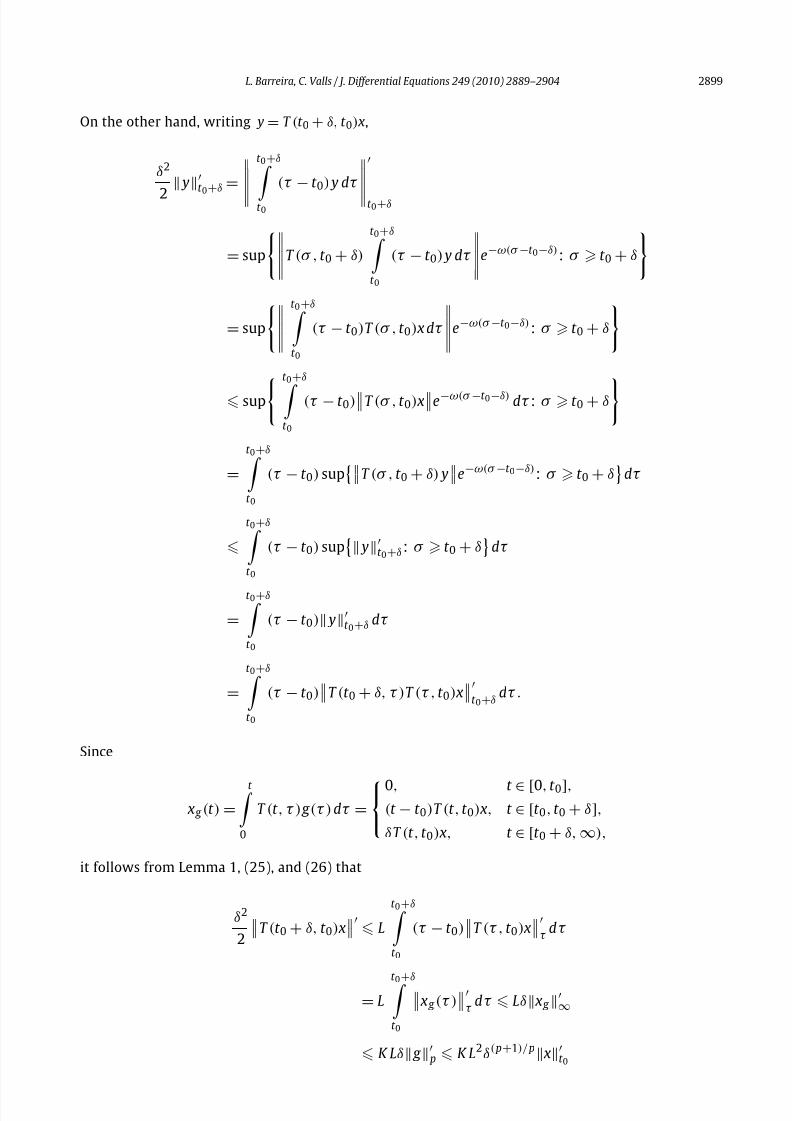
L. Barreira, C. Valls / J. Differential Equations 249 (2010) 2889–2904 2899
On the other hand, writing y = T (t 0 + δ, t 0) x,
δ2
2
yt 0+δ =
t 0+δ
t 0
(τ − t 0) y dτ
t 0+δ
= sup
T (σ , t 0 + δ)
t 0+δ t 0
(τ − t 0) y dτ
e−ω(σ −t 0−δ): σ t 0 + δ
= sup
t 0 +δ t 0
(τ − t 0)T (σ , t 0) x dτ
e−ω(σ −t 0−δ) : σ t 0 + δ
sup t 0+δ
t 0
(τ − t 0)T (σ , t 0) x
e−ω(σ −t 0−δ) dτ : σ t 0 + δ
=
t 0+δ t 0
(τ − t 0) supT (σ , t 0 + δ) y
e−ω(σ −t 0−δ): σ t 0 + δ
dτ
t 0+δ t 0
(τ − t 0) sup
yt 0+δ : σ t 0 + δ
dτ
=
t 0+δ t 0
(τ − t 0) yt 0+δ dτ
=
t 0+δ t 0
(τ − t 0)T (t 0 + δ, τ )T (τ , t 0) x
t 0+δ dτ .
Since
x g (t ) =
t 0
T (t , τ ) g (τ ) dτ =
0, t ∈ [0, t 0],
(t − t 0)T (t , t 0) x, t ∈ [t 0, t 0 + δ],
δT (t , t 0) x, t ∈ [t 0 + δ, ∞),
it follows from Lemma 1, (25), and (26) that
δ2
2
T (t 0 + δ, t 0) x L
t 0 +δ t 0
(τ − t 0)T (τ , t 0) x
τ dτ
= Lt 0 +δ t 0
x g (τ )
τ dτ Lδ x g
∞
K Lδ g p K L2δ( p+1)/ p x
t 0
8/19/2019 Barreira, Valls, 2010
http://slidepdf.com/reader/full/barreira-valls-2010 12/16
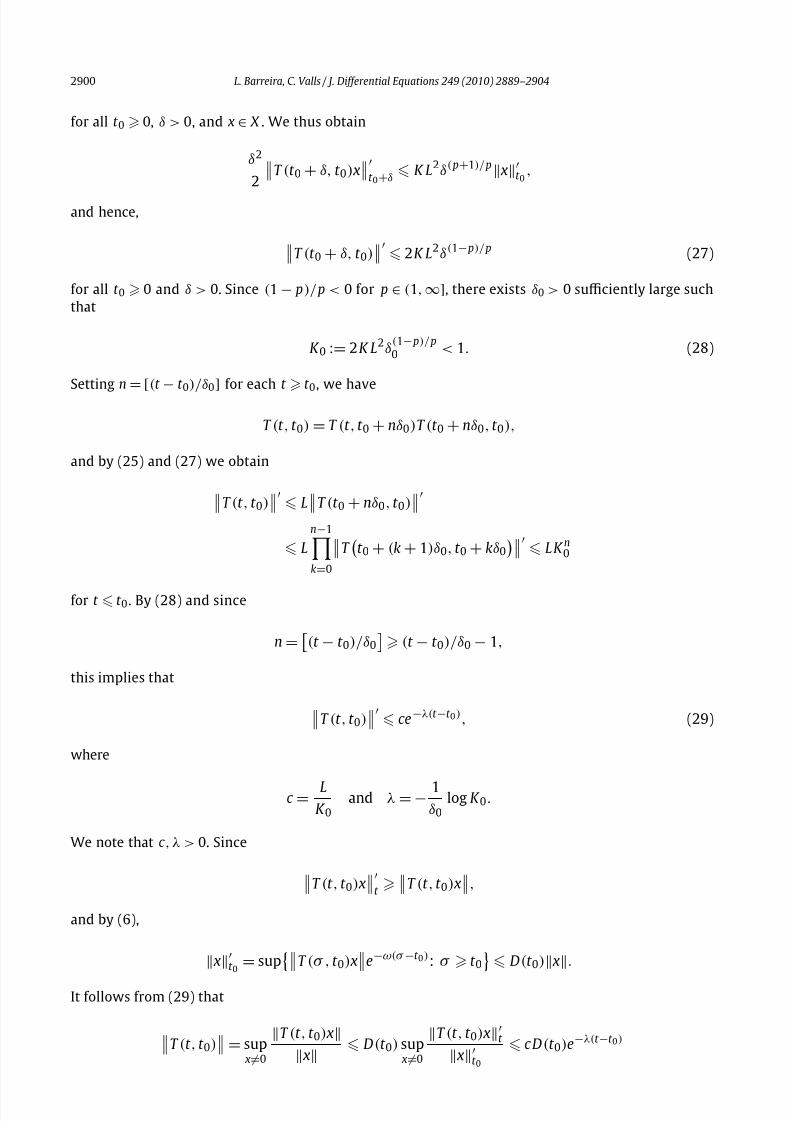
2900 L. Barreira, C. Valls / J. Differential Equations 249 (2010) 2889–2904
for all t 0 0, δ > 0, and x ∈ X . We thus obtain
δ2
2 T (t 0 + δ, t 0) x
t 0+δ K L2δ( p+1)/ p x
t 0,
and hence,
T (t 0 + δ, t 0) 2K L2δ(1− p)/ p (27)
for all t 0 0 and δ > 0. Since (1 − p)/ p < 0 for p ∈ (1, ∞], there exists δ0 > 0 sufficiently large such
that
K 0 := 2K L2δ(1− p)/ p0 < 1. (28)
Setting n = [(t − t 0
)/δ0
] for each t t 0
, we have
T (t , t 0) = T (t , t 0 + nδ0)T (t 0 + nδ0, t 0),
and by (25) and (27) we obtain
T (t , t 0) L
T (t 0 + nδ0, t 0)
L
n−1k=0
T
t 0 + (k + 1)δ0, t 0 + kδ0
L K n0
for t t 0 . By (28) and since
n =
(t − t 0)/δ0
(t − t 0)/δ0 − 1,
this implies that
T (t , t 0) ce−λ(t −t 0 ), (29)
where
c = LK 0
and λ = − 1δ0
log K 0.
We note that c , λ > 0. Since
T (t , t 0) x
t T (t , t 0) x
,
and by (6),
xt 0
= supT (σ , t 0) xe−ω(σ −t 0): σ t 0 D(t 0) x.
It follows from (29) that
T (t , t 0) = sup
x =0
T (t , t 0) x
x D(t 0) sup
x =0
T (t , t 0) xt
xt 0
cD(t 0)e−λ(t −t 0)
8/19/2019 Barreira, Valls, 2010
http://slidepdf.com/reader/full/barreira-valls-2010 13/16
L. Barreira, C. Valls / J. Differential Equations 249 (2010) 2889–2904 2901
for any t t 0. Therefore, the evolution process T is a C -nonuniform exponential contraction with
a = λ and C = c D . This concludes the proof of Theorem 5.
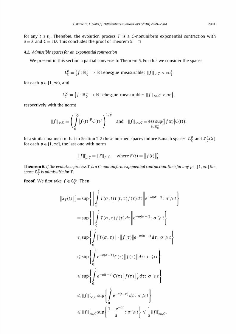
4.2. Admissible spaces for an exponential contraction
We present in this section a partial converse to Theorem 5. For this we consider the spaces
L pC =
f :R+
0 → R Lebesgue-measurable: f p,C < ∞
for each p ∈ [1, ∞), and
L∞C =
f :R+
0 → R Lebesgue-measurable: f ∞,C < ∞
,
respectively with the norms
f p,C =
∞ 0
f (t ) p C (t ) p
1/ p
and f ∞,C = ess supt ∈R+
0
f (t )C (t )
.
In a similar manner to that in Section 2.2 these normed spaces induce Banach spaces L pC and L
pC ( X )
for each p ∈ [1, ∞], the last one with norm
f p,C = F p,C , where F (t ) =
f (t )
t .
Theorem 6. If the evolution process T is a C -nonuniform exponential contraction, then for any p ∈ [1, ∞] the
space L pC is admissible for T .
Proof. We first take f ∈ L∞C . Then
x f (t )
t = sup
t
0
T (σ , t )T (t , τ ) f (τ ) dτ
e−ω(σ −t ): σ t
= sup
t 0
T (σ , τ ) f (τ ) dτ
e−ω(σ −t ): σ t
sup t
0
T (σ , τ ) · f (τ )
e−ω(σ −t ) dτ : σ t
sup
t 0
e−a(σ −τ )C (τ ) f (τ )
dτ : σ t
sup
t 0
e−a(t −τ )C (τ ) f (τ )
τ dτ : σ t
f ∞,C sup
t 0
e−a(t −τ ) dτ : σ t
f ∞,C sup
1 − e−at
a : σ t
1
a f
∞,C .
8/19/2019 Barreira, Valls, 2010
http://slidepdf.com/reader/full/barreira-valls-2010 14/16
2902 L. Barreira, C. Valls / J. Differential Equations 249 (2010) 2889–2904
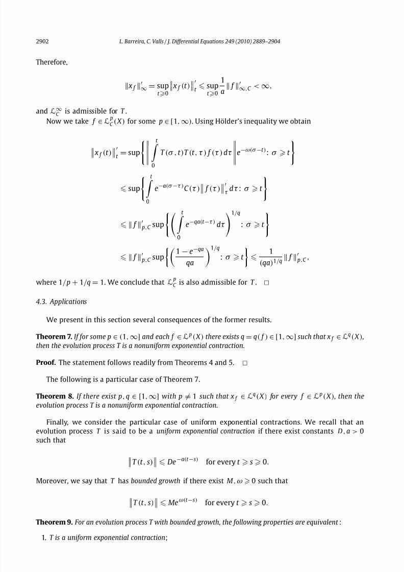
Therefore,
x f ∞ = sup
t 0 x f (t )
t sup
t 0
1
a f
∞,C < ∞,
and L∞C is admissible for T .
Now we take f ∈ L pC ( X ) for some p ∈ [1, ∞). Using Hölder’s inequality we obtain
x f (t )
t = sup
t
0
T (σ , t )T (t , τ ) f (τ ) dτ
e−ω(σ −t ): σ t
sup t
0
e−a(σ −τ )C (τ ) f (τ )
τ dτ : σ t
f p,C sup
t 0
e−qa(t −τ ) dτ
1/q
: σ t
f p,C sup
1 − e−qa
qa
1/q
: σ t
1
(qa)1/q f
p,C ,
where 1/ p + 1/q = 1. We conclude that L pC is also admissible for T .
4.3. Applications
We present in this section several consequences of the former results.
Theorem 7. If for some p ∈ (1, ∞] and each f ∈ L p ( X ) there exists q = q( f ) ∈ [1, ∞] such that x f ∈ L
q( X ),
then the evolution process T is a nonuniform exponential contraction.
Proof. The statement follows readily from Theorems 4 and 5.
The following is a particular case of Theorem 7.
Theorem 8. If there exist p, q ∈ [1, ∞] with p = 1 such that x f
∈ Lq( X ) for every f ∈ L
p( X ), then the
evolution process T is a nonuniform exponential contraction.
Finally, we consider the particular case of uniform exponential contractions. We recall that an
evolution process T is said to be a uniform exponential contraction if there exist constants D, a > 0
such that
T (t , s) De −a(t −s) for every t s 0.
Moreover, we say that T has bounded growth if there exist M , ω 0 such that
T (t , s) Me ω(t −s) for every t s 0.
Theorem 9. For an evolution process T with bounded growth, the following properties are equivalent :
1. T is a uniform exponential contraction;
8/19/2019 Barreira, Valls, 2010
http://slidepdf.com/reader/full/barreira-valls-2010 15/16
L. Barreira, C. Valls / J. Differential Equations 249 (2010) 2889–2904 2903
2. for some p ∈ (1, ∞] the space L p is admissible for T ;
3. for all p ∈ [1, ∞] the space L p is admissible for T .
Proof. By Theorem 6, condition 1 implies condition 3 (since L pD reduces to L p when D is a con-
stant). Moreover, clearly condition 3 implies condition 2. Finally, by Theorem 5, condition 2 impliescondition 1 (using D(s) = D in the proof).
By (6), if T has bounded growth, then
v vt M v, v ∈ X , t ∈ R
+0 .
Therefore, in this case, in the notion of admissibility one can replace each space E ( X ) with E = L p
by the space
f :R+0 → X Bochner-measurable: t →
f (t )
∈ E
,
endowed with the norm
f = F p , where F (t ) = f (t )
.
References
[1] L. Barreira, Ya. Pesin, Lyapunov Exponents and Smooth Ergodic Theory, Univ. Lecture Ser., vol. 23, Amer. Math. Soc., 2002.
[2] L. Barreira, Ya. Pesin, Nonuniform Hyperbolicity, Encyclopedia Math. Appl., vol. 115, Cambridge University Press, 2007.
[3] L. Barreira, J. Schmeling, Sets of “non-typical” points have full topological entropy and full Hausdorff dimension, Israel J.
Math. 116 (2000) 29–70.[4] L. Barreira, C. Valls, Optimal estimates along stable manifolds of non-uniformly hyperbolic dynamics, Proc. Roy. Soc. Edin-
burgh Sect. A 138 (2008) 693–717.
[5] L. Barreira, C. Valls, Stability of Nonautonomous Differential Equations, Lecture Notes in Math., vol. 1926, Springer, 2008.
[6] A. Ben-Artzi, I. Gohberg, Dichotomy of systems and invertibility of linear ordinary differential operators, in: Time-Variant
Systems and Interpolation, in: Oper. Theory Adv. Appl., vol. 56, Birkhäuser, 1992, pp. 90–119.
[7] A. Ben-Artzi, I. Gohberg, M. Kaashoek, Invertibility and dichotomy of differential operators on a half-line, J. Dynam. Differ-
ential Equations 5 (1993) 1–36.
[8] C. Chicone, Yu. Latushkin, Evolution Semigroups in Dynamical Systems and Differential Equations, Math. Surveys Monogr.,
vol. 70, Amer. Math. Soc., 1999.
[9] W. Coppel, Dichotomies in Stability Theory, Lecture Notes in Math., vol. 629, Springer, 1978.
[10] Ju. Dalec’kiı, M. Kreın, Stability of Solutions of Differential Equations in Banach Space, Transl. Math. Monogr., vol. 43, Amer.
Math. Soc., 1974.
[11] D. Henry, Geometric Theory of Semilinear Parabolic Equations, Lecture Notes in Math., vol. 840, Springer, 1981.
[12] N.T. Huy, Exponential dichotomy of evolution equations and admissibility of function spaces on a half-line, J. Funct.
Anal. 235 (2006) 330–354.
[13] Yu. Latushkin, A. Pogan, R. Schnaubelt, Dichotomy and Fredholm properties of evolution equations, J. Operator Theory 58
(2007) 387–414.
[14] B. Levitan, V. Zhikov, Almost Periodic Functions and Differential Equations, Cambridge University Press, 1982.
[15] J. Massera, J. Schäffer, Linear differential equations and functional analysis. I, Ann. of Math. (2) 67 (1958) 517–573.
[16] J. Massera, J. Schäffer, Linear Differential Equations and Function Spaces, Pure Appl. Math., vol. 21, Academic Press, 1966.
[17] M. Megan, B. Sasu, A. Sasu, On nonuniform exponential dichotomy of evolution operators in Banach spaces, Integral Equa-
tions Operator Theory 44 (2002) 71–78.
[18] N.V. Minh, N.T. Huy, Characterizations of dichotomies of evolution equations on the half-line, J. Math. Anal. Appl. 261
(2001) 28–44.
[19] V. Oseledets, A multiplicative ergodic theorem: Liapunov characteristic numbers for dynamical systems, Trans. Moscow
Math. Soc. 19 (1968) 197–221.
[20] K. Palmer, Exponential dichotomies and Fredholm operators, Proc. Amer. Math. Soc. 104 (1988) 149–156.[21] O. Perron, Die Stabilitätsfrage bei Differentialgleichungen, Math. Z. 32 (1930) 703–728.
[22] Ya. Pesin, Families of invariant manifolds corresponding to nonzero characteristic exponents, Math. USSR Izv. 10 (1976)
1261–1305.
[23] P. Preda, M. Megan, Nonuniform dichotomy of evolutionary processes in Banach spaces, Bull. Austral. Math. Soc. 27 (1983)
31–52.
8/19/2019 Barreira, Valls, 2010
http://slidepdf.com/reader/full/barreira-valls-2010 16/16
2904 L. Barreira, C. Valls / J. Differential Equations 249 (2010) 2889–2904
[24] P. Preda, A. Pogan, C. Preda, (L p , Lq )-admissibility and exponential dichotomy of evolutionary processes on the half-line,
Integral Equations Operator Theory 49 (2004) 405–418.
[25] P. Preda, A. Pogan, C. Preda, Schäffer spaces and uniform exponential stability of linear skew-product semiflows, J. Differ-
ential Equations 212 (2005) 191–207.
[26] P. Preda, A. Pogan, C. Preda, Schäffer spaces and exponential dichotomy for evolutionary processes, J. Differential Equa-
tions 230 (2006) 378–391.[27] J. Schäffer, Function spaces with translations, Math. Ann. 137 (1959) 209–262.
[28] N.V. Minh, F. Räbiger, R. Schnaubelt, Exponential stability, exponential expansiveness, and exponential dichotomy of evolu-
tion equations on the half-line, Integral Equations Operator Theory 32 (1998) 332–353.
[29] W. Zhang, The Fredholm alternative and exponential dichotomies for parabolic equations, J. Math. Anal. Appl. 191 (1985)
180–201.