A&A 546, A121 (2012)DOI: 10.1051/0004-6361/201219747c© ESO 2012

Astronomy&

Astrophysics

Radiative properties of magnetic neutron starswith metallic surfaces and thin atmospheres

A. Y. Potekhin1,2,3, V. F. Suleimanov4,5, M. van Adelsberg6, and K. Werner4

1 Centre de Recherche Astrophysique de Lyon (CNRS, UMR 5574), Université Lyon 1, École Normale Supérieure de Lyon,46 allée d’Italie, 69364 Lyon Cedex 07, Francee-mail: palex@astro.ioffe.ru

2 Ioffe Physical-Technical Institute, Politekhnicheskaya 26, St. Petersburg 194021, Russia3 Isaac Newton Institute of Chile, St. Petersburg Branch, Russia4 Institut für Astronomie und Astrophysik, Kepler Center for Astro and Particle Physics, Universität Tübingen, Sand 1,

72076 Tübingen, Germany5 Kazan Federal University, Kremlevskaja Str., 18, Kazan 420008, Russia6 Center for Relativistic Astrophysics, School of Physics, Georgia Institute of Technology, Atlanta, Georgia 30332, USA

Received 4 June 2012 / Accepted 26 August 2012

ABSTRACT

Context. Simple models fail to describe the observed spectra of X-ray-dim isolated neutron stars (XDINSs). Interpretating thesespectra requires detailed studies of radiative properties in the outermost layers of neutron stars with strong magnetic fields. Previousstudies have shown that the strongly magnetized plasma in the outer envelopes of a neutron star may exhibit a phase transition toa condensed form. In this case thermal radiation can emerge directly from the metallic surface without going through a gaseousatmosphere, or alternatively, it may pass through a “thin” atmosphere above the surface. The multitude of theoretical possibilitiescomplicates modeling the spectra and makes it desirable to have analytic formulae for constructing samples of models without goingthrough computationally expensive, detailed calculations.Aims. The goal of this work is to develop a simple analytic description of the emission properties (spectrum and polarization) of thecondensed, strongly magnetized surface of neutron stars.Methods. We have improved our earlier work for calculating the spectral properties of condensed magnetized surfaces. Using theimproved method, we calculated the reflectivity of an iron surface at magnetic field strengths B ∼ 1012 G–1014 G, with various incli-nations of the magnetic field lines and radiation beam with respect to the surface and each other. We constructed analytic expressionsfor the emissivity of this surface as functions of the photon energy, magnetic field strength, and the three angles that determine thegeometry of the local problem. Using these expressions, we calculated X-ray spectra for neutron stars with condensed iron surfacescovered by thin partially ionized hydrogen atmospheres.Results. We develop simple analytic descriptions of the intensity and polarization of radiation emitted or reflected by condensediron surfaces of neutron stars with the strong magnetic fields typical of isolated neutron stars. This description provides boundaryconditions at the bottom of a thin atmosphere, which are more accurate than previously used approximations. The spectra calculatedwith this improvement show different absorption features from those in simplified models.Conclusions. The approach developed in this paper yields results that can facilitate modeling and interpretation of the X-ray spectraof isolated, strongly magnetized, thermally emitting neutron stars.

Key words. stars: neutron – stars: atmospheres – magnetic fields – radiation mechanisms: thermal – X-rays: stars

1. Introduction

Recent observations of neutron stars have provided a wealthof valuable information, but they have also raised many newquestions. Particularly intriguing is the class of radio-quiet neu-tron stars with thermal-like spectra, commonly known as X-raydim isolated neutron stars (XDINSs), or the Magnificent Seven(see, e.g., reviews by Haberl 2007 and Turolla 2009, and ref-erences therein). Some of them (e.g., RX J1856.5−3754) havefeatureless spectra, whereas others (e.g., RX J1308.6+2127 andRX J0720.4−3125) have broad absorption features with energies∼0.2–2 keV. In recent years, an accumulation of observationalevidence has suggested that XDINSs may have magnetic fieldsB ∼ 1013–1014 G and be related to magnetars (e.g., Mereghetti2008).

For interpretating the XDINS spectra, it may be necessary totake the phenomenon of “magnetic condensation” into account.

The strong magnetic field squeezes the electron clouds aroundthe nuclei, thereby increasing the binding and cohesive ener-gies (e.g., Medin & Lai 2006, and references therein). ThereforeXDINSs may be “naked,” with no appreciable atmosphere abovea condensed surface, as first conjectured by Zane et al. (2002),or they may have a relatively thin atmosphere, with the spectrumof outgoing radiation affected by the properties of the condensedsurface beneath the atmosphere, as suggested by Motch et al.(2003).

Reflectivities of condensed metallic surfaces in strong mag-netic fields have been studied in several papers (Brinkmann1980; Turolla et al. 2004; van Adelsberg et al. 2005;Pérez-Azorín et al. 2005). Brinkmann (1980) and Turolla et al.(2004) neglected the motion of ions in the condensed mat-ter, whereas van Adelsberg et al. (2005; hereafter Paper I) andPérez-Azorín et al. (2005) considered two opposite limitingcases, one that neglects the ion motion (“fixed ions”) and another

Article published by EDP Sciences A121, page 1 of 14

A&A 546, A121 (2012)

where the ion response to the electromagnetic wave is treatedby neglecting the Coulomb interactions between the ions (“freeions”). A large difference between these two limits occurs atphoton frequencies below the ion cyclotron frequency, but thetwo models lead to almost the same results at higher photon en-ergies. We expect that in reality the surface spectrum lies be-tween these two limits (see Paper I for discussion). The resultsof Paper I and of Pérez-Azorín et al. (2005) are similar, but differsignificantly from the earlier results. In particular, Turolla et al.(2004) find that collisional damping in the condensed matterleads to a sharp cutoff in the emission at low photon energies, butsuch a cutoff is absent in Paper I and Pérez-Azorín et al. (2005).It is most likely that this difference arises from the “one-mode”description for the transmitted radiation adopted by Turolla et al.(2004, see Paper I for details). All the previous works relied on acomplicated method of finding the transmitted radiation modes,originally due to Brinkmann (1980). We replace it with the morereliable method described below.

Ho et al. (2007, see also Ho 2007) fitted multiwavelengthobservations of RX J1856.5−3754 with a model of a thin, mag-netic, partially ionized hydrogen atmosphere on top of a con-densed iron surface; they also discuss possible mechanisms ofcreation of such a thin atmosphere. Suleimanov et al. (2009) cal-culated various models of fully and partially ionized finite atmo-spheres above a condensed surface including the case of “sand-wich” atmospheres, composed of hydrogen and helium layersabove a condensed surface.

The wide variety of theoretical possibilities complicates themodeling and interpretation of the spectra. To facilitate this task,Suleimanov et al. (2010; hereafter Paper II) suggest an approx-imate treatment, in which the local spectra, together with tem-perature and magnetic field distributions, are fitted by simpleanalytic functions. By being flexible and fast, this approach issuited to constrain stellar parameters prior to performing moreaccurate, but computationally expensive calculations of modelspectra. The reflectivity of the condensed surface was mod-eled by a simple steplike function, which roughly described thepolarization-averaged reflectivity of a magnetized iron surface atB = 1013 G, but depended neither on the magnetic field strengthB nor on the angle ϕ between the plane of incidence and theplane made by the normal to the surface and the magnetic fieldlines.

In the present work, the numerical method of Paper I andthe approximate treatment of Paper II are refined. We developa less complicated and more stable method of calculations andconstruct more accurate fitting formulae for the reflectivities of acondensed, strongly magnetized iron surface, taking the depen-dence on arguments B and ϕ into account. The new fit reproducesthe feature near the electron plasma energy, obtained numeri-cally in Paper I but neglected in Paper II. Two versions of the fitare presented in Sect. 2 for the models of free and fixed ions dis-cussed in Paper I. In addition to the fit for the average reflectivity,we present analytic approximations for each of the two polariza-tion modes, which allow us to calculate the polarization of radi-ation of a naked neutron star. In Sect. 3 we consider the radiativetransfer problem in a finite atmosphere above the condensed sur-face, including the reflection from the inner atmosphere bound-ary with normal-mode transformations, neglected in the previousstudies of thin atmospheres. Conclusions are given in Sect. 4. InAppendix A we describe the method of calculation for the re-flectivity coefficients, which is improved with respect to Paper I.In Appendix B we describe an analytic model of normal-modereflectivities at the inner boundary of a thin atmosphere.

2. Spectral properties of a strongly magnetizedneutron star surface

2.1. Condensed magnetized surface

Most of the known neutron stars have much larger magneticfields B than the natural atomic unit for the field strength B0 =e3m2

ec/�3 = 2.35 × 109 G, which is set by equating the electroncyclotron energy

Ece = �eB/mec = 115.77 B13 keV (1)

to the Hartree unit of energy mee4/�2. Here, me is the electronmass, e the elementary charge, c the speed of light in vacuum,� the Planck constant divided by 2π, and B13 = B/1013 G.Fields with B � B0 profoundly affect the properties of atoms,molecules, and plasma (see, e.g., Haensel et al. 2007, Chap. 4).Ruderman (1971) suggested that the strong magnetic field maystabilize linear molecular chains (polymers) aligned with themagnetic field and eventually turn the surface of a neutron starinto the metallic solid state. Later studies have provided supportfor this conjecture, although the surface density ρs and, espe-cially, the critical temperature Tcrit below which such conden-sation occurs remain uncertain. Order-of-magnitude estimatessuggest

ρs = 8.9 × 103 η AZ−0.6 B1.213 g cm−3, (2)

where A and Z are the atomic mass and charge numbers, andη ∼ 1 an unknown numerical factor, which absorbs the the-oretical uncertainty (see Lai 2001). The value η = 1 corre-sponds to the equation of state provided by the ion-sphere model(Salpeter 1954). More recent results of the zero-temperatureThomas-Fermi model for 56Fe at 1010 G � B � 1013 G (Fushikiet al. 1989; Rögnvaldsson et al. 1993) can be approximated(within 4%) by Eq. (2) with η ≈ 0.2 + 0.0028/B0.56

13 , whereasthe finite-temperature Thomas-Fermi model of Thorolfsson et al.(1998) does not predict magnetic condensation at all. The mostcomprehensive study of cohesive properties of the magnetic con-densed surface has been conducted by Medin & Lai (2006,2007), based on density-functional theory (DFT). Medin & Lai(2006) calculated cohesive energies Qs of the molecular chainsand condensed phases of H, He, C, and Fe in strong magneticfields. A comparison with previous DFT calculations by otherauthors suggests that Qs may vary within a factor of two at B �1012 G, depending on the approximations employed (see Medin& Lai 2006, for references and discussion). Medin & Lai (2007)calculated equilibrium densities of saturated vapors of He, C,and Fe atoms and chains above the condensed surfaces and ob-tained Tcrit at several values of B by equating the vapor densityto ρs. Unlike previous authors, Medin & Lai (2006, 2007) havetaken the electronic band structure of the metallic phase into ac-count self-consistently. However, in the gaseous phase, they stilldid not allow for atomic motion across the magnetic field anddid not take a detailed treatment of excited atomic and molecu-lar states into account. Medin & Lai (2007) calculated the sur-face density assuming that the linear molecular chains (directedalong B) form a rectangular array in the perpendicular plane andthat the distance between the nuclei along the field lines is thesame in the condensed matter as in the separate molecular chain(Medin & Lai 2006; Medin 2012, priv. comm.). Medin & Lai(2007) found that the critical temperature is Tcrit ≈ 0.08Qs/kB.Their numerical results for 56Fe at 0.5 � B13 � 100 can be de-scribed by expression Tcrit ≈ (5 + 2 B13) × 105 K for the criticaltemperature and by Eq. (2) with η ≈ 0.55 for the surface density,

A121, page 2 of 14

A. Y. Potekhin et al.: Spectra of neutron stars with metallic surfaces

with uncertainties below 20% for both quantities. An observa-tional determination of the phase state of a neutron star surfacewould be helpful for improving the theory of matter in strongmagnetic fields.

The density of saturated vapor above the condensed sur-face rapidly decreases with decreasing T (Lai & Salpeter 1997).Therefore, although the surface is hidden by an optically thickatmosphere at T ≈ Tcrit, the atmosphere becomes optically thinat T � Tcrit. Also, as suggested by Motch et al. (2003), theremay be a finite amount of light chemical elements (e.g., H) ontop of the condensed surface of a heavier element (e.g., Fe). Inaddition, the same atmosphere may be optically thick for lowphoton energies and transparent at high energies. The energy atwhich the total optical thickness of a finite atmosphere equalsunity depends on the atmosphere column density, which can inturn depend on temperature. At a fixed energy, the optical thick-ness of the finite atmosphere is different for different photon po-larizations, therefore the atmosphere can be thick for one po-larization mode and thin for another. One should take all thesepossibilities into account while interpreting observed spectra ofneutron stars.

2.2. Formation of the spectrum

2.2.1. Normal modes and polarization vectors

It is well known (e.g., Ginzburg 1970) that under typical con-ditions (e.g., far from the resonances) electromagnetic radiationpropagates in a magnetized plasma in the form of extraordinary(X) and ordinary (O) normal modes. These modes have differentpolarization vectors eX and eO, absorption and scattering coef-ficients, and refraction and reflection coefficients at the surface.Gnedin & Pavlov (1973) studied conditions for the applicabil-ity of the normal-mode description and formulated the radiativetransfer problem in terms of these modes.

Following the works of Shafranov (1967) and Ginzburg(1970), Ho & Lai (2001) derived convenient expressions for thenormal mode polarization vectors in a fully ionized plasma forphoton energies E much higher than the electron plasma energy

Epe =(4π�2e2ne/me

)1/2 ≈ 0.0288√ρZ/A keV, (3)

where ρ is the density in g cm−3. In the complex representationof plane waves with E ∝ e ei(k·r−ωt), in the coordinate systemwhere the z-axis is along the wave vector k, and the magneticfield B lies in the (xz) plane, the polarization vectors are

eM(α) =1√

1 + |KM(α)|2 + |Kz,M(α)|2

⎛⎜⎜⎜⎜⎜⎜⎝iKM(α)

1iKz,M(α)

⎞⎟⎟⎟⎟⎟⎟⎠ , (4)

We use the notation M = X and M = O for the extraordi-nary and ordinary polarization modes, respectively. KM(α) andKz,M(α) are functions of the angle α between B and k. Theyare determined by the dielectric tensor of the plasma and thusdepend on the photon energy E, as well as ρ, B, T and thechemical composition. Ho & Lai (2003) calculated KM and stud-ied the polarization of normal modes including the effect ofthe electron-positron vacuum polarization, while Potekhin et al.(2004) additionally considered an incomplete ionization of theplasma.

2.2.2. Emission and reflection by a condensed surface

The condition E > Epe is usually satisfied for X-rays in neutronstar atmospheres, but not in the condensed matter. We consider a

Fig. 1. Illustration of notations. The z axis is chosen perpendicular tothe surface, and the (xz) plane is chosen parallel to the magnetic fieldlines, which make an angle θB with the normal to the surface. The di-rection of the reflected beam with wave vector kr is determined by thepolar angle θk and the azimuthal angle ϕ, and αr is the angle betweenthe reflected beam and the field lines. Thick solid lines show the re-flected beam and magnetic field directions, thin solid lines illustrate thecoordinates, and dashed lines show the incident photon wave vector ki

and its quadrant. The lines marked e(i,r)1,2 illustrate the basic polarizations

adopted for the description of reflectivities: e(i)1,2 and e(r)

1,2 are perpendic-

ular to the wave vectors ki and ki, respectively; e(i,r)1 are parallel to the

surface, and e(i,r)2 lie in the perpendicular plane. The axes x′ and y′ lie in

the plane made by e(r)1 and e(r)

2 , x′ being aligned in the plane made by Band kr.

surface element that is sufficiently small for the variation in themagnetic field strength and inclination to be neglected. We treatthis small patch as plane, neglecting its curvature and roughness.We choose the Cartesian z axis perpendicular to this plane andthe x axis parallel to the projection of magnetic field lines ontothe xy plane. We denote the angle between the field and the zaxis as θB, the incidence angle of the radiation as θk, and theangle in the xy plane made by the projection of the wave vectoras ϕ (Fig. 1). The angle between the wave vector and magneticfield lines is given by

cosαi,r = sin θB sin θk cosϕ ∓ cos θB cos θk (5)

for the incident and reflected waves, respectively. The surfaceemits radiation with monochromatic intensities

IE, j = J j BE/2 ( j = 1, 2). (6)

Here, the basis for polarization is chosen such that the waveswith j = 1 and 2 are linearly polarized parallel and perpendicularto the incident plane, respectively (Fig. 1); IE, j dΣ dΩ dE dt givesthe energy radiated in the jth wave by the surface element dΣ, inthe energy band (E, E + dE), during time dt, in the solid angleelement dΩ around the direction of the wave vector k. We usethe function

BE =Bν

2π�=

E3

4π3�3c2(eE/kBT − 1), (7)

where Bν is Planck’s spectral radiance and kB the Boltzmannconstant. Dimensionless emissivities for the two polarizations,normalized to blackbody values, are J j = 1−R j, where R j is theeffective reflectivity of mode j defined in Appendix A. The re-flectivities depend on surface material, photon energy, magneticfield strength B and inclination θB, and on the direction of k.For nonpolarized radiation, it is sufficient to consider the meanreflectivity R = (R1 + R2)/2 (see Paper I).

A121, page 3 of 14

A&A 546, A121 (2012)

2.2.3. Reflectivity calculation

A method for calculating reflectivity coefficients was devel-oped in Paper I. However, it is not easy to implement. Thoughit mostly produces correct results, in some ranges of modelparameters it can yield unphysical results, which are difficultto distinguish from the correct ones. In the present work wepresent an improved method that avoids this complication (seeAppendix A).

Using our new method, we calculated the spectral propertiesof a condensed Fe surface and compared the results with thosein Paper I. As in Paper I, we considered two alternative modelsfor the response of ions to electromagnetic waves in the con-densed phase: one neglects the Coulomb interactions betweenions, while the other treats ions as frozen at their equilibriumpositions in the Coulomb crystal (i.e., neglecting their responseto the electromagnetic wave).

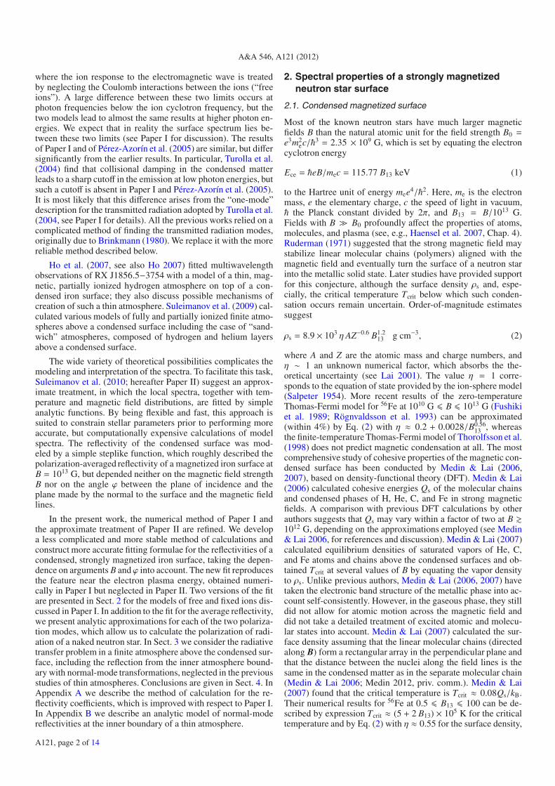
In the first limiting case (thick lines in Fig. 2), the reflectivityexhibits different behavior in three characteristic energy ranges:E < Eci, Eci � E � EC, and E � EC, where

Eci = �ZeB/Amuc = 0.0635 (Z/A) B13 keV (8)

is the ion cyclotron energy, mu is the unified atomic mass unit,and

EC = Eci + E2pe/Ece. (9)

In addition, there is suppression of the reflectivity at E ∼ Epe;the exact position, width, and depth of the suppression dependon the geometry defined by the angles θB, θk, and ϕ.

In the opposite case of immobile ions (thin curves in Fig. 2),the reflectivity has a similar behavior at E > Eci, but differs atE � Eci. It does not exhibit the sharp change at E ≈ Eci, butsmoothly continues to the lower energies. As argued in Paper I,we expect that the actual reflectivity lies between these twoextremes.

The new results, shown in Fig. 2, display the same qualita-tive behavior as in Paper I, but exhibit considerable deviationfrom the previous calculations for some geometric settings inthe energy range Eci � E � EC. Thus, the qualitative results andconclusions of Paper I are correct, but the new method describedin Appendix A is quantitatively more reliable.

If θB = θk = 0, then an approximate analytic solution (ne-glecting the finite electron relaxation rate in the medium; seePaper I for discussion) is R ≈ (R+ + R−)/2, where

R(0)± =∣∣∣∣∣∣n(0)± − 1

n(0)± + 1

∣∣∣∣∣∣2

, n(0)± =⎡⎢⎢⎢⎢⎢⎣1 ± E2

pe

Ece(E ± Eci)

⎤⎥⎥⎥⎥⎥⎦1/2

· (10)

Compared to the numerical results, Eq. (10) provides a good ap-proximation at E � Eci. Therefore, we use it in the analytic fitdescribed below.

2.3. Results for iron surface

In the numerical examples presented below we assume a con-densed 56Fe surface and use the estimate of the surface densitygiven by the ion-sphere model – that is, we set η = 1 in Eq. (2).

2.3.1. Mean reflectivity

In practice, the average normalized emissivity J = 1 − R is usu-ally more important than the specific emissivities R j. In Paper II,

Fig. 2. Dimensionless emissivity J = 1 − R as a function of photonenergy E for a condensed Fe surface with B = 1013 G and T = 106 K.The top panel shows several cases with varying θB and fixed θk = π/4,ϕ = π/4. The bottom panel shows several cases with varying ϕ andfixed θk = π/4, θB = π/4. These plots should be compared with Figs. 5and 6 of Paper I.

R(E) was replaced by a constant in each of the three ranges men-tioned in Sect. 2.2.3 (E < Eci, Eci < E < EC ≈ EC, and E > EC).For simplicity, the values of these three constants were assumedto depend only on θB and θk, but not on ϕ or B. Here we proposea more elaborate and accurate fit, which is a function of E, B, θB,θk, and ϕ, for the magnetic field range 1012 G � B � 1014 G andphoton energy range 1 eV � E � 10 keV. In the approximationof free ions, the average reflectivity of the metallic iron surfaceis approximately reproduced by

J =

⎧⎪⎪⎨⎪⎪⎩JA in Region I,

JB (1 − JC) +JC

1 + Lin Region II.

(11)

Region I is the low-energy region defined by the conditionsE < Eci and JA > JB. Region II is the supplemental range ofrelatively high energies in which either of these conditions is vi-olated. The functions JA, JB, and JC are mainly responsible forthe behavior of the emissivity at E < Eci, Eci < E � EC, andE > EC, respectively, while the function L describes the line atE ≈ Epe. The value

EC = Eci + Epe2/Ece (12)

A121, page 4 of 14

A. Y. Potekhin et al.: Spectra of neutron stars with metallic surfaces

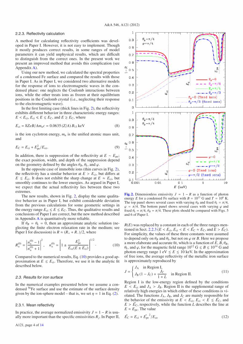
Fig. 3. Dimensionless emissivity J = 1 − R as a function of photonenergy E for condensed Fe surface at B = 1013 G (top panel), B =1012 G and 1014 G (bottom panel), with magnetic field lines normalto the surface, for two angles of incidence θk = 0 and θk = π/4, asmarked near the curves. Solid lines show our numerical results, anddashed lines demonstrate the fit. For comparison, dotted lines reproducethe simplified approximation used in Paper II.

is the energy at which the square of the effective refraction index

n2 = 1 − Epe2

Ece(E − Eci)(13)

(analogous to Eq. (10)) becomes positive with increasing E inthe range E > Eci. In Eqs. (12) and (13),

Epe = Epe

√3 − 2 cos θk. (14)

The low-energy part of the fit in Eq. (11) is given by

JA = [1 − A(E)] J0(E), (15)

where

A(E) =1 − cos θB2√

1 + B13+

[0.7 − 0.45

J0(0)

](sin θk)4 (1 − cosα), (16)

J0(E) = 1 − 12 (R(0)

− + R(0)+ ), and R(0)

± are given by Eq. (10).

Accordingly, J0(0) = 4(√

EC/Eci + 1)−1 (√

Eci/EC + 1)−1

. InEq. (16) and hereafter, α without subscripts denotes min(αr, αi).

In the intermediate energy range, Eci < E � EC, there is awide suppression of the emissivity. We describe this part by thepower-law interpolation between the values at Eci and EC:

JB = (E/EC)pJ(EC), where p =ln[J(EC)/J(Eci)]

ln(EC/Eci)· (17)

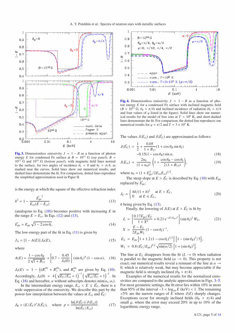
Fig. 4. Dimensionless emissivity J = 1 − R as a function of pho-ton energy E for a condensed Fe surface with inclined magnetic field(B = 1013 G, θB = π/4) and inclined incidence of radiation (θk = π/4and four values of ϕ listed in the figure). Solid lines show our numer-ical results for the model of free ions at T = 106 K, and short-dashedlines demonstrate the fit. For comparison, the dotted line reproduces ournumerical results for ϕ = π/2 and T = 3 × 105 K.

The values J(Eci) and J(EC) are approximated as follows:

J(EC) =12+

0.051 + B13

(1 + cos θB sin θk)

−0.15(1 − cos θB) sinα, (18)

J(Eci) =2n0

(1 + n0)2

(1 +

cos θB − cos θk2 (1 + B13)

), (19)

where n0 = (1 + E2pe/2EceEci)1/2.

The steep slope at E > EC is described by Eq. (10) with Epe

replaced by Epe:

JC =

{4n/(1 + n)2 at E > EC,0 at E � EC,

(20)

n being given by Eq. (13).Finally, the lowering of J(E) at E > EC is fit by

L =

[0.17Epe/EC

1 + X4+ 0.21 e−(E/Epe)2

](sin θk)2 WL, (21)

X =E − EL

2EpeWL(1 − cos θk)−1,

EL = Epe

[1 + 1.2 (1 − cos θk)3/2

] [1 − (sin θB)2/3

],

WL = 0.8 (EC/Epe)0.2√

sin(α/2)[1 + (sin θB)2

].

The line at EL disappears from the fit (L → 0) when radiationis parallel to the magnetic field (α → 0). This property is notexact; our numerical results reveal a remnant of the line at α →0, which is relatively weak, but may become appreciable if themagnetic field is strongly inclined (θB > π/4).

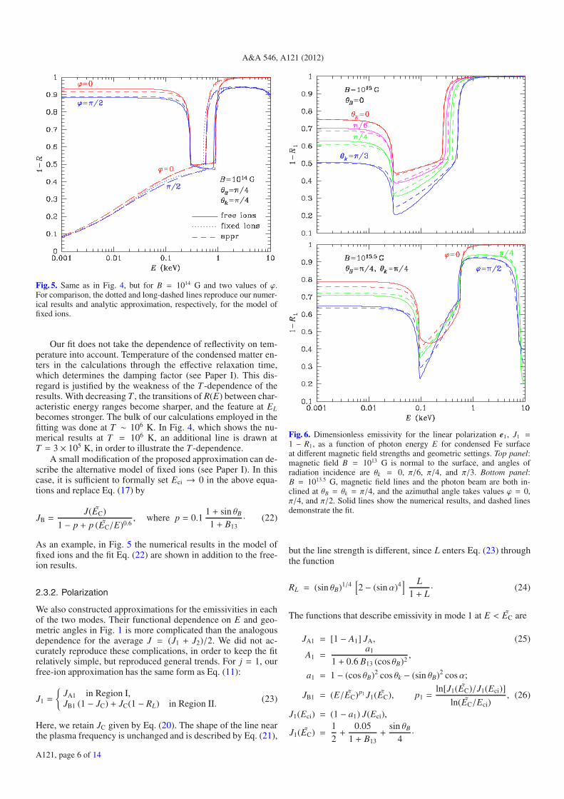
Examples of the numerical results for the normalized emis-sivities are compared to the analytic approximation in Figs. 3–5.For most geometric settings, the fit error lies within 10% in morethan 95% of the interval −3 < log10 E (keV) < 1. The remaining<5% are the narrow ranges of E where J(E) sharply changes.Exceptions occur for strongly inclined fields (θB > π/4) andsmall ϕ, where the error may exceed 20% in up to 10% of thelogarithmic energy range.

A121, page 5 of 14

A&A 546, A121 (2012)

Fig. 5. Same as in Fig. 4, but for B = 1014 G and two values of ϕ.For comparison, the dotted and long-dashed lines reproduce our numer-ical results and analytic approximation, respectively, for the model offixed ions.

Our fit does not take the dependence of reflectivity on tem-perature into account. Temperature of the condensed matter en-ters in the calculations through the effective relaxation time,which determines the damping factor (see Paper I). This dis-regard is justified by the weakness of the T -dependence of theresults. With decreasing T , the transitions of R(E) between char-acteristic energy ranges become sharper, and the feature at ELbecomes stronger. The bulk of our calculations employed in thefitting was done at T ∼ 106 K. In Fig. 4, which shows the nu-merical results at T = 106 K, an additional line is drawn atT = 3 × 105 K, in order to illustrate the T -dependence.

A small modification of the proposed approximation can de-scribe the alternative model of fixed ions (see Paper I). In thiscase, it is sufficient to formally set Eci → 0 in the above equa-tions and replace Eq. (17) by

JB =J(EC)

1 − p + p (EC/E)0.6, where p = 0.1

1 + sin θB1 + B13

· (22)

As an example, in Fig. 5 the numerical results in the model offixed ions and the fit Eq. (22) are shown in addition to the free-ion results.

2.3.2. Polarization

We also constructed approximations for the emissivities in eachof the two modes. Their functional dependence on E and geo-metric angles in Fig. 1 is more complicated than the analogousdependence for the average J = (J1 + J2)/2. We did not ac-curately reproduce these complications, in order to keep the fitrelatively simple, but reproduced general trends. For j = 1, ourfree-ion approximation has the same form as Eq. (11):

J1 =

{JA1 in Region I,JB1 (1 − JC) + JC(1 − RL) in Region II. (23)

Here, we retain JC given by Eq. (20). The shape of the line nearthe plasma frequency is unchanged and is described by Eq. (21),

Fig. 6. Dimensionless emissivity for the linear polarization e1, J1 =1 − R1, as a function of photon energy E for condensed Fe surfaceat different magnetic field strengths and geometric settings. Top panel:magnetic field B = 1013 G is normal to the surface, and angles ofradiation incidence are θk = 0, π/6, π/4, and π/3. Bottom panel:B = 1013.5 G, magnetic field lines and the photon beam are both in-clined at θB = θk = π/4, and the azimuthal angle takes values ϕ = 0,π/4, and π/2. Solid lines show the numerical results, and dashed linesdemonstrate the fit.

but the line strength is different, since L enters Eq. (23) throughthe function

RL = (sin θB)1/4[2 − (sinα)4

] L1 + L

· (24)

The functions that describe emissivity in mode 1 at E < EC are

JA1 = [1 − A1] JA, (25)

A1 =a1

1 + 0.6 B13 (cos θB)2,

a1 = 1 − (cos θB)2 cos θk − (sin θB)2 cosα;

JB1 = (E/EC)p1 J1(EC), p1 =ln[J1(EC)/J1(Eci)]

ln(EC/Eci), (26)

J1(Eci) = (1 − a1) J(Eci),

J1(EC) =12+

0.051 + B13

+sin θB

4·

A121, page 6 of 14

A. Y. Potekhin et al.: Spectra of neutron stars with metallic surfaces

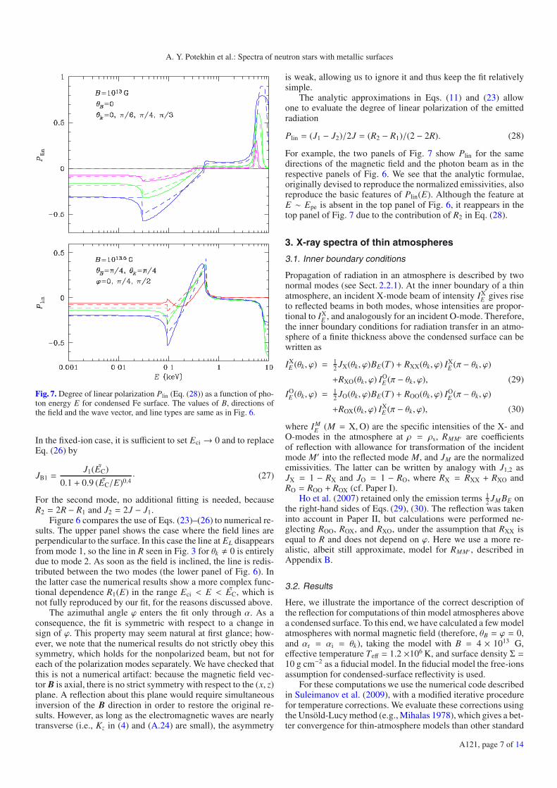
Fig. 7. Degree of linear polarization Plin (Eq. (28)) as a function of pho-ton energy E for condensed Fe surface. The values of B, directions ofthe field and the wave vector, and line types are same as in Fig. 6.

In the fixed-ion case, it is sufficient to set Eci → 0 and to replaceEq. (26) by

JB1 =J1(EC)

0.1 + 0.9 (EC/E)0.4· (27)

For the second mode, no additional fitting is needed, becauseR2 = 2R − R1 and J2 = 2J − J1.

Figure 6 compares the use of Eqs. (23)–(26) to numerical re-sults. The upper panel shows the case where the field lines areperpendicular to the surface. In this case the line at EL disappearsfrom mode 1, so the line in R seen in Fig. 3 for θk � 0 is entirelydue to mode 2. As soon as the field is inclined, the line is redis-tributed between the two modes (the lower panel of Fig. 6). Inthe latter case the numerical results show a more complex func-tional dependence R1(E) in the range Eci < E < EC, which isnot fully reproduced by our fit, for the reasons discussed above.

The azimuthal angle ϕ enters the fit only through α. As aconsequence, the fit is symmetric with respect to a change insign of ϕ. This property may seem natural at first glance; how-ever, we note that the numerical results do not strictly obey thissymmetry, which holds for the nonpolarized beam, but not foreach of the polarization modes separately. We have checked thatthis is not a numerical artifact: because the magnetic field vec-tor B is axial, there is no strict symmetry with respect to the (x, z)plane. A reflection about this plane would require simultaneousinversion of the B direction in order to restore the original re-sults. However, as long as the electromagnetic waves are nearlytransverse (i.e., Kz in (4) and (A.24) are small), the asymmetry

is weak, allowing us to ignore it and thus keep the fit relativelysimple.

The analytic approximations in Eqs. (11) and (23) allowone to evaluate the degree of linear polarization of the emittedradiation

Plin = (J1 − J2)/2J = (R2 − R1)/(2 − 2R). (28)

For example, the two panels of Fig. 7 show Plin for the samedirections of the magnetic field and the photon beam as in therespective panels of Fig. 6. We see that the analytic formulae,originally devised to reproduce the normalized emissivities, alsoreproduce the basic features of Plin(E). Although the feature atE ∼ Epe is absent in the top panel of Fig. 6, it reappears in thetop panel of Fig. 7 due to the contribution of R2 in Eq. (28).

3. X-ray spectra of thin atmospheres

3.1. Inner boundary conditions

Propagation of radiation in an atmosphere is described by twonormal modes (see Sect. 2.2.1). At the inner boundary of a thinatmosphere, an incident X-mode beam of intensity IX

E gives riseto reflected beams in both modes, whose intensities are propor-tional to IX

E , and analogously for an incident O-mode. Therefore,the inner boundary conditions for radiation transfer in an atmo-sphere of a finite thickness above the condensed surface can bewritten as

IXE (θk, ϕ) = 1

2 JX(θk, ϕ)BE(T ) + RXX(θk, ϕ) IXE (π − θk, ϕ)

+RXO(θk, ϕ) IOE (π − θk, ϕ), (29)

IOE (θk, ϕ) = 1

2 JO(θk, ϕ)BE(T ) + ROO(θk, ϕ) IOE (π − θk, ϕ)

+ROX(θk, ϕ) IXE (π − θk, ϕ), (30)

where IME (M = X,O) are the specific intensities of the X- and

O-modes in the atmosphere at ρ = ρs, RMM′ are coefficientsof reflection with allowance for transformation of the incidentmode M′ into the reflected mode M, and JM are the normalizedemissivities. The latter can be written by analogy with J1,2 asJX = 1 − RX and JO = 1 − RO, where RX = RXX + RXO andRO = ROO + ROX (cf. Paper I).

Ho et al. (2007) retained only the emission terms 12 JMBE on

the right-hand sides of Eqs. (29), (30). The reflection was takeninto account in Paper II, but calculations were performed ne-glecting ROO, ROX, and RXO, under the assumption that RXX isequal to R and does not depend on ϕ. Here we use a more re-alistic, albeit still approximate, model for RMM′ , described inAppendix B.

3.2. Results

Here, we illustrate the importance of the correct description ofthe reflection for computations of thin model atmospheres abovea condensed surface. To this end, we have calculated a few modelatmospheres with normal magnetic field (therefore, θB = ϕ = 0,and αr = αi = θk), taking the model with B = 4 × 1013 G,effective temperature Teff = 1.2 ×106 K, and surface density Σ =10 g cm−2 as a fiducial model. In the fiducial model the free-ionsassumption for condensed-surface reflectivity is used.

For these computations we use the numerical code describedin Suleimanov et al. (2009), with a modified iterative procedurefor temperature corrections. We evaluate these corrections usingthe Unsöld-Lucy method (e.g., Mihalas 1978), which gives a bet-ter convergence for thin-atmosphere models than other standard

A121, page 7 of 14

A&A 546, A121 (2012)

Fig. 8. Emergent spectra (top panel) and temperature structures (bottompanel) for the fiducial model atmosphere (solid curve) and for model at-mospheres that are calculated using the fixed-ions approximation for thereflectivity calculations (dashed curves), and the inner boundary condi-tion from Paper II (dotted curves). In the top panel the diluted blackbodyspectrum that fits the high-energy part of the fiducial model spectrum isalso shown (dash-dotted curve).

methods. In our case, the deepest atmosphere point is the up-per point of the condensed surface. The temperature correctionat this point is obtained as follows: the total flux at the bound-ary between the atmosphere and the condensed surface is fixedand, therefore, the following energy balance condition has to besatisfied:

H0 =σSBT 4

eff

4π=

12

∫ ∞0

dE∫ 1

−1

(IXE (μ) + IO

E (μ))μ dμ

= Btot kRL + JR + H−. (31)

Here, σSB is the Stefan-Boltzmann constant, μ = cos θk, and

Btot =

∫ ∞0

BE dE ,

kRL =1

2 Btot

∫ ∞0

BE dE∫ 1

0(1 − R) μ dμ,

JR =12

∫ ∞0

dE

×∫ 1

0

(IXE (μ)(RXX + ROX) + IO

E (μ)(RXO + ROO))μ dμ,

H− =12

∫ ∞0

dE∫ 0

−1

(IXE (μ) + IO

E (μ))μ dμ. (32)

Fig. 9. Top panel: dimensionless emissivities for coefficients of reflec-tion RXX (dashed curve), RXO (dotted curve), ROX (dash-dot-dottedcurve), and ROO (dash-dotted curve). The quantities are calculated atthe bottom of the fiducial model atmosphere for the angle between theradiation propagation and magnetic field, θk = 10◦, together with the to-tal dimensionless emissivity (solid curve). Bottom panel: dimensionlessoutward specific intensities (inner boundary condition) at the bottomof the fiducial model atmosphere for the X-mode (solid curve) and O-mode (dashed curve). For comparison, the dotted curve shows the samefor the X-mode, calculated using the inner boundary condition fromPaper II (in this case the dimensionless specific intensity of the O-modeequals 0.5).

Generally, the condition (31) is not fulfilled at a given temper-ature iteration. Therefore, we perform a linear expansion of theintegrated blackbody intensity:

H0 = (Btot + ΔBtot)kRL + JR + H−, (33)

and find a corresponding temperature correction

ΔT =π

4σSBT 3

(1

kRL

(H0 − Btot kRL − JR − H−

)). (34)

This last-point correction procedure is stable and has a conver-gence rate similar to the Unsöld-Lucy procedure at other depths.

We also changed the depth grid for a better description ofthe temperature structure in thin-atmosphere models. In semi-infinite model atmospheres that do not have a condensed surfaceas a lower boundary, a logarithmically equidistant set of depths isused. However, in thin-atmosphere models, such a set yields in-sufficient accuracy at the boundary between the atmosphere andcondensed surface. To improve the description of the boundary,we divide the model atmosphere into two parts with equal thick-nesses and use logarithmically equidistant depth grids for each

A121, page 8 of 14

A. Y. Potekhin et al.: Spectra of neutron stars with metallic surfaces

Fig. 10. The same as in Fig. 9, but for θk = 60◦.

of them. In the upper part the grid starts from outside (the closestpoints are at the smallest depths), while in the lower part it startsfrom the condensed surface (the closest points are at the deepestdepths). This combined grid allows us to describe the whole at-mosphere with the desired accuracy of 1% for the integral fluxconservation.

In Fig. 8 we show the emergent spectra and temperaturestructures for three different model atmospheres with the samefiducial set of physical parameters. The model spectrum com-puted using the inner boundary condition described in Paper II(the “old model”) significantly differs from the two other modelspectra computed using the improved boundary conditions ofEqs. (29), (30). The latter two models are calculated using thefree (fiducial model) and fixed ions (alternative model) assump-tions for the condensed surface reflectivities.

The differences between the spectra and the temperaturestructures of these two models are very small. The atmo-sphere temperature near the condensed surface with fixed ions isslightly smaller than the temperature near the condensed surfacewith free ions. The flux in the spectrum of the fiducial model isapproximately twice that of the alternative model at photon en-ergies E smaller than the iron cyclotron energy Eci = 0.118 keV.At larger energies the spectra are very close to each other. Wenote that the old model has been computed using the free-ionsassumption.

The difference in the emergent spectra between the old andnew model atmospheres is significant. In the old model, there isa deep depression of the spectrum between Eci and EC with anemission-like feature around the absorption line at the proton cy-clotron energy Ecp = 0.252 keV. In the new spectra this complex

Fig. 11. Top panel: total emergent spectrum of the fiducial model (solidcurve), together with emergent spectra in the X-mode (dashed curve)and in the O-mode (dash-dotted curve). The blackbody spectrum withT = Teff is also shown (dotted curve). Bottom panel: emergent specificintensities of the fiducial model for six angles θ.

feature between Eci and EC is completely different. The total de-pression is not significant, but instead of the flux increase, thereappears a deep absorption feature at photon E � Ecp. This ab-sorption corresponds to the bound-bound transitions in hydrogenatoms in strong magnetic field (Hb−b feature).

It is clear that this difference arises due to the inner bound-ary condition. The bottom panels of Figs. 9 and 10 illustrate thedifference in the outgoing flux at the boundary between the at-mosphere and the condensed surface for the old and new models.This difference is especially large for the flux in the X-mode. Inthe old model we assumed complete reflection in the X-mode;therefore, the reflected flux was small as the atmosphere wasoptically thin at these energies. As a result we found a smallemergent flux at these energies. In the new models, we have sig-nificant mode transformation due to reflection, which causes anappreciable part of the energy from the O-mode to convert intothe X-mode; the converted photons then almost freely escapefrom the atmosphere. The reflectivity coefficients RMM′ for twoangles θk are shown in the upper panels of Figs. 9 and 10.

The total equivalent widths (EWs) of the complex absorptionfeatures in the spectra of the new models are smaller than the EWof this feature in the spectrum of the old model. Nevertheless,they are still significant, with EW ≈ 220−250 eV, if the con-tinuum is assumed to be a diluted blackbody spectrum that fitsthe high-energy tail of the model. The parameters of the dilutedblackbody spectrum are a color correction factor fc = T/Teff =1.2, and a dilution factor D = 1.1−4. The range of values forEW is sufficient to explain the observed absorption features ofXDINSs (for reviews, see Haberl 2007; Turolla 2009).

A121, page 9 of 14

A&A 546, A121 (2012)

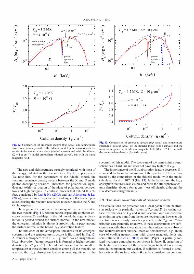
Fig. 12. Comparison of emergent spectra (top panel) and temperaturestructures (bottom panel) of the fiducial model (solid curves) with thesemi-infinite model atmosphere (dashed curves) and with the thinner(Σ = 1 g cm−2) model atmosphere (dotted curves), but with the samemagnetic field.

The new and old spectra are strongly polarized, with most ofthe energy radiated in the X-mode (see Fig. 11, upper panel).We note that, for the parameters of the fiducial model, thevacuum resonance density occurs between the X and O modephoton decoupling densities. Therefore, the polarization signaldoes not exhibit a rotation of the plane of polarization betweenlow and high energies. In contrast, models that exhibit this ef-fect, considered by Lai & Ho (2003) and van Adelsberg & Lai(2006), have a lower magnetic field and higher effective temper-ature, causing the vacuum resonance to occur outside the X andO photospheres.

The angular distribution of the emergent flux is different inthe two models (Fig. 11, bottom panel), especially at photon en-ergies between EC and 4EC. In the old model, the angular distri-bution is peaked around the surface normal. In the new model,the emergent radiation is almost isotropic, with a peak aroundthe surface normal at the broad Hb−b absorption feature.

The influence of the atmosphere thickness on its emergentspectrum and the temperature structure is illustrated in Fig. 12.A thinner atmosphere with Σ = 1 g cm−2 has an insignificantHb−b absorption feature because it is formed at higher columndensities (≈1–2 g cm−2). The fiducial model has the smallesttemperature at these column densities among all the models. Asa result, the Hb−b absorption feature is most significant in the

Fig. 13. Comparison of emergent spectra (top panel) and temperaturestructures (bottom panel) of the fiducial model (solid curves) and themodel atmosphere with different magnetic field (B = 1014 G), but withthe same surface density (dashed curves).

spectrum of this model. The spectrum of the semi-infinite atmo-sphere has a hard tail and does not have any feature at Eci.

The importance of the Hb−b absorption feature decreases if itis located far from the maximum of the spectrum. This is illus-trated by the comparison of the fiducial model with the modelcalculated for B = 1014 G (Fig. 13). In the latter case, the Hb−babsorption feature is less visible and cools the atmosphere at col-umn densities about a few g cm−2 less efficiently, although theEW decreases insignificantly.

3.3. Discussion: toward models of observed spectra

Our calculations are presented for a local patch of the neutron-star surface with particular values of Teff and B. By taking sur-face distributions of Teff and B into account, one can constructan emission spectrum from the entire neutron star; however thisspectrum is necessarily model-dependent, as the Teff and B dis-tributions are generally unknown. If these distributions are suffi-ciently smooth, then integration over the surface makes absorp-tion features broader and shallower, as demonstrated, e.g., in thecase of cooling neutron stars with dipole magnetic fields andsemi-infinite (Ho et al. 2008) or thin (Paper II) partially ion-ized hydrogen atmospheres. As shown in Paper II, smearing ofthe features is stronger, if the crustal magnetic field has a strongtoroidal component, but weaker, if radiation is formed at smallhotspots on the surface, where B can be considered as constant.

A121, page 10 of 14

A. Y. Potekhin et al.: Spectra of neutron stars with metallic surfaces

Using the results of Paper II, Hambaryan et al. (2011) fitted ob-served phase-resolved spectra of XDINS RBS 1223 and derivedconstraints on temperature and magnetic field strength and distri-bution in the X-ray emitting areas, their geometry, and the grav-itational redshift at the surface. The present, more detailed ap-proximations for the reflectivities can be directly used to refinethese fits and constraints.

In our numerical examples presented above, we evaluatedthe density of the condensed matter using Eq. (2) with η = 1.An eventual correction to this approximation is rather straight-forward, once ρs is accurately known. Indeed, the density enterscalculations through Epe ∝ √η (Eq. (3)) and through the damp-ing factor (Paper I). The latter dependence is relatively weak,therefore, it is sufficient to correct Epe in the expressions pre-sented in Sect. 2.

As mentioned in Sect. 3.2, the model spectra are highly po-larized at the stellar surface. However, the observed polariza-tion signal is affected by propagation of the photons throughthe neutron-star magnetosphere. In addition to redshift and lightbending effects near the stellar surface, the mode eigenvectorsevolve adiabatically along with the direction of the changingmagnetic field in the magnetosphere (see, e.g., Heyl & Shaviv2002). The adiabatic evolution continues until the photons nearthe polarization limiting radius, rpl, which is typically many stel-lar radii from the surface. At rpl, the modes couple, with theintensities and eigenvectors frozen thereafter (in addition, sig-nificant circular polarization can be generated in some cases,for example, in radiation from rapidly rotating neutron stars; seevan Adelsberg & Lai 2006, and the references therein).

The main effect of adiabatic photon propagation in the mag-netosphere is on the synthetic polarization signal from a finiteregion of the neutron-star surface. (There is an additional ef-fect for photons propagating through a quasi-tangential regionof magnetic field near the stellar surface; in the majority of casesthis “QT effect” can be neglected – see Wang & Lai 2009, fordetails.) Since the mode properties are fixed at large distancesfrom the star, where the magnetic field is aligned for photon tra-jectories from different areas on the star, the polarization signalis not as diminished due to variation in the surface magnetic fieldas might be expected if vacuum polarization effects are ignored(see Heyl & Shaviv 2002; Heyl et al. 2003). Thus, it is possiblethat polarization features of the local thin atmosphere models de-scribed above may be retained in spectra from a finite region ofthe neutron star. Observed spectra and polarization signals havebeen presented in the literature, employing several atmospheremodels for emission from the entire surface (Heyl et al. 2003)and from a finite sized hotspot (van Adelsberg & Perna 2009).

4. Conclusions

We have improved the method of Paper I for calculating spec-tral properties of condensed magnetized surfaces. Using the im-proved method, we calculated a representative set of reflectiv-ities of a metallic iron surface for the magnetic field strengthsB = 1012 G–1014 G. Based on these calculations, we con-structed analytic expressions for emissivities of the magnetizedcondensed surface in the two normal modes as functions of fivearguments: energy of the emitted X-ray photon E, field strengthB, field inclination θB, and the two angles that determine the pho-ton direction. We considered the alternative limiting approxima-tions of free and fixed ions for calculating the condensed surfacereflectivity.

We improved the inner boundary conditions for the radia-tion transfer equation in a thin atmosphere above a condensed

surface. The new boundary condition accounts for the transfor-mation of normal modes into each other caused by reflectionfrom the condensed surface. To implement this condition wesuggested a method for calculating reflectivities RMM′ in the nor-mal modes used for model atmosphere calculations, based onanalytic approximations to the reflectivities.

We computed a few models of thin, partially ionized hy-drogen atmospheres to investigate the influence of the newboundary condition on their emergent spectra and temperaturestructures. The allowance for mode transformations makes thecomplex absorption feature between Eci and EC less significantand the atomic absorption feature more important. Nevertheless,the equivalent widths of this complex absorption feature in theemergent spectra are still significant (≈200–250 eV) and suffi-cient to explain the observed absorption features in the spectraof XDINSs. Models of thin atmospheres with inclined magneticfields are necessary for detailed descriptions of their spectra. Weplan to compute such models with vacuum polarization and par-tial mode conversion in a future paper.

Acknowledgements. A.Y.P. acknowledges useful discussions with GillesChabrier, the hospitality of the Institute of Astronomy and Astrophysics at theUniversity of Tübingen, and partial financial support from Russian Foundationfor Basic Research (RFBR grant No. 11-02-00253-a) and the Russian LeadingScientific Schools program (grant NSh-3769.2010.2). The work of V.F.S. issupported by the German Research Foundation (DFG) grant SFB/Transregio 7“Gravitational Wave Astronomy”.

Appendix A: Improved reflectivity calculation

In this appendix, we describe several improvements to the meth-ods of Paper I that have enabled us to produce a general, efficientcode, free of numerical difficulties, which computes the correctvalue of the reflectivities over the full range of parameters usedin neutron-star atmosphere modeling.

In general, each incoming linearly polarized wave E(i)1 =

A1e(i)1 and E(i)

2 = A2e(i)2 is partially reflected, giving rise to re-

flected and transmitted fields1

E(r)j = A j

2∑m=1

rm j e(r)m , E(t)

j = A j

2∑m=1

tm j e(t)m . (A.1)

As shown in Paper I, the dimensionless emissivities for the twoorthogonal linear polarizations are J j = 1 − R j, where

R j = |r j1|2 + |r j2|2 ( j = 1, 2). (A.2)

The reflected field amplitudes r11, r12, r21, and r22 were cal-culated in Paper I using an eighth-order polynomial in therefraction index n j to determine the properties of the transmittedmodes. The transmitted wave can be described by two normalmodes, thus, most of the roots obtained from that polynomialrepresent unphysical solutions to the equations. The conditionsto identify the correct roots were derived in Appendix B ofPaper I, with the requirements that the corresponding reflectivi-ties satisfy R1,R2 � 1 and that the function R(E) be continuous.However, for some values of the model parameters, the unphys-ical roots can satisfy the physical constraints on the solution.

Here we propose an improved method, based on a fourth-order polynomial, which allows for easy elimination of the un-physical roots.

1 We use the inverse order of the subscripts in rm j and tm j with respectto the one used in Paper I.

A121, page 11 of 14

A&A 546, A121 (2012)

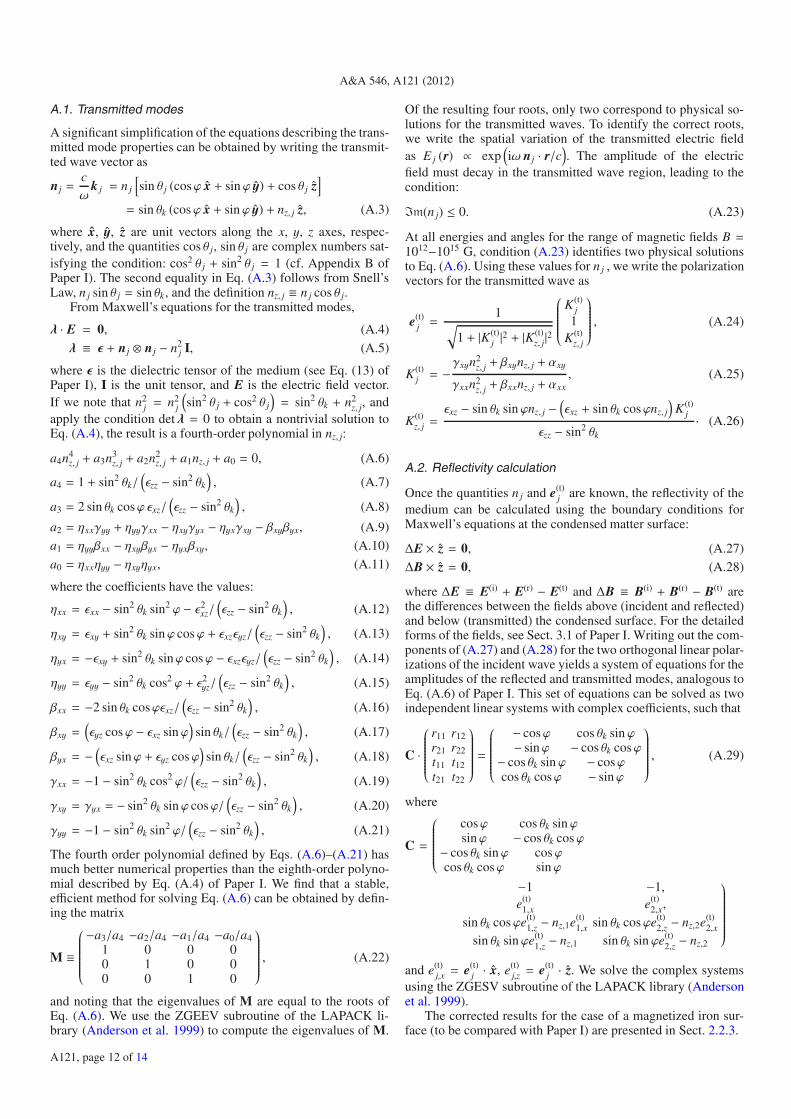
A.1. Transmitted modes

A significant simplification of the equations describing the trans-mitted mode properties can be obtained by writing the transmit-ted wave vector as

nj =cω

k j = n j

[sin θ j (cosϕ x + sin ϕ y) + cos θ j z

]= sin θk (cosϕ x + sin ϕ y) + nz, j z, (A.3)

where x, y, z are unit vectors along the x, y, z axes, respec-tively, and the quantities cos θ j, sin θ j are complex numbers sat-isfying the condition: cos2 θ j + sin2 θ j = 1 (cf. Appendix B ofPaper I). The second equality in Eq. (A.3) follows from Snell’sLaw, n j sin θ j = sin θk, and the definition nz, j ≡ n j cos θ j.

From Maxwell’s equations for the transmitted modes,

λ · E = 0, (A.4)

λ ≡ ε + nj ⊗ nj − n2j I, (A.5)

where ε is the dielectric tensor of the medium (see Eq. (13) ofPaper I), I is the unit tensor, and E is the electric field vector.If we note that n2

j = n2j

(sin2 θ j + cos2 θ j

)= sin2 θk + n2

z, j, andapply the condition detλ = 0 to obtain a nontrivial solution toEq. (A.4), the result is a fourth-order polynomial in nz, j:

a4n4z, j + a3n3

z, j + a2n2z, j + a1nz, j + a0 = 0, (A.6)

a4 = 1 + sin2 θk/(εzz − sin2 θk

), (A.7)

a3 = 2 sin θk cosϕ εxz/(εzz − sin2 θk

), (A.8)

a2 = ηxxγyy + ηyyγxx − ηxyγyx − ηyxγxy − βxyβyx, (A.9)

a1 = ηyyβxx − ηxyβyx − ηyxβxy, (A.10)

a0 = ηxxηyy − ηxyηyx, (A.11)

where the coefficients have the values:

ηxx = εxx − sin2 θk sin2 ϕ − ε2xz/(εzz − sin2 θk

), (A.12)

ηxy = εxy + sin2 θk sinϕ cosϕ + εxzεyz/(εzz − sin2 θk

), (A.13)

ηyx = −εxy + sin2 θk sinϕ cosϕ − εxzεyz/(εzz − sin2 θk

), (A.14)

ηyy = εyy − sin2 θk cos2 ϕ + ε2yz/(εzz − sin2 θk

), (A.15)

βxx = −2 sin θk cosϕεxz/(εzz − sin2 θk

), (A.16)

βxy =(εyz cosϕ − εxz sin ϕ

)sin θk/

(εzz − sin2 θk

), (A.17)

βyx = −(εxz sinϕ + εyz cosϕ

)sin θk/

(εzz − sin2 θk

), (A.18)

γxx = −1 − sin2 θk cos2 ϕ/(εzz − sin2 θk

), (A.19)

γxy = γyx = − sin2 θk sin ϕ cosϕ/(εzz − sin2 θk

), (A.20)

γyy = −1 − sin2 θk sin2 ϕ/(εzz − sin2 θk

), (A.21)

The fourth order polynomial defined by Eqs. (A.6)–(A.21) hasmuch better numerical properties than the eighth-order polyno-mial described by Eq. (A.4) of Paper I. We find that a stable,efficient method for solving Eq. (A.6) can be obtained by defin-ing the matrix

M ≡

⎛⎜⎜⎜⎜⎜⎜⎜⎜⎜⎜⎜⎝−a3/a4 −a2/a4 −a1/a4 −a0/a4

1 0 0 00 1 0 00 0 1 0

⎞⎟⎟⎟⎟⎟⎟⎟⎟⎟⎟⎟⎠ , (A.22)

and noting that the eigenvalues of M are equal to the roots ofEq. (A.6). We use the ZGEEV subroutine of the LAPACK li-brary (Anderson et al. 1999) to compute the eigenvalues of M.

Of the resulting four roots, only two correspond to physical so-lutions for the transmitted waves. To identify the correct roots,we write the spatial variation of the transmitted electric fieldas E j (r) ∝ exp

(iω n j · r/c

). The amplitude of the electric

field must decay in the transmitted wave region, leading to thecondition:

Im(n j) ≤ 0. (A.23)

At all energies and angles for the range of magnetic fields B =1012−1015 G, condition (A.23) identifies two physical solutionsto Eq. (A.6). Using these values for n j , we write the polarizationvectors for the transmitted wave as

e(t)j =

1√1 + |K(t)

j |2 + |K(t)z, j|2

⎛⎜⎜⎜⎜⎜⎜⎜⎜⎜⎝K(t)

j1

K(t)z, j

⎞⎟⎟⎟⎟⎟⎟⎟⎟⎟⎠ , (A.24)

K(t)j = −

γxyn2z, j + βxynz, j + αxy

γxxn2z, j + βxxnz, j + αxx

, (A.25)

K(t)z, j =

εxz − sin θk sin ϕnz, j −(εxz + sin θk cosϕnz, j

)K(t)

j

εzz − sin2 θk· (A.26)

A.2. Reflectivity calculation

Once the quantities n j and e(t)j are known, the reflectivity of the

medium can be calculated using the boundary conditions forMaxwell’s equations at the condensed matter surface:

ΔE × z = 0, (A.27)

ΔB × z = 0, (A.28)

where ΔE ≡ E(i) + E(r) − E(t) and ΔB ≡ B(i) + B(r) − B(t) arethe differences between the fields above (incident and reflected)and below (transmitted) the condensed surface. For the detailedforms of the fields, see Sect. 3.1 of Paper I. Writing out the com-ponents of (A.27) and (A.28) for the two orthogonal linear polar-izations of the incident wave yields a system of equations for theamplitudes of the reflected and transmitted modes, analogous toEq. (A.6) of Paper I. This set of equations can be solved as twoindependent linear systems with complex coefficients, such that

C ·

⎛⎜⎜⎜⎜⎜⎜⎜⎜⎜⎜⎜⎝r11 r12r21 r22t11 t12t21 t22

⎞⎟⎟⎟⎟⎟⎟⎟⎟⎟⎟⎟⎠ =⎛⎜⎜⎜⎜⎜⎜⎜⎜⎜⎜⎜⎝− cosϕ cos θk sin ϕ− sinϕ − cos θk cosϕ

− cos θk sin ϕ − cosϕcos θk cosϕ − sinϕ

⎞⎟⎟⎟⎟⎟⎟⎟⎟⎟⎟⎟⎠ , (A.29)

where

C =

⎛⎜⎜⎜⎜⎜⎜⎜⎜⎜⎜⎜⎝cosϕ cos θk sin ϕsinϕ − cos θk cosϕ

− cos θk sin ϕ cosϕcos θk cosϕ sin ϕ

−1 −1,e(t)

1,x e(t)2,x,

sin θk cosϕe(t)1,z − nz,1e(t)

1,x sin θk cosϕe(t)2,z − nz,2e(t)

2,x

sin θk sin ϕe(t)1,z − nz,1 sin θk sin ϕe(t)

2,z − nz,2

⎞⎟⎟⎟⎟⎟⎟⎟⎟⎟⎟⎟⎟⎟⎟⎠and e(t)

j,x = e(t)j · x, e(t)

j,z = e(t)j · z. We solve the complex systems

using the ZGESV subroutine of the LAPACK library (Andersonet al. 1999).

The corrected results for the case of a magnetized iron sur-face (to be compared with Paper I) are presented in Sect. 2.2.3.

A121, page 12 of 14

A. Y. Potekhin et al.: Spectra of neutron stars with metallic surfaces

Appendix B: Approximations for reflectivitiesat the bottom of a thin atmosphere

B.1. Reflectivities of the normal modes in terms of rmj

In general, the interface between the thin atmosphere and mag-netic condensed surface has reflection and transmission prop-erties that are different from those of the condensed surface invacuum. Therefore, a separate calculation of the reflectivity co-efficients rm j is needed for every set of atmosphere parameters.However, assuming that the atmosphere is sufficiently rarefied,we may approximately replace these coefficients by those in vac-uum. Under these conditions, the plane waves in the atmosphereare almost transverse, so we can approximately set Kz,M → 0 inEq. (4). Then each incident and reflected wave can be expandedover the linear polarization vectors e1 and e2 that have been em-ployed in the reflectivity calculation.

For the incident (i) and reflected (r) beams, we define or-thonormal vectors e(i,r)

1 = z × k/| z × k| = z × ki,r/| sin θk |,e(i)

2 = ki × e(i)1 , and e(r)

2 = e(r)1 × kr, where k denotes the unit

vector along k. In the notations of Fig. 1,

ki,r = sin θk cosϕ x + sin θk sin ϕ y ∓ cos θk z, (B.1)

e(i)1 = e(r)

1 = − sinϕ x + cosϕ y, (B.2)

e(i,r)2 = cos θk (cosϕ x + sin ϕ y) ± sin θk z, (B.3)

where the upper and lower signs in ∓ cos θk are for the inci-dent and reflected waves, respectively. The coordinates in whichEq. (4) is written are (x′, y′, z′) (Fig. 1), defined according to re-lations y′ = B × k/|B × k| and x′ = y′ × k.

The electric field of the incoming ray with unit amplitudeand polarization M′ (M′ =X or M′ =O) can be written as

e(i)M′ = c(i)

M′1e(i)1 + c(i)

M′2e(i)2 , (B.4)

where c(i)M′ j = e(i)

M′ · e(i)j . According to Eqs. (A.1) and (B.4), the

reflected field is

r′XM′e(r)X + r′OM′e

(r)O =

2∑m=1

2∑j=1

rm jc(i)M′ je

(r)m . (B.5)

The amplitudes r′XM′ and r′OM′ of the reflected-field componentsin the X- and O-modes, respectively, are given by the solution ofthe linear system

⎛⎜⎜⎜⎜⎜⎝ c(r)X1 c(r)

O1

c(r)X2 c(r)

O2

⎞⎟⎟⎟⎟⎟⎠(

r′XM′

r′OM′

)=

(r11 r12r21 r22

) ⎛⎜⎜⎜⎜⎜⎝ c(i)X1 c(i)

O1

c(i)X2 c(i)

O2

⎞⎟⎟⎟⎟⎟⎠ , (B.6)

where c(r)M j = e(r)

M · e(r)j . Since the incident X- and O-modes are

incoherent, the normal mode reflectivities in Eqs. (29) and (30)are

RMM′ = |r′MM′ |2. (B.7)

According to Eq. (4),

c(i,r)M j =

iK(i,r)M x′i,r · e(i,r)

j + y′i,r · e(i,r)

j√1 + |K(i,r)

M |2, (B.8)

where K(i,r)M = KM(αi,r). The explicit expressions for the scalar

products in Eq. (B.8) are

ˆx′i,r· e(i,r)

1 = sin θB sin ϕ/sinαi,r, (B.9)

ˆy′i,r· e(i,r)

1 = (cos θB sin θk ± sin θB cos θk cosϕ)/sinαi,r, (B.10)

ˆx′i,r· e(i,r)

2 = (∓ cos θB sin θk − sin θB cos θk cosϕ)/sinαi,r, (B.11)

ˆy′i,r· e(i,r)

2 = ± sin θB sin ϕ (cos2 θk −sin2 θk)/ sinαi,r. (B.12)

Caution should be used when employing approximations for rm jin Eq. (B.6) if one of the normal modes is almost completelyreflected, that is, RMM′ ≈ 1. Such a situation occurs for theX-mode at Eci < E < EC, if both k and B are close to nor-mal (see Paper I). In this case the fit error may exceed (1− RXX)and result in RXX > 1, which is unphysical. In particular, the fit-ting formulae presented below may occasionally give RXX a fewpercent above 1 at very small θB and θk. In such instances oneshould truncate the mode-specific reflectivities, recovered fromthe fit, so as to fulfill the general condition 0 < RMM′ < 1.

B.2. Approximations for rmj

For calculating RMM′ according to Sect. B.1, we use an analyticmodel of the complex reflectivity coefficients rm j, which agreeswith the approximations derived in Sect. 2.3 and roughly repro-duces the computed dependences of rm j = |rm j| exp(iφm j) on Efor many characteristic geometry settings. For the squared mod-uli we use the following expressions:

|r12|2 =⎧⎪⎪⎪⎨⎪⎪⎪⎩

0 in Region I,fE (1 − JB1) (1 − JC)+JCRL(1 − sin θB sin2 ϕ)/2 in Region II,

(B.13)

|r21|2 =⎧⎪⎪⎪⎨⎪⎪⎪⎩

0 in Region I,fE (1 + JB1 − 2JB) (1 − JC)+JCRL sin θk (1 − cosα)/2 in Region II,

(B.14)

|r11|2 = 1 − J1 − |r12|2, |r22|2 = 1 − J2 − |r21|2, (B.15)

and fE ≡ E/(E+ EC/2). The functions J1, J2, JB, JC, JB1, and RL

are defined in Sect. 2.3. In the case of the free-ions model, smallaccidental discontinuities at the boundary of Region I are elimi-nated by truncating |r11|2 and |r22|2 from above by their values atE = Eci. Our approximations for the complex phases are

φ11 =

⎧⎪⎪⎪⎪⎪⎨⎪⎪⎪⎪⎪⎩π in Region I,−π fL, if E > EC,

π + πE − Eci

EC − Eciotherwise,

(B.16)

φ22 =

{π fL, if E > EC,φ11 otherwise, (B.17)

φ12 =

⎧⎪⎪⎪⎪⎪⎨⎪⎪⎪⎪⎪⎩

−π/2 in Region I,π/2 − 2π fL, if E > EC,

πE − (Eci + EC)/2

Eci − ECotherwise,

(B.18)

φ21 = φ12 + π, (B.19)

where

fL =

[1 + exp

(5

EL − E

EL − EC

)]−1

·

A121, page 13 of 14

A&A 546, A121 (2012)

ReferencesAnderson, E., Bai, Z., Bischof, C., et al. 1999, LAPACK User’s Guide

(Philadelphia: Society for Industrial and Applied Mathematics)Brinkmann, W. 1980, A&A, 82, 352Fushiki, I., Gudmundsson, E. H., & Pethick, C. J. 1989, ApJ, 342, 958Ginzburg, V. L. 1970, The Propagation of Electromagnetic Waves in Plasmas,

2nd edn. (London: Pergamon)Gnedin, Yu. N., & Pavlov, G. G. 1973, Zh. Eksper. Teor. Fiz., 65, 1806 (English

transl.: 1974, Sov. Phys.–JETP, 38, 903)Haberl, F. 2007, Ap&SS, 308, 181Haensel, P., Potekhin, A. Y., & Yakovlev, D. G. 2007, Neutron Stars 1: Equation

of State and Structure (New York: Springer)Hambaryan, V., Suleimanov, V., Schwope, A. D., et al. 2011, A&A, 534, A74Heyl, J. S., & Shaviv, N. J. 2002, Phys. Rev. D, 66, 023002Heyl, J. S., Shaviv, N. J., & Lloyd, D. 2003, MNRAS, 342, 134Ho, W. C. G. 2007, MNRAS, 380, 71Ho, W. C. G., & Lai, D. 2001, MNRAS, 327, 1081Ho, W. C. G., & Lai, D. 2003, MNRAS, 338, 233Ho, W. C. G., Kaplan, D. L., Chang, P., van Adelsberg, M., & Potekhin, A. Y.

2007, MNRAS, 376, 793Ho, W. C. G., Potekhin, A. Y., & Chabrier, G. 2008, ApJS, 178, 102Lai, D. 2001, Rev. Mod. Phys., 73, 629Lai, D., & Ho, W. C. G. 2003, Phys. Rev. Lett., 91, 071101Lai, D., & Salpeter, E. E. 1997, ApJ, 491, 270Medin, Z., & Lai, D. 2006, Phys. Rev. A, 74, 062508Medin, Z., & Lai, D. 2007, MNRAS, 382, 1833Mereghetti, S. 2008, A&ARv, 15, 225

Mihalas, D. 1978, Stellar Atmospheres, 2nd edn. (San Francisco: Freeman)Motch, C., Zavlin, V. E., & Haberl, F. 2003, A&A, 408, 323Pérez-Azorín, J. F., Miralles, J. A., & Pons, J. A., 2005, A&A, 433, 275Potekhin, A. Y., Lai, D., Chabrier, G., & Ho, W. C. G. 2004, ApJ, 612, 1034Rögnvaldsson, Ö. E., Fushiki, I., Gudmundsson, E. H., Pethick, C. J., &

Yngvason, J. 1993, ApJ, 416, 276Ruderman, M. A. 1971, Phys. Rev. Lett., 27, 1306Salpeter, E. E. 1954, Austr. J. Phys., 7, 373Shafranov, V. D. 1967, in Rev. Plasma Phys., ed. M. A. Leontovich (New York:

Consultants Bureau), 3, 1Suleimanov, V., Potekhin, A. Y., & Werner, K. 2009, A&A, 500, 891Suleimanov, V., Hambaryan, V., Potekhin, A. Y., et al. 2010, A&A, 522, A111

(Paper II)Thorolfsson, A., Rögnvaldsson, Ö. E., Yngvason, J., & Gudmundsson, E. H.

1998, ApJ, 502, 847Turolla, R. 2009, in Neutron Stars and Pulsars, ed. W. Becker, Astrophys. Space

Sci. Library (Berlin: Springer), 357, 141Turolla, R., Zane, S., & Drake, J. J. 2004, ApJ, 603, 265van Adelsberg, M., & Lai, D. 2006, MNRAS, 373, 1495van Adelsberg, M., & Perna, R. 2009, MNRAS, 399, 1523van Adelsberg, M., Lai, D., Potekhin, A. Y., & Arras, P. 2005, ApJ, 628, 902

(Paper I)Wang, C., & Lai, D. 2009, MNRAS, 398, 515Zane, S., Turolla, R., & Drake, J. J. 2002, in High Resolution X-ray Spectroscopy

with XMM-Newton and Chandra, Proc. International Workshop held at theMullard Space Science Laboratory, ed. G. Branduardi-Raymont (UniversityCollege London, Holmbury St. Mary, Dorking, Surrey, UK), abstract #51

A121, page 14 of 14