aspects of quantum non-locality - quic
TRANSCRIPT

Universite Libre de Bruxelles
Faculte des Sciences
Service de Physique Theorique
ASPECTS OF
QUANTUM NON-LOCALITY
Stefano PIRONIO
These presentee en vue de l’obtention
du grade de Docteur en Sciences
Promoteur: Serge Massar
Annee academique: 2003-2004

Resume
La mecanique quantique predit l’existence de correlations entre particules distantes qui
ne peuvent s’expliquer dans le cadre des theories realistes locales. Suite au developpement
recent de la theorie de l’information quantique, il a ete realise que ces correlations non-
locales ont des implications quant aux capacites de traitement de l’information des systemes
quantiques. Outre une signification physique, elles possedent donc une signification informa-
tionnelle. Cette these traite de differents aspects de la non-localite lies a ces deux facettes
du phenomene.
Nous commencons par un examen de la structure des correlations locales et non-locales.
Nous derivons dans ce contexte de nouvelles inegalites de Bell, et generalisons ensuite le
paradoxe de Greenberger-Horne-Zelinger a des etats quantiques de dimension arbitraire et
composes de plusieurs sous-systemes.
Nous abordons par apres la non-localite du point de vue de la theorie de l’information.
Il est possible de concevoir des theories non-locales consistantes avec le principe de causalite
mais offrant des avantages superieurs a la mecanique quantique en terme de manipulation
de l’information. Nous investiguons l’ensemble des correlations compatibles avec de telles
theories afin d’eclairer l’origine des limitations imposees par le formalisme quantique. Nous
nous interessons egalement a la quantite de communication classique necessaire pour simuler
les correlations non-locales. Nous montrons que cette mesure naturelle de la non-localite est
etroitement liee au degre de violations des inegalites de Bell.
Nous nous tournons ensuite vers des aspects experimentaux. La faible efficacite des
detecteurs utilises dans les experiences de violation des inegalites de Bell reste un obstacle
majeur a une demonstration convaincante de la non-localite, mais aussi a toute utilisation
de la non-localite dans des protocoles d’information quantique. Nous derivons d’une part des
bornes quant a l’efficacite minimale requise pour violer les inegalites de Bell, et d’autre part
des exemples de correlations plus resistante a ces imperfections experimentales.
Finalement, nous cloturons cette these en montrant comment la non-localite, principa-
lement etudiee dans le cadre de systemes decrits par des variables discretes, telles que les
variables de spin, peut egalement se manifester dans des systemes a variables continues, telles
que les variables de position et d’impulsion.
iii


Remerciements
Je souhaite tout d’abord remercier Serge Massar qui a encadre cette these. Je lui suis
profondement reconnaissant de s’etre implique avec tant d’enthousiasme dans cette longue
aventure, d’avoir ete aussi present a mes cotes tout en me laissant une grande liberte. Col-
laborer avec lui a ete une source de motivation extraordinaire et je le remercie pour tout ce
qu’il m’a appris.
Je tiens aussi a remercier chaleureusement Nicolas Cerf pour son soutien et tous les
conseils qu’il m’a donnes. Je le remercie particulierement de m’avoir fait une place dans son
equipe a partir de ma deuxieme annee de doctorat : l’environnement de recherche que j’y ai
trouve ainsi que les contacts avec les autres membres du groupe m’ont fortement inspire et
encourage.
Merci a Jonathan Barrett, avec qui j’ai eu l’occasion de partager un bureau pendant deux
ans et qui est devenu un vrai ami, pour tout ce que nos discussions m’ont apportes. Merci a
Louis-Philippe Lamoureux, l’ontarien-quebecquois-europeen, pour la bonne ambiance qu’il
a fait regner et pour son aide cruciale lors de la phase finale de cette these. Merci a tous
les membres du service de Theorie de l’Information et des Communications et du service de
Physique Theorique pour l’aide qu’ils m’ont chacun fournie a divers moments.
Il n’est pas toujours facile de gerer a la fois une these et des taches d’enseignement. Je
suis tres reconnaissant a Jean-Marie Frere, Pascal Pirotte et Paul Duhamel pour leur soutien
dans ces activites extra-doctorales, sans lequel je n’aurais pu mener a bien cette these.
J’ai eu le plaisir de collaborer avec Bernard Gisin, Noah Linden, Graeme Mitchison, Sandu
Popescu, David Roberts et Jeremie Roland. Je les en remercie et pense particulierement a
Graeme pour son hospitalite. Je remercie egalement Harry Burhman, Jean-Paul Doignon,
Nicolas Gisin et Richard Gill pour des discussions interessantes.
Merci a mes amis et ma famille pour leur soutien, tout particulierement a ma mere et
mon pere. Merci surtout a toi Jenny pour tout l’amour et la force que tu me donnes chaque
jour.
v


Contents
Resume iii
Remerciements v
1 Introduction 1
1.1 Local causality and quantum mechanics . . . . . . . . . . . . . . . . . . . . . . 2
1.2 Non-locality and quantum information . . . . . . . . . . . . . . . . . . . . . . . 6
1.3 Experimental tests of non-locality . . . . . . . . . . . . . . . . . . . . . . . . . . 7
1.4 Outline of the thesis . . . . . . . . . . . . . . . . . . . . . . . . . . . . . . . . . 9
2 Preliminaries 13
2.1 Bell scenario . . . . . . . . . . . . . . . . . . . . . . . . . . . . . . . . . . . . . 13
2.2 Space of joint probabilities . . . . . . . . . . . . . . . . . . . . . . . . . . . . . 14
2.3 Local models . . . . . . . . . . . . . . . . . . . . . . . . . . . . . . . . . . . . . 15
2.4 Deterministic local models . . . . . . . . . . . . . . . . . . . . . . . . . . . . . 16
2.5 Membership in L as a linear program . . . . . . . . . . . . . . . . . . . . . . . . 17
2.6 Bell inequalities . . . . . . . . . . . . . . . . . . . . . . . . . . . . . . . . . . . 18
2.7 Local polytopes . . . . . . . . . . . . . . . . . . . . . . . . . . . . . . . . . . . 19
2.7.1 Affine hull and full-dimensional representation . . . . . . . . . . . . . . . 19
2.7.2 Facet enumeration . . . . . . . . . . . . . . . . . . . . . . . . . . . . . . 20
2.7.3 Solved cases . . . . . . . . . . . . . . . . . . . . . . . . . . . . . . . . . 21
2.7.4 Partial lists of facets . . . . . . . . . . . . . . . . . . . . . . . . . . . . 22
3 More on facet inequalities 25
3.1 Introduction . . . . . . . . . . . . . . . . . . . . . . . . . . . . . . . . . . . . . 25
3.2 Lifting theorems . . . . . . . . . . . . . . . . . . . . . . . . . . . . . . . . . . . 26
3.2.1 Notation and basic results . . . . . . . . . . . . . . . . . . . . . . . . . 27
3.2.2 More parties . . . . . . . . . . . . . . . . . . . . . . . . . . . . . . . . . 29
3.2.3 More outcomes . . . . . . . . . . . . . . . . . . . . . . . . . . . . . . . 30
3.2.4 More inputs . . . . . . . . . . . . . . . . . . . . . . . . . . . . . . . . . 31
3.3 All CHSH polytopes, and beyond . . . . . . . . . . . . . . . . . . . . . . . . . . 32
vii
viii CONTENTS
3.3.1 Bell inequalities from Fourier-Motzkin elimination . . . . . . . . . . . . . 33
3.3.2 Computational results for bipartite two-inputs polytopes . . . . . . . . . 38
3.4 A new family of facet inequalities . . . . . . . . . . . . . . . . . . . . . . . . . . 38
4 Quantum correlations 41
4.1 Definition . . . . . . . . . . . . . . . . . . . . . . . . . . . . . . . . . . . . . . 41
4.2 General properties . . . . . . . . . . . . . . . . . . . . . . . . . . . . . . . . . . 42
4.3 The GHZ paradox . . . . . . . . . . . . . . . . . . . . . . . . . . . . . . . . . . 44
4.4 GHZ paradoxes for many qudits . . . . . . . . . . . . . . . . . . . . . . . . . . . 45
4.4.1 Mermin’s formulation . . . . . . . . . . . . . . . . . . . . . . . . . . . . 46
4.4.2 Generalisation . . . . . . . . . . . . . . . . . . . . . . . . . . . . . . . . 47
4.4.3 Multipartite condition . . . . . . . . . . . . . . . . . . . . . . . . . . . . 52
4.4.4 Multidimensional condition . . . . . . . . . . . . . . . . . . . . . . . . . 52
4.5 Summary . . . . . . . . . . . . . . . . . . . . . . . . . . . . . . . . . . . . . . . 53
5 Non-locality as an information theoretic resource 55
5.1 Introduction. . . . . . . . . . . . . . . . . . . . . . . . . . . . . . . . . . . . . . 55
5.2 Two party correlations . . . . . . . . . . . . . . . . . . . . . . . . . . . . . . . . 57
5.2.1 General structure . . . . . . . . . . . . . . . . . . . . . . . . . . . . . . 57
5.2.2 The two-inputs no-signalling polytope . . . . . . . . . . . . . . . . . . . 58
5.2.3 Resource conversions . . . . . . . . . . . . . . . . . . . . . . . . . . . . 62
5.3 Three party correlations . . . . . . . . . . . . . . . . . . . . . . . . . . . . . . . 67
5.3.1 Definitions . . . . . . . . . . . . . . . . . . . . . . . . . . . . . . . . . . 67
5.3.2 Two inputs and two outputs . . . . . . . . . . . . . . . . . . . . . . . . 68
5.3.3 Simulating tripartite boxes . . . . . . . . . . . . . . . . . . . . . . . . . 71
5.3.4 Non-locality and the environment . . . . . . . . . . . . . . . . . . . . . . 73
5.4 Discussion and open questions . . . . . . . . . . . . . . . . . . . . . . . . . . . 74
6 Communication cost of non-locality 77
6.1 Introduction . . . . . . . . . . . . . . . . . . . . . . . . . . . . . . . . . . . . . 77
6.2 General formalism . . . . . . . . . . . . . . . . . . . . . . . . . . . . . . . . . . 79
6.2.1 Deterministic protocols . . . . . . . . . . . . . . . . . . . . . . . . . . . 79
6.2.2 Bell inequalities . . . . . . . . . . . . . . . . . . . . . . . . . . . . . . . 80
6.2.3 Main results . . . . . . . . . . . . . . . . . . . . . . . . . . . . . . . . . 81
6.2.4 Comparing Bell inequalities . . . . . . . . . . . . . . . . . . . . . . . . . 83
6.2.5 Other measures of communication . . . . . . . . . . . . . . . . . . . . . 84
6.3 Applications . . . . . . . . . . . . . . . . . . . . . . . . . . . . . . . . . . . . . 84
6.3.1 CHSH inequality . . . . . . . . . . . . . . . . . . . . . . . . . . . . . . . 84
6.3.2 More dimensions: the CGLMP inequality . . . . . . . . . . . . . . . . . . 87
6.4 Optimal inequalities and facet inequalities . . . . . . . . . . . . . . . . . . . . . 90

CONTENTS ix
6.5 Summary . . . . . . . . . . . . . . . . . . . . . . . . . . . . . . . . . . . . . . . 91
7 The detection loophole 93
7.1 Introduction . . . . . . . . . . . . . . . . . . . . . . . . . . . . . . . . . . . . . 93
7.2 Bell scenarios with detection inefficiency . . . . . . . . . . . . . . . . . . . . . . 95
7.3 A model that depends on the number of settings . . . . . . . . . . . . . . . . . 96
7.4 An approximate model that depend on d . . . . . . . . . . . . . . . . . . . . . . 101
7.5 Summary . . . . . . . . . . . . . . . . . . . . . . . . . . . . . . . . . . . . . . . 104
8 Bell inequalities resistant to detector inefficiency 107
8.1 Introduction . . . . . . . . . . . . . . . . . . . . . . . . . . . . . . . . . . . . . 107
8.2 Detector efficiency and pair production probability . . . . . . . . . . . . . . . . . 109
8.3 Numerical search . . . . . . . . . . . . . . . . . . . . . . . . . . . . . . . . . . 111
8.4 Optimal Bell inequalities . . . . . . . . . . . . . . . . . . . . . . . . . . . . . . 114
8.5 Results . . . . . . . . . . . . . . . . . . . . . . . . . . . . . . . . . . . . . . . . 115
8.5.1 Arbitrary dimension, two inputs . . . . . . . . . . . . . . . . . . . . . . . 115
8.5.2 3 dimensions, (2 × 3) inputs . . . . . . . . . . . . . . . . . . . . . . . . 117
8.5.3 3 inputs for both parties . . . . . . . . . . . . . . . . . . . . . . . . . . 118
8.5.4 More inputs and more dimensions . . . . . . . . . . . . . . . . . . . . . 119
8.6 Summary . . . . . . . . . . . . . . . . . . . . . . . . . . . . . . . . . . . . . . . 119
8.7 Appendix: Additional results . . . . . . . . . . . . . . . . . . . . . . . . . . . . 120
9 Continuous variables 127
9.1 Introduction . . . . . . . . . . . . . . . . . . . . . . . . . . . . . . . . . . . . . 127
9.2 Generalising the GHZ paradox . . . . . . . . . . . . . . . . . . . . . . . . . . . 128
9.2.1 Translation operators . . . . . . . . . . . . . . . . . . . . . . . . . . . . 129
9.2.2 Modular variables . . . . . . . . . . . . . . . . . . . . . . . . . . . . . . 130
9.2.3 Binary variables . . . . . . . . . . . . . . . . . . . . . . . . . . . . . . . 131
9.2.4 GHZ eigenstates . . . . . . . . . . . . . . . . . . . . . . . . . . . . . . . 134
9.3 Multipartite multidimensional construction . . . . . . . . . . . . . . . . . . . . . 135
Conclusion 137
References 139
Bibliography 141

Chapter 1
Introduction
Quantum mechanics is undoubtedly the most powerful and successful of our scientific the-
ories. It accounts for a wide-ranging variety of phenomena, from the sub-atomic to the
macroscopic scale; its predictions have always been confirmed and this to unmatched degree
of precision; its practical applications are countless. But a scientific theory is more than a
catalogue of explanations, predictions and applications. What is significant, and fascinating,
is the synthesis that relate them all together in a coherent picture and the consequences of
such a picture for our representation of the world. From this perspective, quantum mechan-
ics is less brilliant. Although its mathematical formalism is well understood, difficulties are
encountered when trying to figure out what kind of a world it describes. This is a contro-
versial issue: eighty years after the institution of the theory, there is still no consensus on
how we should interpret it. It is even conceivable that the present formulation of quantum
mechanics does not allow any conclusive answer to this question, and one may speculate that
a modification or an extension of the theory would be required to settle the discussion.
This does not signify, however, that quantum mechanics has no implications at all for
the way we conceive the world. Since the very beginning of the theory, certain of its fea-
tures, including the probabilistic character of its predictions, the prominent role given to the
observer, or the peculiarities associated with the notion of entanglement, have deeply chal-
lenged the validity of our old conceptions about the structure of the physical world. They
strongly suggested that any worldview accommodating them had to be radically different
from the previously prevailing ones, even if which of these features is necessarily intrinsic to
any fundamental description of Nature was part of the already mentioned debate.
A decisive argument illuminating these considerations, and showing that if we do not
have a clear understanding of what the world is according to quantum mechanics, at least
we can make a very precise affirmation about what it is not, was put forward by John
Bell. He showed that the reasonable notion of local causality is incompatible with the
quantum mechanical description of Nature [Bel64, Bel71]. Bell noticed that certain quantum
correlations, such as the one considered by Einstein, Podolsky and Rosen in their famous
1

2 1. Introduction
paper questioning the completeness of quantum mechanics [EPR35], could not be accounted
for by any theory which attributes only locally defined states to its basic physical objects.
Besides the far-reaching consequences of this statement for our understanding of quantum
mechanics, what is remarkable about Bell’s affirmation, is that it can be subject to an
experimental proof. Several tests of non-locality have been made since the 70’s, and although
they are in close agreement with quantum mechanics, they do not completely escape from
a local interpretation because of diverse flaws in the experimental setups. It remains today
a technological challenge to build an experiment demonstrating in a conclusive way the
non-locality inherent to quantum mechanics.
Interestingly, it has recently been realised that non-locality is not only a subject of pure
fundamental interest, but that it is deeply connected to several concepts and applications of
quantum information theory. The origin of quantum information theory lies in the recogni-
tion that if information is stored and processed at the level of quantum systems, interesting
possibilities emerge. For instance, it becomes possible to factor a large number in poly-
nomial time, a task believed to be impossible in classical information theory, to develop
cryptographic protocols whose security is directly ensured by the laws of physics, but also to
carry out tasks with no classical analogue, such as quantum teleportation1. Not surprisingly,
the origin of the advantages offered by quantum information theory can often be traced back
to properties that are not encountered in classical systems such as the notion of entanglement
or the no-cloning principle. Non-locality is one of these non-classical features and it lies at
the core of various quantum information protocols.
Quantum non-locality is thus a phenomenon covering fundamental, experimental and
applied issues. These different facets of non-locality are interrelated, and this makes of it a
rich subject of study which as been receiving an increasing attention in recent years. The
present thesis is devoted to an investigation of some aspects of quantum non-locality, keeping
in mind the different facets of our topic. But before undertaking this detailed analysis, let
us introduce more fully the subject.
1.1 Local causality and quantum mechanics
The intuitive idea of local causality is that what happens in a given space-time region should
not influence what happens in another, space-like separated region. To understand how this
notion may conflict with quantum mechanical predictions, let us discuss its implications in
the general context considered by Bell and already introduced by EPR. Two particles are
produced at a source and move apart towards two observers. Each of them then chooses a
measurement to perform on his particle and obtains a result as illustrated in Figure 1.1. The
setup is arranged so that the two measurements are made in space-like separated regions.
This experiment is characterised by the joint probability pab|xy that the first observer obtains
1Suggested introductions to quantum information are [NC00, Pre].

1.1. Local causality and quantum mechanics 3
Y
b
Source
X
a
Figure 1.1.
the outcome a if he performs a measurement x and that the second obtains the outcome b
for a measurement y. In general, it is found that
pab|xy 6= pa|x pb|y , (1.1)
indicating that the measurements on both wings are not statistically independent from each
other.
Although both wings are space-like separated, there is nothing mysterious by itself in
(1.1). Indeed, while the notion of local causality prevents that there be any causal influence
between two space-like separated regions, this does not exclude the existence of correlations
between them, for these could result from common causes in the overlap Λ of their backward
light cones (see Figure 1.2 where A and B denotes the two measurements regions). A
locally causal interpretation of the correlations (1.1) would then imply that it is once we
have accounted for every causal factor in Λ which could serve to correlate a and b, that the
probabilities associated to these events should become independent.
Λ
BA
x
t
Figure 1.2.
To formalise further this idea, consider a theory which, given a set of variables λ defined
in Λ, allows us to determine the probability P (a, b|x,y, λ) that the outcomes a and b occur
for fixed x, y and λ. Suppose, in addition, that λ provides a complete description of the

4 1. Introduction
variables in Λ that could play a role in bringing the outcomes a and b. Then in a locally
causal theory,
P (a, b|x,y, λ) = P (a|x, λ)P (b|y, λ) . (1.2)
This simply expresses that the correlations between a and b obtained when measuring x and
y originate only from the common causes λ situated in the overlap of the past-light cones of
the two measurements regions.
Note that to determine whether the correlations (1.1) admit in principle such a local
interpretation, we must be sufficiently general so as not to rule out a priori any local causal
theory. We should therefore consider the possibility that the variables λ correspond to
variables which are not yet accounted for by our present theories, or which involve a level of
description more refined than what is currently achievable by our experimental techniques.
In other words, the parameters λ may be “hidden variables”. We then have to consider some
probability distribution q(λ) over these variables, and it is for the averaged probability
pab|xy =
∫dλ q(λ)P (a|x, λ)P (b|y, λ) , (1.3)
that we recover the observed correlations pab|xy if they admit a local interpretation.
Bell showed that there are quantum correlations which do not satisfy the locality con-
dition (1.3). He proved it by deriving an inequality that any correlations of the form (1.3)
have to satisfy, but which is violated by certain quantum correlations. Originally, Bell’s
proof required some extra assumptions on the structure of the correlations [Bel64]. An al-
ternative inequality was later on proposed by Clauser, Horne, Shimony and Holt (CHSH)
which could be deduced directly from (1.3) [CHSH69, Bel71]. The situation considered by
CHSH is one where the two observers have a choice between two measurements to perform
on their particle, and where each measurement leads to two possible outcomes only. If we
denote the binary choice of measurement settings by the values x,y = 0, 1 and the outcomes
by a, b = 0, 1, then the CHSH inequality takes the form
P (a0 = b0) + P (a0 = b1) + P (a1 = b0) − P (a1 = b1)
− P (a0 6= b0) − P (a0 6= b1) − P (a1 6= b0) + P (a1 6= b1) ≤ 2 , (1.4)
where P (ax = by) = p00|xy + p11|xy and P (ax 6= by) = p01|xy + p10|xy. As we have said,
this inequality follows directly from (1.3) and thus holds for every probability distribution
reproducible by a locally causal theory.
Suppose now that the two particles used in the experiment are spin 1/2 particles in the
state
|ψ〉 =| ↑z〉A| ↑z〉B + | ↓z〉A| ↓z〉B√
2. (1.5)
Consider that the measurements made by the first observer correspond to spin measurements
in the x − z plane at angles 0 and π/2, and those made by the second at angles −π/4 and

1.1. Local causality and quantum mechanics 5
π/4. Denote a spin-up outcome by 0 and a spin-down by 1. A straightforward application
of quantum mechanical rules lead to the following probabilities
pab|xy =
{12 cos2(π/8) : if a = b
12 sin2(π/8) : if a 6= b ,
(1.6)
if the pair (x,y) = (0, 0), (1, 0) or (0, 1) of observables are measured. For the pair (x,y) =
(1, 1), the probabilities are similar to (1.6) but with the relations a = b and a 6= b inverted.
Inserting these probabilities in the left-hand side of the CHSH inequality (1.4), we obtain
4[cos2(π/8) − sin2(π/8)] = 2√
2 > 2.
This shows that a locally causal theory cannot reproduce the predictions of quantum
mechanics. This result is a theoretical incompatibility between two possible descriptions of
Nature. Yet, the question remains as which is the appropriate description? The experimental
verification of non-locality involves subtle issues and we will discuss this question later on.
For the moment, let us assume that non-locality is a real property of Nature (to a large
extent this is supported by experiments) and let us move on discussing its implications.
A first observation is that while it may seem that non-local correlations such as (1.6)
conflict with special relativity, they do not allow the two observers to signal from one space-
time region to the other. This is because any local spin measurement performed on the state
(1.5) yields the result up or down with the same probability 1/2. There is thus no way to infer
from the result of a local measurement in one wing of the experiment which measurement has
been performed in the other wing. This no-signalling condition is in fact much more general,
as it holds for every correlations obtained when measuring a quantum entangled state. In
this sense, quantum theory and special relativity are at least not blatantly incompatible.
At this point, it is probably worth emphasing that we use the term “non-locality” in this
dissertation to denote an incompatibility with the mathematical description (1.2) but with-
out prejudging of any non-local effect or “action at a distance” between the two measurement
regions. To understand the necessity to clarify this point it is useful to compare how different
interprations of quantum mechanics cope with Bell’s result. In the de Broglie-Bohm pilot
wave theory [dB28, Boh52], or in the Ghirardi-Rimini-Weber spontaneous collapse model
[GRW86], non-local effects are manifest. In more orthodox views of quantum mechanics,
the situation is less clear. It is generally asserted that no meaningfull description of reality
can be given below some macroscopical level and that no significance should be attached
to quantum mechanics beyond that of a tool that allows to make predictions for specified
experimental configurations. The issues raised by Bell’s theorem are thus simply evaded.
On the other hand, proponents of Everitian approaches to quantum mechanics [Eve57] usu-
ally claim that such interpretations give a completely local account of quantum mechanics
[Bac02]. The contradiction with Bell’s theorem is avoided since in these theories no collapse
of the wave function ever occurs and thus there is no unique outcome assigned to the result
of a measurement. In all these interpretations, however, the pre-quantum way of viewing the
6 1. Introduction
world has been abandoned, as required by Bell’s theorem. Further discussions on the impli-
cations of non-locality for quantum mechanics, and/or its relationship with special relativity,
can be found in [Bel87, CM89, Mau94].
1.2 Non-locality and quantum information
Besides a physical significance, non-locality has also an information theoretic significance.
To rephrase in this perspective the scenario described in the precedent section, consider two
parties, Alice and Bob, who have access to classical resources only. In full generality, these
resources can be divided in three different types: local classical computing devices, “shared
randomness” (that is shared random data that the parties have established by communicating
in the past), and a classical communication channel. Suppose now that Alice and Bob have
to carry out the following task: after having each received from a third party an input, x for
Alice and y for Bob, they must each produce an output a and b, according to the probability
distribution defined around (1.6). The fact that these correlations do not admit a local
interpretation implies that Alice and Bob cannot achieve their task without exchanging a
finite amount of communication. Indeed, if they were able to reproduce these correlations
with local computing devices and shared randomness, but without communication, their
procedure would define a local model of the form (1.3), with λ corresponding to the shared
randomness used.
The generation of non-local correlations by non-communicating observers therefore pro-
vides an example of a task that can be achieved only with quantum resources, i.e., it provides
the archetype of a quantum information protocol. Bell’s result may thus be viewed as a pre-
cursor to the later quantum information developments.
Evidently, the production of non-local correlations is by itself not of direct practical util-
ity. But could two parties that have access to such non-local correlations exploit them in an
interesting way? They can, and the most direct application is in communication complexity.
In this context, the aim is for two (or more) separated observers, that receive each an input
x and y, to compute a function f(x,y) of their inputs while communicating as little as
possible. Although non-local correlations cannot be used by separated parties to communi-
cate (as a consequence of the no-signalling condition mentionned above), they nevertheless
allow to solve communication complexity problems either with a greater probability of suc-
cess or with less communication than can be achieved using purely classical means. That
such distributed computing tasks could be solved more efficiently in a non-local world was
first noticed in [CB97] and [CvDN97]. A good introduction to classical communication com-
plexity is provided by [KN97] and a survey of the early works on quantum communication
complexity can be found in [Bra01].
Communication complexity is only one of the examples of the relevance of non-locality for
quantum information theory, but its role in the field is much wider. For instance, relations

1.3. Experimental tests of non-locality 7
between the non-local properties of quantum states and distillation of entanglement [ASW02]
or security in quantum cryptographic scenarios [FGG+97, SG01, SG02, AGS03] have been
found. More recently, it has been shown that non-local correlations as-such allow for a
quantum key distribution scheme which is stronger than the usually considered ones (in the
sense that its security relies on the validity of the no-signalling principle only, instead of the
validity of the entire quantum mechanical formalism) [BHK04] and the implications of non-
locality for cooperative games with partial information have been investigated [CHTW04].
In view of the above, a study of non-locality in an information theoretic context is
certainly worthwhile. If the practical motivation of such an initiative is obvious, it has also a
fundamental interest. Indeed, it provides us with a new perspective from which to ponder the
consequence of non-locality for our world, and this could in turn lead to significant progresses
about our basic understanding of the subject.
1.3 Experimental tests of non-locality
Of course all these discussions on the implications of non-locality would be pointless without
empirical evidences in favour of this phenomenon. Let us thus comment on the experimental
verifications of non-locality. To implement Bell’s gedanken experiment, it is necessary to
prepare an entangled quantum state, to carry out local measurements on each particle of
the state, and to repeat the procedure many times to determine the observed correlations.
This task is now relatively easily accomplished in the laboratory, at least for sufficiently
simple systems and measurements, such as the ones described in section 1.1. Various tests of
non-locality have thus been made (for a review of these experiments see [TW01]), and they
are in excellent agreement with quantum mechanical predictions. In particular, violations of
the CHSH inequality (1.4) have been observed.
This is not sufficient, however, to conclude that such tests demonstrate the non-local
character of Nature. The reason is that to deduce the locality condition (1.3), and then the
CHSH inequality, several tacit or explicit assumptions have been made and these are not
always encountered in real, hence imperfect, experiments. This leads to so-called loopholes
in Bell experiments, the principal ones being the locality loophole and the detection loophole.
The locality loophole. A central assumption that we have made in Section 1.1 is that the
measurements at the two end of the experimental set-up take place in space-like separated
regions. If this condition is not fulfilled, it is in principle possible for a signal to travel from
one region to the other, and hence to account trivially for the apparent non-locality of the
correlations. In practice, this means that the measurements should be carried out sufficiently
fast and far apart from each other so that no sub-luminal influence can propagate from the
choice of measurement on one wing to the measurement outcome on the other wing.
It must be noted that this implies that the choice of the measurement settings should not
be decided well before the experiment takes place or at the source of the pair of particles when

8 1. Introduction
they leave it, i.e., it should be a truly random local event. In real experiments, the decision of
which measurement to make thus corresponds to the output of a random mechanical device.
But is it not conceivable that the behaviour of this “random” device is in fact governed by
a deterministic underlying process unknown to us? If the state of the apparatus well before
the experiment determines which measurement setting will be chosen, and if this state is
correlated to the hidden variable, it is then trivial for a local model to reproduce seemingly
non-local correlations. It is of course always possible to invoke such a mechanism to account
for the correlations obtained in an experiment (unless real human observers with free will
choose which measurement to make, a solution obviously unpractical). The question is then
no more to try to exclude this possibility but well to render it as physically contrived as
possible by using sufficiently complex random devices to choose the measurement settings.
The detection loophole. In practice, not every signals are detected by the measuring appa-
ratuses, either because of inefficiencies in the apparatuses themselves, or because of particle
losses on the path from the source to the detectors. The detection loophole [Pea70] exploits
the idea that it is the local hidden variable model itself that determines whether a signal will
be registered or not. The particle is then detected only if the setting of the measuring device
concords with a predetermined scheme, changed at each run of the experiment. This allows
a local model to reproduce apparently non-local correlations provided the efficiency of the
detectors is below a certain threshold (which is different for each particular Bell experiment).
Note that recently a new loophole, which is based on ideas similar to the ones at the origin
of the detection loophole, has been identified, namely the time-coincidence loophole [LG03].
How convincing are existing experiments in view of these loopholes? One of the first
experiment providing a reliable demonstration of non-locality was the famous Aspect exper-
iment [ADR82]. It was the first attempting to close the locality loophole. In the set-up used,
however, the measurement settings were not randomly chosen but periodically switched. An
improved experiment has been carried out by Weihs et al [WJS+98] in which the settings of
the measuring devices were randomly chosen. It is generally acknowledged that this exper-
iment has convincingly closed the locality loophole (with the restriction mentioned above).
Both Aspect’s and Weihs’s experiments, however, involve pairs of entangled photons, and
because of the poor efficiency of current single photon detectors suffer from the detection
loophole. Recently an experiment involving massive entangled ions rather than photons has
been realised, for which essentially every particle was detected, and for which the detection
loophole was therefore closed [RKM+01]. This experiment, however, cannot be regarded as
a fully satisfactory test of non-locality since the two ions were only a few µm apart, and
the two measuring regions were causally connected. Thirty years after the first experimental
tests of non-locality, it thus remains a technical challenge to build an experiment closing
both the locality loophole and the detection loophole in a single experiment.
One can wonder what is the purpose of trying to improve these experiments. Indeed, if
locality had to be preserved by exploiting the existing loopholes in Bell experiments, this

1.4. Outline of the thesis 9
would involve an incredibly conspirational theory. Further, given that quantum mechanics
has worked so well in Bell experiments made so far, it would be rather unexpected if it had
suddenly to fail in a loophole-free situation. Nevertheless, what may seem strange to us may
not be strange from Nature’s point of view and given the importance of non-locality and
its far-reaching consequences, a meticulous realisation of an experimental demonstration of
non-locality is certainly justified.
Moreover, before any practical use of non-locality can be made, such as in a communi-
cation complexity protocol, it is crucial that the detection loophole be closed. Indeed any
set of correlations reproducible by a model exploiting the detection loophole can as well be
simulated by non-communicating observers with access to local computers, and thus cannot
be of any help in a distributed computing task where the aim is to reduce the communica-
tion exchanged. Note that on the contrary the locality loophole is not relevant from this
perspective. Indeed, there are no requirements of space-like separation in communication
complexity protocols, and while there may thus be a “hidden” communication accounting
for non-local correlations used in the protocol, this communication should not be taken into
account as it is not on the initiative of the parties that perform the distributed computing
task.
Loopholes in Bell experiments may also be a potential problem for certain quantum
cryptographic schemes where entanglement between the two parties is required to exchange
a secret key. Indeed, the most straightforward way for these parties to test that they share
genuine entanglement – the condition on which depends the security of their protocol – is
through the violation of a Bell inequality. A possible strategy for an eavesdropper to convince
the two parties that they indeed share entanglement when if fact they do not, is then simply
to exploit one of the loopholes in Bell experiments. Such an attack based on the detection
loophole has been proposed in [Lar02].
1.4 Outline of the thesis
We now describe in more detail the aspects of quantum non-locality that are examined in
this thesis. They cover principally three themes.
Before any investigation of non-locality can be made, it is at least necessary to possess
examples of non-local correlations and tools that allow the determination of their non-local
character. This question will be addressed in the first part of the thesis. It is a problem for
which relatively little is known, except for simple scenarios such as the one we considered
previously in this introduction, which involved two observers choosing from two measure-
ments, each of which had two outcomes. There is no reason to think, however, that such
simple scenarios lead to correlations which are fundamental or stronger when compared
with more general ones. For instance recent extensions of the usual non-locality proofs to
situations involving more measurement outcomes and entangled states of higher dimension

10 1. Introduction
led to the discovery of correlations more resistant to experimental imperfections, such as
noise [CGL+02] or detector inefficiencies [MPRG02], generalisations to more measurement
settings allowed the determination of the non-local character of entangled states for which
this status was previously unknown [KKCO02, CG04], and generalisations to more observers
gave new insights into distillation properties of multipartite entangled states [ASW02]. This
motivates the investigation into the characterisation of non-locality that we carry out in the
first part of the dissertation. In Chapter 2, we lay down the general framework necessary
for this investigation (but also necessary for the remaining of the dissertation). We examine
the structure of the sets of correlations that satisfy the locality condition (1.3), and show
that they consist of convex polytopes, the facets of which correspond to optimal Bell in-
equalities. In Chapter 3, we present new results concerning the general facial structure of
these local polytopes. We then determine all local polytopes for which the CHSH inequality
(1.4) constitutes the only non-trivial facet, and conclude the chapter by presenting a new
family of facet inequalities. We then turn to the analysis of quantum non-local correlations
themselves in Chapter 4. We first present succinctly some of their general properties and
then introduce the Greenberger-Horne-Zeilinger paradox [GHZ89], an important argument
to exhibit non-locality in two-dimensional tripartite systems. We show how to generalise
this paradox to situations involving many parties, each sharing a state of dimension higher
than two.
In the second part of the thesis we consider non-locality from an information-theoretic
perspective. As we mentioned earlier, non-locality, although it does not allow two observers
to communicate, is a useful resource in various quantum information protocols, most no-
tably in communication complexity. It is also known that there exist no-signalling non-local
correlations which are not allowed by quantum mechanics, but which are very powerful for
distributed computing tasks, much more than quantum mechanical ones. This suggests that
there exist qualitatively different types of non-local correlations and raises the question of the
origin of the quantum mechanical limitations. To shed light on these issues, we investigate
in Chapter 5 the global structure of the set of no-signalling correlations, which includes the
quantum ones as a subset, and study how interconversions between different sorts of corre-
lations are possible. We then turn to the problem of quantifying non-locality in Chapter 6.
The amount of communication that has to be exchanged between two observers to simulate
classically non-local correlations provides a natural way to quantify their non-locality. This
measure is well adapted to communication complexity applications: if non-local correlations
can be simulated with a given amount of classical communication, they cannot reduce the
communication in a distributed computing task by more than this amount. We show that
the average communication needed to reproduce non-local correlations is closely connected
to the degree by which they violate Bell inequalities.
As we have stated, one of the major loopholes in Bell experiments is the detection loop-
hole. This loophole is problematic for non-locality tests which use entangled photon pairs.

1.4. Outline of the thesis 11
In the third part of the dissertation, we investigate more closely its implications and how it
is possible to evade it. In Chapter 7, we put bounds on the minimum detection efficiency
necessary to violate locality. These bounds depend on simple parameters like the number
of measurement settings or the dimensionality of the entangled quantum state used in Bell
experiments. In Chapter 8, we try to devise new tests of non-locality able to lower the de-
tector efficiency necessary to close the detection loophole. We derive both numerically and
analytically Bell inequalities and quantum measurements that present enhanced resistance
to detector inefficiency.
We supplement this thesis by examining, in Chapter 9, how non-locality, principally stud-
ied for discrete variable systems, can be exhibited in continuous variable systems described
by position and momentum variables. We show how the GHZ paradox introduced in Chapter
4 can be rephrased in this context.


Chapter 2
Preliminaries
This dissertation opens with an examination of the structure of correlations that satisfy the
locality condition (1.3). The motivation for this is that a proper understanding of the prop-
erties shared by local correlations is a necessary preliminary to assert the non-local character
of more general ones. In the Introduction, we showed that certain quantum joint probabilities
are non-local by introducing an inequality violated by these correlations, but satisfied by every
local one. How general is this approach? How well does this particular inequality apply to
more complicated situations? Are there simpler ways than (1.3) to characterise local corre-
lations? These are the issues that this chapter is concerned with. We will address them from
a broad perspective, as the intent is to introduce concepts and notations that will be used in
the subsequent chapters.
2.1 Bell scenario
As a starting point, let us precise the general scenario at the centre of our investigations. We
are interested in experiments of the kind discussed in the Introduction. In such Bell-type
experiments, two entangled particles are produced at a source and move apart to separated
observers. Each observer chooses one from a set of possible measurements to perform and
obtains some outcome. The joint outcome probabilities are determined by the measurements
and the quantum state. This joint probability distribution is our main object of interest,
independently, for most of the subsequent chapters, of the way it is physically implemented.
Abstractly we may describe the situation by saying that two spatially separated parties
have access to a black box. Each party selects a local input from a range of possibilities
and obtains an output. The box determines a joint probability for each output pair given
each input pair. We refer to this scenario as a Bell scenario, which, in general, may involve
more than two parties. It is clear that an experiment with two spin-half particles provides
a particular example of a Bell scenario, with the black box corresponding to the quantum
state, input to measurement choice and output to measurement outcome.
13

14 2. Preliminaries
A Bell scenario is thus defined by
• the number of observers,
• a set of possible inputs for each observer,
• a set of possible outputs for each input of each observer,
• a joint probability of getting the outputs given the inputs.
Notation
To specify the number of parties, inputs and outputs that are involved in a Bell scenario,
the notation (v11, . . . , v1m1; v21, . . . , v2m2
; . . .) will be used, where vij denotes the number of
outputs associated with input j of party i, a comma separates two inputs, and a semicolon
two parties. For instance, a (3, 3 ; 2, 2, 2)-Bell scenario involves two observers, the first having
a choice between two three-valued inputs and the second between three two-valued ones.
When there are n parties, the same number m of inputs per party and the same number v
of outputs per input, the less cumbersome notation (n,m, v) will be used.
For simplicity, we mainly restrict ourselves in the remaining of this chapter to the case of
two parties. This will not narrow the scope of the following discussion as it extends readily
to more parties. The two observers are denoted Alice and Bob, and their inputs x and y
respectively, with x ∈ {0, . . . ,mA−1} and y ∈ {0, . . . ,mB −1}. Their outputs are labelled a
and b, where a ∈ {0, . . . , vx−1} and b ∈ {0, . . . , vy −1}. Note that with respect to the above
notation we have introduced the simplification v1x = vx and v2y = vy. The joint probability
of getting a pair of outputs given a pair of inputs is denoted pab|xy.
2.2 Space of joint probabilities
It is usefull to view the correlations pab|xy as the components of a vector p in Rt,
p =
...
pab|xy
...
, (2.1)
where the number of components is t =∑mA−1
x=0
∑mB−1y=0 vxvy. Not every point in Rt coincides
with a Bell scenario, however, as the joint distributions are subject to several constraints.
Since pab|xy are probabilities, they satisfy positivity,
pab|xy ≥ 0 ∀ a, b,x,y, (2.2)
and normalisation, ∑
a,b
pab|xy = 1 ∀ x,y. (2.3)

2.3. Local models 15
If the choice of input and the subsequent obtaining of output are carried out in space-like
separated regions for each observer, it is necessary, for compatibility with special relativity,
that the correlations obtained cannot be used for superluminal signalling. Specifically, we
require that Alice cannot signal to Bob by her choice of x, and vice versa. This means that
the marginal probabilities pa|x and pb|y are independent of x and y respectively:
∑
b
pab|xy =∑
b
pab|xy′ ≡ pa|x ∀ a,x,y,y′,
∑
a
pab|xy =∑
a
pab|x′y ≡ pb|y ∀ b,y,x,x′.(2.4)
For most of this dissertation, such non-signalling correlations will be the only ones consid-
ered1. In particular, the conditions (2.4) are always satisfied by quantum correlations, as
will become evident in Chapter 4.
The set of points in Rt that satisfy positivity (2.2), normalisation (2.3), and no-signalling
(2.4) (in other words, that satisfy the conditions implied by a proper Bell scenario), will be
denoted P. It is implicit in this thesis that P relates to given numbers of parties, inputs and
outputs. A more complete notation, such as P(n,m, v), would thus specify which particular
class of Bell scenario the set P refers to. But when this additional information will be
unnecessary to the comprehension of the text or deductible from its context, the simpler
notation P will be kept. The same convention will be adopted for the set of local correlations
L, introduced below, and for the set of quantum correlations Q, introduced in Chapter 4.
As a final comment, note that, analogously to the way we view joint probabilities as
column vectors p ∈ Rt, we may identify a row vector (b, b0) ∈ Rt+1 with the inequality2
bp ≥ b0, or, components-wise,∑
a,b,x,y babxy pab|xy ≥ b0.
Having introduced the general framework associated with our basic object pab|xy, we now
turn our attention to the condition of locality.
2.3 Local models
Following the discussion around (1.3) in the Introduction, the correlations pab|xy are said to
be local if there exist well-defined distributions q(λ), P (a|x, λ) and P (b|y, λ) such that
pab|xy =
∫dλ q(λ)P (a|x, λ)P (b|y, λ) (2.5)
holds. The parameter λ is commonly referred to as the hidden variable or the shared ran-
domness, and (2.5) as a classical model, a local-hidden variable model, or simply a local
1The exception will be encountered in Chapter 6, where signalling correlations will be usefull to describe
the simulation of non-local correlations with communication.2It will be clear from the context whether the variable b refers to a Bell inequality, as in bp ≥ b0, or whether
it denotes Bob’s outcome, as in pab|xy.
16 2. Preliminaries
model for the joint probabilities pab|xy. The set of points p ∈ Rt that admit a local model is
denoted L.
Our motivation for studying the structure of the local set is to develop tools that allow
to distinguish local from non-local correlations. The first possibility to determine whether a
given joint probability pab|xy is local or not is to use directly the definition (2.5), i.e., find a
local model or show that any conceivable one should contravene a basic assumption, e. g.,
that q(λ) is negative, that the local hidden probabilities do not factorise: P (ab|xy, λ) 6=P (a|x, λ)P (b|y, λ), etc. This can be a tricky task in general, and the space of possible
strategies is too vast for a systematic approach of the problem. A step towards a better
understanding of the local set, and thus towards a more efficient way of characterising it,
goes through the analysis of deterministic local models.
2.4 Deterministic local models
Historically, local-hidden variable models were first thought of in a deterministic context.
They were indeed discussed in connection with the debate, frequently associated with Ein-
stein, over the fundamental nature of probabilities in quantum mechanics. In a deterministic
local model, the hidden variable λ fully specifies the outcomes that obtain after each mea-
surements; that is the local probabilities P (a|x, λ) only take the value 0 or 1. No such
requirement is imposed on the stochastic model (2.5).
It turns out that the assumption of determinism is no more restrictive than the general
one. Indeed, the local randomness present in the local probability function P (a|x, λ) can
always be incorporated in the shared randomness. To see this, introduce two parameters
µ1, µ2 ∈ [0, 1] in order to define a new hidden-variable λ′ = (λ, µ1, µ2). Let
P ′(a|x, λ′) =
{1 if F (a−1|x, λ) ≤ µ1 < F (a|x, λ)
0 otherwise,(2.6)
where F (a|x, λ) =∑
ea≤a P (a|x, λ), be a new local function for Alice, and define a similar one
for Bob. If we choose q′(λ′) = q′(λ, µ1, µ2) = q(λ) for the new hidden variable distribution,
that is if we uniformly randomise over µ1 and µ2, we clearly recover the predictions of the
stochastic model (2.5). The newly defined model, however, is deterministic. This equivalence
between the two models was first noted by Fine [Fin82].
In a deterministic model, each hidden variable λ defines an assignment of one of the
possible outputs to each input. Indeed, for a fixed value of the hidden parameter λ, and
for a given x, the function P (a|x, λ) vanishes for all a but one. The model as a whole is a
probabilistic mixture of these deterministic assignments of outputs to inputs, with the hidden
variable specifying which particular assignment is chosen in each run of the experiment.
Note that since the total number of inputs and outputs are finite, there can only be a finite
number of such assignments, hence a finite number of hidden variables. More precisely, we
can rephrase the local model (2.5) as follows.

2.5. Membership in L as a linear program 17
Let λ ≡ (λA;λB) = (a0, . . . , amA−1 ; b0, . . . , bmB−1) define an assignment λA(x) = ax and
λB(y) = by of output to each of the input x = 0, . . . ,mA − 1 and y = 0, . . . ,mB − 1. Let
dλ ∈ P be the corresponding deterministic joint probability:
dλab|xy
=
{1 if λA(x) = a and λB(y) = b
0 otherwise.(2.7)
Then the correlations pab|xy are local if and only if they can be written as a mixture of these
deterministic points, i.e.,
pab|xy =∑
λ
qλdλab|xy
qλ ≥ 0,∑
λ
qλ = 1. (2.8)
That we need only consider a finite number of deterministic strategies is a significant
improvement over the broader definition (2.5). As we shall see below, it provides us with an
algorithm to determine whether a joint probability is local or not.
2.5 Membership in L as a linear program
To determine whether the correlations p ∈ Rt are local it suffices to solve
B(p) = min bp− b0
subj to bdλ − b0 ≥ 0 ∀λ .(2.9)
If p is local, the minimum is positive, B(p) ≥ 0. If p is non-local, it is strictly negative,
B(p) < 0.
Indeed, local points are convex combinations of deterministic ones, as expressed by (2.8).
If bdλ ≥ b0 holds for every λ, it therefore also holds, by convexity, for every local correlations.
The minimum in (2.9) is thus positive when p is local. On the other hand, the Separation
Theorem for convex sets [Chv83], implies that there exists a linear half-space {x ∈ Rt | bx =
b0} that separates the convex set L from each p /∈ L. That is, for each non-local p, there
exists a (b, b0) such that bp < b0 and bdλ ≥ b0 for all λ. In this case, the minimum is thus
strictly negative.
This minimisation of a linear function over linear constraints is an instance of linear
programming, a commom optimisation problem for which efficient algorithms are available.
That linear programming techniques could be applied to decide membership in L was first
observed by Zukowski et al [ZKBL99]. The utility of (2.9) will be illustrated in Chapter 8
in the context of a numerical search.
Note, though, that this method to decide whether a point is local or not is not partic-
ularly suited to analytical applications. Moreover, it is computationally intractable when
the number of inputs or parties is large. Indeed, albeit the complexity of most linear pro-
gramming algorithms is polynomial, the size of the problem grows exponentially with the
number of inputs or parties: for a (n,m, v)-Bell scenario there are vmn possible assignments

18 2. Preliminaries
of outputs to inputs, hence vmn constraints in (2.9). A different strategy, however, is directly
suggested by the structure of (2.9).
2.6 Bell inequalities
The inequality (b, b0) that enters in the linear problem is a Bell inequality : an inequality
which is satisfied by every local joint probabilities, but which may be violated by a non-local
one. An example of it is the CHSH inequality (1.4) that we have introduced in Chapter 1.
The procedure (2.9) allows to find, for any p, a Bell inequality that detects its non-locality.
Obviously, if we know a priori a valid inequality for the set of local correlations, such
as the CHSH inequality, we may check whether it is violated by a non-local candidate p. If
this is the case, we are spared the effort of solving the linear problem. If not, we may try
with another Bell inequality. An alternative approach to (2.9) would thus be to find a set
of Bell inequalities that allow to determine unambiguously whether correlations are local or
not. This gives rise to two questions. Does there exist such a set containing only a finite
number of different inequalities? What are the “best” inequalities to consider? These two
points are clarified once we recognise the geometrical configuration of the local region.
As we have observed, L is a convex sum of a finite number of points. It is therefore a
polytope. It is a basic result in polyhedral theory, known as Minkowski’s theorem, that a
polytope can equivalently be represented as the convex hull of a finite set of points, or as
the intersection of finitely many half-spaces:
L ≡ {p ∈ Rt | p =∑
λ
qλdλ, qλ ≥ 0,
∑
λ
qλ = 1} (2.10a)
= {p ∈ Rt | bip ≥ bi0, ∀ i ∈ I}, (2.10b)
where {(bi, bi0) for i ∈ I} is a finite set of (Bell) inequalities. Satisfaction of these constitute
necessary and sufficient conditions for a joint probability to be local. This answers our first
question. The answer to the second – which inequalities should we consider? – is related to
the facial structure of the polytope.
If (b, b0) is a valid inequality for the polytope L, then F = {p ∈ L | bp = b0} is called a
face of L. If F 6= ∅ and F 6= L, it is a proper face. The dimension of a face, or of any affine
subset of Rt, is the maximum number of affinely independent points it contains, minus one.
Proper faces clearly satisfy 0 ≤ dimF ≤ dimL − 1. The two extremal cases correspond to
the vertices and the facets of L.
The vertices of the polytope are nothing but its extreme points. In our case, these are
simply the deterministic points dλ (that they are extremal is implied by the fact that all
their components are 0 or 1). Since they cannot be written as convex combinations of any
other points in L, vertices are necessary to the description (2.10a). Moreover, their convex
hull defines the entire polytope. They thus provide a minimal representation of the form
(2.10a). Analogously, it can be shown that a minimal representation of the form (2.10b)

2.7. Local polytopes 19
is provided by the inequalities that support facets of the polytope [Sch89, Zie95]; minimal
as they are required in the description (2.10b), and since any other valid inequality can be
deduced as a nonnegative combinations of them3.
These notions are easily understood and visualised in two or three dimensions (note,
however, that our low-dimensional intuition is often unreliable in higher dimensions). A
more detailled discussion of these aspects of polyhedral theory, and others, can be found in
[Sch89] or [Zie95]. The significant point relevant to our discussion is that facet inequalities are
the Bell inequalities we are interested in. Indeed, they constitute an efficient, and completely
general, characterisation of the local region. This connection between the search for optimal
Bell inequalities and polyhedral geometry was observed by different authors [Fro81, GM84,
Pit89, Per99, WW02]. What is known about facets of local polytopes will be reviewed in
the next section.
As a final comment, let us mention that other methods, such as the one due to Hardy
[Har92] or the GHZ paradox [GHZ89, Mer90a], have been put forward to establish the non-
local character of quantum correlations without the explicit use of Bell inequalities. Their
advantage is that they provide, together with a non-locality criterion, the quantum corre-
lations themselves which exhibit this non-locality (for this reason, GHZ paradoxes will be
investigated in more details in chapter 4, the chapter concerned with the analysis of quantum
correlations). These arguments, however, are not as general as the approach through Bell
inequalities is, and they can be rephrased in this more universal way.
2.7 Local polytopes
Having identified the set of local correlations as a polytope, let us now examine it more closely
from that viewpoint. A first observation is that this local polytope is not full-dimensional
in Rt, i.e., dimL < t.
2.7.1 Affine hull and full-dimensional representation
Local correlations satisfy the normalisation (2.3) and no-signalling (2.4) conditions. That
they are no-signalling follows directly from the fact that the locality condition imposes that
deterministic correlations factorise: dλab|xy
= dλa|x d
λb|y. No-signalling is then simply the man-
ifestation on average of this factorisation condition. As will be proved in Section 3.2, the
constraints (2.3) and (2.4) fully determine the affine hull of L, that is the affine subspace in
which the polytope lies. In other words, there are no other (linearly independent) equalities
that are satisfied simultaneously by all points in L.
By definition of the no-signalling set, it thus follows that the affine hulls of L and Pcoincide, i.e., dimL = dimP. Instead of working with the joint probabilities p, it will be
sometimes convenient, notably in Chapters 3 and 8, to project them in a subspace Rt′ where
3Facet inequalities form the extreme rays of the polar cone of the polytope [NW88].
20 2. Preliminaries
t′ = dimP. A possible way to realise such a projection is to introduce the marginals pa|x and
pb|y as defined by eqs. (2.4), and discard all quantities that involve the outcomes a = vx − 1
and b = vy − 1. In other words, to move from
p =
(pab|xy
)to p′ =
pa|x
pb|y
pab|xy
with
a 6= vx − 1
b 6= vy − 1.(2.11)
It is easily verified that p′ is a representation equivalent to p as p may be recovered from p′
using the normalisation and no-signalling conditions, and, further, that it is a full-dimensional
representation as all the equalities (2.3) and (2.4) are trivially accounted for in p ′.
Note that when representing probabilities in the full space Rt, Bell inequalities may take
different but equivalent forms. Indeed, if cp = c0 designs one of the normalisation (2.3) or
no-signalling (2.4) conditions, then the inequalities (b, b0) and (b+µc, b0 +µc0), where µ ∈ R,
are equivalent in the sense that
{p ∈ P | bp ≥ b0} = {p ∈ P | (b+ µc)p ≥ b0 + µc0}. (2.12)
One advantage of the full-dimensional description is that Bell inequalities take a unique form
since there are no implicit equalities satisfied by all p′. This may be usefull to check wether
two given Bell inequalities are identical in the sense of (2.12).
Let us illustrate this on the example of the CHSH inequality, which corresponds to the
case a, b,x,y ∈ {0, 1}. We have already introduced it in Chapter 1 and written as
P (a0 = b0) + P (a0 = b1) + P (a1 = b0) − P (a1 = b1)
− P (a0 6= b0) − P (a0 6= b1) − P (a1 6= b0) + P (a1 6= b1) ≤ 2 , (2.13)
where P (ax = by) = p00|xy + p11|xy and P (ax 6= by) = p01|xy + p10|xy. In term of the full set
of correlations pab|xy, this is only one possibility amongst others, however. Introducing the
representation defined by (2.11), the CHSH inequality may be rewritten in the unique way
p0|x0+ p0|y0
− p00|x0y0− p00|x0y1
− p00|x1y0+ p00|x1y1
≥ 0 . (2.14)
In this form it is also known as the CH inequality [CH74]. In the following, Bell inequalities
will indistinctly be expressed using either one of the two representation in (2.11).
2.7.2 Facet enumeration
As mentionned previously, the facets of L correspond to optimal Bell inequalities. The
local polytope, however, is defined in term of its vertices, the local deterministic correlations
dλ. The task of determining the facets of a polytope, given its vertices, is known as the
facet enumeration or convex hull problem. The facet enumeration problem applied to local
polytopes has been solved in some instances, as will be seen in the next subsection. For
2.7. Local polytopes 21
sufficiently simple cases, it is possible to obtain all the facets with the help of computer
codes, such as PORTA [CL] or cdd [Fuk], which are specifically designed for convex hull
computations. However, they all rapidly become excessively time consuming as the number
of parties, inputs or outputs grow. One reason is that these algorithms are not tailored
to our particular polytopes: they do not make use of their symmetries nor of their special
structure. However, more intelligent algorithms would also exhibit that time-consumming
behaviour. Indeed, Pitowsky has shown that the problem of determining membership in
a class of polytopes generalising (2,m, 2)-local polytopes is NP-complete [Pit91]. For these
same polytopes, he shows that determining if an inequality is facet-defining is an NP problem
only if NP = co-NP. The first of these two results has been made more precise in [AIIS04],
where it is shown that deciding membership in L(2,m, 2) itself is NP-complete. It is therefore
highly unlikely that the problem of determining all facet inequalities might be solved in full-
generality.
To conclude this chapter, we will briefly review what has been achieved so far. As the
reader might notice the examples for which we have a complete, or even partial, list of facets
are few. Moreover, most are numerical results. One reason is that it is only recently that
a renewal in the interest for the derivation of new Bell inequalities has emerged, driven by
the connection with other questions in quantum information theory. It is also only recently
that a precise appreciation of the mathematical nature of the problem, enumerating the
facets of a polytope defined by its extreme points, has spread out among researchers to a
large extent. It is thus to be expected that more developments will be made, adding-up to
the following list. Further progress, however, is likely to be limited as a consequence of the
already mentionned results on the computational complexity of the task.
2.7.3 Solved cases
Let us start by enumerating the local polytopes for which the facial structure has been
completely determined. Note that the positivity conditions (2.2) are always facets of these
polytopes, as will be shown in Chapter 3. Only non-trivial facets are thus specified. Remark
also that if an inequality defines a facet of a polytope then it is obviously also the case for
all the inequalities obtained from it by relabelling the outcomes, inputs or parties. What is
thus intended in the following by “an inequality” is the whole class of inequalities obtained
by such operations. We remember that to denote the number of parties, inputs and outputs
pertaining to a given polytope, we use the notation defined in Section 2.1.
• (2, 2, 2): this correspond to the simplest non-trivial polytope4. The unique facet in-
equalities are the CHSH inequality and the ones obtained from it by permutation of
the outcomes [Fin82].
4Indeed the choice of an input must lead to (at least) two different possible outputs for it to have any
significance. Moreover, it is easy to deduce from the no-signalling condition a trivial local model if any of the
two parties has one input available only.

22 2. Preliminaries
• (2, 2 ; 2, . . . , 2): in this case also, all facet inequalities are of the CHSH form, for any
number of inputs on Bob’s side [Sli03, CG04].
• (vx0, vx1
; vy0, vy1
): different cases with vx, vy not exceeding 4 have been computation-
ally investigated in [CG04]. For the instances considered, the CHSH inequalities and
the CGLMP inequalities (introduced below) turn out to be the only facets.
• (2, 3, 2): this case was computationally solved by Froissard [Fro81] who found that
together with the CHSH inequality, the following inequality
p0|x0+ p0|y0
− p00|x0y0− p00|x0y1
− p00|x0y2
− p00|x1y0− p00|x2y0
− p00|x1y1+ p00|x1y2
+ p00|x2y1≥ −1
(2.15)
is facet defining. This result was later on rederived in [Sli03, CG04].
• (2, 2, 2 ; 2, 2, 2, 2): facets of this polytope include the ones obtained in the previous case
together with three new inequalities [CG04].
• (3, 2, 2): all the facets have been enumerated in [PS01]. They can be regrouped in 46
classes, inequivalent under permutations of the parties, inputs or outputs [Sli03].
• (n, 2, 2): the facial structure of a particular projection of these polytopes has been
obtained in [WW02, ZB02] for all n. The projection amounts to consider a function of
the correlations pab|xy rather than the correlations themselves.
2.7.4 Partial lists of facets
In addition to these completely solved cases, family of facet inequalities have also been
identified. However, it is unknown whether they are sufficient to characterise all the facets
of the related polytopes.
• (2, 2, v): the following inequality
[v/2]−1∑
k=0
(1 − 2k
v − 1
)(P (a0 = b0 + k) + P (b0 = a1 + k + 1)
+ P (a1 = b1 + k) + P (b1 = a0 + k)
− [P (a0 = b0 − k − 1) + P (b0 = a1 − k)
+ P (a1 = b1 − k − 1) + P (b1 = a0 − k − 1)])≤ 2 ,
(2.16)
where [v/2] is the integer part of v/2 and P (ax = by + k) =∑v−1
b=0 pb⊕k,b|xy with ⊕denoting addition modulo v, is known as the CGLMP inequality [CGL+02]. It has
been shown to be facet-defining for L(2, 2, v) [Mas03].

2.7. Local polytopes 23
• (2,m, 2): several examples of facet inequalities have been deduced from an analogy
between local polytopes and a class of polytopes commonly studied in the field of
combinatorial optimisation [AIIS04].

Chapter 3
More on facet inequalities
As we have seen in the preceding chapter, facet inequalities form general and efficient tests of
non-locality. However, the local polytopes for which the facial structure has been completely
determined are rather few and correspond mainly to Bell scenarios involving low numbers
of inputs, outputs or parties. If we want to improve our understanding of non-locality,
particularly in more complex situtations, it is thus necessary that we make progress in the
characterisation and derivation of facet inequalities. This chapter contains our own (recent,
hence unpublished) contributions to these efforts.
3.1 Introduction
Firstly, to provide a starting point from which to derive new Bell inequalities, we aim to
shed light on the general structure of local polytopes. For this we will examine whether
inequalities defining facets of simple polytopes can be extended so that they define facets of
more complex polytopes. As was noted by Peres [Per99], and further examined in [AIIS04],
there are trivial ways to “lift” a Bell inequality designed for a particular Bell scenario to more
parties, inputs or outputs. Rather than modifying the inequality itself, so that it applies
to a more complex set of correlations, these processes are best understood when viewed as
reshaping the joint probabilities corresponding to the more complicated situation so that
they fit in the original inequality. Both views are equivalent, however, since if π(p) = p ′ is
a mapping from a polytope L to a simpler polytope L′, the inequality b′p′ ≥ b′0 valid for L′
defines the inequality b′π(p) ≥ b′0 valid for L, which can be rewritten in the form bp ≥ b0
provided the operation π is linear (or that potential non-linearities cancel out, as will be the
case for our extension to more parties). The following operations on the joint probabilities
can be used to lift a given Bell inequality to more parties, outputs or inputs.
• More parties: for each additional observer, select a particular input-output pair. Retain
only the components of the joint probability distribution that contains the selected
25

26 3. More on facet inequalities
pairs to define a new distribution, after appropriate renormalisation1.
• More outputs: join several outputs together so as to obtain an effective number of
outputs matching the required one.
• More inputs: simply discard the probabilities involving the additional inputs.
Does each of these processes produce tight Bell inequalities? More precisely, if the original
inequality is facet-defining, will the lifted one be facet-defining also? We will answer this
question by the affirmative in Section 3.2. This shows that the facial structure of local poly-
topes is organised in a hierarchical way, with all the facets of a given polytope determining,
when lifted in an appropriate way, facets of more complex polytopes involving more inputs,
outputs or parties. For instance, the CHSH inequality is a facet of every (non-trivial) lo-
cal polytope, since it is a facet of the simplest one. It follows that when studying a given
polytope, it is only necessary to characterise facet inequalities that do not belong to lower
polytopes.
These results also suggest the following direction of research for a systematic derivation of
Bell inequalities: starting from a polytope for which the facial structure is known, determine
all the polytopes for which its lifting is sufficient to characterise the entire set of facets; in the
extreme cases, identify the new facets that are necessary to complete the description. We will
follow this approach in Section 3.3, starting from L(2, 2, 2), the simplest non-trivial polytope
for which the unique (non-trivial) facets are the CHSH inequalities. This will allow us to
determine what are the “simplest” inequalities beyond the CHSH one. It turns out that,
in addition to inequalities already listed in the previous chapter, it is necessary to consider
a new Bell inequality corresponding to the polytope L(2, 3 ; 2, 2, 2). We will generalise this
inequality in Section 3.4 by introducing a new family of inequalities which are facets of the
polytopes L(2, v ; 2, . . . 2) with a number of inputs on Bob’s side equal to v.
3.2 Lifting theorems
In this section, we show that the processes to lift a Bell inequality to more parties, outputs
or inputs that we introduced above are facet-preserving. For the particular liftings to more
inputs in the context of L(2,m, 2) polytopes, this was already pointed out in [AIIS04]. We
also mention that in [KvHK98] liftings of facets of partial constraint satisfaction polytopes
(polytopes encountered in certain optimisation problems) were considered. It turns out
that partial constraint satisfaction polytopes over a complete bipartite graph are simply our
bipartite local polytopes. It can then be deduced from the results of [KvHK98] that the
liftings to more outputs and inputs that we have introduced are facet-preserving in the two-
party case. It is in fact these results that inspired the ones presented in the next section.
1Another possibility would have been to trace out the additional observers. It was shown, however, in
[AIIS04] that this does not lead to optimal Bell inequalities.

3.2. Lifting theorems 27
Before presenting them, we first need a notation adapted to to the multipartite situation
and some basic results on local polytopes.
3.2.1 Notation and basic results
As a pretext to introduce the notation we shall use, let us recapitulate the definition of a Bell
scenario given in Section 2.1. A Bell scenario is defined by the number of observers n, a set
Mi of possible inputs for each observer i ∈ N = {1, . . . , n}, a set Vij of possible outputs for
each input j ∈Mi, and a joint probability pk1...kn|j1...jnof getting the outputs ki ∈ Viji when
given the inputs ji ∈ Mi. Introducing the notation k = k1 . . . kn and j = j1 . . . jn, we can
equivalently write the joint probability as pk|j where k ∈ Vj = ×i Viji and j ∈ M = ×iMi
(× denotes cartesian product). As before, the numbers pk|j are viewed as the components
of a vector p ∈ Rt, with t =∏
i
(∑ji|Viji |
).
Similarly to the bipartite case, the constraint of locality
pk1...kn|j1...jn=
∫dλ q(λ)P (k1|j1, λ) . . . P (kn|jn, λ) (3.1)
leads to define the local polytope L as the convex hull of local deterministic strategies dλ.
That is
L = conv.hull
{dλ ∈ Rt | λ ∈×
i×ji
Viji
}(3.2)
where
dλk1...kn|j1...jn
=
{1 if λ1(j1) = k1, . . . , λn(jn) = kn
0 otherwise.(3.3)
Local correlations p ∈ L satisfy the normalisation constraints,
∑
k
pk|j = 1 ∀ j ∈M, (3.4)
and the no-signalling conditions,
∑
kl
pk1...kl...kn|j1...jl...jn=∑
kl
pk1...kl...kn|j1...j′l ...jn
∀ l ∈ N, jl, j′l ∈Ml
∀ ki ∈ Viji , ji ∈Mi (i 6= l)(3.5)
Theorem 3.1. The constraints (3.4) and (3.5) define an affine subspace of Rt of dimension∏i
[∑ji
(|Viji | − 1) + 1]− 1.
Proof. Let pk|j satisfy (3.4) and (3.5). For each subset L of the observers (L ⊆ N) of size l
(l = 1, . . . , n), define the l-marginals pkL|jL ≡ ∑kN\L
pk|j. That this is a proper definition,
i.e., independent of jN\L, follows from the no-signalling conditions. For each set Viji , select
an element uiji ∈ Viji . Of all the l-marginals, retain only the ones such that ki 6= uiji ∀i ∈ L.
In total, there are∏
i
[∑ji
(|Viji | − 1) + 1]− 1 such numbers. It is straightforward to see

28 3. More on facet inequalities
that their knowledge is sufficient to reconstruct, using the normalisation and no-signalling
conditions, the original pk|j. Hence the subspace defined by (3.4) and (3.5) is of dimension
≤ ∏i
[∑ji
(|Viji | − 1) + 1]− 1. Note also that arbitrary values assigned to these marginals
will always lead to a pk|j that satisfies, by construction, (3.4) and (3.5). Therefore the
dimension is in fact equal to∏
i
[∑ji
(|Viji | − 1) + 1]− 1.
The local polytope L is full-dimensional in this subspace:
Theorem 3.2. dimL =∏
i
[∑ji
(|Viji | − 1) + 1]− 1.
Proof. Theorem 3.1 implies that dimL ≤ ∏i
[∑ji
(|Viji | − 1) + 1]− 1. It thus suffices to
exhibit∏
i
[∑ji
(|Viji | − 1) + 1]
affinely independent vertices of L to prove the claim2. For
this note that, up to a relabelling of the components, a vertex dλ can be written as dλ =⊗i d
λii , where dλi
i is a vector of length∑
ji|Viji | defined by
(dλi
i
)ki|ji
=
{1 if λi(ji) = ki
0 otherwise.(3.6)
Let uiji be a fixed element of Viji . For a given i, consider for each j ′i ∈Mi and k′i ∈ Vij′i\{uij′i
},the
∑ji
(|Viji | − 1) vectors dλii defined by λi(j
′i) = k′i and λi(ji) = uiji for ji 6= j′i. In addition,
consider the vector dλii defined by λi(ji) = uiji for all ji. These
∑ji
(|Viji | − 1) + 1 vectors
dλii are obviously linearly independent. The tensor products dλ =
⊗i d
λii of all these points
define∏
i
[∑ji
(|Viji | − 1) + 1]
linearly independent vertices (which are thus also affinely
independent).
The local polytope is also subject to the following positivity constraints
pk|j ≥ 0 ∀k, j . (3.7)
Theorem 3.3. These positivity constraints are trivial facets of L.
Proof. We remember that an inequality bp ≥ b0 is a facet of a polytope L if dimL affinely
independent points of L satisfy bp = b0. Suppose now, without loss of generality, that
k = k1 . . . kn with ki 6= uiji where uiji is chosen as in the proof of Theorem 3.2. Then note
that in that proof, we enumerated dimL+ 1 affinely independent dλ, dimL of which satisfy
dλk|j = 0.
The non-trivial polytopes are the ones for which N , Mi and Vij all have a number
of elements strictly greater than one. Indeed it is trivial to show that: (i) the only facet
inequalities of one-partite polytopes are the positivity constraints; (ii) a polytope with |M i| =
2Remember that the dimension of an affine space is the number of affinely independent points it contains,
minus one.

3.2. Lifting theorems 29
1 for some party i is equivalent to the polytope obtained by discarding that party, i.e.,
N → N \ {i}; (iii) a polytope with |Vij | = 1 for some input j of party i is equivalent to the
polytope obtained by discarding that input, i.e., Mi → Mi \ {j}. In the following we thus
assume that all of these sets have at least two elements.
3.2.2 More parties
Let Ln−1 be a (n − 1)-partite local polytope and let Ln be the polytope obtained from it
by adding a nth party and defining Mni = Mn−1
i for all i ≤ n − 1 and V niji
= V n−1iji
for all
ji ∈Mn−1i , i ≤ n− 1. Let the inequality
∑
j
∑
k
bk j pk|j ≥ 0 (3.8)
be valid for the (n − 1)-partite polytope Ln−1. The fact that it is bounded by zero is not
restrictive since this condition can always be ensured by combining the inequality with one
of the normalisation constraints (3.4). The elements of Ln are of the form p(k, kn)|(j, jn). As
mentioned in Section 3.1, we may obtain from such a joint probability an (n− 1)-partite one
by selecting a particular pair k′n, j′n, and defining pk|j = p(k, k′n)|(j, j′n)/pk′
n|j′n . Inserting this
in (3.8) leads to define the lifting to Ln of the original inequality as
∑
j
∑
k
bk j pk, k′n|j, j′n ≥ 0 (3.9)
where j′n and k′n are fixed. It is straightforward that this inequality is valid if the original one
is, and conversely. Further, the lifting is facet-preserving. To show this, let us first introduce
the following notation and the subsequent lemma.
We denote by dλk|j(k
′n, j
′n) the restriction of the vector dλ
k,kn|j,jnto the components in-
volving k′n, j′n, that is, dλk|j(k
′n, j
′n) is the vector formed by the subset of the components of
dλk,kn|j,jn
that satisfy kn = k′n, jn = j′n.
Lemma 3.4. The inequality (3.9) is a facet of Ln if and only if there exist∏n−1
i=1
[∑ji∈Mi
(|Viji | − 1) + 1]− 1 vertices dλ with λn(j′n) = k′n that satisfy it with equality and for which
the dλk,|j(k
′n, j
′n) are affinely independent.
Proof. For (3.9) to be a facet, dimLn affinely independent vertices dλ must satisfy it with
equality. The extreme points with λn(j′n) 6= k′n provide dimLn+1−∏n−1i=1
[∑ji∈Mi
(|Viji | − 1)
+ 1]
of these. Indeed, they all satisfy (3.9) with equality, since their components involv-
ing k′n, j′n are equal to zero, and they form an affine subspace of dimension dimLn −∏n−1i=1
[∑ji∈Mi
(|Viji | − 1
)+ 1], since they can be identified with the vertices of the polytope
involving one outcome less than Ln for the input j ′n. The remaining∏n−1
i=1
[∑ji∈Mi
(|Viji | − 1)
+1]−1 extreme points satisfying (3.9) with equality are thus to be found amongst those with

30 3. More on facet inequalities
λn(j′n) = k′n. These, together with the previous ones, should be affinely independent. For
this, it is sufficient that the restrictions dλk|j(k
′n, j
′n) of the extreme points with λn(j′n) = k′n
are affinely independent, since these components are null for the vertices with λn(j′n) 6= k′n.
This is also necessary. Indeed, it is not difficult to see that any set of extreme points satisfy-
ing λn(j′n) = k′n and for which the restrictions dλk|j(k
′n, j
′n) are not affinely independent will
not be affinely independent once all the vertices with λn(j′n) 6= k′n are included.
Theorem 3.5. The inequality (3.8) is a facet of Ln−1 if and only if (3.9) is a facet of Ln.
Proof. The inequality (3.8) is a facet of Ln−1 if and only if there exist dimLn−1
=∏n−1
i=1
[∑ji∈Mi
(|Viji | − 1) + 1]− 1 affinely independent vertices dλ that satisfy it with
equality. The theorem then simply follows as a consequence of Lemma 3.4 when noticing
that each vertex of Ln−1 saturating (3.8) defines a vertex of Ln with λn(j′n) = k′n saturating
(3.9), and conversely.
We thus have just shown that any facet inequality of a (n − 1)-partite polytope can be
extended to a facet inequality for a situation involving n parties. This result can be used
sequentially so that facets of (n − k)-party polytopes are lifted to n-partite polytopes. As
an example, the trivial inequalities (3.7) can be viewed as the successive lifting of 1-party
inequalities.
The result holds in the other direction as well, since any facet inequality of the form (3.9)
is the lifting of a (n − 1)-partite inequality. In general, it is thus sufficient to restrict our
attention to genuinely n-partite inequalities, that is on inequalities that cannot be written
in the form (3.9) for some k′n, j′n (and that can neither be written in that form for any
permutation of the parties).
3.2.3 More outcomes
Let L be a n-partite polytope and let Lu be the polytope that admits an extra output u for
the input j ′n of party (without loss of generality) n , that is V unj′n
= Vnj′n ∪ {u}. Let
bp ≥ b0 (3.10)
be a genuinely n-partite inequality, valid for L. This inequality can be lifted to Lu by
grouping the additional output u with an other output k ′n of j′n. This results in the inequality
bp+∑
j
∑
k
bk,k′n j,j′n pk, u|j, j′n ≥ b0 (3.11)
where k = k1 . . . kn−1, j = j1 . . . jn−1. As for the lifting to more parties, this procedure can
be used sequentially. As a consequence of the following lemma, it is facet-preserving.
Lemma 3.6. Let bp ≥ b0 be a genuinely n-partite facet inequality of L. Then there exist∏n−1i=1
[∑ji
(|Viji | − 1) + 1]
vertices dλ with λn(j′n) = k′n that satisfy it with equality and for
which the dλk|j(k
′n, j
′n) are affinely independent.

3.2. Lifting theorems 31
Proof. Let us denote the vertices with the property that λn(j′n) = k′n and which belong to
the facet bp ≥ b0 by dλ′. The only linearly independent equalities satisfied by these vertices,
beside the equality bdλ′= b0 itself, are the implicit equalities (3.4) and (3.5). These con-
straints impose on the vectors dλ′
k|j(k′n, j
′n) a set of equalities formally identical to the implicit
equalities satisfied by the polytope obtained from L by discarding party n. From the dimen-
sion of this polytope, it follows that there are no more than∏n−1
i=1
[∑ji∈Mi
(|Viji | − 1) + 1]
extreme points dλ′for which dλ′
k|j(k′n, j
′n) are affinely independent.
Suppose that this is strictly greater than the actual number of such vertices, so that there
exists an additional constraint
∑
j
∑
k
ck,k′n j,j′n d
λ′
k,k′n|j,j′n = 0 (3.12)
satisfied by all dλ′and which is linearly independent from the implicit equalities. Without
loss of generality, we have supposed that the right-hand side is equal to 0, since if necessary
the equality can be combined with the following normalisation condition satisfied for dλ′:∑
k dλ′
k,k′n|j,j′n = 1. This implies that the additional constraint (3.12) is satisfied not only by
the vertices dλ′but by every dλ that belongs to the facet, since for dλ 6= dλ′
, dλk,k′
n|j,j′n = 0.
It is thus equivalent to the facet bp = b0, since the only equality satisfied by all vertices that
belong to the facet, and which is linearly independent from the implicit equalities, is the
facet itself. But this contradicts the fact that bp ≥ b0 is genuinely n-partite.
Theorem 3.7. If the genuinely n-partite inequality (3.10) is facet-defining for L, its lifting
(3.11) is facet-defining for Lu.
Proof. The dimension of Lu is equal to dimL +∏n−1
i=1
[∑ji
(|Viji | − 1) + 1]. The vertices
of L that belong to the facet bp ≥ b0 provide dimL affinely independent points satisfying
(3.11) with equality. By Lemma (3.6), there exist∏n−1
i=1
[∑ji
(|Viji | − 1) + 1]
vertices dλ
with λn(j′n) = k′n that satisfy (3.10), and thus (3.11), and for which the dλk|j(k
′n, j
′n) are
affinely independent. Replace k′n by u in these vertices. These extreme points still satisfy
(3.11) and are affinely independent with all the previous vertices.
3.2.4 More inputs
Let L be a local polytope and let Lm be a polytope with Mmi ⊇ Mi for all i ∈ N and
V miji
= Viji for all ji ∈ Mi, i ∈ N . To obtain from a joint probability distribution in Lm, a
probability distribution corresponding to L, it suffices to discard all the components involving
inputs in Mmi \Mi. The corresponding lifting of an inequality bp ≥ b0 from L to Lm is then
simply the inequality itself.
Theorem 3.8. Let bp ≥ b0 be a genuinely n-partite facet inequality of L. Then it is also
facet defining for Lm.

32 3. More on facet inequalities
Proof. Consider the polytope defined as Lm except that for each input which is additional
with respect to L is associated a single possible output, i.e., |Viji | = 1 for all ji ∈Mmi \Mi.
Since this polytope has the same dimension as L, the inequality bp ≥ b0 is also facet defining
for it. For each input in Mmi \Mi, lift this inequality to obtain the same number of outputs
as in Lm. This results in the inequality bp ≥ b0, which by Theorem 3.7 is facet defining.
3.3 All CHSH polytopes, and beyond
The CHSH inequality is the unique facet (besides the positivity conditions) of L(2, 2, 2),
the simplest non-trivial local polytope. It follows from the theorems of the previous section
that it is also a facet of every non-trivial polytope. In which cases is it also sufficient to
describe the entire facial structure? To answer this question, let us examine, referring to the
list of Section 2.7.3, the polytopes for which it is known that more complex inequalities are
necessary:
• L(3, 2, 2): contains several inequalities different than CHSH [Sli03].
• L(2, 3, 2): contains the Froissard inequality (2.15) [Fro81].
• L(2, 2, 3): contains the CGLMP inequality (2.16) [CG04].
• L(2, 3 ; 2, 2, 2): inspired by the analytical result presented in the next section, we have
determined all the facets of this polytope using the software cdd [Fuk]. Besides the
CHSH inequality, it contains the following facet inequality
p0|x0+ p0|y0
+ p0|y1− p00|x0y0
−p00|x0y1− p00|x1y0
− p10|x1y1
−p00|x0y2+ p00|x1y2
+ p10|x1y2≥ 0 .
(3.13)
The three first cases imply that CHSH polytopes (polytopes entirely described by the CHSH
inequality) involve two parties, that at least one of the two observer has the choice between
two inputs, and that one of the inputs is associated with two outputs only. The last case intro-
duces further restrictions so that the only remaining possibilities are L(2, 2 ; vy0, . . . , vymB−1
)
and L(2, vx1; vy0
, vy1).
We will see in the next subsection that all the inequalities of L(2, 2 ; vy0, . . . , vymB−1
) are
indeed of the CHSH form. We will then present in the following subsection computational
evidence that strongly suggest that this is also the case for L(2, vx1; vy0
, vy1). This shows
that the polytopes enumerated above are the simplest polytopes beyond the CHSH ones. An
analysis similar to the one we carry out for CHSH polytopes might then also be applied to
these cases.

3.3. All CHSH polytopes, and beyond 33
3.3.1 Bell inequalities from Fourier-Motzkin elimination
A standard procedure to solve facet enumeration problems is the Fourier-Motzkin elimination
method [Sch89, Zie95]. It is this approach that we shall use to construct all the inequalities
for L(2, 2 ; v0, . . . , vmB−1). For this, let us go back to the definition (2.8) of the local polytope,
i.e., the set of points pab|xy satisfying
pab|xy =∑
λ
qλdλab|xy
qλ ≥ 0,∑
λ
qλ = 1. (3.14)
We may view this linear system as a system over the variables(pab|xy, qλ
). If we partly
solve it for the variables qλ, we are left with a set of linear constraints for pab|xy, the Bell
inequalities we are looking for. The Fourier-Motzkin elimination method consists of succes-
sively eliminating each variable qλ, analogously to the way systems of linear equalities are
solved by the Gaussian method. Contrary to Gaussian elimination, Fourier-Motzkin elimi-
nation, however, is not polynomial and thus inefficient in general. We shall see that in our
case it nevertheless allows us to obtain the complete set of Bell inequalities. Before actually
doing this, let us first show that the linear system (3.14) can be considerably simplified by
generalising an argument due to Fine [Fin82].
Recall that the hidden parameter λ = (a0, . . . , amA−1 ; b0, . . . , bmB−1) defines an assign-
ment of output to each of the inputs. The idea of a local model (3.14) is thus just the idea
of a joint probability distribution qλ = qa0...ama−1;b0...bmb−1for the outputs of all the mAmB
inputs, one that returns the pairwise correlations pab|xy as marginals:
qax;by=∑
x′ 6=x,
y′ 6=y
∑
ax′ ,
by′
qa0...ama−1;b0...bmb−1=∑
λ
qλdλab|xy
= pab|xy. (3.15)
This implies in particular the existence of a joint distribution for the mA measurements on
Alice’s side and the mB ones on Bob’s side:
qa0...ama−1≡∑
y
∑
by
qa0...ama−1;b0...bmb−1,
qb0...bmb−1≡∑
x
∑
ax
qa0...ama−1;b0...bmb−1. (3.16)
In quantum mechanics, such joint distributions are ill-defined for incompatible (non-
commuting) measurements, hence the origin of the contradiction with local models. Fine
noticed however, that it is not sufficient that one observer only uses non-commuting observ-
ables to violate locality. Indeed, he shows that the existence of a proper joint distribution
(3.16) for one of the two parties is entirely equivalent to the existence of a local model in
the case of two inputs and two outputs. This is the content of the following theorem which
extends Fine’s results to more settings and outcomes.

34 3. More on facet inequalities
Theorem 3.9. Their exists a joint distribution qa0...ama−1; b0...bmb−1satisfying (3.14) if and
only if there exists mB probability distributions qy
a0...ama−1; bfor each y = 0, . . . ,mB − 1 with
the following two properties:
i) they return the original correlations as marginals:∑
x′ 6=x
∑
ax′
qya0...ama−1; b = pab|xy for all a, b,x , (3.17)
ii) they yield one and the same joint distribution qa0...ama−1on Alice’s side:
∑
b
qya0...ama−1; b ≡ qa0...ama−1for all a0, . . . , ama−1. (3.18)
Proof. The necessary condition is trivial, just observe that the mB distributions of the The-
orem can be obtained from qa0...ama−1; b0...bmb−1as marginals:
qya0...ama−1; b =∑
y′ 6=y
∑
by′
qa0...ama−1; b0...bmb−1. (3.19)
To show sufficiency, set
qa0...ama−1; b0...bmb−1=
∏y
qya0...ama−1; b
(qa0...ama−1
)ma−1 if qa0...ama−16= 0
0 if qa0...ama−1= 0.
(3.20)
It is straightforward to verify, using (3.17) and (3.18), that this defines a solution to (3.14).
Instead of considering the original problem (3.14) over qa0...ama−1; b0...bmb−1, we can thus
look for solutions qya0...am−1 ; b to (3.17) and (3.18). This reduces the size of the linear sys-
tem from(∏mA−1
x=0 vAx
)(∏mB−1y=0 vB
y
)variables to
(∏mA−1x=0 vA
x
)(∑mB−1y=0 vB
y
), an exponential
decrease in the number of unknowns. This simplification will allow us to prove the following.
Theorem 3.10. Apart from the trivial positivity constraints, all facet inequalities of L(2, 2 ;
v0, . . . , vmB−1) are of the CHSH form.
Proof. Particularising the above discussion to the case a,x ∈ {0, 1}, b ∈ {0, . . . , vy − 1},y ∈ {0, . . . ,mB −1}, the correlations pab|xy are local if their exists, for each y, a distribution
qya0a1; b satisfying∑
x′ 6=x
∑
ax′
qya0a1; b = pab|xy ∀ a, b,x (3.21a)
∑
b
qya0a1; b = qa0a1∀a0, a1 (3.21b)
∑
b
∑
x
∑
ax
qya0a1; b = 1 (3.21c)
qya0a1; b ≥ 0 ∀a0, a1, b . (3.21d)

3.3. All CHSH polytopes, and beyond 35
This is thus an ensemble of mB systems, one for each y, coupled through the global pa-
rameters qa0a1, a0, a1 ∈ {0, 1}. Note that eqs. (3.21b) together with (3.21a) imply that
pab|xy satisfy the no-signalling conditions, while (3.21c) implies that it is normalised. We
have seen, however, that these constraints are not all linearly independent, which signifies
that the system (3.21) is redundant. To remove this redundancy, we may introduce the
full-dimensional description of the correlations pab|xy as defined by (2.11). This amounts
to replace the probabilities pab|xy with p0|x, pb|y and p0b|xy where b ∈ {0, . . . , vy − 2} (from
now on, it is always assumed that b is in this range, except if otherwise specified). After
appropriate rearrangements, the above system may then be rewritten in the following form:
qy00; b + qy01; b + qy10; b + qy11; b = pb|y ∀ bqy00; b + qy01; b = p0b|x0y
∀ bqy00; b + qy10; b = p0b|x1y
∀ b(3.22a)
vy−1∑
b=0
qy00; b = q00
vy−1∑
b=0
qy01; b = p0|x0− q00
vy−1∑
b=0
qy10; b = p0|x1− q00
vy−1∑
b=0
qy11; b = 1 − p0|x0− p0|x1
+ q00
(3.22b)
qya0a1; b ≥ 0 ∀a0, a1, b . (3.22c)
The terms q01, q10, q11 appearing in (3.21b) have been replaced by the corresponding values
on the right-hand side of (3.22b).
As mentionned earlier, our goal is to eliminate the q variables so as to remain with a set
of constraints for the correlations p. We can use (3.22a) to express the probabilities qy
01; b,
qy10; b and qy11; b for all b ∈ {0, . . . , vy − 2} in term of qy00; b and the correlations p. This can
then be done similarly for the probabilities qy00; vy−1, q
y01; vy−1, q
y10; vy−1 and qy11; vy−1 using
(3.22b). We are thus left, for each y, with the vy−1 unknowns qy00; b together with the global
parameter q00. Taking into account that the removed variables must be positive, as imposed
by (3.22c), leaves us with a new set of conditions for the remaining parameters. To express
these, we first introduce the following change of variables which will simplify the subsequent
analysis,
γy
b =
b∑
k=0
qy00;k . (3.23)

36 3. More on facet inequalities
We then obtain
γy
0 ≥ 0
γy
0 ≥ −p0|y + p00|x0y+ p00|x1y
γy
0 ≤ p00|x0y
γy
0 ≤ p00|x1y
(3.24a)
γy
b−1 ≤ γy
b
γy
b−1 ≤ γy
b + pb|y − p0b|x0y− p0b|x1y
γy
b−1 ≥ γy
b − p0b|x0y
γy
b−1 ≥ γy
b − p0b|x1y
(b = 1, . . . , vy − 2) (3.24b)
γy
vy−2 ≤ q00
γy
vy−2 ≤ 1 + q00 − p0|x0− p0|x1
−vy−2∑
b=0
pb|y +
vy−2∑
b=0
p0b|x0y+
vy−2∑
b=0
p0b|x1y
γy
vy−2 ≥ q00 − p0|x0+
vy−2∑
b=0
p0b|x0y
γy
vy−2 ≥ q00 − p0|x1+
vy−2∑
b=0
p0b|x1y.
(3.24c)
We now have a system of pure inequalities and can use the Fourier-Motzkin method to
eliminate successively all the γy0 , γ
y1 , . . .. The process consists in combining, for each γy
b , the
inequalities of the form γy
b ≤ C with those like γy
b ≥ D to obtain the condition C ≤ D
independent of γy
b .
Before doing this, let us introduce the following notation. Let Gb be a subset of {0, . . . , b},possibly empty, and Gb = {0, . . . , b} \Gb be the complementary set. Define
P (Gb|y) =∑
b∈Gb
pb|y and P (0Gb|xy) =∑
b∈Gb
p0b|xy . (3.25)
Suppose at iteration b we have the following inequalities for γy
b−1 (it is the case at iteration
1).
γy
b−1 ≥ 0
γy
b−1 ≥ −P (Gb−1|y) + P (0Gb−1|x0y) + P (0Gb−1|x1y) for all Gb−1 6= ∅γy
b−1 ≥ γy
b − p0b|x0y
γy
b−1 ≥ γy
b − p0b|x1y
γy
b−1 ≤ P (0Gb−1|x0y) + P (0Gb−1|x1y) for all Gb−1
γy
b−1 ≤ γy
b
γy
b−1 ≤ γy
b + pb|y − p0b|x0y− p0b|x1y
(3.26)

3.3. All CHSH polytopes, and beyond 37
Then after eliminating γy
b−1 we are left with the following set of inequalities for γy
b :
γy
b ≥ 0
γy
b ≥ −P (Gb|y) + P (0Gb|x0y) + P (0Gb|x1y) for all Gb 6= ∅ (3.27)
γby≤ P (0Gb|x0y) + P (0Gb|x1y) for all Gb ,
and trivial inequalities, such as P (0Gb|x0y)+P (0Gb|x1y) ≥ 0, that we do not keep track of.
These inequalities together with (3.24b) give a system of the form (3.26) for the next step
b+ 1. This iterative process is thus closed, and finishes at step vy − 2 when all inequalities
(3.24b) have been taken into account. At that point we are left with the inequalities (3.24c)
and those (3.27) for γyvy−2. Eliminating this last variable gives
q00 ≥ 0
q00 ≥ P (0|x0) + P (0|x1) − 1
q00 ≤ P (0|x0)
q00 ≤ P (0|x1) (3.28a)
q00 ≥ P (0|x0) + P (0|x1) + P (Gy|y) − P (0Gy|x0y) − P (0Gy|x1y) − 1
q00 ≥ −P (Gy|y) + P (0Gy|x0y) + P (0Gy|x1y)
q00 ≤ P (0|x0) − P (0Gy|x0y) + P (0Gy|x1y)
q00 ≤ P (0|x1) + P (0Gy|x0y) − P (0Gy|x1y)
for all Gy 6= ∅(3.28b)
where we have written p0|x = P (0|x) to uniformise the notation and where Gy = Gvy−2.
Remember that we started with an ensemble of mB systems, one for each y and we have
treated them separately until now. Putting all the systems together, we thus finally find
the subsystem (3.28a), which is independent of y, plus a subsystem of the form (3.28b) for
each y. We have to combine all these inequalities to remove q00. Note that if Bob has one
choice of input only, all Bell inequalities are trivial inequalities arising from the positivity
constraints. This means that combining two inequalities that involve the same y gives rise
to trivial inequalities. The only non-trivial inequalities are thus obtained when combining
two inequalities in (3.28b) with two different values y and y′. These four possibilities lead
to
1 ≥ P (0|x0) + P (Gy|y) − P (0Gy|x0y) − P (0Gy|x1y) − P (0Gy′ |x0y′) + P (0Gy′ |x1y
′) ≥ 0
1 ≥ P (0|x1) + P (Gy|y) − P (0Gy|x0y) − P (0G′y|x1y) + P (0Gy′ |x0y
′) − P (0Gy′ |x1y′) ≥ 0
(3.29)
for all Gy, Gy′ 6= ∅. These inequalities are clearly of the CHSH type, in the CH form (2.14)
(note that the inequalities with the upper bound ≥ 1 can be obtained from the inequalities
with the lower bound ≥ 0 by a simple permutation of the outcomes). They correspond to

38 3. More on facet inequalities
the lifting of the original two-inputs two-outputs CHSH inequality obtained by considering
only pairs of inputs y and y′, and by grouping all the outcomes in Gy and Gy′ in an effective
“0” outcome, and all the remaining outcomes in an effective “1” outcome.
3.3.2 Computational results for bipartite two-inputs polytopes
We now turn to the analysis of L(2, vx1; vy0
, vy1) polytopes. Note that the cases where
vx1= 2 and vy0
, vy1are arbitrary corresponds to a subclass of the polytopes discussed
in the previous section and we already know that in such situations the only inequalities
are of the CHSH type. Using the facet enumeration software PORTA [CL], we explored the
cases vx1, vy0
, vy1≤ 5 (our computer could not handle in reasonable time more general
situations). For all these polytopes, the only non-trivial facet inequalities obtained are also
CHSH inequalities. This suggests the following conjecture.
Conjecture 3.11. Apart from the trivial positivity constraints, all facet inequalities of
L(2, vx1; vy0
, vy1) are of the CHSH form.
Note that there is another argument that supports this conjecture, although it has a more
intuitive character. In Chapter 5, we will determine all the extremal non-local points of the
no-signalling set P. In the two-inputs two-outputs case, there is a one to one correspondence
between these non-local extremal points and the CHSH inequalities, with each extremal
point maximally violating a CHSH inequality. Although this one to one relation does not
hold for more complex situations, it turns out that all the non-local extremal points for
(2, vx1; vy0
, vy1) Bell scenarios are essentially equivalent to the ones of the two-inputs two-
outputs case, in particular they all maximally violate the CHSH inequality. This suggests
that the CHSH inequality is indeed sufficient to reveal the non-locality in (2, vx1; vy0
, vy1)
Bell scenarios.
3.4 A new family of facet inequalities
When determining in the previous section what are the simplest polytopes beyond the CHSH
ones, we have introduced the inequality (3.13) which is facet-defining for L(2, 3 ; 2, 2, 2). It
can easily be generalised to local polytopes Lv associated with (2, v ; 2, . . . , 2)-Bell scenarios
with a number of inputs on Bob’s side equal to v in the following way
P (0|x0) +
v−2∑
k=0
P (0|yk) −v−2∑
k=0
P (00|x0yk) −v−2∑
k=0
P (k0|x1yk)
− P (00|x0yv−1) +
v−2∑
k=0
P (k0|x1yv−1) ≥ 0 . (3.30)
For v = 2, we recover the CHSH inequality (in the CH form), and for v = 3, the facet (3.13).
3.4. A new family of facet inequalities 39
Theorem 3.12. The inequality (3.30) is facet-defining for Lv.
Proof. Let us start by showing that this inequality is valid for Lv. For this it suffices to show
that the lower bound of the Bell expression (3.30) is indeed 0 for deterministic points dλab|xy
.
There are two cases to consider depending on the value of λA(x0). If λA(x0) = 0, using the
fact that deterministic probabilities factorise, dλab|xy
= dλa|xd
λb|y, the Bell expression (3.30)
reduces to 1−dλ0|yl
where l = λA(x1). If λA(x0) = 1, (3.30) is equivalent to∑v−1
k 6=l d0|yk, with
l = λA(x1). In both cases, these expressions are clearly positive.
To show that it defines a facet, we need to find dimLv affinely independent vertices that
satisfy it with equality. From Theorem 3.2, dimLv = v(v + 2). From the above discussion a
vertex saturates (3.30) if λA(x0) = 0, λA(x1) = l, and λB(yl) = 0 or λA(x0) = 1, λA(x1) = l,
and λB(yk) = 1 for all k 6= l. The following v(v + 2) vertices, grouped in four subsets, all
satisfy these conditions:
(i) λA(x0) = 0, λA(x1) = k, λB(yl) = 0 for all l (k = 0, . . . , v − 1)
(ii) λA(x0) = 0, λA(x1) = k, λB(yl) = 1, λB(ym) = 0 for all m 6= l (k, l = 0, . . . , v − 1
and k 6= l)
(iii) λA(x0) = 1, λA(x1) = k, λB(yl) = 1 for all l (k = 0, . . . , v − 1)
(iv) λA(x0) = 1, λA(x1) = k, λB(yk) = 0, λB(yl) = 1 for all l 6= k (k = 0, . . . , v − 1)
Further, they are all affinely independent. Indeed, first note that the vertices from the
first set are affinely independent. If the vertices of the second, third and fourth set are
then successively added, we obtain a resulting set where all points are affinely independent
because each newly introduced vertex has a nonzero component which is equal to zero for
all the previously introduced vertices. For the vertices in the second set, this component is
dk1|x1yl, for the third, dk1|x1yk
, and for the fourth, it is d10|x0yk.
Having defined a new family of Bell inequalities, the next logical step would be to study
how quantum mechanics violates it. We will not carry out this analysis in the present
dissertation, however.


Chapter 4
Quantum correlations
and GHZ paradoxes
Having spent the last two chapters describing in great detail the local region in the space of
joint probabilities, we now turn to the examination of quantum correlations and how they
evade the locality condition. We begin by giving a precise definition of the set of quantum
correlations and by discussing some of their general properties. We then present the example
of the GHZ paradox which involves three parties, each sharing a qubit. Finally, we show
how the GHZ paradox can be generalised to more than three parties, sharing states of higher
dimension. The latter results are based on [2].
4.1 Definition
Quantum correlations result from local measurements performed on distributed subsystems
in a joint quantum state. Remember that a quantum state is represented in full-generality
by a density operator ρ on a Hilbert space H, that is a positive hermitian operator with unit
trace: ρ† = ρ, ρ ≥ 0, tr ρ = 1. As regards the measurements that can be carried on ρ, they
are described, in the most general way, by positive operator-valued measures (POVM) (see
[Per93] or[NC00], for instance). A POVM consists in a set M = {Mk} of positive operators
that sum up to the identity,
Mk ≥ 0,∑
k
Mk = I , (4.1)
with each element Mk corresponding to a possible outcome of the measurement M . The
probability that this outcome occurs when measuring ρ is given by P (k|M,ρ) = tr(Mk ρ).
The set Q of bipartite quantum correlations, is thus defined, for fixed number of inputs
and outputs, as the set of correlations pab|xy for which there exist
• a state ρ in a joint Hilbert space HA ⊗HB ,
41

42 4. Quantum correlations
• for each input x, a POVM Ex = {Exa} in HA, with an element Exa for each output a
of x (thus∑
aExa = IA),
• for each input y, a POVM Fy = {Fyb} in HB, with an element {Fyb} for each output
b of y (thus∑
b Fyb = IB),
such that
pab|xy = tr (Exa ⊗ Fyb ρ) . (4.2)
This definition generalises readily to more parties.
The set Q may equivalently be defined by requiring that the quantum measurements Ex
(and Fy) be usual observables, that is hermitian operators: E†x = Ex. The possible outcomes
a that may occur in the measuring process of Ex then correspond to its eigenvalues and the
elements {Exa} to the orthogonal projectors in its spectral decomposition,
Ex =∑
a
aExa . (4.3)
The equivalence of these two definitions of Q follows from the fact that a POVM on a given
system may always be realised as a projective measurement by appending an ancillary system
to the original one. To any set of POVMs Ex and Fy and quantum state ρ implementing
the correlations (4.2) thus corresponds a set of projective measurements E ′x and F ′
y and a
state ρ⊗µA⊗µB implementing the same pab|xy, where µA and µB denote the necessary local
ancillas.
In Chapter 7, we will be interested in the correlations that can be produced by states
with fixed Hilbert space dimension d. In that case, the reduction from POVMs to hermitian
operators does not hold anymore, and the POVM formalism will thus provide a more general
framework to discuss possible quantum correlations.
4.2 General properties
The following three properties are easily established:
• Q satisfies the no-signalling conditions. This follows immediately when summing (4.2)
over a or b and guarantees that quantum mechanics does not conflict openly with
special relativity. Since Q also satisfies the positivity and normalisation conditions, by
definition of the probability rule, we have that Q ⊆ P.
• Any local correlation may be implemented within a quantum scenario. However, as we
have seen in the Introduction, there exists quantum correlations which are non-local,
hence L ⊂ Q.
• Q is a convex set, that is λp+(1−λ)p′ ∈ Q if p, p′ ∈ Q and λ ≥ 0. This can be shown,
for instance, by generalising the proof given in [Pit02].

4.2. General properties 43
Naturally, we are interested by the non-local elements of Q. There are two basic require-
ments any quantum measurement scenario must satisfy to produce non-local correlations.
The first follows from the observation that if Alice’s (or Bob’s) observables all commute, a
probability distribution for their joint measurement exists, and hence by Theorem 3.9, so does
a local model. Both Alice’s and Bob’s measurements should therefore be non-commuting.
Second, it is clear from (4.2) that any separable state, that is any state of the form
ρ =∑
i
qiρiA ⊗ ρi
B qi ≥ 0,∑
i
qi = 1 (4.4)
admits a local model. It is thus necessary that ρ be non-separable, or entangled 1. Without
surprise, quantum non-locality can thus be traced back to the two features usually seen as
distinguishing quantum from classical behaviour: non-commutativity and entanglement.
Points of Q of special interest are the extremal ones. Indeed, as Q is convex, it can
entirely be characterised by its boundary. Contrary to L, however, Q is not a polytope,
and can therefore be described neither by a finite number of extreme points nor by a finite
number of inequalities. For a slightly less general definition of Q than we have given, a
complete description of the boundary has been given in terms of non-linear inequalities for
the specific case of (2, 2, 2)-Bell scenarios [Cir87, Lan88, Mas03] and in term of an infinite
set of extreme points for (n, 2, 2)-scenarios [WW02]. For more general situations, little is
known.
Nevertheless, as a linear function reaches its maximum on the extreme points of a convex
set2, particular examples of extremal non-local points of Q are provided by the correlations
that maximally violate Bell inequalities. For the CHSH inequality, the highest quantum
violation is 2√
2, a result known as Cirel’son’s bound [Cir80]. This is precisely the value
attained by the correlations we used in the Introduction to show a violation of the CHSH
inequality, indicating that they are extremal in the set of quantum correlations.
In the next section, we will see that another argument, the Greenberger-Horne-Zeilinger
(GHZ) paradox [GHZ89, Mer90a, Mer90b], provides extremal non-local quantum correlations
without resorting explicitely to Bell inequalities. In view of the discussion of the preceding
chapter concerning the complexity of obtaining Bell inequalities for general measurement
settings, this is a property that may prove usefull to exhibit the non-locality of quantum
mechanics for various Bell scenarios. This is precisely the route we will follow after the
following presentation of the GHZ paradox.
1Moreover, non-local correlations may be generated from any entangled state if the state is pure [GP92,
PR92]. Their exist, however, mixed entangled states that always lead to local distributions for any possible
choice of measurements [Wer89, Bar02, TDS03]. Some of these states may nevertheless exhibit non-local
correlations after appropriate local transformations, and thus exhibit a kind of “hidden non-locality” [Pop95].2More precisely we should say that it reaches its maximum on boundary points of the convex set, as
they may not all be extremal if the boundary contains flat regions, such as the ones corresponding to the
intersections of Q with the hyperplanes pab|xy = 0.

44 4. Quantum correlations
4.3 The GHZ paradox
We consider a quantum Bell scenario involving three parties with two inputs and two outputs
each. The corresponding tripartite joint probability distribution is denoted pabc|xyz with
x,y, z ∈ {0, 1} and a, b, c ∈ {0, 1}. Following the prescriptions for a quantum scenario, we
define a joint quantum state and local measurements for each of the three observers. We
assume that the subsystem of each party is described by a Hilbert space H2 of dimension 2
with basis {|0〉, |1〉}. The total system of the three parties is given by the entangled state
|ψ〉 =|000〉 − |111〉√
2, (4.5)
in H2⊗H2⊗H2. Alice’s measurement E0 is described by the orthogonal projectors {|e00〉〈e00|,|e01〉〈e01|} and E1 by {|e10〉〈e10|, |e11〉〈e11|}, where
|e00〉 =|0〉 + |1〉√
2|e01〉 =
|0〉 − |1〉√2
|e10〉 =|0〉 + i|1〉√
2|e11〉 =
|0〉 − i|1〉√2
. (4.6)
Bob’s and Charles’s measurements F0, F1 and G0, G1 are defined in the same way. With
these specifications, it is now straightforward to compute the joint probabilities pabc|xyz.
The components of pabc|xyz for which xyz ∈ {000, 011, 101, 110} deserve a peculiar atten-
tion. We find
pabc|XYZ =
{1/4 : a⊕ b⊕ c = 1
0 : otherwisefor xyz = 000 , (4.7)
and
pabc|XYZ =
{1/4 : a⊕ b⊕ c = 0
0 : otherwisefor xyz = 011, 101, 110 , (4.8)
where ⊕ means addition modulo 2. Let ax denote the outcome Alice obtains after measuring
x, and define similarly by and cz. Then (4.7) and (4.8) express that when Alice, Bob and
Charles perform their local measurements, with certainty their outcomes satisfy the following
relationsa0 ⊕ b0 ⊕ c0 = 1
a0 ⊕ b1 ⊕ c1 = 0
a1 ⊕ b0 ⊕ c1 = 0
a1 ⊕ b1 ⊕ c0 = 0
ax, by, cz ∈ {0, 1} . (4.9)
It is not difficult to convince oneself that no local model can reproduce these correlations.
As we have seen in Chapter 2, local models are equivalent to local deterministic ones. In a
4.4. GHZ paradoxes for many qudits 45
deterministic model, the correlations p are obtained as a probabilistic mixture of determin-
istic points dλ which assign predefinite values λA(x) = ax, λB(y) = by, λC(z) = cz to the
various measurements x, y and z. Since the relations (4.9) arise with probability one, they
should be satisfied by every deterministic vector from which our quantum correlations are
built. There should therefore exist at least one assignment of values ax, by, cz to the different
measurements that satisfy (4.9). But summing the left-hand side and the right-hand side of
(4.9), one gets 0 = 1, a contradiction!
This direct contradiction between local models and quantum mechanics is the essence
of the GHZ paradox. As a proof of non-locality, it is in a sense stronger than those which
make use of Bell inequalities. Indeed the contradiction between local models and quantum
mechanics that is exhibited by the violation of Bell inequalities has a statistical character,
meaning that it is the probabilistic predictions of quantum mechanics that are shown to
be inconsistent with local models. The GHZ paradox shows that even in situations where
quantum mechanics make definite predictions, it may conflict with locality.
It is nevertheless possible to associate a Bell inequality, known as Mermin inequality
[Mer90c], to the GHZ paradox. The inequality is
P (a0 ⊕ b0 ⊕ c0 = 1) + P (a0 ⊕ b1 ⊕ c1 = 0)
+ P (a1 ⊕ b0 ⊕ c1 = 0) + P (a1 ⊕ b1 ⊕ c0 = 0) ≤ 3 , (4.10)
where P (ax ⊕ by ⊕ cz = k) =∑
a,b,c δ(a⊕ b⊕ c = k) pabc|xyz. The local bound is deduced by
noting that a maximum of 3 of the relations in (4.9) can be satisfied by a local model. On the
other hand, the correlations that constitute the GHZ paradox satisfy all of these relations
and thus violate the inequality (4.10) up to 4, the algebraic maximum (which shows that
these correlations are extremal).
Let us mention that, apart from its interest in the discussion of non-locality, the GHZ
paradox is a noteworthy argument in several other aspects, even if we will not discuss them
here in detail. From a fundamental point of view, it provides a Kochen-Specker theorem
[KS67], i.e., an intrinsic contradiction arising when dealing with non-contextual variables
[Mer90a, Mer93]. It is also a powerful primitive for building quantum information theoretic
protocols in the field of communication complexity [CB97], and gives important insights into
tripartite entanglement, since the GHZ state (4.5) is the maximally entangled state of three
qubits [GBP98].
4.4 GHZ paradoxes for many qudits
In this section, we show how to construct GHZ contradictions for three or more parties
sharing an entangled state, each subsystem being of dimension d (a qudit). The paradoxes
we build belong to the class of (n, 2, d)-Bell scenarios. Our generalisation will be based on
an elegant formulation of the GHZ paradox due to Mermin [Mer90a, Mer90b], where the

46 4. Quantum correlations
argument is carried out at the level of operators. We also give precise conditions that every
GHZ paradox must fulfil in order to be genuinely n-partite and d-dimensional.
Several extensions on the original work by GHZ and Mermin have been proposed previ-
ously, like for example GHZ contradictions involving more than three qubits [PRC91]. More
recently, it has also been shown how to carry out a set of measurements on a multipartite
multidimensional system in a generalised GHZ state such that the correlation between the
measurement outcomes exhibit a contradiction with local hidden variable theories of the
GHZ type [ZK99]. However, these last results are not based on relations between a set of
operators. Instead, our work closely parallels Mermin’s original formulation of the GHZ
paradox. This implies, in particular, as in [Mer90a], that each GHZ paradox presented in
this chapter is associated with a state-independent Kochen-Specker theorem as well as a
basis of GHZ states.
4.4.1 Mermin’s formulation
The setting used in Mermin’s formulation is identical to the one we have presented in Section
4.3, except on one point. The values k the outcomes may take are relabelled according to
k ∈ {0, 1} → eiπk ∈ {1,−1}. The observables Ex =∑
k k|exk〉〈exk| associated to the
projectors (4.6) are therefore mapped on the observables Ex =∑
k eiπk|exk〉〈exk|, i.e.
E0 = |e00〉〈e00| − |e01〉〈e01| =
(0 1
1 0
)= U
E1 = |e10〉〈e10| − |e11〉〈e11| =
(0 −ii 0
)= V .
(4.11)
Likewise Bob’s measurements are F0 = U , F1 = V and Charles’s, G0 = U , G1 = V . The
operators U and V simply correspond to the Pauli matrices σx and σy. They satisfy the
anti-commutation relation UV = −V U .
The four sets of inputs xyz = 000, 011, 101, 110 from which the paradox (4.9) is built
thus correspond to the measurement of the following four joint observables,
W1 = UA UB UC
W2 = UA VB VC
W3 = VA UB VC
W4 = VA VB UC ,
(4.12)
where we have introduced subscripts to clarify the role of each party. Using the anti-
commutation relation of U and V , it is straightforward to verify that the four operators
Wi commute. They can thus all be simultaneously diagonalised, i.e., they possess a com-
plete set of common eigenvectors. Furthemore, again because U and V anti-commute, we
find W1W2W3W4 = −I, which implies that the product of the eigenvalues of these four

4.4. GHZ paradoxes for many qudits 47
operators must be equal to −1. For instance, the GHZ state (4.5) is a common eigenstate
of these operators with eigenvalues W1 = −1, W2 = W3 = W4 = 1. The implication of this
is that if Alice, Bob and Charles measure any of the operators Wi on the shared GHZ state,
the product of their outcomes should be equal to the corresponding eigenvalue, or
a0 b0 c0 = −1
a0 b1 c1 = 1
a1 b0 c1 = 1
a1 b1 c0 = 1
ax, by, cz ∈ {−1, 1} . (4.13)
where, as in the previous section, ax denotes the outcome Alice obtains after measuring the
operator corresponding to the input x (i.e., U if x = 0 and V if x = 1) and by, cz are
similarly defined.
In a local model, these outcomes are predetermined, that is a value λA(x) = ax is
associated, prior to the measurement, to the input x and similarly for y and z. However, no
such assignment can reproduce the quantum predictions. Indeed, taking the product of the
left-side of (4.13), one obtains a20a
21 . . . c
21 = 1, whereas the product of the right-hand side
gives −1!
The two formulation of the GHZ paradox we have given are related in a simple way by
the one-to-one mapping k ↔ eiπk between the respective values taken by the outcomes. By
exponentiating or taking the logarithm of these outcomes, one can pass from one formulation
to the other. For instance, the relations (4.9) are obtained as the logarithm of (4.13). Al-
though the two formulation are equivalent, the present one is more convenient, since it allows
to derive the contradiction (4.13) in a straightforward way from the anticommutation prop-
erty of the corresponding observables. This observation is at the basis of our generalisation
of the GHZ paradox to more outcomes.
4.4.2 Generalisation
Let us consider a d-dimensional Hilbert space in which we define the unitary operators
U =
d−1∑
k=0
|(k + 1)mod d〉〈k|
V = eiπp/dd−1∑
k=0
e2πik/d|(k − 1)mod d〉〈k|(4.14)
where p = 0 for d odd and p = 1 for d even. These operators are (up to a phase) the error
operators that are used in multi-dimensional quantum error correcting codes [GKP01]. For
qubits (d = 2), we recover the two operators considered in the preceding section, i.e., the
Pauli matrices. The overall phases in eqs. (4.14) are chosen so that these error operators

48 4. Quantum correlations
satisfy
Ud = V d = I . (4.15)
Their eigenvalues are therefore dth roots of the unity, i.e., they take the form ei2πk/d with k
integer. These operators also obey the commutation relations
V lUk = e2πikl/dUkV l, (4.16)
for all integers k, l.
Our generalisations of the GHZ paradox are based on the measurement of these two
operators U and V . Note that they are unitary and thus do not constitute, properly
speaking, admissible observables. We can nevertheless associate to the unitary operator
U =∑
k eiφk |ek〉〈ek|, where eiφk are its eigenvalues and |ek〉 its eigenvectors, the hermitian
operator E = −i logU =∑
k k|ek〉〈ek|. By measuring E and exponentiating the result,
we obtain one of the eigenvalues of U . Formally, this may be viewed as the result of the
measurement of U . The same idea apply also to the operator V . This is analogous to the
situation of the preceding section where we have seen that it is possible to pass from one
formulation of the GHZ paradox to the other by exponentiating the measurement outcomes.
In that case, however, the operators U and V were Pauli matrices and therefore both unitary
and hermitian.
Let us now turn to the construction of our n partite GHZ paradoxes. Similarly to (4.12),
we consider operators Wi (i = 1, . . . ,M), corresponding to the joint measurement of n
individual operators. A contradiction between quantum mechanics and local models arises
if the following three conditions are satisfied:
1. the operators Wi all commute,
2. the product of the operators W1 . . .WM 6= I,
3. if to each individual operator from which the Wi are build, a c-number (corresponding
to one of its eigenvalue) is assigned, the product W1 . . . WM = 1.
The first condition guarantees that the operators Wi can be simultaneously diagonalised,
i.e., they share a complete set of common eigenvectors. The second one signifies that the
product of the outcomes corresponding to the measurements of the operators Wi, on one of
their eigenstate, is 6= 1. Finally, the third condition implies that a local model, which assigns
a predefinite value to each measurement, predicts that this product should be equal to 1,
contrasting with the quantum prediction.
A simple example of a GHZ paradox for 5 parties each having a ququat (ie., d = 4) is

4.4. GHZ paradoxes for many qudits 49
based on the following 6 product operators:
W1 = U U U U U
W2 = U3 V V V V
W3 = V U3 V V V
W4 = V V U3 V V
W5 = V V V U3 V
W6 = V V V V U 3
(4.17)
Conditions one and two are deduced from UV = iV U , while the third follows from the
fact that U 4 = V 4 = I. An example of a common eigenstate of the above operators with
eigenvalues W1 = +1, W2 = W3 = . . . = W6 = −1 is the generalised GHZ state |Ψ〉 =1√4
∑3k=0 |k〉 ⊗ |k〉 ⊗ |k〉 ⊗ |k〉 ⊗ |k〉.
Let us now generalise the above GHZ contradiction to any odd number M (≥ 3) of
parties, each having a qudit of dimension d = n− 1. The corresponding GHZ operators can
be written asU U U . . . U
Ud−1 V V . . . V
V Ud−1 V . . . V
V V Ud−1 . . . V
......
.... . .
...
V V V . . . Ud−1
︸ ︷︷ ︸n = d+ 1 parties
n+ 1
= d+ 2
operators
(4.18)
where the columns correspond to the n different parties and the lines to the n+ 1 different
operators. We note that the generalised GHZ state |Ψ〉 = 1√d
∑d−1k=0 |k〉⊗n is once more a
common eigenstate of the n+ 1 operators, giving rise to the same kind of contradiction.
This example can be further generalised by considering the n+ 1 operators W1,W2, . . . ,
Wn+1:W1 = U j . . . U j
︸ ︷︷ ︸n terms
W2 = Uk . . . Uk︸ ︷︷ ︸p terms
V l . . . V l︸ ︷︷ ︸q terms
I . . . I︸ ︷︷ ︸r terms
V l . . . V l︸ ︷︷ ︸q terms
Wi = cyclic permutations of W2 (2 < i ≤ n+ 1)
(4.19)
where
2q = n− p− r (4.20)
(n− p− r is thus even).
The first of the conditions that we have listed which is necessary to have a paradox is
satisfied for i 6= 1 because of the cyclic permutations in the construction. The requirement

50 4. Quantum correlations
that W1 also commutes with Wi (i 6= 1) imposes the additional constraint (ei2πjl/d)2q = 1,
or
2q j l = md , (4.21)
where m > 0 is an arbitrary integer. The third condition is satisfied if, in each column, the
number of U ’s and V ’s is a multiple of d. This implies that
2q l = m′ d (4.22)
and
p k + j = m′′ d , (4.23)
with m′,m′′ > 0 being arbitrary integers. [Note that eq. (4.22) implies eq. (4.21)]. The
product of the n+ 1 operators Wi is W1 . . .Wn+1 = e2πi[klpq(n−p+1)/d]I so that, using (4.22),
the second condition yields
km′ p (n− p+ 1) = 2m′′′ + 1 , (4.24)
where m′′′ > 0 is an arbitrary integer. Thus k,m′, p and (n − p + 1) must be odd integers.
This implies that the number of parties n must be odd, and, given eq. (4.22), that the
dimension d must be even regardless of l. From eq. (4.23), we also have that j must be odd,
while eq. (4.20) implies that r is even.
As an illustration, let us consider the special case where l = 1, r = 0 and m′ = 1. Thus,
for any even dimension d and any odd p, there is a GHZ contradiction for n = d+ p parties,
with the exponent j and k given by eq. (4.23). The operators given in eq. (4.18) are just
the subclass j = 1, k = d − 1, p = 1. Another example is that of five qubits (d = 2, n = 5,
p = 3):
U U U U U
U U U V V
V U U U V
V V U U U
U V V U U
U U V V U
︸ ︷︷ ︸5 parties
6
operators(4.25)
The GHZ state |Ψ〉 = (|00000〉+ |11111〉)/√
2 is a common eigenstate of these operators and
gives rise to a paradox. Other families of GHZ contradictions are also possible. For instance,

4.4. GHZ paradoxes for many qudits 51
replacing p = 3 and r = 0 in the above example by p = 1 and r = 2 yields
U U U U U
U V I I V
V U V I I
I V U V I
I I V U V
V I I V U
︸ ︷︷ ︸5 parties
6
operators(4.26)
which is the paradox obtained from the five-qubit error correcting code [DP97]. Here, the
logical state
|0L〉 =1
4
[− |00000〉− |11000〉 − |01100〉 − |00110〉 − |00011〉 − |10001〉+ |10100〉 + |01010〉 + |00101〉 + |10010〉 + |01001〉+ |11110〉 + |01111〉 + |10111〉 + |11011〉 + |11101〉
]
(4.27)
of this five-qubit code gives rise to the paradox.
Although n was restricted to odd numbers in what precedes, it is also possible to build
GHZ contradictions with an even number of parties. In [PRC91], an example for qubits
shared between 4 parties was given which can be generalised to an even number n = d + 2
of qudits as follows:
U V d−1 V d−1 . . . V d−1
Ud−1 V V . . . V
V Ud−1 V . . . V
V V Ud−1 . . . V
......
.... . .
...
V V V . . . Ud−1
V d−1 U U . . . U
︸ ︷︷ ︸n = d+ 2 parties
n+ 2
operators(4.28)
A common eigenstate of these operators is the GHZ state |Ψ〉 = 1√d
∑d−1k=0 e
−iπk(k+2)/d|k〉⊗(d+2).
The above examples thus illustrate that it is possible to construct several families of
GHZ contradictions involving many parties, each sharing a high-dimensional system. We now
examine with care what should be the precise meaning of a multipartite and multidimensional
GHZ paradox.
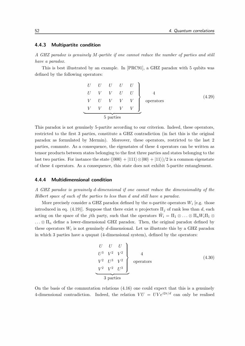
52 4. Quantum correlations
4.4.3 Multipartite condition
A GHZ paradox is genuinely M -partite if one cannot reduce the number of parties and still
have a paradox.
This is best illustrated by an example. In [PRC91], a GHZ paradox with 5 qubits was
defined by the following operators:
U U U U U
U V V U U
V U V V V
V V U V V
︸ ︷︷ ︸5 parties
4
operators(4.29)
This paradox is not genuinely 5-partite according to our criterion. Indeed, these operators,
restricted to the first 3 parties, constitute a GHZ contradiction (in fact this is the original
paradox as formulated by Mermin). Moreover, these operators, restricted to the last 2
parties, commute. As a consequence, the eigenstates of these 4 operators can be written as
tensor products between states belonging to the first three parties and states belonging to the
last two parties. For instance the state (|000〉 + |111〉⊗|00〉 + |11〉)/2 is a common eigenstate
of these 4 operators. As a consequence, this state does not exhibit 5-partite entanglement.
4.4.4 Multidimensional condition
A GHZ paradox is genuinely d-dimensional if one cannot reduce the dimensionality of the
Hilbert space of each of the parties to less than d and still have a paradox.
More precisely consider a GHZ paradox defined by the n-partite operators Wi [e.g. those
introduced in eq. (4.19)]. Suppose that there exist n projectors Πj of rank less than d, each
acting on the space of the jth party, such that the operators Wi = Π1 ⊗ . . . ⊗ ΠnWiΠ1 ⊗. . . ⊗ Πn define a lower-dimensional GHZ paradox. Then, the original paradox defined by
these operators Wi is not genuinely d-dimensional. Let us illustrate this by a GHZ paradox
in which 3 parties have a ququat (4-dimensional system), defined by the operators:
U U U
U3 V 2 V 2
V 2 U3 V 2
V 2 V 2 U3
︸ ︷︷ ︸3 parties
4
operators(4.30)
On the basis of the commutation relations (4.16) one could expect that this is a genuinely
4-dimensional contradiction. Indeed, the relation V U = UV ei2π/d can only be realised
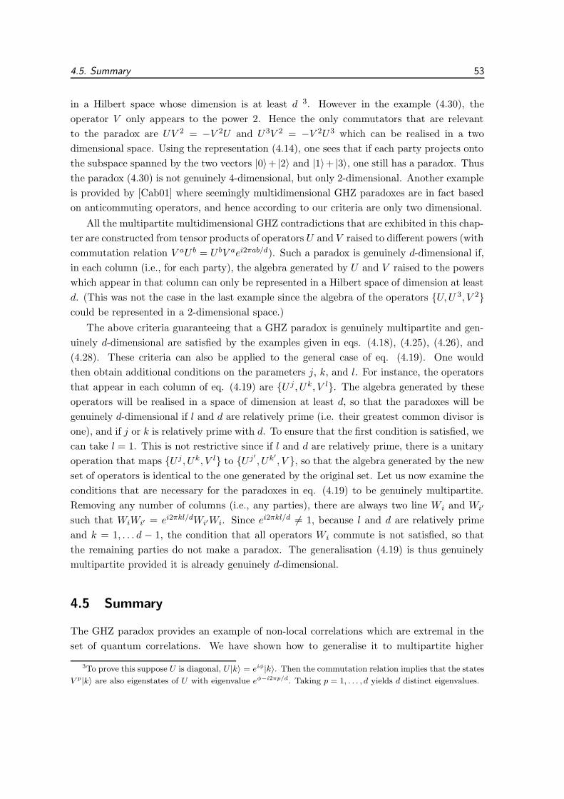
4.5. Summary 53
in a Hilbert space whose dimension is at least d 3. However in the example (4.30), the
operator V only appears to the power 2. Hence the only commutators that are relevant
to the paradox are UV 2 = −V 2U and U3V 2 = −V 2U3 which can be realised in a two
dimensional space. Using the representation (4.14), one sees that if each party projects onto
the subspace spanned by the two vectors |0〉+ |2〉 and |1〉+ |3〉, one still has a paradox. Thus
the paradox (4.30) is not genuinely 4-dimensional, but only 2-dimensional. Another example
is provided by [Cab01] where seemingly multidimensional GHZ paradoxes are in fact based
on anticommuting operators, and hence according to our criteria are only two dimensional.
All the multipartite multidimensional GHZ contradictions that are exhibited in this chap-
ter are constructed from tensor products of operators U and V raised to different powers (with
commutation relation V aU b = U bV aei2πab/d). Such a paradox is genuinely d-dimensional if,
in each column (i.e., for each party), the algebra generated by U and V raised to the powers
which appear in that column can only be represented in a Hilbert space of dimension at least
d. (This was not the case in the last example since the algebra of the operators {U,U 3, V 2}could be represented in a 2-dimensional space.)
The above criteria guaranteeing that a GHZ paradox is genuinely multipartite and gen-
uinely d-dimensional are satisfied by the examples given in eqs. (4.18), (4.25), (4.26), and
(4.28). These criteria can also be applied to the general case of eq. (4.19). One would
then obtain additional conditions on the parameters j, k, and l. For instance, the operators
that appear in each column of eq. (4.19) are {U j , Uk, V l}. The algebra generated by these
operators will be realised in a space of dimension at least d, so that the paradoxes will be
genuinely d-dimensional if l and d are relatively prime (i.e. their greatest common divisor is
one), and if j or k is relatively prime with d. To ensure that the first condition is satisfied, we
can take l = 1. This is not restrictive since if l and d are relatively prime, there is a unitary
operation that maps {U j , Uk, V l} to {U j′ , Uk′, V }, so that the algebra generated by the new
set of operators is identical to the one generated by the original set. Let us now examine the
conditions that are necessary for the paradoxes in eq. (4.19) to be genuinely multipartite.
Removing any number of columns (i.e., any parties), there are always two line Wi and Wi′
such that WiWi′ = ei2πkl/dWi′Wi. Since ei2πkl/d 6= 1, because l and d are relatively prime
and k = 1, . . . d − 1, the condition that all operators Wi commute is not satisfied, so that
the remaining parties do not make a paradox. The generalisation (4.19) is thus genuinely
multipartite provided it is already genuinely d-dimensional.
4.5 Summary
The GHZ paradox provides an example of non-local correlations which are extremal in the
set of quantum correlations. We have shown how to generalise it to multipartite higher
3To prove this suppose U is diagonal, U |k〉 = eiφ|k〉. Then the commutation relation implies that the states
V p|k〉 are also eigenstates of U with eigenvalue eφ−i2πp/d. Taking p = 1, . . . , d yields d distinct eigenvalues.

54 4. Quantum correlations
dimensional systems. Our method is based on operators that are used to construct error-
correcting codes for arbitrary dimension.
Interestingly, in all the GHZ-type paradoxes we have constructed, the dimension is even
and is strictly less than the number of parties. We do not know whether this is necessarily
the case, or if it is due to the restricted set of constructions we have considered. Note that
after the results of this chapter were made public in [2], and motivated by this question,
the authors of [KZ02] have constructed several contradictions of the GHZ type for odd
dimensions. However, their results are not based on an algebra of operators as are the ones
presented here.
We stressed that all the paradoxes which one naively expects to be multipartite and
multidimensional are not necessarily so. In some cases it is possible to reexpress the paradox
in a lower dimensional space, and in other cases the GHZ state associated with the paradox
can be represented as a product of states belonging to different subsets of parties. We
discussed criteria that ensure that a GHZ paradox is truly n-partite and d-dimensional.
As for the original paradox, it is possible to construct from our paradoxes Mermin-like
inequalities such as (4.10). An interesting extension of this work would be to analyse the
structure of these inequalities which could give new insights into multipartite multidimen-
sional nonlocality.
Chapter 5
Non-locality as an information
theoretic resource
We have seen in the preceding chapter that quantum correlations can be non-local, but that
they cannot be used for super-luminal signalling. It is also possible to write down sets of
“super-quantum” correlations that are more non-local than is allowed by quantum mechanics,
yet are still non-signalling. Viewed as an information theoretic resource, super-quantum
correlations are very powerful at reducing the amount of communication needed for distributed
computational tasks. An intriguing question is why quantum mechanics does not allow these
more powerful correlations.
We aim to shed light on the range of quantum possibilities by placing them within a wider
context. With this in mind, we investigate the set of correlations that are constrained only
by the no-signalling principle, i.e., the set P introduced in Section 2.2. This set corresponds
to a polytope, which contains the quantum correlations as a proper subset. We determine
the vertices of the no-signalling polytope in the case that two observers each choose from two
possible measurements with v outcomes. We then investigate the structure of this set from an
information theoretic perspective and consider how interconversions between different sorts of
correlations may be achieved. Finally, we consider some multipartite examples. The results
we present in this chapter are based on [8].
5.1 Introduction.
We have abstractly described a Bell scenario in Section 2.1 by saying that two parties have
access to a black box. When one observer introduces an input, selected from a range of
possibilities, the black box produces an output according to a determined joint probability
distribution pab|xy. As should be clear by now, such boxes can be divided in different types.
Some will allow the observers to signal to one another via their choice of input, others will
not allow signalling – in particular the ones arising from measurements on an entangled
55

56 5. Non-locality as an information theoretic resource
quantum state will not. Of the non-signalling boxes, some will be non-local.
In general, these boxes can be viewed as an information theoretic resource. This is
obvious in the case of signalling boxes, which correspond to two-way classical channels, as
introduced by Shannon [Sha61]. However, as we have mentioned in the introductory chapter,
it is also known that non-local correlations arising from an entangled quantum state, even
though they cannot be used directly for signalling, can be useful in reducing the amount
of signalling that is needed in communication complexity scenarios below what could be
achieved with only shared random data. A local black box is, of course, simply equivalent to
some shared random data, which in turn (depending on the precise nature of the problem)
may be better than nothing [KN97].
What kind of information theoretic resource a box provides is determined by the joint
probability pab|xy and not by the way it is internally implemented. To stress this fact, we will
identify in this chapter a box with the correlations pab|xy it produces, and use interchangeably
the denominations “box” and “correlations”. Of course, the physical resources necessary to
realise a particular box may determine whether it can be implemented by two observers, and
thus ultimately determine what kind of information theoretic tasks they can achieve.
A good question to ask then is, can any set of non-signalling correlations be produced
by measurements on some quantum state? The answer, in fact, is no. This was shown by
Popescu and Rohrlich [PR94], who wrote down a set of correlations that return a value of
4 for the CHSH expression (2.13), the maximum value algebraically possible, yet are non-
signalling. We have said in the preceding chapter that the maximum quantum value is given
by Cirel’son’s theorem as 2√
2. Popescu and Rohrlich concluded that quantum mechanics is
only one of a class of non-local theories consistent with causality. In terms of our boxes, there
are some boxes that are non-signalling but are more non-local than is allowed by quantum
mechanics. It is interesting to note that from an information theoretic point of view, some of
these latter are very powerful. For example, van Dam has shown [vD00] that two observers
who have access to a supply of Popescu-Rohrlich-type boxes would be able to solve essentially
any two-party communication complexity problem with only a constant number of bits of
communication. This should be contrasted with the quantum case, for which it is known
that certain communication complexity problems require at least n bits of communication
even if unlimited shared entanglement is available [CvDN97].
In this chapter, we investigate the set P of non-signalling boxes, considering such boxes as
an information theoretic resource. We have already seen that the set of quantum correlations
is no-signalling and thus is a subset of P. The motivation for studying the wider set is partly
that it is interesting for its own sake. This is true even though no correlations other than
quantum correlations have so far been observed in Nature. Our findings are preliminary,
but it is already clear that the set of non-signalling boxes has interesting structure, and
one finds analogies with other information theoretic resources, in particular with the set of
entangled quantum states. This work is not, however, purely academic. Another motivation

5.2. Two party correlations 57
is that a better understanding of the nature of quantum correlations can be gained by placing
them in a wider setting. Only in this way, for example, can one hope to answer Popescu
and Rohrlich’s original question, of why quantum correlations are not more non-local than
they are. More generally, a proper understanding of the information theoretic capabilities of
quantum mechanics includes an understanding of what cannot be achieved as well as what
can.
This chapter is organised as follows. In Section 5.2.1, we briefly review the general
structure of the set of non-signalling correlations, which form a convex polytope. We then
examine more closely, in Section 5.2.2, the particular case of correlations involving two
possible inputs, obtaining all the vertices of the corresponding polytope. We then consider,
in Section 5.2.3, how interconversions between these extreme points may be achieved using
local operations. Section 5.3 is devoted to three-party correlations and in Section 5.3.4, we
examine how extremal correlations correlate to the environment. We conclude with some
open questions in Section 5.4.
5.2 Two party correlations
5.2.1 General structure
The set P of bipartite no-signalling boxes has been introduced in Section 2.2. It consists in
all the joint probabilities pab|xy that satisfy the conditions of positivity
pab|xy ≥ 0 ∀ a, b,x,y (5.1)
normalisation, ∑
a,b
pab|xy = 1 ∀ x,y, (5.2)
and no-signalling ∑
b
pab|xy =∑
b
pab|xy′ ≡ pa|x ∀ a,x,y,y′
∑
a
pab|xy =∑
a
pab|x′y ≡ pb|y ∀ b,y,x,x′.(5.3)
Since the above constraints are all linear, P is a convex polytope.
We have already investigated two subsets of P, the set L of local correlations and the
set Q of quantum correlations. We have seen that L is itself a convex polytope with vertices
corresponding to local deterministic boxes. Note that these deterministic points are as well
vertices of the polytope P since all their entries dλab|xy
are equal to 0 or 1 (the no-signalling
polytope, however, also contains non-local vertices). The set Q, for its part, is convex but is
not a polytope.
The equalities (5.2) and (5.3) determine the affine subspace in which lies the no-signalling
polytope P. We have seen in Chapter 3, that these equalities also fully define the affine hull
of the local polytope, so that dimL = dimP (and this, of course, is also equal to dimQ).

58 5. Non-locality as an information theoretic resource
On the other hand, the positivity conditions (5.1) define the facets of the no-signalling
polytopes. They also form trivial facets of L, but the local polytope also possess non-trivial
facets which correspond to Bell inequalities. Since the correlations allowed by quantum
mechanics can violate Bell inequalities, L ⊂ Q. However, as they violate the CHSH inequality
only up to Cirel’son’s bound of 2√
2, they form a proper subset of the no-signalling polytope.
Overall, we have that L ⊂ Q ⊂ P. This situation is illustrated in Figure 5.1.
L
NL
L L
L
NL
L
LNL
NL
����
����
����
L
P
Q
Figure 5.1: A schematic representation of the space of non-signalling
correlation boxes. The vertices are labelled L and NL for local and non-
local. Bell inequalities are the facets represented in dashed lines. The
set bounded by these is L. The region accessible to quantum mechanics
is Q. A general non-signalling box ∈ P.
5.2.2 The two-inputs no-signalling polytope
Two outputs
Having rapidly reviewed the general structure of the no-signalling set, we now consider in
detail the simple case in which the two observers, Alice and Bob, are each choosing from two
inputs, each of which has two possible outputs. We thus have that x,y, a, b ∈ {0, 1}. The
probabilities pab|xy thus form a table with 24 entries, although these are not all independent
due to the constraints of Section 5.2.1. The dimension of the polytope is found by subtracting
the number of independent constraints from 24, and turns out to be 8. To understand the
polytope P, we wish to find its vertices. These will be boxes that satisfy all of the constraints
and saturates a sufficient number of the positivity constraints to be uniquely determined.
In the next subsection, we present an argument that allows us to find all the vertices of

5.2. Two party correlations 59
the two-input v-output polytope. Here we simply state the results for the simple two-input
two-output case.
We find that there are 24 vertices, which may be divided into two classes, those cor-
responding to local boxes and those corresponding to non-local boxes. Local vertices are
simply the local deterministic boxes, which assign a definite value to each of Alice’s and
Bob’s inputs. There are thus 16 local vertices, which can be expressed as
pab|xy =
1 : a = αx ⊕ β,
b = γy ⊕ δ
0 : otherwise,
(5.4)
where α, β, γ, δ ∈ {0, 1}. Here and throughout, ⊕ denotes addition modulo 2.
The 8 non-local vertices may be expressed compactly as
pab|xy =
{1/2 : a⊕ b = x.y ⊕ αx ⊕ βy ⊕ γ
0 : otherwise,(5.5)
where α, β, γ ∈ {0, 1}. We will refer to these boxes as Popescu-Rohrlich (PR) boxes.
By using reversible local operations Alice and Bob can convert any vertex in one class into
any other vertex within the same class. There are two types of reversible local operations.
Alice may relabel her inputs, x → x ⊕ 1, and she may relabel her outputs (conditionally on
the input), a→ a⊕αx⊕β. Bob can perform similar operations. Thus up to local reversible
transformations, each local vertex is equivalent to the vertex setting α = 0, β = 0, γ = 0,
δ = 0, i. e,
pab|xy =
{1 : a = 0 and b = 0
0 : otherwise.(5.6)
Each non-local vertex is equivalent to
pab|xy =
{1/2 : a⊕ b = X.Y
0 : otherwise.(5.7)
We note that if we allow irreversible transformations on the outputs we may convert any
non-local vertex into a local vertex.
For the case of two inputs and two outputs, we have seen in Chapters 2 and 3 that the
only non-trivial facets of the local polytope L correspond to the CHSH inequalities (2.13).
There is an important connection between the CHSH inequalities and the non-local vertices
of P. In order to explain this, we first rewrite the CHSH inequalities with a new notation.
Let 〈ij〉 be defined by
〈ij〉 =
1∑
a,b=0
(−1)a+b pab|x=i,y=j. (5.8)

60 5. Non-locality as an information theoretic resource
Then the non-trivial facets of L are equivalent to the following inequalities.
Bαβγ ≡ (−1)γ 〈00〉 + (−1)β+γ 〈01〉+ (−1)α+γ 〈10〉 + (−1)α+β+γ+1 〈11〉 ≤ 2,
(5.9)
where α, β, γ ∈ {0, 1}. For each of the 8 Bell expressions Bαβγ , the algebraic maximum
is Bαβγ = 4. We find that for each choice of α, β, γ the correlations defined by eq. (5.5)
return a value for the corresponding Bell expression of Bαβγ = 4. Thus there is a one-
to-one correspondence between the non-local vertices of P and the non-trivial facets of L,
with each vertex violating the corresponding CHSH inequality up to the algebraic maximum.
These extremal correlations describe in a compact way the logical contradiction in the CHSH
inequalities.
v outputs
We now generalise the results of the preceding section. Again we have two parties, Alice
and Bob, who choose from two inputs x and y ∈ {0, 1}. But we now consider outputs
a ∈ {0, . . . , vx − 1} and b ∈ {0, . . . , vy − 1}.
Theorem 5.1. The non-local vertices of P for two input settings and vx and vy outputs are
equivalent under reversible local relabelling to
pab|xy =
1/k : (b− a) mod k = x.y
a, b ∈ {0, . . . , k − 1}0 : otherwise,
(5.10)
for each k ∈ {2, . . . ,minx,y(vx, vy)}.
We note that the case vx = vy = 2 gives the PR correlations we found previously. If
vx = vy = k = v then the vertex violates the CGLMP inequality (2.16) up to its algebraic
maximum. We call such a box a v-box.
Proof of Theorem 5.1. A probability table pab|xy is a vertex of P if and only if it
is the unique solution of eqs. (5.1),(5.2), and (5.3) with dimP of the positivity inequalities
(5.1) replaced with equalities.
It will be useful to distinguish two kinds of extremal points: partial-output vertices and
full-output vertices. Partial-output vertices are vertices for which at least one of the pa|x = 0
or pb|y = 0. They can be identified with vertices of polytopes P ′ with fewer possible outputs:
v′x < vx or v′y < vy. Conversely, the vertices of a polytope P ′, with v′x < vx or v′y < vy
can be extended to vertices of P by mapping the outcomes of x′ and y
′ to a subset of the
outcomes of x and y, and by assigning a zero probability pa|x = 0 and pb|y = 0 to extra
outcomes. Full-output vertices are vertices for which all pa|x 6= 0 and pb|y 6= 0, i.e., for
which all outputs contribute non-trivially to pab|xy. Thus the extremal points of a given

5.2. Two party correlations 61
two-settings polytope consist of the full-output vertices of that polytope and, by iteration,
of all the full-output vertices of two-settings polytopes with fewer outcomes. Hence in the
following, we need construct only the full-output vertices for a polytope characterised by vx
and vy.
The joint probabilities pab|xy form a table of∑
x,y vxvy entries. These are not all inde-
pendent because of the normalisation and no-signalling conditions. From Theorem 3.1, we
have that the dimension of the no-signalling polytope is
dimP =1∑
x,y=0
vxvy −1∑
x=0
vx −1∑
y=0
vy . (5.11)
This is the number of entries in the table pab|xy that must be set to zero to obtain a vertex.
Moreover, to obtain a full-output vertex, these must be chosen so that neither pa|x = 0 nor
pb|y = 0. If we fix a particular pair of inputs (x,y), then no more than vxvy − max(vx, vy)
probabilities may be set to zero, otherwise there will be fewer than max(vx, vy) probabilities
pab|xy > 0, and thus one of Alice’s or one of Bob’s outcomes will not be output for these
values of x and y. Because of the no-signalling conditions it will not be output for the other
possible pairs of inputs, so the vertex will be a partial-output one. Overall, the maximal
number of allowed zero entries for a full-output vertex is
Z =∑
x,y
(vxvy − max(vx, vy)) . (5.12)
Such a vertex is thus possible if dimP ≤ Z, or
1∑
x=0
vx +1∑
y=0
vy ≥1∑
x,y=0
max(vx, vy) . (5.13)
This condition is fulfilled (with equality) only for vx = vy = v, ∀x,y ∈ {0, 1}.We can thus restrict our analysis to v-outcome polytopes. The extremal points of more
general ones, where vx 6= vy, will be the full-output extremal points of v-outcomes polytopes
for v = 2, . . . ,minx,y(vx, vy).
Using vx = vy = v, ∀x,y ∈ {0, 1} in the discussion before eq. (5.12), it follows that the
dimension of a v-outcome polytope is 4v(v − 1) and that for a given pair of inputs exactly
v(v − 1) probabilities must be assigned the value zero, or equivalently that v probabilities
must be > 0. We can therefore write the probabilities as
pab|xy
{> 0 if b = fxy(a)
= 0 otherwise,(5.14)
where fxy(a) is a permutation of the v outcomes. Indeed, if fxy(a) is not a permutation,
then at least one of Bob’s outcomes will not be output.

62 5. Non-locality as an information theoretic resource
We can relabel Alice’s outcomes for x = 0 so that f01(a) = a, we can relabel those of
Bob for y = 0 so that f00(a) = a and finally those of Alice for x = 1 to have f10(a) = a. In
other words,
pab|xy
{> 0 if (b− a) mod v = 0
= 0 otherwise,(5.15)
for (x,y) ∈ {(0, 0), (0, 1), (1, 0)}. It remains to determine f11. It must be chosen so that the
probability table pab|xy is uniquely determined, i.e., so that specific values are assigned to
the probabilities different from zero. In fact, it is easy to show that this can only be the case
if the permutation f11 is of order v, i.e., f k11(a) = a only for k = 0 mod v.
The only remaining freedom in the relabelling of the outcomes so that property (5.15)
is conserved, is to relabel simultaneously the outputs for all four possible inputs. We can
relabel them globally so that f11(a) = (a + 1) mod v. This implies that pab|11 = 1/v if
(b− a) mod v = 1. This completes the proof. 2
5.2.3 Resource conversions
In the preceding section we found all the vertices of the no-signalling polytope for bipartite,
two-input boxes. As described in the introduction, the ethos adopted in this thesis is that
boxes (in particular, non-local boxes) can be regarded as an information theoretic resource,
and investigated as such. Useful comparisons can be drawn with other information theoretic
resources, including shared random data [AC98], shared secret data [AC93, CP02], and
entanglement [NC00]. In each case, there is a convex set of possible states and a notion of
interconversion between different states. There is also a notion of interconversion between
different resources. Each resource is useful for some task(s) and can be quantified via some
measure(s). Some of this is illustrated in Table 5.1. Note that the quantitative measures
Resource Instantiation Quantitative measure
Shared random data Random variables Mutual information
Shared secret data Random variables Secrecy rate
Entanglement Quantum states Entanglement cost
Non-locality Boxes Classical simulation cost
Table 5.1: Comparison of information theoretic resources.
given are not the only possibilities. Note also that even if the given measure vanishes, a
useful resource may still be present. Thus uncorrelated random variables can still be useful
(as local randomness), as can separable quantum states (for various things), as can local
boxes (as local or shared randomness).
In light of this, it is natural to ask, what interconversions between boxes are possible,
and what would be a good measure of the non-locality of a box? To the second question,

5.2. Two party correlations 63
several answers suggest themselves, such as the amount of classical communication needed
to simulate the box (given that the only other resource is shared random data), and the
degree of violation of Bell inequalities. This will be examined in the next chapter. In this
chapter, however, we concentrate on the first question.
The problem that we consider, then, is whether one can simulate one type of box, using
one or more copies of another type as a resource. Local operations such as relabelling are
of course allowed. As non-locality is the resource that we have in mind, it is also natural
to allow the parties free access to local boxes (i.e., to local and shared randomness). We
note, however, that neither local nor shared randomness can help if the box to be simulated
is a vertex 1, thus none of the protocols we describe below make use of this. We make the
assumption that communication between the parties is not allowed.
In general, outputs for one box can be used as inputs for another box. This allows
non-trivial protocols to be constructed. As an interesting logical possibility, we note that
the temporal order in which each party uses the boxes need not be the same, and that this
allows loops to be constructed that would be ill-defined if it were not for the no-signalling
condition. Such a loop is illustrated in Figure 5.2. In all of the protocols presented below,
however, the parties use the boxes in the same temporal order.
a
X
bY
Figure 5.2: An example of how two parties that are
given two boxes may process locally their inputs and
outputs. They result in simulating another type of box
with inputs x,y and outcomes a, b. Note that due to
the no-signalling condition, the parties can use their
two boxes with a different time ordering.
In the following, we will describe three simple examples. We show that given a v-box and
a v′-box, we can simulate a vv′-box. We will also show that given a vv ′-box, we can simulate
one v-box. Finally, an unlimited supply of v-boxes can simulate a v ′-box to arbitrarily high
precision. In addition, we will describe a negative result: it is not in general possible to go
reversibly from n v-boxes to m v′-boxes, where v 6= v′. Although we only prove this for
1This is easy to see. For each value of the local or shared randomness, one can write down the box that is
simulated, conditioned on that value occurring. The box simulated by the overall protocol is then the average
of these conditional boxes, with the average taken over the possible values of the randomness. But if this box
is a vertex, then each of the conditional boxes must be the same vertex, and the protocol could have been
carried out without the randomness.

64 5. Non-locality as an information theoretic resource
exact transformations, we believe a similar result should hold even if transformations need
only be exact in an asymptotic limit. It follows from this that v and v ′-boxes are ultimately
inequivalent resources and that in our context, it is inappropriate to suppose that they can
be characterised by a single numerical measure of non-locality 2.
Suppose first, then, that Alice and Bob have one v-box and one v ′-box and they wish to
simulate one vv′-box. Simulate means that for each value of x ∈ {0, 1}, a procedure should
be defined for Alice, using the v and v ′-boxes, that eventually enables her to determine the
value of an output a ∈ {0, . . . , vv′ − 1}. Similarly for Bob; for each value of y there is an
eventual output b. The joint probabilities for a and b should satisfy eq. (5.10) (with vv ′
inserted instead of v where necessary).
Protocol 1: 1 v-box and 1 v′-box → 1 vv′-box
Alice. Alice inputs x into the v-box, obtaining outcome α. She then inputs x into the v ′-box
if α = v − 1, and inputs 0 into the v′-box otherwise, obtaining an output α′. Alice’s output
for the protocol is a = α′v + α.
Bob. Bob inputs y into the v-box, obtaining output β, and inputs y into the v ′-box, obtain-
ing output β ′. His output for the protocol is then b = β ′v + β.
Protocol 1 is illustrated in Figure 5.3 for the case v = v ′ = 2.
α β
PR
α’ β’
α.X
PR
YX
Y
Figure 5.3: Making a 4-box from two PR boxes. Alice
inputs x into the first box and α.x into the second,
while Bob inputs y into both boxes. Alice’s output is
given by a = 2α′ + α and Bob’s by b = 2β ′ + β.
2Similar considerations apply to the other resources we have mentioned. In the case of entanglement,
for example, reversible interconversions are not in general possible for mixed states, thus there is no unique
measure of entanglement for mixed states. In the case of shared random data, interconversions by local
operations are rather limited and provide no very meaningful measure of shared randomness. However, if
one expands the set of operations that Alice and Bob are allowed, then the picture changes. Thus in the
case of shared random data, allowing that Alice and Bob can communicate classically, while demanding that
the communication must be subtracted at the end, gives an operational meaning to the mutual information
[AC98]. Inspired by this, it may be interesting to consider conversions between boxes, with classical com-
munication allowed but subtracted at the end, or indeed conversions between entangled quantum states with
quantum communication allowed but subtracted at the end. We do not pursue these questions here.

5.2. Two party correlations 65
We indicate briefly why this protocol works. Recall that a vv ′-box satisfies (b − a)
mod vv′ = xy. Write a = α′v+α and b = β ′v+β, where α can take values α = 0, . . . , v− 1,
and α′ can take values α′ = 0, . . . , v′ − 1, and so on. We see that the condition satisfied by
a vv′-box is equivalent to
β − α mod v = xy
β′ − α′ mod v′ =
{xy : α = v − 1
0 : otherwise.(5.16)
Protocol 1 is designed precisely to satisfy this condition. It is then not difficult to check that
the correct probabilities are reproduced.
We note next that it is easy to convert one vv ′-box into one v-box.
Protocol 2: 1 vv′-box → 1 v-box
Alice. Alice inputs x into the vv′-box, obtaining an output α. Her output for the protocol
is then a = α mod v.
Bob. Bob inputs y into the vv′-box, obtaining an output β. His output for the protocol is
b = β mod v.
Again, it is not difficult to check that (b − a) mod v = xy, and that the correct proba-
bilities are reproduced.
Now we show how n v-boxes can be used to simulate a v ′-box to arbitrarily high precision.
This is done using a combination of Protocols 1 and 2.
Protocol 3: n v-boxes 1 v′-box
Alice and Bob begin by using the n v-boxes to simulate a vn-box, as per Protocol 1. Call
the outputs for the vn-box α and β. They satisfy (β−α) mod vn = xy. Alice and Bob now
use Protocol 2 to obtain something close to a v ′-box: the final outputs are a = α mod v′
and b = β mod v′.
If vn = kv′ for some positive integer k, this protocol works exactly. Otherwise, one can cal-
culate the errors resulting in Protocol 3. Denote by k the largest integer such that kv ′ ≤ vn.
Now we have that if x = 0 or y = 0, then (b − a) mod v ′ = 0 as required. However, the
probabilities are skewed by an amount ∝ 1/k ≈ v ′/vn. If x = y = 1, then the probabilities
are skewed in a similar manner. But in addition we have that if b = vn − 1, then (b − a)
mod v′ = 1 is not satisfied with probability 1/vn. The important thing here is that all errors
tend to zero exponentially fast as n becomes large.
We have seen several examples of how interconversions between non-local extremal boxes
are possible using only local operations. It is also interesting to consider how boxes may
be simulated using only classical communication (CC) and shared random data (SR), i.e.,
without other boxes. For example, we can see that one v-box may be simulated with one bit

66 5. Non-locality as an information theoretic resource
of 1-way communication and log2 v bits of shared randomness.
Protocol 4: 1 bit CC and log2 v bits SR → 1 v-box
Alice and Bob share a random variable α ∈ {0, · · · , v − 1}, where α takes all its possible
values with equal probability 1/v.
Alice. Alice sends her input x to Bob and outputs a = α.
Bob. Bob, knowing x and α, outputs b = (α+ x.y) mod v.
This protocol is optimal regarding the amount of 1-way communication exchanged. This
is a consequence of the following lemma, which places a lower bound on the amount of com-
munication needed to simulate boxes. The lemma is used in the proof of Theorem 5.3, our
final main result for this section.
Lemma 5.2. The simulation of n v−boxes using 1-way communication requires at least n
bits of communication if shared randomness is available, and n+n log2 v bits without shared
randomness.
Proof. Note that this bound can be achieved using Protocol 4 for each of the n boxes,
replacing if necessary n log2 v bits of shared randomness by n log2 v bits of communication
from Alice to Bob.
Let us show that this amount of communication is necessary. Suppose first that both
parties have access to shared random data and that communication is allowed from Alice to
Bob. Bob’s output is thus b = b(Y,C, r) where Y = y1 . . .yn are the joint inputs for Bob,
C is the communication and r the shared data. Note simply that for Alice, there are 2n
possible joint inputs into n v-boxes. If Alice is sending fewer than n bits, there will be at
least one pair of joint inputs for which her communication is the same. Call them X1 and
X2. A careful examination of the definition of a v-box reveals that there will be at least one
joint input of Bob’s into the n boxes such that his output must be different according to
whether Alice’s input was X1 or X2. Thus < n bits of communication are not sufficient.
If Alice and Bob do not have access to shared randomness, then Bob’s output is of the
form b = b(Y,C). The proof then follows by an argument similar to the one used above,
noting that for Alice there are 2n+n log2 d possible joint input-output pairs (X,A). �
These types of considerations will help us to establish the final result of this section.
Theorem 5.3. It is in general impossible, using local reversible operations, exactly to trans-
form n v-boxes into m v′-boxes.
The theorem follows from the following two lemmas.
Lemma 5.4. Using n v-boxes, Alice and Bob can exactly simulate at most n v ′-boxes, for
v ≥ v′.
Lemma 5.5. Using n v′-boxes, Alice and Bob can exactly simulate at most n(1+log2 v′)/(1+
log2 v) < n v-boxes for v′ ≤ v.

5.3. Three party correlations 67
Proof. We prove Lemma 5.4 as follows. We know that we can simulate n v-boxes with n bits
of communication and n log v bits of shared randomness. Suppose that there were a protocol
using only local operations that could convert n v-boxes into N v ′ boxes, for some v′ ≤ v,
where N > n. Then, by combining the simulation of the v-boxes with the protocol for their
conversion, we would have constructed a protocol for simulating N v ′-boxes using only n bits
of communication, in contradiction with Lemma 5.2. The proof of Lemma 5.5 is very similar.
Note that we can simulate n v′-boxes with n+ n log2 v′ bits of classical communication and
no shared randomness. Suppose that there were a protocol that converts n v ′-boxes into N v-
boxes, for some v ≥ v′, where N > n(1+log2 v′)/(1+log2 v). As argued above, it follows from
the fact that v-boxes are vertices that this protocol would not need any additional shared
randomness. Then we would have constructed a protocol for simulating N v-boxes using
only n+ n log2 v′ bits of communication and no shared randomness, again in contradiction
with Lemma 5.2. �
5.3 Three party correlations
5.3.1 Definitions
In this section, we generalise the considerations of the previous sections to consider tripartite
correlations. As before, we consider that correlations are produced by a black box with spec-
ified inputs and outputs, but now the box is assumed to be shared between three separated
parties, A, B and C.
The no-signalling polytope. The tripartite no-signalling polytope P is the set of joint
probability distributions pabc|XY Z , which satisfy positivity,
pabc|xyz ≥ 0 ∀ a, b, c,x,y, z (5.17)
normalisation, ∑
a,b,c
pabc|xyz = 1 ∀ x,y, z (5.18)
and no-signalling, ∑
a
pabc|xyz =∑
a
pabc|x′yz ∀ b, c,y, z,x,x′, (5.19)
with cyclic permutations over A, B and C.
Note that this last condition expresses that if the systems B and C are combined, then A
cannot signal to the resulting composite system BC. It also implies the weaker condition that
A cannot signal to B or C. Another type of no-signalling condition can be imagined however,
which is that if systems A and B are combined, the resulting composite system AB should not
be able to signal to C. This type of condition does not require a separate statement, however,
as it already follows from eq. (5.19). Indeed, we have noticed in the proof of Theorem 3.1 that

68 5. Non-locality as an information theoretic resource
the no-signalling conditions (5.19) imply that all l-partite marginal probability distributions
are well-defined, in particular the reduced probability pc|z is independent of the inputs x and
y, which is the condition that AB cannot signal to C. This can be deduced from (5.19) in
the following way∑
a,b
pabc|x,y,z =∑
a,b
pabc|x′,y,z ∀ b, c,x,x′,y, z
=∑
a,b
pabc|x′,y′,z ∀ c,x,x′,y,y′, z,
(5.20)
where we have first used the fact that A cannot signal to BC and then that B cannot signal
to AC.
Locality conditions. A box is local if the probabilities can be written in the form
pabc|xyz =∑
λ
qλ P (a|x, λ)P (b|y, λ)P (c|z, λ). (5.21)
The set of such boxes form the local polytope L. However, in the tripartite case, as well as
different types of no-signalling condition, there are different types of locality condition, and
we can introduce a refinement to the statement that a box is either local or non-local. We
say that a box is two-way local if either there exists a bi-partition of the parties, say AB
versus C, such that the composite system AB is local versus C, or if the box can be written
as a convex combination of such boxes, i.e.,
pabc|xyz = q12∑
λ12
qλ12P (ab|xy, λ12)P (c|z, λ12)
+ q13∑
λ13
qλ13P (ac|xz, λ13)P (b|y, λ13)
+ q23∑
λ23
qλ23P (bc|yz, λ23)P (a|x, λ23), (5.22)
where q12 + q23 + q13 = 1. It is easy to see that the set of such boxes is again a convex
polytope, denoted L2. Any box that cannot be written in this form demonstrates genuine
three-way non-locality. We have that L ⊂ L2 ⊂ P and also that L ⊂ Q ⊂ P.
In the following, we restrict our attention to the case a, b, c,x,y, z ∈ {0, 1}. We find
the vertices of the polytope P and point out some connections with three-party Bell-type
inequalities. Finally we consider some examples of interconversions, in particular of how to
construct tripartite boxes using PR boxes as a resource.
5.3.2 Two inputs and two outputs
The joint probabilities pabc|xyz of tripartite boxes with two inputs and two outputs per ob-
server form a table of 26 = 64 entries. However eqs. (5.18) and (5.19) introduce redundancies.
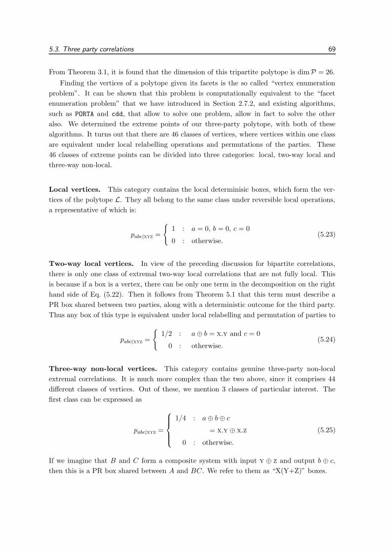
5.3. Three party correlations 69
From Theorem 3.1, it is found that the dimension of this tripartite polytope is dimP = 26.
Finding the vertices of a polytope given its facets is the so called “vertex enumeration
problem”. It can be shown that this problem is computationally equivalent to the “facet
enumeration problem” that we have introduced in Section 2.7.2, and existing algorithms,
such as PORTA and cdd, that allow to solve one problem, allow in fact to solve the other
also. We determined the extreme points of our three-party polytope, with both of these
algorithms. It turns out that there are 46 classes of vertices, where vertices within one class
are equivalent under local relabelling operations and permutations of the parties. These
46 classes of extreme points can be divided into three categories: local, two-way local and
three-way non-local.
Local vertices. This category contains the local determinisic boxes, which form the ver-
tices of the polytope L. They all belong to the same class under reversible local operations,
a representative of which is:
pabc|xyz =
{1 : a = 0, b = 0, c = 0
0 : otherwise.(5.23)
Two-way local vertices. In view of the preceding discussion for bipartite correlations,
there is only one class of extremal two-way local correlations that are not fully local. This
is because if a box is a vertex, there can be only one term in the decomposition on the right
hand side of Eq. (5.22). Then it follows from Theorem 5.1 that this term must describe a
PR box shared between two parties, along with a deterministic outcome for the third party.
Thus any box of this type is equivalent under local relabelling and permutation of parties to
pabc|xyz =
{1/2 : a⊕ b = x.y and c = 0
0 : otherwise.(5.24)
Three-way non-local vertices. This category contains genuine three-party non-local
extremal correlations. It is much more complex than the two above, since it comprises 44
different classes of vertices. Out of these, we mention 3 classes of particular interest. The
first class can be expressed as
pabc|xyz =
1/4 : a⊕ b⊕ c
= x.y ⊕ x.z
0 : otherwise.
(5.25)
If we imagine that B and C form a composite system with input y ⊕ z and output b ⊕ c,
then this is a PR box shared between A and BC. We refer to them as “X(Y+Z)” boxes.

70 5. Non-locality as an information theoretic resource
Correlations in the second class are equivalent to
pabc|xyz =
1/4 : a⊕ b⊕ c
= x.y ⊕ y.z ⊕ x.z
0 : otherwise.
(5.26)
We call them “Svetlichny” correlations (for reasons explained below).
Finally, the third class contains what we call “XYZ” correlations.
pabc|xyz =
{1/4 : a⊕ b⊕ c = x.y.z
0 : otherwise.(5.27)
The XYZ correlations are special because, as W. van Dam pointed out to us [vD04], they
can be used to solve any three party communication complexity problem with only 1 bit
broadcast by each party. He also pointed out that they have a natural generalisation to
n parties: a1 ⊕ a2 ⊕ · · · ⊕ an = x1.x2 . . .xn, where xi ∈ {0, 1} is the input of party i and
ai ∈ {0, 1} the output of party i. These n-party correlations can be used to solve any n
party communication complexity problem with 1 bit broadcast by each party. They can be
constructed from a supply of PR boxes.
We conclude this section with some remarks on these correlation vertices and known
multipartite Bell-type inequalities. First, each of the X(Y+Z), XYZ, and Svetlichny boxes
violates the Mermin inequality (4.10) up to the algebraic maximum. Second, we recall that
inequalities can be written down that detect genuine three-way non-locality. One such is the
Svetlichny inequality [Sve87]. If we define 〈i j k〉 by
〈ijk〉 =∑
a,b,c
(−1)a+b+c pa,b,c|x=i,y=j,z=k, (5.28)
then the Svetlichny inequality is
M = −〈000〉 + 〈001〉 + 〈001〉 + 〈011〉+ 〈100〉 + 〈101〉 + 〈110〉 − 〈111〉 ≤ 4.
(5.29)
Any local or two-way local box must satisfy this inequality. Quantum mechanically we can
obtain M = 4√
2 using a GHZ state (4.5) (although note that different measurements are
needed from those that produce the GHZ paradox [MPR02]). X(Y+Z) boxes do not violate
the Svetlichny inequality (although they must violate some Svetlichny-type inequality as
they are three-way non-local). Svetlichny boxes give M = 8, the algebraic maximum of the
expression (hence their name); XYZ correlations give M = 6.
From the fact that some quantum states violate the Svetlichny inequality, we can conclude
that in the two-input two-output case, Q * L2. From the fact that bipartite correlations
can be more non-local than quantum mechanics allows, we can also conclude that L2 * Q.

5.3. Three party correlations 71
5.3.3 Simulating tripartite boxes
We consider how we may simulate some of these tripartite boxes, using a supply of PR boxes
as a resource. We will give three examples, showing how to simulate an X(Y+Z) box with
two PR boxes, a Svetlichny box with three PR boxes, and an XYZ box with three PR boxes.
First, suppose that two PR boxes are shared, with box 1 between Alice and Bob and
box 2 between Alice and Charles. The following protocol shows how the three observers may
simulate one X(Y+Z) box (see Figure 5.4).
a
c
1 2
2
Z
1a
Y
X
b
Figure 5.4: Making an X(Y+Z) box from 2 PR boxes.
Alice outputs a = a1 ⊕ a2, Bob outputs b and Charles
outputs c.
Protocol 5: 2 PR boxes → 1 X(Y+Z) box
Alice. Alice inputs x into box 1 and box 2, obtaining outputs a1 and a2. She then outputs
a = a1 ⊕ a2.
Bob. Bob inputs y into box 1, obtaining output b.
Charles. Charles inputs z into box 2 obtaining output c.
The protocol works because
a⊕ b⊕ c = a1 ⊕ a2 ⊕ b⊕ c = x.y ⊕ x.z. (5.30)
Suppose now that three PR boxes are shared, with box 1 between Alice and Bob, box 2
between Alice and Charles, and box 3 between Bob and Charles. Protocol 6 (summarised
in Figure 5.5) allows them to simulate one Svetlichny box.
Protocol 6: 3 PR boxes → 1 Svetlichny box
Alice. Alice inputs x into both box 1 and box 2, obtaining a1 and a2. Her final output is
a = a1 ⊕ a2. Bob. Bob inputs y into both box 1 and box 3, obtaining b1 and b3. His final
output is b = b1 ⊕ b3.
Charles. Charles inputs z into both box 2 and box 3, obtaining c2 and c3. His final output
is c = c2 ⊕ c3.

72 5. Non-locality as an information theoretic resource
Z
X
Y3
X
Y
1
a
c
2
2
2
b c3 3
Z
a1
b1
Figure 5.5: Making a Svetlichny box from 3 PR boxes.
Alice outputs a = a1 ⊕ a2, Bob outputs b = b1 ⊕ b3
and Charles outputs c = c2 ⊕ c3.
This works because
a⊕ b⊕ c = a1 ⊕ b1 ⊕ b3 ⊕ c3 ⊕ a2 ⊕ c2
= x.y ⊕ y.z ⊕ x.z.(5.31)
Protocol 7 (summarised in Figure 5.6) shows how to simulate one XYZ box using three PR
boxes.
X a
a
Yb
b c
c
1 2
3
2
2
1
1
3 3
Z
Figure 5.6: Making an XYZ box from 3 PR boxes.
Alice outputs a = a2, Bob outputs b = b3 and Charles
outputs c = c2 ⊕ c3.
Protocol 7: 3 PR boxes → 1 XYZ box
Alice. Alice inputs x into box 1, obtaining an output a1. She then inputs a1 into box 2,
obtaining output a2. Alice’s output for the protocol is a = a2.
Bob. Bob inputs y into box 1, obtaining an output b1. He then inputs b1 into box 3, obtain-
ing output b3. Bob’s output for the protocol is b = b3.
Charles. Charles inputs z into both boxes 2 and 3, obtaining outputs c2 and c3. Charles’
output for the protocol is c = c2 ⊕ c3.

5.3. Three party correlations 73
The protocol works because
a⊕ b⊕ c = a2 ⊕ b3 ⊕ c2 ⊕ c3 = z.a1 ⊕ z.b1 = x.y.z. (5.32)
Finally, we note that it is of course possible to perform conversions among tripartite
boxes. For example, it is easy to see how to make one Svetlichny box using two XYZ
boxes. The protocol is obvious once it is realized that a Svetlichny box is locally equivalent
to a box defined by Eq. (5.26) with xy ⊕ yz ⊕ xz on the right hand side replaced by
xyz⊕ (1 ⊕ x)(1 ⊕ y)(1 ⊕ z). We omit the details.
5.3.4 Non-locality and the environment
Suppose that we have some three party no-signalling distribution pabe|xye with parties A,B
and E. We will show that if the reduced probability distribution pab|xy =∑
e pabe|xye is a
vertex of the bipartite no-signalling polytope, then the composite system AB is local versus
E. This is analogous to the result that pure quantum states cannot be entangled with a third
party or the environment. It means that extremal non-local correlations cannot be correlated
to any other system. (Note that this raises interesting new possibilities for cryptography.
These are investigated in [BHK04].)
By Bayes’ theorempabe|xye = pab|xyee pe|xye
= pab|xyee pe|e(5.33)
where we have used the fact that AB cannot signal to E to deduce the second equality. The
condition that E cannot signal to AB implies
pab|xy =∑
e
pabe|xye ∀e
=∑
e
pab|xyee pe|e ∀e(5.34)
For each value e, the last equality provides a convex decomposition of pab|xy in terms of non-
signalling correlations, with e playing the role of the shared randomness. Since we supposed
that pab|xy is extremal, this decomposition is unique and pab|xyee = pab|xy ∀e,e. We then
deduce
pabe|xye = pab|xy pe|e, (5.35)
i.e., that AB is uncorrelated with E.
A natural question that we leave as an open problem is whether the converse is true: if
pab|xy is in the interior of the no-signalling polytope, is it always possible to extend it to a
tripartite distribution pabe|xye such that AB is non-local versus E? (It is always possible, if
pab|xy is not a vertex, to write it as pab|xy =∑
e pabe|xye, where e takes the single value e = 0.
One can also require that e take several values, in such a way that pabe|xye is non-signalling.
What is non-trivial is the requirement that pabe|xye is non-local in the partition AB versus
E. We do not know if this is possible in general.)

74 5. Non-locality as an information theoretic resource
5.4 Discussion and open questions
In conclusion, we have defined non-signalling correlation boxes and investigated their po-
tential as an information theoretic resource. Once the structure of the set of such boxes is
understood as a convex polytope, it is clear that there are analogies with other information
theoretic resources, in particular the resource of shared quantum states (with non-locality
taking the place of entanglement). With this in mind, we have shown how various inter-
conversions between boxes are possible. The set of multipartite boxes in particular appears
very rich. Finally, we furthered the analogy with quantum states by demonstrating how
non-locality is monogamous, in much the same way that entanglement is monogamous. We
finish with some open questions.
Non-local vertices and Bell inequalities. We saw in Sec. 5.2.2 that for the two-settings
two-outcomes polytope there is a one-to-one correspondence between extremal non-local cor-
relations and facet Bell inequalities. One might wonder whether this one-to-one correspon-
dence holds in general. It appears, however, that for more complicated situations, involving
more possible inputs or outcomes, it does not. It would be interesting to investigate what is
the precise relation between non-local vertices and facet Bell inequalities. This might help
understand further the geometrical structure of non-local correlations.
Other vertices. We have given a complete characterisation of two-inputs extremal non-
local boxes in the bipartite case and presented some examples in the tripartite case. In
general, one might also consider extremal boxes involving more inputs, more outcomes or
more parties.
For instance, a natural way to generate more complex boxes is by taking products of
simpler ones. Suppose Alice and Bob have access to two boxes p0a0b0|x0y0
and p1a1b1|x1y1
,
where for simplicity we consider that there are M possible inputs and v possible outputs for
each box. If Alice inputs x0 and x1 in each of the two boxes and outputs a = d a1 + a0 and
similarly for Bob, they have now produced a non-local box with M 2 inputs and d2 outputs
pab|xy = p0a0b0|x0y0
. p1a1b1|x1y1
, where x = M x1 + x0 and similarly for y. If the two original
boxes were extremal for the (M,d) polytope will the product be extremal for the (M 2, d2)
polytope? In the case of quantum states, the analogous result of course holds - a product of
two pure states is itself a pure state. We have been able to show that in the case of boxes,
the result holds provided that we restrict to extremal boxes with the following property:
the output of one party is uniquely determined when the two inputs and the other party’s
output are specified. This is true for all the vertices presented in this paper. Plausibly it is
true for all vertices, but this is not proven.
Interconversions. We have so far been able to achieve only a limited set of interconver-
sions between extremal boxes. This is especially true for the three party case, where there

5.4. Discussion and open questions 75
are 46 classes of vertices and we have investigated only 5 of these. Understanding what
kinds of interconversions between extremal boxes are possible is necessary to appraise their
relative power as an information-theoretic resource.
The motivation is also to answer the general question of whether there exist inequivalent
types of non-local correlations. Note for instance that the three-way non-local correlations of
Eqs. (5.25), (5.27) and (5.26) cannot be reduced to two-way non-local ones using only local
operations. This follows from the fact that the outcomes for two out of the three parties are
totally independent of one another (unless the outcome of the third party is communicated
to them). In this sense genuinely tripartite extremal correlations and bipartite extremal cor-
relations belong to inequivalent classes. Are there inequivalent classes of bipartite extremal
correlations? In other words, are there two bipartite extremal boxes, such that one cannot
simulate the other even approximately, no matter how many copies are available?
Another problem is whether all bipartite and multipartite correlations can be constructed
using PR boxes, as is the case for all the extremal boxes presented in this paper (and thus
also for probabilistic mixtures of them). PR boxes could then be viewed as the unit of non-
local correlation, in analogy with the bit, qubit and ebit, which are the units of classical and
quantum information theoretic resources.
Interior points. We have only considered conversions between extremal probability dis-
tributions. It would be interesting to consider the interior points of the polytope, which
comprise quantum correlations. In particular we would like to find out if distillation of such
mixed correlations is possible, i.e., if given a number of copies of a mixed box we can by local
operations obtain some number of extremal boxes. Note that Cirel’son’s bound shows that
the quantum correlations Q, are a proper subset of the set of all non-signalling correlations
P. Thus it is impossible to distill correlations in Q to extremal correlations. But apart from
this, we do not know of any constraint on possible distillation of non-local correlations.
Finally, one could consider distillation in a new context, where we allow some commu-
nication between the parties but account for it at the end of the protocol (as noted above,
an analogous approach was considered in Ref. [AC98] in the context of classical distillation
of shared randomness). Alternatively, following Ref. [CP02], one could introduce a new el-
ement, that of secrecy. Suppose that inputs and outputs are considered to be secret, and
that Alice and Bob have a supply of noisy (that is non-extremal) boxes. Can Alice and
Bob distill a supply of extremal boxes, whose inputs and outputs are also secret, via public
communication?
As we outlined at the beginning of this chapter, non-local extremal correlations can be
a very powerful resource for communication complexity problems. This will also be the case
for correlations that can be distilled to these with no or little communication. On the other
hand, Cirel’son’s bound and results in communication complexity [CvDN97] put limits on
the power of quantum mechanics as a resource in distributed tasks. A better understanding
of the possible interconversions between non-local correlations might bring an information

76 5. Non-locality as an information theoretic resource
theoretic explanation of these limitations.
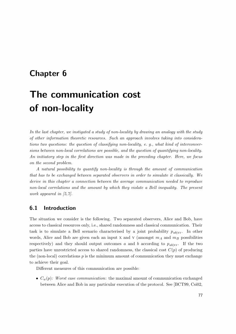
Chapter 6
The communication cost
of non-locality
In the last chapter, we instigated a study of non-locality by drawing an analogy with the study
of other information theoretic resources. Such an approach involves taking into considera-
tions two questions: the question of classifying non-locality, e. g., what kind of interconver-
sions between non-local correlations are possible, and the question of quantifying non-locality.
An initiatory step in the first direction was made in the preceding chapter. Here, we focus
on the second problem.
A natural possibility to quantify non-locality is through the amount of communication
that has to be exchanged between separated observers in order to simulate it classically. We
derive in this chapter a connection between the average communication needed to reproduce
non-local correlations and the amount by which they violate a Bell inequality. The present
work appeared in [5,7].
6.1 Introduction
The situation we consider is the following. Two separated observers, Alice and Bob, have
access to classical resources only, i.e., shared randomness and classical communication. Their
task is to simulate a Bell scenario characterised by a joint probability pab|xy. In other
words, Alice and Bob are given each an input x and y (amongst mA and mB possibilities
respectively) and they should output outcomes a and b according to pab|xy. If the two
parties have unrestricted access to shared randomness, the classical cost C(p) of producing
the (non-local) correlations p is the minimum amount of communication they must exchange
to achieve their goal.
Different measures of this communication are possible:
• Cw(p): Worst case communication: the maximal amount of communication exchanged
between Alice and Bob in any particular execution of the protocol. See [BCT99, Csi02,
77

78 6. Communication cost of non-locality
BT03, TB03].
• C(p): Average communication: the average communication exchanged between Alice
and Bob, where the average is taken over the inputs and the shared randomness. See
[Mau92, Ste00, Met04].
• C∞(p): Asymptotic communication: the limit limn→∞ C(pn)/n, where pn is the proba-
bility distribution obtained when n runs of the Bell scenario are carried out in parallel,
that is when the parties receive n inputs and produce n outputs in one go. See [CGM00].
In each of these definitions the costs are defined with respect to the optimal protocol that
gives the lowest value for each quantity. The asymptotic measure C∞ may be the most ap-
propriate when one is concerned with practical applications that make use of the correlations
but is less preoccupied whether the measurements are performed individually or collectively.
On the other hand, the first two measures of communication relate to the usual Bell scenar-
ios we have considered so far, where the outcomes are determined after each single pair of
inputs is chosen. They thus more properly count the communication necessary to simulate
Bell-type experiments.
Given an arbitrary joint probability distribution p, how can we evaluate its non-locality
according to these measures? A straightforward observation is that if p violates a Bell
inequality, then C(p) > 0. Could violation of a Bell inequality provide further information
on the amount of communication necessary to simulate p? Relations between the worst
case communication Cw and Bell inequalities were examined in [BT03] where the authors
introduced new Bell inequalities that are satisfied by all correlations that necessitate at most
1 bit of communication to be simulated. Violations of such inequalities thus implies that
Cw(p) > 1.
In the present chapter, we concentrate on the average communication C. We first point
out that the degree by which the probabilities p violate a Bell inequality imposes a lower
bound on C(p). This bound is simply a bound on the communication needed to classically
simulate a violation of the inequality by the same amount, that is to simulate any Bell sce-
nario that leads to the same degree of violation of the inequality. In general the correlations
p may violate more than one inequality, and it is thus a priori unclear that violation of a
specific Bell inequality could suffice to characterise entirely the non-local content of the cor-
relations. Yet, we show that to each joint distribution p is associated an optimal inequality
such that the bound the violation imposes on C(p) is saturated, i.e., it gives the minimal
average communication needed to reproduce these correlations. These results are presented
in Section 6.2.
We then apply our formalism to several examples. We investigate in detail the case of
the CHSH inequality (2.13) in Section 6.3.1, and show that for two-inputs and two-outputs
Bell scenarios, the CHSH inequality is always optimal for no-signalling correlations. As we
will see, this implies in particular that√
2 − 1 ' 0.4142 bits are necessary and sufficient on
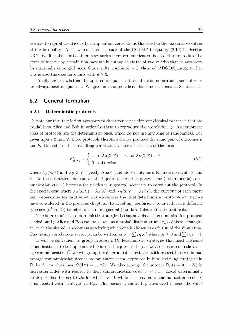
6.2. General formalism 79
average to reproduce classically the quantum correlations that lead to the maximal violation
of the inequality. Next, we consider the case of the CGLMP inequality (2.16) in Section
6.3.2. We find that for two-inputs scenarios more communication is needed to reproduce the
effect of measuring certain non-maximally entangled states of two qutrits than is necessary
for maximally entangled ones. Our results, combined with those of [ADGL02], suggest that
this is also the case for qudits with d ≥ 3.
Finally we ask whether the optimal inequalities from the communication point of view
are always facet inequalities. We give an example where this is not the case in Section 6.4.
6.2 General formalism
6.2.1 Deterministic protocols
To state our results it is first necessary to characterise the different classical protocols that are
available to Alice and Bob in order for them to reproduce the correlations p. An important
class of protocols are the deterministic ones, which do not use any kind of randomness. For
given inputs x and y, these protocols therefore always produce the same pair of outcomes a
and b. The entries of the resulting correlation vector dλ are thus of the form
dλab|xy
=
{1 if λA(x,y) = a and λB(x,y) = b
0 otherwise.(6.1)
where λA(x,y) and λB(x,y) specify Alice’s and Bob’s outcomes for measurements x and
y. As these functions depend on the inputs of the other party, some (deterministic) com-
munication c(x,y) between the parties is in general necessary to carry out the protocol. In
the special case where λA(x,y) = λA(x) and λB(x,y) = λB(y), the outpout of each party
only depends on his local input and we recover the local deterministic protocols dλ that we
have considered in the previous chapters. To avoid any confusion, we introduced a different
typeface (dλ vs dλ) to refer to the more general (non-local) deterministic protocols.
The interest of these deterministic strategies is that any classical communication protocol
carried out by Alice and Bob can be viewed as a probabilistic mixture {qλ} of these strategies
dλ, with the shared randomness specifying which one is chosen in each run of the simulation.
That is any correlations vector p can be written as p =∑
λ qλdλ where qλ ≥ 0 and∑
λ qλ = 1.
It will be convenient to group in subsets Di deterministic strategies that need the same
comunication ci to be implemented. Since in the present chapter we are interested in the aver-
age communication C, we will group the deterministic strategies with respect to the minimal
average communication needed to implement them, expressed in bits. Indexing strategies in
Di by λi, we thus have C(dλi) = ci ∀λi. We also arrange the subsets Di (i = 0, . . . N) in
increasing order with respect to their communication cost: ci < ci+1. Local deterministic
strategies thus belong to D0 for which c0=0, while the maximum communication cost cN
is associated with strategies in DN . This occurs when both parties need to send the value

80 6. Communication cost of non-locality
of their input to the other, so cN = log2mA + log2mB1. We will further illustrate this
grouping of deterministic strategies in Section 6.3.2.
With the above notation, a decomposition of p in terms of deterministic strategies can
be written as
p =∑
i
∑
λi
qλidλi . (6.2)
It then directly follows that the average communication C(p, {qλ}) associated to the protocol
(6.2) is given by
C(p, {qλ}) =∑
i
∑
λi
qλiC(dλi)
=∑
i
∑
λi
qλici =
∑
i
qici , (6.3)
where qi =∑
λiqλi
is the probability to use a strategy from Di. The minimum amount of
communication C(p) necessary to reproduce the correlations p is the minimum of C(p, {qλ})over all possible decompositions of the form (6.2). If there exists a decomposition such that
q0 = 1, i.e., if the correlations can be written as a convex combination of local deterministic
strategies, then C(p) = 0 and the correlations are local. If for every decomposition q0 < 1,
the correlations are non-local and they violate a Bell inequality.
6.2.2 Bell inequalities
Let bp ≤ b0 be a Bell inequality. Since it is satisfied by local correlations (which can be written
as a convex sum of local deterministic strategies dλ0), we clearly have b0 ≥ maxλ0{b dλ0}.
We assume, if necessary by redefining b0, that the inequality is tight, i.e.,
b0 = maxλ0
{b dλ0} . (6.4)
The inequality is thus entirely defined once b is given and by abuse of language, we refer to
b as the “inequality” and b0 as its local bound. The inequality b thus corresponds to a linear
form which associates to each joint distribution p the number B(p) = bp.
We already know that if B(p) > b0, p is non-local. To extract more information from
B(p) than a simple detection of non-locality it is necessary to consider not only the upper
bound b0 the inequality takes on the local subset D0, but also on all the other subsets Di:
bi = maxλi
{b dλi} . (6.5)
1Plausibly for no-signalling correlations, it would be sufficient to consider deterministic strategies with
communication cost c′N ≤ log2(min(mA, mB)). Indeed, it is easy to see that any correlations satisfying the
no-signalling conditions (2.4) can be simulated by one of the parties sending his input to the other. However
it is logically possible that allowing strategies with higher communication cost than c′N would result in lower
communication on average. To avoid loosing full generality, we thus consider the maximal communication
cost to be cN .

6.2. General formalism 81
Given this extra knowledge, a constraint on the decomposition (6.2) can be deduced from
the amount by which p violates the Bell inequality. This turns into a bound on C(p) which
is the basis of the present work.
6.2.3 Main results
Theorem 6.1. For every inequality b and probability distribution p, the following bound
holds:
C(p) ≥ B(p) − b0bj∗ − b0
cj∗ (6.6)
where j∗ is the index such that (bj∗ − b0)/cj∗ = maxj 6=0{(bj − b0)/cj}.
Proof. From (6.2) and (6.5), we deduce B(p) = bp =∑
i
∑λiqλib dλi ≤ ∑
i qibi. Since∑i qi = 1, we find
B(p) − b0 ≤∑
i6=0
qi(bi − b0) (6.7)
or
qj∗ ≥ B(p) − b0bj∗ − b0
−∑
i6=0,j∗
qibi − b0bj∗ − b0
. (6.8)
We thus obtainC(p) =
∑
i
qici
≥ B(p) − b0bj∗ − b0
cj∗ +∑
i6=0,j∗
qi
(ci −
bi − b0bj∗ − b0
cj∗
)
≥ B(p) − b0bj∗ − b0
cj∗
(6.9)
where in the last line we used (bj∗ − b0)/cj∗ ≥ (bi − b0)/ci which follows from the definition
of j∗.
The bound (6.6) the inequality b imposes on the average communication C(p) is pro-
portional to the degree of violation B(p), times a normalisation factorcj∗
bj∗−b0expressed in
units of “communication per amount of violation”. This naturally suggests to rewrite Bell
inequalities in natural units wherecj∗
bj∗−b0= 1 so that (6.6) takes a simpler form:
Theorem 6.2. Every Bell inequality b can be rewritten in a normalised form b ′ such that
b′i ≤ ci ∀i. For the normalised inequality the bound (6.6) becomes
C(p) ≥ B′(p) . (6.10)
Proof. Define the normalised version of the inequality b as
b′ =cj∗
bj∗ − b0
(b− b0
mAmBu
)(6.11)

82 6. Communication cost of non-locality
where j∗ is taken as in Theorem 6.1, and u is a row vector with all entries equal to one:
uabxy = 1 ∀a, b,x,y. Note that up = mAmB since the entries of p satisfy the normalisation
constraints ∑
a,b
pab|xy = 1 ∀ x,y. (6.12)
The effect of the term − b0mAmB
u in (6.11) is thus to shift the value the inequality takes on
p from B(p) to B(p) − b0. We therefore get b′i = maxλi{b′ dλi} =
cj∗
bj∗−b0(bi − b0) ≤ ci where
the last inequality holds by definition of j∗.
We then immediately deduce (6.10), since B ′(p) = b′p =∑
i
∑λiqλib′ dλi ≤ ∑
i qib′i ≤∑
i qici = C(p).
Assuming Bell inequalities are written in this standard way where bi ≤ ci, it follows from
(6.10) that for a given set of probabilities p, the inequality that leads to the strongest bound
on C(p) is the one for which B(p) takes the greatest value. In fact we have:
Theorem 6.3. Let b∗ be the normalised inequality that gives the maximum violation B∗(p) =
maxb{B(p)} for the correlations p, then
C(p) = B∗(p) . (6.13)
Proof. This follows from the duality theorem of linear programming [Sch89]. Indeed B∗(p)
is the solution to the following linear programming problem:
B∗(p) = max bp
subj to b dλi ≤ c1 ∀λ0, . . . , λi, . . . , λN
(6.14)
for the variable b. The dual of that problem is
min∑
i
∑
λi
ciqλi=∑
i
ciqi
subj to∑
i
∑
λi
qλidλi = p
qλi≥ 0 ∀λ0, . . . , λi, . . . , λN
(6.15)
for the variables qλi. The solution to the dual problem is C(p) since it just amounts to search
for the optimal decomposition {qλi} of p which leads to the lowest average communication
(note that the condition∑
i
∑λiqλi
= 1 is in fact already implied by the normalisation
conditions that dλi and p satisfy). Now, the duality theorem of linear programming states
that if the primal (dual) has an optimal solution, then the dual (primal) problem also has
an optimal solution and moreover the two solutions coincide, i.e. B∗(p) = C(p).
This last result introduces the concept of an optimal inequality b∗ from the commu-
nication point of view for the correlations p. Indeed the bounds (6.6) and (6.10) can be
interpreted as bounds on the communication necessary to simulate classically a violation of
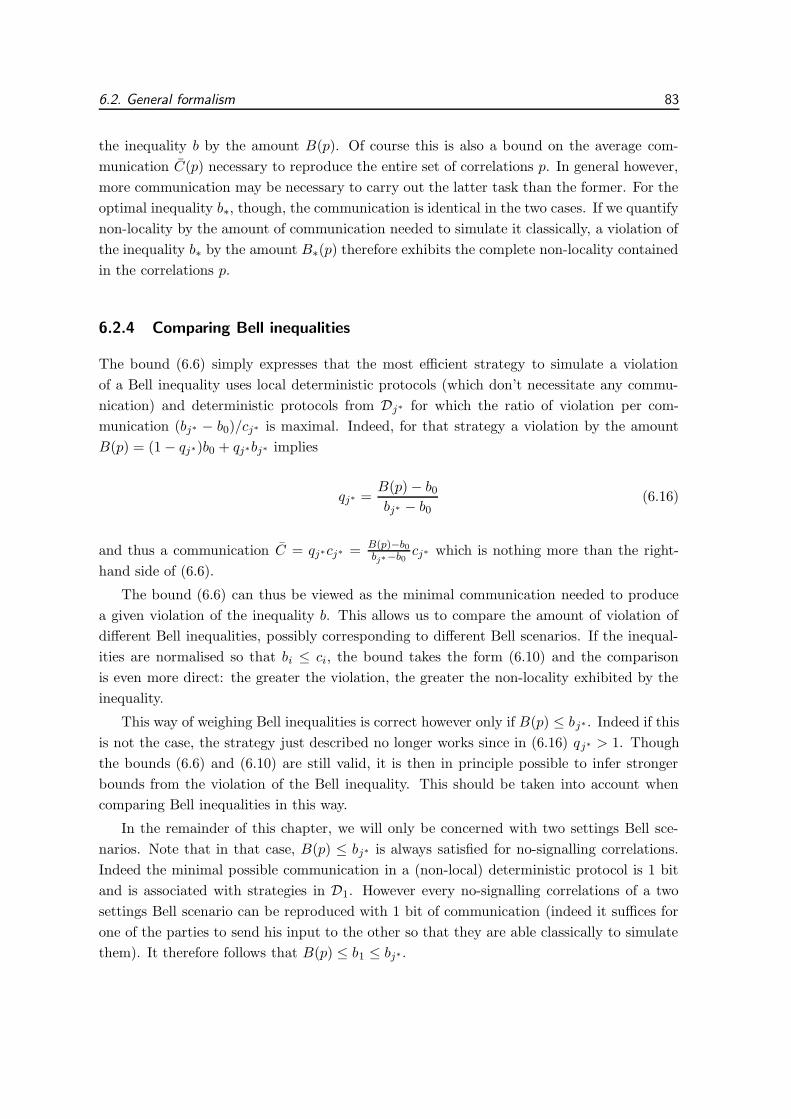
6.2. General formalism 83
the inequality b by the amount B(p). Of course this is also a bound on the average com-
munication C(p) necessary to reproduce the entire set of correlations p. In general however,
more communication may be necessary to carry out the latter task than the former. For the
optimal inequality b∗, though, the communication is identical in the two cases. If we quantify
non-locality by the amount of communication needed to simulate it classically, a violation of
the inequality b∗ by the amount B∗(p) therefore exhibits the complete non-locality contained
in the correlations p.
6.2.4 Comparing Bell inequalities
The bound (6.6) simply expresses that the most efficient strategy to simulate a violation
of a Bell inequality uses local deterministic protocols (which don’t necessitate any commu-
nication) and deterministic protocols from Dj∗ for which the ratio of violation per com-
munication (bj∗ − b0)/cj∗ is maximal. Indeed, for that strategy a violation by the amount
B(p) = (1 − qj∗)b0 + qj∗bj∗ implies
qj∗ =B(p) − b0bj∗ − b0
(6.16)
and thus a communication C = qj∗cj∗ = B(p)−b0bj∗−b0
cj∗ which is nothing more than the right-
hand side of (6.6).
The bound (6.6) can thus be viewed as the minimal communication needed to produce
a given violation of the inequality b. This allows us to compare the amount of violation of
different Bell inequalities, possibly corresponding to different Bell scenarios. If the inequal-
ities are normalised so that bi ≤ ci, the bound takes the form (6.10) and the comparison
is even more direct: the greater the violation, the greater the non-locality exhibited by the
inequality.
This way of weighing Bell inequalities is correct however only if B(p) ≤ bj∗. Indeed if this
is not the case, the strategy just described no longer works since in (6.16) qj∗ > 1. Though
the bounds (6.6) and (6.10) are still valid, it is then in principle possible to infer stronger
bounds from the violation of the Bell inequality. This should be taken into account when
comparing Bell inequalities in this way.
In the remainder of this chapter, we will only be concerned with two settings Bell sce-
narios. Note that in that case, B(p) ≤ bj∗ is always satisfied for no-signalling correlations.
Indeed the minimal possible communication in a (non-local) deterministic protocol is 1 bit
and is associated with strategies in D1. However every no-signalling correlations of a two
settings Bell scenario can be reproduced with 1 bit of communication (indeed it suffices for
one of the parties to send his input to the other so that they are able classically to simulate
them). It therefore follows that B(p) ≤ b1 ≤ bj∗.
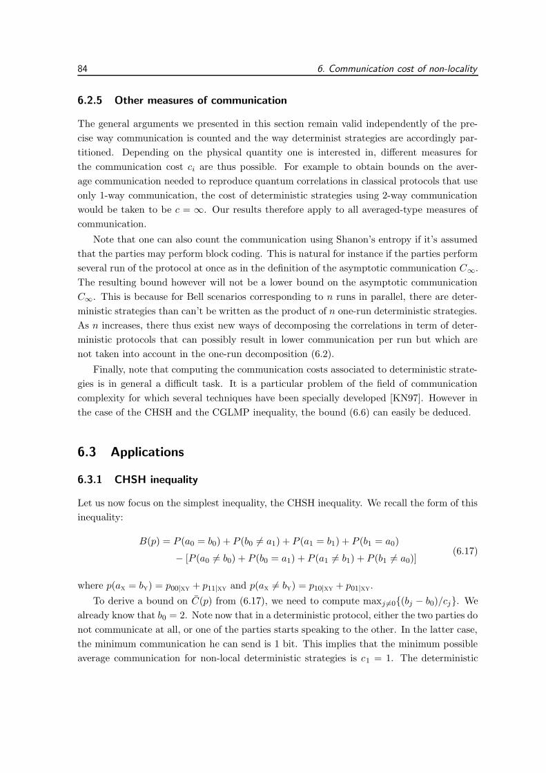
84 6. Communication cost of non-locality
6.2.5 Other measures of communication
The general arguments we presented in this section remain valid independently of the pre-
cise way communication is counted and the way determinist strategies are accordingly par-
titioned. Depending on the physical quantity one is interested in, different measures for
the communication cost ci are thus possible. For example to obtain bounds on the aver-
age communication needed to reproduce quantum correlations in classical protocols that use
only 1-way communication, the cost of deterministic strategies using 2-way communication
would be taken to be c = ∞. Our results therefore apply to all averaged-type measures of
communication.
Note that one can also count the communication using Shanon’s entropy if it’s assumed
that the parties may perform block coding. This is natural for instance if the parties perform
several run of the protocol at once as in the definition of the asymptotic communication C∞.
The resulting bound however will not be a lower bound on the asymptotic communication
C∞. This is because for Bell scenarios corresponding to n runs in parallel, there are deter-
ministic strategies than can’t be written as the product of n one-run deterministic strategies.
As n increases, there thus exist new ways of decomposing the correlations in term of deter-
ministic protocols that can possibly result in lower communication per run but which are
not taken into account in the one-run decomposition (6.2).
Finally, note that computing the communication costs associated to deterministic strate-
gies is in general a difficult task. It is a particular problem of the field of communication
complexity for which several techniques have been specially developed [KN97]. However in
the case of the CHSH and the CGLMP inequality, the bound (6.6) can easily be deduced.
6.3 Applications
6.3.1 CHSH inequality
Let us now focus on the simplest inequality, the CHSH inequality. We recall the form of this
inequality:
B(p) = P (a0 = b0) + P (b0 6= a1) + P (a1 = b1) + P (b1 = a0)
− [P (a0 6= b0) + P (b0 = a1) + P (a1 6= b1) + P (b1 6= a0)](6.17)
where p(ax = by) = p00|xy + p11|xy and p(ax 6= by) = p10|xy + p01|xy.
To derive a bound on C(p) from (6.17), we need to compute maxj 6=0{(bj − b0)/cj}. We
already know that b0 = 2. Note now that in a deterministic protocol, either the two parties do
not communicate at all, or one of the parties starts speaking to the other. In the latter case,
the minimum communication he can send is 1 bit. This implies that the minimum possible
average communication for non-local deterministic strategies is c1 = 1. The deterministic

6.3. Applications 85
protocol dλ where λ is defined in the following way
λA(x,y) = 0 for x,y = 0, 1
λB(0, 0) = 0 λB(1, 0) = 1 λB(0, 1) = 0 λB(1, 1) = 0(6.18)
can be implemented with 1 bit of communication. Indeed it suffices for Alice to send the
value of her input to Bob. Moreover, the value B(dλ) it takes on the inequality (6.17) is the
maximum possible B(dλ) = 4. It follows that maxj 6=0{(bj − b0)/cj} = (4 − 2)/1 = 2, so that
for the CHSH inequality the bound (6.6) becomes
C(p) ≥ 1
2B(p) − 1 . (6.19)
This implies for instance that to reproduce the optimal quantum correlations at least√2 − 1 ' 0.4142 bits of communication are necessary. Note that to reproduce all possible
von Neumann measurements on a Bell state 1 bit is sufficient [TB03].
Is it possible to find a protocol that reproduces these correlations with that amount
C(p) =√
2− 1 of communication? It turns out in fact that the CHSH inequality is optimal,
i.e., the bound (6.19) is saturated, for all no-signalling correlations.
Theorem 6.4. C(p) = 12B(p) − 1 bits of communication are necessary and sufficient to
simulate all two-inputs and two-outputs no-signalling correlations that violate the CHSH
inequality (6.17).
Proof. As the “necessary” part follows from the bound (6.19), we just have to exhibit a
classical protocol that reproduces the correlations with that amount of communication.
First note that when the bound (6.6) is saturated, it follows from the proof of Theorem
6.1 that the optimal protocol uses only strategies from D0 and Dj∗ and moreover in these
subsets only strategies that attain the maximal values b0 and bj∗ on the inequality b (there
could be more than one subset Dj∗ if they are several indexes j∗ for which (bj∗ − b0)/cj∗is maximum). In our case, this implies that the optimal protocol must be built from local
strategies dλ0 and from 1-bit strategies dλ1 such that b dλ0 = b0 = 2 and b dλ1 = b1 = 4.
The entries of the vectors p corresponding to the Bell scenario associated with the CHSH
inequality consist of 16 probabilities pab|xy since a, b, x and y each take two possible values.
Half of these probabilities appear with a plus sign in the CHSH expression (6.17) and half of
them with a minus sign. Since the entries of a deterministic strategy are either equal to 0 or
1, for it to satisfy B(dλ) = 2, it must contribute to (6.17) with one “−” and three “+” For
local strategies, which assign local values λA(x) and λB(y) to Alice’s and Bob’s outcomes,
this leaves eight possibilities. Indeed if we choose one of the eight entries appearing in (6.17)
with a “−” sign to be equal to one, the requirement that three entries appearing with a
“+” sign must also be equal to one, fully determines the functions λA(x) and λB(y). The
resulting eight possible local strategies dλ0 (λ0 = 0, . . . 7) are given in Table 6.1.
On the other hand, for a deterministic strategy to attain B(dλ) = 4, it must contribute
to (6.17) with four terms weighted by a “+”. The assignment of outcomes of 1-bit strategies
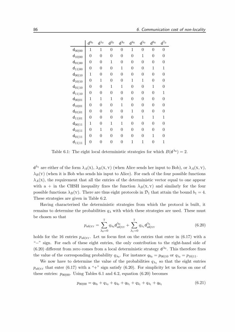
86 6. Communication cost of non-locality
d00 d10 d20 d30 d40 d50 d60 d70
d00|00 1 1 0 0 1 0 0 0
d10|00 0 0 0 0 0 1 0 0
d01|00 0 0 1 0 0 0 0 0
d11|00 0 0 0 1 0 0 1 1
d00|10 1 0 0 0 0 0 0 0
d10|10 0 1 0 0 1 1 0 0
d01|10 0 0 1 1 0 0 1 0
d11|10 0 0 0 0 0 0 0 1
d00|01 1 1 1 0 0 0 0 0
d10|01 0 0 0 1 0 0 0 0
d01|01 0 0 0 0 1 0 0 0
d11|01 0 0 0 0 0 1 1 1
d00|11 1 0 1 1 0 0 0 0
d10|11 0 1 0 0 0 0 0 0
d01|11 0 0 0 0 0 0 1 0
d11|11 0 0 0 0 1 1 0 1
Table 6.1: The eight local deterministic strategies for which B(dλ0) = 2.
dλ1 are either of the form λA(x), λB(x,y) (when Alice sends her input to Bob), or λA(x,y),
λB(y) (when it is Bob who sends his input to Alice). For each of the four possible functions
λA(x), the requirement that all the entries of the deterministic vector equal to one appear
with a + in the CHSH inequality fixes the function λB(x,y) and similarly for the four
possible functions λB(y). There are thus eight protocols in D1 that attain the bound b1 = 4.
These strategies are given in Table 6.2.
Having characterised the deterministic strategies from which the protocol is built, it
remains to determine the probabilities qλ with which these strategies are used. These must
be chosen so that
pab|xy =
7∑
λ0=0
qλ0dλ0
ab|xy+
7∑
λ1=0
qλ1dλ1
ab|xy(6.20)
holds for the 16 entries pab|xy. Let us focus first on the entries that enter in (6.17) with a
“−” sign. For each of these eight entries, the only contribution to the right-hand side of
(6.20) different from zero comes from a local deterministic strategy dλ0 . This therefore fixes
the value of the corresponding probability qλ0. For instance q00
= p00|10 or q10= p10|11.
We now have to determine the value of the probabilities qλ1so that the eight entries
pab|xy that enter (6.17) with a “+” sign satisfy (6.20). For simplicity let us focus on one of
these entries: p00|00. Using Tables 6.1 and 6.2, equation (6.20) becomes
p00|00 = q00+ q10
+ q40+ q01
+ q21+ q41
+ q61(6.21)

6.3. Applications 87
d01 d11 d21 d31 d41 d51 d61 d71
d00|00 1 0 1 0 1 0 1 0
d10|00 0 0 0 0 0 0 0 0
d01|00 0 0 0 0 0 0 0 0
d11|00 0 1 0 1 0 1 0 1
d00|10 0 0 0 0 0 0 0 0
d10|10 0 0 1 1 1 0 1 0
d01|10 1 1 0 0 0 1 0 1
d11|10 0 0 0 0 0 0 0 0
d00|01 1 0 1 0 1 1 0 0
d10|01 0 0 0 0 0 0 0 0
d01|01 0 0 0 0 0 0 0 0
d11|01 0 1 0 1 0 0 1 1
d00|11 1 1 0 0 1 1 0 0
d10|11 0 0 0 0 0 0 0 0
d01|11 0 0 0 0 0 0 0 0
d11|11 0 0 1 1 0 0 1 1
Table 6.2: The eight 1-bit deterministic strategies for which B(dλ1) = 4.
or
q01+ q21
+ q41+ q61
= p00|00 − p00|10 − p10|11 − p01|01 (6.22)
where we replaced each of the probabilities qλ0with their value previously determined. From
(6.17), and using the normalisation conditions (2.4) and the no-signalling conditions (2.3),
it is not difficult to see that the left-hand side of this equation is equal to (B(p)− 2)/4. The
same argument can be carried for all the seven other entries that contribute to the CHSH
inequality with a “+” sign, each time finding that the sum of four probabilities qλ1equals
(B(p) − 2)/4. Taking qλ1 = (B(p) − 2)/16 for λ1 = 0, . . . , 7 one therefore obtains a solution
to (6.20).
The communication associated to this protocol is thus C =∑
λ qλC(dλ) =∑7
λ1=0 qλ1=
12B(p) − 1.
6.3.2 More dimensions: the CGLMP inequality
We have introduced the CGLMP inequality (2.16) in Chapter 2. It was originally derived
to study non-locality in d-dimensional systems. We recall that this inequality refers to
measurement scenarios where Alice’s and Bob’s local settings take two values x,y = 0, 1
and each measurement gives d possible outcomes a, b = 0, . . . , d− 1. The value the CGLMP

88 6. Communication cost of non-locality
inequality takes on a joint probability distribution p is
Bd(p) =
[d/2]−1∑
k=0
(1 − 2k
d− 1
)(P (a0 = b0 + k) + P (b0 = a1 + k + 1)
+ P (a1 = b1 + k) + P (b1 = a0 + k)
− [P (a0 = b0 − k − 1) + P (b0 = a1 − k)
+ P (a1 = b1 − k − 1) + P (b1 = a0 − k − 1)]),
(6.23)
where [d/2] is the integer part of d/2 and P (ax = by + k) =∑d−1
b=0 pb⊕k,b|xy with ⊕ denoting
addition modulo d. As shown in [CGL+02], for each d the local bound of the inequality is
bd0 = 2.
When d = 2 we recover the CHSH inequality and in that case the maximal quantum
violation is b2QM ' 2.828. For d > 2, the (conjectured) maximal violations obtained from
maximally entangled (ME) qudits are given in [CGL+02]. For qutrits the maximum is
b3ME ' 2.8729 > b2QM and this value increases with d. This suggests that the CGLMP
inequality exhibits stronger non-local correlations for larger d. This has been made more
precise by connecting the violation of the CGLMP inequality to the resistance of the corre-
lations to the admixture of noise [CGL+02]. It has however been argued in [ADGL02], that
the resistance to noise is not a good measure of non-locality. Counter-intuitively, it was also
remarked in [ADGL02] that for d > 2 the strongest violation of the CGLMP inequality is
obtained using non-maximally entangled (NME) states. For qutrits, for instance, the max-
imal violation obtained from a non-maximally entangled state is b3NME ' 2.9149 > b3ME.
Moreover, this discrepancy between maximally and non-maximally entangled states grows
with the dimension. This raises several questions on how one should interpret and compare
these manifestations of non-locality.
A natural answer is through the bound (6.6). The derivation of the bound for the CHSH
inequality in the previous section can directly be applied to the CGLMP inequality. This
yields
Cd(p) ≥ 1
2Bd(p) − 1 . (6.24)
This bound is thus the same for inequalities with different d in the family (6.23), and the
strength of these different inequalities can therefore simply be measured by the degree by
which they are violated. This confirms the intuition that the non-locality displayed by the
CGLMP inequality grows with the dimension d.
On the other hand, the fact that for d > 2 the CGLMP inequality is maximally vi-
olated for non-maximally entangled states translates into more severe constraints on the
average communication necessary to reproduce correlations obtained by measuring certain
non-maximally entangled states than maximally entangled ones. For instance, for qutrits
(6.24) implies that C3ME ≥ 0.4365 while C3
NME ≥ 0.4575. It could however be that for these

6.3. Applications 89
correlations the CGLMP inequality is not optimal and that another inequality will impose
stronger bounds for maximally entangled states.
To verify that assertion, we numerically solved the linear programming problem (6.15)
for the correlations that maximally violate the CGLMP inequality both on maximally and
non-maximally entangled states for d ≤ 8. There exists many different algorithms for linear
programming and the only difficulty in solving (6.15) is to characterise the sets Di of deter-
ministic strategies and their corresponding communication costs ci. A deterministic strategy
assigns a definite value λA(x,y) to Alice’s outcomes and λB(x,y) to Bob’s outcomes for each
of the four possible pairs of inputs (x,y). To simplify the notation we write λx(y) = λA(x,y)
and λy(x) = λB(x,y). There are two possibilities for λx: either λx is constant (cst), i.e.,
λx(0) = λx(1), and given input x Alice does not need any information from Bob to determine
her output; or λx 6= cst, that is λx(0) 6= λx(1), and Alice’s outcome depends not only on her
local setting x but also on Bob’s one. In that case Alice needs one bit of information from
Bob to output her result. The situation is similar for Bob. This leads to four possible sets
of deterministic strategies:
i) D0: the set of local deterministic strategies for which λx = cst and λy = cst for x = 0, 1
and y = 0, 1. These don’t need any communication to be implemented: c0 = 0.
ii) D1: the strategies where λx = cst for x = 0, 1 and at least one of the λy 6= cst.
These strategies necessitate 1 bit of communication from Alice to Bob. This set also
contains the reverse strategies which need 1 bit of communication from Bob to Alice.
The communication cost associated to D1 is therefore c1 = 1.
iii) D2: the protocols where λx = cst for one of the two values x = 0 or x = 1, λx 6= cst for
the other value x and at least one of the λy 6= cst. These strategies can be implemented
by Alice sending one bit to Bob, the value of her input, and then Bob sending back
to Alice the value of his input if Alice’s input equals x. The average communication
exchanged is 3/2 bits so that c2 = 3/2. This set also contains the strategies where
Alice’s and Bob’s positions are permuted.
iv) D3: λx 6= cst and λy 6= cst for x = 0, 1 and y = 0, 1. To implement these strategies
both parties need to know the input of the other, so c3 = 2.
With this assignment of communication costs to deterministic strategies and for the corre-
lations considered (d ≤ 8), it turns out from the results of the numerical optimisation (6.15)
that the CGLMP inequality is optimal, i.e., the bound (6.24) is saturated. For these partic-
ular measurements, those that gives rise to the maximal violation of the CGLMP inequality,
more communication is thus necessary to reproduce results obtained on non-maximally en-
tangled states than maximally entangled ones.
It is nevertheless possible that these measurements are not optimal to detect the non-
locality of maximally entangled states. We performed numerical searches for d = 3, opti-
mising the two projection measurements the parties carry out on the maximally entangled

90 6. Communication cost of non-locality
state. We found that the measurements that necessitate the maximal communication to be
simulated are the ones that maximise the CGLMP inequality.
These results therefore suggest that two measurement settings on each side do not op-
timally detect the non-locality of maximally entangled states for d ≥ 3. It is still possible
that the simulation of POVMs would necessitate further communication. However, concur-
ring with [ADGL02], we believe that more settings per site and a corresponding new Bell
inequality are needed.
6.4 Optimal inequalities and facet inequalities
As we have seen in Chapter 2, the CHSH and the CGLMP inequalities are facet inequalities.
For two-inputs and two-outputs Bell scenarios, the CHSH is the unique (up to symmetries)
non-trivial facet inequality. It turns out that it is also optimal with respect to the aver-
age communication C for all no-signalling correlations. For Bell scenarios involving more
outcomes, we have seen that the CGLMP inequality is optimal at least for certain correla-
tions. Is it the case that for no-signalling correlations optimal inequalities are always facet
inequalities?
To answer this question, consider the following correlations belonging to a two-inputs
three-outputs Bell scenario: Alice and Bob share the maximally entangled state of two
qutrits |ψ〉 = 1/√
3(|00〉 + |11〉 + |22〉). The measurements they perform consist of two
stages. First they carry out a unitary transformation on their part of the entangled state
given by
|k〉 → eiφx(k)
√3
(|0〉 + ei2πk/3|1〉 + ei4πk/3|2〉
)(6.25)
for Alice, and
|k〉 → eiφy(k)
√3
(|0〉 + e−i2πk/3|1〉 + e−i4πk/3|2〉
)(6.26)
for Bob. Then they both make a measurement in the basis {|0〉, |1〉, |2〉}. The settings of
their measuring apparatus are thus determined by the three phases φx and φy they use.
For Alice, these are given by φ0 = (0, 0, 0) and φ1 = (0, 0, π/2), while for Bob they are
φ0 = (0, 0, π/4) and φ1 = (0, 0,−π/4). This leads to the probabilities
P (ax = by) =(5 + (−1)f(x,y)2
√2)/9
P (ax = by + 1) =(2 − (−1)f(x,y)
√2)/9
P (ax = by + 2) =(2 − (−1)f(x,y)
√2)/9
(6.27)
where f(x, y) = x(y + 1).
Consider now the following inequality,
B(p) = P (a0 = b0) + P (a0 = b1)
+ P (a1 = b1) + P (a1 = b0 + 1) + P (a1 = b0 + 2) .(6.28)

6.5. Summary 91
It is easily checked that b0 = 3 and that b1 = 4, the algebraic maximum. Hence C(p) ≥(B(p)− 3)/(4− 3) = B(p)− 3. The correlations (6.27) violate this inequality by the amount
B(p) = 19 (19 + 8
√2) ' 3.3682, and so at least C(p) ≥ 0.3682 bits of communication are
necessary to simulate them classicly. In comparison, the CGLMP inequality (6.23) gives the
bound C(p) ≥ 23(√
2− 1) ' 0.2761. The inequality (6.28) is thus stronger than the CGLMP
inequality from the communication point of view for the correlations (6.27). Moreover, we
have solved numerically the linear problem (6.15) for these particular correlations, and found
that C(p) = 0.3682, so that the inequality (6.28) is optimal.
The inequality (6.28), however, is not a facet inequality. Indeed, the dimension of the
two-inputs three-outputs local polytope is 24, and so at least 24 affinely independent vertices
should belong to (6.28) for it to be a facet. It is easily checked however that there are only 21
local deterministic strategies that attain the limit B(dλ0) = b0 = 2 for the inequality (6.28).
Does there exist a facet inequality that imposes the same bound C(p) ≥ 0.3682 as (6.28)?
For the Bell scenario that concerns us it is known that all non-trivial facet inequalities are ei-
ther the CGLMP inequality or the lifting of the CHSH inequality to three outcomes [CG04].
We have already said that the bound on the communication imposed by the CGLMP in-
equality is suboptimal. It can be checked that this is also the case for the different possible
liftings of the CHSH inequality2. This example thus shows that there exist quantum cor-
relations for which the strongest bound on C(p) deduced from facet inequalities is lower
than the (optimal) bound given from a non-facet inequality: if facet inequalities are optimal
“detectors” of non-locality, non-facet inequalities can be better “meters” of non-locality.
6.5 Summary
We have shown that the average communication necessary to simulate classically a violation
of a Bell inequality is proportional to the degree of violation of the inequality. Moreover, to
each set of correlations is associated an optimal inequality for which that communication is
also sufficient to reproduce the entire set of correlations. The key ingredient was to compare
the amount of violation of Bell inequalities not only with the maximum value they take on
local deterministic strategies, but also on non-local ones that necessitate some communication
to be implemented.
Part of the interest of this work is that it gives a physical meaning to the degree of
violation of Bell inequalities and thus provides an objective way to compare violation of
different inequalities. It also provides a tool to characterise and quantify the non-locality
2As we have noted in Section 2.7.1 of Chapter 2, Bell inequalities may take different forms due to the
no-signalling conditions. If these forms are equivalent for correlations that satisfy the no-signalling conditions,
they are not equivalent for the non-local deterministic points dλ that are signalling. They thus lead to different
bound on C(p). It should therefore be checked that for all possible way to rewrite the CGLMP inequalities
and the liftings of the CHSH inequality, it is still the case that they are suboptimal. This has been done in
[Pir03].

92 6. Communication cost of non-locality
inherent in quantum correlations. As a result, for instance, for two measurements on each
side it seems that the correlations that necessitate the most communication to be reproduced
are obtained on non-maximally entangled states rather than on maximally entangled ones
for d > 2. It would be interesting to know whether this is still the case for more settings and
if not, what is the corresponding Bell inequality.

Chapter 7
The detection loophole
We now turn to the third main issue that will concern us in this thesis, the problem of loop-
holes in experimental tests of non-locality, and more specifically the detection loophole. Clos-
ing the detection loophole is important to demonstrate in a conclusive way the non-locality
of quantum mechanics, but is also indispensable before any practical use of non-locality can
be made. In this chapter, we put bounds on the minimum detection efficiency necessary
to produce non-local correlations in Bell-type experiments. These bounds depend on simple
parameters like the number of measurement settings or the dimensionality of the entangled
quantum state. We derive them by constructing explicit local models which reproduce the
quantum correlations for sufficiently small detectors efficiency. The content of this chapter
is based on [6].
7.1 Introduction
The use of entangled photons seems inevitable in present and future non locality tests since it
is the easiest and most straightforward way to achieve the space-like separated measurements
required to close the locality loophole1. It is also inevitable for implementing applications of
non-locality, such as distributed computing tasks or cryptographic schemes, which involve a
spatial separation between the parties (even if this spatial separation should not necessarily
be a strict space-like separation). For such optical experiments, however, the low efficiency
of the available detectors is a problematic issue. In particular, the detection loophole has
yet to be closed.
The performance of single photon detectors depends on the wavelength at which the
experiment is carried out. For visible light, detectors can have efficiencies up to 70% [EGG].
These, however, are further decreased by losses induced by the optical components in the
1Note that a scheme has been proposed to entangle two ions in spatially separated cavities using the
technique of entanglement swapping [BPH03]. However, this protocol is experimentally very challenging for
the moment.
93

94 7. The detection loophole
photon’s path so that the achievable overall detection efficiencies are well below 70%. For
instance, in [WJS+98] the overall detection efficiency is about 5%. At telecom wavelength
(1550 nm), which is well suited for long distance experiments, detectors have efficiencies of
only 10% to 20% [IDQ]. In contrast, the required detector efficiency to observe a genuine vi-
olation of the CHSH inequality, the test of non-locality most commonly used in experiments,
is 82% for measurements performed on maximally entangled states, and this threshold can
be lowered down to 67% if non-maximally entangled states are used (in this case, however,
the experiments become much more sensitive to potential noise) [Ebe93]. Improvements on
the efficiency of single photon detectors can be expected, but the detection loophole will
remain a central problem for optical tests of quantum non locality in the foreseeable future.
Note that besides their limited efficiency, detectors are also subject to other kind of
imperfections, such as dark counts. For visible light, dark counts rates are of a few hundreds
counts per second [EGG] and thus negligible in comparison with the signal counts which can
be of the order of 104s−1. At telecom wavelength, dark counts rates reach 104s−1 [IDQ] and
can therefore become more problematic. This specific noise and other types of errors, such as
the probability for the detectors to give the wrong result or the noise produced at the source
of entangled particles, add up to deteriorate the correlations between double coincidence
events. Yet, in recent optical Bell tests, visibilities up to 95% [WJS+98, TBZG00] have
been obtained. These errors thus, although not negligible, are not a fundamental limitation,
contrary to detection inefficiencies.
The current experimental situation thus motivate a careful examination of the conse-
quences of the detection loophole and possible ways to circumvent it. The idea behind the
detection loophole is that in the presence of unperfect detectors, local hidden variables can
“mask” results in contradiction with quantum mechanics by telling the detectors not to fire.
This is at the origin of several local models able to reproduce particular quantum correlations
if the detector efficiencies are below some threshold value. We can formalise the situation
as follows. Each detector has a probability η of giving a result and a probability 1 − η of
not giving a result. If η is sufficiently small, the quantum correlations produced in a Bell
experiment can be explained by a local model. We denote by η∗ the maximum detection
efficiency for which a local model exists. Thus if η > η∗ the correlations are indeed non-local.
In the present chapter, we investigate the resistance of Bell-type experiments to inefficient
detectors. Specifically, we put bounds on η∗ to understand how much this resistance can in
principle be improved. For this, we construct several local models that take advantage of the
inefficiency of the detectors to reproduce the quantum correlations. Local models exploiting
the detection loophole have already been constructed to reproduce the result of specific
experiments [San92, SF02]. There have also been attempts to build more general local models
that can for example reproduce measurements performed on the singlet state [GG99, Lar99]
or experiments performed using parametric-down conversion sources [CMRDS02]. Here, we
try to be more general than that. Indeed, our purpose is to understand how η∗ is constrained
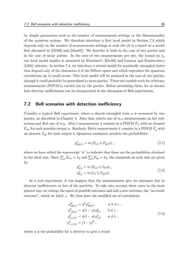
7.2. Bell scenarios with detection inefficiency 95
by simple parameters such as the number of measurements settings or the dimensionality
of the quantum system. We therefore introduce a first local model in Section 7.3 which
depends only on the number of measurements settings at each site (it is a based on a model
first discussed in [GG99] and [Mas02]). We describe it both in the case of two parties and
in the case of many parties. In the case of two measurements per site, the bound on η∗our local model implies is saturated by Eberhard’s [Ebe93] and Larsson and Semitecolos’s
[LS01] schemes. In section 7.4, we introduce a second model for maximally entangled states
that depend only of the dimension d of the Hilbert space and which reproduce the quantum
correlations up to small errors. This local model will be analysed in the case of two parties,
altough it could probably be generalised to more parties. These two models work for arbitrary
measurements (POVM’s) carried out by the parties. Before presenting them, let us discuss
how detector inefficiencies can be incorporated in the discussion of Bell experiments.
7.2 Bell scenarios with detection inefficiency
Consider a typical Bell experiment, where a shared entangled state ρ is measured by two
parties, as described in Chapter 4. Alice thus selects one of mA measurements on her sub-
system and Bob one of mB. Alice’s measurement x consists in a POVM Ex with an element
Exa for each possible output a. Similarly, Bob’s measurement y consists in a POVM Fy with
an element Fyb for each output b. Quantum mechanics predicts the probabilities
p?ab|xy
= tr (Exa ⊗ Fyb ρ) , (7.1)
where we have added the superscript “?” to indicate that these are the probabilities obtained
in the ideal case. Since∑
aExa = IA and∑
b Fyb = IB, the marginals on each side are given
by
p?a|x = tr (Exa ⊗ IB ρ) ,
p?b|y = tr (IA ⊗ Fyb ρ) .
(7.2)
In a real experiment, it can happen that the measurements give no outcomes due to
detector inefficiencies or loss of the particles. To take into account these cases in the most
general way, we enlarge the space of possible outcomes and add a new outcome, the “no-result
outcome”, which we label ⊥. We then have the modified set of correlations
pηab|xy
= η2 p?ab|xy
a, b 6=⊥ ,
pη⊥b|xy
= η(1 − η) p?b|y b 6=⊥ ,
pηa⊥|xy
= η(1 − η) p?a|x a 6=⊥ ,
pη⊥⊥|xy
= (1 − η)2 ,
(7.3)
where η is the probability for a detector to give a result.

96 7. The detection loophole
On the other hand, correlations predicted by a local hidden-variable theory are of the
form
p`ab|xy
=∑
λ
q(λ)P (a|x, λ)P (b|y, λ) , (7.4)
where a and b can take either a value different from ⊥, or the value ⊥. In the latter case the
local model just instructs the detector not to fire.
7.3 A model that depends on the number of settings
A classical theory can reproduce all the results of quantum mechanics if information on
which measurement has been selected can flow from one side to the other. It is to guarantee
that such mechanism cannot account of the observed data that measurements in Bell tests
must be carried out at spatially separated regions. A local model can nevertheless exploit
the limited detection efficiency by guessing a priori which measurement will be performed
on one side. If the actual measurement and the guessed one coincide, the model will output
results in agreement with quantum mechanics. If they do not, it simply tells the detectors
not to fire. Building a local model out of this idea will enable us to prove the following
bound:
Theorem 7.1. In experiments where Alice can choose between mA measurements and Bob
mB, the maximum detection efficiency η∗ for which a local model exists is at least
η∗ ≥mA +mB − 2
mAmB − 1. (7.5)
Proof : The proof consist of constructing a local model that reproduces the correlations
(7.3) with η given by the bound. In this model, the local hidden variable λ consists of the
pair λ = (a′,x′) where x′ corresponds to one of the mA possible measurements of Alice
and a′ to one of the possible outcomes. x′ is chosen with probability 1/mA and a′ with
probability p?a′|x′ , so that q(λ) = 1
mAp?
a′|x′ . If Alice’s actual measurement x coincides with
x′ (this occurs with probability 1/mA), Alice outputs a′, otherwise she outputs ⊥. We thus
have P (a|X, λ) = δaa′δxx′ if a 6=⊥ and P (a|x, λ) = 1 − δxx′ if a =⊥. On the other hand,
Bob always gives an output different from ⊥. He randomly chooses a result b using the
probability distribution P (b|y, λ) = p?a′b|x′y
/p?a′|x′ .
So far, Alice’s efficiency ηA is equal to 1/mA and Bob’s efficiency ηB = 1. To make
the protocol symmetric, Alice and Bob must exchange their role part of the time. This is
done with the help of a supplementary hidden-variable which tells both parties to run the
protocol as above with probability q1 and the permuted one with probability 1 − q1. There
is then one problem left with the model, it never happens that both detectors do not fire.
This can be corrected by adding yet another supplementary hidden-variable that instructs
Alice’s and Bob’s detectors to both produce the result ⊥ with probability (1 − q2) and to

7.3. A model that depends on the number of settings 97
proceed as above with probability q2. Using (7.4), it is then not difficult to check that our
model produces the following correlations:
p`ab|xy
= q2
(q1mA
+1 − q1mB
)p?
ab|xy,
p`⊥b|xy
= q2 q1mA − 1
mAp?
b|y ,
p`a⊥|xy
= q2 (1 − q1)
(mB − 1
mB
)p?
a|x ,
p`⊥⊥|xy
= 1 − q2 .
(7.6)
These correlations are similar to the quantum ones (7.3), modulo the detection probabilities,
i.e., the probability that both Alice and Bob’s, Alice’s only, Bob’s only, or neither detector
fires. The two distributions will be identical if these detection probabilities coincide:
η2 = q2
(q1mA
+1 − q1mB
),
η(1 − η) = q2 q1mA − 1
mA,
η(1 − η) = q2 (1 − q1)
(mB − 1
mB
),
(1 − η)2 = 1 − q2 .
(7.7)
Solving for η gives the right-hand side of (7.5). 2
When mA = mB = 2, the simplest non-trivial case, our bound predicts η∗ ≥ 2/3. It
follows from Eberhard’s result [Ebe93] that this value is optimal. Indeed Eberhard has shown
that there exists a 2-inputs Bell experiment performed on a non-maximally entangled state
of two qubits that violates locality for value of η arbitrarily close to 2/3. For larger values of
mA and mB , η∗ as given by (7.5) decreases and tends to zero when both mA and mB tend to
infinity. It is not known whether our bound can be attained by quantum mechanics in these
situations. However note that there are quantum correlations produced by experiments with
exponentially many measurement settings, and for which η∗ is exponentially small [Mas02].
It is thus at least possible to approach the bound (7.5) for large mA, mB .
We have attempted to generalise this result to the case of many parties. For simplicity
we have considered the case where each party can choose between the same number m of
measurements.
We have only been able to prove our strongest result for less than 500 parties because
we had to resort to numerical computations to finish the proof. We state it as a conjecture:
Conjecture 7.2 (proven for n ≤ 500). In a Bell experiment with n parties, each of whose
measuring apparatus can have m settings,
η∗ ≥n
(n− 1)m+ 1. (7.8)
98 7. The detection loophole
When the number of measurements on each site is m = 2, the bound (7.8) reduces to
η∗ ≥n
2n− 1. (7.9)
For two parties, we recover Eberhard’s threshold η∗ ≥ 2/3 and as we have already mentioned
this bound can be saturated by quantum mechanics. However, the threshold (7.9) can be
saturated by quantum mechanics for the other values of n as well. Indeed Larsson and
Semitecolos [LS01] have generalised Eberhard’s result to the case of many parties and have
shown that n qubits in a non-maximally entangled state can lead to a violation of locality
for detection efficiencies η arbitrarily close to (7.9) for any n.
For a number of measurements settings m > 2, it is not known whether the bound (7.8)
can be saturated. However one can come close to saturating it when the number of parties
is large. Indeed for large m, fixed m, eq. (7.8) becomes η∗ ≥ 1/m + O(1/n). And in
[BHMR03] it is shown that there exists a measurement scenario for m = 2l (l = 1, 2, . . .)
settings performed on n qubits that exhibit non-locality for value of η approaching 1/m as
n→ ∞ for fixed l.
As a final remark, note that our conjecture seems quite constraining as regards the
possible decrease of η∗ by increasing the number of parties. Indeed, for fixed m, replacing
n = 2 by n → ∞ one can expect at best a decrease of η∗ by a factor of 2m/(m + 1) ≤ 2.
From the resistance to detection inefficiency point of view, it seems thus more advantageous
to consider experiments with many settings than with many parties.
As mentioned above we have not been able to prove eq. (7.8) for all numbers of parties.
However we have been able to prove a weaker result valid for any number n of parties. In
this weaker result we do not ask the local model to reproduce all the quantum correlations.
Rather, we only ask that if all the detectors click, then the correlations exactly coincide
with the quantum correlations. On the other hand we do not put any constraint on the
correlations when one or more of the detectors do not click. This type of model has been
considered previously in [Mas02, BHMR03].
Theorem 7.3. Consider Bell experiments with n parties and m measurements settings per
site. We require that if all detectors click, the correlations should coincide with the quantum
correlations, but we do not put any condition on the correlations when one or more of the
detectors do not click. Then the maximum detection efficiency η∗ for which a local model
exists satisfies
η∗ ≥1
m(n−1)/n(7.10)
We begin by proving Theorem 7.3. We then turn to the arguments behind conjecture
7.2.
Proof of Theorem 7.3 :
As in Theorem 7.1, we can build a local model to reproduce the correlations based on
the remark that it is possible to predict outcomes for all measurements performed at one

7.3. A model that depends on the number of settings 99
site if measurements are guessed at the other sites. A hidden-variable will thus predetermine
particular measurements and corresponding outcomes for n−1 of the parties. If the guessed
and the actual measurements coincide, which happens with probability 1/m, these parties
output the selected result, if not, which happens with probability (m− 1)/m their detectors
keep quiet. Assuming that the measurements performed by the other parties are the ones
specified by the hidden variable, the last party always outputs a result different from ⊥.
Since each party has the choice between the same number m of measurements there is no
privileged site and each party has the same probability 1/n to be selected as the special one
for which the detector always fires.
Thus when all detectors click, which occurs with probability 1/m(n−1), the results ob-
tained will agree with those of quantum mechanics. This probability should be identified
with ηn, the probability that all detectors click. This proves Theorem 7.3. 2
We now turn to Conjecture 7.2.
Proof of Conjecture 7.2 for n ≤ 500 :
The basic idea is to try to use the local model introduced in the proof of Theorem 7.3 to
reproduce all the correlations, and not only the restricted one obtained when all detectors
click.
Note that in the model introduced in the proof of Theorem 7.3, a detector clicks only if
we are sure that it will output an answer that agrees with quantum mechanics. The only
way for the local model and quantum mechanics to differ is thus in the probabilities that the
detectors click, not in the correlations of outputs conditional on the firing of the detector.
Similarly to (7.7), predictions of quantum mechanics and the local model will therefore be
identical provided they give the same detection probabilities q(k) that k given detectors don’t
fire and the remaining n− k do. For quantum mechanics these probabilities are given by
qQM(k) = ηn−k(1 − η)k . (7.11)
In particular this implies that the ratios
qQM(k)
qQM(k + 1)=
η
1 − η(7.12)
are independent of k.
The local model introduced in Theorem 7.3 predicts the probabilities
qLM(k) =n− k
n
(m− 1)k
mn−1(7.13)
(see eq. (7.16) with i = 0 and the explanation in the paragraph following eq. (7.16)). It has
thus the property thatqLM (0)
qLM (1)=
n
(n− 1)(m− 1). (7.14)
Using eq. (7.12) and solving for η yields eq. (7.8). This is the basis for Conjecture 7.2.

100 7. The detection loophole
But from (7.13) we also deduce
qLM (1)
qLM (2)>qLM (0)
qLM (1)(7.15)
in contradiction with (7.12). Furthermore the model introduced in Theorem 7.3 never in-
structs the n detectors to keep quiet simultaneously.
We can try to correct the model so as to recover eq. (7.12), while leaving (7.14) un-
changed, by increasing the probability qLM (k), k ≥ 2 that more than one party does not
fire.
A natural way to extend our protocol so that it can reproduce the whole set of correlations
is thus to introduce the possibility for it to constrain i (i = 2, . . . , n) of the parties to output
⊥, similarly to the proof of Theorem 7.1 where part of the time Alice and Bob had both to
produce result ⊥The new local model will therefore be build out of a family of n protocols Pi (i =
0, 2, . . . , n). In protocol Pi, a subset of i of the n parties is forced to output ⊥ independently
of the measurement performed at these i sites. Since there are(ni
)possible choices of i parties
among the n, the probability that one particular subset is chosen is 1/(n
i
). The protocol then
works as before with n replaced by n− i. The probabilities q i(k) that k given detectors don’t
fire and the remaining n− k do for protocol Pi are given by
qi(k) =
0 k < i,(k
i
)(ni
) n− k
n− i
(m− 1)k−i
mn−i−1k ≥ i
1 k and i = n.
(7.16)
The first and the last case of (7.16) are trivial. Indeed, in our protocols at least i parties
produce the result ⊥ so that their contribution to events where k < i parties don’t fire
is null. On the other hand, the protocol Pn always outputs ⊥ for the n parties. For the
remaining case when k ≥ i detectors don’t click, the subset of i parties that are forced to
output ⊥ must certainly be included in the subset of the k parties that don’t click. Since
there are(k
i
)subset out of the
(ni
)possible that satisfy this condition we have the term(k
i
)/(n
i
). Secondly, the special party for which the detector always fires cannot be one of the
k not clicking. There thus remains only n−k possibilities over the n− i original ones, hence
the term (n−k)/(n− i). Finally, in the remaining n− i−1 parties k− i of them must output
⊥, which happens with probability (m− 1)k−i/mn−i−1.
If the local model instructs to use protocol Pi (i = 0, 2, . . . n) with probability ri we find
qLM (k) = r0q0(k) +
n∑
i=2
riqi(k)
= r0q0(k) +
k∑
i=2
riqi(k)
(7.17)
7.4. An approximate model that depend on d 101
since qi(k) = 0 for i > k.
As already stated above our model predicts the correct probabilities conditional on the
firing of the detectors. It will thus properly reproduce the quantum probabilities obtained
in an experiment provided the detection probabilities satisfy qLM (k) = qQM(k) or
ηn−k(1 − η)k = r0 q0(k) +
k∑
i=2
ri qi(k) for all k. (7.18)
This will be the case if this set of equations for the ri admits a solution such that the ri are
positive and sum to one, i.e., they form an actual probability distribution.
The fact that they sum to one is already implied by the structure of (7.18). Indeed
summing both sides of (7.18) over all possible subsets of parties for which the detectors fire
and do not fire, we deduce that r0+∑n
i=2 ri = 1, since∑
k
(nk
)ηn−k(1−η)k =
∑k
(nk
)qi(k) = 1.
To check whether the pi are positive we use
η
1 − η=q0(0)
q0(1)=
∑k−1i=0 riq
i(k − 1)∑k
i=0 riqi(k)
, (7.19)
to write
rk =1
qk(k)
k−1∑
i=0
ri
(q0(1)
q0(0)qi(k − 1) − qi(k)
). (7.20)
This defines recursively the ri starting from r0 = cst > 0 and r1 = 0. Note that the ri
depend on n and m. If we define sk = mk/(m − 1)k rk we obtain for the sk the recursive
definition
sk =1
q′k(k)
k−1∑
i=0
si
(q′0(1)q′0(0)
q′i(k − 1) − q′i(k)
)(7.21)
where q′i(k) = mn−i−1/(m−1)k−i qi(k). Since the q′i(k) are independent of m so are the sk.
If all the si are positive for given n it thus follows that all the ri are also positive for that
given n and for all values of m. We checked this positivity condition for the si for n ≤ 500
using a symbolic mathematics software (Mathematica) that performs exact computations
(indeed, recursive equations as (7.21) are sensitive to small numerical perturbations and we
did not find any stable method of solving (7.21) using finite precision arithmetics). This
concludes the proof of Conjecture 7.2 for n ≤ 500. 2
7.4 An approximate model that depend on d
We now present a local model inspired by the communication protocol described in [MBCC01].
Though this model is probably not optimal, it shows that it is in principle possible to build
local models that depend only on the dimension d of the quantum system. In this model η de-
creases exponentially with d. This behaviour of η must be shared by all models that depends
only on the dimension since in [Mas02] it is shown that there are quantum correlations which

102 7. The detection loophole
are non local even when the detector efficiency is exponentially small in d. Note however that
the quantum correlations in [Mas02] require an almost complete absence of noise to exhibit
non-locality, whereas the model described below reproduces noisy correlations (although the
amount of noise decreases with the dimension for fixed η).
Note: for simplicity of notation, in this section the probabilities p` we compute or refer
to are probabilities conditional on the firing of both the detectors.
Theorem 7.4. For measurements performed on the maximally entangled state |Φ〉 =∑d−1i=0
1√d|ii〉 and for given ε < 2d, there exists a local model that produces a probability
distribution p`ab|xy
such that for all x,y,
p`a|x = p?
a|x ,
p`b|y = p?
b|y ,
|p`ab|xy
− p?ab|xy
| ≤ ε p?a|x p
?b|y ,
(7.22)
when the efficiency of the detectors is
η =( ε
4d
)2(d−1). (7.23)
Proof : We recall that Alice and Bob carry out the POVM’s Ex and Fy with elements
Exa and Eyb. Without loss of generality we can suppose that Exa and Fyb are rank one
[Bar02]. We rewrite them as
Exa = |xa| |xa〉〈xa|Fyb = |yb| |yb〉〈yb| ,
(7.24)
where |xa〉, |yb〉 are normalised states. In the case of the maximally entangled state, the
marginals and the joint outcome probability are
p?ab|xy
=1
d|xa||yb||〈x∗a|yb〉|2
p?a|x =
|xa|d , p?
b|y =|yb|d ,
(7.25)
where |x∗a〉 =∑
i xi∗a |i〉 with xi
a the components of |xa〉 in the basis where |Φ〉 = 1√d
∑i |ii〉.
The local hidden variable consists of the classical description of a pure quantum state |φ〉.This state is uniformly chosen in the Hilbert space using the invariant measure over SU(d).
Alice’s strategy is the following: she first chooses a with probability |xa|/d, in agreement
with the marginal probability p?a|x. Having fixed a she then computes s = |〈φ|xa〉|2. If
s < cos2 δ, she outputs “no result”. If s ≥ cos2 δ, she outputs a (where δ > 0 will be fixed
below). The probability Q for Alice to give an outcome is
Q =
∫
SU(d)dφ Θ(|〈φ|xa〉|2 − cos2 δ) . (7.26)

7.4. An approximate model that depend on d 103
To compute this expression we write |φ〉 = cos θ|xa〉+ eiρ sin θ|φd−1〉 where |φd−1〉 lies in the
subspace orthogonal to |xa〉. Since dφ = d−1π cos θ(sin θ)2d−3 dθ dρ dφd−1 we find
Q = 2(d− 1)
∫ π/2
0dθ cos θ(sin θ)2d−3Θ(cos2 θ − cos2 δ)
= (sin δ)2(d−1) .
(7.27)
As expected, the probability to give an outcome is independent of Alice’s particular result
a.
Bob’s strategy is as follows: he gives output b with probability
P (b|y, φ) = |yb||〈φ∗|yb〉|2 . (7.28)
This results in the marginal probability
p`b|y =
∫
SU(d)dφP (b|y, φ)
= 2(d − 1) |yb|∫ π/2
0dθ cos3 θ(sin θ)2d−3
=|yb|d,
(7.29)
where we have taken |φ〉 = cos θ|y∗b 〉 + eiρ sin θ|φd−1〉 and |φ∗d−1〉 orthogonal to |yb〉 to pass
from the first line to the second one.
Let us now compute the joint probability of outcomes a and b given that an outcome has
been produced:
p`ab|xy
=1
Q
∫
SU(d)dφ P (a|x, φ)P (b|y, φ)
=1
Q
∫
SU(d)dφ
|xa|d
Θ(|〈φ|xa〉|2 − cos2 δ)|yb||〈φ∗|yb〉|2 .
(7.30)
To compute how much this differs from the true probability, let us evaluate
D = |〈φ∗|yb〉|2 − |〈x∗a|yb〉|2 . (7.31)
Writing |φ〉 = cos θ|xa〉 + eiρ sin θ|φd−1〉 where 〈xa|φd−1〉 = 0 we find
|D| = | − sin2 θ|〈x∗a|yb〉|2 + sin2 θ|〈φ∗d−1|yb〉|2
+ (sin θ cos θ〈x∗a|yb〉〈yb|φ∗d−1〉 + c.c). |≤ sin2 θ + 2 sin θ .
(7.32)
104 7. The detection loophole
From which we deduce
|p`ab|xy
− p?ab|xy
|
≤ 1
Q
|xa|d
|yb|2(d− 1)
∫ π/2
0dθ cos θ(sin θ)2d−3
× Θ(cos2 θ − cos2 δ)(sin2 θ + 2 sin θ)
≤ 1
Q
|xa|d
|yb|2(d− 1)(sin2 δ + 2 sin δ)
×∫ δ
0dθ cos(θ)(sin θ)2d−3
=1
d|xa||yb|(sin2 δ + 2 sin δ) = εp?
a|xp?b|y ,
(7.33)
where we have taken ε = d(sin2 δ + 2 sin δ).
In the above protocol the roles of Alice and Bob are not symmetric and it never happens
that both detectors do not click. Upon letting them take randomly one of the two roles above
and forcing both detectors to stay quiet part of the time, as in the previous local models,
one sees that the model we have constructed has detector efficiency η/(1− η) = 2Q/(1 −Q)
or
η =2(sin δ)2(d−1)
1 + (sin δ)2(d−1)
≥ sin δ2(d−1)
≥( ε
4d
)2(d−1),
(7.34)
since sin δ ≥ ε/2d − ε2/8d2 ≥ ε/4d when (ε < 2d). 2
7.5 Summary
We have exhibited local models that depend only on the dimensionality of the quantum
system or only on the number of settings of each party’s measurement apparatus. These
models show that there exist general constraints on the violation of locality independently
of the particular settings of Bell experiments. They help point out which parameters are
important when trying to find quantum experiments that exhibit strong non-locality. The
existence of these local models will serve as a guiding principle for the numerical search of
Bell inequalities resistant to detection inefficiency carried out in the next chapter.
Our models can also have implications in the design of loophole-free tests of Bell in-
equalities. In experiments involving photons the detection loophole remains the last serious
loophole to be closed. It would therefore be interesting to find Bell scenarios that violate lo-
cality for efficiencies of the detectors close to the actual value of our current photo-detectors.
Our result shows that to go beyond Eberhard’s threshold of η∗ ≥ 2/3 (or to go beyond
Larsson and Semitecolos’s threshold for many parties) it is necessary to consider Bell exper-

7.5. Summary 105
iments with more than two measurements per site. This strengthens the recent interest in
Bell inequalities involving many measurement settings [KKCO02, SDSZ02].


Chapter 8
Bell inequalities resistant
to detector inefficiency
Motivated by the results of the preceding chapter, we derive both numerically and analytically
Bell inequalities and quantum measurements that present enhanced resistance to detector
inefficiency for small dimensionality d = 2, 3, 4 and 2 or more measurement settings at
each side. In particular, we describe several Bell inequalities which appear to be optimal
with respect to inefficient detectors in these situations. We also generalise the CGLMP
inequalities to take into account the inefficiency of detectors. In addition we consider the
possibility for pairs of entangled particles to be produced with probability less than one. We
show that when the pair production probability is small, one must in general use different
Bell inequalities than when the pair production probability is high. The results presented in
this chapter are based on [3].
8.1 Introduction
To describe “no-result” outcomes, we introduced in the preceding chapter the parameter η
that takes into account both the detector inefficiency and possible losses of the particle on
its way from the source to the measuring device. There is, however, another reason why a
measuring apparatus might fail to register an outcome: because the pair of particles has not
been produced by the source of entangled systems. To take into account this possibility, we
introduce in this chapter an additional parameter, γ, the pair production probability. If we
include the effect of γ, the probabilities (7.3) obtained in a quantum experiment then take
the formpγη
ab|xy= γη2 p?
ab|xya, b 6=⊥ ,
pγη⊥b|xy
= γη(1 − η) p?b|y b 6=⊥ ,
pγηa⊥|xy
= γη(1 − η) p?a|x a 6=⊥ ,
pγη⊥⊥|xy
= γ(1 − η)2 + (1 − γ) .
(8.1)
107

108 8. Bell inequalities resistant to detector inefficiency
Note that the inclusion of γ in the preceding chapter would not have affected the discussion
nor the bounds we obtained on η∗. Indeed, although the models we presented refer to the
situation γ = 1, they can trivially be extended to a situation γ < 1 without modifying the
value of η∗, by increasing the probability that both detectors do not fire.
The parameter γ may be important for sources involving parametric down conversion
where γ is typically less than 10%. So far, discussions on the detection loophole where con-
centrating on η, overlooking γ. However we will show below that both quantities play a role
in the detection loophole and clarify the relation between these two parameters. In particular
we will introduce two different detector thresholds: ηγ∗ , the value above which quantum corre-
lations exhibit non-locality for given γ, and η∀γ∗ , the value above which quantum correlations
exhibit non-locality independently of the value of γ.
We have written a numerical algorithm to determine these two thresholds for given quan-
tum state and quantum measurements. We then searched for optimal measurements such
that ηγ=1∗ and η∀γ
∗ acquire the lowest possible value. We have mentioned that quantum me-
chanics violate the CHSH inequality if the detector efficiency η is above = 2/(√
2+1) ≈ 0.8284
for the maximally entangled state of two qubits. The results of the preceding chapter, and
also those obtained in [Mas02], where it is shown that in the limit of large dimensional
systems and large number of settings the efficiency threshold can be arbitrarily lowered for
maximally entangled states, suggest that the way to devise optimal tests with respect to the
resistance to detector inefficiencies is to increase the dimension of the quantum systems and
the number of different measurements performed by each party. We have thus performed
numerical searches for increasing dimensions and number of settings starting from the two
qubit, two settings situation of the CHSH inequality. Our results concern “multiport beam
splitters measurements” [ZZH97] performed on maximally entangled states1. Part of these
results are accounted for by existing Bell inequalities, the other part led us to introduce new
Bell inequalities.
The main conclusions that can be drawn from this work are:
1. Even in dimension 2, one can improve the resistance to inefficient detectors by increas-
ing the number of settings.
2. One can further increase the resistance to detection inefficiencies by increasing the
dimension.
3. There are different optimal measurements settings and Bell inequalities for a source
that produces entangled particles with high probability (γ ≈ 1) and one that produces
1Note that in the two-outputs two-inputs case, the bound of the preceding chapter is saturated by Eber-
hard’s scheme which uses non-maximally entangled states [Ebe93]. It is thus probable that considering non-
maximally entangled states and arbitrary measurements would have been more efficient than the restricted
set of operations we examine here. However, the advantages of our approach is that it reduces considerably
the number of parameters we have to optimise in the numerical search, and this in turn improves greatly its
speed.
8.2. Detector efficiency and pair production probability 109
them extremely rarely (γ → 0). Bell inequalities associated with this last situation
provide a detection threshold that does not depend on the value of the pair production
probability.
4. For the measurement scenarios numerically accessible, only small improvements in
threshold detector efficiency are achieved. For instance the maximum change in thresh-
old detector efficiency we found is approximatively 4%
This chapter is organised as follows. First, we clarify the role played by γ in the detection
loophole and we examine how the thresholds ηλ∗ and η∀λ
∗ can be deduced from the violation
of a Bell inequality in Section 8.2. We then present the technique we used to perform the
numerical searches in Section 8.3 and to construct the new Bell inequalities presented in this
chapter in Section 8.4. Section 8.5 contains our results. In particular in Section 8.5.1 we
generalise the family of CGLMP inequalities to take into account detection inefficiencies and
in 8.5.3 we present two different Bell inequalities associated to the two-dimensional three by
three inputs Bell scenario. In the appendix to this chapter, we collect all the measurement
settings and Bell inequalities we have obtained.
8.2 Detector efficiency, pair production probability,
and violation of Bell inequalities
For a given quantum mechanical probability distribution p? defined by (7.1), and for a given
pair production probability γ, the maximum value of the detector efficiency η for which
there exists a local model able to reproduce the probabilities pγη introduced in eqs. (8.1)
will be denoted ηγ∗ (it is understood that this threshold depends on p?). It has been argued
[GG99, Gis02] that η∗ should not depend on γ. The idea behind this argument is that the
outcomes (⊥,⊥) obtained when the pair of particles is not created are trivial and hence it
seems safe to discard them. A more practical reason, is that the pair production rate is
rarely measurable in experiments. Whatever, the logical possibility exists that a local theory
can exploit the pair production rate. Indeed, we will show below that this is the case when
the number of settings of the measurement apparatus is larger than 2. This motivates our
definition of threshold detection efficiency valid for all values of γ
η∀γ∗ = max
γ 6=0(ηγ
∗ ) = limγ→0
ηγ∗ . (8.2)
The second equality follows from the fact that if a local model exists for a given value of γ
it also exists for a lower value of γ.
To determine the thresholds ηγ∗ and η∀γ
∗ , it is necessary to decide when the quantum
correlations (8.1) cannot be reproduced by a local model. As usual, the most straightforward
way to achieve this is to exhibit a violation of a Bell inequality. Let us therefore consider
110 8. Bell inequalities resistant to detector inefficiency
a Bell inequality B(p) = bp ≤ b0, defined over the probabilities pab|xy obtained in real
experiments, i. e., a and b can both take the value ⊥. We can rewrite it as
B(p) = bp
= B��(p) +B�⊥(p) +B⊥�(p) +B⊥⊥(p) ≤ b0 ,(8.3)
whereB��(p) =
∑
x,y
∑
a,b6=⊥babxypab|xy
B⊥�(p) =∑
x,y
∑
b6=⊥b⊥bxyp⊥b|xy
B�⊥(p) =∑
x,y
∑
a6=⊥ba⊥xypa⊥|xy
B⊥⊥(p) =∑
x,y
b⊥⊥xyp⊥⊥|xy .
(8.4)
Let us study the structure of the Bell expression B(pγη) as given by quantum mechanics.
Inserting the quantum probabilities (8.1) into the left-hand side of (8.3) we obtain
B(pγη) = γη2B��(p?) + γη(1 − η)B�⊥(p?)
+ γη(1 − η)B⊥�(p?) + (1 + γ(η2 − 2η))
∑
x,y
b⊥⊥xy ,(8.5)
whereB��(p
?) =∑
x,y
∑
a,b6=⊥babxyp
?ab|xy
B�⊥(p?) =∑
x,y
∑
b6=⊥b⊥bxyp
?b|y
B⊥�(p?) =
∑
x,y
∑
a6=⊥ba⊥xyp
?a|x .
(8.6)
For η = 0, there evidently exists a trivial local model model that reproduce the correla-
tions pγη and so the Bell inequality cannot be violated. Replacing η by 0 in (8.5) we therefore
deduce that ∑
x,y
b⊥⊥xy ≤ b0 . (8.7)
This divides the set of Bell inequalities into two groups: those such that∑
x,y b⊥⊥xy < b0
and those for which∑
x,y b⊥⊥xy = b0. Let us consider the first group. For small γ, these
inequalities will cease to be violated. Indeed, taking η = 1 (the maximum possible value of
the detector efficiency), (8.5) reads
B(pγη=1) = γB��(p?) + (1 − γ)
∑
x,y
b⊥⊥xy . (8.8)
The condition for violation of the Bell inequality is B(pγη=1) > b0. But since∑
x,y b⊥⊥xy
< b0, for sufficiently small γ we will have B(pγη=1) < b0 and the inequality will not be
8.3. Numerical search 111
violated. These inequalities can therefore not be used to derive threshold η∀γ∗ that do not
depend on γ. But they are still interesting and will provide a threshold ηγ∗ depending on γ.
Let us now consider the inequalities such that∑
x,y b⊥⊥xy = b0. Then γ cancels in (8.5) and
the condition for violation of the Bell inequality is that η must be greater than
η∀γ∗ =
2b0 −B⊥�(p?) −B�⊥(p?)
b0 +B��(p?) −B⊥�(p?) −B�⊥(p?). (8.9)
It is interesting to note that if quantum mechanics violates a Bell inequality for perfect
sources γ = 1 and perfect detectors η = 1, then there exists a Bell inequality that will be
violated for η < 1 and γ → 0. That is there necessarily exists a Bell inequality that is
insensitive to the pair production probability. Indeed the violation of a Bell inequality in
the case γ = 1, η = 1 implies that there exists a Bell inequality such that B��(p?) > b0. Let
us then build the following inequality
B(p) = B��(p) + B�⊥(p) + B⊥�(p) +∑
x,y
b⊥⊥xyp⊥⊥xy ≤ b0 (8.10)
where∑
x,y b⊥⊥xy = b0 and we take in B�⊥(p) and B⊥�(p) sufficiently negative terms to
insure that B(p) ≤ b0 for all local correlations. For this inequality, η∀γ∗ =
[2b0 − B�⊥(p?)
− B⊥�(p?)]/[b0 +B��(p
?) − B�⊥(p?) − B⊥�(p?)]< 1, which shows that Bell inequalities
valid ∀γ always exist. One can, in principle, optimise this inequality by taking B�⊥(p) and
B⊥�(p) as large as possible while ensuring that (8.10) is obeyed for local correlations.
From the experimentalist’s point of view, Bell tests involving inequalities that depend on
γ need all events to be taken into account, including (⊥, ⊥) outcomes, while in tests involving
inequalities insensitive to the pair production probability, it is sufficient to take into account
events where at least one of the parties produces a result, i.e., double non-detection events (⊥,⊥) can be discarded. Indeed, first note that one can always use the normalisation conditions
(2.3) to rewrite a Bell inequality such as (8.3) in a form where the term B⊥⊥(p) does not ap-
pear. Second, when∑
x,y b⊥⊥xy = b0, this yields an inequality of the form B��(p)+B�⊥(p)+
B⊥�(p) ≤ 0, which we can rewrite as (B��(p) +B�⊥(p) +B⊥�(p)) /[γ(1 −
(1 − η)2
)]≤ 0
where γ(1 − (1 − η)2
)= 1−pγη
⊥⊥|xyis the probability that at least one detector clicks. Thus
we obtain a new inequality expressed in terms of the ratios pγηab|xy
/(1 − pγη⊥⊥|xy
), so that to
check it one needs only consider events where at least one detector fires.
8.3 Numerical search
We have carried numerical searches to find quantum measurements such that the thresholds
ηγ=1∗ and η∀γ
∗ acquire the lowest possible value. This search is carried out in two steps.
First of all, for given quantum mechanical probabilities, we have determined the maximum
value of η for which there exists a local hidden variable model. Second we have varied the

112 8. Bell inequalities resistant to detector inefficiency
possible measurements made by the two parties to find quantum probabilities that yield the
minimum values of η∗.
In order to carry out the first step of the numerical search, we have used the fact that
the question of whether the probabilities pγη can be reproduced by a local model, that is
whether they satisfy
∑
λ
qλdλ = pγη qλ ≥ 0,
∑
λ
qλ = 1 , (8.11)
where dλ are local deterministic correlations, can be cast (see Section 2.5) as a linear program
for which there exist efficient algorithms. We have written a program which, given γ, η, a
quantum state, and a set of quantum measurements computes pγη and then determines
whether (8.11) admits a solution or not. ηγ∗ is then determined by performing a dichotomic
search on the maximal value of η for which a solution exists.
However when searching for η∀γ∗ it is possible to dispense with the dichotomic search
by using the following trick. First of all, because of the normalisation and no-signalling
conditions, we can work in the “full-dimensional” representation defined by (2.11), that is
we can work only with the probabilities pγηa|x, pγη
b|y and pγηab|xy
where both a and b are 6=⊥.
Second, we define rescaled probabilities qλ = 1γη qλ. Using the expression (8.1) for the pγη,
the system of equations (8.11) then becomes∑
λ
qλdλa|x = p?
a|x a 6=⊥∑
λ
qλdλb|y = p?
b|y b 6=⊥∑
λ
qλdλab|xy
= η p?ab|xy
a, b 6=⊥
qλ ≥ 0∑
λ
qλ =1
γη.
(8.12)
Note that γ only appears in the last equation. We want to find the maximum η such that
these equations are obeyed for all values of γ. Since 0 < γ ≤ 1 2, we can replace the last
equation by the condition ∑
λ
qλ ≥ 1. (8.13)
In this form η now enters linearly in the system (8.12) and the search for η∀γ∗ has become a
linear optimisation problem which can be efficiently solved numerically.
Given the two algorithms that compute ηγ=1∗ and η∀γ
∗ for given quantum probabilities,
the last part of the program is to find the optimal measurements. In our search over
2Actually (8.13) corresponds to 0 < γ ≤ 1
ηso that γ can be greater than 1. But as stated earlier, if a
local model exists for a given value of γ it is trivial to extend it to a local model for a lower value of γ. The
maximum of ηγ∗ over the set γ ∈ ]0, 1/η] will thus be equal to the maximum over the set γ ∈ ]0, 1].

8.3. Numerical search 113
the space of quantum strategies we first considered the maximally entangled state |Ψ〉 =
1/√d∑d−1
j=0 |j〉A|j〉B in dimension d. The possible measurements Ex and Fy we considered
are the “multiport beam splitters” measurements described in [ZZH97] and which have in pre-
vious numerical searches yielded highly non local quantum correlations [KGZ+01, DKZ01].
These measurements are parametrised by d phases (φ1x, . . . φ
dx) and (φ1
y, . . . φdy) and involve
the following steps: first each party acts with the phase φx(j) or φy(j) on the state |j〉, they
then both carry out a discrete Fourier transform. This brings the state |Ψ〉 to:
|Ψ〉 =1
d3/2
d−1∑
j,k,l=0
exp
[i
(φx(j) − φy(j) +
2π
dj(k − l)
)]|k〉A|l〉B . (8.14)
Alice then measures |k〉A and Bob |l〉B . The quantum probabilities (7.3) and (7.2) thus take
the form
p?ab|xy
=1
d3|d−1∑
j=0
exp[i(φx(j) − φy(j) +
2πj
d(a− b)
)]|2
p?a|x = 1/d
p?a|x = 1/d .
(8.15)
The search for minimal ηγ=1∗ and η∀γ
∗ then reduces to a non-linear optimisation problem
over Alice’s and Bob’s phases. For this, we used the “amoeba” search procedure with its
starting point fixed by the result of a randomised search algorithm. The amoeba procedure
[NM65] finds the extremum of a non-linear function F of N variables by constructing a
simplex of N + 1 vertices. At each iteration, the method evaluates F at one or more trial
point. The purpose of each iteration is to create a new simplex in which the previous worst
vertex has been replaced. The simplex is altered by reflection, expansion or contraction,
depending on whether F is improving. This is repeated until the diameter of the simplex is
less than the specified tolerance.
Note that these searches are time-consuming. Indeed, the first part of the computation,
the solution to the linear problem, involves the optimisation of (d+1)mA+mB parameters, the
hidden-variables probabilities qλ (the situation is even worse for ηγ∗ , since the linear problem
has to be solved several times while performing a dichotomic search for ηγ∗ ). Then when
searching for the optimal measurements, the first part of the algorithm has to be performed
for each phase settings. This results in a rapid exponential growth of the time needed to
solve the entire problem with the dimension and the number of settings involved. A second
factor that complicates the search for optimal measurements is that, due to the relatively
large number of parameters that the algorithm has to optimise, it can fail to find the global
minimum and converge to a local minimum. This is one of the reasons why, as a first step,
we restricted our searches to “multiport beam splitter” measurements since the number of
parameters needed to describe them is much less than for general projective measurements
or POVMs.

114 8. Bell inequalities resistant to detector inefficiency
Results for setups which our computers could handle in reasonable time are summarised in
Table 8.1 (p.116). In dimension 2, we also performed more general searches using projective
measurements but the results we obtained were the same as for the multiport beam splitters
described above.
8.4 Optimal Bell inequalities
Upon finding the optimal quantum measurements and the corresponding values of η∗, we
have tried to find the Bell inequalities which yield these threshold detector efficiencies. This
is essential to confirm analytically these numerical results but also in order for them to have
practical significance, ie., to be possible to implement them in an experiment.
To find these inequalities, we have used the approach developed in [CGL+02]. The
first idea of this approach is to make use of the symmetries of the quantum probabilities
and to search for Bell inequalities which have the same symmetry. Thus for instance if
pab|xy = p(a+j)(b+j)|xy for all j ∈ {0, . . . , d− 1} and where addition is understood modulo d,
then it is useful to introduce the probabilities
P (ax = by + k) =d−1∑
j=0
pj(k+j)|xy
P (ax 6= by + k) =d−1∑
j=0l 6=k
pj(l+j)|xy
(8.16)
and to search for Bell inequalities written as linear combinations of the P (ax = by + k) and
P (ax 6= by + k). This reduces considerably the number of Bell inequalities among which one
must search in order to find the optimal one. The second idea is to search for the logical
contradictions which force the Bell inequality to take a small value in the case of local models.
Thus the Bell inequality will contain terms with different weights, positive and negative, but
the local model cannot satisfy all the relations with the large positive weights. Once we had
identified a candidate Bell inequality, we ran a computer program that enumerated all the
local deterministic strategies dλ and computed the local bound of the inequality (it suffices
to consider them since all the other local points are obtained as convex combinations of the
deterministic ones).
However when the number of settings, mA and mB , and the dimensionality d increase,
it becomes more and more difficult to find the optimal Bell inequalities using the above
analytical approach. We therefore developed an alternative method based on the numerical
algorithm which is used to find the threshold detection efficiency.
The idea of this numerical approach is based on the fact at the threshold η∗, the quantum
probabilities pγη∗ belongs to the boundary, i.e, to one of the faces, of the local polytope Ldetermined by eqs (8.11). The solution q∗λ to these equations at the threshold is computed by

8.5. Results 115
our algorithm and it corresponds to the convex combinations of local deterministic strategies
that reproduce the quantum correlations. From this solution it is then possible to construct
a Bell inequality. Indeed, the face F to which pγη∗ belongs is the affine subspace passing
through the deterministic strategies involved in the convex combination q∗λ. Either, this
face F is a facet, i.e., an affine subspace of dimension dim(L) − 1, or F is of dimension
lower than dim(L)−1. In the first case, the hyperplane supporting F correspond to the Bell
inequality we are looking. In the second case, there is an infinity of hyperplanes of dimension
dim(L) − 1 passing by F , indeed every vector b belonging to the space orthogonal to the
face F determines such a hyperplane. To select one of these hyperplanes lying outside the
polytope, and thus corresponding effectively to a Bell inequality, we took as vector b the
component normal to F of the vector which connects the centre of the polytope and the
quantum probabilities when η = 1: pγη=1. Though this choice of b is arbitrary, it yields Bell
inequalities which preserve the symmetry of the probabilities pγη.
As in the analytical method given above, we have verified by enumeration of the deter-
ministic strategies that this hyperplane is indeed a Bell inequality (ie., that it lies on one
side of the polytope) and that it yields the threshold detection efficiency η∗.
8.5 Results
Our results are summarised in Table 8.1. We now describe them in more detail.
8.5.1 Arbitrary dimension, two inputs
For dimensions up to 7, we found numerically that ηγ=1∗ = η∀γ
∗ . The optimal measurements
we found are identical to those maximising the generalisation of the CHSH inequality to
higher dimensional systems [CGL+02], thus confirming their optimality not only for the
resistance to noise but also for the resistance to inefficient detectors. Our values of η∗ are
identical to those given in [DKZ01] where ηγ=1∗ has been calculated for these particular
settings for 2 ≤ d ≤ 16.
We now derive a Bell inequality that reproduces analytically these numerical results
(which has also been derived by N. Gisin [Gis02]). Our Bell inequality is based on the
generalisation of the CHSH inequality obtained in [CGL+02]. We recall the form of the Bell
expression used in this inequality:
Bd,2×2��
(p) =
[d/2]−1∑
k=0
(1 − 2k
d− 1
)(P (a0 = b0 + k) + P (b0 = a1 + k + 1)
+ P (a1 = b1 + k) + P (b1 = a0 + k)
− [P (a0 = b0 − k − 1) + P (b0 = a1 − k)
+ P (a1 = b1 − k − 1) + P (b1 = a0 − k − 1)]).
(8.17)

116 8. Bell inequalities resistant to detector inefficiency
d mA ×mB ηγ=1∗ η∀γ
∗ q Bell inequality
2 2 × 2 0.8284 0.8284 0.2929 CHSH
2 3 × 3 0.8165 0.2000Original
(see also ref [Bel64, Wig70])
2 3 × 3 0.8217 0.2859 Original
2 3 × 4 0.8216 0.2862 Original
2 4 × 4 0.8214 0.2863 Original
3 2 × 2 0.8209 0.8209 0.3038 CGLMP
3 2 × 3 0.8182 0.8182 0.2500Original
(related to ref [BPG03])
3 3 × 3 0.8079 0.2101 Original
3 3 × 3 0.8146 0.2971 Original
4 2 × 2 0.8170 0.8170 0.3095 CGLMP
4 2 × 3 0.8093 0.2756 Original
4 3 × 3 0.7939 0.2625 Original
5 2 × 2 0.8146 0.8146 0.3128 CGLMP
6 2 × 2 0.8130 0.8130 0.3151 CGLMP
7 2 × 2 0.8119 0.8119 0.3167 CGLMP
∞ 2 × 2 0.8049 0.8049 0.3266 CGLMP
Table 8.1: Optimal threshold detector efficiency for varying dimension d and number
of settings mA ×mB for the detectors. ηγ=1∗ is the threshold efficiency for a source
such that the pair production probability γ = 1 while η∀γ∗ is the threshold efficiency
independent of γ. The column q gives the amount of white noise q that can be added
to the entangled state so that it still violates locality (we use the same definition
of noise as that given in [KGZ+01, DKZ01]). The last column refers to the Bell
inequality that reproduce the detection threshold. New inequalities introduced here
are indicated by “Original”.
For local theories, Bd,2×2��
(p) ≤ 2 as shown in [CGL+02] where the value of Bd,2×2��
(p?) given
by the optimal quantum measurements is also described. In order to take into account
“no-result” outcomes we introduce the following inequalities:
Bd,2×2(p) = Bd,2×2��
(p) +1
2
∑
x,y
P (ax =⊥, by =⊥) ≤ 2 (8.18)
(where the notation P (ax =⊥, by =⊥) = p⊥⊥|xy is used). Let us prove that the maximal
allowed value of Bd,2×2(p) for local theories is 2. To this end it suffices to enumerate all the
deterministic strategies which assign a local value to each ax, by. First, if all the local values
correspond to a “result” outcome then Bd,2×2��
(p) ≤ 2 and Bd,2×2⊥⊥ (p) = 1
2
∑x,y P (ax =⊥

8.5. Results 117
, by =⊥) = 0 so that Bd,2×2(p) ≤ 2; if one of the local variables is equal to ⊥ then again
Bd,2×2��
(p) ≤ 2 (since the maximal weight of a probability in Bd,2×2��
(p) is one and they are only
two such probabilities different from zero) and Bd,2×2⊥⊥ (p) = 0; if there are two ⊥ outcomes,
then Bd,2×2��
(p) ≤ 1 and Bd,2×2⊥⊥ (p) ≤ 1; while if there are three or four ⊥ then Bd,2×2
��(p) = 0
and Bd,2×2⊥⊥ (p) ≤ 2.
Note that the inequality (8.18) obeys the condition∑
x,y b⊥⊥xy = b0, hence it will provide
a bound on η∀γ∗ . Using eq. (8.9), we obtain the value of η∀γ
∗ :
η∀γ∗ =
4
Bd,2×2��
(p?) + 2. (8.19)
Inserting the optimal values of Bd,2×2��
(p?) given in [CGL+02] this reproduces our numerical
results and those of [DKZ01]. As an example, for dimension 3, B3��
(p?) = 2.873 so that
η∀γ∗ = 0.8209. When d→ ∞, (8.19) gives the limit η∀γ
∗ = 0.8049.
8.5.2 3 dimensions, (2 × 3) inputs
For three-dimensional systems, we found that adding one setting to one of the party decreases
both ηγ=1∗ and η∀γ
∗ from 0.8209 to 0.8182 (In the case of d = 2, it is necessary to take three
settings on each side to get an improvement). The optimal settings involved are φx1=
(0, 0, 0), φx2= (0, 2π/3, 0), φy1
= (0, π/3, 0), φy2= (0, 2π/3,−π/3), φy3
= (0,−π/3,−π/3).We have derived a Bell expression associated to these measurements:
B3,2×3��
(p) = +[P (a1 = b1) + P (a1 = b2) + P (a1 = b3)
+ P (a2 = b1 + 1) + P (a2 = b2 + 2) + P (a2 = b3)]
− [P (a1 6= b1) + P (a1 6= b2) + P (a1 6= b3)
+ P (a2 6= b1 + 1) + P (a2 6= b2 + 2) + P (a2 6= b3)] .
(8.20)
The maximal value of B3,2×3��
(p) for classical theories is 2 since for any choice of local variables
4 relations with a “+” can be satisfied but then two with a “−” are also satisfied. For example
we can satisfy the first four relations but this implies a2 = b2 + 1 and a2 = b3 + 1 which
gives 2 minus terms. The maximal value of B3,2×3��
(p) for quantum mechanics is given for the
settings described above and is equal to B3,2×3��
(p?) = 10/3. To take into account detection
inefficiencies consider the following inequality:
B3,2×3(p) = B3,2×3��
(p) +B3,2×3⊥�
(p) +B3,2×3⊥⊥ (p) ≤ 2 (8.21)
where
B3,2×3⊥�
(p) = −1
3
∑
x,y
P (ax =⊥, by 6=⊥) (8.22)
and
B3,2×3⊥⊥ (p) =
1
3
∑
x,y
P (ax =⊥, by =⊥). (8.23)

118 8. Bell inequalities resistant to detector inefficiency
B�⊥ is taken equal to zero. The principle used to show that B3,2×3(p) ≤ 2, is the same
as the one used to prove that Bd,2×2(p) ≤ 2. For example if a1 =⊥ then B3,2×3��
(p) ≤ 3,
B3,2×3⊥�
(p) = −1 and B3,2×3⊥⊥ (p) = 0 so that B3,2×3(p) ≤ 3 − 1 = 2. From (8.21) and the joint
probabilities (8.15) for the optimal quantum measurements we deduce:
η∀γ∗ =
6103 + 4
=9
11' 0.8182 (8.24)
in agreement with our numerical result.
Note that in [BPG03], an inequality formally identical to (8.20) has been introduced.
However, the measurement scenario involves two measurements on Alice’s side and nine
binary measurements on Bob’s side. By grouping appropriately the outcomes, this measure-
ment scenario can be associated to an inequality formally identical to (8.20) for which the
violation reaches 2√
3. According to (8.24), this results in a detection efficiency threshold
η∀γ∗ of 6/(2
√3 + 4) ≈ 0.8038.
8.5.3 3 inputs for both parties
For 3 settings per party, things become more surprising. We have found measurements that
lower ηγ=1∗ and η∀γ
∗ with respect to 2 × 2 or 2 × 3 settings. But contrary to the previous
situations, ηγ=1∗ is not equal to η∀γ
∗ , and the two optimal values are obtained for two different
sets of measurements. We present in this section the two Bell inequalities associated to each
of these situations for the qubit case. Let us first begin with the inequality for ηγ=1∗ :
B2,3×3,γ��
(p) = E(a1, b2) +E(a1, b3) +E(a2, b1)
+E(a3, b1) −E(a2, b3) −E(a3, b2)
− 4
3P (a1 6= b1) −
4
3P (a2 6= b2) −
4
3P (a3 6= b3) ≤ 2
(8.25)
where E(ax, by) = P (ax = by) − P (ax 6= by). As usual, the fact that B2,3×3��
(p) ≤ 2 follows
from considering all deterministic classical strategies. The maximal quantum mechanical
violation for this inequality is 3 and is obtained by performing the same measurements on
both sides defined by the following phases: φx1= φy1
= (0, 0), φx2= φy2
= (0, π/3),
φx3= φy3
= (0,−π/3). It is interesting to note that this inequality and these settings
are related to those considered by Bell [Bel64] and Wigner [Wig70] in the first works on
quantum non-locality. But whereas in these works it was necessary to suppose that ax and
by are perfectly (anti-)correlated when x = y in order to derive a contradiction with local
hidden-variable theories, here imperfect correlations P (ax 6= bx) > 0 can also lead to a
contradiction since they are included in the Bell inequality.
If we now consider “no-result” outcomes, we can use B2,3×3,γ��
(p) without adding extra
terms and the quantum correlations obtained from the optimal measurements violate the
inequality if
γη2 >2
B2,3×3,γ��
(p?)=
2
3. (8.26)

8.6. Summary 119
Taking γ = 1, we obtain ηγ=1∗ =
√2/3 ' 0.8165. For smaller value of γ, ηγ
∗ increases until
ηγ∗ = 16/19 is reached for γ ' 0.9401. At that point the contradiction with local theories
ceases to depend on the production rate γ. It is then advantageous to use the following
inequality
B2,3×3,∀γ��
(p) =2
3E(a1, b2) +
4
3E(a1, b3) +
4
3E(a2, b1)
+2
3E(a3, b1) −
4
3E(a2, b3) −
2
3E(a3, b2)
− 4
3P (a1 6= b1) −
4
3P (a2 6= b2) −
4
3P (a3 6= b3) ≤ 2 .
(8.27)
This inequality is similar to the former one (8.25) but the symmetry between the E(ax, by)
terms has been broken: half of the terms have an additional weight of 1/3 and the others of
−1/3. The total inequality involving “no-result” outcomes is
B2,3×3,∀γ(p) = B2,3×3,∀γ��
(p) +B2,3×3,∀γ⊥�
(p) +B2,3×3,∀γ�⊥ (p) +B2,3×3,∀γ
⊥⊥ (p) ≤ 2 . (8.28)
The particular form of the terms B2,3×3,∀γ⊥�
(p), B2,3×3,∀γ�⊥ (p) and B2,3×3,∀γ
⊥⊥ (p) is given in the
appendix to this chapter. The important point is that∑
x,y,k(bk⊥xy + b⊥kxy) = −8/3 and∑x,x b⊥⊥xy = 2. Thus, from (8.9), (8.6) and (8.15), we deduce
η∀γ∗ =
4 + 43
B2,3×3,∀γ��
(p?) + 2 + 43
. (8.29)
The measurements that optimise the former inequality (8.25) give the threshold η∀γ∗ = 16/19.
However these measurements are not the optimal ones for (8.27). The optimal phase settings
are given in the appendix. Using these settings it follows that B2,3×3,∀γ��
(p?) = 3.157 and
η∀γ∗ ' 0.8217.
One may argue that the situation we have presented here is artificial and results from the
fact that we failed to find the optimal inequality valid for all γ which would otherwise have
given a threshold η∀γ∗ = 0.8165 identical to the threshold ηγ=1
∗ . However, this cannot be the
case since for γ > 1 and η > ηγ=1∗ there exists a local model that reproduces the quantum
correlations. This local model is simply given by the result of the first part of our algorithm
described in 8.3.
8.5.4 More inputs and more dimensions
Our numerical algorithm has also yielded further improvements when the number of settings
increases or the dimension increases. These results are summarised in Table 8.1. For more
details, see the appendix.
8.6 Summary
In summary we have obtained using both numerical and analytical techniques a large num-
ber of Bell inequalities and optimal quantum measurements that exhibit an enhanced re-

120 8. Bell inequalities resistant to detector inefficiency
sistance to detector inefficiency. This should be contrasted with the work (reported in
[KGZ+01, DKZ01]) devoted to searching for Bell inequalities and measurements with in-
creased resistance to noise. In this case only a single family has been found involving
two settings on each side despite extensive numerical searches (mainly unpublished but see
[ZKBL99]). Thus the structure of Bell inequalities resistant to inefficient detectors seems
much richer.
It should be noted that for the Bell inequalities we have found, the amount by which
the threshold detector efficiency η∗ decreases is very small, of the order of 4%. This is
tantalizing because we know that for sufficiently large dimension and sufficiently large number
of settings, the detector efficiency threshold decreases exponentially [Mas02]. To increase
further the resistance to inefficient detectors, it would perhaps be necessary to consider
more general measurements than the one we considered in this work or use non-maximally
entangled states. There may thus be a Bell inequality of real practical importance for closing
the detection loophole just around the corner.
8.7 Appendix: Additional results
For completeness, we present in detail all the Bell inequalities and optimal phase settings we
have found. This includes also the results of Table 8.1 which have not been discussed in the
text.
• mA = 2, mB = 2, ∀γmA = 2, mB = 2, ∀γmA = 2, mB = 2, ∀γBell inequality:
Bd,2×2(p) =
[d/2]−1∑
k=0
(1 − 2k
d− 1
)
(+[P (a1 = b1 + k) + P (b1 = a2 + k + 1)
+ P (a2 = b2 + k) + P (b2 = a1 + k)]
− [P (a1 = b1 − k − 1) + P (b1 = a2 − k)
+ P (a2 = b2 − k − 1) + P (b2 = a1 − k − 1)])
+1
2
2∑
x,y=1
P (ax =⊥, by =⊥) ≤ 2
Optimal phase settings:
φx1(j) = 0 φx2
(j) = πd j
φy1(j) = π
2dj φy2(j) = − π
2dj
Maximal violation:
Bd,2×2(p?) = 4d
[d/2]−1∑
k=0
(1 − 2k
d− 1
)(qk − q−k−1)
8.7. Appendix: Additional results 121
where qk = 1/(2d3 sin2[π(k + 1/4)/d]
).
Detection threshold: η∀γ∗ = 4
Bd,2×2(p?)+2
• d = 2, mA = 3, mB = 3, γd = 2, mA = 3, mB = 3, γd = 2, mA = 3, mB = 3, γ
Bell inequality:
B2,3×3,γ(p) = E(a1, b2) +E(a1, b3)
+E(a2, b1) +E(a3, b1) −E(a2, b3)
−E(a3, b2) −4
3P (a1 6= b1)
− 4
3P (a2 6= b2) −
4
3P (a3 6= b3) ≤ 2
where E(ax, by) = P (ax = by) − P (ax 6= by).
Optimal phase settings:
φx1= (0, 0) φx2
= (0, π/3) φx3= (0,−π/3)
φy1= (0, 0) φy2
= (0, π/3) φy3= (0,−π/3)
Maximal violation: B2,3×3,γ(p?) = 3
Detection threshold: ηγ∗ =
√23γ
• d = 2, mA = 3, mB = 3, ∀γd = 2, mA = 3, mB = 3, ∀γd = 2, mA = 3, mB = 3, ∀γBell inequality:
B2,3×3,∀γ(p) =2
3E(a1, b2) +
4
3E(a1, b3)
+4
3E(a2, b1) +
2
3E(a3, b1) −
4
3E(a2, b3)
− 2
3E(a3, b2) −
4
3P (a1 6= b1)
− 4
3P (a2 6= b2) −
4
3P (a3 6= b3)
− 2
3F⊥(a1, b2) −
4
3F⊥(a2, b3) −
2
3F⊥(a3, b1)
+2
3F⊥(a3, b2) +
4
3P (a2 =⊥, b1 6=⊥)
+4
3P (a1 6=⊥, b3 =⊥) +
4
3P (a1 =⊥, b1 =⊥)
+4
3P (a2 =⊥, b1 =⊥) +
4
3P (a1 =⊥, b3 =⊥) ≤ 2
where E(ax, by) = P (ax = by)−P (ax 6= by) and F⊥(ax, by) = P (ax =⊥, by 6=⊥)+P (ax 6=⊥, by =⊥) + P (ax =⊥, by =⊥).

122 8. Bell inequalities resistant to detector inefficiency
Optimal phase settings:
φx1= (0, 0) φx2
= (0, 1.3934)
φx3= (0,−0.7558)
φy1= (0, 0.5525) φy2
= (0, 1.3083)
φy3= (0,−0.8410)
Maximal violation: B2,3×3,∀γ(p?) = 3.157
Detection threshold: η∀γ∗ = 0.8217
• d = 2, mA = 3, mB = 4, ∀γd = 2, mA = 3, mB = 4, ∀γd = 2, mA = 3, mB = 4, ∀γ
Bell inequality:
B2,3×4,∀γ = −P (a1 6= b2) − P (a1 6= b3) − P (a1 6= b4)
+ P (a2 = b1) + P (a2 = b2) − P (a2 6= b3)
+ P (a2 6= b4) − P (a3 = b1) + P (a3 = b2)
− P (a3 6= b2) + P (a3 6= b3) − P (a3 = b4)
+ P (a1 6=⊥, b1 =⊥) + P (a2 =⊥, b1 6=⊥)
− P (a3 6=⊥, b1 =⊥) − P (a1 =⊥, b2 6=⊥)
+ P (a1 =⊥, b1 =⊥) + P (a2 =⊥, b2 =⊥) ≤ 2
Optimal phase settings:
φx1= (0, 0) φx2
= (0, 0.7388)
φx3= (0, 2.1334)
φy1= (0,−0.1347) φy2
= (0, 1.2938)
φy3= (0,−0.0757) φy4
= (0,−1.0891)
Maximal violation: B2,3×4(p?) = 2.8683
Detection threshold: η∗∀γ = 0.8216

8.7. Appendix: Additional results 123
• d = 2, mA = 4, mB = 4, ∀γd = 2, mA = 4, mB = 4, ∀γd = 2, mA = 4, mB = 4, ∀γBell inequality:
B2,4×4,∀γ(p) = −P (a1 = b1) + P (a1 6= b3) − P (a2 = b1)
− P (a2 = b2) + P (a2 6= b4) + P (a3 6= b1)
− P (a3 6= b2) − P (a3 6= b3) − P (a4 6= b1)
− P (a4 = b2) − P (a4 = b3) + P (a4 6= b4)
+ P (a1 6=⊥, b4 =⊥) − P (a4 6=⊥, b1 =⊥)
+ P (a1 =⊥, b1 =⊥) + P (a1 =⊥, b4 =⊥) ≤ 2
Optimal phase settings:
φx1= (0, 0) φx2
= (0, 0.0958)
φx3= (0, 2.1856) φx4
= (0, 4.5944)
φy1= (0, 4.0339) φy2
= (0, 3.3011)
φy3= (0, 2.2493) φy4
= (0, 2.3454)
Maximal violation: B2,4×4(p?) = 2.8697
Detection threshold: η∀γ∗ = 0.8214
• d = 3, mA = 2, mB = 3, ∀γd = 3, mA = 2, mB = 3, ∀γd = 3, mA = 2, mB = 3, ∀γBell inequality:
B3,2×3,γ(p) = +[P (a1 = b1) + P (a1 = b2) + P (a1 = b3)
+ P (a2 = b1 + 1) + P (a2 = b2 + 2) + P (a2 = b3)]
− [P (a1 6= b1) + P (a1 6= b2) + P (a1 6= b3)
+ P (a2 6= b1 + 1) + P (a2 6= b2 + 2) + P (a2 6= b3)]
− 1
3
∑
x,y
P (ax =⊥, by 6=⊥)
+1
3
∑
x,y
P (ax =⊥, by =⊥) ≤ 2
Optimal phase settings:
φx1= (0, 0, 0) φx2
= (0, 2π/3, 0)
φy1= (0, π/3, 0) φy2
= (0, 2π/3,−π/3)φy3
= (0,−π/3,−π/3)
Maximal violation: B3,2×3(p?) = 103
Detection threshold: η∀γ∗ = 9
11 ' 0.8182

124 8. Bell inequalities resistant to detector inefficiency
• d = 3, mA = 3, mB = 3, γd = 3, mA = 3, mB = 3, γd = 3, mA = 3, mB = 3, γ
Bell inequality:
B3,3×3,γ(p) = E1(a1, b2) +E2(a1, b3)
+E2(a2, b1) −E2(a2, b3) +E1(a3, b1)
−E1(a3, b2) − P (a1 6= b1)
− P (a2 6= b2) − P (a3 6= b3) ≤ 2
Optimal phase settings:
φx1= (0, 0, 0) φx2
= (0, 2π/9, 4π/9)
φx3= (0,−2π/9,−4π/9)
φy1= (0, 0, 0) φy2
= (0, 2π/9, 4π/9)
φy3= (0,−2π/9,−4π/9)
Maximal violation: B3,3×3(p?) = 3.0642
Detection threshold: ηγ∗ = 2
3.0642γ
• d = 3, mA = 3, mB = 3, ∀γd = 3, mA = 3, mB = 3, ∀γd = 3, mA = 3, mB = 3, ∀γ
Bell inequality:
B3,3×3,∀γ(p) = −5
3P (a1 = b1) −
4
3P (a1 = b1 + 2)
+ P (a1 = b2) +5
3P (a1 = b2 + 1) − 5
3P (a1 = b3)
− P (a1 = b3 + 2) +5
3P (a2 = b1) − 2P (a2 = b1 + 1)
− 5
3P (a2 = b2) + 2P (a2 = b2 + 1) − P (a2 = b3 + 1)
− 5
3P (a2 = b3 + 2) − 11
3P (a3 = b1) − 2P (a3 = b1 + 2)
+2
3P (a3 = b2) + 2P (a3 = b2 + 1) +
5
3P (a3 = b3)
+ P (a3 = b3 + 2) +5
3P (a1 6=⊥, b1 =⊥)
− 5
3P (a2 6=⊥, b1 =⊥) − 2P (a3 6=⊥, b1 =⊥)
+ 2P (a1 6=⊥, b2 =⊥) +5
3P (a1 =⊥, b1 =⊥)
+ 2P (a1 =⊥, b2 =⊥) ≤ 11/3

8.7. Appendix: Additional results 125
Optimal phase settings:
φx1= (0, 0, 0) φx2
= (0, 1.4376, 2.8753)
φx3= (0, 0.5063, 1.0125)
φy1= (0, 2.0452, 4.0904) φy2
= (0, 2.9758,−0.3315)
φy3= (0, 1.3839, 2.7678)
Maximal violation: B3,3×3(p?) = 5.3358
Detection threshold: η∀γ∗ = 0.8146
• d = 4, mA = 2, mB = 3, ∀γd = 4, mA = 2, mB = 3, ∀γd = 4, mA = 2, mB = 3, ∀γBell inequality:
B4,2×3,∀γ(p) = P (a1 = b1 + 1) + 2P (a1 = b1 + 2)
+ 2P (a1 = b2) + P (a1 = b2 + 1) + 2P (a1 = b3)
+ 2P (a2 = b1 + 1) + P (a2 = b1 + 2) + P (a2 = b2)
+ 2P (a2 = b2 + 1) + 2P (a2 = b3 + 2)
+4
3
∑
x
P (ax =⊥, b1 6=⊥) +1
3
∑
x
P (ax =⊥, b2 6=⊥)
+1
3
∑
x
P (ax =⊥, b3 6=⊥) +5
3
∑
y
P (a1 6=⊥, by =⊥)
+1
3
∑
y
P (a2 6=⊥, by =⊥) +8
3P (a1 =⊥, b1 =⊥)
+5
3P (a1 =⊥, b2 =⊥) +
5
3P (a1 =⊥, b3 =⊥)
+4
3P (a2 =⊥, b1 =⊥) +
1
3P (a2 =⊥, b2 =⊥)
+1
3P (a2 =⊥, b3 =⊥) ≤ 8
Optimal phase settings:
φx1= (0, 0, 0, 0)
φx2= (0,−1.1397, 2.0019, 3.1416)
φy1= (0, 1.7863,−0.5698, 2.3562)
φy2= (0, 0.2155, 5.7133, 0.7854)
φy3= (0, 1.0009, 1.0009, 0)
Maximal violation: B4,2×3(p?) = 9.4142
Detection threshold: η∀γ∗ = 0.8093

126 8. Bell inequalities resistant to detector inefficiency
• d = 4, mA = 3, mB = 3, ∀γd = 4, mA = 3, mB = 3, ∀γd = 4, mA = 3, mB = 3, ∀γBell inequality:
B4,3×3,∀γ(p) = −P (a1 = b1 + 2) + P (a1 = b1 + 3)
+ 2P (a1 = b2 + 1) − P (a1 = b2 + 2) − P (a1 = b3)
− 3P (a1 = b3 + 1) − 2P (a1 = b3 + 2) − P (a2 = b1)
+ P (a2 = b1 + 1) − P (a2 = b2 + 1) + P (a2 = b2 + 2)
+ 2P (a2 = b3 + 3) + 2P (a3 = b1 + 1) + P (a3 = b2)
− 2P (a3 = b2 + 2) − P (a3 = b2 + 3) + 2P (a3 = b3)
+ P (a3 = b3 + 2) +∑
x
P (ax =⊥, b1 6=⊥)
+ P (a1 6=⊥, b1 =⊥) + P (a1 6=⊥, b2 =⊥)
− P (a1 =⊥, b3 6=⊥) + P (a3 =⊥, b3 6=⊥)
+ P (a3 6=⊥, b3 =⊥) + 2P (a1 =⊥, b1 =⊥)
+ P (a1 =⊥, b2 =⊥) + P (a2 =⊥, b1 =⊥)
+ P (a3 =⊥, b1 =⊥) + P (a3 =⊥, b3 =⊥) ≤ 6
Optimal phase settings:
φx1= (0, 0, 0, 0)
φx2= (0,−1.2238,−1.1546, 3.9048)
φx3= (0, 3.1572, 3.8330, 0.7070)
φy1= (0,−0.9042, 1.7066, 0.8025)
φy2= (0, 2.5844, 3.6937,−0.0051)
φy3= (0, 4.1396, 3.0022, 7.1419)
Maximal violation: B4,3×3(p?) = 7.5576
Detection threshold: η∀γ∗ = 0.7939

Chapter 9
Continuous variables
Until now we have discussed non-locality only for Bell scenarios involving a discrete number
of measurement outcomes and quantum states of finite dimension. In this chapter, we show
how non-locality can also be revealed in the context of infinite dimensional Hilbert space
described by continuous variables. Specifically, we show how to construct a GHZ paradox for
such systems. The paradox we present is revealed by carrying out position and momentum
measurements and can be ascribed to the anticommutation of certain translation operators
in phase space. We rephrase it in terms of modular and binary variables and show that the
origin of the paradox is then due to the fact that the associativity of addition of modular
variables is true only for c-numbers but does not hold for operators. This chapter is based
on [1,4]
9.1 Introduction
Most of the experimentally testable contradictions between quantum mechanics and locally
causal theories have been constructed for discrete variables such as spin. However, the ar-
gument which triggered the discussion about the compatibility between quantum mechanics
and local realistic descriptions of nature, the argument of Einstein, Podolsky and Rosen
[EPR35], was based on measurements of continuous systems described by conjugate vari-
ables x and p with commutation relation [x, p] = i (we have taken ~ = 1), such as position
and momentum. It is therefore interesting to know how the nonlocal character of quantum
correlations can be demonstrated with these systems.
An example of continuous variables system is provided by the electromagnetic field with
the quadratures of the field corresponding to position x and momentum p. Experimentally
the operations that are easy to carry out on optical fields involve linear optics, squeezing
and homodyne detection. Using these operations, the states that can be prepared are Gaus-
sian states [GC02, EP03]. But Gaussian states possess a Wigner function which is positive
everywhere and so provide a trivial local-hidden variable model for measurements of x or p.
127

128 9. Continuous variables
To exhibit non-locality in these systems, it is thus necessary to drop some of the require-
ments imposed by current day experimental techniques. For instance one can invoke more
challenging measurements such as photon counting measurements or consider more general
states that will necessitate higher order non-linear couplings to be produced. Using these two
approaches it has recently been possible to extend from discrete variables to continuous vari-
ables systems several non-locality tests, such as Bell inequalities [BW98, KWM00, CPHZ02]
or Hardy’s non-locality proof [YHS99].
In this chapter, we generalise the original GHZ paradox for qubits to continuous variables.
Our approach is related to the one introduced by Clifton [Cli00]. Note that after our results
were made public in [1], a generalisation of the GHZ paradox involving measurements of
the parity of the number of photons was presented in [CZ01]. In contrast our construction
involves simple measurements of position and momentum variables.
Note also that besides a fundamental interest, a recent motivation to study non-locality in
continuous variable systems comes from the fact that quadratures can be measured with high
efficiency through homodyning detection. This opens a new approach for closing the detec-
tion loophole which has been followed by different works [NC04, GPSFC+04a, GPSFC04b].
9.2 Generalising the GHZ paradox
The original GHZ paradox is based on measurements made on a common eigenstate of
products of Pauli operators. Our generalisation of this paradox from discrete to continuous
variables is inspired by the analogy between the EPR state for continuous variables
|ΨEPR〉 =
∫dx |x〉A|−x〉B (9.1)
and the singlet state for discrete systems
|Ψ−〉 =| ↑z〉A| ↓z〉B − | ↓z〉A| ↑z〉B√
2(9.2)
first introduced by Bohm [Boh51] in his discussion of the EPR correlations. These states
can be defined in terms of the operators of which they are eigenstates:
(xA + xB)|ΨEPR〉 = 0 , (pA − pB)|ΨEPR〉 = 0 (9.3)
and
σAz σ
Bz |Ψ−〉 = −|Ψ−〉 , σA
x σBx |Ψ−〉 = −|Ψ−〉 . (9.4)
This suggests that the way to pass from discrete variables to continuous variables is to replace
products of Pauli matrices by sums of position and momentum operators. But then one does
not see how to obtain a GHZ paradox of the form presented in Chapter 4, since it is the
non-commutativity of the Pauli matrices which was essential to derive the contradiction, and
addition of operators is always commutative. We shall show that their are two equivalent

9.2. Generalising the GHZ paradox 129
ways to circumvent this. One way, first proposed by Clifton [Cli00], is to work with products
of translation operators of the form exp(iαx) and exp(iβp); the second is to work with sums
of modular variables. The origin of the paradox is in one case the non-commutativity of
translation operators and in the second the non associativity of the modulo operation for
operators. Finally we introduce a new kind of variable, which we call binary variables, in
terms of which the continuous variable GHZ paradox can be mapped onto the usual GHZ
paradox for spins.
9.2.1 Translation operators
Let us introduce the dimensionless variables
x =x√πL
and p =p L√π, (9.5)
where L is an arbitrary length scale. Consider the translation operators in phase space
U = exp(iπx) and V = exp(iπp) . (9.6)
These unitary operators obey the anti-commutation relation
UV = −V U and UV † = −V †U . (9.7)
This follows from the identity
exp(iαπx) exp(iβπp) = exp(−iαβπ) exp(iβπp) exp(iαπx) , (9.8)
which is a consequence of [x, p] = i/π and eAeB = e[A,B]eBeA (valid if A and B commute
with their commutator).
The original GHZ paradox presented in Chapter 4 was build out of unitary operators
similar to U and V with anti-commutation relation (9.7). It is thus straightforward to
rephrase it in the context of continuous variables systems. Indeed, let us construct the
following four GHZ operators:
W1 = UA UB UC
W2 = V †A VB U †
C
W3 = U †A V †
B VC
W4 = VA U †B V †
C
(9.9)
As we did in Chapter 4, we note that the following three properties hold:
1. W1,W2,W3,W4 all commute. Thus they can be simultaneously diagonalised (in fact
they share a complete set of common eigenvectors).

130 9. Continuous variables
2. The product W1W2W3W4 = −IABC .
3. If a complex number of unit norm is assigned to all the operators Uj and Vj (j =
A,B,C), the product W1W2W3W4 = 1.
These properties are easily proven using (9.7). Any common eigenstate of W1,W2,W3,W4
will thus give rise to a GHZ paradox. Indeed suppose that the parties measure the hermitian
operators xj or pj, j = A,B,C on this common eigenstate. The result of the measurement
associates a complex number of unit norm to either the Uj or Vj unitary operators. If one of
the combinations of operators that occurs in eq. (9.9) is measured, a value can be assigned
to one of the operators W1,W2,W3,W4. Quantum mechanics imposes that this value is
equal to the corresponding eigenvalue. Moreover – due to property 2 – the product of the
eigenvalues is −1. But this is in contradiction with a local model, because of property 3.
Remark that all other tests of non-locality for continuous variable systems [BW98,
KWM00, CPHZ02, YHS99, CZ01] use measurements with a discrete spectrum (such as the
parity photon number) or involve only a discrete set of outcomes (such as the probability
that x > 0 or x < 0). In our version of the GHZ paradox for continuous variables this
discrete character does not seem to appear at first sight. However it turns out that is is
also the case thought in a subtle way because (9.9) can be viewed as an infinite set of 2
dimensional paradoxes. To see this, and to describe the state that yields the paradox, let us
pursue the algebraic analysis.
9.2.2 Modular variables
Let |Ψ〉 be a simultaneous eigenstate of the GHZ operators (9.9). By taking the logarithm
of these operators, we obtain the following identities in terms of hermitian quantities
(xA + xB + xC)mod2|Ψ〉 = η1|Ψ〉,(−xA + pB − pC)mod2|Ψ〉 = η2|Ψ〉,(−pA − xB + pC)mod2|Ψ〉 = η3|Ψ〉,
(pA − pB − xC)mod2|Ψ〉 = η4|Ψ〉,
(9.10)
where the eigenvalues ηk ∈ [0, 2[ obey the relation
(η1 + η2 + η3 + η4)mod 2 = 1 . (9.11)
We recall that if |s〉 is an eigenvector of the operator S with eigenvalue s, then the mod-
ular operator (S)mod k is defined by (S)mod k|s〉 = (s)mod k|s〉. Modular variables were
introduced in [APP69] as a general tool to study non-locality in quantum mechanics. It is
interesting that they reappear in the context of the GHZ paradox.
In the case of eq. (9.10), the paradox arises because the associativity of the modulo
operation (S+T )mod k = (Smodk+T mod k)mod k which holds for c-numbers is in general
9.2. Generalising the GHZ paradox 131
not valid when S and T are non-commuting operators. Thus in a local hidden variable theory
one must assign real values to (xj)mod 2 and to (pj)mod 2. Then taking the sum of the 4
equations in (9.10) and using the associativity property of modulo for c-numbers one finds
(η1 + η2 + η3 + η4)mod 2 = 0 in contradiction with the quantum condition eq. (9.11).
9.2.3 Binary variables
We shall now rephrase the GHZ paradox eq. (9.10) in a different way by using binary vari-
ables. Consider a position eigenstate |x〉 and write its eigenvalue in base 2 as
x = (−1)sgnxL√π
+∞∑
n=−∞[x]n2n . (9.12)
This allows us to introduce the binary operators [x]n defined by
[x]n|x〉 = [x]n|x〉 . (9.13)
The modular position is then written as
(x)mod2k =
k−1∑
n=−∞[x]n2n . (9.14)
Similarly we can introduce the operators [p]n using the base 2 decomposition of momentum
p = (−1)sgnp√π
L
+∞∑
n=−∞[p]n2n . (9.15)
Using these definitions we have the relation
(z)mod 2k+1 = (z)mod 2k + [z]k2k (9.16)
for z = x, p (from now on we drop the “” over operators since it will be clear from the
context whether x and p denote operators or c-numbers).
An easy way of measuring the binary observables [x]n or [p]n is to measure the position
x or momentum p, and from their decomposition in base two (9.12) and (9.15) extract [x]n
or [p]n. This is sufficient for the paradox we will present subsequently. However using this
procedure we have more information than necessary, since we learn not only [z]n but all
the variables [z]m for −∞ < m < ∞. This implies in particular that we cannot use this
measurement procedure for preparing an arbitrary eigenstate of [z]n. For this situation, a
more sophisticated scheme is needed. For instance, if x corresponds to the position of a
particle, to measure [x]n we can use an array in the direction x of reflecting mirrors, each
mirror being positioned from x = L√πk2n to x = L
√π(k + 1)2n, where −∞ < k <∞ is an
even integer. To measure [x]n we let the particle impinge on the array of mirror and check

132 9. Continuous variables
whether it passes through the array or wether it is reflected. If the particle passes [x]n = 1,
otherwise [x]n = 0. We also point out that a technique for measuring modular variables in
the optical context has been proposed in [GKP01].
Turning back to the analysis of the GHZ equation, we can rewrite eqs. (9.10) using (9.16)
as ((xA)mod 1 + (xB)mod 1 + (xC)mod 1
+ [xA]0 + [xB ]0 + [xC ]0)mod2 |Ψ〉 = η1|Ψ〉(
− (xA)mod 1 + (pB)mod 1 − (pC)mod 1
+ [xA]0 + [pB ]0 + [pC ]0)mod2 |Ψ〉 = η2|Ψ〉(
− (pA)mod1 − (xB)mod 1 + (pC)mod 1
+ [pA]0 + [xB ]0 + [pC ]0)mod2 |Ψ〉 = η3|Ψ〉(
(pA) mod1 − (pB)mod 1 − (xC)mod1
+ [pA]0 + [pB]0 + [xC ]0)mod2 |Ψ〉 = η4|Ψ〉
(9.17)
where we have used the fact that [−z]0 = [z]0.
In order to understand the structure of eq. (9.17), we note that (9.8) implies that
(x)mod2k and (p)mod2l commute if k + l ≤ 1. Indeed, (x)mod 2k and ei 2
2k πxhave the
same eigenstates and similarly (p)mod 2l and ei 2
2l πp. Thus if e
i 2
2k πxand e
i 2
2l πpcommute,
they share a common basis of eigenstates, and therefore (x)mod2k and (p)mod2l do too.
But from (9.8), ei 2
2k πxand e
i 2
2l πpcommute only if k+ l ≤ 1. Using (9.16), we also have that
(x)mod 2k and [p]m commute if k +m ≤ 0; (p)mod 2l and [x]m commute if l +m ≤ 0; [x]n
and [p]m commute if n+m ≤ −1.
From these properties we deduce that the mod1 terms on the left hand side of the four
equations (9.17) commute with all the other terms that appear in these equations. These
terms are therefore not essential to the paradox and can be dropped. Omitting them yields
the following simple form for eq. (9.17)
([xA]0 + [xB ]0 + [xC ]0)mod 2|Ψ〉 = b1|Ψ〉([xA]0 + [pB]0 + [pC ]0)mod 2|Ψ〉 = b2|Ψ〉([pA]0 + [xB]0 + [pC ]0)mod 2|Ψ〉 = b3|Ψ〉([pA]0 + [pB]0 + [xC ]0)mod 2|Ψ〉 = b4|Ψ〉
(9.18)
where b1,2,3,4 ∈ {0, 1} satisfy
(b1 + b2 + b3 + b4)mod 2 = 1 . (9.19)
Once again the paradox is due to the associativity of the binary operation [[a]k +[b]k]k =
[a + b]k which holds for c-numbers but does not hold for operators. (As an example the
sum of two even integers is an even integer, but the sum of two operators both of whose
eigenvalues are even integers, is in general not an operator whose eigenvalues are only even
integers).

9.2. Generalising the GHZ paradox 133
Exponentiating eq. (9.18) we obtain
eiπ[xA]0eiπ[xB ]0eiπ[xC ]0 |Ψ〉 = eiπb1 |Ψ〉,eiπ[xA]0eiπ[pB ]0eiπ[pC ]0 |Ψ〉 = eiπb2 |Ψ〉,eiπ[pA]0eiπ[xB ]0eiπ[pC ]0 |Ψ〉 = eiπb3 |Ψ〉,eiπ[pA]0eiπ[pB ]0eiπ[xC ]0 |Ψ〉 = eiπb4 |Ψ〉.
(9.20)
We now show that this is identical to the original GHZ paradox for spins. Indeed the
operators U = eiπd[x]0 , V = eiπd[p]0 , and Z = −iUV are a representation of SU(2) that obey
the usual commutation relations [U, V ] = 2iZ and cyclic permutations. This can be verified
using the eigenstates of Z:
| ↑〉x0,p0=
1√2
( ∞∑
k=−∞eiπ2kp0 |x = x0 + 2k〉
+i∞∑
k=−∞eiπ(2k+1)p0 |x = x0 + 2k + 1〉
)
=e−iπx0p0
√2
( ∞∑
k=−∞e−ikπx0 |p = p0 + k〉
+i
∞∑
k=−∞e−ikπ(x0+1)|p = p0 + k〉
)
(9.21)
and
| ↓〉x0,p0=
1√2
( ∞∑
k=−∞
1√2eiπ2kp0 |x = x0 + 2k〉
−i∞∑
k=−∞eiπ(2k+1)p0 |x = x0 + 2k + 1〉
)
=e−iπx0p0
√2
( ∞∑
k=−∞e−ikπx0 |p = p0 + k〉
−i∞∑
k=−∞e−ikπ(x0+1)|p = p0 + k〉
)
(9.22)
where x0 and p0 ∈ [0, 1[ and where we have defined
|x〉 as |x =√πLx〉 and |p〉 as |p =
√πp/L〉 . (9.23)
These states form a basis of the Hilbert space. The action of U , V and Z on them is
U | ↑〉x0,p0= | ↓〉x0,p0
, U | ↓〉x0,p0= | ↑〉x0 ,p0
,
V | ↑〉x0 ,p0= i| ↓〉x0 ,p0
, , V | ↓〉x0,p0= −i| ↑〉x0,p0
,
Z| ↑〉x0,p0= | ↑〉x0 ,p0
, , Z| ↓〉x0,p0= −| ↓〉x0,p0
.
(9.24)

134 9. Continuous variables
This shows that the GHZ paradox we have constructed for continuous variables is not fun-
damentally different from the original paradox expressed in term of Pauli operators. It is
only expressed in terms of an SU(2) sub-algebra of an infinite dimensional Hilbert space.
9.2.4 GHZ eigenstates
To conclude we now describe the common eigenstate of the four GHZ operators in the case
of eqs.(9.10) and (9.20). Define
|bi〉z = | ↑〉zif bi mod2 = 0
= | ↓〉zif bi mod2 = 1 (9.25)
where the states | ↑〉z and | ↓〉z are defined in eqs. (9.21) and (9.22) and where z = x0, p0.
Using this notation, the state
|ψ(b, z)〉 =1√2
(|b2〉zA |b3〉zB |b4〉zC
+ (−1)b1 |b2 + 1〉zA |b3 + 1〉zB |b4 + 1〉zC
), (9.26)
depending on the variables b = (b1, b2, b3, b4) and z = (zA, zB , zC), is a solution of eq. (9.20).
The general eigenstate of eq. (9.20) is then of the form
|Ψ〉(b) =
∫dz f(z)|ψ(b, z)〉 (9.27)
where f(z) is some normalised function.
Finally, we can use this expression to obtain the eigenstates of eq (9.10) (or equivalently
(9.17)). It is easy to check that
[(wA)mod 1 + (wB)mod 1 + (wC)mod1
]|ψ(b, z)〉
=[wA
0 + wB0 + wC
0
]|ψ(b, z)〉
(9.28)
where w stands for x or p. Therefore inserting the state (9.26) into eq. (9.17) we obtain the
equations(xA
0 + xB0 + xC
0 + b1)mod2 = η1
(−xA0 + pB
0 − pC0 + b2)mod2 = η2
(−pA0 − xB
0 + pC0 + b3)mod2 = η3
(pA0 − pB
0 − xC0 + b4)mod2 = η4 .
(9.29)
The general solution of eq. (9.17) is then an arbitrary superposition of states (9.26) for which
b, z obey the constraints (9.29). If we denote by Ξ the set of solutions of (9.29), then the
general solution can be written
|Ψ〉 =
∫
Ξdξ g(ξ) |ψ(ξ)〉 (9.30)
9.3. Multipartite multidimensional construction 135
where ξ = (b, z).
Note that multi-particle non-local states for continuous variables have been considered
previously by van Loock and Braunstein [vLB01]. One of the interests of these states is
that they can be easily constructed using squeezed states and beam splitters. But the
measurements that exhibit the non locality are complicated and cannot be realized in the
laboratory at present. On the other hand the states we discuss here seem significantly more
complicated to construct than those considered by van Loock and Braunstein as they cannot
be constructed using squeezers and beam splitters. But the measurements that exhibit the
non locality are simple position and momentum measurements.
9.3 Multipartite multidimensional construction
To conclude this chapter, we show that the generalisations of the original GHZ paradox to
more parties and systems of higher dimensions, that we have presented in Chapter 4, can
as well be transposed in the continuous variable context. These paradoxes were build using
d-dimensional unitary operators with commutation relations:
UV = e2πi/dV U (9.31)
which is a generalisation of the anticommutation relation of spin operators for two-dimensional
systems. This commutation relation can be realised in a continuous variables system by in-
troducing the translation operators in phase space
Uα = exp(iαπx) and V β = exp(iβπp) , , (9.32)
which satisfy
UαV β = eiαβπV βUα . (9.33)
It thus suffices to choose the coefficients α and β such that αβ = 2/d with d integer, to
rephrase with minor modifications all the paradoxes of Chapter 4 in the context of infinite-
dimensional Hilbert space.
Let us for instance generalise to continuous variables the paradox (4.17) for 5 parties each
having a 4 dimensional system. We now consider the operators U±q, V q and V −3q where
q = 1/√
2. They obey the commutation relation U±qV q = e±iπ/2V qU±q and U±qV −3q =
e±iπ/2V −3qU±q. Consider now the six unitary operators
W1 = U q U q U q U q U q
W2 = U−q V −3q V q V q V q
W3 = V q U−q V −3q V q V q
W4 = V q V q U−q V −3q V q
W5 = V q V q V q U−q V −3q
W6 = V −3q V q V q V q U−q
(9.34)
136 9. Continuous variables
One easily shows that these six unitary operators commute and that their product is minus
the identity operator. Furthermore if one assigns a classical value to x and to p for each
party, then the product of the operators takes the value +1. Hence, using the same argument
as before, we have a contradiction.
There is a slight difference between the paradox (9.34) and the 4-dimensional paradox
described in Chapter 4. The origin of this difference is that in a d-dimensional Hilbert space,
if unitary operators U and V obey UV = eiπ/dV U , then Ud = V d = I (up to a phase
which we set to 1), or equivalently, U d−1 = U † and V d−1 = V †. In the continuous case
these relations no longer hold and the GHZ operators Wi’s must be slightly modified, i.e.
the operators U−q = U q† and V −3q = V 3q† have to be explicitly introduced in order for the
product of the Wi’s to give minus the identity. Note that the same remark applies to the
previous paradox (9.9) where in the discrete 2-dimensional version U † = U and V † = V .

Conclusion
Forty years after Bell’s pioneering paper, there are many features of quantum non-locality
that remain poorly understood. If much of the discussion following Bell’s discovery focused
on the physical significance of non-locality, and this discussion appropriately continues today,
for many years our understanding of non-locality itself did not go much beyond the fact that
the singlet state violates the CHSH inequality. At the end of the eighties, the situation
gradually evolved, non-locality was further investigated and new questions were addressed.
This process accelerated with the impetus imparted by the field of quantum information
theory, which provided a new conceptual framework from which to apprehend non-locality.
But while parts of quantum information theory are by now mature, the role of non-locality
in the field, and its contribution to our understanding of non-locality, are less advanced.
This thesis should be envisaged in that context. We have explored several aspects of non-
locality, and doing this, have improved our comprehension of the subject. But there are
many questions that remain unanswered or that require further analysis.
In Chapter 3, we made progress in the characterisation of the facial structure of local
polytopes. Yet much remains to be done. It is a question that spans the traditional borders
of scientific disciplines as enumerating the facets of a convex polytope is a problem that has
long been studied in integer and combinatorial optimisation theory. Recently researchers in
that field have applied their techniques and expertise to derive new Bell inequalities [AIIS04].
Further developments are likely to emerge from such an exchange. In Chapter 4, we explored
multipartite non-locality by generalising the GHZ paradox. But GHZ correlations are rather
peculiar and we still lack a good understanding of the structure of non-local correlations
shared between more than two observers. We know that entanglement in multipartite quan-
tum states is much more complicated than it is in bipartite states and the same should be
expected for quantum non-locality. This is only starting to be fully appreciated [JLM04].
In Chapter 5 and Chapter 6, we took an information-theoretic approach to non-locality.
We have already discussed the many questions raised by our investigations. Answering these
questions will contribute to refine our perception of non-locality. It will also be valuable to
find new examples of information-theoretic protocols for which the non-locality of quantum
correlations provide an advantage, a problem that we have not tackled in this thesis. In
particular, we should explore further the role of non-locality in applications other than
137

138 9. Continuous variables
distributed computing. A recent work has examined the potential of non-locality for key
distribution [BHK04], but we could also consider more possibilities and ask, for instance, if
non-locality is in any way significant for quantum computation.
As regards the problem of loopholes in Bell-types experiments, it is certainly worthwhile
to pursue the analysis we have undertaken in this thesis. In particular, it would be interesting
to know if the bounds that we have obtained in Chapter 7 can be approached for measurement
scenarios more general than the one we considered in Chapter 8. Of course such research
will benefit from a better characterisation of non-locality, such as the one we undertook
in the first part of the dissertation. Note, however, that our approach, trying to lower
the minimal detector efficiency required to violate locality, may not be the most relevant
one to close the detection loophole. We briefly mentioned in Chapter 9 the interest of
continuous variables systems in this context and the promising new line of research it offers
[GPSFC04b]. Non-locality tests will also benefit (and have already benefited) from the
considerable improvements that the field of quantum information has driven in our ability
to manipulate quantum systems. Considering all these advances, we may expect that a
conclusive experimental proof of non-locality is not so far away.

References
This thesis is partly based on the following papers.
[1] Greenberger-Horne-Zeilinger paradox for continuous variables,
S. Massar and S. Pironio,
Physical Review A 64, 062108 (2001).
[2] Greenberger-Horne-Zeilinger Paradoxes for Many Qudits,
N. J. Cerf, S. Massar and S. Pironio,
Physical Review Letters 89, 080402 (2002).
[3] Bell inequalities resistant to detector inefficiency,
S. Massar, S. Pironio, J. Roland and B. Gisin,
Physical Review A 66, 052112 (2002).
[4] Multipartite Greenberger-Horne-Zeilinger paradoxes for continuous variables,
S. Massar and S. Pironio,
In “Quantum Information with Continuous Variables”, edited by S. L. Braunstein and
A. K. Pati (Kluwer Acadamic Publishers, Dordrecht), p.105 (2003).
[5] Violation of Bell inequalities as lower bounds on the communication cost of non-local
correlations,
S. Pironio,
Physical Review A 68, 062102 (2003).
[6] Violation of local realism vs detection efficiency,
S. Massar and S. Pironio,
Physical Review A 68, 062109 (2003).
[7] Bell inequalities and the communication cost of non-local correlations,
S. Pironio,
In the “Proceedings of the Fifth Workshop on Mysteries, Puzzles and Paradoxes in
Quantum Mechanics” (Gargnano, Italy, 2003), Journal of Modern Optics 15, 1095
(2004).
[8] Non-local correlations as an information theorethic resource,
J. Barrett, N. Linden, S. Massar, S. Pironio, S. Popescu and D. Roberts,
quant-ph/040409, (2004).
139


Bibliography
[AC93] R. Ahlswede and I. Csiszar, IEEE Transactions on Information Theory 39,
1121 (1993).
[AC98] R. Ahlswede and I. Csiszar, IEEE Transactions on Information Theory 44,
225 (1998).
[ADGL02] A. Acın, T. Durt, N. Gisin, and J. I. Latorre, Physical Review A 65, 052325
(2002).
[ADR82] A. Aspect, J. Dalibard, and G. Roger, Physical Review Letters 49, 1804
(1982).
[AGS03] A. Acın, N. Gisin, and V. Scarani, Quantum Information and Computation
3, 563 (2003).
[AIIS04] D. Avis, H. Imai, T. Ito, and Y. Sasaki, quant-ph/0404014 (2004).
[APP69] Y. Aharonov, H. Pendleton, and A. Petersen, International Journal of Theo-
ritical Physics 2-3, 213 (1969).
[ASW02] A. Acın, V. Scarani, and M. M. Wolf, Physical Review A 66, 042323 (2002).
[Bac02] G. Bacciagaluppi, in Modality, Probability, and Bell’s Theorems, edited by
T. Placek and J. Butterfield (Kluwer Academic Publishers, Dordrecht, 2002),
vol. 64 of NATO Science Series.
[Bar02] J. Barrett, Physical Review A 65, 042302 (2002).
[BCT99] G. Brassard, R. Cleve, and A. Tapp, Physical Review Letters 83, 1874 (1999).
[Bel64] J. S. Bell, Physics 1, 195 (1964).
[Bel71] J. S. Bell, in Proceedings of the International School of Physics “Enrico
Fermi”, course IL (Academic, New-York, 1971).
[Bel87] J. S. Bell, Speakable and unspeakable in quantum mechanics (Cambridge Uni-
versity Press, Cambridge, 1987).
141

142 BIBLIOGRAPHY
[BHK04] J. Barrett, L. Hardy, and A. Kent, quant-ph/0405101 (2004).
[BHMR03] H. Buhrman, P. Høyer, S. Massar, and H. Rohrig, Physical Review Letters
91, 047903 (2003).
[Boh51] D. Bohm, Quantum Theory (Prentice-Hall, Englewood Cliffs, 1951).
[Boh52] D. Bohm, Physical Review 85, 165 (1952).
[BPG03] H. Bechmann-Pasquinucci and N. Gisin, Quantum Information and Compu-
tation 3, 157 (2003).
[BPH03] D. E. Browne, M. B. Plenio, and S. F. Huelga, Physical Review Letters 91,
067901 (2003).
[Bra01] G. Brassard (2001), quant-ph/0101005.
[BT03] D. Bacon and B. F. Toner, Physical Review Letters 90, 157904 (2003).
[BW98] K. Banaszek and K. Wodkiewicz, Physical Review A 58, 4345 (1998).
[Cab01] A. Cabello, Physical Review A 63, 22104 (2001).
[CB97] R. Cleve and H. Buhrman, Physical Review A 56, 1201 (1997).
[CG04] D. Collins and N. Gisin, Journal of Physics A: Mathematical and General 37,
1775 (2004).
[CGL+02] D. Collins, N. Gisin, N. Linden, S. Massar, and S. Popescu, Physical Review
Letters 88, 040404 (2002).
[CGM00] N. J. Cerf, N. Gisin, and S. Massar, Physical Review Letters 84, 2521 (2000).
[CH74] J. F. Clauser and M. A. Horne, Physical Review D 10, 526 (1974).
[CHSH69] J. F. Clauser, M. A. Horne, A. Shimony, and R. A. Holt, Physical Review
Letters 23, 880 (1969).
[CHTW04] R. Cleve, P. Høyer, B. Toner, and J. Watrous (2004), quant-ph/0404076.
[Chv83] V. Chvatal, Linear Programming (W. H. Freeman, New York, 1983).
[Cir80] B. S. Cirel’son, Letters in Mathematical Physics 4, 83 (1980).
[Cir87] B. S. Cirel’son, Journal of Soviet Mathematics 36, 557 (1987).
[CL] T. Christof and A. Loebel, PORTA: a POlyhedron Representation Trans-
formation Algorithm, available at http:\\www.zib.de/Optimization/
Software/Porta/.

BIBLIOGRAPHY 143
[Cli00] R. Clifton, Physics Letters A 271, 1 (2000).
[CM89] J. T. Cushing and E. McMullin, eds., Philosophical Consequences of Quantum
Theory: Reflections on Bell’s Theorem (University of Notre Dame Press,
Notre Dame, 1989).
[CMRDS02] A. Casado, T. Marshall, R. Risco-Delgado, and E. Santos (2002), quant-ph/
0202097.
[CP02] D. Collins and S. Popescu, Physical Review A 65, 032321 (2002).
[CPHZ02] Z. Chen, J. Pan, G. Hou, and Y. Zhang, Physical Review Letters 88, 040406
(2002).
[Csi02] J. A. Csirik, Physical Review A 66, 014302 (2002).
[CvDN97] R. Cleve, W. van Dam, and N. Nielsen, quant-ph/9708019 (1997).
[CZ01] Z. Chen and Y. Zhang, Physical Review A 65, 044102 (2001).
[dB28] L. de Broglie, in Rapport du Veme Congres de Physique Solvay (Gauthier-
Villars, Paris, 1928).
[DKZ01] T. Durt, D. Kaszlikowski, and M. Zukowski, Physical Review A 64, 024101
(2001).
[DP97] D. DiVincenzo and A. Peres, Physical Review A 55, 4089 (1997).
[Ebe93] P. H. Eberhard, Physical Review A 47, R747 (1993).
[EGG] EG&G single photon detector SPCM-AQ, characteristics available at http:
//www.coseti.org/eggpho\_1.htm.
[EP03] J. Eisert and M. B. Plenio (2003), quant-ph/0312071.
[EPR35] A. Einstein, B. Podolsky, and N. Rosen, Physical Review 47, 777 (1935).
[Eve57] H. Everett, Review of Modern Physics 29, 454 (1957).
[FGG+97] C. Fuchs, N. Gisin, R. B. Griffiths, C.-S. Niu, and A. Peres, Physical Review
A 56, 1163 (1997).
[Fin82] A. Fine, Physical Review Letters 48, 291 (1982).
[Fro81] M. Froissard, Nuovo Cimento B 64, 241 (1981).
[Fuk] K. Fukuda, cdd/cdd+: a C/C++ implementation of the Double Description
method, available at http://www.cs.mcgill.ca/fukuda/soft/cdd\_home/
cdd.html.
144 BIBLIOGRAPHY
[GBP98] N. Gisin and H. Bechmann-Pasquinucci, Physics Letters A 246, 1 (1998).
[GC02] G. Giedke and J. I. Cirac, Physical Review A 66, 032316 (2002).
[GG99] N. Gisin and B. Gisin, Physics Letters A 260, 323 (1999).
[GHZ89] D. M. Greenberger, M. A. Horne, and A. Zeilinger, in Bell’s Theorem, Quan-
tum Theory, and Conceptions of the Universe, edited by M. Kafatos (Kluwer
Academic Publishers, Dordrecht, 1989), p. 69.
[Gis02] N. Gisin, Private communication (2002).
[GKP01] D. Gottesman, A. Kitaev, and J. Preskill, Physical Review A 64, 012310
(2001).
[GM84] A. Garg and N. D. Mermin, Foundations of Physics 14, 1 (1984).
[GP92] N. Gisin and A. Peres, Physics Letters A 162, 15 (1992).
[GPSFC+04a] R. Garcıa-Patron Sanchez, J. Fiurasek, N. Cerf, J. Wenger, R. Tualle-Brouri,
and P. Grangier, quant-ph/0403191 (2004a).
[GPSFC04b] R. Garcıa-Patron Sanchez, J. Fiurasek, and N. J. Cerf (2004b), quant-ph/
0407181.
[GRW86] G. C. Ghirardi, A. Rimini, and T. Weber, Physical Review D 34, 470 (1986).
[Har92] L. Hardy, Physical Review Letters 68, 2981 (1992).
[IDQ] id Quantique Single photon detection module, characteristics available at
http://www.idquantique.com/spcm.html.
[JLM04] N. S. Jones, N. Linden, and M. Massar (2004), quant-ph/0407018.
[KGZ+01] D. Kaszlikowski, P. Gnacinski, M. Zukowski, W. Miklaszewski, and
A. Zeilinger, Physical Review Letters 85, 4418 (2001).
[KKCO02] D. Kaszlikowski, L. C. Kwek, J. Chen, and C. H. Oh, Physical Review A 66,
052309 (2002).
[KN97] E. Kushilevitz and N. Nisan, Communication Complexity (Cambridge Uni-
versity Press, Cambridge, 1997).
[KS67] S. Kochen and E. P. Specker, Journal of Mathematics and Mechanics 17, 59
(1967).
[KvHK98] A. M. C. A. Koster, S. P. M. van Hoesel, and A. W. J. Kolen, Operations
Research Letters 23, 89 (1998).

BIBLIOGRAPHY 145
[KWM00] A. Kuzmich, I. A. Walmsley, and L. Mandel, Physical Review Letters 85,
1349 (2000).
[KZ02] D. Kaszlikowski and M. Zukowski, Physical Review A 66, 042107 (2002).
[Lan88] L. J. Landau, Foundations of Physics 18, 449 (1988).
[Lar99] J.-A. Larsson, Physics Letters A 256, 245 (1999).
[Lar02] J.-A. Larsson, Quantum Information and Computation 2, 434 (2002).
[LG03] J.-A. Larsson and R. Gill, quant-ph/0312035 (2003).
[LS01] J.-A. Larsson and J. Semitecolos, Physical Review A 63, 022117 (2001).
[Mas02] S. Massar, Physical Review A 65, 032121 (2002).
[Mas03] L. Masanes, Quantum Information and Computation 3, 345 (2003).
[Mau92] T. Maudlin, in Proceedings of the Biennal Meeting of the Philosophy of Sci-
ence Association, edited by D. Hull, M. Forbes, and K. Okruhlik (1992),
vol. 1, pp. 404–417.
[Mau94] T. Maudlin, Quantum Non-Locality and Relativity (Blackwell Publishers, Ox-
ford, 1994).
[MBCC01] S. Massar, D. Bacon, N. J. Cerf, and R. Cleve, Physical Review A 63, 052305
(2001).
[Mer90a] N. D. Mermin, Physical Review Letters 65, 3373 (1990a).
[Mer90b] N. D. Mermin, Physics Today 43, 9 (1990b).
[Mer90c] N. D. Mermin, Physical Review Letters 65, 1838 (1990c).
[Mer93] N. D. Mermin, Review of Modern Physics 65, 803 (1993).
[Met04] A. A. Methot, European Journal of Physics D 29, 445 (2004).
[MPR02] P. Mitchell, S. Popescu, and D. Roberts, quant-ph/0202009 (2002).
[MPRG02] S. Massar, S. Pironio, J. Roland, and B. Gisin, Physical Review A 66, 052112
(2002).
[NC00] M. A. Nielsen and I. Chuang, Quantum Computation and Quantum Informa-
tion (Cambridge University Press, Cambridge, 2000).
[NC04] H. Nha and H. J. Carmichael, Physical Review Letters 93, 020401 (2004).

146 BIBLIOGRAPHY
[NM65] J. A. Nelder and R. Mead, Computer Journal 7, 308 (1965).
[NW88] G. Nemhauser and L. Wolsey, Integer and Combinatorial Optimization (John
Wiley & Sons, New-York, 1988).
[Pea70] J. A. Pearle, Physical Review D 2, 1418 (1970).
[Per93] A. Peres, Quantum Theory: Concepts and Methods, vol. 57 of Fundamental
Theories of Physics (Kluwer Academic Publishers, Dordrecht, 1993).
[Per99] A. Peres, Foundations of Physics 29, 589 (1999).
[Pir03] S. Pironio, Phys. Rev. A 68, 062102 (2003).
[Pit89] I. Pitowsky, Quantum Probability, Quantum Logic, vol. 321 of Lecture Notes
in Physics (Springer, Heidelberg, 1989).
[Pit91] I. Pitowsky, Mathematical Programming 50, 395 (1991).
[Pit02] I. Pitowsky, in Quantum Theory: Reconsideration of Foundations, edited by
A. Khrennikov (Vaxjo University press, Vaxjo, 2002), p. 299.
[Pop95] S. Popescu, Physical Review Letters 74 (1995).
[PR92] S. Popescu and D. Rohrlich, Physics Letters A 166, 293 (1992).
[PR94] S. Popescu and D. Rohrlich, Found. Phys. 24, 379 (1994).
[PRC91] C. Pagonis, M. L. G. Redhead, and R. K. Clifton, Physics Letters A 155, 441
(1991).
[Pre] J. Preskill, Quantum Computation, Ph219 Lecture Notes, available at http:
//www.theory.caltech.edu/~preskill/ph219.
[PS01] I. Pitowsky and K. Svozil, Physical Review A 64, 014102 (2001).
[RKM+01] M. A. Rowe, D. Kielpinski, V. Meyer, C. A. Sackett, W. M. Itano, C. Monroe,
and D. J. Wineland, Nature 409, 791 (2001).
[San92] E. Santos, Physical review A 46, 3646 (1992).
[Sch89] A. Schrijver, Theory of linear and integer programming, Wiley-Interscience
series in discrete mathematics (John Wiley & Sons, 1989).
[SDSZ02] A. Sen De, U. Sen, and M. Zukowski, Physical Review A 66, 062318 (2002).
[SF02] L. E. Szabo and A. Fine, Physical Review Letters A 295, 229 (2002).
[SG01] V. Scarani and N. Gisin, Physical Review Letters 87, 117901 (2001).

BIBLIOGRAPHY 147
[SG02] V. Scarani and N. Gisin, Physical Review A 65, 012300 (2002).
[Sha61] C. Shannon, in Proceedings of the Fourth Berkeley Symposium on Mathemat-
ical Statistics and Probability, edited by J. Neyman (University of California
Press, Berkeley, CA, 1961), vol. 1, pp. 611–644.
[Sli03] C. Sliwa, Physics Letters A 317, 165 (2003).
[Ste00] M. Steiner, Physical Letters A 270, 239 (2000).
[Sve87] G. Svetlichny, Physical Review D 35, 3066 (1987).
[TB03] B. F. Toner and D. Bacon, Physical Review Letters 91, 187904 (2003).
[TBZG00] W. Tittel, J. Brendel, H. Zbinden, and N. Gisin, Physical Review Letters 84,
4737 (2000).
[TDS03] B. M. Terhal, A. C. Doherty, and D. Schwab, Physical Review Letters 90,
157903 (2003).
[TW01] W. Tittel and G. Weihs, Quantum Information and Communication 1, 3
(2001).
[vD00] W. van Dam, Ph.D. thesis, University of Oxford, Department of Physics
(2000), available at http://web.mit.edu/vandam/www/publications.html.
[vD04] W. van Dam, Private communication (reported by Serge Massar) (2004).
[vLB01] P. van Loock and S. Braunstein, Physical Review A 63, 022106 (2001).
[Wer89] M. F. Werner, Physical Review A 40, 4277 (1989).
[Wig70] E. P. Wigner, American Journal of Physics 38, 1005 (1970).
[WJS+98] G. Weihs, T. Jennewein, C. Simon, H. Weinfurter, and A. Zeilinger, Physical
Review Letters 81, 5039 (1998).
[WW02] R. F. Werner and M. M. Wolf, Physical Review A 64, 032112 (2002).
[YHS99] B. Yurke, M. Hillery, and D. Stoler, Physical Review A 60, 3444 (1999).
[ZB02] M. Zukowski and C. Brukner, Physical Review Letters 88, 210401 (2002).
[Zie95] G. M. Ziegler, Lectures on Polytopes, vol. 152 of Graduate texts in Mathemat-
ics (Springer-Verlag, New-York, 1995).
[ZK99] M. Zukowski and D. Kaszlikowski, Physical Review A 59, 3200 (1999).

148 BIBLIOGRAPHY
[ZKBL99] M. Zukowski, D. Kaszlikowski, A. Baturo, and J. Larsson, quant-ph/9910058
(1999).
[ZZH97] M. Zukowski, A. Zeilinger, and M. A. Horne, Physical Review A 55, 2564
(1997).