anyon condensation - vrije universiteit amsterdameliens/sebas/thesis.pdf · anyon condensation...
TRANSCRIPT
Anyon condensationTopological symmetry breaking phase transitions and
commutative algebra objects in braided tensor categories
Author: Supervisors:Sebas Eliens Prof. Dr. F.A. [email protected] Instituut voor Theoretische Fysica
Prof. Dr. E.M. OpdamKorteweg de Vries Instituut
Master’s ThesisTheoretical Physics and Mathematical Physics
Universiteit van Amsterdam31 December 2010

ii
Abstract
This work has two aspects. We discuss topological order for planar systemsand explore a graphical formalism to treat topological symmetry breakingphase transition. In the discussion of topological order, we focus on the roleof quantum groups and modular tensor categories. Especially the graph-ical formalism based on category theory is treated extensively. We haveincorporated topological symmetry breaking phase transitions, induced bya bosonic condensate, in this formalism. This allows us to calculate generaloperators for the broken phase using the data for the original phase. Asan application, we show how to treat topological symmetry breaking on thelevel of the topological S-matrix and illustrate this in two representativeexamples from the su(2)k series. This approach can be viewed as an ap-plication of the theory of commutative algebra objects in modular tensorcategories.

iv

Sometimes a scream is better than a thesis
Manfred Eigen

ii
Contents
1 Introduction 1
2 Topological order in the plane 5
2.1 Anyons . . . . . . . . . . . . . . . . . . . . . . . . . . . . . . . . . . . . 5
2.2 The fractional quantum Hall effect . . . . . . . . . . . . . . . . . . . . . 8
2.2.1 Conformal and topological quantum field theory . . . . . . . . . 11
2.3 Other approaches to topological order . . . . . . . . . . . . . . . . . . . 13
3 Quantum groups in planar physics 15
3.1 Discrete Gauge Theory . . . . . . . . . . . . . . . . . . . . . . . . . . . . 16
3.1.1 Multi-particle states . . . . . . . . . . . . . . . . . . . . . . . . . 18
3.1.2 Topological interactions . . . . . . . . . . . . . . . . . . . . . . . 19
3.1.3 Anti-particles . . . . . . . . . . . . . . . . . . . . . . . . . . . . . 21
3.2 General remarks . . . . . . . . . . . . . . . . . . . . . . . . . . . . . . . 22
3.3 Chern-Simons theory and Uq[su(2)] . . . . . . . . . . . . . . . . . . . . . 24
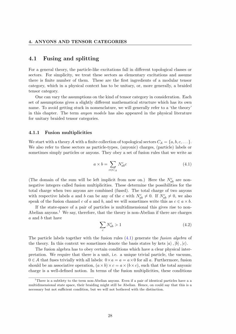
4 Anyons and tensor categories 27
4.1 Fusing and splitting . . . . . . . . . . . . . . . . . . . . . . . . . . . . . 28
4.1.1 Fusion multiplicities . . . . . . . . . . . . . . . . . . . . . . . . . 28
4.1.2 Diagrams and F -symbols . . . . . . . . . . . . . . . . . . . . . . 29
4.1.3 Gauge freedom . . . . . . . . . . . . . . . . . . . . . . . . . . . . 34
4.1.4 Tensor product and quantum trace . . . . . . . . . . . . . . . . . 35
4.1.5 Topological Hilbert space . . . . . . . . . . . . . . . . . . . . . . 36
4.2 Braiding . . . . . . . . . . . . . . . . . . . . . . . . . . . . . . . . . . . . 37
4.3 Pentagon and Hexagon relations . . . . . . . . . . . . . . . . . . . . . . 39
4.4 Modularity . . . . . . . . . . . . . . . . . . . . . . . . . . . . . . . . . . 40
4.4.1 Verlinde formula . . . . . . . . . . . . . . . . . . . . . . . . . . . 44
4.5 States and amplitudes . . . . . . . . . . . . . . . . . . . . . . . . . . . . 45
iii
CONTENTS
5 Examples of anyon models 495.1 Fibonacci . . . . . . . . . . . . . . . . . . . . . . . . . . . . . . . . . . . 505.2 Quantum double . . . . . . . . . . . . . . . . . . . . . . . . . . . . . . . 51
5.2.1 Fusion rules . . . . . . . . . . . . . . . . . . . . . . . . . . . . . . 525.2.2 Computing the F -symbols . . . . . . . . . . . . . . . . . . . . . . 535.2.3 Braiding . . . . . . . . . . . . . . . . . . . . . . . . . . . . . . . . 55
5.3 The su(2)k theories . . . . . . . . . . . . . . . . . . . . . . . . . . . . . . 56
6 Bose condensation in topologically ordered phases 616.1 Topological symmetry breaking . . . . . . . . . . . . . . . . . . . . . . . 62
6.1.1 Particle spectrum and fusion rules of T . . . . . . . . . . . . . . . 636.1.2 Confinement . . . . . . . . . . . . . . . . . . . . . . . . . . . . . 66
6.2 Commutative algebra objects as Bose condensates . . . . . . . . . . . . 686.2.1 The condensate . . . . . . . . . . . . . . . . . . . . . . . . . . . . 696.2.2 The particle spectrum of T . . . . . . . . . . . . . . . . . . . . . 746.2.3 Derived vertices . . . . . . . . . . . . . . . . . . . . . . . . . . . . 796.2.4 Confinement . . . . . . . . . . . . . . . . . . . . . . . . . . . . . 79
6.3 Breaking su(2)10 . . . . . . . . . . . . . . . . . . . . . . . . . . . . . . . 83
7 Indicators for topological order 877.1 Topological entanglement entropy . . . . . . . . . . . . . . . . . . . . . . 887.2 Topological S-matrix as an order parameter . . . . . . . . . . . . . . . . 91
8 Conclusion and outlook 97
A Quasi-triangular Hopf algebras 99
B Tensor categories: from math to physics 103B.1 Objects, morphisms and functors . . . . . . . . . . . . . . . . . . . . . . 103B.2 Direct sum . . . . . . . . . . . . . . . . . . . . . . . . . . . . . . . . . . 105B.3 Tensor categories . . . . . . . . . . . . . . . . . . . . . . . . . . . . . . . 106
B.3.1 Unit object . . . . . . . . . . . . . . . . . . . . . . . . . . . . . . 107B.3.2 Strictness and coherence . . . . . . . . . . . . . . . . . . . . . . . 107B.3.3 Fusion rules . . . . . . . . . . . . . . . . . . . . . . . . . . . . . . 108B.3.4 Diagrams . . . . . . . . . . . . . . . . . . . . . . . . . . . . . . . 108
B.4 Duals . . . . . . . . . . . . . . . . . . . . . . . . . . . . . . . . . . . . . 109B.5 Braiding . . . . . . . . . . . . . . . . . . . . . . . . . . . . . . . . . . . . 111
B.5.1 Ribbon structure . . . . . . . . . . . . . . . . . . . . . . . . . . . 112B.6 Categories for anyon models . . . . . . . . . . . . . . . . . . . . . . . . . 113
C Data for su(2)10 115
References 117
Dankwoord 123
iv
CHAPTER 1
Introduction
The theory of phases and phase transitions plays a central role in our understanding ofmany physical systems. Topological phases, or topologically ordered phases, pose aninteresting problem for theorists in this respect, as they fall outside of the conventionalscheme to understand phases that occur in terms of the breaking of symmetries. Theformalism of topological symmetry breaking, based on the breaking of an underlyingquantum group symmetry, can be viewed as an extension of this theory to the contextof topological phases. We will discuss topological symmetry breaking and connect itto the notion of commutative algebras in modular tensor categories. In particular, weput topological symmetry breaking in a graphical form, applying notions from tensorcategories, which gives the freedom to calculate general operators for the phases underconsideration.
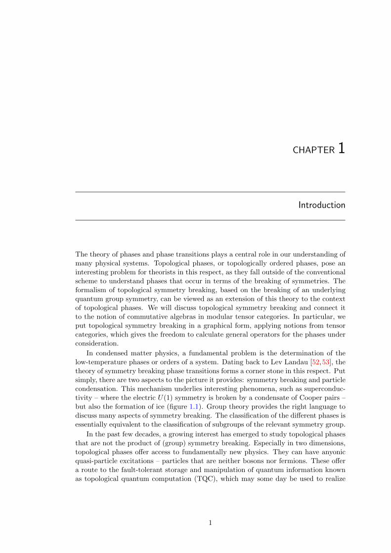
In condensed matter physics, a fundamental problem is the determination of thelow-temperature phases or orders of a system. Dating back to Lev Landau [52,53], thetheory of symmetry breaking phase transitions forms a corner stone in this respect. Putsimply, there are two aspects to the picture it provides: symmetry breaking and particlecondensation. This mechanism underlies interesting phenomena, such as superconduc-tivity – where the electric U(1) symmetry is broken by a condensate of Cooper pairs –but also the formation of ice (figure 1.1). Group theory provides the right language todiscuss many aspects of symmetry breaking. The classification of the different phases isessentially equivalent to the classification of subgroups of the relevant symmetry group.
In the past few decades, a growing interest has emerged to study topological phasesthat are not the product of (group) symmetry breaking. Especially in two dimensions,topological phases offer access to fundamentally new physics. They can have anyonicquasi-particle excitations – particles that are neither bosons nor fermions. These offera route to the fault-tolerant storage and manipulation of quantum information knownas topological quantum computation (TQC), which may some day be used to realize
1
1. INTRODUCTION
Figure 1.1: The structure of an ice crystal - If water freezes, or any other liquid-to-solid transition, the molecules order in a regular lattice structure. This breaks thetranslational and rotational symmetry of the fluid state. Using group theory, one can seethat there are 230 qualitatively different types of crystals corresponding to the 230 spacegroups
the dream of building a quantum computer.
The best known physical realization of topological phases occurs in the fractionalquantum Hall fluids. These exotic states in two-dimensional electron gases submittedto a strong perpendicular magnetic field have quantum numbers that are conserveddue to topological properties, not because of symmetry. Similar phases might occur inrotating Bose gases, high Tc superconductors, and possibly many more systems. Onecan in fact show that there is an infinite number of different topological phases possible,which suggests a world of possibilities if we ever gain enough control to engineer systemsthat realize a phase of choice.
From a mathematical point of view, interesting structures have entered the the-ory. The description and study of topological phases involve conformal field theory,topological quantum field theory, quantum groups and tensor categories, and all thesestructures are heavily interlinked. They are studied by mathematicians and theoreticalphysicists alike and link topics like string theory, low-dimensional topology and knottheory to condensed matter physics.
In this thesis we discuss topological ordered planar systems, and in particular thedescription using quantum groups and how these lead to tensor categories. In fact, weprefer the tensor category viewpoint from which the theory can be neatly summarizedby a set of F -symbols and R-symbols. We show how to calculate these in examplesrelated to discrete gauge theories and Chern-Simons theory.
Our main goal is to discuss how the breaking of quantum group symmetry canbe understood from the perspective of tensor categories. In the topological symmetrybreaking scheme, a key role is played by the formation of a bosonic condensate. Inthis thesis, we argue that this notion corresponds to a commutative algebra object inbraided tensor categories.
Using the formulation of topological symmetry breaking in terms of tensor cate-gories, one can write down and calculate diagrammatic expressions for operators in thebroken phase. This allows us to describe phase transition on the level of the topologicalS-matrix, an important invariant for the theory. We illustrate this in two representa-tive examples. This shows the usefulness of the topological S-matrix, related to the
2
exchange statistics of the particles, as an indicator for topological orders.
Another important indicator for topological order is the topological entanglemententropy. The quantum dimension of the condensate, or quantum embedding index,appears as a universal quantity characterizing the phase transitions and relating thetopological entanglement entropy of the different phases.
This thesis is organized as follows.
Chapter 2
In this chapter, we discuss some aspects of topological order in greater detail, namelyanyons and the fractional quantum Hall effect. The larger picture of how conformal fieldtheory, topological field theory and topological order are related is discussed briefly. Wealso point out some other developments in the field.
Chapter 3
The appearance of quantum groups as the underlying symmetry for topological phasesis discussed. Discrete gauge theories are taken as a representative example. The under-lying symmetry is the so-called quantum double D[H]. It can be understood physicallyas an algebra of gauge transformations and flux projections, which gives an intuitivepicture of how interacting electric and magnetic degrees of freedom can lead to mate-rialized quantum group symmetry. On a more formal level, we discuss the quantumgroup Uq[su(2)] which is important for the quantization of Chern-Simons theory andsu(2)(k) Wess-Zumino-Witten models.
Chapter 4
Here, we introduce in detail the graphical formalism for topological phases. One needsa finite set of charges, a description of fusion rules, so called F -symbols and R-symbolsto describe the topological properties of anyons completely. An important quantityis the topological S-matrix. Together with the T -matrix it forms a representation ofthe modular group. As an application and illustration of the graphical formalism wegive a proof of the Verlinde formula. Finally, quantum states, density matrices and thecalculation of physical amplitudes is discussed.
Chapter 5
The calculation of topological data for the quantum double D[H] is illustrated and wepresent general formulas for the su(2)k models.
Chapter 6
In this chapter, we start the discussion of topological symmetry breaking. Topologicalsymmetry breaking is a way to construct from a theory A describing the unbrokenphase, a theory T and a theory U. The T-theory describes the broken phase, but may
3
1. INTRODUCTION
include excitations that braid non-trivially with the condensate. These excitationscannot occur in the bulk of the broken phase as the disruption of the condensatecosts energy. They get confined to the boundary or as T-hadrons. Projecting out theconfined excitations one gets the unconfined theory U-that describes the bulk of thebroken phase.
We put this scheme in the context of the graphical formalism of chapter 4. Wediscuss how to find a well-defined condensate and how to construct the particle spectrumupon this. The conditions for confinement are reconsidered and it is shown that thereis an operator that projects out confined excitations.
Chapter 7
The quantum dimension of the condensate – or quantum embedding index – q ap-pears as a universal ratio between the quantum dimensions of the broken phase andthe unbroken phase. This can physically be understood as a relation in terms of thetopological entanglement entropy. We show how this universality of q follows from theassumption of topological symmetry breaking.
Finally, we give the main application of the graphical formalism for topologicalsymmetry breaking. We show that the symmetry breaking phase transition can be de-scribed directly on the level of the topological S-matrix. The diagrammatic calculationgives insight in the nature of topological symmetry breaking phase transitions. Thecondensate appears explicitly where in the original formulation it could always be leftout.
Chapter 8
The last chapter contains concluding remarks and and indicates possible paths forfuture research.
4
CHAPTER 2
Topological order in the plane
In this chapter, we give a brief discussion of some essential topics concerning topologicalphases and topological order in 2+1 dimensions. These are anyons, the FQH effect,some generalities of the mathematical structures that are involved. This chapter servesas more elaborate introduction and to sketch a bit of history of the topic. Relevantreferences are included.
2.1 Anyons
In the most mundane spacetime, that of 3+1 dimensions, particles fall in precisely twoclasses: bosons and fermions. These can either be defined by their exchange propertiesor by their spins. The importance of this difference between particles can of coursenot be overstated. It is at the root of the Pauli exclusion principle and Bose-Einsteincondensation, and determines whether macroscopic numbers of particles obey Fermi-Dirac or Bose-Einstein statistics.
According to textbook quantum mechanics, the wave function of a multi-particlestate of fermions is obtained by anti-symmetrising the tensor product of single-particlewave functions, while for bosons the wave function is symmetrised. This procedurelong stood as a corner stone of quantum mechanics and is still procedure in manyapplications. But one may object that in a quantum theory with indistinguishableparticles, the labelling of particle coordinates has no physical significance and bringsunobservable elements into the theory.
The consequences of above observation were first fully appreciated by Leinaas andMyrheim. In their seminal paper [57], they show that the exchange properties ofparticles are tightly connected to the topology of the configuration space of multi-particle systems. In fact, as was shown in [51], particle types correspond to unitaryrepresentations of the fundamental group of this space.
5
2. TOPOLOGICAL ORDER IN THE PLANE
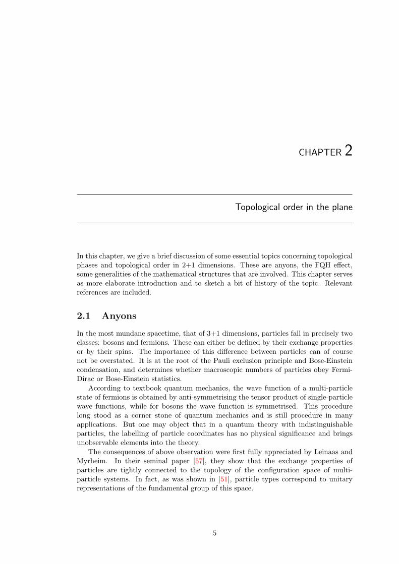
Let us discuss this in a spacetime picture. The trajectories of particles can nowconveniently be imagined by their world lines through spacetime. We will consider tra-jectories that leave the system in a configuration identical to the initial configurationand that do not have intersecting world lines. These correspond to free propagationof the system without scattering events. If the particles are distinguishable, the worldlines should start and end at the same spatial coordinates. If the particles are indistin-guishable, the world lines are allowed to interchange spatial coordinates.
Figure 2.1: Spacetime trajectories - Two spacetime trajectories for a system of threeparticles with identical initial and final states. If the particles are of different type, worldlines should start and end at the same coordinates in space (left), while for indistinguishableparticles, permutations of spatial coordinates are allowed (right).
The trajectories fall in distinct topological classes, depending on whether or not theycan be deformed into each other by smooth deformations of the world lines (withoutintermediate intersections). If space has three or more dimensions one can see thatthere is no topologically different notion of ‘under’ and ‘over’ crossing of world lines,but any exchange of coordinates is simply that: an exchange. Therefore the exchangeof particles is governed by the permutation group SN .
However, when the particles live in a plane – so spacetime is three-dimensional –such a distinction of crossings becomes essential to incorporate the difference betweeninterchanging the particles clockwise or counter-clockwise. The relevant group is notSN but BN , Artins N -stranded braid group [3].
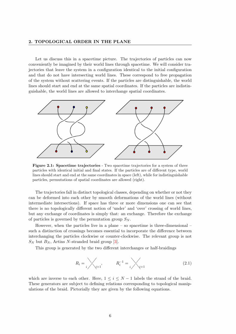
This group is generated by the two different interchanges or half-braidings
Ri =i i+1
, R−1i =
i i+1(2.1)
which are inverse to each other. Here, 1 ≤ i ≤ N − 1 labels the strand of the braid.These generators are subject to defining relations corresponding to topological manip-ulations of the braid. Pictorially they are given by the following equations.
6
2.1 Anyons
We can also write them algebraically as
RiRj = RjRi for |i− j| ≥ 2
RiRi+1Ri = Ri+1RiRi+1 for 1 ≤ i ≤ N − 1(2.2)
The second relation is the famous Yang-Baxter equation [15,86,87].
As remarked before, the important difference between particles in the plane andparticles in three-dimensional space is the difference between over and under crossingsof world lines. The relation to statistics in higher dimensions represented on the levelof groups due the fact that we can pass from the braid group BN to the permutationgroup SN by implying the relation Ri = R−1
i , or equivalently (Ri)2 = 1. This one
extra relation makes a huge difference for the properties of the group. While thepermutation group is finite (|SN | = N !), the braid group is infinite, even for twostrands. The representation theory of the braid group is therefore much richer thanthat of the permutation group. This gives the possibility of highly non-trivial exchangestatistics in 2+1 dimensions, also referred to as ’braid statistics’. Particles that obeythese exotic braid statistic were dubbed anyons by Wilczek [80]. Bosons and fermions,in this context, just correspond to two of an infinite number of possibilities. Sincedistinguishable anyons can also have nontrivial braiding, it is better to think of braidingstatistics as a kind of topological interaction.
Bosons and fermions correspond to the two one-dimensional representations of SN ,even and odd respectively. In principle, higher dimensional representations of SN ,known as ‘parastatistics’ [39], could lead to more particle types, but it has been shownthat these can be reduced to the one-dimensional representations at the cost of intro-ducing additional quantum numbers [31].
One-dimensional representations of the braid group simply correspond to a choiceof phase exp(iθ) assigned to an elementary interchange. Since, in this case the orderof the exchange is unimportant because phases commute, anyons corresponding toone-dimensional representaions are called Abelian. However, it is no longer true thathigher dimensional representations of the braid group can be reduced. This gives riseto so called non-Abelian anyons, particles that implement higher dimensional braid
7
2. TOPOLOGICAL ORDER IN THE PLANE
statistics. These non-Abelian anyons are the ones that can be used for topologicalquantum computation as suggested by Kitaev in [49]. See [64,66] for a review.
2.2 The fractional quantum Hall effect
Because the most prominent system with anyonic excitations is the fractional QuantumHall effect, we include a brief discussion of some relevant aspects. For greater detail,we refer to the literature. See e.g. [65, 88] for a thorough introduction.
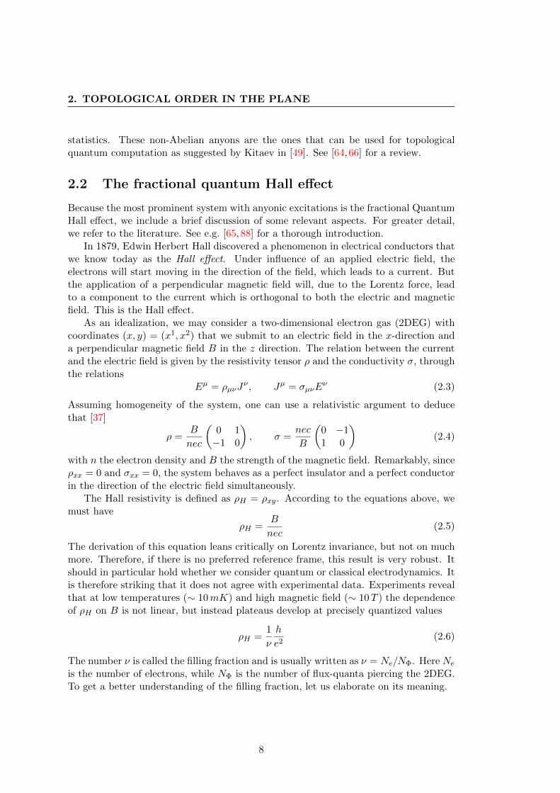
In 1879, Edwin Herbert Hall discovered a phenomenon in electrical conductors thatwe know today as the Hall effect. Under influence of an applied electric field, theelectrons will start moving in the direction of the field, which leads to a current. Butthe application of a perpendicular magnetic field will, due to the Lorentz force, leadto a component to the current which is orthogonal to both the electric and magneticfield. This is the Hall effect.
As an idealization, we may consider a two-dimensional electron gas (2DEG) withcoordinates (x, y) = (x1, x2) that we submit to an electric field in the x-direction anda perpendicular magnetic field B in the z direction. The relation between the currentand the electric field is given by the resistivity tensor ρ and the conductivity σ, throughthe relations
Eµ = ρµνJν , Jµ = σµνE
ν (2.3)
Assuming homogeneity of the system, one can use a relativistic argument to deducethat [37]
ρ =B
nec
(0 1−1 0
), σ =
nec
B
(0 −11 0
)(2.4)
with n the electron density and B the strength of the magnetic field. Remarkably, sinceρxx = 0 and σxx = 0, the system behaves as a perfect insulator and a perfect conductorin the direction of the electric field simultaneously.
The Hall resistivity is defined as ρH = ρxy. According to the equations above, wemust have
ρH =B
nec(2.5)
The derivation of this equation leans critically on Lorentz invariance, but not on muchmore. Therefore, if there is no preferred reference frame, this result is very robust. Itshould in particular hold whether we consider quantum or classical electrodynamics. Itis therefore striking that it does not agree with experimental data. Experiments revealthat at low temperatures (∼ 10mK) and high magnetic field (∼ 10T ) the dependenceof ρH on B is not linear, but instead plateaus develop at precisely quantized values
ρH =1
ν
h
e2(2.6)
The number ν is called the filling fraction and is usually written as ν = Ne/NΦ. Here Ne
is the number of electrons, while NΦ is the number of flux-quanta piercing the 2DEG.To get a better understanding of the filling fraction, let us elaborate on its meaning.
8
2.2 The fractional quantum Hall effect
From analysing the single-particle Hamiltonian, one sees that the energy spectrumforms so called Landau levels
En = (n+1
2)~ωc, ωc =
eB
mc(2.7)
In a finite sized system of area A, the available number of states for each Landau levelturns out to be [37]
NΦ = AB
Φ0(2.8)
Here Φ0 = hce is the fundamental flux quantum, so apparently the number of available
states for each energy level is the same as the number of flux-quanta that pierce thesystem. Hence, ν = Ne/NΦ is the ratio between the number of filled energy states –the electrons – and the number of available energy states, which is why it is called thefilling fraction.
Plateaus at integer values for the filling fraction were first reported in 1980 by vonKlitzing at al. [50], and are referred to as the integer quantum Hall effect (IQHE).Plateaus at fractional filling fractions – found two years later by Tsui et al. [74] –are the hallmark for the fractional quantum Hall effect (FQHE). While the IQHEcan essentially be understood from the single particle physics, neglecting the Coulombinteraction, the FQHE represents an intriguing interplay of many interacting electrons.The Coulomb interaction is crucial to explain its features.
Application of a magnetic field normal to the planefurther quantizes the in-plane motion into Landau levelsat energies Ei!(i"1/2)!"c , where "c!eB/m* repre-sents the cyclotron frequency, B the magnetic field, andm* the effective mass of electrons having charge e. Thenumber of available states in each Landau level, d!2eB/h , is linearly proportional to B. The electron spincan further split the Landau level into two, each holdingeB/h states per unit area. Thus the energy spectrum ofthe 2D electron system in a magnetic field is a series ofdiscrete levels, each having a degeneracy of eB/h (Andoet al., 1983).
At low temperature (T#Landau/spin splitting) and ina B field, the electron population of the 2D system isgiven simply by the Landau-level filling factor #!n/d!n/(eB/h). As it turns out, # is a parameter of centralimportance to 2D electron physics in high magneticfields. Since h/e!$0 is the magnetic-flux quantum, # de-notes the ratio of electron density to magnetic-flux den-sity, or more succinctly, the number of electrons per fluxquantum. Much of the physics of 2D electrons in a Bfield can be cast in terms of this filling factor.
Most of the experiments performed on 2D electronsystems are electrical resistance measurements, althoughin recent years several more sophisticated experimentaltools have been successfully employed. In electricalmeasurements, two characteristic voltages are measuredas a function of B, which, when divided by the appliedcurrent, yield the magnetoresistance Rxx and the Hallresistance Rxy (see insert Fig. 1). While the former, mea-sured along the current path, reduces to the regular re-sistance at zero field, the latter, measured across the cur-rent path, vanishes at B!0 and, in an ordinaryconductor, increases linearly with increasing B. ThisHall voltage is a simple consequence of the Lorentzforce’s acting on the moving carriers, deflecting theminto the direction normal to current and magnetic field.According to this classical model, the Hall resistance isRxy!B/ne , which has made it, traditionally, a conve-nient measure of n.
It is evident that in a B field current and voltage areno longer collinear. Therefore the resistivity % which issimply derived from Rxx and Rxy by taking into accountgeometrical factors and symmetry, is no longer a num-ber but a tensor. Accordingly, conductivity & and resis-tivity are no longer simply inverse to each other, butobey a tensor relationship &! %$1. As a consequence,for all cases of relevance to this review, the Hall conduc-tance is indeed the inverse of the Hall resistance, but themagnetoconductance is under most conditions propor-tional to the magnetoresistance. Therefore, at vanishingresistance (%!0), the system behaves like an insulator(&!0) rather than like an ideal conductor. We hastento add that this relationship, although counterintuitive,is a simple consequence of the Lorentz force’s acting onthe electrons and is not at the origin of any of the phe-nomena to be reviewed.
Figure 1 shows a classical example of the characteris-tic resistances of a 2D electron system as a function ofan intense magnetic field at a temperature of 85 mK.
The striking observation, peculiar to 2D, is the appear-ance of steps in the Hall resistance Rxy and exception-ally strong modulations of the magnetoresistance Rxx ,dropping to vanishing values. These are the hallmarks ofthe quantum Hall effects.
III. THE INTEGRAL QUANTUM HALL EFFECT
Integer numbers in Fig. 1 indicate the position of theintegral quantum Hall effect (IQHE) (Von Klitzing,et al., 1980). The associated features are the result of thediscretization of the energy spectrum due to confine-ment to two dimensions plus Landau/spin quantization.
At specific magnetic fields Bi , when the filling factor#!n/(eB/h)!i is an integer, an exact number of theselevels is filled, and the Fermi level resides within one ofthe energy gaps. There are no states available in thevicinity of the Fermi energy. Therefore, at these singularpositions in the magnetic field, the electron system isrendered incompressible, and its transport parameters(Rxx ,Rxy) assume quantized values (Laughlin, 1981).Localized states in the tails of each Landau/spin level,which are a result of residual disorder in the 2D system,extend the range of quantized transport from a set ofprecise points in B to finite ranges of B, leading at inte-ger filling factors to the observed plateaus in the Hall
FIG. 1. Composite view showing the Hall resistance Rxy!Vy /Ix and the magnetoresistance Rxx!Vx /Ix of a two-dimensional electron system of density n!2.33%1011 cm$2 at atemperature of 85 mK, vs magnetic field. Numbers identify thefilling factor #, which indicates the degree to which the se-quence of Landau levels is filled with electrons. Instead of ris-ing strictly linearly with magnetic field, Rxy exhibits plateaus,quantized to h/(#e2) concomitant with minima of vanishingRxx . These are the hallmarks of the integral (#!i!integer)quantum Hall effect (IQHE) and fractional (#!p/q) quantumHall effect (FQHE). While the features of the IQHE are theresults of the quantization conditions for individual electronsin a magnetic field, the FQHE is of many-particle origin. Theinsert shows the measurement geometry. B!magnetic field,Ix!current, Vx!longitudinal voltage, and Vy!transverse orHall voltage. From Eisenstein and Stormer, 1990.
S299H. L. Stormer, D. C. Tsui, and A. C. Gossard: The fractional quantum Hall effect
Rev. Mod. Phys., Vol. 71, No. 2, Centenary 1999
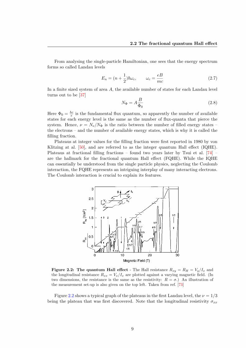
Figure 2.2: The quantum Hall effect - The Hall resistance Rxy = RH = Vy/Ix andthe longitudinal resistance Rxx = Vx/Ix are plotted against a varying magnetic field. (Intwo dimensions, the resistance is the same as the resistivity: R = σ.) An illustration ofthe measurement set-up is also given on the top left. Taken from ref. [73]
Figure 2.2 shows a typical graph of the plateaus in the first Landau level, the ν = 1/3being the plateau that was first discovered. Note that the longitudinal resistivity σxx
9
2. TOPOLOGICAL ORDER IN THE PLANE
drops to zero at the plateaus. which means that the conductivity tensor is off-diagonalas in equation (2.4). Hence, a dissipationless transverse current flows in response to anapplied electric field. In particular, when we thread an extra magnetic flux quantumthrough the medium, the system will expel a net charge of νe due to the inducedmagnetic field. Or, put differently, this will create a quasi-hole of charge −νe and oneflux quantum, illustrating the intimate coupling between charge and flux in the quantumHall effect. It is a first indication that these systems harvest elementary quasi-particleexcitations that are charge-flux composites, which, due to the internal Aharonov-Bohminteraction, can be anyons. The peculiar fact that these quasi-particles have fractionalcharge when ν is non-integer has been experimentally verified in [38].
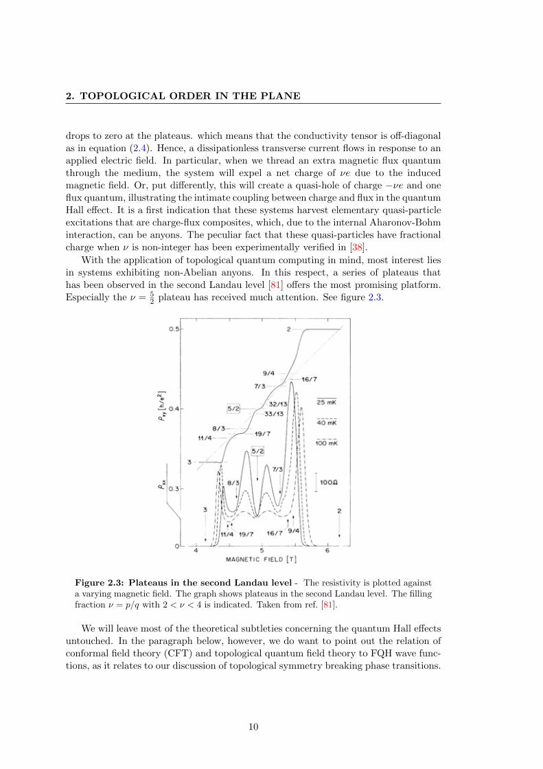
With the application of topological quantum computing in mind, most interest liesin systems exhibiting non-Abelian anyons. In this respect, a series of plateaus thathas been observed in the second Landau level [81] offers the most promising platform.Especially the ν = 5
2 plateau has received much attention. See figure 2.3.
Figure 2.3: Plateaus in the second Landau level - The resistivity is plotted againsta varying magnetic field. The graph shows plateaus in the second Landau level. The fillingfraction ν = p/q with 2 < ν < 4 is indicated. Taken from ref. [81].
We will leave most of the theoretical subtleties concerning the quantum Hall effectsuntouched. In the paragraph below, however, we do want to point out the relation ofconformal field theory (CFT) and topological quantum field theory to FQH wave func-tions, as it relates to our discussion of topological symmetry breaking phase transitions.
10
2.2 The fractional quantum Hall effect
2.2.1 Conformal and topological quantum field theory
Over the years, a series of wave functions has been proposed to capture the physics ofthe fractional quantum Hall effect at different plateaus, the Laughlin wave function [55]being the first. It can account for the plateaus at filling fraction ν = 1/M for odd M ,and reads
ΨL(z) =∏i<j
(zi − zj)M exp
[1
4
∑i
|zi|2]
(2.9)
Here, the zi label the complex coordinates for Ne electrons.1
The Laughlin state describes an electronic system where the electrons carry mag-netic vortices. This attachment of vortices to electrons is paradigmatic for the variousquantum Hall states that have been proposed in the literature. Note that to ensurea fermionic system, i.e. the wave function is anti-symmetric under interchange of thecoordinates, we need M to be odd.
Skipping subsequent developments in the history of the FQHE (e.g. the Haldane-Halparin hierarchy [43, 44, 56] and the composite fermion approach by Jain [45]), wewant to turn our attention to an observation first made by Moore and Read. In [63]they noted that the Laughlin wave function could be obtained as a correlator in acertain rational conformal field theory (RCFT). In fact, they argue that this relationshould be general and conjecture that every FQHE state should be related to conformalfield theory, which would give a means to classify FQHE states.
Without going into the details of conformal field theory (see e.g. [33, 36] for in-troductory texts and [62, 63] for further information), let us reflect for a moment onthe picture they sketch. They motivate their search for a formulation in terms ofRCFT by pointing to the development of Ginzberg-Landau effective field theories forthe FQHE effect where the action contains a Chern-Simons term. Witten showed [83]that there is a connection between Chern-Simon theory in a three dimensional bulk anda Wess-Zumino-Witten theory on the two-dimensional edge. Moore and Read arguethat the long range effective field theory should essentially constitute a pure Chern-Simons theory and that a related RCFT should come in to play when we consider atwo-dimensional edge of the spacetime. Interestingly, the RCFT can account for wavefunctions by means of correlators in a (2+0)d interpretation, but also governs the edgeexcitation in a (1+1)d interpretation.
Chern-Simons theory is an example of a topological quantum field theory (TQFT).This is apparent from the fact that the spacetime metric does not enter the Chern-Simons action
SCS =k
4π
∫d3x Tr εµνρ(aµ∂νaρ +
2
3aµaνaρ). (2.10)
A topological quantum field theory is generally a quantum field theory for which allcorrelation functions are invariant under arbitrary smooth deformations of the basemanifold [4, 84].
1The magnetic length `B =√
~ceB
is set to unity, or, equivalently, the complex coordinates are taken
z = (x+ iy)/`B .
11
2. TOPOLOGICAL ORDER IN THE PLANE
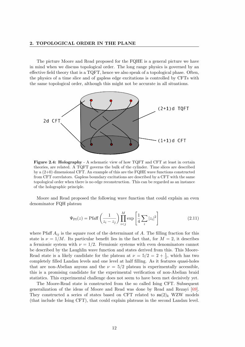
The picture Moore and Read proposed for the FQHE is a general picture we havein mind when we discuss topological order. The long range physics is governed by aneffective field theory that is a TQFT, hence we also speak of a topological phase. Often,the physics of a time slice and of gapless edge excitations is controlled by CFTs withthe same topological order, although this might not be accurate in all situations.
Figure 2.4: Holography - A schematic view of how TQFT and CFT at least in certaintheories, are related. A TQFT governs the bulk of the cylinder. Time slices are describedby a (2+0) dimensional CFT. An example of this are the FQHE wave functions constructedfrom CFT correlators. Gapless boundary excitations are described by a CFT with the sametopological order when there is no edge reconstruction. This can be regarded as an instanceof the holographic principle.
Moore and Read proposed the following wave function that could explain an evendenominator FQH plateau
ΨPf(z) = Pfaff
(1
zi − zj
) M∏i<j
exp
[1
4
∑i
|zi|2]
(2.11)
where Pfaff Aij is the square root of the determinant of A. The filling fraction for thisstate is ν = 1/M . Its particular benefit lies in the fact that, for M = 2, it describesa fermionic system with ν = 1/2. Fermionic systems with even denominators cannotbe described by the Laughlin wave function and states derived from this. This Moore-Read state is a likely candidate for the plateau at ν = 5/2 = 2 + 1
2 , which has twocompletely filled Landau levels and one level at half filling. As it features quasi-holesthat are non-Abelian anyons and the ν = 5/2 plateau is experimentally accessible,this is a promising candidate for the experimental verification of non-Abelian braidstatistics. This experimental challenge does not seem to have been met decisively yet.
The Moore-Read state is constructed from the so called Ising CFT. Subsequentgeneralization of the ideas of Moore and Read was done by Read and Rezayi [69].They constructed a series of states based on CFT related to su(2)k WZW models(that include the Ising CFT), that could explain plateaus in the second Landau level.
12
2.3 Other approaches to topological order
Interestingly, one of these states encompasses so called Fibonacci anyons which areuniversal for quantum computation.
2.3 Other approaches to topological order
The FQHE in 2DEGs is not the only place to look for (non-Abelian) anyons. Systemsthat might have states very similar to the FQH states discussed above are px + ipysuperconductors [26,41] and rotating Bose gases [24,25,68], though the latter of coursewould display a bosonic version of the FQHE.
We should also note the existence of two lattice models that realize topologicalorder, at this point. The first is known as the Kitaev model. In its most generalform, this model features interacting spins placed on the edges of an arbitrary lattice[49]. The spins are labelled by the elements of a group. The Hamiltonian consists ofmutually commuting projectors, and is therefore completely solvable. The projectorscan be recognized as generalizations of either electric or magnetic interactions. Theelectric operators act on the edges joining at a vertex and ensure that the ground statetransforms trivially under the action of the group, which can be seen as a sort of gaugetransformation. The magnetic operators act on plaquettes and essentially project outstates of trivial flux through the plaquette. In the simplest case, where the spins arelabelled by Z2 and a square lattice is taken, the ground state can be readily identifiedas a loop gas.
This lattice model realizes a discrete gauge theory.1 For more information we referto the literature. Especially [17] and [16] are interesting in the context of this thesis.They study the Kitaev model with boundary, which can be seen as an explicit sym-metry breaking mechanism and relates to the phase transitions that we will discussin subsequent chapters. These gauge theories might also be realizable in Josephsonjunction arrays [29].
The other paradigmatic lattice model for topological order was introduced by Levinand Wen under the name of string-net condensates [59]. This system lives on a trivalentlattice, where, again, spins are placed on edges and interact at vertices. The input istensor category. We will discuss these structures in detail in chapter 4. The Hamiltonianhas a similar structure as in the Kitaev model and is also completely solvable.
Remarkably, it has been shown that the Kitaev model can be mapped to a Levin-Wen type model, making the Kitaev model essentially a special case of the more generalstring-net models.
In the next chapter we will discuss the role of quantum groups in (2+1)d. Inmany concrete situations these can be identified as the underlying symmetry structure.Regardless of the name, these are actually not groups but should be regarded as ageneralization. Formally, they are certain type of algebras with additional structures(see chapter 3 and appendix A).
1Discrete gauge theories are discussed in chapter 3.
13

2. TOPOLOGICAL ORDER IN THE PLANE
14
CHAPTER 3
Quantum groups in planar physics
In the previous chapter we discussed aspects of topological order, such as anyonic quasi-particle excitations and the quantum Hall effect. In the present chapter we will discussthe symmetries underlying topological order. Special to planar physics, especially whenelectric and magnetic degrees of freedom start to interact, is the occurrence of so calledquantum group symmetry. Quantum groups generalize group symmetries in manyways. This full symmetry is often not manifest in the Hamiltonian or Lagrangian ofthe theory.
Symmetries of the Hamiltonian are represented on the quantum level as operatorscommuting with the Hamiltonian. Since commuting operators can be diagonalized si-multaneously, the energy eigenstates can be labelled by quantum numbers coming fromthe symmetry operators. But it might happen that there is a larger set of commut-ing operators. This gives an idea of how symmetries not directly apparent from theHamiltonian or Lagrangian can materialize. In this chapter we will first illustrate theoccurrence of quantum group symmetry in the context of discrete gauge theories. Theelectric and magnetic excitations can be treated on equal footing, in these theories,when viewed as irreducible representation of the quantum double of the residual gaugegroup. Then we give a more formal treatment of the constituents of quantum groups,or quasi-triangular Hopf algebras as they are also called. Finally, we will discuss thequantum group Uq[su(2)] that is related to Chern-Simons theory and the Wess-Zumino-Witten model for conformal field theory.
A more formal treatment of the generalities of quantum groups is put forth theappendix A.
15
3. QUANTUM GROUPS IN PLANAR PHYSICS
3.1 Discrete Gauge Theory
Suppose we start out with a (2+1)d Yang-Mills-Higgs theory with a gauge group G.We speak of a discrete gauge theory (DGT) when the continuous gauge group G isspontaneously broken down to a discrete, usually finite, subgroup H. Hence, this canbe regarded as a gauge theory with residual gauge group H.
The Higgs mechanism causes the gauge field to acquire a mass, making all localinteractions freeze out in the low-energy regime, effectively leaving only topologicalinteractions. In this limit, the theory becomes a TQFT [11]. Below, we give a quickoverview of the aspects that are important for our present purpose. See [67] for anelaborate exposition on which this approach is based.
A DGT has electric particles labelled by the irreps {α} of the residual gauge group,which, before we mod out by gauge transformations to get the physical Hilbert space,carry the corresponding representation module Vα as an internal Hilbert space. Further-more, a DGT also has magnetic particles, or fluxes, associated to topological defects.1
We think of the fluxes as defined by their effect on charges in an Aharonov-Bohm typescattering experiment [1]. An electric charge α taken around a flux will feel the influ-ence of the flux as a transformation in its internal Hilbert space Vα by the action ofsome h ∈ H. We denote the flux as a ket |h〉 labelled by the transformation h ∈ H itinduces. However, since a flux measurement followed by a gauge transformation shouldgive the same result as applying a gauge transformation first and do the flux measure-ment in the transformed system we find gh = h′g, where h, h′ is the flux measuredbefore or after the gauge g transformation respectively. Hence the gauge transforma-tions has to act on the flux by conjugation, so the gauge invariant labelling is in fact bythe conjugacy classes of H rather than just elements. Hence, while electric excitationscarry representation modules as an internal Hilbert space, the internal space of fluxesis given by a conjugacy class.
Revealing the algebraic structure of the theory puts the foregoing on a firmer foot-ing. Define the flux measurement operators {Ph}h∈H that satisfy the projector algebra
PhPh′ = δhh′Ph (3.1)
Since gauge transformations g ∈ H act on fluxes by conjugation, we must have
gPh = Pghg−1 g (3.2)
The full algebra of gauge transformations and flux projections is spanned by the com-binations
{Ph g}, h, g ∈ H (3.3)
that obey the multiplication rule
Ph g Ph′ g′ = δh,ghg−1Ph gg
′ (3.4)
1Note that we use electric and magnetic as general terminology for the two distinct types of particle-like excitations and it does not imply that the gauge group is U(1).
16
3.1 Discrete Gauge Theory
This is in fact the quantum double D(H) of H which can obtained from any finitegroup by a general construction due to Drinfel’d [30]. Note that the multiplication rulesays that this algebra has a unit 1 =
∑h Ph e.
The full particle spectrum of a DGT with residual gauge group H can be recoveredas the set of irreducible representations of D[H].1 Indeed, one finds back the irrepsof H corresponding to electric particles, as well as the conjugacy classes, belonging tofluxes. But there is a third class of irreps corresponding to flux-charge composites ordyons. Physically, this is very interesting, because due to the Aharonov-Bohm effect,these composites can have fractional spin and can be true anyons.
The representation theory of D(H) was first worked out in [28], but we again follow[67]. It turns out that the irreducible representations of D(H) can be labelled uniquelyby a conjugacy class A of H, and an irreducible representation of the centralizer ofsome representing element of A. Thus, when the conjugacy class {e} of the identityelement is taken, or that of any other central element, we find the irreps of H. Butapparently, for general non-trivial fluxes, not all transformations can be implementedstraightforwardly on the charge part.
To make the action of D(H) explicit, we will have to make a few choices. Pick someorder for the elements of A and write
A = {Ah1,Ah2, . . . ,
Ahk} (3.5)
Let C(A) be the centralizer of Ah1 and fix a set X(A) = {Ax1,Ax2, . . . ,
Axk} of rep-
resentatives for the equivalence classes H/C(A), such that Ahi = AxiAh1
Ax−1i . Let us
take Ax1 = e, the unit element of H, for convenience. These choices will effect some ofthe specifics in what follows but a different choice would lead to a unitary equivalentrepresentation of D(H).
The internal Hilbert space V Aα of a particle with flux A and centralizer charge α is
now spanned by the quantum states
∣∣Ahi, αvj⟩ , i = 1, . . . , k,j = 1, . . . ,dimα
(3.6)
where we have chosen a basis {| αvj〉} for the centralizer representation α. The action ofan element Ph g of D(H) on these basis states, i.e. the effect of a gauge transformationg followed by a flux measurement Ph, is given by
ΠAα (Ph g)
∣∣Ahi, αvj⟩ = δh,g Ahig−1
∣∣g Ahig−1,Πα(g)mjαvm
⟩(3.7)
(where summation over repeated indices is implied), with
g ≡ Ax−1g Axi (3.8)
and Axk the element of X(A) associated to hk = g Ahig−1. Note that the element
g commutes with Ah1 as it should. Thus when acting on dyons, g is the part of the
1We will assume representations to be unitary throughout the text
17
3. QUANTUM GROUPS IN PLANAR PHYSICS
transformation that slips through the conjugation of the flux, and which is subsequentlyimplemented on the charge.
This gives an explicit description of the irreps of D(H) including how the action ofelements Ph g can be worked out. The single-particle states of the theory correspondto these irreps. Before we discuss multi-particle states, let us point out a subtletyconcerning unitarity of the theory. In order to preserve the inner product of quantumstates, we should have
ΠAα (Ph g)† = ΠA
α (Pg−1hg g−1) (3.9)
Hence it makes sense to define (Ph g)∗ = Pg−1hg g−1, and more generally∑
h,g
ch,g Ph g
∗ =∑h,g
c∗h,g Pg−1hg g−1 (3.10)
where a ∗ on the coefficients ch,g just means complex conjugation. Formally, thisturns D[H] into a Hopf-∗-algebra. Representations obeying (3.9) are said to respect∗-structure. This gives the proper definition of a unitary representation.
3.1.1 Multi-particle states
To let D(H) act on a two-particle state, one needs a prescription of how an elementPh g acts on V A
α ⊗ V Bβ . Corresponding to intuitive expectations, the element Ph g
implements the gauge transformation g on both particles and then projects out thetotal flux. Thus, we act on a state
∣∣Ahi, αvj⟩ ∣∣Bhk, βvl⟩ with∑h′h′′=h
ΠAα (Ph′ g)⊗ΠB
β (Ph′′ g) (3.11)
Formally, this is nicely captured by the definition of a coproduct
∆: D(H)→ D(H)⊗D(H) (3.12)
by
∆(Ph g) =∑
h′h′′=h
Ph′ g ⊗ Ph′′ g (3.13)
The action of Ph g on a two-particle state is then defined as the application of ΠAα ⊗ΠB
β
on ∆(Phg), which indeed gives (3.11).The action on three-particle states is produced by first applying ∆ to produce an
element of D[H]⊗D[H] and then apply ∆ again on either the left or the right tensorleg. Starting out with the element Ph g, either choice produces∑
h′h′′h′′′=h
Ph′ g ⊗ Ph′′ g ⊗ Ph′′′ g (3.14)
as an element of D[H]⊗3. Then we apply ΠAα ⊗ ΠB
β ⊗ ΠCγ on this element to act on
V Aα ⊗ V B
β ⊗ V Cγ . Note that when we describe the transformation in words, it is again
18
3.1 Discrete Gauge Theory
the application of the gauge transformation g on all three particles followed by a totalflux measurement projecting out flux h.
Extending the action of Ph g on states with more than three particles is now straight-forward. The resulting transformation is again the global gauge transformation g fol-lowed by the flux measurement. On a formal level, this is achieved by consecutiveapplication of the coproduct to get an element in D[h]n and letting each tensor leg acton the corresponding particle.
The tensor product representations of D(H) that we obtain using the coproductare in general not irreducible, but they can always be decomposed into a direct sum ofirreducible representations. Thus the space V A
α ⊗V Bβ can be written as a direct sum of
subspaces that transform irreducibly, leading to the decomposition rules
ΠAα ⊗ΠB
β =⊕(C,γ)
NABγαβC ΠC
γ (3.15)
These so-called fusion rules play an important role when we start discussing the generalformalism for anyonic theories in de next chapter. Note that the representation Π{e}0has trivial fusion (where 0 denotes the trivial representation of H). This correspondsto the zero-particle state or vacuum of the theory. The map Π{e}0 : D[H]→ C can alsobe called the counit, and is then often denoted with ε. This is a general constituent ofa quantum group, and should satisfy certain compatibility conditions with regard tothe comultiplication.
3.1.2 Topological interactions
As remarked before, in the low-energy limit, the excitations of a DGT interact solelyby Aharonov-Bohm type, topological interactions. A very nice feature of DGT theoriesis that the precise form of these interactions can be deduced from intuitive reasoning.
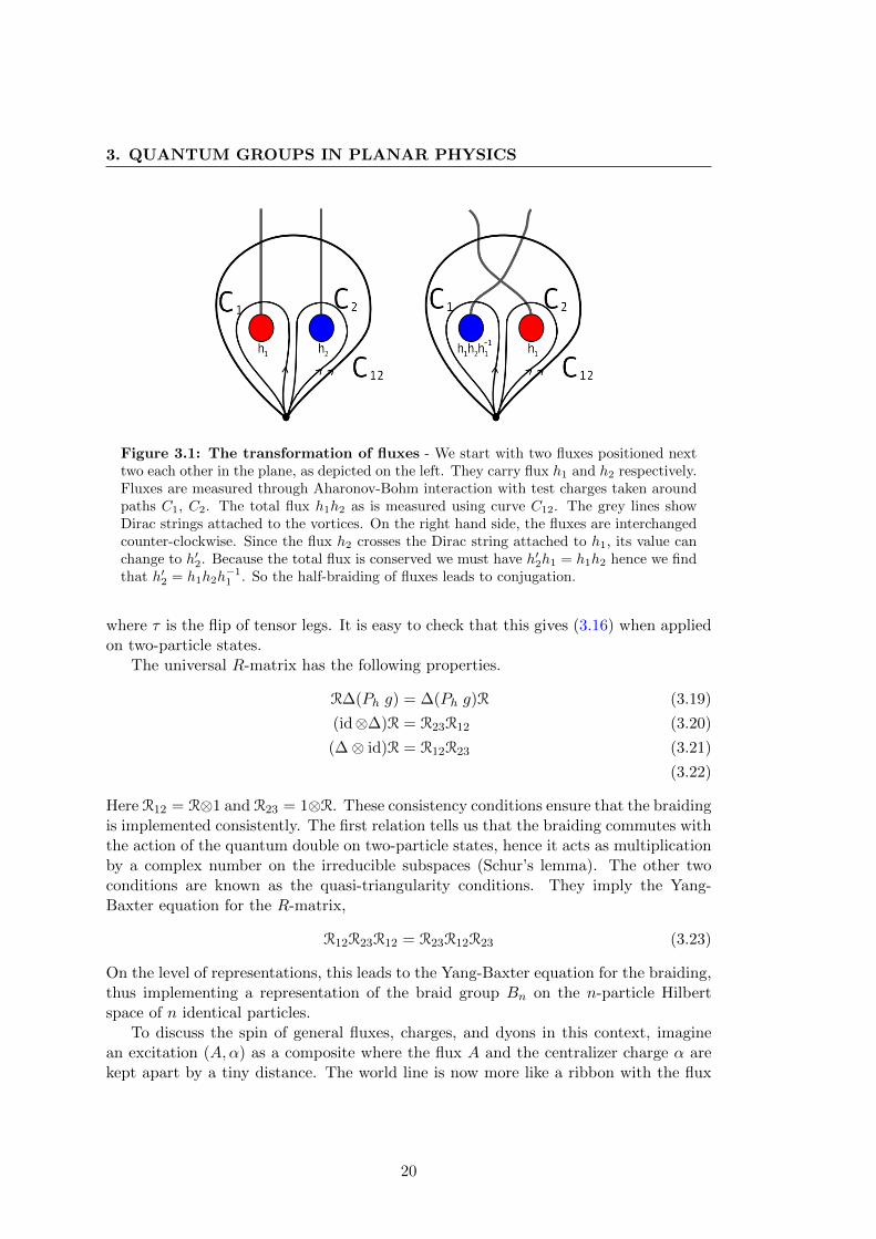
Suppose we have two fluxes with values h1 and h2. As is illustrated in figure 3.1,the requirement that the total flux has to be conserved leads to the conclusion that acounter-clockwise interchange results in commutation of h2 by h1. A charge crossingthe h1 Dirac line that is depicted in the figure picks up the action of h1 in its internalHilbert space. Hence we conclude that the general braiding operator acts as
R(A,α),(B,β)
(∣∣Ahi, αvj⟩ ∣∣∣Bhm, βvn⟩) =∣∣∣Ahi Bhm Ah
−1i ,Πβ(Ahi)
βvn
⟩ ∣∣Ahi, αvj⟩ (3.16)
This transformation can be accomplished by composing the action of a special elementin D[H]⊗D[H], called the universal R-matrix, on V A
α ⊗ V Bβ , with flipping the tensor
legs. The universal R-matrix for D[H] is
R ≡∑g,h
Pg e⊗ Ph g (3.17)
Acting on a two-particle state, R indeed measures the flux of the left particle andimplements it on the right particle. We can now define
R(A,α),(B,β) = τ(ΠAα ⊗ΠB
β )(R) (3.18)
19
3. QUANTUM GROUPS IN PLANAR PHYSICS
Figure 3.1: The transformation of fluxes - We start with two fluxes positioned nexttwo each other in the plane, as depicted on the left. They carry flux h1 and h2 respectively.Fluxes are measured through Aharonov-Bohm interaction with test charges taken aroundpaths C1, C2. The total flux h1h2 as is measured using curve C12. The grey lines showDirac strings attached to the vortices. On the right hand side, the fluxes are interchangedcounter-clockwise. Since the flux h2 crosses the Dirac string attached to h1, its value canchange to h′2. Because the total flux is conserved we must have h′2h1 = h1h2 hence we findthat h′2 = h1h2h
−11 . So the half-braiding of fluxes leads to conjugation.
where τ is the flip of tensor legs. It is easy to check that this gives (3.16) when appliedon two-particle states.
The universal R-matrix has the following properties.
R∆(Ph g) = ∆(Ph g)R (3.19)
(id⊗∆)R = R23R12 (3.20)
(∆⊗ id)R = R12R23 (3.21)
(3.22)
Here R12 = R⊗1 and R23 = 1⊗R. These consistency conditions ensure that the braidingis implemented consistently. The first relation tells us that the braiding commutes withthe action of the quantum double on two-particle states, hence it acts as multiplicationby a complex number on the irreducible subspaces (Schur’s lemma). The other twoconditions are known as the quasi-triangularity conditions. They imply the Yang-Baxter equation for the R-matrix,
R12R23R12 = R23R12R23 (3.23)
On the level of representations, this leads to the Yang-Baxter equation for the braiding,thus implementing a representation of the braid group Bn on the n-particle Hilbertspace of n identical particles.
To discuss the spin of general fluxes, charges, and dyons in this context, imaginean excitation (A,α) as a composite where the flux A and the centralizer charge α arekept apart by a tiny distance. The world line is now more like a ribbon with the flux
20
3.1 Discrete Gauge Theory
and the centralizer charge attached to opposite edges. A 2π rotation corresponds to afull twist of the ribbon, such that the charge winds around the flux. This implementsthe flux on the charge. This is generally accomplished by the letting the element∑
h
Ph h (3.24)
act, which results in ∑h
ΠAα (Ph h)
∣∣Ahi, αvj⟩ =∣∣Ahi,Πα(h1) αvj
⟩(3.25)
as can be seen from working out the rule (3.7). Since the element h1 commutes bydefinition with all elements of the centralizer C(A), we have
Πα(h1) = e2πih(A,α)1α (3.26)
as this follows from Schur’s lemma applied on the unitary irrep α. The phase θ(A,α) =exp(2πih(A,α)) is the spin of the (A,α)-particle. The element
∑h Ph h from equation
(3.24) is called the ribbon element of D[H]. Note that only true dyons can have θ(A,α) 6=±1.
3.1.3 Anti-particles
In DGTs every particle-type (A,α) has a unique conjugate particle-type (A, α) withthe special property that, as a pair, they can fuse to the vacuum, which is formalizedin the fusion rule
ΠAα ⊗ΠA
α = Π{e}0 + . . . (3.27)
As a representation of D[H], we can give the structure of (A, α) explicitly. The repre-sentation module of (A, α) is just the dual of the representation module of (A,α), i.e.V Aα = (V A
α )∗. The action of Ph g on a state⟨Ahi,
αvj∣∣ is given by
ΠAα (Ph g) :
⟨Ahi,
αvj∣∣→ ⟨
Ahi,αvj∣∣ΠA
α
(Pg−1h−1g g
−1)
(3.28)
Indeed, we do find a one-dimensional subspace in V Aα ⊗ V A
α that transforms like thevacuum under the action of D[H], namely the subspace spanned by∑
i,j
∣∣Ahi, αvj⟩ ⟨Ahi, αvj∣∣ (3.29)
We will show that the subspace spanned by this element transforms trivially, below.
Recall that the vacuum representation is given by
Π{e}0 (Ph g) = ε(Ph g) = δh,e (3.30)
21
3. QUANTUM GROUPS IN PLANAR PHYSICS
Now note that, in general, elements of V Aα ⊗V A
α can be regarded as linear operators onV Aα . In particular we have∑
i,j
∣∣Ahi, αvj⟩ ⟨Ahi, αvj∣∣ = 1(A,α) (3.31)
where 1(A,α) denotes the identity operator on V Aα . In particular it commutes with the
representation matrices. From this, it is easy to deduce that, as a state, it transformslike the vacuum as claimed. Indeed, working out the action of Ph g on 1(A,α) gives∑
h′h′′=h
ΠAα (Ph′ g)1(A,α)Π
Aα (Pg−1h′′−1g g
−1) =∑
h′h′′=h
δh′,h′′−1ΠAα (Ph′ g
−1g)1(A,α)
=∑h′
δh,eΠAα (Ph′ e)1(A,α) (3.32)
Note the subtle difference between (Ph g)∗ and S(Ph g).Again, it is a general feature that quantum group symmetry incorporates anti-
particles in a natural way. For this we need a linear map S from the quantum groupto itself, which is called the antipode, satisfying∑
(a)
S(a′)a′′ = 1ε(a) =∑(a)
a′S(a′′) (3.33)
for all elements a of the quantum group. Here we have made use of the Sweedlernotation
∆(a) =∑(a)
a′ ⊗ a′′ (3.34)
which generalizes
∆(Ph g) =∑h′h′′
Ph′ g ⊗ Ph′′ g (3.35)
to arbitrary cases.
3.2 General remarks
The discussion above is included to give a general idea of quantum group symmetry. It ispossible to give rigorous and general definitions of the essential structures that appearedabove, and to define in general what we mean by a quantum group. Let us give theusual mathematical nomenclature and some relevant references. Suppose we start withan associative algebra H that has a unit 1 ∈ H. Definition of a comultiplication ∆ andcounit ε satisfying certain axioms gives a coalgebra structure, which, if it is compatiblewith the algebra structure, makes H a bialgebra. If there is an antipode, this makesit a Hopf algebra. It can be shown that the antipode, if it exists, is unique, such thatany bialgebra has at most one Hopf algebra structure. The involution or ∗-structurenecessary to define unitary representations makes it a Hopf-∗-algebra.
22
3.2 General remarks
The most important feature in relation to planar physics is the possibility of non-trivial braiding. This is given by the existence of a universal R-matrix, which is anelement of H ⊗ H. It has to satisfy certain consistency relations which ensure thatthe braiding of representations obey the Yang-Baxter equation. The name for a Hopfalgebra with universal R-matrix is quasi-triangular.
It is nice to contemplate what is really new for quantum groups in comparison withthe usual group symmetries abundant in physics. Let us consider two important cases,symmetries given by a finite group H and symmetries given by a continuous Lie groupG.
instead of the group H, we can alternatively work with the group algebra C[H]without lossing any information. This is just the complex algebra generated by thegroup elements with the multiplication given by the group operation.
C[H] =⊕g∈H
Cg,
(∑g
cgg
)·
∑g′
cg′g′
=∑g,g′
cgcg′ gg′ (3.36)
This is in fact a Hopf algebra with comultiplication, counit and antipode
∆(g) = g ⊗ g, ε(g) = 1, S(g) = g−1 (3.37)
It is quasi-triangular, with universal R-matrix
R = e⊗ e (3.38)
where e is the unit element of H. Since this universal R-matrix is trivial, braiding justamount to flipping the tensor legs. This gives rise to the usual particle statistics inhigher dimensions. We might call C[H] triangular, instead of quasi-triangular.
For Lie groups G the situation is similar. Instead of the Lie group, one usuallyworks with the Lie algebra g. We usually allow for normal products xy apart from thebracket [x, y] and incorporate a unit 1 element, which is very natural if we think of thisLie algebra as an algebra of symmetry operators. Formally, this leads to the universalenveloping algebra U [g], which is generated by the unit 1 and the elements of g subjectto the relations
xy − yx = [x, y] (3.39)
It becomes a (quasi-)triangular Hopf algebra by defining
∆(1) = 1⊗ 1 ∆(x) = x⊗ 1 + 1⊗ xε(1) = 1 ε(x) = 0S(1) = 1 S(x) = −x
R = 1⊗ 1
(3.40)
which can be seen as the infinitesimal version of the definitions given for C[H].When we use the term quantum group, we have quasi-triangular Hopf algebras
in mind, with a non-trivial R-matrix leading to interesting braiding. Some authors
23
3. QUANTUM GROUPS IN PLANAR PHYSICS
seem to prefer to use the term quantum group only for quasi-triangular Hopf algebrasthat occur as q-deformations of semi-simple Lie algebras discussed below, or to includequasi-Hopf algebras, for which the coproduct does not precisely satisfy the axioms for acoalgebra, but do almost. For more general information on quantum groups and precisedefinitions, we refer to the literature, for example [46,60].
3.3 Chern-Simons theory and Uq[su(2)]
The quantum doubles that can be obtained via the Drinfel’d construction form animportant class of examples of quantum groups. The other important class comes froma semi-simple Lie algebra by “q-deformation” of the universal enveloping algebra. Wewill discuss an important example, Uq[su(2)], that comes from the Lie algebra su(2). Itplays an important role in the quantization of Chern-Simons theory with gauge groupSU(2) [84] and in the Wess-Zumino-Witten models for CFT [79,82] based on the affinealgebra of su(2) at level k. We follow [72].
One can view Uq[su(2)] as the algebra generated by the unit 1 and the three elementsH,L+ and L−, which satisfy the relations
[H,L±] = ±2L± (3.41)
[L+, L−] =qH/2 − q−H/2q1/2 − q−1/2
(3.42)
where q is a formal parameter that may be set to any non-zero complex number. Thecoproduct ∆ is given on the generators by
∆(1) = 1⊗ 1 (3.43)
∆(H) = 1⊗H +H ⊗ 1 (3.44)
∆(L±) = L± ⊗ qH/4 + q−H/4 ⊗ L± (3.45)
The counit and antipode are
ε(1) = 1, ε(H) = 0, ε(L±) = 0 (3.46)
S(1) = 1, S(H) = −H, S(L±) = −q∓1/4L± (3.47)
There is a ∗-structure given by
(L±)∗ = L∓, H∗ = H (3.48)
giving rise to the notion of unitary representations. Without the ∗-structure, it isperhaps better to call this algebra Uq[sl(2)] instead of Uq[su(2)], under which name thisquantum group usually appears in the literature.
In the limit q → 1, we recover the definitions for the universal enveloping U [su(2)]algebra of su(2), for instance
[L+, L−] = H (3.49)
24
3.3 Chern-Simons theory and Uq[su(2)]
Therefore, it is sensible to talk about a q-deformation of U [su(2)].If q is not a root of unity, the representation theory is very similar to that of U [su(2)].
For every half-integer j ∈ 12Z there is an irreducible highest weight representation of
dimension d = 2j+ 1 with highest weight λ = 2j. The representation modules V λ havean orthonormal basis
|j,m〉 , m ∈ {−j,−j + 1, . . . , j − 1, j} (3.50)
The action of the generators is
Πλ(H) |j,m〉 = 2m |j,m〉 (3.51)
L± |j,m〉 =√
[j ∓m]q[j ±m±1]q |j,m± 1〉 (3.52)
Here we have used the notation
[m]q =qm/2 − q−m/2q1/2 − q−1/2
(3.53)
for the so called q-numbers that enter the formula to the commutation relation [L+, L−] =[H]q.
A formal expression for the universal R-matrix of Uq[su(2)] is
R = qH⊗H
4
∞∑n=0
(1− q−1)n
[n]q!qn(1−n)/4
(qnH/4(L+)n
)⊗(q−nH/4(L−)n
)(3.54)
From this expression, one can work out the action on representations. This produces anon-trivial braiding in a similar fashion as we saw for DGT and the quantum double.
In relation to Chern-Simons theory and the WZW models, the most interesting caseis, however, when q is not a root of unity. In that case, the representation theory ofUq[su(2)] changes drastically. We will not go in to the details of the mathematical tricksneeded to find the right notion representations that describe charges in these physicaltheories. These can be read, for instance, in [46,60] or [72], but the right definition wasfirst discovered in [42]. In this case, we denote the resulting theory as su(2)k, where kis related to q as q = exp( 2πi
k+2). We will come back to these theories in chapter 5.
25

3. QUANTUM GROUPS IN PLANAR PHYSICS
26
CHAPTER 4
Anyons and tensor categories
As discussed in the previous chapter, quantum group symmetry can account for fusionand non-trivial braiding of excitations in (2+1)-dimensional systems. But the physicalstates usually correspond to the unitary irreps rather than the internal states of therepresentation modules. Also, in the case of Uq[su(2)] modules for q a root of unity,the identification of representations with particle types is not straight forward. Onemay ask if a rigorous formalism exists that treats these theories on the level of theexcitations rather than the underlying symmetries. The answer is yes.
Mathematically, the representations of a quantum group (often) form a modulartensor category, a structure that may be defined independently. In this chapter weintroduce many generalities of these tensor categories as they arise in physical appli-cations. These capture the topological properties, including the addition of quantumnumbers (fusion), of many theories in a very general way and allow for a graphicalformalism which can be regarded as a kind of topological Feynman diagrams. Theycan be constructed from quantum groups, but also arise directly from a (rational) CFTand can be used describe the excitations in Kitaev and Levin-Wen type lattice modelsdirectly. They are generally related to topological quantum field theories.
In stead of relying heavily on the language of category theory, we have chosen a routealong the lines of [22, 66]. This means that we focus on concreteness and calculability,in favour of formal language. For the mathematically inclined, this basically meansthat we assume the category to be strict and construct everything in terms of simpleobjects. A paper in the mathematical physics literature that treats tensor categoriesin a similar fashion is [34] where symmetries of the F -symbols (to be defined below)are derived. Proper mathematical textbooks are [14,75].
We have particularly relied on [22] for this chapter. In appendix B we give a moremathematically formulated description of the kind of categories that we consider, andpoint out how this connects to the formulation below.
27
4. ANYONS AND TENSOR CATEGORIES
4.1 Fusing and splitting
For a general theory, the particle-like excitations fall in different topological classes orsectors. For simplicity, we treat these sectors as elementary excitations and assumethere is finite number of them. These are the first ingredients of a modular tensorcategory, which in a physical context has to be unitary, or, more generally, a braidedtensor category.
One can vary the assumptions on the kind of tensor category in consideration. Eachset of assumptions gives a slightly different mathematical structure which has its ownname. To avoid getting stuck in nomenclature, we will generally refer to a ‘the theory’in this chapter. The term anyon models has also appeared in the physical literaturefor unitary braided tensor categories.
4.1.1 Fusion multiplicities
We start with a theory A with a finite collection of topological sectors CA = {a, b, c, . . . }.We also refer to these sectors as particle-types, (anyonic) charges, (particle) labels orsometimes simply particles or anyons. They obey a set of fusion rules that we write as
a× b =∑c∈CA
N cabc (4.1)
(The domain of the sum will be left implicit from now on.) Here the N cab are non-
negative integers called fusion multiplicities. These determine the possibilities for thetotal charge when two anyons are combined (fused). The total charge of two anyonswith respective labels a and b can be any of the c with N c
ab 6= 0. If N cab 6= 0, we also
speak of the fusion channel c of a and b, and we will sometimes write this as c ∈ a× b.If the state-space of a pair of particles is multidimensional this gives rise to non-
Abelian anyons.1 We say, therefore, that the theory is non-Abelian if there are chargesa and b that have ∑
c
N cab > 1 (4.2)
The particle labels together with the fusion rules (4.1) generate the fusion algebra ofthe theory. In this context we sometimes denote the basis states by kets |a〉 , |b〉 , |c〉.
The fusion algebra has to obey certain conditions which have a clear physical inter-pretation. We require that there is a unit, i.e. a unique trivial particle, the vacuum,0 ∈ A that fuses trivially with all labels: 0×a = a = a×0 for all a. Furthermore, fusionshould be an associative operation, (a× b)× c = a× (b× c), such that the total anyoniccharge is a well-defined notion. In terms of the fusion multiplicities, these conditions
1There is a subtlety to the term non-Abelian anyons. Even if a pair of identical particles have a amultidimensional state space, their braiding might still be Abelian. Hence, on could say that this is anecessary but not sufficient condition, but we will not bothered with the distinction.
28
4.1 Fusing and splitting
can translate to
N b0a =N b
a0 = δab (4.3)∑e
N eabN
dec =
∑f
NdafN
fbc (4.4)
We also require that the fusion rules are commutative, such that a × b = b × a. Thisshould hold for (2+1)-dimensional systems, since there is no way to define left and rightunambiguously. We can lift this requirement if we consider charges of a (1+1)d system,for example when we look at boundary excitations. Finally, each charge a ∈ CA shouldhave a unique conjugate charge a ∈ CA or anti-particle such that a and a can annihilate
a× a = 0 +∑c 6=0
N c”abc (4.5)
This does not mean that a and a can only fuse to the vacuum, as there might be c 6= 0with N c
aa 6= 0. Note that ¯a = a.The following relations for the fusion multiplicities also follow from these conditions
on fusion
N0ab = δba (4.6)
N cab = N c
ba = N abc = N c
ac (4.7)
The first line is just the anti-particle property. The second line can be derived usingcommutativity and associativity.
It is useful to define the fusion matrices Na with
(Na)bc = N cab (4.8)
The fusion rules give
NaNb =∑c
N cabNc (4.9)
which shows that the fusion matrices provide a representation of the fusion algebra.This is just the representation of the fusion algebra that is obtained by letting it acton itself via the fusion product. Associativity of the fusion rules translates to commu-tativity of the fusion matrices, such that
NaNb = NbNa (4.10)
The explicit diagonalization of the fusion matrices is a very interesting result, that wecome back to in section 4.4.
4.1.2 Diagrams and F -symbols
Special about the formalism based on category theory in comparison with the quantumgroup approach is that internal states are totally left out of the picture. This makes
29
4. ANYONS AND TENSOR CATEGORIES
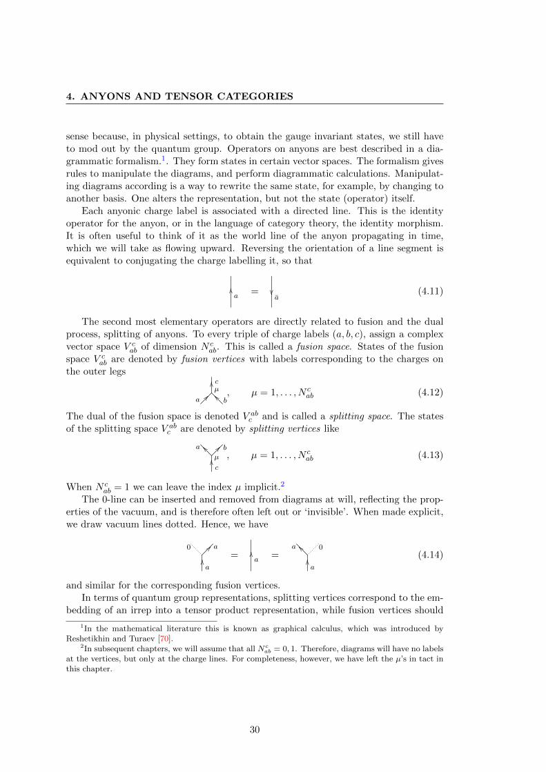
sense because, in physical settings, to obtain the gauge invariant states, we still haveto mod out by the quantum group. Operators on anyons are best described in a dia-grammatic formalism.1. They form states in certain vector spaces. The formalism givesrules to manipulate the diagrams, and perform diagrammatic calculations. Manipulat-ing diagrams according is a way to rewrite the same state, for example, by changing toanother basis. One alters the representation, but not the state (operator) itself.
Each anyonic charge label is associated with a directed line. This is the identityoperator for the anyon, or in the language of category theory, the identity morphism.It is often useful to think of it as the world line of the anyon propagating in time,which we will take as flowing upward. Reversing the orientation of a line segment isequivalent to conjugating the charge labelling it, so that
OOa
= ��a
(4.11)
The second most elementary operators are directly related to fusion and the dualprocess, splitting of anyons. To every triple of charge labels (a, b, c), assign a complexvector space V c
ab of dimension N cab. This is called a fusion space. States of the fusion
space V cab are denoted by fusion vertices with labels corresponding to the charges on
the outer legs
µ??
a__b
OO c, µ = 1, . . . , N c
ab (4.12)
The dual of the fusion space is denoted V abc and is called a splitting space. The states
of the splitting space V abc are denoted by splitting vertices like
µ
__a ?? bOOc
, µ = 1, . . . , N cab (4.13)
When N cab = 1 we can leave the index µ implicit.2
The 0-line can be inserted and removed from diagrams at will, reflecting the prop-erties of the vacuum, and is therefore often left out or ‘invisible’. When made explicit,we draw vacuum lines dotted. Hence, we have
0 ?? aOOa
=OOa
=__a 0
OOa
(4.14)
and similar for the corresponding fusion vertices.In terms of quantum group representations, splitting vertices correspond to the em-
bedding of an irrep into a tensor product representation, while fusion vertices should
1In the mathematical literature this is known as graphical calculus, which was introduced byReshetikhin and Turaev [70].
2In subsequent chapters, we will assume that all Ncab = 0, 1. Therefore, diagrams will have no labels
at the vertices, but only at the charge lines. For completeness, however, we have left the µ’s in tact inthis chapter.
30
4.1 Fusing and splitting
be thought of as the projection onto an irreducible subspace of a tensor product repre-sentation.
General anyon operators can be made by stacking fusion and splitting vertices andtaking linear combinations. The intermediate charges of connected charge lines haveto agree and the vertices should be allowed by the fusion rules, otherwise the wholediagram evaluates to zero. This gives a diagrammatic encoding of charge conservation.As a general notation we write V a1,...,am
a′1,...,a′n
for the vector space of operators that take
n anyons with charges a′1, . . . , a′n as input and which produce m anyons of charges
a1, . . . , am.An important example is V abc
d . Operators of this space can be made by stackingtwo splitting vertices on top of each other. The choice we have of connecting the topvertex either on the right or on the left of the bottom vertex leads to two differentbases of V abc
d . The change of basis in these spaces is given by so called F -symbols1
[F abcd ](e,α,β)(f,µ,ν), which are an important piece of data for these models. They aredefined by the diagrammatic equation
a b c
d
eα
β
__ ?? ??
OO__ =
∑f,µ,ν
[F abcd ](e,α,β)(f,µ,ν)
a b c
d
fµ
ν
__ __ ??
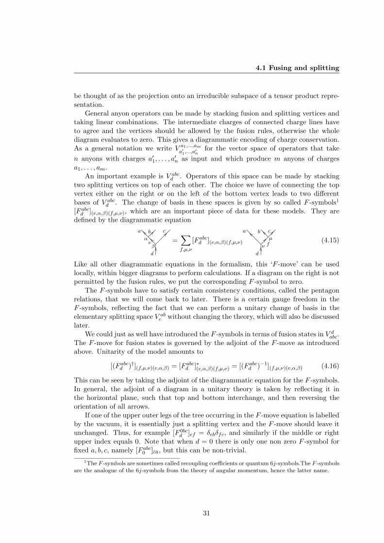
OO?? (4.15)
Like all other diagrammatic equations in the formalism, this ‘F -move’ can be usedlocally, within bigger diagrams to perform calculations. If a diagram on the right is notpermitted by the fusion rules, we put the corresponding F -symbol to zero.
The F -symbols have to satisfy certain consistency conditions, called the pentagonrelations, that we will come back to later. There is a certain gauge freedom in theF -symbols, reflecting the fact that we can perform a unitary change of basis in theelementary splitting space V ab
c without changing the theory, which will also be discussedlater.
We could just as well have introduced the F -symbols in terms of fusion states in V dabc.
The F -move for fusion states is governed by the adjoint of the F -move as introducedabove. Unitarity of the model amounts to
[(F abcd )†](f,µ,ν)(e,α,β) = [F abcd ]∗(e,α,β)(f,µ,ν) = [(F abcd )−1](f,µ,ν)(e,α,β) (4.16)
This can be seen by taking the adjoint of the diagrammatic equation for the F -symbols.In general, the adjoint of a diagram in a unitary theory is taken by reflecting it inthe horizontal plane, such that top and bottom interchange, and then reversing theorientation of all arrows.
If one of the upper outer legs of the tree occurring in the F -move equation is labelledby the vacuum, it is essentially just a splitting vertex and the F -move should leave itunchanged. Thus, for example [F 0bc
d ]ef = δebδfc, and similarly if the middle or rightupper index equals 0. Note that when d = 0 there is only one non zero F -symbol forfixed a, b, c, namely [F abc0 ]ca, but this can be non-trivial.
1The F -symbols are sometimes called recoupling coefficients or quantum 6j-symbols.The F -symbolsare the analogue of the 6j-symbols from the theory of angular momentum, hence the latter name.
31
4. ANYONS AND TENSOR CATEGORIES
The pairing of V abc and V c
ab or the inner product of fusion/splitting states, is againdenoted by stacking the appropriate diagrams. We think of the elements of V ab
c as ketsand of the elements of V c
ab as bras. Composition of operators is written from bottomto top, in accordance with the flow of time. The conservation of anyonic charge is alsotaken into account in the diagrams, which gives
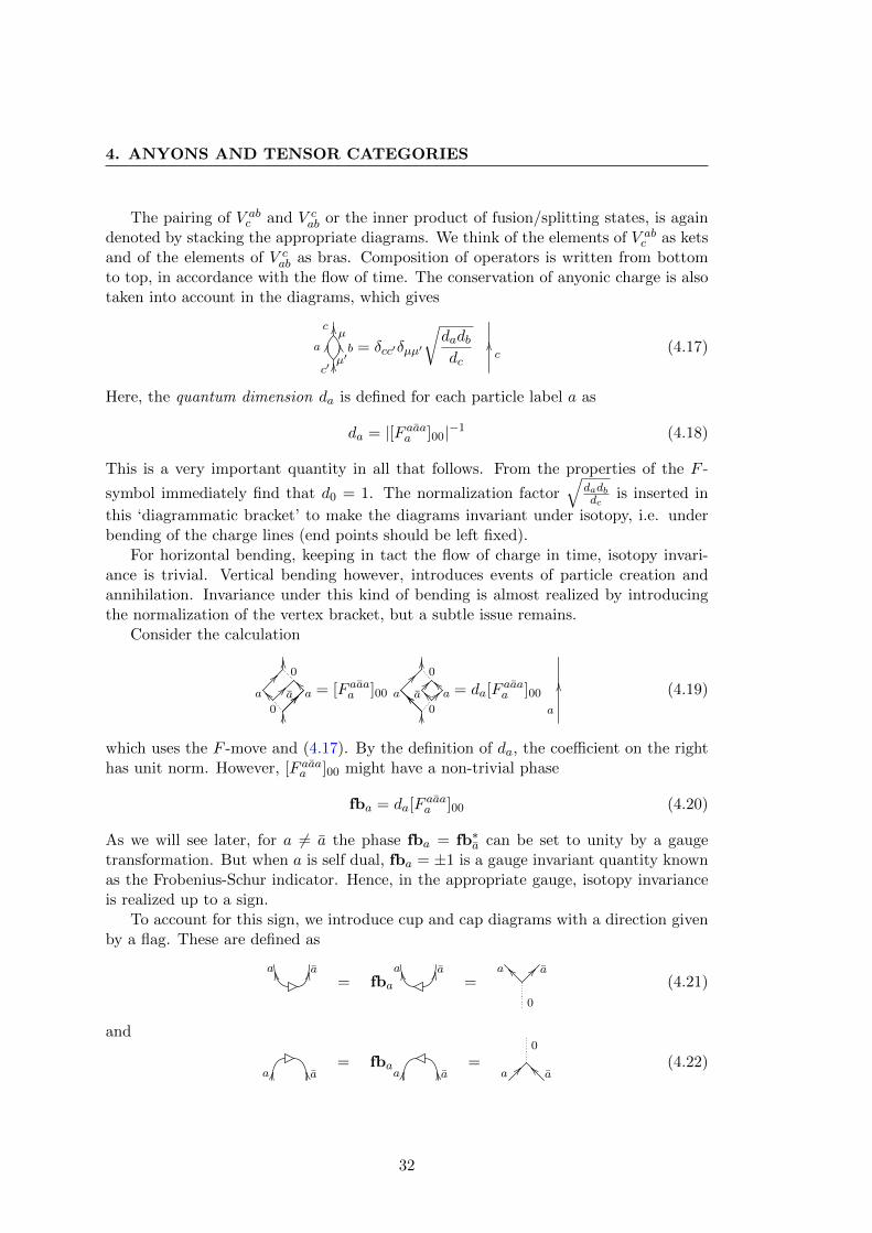
c
a b
c′
µ
µ′
OOLL RROO
= δcc′δµµ′
√dadbdc
OOc
(4.17)
Here, the quantum dimension da is defined for each particle label a as
da = |[F aaaa ]00|−1 (4.18)
This is a very important quantity in all that follows. From the properties of the F -
symbol immediately find that d0 = 1. The normalization factor√
dadbdc
is inserted in
this ‘diagrammatic bracket’ to make the diagrams invariant under isotopy, i.e. underbending of the charge lines (end points should be left fixed).
For horizontal bending, keeping in tact the flow of charge in time, isotopy invari-ance is trivial. Vertical bending however, introduces events of particle creation andannihilation. Invariance under this kind of bending is almost realized by introducingthe normalization of the vertex bracket, but a subtle issue remains.
Consider the calculation
OO????__??__
??OO
a a a
0
0
= [F aaaa ]00
OO____
??OO
__ ???? __
a a a
0
0
= da[Faaaa ]00
a
OO(4.19)
which uses the F -move and (4.17). By the definition of da, the coefficient on the righthas unit norm. However, [F aaaa ]00 might have a non-trivial phase
fba = da[Faaaa ]00 (4.20)
As we will see later, for a 6= a the phase fba = fb∗a can be set to unity by a gaugetransformation. But when a is self dual, fba = ±1 is a gauge invariant quantity knownas the Frobenius-Schur indicator. Hence, in the appropriate gauge, isotopy invarianceis realized up to a sign.
To account for this sign, we introduce cup and cap diagrams with a direction givenby a flag. These are defined as
a aRR LL= fba
a aRR LL=
__a ?? a
0
(4.21)
and
a aLL RR = fbaa aLL RR = ??
a__a
0
(4.22)
32
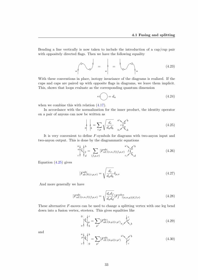
4.1 Fusing and splitting
Bending a line vertically is now taken to include the introduction of a cap/cup pairwith oppositely directed flags. Then we have the following equality
aMM
NN
=a
OO=
aQQ
PP
(4.23)
With these conventions in place, isotopy invariance of the diagrams is realized. If thecups and caps are paired up with opposite flags in diagrams, we leave them implicit.This, shows that loops evaluate as the corresponding quantum dimension
aOO
= da (4.24)
when we combine this with relation (4.17).In accordance with the normalization for the inner product, the identity operator
on a pair of anyons can now be written as
a b
OO OO =∑c,µ
√dcdadb
a b
a b
cµ
µ
__ ??
?? __OO (4.25)
It is very convenient to define F -symbols for diagrams with two-anyon input andtwo-anyon output. This is done by the diagrammatic equations
a b
c d
eαβOO
OO
OO
OO__ =
∑(f,µ,ν)
[F abcd ](e,α,β)(f,µ,ν)
a b
c d
fµ
ν
__ ??
?? __OO (4.26)
Equation (4.25) gives
[F abab ]0,(c,µ,ν) =
√dcdadb
δµ,ν (4.27)
And more generally we have
[F abcd ](e,α,β)(f,µ,ν) =
√dedfdadd
[F cebf ]∗(a,α,µ)(d,β,ν) (4.28)
These alternative F -moves can be used to change a splitting vertex with one leg benddown into a fusion vertex, etcetera. This gives equalities like
0 c
a b
aµOO OO
OO__ =
∑µ′
[F 0cab ](a,µ)(c,µ′)
µ′??a
__b
OO c(4.29)
anda b
c 0
bµ
OO
OO OO__ =
∑µ′
[F abc0 ](a,µ)(c,µ′) µ′
__a ?? bOOc
(4.30)
33
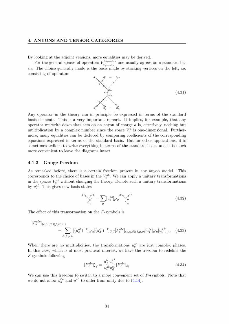
4. ANYONS AND TENSOR CATEGORIES
By looking at the adjoint versions, more equalities may be derived.
For the general spaces of operators V a1,...,ama′1,...,a
′n
one usually agrees on a standard ba-
sis. The choice generally made is the basis made by stacking vertices on the left, i.e.consisting of operators
a1 a2 ... am
a′1 a′2 ... a′n
. . .
e
. ..
µ2
µm
µ′2
µ′n
??
??
OO
____ ?? ??
__ __
(4.31)
Any operator in the theory can in principle be expressed in terms of the standardbasis elements. This is a very important remark. It implies, for example, that anyoperator we write down that acts on an anyon of charge a is, effectively, nothing butmultiplication by a complex number since the space V a
a is one-dimensional. Further-more, many equalities can be deduced by comparing coefficients of the correspondingequations expressed in terms of the standard basis. But for other applications, it issometimes tedious to write everything in terms of the standard basis, and it is muchmore convenient to leave the diagrams intact.
4.1.3 Gauge freedom
As remarked before, there is a certain freedom present in any anyon model. Thiscorresponds to the choice of bases in the V ab
c . We can apply a unitary transformationsin the spaces V ab
c without changing the theory. Denote such a unitary transformationsby uabc . This gives new basis states
µ′
__a ?? bOOc
=∑µ
[uabc ]µ′µ µ
__a ?? bOOc
(4.32)
The effect of this transormation on the F -symbols is
[F abcd ](e,α′,β′)(f,µ′,ν′)
=∑
α,β,µ,ν
[(uabe )−1]α′α[(uecd )−1]β′β[F abcd ](e,α,β)(f,µ,ν)[ubcf ]µ′µ[uafd ]ν′ν (4.33)
When there are no multiplicities, the transformations uabc are just complex phases.In this case, which is of most practical interest, we have the freedom to redefine theF -symbols following
[F abcd ]′ef =ubcf u
afd
uabe uecd
[F abcd ]ef (4.34)
We can use this freedom to switch to a more convenient set of F -symbols. Note thatwe do not allow u0a
a and ua0 to differ from unity due to (4.14).
34
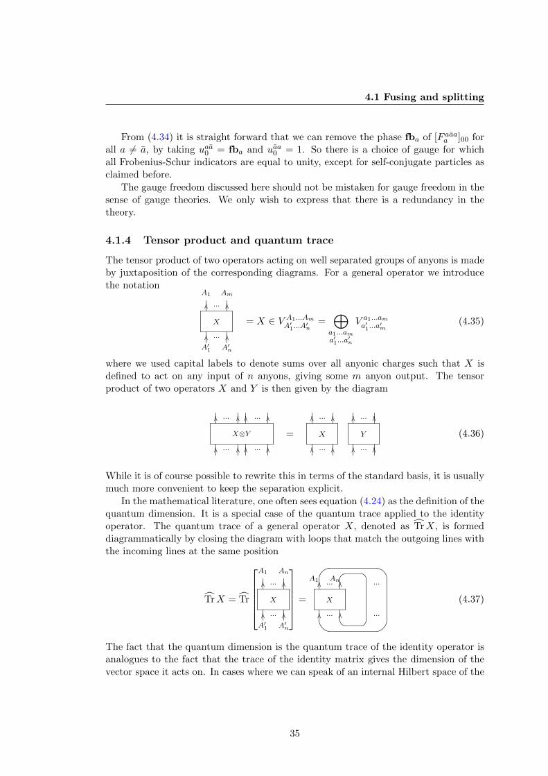
4.1 Fusing and splitting
From (4.34) it is straight forward that we can remove the phase fba of [F aaaa ]00 forall a 6= a, by taking uaa0 = fba and uaa0 = 1. So there is a choice of gauge for whichall Frobenius-Schur indicators are equal to unity, except for self-conjugate particles asclaimed before.
The gauge freedom discussed here should not be mistaken for gauge freedom in thesense of gauge theories. We only wish to express that there is a redundancy in thetheory.
4.1.4 Tensor product and quantum trace
The tensor product of two operators acting on well separated groups of anyons is madeby juxtaposition of the corresponding diagrams. For a general operator we introducethe notation
X
A1 Am
A′1 A′n
OO OO
OO OO
...
...
= X ∈ V A1...AmA′1...A
′n
=⊕a1...ama′1...a
′n
V a1...ama′1...a
′m
(4.35)
where we used capital labels to denote sums over all anyonic charges such that X isdefined to act on any input of n anyons, giving some m anyon output. The tensorproduct of two operators X and Y is then given by the diagram
X⊗Y
OO OO
OO OO
OOOO
OOOO
...
...
...
...
= X
OO OO
OO OO
...
...
Y
OO OO
OO OO
...
...
(4.36)
While it is of course possible to rewrite this in terms of the standard basis, it is usuallymuch more convenient to keep the separation explicit.
In the mathematical literature, one often sees equation (4.24) as the definition of thequantum dimension. It is a special case of the quantum trace applied to the identityoperator. The quantum trace of a general operator X, denoted as TrX, is formeddiagrammatically by closing the diagram with loops that match the outgoing lines withthe incoming lines at the same position
TrX = Tr
X
A1 An
A′1 A′n
OO OO
OO OO
...
...
= X
A1 AnOO OO
OO OO
...
...
...
...
(4.37)
The fact that the quantum dimension is the quantum trace of the identity operator isanalogues to the fact that the trace of the identity matrix gives the dimension of thevector space it acts on. In cases where we can speak of an internal Hilbert space of the
35
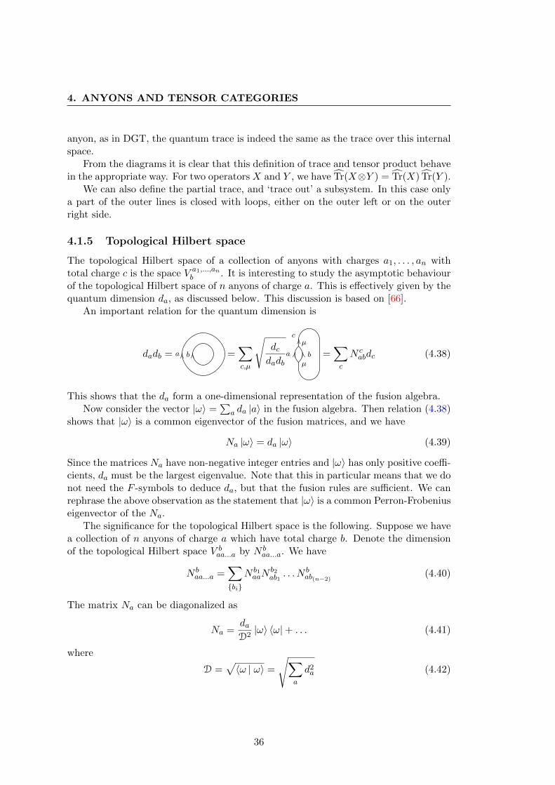
4. ANYONS AND TENSOR CATEGORIES
anyon, as in DGT, the quantum trace is indeed the same as the trace over this internalspace.
From the diagrams it is clear that this definition of trace and tensor product behavein the appropriate way. For two operators X and Y , we have Tr(X⊗Y ) = Tr(X) Tr(Y ).
We can also define the partial trace, and ‘trace out’ a subsystem. In this case onlya part of the outer lines is closed with loops, either on the outer left or on the outerright side.
4.1.5 Topological Hilbert space
The topological Hilbert space of a collection of anyons with charges a1, . . . , an withtotal charge c is the space V a1,...,an
b . It is interesting to study the asymptotic behaviourof the topological Hilbert space of n anyons of charge a. This is effectively given by thequantum dimension da, as discussed below. This discussion is based on [66].
An important relation for the quantum dimension is
dadb = b OOa OO =∑c,µ
√dcdadb
a b
cµ
µ
OO
LL RR =∑c
N cabdc (4.38)
This shows that the da form a one-dimensional representation of the fusion algebra.Now consider the vector |ω〉 =
∑a da |a〉 in the fusion algebra. Then relation (4.38)
shows that |ω〉 is a common eigenvector of the fusion matrices, and we have
Na |ω〉 = da |ω〉 (4.39)
Since the matrices Na have non-negative integer entries and |ω〉 has only positive coeffi-cients, da must be the largest eigenvalue. Note that this in particular means that we donot need the F -symbols to deduce da, but that the fusion rules are sufficient. We canrephrase the above observation as the statement that |ω〉 is a common Perron-Frobeniuseigenvector of the Na.
The significance for the topological Hilbert space is the following. Suppose we havea collection of n anyons of charge a which have total charge b. Denote the dimensionof the topological Hilbert space V b
aa...a by N baa...a. We have
N baa...a =
∑{bi}
N b1aaN
b2ab1
. . . N bab(n−2)
(4.40)
The matrix Na can be diagonalized as
Na =daD2|ω〉 〈ω|+ . . . (4.41)
where
D =√〈ω | ω〉 =
√∑a
d2a (4.42)
36
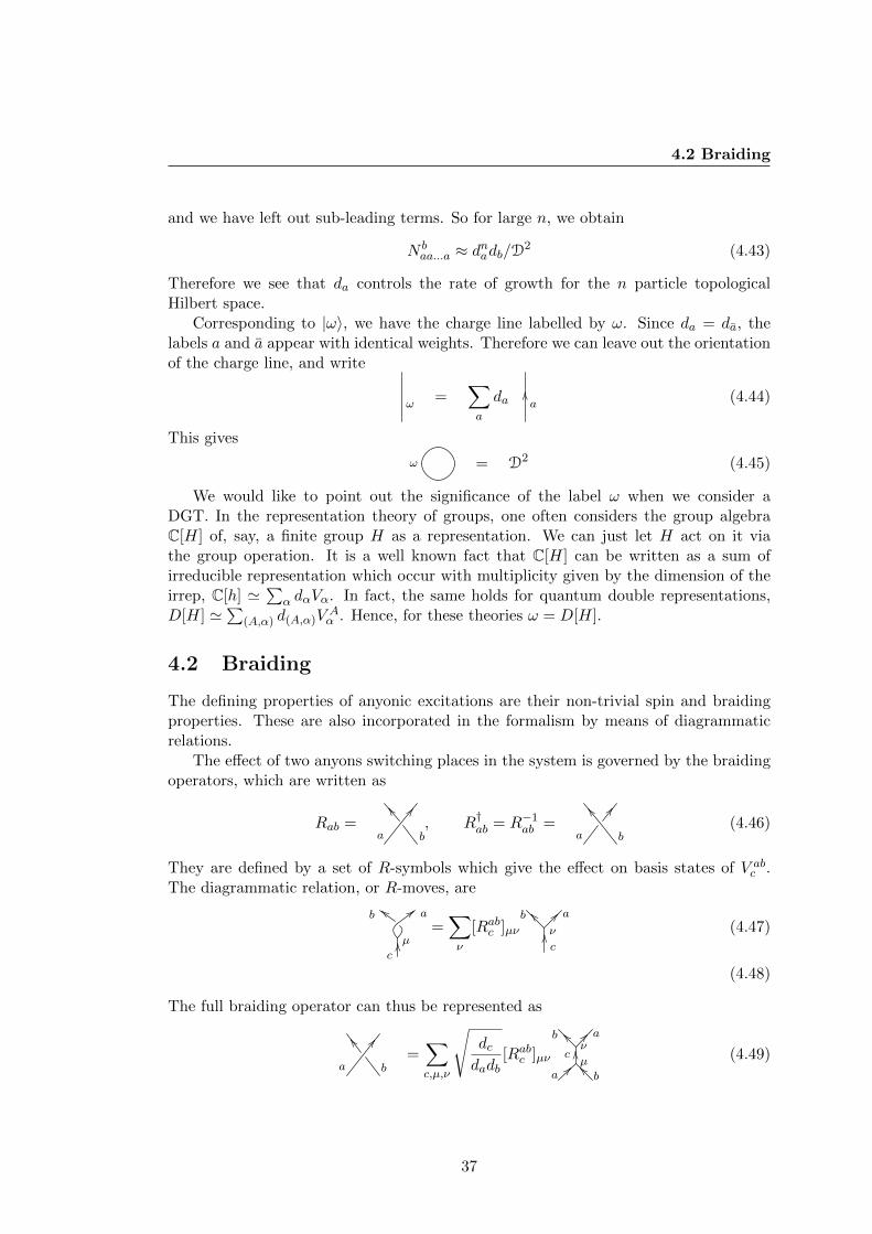
4.2 Braiding
and we have left out sub-leading terms. So for large n, we obtain
N baa...a ≈ dnadb/D2 (4.43)
Therefore we see that da controls the rate of growth for the n particle topologicalHilbert space.
Corresponding to |ω〉, we have the charge line labelled by ω. Since da = da, thelabels a and a appear with identical weights. Therefore we can leave out the orientationof the charge line, and write
ω=
∑a
daOOa
(4.44)
This gives
ω = D2 (4.45)
We would like to point out the significance of the label ω when we consider aDGT. In the representation theory of groups, one often considers the group algebraC[H] of, say, a finite group H as a representation. We can just let H act on it viathe group operation. It is a well known fact that C[H] can be written as a sum ofirreducible representation which occur with multiplicity given by the dimension of theirrep, C[h] ' ∑α dαVα. In fact, the same holds for quantum double representations,D[H] '∑(A,α) d(A,α)V
Aα . Hence, for these theories ω = D[H].
4.2 Braiding
The defining properties of anyonic excitations are their non-trivial spin and braidingproperties. These are also incorporated in the formalism by means of diagrammaticrelations.
The effect of two anyons switching places in the system is governed by the braidingoperators, which are written as
Rab =a b
BB[[, R†ab = R−1
ab =a b
CC\\(4.46)
They are defined by a set of R-symbols which give the effect on basis states of V abc .
The diagrammatic relation, or R-moves, are
b a
µOOc
;;cc
=∑ν
[Rabc ]µν ν
__b ?? aOOc
(4.47)
(4.48)
The full braiding operator can thus be represented as
a b
BB[[=∑c,µ,ν
√dcdadb
[Rabc ]µν
b a
a b
cν
µ
__ ??
?? __OO (4.49)
37
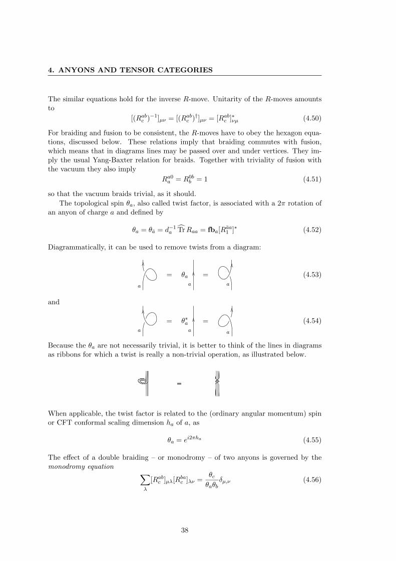
4. ANYONS AND TENSOR CATEGORIES
The similar equations hold for the inverse R-move. Unitarity of the R-moves amountsto
[(Rabc )−1]µν = [(Rabc )†]µν = [Rabc ]∗νµ (4.50)
For braiding and fusion to be consistent, the R-moves have to obey the hexagon equa-tions, discussed below. These relations imply that braiding commutes with fusion,which means that in diagrams lines may be passed over and under vertices. They im-ply the usual Yang-Baxter relation for braids. Together with triviality of fusion withthe vacuum they also imply
Ra0a = R0b
b = 1 (4.51)
so that the vacuum braids trivial, as it should.
The topological spin θa, also called twist factor, is associated with a 2π rotation ofan anyon of charge a and defined by
θa = θa = d−1a TrRaa = fba[R
aa1 ]∗ (4.52)
Diagrammatically, it can be used to remove twists from a diagram:
a
OO
= θaa
OO=
a
OO
(4.53)
and
a
OO
= θ∗aa
OO=
a
OO
(4.54)
Because the θa are not necessarily trivial, it is better to think of the lines in diagramsas ribbons for which a twist is really a non-trivial operation, as illustrated below.
When applicable, the twist factor is related to the (ordinary angular momentum) spinor CFT conformal scaling dimension ha of a, as
θa = ei2πha (4.55)
The effect of a double braiding – or monodromy – of two anyons is governed by themonodromy equation ∑
λ
[Rabc ]µλ[Rbac ]λν =θcθaθb
δµ,ν (4.56)
38
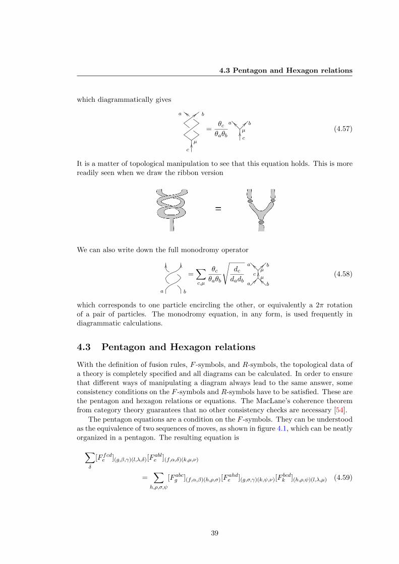
4.3 Pentagon and Hexagon relations
which diagrammatically gives
c
µ
a b
OO
;;cc
=θcθaθb
µ
__a ?? bOOc
(4.57)
It is a matter of topological manipulation to see that this equation holds. This is morereadily seen when we draw the ribbon version
We can also write down the full monodromy operator
a b
OO OO
=∑c,µ
θcθaθb
√dcdadb
a b
a b
cµ
µ
__ ??
?? __OO (4.58)
which corresponds to one particle encircling the other, or equivalently a 2π rotationof a pair of particles. The monodromy equation, in any form, is used frequently indiagrammatic calculations.
4.3 Pentagon and Hexagon relations
With the definition of fusion rules, F -symbols, and R-symbols, the topological data ofa theory is completely specified and all diagrams can be calculated. In order to ensurethat different ways of manipulating a diagram always lead to the same answer, someconsistency conditions on the F -symbols and R-symbols have to be satisfied. These arethe pentagon and hexagon relations or equations. The MacLane’s coherence theoremfrom category theory guarantees that no other consistency checks are necessary [54].
The pentagon equations are a condition on the F -symbols. They can be understoodas the equivalence of two sequences of moves, as shown in figure 4.1, which can be neatlyorganized in a pentagon. The resulting equation is∑
δ
[F fcde ](g,β,γ)(l,λ,δ)[Fable ](f,α,δ)(k,µ,ν)
=∑h,ρ,σ,ψ
[F abcg ](f,α,β)(h,ρ,σ)[Fahde ](g,σ,γ)(k,ψ,ν)[F
bcdk ](h,ρ,ψ)(l,λ,µ) (4.59)
39
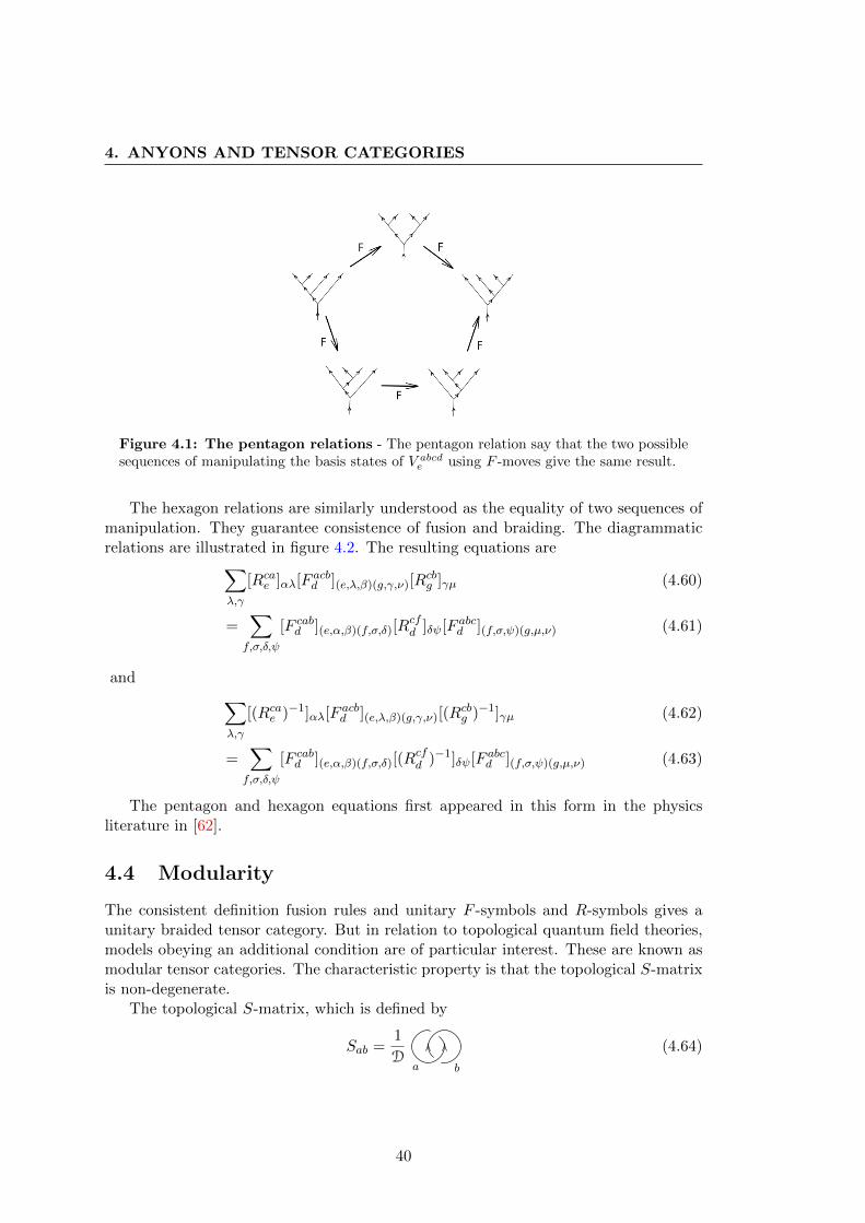
4. ANYONS AND TENSOR CATEGORIES
Figure 4.1: The pentagon relations - The pentagon relation say that the two possiblesequences of manipulating the basis states of V abcde using F -moves give the same result.
The hexagon relations are similarly understood as the equality of two sequences ofmanipulation. They guarantee consistence of fusion and braiding. The diagrammaticrelations are illustrated in figure 4.2. The resulting equations are∑
λ,γ
[Rcae ]αλ[F acbd ](e,λ,β)(g,γ,ν)[Rcbg ]γµ (4.60)
=∑f,σ,δ,ψ
[F cabd ](e,α,β)(f,σ,δ)[Rcfd ]δψ[F abcd ](f,σ,ψ)(g,µ,ν) (4.61)
and ∑λ,γ
[(Rcae )−1]αλ[F acbd ](e,λ,β)(g,γ,ν)[(Rcbg )−1]γµ (4.62)
=∑f,σ,δ,ψ
[F cabd ](e,α,β)(f,σ,δ)[(Rcfd )−1]δψ[F abcd ](f,σ,ψ)(g,µ,ν) (4.63)
The pentagon and hexagon equations first appeared in this form in the physicsliterature in [62].
4.4 Modularity
The consistent definition fusion rules and unitary F -symbols and R-symbols gives aunitary braided tensor category. But in relation to topological quantum field theories,models obeying an additional condition are of particular interest. These are known asmodular tensor categories. The characteristic property is that the topological S-matrixis non-degenerate.
The topological S-matrix, which is defined by
Sab =1
Da b
OO OO (4.64)
40
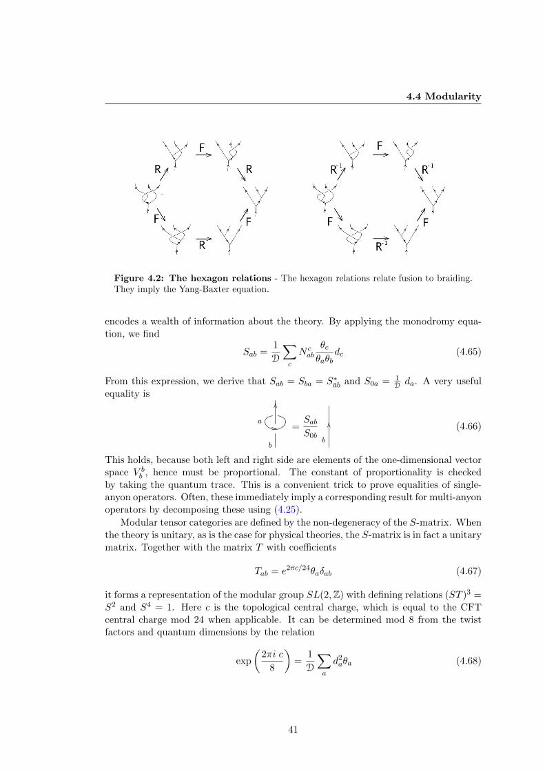
4.4 Modularity
Figure 4.2: The hexagon relations - The hexagon relations relate fusion to braiding.They imply the Yang-Baxter equation.
encodes a wealth of information about the theory. By applying the monodromy equa-tion, we find
Sab =1
D
∑c
N cab
θcθaθb
dc (4.65)
From this expression, we derive that Sab = Sba = S∗ab and S0a = 1Dda. A very useful
equality is
b
a
OO
// =SabS0b
b
OO(4.66)
This holds, because both left and right side are elements of the one-dimensional vectorspace V b
b , hence must be proportional. The constant of proportionality is checkedby taking the quantum trace. This is a convenient trick to prove equalities of single-anyon operators. Often, these immediately imply a corresponding result for multi-anyonoperators by decomposing these using (4.25).
Modular tensor categories are defined by the non-degeneracy of the S-matrix. Whenthe theory is unitary, as is the case for physical theories, the S-matrix is in fact a unitarymatrix. Together with the matrix T with coefficients
Tab = e2πc/24θaδab (4.67)
it forms a representation of the modular group SL(2,Z) with defining relations (ST )3 =S2 and S4 = 1. Here c is the topological central charge, which is equal to the CFTcentral charge mod 24 when applicable. It can be determined mod 8 from the twistfactors and quantum dimensions by the relation
exp
(2πi c
8
)=
1
D
∑a
d2aθa (4.68)
41
4. ANYONS AND TENSOR CATEGORIES
This is all well known, but since it is an interesting application of the diagrammaticformalism we include a derivation based on [14] of the relations between S and T below.
Let
p± =∑a
d2aθ±1a (4.69)
The following equations hold
b
ω
OO
= p+θ−1b
b
OO,
b
ω
OO
= p−θbb
OO(4.70)
To show these equalities, note that the left and right hand side of these equationsmust be proportional, since they are both single-anyon operators. Hence we take thequantum trace on either side to check the proportionality constant. For the equationinvolving p+, the quantum trace of the right hand side is evidently p+db/θb, while theleft hand side gives ∑
a
daθaDSab =∑a,c
N cabdadcθc/θb (4.71)
=∑c
d2cθcdb/θb (4.72)
= p+db/θb (4.73)
Here we used that∑
aNcabda =
∑aN
acbda = dbdc by (4.38), the symmetries of the fusion
coefficients, and the fact that da = da. As a consequence we get
a b
ω
OO OO
= p+θ−1a θ−1
b
ba
OOOO
(4.74)
To see this, apply the ribbon property on the double clockwise braid on the right handside, i.e. on the operator (R†ab)
2, and compare with (4.70).
Define
T ′ab = θaδab, Cab = δab (4.75)
Thus T ′ is just T with the phase in front left out, and C is the charge conjugationmatrix. Clearly, C commutes with S and with T ′, and C2 = 1. But more interestingly
1. (ST ′)3 = p+S2C/D
2. (ST ′−1)3 = p−S2/D
3. S2 = p+p−C/D2
42
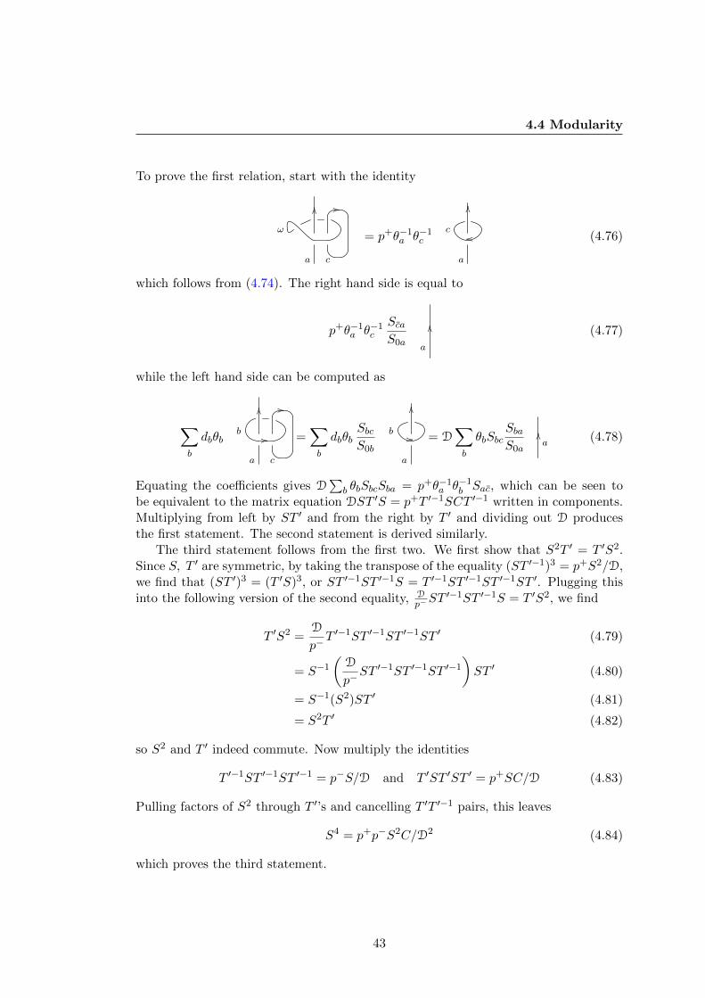
4.4 Modularity
To prove the first relation, start with the identity
a c
ω
OO //
= p+θ−1a θ−1
c
a
c
OO
oo (4.76)
which follows from (4.74). The right hand side is equal to
p+θ−1a θ−1
c
ScaS0a
a
OO(4.77)
while the left hand side can be computed as
∑b
dbθb
a c
b
OO
//
//
=∑b
dbθbSbcS0b
a
b
OO
// = D∑b
θbSbcSbaS0a
OOa
(4.78)
Equating the coefficients gives D∑
b θbSbcSba = p+θ−1a θ−1
b Sac, which can be seen tobe equivalent to the matrix equation DST ′S = p+T ′−1SCT ′−1 written in components.Multiplying from left by ST ′ and from the right by T ′ and dividing out D producesthe first statement. The second statement is derived similarly.
The third statement follows from the first two. We first show that S2T ′ = T ′S2.Since S, T ′ are symmetric, by taking the transpose of the equality (ST ′−1)3 = p+S2/D,we find that (ST ′)3 = (T ′S)3, or ST ′−1ST ′−1S = T ′−1ST ′−1ST ′−1ST ′. Plugging thisinto the following version of the second equality, D
p−ST′−1ST ′−1S = T ′S2, we find
T ′S2 =D
p−T ′−1ST ′−1ST ′−1ST ′ (4.79)
= S−1
(D
p−ST ′−1ST ′−1ST ′−1
)ST ′ (4.80)
= S−1(S2)ST ′ (4.81)
= S2T ′ (4.82)
so S2 and T ′ indeed commute. Now multiply the identities
T ′−1ST ′−1ST ′−1 = p−S/D and T ′ST ′ST ′ = p+SC/D (4.83)
Pulling factors of S2 through T ′’s and cancelling T ′T ′−1 pairs, this leaves
S4 = p+p−S2C/D2 (4.84)
which proves the third statement.
43
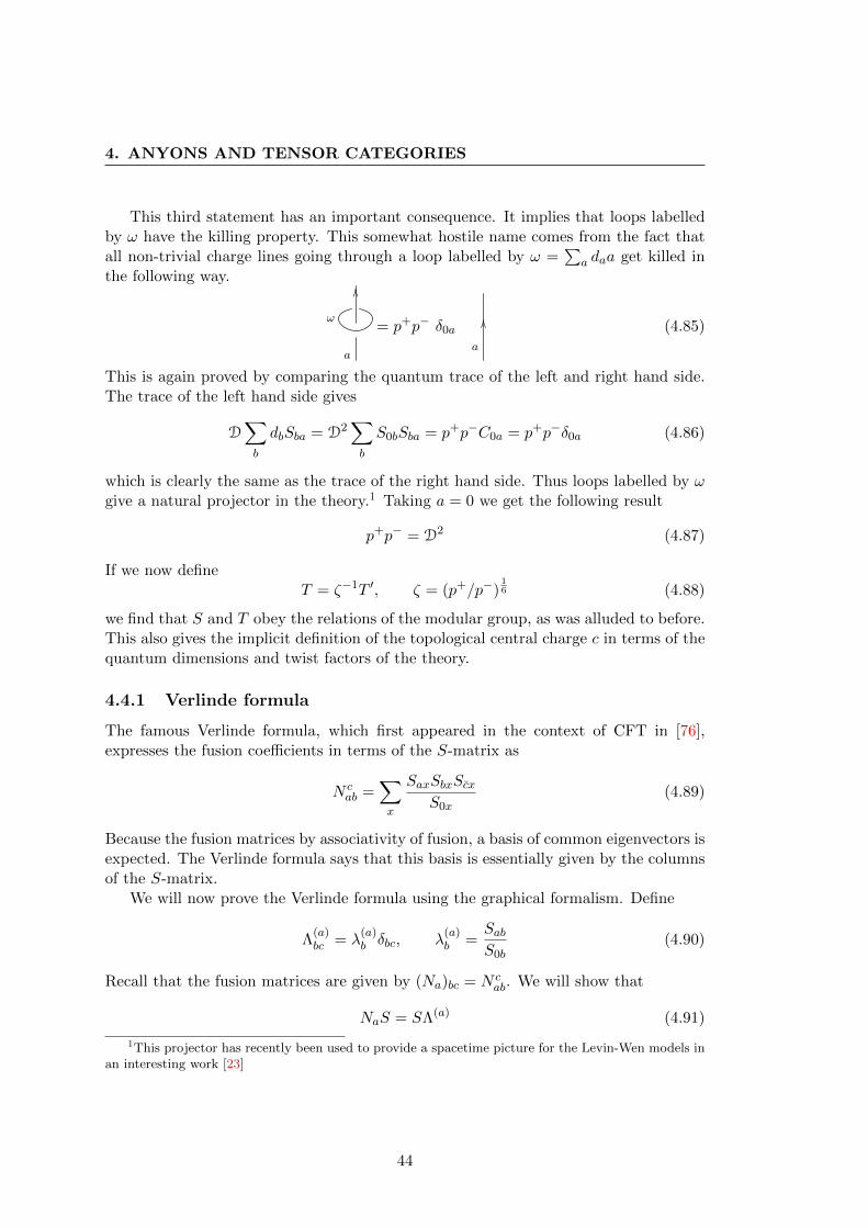
4. ANYONS AND TENSOR CATEGORIES
This third statement has an important consequence. It implies that loops labelledby ω have the killing property. This somewhat hostile name comes from the fact thatall non-trivial charge lines going through a loop labelled by ω =
∑a daa get killed in
the following way.
a
ω
OO
= p+p− δ0a
a
OO(4.85)
This is again proved by comparing the quantum trace of the left and right hand side.The trace of the left hand side gives
D∑b
dbSba = D2∑b
S0bSba = p+p−C0a = p+p−δ0a (4.86)
which is clearly the same as the trace of the right hand side. Thus loops labelled by ωgive a natural projector in the theory.1 Taking a = 0 we get the following result
p+p− = D2 (4.87)
If we now defineT = ζ−1T ′, ζ = (p+/p−)
16 (4.88)
we find that S and T obey the relations of the modular group, as was alluded to before.This also gives the implicit definition of the topological central charge c in terms of thequantum dimensions and twist factors of the theory.
4.4.1 Verlinde formula
The famous Verlinde formula, which first appeared in the context of CFT in [76],expresses the fusion coefficients in terms of the S-matrix as
N cab =
∑x
SaxSbxScxS0x
(4.89)
Because the fusion matrices by associativity of fusion, a basis of common eigenvectors isexpected. The Verlinde formula says that this basis is essentially given by the columnsof the S-matrix.
We will now prove the Verlinde formula using the graphical formalism. Define
Λ(a)bc = λ
(a)b δbc, λ
(a)b =
SabS0b
(4.90)
Recall that the fusion matrices are given by (Na)bc = N cab. We will show that
NaS = SΛ(a) (4.91)
1This projector has recently been used to provide a spacetime picture for the Levin-Wen models inan interesting work [23]
44
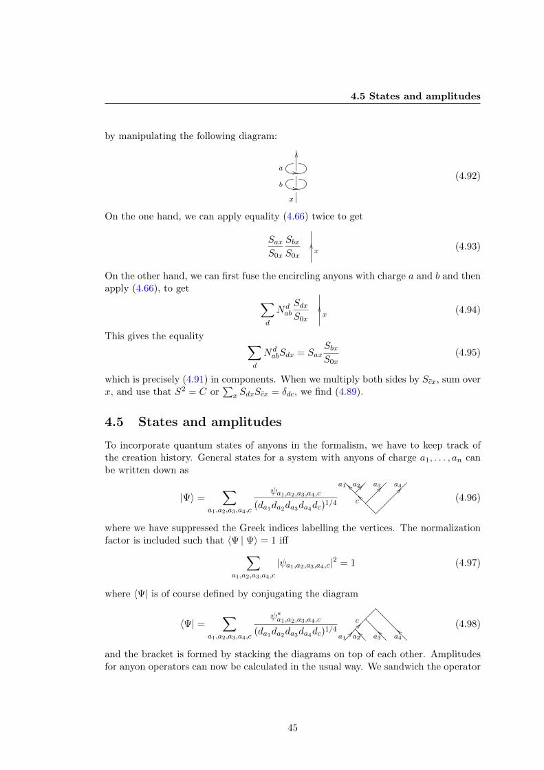
4.5 States and amplitudes
by manipulating the following diagram:
x
b
a
OO
//
//(4.92)
On the one hand, we can apply equality (4.66) twice to get
SaxS0x
SbxS0x
OOx
(4.93)
On the other hand, we can first fuse the encircling anyons with charge a and b and thenapply (4.66), to get ∑
d
Ndab
SdxS0x
OOx
(4.94)
This gives the equality ∑d
NdabSdx = Sax
SbxS0x
(4.95)
which is precisely (4.91) in components. When we multiply both sides by Scx, sum overx, and use that S2 = C or
∑x SdxScx = δdc, we find (4.89).
4.5 States and amplitudes
To incorporate quantum states of anyons in the formalism, we have to keep track ofthe creation history. General states for a system with anyons of charge a1, . . . , an canbe written down as
|Ψ〉 =∑
a1,a2,a3,a4,c
ψa1,a2,a3,a4,c
(da1da2da3da4dc)1/4
a1 a2 a3 a4
c
__ ?? ?? ??__ (4.96)
where we have suppressed the Greek indices labelling the vertices. The normalizationfactor is included such that 〈Ψ | Ψ〉 = 1 iff∑
a1,a2,a3,a4,c
|ψa1,a2,a3,a4,c|2 = 1 (4.97)
where 〈Ψ| is of course defined by conjugating the diagram
〈Ψ| =∑
a1,a2,a3,a4,c
ψ∗a1,a2,a3,a4,c
(da1da2da3da4dc)1/4
a1 a2 a3 a4
c
?? __ __ __?? (4.98)
and the bracket is formed by stacking the diagrams on top of each other. Amplitudesfor anyon operators can now be calculated in the usual way. We sandwich the operator
45
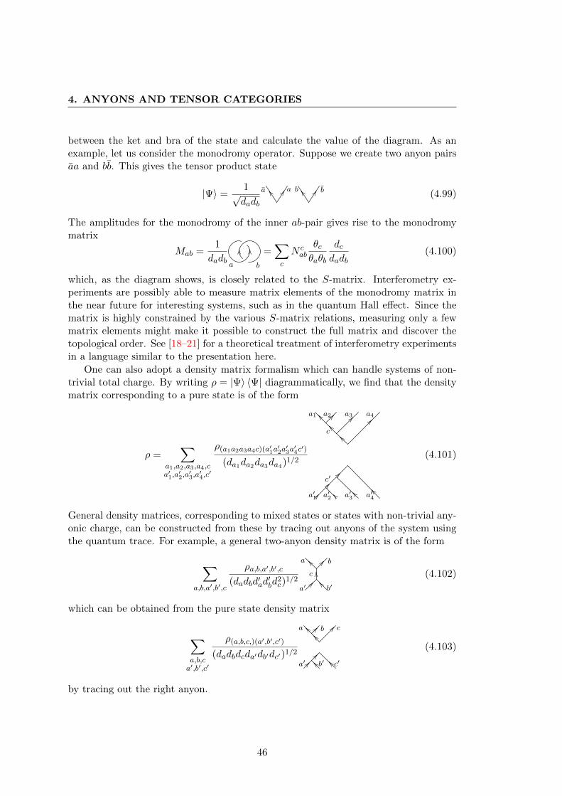
4. ANYONS AND TENSOR CATEGORIES
between the ket and bra of the state and calculate the value of the diagram. As anexample, let us consider the monodromy operator. Suppose we create two anyon pairsaa and bb. This gives the tensor product state
|Ψ〉 =1√dadb
a a bbZZ DD ZZ DD(4.99)
The amplitudes for the monodromy of the inner ab-pair gives rise to the monodromymatrix
Mab =1
dadb a b
OO OO =∑c
N cab
θcθaθb
dcdadb
(4.100)
which, as the diagram shows, is closely related to the S-matrix. Interferometry ex-periments are possibly able to measure matrix elements of the monodromy matrix inthe near future for interesting systems, such as in the quantum Hall effect. Since thematrix is highly constrained by the various S-matrix relations, measuring only a fewmatrix elements might make it possible to construct the full matrix and discover thetopological order. See [18–21] for a theoretical treatment of interferometry experimentsin a language similar to the presentation here.
One can also adopt a density matrix formalism which can handle systems of non-trivial total charge. By writing ρ = |Ψ〉 〈Ψ| diagrammatically, we find that the densitymatrix corresponding to a pure state is of the form
ρ =∑
a1,a2,a3,a4,ca′1,a
′2,a′3,a′4,c′
ρ(a1a2a3a4c)(a′1a′2a′3a′4c′)
(da1da2da3da4)1/2
a1 a2 a3 a4
c
a′1 a′2 a′3 a′4
c′
__ ?? ?? ??
____
?? __ __ __
????
(4.101)
General density matrices, corresponding to mixed states or states with non-trivial any-onic charge, can be constructed from these by tracing out anyons of the system usingthe quantum trace. For example, a general two-anyon density matrix is of the form
∑a,b,a′,b′,c
ρa,b,a′,b′,c
(dadbd′ad′bd
2c)
1/2
a b
a′ b′
c
__ ??
?? __OO (4.102)
which can be obtained from the pure state density matrix
∑a,b,ca′,b′,c′
ρ(a,b,c,)(a′,b′,c′)
(dadbdcda′db′dc′)1/2
a b c
a′ b′ c′
??____ ??
__???? __
(4.103)
by tracing out the right anyon.
46
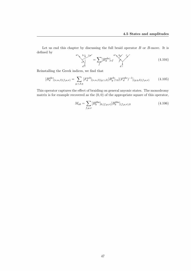
4.5 States and amplitudes
Let us end this chapter by discussing the full braid operator B or B-move. It isdefined by
a b c
d
e
OO[[ =
∑f
[Babcd ]ef
a b c
d
f
__ ?? ??
OO__ (4.104)
Reinstalling the Greek indices, we find that
[Babcd ](e,α,β)(f,µ,ν) =
∑g,γ,δ,η
[F acbd ](e,α,β)(g,γ,δ)[Rcbg ]γη[(F
abcd )−1](g,η,δ)(f,µ,ν) (4.105)
This operator captures the effect of braiding on general anyonic states. The monodromymatrix is for example recovered as the (0, 0) of the appropriate square of this operator,
Mab =∑f,µ,ν
[Babab ]0,(f,µ,ν)[B
abab ](f,µ,ν),0 (4.106)
47

4. ANYONS AND TENSOR CATEGORIES
48
CHAPTER 5
Examples of anyon models
In principle, the unitary braided tensor categories discussed in chapter 4 can be con-structed in a three step procedure: First, fix a set of particle labels and fusion rules.Next, solve the pentagon relation to find a consistent set of F -symbols. Finally, solvethe hexagon relations to find R-symbols.
If no solution to the pentagon relations exists, the declared fusion rules are inconsis-tent with local quantum mechanics and no model with these fusion rules exists. Whenwe do find a solution to the pentagon relations, but not to the hexagon relations, thereis no way to define a consistent braiding for the anyons which excludes the model withthese fusion rules as an effective theory for bulk anyons but, as we will see, might de-scribe boundary effects of a medium carrying anyons. If there are multiple solutionsfor the pentagon/hexagon relations that are not related by a gauge transformation,there are apparently non-equivalent anyon models that obey the same fusion rules. Atheorem know as Ocneanu rigidity ensures that, for a given set of fusion rules, therecan only be a finite number of non-equivalent anyon models.
Although the procedure outlined above can in principle be used to find all anyonmodels, in practice it is not feasible to find many interesting models this way. Thereason is that the number of equations in the pentagon relations, as well as the numberof variables, grows very rapidly with the number of charges in the theory. For smallnumbers of charges, some classification results have been obtained by direct attack ofthe pentagon/hexagon relations. For example, all models with up to four charges wereclassified in [71]. Also, in [22], solutions to the pentagon and hexagon relations werefound explicitly for a number of interesting fusion rules by solving them directly.
Most known models, however, were constructed via a completely different route,namely as representation categories of quantum group that we discussed before. Inthis chapter we will show how to obtain the fusion rules, F -symbols and R-symbolsfor the quantum double. We will also give this data for the su(2)k theories related to
49

5. EXAMPLES OF ANYON MODELS
Uq[su(2)], Chern-Simons theory and the WZW-models and we flesh out the details forsome representative examples that will be used later. But we will start by discussingthe well know Fibonacci anyons, for which the pentagon and hexagon equations can besolved by hand.
5.1 Fibonacci
Suppose we have only one non-trivial charge besides the vacuum, which we label by 1.The two possibilities for the one non-trivial fusion rule are 1× 1 = 0 and 1× 1 = 0 + 1.The first gives an Abelian theory that is not very interesting, so we take the secondrule. This fixes the theory completely, as we will see, and gives rise to the so-calledFibonacci anyons. The discussion below is based on [66].
The F -symbols we need to find are [F 1110 ]ef and [F 111
1 ]ef . The matrix [F 1110 ]ef , has
only one non-zero component, which we can set to unity. This gives
[F 1110 ]ef = δe1δf1 (5.1)
This leaves us with the task to find the 2× 2 matrix F with Fef = [F 1110 ]ef . Since we
are looking for a unitary theory, we search an F of the form
F =
(z ww∗ z
)(5.2)
with |z|2 + |w|2 = 1. Without multiplicities in the theory, the pentagon relationssimplify to
[F fcde ]gl[Fable ]fk =
∑h
[F abcg ]fh[F ahde ]gk[Fbcdk ]hl (5.3)
Now take a= b= c= d= e= f = k = 1 and g = l= 0. The pentagon equation for thiscombination of labels is
[F 1111 ]00 = [F 111
1 ]01[F 1111 ]10 (5.4)
which gives z = |w|2. This leads us to the general solution
F =
(φ−1 eiθ
√φ−1
e−iθ√φ−1 −φ−1
)(5.5)
where φ = 1+√
52 , i.e the golden ratio. The phase eiθ can be set to unity with a gauge
transformation. All pentagon relations are now indeed satisfied.Next we will solve the hexagon relations. Without multiplicities, these take the
following form.
Race [F acbd ]egRbcg =
∑f
[F cabd ]efRfcd [F abcd ]fg (5.6)
(Race )−1[F acbd ]eg(Rbcg )−1 =
∑f
[F cabd ]ef (Rfcd )−1[F abcd ]fg (5.7)
50

5.2 Quantum double
Since the vacuum braids trivially, we only need to find the R-symbols with the twoupper indices equal to 1, so only R0 = R11
0 and R1 = R111 corresponding to a pair of
Fibonacci anyons having trivial or non-trivial total charge respectively. We find
R0 = e−4πi/5, R1 = e3πi/5 (5.8)
We can read off the quantum dimension d1 = 1+√
52 from F , and find that then non-
trivial particle has spin θ1 = fb1(R110 )∗ = e2πi 2
5 .
Now let Nn0 = N1×n
0 be the dimension of the topological Hilbert space of n Fibonaccianyons with trivial total charge. It is easy to see that
N10 = 0, N2
0 = 1, N30 = 1, N4
0 = 2, N50 = 3 (5.9)
when looking at the number of fusion states explicitly. In general, the Nn0 obey a simple
recursion relation. If the first two particles have trivial total charge, the n − 2 otherparticles can fuse in Nn−2
0 different ways. When the charge of the first two particlesis 1, the other n − 2 charges can combine with this charge in Nn−1
0 ways. So themulitplicities obey the recursion relation
Nn0 = Nn−1
0 +Nn−20 (5.10)
which is well known to produce the Fibonacci numbers. Indeed, one recognises the firstof these in the list 5.9 This is why these anyons are given their specific name.
5.2 Quantum double
Using the facts about the quantum double D[H] and its representations from chapter3, it is possible to deduce fusion rules, F -symbols and R-symbols, and thus to obtain adescription of the fusion braiding properties of the excitations in discrete gauge theoriesin the language of the previous chapter.
The connection with the graphical formalism and the representations of the quan-tum double is as follows. Diagrams correspond to operators that commute with theaction of D[H] in the internal space, i.e. operators that are gauge invariant operatorsand commute with flux projections. By Schurs lemma, these must be proportional tothe identity for irreps.
The identity operator of the carrier space V Aα is represented by a charge line labelled
by a = (A,α) directed upwards. The splitting vertex labelled by a = (A,α), b = (B, β)on top and c = (C, γ) on the bottom is identified with the inclusion of V C
γ in V Aα ⊗V B
β ,up to a scale factor. The dual fusion vertex, on the other hand, is associated withthe projection onto V C
γ as irreducible subspace of V Aα ⊗ V B
β . If there are multiple
copies of V Cγ present in V A
α ⊗ V Bβ , we can label them with indices µ. Note that a
unitary transformation on the µ’s in ⊕µ(V Cγ )µ leaves the representations in tact. The
quantum dimension and quantum trace correspond to the usual dimension and trace
51
5. EXAMPLES OF ANYON MODELS
of the modules V Aα .
OOa
identity, µ
__a ?? bOOc
inclusion, µ??
a__b
OO cprojection (5.11)
Throughout this section, it will be very convenient to condense the notation, as thediscussion above already shows. We agree to write a, b, c, . . . for the particle-labels(A,α), (B, β), (C, γ), . . . . To avoid confusing the internal space V A
α with the fusion/splittingspaces, we will also refer to it as a, and similar for the other particle labels. The rep-resentation maps are denoted Πa = ΠA
α , etcetera. We can label the basis states of a byindices i = 1, . . . , da. We denote the basis states of a therefore as
{|a, i〉}, i = 1, . . . , da (5.12)
leaving the particle label explicit, in stead of |hj , αvk〉 as we did before. The coordinatefunctions of the representation matrices are denoted Πa
ij . The fusion product a×bmeansthe tensor product representation.
5.2.1 Fusion rules
The fusion coefficients N cab, corresponding to the decomposition
a× b = Πa ⊗Πb =⊕c
Πc∑c
N cabc (5.13)
can be obtained by using certain orthogonality relations for the characters of represen-tation. These are well known in the case of groups, but generalize to representationsof the quantum double. It means that for unitary representations, we have
1
|H|∑h,g
Tr (Πa(Ph g)) Tr(
Πb(Ph g)∗)
= δab (5.14)
In fact, more general orthogonality relations for the coordinate functions ¶aij . Theyobey ∑
h,g∈HΠaij(Ph g)∗Πb
kl(Ph g) = δa,b δi,k δj,l (5.15)
This follows from Woronowiczes theory of pseudogroups [85] and generalize the wellknown Schur orthogonality relations for groups. We will use them heavily in the cal-culation of F -symbols.
From the orthogonality of characters, we see that the fusion multiplicities may beobtained from the representations matrices as
N cab =
1
|H|∑h,g
Tr(
Πa ⊗Πb(∆(Ph g)))
Tr (Πc(Ph g)∗) (5.16)
=∑h,g
∑h′h′′=h
∑i,j
Πaij(Ph′ g)Πb
ij(Ph′′ g)
(∑k
Πckk(Ph g)
)(5.17)
Next, we show how to calculate F -symbols.
52
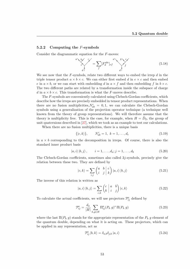
5.2 Quantum double
5.2.2 Computing the F -symbols
Consider the diagrammatic equation for the F -moves:
a b c
d
e
__ ?? ??
OO__ =
∑f
[F abcd ]ef
a b c
d
f
__ __ ??
OO?? (5.18)
We see now that the F -symbols, relate two different ways to embed the irrep d in thetriple tensor product a × b × c. We can either first embed d in e × c and then embede in a× b, or we can start with embedding d in a× f and then embedding f in b× c.The two different paths are related by a transformation inside the subspace of charged in a× b× c. This transformation is what the F -moves describe.
The F -symbols are conveniently calculated using Clebsch-Gordan coefficients, whichdescribe how the irreps are precisely embedded in tensor product representations. Whenthere are no fusion multiplicities,N c
ab = 0, 1, we can calculate the Clebsch-Gordansymbols using a generalization of the projection operator technique (a technique wellknown from the theory of group representations). We will therefore assume that thetheory is multiplicity free. This is the case, for example, when H = D2, the group ofunit quaternions described in [27], which we took as an example to test our calculations.
When there are no fusion multiplicities, there is a unique basis
{|c, k〉}, N cab = 1, k = 1, . . . , dc (5.19)
in a × b corresponding to the decomposition in irreps. Of course, there is also thestandard inner product basis
|a, i〉 |b, j〉 , i = 1, . . . , da; j = 1, . . . , db (5.20)
The Clebsch-Gordan coefficients, sometimes also called 3j-symbols, precisely give therelation between these two. They are defined by
|c, k〉 =∑i,j
(a b ci j k
)|a, i〉 |b, j〉 (5.21)
The inverse of this relation is written as
|a, i〉 |b, j〉 =∑c,k
(c a bk i j
)|c, k〉 (5.22)
To calculate the actual coefficients, we will use projectors Paij defined by
Paij =da|H|
∑h,g∈H
Πaij(Ph g)∗Π(Ph g) (5.23)
where the last Π(Ph g) stands for the appropriate representation of the Ph g element ofthe quantum double, depending on what it is acting on. These projectors, which canbe applied in any representation, act as
Paij |b, k〉 = δa,bδj,k |a, i〉 (5.24)
53
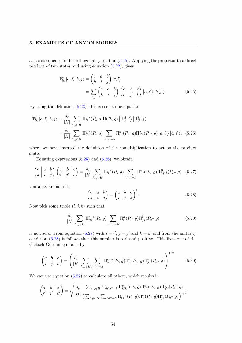
5. EXAMPLES OF ANYON MODELS
as a consequence of the orthogonality relation (5.15). Applying the projector to a directproduct of two states and using equation (5.22), gives
Pclk |a, i〉 |b, j〉 =
(c a bk i j
)|c, l〉
=∑i′,j′
(c a bk i j
)(a b ci′ j′ l
) ∣∣a, i′⟩ ∣∣b, j′⟩ . (5.25)
By using the definition (5.23), this is seen to be equal to
Pclk |a, i〉 |b, j〉 =dc|H|
∑h,g∈H
Πclk∗(Ph g)Π(Ph g)
∣∣ΠAα , i⟩ ∣∣ΠB
β , j⟩
=dc|H|
∑h,g∈H
Πclk∗(Ph g)
∑h′h′′=h
Πai′i(Ph′ g)Πb
j′j(Ph′′ g)∣∣a, i′⟩ ∣∣b, j′⟩ , (5.26)
where we have inserted the definition of the comultiplication to act on the productstate.
Equating expressions (5.25) and (5.26), we obtain(c a bk i j
)(a b ci′ j′ l
)=
dc|H|
∑h,g∈H
Πclk∗(Ph g)
∑h′h′′=h
Πai′i(Ph′ g)ΠB
βj′j(Ph′′ g) (5.27)
Unitarity amounts to (c a bk i j
)=
(a b ci j k
)∗. (5.28)
Now pick some triple (i, j, k) such that
dc|H|
∑h,g∈H
Πckk∗(Ph g)
∑h′h′′=h
Πaii(Ph′ g)Πb
jj(Ph′′ g) (5.29)
is non-zero. From equation (5.27) with i = i′, j = j′ and k = k′ and from the unitaritycondition (5.28) it follows that this number is real and positive. This fixes one of theClebsch-Gordan symbols, by
(a b ci j k
)=
dc|H|
∑h,g∈H
∑h′h′′=h
Πckk∗(Ph g)Πa
ii(Ph′ g)Πbjj(Ph′′ g)
1/2
(5.30)
We can use equation (5.27) to calculate all others, which results in(a b ci′ j′ k′
)=
√dc|H|
∑h,g∈H
∑h′h′′=h Πc
k′k∗(Ph g)Πa
i′i(Ph′ g)Πbj′j(Ph′′ g)(∑
h,g∈H∑
h′h′′=h Πckk∗(Ph g)Πa
ii(Ph′ g)Πbjj(Ph′′ g)
)1/2
54
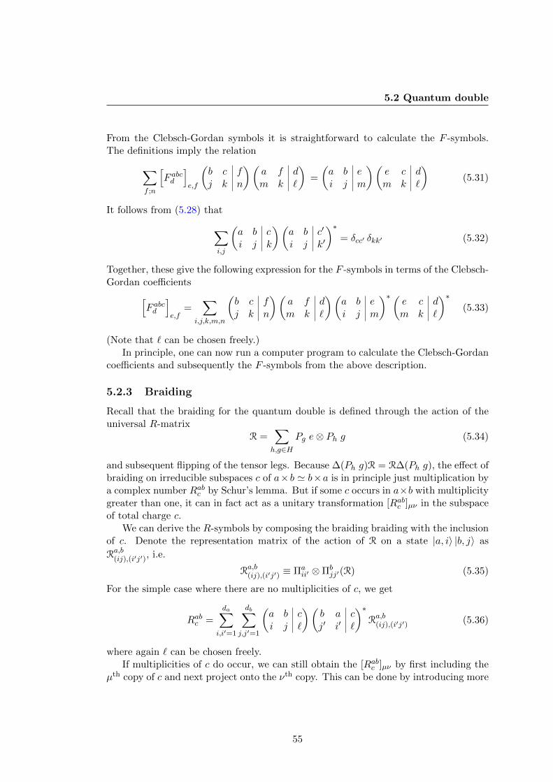
5.2 Quantum double
From the Clebsch-Gordan symbols it is straightforward to calculate the F -symbols.The definitions imply the relation∑
f ;n
[F abcd
]e,f
(b c fj k n
)(a f dm k `
)=
(a b ei j m
)(e c dm k `
)(5.31)
It follows from (5.28) that∑i,j
(a b ci j k
)(a b c′
i j k′
)∗= δcc′ δkk′ (5.32)
Together, these give the following expression for the F -symbols in terms of the Clebsch-Gordan coefficients[
F abcd
]e,f
=∑
i,j,k,m,n
(b c fj k n
)(a f dm k `
)(a b ei j m
)∗(e c dm k `
)∗(5.33)
(Note that ` can be chosen freely.)In principle, one can now run a computer program to calculate the Clebsch-Gordan
coefficients and subsequently the F -symbols from the above description.
5.2.3 Braiding
Recall that the braiding for the quantum double is defined through the action of theuniversal R-matrix
R =∑h,g∈H
Pg e⊗ Ph g (5.34)
and subsequent flipping of the tensor legs. Because ∆(Ph g)R = R∆(Ph g), the effect ofbraiding on irreducible subspaces c of a× b ' b×a is in principle just multiplication bya complex number Rabc by Schur’s lemma. But if some c occurs in a×b with multiplicitygreater than one, it can in fact act as a unitary transformation [Rabc ]µν in the subspaceof total charge c.
We can derive the R-symbols by composing the braiding braiding with the inclusionof c. Denote the representation matrix of the action of R on a state |a, i〉 |b, j〉 as
Ra,b(ij),(i′j′), i.e.
Ra,b(ij),(i′j′) ≡ Πa
ii′ ⊗Πbjj′(R) (5.35)
For the simple case where there are no multiplicities of c, we get
Rabc =
da∑i,i′=1
db∑j,j′=1
(a b ci j `
)(b a cj′ i′ `
)∗Ra,b(ij),(i′j′) (5.36)
where again ` can be chosen freely.If multiplicities of c do occur, we can still obtain the [Rabc ]µν by first including the
µth copy of c and next project onto the νth copy. This can be done by introducing more
55
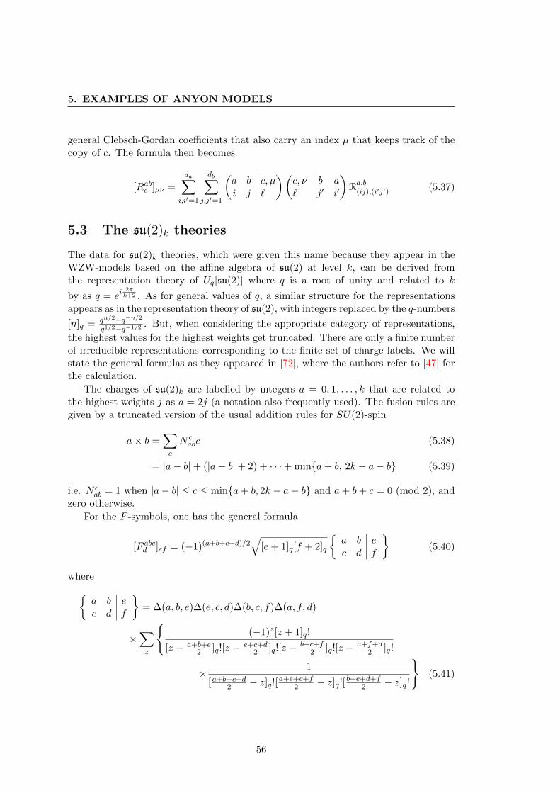
5. EXAMPLES OF ANYON MODELS
general Clebsch-Gordan coefficients that also carry an index µ that keeps track of thecopy of c. The formula then becomes
[Rabc ]µν =
da∑i,i′=1
db∑j,j′=1
(a b c, µi j `
)(c, ν b a` j′ i′
)Ra,b(ij),(i′j′) (5.37)
5.3 The su(2)k theories
The data for su(2)k theories, which were given this name because they appear in theWZW-models based on the affine algebra of su(2) at level k, can be derived fromthe representation theory of Uq[su(2)] where q is a root of unity and related to k
by as q = ei2πk+2 . As for general values of q, a similar structure for the representations
appears as in the representation theory of su(2), with integers replaced by the q-numbers
[n]q = qn/2−q−n/2q1/2−q−1/2 . But, when considering the appropriate category of representations,
the highest values for the highest weights get truncated. There are only a finite numberof irreducible representations corresponding to the finite set of charge labels. We willstate the general formulas as they appeared in [72], where the authors refer to [47] forthe calculation.
The charges of su(2)k are labelled by integers a = 0, 1, . . . , k that are related tothe highest weights j as a = 2j (a notation also frequently used). The fusion rules aregiven by a truncated version of the usual addition rules for SU(2)-spin
a× b =∑c
N cabc (5.38)
= |a− b|+ (|a− b|+ 2) + · · ·+ min{a+ b, 2k − a− b} (5.39)
i.e. N cab = 1 when |a− b| ≤ c ≤ min{a+ b, 2k − a− b} and a+ b+ c = 0 (mod 2), and
zero otherwise.
For the F -symbols, one has the general formula
[F abcd ]ef = (−1)(a+b+c+d)/2√
[e+ 1]q[f + 2]q
{a b ec d f
}(5.40)
where{a b ec d f
}= ∆(a, b, e)∆(e, c, d)∆(b, c, f)∆(a, f, d)
×∑z
{(−1)z[z + 1]q!
[z − a+b+e2 ]q![z − e+c+d
2 ]q![z − b+c+f2 ]q![z − a+f+d
2 ]q!
× 1
[a+b+c+d2 − z]q![a+e+c+f
2 − z]q![ b+e+d+f2 − z]q!
}(5.41)
56
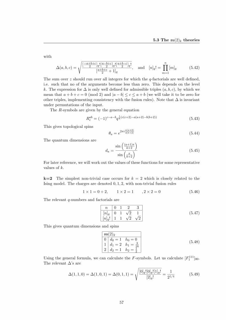
5.3 The su(2)k theories
with
∆(a, b, c) =
√[−a+b+c
2 ]q![a−b+c
2 ]q![a+b−c
2 ]q!
[a+b+c2 + 1]q
, and [n]q! =n∏
m=1
[m]q (5.42)
The sum over z should run over all integers for which the q-factorials are well defined,i.e. such that no of the arguments become less than zero. This depends on the levelk. The expression for ∆ is only well defined for admissible triples (a, b, c), by which wemean that a+ b+ c = 0 (mod 2) and |a− b| ≤ c ≤ a+ b (we will take it to be zero forother triples, implementing consistency with the fusion rules). Note that ∆ is invariantunder permutations of the input.
The R-symbols are given by the general equation
Rabc = (−1)c−a−bq18
(c(c+2)−a(a+2)−b(b+2)) (5.43)
This gives topological spins
θa = e2πi
a(a+2)4(k+2) (5.44)
The quantum dimensions are
da =sin(
(a+1)πk+2
)sin(
πk+2
) (5.45)
For later reference, we will work out the values of these functions for some representativevalues of k.
k=2 The simplest non-trivial case occurs for k = 2 which is closely related to theIsing model. The charges are denoted 0, 1, 2, with non-trivial fusion rules
1× 1 = 0 + 2, 1× 2 = 1 , 2× 2 = 0 (5.46)
The relevant q-numbers and factorials are
n 0 1 2 3
[n]q 0 1√
2 1
[n]q! 1 1√
2√
2
(5.47)
This gives quantum dimensions and spins
su(2)2
0 d0 = 1 h0 = 01 d1 = 2 h1 = 3
162 d2 = 1 h2 = 1
2
(5.48)
Using the general formula, we can calculate the F -symbols. Let us calculate [F 1111 ]00.
The relevant ∆’s are
∆(1, 1, 0) = ∆(1, 0, 1) = ∆(0, 1, 1) =
√[0]q![0]q![1]q!
[2]q!=
1
21/4(5.49)
57
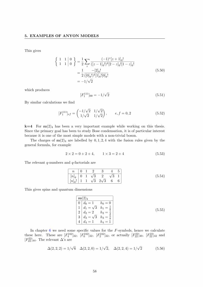
5. EXAMPLES OF ANYON MODELS
This gives {1 1 01 1 0
}=
1
2
∑z
(−1)z[z + 1]q!
([z − 1]q!)4[2− z]q![1− z]q!
=1
2
−[2]q!
([0]q!)4[1]q![0]q!
= −1/√
2
(5.50)
which produces
[F 1111 ]00 = −1/
√2 (5.51)
By similar calculations we find
[F 1111 ]ef =
(−1/√
2 1/√
2
1/√
2 1/√
2
), e, f = 0, 2 (5.52)
k=4 For su(2)4 has been a very important example while working on this thesis.Since the primary goal has been to study Bose condensation, it is of particular interestbecause it is one of the most simple models with a non-trivial boson.
The charges of su(2)4 are labelled by 0, 1, 2, 4 with the fusion rules given by thegeneral formula, for example
2× 2 = 0 + 2 + 4, 1× 3 = 2 + 4 (5.53)
The relevant q-numbers and q-factorials are
n 0 1 2 3 4 5
[n]q 0 1√
3 2√
3 1
[n]q! 1 1√
3 2√
3 6 6
(5.54)
This gives spins and quantum dimensions
su(2)4
0 d0 = 1 h0 = 0
1 d1 =√
3 h1 = 18
2 d2 = 2 h2 = 13
3 d3 =√
3 h3 = 58
4 d4 = 1 h4 = 1
(5.55)
In chapter 6 we need some specific values for the F -symbols, hence we calculatethese here. These are [F 242
4 ]22, [F 2420 ]22, [F 242
2 ]22, or actually [F 2222 ]40, [F 22
22 ]42 and[F 22
22 ]44. The relevant ∆’s are
∆(2, 2, 2) = 1/√
6 ∆(2, 2, 0) = 1/√
2, ∆(2, 2, 4) = 1/√
2 (5.56)
58
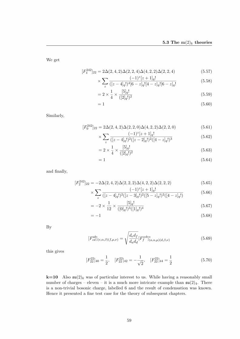
5.3 The su(2)k theories
We get
[F 2424 ]22 = 2∆(2, 4, 2)∆(2, 2, 4)∆(4, 2, 2)∆(2, 2, 4) (5.57)
×∑z
(−1)z[z + 1]q!
([z − 4]q!)4[6− z]q![4− z]q![6− z]q!(5.58)
= 2× 1
4× [5]q!
([2]q!)2(5.59)
= 1 (5.60)
Similarly,
[F 2420 ]22 = 2∆(2, 4, 2)∆(2, 2, 0)∆(4, 2, 2)∆(2, 2, 0) (5.61)
×∑z
(−1)z[z + 1]q!
([z − 4]q!)2([z − 2]q!)2([4− z]q!)3(5.62)
= 2× 1
4× [5]q!
([2]q!)2(5.63)
= 1 (5.64)
and finally,
[F 2422 ]22 = −2∆(2, 4, 2)∆(2, 2, 2)∆(4, 2, 2)∆(2, 2, 2) (5.65)
×∑z
(−1)z[z + 1]q!
([z − 4]q!)2([z − 3]q!)2([5− z]q!)2([4− z]q!)(5.66)
= −2× 1
12× [5]q!
([0]q!)3([1]q!)4(5.67)
= −1 (5.68)
By
[F abcd ](e,α,β)(f,µ,ν) =
√dedfdadd
[F cebf ]∗(a,α,µ)(d,β,ν) (5.69)
this gives
[F 2222 ]40 =
1
2, [F 22
22 ]42 = − 1√2, [F 22
22 ]44 =1
2(5.70)
k=10 Also su(2)k was of particular interest to us. While having a reasonably smallnumber of charges – eleven – it is a much more intricate example than su(2)4. Thereis a non-trivial bosonic charge, labelled 6 and the result of condensation was known.Hence it presented a fine test case for the theory of subsequent chapters.
59
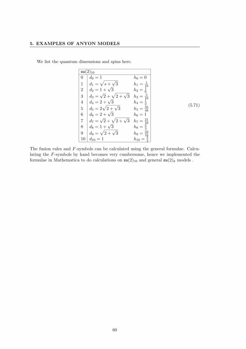
5. EXAMPLES OF ANYON MODELS
We list the quantum dimensions and spins here.
su(2)10
0 d0 = 1 h0 = 0
1 d1 =√s+√
3 h1 = 116
2 d2 = 1 +√
3 h2 = 16
3 d3 =√
2 +√
2 +√
3 h3 = 516
4 d4 = 2 +√
3 h4 = 12
5 d5 = 2√
2 +√
3 h5 = 3548
6 d6 = 2 +√
3 h6 = 1
7 d7 =√
2 +√
2 +√
3 h7 = 2116
8 d8 = 1 +√
3 h8 = 53
9 d9 =√
2 +√
3 h9 = 3316
10 d10 = 1 h10 = 52
(5.71)
The fusion rules and F -symbols can be calculated using the general formulae. Calcu-lating the F -symbols by hand becomes very cumbersome, hence we implemented theformulae in Mathematica to do calculations on su(2)10 and general su(2)k models .
60
CHAPTER 6
Bose condensation in topologically ordered phases
In this chapter, we start the study of phase transitions between topologically orderedphases, which is the main goal of this thesis. The theory developed in the previouschapters is used to extend the formalism for topological symmetry breaking phasetransitions. This should allow one to construct a full diagrammatic formalism fortopological symmetry breaking, such that arbitrary diagrams for the symmetry-brokenphase can be calculated, using data from the original theory only.
We start with a short review of the topological symmetry breaking approach, whichis based on quantum group symmetry breaking by a bosonic condensate. The mainidea is that a mechanism of symmetry breaking, very similar to spontaneous symmetrybreaking known from the ordinary theory of phase transitions, can account for manytransitions between topological phases, only the symmetry is given by a quantum group.This was first explored in the context of discrete gauge theories in [5, 8]. Later, theformalism was refined and applied to nematic phases in liquid crystals in [7, 12, 61].These earlier approaches had the drawback that they were not applicable to treat casesmost interesting for the FQHE, where non-integer quantum dimensions occur. In [9],a general scheme was laid out that can also handle these cases.
An important feature of this general scheme is that the explicit description of thequantum group disappears and everything is done on the level of the representations,or particle labels. In mathematical terminology, on might say that the representationcategory of the quantum group is put centerstage while the quantum group itself is putto the background. It could therefore be expected that there is a connection with themathematical literature on (modular) tensor categories.
The generalization of the notion of a subgroup to the appropriate category theoret-ical context is a commutative algebra, as argued in [48]. The results of [9] and [48] arein perfect agreement, although the language is very different in many respects. Thismotivated the study of the mathematical literature to see what physically meaningful
61
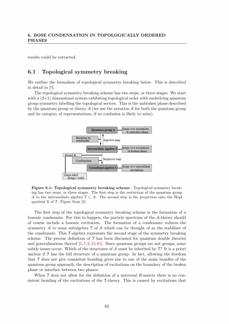
6. BOSE CONDENSATION IN TOPOLOGICALLY ORDEREDPHASES
results could be extracted.
6.1 Topological symmetry breaking
We outline the formalism of topological symmetry breaking below. This is describedin detail in [9].
The topological symmetry breaking scheme has two steps, or three stages. We startwith a (2+1) dimensional system exhibiting topological order with underlying quantumgroup symmetry labelling the topological sectors. This is the unbroken phase describedby the quantum group or theory A (we use the notation A for both the quantum groupand its category of representations, if no confusion is likely to arise).
Figure 6.1: Topological symmetry breaking scheme - Topological symmetry break-ing has two steps, or three stages. The first step is the restriction of the quantum groupA to the intermediate algebra T ⊂ A. The second step is the projection onto the Hopfquotient U of T. Figure from [9].
The first step of the topological symmetry breaking scheme is the formation of abosonic condensate. For this to happen, the particle spectrum of the A-theory shouldof course include a bosonic excitation. The formation of a condensate reduces thesymmetry A to some subalgebra T of A which can be thought of as the stabilizer ofthe condensate. This T-algebra represents the second stage of the symmetry breakingscheme. The precise definition of T has been discussed for quantum double theoriesand generalizations thereof [5, 7, 8, 12,61]. Since quantum groups are not groups, somesubtle issues occur. Which of the structures of A must be inherited by T? It is a prioriunclear if T has the full structure of a quantum group. In fact, allowing the freedomthat T does not give consistent braiding gives rise to one of the main benefits of thequantum group approach, the description of excitations on the boundary of the brokenphase or interface between two phases.
When T does not allow for the definition of a universal R-matrix there is no con-sistent braiding of the excitations of the T-theory. This is caused by excitations that
62
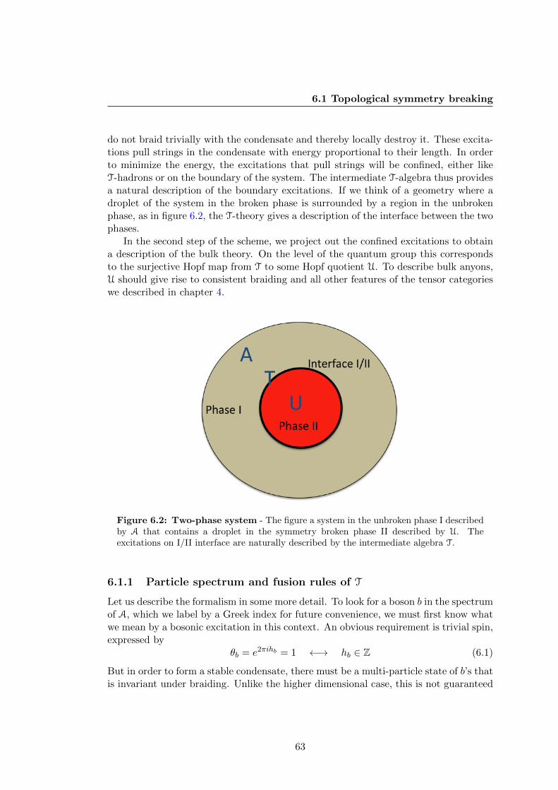
6.1 Topological symmetry breaking
do not braid trivially with the condensate and thereby locally destroy it. These excita-tions pull strings in the condensate with energy proportional to their length. In orderto minimize the energy, the excitations that pull strings will be confined, either likeT-hadrons or on the boundary of the system. The intermediate T-algebra thus providesa natural description of the boundary excitations. If we think of a geometry where adroplet of the system in the broken phase is surrounded by a region in the unbrokenphase, as in figure 6.2, the T-theory gives a description of the interface between the twophases.
In the second step of the scheme, we project out the confined excitations to obtaina description of the bulk theory. On the level of the quantum group this correspondsto the surjective Hopf map from T to some Hopf quotient U. To describe bulk anyons,U should give rise to consistent braiding and all other features of the tensor categorieswe described in chapter 4.
Figure 6.2: Two-phase system - The figure a system in the unbroken phase I describedby A that contains a droplet in the symmetry broken phase II described by U. Theexcitations on I/II interface are naturally described by the intermediate algebra T.
6.1.1 Particle spectrum and fusion rules of T
Let us describe the formalism in some more detail. To look for a boson b in the spectrumof A, which we label by a Greek index for future convenience, we must first know whatwe mean by a bosonic excitation in this context. An obvious requirement is trivial spin,expressed by
θb = e2πihb = 1 ←→ hb ∈ Z (6.1)
But in order to form a stable condensate, there must be a multi-particle state of b’s thatis invariant under braiding. Unlike the higher dimensional case, this is not guaranteed
63
6. BOSE CONDENSATION IN TOPOLOGICALLY ORDEREDPHASES
by the trivial spin condition. Suppose a bb-pair has total charge c. The monodromy ofthe two b’s leads to a phase exp(2πihc) as follows from
c
b b
OO
;;cc
= e2πi(hc−2hb)__b ?? bOOc
= e2πihc__b ?? bOOc
(6.2)
Therefore, a second condition is necessary, namely that there is a fusion channel c ∈ b×bwith hc ∈ Z.
One might argue that a full definition should guarantee that there is a fusion channelthat is completely invariant under monodromies or even braidings for b×n for any n.This condition is much more involved to check when only the spins and quantumdimensions of the theory are known/used, as is the case in [9]. In the approach thatwe will develop later, this is in fact guaranteed by the conditions that we impose. Thishas the draw back that we need the F -symbols and R-symbols, which might be harderto obtain.
But for now, a working definition of a boson is
If a charge b ∈ A has
1. Trivial spin, hb ∈ Z,
2. A fusion channel c ∈ b× b with hc ∈ Z.
then b is a boson.
We will illustrate the theory for su(2)4, with fields 0, 1, 2, 3, 4 and non-trivial fusionrules
1× 1 = 0 + 21× 2 = 1 + 3 2× 2 = 0 + 2 + 41× 3 = 2 + 4 2× 3 = 1 + 3 3× 3 = 0 + 21× 4 = 3 2× 4 = 2 3× 4 = 1 4× 4 = 0
(6.3)
For convenience, we list the spins and quantum dimensions again.
su(2)4
0 d0 = 1 h0 = 0
1 d1 =√
3 h1 = 18
2 d2 = 2 h2 = 13
3 d3 =√
3 h3 = 58
4 d4 = 1 h4 = 1
(6.4)
From this we see that 4 is non-trivial boson, according to the conditions formulatedabove. It has trivial spin and, because 4× 4 = 0, also the second condition is satisfied.
The next step is to work out what happens after condensation. Restricting thesymmetry to T ⊂ A can be noticed on the level of representations by two effects.
64
6.1 Topological symmetry breaking
Different representations of A might be isomorphic when we restrict to the subalgebraT, which gives identifications. And, representations that were irreducible under theaction of A might have invariant subspaces under the transformations of T, which leadsto decomposition into a direct sum of irreducible T-modules. This, we call splitting.These effects are fully captured by a set of branching rules, or restriction map,
a→∑t
ntat (restriction) (6.5)
that can be regarded as a linear map of the fusion algebras. Here the t’s are labels forthe T-particle spectrum and the nta’s are multiplicities denoting the number of times toccurs in the restriction of a.
There are three important, physically motivated, conditions on these branchingrules.
1. The condensed boson should restrict to the new vacuum (which we also denoteby 0), so
b→ 0 +∑t6=0
ntbt (6.6)
2. The restriction should respect the fusion rules(∑t
ntat
)×(∑
t
nsbs
)=∑r
N cabn
rcr (6.7)
3. The restriction of particles and antiparticle should be consistent
a→∑t
ntat (6.8)
As a consequence of these assumptions and the uniqueness of the vacuum, 0 mustrestrict to the new vacuum
0→ 0 (6.9)
and the quantum dimensions are preserved
da =∑t
ntadt (6.10)
Using these conditions one can in general derive the particle spectrum and fusion rulesof the T theory.
Returning to the su(2)4 example, we see that 4→ 0, since d4 = 1 and therefore nomore labels are allowed to occur in the restriction. Because 4×1 = 3 and 4×3 = 1, weimmediately conclude that 3 and 1 become indistinguishable after symmetry breaking.We will denote the corresponding T-label by 1. Finally, let us look at the fusion of 2with itself
2× 2 = 0 + 2 + 4→ 0 +∑t
nt2t+ 0 (6.11)
65
6. BOSE CONDENSATION IN TOPOLOGICALLY ORDEREDPHASES
Since the vacuum appears twice on the right, the restriction of 2 must have more thanone particle. Otherwise, this particle would be able to annihilate with itself in twodifferent ways which is inconsistent with well defined fusion. Since d2 = 2, this ispossible and in fact leads us to conclude that 2 → 21 + 22, with,d2i = 1. Hence, thebroken phase has four sectors: 0, 1, 21 and 22.
The fusion rules of 1 can be straightforwardly induced. Because in the unbrokenphase we had 1× 1 = 0 + 2, in the broken phase we have 1× 1 = 0 + 21 + 22. This alsoshows that neither 21 nor 22 will be identical to the vacuum 0 in the broken phase, sincethis would imply the splitting of 1, which is impossible because d1 < 2. Now, turning tothe fusion rules for 21 and 22, we find that they are either self-dual, 21×21 = 22×22 = 0,or are dual to each other, 21× 22 = 22× 21 = 0. Using the fusion rule 2× 2 = 0 + 2 + 4and our current knowledge, we see that
0 + 21 + 22 + 0 = (21 + 22)× (21 + 22)
= 21 × 21 + 21 × 22 + 22 × 21 + 22 × 22 (6.12)
So if we assume that 21 and 22 are self-dual, we find that 21× 22 = 21 and 22× 21 = 22
or 21 × 22 = 22 and 22 × 21 = 21. Either way, one easily concludes that associativity isviolated by evaluating 21 × (22 × 21) and (21 × 22)× 21. Thus, the fusion rules of thebroken phase are symmetric and given by
1× 1 = 0 + 21 + 22
1× 21 = 1 21 × 21 = 22
1× 22 = 1 21 × 22 = 0 22 × 22 = 21
(6.13)
Note that the symmetry of the fusion rules is not a requirement in this formalism. SinceT does not have a consistent braiding, the fusion rules can be non-commutative.
6.1.2 Confinement
We now turn to the confinement projection, the second step of the formalism. Inorder to implement this step, a characterization of the sectors of T that get confined isnecessary.
In order to get a theory U with well defined braiding, we must be able to assigntwist factors to the charges of the U theory. It is therefore logical to assume that, foran unconfined excitation u of the U-theory, all charges of A that restrict to u have thesame twist factors.
Define the lift as the adjoint of the restriction.
t→∑a
ntaa, (lift) (6.14)
This lifts the charge t of T into the theory A as the sum of charges that have t inthere restriction (including multiplicities) . The confinement condition can now beformulated as follows
66
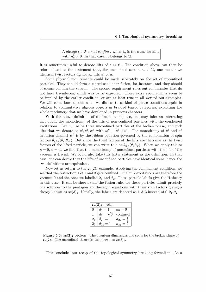
6.1 Topological symmetry breaking
A charge t ∈ T is not confined when θa is the same for all awith nta 6= 0. In that case, it belongs to U.
It is sometimes useful to denote lifts of t as ti. The condition above can then bereformulated as the statement that, for unconfined sectors u ∈ U, one must haveidentical twist factors θui for all lifts ui of u.
Some physical requirements could be made separately on the set of unconfinedparticles. They should form a closed set under fusion, for instance, and they shouldof course contain the vacuum. The second requirement rules out condensates that donot have trivial-spin, which was to be expected. These extra requirements seem tobe implied by the earlier condition, or are at least true in all worked out examples.We will come back to this when we discuss these kind of phase transitions again inrelation to commutative algebra objects in braided tensor categories, exploiting thewhole machinery that we have developed in previous chapters.
With the above definition of confinement in place, one may infer an interestingfact about the monodromy of the lifts of non-confined particles with the condensedexcitations. Let u, v, w be three unconfined particles of the broken phase, and picklifts that we denote as ui, vj , wk with wk ∈ ui × vj . The monodromy of ui and vj
in fusion channel wk is by the ribbon equation governed by the combination of spinfactors θwk/(θuiθvj ). But since the twist factors of the lifts are the same as the twistfactors of the lifted particle, we can write this as θw/(θuθw). When we apply this tou = 0, v = w, we find that the monodromy of unconfined particles with the lift of thevacuum is trivial. We could also take this latter statement as the definition. In thatcase, one can derive that the lifts of unconfined particles have identical spins, hence thetwo definitions are equivalent.
Now let us return to the su(2)4 example. Applying the confinement condition, wesee that the restriction 1 of 1 and 3 gets confined. The bulk excitations are therefore thevacuum 0 and the ones we labelled 21 and 22. These particle labels give the U-theoryin this case. It can be shown that the fusion rules for these particles admit preciselyone solution to the pentagon and hexagon equations with these spin factors giving atheory known as su(3)1. Usually, the labels are denoted as 1, 3, 3 instead of 0, 21, 22.
su(2)4 broken
0 d0 = 1 h0 = 0
1 d1 =√
3 confined21 d21 = 1 h21 = 1
322 d22 = 1 h22 = 1
3
Figure 6.3: su(2)4 broken - The quantum dimensions and spins for the broken phase ofsu(2)4. The unconfined theory is also known as su(3)1.
This concludes our recap of the topological symmetry breaking formalism. As a
67
6. BOSE CONDENSATION IN TOPOLOGICALLY ORDEREDPHASES
last remark, let us point out interesting observations that were done regarding thetotal quantum dimension and the central charge of the theories involved. For the totalquantum dimensions, the relation
DA
DT
=DT
DU
(6.15)
was found. (This can actually be understood as a relation concerning the entropy ofthe different phases, as we will discuss in the next chapter). It was also found that thecentral charge is conserved under these kind of phase transition,
cA = cU (6.16)
This is also nicely understood by the fact that in a CFT setting, topological symmetrybreaking is dual to conformal extensions, as is discussed in [9].
The latter equation seems to limit the applicability of topological symmetry break-ing to a restricted range of phase transitions. Phase transitions that change the valueof c seem to lie outside the formalism. In [10], however, the formalism was applied inthe context of the quantum Hall effect to multilayer systems. This way, a c-changingphase transition could be accounted for by incorporating an auxiliary layer, and theresults were in agreement with the CFT approach in [40]. The multi-layer approachextends the applicability considerably.
6.2 Commutative algebra objects as Bose condensates
The study of the mathematical literature on commutative algebras in braided tensorcategories, in relation to topological symmetry breaking was suggested becausethe for-mulas for the total quantum dimension central charge also appear in this context. Inthe next section, we will use this mathematics to extend the formulation of the topo-logical symmetry breaking scheme and augment it with the diagrammatics developedin chapter 4. A pivotal aspect in this formulation is that that we identify the sectorst of T with the lift
∑t n
at . Hence diagrams for T and U can be interpreted as certain
superpositions of diagrams of A, allowing calculation using the F - and R-symbols fromthe A-theory.
For this tensor category approach to topological symmetry breaking, we take acommutative algebra object in a modular tensor category [35,48] as the definition of abosonic condensate. Algebras in modular tensor categories have appeared in relation tophysics, for example as boundary conditions in boundary CFT [35], but they have notreally been related to symmetry breaking phase transitions and particle condensation.
We believe this is interesting for a couple of reasons. Tensor categories provide theappropriate language to discuss topological order in many cases. It is more conciseand accurate than the explicit use of quantum groups and describes to the physicalexcitations. This becomes apparent, for example, in the formulation of the Levin-Wenmodels in terms of categories and the fact that it is not straight forward to treat thesu(2)k models as Uq[su(2)] representations. Also, the treatment of topological symmetry
68
6.2 Commutative algebra objects as Bose condensates
breaking on the level of general quantum groups is likely to become cumbersome. Thetopological data captured by the F - and R-symbols, on the other hand, is physicallyintuitive.
Commutative algebra objects in modular tensor categories provide a rigorous wayto construct the tensor category of the symmetry broken phase. Because all diagramslive in the A theory, an extra benefit is that a sort of intermediate viewpoint can beattained. One can, so to say, look in between the transition from A to T. Related work(in progress) by Jesper Romers shows that this might be necessary when phase tran-sitions in studying a lattice formulation of DGT numerically. Because diagrammaticcalculations can be done, it is also possible to answer different questions. In the nextchapter, we apply the formalism below to study the faith of the topological S-matrixunder topologically symmetry breaking phase transitions.
We would like to point out that in a completely different context, there appearedevidence that condensates in the kind of systems under consideration carry an algebrastructure (in the appropriate sense). In [16] the authors study the Kitaev model withboundary and show explicitly that introduction of the boundary leads to condensationof excitations that, collectively, are endowed with the structure of an algebra object inthe category of representations of the underlying quantum double symmetry group.
For the discussion below, we made heavy use of [48].
6.2.1 The condensate
The intuition we should bear in mind for the tensor category approach to topologicalsymmetry breaking is that charges of the intermediate theory T are identified withtheir lift in A. In particular, the new vacuum will be formed out of all particles thatcondense. This gives rise to a condensate
φ = 0 + δ1 + · · ·+ δn (6.17)
We will use Greek indices for the condensed excitations from now on.1 But for asatisfactory alternative description of the symmetry breaking scheme, we actually haveto turn this logic around, since we do not want to rely an analysis along the lines ofthe previous section, or prior knowledge of the broken phase. In stead, we will have toguess the condensate (as we chose a boson to condense) and check that it obeys theright consistency conditions.
Therefore, fix some φ = 0 + δ1 + · · ·+ δn. Which consistency conditions should berequired. We want to consider φ as the new vacuum and the conditions on φ can allbe related back to this requirement.
As a first condition, in line with (A.13), if δ ∈ φ we should also have δ ∈ φ. In otherwords, we require φ = φ.
To keep the discussion transparent, we will often assume that there is only one non-trivial particle that condenses, so φ = 0 + δ. Note that in this situation, φ = φ means
1These should of course not be mistaken with the indices labelling vertices in chapter 4. The theoryA is assumed to be multiplicity free.
69
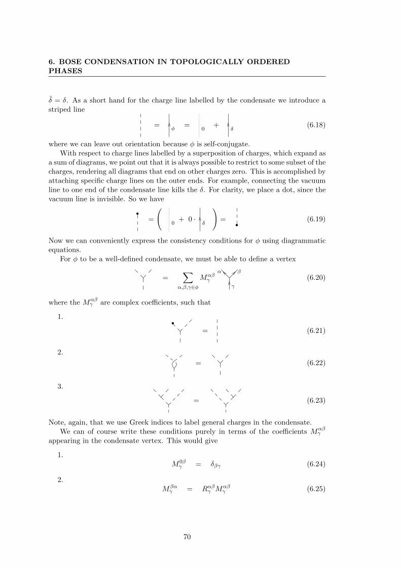
6. BOSE CONDENSATION IN TOPOLOGICALLY ORDEREDPHASES
δ = δ. As a short hand for the charge line labelled by the condensate we introduce astriped line
=OOφ
=0
+OOδ
(6.18)
where we can leave out orientation because φ is self-conjugate.With respect to charge lines labelled by a superposition of charges, which expand as
a sum of diagrams, we point out that it is always possible to restrict to some subset of thecharges, rendering all diagrams that end on other charges zero. This is accomplished byattaching specific charge lines on the outer ends. For example, connecting the vacuumline to one end of the condensate line kills the δ. For clarity, we place a dot, since thevacuum line is invisible. So we have
•=
(0
+ 0 · OOδ
)=
•(6.19)
Now we can conveniently express the consistency conditions for φ using diagrammaticequations.
For φ to be a well-defined condensate, we must be able to define a vertex
=∑
α,β,γ∈φMαβγ
__α ?? βOOγ
(6.20)
where the Mαβγ are complex coefficients, such that
1.•
= (6.21)
2.
= (6.22)
3.
= (6.23)
Note, again, that we use Greek indices to label general charges in the condensate.We can of course write these conditions purely in terms of the coefficients Mαβ
γ
appearing in the condensate vertex. This would give
1.M0βγ = δβγ (6.24)
2.Mβαγ = Rαβγ Mαβ
γ (6.25)
70
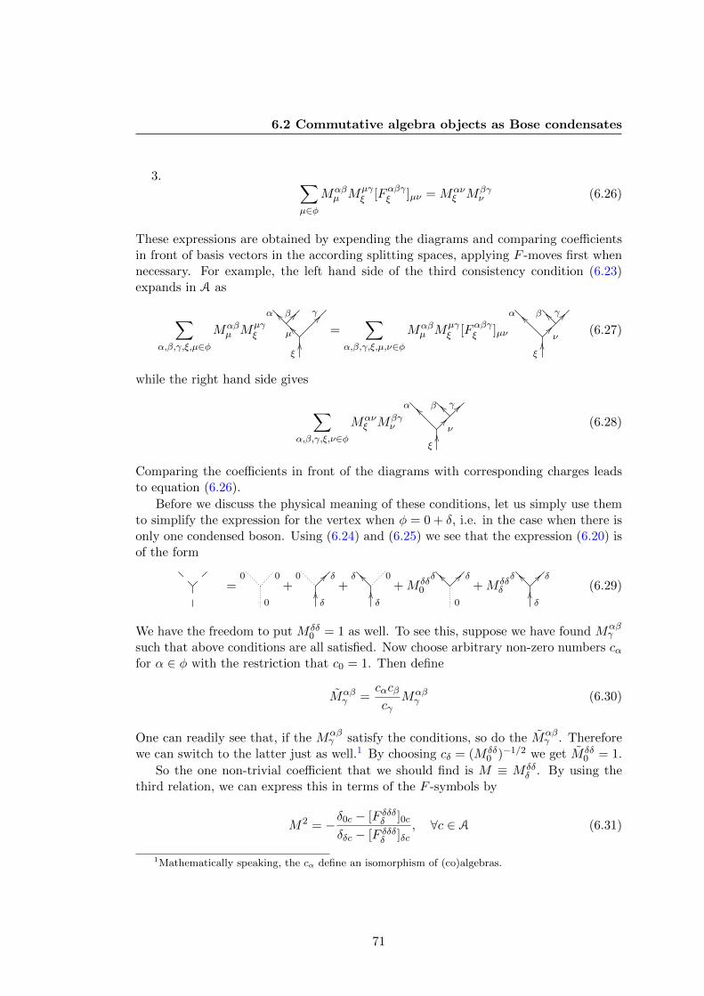
6.2 Commutative algebra objects as Bose condensates
3. ∑µ∈φ
Mαβµ Mµγ
ξ [Fαβγξ ]µν = Mανξ Mβγ
ν (6.26)
These expressions are obtained by expending the diagrams and comparing coefficientsin front of basis vectors in the according splitting spaces, applying F -moves first whennecessary. For example, the left hand side of the third consistency condition (6.23)expands in A as
∑α,β,γ,ξ,µ∈φ
Mαβµ Mµγ
ξ
α β γ
ξ
µ
__ ?? ??
OO__ =
∑α,β,γ,ξ,µ,ν∈φ
Mαβµ Mµγ
ξ [Fαβγξ ]µν
α β γ
ξ
ν
__ __ ??
OO?? (6.27)
while the right hand side gives
∑α,β,γ,ξ,ν∈φ
Mανξ Mβγ
ν
α β γ
ξ
ν
__ __ ??
OO?? (6.28)
Comparing the coefficients in front of the diagrams with corresponding charges leadsto equation (6.26).
Before we discuss the physical meaning of these conditions, let us simply use themto simplify the expression for the vertex when φ = 0 + δ, i.e. in the case when there isonly one condensed boson. Using (6.24) and (6.25) we see that the expression (6.20) isof the form
=0 0
0
+0 ?? δOOδ
+__δ 0
OOδ
+M δδ0
__δ ?? δ
0
+M δδδ
__δ ?? δOOδ
(6.29)
We have the freedom to put M δδ0 = 1 as well. To see this, suppose we have found Mαβ
γ
such that above conditions are all satisfied. Now choose arbitrary non-zero numbers cαfor α ∈ φ with the restriction that c0 = 1. Then define
Mαβγ =
cαcβcγ
Mαβγ (6.30)
One can readily see that, if the Mαβγ satisfy the conditions, so do the Mαβ
γ . Thereforewe can switch to the latter just as well.1 By choosing cδ = (M δδ
0 )−1/2 we get M δδ0 = 1.
So the one non-trivial coefficient that we should find is M ≡ M δδδ . By using the
third relation, we can express this in terms of the F -symbols by
M2 = −δ0c − [F δδδδ ]0c
δδc − [F δδδδ ]δc, ∀c ∈ A (6.31)
1Mathematically speaking, the cα define an isomorphism of (co)algebras.
71
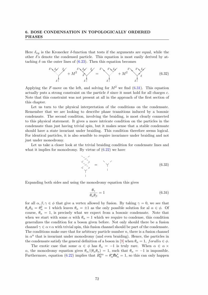
6. BOSE CONDENSATION IN TOPOLOGICALLY ORDEREDPHASES
Here δxy is the Kronecker δ-function that tests if the arguments are equal, while theother δ’s denote the condensed particle. This equation is most easily derived by at-taching δ on the outer lines of (6.23). Then this equation becomes
δ δ δ
δ
__ ?? ??
OO+M2
δ δ δ
δ
δ
__ ?? ??
OO__ =
δ δ δ
δ
__ __ ??
OO+M2
δ δ δ
δ
δ
__ __ ??
OO?? (6.32)
Applying the F -move on the left, and solving for M2 we find (6.31). This equationactually puts a strong constraint on the particle δ since it must hold for all charges c.Note that this constraint was not present at all in the approach of the first section ofthis chapter.
Let us turn to the physical interpretation of the conditions on the condensate.Remember that we are looking to describe phase transitions induced by a bosoniccondensate. The second condition, involving the braiding, is most clearly connectedto this physical statement. It gives a more intricate condition on the particles in thecondensate than just having trivial spin, but it makes sense that a stable condensateshould have a state invariant under braiding. This condition therefore seems logical.For identical particles, it is also sensible to require invariance under braiding and notjust under monodromy.
Let us take a closer look at the trivial braiding condition for condensate lines andwhat it implies for monodromy. By virtue of (6.22) we have
= (6.33)
Expanding both sides and using the monodromy equation this gives
θγθαθβ
= 1 (6.34)
for all α, β, γ ∈ φ that give a vertex allowed by fusion. By taking γ = 0, we see thatθαθα = θ2
α = 1 which leaves θα = ±1 as the only possible solution for al α ∈ φ. Ofcourse, θα = 1, is precisely what we expect from a bosonic condensate. Note thatwhen we start with some α with θα = 1 which we require to condense, this conditiongeneralizes the condition for a boson given before. Not only should there be a fusionchannel γ ∈ α×α with trivial spin, this fusion channel should be part of the condensate.The conditions make sure that for arbitrary particle number n, there is a fusion channelin αn that is invariant under monodromy (and even braiding). Hence, the particles inthe condensate satisfy the general definition of a boson in [9] when θα = 1, forallα ∈ φ.
The exotic case that some α ∈ φ has θα = −1 is truly rare. When α ∈ α ×α, the monodromy equation gives θα/(θαθα) = 1, such that θα = −1 is impossible.Furthermore, equation (6.22) implies that Rαα0 = θ∗αfb∗α = 1, so this can only happen
72
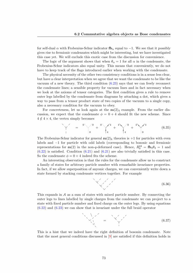
6.2 Commutative algebra objects as Bose condensates
for self-dual α with Frobenius-Schur indicator fbα equal to −1. We see that it possiblygives rise to fermionic condensates which might be interesting, but we have investigatedthis case yet. We will exclude this exotic case from the discussion for convenience.
The logic of the argument shows that when θα = 1 for all α in the condensate, theFrobenius-Schur indicators also equal unity. This means that conveniently, we do nothave to keep track of the flags introduced earlier when working with the condensate.
The physical necessity of the other two consistency conditions is in a sense less clear,but have a clear interpretation when we agree that we want the condensate to be like thevacuum of a new theory. The third condition (6.23) says that we can freely reconnectthe condensate lines; a sensible property for vacuum lines and in fact necessary whenwe look at the axioms of tensor categories. The first condition gives a rule to removeouter legs labelled by the condensate from diagrams by attaching a dot, which gives away to pass from a tensor product state of two copies of the vacuum to a single copy,also a necessary condition for the vacuum to obey.
For concreteness, let us look again at the su(2)4 example. From the earlier dis-cussion, we expect that the condensate φ = 0 + 4 should fit the new scheme. Since4 /∈ 4× 4, the vertex simply becomes
=0 0
0
+0 ?? 4OO4
+__4 0
OO4
+__4 ?? 4
0
(6.35)
The Frobenius-Schur indicator for general su(2)k theories is +1 for particles with evenlabels and −1 for particle with odd labels (corresponding to bosonic and fermionicrepresentations for su(2) in the non-q-deformed case). Hence, R44
0 = fb4θ4 = 1 and(6.22) is satisfied. Condition (6.21) and (6.21) are also trivially satisfied in this case.So the condensate φ = 0 + 4 indeed fits the scheme.
An interesting observation is that the rules for the condensate allow us to constructa family of states for arbitrary particle number with remarkable invariance properties.In fact, if we allow superposition of anyonic charges, we can conveniently write down astate formed by stacking condensate vertices together. For example
(6.36)
This expands in A as a sum of states with mixed particle number. By connecting theouter legs to lines labelled by single charges from the condensate we can project to astate with fixed particle number and fixed charge on the outer legs. By using equations(6.22) and (6.23) we can show that is invariant under the full braid operator
= (6.37)
This is a hint that we indeed have the right definition of bosonin condensate. Notethat the most general conditions discussed in [9] are satisfied if this definition holds in
73
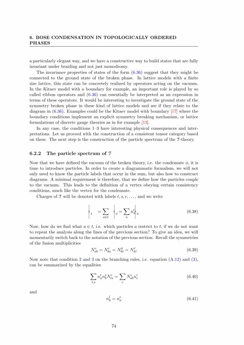
6. BOSE CONDENSATION IN TOPOLOGICALLY ORDEREDPHASES
a particularly elegant way, and we have a constructive way to build states that are fullyinvariant under braiding and not just monodromy.
The invariance properties of states of the form (6.36) suggest that they might beconnected to the ground state of the broken phase. In lattice models with a finitesize lattice, this state can be concretely realized by operators acting on the vacuum.In the Kitaev model with a boundary for example, an important role is played by socalled ribbon operators and (6.36) can essentially be interpreted as an expression interms of these operators. It would be interesting to investigate the ground state of thesymmetry broken phase in these kind of lattice models and see if they relate to thediagram in (6.36). Examples could be the Kitaev model with boundary [17] where theboundary conditions implement an explicit symmetry breaking mechanism, or latticeformulations of discrete gauge theories as in for example [13].
In any case, the conditions 1–3 have interesting physical consequences and inter-pretations. Let us proceed with the construction of a consistent tensor category basedon these. The next step is the construction of the particle spectrum of the T-theory.
6.2.2 The particle spectrum of T
Now that we have defined the vacuum of the broken theory, i.e. the condensate φ, it istime to introduce particles. In order to create a diagrammatic formalism, we will notonly need to know the particle labels that occur in the sum, but also how to constructdiagrams. A minimal requirement is therefore, that we define how the particles coupleto the vacuum. This leads to the definition of a vertex obeying certain consistencyconditions, much like the vertex for the condensate.
Charges of T will be denoted with labels t, s, r, . . . , and we write
OOt
=∑a∈t
OOa
=∑a
ntaOOa
(6.38)
Now, how do we find what a ∈ t, i.e. which particles a restrict to t, if we do not wantto repeat the analysis along the lines of the previous section? To give an idea, we willmomentarily switch back to the notation of the previous section. Recall the symmetriesof the fusion multiplicities
N cab = N c
ba = N abc = N c
ac (6.39)
Now note that condition 2 and 3 on the branching rules, i.e. equation (A.12) and (3),can be summarized by the equalities∑
t,s
ntansbN
rts =
∑c
N cabn
rc (6.40)
and
nta = nta (6.41)
74
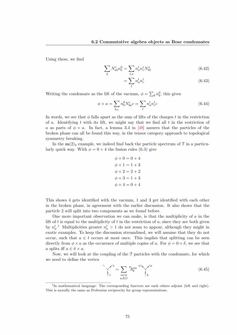
6.2 Commutative algebra objects as Bose condensates
Using these, we find ∑b
N cabn
0b =
∑t,s
ntanscN
st0 (6.42)
=∑t
ntantc (6.43)
Writing the condensate as the lift of the vacuum, φ =∑
b n0b , this gives
φ× a =∑b,c
n0bN
cbac =
∑t
ntantcc (6.44)
In words, we see that φ falls apart as the sum of lifts of the charges t in the restrictionof a. Identifying t with its lift, we might say that we find all t in the restriction ofa as parts of φ × a. In fact, a lemma 3.4 in [48] assures that the particles of thebroken phase can all be found this way, in the tensor category approach to topologicalsymmetry breaking.
In the su(2)4 example, we indeed find back the particle spectrum of T in a particu-larly quick way. With φ = 0 + 4 the fusion rules (6.3) give
φ× 0 = 0 + 4
φ× 1 = 1 + 3
φ× 2 = 2 + 2
φ× 3 = 1 + 3
φ× 4 = 0 + 4
This shows 4 gets identified with the vacuum, 1 and 3 get identified with each otherin the broken phase, in agreement with the earlier discussion. It also shows that theparticle 2 will split into two components as we found before.
One more important observation we can make, is that the multiplicity of a in thelift of t is equal to the multiplicity of t in the restriction of a, since they are both givenby nta.
1 Multiplicities greater nta > 1 do not seam to appear, although they might inexotic examples. To keep the discussion streamlined, we will assume that they do notoccur, such that a ∈ t occurs at most once. This implies that splitting can be seendirectly from φ× a as the occurence of multiple copies of a. For φ = 0 + δ, we see thata splits iff a ∈ δ × a.
Now, we will look at the coupling of the T particles with the condensate, for whichwe need to define the vertex
?? tOOt
=∑α∈φa,b∈t
(t)Aαab
__α ?? aOOb
(6.45)
1In mathematical language: The corresponding functors are each others adjoint (left and right).This is morally the same as Frobenius reciprocity for group representations.
75
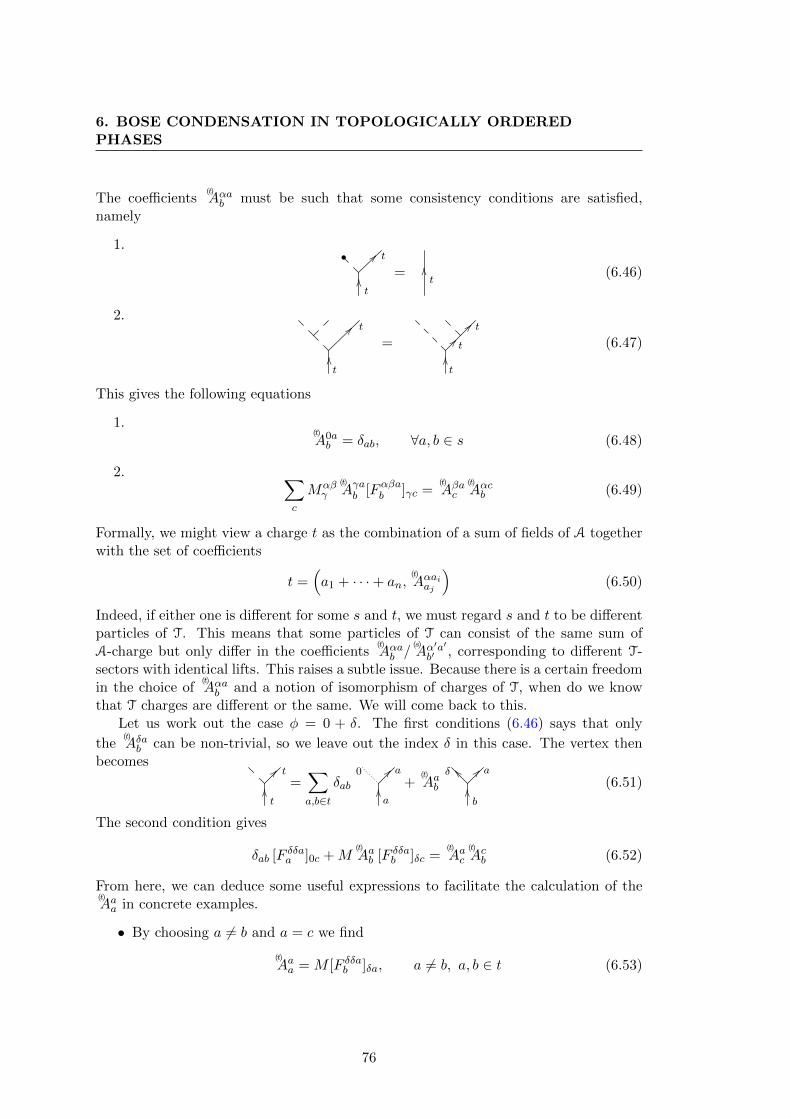
6. BOSE CONDENSATION IN TOPOLOGICALLY ORDEREDPHASES
The coefficients(t)Aαab must be such that some consistency conditions are satisfied,
namely
1.• ?? t
OOt
=OOt
(6.46)
2.t
t
??
OO=
t
t
t
??
OO?? (6.47)
This gives the following equations
1.(t)A0ab = δab, ∀a, b ∈ s (6.48)
2. ∑c
Mαβγ
(t)Aγab [Fαβab ]γc =
(t)Aβac
(t)Aαcb (6.49)
Formally, we might view a charge t as the combination of a sum of fields of A togetherwith the set of coefficients
t =(a1 + · · ·+ an,
(t)Aαaiaj
)(6.50)
Indeed, if either one is different for some s and t, we must regard s and t to be differentparticles of T. This means that some particles of T can consist of the same sum ofA-charge but only differ in the coefficients
(t)Aαab /
(s)Aα′a′b′ , corresponding to different T-
sectors with identical lifts. This raises a subtle issue. Because there is a certain freedomin the choice of
(t)Aαab and a notion of isomorphism of charges of T, when do we know
that T charges are different or the same. We will come back to this.Let us work out the case φ = 0 + δ. The first conditions (6.46) says that only
the(t)Aδab can be non-trivial, so we leave out the index δ in this case. The vertex then
becomes ?? tOOt
=∑a,b∈t
δab0 ?? aOOa
+(t)Aab
__δ ?? aOOb
(6.51)
The second condition gives
δab [F δδaa ]0c +M(t)Aab [F δδab ]δc =
(t)Aac
(t)Acb (6.52)
From here, we can deduce some useful expressions to facilitate the calculation of the(t)Aaa in concrete examples.
• By choosing a 6= b and a = c we find
(t)Aaa = M [F δδab ]δa, a 6= b, a, b ∈ t (6.53)
76
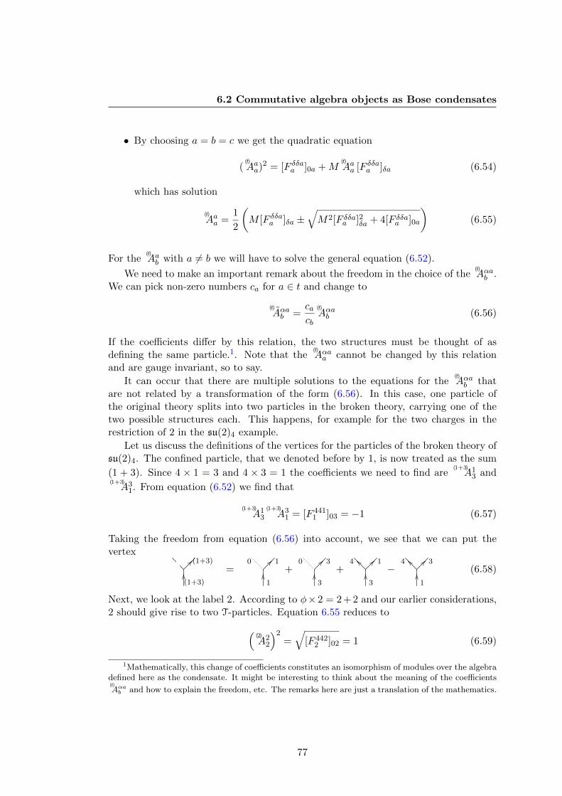
6.2 Commutative algebra objects as Bose condensates
• By choosing a = b = c we get the quadratic equation
((t)Aaa)
2 = [F δδaa ]0a +M(t)Aaa [F δδaa ]δa (6.54)
which has solution
(t)Aaa =
1
2
(M [F δδaa ]δa ±
√M2[F δδaa ]2δa + 4[F δδaa ]0a
)(6.55)
For the(t)Aab with a 6= b we will have to solve the general equation (6.52).
We need to make an important remark about the freedom in the choice of the(t)Aαab .
We can pick non-zero numbers ca for a ∈ t and change to
(t)Aαab =
cacb
(t)Aαab (6.56)
If the coefficients differ by this relation, the two structures must be thought of asdefining the same particle.1. Note that the
(t)Aαaa cannot be changed by this relation
and are gauge invariant, so to say.
It can occur that there are multiple solutions to the equations for the(t)Aαab that
are not related by a transformation of the form (6.56). In this case, one particle ofthe original theory splits into two particles in the broken theory, carrying one of thetwo possible structures each. This happens, for example for the two charges in therestriction of 2 in the su(2)4 example.
Let us discuss the definitions of the vertices for the particles of the broken theory ofsu(2)4. The confined particle, that we denoted before by 1, is now treated as the sum
(1 + 3). Since 4 × 1 = 3 and 4 × 3 = 1 the coefficients we need to find are(1+3)A1
3 and(1+3)A3
1. From equation (6.52) we find that
(1+3)A1
3
(1+3)A3
1 = [F 4411 ]03 = −1 (6.57)
Taking the freedom from equation (6.56) into account, we see that we can put thevertex
??(1+3)
OO(1+3)
=0 ?? 1OO1
+0 ?? 3OO3
+__4 ?? 1OO3
−__4 ?? 3OO1
(6.58)
Next, we look at the label 2. According to φ× 2 = 2 + 2 and our earlier considerations,2 should give rise to two T-particles. Equation 6.55 reduces to(
(2)A2
2
)2=√
[F 4422 ]02 = 1 (6.59)
1Mathematically, this change of coefficients constitutes an isomorphism of modules over the algebradefined here as the condensate. It might be interesting to think about the meaning of the coefficients(t)
Aαab and how to explain the freedom, etc. The remarks here are just a translation of the mathematics.
77
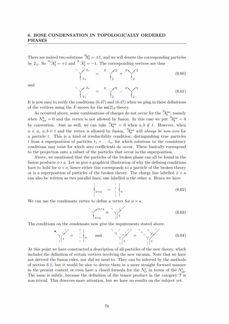
6. BOSE CONDENSATION IN TOPOLOGICALLY ORDEREDPHASES
There are indeed two solutions(2)A2
2 = ±1, and we will denote the corresponding particles
by 2±. So(2+)A2
2 = +1 and(2−)A2
2 = −1. The corresponding vertices are thus
?? 2+
OO2+
=0 ?? 2OO2
+__4 ?? 2OO2
(6.60)
and ?? 2+
OO2+
=0 ?? 2OO2
−__4 ?? 2OO2
(6.61)
It is now easy to verify the conditions (6.47) and (6.47) when we plug in these definitionsof the vertices using the F -moves for the su(2)4-theory.
As occurred above, some combinations of charges do not occur for the(t)Aαab , namely
when N bαa = 0 and the vertex is not allowed by fusion. In this case we put
(t)Aαab = 0
by convention. Just as well, we can take(t)Aαab = 0 when a, b /∈ t. However, when
α ∈ φ, a, b ∈ t and the vertex is allowed by fusion,(t)Aαab will always be non-zero for
a particle t. This is a kind of irreducibility condition, distinguishing true particlest from a superposition of particles t1 + . . . tn, for which solutions to the consistencyconditions may exist for which zero coefficients do occur. These basically correspondto the projection onto a subset of the particles that occur in the superposition.
Above, we mentioned that the particles of the broken phase can all be found in thefusion products φ×a. Let us give a graphical illustration of why the defining conditionshave to hold for φ× a, hence either this corresponds to a particle of the broken theoryor is a superposition of particles of the broken theory. The charge line labelled φ × acan also be written as two parallel lines, one labelled φ the other a. Hence we have
OOφ×a =
OOa
(6.62)
We can use the condensate vertex to define a vertex for φ× a.
?? φ×aOOφ×a
≡a
??(6.63)
The conditions on the condensate now give the requirements stated above.
•
a
??=
OOa
anda
??=
a
??(6.64)
At this point we have constructed a description of all particles of the new theory, whichincludes the definition of certain vertices involving the new vacuum. Note that we havenot derived the fusion rules, nor did we need to. They can be inferred by the methodsof section 6.1, but it would be nice to derive them in a more straight forward mannerin the present context or even have a closed formula for the N r
ts in terms of the N cab.
The issue is subtle, because the definition of the tensor product in the category T isnon-trivial. This deserves more attention, but we have no results on the subject yet.
78

6.2 Commutative algebra objects as Bose condensates
6.2.3 Derived vertices
The definition of the vertices as in (6.20) and (6.45) allow us to derive several vertices.The condensate vertex with two legs down is defined as
=∑
α,β,γ∈φ
(Mβαγ
)??
α__β
OO γ
(6.65)
We furthermore define
??s
OO s=∑α∈φa,b∈s
((s)Aab )
∗ ??a
__α
OO b(6.66)
This is convenient for the discussion of the S-matrix for the broken phase. Formally,these morphisms correspond to the duals of the splitting versions.
With these definitions in place, we find
= q (6.67)
with q = dφ, at least in all our examples.
6.2.4 Confinement
The confinement in the present context is the same as it was in the earlier discussion.Recall that unconfined particles were characterized by the condition that all charges inthe lift have identical twist factors, or equivalently, that the lift has trivial monodromywith the lift of the vacuum, i.e. the condensate. The second condition, which is in factslightly more general as it can be used for condensates with θα 6= 1, is nicely expresseddiagrammatically as
t
t
OO
77
=
?? t
OOt
(6.68)
Using the monodromy equation, we find that this is equivalent to
θa/(θαθb) = 1, ∀a, b ∈ t, α ∈ φ (6.69)
Because θα = 1 for all particles α of the condensate, we indeed recover the conditionthat
θa = θb, ∀a, b ∈ t (6.70)
which is precisely the statement that all lifts have equal topological spin.
79
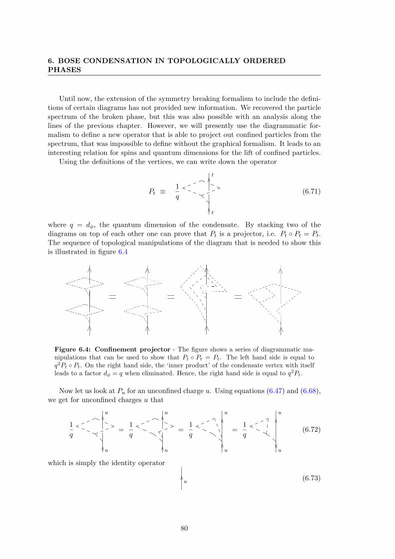
6. BOSE CONDENSATION IN TOPOLOGICALLY ORDEREDPHASES
Until now, the extension of the symmetry breaking formalism to include the defini-tions of certain diagrams has not provided new information. We recovered the particlespectrum of the broken phase, but this was also possible with an analysis along thelines of the previous chapter. However, we will presently use the diagrammatic for-malism to define a new operator that is able to project out confined particles from thespectrum, that was impossible to define without the graphical formalism. It leads to aninteresting relation for spins and quantum dimensions for the lift of confined particles.
Using the definitions of the vertices, we can write down the operator
Pt ≡1
q
t
t
OO
OO
(6.71)
where q = dφ, the quantum dimension of the condensate. By stacking two of thediagrams on top of each other one can prove that Pt is a projector, i.e. Pt ◦ Pt = Pt.The sequence of topological manipulations of the diagram that is needed to show thisis illustrated in figure 6.4
Figure 6.4: Confinement projector - The figure shows a series of diagrammatic ma-nipulations that can be used to show that Pt ◦ Pt = Pt. The left hand side is equal toq2Pt ◦ Pt. On the right hand side, the ‘inner product’ of the condensate vertex with itselfleads to a factor dφ = q when eliminated. Hence, the right hand side is equal to q2Pt.
Now let us look at Pu for an unconfined charge u. Using equations (6.47) and (6.68),we get for unconfined charges u that
1
q
u
u
OO
OO
=1
q
u
u
OO
OO
=1
q
u
u
OO
OO
=1
q
u
u
OO
OO
(6.72)
which is simply the identity operator
OOu
(6.73)
80
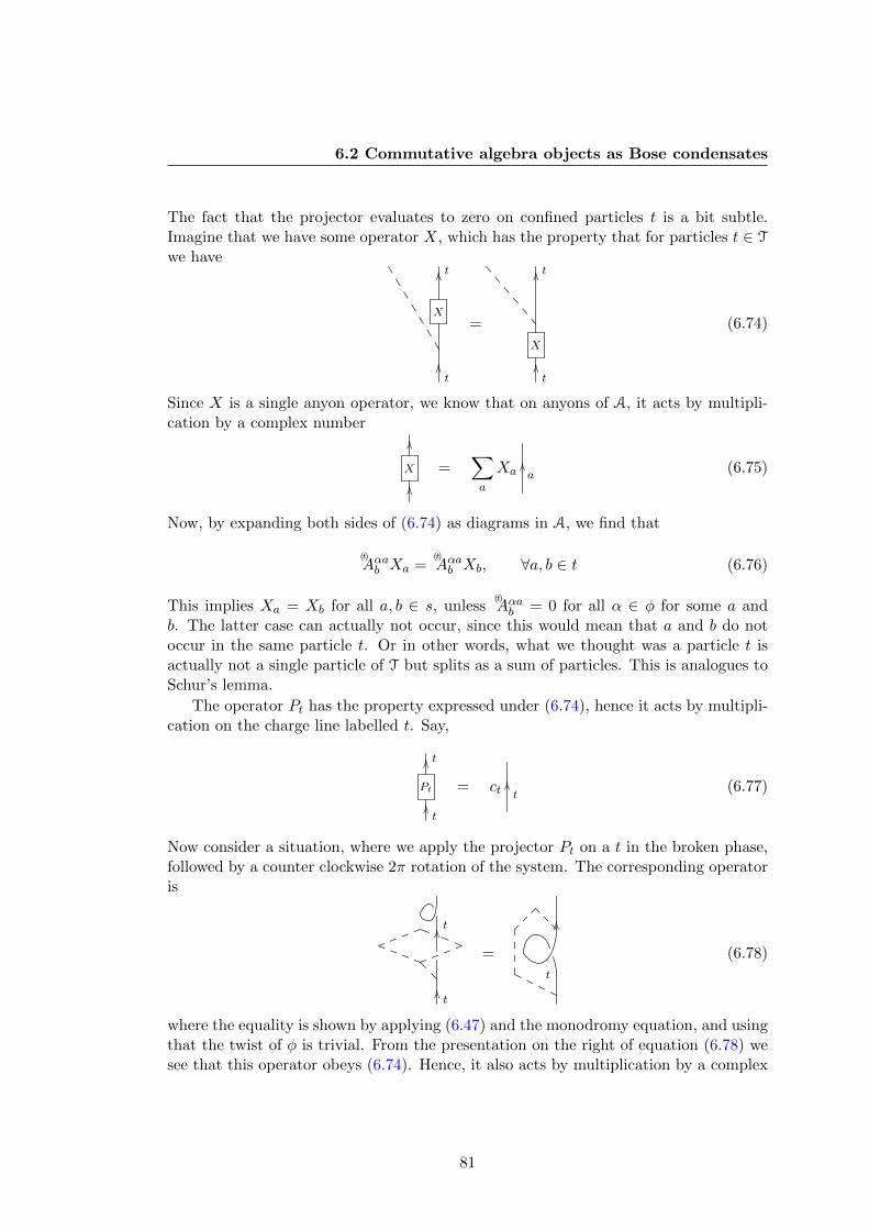
6.2 Commutative algebra objects as Bose condensates
The fact that the projector evaluates to zero on confined particles t is a bit subtle.Imagine that we have some operator X, which has the property that for particles t ∈ T
we have
t
t
X
OO
OO
=
t
t
X
OO
OO
(6.74)
Since X is a single anyon operator, we know that on anyons of A, it acts by multipli-cation by a complex number
X
OO
OO
=∑a
XaOOa
(6.75)
Now, by expanding both sides of (6.74) as diagrams in A, we find that
(t)Aαab Xa =
(t)Aαab Xb, ∀a, b ∈ t (6.76)
This implies Xa = Xb for all a, b ∈ s, unless(t)Aαab = 0 for all α ∈ φ for some a and
b. The latter case can actually not occur, since this would mean that a and b do notoccur in the same particle t. Or in other words, what we thought was a particle t isactually not a single particle of T but splits as a sum of particles. This is analogues toSchur’s lemma.
The operator Pt has the property expressed under (6.74), hence it acts by multipli-cation on the charge line labelled t. Say,
t
t
PtOO
OO
= ctOOt
(6.77)
Now consider a situation, where we apply the projector Pt on a t in the broken phase,followed by a counter clockwise 2π rotation of the system. The corresponding operatoris
t
t
OO
OO
=
t
OO
(6.78)
where the equality is shown by applying (6.47) and the monodromy equation, and usingthat the twist of φ is trivial. From the presentation on the right of equation (6.78) wesee that this operator obeys (6.74). Hence, it also acts by multiplication by a complex
81
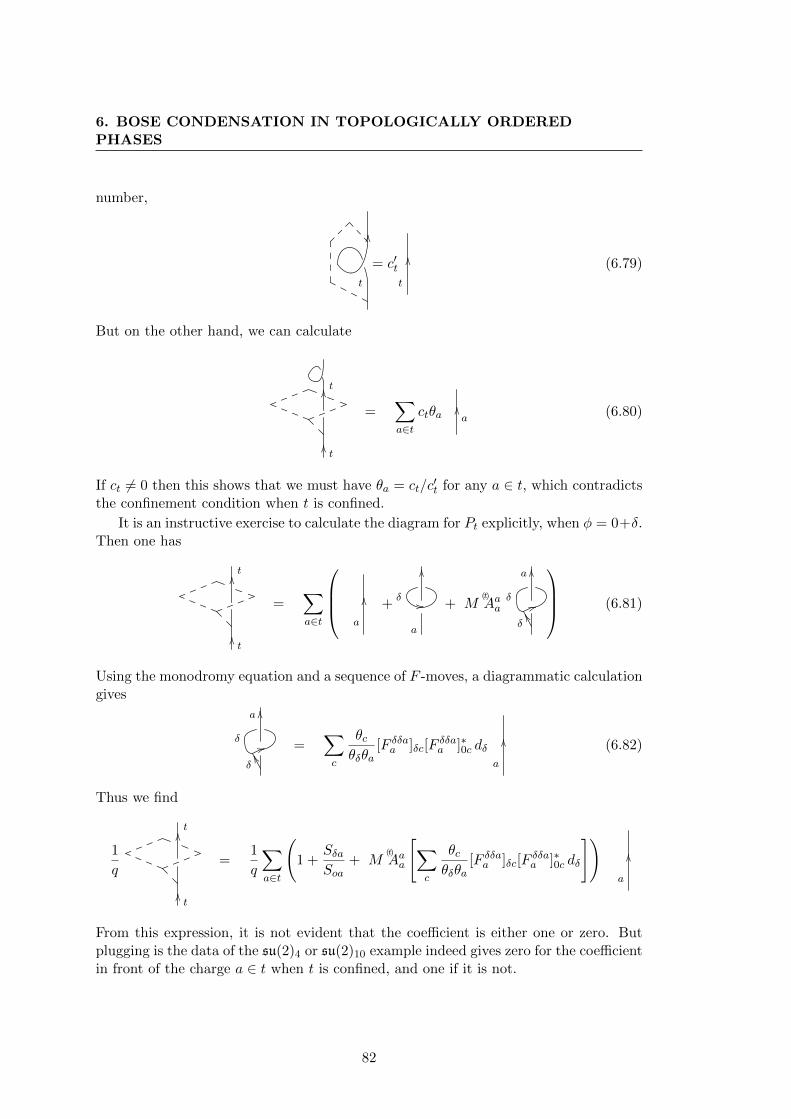
6. BOSE CONDENSATION IN TOPOLOGICALLY ORDEREDPHASES
number,
t
OO
= c′tt
OO(6.79)
But on the other hand, we can calculate
t
t
OO
OO
=∑a∈t
ctθaOOa
(6.80)
If ct 6= 0 then this shows that we must have θa = ct/c′t for any a ∈ t, which contradicts
the confinement condition when t is confined.
It is an instructive exercise to calculate the diagram for Pt explicitly, when φ = 0+δ.Then one has
t
t
OO
OO
=∑a∈t
a
OO+
a
δ
OO
// + M(t)Aaa
δ
a
δ
OO
44WW
(6.81)
Using the monodromy equation and a sequence of F -moves, a diagrammatic calculationgives
δ
a
δ
OO
44WW =
∑c
θcθδθa
[F δδaa ]δc[Fδδaa ]∗0c dδ
a
OO(6.82)
Thus we find
1
q
t
t
OO
OO
=1
q
∑a∈t
(1 +
SδaSoa
+ M(t)Aaa
[∑c
θcθδθa
[F δδaa ]δc[Fδδaa ]∗0c dδ
])a
OO
From this expression, it is not evident that the coefficient is either one or zero. Butplugging is the data of the su(2)4 or su(2)10 example indeed gives zero for the coefficientin front of the charge a ∈ t when t is confined, and one if it is not.
82
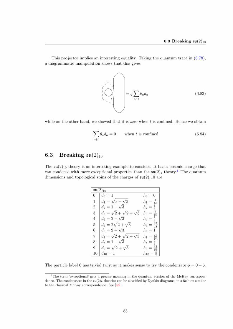
6.3 Breaking su(2)10
This projector implies an interesting equality. Taking the quantum trace in (6.78),a diagrammatic manipulation shows that this gives
t
OO
= q∑a∈t
θada (6.83)
while on the other hand, we showed that it is zero when t is confined. Hence we obtain
∑a∈t
θada = 0 when t is confined (6.84)
6.3 Breaking su(2)10
The su(2)10 theory is an interesting example to consider. It has a bosonic charge thatcan condense with more exceptional properties than the su(2)4 theory.1 The quantumdimensions and topological spins of the charges of su(2)(10 are
su(2)10
0 d0 = 1 h0 = 0
1 d1 =√s+√
3 h1 = 116
2 d2 = 1 +√
3 h2 = 16
3 d3 =√
2 +√
2 +√
3 h3 = 516
4 d4 = 2 +√
3 h4 = 12
5 d5 = 2√
2 +√
3 h5 = 3548
6 d6 = 2 +√
3 h6 = 1
7 d7 =√
2 +√
2 +√
3 h7 = 2116
8 d8 = 1 +√
3 h8 = 53
9 d9 =√
2 +√
3 h9 = 3316
10 d10 = 1 h10 = 52
The particle label 6 has trivial twist so it makes sense to try the condensate φ = 0 + 6.
1The term ‘exceptional’ gets a precise meaning in the quantum version of the McKay correspon-dence. The condensates in the su(2)k theories can be classified by Dynkin diagrams, in a fashion similarto the classical McKay correspondence. See [48].
83
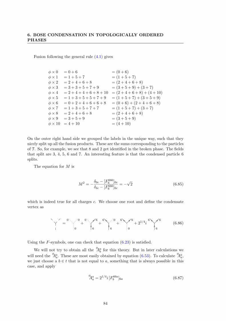
6. BOSE CONDENSATION IN TOPOLOGICALLY ORDEREDPHASES
Fusion following the general rule (4.1) gives
φ× 0 = 0 + 6 = (0 + 6)φ× 1 = 1 + 5 + 7 = (1 + 5 + 7)φ× 2 = 2 + 4 + 6 + 8 = (2 + 4 + 6 + 8)φ× 3 = 3 + 3 + 5 + 7 + 9 = (3 + 5 + 9) + (3 + 7)φ× 4 = 2 + 4 + 4 + 6 + 8 + 10 = (2 + 4 + 6 + 8) + (4 + 10)φ× 5 = 1 + 3 + 5 + 5 + 7 + 9 = (1 + 5 + 7) + (3 + 5 + 9)φ× 6 = 0 + 2 + 4 + 6 + 6 + 8 = (0 + 6) + (2 + 4 + 6 + 8)φ× 7 = 1 + 3 + 5 + 7 + 7 = (1 + 5 + 7) + (3 + 7)φ× 8 = 2 + 4 + 6 + 8 = (2 + 4 + 6 + 8)φ× 9 = 3 + 5 + 9 = (3 + 5 + 9)φ× 10 = 4 + 10 = (4 + 10)
On the outer right hand side we grouped the labels in the unique way, such that theynicely split up all the fusion products. These are the sums corresponding to the particlesof T. So, for example, we see that 8 and 2 get identified in the broken phase. The fieldsthat split are 3, 4, 5, 6 and 7. An interesting feature is that the condensed particle 6splits.
The equation for M is
M2 = −δ0c − [F 6666 ]0c
δδc − [F 6666 ]6c
= −√
2 (6.85)
which is indeed true for all charges c. We choose one root and define the condensatevertex as
=0 0
0
+0 ?? 6OO6
+__6 0
OO6
+__6 ?? 6
0
+ 21/4i__6 ?? 6OO6
(6.86)
Using the F -symbols, one can check that equation (6.23) is satisfied.
We will not try to obtain all the(t)Aab for this theory. But in later calculations we
will need the(t)Aaa. These are most easily obtained by equation (6.53). To calculate
(t)Aaa,
we just choose a b ∈ t that is not equal to a, something that is always possible in thiscase, and apply
(t)Aaa = 21/4i [F 66a
b ]6a (6.87)
84
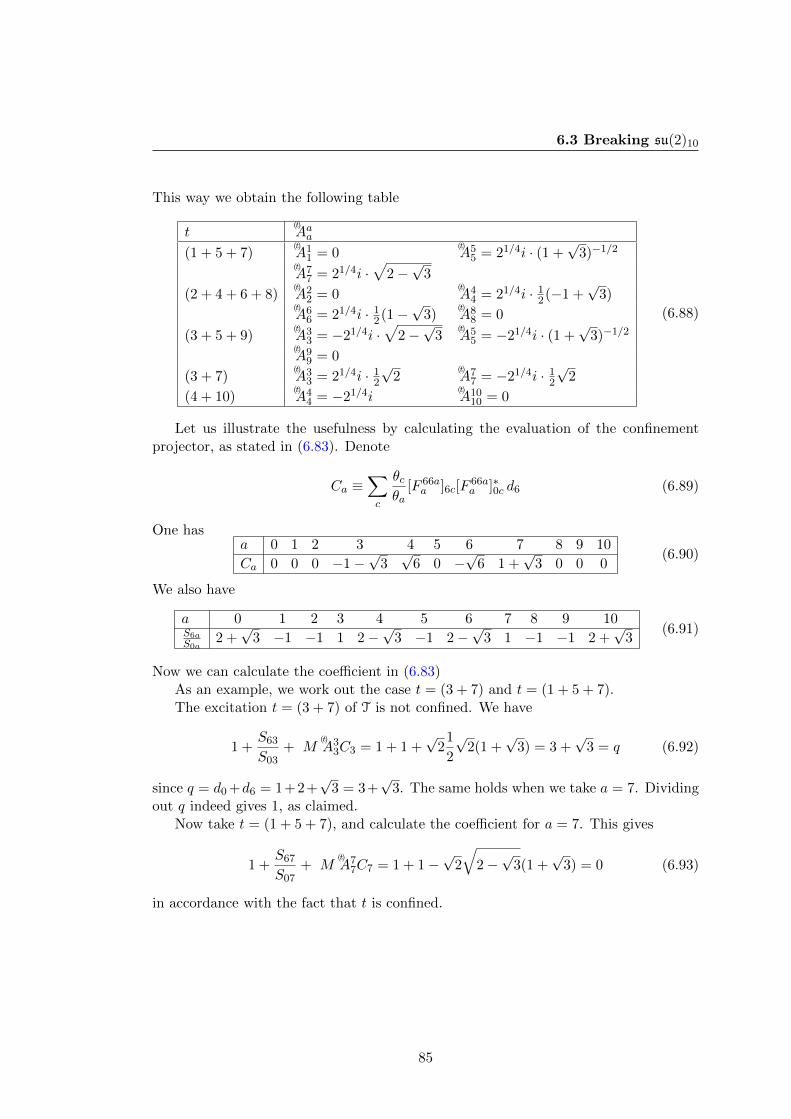
6.3 Breaking su(2)10
This way we obtain the following table
t(t)Aaa
(1 + 5 + 7)(t)A1
1 = 0(t)A5
5 = 21/4i · (1 +√
3)−1/2
(t)A7
7 = 21/4i ·√
2−√
3
(2 + 4 + 6 + 8)(t)A2
2 = 0(t)A4
4 = 21/4i · 12(−1 +
√3)
(t)A6
6 = 21/4i · 12(1−
√3)
(t)A8
8 = 0
(3 + 5 + 9)(t)A3
3 = −21/4i ·√
2−√
3(t)A5
5 = −21/4i · (1 +√
3)−1/2
(t)A9
9 = 0
(3 + 7)(t)A3
3 = 21/4i · 12
√2
(t)A7
7 = −21/4i · 12
√2
(4 + 10)(t)A4
4 = −21/4i(t)A10
10 = 0
(6.88)
Let us illustrate the usefulness by calculating the evaluation of the confinementprojector, as stated in (6.83). Denote
Ca ≡∑c
θcθa
[F 66aa ]6c[F
66aa ]∗0c d6 (6.89)
One hasa 0 1 2 3 4 5 6 7 8 9 10
Ca 0 0 0 −1−√
3√
6 0 −√
6 1 +√
3 0 0 0(6.90)
We also have
a 0 1 2 3 4 5 6 7 8 9 10S6aS0a
2 +√
3 −1 −1 1 2−√
3 −1 2−√
3 1 −1 −1 2 +√
3(6.91)
Now we can calculate the coefficient in (6.83)As an example, we work out the case t = (3 + 7) and t = (1 + 5 + 7).The excitation t = (3 + 7) of T is not confined. We have
1 +S63
S03+ M
(t)A3
3C3 = 1 + 1 +√
21
2
√2(1 +
√3) = 3 +
√3 = q (6.92)
since q = d0 +d6 = 1+2+√
3 = 3+√
3. The same holds when we take a = 7. Dividingout q indeed gives 1, as claimed.
Now take t = (1 + 5 + 7), and calculate the coefficient for a = 7. This gives
1 +S67
S07+ M
(t)A7
7C7 = 1 + 1−√
2
√2−√
3(1 +√
3) = 0 (6.93)
in accordance with the fact that t is confined.
85

6. BOSE CONDENSATION IN TOPOLOGICALLY ORDEREDPHASES
86
CHAPTER 7
Indicators for topological order
Because topologically ordered phases defy the Landau symmetry breaking scheme ofcharacterization by local order parameters, other indicators not based on symmetryhave appeared in the literature. These are ground state degeneracy on surfaces of non-zero genus [32, 77], fractional of quantum numbers (charge [55], spin [2]), gapless edgeexcitations [78], and topological entanglement entropy [58, 66]. It is clearly of inter-est to know the behaviour of these indicators under a topological symmetry breakingphase transition. The topological entanglement entropy, that has been related to thetotal quantum dimension, shows an interesting relation with the quantum dimensionof the condensate. This condensate quantum dimension q = dφ seems an interestingnumber characterizing the phase transition. It can be computed as the ratio betweenthe quantum dimensions of the lift of an arbitrary sector t of the broken phase and thequantum dimension of t itself. One can show that the increase in topological entangle-ment entropy in each step of the phase transition is log
√q for a disc-like geometry.
Another interesting problem is to construct ‘topological order parameters’, oper-ators that can be used to ‘measure’ the kind of topological order and signal phasetransitions, in simulations or experiments. The topological S-matrix is a particularlyinteresting object. Through interferometry measurements it might become possiblesoon to obtain matrix elements of the topological S-matrix in, for example, FQH states.On the other hand, it decodes a lot of information about the underlying theory. In thischapter, we will also show how to obtain the topological S-matrix using the tensorcategory approach to topological symmetry breaking.
87
7. INDICATORS FOR TOPOLOGICAL ORDER
7.1 Topological entanglement entropy
For a quantum system described by a density matrix ρ, the von Neumann entropy SEis defined as
SE = −Tr ρ log ρ (7.1)
For a gapped system in a planar region with boundary of length L, it takes the form
SE = αL− γ + . . . (7.2)
The ellipses represent terms that vanish in the limit L → ∞. The universal additiveconstant −γ characterizes global features of the entanglement in the ground state andhas been called the topological entanglement entropy. It signals non-trivial topologicalorder and in [58, 66] it was shown that for a disc-like geometry it relates to the totalquantum dimension of the theory underlying the topological order as
γ = logD (7.3)
In a topological symmetry breaking phase transition A→ T → U, the relation betweenthe total quantum dimensions DA,DT and DU therefore relates the topological entropyof the different phases. In particular the topological entanglement entropy increases byan amount
γA − γU = logDA
DU
(7.4)
We will show that this ratio is directly related to q = dφ, the quantum dimension ofthe condensate. This is in fact equal to
q =
∑a n
taa
dt(7.5)
for any t in the T-theory.We will prove that the right hand side of equation (7.5) is indeed not depending on
the choice of t. But let us first make a remark on notational conventions and assump-tions for this section. Throughout this section, we use the notation and assumptions andterminology of the original approach to topological quantum group symmetry breaking.In the literature on commutative algebras in tensor categories the same result is present(see [48]). But it is interesting that one can derive this from less involved assumptions.
Now, to show (7.5), we will just need the description of the theories on the level ofthe fusion algebas which we will also denote with A,T and U. The fusion product iswritten |a〉×|b〉 =
∑cN
cab |c〉 for A. This defines the fusion matrices Na by (Na)
cb = N c
ab.For T we use the same notations, but with {a, b, c} → {t, r, s}. Recall that the vector
|ωA〉 =∑a
da |a〉 (7.6)
is a common Perron-Frobenius eigenvector for the fusion matrices Na with eigenvalueequations
Na |ωA〉 = da |ωA〉 (7.7)
88
7.1 Topological entanglement entropy
where da is the quantum dimension of the charge a. This can be checked explicitlyfrom the relation
dadb = N cabdc (7.8)
Similarly,
|ωT〉 =∑t
dt |t〉 (7.9)
is a common Perron-Frobenius eigenvector for the fusion matrices Nt, even though thesedo not necessarily commute.
The phase transition is described by the restriction map, as discussed in the previouschapter. This is conveniently written as B : A→ T. The lift is regarded as the transposemap B† : T → A. Written out explicitly, we have
B |a〉 =∑t
nta |t〉 , B† |t〉 =∑a
nta |a〉 (7.10)
The restriction is required to commute with fusion. This can be written as B |a〉 ×B |b〉 = B(|a〉 × |b〉) or more explicitly
nta = nta,∑t,s
ntansbN
rts =
∑c
N cabn
rc (7.11)
We will study the behaviour of the Perron-Frobenius eigenvectors |ωA〉 and |ωT〉 underthe restriction and lift. We have
B† |ωT〉 =∑a,t
ntadt |a〉 (7.12)
=∑a
da |a〉 (7.13)
= |ωT〉 (7.14)
This holds, because quantum dimensions are conserved under the restriction.We will now show that
B |ωA〉 = q |ωT〉 (7.15)
Let us define the map M : T → T by
M ≡∑a
Ma =∑a,t
ntaNt (7.16)
i.e. Ma is the fusion matrix of the restriction of a and M is obtained by taking the sumover all charges a of A.The matrix elements of M are all strictly positive, since for anys, r ∈ T there is some t ∈ T with N r
ts > 0 and also any t ∈ T occurs in the decompositionof some a ∈ A. By the Perron-Frobenius theorem, the eigenspace of M correspondingto the Perron-Frobenius eigenvalue
∑a da is non-degenerate and spanned by |ωT〉. If
we can show thatMB |ωA〉 = (
∑a
da)B |ωA〉 (7.17)
89
7. INDICATORS FOR TOPOLOGICAL ORDER
it therefore follows that B |ωA〉 = λ |ωT〉 for some λ ∈ C. In components, equation(7.17) reads ∑
a,c,s,r
dcnran
scN
srt =
∑a,b
dadbnbt (7.18)
To prove this equation, we manipulate the left hand side using N srt = N t
rs and nranra,
apply (7.11), use that N bac = N c
ab = N cba and finally apply (7.8). Some intermediate
results are shown in the following computation∑a,c,s,r
dcnran
scN
srt =
∑a,c,s,r
dcnran
scN
trs (7.19)
=∑a,b,c
dcNbacn
tn (7.20)
=∑a,b,c
dcNcabn
tb (7.21)
=∑a,b
dadbntb (7.22)
Now compare components on the left and right hand side of B |ωA〉 = λ |ωT〉. One finds
λ =
∑a n
tada
dt= q (7.23)
so the fraction is indeed independent of the choice of t. The equation of the number qresembles the embedding index introduced by Dynkin in his work on the classificationof subalgebras of compact Lie algebras, hence it was named the quantum embeddingindex [6].
From B |ωA〉 = Q |ωT〉 and B† |ωT〉 = |ωA〉 it follows that the integer square matricesB†B and BB† satisfy
B†B |ωA〉 = q |ωA〉 and (7.24)
BB† |ωT〉 = q |ωT〉 (7.25)
From this we see that q = D2A/D
2T because
D2A = 〈ωA | ωA〉 = 〈ωT|BB† |ωT〉 = q 〈ωT | ωT〉 = qD2
T (7.26)
If we used (6.15), we find that
DA
DT
=DT
DU
=√q (7.27)
This shows that the topological entropy of the respective phases changes following
γA+ log
√q// γT
+ log√q// γU (7.28)
90
7.2 Topological S-matrix as an order parameter
For a complete result, it would be nice to prove the relations on the total quantumdimensions. In [48], this is done by proving that U is a modular tensor category when A
is modular, and proving that there is a kind of commutation relation for the S-matricesof the respective theories and the restriction map. If we agree to denote the S-matrixof U by Suv, where u, v run over the U-labels, one has BS = SB, or in components∑
a
nuaSab =∑u
Suvnvb (7.29)
7.2 Topological S-matrix as an order parameter
Much of the information about the topological order of a system is encoded in thetopological S-matrix. Knowing the S-matrix gives direct access to the quantum di-mensions of the charges, as well as the total quantum dimension, and the fusion rulescan be derived via the Verlinde formula. In addition, it is important in experimentalverification of topological order, as it is closely related to the monodromy matrix thatoften appears in the probabilities for interferometry experiments.
Using the extended formalism for topological symmetry breaking from the lastchapter, we can study the effect of the formation of a Bose condensate on the S-matrixof the theory diagrammatically. We write down an explicit formula and illustrate thisby calculations for the su(2)4 and su(2)10 example.
It will be convenient to leave the normalization factor D−1 out of the definitionof the S-matrix is this section. Hence, we define the S-matrix of A simply as theevaluation of the well known Hopf link
Sab =a b
OO OO (7.30)
The monodromy equation lets us express the S-matrix in terms of the fusion multiplic-ities, quantum dimensions and twist factors as
Sab =∑c
N cab
θaθbθc
dc (7.31)
For su(2)4, this gives for example
Sab =
a, b 0 1 2 3 4
0 1√
3 2√
3 1
1√
3√
3 0 −√
3 −√
32 2 0 −2 0 2
3√
3 −√
3 0√
3 −√
3
4 1 −√
3 2 −√
3 1
(7.32)
The S-matrix describes a process where two particle-anti-particle-pairs are drawn outof the vacuum, the two particles undergo a full monodromy and the pair annihilates
91
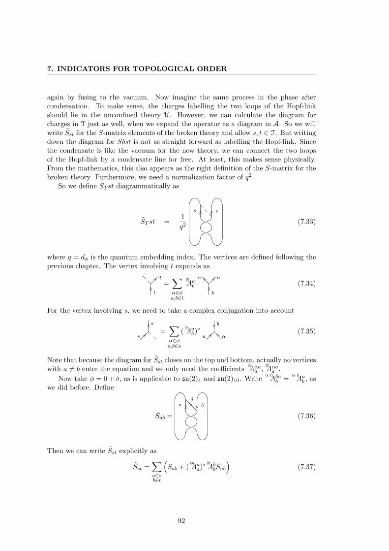
7. INDICATORS FOR TOPOLOGICAL ORDER
again by fusing to the vacuum. Now imagine the same process in the phase aftercondensation. To make sense, the charges labelling the two loops of the Hopf-linkshould lie in the unconfined theory U. However, we can calculate the diagram forcharges in T just as well, when we expand the operator as a diagram in A. So we willwrite Sst for the S-matrix elements of the broken theory and allow s, t ∈ T. But writingdown the diagram for Sbst is not as straight forward as labelling the Hopf-link. Sincethe condensate is like the vacuum for the new theory, we can connect the two loopsof the Hopf-link by a condensate line for free. At least, this makes sense physically.From the mathematics, this also appears as the right definition of the S-matrix for thebroken theory. Furthermore, we need a normalization factor of q2.
So we define ST st diagrammatically as
ST st =1
q2
OOs OO t
(7.33)
where q = dφ is the quantum embedding index. The vertices are defined following theprevious chapter. The vertex involving t expands as
?? tOOt
=∑α∈φa,b∈t
(t)Aab
__α ?? aOOb
(7.34)
For the vertex involving s, we need to take a complex conjugation into account
??s
OO s=∑α∈φa,b∈s
((s)Aab )
∗ ??a
__α
OO b(7.35)
Note that because the diagram for Sst closes on the top and bottom, actually no verticeswith a 6= b enter the equation and we only need the coefficients
(s)Aαaa ,
(t)Aαaa .
Now take φ = 0 + δ, as is applicable to su(2)4 and su(2)10. Write(s,t)Aδab =
(s,t)Aab , as
we did before. Define
Sab =
OOa OO b__ δ
(7.36)
Then we can write Sst explicitly as
Sst =∑a∈sb∈t
(Sab + (
(s)Aaa)
∗ (t)AbbSab
)(7.37)
92
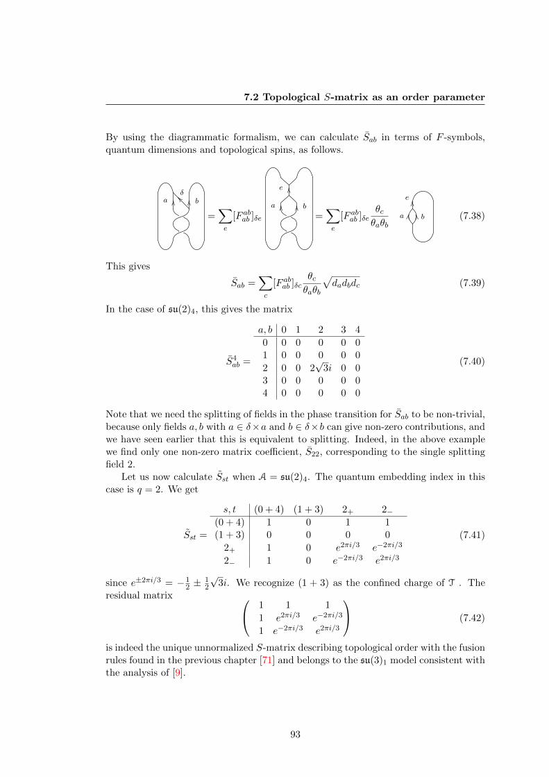
7.2 Topological S-matrix as an order parameter
By using the diagrammatic formalism, we can calculate Sab in terms of F -symbols,quantum dimensions and topological spins, as follows.
OOa OO b__ δ
=∑e
[F abab ]δe
OOa OO b
OOe
=∑e
[F abab ]δeθcθaθb
a b
e OO
LL RR (7.38)
This gives
Sab =∑c
[F abab ]δcθcθaθb
√dadbdc (7.39)
In the case of su(2)4, this gives the matrix
S4ab =
a, b 0 1 2 3 4
0 0 0 0 0 01 0 0 0 0 0
2 0 0 2√
3i 0 03 0 0 0 0 04 0 0 0 0 0
(7.40)
Note that we need the splitting of fields in the phase transition for Sab to be non-trivial,because only fields a, b with a ∈ δ×a and b ∈ δ×b can give non-zero contributions, andwe have seen earlier that this is equivalent to splitting. Indeed, in the above examplewe find only one non-zero matrix coefficient, S22, corresponding to the single splittingfield 2.
Let us now calculate Sst when A = su(2)4. The quantum embedding index in thiscase is q = 2. We get
Sst =
s, t (0 + 4) (1 + 3) 2+ 2−(0 + 4) 1 0 1 1(1 + 3) 0 0 0 0
2+ 1 0 e2πi/3 e−2πi/3
2− 1 0 e−2πi/3 e2πi/3
(7.41)
since e±2πi/3 = −12 ± 1
2
√3i. We recognize (1 + 3) as the confined charge of T . The
residual matrix 1 1 1
1 e2πi/3 e−2πi/3
1 e−2πi/3 e2πi/3
(7.42)
is indeed the unique unnormalized S-matrix describing topological order with the fusionrules found in the previous chapter [71] and belongs to the su(3)1 model consistent withthe analysis of [9].
93
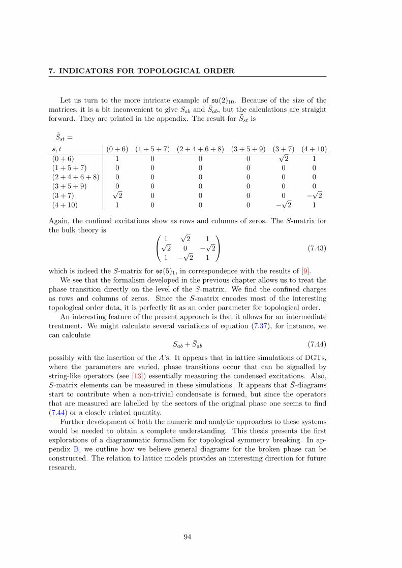
7. INDICATORS FOR TOPOLOGICAL ORDER
Let us turn to the more intricate example of su(2)10. Because of the size of thematrices, it is a bit inconvenient to give Sab and Sab, but the calculations are straightforward. They are printed in the appendix. The result for Sst is
Sst =
s, t (0 + 6) (1 + 5 + 7) (2 + 4 + 6 + 8) (3 + 5 + 9) (3 + 7) (4 + 10)
(0 + 6) 1 0 0 0√
2 1(1 + 5 + 7) 0 0 0 0 0 0(2 + 4 + 6 + 8) 0 0 0 0 0 0(3 + 5 + 9) 0 0 0 0 0 0
(3 + 7)√
2 0 0 0 0 −√
2
(4 + 10) 1 0 0 0 −√
2 1
Again, the confined excitations show as rows and columns of zeros. The S-matrix forthe bulk theory is 1
√2 1√
2 0 −√
2
1 −√
2 1
(7.43)
which is indeed the S-matrix for so(5)1, in correspondence with the results of [9].We see that the formalism developed in the previous chapter allows us to treat the
phase transition directly on the level of the S-matrix. We find the confined chargesas rows and columns of zeros. Since the S-matrix encodes most of the interestingtopological order data, it is perfectly fit as an order parameter for topological order.
An interesting feature of the present approach is that it allows for an intermediatetreatment. We might calculate several variations of equation (7.37), for instance, wecan calculate
Sab + Sab (7.44)
possibly with the insertion of the A’s. It appears that in lattice simulations of DGTs,where the parameters are varied, phase transitions occur that can be signalled bystring-like operators (see [13]) essentially measuring the condensed excitations. Also,S-matrix elements can be measured in these simulations. It appears that S-diagramsstart to contribute when a non-trivial condensate is formed, but since the operatorsthat are measured are labelled by the sectors of the original phase one seems to find(7.44) or a closely related quantity.
Further development of both the numeric and analytic approaches to these systemswould be needed to obtain a complete understanding. This thesis presents the firstexplorations of a diagrammatic formalism for topological symmetry breaking. In ap-pendix B, we outline how we believe general diagrams for the broken phase can beconstructed. The relation to lattice models provides an interesting direction for futureresearch.
94

7.2 Topological S-matrix as an order parameter
q=2
95

7. INDICATORS FOR TOPOLOGICAL ORDER
96
CHAPTER 8
Conclusion and outlook
We have discussed topological order for planar systems, and in particular the role ofquantum groups and modular tensor categories. A general graphical formalism fortopologically ordered phases based on tensor categories was discussed. As discussed inchapter 4, the essential data is given by fusion coefficients N c
ab, F -symbols [F abcd ]ef andR-symbols Rabc . We showed how to calculate these for the quantum double theorieswithout multiplicities and the important su(2)k series in chapter.
Making use of the literature on tensor categories, we have reconsidered topologicalsymmetry breaking phase transitions and argued that Bose condensates, in this setting,correspond to commutative algebra objects. A diagrammatic formalism for topologicalsymmetry breaking was subsequently explored. The necessary consistency conditionswere solved explicitly for representative examples.
We derived some new information regarding topological symmetry breaking in thisthesis. The particle spectrum of broken theory can be derived by calculating φ× a. Itwas also shown that the quantum dimension of the condensate is a universal numberq, the quantum embedding index, that characterizes the phase transitions and in factrelates to the topological entanglement entropy.
Using the extended formalism for topological symmetry breaking, we could studythe S-matrix analytically before and after the phase transition. We recovered the resultsof the breaking of su(2)4 and su(2)10. This suggests the usefulness of the S-matrix asan order parameter for topological order.
The link that exists between commutative algebras in braided tensor categories andBose condensates suggests that this structure should appear in a variety of physicalcontexts. If it, indeed, turns out that topological symmetry breaking is the leading un-derlying mechanism for phase transitions between planar topologically ordered phases,this gives commutative algebras in braided tensor categories a role analogues to therole of subgroups in the regular theory of symmetry breaking phase transitions. Fur-
97
8. CONCLUSION AND OUTLOOK
ther explorations in this direction are an interesting endeavour and should definitelybe continued.
One can imagine several directions. For instance, further application in addressingquestions physical contexts such as the FQHE and topological quantum computationare likely to lead to interesting insights. Using the graphical formalism, it should forexample be possible to discuss questions concerning interferometry measurements forsystems with multiple phases.
Furthermore, relating the results to lattice simulations that calculate can furtherreveal the significance and meaning of the coefficients that were needed to solve theequations that resulted from the consistency conditions of the condensate and chargevertices. Many questions remain in this area.
While we believe that the theory of algebras in tensor categories provides a con-structive way to construct the category of the broken phase, the formalism can stillbe refined. For example, how do we obtain the fusion multiplicities in a more directmanner? To clarify such questions, it is useful to further study and translate the math-ematical results from the tensor category literature to a physical context. We thinkthat inspecting notions that play an important role in the mathematical literature andassessing their physical relevance will lead to a considerable amount of interesting anduseful work. An example might be the center construction, which produces a commuta-tive algebra in the center (quantum double) of the category from any non-commutativealgebra. This could relate to phase transitions in the Levin-Wen models, as the cat-egory that governs excitations is the center (double) of the category that is used asinput in these models.
Finally, either from a mathematicians of physicists perspective, it is interesting toidentify the results from the tensor category approachin alternative formulations. Forinstance, one could study topological quantum field theory, or search for relations toquestions in low-dimensional topology.
In conclusion, a considerable amount of interesting and useful work lies ahead tobe undertaken.
98
APPENDIX A
Quasi-triangular Hopf algebras
Below is a gathering of the axioms of quasi-triangular Hopf algebras (or quantumgroups) with the corresponding mathematical nomenclature. We refer to [46] and [75]for a thorough treatment.
A Hopf algebra H is, in short, a bialgebra with an antipode. A bit more elaborate,this means that we have an associative algebra with multiplication m : H ⊗ H → H
and unit 1 : C→ H. Associativity is give by the condition
m(m⊗ id) = m(id⊗m) (A.1)
The unit axiom is
m(1⊗ id) = m(id⊗1) = id (A.2)
Here id is the identity on H.
It is also required that H is a coalgebra, which requires the definition of a comulti-plication
∆: H → H ⊗H (A.3)
and a counit
ε : H → C (A.4)
They have to satisfy the coassociativity axiom
(id⊗∆)∆ = (∆⊗ id)∆ (A.5)
and the counit property
(ε⊗ id)∆ = id = (id⊗)ε∆ (A.6)
There is a natural multiplication, also denoted m, on H⊗H. For elements a1⊗ a2 andb1⊗b2 of H⊗H, this is m(a1⊗a2, b1⊗b2) = m(a1, b1)⊗m(a2, b2). An algebra that is also
99
A. QUASI-TRIANGULAR HOPF ALGEBRAS
a coalgebra, is called a bialgebra if the algebra and coalgebra structure are compatible.Compatibility can be formulated as the requirement that the comultiplication andcounit are algebra homorphisms (i,e, commute with the appropriate multiplication).
One ingredient is still lacking to make H a Hopf algebra, namely the existence ofan antipode. This is a linear map S : H→ H satisfying
m(id⊗S)∆ = 1ε = m(S ⊗ id)∆ (A.7)
It can be shown that, if a bialgebra admits an antipode, it is unique. So there is atmost one Hopf algebra structure on any bialgebra.
Now what is the significance of Hopf algebras to physics? We are of course interestedin the representations of H to describe the particle spectrum in some (2+1)d quantumtheory. The comultiplication gives the definition of tensor product representationsneeded to describe multi-particle states. Suppose α, β are two representations of H
with carrier spaces Vα, Vβ given by Πα,β : H → End(Vα,β). Then we define the tensorproduct representation α⊗ β, acting on Vα ⊗ Vβ, by
Πα⊗β(a) ≡ Πα ⊗Πβ(∆(a)), a ∈ H (A.8)
Coassociativity ensures that multi-particle states defined by successive application ofthe copruduct do not depend on the chosen order for the application of the comultipli-cation. The tensor product representations will generally fall apart as direct sums ofirreducible representations. This gives rise to the fusion rules of the theory.
The counit gives the definition of the trivial representation Π0 = ε. The counitproperty precisely provides the triviality of fusion on the level of representations, 0⊗α =α = α⊗ 0, because
Π0⊗α(a) = (ε⊗Πα)∆(a) = Πα(ε⊗ id)∆(a) = Πα(a) (A.9)
The notion of anti-particles or conjugate charges (dual representations) is implementedusing the antipode. Let us denote the conjugate (or dual) representation of α by α. Wecan define such a representation on the dual vector space V ∗α by means of the antipodeas
Πα(a) = Πα(S(a))T (A.10)
where the T denotes matrix transposition.The ingredient needed to describe the braiding of representations of a Hopf algebra
is the universal R-matrix. This is an invertible element R ∈ H ⊗ H which has theproperties
∆op(a)R = R∆(a) (∀a ∈ H) (A.11)
(∆⊗ id)(R) = R13R23 (A.12)
(id⊗∆)(R) = R13R12 (A.13)
Here ∆op = σ∆ is the composition of the comultiplication with the exchange σ of tensorfactors in H ⊗H. The notation Rij is an abbreviation for the action of R on the ith
100
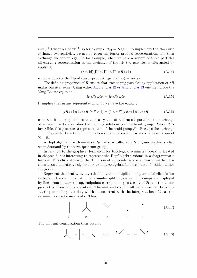
and jth tensor leg of H⊗3, so for example R12 = R ⊗ 1. To implement the clockwiseexchange two particles, we act by R on the tensor product representation, and thenexchange the tensor legs. So for example, when we have a system of three particlesall carrying representation α, the exchange of the left two particles is effectuated byapplying
(τ ⊗ id)(Πα ⊗Πα ⊗Πα)(R⊗ 1) (A.14)
where τ denotes the flip of tensor product legs τ |v〉 |w〉 = |w〉 |v〉.The defining properties of R ensure that exchanging particles by application of τR
makes physical sense. Using either A.11 and A.12 or A.11 and A.13 one may prove theYang-Baxter equation
R12R13R23 = R23R13R12 (A.15)
It implies that in any representation of H we have the equality
(τR⊗ 1)(1⊗ τR)(τR⊗ 1) = (1⊗ τR)(τR⊗ 1)(1⊗ τR) (A.16)
from which one may deduce that in a system of n identical particles, the exchangeof adjacent particle satisfies the defining relations for the braid group. Since R isinvertible, this generates a representation of the braid group Bn. Because the exchangecommutes with the action of H, it follows that the system carries a representation ofH ×Bn
A Hopf algebra H with universal R-matrix is called quasitriangular, so this is whatwe understand by the term quantum group.
In relation to the graphical formalism for topological symmetry breaking treatedin chapter 6 it is interesting to represent the Hopf algebra axioms in a diagrammaticfashion. This elucidates why the definition of the condensate is known to mathemati-cians as an commutative algebra, or actually coalgebra, in the context of braided tensorcategories.
Represent the identity by a vertical line, the multiplication by an unlabelled fusionvertex and the comultiplication by a similar splitting vertex. Thus maps are displayedby lines from bottom to top, endpoints corresponding to a copy of H and the tensorproduct is given by juxtaposition. The unit and counit will be represented by a linestarting or ending at a dot, which is consistent with the interpretation of C as thevacuum module by means of ε. Thus
id m ∆ 1
•
ε
•(A.17)
The unit ant counit axiom then become
•= =
•and
•= =
•(A.18)
101
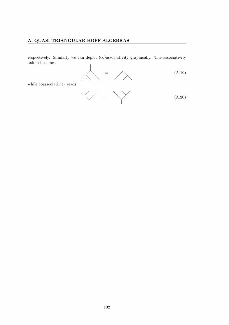
A. QUASI-TRIANGULAR HOPF ALGEBRAS
respectively. Similarly we can depict (co)associativity graphically. The associativityaxiom becomes
= (A.19)
while coassociativity reads
= (A.20)
102
APPENDIX B
Tensor categories: from math to physics
We present a sketch of the definitions of a tensor category and the relevant additionalstructure that underlies the main body of the text. See [54] for the standard introduc-tion to category theory. See [14] or [75] for a thorough treatment of tensor categoriesand the mathematics of modular functors, modular tensor categories and TQFT. Adiscussion of tensor categories in relation to quantum groups is also included in [46].An influential paper on the relation of tensor categories to invariants of knots and three-manifolds is [70] which also includes a concise and clear recap of tensor categories. Weoutline the formalities such that it becomes clear how they relate to the main body ofthe text. For a thorough treatment, we must refer to the literature.
B.1 Objects, morphisms and functors
Much of mathematics can be understood in terms of properties of the structure preserv-ing maps, such as homomorphisms of groups, acting between objects of a certain class,e.g. groups, leaving out the internal structure of the object. This is the central idea ofa category. Examples are the category of topological spaces with homeomorphisms, thecategory of sets and maps, the category of groups and group homomorphisms, the cat-egory of 3-dimensional manifolds and smooth maps and the category of vector spaceswith linear maps.
A category A consists of a class Ob(A), elements of which are called the objectsof A, and a class Hom(A), elements of which are called the morphisms of A. Anymorphism f has a source A ∈ Ob(A) and a target B ∈ Ob(A) and are is often denotedby an arrow f : A→ B or
Af−→ B (B.1)
The morphisms from A to B are also denoted by HomA(A,B), or simply Hom(A,B).
103
B. TENSOR CATEGORIES: FROM MATH TO PHYSICS
If f ∈ Hom(A,B) and g ∈ Hom(B,C) we can compose the morphisms f and g.Composition is denoted gf (often g ◦ f). In a diagram, we have the correspondingcomposition of arrows
gf : Af−→ B
g−→ C (B.2)
For any object A there is a special morphism called the identity idA which obeys
idA f = f = f idA, ∀f ∈ Hom(A,A) (B.3)
A morphism f : A→ B is called an isomorphism if there exists an morphism f−1 : B →A such that
f−1f = idA, ff−1 = idB, (B.4)
The right notion for maps between categories is that of a functor. A functor F : A→B consists of a map F : Ob(A)→ Ob(B) and a map F : Hom(A)→ Hom(B) such that
• F (idA) = FidF (A)for all A ∈ Ob(A)
• if f : A→ B then F (f) : F (A)→ F (B)
• if f and g are morphism of A then
F (fg) = F (f)F (g) (B.5)
From two categories A and B, one can construct the product category A×B. If A,Bdescribe physical systems, this corresponds to the combined system when they do notinteract. Objects of A × B are pairs of objects (A,B), with A ∈ Ob(A), B ∈ Ob(B),and morphisms are just pairs of morphisms, or written formally
HomA×D((A,B), (A′, B′)) = HomA(A,A′)×HomB(B,B′) (B.6)
If F and G are two functors and F : A→ B, G : BA, a natural transformation α : F →G is a family of morphisms αA : F (A)→ G(A) such that the diagram
F (A)αA //
F (f)��
G(A)
G(f)��
F (B)αB // G(B)
(B.7)
commutes. If αA is an isomorphism for every A, α is called a natural isomorphism.There is a notion of equivalence for categories. Two categories A and B are equiv-
alent if there are functors F : A → B and G : B → A such that the compositions FGand GF are naturally isomorphic to the respective identity functors.
We are interested in categories to model anyons. To regard certain objects asanyons and morphisms as anyon operators, these categories should incorporate fusionand braiding. Fusion requires the definition of a tensor product and direct sum in thesecategories. We will outline the definitions below.
104
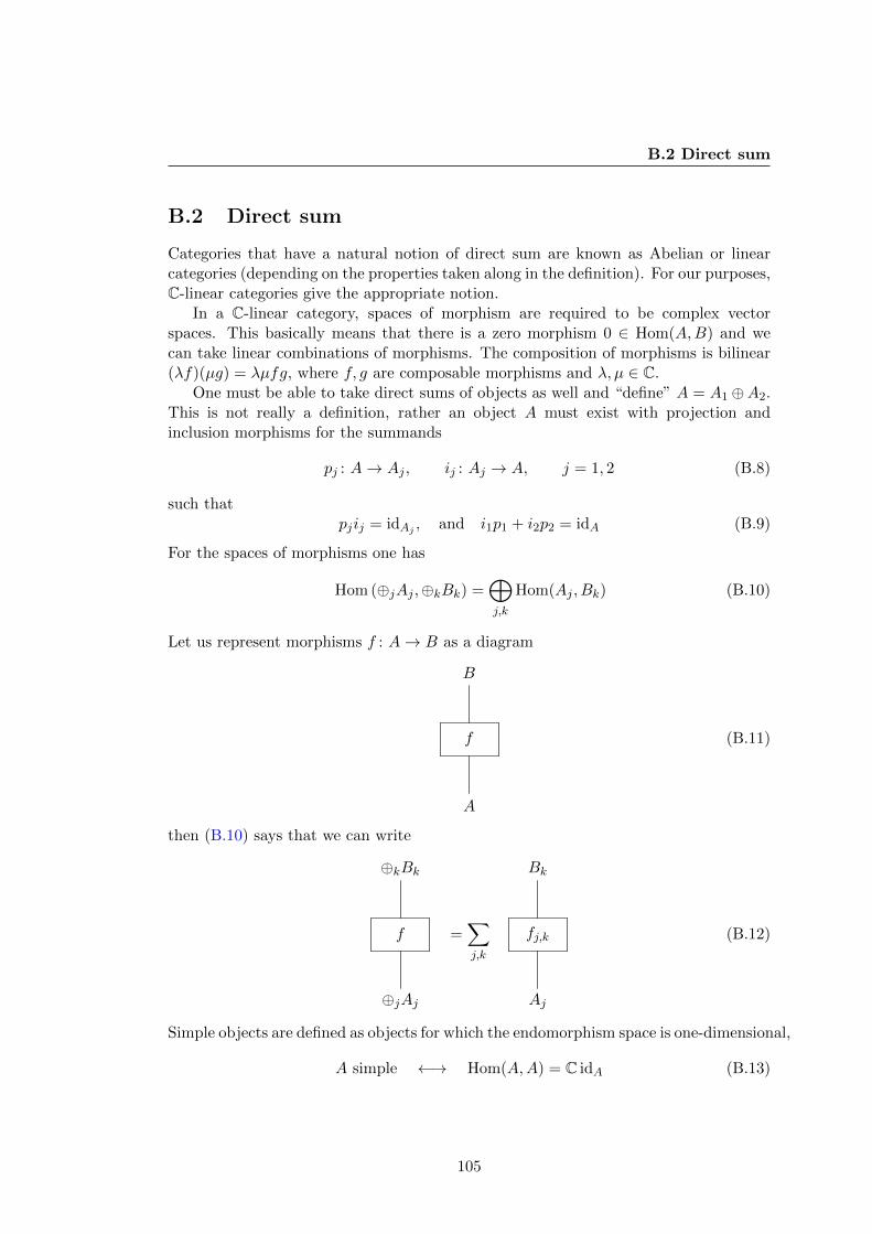
B.2 Direct sum
B.2 Direct sum
Categories that have a natural notion of direct sum are known as Abelian or linearcategories (depending on the properties taken along in the definition). For our purposes,C-linear categories give the appropriate notion.
In a C-linear category, spaces of morphism are required to be complex vectorspaces. This basically means that there is a zero morphism 0 ∈ Hom(A,B) and wecan take linear combinations of morphisms. The composition of morphisms is bilinear(λf)(µg) = λµfg, where f, g are composable morphisms and λ, µ ∈ C.
One must be able to take direct sums of objects as well and “define” A = A1 ⊕A2.This is not really a definition, rather an object A must exist with projection andinclusion morphisms for the summands
pj : A→ Aj , ij : Aj → A, j = 1, 2 (B.8)
such thatpjij = idAj , and i1p1 + i2p2 = idA (B.9)
For the spaces of morphisms one has
Hom (⊕jAj ,⊕kBk) =⊕j,k
Hom(Aj , Bk) (B.10)
Let us represent morphisms f : A→ B as a diagram
f
A
B
(B.11)
then (B.10) says that we can write
f
⊕jAj
⊕kBk
=∑j,k
fj,k
Aj
Bk
(B.12)
Simple objects are defined as objects for which the endomorphism space is one-dimensional,
A simple ←→ Hom(A,A) = C idA (B.13)
105
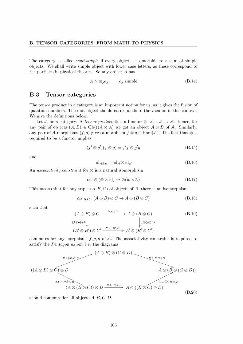
B. TENSOR CATEGORIES: FROM MATH TO PHYSICS
The category is called semi-simple if every object is isomorphic to a sum of simpleobjects. We shall write simple object with lower case letters, as these correspond tothe particles in physical theories. So any object A has
A ' ⊕jaj , aj simple (B.14)
B.3 Tensor categories
The tensor product in a category is an important notion for us, as it gives the fusion ofquantum numbers. The unit object should corresponds to the vacuum in this context.We give the definitions below.
Let A be a category. A tensor product ⊗ is a functor ⊗ : A × A → A. Hence, forany pair of objects (A,B) ∈ Ob(()A × A) we get an object A ⊗ B of A. Similarly,any pair of A-morphisms (f, g) gives a morphism f ⊗ g ∈ Hom(A). The fact that ⊗ isrequired to be a functor implies
(f ′ ⊗ g′)(f ⊗ g) = f ′f ⊗ g′g (B.15)
andidA⊗B = idA⊗ idB (B.16)
An associativity constraint for ⊗ is a natural isomorphism
α : ⊗ (⊗× id)→ ⊗(id×⊗) (B.17)
This means that for any triple (A,B,C) of objects of A, there is an isomorphism
αA,B,C : (A⊗B)⊗ C → A⊗ (B ⊗ C) (B.18)
such that
(A⊗B)⊗ C αA,B,C //
(f⊗g)⊗h��
A⊗ (B ⊗ C)
f⊗(g⊗h)��
(A′ ⊗B′)⊗ C ′αA′,B′,C′ // A′ ⊗ (B′ ⊗ C ′)
(B.19)
commutes for any morphisms f, g, h of A. The associativity constraint is required tosatisfy the Pentagon axiom, i.e. the diagrams
(A⊗B)⊗ (C ⊗D)
A⊗ (B ⊗ (C ⊗D))
A⊗ ((B ⊗ C)⊗D)(A⊗ (B ⊗ C))⊗D
((A⊗B)⊗ C)⊗D
αA,B,C⊗D
**
idA⊗αB,C,D
77
αA,B⊗C,D //αA,B,C⊗idD
''
αA⊗B,C,D
55
(B.20)should commute for all objects A,B,C,D.
106
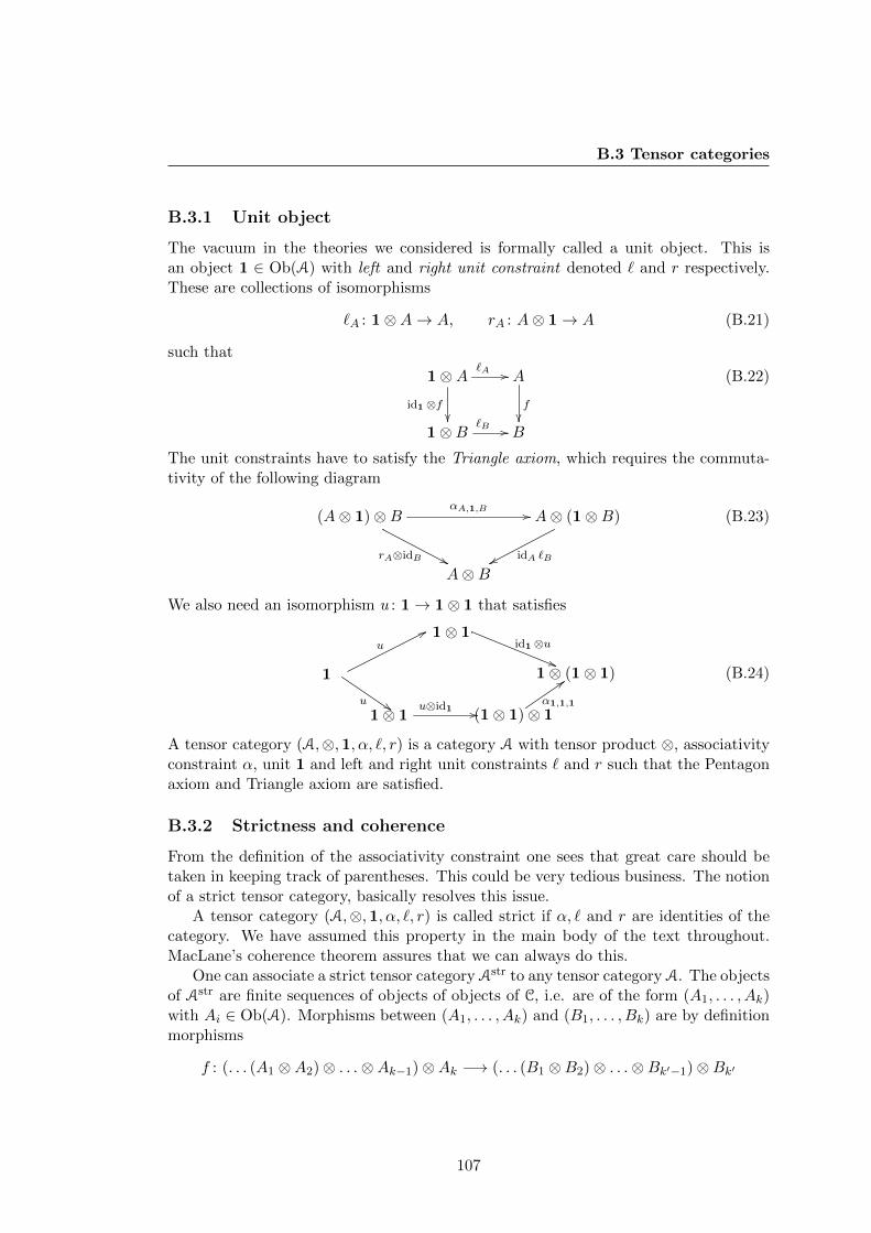
B.3 Tensor categories
B.3.1 Unit object
The vacuum in the theories we considered is formally called a unit object. This isan object 1 ∈ Ob(A) with left and right unit constraint denoted ` and r respectively.These are collections of isomorphisms
`A : 1⊗A→ A, rA : A⊗ 1→ A (B.21)
such that
1⊗Aid1⊗f
��
`A // A
f��
1⊗B `B // B
(B.22)
The unit constraints have to satisfy the Triangle axiom, which requires the commuta-tivity of the following diagram
(A⊗ 1)⊗B
rA⊗idB &&
αA,1,B // A⊗ (1⊗B)
idA `BxxA⊗B
(B.23)
We also need an isomorphism u : 1→ 1⊗ 1 that satisfies
1⊗ 1
1⊗ (1⊗ 1)
(1⊗ 1)⊗ 11⊗ 1
1
id1⊗u))
α1,1,1
::
u⊗id1 //u $$
u
77
(B.24)
A tensor category (A,⊗,1, α, `, r) is a category A with tensor product ⊗, associativityconstraint α, unit 1 and left and right unit constraints ` and r such that the Pentagonaxiom and Triangle axiom are satisfied.
B.3.2 Strictness and coherence
From the definition of the associativity constraint one sees that great care should betaken in keeping track of parentheses. This could be very tedious business. The notionof a strict tensor category, basically resolves this issue.
A tensor category (A,⊗,1, α, `, r) is called strict if α, ` and r are identities of thecategory. We have assumed this property in the main body of the text throughout.MacLane’s coherence theorem assures that we can always do this.
One can associate a strict tensor category Astr to any tensor category A. The objectsof Astr are finite sequences of objects of objects of C, i.e. are of the form (A1, . . . , Ak)with Ai ∈ Ob(A). Morphisms between (A1, . . . , Ak) and (B1, . . . , Bk) are by definitionmorphisms
f : (. . . (A1 ⊗A2)⊗ . . .⊗Ak−1)⊗Ak −→ (. . . (B1 ⊗B2)⊗ . . .⊗Bk′−1)⊗Bk′
107
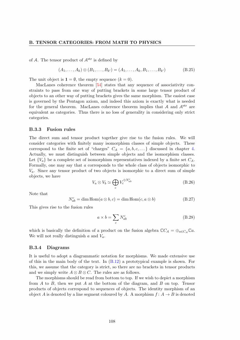
B. TENSOR CATEGORIES: FROM MATH TO PHYSICS
of A. The tensor product of Astr is defined by
(A1, . . . , Ak)⊗ (B1, . . . , Bk′) = (A1, . . . , Ak, B1, . . . , Bk′) (B.25)
The unit object is 1 = ∅, the empty sequence (k = 0).MacLanes coherence theorem [54] states that any sequence of associativity con-
straints to pass from one way of putting brackets in some large tensor product ofobjects to an other way of putting brackets gives the same morphism. The easiest caseis governed by the Pentagon axiom, and indeed this axiom is exactly what is neededfor the general theorem. MacLanes coherence theorem implies that A and Astr areequivalent as categories. Thus there is no loss of generality in considering only strictcategories.
B.3.3 Fusion rules
The direct sum and tensor product together give rise to the fusion rules. We willconsider categories with finitely many isomorphism classes of simple objects. Thesecorrespond to the finite set of “charges” CA = {a, b, c, . . . } discussed in chapter 4.Actually, we must distinguish between simple objects and the isomorphism classes.Let {Va} be a complete set of isomorphism representatives indexed by a finite set CA.Formally, one may say that a corresponds to the whole class of objects isomorphic toVa. Since any tensor product of two objects is isomorphic to a direct sum of simpleobjects, we have
Va ⊗ Vb '⊕c
V⊕Nc
abc (B.26)
Note thatN cab = dim Hom(a⊗ b, c) = dim Hom(c, a⊗ b) (B.27)
This gives rise to the fusion rules
a× b =∑c
N cab (B.28)
which is basically the definition of a product on the fusion algebra CCA = ⊕a∈CACa.
We will not really distinguish a and Va.
B.3.4 Diagrams
It is useful to adopt a diagrammatic notation for morphisms. We made extensive useof this in the main body of the text. In (B.12) a prototypical example is shown. Forthis, we assume that the category is strict, so there are no brackets in tensor productsand we simply write A⊗B ⊗ C. The rules are as follows.
The morphisms should be read from bottom to top. If we wish to depict a morphismfrom A to B, then we put A at the bottom of the diagram, and B on top. Tensorproducts of objects correspond to sequences of objects. The identity morphism of anobject A is denoted by a line segment coloured by A. A morphism f : A→ B is denoted
108
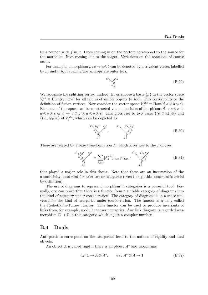
B.4 Duals
by a coupon with f in it. Lines coming in on the bottom correspond to the source forthe morphism, lines coming out to the target. Variations on the notations of courseoccur.
For example, a morphism µ : c→ a⊗b can be denoted by a trivalent vertex labelledby µ, and a, b, c labelling the appropriate outer legs,
µ
__a ?? bOOc
(B.29)
We recognise the splitting vertex. Indeed, let us choose a basis {µ} in the vector spaceV abc ≡ Hom(c, a ⊗ b) for all triples of simple objects (a, b, c). This corresponds to the
definition of fusion vertices. Now consider the vector space V abcd ≡ Hom(d, a ⊗ b ⊗ c).
Elements of this space can be constructed via composition of morphisms d→ e⊗ c→a ⊗ b ⊗ c or d → a ⊗ f ⊗ a ⊗ b ⊗ c. This gives rise to two bases {(α ⊗ idc)β} and{(ida⊗µ)ν} of V abc
d , which can be depicted as
a b c
d
eα
β
__ ?? ??
OO__ ,
a b c
d
fµ
ν
__ __ ??
OO?? (B.30)
These are related by a base transformation F , which gives rise to the F -moves
a b c
d
eα
β
__ ?? ??
OO__ =
∑f,µ,ν
[F abcd ](e,α,β)(f,µ,ν)
a b c
d
fµ
ν
__ __ ??
OO?? (B.31)
that played a major role in this thesis. Note that these are an incarnation of theassociativity constraint for strict tensor categories (even though this constraint is trivialby definition).
The use of diagrams to represent morphism in categories is a powerful tool. For-mally, one can prove that there is a functor from a suitable category of diagrams intothe kind of category under consideration. The category of diagrams is in a sense uni-versal for the kind of categories under consideration. The functor is usually calledthe Reshetikhin-Turaev functor. This functor can be used to produce invariants oflinks from, for example, modular tensor categories. Any link diagram is regarded as amorphism C→ C in this category, which is just a complex number.
B.4 Duals
Anti-particles correspond on the categorical level to the notions of rigidity and dualobjects.
An object A is called rigid if there is an object A∗ and morphisms
iA : 1→ A⊗A∗, eA : A∗ ⊗A→ 1 (B.32)
109
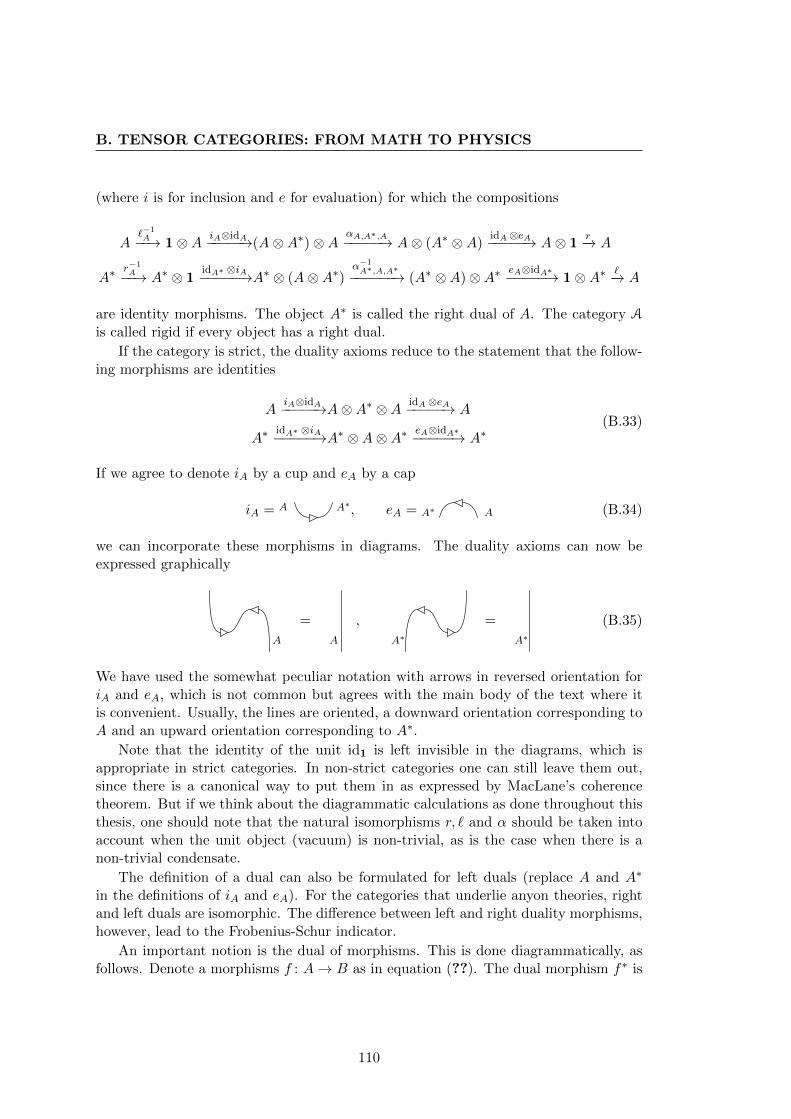
B. TENSOR CATEGORIES: FROM MATH TO PHYSICS
(where i is for inclusion and e for evaluation) for which the compositions
A`−1A−−→ 1⊗A iA⊗idA−−−−−→(A⊗A∗)⊗A αA,A∗,A−−−−−→ A⊗ (A∗ ⊗A)
idA⊗eA−−−−−→ A⊗ 1r−→ A
A∗r−1A−−→ A∗ ⊗ 1
idA∗ ⊗iA−−−−−→A∗ ⊗ (A⊗A∗)α−1A∗,A,A∗−−−−−−→ (A∗ ⊗A)⊗A∗ eA⊗idA∗−−−−−→ 1⊗A∗ `−→ A
are identity morphisms. The object A∗ is called the right dual of A. The category A
is called rigid if every object has a right dual.
If the category is strict, the duality axioms reduce to the statement that the follow-ing morphisms are identities
AiA⊗idA−−−−−→A⊗A∗ ⊗A idA⊗eA−−−−−→ A
A∗idA∗ ⊗iA−−−−−→A∗ ⊗A⊗A∗ eA⊗idA∗−−−−−→ A∗
(B.33)
If we agree to denote iA by a cup and eA by a cap
iA = A A∗, eA = A∗ A (B.34)
we can incorporate these morphisms in diagrams. The duality axioms can now beexpressed graphically
A
=
A
,
A∗
=
A∗
(B.35)
We have used the somewhat peculiar notation with arrows in reversed orientation foriA and eA, which is not common but agrees with the main body of the text where itis convenient. Usually, the lines are oriented, a downward orientation corresponding toA and an upward orientation corresponding to A∗.
Note that the identity of the unit id1 is left invisible in the diagrams, which isappropriate in strict categories. In non-strict categories one can still leave them out,since there is a canonical way to put them in as expressed by MacLane’s coherencetheorem. But if we think about the diagrammatic calculations as done throughout thisthesis, one should note that the natural isomorphisms r, ` and α should be taken intoaccount when the unit object (vacuum) is non-trivial, as is the case when there is anon-trivial condensate.
The definition of a dual can also be formulated for left duals (replace A and A∗
in the definitions of iA and eA). For the categories that underlie anyon theories, rightand left duals are isomorphic. The difference between left and right duality morphisms,however, lead to the Frobenius-Schur indicator.
An important notion is the dual of morphisms. This is done diagrammatically, asfollows. Denote a morphisms f : A→ B as in equation (??). The dual morphism f∗ is
110
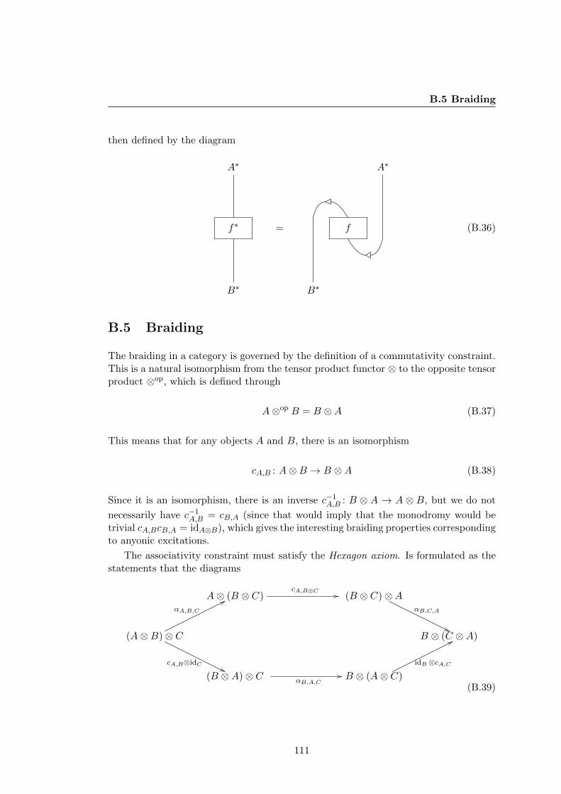
B.5 Braiding
then defined by the diagram
f∗
B∗
A∗
=
B∗
A∗
f (B.36)
B.5 Braiding
The braiding in a category is governed by the definition of a commutativity constraint.This is a natural isomorphism from the tensor product functor ⊗ to the opposite tensorproduct ⊗op, which is defined through
A⊗op B = B ⊗A (B.37)
This means that for any objects A and B, there is an isomorphism
cA,B : A⊗B → B ⊗A (B.38)
Since it is an isomorphism, there is an inverse c−1A,B : B ⊗ A → A ⊗ B, but we do not
necessarily have c−1A,B = cB,A (since that would imply that the monodromy would be
trivial cA,BcB,A = idA⊗B), which gives the interesting braiding properties correspondingto anyonic excitations.
The associativity constraint must satisfy the Hexagon axiom. Is formulated as thestatements that the diagrams
(A⊗B)⊗ C
A⊗ (B ⊗ C) (B ⊗ C)⊗A
(B ⊗A)⊗ C B ⊗ (A⊗ C)
B ⊗ (C ⊗A)
αA,B,C
77
cA,B⊗idC''
cA,B⊗C //
αB,A,C//
αB,C,A
''
idB ⊗cA,C
77
(B.39)
111
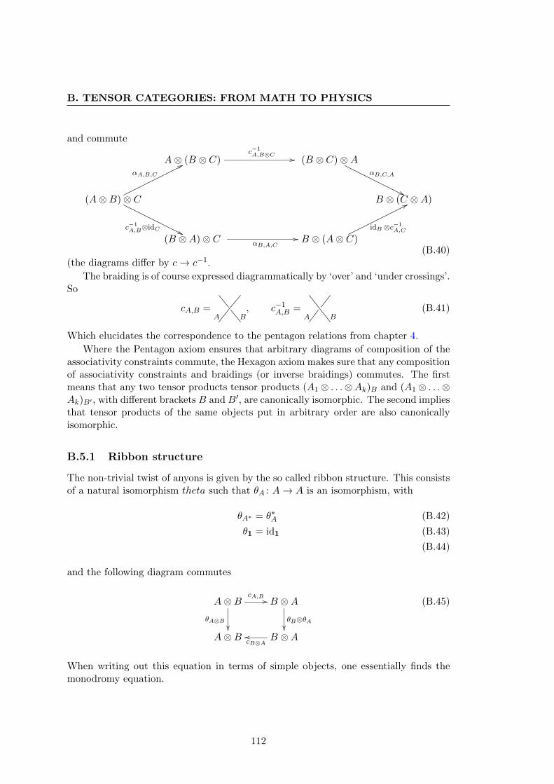
B. TENSOR CATEGORIES: FROM MATH TO PHYSICS
and commute
(A⊗B)⊗ C
A⊗ (B ⊗ C) (B ⊗ C)⊗A
(B ⊗A)⊗ C B ⊗ (A⊗ C)
B ⊗ (C ⊗A)
αA,B,C
77
c−1A,B⊗idC ''
c−1A,B⊗C //
αB,A,C//
αB,C,A
''
idB ⊗c−1A,C
77
(B.40)(the diagrams differ by c→ c−1.
The braiding is of course expressed diagrammatically by ‘over’ and ‘under crossings’.So
cA,B =A B
, c−1A,B =
A B(B.41)
Which elucidates the correspondence to the pentagon relations from chapter 4.
Where the Pentagon axiom ensures that arbitrary diagrams of composition of theassociativity constraints commute, the Hexagon axiom makes sure that any compositionof associativity constraints and braidings (or inverse braidings) commutes. The firstmeans that any two tensor products tensor products (A1 ⊗ . . .⊗Ak)B and (A1 ⊗ . . .⊗Ak)B′ , with different brackets B and B′, are canonically isomorphic. The second impliesthat tensor products of the same objects put in arbitrary order are also canonicallyisomorphic.
B.5.1 Ribbon structure
The non-trivial twist of anyons is given by the so called ribbon structure. This consistsof a natural isomorphism theta such that θA : A→ A is an isomorphism, with
θA∗ = θ∗A (B.42)
θ1 = id1 (B.43)
(B.44)
and the following diagram commutes
A⊗BθA⊗B
��
cA,B // B ⊗AθB⊗θA��
A⊗B B ⊗AcB⊗Aoo
(B.45)
When writing out this equation in terms of simple objects, one essentially finds themonodromy equation.
112
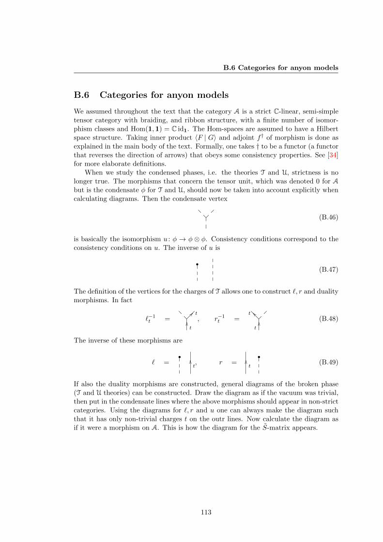
B.6 Categories for anyon models
B.6 Categories for anyon models
We assumed throughout the text that the category A is a strict C-linear, semi-simpletensor category with braiding, and ribbon structure, with a finite number of isomor-phism classes and Hom(1,1) = C id1. The Hom-spaces are assumed to have a Hilbertspace structure. Taking inner product 〈F | G〉 and adjoint f † of morphism is done asexplained in the main body of the text. Formally, one takes † to be a functor (a functorthat reverses the direction of arrows) that obeys some consistency properties. See [34]for more elaborate definitions.
When we study the condensed phases, i.e. the theories T and U, strictness is nolonger true. The morphisms that concern the tensor unit, which was denoted 0 for A
but is the condensate φ for T and U, should now be taken into account explicitly whencalculating diagrams. Then the condensate vertex
(B.46)
is basically the isomorphism u : φ → φ ⊗ φ. Consistency conditions correspond to theconsistency conditions on u. The inverse of u is
•(B.47)
The definition of the vertices for the charges of T allows one to construct `, r and dualitymorphisms. In fact
`−1t =
?? tOOt
, r−1t =
__tOO
t
(B.48)
The inverse of these morphisms are
` =• OO
t, r =
OOt
•(B.49)
If also the duality morphisms are constructed, general diagrams of the broken phase(T and U theories) can be constructed. Draw the diagram as if the vacuum was trivial,then put in the condensate lines where the above morphisms should appear in non-strictcategories. Using the diagrams for `, r and u one can always make the diagram suchthat it has only non-trivial charges t on the outr lines. Now calculate the diagram asif it were a morphism on A. This is how the diagram for the S-matrix appears.
113

B. TENSOR CATEGORIES: FROM MATH TO PHYSICS
114
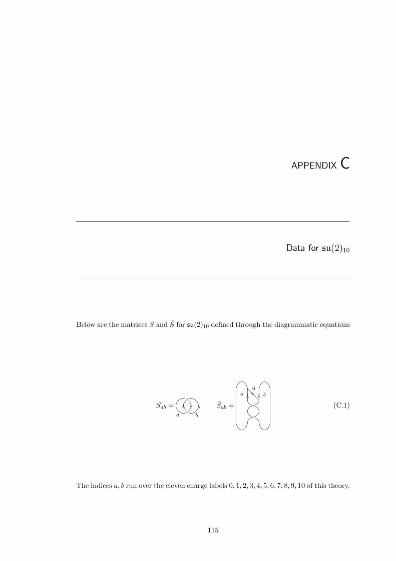
APPENDIX C
Data for su(2)10
Below are the matrices S and S for su(2)10 defined through the diagrammatic equations
Sab =a b
OO OO , Sab =
OOa OO b__ 6
(C.1)
The indices a, b run over the eleven charge labels 0, 1, 2, 3, 4, 5, 6, 7, 8, 9, 10 of this theory.
115
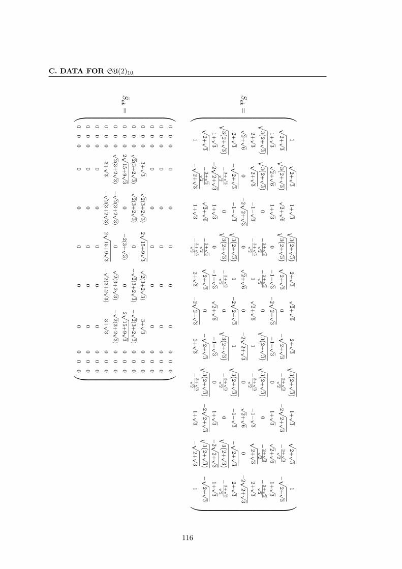
C. DATA FOR SU(2)10
Sab
=
1√
2+√
31+√
3√
3(2+√
3)2+√
3√
2+√
62+√
3√
3(2+√
3)1+√
3√
2+√
31
√2+√
3√
3(2+√
3)√
2+√
6√
3(2+√
3)√
2+√
30
− √2+√
3−
3+√
3√2
−2 √
2+√
3−
3+√
3√
2− √
2+√
3
1+√
3√
2+√
61+√
30
−1−√
3−
2 √2+√
3−
1−√
30
1+√
3√
2+√
61+√
3√
3(2+√
3) √3(
2+√
3)0
−3+√3
√2
−3+√3
√2
0√
3(2+√
3) √3(
2+√
3)0
−3+√
3√
2−
3+√
3√2
2+√
3√
2+√
3−
1−√
3−
3+√3
√2
1√
2+√
61
−3+√
3√2
−1−√
3√
2+√
32+√
3√
2+√
60
−2 √
2+√
30
√2+√
60
−2 √
2+√
30
√2+√
60
−2 √
2+√
3
2+√
3− √
2+√
3−
1−√
3√
3(2+√
3)1
−2 √
2+√
31
√3(
2+√
3)−
1−√
3− √
2+√
32+√
3√
3(2+√
3)−
3+√3
√2
0√
3(2+√
3)−
3+√3
√2
0√
3(2+√
3)−
3+√
3√2
0√
3(2+√
3)−
3+√
3√2
1+√
3−
2 √2+√
31+√
30
−1−√
3√
2+√
6−
1−√
30
1+√
3−
2 √2+√
31+√
3√
2+√
3−
3+√3
√2
√2+√
6−
3+√3
√2
√2+√
30
− √2+√
3√
3(2+√
3)−
2 √2+√
3 √3(
2+√
3)− √
2+√
3
1− √
2+√
31+√
3−
3+√3
√2
2+√
3−
2 √2+√
32+√
3−
3+√
3√2
1+√
3− √
2+√
31
Sab
=
00
00
00
00
00
0
00
00
00
00
00
0
00
00
00
00
00
0
00
03+√
3√
2(3
+2 √
3)
2 √15+
9 √3
√2(3
+2 √
3)
3+√
30
00
00
0√
2(3
+2 √
3)√
2(3
+2 √
3)
0−√
2(3
+2 √
3)−√
2(3
+2 √
3)
00
0
00
02 √
15+
9 √3
0−
2(3
+√
3)
02 √
15+
9 √3
00
0
00
0√
2(3
+2 √
3)−√
2(3
+2 √
3)
0√
2(3
+2 √
3)−√
2(3
+2 √
3)
00
0
00
03+√
3−√
2(3
+2 √
3)
2 √15+
9 √3−√
2(3
+2 √
3)
3+√
30
00
00
00
00
00
00
0
00
00
00
00
00
0
00
00
00
00
00
0
116
References
[1] Y. Aharonov and D. Bohm. Significance of electromagnetic potentials in the quan-tum theory. Phys. Rev., 115(3):485–491, Aug 1959.
[2] Daniel Arovas, J. R. Schrieffer, and Frank Wilczek. Fractional statistics and thequantum hall effect. Phys. Rev. Lett., 53(7):722–723, Aug 1984.
[3] Emil Artin. Theorie der zopfe. Abhandlungen aus dem Mathematischen Seminarder Universitat Hamburg, 4:47–72, 1925. 10.1007/BF02950718.
[4] M Atiyah. Topological quantum field theories. Publications Mathematiques del’IHES, Jan 1988.
[5] Bais, B Schroers, and J Slingerland. Hopf symmetry breaking and confinement in(2+ 1)-dimensional gauge theory. Journal of High Energy Physics, JHEP05, Jan2003.
[6] F Bais and J Slingerland. Topological entanglement entropy relations for multiphase systems with interfaces. Jan 2010.
[7] F. A. Bais and C. J. M. Mathy. Defect-mediated melting and the breaking ofquantum double symmetries. Phys. Rev. B, 73(22):224120, Jun 2006.
[8] F. A. Bais, B. J. Schroers, and J. K. Slingerland. Broken quantum symmetry andconfinement phases in planar physics. Phys. Rev. Lett., 89(18):181601, Oct 2002.
[9] F. A. Bais and J. K. Slingerland. Condensate-induced transitions between topo-logically ordered phases. Phys. Rev. B, 79(4):045316, Jan 2009.
[10] F. A. Bais, J. K. Slingerland, and S. M. Haaker. Theory of topological edges anddomain walls. Phys. Rev. Lett., 102(22):220403, Jun 2009.
[11] F. Alexander Bais, Peter van Driel, and Mark de Wild Propitius. Quantum sym-metries in discrete gauge theories. Physics Letters B, 280(1-2):63 – 70, 1992.
117
REFERENCES
[12] F.A. Bais and C.J.M. Mathy. The breaking of quantum double symmetries bydefect condensation. Annals of Physics, 322(3):552 – 598, 2007.
[13] F.A. Bais and J.C. Romers. Anyonic order parameters for discrete gauge theorieson the lattice. Annals of Physics, 324(5):1168 – 1175, 2009.
[14] Bojko Bakalov and Alexander A. Kirillov. Lectures on tensor categories and mod-ular functors. American Mathematical Society, 2001.
[15] R. J. Baxter. Exactly Solved Models in Statistical Mechanics. Academic Press,1982.
[16] S. Beigi, P. Shor, and D. Whalen. The kitaev model with boundary: Condensationsand symmetries. Jan 2010.
[17] H. Bombin and M. A. Martin-Delgado. Family of non-abelian kitaev models on alattice: Topological condensation and confinement. Phys. Rev. B, 78(11):115421,Sep 2008.
[18] Parsa Bonderson, Michael Freedman, and Chetan Nayak. Measurement-onlytopological quantum computation via anyonic interferometry. Annals of Physics,324(4):787 – 826, 2009.
[19] Parsa Bonderson, Michael Freedman, and Chetan Nayak. Measurement-onlytopological quantum computation via anyonic interferometry. Annals of Physics,324(4):787 – 826, 2009.
[20] Parsa Bonderson, Alexei Kitaev, and Kirill Shtengel. Detecting non-abelian statis-tics in the ν = 5/2 fractional quantum hall state. Phys. Rev. Lett., 96(1):016803,Jan 2006.
[21] Parsa Bonderson, Kirill Shtengel, and J.K. Slingerland. Interferometry of non-abelian anyons. Annals of Physics, 323(11):2709 – 2755, 2008.
[22] Parsa Hassan Bonderson. Non-Abelian anyons and interferometry. PhD thesis,Cal. Tech., 2007.
[23] F.J. Burnell and Steven H. Simon. Space-time geometry of topological phases.Annals of Physics, 325(11):2550 – 2593, 2010.
[24] N. R. Cooper. Exact ground states of rotating bose gases close to a feshbachresonance. Phys. Rev. Lett., 92(22):220405, Jun 2004.
[25] N. R. Cooper, N. K. Wilkin, and J. M. F. Gunn. Quantum phases of vortices inrotating bose-einstein condensates. Phys. Rev. Lett., 87(12):120405, Aug 2001.
[26] Sankar Das Sarma, Chetan Nayak, and Sumanta Tewari. Proposal to stabilize anddetect half-quantum vortices in strontium ruthenate thin films: Non-abelian braid-ing statistics of vortices in a px+ipy superconductor. Phys. Rev. B, 73(22):220502,Jun 2006.
118
REFERENCES
[27] Mark de Wild Propitius. Topological interactions in broken gauge theories. PhDthesis, Universiteit van Amsterdam, Nov 1995.
[28] R. Dijkgraaf, V. Pasquier, and P. Roche. Quasi hope algebras, group cohomologyand orbifold models. Nuclear Physics B - Proceedings Supplements, 18(2):60 – 72,1991.
[29] Benoit Doucot, Lev B. Ioffe, and Julien Vidal. Discrete non-abelian gauge the-ories in josephson-junction arrays and quantum computation. Phys. Rev. B,69(21):214501, Jun 2004.
[30] Vladimir Drinfeld. Quantum groups. Journal of Mathematical Sciences, 41(2):898–915, 1988.
[31] K. Druhl, R. Haag, and J. E. Roberts. On parastatistics. Communications inMathematical Physics, 18:204–226, 1970. 10.1007/BF01649433.
[32] Torbjorn Einarsson. Fractional statistics on a torus. Phys. Rev. Lett., 64(17):1995–1998, Apr 1990.
[33] Philippe Di Francesco, Pierre Mathieu, and David Senechal. Conformal FieldTheory. Springer, Jan 1997.
[34] J Fuchs, A Ganchev, K Szlachanyi, and P Vecseryes. s4 symmetry of 6j sym-bols and frobenius-schur indicators in rigid monoidal c∗ categories. Journal ofMathematical Physics, 40:408–426, Jan 1999.
[35] J Fuchs and C Schweigert. Category theory for conformal boundary conditions.In Stephan Berman, editor, Vertex operator algebras in mathematics and physics.Jun 2001.
[36] Paul Ginsparg. Applied conformal field theory. Nov 1988.
[37] S. Girvin. The quantum hall effect: Novel excitations and broken symmetries. InA. Comtet, T. Jolicoeur, S. Ouvry, and F. David, editors, Topological aspects oflow dimensional systems, volume 69 of Les Houches, pages 53–175. Springer Berlin/ Heidelberg, 1999.
[38] V. J. Goldman and B. Su. Resonant tunneling in the quantum hall regime: Mea-surement of fractional charge. Science, 267(5200):1010–1012, 1995.
[39] H. S. Green. A generalized method of field quantization. Phys. Rev., 90(2):270–273,Apr 1953.
[40] E. Grosfeld and K. Schoutens. Non-abelian anyons: When ising meets fibonacci.Phys. Rev. Lett., 103(7):076803, Aug 2009.
[41] V. Gurarie, L. Radzihovsky, and A. V. Andreev. Quantum phase transitions acrossa p-wave feshbach resonance. Phys. Rev. Lett., 94(23):230403, Jun 2005.
119
REFERENCES
[42] Henning Haahr Andersen and Jan Paradowski. Fusion categories arising fromsemisimple lie algebras. Communications in Mathematical Physics, 169:563–588,1995. 10.1007/BF02099312.
[43] F. D. M. Haldane. Fractional quantization of the hall effect: A hierarchy of in-compressible quantum fluid states. Phys. Rev. Lett., 51(7):605–608, Aug 1983.
[44] B. I. Halperin. Statistics of quasiparticles and the hierarchy of fractional quantizedhall states. Phys. Rev. Lett., 52(18):1583–1586, Apr 1984.
[45] J. K. Jain. Composite-fermion approach for the fractional quantum hall effect.Phys. Rev. Lett., 63(2):199–202, Jul 1989.
[46] C Kassel. Quantum Groups. Graduate texts in mathematics. Springer-Verlag,1995.
[47] A. N. Kirillov and N. Yu. Reshetikhin. The yangians, bethe ansatz and combina-torics. Letters in Mathematical Physics, 12:199–208, 1986. 10.1007/BF00416510.
[48] Alexander Kirillov and Viktor Ostrik. On a q-analogue of the mckay correspon-dence and the ade classification of sl2 conformal field theories. Advances in Math-ematics, 171(2):183 – 227, 2002.
[49] A. Yu. Kitaev. Fault-tolerant quantum computation by anyons. Annals of Physics,303(1):2 – 30, 2003.
[50] K. v. Klitzing, G. Dorda, and M. Pepper. New method for high-accuracy deter-mination of the fine-structure constant based on quantized hall resistance. Phys.Rev. Lett., 45(6):494–497, Aug 1980.
[51] Michael G. G. Laidlaw and Cecile Morette DeWitt. Feynman functional integralsfor systems of indistinguishable particles. Phys. Rev. D, 3(6):1375–1378, Mar 1971.
[52] Lev Davidovich Landau. On the theory of phase tansitions ii. Phys. Z. Sowjet.,11(545), Oct 1937.
[53] Lev Davidovich Landau. On the theory of phase transitions i. Phys. Z. Sowjet.,11(26), Jan 1937.
[54] Saunders Mac Lane. Categories for the working mathematician. Springer-Verlag,Jan 1998.
[55] R. B. Laughlin. Anomalous quantum hall effect: An incompressible quantum fluidwith fractionally charged excitations. Phys. Rev. Lett., 50(18):1395–1398, May1983.
[56] R.B. Laughlin. Primitive and composite ground states in the fractional quantumhall effect. Surface Science, 142(1-3):163 – 172, 1984.
120
REFERENCES
[57] J. Leinaas and J. Myrheim. On the theory of identical particles. Il Nuovo CimentoB (1971-1996), 37:1–23, 1977. 10.1007/BF02727953.
[58] Michael Levin and Xiao-Gang Wen. Detecting topological order in a ground statewave function. Phys. Rev. Lett., 96(11):110405, Mar 2006.
[59] Michael A. Levin and Xiao-Gang Wen. String-net condensation: A physical mech-anism for topological phases. Phys. Rev. B, 71(4):045110, Jan 2005.
[60] Shahn Majid. Foundations of quantum group theory. Cambridge University Press.
[61] C.J.M. Mathy and F.A. Bais. Nematic phases and the breaking of double symme-tries. Annals of Physics, 322(3):709 – 735, 2007.
[62] G Moore and N Seiberg. Classical and quantum conformal field theory. Commu-nications in Mathematical Physics, 123:177–254, Jan 1989.
[63] Gregory Moore and Nicholas Read. Nonabelions in the fractional quantum halleffect. Nuclear Physics B, 360(2-3):362 – 396, 1991.
[64] Chetan Nayak, Steven H. Simon, Ady Stern, Michael Freedman, and SankarDas Sarma. Non-abelian anyons and topological quantum computation. Rev.Mod. Phys., 80(3):1083–1159, Sep 2008.
[65] R. E. Prange, S. M. Girvin, and K. von Klitzing, editors. The Quantum Hall effect.Springer - New York.
[66] J Preskill. Topological quantum computation, lecture notes. 2004.
[67] M Propitius and F Bais. Discrete gauge theories. Jan 1998.
[68] N Read and N Cooper. Incompressible liquid state of rapidly rotating bosons atfilling factor 3/2. Phys Rev. Lett., Jan 2005.
[69] N Read and E Rezayi. Beyond paired quantum hall states: Parafermions andincompressible states in the first excited landau level. Phys. Rev. B, Jan 1999.
[70] N Reshetikhin and V G Turaev. Comm. Math. Phys., 127:1–26, Jan 1990.
[71] Eric Rowell, Richard Stong, and Zhenghan Wang. On classification of modulartensor categories. Dec 2007.
[72] J Slingerland and F Bais. Quantum groups and non-abelian braiding in quantumhall systems. Nucl Phys B, Jan 2001.
[73] Horst L. Stormer, Daniel C. Tsui, and Arthur C. Gossard. The fractional quantumhall effect. Rev. Mod. Phys., 71(2):S298–S305, Mar 1999.
[74] D. C. Tsui, H. L. Stormer, and A. C. Gossard. Two-dimensional magnetotransportin the extreme quantum limit. Phys. Rev. Lett., 48(22):1559–1562, May 1982.
121
REFERENCES
[75] V.G. Turaev. Quantum Invariants of Knots and 3-Manifolds. De Gruyter, Jan2010.
[76] Erik Verlinde. Fusion rules and modular transformations in 2d conformal fieldtheory. Nuclear Physics B, 300:360 – 376, 1988.
[77] X. G. Wen and Q. Niu. Ground-state degeneracy of the fractional quantum hallstates in the presence of a random potential and on high-genus riemann surfaces.Phys. Rev. B, 41(13):9377–9396, May 1990.
[78] Xiao-Gang Wen. Topological orders and edge excitations in fractional quantum hallstates. In Hendrik Geyer, editor, Field Theory, Topology and Condensed MatterPhysics, volume 456 of Lecture Notes in Physics, pages 155–176. Springer Berlin/ Heidelberg, 1995. 10.1007/BFb0113370.
[79] J. Wess and B. Zumino. Consequences of anomalous ward identities. PhysicsLetters B, 37(1):95 – 97, 1971.
[80] Frank Wilczek. Quantum mechanics of fractional-spin particles. Phys. Rev. Lett.,49(14):957–959, Oct 1982.
[81] R. Willett, J. P. Eisenstein, H. L. Stormer, D. C. Tsui, A. C. Gossard, and J. H.English. Observation of an even-denominator quantum number in the fractionalquantum hall effect. Phys. Rev. Lett., 59(15):1776–1779, Oct 1987.
[82] Edward Witten. Global aspects of current algebra. Nuclear Physics B, 223(2):422– 432, 1983.
[83] Edward Witten. Non-abelian bosonization in two dimensions. Communications inMathematical Physics, 92:455–472, 1984. 10.1007/BF01215276.
[84] Edward Witten. Topological quantum field theory. Communications in Mathe-matical Physics, 117:353–386, 1988. 10.1007/BF01223371.
[85] S. L. Woronowics. Comm. Math. Phys., 111(4):613–665, 1987.
[86] C. N. Yang. Some exact results for the many-body problem in one dimension withrepulsive delta-function interaction. Phys. Rev. Lett., 19(23):1312–1315, Dec 1967.
[87] C. N. Yang. s matrix for the one-dimensional n-body problem with repulsive orattractive δ-function interaction. Phys. Rev., 168(5):1920–1923, Apr 1968.
[88] Daijiro Yoshioka. The quantum Hall effect. Springer-Verlag, Jan 2002.
122
Dankwoord
De laatste paginas van mijn scriptie wil ik graag gebruiken om de mensen te bedankendie het werk aan deze scriptie en mijn tijd als student aan de UvA mogelijk, dan-wel aangenaam hebben gemaakt. Laat ik in goed gebruik beginnen met mijn beidebegeleiders, Sander Bais en Eric Opdam.
Beste Sander, het is een interessante tijd en een fantastisch project geweest. Het wasniet altijd even makkelijk, zeker met andere werkzaamheden zoals het onderwijsprojectDe Praktijk erbij, maar ik heb enorm veel van je geleerd en ben blij met het resultaat.Het is een geluk en een eer bij je te kunnen hebben afstuderen.
Beste Eric, je hebt als geen ander mijn pad als student aan de UvA meegemaakten bent van dicht bij betrokken geweest bij alle grote projecten die ik heb gedaan:mijn bachelorscriptie, TopWis Poincare en nu deze scriptie. Bedankt voor alle leuke engoede gesprekken, over wiskunde, maar ook het wel en wee van de universiteit, Japanen alle andere zaken. Ook bedankt voor de goede colleges en je cruciale inbreng ensturing tijdens kritische momenten van beide scripties en TopWis Poincare.
Dan zijn er alle docenten waar ik veel aan heb gehad en die ik graag wil bedankenvoor goed onderwijs en prettige samenwerking als student assistent. Met name HenkPijls, Leo Dorst en Harry Buhrman hebben een beslissende rol gespeeld bij mijn keuzes.In het kader van deze scriptie hoort daar ook Joost Slingerland bij waarmee ik enkeleinhoudelijke gesprekken heb gevoerd.
Een groot deel van de tijd dat ik aan mijn scriptie werkte heb ik ook bij De Praktijkop kantoor gezeten voor het onderwijsproject TopWis Poincare. Iedereen daar bedanktvoor de geweldige tijd, de onvergetelijke trip naar NY en bedrijfsuitjes, Discovery,enzovoort. Yuri, Niels en Miranda, bedankt voor de hele prettige en samenwerking.Alex en alle anderen, bedankt voor de goede sfeer, leuke lunches, goede muziek, ...
Zonder vrienden, met wie bier drinken en studeren vaak hand in hand gingen, hadik nooit zo’n goede tijd gehad. Bob en Jacobien, met jullie is dit avontuur begonnenbij onze eerste colleges dynamische systemen en klassieke mechanica. Zo lang geleden...Sjoert, bedankt dat je me af en toe richting de natuurkunde hebt proberen te trekken.
123
DANKWOORD
Olaf, met niemand is het beter om half-dronken over natuurkunde praten dan met jou.Ik hoop dat we elkaar nog veel zullen zien en ook inhoudelijk elkaar niet (helemaal) uithet oog zullen verliezen, of ik nou natuurkundige word of niet. Jesper, ’t was top ommet je samen te werken en drie dagen te wachten totdat Mathematica was uitgerekendaan onze matrix. Wat een feest toen het goede antwoord eruit kwam rollen. Ik hoop dathet nog tot een mooi resultaat leidt en wens je veel succes met je promotie. Shannah,je was een inspirerend voorganger bij Bais. Heel veel succes in, vast en zeker, eenfantastische carriere.
De mensen die niet per se samen met mij hebben gestudeerd, maar het wel met mijhebben moeten stellen als ik met mijn gedachten ergens anders was zijn, niet minderbelangrijk. Bertus, bedankt voor een dierbare vriendschap die hoop ik nooit over gaat.Nick, wat een topavonturen hebben we beleefd. Op de fiets naar de klimaattop inKopenhagen en vierde op de Taikai op Bali. Alle beta-gammas en andere vriendenwaarmee ik veel heb beleefd, ’t was mooi. Alle vrienden in Indonesie, die ik snel weerhoop te zien, met name natuurlijk Rima.
Mijn ouders mogen uiteraard niet ontbreken in dit lijstje. Zonder jullie was vanzelf-sprekend niks van dit al mogelijk geweest. Tatja en Nicollette, wat prijs ik me gelukkigmet twee zulke moeders. Anton, niet alleen op persoonlijk vlak ben je een steun entoeverlaat, ook inhoudelijk en praktisch op academisch gebied is het moeilijk voor testellen wat ik zonder je zou moeten. Je hebt de moeite genomen om dit stuk pa-pier te helemaal door te lezen en van nuttige commentaren te voorzien en mijn tallozeslordigheden eruit te halen, waarvoor veel bewondering en dank.
Katja, bedankt voor alles, niet in het minst omdat je de hip hop levend houdt. OokCeline, Roos, Nina, Floor, bedankt voor de groove en lol en de zaterdagen van pureontspanning tijdens het choreografieproject.
Iris, bedankt voor de updates over neuroscience zo nu en dan en natuurlijk al hetandere. Iedereen die ik niet bij name noem, het is een geluk jullie te kennen.
Als laatste wil ik mijn vriendin Zora in het zonnetje zetten. Je hebt alle onzekerheiddie van tijd tot tijd de kop op stak over het slagen van dit afstudeerproject over je heengehad. Bedankt voor de steun en het geduld. En wat ben ik blij om met je samen tezijn en zie ik uit naar onze reis!
124