1

Analyse du transcriptome

Emmanuel Barillot, Franck Rapaport

Jean-Philippe Vert et Andrei Zinovyev

Institut Curie et Ecole des Mines de Paris

Journee ACI IMPBIO, Lyon, France, July 5, 2005.

2

Plan

1. Introduction a l’analyse du transcriptome

2. Une approche pour l’analyse de voies metaboliques

3. Le projet Kernelchip : cancer et regulation

3

Partie 1

Introduction a l’analyse dutranscriptome

4

En bref...

• Le genome humain contient environ 25,000 genes,

codant 100,000+ proteines

• Comprendre la vie = comprendre comment ces proteines

interagissent et sont regulees ?

• Les puces a ADN mesurent la quantite d’ARNm

(presque les proteines...) pour tous les genes

simultanement, a un instant donne.

5

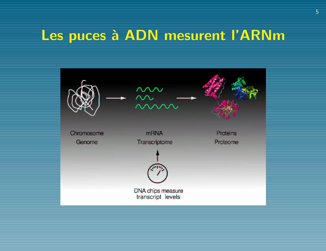
Les puces a ADN mesurent l’ARNm

6

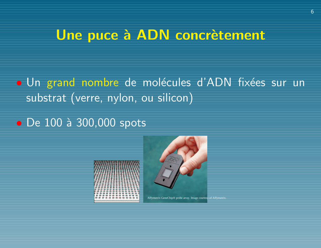
Une puce a ADN concretement

• Un grand nombre de molecules d’ADN fixees sur un

substrat (verre, nylon, ou silicon)

• De 100 a 300,000 spots

Affymetrix GeneChip® probe array. Image courtesy of Affymetrix.

7

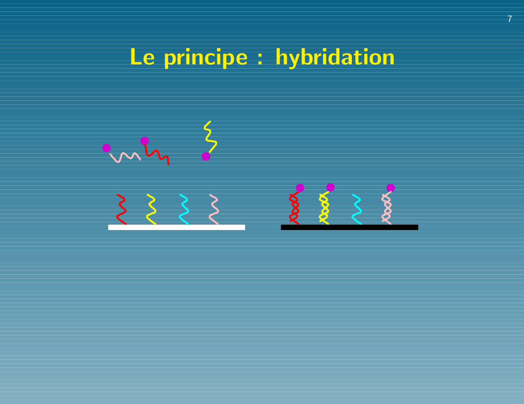
Le principe : hybridation

8

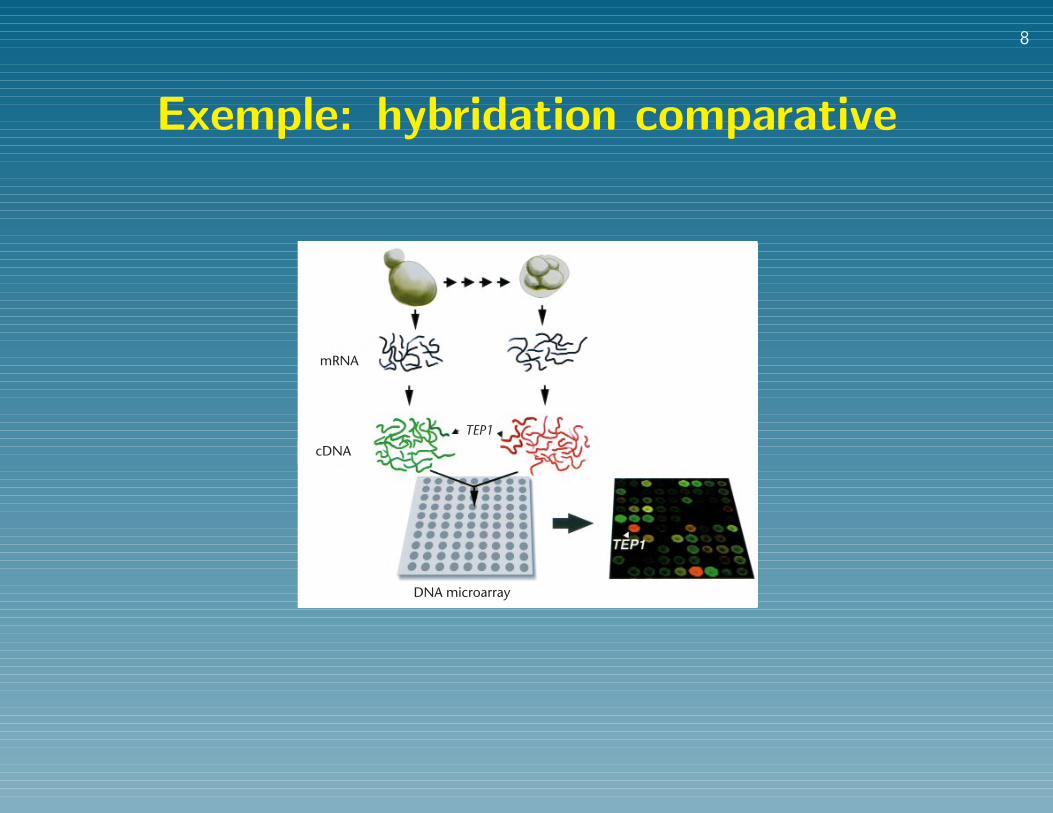
Exemple: hybridation comparativereview

34 nature genetics supplement • volume 21 • january 1999

The properties of genes that can be explored and exploitedusing DNA microarrays are diverse. For each property weexplore, the challenge is simply to find an experimental methodthat turns that property into the basis for differential fractiona-tion of DNA or RNA sequences. This is trivial when the propertyis differential expression at the mRNA level comparing therelative abundance of mRNA from each gene is simply a matterof measuring the differential hybridization to a DNA microarrayof fluorescently labelled cDNAs prepared from two mRNA sam-ples.Other properties require less direct approaches5,14–17. Wehave found, however, that many of the most important attributesof genes, ranging from their transcription and translation, to thesubcellular localization of their products, to their genotype, totheir mutant phenotypes, can be studied conveniently and eco-nomically on a genome-wide basis using DNA microarrays.

Fast, cheap and easy to controlSeveral features of DNA microarray technology make it particu-larly well suited to exploratory research. (i) It is (relatively) cheap:the capital cost for building both an arrayer and scanner is nowless than $60,000, and the marginal cost per copy of the yeastgenome microarray is currently about $20. Ongoing developmentefforts in academic and commercial labs and competition amongcommercial suppliers should continue to bring the cost down.Thus, if we are curious about a process, or a mutant phenotype,we can easily just ‘take a look’ without agonizing over cost. (ii) It isflexible and universal: as we continue to learn more about addi-tional genomes, we need to be able to convert the informationinto tools for exploration quickly and inexpensively. In addition

to more than a thousand arrays of the complete yeast genome, wehave already printed hundreds of copies each of arrays of morethan 95% of all the predicted genes of Mycobacterium tuberculosis,all the predicted genes of Escherichia coli, 3,000 Drosophilamelanogaster genes, thousands of C. elegans genes, over 14,000human genes, all cytomegalovirus genes and over 3,000 Plasmod-ium falciparum genes (unpublished data). (iii) It is fast: the totaltime currently required to print 150 copies of an array of 12,000genes is now about a day. (iv) It is user-friendly: the convenient,solid, open format of the microscope slide, the non-radioactive,non-toxic, low-volume (10 µl) hybridization solution and thecomforting knowledge that the arrays are cheap and easilyreplaced all make everyone using the system feel comfortable per-forming the exploratory, adventurous experiments that we thinkare called for in this phase of the genome project.

Using DNA microarrays to study gene expressionon a genomic scaleThe study of gene expression on a genomic scale is the most obvi-ous opportunity made possible by complete genome sequencesof the model organisms, and experimentally the most straight-forward. Four characteristics of the regulation of gene expressionat the level of transcript abundance account for the great valueand appeal of genome-wide surveys of transcript levels. First, it iseminently feasibleDNA microarrays make it easy to measurethe transcripts for every gene at once (much as we might wish tobe able to measure the abundance of the final products of everygene, or better still the biochemical activity of the products ofevery gene, there is no practical generic tool for doing so…yet).The second reason is the tight connection between the functionof a gene product and its expression pattern. As a rule, each geneis expressed in the specific cells and under the specific conditionsin which its product makes a contribution to fitness. Just as nat-ural selection has precisely tuned the biochemical properties ofthe gene product, so it has tuned the regulatory properties thatgovern when and where the product is made and in what quan-tity. The logic of natural selection, as well as experimental evi-dence, provides part of the basis for our belief that there is asensible link between the expression pattern and the function ofits gene product. Thirty years of molecular biology have providednumerous examples of genes that function under specific condi-tions and whose expression is tightly restricted to those condi-tions. The generality and exquisite precision of this link isrevealed by a global examination of the expression patterns of allthe genes of yeast, as described below. Third, promoters functionas transducers, responding to inputs of information about theidentity, environment and internal state of a cell by changing thelevel of transcription of specific genes. Thus, as we learn whatinformation is transduced by the promoter of each gene, we canbegin to read this information from the profile of transcripts,easily obtained using a DNA microarray. Fourth, the set of genesexpressed in a cell determine what the cell is made of, what bio-chemical and regulatory systems are operative, how the cell isbuilt and what it can and cannot do. As we learn to infer the bio-logical consequences of specific features of gene expression pat-terns using our growing knowledge of the functions of individualsets of genes, we can use microarrays as ‘microscopes’ to see acomprehensive, dynamic molecular picture of the living cell.

A new kind of mapIn the past two years, we and others have studied the expressionpatterns of all the yeast genes, in a wide variety of circumstances,using microarray hybridization8,9,18–22. As every gene in the yeastgenome can be represented on the microarrays, the picture ofgene expression that emerges is comprehensive.

Fig. 1 Gene expression analysis using a DNA microarray. In this illustration,mRNA samples from vegetative and sporulating yeast cells are compared. Thetotal pool of messenger RNA from each cell population is used to prepare fluo-rescently labelled cDNA by reverse transcription in the presence of fluores-cently labelled nucleotide precursors. To allow direct comparison of theabundance of each gene in the two samples, the two samples are labelled withdifferent fluorsin this example, a red fluor for the mRNA from sporulatingyeast and a green fluor for the mRNA from the vegetative yeast cells. The twofluorescently labelled cDNAs are then mixed and hybridized with a DNAmicroarray in which each yeast gene is represented as a distinct spot of DNA.Irrespective of their fluorescent labels, the cDNA sequences representing eachindividual transcript hybridize specifically with the corresponding genesequence in the array. Thus, the relative abundance in sporulating as comparedwith vegetative yeast cells of the transcripts from each gene is reflected by theratio of ‘red’ to ‘green’ fluorescence measured at the array element represent-ing that gene. For example, the greater relative abundance of the TEP1 mRNAin the sporulating cells results in a high ratio of red-labelled to green-labelledcopies of the corresponding cDNA, and an equivalent ratio of red to green sig-nal hybridized at the array element composed of DNA from TEP1.

mRNA

TEP1cDNA

DNA microarray

© 1999 Nature America Inc. • http://genetics.nature.com

© 19

99 N

atur

e Am

eric

a In

c. •

http

://ge

netic

s.na

ture

.com

9

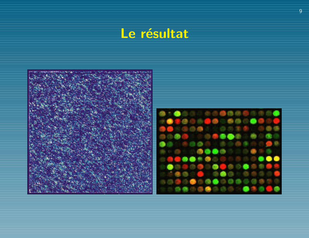
Le resultat

10

Le transcriptome

Le transcriptome reflete

• la source du tissue, l’organe, le type de cellules

• l’activite et l’etat du tissue:

? etat de developpement, croissance, mort

? cycle cellulaire

? malade / sain

? reponse a des therapie

11

Les espoirs

• decouverte de cibles therapeutiques

• diagnostic et pronostic medical

• pharmacogenomique

• biologie des systemes etc...

12

Analyse typique du transcriptome

• Analyse d’image, normalisation

• Detection de genes differentiellement exprimes

• Analyse exploratoire, clustering

• Analyse discriminante

• Reconstruction de reseaux genetiques

13

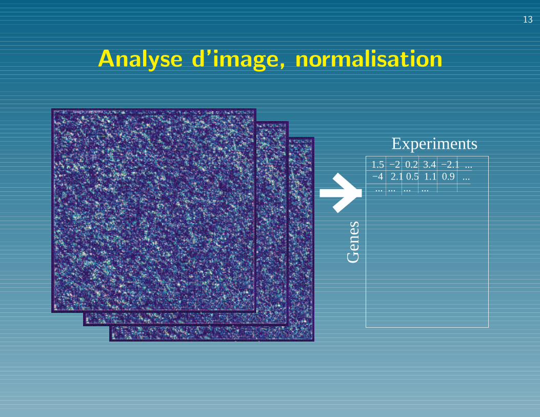
Analyse d’image, normalisation

Experiments

Gen

es

1.5 −2 0.2 3.4 −2.1 ...−4 2.1 0.5 1.1 0.9 ...... ... ... ...

14

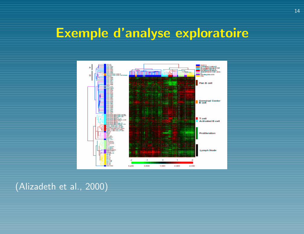
Exemple d’analyse exploratoire

(Alizadeth et al., 2000)

15

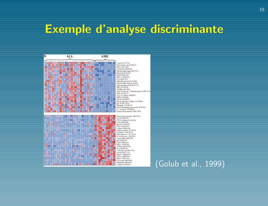
Exemple d’analyse discriminante

that class discovery could be tested by classprediction: If putative classes reflect truestructure, then a class predictor based onthese classes should perform well.

To test this hypothesis, we evaluated theclusters A1 and A2. We constructed predic-tors to assign new samples as “type A1” or“type A2.” Predictors that used a wide rangeof different numbers of informative genesperformed well in cross-validation. For ex-ample, a 20-gene predictor gave 34 accuratepredictions with high prediction strength, oneerror, and three uncertains (34). The one“error” was the assignment of the sole AMLsample in class A1 to class A2, and two of thethree uncertains were ALL samples in classA2. The cross-validation thus not onlyshowed high accuracy, but actually refinedthe SOM-defined classes: With one excep-tion, the subset of samples accurately classi-fied in cross-validation were those perfectlysubdivided by the SOM into ALL and AML

classes. The results suggest an iterative pro-cedure for refining clusters, in which an SOMis used to initially cluster the data, a predictoris constructed, and samples not correctly pre-dicted in cross-validation are removed. Theedited data set could then be used to generatean improved predictor to be tested on anindependent data set (35).

We then tested the class predictor of theA1-A2 distinction on the independent data set.In the general case of class discovery, predic-tors for novel classes cannot be assessed for“accuracy” on new samples, because the “right”way to classify the independent samples is notknown. Instead, however, one can assesswhether the new samples are assigned a highprediction strength. High prediction strengthsindicate that the structure seen in the initial dataset is also seen in the independent data set. Theprediction strengths, in fact, were quite high:The median PS was 0.61, and 74% of sampleswere above threshold (Fig. 4B). To assess these

results, we performed the same analyses withrandom clusters. Such clusters consistentlyyielded predictors with poor accuracy in cross-validation and low prediction strength on theindependent data set (Fig. 4B). On the basis ofsuch analysis (36), the A1-A2 distinction canbe seen to be meaningful, rather than simply astatistical artifact of the initial data set. Theresults thus show that the AML-ALL distinc-tion could have been automatically discoveredand confirmed without previous biologicalknowledge.

We then sought to extend the class dis-covery by searching for finer subclasses ofthe leukemias. We used a SOM to divide thesamples into four clusters (denoted B1 toB4). We subsequently obtained immunophe-notype data on the samples and found that thefour classes largely corresponded to AML,T-lineage ALL, B-lineage ALL, and B-lin-eage ALL, respectively (Fig. 4C). The four-cluster SOM thus divided the samples along

Fig. 3. (A) Prediction strengths. The scatter-plots show the prediction strengths (PSs) forthe samples in cross-validation (left) and on theindependent sample (right). Median PS is de-noted by a horizontal line. Predictions with PS! 0.3 are considered as uncertain. (B) Genesdistinguishing ALL from AML. The 50 genesmost highly correlated with the ALL-AML classdistinction are shown. Each row corresponds toa gene, with the columns corresponding toexpression levels in different samples. Expres-sion levels for each gene are normalized acrossthe samples such that the mean is 0 and the SDis 1. Expression levels greater than the meanare shaded in red, and those below the meanare shaded in blue. The scale indicates SDsabove or below the mean. The top panel showsgenes highly expressed in ALL, the bottom panel shows genes morehighly expressed in AML. Although these genes as a group appearcorrelated with class, no single gene is uniformly expressed across the class,

illustrating the value of a multigene prediction method. For a complete listof gene names, accession numbers, and raw expression values, see www.genome.wi.mit.edu/MPR.

B

R E P O R T S

15 OCTOBER 1999 VOL 286 SCIENCE www.sciencemag.org534

(Golub et al., 1999)

16

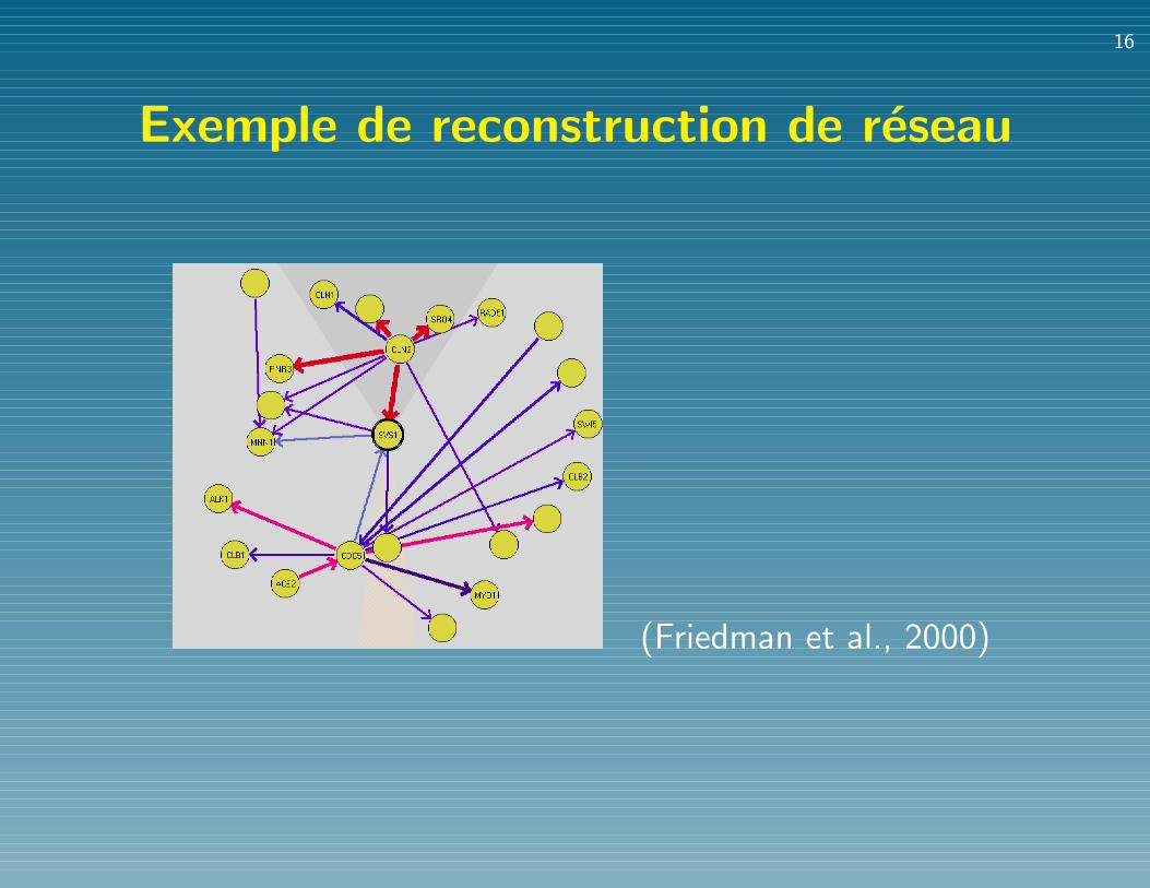
Exemple de reconstruction de reseauUSING BAYESIAN NETWORKS 611

FIG. 2. An example of the graphical display of Markov features. This graph shows a “local map” for the geneSVS1. The width (and color) of edges corresponds to the computed con!dence level. An edge is directed if there is asuf!ciently high con!dence in the order between the genes connected by the edge. This local map shows that CLN2separates SVS1 from several other genes. Although there is a strong connection between CLN2 to all these genes,there are no other edges connecting them. This indicates that, with high con!dence, these genes are conditionallyindependent given the expression level of CLN2.

4.1. Robustness analysis

We performed a number of tests to analyze the statistical signi!cance and robustness of our procedure.Some of these tests were carried out on a smaller data set with 250 genes for computational reasons.

To test the credibility of our con!dence assessment, we created a random data set by randomly permutingthe order of the experiments independently for each gene. Thus for each gene the order was random, butthe composition of the series remained unchanged. In such a data set, genes are independent of each other,and thus we do not expect to !nd “real” features. As expected, both order and Markov relations in therandom data set have signi!cantly lower con!dence. We compare the distribution of con!dence estimatesbetween the original data set and the randomized set in Figure 3. Clearly, the distribution of con!denceestimates in the original data set have a longer and heavier tail in the high con!dence region. In thelinear-Gaussian model we see that random data does not generate any feature with con!dence above 0.3.The multinomial model is more expressive and thus susceptible to over-!tting. For this model, we see asmaller gap between the two distributions. Nonetheless, randomized data does not generate any featurewith con!dence above 0.8, which leads us to believe that most features that are learned in the original dataset with such con!dence are not artifacts of the bootstrap estimation.

(Friedman et al., 2000)

17

Partie 2

Une approche pour l’analyse devoies metaboliques

18

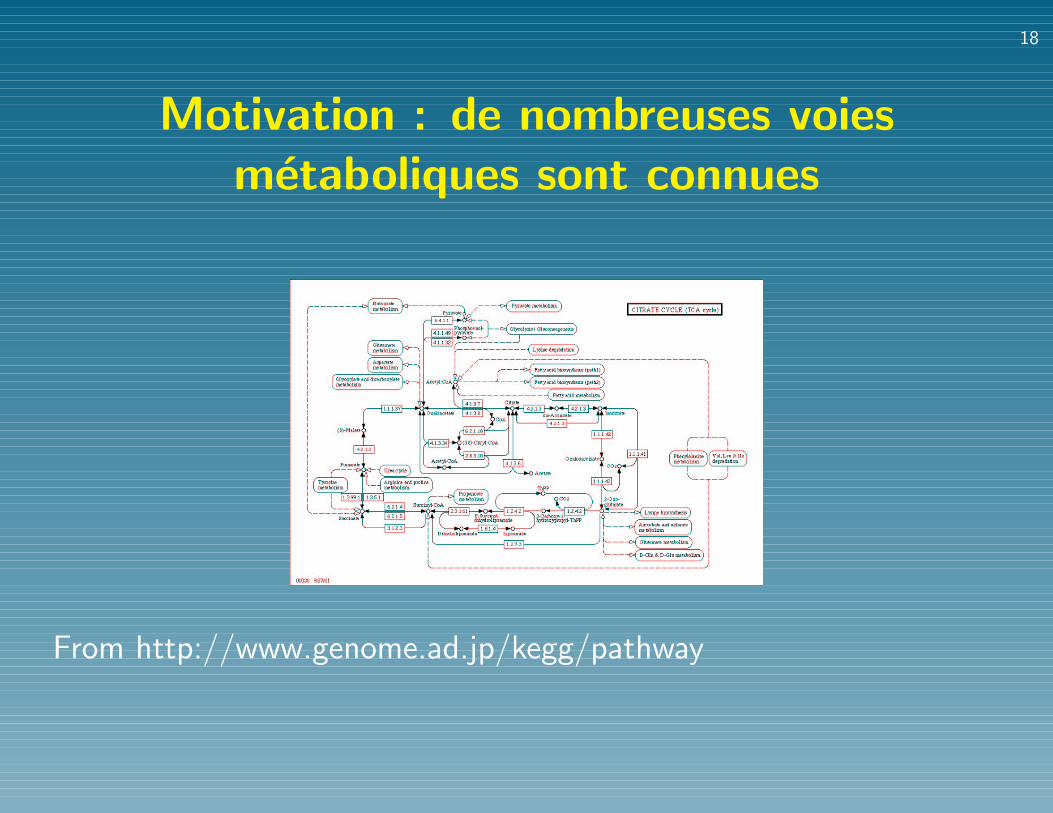
Motivation : de nombreuses voiesmetaboliques sont connues

From http://www.genome.ad.jp/kegg/pathway

19

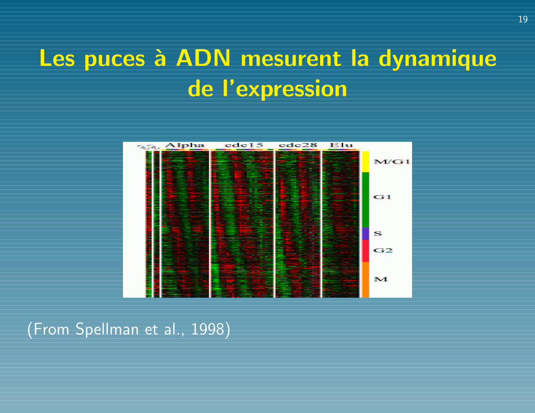
Les puces a ADN mesurent la dynamiquede l’expression

(From Spellman et al., 1998)

20

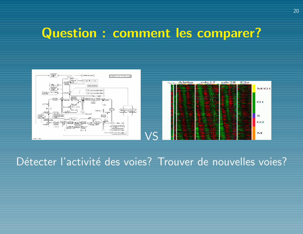
Question : comment les comparer?

VS

Detecter l’activite des voies? Trouver de nouvelles voies?

21

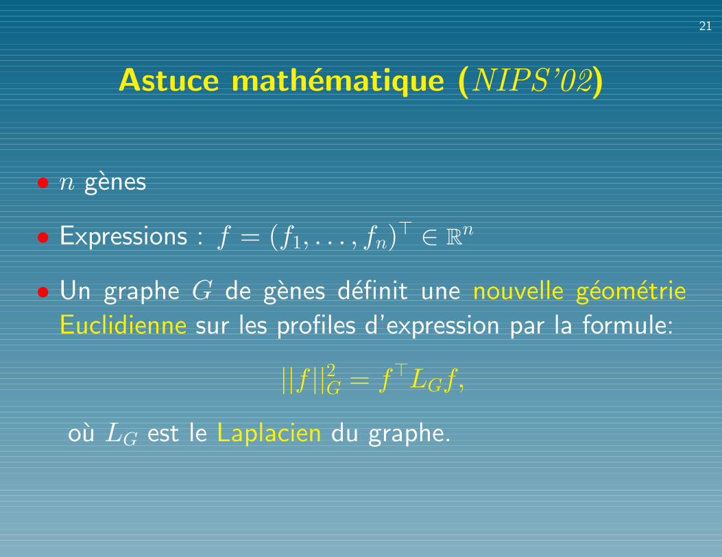
Astuce mathematique (NIPS’02)

• n genes

• Expressions : f = (f1, . . . , fn)> ∈ Rn

• Un graphe G de genes definit une nouvelle geometrie

Euclidienne sur les profiles d’expression par la formule:

||f ||2G = f>LGf,

ou LG est le Laplacien du graphe.

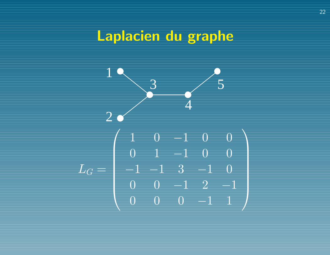
22

Laplacien du graphe

1

2

3

4

5

LG =

1 0 −1 0 00 1 −1 0 0−1 −1 3 −1 00 0 −1 2 −10 0 0 −1 1

23

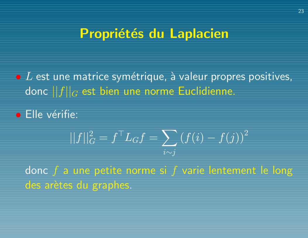
Proprietes du Laplacien

• L est une matrice symetrique, a valeur propres positives,

donc ||f ||G est bien une norme Euclidienne.

• Elle verifie:

||f ||2G = f>LGf =∑i∼j

(f(i)− f(j))2

donc f a une petite norme si f varie lentement le long

des aretes du graphes.

24

Pourquoi ||f ||G?

• Les voies metaboliques sont des composantes connexes

du graphe

• Controler ||f ||G assure que f varie peu au sein de voies

metaboliques potentielles

• Plusieurs problemes se formulent naturellement a partir

de cette norme

25

Exemple 1 : Regression regularisee

• Supposons qu’a chaque donnee d’expression xi ∈ Rn

soit associee une covariable yi ∈ R (age, developpement

d’une tumeur, niveau de pollution, ...)

• La regression par moindre carres classique cherche un

vecteur w ∈ Rn qui minimise:

minw∈Rn

p∑i=1

(w>xi − yi

)2.

26

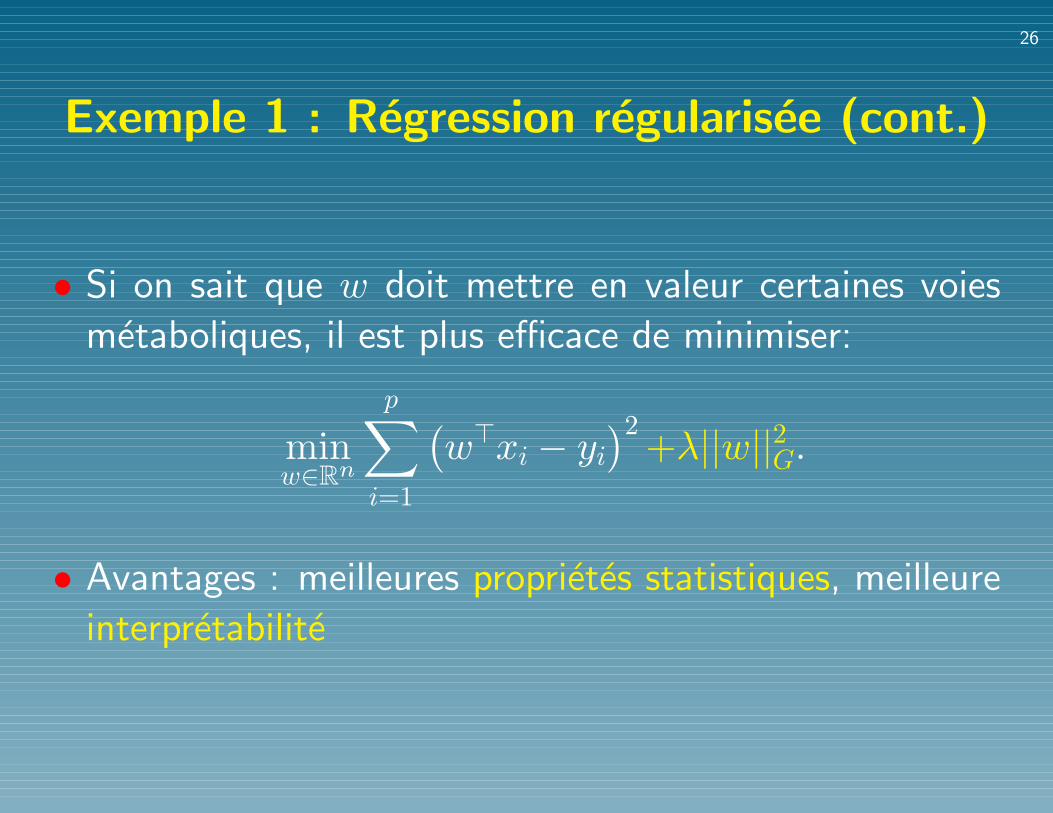
Exemple 1 : Regression regularisee (cont.)

• Si on sait que w doit mettre en valeur certaines voies

metaboliques, il est plus efficace de minimiser:

minw∈Rn

p∑i=1

(w>xi − yi

)2+λ||w||2G.

• Avantages : meilleures proprietes statistiques, meilleure

interpretabilite

27

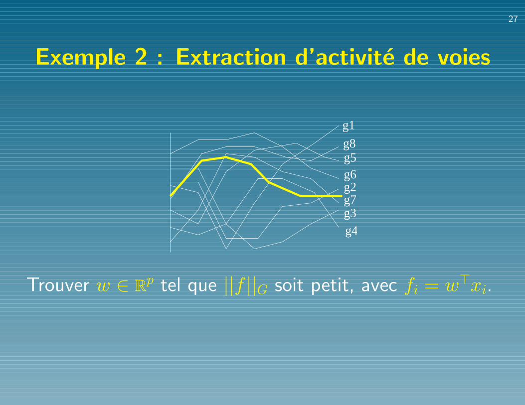
Exemple 2 : Extraction d’activite de voies

g1

g5g6

g7g3g4

g8

g2

Trouver w ∈ Rp tel que ||f ||G soit petit, avec fi = w>xi.

28

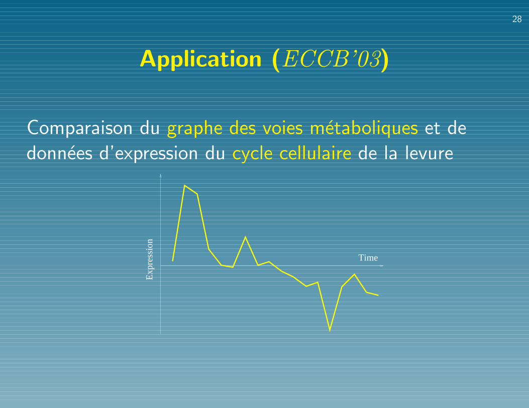
Application (ECCB’03)

Comparaison du graphe des voies metaboliques et de

donnees d’expression du cycle cellulaire de la levure

Time

Exp

ress

ion

29

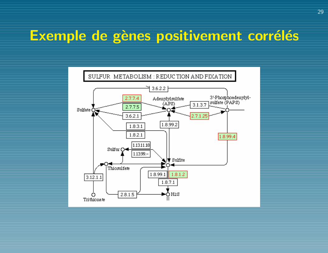
Exemple de genes positivement correles

30

Autres applications

• Extraction de features pour la classification supervisee

de genes (NIPS’02)

• Extraction de features pour la classification non

supervisee et la detection d’operons dans les genomes

bacteriens (ISMB’03)

• Reconstruction de reseaux genetiques (ISMB’04,NIPS’04, ISMB’05).

31

Partie 3

Le projet Kernelchip (2004-07):cancer et regulation

32

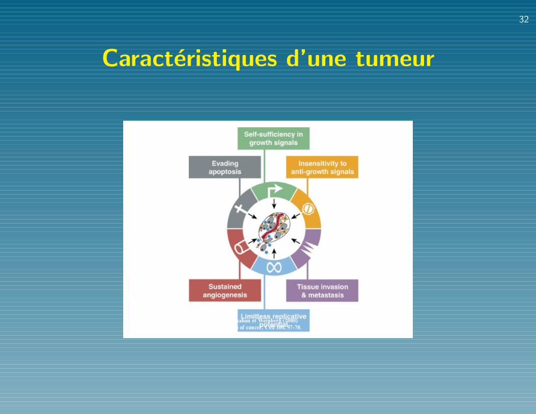
Caracteristiques d’une tumeur

33

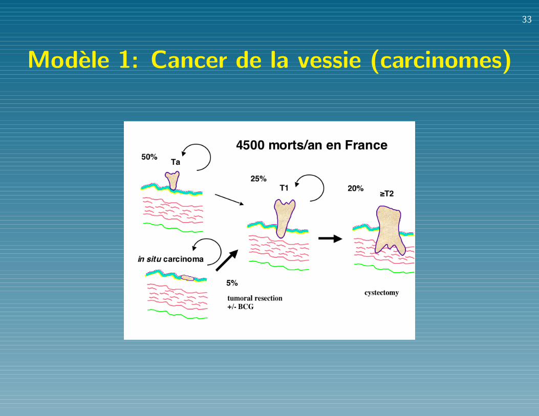
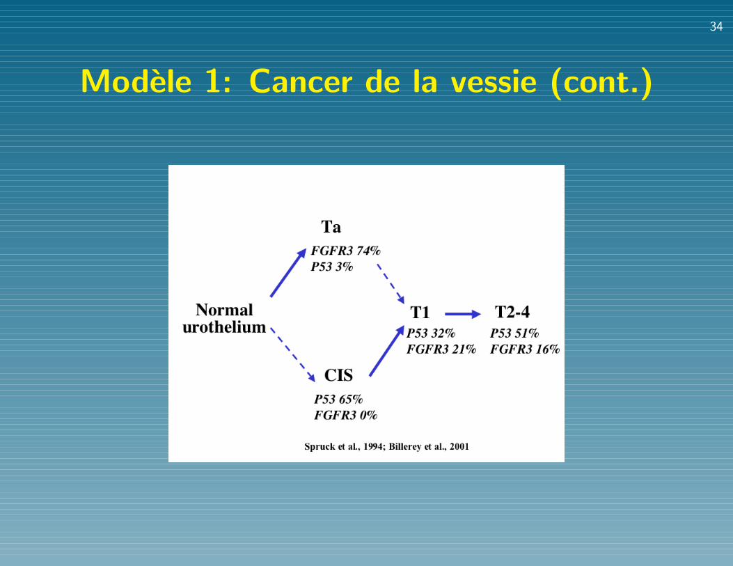
Modele 1: Cancer de la vessie (carcinomes)

34

Modele 1: Cancer de la vessie (cont.)

35

Modele 2: Tumeur d’Ewing

36

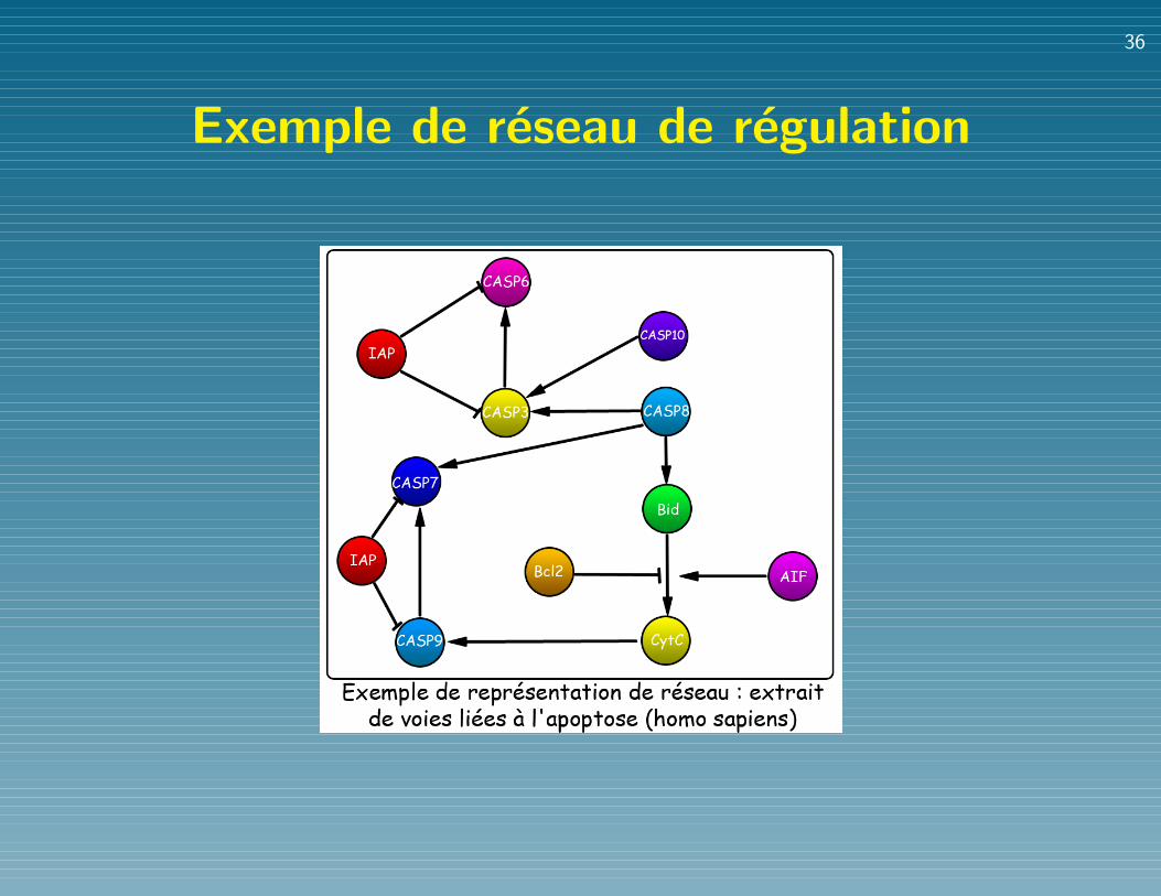
Exemple de reseau de regulation

37

Donnees

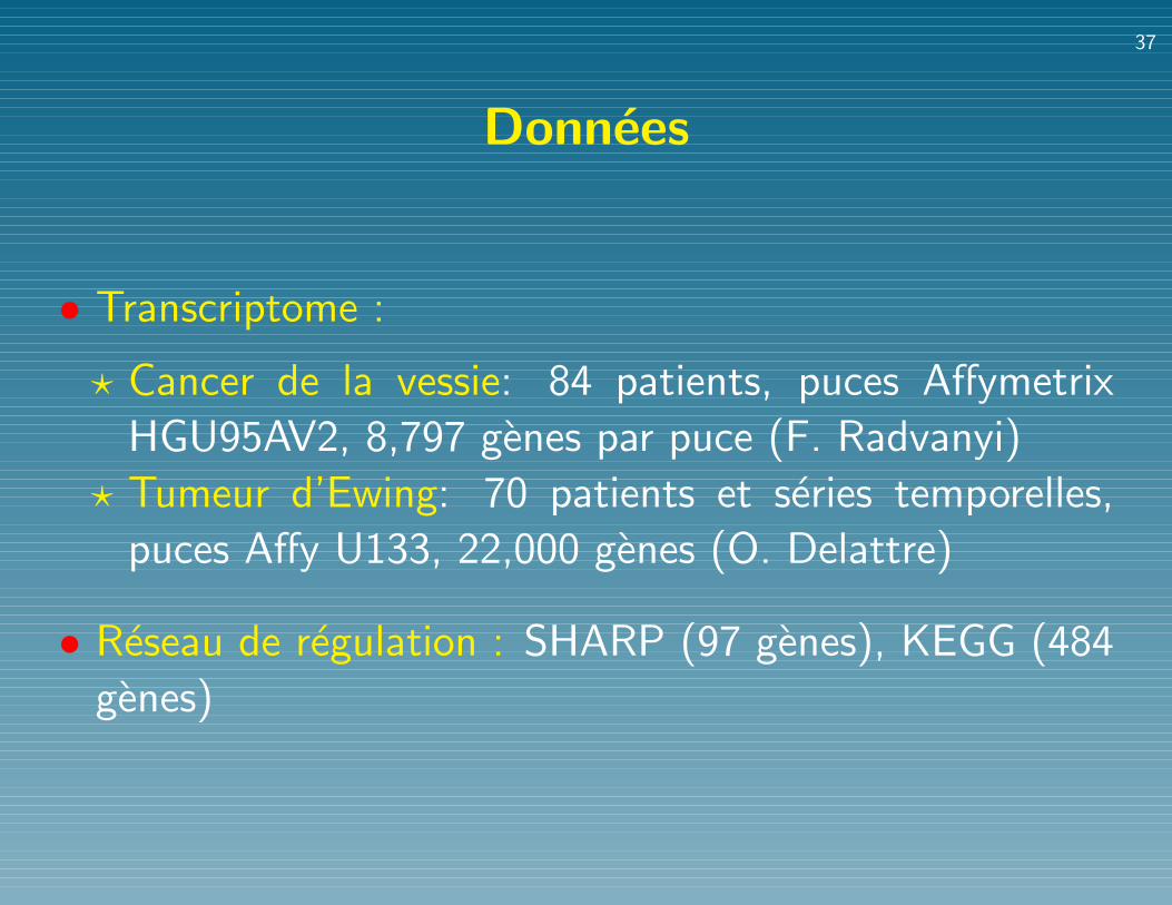
• Transcriptome :

? Cancer de la vessie: 84 patients, puces Affymetrix

HGU95AV2, 8,797 genes par puce (F. Radvanyi)

? Tumeur d’Ewing: 70 patients et series temporelles,

puces Affy U133, 22,000 genes (O. Delattre)

• Reseau de regulation : SHARP (97 genes), KEGG (484

genes)

38

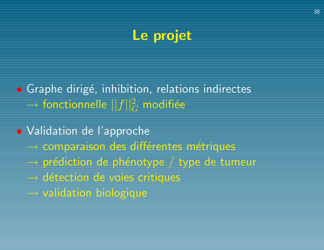
Le projet

• Graphe dirige, inhibition, relations indirectes

→ fonctionnelle ||f ||2G modifiee

• Validation de l’approche

→ comparaison des differentes metriques

→ prediction de phenotype / type de tumeur

→ detection de voies critiques

→ validation biologique

39

Conclusion

40

Conclusion

• Richesse et quantite des donnees du transcriptome

• Necessite d’integrer et de croiser ces donnees avec

d’autres sources d’information

• Les donnees de graphes (interaction, regulation...)

necessitent des developpements mathematiques

particuliers