analyse de la convergence de l’algorithme fastica
TRANSCRIPT

Numero d’ordre:41090
Universite des Sciences et Technologies deLille
Ecole Doctorale Sciences Pour l’Ingenieur LilleNord-de-France
T H E S E
pour obtenir le titre de
Docteur en SciencesMention : MATHEMATIQUES APPLIQUEES
Presentee et soutenue le 10 Juin 2013
Analyse de la convergence del’algorithme FastICA:
Echantillon de taille finie etinfinie
par
Tianwen Wei
Composition du Jury:
Directeur de these : Azzouz Dermoune - Universite Lille 1Rapporteurs : Pierre Comon - Universite de Grenoble
Ali Mohammad-Djafari - Universite Paris-SudExaminateurs : Stephane Gaiffas - Ecole Polytechnique Paris
Guillaume Lecue - Universite Paris-EstCristian Preda - Universite Lille 1Nicolas Wicker - Universite Lille 1


Remerciements
Je souhaite tout d’abord exprimer ma profonde gratitude au ProfesseurAzzouz Dermoune, mon directeur de these pour avoir dirige ce travail. Sarigueur, sa clairvoyance, sa patience ainsi que le soutien qu’il m’a toujoursapporte, m’ont permis de mener a bien cette these. Je n’oublierai jamaisses qualites scientifiques et humaines qui ont contribue enormement a laprogression de mes travaux de recherche.
Mes sincere remerciements sont egalement adresses a Nadji Rahmania,professeur et collaborateur dans notre groupe de travail, pour ses conseilsprecieux qu’il m’a accorde tout au long de ces annees de travail.
Un grand merci a Pierre Comon et Ali-Mohammad Djafari, qui ontaccepte de rapporter cette these. Leurs lectures attentives m’ont permisd’ameliorer mon travail. Je tiens a remercier egalement les autres mem-bres du jury: Guillaume Lecue, Stephane Gaiffas, Cristian Preda et NicolasWicker, qui sont venus de loin ou de pres.
Je suis tres honore que Appo Hyvarinen, le createur de l’algorithmeFastICA, qui est l’un des specialistes internationaux les plus reconnus de mondomaine de recherche, ait accepte de nous acceuillir a l’universite d’Helsinki.Je le remercie vivement.
J’exprime toute ma reconnaissance a mes anciens enseignants et plusparticulierement a Antoine Ayache, Tran Viet Chi, Youri Davydov et RaduStoica, qui par la qualite de leurs cours, ont considerablement contribue ame donner envie de faire une these. Je suis aussi reconnaissant a ThierryGoudon, pour l’aide qu’il m’a apporte quand je faisait mon masteur.
Je tiens a remercier les anciens doctorants chinois du bureau, Qidi Penget Ying Chen, pour les moments merveilleurs que nous avions passe ensemblependant ces annees. Je n’ai pas oublie non plus ma chere Ying, ainsi que lesautres amis chinois et internationaux sur Lille, Jianwei, Cheng, Xian, Jing,Chen, Zuqi, Martin, Elsa, Sophie, Safa, Vincent, Xavier, etc.
J’exprime ma profonde gratitude a Changgui Zhang. C’est grace a luique j’aie l’opportunie de venir etudier en France, ce qui a radicalementchange ma vie.
Finalement, je pense beaucoup a ma mere Jie Yang et mon pere YueqingWei, qui m’ont soutenu unconditionnellement malgre la distance tout au longde mes etudes en France. Je les remercie du fond de mon coeur pour leursacrifice enorme.

ii
Analyse de la convergence de l’algorithmeFastICA: Echantillon de taille finie et infinie
Resume
L’algorithme FastICA est l’un des algorithmes les plus populaires dansle domaine de l’analyse en composantes independantes (ICA). Il existe deuxversions de FastICA: Celle qui correspond au cas ou l’echantillon est de tailleinfinie, et celle qui traite de la situation concrete, ou seul un echantillonde taille finie est disponible. Dans cette these, nous avons fait une etudedetaillee des vitesses de convergence de l’algorithme FastICA dans le cas oula taille de l’echantillon est finie ou infinie, et nous avons etabli cinq criterespour le choix des fonctions de non-linearite.
Dans les trois premiers chapitres, nous avons introduit le probleme del’ICA et revisite les resultats existants. Dans le Chapitre 4, nous avonsetudie la convergence du FastICA empirique et le lien entre la limite de Fas-tICA empirique et les points critiques de la fonction de contraste empirique.Dans le Chapitre 5, nous avons utilise la technique du M-estimateur pourobtenir la normalite asymptotique et la matrice de covariance asymptotiquede l’estimateur FastICA. Ceci nous a permis aussi de deduire quatre criterespour choisir les fonctions de non-linearite. Un cinquieme critere de choixde non-linearite a ete etudie dans le chapitre 6. Ce critere est base surune etude fine de la vitesse de convergence de FastICA empirique. Nousavons illustre chaque chapitre par des resultats numeriques qui valident nosresultats theoriques.
Contents
List of Notations 1
1 Introduction 3
2 Preliminaries 7
2.1 Theoretical ICA . . . . . . . . . . . . . . . . . . . . . . . . . 7
2.1.1 Theoretical ICA Model . . . . . . . . . . . . . . . . . 7
2.1.2 Data preprocessing . . . . . . . . . . . . . . . . . . . . 10
2.1.3 Contrast function . . . . . . . . . . . . . . . . . . . . . 11
2.1.4 FastICA algorithm . . . . . . . . . . . . . . . . . . . . 17
2.2 Empirical ICA . . . . . . . . . . . . . . . . . . . . . . . . . . 22
2.2.1 Empirical ICA Model . . . . . . . . . . . . . . . . . . 22
2.2.2 Probability measure based on observation data . . . . 23
2.2.3 Empirical FastICA algorithm . . . . . . . . . . . . . . 26
3 Theoretical FastICA Algorithm 27
3.1 Assumptions and method . . . . . . . . . . . . . . . . . . . . 27
3.2 Minimizers of contrast function and fixed points of FastICA 30
3.3 Local Convergence of the FastICA Algorithm . . . . . . . . . 32
3.4 Numerical results . . . . . . . . . . . . . . . . . . . . . . . . . 35
3.4.1 Examples of contrast function and FastICA . . . . . . 35
3.4.2 The radius of convergence of FastICA with generalizedGaussian distribution . . . . . . . . . . . . . . . . . . 37
3.5 Proofs . . . . . . . . . . . . . . . . . . . . . . . . . . . . . . . 42
3.5.1 Proof of Proposition 3.2.1 . . . . . . . . . . . . . . . . 42
3.5.2 Proof of Proposition 3.3.5 . . . . . . . . . . . . . . . . 44
4 Four FastICA estimators 47
4.1 Approach to empirical FastICA . . . . . . . . . . . . . . . . . 47
4.2 Local convergence of empirical FastICA algorithm . . . . . . 50
4.3 Numerical results . . . . . . . . . . . . . . . . . . . . . . . . 51
4.4 Proof of Proposition 4.1.6 . . . . . . . . . . . . . . . . . . . . 56
4.4.1 Proof of (4.1.6)-(4.1.8) for k = 1. . . . . . . . . . . . . 56
4.4.2 Proof of (4.1.6)-(4.1.8) for k = 4. . . . . . . . . . . . . 58
4.4.3 Proof of (4.1.9) and (4.1.10) . . . . . . . . . . . . . . . 61
5 Asymptotic Analysis of FastICA estimators 63
5.1 Statement of the main result . . . . . . . . . . . . . . . . . . 63
5.1.1 Related works . . . . . . . . . . . . . . . . . . . . . . . 65
5.2 Method of Lagrange multipliers . . . . . . . . . . . . . . . . . 67

iv Contents
5.2.1 Lagrange function of optimization problem (5.2.2) . . 685.2.2 Lagrange function of optimization problem (5.2.3) . . 68
5.3 M-estimators . . . . . . . . . . . . . . . . . . . . . . . . . . . 725.4 Numerical results . . . . . . . . . . . . . . . . . . . . . . . . . 735.5 Proofs . . . . . . . . . . . . . . . . . . . . . . . . . . . . . . . 76
5.5.1 Proof of Lemma 5.3.4 . . . . . . . . . . . . . . . . . . 765.5.2 Proof of Theorem 5.1.1 . . . . . . . . . . . . . . . . . 76
6 Asymptotic Analysis of the Gradient of the FastICA Func-tion 816.1 Statement of the main result . . . . . . . . . . . . . . . . . . 816.2 Numerical results . . . . . . . . . . . . . . . . . . . . . . . . . 826.3 Proofs . . . . . . . . . . . . . . . . . . . . . . . . . . . . . . . 83
6.3.1 Proof of Proposition 6.1.1 . . . . . . . . . . . . . . . . 836.3.2 Proof of Corollary 6.1.3 . . . . . . . . . . . . . . . . . 86
7 Conclusion and Perspective 877.1 Summary of results . . . . . . . . . . . . . . . . . . . . . . . . 877.2 Upcoming challenges . . . . . . . . . . . . . . . . . . . . . . . 88
7.2.1 Spurious local optima . . . . . . . . . . . . . . . . . . 887.2.2 Convergence radius . . . . . . . . . . . . . . . . . . . . 897.2.3 Convergence and asymptotic behavior of FastICA for
the extraction of several sources . . . . . . . . . . . . 89References . . . . . . . . . . . . . . . . . . . . . . . . . . . . . . . . 90

List of Notations
Typesetting convention
a, b, c lower case letter signifies real scalara,b, c boldface lower case letter signifies column real vectorA,B,C boldface upper case letter signifies real matrix(A)ij (i, j)-th entry of the matrix Ax(t) the t-th realization of random vector x
Operations
aT, AT the transpose of a vector or matrixE[·] the mathematical expectation operatorCov(x) the variance or covariance matrix of xvec(·) the operation that reshapes the columns of a matrix into a long column vector‖ · ‖ Euclidean norm for vector; induced L2 norm (spectral norm) for matrixdef= be defined as

2 Contents
Particular notations
A the mixing matrixI the identity matrixΠv the orthogonal projection matrix that project onto span(v)Π⊥v the orthogonal projection matrix that project onto span(v)⊥
a a generic column of the mixing matrix Aai the i-th column of the mixing matrix Aei the i-th column of the identity matrixs = (s1, . . . , sd)
T the source signalx = (x1, . . . , xd)
T the observed signalRd the set of d-dimensional real column vectorsRn×m the set of n×m real matricesS the set of vectors having unit normBr(v) the set {w ∈ Rd : ‖w − v‖ = r}span(v) the linear subspace spanned by vector vG(·) the nonlinearity functionG(·, µ) the theoretical contrast function with underlying nonlinearity GG(·, µkN ) the empirical contrast function with underlying nonlinearity Gg(·) the derivative of nonlinearity G(·)I(z) the mutual information of random vector zJ (z) the negentropy of random vector zKL(p||q) the Kullback-Leibler divergence between pdf p and qf(·, µ) the theoretical FastICA functionf(·, µkN ) the empirical FastICA functionL(·) the Lagrange functionµ the probability distribution of the observed signal xµkN the k-th discrete probability distribution based on a sample of x

Chapter 1
Introduction
The author’s work during four years of study consists of two independent parts.
The first part concerns the study of the generalized linear model, which leads to
the publication (Dermoune, Rahmania, & Wei, 2012). Due to the lack of time,
this work will not be incorporated in this thesis. The second part of the author’s
work concerns the study of the FastICA algorithm. The main results of this part
is published (Dermoune & Wei, 2013) in the journal IEEE Transaction on Signal
Processing. This thesis is a completion of this paper.
The Blind Source Separation (Comon & Jutten, 2010; Jutten & Comon,n.d.; Jutten & Taleb, 2000), often abbreviated as BSS, is a statistical andcomputational method for revealing hidden factors that underlie sets of ran-dom variable or signals. The term “blind” is intended to imply that suchmethods can separate data into source signals with the absence or priorinformation about the nature of the source signals and the process thatmixes these signals. The BSS problem, first formulated in the early 80s,is a fast growing research area in the past thirty years. It has drawn greatattention of many researchers, notably those from neural network and signalprocessing community, and it has become a widely used data analysis andsignal processing technique with application in many diverse fields, such asbiomedical signal processing, image processing, acoustic signal separation,telecommunications, fault diagnosis, and financial time series (Comon &Jutten, 2010; Hyvarinen, Karhunen, & Oja, 2001; Makeig, Bell, Jung, & Se-jnowski, 1996; M. Ichir, 2006; Vigario & Oja, 2008; Makino, Lee, & Sawada,2007; Brandstein & Ward, 2001).
A general framework for solving BSS problems is called the IndependentComponent Analysis (ICA) (Hyvarinen et al., 2001; Stone, 2004; Jutten,1987; Comon, 1994; Hyvarinen & Oja, 2000), which is based on, as the namesuggests, the simple and fundamental assumption that the unknown sourcesare statistically independent. This assumption is physically realistic due tothe fact that different physical processes (e.g. different people speaking)generate statistically independent signals. Aside from the independence ofsource signals, typical ICA assumptions also include the linearity and theinstantaneousness of the mixture. Even though there exist some methodsfor which an algebraic solution to the ICA problem may be found, otheriterative methods are very popular. Particularly, in practical real-worldproblems, people work with a large number of observed variables and datapoints, in which case an efficient numerical algorithm is even necessary, since

4 Chapter 1. Introduction
the precise algebraic solution can only be estimated from the data. Up todate, there exist various algorithms (Delfosse & Loubaton, 1995; Cardoso& Souloumiac, 1993; Tugnait, 1997; Comon & Moreau, 1997; Chevalier,Albera, Comon, & Ferreol, 2004; Zarzoso & Comon, 2010) in the domain ofICA, among which the so called FastICA algorithm, proposed by Hyvarinenand Oja (Hyvarinen & Oja, 2000, 1997) from Finnish school, is arguably themost popular one. The success of FastICA can be attributed its simplicity,ease of implementation and flexibility to choose the nonlinearity function.
There are two versions of FastICA: the theoretical FastICA and theempirical FastICA. The former corresponds to the ideal case that the math-ematical expectation appeared in the formulation of the algorithm can beprecisely computed, while the latter deals with the practical situation, whereonly a finite sample is available and hence the mathematical expectationmust be approximated by a sample average. The theoretical FastICA hasalready been extensively studied by many researchers during the past decade(Hyvarinen & Oja, 1997; Hyvarinen, 1999; Regalia & Kofidis, 2003; Oja,2002; Douglas, 2003), while the empirical FastICA still poses many theoret-ical and numerical problems.
In this thesis, we are particularly interested in the following questions:
1) Does the empirical FastICA algorithm always converge?
2) The empirical FastICA is an estimator of the theoretical FastICA.What about its asymptotic performance?
3) Does the empirical FastICA algorithm have a quadratic convergencespeed? What is the best choice of the nonlinearity function in termsof convergence speed?
Even though there exist some partial answers to these questions in the lit-erature (Hyvarinen, 1997; Tichavsky, Koldovsky, & Oja, 2006; Oja & Yuan,2006; Ollila, 2010; Leshem & van der Veen, 2008), most of them are basedon simulations; formal developments are often lacking. This thesis aims atfilling this lack as well as providing some insight, too.
This thesis is organized as follows. Chapter 2 is preliminary. In thischapter, we will introduce the data model and the assumptions, the notionof contrast function, preprocessing procedure, and finally the FastICA al-gorithm. Experienced readers may skip this chapter. In Chapter 3, we willdevelop a new method to reestablish all the classical results concerning thetheoretical FastICA, such as the quadratic convergence speed and the limitof FastICA as the local minimizer of the contrast function. In Chapter 4, wewill use the same method to tackle the empirical FastICA and give answerto Question 1) listed above. We will propose four empirical FastICA esti-mators, defined as the limit of the empirical FastICA algorithm, each withrespect to a particular measure based on the sample. We will show that with

5
probability one, all of the four estimators are well defined in the sense thatthe respective algorithm is convergent. Chapter 5 is devoted to the studyof the asymptotic performance of empirical FastICA estimator. We will usethe technique of M-estimator to derive the asymptotic normality of empir-ical FastICA estimator and its asymptotic covariance matrix. Besides, wewill compare four criteria which measure the asymptotic performance of theempirical FastICA estimator. The main result of this chapter is Theorem5.1.1, which answers Question 2). Finally, we adress Question 3) in Chapter6. We will present a new criterion for the nonlinearity function based uponthe convergence speed of FastICA, and give some numerical results.


Chapter 2
Preliminaries
Contents
2.1 Theoretical ICA . . . . . . . . . . . . . . . . . . . 7
2.1.1 Theoretical ICA Model . . . . . . . . . . . . . . . 7
2.1.2 Data preprocessing . . . . . . . . . . . . . . . . . . 10
2.1.3 Contrast function . . . . . . . . . . . . . . . . . . . 11
2.1.4 FastICA algorithm . . . . . . . . . . . . . . . . . . 17
2.2 Empirical ICA . . . . . . . . . . . . . . . . . . . . 22
2.2.1 Empirical ICA Model . . . . . . . . . . . . . . . . 22
2.2.2 Probability measure based on observation data . . 23
2.2.3 Empirical FastICA algorithm . . . . . . . . . . . . 26
In this chapter, we will introduce briefly the data model of ICA, da-ta centering and whitening, the important notions of contrast functions andeventually an iterative method called the FastICA algorithm. We will distin-guish from the very beginning two versions of ICA that differ in nature: thetheoretical ICA, where we work with a theoretical framework (i.e. the ex-act probability distribution of the observed signal is supposed to be known)and do not care its real-world realization. In this case, the mathematicalexpectation is calculable, hence everything under consideration is purely de-terministic. Next, we will consider the empirical ICA, which corresponds tothe practical situation, where we do not have a direct access of the distribu-tion of the observed signal and have to estimate it through sampling.
2.1 Theoretical ICA
2.1.1 Theoretical ICA Model
Let us start by introducing the noiseless linear ICA model:
x = As, (2.1.1)
where
• sdef= (s1, . . . , sd)
T denotes the unknown source signals. The compo-nents s1, . . . , sd are mutually independent and none of them is Gaus-sian.
• xdef= (x1, . . . , xd)
T denotes the observed signals.

8 Chapter 2. Preliminaries
• The unknown mixing matrix A is a non-singular square matrix.
In the sequel, we will use the Greek letter µ to denote the probability dis-tribution of the observed signal x. ICA model 2.1.1 will be referred toas the theoretical ICA model, which means that there is no samplinginvolved and the signal x is perfectly observed in the sense that its ex-act probability distribution µ is known. The hypothesis that the sourcesignal s has independent components is fundamental for ICA, while thenon-gaussianity of s is necessary1 for the separation of the sources (Comon,1994). Besides, matrix A being square means dim(x) = dim(s), which isnot very restrictive. Clearly, if A is not square, it is not invertible, but ifdim(x) > dim(s) = rank(A) = d, it is still possible to recover the sources.In this so called overdetermined case, it suffices to discard some componentsof the mixture vector x that can be generated by a linear combination ofother rows of the mixing matrix. One can use Principal Component Analysis(PCA), to project the mixture data to a d-dimensional space without anyloss of information, see (Hyvarinen et al., 2001) for more detail. Althoughother models (noisy, nonlinear or with convolutive mixture) are also consid-ered by some authors, model (2.1.1) with the assumptions given above isthe simplest but also the most common one for ICA (Hyvarinen et al., 2001;Hyvarinen & Oja, 2000).
The aim of ICA is to recover the independent components of the sourcesignal s based on the knowledge of µ only. It’s beneficial to recall here thenotion of independence for a family of random variables:
Definition 2.1.1 (Independence). Let z1, . . . , zd be random variables hav-ing probability density function pz1 , . . . , pzd. We say z1, . . . , zd are mutuallyindependent if and only if their joint probability density function pz satisfies
pz =d∏i=1
pzi .
The recovery of s can be achieved by finding the inverse of the mixingmatrix A. However, under current assumptions the inverse A−1 cannotbe identified. One reason is that with both A and s being unknown tous, we can never determine the scale (i.e. variance) of s by the knowledgeof x alone. This is because any scalar multiplier to components of s couldalways be canceled by multiplying A by a diagonal matrix. See the followingexample:
Example 2.1.2. Let ξ1, ξ2 be two random variables whose distributions arenot Gaussian. Consider the following two ICA models:
x = As, x′ = A′s′,
1To be precise, at most one component of s can be Gaussian. In this thesis, we supposethat none of the sources can be Gaussian for simplicity.
2.1. Theoretical ICA 9
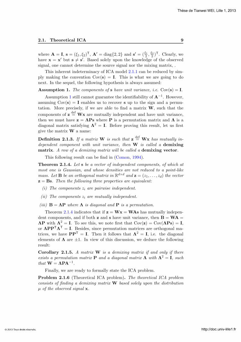
where A = I, s = (ξ1, ξ2)T, A′ = diag{2, 2} and s′ = ( ξ12 ,ξ22 )T. Clearly, we
have x = x′ but s 6= s′. Based solely upon the knowledge of the observedsignal, one cannot determine the source signal nor the mixing matrix, .
This inherent indeterminacy of ICA model 2.1.1 can be reduced by sim-ply making the convention Cov(s) = I. This is what we are going to donext. In the sequel, the following hypothesis is always assumed:
Assumption 1. The components of s have unit variance, i.e. Cov(s) = I.
Assumption 1 still cannot guarantee the identifiability of A−1. However,assuming Cov(s) = I enables us to recover s up to the sign and a permu-tation. More precisely, if we are able to find a matrix W, such that the
components of zdef= Wx are mutually independent and have unit variance,
then we must have z = ΛPs where P is a permutation matrix and Λ is adiagonal matrix satisfying Λ2 = I. Before proving this result, let us firstgive the matrix W a name:
Definition 2.1.3. If a matrix W is such that zdef= Wx has mutually in-
dependent component with unit variance, then W is called a demixingmatrix. A row of a demixing matrix will be called a demixing vector.
This following result can be find in (Comon, 1994).
Theorem 2.1.4. Let s be a vector of independent components, of which atmost one is Gaussian, and whose densities are not reduced to a point-likemass. Let B be an orthogonal matrix in Rd×d and z = (z1, . . . , zd) the vectorz = Bs. Then the following three properties are equivalent:
(i) The components zi are pairwise independent.
(ii) The components zi are mutually independent.
(iii) B = ΛP where Λ is diagonal and P is a permutation.
Theorem 2.1.4 indicates that if z = Wx = WAs has mutually indepen-dent components, and if both z and s have unit variance, then B = WA =ΛP with Λ2 = I. To see this, we note first that Cov(z) = Cov(ΛPs) = I,or ΛPPTΛT = I. Besides, since permutation matrices are orthogonal ma-trices, we have PPT = I. Then it follows that Λ2 = I, i.e. the diagonalelements of Λ are ±1. In view of this discussion, we deduce the followingresult:
Corollary 2.1.5. A matrix W is a demixing matrix if and only if thereexists a permutation matrix P and a diagonal matrix Λ with Λ2 = I, suchthat W = ΛPA−1.
Finally, we are ready to formally state the ICA problem.
Problem 2.1.6 (Theoretical ICA problem). The theoretical ICA problemconsists of finding a demixing matrix W based solely upon the distributionµ of the observed signal x.

10 Chapter 2. Preliminaries
Figure 2.1: Recovering 3 independent components from their mixtures usingICA.
2.1.2 Data preprocessing
Before implementing any ICA method to solve ICA problem 2.1.6, it isusually convenient (necessary in the case of FastICA) to preprocess the data,so that it would be as simple as possible to deal with. Common preprocessingprocedures originate from Principle Component Analysis (PCA), includingcentering and whitening.
Centering is always the first preprocessing procedure. It consists of sub-tracting from x its mean E[x] to fabricate a new random vector that has zeromean. Whitening normally comes after centering. It aims at transformingthe centered signal into a white one, i.e. the one whose components havingunit variance and decorrelated. This can be achieved by multiplying thecentered signal by Cov(x)−
12 . For model 2.1.1, centering and whitening are
feasible since both E[x] and Cov(x) can be drawn from µ.
Definition 2.1.7. For theoretical ICA model, the preprocessed signal is de-fined as
xdef= Cov(x)−
12 (x− E[x]). (2.1.2)
Now let’s look closely at (2.1.2). We have
x = Cov(x)−12 A(s− E[s]
)= As, (2.1.3)
where Adef= Cov(x)−
12 A and s
def= s− E[s]. Clearly, both x and s have zero
mean and independent components. Besides, we claim that the matrix A is a
2.1. Theoretical ICA 11
orthogonal. In fact, by the assumption Cov(s) = I, we have Cov(x) = AAT.It follows that
AAT = (AAT)−12 AAT(AAT)−
12 = I.
In view the discussion above, we can deduce the following result:
Lemma 2.1.8. Through centering and whitening, we can always transformthe theoretical ICA model into an equivalent one, namely
x = As (2.1.4)
where Adef= (AAT)−1/2A is orthogonal and s
def= s− E[s] has zero mean.
Now that we can always work with model 2.1.4, the following additionalassumptions can be added for theoretical ICA model 2.1.1 without loss ofgenerality :
Assumption 2. 1) The source signal s has zero mean, i.e. E[s] = 0,
2) The mixing matrix A is orthogonal, i.e. AAT = I.
Assumption 2 together with Corollary 2.1.5 lead us to the following re-sult:
Proposition 2.1.9. The demixing matrix W is orthogonal. Moreover, thereexists a permutation matrix P and a diagonal matrix Λ with Λ2 = I, suchthat W = ΛPAT.
Proposition 2.1.9 tells us that the rows of the demixing matrix W areaT
1 , . . . ,aTd up to the sign, where a1, . . . ,ad are columns of A.
2.1.3 Contrast function
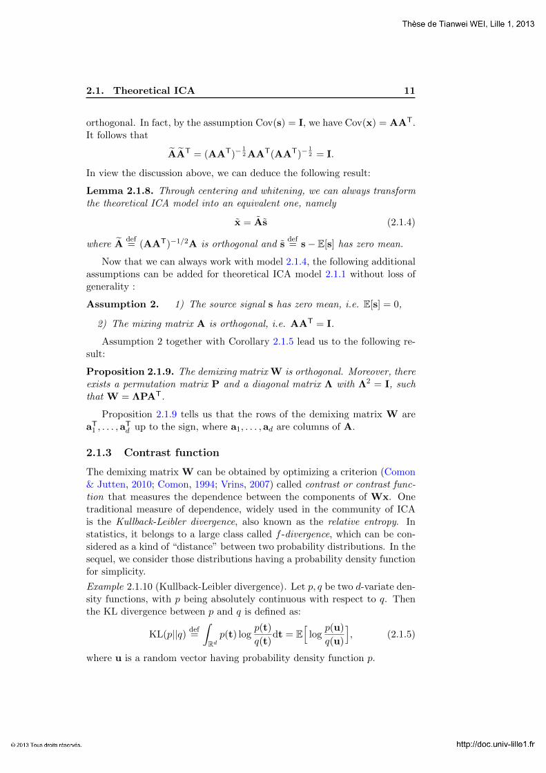
The demixing matrix W can be obtained by optimizing a criterion (Comon& Jutten, 2010; Comon, 1994; Vrins, 2007) called contrast or contrast func-tion that measures the dependence between the components of Wx. Onetraditional measure of dependence, widely used in the community of ICAis the Kullback-Leibler divergence, also known as the relative entropy. Instatistics, it belongs to a large class called f -divergence, which can be con-sidered as a kind of “distance” between two probability distributions. In thesequel, we consider those distributions having a probability density functionfor simplicity.
Example 2.1.10 (Kullback-Leibler divergence). Let p, q be two d-variate den-sity functions, with p being absolutely continuous with respect to q. Thenthe KL divergence between p and q is defined as:
KL(p||q) def=
∫Rd
p(t) logp(t)
q(t)dt = E
[log
p(u)
q(u)
], (2.1.5)
where u is a random vector having probability density function p.

12 Chapter 2. Preliminaries
Figure 2.2: Comparison between source signal, observed signal, preprocessedsignal and extracted signal in a 2d plane.
Kullback-Leibler divergence is not a true metric distance, since it is notsymmetrical, i.e. KL(p||q) 6= KL(q||p), and does not satisfy the triangleinequality. Nevertheless, we have the property KL(p||q) ≥ 0 with equality if
and only if p = q almost everywhere. To see this, we define Ydef= q(u)/p(u),
then there holds E[Y ] = 1. Now applying Jensens inequality, we get:
KL(p||q) = −E[
logq(u)
p(u)
]= −E
[log Y
]≥ logE[Y ] = 0.
This important property ensures that Kullback-Leibler divergence is a legit-imate measure of distance between two probability densities.
In the context of ICA, we are interested in the divergence between thejoint density and the product of the marginal densities of a random vector.This thought leads us to the notion of mutual information.
Definition 2.1.11 (Mutual information). The mutual information of a ran-
dom vector z = (z1, . . . , zd)T is defined as I(z)
def= KL
(pz
∣∣∣∣∣∣ d∏k=1
pzk
).
The notion of mutual information originates from the information theory.It can be interpreted as the code length reduction obtained by coding thewhole vector instead of the separate components. In general, better codescan be obtained by coding the whole vector. However, if the componentsare independent, they give no information on each other, and one couldjust as well code the variables separately without increasing code length. In
2.1. Theoretical ICA 13
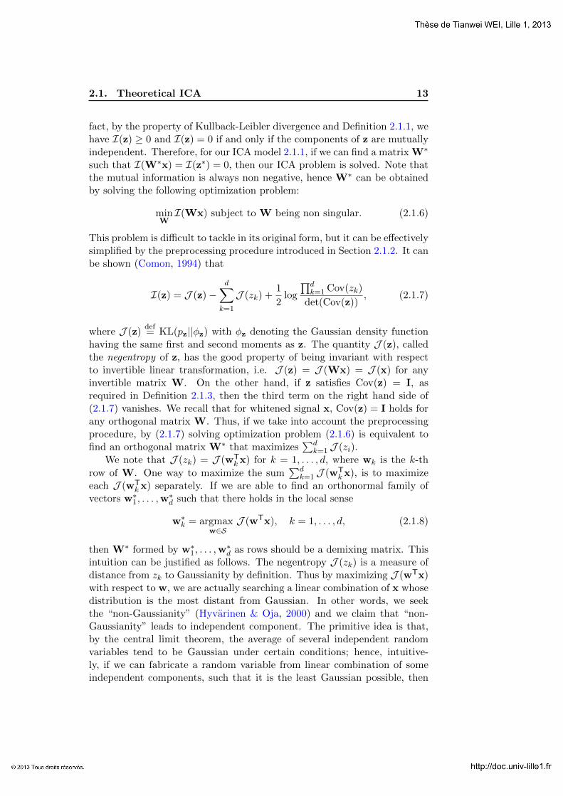
fact, by the property of Kullback-Leibler divergence and Definition 2.1.1, wehave I(z) ≥ 0 and I(z) = 0 if and only if the components of z are mutuallyindependent. Therefore, for our ICA model 2.1.1, if we can find a matrix W∗
such that I(W∗x) = I(z∗) = 0, then our ICA problem is solved. Note thatthe mutual information is always non negative, hence W∗ can be obtainedby solving the following optimization problem:
minWI(Wx) subject to W being non singular. (2.1.6)
This problem is difficult to tackle in its original form, but it can be effectivelysimplified by the preprocessing procedure introduced in Section 2.1.2. It canbe shown (Comon, 1994) that
I(z) = J (z)−d∑
k=1
J (zk) +1
2log
∏dk=1 Cov(zk)
det(Cov(z)), (2.1.7)
where J (z)def= KL(pz||φz) with φz denoting the Gaussian density function
having the same first and second moments as z. The quantity J (z), calledthe negentropy of z, has the good property of being invariant with respectto invertible linear transformation, i.e. J (z) = J (Wx) = J (x) for anyinvertible matrix W. On the other hand, if z satisfies Cov(z) = I, asrequired in Definition 2.1.3, then the third term on the right hand side of(2.1.7) vanishes. We recall that for whitened signal x, Cov(z) = I holds forany orthogonal matrix W. Thus, if we take into account the preprocessingprocedure, by (2.1.7) solving optimization problem (2.1.6) is equivalent tofind an orthogonal matrix W∗ that maximizes
∑dk=1 J (zi).
We note that J (zk) = J (wTk x) for k = 1, . . . , d, where wk is the k-th
row of W. One way to maximize the sum∑d
k=1 J (wTk x), is to maximize
each J (wTk x) separately. If we are able to find an orthonormal family of
vectors w∗1, . . . ,w∗d such that there holds in the local sense
w∗k = argmaxw∈S
J (wTx), k = 1, . . . , d, (2.1.8)
then W∗ formed by w∗1, . . . ,w∗d as rows should be a demixing matrix. This
intuition can be justified as follows. The negentropy J (zk) is a measure ofdistance from zk to Gaussianity by definition. Thus by maximizing J (wTx)with respect to w, we are actually searching a linear combination of x whosedistribution is the most distant from Gaussian. In other words, we seekthe “non-Gaussianity” (Hyvarinen & Oja, 2000) and we claim that “non-Gaussianity” leads to independent component. The primitive idea is that,by the central limit theorem, the average of several independent randomvariables tend to be Gaussian under certain conditions; hence, intuitive-ly, if we can fabricate a random variable from linear combination of someindependent components, such that it is the least Gaussian possible, then

14 Chapter 2. Preliminaries
the obtained random variable itself should coincide with one of the under-lying independent components. This argument seems a bit too wild, butthe conclusion can be made rigourous. The following result is a variation ofTheorem 11 (page 58) in (Vrins, 2007):
Theorem 2.1.12. Let s = (s1, . . . , sd) be the source signal with independentcomponents among which none is Gaussian. Then the mapping w ∈ S →J (wTs) reaches local maximum at w = ±ei for i = 1, . . . , d.
Now let us examine (2.1.8). The maximization of J (wTx) requires thecalculation of an integral of type (2.1.5) where the probability density func-tion of x is directly involved. This is not a easy task from a practical pointof view. One way to overcome this difficulty is to use quantities that aremore easily accessible such as moments or cumulants to approximate the ne-gentropy. The following formula (Comon, 1994) is a classical approximationfor z of zero mean and unit variance.:
J (z) ≈ 1
12κ2
3 +1
48κ2
4 +7
48κ4
3 −1
8κ2
3κ4, (2.1.9)
where κi stands for the i-th order cumulant of the underlying the randomvariable. Approximations of type (2.1.9) have the drawback of being non ro-bust against outliers in practice. An alternative approximation (Hyvarinen& Oja, 2000) is the following:
J (z) ≈n∑i=1
ci
(E[Gi(z)−Gi(v)]
)2, (2.1.10)
where ci are some positive constants, v is a standard Gaussian random vari-able, and the functions Gi are some nonquadratic functions. The advantageof (2.1.10) is that by choosing an appropriate G, we can obtain approxima-tions of negentropy that are better than the one given in (2.1.9). Note thatthe term on the right hand side of (2.1.10) is not always a valid approxi-mation of the negentropy, but the term by itself can always be used as ameasure of non-Gaussianity that is consistent in the sense that it is alwaysnon negative, and equal to zero if z has a Gaussian distribution.
The simplest case of (2.1.10) is n = 1, where we have
J (z) ∝(E[G(z)−G(v)]
)2. (2.1.11)
If we are to maximize J (z) = J (wTx) subject to ‖w‖ = 1 using approxi-mation 2.1.11, we need only to maximize or minimize E[G(wTx)]. In fact,for any w having unit norm, we always have E[wTx] = 0 and Cov(wTx) = 1by Assumption 2. Therefore, the Gaussian random variable v which by def-inition has the same first and second moments as z = wTx, is independentof the choice of w. We then deduce that E[G(v)] is a constant for fixed G.

2.1. Theoretical ICA 15
Now that approximation (2.1.11) is a quadratic function of E[G(wTx)], itreaches its maximum if and only if E[G(wTx)] is maximized or minimized.
Due to reasons stated above, in this thesis we will only consider thefollowing type of contrast function:
Definition 2.1.13. Let G(·) be a twice continuously differentiable nonlinearand nonquadratic function, referred to as the nonlinearity, and x be theobserved signal. The function G(·, µ) : S → R defined by
G(w, µ)def= Eµ[G(wTx)], w ∈ S (2.1.12)
is called the contrast function.
Remark 2.1.14. In the notation of contrast function, we use the same letterG to indicate its connection with the nonlinearity function G(·). The secondargument µ of G(w, µ) refers to the underlying probability distribution withrespect to which the mathematical expectation is taken. Whenever there isno risk of confusion, the theoretical probability distribution µ in the notationEµ[·] is omitted for simplicity.
Remark 2.1.15. In order to be consistent with the notation used in(Hyvarinen & Oja, 2000; Hyvarinen, 1999), we write g(x)
def= G′(x), the
derivative of G(x). By abuse of language, both g(·) and G(·) will be re-ferred to as the “nonlinearity function”. Besides, in order to distinguishfrom the empirical contrast function that will be defined in Chapter 4, wewill sometimes call G(w, µ) the theoretical contrast function.
The following theorem (Hyvarinen & Oja, 2000) confirms that the con-trast function G(·, µ) defined in (2.1.12) can be utilized as a criterion forICA.
Theorem 2.1.16. Consider model 2.1.1 with Assumption 1 and 2. and letai be the i-th column vector of the mixing matrix A. Then ±ai is a localminimizer or maximizer of the contrast function G(·, µ) on the unit sphereS for i = 1, . . . , d, provided that
E[g′(si)− g(si)si] 6= 0. (2.1.13)
Remark 2.1.17. The condition (2.1.13) is consistent with the requirementthat the source signals s1, . . . , sd must not be Gaussian. In fact, if this isthe case for si, then we have
E[g′(si)− g(si)si] =
∫Rφ(x)
(g′(x)− g(x)x
)dx
=
∫Rφ(x)g′(x)dx−
∫Rφ(x)g(x)xdx
= φ(x)g(x)∣∣∣∞−∞−∫Rg(x)dφ(x)−
∫Rφ(x)g(x)xdx,
16 Chapter 2. Preliminaries
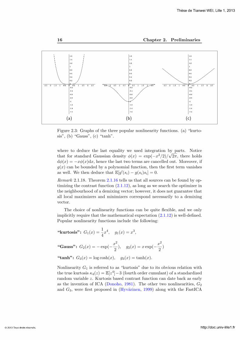
(a) (b) (c)
Figure 2.3: Graphs of the three popular nonlinearity functions. (a) “kurto-sis”, (b) “Gauss”, (c) “tanh”.
where to deduce the last equality we used integration by parts. Noticethat for standard Gaussian density φ(x) = exp(−x2/2)/
√2π, there holds
dφ(x) = −xφ(x)dx, hence the last two terms are cancelled out. Moreover, ifg(x) can be bounded by a polynomial function, then the first term vanishesas well. We then deduce that E[g′(si)− g(si)si] = 0.
Remark 2.1.18. Theorem 2.1.16 tells us that all sources can be found by op-timizing the contrast function (2.1.12), as long as we search the optimizer inthe neighbourhood of a demixing vector; however, it does not guarantee thatall local maximizers and minimizers correspond necessarily to a demixingvector.
The choice of nonlinearity functions can be quite flexible, and we onlyimplicitly require that the mathematical expectation (2.1.12) is well-defined.Popular nonlinearity functions include the following:
“kurtosis”: G1(x) =1
4x4, g1(x) = x3,
“Gauss”: G2(x) = − exp(−x2
2), g2(x) = x exp(−x
2
2)
“tanh”: G3(x) = log cosh(x), g3(x) = tanh(x).
Nonlinearity G1 is referred to as “kurtosis” due to its obvious relation withthe true kurtosis κ4(z) = E[z4]−3 (fourth order cumulant) of a standardizedrandom variable z. Kurtosis based contrast function can date back as earlyas the invention of ICA (Donoho, 1981). The other two nonlinearities, G2
and G3, were first proposed in (Hyvarinen, 1999) along with the FastICA

2.1. Theoretical ICA 17
algorithm. Contrast functions based on the latter two nonlinearities havethe advantage of being more robust against outliers.
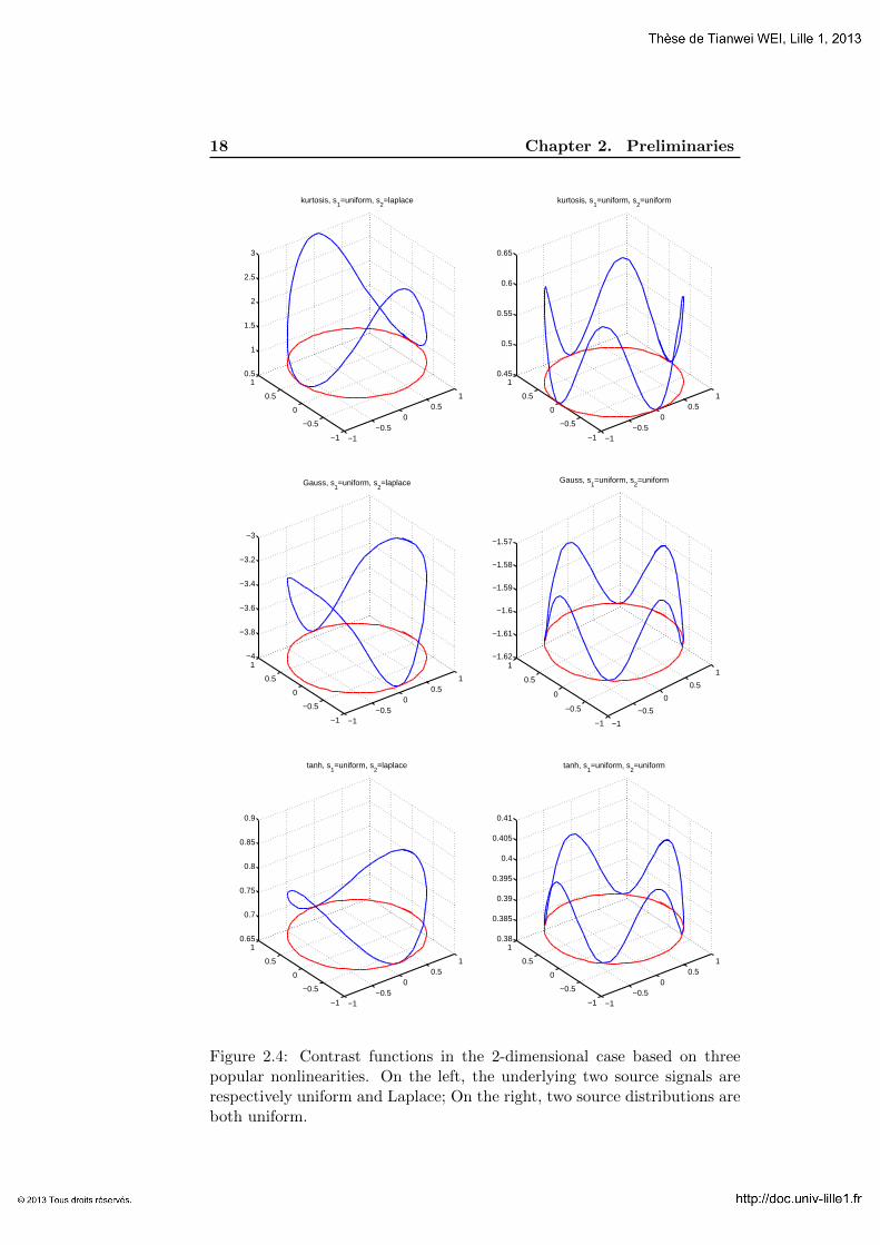
Example 2.1.19. We plotted the contrast functions in the 2-dimensional casebased on three popular nonlinearities: “kurtosis”, “Gauss” and “tanh”. T-wo different scenarios are considered: (i), Two source signals have differentdistributions (one uniform and one Laplace); (ii), Two source distributionsare the same (both uniform). In this simplest case, according to Theorem2.1.16, there should be exactly 4 demixing vectors, namely ±a1,±a2, whichare either local maximizers or minimizers of the contrast function. There-fore, if the contrast function is turned out to have more than 4 local optima,then there must exist spurious solution of the demixing vector. From thefigure, we observe that when the two source signals have different distribu-tions, then the corresponding contrast functions possess exactly 4 optima(2 global maxima and 2 global minima). On the contrary, if the two sourcedistributions are all uniform, then in all the three cases there exist 8 optima.This means that 4 optima do not correspond to a demixing vector.
2.1.4 FastICA algorithm
As we have seen in the last section, independent components can be recov-ered by optimizing the contrast function G(w, µ) subject to the constraint‖w‖ = 1. In principle, we can either try to find an algebraic solution to theoriginal optimization problem, or we can use an adaptive method to gener-ate a sequence that converges to the true solution. However, in most cases,an analytic closed-form solution for ICA problem does not exist, hence wemust resort to the adaptive method.
This thesis aims at giving a rigorous analysis of a popular adaptivemethod called FastICA, also known as The fixed-point algorithm. It is oneof the most successful algorithms for independent component analysis interms of accuracy and low computational complexity. It was first proposedby Hyvarinen and Oja from Finnish school (Hyvarinen, 1999) in late 90s.There are two versions of FastICA: one-unit FastICA and symmetric Fas-tICA. As the name suggests, one-unit FastICA corresponds to the one-unitseparation, which estimates one row at a time of the demixing matrix W,while symmetric FastICA (Oja, 2002; Oja & Yuan, 2006) corresponds tothe simultaneous separation which estimates W as a whole. The analysis ofsymmetric FastICA is beyond the scope of this thesis, and we will herebyconcentrate on the one-unit version of FastICA.
In what follows, a nonlinearity function g = G′ is supposed to be fixed.The original form of one-unit FastICA algorithm can be stated as follows:
Algorithm 2.1.20 (One-unit FastICA for extraction of one source).
1. Choose an arbitrary initial point w ∈ S.
18 Chapter 2. Preliminaries
−1−0.5
00.5
1
−1
−0.5
0
0.5
10.5
1
1.5
2
2.5
3
kurtosis, s1=uniform, s
2=laplace
−1−0.5
00.5
1
−1
−0.5
0
0.5
10.45
0.5
0.55
0.6
0.65
kurtosis, s1=uniform, s
2=uniform
−1−0.5
00.5
1
−1
−0.5
0
0.5
1−4
−3.8
−3.6
−3.4
−3.2
−3
Gauss, s1=uniform, s
2=laplace
−1
−0.5
0
0.5
1
−1
−0.5
0
0.5
1−1.62
−1.61
−1.6
−1.59
−1.58
−1.57
Gauss, s1=uniform, s
2=uniform
−1−0.5
00.5
1
−1
−0.5
0
0.5
10.65
0.7
0.75
0.8
0.85
0.9
tanh, s1=uniform, s
2=laplace
−1−0.5
00.5
1
−1
−0.5
0
0.5
10.38
0.385
0.39
0.395
0.4
0.405
0.41
tanh, s1=uniform, s
2=uniform
Figure 2.4: Contrast functions in the 2-dimensional case based on threepopular nonlinearities. On the left, the underlying two source signals arerespectively uniform and Laplace; On the right, two source distributions areboth uniform.

2.1. Theoretical ICA 19
2. Run the following iteration until convergence:
w+ ← E[g′(wTx)w − g(wTx)x]
w← w+
‖w+‖.
FastICA algorithm 2.1.20 was derived initially as an approximate New-ton method applied to the optimization problem
minw∈S
E[G(wTx)] or maxw∈S
E[G(wTx)]. (2.1.14)
By the method of Lagrange multipliers, we know that optima of E[G(wTx)]subject to the constraint ‖w‖ = 1 can be obtained by setting the first orderderivative of the corresponding Lagrange function L (w, λ) to zero, where
L (w, λ)def= E[G(wTx)] +
λ
2(‖w‖2 − 1).
Now we try to solve
∂wL (w, λ) = E[g(wTx)x] + λw = 0 (2.1.15)
using Newton’s method, where ∂w denotes the partial derivative with respectto w. We recall that Newton’s method is a iterative scheme that can be usedto find numerically the roots of a smooth real valued function F : Rd → Rd.
Algorithm 2.1.21 (Newton’s method).
1. Choose an initial estimate y0 ∈ Rd.
2. Calculate
yi+1 = yi −(F ′(yi)
)−1F (yi) (2.1.16)
for i = 1, 2, . . . until convergence is achieved.
Now let us define F (w) = ∂wL (w, λ) and take λ as a constant. In orderto apply Algorithm 2.1.21, we need to invert the Jacobian matrix F ′, whereby (2.1.15)
F ′(w) = E[g′(wTx)xxT] + λI. (2.1.17)
To simplify the inversion of this matrix, we use the approximation
E[g′(wTx)xxT] ≈ E[g′(wTx)]E[xxT] = E[g′(wTx)I], (2.1.18)
where to deduce the last equality we used the fact that the observed signal xis whitened. Note that if we use approximation (2.1.18), then the Jacobianmatrix F ′(w) becomes diagonal:
F ′(w) ≈ E[g′(wTx) + λ]I,

20 Chapter 2. Preliminaries
hence it can be easily inverted. It then follows that
F ′(w) ≈(E[g′(wTx) + λ]
)−1I. (2.1.19)
Using (2.1.15) and (2.1.19) to (2.1.16), we obtain the following approxima-tive Newton iteration:
w+ = w − E[g(wTx)x] + λw
E[g′(wTx) + λ]. (2.1.20)
Note that (2.1.20) can be further simplified:
w+ =1
E[g′(wTx) + λ]
(wE[g′(wTx) + λ]−
(E[g(wTx)x] + λw
))=
1
E[g′(wTx) + λ]
(E[g′(wTx)w − g(wTx)x]
). (2.1.21)
Since we shall eventually project w+ back to the unit sphere S by multiply-ing 1/‖w+‖, coefficient 1/E[g′(wTx) + λ] in (2.1.21) can be removed. Thisgives the FastICA iteration:
w+ = E[g′(wTx)w − g(wTx)x]
w =w+
‖w+‖.
Remark 2.1.22. The heuristic derivation given above shows how the FastI-CA algorithm is inspired from Newton’s method, but it does not explainwhy the algorithm should work. Theoretical result (Hyvarinen, 1999) thatguarantees the validity of FastICA is Theorem 2.1.23 stated below, and wewill discuss it in detail in Chapter 3. Here, we just point out that themost important advantages of FastICA over the original Newton’s methodis that while retaining a quadratic convergence speed as Newton’s method,the FastICA algorithm does not require the inversion of any matrix. Thismakes its computational complexity significantly lower than that of New-ton’s method. Besides, unlike Newton’s method where bad initial estimatemay result in the failure of convergence, numerical experiments indicate thatFastICA performs generally very well regardless of the initial point w0.
Theorem 2.1.23 ((Hyvarinen, 1999)). Consider model 2.1.1 with Assump-tion 1 and 2. Let ai be the i-th column vector of the mixing matrix A suchthat
E[g′(si)− g(si)si] 6= 0. (2.1.22)
Then there exists r > 0, such that if w0 ∈ S∩Br(ai), the sequence generatedby the FastICA algorithm 2.1.20 converges to ai.

2.1. Theoretical ICA 21
Theorem 2.1.23 states that FastICA algorithm converges to some columnof the mixing matrix (which is a demixing vector), but it is not known inadvance which colomn the algorithm finds. The limit of FastICA mainlydepends on the neighborhood Br(ai) within which lies the initial iterate.If we wish to find more than one demixing vector without the algorithmconverging to the same vector twice, a decorrelation or “deflation” constraint(Delfosse & Loubaton, 1995) must be added: at each step, the i-th estimatedvector must be perpendicular to the i−1 previously found vectors, since thedemixing matrix should be orthogonal. This is usually achieved by using aGram-Schmidt type of orthogonalization method :
Algorithm 2.1.24 (One-unit FastICA for extraction of d sources).
1. Set p = 0.
2. Choose an arbitrary initial point w ∈ S.
3. Run the following iteration until convergence:
w+ = E[g′(wTx)w − g(wTx)x]
w+ = w+ −p∑i=1
wiwTi w+. (2.1.23)
w =w+
‖w+‖.
4. Write wp+1 = w. If p < d − 1, set p = p + 1 then go back to step 2;stop the algorithm otherwise.
Note that the difference between Algorithm 2.1.20 and Algorithm 2.1.24is essentially procedure (2.1.23). Analysis of this additional deflation proce-dure is beyond the scope of our work, and we will concentrate on Algorithm2.1.20. Note that Step 2 of Algorithm 2.1.20 can be represented by theiteration of the following mapping f : Rd → Rd:
w→ Eµ[g′(wTx)w − g(wTx)x]
‖Eµ[g′(wTx)w − g(wTx)x]‖. (2.1.24)
Unsurprisingly, many properties of the FastICA algorithm can be revealedby studying mapping (2.1.24). Thus, it deserves a name in its own right.
Definition 2.1.25. For w ∈ Rd, we define
h(w, µ)def= Eµ[g′(wTx)w − g(wTx)x], (2.1.25)
f(w, µ)def=
h(w, µ)
‖h(w, µ)‖. (2.1.26)
The mapping f(·, µ) : Rd → Rd is called the FastICA function.
22 Chapter 2. Preliminaries
Using this notation, we can rewrite algorithm 2.1.20 as follows:
Algorithm 2.1.26.
1. Choose an arbitrary initial point w0 on the unit sphere S.
2. Run the following iteration until convergence:
w← f(w, µ).
FastICA function (2.1.26) will sometimes be called the theoretical Fas-tICA function. The term “theoretical” is added to highlight its underlyingtheoretical ICA model, where we have perfect knowledge of the distributionµ and hence all the mathematical expectations involved can be preciselyevaluated. Likewise, FastICA Algorithm 2.1.20 or 2.1.26 may be referred toas the theoretical FastICA algorithm. However, when there is no riskof confusion, the term “theoretical” is sometimes omitted for brevity.
Aside from results given in Theorem 2.1.23, the theoretical FastICAalgorithm is proven to possess the following properties:
• It has locally at least a quadratic convergence speed (Hyvarinen, 1999).In the following particular cases, the convergence speed is even cubic(Shen, Kleinsteuber, & Huper, 2008):
– The nonlinearity is “kurtosis”;
– The nonlinearity G(·) is a even function and the extracted sourcesignal si has a symmetrical distribution;
– All the sources other than the extracted source si have a sym-metrical distribution.
• The convergence is monotonic (Regalia & Kofidis, 2003). More pre-cisely, for a FastICA generated sequence {wn} that converges to ai forsome i, the sequence {G(wn, µ)} converges monotonically to G(ai, µ).
2.2 Empirical ICA
2.2.1 Empirical ICA Model
In practice, people work with a finite number of independent and identicallydistributed (i.i.d.) realizations of the observed signal x. More precisely,only a finite sequence x(1), . . . ,x(N) is available with each x(t) issued frommodel 2.1.1:
x(t) = As(t), t = 1, . . . , N, (2.2.1)
where

2.2. Empirical ICA 23
• The index t is the realization label. All the realizations are independentand identically distributed .
• The source signals s(1), . . . , s(N) are unknown, non-Gaussian and d-dimensional. Moreover, they have independent components with unitvariance.
• The observed signals x(1), . . . ,x(N) are known, while their probabilitydistribution µ is not.
• The unknown mixing matrix A is a non-singular square matrix.
Remark 2.2.1. Assumption 1 on page 9 is already taken into account inthe description above, while Assumption 2 on page 11 is not. That is, wedo suppose that the source signal is not Gaussian and has unit variance,but for now it can have non-zero mean and the mixing matrix need not beorthogonal.
In what follows, (2.2.1) will be referred to as the empirical ICA model. Theaim of empirical ICA becomes estimating the mixing matrix W.
Problem 2.2.2 (Empirical ICA problem). The empirical ICA problem con-
sists of giving an estimation W of the demixing matrix W based upon theobservation x(1), . . . ,x(N).
2.2.2 Probability measure based on observation data
Now let us consider the empirical ICA problem 2.2.2. In order to implementthe FastICA algorithm, one must do the following:
• Make sure that the observed signal x have zero mean and unit variance;
• Find way to evaluate the FastICA function (2.1.26).
As explained in Section 2.1.2, the first task can be done by centering andwhitening the observed signal x(1), . . . ,x(N). Although the exact valueof E[x] and Cov(x) needed to carry out data preprocessing are not known,these quantities can always be estimated by the sample mean and the samplevariance respectively :
E[x] ≈ xdef=
1
N
N∑t=1
x(t) (2.2.2)
Cov(x) ≈ CNdef=
1
N
N∑t=1
x(t)x(t)T − xxT. (2.2.3)

24 Chapter 2. Preliminaries
Using (2.2.2) and (2.2.3), we can represent the centered and whitened dataas (similar to 2.1.3)
x(t) =
(1
N
N∑t=1
x(t)x(t)T − xxT
)− 12 (
x(t)− 1
N
N∑t=1
x(t))
= C− 1
2N
(x(t)− x
), t = 1, . . . , N.
Clearly, the preprocessed data x(1), . . . , x(N) has the following properties:
• zero sample mean:1
N
N∑t=1
x(t) = 0.
• unit sample variance:
1
N
N∑t=1
(x(t)− 1
N
N∑t=1
x(t))(
x(t)− 1
N
N∑t=1
x(t))T
= I.
We then assert that the preprocessed data x(1), . . . , x(N) can be used toimplement the FastICA algorithm.
As for the second task, we can follow the same route. Although the Fas-tICA function (2.1.25) cannot be directly evaluated due to the fact that wedo not know µ, it can always be estimated by an appropriate estimator. Aswhat we did in (2.2.2) and (2.2.3), the sample average is a natural candidate.We first calculate
h(w, µ) ≈ 1
N
N∑t=1
(g′(wTx(t))w − g(wTx(t))x(t)
),
and then project it to S to obtain an estimate of f(w, µ).
These ideas lead us to consider the following discrete measures (i.e. dis-tributions) constructed upon the observation x(1), . . . ,x(N):
µ1N =
1
N
N∑t=1
δx(t) (2.2.4)
µ2N =
1
N
N∑t=1
δ(x(t)−x) (2.2.5)
µ3N =
1
N
N∑t=1
δQ−1/2N x(t)
(2.2.6)
µ4N =
1
N
N∑t=1
δC−1/2N (x(t)−x)
(2.2.7)

2.2. Empirical ICA 25
where
QN =1
N
N∑t=1
x(t)x(t)T .
Clearly, distributions (2.2.4)-(2.2.7) satisfy the property µkN (R) = 1 for k =1, 2, 3, 4, hence they are all probability distributions. Then for any functionf(·), we can define the mathematical expectation of f(z) with respect to thedistribution µkN of z:
EµkN [f(z)]def=
∫f(z)µkN (dz) =
1
N
N∑t=1
f(z(t)), (2.2.8)
where z(1), . . . , z(N) denotes the support of z. Thanks to (2.2.8), the math-ematical expectation operator EµkN [·] can be used to denote the average of
f(·) evaluated at z(1), . . . , z(N). Note that for each k = 1, 2, 3, 4, definition(2.2.8) can be explicitly written as:
Eµ1N [f(z)]def=
1
N
N∑i=1
f(wTx(t))
Eµ2N [f(z)]def=
1
N
N∑i=1
f(wT(x(t)− x))
Eµ3N [f(z)]def=
1
N
N∑i=1
f(wTQ−1/2N x(t))
Eµ4N [f(z)]def=
1
N
N∑i=1
f(wTC−1/2N (x(t)− x)).
It is easy to see that distributions (2.2.4)-(2.2.7) have specific mean-ings. More precisely, µ1
N stands for the classical empirical measure arisingfrom the sample x(1), . . . ,x(N), while µ2
N , µ3N and µ4
N can respectivelybe considered as the “empirical measure” based upon the centered data
{x(k)− x}, the whitened data {Q−1/2N x(k)} and the centered and whitened
data {C−1/2N (x(k)− x)}. Of course, the utility of these distributions depend
on the particular assumption of the model. In the most general case, wherethe source signal may have non-zero mean and the mixing matrix is arbitrary(with full rank), the data preprocessing is necessary and hence only µ4
N ismeaningful. Nevertheless, on occasion people encounter, for example, sig-nals that have intrinsically zero mean. In this case, the centering procedurecan be omitted, then both µ3
N and µ4N are valid for ICA. Likewise, if the
observed signal is naturally uncorrelated, then the whitening procedure isno longer needed and we may therefore consider µ2
N and µ4N . As a summary,
we distinguish the following situations:

26 Chapter 2. Preliminaries
1. E[x] = 0 and Cov(x) = I: µ1N − µ4
N are all suitable.
2. E[x] 6= 0 and Cov(x) = I: only µ2N and µ4
N are suitable.
3. E[x] = 0 and Cov(x) 6= I: only µ3N and µ4
N are suitable.
4. E[x] 6= 0 and Cov(x) 6= I: only µ4N is suitable.
In Chapter 4 and 5 that are dedicated to empirical ICA, we consider onlythe first situation and study all four measures µ1
N − µ4N . We claim that,
although it seems to be the most particular case at first glance, we do notactually lose any generality. As a matter of fact, constructing µ4
N requiresdata centering and whitening regardless the actual mean and variance ofthe observed signal. Therefore, when studying µ4
N , we always work withcentered and whitened signal, as such their original mean and variance areirrelevant. For this reason, we do not exploit the properties E[x] = 0 andCov(x) = I during our study, and the latter assumptions are merely madefor the possibility of comparing the “performance” of all four measures.
2.2.3 Empirical FastICA algorithm
Using distribution µkN , we are now able to define the empirical FastICAfunction, and hence the empirical FastICA algorithm. The empirical Fas-tICA function is essentially a generalization of the theoretical one, becausewe only replace the measure µ in Definition 2.1.25 by µkN for k = 1, 2, 3, 4:
Definition 2.2.3. For w ∈ Rd and k = 1, 2, 3, 4, we define
h(w, µkN )def= EµkN
[g′(wTz)w − g(wTz)z
](2.2.9)
f(w, µkN )def=
h(w, µkN )
‖h(w, µkN )‖. (2.2.10)
We call f(·, µkN ) the empirical FastICA function with respect to µkN , orsimply the empirical FastICA function.
Similar to the theoretical case, the empirical FastICA algorithm is ascheme of self-iteration of f(·, µkN ):
Algorithm 2.2.4 (Empirical FastICA).
1. Choose an arbitrary initial point w on the unit sphere S.
2. Run the following iteration until convergence:
w← f(w, µkN ).
The definition of Algorithm 2.2.4 does not guarantee its convergence.Although numerical simulation suggests that the convergence does hold, andit is a priori admitted by many authors, a rigorous prove of its convergenceis still mixing in the community. The eager to fill this blank is the startingpoint of the whole work, and this task will be accomplished in Chapter 4.

Chapter 3
Theoretical FastICAAlgorithm
Contents
3.1 Assumptions and method . . . . . . . . . . . . . 27
3.2 Minimizers of contrast function and fixed pointsof FastICA . . . . . . . . . . . . . . . . . . . . . . 30
3.3 Local Convergence of the FastICA Algorithm . 32
3.4 Numerical results . . . . . . . . . . . . . . . . . . 35
3.4.1 Examples of contrast function and FastICA . . . . 35
3.4.2 The radius of convergence of FastICA with gener-alized Gaussian distribution . . . . . . . . . . . . 37
3.5 Proofs . . . . . . . . . . . . . . . . . . . . . . . . . 42
3.5.1 Proof of Proposition 3.2.1 . . . . . . . . . . . . . . 42
3.5.2 Proof of Proposition 3.3.5 . . . . . . . . . . . . . . 44
This chapter is intended to reestablish the classical results concern-ing the theoretical FastICA algorithm. We will study the link betweenthe critical points of the contrast function and the convergence of theFastICA algorithm. We will show that the columns of the mixing ma-trix are local minimizers of the contrast function and prove the relationa ∈ Min
(G(w, µ)
)⊂ Fix
(f(w, µ)
), where Min
(G(w, µ)
)and Fix
(f(w, µ)
)denotes respectively the set of local minimizers of the contrast functionG(w, µ) on the unit sphere and the set of fixed points of the FastICA func-tion f(w, µ). Moreover, we will show that the FastICA algorithm convergeswith at least a quadratic convergence speed to each column a of the mixingmatrix.
3.1 Assumptions and method
Throughout this Chapter, we consider the theoretical ICA model (2.1.1)with Assumption 1 and 2, i.e.
x = As, (3.1.1)
where
• The observed signal x has probability distribution µ with E[x] = 0and E[xxT] = I.

28 Chapter 3. Theoretical FastICA Algorithm
• The source signal s has independent, non-Gaussian components withE[s] = 0 and E[ssT] = I.
• The mixing matrix A = (a1, . . . ,ad) is orthogonal, i.e. AAT = I.
Aside from the basic assumptions listed above, in our analysis we need thefollowing additional hypotheses:
Assumption 3. (i) The nonlinearity function G has continuous deriva-tives up to the fourth order. Moreover, there exits p > 0 such thatG(k)(t) ≤ c|t|p for k = 0, . . . , 4, where c is some positive constant.
(ii) The random vector x has finite moment of any order.
(iii) The function H(·, µ) : Rd → R defined by
H(w, µ)def= Eµ[g′(wTx)− g(wTx)(wTx)] (3.1.2)
satisfies H(a, µ) > 0.
We claim that none of the assumptions above is restrictive. First, it iseasily seen that three most popular nonlinearity functions, namely “kurto-sis”, i.e. g(x) = x3, “Gauss”, i.e. g(x) = −x exp(−x2/2) and “tanh”, i.e.g(x) = tanh(x) satisfy assumption (i). As for assumption (ii), we claimthat it was made in its current form to lighten the proof, and can be easilyweakened. In fact, we require only that x has finite moment up to somel-th order, with l depending on p. Lastly, we point out that convergenceof the FastICA algorithm relies on the necessary condition H(a, µ) 6= 0, see(Hyvarinen, 1999). To develop a rigorous convergence analysis of the FastI-CA algorithm, one needs to avoid the well-known sign-flipping phenomenon,i.e. FastICA oscillates between neighborhoods of two antipodes on the unitsphere, which causes the discontinuity of the corresponding FastICA map onthe unit sphere. Although one can overcome this difficulty by generalizingthe notion of algorithm convergence, or by using the concept of principalfiber bundles (Shen et al., 2008), we choose to make the convention thatH(a, µ) > 0 to ensure that the convergence takes place in the traditionalsense. Assumption (iii) has the advantage of being simple and always feasi-ble for one-unit FastICA, and one needs only to choose the appropriate signfor the underlying nonlinearity function. The following remark reveals theconnection of (3.1.2) with Hermit polynomial, which leads us to adopt thenotation H(·, ·).Remark 3.1.1. Let us define Hn(·, ·) : Cn × R→ R :
Hn(g, t) =1
γ(t)
dn(γ g)(t)
dnt,
where γ(t) = 1√2π
exp(− t2
2 ). We remark that Hn+1(g, t) = Hn(H1(g, ·), t),and Hn(1, t) = (−1)nHn(t) where Hn is the Hermit polynomial of degree n.
3.1. Assumptions and method 29
In particular, the Hermit polynomial of degree 4 is x4 − 6x2 + 3, which isessentially the kurtosis when regarded as the nonlinearity function. Startingfrom a non-linearity function g, we get the sequence of non-linearity func-tions Hn(g, t), n = 1, . . .. Finally, the function H(w, µ) defined in (3.1.2)can be written as H(w, µ) = Eµ[H1(g,wTx)]. More generally, let us denoteHn(g,w, µ) = Eµ[Hn(g,wTx)]. We will see at least numerically that a is alocal minimizer of H2n(g,w, µ), but it is a local maximizer of H2n+1(g,w, µ).
In this chapiter, the following orthogonal projection method is frequentlyused. For any w ∈ S, we denote by Πw the matrix of the orthogonalprojection from Rd to span(w) and by Π⊥w the matrix of the orthogonalprojection from Rd to span(w)⊥. Clearly, we have
Πw = wwT, (3.1.3)
Π⊥w = I−wwT. (3.1.4)
For any x ∈ Rd, we have the orthogonal decomposition
x = Πwx + Π⊥wx, (3.1.5)
The following result shows that the decomposition (3.1.5) is vital in ouranalysis.
Lemma 3.1.2. Let x be the signal defined in (3.1.1) and a be a column ofthe mixing matrix A. Then Πax and Π⊥a x are independent random vectors.
Proof. Let us write A =(a1, · · ·ad
)and consider its ith column vector
ai. First, we show that aTi x and x − ai(a
Ti x) are independent. Since A is
orthogonal, we have aTi A = eTi . It follows that aT
i x = aTi As = si. On the
other hand, we have also x = As =∑d
j=1 ajsj . Hence
x− ai(aTi x) =
d∑j=1
ajsj − aisi =∑i 6=j
aisi.
By the hypothesis that s has independent components, we get the indepen-dence between aTx and (I− aaT)x. 2
Remark 3.1.3. Lemma 3.1.2 is a direct consequence of the fundamental hy-pothesis of ICA. It states that the observed signal x can be decomposedinto a sum of two independent and perpendicular signals. Inversely, for arandom vector x, if there exists an orthonormal set of d vectors a1, . . . ,adsuch that aia
Ti x and (I−aia
Ti )x are independent, then there exists a matrix
Adef= (a1, . . . ,ad) and a random vector s with independent components such
that x = As. Hence, Lemma 3.1.2 completely characterizes the ICA model2.1.1

30 Chapter 3. Theoretical FastICA Algorithm
3.2 Minimizers of contrast function and fixedpoints of FastICA
Proposition 3.2.1. For any w,v ∈ S, we have
G(w, µ) = G(v, µ) + (w − v)Tϕ(v, µ) +1
2(w − v)TK(v, µ)(w − v) +O(‖w − v‖3),
where ϕ(v, µ) and K(v, µ) are defined by
ϕ(v, µ)def= E[g(vTx)Π⊥v x], (3.2.1)
K(v, µ)def= H(v, µ)I + E[g′(vTx)Π⊥v (xxT − I)Π⊥v ]. (3.2.2)
Proof. See Section 3.5.1.
Lemma 3.2.2. A vector v is a fixed point of the FastICA function if andonly if ϕ(v, µ) = 0 and H(v, µ) > 0.
Proof. By definition, vector v is a fixed point of f(·, µ) if and only iff(v, µ) = v. Note that
f(v, µ) =1
‖h(v, µ)‖E[g′(vTx)v − g(vTx)x]
=1
‖h(v, µ)‖E[g′(vTx)v − g(vTx)Πvx− g(vTx)Π⊥v x]
=1
‖h(v, µ)‖
(H(v, µ)v −ϕ(v, µ)
),
where the term ϕ(v, µ) = E[g(vTx)Π⊥v x] is perpendicular to v. Thereforef(v, µ) is parallel to v if and only if ϕ(v, µ) = 0. Note that in this case wehave
‖h(v, µ)‖ =(‖H(v, µ)v‖2 + ‖ϕ(v, µ)‖2
)1/2= |H(v, µ)|.
Then f(v, µ) = v implies H(v, µ) > 0. 2
Remark 3.2.3. We clarify that a point v being a fixed point of the FastICAfunction f(v, µ) means it satisfies v = f(v, µ), and it does not need to bethe limit of the FastICA algorithm. In the next section, we will see thatother condition is needed for the FastICA algorithm to converge to v. Inthis thesis, we will avoid using the statement like “fixed point of the FastICAalgorithm” since it makes confusion.
From Proposition 3.2.1 and Lemma 3.2.2, we deduce immediately thefollowing result.
Proposition 3.2.4. If v is a fixed point of the FastICA function and ifthe matrix K(v, µ) is positive definite, then v is a local minimizer of thecontrast function.

3.2. Minimizers of contrast function and fixed points of FastICA31
Proposition 3.2.5. If v is a local minimizer of the contrast functionG(w, µ) on S, and if H(v, µ) > 0, then it is a fixed point of the FastICAfunction.
Proof. From Taylor’s formula, we have
G(w, µ) = G(v, µ) + (w − v)TE[g(vTx)x] +O(‖w − v‖2),
or equivalently
G(w, µ)−G(v, µ)
‖w − v‖=
(w − v)TE[g(vTx)x]
‖w − v‖+O(‖w − v‖). (3.2.3)
On the one hand, we can show that{u : u = lim
w∈S→v
w − v
‖w − v‖
}= span(v⊥).
On the other hand, if v is a local minimizer of the contrast function on S,then for all w ∈ S near v we have
G(w, µ)−G(v, µ)
‖w − v‖≥ 0.
Applying this result to (3.2.3) and letting w→ v, we obtain
limw∈S→v
E[(w − v)T g(vTx)x
‖w − v‖
]≥ 0.
Hence, we have E[g(vTx)uTx] ≥ 0 for all u ∈ span(v⊥), which implies thatϕ(v, µ) = E[g(vTx)Πv⊥x] = 0. This condition along with the hypothesisH(v, µ) > 0 gives v = f(v, µ). 2
Proposition 3.2.6. The vector a is a fixed point of the FastICA function.It is also a local minimizer of the contrast function on S.
Proof. Let us show that a being a column of A implies
ϕ(a, µ) = 0 and K(a, µ) = H(a, µ)I.
By Lemma 3.1.2, the random vectors aTx and (I− aaT)x are independent.Then it follows from the assumption E[x] = 0 that
ϕ(a, µ) = E[g(aTx)(I− aaT)x] = E[g(aTx)]E[(I− aaT)x] = 0.
To prove the second, let us denote L(w, µ)def= E[g′(wTx)Π⊥v (xxT − I)Π⊥v ].
Using the decomposition x = aaTx + (I− aaT)x, we get
L(a, µ) = E[g′(aTx)(xxT − aaTxxTaaT − I + aaT)]
= E[g′(aTx)
((aaTx + (I− aaT)x)(aaTx + (I− aaT)x)T
−aaTxxTaaT − I + aaT)]
= E[g′(aTx)
(aaTxxT(I− aaT) + (I− aaT)xxaaT
+ (I− aaT)xxT(I− aaT)− I + aaT)]. (3.2.4)

32 Chapter 3. Theoretical FastICA Algorithm
Note that we have
E[g′(aTx)aaTxxT(I− aaT)
]= E
[g′(aTx)aaTx
]E[xT(I− aaT)
]= 0 (3.2.5)
by the independence between aTx and (I− aaT)x, and
E[(I− aaT)xxT(I− aaT)
]= I− aaT (3.2.6)
by the assumption E[xxT] = I. Applying (3.2.5) and (3.2.6) to (3.2.4), weobtain L(a, µ) = 0 and K(a, µ) = H(a, µ)I.
Finally, we deduce from Lemma 3.2.2 that a is a fixed point of theFastICA function, and from Proposition 3.2.4 that it is also a local minimizerof the contrast function. 2
3.3 Local Convergence of the FastICA Algorithm
Proposition 3.3.1. Let v be a fixed point of the FastICA function f(·, µ).If ‖∇f(v, µ)‖ < 1, then starting near v, the FastICA algorithm convergesto v.
Proof. Since ‖∇f(v, µ)‖ < 1, by the continuity of ∇f(·, µ), there exists0 < K < 1 and r > 0, such that supw∈Br(v) ‖∇f(w)‖ < K. Hence, forw0 ∈ Br(v), we have
‖w1 − v‖ = ‖f(w0, µ)− f(v, µ)‖ ≤ K · ‖w0 − v‖. (3.3.1)
It follows that ‖wn− v‖ ≤ Kn · ‖w0− v‖. Consequently, {wn} is a Cauchysequence that converges to v. 2
Lemma 3.3.2. For all w ∈ S, we have
∇h(w, µ) = Eµ[g′′(wTx)wxT + g′(wTx)I− g′(wTx)xxT],
∇f(w, µ) =
(‖h(w, µ)‖2I− h(w, µ)h(w, µ)T
)∇h(w, µ)
‖h(w, µ)‖3.
Proposition 3.3.3. Let a be a column of the mixing matrix A such thatH(a, µ) defined in (3.1.2) is not zero. Then we have
h(a, µ) = H(a, µ)a (3.3.2)
∇h(a, µ) = γ(a, µ)aaT (3.3.3)
f(a, µ) = a (3.3.4)
∇f(a, µ) = 0, (3.3.5)
where γ(·, µ) is some scalar valued function.

3.3. Local Convergence of the FastICA Algorithm 33
Proof.
(i). we have
h(a, µ) = Eµ[g′(aTx)a− g(aTx)x]
= Eµ[g′(aTx)a− g(aTx)Πax]− Eµ[g(aTx)Π⊥a x].
Since a is such that ϕ(a, µ) = Eµ[g(aTx)Π⊥a x] = 0, we get
h(a, µ) = Eµ[g′(aTx)a− g(aTx)Πax]
= Eµ[g′(aTx)a− g(aTx)(aTx)a]
= H(a, µ)a,
with H(a, µ) = Eµ[g′(aTx)a− aTx g(aTx)a].
(ii). Substituting x by Πax + Π⊥a x in
∇h(a, µ) = Eµ[g′′(aTx)axT + g′(aTx)I− g′(aTx)xxT],
we obtain
∇h(a, µ) = Eµ[g′′(aTx)a(xTΠa + xTΠ⊥a ) + g′(aTx)(aaT − aaTxxTaaT)].
By the assumption on a and the fact that Eµ[x] = 0, we have
Eµ[g′′(aTx)xTΠ⊥a ] = Eµ[g′′(aTx)]Eµ[xTΠ⊥a ] = 0.
It follows that
∇h(a, µ) = Eµ[g′′(aTx)a(xTΠa) + g′(aTx)(aaT − aaTxxTaaT)]
= Eµ[g′′(aTx)axTaaT + g′(aTx)(aaT − aaTxxTaaT)]
= Eµ[g′′(aTx)(xTa)aaT + g′(aTx)(aaT − (xTa)2aaT)]
= γ(a, µ)aaT,
where
γ(a, µ) = Eµ[g′′(aTx)xTa + g′(aTx)(1− (aTx)2)]. (3.3.6)
(iii). The equality f(a, µ) = a is a direct consequence of (i).
(iv). Then applying (i) and (ii) to
∇f(w, µ) =(‖h(w, µ)‖2I− h(w, µ)h(w, µ)T)∇h(w, µ)
‖h(w, µ)‖3
yields gives ∇f(a, µ) = 0. 2

34 Chapter 3. Theoretical FastICA Algorithm
Equalities (3.3.2) and (3.3.4) are just a consequence of the independenceof the random vectors Πax and Π⊥a x, while (3.3.3) and (3.3.5) are, to ourknowledge, new. The fact f(a, µ) = a shows that the columns of the mix-ing matrix A are fixed points of the FastICA algorithm with respect to µ,while ∇f(a, µ) = 0 confirms that starting near v, the FastICA algorithmconverges to v, according to Proposition 3.3.1. Moreover, ∇f(a, µ) = 0implies that the sequence {wn} generated by FastICA converges to a witha quadratic convergence speed. In fact, using Taylor’s formula and takinginto account of (3.3.4) (3.3.5), we obtain
wn+1 = f(wn, µ) = f(a, µ) +∇f(a, µ)(wn − a) +O(‖wn − a‖2)
= a +O(‖wn − a‖2),
where the lth entry of the vector O(‖wn − a‖2) equals to
1
2
∑1≤i,j≤d
∂wi∂wjf l(ξl, µ)(wn − a)i(wn − a)j .
which is bounded by
d
2sup
1≤i,j,l≤d,w∈Br(a)|∂wi∂wjf l(w, µ)|‖wn − a‖2.
It follows that
supn
‖wn+1 − a‖‖wn − a‖2
≤ +∞. (3.3.7)
The following theorem summarizes the discussion above.
Theorem 3.3.4. There exists r > 0, such that if w0 ∈ S ∩Br(a), then thesequence generated by the FastICA algorithm converges to a, i.e.
limk→∞
wk = a,
Moreover, the convergence speed is quadratic.
Hyvarinen has already showed the quadratic speed of convergence of theFastICA algorithm (Hyvarinen & Oja, 1997; Hyvarinen, 1999). He provedthat h(w) = h(a) + O(‖w − a‖2) for all w ∈ S ∩Br(a) for small r, andthen he derived that f(w) = f(a)+O(‖w−a‖2) for all w ∈ S ∩Br(a). Weemphasize that ∇f(a) = 0 is not a direct consequence of the latter equality.For example we can show that
G(w, µ) = G(a, µ) +O(|w − a|2)
for w ∈ S ∩Br(a), but ∇G(a, µ) 6= 0. In our proof we show that ∇f(a) = 0and then f(w) = f(a) +O(‖w− a‖2) for all w ∈ Br(a). Hence, our resultshows that the term
O(‖w − a‖2) =1
2(w − a)T∇2f(v)(w − a)
where v ∈ [a,w].

3.4. Numerical results 35
Proposition 3.3.5. If G(x) = x4, then we have ∇2f(a, µ) = 0. As a result,the convergence speed of FastICA algorithm is cubic.
Proof. See Section 3.5.2.
Hyvarinen and Oja have already showed the cubic speed of convergence ofthe FastICA algorithm for the kurtosis non-linearity (Hyvarinen, 1999; Oja,2002). They proved that h(w) = h(a) +O(‖w− a‖3) for all w ∈ Br(a)∩Sfor small r, and then he derived that f(w) = f(a) + O(‖w − a‖3) for allw ∈ S∩Br(a). As we showed in the first commentary ∇f(a) = 0,∇2f(a) =0 is not a direct consequence of the latter equality. In our proof we showthat ∇f(a) = 0,∇2f(a) = 0 and then f(w) = f(a) + O(‖w − a‖3) for allw ∈ Br(a). Hence, our result shows that the term
O(‖w − a‖3) =1
6
∑i,j,k
∂3wiwjwk
f(v)(wi − ai)(wj − aj)(wk − ak)
where v lies between a and w.
3.4 Numerical results
3.4.1 Examples of contrast function and FastICA
In the sequel, we consider the case d = 2 that the two source signals s1, s2
have respectively Laplace and uniform distribution. We take kurtosis as thenonlinearity function, i.e. G(x) = x4. Besides, without loss of generality, wesuppose that A = I. It is clear that any vector w ∈ S can be parameterizedby a scalar θ ∈ [0, 2π) via w(θ) = (cos(θ), sin(θ))T, and hence the contrastfunction can be represented as a mapping
θ → G(w(θ), µ) = E[G(cos(θ)s1 + sin(θ)s2)]. (3.4.1)
This approach, called angular parametrization (Vrins, 2007) is convenientfor visualizing the numerical results in a 2D-plan. Note that we have A =(e1, e2) and w(0) = e1, w(π/2) = e2, w(π) = −e1, w(3π/2) = −e2.
Example 3.4.1. In Fig 3.1, we plot G(w(θ, µ)) and H(w(θ), µ). We observefrom the figure that, the contrast function attains its minimum at θ =π/2, 3π/2, which correspond to ±e2, and the function H(w, µ) has positivevalue at both points. Inversely, at θ = 0, π, or ±e1, we have H(w, µ) < 0and G(w, µ) attains its local maximum. This example confirms Proposition3.2.6.
Example 3.4.2. In Fig 3.2, we illustrate how FastICA algorithm convergesto the local minimizer (or maximizer) of the contrast function. We iter-ated FastICA three times for input w0(θ) = (cos(θ), sin(θ)) with θ rang-ing from 0 to π. We recorded the outcome of each iteration, namely

36 Chapter 3. Theoretical FastICA Algorithm
0 ≤ θ < 2π
0 pi/2 pi 3pi/2 2pi1
2
3
4
5
6
7
0 ≤ θ < 2π
0 pi/2 pi 3pi/2 2pi−15
−10
−5
0
5
G(w(θ),µ)
H(w(θ),µ)
Figure 3.1: G(w(θ), µ) and H(w(θ), µ).
0≤ θ < 2π
Convergence of FastICA
←θ1=1.005 θ
2=2.137→
0 pi/4 pi/2 3pi/4 pi1.5
2
2.5
3
3.5
4
4.5
5
5.5
6
Contrast functionFirst iterationSecond iterationThird iteration
Figure 3.2: Convergence of FastICA.

3.4. Numerical results 37
wi(θ)def= f(wi−1(θ), µ) for i = 1, 2, 3 and for 0 ≤ θ ≤ π, and then plot-
ted G(wi(θ), µ), i.e. the contrast function evaluated at these points. Inthe figure, the black solid curve represents the contrast function (4.3.1),or equivalently θ → G(w0(θ), µ) while the mark “◦”, “+” and “×” standsrespectively for the mapping θ → G(wi(θ), µ) with i = 1, 2, 3. From thegraph, we observe that for any initial input w0(θ), as the index i aug-ments, G(wi(θ), µ) tends to either G(e1, µ) or G(e2, µ) monotonically, thelatter being a local minimum of G(w, µ). A study of the monotonic conver-gence of the FastICA algorithm can be found in (Regalia & Kofidis, 2003).Moreover, if the angle θ of w0 lies within the interval (1.005, 2.137), thenG(wi(θ), µ)→ G(e2, µ).
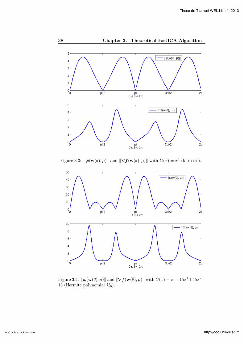
Example 3.4.3. It is of interest to see among S which are fixed points of theFastICA function f(w, µ). By Lemma 3.2.2, fixed points are the solutions ofthe equation ϕ(w, µ) = 0. In Fig 3.3, we plot the mapping θ → ‖ϕ(w(θ), µ)‖and θ → ‖∇f(w(θ), µ)‖ for kurtosis nonlinearity function. We observe that‖ϕ(w, µ)‖ has exactly 4 zeros which are ±e1 and ±e2. Therefore, any vectorother than ±e1 and ±e2 cannot be fixed point of f(w, µ). Besides, we findout that ‖∇f(w(θ), µ)‖ vanishes only at ±e1 and ±e2. In Fig 3.4, we plotthe same mapping using Hermite polynomial H6 = x6 − 15x4 + 45x2 − 15as the nonlinearity function. From the graph, we observe that in this case,‖ϕ(w(θ), µ)‖ has 8 zeros including ±e1 and ±e2. ‖∇f(w(θ), µ)‖ however,as in the case of kurtosis nonlinearity, it vanishes only at ±e1 and ±e2.
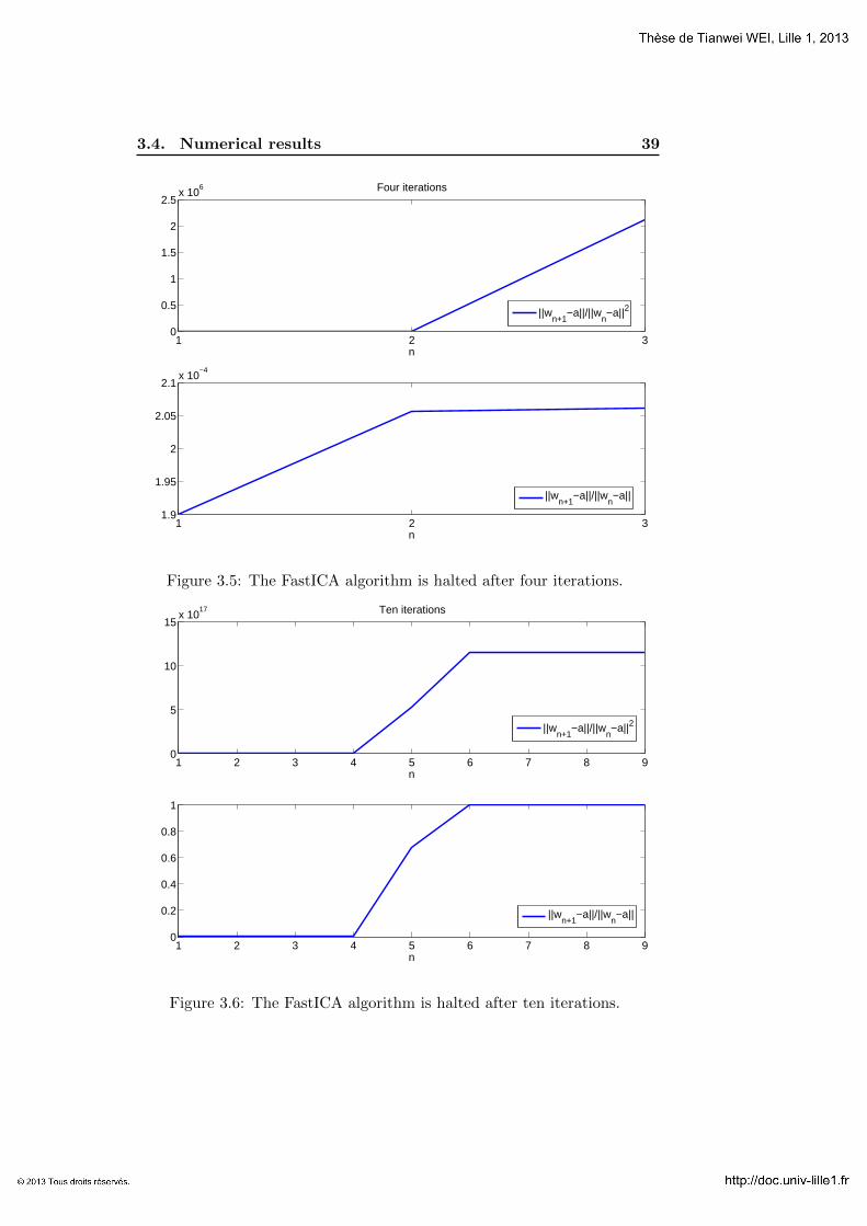
Example 3.4.4. Theoretically, the FastICA algorithm has a quadratic conver-gence speed for a general nonlinearity function, and in the case of kurtosis,as indicated in Corollary 3.3.5, the convergence speed is even cubic. It is ofinterest to see if this is really the case in the numerical simulations. In thisexample, we choose an arbitrary initial point w0(θ) such that the angle θis near π/2. Starting from w0(θ), the FastICA algorithm yields a sequence{wn} that converges to w(π/2) = e2. In Fig 3.5 and 3.6, we plot respec-tively ‖wn+1 − e2‖/‖wn − e2‖2 and ‖wn+1 − e2‖/‖wn − e2‖ for differentn. From the graph, we see that even for the kurtosis nonlinearity, the ratio‖wn+1−e2‖/‖wn−e2‖2 explodes immediately while ‖wn+1−e2‖/‖wn−e2‖remains stable at a level of approximately 2.05×10⁻⁴ for the first 4 iterations.This implies very fast linear convergence. However, as n increases further,it seems that the computer considers the sequence as “already converged”,since ‖wn+1 − e2‖/‖wn − e2‖ becomes stable at 1.
3.4.2 The radius of convergence of FastICA with generalizedGaussian distribution
The aim of this section is to study the radius of convergence of the sourcesignals. This notion is defined as follows.
38 Chapter 3. Theoretical FastICA Algorithm
0 pi/2 pi 3pi/2 2pi0
1
2
3
4
5
0 ≤ θ < 2π
0 pi/2 pi 3pi/2 2pi0
1
2
3
4
5
0 ≤ θ < 2π
||ψ(w(θ), µ)||
||∇ f(w(θ), µ)||
Figure 3.3: ‖ϕ(w(θ), µ)‖ and ‖∇f(w(θ), µ)‖ with G(x) = x4 (kurtosis).
0 pi/2 pi 3pi/2 2pi0
10
20
30
40
50
0 ≤ θ < 2π
||ψ(w(θ), µ)||
0 pi/2 pi 3pi/2 2pi0
2
4
6
8
10
0 ≤ θ < 2π
||∇ f(w(θ), µ)||
Figure 3.4: ‖ϕ(w(θ), µ)‖ and ‖∇f(w(θ), µ)‖ with G(x) = x6−15x4+45x2−15 (Hermite polynomial H6).
3.4. Numerical results 39
1 2 30
0.5
1
1.5
2
2.5x 10
6
n
Four iterations
1 2 31.9
1.95
2
2.05
2.1x 10
−4
n
||wn+1
−a||/||wn−a||2
||wn+1
−a||/||wn−a||
Figure 3.5: The FastICA algorithm is halted after four iterations.
1 2 3 4 5 6 7 8 90
5
10
15x 10
17
n
Ten iterations
1 2 3 4 5 6 7 8 90
0.2
0.4
0.6
0.8
1
n
||wn+1
−a||/||wn−a||2
||wn+1
−a||/||wn−a||
Figure 3.6: The FastICA algorithm is halted after ten iterations.
40 Chapter 3. Theoretical FastICA Algorithm
Definition 3.4.5. The radius of convergence of si is the largest real numberr, such that if the initial input w0 of the FastICA algorithm lies in the ballBr(ai), then the FastICA algorithm is guaranteed to converge to ai.
We have already encountered the radius of convergence in the previoussections, although the name was not formally employed. In Section 3.3, weactually studied the theoretical existence of the radius of convergence, whileits quantitative value was still untouched. The latter is of great importancein practice, since it determines the likelihood of extracting of a source whenthe initial input w0 was chosen arbitrarily on S. It is clear that the radius ofconvergence depends on the number of sources, the distribution of sourcesand the choice of nonlinearity function. In the simplest case that d = 2,each vector on S is parameterized by its angle θ on the unit circle. Thus theradius of convergence associated to si can be characterized by an interval(θi−θ′, θi+θ′), where θi stands for the angle of ai. Fig 3.2 gives an exampleof the radius of convergence of s2. If the angle θ0 of the initial input w0
lies in (1.005, 2.137) or(π
2− 0.566,
π
2+ 0.566
), then the FastICA algorithm
converges to e2.In this section, we will consider the source signal that has the generalized
Gaussian distribution. The generalized Gaussian distribution is a paramet-ric family of symmetrical distributions, whose probability density function(PDF) is given by (Tichavsky et al., 2006; Waheed & Salam, 2002)
f(x) =λβ
2Γ(1/λ)exp(−(β|x|)λ),
where λ and β are parameters and Γ(·) is the Gamma function. By thehypothesis of ICA, the source signal has unit variance. This is achieved bysetting
β =
√Γ(3/λ)
Γ(1/λ).
The generalized Gaussian family encompasses the ordinary normal distribu-tion for λ = 2, the Laplace distribution for λ = 1 and the uniform distri-bution in the limit λ → ∞. In the sequel, the generalized Gaussian familywith parameter λ will be abbreviated as GG(λ).
Example 3.4.6. We suppose that s1 has the generalized Gaussian distributionwith parameter λ varying from 1 to 9 and s2 has uniform distribution. Foreach λ > 0, there exists an interval
(− θ(λ), θ(λ)
)that stands for the ball
of convergence of the source signal s1. In Fig 3.8, we plotted the curveλ → θ(λ). From the figure, we observe that (i), for λ close to 2, i.e. whenthe signal s1 is close to Gaussian, the angle θ(λ) tends to 0; (ii), for largeλ, i.e. when the signal s1 is close to uniform, the angle θ(λ) tends to π/4.Observation (i) means that if we choose arbitrarily w0 ∈ S, then the FastICA

3.4. Numerical results 41
−5 −4 −3 −2 −1 0 1 2 3 4 50
0.1
0.2
0.3
0.4
0.5
0.6
0.7
0.8PDF of generalized Gaussian distribution
λ=1λ=2λ=4λ=9
Figure 3.7: The probability density function of GG(λ) for λ = 1, 2, 4, 9.
1 2 3 4 5 6 7 8 90
pi/4
λ
θ(λ)
Figure 3.8: The radius of convergence of s2, represented by an angle θ(λ),versus the parameter λ.
42 Chapter 3. Theoretical FastICA Algorithm
algorithm will very likely yield a sequence that converges to e2. In theextreme case that the signal λ = 2, we have θ(λ) = 0 and hence we cannotextract s1 directly using FastICA algorithm1. Observation (ii) is logical,since when the two sources have the same distribution, neither of the twoshould be “privileged” in the extraction.
3.5 Proofs
3.5.1 Proof of Proposition 3.2.1
The following lemmas are useful in the proof of Proposition 3.2.1.
Lemma 3.5.1. For any w,u ∈ S, we have
(w − u)Tu = −‖w − u‖2
2.
Proof. We have
‖w − u‖2 = (w − u)T(w − u) = wTw −wTu− uTw + uTu.
Since w,u ∈ S, there holds wTw = uTu = 1. It follows that
‖w − u‖2 = 2(uTu−wTu) = −2(w − u)Tu.
2
Lemma 3.5.2. For any v ∈ S, we have
(w − v)TE[g′(vTx)xxT](w − v)
= (w − v)T(E[g′(vTx)I + L(v, µ)]
)(w − v) +O(‖w − v‖4),
where
L(v, µ)def= E[g′(vTx)Π⊥v (xxT − I)Π⊥v ].
In particular, if v = a, we have L(a, µ) = 0.
Proof. Using (3.1.5), we have
E[g′(vTx)xxT] = E[g′(vTx)(Πvx + Π⊥v x)(Πvx + Π⊥v x)T]
= E[g′(vTx)(ΠvxxTΠv + Π⊥v xxTΠv + ΠvxxTΠ⊥v + Π⊥v xxTΠ⊥v )].
Note that
L(v, µ) = E[g′(vTx)Π⊥v (xxT − I)Π⊥v ]
= E[g′(vTx)(Π⊥v xxTΠv + ΠvxxTΠ⊥v + Π⊥v xxTΠ⊥v − I + vvT)].
1In this case, however, we can extract s2 and then use the deflation method to get s1.

3.5. Proofs 43
Hence we have
E[g′(vTx)xxT] = E[g′(vTx)
(vvTxxTvvT − vvT
)]+ E
[g′(vTx)I
]+ L(v, µ).
(3.5.1)
By Lemma 3.5.1, we have:
(w − v)TE[g′(vTx)vvTxxTvvT
](w − v) = E
[(vTx)2g′(vTx)
]‖w − v‖4
4,
(w − v)TE[g′(vTx)vvT](w − v) = E[g′(vTx)]‖w − v‖4
4.
It follows from (3.5.1) that
(w − v)TE[g′(vTx)xxT](w − v)
= (w − v)T(E[g′(vTx)]I + L(v, µ)
)(w − v) + E
[((vTx)2 − 1)g′(vTx)
]‖w − v‖4
4.
2
Proof of Proposition 3.2.1. Using Taylor’s formula, we have for anya, b ∈ R:
G(b) = G(a) + g(a)(b− a) +1
2g′(a)(b− a)2 +
1
6g′′(δb+ (1− δ)a
)(b− a)3,
where 0 < δ < 1. Now setting b = wTx, a = vTx and taking mathematicalexpectation, we get
E[G(wTx)] = E[G(vTx)] + (w − v)TE[g(vTx)x] +1
2(w − v)TE[g′(vTx)xxT](w − v)
+1
6E[g′′(ξTx)((w − v)Tx)3],
where ξ = δw + (1− δ)v. Using the decomposition
x = Πvx + Π⊥v x = (vTx)v + (I− vvT)x,
we get
(w − v)TE[g(vTx)x] = (w − v)TE[g(vTx)(Πvx + Π⊥v x)]
= E[vTxg(vTx)](w − v)Tv + (w − v)Tϕ(v, µ),
where ϕ(v, µ)def= E[g(vTx)Π⊥v x]. By Lemma 3.5.1, we have
E[vTxg(vTx)](w − v)Tv = −‖w − v‖2
2E[vTxg(vTx)].
It follows that
(w − v)TE[g(vTx)x] = −‖w − v‖2
2E[vTxg(vTx)] + (w − v)Tϕ(v, µ)
= −1
2(w − v)TE[vTxg(vTx)](w − v) + (w − v)Tϕ(v, µ)
. (3.5.2)

44 Chapter 3. Theoretical FastICA Algorithm
Using (3.5.2) and Lemma 3.5.2, we get
G(w, µ) = G(v, µ) + (w − v)TE[g(vTx)x] +1
2(w − v)TE[g′(vTx)xxT](w − v)
+1
6E[g′′(ξTx)((w − v)Tx)3]
= G(v, µ) + (w − v)Tϕ(v) +1
2(w − v)TK(v, µ)(w − v) +O(‖w − v‖3).
2
3.5.2 Proof of Proposition 3.3.5
In the sequel, we consider the ith column of A, i.e. a = ai. Besides, wedenote by bT
j the jth row of A, and by Aji the ith entry of bj . It is easyto see that the following relations hold:
Aei = ai, Abj = ej .
The hypothesis G(x) = x4 implies that g(x) = 4x3, g′(x) = 12x2 andg′′(x) = 24x. As a result, we have E[g′′(si)] = 0 and E[g′(si)] = 12.
To show the cubic convergence speed, it suffices to prove that∇2f(ai, µ) = 0, or equivalently, ∂wj∇f(ai, µ) = 0 for all j = 1, . . . , d. Notethat
∇f(w, µ)‖h(w, µ)‖3 =(‖h(w, µ)‖2I− h(w, µ)h(w, µ)T
)∇h(w, µ).
It follows that
∂wi∇f(w, µ)‖h(w, µ)‖3 +∇f(w, µ)∂wi‖h(w, µ)‖= ∂wi
((‖h(w, µ)‖2I− h(w, µ)h(w, µ)T
)∇h(w, µ)
).
Since ‖h(ai, µ)‖3 6= 0 and ∂wi‖h(ai, µ)‖ = 0, equality ∂wj∇f(ai, µ) = 0holds if and only if
∂wj
((‖h(ai, µ)‖2I− h(ai, µ)h(ai, µ)T
)∇h(ai, µ)
)= 0. (3.5.3)
Next, we shall show that (3.5.3) indeed holds for j = 1, . . . , d.
Step 1. Let’s first prove that(∂wj
(‖h(ai, µ)‖2I− h(ai, µ)h(ai, µ)T
))∇h(ai, µ) = 0.
From Proposition 3.3.3, we get ∇h(ai, µ) = γ(ai, µ)aiaTi . Besides, we have
∂wj‖h(w, µ)‖2 = 2h(w, µ)T∂wjh(w, µ)
∂wj
(h(w, µ)h(w, µ)T
)=(∂wjh(w, µ)
)h(w, µ)T + h(w, µ)∂wjh(w, µ)T.

3.5. Proofs 45
We then deduce that
∂wj‖h(ai, µ)‖2 = 2E[g′(si)ai − g(si)x]TE[g′′(si)aixj + g′(si)ej − g′(si)xxj ]= 2E[g′(si)ei − g(si)s]TATAE[g′′(si)eixj + g′(si)bj − g′(si)sxj ]= 2E[g′(si)ei − g(si)s]T
(24Ajiei + 12bj − (12bj − 12Ajiei + 12AjiE[s4
i ]ei))
= 2H(ai, µ)eTi (12κei)
= 24κH(ai, µ),
∂wj
(h(ai, µ)h(ai, µ)T
)= E[g′(si)ai − g(si)x]E[g′′(si)aixj + g′(si)ej − g′(si)xxj ]T
+E[g′′(si)aixj + g′(si)ej − g′(si)xxj ]E[g′(si)ai − g(si)x]T
= aiH(ai, µ)(12κei)TAT + A(12κei)H(ai, µ)aT
i
= 24κH(ai, µ)aiaTi ,
where κdef= 3− E[s4
i ]. It follows that(∂wj
(‖h(w, µ)‖2I− h(w, µ)h(w, µ)T
))∇h(w, µ)
=(
24κH(ai, µ)I− 24κH(ai, µ)aiaTi
)γ(ai, µ)aia
Ti = 0.
Step 2. We now show that(‖h(ai, µ)‖2I− h(ai, µ)h(ai, µ)T
)∂wi∇h(ai, µ) = 0.
We have
∂wj∇h(w, µ) = ∂wjEµ[g′′(wTx)wxT + g′(wTx)I− g′(wTx)xxT]
= Eµ[g′′′(wTx)xjwxT + g′′(wTx)ejxT + g′′(wTx)xjI− g′′(wTx)xjxxT]
It follows that
∂wj∇h(ai, µ) = Eµ[g′′′(si)xjaixT + g′′(si)ejx
T + g′′(si)xjI− g′′(si)xjxxT].
Applying the assumption that g = G′ = 4x3, we get
Eµ[g′′′(si)xjaixT] = 0
E[g′′(si)ejxT] = ejE[g′′(si)s
T]AT
= ejE[g′′(si)si]eTi AT
= 24ejaTi ,
E[g′′(si)xjI] = E[g′′(si)Ajisi]I
= 24AjiI
and
E[g′′(si)xjxxT] = AE[g′′(si)xjssT]AT,

46 Chapter 3. Theoretical FastICA Algorithm
where
E[g′′(si)xjssT]
=
E[g′′(si)xjs1s1] · E[g′′(si)xjs1si] · E[g′′(si)xjs1sd]
... ·... ·
...E[g′′(si)xjsis1] · E[g′′(si)xjsisi] · E[g′′(si)xjsisd]
... ·... ·
...E[g′′(si)xjsds1] · E[g′′(si)xjsdsi] · E[g′′(si)xjsdsd]
=
24Aji · 24Aj1 · 0
... ·... ·
...24Aj1 · 24AjiE[s4
i ] · 24Ajd... ·
... ·...
0 · 24Ajd · 24Aji
= 24AjiI + 24eib
Tj + 24bje
Ti − 72Ajieie
Ti + 24AjiE[s4
i ]eieTi .
It follows that
E[g′′(si)xjxxT] = A(24AjiI + 24eibTj + 24bje
Ti − 72Ajieie
Ti + 24AjiE[s4
i ]eieTi )AT
= 24AjiI + 24aieTj + 24eja
Ti − 72Ajiaia
Ti + 24AjiE[s4
i ]aiaTi .
We then deduce that
∂wj∇h(ai, µ) = Eµ[g′′′(si)xjaixT + g′′(si)ejx
T + g′′(si)xjI− g′′(si)xjxxT]
= 24ejaTi + 24AjiI− (24AjiI + 24aie
Tj + 24eja
Ti − 72Ajiaia
Ti
+24AjiE[s4i ]aia
Ti )
= −24aieTj + 72Ajiaia
Ti − 24AjiE[s4
i ]aiaTi
= −24aieTj + 24κAjiaia
Ti .
On the other hand, we get from Proposition 3.3.3 that
‖h(ai, µ)‖2I− h(ai, µ)h(ai, µ)T = H(ai, µ)2(I− aiaTi ).
As a result, (‖h(ai, µ)‖2I− h(ai, µ)h(ai, µ)T
)∂wj∇h(ai, µ)
= H(ai, µ)2(I− aiaTi )(−24aie
Tj + 24κAjiaia
Ti ) = 0.
Finally, using the fact that
∂wj
((‖h(w, µ)‖2I− h(w, µ)h(w, µ)T
)∇h(w, µ)
)= ∂wj
(‖h(w, µ)‖2I− h(w, µ)h(w, µ)T
)∇h(w, µ)
+(‖h(w, µ)‖2I− h(w, µ)h(w, µ)T
)∂wi∇h(w, µ),
we achieve the proof.

Chapter 4
Four FastICA estimators
Contents
4.1 Approach to empirical FastICA . . . . . . . . . . 47
4.2 Local convergence of empirical FastICA algorithm 50
4.3 Numerical results . . . . . . . . . . . . . . . . . . 51
4.4 Proof of Proposition 4.1.6 . . . . . . . . . . . . . 56
4.4.1 Proof of (4.1.6)-(4.1.8) for k = 1. . . . . . . . . . . 56
4.4.2 Proof of (4.1.6)-(4.1.8) for k = 4. . . . . . . . . . . 58
4.4.3 Proof of (4.1.9) and (4.1.10) . . . . . . . . . . . . . 61
In this chapiter, we work with the empirical ICA model 2.2.1 with As-sumption 3. Besides, we suppose that E[x] = 0 and Cov(x) = I so thatµ1N -µ4
N can all be tackled in a unified framework. The aim of this chap-ter is to prove the convergence of the empirical FastICA algorithm and theconsistency of the FastICA estimator with respect to µ1
N -µ4N . We start
by introducing the notion of empirical contrast function and the uniformstrong law of large numbers (USLLN). By generalizing results established inChapter 3, we establish a link between the local minimizers of the empiricalcontrast functions and the fixed points of the empirical FastICA function-s. Finally, we show that the empirical FastICA algorithms is almost surelyconvergent provided that the sample size N is large enough.
4.1 Approach to empirical FastICA
One purpose of this thesis is to investigate the convergence of empiricalFastICA algorithm. Intuitively, the convergence should take place with largeprobability for large N , since the empirical FastICA algorithm is merelyan approximation of the theoretical one, and these two can be arbitrarilyclose. Although this conjecture is supported by numerical simulation, andis implicitly taken as a hypothesis by many authors, there does not yetexist a rigorous proof in the community. In this chapter, we aim at fillingthis blank. Note that since the empirical FastICA algorithm depends onthe particular realizations of the observed signal, we cannot expect to geta deterministic result. Fig 4.1 illustrates an example where the empiricalFastICA algorithm fails to converge (see Example 4.3.1 for more detail).
In Chapter 3, we used a fixed-point argument to prove the convergenceof theoretical FastICA algorithm. Here, we hope to follow the same idea.Recall that the key to the convergence of theoretical FastICA algorithm was
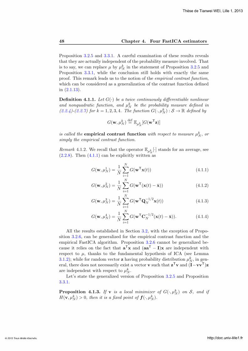
48 Chapter 4. Four FastICA estimators
Proposition 3.2.5 and 3.3.1. A careful examination of these results revealsthat they are actually independent of the probability measure involved. Thatis to say, we can replace µ by µkN in the statement of Proposition 3.2.5 andProposition 3.3.1, while the conclusion still holds with exactly the sameproof. This remark leads us to the notion of the empirical contrast function,which can be considered as a generalization of the contrast function definedin (2.1.13).
Definition 4.1.1. Let G(·) be a twice continuously differentiable nonlinearand nonquadratic function, and µkN be the probability measure defined in(2.2.4)-(2.2.7) for k = 1, 2, 3, 4. The function G(·, µkN ) : S → R defined by
G(w, µkN )def= EµkN [G(wTz)]
is called the empirical contrast function with respect to measure µkN , orsimply the empirical contrast function.
Remark 4.1.2. We recall that the operator EµkN [·] stands for an average, see
(2.2.8). Then (4.1.1) can be explicitly written as
G(w, µ1N ) =
1
N
N∑i=1
G(wTx(t)) (4.1.1)
G(w, µ2N ) =
1
N
N∑i=1
G(wT(x(t)− x)) (4.1.2)
G(w, µ3N ) =
1
N
N∑i=1
G(wTQ−1/2N x(t)) (4.1.3)
G(w, µ4N ) =
1
N
N∑i=1
G(wTC−1/2N (x(t)− x)). (4.1.4)
All the results established in Section 3.2, with the exception of Propo-sition 3.2.6, can be generalized for the empirical contrast function and theempirical FastICA algorithm. Proposition 3.2.6 cannot be generalized be-cause it relies on the fact that aTx and (aaT − I)x are independent withrespect to µ, thanks to the fundamental hypothesis of ICA (see Lemma3.1.2); while for random vector z having probability distribution µkN , in gen-eral, there does not necessarily exist a vector v such that zTv and (I−vvT)zare independent with respect to µkN .
Let’s state the generalized version of Proposition 3.2.5 and Proposition3.3.1.
Proposition 4.1.3. If v is a local minimizer of G(·, µkN ) on S, and ifH(v, µkN ) > 0, then it is a fixed point of f(·, µkN ).
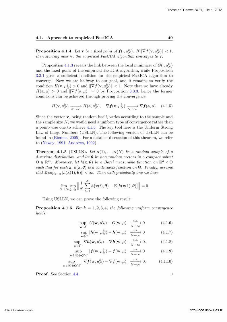
4.1. Approach to empirical FastICA 49
Proposition 4.1.4. Let v be a fixed point of f(·, µkN ). If ‖∇f(v, µkN )‖ < 1,then starting near v, the empirical FastICA algorithm converges to v.
Proposition 4.1.3 reveals the link between the local minimizer of G(·, µkN )and the fixed point of the empirical FastICA algorithm, while Proposition3.3.1 gives a sufficient condition for the empirical FastICA algorithm toconverge. Now we are halfway to our goal, and it remains to verify thecondition H(v, µkN ) > 0 and ‖∇f(v, µkN )‖ < 1. Note that we have alreadyH(a, µ) > 0 and ‖∇f(a, µ)‖ = 0 by Proposition 3.3.3, hence the formerconditions can be achieved through proving the convergence
H(v, µkN ) −−−−→N→∞
H(a, µkN ), ∇f(v, µkN ) −−−−→N→∞
∇f(a, µ). (4.1.5)
Since the vector v, being random itself, varies according to the sample andthe sample size N , we would need a uniform type of convergence rather thana point-wise one to achieve 4.1.5. The key tool here is the Uniform StrongLaw of Large Numbers (USLLN). The following version of USLLN can befound in (Bierens, 2005). For a detailed discussion of this theorem, we referto (Newey, 1991; Andrews, 1992).
Theorem 4.1.5 (USLLN). Let x(1), . . . ,x(N) be a random sample of ad-variate distribution, and let θ be non random vectors in a compact subsetΘ ∈ Rm. Moreover, let h(x,θ) be a Borel measurable function on Rd × Θsuch that for each x, h(x,θ) is a continuous function on Θ. Finally, assumethat E[supθ∈Θ |h(x(1),θ)|] <∞. Then with probability one we have
limN→∞
supθ∈Θ
∥∥∥ 1
N
N∑t=1
h(x(t),θ
)− E
[h(x(1),θ)
]∥∥∥ = 0.
Using USLLN, we can prove the following result:
Proposition 4.1.6. For k = 1, 2, 3, 4, the following uniform convergenceholds:
supw∈S‖G(w, µkN )−G(w, µ)‖ a.s.−−−−→
N→∞0 (4.1.6)
supw∈S‖h(w, µkN )− h(w, µ)‖ a.s.−−−−→
N→∞0 (4.1.7)
supw∈S‖∇h(w, µkN )−∇h(w, µ)‖ a.s.−−−−→
N→∞0. (4.1.8)
supw∈Br(a)∩S
‖f(w, µkN )− f(w, µ)‖ a.s.−−−−→N→∞
0 (4.1.9)
supw∈Br(a)∩S
‖∇f(w, µkN )−∇f(w, µ)‖ a.s.−−−−→N→∞
0. (4.1.10)
Proof. See Section 4.4. 2

50 Chapter 4. Four FastICA estimators
4.2 Local convergence of empirical FastICA algo-rithm
Proposition 4.2.1. For any r > 0, the empirical contrast function G(·, µkN )has a local minimizer in Br(a) ∩ S with probability one for large N .
Proof. First, we note that G(w, µkN ) has a minimizer on the compactBr(a) ∩ S since G(·, µkN ) is a continuous function. Now we prove that thisminimizer is located inside of Br(a) ∩ S.
Since a is the unique local minimizer of G(·, µ) on Br(a) ∩ S, the valueof G(·, µ) on the frontier of Br(a)∩S is strictly larger than G(a, µ). Denote
εdef= inf
w∈S,‖w−a‖=rG(w, µ). By the uniform convergence
supw∈Br(a)∩S
‖G(w, µkN )−G(w, µ)‖ a.s.−−−−→N→∞
0,
we obtain that with probability one, there exists N , such that
supw∈Br(a)∩S
‖G(w, µkN )−G(w, µ)‖ < ε
2.
It follows that
infw∈S,‖w−a‖=r
G(w, µkN ) > G(a, µkN ).
This means that the local minimizer of G(·, µkN ) is inside of Br(a) ∩ S. 2
Lemma 4.2.2. There exists r > 0, such that with probability one there holdsinfw∈Br(a)∩S H(w, µkN ) > 0 for large N .
Proof. First, we note that H(w, ν) = wTh(w, ν) for any w ∈ S. Thenfrom (4.1.7) we deduce immediately
supw∈S‖H(w, µkN )−H(w, µ)‖ a.s.−−−−→
N→∞0. (4.2.1)
Besides, since H(a, µ) > 0 and H(·, µ) is a continuous function, there existsr > 0 such that
infw∈Br(a)∩S
H(w, µkN ) > 0. (4.2.2)
By the triangle inequality, we have H(w, µkN ) ≥ H(w, µ) − |H(w, µ) −H(w, µkN )|. Then it follows that
infw∈Br(a)∩S
H(w, µkN ) ≥ infw∈Br(a)∩S
H(w, µ)− supw∈Br(a)∩S
|H(w, µ)−H(w, µkN )|.
Applying uniform convergence (4.2.1) and bound (4.2.2), we then get theconclusion. 2

4.3. Numerical results 51
Proposition 4.2.3. There exists 0 < K < 1, r > 0 such that with probabil-ity one, we have sup
w∈Br(a)∩S‖∇f(w, µkN )‖ ≤ K for large N .
Proof. Since ‖h(w, µ)‖ > 0 holds in a neighborhood of a, the func-tion f(·, µ) is continuous in this neighborhood. Therefore, by the fact∇f(a, µ) = 0, there exists r > 0 such that in w ∈ Br(a) ∩ S, we have
supw∈Br(a)∩S
‖∇f(w, µ)‖ < K. It follows that
supBr(a)∩S
‖∇f(w, µ4N )‖
≤ supw∈Br(a)∩S
‖∇f(w, µ4N )−∇f(w, µ)‖+ sup
w∈Br(a)∩S‖∇f(w, µ)‖
≤ supw∈Br(a)∩S
‖∇f(w, µ4N )−∇f(w, µ)‖+K.
Then applying (4.1.9) of Proposition 4.1.6, we achieve the proof. 2
Theorem 4.2.4. There exists r > 0 such that if w0 ∈ Br(a)∩S, then withprobability one, the empirical FastICA algorithm with respect to measureµkN converges to a local minimizer akN of the contrast function G(w, µkN ) forlarge N . Moreover, akN is consistent estimator of a.
Proof. By Theorem 4.2.1 and Lemma 4.2.2, we deduce that there exists apositive number r, which can be arbitrarily small, such that with probabilityone G(·, µkN ) has a local minimizer akN in Br(a)∩ S and H(akN , µ
kN ) > 0 for
large N . Then it follows from Proposition 4.1.3 that akN is a fixed point ofthe empirical FastICA function f(·, µkN ). Besides, by Proposition 4.2.3 wehave also ‖∇f(akN , µ
kN )‖ < 1. In view of these facts, applying Proposition
4.1.4, we achieve the convergence of empirical FastICA algorithm. Lastly,the consistency of the estimator akN comes from Theorem 4.2.1. 2
Remark 4.2.5. Theorem 4.2.4 does not say that the limit of empirical Fas-tICA is necessarily a local minimizer of the empirical contrast function,it states only that this event occurs with probability one for large N . Inpractice, especially when the sample size is relatively small, it is possible,although very rare, that FastICA eventually converges to a saddle point ofthe empirical contrast function. Some authors (Tichavsky et al., 2006; Oja& Yuan, 2006) have noticed the fact that the empirical FastICA algorithmsearches the stationary point of the empirical contrast function, but nonehas given a proof.
4.3 Numerical results
In this section, all the settings are the same as in Chapter 2, i.e. we considerthe case d = 2 that the two source signals s1, s2 have respectively Laplace

52 Chapter 4. Four FastICA estimators
N=10 N=100 N=200 N=500 N=1000
kurt, k = 1 1743 204 84 10 1
kurt, k = 2 1443 226 77 7 0
kurt, k = 3 3921 538 40 0 0
kurt, k = 4 3883 571 36 0 0
gaus, k = 1 978 241 58 2 0
gaus, k = 2 1061 229 51 1 0
gaus, k = 3 951 0 0 0 0
gaus, k = 4 732 0 0 0 0
tanh, k = 1 850 827 480 126 11
tanh, k = 2 906 865 539 134 10
tanh, k = 3 203 0 0 0 0
tanh, k = 4 56 0 0 0 0
Table 4.1: Number of failure of convergence among 10000 trials.
and uniform distribution. We take G(x) = x4 and suppose that A = I.Then we have w(θ) = (cos(θ), sin(θ))T, and
θ → G(w(θ), ν) = E[G(cos(θ)s1 + sin(θ)s2)]. (4.3.1)
We recall that A = (e1, e2) and w(0) = e1, w(π/2) = e2, w(π) = −e1,w(3π/2) = −e2.
Example 4.3.1. Fig. 4.1 illustrates a failure of convergence of the empiricalFastICA algorithm. In the simulation, we generate a very small samplewith N = 10, run FastICA with respect to µ1
N for 50 iterations and plot
the quantity εndef= ‖wn+1 − wn‖ versus the iteration times n. Clearly, if
the algorithm converges, we should have εn → 0. The simulation showsthat both cases are possible: depending on the specific sample, the FastICAalgorithm can be either convergent or non-convergent. Fig 4.2 shows a caseof successful convergence under the same settings. In fact, for the case ofN = 10 and kurtosis nonlinearity function, the convergence of empiricalFastICA with respect to µ1
N takes place more than 80% of the times.Tab. 4.1 shows the number of failure of convergence among 10000 inde-
pendent trials. Different sample sizes (from N = 10 to N = 1000), differentnonlinearity functions (“kurtosis”, “Gauss” and “tanh”) and different mea-sures µkN (k = 1, 2, 3, 4) are considered. Numbers in boldface signify thatthey correspond to the lowest failure rate in their category. From the table,we observe that: 1) In most cases, the centering and whitening procedurecan significantly improve the chance of convergence. If the sample size largerthan 500, then the convergence of the algorithm with respect to µ3
N or µ4N is
almost guaranteed for all three nonlinearity functions. The only exceptionis case of kurtosis nonlinearity along with a small sample size (N ≤ 100). In

4.3. Numerical results 53
0 5 10 15 20 25 30 35 40 45 500.2
0.4
0.6
0.8
1
1.2
1.4
1.6
n
||wn+
1 − w
n||
Figure 4.1: FastICA fails to converge.
0 5 10 15 20 25 30 35 40 45 500
0.01
0.02
0.03
0.04
0.05
0.06
0.07
0.08
0.09
0.1
n
||wn+
1 − w
n||
Figure 4.2: FastICA converges successfully.
54 Chapter 4. Four FastICA estimators
this case, the empirical FastICA algorithm with respect to µ1N and µ2
N per-forms better in terms of the convergence possibility; 2) If we consider onlyµ3N and µ4
N , then the kurtosis nonlinearity is the least reliable in terms of theconvergence possibility. To achieve zero failure, “kurtosis” needs a samplesize no less than 500, while “Gauss” and “tanh” require only N = 100. 3) Ifwe have a very large sample size, say N > 1000, then the convergence is nolonger a problem since the chance of convergence failure is less than 0.1%.
0 pi/2 pi 3pi/2 2pi1
2
3
4
5
6
0 ≤ θ < 2π
FastICA w.r.t. µN1
0 pi/2 pi 3pi/2 2pi1
2
3
4
5
6
0 ≤ θ < 2π
FastICA w.r.t. µN2
0 pi/2 pi 3pi/2 2pi1
2
3
4
5
6
0 ≤ θ < 2π
FastICA w.r.t. µN3
0 pi/2 pi 3pi/2 2pi1
2
3
4
5
6
0 ≤ θ < 2π
FastICA w.r.t. µN4
G(w(θ),µ)
G(w(θ),µN1 )
G(w(θ),µ)
G(w(θ),µN2 )
G(w(θ),µ)
G(w(θ),µN3 )
G(w(θ),µ)
G(w(θ),µN4 )
Figure 4.3: The empirical contrast function looks ill-conditioned due tosmall sample size (N = 100). However, empirical FastICA still converges asexpected to a local minimizer of the respective contrast function.
Example 4.3.2. The purpose of this example is to numerically validate The-orem 4.2.4, which states that the FastICA algorithm yields a sequence thatconverges to a local minimizer of the respective contrast function. As what
4.3. Numerical results 55
0 pi/2 pi 3pi/2 2pi0
2
4
6
8
10
0 ≤ θ < 2π
FastICA w.r.t. µN1
0 pi/2 pi 3pi/2 2pi0
2
4
6
8
10
0 ≤ θ < 2π
FastICA w.r.t. µN2
0 pi/2 pi 3pi/2 2pi1
2
3
4
5
6
0 ≤ θ < 2π
FastICA w.r.t. µN3
0 pi/2 pi 3pi/2 2pi1
2
3
4
5
6
0 ≤ θ < 2π
FastICA w.r.t. µN4
G(w(θ),µ)
G(w(θ),µN1 )
G(w(θ),µ)
G(w(θ),µN2 )
G(w(θ),µ)
G(w(θ),µN3 )
G(w(θ),µ)
G(w(θ),µN4 )
Figure 4.4: With moderate sample size (N = 1000), the empirical contrastfunction is relatively well-behaved. In this case, empirical FastICA givesgood estimate.

56 Chapter 4. Four FastICA estimators
we did in Example 3.4.2, we iterated FastICA three times for initial inputw0(θ) = (cos(θ), sin(θ)), with initial angle θ ranging from 0 to 2π. We
recorded the outcome of each iteration, namely wi(θ)def= f(wi−1(θ), µkN ) for
i = 1, 2, 3, and then plotted G(wi(θ), µkN ), using marks “◦”, “+” and “×”,
which correspond respectively to i = 1, 2, 3. In Fig 4.3, we used a small sam-ple with N = 100, which leads to an ill-behaved G(·, µkN ). However, fromthe graph we observe that the empirical FastICA algorithm could still con-verge to a local minimizer of G(·, µkN ). In Fig 4.4, we increased the samplesize to N = 1000. It is easily seen that, with increased sample size, G(·, µkN )is closer to G(·, µkN ) and the empirical FastICA algorithm exhibits betterperformance, especially for k = 3, 4.
Example 4.3.3. In this example, we are interested in the convergence speedof the empirical FastICA algorithm. We refer to Example 3.4.4 for a com-parison with the “theoretical” version of the algorithm. Here, we choose anarbitrary initial point w0(θ) near e2 and run FastICA for 9 iterations. InFig 4.5, we plot ‖wn+1 − akN‖/‖wn − akN‖ for different sample size, name-ly, N = 102, 103 and 104. From the figure, we see that due to finite sizeof the sample, we only have a linear convergence speed since the ratio‖wn+1−akN‖/‖wn−akN‖ remains positive and stable during the entire sim-ulation. Nevertheless, we also notice that the increase of the sample sizeN causes the drop of the ratio towards 0, which is logical for the reasonthat we would have a zero ratio if N = +∞. Lastly, we point out that themagnitude of the ratio ‖wn+1 − e2‖/‖wn − e2‖ in Example 3.4.4 is at thelevel 10−4, whereas here our ‖wn+1 − akN‖/‖wn − akN‖ for N = 104 is ataround 10−2.
4.4 Proof of Proposition 4.1.6
We will only provide the proof of the case k = 1 and k = 4, since the sameapproach applies easily to the case k = 2, 3. The proof will be divided intoseveral parts. First, we will use the USLLN to prove (4.1.6)-(4.1.8) for thecase k = 1, which is the keystone of the whole proof. Next, we will use theseresults to prove (4.1.6)-(4.1.8) for the case k = 4. Finally, we will show that(4.1.9) and (4.1.10) are direct consequences of (4.1.6)-(4.1.8).
4.4.1 Proof of (4.1.6)-(4.1.8) for k = 1.
We begin by proving (4.1.6)-(4.1.8) for the case k = 1. To show the uniformconvergence, it suffices to verify that the functions G(w, µ1
N ), h(w, µ1N ) and
∇h(w, µ1N ) each satisfies the hypothesis of the USLLN. We claim that this
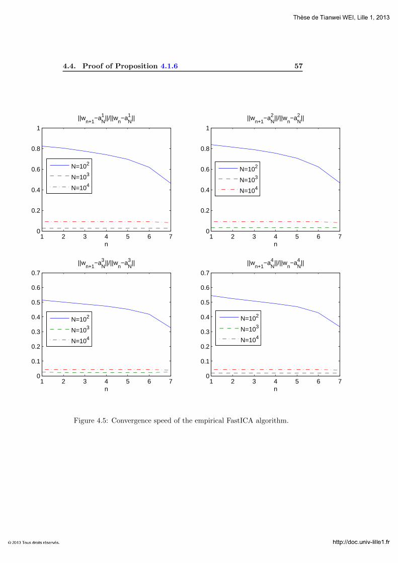
4.4. Proof of Proposition 4.1.6 57
1 2 3 4 5 6 70
0.2
0.4
0.6
0.8
1
||wn+1
−aN1 ||/||w
n−a
N1 ||
n
1 2 3 4 5 6 70
0.2
0.4
0.6
0.8
1
||wn+1
−aN2 ||/||w
n−a
N2 ||
n
1 2 3 4 5 6 70
0.1
0.2
0.3
0.4
0.5
0.6
0.7
||wn+1
−aN3 ||/||w
n−a
N3 ||
n
1 2 3 4 5 6 70
0.1
0.2
0.3
0.4
0.5
0.6
0.7
||wn+1
−aN4 ||/||w
n−a
N4 ||
n
N=102
N=103
N=104
N=102
N=103
N=104
N=102
N=103
N=104
N=102
N=103
N=104
Figure 4.5: Convergence speed of the empirical FastICA algorithm.

58 Chapter 4. Four FastICA estimators
is guaranteed by Assumption 3. In fact, we have
E[
supw∈S|G(wTx)|
]≤ E
[supw∈S
c|wTx|p]≤ cE
[‖x‖p
]<∞,
E[
supw∈S‖g′(wTx)w − g(wTx)x‖
]≤ E
[supw∈S‖g′(wTx)‖‖w‖+ ‖g(wTx)‖‖x‖
]≤ E
[supw∈S
c|wTx|p‖w‖+ c|wTx|p‖x‖]
≤ cE[‖x‖p + ‖x‖p+1
]<∞,
and
E[
supw∈S‖g′′(wTx)wxT + g′(wTx)I− g′(wTx)xxT‖
]≤ E
[supw∈S‖g′′(wTx)‖‖w‖‖x‖+ ‖g′(wTx)‖+ ‖g′(wTx)‖‖x‖2
]≤ cE
[‖x‖p + ‖x‖p+1 + ‖x‖p+2
]<∞.
Then the proof of (4.1.6)-(4.1.8) for the case k = 1 is achieved.
4.4.2 Proof of (4.1.6)-(4.1.8) for k = 4.
Note that we have
supw∈S‖G(w, µ)−G(w, µ4
N )‖
≤ supw∈S
(‖G(w, µ)−G(w, µ1
N )‖+ ‖G(w, µ1N )−G(w, µ4
N )‖)
≤ supw∈S‖G(w, µ)−G(w, µ1
N )‖+ supw∈S‖G(w, µ1
N )−G(w, µ4N )‖.
Hence, for (4.1.6) it suffices to show
supw∈S‖G(w, µ1
N )−G(w, µ4N )‖ a.s.−−−−→
N→∞0. (4.4.1)
Similarly, to prove (4.1.7) and (4.1.8) for the case k = 4, we have to showthat
supw∈S‖h(w, µ1
N )− h(w, µ4N )‖ a.s.−−−−→
N→∞0, (4.4.2)
supw∈S‖∇h(w, µ1
N )−∇h(w, µ4N )‖ a.s.−−−−→
N→∞0. (4.4.3)
To proceed, we need the following result:
Lemma 4.4.1. Let Φ(u, v, w) be a polynomial function of three variablesu, v and w. Then we have the following convergence:
1
N
N∑t=1
Φ(‖x(t)‖, ‖C−1/2N ‖, ‖x‖) a.s.−−−−→
N→∞E[Φ(‖x(1)‖, ‖I‖, 0
)]. (4.4.4)
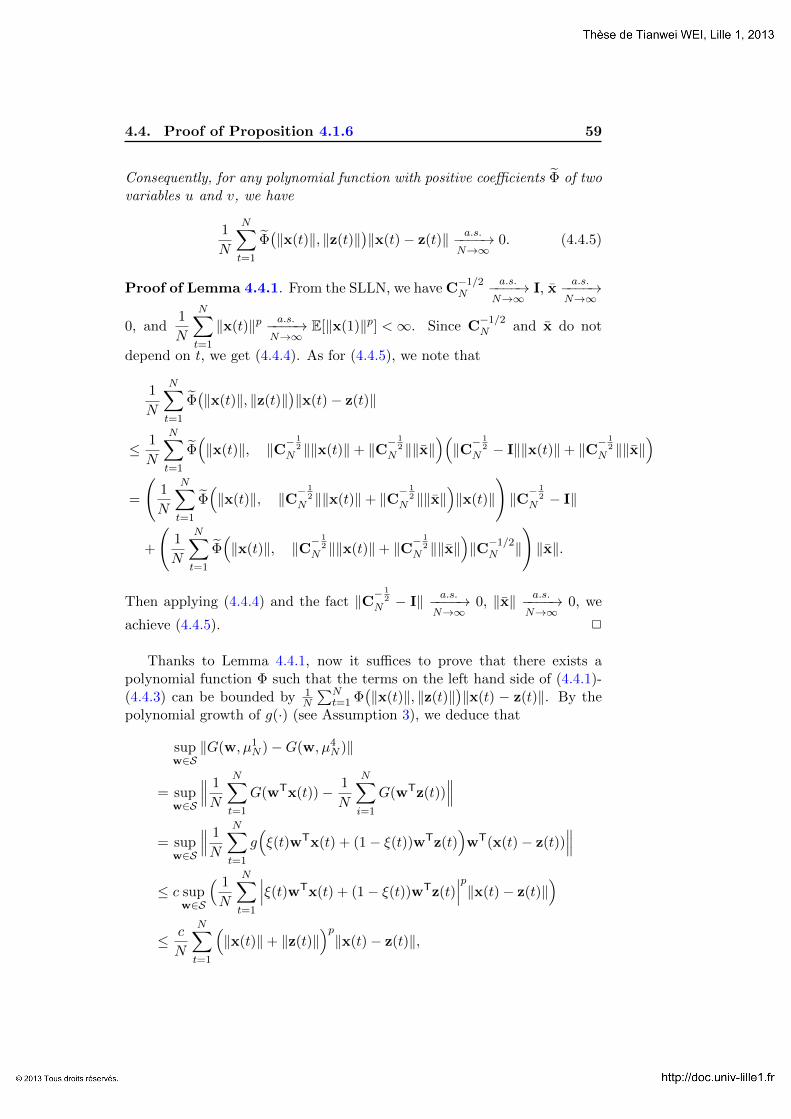
4.4. Proof of Proposition 4.1.6 59
Consequently, for any polynomial function with positive coefficients Φ of twovariables u and v, we have
1
N
N∑t=1
Φ(‖x(t)‖, ‖z(t)‖
)‖x(t)− z(t)‖ a.s.−−−−→
N→∞0. (4.4.5)
Proof of Lemma 4.4.1. From the SLLN, we have C−1/2N
a.s.−−−−→N→∞
I, xa.s.−−−−→
N→∞
0, and1
N
N∑t=1
‖x(t)‖p a.s.−−−−→N→∞
E[‖x(1)‖p] <∞. Since C−1/2N and x do not
depend on t, we get (4.4.4). As for (4.4.5), we note that
1
N
N∑t=1
Φ(‖x(t)‖, ‖z(t)‖
)‖x(t)− z(t)‖
≤ 1
N
N∑t=1
Φ(‖x(t)‖, ‖C−
12
N ‖‖x(t)‖+ ‖C−12
N ‖‖x‖)(‖C−
12
N − I‖‖x(t)‖+ ‖C−12
N ‖‖x‖)
=
(1
N
N∑t=1
Φ(‖x(t)‖, ‖C−
12
N ‖‖x(t)‖+ ‖C−12
N ‖‖x‖)‖x(t)‖
)‖C−
12
N − I‖
+
(1
N
N∑t=1
Φ(‖x(t)‖, ‖C−
12
N ‖‖x(t)‖+ ‖C−12
N ‖‖x‖)‖C−1/2
N ‖
)‖x‖.
Then applying (4.4.4) and the fact ‖C−12
N − I‖ a.s.−−−−→N→∞
0, ‖x‖ a.s.−−−−→N→∞
0, we
achieve (4.4.5). 2
Thanks to Lemma 4.4.1, now it suffices to prove that there exists apolynomial function Φ such that the terms on the left hand side of (4.4.1)-(4.4.3) can be bounded by 1
N
∑Nt=1 Φ
(‖x(t)‖, ‖z(t)‖
)‖x(t) − z(t)‖. By the
polynomial growth of g(·) (see Assumption 3), we deduce that
supw∈S‖G(w, µ1
N )−G(w, µ4N )‖
= supw∈S
∥∥∥ 1
N
N∑t=1
G(wTx(t))− 1
N
N∑i=1
G(wTz(t))∥∥∥
= supw∈S
∥∥∥ 1
N
N∑t=1
g(ξ(t)wTx(t) + (1− ξ(t))wTz(t)
)wT(x(t)− z(t))
∥∥∥≤ c sup
w∈S
( 1
N
N∑t=1
∣∣∣ξ(t)wTx(t) + (1− ξ(t))wTz(t)∣∣∣p‖x(t)− z(t)‖
)≤ c
N
N∑t=1
(‖x(t)‖+ ‖z(t)‖
)p‖x(t)− z(t)‖,

60 Chapter 4. Four FastICA estimators
where ξ(t) is an intermediate value between 0 and 1. Similarly, we have
supw∈S‖h(w, µ1
N )− h(w, µ4N )‖
= supw∈S
∥∥∥ 1
N
N∑t=1
(g′(wTx(t)
)w − g
(wTx(t)
)x(t)
)− 1
N
N∑t=1
(g′(wTz(t)
)w − g
(wTz(t)
)z(t)
)∥∥∥= sup
w∈S
∥∥∥∥ 1
N
N∑t=1
[(g′(wTx(t)
)− g′
(wTz(t)
))w −
(g(wTx(t)
)z(t)− g
(wTz(t)
)z(t)
)−(g(wTx(t)
)x(t)− g
(wTx(t)
)z(t)
)]∥∥∥∥≤ sup
w∈S
[∥∥∥ 1
N
N∑t=1
g′′(ξ1(t)wTx(t) + (1− ξ1(t))wTz(t)
)wT(x(t)− z(t)
)w∥∥∥
+∥∥∥ 1
N
N∑t=1
g′(ξ2(t)wTx(t) + (1− ξ2(t))wTz(t)
)wT(x(t)− z(t)
)z(t)
∥∥∥+∥∥∥ 1
N
N∑t=1
(g(wTx(t))(x(t)− z(t))
)∥∥∥]
≤ 1
N
N∑t=1
(‖x(t)‖+ ‖z(t)‖
)p∥∥x(t)− z(t)∥∥+
1
N
N∑t=1
(‖x(t)‖+ ‖z(t)‖
)p‖z(t)‖∥∥x(t)− z(t)
∥∥+
1
N
N∑t=1
‖x(t)‖p∥∥x(t)− z(t)
∥∥≤ 1
N
N∑t=1
[(‖x(t)‖+ ‖z(t)‖
)p+(‖x(t)‖+ ‖z(t)‖
)p‖z(t)‖+ ‖x(t)‖p]∥∥x(t)− z(t)
∥∥,where in the last line the term in the brackets is a polynomial of ‖x(t)‖ and‖z(t)‖. Using the same approach again, we can show that
supw∈S‖∇h(w, µ1
N )−∇h(w, µ4N )‖
= supw∈S
(∥∥∥ 1
N
N∑t=1
[g′′(wTx(t)
)wx(t)T + g′
(wTx(t)
)I− g′
(wTx(t)
)x(t)x(t)T
]− 1
N
N∑t=1
[g′′(wTz(t)
)wz(t)T + g′
(wTz(t)
)I− g′
(wTz(t)
)x(t)z(t)T
]∥∥∥)
≤ supw∈S
(1
N
N∑t=1
(‖g′′(wTx(t)
)wx(t)T − g′′
(wTz(t)
)wz(t)T‖+ ‖g′
(wTx(t)
)I− g′
(wTz(t)
)I‖

4.4. Proof of Proposition 4.1.6 61
+∥∥g′(wTx(t)
)x(t)x(t)T − g′
(wTz(t)
)z(t)z(t)T
∥∥))
≤ 1
N
N∑t=1
(Φ1(‖x‖, ‖z(t)‖) + Φ2(‖x‖, ‖z(t)‖) + Φ3(‖x‖, ‖z(t)‖)
)‖x(t)− z(t)‖,
where Φi are polynomial functions, i = 1, 2, 3.
4.4.3 Proof of (4.1.9) and (4.1.10)
Let us first introduce the following lemma:
Lemma 4.4.2. Let {yN (·)} be a sequence of functions Rd 7→ Rm, such that
supθ∈Θ‖yN (θ)− y(θ)‖ −−−−→
N→∞0, (4.4.6)
where Θ is a compact subset of Rd and y(·) is a continuous function. LetP : Rm → Rn be a derivable mapping such that ∇P(·) is continuous in theset V = {c : infθ∈Θ ‖c− y(θ)‖ ≤ ε} for some ε > 0. Then we have
supθ∈Θ‖P(yN (θ))− P(y(θ))‖ −−−−→
N→∞0. (4.4.7)
Proof. Let us denote the ith component of P by Pi. It suffices to provethat
supθ∈Θ|Pi(yN (θ))− Pi(y(θ))| −−−−→
N→∞0, i = 1, . . . , n. (4.4.8)
We have
supθ∈Θ|Pi(yN (θ))− Pi(y(θ))|
= supθ∈Θ
∣∣∣∇Pi(cyN (θ) + (1− c)y(θ))(
yN (θ)− y(θ))∣∣∣
≤ supθ∈Θ
∥∥∥∇Pi(cyN (θ) + (1− c)y(θ))∥∥∥× sup
θ∈Θ
∥∥∥yN (θ)− y(θ)∥∥∥.
Denote uN (θ)def= cyN (θ) + (1 − c)y(θ). Then by (4.4.6), we have
supθ∈Θ ‖uN (θ) − y(θ)‖ −−−−→N→∞
0. Then it follows from the continuity of
∇P and the compactness of V that
supθ∈Θ
∥∥∇Pi(uN (θ))∥∥ ≤ sup
u∈V
∥∥∇Pi(u)∥∥ <∞
holds almost surely for large N . Thus we achieved (4.4.8), and (4.4.7)follows. 2

62 Chapter 4. Four FastICA estimators
To prove (4.1.9), let us consider the mapping P1 : Rd → Rd defined by
P1(x)def= x/‖x‖. Clearly, P1 has continuous derivative in Rd/{0}. Besides,
we have f(w, ν) = P1(h(w, ν)) for any measure ν. Note that ‖h(w, µ)‖ 6= 0in Br(a)∩S since h(·, µ) is continuous and ‖h(a, µ)‖ = |H(a, µ)| > 0. Thenby Lemma 4.4.2 and (4.1.7), we get
supw∈Br(a)∩S
‖f(w, µkN )− f(w, µ)‖
= supw∈Br(a)∩S
‖P1(h(w, µkN )
)− P1
(h(w, µ)
)‖ a.s.−−−−→
N→∞0.
As for (4.1.10), we consider the mapping P2 : Rd×Rd×d → Rd×d definedby
P2(x,y)def=
(‖x‖2I− xxT)y
‖x‖3.
Clearly, P2 is continuous in Rd×Rd×d/{0×Rd×d} and it can be consideredas a mapping from Rd2+d to Rd2 . Applying Lemma 4.4.2, we get
supw∈Br(a)∩S
‖∇f(w, µkN )−∇f(w, µ)‖
= supw∈Br(a)∩S
∥∥∥P2(h(w, µkN ),∇h(w, µkN )
)− P2
(h(w, µ),∇h(w, µ)
)∥∥∥ a.s.−−−−→N→∞
0.

Chapter 5
Asymptotic Analysis ofFastICA estimators
Contents
5.1 Statement of the main result . . . . . . . . . . . 63
5.1.1 Related works . . . . . . . . . . . . . . . . . . . . . 65
5.2 Method of Lagrange multipliers . . . . . . . . . . 67
5.2.1 Lagrange function of optimization problem (5.2.2) 68
5.2.2 Lagrange function of optimization problem (5.2.3) 68
5.3 M-estimators . . . . . . . . . . . . . . . . . . . . . 72
5.4 Numerical results . . . . . . . . . . . . . . . . . . 73
5.5 Proofs . . . . . . . . . . . . . . . . . . . . . . . . . 76
5.5.1 Proof of Lemma 5.3.4 . . . . . . . . . . . . . . . . 76
5.5.2 Proof of Theorem 5.1.1 . . . . . . . . . . . . . . . 76
In Chapter 2 we showed that the column a of the mixing matrix A is a
local minimizer of the theoretical contrast function G(w, µ)def= Eµ[G(wTx)]
on S. In Chapter 3 we proposed four estimators G(w, µkN )def= EµkN [G(wTz)]
of the contrast function G(w, µ), and showed that for each k, the empiricalcontrast function G(w, µkN ) has a local minimizer akN near the column a onS. We also proved the consistency of the empirical FastICA estimator byshowing akN → a almost surely as N tends to infinity. These facts suggestthat the empirical FastICA estimator is actually an M-estimator. The aimof this chapter is to use the theory of M-estimator to derive the asymp-totic normality and the asymptotic covariance matrix of our four empiricalFastICA estimators.
5.1 Statement of the main result
We start by announcing the main result of this chapter. The followingnotations are adopted to simplify the formula:
ηidef= E[g(si)]
αidef= E[g(si)si]
ρidef= E[g′(si)]
βidef= E[g(si)
2]
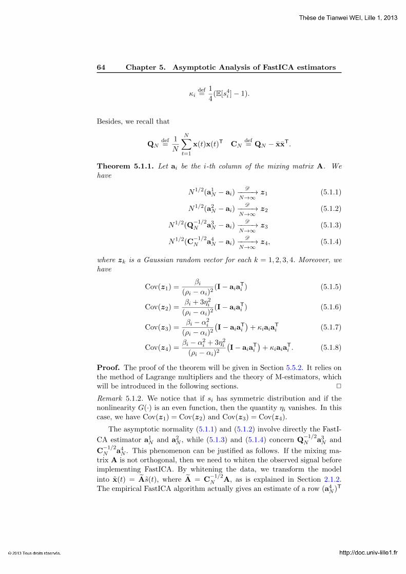
64 Chapter 5. Asymptotic Analysis of FastICA estimators
κidef=
1
4(E[s4
i ]− 1).
Besides, we recall that
QNdef=
1
N
N∑t=1
x(t)x(t)T CNdef= QN − xxT.
Theorem 5.1.1. Let ai be the i-th column of the mixing matrix A. Wehave
N1/2(a1N − ai)
D−−−−→N→∞
z1 (5.1.1)
N1/2(a2N − ai)
D−−−−→N→∞
z2 (5.1.2)
N1/2(Q−1/2N a3
N − ai)D−−−−→
N→∞z3 (5.1.3)
N1/2(C−1/2N a4
N − ai)D−−−−→
N→∞z4, (5.1.4)
where zk is a Gaussian random vector for each k = 1, 2, 3, 4. Moreover, wehave
Cov(z1) =βi
(ρi − αi)2(I− aia
Ti ) (5.1.5)
Cov(z2) =βi + 3η2
i
(ρi − αi)2(I− aia
Ti ) (5.1.6)
Cov(z3) =βi − α2
i
(ρi − αi)2
(I− aia
Ti
)+ κiaia
Ti (5.1.7)
Cov(z4) =βi − α2
i + 3η2i
(ρi − αi)2
(I− aia
Ti
)+ κiaia
Ti . (5.1.8)
Proof. The proof of the theorem will be given in Section 5.5.2. It relies onthe method of Lagrange multipliers and the theory of M-estimators, whichwill be introduced in the following sections. 2
Remark 5.1.2. We notice that if si has symmetric distribution and if thenonlinearity G(·) is an even function, then the quantity ηi vanishes. In thiscase, we have Cov(z1) = Cov(z2) and Cov(z3) = Cov(z4).
The asymptotic normality (5.1.1) and (5.1.2) involve directly the FastI-
CA estimator a1N and a2
N , while (5.1.3) and (5.1.4) concern Q−1/2N a3
N and
C−1/2N a4
N . This phenomenon can be justified as follows. If the mixing ma-trix A is not orthogonal, then we need to whiten the observed signal beforeimplementing FastICA. By whitening the data, we transform the model
into x(t) = As(t), where A = C−1/2N A, as is explained in Section 2.1.2.
The empirical FastICA algorithm actually gives an estimate of a row (a4N )T

5.1. Statement of the main result 65
of A−1 = A−1C1/2N . Hence, to find the corresponding row of the original
demixing matrix A−1, one needs to take (a4N )TC
−1/2N , or C
−1/2N a4
N .The inconvenience of (5.1.5)-(5.1.8) is that they depend on the mixing
matrix A. If we are to propose a performance criterion for the choice ofnonlinearity, it is better to use the gain matrix.
Definition 5.1.3. Let W be an estimate of A−1. The gain matrix G asso-
ciated to W is defined as Gdef= WA.
Let G(k) be the gain matrix of the FastICA estimator with respect to
measure µkN for k = 1, 2, 3, 4 and its (i, j)-entry be denoted by G(k)ij . By
Definition 5.1.3, we have G(k)ij = (akN )Taj for k = 1, 2; G
(3)ij = (a3
N )TQ−1/2N aj
for k = 3 and G(4)ij = (a4
N )TC−1/2N aj for k = 4, where akN is the FastICA
estimator of ai. From Theorem 5.1.1, we get immediately the followingcorollary:
Corollary 5.1.4. Let G(k) be the gain matrix of the FastICA estimator with
respect to measure µkN for k = 1, 2, 3, 4. We denote by G(k)ij the (i, j)-entry
of G(k). For i = 1, . . . , d and j 6= i we have
N1/2G(k)ij
D−−−−→N→∞
N (0, V(k)ij )
where V kij is given by
V(k)ij =
βi(ρi − αi)2
(5.1.9)
V(k)ij =
βi + 3η2i
(ρi − αi)2(5.1.10)
V(k)ij =
βi − α2i
(ρi − αi)2(5.1.11)
V(k)ij =
βi − α2i + 3η2
i
(ρi − αi)2. (5.1.12)
5.1.1 Related works
Several studies (Hyvarinen, 1997; Tichavsky et al., 2006; Shimizu,Hyvarinen, Yutaka, Hoyer, & Kerminen, 2006; Ollila, 2010; Reyhani, Yli-paavalniemi, Vigario, & Oja, 2012) concerning the asymptotic behavior ofFastICA already exist.
The first attempt to calculate the asymptotic covariance matrix of Fas-tICA estimator was due to Hyvarinen (Hyvarinen, 1997). In his paper, hederived the trace of the asymptotic covariance matrix of his FastICA esti-mator:
C(A)βi − α2
i
(ρi − αi)2,
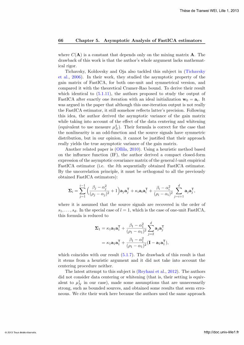
66 Chapter 5. Asymptotic Analysis of FastICA estimators
where C(A) is a constant that depends only on the mixing matrix A. Thedrawback of this work is that the author’s whole argument lacks mathemat-ical rigor.
Tichavsky, Koldovsky and Oja also tackled this subject in (Tichavskyet al., 2006). In their work, they studied the asymptotic property of thegain matrix of FastICA, for both one-unit and symmetrical version, andcompared it with the theoretical Cramer-Rao bound. To derive their resultwhich identical to (5.1.11), the authors proposed to study the output ofFastICA after exactly one iteration with an ideal initialization w0 = ai. Itwas argued in the paper that although this one-iteration output is not reallythe FastICA estimator, it still somehow reflects latter’s precision. Followingthis idea, the author derived the asymptotic variance of the gain matrixwhile taking into account of the effect of the data centering and whitening(equivalent to use measure µ4
N ). Their formula is correct for the case thatthe nonlinearity is an odd-function and the source signals have symmetricdistribution, but in our opinion, it cannot be justified that their approachreally yields the true asymptotic variance of the gain matrix.
Another related paper is (Ollila, 2010). Using a heuristic method basedon the influence function (IF), the author derived a compact closed-formexpression of the asymptotic covariance matrix of the general l-unit empiricalFastICA estimator (i.e. the lth sequentially obtained FastICA estimator.By the uncorrelation principle, it must be orthogonal to all the previouslyobtained FastICA estimators):
Σi =i−1∑j=1
( βj − α2j
(ρj − αj)2+ 1)aja
Tj + κiaia
Ti +
βi − α2i
(ρi − αi)2
d∑j=i+1
ajaTj ,
where it is assumed that the source signals are recovered in the order ofs1, . . . , sd. In the special case of l = 1, which is the case of one-unit FastICA,this formula is reduced to
Σ1 = κ1a1aT1 +
β1 − α21
(ρ1 − α1)2
d∑j=2
ajaTj
= κ1a1aT1 +
β1 − α21
(ρ1 − α1)2(I− a1a
T1 ),
which coincides with our result (5.1.7). The drawback of this result is thatit stems from a heuristic argument and it did not take into account thecentering procedure neither.
The latest attempt to this subject is (Reyhani et al., 2012). The authorsdid not consider data centering or whitening (that is, their setting is equiv-alent to µ1
N in our case), made some assumptions that are unnecessarilystrong, such as bounded sources, and obtained some results that seem erro-neous. We cite their work here because the authors used the same approach

5.2. Method of Lagrange multipliers 67
of M-estimator as is employed in this thesis to establish the asymptoticnormality of the FastICA estimator.
5.2 Method of Lagrange multipliers
In mathematical optimization, the method of Lagrange multipliers providesa strategy for finding the local minima of a function subject to an equal-ity constraints. For a detailed discussion about this subject, we refer to(Luenberger & Ye, 2008; Nesterov, 2004). Consider the optimization prob-lem
minimize Φ(w)
subject to q(w) = 0,
where Φ(w) is a mapping from Rn to R and q(w) is a mapping from Rnto Rm. We are going to recall the necessary condition for a point to belocal minimizer of Φ(·) subject to equality constraint q(·). Before statingthe result, we define the Lagrange function associated to the optimizationproblem:
L (w,λ) = Φ(w) + λTq(w). (5.2.1)
The following theorem is well-known.
Theorem 5.2.1 (First-Order Necessary Conditions). Let w∗ be a local min-imizer of Φ(·) subject to the constraint q(w) = 0. Assume further that w∗
is a regular point, i.e.
∇q(w∗) 6= 0.
Then there exists λ∗ ∈ Rm called Lagrange multiplier such that (w∗,λ∗) is astationary point of the Lagrange function (5.2.1). More precisely, the couple(w∗,λ∗) satisfies
∂wL (w∗,λ∗) = 0
∂λL (w∗,λ∗) = 0.
Let us apply this theorem to the optimization of our contrast functions:
a = argminw∈Br(a)∩S
G(w, µ), (5.2.2)
akN = argminw∈Br(a)∩S
G(w, µkN ). (5.2.3)

68 Chapter 5. Asymptotic Analysis of FastICA estimators
5.2.1 Lagrange function of optimization problem (5.2.2)
Here, Φ(w) = G(w, µ) and q(w) = ‖w‖2 − 1. The Lagrange function isgiven by
L (w, λ) = G(w, µ) + λ(‖w‖2 − 1).
By Theorem 5.2.1, we get the following first order condition:
Lemma 5.2.2. There exists λa such that (a, λa) is a solution of the equation
E[ψ1(x,θ)] = 0, where θdef= (w, λ) and
ψ1(x,θ)def=
[g(wTx
)x + 2λw
‖w‖2 − 1
]. (5.2.4)
Proof. We recall that G(w, µ) = E[G(wTx)]. Then we have the first ordercondition
E[g(aTx)x] + 2λaa = 0 (5.2.5)
‖a‖2 − 1 = 0.
Multiplying aT from left in (5.2.5), we obtain
λa = −1
2E[g(aTx
)aTx].
2
5.2.2 Lagrange function of optimization problem (5.2.3)
Lagrange function for the case k = 1.This case is similar to (5.2.2). We have
a1N = argmin
w∈Br(a)∩SG(w, µ1
N ) = argminw∈Br(a)∩S
1
N
N∑t=1
G(wTx(t)).
Then we can deduce immediately the Lagrange function:
L1(w, λ) =1
N
N∑t=1
G(wTx(t)) + λ(‖w‖2 − 1).
Using the same proof as that of Lemma 5.2.2, we get the following result.
Lemma 5.2.3. There exists λ1N such that θ1
N = (a1N , λ
1N ) is a solution of
the equation1
N
N∑t=1
ψ1(x,θ) = 0, where ψ1(x,θ) is defined in (5.2.4) and
λ1N = − 1
2N
N∑t=1
g(
(a1N )Tx(t)
)(a1N )Tx(t).

5.2. Method of Lagrange multipliers 69
Lagrange function for the case k = 2.We have
a2N = argmin
w∈Br(a)∩SG(w, µ2
N ) = argminw∈Br(a)∩S
1
N
N∑t=1
G(wT(x(t)− x)).(5.2.6)
Here, Φ(w) = G(w, µ2N ) and q(w) = ‖w‖2−1. However, we prefer to intro-
duce the auxiliary constraint x = m, and write the optimization problem inthe following equivalent form:
minimize Φ(w,m) =1
N
N∑t=1
G(wT(x(t)−m)
)(5.2.7)
subject to q(w,m) =
[‖w‖2 − 1x−m
]= 0.
The reason for this will be explained in the next section. Now, the corre-sponding Lagrange function is given by
L2(w,m, λ,k)def=
1
N
N∑t=1
G(wT(x(t)−m)) + λ(‖w‖2 − 1
)+ kT(x−m).
(5.2.8)
Lemma 5.2.4. There exist m2N , λ
2N and k2
N such that θ2N
def=
(a2N ,m
2N , λ
2N ,k
2N ) is a solution of the system
1
N
N∑t=1
ψ2(x,θ) = 0, where
θ = (w,m, λ,k) and
ψ2(x,θ)def=
g(wT(x−m)
)(x−m) + 2λw
g(wT(x−m)
)w + k
‖w‖2 − 1x−m
.
Moreover, we have explicitly m2N = x and
λ2N = − 1
2N
N∑t=1
g(
(a2N )T(x(t)− x)
)(a2N )T(x(t)− x) (5.2.9)
k2N = − 1
N
N∑t=1
g(
(a2N )T(x(t)− x)
)a2N (5.2.10)
Proof. Since (a2N , x) is a solution of the optimization problem (5.2.7), it
follows from Theorem 5.2.1 the existence of λ2N and k2
N . Now it remains to

70 Chapter 5. Asymptotic Analysis of FastICA estimators
prove (5.2.9) and (5.2.10). Note that1
N
N∑t=1
ψ2(x,θ) = 0 is equivalent to
1
N
N∑t=1
g(wT(x(t)−m)
)(x−m) + 2λw = 0, (5.2.11)
1
N
N∑t=1
g(wT(x(t)−m)
)w + k = 0, (5.2.12)
‖w‖2 − 1 = 0,
x−m = 0.
In (5.2.11), multiplying wT on the left and substituting (w,m) by (a2N , x),
we obtain (5.2.9) and (5.2.10) follows directly from (5.2.12). 2
Lagrange function for the case k = 3.We have
a3N = argmin
w∈Br(a)∩SG(w, µ3
N ) = argminw∈Br(a)∩S
1
N
N∑t=1
G(wTQ
−1/2N x(t)
).
Here, Φ(w) = G(w, µ2N ) and q(w) = ‖w‖2− 1. However, we prefer to write
a3N = Q
1/2N
(argmin
wTQ1/2N ∈Br(a)∩S
1
N
N∑t=1
G(wTx(t)
))and study
b3N
def= argmin
wTQ1/2N ∈Br(a)∩S
1
N
N∑t=1
G(wTx(t)
)(5.2.13)
for reasons that will be given in the next section. We note that b3N =
Q−1/2N a3
N and the constraint appeared in (5.2.13) has the following equivalentform:
{w : wTQ1/2N ∈ S} = {w : wTQNw = 1}
It follows that the Lagrange function is given by
L3(w, λ)def=
1
N
N∑t=1
G(wTx(t)) + λ(wTQNw − 1
).
Using the same proof as that of Lemma 5.2.2, we get the following result.
5.2. Method of Lagrange multipliers 71
Lemma 5.2.5. There exists λ3N such that (b3
N , λ3N ) is a solution of the
equation1
N
N∑t=1
ψ3(x,θ) = 0, where θ = (w, λ) and
ψ3(x,θ)def=
[g(wTx)x + 2λxxTw
(wTx)2 − 1
].
Moreover, we have explicitly
λ3N = − 1
2N
N∑t=1
g(
(b3N )Tx(t)
)(b3
N )Tx(t).
Lagrange function for the case k = 4.We have
a4N = argmin
w∈Br(a)∩SG(w, µkN )
= argminw∈Br(a)∩S
1
N
N∑t=1
G(wTC
−1/2N (x(t)− x)
). (5.2.14)
For reasons that will be given in the next section, we prefer to write
a4N = C
1/2N
(argmin
wTC1/2N ∈Br(a)∩S
1
N
N∑t=1
G(wT(x(t)− x)
))(5.2.15)
and study
b4N
def= argmin
wTC1/2N ∈Br(a)∩S
1
N
N∑t=1
G(wT(x(t)− x)
). (5.2.16)
Then by (5.2.15) we have b4N = C
−1/2N akN . We note that the constraint
appeared in (5.2.16) has the following equivalent form:
{w : wTC1/2N ∈ S} = {w : wTCNw = 1}
= {w : wTQNw − (wTx)2 = 1}. (5.2.17)
Introducing the auxiliary constraint x = m, and in view of (5.2.17), we canwrite the optimization problem (5.2.16) in the following form:
minimize Φ(w,m) =1
N
N∑t=1
G(wT(x(t)−m)
)subject to q(w,m) =
[wTQNw − (wTm)2 − 1
x−m
]= 0.
72 Chapter 5. Asymptotic Analysis of FastICA estimators
It follows that the corresponding Lagrange function is given by
L4(w,m, λ,k)def=
1
N
N∑t=1
G(wT(x(t)−m)) + λ(wTQNw − (wTm)2 − 1
)+kT(x−m). (5.2.18)
Using the same proof as that of Lemma 5.2.4, we get the following result.
Lemma 5.2.6. There exist m4N , λ
4N and k4
N such that θ4N
def=
(b4N ,m
4N , λ
4N ,k
4N ) is a solution of the equation
1
N
N∑t=1
ψ4(x,θ) = 0, where
θ = (w,m, λ,k) and
ψ4(x,θ)def=
g(wT(x−m)
)(x−m) + 2λxxTw − 2λ(wTm)m,
(wTx)2 − (wTm)2 − 1,x−m,
−g(wT(x−m)
)w − 2λ(wTm)w − k.
.Moreover, we have explicitly m4
N = x and
λ4N = − 1
2N
N∑t=1
g(
(b4N )T(x(t)−mN )
)(b4
N )T(x(t)−mN )
k4N = − 1
N
N∑t=1
g(
(b4N )T(x(t)−mN )
)b4N − 2λ4
N ((b4N )TmN )b4
N ,
5.3 M-estimators
Definition 5.3.1. Let ψ : Rd × Rm 7→ Rn be a measurable function. Asolution θN of the equation
N∑t=1
ψ(x(t),θ) = 0 (5.3.1)
is called M-estimator.
We note that∑N
t=1ψ(x(t),θ) is an empirical approximation ofE[ψ(x(t),θ)] for all θ. Therefore, intuitively, under appropriate conditionsthe M-estimator θN obtained by solving (5.3.1) should converge to θ0, whichis a root of the equation E[ψ(x(t),θ)] = 0. This is indeed true. For a de-tailed discussion of this subject, we refer to (van der Vaart, 2000). Now thatθN → θ0, we are interested in the order at which the discrepancy θN − θ0
converges to zero. Regarding this problem, we have the following result:

5.4. Numerical results 73
Theorem 5.3.2. For each θ in an open set of Euclidean space, let x →ψ(x,θ) be a measurable vector valued function such that, for every θ1 and θ2
in a neighborhood of θ0 and a measurable function K(·) with E[K(x)2] <∞,
‖ψ(x,θ1)−ψ(x,θ2)‖ ≤ K(x)‖θ1 − θ2‖.
Assume that E[‖ψ(x,θ0)‖2] <∞ and that the map θ → E[ψ(x,θ)] is differ-
entiable at a zero θ0, with nonsingular derivative matrix Vθ0. If θNP−→ θ0,
then
√N(θN − θ0)
D−−−−→N→∞
Z,
where Z is the solution of the system Vθ0Z = Y with Y ∼N (0,E[ψ(x,θ0)ψ(x,θ0)T]).
In order to apply the theorem, we need to find the function ψ associ-ated to the optimization problem (5.2.3) for k = 1, 2, 3, 4, such that the
corresponding zero satisfies θNP−→ θ0.
Proposition 5.3.3. Let ψk(x,θ) and θkN be defined in Lemma 5.2.2, 5.2.4,5.2.5, and 5.2.6 for k = 1, 2, 3, 4.
(i). θkNa.s.−−−−→
N→∞(a, λa) for k = 1, 3,
(ii). θkNa.s.−−−−→
N→∞(a,ma, λa,ka) for k = 2, 4,
where ma = 0, λa = −12E[g(aTx)aTx] and ka = −E[g(aTx)a].
Proof. It suffices to use the same argument as in Lemma 4.2.4. 2
Lemma 5.3.4. There exists a neighborhood Br(θa) of θa, and a measurablefunction K(x) with E[K(x)2] < ∞ such that for any θ1,θ2 ∈ Br(θa), wehave
‖ψ(x,θ1)−ψ(x,θ2)‖ ≤ K(x)‖θ1 − θ2‖.
Proof. See Appendix.
5.4 Numerical results
Example 5.4.1. The purpose of this example is to compare the theoreticalvalue of Trace(Cov(zk)) with its finite sample estimate. Our simulation isimplemented as follows. We take a sample of size N = 1000 × 2l, withl = 1, . . . , 7 corresponding to the horizonal axis in the figure. For each l,we run empirical FastICA to obtain the estimator akN , and then calculate
εdef= N‖akN − a‖2. We repeat this procedure independently 100 times, and

74 Chapter 5. Asymptotic Analysis of FastICA estimators
1 2 3 4 5 6 70
5
10
15
20LAPLACE DISTRIBUTION, CRITERION 1
SAMPLE SIZE
ME
AN
SQ
UA
RE
ER
RO
R
kurtosisGausstanh
(a)
1 2 3 4 5 6 720
30
40
50UNIFORM DISTRIBUTION, CRITERION 1
tanh
1 2 3 4 5 6 72
4
6
8
SAMPLE SIZE
kurtosisGauss
(b)
1 2 3 4 5 6 75
6
7
8LAPLACE DISTRIBUTION, CRITERION 3
kurtosis, Esti. on the spherekurtosis, Esti. on the ellipse
1 2 3 4 5 6 72
3
4
ME
AN
SQ
UA
RE
ER
RO
R
Gauss, Esti. on the sphereGauss, Esti. on the ellipse
1 2 3 4 5 6 72
3
4
SAMPLE SIZE
tanh, Esti. on the spheretanh, Esti. on the ellipse
(c)
1 2 3 4 5 6 7
0.7
0.8
0.9
1UNIFORM DISTRIBUTION, CRITERION 3
kurtosis, Esti. on the spherekurtosis, Esti. on the ellipse
1 2 3 4 5 6 70.9
1
1.1
1.2
Gauss, Esti. on the sphereGauss, Esti. on the ellipse
1 2 3 4 5 6 70.8
1
1.2
1.4
SAMPLE SIZE
tanh, Esti. on the spheretanh, Esti. on the ellipse
(d)
Figure 5.1: Mean square errors of E[N‖a1N − a‖2], E[N‖a3
N − a‖2],
E[N‖Q−1/2N a3
N − a‖2] versus the sample size N = 1000× 2n.
take εdef= 1
100
∑100t=1 ε(t) as the estimate of the Trace(Cov(zk)). Letting l vary
from 1 to 7, we then get a zigzag representing the finite sample estimate ofTrace(Cov(zk)). Our result, a zigzag and a straight line (representing thetheoretical value of Trace(Cov(zk))) is plotted in Fig. 5.1, where (a)-(d)each corresponds to a different case.
Figure (a) corresponds to the extraction of a Laplace source signal usingµ1N with three different nonlinearity functions, namely “kurtosis”, “Gauss”
and “tanh”. From the figure, we observe that all three zigzags, each corre-sponding to a different nonlinearity function, coincide well with the respec-tive straight lines. Figure (b) is the same as Figure (a) except for the uniformsource signal. In Figure (c) and (d), we tackle the distribution µ3
N . Although
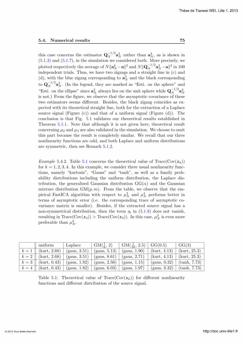
5.4. Numerical results 75
this case concerns the estimator Q−1/2N a3
N rather than a3N , as is shown in
(5.1.3) and (5.1.7), in the simulation we considered both. More precisely, we
plotted respectively the average of N‖akN−a‖2 and N‖Q−1/2N a3
N−a‖2 in 100independent trials. Thus, we have two zigzags and a straight line in (c) and(d), with the blue zigzag corresponding to a3
N and the black corresponding
to Q−1/2N a3
N . (In the legend, they are marked as “Esti. on the sphere” and
“Esti. on the ellipse” since a3N always lies on the unit sphere while Q
−1/2N a3
N
is not.) From the figure, we observe that the asymptotic covariance of thesetwo estimators seems different. Besides, the black zigzag coincides as ex-pected with its theoretical straight line, both for the extraction of a Laplacesource signal (Figure (c)) and that of a uniform signal (Figure (d)). Theconclusion is that Fig. 5.1 validates our theoretical results established inTheorem 5.1.1. Note that although it is not given here, theoretical resultconcerning µ2 and µ4 are also validated in the simulation. We choose to omitthis part because the result is completely similar. We recall that our threenonlinearity functions are odd, and both Laplace and uniform distributionsare symmetric, then see Remark 5.1.2.
Example 5.4.2. Table 5.1 concerns the theoretical value of Trace(Cov(zk))for k = 1, 2, 3, 4. In this example, we consider three usual nonlinearity func-tions, namely “kurtosis”, “Gauss” and “tanh”, as well as a family prob-ability distributions including the uniform distribution, the Laplace dis-tribution, the generalized Gaussian distribution GG(α) and the Gaussianmixture distribution GM(p,m). From the table, we observe that the em-pirical FastICA algorithm with respect to µ3
N and µ4N performs better in
terms of asymptotic error (i.e. the corresponding trace of asymptotic co-variance matrix is smaller). Besides, if the extracted source signal has anon-symmetrical distribution, then the term ηi in (5.1.8) does not vanish,resulting in Trace(Cov(z4)) > Trace(Cov(z3)). In this case, µ3
N is even morepreferable than µ4
N .
uniform Laplace GM(16 , 2) GM( 1
10 , 2.5) GG(0.5) GG(3)
k = 1 (kurt, 2.68) (gaus, 3.51) (gaus, 5.13) (gaus, 1.90) (kurt, 4.13) (kurt, 25.3)
k = 2 (kurt, 2.68) (gaus, 3.51) (gaus, 8.61) (gaus, 2.71) (kurt, 4.13) (kurt, 25.3)
k = 3 (kurt, 0.43) (gaus, 1.82) (gaus, 2.56) (gaus, 1.15) (gaus, 0.32) (tanh, 7.73)
k = 4 (kurt, 0.43) (gaus, 1.82) (gaus, 6.03) (gaus, 1.97) (gaus, 0.32) (tanh, 7.73)
Table 5.1: Theoretical value of Trace(Cov(zk)) for different nonlinearityfunctions and different distribution of the source signal.

76 Chapter 5. Asymptotic Analysis of FastICA estimators
5.5 Proofs
5.5.1 Proof of Lemma 5.3.4
We recall that
ψ(x,θ) =
g(wT(x−m)
)(x−m) + 2λxxTw − 2λ(wTm)m
−g(wT(x−m)
)w − 2λ(wTm)w − k
(wTx)2 − (wTm)2 − 1x−m
.By Assumption 3, the function g has continuous derivative and satisfiesg(t) ≤ c|t|p. It follows that
ψ(x,θ1)−ψ(x,θ2) = ∂θψ(x, ξ)(θ1 − θ2), (5.5.1)
where each component of the matrix ∂θψ(x, ξ) can be bounded by a poly-nomial of ‖x‖ and ‖ξ‖. Since ξ is an intermediate point between θ1 and θ2,which belongs to the compact Br(θ0), we can find a polynomial functionK(·) such that
‖∂θψ(x, ξ)‖ ≤ K(x)
and E[K(x)2] < +∞. Hence, we deduce from (5.5.1) that
‖ψ(x,θ1)−ψ(x,θ2)‖ ≤ K(x)‖θ1 − θ2‖.
5.5.2 Proof of Theorem 5.1.1
Here we give only the proof for the case k = 4 since it is the most complicatedcase, and the same method applies to the cases k = 1, 2, 3. In the sequel, tosimplify the notation, we will omit the superscript of ψ4 and write ψ(x,θ)instead. Besides, we denote θ = (θ1,θ2,θ3,θ4) = (w,m, λ,k),
ψ(x,θ) =
ψ1(x,θ)ψ2(x,θ)ψ3(x,θ)ψ4(x,θ)
=
g(wT(x−m)
)(x−m) + 2λxxTw − 2λ(wTm)m
−g(wT(x−m)
)w − 2λ(wTm)w − k
(wTx)2 − (wTm)2 − 1x−m
.and
∂θψ(x,θ)def=
ψ11 ψ12 ψ13 ψ14
ψ21 ψ22 ψ23 ψ24
ψ31 ψ32 ψ33 ψ34
ψ41 ψ42 ψ43 ψ44
,where ψij
def= ∂θj
ψi.
5.5. Proofs 77
From Proposition 5.3.3 and Lemma 5.3.4, we see that the hypotheses ofTheorem 5.3.2 are satisfied for θN ,θa and ψ. Applying Theorem 5.3.2, weget the following asymptotic result:
√N(θN − θa)
D−−−−→N→∞
Z, (5.5.2)
where Z is such that
E[∂θψ(x,θa)]Z = Y (5.5.3)
with Y ∼ N (0,E[ψ(x,θa)ψ(x,θa)T]). Let us denote
P = E[∂θψ(x,θa)] =
P11 P12 P13 P14
P21 P22 P23 P24
P31 P32 P33 P34
P41 P42 P43 P44
, Z =
zazmzλzk
Y =
yaymyλyk
.Then system (5.5.3) can be written as
ya = P11za + P12zm + P13zλ + P14zk,
ym = P21za + P22zm + P23zλ + P24zk,
yλ = P31za + P32zm + P33zλ + P34zk,
yk = P41za + P42zm + P43zλ + P44zk.
Note that we are only interested in za. In what follows, we will computethe explicit form of za and deduce its covariance matrix.
Step 1. In the first step, we will compute the matrix E[∂θψ(x,θa)] andE[ψ(x,θa)ψ(x,θa)T] explicitly. Let us denote
R = E[ψ(x,θa)ψ(x,θa)T] =
R11 R12 R13 R14
R21 R22 R23 R24
R31 R32 R33 R34
R41 R42 R43 R44
.Since P,R and ∂θψ(x,θ) are all symmetric matrices, it suffices to calculatetheir upper triangular elements. We have
ψ11 = g′(wT(x−m)
)(x−m)(x−m)T + 2λ(xxT −mmT),
ψ12 = −g′(wT(x−m))(x−m)wT − g(wT(x−m))I− 2(λmwT + (wTm)I
),
ψ13 = 2(wTx)x− 2(wTm)m,
ψ14 = 0,
ψ22 =(g′(wT(x−m))− 2λ
)wwT,
ψ23 = −2(wTm)wT
ψ24 = −I,
ψ33 = 0,
ψ34 = 0,
ψ44 = 0.

78 Chapter 5. Asymptotic Analysis of FastICA estimators
Hence
P11 = E[(g′(aTx) + 2λa
)xxT
], (5.5.4)
P12 = −E[g′(aTx)xaT]− E[g(aTx)]I, (5.5.5)
P13 = 2a, (5.5.6)
P14 = 0, (5.5.7)
P22 = E[g′(aTx)− 2λa]aaT, (5.5.8)
P23 = 0, (5.5.9)
P24 = −I, (5.5.10)
P33 = 0, (5.5.11)
P34 = 0, (5.5.12)
P44 = 0, (5.5.13)
(5.5.14)
To calculate R, we first notice that
ψ(x,θa) =
−g(aTx)a− ka(
g(aTx) + 2λa(aTx))x
(aTx)2 − 1x
.Then we have
R11 = E[(g(aTx) + 2λa(aTx)
)2xxT
], (5.5.15)
R12 = −E[(g(aTx) + 2λa(aTx)
)(g(aTx)aT + kT
a )], (5.5.16)
R13 = E[(g(aTx) + 2λa(aTx)
)((aTx)2 − 1)x
], (5.5.17)
R14 = E[(g(aTx) + 2λa(aTx)
)xxT
], (5.5.18)
R22 = E[(g(aTx)a + ka)(g(aTx)aT + kTa )],
R23 = −E[((aTx)2 − 1)(g(aTx)aT + kT
a )], (5.5.19)
R24 = −E[(g(aTx)xaT + xkTa )],
R33 = E[((aTx)2 − 1)2
], (5.5.20)
R34 = E[((aTx)2 − 1)xT
], (5.5.21)
R44 = I. (5.5.22)
Step 2. Let us denote
Z =
zazmzλzk
and Y =
yaymyλyk
.

5.5. Proofs 79
The first line of the system PZ = Y gives
ya = P11za + P12zm + P13zλ + P14zα
= E[(g′(aTx) + 2λ
)xxT
]za − E[g′(aTx)xaT + g(aTx)I]zm + 2azλ.
Multiplying both sides of the equation above by (I− aaT) gives
(I− aaT)ya = E[(g′(aTx) + 2λa
)(I− aaT)xxT
]za + 2(I− aaT)azλ
−E[g′(aTx)(I− aaT)xaT + g(aTx)(I− aaT)]zm
= E[(g′(aTx)− g(aTx)aTx
)](I− aaT)za
−E[g(aTx)(I− aaT)]zm,
or equivalently
(I− aaT)yaE[(g′(aTx)− g(aTx)aTx
)]= (I− aaT)za −
E[g(aTx)(I− aaT)]
E[(g′(aTx)− g(aTx)aTx
)]zm. (5.5.23)
Besides, by (5.5.5)-(5.5.12) we have
ym = P21za + P22zm + P23zλ + P24zk = 2aTza, (5.5.24)
yλ = P31za + P32zm + P33zλ + P34zk = −zm,
among which (5.5.24) implies ayλ/2 = aaTza.Using these results to (5.5.23) gives
za =(I− aaT)ya
E[(g′(aTx)− g(aTx)aTx
)] +ayλ
2+
E[g(aTx)](I− aaT)ykE[(g′(aTx)− g(aTx)aTx
)] .Step 3. In the last step, we will use the fact that Cov(Y) = R to
compute Cov(za). Note that H(a, µ) = E[g′(aTx) − g(aTx)aTx
]. Now for
simplicity we write
za = c1(I− aaT)ya + c3ayλ + c4(I− aaT)yk,
where
c1 =1
H(a, µ), c3 =
1
2, c4 =
E[g(aTx)]
H(a, µ).
We notice that (5.5.2) yields Cov(Y) = R. Thus
Cov(za) = c21(I− aaT)R11(I− aaT) + c2
3aR33aT + c2
4(I− aaT)R44(I− aaT)
+c1c3(I− aaT)R13aT + c1c3aR31(I− aaT) + c1c4(I− aaT)R14(I− aaT)
+c1c4(I− aaT)R41(I− aaT) + c3c4aR34(I− aaT) + c3c4(I− aaT)R34aT.

80 Chapter 5. Asymptotic Analysis of FastICA estimators
Using (5.5.15)-(5.5.20), we deduce that
(I− aaT)R11(I− aaT) = E[(g(aTx) + 2λa(aTx)
)2](I− aaT)
=(E[(g(aTx)
)2]− (E[g(aTx)aTx])2)
(I− aaT),
aR33aT = Cov
((aTx)2
)(aaT),
(I− aaT)R44(I− aaT) = I− aaT,
(I− aaT)R13aT = 0,
(I− aaT)R14(I− aaT) = E[g(aTx)
](I− aaT),
aR34(I− aaT) = 0.
It follows that
Cov(z4) =E[(g(aTx)
)2]− (E[g(aTx)aTx])2
+ 3(E[g(aTx)]
)2
(E[(g′(aTx)− g(aTx)aTx
)])2 (I− aaT)
+Cov
((aTx)2
)4
(aaT). (5.5.25)
2

Chapter 6
Asymptotic Analysis of theGradient of the FastICA
Function
Contents
6.1 Statement of the main result . . . . . . . . . . . 81
6.2 Numerical results . . . . . . . . . . . . . . . . . . 82
6.3 Proofs . . . . . . . . . . . . . . . . . . . . . . . . . 83
6.3.1 Proof of Proposition 6.1.1 . . . . . . . . . . . . . . 83
6.3.2 Proof of Corollary 6.1.3 . . . . . . . . . . . . . . . 86
In Chapter 3 (see e.g. Example 4.3.3), we have shown that although thetheoretical FastICA converges with a quadratic convergence speed, the con-vergence speed of empirical FastICA is only linear. Clearly, the convergencespeed, characterized by limn→∞ ‖wn+1 − akN‖/‖wn − akN‖, depends on thegradient∇f(akN , µ
kN ) which is close to∇f(a, µkN ) for large N . Thus to study
the convergence speed, it is better to focus on ∇f(a, µkN ) since it is moreanalytically trackable than ∇f(akN , µ
kN ). A new criterion of optimality of
the nonlinearity function, suggested by Hyvarinen to us, is to optimize theasymptotic covariance matrix of N1/2∇f(a, µkN ), such that one can attainthe fastest possible convergence speed of FastICA.
In this chapter, we will derive the explicit form of the latter asymptoticcovariance matrix for k = 1 and give some numerical example for the two-dimensional case.
6.1 Statement of the main result
In the sequel, for simplicity we suppose that the mixing matrix A of model3.1.1 is the identity matrix, and we are interested in the extraction of thesource signal s1, which in turn corresponds to the estimation of the first col-umn of A, namely, e1. Before announcing our main result, let us introducesome notations. We denote by vec(·) the operation that reshapes columnsof a matrix in one long column vector. For a random matrix M, we write
Cov(M)def= Cov(vec(M)). Besides, we define
h(w)def= g′(wTs)w − g(wTs)s.

82Chapter 6. Asymptotic Analysis of the Gradient of the FastICA
Function
We denote by hi the ith component of the random vector h(e1), and by∇hijthe ijth component of the matrix ∇h(e1). Now we are ready to announcethe main result of the chapter:
Proposition 6.1.1. We have
√N∇f(e1, µ
1N )
D−−−−→N→∞
N (0,Σ),
where
Σ =1
|H(e1, µ)|4Cov
(− ‖∇h(e1, µ)‖
d∑i=2
hi vec(eieT1 )
+|H(e1, µ)|d∑
i=2,j=1
∇hij vec(eieTj )), (6.1.1)
and we recall that
H(e1, µ) = E[g′(s1)− g(s1)s1],
‖∇h(e1, µ)‖ = |E[s1g′′(s1) + (1− s2
1)g′(s1)]|.
Remark 6.1.2. The asymptotic covariance matrix Σ of ∇f(e1, µ1N ) depends
not only on the probability distribution of s1, but also on the probabilitydistribution of the rest source signals, according to (6.1.1).
In the 2-dimensional case, formula (6.1.1) can be significantly simplified.We can easily derive the following corollary:
Corollary 6.1.3. In the case d = 2, we have
Trace(Σ)=1
|H(e1, µ)|4(‖H(e1, µ)‖2Cov(∇h22) + Cov
(|H(e1, µ)|∇h21
−‖∇h(e1, µ)‖h2
)),
where
Cov(h2) = E[g2(s1)]
Cov(h2,∇h21) = E[s1g(s1)g′(s1)]
Cov(∇h21) = E[(s1g′(s1))2]
Cov(∇h22) = E[(g′(s1))2]E[s42 − 1].
6.2 Numerical results
Example 6.2.1. We consider the extraction of s1 from a mixture of two sourcesignals s1, s2 that have probability distributions including the uniform dis-tribution, the Laplace distribution, the generalized Gaussian distribution
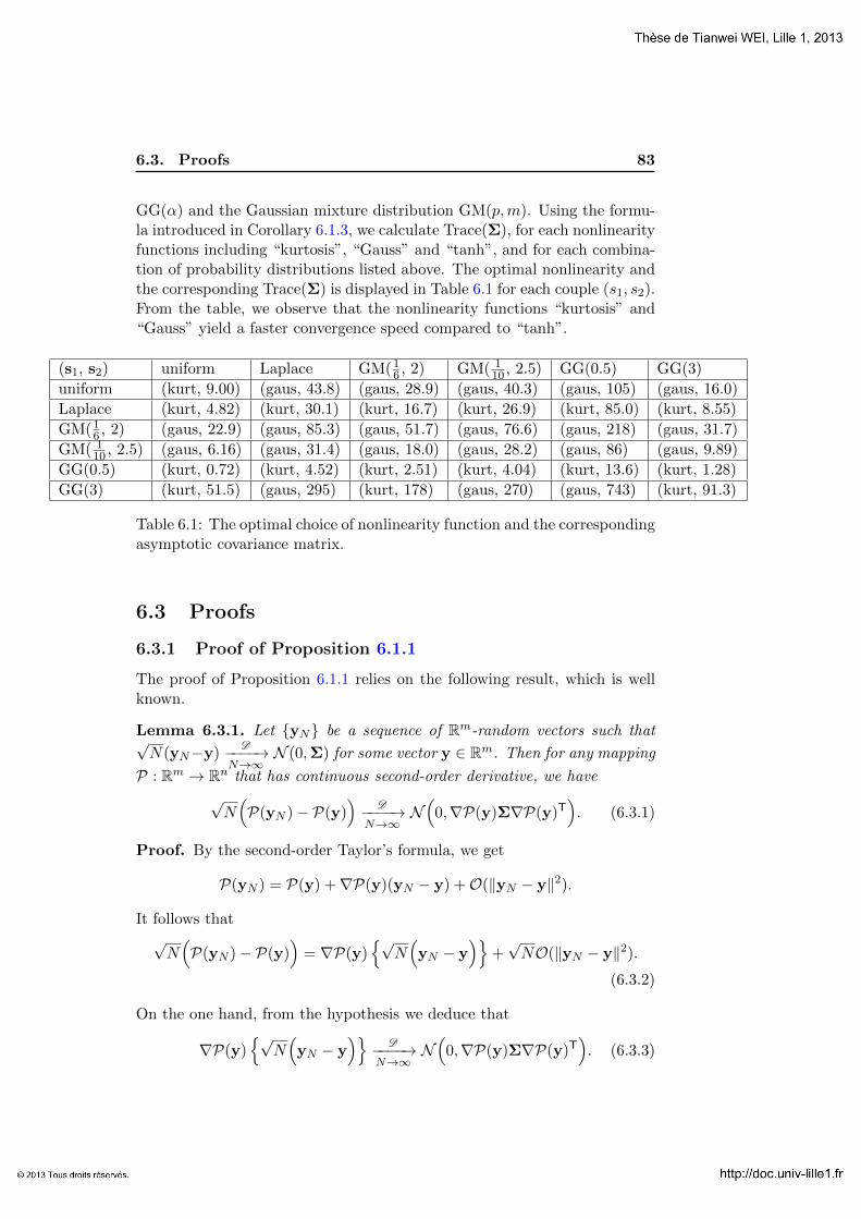
6.3. Proofs 83
GG(α) and the Gaussian mixture distribution GM(p,m). Using the formu-la introduced in Corollary 6.1.3, we calculate Trace(Σ), for each nonlinearityfunctions including “kurtosis”, “Gauss” and “tanh”, and for each combina-tion of probability distributions listed above. The optimal nonlinearity andthe corresponding Trace(Σ) is displayed in Table 6.1 for each couple (s1, s2).From the table, we observe that the nonlinearity functions “kurtosis” and“Gauss” yield a faster convergence speed compared to “tanh”.
(s1, s2) uniform Laplace GM(16 , 2) GM( 1
10 , 2.5) GG(0.5) GG(3)
uniform (kurt, 9.00) (gaus, 43.8) (gaus, 28.9) (gaus, 40.3) (gaus, 105) (gaus, 16.0)
Laplace (kurt, 4.82) (kurt, 30.1) (kurt, 16.7) (kurt, 26.9) (kurt, 85.0) (kurt, 8.55)
GM(16 , 2) (gaus, 22.9) (gaus, 85.3) (gaus, 51.7) (gaus, 76.6) (gaus, 218) (gaus, 31.7)
GM( 110 , 2.5) (gaus, 6.16) (gaus, 31.4) (gaus, 18.0) (gaus, 28.2) (gaus, 86) (gaus, 9.89)
GG(0.5) (kurt, 0.72) (kurt, 4.52) (kurt, 2.51) (kurt, 4.04) (kurt, 13.6) (kurt, 1.28)
GG(3) (kurt, 51.5) (gaus, 295) (kurt, 178) (gaus, 270) (gaus, 743) (kurt, 91.3)
Table 6.1: The optimal choice of nonlinearity function and the correspondingasymptotic covariance matrix.
6.3 Proofs
6.3.1 Proof of Proposition 6.1.1
The proof of Proposition 6.1.1 relies on the following result, which is wellknown.
Lemma 6.3.1. Let {yN} be a sequence of Rm-random vectors such that√N(yN−y)
D−−−−→N→∞
N (0,Σ) for some vector y ∈ Rm. Then for any mapping
P : Rm → Rn that has continuous second-order derivative, we have
√N(P(yN )− P(y)
)D−−−−→
N→∞N(
0,∇P(y)Σ∇P(y)T). (6.3.1)
Proof. By the second-order Taylor’s formula, we get
P(yN ) = P(y) +∇P(y)(yN − y) +O(‖yN − y‖2).
It follows that
√N(P(yN )− P(y)
)= ∇P(y)
{√N(yN − y
)}+√NO(‖yN − y‖2).
(6.3.2)
On the one hand, from the hypothesis we deduce that
∇P(y){√
N(yN − y
)}D−−−−→
N→∞N(
0,∇P(y)Σ∇P(y)T). (6.3.3)

84Chapter 6. Asymptotic Analysis of the Gradient of the FastICA
Function
On the other hand, ‖yN − y‖ is of order Op(N−1/2). Hence we have
√NO(‖yN − y‖2)
P−−−−→N→∞
0. (6.3.4)
Letting N → ∞ in equality (6.3.2) and noticing (6.3.3) and (6.3.4), weachieve (6.3.1). 2
Proof of Proposition 6.1.1The idea of the proof is quite straightforward. First, we notice that
∇f(e1, µ1N ) =
(‖h(e1, µ1N )‖2I− h(e1, µ
1N )hT(e1, µ
1N ))∇h(e1, µ
1N )
‖h(e1, µ1N )‖3
,
which is a function of h(e1, µ1N ) and ∇h(e1, µ
1N ). By the central limit the-
orem, we have
√N{
vec(h(e1, µ
1N ),∇h(e1, µ
1N ))− vec
(h(e1, µ),∇h(e1, µ)
)}(6.3.5)
D−−−−→N→∞
N(
0,Cov(
vec(h(e1),∇h(e1)))), (6.3.6)
where vec(w,M) denotes the operation that combines w and vec(M) intoone long column vector for any vector w and matrix M. Besides, due to thefact
‖h(e1, µ1N )‖3 a.s.−−−−→
N→∞‖h(e1, µ)‖3 6= 0, (6.3.7)
we need only to study the numerator of ∇f(e1, µ1N ) thanks to Slutsky’s
Lemma. Applying Lemma 6.3.1, we are going to achieve the task as follow-ing.
Let’s define the mapping P : Rd × Rd×d 7→ Rd×d by
P(w,M)def= (‖w‖2I−wwT)M.
We have P(h(e1, µ),∇h(e1, µ)
)= 0 and
∇f(e1, ν) =P(h(e1, ν),∇h(e1, ν)
)‖h(e1, ν)‖3
(6.3.8)
for any measure ν. Thus we need only to study the limit of
√NP
(h(e1, µ
1N ),∇h(e1, µ
1N ))
as N tends to infinity.

6.3. Proofs 85
Let us denote respectively by ∇wiP(·, ·) and ∇MijP(·, ·) the partialderivative of P(·, ·) with respect to the ith component of its first argument,and the ijth component of its second argument. For 1 ≤ i, j ≤ d We have:
∇wiP(w,M) = 2wiM− (eiwT + weTi )M,
∇MijP(w,M) = (‖w‖2eieTj −wwTeieTj ).
Now, we are going to calculate the first order partial derivatives of P(·, ·) atthe point
Hdef=(h(e1, µ),∇h(e1, µ)
)∈ Rd × Rd×d.
Since
h(e1, µ) = E[g′(s1)− s1g(s1)]e1,
∇h(e1, µ) = E[s1g′′(s1) + (1− s2
1)g′(s1)]e1eT1 ,
it follows that
∇w1P(H)
= 0 (6.3.9)
∇wiP(H)
= −‖h(e1, µ)‖‖∇h(e1, µ)‖eieT1 (6.3.10)
∇M1jP(H)
= 0 (6.3.11)
∇MijP(H)
= ‖h(e1, µ)‖2eieTj (6.3.12)
for i = 2, ..., d, j = 1, ..., d.Applying Lemma 6.3.1, we obtain
√N{P(h(e1, µ
1N ),∇h(e1, µ
1N ))− P
(H)}
=√NP
(h(e1, µ
1N ),∇h(e1, µ
1N ))
D−−−−→N→∞
N (0,Σ0), (6.3.13)
where
Σ0 = ∇P(H) Cov(
vec(h(e1),∇h(e1)))∇P(H)T
= Cov
d∑i=1
hivec(∇wiP
(H))
+d∑
i,j=1
∇hijvec(∇MijP
(H))
= Cov(− ‖∇h(e1, µ)‖‖h(e1, µ)‖
d∑i=2
hivec(eieT1 )
+‖h(e1, µ)‖2d∑
i=2,j=1
∇hijvec(eieTj )),
thanks to (6.3.9)-(6.3.12). Finally, we deduce from (6.3.7), (6.3.8) and(6.3.13) that
√N∇f(a, µ1
N )D−−−−→
N→∞N(
0,Σ0
‖h(e1, µ)‖6),
from which the result follows.

86Chapter 6. Asymptotic Analysis of the Gradient of the FastICA
Function
6.3.2 Proof of Corollary 6.1.3
In the case of d = 2, we need only to compute the covariance matrix of(h2,∇h21,∇h22). We recall that
h2 = −s2g(s1)
Cov(h2) = E[g2(s1)].
Concerning the matrix ∇h(e1), we have
∇h22 = g′(s1)(1− s22)
∇h21 = −s2s1g′(s1).
Hence, the covariance matrix of the vector (h2,∇h21,∇h22) is given by:
Cov(h2) = E[g2(s1)]
Cov(h2,∇h21) = E[s1g(s1)g′(s1)]
Cov(∇h21) = E[(s1g′(s1))2]
Cov(∇h22) = E[(g′(s1))2]E[s42 − 1].
which achieves the proof.

Chapter 7
Conclusion and Perspective
7.1 Summary of results
In this thesis, we have given a unified study of both theoretical and empiricalversions of the deflation based (one-unit) FastICA algorithm,
In Chapter 3, we proved that the theoretical FastICA algorithm con-verges to a column of the mixing matrix with at least a quadratic conver-gence speed. In particular, if the underlying nonlinearity function is kurtosis,the convergence speed is even cubic. Although these results (e.g. Theorem3.3.4, Proposition 3.3.5) are already well-known, our approach is novel andrigorous. We calculated the gradient of the FastICA function, and showedthat the gradient would vanish at the columns of the mixing matrix A. Fromthis fact, the quadratic convergence speed of the theoretical FastICA algo-rithm is immediately derived. In the case of kurtosis nonlinearity, the secondderivative of the FastICA function vanishes, leading to a cubic convergencespeed. Moreover, we proved that any local minimizer of the theoretical con-trast function is always a fixed point of the theoretical FastICA function.This characterization is, to our knowledge, new. It also gave some insightto the study of empirical FastICA algorithm.
In Chapter 4, we studied the convergence of four empirical FastICAalgorithms. The main result of this chapter is that each empirical FastICAalgorithm converges to a local minimizer of the respective empirical contrastfunction with probability one, provided that the sample size is large enough.As a corollary of this result, we showed that each FastICA estimator, definedas the limit of the empirical FastICA algorithm, is a consistent estimatorof a column of the mixing matrix. Before our attempt, the convergence ofFastICA algorithm in the finite sample case was only supported by numericalsimulation but never theoretically confirmed.
In Chapter 5, we gave the explicit closed form of the asymptotic covari-ance matrix of our FastICA estimators. Although similar results alreadyexist in the literature, our approach is the only mathematically rigourousone, and we addressed four different scenarios all together, which enablesthe measuring of the effect of data centering and whitening. We also madea comparison of the existing results was made in Section 5.1.1.
In Chapter 6, we studied the gradient of the empirical FastICA algorithmand derived a new criterion of optimality of the choice of nonlinearity func-tion. This new criterion consists of optimizing the asymptotic covariance
88 Chapter 7. Conclusion and Perspective
matrix of the gradient of the empirical FastICA function at the column ofthe mixing matrix, such that one can attain the fastest possible convergencespeed of the empirical FastICA algorithm. We derived the explicit form ofthe latter asymptotic covariance matrix and gave some numerical examplefor two sources.
7.2 Upcoming challenges
Although this thesis gives elements of answer to some interesting issues con-cerning the empirical FastICA algorithm, there are still questions remainingunsolved.
7.2.1 Spurious local optima
Spurious local optimizers of the contrast function are those optimizers thatdo not correspond to any demixing vectors. Convergence of ICA algorithmto spurious local optimizers are the very thing we hope to avoid. There aretwo ways to achieve this: we can either choose carefully the contrast functionso that it does not possess spurious local optima (this is the case for mutualinformation based contrast function, see (Comon, 1994)), or we design anICA algorithm which can somehow, intelligently converge to the right opti-ma. In the continued study we actually proved the following inclusion forFastICA:
D ⊂ L ⊂ O ⊂ F,
whereD
def= {±ai, i = 1, . . . , d};
Fdef= {v ∈ Rd : f(v, µ) = ±v};
Ldef= {v ∈ F : ‖∇f(v, µ)‖ < 1};
Odef= {v ∈ S : v is a local optimizer of G(·, µ)}.
This inclusion suggests that unlike the other gradient-ascent type algorithm-s, FastICA algorithm does not searches blindly all the local optima of thecontrast function; it can automatically filter those spurious optimizers whichare not stable fixed points. Now the vital question is if any of these inclu-sions, especially D ⊂ L, is indeed an equality. If we can show, or at leastgive some sufficient condition under which D = L, i.e. FastICA always yielddemixing vectors, then we can assert that the algorithm is theoretically reli-able. For kurtosis nonlinearity, this is done in (Douglas, 2003). Nevertheless,we believe that the equality D = L cannot be true in general, although wehave never encountered systematic violation of it in repeated experiments.We are not able to provide a proof or come up with a counter-example atthe moment.

7.2. Upcoming challenges 89
At least, it is easy to give an example where the inclusion L ⊂ O isstrict. It is known that in the simplest 2-dimensional case, if the two sourcesignal have the same distribution, then there must exist local optima thatdo not correspond to the demixing vectors (see e.g. Fig. 2.4). This is thecase where we have
D = L ⊂ O = F.
7.2.2 Convergence radius
In Section 3.4.2, we have briefly talked about the convergence radius ofthe FastICA algorithm. For each source signal si, its convergence radiusis defined to be the largest real number r, such that if the initial inputw0 of the FastICA algorithm lies in the ball Br(ai), then the FastICAalgorithm is guaranteed to converge to the corresponding demixing vectorai. Experiments shows that source signals that are comparatively closer toGaussian correspond to a smaller convergence radius. We believe that thiscan be theoretically proved, with the underlying measure of Gaussianity:
|H(ai, µ)| = |E[g′(si)− g(si)si]|.
This quantity vanishes if si has a Gaussian distribution, as is shown inSection 3.1. We predict that if the source signal si, non-necessarily beingGaussian, has a very small |E[g′(si)−g(si)si]|, then it would be very difficultto recover with one-unit FastICA and the underlying nonlinearity G(·), sincemost initial iterate of the algorithm would make the algorithm converge toelsewhere. Using another nonlinearity may resolve this problem though.
7.2.3 Convergence and asymptotic behavior of FastICA forthe extraction of several sources
In this thesis, we have only considered the extraction of only one sourceusing one-unit FastICA. This scenario is easy to analyze, since the deflationprocedure (2.1.23) can be omitted. In this case, if we are to recover all thesources, the starting points need to locate in the neighborhood of differentcolumns of the mixing matrix, so that the algorithm can converge to dif-ferent limits. However, in real world problem, this may be unrealistic orcomputational costly. For example, many different starting point on S mayend up yielding the same source, while some source (especially those whoseprobability distribution is close to Gaussian) may never be recovered due tosmall convergence radius, as is previously explained In order to effectivelyextract all the sources, one need to implement either symmetrical FastICA,or the original one-unit FastICA with a decorrelation procedure: to avoidrecovering twice a same source, at each iteration step, the i-th recoveredsource must be orthogonal to the i− 1 previously extracted sources.

90 Chapter 7. Conclusion and Perspective
The questions that motivate this thesis remain still open for these ver-sions of FastICA. Namely, when extracting the 2nd, 3rd, . . ., n-th sources,how does the additional procedure influence the convergence of the one-unit FastICA algorithm? What is the asymptotic covariance matrix of thesequentially obtained FastICA estimators? What about the symmetricalversion of FastICA in the finite sample case? The difficulty lies in the factthat if the sample size is finite, the minimizers of the empirical contrastfunction does not form an orthogonal matrix in general, while both one-unitFastICA and symmetrical FastICA can only yield an orthogonal estimateof the demixing matrix. This means that unlike the case of extracting onlyone source, when trying to recover all the sources, the FastICA estimatorscannot be the local minimizers of the empirical contrast function. This factis problematic since the whole analysis presented in this thesis is based up-on the link between the local minimizers of the contrast function and fixedpoints of the FastICA function.
By generalizing some ideas used in this thesis, we derived heuristicallythe asymptotic covariance matrix for symmetrical FastICA:
Ri=d∑j 6=i
βi − α2i + βj − α2
j + (ρj − αj)2 − η2j
(|ρi − αi|+ |ρj − αj |)2bjb
Tj + κiaia
Ti
+( d∑j 6=i
sign(ρj − αj)ηjaj|ρi − αi|+ |ρj − αj |
)( d∑j 6=i
sign(ρj − αj)ηjaTj
|ρi − αi|+ |ρj − αj |
).
This formula should be correct since it coincides with the formula given in(Tichavsky et al., 2006) using another heuristic method. However, someissues are still to be resolved if we hope to render the whole argument rig-orous.
References
Andrews, D. W. K. (1992, June). Generic uniform convergence. EconometricTheory , 02 (9). (Cited on page 49.)
Bierens, H. (2005). Introduction to the mathematical and statistical founda-tions of econometrics. In (p. 171). Cambridge University Press. (Citedon page 49.)
Brandstein, M., & Ward, D. B. (2001). Microphone arrays: Signal processingtechniques and applications. New York: Springer. (Cited on page 3.)
Cardoso, J. F., & Souloumiac, A. (1993, December). Blind beamforming fornon-Gaussian signals. IEEE Proceedings-F , 140 (6), 362-370. (Citedon page 4.)
Chevalier, P., Albera, L., Comon, P., & Ferreol, A. (2004, July). Compara-tive performance analysis of eight blind source separation methods on

References 91
radio-communications signals. In Joint conf. neural netw. (p. 273-278).(Cited on page 4.)
Comon, P. (1994, April). Independent component analysis: a new concept?Signal Processing , 36 (3), 287-314. (Cited on pages 3, 8, 9, 11, 13, 14and 88.)
Comon, P., & Jutten, C. (2010). Handbook of blind source separation:Independent component analysis and applications. In (p. 179-227).Academic Press. (Cited on pages 3 and 11.)
Comon, P., & Moreau, E. (1997, April). Improved contrast dedicated toblind separation in communications. In Proc. icassp-97. (Cited onpage 4.)
Delfosse, N., & Loubaton, P. (1995, July). Adaptive blind separation ofindependent sources. Signal Processing , 45 , 59-83. (Cited on pages 4and 21.)
Dermoune, A., Rahmania, N., & Wei, T. (2012). General linear mixed modeland signal extraction problem with constraint. Journal of MultivariateAnalysis, 105 , 311-321. (Cited on page 3.)
Dermoune, A., & Wei, T. (2013, April). FastICA algorithm: Five criteriafor the optimal choice of the nonlinearity function. IEEE transactionon Signal Processing , 61 (8), 2078-2087. (Cited on page 3.)
Donoho, D. (1981). On minimum entropy deconvolution. In Applied time se-ries analysis ii (p. 565-609). New York: Academic. (Cited on page 16.)
Douglas, S. (2003, apr). On the convergence behavior of the fastica algorith-m. In Proc. 4th symp. independent component analysis blind sourceseparation (p. 409-414). (Cited on pages 4 and 88.)
Hyvarinen, A. (1997). One-unit contrast functions for independent compo-nent analysis: A statistical analysis. In Proc. ieee nnsp workshop ’97.(Cited on pages 4 and 65.)
Hyvarinen, A. (1999). Fast and robust fixed-point algorithms for indepen-dent component analysis. IEEE Transactions on Neural Networks,10 (3), 626-634. (Cited on pages 4, 15, 16, 17, 20, 22, 28, 34 and 35.)
Hyvarinen, A., Karhunen, J., & Oja, E. (2001). Independent componentanalysis. New York: Wiley-Interscience. (Cited on pages 3 and 8.)
Hyvarinen, A., & Oja, E. (1997). A fast fixed-point algorithm for inde-pendent component analysis. Neural Computation, 9 (7), 1483-1492.(Cited on pages 4 and 34.)
Hyvarinen, A., & Oja, E. (2000). Independent component analysis: Algo-rithms and applications. Neural Networks, 13 (4-5), 411-430. (Citedon pages 3, 4, 8, 13, 14 and 15.)
Jutten, C. (1987). Calcul neuromimetique et traitement du signal: analyseen composantes indpendantes. These detat es sciences physiques, UJF-INP Grenoble. (Cited on page 3.)
Jutten, C., & Comon, P. (n.d.). De la separation des sources a l’analyse encomposantes independante. (Cited on page 3.)
92 Chapter 7. Conclusion and Perspective
Jutten, C., & Taleb, A. (2000). Source separation: From dusk till dawn. In2nd int. workshop on independent component analysis and blind sourceseparation (ica 2000). (Cited on page 3.)
Leshem, A., & van der Veen, A.-J. (2008, September). Blind source separa-tion: the location of local minima in the case of finitely many samples.IEEE transactions on Signal Processing , 56 (9), 4340-4353. (Cited onpage 4.)
Luenberger, D. G., & Ye, Y. (2008). Linear and nonlinear programming. In(Third ed.). Springer. (Cited on page 67.)
Makeig, S., Bell, A., Jung, T.-P., & Sejnowski, T. (1996). Independent com-ponent analysis of electroen-cephalographic data. Advances in NeuralInformation Processing Systems(9), 145-151. (Cited on page 3.)
Makino, S., Lee, T.-W., & Sawada, H. (2007). Blind speech separation.Dordrecht, the Netherlands: Springer. (Cited on page 3.)
M. Ichir, A., M. Mohammad-Djafari. (2006, July). Hidden Markov modelsfor wavelet-based blind source separation. IEEE transactions on ImageProcessing , 15 (7), 1887-1899. (Cited on page 3.)
Nesterov, Y. (2004). Introductory lectures on convex optimization: A basiccourse. Boston/Dordrecht/London: Kluwer. (Cited on page 67.)
Newey, W. K. (1991, July). Uniform convergence in probability and s-tochastic equicontinuity. Econometrica, 59 (4), 1161-1167. (Cited onpage 49.)
Oja, E. (2002, November). Convergence of the symmetrical FastICA algo-rithm. In 9th int. conf. neural information processing (iconip). (Citedon pages 4, 17 and 35.)
Oja, E., & Yuan, Z. (2006). The FastICA algorithm revisited: Convergenceanalysis. IEEE transactions on Neural Networks, 17 (6). (Cited onpages 4, 17 and 51.)
Ollila, E. (2010, March). The deflation-based FastICA estimator: Statisticalanalysis revisited. IEEE transactions on Signal Processing , 58 (3).(Cited on pages 4, 65 and 66.)
Regalia, P. A., & Kofidis, E. (2003, July). Monotonic convergence of fixed-point algorithms for ICA. IEEE transactions on Neural Network ,14 (4), 943-949. (Cited on pages 4, 22 and 37.)
Reyhani, N., Ylipaavalniemi, J., Vigario, R., & Oja, E. (2012). Consistencyand asymptotic normality of FastICA and bootstrap FastICA. SignalProcessing , 92 , 1767-1778. (Cited on pages 65 and 66.)
Shen, H., Kleinsteuber, M., & Huper, K. (2008, June). Local convergenceanalysis of FastICA and related algorithms. IEEE transactions onNeural Network , 19 (6), 1022-1032. (Cited on pages 22 and 28.)
Shimizu, A., Hyvarinen, A., Yutaka, K., Hoyer, P., & Kerminen, A. J.(2006). Testing signifcance of mixing and demixing coefficients in ICA.In Int. conf. independent component analysis (ica 2006). (Cited onpage 65.)

References 93
Stone, J. V. (2004, sep). Independent component analysis: A tutorialintroduction. A Bradfort Book. (Cited on page 3.)
Tichavsky, P., Koldovsky, Z., & Oja, E. (2006, April). Performance analysisof the FastICA algorithm and Cramer-Rao bounds for linear indepen-dent component analysis. IEEE transactions on Signal Processing ,54 (4), 1189-1203. (Cited on pages 4, 40, 51, 65, 66 and 90.)
Tugnait, J. K. (1997, March). Identification and deconvolution of multichan-nel non-Gaussian processes using higher order statistics and inversefilter criteria. IEEE Transactions on Signal Processing , 45 , 658-672.(Cited on page 4.)
van der Vaart, A. (2000). Asymptotic statistics. In (chap. 5). CambridgeUniversity Press. (Cited on page 72.)
Vigario, R., & Oja, E. (2008). BSS and ICA in neuroinformatics: Fromcurrent practices to open challenges. IEEE Reviews in BiomedicalEngineering(1), 50-61. (Cited on page 3.)
Vrins, F. D. (2007). Contrast properties of entropic criteria for blind sourceseparation, a unifying framework based on information-theoretic in-equalities. Unpublished doctoral dissertation, Universite Catholiquede Louvain. (Cited on pages 11, 14 and 35.)
Waheed, K., & Salam, F. M. (2002, August). Blind source recovery using anadaptive generalized Gaussian score function. In in proc. 45th midwestsymp. circuits systems (mwscas) (p. 656-659). (Cited on page 40.)
Zarzoso, V., & Comon, P. (2010, February). Robust independent compo-nent analysis by iterative maximization of the kurtosis contrast withalgebraic optimal step size. IEEE Transactions on Neural Networks,21 (2), 248-261. (Cited on page 4.)