alberto brunete gonzalez
TRANSCRIPT
8/21/2019 Alberto Brunete Gonzalez
http://slidepdf.com/reader/full/alberto-brunete-gonzalez 1/311
UNIVERSIDAD POLITECNICA DE MADRIDESCUELA TECNICA SUPERIOR DE INGENIEROS INDUSTRIALES
Design and Control of Intelligent
Heterogeneous Multi-configurable
Chained Microrobotic Modular
Systems
PhD Thesis
Alberto Brunete GonzalezIngeniero de Telecomunicaci´ on
2010

8/21/2019 Alberto Brunete Gonzalez
http://slidepdf.com/reader/full/alberto-brunete-gonzalez 2/311

8/21/2019 Alberto Brunete Gonzalez
http://slidepdf.com/reader/full/alberto-brunete-gonzalez 3/311
DEPARTAMENTO DE AUTOMATICA, INGENIERIA ELECTRONICA EINFORMATICA INDUSTRIAL
ESCUELA TECNICA SUPERIOR DE INGENIEROS INDUSTRIALES
Design and Control of Intelligent
Heterogeneous Multi-configurable
Chained Microrobotic Modular
Systems
PhD Thesis
Alberto Brunete GonzalezIngeniero de Telecomunicaci´ on
Supervisors
Ernesto Gambao GalanDoctor Ingeniero Industrial
Miguel Hernando GutierrezDoctor Ingeniero Industrial
2010

8/21/2019 Alberto Brunete Gonzalez
http://slidepdf.com/reader/full/alberto-brunete-gonzalez 4/311

8/21/2019 Alberto Brunete Gonzalez
http://slidepdf.com/reader/full/alberto-brunete-gonzalez 5/311
Tıtulo:Design and Control of Intelligent Heterogeneous
Multi-configurable Chained Microrobotic Modular Systems
Autor:Alberto Brunete Gonzalez
Ingeniero de Telecomunicacion
(D-15)
Tribunal nombrado por el Magfco. y Excmo. Sr. Rector de la Universidad Politecnica
de Madrid, el dıa de de 2010
Presidente:
Vocal:
Vocal:
Vocal:
Secretario:
Suplente:
Suplente:
Realizado el acto de lectura y defensa de la tesis el dıa de deen la E.T.S.I. / Facultad
El Presidente: El Secretario:
Los Vocales:

8/21/2019 Alberto Brunete Gonzalez
http://slidepdf.com/reader/full/alberto-brunete-gonzalez 6/311

8/21/2019 Alberto Brunete Gonzalez
http://slidepdf.com/reader/full/alberto-brunete-gonzalez 7/311
Dedication
Version 0.95
vii

8/21/2019 Alberto Brunete Gonzalez
http://slidepdf.com/reader/full/alberto-brunete-gonzalez 8/311
viii

8/21/2019 Alberto Brunete Gonzalez
http://slidepdf.com/reader/full/alberto-brunete-gonzalez 9/311
Abstract
The objective of this thesis is the “Design and Control of Intelligent Heterogeneous Multi-configurable Chained Microrobotic Modular Systems”. That is, the development of mod-ular microrobots composed of different types of modules able to perform different typesof movements (gaits), that can have different (chained) configurations depending on the
task to perform.Heterogenous is the key word in this thesis. It is possible to find in literature many
designs concerning modular robots, but almost all of them are homogenous: all are com-posed of the same modules except for some designs having two different modules but oneof them passive. In this thesis, several active modules are proposed (rotation, support,extension, helicoidal, etc.) that can be combined and execute different gaits.
The original idea was to make the robots as smaller as possible, reaching in the enda final diameter of 27mm. Although they are not really microrobots, they are in themesoscale (from hundreds of microns to tens of centimeters) and in literature they arecalled for simplicity minirobots or microrobots.
Several modules have been developed: the rotation module (indeed it is a doublerotation module, but for simplicity it is called rotation module) v1 and v2, the helicoidalmodule v1 and v2, the support module v1, v1.1 and v2, the extension module v1 and v2,the camera module v1 and v2, the contact module (it is included in the camera module v2)and the battery module. Some others are still in the design or conceptual phase, but theycan be simulated. They are the SMA-based module (there is already a prototype), thetraveler module (in the design phase) and the sensor module (in a conceptual phase). Allmodules have been designed with the idea to miniaturized them in the future, and so boththe electronic and the embedded control programs are as simple as possible (maintainingthe planned functionality).
Parallel to the construction of the modules a simulator has been developed to pro-
vide a very efficient way of prototyping and verification of control algorithms, hardwaredesign, and exploring system deployment scenarios. It is built upon an existing opensource implementation of rigid body dynamics, the Open Dynamics Engine (ODE). Simu-lated modules have been designed as simple as possible (using simple primitives) to makesimulation fluid, but trying to reflect as much as possible its real physic conditions andparameters, its electronics and communication buses, and the software embedded in themodules. The simulator has been validated using the information gathered from real mod-ules experiments and this has helped to adjust the parameters of the simulator to have anaccurate model.
Although the first idea was to develop the microrobot for pipe inspection, the expe-rience acquired with the first prototypes causes to realize that locomotion systems used
inside pipes could also be suitable outside them, and that the prototypes and the control
ix
8/21/2019 Alberto Brunete Gonzalez
http://slidepdf.com/reader/full/alberto-brunete-gonzalez 10/311
architecture were useful in open spaces. In this way, research was extended to open spacesand the ego-positioning system was added.
The EGO-positioning system is a method that allows all individual robots of a swarm
to know their own positions and orientations based in the projection of sequences of codedimages composed of horizontal and vertical stripes over photodiodes placed on the robots.This concept can also be applied to the modules in order for them to know their positionand orientation, and to send commands to all of them at the same time.
To manage all of this a control architecture based on behaviors has been developed.Since the modules cannot have a big processor, a central control is included in the ar-chitecture to take the high level control. The central control has a model-based subpartand another part based on behaviors. The embedded control in the modules is entirelybehavior-based. Between this two there is an heterogenous agent (layer) that allows thecentral control to treat all modules in the same way, since the heterogenous layer trans-lates its commands into module specific commands. A behavior-based architecture has
been chosen because it is specifically appropriate for designing and controlling biologicallyinspired robots, it has proven to be suitable for modular systems and it integrates verywell both low and high level control.
In order to communicate all actors (behaviors, modules and central control), a commu-nication protocol based on I2C has been developed. It allows to send messages from theoperator to the central control, from central control to the modules and between behaviors.
A Module Description Language (MDL) has been designed, a language that allowsmodules to transmit their capabilities to the central control, so it can process this infor-mation and choose the best configuration and parameters for the microrobot.
Inside the control architecture an offline genetic algorithm has been developed in orderto: first, determine the modules to use to have an optimal configuration for an specific
task (configuration demand), and second, determine the optimum parameters for bestperformance for a given module configuration (parameter optimization).
Thus, the main contributions that can be found in this thesis are: the design andconstruction of an Heterogeneous Modular Multi-configurable Chained Microrobot ableto perform different gaits (snake-like, inch-worm, helicoidal, combination), the design of acommon interface for the modules, a behavior-based control architecture for heterogenouschained modular robot, a simulator for the physics and dynamics (including the designof a servo model), electronics, communications and embedded software routines of themodules, and finally, the enhancement of the ego-positioning system.
x

8/21/2019 Alberto Brunete Gonzalez
http://slidepdf.com/reader/full/alberto-brunete-gonzalez 11/311
Resumen
El objetivo de esta tesis es el diseno y control de microrobots inteligentes modularesheterogeneos multiconfigurables de tipo cadena. Es decir, el desarrollo de microrobotsmodulares compuestos por diferentes tipos de modulos capaces de realizar diferentes tiposde movimientos (gaits en ingles), que pueden ser dispuestos en diferentes configuraciones
(siempre en cadena) dependiendo de la tarea a realizar.Heterogeneo es la palabra clave en esta tesis. Es posible encontrar en la literatura
muchos disenos sobre robots modulares, pero casi todos ellos son homogeneos: todos secomponen de los mismos modulos, excepto en algunos disenos que tienen dos modulosdiferentes, pero uno de ellos pasivo. En esta tesis, se proponen varios modulos activos(rotacion, soporte, extension, helicoidales, etc) que se pueden combinar y ejecutar difer-entes movimientos, ademas de otros pasivos (baterıas, sensores, medicion de la distanciarecorrida) como complemento a los primeros.
La idea original era hacer los robots lo mas pequenos posible, alcanzando finalmenteun diametro de 27 mm. Aunque no se puedan considerar tecnicamente como microrobots,estan en la mesoescala (entre cientos de micras y decenas de centımetros) y en la literaturase les suele llamar por simplicidad minirrobots o microrrobots.
Durante el desarrollo de esta tesis, varios modulos han sido desarrollados: el modulode rotacion (en realidad se trata de un modulo de doble rotacion, pero por simplicidad sele llama modulo de rotacion) v1 y v2, el modulo helicoidal v1 y v2, el modulo de soportev1, v1.1 y v2, el modulo de extension v1 y v2, el modulo de camara v1 y v2, el modulode contacto (que esta incluido en el modulo de la camara v2) y el modulo de baterıa.Algunos otros estan todavıa en fase de diseno o conceptual, pero pueden ser utilizadosen la simulacion. Son el modulo basado en SMA (ya existe un prototipo), el modulode medicion de distacia recorrida (en fase de diseno) y el modulo de sensores (en faseconceptual). Todos los modulos han sido disenados con la idea de ser miniaturizados enel futuro, por lo que tanto la electronica como los programas de control integrados se hanhecho tan simples como es posible (manteniendo por supuesto la funcionalidad prevista).
Paralelamente a la construccion de los modulos se ha desarrollado un simulador paraproporcionar un medio eficaz de creacion de prototipos y de verificacion de los algoritmosde control, diseno de hardware, y exploracion de escenarios de despliegue del sistema.Esta construido sobre un software (libre y de codigo abierto) de simulacion de dinamicade cuerpos rıgidos, el Open Dynamics Engine (ODE). Los modulos simulados se handisenado de la forma mas simple posible (usando primitivas simples) para hacer fluida lasimulacion, pero tratando de reflejar lo mas posible sus condiciones reales y los parametrosfısicos, sus componentes electronicos y buses de comunicacion, y el software incluido enlos modulos. El simulador ha sido validado con la informacion obtenida en experimentos
con modulos reales, y esto ha ayudado a ajustar los par ametros del simulador para tener
xi

8/21/2019 Alberto Brunete Gonzalez
http://slidepdf.com/reader/full/alberto-brunete-gonzalez 12/311
un modelo preciso.Aunque la primera idea fue desarrollar el microrobot para la inspeccion de tuberıas, la
experiencia adquirida con los primeros prototipos mostro que los sistemas de locomocion
utilizados en el interior de tuberıas tambien podrıan ser adecuados fuera de ellas, y que losprototipos y la arquitectura de control son utiles en espacios abiertos. De esta manera, lainvestigacion se extendio a los espacios abiertos y se anadio el sistema de “ego-positioning”.
El sistema de “ego-positioning” es un metodo que permite a los robots de un enjambreconocer su posicion y orientacion basadas en la proyeccion de secuencias de imagenescodificadas compuesto por rayas horizontales y verticales sobre fotodiodos colocados enlos robots. Este concepto tambien puede aplicarse a los modulos de un microrobot paraque puedan conocer su posicion y orientacion, y para enviar comandos a todos ellos almismo tiempo.
Para gestionar todo esto se ha desarrollado una arquitectura de control basada encomportamientos. Dado que los modulos no pueden tener un procesador de grandes ca-
pacidades, se incluye en la arquitectura un control central para proporcionar control dealto nivel. El control central tiene una parte basada en modelos y otra parte basada encomportamientos. El control integrado en los modulos esta totalmente basado en compor-tamientos. Entre los dos hay un agente heterogeneo (o capa) que permite que el controlcentral trate a todos los modulos de la misma manera, ya que la capa heterogenea traducesus ordenes a comandos especıficos del modulo. Esta arquitectura basada en compor-tamientos ha sido elegida porque es especialmente adecuada para el diseno y control derobots inspirados en sistemas biologicos, ha demostrado ser adecuada para sistemas mod-ulares e integra muy bien niveles altos y bajos de control.
Con el fin de comunicar a todos los actores (los comportamientos, los m odulos y elcontrol central), se ha desarrollado un protocolo de comunicaci on basado en I 2C . Este
protocolo permite enviar mensajes del operador al control central, desde el control centrala los modulos y entre comportamientos.
Dentro de la arquitectura tambien se ha desarrollado un “Lenguaje de Descripcionde Modulos”(MDL por sus siglas en ingles “Module Description Language”), un lenguajeque permite a los modulos transmitir sus capacidades al control central, para que puedaprocesar esta informacion y elegir la mejor configuracion y los parametros del microrobot.
Dentro de la arquitectura de control se ha desarrollado un algoritmo genetico con elfin de: primero, determinar los modulos a utilizar para tener una configuracion optimapara una tarea especıfica (peticion de configuracion), y segundo, determinar los parametrosoptimos para el mejor funcionamiento de un modulo dada una configuracion (optimizacionde parametros).
Como resumen, las principales contribuciones que se pueden encontrar en esta tesisson: el diseno y la construccion de un microrobot modular heterogeneo multiconfigurablede tipo cadena capaz de llevar a cabo diferentes sistemas de locomocion (de tipo serpiente,gusano, helicoidal y combinacion de los anteriores), el diseno de un interfaz comun para losmodulos, una arquitectura de control basada en comportamientos para robots modularesheterogeneos de tipo cadena, un simulador de la fısica y la dinamica (incluyendo el disenode un modelo de servo), electronica, comunicaciones y rutinas embebidas de software delos modulos y finalmente, la mejora del sistema de “ego-positioning”.
xii

8/21/2019 Alberto Brunete Gonzalez
http://slidepdf.com/reader/full/alberto-brunete-gonzalez 13/311
Contents
Abstract ix
Resumen xi
Contents xiii
List of Figures xvii
List of Tables xxiii
Acknowledgements xxvii
1 Introduction 1
1.1 Motivation and framework of the thesis . . . . . . . . . . . . . . . . . . . . 1
1.2 Topics of the thesis . . . . . . . . . . . . . . . . . . . . . . . . . . . . . . . . 2
1.2.1 About Microrobotics . . . . . . . . . . . . . . . . . . . . . . . . . . . 21.2.2 About Modular Robots . . . . . . . . . . . . . . . . . . . . . . . . . 3
1.2.3 About Pipe Inspection Robots . . . . . . . . . . . . . . . . . . . . . 31.3 Objectives of the thesis . . . . . . . . . . . . . . . . . . . . . . . . . . . . . 4
1.4 Overview of the thesis . . . . . . . . . . . . . . . . . . . . . . . . . . . . . . 6
2 Review on Modular, Pipe Inspection and Micro Robotic Systems 9
2.1 The origins . . . . . . . . . . . . . . . . . . . . . . . . . . . . . . . . . . . . 10
2.2 Modular robots . . . . . . . . . . . . . . . . . . . . . . . . . . . . . . . . . . 13
2.2.1 PolyBot and PolyPod . . . . . . . . . . . . . . . . . . . . . . . . . . 13
2.2.2 M-TRAN . . . . . . . . . . . . . . . . . . . . . . . . . . . . . . . . . 15
2.2.3 CONRO . . . . . . . . . . . . . . . . . . . . . . . . . . . . . . . . . . 182.2.4 Molecube . . . . . . . . . . . . . . . . . . . . . . . . . . . . . . . . . 19
2.2.5 Crystalline and Molecule robots . . . . . . . . . . . . . . . . . . . . . 22
2.2.6 Telecube and Proteo (Digital Clay) . . . . . . . . . . . . . . . . . . . 24
2.2.7 Chobie . . . . . . . . . . . . . . . . . . . . . . . . . . . . . . . . . . . 272.2.8 ATRON . . . . . . . . . . . . . . . . . . . . . . . . . . . . . . . . . . 29
2.2.9 Active Cord Mechanism (ACM) . . . . . . . . . . . . . . . . . . . . 31
2.2.10 WormBot . . . . . . . . . . . . . . . . . . . . . . . . . . . . . . . . . 32
2.2.11 Others . . . . . . . . . . . . . . . . . . . . . . . . . . . . . . . . . . . 34
2.3 Microrobots . . . . . . . . . . . . . . . . . . . . . . . . . . . . . . . . . . . . 352.3.1 Micro size modular machine using SMAs . . . . . . . . . . . . . . . . 36
2.3.2 Denso Corporation . . . . . . . . . . . . . . . . . . . . . . . . . . . . 36
xiii
8/21/2019 Alberto Brunete Gonzalez
http://slidepdf.com/reader/full/alberto-brunete-gonzalez 14/311
2.3.3 Endoscope microrobots . . . . . . . . . . . . . . . . . . . . . . . . . 382.3.4 LMS, LAB and LAI microrobots . . . . . . . . . . . . . . . . . . . . 382.3.5 12-legged endoscopic capsular robot . . . . . . . . . . . . . . . . . . 41
2.4 Pipe Inspection robots . . . . . . . . . . . . . . . . . . . . . . . . . . . . . . 412.4.1 MRInspect . . . . . . . . . . . . . . . . . . . . . . . . . . . . . . . . 422.4.2 FosterMiller . . . . . . . . . . . . . . . . . . . . . . . . . . . . . . . . 422.4.3 Helipipe . . . . . . . . . . . . . . . . . . . . . . . . . . . . . . . . . . 422.4.4 Theseus . . . . . . . . . . . . . . . . . . . . . . . . . . . . . . . . . . 43
2.5 Robot Summary . . . . . . . . . . . . . . . . . . . . . . . . . . . . . . . . . 442.6 Conclusions . . . . . . . . . . . . . . . . . . . . . . . . . . . . . . . . . . . . 44
3 Review on Control Architectures for Modular Microrobots 493.1 Classification of control architectures . . . . . . . . . . . . . . . . . . . . . . 503.2 Behaviour-Based Systems . . . . . . . . . . . . . . . . . . . . . . . . . . . . 54
3.2.1 What is a behavior? . . . . . . . . . . . . . . . . . . . . . . . . . . . 543.2.2 Behavior-based systems . . . . . . . . . . . . . . . . . . . . . . . . . 553.2.3 Behavior representation . . . . . . . . . . . . . . . . . . . . . . . . . 553.2.4 Behavioral encoding . . . . . . . . . . . . . . . . . . . . . . . . . . . 583.2.5 Emergent behavior . . . . . . . . . . . . . . . . . . . . . . . . . . . . 593.2.6 Behavior coordination . . . . . . . . . . . . . . . . . . . . . . . . . . 60
3.3 Behavior-Based Architectures . . . . . . . . . . . . . . . . . . . . . . . . . . 633.3.1 Subsumption Architecture . . . . . . . . . . . . . . . . . . . . . . . . 643.3.2 Motor Schemas . . . . . . . . . . . . . . . . . . . . . . . . . . . . . . 653.3.3 Activation Networks . . . . . . . . . . . . . . . . . . . . . . . . . . . 673.3.4 DAMN . . . . . . . . . . . . . . . . . . . . . . . . . . . . . . . . . . 69
3.3.5 CAMPOUT . . . . . . . . . . . . . . . . . . . . . . . . . . . . . . . . 693.4 Hybrid Deliberate-Reactive Architectures . . . . . . . . . . . . . . . . . . . 72
3.4.1 3-Tiered (3T) . . . . . . . . . . . . . . . . . . . . . . . . . . . . . . . 733.4.2 Aura . . . . . . . . . . . . . . . . . . . . . . . . . . . . . . . . . . . . 733.4.3 Atlantis . . . . . . . . . . . . . . . . . . . . . . . . . . . . . . . . . . 743.4.4 Saphira . . . . . . . . . . . . . . . . . . . . . . . . . . . . . . . . . . 753.4.5 DD&P . . . . . . . . . . . . . . . . . . . . . . . . . . . . . . . . . . . 77
3.5 Modular Robot Architectures . . . . . . . . . . . . . . . . . . . . . . . . . . 783.5.1 CONRO . . . . . . . . . . . . . . . . . . . . . . . . . . . . . . . . . . 783.5.2 M-TRAN . . . . . . . . . . . . . . . . . . . . . . . . . . . . . . . . . 803.5.3 Polybot . . . . . . . . . . . . . . . . . . . . . . . . . . . . . . . . . . 81
3.6 Adaptive Behavior . . . . . . . . . . . . . . . . . . . . . . . . . . . . . . . . 833.6.1 Reinforcement Learning . . . . . . . . . . . . . . . . . . . . . . . . . 833.6.2 Neural Networks . . . . . . . . . . . . . . . . . . . . . . . . . . . . . 833.6.3 Fuzzy Behavioral Control . . . . . . . . . . . . . . . . . . . . . . . . 843.6.4 Genetic Algorithms . . . . . . . . . . . . . . . . . . . . . . . . . . . . 85
3.7 Conclusions . . . . . . . . . . . . . . . . . . . . . . . . . . . . . . . . . . . . 87
4 Electromechanical design 894.1 Developed modules hardware description . . . . . . . . . . . . . . . . . . . . 90
4.1.1 Rotation Module . . . . . . . . . . . . . . . . . . . . . . . . . . . . . 904.1.2 Support and Extension modules . . . . . . . . . . . . . . . . . . . . 95
4.1.3 Helicoidal drive module . . . . . . . . . . . . . . . . . . . . . . . . . 101
xiv

8/21/2019 Alberto Brunete Gonzalez
http://slidepdf.com/reader/full/alberto-brunete-gonzalez 15/311
4.1.4 Camera module . . . . . . . . . . . . . . . . . . . . . . . . . . . . . . 1044.1.5 Batteries module . . . . . . . . . . . . . . . . . . . . . . . . . . . . . 105
4.2 Other modules . . . . . . . . . . . . . . . . . . . . . . . . . . . . . . . . . . 106
4.2.1 SMA-based module . . . . . . . . . . . . . . . . . . . . . . . . . . . . 1064.2.2 Traveler module . . . . . . . . . . . . . . . . . . . . . . . . . . . . . 1064.2.3 Sensor module . . . . . . . . . . . . . . . . . . . . . . . . . . . . . . 107
4.3 Embedded electronics description . . . . . . . . . . . . . . . . . . . . . . . . 1084.3.1 Common interface . . . . . . . . . . . . . . . . . . . . . . . . . . . . 1084.3.2 Actuator control . . . . . . . . . . . . . . . . . . . . . . . . . . . . . 1084.3.3 Sensor management . . . . . . . . . . . . . . . . . . . . . . . . . . . 1094.3.4 I 2C communication . . . . . . . . . . . . . . . . . . . . . . . . . . . 1094.3.5 Synchronism lines communication . . . . . . . . . . . . . . . . . . . 1094.3.6 Auto protection and adaptable motion . . . . . . . . . . . . . . . . . 1104.3.7 Self orientation detection . . . . . . . . . . . . . . . . . . . . . . . . 111
4.4 Chained configurations . . . . . . . . . . . . . . . . . . . . . . . . . . . . . . 1134.4.1 Homogeneous configurations . . . . . . . . . . . . . . . . . . . . . . . 1134.4.2 Heterogeneous configurations . . . . . . . . . . . . . . . . . . . . . . 121
4.5 Conclusions . . . . . . . . . . . . . . . . . . . . . . . . . . . . . . . . . . . . 122
5 Simulation Environment 1255.1 Physics and dynamics simulator . . . . . . . . . . . . . . . . . . . . . . . . . 126
5.1.1 Open Dynamics Engine (ODE) . . . . . . . . . . . . . . . . . . . . . 1265.1.2 Servomotor model . . . . . . . . . . . . . . . . . . . . . . . . . . . . 1275.1.3 Modules physical model . . . . . . . . . . . . . . . . . . . . . . . . . 1295.1.4 Environment model . . . . . . . . . . . . . . . . . . . . . . . . . . . 133
5.2 Electronic and control simulator . . . . . . . . . . . . . . . . . . . . . . . . 1335.2.1 Software description . . . . . . . . . . . . . . . . . . . . . . . . . . . 1335.2.2 Actuator control . . . . . . . . . . . . . . . . . . . . . . . . . . . . . 1345.2.3 Sensor management . . . . . . . . . . . . . . . . . . . . . . . . . . . 1355.2.4 I 2C communication . . . . . . . . . . . . . . . . . . . . . . . . . . . 1365.2.5 Synchronism lines communication . . . . . . . . . . . . . . . . . . . 1365.2.6 Simulation of the power consumption . . . . . . . . . . . . . . . . . 136
5.3 Class implementation . . . . . . . . . . . . . . . . . . . . . . . . . . . . . . 1375.3.1 I 2C classes . . . . . . . . . . . . . . . . . . . . . . . . . . . . . . . . 1375.3.2 Servo class . . . . . . . . . . . . . . . . . . . . . . . . . . . . . . . . 1385.3.3 Module classes . . . . . . . . . . . . . . . . . . . . . . . . . . . . . . 138
5.3.4 Central Control class . . . . . . . . . . . . . . . . . . . . . . . . . . . 1415.3.5 Robot class . . . . . . . . . . . . . . . . . . . . . . . . . . . . . . . . 1415.3.6 Graphical User Interface classes . . . . . . . . . . . . . . . . . . . . . 141
5.4 Heterogenous modular robot . . . . . . . . . . . . . . . . . . . . . . . . . . 1415.5 Conclusions . . . . . . . . . . . . . . . . . . . . . . . . . . . . . . . . . . . . 144
6 Positioning System for Mobile Robots: Ego-Positioning 1476.1 Brief on Positioning Systems for Mobile Robots . . . . . . . . . . . . . . . . 147
6.1.1 IR light emission-detection . . . . . . . . . . . . . . . . . . . . . . . 1486.1.2 Electrical fields . . . . . . . . . . . . . . . . . . . . . . . . . . . . . . 1506.1.3 Wireless Ethernet . . . . . . . . . . . . . . . . . . . . . . . . . . . . 150
6.1.4 Ultrasound systems . . . . . . . . . . . . . . . . . . . . . . . . . . . 152
xv

8/21/2019 Alberto Brunete Gonzalez
http://slidepdf.com/reader/full/alberto-brunete-gonzalez 16/311
6.1.5 Electromagnetic . . . . . . . . . . . . . . . . . . . . . . . . . . . . . 152
6.1.6 Pressure sensors . . . . . . . . . . . . . . . . . . . . . . . . . . . . . 153
6.1.7 Visual systems . . . . . . . . . . . . . . . . . . . . . . . . . . . . . . 153
6.2 Introduction to EGO-positioning . . . . . . . . . . . . . . . . . . . . . . . . 1546.3 Hardware . . . . . . . . . . . . . . . . . . . . . . . . . . . . . . . . . . . . . 156
6.3.1 Sensing devices . . . . . . . . . . . . . . . . . . . . . . . . . . . . . . 156
6.3.2 Beamer . . . . . . . . . . . . . . . . . . . . . . . . . . . . . . . . . . 158
6.4 Software . . . . . . . . . . . . . . . . . . . . . . . . . . . . . . . . . . . . . . 163
6.4.1 EGO-positioning procedures: theory and performances . . . . . . . . 163
6.4.2 I-Swarm considerations . . . . . . . . . . . . . . . . . . . . . . . . . 165
6.4.3 Image Sequence Programming . . . . . . . . . . . . . . . . . . . . . 166
6.4.4 Alice software . . . . . . . . . . . . . . . . . . . . . . . . . . . . . . . 167
6.4.5 I-Swarm software . . . . . . . . . . . . . . . . . . . . . . . . . . . . . 168
6.5 Applications . . . . . . . . . . . . . . . . . . . . . . . . . . . . . . . . . . . . 1686.5.1 Transmission of commands . . . . . . . . . . . . . . . . . . . . . . . 168
6.5.2 Programming robots . . . . . . . . . . . . . . . . . . . . . . . . . . . 169
6.6 Results and conclusions . . . . . . . . . . . . . . . . . . . . . . . . . . . . . 169
7 Control Architecture 173
7.1 Description . . . . . . . . . . . . . . . . . . . . . . . . . . . . . . . . . . . . 174
7.2 Communication protocol . . . . . . . . . . . . . . . . . . . . . . . . . . . . . 176
7.2.1 Layer structure . . . . . . . . . . . . . . . . . . . . . . . . . . . . . . 176
7.2.2 Command messages structure . . . . . . . . . . . . . . . . . . . . . . 176
7.2.3 Low level commands (LLC) . . . . . . . . . . . . . . . . . . . . . . . 1787.2.4 High level commands (HLC) . . . . . . . . . . . . . . . . . . . . . . 180
7.3 Module Description Language (MDL) . . . . . . . . . . . . . . . . . . . . . 182
7.4 Working modes . . . . . . . . . . . . . . . . . . . . . . . . . . . . . . . . . . 183
7.5 Onboard control . . . . . . . . . . . . . . . . . . . . . . . . . . . . . . . . . 184
7.5.1 Embedded Behaviors . . . . . . . . . . . . . . . . . . . . . . . . . . . 185
7.5.2 Behavior fusion . . . . . . . . . . . . . . . . . . . . . . . . . . . . . . 194
7.6 Heterogeneous layer . . . . . . . . . . . . . . . . . . . . . . . . . . . . . . . 195
7.6.1 Communications . . . . . . . . . . . . . . . . . . . . . . . . . . . . . 196
7.6.2 Configuration check . . . . . . . . . . . . . . . . . . . . . . . . . . . 196
7.6.3 MDL phase . . . . . . . . . . . . . . . . . . . . . . . . . . . . . . . . 1977.7 Central control . . . . . . . . . . . . . . . . . . . . . . . . . . . . . . . . . . 197
7.7.1 Rules . . . . . . . . . . . . . . . . . . . . . . . . . . . . . . . . . . . 198
7.7.2 Inference Engine . . . . . . . . . . . . . . . . . . . . . . . . . . . . . 199
7.7.3 Central control Behaviors . . . . . . . . . . . . . . . . . . . . . . . . 200
7.7.4 Behavior fusion . . . . . . . . . . . . . . . . . . . . . . . . . . . . . . 204
7.8 Offline Control . . . . . . . . . . . . . . . . . . . . . . . . . . . . . . . . . . 205
7.8.1 Brief on genetic algorithms . . . . . . . . . . . . . . . . . . . . . . . 206
7.8.2 Codification and set up . . . . . . . . . . . . . . . . . . . . . . . . . 209
7.8.3 Phases of the GAs . . . . . . . . . . . . . . . . . . . . . . . . . . . . 211
7.9 Conclusions . . . . . . . . . . . . . . . . . . . . . . . . . . . . . . . . . . . . 216
xvi

8/21/2019 Alberto Brunete Gonzalez
http://slidepdf.com/reader/full/alberto-brunete-gonzalez 17/311
8 Test and Results 2198.1 Real tests . . . . . . . . . . . . . . . . . . . . . . . . . . . . . . . . . . . . . 219
8.1.1 Camera/Contact Module . . . . . . . . . . . . . . . . . . . . . . . . 220
8.1.2 Helicoidal . . . . . . . . . . . . . . . . . . . . . . . . . . . . . . . . . 2208.1.3 Worm-like . . . . . . . . . . . . . . . . . . . . . . . . . . . . . . . . . 2208.1.4 Snake-like . . . . . . . . . . . . . . . . . . . . . . . . . . . . . . . . . 223
8.2 Validation tests . . . . . . . . . . . . . . . . . . . . . . . . . . . . . . . . . . 2238.2.1 Servomotor tests . . . . . . . . . . . . . . . . . . . . . . . . . . . . . 2238.2.2 Inchworm tests . . . . . . . . . . . . . . . . . . . . . . . . . . . . . . 2318.2.3 Helicoidal module test . . . . . . . . . . . . . . . . . . . . . . . . . . 2328.2.4 Snake-like gait tests . . . . . . . . . . . . . . . . . . . . . . . . . . . 232
8.3 Simulation tests . . . . . . . . . . . . . . . . . . . . . . . . . . . . . . . . . . 2368.3.1 Locomotion tests . . . . . . . . . . . . . . . . . . . . . . . . . . . . . 2368.3.2 Control tests . . . . . . . . . . . . . . . . . . . . . . . . . . . . . . . 242
9 Conclusions and Future Works 2479.1 Conclusions . . . . . . . . . . . . . . . . . . . . . . . . . . . . . . . . . . . . 2479.2 Main contributions of the thesis . . . . . . . . . . . . . . . . . . . . . . . . . 2489.3 Publications and Merits . . . . . . . . . . . . . . . . . . . . . . . . . . . . . 249
9.3.1 Publications . . . . . . . . . . . . . . . . . . . . . . . . . . . . . . . . 2499.3.2 Merits . . . . . . . . . . . . . . . . . . . . . . . . . . . . . . . . . . . 251
9.4 Future Work . . . . . . . . . . . . . . . . . . . . . . . . . . . . . . . . . . . 251
A Fabrication technologies 253A.1 Stereolithography . . . . . . . . . . . . . . . . . . . . . . . . . . . . . . . . . 253
A.1.1 Part generation mechanics . . . . . . . . . . . . . . . . . . . . . . . . 253A.1.2 Images from real work process . . . . . . . . . . . . . . . . . . . . . 254A.1.3 Advantages, drawbacks and limitations . . . . . . . . . . . . . . . . 255
A.2 Micro-milling . . . . . . . . . . . . . . . . . . . . . . . . . . . . . . . . . . . 257
B Terms and Concepts 261
C Equipment used 267C.1 Hardware . . . . . . . . . . . . . . . . . . . . . . . . . . . . . . . . . . . . . 267C.2 Software . . . . . . . . . . . . . . . . . . . . . . . . . . . . . . . . . . . . . . 269
C.2.1 Modelling . . . . . . . . . . . . . . . . . . . . . . . . . . . . . . . . . 269C.2.2 Simulation . . . . . . . . . . . . . . . . . . . . . . . . . . . . . . . . 269
C.2.3 Microchip programming . . . . . . . . . . . . . . . . . . . . . . . . . 270C.2.4 Editing . . . . . . . . . . . . . . . . . . . . . . . . . . . . . . . . . . 270
Glossary 273
Bibliography 275
xvii

8/21/2019 Alberto Brunete Gonzalez
http://slidepdf.com/reader/full/alberto-brunete-gonzalez 18/311
xviii

8/21/2019 Alberto Brunete Gonzalez
http://slidepdf.com/reader/full/alberto-brunete-gonzalez 19/311
List of Figures
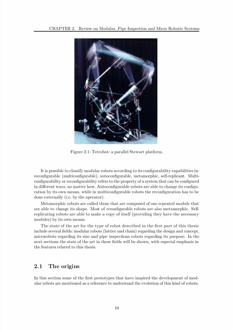
2.1 Tetrobot: a parallel Stewart platform. . . . . . . . . . . . . . . . . . . . . . 102.2 Real picture of CEBOT . . . . . . . . . . . . . . . . . . . . . . . . . . . . . 112.3 Fracta robot . . . . . . . . . . . . . . . . . . . . . . . . . . . . . . . . . . . . 122.4 Metamorphic robot . . . . . . . . . . . . . . . . . . . . . . . . . . . . . . . . 132.5 Polypod . . . . . . . . . . . . . . . . . . . . . . . . . . . . . . . . . . . . . . 142.6 Different configurations of PolyBot . . . . . . . . . . . . . . . . . . . . . . . 152.7 Different versions of PolyBot main modules . . . . . . . . . . . . . . . . . . 152.8 Overview of M-TRAN . . . . . . . . . . . . . . . . . . . . . . . . . . . . . . 162.9 M-TRAN main module . . . . . . . . . . . . . . . . . . . . . . . . . . . . . 172.10 Different configurations of M-TRAN . . . . . . . . . . . . . . . . . . . . . . 172.11 Main module of CONRO . . . . . . . . . . . . . . . . . . . . . . . . . . . . 182.12 Different configurations of CONRO . . . . . . . . . . . . . . . . . . . . . . . 192.13 Example of reconfiguration in Molecube . . . . . . . . . . . . . . . . . . . . 202.14 Molecubes new design (2007) . . . . . . . . . . . . . . . . . . . . . . . . . . 21
2.15 Crystalline robot . . . . . . . . . . . . . . . . . . . . . . . . . . . . . . . . . 222.16 Molecule robot . . . . . . . . . . . . . . . . . . . . . . . . . . . . . . . . . . 242.17 Telecube . . . . . . . . . . . . . . . . . . . . . . . . . . . . . . . . . . . . . . 252.18 Digital Clay Modules . . . . . . . . . . . . . . . . . . . . . . . . . . . . . . . 262.19 Slide motion mechanism of Chobie II . . . . . . . . . . . . . . . . . . . . . . 282.20 Chobie reconfiguration . . . . . . . . . . . . . . . . . . . . . . . . . . . . . . 292.21 ATRON . . . . . . . . . . . . . . . . . . . . . . . . . . . . . . . . . . . . . . 292.22 Active Cord Mechanism (ACM): version III (a), R3 (b), R4 (c) and R5 (d) 312.23 WormBot: CPG-driven Autonomous Robot . . . . . . . . . . . . . . . . . . 332.24 Prototype from the University of Camberra . . . . . . . . . . . . . . . . . . 342.25 Superbot modules . . . . . . . . . . . . . . . . . . . . . . . . . . . . . . . . 35
2.26 MAAM and Vertical Modules . . . . . . . . . . . . . . . . . . . . . . . . . . 362.27 I-Cubes . . . . . . . . . . . . . . . . . . . . . . . . . . . . . . . . . . . . . . 372.28 Basic motion of Micro SMA . . . . . . . . . . . . . . . . . . . . . . . . . . . 382.29 Estructure and real module of Micro SMA . . . . . . . . . . . . . . . . . . . 382.30 Denso microrobot . . . . . . . . . . . . . . . . . . . . . . . . . . . . . . . . . 392.31 Endoscope microrobots . . . . . . . . . . . . . . . . . . . . . . . . . . . . . . 392.32 LAI, LMS and LAB microrobots . . . . . . . . . . . . . . . . . . . . . . . . 402.33 12-legged endoscopic capsular robot . . . . . . . . . . . . . . . . . . . . . . 412.34 MRInspect pipe inspection robot . . . . . . . . . . . . . . . . . . . . . . . . 422.35 Foster Miller pipe inspection robot . . . . . . . . . . . . . . . . . . . . . . . 432.36 Helipipe . . . . . . . . . . . . . . . . . . . . . . . . . . . . . . . . . . . . . . 44
2.37 Thes-I pipe inspection robot . . . . . . . . . . . . . . . . . . . . . . . . . . . 45
xix
8/21/2019 Alberto Brunete Gonzalez
http://slidepdf.com/reader/full/alberto-brunete-gonzalez 20/311
2.38 Thes-III pipe inspection robot . . . . . . . . . . . . . . . . . . . . . . . . . . 45
3.1 AI models: a) Deliberative b) Reactive c) Hybrid d) Behavior-based . . . . 50
3.2 NASREM architecture . . . . . . . . . . . . . . . . . . . . . . . . . . . . . . 523.3 Example of stimulus response diagram . . . . . . . . . . . . . . . . . . . . . 563.4 FSA encoding a door traversal mechanisms . . . . . . . . . . . . . . . . . . 573.5 Potential fields . . . . . . . . . . . . . . . . . . . . . . . . . . . . . . . . . . 593.6 Basic block in subsumption architecture . . . . . . . . . . . . . . . . . . . . 61
3.7 Fuzzy command fusion example . . . . . . . . . . . . . . . . . . . . . . . . . 633.8 Example of structure in subsumption architecture . . . . . . . . . . . . . . . 643.9 Subsumption AFSM of a Three Layered Robot . . . . . . . . . . . . . . . . 653.10 Structure of Motor Schemas . . . . . . . . . . . . . . . . . . . . . . . . . . . 663.11 Activation Networks . . . . . . . . . . . . . . . . . . . . . . . . . . . . . . . 683.12 DAMN architecture . . . . . . . . . . . . . . . . . . . . . . . . . . . . . . . 69
3.13 CAMPOUT: block diagram . . . . . . . . . . . . . . . . . . . . . . . . . . . 713.14 3T intelligent controll architecture . . . . . . . . . . . . . . . . . . . . . . . 743.15 Aura Architecture . . . . . . . . . . . . . . . . . . . . . . . . . . . . . . . . 753.16 Atlantis Architecture . . . . . . . . . . . . . . . . . . . . . . . . . . . . . . . 763.17 Saphira system architecture . . . . . . . . . . . . . . . . . . . . . . . . . . . 773.18 DD&P Controller . . . . . . . . . . . . . . . . . . . . . . . . . . . . . . . . . 783.19 Control Architecture of M-TRAN . . . . . . . . . . . . . . . . . . . . . . . . 813.20 Polybot control scheme . . . . . . . . . . . . . . . . . . . . . . . . . . . . . 823.21 Neural Networks Scheme . . . . . . . . . . . . . . . . . . . . . . . . . . . . . 84
3.22 Fuzzy Logic . . . . . . . . . . . . . . . . . . . . . . . . . . . . . . . . . . . . 853.23 GA scheme in M-TRAN . . . . . . . . . . . . . . . . . . . . . . . . . . . . . 86
4.1 Detail of a wheel of the helicoidal module . . . . . . . . . . . . . . . . . . . 90
4.2 Gearhead design . . . . . . . . . . . . . . . . . . . . . . . . . . . . . . . . . 914.3 Rotation module V1 . . . . . . . . . . . . . . . . . . . . . . . . . . . . . . . 924.4 Rotation module v2 plus camera . . . . . . . . . . . . . . . . . . . . . . . . 924.5 Snake configuration plus camera . . . . . . . . . . . . . . . . . . . . . . . . 934.6 Reference system for Denavit-Hartenberg . . . . . . . . . . . . . . . . . . . 944.7 Worm-like microrobot V1 . . . . . . . . . . . . . . . . . . . . . . . . . . . . 974.8 Support module 1.1 . . . . . . . . . . . . . . . . . . . . . . . . . . . . . . . 974.9 Support module v2.0 . . . . . . . . . . . . . . . . . . . . . . . . . . . . . . . 98
4.10 Inchworm configuration based on v2.1 modules plus camera . . . . . . . . . 98
4.11 Extension module detailed mechanism . . . . . . . . . . . . . . . . . . . . . 994.12 Coordinate system for the kinematics of the support module . . . . . . . . . 1004.13 Kinematics diagrams of the extension module . . . . . . . . . . . . . . . . . 1014.14 Helicoidal module v1 . . . . . . . . . . . . . . . . . . . . . . . . . . . . . . . 1024.15 Helicoidal module V2 plus camera . . . . . . . . . . . . . . . . . . . . . . . 1034.16 Camera module v1 . . . . . . . . . . . . . . . . . . . . . . . . . . . . . . . . 104
4.17 Camera module v2 . . . . . . . . . . . . . . . . . . . . . . . . . . . . . . . . 1044.18 Batteries Module . . . . . . . . . . . . . . . . . . . . . . . . . . . . . . . . . 1054.19 SMA-based modules . . . . . . . . . . . . . . . . . . . . . . . . . . . . . . . 1074.20 Traveler Module . . . . . . . . . . . . . . . . . . . . . . . . . . . . . . . . . 1074.21 Common interface . . . . . . . . . . . . . . . . . . . . . . . . . . . . . . . . 108
4.22 Camera electronic circuits . . . . . . . . . . . . . . . . . . . . . . . . . . . . 109
xx

8/21/2019 Alberto Brunete Gonzalez
http://slidepdf.com/reader/full/alberto-brunete-gonzalez 21/311
4.23 Auto-protection control scheme . . . . . . . . . . . . . . . . . . . . . . . . . 1104.24 Auto-protection circuits . . . . . . . . . . . . . . . . . . . . . . . . . . . . . 1104.25 Consumption output . . . . . . . . . . . . . . . . . . . . . . . . . . . . . . . 112
4.26 Accelerometer tests: still module . . . . . . . . . . . . . . . . . . . . . . . . 1144.27 Module moving along a linear trajectory in the XY plane . . . . . . . . . . 1154.28 Servo moving from 30 to 150 with no load . . . . . . . . . . . . . . . . . 1154.29 Servo moving from 150 to 30 loaded . . . . . . . . . . . . . . . . . . . . . 1164.30 Snake-like configuration . . . . . . . . . . . . . . . . . . . . . . . . . . . . . 1164.31 Snake movements . . . . . . . . . . . . . . . . . . . . . . . . . . . . . . . . . 117
4.32 Snake-like configurations . . . . . . . . . . . . . . . . . . . . . . . . . . . . . 1184.33 Snake-like microrobot inside pipes . . . . . . . . . . . . . . . . . . . . . . . 1194.34 Graphical User Interface . . . . . . . . . . . . . . . . . . . . . . . . . . . . . 1204.35 Worm-like module: Sequence of movement . . . . . . . . . . . . . . . . . . . 1214.36 Helicoidal configuretion . . . . . . . . . . . . . . . . . . . . . . . . . . . . . 121
4.37 Multi-modular configuration . . . . . . . . . . . . . . . . . . . . . . . . . . . 122
5.1 Simulation Environment . . . . . . . . . . . . . . . . . . . . . . . . . . . . . 1265.2 Mathematical model of the servomotor . . . . . . . . . . . . . . . . . . . . . 1275.3 Rotation Module and Helicoidal Module . . . . . . . . . . . . . . . . . . . . 1305.4 Inchworm Modules . . . . . . . . . . . . . . . . . . . . . . . . . . . . . . . . 131
5.5 Touch Module and Traveler Module . . . . . . . . . . . . . . . . . . . . . . 1335.6 Accelerometer axis sketch . . . . . . . . . . . . . . . . . . . . . . . . . . . . 1355.7 Class diagram . . . . . . . . . . . . . . . . . . . . . . . . . . . . . . . . . . . 1375.8 Class interaction . . . . . . . . . . . . . . . . . . . . . . . . . . . . . . . . . 1395.9 Elbow Negotiation . . . . . . . . . . . . . . . . . . . . . . . . . . . . . . . . 143
6.1 Experimental setup of iGPS . . . . . . . . . . . . . . . . . . . . . . . . . . . 1486.2 Behavior of the system for irregular floors . . . . . . . . . . . . . . . . . . . 1496.3 NorthStar . . . . . . . . . . . . . . . . . . . . . . . . . . . . . . . . . . . . . 1496.4 Indoor positioning network . . . . . . . . . . . . . . . . . . . . . . . . . . . 150
6.5 Illustration of time difference of arrival (TDOA) localization . . . . . . . . . 1516.6 Example of wireless ethernet distribution of five base stations (enumerated
small circles) . . . . . . . . . . . . . . . . . . . . . . . . . . . . . . . . . . . 151
6.7 MotionStar system . . . . . . . . . . . . . . . . . . . . . . . . . . . . . . . . 1536.8 Smart Floor plate (left) and load cell (right) . . . . . . . . . . . . . . . . . . 1546.9 Ego-positioning system . . . . . . . . . . . . . . . . . . . . . . . . . . . . . . 154
6.10 Position and orientation calculation (a) and ”Alice” robot (b) . . . . . . . . 1556.11 Ego-positioning extension to chained modular robots . . . . . . . . . . . . . 1566.12 BPW34 main features (a) and photodiodes board (b) . . . . . . . . . . . . . 1576.13 Optimal RC Filter (a) and Spectral sensitivity of aSi:H (b) . . . . . . . . . 158
6.14 Current comparator for I-SWARM . . . . . . . . . . . . . . . . . . . . . . . 1586.15 Color wheel of the DLP beamer . . . . . . . . . . . . . . . . . . . . . . . . . 1596.16 Response of the beamer to a white image . . . . . . . . . . . . . . . . . . . 1596.17 Response of the beamer (without color wheel) to a white image . . . . . . . 1 6 06.18 Response of the photodiode to a red image (a) and a yellow image (b) . . . 1606.19 Response of the photodiode to a projection of sequences of black and white
images at 60 Hz (a) and 85 Hz (b) . . . . . . . . . . . . . . . . . . . . . . . 161
6.20 Response of the photodiode to a grey image . . . . . . . . . . . . . . . . . . 161
xxi

8/21/2019 Alberto Brunete Gonzalez
http://slidepdf.com/reader/full/alberto-brunete-gonzalez 22/311
6.21 Response of the photodiode to a projection of sequences of 3 (a) and 4 (b)different grey scale images at 60 Hz . . . . . . . . . . . . . . . . . . . . . . . 162
6.22 Distribution of intensity . . . . . . . . . . . . . . . . . . . . . . . . . . . . . 162
6.23 Output voltage for a black and white sequence at the point of higher (a)and lower (b) illumination . . . . . . . . . . . . . . . . . . . . . . . . . . . . 163
6.24 Binary (a) and Gray (b) code . . . . . . . . . . . . . . . . . . . . . . . . . . 1646.25 Sampling time to get the RGB values of the projected image . . . . . . . . 1656.26 Interruption Service Routine ”Photodiodes” (a) and function ”SequenceTest”
(b) pseudocode . . . . . . . . . . . . . . . . . . . . . . . . . . . . . . . . . . 1686.27 Sampling procedure . . . . . . . . . . . . . . . . . . . . . . . . . . . . . . . 1696.28 Function ”EGO Position” (a) and Main program (b) pseudocode . . . . . . 1706.29 Gray to Binary conversion scheme . . . . . . . . . . . . . . . . . . . . . . . 171
6.30 Success - error rate . . . . . . . . . . . . . . . . . . . . . . . . . . . . . . . . 172
7.1 Control Scheme . . . . . . . . . . . . . . . . . . . . . . . . . . . . . . . . . . 1747.2 Control Layers . . . . . . . . . . . . . . . . . . . . . . . . . . . . . . . . . . 175
7.3 Behavior sketch . . . . . . . . . . . . . . . . . . . . . . . . . . . . . . . . . . 1757.4 HLC and LLC commands . . . . . . . . . . . . . . . . . . . . . . . . . . . . 1767.5 Communication Layers . . . . . . . . . . . . . . . . . . . . . . . . . . . . . . 1777.6 I 2C frames . . . . . . . . . . . . . . . . . . . . . . . . . . . . . . . . . . . . 1787.7 Behavior scheme . . . . . . . . . . . . . . . . . . . . . . . . . . . . . . . . . 185
7.8 Heat dissipation sketch . . . . . . . . . . . . . . . . . . . . . . . . . . . . . . 1877.9 Maximun servomotor consumption with blocking . . . . . . . . . . . . . . . 1897.10 Extension module at its higher and lower position . . . . . . . . . . . . . . 1907.11 Behavior fusion scheme . . . . . . . . . . . . . . . . . . . . . . . . . . . . . 195
7.12 Configuration check sequence diagram . . . . . . . . . . . . . . . . . . . . . 1967.13 Ext / Contraction capabilites: a) grade 3 and b) grade 1 . . . . . . . . . . . 198
7.14 Behavior fusion scheme for Central Control behaviors . . . . . . . . . . . . 2057.15 Roulette probabilty . . . . . . . . . . . . . . . . . . . . . . . . . . . . . . . . 2137.16 Single point crossover example . . . . . . . . . . . . . . . . . . . . . . . . . 2147.17 Mutation example . . . . . . . . . . . . . . . . . . . . . . . . . . . . . . . . 215
8.1 Images taken form the camera inside a pipe . . . . . . . . . . . . . . . . . . 2208.2 Camera Interface . . . . . . . . . . . . . . . . . . . . . . . . . . . . . . . . . 2218.3 Helicoidal module inside a pipe . . . . . . . . . . . . . . . . . . . . . . . . . 2218.4 Worm module tests . . . . . . . . . . . . . . . . . . . . . . . . . . . . . . . . 222
8.5 Snake-like movement over undulated terrain . . . . . . . . . . . . . . . . . . 2238.6 Corner negotiation . . . . . . . . . . . . . . . . . . . . . . . . . . . . . . . . 2248.7 30to 120unloaded: rotation angle . . . . . . . . . . . . . . . . . . . . . . . 2258.8 30to 120unloaded: intensity . . . . . . . . . . . . . . . . . . . . . . . . . . 2258.9 30to 120unloaded: torque . . . . . . . . . . . . . . . . . . . . . . . . . . . 2268.10 30to 120loaded: rotation angle . . . . . . . . . . . . . . . . . . . . . . . . 2268.11 30to 120loaded: intensity . . . . . . . . . . . . . . . . . . . . . . . . . . . 227
8.12 30to 120loaded: tau . . . . . . . . . . . . . . . . . . . . . . . . . . . . . . 2278.13 90to 30unloaded: rotation angle . . . . . . . . . . . . . . . . . . . . . . . 2288.14 90to 30unloaded: intensity . . . . . . . . . . . . . . . . . . . . . . . . . . . 2288.15 90to 30unloaded: tau . . . . . . . . . . . . . . . . . . . . . . . . . . . . . 229
8.16 90
to 30
unloaded: rotation angle . . . . . . . . . . . . . . . . . . . . . . . 229
xxii

8/21/2019 Alberto Brunete Gonzalez
http://slidepdf.com/reader/full/alberto-brunete-gonzalez 23/311
8.17 90to 30unloaded: intensity . . . . . . . . . . . . . . . . . . . . . . . . . . . 2308.18 90to 30unloaded: tau . . . . . . . . . . . . . . . . . . . . . . . . . . . . . 2308.19 Rotation module v1 torque test . . . . . . . . . . . . . . . . . . . . . . . . . 231
8.20 1D sinusoidal movement . . . . . . . . . . . . . . . . . . . . . . . . . . . . . 2338.21 Turning movement . . . . . . . . . . . . . . . . . . . . . . . . . . . . . . . . 2338.22 Rolling movement . . . . . . . . . . . . . . . . . . . . . . . . . . . . . . . . 2348.23 Rotating movement . . . . . . . . . . . . . . . . . . . . . . . . . . . . . . . . 2358.24 Lateral shifting movement . . . . . . . . . . . . . . . . . . . . . . . . . . . . 2358.25 R+H elbow negotiation . . . . . . . . . . . . . . . . . . . . . . . . . . . . . 2378.26 R+H elbow negotiation depending on pipe diameter . . . . . . . . . . . . . 2388.27 Rotation + passive modules in a vertical sinusoidal movement . . . . . . . . 2398.28 Rotation + passive modules negotiating an elbow with and without heli-
coidal module . . . . . . . . . . . . . . . . . . . . . . . . . . . . . . . . . . . 2408.29 Inchworm locomotion composed of several extension and support modules . 241
8.30 Example of heterogenous configuration . . . . . . . . . . . . . . . . . . . . . 2428.31 Configuration check example . . . . . . . . . . . . . . . . . . . . . . . . . . 2438.32 Example of orientation behavior . . . . . . . . . . . . . . . . . . . . . . . . 2448.33 Contact, Rotation, Helicoidal and Passive . . . . . . . . . . . . . . . . . . . 2448.34 Contact and rotation modules . . . . . . . . . . . . . . . . . . . . . . . . . . 2458.35 Example of chain splitting . . . . . . . . . . . . . . . . . . . . . . . . . . . . 246
A.1 Stereolithography process . . . . . . . . . . . . . . . . . . . . . . . . . . . . 254A.2 Support columns removal . . . . . . . . . . . . . . . . . . . . . . . . . . . . 254A.3 Laser trajectory . . . . . . . . . . . . . . . . . . . . . . . . . . . . . . . . . . 255A.4 Solidification process . . . . . . . . . . . . . . . . . . . . . . . . . . . . . . . 256
A.5 Post-cure oven . . . . . . . . . . . . . . . . . . . . . . . . . . . . . . . . . . 256A.6 Detail of some parts of the rotation module v1 . . . . . . . . . . . . . . . . 257A.7 Micro-milling system . . . . . . . . . . . . . . . . . . . . . . . . . . . . . . . 258A.8 Fixation System . . . . . . . . . . . . . . . . . . . . . . . . . . . . . . . . . 258A.9 Contouring machining . . . . . . . . . . . . . . . . . . . . . . . . . . . . . . 259A.10 Helicoidal module leg generated by micromachining . . . . . . . . . . . . . . 260
C.1 U2C-12 card . . . . . . . . . . . . . . . . . . . . . . . . . . . . . . . . . . . . 268C.2 Communication box . . . . . . . . . . . . . . . . . . . . . . . . . . . . . . . 268
xxiii

8/21/2019 Alberto Brunete Gonzalez
http://slidepdf.com/reader/full/alberto-brunete-gonzalez 24/311
xxiv

8/21/2019 Alberto Brunete Gonzalez
http://slidepdf.com/reader/full/alberto-brunete-gonzalez 25/311
List of Tables
1.1 Use Cases . . . . . . . . . . . . . . . . . . . . . . . . . . . . . . . . . . . . . 4
2.1 3-D Robots summary . . . . . . . . . . . . . . . . . . . . . . . . . . . . . . . 46
2.2 2-D Robots summary . . . . . . . . . . . . . . . . . . . . . . . . . . . . . . . 46
2.3 1-D Robots summary . . . . . . . . . . . . . . . . . . . . . . . . . . . . . . . 46
3.1 Subsumption Architecture . . . . . . . . . . . . . . . . . . . . . . . . . . . . 65
3.2 Motor Schemas Architecture . . . . . . . . . . . . . . . . . . . . . . . . . . . 67
3.3 Activation Networks Architecture . . . . . . . . . . . . . . . . . . . . . . . . 69
3.4 DAMN Architecture . . . . . . . . . . . . . . . . . . . . . . . . . . . . . . . 70
3.5 Control Architecture for Multi-robot Planetary Outposts (CAMPOUT) Ar-chitecture . . . . . . . . . . . . . . . . . . . . . . . . . . . . . . . . . . . . . 72
4.1 Modules main characteristics . . . . . . . . . . . . . . . . . . . . . . . . . . 90
4.2 Denavit-Hartenberg parameters . . . . . . . . . . . . . . . . . . . . . . . . . 93
4.3 Velocity in a 30cm ø pipe at different angles (helicoidal module) . . . . . . 1034.4 Velocity in a 30cm ø pipe at different angles (2nd helicoidal module) . . . . 103
4.5 Power Consumption . . . . . . . . . . . . . . . . . . . . . . . . . . . . . . . 111
6.1 Setup description . . . . . . . . . . . . . . . . . . . . . . . . . . . . . . . . . 156
6.2 Color coding table . . . . . . . . . . . . . . . . . . . . . . . . . . . . . . . . 165
6.3 Programming time and speed . . . . . . . . . . . . . . . . . . . . . . . . . . 170
7.1 LLC1 commands: sending . . . . . . . . . . . . . . . . . . . . . . . . . . . . 179
7.2 LLC1 commands: answering . . . . . . . . . . . . . . . . . . . . . . . . . . . 179
7.3 LLC2 commands: sending . . . . . . . . . . . . . . . . . . . . . . . . . . . . 180
7.4 LLC2 commands: answering . . . . . . . . . . . . . . . . . . . . . . . . . . . 180
7.5 HLC commands: sending . . . . . . . . . . . . . . . . . . . . . . . . . . . . 181
7.6 HLC commands: answering . . . . . . . . . . . . . . . . . . . . . . . . . . . 181
7.7 Behavior encoding: Avoid overheating . . . . . . . . . . . . . . . . . . . . . 188
7.8 Behavior encoding: Avoid actuator damage . . . . . . . . . . . . . . . . . . 188
7.9 Behavior encoding: Avoid mechanical damages . . . . . . . . . . . . . . . . 190
7.10 Behavior encoding: Self diagnostic . . . . . . . . . . . . . . . . . . . . . . . 191
7.11 Behavior encoding: Situation awareness . . . . . . . . . . . . . . . . . . . . 191
7.12 Behavior encoding: Environment diagnostic . . . . . . . . . . . . . . . . . . 192
7.13 Behavior encoding: Vertical sinusoidal movement . . . . . . . . . . . . . . . 193
7.14 Behavior encoding: Horizontal sinusoidal movement . . . . . . . . . . . . . 193
7.15 Behavior encoding: Worm-like movement . . . . . . . . . . . . . . . . . . . 194
xxv

8/21/2019 Alberto Brunete Gonzalez
http://slidepdf.com/reader/full/alberto-brunete-gonzalez 26/311
7.16 Behavior encoding: Push-Forward movement . . . . . . . . . . . . . . . . . 1947.17 Table of Rules . . . . . . . . . . . . . . . . . . . . . . . . . . . . . . . . . . . 1997.18 Behavior encoding: Balance / Stability . . . . . . . . . . . . . . . . . . . . . 201
7.19 Behavior encoding: Straight forward / backwards . . . . . . . . . . . . . . . 2027.20 Behavior encoding: Edge Following . . . . . . . . . . . . . . . . . . . . . . . 2027.21 Behavior encoding: Pipe Following . . . . . . . . . . . . . . . . . . . . . . . 2037.22 Behavior encoding: Obstacle negotiation . . . . . . . . . . . . . . . . . . . . 2037.23 GA Configuration demand genes value range . . . . . . . . . . . . . . . . . 2097.24 GA Configuration demand parameters . . . . . . . . . . . . . . . . . . . . . 2107.25 GA Parameter optimization genes value range . . . . . . . . . . . . . . . . . 211
8.1 Speed and slope for different configurations . . . . . . . . . . . . . . . . . . 2208.2 Parameters for the servomotor tests . . . . . . . . . . . . . . . . . . . . . . 2248.3 Speed test of the inchworm configuration . . . . . . . . . . . . . . . . . . . 231
8.4 Speed test of helicoidal module . . . . . . . . . . . . . . . . . . . . . . . . . 232
xxvi

8/21/2019 Alberto Brunete Gonzalez
http://slidepdf.com/reader/full/alberto-brunete-gonzalez 27/311
Acknowledgements
xxvii

8/21/2019 Alberto Brunete Gonzalez
http://slidepdf.com/reader/full/alberto-brunete-gonzalez 28/311
xxviii
8/21/2019 Alberto Brunete Gonzalez
http://slidepdf.com/reader/full/alberto-brunete-gonzalez 29/311
Chapter 1
Introduction
“When I read a book I seem to read it with my eyes only, but now and then I come across a passage, perhaps only a phrase, which has a meaning for me, and it becomes
part of me”
W. Somerset Maugham
1.1 Motivation and framework of the thesis
The idea that has given place to this thesis is the lack of multiconfigurable heterogenousmicrorobotic systems to inspect the inner part of narrow pipes. There are many robotsfor pipe inspection, but they are too big. There are a lot of modular systems (both latticeand chain) but they are homogenous and also too wider and box-shaped what makesthem not suitable for pipes. And there are microrobots for colonoscopy but they are tooslow for pipe inspection. In summary, the idea of the thesis is to put together all theseadvantages of modules, micro and pipe inspection robots into a “Intelligent HeterogeneousMulti-configurable Chained Microrobotic Modular System”
After a rigorous study of the state of the art, it was decided that this thesis should lieamongst three fields: micro-robotics, modular robots and pipe-inspection robots. Thereare many robots and studies in each of these fields, but there are none that combines allof them. This thesis tries to create a model to develop microrobots capable to move innarrow pipes to explore them. The purpose is to do it by using modular robotic principles.
Once the basics of the research were clear, a control scheme had to be built uponthe mechanical system. And the selected approach was behavior-based control, for manyreasons that will be described in chapter 7.
After some time of research, it was necessary to increase the dimensions of the proto-types in order to facilitate the fabrication of the prototypes, so the target pipe diameters
moved to 40mm diameter. This made possible to build more robust prototypes and to add
1

8/21/2019 Alberto Brunete Gonzalez
http://slidepdf.com/reader/full/alberto-brunete-gonzalez 30/311
CHAPTER 1. Introduction
some other functionalities. This is the reason why in this thesis it is talked about micro-robots: although the measures of the prototypes are a little bit bigger for a microrobot,the concept was created to be applicable to a microrobot.
Although the first idea was to develop the microrobot for pipe inspection, the expe-rience acquired with the first prototypes causes to realize that locomotion systems usedinside pipes were also suitable outside them, and that the prototypes and the control ar-chitecture were useful in open spaces. That is why research was extended to open spacesand the ego-positioning system was added.
This thesis has been developed along three projects: MICROROB (TAMAI), MICRO-MULT (MICROTEC) and I-SWARM.
The purpose of the MICROTUB project is the design and construction of a micro-robot able to move in pipes and tubes (straight or not) of about 26mm diameter. Thedevelopment of this micro-robot will guide to the automation of inspection and mainte-
nance of pipes and tubes at a lower cost in for example sewer systems, gas pipelines, water,gas and heating pipes in buildings, etc.
MICROMULT stands for Multi-configurable Micro-robotic Systems. It is the subpro- ject 1 in the pro ject MICROTEC (Integration of Micromanufacturing, Microassembly andMicrorobotics technologies)
The main goals of MICROMULT are:
• design and construction of a multi-configurable heterogeneous modular micro-roboticsystem able to move in narrow environments.
• design and construction of a micro-assembly robotic station to develop micro-assembly,
micro-gripping and micro-machining techniques.
The I- SWARM project intends to lead the way towards the development of an artificialant and thus make a significant step forward in robotics research by bringing togetherexpertise in micro-robotics, in distributed and adaptive systems as well as in self-organisingbiological swarm systems. Building on the expertise of two EC-funded projects, MINIMANand MiCRoN, this project will produce technological advances to facilitate the mass-production of micro-robots, which can then be employed as a “real” swarm consistingof up to 1000 robot clients. These clients will all be equipped with limited, on-boardintelligence. Such a robot swarm can perform a variety of applications, including microassembly, biological, medical or cleaning tasks.
1.2 Topics of the thesis
1.2.1 About Microrobotics
Microrobotics (or microbotics) is the field of miniature robotics, in particular mobile robotswith characteristic dimensions less than 1 mm. The term can also be used for robotscapable of handling micrometer size components, which is the case of the robots developpedin this thesis, in which some components are smaller than 1 mm. Generally speaking, the
term microrobot is used to described very small robots.
2
8/21/2019 Alberto Brunete Gonzalez
http://slidepdf.com/reader/full/alberto-brunete-gonzalez 31/311
1.2. Topics of the thesis
The earliest research and conceptual design of such small robots was conducted inthe early 1970s in (then) classified research for U.S. intelligence agencies. Applicationsenvisioned at that time included prisoner of war rescue assistance and electronic intercept
missions. The underlying miniaturization support technologies were not fully developedat that time, so that progress in prototype development was not immediately forthcomingfrom this early set of calculations and concept design.
The concept of building very small robots, and benefiting from recent advances inMicro Electro Mechanical Systems (MEMS) was publicly introduced in the seminal paperby Anita M. Flynn, “Gnat Robots (and How They Will Change Robotics)” [Flynn, 1987].
Microbots were born thanks to the appearance of the microcontroller in the lastdecade of the 20th century, and the appearance of miniature mechanical systems on silicon(MEMS), although many microbots do not use silicon for mechanical components otherthan sensors.
One of the major challenges in developing a microrobot is to achieve motion using avery limited power supply. In this thesis microrobots need a power supply cable to work.
1.2.2 About Modular Robots
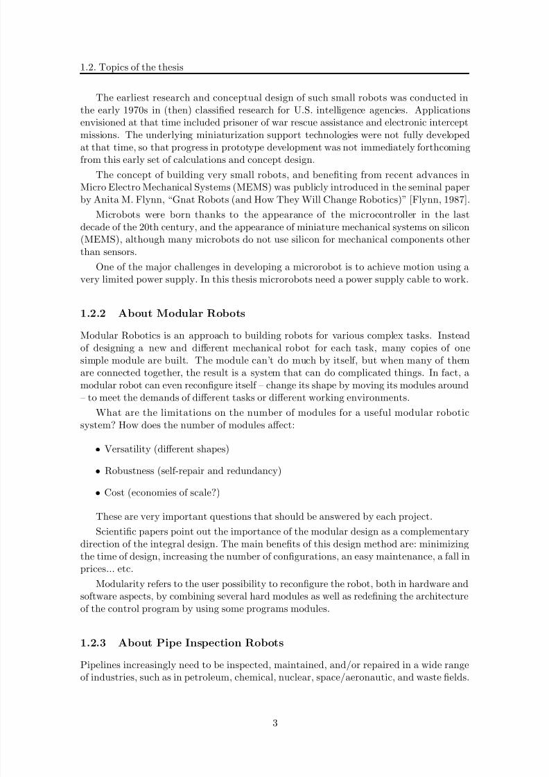
Modular Robotics is an approach to building robots for various complex tasks. Insteadof designing a new and different mechanical robot for each task, many copies of onesimple module are built. The module can’t do much by itself, but when many of themare connected together, the result is a system that can do complicated things. In fact, amodular robot can even reconfigure itself – change its shape by moving its modules around– to meet the demands of different tasks or different working environments.
What are the limitations on the number of modules for a useful modular roboticsystem? How does the number of modules affect:
• Versatility (different shapes)
• Robustness (self-repair and redundancy)
• Cost (economies of scale?)
These are very important questions that should be answered by each project.
Scientific papers point out the importance of the modular design as a complementary
direction of the integral design. The main benefits of this design method are: minimizingthe time of design, increasing the number of configurations, an easy maintenance, a fall inprices... etc.
Modularity refers to the user possibility to reconfigure the robot, both in hardware andsoftware aspects, by combining several hard modules as well as redefining the architectureof the control program by using some programs modules.
1.2.3 About Pipe Inspection Robots
Pipelines increasingly need to be inspected, maintained, and/or repaired in a wide range
of industries, such as in petroleum, chemical, nuclear, space/aeronautic, and waste fields.
3
8/21/2019 Alberto Brunete Gonzalez
http://slidepdf.com/reader/full/alberto-brunete-gonzalez 32/311
CHAPTER 1. Introduction
Tests Basic General ConfigurationDemand
Surveillance
Robot Configuration Known Known Known Unknown KnownHomogeneity Homogeneous Homogeneous Heterogeneous Heterogeneous Heterogeneous
Environment Known Unknown Unknown Known UnknownTask Known Known Known Known Unknown
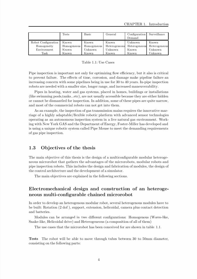
Table 1.1: Use Cases
Pipe inspection is important not only for optimizing flow efficiency, but it also is criticalto prevent failure. The effects of time, corrosion, and damage make pipeline failure anincreasing concern with some pipelines being in use for 30 to 40 years. In-pipe inspectionrobots are needed with a smaller size, longer range, and increased maneuverability.
Pipes in heating, water and gas systems, placed in homes, buildings or installations
(like swimming pools,tanks...etc), are not usually accessible because they are either hiddenor cannot be dismantled for inspection. In addition, some of these pipes are quite narrow,and most of the commercial robots can not get into them.
As an example, the inspection of gas transmission mains requires the innovative mar-riage of a highly adaptable/flexible robotic platform with advanced sensor technologiesoperating as an autonomous inspection system in a live natural gas environment. Work-ing with New York GAS and the Department of Energy, Foster-Miller has developed andis using a unique robotic system called Pipe Mouse to meet the demanding requirementsof gas pipe inspection.
1.3 Objectives of the thesis
The main objective of this thesis is the design of a multiconfigurable modular heteroge-neous microrobot that gathers the advantages of the microrobots, modular robots andpipe inspection robots. This includes the design and fabrication of modules, the design of the control architecture and the development of a simulator.
The main objectives are explained in the following sections.
Electromechanical design and construction of an heteroge-
neous multi-configurable chained microrobotIn order to develop an heterogenous modular robot, several heterogenous modules have tobe built: Rotation (2 dof ), support, extension, helicoidal, camera plus contact detectionand batteries.
Modules can be arranged in two different configurations: Homogenous (Worm-like,Snake-like, Helicoidal drive) and Heterogeneous (a composition of all of them)
The use cases that the microrobot has been conceived for are shown in table 1.1.
Tests The robot will be able to move through tubes between 30 to 50mm diameter,
consisting on the following parts:
4
8/21/2019 Alberto Brunete Gonzalez
http://slidepdf.com/reader/full/alberto-brunete-gonzalez 33/311
1.3. Objectives of the thesis
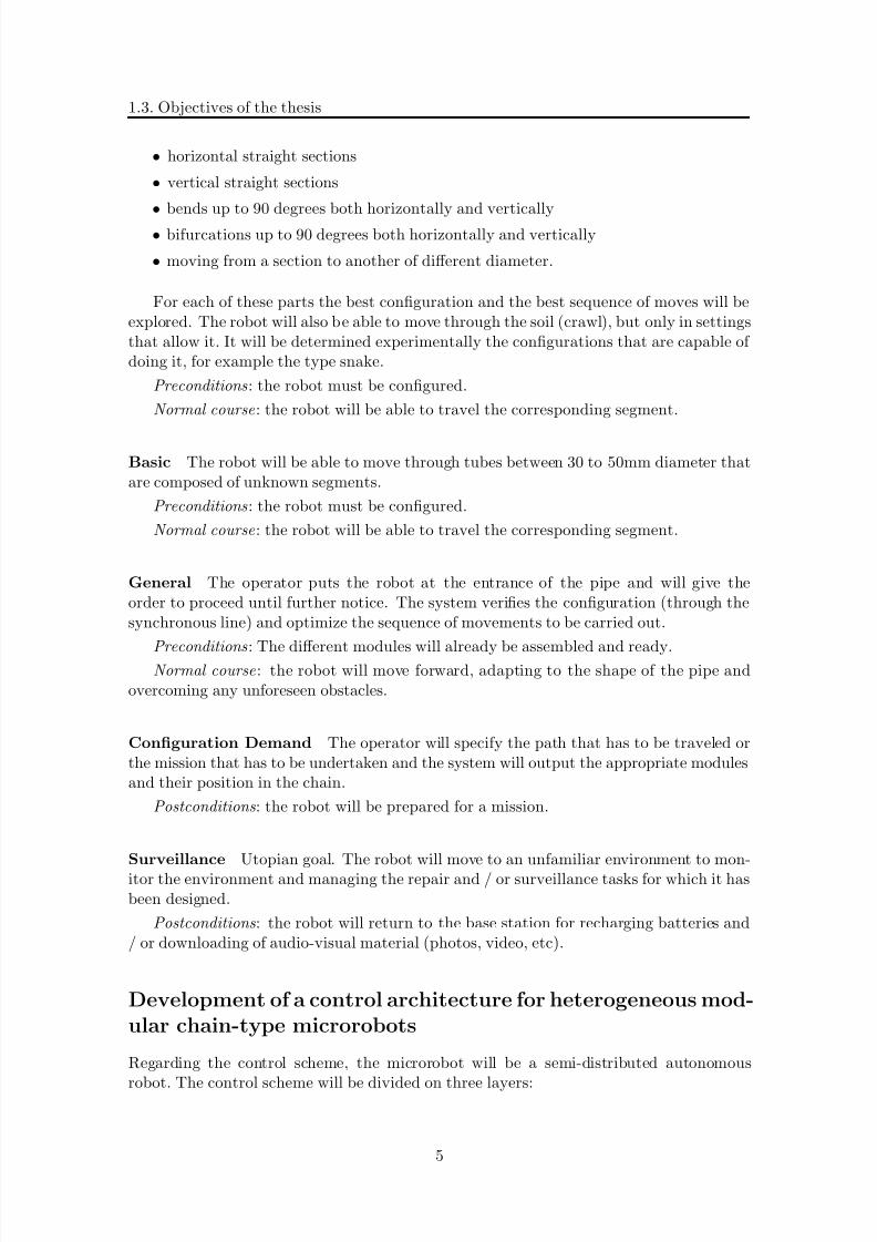
• horizontal straight sections
• vertical straight sections
• bends up to 90 degrees both horizontally and vertically
• bifurcations up to 90 degrees both horizontally and vertically
• moving from a section to another of different diameter.
For each of these parts the best configuration and the best sequence of moves will beexplored. The robot will also be able to move through the soil (crawl), but only in settingsthat allow it. It will be determined experimentally the configurations that are capable of doing it, for example the type snake.
Preconditions : the robot must be configured.
Normal course : the robot will be able to travel the corresponding segment.
Basic The robot will be able to move through tubes between 30 to 50mm diameter thatare composed of unknown segments.
Preconditions : the robot must be configured.
Normal course : the robot will be able to travel the corresponding segment.
General The operator puts the robot at the entrance of the pipe and will give theorder to proceed until further notice. The system verifies the configuration (through thesynchronous line) and optimize the sequence of movements to be carried out.
Preconditions : The different modules will already be assembled and ready.Normal course : the robot will move forward, adapting to the shape of the pipe and
overcoming any unforeseen obstacles.
Configuration Demand The operator will specify the path that has to be traveled orthe mission that has to be undertaken and the system will output the appropriate modulesand their position in the chain.
Postconditions : the robot will be prepared for a mission.
Surveillance Utopian goal. The robot will move to an unfamiliar environment to mon-itor the environment and managing the repair and / or surveillance tasks for which it hasbeen designed.
Postconditions : the robot will return to the base station for recharging batteries and/ or downloading of audio-visual material (photos, video, etc).
Development of a control architecture for heterogeneous mod-ular chain-type microrobots
Regarding the control scheme, the microrobot will be a semi-distributed autonomous
robot. The control scheme will be divided on three layers:
5
8/21/2019 Alberto Brunete Gonzalez
http://slidepdf.com/reader/full/alberto-brunete-gonzalez 34/311
CHAPTER 1. Introduction
• Low level: embedded in each module. It will control the movements of the moduleand the response to external unexpected extimuli. Easy to implement in smallmodules with limited microcontrollers.
• Heterogenous layer: it is the interpreter from the high level control to the low levelcontrol of each module.
• High level: central control, planning. Thinks of the microrobot as a whole, not eachmodule individually.
The control architecture will be enhance with an offline genetic algorithm aimed atimproving the configuration of the microrobotic modular chain and to optimize its loco-motion parameters.
Development of a simulator for the previous microroboticsystems
Due to the limitations in the fabrication process and its high cost, a simulation environ-ment will be created with several purposes: to develop the control architecture withoutdamaging the modules and to developed new prototypes and test them before fabricatingthem.
The physical simulator will include an electronic simulator that emulates the micro-controller program that is running on the modules, including physical signals (synchro-nization signal), I2C communications, etc. To maintain the independence of each module,
each control programs will run in a different thread.
This design facilitates the transfer of the code from the simulator to real modules.
Development of systems for position measurement and trav-eled distance measurement
A system will be developed and integrated in the robot that allows to know the positionin open spaces and the traveled distance inside pipes.
1.4 Overview of the thesis
Chapter 2 and Chapter 3 will give an overview of the state of the art in “Modular,Pipe Inspection and Micro Robotic Systems” and “ Control Architectures for ModularMicrorobots”
Chapter 4 will present the modules developed and its different versions, how theyhave evolved and the problems that have appeared during its construction.
The simulation environment that has been created will be described in Chapter 5.It will explain the physical dynamic engine, the control and electronic simulation and the
programming structure.
6
8/21/2019 Alberto Brunete Gonzalez
http://slidepdf.com/reader/full/alberto-brunete-gonzalez 35/311
1.4. Overview of the thesis
Chapter 6 will be dedicated to a positioning system that allows the robot to knowits position in open space, based on the emission of coded images and its reception viaphotodiodes.
The control architecture will be explained in Chapter 7: the behavior-based architec-ture, the communication system and the Module Description Language (MDL), the layerswith the high and low level controls and the offline genetic algorithm for optimization.
Chapter 8 will show the test that have been performed and its results, with realmodules and in the simulator.
Finally, Chapter 9 will show the conclusions, some remarks about the main contri-bution of the thesis and related publications and the future work.
7
8/21/2019 Alberto Brunete Gonzalez
http://slidepdf.com/reader/full/alberto-brunete-gonzalez 36/311
CHAPTER 1. Introduction
8

8/21/2019 Alberto Brunete Gonzalez
http://slidepdf.com/reader/full/alberto-brunete-gonzalez 37/311
Chapter 2
Review on Modular, PipeInspection and Micro Robotic
Systems
”Everything should be made as simple as possible, but not one bit simpler”
Albert Einstein
The key word in modular robot is “module”. But what is a “module”? In this thesisit will be used the following definition1: “A module is a piece or a set of pieces that are repeated in a construction of any kind, to make it easier, regular and economic” . Thus,a robotic module would be: “A module that performs totally or partially typical tasks of a robot, and that has the possibility to interact with other modules”. Finally, a modularrobot is a “robot composed of modules, i.e., a robot composed of parts that have indepen-dent functionalities but that are able to interact with each other in one or another way,giving as a result an entity with new capabilities”.
What are the advantages of using modular robots? Some of the main advantages are:
• Provide the system with configurability: multiconfigurability, reconfigurability andautoconfigurability
• Increase fault tolerance: a module can fail without compromising the whole system
• Make system scalable: new modules can be added without reconfiguration of thewhole system.
• Reduce the cost of large production because only one or few modules have to bemassively produced and there is no assembly needed between parts.
1
From the “Real Academia Espanola (RAE)”
9
8/21/2019 Alberto Brunete Gonzalez
http://slidepdf.com/reader/full/alberto-brunete-gonzalez 38/311
CHAPTER 2. Review on Modular, Pipe Inspection and Micro Robotic Systems
Figure 2.1: Tetrobot: a parallel Stewart platform.
It is possible to classify modular robots according to its configurability capabilities in:reconfigurable (multiconfigurable), autoconfigurable, metamorphic, self-replicant. Multi-configurability or reconfigurability refers to the property of a system that can be configuredin different ways, no matter how. Autoconfigurable robots are able to change its configu-ration by its own means, while in multiconfigurable robots the reconfiguration has to bedone externally (i.e. by the operator).
Metamorphic robots are called those that are composed of one repeated module thatare able to change its shape. Most of reconfigurable robots are also metamorphic. Self-replicating robots are able to make a copy of itself (providing they have the necessarymodules) by its own means.
The state of the art for the type of robot described in the first part of this thesis
include several fields: modular robots (lattice and chain) regarding the design and concept,microrobots regarding its size and pipe inspections robots regarding its purpose. In thenext sections the state of the art in these fields will be shown, with especial emphasis inthe features related to this thesis.
2.1 The origins
In this section some of the first prototypes that have inspired the development of mod-ular robots are mentioned as a reference to understand the evolution of this kind of robots.
10

8/21/2019 Alberto Brunete Gonzalez
http://slidepdf.com/reader/full/alberto-brunete-gonzalez 39/311
2.1. The origins
Figure 2.2: Real picture of CEBOT
TETROBOT [Hamlin and Sanderson, 1996], from the Rensselaer Polytechnic Insti-tute, is a modular system for the design, implementation and control of a class of highlyredundant parallel robotic mechanisms developed in 1996 (figure 2.1). It is an actuatedrobotic structure which may be reassembled into many different configurations while stillbeing controlled by the same hardware and software architecture. Some implementationsthat can be obtained are a double octahedral platform, a tetrahedral arm and a six–leggedwalker.
Main researchers: G.J. Hamlin and A.C. Sanderson
Web: http://www.rpi.edu/dept/cie/faculty_sanderson.html
CEBOT (Cellular Robotic System) [Fukuda and Kawauchi, 1990], from Nagoya Uni-versity, is a dynamically configurable robot that has the capability of self-organizing,self-evolution and functional amplification (ability of a system to coordinate together toaccomplish tasks that cannot be performed by the individual units themselves).
The CEBOT (figure 2.2) consists of many robotic units with a simple function, namedcell. The CEBOT can reconfigure the whole system depending on given tasks and en-vironments and organize collective or swarm intelligence. The concept of the CEBOTis based on biological organization constructed by enormous natural cells. This researchproject includes mutual communication between cells, the optimum dynamic knowledge
allocation among cells, the reconfiguration strategy of the system and the artificial-lifesuch as the cooperative behavior modeling of ants. This invokes many interesting researchproblems, such as dynamic decentralized planning, dynamic distribution and coordinatedcontrol system as well as hardware systems. Experiments in automated re-configurationwere carried out, but the robot did not self-reconfigure because a manipulator arm wasrequired for this.
Main researcher: T. Fukuda.
Web: http://www.mein.nagoya-u.ac.jp/staff/fukuda-e.html
Fracta was created at the Murata Laboratory. The Murata Lab has been one of the
first in researching modular reconfigurable robots. There, it has been developed from 1998,
11
8/21/2019 Alberto Brunete Gonzalez
http://slidepdf.com/reader/full/alberto-brunete-gonzalez 40/311
CHAPTER 2. Review on Modular, Pipe Inspection and Micro Robotic Systems
(a) 2D (b) 3D Universal Structure
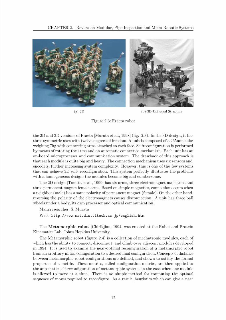
Figure 2.3: Fracta robot
the 2D and 3D versions of Fracta [Murata et al., 1998] (fig. 2.3). In the 3D design, it hasthree symmetric axes with twelve degrees of freedom. A unit is composed of a 265mm cubeweighing 7kg with connecting arms attached to each face. Selfreconfiguration is performedby means of rotating the arms and an automatic connection mechanism. Each unit has anon-board microprocessor and communication system. The drawback of this approach isthat each module is quite big and heavy. The connection mechanism uses six sensors and
encoders, further increasing system complexity. However, this is one of the few systemsthat can achieve 3D self- reconfiguration. This system perfectly illustrates the problemswith a homogeneous design: the modules become big and cumbersome.
The 2D design [Tomita et al., 1999] has six arms, three electromagnet male arms andthree permanent magnet female arms. Based on simple magnetics, connection occurs whena neighbor (male) has a same polarity of permanent magnet (female). On the other hand,reversing the polarity of the electromagnets causes disconnection. A unit has three ballwheels under a body, its own processor and optical communication.
Main researcher: S. Murata
Web: http://www.mrt.dis.titech.ac.jp/english.htm
The Metamorphic robot [Chirikjian, 1994] was created at the Robot and ProteinKinematics Lab, Johns Hopkins University.
The Metamorphic robot (figure 2.4) is a collection of mechatronic modules, each of which has the ability to connect, disconnect, and climb over adjacent modules developedin 1994. It is used to examine the near-optimal reconfiguration of a metamorphic robotfrom an arbitrary initial configuration to a desired final configuration. Concepts of distancebetween metamorphic robot configurations are defined, and shown to satisfy the formalproperties of a metric. These metrics, called configuration metrics, are then applied tothe automatic self-reconfiguration of metamorphic systems in the case when one moduleis allowed to move at a time. There is no simple method for computing the optimal
sequence of moves required to reconfigure. As a result, heuristics which can give a near
12

8/21/2019 Alberto Brunete Gonzalez
http://slidepdf.com/reader/full/alberto-brunete-gonzalez 41/311
2.2. Modular robots
Figure 2.4: Metamorphic robot
optimal solution must be used. The technique of Simulated Annealing is used to drive thereconfiguration process with configuration metrics as cost functions.
Main researcher: G. Chirikjian
Web: http://caesar.me.jhu.edu/research/metamorphic_robot.html
2.2 Modular robots
In this section the most important designs on modular robots are described. Most of
them are chain, lattice or hybrid modular robots. Lattice architectures have units thatare arranged and connected in some regular, space-filling three-dimensional pattern, suchas a cubical or hexagonal grid. Control and motion are executed in parallel. Latticearchitectures usually offer simpler computational representation that can be more easilyscaled to complex systems.
Chain/tree architectures have units that are connected together in a string or treetopology. This chain or tree can fold up to become space filling, but underlying architectureis serial. Chain architectures can reach any point in space, and are therefore more versatilebut more computationally difficult to represent and analyze.
2.2.1 PolyBot and PolyPod
PARC - Palo Alto Research Center.
Systems and Practices Laboratory. Modular Robotics Lab.
Main Researcher: Mark Yim.
http://www2.parc.com/spl/projects/modrobots/
Polypod is a bi-unit modular robot developed in 1994. This means that the robot isbuilt up of exactly two types of modules that are repeated many times. This repetitionmakes manufacturing easier and cheaper. Dynamic reconfigurability [Yim, 1994] allows the
robot to be highly versatile, reconfiguring itself to whatever shape best suits the current
13

8/21/2019 Alberto Brunete Gonzalez
http://slidepdf.com/reader/full/alberto-brunete-gonzalez 42/311
CHAPTER 2. Review on Modular, Pipe Inspection and Micro Robotic Systems
(a) Main modules (b) Different configurations
Figure 2.5: Polypod
task. To study this versatility, locomotion was chosen as the class of tasks for examination.
Polypod (fig. 2.5) is made up of two types of modules called Segments and Nodes.Segments are two degree of freedom parallel mechanisms composed of 10 links. Thekinematics of the resulting mechanism is similar to two prismatic joints joined togetherby a revolute joint where the prismatic joints are constrained to have the same length.
The structure is essentially a two four bar linkages attached by two other links with anadded sliding bar constraining four joints in the two four bars to remain collinear. The twodegrees of freedom are not exactly a prismatic degree of freedom and a revolute degree of freedom, but it is easy to intuitively think of it that way. The revolute degree of freedomhas a range of motion of +45 and -45 degrees, and the prismatic degree of freedom canchange the length of the module from about 1 inch to 2.5 inches tall.
Each segment module contains all the components to be a stand-alone robot in it-self (except for power): processor (Motorola XC68HC11E2), two DC motors, IR prox-imity sensing, crude force/torque sensing, joint angle position sensing (potentiometers)and Inter-module Communication: SPI plus local IR communication between adjacentmodules.
Power is supplied by the second type of modules called Nodes. Nodes are rigid cubeshaped modules roughly 5cmx5cmx5cm with 6 connection ports whose main purpose is tohold gel-cell batteries and to allow for non-serial chain robots.
PolyBot [Yim et al., 2000] [Yim et al., 2001] [Yim et al., 2007] is the evolution of PolyPod from year 1997 (fig. 2.6). It is made up of many repeated modules. Each module
is virtually a robot itself having a computer, a motor, sensors and the ability to attachto other modules. In some cases, power is supplied off board and passed from module tomodule. These modules attach together to form chains, which can be used like an arm ora leg or a finger depending on the task at hand.
PolyBot has gone through many variations with three basic generations. The evolutionof the main module can be seen in fig. 2.7.
The first generation of PolyBot has the basic ideas shared in all the generations of repeated modules being about 5 cm on a side. The modules are built up from simple hobbyRC servos, power and computation are supplied offboard. The modules are manuallyscrewed together, so they do not self-reconfigure.
Following versions were integrating more robust servos, connection plates, power supply
14

8/21/2019 Alberto Brunete Gonzalez
http://slidepdf.com/reader/full/alberto-brunete-gonzalez 43/311
2.2. Modular robots
Figure 2.6: Different configurations of PolyBot
Figure 2.7: Different versions of PolyBot main modules
(NiMH batteries) and electronics (on board control with a PIC16F877). The modules mayrun either fully autonomously or under supervisory control from a PC sending commandsthrough a wired or wireless radio link.
Generation II of PolyBot includes onboard computing (Power PC 555) as well as theability to reconfigure automatically via shape memory alloy actuated latches. Docking of the chains is aided by infrared emitters and detectors.
The last version, v.III, is 5cm x 5cm x 5cm and weights 70 grams. It has a DC motorwith Hall effect sensor, a potentiometer for angle measurement, 4 accelerometers, contactsensors and 4 IR leds for inter-module communications. The main processing unit is stilla PowerPC and the communications amongst the modules are done via a CAN bus.
2.2.2 M-TRAN
Intelligent Systems Institute.
National Institute of Advanced Industrial Science and Technology (AIST).
Main researcher: H. Kurokawa and S. Murata
http://unit.aist.go.jp/is/frrg/dsysd/mtran3/index.htm
15

8/21/2019 Alberto Brunete Gonzalez
http://slidepdf.com/reader/full/alberto-brunete-gonzalez 44/311
CHAPTER 2. Review on Modular, Pipe Inspection and Micro Robotic Systems
Figure 2.8: Overview of M-TRAN
M-TRAN (Modular TRANsformer) [Murata et al., 2002] [Kurokawa et al., 2003] [Mu-rata and Kurokawa, 2007] [Yoshida et al., 2003] is a self-reconfigurable modular robot thathas been developed by AIST and Tokyo-Tech since 1998. A number of M-TRAN modulescan form:
• a 3-D structure which changes its own configuration
• a 3-D structure which generates smaller robots
• a multi-DOF robot which flexibly locomotes
• a robot which metamorphoses
The M-TRAN system can change its 3-D structure and its motion in order to adaptitself to the environment. In small sized configuration, it walks in a form of legged robot,then metamorphoses into a snake-like robot to enter narrow spaces (fig. 2.8). A largestructure can gradually change its configuration to make a flow-like motion, climb a stepby transporting modules one by one, and produce a tower structure to look down. Itcan also generate multiple walkers. Possible applications of the M-TRAN are autonomousexploration under unknown environment such as planetary explorations, or search andrescue operation in disaster areas.
The design of M-TRAN has the advantages of two types of modular robots, lattice
type and chain (linear) type. This hybrid design, unique 3-D shape of the block parts,and parallel joint axes are all keys to realize a flexible self-reconfigurable robotic system.
An M-TRAN module is composed of two blocks (1/2 cubic and 1/2 cylindrical) and alink (Fig.2.9). Each of the three flat surfaces of each block can mechanically connect andcouple with a surface of another module. All the connection surfaces have their genderand an active (male) surface can couple with a passive (female) surface in four possiblerelative orientations. The connection is controlled by the module itself.
As M-TRAN I and II used permanent magnets and SMA actuators for their connectionmechanism (details), it was time and energy consuming to control module connection. Inorder for faster and more power-effective consuming connection, a mechanical connector
was designed in M-TRAN III.
16
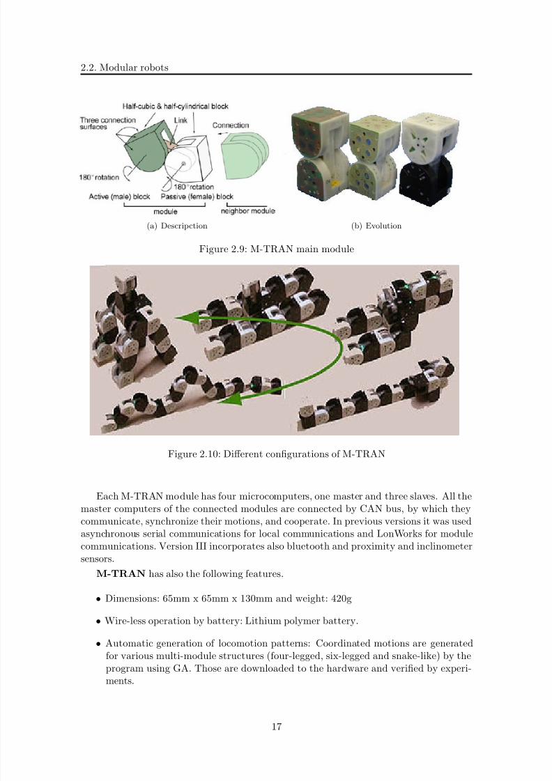
8/21/2019 Alberto Brunete Gonzalez
http://slidepdf.com/reader/full/alberto-brunete-gonzalez 45/311
2.2. Modular robots
(a) Descripction (b) Evolution
Figure 2.9: M-TRAN main module
Figure 2.10: Different configurations of M-TRAN
Each M-TRAN module has four microcomputers, one master and three slaves. All themaster computers of the connected modules are connected by CAN bus, by which theycommunicate, synchronize their motions, and cooperate. In previous versions it was usedasynchronous serial communications for local communications and LonWorks for module
communications. Version III incorporates also bluetooth and proximity and inclinometersensors.
M-TRAN has also the following features.
• Dimensions: 65mm x 65mm x 130mm and weight: 420g
• Wire-less operation by battery: Lithium polymer battery.
• Automatic generation of locomotion patterns: Coordinated motions are generatedfor various multi-module structures (four-legged, six-legged and snake-like) by theprogram using GA. Those are downloaded to the hardware and verified by experi-
ments.
17

8/21/2019 Alberto Brunete Gonzalez
http://slidepdf.com/reader/full/alberto-brunete-gonzalez 46/311
CHAPTER 2. Review on Modular, Pipe Inspection and Micro Robotic Systems
Figure 2.11: Main module of CONRO
• Distributed control: The robot motion is controlled by all the modules CPUs.
• Motion generation: Locomotion for several structure robots is automatically gener-ated in the host PC by using CPG technique and GA. Then such locomotion patternsare played back by the hardware.
• M-TRAN can achieve quadruped walker, H-shape, snake and a caterpillar configu-rations amongst others(fig. 2.10).
M-TRANs concept is very similar to the one presented in this thesis, with the exceptionthat M-TRAN is homogeneous and Microtub is heterogenous.
2.2.3 CONRO
Polymorphic Robotics Laboratory. Information Science Institute.
University of Southern California.
Main reseacher: P. Will.
http://www.isi.edu/robots/conro/
The CONRO self-reconfigurable robot [Shen et al., 2000] [Shen et al., 2002] [Salemiet al., 2004] is made of a set of connectable modules 2.11. Each module is an autonomousunit that contains two batteries, one STAMP II micro-controller, two motors, four pairsof IR transmitters/receivers and four docking connectors to allow connections with othermodules.
Modules can be connected together by their docking connectors, located at either endof each module. Male connectors consist of two pins. Female connectors have an SMA-triggered locking/releasing mechanism. Each module has two degrees of freedom: DOF1for pitch (up and down) and DOF2 for yaw (left and right). With these two DOFs, asingle module can wiggle its body but cannot change its location. However, when two ormore modules connect to form a structure, they can accomplish many different types of locomotion. For example, a body of six legs can perform hexapod gaits, while a chainof modules can mimic a snake or a caterpillar motion (fig. 2.12). To make an n-module
caterpillar move forward, each module˜Os DOF1 goes through a series of positions and
18

8/21/2019 Alberto Brunete Gonzalez
http://slidepdf.com/reader/full/alberto-brunete-gonzalez 47/311
2.2. Modular robots
Figure 2.12: Different configurations of CONRO
the synchronized global effect of these local motions is a forward movement of the wholecaterpillar.
CONRO modules communicate with one another using IR transmitters and receivers.When a module is connected to another module via a connector, the two pairs of IRtransmitters/receivers at the docked connectors will be aligned to form a bi-directionalcommunication link. Since each module has four connectors, each module can have upto four communication links. The IR transmitters/receivers can also be used as dockingproximity sensors for guiding two modules to dock to each other during a reconfigurationaction. A selfreconfigurable robot can be viewed as a network of autonomous systems withcommunication links between modules. The topology of this network is dynamic becausea robot may choose to reconfigure itself at any time.
To increase the flexibility of controlling self-reconfigurable robots, it has been designedand implemented a distributed control mechanism based on the biological concept of hor-mones. Similar to a content-based message, a hormone is a signal that triggers differentactions at different subsystems and yet leaves the execution and coordination of theseactions to the local subsystems. For example, when a human experiences sudden fear,a hormone released by the brain causes different actions, e.g., the mouth opens and thelegs jump. Using this property, it has been designed a distributed control mechanism thatreduces the communication cost for locomotion controls, yet maintains global synchro-nization and execution monitoring.
In parallel with the hardware implementation of the CONRO robot, there is a Newto-
nian mechanics based simulator, Working Model 3D, to develop the hormone-based controltheory, with the objective that the theory and its related algorithms will eventually bemigrated to the real robots. This control theory is explained in chapter 3.
2.2.4 Molecube
Computational Synthesis Laboratory (CCSL)
Cornell University.
Main researchers: V. Zykov and H. Lipson
http://ccsl.mae.cornell.edu/self_replication
http://www.molecubes.org/
19

8/21/2019 Alberto Brunete Gonzalez
http://slidepdf.com/reader/full/alberto-brunete-gonzalez 48/311
CHAPTER 2. Review on Modular, Pipe Inspection and Micro Robotic Systems
Figure 2.13: Example of reconfiguration in Molecube
Molecubes [Zykov et al., 2005] are made up of a series of modular cubes, each contain-ing identical machinery and the complete computer program for replication. The cubeshave electromagnets on their faces that allow them to selectively attach to and detachfrom one another, and a complete robot consists of several cubes linked together. Eachcube is divided in half along a diagonal, which allows a robot composed of many cubes tobend, reconfigure and manipulate other cubes. For example, a tower of cubes can benditself over at a right angle to pick up another cube (fig. 2.13).
Each module of the self-replicating robot is a cube about 10 cm on a side, able to
swivel along a diagonal. To begin replication, the stack of cubes bends over and sets itstop cube on the table. Then it bends to one side or another to pick up a new cube anddeposit it on top of the first. By repeating the process, one robot made up of a stackof cubes can create another just like itself. Since one robot cannot reach across anotherrobot of the same height, the robot being built assists in completing its own construction.
A physical system is self-reproducing if it can construct a detached, functional copyof itself. Self-reproduction differs from self-assembly, in which the resulting system is notable to make, catalyze or in some other way induce more copies of itself.
In its second version, Molecubes design has been miniaturized, simplified, and ruggedi-zed [Zykov et al., 2007] (fig. 2.14). Each module has a shape of a cube with rounded corners
and comprises approximately two triangular pyramidal halves connected with their bases
20

8/21/2019 Alberto Brunete Gonzalez
http://slidepdf.com/reader/full/alberto-brunete-gonzalez 49/311
2.2. Modular robots
Figure 2.14: Molecubes new design (2007)
so that their main axes are coincident. These cube halves are rotated by the robot motorabout a common axis relative to each other. Each of the six faces of a robot is equipped
with an electromechanical connector that can be used to join two modules together. Sym-metric connector design allows 4 possible relative orientations of two connected moduleinterfaces, each resulting in different robot kinematics. Each of the two halves of everyrobotic module is equipped with one Atmel Mega16 microprocessor. Both microprocessorsare connected through a RS232 bus, to which all other joined actuator, controller, andother add-on robotic modules are connected.
Every cube in the automata also has an associated “software” controller, which de-termines the next state of the cube magnets, which halves of a cube should swivel, andwhether the cube should overwrite the controllers of its neighbors.
Every iteration, a molecube controller receives four binary bits of input, indicating
which of the four neighboring cells are filled by a cube (von Neumann neighborhood), andproduces binary output to control the cube. The von Neumann neighborhood was chosenbecause real molecubes are much simpler to build with inputs on cube faces. For clarity,the cube controller is broken up into three logical sections: magnet controller, swivelcontroller, and overwrite controller. The magnet controller outputs four bits indicatingthe new on/off state of each magnet A, B, C, and D. A cube can be flipped and movedin the automata, so the magnets are labeled with letters to emphasize that a particularmagnet is not always pointing in a particular direction. The swivel controller outputsfour bits indicating whether each of the cube halves should swivel. Because there aretwo possible swivel cuts through the cube, only two of these bits are used in a particularcube. The other two bits are used when the controller is copied to a cube with a different
direction swivel cut, allowing the rules to specify independent behavior for the two cube
21
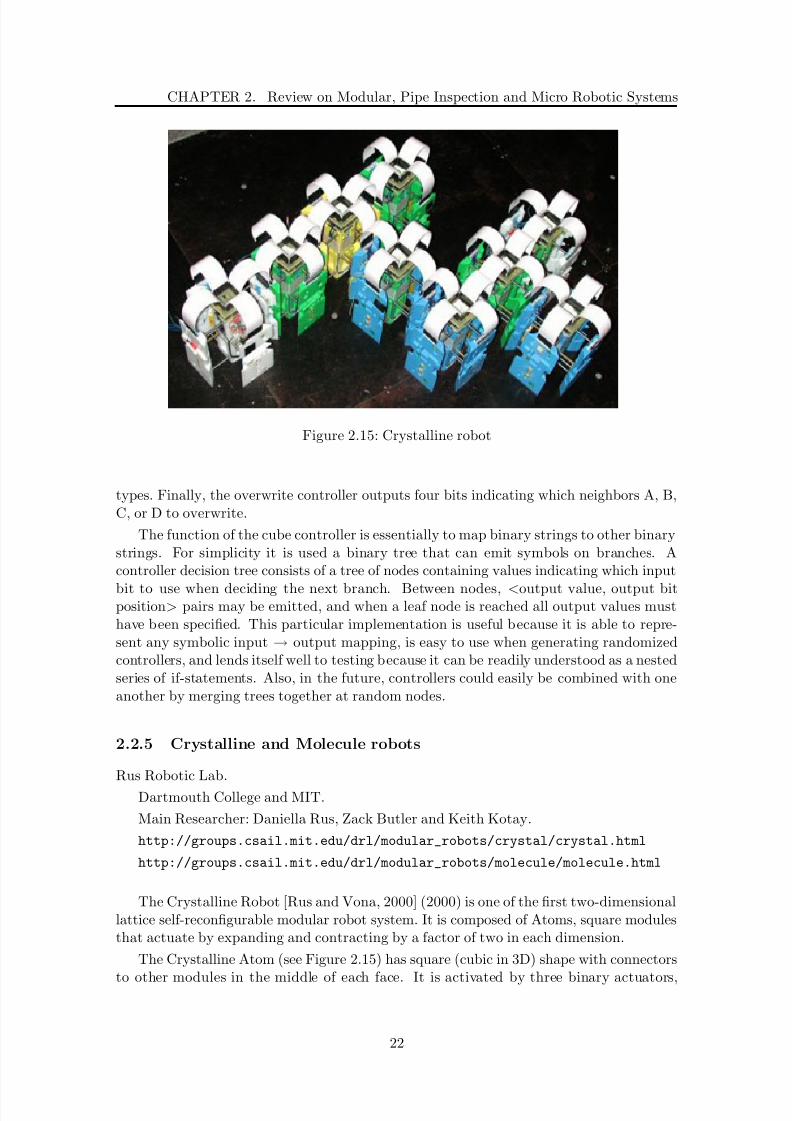
8/21/2019 Alberto Brunete Gonzalez
http://slidepdf.com/reader/full/alberto-brunete-gonzalez 50/311
CHAPTER 2. Review on Modular, Pipe Inspection and Micro Robotic Systems
Figure 2.15: Crystalline robot
types. Finally, the overwrite controller outputs four bits indicating which neighbors A, B,C, or D to overwrite.
The function of the cube controller is essentially to map binary strings to other binarystrings. For simplicity it is used a binary tree that can emit symbols on branches. Acontroller decision tree consists of a tree of nodes containing values indicating which input
bit to use when deciding the next branch. Between nodes, <output value, output bitposition> pairs may be emitted, and when a leaf node is reached all output values musthave been specified. This particular implementation is useful because it is able to repre-sent any symbolic input → output mapping, is easy to use when generating randomizedcontrollers, and lends itself well to testing because it can be readily understood as a nestedseries of if-statements. Also, in the future, controllers could easily be combined with oneanother by merging trees together at random nodes.
2.2.5 Crystalline and Molecule robots
Rus Robotic Lab.
Dartmouth College and MIT.
Main Researcher: Daniella Rus, Zack Butler and Keith Kotay.
http://groups.csail.mit.edu/drl/modular_robots/crystal/crystal.html
http://groups.csail.mit.edu/drl/modular_robots/molecule/molecule.html
The Crystalline Robot [Rus and Vona, 2000] (2000) is one of the first two-dimensionallattice self-reconfigurable modular robot system. It is composed of Atoms, square modulesthat actuate by expanding and contracting by a factor of two in each dimension.
The Crystalline Atom (see Figure 2.15) has square (cubic in 3D) shape with connectors
to other modules in the middle of each face. It is activated by three binary actuators,
22

8/21/2019 Alberto Brunete Gonzalez
http://slidepdf.com/reader/full/alberto-brunete-gonzalez 51/311
2.2. Modular robots
one to permit the side length of the square to shrink and expand and two to make orbreak connections to other Atoms. This actuation scheme allows an individual module torelocate to arbitrary positions on the surface of a structure of modules in constant time.
The Atom uses complimentary rack and pinion mechanisms to implement the contrac-tion and expansion actuation, a similar mechanism used in the support module v1.1.
Each Atom contains an on-board processor (Atmel AT89C2051 microcontroller), powersupply (five 2/3 A Lithium batteries), and support circuitry, which allows both fullyuntethered and tethered operations. Atoms are connected by a wired serial link to ahost computer to download programs. For untethered operations, an experiment specificoperating program specified as a state sequence is first downloaded over a tether. Whenthe tether is removed, an on-board IR receiver is used to detect synchronization beaconsfrom the host.
Crystalline robot systems are dynamic structures: they can move using sequences of
reconfigurations to implement locomotion gaits, and they can undergo shape metamor-phosis. The dynamic nature of these systems is supported by the ability of individualmodules to move globally relative to the structure. The basic operations in a Crystallinerobot system are:
• (expand < atom >, < dimension >) - expand a compressed Atom in the desireddimension (z,y, or z)
• (contract < atom >, < dimension >) - compress an expanded Atom in the desireddimension
• (bond < atom >, < dimension >) - activate one of the Atom’s connectors to bond
with a neighboring Atom in the structure
• (f ree < atom >, < dimension >) - deactivate one of the Atom’s connectors to breaka bond with a neighboring Atom in the structure
The Molecule Robot [Kotay et al., 1998] [Kotay and Rus, 2005] is a self-reconfiguringrobot consists of a set of identical modules that can dynamically and autonomously re-configure in a variety of shapes, to best fit the terrain, environment, and task. Self-reconfiguration leads to versatile robots that can support multiple modalities of locomo-tion and manipulation. For example, a self-reconfiguring robot can aggregate as a snaketo traverse a tunnel and then reconfigure as a six-legged robot to traverse rough terrain,
such as a lunar surface, and change shape again to climb stairs and enter a building.A Molecule robot consists of two atoms linked by a rigid connection called a bond.
Each atom has five inter-Molecule connection points and two degrees of freedom. Onedegree of freedom allows the atom to rotate 180 degrees relative to its bond connection,and the other degree of freedom allows the atom (thus the entire Molecule) to rotaterelative 180 degrees relative to one of the inter-Molecule connectors at a right angle to thebond connection.
The Molecule is controlled by two types of software: low-level assembly code in theonboard processor(s), and high-level code on a workstation.
Molecules control is focused on locomotion gait development. As an example, self-
reconfiguring robots can climb stairs even in the absence of models of the height, width,
23

8/21/2019 Alberto Brunete Gonzalez
http://slidepdf.com/reader/full/alberto-brunete-gonzalez 52/311
CHAPTER 2. Review on Modular, Pipe Inspection and Micro Robotic Systems
Figure 2.16: Molecule robot
and length of the stairway. The robot will be given the command to move forward.The robot will proceed with a translation motion until the front sensors mounted onthe forward modules detect an obstacle (e.g., the first step). At this point the robotwill change the locomotion modality from translation to stacking. When the top modules
detect free space again (that is, after the first step has been cleared), the robot will changelocomotion modality again to unstacking and then translation. These capabilities lead toon-line algorithms for navigation that take advantage of self-reconfiguring capabilities tocreate a ”water-flow”-like locomotion.
In Molecules it is used a generic algorithm [Butler et al., 2004] for implementing the”water-flow” locomotion gait using the self-reconfiguration property. In this gait a groupof modules tumble on top of each other to implement forward progress. The efficiency of this gait is analyzed in terms of the number of actuations, and this result helps to developa rolling gait which is dynamically but not statically stable. Using self-reconfiguration, agroup of modules can actively change their center of mass to generate forward motion. Itis demonstrated that the dynamically stable algorithm is more efficient and the locomotion
tumbling gait on a four-module Molecule robot.
2.2.6 Telecube and Proteo (Digital Clay)
PARC - Palo Alto Research Center.
Systems and Practices Laboratory. Modular Robotics Lab.
Main Researcher: Mark Yim.
http://www2.parc.com/spl/projects/modrobots/
Telecube modules [Suh et al., 2002] are cube shaped modules with faces that can
24

8/21/2019 Alberto Brunete Gonzalez
http://slidepdf.com/reader/full/alberto-brunete-gonzalez 53/311
2.2. Modular robots
(a) Module (b) Example of module reconfiguration in a net
Figure 2.17: Telecube
extend out doubling the length of any dimension. Each face ”telescopes” out, thus thename. Each face also has a latching mechanism to attach or detach from any otherface of a neighboring module. Shape memory alloy and permanent switching magnettechnologies has been experimented in various versions of this system. This work buildson the ”Crystalline” robot by Marty Vona and Daniela Rus starting at Dartmouth. Theirinitial Crystalline modules are 2D squares with one degree of freedom (all faces expandedat the same time). The telecube modules are 3D with every face having the ability toextend or contract independently. One module reconfigures from one site on a virtual gridby detaching from all modules except one. Then extending (or contracting) the faces thatare attached the module moves to the neighboring site.
The target size for the module is a cube that is 5 centimeters on a side. Packingactuators, electronics and structure into that small size to get the needed functionality isone of the more difficult parts of developing the module. There are two main mechanicalfunctions:
1. Latch/unlatch from neighboring faces and
2. Telescope the faces (expand/collapse)
Each of the faces, called a connection plate, has a remotely controllable means toreversibly clamp onto and to transmit power and data to the neighboring module. Thedevices which produce the linear extension/contraction and module to module clamps are
called the telescoping-tube linear actuator and the switching permanent magnet devices,respectively.
Each module is also given simple sensing and communication abilities. Modules cansend messages through their faceplates to their immediate neighbors using a low bandwidthIR link. Each module can also gauge the extension of each faceplate, read the contactsensor on each of the faces, and determine whether it is latched to a neighboring module.
Locomotion control is similar to the Crystalline robot. It has the same low-levelprimitives (Extend arm, connect, etc.), over which more complicated actions have beenbuild, like Move(direction).
To achieve completeness of reconfiguration, meta-modules (group of 8 individual Tele-
cubes) are created. The cubes are arranged in a tight cube with their arms fully retracted.
25

8/21/2019 Alberto Brunete Gonzalez
http://slidepdf.com/reader/full/alberto-brunete-gonzalez 54/311
CHAPTER 2. Review on Modular, Pipe Inspection and Micro Robotic Systems
Figure 2.18: Digital Clay Modules
Three locomotion primitives are defined: Move, Roll and S-Roll. Move is the explicitsequence of actions that allows a module to move along a given direction. For example,Move(EAST) would result with a meta-module at (x, y,z) to move to position (x + 1,y,z).
The Roll allows for one meta-module to ”roll” around a corner of another meta-module.For example, Roll(EAST, SOUTH) results in a meta-module at (x, y, z) to move to posi-tion(x + 1, y - 1, z). An S-Roll is similar to Roll but making and ”s” shape.
Proteo (Digital Clay) is the continuation of Telecubes. There are two approachesto understanding digital clay. First approach: it is a stripped down version of a modularrobot. That is, there is:
1. no active coupling
2. no actuation for producing module to module motions.
Changes to an assembly of modules is made by a user. But it embodies one veryimportant aspect that the modules have some capacity to sense or know their own ori-entation in space with respect to other modules. As such it may be a useful hardwaresystem for testing software, communications, power distribution for physically modularand reconfigurable systems.
The other approach is to see it as a 3 dimensional human-computer interface. A struc-ture where physical changes made to the structure are represented in a computer model.As with clay the user shapes the material into some form or orientation. The orientationor distribution of the inherently regular structure is sensed and directly represented in thecomputer. It is a kind of smart material or structure that a user (or designer) can actually
experience in real 3D space, and yet has a direct representation in a cad program.
There are two kinds of structures one can imagine. The first is made up of permanentlyconnected modules. It is made up of tetrahedral nodes connected by several right anglelinks which are free to rotate. The overall topology is similar to the molecular structureof diamond. The resulting structure can be freely molded. Angle sensors at each jointcould provide the information necessary for a computer model of the structure. For sucha structure to be useful would require a large number of nodes and a very large numberof calculations.
The second type is made up of an assembly of individual modules. Each individualmodule must be able to sense to which other modules it is connected as well as its orien-
tation with respect to the other modules, i.e. which face is connected to which. Thus each
26

8/21/2019 Alberto Brunete Gonzalez
http://slidepdf.com/reader/full/alberto-brunete-gonzalez 55/311
2.2. Modular robots
module must have its own identity within the assembly, and each of the 12 faces musthave a unique identity within a module.
Each module is made of a flex circuit with 12 rigid backer boards and a single com-
ponent sheet which folds into the center of the module. Each module has an 8 MHz PICprocessor with 6 serial ports communicating in pairs to each of the twelve faces. Each facehas 4 sets of three connection pads–power, ground, and communication. Each group of connection pads is backed by a NdFeB magnet (2 north, 2 south) one of which is attachedto the center of a spiral cut in the Kapton to insure a good connection.
2.2.7 Chobie
Biomechanics laboratory. Department of Mechanical and Control Engineering.
Graduate School of Science and Engineering.
Tokyo Institute of Technology.Main researcher: N. Inou
http://www.mech.titech.ac.jp/ ~inouhp/index.html
CHOBIE (Cooperative Hexahedral Objects for Building with Intelligent Enhancement)[Inou et al., 2003] [Suzuki et al., 2007] [Suzuki et al., 2006] is a cellular robot designed forsupporting large outer forces that cooperatively can transform the mechanical structurethat is forming by reconfiguration. Each cellular robot communicates with adjacent robotsand determines the behavior where it should be positioned. They form the structure bysuccessive cooperative movements. CHOBIE has slide motion mechanisms with some
mechanical constraints for large stiffness even in movement.Figure 2.19 shows the slide motion mechanism. It consists of two lateral boards and a
central board. The central board is sandwiched by the two lateral boards and all the boardsare tightly connected. The two lateral boards include symmetrical motion mechanismsthat consist of two sets of wheels. They are allocated in vertical and horizontal directions,which enable the two directional motions of cellular robots. The only one DC motor isembedded in each lateral board, and jointly drives 4 wheels that are placed on the sameplane through a drive shaft in the central board.
To endow the robot with autonomy, several devices were integrated into each robot:sensors, an electric controller and electric battery. The width of the central board is 50mm.Photo sensors that communicate with neighboring robots are embedded on the surface of
the frame and force sensors are attached at the corner of a portion that produces largestrain by outer forces . The controller chosen was a PIC16F84.
Performance of CHOBIE II is achieved by succession of structural transformations. Ineach transformation process, some robots drive their motors and the other don’t drive,the former are called ”D” as meaning of ”driving robot” and the later ”R” as meaning of ”resting robot”.
Each robot communicates with surrounding robots and acquires the information aboutthe state of the structure. But it cannot process complicated data because it doesn’t havepowerful calculation function.
In [Suzuki et al., 2006] it is proposed a scheme to accomplish the cooperative move-
ments focusing on a characteristic position which enables simultaneous driving. The posi-
27
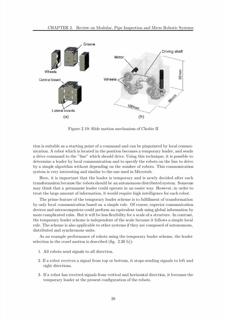
8/21/2019 Alberto Brunete Gonzalez
http://slidepdf.com/reader/full/alberto-brunete-gonzalez 56/311
CHAPTER 2. Review on Modular, Pipe Inspection and Micro Robotic Systems
Figure 2.19: Slide motion mechanism of Chobie II
tion is suitable as a starting point of a command and can be pinpointed by local commu-nication. A robot which is located in the position becomes a temporary leader, and sendsa drive command to the ”line” which should drive. Using this technique, it is possible todetermine a leader by local communication and to specify the robots on the line to drive
by a simple algorithm without depending on the number of robots. This communicationsystem is very interesting and similar to the one used in Microtub.
Here, it is important that the leader is temporary and is newly decided after eachtransformation because the robots should be an autonomous distributed system. Someonemay think that a permanent leader could operate in an easier way. However, in order totreat the large amount of information, it would require high intelligence for each robot.
The prime feature of the temporary leader scheme is to fulfillment of transformationby only local communication based on a simple rule. Of course, superior communicationdevices and microcomputers could perform an equivalent task using global information bymore complicated rules. But it will be less flexibility for a scale of a structure. In contrast,the temporary leader scheme is independent of the scale because it follows a simple local
rule. The scheme is also applicable to other systems if they are composed of autonomous,distributed and synchronous units.
As an example performance of robots using the temporary leader scheme, the leaderselection in the crawl motion is described (fig. 2.20 b)):
1. All robots send signals to all direction.
2. If a robot receives a signal from top or bottom, it stops sending signals to left andright directions.
3. If a robot has received signals from vertical and horizontal direction, it becomes the
temporary leader at the present configuration of the robots.
28

8/21/2019 Alberto Brunete Gonzalez
http://slidepdf.com/reader/full/alberto-brunete-gonzalez 57/311
2.2. Modular robots
(a) Crawl motion with five robots (b) Procedure of determining a Leader
Figure 2.20: Chobie reconfiguration
(a) Several modules on different configurations (b) ATRON module without electron-ics and batteries
Figure 2.21: ATRON
In figure 2.20 a) it is possible to see the crawl motion with five robots.
2.2.8 ATRON
The Maersk Mc-Kinney Moeller Institute for Production Technology.
University of Southern Denmark.
Project Coordinator: H. Hautop LUND
The HYDRA consortium consists also of Mobile Robots Group from University of Edinburgh, AI Lab from University of Zurich and LEGO Platform Development Formermember: EVALife from University of Aarhus
Web-site of Project: http://hydra.mip.sdu.dk
ATRON is a lattice based self-reconfigurable robot [Jorgensen et al., 2004]. The
29
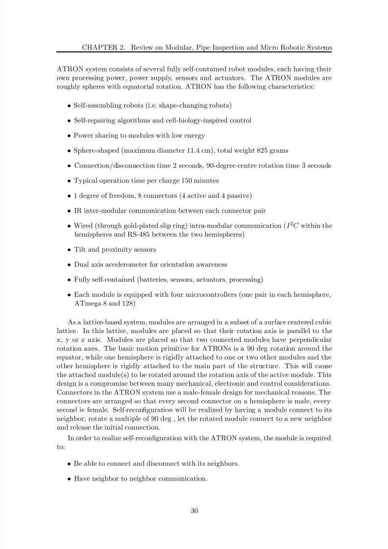
8/21/2019 Alberto Brunete Gonzalez
http://slidepdf.com/reader/full/alberto-brunete-gonzalez 58/311
CHAPTER 2. Review on Modular, Pipe Inspection and Micro Robotic Systems
ATRON system consists of several fully self-contained robot modules, each having theirown processing power, power supply, sensors and actuators. The ATRON modules areroughly spheres with equatorial rotation. ATRON has the following characteristics:
• Self-assembling robots (i.e. shape-changing robots)
• Self-repairing algorithms and cell-biology-inspired control
• Power sharing to modules with low energy
• Sphere-shaped (maximum diameter 11.4 cm), total weight 825 grams
• Connection/disconnection time 2 seconds, 90-degree centre rotation time 3 seconds
• Typical operation time per charge 150 minutes
• 1 degree of freedom, 8 connectors (4 active and 4 passive)
• IR inter-modular communication between each connector pair
• Wired (through gold-plated slip ring) intra-modular communication (I 2C within thehemispheres and RS-485 between the two hemispheres)
• Tilt and proximity sensors
• Dual axis accelerometer for orientation awareness
• Fully self-contained (batteries, sensors, actuators, processing)
• Each module is equipped with four microcontrollers (one pair in each hemisphere,ATmega 8 and 128)
As a lattice-based system, modules are arranged in a subset of a surface centered cubiclattice. In this lattice, modules are placed so that their rotation axis is parallel to thex, y or z axis. Modules are placed so that two connected modules have perpendicularrotation axes. The basic motion primitive for ATRONs is a 90 deg rotation around theequator, while one hemisphere is rigidly attached to one or two other modules and theother hemisphere is rigidly attached to the main part of the structure. This will causethe attached module(s) to be rotated around the rotation axis of the active module. This
design is a compromise between many mechanical, electronic and control considerations.Connectors in the ATRON system use a male-female design for mechanical reasons. Theconnectors are arranged so that every second connector on a hemisphere is male, everysecond is female. Self-reconfiguration will be realized by having a module connect to itsneighbor, rotate a multiple of 90 deg , let the rotated module connect to a new neighborand release the initial connection.
In order to realize self-reconfiguration with the ATRON system, the module is requiredto:
• Be able to connect and disconnect with its neighbors.
• Have neighbor to neighbor communication.
30

8/21/2019 Alberto Brunete Gonzalez
http://slidepdf.com/reader/full/alberto-brunete-gonzalez 59/311
2.2. Modular robots
Figure 2.22: Active Cord Mechanism (ACM): version III (a), R3 (b), R4 (c) and R5 (d)
• Be able to sense the state of its connectors.
• Perform 360 deg rotation around the equator.
Like the M-TRAN module, the ATRON has two “parts” connected by an actuated joint. Where the M-TRAN is actuated around two parallel axes, the ATRON is actuatedaround the axis perpendicular to the equatorial plane. The ATRON module, shown infigure 2.26, is built mainly from aluminum with some brass (gearing for the center motor)and steel (passive connectors and needle bearing in the center). In the ATRON, someinteresting properties from M-TRAN and CONRO are combined.
2.2.9 Active Cord Mechanism (ACM)
Hirose and Yoneda Lab. Dept. of Mechanical and Aerospace Engineering.
Tokyo Institute of Technology.
Main Researcher: S. Hirose and K.Yoneda.
ACM [Hirose, 1993] was the first robot using the principles of a serpentine movement
which is the same as actual snakes (fig. 2.22 a)). It was created in 1972, and it could
31

8/21/2019 Alberto Brunete Gonzalez
http://slidepdf.com/reader/full/alberto-brunete-gonzalez 60/311
CHAPTER 2. Review on Modular, Pipe Inspection and Micro Robotic Systems
move at a speed of approximately 40 cm/sec . The entire length of the device is 2 m,and it has 20 joints. Each joint consists of servo-mechanisms that can bend to the leftand right. To make contact with the ground, casters were installed along the direction of
the body, and characteristics were added that make it easy to slide in the direction of thetorso and difficult to slide in the normal direction. The propulsion motion was conductedby inputting command values which impart sinusoidal bending motions to the head jointservo-mechanism, and that bending signal was shifted at a fixed speed to the following
joint servo-mechanisms. When this is done, the body as a whole begins to move by sendinga wave to the rear, but in order for the torso to slide over the floor surface with the casters,all of the torso joints produced a serpentine movement like the flow of water which tracesthe same loci. This principal of propulsion corresponds to the swimming motion of eel.
It has installed tactile sensors, based on limit switches, onto the sides of all the joints.It is indispensable to know the tactile conditions between the torso and the environmentin an Active Cord Mechanism, but it is no good to simply bend the joint that is touched
by an object. It is best that both neighboring joints also bend at a speed one-half inthe opposite direction at the same time. This control closely corresponds with the kindof “lateral inhibition” type neural net which is seen in the nervous system. Using lateralinhibition type controls, the ACM III is capable of smooth movement which autonomouslycoiled around optionally shaped objects, and of propulsion while following along a labyrinthin the shape of the labyrinth, by combining this lateral inhibition control with angularinformation shift control.
The version R3 of ACM (fig. 2.22 b) ) is composed of 20 modules and has 2 dof (3Dmovement). The size is 1755 x 110 x 110 mm and the weight 12.1 kg. The movable angleis ±62.5 deg and the output torque 19.1 Nm. moderately, with a moderate move speedat serpentine locomotion secured. The most characteristic part is a large-sized passivitywheel which can be easily detached and attached, and which covers the whole body. Itcan perform conventional serpentine locomotion, lateral rolling, parallel translation andsinus-lifting and pedal wave promotion.
ACM-R4 (fig. 2.22 c) ) has the following 3 characteristics: active wheels, dust andwater proof and overload protection.
ACM-R5 (fig. 2.22 d) ) can operate both on ground and in water undulating its longbody. It is equipped with paddles and passive wheels around the body. To generatepropulsive force by undulation, the robot need a resistance property as it glides freelyin tangential direction but cannot in normal direction. Due to the paddles and passivewheels, ACM-R5 obtains that character both in water and on ground.
The control system of ACM-R5 is an advanced one. Each joint unit has CPU, bat-tery, motors, so they can operate independently. Through communication lines each unitexchanges signals and automatically recognizes its number from the head, and how manyunits join the system. Thanks to this system operators can remove, add, and exchangeunits freely and they can operate ACM-R5 flexibly according to situations.
2.2.10 WormBot
Institute of Neuromorphic Engineering and Institute of Neuroinformatics.
ETH (University of Zurich)
32
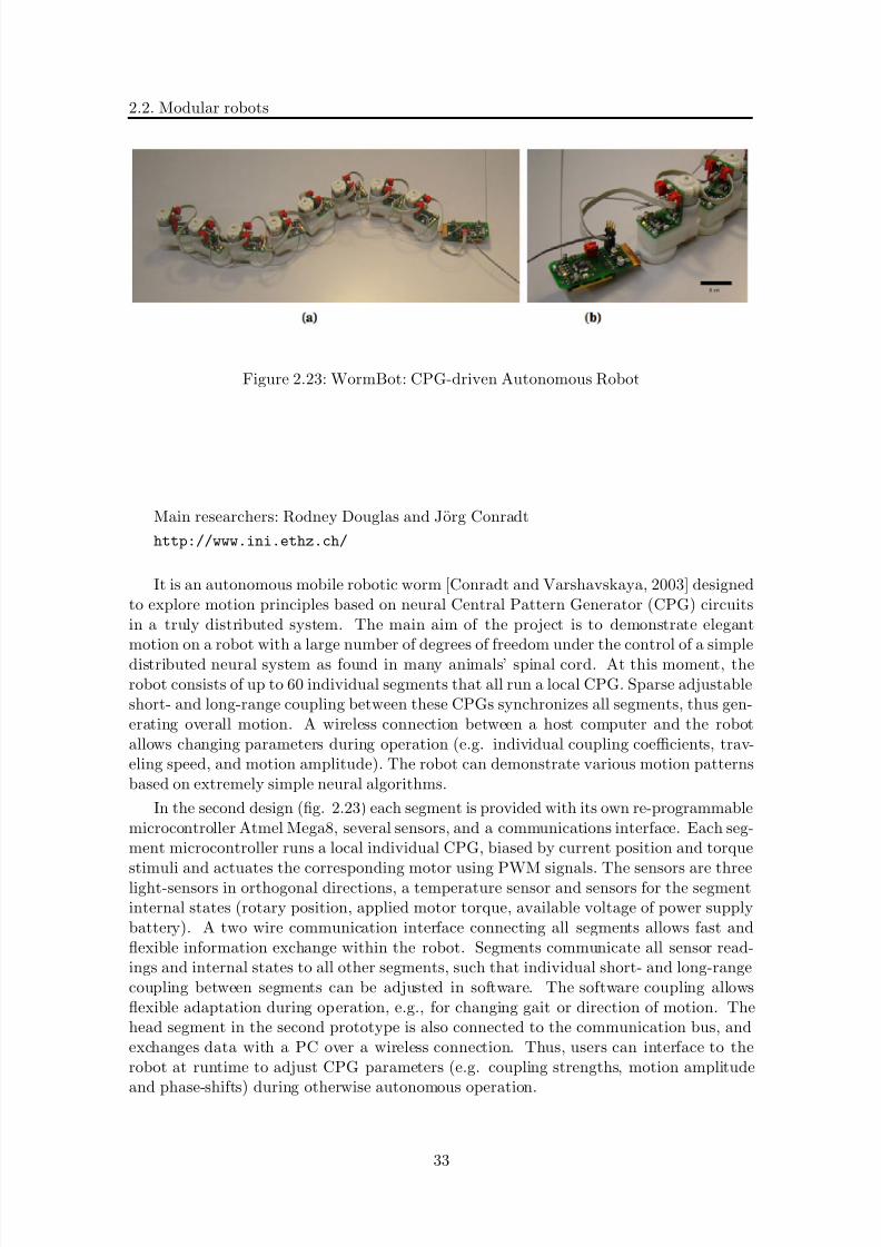
8/21/2019 Alberto Brunete Gonzalez
http://slidepdf.com/reader/full/alberto-brunete-gonzalez 61/311
2.2. Modular robots
Figure 2.23: WormBot: CPG-driven Autonomous Robot
Main researchers: Rodney Douglas and Jorg Conradt
http://www.ini.ethz.ch/
It is an autonomous mobile robotic worm [Conradt and Varshavskaya, 2003] designedto explore motion principles based on neural Central Pattern Generator (CPG) circuitsin a truly distributed system. The main aim of the project is to demonstrate elegantmotion on a robot with a large number of degrees of freedom under the control of a simpledistributed neural system as found in many animals’ spinal cord. At this moment, therobot consists of up to 60 individual segments that all run a local CPG. Sparse adjustableshort- and long-range coupling between these CPGs synchronizes all segments, thus gen-erating overall motion. A wireless connection between a host computer and the robotallows changing parameters during operation (e.g. individual coupling coefficients, trav-eling speed, and motion amplitude). The robot can demonstrate various motion patternsbased on extremely simple neural algorithms.
In the second design (fig. 2.23) each segment is provided with its own re-programmablemicrocontroller Atmel Mega8, several sensors, and a communications interface. Each seg-ment microcontroller runs a local individual CPG, biased by current position and torque
stimuli and actuates the corresponding motor using PWM signals. The sensors are threelight-sensors in orthogonal directions, a temperature sensor and sensors for the segmentinternal states (rotary position, applied motor torque, available voltage of power supplybattery). A two wire communication interface connecting all segments allows fast andflexible information exchange within the robot. Segments communicate all sensor read-ings and internal states to all other segments, such that individual short- and long-rangecoupling between segments can be adjusted in software. The software coupling allowsflexible adaptation during operation, e.g., for changing gait or direction of motion. Thehead segment in the second prototype is also connected to the communication bus, andexchanges data with a PC over a wireless connection. Thus, users can interface to therobot at runtime to adjust CPG parameters (e.g. coupling strengths, motion amplitude
and phase-shifts) during otherwise autonomous operation.
33
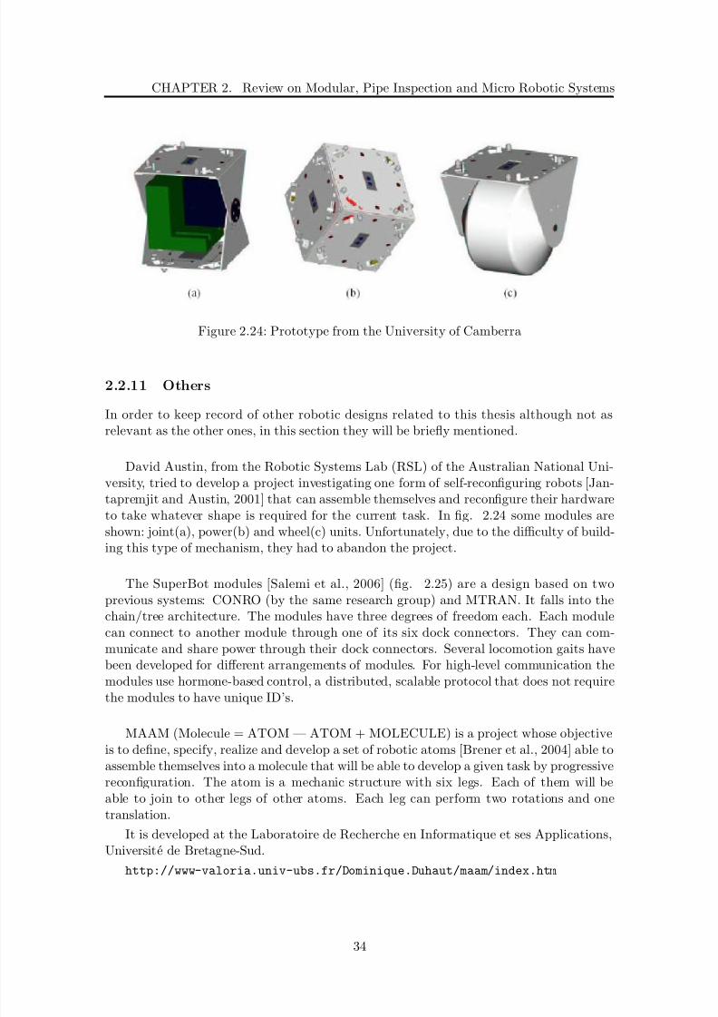
8/21/2019 Alberto Brunete Gonzalez
http://slidepdf.com/reader/full/alberto-brunete-gonzalez 62/311
CHAPTER 2. Review on Modular, Pipe Inspection and Micro Robotic Systems
Figure 2.24: Prototype from the University of Camberra
2.2.11 Others
In order to keep record of other robotic designs related to this thesis although not asrelevant as the other ones, in this section they will be briefly mentioned.
David Austin, from the Robotic Systems Lab (RSL) of the Australian National Uni-versity, tried to develop a project investigating one form of self-reconfiguring robots [Jan-tapremjit and Austin, 2001] that can assemble themselves and reconfigure their hardwareto take whatever shape is required for the current task. In fig. 2.24 some modules are
shown: joint(a), power(b) and wheel(c) units. Unfortunately, due to the difficulty of build-ing this type of mechanism, they had to abandon the project.
The SuperBot modules [Salemi et al., 2006] (fig. 2.25) are a design based on twoprevious systems: CONRO (by the same research group) and MTRAN. It falls into thechain/tree architecture. The modules have three degrees of freedom each. Each modulecan connect to another module through one of its six dock connectors. They can com-municate and share power through their dock connectors. Several locomotion gaits havebeen developed for different arrangements of modules. For high-level communication themodules use hormone-based control, a distributed, scalable protocol that does not requirethe modules to have unique ID’s.
MAAM (Molecule = ATOM — ATOM + MOLECULE) is a project whose objectiveis to define, specify, realize and develop a set of robotic atoms [Brener et al., 2004] able toassemble themselves into a molecule that will be able to develop a given task by progressivereconfiguration. The atom is a mechanic structure with six legs. Each of them will beable to join to other legs of other atoms. Each leg can perform two rotations and onetranslation.
It is developed at the Laboratoire de Recherche en Informatique et ses Applications,Universite de Bretagne-Sud.
http://www-valoria.univ-ubs.fr/Dominique.Duhaut/maam/index.htm
34

8/21/2019 Alberto Brunete Gonzalez
http://slidepdf.com/reader/full/alberto-brunete-gonzalez 63/311
2.3. Microrobots
Figure 2.25: Superbot modules
I-Cubes [Unsal and Khosla, 2000] is a class of modular self-reconfigurable bipartiterobotic system developed in 2000 in the Advanced Mechatronics Laboratory, CarnegieMelon University. It is of interest because it is an heterogeneous system composed of independently controlled mechatronic modules (links) and passive connection elements
(cubes). A link has the ability to connect to and disconnect from the face of a cube.While attached to a cube on one end, links are also capable of moving themselves andanother cube attached to the other end. All active (link) and passive (cube) modules arecapable of allowing power and information flow to their neighboring modules.
http://www-2.cs.cmu.edu/~unsal/research/ices/cubes/
M. Chen, from the Modular robotic and Robot Locomotion Group, School of MPE,NTU (Singapure) has also been researching in modular robotics [Chen, 1994]. But thiswork was focused on robotic arms.
T. Fujii and K. Hosokawa from the Institute of Industrial Science, Tokyo University,where also working in the ’Vertical Modules’ (fig. 2.26(b)), a kind of reconfigurable mod-ular robot.
2.3 Microrobots
This section is dedicated to robots that have miniaturization as its main characteristic,i.e. microrobots, being a microrobot a miniaturized, sophisticated machine designed toperform a specific task or tasks repeatedly and with precision. Microrobots typically have
dimensions ranging from a fraction of a millimeter up to several millimeters.
35
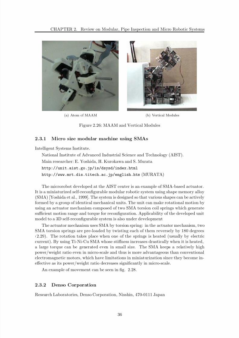
8/21/2019 Alberto Brunete Gonzalez
http://slidepdf.com/reader/full/alberto-brunete-gonzalez 64/311
CHAPTER 2. Review on Modular, Pipe Inspection and Micro Robotic Systems
(a) Atom of MAAM (b) Vertical Modules
Figure 2.26: MAAM and Vertical Modules
2.3.1 Micro size modular machine using SMAs
Intelligent Systems Institute.
National Institute of Advanced Industrial Science and Technology (AIST).
Main researcher: E. Yoshida, H. Kurokawa and S. Murata
http://unit.aist.go.jp/is/dsysd/index.html
http://www.mrt.dis.titech.ac.jp/english.htm (MURATA)
The microrobot developed at the AIST center is an example of SMA-based actuator.It is a miniaturized self-reconfigurable modular robotic system using shape memory alloy(SMA) [Yoshida et al., 1999]. The system is designed so that various shapes can be activelyformed by a group of identical mechanical units. The unit can make rotational motion byusing an actuator mechanism composed of two SMA torsion coil springs which generatesufficient motion range and torque for reconfiguration. Applicability of the developed unitmodel to a 3D self-reconfigurable system is also under development
The actuator mechanism uses SMA by torsion spring: in the actuator mechanism, twoSMA torsion springs are pre-loaded by twisting each of them reversely by 180 degrees
(2.29). The rotation takes place when one of the springs is heated (usually by electriccurrent). By using Ti-Ni-Cu SMA whose stiffness increases drastically when it is heated,a large torque can be generated even in small size. The SMA keeps a relatively highpower/weight ratio even in micro-scale and thus is more advantageous than conventionalelectromagnetic motors, which have limitations in miniaturization since they become in-effective as its power/weight ratio decreases significantly in micro-scale.
An example of movement can be seen in fig. 2.28.
2.3.2 Denso Corporation
Research Laboratories, Denso Corporation, Nisshin, 470-0111 Japan
36
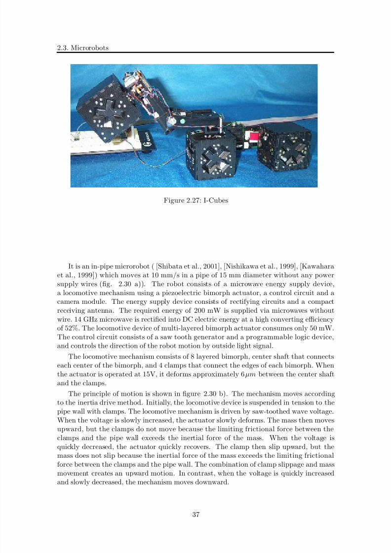
8/21/2019 Alberto Brunete Gonzalez
http://slidepdf.com/reader/full/alberto-brunete-gonzalez 65/311
2.3. Microrobots
Figure 2.27: I-Cubes
It is an in-pipe microrobot ( [Shibata et al., 2001], [Nishikawa et al., 1999], [Kawaharaet al., 1999]) which moves at 10 mm/s in a pipe of 15 mm diameter without any powersupply wires (fig. 2.30 a)). The robot consists of a microwave energy supply device,
a locomotive mechanism using a piezoelectric bimorph actuator, a control circuit and acamera module. The energy supply device consists of rectifying circuits and a compactreceiving antenna. The required energy of 200 mW is supplied via microwaves withoutwire. 14 GHz microwave is rectified into DC electric energy at a high converting efficiencyof 52%. The locomotive device of multi-layered bimorph actuator consumes only 50 mW.The control circuit consists of a saw tooth generator and a programmable logic device,and controls the direction of the robot motion by outside light signal.
The locomotive mechanism consists of 8 layered bimorph, center shaft that connectseach center of the bimorph, and 4 clamps that connect the edges of each bimorph. Whenthe actuator is operated at 15V, it deforms approximately 6 µm between the center shaftand the clamps.
The principle of motion is shown in figure 2.30 b). The mechanism moves accordingto the inertia drive method. Initially, the locomotive device is suspended in tension to thepipe wall with clamps. The locomotive mechanism is driven by saw-toothed wave voltage.When the voltage is slowly increased, the actuator slowly deforms. The mass then movesupward, but the clamps do not move because the limiting frictional force between theclamps and the pipe wall exceeds the inertial force of the mass. When the voltage isquickly decreased, the actuator quickly recovers. The clamp then slip upward, but themass does not slip because the inertial force of the mass exceeds the limiting frictionalforce between the clamps and the pipe wall. The combination of clamp slippage and massmovement creates an upward motion. In contrast, when the voltage is quickly increased
and slowly decreased, the mechanism moves downward.
37

8/21/2019 Alberto Brunete Gonzalez
http://slidepdf.com/reader/full/alberto-brunete-gonzalez 66/311
CHAPTER 2. Review on Modular, Pipe Inspection and Micro Robotic Systems
Figure 2.28: Basic motion of Micro SMA
Figure 2.29: Estructure and real module of Micro SMA
2.3.3 Endoscope microrobots
A broad background in microrobots can be found in endoscope robots. Although their sizeis the smallest of all microrobots, its capacities regarding movement and degrees of freedomare very limited. The average mechanism allows only bending (the forward movement hasto be done by the operator), as in figure 2.31(a), and the use of a gripper ( [Maeda et al.,1996], [Ikuta et al., 1988]) as in figure 2.31(b).
On the contrary, a few others are able to self propulsion, most of them performing awork-like movement [Peirs et al., 2001], [Kim et al., 2002], as in figure 2.31(b).
2.3.4 LMS, LAB and LAI microrobots
Laboratoire d’ Automatique Industrielle (LAI) - INSA de Lyon
38

8/21/2019 Alberto Brunete Gonzalez
http://slidepdf.com/reader/full/alberto-brunete-gonzalez 67/311
2.3. Microrobots
Figure 2.30: Denso microrobot
(a) Active endoscope with SMA coil springs (b) Example of worm-like endoscope microrobot
Figure 2.31: Endoscope microrobots
Laboratoire de Mecanique des Solides (LMS) - Universite de Poitiers
Laboratoire d’ Automatique de Besangon (LAB)
The microrobots from LAI, LMS and LAB are the result of the investigations of 3laboratories involved in the micro robotics workgroup of the French National Centre of
the Scientific Research(CNRS) [Anthierens et al., 2000]. They have been conceived toanswer the locomotion problem inside industrial tubes of small diameter.
The LMS (fig. 2.32 b) ) polymodular flexible microrobot is able to progress insideempty man-made canalization presenting bends. The first realized prototype has got adiameter of about 30 mm, but all work is done with the purpose to improve design andmachining techniques to realize a micro robot capable of inspecting canalization of lessthan 10 mm diameter.
This robot is constituted of five juxtaposed identical modules, called ’locomotion mod-ules’. The locomotion modules are joined together by passive elastic links, nearly jointed
coil springs, which present a resistive behavior to push or pull solicitation, but a compliance
39
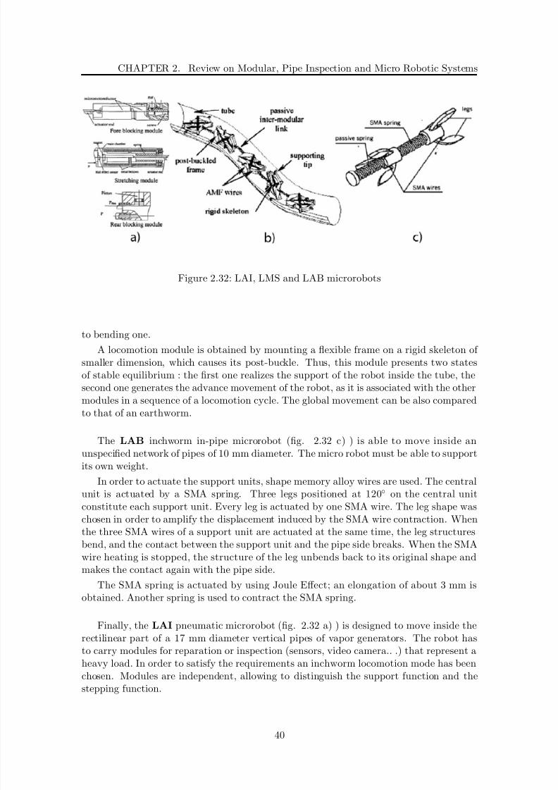
8/21/2019 Alberto Brunete Gonzalez
http://slidepdf.com/reader/full/alberto-brunete-gonzalez 68/311
CHAPTER 2. Review on Modular, Pipe Inspection and Micro Robotic Systems
Figure 2.32: LAI, LMS and LAB microrobots
to bending one.
A locomotion module is obtained by mounting a flexible frame on a rigid skeleton of smaller dimension, which causes its post-buckle. Thus, this module presents two statesof stable equilibrium : the first one realizes the support of the robot inside the tube, thesecond one generates the advance movement of the robot, as it is associated with the othermodules in a sequence of a locomotion cycle. The global movement can be also compared
to that of an earthworm.
The LAB inchworm in-pipe microrobot (fig. 2.32 c) ) is able to move inside anunspecified network of pipes of 10 mm diameter. The micro robot must be able to supportits own weight.
In order to actuate the support units, shape memory alloy wires are used. The centralunit is actuated by a SMA spring. Three legs positioned at 120 on the central unitconstitute each support unit. Every leg is actuated by one SMA wire. The leg shape waschosen in order to amplify the displacement induced by the SMA wire contraction. Whenthe three SMA wires of a support unit are actuated at the same time, the leg structuresbend, and the contact between the support unit and the pipe side breaks. When the SMA
wire heating is stopped, the structure of the leg unbends back to its original shape andmakes the contact again with the pipe side.
The SMA spring is actuated by using Joule Effect; an elongation of about 3 mm isobtained. Another spring is used to contract the SMA spring.
Finally, the LAI pneumatic microrobot (fig. 2.32 a) ) is designed to move inside therectilinear part of a 17 mm diameter vertical pipes of vapor generators. The robot hasto carry modules for reparation or inspection (sensors, video camera.. .) that represent aheavy load. In order to satisfy the requirements an inchworm locomotion mode has beenchosen. Modules are independent, allowing to distinguish the support function and the
stepping function.
40

8/21/2019 Alberto Brunete Gonzalez
http://slidepdf.com/reader/full/alberto-brunete-gonzalez 69/311
2.4. Pipe Inspection robots
Figure 2.33: 12-legged endoscopic capsular robot
The central actuator is composed of a flexible part (metal bellows) that is stressedunder pressure and a rod as a pneumatic jack. When the pressure in the chamber (outsidethe metal bellows) is falling down, metal bellows work like a spring and then their lengthis increasing to reach the initial state (length). That means the rod of actuator movesback.
2.3.5 12-legged endoscopic capsular robot
This microrobot (figure 2.33) is included in the mesoscale (from hundreds of microns totens of centimeters). It has a robotic legged locomotion mechanism [Valdastri et al., 2009]that is compact and strikes a balance between conflicting design objectives, exhibiting highfoot forces and low power consumption. It enables a small robot to traverse a compliant,slippery, tubular environment, even while climbing against gravity. This mechanism isuseful for many mesoscale locomotion tasks, including endoscopic capsule robot locomotionin the gastrointestinal tract. It has enabled fabrication of the first legged endoscopiccapsule robot whose mechanical components match the dimensions of commercial pillcameras (11 mm diameter by 25 mm long). A novel slot-follower mechanism driven vialead screw enables the mechanical components of the capsule robot to be as small whilesimultaneously generating 0.63 N average propulsive force at each leg tip.
It has been tested in a series of ex vivo experiments demonstrating ability to traversethe intestine in a manner suitable for inspection of the colon in a time period equivalentto standard colonoscopy (about 30 min) at an average speed of about 50mm/min.
2.4 Pipe Inspection robots
Pipe inspection is the main task the results of this thesis are aimed to. Nowadays thereare several robots capable of performing this mission, amongst which it is possible to findMRInspect (III y IV) [Roh and Choi, 2004], Pipe Mouse by Foster Millar [fos, ], and
GMD-Snake2 [Worst and Linnemann, 1996] [Klaassen and Paap, 1999]. Although their
41

8/21/2019 Alberto Brunete Gonzalez
http://slidepdf.com/reader/full/alberto-brunete-gonzalez 70/311
CHAPTER 2. Review on Modular, Pipe Inspection and Micro Robotic Systems
Figure 2.34: MRInspect pipe inspection robot
dimensions are beyond the limits pursued in this thesis (the former robots are design tofit in pipes whose diameter is 88mm (Foster), 100mm (MRInspect) and 135mm (GMD)),they present very interesting features that, which once miniaturized, could be included inthe prototype described in this thesis.
2.4.1 MRInspect
MRInspect IV (Multifunctional Robotic crawler for INpipe inSPECTion) [Roh and Choi,2004] [Roh et al., 2008] has been developed for the inspection of urban gas pipelines with anominal 4-inch inside diameter. Its steering capability with three-dimensional differentiallydriven method provides the outstanding mobility for navigation and the new mechanismfor steering can easily adjust itself to most of pipelines or fitting, in which other formerin-pipe robots can hardly travel.
2.4.2 FosterMiller
Another robot that is able to adapt to changes in gas piping is Pipe Mouse [fos, ], anautonomous inspection system for a live natural gas environment developed by Foster-
Miller together with New York GAS and the Department of Energy. Pipe Mouse is atrain-like robotic platform. Both front and rear drive cars propel the train forwards andbackwards inside the pipeline. Like a train, the platform includes additional ”cars” to carrythe required payloads. The cars are used for various purposes including the installationand positioning of sensor modules, the system power supply, data acquisition/storagecomponents, location/position devices and onboard micro-processors/electronics.
2.4.3 Helipipe
The architecture is based on helicoidal motion of the driving body (the rotor) direct
actuated by a DC motor with a built-in gear reducer, fixed on a driven body (the stator).
42

8/21/2019 Alberto Brunete Gonzalez
http://slidepdf.com/reader/full/alberto-brunete-gonzalez 71/311
2.4. Pipe Inspection robots
Figure 2.35: Foster Miller pipe inspection robot
Both bodies use wheeled structures on elastic suspensions. One or two universal jointsbetween bodies are used especially for curved pipes. The friction is used to produce the
active force (no direct actuated wheels) and self -guiding on the way (curved, horizontalor vertical parts). Three different prototypes (locomotion systems) have been done for 70mm and 40 mm diameter of pipes. Two of them are completely autonomous with powersupply on board and wireless control. Because of its high reliability (thanks to a verysimple kinematics) the robots can be used for inspection or carry out tasks. See [Horodincaet al., 2002] for more information.
2.4.4 Theseus
Theseus [Hirose et al., 1999] are a set of in-pipe inspection vehicles for pipes of 25, 50 and100mm diameter.
Thes-I (figure 2.37) is designed for gas pipes of 50mm in diameter. The rolling wheelof the robot has four spring wires radial attached around it, and free rollers are installedat the end of the spring with some inclination angle. As the free rollers are pressed oninside wall of the pipe and driven to the circumference direction, it generates screw motionand moves along the pipe. The Thes-I has a pair of rolling wheels rotating to the oppositedirection to cancel reaction torque. The main feature of the mechanism is that, as the freerollers are supported by spring wires and the inclination angle of the free rollers changesaccording to the magnitude of the resistance force, it shows the function of load sensitivetransmission and automatically reduces the velocity and increases the thrusting force whenit encounters large resistance force for propulsion.
Thes-III (figure 2.38) is designed for gas pipes of 150mm in diameter. Thes-III in-troduced the layout of the active wheels arraying radial in a ”wheel plane”, and drivethe wheels while pressing them on inside the pipe with spring force. But if the wheelsare driven like this, the wheel plane tends to be inclined and it can not maintain verticalposture in relation to the pipeline axis. Thes-III thus introduced the detect wheels foreach active wheels, in order to detect the inclination angle of the active wheel in respectto the pipeline axis, and at the same time, feedback control was executed to maintain thevertical posture. Thanks to these, Thes-III can easily follow the bending of the pipeline
and it smoothly makes tight turn on the elbow joints.
43

8/21/2019 Alberto Brunete Gonzalez
http://slidepdf.com/reader/full/alberto-brunete-gonzalez 72/311
CHAPTER 2. Review on Modular, Pipe Inspection and Micro Robotic Systems
Figure 2.36: Helipipe
2.5 Robot Summary
In tables 2.1, 2.2 and 2.3, a summary of the main properties of the modular robots shownbefore can be viewed2
2.6 Conclusions
Along this chapter, many different designs regarding chain and lattice modular robots,microrobots and pipe pipe inspection robots have been shown. Each of them has beenincluded in this review for its especial characteristics in a specific field.
But first of all, it is important to remark that regarding the types of modules the
robots are composed of, most modular designs are homogeneous, at least in a locomotionsense (Polypod and I-Cubes have two types of modules, but one of them is passive, itsfunction is mainly to carry the power supply). There is a lack of heterogenous drive modulecombination, one of the objectives of this thesis. Thus, there is no clear state of the artthe microrobot propose in this thesis can be compared to, but several fields like the onesmentioned in this chapter: chain and lattice modular robots, microrobots and pipe pipeinspection robots.
Regarding chain and lattice robots, they have two drawbacks: they are medium size,not suitable for narrow pipes, and they are homogeneous. Most of the reconfigurable
2The characteristics left in blank where not available from the publications or websites of the authors
at the moment of the publication.
44
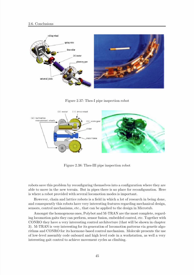
8/21/2019 Alberto Brunete Gonzalez
http://slidepdf.com/reader/full/alberto-brunete-gonzalez 73/311
2.6. Conclusions
Figure 2.37: Thes-I pipe inspection robot
Figure 2.38: Thes-III pipe inspection robot
robots save this problem by reconfiguring themselves into a configuration where they areable to move in the new terrain. But in pipes there is no place for reconfiguration. Here
is where a robot provided with several locomotion modes is important.
However, chain and lattice robots is a field in which a lot of research in being done,and consequently this robots have very interesting features regarding mechanical design,sensors, control mechanisms, etc., that can be applied to the design in Microtub.
Amongst the homogenous ones, Polybot and M-TRAN are the most complete, regard-ing locomotion gaits they can perform, sensor fusion, embedded control, etc. Together withCONRO they have a very interesting control architecture (that will be shown in chapter3). M-TRAN is very interesting for its generation of locomotion patterns via genetic algo-rithms and CONRO for its hormone-based control mechanism. Molecule presents the useof low-level assembly code onboard and high level code in a workstation, as well a very
interesting gait control to achieve movement cycles as climbing.
45

8/21/2019 Alberto Brunete Gonzalez
http://slidepdf.com/reader/full/alberto-brunete-gonzalez 74/311
CHAPTER 2. Review on Modular, Pipe Inspection and Micro Robotic Systems
3D Class Homo/Hetero DOF Self reconfig Battery Control Year
Polypod Chain Hetero(2 types) 2 No Yes C 1993
Tetrobot Chain Homo 1 x Yes C 1996Fracta3D Lattice Homo 6 Yes ? ? 1995Molecule Lattice Homo 4 Yes x C 1998CONRO Chain Homo 2 No x C/D 1998Polybot Chain Homo 1 Yes No C/D 1998Telecube Lattice Homo 2 Yes Yes C 1998
I-Cube Lattice Hetero(2 types) 3 Yes x C 1999M-TRANIII Hybrid Homo 2 Yes Yes D/C 2005
ATRON Lattice Homo 1 Yes Yes D 2003Superbot Hybrid Homo 3 Yes Yes C/D 2005Molecube Chain Homo 1 Yes ? No 2005
Table 2.1: 3-D Robots summary2D Class Homo/Hetero DOF Self reconfig Battery Control Year
CEBOT Mobile Hetero 1-3 Yes x C 1988Metamorphic Lattice Homo 3 Yes x C 1993
Fracta2D ? Homo 0 Yes x D 1994Chobie Lattice Homo 1 Yes Yes C 2003
Micro-module ? Homo 2 Yes x CCrystalline Lattice Homo 2 Yes No C 1999
Table 2.2: 2-D Robots summary
1D Class Homo/Hetero DOF Self reconfig Battery Control Year
ACM Chain Homo 1 No No C 1972ACM R5 Chain Homo 1 No Yes C/D 2007Wormbot Chain Homo 1 No No C 2003
Table 2.3: 1-D Robots summary
Regarding intermodule local communication, Telecube shows the use of contact sensorfaces as a communication mechanism and to know if there are other modules connected,
very similar to the concept of synchronism line that will be presented later on. A similarconcept is found in Chobie, which presents a control algorithm in which a leader (thatcontrols the transformation phase) is determined by local communications and changedevery transformation. ACM also uses a communication line to know the configuration of the chain robot.
In the electronic side, Digital clay stands out for the use of flexible circuit boards, simi-lar to the ones used in the modules of these thesis. ATRON presents I 2C communicationsand power sharing between modules.
Other interesting features can be found in Molecube, introducing the concept of self-replication, the ability to create another robot similar to itself from separate modules, and
Chrystalline, presenting the use of extension-contraction mechanisms in lattice robots.
46
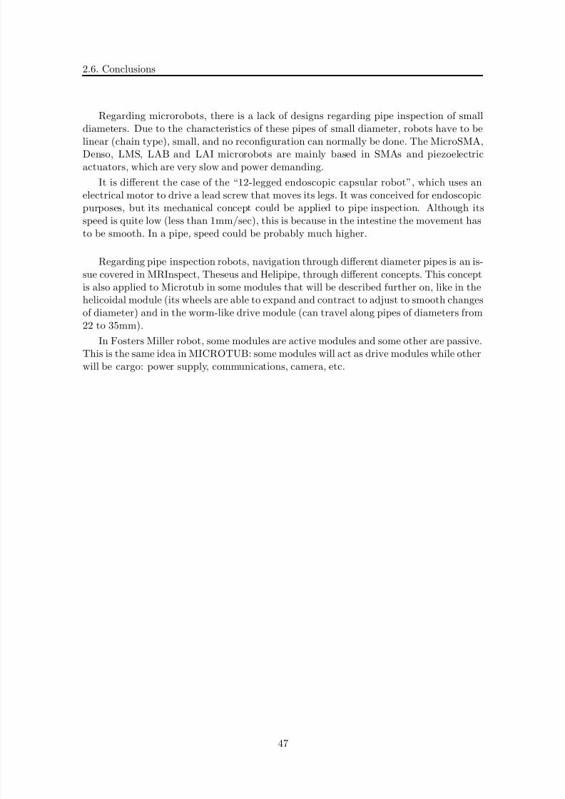
8/21/2019 Alberto Brunete Gonzalez
http://slidepdf.com/reader/full/alberto-brunete-gonzalez 75/311
2.6. Conclusions
Regarding microrobots, there is a lack of designs regarding pipe inspection of smalldiameters. Due to the characteristics of these pipes of small diameter, robots have to be
linear (chain type), small, and no reconfiguration can normally be done. The MicroSMA,Denso, LMS, LAB and LAI microrobots are mainly based in SMAs and piezoelectricactuators, which are very slow and power demanding.
It is different the case of the “12-legged endoscopic capsular robot”, which uses anelectrical motor to drive a lead screw that moves its legs. It was conceived for endoscopicpurposes, but its mechanical concept could be applied to pipe inspection. Although itsspeed is quite low (less than 1mm/sec), this is because in the intestine the movement hasto be smooth. In a pipe, speed could be probably much higher.
Regarding pipe inspection robots, navigation through different diameter pipes is an is-
sue covered in MRInspect, Theseus and Helipipe, through different concepts. This conceptis also applied to Microtub in some modules that will be described further on, like in thehelicoidal module (its wheels are able to expand and contract to adjust to smooth changesof diameter) and in the worm-like drive module (can travel along pipes of diameters from22 to 35mm).
In Fosters Miller robot, some modules are active modules and some other are passive.This is the same idea in MICROTUB: some modules will act as drive modules while otherwill be cargo: power supply, communications, camera, etc.
47

8/21/2019 Alberto Brunete Gonzalez
http://slidepdf.com/reader/full/alberto-brunete-gonzalez 76/311
CHAPTER 2. Review on Modular, Pipe Inspection and Micro Robotic Systems
48

8/21/2019 Alberto Brunete Gonzalez
http://slidepdf.com/reader/full/alberto-brunete-gonzalez 77/311
Chapter 3
Review on Control Architecturesfor Modular Microrobots
”It has yet to be proven that intelligence has any survival value”
Arthur C. Clarke
In order to develop tasks, microrobots, and robots in general, need a brain. In thecase of modular robots, each module needs a brain. There are many theories (controlarchitectures) on how to build that brain and how to interconnect each of them in order
to build a bigger brain.Control architectures can be classified in a first step in deliberative and reactive ar-
chitectures. The deliberative or planner-based architecture is the classic “model-based”artificial intelligence (AI), also called “Good old-fashioned AI” in the tradition of Mc-Carthy [McCarthy, 1958], based on models. In the 80’s purely reactive architectures ap-peared with the “Subsumption” architecture of Brooks [Brooks, 1986], giving rise to thenew “behavior-based” AI, based on the direct connection between sensors and actuators(figure 3.1). After that, hybrid and behavior-based architectures were born, as a mixtureof the former ones, using reactive layers and for fast reaction to unforeseen events and lowlevel control, and deliberative layers for planning and high level control.
Another important classification is between centralized and distributed control. Incentralized control the decisions are taken by one agent (module, computer, etc.), while indistributed control decisions are taken between several agents. It is also possible to combineboth of them, for example having a distributed control for simple or individual tasks anda central control for tasks that require planning or cooperation between agents. Each of them has its advantages and disadvantages. Centralized control is easier to implement,but depends on one only agent, if it fails the whole systems falls. In distributed systems,if one agent fails the rest can still keep working. Distributed systems have on the contrarythe problem of synchronization and coordination of agents, which is missing in centralizedcontrol.
This chapter is dedicated to describe the control architectures this thesis is based
on. The first section will explain the difference between deliberative, reactive, hybrid
49

8/21/2019 Alberto Brunete Gonzalez
http://slidepdf.com/reader/full/alberto-brunete-gonzalez 78/311
CHAPTER 3. Review on Control Architectures for Modular Microrobots
Figure 3.1: AI models: a) Deliberative b) Reactive c) Hybrid d) Behavior-based
and behavior-based architectures. Following sections will be dedicated to the study of behavior-based systems and architectures, since it is the type of control chosen for thecontrol of the MICROTUB robot. Also hybrid architectures will be covered. Finally,some interesting control designs of some state of the art robots will be described. In thelast section, a brief summary on adaptive control (use for high level control) is presented.
3.1 Classification of control architectures
Autonomous agents control architectures can then be classified in four main types:
• Deliberative or planner-based
• Purely reactive
• Hybrid
• Behavior-based
Deliberative (Planning): The architecture of robots built using this approach (seefigure 3.1) consists of a set of functional blocks which form a closed loop through whichthe information flows from the robot’s environment, via sensing, through the robot andback to the environment, via actuator control, closing the feedback loop (sense − > plan− > act). Thus, it is called a “top-down” architecture. For the most part they have asequential order of executing each process, by sensing, building a representation (model)of the state of the world, planning (presumably based on an a priori model and the builtmodel) and thus actuator control. This traditional approach has proved suitable for high-level activities such as global planning, scheduling of activities, but due to its inherentsequential ordering of the blocks this approach has proved inappropriate for dynamicenvironments which require timely responses. As a summary:
• Top-down
• Sense − > Plan − > Act
50

8/21/2019 Alberto Brunete Gonzalez
http://slidepdf.com/reader/full/alberto-brunete-gonzalez 79/311
3.1. Classification of control architectures
• Rely on a centralized world (symbolic) model
• Information in the world model is used by the planner to produce the most appro-priate actions
• Estimation of performance
• Uncertainty in sensing/action and changes in environment require re-planning
• Poorly scaling with complexity
• Poor timely responses
Some examples of deliberative architectures are: NASREM [Albus et al., 1988], VINAV[Andersen et al., 1992], Stanford Cart [Cox and Wilfong, 1990].
Traditional planning architectures were the first robotic architectures that appeared,and one of the most used has been NASREM [Albus et al., 1988].
The NASREM architecture (NASA/NBS Standard Reference Model for TelerobotControl System Architecture), proposed by Albus, is represented in Figure 3.2. The per-ceived information passes through several processing stages until a coherent view of thecurrent situation is obtained. After that, a plan is adopted and successively decomposedby other modules until the desired actions can be directly executed by the actuators. Itis composed by 6 levels:
• Servo: servo control
• Primitive: generates smooth trajectories
• Elemental move: collission free paths
• Task: converts actions into elemental moves
• Service Bay: converts group actions into single object actions
• Service mission: decomposes missions into “service bay” commands
Reactive: In reactive systems, intelligent behavior is achieved through combinationof a set of rules, each connecting perception to action. Systems consist of concurrentlyexecuted modules achieving specific tasks. Ex. avoid obstacle, follow wall...etc. Represen-tative of such systems is Brooks’ subsumption architecture, in which the robot architectureconsists of a set of hardwired (behavioral) reactive modules. As a summary:
• Bottom-up: it starts with a relatively simple abstract set of rules that is built tolearn by itself
• Sense < − > Act
• Control as a pre-programmed condition-action pairs with minimal internal state.Parallel processing
• No internal models
• Direct connection between stimuli and response. E.g. table, rules, circuit...etc
• Rely on:
– direct coupling between sensing and action
– fast feedback from the environment
51

8/21/2019 Alberto Brunete Gonzalez
http://slidepdf.com/reader/full/alberto-brunete-gonzalez 80/311
CHAPTER 3. Review on Control Architectures for Modular Microrobots
Figure 3.2: NASREM architecture
• Good if completely specified at design time
• Similar to planner with all plans computed offline before hand
• Poorly scaling with complexity
Some examples of reactive architectures are: Subsumption architecture [Brooks, 1986],Activation Networks [Maes, 1990]
Hybrid: take advantage of the potential strengths of both schools (traditional andreactive). Hybrid system architectures can be characterized by combining high-level delib-
erative activities of the traditional planning approach with the low-level reactive behaviorsof the reactive approach. The reactive behaviors ensure safe navigation, enabling the robotto handle run-time contingencies and emergency situations while the deliberative high-levelpart of the system is committed to achieving the overall task. By guiding the reactivebehaviors to achieve specific goals, the planning component ensure efficient use of systemresources.
• Compromise between reactive and deliberative
– Low level reactive control
– Higher level decision making planner
– Intermediate level(s)
52

8/21/2019 Alberto Brunete Gonzalez
http://slidepdf.com/reader/full/alberto-brunete-gonzalez 81/311
3.1. Classification of control architectures
• Separate control system into two or more communicating but otherwise independentparts (with different updating functions)
– Low level − > safety– Highest level − > select action sequences.
• Usually called ”Three Layer Architectures”
Some examples of hybrid architectures are: Aura [Arkin and Balch, 1997], Atlantis[Gat, 1992], Saphira [Konolige et al., 1997], 3T [Bonasso et al., 1995], DDP [Schonherrand Hertzberg, 2002].
Behavior-based: It is an extension of reactive architectures but lies between reactiveand deliberative. It is theoretically different from a reactive architecture. It is a method-ology for designing and controlling (autonomous) artificial systems/agents (robots) basedon biological systems. Behaviors are seen as control laws. Behaviors can store state andinformation, and integrate both low and high level control. Behaviors operate in paralleland are as simple as possible. Basic reactions to stimuli are combined to generate resultant(emerged) behaviors. As a summary:
• Started with R. Brooks and his Subsumption architecture.
• Extension of reactive arch. but between reactive and deliberative. Different fromreactive.
• Methodology for designing and controlling (autonomous) artificial systems/agents(robots) based on biological systems.
• Behavior = control law.• Behavior can store state and information.
• Integrate both low and high level control.
• Approach to modularity.
• Behaviors operate in parallel.
• Behaviors as simple as possible.
• Designed at different levels.
The key difference between behavior-based and hybrid systems is in the way represen-tation and time-scale are handled. Hybrid systems typically employ a low-level reactivesystem that operates on a short time-scale, and a high-level planner that operates on along time-scale. The two interact through a middle layer. Behavior-based systems attemptto make the representation, and thus the time-scale, of the system, uniform. Behavior-based representations are parallel, distributed, and active, in order to accommodate thereal-time demands of other parts of the system. They are implemented using the behaviorstructure, much like the rest of the system.
In general terms, it is said that reactive systems, in comparison to Behavior and Hybridbased systems are:
• Less powerful
• Good for well-defined tasks and environments and well-equipped robot
53

8/21/2019 Alberto Brunete Gonzalez
http://slidepdf.com/reader/full/alberto-brunete-gonzalez 82/311
CHAPTER 3. Review on Control Architectures for Modular Microrobots
• Great run-time efficiency but poor flexibility
• Relation between Built-in information vs On-line computation
and Behavior-based in comparison to Planner-based are:
• Less clear
• Depends on the behaviors, its definition and application.
Some examples of hybrid architectures are: DAMN [Rosenblatt, 1995], Motor Schemas[Arkin, 1987], CAMPOUT [Pirjanian et al., 2000].
3.2 Behaviour-Based Systems
3.2.1 What is a behavior?
In the Webster dictionary, three definitions of the word behavior can be found:
1. the manner of conducting oneself
2. anything that an organism does involving action and response to stimulation
3. the response of an individual, group, or species to its environment
Simply put, a behavior is a reaction to a stimulus [Arkin, 1998]. Other definitioncould be: anything observable that the system or robot does. It is clear that it is quite anintuitive concept and that there is not a precise definition.
M. Mataric [Mataric, 1994] defines behaviors as processes or control laws that achieveand/or maintain goals. For example, ’avoid-obstacles’ maintains the goal of preventingcollisions, ’go-home’ achieves the goal of reaching some home destination.
Behaviors can be implemented either in software or hardware; as a processing elementor a procedure. Each behavior can take inputs from the robot’s sensors (e.g., camera,ultrasound, infra-red, tactile) and/or from other behaviors in the system, and send outputsto the robot’s effectors (e.g, wheels, grippers, arm, speech) and/or to other behaviors.Thus, a behavior-based controller is a structured network of such interacting behaviors.
She also states that behaviors themselves can have state, and can form representationswhen networked together. Thus, unlike reactive systems, behavior-based systems are notlimited in their expressive and learning capabilities.
It is important to differentiate between behavior and action. A behavior is basedon dynamic processes operating in parallel under no central control acting as fast cou-plings between sensors and motors. It is exploiting emergence by using properties of theenvironment and side-effects from combined processes. And finally it is reactive.
Action is discrete in time (well defined start and end points, allows pre- and post-conditions) avoidance of side-effects (only one or few actions at a time, conflicts are un-desired and avoided) and deliberative. Actions are building blocks for behaviors.
Some important questions that can arise are: how do we distinguish internal behaviors(components of a BBS) and externally observable behaviors? Should we distinguish?
Behaviors are tightly connected to reactive robots. Reactive robots display desired
external behaviors, e.g. avoiding obstacles, collecting cans, walking...etc.
54

8/21/2019 Alberto Brunete Gonzalez
http://slidepdf.com/reader/full/alberto-brunete-gonzalez 83/311
3.2. Behaviour-Based Systems
3.2.2 Behavior-based systems
Behavior-based systems consist of sequential modules achieving independent functions.
Abstract representation is usually avoided in these systems. Behaviors are the buildingblocks of the system. They have its basis in biological studies and so biology is an inspi-ration for design. Example: generate a motor response from a given perceptual stimulus.
The main properties of behavior-based systems are:
• Ability to act in real time
• Ability to use representations to generate efficient (not only reactive) behavior
• Ability to use a uniform structure and representation throughout the system (so nointermediate layer)
Other important properties are:
• Achieve specific tasks/goals: avoid others, find friend, go home
• Typically executed concurrently
• Can store state and be used to construct world models/representations
• Can directly connect sensors to effectors
• Can take inputs from other behaviors and send outputs to other behaviors (connec-tion in networks)
• Typically higher-level than actions (“go home”, while an action would be “turn left45 degrees”)
• The can be inhibited by other behaviors or agents• They can be prioritized
3.2.3 Behavior representation
Behaviors can be expressed by different representations. When a control system is beingdesigned, the task is broken down into desired external behaviors.
There are several ways to express a behavior, there is not a universal method. Someof the most common are:
• Functional notation
• Stimulus response (SR) diagrams
• Finite state machines/automata (FSA)
• Rule-based representations
• Formal methods: RS (Robot Schema) and Situated Automata
Stimulus response (SR) diagrams
These are the most intuitive and the least formal method of expression. Any behaviorcan be represented as a generated response to a given stimulus computed by a specific
behavior (figure 3.3).
55

8/21/2019 Alberto Brunete Gonzalez
http://slidepdf.com/reader/full/alberto-brunete-gonzalez 84/311
CHAPTER 3. Review on Control Architectures for Modular Microrobots
Figure 3.3: Example of stimulus response diagram
Functional notation
A mathematical methods can be used to describe the same relationships using a functionalnotation.
b(s) = r (3.1)
Where:
• s = stimulus
• r = range of response
• b = behavioral mapping between S and R
Example for a navigational task of getting to a classroom:
coordinate-behaviors (
move-to-classroom ( detect-classroom-location ),
avoid-objects ( detect-objects ),
dodge-students ( detect-students ),
stay-to-right-on-path ( detect-path ),
defer-to-elders ( detect-elders )
) = motor-response
It is easily convertible to functional languages like LISP [McCarthy, 1960].
Finite State Automata (FSA)
FSA have very useful properties when describing aggregations and sequences of behaviors.They make explicit the behaviors active at any given time and the transitions betweenthem. They are not so useful when encoding a single behavior.
A Finite State Automata is set up with sensor-events on the arcs and actions in eachstate, see figure 3.4. The idea is that the robot is in one state doing one action, until thetransition-condition on one of the arcs leading from this state is satisfied, resulting in achange to the state at the other end of the arc. One problem with this approach is, thatit gets increasingly difficult for a programmer to maintain the overview of the behavior of
the system as the number of states gets larger.
56
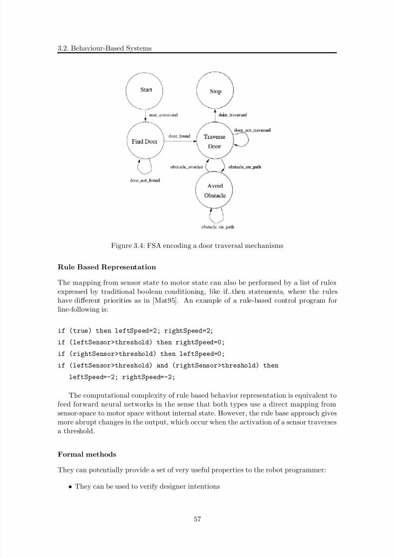
8/21/2019 Alberto Brunete Gonzalez
http://slidepdf.com/reader/full/alberto-brunete-gonzalez 85/311
3.2. Behaviour-Based Systems
Figure 3.4: FSA encoding a door traversal mechanisms
Rule Based Representation
The mapping from sensor state to motor state can also be performed by a list of rules
expressed by traditional boolean conditioning, like if..then statements, where the ruleshave different priorities as in [Mat95]. An example of a rule-based control program forline-following is:
if (true) then leftSpeed=2; rightSpeed=2;
if (leftSensor>threshold) then rightSpeed=0;
if (rightSensor>threshold) then leftSpeed=0;
if (leftSensor>threshold) and (rightSensor>threshold) then
leftSpeed=-2; rightSpeed=-2;
The computational complexity of rule based behavior representation is equivalent tofeed forward neural networks in the sense that both types use a direct mapping fromsensor-space to motor space without internal state. However, the rule base approach givesmore abrupt changes in the output, which occur when the activation of a sensor traversesa threshold.
Formal methods
They can potentially provide a set of very useful properties to the robot programmer:
• They can be used to verify designer intentions
57
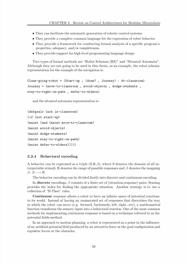
8/21/2019 Alberto Brunete Gonzalez
http://slidepdf.com/reader/full/alberto-brunete-gonzalez 86/311
CHAPTER 3. Review on Control Architectures for Modular Microrobots
• They can facilitate the automatic generation of robotic control systems
• They provide a complete common language for the expression of robot behavior
• They provide a framework for conducting formal analysis of a specific program’sproperties, adequacy, and/or completeness.
• They provide support for high level programming language design
Two types of formal methods are “Robot Schemas (RS)” and “Situated Automata”.Although they are not going to be used in this thesis, as an example, the robot schemarepresentation for the example of the navigation is:
Class-going-robot = (Start-up ; (done? , Journey) : At-classroom)
Journey = (move-to-classroom , avoid-objects , dodge-students ,
stay-to-right-on-path , defer-to-elders)
and the situated automata representation is:
(defgoalr (ach in-classroom)
(if (not start-up)
(maint (and (maint move-to-classroom)
(maint avoid-objects)
(maint dodge-students)
(maint stay-to-right-on-path)(maint defer-to-elders)))))
3.2.4 Behavioral encoding
A behavior can be expressed as a triple (S,R,β ), where S denotes the domain of all in-terpretable stimuli, R denotes the range of possible responses and β denotes the mappingβ : S −→ R.
The behavior encoding can be divided firstly into discrete and continuous encoding.
In discrete encodings, β consists of a finite set of (situation,response) pairs. Sensing
provides the index for finding the appropriate situation. Another strategy is to use acollection of “If-Then” rules.
Continuous response allows a robot to have an infinite space of potential reactionsto its world. Instead of having an enumerated set of responses that discretizes the wayin which the robot can move (e.g. forward, backwards, left, right...etc), a mathematicalfunction transforms the sensory input into a behavioral reaction. One of the most commonmethods for implementing continuous response is based on a technique referred to as thepotential fields method.
In an approach to motion planning: a robot is represented as a point in the influenceof an artificial potential field produced by an attractive force at the goal configuration and
repulsive forces at the obstacles.
58

8/21/2019 Alberto Brunete Gonzalez
http://slidepdf.com/reader/full/alberto-brunete-gonzalez 87/311
3.2. Behaviour-Based Systems
Figure 3.5: Potential fields
U (q ) = U att(q ) + U rep(q ) (3.2)
3.2.5 Emergent behavior
The cathedral termite, found in parts of Australia, is capable of creating mounds for thecolony well over 10 feet high. Individual cathedral termites are just standard-lookingbugs with a tiny little primitive brain. But when combined with others of its species,the cathedral termite is capable of constructing a huge, complex hive to house the colony.Unlike human building projects, however, there is no foreman, no plan, and it’s unlikelythat any termite even knows what it is helping to create. [Emergent Behavior - ThrivingAt The Edge Of Chaos by Chris Rollins]
How is this possible?
The answer lies in the fact that sometimes, a system can provide more complexitythan the sum of its parts - leading to what scientists call ”emergent behavior.” Emergentbehavior could be defined as a behavior of a system that is not explicitly described by thebehavior of the components of the system, and is therefore unexpected to a designer orobserver.
Emergent behavior is an important but not well-understood phenomenon. Robot be-haviors “emerge” from
• interactions of rules
• interactions of behaviors• interactions of either with environment
There is a coded behavior in the programming scheme, a observed behavior in the eyesof the observer, but there is no one-to-one mapping between the two.
Example: Emergent flocking. When programming multiple robots under the followingpremises:
• don’t run into any other robot
• don’t get too far from other robots
• keep moving if you can
59
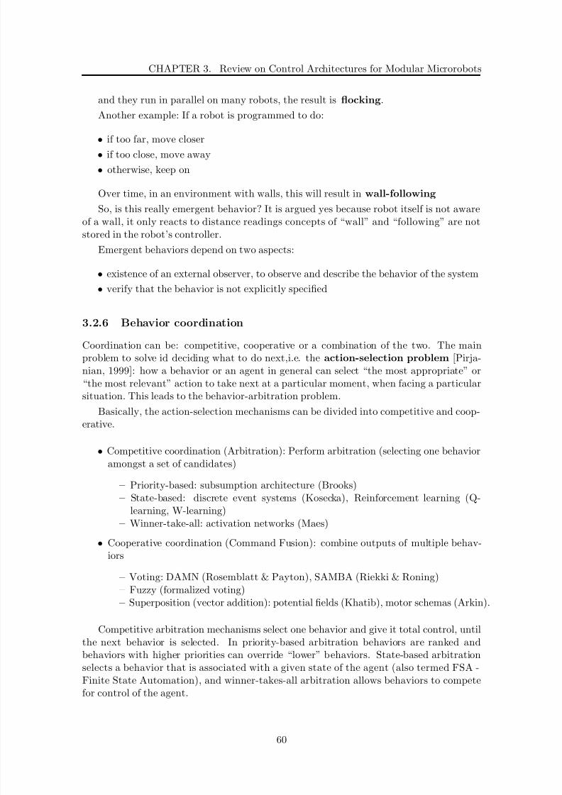
8/21/2019 Alberto Brunete Gonzalez
http://slidepdf.com/reader/full/alberto-brunete-gonzalez 88/311
CHAPTER 3. Review on Control Architectures for Modular Microrobots
and they run in parallel on many robots, the result is flocking.
Another example: If a robot is programmed to do:
• if too far, move closer• if too close, move away
• otherwise, keep on
Over time, in an environment with walls, this will result in wall-following
So, is this really emergent behavior? It is argued yes because robot itself is not awareof a wall, it only reacts to distance readings concepts of “wall” and “following” are notstored in the robot’s controller.
Emergent behaviors depend on two aspects:
• existence of an external observer, to observe and describe the behavior of the system• verify that the behavior is not explicitly specified
3.2.6 Behavior coordination
Coordination can be: competitive, cooperative or a combination of the two. The mainproblem to solve id deciding what to do next,i.e. the action-selection problem [Pirja-nian, 1999]: how a behavior or an agent in general can select “the most appropriate” or“the most relevant” action to take next at a particular moment, when facing a particularsituation. This leads to the behavior-arbitration problem.
Basically, the action-selection mechanisms can be divided into competitive and coop-erative.
• Competitive coordination (Arbitration): Perform arbitration (selecting one behavioramongst a set of candidates)
– Priority-based: subsumption architecture (Brooks)– State-based: discrete event systems (Kosecka), Reinforcement learning (Q-
learning, W-learning)– Winner-take-all: activation networks (Maes)
• Cooperative coordination (Command Fusion): combine outputs of multiple behav-
iors
– Voting: DAMN (Rosemblatt & Payton), SAMBA (Riekki & Roning)– Fuzzy (formalized voting)– Superposition (vector addition): potential fields (Khatib), motor schemas (Arkin).
Competitive arbitration mechanisms select one behavior and give it total control, untilthe next behavior is selected. In priority-based arbitration behaviors are ranked andbehaviors with higher priorities can override “lower” behaviors. State-based arbitrationselects a behavior that is associated with a given state of the agent (also termed FSA -Finite State Automation), and winner-takes-all arbitration allows behaviors to compete
for control of the agent.
60

8/21/2019 Alberto Brunete Gonzalez
http://slidepdf.com/reader/full/alberto-brunete-gonzalez 89/311
3.2. Behaviour-Based Systems
Figure 3.6: Basic block in subsumption architecture
Command Fusion ASMs combine recommendations from several behaviors to forma consensus control action, aggregating one or more behaviors according to some rule;essentially the difference between different command fusion architectures resides in thefunction which is used to aggregate behaviors.
Priority-based
The most well known implementation of a priority-based architecture is the subsumptionarchitecture, described by Brooks [Brooks, 1986]. In this architecture, the agent acquires
levels of competence in a layered format; this also allows modularity and upgrading withmore complex higher-level behaviors. Higher-level layers subsume lower levels when theywish to assume control - this is done by suppressing signals sent from the higher levelbehaviors to inhibit the lower level behaviors (3.6). More complex behavioral patternsare obtained using priorities and subsumption relations between the behaviors, such thatcertain behaviors can override others, or behaviors can operate in parallel, when two ormore behaviors are signaled by a stimulus. This architecture will be described on 3.3.1.
State-based
Behavior selection is done using state transition where upon detection of a certain event
a shift is made to a new state and thus a new behavior. Using this formalism systems aremodeled in terms of a finite state automata (FSA) where states correspond to executionof actions/behaviors and events, which correspond to observations and actions, causetransitions between the states. See example of FSA in figure 3.4.
State-based arbitration architectures include Discrete Event Systems [Kosecka andBajsy, 1993] and Bayesian Decision Analysis [Kristensen, 1997]. In Discrete Event Systems(DES) agents are modeled in terms of finite state automata (FSA) where states correspondto execution of actions/behaviors and events correspond to observations and actions, andcause transitions between the states.
Bayesian Decision Analysis is based on sensor selection. The objective is to choose
the action that maximizes the expected utility of the agent. Selection of an action is
61

8/21/2019 Alberto Brunete Gonzalez
http://slidepdf.com/reader/full/alberto-brunete-gonzalez 90/311
CHAPTER 3. Review on Control Architectures for Modular Microrobots
based around maximization of the expected utility, using Bayesian probability.Each sensingaction is associated with a certain cost or expense and benefit is associated with theinformation provided by the sensing action. It is a probabilistic method. Example: going
through the doorway when the door is open/closed.
Winner-take-all
Here the behaviors actively compete with each other based on sensory information andagent’s goals and intentionality.
”Activation Networks” from Maes [Maes, 1990] is based on an engine where a commu-nity of behaviors works to reduce the difference between present and desired state. Eachbehavior is specified in terms of pre- and post-conditions, and an activation level, whichgives a real-valued indication of the relevance of the behavior in a particular situation.The higher the activation level of a behavior, the more likely it is that this behavior willinfluence the output of the agent. Once specified, a set of competence behaviors is com-piled into a spreading activation network, in which the modules are linked to one-anotherin ways defined by their pre- and post-conditions.
Behaviors are activated by their activation energy reaching a specified level; activa-tion energy is added and removed to the network of behaviors by external (goal, state,inhibition) and internal (predecessor, successor, inhibition) sources (figure 3.11).
When the activation level of an executable behavior exceeds a specified threshold, itis selected to execute the most appropriate action from its point of view.
VotingMany voting architectures exist, all sharing the common feature that a polling mechanismis employed to select between “competing behaviors”.
Each active behavior has a certain number of votes to give to the behavioral responseset previously defined. The response with more votes is the action selected.
An example of a voting command fusion architecture is the DAMN architecture [Rosen-blatt, 1995], covered in 3.3.4.
Fuzzy
Fuzzy architectures uses fuzzy inference and behavior rules which are combined into amultivalued output. Behaviors that compete for control of the robot are then coordinatedto resolve potential conflicts. Fuzzy behavior coordination is performed by combining thefuzzy outputs of the behaviors using an appropriate operator; they are then defuzzed atthe end to provide a clean final control action (figure 3.7).
Each behavior is synthesized by a rule-base controlled by an inference engine to producea multivalued output that encodes the desirability of each action from the behaviorOs pointof view. Example:
IF obstacle is close THEN avoid collision
IF NOT (obstacle is close) THEN follow target
62
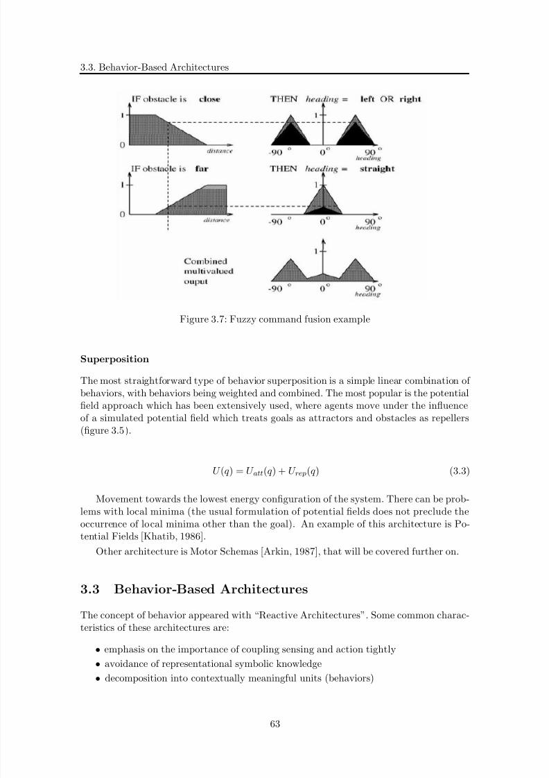
8/21/2019 Alberto Brunete Gonzalez
http://slidepdf.com/reader/full/alberto-brunete-gonzalez 91/311
3.3. Behavior-Based Architectures
Figure 3.7: Fuzzy command fusion example
Superposition
The most straightforward type of behavior superposition is a simple linear combination of behaviors, with behaviors being weighted and combined. The most popular is the potential
field approach which has been extensively used, where agents move under the influenceof a simulated potential field which treats goals as attractors and obstacles as repellers(figure 3.5).
U (q ) = U att(q ) + U rep(q ) (3.3)
Movement towards the lowest energy configuration of the system. There can be prob-lems with local minima (the usual formulation of potential fields does not preclude theoccurrence of local minima other than the goal). An example of this architecture is Po-tential Fields [Khatib, 1986].
Other architecture is Motor Schemas [Arkin, 1987], that will be covered further on.
3.3 Behavior-Based Architectures
The concept of behavior appeared with “Reactive Architectures”. Some common charac-teristics of these architectures are:
• emphasis on the importance of coupling sensing and action tightly
• avoidance of representational symbolic knowledge
• decomposition into contextually meaningful units (behaviors)
63

8/21/2019 Alberto Brunete Gonzalez
http://slidepdf.com/reader/full/alberto-brunete-gonzalez 92/311
CHAPTER 3. Review on Control Architectures for Modular Microrobots
Figure 3.8: Example of structure in subsumption architecture
Behavior-based architectures were based on reactive architectures, but are not thesame, as it was explained before. In the following sections some of these architectures will
be described.
3.3.1 Subsumption Architecture
Brooks subsumption architecture [Brooks, 1986], is one of the best known implementationsof behavior that does not include a world model. Subsumption architecture systems areincrementally built up of competences, where a new competence can subsume behaviorgenerated by the already existing competences, thereby altering the behavior of the system.The competences all run simultaneously, and each can react on the present sensor state,which gives a reactive behavior. The subsumption architecture is illustrated in figure3.6. This figure shows how the higher levels can overwrite (subsume) the output of the
lower levels. The figure does not show that the higher levels can also change the behaviorgenerated by the lower levels. The system can be partitioned at any level, and the layersbelow form a complete operational control system.
Several different robotic systems have been built using this approach. However, theadding of new competences to a subsumption architecture system becomes increasinglydifficult as the system gets larger, because of the many different possibilities of connectingthe new competence, and because the generated behavior is an emergent property of theinteraction between all the competences
At the lowest level, each behavior is represented using an augmented finite state ma-chine (AFSM), as shown in figure 3.8. Stimulus or response signals can be suppressed or
inhibited by other active behaviors.There is no global memory, bus or clock. Each behavioral layer is mapped onto its own
processor. No central world models. Figure 3.9 shows an example of three layered robot.
Coordination in subsumption has two primary mechanisms:
• Inhibition: to prevent a signal from reaching the actuators
• Suppression : prevents a signal from being transmitted and replaces it with a sup-pressing message.
The lowest level layer of control makes sure that the robot does not come into contactwith other objects. If something approaches the robot it will move away. The first level
layer of control, when combined with the zeroth, imbues the robot with the ability to
64
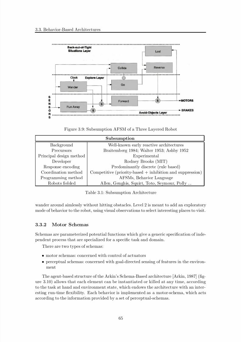
8/21/2019 Alberto Brunete Gonzalez
http://slidepdf.com/reader/full/alberto-brunete-gonzalez 93/311
3.3. Behavior-Based Architectures
Figure 3.9: Subsumption AFSM of a Three Layered Robot
Subsumption
Background Well-known early reactive architecturesPrecursors Braitemberg 1984; Walter 1953; Ashby 1952
Principal design method ExperimentalDeveloper Rodney Brooks (MIT)
Response encoding Predominantly discrete (rule based)Coordination method Competitive (priority-based + inhibition and suppression)
Programming method AFSMs, Behavior LanguageRobots fielded Allen, Genghis, Squirt, Toto, Seymour, Polly ...
Table 3.1: Subsumption Architecture
wander around aimlessly without hitting obstacles. Level 2 is meant to add an exploratorymode of behavior to the robot, using visual observations to select interesting places to visit.
3.3.2 Motor Schemas
Schemas are parameterized potential functions which give a generic specification of inde-
pendent process that are specialized for a specific task and domain.There are two types of schemas:
• motor schemas: concerned with control of actuators
• perceptual schemas: concerned with goal-directed sensing of features in the environ-ment
The agent-based structure of the Arkin’s Schema-Based architecture [Arkin, 1987] (fig-ure 3.10) allows that each element can be instantiated or killed at any time, accordingto the task at hand and environment state, which endows the architecture with an inter-esting run-time flexibility. Each behavior is implemented as a motor-schema, which acts
according to the information provided by a set of perceptual-schemas.
65

8/21/2019 Alberto Brunete Gonzalez
http://slidepdf.com/reader/full/alberto-brunete-gonzalez 94/311
CHAPTER 3. Review on Control Architectures for Modular Microrobots
Figure 3.10: Structure of Motor Schemas
Motor schemas are similar to animal behaviors. The may have internal parameters thatprovide additional flexibility. Each of them has an output (action vector) that defines theway the robot should move. Perceptual schemas are embedded in each motor schema,and provide the environmental information specific for that particular behavior. They
are recursively defined, that is, there can be perceptual subschemas providing informationthat will be processed by the perceptual schema.
Many different motor schemas have been defined, including:
• Move-ahead: move in a particular compass direction
• Move-to-goal: move towards a detected goal object. Two versions exist of thisschema: ballistic and controlled
• Avoid-static-obstacle: move away from passive or non threatening navigational bar-riers
• Dodge: sidestep an approaching ballistic projectile
• Escape: move away from the projected intercept point between the robot and anapproaching predator
• Stay-on-path: move toward the center of a path, road, or hallway. For three-dimensional navigation, this becomes the stay-in-channel schema
• Noise: move in a random direction for a certain amount of time
• Follow-the-leader: move to a particular location displaced somewhat from a possiblymoving object. (The robot acts as if it is leashed invisibly to the moving object.)
• Probe: move toward open areas
66

8/21/2019 Alberto Brunete Gonzalez
http://slidepdf.com/reader/full/alberto-brunete-gonzalez 95/311
3.3. Behavior-Based Architectures
Motor Schemas
Background Reactive component of AuRA ArchitecturePrecursors Arbib 1981; Khatib 1985
Principal design method Ethologically guidedDeveloper Ronald Arkin (Georgia Tech)
Response encoding Continuous using potential field analogCoordination method Cooperative via vector summation and normalizationProgramming method Parameterized behavioral libraries
Robots fielded HARV, George, Ren and Stimpy, Buzz ...
Table 3.2: Motor Schemas Architecture
• Dock: approach an object from a particular direction
• Avoid-past: move away from areas recently visited• Move-up, move-down, maintain-altitude: move upward or downward or follow an
isocontour in rough terrain
• Teleautonomy: allows human operator to provide internal bias to the control systemat the same level as another schema
The cooperative coordination mechanism is based on weighted vectorial sum, whereweights allow to distinguish motor-schemas in terms of priority. Modularity is providedby its agent-based nature and standard vectorial form for motor-schemas output. In thisline, a set of motor-schemas and respective coordination nodes can be aggregated into a
single motor-schema, also called of assemblage behavior. An external entity, a sequencer,can select which behavioral assemblages are active according to the task/environment. Infigure 3.10 it would be situated between the ”VECTOR Σ” and the ”Robot motors”.
Arkin: “The task of robot programming is fundamentally simplified through the useof a divide and conquer strategy”.
Example: an obstacle avoidance motor schema can control the robot away from theobstacle. In order to detect obstacles several obstacle detection perceptual schemas canbe instantiated to keep track of obstacles and feed the obstacle positions to associatedobstacle avoidance motor schemas.
3.3.3 Activation Networks
It is a combination of traditional planners and reactive systems developed by Maes [Maes,1990]. The architecture consists of a set of behaviors or competence modules which areconnected to form a network (figure 3.11). Action-selection is modeled as an emergentproperty of an activation/inhibition dynamics among these modules. The set of behaviorsreduce the difference between the systems present state and a goal state. Arbitrationamong modules is a run-time process, which changes according to goals and current situ-ation.
In the network each behavior is represented by a tuple (ci, ai, di, αi) describing:
1. the preconditions under which it is executable (i.e. can be applied)
67

8/21/2019 Alberto Brunete Gonzalez
http://slidepdf.com/reader/full/alberto-brunete-gonzalez 96/311
CHAPTER 3. Review on Control Architectures for Modular Microrobots
Figure 3.11: Activation Networks
2. the effects after successful execution in form of an add-list ai and delete-list di
3. activation level αi which is a measure of applicability of the behavior
External sources of activation are: activation by the state, activation by the goals andinhibition by protected goals.
Internal sources of activation are: activation of successors, activation of predecessorsand inhibition of conflictors.
This ASM deals only with selection of behaviors and not with motor actions. When abehavior is selected it will perform the most appropriate action from its point of view (itis a winner-take-all mechanism).
The internal mechanisms of a competence model are independent of the architecture.
A competence model has a condition list, which aggregates all conditions to be met beforethe module becomes executable, an add list and a delete list, which are the effects of the module. Successor links connect add list items of one competence to condition listof another competence. A predecessor link from module X to module Y exists for eachsuccessor link from Y to X. A conflicter link connects delete list items of one competenceto condition list of another competence. Provided that, a competence is executable, itsactivation value is above a certain threshold, and it is greater than all other competencemodules’ activation, the competence is allowed to perform real actions (i.e. actuate directlyin the actuators). Briefly, activation is increased every time an item in the condition list ismet and by the achievement of a global goal. Then, activation flows between competencemodules via successor, precessor, and conflictor links. A decay function ensures that the
overall activation level remains constant.
68

8/21/2019 Alberto Brunete Gonzalez
http://slidepdf.com/reader/full/alberto-brunete-gonzalez 97/311
3.3. Behavior-Based Architectures
Activation Networks
Background Dynamic competition systemPrecursors Minsky 1986; Hillis 1988
Principal design method ExperimentalDeveloper Pattie Maes (MIT)
Response encoding DiscreteCoordination method Arbitration via action-selectionProgramming method Competence modules
Robots fielded Only simulation
Table 3.3: Activation Networks Architecture
Figure 3.12: DAMN architecture
3.3.4 DAMN
DAMN is a Distributed Architecture for Mobile Navigation [Rosenblatt, 1995] which con-sists of a set of asynchronous behaviors that pursue the system goals based on the currentstate of the environment. Each behavior votes for or against the set of actions constitutingthe possible set of actions of the agent. The best action is the one with the maximumweighted sum of the received votes. Each behavior is assigned a weight. These weightsreflect the relative importance or priority of the behavior in a given context. The arbiteris then responsible for combining the behaviors’ votes and generating actions which re-flects their objectives and priorities. A behavior can be a reactive behavior as well as aplanning module. Well suited for integration of high level deliberative planners with lowlevel reactive behaviors.
3.3.5 CAMPOUT
CAMPOUT is a Control Architecture for Multi-robot Planetary Outposts [Pirjanian et al.,2000] [Pirjanian et al., 2001] by the Jet Propulsion Lab in Pasadena, CA. It is a three
layer behavior-based system:
69

8/21/2019 Alberto Brunete Gonzalez
http://slidepdf.com/reader/full/alberto-brunete-gonzalez 98/311
CHAPTER 3. Review on Control Architectures for Modular Microrobots
DAMN (Distributed Architecture for Mobile Navigation)
Background Fine-grained subsumption-style architecturePrecursors Brooks 1986; Zadeh 1973
Principal design method ExperimentalDeveloper Julio Rosenblatt (CMU)
Response encoding Discrete vote setsCoordination method Multiple winner-take-all arbitersProgramming method Custom
Robots fielded DARPA ALV and UGV vehicles
Table 3.4: DAMN Architecture
• Low level control routines.
• Middle behavior layer that uses either the BISMARC (Biologically Inspired System
for Map-based Autonomous Rover Control) or MOBC (Multi-Objective BehaviorControl) action selection mechanisms.
• Hierarchical task planning, allocation and monitoring
CAMPOUT includes the necessary group behaviors and communication mechanismsfor the coordinated and cooperative control of heterogeneous robotic platforms. It is a dis-tributed, hybrid, behavior-based system because it couples reactive and local deliberativebehaviors without the need for a centralized planner.
Control architectures closest to CAMPOUT are ALLIANCE, DAMN, BISMARC andMOBC.
Its main characteristics are:
• Cognizant of failure and Fault tolerant
• Distributed control
• Scalable and Ease of integration
• Rational decision making
• Explicit knowledge
• Uncertainty handling
• Adaptivity and Learning capabilities
• Hybrid
• Formal framework
• Small overhead
Behaviors are divided in the following classes:
• Primitive Behavior Library: behavior producing module (behavior). A behavior isa perception to action mapping module that based on selective sensory informationproduces actions in order to maintain or achieve a given, well specified task objective.Ex. AvoidObstacle and GotoTarget
• Composite Behaviors: combination of lower-level behaviors. Example: SafeNaviga-
tion
70

8/21/2019 Alberto Brunete Gonzalez
http://slidepdf.com/reader/full/alberto-brunete-gonzalez 99/311
3.3. Behavior-Based Architectures
Figure 3.13: CAMPOUT: block diagram
• Communication Behaviors: interaction with other robots
• Shadow Behaviors (s-behaviors): a remote behavior (including for example stateinformation) running on a separate robot
• Cooperation/Coordination Behaviors: coordination between c-behaviors and s-behaviors
CAMPOUT uses the following control mechanisms:
• Arbitration mechanisms
– Suitable for arbitrating between the set of active behaviors in accord with thesystem’s changing objectives and requirements.
– CAMPOUT implements
∗ priority-based arbitration, where behaviors with higher priorities are al-lowed to suppress the output of behaviors with lower priorities;
∗ state-based arbitration which is based on the discrete event systems (DES)
formalism, and is suitable for behavior sequencing.
• Command fusion mechanisms
– Voting: interpret the output of each behavior as votes for or against possibleactions and the action with the maximum weighted sum of votes is selected(DAMN-style based on BISMARC);
– Fuzzy command fusion mechanisms that use fuzzy logic and inference to for-malize the action selection processes;
– Multiple objective behavior fusion mechanisms that select an action with thebest trade-off between the task objectives and which satisfies the behavioral
objectives as much as possible based on multiple objective decision theory
71

8/21/2019 Alberto Brunete Gonzalez
http://slidepdf.com/reader/full/alberto-brunete-gonzalez 100/311
CHAPTER 3. Review on Control Architectures for Modular Microrobots
CAMPOUT
Background ALLIANCE, DAMN, BISMARC and MOBCPrecursors DAMN, ALLIANCE
Principal design method ExperimentalDeveloper JPL
Response encoding Both discrete and continuousCoordination method Several: priority-based, state-based, voting, fuzzy, etc.Programming method Distributed
Robots fielded Campout Rover
Table 3.5: Control Architecture for Multi-robot Planetary Outposts (CAMPOUT) Archi-tecture
Communications infrastructure: Provides a set of tools and functions for intercon-
necting a set of robots and/or behaviors for sharing resources (e.g., sensors or actuators),exchanging information (e.g., state, percepts), synchronization, rendezvous etc.
• Synchronization: Signal (destination, sig) and Wait (source, sig) can be used to sendand wait for a signal to and from a given robot
• Data exchange: SendEvent (destination, event) and GetEvent (source, event) canbe used to send and receive an event structure
• Behavior exchange: SendObjective (destination, objective) and GetObjective (source,objective) can be used to send and receive objective functions (multivalued behavioroutputs)
3.4 Hybrid Deliberate-Reactive Architectures
Everybodys got plans... until they get hit (M. Tyson)
There is a need to solve the drawbacks of reactive and deliberative systems. And thoseare the hybrid architectures. Some strategies to do this are:
• Selection: Planning is viewed as configuration. Planner determines the behavioralcomposition
• Advising: Planning is viewed as advice giving. Planner suggests and reactive levelmay or may not use it.
• Adaptation: Planning is viewed as adaptation. Planner modify reactive componentsdepending on environment changes
• Postponing: Planning is viewed as a least commitment process. Plans are elaboratedonly as necessary.
Modern robot control architectures are hybrid , i.e., they contain different layers forreactive and for deliberative control components. Typically, a middle layer (sometimescalled sequencing layer) mediates between the reactive and the deliberative components,
resulting in a three-layer architecture.
72
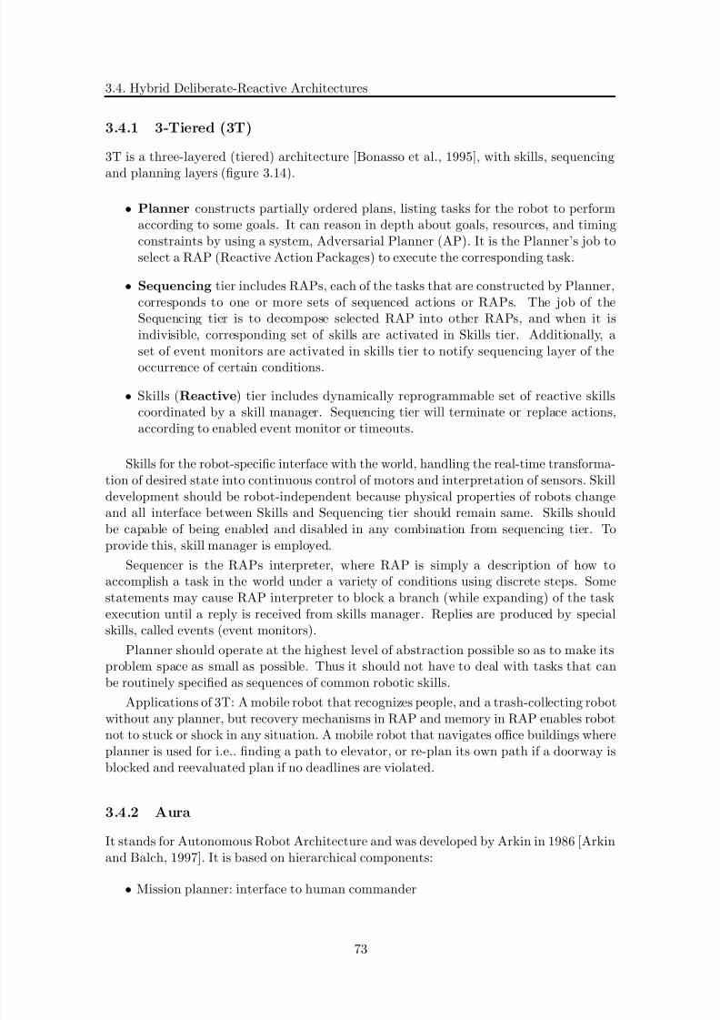
8/21/2019 Alberto Brunete Gonzalez
http://slidepdf.com/reader/full/alberto-brunete-gonzalez 101/311
3.4. Hybrid Deliberate-Reactive Architectures
3.4.1 3-Tiered (3T)
3T is a three-layered (tiered) architecture [Bonasso et al., 1995], with skills, sequencing
and planning layers (figure 3.14).
• Planner constructs partially ordered plans, listing tasks for the robot to performaccording to some goals. It can reason in depth about goals, resources, and timingconstraints by using a system, Adversarial Planner (AP). It is the Planner’s job toselect a RAP (Reactive Action Packages) to execute the corresponding task.
• Sequencing tier includes RAPs, each of the tasks that are constructed by Planner,corresponds to one or more sets of sequenced actions or RAPs. The job of theSequencing tier is to decompose selected RAP into other RAPs, and when it isindivisible, corresponding set of skills are activated in Skills tier. Additionally, a
set of event monitors are activated in skills tier to notify sequencing layer of theoccurrence of certain conditions.
• Skills (Reactive) tier includes dynamically reprogrammable set of reactive skillscoordinated by a skill manager. Sequencing tier will terminate or replace actions,according to enabled event monitor or timeouts.
Skills for the robot-specific interface with the world, handling the real-time transforma-tion of desired state into continuous control of motors and interpretation of sensors. Skilldevelopment should be robot-independent because physical properties of robots changeand all interface between Skills and Sequencing tier should remain same. Skills should
be capable of being enabled and disabled in any combination from sequencing tier. Toprovide this, skill manager is employed.
Sequencer is the RAPs interpreter, where RAP is simply a description of how toaccomplish a task in the world under a variety of conditions using discrete steps. Somestatements may cause RAP interpreter to block a branch (while expanding) of the taskexecution until a reply is received from skills manager. Replies are produced by specialskills, called events (event monitors).
Planner should operate at the highest level of abstraction possible so as to make itsproblem space as small as possible. Thus it should not have to deal with tasks that canbe routinely specified as sequences of common robotic skills.
Applications of 3T: A mobile robot that recognizes people, and a trash-collecting robot
without any planner, but recovery mechanisms in RAP and memory in RAP enables robotnot to stuck or shock in any situation. A mobile robot that navigates office buildings whereplanner is used for i.e.. finding a path to elevator, or re-plan its own path if a doorway isblocked and reevaluated plan if no deadlines are violated.
3.4.2 Aura
It stands for Autonomous Robot Architecture and was developed by Arkin in 1986 [Arkinand Balch, 1997]. It is based on hierarchical components:
• Mission planner: interface to human commander
73

8/21/2019 Alberto Brunete Gonzalez
http://slidepdf.com/reader/full/alberto-brunete-gonzalez 102/311
CHAPTER 3. Review on Control Architectures for Modular Microrobots
Figure 3.14: 3T intelligent controll architecture
• Spatial Reasoner (Navigator): cartographic knowledge stored in memory to con-struct paths. A*
• Plan Sequencer (Pilot): translates the path into motor behaviors
It uses schemas as reactive component. Once reactive execution begins, the deliberativecomponent is not reactivated until failure (lack of progress). Some of its principles are:modularity, flexibility, generalizability.
3.4.3 Atlantis
Atlantis (Three-Layer Architecture for Navigating Through Intricate Situations) [Gat,1992], like the subsumption architecture, is built in layers as shown in figure 3.16. InAtlantis, however, all instantiations of the architecture have the same three layers, each of which always performs the same duty. This architecture is both asynchronous and hetero-
geneous. None of the layers is in charge of the others, and activity is spread throughout
74

8/21/2019 Alberto Brunete Gonzalez
http://slidepdf.com/reader/full/alberto-brunete-gonzalez 103/311
3.4. Hybrid Deliberate-Reactive Architectures
Figure 3.15: Aura Architecture
the architecture.
The Control Layer directly reads sensors and sends reactive commands to the effectorsbased on the readings. The stimulus-response mapping is given to it by the sequencinglayer. It is implemented in ALFA, a LISP-based programming language
The Sequencing Layer has a higher-level view of robotic goals than the control layer.It tells the control layer below it when to start and stop actions.
The Deliberative Layer responds to requests from the sequencing layer to performdeliberative computations. It consists of traditional LISP-based AI planning algorithmsspecific to the task at hand. The planner’s output is viewed only as advice to the sequencerlayer: it is not necessarily followed or implemented verbatim.
3.4.4 Saphira
The Saphira architecture [Konolige et al., 1997] is an integrated sensing and control systemfor robotics applications (figure 3.17). Perceptual routines are on the left, action routineson the right. The vertical dimension gives an indication of the cognitive level of processing,with high-level behaviors and perceptual routines at the top. Control is coordinated byPRS-Lite, which instantiates routines for navigation, planning, execution monitoring, andperceptual coordination. At the center is the LPS (Local Perception Space), a geometricrepresentation of space around the robot. Because different tasks demand different repre-sentations, the LPS is designed to accommodate various levels of interpretation of sensorinformation, as well as a priori information from sources such as maps. The LPS givesthe robot an awareness of its immediate environment, and is critical in the tasks of fusingsensor information, planning local movement, and integrating map information.
Saphira architecture is an integrated sensing and control system, which includes LocalPerception Space (LPS) at its center containing different levels of representation (from
occupancy grids, to geometric representation to high level artifacts of the world). Internal
75

8/21/2019 Alberto Brunete Gonzalez
http://slidepdf.com/reader/full/alberto-brunete-gonzalez 104/311
CHAPTER 3. Review on Control Architectures for Modular Microrobots
Figure 3.16: Atlantis Architecture
artifacts (like it is a chair, doorway etc.) are viewed as beliefs of robot about the envi-ronment. Perception and action modules in levels of complexity, all interact with LPS.As another central module, Procedural Reasoning System (PRS) is used in more complexbehaviors and in interaction with modules like speech input, schema library, topologicalplanner.
At control level Saphira is behavior based, behaviors are written and combined us-ing techniques based on fuzzy logic. These rules produce desirability function for eachbehavior, the fuzzy connectives are used to combine different behaviors based on theircontexts (context depending blending), and defuzzification is used to choose preferredcontrol among selected behaviors, generally taking average.
Basic behaviors take their inputs from the LPS and use information like occupancydata. Some behaviors like goal-seeking behaviors take input from artifacts. For example,the behavior cross-door uses the coordinates of a door artifact in the LPS as an input.
Basic behaviors are combined to form complex behaviors, where outputs of desirabilityfunctions for behaviors are combined (for example through a minimum operation as definedby context dependent blending and defuzzification). In such a way for example if there
is an obstacle ahead, and there are two choices, turn left or right, the selection is doneaccording to the overall goal position.
The coordination mechanism is very similar to potential fields method.
PRS-Lite: Management process involves determining when to activate/deactivate be-haviors as part of execution of a task, as well as coordinating them with other activitiesin the system. It provides the smooth integration of goal-driven and event-driven activity,while remaining responsive to unexpected changes in the world. The representational basisof PRS-Lite is the activity schema, a parameterized finite-state-machine whose arcs arelabelled with goals to be achieved. Each schema embodies procedural knowledge of howto attain some objective via sequence of subgoals, perceptual checks, primitive actions,
and behaviors.
76
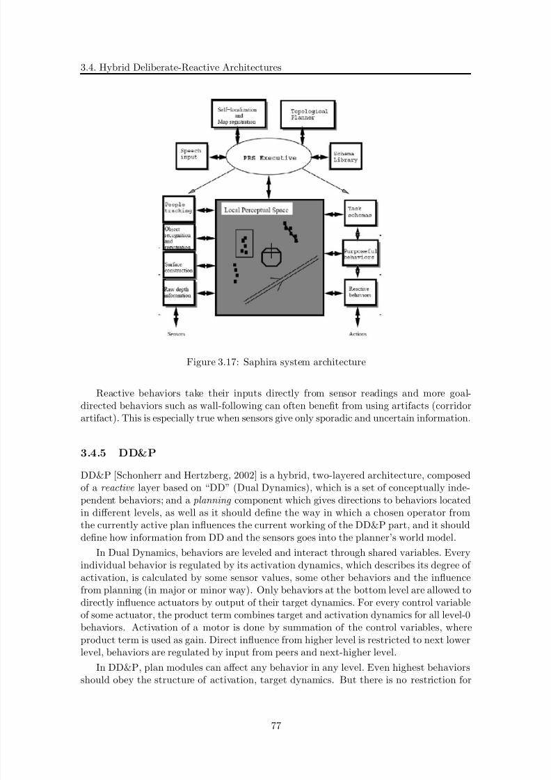
8/21/2019 Alberto Brunete Gonzalez
http://slidepdf.com/reader/full/alberto-brunete-gonzalez 105/311
3.4. Hybrid Deliberate-Reactive Architectures
Figure 3.17: Saphira system architecture
Reactive behaviors take their inputs directly from sensor readings and more goal-
directed behaviors such as wall-following can often benefit from using artifacts (corridorartifact). This is especially true when sensors give only sporadic and uncertain information.
3.4.5 DD&P
DD&P [Schonherr and Hertzberg, 2002] is a hybrid, two-layered architecture, composedof a reactive layer based on “DD” (Dual Dynamics), which is a set of conceptually inde-pendent behaviors; and a planning component which gives directions to behaviors locatedin different levels, as well as it should define the way in which a chosen operator fromthe currently active plan influences the current working of the DD&P part, and it shoulddefine how information from DD and the sensors goes into the planner’s world model.
In Dual Dynamics, behaviors are leveled and interact through shared variables. Everyindividual behavior is regulated by its activation dynamics, which describes its degree of activation, is calculated by some sensor values, some other behaviors and the influencefrom planning (in major or minor way). Only behaviors at the bottom level are allowed todirectly influence actuators by output of their target dynamics. For every control variableof some actuator, the product term combines target and activation dynamics for all level-0behaviors. Activation of a motor is done by summation of the control variables, whereproduct term is used as gain. Direct influence from higher level is restricted to next lowerlevel, behaviors are regulated by input from peers and next-higher level.
In DD&P, plan modules can affect any behavior in any level. Even highest behaviors
should obey the structure of activation, target dynamics. But there is no restriction for
77

8/21/2019 Alberto Brunete Gonzalez
http://slidepdf.com/reader/full/alberto-brunete-gonzalez 106/311
CHAPTER 3. Review on Control Architectures for Modular Microrobots
Figure 3.18: DD&P Controller
planning. Off-the-shelf propositional planner is used here: IPP. Given a set of missiongoals by human user, the planner is supposed to generate and keep updated an orderedset of abstract actions as the current plan and to determine at each of its time cyclesthe operator of that plan that proposes to execute, given its current knowledge aboutthe environment (in the KB - Knowledge Base). Executing an operator means biasingbehaviors rather than exerting hard control. An operator chosen for execution stimulates(++) or mutes (–). Information flow from the DD part to the deliberative part in form of the activation history of the behaviors, yielding an image of the environment as perceived
through the eyes of the useful behavior.Figure 3.18 shows the schema of an DD&P controller. Left part is a two-level DD
behavior set. Arrows among the behavior represent (possible) activation flow; currentactivation is represented by the blankness level of behaviors. Arrows meeting behaviorsfrom the left represent sensor input or input from behaviors of the same level.
3.5 Modular Robot Architectures
3.5.1 CONRO
From the University of Southern California, by P. Will.
CONRO [Shen et al., 2000] [Shen et al., 2002] [Salemi et al., 2004] presents a distributedcontrol mechanism inspired by the concept of hormones in biological systems.
Hormones are special messages that can trigger different actions in different modules.They can be used to coordinate motions and reconfiguration in the context of limitedcommunications and dynamic network topologies.
A self-reconfigurable robot can be viewed as a network of autonomous systems with
communication links between modules.
78

8/21/2019 Alberto Brunete Gonzalez
http://slidepdf.com/reader/full/alberto-brunete-gonzalez 107/311
3.5. Modular Robot Architectures
Communication description
Each module has a unique ID and maintains a set of active communication link. To send
a message from a module P to a module Q in this network, P sends the message to allof its active links. Upon receiving a message, a module will either keep the message, orrelay the message to all of its active links except the link through which the message wasreceived. Loops must be prevented.
Master vs masterless
Master controlled systems are characterize by
• Advantage: synchronization
• Disadvantage: communication cost
And masterless control system by
• Free from communication, scalable
• Loss of robustness, synchronization based on a internal clock
The CONRO control lies between both of them. It reduces the cost of communicationwhile keeping some degree of synchronization.
Hormones
Formally, a hormone message is a special type of message that has three important prop-erties:
1. a hormone has no particular destination but floats in a distributed system
2. a hormone has a lifetime
3. the same hormone may trigger different actions at different receiving sites. For
example:modification and relay of the hormone, execution of certain local actions,or destruction of the received hormone.
A hormone is terminated in three possible ways:
• when it reaches its destination
• when its lifetime expires
• when it has nowhere to go (e.g., it arrives at a module that has no outlinks).
Since no hormone can live forever, this prevents them from circulating in the network
indefinitely.
79
8/21/2019 Alberto Brunete Gonzalez
http://slidepdf.com/reader/full/alberto-brunete-gonzalez 108/311
CHAPTER 3. Review on Control Architectures for Modular Microrobots
Hormone classes
Hormone messages are classified into three classes:
1. Hormones for action specification. E.g. h(x) that will cause a receiving module torelay its current DOF1 position to the next module and then move its DOF1 to thex position
2. Hormones for synchronization: since hormones can “wait” at a site for the occurrenceof certain events before traveling further, they can be used as tokens for synchronizingevents between modules. “s” can be designed to ensure that all modules finish their
job before the next step begins.
3. Hormones for dynamic grouping of modules. In any distributed system, it is oftenuseful to define a set of entities dynamically as a special group for certain operations.Hormones can be used to define sets on the fly. Each module in the self-reconfigurablerobot has a set of local variables mi that can be “marked” dynamically by the moduleitself.
Hormone management
No module can be the generator of two or more hormone sequences simultaneously. Amodule can become the generator of a hormone sequence in two ways:
• Self-promoted (i.e. by sensors)
• Instructed (i.e. by a hormone)
3.5.2 M-TRAN
From the National Institute of Advanced Industrial Science and Technology (AIST) andTokyo Institute of Technology, by S. Murata [Murata et al., 2002] [Kurokawa et al., 2003][Kamimura et al., 2004] [Kurokawa et al., 2005] [Yoshida et al., 2003].
The MTRAN II controller is distributed, i.e., the controllers are distributed in all themodules. However, self-reconfiguration motion is made by global synchronization. Eachmodule has its fixed role and its own sequence data. One module is selected as a masterand others works as slaves. Global synchronization is maintained by master’s polling.
Decentralized controller system: various types of controllers, centralized /decentralizedand synchronous / asynchronous The system consists of three layers.
1. The bottom layer contains several functions of the slave controllers directly relatedto the hardware and an interface between the master and slaves. They includePID/trajectory control of motors, connection control, and data acquisition by severalsensors.
2. The middle layer is for communication among modules and realizes mainly two func-tions; remote control of other modules and a shared memory. CAN communication
3. In the upper layer, a sequence program designed by the kinematics simulator isinterpreted and executed.
80
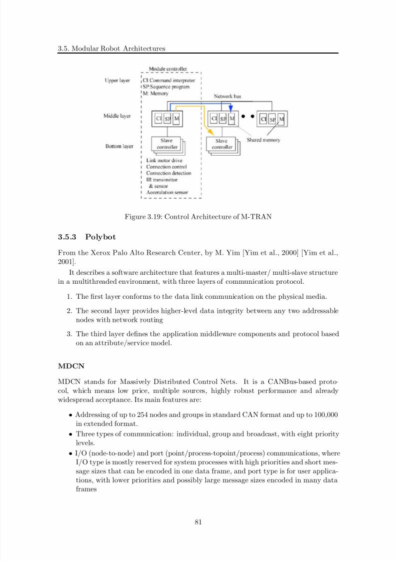
8/21/2019 Alberto Brunete Gonzalez
http://slidepdf.com/reader/full/alberto-brunete-gonzalez 109/311
3.5. Modular Robot Architectures
Figure 3.19: Control Architecture of M-TRAN
3.5.3 Polybot
From the Xerox Palo Alto Research Center, by M. Yim [Yim et al., 2000] [Yim et al.,2001].
It describes a software architecture that features a multi-master/ multi-slave structurein a multithreaded environment, with three layers of communication protocol.
1. The first layer conforms to the data link communication on the physical media.
2. The second layer provides higher-level data integrity between any two addressablenodes with network routing
3. The third layer defines the application middleware components and protocol basedon an attribute/service model.
MDCN
MDCN stands for Massively Distributed Control Nets. It is a CANBus-based proto-
col, which means low price, multiple sources, highly robust performance and alreadywidespread acceptance. Its main features are:
• Addressing of up to 254 nodes and groups in standard CAN format and up to 100,000in extended format.
• Three types of communication: individual, group and broadcast, with eight prioritylevels.
• I/O (node-to-node) and port (point/process-topoint/process) communications, whereI/O type is mostly reserved for system processes with high priorities and short mes-sage sizes that can be encoded in one data frame, and port type is for user applica-tions, with lower priorities and possibly large message sizes encoded in many data
frames
81

8/21/2019 Alberto Brunete Gonzalez
http://slidepdf.com/reader/full/alberto-brunete-gonzalez 110/311
CHAPTER 3. Review on Control Architectures for Modular Microrobots
(a) Nodes and Segments in Poly-bot
(b) Service=square and Attributes=ellipse
Figure 3.20: Polybot control scheme
CAN bus has a limitation on the number of CAN controllers on one network -¿ AnMDCN bridging has been implemented to transfer messages between multiple CAN buses
Attribute/Service Model
Multi-threading is essential for efficient handling of multiple hardware requests and com-putation in real-time. Global tasks such as locomotion and reconfiguration require com-munication between different modules.
The Attribute/Service model is a general and simple framework for applications thatrequire programming with multiple tasks/threads on multiple processors.
The Attribute/Service model is a component based architecture, where componentsare either attributes or services distributed over the communication network.
Attributes are abstractions for shared memory/resources among multiple threadslocated in one or more processors. E.g. desired joint angle. Services are abstractionsof hardware or software routines. In general: hardware services correspond to settings in
registers controlling hardware peripherals and software services are threads that run forparticular tasks. An example of a hardware service can be actuating a latch for docking.Both attributes and services are accessible either locally or remotely.
Example
In PolyBot G3, masters are running on nodes and slaves are running on segments. Bothmasters and slaves are multi-threaded.
Master and slaves run some common components, such as Attribute/Service servers,IR ranging and other local sensing attached to the module.
Masters also run MDCN routers, global computation such as planning and inverse
82

8/21/2019 Alberto Brunete Gonzalez
http://slidepdf.com/reader/full/alberto-brunete-gonzalez 111/311
3.6. Adaptive Behavior
kinematics, global environment sensing etc.
Slaves run motor control and local gait table generation.
PolyBot tasks are divided into three categories: locomotion, manipulation and recon-
figuration, where locomotion is essentially a dual of reconfiguration.
3.6 Adaptive Behavior
3.6.1 Reinforcement Learning
Reinforcement learning (RL) is a class of learning algorithm where a scalar evaluation(reward) of the performance of the algorithm is available from the interaction with theenvironment. The goal of a RL algorithm is to maximize the expected reward by adjust-
ing some value functions. This adjustment determines the control policy that is beingapplied. The evaluation is generated by a reinforcement function which is located in theenvironment.
In Q-learning, the learning problem is divided into a set of simpler problems eachlearned separately by a Q-learning module A Q-learning Action Selection Mechanismsarbitrates among the modules
In W-learning (W = weight), each module/behavior recommends an action with someweight. The action with the highest weight is selected and executed. The W-values arethen modified based on the difference between the winning action and the action desiredby the behavior
3.6.2 Neural Networks
Many roboticist have experimented with Neural Networks for controlling robots [Mad00][FN98] [CM96]. The behavior produced by neural networks is an emergent property of the weights of the connections, and the positions of motors and sensors on the real robot.One advantage of neural networks is that a robust solution often can be found due tothe neurons natural way of handling noise. One disadvantage is that it is difficult toset the weights by hand, and that simulation time of the network increases linearly withthe number of connections between nodes, that is O(n2) with the number of nodes, andtherefore does not scale too well. Another disadvantage is, that since the output of aneural network is produced by an interplay of the weights of many different connections,it can be very difficult to “read” the network, as well as to “write” a network by hand.Because of this, different machine learning techniques are often used to set the weights,such as back-propagation and artificial evolution. When using neural networks to controla robot, two different methods can be used: the neural network can be directly connectedto the motors, or it can be used to select a preprogrammed action.
Direct control A feed forward neural network can be set up to connect the sensorsof a robot with the motors, as shown in figure 3.21(a). In this approach, the speeds of the motors are determined by the activation of the output nodes of the neural network.Some simple transformation is applied to the activation of the neural network, to giveappropriate values for the speeds of the motors, but otherwise the motors are directly
controlled by the neural network. This approach gives a purely reactive behavior by a one
83
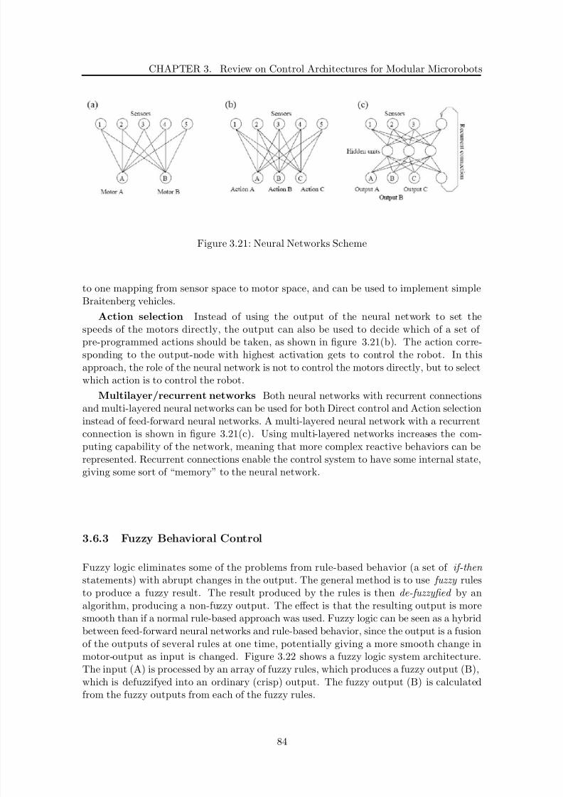
8/21/2019 Alberto Brunete Gonzalez
http://slidepdf.com/reader/full/alberto-brunete-gonzalez 112/311
CHAPTER 3. Review on Control Architectures for Modular Microrobots
Figure 3.21: Neural Networks Scheme
to one mapping from sensor space to motor space, and can be used to implement simpleBraitenberg vehicles.
Action selection Instead of using the output of the neural network to set thespeeds of the motors directly, the output can also be used to decide which of a set of pre-programmed actions should be taken, as shown in figure 3.21(b). The action corre-sponding to the output-node with highest activation gets to control the robot. In thisapproach, the role of the neural network is not to control the motors directly, but to selectwhich action is to control the robot.
Multilayer/recurrent networks Both neural networks with recurrent connectionsand multi-layered neural networks can be used for both Direct control and Action selection
instead of feed-forward neural networks. A multi-layered neural network with a recurrentconnection is shown in figure 3.21(c). Using multi-layered networks increases the com-puting capability of the network, meaning that more complex reactive behaviors can berepresented. Recurrent connections enable the control system to have some internal state,giving some sort of “memory” to the neural network.
3.6.3 Fuzzy Behavioral Control
Fuzzy logic eliminates some of the problems from rule-based behavior (a set of if-then statements) with abrupt changes in the output. The general method is to use fuzzy rulesto produce a fuzzy result. The result produced by the rules is then de-fuzzyfied by analgorithm, producing a non-fuzzy output. The effect is that the resulting output is moresmooth than if a normal rule-based approach was used. Fuzzy logic can be seen as a hybridbetween feed-forward neural networks and rule-based behavior, since the output is a fusionof the outputs of several rules at one time, potentially giving a more smooth change inmotor-output as input is changed. Figure 3.22 shows a fuzzy logic system architecture.The input (A) is processed by an array of fuzzy rules, which produces a fuzzy output (B),which is defuzzifyed into an ordinary (crisp) output. The fuzzy output (B) is calculated
from the fuzzy outputs from each of the fuzzy rules.
84

8/21/2019 Alberto Brunete Gonzalez
http://slidepdf.com/reader/full/alberto-brunete-gonzalez 113/311
3.6. Adaptive Behavior
Figure 3.22: Fuzzy Logic
3.6.4 Genetic Algorithms
Genetic Algorithms (GAs) form a class of gradient descent methods in which a high-quality solution is found by applying a set of biologically inspired operators to individualpoints within a search space, yielding better generations of solutions over an evolutionarytimescale. The fitness of each member of the population is computed using an evaluationfunction, called the fitness function, that measures how well each individual performs
with respect to the task. The population’s best members are rewarded according to theirfitness, and poorly performing individuals are punished or deleted.
It it important to say that this method does nor guarantee an optimal global solution,but it generally produces high-quality solutions.
Two elements are required for any problem before a genetic algorithm can be used tosearch for a solution: First, there must be a method of representing a solution in a mannerthat can be manipulated by the algorithm. Traditionally, a solution can be represented bya string of bits, numbers or characters. Second, there must be some method of measuringthe quality of any proposed solution: the fitness function.
A GA is composed of the initialization, selection, reproduction and termination steps.
Initialization: Initially many individual solutions are randomly generated to form aninitial population. The population size depends on the nature of the problem, but typicallycontains several hundreds or thousands of possible solutions. Traditionally, the populationis generated randomly, covering the entire range of possible solutions (the search space).Occasionally, the solutions may be “seeded” in areas where optimal solutions are likely tobe found.
Selection: During each successive epoch, a proportion of the existing population isselected to breed a new generation. Individual solutions are selected through a fitness-based process, where fitter solutions (as measured by a fitness function) are typicallymore likely to be selected. Certain selection methods rate the fitness of each solution andpreferentially select the best solutions. Other methods rate only a random sample of the
population, as this process may be very time-consuming.
85

8/21/2019 Alberto Brunete Gonzalez
http://slidepdf.com/reader/full/alberto-brunete-gonzalez 114/311
CHAPTER 3. Review on Control Architectures for Modular Microrobots
Figure 3.23: GA scheme in M-TRAN
Most functions are stochastic and designed so that a small proportion of less fit so-lutions are selected. This helps keep the diversity of the population large, preventing
premature convergence on poor solutions. Popular and well-studied selection methodsinclude roulette wheel selection and tournament selection.
Reproduction: The next step is to generate a second generation population of so-lutions from those selected through genetic operators: crossover (or recombination), andmutation.
For each new solution to be produced, a pair of “parent” solutions is selected forbreeding from the pool selected previously. By producing a “child” solution using theabove methods of crossover and mutation, a new solution is created which typically sharesmany of the characteristics of its “parents”. New parents are selected for each child, andthe process continues until a new population of solutions of appropriate size is generated.
These processes ultimately result in the next generation population of chromosomesthat is different from the initial generation. Generally the average fitness will have in-creased by this procedure for the population, since only the best organisms from the firstgeneration are selected for breeding.
Termination: This generational process is repeated until a termination condition hasbeen reached. Common terminating conditions are:
• A solution is found that satisfies minimum criteria
• Fixed number of generations reached
• Allocated budget (computation time/money) reached
• The highest ranking solution’s fitness is reaching or has reached a plateau such that
86

8/21/2019 Alberto Brunete Gonzalez
http://slidepdf.com/reader/full/alberto-brunete-gonzalez 115/311
3.7. Conclusions
successive iterations do no longer produce better results
• Manual inspection
• Combinations of the above
GAs can be found in many robots to develop its controllers or algorithms. In M-TRAN( [Kamimura et al., 2003]) it is used an automatic locomotion generation method (calledALPG) aimed at making locomotion of arbitrary module configurations using neural oscil-lator as a model of CPG (Central Pattern Generator) and Genetic Algorithm for evolvingparameters (figure 3.23).
ATRON makes also use of GAs to see how well the collective of modules performsa given task when artificial evolution was applied to develop the individual controllers[Ostergaard and Lund, 2003]. The evolutionary algorithm was a simple GA working on
a string of bytes. Each byte is considered one gene, and mutation operations can eitherreplace the byte with a random byte, flip a bit, or add a truncated gaussian distributedrandom byte to the gene. A population size of 500 is used with the best 50% of theindividuals used as candidates for reproduction (rank based), mutation rate of 5% pergene, two-parent 10 point crossover and one elite individual.
The fitness function (for maximization) was simply the sum of x-coordinates of themodules integrated over time (200 time steps), to make the modules perform a simplelocomotion task along the x-axis.
3.7 Conclusions
This chapter has been dedicated to describe control systems and algorithms suitable formodular microrobots. In this way, several control architectures have been presented, withespecial emphasis in the behavior based architectures. Its main characteristics have beenexplained and the differences with deliberative, reactive and hybrid architectures havebeen pointed out.
Behavior-based architectures are especially suited for microrobots because they includethe possibility to react in real-time to the unforeseen (very important in field robotics), tobe coded in simple procedures that don’t need a big hardware to run (very important ina microrobot), and to still be able to perform high level control.
A review of the most important behavior-based architectures has been given, frompure reactive architectures like subsumption, to more hybrid like motor schemas, activationnetworks or DAMN. Also state of the art architectures like CAMPOUT has been reviewed.
The subsumption architecture is very interesting from the point of view of fast responseto external events, since it is a pure reactive architecture. Motor schemas introduces theconcepts of motor and perceptual schemas, separating actuator related functions (motorschemas) and sensor related functions (perceptual schemas), and presenting the use of perceptual schemas as recursive information generation process that may lead to a kind of “high level” control. Activation networks presents the concept of activation preconditionsof behaviors, that is, the situations that have to be fulfilled for the behavior to take con-trol. DAMN introduces the concept of an arbiter between the behaviors votes that takes
into consideration the objectives and priorities. Thus, it is well suited for integration
87

8/21/2019 Alberto Brunete Gonzalez
http://slidepdf.com/reader/full/alberto-brunete-gonzalez 116/311
CHAPTER 3. Review on Control Architectures for Modular Microrobots
of high level deliberative control with low level reactive behaviors. Finally, CAMPOUTis a very interesting architecture because integrates different types of behaviors (primi-tive, composite, communication, coordination, etc.), and different arbitration mechanisms
(priority-based, state-based, voting, fuzzy, etc.), a clear example of the great flexibilitythat provides the use of behavior-based architectures.
Most of the hybrid architectures included in this section are based on three layers:reactive, middle (sequencer), and deliberative. There is a clear tendency in the controldesign to this three layer scheme. This underlines the importance of a layer that links thereactive and deliberative parts of the architecture. Although the architecture proposedin this thesis does not follow an architecture with a defined three layer scheme, there isalso a middle layer that interconnects (translates) the embedded control with the centralcontrol.
Regarding modular robot architectures, three of them have been reviewed: CONRO,Polybot and M-TRAN. CONRO presents the concept of hormones, special messages thatcan trigger different actions in different modules. This is similar in Microtub, becausesome commands are send to all modules, but each of them adapt the command to itscharacteristics. M-TRAN shows two interested features: one is that although it uses adistributed control, for some tasks like reconfigurations, central control is used, showinghow complicated (or even impossible) it is to have a pure distributed mechanism. Theother feature is the three layer architecture similar to Microtub, with low-level, middlelayer for communication and high level control. Polybot presents the attribute/servicemodel, especially design for complex tasks that require communication between differentmodules.
Finally, a brief summary of adaptive behavior techniques has been given, including
reinforcement learning, neural networks and fuzzy control. An extended description of ge-netic algorithms (with examples of the use in modular robots like M-TRAN and ATRON)has been done since they are used in this thesis.
88
8/21/2019 Alberto Brunete Gonzalez
http://slidepdf.com/reader/full/alberto-brunete-gonzalez 117/311
Chapter 4
Electromechanical design
“Design can be art. Design can be aesthetics. Design is so simple, that’s why it is socomplicated”
Paul Rand
In this chapter, the microrobotic modules used in this thesis will be described. Theirmechanical principles, their electronics, their concepts of work, the different versions theyhave been through and the reasons why they have been designed will be covered in the
next sections.Some modules have been designed and built. They are the rotation module (indeed it
is a double rotation module, but for simplicity it will be called rotation module) v1 andv2, the helicoidal module v1 and v2, the support module v1, v1.1 and v2, the extensionmodule v1 and v2, the camera module v1 and v2, the contact module (it is includedin the camera module v2) and the battery module. Some others are still in the designor conceptual phase, they are being designed but they have not been built yet. Theyare the SMA-based module (there is already a prototype), the traveler module (in thedesign phase) and the sensor module (in a conceptual phase). Table 4.1 shows the maincharacteristics of the developed modules.
The most important characteristic of all modules is its tiny diameter, 27mm, the
smallest diameter found in a robot like this. Some parts thickness are thinner than 1mm.As an example, a detail of one of the wheels made for the helicoidal modules can be seenin fig. 4.1
The reason why there have been build so many different modules is to implementdifferent locomotion gaits, depending on the environment the robot is moving in. Thesegaits are: helicoidal (with the helicoidal module), snake-like (with the rotation module),inchworm (with the support and extension modules) and a combination of all or some of them.
Due to the narrowness of the pipes, it is not possible to rearrange the position of the modules, so it is important that the microrobot can choose amongst different gaits
depending on the stretch.
89
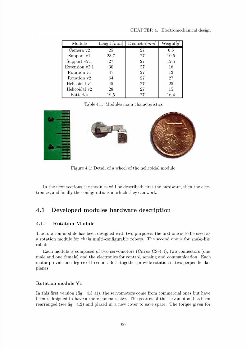
8/21/2019 Alberto Brunete Gonzalez
http://slidepdf.com/reader/full/alberto-brunete-gonzalez 118/311
CHAPTER 4. Electromechanical design
Module Length[mm] Diameter[mm] Weight[g]
Camera v2 25 27 6,5Support v1 23,7 27 10,5
Support v2.1 27 27 12,5Extension v2.1 30 27 16
Rotation v1 47 27 13Rotation v2 64 27 27
Helicoidal v1 45 27 25Helicoidal v2 28 27 15
Batteries 19,5 27 16,4
Table 4.1: Modules main characteristics
Figure 4.1: Detail of a wheel of the helicoidal module
In the next sections the modules will be described: first the hardware, then the elec-tronics, and finally the configurations in which they can work.
4.1 Developed modules hardware description
4.1.1 Rotation Module
The rotation module has been designed with two purposes: the first one is to be used asa rotation module for chain multi-configurable robots. The second one is for snake-like
robots.Each module is composed of two servomotors (Cirrus CS-4.4), two connectors (one
male and one female) and the electronics for control, sensing and communication. Eachmotor provide one degree of freedom. Both together provide rotation in two perpendicularplanes.
Rotation module V1
In this first version (fig. 4.3 a)), the servomotors come from commercial ones but havebeen redesigned to have a more compact size. The gearset of the servomotors has been
rearranged (see fig. 4.2) and placed in a new cover to save space. The torque given for
90
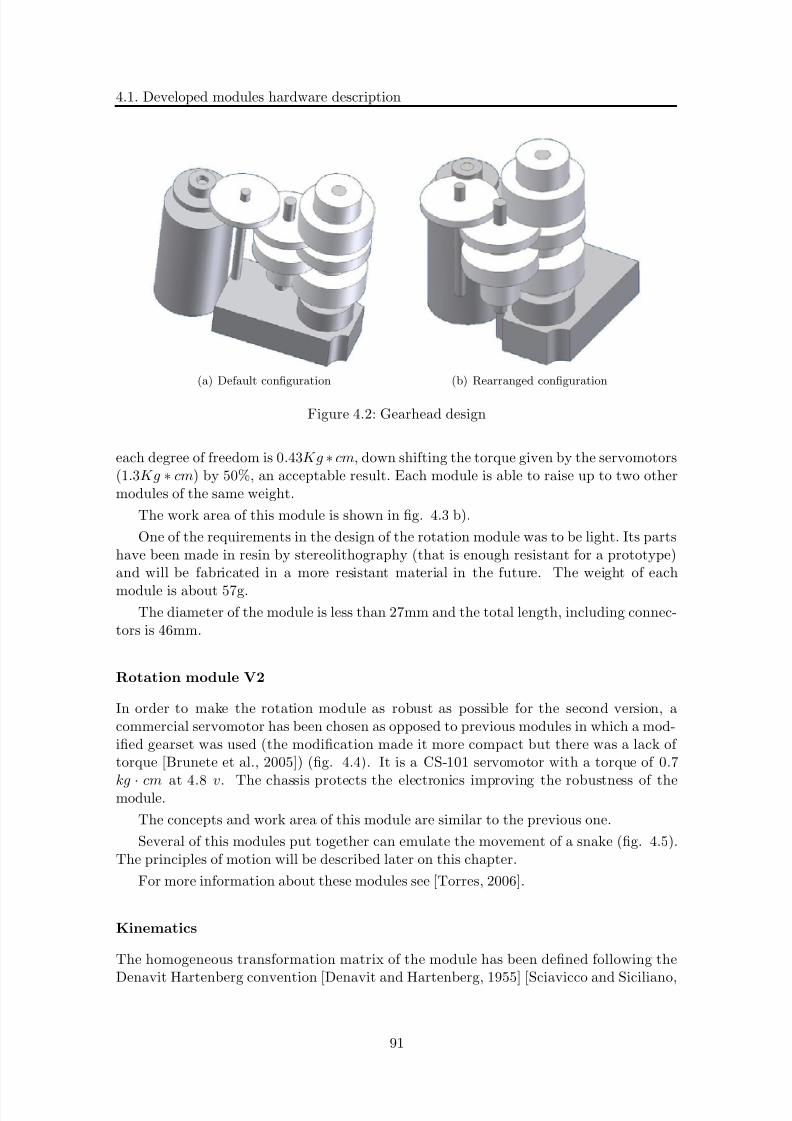
8/21/2019 Alberto Brunete Gonzalez
http://slidepdf.com/reader/full/alberto-brunete-gonzalez 119/311
4.1. Developed modules hardware description
(a) Default configuration (b) Rearranged configuration
Figure 4.2: Gearhead design
each degree of freedom is 0.43Kg ∗ cm, down shifting the torque given by the servomotors(1.3Kg ∗ cm) by 50%, an acceptable result. Each module is able to raise up to two othermodules of the same weight.
The work area of this module is shown in fig. 4.3 b).
One of the requirements in the design of the rotation module was to be light. Its partshave been made in resin by stereolithography (that is enough resistant for a prototype)and will be fabricated in a more resistant material in the future. The weight of each
module is about 57g.The diameter of the module is less than 27mm and the total length, including connec-
tors is 46mm.
Rotation module V2
In order to make the rotation module as robust as possible for the second version, acommercial servomotor has been chosen as opposed to previous modules in which a mod-ified gearset was used (the modification made it more compact but there was a lack of torque [Brunete et al., 2005]) (fig. 4.4). It is a CS-101 servomotor with a torque of 0.7
kg · cm at 4.8 v. The chassis protects the electronics improving the robustness of themodule.
The concepts and work area of this module are similar to the previous one.
Several of this modules put together can emulate the movement of a snake (fig. 4.5).The principles of motion will be described later on this chapter.
For more information about these modules see [Torres, 2006].
Kinematics
The homogeneous transformation matrix of the module has been defined following the
Denavit Hartenberg convention [Denavit and Hartenberg, 1955] [Sciavicco and Siciliano,
91
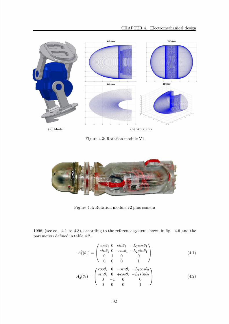
8/21/2019 Alberto Brunete Gonzalez
http://slidepdf.com/reader/full/alberto-brunete-gonzalez 120/311
CHAPTER 4. Electromechanical design
(a) Model (b) Work area
Figure 4.3: Rotation module V1
Figure 4.4: Rotation module v2 plus camera
1996] (see eq. 4.1 to 4.3), according to the reference system shown in fig. 4.6 and theparameters defined in table 4.2.
A01(θ1) =
cosθ1 0 sinθ1 −L2cosθ1sinθ1 0 −cosθ1 −L2sinθ1
0 1 0 00 0 0 1
(4.1)
A12(θ2) =
cosθ2 0 −sinθ2 −L1cosθ2sinθ2 0 +cosθ2 −L1sinθ2
0 −1 0 0
0 0 0 1
(4.2)
92

8/21/2019 Alberto Brunete Gonzalez
http://slidepdf.com/reader/full/alberto-brunete-gonzalez 121/311
4.1. Developed modules hardware description
Figure 4.5: Snake configuration plus camera
Table 4.2: Denavit-Hartenberg parameters
ai di αi θi
q 1 −L2 0 π/2 θ1
q 2 −L1 0 −π/2 θ2
A02
= A01
(θ1) ∗ A12
(θ2) =
=
cθ1cθ2 −sθ1 −cθ1sθ2 −L1cθ1cθ2 − L2cθ1sθ1cθ2 cθ1 −sθ1sθ2 −L1sθ1cθ2 − L2sθ1
sθ2 0 cθ2 −L1sθ20 0 0 1
(4.3)
To refer the system to the coordinate system XYZ situated at the origin, it is just
enough to apply a translation in the X axis, obtaining the matrix (4.4)
93
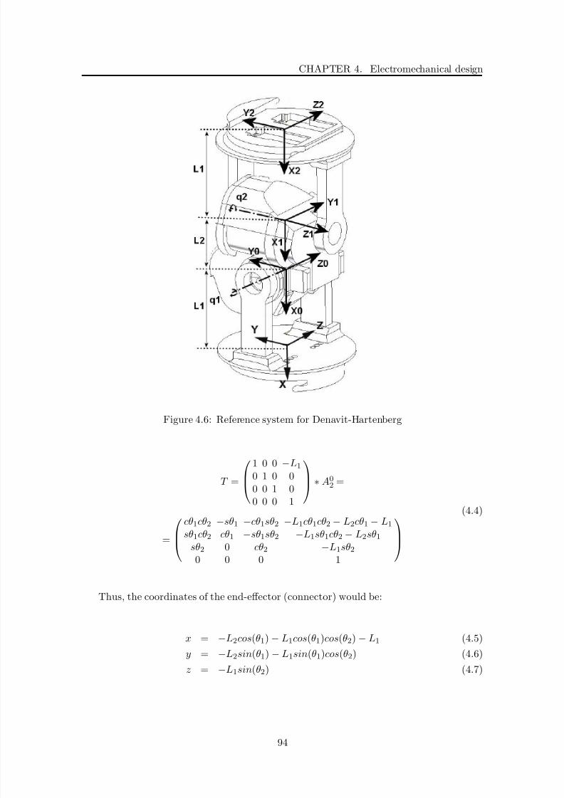
8/21/2019 Alberto Brunete Gonzalez
http://slidepdf.com/reader/full/alberto-brunete-gonzalez 122/311
CHAPTER 4. Electromechanical design
Figure 4.6: Reference system for Denavit-Hartenberg
T =
1 0 0 −L1
0 1 0 00 0 1 00 0 0 1
∗ A0
2 =
=
cθ1cθ2 −sθ1 −cθ1sθ2 −L1cθ1cθ2 − L2cθ1 − L1
sθ1cθ2 cθ1 −sθ1sθ2 −L1sθ1cθ2 − L2sθ1sθ2 0 cθ2 −L1sθ2
0 0 0 1
(4.4)
Thus, the coordinates of the end-effector (connector) would be:
x = −L2cos(θ1) − L1cos(θ1)cos(θ2) − L1 (4.5)
y = −L2sin(θ1) − L1sin(θ1)cos(θ2) (4.6)
z = −L1sin(θ2) (4.7)
94
8/21/2019 Alberto Brunete Gonzalez
http://slidepdf.com/reader/full/alberto-brunete-gonzalez 123/311
4.1. Developed modules hardware description
from where it is possible to easily obtain the inverse kinematics equations :
θ2 = arcsin(−z/L1) (4.8)
θ1 = arcsin(−x − L1/(L2 + L1cos(θ2))) (4.9)
The coordinate systems have been chosen in order to have the same orientation in theend-effector and in the reference system. In this way, if several modules are connectedtogether, the homogeneous transformation matrix of the whole system can be computedby multiplying the homogeneous transformation matrix of every single module (eq. 4.10).
T 0n = T 01 ∗ T 12 ∗ ... ∗ T n−1n (4.10)
4.1.2 Support and Extension modules
Although these modules can be used separately, the expansion and support modules (fig-ures 4.7 and 4.10) were designed to work together to simulate the movement of an inch-worm. The support module is used to fix the microrobot to the pipe, avoiding the mi-crorobot to slide, while the extension module is used to extend the robot (make it goforward), and to turn to right and left. A drive unit is composed of two support modulesand one expansion module (fig. 4.7). An advantage of this kind of motion is that the robotmanages to maintain a firm grip on the surface at all times while other types of motion,for example helicoidal motion, could show a tendency to slip as the slope increases.
The support module can be used together with others modules, as for example thehelicoidal and the rotation modules, to provide a firm grip while the robot is turning.
Support and Extension modules V1
The first prototypes were design to test the locomotion principle and how small the micro-robot could be made. In this prototype all modules use a 21x13x9mm microservomotor
(Cirrrus LS-3.0). It is a linear servo which weights 3.0g, has a maximum deflection of 14mm in 0.15 sec and provides a maximum output force of 200g. The support modulesuse one servo and the expansion module uses two.
The support module consists of three rubber bands positioned around the module at120o from each other, which are bent when the servomotor is activated, exercising a forceagainst the walls of the pipe that allows the module to be still.
The extension module consists of two arms (each of them drove by a servo) that allowsexpansion-contraction movements, as well as turns, depending on the relative positionbetween arms (fig 4.7 b)).
When designing the mechanism, in a very first time it was thought to use two per-
pendicular bars that lean in a base panel where they can rotate. If any of the bars push
95

8/21/2019 Alberto Brunete Gonzalez
http://slidepdf.com/reader/full/alberto-brunete-gonzalez 124/311
CHAPTER 4. Electromechanical design
the plane, it turns. The panel can turn around an axis that is the perpendicular bisectorof the segment joining the two contact points of the bars. If both push, the panel goesforward, and if they pull, it goes back.
However, there is a problem with this design: if the ends are not rigidly connected inthe servo end, the system would have one dof free, and if they are, the system will breakbecause the distance between the bars should be shorter when the panel turns, but it isnot possible since the connection is rigid.
Thus, the first idea was change into the mechanism shown in fig. 4.7 b). Having fourbars make it possible. There are two straight bars and two driver bars. All the jointshave one dof (rotation). All together confer the base panel two dof: one rotational andone translational. The straight bars are used to move and turn the base panel. The driverbars are used to avoid lateral displacement of the base panel.
The module has been tested in different pipes. The results obtained are shown in the
following table:• Minimum pipe diameter: 22mm
• Maximum pipe diameter: 35mm
• Maximum angle of rotation of the expansion module: 40o
• Maximum lengthening: 7.5mm
• Average speed at 0o- 90o: 2mm/seg
The main advantage of the servomotor used in this prototypes is its small size and itsgood torque. On the other hand, it is very fragile and some parts are weak, breaking veryeasily under stress circumstances. Also, the position sent by PWM to the servo remains
saved until a new one is sent, even after power switch off. This is a problem if the servogets stuck because switch off the power would not be enough, it would be necessary tosend a new PWM position command. Finally, it does not have a cover and the gears cantouch the walls or others parts and break.
Support module V1.1
In order to improve the robustness of the 1.0 support module, a new support module wascreated (fig. 4.8). The servomotor was replaced by a rotational one (Cirrus CS-4.4) thatwas linked to two racks fixed to two plates. By turning the servomotor, the two platescan be expanded or contracted.
The mechanism works properly, but it slides when it is in the pipe, due to the resinthe plates are made of. The plates must be covered by non slippery material in order touse them.
The module was not used because its big size. Since it is a support module with noself propulsion nor turning possibilities it was necessary to make it smaller.
Support and Extension modules V2
In order to solve the problems of previous versions, another prototype was created witha new design and parts, but the same principle of movement. The second prototypes
incorporate rotational servomotors instead of the linear ones, increasing the robustness.
96
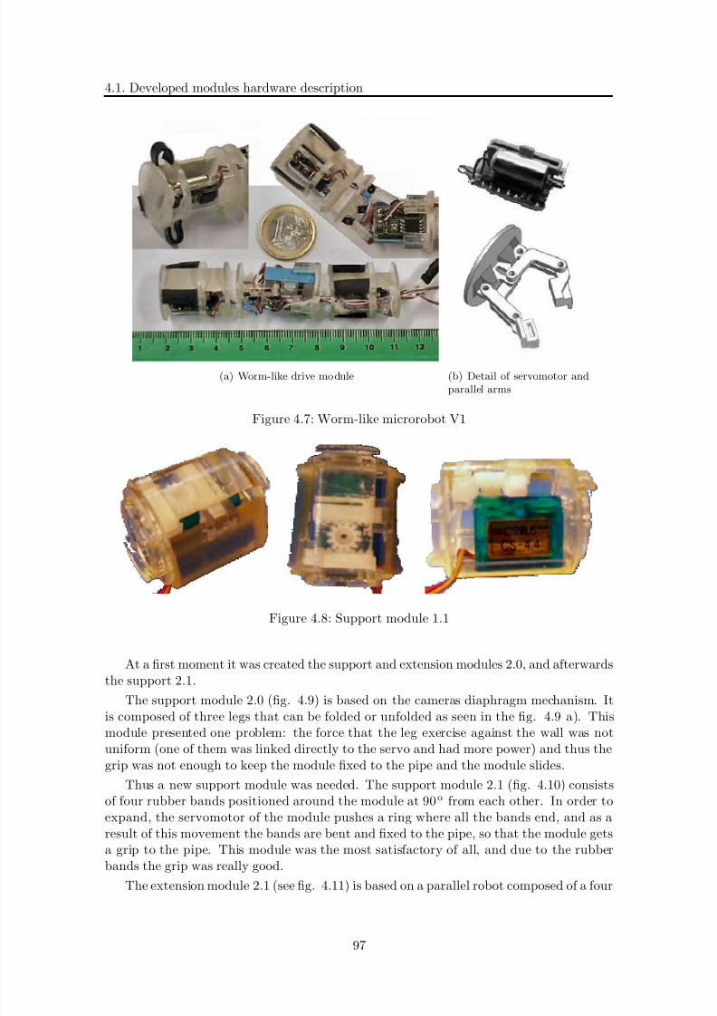
8/21/2019 Alberto Brunete Gonzalez
http://slidepdf.com/reader/full/alberto-brunete-gonzalez 125/311
4.1. Developed modules hardware description
(a) Worm-like drive mo dule (b) Detail of servomotor andparallel arms
Figure 4.7: Worm-like microrobot V1
Figure 4.8: Support module 1.1
At a first moment it was created the support and extension modules 2.0, and afterwardsthe support 2.1.
The support module 2.0 (fig. 4.9) is based on the cameras diaphragm mechanism. It
is composed of three legs that can be folded or unfolded as seen in the fig. 4.9 a). Thismodule presented one problem: the force that the leg exercise against the wall was notuniform (one of them was linked directly to the servo and had more power) and thus thegrip was not enough to keep the module fixed to the pipe and the module slides.
Thus a new support module was needed. The support module 2.1 (fig. 4.10) consistsof four rubber bands positioned around the module at 90o from each other. In order toexpand, the servomotor of the module pushes a ring where all the bands end, and as aresult of this movement the bands are bent and fixed to the pipe, so that the module getsa grip to the pipe. This module was the most satisfactory of all, and due to the rubberbands the grip was really good.
The extension module 2.1 (see fig. 4.11) is based on a parallel robot composed of a four
97

8/21/2019 Alberto Brunete Gonzalez
http://slidepdf.com/reader/full/alberto-brunete-gonzalez 126/311
CHAPTER 4. Electromechanical design
Figure 4.9: Support module v2.0
Figure 4.10: Inchworm configuration based on v2.1 modules plus camera
bar linkage (two crank-connecting rod mechanisms with a common slide bar) between thebase and the top end, and a sliding bar in the center to eliminate one degree of freedomas in the previous module, the lateral displacement. The relative movement of each arm(driven by a servomotor) changes the length of the module and the orientation of the topend. Consequently the module can extend and also turn. It is a similar design to theprevious one but with rotational servos instead of linear ones.
For more information about these modules see [Santos, 2007].
Kinematics
The kinematics of the support module are very simple but it is good to know them inorder to calculate the kinematics for the whole robot chain. It can be calculated with theeq. 4.11 according to the axis shown in fig. 4.12, being L3 the length of the module.
T =
1 0 0 −L3
0 1 0 00 0 1 00 0 0 1
(4.11)
98
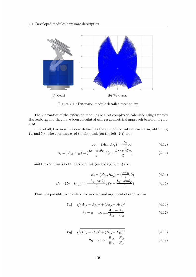
8/21/2019 Alberto Brunete Gonzalez
http://slidepdf.com/reader/full/alberto-brunete-gonzalez 127/311
4.1. Developed modules hardware description
(a) Model (b) Work area
Figure 4.11: Extension module detailed mechanism
The kinematics of the extension module are a bit complex to calculate using DenavitHartenberg, and they have been calculated using a geometrical approach based on figure4.13.
First of all, two new links are defined as the sum of the links of each arm, obtainingY A and Y B. The coordinates of the first link (on the left, Y A) are:
A0 = (A0x, A0y) = (
L6
2 , 0) (4.12)
A1 = (A1x, A1y) = (L5 · cosθF
2 , Y F +
L5 · sinθF 2
) (4.13)
and the coordinates of the second link (on the right, Y B) are:
B0 = (B0x, B0y) = (−L6
2 , 0) (4.14)
B1 = (B1x, B1y) = (−L5 · cosθF
2 , Y F −
L5 · sinθF 2
) (4.15)
Thus it is possible to calculate the module and argument of each vector:
|Y A| =
(A1x − A0x)2 + (A1y − A0y)2 (4.16)
θA = π − arctan A1y − A0y
A1x − A0x
(4.17)
|Y B| =
(B1x − B0x)2 + (B1y − B0y)2 (4.18)
θB = arctan B1y − B0y
B1x − B0x
(4.19)
99

8/21/2019 Alberto Brunete Gonzalez
http://slidepdf.com/reader/full/alberto-brunete-gonzalez 128/311
CHAPTER 4. Electromechanical design
Figure 4.12: Coordinate system for the kinematics of the support module
It is important not to forget that the central point of the end connector (C in 4.13 a))moves always in a line due to the mechanism to which it is attached (a bar that movesbetween the two servos and thus it can only move upwards and backwards). It holds that:
|Y A| · cos θA = − |Y B| · cos θB (4.20)
And finally the inverse kinematic equations can be obtained applying the law of cosinesin triangle L1, L2, Y A and L3, L4, Y B:
q 1 = θA − arccos L2
1 − L2
2 − |Y A|
2
−2 · L1 · |Y A| (4.21)
q 2 = θB − arccos
L24 − L2
3 − |Y B|
2
−2 · L3 · |Y B | (4.22)
Direct kinematics are a little more complicates to obtain. In order to make computationfaster, an approximation has been done: considering that the argument of Y A and Y B isalways 90. This not true when ΘF = 0, but the difference is negligible. Thus it is possibleto write:
Y A = L1 · cos(90 − q 1) +
L22 − L2
1 · sin2(90 − q 1) (4.23)
Y B = L3 · cos(90 − q 2) +
L2
4 − L2
3 · sin2
(90 − q 2) (4.24)
100

8/21/2019 Alberto Brunete Gonzalez
http://slidepdf.com/reader/full/alberto-brunete-gonzalez 129/311
4.1. Developed modules hardware description
Figure 4.13: Kinematics diagrams of the extension module
Making use of equation 4.20, it is obtained:
Y A · cos θA + L5 · cos θF + Y B · cos θB = L6 (4.25)
Y A · sin θA + L5 · sin θF − Y B · sin θB = 0 (4.26)
And thus the direct kinematic equations are obtained:
θF = tan−1
Y B · sin θB − Y A · sin θA
L6 − Y B · cos θB − Y A · cos θA (4.27)
Y F = Y B · sin θB + Y A · sin θA
2 (4.28)
4.1.3 Helicoidal drive module
The helicoidal module is so called because of the placement of its front wheels making anhelix (fig. 4.14 a)). This module was designed to be a fast drive module. It is composedof two parts: the body and the rotating head. The wheels in the rotating head aredistributed along the crown making a 15o angle with the vertical. When the head turns, it
goes forward in a helicoidal movement that pulls the body of the microrobot. The wheels
101
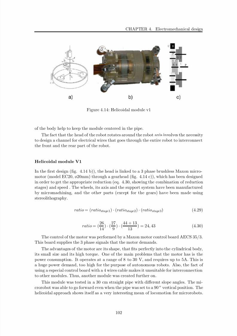
8/21/2019 Alberto Brunete Gonzalez
http://slidepdf.com/reader/full/alberto-brunete-gonzalez 130/311
CHAPTER 4. Electromechanical design
Figure 4.14: Helicoidal module v1
of the body help to keep the module centered in the pipe.
The fact that the head of the robot rotates around the robot axis involves the necessityto design a channel for electrical wires that goes through the entire robot to interconnectthe front and the rear part of the robot.
Helicoidal module V1
In the first design (fig. 4.14 b)), the head is linked to a 3 phase brushless Maxon micro-
motor (model EC20, ø20mm) through a gearhead (fig. 4.14 c)), which has been designedin order to get the appropriate reduction (eq. 4.30, showing the combination of reductionstages) and speed . The wheels, its axis and the support system have been manufacturedby micromachining, and the other parts (except for the gears) have been made usingstereolithography.
ratio = (ratiostage1) · (ratiostage2) · (ratiostage3) (4.29)
ratio = (26
14) · (
27
9 ) · (
44 + 13
13 ) = 24, 43 (4.30)
The control of the motor was performed by a Maxon motor control board AECS 35/3.This board supplies the 3 phase signals that the motor demands.
The advantages of the motor are its shape, that fits perfectly into the cylindrical body,its small size and its high torque. One of the main problems that the motor has is thepower consumption. It operates at a range of 8 to 30 V, and requires up to 5A. This isa huge power demand, too high for the purpose of autonomous robots. Also, the fact of using a especial control board with a 4 wires cable makes it unsuitable for interconnectionto other modules. Thus, another module was created further on.
This module was tested in a 30 cm straight pipe with different slope angles. The mi-crorobot was able to go forward even when the pipe was set to a 90 o vertical position. The
helicoidal approach shows itself as a very interesting mean of locomotion for microrobots.
102

8/21/2019 Alberto Brunete Gonzalez
http://slidepdf.com/reader/full/alberto-brunete-gonzalez 131/311
4.1. Developed modules hardware description
Angle () 0 15 30 45 60 75 90
Velocity (mm/s) 30 27 22 19 15 13 12
Table 4.3: Velocity in a 30cm ø pipe at different angles (helicoidal module)
Figure 4.15: Helicoidal module V2 plus camera
The results obtained for this module are shown in table 4.3.
For more information about these modules see [del Monte Garrido, 2004].
Helicoidal module V2
A second prototype was developed in order to solve the problems of the previous one(especially the consumption)(fig. 4.15 a)). The design principles were the same, but twomodifications were made: the Maxon motor was replaced by a servomotor (Cirrus CS-3)and the gearser was simplified (eq. 4.31). Although the torque was reduced by the motorchange, so it was the gear reduction (fig. 4.15 b) and c)), being in this way compensated.Thus, it was enough to go forward, but the consumption was considerably decreased. Alsothe size was smaller due to the reduction of the motor and the gearset.
ratio = (
44 + 13
13 ) = 4, 38 (4.31)
In table 4.3 the results of the second prototype are shown. They are slower than inthe previous prototype, but this is due not only to the new motor and gearset but alsoto the some assembling problems that let some parts a bit loose, probably because of thetolerance of the stereolitography process.
Angle () 0 90
Velcity (mm/s) 10 4
Table 4.4: Velocity in a 30cm ø pipe at different angles (2nd helicoidal module)
103

8/21/2019 Alberto Brunete Gonzalez
http://slidepdf.com/reader/full/alberto-brunete-gonzalez 132/311
CHAPTER 4. Electromechanical design
(a) Detail of camera parts (b) Detail of the rotation axis
Figure 4.16: Camera module v1
(a) Detail of module (b) Detail of the pin-hole cam-era
Figure 4.17: Camera module v2
Kinematics
The kinematics of the helicoidal module are very simple and similar to the kinematics of the support module. They can be calculated from eq. 4.11 according to the axis shown infig. 4.12, being L3 the length of the module.
4.1.4 Camera module
The camera module plays a very important part in environment information acquisition,in order to detect holes, breakages or cracks in the pipes. The module is provided witha CMOS B&W camera which allows to visualize the inner part of the pipe and, in thesecond version, with contact sensors which allow to detect obstacles (i.e. turns) inside the
pipe. The reason for using a B&W camera is that it was the smallest one available at thatmoment.
Camera module V1
This module (4.16) is a 2 degrees of freedom structure composed of two servomotors(Cirrus CS3), a camera (FR220 CMOS B&W) and two leds for illumination. Thanks tothe common interface, it can be assembled to any of the previous modules. Ideally thetwo rotation axis should be aligned with the centre of mass, but it was not possible dueto the small size of the module, and one of the rotation axis had to be moved. This is the
reason why the camera is not symmetric.
104

8/21/2019 Alberto Brunete Gonzalez
http://slidepdf.com/reader/full/alberto-brunete-gonzalez 133/311
4.1. Developed modules hardware description
Figure 4.18: Batteries Module
The camera used is a 8x8x20mm CMOS black and white camera, whose main charac-teristics are: 320x240 pixels composite video, 20mA@9V, 7-12V. The main characteristicsof the servomotors are: 6.3mm x 22.25mm x 10.10 mm, 2.85 g, 400g/cm and 0.18 s/60oat 4.8V.
For more information about these modules see [Lenero, 2004].
Camera module V2
This second module (4.17) presents some new features in respect to the previous one. Thetwo degrees of freedom have been suppressed to make the module shorter. And a bumperdetection mechanism has been incorporated (three contact sensors). Also the camera hasbeen replaced by a similar one of smaller dimensions (8 , 5mm × 8, 5mm × 10mm), theFR220P. The number of LEDs has been increased from 2 to 4 to increase the luminosity.
The camera is switched on and off through a MOSFET. Additionally, the 4 LEDs forillumination are controlled by 2 MOSFET diodes (each diode controls two leds), allowingthe micro-controller to vary light intensity by means of a PWM signal.
For more information about these modules see [Santos, 2007].
4.1.5 Batteries module
The purpose of this module is to act as the power supply of the microrobot. It is base on6V watch batteries giving 640mAh. They were the most powerful batteries that could befoung having the size restriction of 27mm diameter and light weight.
The module was designed to keep the batteries, so it was very simple (fig 4.18). Thelength is 19.5mm and its weight is 16.4g.
The tests were not very successful due to the discharge curve, that went down to 2V atthe demanded intensity, voltage that was not enough to move the servomotors (although
good enough to keep the microcontroller on).
105

8/21/2019 Alberto Brunete Gonzalez
http://slidepdf.com/reader/full/alberto-brunete-gonzalez 134/311
CHAPTER 4. Electromechanical design
Due to the problem mentioned above, the module has to be redesigned, and we arewaiting to find a proper power supply unit.
Kinematics
The kinematics of this module are very simple and similar, as well of all pig-type modules,to the support module, but it is good to know them in order to calculate the kinematics of the whole robot chain. It can be calculated with the eq. 4.11 according to the axis shownin fig. 4.12, being L3 = 19, 5mm.
4.2 Other modules
This section describes some modules that are still in a conceptual phase and has not beenbuilt yet (traveler module and the sensor module) and the SMA-based module.
4.2.1 SMA-based module
This module uses Shape Memory Alloys (SMA) to achieve a worm-like system of locomo-tion, based on contraction and expansion of the SMAs. Each module is composed of asupport board, a control boards (act as support boards that additionally holds the elec-tronics), SMAs wires to make the contraction and springs to make the expansion whenthe SMAs releases (fig. 4.19).
The onboard electronic for this microrobot is based on a PIC SMD of just 5x5 mm. Itis possible to put up to 32 modules together. Each module has three degrees of freedom.There are also 4 wires that go through the entire microrobot carrying the control signals.
The main advantages of this module are a simple electronic circuit and a great ver-satility (it can both contract-expand and rotate). The main disadvantages are the powerconsumption, too high, the assembling difficulty and the lack of robustness. Thus thistype of microrobot has not been used as a locomotion module for the heterogenous robot.However, it could be interesting as a manipulator for an end-effector module that does notneed to handle heavy weights. For it used in combination with other modules it would benecessary to add the common connector to its ends.
4.2.2 Traveler module
The purpose of this module is to measure the traveled distance inside a pipe.
The traveler module (fig. 4.20) is still a concept and has not been manufactured yet.It has been designed and tested in the simulation environment. It is composed of threewheels provided with encoders that detects the distance that the microrobot has traveled.
The module is designed so that at least one wheel is in touch with the pipe in everymoment. But it is possible that two or three wheels are in contact at the same time, so themeasures of the encoders may differ at the end of the trajectory. That is why algorithmsmust be applied in order to obtain useful data. Data coming from other sensors (like
accelerometers) of the microrobot can also be integrated in order to get useful information.
106

8/21/2019 Alberto Brunete Gonzalez
http://slidepdf.com/reader/full/alberto-brunete-gonzalez 135/311
4.2. Other modules
Figure 4.19: SMA-based modules
4.2.3 Sensor module
The sensor module is a module conceived to carry several types of sensors, like proximity,accelerometer, humidity and temperature. It is still in a conceptual phase.
Accelerometer sensors have already been placed in some of the modules and they willbe described in section 4.3.7. Proximity sensors will be used to navigate, by detectingbifurcations. Temperature and humidity measurement and log can be obtained incorpo-rating a chip like the Maxim DS1923.
Figure 4.20: Traveler Module
107

8/21/2019 Alberto Brunete Gonzalez
http://slidepdf.com/reader/full/alberto-brunete-gonzalez 136/311
CHAPTER 4. Electromechanical design
Figure 4.21: Common interface
4.3 Embedded electronics description
The electrical design of the modules have been done under two premises: simplicity andlow-consumption. For that reason a low consumption microcontroller has been chosen
(NanoWatt technology).Every module is provided with an electronic control board (with a low consumption
PIC microcontroller PIC16F767) which is able to perform the following tasks:
1. Control of actuators (servomotors)
2. Communications via I 2C
3. Communications with adjacent modules via synchronism lines
4. Manage several types of sensors
5. Auto-protection and adaptable motion
6. Self-orientation detection
7. Low-level embedded control
The low-level control will be described in chapter 7. The remaining features will bedescribed next.
4.3.1 Common interface
A common interface (fig. 4.21) has been designed to connect all modules and to allow abus carrying all necessary wires and signals to go from one another. This electrical buscarries 8 wires:
• Power (5v) and ground• I 2C communication: data and clock
• 2 synchronism line
• 2 auxiliary line (for video signal for example)
4.3.2 Actuator control
The electronic board is ready to control different types of actuators, like servomotors andleds. The servomotors are controlled by PWM signals sent from the microcontroller (fig.
4.23).
108

8/21/2019 Alberto Brunete Gonzalez
http://slidepdf.com/reader/full/alberto-brunete-gonzalez 137/311
4.3. Embedded electronics description
(a) Led control circuit (b) Bump detection circuit
Figure 4.22: Camera electronic circuits
The leds in the camera module can also be controlled through the electronic circuit
shown in fig. 4.22(a). In the camera module there are two circuits, and each of them isable to control 2 leds.
4.3.3 Sensor management
The electronic board is capable of controlling different types of sensors, as for example:bumpers, accelerometers, power consumption.
The bumper detection system is implemented in the circuit of the camera moduleshown in fig. 4.22(b). Thanks to this circuit the servo can read the output of each of the three bumpers placed in the front part of the camera module. It is a basic circuit
composed of a button and a filter to avoid bouncing of the signal.
Accelerometers will be covered in section 4.3.7.
4.3.4 I 2C communication
I 2C has been chosen as opposed to other protocols because it is already integrated in smallmicrocontrollers, only two bus lines are required and no terminators are needed, amongstothers. I 2C is a very well known bus and information can be found over the internet. Abrief summary is included in Annex ??.
4.3.5 Synchronism lines communication
The synchronism lines are used for low level communication between adjacent modules.It is a kind of peer to peer communication, unidirectional in each line. Since there aretwo lines, the communication is bidirectional. The communication along the microrobotis from module to module, and it seems like passing a baton. Thanks to these lines, everymodule can be aware of which other modules are close to it, and the central control of therobot is able to know which is the configuration of the microrobot.
Synchronism lines are connected from the digital output of one module to a digital
input of the next.
109
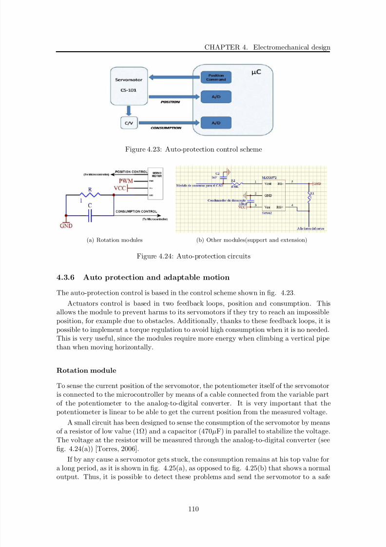
8/21/2019 Alberto Brunete Gonzalez
http://slidepdf.com/reader/full/alberto-brunete-gonzalez 138/311
CHAPTER 4. Electromechanical design
Figure 4.23: Auto-protection control scheme
(a) Rotation mo dules (b) Other mo dules(support and extension)
Figure 4.24: Auto-protection circuits
4.3.6 Auto protection and adaptable motion
The auto-protection control is based in the control scheme shown in fig. 4.23.
Actuators control is based in two feedback loops, position and consumption. Thisallows the module to prevent harms to its servomotors if they try to reach an impossibleposition, for example due to obstacles. Additionally, thanks to these feedback loops, it ispossible to implement a torque regulation to avoid high consumption when it is no needed.This is very useful, since the modules require more energy when climbing a vertical pipethan when moving horizontally.
Rotation module
To sense the current position of the servomotor, the potentiometer itself of the servomotoris connected to the microcontroller by means of a cable connected from the variable partof the potentiometer to the analog-to-digital converter. It is very important that thepotentiometer is linear to be able to get the current position from the measured voltage.
A small circuit has been designed to sense the consumption of the servomotor by meansof a resistor of low value (1Ω) and a capacitor (470µF) in parallel to stabilize the voltage.The voltage at the resistor will be measured through the analog-to-digital converter (seefig. 4.24(a)) [Torres, 2006].
If by any cause a servomotor gets stuck, the consumption remains at his top value fora long period, as it is shown in fig. 4.25(a), as opposed to fig. 4.25(b) that shows a normal
output. Thus, it is possible to detect these problems and send the servomotor to a safe
110

8/21/2019 Alberto Brunete Gonzalez
http://slidepdf.com/reader/full/alberto-brunete-gonzalez 139/311
4.3. Embedded electronics description
Single Module Single Module Loaded
At Rest (mA) 10-15 30-35Peak (moving 1 servo) (mA) 500 500
Peak (moving 2 servo) (mA) 1000 1000Average (1 servo) (mA) 200 250Average (2 servo) (mA) 400 500
Table 4.5: Power Consumption
position or to stop sending position commands (so the servomotor turns loose) to avoidits damage.
Power consumption for rotation module v1 is shown in table 4.5. It is very importantto have low consumption in order to make robots more autonomous or avoid overheating.As it is possible to see, the consumption of the module at rest is very low.
Other modules
Newer modules starting from the support and extension v2 were equipped with IC MAX4372.It is used to sense the current. The connection diagram is shown in fig. 4.24(b). Theconcept is the same as the previous one, but the resistor and capacitor were replaced bythe MAX4372. The output of the IC was taken to a low pass filter to filter the noise madeby the PWM of the servomotor, and then to the A/D converter of the microcontroller.The filter has a cutoff frequency of f c = 0.33Hz [Santos, 2007].
4.3.7 Self orientation detection
Modules are equipped with three-axis accelerometers. With these new sensors inside themicro-robot, it is possible to know how the robot is oriented in relation to the ground(measuring the acceleration vector of gravity) and in which direction it is moving (andhow fast).
The three-axis accelerometer used is the MXR9150. This sensor can measure ±5g witha sensitivity of 150mV/g at 3.0V . It is also able to detect both dynamic (e.g. movement)and static accelerations (e.g. gravity). The MXR9150 provides three radiometric analog
outputs set to 50% of the power supply voltage at 0g, 1.5V in this case [Torres, 2006][Santos, 2007].
In figure 4.26 it is possible to see the measurement of the gravity when the module isplaced with its Z axis down (a) and X axis down (b).
Figures 4.27, 4.28 and 4.29 show the results of some experiments. Figure 4.27 showsthe output of the accelerometers when the module is moving along a linear trajectory inthe XY plane, forward and backwards. The signals are very clear. In the Z axis there isno variation while in the X and Y axis the signals rise and fall when the module movesforward and backward.
In figure 4.28 the rotation module is moving one servomotor from 30 to 150 with no
load (about 0,35 kg*cm). The top figure shows the rotated angle. In the middle figure,
111
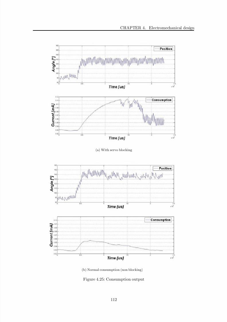
8/21/2019 Alberto Brunete Gonzalez
http://slidepdf.com/reader/full/alberto-brunete-gonzalez 140/311
CHAPTER 4. Electromechanical design
(a) With servo blocking
(b) Normal consumption (non blocking)
Figure 4.25: Consumption output
112
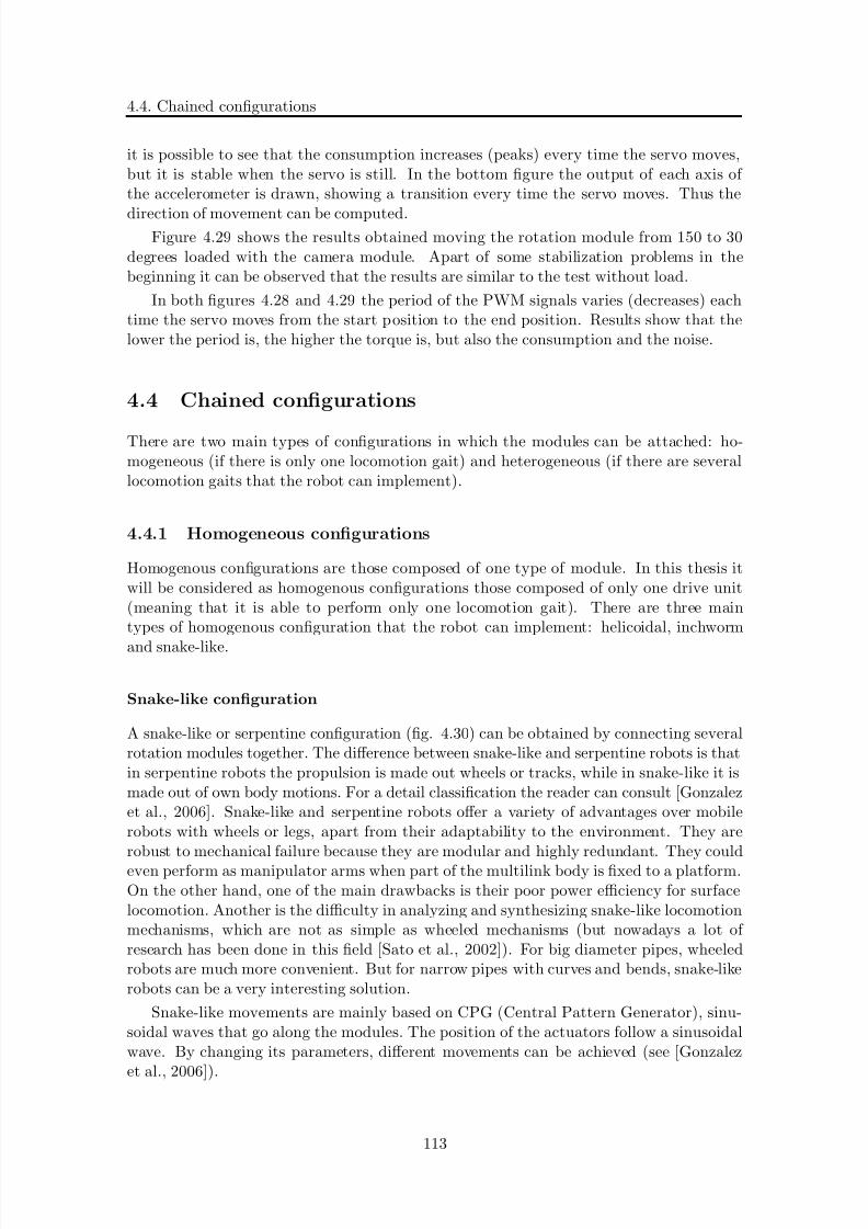
8/21/2019 Alberto Brunete Gonzalez
http://slidepdf.com/reader/full/alberto-brunete-gonzalez 141/311
4.4. Chained configurations
it is possible to see that the consumption increases (peaks) every time the servo moves,but it is stable when the servo is still. In the bottom figure the output of each axis of the accelerometer is drawn, showing a transition every time the servo moves. Thus the
direction of movement can be computed.Figure 4.29 shows the results obtained moving the rotation module from 150 to 30
degrees loaded with the camera module. Apart of some stabilization problems in thebeginning it can be observed that the results are similar to the test without load.
In both figures 4.28 and 4.29 the period of the PWM signals varies (decreases) eachtime the servo moves from the start position to the end position. Results show that thelower the period is, the higher the torque is, but also the consumption and the noise.
4.4 Chained configurations
There are two main types of configurations in which the modules can be attached: ho-mogeneous (if there is only one locomotion gait) and heterogeneous (if there are severallocomotion gaits that the robot can implement).
4.4.1 Homogeneous configurations
Homogenous configurations are those composed of one type of module. In this thesis itwill be considered as homogenous configurations those composed of only one drive unit(meaning that it is able to perform only one locomotion gait). There are three maintypes of homogenous configuration that the robot can implement: helicoidal, inchworm
and snake-like.
Snake-like configuration
A snake-like or serpentine configuration (fig. 4.30) can be obtained by connecting severalrotation modules together. The difference between snake-like and serpentine robots is thatin serpentine robots the propulsion is made out wheels or tracks, while in snake-like it ismade out of own body motions. For a detail classification the reader can consult [Gonzalezet al., 2006]. Snake-like and serpentine robots offer a variety of advantages over mobilerobots with wheels or legs, apart from their adaptability to the environment. They arerobust to mechanical failure because they are modular and highly redundant. They couldeven perform as manipulator arms when part of the multilink body is fixed to a platform.On the other hand, one of the main drawbacks is their poor power efficiency for surfacelocomotion. Another is the difficulty in analyzing and synthesizing snake-like locomotionmechanisms, which are not as simple as wheeled mechanisms (but nowadays a lot of research has been done in this field [Sato et al., 2002]). For big diameter pipes, wheeledrobots are much more convenient. But for narrow pipes with curves and bends, snake-likerobots can be a very interesting solution.
Snake-like movements are mainly based on CPG (Central Pattern Generator), sinu-soidal waves that go along the modules. The position of the actuators follow a sinusoidalwave. By changing its parameters, different movements can be achieved (see [Gonzalez
et al., 2006]).
113

8/21/2019 Alberto Brunete Gonzalez
http://slidepdf.com/reader/full/alberto-brunete-gonzalez 142/311
CHAPTER 4. Electromechanical design
(a) Z axis pointing down
(b) X axis pointing down
Figure 4.26: Accelerometer tests: still module
114
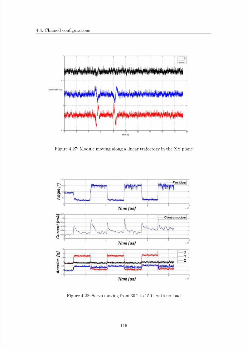
8/21/2019 Alberto Brunete Gonzalez
http://slidepdf.com/reader/full/alberto-brunete-gonzalez 143/311
4.4. Chained configurations
Figure 4.27: Module moving along a linear trajectory in the XY plane
Figure 4.28: Servo moving from 30 to 150 with no load
115

8/21/2019 Alberto Brunete Gonzalez
http://slidepdf.com/reader/full/alberto-brunete-gonzalez 144/311
CHAPTER 4. Electromechanical design
Figure 4.29: Servo moving from 150
to 30
loaded
Figure 4.30: Snake-like configuration
116
8/21/2019 Alberto Brunete Gonzalez
http://slidepdf.com/reader/full/alberto-brunete-gonzalez 145/311
4.4. Chained configurations
(a) Turning (1), rotating (2) and rolling (3)
(b) Serpentine, side-winding, concertina and rectilinear
Figure 4.31: Snake movements
With CPG it is possible to simulate some of the movements of the snakes (see fig.4.31(b)):
• Serpentine locomotion: is the most common method of travel used by snakes. Eachpoint of the body follows along the S-shaped path established by the head andneck, much like the cars of a train following the track. The key property of snakesin achieving serpentine locomotion is the difference in the friction coefficients forthe tangential and the normal directions with respect to the body. In particular,the normal friction tends to be much larger than the tangential friction, leading toavoidance of side slipping.
• Caterpillar (vertical serpentine or rectilinear): This slower technique also contractsthe body into curves, but these waves are much smaller and curve up and downrather than side to side. When a snake uses caterpillar movement, the tops of eachcurve are lifted above the ground as the ventral scales on the bottoms push againstthe ground, creating a rippling effect similar to how a caterpillar looks when it walks.The friction parameters are not so important.
• Sidewinding: in environments with few resistance points, snakes may use a variationof serpentine motion to get around. Contracting their muscles and flinging their
bodies, sidewinders create an S-shape that only has two points of contact with the
117

8/21/2019 Alberto Brunete Gonzalez
http://slidepdf.com/reader/full/alberto-brunete-gonzalez 146/311
CHAPTER 4. Electromechanical design
(a) Configuration 1 (b) Configuration 2
(c) Configuration 3 (d) Configuration 4
Figure 4.32: Snake-like configurations
ground; when they push off, they move laterally. Using this gait, the robot movesparallel to its body axis.
Another common mode (gait) of locomotion in snakes that cannot be achieved by CPGsis concertina [Gray and Lissmann, 1950] [Lissmann, 1950], see figure 4.31(b). Concertinais the method used to climb. The snake extends its head and the front of its body along thevertical surface and then finds a place to grip with its ventral scales. To get a good hold,it bunches up the middle of its body into tight curves that grip the surface while it pullsits back end up; it then springs forward again to find a new place to grip with its scales.This movement can be achieved by especial sequences of preprogrammed movements.
There are some other movements that can be created that are not inspired by realsnakes (figure 4.31(a)):
• Rolling: The robot can roll around its body axis. The same sinusoidal signal isapplied to all the vertical joints and a 90out of phase sinusoidal signal is applied tohorizontal joints.
• Turning: The robot can move along an arc, turning left or right. The vertical jointsare moving as in 1D sinusoidal gait and the horizontal joints are at fixed positionall the time. The robot has the shape of an arc. The radius of curvature of thetrajectory can be modified by modifying the offset of the horizontal joints.
• Rotating: The robot can also rotate parallel to the ground clock-wise or anti-
clockwise. The robot can change its orientation in the plane. A phase difference
118

8/21/2019 Alberto Brunete Gonzalez
http://slidepdf.com/reader/full/alberto-brunete-gonzalez 147/311
4.4. Chained configurations
(a) Inside a ø40mm pipe
(b) Negotiating an elbow in a ø50mm pipe
Figure 4.33: Snake-like microrobot inside pipes
of 5is applied to the horizontal joints and 120for the vertical.
The most suitable locomotion gait for pipes turns out to be rectilinear and concertina(for climbing). Inside the pipe there is not much space for sidewinding. Serpentine lo-comotion is more suitable to negotiate bends and for straight stretches when the frictionbetween the robot and the pipe is strong enough. If the friction is small, or to climb pipes,rectilinear and concertina locomotion are more appropriate.
The snake-like configuration is a very versatile robot which can adopt several shapes.In fig. 4.32 different configurations are shown: Caterpillar (fig. 4.32(a)), serpentine (fig.4.32(b)), circle (fig. 4.32(c)) and helix (fig. 4.32(d)). Due to the 2 dof the robot can adoptmany 3D configurations.
The microrobot fits in pipes of 40 mm diameter (fig. 4.33(a)) and is able to negotiate90o angles (fig. 4.33(b)) in 50mm diameter pipes.
A specific GUI has been implemented for the control of snake-like microrobots (fig.4.34). With it, it is possible to:
• simulate movements
• telecontrol the robot
• record sets of movements and send them to the robot for later execution.
119

8/21/2019 Alberto Brunete Gonzalez
http://slidepdf.com/reader/full/alberto-brunete-gonzalez 148/311
CHAPTER 4. Electromechanical design
Figure 4.34: Graphical User Interface
Worm-like configuration
The inchworm strategy is simple yet extraordinarily powerful. Having an body withextension capabilities and many small foot pads placed at either end of its body, theinchworm’s mode of locomotion is to firmly attach the rear portion of its body to a
surface via its foot pads, extending the remainder of its body forward, attaching it to thesurface and bring ing the rear part of its body to meet the forward part. In this way, theinchworm always has at least one portion of its body firmly attached to a surface.
This type of movement is particularly suited to unstructured or even hostile environ-ments. As an inchworm moves forward it has the opportunity to sense what is in front of it without having to commit to attaching to an inappropriate surface. At the same time,the system’s low silhouette and centre of gravity provides the animal with a high degreeof stability.
An inchworm configuration (fig. 4.21) can be obtained by connecting two supportand one extension modules together (support - extension - support). The sequence of movement in an inchworm robot is as follows (fig. 4.35):
1. The rear module (3) expands (making pressure against the pipe) and the front one(1) releases.
2. The central module (2) expands straight or in angle.
3. The front module expands and the rear one releases.
4. The central module contracts.
This way of locomotion requires two different types of modules, and thus it could beconsidered heterogenous. But since it is a single locomotion gait, it is included in the
homogenous section.
120
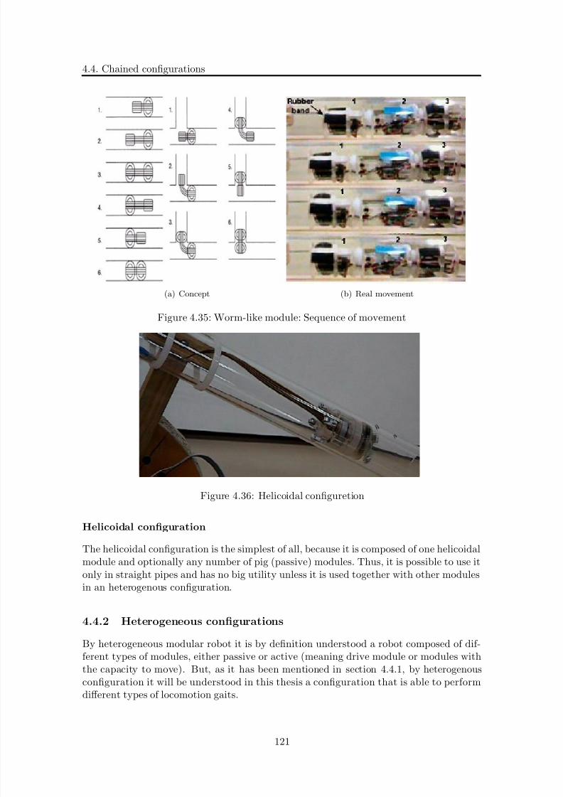
8/21/2019 Alberto Brunete Gonzalez
http://slidepdf.com/reader/full/alberto-brunete-gonzalez 149/311
4.4. Chained configurations
(a) Concept (b) Real movement
Figure 4.35: Worm-like module: Sequence of movement
Figure 4.36: Helicoidal configuretion
Helicoidal configuration
The helicoidal configuration is the simplest of all, because it is composed of one helicoidal
module and optionally any number of pig (passive) modules. Thus, it is possible to use itonly in straight pipes and has no big utility unless it is used together with other modulesin an heterogenous configuration.
4.4.2 Heterogeneous configurations
By heterogeneous modular robot it is by definition understood a robot composed of dif-ferent types of modules, either passive or active (meaning drive module or modules withthe capacity to move). But, as it has been mentioned in section 4.4.1, by heterogenousconfiguration it will be understood in this thesis a configuration that is able to perform
different types of locomotion gaits.
121

8/21/2019 Alberto Brunete Gonzalez
http://slidepdf.com/reader/full/alberto-brunete-gonzalez 150/311
CHAPTER 4. Electromechanical design
Figure 4.37: Multi-modular configuration
Although there are some developments including heterogenous modules, they only have
one active module (the others are passive) as it has been shown in chapter 2, and so thereis not a single one that combines several drive units.
The heterogeneous modular microrobot considered here can be any combination of the previous modules. An example can be found in figure 4.37. Of course some of theconfigurations will work better than others, and this will be studied in this thesis. Thecontrol layer of the microrobot is able to detect what kind of modules it is composed of andto select the optimum locomotion gait at every moment. Also it is possible to reconfigurethe micro-robot depending on the task being performed in order to adapt to the differentvariety of pipes that can be found.
For example, a microrobot composed only of rotation modules is very slow in a narrowpipe, but combined with one or two helicoidal modules it can move much faster but stillnegotiate turns.
Another example: the helicoidal module is very fast in pipes of a specific diameter,but combined with the worm-like modules, it is able to pass parts of the pipe of differentdiameter or with broken parts.
The list of examples is quite long and it can be incremented by adding new modulesin the future with new locomotion modes.
The heterogeneous configurations will be deeply described in chapter 5.
4.5 Conclusions
In this chapter the modules that have been designed and built have been described bothin the hardware and the electronic sides. The different versions of the helicoidal, support,extension, rotation, camera and batteries modules have been stated and the reasons tobuild them and evolve from one prototype to another, have been explained. Some othermodules that are under development have also been mentioned, like the traveler and thesensor modules. The SMA-based module has also been described although it is not goingto be used for the moment because of its high consumption and difficulty to be mounted.
Although in the beginning it was a priority to make the modules as small as possible(i.e. in the rotation module v1 the gearset was rearranged to gain space), there was a
tendency afterwards to make the modules bigger in order to improve the robustness and
122

8/21/2019 Alberto Brunete Gonzalez
http://slidepdf.com/reader/full/alberto-brunete-gonzalez 151/311
4.5. Conclusions
stability of the modules. Thus, although the robot should be referred as minirobot, theterm microrobot is still used since it was the original design, and indeed, in literaturethe term microrobot is used for small robots of about tens of millimeters [Caprari, 2003]
[Kawahara et al., 1999] [Xiao et al., 2004] [Yoshida et al., 2002]. . .Each type of module is followed by its kinematic description, that helps to understand
the module and to facilitate its future use.
All modules have been designed as small as possible, and finally a diameter of 27mmhas been selected as the default for all of them. Some of them could have been smaller, butin order to keep the same connector, the 27mm of diameter has been respected. Thus, theyare able to travel in pipes of 40mm diameter, but in order to make turns it is necessaryto have a bigger one (50mm diameter pipe is ok).
There is a couple of modules that has not been built yet, the traveler and the sensormodules. The traveler module has nevertheless been used in the simulator and it will be
described in chapter 5.The electronics of the modules have also been described. Although each module has a
different electronics, all of them share the same concept, and thus they can work together,sharing a common interface and bus (I 2C ). In general, apart from accelerometers and po-sition and consumption control, modules are lacking sensor integration (IR, temperature,humidity sensors, etc.), which was not possible to integrate in the current versions of themodules. However, some of them are simulated in chapter 5 and used in the simulatedmicrorobot (for example the use or IR sensors).
While many other prototypes are composed of homogeneous modules, in this researchit has been sought to have different drive modules and locomotion gaits: helicoidal, worm-like and snake-like (in its different ways, like serpentine, rectilinear, side-winding, etc.).
Its use in homogeneous configurations have been described. How to use them togetherand coordinate them in heterogenous configurations will be treated in the chapter 5.
It is important to remark how difficult and how much time and money it involves tohave so many different prototypes working together, one of the reasons why some similarresearches have been cancelled [Jantapremjit and Austin, 2001].
123

8/21/2019 Alberto Brunete Gonzalez
http://slidepdf.com/reader/full/alberto-brunete-gonzalez 152/311
CHAPTER 4. Electromechanical design
124
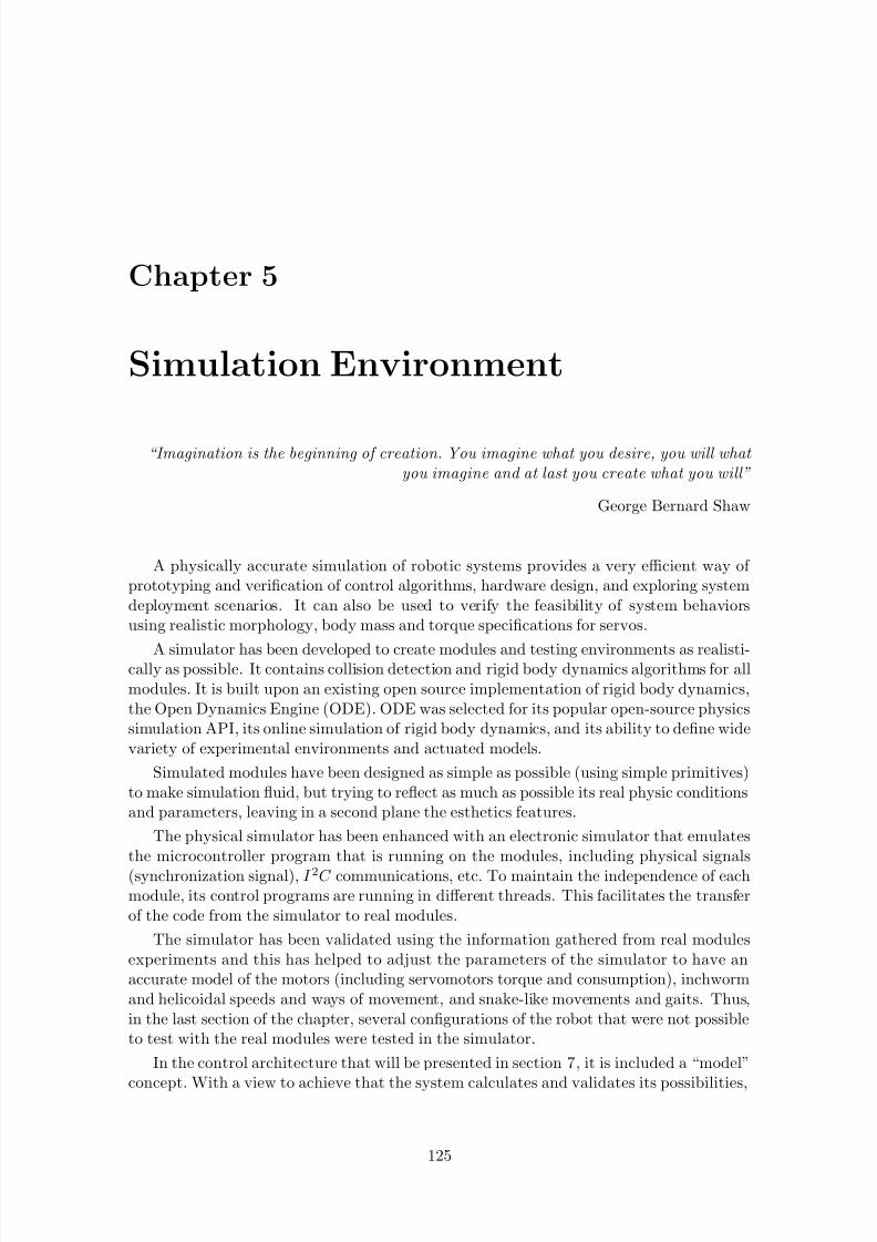
8/21/2019 Alberto Brunete Gonzalez
http://slidepdf.com/reader/full/alberto-brunete-gonzalez 153/311
Chapter 5
Simulation Environment
“Imagination is the beginning of creation. You imagine what you desire, you will what you imagine and at last you create what you will”
George Bernard Shaw
A physically accurate simulation of robotic systems provides a very efficient way of prototyping and verification of control algorithms, hardware design, and exploring systemdeployment scenarios. It can also be used to verify the feasibility of system behaviorsusing realistic morphology, body mass and torque specifications for servos.
A simulator has been developed to create modules and testing environments as realisti-cally as possible. It contains collision detection and rigid body dynamics algorithms for allmodules. It is built upon an existing open source implementation of rigid body dynamics,the Open Dynamics Engine (ODE). ODE was selected for its popular open-source physicssimulation API, its online simulation of rigid body dynamics, and its ability to define widevariety of experimental environments and actuated models.
Simulated modules have been designed as simple as possible (using simple primitives)to make simulation fluid, but trying to reflect as much as possible its real physic conditionsand parameters, leaving in a second plane the esthetics features.
The physical simulator has been enhanced with an electronic simulator that emulatesthe microcontroller program that is running on the modules, including physical signals
(synchronization signal), I 2C communications, etc. To maintain the independence of eachmodule, its control programs are running in different threads. This facilitates the transferof the code from the simulator to real modules.
The simulator has been validated using the information gathered from real modulesexperiments and this has helped to adjust the parameters of the simulator to have anaccurate model of the motors (including servomotors torque and consumption), inchwormand helicoidal speeds and ways of movement, and snake-like movements and gaits. Thus,in the last section of the chapter, several configurations of the robot that were not possibleto test with the real modules were tested in the simulator.
In the control architecture that will be presented in section 7, it is included a “model”
concept. With a view to achieve that the system calculates and validates its possibilities,
125
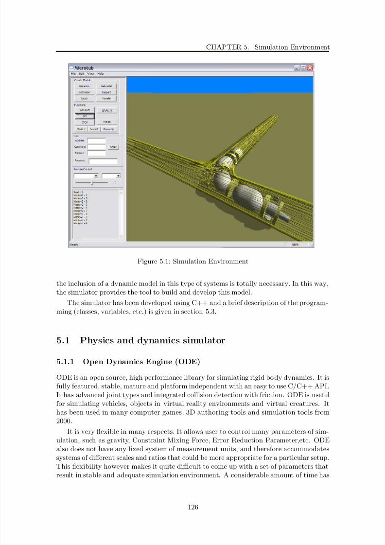
8/21/2019 Alberto Brunete Gonzalez
http://slidepdf.com/reader/full/alberto-brunete-gonzalez 154/311
CHAPTER 5. Simulation Environment
Figure 5.1: Simulation Environment
the inclusion of a dynamic model in this type of systems is totally necessary. In this way,the simulator provides the tool to build and develop this model.
The simulator has been developed using C++ and a brief description of the program-ming (classes, variables, etc.) is given in section 5.3.
5.1 Physics and dynamics simulator
5.1.1 Open Dynamics Engine (ODE)
ODE is an open source, high performance library for simulating rigid body dynamics. It isfully featured, stable, mature and platform independent with an easy to use C/C++ API.It has advanced joint types and integrated collision detection with friction. ODE is usefulfor simulating vehicles, objects in virtual reality environments and virtual creatures. Ithas been used in many computer games, 3D authoring tools and simulation tools from2000.
It is very flexible in many respects. It allows user to control many parameters of sim-ulation, such as gravity, Constraint Mixing Force, Error Reduction Parameter,etc. ODEalso does not have any fixed system of measurement units, and therefore accommodatessystems of different scales and ratios that could be more appropriate for a particular setup.This flexibility however makes it quite difficult to come up with a set of parameters that
result in stable and adequate simulation environment. A considerable amount of time has
126

8/21/2019 Alberto Brunete Gonzalez
http://slidepdf.com/reader/full/alberto-brunete-gonzalez 155/311
5.1. Physics and dynamics simulator
Figure 5.2: Mathematical model of the servomotor
been spent testing different combinations of these settings and the experience has beenused to produce a tuned simulation that models most accurately the possible real settingsof the modules.
For more information about ODE, the reader can consult its webpage1.
5.1.2 Servomotor model
Although ODE provides a model for a motor, a more accurate model was needed in orderto simulate the servomotor used in the modules. Thus, a real servomotor model has beendeveloped (fig. 5.2). This model is built upon the existing motor model provided in theODE library adding a simulation of its parameters.
The parameters are the typical ones in motors:
• Kτ [N · m/A] is the torque constant
• K m[V/rad/s] is the counter-electromotive force constant
• K p[V/rad] is the proportional servo control constant
• Lm[H ] and R[Ω] are the electrical parameters of the motor, inductance and resistor
• J m[N · m/rad/s2] is the inertia parameter of the motor itself
• Bm[N · m/rad/s] is the friction coefficient of the motor itself
Also, there are some variables that are used which meaning is:
• θm[rad] is the actual angle (gotten from ODE)
• θr[rad] is the desired angle
• ω[rad/s] is the velocity
• ea[V ] is the voltage of the stator
1
http://www.ode.org/ and http://opende.sourceforge.net/wiki/index.php/Main_Page
127

8/21/2019 Alberto Brunete Gonzalez
http://slidepdf.com/reader/full/alberto-brunete-gonzalez 156/311
CHAPTER 5. Simulation Environment
• i[A] is the intensity of the current
• em[V ] is the inducted voltage
• τ [N · m] is the electromechanical torque of the motor
• τ loss[N · m] is the loss of torque due to all intrinsic factors
• τ effective[N · m] is the effective torque sent to ODE to move the servomotor to thedesired position
• if [A] is the intensity measured after the low pass RC filter that is used in the realmodules to filter the noise (fig. 4.24). Although it has no purpose for the servomotormodel, it is necessary to compare the signal from the real and the simulated modules.
In the next paragraph the equations used for the simulation to compute the torque arepresented in the continuous time:
ω(t) = dθ(t)
dt (5.1)
ea(t) = K p · (θr(t) − θm(t)) (5.2)
em(t) = K m · ω(t) (5.3)
ea(t) − em(t) = LmdI (t)
dt + i(t) · R (5.4)
τ (t) = K τ · i(t) (5.5)
τ loss(t) = J m · α(t) + Bm · ω(t) = J m · d2θ(t)
d2t + Bm ·
dθ(t)
dt (5.6)
τ effective(t) = τ (t) − τ loss(t) (5.7)
α[rad/s2] is the angular acceleration.
It is necessary to transform these equations to compute them. Starting from 5.1, itcan be expressed in the Laplace domain as:
ω(s) = θ(s) · s (5.8)
where s ∈ C . Applying the transformation s = 1−z−1
T , where T is the sampling period,
it is obtained in the Z domain:
ω(z) = θ(z) · 1 − z−1
T (5.9)
where z ∈ C. Thus:
ω(z) = θ(z) − θ(z) · z−1
T (5.10)
and thus, applying the inverse transform, the discrete time equation is obtained:
128

8/21/2019 Alberto Brunete Gonzalez
http://slidepdf.com/reader/full/alberto-brunete-gonzalez 157/311
5.1. Physics and dynamics simulator
ω[n] = θ[n] − θ[n − 1]
T (5.11)
where n is the discrete time. To simplify, the process is the following:
x(t) ⇒ X (s) ⇒ X (z) ⇒ x[n] (5.12)
Doing the same process to all the equations, the following equations are obtained:
ea[n] = K p · (θr[n] − θm[n]) (5.13)
em[n] = K m · ω[n] (5.14)
i[n] = (ea[n] − em[n]) · T + Lm · i[n − 1]
Lm + R · T (5.15)
τ [n] = K τ · i[n] (5.16)
τ loss[n] = J mT 2
(θ[n] − 2 · θ[n − 1] + θ[n − 2]) + Bm
T (θ[n] − θ[n − 1]) (5.17)
τ effective[n] = τ [n] − τ loss[n] (5.18)
E a must be limited to 5V, because that is the maximum voltage provided by thepower supply. In fig. 5.2 it is the block before ea. In the real modules, the control of theservomotor is done by PWM.
There is a range [0..I threshold] where the intensity does not produce any torque due tothe friction static coefficient. This is represented in fig. 5.2 with the block before K t.
5.1.3 Modules physical model
For the purposes of better performance and stability, the model of the modules were sim-plified to a set of standard geometrical primitives (such as spheres, cubes, cylinders..etc)connected by degrees of freedom, which were defined as (powered) joints. This simpli-fication of changing odd shapes into standard shapes was necessary to make simulationscalable (collision detection with odd shapes are very expensive in ODE). However, di-mensions and masses were the values of the real modules.
The created geometric morphology model was assigned dynamic properties that corre-spond to the modules design specifications. Masses for each body part were assigned realvalues. Degrees of freedom were limited by maximum torque and speed available fromspecifications of servomotors selected to be deployed in each module. To ensure properinteraction of modules with the simulated environment, friction coefficients were set tovalues estimated for materials to be used for module manufacturing and possible surface
materials. These values were adjusted and validated experimentally in a last step, as it
129

8/21/2019 Alberto Brunete Gonzalez
http://slidepdf.com/reader/full/alberto-brunete-gonzalez 158/311
CHAPTER 5. Simulation Environment
(a) Rotation Module (b) Helicoidal Module
Figure 5.3: Rotation Module and Helicoidal Module
will be shown in section 8.2.
To be capable of producing behaviors with different functionalities, modules should beable to dock to each other forming different configuration shapes. In design specification,modules have two docking faces, one on each side. In the simulated environment, thedocking capability was implemented by using a fixed joint that is created connecting twosides of different modules. This allows the modules to be attached to each other andmaintain the relative positions fixed.
All modules try to keep as highly as possible the most possible similarities with thereal ones, either in mechanics (joints, dof, shape, mass...etc) or in electronics.
Each module model will be described in more detail in the following sections.
Rotation Module
The rotation module (fig. 5.3 a)) is simulated by a capsule and two cylinders as connectors.It has two servomotors to provide the two degrees of freedom.
Each servomotor is limited to 180as real servomotors do.
Helicoidal Module
The helicoidal module (fig. 5.3 b)) is simulated by a pig module (passive) upon which aforce is applied in the direction of movement, in order to simulate the driving force of therotating head of the module.
This is a simplified model of the real module in order to make the simulation fasterand less expensive in terms of CPU consumtion.
Support Module
The support module (fig. 5.4 a)) is simulated by three cubes that simulate the armswith three servomotors and two cylinders as connectors. The real module has only one
servomotor, but this is an easy way for simulation. One servomotor is the active one, the
130

8/21/2019 Alberto Brunete Gonzalez
http://slidepdf.com/reader/full/alberto-brunete-gonzalez 159/311
5.1. Physics and dynamics simulator
(a) Support Module (b) Extension Module
Figure 5.4: Inchworm Modules
one that can be accessed and modified, and the other two just copy the position of themain one.
In order to make the simulation more accurate, the passive servomotors should have asmaller torque that the main one, because in the real module there is only one servomotorthat sends more torque to one arm than to the other two.
Extension Module
The extension module (fig. 5.4 b)) is simulated by two cubes that can slide one over theother in order to simulate the elongation of the modules. A control has been implementedto simulate a linear servomotor (equations 5.19 and 5.20). A circular servomotor in thefront can simulate the rotation dof of the real module.
F max = F maxservo (5.19)
V = l0(P osref − P osservo) (5.20)
being F maxservo the maximum force of the servomotor, l0 a proportional coefficient,
P osref the desired position and P osservo the actual position of the linear servomotor.
Touch Module
The touch module (fig. 5.5 a)) simulates the camera and the touch sensor. The camerais not simulated in any way but by including its weight in the total weight of the module.The touch sensor is simulated by means of a cylinder that detects collisions.
The collision detection is simulated by the detection of the contact of the surface of thecylinder (any part) with other object (i.e. the pipe), which is quite accurate, because thereal module has a cover stuck to three contact sensors. When the cover touches anything
it is detected by the sensors.
131

8/21/2019 Alberto Brunete Gonzalez
http://slidepdf.com/reader/full/alberto-brunete-gonzalez 160/311
CHAPTER 5. Simulation Environment
Traveler Module
The traveler module (fig. 5.5 b)) is still a concept, there is no real module yet. It has been
designed for the simulation, not in reality. It is composed of three wheels provided withencoders that measures the distance that the microrobot has traveled.
The encoder is simulated by calling a function that gives the rotation (in degrees) of the wheel. The function is provided by the ODE API.
Since there are three encoders and each of them can measure different distances depend-ing on weather they are in contact with the surface or not, it is necessary an algorithm toextract an accurate value from the single ones. This algorithm is embedded in the controlprogram of the module.
Encoders are taking measures continuously. At every step of the control algorithm(every 15ms aprox), it takes a measurement of each of the three encoders and calculatesthe maximum value of the three. This value adds up to the total value, that is the traveleddistance for the microrobot.
In order to simulate real wheel with encoders it is necessary to add some extra frictionto the wheels so they don’t keep turning due to the inertia. For each wheel, a torqueproportional to its angular velocity is applied in the opposite turning direction.
%Pseudocode for traveled distance measurement
repeat
m1 = measurement encoder 1
m2 = measurement encoder 2
m3 = measurement encoder 3
mtotal = mtotal + max(m1,m2,m3)
av1 = angular velocity wheel 1
av2 = angular velocity wheel 2
av3 = angular velocity wheel 3
torque1 = Kforce * av1
torque2 = Kforce * av2
torque3 = Kforce * av3
apply torque1, torque2, torque3
132
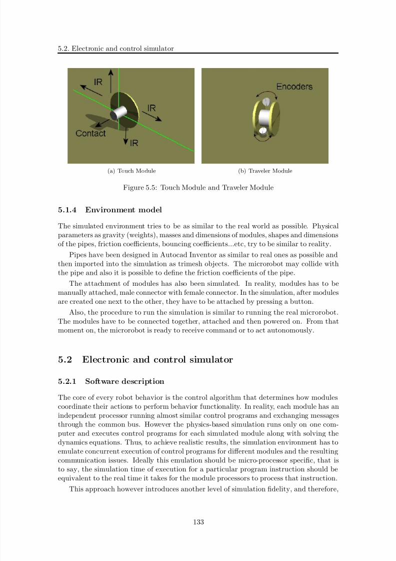
8/21/2019 Alberto Brunete Gonzalez
http://slidepdf.com/reader/full/alberto-brunete-gonzalez 161/311
5.2. Electronic and control simulator
(a) Touch Module (b) Traveler Module
Figure 5.5: Touch Module and Traveler Module
5.1.4 Environment model
The simulated environment tries to be as similar to the real world as possible. Physicalparameters as gravity (weights), masses and dimensions of modules, shapes and dimensionsof the pipes, friction coefficients, bouncing coefficients...etc, try to be similar to reality.
Pipes have been designed in Autocad Inventor as similar to real ones as possible andthen imported into the simulation as trimesh objects. The microrobot may collide withthe pipe and also it is possible to define the friction coefficients of the pipe.
The attachment of modules has also been simulated. In reality, modules has to be
manually attached, male connector with female connector. In the simulation, after modulesare created one next to the other, they have to be attached by pressing a button.
Also, the procedure to run the simulation is similar to running the real microrobot.The modules have to be connected together, attached and then powered on. From thatmoment on, the microrobot is ready to receive command or to act autonomously.
5.2 Electronic and control simulator
5.2.1 Software description
The core of every robot behavior is the control algorithm that determines how modulescoordinate their actions to perform behavior functionality. In reality, each module has anindependent processor running almost similar control programs and exchanging messagesthrough the common bus. However the physics-based simulation runs only on one com-puter and executes control programs for each simulated module along with solving thedynamics equations. Thus, to achieve realistic results, the simulation environment has toemulate concurrent execution of control programs for different modules and the resultingcommunication issues. Ideally this emulation should be micro-processor specific, that isto say, the simulation time of execution for a particular program instruction should beequivalent to the real time it takes for the module processors to process that instruction.
This approach however introduces another level of simulation fidelity, and therefore,
133

8/21/2019 Alberto Brunete Gonzalez
http://slidepdf.com/reader/full/alberto-brunete-gonzalez 162/311
CHAPTER 5. Simulation Environment
considerable overhead. It has been decided to follow a simpler route and use concurrencymechanisms provided by the operating system –namely threads– to emulate simultaneouslyrunning modules. Each simulated module control program has its own independent thread
of execution which runs in an infinite loop. The physics simulation engine spawns all themodule threads in the setup routine and then proceeds to the simulation loop. Eachmodule thread yields execution control at the end of its program loop to give controlto the simulation thread which thus has highest execution priority. This helps to makesimulation smooth and reduce CPU load.
In order to simulate the existence of independent microcontrollers (processors), thereare several threads running on the same machine:
• 1 thread for each module
• 1 thread for the central control
• 1 thread for the simulation, in charge of iterate the world and physical parametersof the modules (i.e. servos)
• 1 thread for offline genetic algorithm computation (it is only running when the GAneeds to be computed)
The emulated concurrency also forces discipline on control program development. Thefact that each simulated module runs an independent piece of code requires deep consid-eration of synchronization and sensor data propagation among modules in configuration.Thus semaphores (critical sections) have been used to protect data that is accessed byseveral threads at the same time. This realistic approach makes the developed control al-gorithms much more suitable for transferring them onto real modules, and makes it easier
to move the code from simulation algorithms to embedded routines running in modulesmicrocontroller.
The simulator is divided in four parts:
• A part OS dependent that governs the inputs (mouse, buttons, etc.) and outputs(messages)
• The physics simulation (ODE)
• The central control
• The control of every module
Simulation parameters
The main application has a timer that executes two tasks every 20ms: the simulationlooproutine and the drawing stuff. Thus the simulation is painted every 20 ms.
The simulationloop routine is in charge of iterate the world the defined step, that isusually 0.0005s (i.e. 0.5ms), as many times as possible (i.e. 40 times: 20 / 0.5).
5.2.2 Actuator control
The position where the servo has to move is sent normally through a PWM signal (from
the microcontroller to the servo). In the simulation this is done by simulating the behavior
134
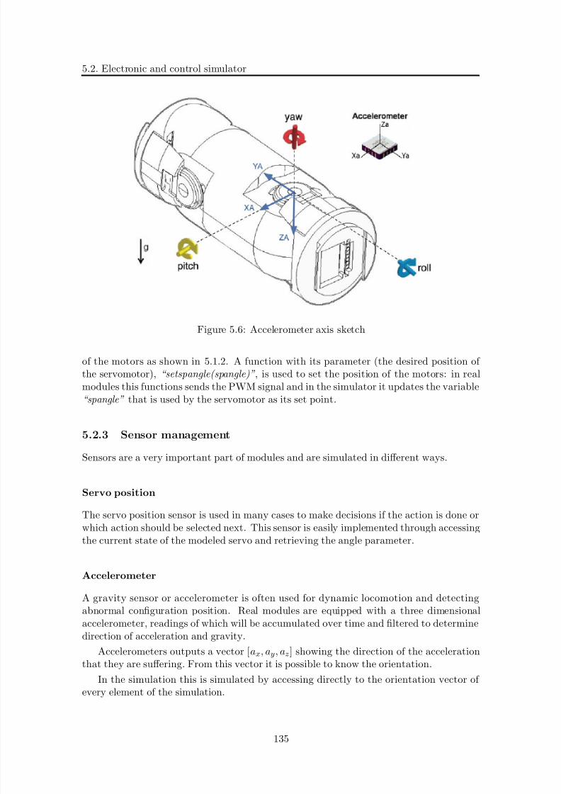
8/21/2019 Alberto Brunete Gonzalez
http://slidepdf.com/reader/full/alberto-brunete-gonzalez 163/311
5.2. Electronic and control simulator
Figure 5.6: Accelerometer axis sketch
of the motors as shown in 5.1.2. A function with its parameter (the desired position of the servomotor), “setspangle(spangle)”, is used to set the position of the motors: in realmodules this functions sends the PWM signal and in the simulator it updates the variable“spangle” that is used by the servomotor as its set point.
5.2.3 Sensor management
Sensors are a very important part of modules and are simulated in different ways.
Servo position
The servo position sensor is used in many cases to make decisions if the action is done orwhich action should be selected next. This sensor is easily implemented through accessingthe current state of the modeled servo and retrieving the angle parameter.
Accelerometer
A gravity sensor or accelerometer is often used for dynamic locomotion and detectingabnormal configuration position. Real modules are equipped with a three dimensionalaccelerometer, readings of which will be accumulated over time and filtered to determinedirection of acceleration and gravity.
Accelerometers outputs a vector [ax, ay, az] showing the direction of the accelerationthat they are suffering. From this vector it is possible to know the orientation.
In the simulation this is simulated by accessing directly to the orientation vector of
every element of the simulation.
135

8/21/2019 Alberto Brunete Gonzalez
http://slidepdf.com/reader/full/alberto-brunete-gonzalez 164/311
CHAPTER 5. Simulation Environment
When the module is stopped, it is sometimes possible to calculate its orientation fromthe output of the accelerometers, a vector [ax, ay, az ].
For example, if the module is in the position shown in picture figure 5.6, the pitch
(rotation in the X axis) can be calculated as in eq. 5.21 and the roll (rotation in the Yaxis) as in eq. 5.22. For the yaw, extra computation is needed.
θ = arctan ay
az(5.21)
φ = arctan az
ax(5.22)
Encoders
The traveler module will be equipped with encoders in each of its three wheels in order toevaluate the distance it has traveled.
This is simulated by a function that reads the rotation of the wheel every certainamount of time and calculates how much the wheel has rotated in that period.
When it has the information of all the wheels, this information is processed to computethe distance traveled by the module.
5.2.4 I 2C communication
I 2C is simulated through different classes: message, bus, and message queue. In reality, if a message is sent to the bus, is listened by everybody that is connected to the bus. This
is by definition because all modules are connected to the bus and detect the differencesin voltage of the wires. But in the simulation has to be implemented through a functionthat sends the message to all modules connected to the bus.
5.2.5 Synchronism lines communication
The synchronism line is done by two internal variables of the modules, one for the S insignal, and one for the S out.
5.2.6 Simulation of the power consumption
As it has been shown in section 4.3.6, the auto protection mechanism is based in themeasurements of the consumption and position of the servomotors.
The servo position sensor is measured accessing the current state of the modeled servoand retrieving its angle parameter.
For the consumption control, a model to simulate the consumption has been developedfollowing the real design used in the control boards of the modules. This model has beenincluded in the servomotor model, and calculates the current that is consuming the motor.It is an experimental model taken from the tests with real modules.
If the consumption is increasing but the servo is not moving, there is almost certainly
a problem (i.e. the servo is stuck).
136
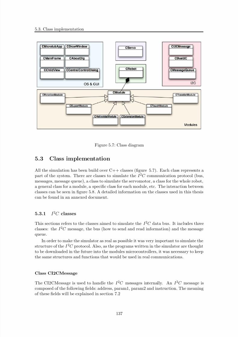
8/21/2019 Alberto Brunete Gonzalez
http://slidepdf.com/reader/full/alberto-brunete-gonzalez 165/311
5.3. Class implementation
Figure 5.7: Class diagram
5.3 Class implementation
All the simulation has been build over C++ classes (figure 5.7). Each class represents a
part of the system. There are classes to simulate the I 2
C communication protocol (bus,messages, message queue), a class to simulate the servomotor, a class for the whole robot,a general class for a module, a specific class for each module, etc. The interaction betweenclasses can be seen in figure 5.8. A detailed information on the classes used in this thesiscan be found in an annexed document.
5.3.1 I 2C classes
This sections refers to the classes aimed to simulate the I 2C data bus. It includes threeclasses: the I 2C message, the bus (how to send and read information) and the message
queue.In order to make the simulator as real as possible it was very important to simulate the
structure of the I 2C protocol. Also, as the programs written in the simulator are thoughtto be downloaded in the future into the modules microcontrollers, it was necessary to keepthe same structures and functions that would be used in real communications.
Class CI2CMessage
The CI2CMessage is used to handle the I 2C messages internally. An I 2C message iscomposed of the following fields: address, param1, param2 and instruction. The meaning
of these fields will be explained in section 7.2
137

8/21/2019 Alberto Brunete Gonzalez
http://slidepdf.com/reader/full/alberto-brunete-gonzalez 166/311
CHAPTER 5. Simulation Environment
Class CBusI2C
It emulates the behavior of the I 2C bus and send messages to/from modules and PC. It
provides two functions used to send I 2
C messages: sendi2cmessage (Send an I2C messageto a specific address) and forwardI2Cmsg (Forward an I2C message in the bus).
The first function is used to send an I 2C message (one of the parameters). The bodyof this function will substituted by the specific code of the module (it depends on thelibraries that it used) in C, assembler or whatever.
The second function is used to simulate the behavior of the bus: if a message is sentto the bus, is listened by everybody that is connected to the bus. In real life this isimplemented by definition because all modules are connected to the bus and detect thedifferences in voltage of the wires. But in the simulation has to be implemented througha function. This function calls the function getI2Cmsg of each module to deliver themessage.
The structure of the I 2C frames will be explained in figure 7.6.
Class CMessageQueue
A class to simulate a queue of messages for each module. When a message arrives it iscopied to a queue to be handle while other messages are arriving.
5.3.2 Servo class
This class is aimed to simulate the control of the servomechanism. This control is usually
done by the electronics of the servomotor, but since in ODE it is used a simple motor itwas necessary to use an added control to be accurate.
The class is called CServo and it mainly develops the procedure described in section5.1.2.
The position where the servo has to move is sent normally through a PWM signal (fromthe microcontroller to the servo). In the simulation is done by the function setspangle usedby each module to set the position of the servo. In real modules this function is changedfor the PWM control function.
5.3.3 Module classes
This classes are intended to simulate the electronic inside the modules. It is composedby a common class (CModule) that includes all that is common to all modules and onedifferent class for each type of module: rotation (CRotationModule), support (CSup-portModule), extension (CExtensionModule), helicoidal (CHelicoidalModule), touch andcamera (CTouchModule) and traveler (CTravelerModule).
Class CModule
It is a general class from which the module inherit. It includes all common characteristics
of the modules:
138
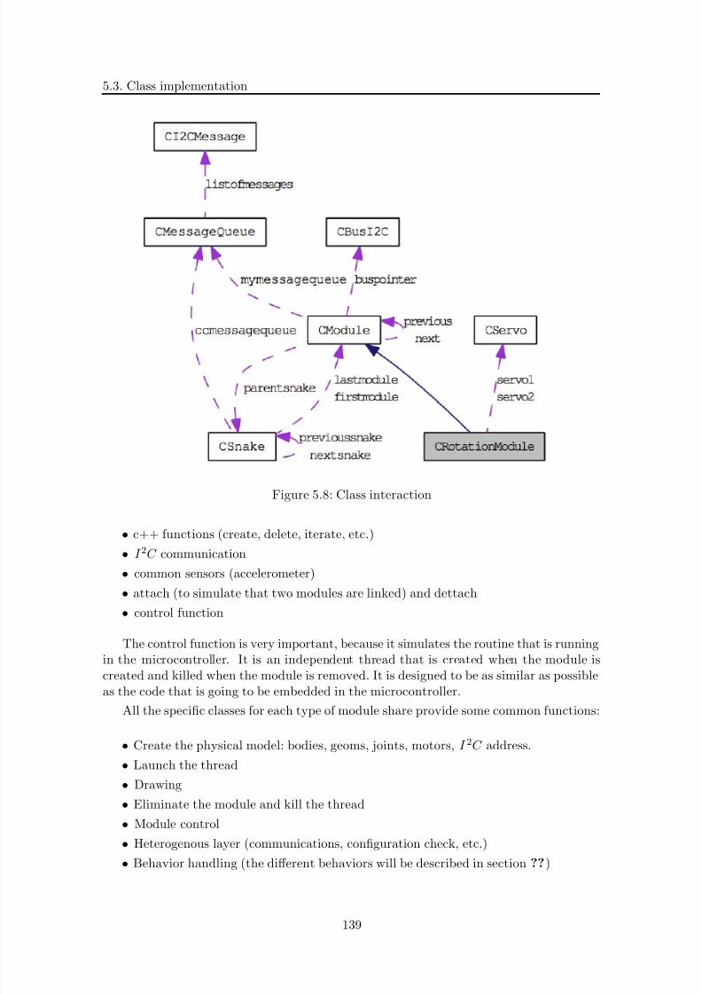
8/21/2019 Alberto Brunete Gonzalez
http://slidepdf.com/reader/full/alberto-brunete-gonzalez 167/311
5.3. Class implementation
Figure 5.8: Class interaction
• c++ functions (create, delete, iterate, etc.)
• I 2C communication
• common sensors (accelerometer)
• attach (to simulate that two modules are linked) and dettach
• control function
The control function is very important, because it simulates the routine that is runningin the microcontroller. It is an independent thread that is created when the module iscreated and killed when the module is removed. It is designed to be as similar as possible
as the code that is going to be embedded in the microcontroller.All the specific classes for each type of module share provide some common functions:
• Create the physical model: bodies, geoms, joints, motors, I 2C address.
• Launch the thread
• Drawing
• Eliminate the module and kill the thread
• Module control
• Heterogenous layer (communications, configuration check, etc.)
• Behavior handling (the different behaviors will be described in section ??)
139
8/21/2019 Alberto Brunete Gonzalez
http://slidepdf.com/reader/full/alberto-brunete-gonzalez 168/311
CHAPTER 5. Simulation Environment
Class CRotationModule
The class represents the rotation module. Besides the features described previously, it
provides the following functions:
• Control of two servomotors
• Iterate servomotors
• Central pattern generation (CPG)
Class CSupportModule
This class represents the support module. Besides the features described previously, itprovides the following functions:
• Control of one servomotor
• Iterate the servomotor
• Expansion and contraction movements
Class CExtensionModule
This class represents the extension module. Besides the features described previously, itprovides the following functions:
• Control of one servomotor and a linear servomotor
• Iterate the servomotors
• Extension and contraction movements
Class CHelicoidalModule
This class represents the helicoidal module. Besides the features described previously, itprovides the following functions:
• Control of simulated motor that pushes forward
Class CTouchModule
This class represents the touch/camera module. Besides the features described previously,it provides the following functions:
• Control of touch sensor
• Control of IR sensors
140
8/21/2019 Alberto Brunete Gonzalez
http://slidepdf.com/reader/full/alberto-brunete-gonzalez 169/311
5.4. Heterogenous modular robot
Class CTravelerModule
This class represents the traveler module. Besides the features described previously, it
provides the following functions:
• Control of simulated encoder
• Control of odometry
5.3.4 Central Control class
The CCentralControl class is used to simulate the central control. As well as the modulesclasses, an independent thread is created for its object when is created.
It simulates an independent thread where it is running all the central control behaviors.It communicates via the I 2C bus with the modules. The behaviors are member functions
of the class.
5.3.5 Robot class
This class (CRobot) represents the whole robot, and it is used to keep a record of themodules that the microrobot is composed of, its position, etc.
It is a linked list of the modules. It is used for iterations, I 2C communications, todraw the modules, attachment, etc.
5.3.6 Graphical User Interface classes
This are the classes that implement the structure of the simulator and the graphical userinterface. It is composed of the classes of the main program, the dialogs, the differentviews and the classes for drawing (with the OpenGL commands).
Class CMicrotubApp, CMainFrame and CChildView This are the classes createdby default in the visual studio environment. They refer to the main application, the mainframe and draw environment.
Class CAboutDialog A dialog with information about the version of the application.
Class CCentralControlDialog The dialog with the operator / central control com-mands: create modules, attach modules, set gravity, run the simulator clear, etc.
Class CDrawWindow This is the class in charge of drawing the ODE environment.
5.4 Heterogenous modular robot
Thanks to the simulator it is possible to develop movement algorithms for the microrobot
composed of different types of drive modules. The simulator helps to detect problems
141

8/21/2019 Alberto Brunete Gonzalez
http://slidepdf.com/reader/full/alberto-brunete-gonzalez 170/311
CHAPTER 5. Simulation Environment
before the real modules are built, but also helps to detect bad and optimum configurations.It is a test bench where it is easier and faster to test different configurations.
The simulator has helped to identify the minimum number of modules that are needed
in order to use a helicoidal module (figure 5.9(a)). It is compose of a contact module,two rotations and one helicoidal. This is because using only one rotation module, themicrorobot may get stuck in the pipe when negotiating an elbow.
Starting from the locomotion gaits presented in chapter 4, combining them and/oradding other modules, it is possible to obtain better configurations, in the sense of faster,more robust or configurations that are able to go to different places.
Several rotation plus helicoidal
Here it is possible to detect which is the optimal position for the helicoidal module in the
rotation module chain, or how many helicoidal modules are the optimum.Figure 5.9(b) shows the microrobot in a exploration task. This includes going forward
and negotiating an elbow when a bifurcation is detected by the contact module. Themicrorobot is composed of the following modules: one contact, two rotation, one helicoidal,two rotation and one passive. The main drive force is made by the helicoidal module. Therotation modules help to go forward with a snake-like movement, but their main task isto turn.
Several support plus several extension modules
The inchworm gait can be improved by adding more modules. The homogeneous inchwormconfiguration is composed of support + extension + support. In stead of one module it ispossible to put more than one, obtaining the advantages:
• more grip, since there several support modules grasping the pipe
• more velocity, because the extension is the number of modules times the extensionof one module in the same time
Rotation plus helicoidal plus support
The problem of the helicoidal module is that in order to have grip, all its wheels must bein touch with the pipe. In bifurcations this is not always possible. Adding the rotationand the support modules allows the microrobot to turn while the support module holdsthe microrobot, and the rotation module turns putting the helicoidal module in the nextstretch of the pipe to continue moving forward.
Several rotation plus support plus extension plus helicoidal
In this combination all the locomotion gaits are together: snake-like, worm-like and heli-
coidal. The microrobot can change from one to another depending on the situation.
142
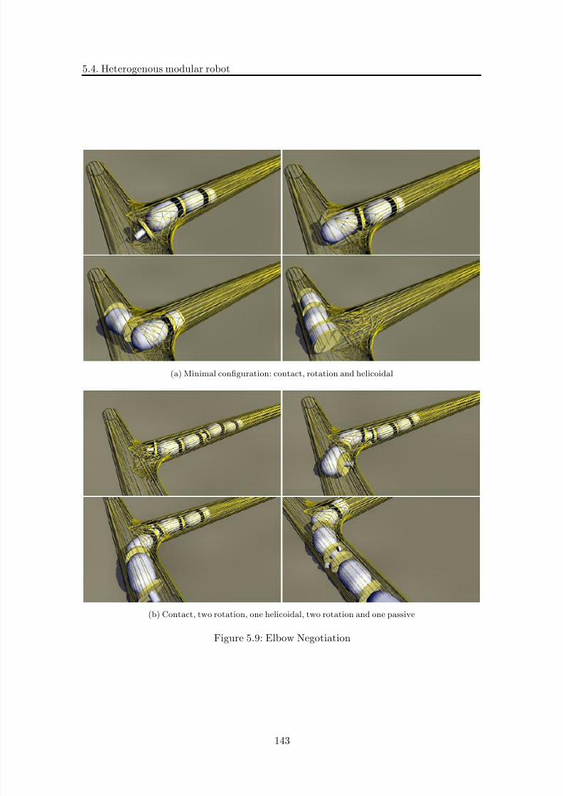
8/21/2019 Alberto Brunete Gonzalez
http://slidepdf.com/reader/full/alberto-brunete-gonzalez 171/311
5.4. Heterogenous modular robot
(a) Minimal configuration: contact, rotation and helicoidal
(b) Contact, two rotation, one helicoidal, two rotation and one passive
Figure 5.9: Elbow Negotiation
143

8/21/2019 Alberto Brunete Gonzalez
http://slidepdf.com/reader/full/alberto-brunete-gonzalez 172/311
CHAPTER 5. Simulation Environment
The extension module, since it has one rotation dof, can take part in some of the snake-like movements. Other modules can act as passive modules in the snake-like movementswithout affecting the overall movement.
5.5 Conclusions
This chapter has been dedicated to explain the simulator that has been used in this thesis.The main reasons why this simulator has been build are:
• it is a fast way to test prototypes before building them, because it is too expensiveto build a module without having a certainty that it is going to work more or lessas expected
• provides a very efficient way of prototyping and verification of control algorithmsand hardware
• provides a tool to build and develop the model for the algorithms that will be usedin the modules
The simulator has been built upon an existing open source implementation of rigidbody dynamics, the Open Dynamics Engine (ODE). ODE was selected for its popularopen-source physics simulation API, its online simulation of rigid body dynamics, and itsability to define wide variety of experimental environments and actuated models.
Over ODE it has been build a complex system to emulate the behavior of the mi-crorobot. Since most of the modules use the same servomotor, an accurate model of theservomotor has been build. Regarding the hardware, modules have been designed as sim-ple as possible (using simple primitives) to make simulation fluid, but trying to reflectas much as possible its real physic conditions and parameters, leaving in a second planethe esthetics features. The morphology, body mass and torque specifications have beenrespected as much as possible.
The environment has also been simulated with especial regard to frictions, collisionsand interactions between objects.
Over all of this, an electronic and control simulator part has been placed. The sim-ulated control program emulates the behavior of the modules by concurrent execution of
control programs for each module and the resulting communication issues. Each simulatedmodule control program has its own independent thread of execution which runs in aninfinite loop. There is another thread for the central control and for the GUI.
It has also been simulated the actuator control, the sensors (accelerometers, encoders)management, the I 2C communication, the synchronism lines and the power consumption.
Everything has been developed in C++ and has been structured in classes for themodules, the robot, the I 2C communications, etc. All classes have been described but thereader can find more information in an annexed document that describes in detail all thecode.
Finally, last section describes how the simulator can be used to test different heteroge-
nous configurations obtaining interesting conclusions about its locomotion and behavior.
144
8/21/2019 Alberto Brunete Gonzalez
http://slidepdf.com/reader/full/alberto-brunete-gonzalez 173/311
5.5. Conclusions
This simulator has been validated comparing the results of the simulator with theones obtained from real modules (see section 8.2), having very satisfactory results. It hasproved to be a very valid tool for testing configurations and develop prototypes. It helps
to obtain results much faster than with real modules and to avoid that the modules breakduring tests.
145
8/21/2019 Alberto Brunete Gonzalez
http://slidepdf.com/reader/full/alberto-brunete-gonzalez 174/311
CHAPTER 5. Simulation Environment
146
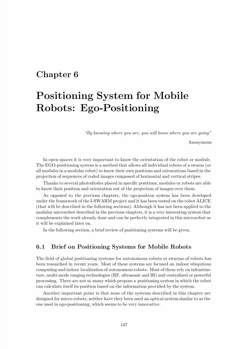
8/21/2019 Alberto Brunete Gonzalez
http://slidepdf.com/reader/full/alberto-brunete-gonzalez 175/311
Chapter 6
Positioning System for MobileRobots: Ego-Positioning
“By knowing where you are, you will know where you are going”
Anonymous
In open spaces it is very important to know the orientation of the robot or module.The EGO-positioning system is a method that allows all individual robots of a swarm (orall modules in a modular robot) to know their own positions and orientations based in theprojection of sequences of coded images composed of horizontal and vertical stripes.
Thanks to several photodiodes placed in specific positions, modules or robots are ableto know their position and orientation out of the projection of images over them.
As opposed to the previous chapters, the ego-position system has been developedunder the framework of the I-SWARM project and it has been tested on the robot ALICE(that will be described in the following sections). Although it has not been applied to themodular microrobot described in the previous chapters, it is a very interesting system thatcomplements the work already done and can be perfectly integrated in this microrobot asit will be explained later on.
In the following section, a brief review of positioning systems will be given.
6.1 Brief on Positioning Systems for Mobile Robots
The field of global positioning systems for autonomous robots or swarms of robots hasbeen researched in recent years. Most of these systems are focused on indoor ubiquitouscomputing and indoor localization of autonomous robots. Most of them rely on infrastruc-ture, multi-mode ranging technologies (RF, ultrasonic and IR) and centralized or powerfulprocessing. There are not so many which propose a positioning system in which the robotcan calculate itself its position based on the information provided by the system.
Another important point is that none of the systems described in this chapter aredesigned for micro-robots, neither have they been used an optical system similar to as the
one used in ego-positioning, which seems to be very innovative.
147

8/21/2019 Alberto Brunete Gonzalez
http://slidepdf.com/reader/full/alberto-brunete-gonzalez 176/311
CHAPTER 6. Positioning System for Mobile Robots: Ego-Positioning
Figure 6.1: Experimental setup of iGPS
Some descriptions of the systems have been obtained from [Hightower and Boriello,2001].
The following sections shows a review of some systems divided by the type of sen-
sor/detection that they use.
6.1.1 IR light emission-detection
The iGPS (indoor GPS) described in [Hada and Takase, 2001], is a system for multiplemobile robot localization inside office buildings. It is based on the IR light detection witha camera of the emitted IR light by the robots.
In the article [Hernandez et al., 2003] a low cost system for mobile robots indoorlocalization is presented. The system is composed of an emitter located on a wall and areceptor at the top of the robot. The emitter is a laser pointer acting like B beacon, andthe receptor is a cylinder made by 32 independent photovoltaic cells. The robot’s positionand orientation are obtained from the times of impact of the laser an each cell.
The NorthStar system [nor, ] uses triangulation to measure position and heading inrelation to IR light spots that can be projected onto the ceiling (or other visible sur-face). Because each IR light spot has a unique signature, the detector can instantly andunambiguously localize. Because the NorthStar detector directly measures position andheading, a localization result is intrinsically robust. A NorthStar-enabled product does notrequire prior training or mapping to measure its position. There is no need for expensive
computational capabilities.
148
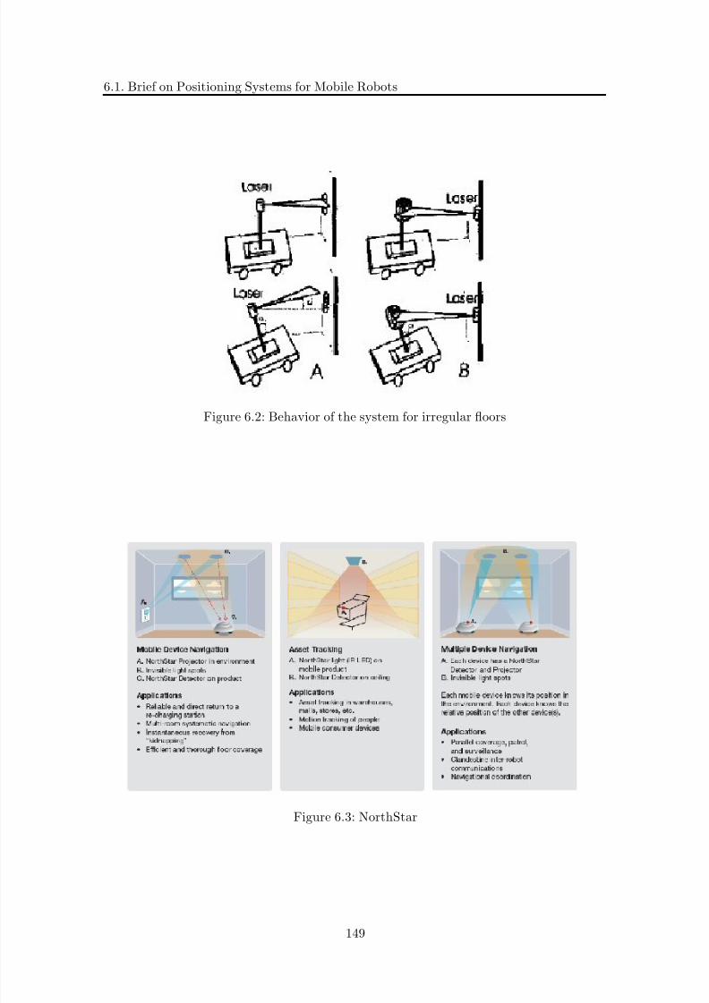
8/21/2019 Alberto Brunete Gonzalez
http://slidepdf.com/reader/full/alberto-brunete-gonzalez 177/311
6.1. Brief on Positioning Systems for Mobile Robots
Figure 6.2: Behavior of the system for irregular floors
Figure 6.3: NorthStar
149
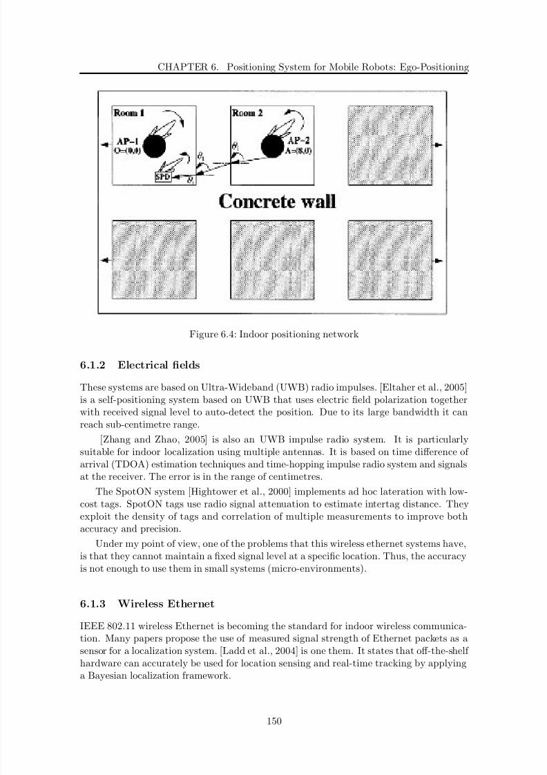
8/21/2019 Alberto Brunete Gonzalez
http://slidepdf.com/reader/full/alberto-brunete-gonzalez 178/311
CHAPTER 6. Positioning System for Mobile Robots: Ego-Positioning
Figure 6.4: Indoor positioning network
6.1.2 Electrical fields
These systems are based on Ultra-Wideband (UWB) radio impulses. [Eltaher et al., 2005]is a self-positioning system based on UWB that uses electric field polarization togetherwith received signal level to auto-detect the position. Due to its large bandwidth it canreach sub-centimetre range.
[Zhang and Zhao, 2005] is also an UWB impulse radio system. It is particularlysuitable for indoor localization using multiple antennas. It is based on time difference of arrival (TDOA) estimation techniques and time-hopping impulse radio system and signalsat the receiver. The error is in the range of centimetres.
The SpotON system [Hightower et al., 2000] implements ad hoc lateration with low-cost tags. SpotON tags use radio signal attenuation to estimate intertag distance. Theyexploit the density of tags and correlation of multiple measurements to improve bothaccuracy and precision.
Under my point of view, one of the problems that this wireless ethernet systems have,is that they cannot maintain a fixed signal level at a specific location. Thus, the accuracyis not enough to use them in small systems (micro-environments).
6.1.3 Wireless Ethernet
IEEE 802.11 wireless Ethernet is becoming the standard for indoor wireless communica-tion. Many papers propose the use of measured signal strength of Ethernet packets as asensor for a localization system. [Ladd et al., 2004] is one them. It states that off-the-shelf hardware can accurately be used for location sensing and real-time tracking by applying
a Bayesian localization framework.
150

8/21/2019 Alberto Brunete Gonzalez
http://slidepdf.com/reader/full/alberto-brunete-gonzalez 179/311
6.1. Brief on Positioning Systems for Mobile Robots
Figure 6.5: Illustration of time difference of arrival (TDOA) localization
Figure 6.6: Example of wireless ethernet distribution of five base stations (enumeratedsmall circles)
151

8/21/2019 Alberto Brunete Gonzalez
http://slidepdf.com/reader/full/alberto-brunete-gonzalez 180/311
CHAPTER 6. Positioning System for Mobile Robots: Ego-Positioning
[Dardari and Conti, 2004] addresses indoor localization techniques through ad-hocwireless networks, where anchors and unknown nodes are randomly positioned in a squaredarea. The position of unknown nodes is estimated starting from received signal strength
(RSSI) measurements, since nodes are assumed to be not equipped with specialized local-ization hardware.
[Haeberlen et al., 2004] allows for remarkably accurate localization across an entireoffice building using nothing more than the built-in signal intensity meter supplied bystandard 802.11 cards. The system can be trained in less than one minute per office orregion, walking around with a laptop and recording the observed signal intensities of thebuilding’s unmodified base stations. It is possible to localize a user correctly in over 95
[Serrano et al., 2004] describes a method to estimate the position of a mobile robotin an indoor scenario using the odometric calculus and the WiFi energy received from thewireless infrastructure. This energy will be measured by wireless network card on-board amobile robot, and it will be used as another regular sensor to improve position estimation.
RADAR [Bahl and Padmanabhan, 2000] has been developed by the Microsoft Researchgroup. It is a building-wide tracking system based on the IEEE 802.11 WaveLAN wirelessnetworking technology. RADAR measures, at the base station, the signal strength andsignal-to-noise ratio of signals that wireless devices send, then it uses this data to computethe 2D position within a building. Microsoft has developed two RADAR implementations:one using scene analysis and the other using lateration. Several commercial companiessuch as WhereNet (http://www.widata.com) and Pinpoint (http://www.pinpointco.com)sell wireless asset-tracking packages, which are similar in form to RADAR.
Again, these systems present the same problems as in the previous section.
6.1.4 Ultrasound systems
The Cricket Location Support System [Priyantha et al., 2000] uses ultrasound emitters tocreate the infrastructure and embeds receivers in the object being located. This approachforces the objects to perform all their own triangulation computations. Cricket uses theradio frequency signal not only for synchronization of the time measurement, but also todelineate the time region during which the receiver should consider the sounds it receives.Cricket uses ultrasonic time-of-flight data and a radio frequency control signal. Cricketimplements both the lateration and proximity techniques. Receiving multiple beacons letsreceivers triangulate their position. Receiving only one beacon still provides useful prox-
imity information when combined with the semantic string the beacon transmits on theradio. Cricket’s advantages include privacy and decentralized scalability, while its disad-vantages include a lack of centralized management or monitoring and the computationalburden-and consequently power burden- that timing and processing both the ultrasoundpulses and RF data place on the mobile receivers.
6.1.5 Electromagnetic
Electromagnetic sensing offers a classic position tracking method [Raab et al., 1979] [Pa-perno et al., 2001].
Tracking systems such as MotionStar (http://www.ascension-tech.com/products/motionstar.php)
152

8/21/2019 Alberto Brunete Gonzalez
http://slidepdf.com/reader/full/alberto-brunete-gonzalez 181/311
6.1. Brief on Positioning Systems for Mobile Robots
Figure 6.7: MotionStar system
sense precise physical positions relative to the magnetic transmitting antenna. These sys-tems offer the advantage of very high precision and accuracy, on the order of less than 1mm spatial resolution, 1 ms time resolution, and 0.1 orientation capability. Disadvan-
tages include steep implementation costs and the need to tether the tracked object to acontrol unit. Further, the sensors must remain within 1 to 3 meters of the transmitter,and accuracy degrades with the presence of metallic objects in the environment.
6.1.6 Pressure sensors
In Georgia Tech’s Smart Floor [Orr and Abowd, 2000] proximity location system, embed-ded pressure sensors capture footfalls, and the system uses the data for position trackingand pedestrian recognition. This unobtrusive direct physical contact system does not re-quire people to carry a device or wear a tag. However, the system has the disadvantages
of poor scalability and high incremental cost because the floor of each building in whichSmartFloor is deployed must be physically altered to install the pressure sensor grids.
6.1.7 Visual systems
Microsoft Research’s Easy Living [Krumm et al., 2000] uses real-time 3D cameras to pro-vide stereo-vision positioning capability in a home environment. Although Easy Livinguses high-performance cameras, vision systems typically use substantial amounts of pro-cessing power to analyze frames captured with comparatively low-complexity hardware.
State-of-the-art integrated systems [Darrell et al., 1998] demonstrate that multimodal
processing-silhouette, skin color, and face pattern-can significantly enhance accuracy. Vi-
153
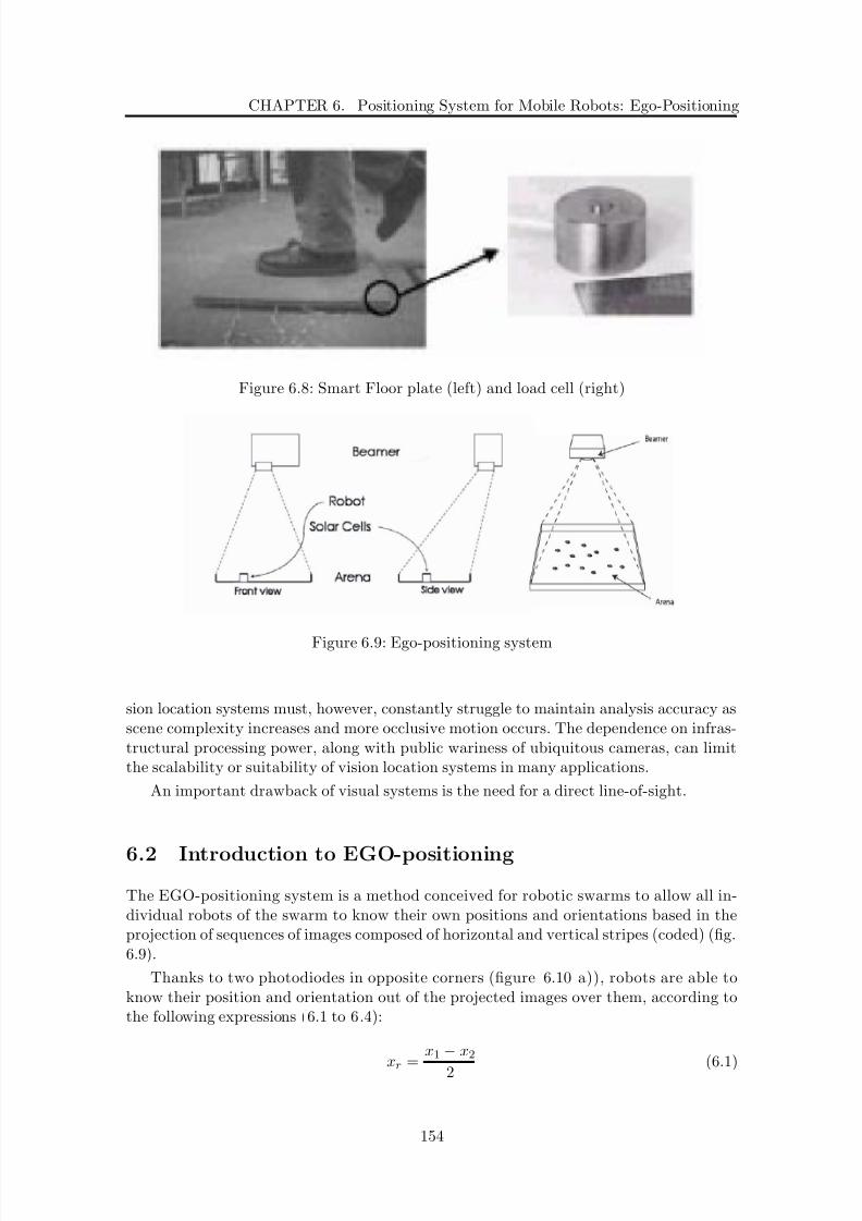
8/21/2019 Alberto Brunete Gonzalez
http://slidepdf.com/reader/full/alberto-brunete-gonzalez 182/311
CHAPTER 6. Positioning System for Mobile Robots: Ego-Positioning
Figure 6.8: Smart Floor plate (left) and load cell (right)
Figure 6.9: Ego-positioning system
sion location systems must, however, constantly struggle to maintain analysis accuracy asscene complexity increases and more occlusive motion occurs. The dependence on infras-tructural processing power, along with public wariness of ubiquitous cameras, can limitthe scalability or suitability of vision location systems in many applications.
An important drawback of visual systems is the need for a direct line-of-sight.
6.2 Introduction to EGO-positioning
The EGO-positioning system is a method conceived for robotic swarms to allow all in-dividual robots of the swarm to know their own positions and orientations based in theprojection of sequences of images composed of horizontal and vertical stripes (coded) (fig.6.9).
Thanks to two photodiodes in opposite corners (figure 6.10 a)), robots are able toknow their position and orientation out of the projected images over them, according tothe following expressions (6.1 to 6.4):
xr =
x1 − x2
2 (6.1)
154

8/21/2019 Alberto Brunete Gonzalez
http://slidepdf.com/reader/full/alberto-brunete-gonzalez 183/311
6.2. Introduction to EGO-positioning
a) b)
Figure 6.10: Position and orientation calculation (a) and ”Alice” robot (b)
yr = y1 − y2
2 (6.2)
α = β − δ (6.3)
δ = arctan ∆X
∆Y (6.4)
The idea of EGO-positioning can also be used in the modules described in chapter 4,
extending the 2D situation of the photodiodes to a 3D scenario as shown in picture 6.11Projected images can also be divided in regions to transmit different information to
groups of robots.
In order to experiment the ego-positioning concept, tests have been performed on therobot ”Alice” (see fig. 6.10 b)). In some of the next paragraphs there will be separatenotes for ”Alice” and ”I-Swarm” robots.
The setup used for Alice is shown in the table 6.1 compared to the setup that isprobably going to be used for I-SWARM.
Although for Alice a different stripe width has been chosen for the x and y axis, inI-SWARM it is the same, which implies to have a different number of stripes for both axis.
The minimum resolution that can be chosen is the pixel size, which is 0.29 mm.
155
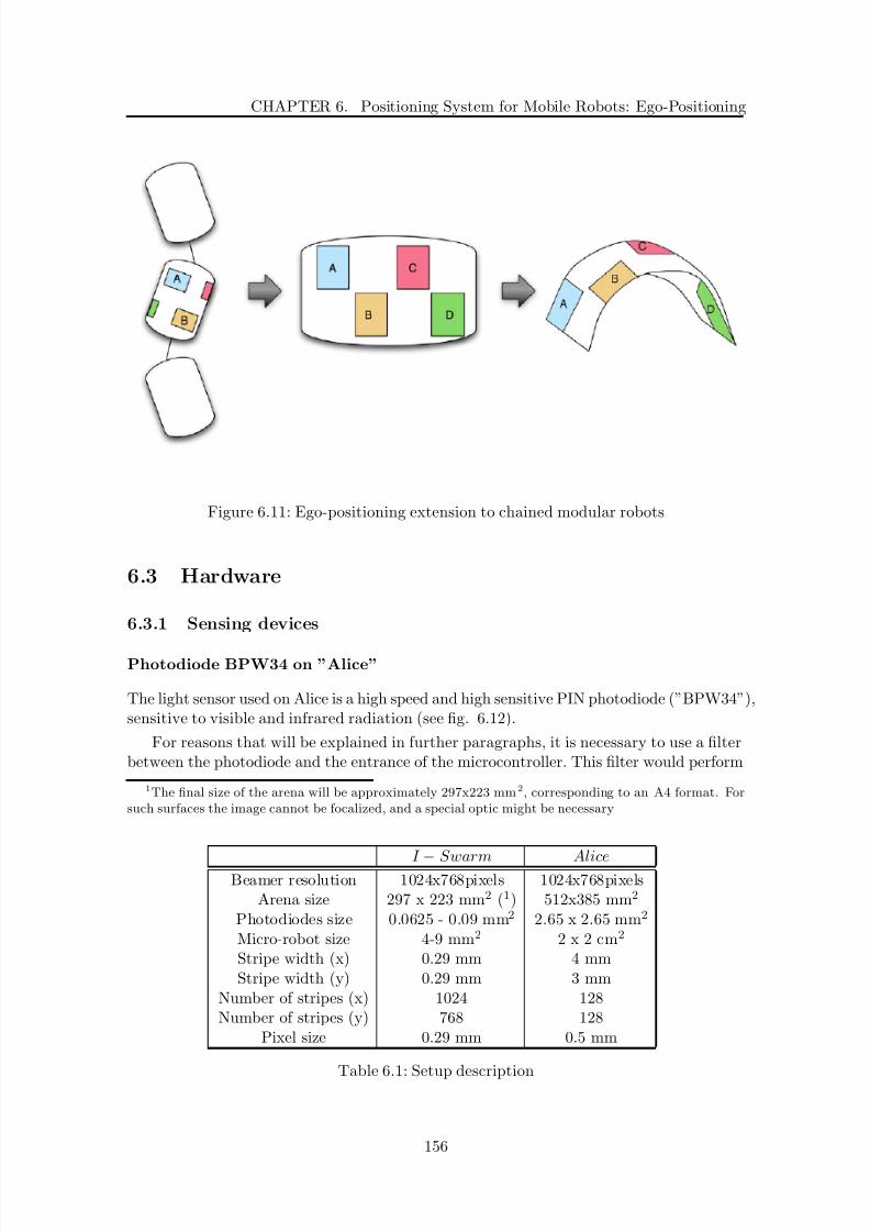
8/21/2019 Alberto Brunete Gonzalez
http://slidepdf.com/reader/full/alberto-brunete-gonzalez 184/311
CHAPTER 6. Positioning System for Mobile Robots: Ego-Positioning
Figure 6.11: Ego-positioning extension to chained modular robots
6.3 Hardware
6.3.1 Sensing devices
Photodiode BPW34 on ”Alice”
The light sensor used on Alice is a high speed and high sensitive PIN photodiode (”BPW34”),sensitive to visible and infrared radiation (see fig. 6.12).
For reasons that will be explained in further paragraphs, it is necessary to use a filterbetween the photodiode and the entrance of the microcontroller. This filter would perform
1The final size of the arena will be approximately 297x223 mm2, corresponding to an A4 format. Forsuch surfaces the image cannot be focalized, and a special optic might be necessary
I − Swarm AliceBeamer resolution 1024x768pixels 1024x768pixels
Arena size 297 x 223 mm2 (1) 512x385 mm2
Photodiodes size 0.0625 - 0.09 mm2 2.65 x 2.65 mm2
Micro-robot size 4-9 mm2 2 x 2 cm2
Stripe width (x) 0.29 mm 4 mmStripe width (y) 0.29 mm 3 mm
Number of stripes (x) 1024 128Number of stripes (y) 768 128
Pixel size 0.29 mm 0.5 mm
Table 6.1: Setup description
156

8/21/2019 Alberto Brunete Gonzalez
http://slidepdf.com/reader/full/alberto-brunete-gonzalez 185/311
6.3. Hardware
a) b)
Figure 6.12: BPW34 main features (a) and photodiodes board (b)
the following tasks:
• Transform the current coming from the photodiode into voltage that can be read bythe analog-to-digital converter
• Polarize the photodiode
• Low pass filter to get rid of the glitch and to stabilize the signal
The proposed filter is shown in fig. 6.13 a). The first resistor allows setting the outputreference voltage to any value (so it is possible to saturate the signal to avoid the effectsof the beamer). Assuming the input impedance of the ADC is very high, the cut off frequency can be set by:
F c = 1
(R1 + R2) ∗ C (6.5)
Solar cell on I-Swarm (aSi:H)
One possible solution for I-SWARM is to use amorphous silicon photodiodes (aSi:H) whose
spectral sensitivity is shown in picture 6.13 b):The robots that will be used in the project I-SWARM will be as small as possible.
This means that the integration of resistors will be avoided if possible in order to savespace, due to the large size of the required resistors.
Because of this a ”current comparator” will be used as a signal conditioning stage(see fig. 6.14). It will compare the current coming from the photodiode with a referencecurrent and will output a voltage level (logical 0 or 1) corresponding to the value of thelevel of intensity of the image projected over the photodiode (normally a black or whiteimage).
An estimation of the maximum current that the solar cell can give is Isc = 45µA/mm2
(for more information see Deliverable D.5.2.Powering). For a total surface between 0.0625
157

8/21/2019 Alberto Brunete Gonzalez
http://slidepdf.com/reader/full/alberto-brunete-gonzalez 186/311
CHAPTER 6. Positioning System for Mobile Robots: Ego-Positioning
a) b)
Figure 6.13: Optimal RC Filter (a) and Spectral sensitivity of aSi:H (b)
Figure 6.14: Current comparator for I-SWARM
mm2 and 0.09 mm2 it gives a maximum current of 2.81 µA to 4.05 µA.
The reference current should be adapted depending on the threshold to a percentage
of this value. For example if the threshold is set to 50%, the reference current will bebetween 1.905 µA and 2.025 µA.
If there is a second source of light (to increase the power received by the robots) thethreshold and the reference current should be increased and adapted to the new powering.
6.3.2 Beamer
Beamer characterization
The color of images is produced by a color disk (see fig. 6.15) in the DLP beamer (Digital
Light Processing beamer). This color disk is divided in 4 regions: red, green, blue and
158

8/21/2019 Alberto Brunete Gonzalez
http://slidepdf.com/reader/full/alberto-brunete-gonzalez 187/311
6.3. Hardware
Figure 6.15: Color wheel of the DLP beamer
(a) Not saturated (b) Saturated
Figure 6.16: Response of the beamer to a white image
transparent. The white color is achieved by the combination of all the colors.
When a white image is projected over the photodiode, the output obtained is shownin figure 6.16 a).
However, due to the polarization circuit of the photodiode (3.3V for the maximumlevel of intensity), the output of the photodiode is usually saturated, as it is shown infigure 6.16 b).
It is possible to see that all color levels are saturated (except for the blue). With ahigher resistance it would also be saturated. With a smaller value the previous figure isobtained.
Without color wheel fig. 6.17 is obtained for a white image.
In any case, the signal has to be filtered in order to obtain a stable signal at theentrance of the analog-to-digital converter of the microcontroller and to avoid the glitchesobserved in the pictures. These glitches are repetitive at a frequency of 60 Hz and thetypical width is about 40 µs.
For red, green and blue colors fig. 6.18 a) is obtained.
For its combination two by two (yellow, purple and cyan), which is a pulse of double
width, half for each color which forms it, the output is shown in fig. 6.18 b).
159
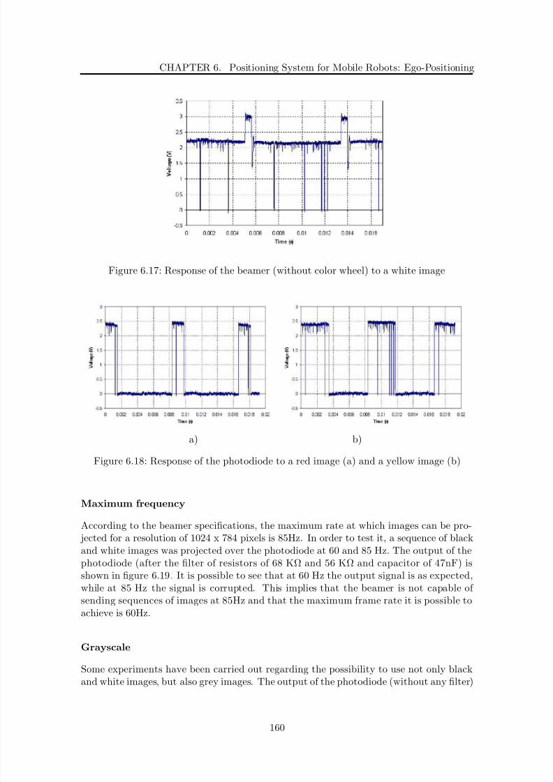
8/21/2019 Alberto Brunete Gonzalez
http://slidepdf.com/reader/full/alberto-brunete-gonzalez 188/311
CHAPTER 6. Positioning System for Mobile Robots: Ego-Positioning
Figure 6.17: Response of the beamer (without color wheel) to a white image
a) b)
Figure 6.18: Response of the photodiode to a red image (a) and a yellow image (b)
Maximum frequency
According to the beamer specifications, the maximum rate at which images can be pro- jected for a resolution of 1024 x 784 pixels is 85Hz. In order to test it, a sequence of black
and white images was projected over the photodiode at 60 and 85 Hz. The output of thephotodiode (after the filter of resistors of 68 KΩ and 56 KΩ and capacitor of 47nF) isshown in figure 6.19. It is possible to see that at 60 Hz the output signal is as expected,while at 85 Hz the signal is corrupted. This implies that the beamer is not capable of sending sequences of images at 85Hz and that the maximum frame rate it is possible toachieve is 60Hz.
Grayscale
Some experiments have been carried out regarding the possibility to use not only black
and white images, but also grey images. The output of the photodiode (without any filter)
160

8/21/2019 Alberto Brunete Gonzalez
http://slidepdf.com/reader/full/alberto-brunete-gonzalez 189/311
6.3. Hardware
a) b)
Figure 6.19: Response of the photodiode to a projection of sequences of black and whiteimages at 60 Hz (a) and 85 Hz (b)
Figure 6.20: Response of the photodiode to a grey image
when a 50% grey image is projected is show in figure 6.20:
This means that the only possibility to detect it is to filter the signal via a low passfilter and detect the mean value of the signal.
Figure 6.21 shows the output (with the same filter as before) of the photodiode when
a sequence of images composed by Black-Grey-White (3 levels) and Black-Grey1-Grey2-White (4 levels) are projected.
It is possible to see that it would be possible to detect up to 4 levels of grey, but ac-tually, the outputs of the analog-to-digital converter for 4 levels of grey are too close andsometimes they overlap. Thus, the recommended number of levels that can be detected is3.
• Maximun number of levels that could be detected: 4
• Recommended number of levels: 3
161
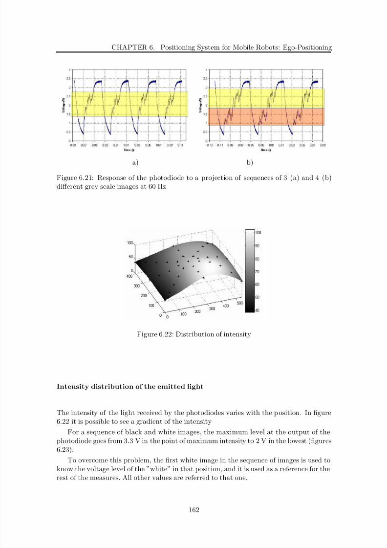
8/21/2019 Alberto Brunete Gonzalez
http://slidepdf.com/reader/full/alberto-brunete-gonzalez 190/311
CHAPTER 6. Positioning System for Mobile Robots: Ego-Positioning
a) b)
Figure 6.21: Response of the photodiode to a projection of sequences of 3 (a) and 4 (b)different grey scale images at 60 Hz
Figure 6.22: Distribution of intensity
Intensity distribution of the emitted light
The intensity of the light received by the photodiodes varies with the position. In figure6.22 it is possible to see a gradient of the intensity
For a sequence of black and white images, the maximum level at the output of thephotodiode goes from 3.3 V in the point of maximum intensity to 2 V in the lowest (figures6.23).
To overcome this problem, the first white image in the sequence of images is used toknow the voltage level of the ”white” in that position, and it is used as a reference for the
rest of the measures. All other values are referred to that one.
162

8/21/2019 Alberto Brunete Gonzalez
http://slidepdf.com/reader/full/alberto-brunete-gonzalez 191/311
6.4. Software
a) b)
Figure 6.23: Output voltage for a black and white sequence at the point of higher (a) andlower (b) illumination
6.4 Software
6.4.1 EGO-positioning procedures: theory and performances
Binary code
It is the simplest code. The arena is divided into 128 stripes for both the horizontal andvertical planes and each stripe is then codified with 7 bits, meaning ”0” is equal to black
and ”1” to white. See fig. 6.24 a).
Gray code
A Gray code is a binary numeral system where two successive values differ in only onedigit. In our particular case, as we can see in the next figure, this means that there arealways (except in the ends) two stripes of the same color together (in the binary code theyalternate always), what reduces the error rate to almost half when the photodiode is inthe middle of two stripes. See fig. 6.24 b).
Performance
For transmission at 60 Hz with Black and White sequences images:
• Start bits: 3 (B-B-W for binary , B-W-W for gray ...etc)
• Position bits: 14 (7+7)
• Stop bits: 0
• Time (at 60Hz): 0.28s
• Data rate: 60 bits/s (1 bit 0.017 s, 1 kB 133.3 s)
163

8/21/2019 Alberto Brunete Gonzalez
http://slidepdf.com/reader/full/alberto-brunete-gonzalez 192/311
CHAPTER 6. Positioning System for Mobile Robots: Ego-Positioning
a) b)
Figure 6.24: Binary (a) and Gray (b) code
For transmission at 60 Hz with 3 color images (Black, White and Grey(RGB=(130,130,130))):
• Start bits: 3 (B-W-B)
• Position bits: 10 (5+5)(symbols)
• Stop bits: 0
• Time (at 60Hz):0.22 sec
• Data rate: 60 symbols/s (90bits/s) (1 bit 0.01 s, 1 kB 88.8 s)
Color-based transmission
It is possible to use the way the beamer produces the colors (seen in section 6.3.2) to senddata at a higher rate.
If the signal is sample at the right points , the value of red, blue and green of the
emitted color can be obtained (fig. 6.25). Thus, it is possible to send three bits with everyimage, and the data rate will be multiplied by 3.
Thus the sequence of bits that is to be sent can be divided into pieces of three andcodified according to table 6.2:
In the reception, the image has to be sampled to get the three values of blue, red andgreen and remake the original sequence of bits.
For example, if the sequence to be sent is
01000110111001010 (startcode, xpos, ypos) (6.6)
The sequence is divided in
164

8/21/2019 Alberto Brunete Gonzalez
http://slidepdf.com/reader/full/alberto-brunete-gonzalez 193/311
6.4. Software
Figure 6.25: Sampling time to get the RGB values of the projected image
BLU E RED GRE EN
0 0 0 Black0 0 1 Green Suitable0 1 0 Red for0 1 1 Yellow Startcode
1 0 0 Blue
1 0 1 Cyan1 1 0 Purple1 1 1 White
Table 6.2: Color coding table
010 − 001 − 101 − 110 − 010 − 1 0 + 0 to complete (6.7)
And then the images
Green − Blue − Purple − Y ellow − Green− Red (6.8)
will be projected by the beamer. In the reception, the microcontroller will get threesamples for each image, corresponding to the three bits that it has coded.
6.4.2 I-Swarm considerations
In Alice, 7 bits (meaning 7 images) are used to send the position in the horizontal axisand 7 for the vertical one. That is because the stripe resolution (i.e. the size of thephotodiodes) needed is 4 mm and 3 mm.
In the I-SWARM project, the stripe resolution that is required is about 0.25 to 0.3mm.
165

8/21/2019 Alberto Brunete Gonzalez
http://slidepdf.com/reader/full/alberto-brunete-gonzalez 194/311
CHAPTER 6. Positioning System for Mobile Robots: Ego-Positioning
In this document it will be taken 0.29mm as the reference value. This means that 1024stripes for X and 768 stripes for Y have to be used to cover the entire arena. Thus, 10 bitmust be used to transmit the position (29 = 512 and 210 = 1024).
An estimation of the performance it would be possible to have for I-SWARM fortransmission at 60 Hz with Black and White sequences images is:
• Start bits: 3 (B-B-W for binary , B-W-W for gray ...etc)
• Position bits: 20 (10+10)
• Stop bits: 0
• Number of color images to send: 23
• Time (at 60Hz): 0.38s
• Data rate: 60 bits/s (1 bit 0.017 s, 1 kB 133.3 s)
If using the color-based transmission technique described in the previous section, at60 Hz, and for I-SWARM, the results would be:
• Start bits: 3 (B-B-W for binary , B-W-W for gray ...etc)
• Position bits: 20 (10+10)
• Stop bits: 0
• Number of color images to send: 8 (23 / 3)
• Time (at 60Hz): 0.13 (8/60)
• Data rate: 180 bits/s (1 bit 0.0055 s, 1 kB 44.4 s)
6.4.3 Image Sequence Programming
The images that are projected over the arena are drawn using the DirectX library. Thislibrary allows accessing the graphic card directly, which is much faster than using a video.In addition, it gives the following advantages:
• The frame rate is guaranteed.
• It doesn’t need a fast processor, just a good graphic card.
• It is possible to change the sequence easily
• It is also possible to send individual information to the robots - Unidirectional com-munication. Application: robot programming.
• A user interface can be implemented
There are two possible ways to generate the sequence:
166
8/21/2019 Alberto Brunete Gonzalez
http://slidepdf.com/reader/full/alberto-brunete-gonzalez 195/311
6.4. Software
• Draw the images and show them in real time
• Preload the images in memory and change from one to another
The second one is a little bit faster because the images are already in memory, but hasthe inconvenient that every time we want to change the sequence new images have to bemade. On the contrary, the first approach let the user draw anything in the screen and tochange the sequence even in real time.
6.4.4 Alice software
The software for Alice is divided mainly in the following parts:
-Interruption Service Routine ”Photodiodes”: reads the value from the Analog-to-Digital converter fig. 6.26 a).
For projection at 60 Hz the microprocessor have to sample every 1/60=16.666ms. Forsome microprocessors (like Alice) it is not feasible to sample at that rate.
To overcome this problem, what it has been done for Alice is to sample the signalcoming from the photodiode with an alternating period: every 17-16-17ms. Thus, it issynchronized every 3 samples (50ms).
-Function ”SequenceTest”: it checks continuously for a sequence of EGO-positionand process it fig. 6.26 b).
In order to take samples when the signal is stable (in the middle of the pulse) and notin the raising or falling edges, a procedure has been developed (see fig. 6.27).
Normally a white image is projected by default. All the EGO-positioning sequencesstart with a black image (part of the start code) to show the beginning of the sequence.As shown in the figure, the signal is sample every 1ms. When a black image is detected,the center of the pulse is calculated, and from then one sample is taken every 1/60 secondsapproximately.
With this procedure, the successful sequences received rate has reached the 100%
(60Hz).
-Function ”EGO Position”: Decodes de sequence of images received and calculatethe position and orientation (fig. 6.28 a)).
-Main program: an infinite loop that which calls the functions SequenceTest andEGO-position (fig. 6.28 b)).
The size of the program as it is right now is 6.44 KB of Flash memory and 118 bytesof RAM. Just the EGO position procedure would be about 2KB of Flash memory and 80
bytes of RAM.
167

8/21/2019 Alberto Brunete Gonzalez
http://slidepdf.com/reader/full/alberto-brunete-gonzalez 196/311
CHAPTER 6. Positioning System for Mobile Robots: Ego-Positioning
a) b)
Figure 6.26: Interruption Service Routine ”Photodiodes” (a) and function ”SequenceTest”(b) pseudocode
6.4.5 I-Swarm software
In the I-SWARM robots some of the software will be implemented via hardware in orderto make the programs faster and smaller. An example of what can be done by hardwareis the pass from binary to Gray code and vice versa (fig. 6.29).
In Alice, the subroutine is checking every 1ms if there is a start of sequence (i.e. apass from white to black). In order to save energy in I-SWARM, the scanning for a start
of sequence will be done only when the robot want to know its position and orientation.
6.5 Applications
6.5.1 Transmission of commands
Using the same principle of image transmission as in EGO-positioning, it is possible tosend data, i.e. codify some commands and send them to the robots.
For example we can codify a command that is ”go to a position”. For that a new start
code is needed. Then the target position is sent codified in the same way as images for
168
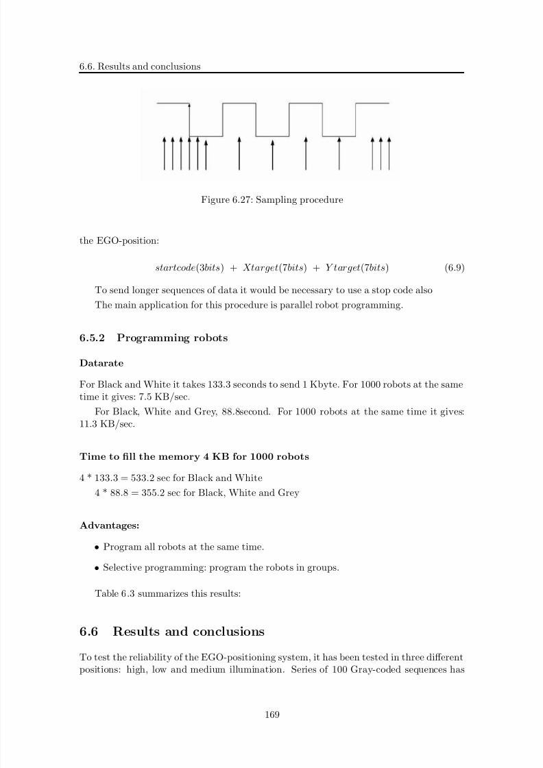
8/21/2019 Alberto Brunete Gonzalez
http://slidepdf.com/reader/full/alberto-brunete-gonzalez 197/311
6.6. Results and conclusions
Figure 6.27: Sampling procedure
the EGO-position:
startcode(3bits) + Xtarget(7bits) + Y target(7bits) (6.9)
To send longer sequences of data it would be necessary to use a stop code also
The main application for this procedure is parallel robot programming.
6.5.2 Programming robots
Datarate
For Black and White it takes 133.3 seconds to send 1 Kbyte. For 1000 robots at the sametime it gives: 7.5 KB/sec.
For Black, White and Grey, 88.8second. For 1000 robots at the same time it gives:11.3 KB/sec.
Time to fill the memory 4 KB for 1000 robots
4 * 133.3 = 533.2 sec for Black and White
4 * 88.8 = 355.2 sec for Black, White and Grey
Advantages:
• Program all robots at the same time.
• Selective programming: program the robots in groups.
Table 6.3 summarizes this results:
6.6 Results and conclusions
To test the reliability of the EGO-positioning system, it has been tested in three different
positions: high, low and medium illumination. Series of 100 Gray-coded sequences has
169

8/21/2019 Alberto Brunete Gonzalez
http://slidepdf.com/reader/full/alberto-brunete-gonzalez 198/311
CHAPTER 6. Positioning System for Mobile Robots: Ego-Positioning
a) b)
Figure 6.28: Function ”EGO Position” (a) and Main program (b) pseudocode
Black and white Black, white and greyTime to send 1 KB 133.3 sec 88.8 sec
Time to send 1 KB for 1000 robots 7.5 KB/s 11.3 KB/sTime to fill memory (4 KB) for 1000 robots 533.2 sec 355.2 sec
Table 6.3: Programming time and speed
been projected at 60 Hz every 2 seconds, and the position and orientation given by thealgorithm have been recorded. The results are shown in figure 6.30.
The results are very similar in the three positions, achieving successful rates of 98-99%.
The 1-2% errors are mainly due to:
• Oscillations in the beamer
• Placement of the photodiode between two stripes. This may cause that the receivedsignal has a mean value similar to the threshold, and due to this the oscillations andnoise may be more significant
• Threshold upset
The adjustment of the threshold is a very important issue, and it has a great influencein the successful rate. For the measures taken before it was set to 68% of the maximum
(173 out of 255 in the A/D converter).
170
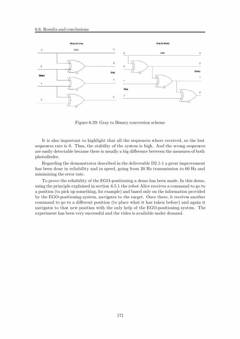
8/21/2019 Alberto Brunete Gonzalez
http://slidepdf.com/reader/full/alberto-brunete-gonzalez 199/311
6.6. Results and conclusions
Figure 6.29: Gray to Binary conversion scheme
It is also important to highlight that all the sequences where received, so the lostsequences rate is 0. Thus, the stability of the system is high. And the wrong sequencesare easily detectable because there is usually a big difference between the measures of bothphotodiodes.
Regarding the demonstrator described in the deliverable D2.1-1 a great improvementhas been done in reliability and in speed, going from 20 Hz transmission to 60 Hz andminimizing the error rate.
To prove the reliability of the EGO-positioning a demo has been made. In this demo,using the principle explained in section 6.5.1 the robot Alice receives a command to go toa position (to pick up something, for example) and based only on the information providedby the EGO-positioning system, navigates to the target. Once there, it receives anothercommand to go to a different position (to place what it has taken before) and again itnavigates to that new position with the only help of the EGO-positioning system. Theexperiment has been very successful and the video is available under demand.
171

8/21/2019 Alberto Brunete Gonzalez
http://slidepdf.com/reader/full/alberto-brunete-gonzalez 200/311
CHAPTER 6. Positioning System for Mobile Robots: Ego-Positioning
Figure 6.30: Success - error rate
172
8/21/2019 Alberto Brunete Gonzalez
http://slidepdf.com/reader/full/alberto-brunete-gonzalez 201/311
Chapter 7
Control Architecture
“To repeat what others have said, requires education; to challenge it, requires brains”
Mary Pettibone Poole
The control architecture to be described is a general architecture aimed at chainedmodular robots composed of different types of modules (heterogeneous modules) thatcan be arranged in different configurations, what is called multi-configurability. Thus,the robot can be manually assembled in different configurations depending on the chosentask. It is important to note that the architecture is not limited to the modules and theircapabilities described in chapter 4, but it can be extended to many other modules and
configurations.Since it is not desirable to reprogram each module every time a new configuration or a
new task is chosen, the control architecture provides a mechanism for the central control(CC) and the modules to realize which is the configuration of the microrobot and behaveaccording to this configuration. Thanks to this control architecture, the microrobot is ableto receive simple and complex commands and execute them no matter the configurationit may have. Example: go, stop, turn, explore, etc.
The proposed control architecture is based on behaviors and is divided in three layers:a low control layer embedded in the modules that takes decisions for the modules, ahigh control layer that takes decisions that concern the whole robot, and an heterogenousmiddle layer that acts as interpreter between the central control and the modules. The
heterogenous layer has a high importance because it makes the modules homogenous tothe CC, facilitating its control.
A Module Description Language (MDL) has been defined to describe the capabilities(both driving and sensorial) of the modules. Thanks to MDL each module is able to reportto the CC what they are able to do (their capabilities, i.e. rotate, push forward, measuretemperature, measure distance, etc.) and the central control can set up actions for thewhole robot.
The different modules of the microrobot have to be manually assembled at the begin-ning, due to the characteristics of the mechanical connectors. But future modules couldbe able to attach and detach by themselves, via electromechanical latches or magnets, as
in [Murata et al., 2002] [Yim et al., 2000]
173
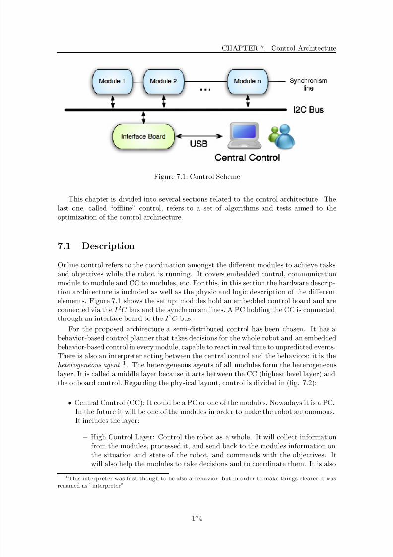
8/21/2019 Alberto Brunete Gonzalez
http://slidepdf.com/reader/full/alberto-brunete-gonzalez 202/311
CHAPTER 7. Control Architecture
Figure 7.1: Control Scheme
This chapter is divided into several sections related to the control architecture. Thelast one, called “offline” control, refers to a set of algorithms and tests aimed to theoptimization of the control architecture.
7.1 Description
Online control refers to the coordination amongst the different modules to achieve tasksand objectives while the robot is running. It covers embedded control, communicationmodule to module and CC to modules, etc. For this, in this section the hardware descrip-
tion architecture is included as well as the physic and logic description of the differentelements. Figure 7.1 shows the set up: modules hold an embedded control board and areconnected via the I 2C bus and the synchronism lines. A PC holding the CC is connectedthrough an interface board to the I 2C bus.
For the proposed architecture a semi-distributed control has been chosen. It has abehavior-based control planner that takes decisions for the whole robot and an embeddedbehavior-based control in every module, capable to react in real time to unpredicted events.There is also an interpreter acting between the central control and the behaviors: it is theheterogeneous agent 1. The heterogeneous agents of all modules form the heterogeneouslayer. It is called a middle layer because it acts between the CC (highest level layer) andthe onboard control. Regarding the physical layout, control is divided in (fig. 7.2):
• Central Control (CC): It could be a PC or one of the modules. Nowadays it is a PC.In the future it will be one of the modules in order to make the robot autonomous.It includes the layer:
– High Control Layer: Control the robot as a whole. It will collect informationfrom the modules, processed it, and send back to the modules information onthe situation and state of the robot, and commands with the objectives. Itwill also help the modules to take decisions and to coordinate them. It is also
1This interpreter was first though to be also a behavior, but in order to make things clearer it was
renamed as ”interpreter”
174

8/21/2019 Alberto Brunete Gonzalez
http://slidepdf.com/reader/full/alberto-brunete-gonzalez 203/311
7.1. Description
Figure 7.2: Control Layers
Figure 7.3: Behavior sketch
in charge of planning. It is composed of several parts, amongst which is aninference engine and a behavior-based control.
• Onboard Control: it is embedded in each module and it is based on behaviors. Itincludes the layers:
– Heterogeneous (Middle) Layer: agent that translates commands coming fromthe CC into specific module commands. For example, it translates the command”extend” into movements of the servomotors.
– Low Control Layer: Composed of behaviors. It allows the modules to react inreal time (for example to sense external and internal stimuli, as overheating,unreachable positions, adapt to the pipe shape, etc.) and to perform tasks thatdon’t need the CC (movements, communication with adjacent modules, simpletasks, etc.).
According to section 3.2.1, ”behavior” has several meanings. Within the framework of this thesis, a behavior is going to be considered as an independent procedure or functionthat is in charge of a specific task. Behaviors may have states or be influenced by thestate of the module (fig. 7.3).
The robot is controlled as a whole, taking into account the current configuration of
the microrobot (all modules). There is no need to send specific commands to each module
175

8/21/2019 Alberto Brunete Gonzalez
http://slidepdf.com/reader/full/alberto-brunete-gonzalez 204/311
CHAPTER 7. Control Architecture
Figure 7.4: HLC and LLC commands
every time (only when a specific order is to be send to a specific module, for example to
retrieve specific data from it). Every module can perform individual actions and behavein a different way to the same commands.
Considering the modules plus the central control as a whole, the microrobot can behaveautonomously (from the point of view of control, it still needs to be power supplied),without any need of human intervention.
7.2 Communication protocol
The communication protocol is used for communication between modules and CC. It isbased on I 2C , upon which the message structure is built.
7.2.1 Layer structure
The communication protocol can be divided in layers, as shown in figure 7.5. The twobottom levels are directly the physical and data link layers of the I 2C protocol. Overthese two levels the application data level is build, which is the responsible of forming themessages that are going to be sent amongst the modules and central control
Messages can be divided in (see figure 7.4):
• High level commands (HLC): messages sent from the operator to the central control
• Low level commands (LLC): messages sent from the CC to the modules. Accordingto the processing of the messages in the module, LLC messages can be divided in:
– LLC level 2 (LLC2), if they don’t have to be translated by the heterogeneouslayer
– LLC level 1 (LLC1), if they have to be translated by the heterogeneous layer
7.2.2 Command messages structure
I 2
C messages have the structure shown in figure 7.6.
176

8/21/2019 Alberto Brunete Gonzalez
http://slidepdf.com/reader/full/alberto-brunete-gonzalez 205/311
7.2. Communication protocol
Figure 7.5: Communication Layers
In simulation, I 2C messages are structures composed of the three fields: address,instruction and parameters (depending on the instruction it may have none, one or severalparameters)
Address + Instruction + Parameter (+ Parameter2 + ... + etc.)
When they have to be transmitted thought the real I 2C bus, messages have to beformatted into the I 2C data link format. I 2C frames are composed of:
• a start condition (S)
• address (7 bits)
• read/write flag
• data (1 byte) + 1 bit (acknowledgement) (as many times as necessary to transmitall the necessary data)
• a stop condition (P)
Addresses are natural numbers starting from 0 up to 63 (27).
• Address 63 is for the CC
• Address 0 is for broadcast messages• Addresses from 1 to 62 are for the modules
Each module has a pre-defined address assigned when it is programmed.
Parameters are codified in the following way: the first byte for the type of parameter(it is also used to know the length of the bytes coming afterwards) and the following bytesfor the information.
• angles ([−90..90]): 1 byte - degrees
• enum: 1 byte - natural numbers
• string: 1 byte per character
177

8/21/2019 Alberto Brunete Gonzalez
http://slidepdf.com/reader/full/alberto-brunete-gonzalez 206/311
CHAPTER 7. Control Architecture
Figure 7.6: I 2C frames
• integer: 2 bytes• value: 2 bytes
• bool: 1 bit
7.2.3 Low level commands (LLC)
Low level commands are the commands sent by the CC to the modules and the answersto these messages. Commands LLC1 are shown in table 7.1 and the answer messages intable 7.2 and LLC2 are shown in table 7.3 and the answer messages in table 7.4.
The parameters of SIM and AIM are:
• 1: Average consumption
• 2: Consumption peaks
• 3: Number of working motors
• 4: Orientation
• 5: Distance covered
• 6: State of the batteries
• 7: State of contraction/extention
2The expansion and contraction instructions have no parameters because the module itself knows how
much it has to extend or contract.
178

8/21/2019 Alberto Brunete Gonzalez
http://slidepdf.com/reader/full/alberto-brunete-gonzalez 207/311
7.2. Communication protocol
Acronym Instruction Description/Remarks Parameters
MS1 Move Servo 1 Indicates the position of the servo 1 AngleMS2 Move Servo 2 Indicates the position of the servo 2 AngleGS1 Get Value Servo 1 Demands the position of the servo 1 NoneGS2 Get Value Servo 2 Demands the position of the servo 2 NoneEX Expansion For extension/support module None 2
CT Contraction For extension/support module None 2
INH Inchworm position Indicates the position in the inchworm gait:first support (1), extension (2) or second sup-port (3)
[1..3]
GP Get Position To demand what is the position in the chain NoneGPS Get Position Start Chain identification phase starts NoneGPF Get Position Finish Chain identification phase ends NoneSPT Split Detach from the previous module NoneATT Attach Attach to the previous module None
Table 7.1: LLC1 commands: sending
Acronym Instruction Description/Remarks Data
SS1 Send Value Servo 1 Send the value of servo 1 AngleSS2 Send Value Servo 2 Send the value of servo 2 AngleTS Touch Sensor It points out that the touch sensor has
been activatedEnum
TSF Touch Sensor Final The elbow mode is over NonePC1 My Position in Chain is First Answer from the first module NonePCM My Position in Chain is Middle Answer from the modules except the
first and lastNone
PML My Position in Chain is Last Answer from the last module None
Table 7.2: LLC1 commands: answering
179
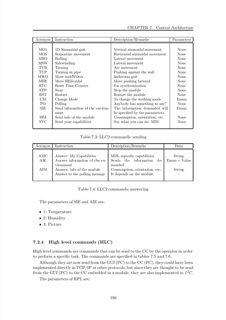
8/21/2019 Alberto Brunete Gonzalez
http://slidepdf.com/reader/full/alberto-brunete-gonzalez 208/311
CHAPTER 7. Control Architecture
Acronym Instruction Description/Remarks Parameters
MO1 1D Sinusoidal gait Vertical sinusoidal movement None
MOS Serpentine movement Horizontal sinusoidal movement NoneMRO Rolling Lateral movement NoneMSW Sidewinding Lateral movement NoneTUR Turning Arc movement NoneTUP Turning in pipe Pushing against the wall None
MWO Move inchWOrm Inchworm gait NoneMHE Move HElicoidal Move pushing forward NoneRTC Reset Time Counter For synchronization NoneSTP Stop Stop the module NoneRST Restart Restart the module NoneCM Change Mode To change the working mode EnumPO Polling Anybody has something to say? NoneSIE Send information of the environ-
ment
The information demanded will
be specified by the parameters
Enum
SIM Send info of the module Consumption, orientation, etc. NoneSYC Send your capabilities Say what you can do: MDL None
Table 7.3: LLC2 commands: sending
Acronym Instruction Description/Remarks Data
AMC Answer: My Capabilities MDL especific capabilities StringAIE Answer information of the en-
vironmentSends the information de-manded
Enum + Value
AIM Answer: info of the module Consumption, orientation, etc. String- Answer to the polling message It depends on the module -
Table 7.4: LLC2 commands: answering
The parameters of SIE and AIE are:
• 1: Temperature
• 2: Humidity
• 3: Picture
7.2.4 High level commands (HLC)
High level commands are commands that can be send to the CC by the operator in orderto perform a specific task. The commands are specified in tables 7.5 and 7.6.
Although they are now send from the GUI (PC) to the CC (PC), they could have beenimplemented directly in TCP/IP or other protocols, but since they are thought to be sendfrom the GUI (PC) to the CC embedded in a module, they are also implemented in I 2C .
The parameters of RPL are:
180

8/21/2019 Alberto Brunete Gonzalez
http://slidepdf.com/reader/full/alberto-brunete-gonzalez 209/311
7.2. Communication protocol
Acronym Instruction Description/Remarks Parameters
STP Stop Refers to the whole robot NoneRST Restart Refers to the whole robot NoneRPL Reach a place Go to the end of a part of the
pipe, go to the next bifurcation,go to a specific coordinate, etc.The place will be specified bythe parameters
Enum + Value
DO Do a task Repair, make a hole, etc.The
task is specified by the param-eter
Enum
EXP Explore NoneSIR Send information of the robot The information demanded will
be specified by the parametersEnum
SIE Send information of the envi-ronment
The information demanded willbe specified by the parameters
Enum
Table 7.5: HLC commands: sending
Acronym Instruction Description/Remarks Data
AIR Answer information of therobot
Sends the information de-manded
Enum + Value
AIE Answer information of the en-vironment
Sends the information de-manded
Enum + Value
Table 7.6: HLC commands: answering
181

8/21/2019 Alberto Brunete Gonzalez
http://slidepdf.com/reader/full/alberto-brunete-gonzalez 210/311
CHAPTER 7. Control Architecture
• A first value to indicate the type of position:
– 0: Coordinates (x,y ,z), in millimiters (3 integers)
– 1: The end of this part of the pipe– 2: The next bifurcation– 3: Until you touch something– 4: Home
• Coordinates (x,y ,z)
The parameters of DO are:
• 1: Repair
• 2: Make a hole
The parameters of SIR and AIR are:
• 1: Average consumption, mA (1 integer)
• 2: Consumption peaks, mA (1 integer)
• 3: Working modules, array of module IDs (string)
• 4: Orientation, degrees, (3 angle)
• 5: Distance covered, millimimeters (1 integer)
• 6: State of the batteries, ok or no ok, (bool)
The parameters of SIE and AIE are:
• 1: Temperature (1 integer)
• 2: Humidity (1 integer)
• 3: Picture
7.3 Module Description Language (MDL)
The Module Description Language (MDL) is a language created to describe the capabilitiesof one module to the CC and other modules, in order to create units (groups of modules)that are able to perform more complicated tasks.
MDL is based on a series of indicators that describe generally the tasks that the moduleis able to do:
• Ext:Extend/Contract
• Sup:Get fixed to the pipe
• Push pipe: Push in pipe3
• Push flat: Push in open air
• RotX: Rotate in its x axis
3For simplicity it is not distinguished between pushing forward and backwards, because most of the
systems that are able to push forward can also push backwards
182
8/21/2019 Alberto Brunete Gonzalez
http://slidepdf.com/reader/full/alberto-brunete-gonzalez 211/311
7.4. Working modes
• RotY: Rotate in its y axis
• RotZ: Rotate in its z axis
• Att: Attach / Detach to / from other modules
• Sense proximity front
• Sense proximity backwards
• Sense proximity lateral
• Sense temperature
• Sense humidity
• Sense gravity
• Grab
• Repair pipe
• Drill
• Power supply
Each parameter is associated to a value indicating the level in which the module canperform such task. This value is divided in four levels:
• 0: no competence for that skill
• 1: little competence
• 2: medium competence
• 3: good competence
All the values referring the tasks are packed into a single structure, an array of valuesfrom 0 to 3. For example, for the rotation module it would be:
Rot_mod(MDL) = [000033000000300000]
and the helicoidal module:
Heli_mod(MDL) = [00310000000000000]
Every time the module is demanded about its capabilities, it will send this arraycorresponding to the tasks that it can or cannot do.
Then, if a rotation module is next to some other modules that can ”rotate” in thesame axis as it does, they can form a unit that moves as a snake. If a extension module ispreceded and followed by modules that have the ability to ”expand/contract”, they canform a unit that moves as a worm, and so on.
7.4 Working modes
The working mode (WM), or simply the mode, of a module refers to the situation inwhich the module or the robot is. It is information that the CC sends to the modulesafter processing the information previously sent by the modules to the CC after compilingthe data obtained from its sensors.
This working mode can be:
183
8/21/2019 Alberto Brunete Gonzalez
http://slidepdf.com/reader/full/alberto-brunete-gonzalez 212/311
CHAPTER 7. Control Architecture
1. Inside a pipe
• Straight pipe
• Elbow/Bifurcation• Horizontal pipe
• Vertical pipe
• Upwards pipe
• Downwards pipe
• Obstacle detected in coordinates (x,y ,z)
2. Open air 4
• Plain
• Uphill
• Downhill
• Obstacle detected in coordinates (x,y ,z)
3. General
• Low consumption mode
• Fast mode
• Silence mode
It is information that has to be known by every behavior of the module in order toperform its tasks.
7.5 Onboard control
Onboard control refers to the control programs running on each of the modules. It is mainlybased on behaviors, as it has been already stated. The behaviors will be enumerated in afirst step and described subsequently.
All behaviors share some common characteristics:
• Its goal can be:
– To perform an activity
– To attain a goal
– To maintain some state
• Are encoded to be relatively simple
• Are introduced into the system incrementally, from the simple to the more complex
4Open air can also be considered a wide pipe (a pipe with a big diameter) in which the microrobot can
perform movements as if it was in the open air
184

8/21/2019 Alberto Brunete Gonzalez
http://slidepdf.com/reader/full/alberto-brunete-gonzalez 213/311
7.5. Onboard control
Figure 7.7: Behavior scheme
• Can be concurrently executed
• Encode time-extended processes, not atomic actions
• Their inputs may come from sensors or from other behaviors, as well as its outputsmay go to actuators or to other behaviors
Generally, behaviors can be described as in fig. 7.7. The activation conditions are
the only conditions for the behavior to run. If these conditions are fulfilled, the behaviorwill run. Some behaviors don’t have activation conditions, and they are always running.Examples of activation conditions are: command (form CC or operator), enable signalsfrom other behaviors, low battery, etc.
Stimuli are the inputs of the behaviors, for example: position of the module, position of the actuators, internal variables (intensity, torque), state of the module, etc. And Actionsare the output of the behavior, what it wants to do: position of the module, orientation,block motor x, module state, actuator position, etc. The outputs of behaviors have to becoordinated, as it will be explained in following sections.
Behavioral mapping refers to the algorithm that relates the inputs and the outputs.As it was shown in chapter 3 it could be discrete or continuous, and it can be expressed
by pseudocode, finite state machines, etc.
7.5.1 Embedded Behaviors
There are several types of behaviors that have been classified in several categories (asdescribed in [Arkin, 1998]), according to the type and complexity of the tasks they aredeveloping. Some behaviors perform simple tasks, while some behaviors are based in otherbehaviors to perform more complex tasks.
The behaviors that have been defined are:
1. Survival behaviors: try to maintain the integrity of the module.
185

8/21/2019 Alberto Brunete Gonzalez
http://slidepdf.com/reader/full/alberto-brunete-gonzalez 214/311
CHAPTER 7. Control Architecture
• Avoid overheating
• Avoid actuator damage
• Avoid mechanical damages (singular points, stress positions, etc.)
2. Perceptual behaviors: try to gather information about the module and its environ-ment
• Self diagnostic (to check if the module is working properly)
• Situation awareness (to check if it is in a pipe, open air, etc.)
• Environment diagnostic (temperature, humidity, images, etc.)
3. Walking behaviors
• Vertical sinusoidal movement
• Horizontal sinusoidal movement
• Worm-like movement
• Push-Forward movement
The execution of each behavior is independent of the others and is influenced by thesituation and state in that particular moment. Not all behaviors can act at the same time,thus they have to be coordinated
A description of the implemented behaviors is given next, followed by the coordinationmechanisms.
Avoid overheating
The purpose of this behavior is to control that the accumulated heat is under certainlimits that don’t damage the circuits. A lot of heat produced, for example, in the coil of the motors by the electric current may lead to have it burnt.
To avoid overheating of the circuits the current (that is the main source of heat -mainlydue to the consumption of the motors/servomotors) has to be limited.
The dissipated thermal power through the wires of the motor is proportional to theintensity and the electrical resistance. Part of this power is transmitted to the environmentand part is absorbed by the wire (this is the cause of the overheating) as shown in figure
7.8 and equation 7.1. Equation 7.1 lead to equation 7.2, where:
• RΩ is the electrical resistance in [Ω]
• I is the electrical current in [A]
• T m is the temperature of the motor in [C ]
• T e is the temperature of the environment in [C ]
• Rth is the thermal resistance [C/W ]
• C th is the thermal capacitance [W · s/
C ]
186
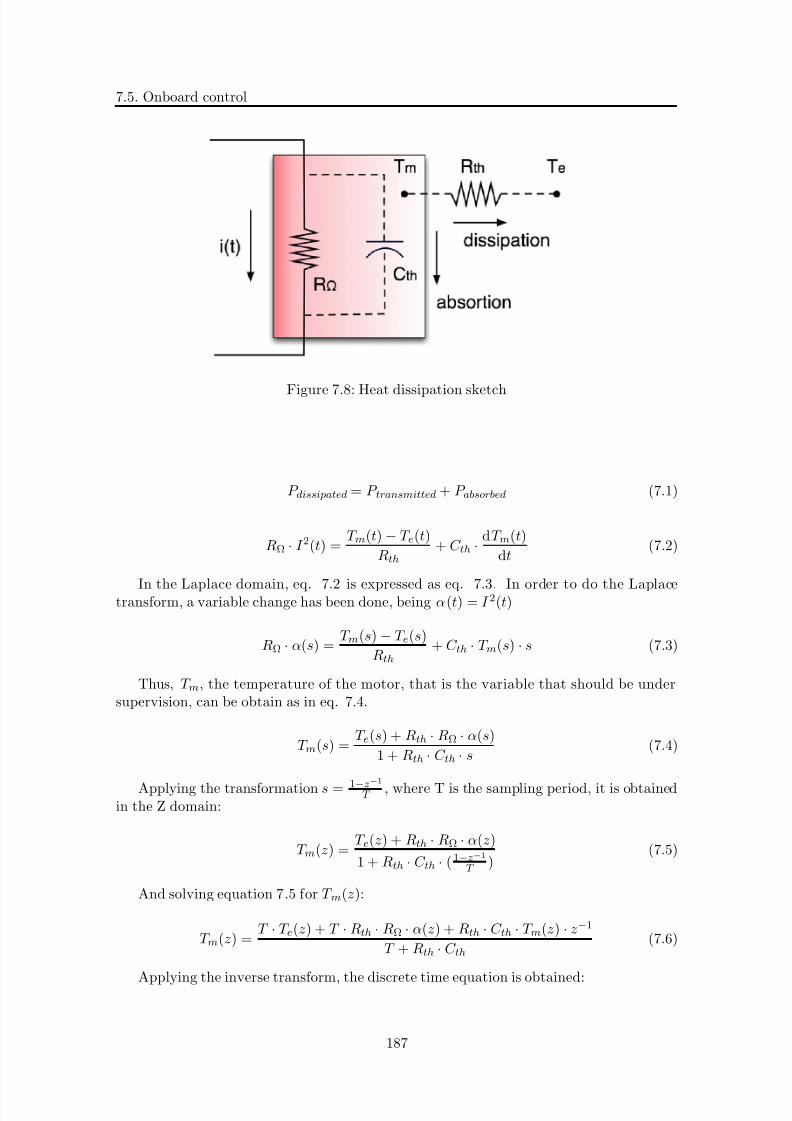
8/21/2019 Alberto Brunete Gonzalez
http://slidepdf.com/reader/full/alberto-brunete-gonzalez 215/311
7.5. Onboard control
Figure 7.8: Heat dissipation sketch
P dissipated = P transmitted + P absorbed (7.1)
RΩ · I 2(t) = T m(t) − T e(t)
Rth
+ C th · dT m(t)
dt (7.2)
In the Laplace domain, eq. 7.2 is expressed as eq. 7.3. In order to do the Laplacetransform, a variable change has been done, being α(t) = I 2(t)
RΩ · α(s) = T m(s) − T e(s)
Rth
+ C th · T m(s) · s (7.3)
Thus, T m, the temperature of the motor, that is the variable that should be undersupervision, can be obtain as in eq. 7.4.
T m(s) = T e(s) + Rth · RΩ · α(s)
1 + Rth · C th · s (7.4)
Applying the transformation s = 1−z−1
T , where T is the sampling period, it is obtainedin the Z domain:
T m(z) = T e(z) + Rth · RΩ · α(z)
1 + Rth · C th · (1−z−1
T )
(7.5)
And solving equation 7.5 for T m(z):
T m(z) = T · T e(z) + T · Rth · RΩ · α(z) + Rth · C th · T m(z) · z−1
T + Rth · C th(7.6)
Applying the inverse transform, the discrete time equation is obtained:
187

8/21/2019 Alberto Brunete Gonzalez
http://slidepdf.com/reader/full/alberto-brunete-gonzalez 216/311
CHAPTER 7. Control Architecture
Behavior: Avoid overheating
Activation conditions None (always running)Inputs (Stimuli) Internal variables: I 1, I 2, etc.
Outputs (Actions) Block M 1, Block M 2, etc.
Table 7.7: Behavior encoding: Avoid overheating
Behavior: Avoid actuator damage
Activation conditions None (always running)Inputs (Stimuli) Internal variables: I 1,Θ1,I 2,Θ2,etc.Outputs (Actions) Block M 1, Block M 2, etc.
Table 7.8: Behavior encoding: Avoid actuator damage
T m[n] = T · T e[n] + T · Rth · RΩ · α[n] + Rth · C th · T m[n − 1]T + Rth · C th
(7.7)
T m[n] = T · T e[n] + T · Rth · RΩ · I 2[n] + Rth · C th · T m[n − 1]
T + Rth · C th(7.8)
The temperature of the environment is measured by a temperature sensor, the electricalcurrent is calculated as in equation 5.15 and the electrical and thermal resistance, andthermal capacitance are constants.
The behavior is monitoring continuously the temperature and intensity, and in casethat overheating in the servomotors is detected, they are stopped immediately.
Avoid actuator damage
The purpose of this behavior is to control that the torque of the motors in under certainlimits that don’t damage the motors / actuators. If it is too high the servomotors arestopped immediately.
This is achieved by controlling that the current intensity is under a certain limit. Thislimit has been obtained experimentally. In figure 7.9, the servomotor is trying to movefrom 100 to 180, but it is blocked at 135. The consumption is blocked around 120mA.
Avoid mechanical damages
This behavior is in charge of the mechanical security of the module, taken care of anypossible danger it may suffer by wrong use of the actuators.
One of the tasks this behavior is in charge of, is to avoid singular points. Singularitieshave to be avoided because they produce unexpected results, since joints are forced tomove at impossible speeds by the actuators, or to places that cannot be reached. Thereare two possible singular points:
• in the limits of the workspace of the robot
• inside the workspace of the robot
188
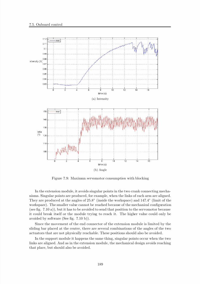
8/21/2019 Alberto Brunete Gonzalez
http://slidepdf.com/reader/full/alberto-brunete-gonzalez 217/311
7.5. Onboard control
(a) Intensity
(b) Angle
Figure 7.9: Maximun servomotor consumption with blocking
In the extension module, it avoids singular points in the two crank connecting mecha-nisms. Singular points are produced, for example, when the links of each arm are aligned.
They are produced at the angles of 25.8 (inside the workspace) and 147.4 (limit of theworkspace). The smaller value cannot be reached because of the mechanical configuration(see fig. 7.10 a)), but it has to be avoided to send that position to the servomotor becauseit could break itself or the module trying to reach it. The higher value could only beavoided by software (See fig. 7.10 b)).
Since the movement of the end connector of the extension module is limited by thesliding bar placed at the center, there are several combinations of the angles of the twoactuators that are not physically reachable. These positions should also be avoided.
In the support module it happens the same thing, singular points occur when the twolinks are aligned. And as in the extension module, the mechanical design avoids reaching
that place, but should also be avoided.
189
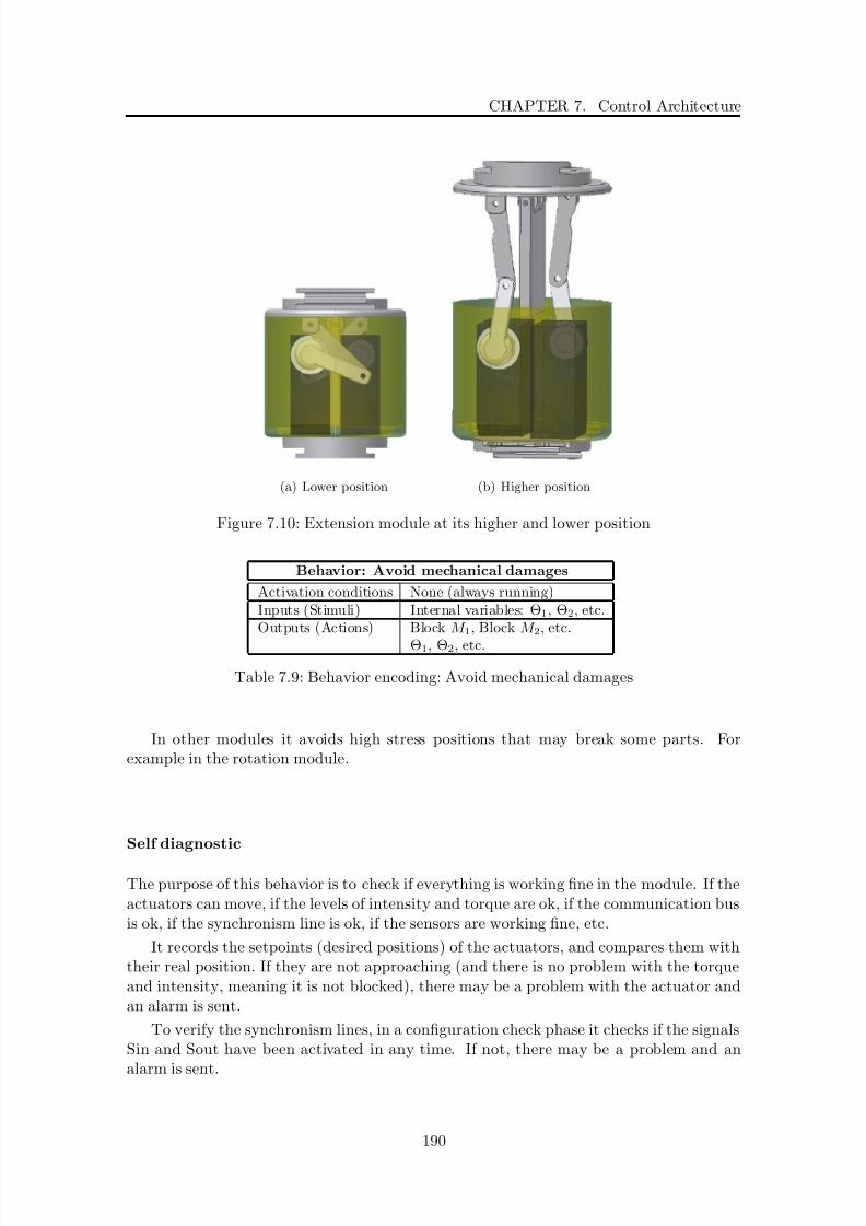
8/21/2019 Alberto Brunete Gonzalez
http://slidepdf.com/reader/full/alberto-brunete-gonzalez 218/311
CHAPTER 7. Control Architecture
(a) Lower position (b) Higher position
Figure 7.10: Extension module at its higher and lower position
Behavior: Avoid mechanical damages
Activation conditions None (always running)Inputs (Stimuli) Internal variables: Θ1, Θ2, etc.Outputs (Actions) Block M 1, Block M 2, etc.
Θ1, Θ2, etc.
Table 7.9: Behavior encoding: Avoid mechanical damages
In other modules it avoids high stress positions that may break some parts. Forexample in the rotation module.
Self diagnostic
The purpose of this behavior is to check if everything is working fine in the module. If theactuators can move, if the levels of intensity and torque are ok, if the communication busis ok, if the synchronism line is ok, if the sensors are working fine, etc.
It records the setpoints (desired positions) of the actuators, and compares them withtheir real position. If they are not approaching (and there is no problem with the torqueand intensity, meaning it is not blocked), there may be a problem with the actuator andan alarm is sent.
To verify the synchronism lines, in a configuration check phase it checks if the signalsSin and Sout have been activated in any time. If not, there may be a problem and an
alarm is sent.
190

8/21/2019 Alberto Brunete Gonzalez
http://slidepdf.com/reader/full/alberto-brunete-gonzalez 219/311
7.5. Onboard control
Behavior: Self diagnostic
Activation conditions No low batteryInputs (Stimuli) Internal variables: Θ1, Θ2, etc.
I
2
C Communications stateSynchronism line communications stateSensors state
Outputs (Actions) Module state [OK,PROBLEM]
Table 7.10: Behavior encoding: Self diagnostic
Behavior: Situation awareness
Activation conditions No low batteryInputs (Stimuli) Contact sensor
IR sensorsInternal variables: Θ1, Θ2,etc.
Outputs (Actions) Module situation [narrow pipe, wide pipe, open space]
Touch detected
Table 7.11: Behavior encoding: Situation awareness
Situation awareness
This behavior tries to know where is the module/microrobot: inside a narrow pipe, a widepipe, open air. It makes use of the contact sensors, IR sensors, and the intensity andtorque control system of the servomotors, amongst other sensors.
Thanks to the IR sensors, the module is capable to know if it is in the open environmentor inside a pipe. If it is inside a pipe, it can detect if it is a wide pipe or a narrow one.
Thanks to the contact sensor it can detect if has crashed into something and thus otherbehaviors may act consequently: if it is in an open environment, it may go around theobstacle, if it is inside a pipe, the IR will tell if it is an elbow or a bifurcation, and it willbe able to negotiate the elbow or choose a path in the bifurcation.
The touch (and camera) module plays a very important role because it is the one thathas touch sensors to detect obstacles, in this case elbows and bifurcations. When thetouch module detects an obstacle sends a message to the CC, and the CC distributes theinformation to all the modules.
Environment diagnostic
This behavior is in charge of gathering information from the sensors (contact, IR, temper-ature, humidity, etc.) and taking images. It is continuously computing the data comingfrom its sensors (whatever they are) and storing them.
It is capable of doing an historical record of these values to use them whenever it isnecessary:
• if the temperature or the humidity is increasing dangerously
• if it is approaching the end of a pipe by analyzing the pictures taken from the camera
If the module is running down on battery it may stop working.
191

8/21/2019 Alberto Brunete Gonzalez
http://slidepdf.com/reader/full/alberto-brunete-gonzalez 220/311
CHAPTER 7. Control Architecture
Behavior: Environment diagnostic
Activation conditions No low batteryInputs (Stimuli) Data form sensors: temperature, humidity
picturesOutputs (Actions) Temperature alertHumidity alertHistorical of temperature, humidity, etc.Image processing data
Table 7.12: Behavior encoding: Environment diagnostic
It can detect if the module has touched something, it if close to an object (wall, pipe),etc.
Vertical sinusoidal movement
This behavior is found in modules with one rotation dof. By moving the rotation actua-tor following a sinusoidal wave, the module help the microrobot to perform a snake-likemovement:
P os = A ∗ sin(ω ∗ t + φ) (7.9)
All parameters are constant but the time “t”. There are two ways to synchronize “t”:
• “t” is reseted at the same time for all modules when a start sequence message isreceived from the CC. This is the easiest way but the drawback is that they can lose
synchronization. To avoid this a synchronization message is sent every 2 seconds.
• using the synchronism line:
– the first module steps “t” and activates the output synchronism line
– the second detects the input line activated, steps “t” and activates the outputline
– and so on, until the last module detects the input line activated, steps “t”,activates its input line
– the penultimate module detects the output line activated, steps “t” and acti-vates the input line
– etc.
Both ways have been implemented. In chapter 8 they will be analyzed and some resultswill be given.
Horizontal sinusoidal movement
This behavior is in charge of two things: movement with horizontal joints and turningmovements.
Forward movement can be achieved performing, for example, serpentine movements,
and it is similar to the one described in the Vertical sinusoidal movement section.
192

8/21/2019 Alberto Brunete Gonzalez
http://slidepdf.com/reader/full/alberto-brunete-gonzalez 221/311
7.5. Onboard control
Behavior: Vertical sinusoidal movement
Activation conditions CommandMission
Inputs (Stimuli) Synchronism linesΘ1, Θ2, etc.Outputs (Actions) Θ1, Θ2, etc.
Table 7.13: Behavior encoding: Vertical sinusoidal movement
Behavior: Horizontal sinusoidal movement
Activation conditions CommandMission
Inputs (Stimuli) Synchronism linesΘ1, Θ2, etc.
Outputs (Actions) Θ1, Θ2, etc.
Table 7.14: Behavior encoding: Horizontal sinusoidal movement
Regarding turns, in open spaces, turns are achieved by putting horizontal joints at afixed position all the time. The robot has the shape of an arc. The radius of curvatureof the trajectory can be modified by modifying the degree of rotation of the horizontal
joints.
Inside pipes, it is also possible to go forward by pushing against the pipe walls. Thesequence is as follows (fig. 8.34):
• The first module (M1) turns 90 degrees.
• M1 turns up the synchronism line with module M2.• When M2 detects the synchronism line up, M2 turns 90 degrees.
• When M2 has turn a predetermined angle (about 60 degrees), M2 turns downs thesynchronism line with M1.
• M1 gets back to the initial 0 degrees position.
• When M2 has turned 90 degrees turns up the synchronism line with M3 and so on.
Passive modules have nothing to do but to “pass the token” to the next module(through the synchronism line).
This solution includes P2P communication between adjacent modules besides the I 2C
communication. An slave module can only communicate with adjacent modules.
Worm-like movement
This behavior can be found in modules with extension-contraction capabilities. Eachmodule knows if it has “support” or “extension” capabilities. Worm like movement isperformed by combination of extension-contraction mechanisms.
The mechanism is the following:
• the first module with support capabilities (S1) expands, and activates the output
synchronism line
193

8/21/2019 Alberto Brunete Gonzalez
http://slidepdf.com/reader/full/alberto-brunete-gonzalez 222/311
CHAPTER 7. Control Architecture
Behavior: Worm-like movement
Activation conditions CommandMission
Inputs (Stimuli) Synchronism linesΘ1, Θ2 (Extension/Contraction state), etc.Outputs (Actions) Θ1, Θ2 (Extension/Contraction), etc.
Table 7.15: Behavior encoding: Worm-like movement
Behavior: Push-Forward movement
Activation conditions CommandMission
Inputs (Stimuli) Synchronism linesOutputs (Actions) Push, Stop, etc.
Table 7.16: Behavior encoding: Push-Forward movement
• the next module with extension capabilities (E) contracts and activates the outputline
• the next module with support capabilities (S2) expands and activates the input line
• E activates the input line
• S1 releases and activates the output line
• E expands and activates de input line
• Everything is repeated
A sketch of this procedure can be seen in former fig. 4.35.
Push-Forward movement
This behavior can be found in modules which has self-propulsion capabilities, like thehelicoidal module. This behavior is in charge of activating the actuator to move forwardor backwards as demanded.
7.5.2 Behavior fusion
Behavior coordination is a complex task. Some behaviors collaborate to achieve its goal(cooperation), some others compete (competition) and some others act independently formeach other. In figure 7.11 the scheme is explained.
Behaviors are divided in sets of priorities and tasks.
Walking behaviors (vertical sinusoidal, horizontal sinusoidal, etc.) control the actu-ators of the module, some of them control one actuator, other two, etc. They may becomplimentary, and thus, its output is combined to achieve its goal. Its output is subjectto LLC1 commands coming directly from the CC.
Perceptual behaviors act independently since they only inform and they have no ac-tuator control. But its output feeds back the other behavior with information regarding
broken actuators, current situation, etc.
194

8/21/2019 Alberto Brunete Gonzalez
http://slidepdf.com/reader/full/alberto-brunete-gonzalez 223/311
7.6. Heterogeneous layer
Figure 7.11: Behavior fusion scheme
Survival behaviors have the highest priority (if they compete with other behaviors they
will win) since they try to keep the module up and running. They can inhibit the outputof the other behavior if they put in danger the integrity of the module. For example, if theoutput of a behavior is to move a servomotor to an specific position and in this positionthe consumption is too high, the position is released.
7.6 Heterogeneous layer
The heterogeneous layer is in charge of several tasks that take place between the moduleand the CC and/or other modules, amongst which it is the communication. Every timea command is received by the module, it is processed by the heterogenous layer and
translated into specific instructions for the module. On the other hand, when the moduleneeds to send a message, it is done by the heterogenous layer.
For example, when an action has to be done (i.e. “go straight forward”), the CC sendsan I 2C message to every module with the command to follow. The heterogeneous layer of each module translate this message to proper commands of the module. It is importantto remark that all messages are the same, no matter which module they are aimed to, andthus it is the module that knows what actions it has to perform.
The heterogenous layer is in charge of the following tasks:
1. Communications
2. Configuration check
195
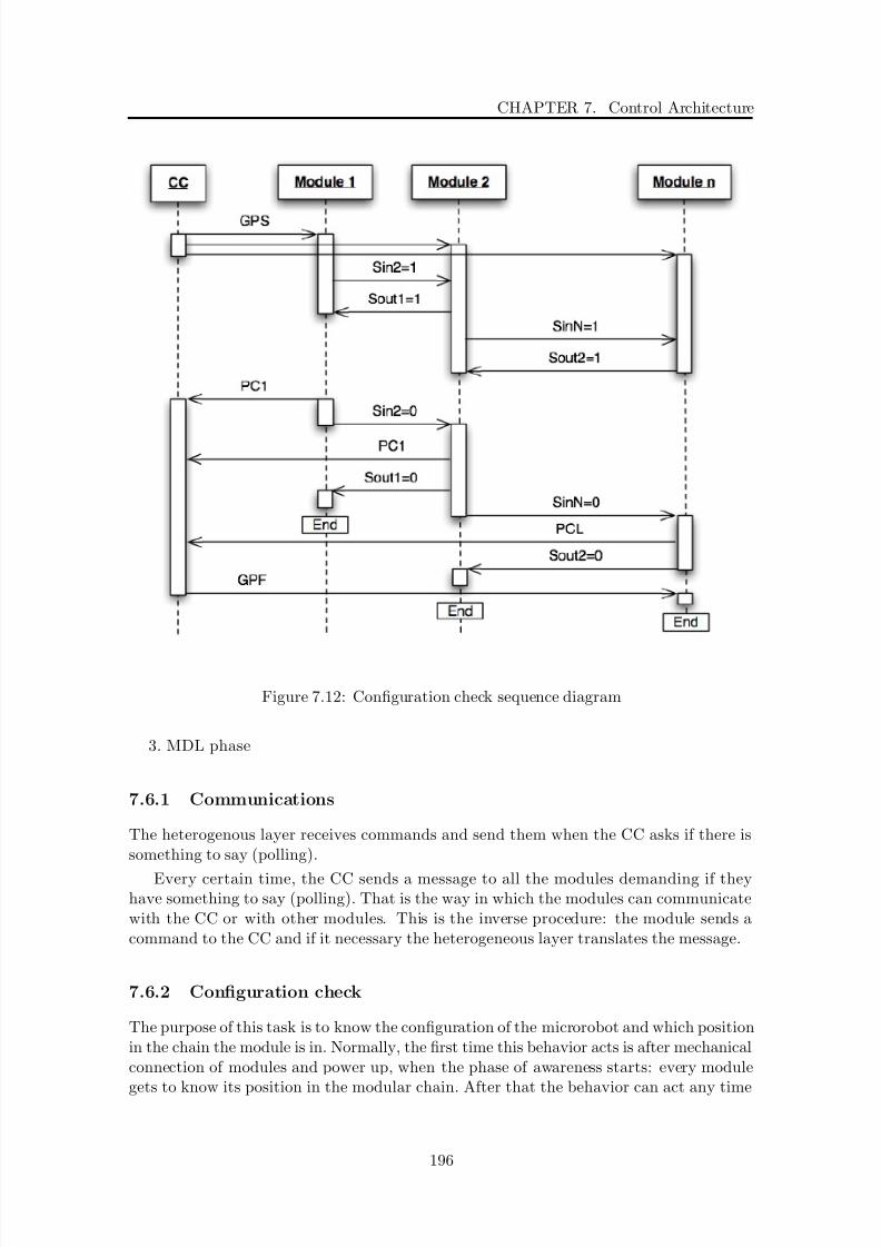
8/21/2019 Alberto Brunete Gonzalez
http://slidepdf.com/reader/full/alberto-brunete-gonzalez 224/311
CHAPTER 7. Control Architecture
Figure 7.12: Configuration check sequence diagram
3. MDL phase
7.6.1 Communications
The heterogenous layer receives commands and send them when the CC asks if there issomething to say (polling).
Every certain time, the CC sends a message to all the modules demanding if theyhave something to say (polling). That is the way in which the modules can communicatewith the CC or with other modules. This is the inverse procedure: the module sends acommand to the CC and if it necessary the heterogeneous layer translates the message.
7.6.2 Configuration check
The purpose of this task is to know the configuration of the microrobot and which positionin the chain the module is in. Normally, the first time this behavior acts is after mechanicalconnection of modules and power up, when the phase of awareness starts: every module
gets to know its position in the modular chain. After that the behavior can act any time
196
8/21/2019 Alberto Brunete Gonzalez
http://slidepdf.com/reader/full/alberto-brunete-gonzalez 225/311
7.7. Central control
it is necessary to know the configuration (after split up, if a module is broken, etc.)
This procedure is as follows (see fig. 7.12):
• The CC sends an GPS message to all modules.
• All modules activate their synchronism lines.
• The one which is the first (it knows that it is the first because its S in synchronismline is down) replies with a PC1 message (this message is sent to the CC and includesthe “ID” of the module: “r” for rotation, “s” for support, etc.).
• The first module puts the S out synchronism line down, so the second module knowsit goes next (because now its S in synchronism line is down).
• The second module sends a PC1 message and puts its S in synchronism line down,
so the first module knows it has finished.
• The CC keeps collecting all the messages.
• It goes the same way for all modules.
• When it is the turn of the last module (it knows it is the last because its S outsynchronism line is down) it sends a PCL message
• The CC send a GPF message, so the last module knows it has finished.
7.6.3 MDL phase
MDL phase follows a similar mechanism as the “configuration check” phase, but insteadof sending the “id”, the module sends the MDL string showing its capabilities.
7.7 Central control
The central control (CC) is in charge of the most complicated calculations, as it is runningin a more powerful processor (either in an external PC -nowadays- or in a specific module-in the future- ).
Central control represents the high control layer in the control architecture. It takescare of the main decisions of the robot, what it is going to do and how, independently of the module composition of the microrobot.
Central control is also based in behaviors, but in this case the behaviors have the wholemicrorobot as its target.
In order to know what the robot is capable of, the central control makes use of anexpert system based on rules that takes the MDL commands coming from each of themodules and outputs a set of capabilities of the whole microrobot.
Each module has several features that defines what it can do. But a set of modulestogether can have newer features. Modules can be grouped in units to have different
capabilities, units can in turn be grouped in super-units to have newer capabilities. For
197

8/21/2019 Alberto Brunete Gonzalez
http://slidepdf.com/reader/full/alberto-brunete-gonzalez 226/311
CHAPTER 7. Control Architecture
Figure 7.13: Ext / Contraction capabilites: a) grade 3 and b) grade 1
example, the rotation module doesn’t have extension/contraction capabilities, but a unitcomposed of three rotation modules together do have that feature (eq. 7.10 and 7.11).
Rot mod+Rot mod+Rot mod+Open air => Extension/Contraction (grade 3) (7.10)
Rot mod + Rot mod + Rot mod + Pipe => Extension/Contraction (grade 1) (7.11)
It is possible to see that the same combination of modules may have different resultsdepending if the microrobot is inside the pipe or in the open air (fig. 7.13).
This expert system is based on a set rules and an Inference Engine. The rules arealready pre-charged, but new rules could be added by learning.
7.7.1 Rules
The capabilities of the whole microrobot are the consequence of the combination of thecapabilities of all the modules and its position in the chain. It is not the same having aextension module in between two support modules, that having the extension module atthe side of two support modules in a row. In the first case the chain could perform aninchworm movement while in the second one it is not possible.
As we have seen, the functionalities of the modules can be useful or not for a determinedtask depending on where they are placed. This importance is linked to three possible
location of the modules:
198
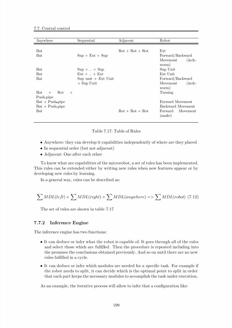
8/21/2019 Alberto Brunete Gonzalez
http://slidepdf.com/reader/full/alberto-brunete-gonzalez 227/311
7.7. Central control
Anywhere Sequential Adjacent Robot
Bat Rot + Rot + Rot Ext
Bat Sup + Ext + Sup Forward/BackwardMovement (inch-worm)
Bat Sup + .. + Sup Sup UnitBat Ext + .. + Ext Ext UnitBat Sup unit + Ext Unit
+ Sup UnitForward/BackwardMovement (inch-worm)
Bat + Rot +Push pipe
Turning
Bat + Push pipe Forward MovementBat + Push pipe Backward MovementBat Rot + Rot + Rot Forward Movement
(snake)
Table 7.17: Table of Rules
• Anywhere: they can develop it capabilities independently of where are they placed
• In sequential order (but not adjacent)
• Adjacent: One after each other
To know what are capabilities of the microrobot, a set of rules has been implemented.This rules can be extended either by writing new rules when new features appear or by
developing new rules by learning.
In a general way, rules can be described as:
M DL(left) +
M DL(right) +
M DL(anywhere) =>
M DL(robot) (7.12)
The set of rules are shown in table 7.17
7.7.2 Inference Engine
The inference engine has two functions:
• It can deduce or infer what the robot is capable of. It goes through all of the rulesand select those which are fulfilled. Then the procedure is repeated including intothe premises the conclusions obtained previously. And so on until there are no newrules fulfilled in a cycle.
• It can deduce or infer which modules are needed for a specific task. For example if the robot needs to split, it can decide which is the optimal point to split in orderthat each part keeps the necessary modules to accomplish the task under execution.
As an example, the iterative process will allow to infer that a configuration like:
199
8/21/2019 Alberto Brunete Gonzalez
http://slidepdf.com/reader/full/alberto-brunete-gonzalez 228/311
CHAPTER 7. Control Architecture
Sup mod + Rot mod + Rot mod + Rot mod + Sup mod
can move as a worm.
7.7.3 Central control Behaviors
Continuing with the classification made in section 7.5.1 the behaviors that have beendefined for the central control are shown in the following bullets. As explained before,some behaviors perform simpler tasks, while others are based in them to perform morecomplex tasks.
1. Postural behaviors
• Balance / Stability
2. Walking behaviors
• Move straight forward/backwards
• Turn to left/right
• Move laterally
• Rotate
3. Path following behaviors
• Edge following
• Pipe following
• Stripe following
4. Protective behaviors
• Obstacle negotiation
5. Exploration behaviors
• Wandering
6. Goal Oriented behaviors
• Reach a landmark
• Reach a place
• Find a pipe break
• Repair
200
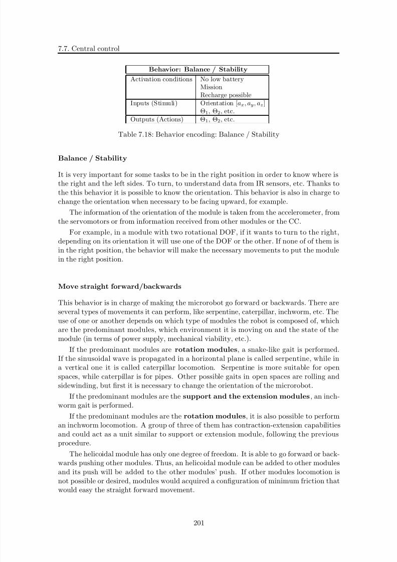
8/21/2019 Alberto Brunete Gonzalez
http://slidepdf.com/reader/full/alberto-brunete-gonzalez 229/311
7.7. Central control
Behavior: Balance / Stability
Activation conditions No low batteryMission
Recharge possibleInputs (Stimuli) Orientation [ax, ay, az]Θ1, Θ2, etc.
Outputs (Actions) Θ1, Θ2, etc.
Table 7.18: Behavior encoding: Balance / Stability
Balance / Stability
It is very important for some tasks to be in the right position in order to know where isthe right and the left sides. To turn, to understand data from IR sensors, etc. Thanks tothe this behavior it is possible to know the orientation. This behavior is also in charge tochange the orientation when necessary to be facing upward, for example.
The information of the orientation of the module is taken from the accelerometer, fromthe servomotors or from information received from other modules or the CC.
For example, in a module with two rotational DOF, if it wants to turn to the right,depending on its orientation it will use one of the DOF or the other. If none of of them isin the right position, the behavior will make the necessary movements to put the modulein the right position.
Move straight forward/backwards
This behavior is in charge of making the microrobot go forward or backwards. There areseveral types of movements it can perform, like serpentine, caterpillar, inchworm, etc. Theuse of one or another depends on which type of modules the robot is composed of, whichare the predominant modules, which environment it is moving on and the state of themodule (in terms of power supply, mechanical viability, etc.).
If the predominant modules are rotation modules, a snake-like gait is performed.If the sinusoidal wave is propagated in a horizontal plane is called serpentine, while ina vertical one it is called caterpillar locomotion. Serpentine is more suitable for openspaces, while caterpillar is for pipes. Other possible gaits in open spaces are rolling andsidewinding, but first it is necessary to change the orientation of the microrobot.
If the predominant modules are the support and the extension modules, an inch-worm gait is performed.
If the predominant modules are the rotation modules, it is also possible to performan inchworm locomotion. A group of three of them has contraction-extension capabilitiesand could act as a unit similar to support or extension module, following the previousprocedure.
The helicoidal module has only one degree of freedom. It is able to go forward or back-wards pushing other modules. Thus, an helicoidal module can be added to other modulesand its push will be added to the other modules’ push. If other modules locomotion isnot possible or desired, modules would acquired a configuration of minimum friction that
would easy the straight forward movement.
201
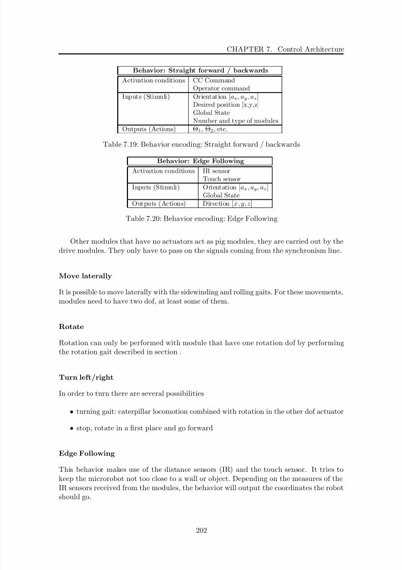
8/21/2019 Alberto Brunete Gonzalez
http://slidepdf.com/reader/full/alberto-brunete-gonzalez 230/311
CHAPTER 7. Control Architecture
Behavior: Straight forward / backwards
Activation conditions CC CommandOperator command
Inputs (Stimuli) Orientation [ax, ay, az]Desired position [x,y,z]Global StateNumber and type of modules
Outputs (Actions) Θ1, Θ2, etc.
Table 7.19: Behavior encoding: Straight forward / backwards
Behavior: Edge Following
Activation conditions IR sensorTouch sensor
Inputs (Stimuli) Orientation [ax, ay, az]Global State
Outputs (Actions) Direction [x,y,z]
Table 7.20: Behavior encoding: Edge Following
Other modules that have no actuators act as pig modules, they are carried out by thedrive modules. They only have to pass on the signals coming from the synchronism line.
Move laterally
It is possible to move laterally with the sidewinding and rolling gaits. For these movements,
modules need to have two dof, at least some of them.
Rotate
Rotation can only be performed with module that have one rotation dof by performingthe rotation gait described in section .
Turn left/right
In order to turn there are several possibilities
• turning gait: caterpillar locomotion combined with rotation in the other dof actuator
• stop, rotate in a first place and go forward
Edge Following
This behavior makes use of the distance sensors (IR) and the touch sensor. It tries tokeep the microrobot not too close to a wall or object. Depending on the measures of theIR sensors received from the modules, the behavior will output the coordinates the robot
should go.
202
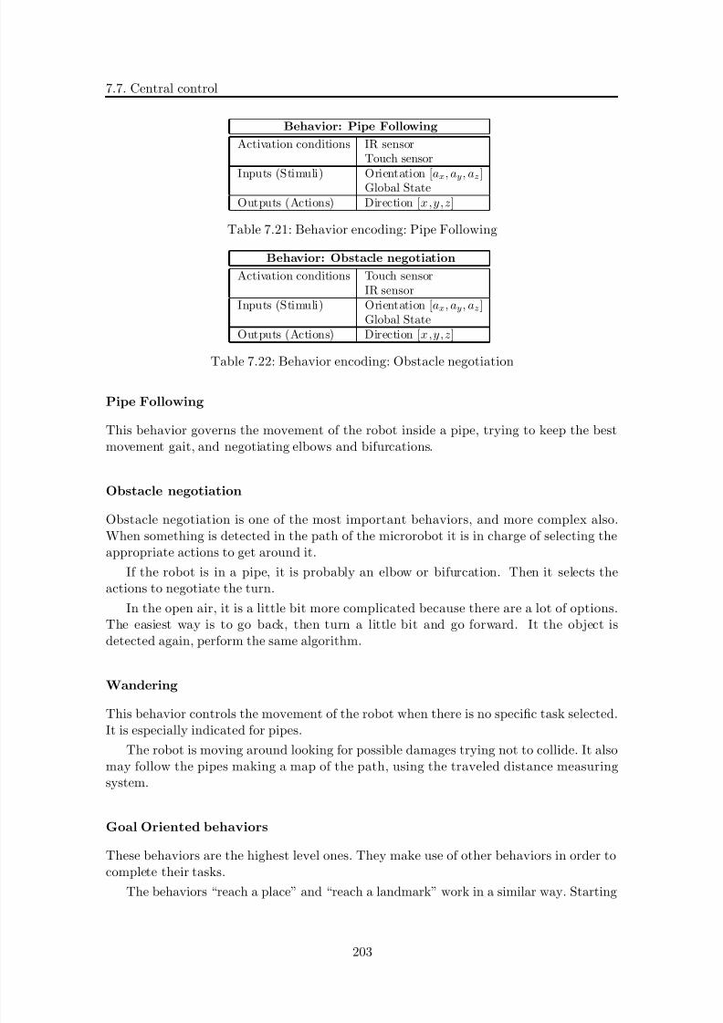
8/21/2019 Alberto Brunete Gonzalez
http://slidepdf.com/reader/full/alberto-brunete-gonzalez 231/311
7.7. Central control
Behavior: Pipe Following
Activation conditions IR sensorTouch sensor
Inputs (Stimuli) Orientation [ax, ay, az]Global StateOutputs (Actions) Direction [x,y,z]
Table 7.21: Behavior encoding: Pipe Following
Behavior: Obstacle negotiation
Activation conditions Touch sensorIR sensor
Inputs (Stimuli) Orientation [ax, ay, az]Global State
Outputs (Actions) Direction [x,y,z]
Table 7.22: Behavior encoding: Obstacle negotiation
Pipe Following
This behavior governs the movement of the robot inside a pipe, trying to keep the bestmovement gait, and negotiating elbows and bifurcations.
Obstacle negotiation
Obstacle negotiation is one of the most important behaviors, and more complex also.
When something is detected in the path of the microrobot it is in charge of selecting theappropriate actions to get around it.
If the robot is in a pipe, it is probably an elbow or bifurcation. Then it selects theactions to negotiate the turn.
In the open air, it is a little bit more complicated because there are a lot of options.The easiest way is to go back, then turn a little bit and go forward. It the object isdetected again, perform the same algorithm.
Wandering
This behavior controls the movement of the robot when there is no specific task selected.It is especially indicated for pipes.
The robot is moving around looking for possible damages trying not to collide. It alsomay follow the pipes making a map of the path, using the traveled distance measuringsystem.
Goal Oriented behaviors
These behaviors are the highest level ones. They make use of other behaviors in order tocomplete their tasks.
The behaviors “reach a place” and “reach a landmark” work in a similar way. Starting
203

8/21/2019 Alberto Brunete Gonzalez
http://slidepdf.com/reader/full/alberto-brunete-gonzalez 232/311
CHAPTER 7. Control Architecture
from its own position, it estimates where is the objective and move the robot in thatdirection. In a pipe, the objective could be
• go to the next bifurcation• go forward/backwards 2 meters
• go up/down
In open air, objectives can be:
• go to position (x,y)
• go to the next corner
• get into the pipe in front
The behavior “find a pipe break” makes use of the wandering behavior to move insidethe pipe while looking for breaks or holes with he camera and IR sensors.
The repair behavior is not implemented, but it is an example of what it will be possibleto do when repairing tools were developed and added to the robot. The behavior will bein charge of the movement of the robot while repairing the damaged pipe.
7.7.4 Behavior fusion
A behavior fusion scheme for the CC algorithms can be found in figure 7.14. Higherlevel behaviors (i.e. path following, obstacle negotiation, exploration (wandering) andgoal oriented) follow a subsumption-like procedure to coordinate. If no one wants to takecontrol, “wandering” is the active behavior, but it can be subsumed by “path following”,which in its turn can be subsumed by “goal oriented”, and finally this one by “obstaclenegotiation”. Thus, “obstacle negotiation” is the behavior with the higher level.
Each of the path following and goal oriented behaviors contribute to the selection of the place to go. Thus, it is shown in the bottom part of the figure 7.14 as a summation of all the individual outputs.
The output of all of the previous behaviors is the coordinates or directions where theywant to go. This output is received by the walking behaviors, which compete amongstthem for the control of the modules. The output of the action selection mechanism canbe suppressed by the “balance/stability” behavior, which is in charge of keeping the mi-
crorobot in the most appropriate position.
Action Selection Mechanism
The outputs of the four walking behaviors (go forward, turn, move laterally and rotate)have to be merged into a unique output. Since they are all competing behaviors, thereshould be a winner that takes the decision to follow. The selection criteria depends ontwo factors: the situation and the place the microrobot is going to.
The situation is very important because it is not the same to move inside a pipe thanin the open air, or to move in a plain terrain / pipe than in an uphill terrain / vertical
pipe.
204
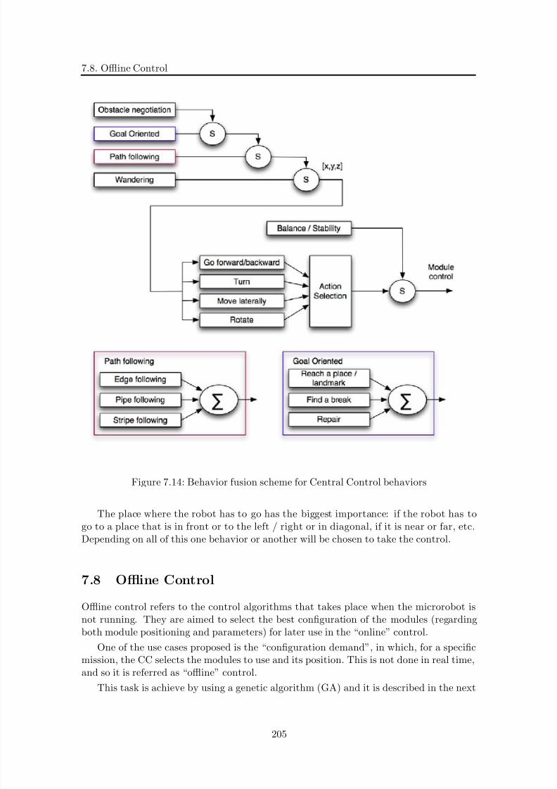
8/21/2019 Alberto Brunete Gonzalez
http://slidepdf.com/reader/full/alberto-brunete-gonzalez 233/311
7.8. Offline Control
Figure 7.14: Behavior fusion scheme for Central Control behaviors
The place where the robot has to go has the biggest importance: if the robot has togo to a place that is in front or to the left / right or in diagonal, if it is near or far, etc.Depending on all of this one behavior or another will be chosen to take the control.
7.8 Offline Control
Offline control refers to the control algorithms that takes place when the microrobot isnot running. They are aimed to select the best configuration of the modules (regardingboth module positioning and parameters) for later use in the “online” control.
One of the use cases proposed is the “configuration demand”, in which, for a specificmission, the CC selects the modules to use and its position. This is not done in real time,and so it is referred as “offline” control.
This task is achieve by using a genetic algorithm (GA) and it is described in the next
205

8/21/2019 Alberto Brunete Gonzalez
http://slidepdf.com/reader/full/alberto-brunete-gonzalez 234/311
CHAPTER 7. Control Architecture
sections.
GAs can also be used to optimize parameters in the microrobot. For example, in asnake-like configuration, the microrobot is composed of rotation modules that moves one
of its dof following a sinusoidal wave:
P os = A ∗ sin(ω ∗ t + φ) (7.13)
All the parameters, A, ω and φ can be optimized to make the microrobot faster, tohave lower consumption or anything else.
For the rest of this section, two options for GA will be considered:
• configuration demand: in heterogenous configurations, for a given task, the GA hasto determine the modules to use to have an optimal configuration.
• parameter optimization: for a given configuration, the GA has to determine the opti-mum parameters for the best performance. This is especially useful in homogeneousconfigurations when the microrobot is performing a snake or inchworm movement.
7.8.1 Brief on genetic algorithms
A GA is a search technique used in computing to find exact or approximate solutions tooptimization and search problems. Genetic algorithms are categorized as global searchheuristics. Genetic algorithms are a particular class of evolutionary algorithms (EA) thatuse techniques inspired by evolutionary biology such as inheritance, mutation, selection,
and crossover.
Genetic algorithms are implemented in a computer simulation in which a population of abstract representations (called chromosomes or the genotype of the genome) of candidatesolutions (called individuals, creatures, or phenotypes) to an optimization problem evolvestoward better solutions. Traditionally, solutions are represented in binary as strings of 0sand 1s, but other encodings are also possible. The evolution usually starts from a popu-lation of randomly generated individuals and happens in generations. In each generation,the fitness of every individual in the population is evaluated, multiple individuals arestochastically selected from the current population (based on their fitness), and modi-fied (recombined and possibly randomly mutated) to form a new population. The newpopulation is then used in the next iteration of the algorithm. Commonly, the algorithmterminates when either a maximum number of generations has been produced, or a satis-factory fitness level has been reached for the population. If the algorithm has terminateddue to a maximum number of generations, a satisfactory solution may or may not havebeen reached.
A typical GA requires:
1. a genetic representation of the solution domain
2. a fitness function to evaluate the solution domain
A standard representation of the solution is as an array of bits. Arrays of other types
and structures can be used in essentially the same way. The main property that makes
206
8/21/2019 Alberto Brunete Gonzalez
http://slidepdf.com/reader/full/alberto-brunete-gonzalez 235/311
7.8. Offline Control
these genetic representations convenient is that their parts are easily aligned due to theirfixed size, which facilitates simple crossover operations. Variable length representationsmay also be used, but crossover implementation is more complex in this case.
The fitness function is defined over the genetic representation and measures the qual-ity of the represented solution. The fitness function is always problem dependent. Forinstance, in the knapsack problem one wants to maximize the total value of objects thatcan be put in a knapsack of some fixed capacity. A representation of a solution might bean array of bits, where each bit represents a different object, and the value of the bit (0 or1) represents whether or not the object is in the knapsack. Not every such representationis valid, as the size of objects may exceed the capacity of the knapsack. The fitness of thesolution is the sum of values of all objects in the knapsack if the representation is valid,or 0 otherwise.
Once genetic representation is done and the fitness function defined, GA proceeds toinitialize a population of solutions randomly, then improve it through repetitive applicationof mutation, crossover, inversion and selection operators.
Example of a simple generational genetic algorithm
A simple GA can be described with the following pseudocode:
BEGIN /*Simple GA*/
Generate initial population
Evaluate the fitness of each individual in that population
WHILE NOT finished DO
BEGIN /*Produce new generation*/
FOR (population_size / 2) DO
BEGIN /*Reproduction cycle*/
Select 2 individuals (based on fitness function probability)
Crossover the 2 individuals with a probability
Mutate the 2 individuals with a probability
Evaluate the new individuals
Insert new individuals into populationEND
IF population_has_converged THEN /*time limit, convergence, etc.*/
finished:=true
END
END
The algorithm proposed in this thesis starts from this algorithm to build a more com-
plex and evolved GA.
207

8/21/2019 Alberto Brunete Gonzalez
http://slidepdf.com/reader/full/alberto-brunete-gonzalez 236/311
CHAPTER 7. Control Architecture
Phases of a GA
More advanced GA are divided in different phases:
1. Initialization: individual solutions are randomly generated to form the initial pop-ulation. The population is generated randomly, covering the entire range of possiblesolutions (the search space).
2. Evaluation: consists on applying the fitness function on every individual of thepopulation. The result of the evaluation will help to select the best individuals forreproduction.
3. Selection: during each generation, a proportion of the existing population is selectedto breed a new generation, what is called the mating pool. Individual solutions areselected through a fitness-based process, where fitter solutions are more likely to
be selected. Most functions are stochastic and designed so that a small proportionof less fit solutions are selected. This helps keep the diversity of the populationlarge, preventing premature convergence on poor solutions. Popular and well-studiedselection methods include roulette wheel selection and tournament selection.
4. Reproduction: it is aimed to generate a new population through the applicationof genetic operators: single/two/uniform/arithmetic point crossover, mutation (bitinversion, order changing, adding a number ).
It is very important to define the probability of crossover and mutation to findreasonable settings for the problem being worked on. A very small mutation rate maylead to genetic drift. A recombination rate that is too high may lead to premature
convergence of the GA. A mutation rate that is too high may lead to loss of goodsolutions unless there is elitist selection.
5. Termination: when the terminating condition has been reached, the GA ends.Common terminating conditions are:
• A solution is found that satisfies minimum criteria• Fixed number of generations has been reached• Allocated budget (computation time/money) has been reached• The highest ranking solution’s fitness is reaching or has reached a plateau such
that successive iterations no longer produce better results• Manual inspection
• Combinations of the above
Remarks
One problem that may appear is that GAs may have a tendency to converge towardslocal optima or even arbitrary points rather than the global optimum of the problem.The likelihood of this occurring depends on the shape of the fitness landscape: certainproblems may provide an easy ascent towards a global optimum, others may make it easierfor the function to find the local optima.
This problem may be alleviated by using a different fitness function, increasing the
rate of mutation (called triggered hypermutation), occasionally introducing entirely new,
208
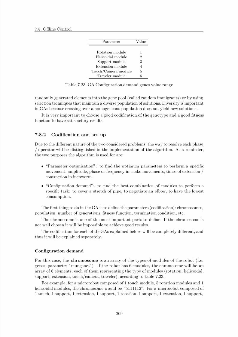
8/21/2019 Alberto Brunete Gonzalez
http://slidepdf.com/reader/full/alberto-brunete-gonzalez 237/311
7.8. Offline Control
Parameter Value
Rotation module 1
Helicoidal module 2Support module 3Extension module 4
Touch/Camera module 5Traveler module 6
Table 7.23: GA Configuration demand genes value range
randomly generated elements into the gene pool (called random immigrants) or by usingselection techniques that maintain a diverse population of solutions. Diversity is importantin GAs because crossing over a homogeneous population does not yield new solutions.
It is very important to choose a good codification of the genotype and a good fitnessfunction to have satisfactory results.
7.8.2 Codification and set up
Due to the different nature of the two considered problems, the way to resolve each phase/ operator will be distinguished in the implementation of the algorithm. As a reminder,the two purposes the algorithm is used for are:
• “Parameter optimization”: to find the optimum parameters to perform a specificmovement: amplitude, phase or frequency in snake movements, times of extension /
contraction in inchworm.
• “Configuration demand”: to find the best combination of modules to perform aspecific task: to cover a stretch of pipe, to negotiate an elbow, to have the lowestconsumption.
The first thing to do in the GA is to define the parameters (codification): chromosomes,population, number of generations, fitness function, termination condition, etc.
The chromosome is one of the most important parts to define. If the chromosome isnot well chosen it will be impossible to achieve good results.
The codification for each of theGAs explained before will be completely different, and
thus it will be explained separately.
Configuration demand
For this case, the chromosome is an array of the types of modules of the robot (i.e.genes, parameter ”numgenes”). If the robot has 6 modules, the chromosome will be anarray of 6 elements, each of them representing the type of modules (rotation, helicoidal,support, extension, touch/camera, traveler), according to table 7.23.
For example, for a microrobot composed of 1 touch module, 5 rotation modules and 1helicoidal modules, the chromosome would be “5111112”. For a microrobot composed of
1 touch, 1 support, 1 extension, 1 support, 1 rotation, 1 support, 1 extension, 1 support,
209
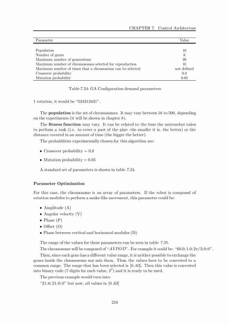
8/21/2019 Alberto Brunete Gonzalez
http://slidepdf.com/reader/full/alberto-brunete-gonzalez 238/311
CHAPTER 7. Control Architecture
Parameter Value
Population 16
Number of genes 6Maximum number of generations 20Maximum number of chromosomes selected for reproduction 16Maximum number of times that a chromosome can be selected not definedCrossover probability 0.8Mutation probability 0.05
Table 7.24: GA Configuration demand parameters
1 rotation, it would be “534313431”.
The population is the set of chromosomes. It may vary between 16 to 500, dependingon the experiments (it will be shown in chapter 8).
The fitness function may vary. It can be related to the time the microrobot takesto perform a task (i.e. to cover a part of the pipe -the smaller it is, the better) or thedistance covered in an amount of time (the bigger the better).
The probabilities experimentally chosen for this algorithm are:
• Crossover probability = 0.8
• Mutation probability = 0.05
A standard set of parameters is shown in table 7.24.
Parameter Optimization
For this case, the chromosome is an array of parameters. If the robot is composed of rotation modules to perform a snake-like movement, this parameter could be:
• Amplitude (A)
• Angular velocity (V)
• Phase (P)
• Offset (O)• Phase between vertical and horizontal modules (D)
The range of the values for these parameters can be seen in table 7.25.
The chromosome will be composed of “AVPOD”. For example it could be: “60.0; 1.0; 2π/3;0;0”.
Then, since each gene has a different value range, it is neither possible to exchange thegenes inside the chromosome nor mix them. Thus, the values have to be converted to acommon range. The range that has been selected is [0..63]. Then this value is convertedinto binary code (7 digits for each value, 27) and it is ready to be used.
The previous example would turn into:
“21; 6; 21; 0; 0” but now, all values in [0..63]
210

8/21/2019 Alberto Brunete Gonzalez
http://slidepdf.com/reader/full/alberto-brunete-gonzalez 239/311
7.8. Offline Control
Parameter Value
Amplitud [−90..90]
Angular velocity [0..10]Phase [0..2π]Offset [0..90]
Phase between vertical and horizontal modules [0..2π]
Table 7.25: GA Parameter optimization genes value range
that in binary is: “0010101; 0000110; 0010101; 0000000; 0000000”
And so the individual is: “00101010000110001010100000000000000”
If the robot is composed of support and extension modules to perform an inchworm
movement, this parameter will be:
• Extension time (T)
• Expansion time (P)
• Extension lenght (L)
• Support servo angle (S)
The chromosome is “TPL S ”, and it would follow the same transformation as before.
7.8.3 Phases of the GAs
Initialization
Initially many individual solutions are randomly generated to form the initial populationspecified previously. The population size depends on the nature of the problem, buttypically contains several hundreds or thousands of possible solutions. The populationis generated randomly, covering the entire range of possible solutions (the search space).Occasionally, the solutions may be ”seeded” in areas where optimal solutions are likely tobe found, but this is not the case.
In the configuration demand, genes are random number between 0 and 6. In theparameter optimization, genes are random number selected from the possible values, asseen in table 7.25.
Evaluation
The evaluation consists on applying the fitness function on every chromosome of thepopulation.
The fitness function is a function that evaluates the performance of the chromosome.For that reason, it transforms the chromosome into the modules that represents and runthe simulator with these modules.
The fitness function is a procedure that follows the next steps:
• starts the simulation
211

8/21/2019 Alberto Brunete Gonzalez
http://slidepdf.com/reader/full/alberto-brunete-gonzalez 240/311
CHAPTER 7. Control Architecture
• creates the modules specified by the genes
• runs the simulation (faster than in normal simulation) to achieve the specified ob- jective. Several objectives have been specified:
• terminates the simulation when:
1. either the objectives are completed
2. or the maximum number of iterations have been reached
• returns a value (depending on the goal):
– cover a part of the pipe in as little time as possible: the fitness function returnstime[s].
– cover a part of the pipe with the lowest possible consumption: the fitnessfunction returns intensity[A].
– negotiate an elbow: the fitness function returns time[s].– cover a distance in open air: the fitness function returns time[s].
The values return for the fitness function are stored for later use in selection phase.
For example, let’s suppose that we have 6 chromosomes composed of 6 modules:
C1:RRRRRR=‘‘111111’’
C2:CRRRRH=‘‘511112’’
C3:RRRHHH=‘‘111222’’
C4:CRSEST=‘‘513436’’
C5:SESSES=‘‘343343’’
C6:RSRSRS=‘‘131313’’
and the fitness function calculates the distance it covers in a straight pipe in 20s. Thefollowing results are obtained:
C1:0.4m
C2:0.6m
C3:1m
C4:0.45m
C5:0.8m
C6:0.2m
Selection
After all the population has been evaluated, the selection phase starts. During eachgeneration, a proportion of the existing population is selected to breed a new generation,what is called the mating pool. Individual solutions are selected through a fitness-based
process, where fitter solutions are more likely to be selected.
212

8/21/2019 Alberto Brunete Gonzalez
http://slidepdf.com/reader/full/alberto-brunete-gonzalez 241/311
7.8. Offline Control
Figure 7.15: Roulette probabilty
The basic part of the selection process is to stochastically select from one generation tocreate the basis of the next generation. The requirement is that the fittest chromosomes
have a greater chance of transmitting their genetic information than weaker ones. Thisreplicates nature in that fitter individuals will tend to have a better probability of survivaland will go forward to form the mating pool for the next generation. Weaker individualsare not without a chance. In nature such individuals may have genetic coding that mayprove useful to future generations.
In this theses the roulette wheel selection, a stochastic sampling done with replacement,has been used.
This sampling method selects parents according to a spin of a weighted roulette wheel(fig. 7.15). The roulette wheel is weighted according to the fitness values obtained pre-viously. A high-fit value will have more area assigned to it on the wheel and hence, a
higher probability of ending up as the choice when the biased roulette wheel is spun. Theroulette wheel selection is a high-variance process with a fair amount of scatter betweenexpected and actual number of copies.
Taking the example of the distance covered in 20s, the previous chromosomes have thefollowing selection probabilities:
C1:0.12, 12\%
C2:0.17, 17\%
C3:0.29, 29\%
C4:0.13, 13\%
213
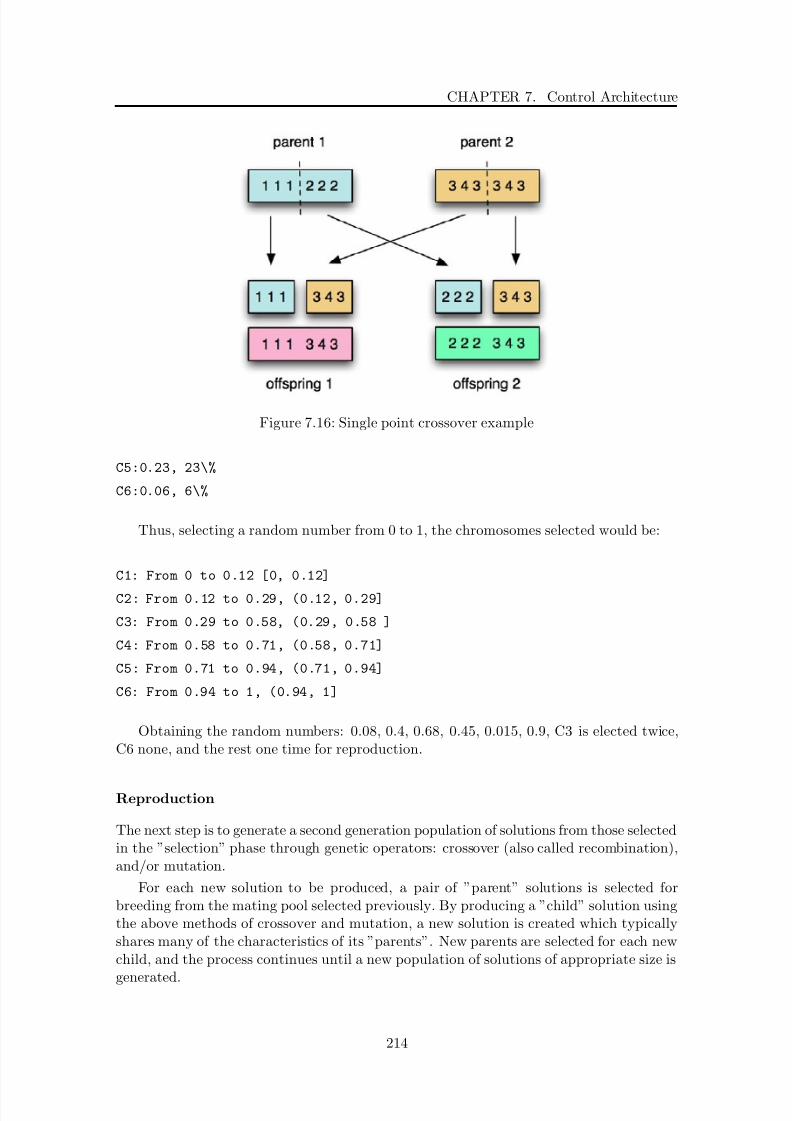
8/21/2019 Alberto Brunete Gonzalez
http://slidepdf.com/reader/full/alberto-brunete-gonzalez 242/311
CHAPTER 7. Control Architecture
Figure 7.16: Single point crossover example
C5:0.23, 23\%
C6:0.06, 6\%
Thus, selecting a random number from 0 to 1, the chromosomes selected would be:
C1: From 0 to 0.12 [0, 0.12]
C2: From 0.12 to 0.29, (0.12, 0.29]
C3: From 0.29 to 0.58, (0.29, 0.58 ]
C4: From 0.58 to 0.71, (0.58, 0.71]
C5: From 0.71 to 0.94, (0.71, 0.94]
C6: From 0.94 to 1, (0.94, 1]
Obtaining the random numbers: 0.08, 0.4, 0.68, 0.45, 0.015, 0.9, C3 is elected twice,C6 none, and the rest one time for reproduction.
Reproduction
The next step is to generate a second generation population of solutions from those selectedin the ”selection” phase through genetic operators: crossover (also called recombination),and/or mutation.
For each new solution to be produced, a pair of ”parent” solutions is selected forbreeding from the mating pool selected previously. By producing a ”child” solution usingthe above methods of crossover and mutation, a new solution is created which typicallyshares many of the characteristics of its ”parents”. New parents are selected for each newchild, and the process continues until a new population of solutions of appropriate size is
generated.
214

8/21/2019 Alberto Brunete Gonzalez
http://slidepdf.com/reader/full/alberto-brunete-gonzalez 243/311
7.8. Offline Control
Figure 7.17: Mutation example
These processes ultimately result in the next generation population of chromosomesthat is different from the initial generation. Generally the average fitness will have in-
creased by this procedure for the population, since only the best organisms from the firstgeneration are selected for breeding, along with a small proportion of less fit solutions, forreasons already mentioned previously.
In this thesis, it is used ”single point crossover” (figure 7.16): one crossover point isselected, the genes from the beginning of the chromosome to the crossover point is copiedfrom one parent, and the rest is copied from the second parent.
The crossover point is selected randomly and could be any number between 1 and thelength of the chromosome - 1.
Afterwards mutation is being performed. Each gene of each chromosome may bechanged based on the mutation probability. For each gene a random number is selected,
and if it is smaller that the mutation probability the gene is changed for another numberobtained randomly (figure 7.17).
In the same example as before, we take two parents for the crossover, “111222” and“343343”. Then a number from 1 to 5 is selected randomly, obtaining 3, so the first 3genes of parent 1 go the first offspring, and the last 3 genes go to the second offspring.The opposite with parent 2.
In the case of mutation, if the chosen parent is “513436”, a random number from 0 to1 is obtained for each gene. If it is smaller than the mutation probability, the gene change.In this case, the only gene that changes is the fourth one. Another random number isselected from 1 to 6 (the number of modules) that will replace the gene. In this case it isthe “1”.
Termination
This generational process is repeated until a termination condition has been reached.
In our case the conditions used are when a fixed number of generations has beenreached (50) or the highest ranking solution’s fitness is reaching or has reached a plateau
such that successive iterations no longer produce better results.
215

8/21/2019 Alberto Brunete Gonzalez
http://slidepdf.com/reader/full/alberto-brunete-gonzalez 244/311
CHAPTER 7. Control Architecture
7.9 Conclusions
In this chapter a control architecture for chained modular robots composed of hetero-
geneous modules has been presented. This architecture is not limited to the modulesdeveloped in chapter 4 but to any kind of chained module able to work and interact withthe others.
Amongst all possible choices stated in 3.1 a behavior-based architecture has beenchosen because:
• it is specifically appropriate for designing and controlling semi-autonomous artificialmicrorobots based on biological systems
• it is suitable for modular systems
• it integrates both low and high level control
The control architecture is structured in three levels. It is similar to an hybrid archi-tecture, and indeed it has many features of them, but behaviors can be found both in lowand high level control layers, not only in the reactive layer.
The lower level is entirely based on behavior and includes behaviors related to themodule, as for example reactive behaviors that take care of the “health” of the module,walking behaviors in charge of the movement of the robot and perceptual behaviors incharge of gathering information about the module and its environment.
On the contrary, the higher level has two main parts: one is also behavior-based,composed by behaviors related to the whole microrobot. The other is an inference enginein charge of taking decisions based on the information provided by the modules. Behaviorsin this layer take care of the stability of the robot, of its movement, reaching goals andavoiding obstacles, etc.
Behavior fusion is a very important part at both low and high levels. Both coordinationand competition are selected depending on the behaviors. Also noteworthy on their ownare the the coordination of walking behaviors, since the combination of heterogenous drivemovements is one the distinguishing elements of this thesis.
It is important to highlight the role of the intermediate layer, that allows the centralcontrol to treat all modules in the same way, since the heterogenous layer translates itscommands into module specific commands.
In order to communicate all actors, a communication protocol based on I 2C has been
developed. It allows to send messages from the operator to the central control, fromcentral control to the modules and between behaviors.
Another important part of the control architecture is the Module Description Language(MDL), a language that has been developed to allow modules to transmit their capabilitiesto the central control, so it can process this information and choose the best configurationand parameters for the microrobot.
The architecture includes as well an offline genetic algorithm aimed at optimizing theconfiguration of the modules and its locomotion parameters in order to achieve the bestconfiguration for a set of modules and the best locomotion gait for a configuration.
To conclude, the control architecture described in this chapter presents a new solution
to control chained modular microrobots composed by several drive units, contributing
216

8/21/2019 Alberto Brunete Gonzalez
http://slidepdf.com/reader/full/alberto-brunete-gonzalez 245/311
7.9. Conclusions
with a new research line to the world of modular robots, mainly composed of homogenousmodules.
217

8/21/2019 Alberto Brunete Gonzalez
http://slidepdf.com/reader/full/alberto-brunete-gonzalez 246/311
CHAPTER 7. Control Architecture
218

8/21/2019 Alberto Brunete Gonzalez
http://slidepdf.com/reader/full/alberto-brunete-gonzalez 247/311
Chapter 8
Test and Results
“Don’t be afraid to give your best to what seemingly are small jobs. Ever time you conquer one it makes you that much stronger. If you do the little jobs well, the big ones
tend to take care of themselves”
Dale Carnegie
In this chapter some of the tests performed are presented. It is divided in three parts:
the first part shows experiments with the real modules. Due to the limitations of the realmodules, these experiments cover locomotion tests of snake-like, worm-like and helicoidalconfigurations separately.
The next section is dedicated to validation tests aimed at proving the suitability of the simulated modules with respect to the real ones. Several tests have been performedregarding consumption, torque and speed.
The goal of the final section is to show the experiments carried out in the simulator toprove the concepts presented in this thesis, regarding heterogenous modular robots, thatcouldn’t be tested in real modules.
8.1 Real tests
It is not possible to perform the same tests with real modules than with simulated ones,due to several reasons: not all modules have been build, some modules are not robustenough to do some movements, some modules features does not work as expected...etc.But nevertheless, many test can be done to prove some of the concepts of the hardwareand software design.
In order to compare the characteristics of each type of drive module, several testshave been performed to prove each type of locomotion: helicoidal, inchworm (two supportmodules plus one extension module) and snake-like. Table 8.1 shows the speed of the
robot at different angles and with different configurations.
219

8/21/2019 Alberto Brunete Gonzalez
http://slidepdf.com/reader/full/alberto-brunete-gonzalez 248/311
CHAPTER 8. Test and Results
Slope Speed[cm/s] Modules involved
0 2,5 Inchworm30 2 Inchworm
45
1,5 Inchworm & Camera90 1,3 Inchworm & Camera90 1 Inchworm, Rotation & Camera0 3 Helicoidal v1.0
90 1,2 Helicoidal v1.0
Table 8.1: Speed and slope for different configurations
Figure 8.1: Images taken form the camera inside a pipe
8.1.1 Camera/Contact Module
The camera/contact module is provided with a camera for exploration tasks. As it isshown in fig. 8.1, with the camera it is possible to distinguish objects stuck in the pipe(subfigure b) and c)), the way out (a)) and breakages in case there were any. It is alsoshown (subfigure d)) that it provides enough illumination in the open air.
In case that the microrobot is teleoperated, a GUI has been developed to visualize andcontrol the camera and its leds (fig. 8.2).
8.1.2 Helicoidal
The helicoidal module has proved to be the fastest module inside pipes (the only environ-
ment where it can be used due to its configuration with a rotating head that needs thepipe to push against and move forward).
In figure 8.3 it is possible to see the module going forward and up in the pipes. Inorder to turn it needs other modules to help, i.e. rotation module.
8.1.3 Worm-like
The worm-like configuration is slower that the helicoidal module, but is more versatile. Itcan perform turns and it can adapt to pipes of different diameters. In fig. 8.4 it is possibleto see the microrobot going forward in a pipe at two different slopes, 0 and 30 degrees,
and also negotiating an elbow.
220

8/21/2019 Alberto Brunete Gonzalez
http://slidepdf.com/reader/full/alberto-brunete-gonzalez 249/311
8.1. Real tests
Figure 8.2: Camera Interface
Figure 8.3: Helicoidal module inside a pipe
221
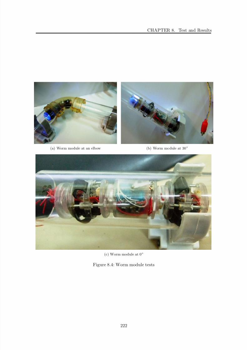
8/21/2019 Alberto Brunete Gonzalez
http://slidepdf.com/reader/full/alberto-brunete-gonzalez 250/311
CHAPTER 8. Test and Results
(a) Worm module at an elbow (b) Worm module at 30
(c) Worm module at 0
Figure 8.4: Worm module tests
222

8/21/2019 Alberto Brunete Gonzalez
http://slidepdf.com/reader/full/alberto-brunete-gonzalez 251/311
8.2. Validation tests
Figure 8.5: Snake-like movement over undulated terrain
8.1.4 Snake-like
The snake-like configuration is the most versatile configuration of all. Its main feature isthat it can be able to move in the free space, i.e. outside pipes. As an example, in fig. 8.5the microrobot is negotiating an undulated terrain.
Another advantage of this configuration is that the robot can use obstacles (like anelbow in a pipe or a corner) to help it to go forward, as in figure 8.6.
8.2 Validation tests
This section shows some experiments aimed to validate the simulation environment by
comparison with the real modules that have been already developed. The experimentscover mainly position, intensity and torque tests.
8.2.1 Servomotor tests
A complete model of the servomotors used has been developed as described in section5.1.2. In order to validate its operation, two tests have been performed with rotationmodules v2, one rising its own weight and another one rising the batteries module of mass13,2g. In both cases the servo has moved from 30to 120and from 90to 30.
Position and intensity have been measured through the A/D converter. The maximum
223
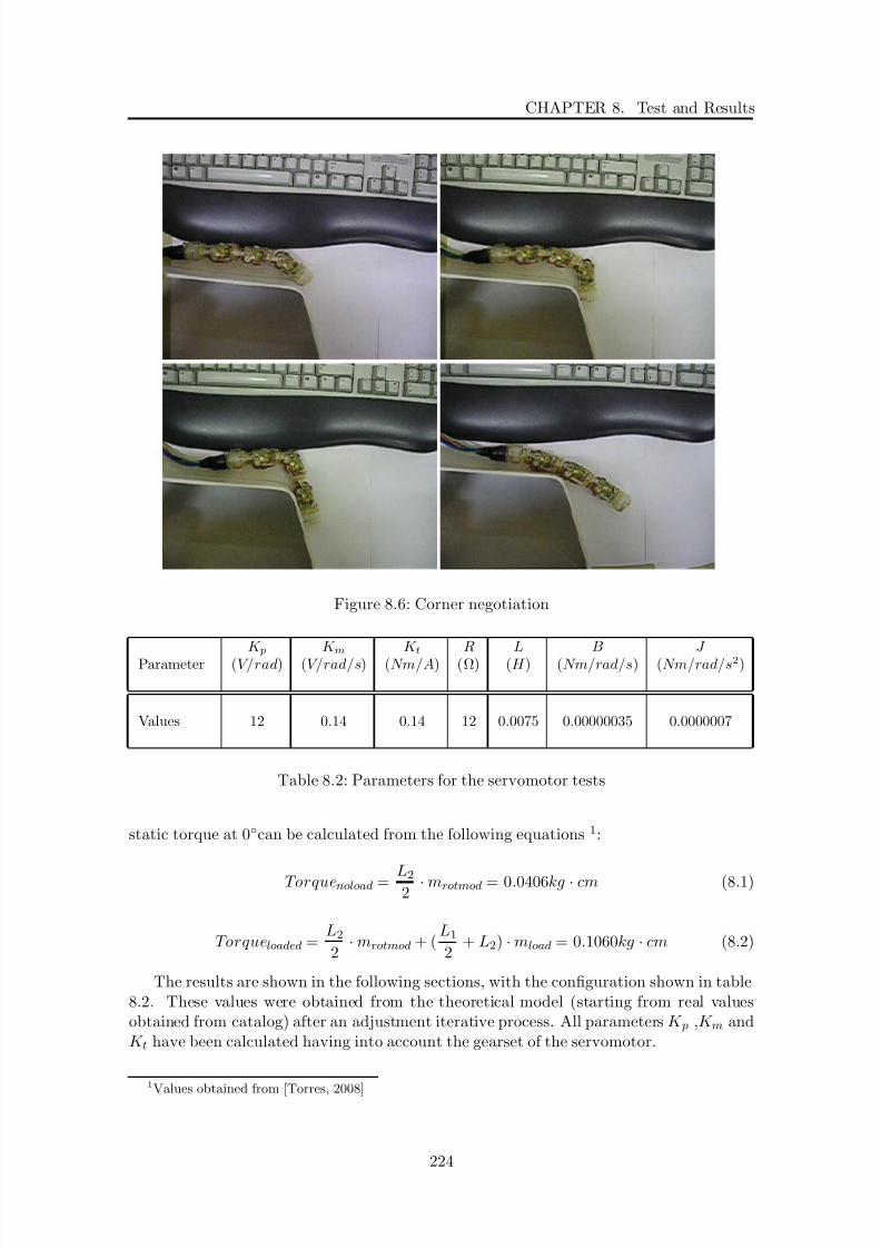
8/21/2019 Alberto Brunete Gonzalez
http://slidepdf.com/reader/full/alberto-brunete-gonzalez 252/311
CHAPTER 8. Test and Results
Figure 8.6: Corner negotiation
K p K m K t R L B J Parameter (V/rad) (V/rad/s) (Nm/A) (Ω) (H ) (Nm/rad/s) (Nm/rad/s2)
Values 12 0.14 0.14 12 0.0075 0.00000035 0.0000007
Table 8.2: Parameters for the servomotor tests
static torque at 0can be calculated from the following equations 1:
Torquenoload = L2
2 · mrotmod = 0.0406kg · cm (8.1)
Torqueloaded = L2
2 · mrotmod + (
L1
2 + L2) · mload = 0.1060kg · cm (8.2)
The results are shown in the following sections, with the configuration shown in table8.2. These values were obtained from the theoretical model (starting from real valuesobtained from catalog) after an adjustment iterative process. All parameters K p ,K m andK t have been calculated having into account the gearset of the servomotor.
1
Values obtained from [Torres, 2008]
224

8/21/2019 Alberto Brunete Gonzalez
http://slidepdf.com/reader/full/alberto-brunete-gonzalez 253/311
8.2. Validation tests
30to 120unloaded
Figure 8.7: 30to 120unloaded: rotation angle
Figure 8.8: 30
to 120
unloaded: intensity
225

8/21/2019 Alberto Brunete Gonzalez
http://slidepdf.com/reader/full/alberto-brunete-gonzalez 254/311
CHAPTER 8. Test and Results
Figure 8.9: 30to 120unloaded: torque
30to 120loaded
Figure 8.10: 30
to 120
loaded: rotation angle
226

8/21/2019 Alberto Brunete Gonzalez
http://slidepdf.com/reader/full/alberto-brunete-gonzalez 255/311
8.2. Validation tests
Figure 8.11: 30to 120loaded: intensity
Figure 8.12: 30
to 120
loaded: tau
227

8/21/2019 Alberto Brunete Gonzalez
http://slidepdf.com/reader/full/alberto-brunete-gonzalez 256/311
CHAPTER 8. Test and Results
90to 30unloaded
Figure 8.13: 90to 30unloaded: rotation angle
Figure 8.14: 90
to 30
unloaded: intensity
228
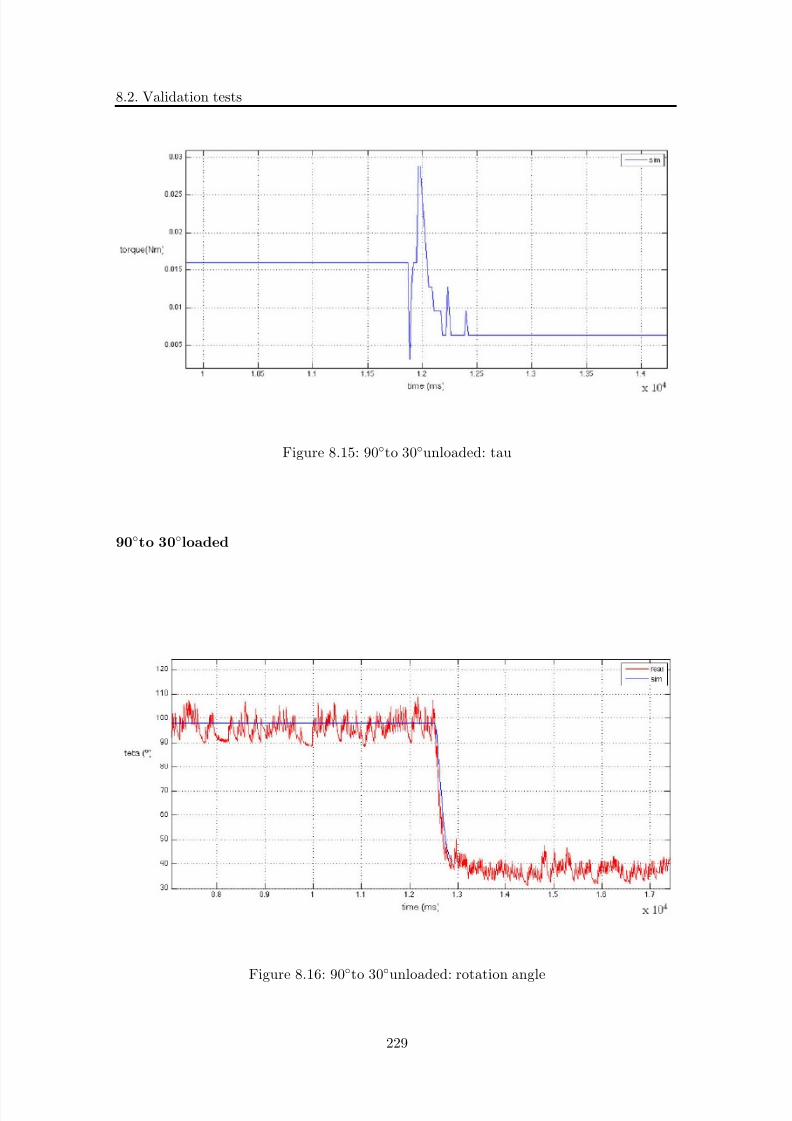
8/21/2019 Alberto Brunete Gonzalez
http://slidepdf.com/reader/full/alberto-brunete-gonzalez 257/311
8.2. Validation tests
Figure 8.15: 90to 30unloaded: tau
90to 30loaded
Figure 8.16: 90
to 30
unloaded: rotation angle
229
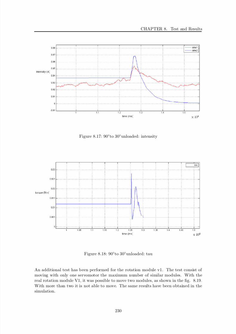
8/21/2019 Alberto Brunete Gonzalez
http://slidepdf.com/reader/full/alberto-brunete-gonzalez 258/311
CHAPTER 8. Test and Results
Figure 8.17: 90to 30unloaded: intensity
Figure 8.18: 90to 30unloaded: tau
An additional test has been performed for the rotation module v1. The test consist of moving with only one servomotor the maximum number of similar modules. With thereal rotation module V1, it was possible to move two modules, as shown in the fig. 8.19.With more than two it is not able to move. The same results have been obtained in the
simulation.
230
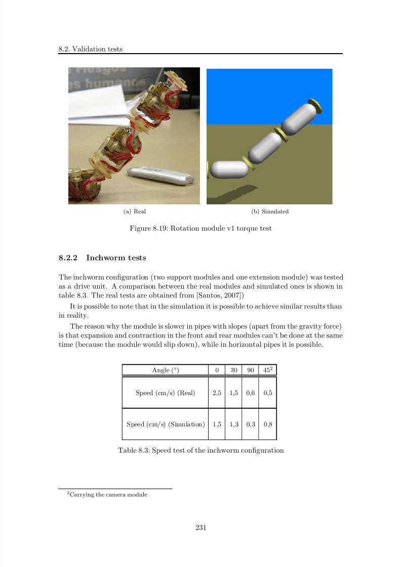
8/21/2019 Alberto Brunete Gonzalez
http://slidepdf.com/reader/full/alberto-brunete-gonzalez 259/311
8.2. Validation tests
(a) Real (b) Simulated
Figure 8.19: Rotation module v1 torque test
8.2.2 Inchworm tests
The inchworm configuration (two support modules and one extension module) was testedas a drive unit. A comparison between the real modules and simulated ones is shown in
table 8.3. The real tests are obtained from [Santos, 2007])It is possible to note that in the simulation it is possible to achieve similar results than
in reality.
The reason why the module is slower in pipes with slopes (apart from the gravity force)is that expansion and contraction in the front and rear modules can’t be done at the sametime (because the module would slip down), while in horizontal pipes it is possible.
Angle () 0 30 90 452
Speed (cm/s) (Real) 2,5 1,5 0,6 0,5
Speed (cm/s) (Simulation) 1,5 1,3 0,3 0,8
Table 8.3: Speed test of the inchworm configuration
2
Carrying the camera module
231
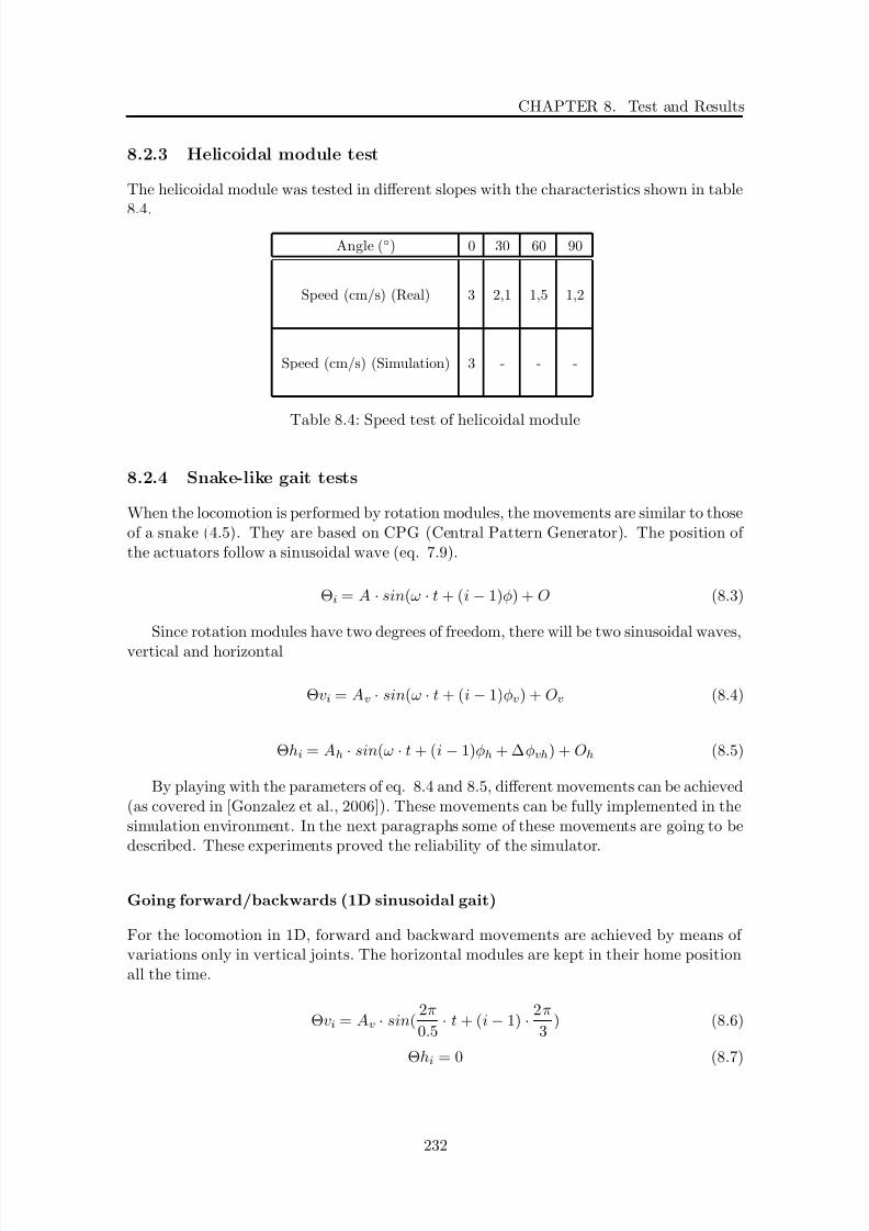
8/21/2019 Alberto Brunete Gonzalez
http://slidepdf.com/reader/full/alberto-brunete-gonzalez 260/311
CHAPTER 8. Test and Results
8.2.3 Helicoidal module test
The helicoidal module was tested in different slopes with the characteristics shown in table
8.4.
Angle () 0 30 60 90
Speed (cm/s) (Real) 3 2,1 1,5 1,2
Speed (cm/s) (Simulation) 3 - - -
Table 8.4: Speed test of helicoidal module
8.2.4 Snake-like gait tests
When the locomotion is performed by rotation modules, the movements are similar to thoseof a snake (4.5). They are based on CPG (Central Pattern Generator). The position of the actuators follow a sinusoidal wave (eq. 7.9).
Θi = A · sin(ω · t + (i − 1)φ) + O (8.3)
Since rotation modules have two degrees of freedom, there will be two sinusoidal waves,
vertical and horizontal
Θvi = Av · sin(ω · t + (i − 1)φv) + Ov (8.4)
Θhi = Ah · sin(ω · t + (i − 1)φh + ∆φvh) + Oh (8.5)
By playing with the parameters of eq. 8.4 and 8.5, different movements can be achieved(as covered in [Gonzalez et al., 2006]). These movements can be fully implemented in thesimulation environment. In the next paragraphs some of these movements are going to bedescribed. These experiments proved the reliability of the simulator.
Going forward/backwards (1D sinusoidal gait)
For the locomotion in 1D, forward and backward movements are achieved by means of variations only in vertical joints. The horizontal modules are kept in their home positionall the time.
Θvi = Av · sin(2π
0.5 · t + (i − 1) ·
2π
3 ) (8.6)
Θhi = 0 (8.7)
232

8/21/2019 Alberto Brunete Gonzalez
http://slidepdf.com/reader/full/alberto-brunete-gonzalez 261/311
8.2. Validation tests
Figure 8.20: 1D sinusoidal movement
Figure 8.21: Turning movement
Turning
The robot can move along an arc, turning left or right. The vertical joints are movingas in 1D sinusoidal gait and the horizontal joints are at fixed position all the time. Therobot has the shape of an arc. The radius of curvature of the trajectory can be modifiedby modifying the offset of the horizontal joints.
Θvi = 60 · sin(2π
0.5 · t + (i − 1) ·
2π
3 ) (8.8)
Θhi = 0 (8.9)
In the example shown in figure 8.21 it has been used a value Θhi = 30. Experimentally,it has been proof that this configuration is able to stand for Θhi > 24. If Θhi < 24 themicrorobot would fall down.
Rolling
The robot can roll around its body axis. The same sinusoidal signal is applied to all thevertical joints and a ninety degrees out of phase sinusoidal signal is applied to horizontal
joints.
233
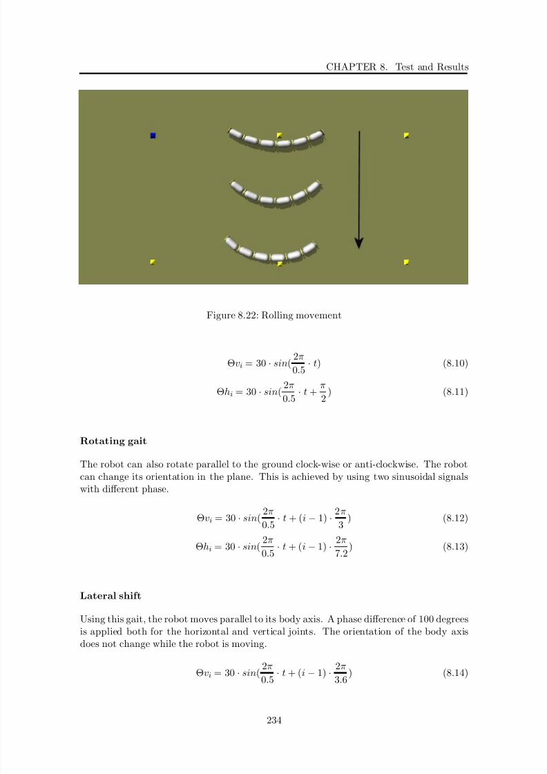
8/21/2019 Alberto Brunete Gonzalez
http://slidepdf.com/reader/full/alberto-brunete-gonzalez 262/311
CHAPTER 8. Test and Results
Figure 8.22: Rolling movement
Θvi = 30 · sin(2π
0.5 · t) (8.10)
Θhi = 30 · sin(2π
0.5 · t +
π
2) (8.11)
Rotating gait
The robot can also rotate parallel to the ground clock-wise or anti-clockwise. The robotcan change its orientation in the plane. This is achieved by using two sinusoidal signalswith different phase.
Θvi = 30 · sin(2π
0.5 · t + (i − 1) ·
2π
3 ) (8.12)
Θhi = 30 · sin( 2π0.5
· t + (i − 1) · 2π7.2
) (8.13)
Lateral shift
Using this gait, the robot moves parallel to its body axis. A phase difference of 100 degreesis applied both for the horizontal and vertical joints. The orientation of the body axisdoes not change while the robot is moving.
Θvi = 30 · sin(
2π
0.5 · t + (i − 1) ·
2π
3.6 ) (8.14)
234

8/21/2019 Alberto Brunete Gonzalez
http://slidepdf.com/reader/full/alberto-brunete-gonzalez 263/311
8.2. Validation tests
Figure 8.23: Rotating movement
Figure 8.24: Lateral shifting movement
235

8/21/2019 Alberto Brunete Gonzalez
http://slidepdf.com/reader/full/alberto-brunete-gonzalez 264/311
CHAPTER 8. Test and Results
Θhi = 30 · sin(2π
0.5 · t + (i − 1) ·
2π
3.6) (8.15)
8.3 Simulation tests
The simulator has been used to carry out several experiments concerning new locomotiongaits combining different types of modules, the performance of the different behaviorsused, the control algorithms and the evolution through the genetic algorithms, amongstothers. In the following subsections these tests are presented.
8.3.1 Locomotion tests
In section 8.2 it has been proven that the simulator is able to successfully simulate the
snake-like, inchworm and helicoidal gaits. In this section new types of movements devel-oped using the simulator are described.
These new types of movements have been achieved by combining all modules in differ-ent ways.
In the experiments, it will be mentioned the use of “passive” modules, meaning moduleswithout drive capabilities. Passive modules will be represented by “battery” or “traveler”modules.
Rotation plus helicoidal modules
Rotation modules can perform several types of snake-like movement. Although thesemovements can be quite fast in open air, inside pipes this movement can be quite slow.By combining rotation modules with helicoidal modules, it is still possible to do snake-likemovements while increasing the speed of movement.
Helicoidal modules push forward trying to make the robot go forward while the rotationmodules perform a snake-like gait that also helps to go forward, reduces the friction (lessparts are touching the pipe) and allow rotations.
The inner diameter chosen for the experiments is usually 36mm. This is enough forrotation modules to negotiate elbows. But when including helicoidal modules in the chain,depending on the position of the helicoidal modules, the robot will be able to negotiatethe elbow or not. In figure 8.25 it is possible to see that for the 36mm diameter the robot
gets stuck in the elbow (a) and b)). With a higher diameter of 40mm, it negotiates theelbow without problems (c) and d)).
But if the helicoidal modules are placed in the front and the back, the robot is able tonegotiate the 36mm elbow, as shown in figure 8.25.
The simulator is very useful to identify the dimensions of the modules to fit in a specificpipe.
Rotation plus passive modules
In section 8.2.4 several movements achieved with the rotation modules have been shown.
This movements can still be performed if there are other modules placed between the
236

8/21/2019 Alberto Brunete Gonzalez
http://slidepdf.com/reader/full/alberto-brunete-gonzalez 265/311
8.3. Simulation tests
Figure 8.25: R+H elbow negotiation
237

8/21/2019 Alberto Brunete Gonzalez
http://slidepdf.com/reader/full/alberto-brunete-gonzalez 266/311
CHAPTER 8. Test and Results
Figure 8.26: R+H elbow negotiation depending on pipe diameter
238

8/21/2019 Alberto Brunete Gonzalez
http://slidepdf.com/reader/full/alberto-brunete-gonzalez 267/311
8.3. Simulation tests
Figure 8.27: Rotation + passive modules in a vertical sinusoidal movement
rotation modules.
In figure 8.27, the importance of the position of the passive modules in the chain canbe observed. In figures a) and b) the movement of the microrobot is almost negligible.However, if the passive modules are placed symmetrically, the robot can perform the samemovement. This is extensible to many snake-like movements.
In figure 8.28 it is possible to observe that the negotiation of elbows depends in animportant way on the overall drive force of the microrobot. In figures a) and b) the robotcomposed of touch, rotation and passive modules gets stuck in an elbow. With the helpof an helicoidal module, in figure c) and d) the microrobot is able to manage the elbow.
Several support plus extension modules
It is possible to combine several support modules to create support units, and severalextension modules to create extension units. After the MDL phase, the CC is able todetect the support and extension modules and to identify support and extension units.
These units can be composed of a different number of modules, from one to several.In figure 8.29 it is possible to see an example of unit composed of 2 modules (a) andb)), three modules (c) and d)) and a combination (e) and f)). In g), an example of twodifferent inchworm drive units working together, to show that modules are aware of theirposition (although this configuration does not work because the support modules of one
unit avoids the movement of the extension module of the other unit).
239

8/21/2019 Alberto Brunete Gonzalez
http://slidepdf.com/reader/full/alberto-brunete-gonzalez 268/311
CHAPTER 8. Test and Results
Figure 8.28: Rotation + passive modules negotiating an elbow with and without helicoidalmodule
240

8/21/2019 Alberto Brunete Gonzalez
http://slidepdf.com/reader/full/alberto-brunete-gonzalez 269/311
8.3. Simulation tests
Figure 8.29: Inchworm locomotion composed of several extension and support modules
241

8/21/2019 Alberto Brunete Gonzalez
http://slidepdf.com/reader/full/alberto-brunete-gonzalez 270/311
CHAPTER 8. Test and Results
Figure 8.30: Example of heterogenous configuration
Rotation plus support plus extension plus helicoidal modules
By combining several types of movements, several types of movements work together:snake-like, worm-like and helicoidal. Each of them fit better for each situation in pipes oropen air.
Figure 8.30 shows an example of the touch, rotation, helicoidal, extension and supportmodules working together and performing simultaneously vertical sinusoidal, helicoidaland worm-like movements.
8.3.2 Control tests
Configuration check
The configuration check phase is used to determine which modules are connected andin which order, as explained in section 7.6.2. This information is used by modules andespecially the CC to specify types of movements and patterns.
This phase starts when the button “PowerUp” is pressed in the simulator, or the
modules are powered up in real life. An example of the results can be seen in picture 8.31.
242

8/21/2019 Alberto Brunete Gonzalez
http://slidepdf.com/reader/full/alberto-brunete-gonzalez 271/311
8.3. Simulation tests
Figure 8.31: Configuration check example
Orientation
For certain movements It is important to keep a specific posture. For example, in thevertical sinusoidal wave movement, if the robot lays down, it is necessary to recover theposition before continue with the vertical sinusoidal move.
In figure 8.32 an example of the performance of the orientation behavior is shown. Ina) it is possible to see that the first degree of freedom is horizontal. In b) the robot makes
an arc, and consequently in falls down as shown in c). Then it puts back straight, leavingthe first degree of freedom vertical.
Wandering
Figures 8.34 and 8.33 show an example of the microrobot executing the “wandering”behavior. This includes going forward and negotiating an elbow when a bifurcation isdetected by the “contact” module.
In the first case (figure 8.34), the micro-robot is composed of one contact and severalrotation modules. The micro-robot goes forward in a snake-like movement (using one of
the DOF). When it reaches the elbow, the micro-robot uses the other DOF of the moduleto make the turn.
In the second case (figure 8.33), the micro-robot is composed of the following modules:one contact, two rotation, one helicoidal, two rotation and one passive. The main driveforce is made by the helicoidal module. The rotation modules help a little bit in goingforward, but their main task is to turn.
Split
If the microrobot is composed of enough modules it may split (at a bifurcation for example)
in order to explore several stretches at the same time.
243

8/21/2019 Alberto Brunete Gonzalez
http://slidepdf.com/reader/full/alberto-brunete-gonzalez 272/311
CHAPTER 8. Test and Results
Figure 8.32: Example of orientation behavior
Figure 8.33: Contact, Rotation, Helicoidal and Passive
244
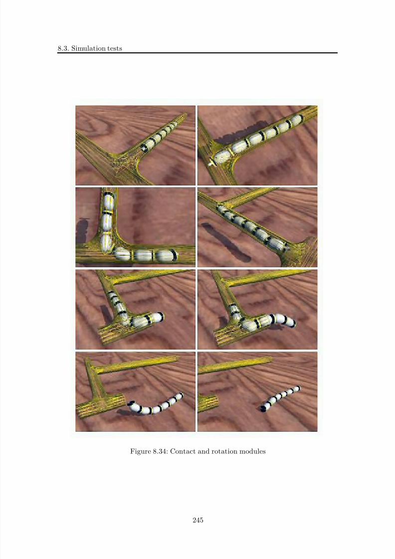
8/21/2019 Alberto Brunete Gonzalez
http://slidepdf.com/reader/full/alberto-brunete-gonzalez 273/311
8.3. Simulation tests
Figure 8.34: Contact and rotation modules
245

8/21/2019 Alberto Brunete Gonzalez
http://slidepdf.com/reader/full/alberto-brunete-gonzalez 274/311
CHAPTER 8. Test and Results
Figure 8.35: Example of chain splitting
Figure 8.35 shown an example of splitting. In a) the robot is a chain composed of 6
modules. In b) it splits in two parts, and in c) each part composed of three modules movesas an independent unit.
246

8/21/2019 Alberto Brunete Gonzalez
http://slidepdf.com/reader/full/alberto-brunete-gonzalez 275/311
Chapter 9
Conclusions and Future Works
“Un libro, como un viaje, se comienza con inquietud y se termina con melancolıa (A book, like a journey, begins with concern and ends with melancholy)”
Jose de Vasconcelos
9.1 Conclusions
Along the previous chapters a description of the work that has been done designing andconstructing an heterogeneous modular multi-configurable chain-type microrobot has beengiven.
Starting from an analysis of the state of the art on modular, pipe inspection andmicrorobotic systems, it has been determined a lack of a microrobotic system as the onedescribed in this thesis. This is the reason that has motivated the start of this thesis.
Several modules have been developed to perform different types of movements (someof them new), and what is more important, a combination of all of them.
A simulator has been developed to go beyond the limits of the mechanical modules andto develop modules with more capacities and abilities. This simulator has been developedover a physics dynamic engine (ODE) to maintain the veracity in all the experiments.The simulator has been tested and validated through comparison with the real modulestests and some examples have been given. New locomotion gaits have been presented andexplained.
On top of all of this, a behavior-based control architecture specifically designed forheterogenous chain-type modular robots has been developed. While inspired by the phi-losophy of reactive control, behavior-based systems are fundamentally more expressive andpowerful, enabling representation, planning, and learning capabilities. Distributed behav-iors are used as the underlying building blocks for these capabilities, allowing behavior-based systems to take advantage of dynamic interactions with the environment rather
than rely solely on explicit reasoning and planning. As the complexity of robots continues
247

8/21/2019 Alberto Brunete Gonzalez
http://slidepdf.com/reader/full/alberto-brunete-gonzalez 276/311
CHAPTER 9. Conclusions and Future Works
to increase, behavior-based principles and their applications in robot architectures andde- ployed systems evolve as well, demonstrating increasingly higher levels of situatedintelligence and autonomy.
Although the architecture is generally behavior-based, it has also a central control thatis model-based and takes decisions for the whole robot and provides behaviors with usefulinformation.
In order to control the modules already designed and some other that may come inthe future, a Module Description Language (MDL) has been developed for the modules tocommunicate their capabilities (push, rotate, extend, measure temperature, sense proxim-ity, etc.).
Another important point in the control architecture is the offline genetic algorithm,that allow the microrobot to optimize the modules layout and its locomotion parametersfor specific tasks.
Finally, some test presenting the results and the feasability of the algorithms have beenincluded.
9.2 Main contributions of the thesis
This thesis presents the following original contributions:
Electromechanical design and construction of an heterogeneous multi-configurable
chain-type microrobot
The main contribution of this thesis lies in its contribution to the chain-type modularmicrorobots with the inclusion of heterogeneous multiconfigurables modules to achievethe combination of different types of movements. As opposed to the literature reviewedin chapter 2, where most of the designs are homogeneous, it has been decided to choose aheterogeneous configuration to allow the inclusion of different types of modules.
A common mechanical interface has been designed to physically connect the modulesand to carry the control signals and the power supply to all modules.
An original mechanism has been presented for the extension module v1.
Control architecture for chain-type heterogenous modular robots
The control architecture is itself, an original contribution, because there is no architecturefor this kind of heterogenous robots. One of the most familiar is the CONRO controlbased in hormones, but it is designed for homogenous modules, not for heterogenous.
The heterogenous agent placed between the embedded control and the central controlis a contribution. Although it is similar to the medium layer in three layers architectures,it is new in the sense that it acts as an interpreter between the CC and different modules.Thus the CC can send global commands to all modules and the heterogenous agent willtranslate them to the modules.
The Module Description Language (MDL) has been especially designed for this archi-
tecture, allowing modules to send their capabilities to the CC.
248

8/21/2019 Alberto Brunete Gonzalez
http://slidepdf.com/reader/full/alberto-brunete-gonzalez 277/311
9.3. Publications and Merits
Several behaviors have been designed, both for the CC and the embedded control. Itis especially new the behaviors related to gait control, since modules can perform severaltypes of movements.
An offline genetic algorithm has been developed to optimize the configuration of thelayout of the modules and its parameters. It has been integrated with the simulator.
Simulation environment for chain-type heterogenous modular robots
The simulation has been a very important part in the thesis, and although similar de-velopments can be found (like in [Salemi et al., 2006]), this one presents a very powerfulmodel of the servomotor model integrated in the physical dynamic simulator based onODE. As in previous points, it is unique in the sense that it allows the simulation of thecombination of heterogenous gaits
The electronic and control simulation, together with the fact that the code written inthe simulator for the modules is ready to be transferred to the real microprocessors (withminor changes) are very important contributions, although not original, and may inspirefuture deigns.
A traveled distance measurement system for chain-type heterogenous robots has beendesigned (the traveler module) based on the combination of several encoders.
Enhancement of the ego-positioning system
The ego-position concept developed for the I-SWARM robots has been enhanced in orderto use different codes (binary, gray) and scales (levels of intensity or grey scales).
Although first conceived for self detection of the position and rotation, the ego-positioningsystem has been enhanced to allow the transmission of commands and the programmingof the robots.
9.3 Publications and Merits
Throughout these years of research, the following publications related to the theses have
been produced.
9.3.1 Publications
Journal Articles
“A Proposal for a Multi-Drive Heterogeneous Modular Pipe-Inspection Micro-robot”. Brunete, A.; Torres, J.; Hernando, M. and Gambao, E. (2008). InternationalJournal of Information Acquisition, Vol.5, Issue 2, pp 111 – 126
249
8/21/2019 Alberto Brunete Gonzalez
http://slidepdf.com/reader/full/alberto-brunete-gonzalez 278/311
CHAPTER 9. Conclusions and Future Works
Book Chapters
“Arquitectura para robots modulares multiconfigurables heterogeneos de tipo
cadena”. Brunete, A.; Torres, J.; Hernando, M. and Gambao, E. (2007). Arquitecturasde control para robots. Escuela Tecnica Superior de Ingenieros Industriales (ETSII), Uni-versidad Politecnica de Madrid (UPM).pp 151–167. ISBN:978-84-7484-196-1.
Conference Proceedings
“Multi-Drive Control for In-Pipe Snakelike Heterogeneous Modular Micro-
Robots”. Brunete, A.; Torres, J.; Hernando, M. and Gambao, E. (2007). Proceedings of the 2007 IEEE International Conference on Robotics and Biomimetics (ROBIO 2007).
“A 2 DoF Servomotor-based Module for Pipe Inspection Modular Micro-robots”. Brunete, A.; Torres, J.; Hernando, M. and Gambao, E. (2006). Proceedings of the 2006 IEEE International Conference on Intelligent Robots and Systems (IROS).
“Solar Powering with Integrated Global Positioning System for mm3 SizeRobots”. Boletis, A.; Brunete, A.; Driesen, W. and Breguet, J. M. (2006). Proceedingsof the 2005 IEEE International Conference on Intelligent Robots and Systems (IROS).
“Multiconfigurable Inspection Robots for Low Diameter Canalizations”.Gambao, E.; Brunete, A. and Hernando, M. (2005). International Symposium on Au-tomation and Robotics in Construction (ISARC).
“Modular Multiconfigurable Architecture for Low Diameter Pipe Inspec-tion Microrobots”. Brunete, A.; Hernando, M. and Gambao, E. (2005) Proceedings of the 2005 IEEE International Conference on Robotics and Automation (ICRA).
“Drive Modules for Pipe Inspection Microrobots”. Brunete, A.; Hernando,M. and Gambao, E. (2004) Proceedings of the 2004 IEEE International Conference on
Mechatronics and Robotics (MECHROB), pp. 925 - 930.
Conference Video Proceedings
“Drive Modules for Low Diameter Pipe Inspection Multiconfigurable Micro-robots”. Brunete, A.; Hernando, M. and Gambao, E. (2006). Video Proceedings of the2006 IEEE International Conference on Robotics and Automation (ICRA)
250

8/21/2019 Alberto Brunete Gonzalez
http://slidepdf.com/reader/full/alberto-brunete-gonzalez 279/311
9.4. Future Work
Conference Poster Sessions
“Drive Modules for Low Diameter Pipe Inspection Multiconfigurable Micro-
robots”. Brunete, A.; Hernando, M. and Gambao, E. (2006). Proceedings of the 2006IEEE International Conference on Robotics and Automation (ICRA)(Poster)
9.3.2 Merits
Nominations to best paper in a conference
“Multi-Drive Control for In-Pipe Snakelike Heterogeneous Modular Micro-Robots”. Brunete, A.; Torres, J.; Hernando, M. and Gambao, E. (2007). Proceedings of the 2007 IEEE International Conference on Robotics and Biomimetics (ROBIO 2007).
Campus de Excelencia
Elected for participacipation in the 2005 Campus de Excelencia, by the ANECA (AgenciaNacional de Evaluacion de la Calidad y Acreditacion), based on the thesis’ interests andmerits.
http://www.campusdeexcelencia.info/index.php
9.4 Future Work
Several ideas that will be researched in the future are:
Embedding of the Central Control in a specific module
In stead of having the central control in a PC, it can be embedded in a specific modulewith a more powerful processor.
Development of new modules
Some ideas regarding new modules are already being considered:
• Centipede: legs can be simulated with piezoelectric actuators (i.e. I-Swarw) orsimilar to [Valdastri et al., 2009]
• Module with two drive wheels (especially for open spaces)
• Newer versions of the modules more robust
• Construction of the modules ”traveler” and ”sensor”
251

8/21/2019 Alberto Brunete Gonzalez
http://slidepdf.com/reader/full/alberto-brunete-gonzalez 280/311
CHAPTER 9. Conclusions and Future Works
Learning of new rules by the Central Control based on the experience acquired
The design of the central control and its inference engine leads in the future to include
learning algorithms to develop new rules online, i.e. while the robot is moving and not inthe simulation (offline).
Coordination between several microrobots
Moving a little bit into the swarm robotics, and interesting line of research would be tohave several microrobots to explore the environment and the way they coordinate to sharetasks out.
Split and rejoining tasks would be of a lot of interest for those purposes.
Visual control
The inclusion of visual control would give the camera module another very interestingsensorial capability to auto-detect obstacles.
252

8/21/2019 Alberto Brunete Gonzalez
http://slidepdf.com/reader/full/alberto-brunete-gonzalez 281/311
Appendix A
Fabrication technologies
A.1 Stereolithography
The stereolithography process was first developed in the field of rapid prototyping, whichwas capable of generating physical parts with features and refinements that made it at-tractive and useful as an aid in the development of new products. The generation systemdiscussed here was patented in 1986 by the company 3Dsystem.
Basically the system relies on the possibility for certain resins, especially designed forit, to solidify when attacked by a laser beam of very specific frequency and power.
As usual in the various rapid prototyping techniques currently existing, aimed at the
generation of physical parts, these parts are made by horizontal laminated of theoreticalgeometry made by 3D design software. Together, all of them should lead to the desiredpiece. The starting point in all cases is a file in STL format.
A.1.1 Part generation mechanics
The work area consists of a vat containing liquid resin, an elevation plate in which thesupport for the parts and the parts themselves are generated, a stabilizing bar, the lasertransmitter and a set of mirrors that enable to project the laser beam precisely on the topsheet of the resin tray where it draws the outline of the different horizontal slices of the
part, as well as the inner padding.
The tray that supports the columns (required for the overhangs of the part not tocollapse at the bottom of the tray) and the part, get down in the resin, immersing thewhole set a distance of typically 0.15mm, which defines the layer hop of the part togenerate. To avoid surface deformations to the top layer that could be caused due tosurface tension of the liquid resin, a stabilizing bar that will ensure a completely flat andsmooth surface is moved over the surface.
At this point, the laser beam is directed by the mirrors to the surface of the resin,drawing the outline and the inner padding to be solidified. This process will be moreor less hardworking in terms of the total area that the laser has to cover. It may be
necessary to stop the process a few seconds to ensure that all resin attacked by the beam
253
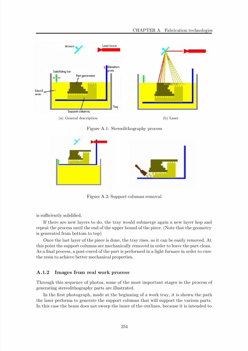
8/21/2019 Alberto Brunete Gonzalez
http://slidepdf.com/reader/full/alberto-brunete-gonzalez 282/311
CHAPTER A. Fabrication technologies
(a) General description (b) Laser
Figure A.1: Stereolithography process
Figure A.2: Support columns removal
is sufficiently solidified.
If there are new layers to do, the tray would submerge again a new layer hop andrepeat the process until the end of the upper bound of the piece. (Note that the geometryis generated from bottom to top)
Once the last layer of the piece is done, the tray rises, so it can be easily removed. At
this point the support columns are mechanically removed in order to leave the part clean.As a final process, a post-cured of the part is performed in a light furnace in order to curethe resin to achieve better mechanical properties.
A.1.2 Images from real work process
Through this sequence of photos, some of the most important stages in the process of generating stereolithography parts are illustrated.
In the first photograph, made at the beginning of a work tray, it is shown the paththe laser performs to generate the support columns that will support the various parts.
In this case the beam does not sweep the inner of the outlines, because it is intended to
254

8/21/2019 Alberto Brunete Gonzalez
http://slidepdf.com/reader/full/alberto-brunete-gonzalez 283/311
A.1. Stereolithography
Figure A.3: Laser trajectory
get a fragile support that is easy to remove later.
In the second picture, the solidification process of the resin has been finalized andtherefore the tray is located in its uppermost position to proceed with removal.
In the next image it is shown the column removal process, in order to release the parts.
They have to be scrupulously cleaned to remove any residue that may contain liquid resin.Finally, in the following pictures, it is shown the post-curing furnace and the parts
inside it.
A.1.3 Advantages, drawbacks and limitations
It may be noted as advantages:
1. It is one of the rapid prototyping techniques more accurate from a dimensional pointof view, making it particularly suitable for parts in which this feature has a special
relevance. As a rule, it is generally considered a good technique to apply in smallparts with many details.
2. The parts obtained are pleasant to touch and sight, can be polished and/or paintwith ease, resulting in excellent surface finishes. They are therefore very suitable tobe used as models, in the case of wanting to subsequently create silicone molds andthen make vacuum casting in materials with similar characteristics to the final ones.
3. The final material is translucent, making it likely to be particularly suitable forcertain sets where you want to appreciate (or at least imply), internal interferences.
And as drawbacks it can be pointed out that, although progress has being made in
the development of new photosensitive resins with better mechanical properties, the most
255

8/21/2019 Alberto Brunete Gonzalez
http://slidepdf.com/reader/full/alberto-brunete-gonzalez 284/311
CHAPTER A. Fabrication technologies
Figure A.4: Solidification process
Figure A.5: Post-cure oven
commonly used are fragile and inflexible, and once cured, the parts are very sensitive toboth humidity (including the atmosphere) and temperature. These two parameters may
easily cause the lost of their mechanical characteristics and suffer dimensional changesover time.
As limitations it is possible to say:
1. The work process of stereolithography causes the different layers of the solidifiedpart to require support columns to avoid collapsing and finishing at the bottom of the tray. These columns should be generated in parts of the part it would be easy toextract from, so that the orientation of the piece in the tray cannot be free. If this isnot taken into account, geometries that are affected by interior columns that cannotbe removed and that make it partially or completely lose their usefulness might have
been generated.
256

8/21/2019 Alberto Brunete Gonzalez
http://slidepdf.com/reader/full/alberto-brunete-gonzalez 285/311
A.2. Micro-milling
Figure A.6: Detail of some parts of the rotation module v1
2. Within the working area of the tray it is possible to place different pieces, but alwaysat the same level. It is not possible, or at least appropriate, try to nest parts oneach other.
3. Although the level of detail is established by the precision set by the layer hop (whichallows for extrusions or indentations on the surfaces), generally is not desirable tomake wall thicknesses below 1 mm because of the fragility of the material. In extremecases, depending on the size of the potential overhang, it is possible to obtain verticalwalls of 0.6 mm and horizontal of 0.8 mm thickness.
A.2 Micro-milling
Micro-milling is a process that becomes more important as sectors such as medicine,telecommunications, and aerospace demand parts increasingly smaller. Unlike what hap-pens with conventional milling, in micro-milling there is a lack of recommendations forprocess operation and cutting conditions selection. One of the tasks in which a lot of research is being done is the development of recommendations obtained by several pro-cedures based on empirical methods, or contrasted with those provided by the limited
literature in this field. Most of the work carried out in this area comes from extrapolat-
257

8/21/2019 Alberto Brunete Gonzalez
http://slidepdf.com/reader/full/alberto-brunete-gonzalez 286/311
CHAPTER A. Fabrication technologies
Figure A.7: Micro-milling system
Figure A.8: Fixation System
ing the knowledge gained in conventional and high speed milling, with the use of verysmall diameter tools on small pieces, as well as defining the needs of measurement andverification procedures in this type of parts.
The micro-milling imposes restrictions on the machines and tooling used:
1. The machines should be equipped with high speed cutting spindles to reach theappropriate cutting speed with the small dimension tools used.
2. Due to the small part dimensions, it is required a very accurate axis positioning.
3. The fastening of the part is a new challenge to be solved, given the lack of fasteningsystems adapted to the new sizes similar to the conventional ones.
The achievable dimensional characteristics will be limited by the minimum size of theavailable tool. In known commercial tools (named sintering carbide microgram), those
dimensions are on the order of 20 µm.
258
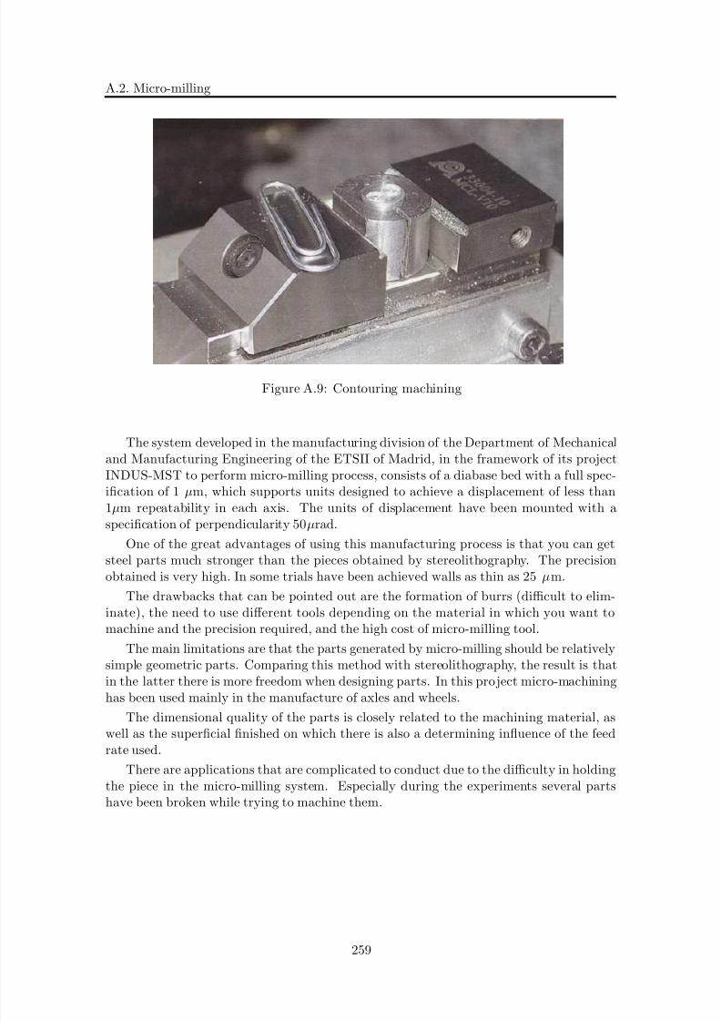
8/21/2019 Alberto Brunete Gonzalez
http://slidepdf.com/reader/full/alberto-brunete-gonzalez 287/311
A.2. Micro-milling
Figure A.9: Contouring machining
The system developed in the manufacturing division of the Department of Mechanicaland Manufacturing Engineering of the ETSII of Madrid, in the framework of its projectINDUS-MST to perform micro-milling process, consists of a diabase bed with a full spec-ification of 1 µm, which supports units designed to achieve a displacement of less than1µm repeatability in each axis. The units of displacement have been mounted with aspecification of perpendicularity 50µrad.
One of the great advantages of using this manufacturing process is that you can getsteel parts much stronger than the pieces obtained by stereolithography. The precisionobtained is very high. In some trials have been achieved walls as thin as 25 µm.
The drawbacks that can be pointed out are the formation of burrs (difficult to elim-inate), the need to use different tools depending on the material in which you want tomachine and the precision required, and the high cost of micro-milling tool.
The main limitations are that the parts generated by micro-milling should be relativelysimple geometric parts. Comparing this method with stereolithography, the result is thatin the latter there is more freedom when designing parts. In this project micro-machininghas been used mainly in the manufacture of axles and wheels.
The dimensional quality of the parts is closely related to the machining material, aswell as the superficial finished on which there is also a determining influence of the feedrate used.
There are applications that are complicated to conduct due to the difficulty in holdingthe piece in the micro-milling system. Especially during the experiments several partshave been broken while trying to machine them.
259

8/21/2019 Alberto Brunete Gonzalez
http://slidepdf.com/reader/full/alberto-brunete-gonzalez 288/311
CHAPTER A. Fabrication technologies
Figure A.10: Helicoidal module leg generated by micromachining
260
8/21/2019 Alberto Brunete Gonzalez
http://slidepdf.com/reader/full/alberto-brunete-gonzalez 289/311
Appendix B
Terms and Concepts
Robustness
The ability to handle imperfect inputs, unexpected events and sudden malfunctions.
Reliability
The ability to operate without failures or performance degradation over a certain period.
Modularity
The ability of control system of autonomous vehicles to be divided into smaller subsystems(or modules) that can be separately and incrementally designed, implemented, debuggedand maintained.
Flexibility
Experimental robotics require continuous changes in the design during the implementationphase. Therefore, flexible control structures are required to allow the design to be guidedby the success or failure of the individual elements.
Expandability
A long time is required to design, build and test the individual components of a robot.Therefore, an expandable architecture is desirable in order to be able to build the systemincrementally.
Adaptability
As the state of the world changes very rapidly and unpredictably, the control system must
be adaptable in order to switch smoothly and rapidly between different control strategies.
261

8/21/2019 Alberto Brunete Gonzalez
http://slidepdf.com/reader/full/alberto-brunete-gonzalez 290/311
CHAPTER B. Terms and Concepts
Classification of Modular Robots
Modular robotic systems can be generally classified into several architectural groups by
the geometric arrangement of their unit (lattice vs. chain). Several systems exhibit hybridproperties.
• Lattice architectures have units that are arranged and connected in some regular,space-filling three-dimensional pattern, such as a cubical or hexagonal grid. Con-trol and motion are executed in parallel. Lattice architectures usually offer simplercomputational representation that can be more easily scaled to complex systems.
• Chain/tree architectures have units that are connected together in a string or treetopology. This chain or tree can fold up to become space filling, but underlyingarchitecture is serial. Chain architectures can reach any point in space, and aretherefore more versatile but more computationally difficult to represent and analyze.
Tree architectures may resemble a bush robot
Modularity and Reconfigurability
Modularity is a general systems concept, typically defined as a continuum describing thedegree to which a system components may be separated and recombined. It refers to boththe tightness of coupling between components, and the degree to which the rules of thesystem architecture enable (or prohibit) the mixing and matching of components.
Modular robots are composed of different copies of simple modules. Modules can’tdo much by themselves, but when many of them are connected together, a system that
can do complicated things appears. In fact, a modular robot can even be reconfigured indifferent ways to meet the demands of different tasks or different working environments.Each module is virtually a robot in itself having a computer, a motor, sensors and theability to attach to other modules.
Multiconfigurability vs self-reconfigurability
Reconfigurable robots present the ability to change its configuration either manually orautonomously. If the reconfiguration is done autonomously, it is called self-reconfiguration.On the other hand, if the reconfiguration has to be done manually, we talk about multi-configuration. Modules attach together to form chains (which can be used like an arm, a
leg or a finger), caterpillar, double-thread caterpillar, wheel, 4/6 leg walker, sidewinder,spider, etc.
In the development of inpipe robots, autoconfigurability is not an essential charac-teristic due to the lack of space inside the tube to change configuration. It is betterto talk about multiconfiguration: the robot presents different configurations prior taskdevelopment. Once the task is started, the configuration must be kept.
Homogeneous vs Heterogeneous modules
Depending on the type of modules that the robot is compound of, the robot can be
classified in homogeneous (all the modules are the same) and heterogeneous (different
262

8/21/2019 Alberto Brunete Gonzalez
http://slidepdf.com/reader/full/alberto-brunete-gonzalez 291/311
modules). Modular robots can be defined as in [Yim et al., 2001] as a n-modular robots,being n the number of different modules. The main advantage of homogeneous robotsis that they are easy to build. On the contrary they are limited in the movement gaits.
Heterogeneous robots are more versatile and can perform other tasks and several movementgaits.
Miniaturization
The term microrobot appears nowadays in many articles referring to mini-robots, robotsof very small dimensions (millimeters). This is because we are still far from seeing areal ’micro’ robot (µm). Keeping in mind that for most of the researches it is not pos-sible to build a real microrobot, it is necessary to miniaturize its components and tomake the mechanical and electronic design together to minimize the space (mechatronics).This work is what has been carried out, and it is what makes the design so expensive.Miniaturization can be seen in many microrobots too, as in the microrobot of DENSOCorporation [Nishikawa et al., 1999], the Micro Modular Robot of AIST [Yoshida et al.,2002], and the three microrobots of the French CNRS: LMS, LAB and LAI [Anthierenset al., 2000]. SMAs are extensively used in microrobots because they give a good torque insmall displacements. It is used for example in the former robots. Polybot and M-TRANuse shape memory alloy as latches and docking of modules together with infrared emittersand detectors aid. SMAs could be very useful too for grippers and connecting pads. Themain disadvantage is the great power consumption.
Energy supply
Energy supply is a big problem in mobile microrobots because the available suppliedpower is very limited. Most of developers adopt batteries or cable as the solution totransfer power supply to the robot. In autonomous micro-robots the solution is limitedto onboard batteries. A very innovative solution is presented by DENSO Corporation,which has solved this problem in its Microrobot [Nishikawa et al., 1999] by developing awireless energy supply system (together with a low power consumed actuator, high efficientenergy conversion device and power management system). The microrobot functions as acomplete wireless link system traveling in small pipes at 10mm per second with wirelessdata communication of 2.5Mbps and wireless energy supply of 480mW. It includes devicessuch as CCD camera, locomotive actuator, control circuit, wireless energy supply device,
and RF circuit installed into a small body of 10mm diameter and 50mm length. To sendenergy through radio frequency is a very interesting solution but it is limited to low powerdevices.
Centralized vs Distributed control
Generally most of the robots use centralized control: one agent (PC, one of the modules)tells every module what it has to do in every moment. A distributed system is a collectionof (probably heterogeneous) automata whose distribution is transparent to the user sothat the system appears as one local machine. It is possible to consider the microrobot as
a distributed system, in which every module do their job but it looks like a whole entity
263

8/21/2019 Alberto Brunete Gonzalez
http://slidepdf.com/reader/full/alberto-brunete-gonzalez 292/311
CHAPTER B. Terms and Concepts
to an external observer. This is the case of M-TRAN: the robot motion is controlled byall the modules CPUs. Either if it is a PC (as it is now) or one of the modules (in thefuture), a great intelligence centralized control makes the control much more powerful and
easy to implement.
Statically Stable Locomotion
Locomotion is defined to be the act or power of moving from place to place. Staticallystable locomotion has the added constraint that the moving body be stable at all times.In other words, if the body were to instantaneously stop all motion, the body would stillbe standing. More specifically, the vertical projection of the center of gravity will becontained within the convex hull of the body’s points of contact with the ground at alltimes.
Gaits
A gait is defined to be one cycle of a repeated pattern of motion that is used to move fromone place to another. Simple gaits are those which cannot be broken down into separategaits. This is as opposed to compound gaits which are combinations of simple gaits. Oneexample of two simple gaits being combined into a compound gait is a (1) person walking,(2) a small toy 4-wheeled car, (1+2) a person roller skating.
Servomotors
Servomotors are a special type of motor characterized by their ability to position imme-diately in any position within its operating range.
Servos are composed of an electric motor mechanically linked to a potentiometer.Pulse-width modulation (PWM) signals sent to the servo are translated into position com-mands by electronics inside the servo. When the servo is commanded to rotate, the motoris powered until the potentiometer reaches the value corresponding to the commandedposition.
Due to their affordability, reliability, and simplicity of control by microprocessors, RCservos are often used in small-scale robotics applications.
The servo is controlled by three wires: ground (usually black/orange), power (red) andcontrol (brown/other color). This wiring sequence is not true for all servos, for example theS03NXF Std. Servo is wired as brown (negative), red (positive) and orange (signal). Theservo will move based on the pulses sent over the control wire, which set the angle of theactuator arm. The servo expects a pulse every 20 ms in order to gain correct informationabout the angle. The width of the servo pulse dictates the range of the servo’s angularmotion.
A servo pulse of 1.5 ms width will set the servo to its ”neutral” position, or 90 . Forexample a servo pulse of 1.25 ms could set the servo to 0 and a pulse of 1.75 ms could setthe servo to 180. The physical limits and timings of the servo hardware varies betweenbrands and models, but a general servo’s angular motion will travel somewhere in the
range of 180
- 210
and the neutral position is almost always at 1.5 ms.
264
8/21/2019 Alberto Brunete Gonzalez
http://slidepdf.com/reader/full/alberto-brunete-gonzalez 293/311
I 2C
I 2C (Inter-Integrated Circuit) is a multi-master serial computer bus invented by Philips
that is used to attach low-speed peripherals to a motherboard, embedded system, orcellphone.
I 2C uses only two bidirectional open-drain lines, Serial Data (SDA) and Serial Clock(SCL), pulled up with resistors. Typical voltages used are +5 V or +3.3 V althoughsystems with other, higher or lower, voltages are permitted.
The I 2C reference design has a 7-bit address space with 16 reserved addresses, so amaximum of 112 nodes can communicate on the same bus. The most common I 2C busmodes are the 100 kbit/s standard mode and the 10 kbit/s low-speed mode, but clockfrequencies down to DC are also allowed. Recent revisions of I 2C can host more nodesand run faster (400 kbit/s Fast mode, 1 Mbit/s Fast mode plus or Fm+, and 3.4 Mbit/sHigh Speed mode), and also support other extended features, such as 10-bit addressing.
The reference design, as mentioned above, is a bus with a clock (SCL) and data (SDA)lines with 7-bit addressing. The bus has two roles for nodes: master and slave:
• Master node: node that issues the clock and addresses slaves
• Slave node: node that receives the clock line and address.
The bus is a multi-master bus which means any number of master nodes can be present.Additionally, master and slave roles may be changed between messages (after a STOP issent).
265

8/21/2019 Alberto Brunete Gonzalez
http://slidepdf.com/reader/full/alberto-brunete-gonzalez 294/311
CHAPTER B. Terms and Concepts
266
8/21/2019 Alberto Brunete Gonzalez
http://slidepdf.com/reader/full/alberto-brunete-gonzalez 295/311
Appendix C
Equipment used
C.1 Hardware
Dimax U2C-12 card
The Dimax U2C-12 (fig. C.1), all-in-one USB-I2C, USB-SPI and USB-GPIO Bridge de-vice, converts PC USB transactions to the I2C Master, SPI Master transactions and GPIOfunctions. U2C-12 turns the PC running Windows, Linux or MacOS into acomprehensiveI2C/SPI Bus master.
GTP USB Lite Programmer
GTP USB Lite is a simple USB based PIC programmer that is capable of programmingalmost any type of PIC till date, with good software support (winpic800) on the PC side.
Communication Box
The communication box (fig. C.2) is a device that has been build in order to integrate all
necessary equipment to run the microrobot, including:
• 5V power supply
• Dimax U2C-12 card
• GTP USB Lite Programmer
A box has been designed integrating all of these elements, so it is easy to connect to
the robot, download software and send commands.
267
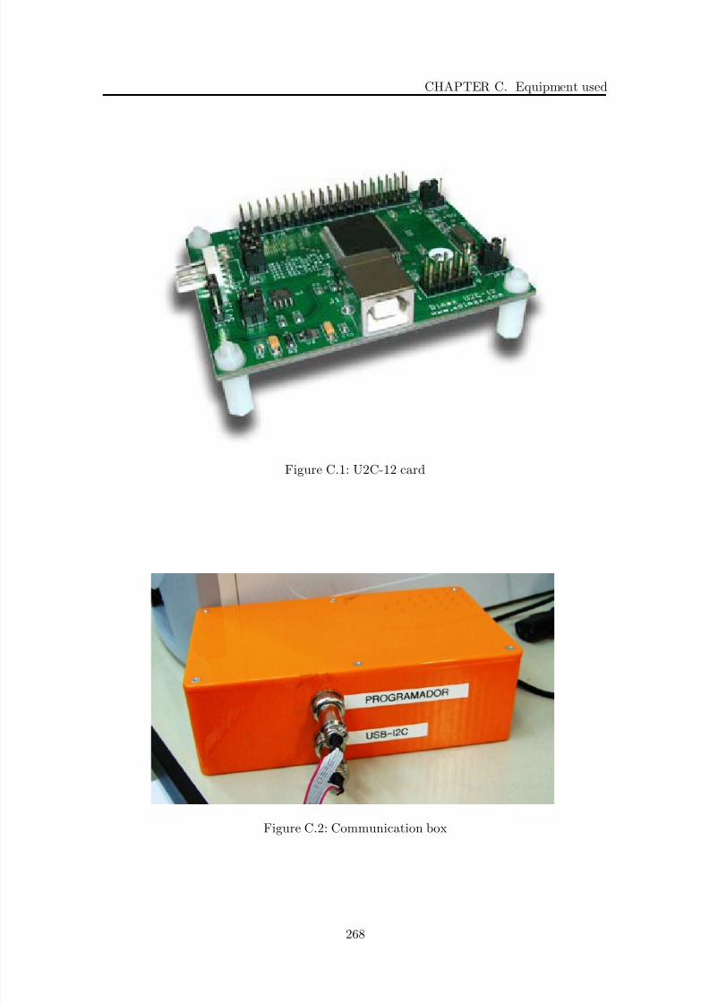
8/21/2019 Alberto Brunete Gonzalez
http://slidepdf.com/reader/full/alberto-brunete-gonzalez 296/311
CHAPTER C. Equipment used
Figure C.1: U2C-12 card
Figure C.2: Communication box
268
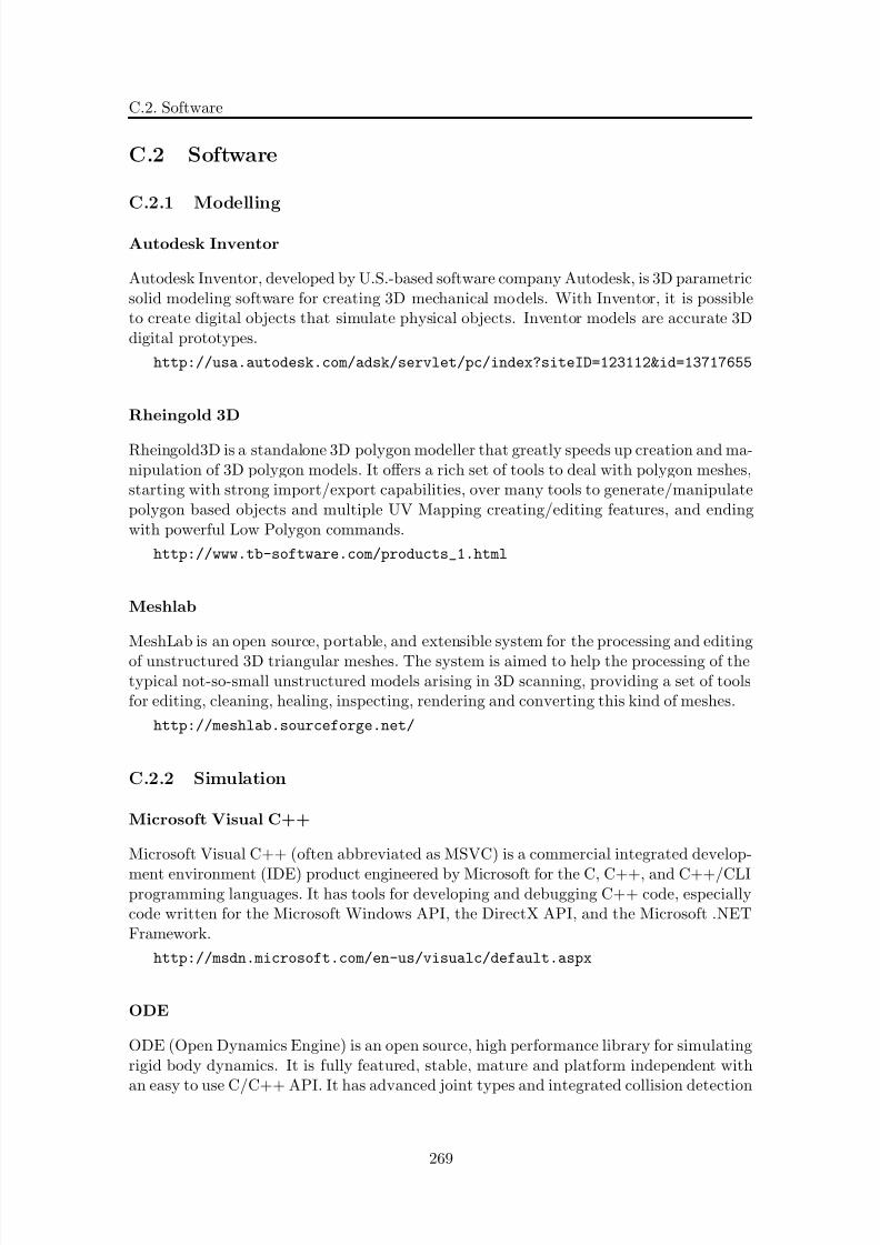
8/21/2019 Alberto Brunete Gonzalez
http://slidepdf.com/reader/full/alberto-brunete-gonzalez 297/311
C.2. Software
C.2 Software
C.2.1 Modelling
Autodesk Inventor
Autodesk Inventor, developed by U.S.-based software company Autodesk, is 3D parametricsolid modeling software for creating 3D mechanical models. With Inventor, it is possibleto create digital objects that simulate physical objects. Inventor models are accurate 3Ddigital prototypes.
http://usa.autodesk.com/adsk/servlet/pc/index?siteID=123112&id=13717655
Rheingold 3D
Rheingold3D is a standalone 3D polygon modeller that greatly speeds up creation and ma-nipulation of 3D polygon models. It offers a rich set of tools to deal with polygon meshes,starting with strong import/export capabilities, over many tools to generate/manipulatepolygon based objects and multiple UV Mapping creating/editing features, and endingwith powerful Low Polygon commands.
http://www.tb-software.com/products_1.html
Meshlab
MeshLab is an open source, portable, and extensible system for the processing and editing
of unstructured 3D triangular meshes. The system is aimed to help the processing of thetypical not-so-small unstructured models arising in 3D scanning, providing a set of toolsfor editing, cleaning, healing, inspecting, rendering and converting this kind of meshes.
http://meshlab.sourceforge.net/
C.2.2 Simulation
Microsoft Visual C++
Microsoft Visual C++ (often abbreviated as MSVC) is a commercial integrated develop-
ment environment (IDE) product engineered by Microsoft for the C, C++, and C++/CLIprogramming languages. It has tools for developing and debugging C++ code, especiallycode written for the Microsoft Windows API, the DirectX API, and the Microsoft .NETFramework.
http://msdn.microsoft.com/en-us/visualc/default.aspx
ODE
ODE (Open Dynamics Engine) is an open source, high performance library for simulatingrigid body dynamics. It is fully featured, stable, mature and platform independent with
an easy to use C/C++ API. It has advanced joint types and integrated collision detection
269

8/21/2019 Alberto Brunete Gonzalez
http://slidepdf.com/reader/full/alberto-brunete-gonzalez 298/311
CHAPTER C. Equipment used
with friction. ODE is useful for simulating vehicles, objects in virtual reality environmentsand virtual creatures. It is currently used in many computer games, 3D authoring toolsand simulation tools.
http://www.ode.org/ and http://opende.sourceforge.net/wiki
MATLAB
MATLAB is a numerical computing environment and fourth-generation programming lan-guage. Developed by The MathWorks, MATLAB allows matrix manipulation, plotting of functions and data, implementation of algorithms, creation of user interfaces, and inter-facing with programs in other languages. Although it is numeric only, an optional toolboxuses the MuPAD symbolic engine, allowing access to computer algebra capabilities. Anadditional package, Simulink, adds graphical multidomain simulation and Model-Based
Design for dynamic and embedded systems.It has been used in this thesis for the validation part, for data management and figure
development of the modules’ servomotors variables intensity, torque and angle position.
http://www.mathworks.com/products/matlab/
C.2.3 Microchip programming
MPLAB
MPLAB Integrated Development Environment (IDE) is a free, integrated toolset for thedevelopment of embedded applications employing Microchip’s PIC¨ and dsPIC¨ micro-controllers. MPLAB IDE runs as a 32-bit application on MS Windows¨, is easy to use andincludes a host of free software components for fast application development and super-charged debugging. MPLAB IDE also serves as a single, unified graphical user interfacefor additional Microchip and third party software and hardware development tools. Mov-ing between tools is a snap, and upgrading from the free software simulator to hardwaredebug and programming tools is done in a flash because MPLAB IDE has the same userinterface for all tools.
As a C compiler has been used PIC-C Compiler.
http://www.microchip.com
C.2.4 Editing
LATEX
LaTeX is a document markup language and document preparation system for the Textype- setting program. Within the typesetting system, its name is styled as LATEX.
LaTeX is most widely used by mathematicians, scientists, engineers, philosophers,economists and other scholars in academia and the commercial world, and other profes-sionals. As a primary or intermediate format, LaTeX is used because of the high qualityof typesetting achievable by TeX. The typesetting system offers programmable desktop
publishing features and extensive facilities for automating most aspects of typesetting and
270

8/21/2019 Alberto Brunete Gonzalez
http://slidepdf.com/reader/full/alberto-brunete-gonzalez 299/311
C.2. Software
desktop publishing, including numbering and cross-referencing, tables and figures, pagelayout and bibliographies.
LaTeX is intended to provide a high-level language that accesses the power of TeX.
LaTeX essentially comprises a collection of TeX macros and a program to process LaTeXdocuments. Because the TeX formatting commands are very low-level, it is usually muchsimpler for end-users to use LaTeX.
LaTeX was originally written in the early 1980s by Leslie Lamport at SRI International.It has become the dominant method for using TeX -relatively few people write in plainTeX anymore.
The term LaTeX refers only to the language in which documents are written, not tothe editor used to write those documents. In order to create a document in LaTeX, a.tex file must be created using some form of text editor. While most text editors can beused to create a LaTeX document, a number of editors have been created specifically for
working with LaTeX.For the writing of this theses two programs have been used: TexShop and MacTEX(for
Mac) and TexnicCenter and MikTEX (for Windows).
http://www.uoregon.edu/ ~koch/texshop/
http://www.tug.org/mactex/2009/
http://www.texniccenter.org/
http://miktex.org/
JabRef
JabRef is an open source bibliography reference manager. The native file format used byJabRef is BibTeX, the standard LaTeX bibliography format. JabRef runs on the Java VM(version 1.5 or newer), and should work equally well on Windows, Linux and Mac OS X.
BibTeX is an application and a bibliography file format written by Oren Patashnikand Leslie Lamport for the LaTeX document preparation system.
Bibliographies generated by LaTeX and BibTeX from a BibTeX file can be formattedto suit any reference list specifications through the use of different BibTeX style files.
http://jabref.sourceforge.net/
CamStudio
CamStudio is a screencasting program for Microsoft Windows released as free software.The software renders videos in an AVI format. It can also convert these AVIs into FlashVideo format, embedded in SWF files. CamStudio is coded in Microsoft Visual C++.
It has been mainly used for recording videos from the simulator environment.
http://camstudio.org/
271

8/21/2019 Alberto Brunete Gonzalez
http://slidepdf.com/reader/full/alberto-brunete-gonzalez 300/311
CHAPTER C. Equipment used
272
8/21/2019 Alberto Brunete Gonzalez
http://slidepdf.com/reader/full/alberto-brunete-gonzalez 301/311
Glossary
ACM Active Cord Mechanism, 35
ASM Action-Selection Mechanisms, 55
CAMPOUT Control Architecture forMulti-robot Planetary Outposts, 66
CAN Controller Area Network, 80
CC Central Control, 117
CEBOT Cellular Robotic System, 10
CHOBIE Cooperative Hexahedral Ob- jects for Building with Intelligent En-hancement, 24
CPG Central Pattern Generator, 37
DAMN Distributed Architecture for Mo-bile Navigation, 64
DD&P Dual Dynamics & Planning, 76
dof Degree of Freedom, 94
EGO-positioning Auto-positioning Sys-tem, 163
FSA Finite State Automata, 52
GA Genetic Algorithms, 82, 128
HLC High Level Commands, 120
I-SWARM Intelligent Small-World Au-tonomous Robots for Micro-manipulation, 164
I 2C Inter-Integrated Circuit, 109, 110, 117,119, 135, 141, 205
Inference Engine Inference Engine, 123
LLC Low Level Commands, 119
M-TRAN Modular TRANsformer, 14
MAAM Molecule Atom Atom Molecule,26
MDCN Massively Distributed ControlNets, 80
MDL Module Description Language, 117
ODE Open Dynamics Engine, 135
RL Reinforcement Learning, 81
SMA Shape Memory Alloy, 30, 31, 34
SR Stimulus response, 51
273

8/21/2019 Alberto Brunete Gonzalez
http://slidepdf.com/reader/full/alberto-brunete-gonzalez 302/311
Glossary
274

8/21/2019 Alberto Brunete Gonzalez
http://slidepdf.com/reader/full/alberto-brunete-gonzalez 303/311
Bibliography
[fos, ] Fostermiler: http://www.foster-miler.com/.
[nor, ] Northstar: http://www.evolution.com/products/northstar/.
[Albus et al., 1988] Albus, J., Lumia, R., and McCain, H. (1988). Hierarchical controlof intelligent machines applied to space station telerobots. IEEE Transactions on Aerospace and Electronic Systems,, 24(5):535 – 541.
[Andersen et al., 1992] Andersen, C. S., Christensen, H. I., Kirkeby, N. O. S., Knudsen,L. F., and Madsen, C. B. (1992). Vinav, a system for vision supported navigation.In Christensen, H. I., editor, Proceedings Nordic Summer School on Active Vision and Geometric Modeling, Aalborg, 1992 , pages 251–257. Laboratory of Image Analysis.
[Anthierens et al., 2000] Anthierens, C., Libersa, C., Touaibia, M., Betemps, M., Arsi-cault, M., and Chaillet, N. (2000). Micro robots dedicated to small diameter canaliza-tion exploration. In Proceedings of the 2000 IEEE/RSJ International Conference on
Intelligent Robots and Systems , pages 480–485.
[Arkin, 1987] Arkin, R. (1987). Motor schema based navigation for a mobile robot: Anapproach to programming by behavior. In IEEE International Conference on Robotics and Automation , volume 4, pages 264 – 271.
[Arkin, 1998] Arkin, R. C. (1998). Behavior-Based Robotics . MIT Press.
[Arkin and Balch, 1997] Arkin, R. C. and Balch, T. (1997). Aura: Principles and practicein review. Journal of Experimental and Theoretical Artificial Intelligence , 9:175–189.
[Bahl and Padmanabhan, 2000] Bahl, P. and Padmanabhan, V. (2000). Radar: An in-
building rf-based user location and tracking system. In IEEE Proceedings of Infocom ,pages 775 – 784, IEEE CS Press, Los Alamitos, Calif.
[Bonasso et al., 1995] Bonasso, R. P., Kortenkamp, D., Miller, D. P., and Slack, M. (1995).Experiences with an architecture for intelligent, reactive agents. Journal of Experimental and Theoretical Artificial Intelligence , 9:237–256.
[Brener et al., 2004] Brener, N., BenAmar, F., and Bidaud, P. (2004). Analysis of self-reconfigurable modular systems: a design proposal for multi-modes locomotion. In IEEE International Conference on Robotics and Automation , volume 1, pages 996–1001.
[Brooks, 1986] Brooks, R. A. (1986). A robust layered control system for a mobile robot.
IEEE Journal of Robotics and Automation , 2(1):14–23.
275

8/21/2019 Alberto Brunete Gonzalez
http://slidepdf.com/reader/full/alberto-brunete-gonzalez 304/311
BIBLIOGRAPHY
[Brunete et al., 2005] Brunete, A., Hernando, M., and Gambao, E. (2005). Modular mul-ticonfigurable architecture for low diameter pipe inspection microrobots. In Proceed-ings of the 2005 IEEE International Conference on Robotics and Automation (ICRA),
Barcelona, Spain.
[Butler et al., 2004] Butler, Z., Kotay, K., Rus, D., and Tomita, K. (2004). Generic de-centralized locomotion control for lattice-based self-reconfigurable robots. Intl. Journal of Robotics Research , 23(9):919–937.
[Caprari, 2003] Caprari, G. (2003). Autonomous Microrobots: Applications and Limita-tions . PhD thesis, ECOLE POLYTECHNIQUE FEDERALE DE LAUSANNE.
[Chen, 1994] Chen, M. (1994). Theory and Applications of Modular Reconfigurable Robotic Systems . PhD thesis, Division of Engineering and Applied Science, California Instituteof Technology, Pasadena, CA, USA.
[Chirikjian, 1994] Chirikjian, G. S. (1994). Kinematics of a metamorphic robotic system.In Proceedings of the 1994 IEEE International Conference on Robotics and Automation ,pages 449–455.
[Conradt and Varshavskaya, 2003] Conradt, J. and Varshavskaya, P. (2003). Distributedcentral pattern generator control for a serpentine robot. In Proceedings of the Interna-tional Conference on Artificial Neural Networks (ICANN), pages 338 – 341, Istanbul,Turkey.
[Cox and Wilfong, 1990] Cox, I. J. and Wilfong, G. T. (1990). The stanford cart and thecmu rover. Autonomous Robot Vehicles , 1:407–419.
[Dardari and Conti, 2004] Dardari, D. and Conti, A. (2004). A sub-optimal hierarchicalmaximum likelihood algorithm for collaborative localization in ad-hoc networks. InFirst Annual IEEE Communications Society Conference on Sensor and Ad Hoc Com-munications and Networks , pages 425 – 429.
[Darrell et al., 1998] Darrell, T., Gordon, G., Harville, M., and Woodfill, J. (1998). Inte-grated person tracking using stereo, color, and pattern detection. In Proceedings of the Conference on Computer Vistion and Pattern Recognition , pages 601 – 609.
[del Monte Garrido, 2004] del Monte Garrido, S. (2004). Diseno y construccion del modulotractor de un microrobot para inspeccion de tuberias. Master’s thesis, E.T.S.I.I. - UPM.
[Denavit and Hartenberg, 1955] Denavit, J. and Hartenberg, R. (1955). A kinematic no-tation for lower-pair mechanisms based on matrices. Transactions of the ASME Journal of Applied Mechanisms , 23:215–221.
[Eltaher et al., 2005] Eltaher, A., Ghalayini, I., and Kaiser, T. (2005). Towards uwb self-positioning systems for indoor environments based on electric field polarization, signalstrength and multiple antennas 5-7 sept. 2005 page(s):. In 2nd International Symposium on Wireless Communication Systems , pages 389 – 393.
[Flynn, 1987] Flynn, A. M. (1987). Gnat robots (and how they will change robotics. In
Proceedings of the IEEE Micro Robots and Teleoperators Workshop, Hyannis, MA.
276
8/21/2019 Alberto Brunete Gonzalez
http://slidepdf.com/reader/full/alberto-brunete-gonzalez 305/311
BIBLIOGRAPHY
[Fukuda and Kawauchi, 1990] Fukuda, T. and Kawauchi, Y. (1990). Cellular robotic sys-tem(cebot) as one of the realization of self-organizing intelligent universal manipulator.In Proceedings of the 1990 IEEE International Conference on Robotics and Automation ,
pages 662–667.
[Gat, 1992] Gat, E. (1992). Integrating planning and reacting in a heterogeneous asyn-chronous architecture for controlling real-world mobile robots. In Proceedings of the National Conference on Artificial Intelligence (AAAI), pages 809–815.
[Gonzalez et al., 2006] Gonzalez, J., Zhang, H., Boemo, E., and Zhang, J. (2006). Locomo-tion of a modular robot with eight pitch-yaw-connecting modules. In 9th International Conference on Climbing and Walking Robots .
[Gray and Lissmann, 1950] Gray, J. and Lissmann, H. (1950). The kinetics of locomotionof the grass-snake. J. Exp. Biology , 26:354 – 367.
[Hada and Takase, 2001] Hada, Y. and Takase, K. (2001). Multiple mobile robot naviga-tion using the indoor global positioning system (igps). In Proceedings. 2001 IEEE/RSJ International Conference on Intelligent Robots and Systems , volume 2, pages 1005 –1010.
[Haeberlen et al., 2004] Haeberlen, A., Flannery, E., Ladd, A. M., Rudys, A., Wallach,D. S., and Kavraki, L. E. (2004). Practical robust localization over large-scale 802.11wireless networks. In Proceedings of the Tenth ACM International Conference on Mobile Computing and Networking (MOBICOM’04).
[Hamlin and Sanderson, 1996] Hamlin, G. J. and Sanderson, A. C. (1996). Tetrobot mod-
ular robotics: prototype and experiments. In Proceedings of the 1996 IEEE International Conference on Intelligent Robots and Systems , volume 2, pages 390–395.
[Hernandez et al., 2003] Hernandez, S., Morales, C., Torres, J., and Acosta, L. (2003).A new localization system for autonomous robots. In Proceedings. ICRA ’03. IEEE International Conference on Robotics and Automation , volume 2, pages 1588 – 1593.
[Hightower and Boriello, 2001] Hightower, J. and Boriello, G. (2001). Localization sys-tems for ubiquitous computing. IEEE Computer , 34(8):57–66.
[Hightower et al., 2000] Hightower, J., Want, R., and Borriello, G. (2000). Spoton: Anindoor 3d location sensing technology based on rf signal strength. Technical Report2000-02-02, University of Washington, Computer Science and Engineering.
[Hirose, 1993] Hirose, S. (1993). Biologically Inspired Robots: Snake-Like Locomotors and Manipulators . Oxford University Press, New York, USA.
[Hirose et al., 1999] Hirose, S., Ohno, H., Mitsui, T., and Suyama, K. (1999). Designof in-pipe inspection vehicles for 25, 50, 150mm pipes. In Proceedings. 1999 IEEE International Conference on Robotics and Automation , volume 3, pages 2309 – 2314.
[Horodinca et al., 2002] Horodinca, M., Doroftei, I., Mignon, E., and Preumont, A.(2002). A simple architecture for in-pipe inspection robots. In International Collo-
quium on Mobile and Autonomous Systems , Magdeburd.
277

8/21/2019 Alberto Brunete Gonzalez
http://slidepdf.com/reader/full/alberto-brunete-gonzalez 306/311
BIBLIOGRAPHY
[Ikuta et al., 1988] Ikuta, K., Tsukamoto, M., and Hirose, S. (1988). Shape memoryalloy servo actuator system with electric resistance feedback and application for activeendoscope. In Robotics and Automation, 1988. Proceedings., 1988 IEEE International
Conference on , pages 427–430 vol.1.
[Inou et al., 2003] Inou, N., Minami, K., and Koseki, M. (2003). Group robots forming amechanical structure. In Proceedings 2003 IEEE International Symposium on Compu-tational Intelligence in Robotics and Automation , Kobe, Japan.
[Jantapremjit and Austin, 2001] Jantapremjit, P. and Austin, D. (2001). Design of a mod-ular self-reconfigurable robot. In Australian Conference on Robotics and Automation .
[Jorgensen et al., 2004] Jorgensen, M., Ostergaard, E., and Lund, H. (2004). Modularatron: Modules for a self-reconfigurable robot. In Proceedings of the 2004 IEEE/RSJ International Conference on Intelligent Robots and Systems , Japan.
[Kamimura et al., 2003] Kamimura, A., Kurokawa, H., Toshida, E., Tomita, K., Murata,S., and Kokaji, S. (2003). Automatic locomotion pattern generation for modular robots.In IEEE International Conference on Robotics and Automation, 2003. Proceedings.ICRA ’03., volume 1, pages 714 – 720.
[Kamimura et al., 2004] Kamimura, A., Kurokawa, H., Yoshida, E., Tomita, K., Kokaji,S., and Murata, S. (2004). Distributed adaptive locomotion by a modular roboticsystem, m-tran ii. In Proceedings of IEEE/RSJ International conference on Intelligent Robots and Systems , pages 2370–2377.
[Kawahara et al., 1999] Kawahara, N., Shibata, T., and Sasaya, T. (1999). In-pipe wireless
microrobot. Proc SPIE, Microrobotics and Microassembly , 3834:166–171.
[Khatib, 1986] Khatib, O. (1986). Real-time obstacle avoidance for manipulators andmobile robots. The International Journal of Robotics Research , 5:90 – 98.
[Kim et al., 2002] Kim, B., Jeong, Y., Lim, H., Kim, T. S., Park, J., Dario, P., Menci-assi, A., and Choi, H. (2002). Smart colonoscope system. In Proceedings of the 2002 IEEE/RSJ Int. Conf. on Intelligent Robots and Systems .
[Klaassen and Paap, 1999] Klaassen, B. and Paap, K. (1999). Gmd-snake2: a snake-likerobot driven by wheels and a method for motion control. In Proceedings of the 1999 IEEE International Conference on Robotics and Automation , volume 4, pages 3014–
3019.
[Konolige et al., 1997] Konolige, K., Myers, K., Ruspini, E., and Saffiotti, A. (1997). Thesaphira architecture: A design for autonomy. Journal of Experimental and Theoretical Artificial Intelligence , 9:215–235.
[Kosecka and Bajsy, 1993] Kosecka, J. and Bajsy, R. (1993). Discrete event systems forautonomous mobile agents. In Proceedings of the Intelligent Robotic Systems Conference ,pages 21 – 31.
[Kotay and Rus, 2005] Kotay, K. and Rus, D. (2005). Efficient locomotion for a self-reconfiguring robot. In Proc. of IEEE Intl. Conf. on Robotics and Automation ,
Barcelona, Spain.
278

8/21/2019 Alberto Brunete Gonzalez
http://slidepdf.com/reader/full/alberto-brunete-gonzalez 307/311
BIBLIOGRAPHY
[Kotay et al., 1998] Kotay, K., Rus, D., Vona, M., and McGray, C. (1998). The self-reconfiguring robotic molecule. In Proceedings of the 1998 IEEE International Confer-ence on Robotics and Automation , pages 424–431.
[Kristensen, 1997] Kristensen, S. (1997). Sensor planning with bayesian decision theory.Robotics and Autonomous Systems , 19:273–286.
[Krumm et al., 2000] Krumm, J., Harris, S., Meyers, B., Brumitt, B., Hale, M., andShafer, S. (2000). Multi-camera multi-person tracking for easy living. In Third IEEE International Workshop on Visual Surveillance , pages 3 – 10. IEEE Press, Piscataway,N.J.
[Kurokawa et al., 2003] Kurokawa, H., Kamimura, A., Yoshida, E., Tomita, K., Kokaji,S., and Murata, S. (2003). M-tran ii: metamorphosis from a four-legged walker to acaterpillar. In Proceedings of the 2003 IEEE/RSJ International Conference on Intelli-
gent Robots and Systems, 2003 , volume 3, pages 2454 – 2459.[Kurokawa et al., 2005] Kurokawa, H., Tomita, K., Kamimura, A., Yoshida, E., Kokaji,
S., and Murata, S. (2005). Distributed self-reconfiguration control of modular robotm-tran. In IEEE International Conference on Mechatronics and Automation , volume 1,pages 254 – 259.
[Ladd et al., 2004] Ladd, A., Bekris, K., Rudys, A. P., Wallach, D., and Kavraki, L.(2004). On the feasibility of using wireless ethernet for indoor localization. IEEE Transactions on Robotics and Automation , 20:555 – 559.
[Lenero, 2004] Lenero, M. (2004). Sistema de control para robot de inspeccion de tuberıas.Master’s thesis, E.T.S.I.I. - UPM.
[Lissmann, 1950] Lissmann, H. (1950). Rectilinear locomotion in a snake (boa occiden-talis). J. Exp. Biol , 26:368 – 379.
[Maeda et al., 1996] Maeda, S., Abe, K., Yamamoto, K., Tohyama, O., and Ito, H. (1996).Active endoscope with sma (shape memory alloy) coil springs. In Micro Electro Me-chanical Systems, 1996, MEMS ’96, Proceedings. ’An Investigation of Micro Structures,Sensors, Actuators, Machines and Systems’. IEEE, The Ninth Annual International Workshop on , pages 290–295.
[Maes, 1990] Maes, P. (1990). Situated agents can have goals. In Maes, P., editor, De-signing Autonomous Agents , pages 49–70. MIT Press.
[Mataric, 1994] Mataric, M. J. (1994). Interaction and Intelligent Behavior . PhD thesis,Massachissetts Institute of Technology (MIT).
[McCarthy, 1958] McCarthy, J. (1958). Programs with common sense. In Proceedings of the Symposium on the Mechanization of Thought Processes , National Physical Labora-tory, Teddington, England. H. M. Stationery Office.
[McCarthy, 1960] McCarthy, J. (1960). Recursive functions of symbolic expressions andtheir computation by machine, part i. Commun. ACM , 3(4):184–195.
[Murata and Kurokawa, 2007] Murata, S. and Kurokawa, H. (2007). Self-reconfigurable
robots. Robotics & Automation Magazine, IEEE , 14(1):71–78.
279
8/21/2019 Alberto Brunete Gonzalez
http://slidepdf.com/reader/full/alberto-brunete-gonzalez 308/311
BIBLIOGRAPHY
[Murata et al., 1998] Murata, S., Kurokawa, H., Yoshida, E., Tomita, K., and Kokaji, S.(1998). A 3-d self-reconfigurable structure. In Proceedings of the 1998 IEEE Interna-tional Conference on Robotics and Automation , pages 432–439.
[Murata et al., 2002] Murata, S., Yoshida, E., Kamimura, A., Kurokawa, H., Tomita,K., and Kokaji, S. (2002). M-tran: self-reconfigurable modular robotic system. InProceedings of the IEEE/ASME Transactions on Mechatronics , volume 7.
[Nishikawa et al., 1999] Nishikawa, H., Sasaya, T., Shibata, T., Kaneko, T., Mitumoto, N.,Kawakita, S., and Kawahara, N. (1999). In-pipe wireless micro locomotive system. InMicromechatronics and Human Science, Proceedings of 1999 International Symposium on , pages 141–147, Japan.
[Orr and Abowd, 2000] Orr, R. and Abowd, G. (2000). The smart floor: A mechanismfor natural user identification and tracking. In Proceedings of the 2000 Conference on
Human Factors in Computing Systems . ACM Press, New York.
[Ostergaard and Lund, 2003] Ostergaard, E. H. and Lund, H. H. (2003). Evolving controlfor modular robotic units. In Proceedings. 2003 IEEE International Symposium on Computational Intelligence in Robotics and Automation, 2003., volume 2, pages 886 –892.
[Paperno et al., 2001] Paperno, E., Sasada, I., and Leonovich, E. (2001). A new methodfor magnetic position and orientation tracking. IEEE Transactions on Magnetics ,37:1938 – 1940.
[Peirs et al., 2001] Peirs, J., Reynaerts, D., and Brussel, H. V. (2001). A miniature manip-
ulator for integration in a self-propelling endoscope. Sensors and Actuators A, 92:343–349.
[Pirjanian, 1999] Pirjanian, P. (1999). Behaviour coordination mechanisms. Technicalreport, University of Southern California.
[Pirjanian et al., 2001] Pirjanian, P., Huntsberger, T., , and Schenker, P. (2001). De-velopment of campout and its further applications to planetary rover operations: Amultirobot control architecture. In In Proc. SPIE Sensor Fusion and Decentralized Control in Robotic Systems .
[Pirjanian et al., 2000] Pirjanian, P., Huntsberger, T. L., Trebi-Ollennu, A., Aghazarian,
H., Das, H., Joshi, S. S., and Schenker, P. S. (2000). CAMPOUT: a control architecturefor multirobot planetary outposts. In Proceedings of SPIE , pages 221–230.
[Priyantha et al., 2000] Priyantha, N., Chakraborty, A., and Balakrishnan, H. (2000). Thecricket location-support system. In Proceedings of the 6th International Conference on Mobile Computing and Networking , pages 32 – 43. ACM Press, New York.
[Raab et al., 1979] Raab, F., Blood, E., Steiner, T., and Jones, H. (1979). Magnetic posi-tion and orientation tracking system. IEEE Transactions on Aerospace and Electronic Systems , AES-15(5):709–717.
[Roh and Choi, 2004] Roh, S. and Choi, H. (2004). Differential-drive in-pipe robot for
moving inside urban gas pipelines. IEEE Transactions on Robotics .
280

8/21/2019 Alberto Brunete Gonzalez
http://slidepdf.com/reader/full/alberto-brunete-gonzalez 309/311
BIBLIOGRAPHY
[Roh et al., 2008] Roh, S., Choi, H., Lee, J., Kim, D., and Moon, H. (2008). Modularizedin-pipe robot capable of selective navigation inside of pipelines. In Proceedings of the 2008 IEEE International Conference on Intelligent Robots and Systems .
[Rosenblatt, 1995] Rosenblatt, J. K. (1995). Damn: A distributed architecture for mobilenavigation. In AAAI Spring Symposium on Lessons Learned from Implemented Software Architectures for Physical Agents , MEnlo Park, CA. AAAI Press.
[Rus and Vona, 2000] Rus, D. and Vona, M. (2000). A physical implementation of theself-reconfiguring crystalline robot. In IEEE International Conference on Robotics and Automation , pages 1726–1733.
[Salemi et al., 2006] Salemi, B., Moll, M., and Shen, W.-M. (2006). Superbot: A deploy-able, multi-functional, and modular self-reconfigurable robotic system. In Intelligent Robots and Systems, 2006 IEEE/RSJ International Conference on , pages 3636–3641.
[Salemi et al., 2004] Salemi, B., Will, P., and Shen, W.-M. (2004). Autonomous discoveryand functional response to topology change in self-reconfigurable robots. In Intelligent Robots and Systems, 2004. (IROS 2004). Proceedings. 2004 IEEE/RSJ International Conference on , volume 3, pages 2667–2672 vol.3.
[Santos, 2007] Santos, L. (2007). Diseno y construccion de un micro-robot modular mul-ticonfigurable. Master’s thesis, E.T.S.I.I. - UPM.
[Sato et al., 2002] Sato, M., Fukaya, M., and Iwasaki, T. (2002). Serpentine locomotionwith robotic snakes. Control Systems Magazine, IEEE , 22:64 – 81.
[Schonherr and Hertzberg, 2002] Schonherr, F. and Hertzberg, J. (2002). The dd&p robotcontrol architecture (a preliminary report). In Revised Papers from the International Seminar on Advances in Plan-Based Control of Robotic Agents,, pages 249–269, London,UK. Springer-Verlag.
[Sciavicco and Siciliano, 1996] Sciavicco, L. and Siciliano, B. (1996). Modelling and Con-trol of Robot Manipulators . McGraw-Hill.
[Serrano et al., 2004] Serrano, O., J.M.Canas, Matellan, V., and Rodero, L. (2004). Robotlocalization using wifi signal without intensity map. In Proceedings of V Workshop de Agentes Fısicos , Universitat de Girona,.
[Shen et al., 2000] Shen, W.-M., Lu, Y., and Will, P. (2000). Hormone-based controlfor self-reconfigurable robots. In Proceedings of the International Conference on Au-tonomous Agents , Barcelona, Spain.
[Shen et al., 2002] Shen, W.-M., Salemi, B., and Will, P. (2002). Hormone-inspired adap-tive communication and distributed control for CONRO self-reconfigurable robots. EEE Transactions on Robotics and Automation , 18(5):700–712.
[Shibata et al., 2001] Shibata, T., Sasaya, T., and Kawahara, N. (2001). Development of in-pipe microrobot using microwave energy transmission. Electronics and Communica-
tions in Japan (Part II: Electronics), 84:1 – 8.
281
8/21/2019 Alberto Brunete Gonzalez
http://slidepdf.com/reader/full/alberto-brunete-gonzalez 310/311
BIBLIOGRAPHY
[Suh et al., 2002] Suh, J., Homans, S., and Yim, M. (2002). Telecubes: mechanical de-sign of a module for self-reconfigurable robotics. In IEEE International Conference on Robotics and Automation , volume 4, pages 4095–4101.
[Suzuki et al., 2006] Suzuki, Y., Inou, N., Kimura, H., and Koseki, M. (2006). Reconfig-urable group robots adaptively transforming a mechanical structure (crawl motion andadaptive transformation with new algorithms). In Proceedings of the 2006 IEEE/RSJ International Conference on Intelligent Robots and Systems , pages 2200–2205.
[Suzuki et al., 2007] Suzuki, Y., Inou, N., Kimura, H., and Koseki, M. (2007). Reconfig-urable group robots adaptively transforming a mechanical structure (numerical expres-sion of criteria for structural transformation and automatic motion planning method).In Proceedings of the 2007 IEEE/RSJ International Conference on Intelligent Robots and Systems , pages 2361–2367.
[Tomita et al., 1999] Tomita, K., Murata, S., Kurokawa, H., Yoshida, E., and Kokaji, S.(1999). Self-assembly and self-repair method for a distributed mechanical system. IEEE Transactions on Robotics and Automation , pages 1035–1045.
[Torres, 2006] Torres, J. (2006). Diseno mecatronico de un micro-robot serpiente modular.Master’s thesis, E.T.S.I.I - UPM.
[Torres, 2008] Torres, J. (2008). Diseno mecatronico de un sistema micro-robotico. Mas-ter’s thesis, Universidad Politecnica de Madrid (UPM).
[Unsal and Khosla, 2000] Unsal, C. and Khosla, P. K. (2000). Mechatronic design of
a modular self-reconfigurable robotics system. In IEEE International Conference on Intelligent Robots and Systems , pages 1742–1747.
[Valdastri et al., 2009] Valdastri, P., Webster, R., Quaglia, C., Quirini, M., Menciassi, A.,and Dario (2009). A new mechanism for mesoscale legged locomotion in complianttubular environments. IEEE Transactions on Robotics , 25:1047 – 1057.
[Worst and Linnemann, 1996] Worst, R. and Linnemann, R. (1996). Construction andoperation of a snake-like robot. In IEEE International Joint Symposium on Intelligence and Systems , pages 164–169, Japan.
[Xiao et al., 2004] Xiao, J., Xiao, J., Xi, N., Tummala, R. L., and Mukherjee, R. (2004).
Fuzzy controller for wall-climbing microrobots. IEEE Transactions on Fuzzy Systems ,12(4):466–480.
[Yim, 1994] Yim, M. (1994). New locomotion gaits. In Proceedings of the 1994 IEEE International Conference on Robotics and Automation , pages 2508–2514.
[Yim et al., 2000] Yim, M., Duff, D., and Roufas, K. (2000). Polybot: A modular recon-figurable robot. In Proceedings of the 2000 IEEE International Conference on Robotics and Automation , pages 514–520.
[Yim et al., 2001] Yim, M., Duff, D., and Roufas, K. (2001). Evolution of polybot: A mod-
ular reconfigurable robot. In COE/Super-Mechano-Systems Workshop, Tokyo, Japan.
282
8/21/2019 Alberto Brunete Gonzalez
http://slidepdf.com/reader/full/alberto-brunete-gonzalez 311/311